DISCRETE APPLIED

ELSEVIER Discrete Applied Mathematics 55 (1994) 197-218

MATHEMATICS

Approximation algorithms for the Geometric Covering Salesman Problem*

Esther M. Arkin”,*, Refael Hassinb*l

Received 16 August 1992: revised 2 June 1993

Abstract

We introduce a geometric version of the Covering Salesman Problem: Each of the n sales-

man’s clients specifies a neighborhood in which they are willing to meet the salesman. Identifying a tour of minimum length that visits all neighboirhoods is an NP-hard problem, since it is a generalization of the Traveling Salesman Problem. We present simple heuristic procedures for constructing tours, for a variety of neighborhood types, whose length is guaranteed to be within a constant factor of the length of an optimal tour. The neighborhoods we consider include parallel unit segments, translates of a polygonal region, and circles.

1. Introduction

A salesman wants to meet a set of potential buyers. Each buyer specifies a compact

set in the plane, his neiyhhorhood, within which he is willing to meet. For example, the

neighborhoods may be disks centered at the buyers locations, and each disk’s radius

specifies the distance that a buyer is willing to travel to the meeting place. The

salesman wants to compute a tour of shortest length that intersects all of the buyers

neighborhoods and finally returns to his initial departure point. (Note that the

neighborhoods may overlap partially.) The problem generalizes the Euclidean Travel-

ing Salesman Problem (TSP) in which the areas specified by the buyers are single

points, and consequently it is NP-hard [ 16, 131.

On the other hand, it is known that the optimal tour of Euclidean Traveling

Salesman (and in fact any symmetric TSP obeying the triangle inequality) can be

‘Partially supported by NSF Grants DMS 8903304 and ECSE-8857642.

*Corresponding author. Email: estie@ams.sunysb.edu. ’ E-mail: hassin(a’math.tau.ac.il.

0166-218X/94/$07.00 Co 1994-Elsevier Science B.V. All rights reserved SSDI 0166-218X(93)E0128-L

approximated by a tour of length at most one and a half times the optimal tour [6].

Such approximation algorithms are available also for some generalizations of the TSP

(see [4,5, 9-12, 14, 171). In this paper we construct algorithms with a bounded error

ratio for some important cases of the Traveling Salesman with Neighborhoods Problem.

If all the neighborhoods are translates of each other, we can think of our problem as

a “sweeper” problem: Given a broom of some shape, and points in the plane over

which we wish to sweep, find the shortest path that will sweep over all required points.

A continuous version of this problem, in which the points to be swept form a simple

polygon, or a polygon with holes, is known as the milling problem and has a variety of

applications (see [ 15, 31).

The general method we use is to “represent” each neighborhood by a carefully

chosen point in the neighborhood, and then apply a known approximation algorithm

to these points in the plane. However, some naive choices for such representing points

fail to deliver an approximation algorithm with a bounded error ratio. In Section 5,

we discuss such examples. In Section 2, we give a method for choosing representative

points for neighborhoods that are parallel unit segments. We show that this method

does produce a constant approximation to the optimal tour. In Section 3, we describe

some simple lower bounds on the length of the optimal tour. In Section 4, we discuss

some extensions of this method to neighborhoods that are translates of a connected

region. We also give a Combination Lemma that allows us to approximate a problem

with regions of several different types, by combining approximations of each type.

Thus for instance, we can approximate regions that are unequal length parallel

segments, or segments parallel to one of k different directions.

We will assume (unless otherwise stated) that the initial location of the salesman can

be viewed as a region of the same type as the customers regions. An alternative is to

consider the salesman’s initial location as a point region and combine this region with

an approximate tour on all other regions using the Combination Lemma.

It is interesting to compare our methods to those used by Current and Schilling [8].

The problem considered in their paper is a graph version of ours: Given a directed

graph, non-negative costs associated with each arc, and a constant S, find a tour of

minimum length such that all nodes not in the tour are at distance at most S from

some node in the tour. Their heuristic proceeds by first finding a minimum vertex

cover of the nodes and then approximating the shortest tour on the covering nodes.

Unfortunately the first step of this procedure requires a solution of another NP-hard

problem, and even if somehow this solution is obtained, there is no guarantee on how well

this heuristic will perform. Our heuristic also starts with a covering problem which can be

solved optimally in linear time after sorting, and results in a bounded performance ratio.

2. Parallel unit segments

In this section, we assume throughout that the regions are unit segments parallel to

the .x-axis. Let p denote the constant factor by which we can approximate an optimal

tour on a set of points in the plane. (Currently p = 1.5, [6] .) Our result is the following

theorem.

Theorem 1. Giorn parallel equal length segments in the plane, we canjnd, in polynomial

time, a tour visiting all segments, of length at most (33 + 1)p times the length of an

optimal such tour.

Proof. Our approximation algorithm is simple: We first cover the unit segments by

a minimum number of vertical lines. (A set of lines is said to cover a set of segments if

each segment is intersected by at least one line from the covering set. We refer to the

lines as stabbers or covering lines.) We do this in a greedy fashion. Our leftmost line is

as far right as possible, namely at the leftmost right endpoint of a segment. Removing

all segments covered by previous lines, we repeat this procedure, until all segments are

covered. If one or two covering lines suffice, our approximation is trivial, and is

described below. Otherwise, three or more covering lines are necessary, and the

second step of our algorithm is to represent each unit segment by the point in which it

intersects the covering lines. Note that by our construction of covering lines, each unit

segment has a unique representative point. Finally we use these points as input to

a bounded error TSP algorithm for points. Clearly, the resulting tour is a tour on the

original segments. We will show that its length is within a constant factor of an

optimal tour, but first we complete the discussion of the one or two covering lines

cases.

It is interesting to note that we do not use the fact that the segments are of equal

length, in the special case that one or two covering lines suffice. Indeed, as long as

arbitrary length segments parallel to the x-axis can be stabbed by at most two lines

parallel to the y-axis, an approximation algorithm is trivial. We use the following

notation: y, is the minimum y-value of a segment, and y, the maximum value.

Case 1 (All segments stabbed by a single line): It is easy to construct an optimal

tour: Double the segment on a single covering line from y1 to y,.

Case 2 (Two covering lines are necessary and sufficient): We construct a tour as

follows: Let x1 be the smallest x-value of a right endpoint of a segment. Let x2 be the

greatest x-value of a left endpoint of a segment. Clearly, x, < x2, otherwise one line

could have covered all segments. Let yI and y2 be as before. The tour constructed

is a rectangle whose sides are parallel to the axes, cornered at (x,,y,), (xz,yl),

(x2, y2), and (x1, ~1~). Clearly, this tour visits all segments, and its length is

2(x2 - x1 + y, - y,). In Section 3 we show that LB1 = 2J(xz - x1)’ + (y2 - Y,)~ is

a lower bound on the length of an optimal tour. Hence we produced a tour of length

at most 4 times the length of an optimal tour.

Case 3 (Three or more lines are needed to cover the segments): We will show that

an optimal tour using the representative points is of length at most 34 + 1 times the

length of an optimal tour on the unit segments. We need some notation: Let lj,

j = 1, . . , k be the collection of covering lines given in increasing order of their x value.

Let OPT be an optimal tour on the unit segments. Let {dij be the sequence of

200 E.M. Arkitl, R. Hassitl 1 Discrete Applktl Muthrrmtics 55 11994) 197-218

h

Fig. I. Defimtion of a block.

intersection points of OPT with the lines, in cyclic order around OPT. We consider the

corresponding sequence of intersected lines, and see that there may be multiple

consecutive crossings of each particular line. We pick a subsequence of (di} corres-

ponding to the first crossing point in each such consecutive sequence. To avoid double

subscripts we denote this subsequence of the intersection points, in cyclic order

around the tour, by {hi]‘, i = 1, . . . , m. Now, an optimal tour can be partitioned by the

points {bi} into blocks, Bi, which are the parts of the tour between hi and hi+ L (,_, ,,,).

(To simplify notation, from now on we drop the (modm) term.)

Fig. 1 illustrates the definition of a block in which three stabbing lines are involved:

Ij_ r, lj and lj+ 1. The optimal tour (shown in part by the dotted polygonal line) crosses

line Ij three consecutive times, the first such crossing is defined to be hi. Then OPT crosses Ij+ 1, and this crossing point defines bi + 1. The block Bi is the part of OPT from

hi to bi+l. We define the height of a block Bi,

k(Bi) = max y - min y LX. I’) E B, I’, Y) E B,

where (x, y) are the coordinates of points in the block (and hence by definition points

in the optimal tour). Similarly we define the width of a block,

W(Bi) E max x - min x. (Y,)‘)EB, (x, ?‘I E B,

See Fig. 1. From these definitions it is easy to see that the length of a block Bi is at least

Jk’(Bi) + W2(Bi). (This fact is formally proved in Section 3.) We use it to justify

inequality (5) below. We drop the Bi when it is clear which is the block in question.

Note that the width of Bi is at most one less than the horizontal distance between

lj_ 1 and Ij+ 1. (This is true because a block starts and ends at two different covering

lines, hence, either the rightmost or leftmost point of the block is a covering line. Thus

we underestimate only on one side, and this underestimation is by at most the length

of a segment.)

E.M. Arkirt, R. Hassit ))) Di.w,ete Applird Mathetmti~.~ 55 (1994) 197-218 201

To complete the proof we exhibit an Eulerian graph, T, which is a union of subtours

{T)Y=“=,, where Ti contains both hi and hi+ 1. These subtours satisfy two properties:

First, each K “visits” all unit segments that Bi “visits”, but does so at the representative

points of the segments (i.e., their crossing points with the covering lines). Second, the

length of K is at most 33 + 1 times the length of I$. Since the length of an optimal tour

on the representative points is no longer than the length of T, and the length of an optimal

tour on the unit segments is the sum of the lengths of Bi, we get the desired result.

Denote I(Bi) the set of unit segments intersected by block Bi. The construction of T

depends on I(Bi), and on the lines covering these segments. We note that at most three

lines cover the segments I(Bi): the two (different) lines on which hi and hi+ 1 lie (i.e.,

where the block begins and ends) and possibly the line on hi’s opposite side. Without

loss of generality, let hi be on line lj and hi+ 1 be on line Ii+, . The unit segments in I(Bi)

are of three types: Segments covered by lj+ i, segments covered by lj, and segments

covered by lj _ 1. By our construction, no other unit segment can be intersected by Bi.

Of course, I(Bi) need not contain segments of all the three types and in particular it

may even be an empty set.

For each line intersecting at least one unit segment in the block, its top (resp.

hottorn) with respect to the block, is the point on it intersected by the highest (resp.

lowest) y valued unit segment in the block. If lj (rj+ i) does not intersect a segment, its

top and bottom are both defined to be the y value of bi (hi+ r). We are now ready to

describe T. There are two cases: (1) Bi visits no segments covered by line lj_ 1, and (2)

Bi visits at least one segment covered by lj- 1. In the first case, K is comprised of the

following line segments: From the top of line lj, to the bottom of the same line, to the

botton of the line lj+ 1, to the top of that line, to the top of lj. By Fact 1 the ratio of the

length of z to the length of Bi is bounded by 2,,6.

In the second case, T is comprised of the following line segments: From the top of

line lj_, , to the bottom of the same line, to the bottom of the line lj, to the top of that

line, to the top of lj+ 1, to the bottom of that line, to the top of lj_ 1. We claim that ratio

of the length of 7; to the length of Bi (which we denote by l~il) is bounded by 3J5 + 1.

To see this, consider the rectangle of size hw’ that encloses Bi, with corners

A, I?, C, D in clockwise order from the lower left, where A, i? are on lj_ 1, C, D on lj+ 1. Let E on its upper edge, F on its lower edge, be the points on 1,. Note that MI’ < w + 1.

(See Fig. 2.) We are looking for the positions of points a, h,c, d, e,f (where a,,f; c are

above A, F, C and h,e, d below B, E, D but above a,f; c as in the figure) that will

maximize the ratio of the length of the tour a, h,c,d,e,,f; a to the diagonal of the

rectangle that encloses Bi, which is dm.

Clearly, such a tour will have b = B and c = C. Then, if a has a smaller JJ coordinate

thanf the tour will have a = A and thenf = F. Else, it will clearly havef = F and then

also a = A. Similarly, the tour will have E = e and D = d. The length of the tour is then

(K( < (M: + 1) + 3h + ,/h2 + (w + l)*

<(\v+ 1)+3h+,,/=+ 1

(1)

(2)

202 E.M. Arkin. R. Hassin 1 Discwia Applied Mallwnzatics 55 (1994) 197-218

B

b

a

A

lj-1

Fig. 2. The tour 7;

<3(w+h)+$-%7

< (3Jz + l,JW

= (3s + l)lBJ.

ljtl

h

(3)

(4)

(9

Inequality (1) follows by the triangle inequality. Inequality (3) relies on the fact that

w 3 1. This is true because the width of any block is at least the distance between two

consecutive covering lines, which is at least one, the length of the segments. Inequality

(4) follows from the fact that (w + h) < $Jm. In Section 3 we show that

a closed walk touching all four sides of a rectangle has length at least twice the

diagonal. For (5) we are using a consequence of this fact which implies that a walk that

is not necessarily closed but visits all four sides of a rectangle has length at least the

diagonal of the rectangle.

Notice that we have the vertical portions of 7;: traverse each of the covering lines,

each line between its top and bottom, and thus T visits all unit segments visited by &.

Hence T is an Eulerian graph meeting all segments, in an order possibly different from

the order they are visited by the optima1 tour. This concludes our proof for parallel

unit line segments. 0

It is interesting to note that the approximate tour we obtain may visit the segments

in a different order than an optima1 tour. Fig. 3 shows a partial example in which the

E.M. Arkin. R. Hassin / Discrrtr Applied Mathcwzatics 55 (1994) 197-218 203

Fig. 3. APX uses a different order than OPT.

order in which the approximate tour visits the segments is very different from the

order used by the optimal tour. (The figure is exaggerated, and should be understood

to imply that the segments are all very close to the covering line 12. The partial tour is

shown by a dotted line.) The part of the optimal tour shown here is all a single block.

The order APX uses is to first visit all segments stabbed by jr, then all stabbed by Iz

and last the segments stabbed by j3.

3. Lower bounds

Our first lower bound, LBi, is derived by considering a rectangle for which we

know that the optimal tour (and in fact any tour visiting all regions) must “touch” all

of its four sides. We begin with regions that are unit segments parallel to the x-axis.

Let x1 be the smallest x-value of a right endpoint of a segment. Let x2 be the

greatest x-value of a left endpoint of a segment. Assume x1 G x2. (If this assumption is

not satisfied then the segments have a common x coordinate and an optimal solution

is obvious.) Let y, be the maximum y-value of a segment, y, the minimum value. Set

LB, = 2 (x2 - x1)’ + (y, - y,)‘. Any tour visiting all segments must go as far to

the left as xi, as far to the right as x2, as far down as y, and as far up as y,. Thus a tour

must visit all four sides of the rectangle whose corners are (xi, y,), (x1, y2), (x2, y2),

and (x,,y,). The following fact which we prove below shows that any tour that

touches all four sides of a rectangle, must have length at least twice the diagonal,

implying that LB, is a lower bound for OPT. If we wish to include the special

instances for which x1 > x2 in this lower bound we can write more generally

LB, = ((x2 - x1)+)2 + ( y, - y,)‘. (We use the notation a+ = max(O, a).)

Fact 1. A tour touching all ji)ur sides of a rectangle is of length at least twice the

diagonal of the rectangle.

a

h-

Fig. 4. A tour touching four sides of a rectangle.

Proof. Consider a shortest tour touching all four sides of the rectangle. Clearly, such

a tour is non-self intersecting. Thus we may think of this tour as starting at a point

.4 on the left vertical side of the rectangle. continue to R, a point on the top horizontal

side of the rectangle, to C, a point on the right vertical side, to D a point on the bottom

side and back to A. Let a, be the length of the interval between A and B, dz, d3, and

d, the interval lengths of the segments BC, CD, and DA respectively. Let d be the

length of the diagonal of the rectangle, which is at height 11 and width w (see Fig. 4).

We observe that the angle at which the tour hits each side is equal to the angle with

which it departs that side, by Sncll’s law.

Consider the four right triangles created by an edge of the tour and the rectangle.

These triangles are similar since their angles are the same. Let x, IV - x, a and c be the

length as before, and let h - a (resp. h - c) be the length of the segment between the

bottom left (resp. right) corner and A (resp. C). Let y and w ~ y be the lengths of the

segments between the bottom left corner and D, and the bottom right corner and

D respectively. By the similarity we have

X Y W-Y w - x -=-~_---__ a h-a h-c c .

Thus y = (h - ~)@/a), h - c = (w - (h - a)(.x/nj)@/x), and c = h - (w(a/x) -

(h - a)). Using similarity again, we get that the last length c is also equal to

(a/x)(w - x). Cleaning up terms we get x/a = w/h. Now dl = x/sin a and dz = (w - x)/

sin r and sin 9 = w/d, yielding that d, + d, = d and similarly d, + d, = d. 0

We can state a corresponding lower bound for more general regions. Let the

diameter, 6, of a region be the distance between the two points in the region farthest

apart. We consider the case in which the diameters are parallel segments, such as when

the regions are all translates of the same shape. Without loss of generality we assume

that the diameter is between two points whose y-value is the same (i.e., the two points

in the region determining the diameter lie parallel to the x-axis). Here, we define

x1, x2, y, and y, as above, using the diameters of the regions as the segments. Next, let

y,(R) be the maximum y-vaIue of the region by which y, was defined, and let y*(R) be

the minimum y-value of the region by which y, was defined. We may have

y,(R) 3 y,(R). The lower bound on the length of the optimal tour is now LB,

= 2&X, - x1)‘J2 + ((Y,(R) - Yl(Q)+)2. In Section 4 we will use another rectangle to generate such a lower bound. Consider

the smallest perimeter rectangle touching all regions. The fact that this rectangle has

minimal perimeter implies that there are contact-critical points, one on each side of

the rectangle, where a region “barely touches” the rectangle. Thus again we can lower

bound the length of an optimal tour by twice the length of the diagonal of this

rectangle. Note that we do not have to restrict such a rectangle to have sides parallel

or perpendicular to the diameters, any direction will do. The important property is

that an optimal tour must visit all four sides of the rectangle and thus have length

bounded below by twice the length of its diagonal.

A second lower bound can be obtained by considering distances between pairs of

regions. Let dij be the distance between regions i and j, measured as the distance

between the nearest pair of points on these two regions. Consider a complete graph

G where each node corresponds to a region and the length of the arc connecting nodes

i and j is dij. Let LB2 be the length of a shortest tour on G. Clearly, LB2 is a lower

bound on OPT.

Let LB = max{LB,, LB2}. Fig. 5 demonstrates that LB/OPT may be arbitrarily

close to zero, even when the regions are parallel equal length segments. In this

example there are n segments, divided into fi “zigzags”, each of which contains

,/L segments. In this case we see that LB, is determined by the dotted rectangle, LB,

is two times the height of the dotted rectangle. On the other hand, as n tends to

infinity, the segments are very short compared to the sides of the rectangle, and in fact

are almost like points densly spread in the rectangle. The length of an optimal tour on

such segments tends to infinity as n tends to infinity.

Fig. 5. LB/OPT approaches zero

206 E.M. Arkin. R. Hassin I Discwic~ Applied Matken~atic.~ 55 (1994) 197-218

It is interesting to see that, in the above example, LB, (and thus possibly LB) may

be increased if we delete regions, resulting in a tighter lower bound. This idea can be

formalized as follows: Let S be the set of regions. For each subset S’ G S let LB,(S’) be

the resulting lower bound when all regions in S\S’ are deleted. Then set LB;

= maxs E s{LB,(S’)}, and LB’ = max{LB,, LB;}. It is an open question whether the

ratio LB’/OPT can be made arbitrarily close to zero or it is bounded below by some

positive constant. If the latter is true, it is interesting to ask whether the optimizing S’

can be computed efficiently (i.e., in polynomial time).

4. Extensions

4.1. Translate regions

Our next generalization is to regions that are translates of the same convex body,

e.g., a unit circle or rectangle. (Simple modifications that allow the regions to be

non-convex are discussed below.) Our idea is to imitate our algorithm for segments.

Recall, the diameter, 6, of a region is the distance between the two points in the region

farthest apart. Without loss of generality we assume that the diameter is between two

points whose y-value is the same. Now treating these diameters as equal parallel

segments of length 6, we find a minimum cover by vertical lines (covering these

diameters). Next, we pick a representing point from each region to be the point of

intersection of the diameter and the covering line. By the convexity assumption, this

point is in the region. Let y be the height of a region, namely the vertical distance

between the points in a region with highest and lowest y-value. Note that y < 6. We

further define ni (n2) to be the vertical distance between the representing point and the

highest (resp. lowest) point in the region. By definition q = ni + yz. Again, we

separate our discussion to the cases in which one, two, or three or more covering lines

are necessary. However, unlike the unit segment case, in which the one and two

covering lines cases were trivial, here, these are the more difficult to extend. The

intuitive reason is that very short optimal tours are possible in these cases, and

a constant factor approximation is harder to obtain.

A first attempt to extend treatment of the segment regions to convex (or general)

regions if one line suffices to stab all regions is to pick again a vertical segment that is

part of the stabbing line and double it. The following example illustrates the failure of

this straightforward generalization.

Example 1. The regions are disks. Consider two unit disks separated by and tangent

to a vertical line. Let 2x be the length of the vertical segment between the tangent

points, and hence the approximation is 4x. Let 2y be the distance between the disks

(implying that 4y is the optimal tour length). Then (1 + y)’ = 1 + .x2, so the ratio of

the approximated tour to the optimal tour is equal to x/y = ,/m, which tends

to infinity as y tends to zero (see Fig. 6).

207

2x

I

<I; 2Y

0

Fig. 6. Example 1

Next we describe an approximation method for translate convex regions which

does produce a constant performance ratio. Recall that p denotes the constant factor

by which we can approximate an optimal tour on a set of points in the plane. We need

the following simple fact.

Fact 2. For constants a and h, thefbllowing inequality holds for all w and h:

aw + hh < Jaz+h2dm.

Proof. Immediate, by squaring both sides of the inequality. 0

Theorem 2. Given translates of a convex region in the plane we can jind in polynomial

time, a tour visiting all regions, of length at most (Jm + 1)p times the length qfan

optimal such tour.

Proof. We separate our discussion into three cases, depending on whether one two or

more lines are necessary to cover the diameters of the regions.

Case 1 (One stabbing line suffices): Find the smallest perimeter rectangle, whose

sides are aligned with the axes, that touches all regions. (Here, and whenever discuss-

ing minimum perimeter rectangles touching all regions, we consider a rectangle to be

the two dimensional region enclosed by its perimeter.) Note that some regions may lie

completely inside the rectangle. Denote the width of the rectangle by Wand its height

by H. By Fact 1, the length of an optimal tour is at least 2Jm. Note that the

perimeter of the rectangle may not be a “legal” tour for the regions, because it may not

visit all regions (namely the regions completely inside the rectangle). We add (twice)

the vertical segment from the bottom of the rectangle to its top. This doubled segment

is placed at the middle of the horizontal sides. With this addition we get a tour that is

guaranteed to visit all regions. This crucially relies on the fact that all regions can be

stabbed by a single vertical line, and thus all lie in a vertical strip of width 26. Hence

IV< 26, implying that the regions are at least as wide as half of the rectangle. The

208 E.M. Arkin, R. Hassin / Discrete Applied Mathematics 55 (1994) 197-218

length of this tour is 2 W + 4H which is, by Fact 2, at most 2$dm which is

at most fi times the optimal tour length.

We discuss briefly how to find (in polynomial time) a minimum-perimeter rectangle

touching all regions whose sides are parallel to the coordinate axes. If the regions in

question are simple polygons, then a minimum-perimeter rectangle is determined by

four contact points, which will be vertices of the regions touching the edges of the

rectangle. A naive algorithm follows immediately: Examine all rectangles determined

by quadruples of region vertices and edges, check each to see if it touches all regions,

and select a minimum-perimeter such rectangle. If the regions are circles, then it is

easy to show that the only contact points between circle boundaries and the boundary

of a minimum-perimeter rectangle are points tangent to lines parallel to the axes and

to 45” lines (in order to accommodate corner solutions). The naive algorithm can then

be applied to this case as well. Using techniques similar to [ 11, a faster algorithm can

be designed (private communication with Suri). For a set of convex polygons, an O(n)

time algorithm using linear programming with four variables, has been obtained by

D. Rappaport (private communication).

Case 2 (Two stabbing lines): Let us assume that we pick the two stabbing lines to

be as close to each other as possible, and denote by D the (horizontal) distance

between these two lines. There are two cases to consider: 2.1. D 2 6, and 2.2. D < 6. Case 2.1 (D 2 6): This case is similar to the unit segment case. Define x1 to be the

smallest x-value of a right endpoint of a diameter, and x2 be the largest x-value of

a left endpoint of a diameter (as we did for the unit segment case). Then by definition

X 2- x1 = D. Next, let y, be the minimum y-value of a diameter, and yr(R) be the

maximum y-value of that region. Similarly, let y, be the maximum y-value of

a diameter and y,(R) be the minimum y-value of that region. Again these corres-

pond to the unit segment case, where yl < y,, but we may have yl(R) > y,(R). However, y, - y, d (y2(R) - yl(R))+ + q, where q is the height of the regions and

a + E max(a, 0).

bound the

2$(x, f::; + ((yz(R) - ;l;R))+)2

length of the optimal tour is

( see Section 3). The approximation tour we

construct is a rectangle whose sides are parallel to the axes, and cornered at (x1, yr ), (x2, yr), (x2, y2), and (xr, y2). Let the length of this tour be denoted by APX, and the

length of the optimal tour be denoted by OPT.

APX = 2(x* - x1) + 2(y, - y1)

G 20 + 2(yzW - YI(@)+

< 40 + ~(Y,(R) - YIW)+

+ 211

(6)

G 243&* + ((yz(R) - YI(R)+))~

< $OPT.

(7)

Here (6) follows from our assumption of Case 1: q < 6 < D and (7) follows from

Fact 2.

E.M. Arkin. R. Hassin / Di.wrefe Applied Matlwrnutics 55 (1994) 197-218 209

Case 2.2 (D < 6): Here we find a rectangle of minimum perimeter, whose sides are

parallel to the axes, that touches all regions. Denote the width of the rectangle by

W and its height by H. By Fact 1, the length of an optimal tour is at least

2m+ HZ. Note that the perimeter of the rectangle may not be a tour, because it

may not visit all regions (namely the regions completely inside the rectangle). How-

ever, adding (twice) the vertical segments from the bottom of the rectangle to its top, at

its one third and two third points width-wise, does produce a tour guaranteed to visit

all regions. The reason is similar to the one stabbing line case: All regions are stabbed

by two vertical lines which are separated by at most 6 (by the assumption D < 6), and

thus all lie in a vertical strip of width 36. Hence W < 36, implying that the regions are

at least as wide as one third of the rectangle. The length of this tour is

2 W + 6H, which is at most 2fiJw, which is at most fi times the

optimal tour length.

Case 3 (Three or more covering lines): This case is very similar to the segment case.

We define blocks, Bi, and their heights and widths as before. The definition of the top

(and bottom) of a line with respect to a block is modified slightly to reflect the fact that

regions have a height. The top of the line in a block in the higher of the highest point

visited by the block and the highest representing point in the block. Similarly define

the bottom of a line with respect to a block. Noting that the top (bottom) of a line with

respect to block Bi is at most g, higher (qI lower) than the highest (lowest) crossing

point of this line by block Bi, we get that the distance between the top and bottom of

a line in block Bi is at most q + k(Bi). T is defined as before noting the modifications

of the top and bottom definitions. Clearly, j’i visits all regions that are visited by Bi. To

bound the length of K we have, instead of Equations (l)-(5):

ITil d (w + 6) + 3(h + ?I) + J(h + V/)2 + (w + s)2 (8)

d W + 6 + 3(k + y) + IBil + 6 + ‘1 (9)

d 7~ + 3k + I Bil (10)

d (J72+32 + 1)lBJ. (11)

Inequality (10) relies on the fact that ‘1 < 6, and w(Bi) > 6. Inequality (11) follows from

Fact 2. This concludes our proof for translates of a convex region. q

The analysis for the case of three or more covering lines did not require the full

description of the body, of which the regions were translates, only its diameter. In fact

we do not require that all regions be translates of one body; it suffices that the diameters

of all the regions are parallel equal length segments, and that the regions are convex.

However, the seemingly simpler cases in which one or two covering lines suffice require

us to find a rectangle as described. This can be done in polynomial time for regions such

as polygons or splinegons, but may present a problem for more general regions.

Translates of connected non-convex regions can also be approximated, assuming

their representation is such that the computation of the minimum perimeter rectangle

210 E.M. Arkin, R. Hatsin / Discrric Applied Marherm~ic.s 55 (1994) 197-218

is easy. In the following theorem, the diameter of a region is the maximum Euclidean

distance between any pair of its points.

Theorem 3. Given translates of a connected (not necessarily convex) region in the plane

we can find, in polynomial time, a tour visiting all regions, of length at most

(,,/m + 1)p times the length of an optimal such tour.

Proof. We begin, as in other cases, by covering the regions greedily by vertical lines.

Since the regions are connected, we have, as before, that the distance between covering

lines is at least the diameter of the regions. (Note that if the regions are not connected,

a greedy cover might use very close stabbers. As a result, we are not able to use an

inequality similar to (2) to prove a bound in this case.)

If one or two covering lines suffice to cover the regions, then our approximation

scheme is identical to the convex case.

If three or more vertical lines are necessary to cover the diameters, only a slight

modification to the definitions and analysis is needed to obtain a constant error ratio.

The ratio obtained is only somewhat worse than the convex case. We must modify our

definition of a representing point, since the intersection between the covering lines and

diameter of a region may be outside a region. Instead, we choose as a representing

point (arbitrarily) any point in the intersection of the region with the covering line.

The top (bottom) of a line with respect to a block is the point on the line with highest

(resp. lowest) y-value in a region visited by this block. Here we bound the top (and

bottom) of a line in a block to be at most q away from the highest (lowest) point visited

by the block, and so the distance between the top and bottom of a block is at most

2g + h(B,). We proceed as before:

ITI < (w + 6) + 3(h + 217) + J(h + 2i7)* + (w + 8)’

< llw + 3h + IBil

< (JFTF + 1)IBil. q

4.2. Combining appro.uimations

The lemma we describe next, which we refer to as the Combination Lemma, allows us

to approximate a problem with regions of several different types, by combining

approximations of each type. This lemma can be applied for instance, to the case in

which the regions are unit segments parallel to one of k different directions (e.g., k = 2

and segments are parallel to either the x-axis or the y-axis). The error ratio obtained is

k(c + 2) - 2, where c denotes the error ratio of the single direction problem. Another

application is to the case in which the segments are parallel, but may be of one of

k different lengths, including zero length segments, namely points.

Lemma 1 (Combination Lemma). Given regions that can he partitioned into two types,

and constants c, , c2 bounding the error ratios which we can approximate the optimal

tours on regions qf types 1 and 2, then we can approximate the optimal tour on all regions

with an error ratio bounded by cl + cl + 2.

Proof. Let OPT1 and OPT, be the optimal tour lenghts for regions of type 1 and 2.

Let OPT be the overall optimal tour length. By the triangle inequality, each sub-

problem’s optimal value is bounded by the optimal value to the original problem

(OPT, < OPT). Denote by APXr, APXz and APX the approximate tour lengths for

regions of type 1, 2, and all regions, obtained by methods described below. We now

describe two heuristics. Our algorithm constructs the two approximations produced

by these heuristics, and chooses the best of them. We will distinguish two cases, and

describe for each of them the heuristic that guarantees the claimed bound. Let 6, and

6, be the diameters of the two region types. Our proof consists of two cases: Case 1:

26, + 26, < OPT, Case 2: 26, + 26, > OPT.

Cuse 1: Obtain APXl and APX, by the hypothesis of the theorem, with corres-

ponding bounds c1 and cl. Let D be the minimum distance between a point in a type

1 region and a point in a type 2 region. Clearly 20 < OPT. We obtain APX by

combining the two approximate solutions into a tour visiting all regions by “gluing”

the tours together at the place in which the two region types are closest to each other.

This “glue” has length bounded by 2(D + 6, + 6,): Thus we have

APX < APX, + APX, + 20 + 26, + 26,

< c,OPT, + c,OPT, + OPT + OPT

< (cl + c-2 + 2)OPT.

Case 2: We begin by constructing a minimum perimeter rectangle (whose sides are

parallel or perpendicular to a fixed direction of our choice) that touches all regions (of

both types). Denote the lengths of the sides of the rectangle by Wand H. We know

that OPT 3 2,/m. Without loss of generality we assume that 6, < 6,. We

further partition Case 2 into two subcases: Case 2a: 6, > OPT/4 (and the definition of

Case 2, again 6, > OPT/4), Case 2b: 6, < OPT/4 (and hence 6, > OPT/4).

Case 2a: Build APX by going around the perimeter of the rectangle combined with

two (doubled) stabbing segments, one for each region type, that visit all regions not

visited by the perimeter of the rectangle. Finding such stabbers is an easy task: We

ignore all regions stabbed by the boundary of the rectangle and find a line cover for

regions of each type, using lines perpendicular to the direction of the diameter. We

claim that one line suffices, since the length of each diameter is at least half the length

of the rectangle’s diagonal in Case 2a. In fact, only the part of the covering line inside

the rectangle is sufficient to stab all regions of one type completely in the rectangle. We

use this segment of the covering line, as the stabbing segment needed by APX. The

length of the segment is bounded by the length of the diagonal of the rectangle,

and since we are adding two segments, each doubled, our approximation length is

212 E.M. Arkin, R. Hassin / Di.were Applied h4athenzatic.s 55 (1994) 197-218

bounded by the perimeter of the rectangle (2W + 2H) plus four diagonals

(4J_

< SJW” + H2

< 40PT.

Case 2b: Obtain APXt by the hypothesis of the theorem, with bound ci. Build

APX2 as in Case 2a, this time using only one stabber, to visit only regions of type 2 not

visited by the rectangle perimeter. Next we glue together the two approximations. The

length of this glue depends on the distance between the rectangle of APX2 and APXl.

If APX, crosses the rectangle, clearly, the glue length is zero. If APXl lies completely

inside the rectangle then the length of glue is at most the minimum of Wand H. The

remaining possibility is that APXl lies completely outside of the rectangle, but recall

this rectangle touches all regions, and hence APX, can be at most 6, away from the

rectangle. In this case glue of length 26i < OPT/2 suffices. In summary, in all three

cases the glue length is bounded by OPT/2:

APX d APXl + 2W + 2H + 2,/w + glue

< cIOPT, + 2(1 + &)dm + OPT/2

< ctOPT + (1 + ,/2)OPT + OPT/2

< (cl + 1.5 + fi)OPT.

To complete the proof we recall that Ci > 1 in all cases, and thus the bounds of

Cases 2a and 2b are at least as good as the bound claimed in the lemma. 0

We can use this lemma repeatedly to obtain approximations to more than two

region types. The bound we obtain for combining k different regions types with

individual approximation bounds of cl, c2, . . . . ck is ci + c2 + ... + ck + 2(k - 1). In

the section below, we show how to use the Combination Lemma to obtain an

approximation in the case that the regions are parallel line segments of varying

lengths.

4.3. Unequal segments

We now describe two algorithms that approximate the optimal tour when the

regions are parallel segments of arbitrary lengths, although point regions are not

allowed. (Point regions can most easily be incorporated using the Combination

Lemma.) Without loss of generality, let the shortest region be a segment of unit length,

and the longest segment be of length r. To simplify matters, we further assume that r is

an integer, otherwise we can replace Y by its ceiling. The first algorithm and its analysis

are straightforward generalizations of the previous ones: Cover the segments by

E.M. Arkin. R. Hussin 1 Dixwte Applied Mnthermtic.r 55 11994) 197 218 213

a minimum number of vertical lines. If one or two lines suffice to cover the segments,

the analysis is identical to the equal length segment case. Otherwise, choose as

a representative point of each segment, the rightmost intersection with a covering line.

Define blocks, their heights and widths as before. Note that whereas a block visited

segments covered by at most three different lines when all segments were of the same

length, now a block may visit segments whose representative point is on one of at

most r + 2 different covering lines. This follows from our choice of the representative

point as the rightmost crossing by a stabbing line. (Leftmost crossing would work

equally well. However, if we were to choose any crossing point as the representative

point, a block could possibly visit segments stabbed by up to 2r + 1 different stabbing

lines.) Furthermore, the width of a block is at most 2r less than the distance between

the left and rightmost covering lines in the block, because we may be “off” by r on

each side of the block. Note that we cannot improve this bound to 2r - 1 and thus

match the bound for the equal case. To see this, let hi be on covering line lj and hi+ 1 on

line Ij+ 1. The block can contain regions covered by lines Ij_ 1 and 1j+, which are at

distance at most r from the tour on each of its sides. We construct Ti to go between the

top and bottom of each line in the block (if the line has a representative point of any

visited segments on it). Between covering lines, Ti simply travels from the top (bottom)

of one line to the top (bottom) of another, as necessary. The length of this vertical

and horizontal traveling of subtour Ti is bounded by (r + 2)k(Bi) + w(Bi) + 2r +

k2 + (w(B,) + 2r)‘. We conclude the proof as before:

I Tl < (r + 2)k(Bi) + w(Bi) + 2r + Jk(Bi)’ + (M.(Bi) + 2r)*

< (r + 2)k(Bi) + (4r + l)w(Bi) + Jk(Bi)* + w(Bi)*

<.f(r)Jk*(Bi) + bt”(Bi)

G.fWlBil.

Heref(r) = J(r + 2)* + (4r + l)* + 1 is obtained from Fact 2, and can be bounded

above by the simpler expression J17r+J 5 + 1. If r is even, this bound can be

improved slightly, since the closing of the subtour Ti will be bounded by w(Bi) + 2r

instead of the diagonal k(Bi)’ + (w(Bi) + 2r)‘. The resulting bound in the even

r case is thusf(r) = $(r + 2). Recall that p denotes the constant factor by which we

can approximate an optimal tour on a set of points in the plane. We have shown the

following theorem.

Theorem 4. Given parallel segments in the plane, qf lengths between 1 and r, we can,jind,

in polynomial time, u tour visiting all segments, of length at most f (r),,hp times the

length qf an optimal suck tour.

Note that the bound is not quite as good as the one obtained when r = 1, namely all

segments are of equal length. We conclude this section by describing a second

algorithm, which uses the Combination Lemma to obtain an approximation bound of

214 E.M. Arkin. R. Hassin 1 Discretr Applied Mathematics 55 (1994) 197-218

O(log r) for regions that are parallel line segment of length between 1 and r > 2. First,

divide the segments into logr classes, where class i contains all segments of lengths

between 2” and 2’. Now approximate the optimal tour on each class using the

method above. Note that within each classes the ratio of the longest segment to the

shortest is bounded by 2, so this yields an approximation factor of ci = (3.2 + 3)s

= 9fi. Using the Combination Lemma log r times yields a bound of (9a + 2) log r.

We have shown the following theorem.

Theorem 5. Given parallel segments in the plane, of lengths between 1 and r 2 2, we can

find, in polynomial time, a tour visiting all segments, of length at most (9$ + 2)p log r

times the length of an optimal such tour.

One might ask whether a better bound in the case of unequal length parallel

segments is possible. In particular, it is possible to get a bound in which r, the ratio of

the longest to shortest segment, does not appear. This does not seem possible using

our algorithm as the example in Fig. 7 shows. In this example covering lines are

determined by the short segments on top, and every longer segment is intersected by

covering lines many times. As long as we restrict our choice of which such an

intersection point we select to represent a segment to the rightmost, or leftmost, or

“middle” intersection, the resulting tour is “long”. A better approximation is possible

here using the Combination Lemma, which will give a bound of O(logr) instead of

O(r), but we cannot completely remove r from the approximation factor.

Fig. 7. r appears in ratio of APXjOPT.

E.M. Arkin. R. Hassir? / Discretr Applied Mathematics 55 (1994) 197-218 215

5. Counterexamples

This section contains examples that show that some other (more naive) methods for

picking a representative point in each region may not yield a constant error ratio. The

first such example is the most naive. Pick an arbitrary point in each region. It is easy to

generate examples that show that even when all regions are unit segments parallel to

the x-axis, and the representing point is chosen to be the middle point of the segment,

the result can be arbitrarily bad. Start with an arbitrary simple polygon in the plane,

whose perimeter is much longer than its height. We make this polygon an optimal

tour on the midpoints of some segments, by placing many (equal-length horizontal)

segment midpoints along it. However, if the segments are long enough, such that one

vertical line suffices to stab all segments, then an optimal tour will be a vertical line

segment of length twice the height of the polygon, which is small relative to its perimeter.

Other possible choices for representing points are based on trying to extend the tree

heuristic which works so well for point regions (i.e., the classical Euclidean TSP). In

this heuristic we build a minimum spanning tree on the points, complete it to an

Euclidean tour which is then shortcut to a TSP tour. There are several ways in which

we can think of building a minimum spanning tree on a set of parallel unit segments

(which are all equivalent for points in the plane). Suppose we have somehow connec-

ted a subset of the segments into a forest, and picked representing points on them. We

can pick the next segment to be connected by a “Prim” type algorithm: Pick a point

on some segment not yet visited, that is closest to points already selected. Alterna-

tively we can think of a “Kruskal” type algorithm that decides next to connect any two

segments whose distance between them is minimized, as long as no cycles are closed.

Of course for parallel segments, the points on the segments minimizing the distance

may not be unique, so this algorithm is not fully specified. There are two alternatives:

The simple alternative is to choose one such minimizing pair arbitrarily, the second,

and more complex is to try to optimize over all choices of minimizing points.

Unfortunately, we do not know how to accomplish this in polynomial time, so we do

not analyze the possible success of this second method (and we refer to the first

alternative as our “Kruskal” type algorithm).

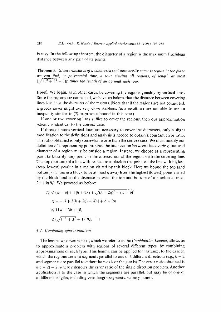
Intitutively it is not surprising that both algorithms fail to produce the desired

result, as the examples of Figs. 8 and 9 show. The Prim type algorithm picks

a representative point in a myopic fashion, a choice that may prove to be disastrous

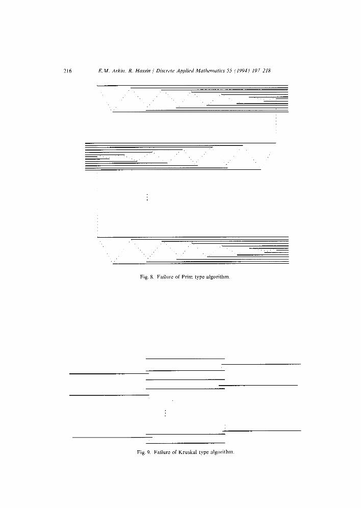
later. The Kruskal type algorithm fails for the opposite reason of allowing too much

flexibility in the choice of which point(s) will be used to connect the segments and thus

allows the salesman to travel within the regions “for free”.

The approximation in Fig. 8 (shown by a dotted line) picks the nearest point on

a segment not yet connected, and is thus made to zigzag, while the optimal tour is

a rectangle of much shorter length. Notice that all the segments in this example can be

made to be of equal length by extending them to the right or left appropriately.

In the example of Fig. 9, each of the middle segments has two points chosen by

a “Kruskal” type algorithm. If we build our approximation by connecting points

216 E.M. Arkin, R. Hassin 1 Discretr Applied Matlxwmtics 55 (IYYI) 197-218

._ L

: -...... . . .

:

. . :.

.’ “.- _’

Fig. 8. Failure of Prim type algorithm

Fig. 9. Failure of Kruskal type algorithm.

E.M. Arkin, R. Hassin / Discrrtr Applied Mathrmutics 55 (1994) 197-218 217

chosen in the same region by the segment they share a very poor approximation

results. Alternatively, we can choose to include all points selected by the Kruskal type

algorithm. as input to a approximation TSP algorithm, but this too (although

successful in the example given) may yield bad approximations in general.

6. Concluding remarks

We conclude this paper by mentioning some open problems. These correspond to

cases for which we have not been able to find a polynomial time algorithm to

approximate, with a bounded performance guarantee, an optimal TSP tour (or prove

that no such approximation exists unless P = NP).

The first such open problem is for regions that are non-uniform parallel elements.

One would like a bound independent of the ratio r between longest and shortest

segment. We assume that the number of distinct sizes is not fixed, and more strongly,

that the segments cannot be divided into classes, such that within each class the ratio

of the longest to shortest segment is small. Otherwise an approximation can be found

by combining approximations for the individual classes.

The second open problem concerns non-parallel unit segments (where the number

of directions is not fixed, and the ratio of their projections on a given direction is not

bounded).

The third open problem concerns regions (convex or non-convex) which can be

quite general, as long as their diameter is known. Here we cannot apply our minimum

perimeter rectangle approach, because we may not be able to efficiently compute such

a rectangle.

A related question is whether we can approximate non-connected regions, such as

regions each of which is comprised of two points.

Other generalizations may be quite straightforward, such as regions in higher

dimensions.

References

[I] A. Aggarwal and S. Suri, Fast algorithms for computing the largest empty rectangle, in: Proceedings

of the 3rd Annual ACM Symposium on Computational Geometry (1987) 278-289.

[2] S. Anily and R. Hassin, The swapping problem, Networks 22 (1992) 419-433.

[3] E.M. Arkin, S.P. Fekete and J.S.B. Mitchell, The lawnmover problem, submitted.

[4] E. Benavent, V. Campos, A. Corberdn and E. Mota, Analisis de heuristicos parael problema del

carter0 rural, Trab. Estadistica Invest, Oper. 36 (1985) 27738.

[5] D. Bienstock, M. Goemans, D. Simchi-Levi and D. Williamson, A note on the prize collecting

traveling salesman problem, Technical Report, Columbia University (1990).

[6] N. Christofides, Worst-case analysis of a new heuristic for the traveling salesman problem, Technical Report, GSIA, Carnegie-Mellon University (1976).

[7] G. Cornuejols and G.L. Nemhauser, Tight bounds for Christofides’ traveling salesman heuristic,

Math. Programming 14 (1978) 116~121.

218 E.M. Arkin, R. Hassin 1 Discrete Applied Mathematics 55 (1994) 197-218

[S] J.T. Current and D.A. Schilling, The covering salesman problem, Transportion Sci. 23 (1989) 208-213.

191 G.N. Frederickson, Approximation algorithms for some postman problems, J. ACM 26 (1979)

208-2 13.

[IO] G.N. Frederickson, M.S. Hecht and C.E. Kim, Approximation algorithms for some routing problems,

SIAM J. Comput. 7 (1978) 178-193.

[I I] A.M. Frieze, Worst-case analysis of algorithms for the traveling salesman problem, Oper. Res.

Verfahren 32 (1979) 93-l 12.

[I21 A.M. Frieze, An extension of Christofides heuristic to the k-person traveling salesman problem,

Discrete Appl. Math. 6 (1983) 79-83.

[ 131 M.R. Carey, R.L. Graham and DS. Johnson, Some NP-complete geometric problems, in: Proceedings

of the 8th Annual ACM Symposium on Theory of Computing (1976) 10-22. [I41 D.S. Johnson and C.H. Papadimitrious, Performance guarantees for heuristics, in: E.L. Lawler, J.K.

Lenstra, A.H.G. Rinnooy Kan and D.B. Shmoys, eds., The Traveling Salesman Problem, Ch. 5

(Wiley, New York, 1985).

[I57 S. Ntafos, Watchman routes under limited visibility, Comput. Geom. I (1992) 1499170.

[16] C.H. Papadimitriou, The Euclidean traveling salesman problem is NP-complete, Theoret. Comput.

Sci. 4 (1977) 2377244.

[17] D.J. Rosenkrantz, R.E. Stearns and P.M. Lewis II, An analysis of several heuristics for the traveling

salesman problem, SIAM J. Comput. 6 (1977) 563-581.