Embed Size (px)
Citation preview
Workshop on Agricultural Air Quality
Arkansas Swine Odor Survey
K.W. VanDevender University of Arkansas, Division of Agriculture - Extension, Little Rock, Arkansas
Swine Odor Survey Participants Arkansas Pork Producer’s Association
National Pork Board University of Arkansas, Division of Agriculure, Cooperative Extension Service
USDA, Natural Resource Conservation Service Arkansas Department of Environmental Quality
Arkansas Natural Resources Commission University of Arkansas, Division of Agriculure, Animal Science Department
Tyson Foods Inc. Swine Division Cargill Pork
Arkansas Swine Producers Individuals from the General Public
Background This survey was conducted at the request of the Arkansas Pork Producer’s Association. The objective was to make an unbiased assessment of the odors typically found on swine farms. This information can be used as a guide for future research, demonstration and educational efforts in addressing odor mitigation.
The survey was conducted on 36 randomly selected farms in 7 counties in northwest, westcentral and southwest Arkansas. From September 1996 to June 1997, 1,157 odor measurements were made at 253 locations.
This document is a summary of the final report for the survey. An electronic version of the report can be found at www.aragriculture.org/agengineering/anmanmortmgmt/swineodorsurvey.
Survey Setup
Odor Measurement Teams The unbiased measurement of odors is complex. People evaluate odors based on their impressions of the strength and unpleasantness of the odor. As this is a subjective process, people perceive odors differently. For this reason, the survey used a team approach. This ensured that an average measurement could be determined at each location. To help ensure unbiased measurements, the team members included individuals from the Cooperative Extension Service, Natural Resource Conservation Service, Tyson, Cargill and the general public. There were seven teams, one for each county.
Odor Measurement Methods Two different ranking methods were used to make odor measurements. Due to limited funds and time constraints, most of the team “sniffed” the odor and assigned a numeric rank. One team member used a scentometer to assign a numeric rank. A scentometer is an instrument with a series of different sized holes and activated charcoal filters. They allow purified air to be breathed prior to each measurement. The odor ranks are correlated to the ratio of odorous air to purified air. For both methods, the possible odor ranks ranged from “non-detectable” to “strongly offensive.”
1175
Workshop on Agricultural Air Quality
Table 1. Interpretation of Odor Rank Values Odor Description Scentometer Rank Nasal Rank Combined Rank* Non-Detectable 1 1 1
2 Detectable But Non-Offensive 3 2 2
4** Mildly Offensive 5** 3 3
6*** 4 4 Strongly Offensive 7*** *Combined ranks used for combined measurements. The scentometer ranks were scaled prior to combining with nasal ranks. **Scentometer odor ranks historically associated with the start of complaints. ***Scentometer odor ranks historically associated with serious nuisance odors.
Odor Measurement Process Each team spent a day every other week collecting measurements. At each farm, the team moved upwind toward the potential odor source. Measurements were made at various distances. At each measurement site, team members recorded their odor measurement, the distance from the odor source, temperature, wind speed, relative humidity and any written comments.
Survey Results
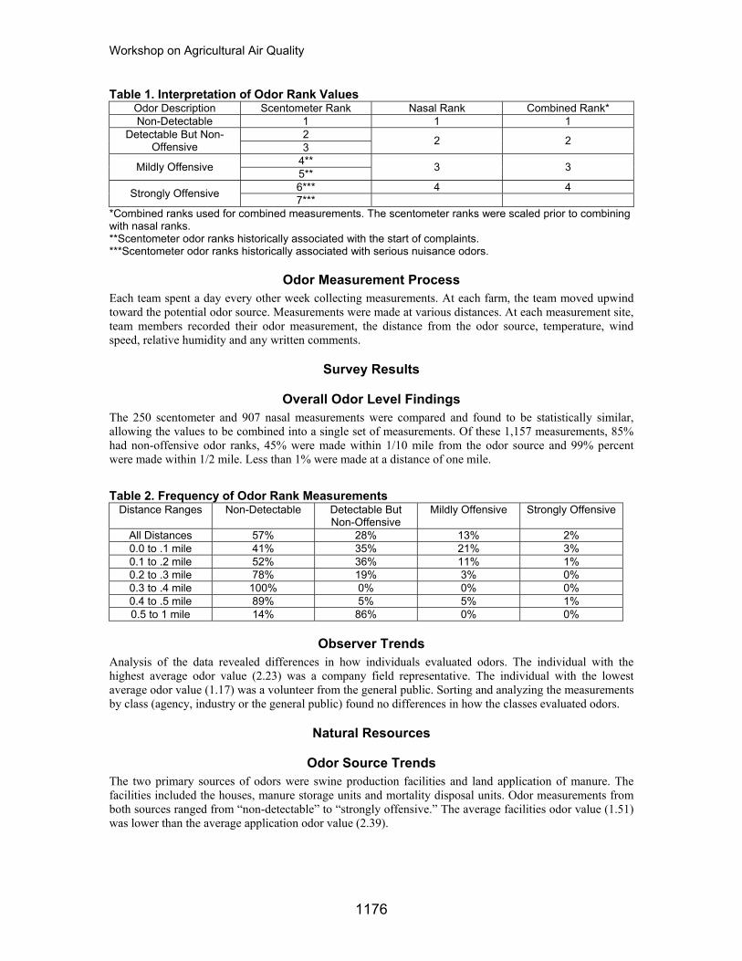
Overall Odor Level Findings The 250 scentometer and 907 nasal measurements were compared and found to be statistically similar, allowing the values to be combined into a single set of measurements. Of these 1,157 measurements, 85% had non-offensive odor ranks, 45% were made within 1/10 mile from the odor source and 99% percent were made within 1/2 mile. Less than 1% were made at a distance of one mile.
Table 2. Frequency of Odor Rank Measurements
Distance Ranges Non-Detectable Detectable But Non-Offensive
Mildly Offensive Strongly Offensive
All Distances 57% 28% 13% 2% 0.0 to .1 mile 41% 35% 21% 3% 0.1 to .2 mile 52% 36% 11% 1% 0.2 to .3 mile 78% 19% 3% 0% 0.3 to .4 mile 100% 0% 0% 0% 0.4 to .5 mile 89% 5% 5% 1% 0.5 to 1 mile 14% 86% 0% 0%
Observer Trends Analysis of the data revealed differences in how individuals evaluated odors. The individual with the highest average odor value (2.23) was a company field representative. The individual with the lowest average odor value (1.17) was a volunteer from the general public. Sorting and analyzing the measurements by class (agency, industry or the general public) found no differences in how the classes evaluated odors.
Natural Resources
Odor Source Trends The two primary sources of odors were swine production facilities and land application of manure. The facilities included the houses, manure storage units and mortality disposal units. Odor measurements from both sources ranged from “non-detectable” to “strongly offensive.” The average facilities odor value (1.51) was lower than the average application odor value (2.39).
1176
Workshop on Agricultural Air Quality
Distance Trends Odor intensity decreased as distance increased. There were also differences between the sources of odors. Within 1/10 mile of the source, the average odor value was 1.76 for the facilities and 2.58 for the manure applications. The maximum distance that an offensive odor was recorded was 3/10 mile for facilities and 1/2 mile for manure applications. Statistical tests also revealed that while odor intensity was related to distance, other factors also affected odor intensity.
Animal Population and Manure Storage Trends Differences in odor measurements were found for the various types of swine production operations and manure storage units. However, there were no easily identifiable trends. The lack of trends was probably due to two factors. First, the facility-based measurements were for odors coming from both the swine houses and manure storage units. Also, the survey included a relatively small number of some types of production systems and manure storage systems. This resulted in a smaller number of measurements for some systems, making it more likely that other factors, such as weather and topography, obscured any trends in odor levels.
Appearance Trends Farms with better appearance ranks were associated with lower odor measurements. The differences could be due to appearance influencing the assigned odor ranks. Another possibility is that differences in overall farm management result in true differences in odor levels.
Conclusions • This survey provides information to help quantify existing odor levels typically associated with
swine production. • The small percentage of the odors found to be offensive implies that a significant portion of odor
concerns is due to the relatively infrequent occurrence of offensive odors. • An individual’s association with swine production did not influence how odors were evaluated. • The land application of manure tended to generate more odors than the facilities. • Distance is a significant factor, but not the only factor, affecting odor intensity. Odor intensity was
found to decrease as distances increased. • Odor management practices will have to consider many factors to be effective. This is supported by
the fact that other influencing factors masked odor trends with animal populations or manure storage units.
• Farms with a good overall appearance had lower odor levels than farms with a poor appearance. • The survey results provide valuable information to guide future research, demonstration and
educational efforts addressing odor mitigation.
References VanDevender, K., 1998. Arkansas Swine Odor Survey. Project Report. University of Arkansas Division of Agriculture. www.aragriculture.org/agengineering/anmanmortmgmt/swineodorsurvey (Febuary 15, 2006)
Acknowledgement Without the support of the individuals and organizations participating in this survey this project would not have been possible. The Arkansas Pork Producer’s Association and the National Pork Board provided the funds to purchase the necessary equipment and supplies. The members of the odor teams contributed their time and effort. The landowners provided access to their farms for making odor measurements. The various agencies and industry groups provided support in the planning, farm selection, and implementation of the project.
1177
Workshop on Agricultural Air Quality
Greenhouse Gas Emission Reductions and Carbon Credits from Implementation of Aerobic Manure Treatment Systems in Swine Farms
Matias B. Vanotti1, Ariel A. Szögi1 and Carlos A. Vives2
1US Department of Agriculture, ARS, Coastal Plains Soil, Water, and Plant Research Center 2611 W. Lucas Street, Florence, SC 29501, USA
2Agrosuper, Agricola Super Limitada, Rancagua c.c. 333, Chile Abstract Trading of carbon and NOx emission reductions is an attractive approach to help producers implement cleaner treatment technologies to replace current anaerobic lagoons. Our objectives were to determine greenhouse gas (GHG) emission reductions from implementation of aerobic technology (Supersoil project) in North Carolina swine farms. Emission reductions were determined using approved methodology in conjunction with monitoring information collected during full-scale demonstration of the new treatment system in a 4,360-head swine operation in North Carolina. Emission sources for the project and baseline manure management system were methane emissions from the decomposition of manure under anaerobic conditions and nitrous oxide emissions during storage and handling of manure in the manure management system. Emission reductions resulted from the difference between total project and baseline emissions. The project activity included an on-farm wastewater treatment system consisting of liquid-solid separation, treatment of the separated liquid using aerobic biological N removal, chemical disinfection and soluble P removal using lime. The project activity was completed with a centralized facility that used aerobic composting to process the separated solids. Replacement of the lagoon technology with the cleaner aerobic technology reduced GHG emissions 98.9%, from 4,712 Tonnes of carbon dioxide equivalents (CO2-eq) to 50 Tonnes CO2-eq/year. Total net emission reductions by the project activity in the 4,360-head finishing operation were 4,632.8 Tonnes CO2-eq per year. The dollar value from implementation of the Supersoil project in this swine farm was $9,960.54/year. This translates into a direct economic benefit to the producer of $0.91 per finished pig. Thus, GHG emission reductions and credits can help compensate for the higher installation cost of cleaner aerobic technologies and facilitate producer adoption of environmentally superior technologies to replace current anaerobic lagoons in North Carolina.
Introduction Anaerobic lagoons are widely used to treat and store liquid manure from confined swine production facilities (Barker, 1996). Environmental and health concerns with the lagoon technology include emissions of ammonia (Aneja et al., 2000; Szogi et al., 2006), odors (Loughrin et al., 2006), pathogens (Sobsey et al., 2001), and water quality deterioration (Mallin, 2000). Widespread objection to the use of anaerobic lagoons for swine manure treatment in North Carolina prompted a state government-industry framework to search for alternative technologies that directly eliminate anaerobic lagoons as a method of treatment. In July 2000, the Attorney General of North Carolina reached an agreement with Smithfield Foods, Inc. and its subsidiaries (the largest hog producing companies in the USA) to develop and demonstrate environmentally superior waste management technologies for implementation onto farms located in North Carolina that are owned by these companies. In October 2000, the Attorney General reached a similar agreement with Premium Standard Farms, the second largest pork producer in the USA. The agreement defines an environmentally superior technology (EST) as any technology, or combination of technologies, that (1) is permittable by the appropriate governmental authority; (2) is determined to be technically, operationally, and economically feasible; and (3) meets the following five environmental performance standards (Williams, 2005):
1. Eliminate the discharge of animal waste to surface waters and groundwater through direct discharge, seepage, or runoff;
2. Substantially eliminate atmospheric emissions of ammonia; 3. Substantially eliminate the emission of odor that is detectable beyond the boundaries of the swine
farm; 4. Substantially eliminate the release of disease-transmitting vectors and airborne pathogens;
1178
Workshop on Agricultural Air Quality
5. Substantially eliminate nutrient and heavy metal contamination of soil and groundwater.
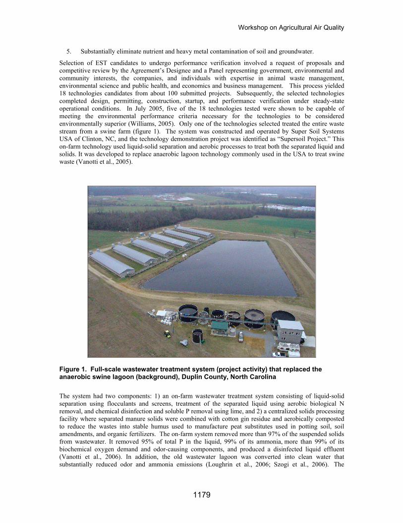
Selection of EST candidates to undergo performance verification involved a request of proposals and competitive review by the Agreement’s Designee and a Panel representing government, environmental and community interests, the companies, and individuals with expertise in animal waste management, environmental science and public health, and economics and business management. This process yielded 18 technologies candidates from about 100 submitted projects. Subsequently, the selected technologies completed design, permitting, construction, startup, and performance verification under steady-state operational conditions. In July 2005, five of the 18 technologies tested were shown to be capable of meeting the environmental performance criteria necessary for the technologies to be considered environmentally superior (Williams, 2005). Only one of the technologies selected treated the entire waste stream from a swine farm (figure 1). The system was constructed and operated by Super Soil Systems USA of Clinton, NC, and the technology demonstration project was identified as “Supersoil Project.” This on-farm technology used liquid-solid separation and aerobic processes to treat both the separated liquid and solids. It was developed to replace anaerobic lagoon technology commonly used in the USA to treat swine waste (Vanotti et al., 2005).
Figure 1. Full-scale wastewater treatment system (project activity) that replaced the anaerobic swine lagoon (background), Duplin County, North Carolina
The system had two components: 1) an on-farm wastewater treatment system consisting of liquid-solid separation using flocculants and screens, treatment of the separated liquid using aerobic biological N removal, and chemical disinfection and soluble P removal using lime, and 2) a centralized solids processing facility where separated manure solids were combined with cotton gin residue and aerobically composted to reduce the wastes into stable humus used to manufacture peat substitutes used in potting soil, soil amendments, and organic fertilizers. The on-farm system removed more than 97% of the suspended solids from wastewater. It removed 95% of total P in the liquid, 99% of its ammonia, more than 99% of its biochemical oxygen demand and odor-causing components, and produced a disinfected liquid effluent (Vanotti et al., 2006). In addition, the old wastewater lagoon was converted into clean water that substantially reduced odor and ammonia emissions (Loughrin et al., 2006; Szogi et al., 2006). The
1179
Workshop on Agricultural Air Quality
centralized facility produced quality composts that conserved 96.5% of the nitrogen into a stabilized product that met Class A biosolids standards due to high pathogen reduction (Vanotti, 2005).
Although this clean technology was determined to be technically and operationally feasible and it was able to meet the strict technical environmental performance standards of an environmentally superior technology (EST), a contingency project was subsequently planned to demonstrate a second-generation, lower-cost version of the treatment system (i.e., annual cost should be similar to baseline lagoon technology) to meet unconditional EST status. Second-generation technology development involved simplification of processes and operation based on lessons learned during testing of the first-generation system.
Capital investment is the most important barrier for widespread adoption of cleaner treatment technology due to higher costs involved compared to the baseline lagoon technology. On the other hand, proven environmental benefits from implementation of the new superior technologies are often difficult to translate in terms of direct economic benefits that can offset the investment barrier. Fortunately, new programs are being created on global reduction of anthropogenic emissions of greenhouse gases (GHG) that can help compensate for the higher installation cost of the cleaner technologies, and therefore favor technology adoption by producers. Such a program was recently implemented by Agricola Super Limitada (Agrosuper), the largest swine production company in Chile. The company initiated a voluntary adoption of advanced waste management systems (anaerobic and aerobic treatment of manure); implementation of the more expensive technology was greatly influenced by the adoption of the Kyoto Protocol and the Clean Development Mechanism. As a result, advanced technologies are being phased in gradually in all of Agrosuper’s swine production units to replace the existing anaerobic lagoon technology. The company used revenues from the sale of Certified Emission Reductions (CERs) to partially finance the advanced waste management systems. This voluntary adoption case is significant to North Carolina because the company is phasing out lagoon technology that was implemented years ago using the North Carolina traditional anaerobic lagoon treatment model. To accomplish this purpose, Agrosuper developed a project activity at a 118,800 finishing swine facility in Chile that led to an approved UNFCCC/CCNUCC methodology (AM0006, 2004). The advantage of this methodology is that it considers aerobic components in addition to anaerobic digesters and flaring that are the focus of other approved methods for quantification of GHG emission reduction in animal manure systems (i.e., AM0016). Thus, the methodology is very suitable for quantification of GHG emission reductions in the Supersoil project which relies heavily on aerobic processes to treat the manure.
Our objectives were to determine greenhouse gas (GHG) emission reductions from implementation of the cleaner aerobic technology (Supersoil project) in North Carolina swine farms compared to the current anaerobic lagoon system (baseline scenario). GHG emission reductions were determined using approved methodology AM0006 in conjunction with monitoring information collected during full-scale demonstration of the treatment system.
Materials and Methods The baseline activity was the traditional anaerobic lagoon–sprayfield technology for a farm with 4,360-head finishing pigs in North Carolina. The project activity consisted of the implemented advanced system (Supersoil project) in an identical farm. Determination of GHG emission reductions by the environmentally superior technology was made using approved methodology described in AM0006 (2004).
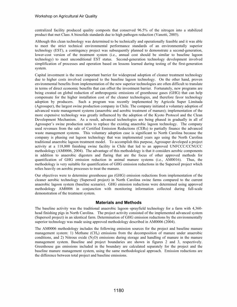
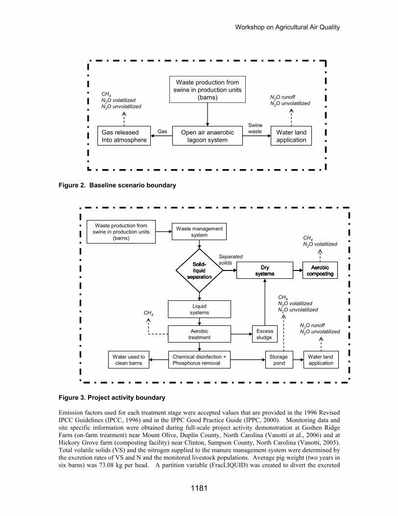
The AM0006 methodology includes the following emission sources for the project and baseline manure management system: 1) Methane (CH4) emissions from the decomposition of manure under anaerobic conditions, and 2) Nitrous oxide (N2O) emissions during storage and handling of manure in the manure management system. Baseline and project boundaries are shown in figures 2 and 3, respectively. Greenhouse gas emissions included in the boundary are calculated separately for the project and the baseline manure management system, using the same methodological approach. Emission reductions are the difference between total project and baseline emissions.
1180
Workshop on Agricultural Air Quality
Waste production fromswine in production units
(barns)
Open air anaerobic lagoon system
Gas releasedInto atmosphere
Water land application
CH4 N2O volatilizedN2O unvolatilized
GasSwinewaste
N2O runoffN2O unvolatilized
Figure 2. Baseline scenario boundary
Liquid systems
Aerobic treatment
Waste production fromswine in production units
(barns)
Waste managementsystem
Dry systems
Aerobiccomposting
Chemical disinfection +Phosphorus removal
Storage pond
Water used toclean barns
Water land application
Excesssludge
Solid-liquid
separation
Separatedsolids
Dry systems
Aerobiccomposting
Solid-liquid
separation
Dry systems
Aerobiccomposting
Solid-liquid
separation
Dry systems
Aerobiccomposting
Solid-liquid
separation
CH4N2O volatilized
CH4
CH4N2O volatilizedN2O unvolatilized
N2O runoffN2O unvolatilized
Figure 3. Project activity boundary
Emission factors used for each treatment stage were accepted values that are provided in the 1996 Revised IPCC Guidelines (IPCC, 1996) and in the IPPC Good Practice Guide (IPPC, 2000). Monitoring data and site specific information were obtained during full-scale project activity demonstration at Goshen Ridge Farm (on-farm treatment) near Mount Olive, Duplin County, North Carolina (Vanotti et al., 2006) and at Hickory Grove farm (composting facility) near Clinton, Sampson County, North Carolina (Vanotti, 2005). Total volatile solids (VS) and the nitrogen supplied to the manure management system were determined by the excretion rates of VS and N and the monitored livestock populations. Average pig weight (two years in six barns) was 73.08 kg per head. A partition variable (FracLIQUID) was created to divert the excreted
1181
Workshop on Agricultural Air Quality
VS and N into the liquid system (figure 3). FracLIQUID was determined based on monitored BOD5 and TN before and after solid-liquid separation. The difference (FracSOLID = 1 – FracLIQUID) determined the amount of VS or TN that was diverted into the dry system. For second and subsequent stages, methane emissions were calculated based on the measurement of the monitored BOD5 and the quantity of manure flowing to that treatment stage (Option A in method AM0006). The BOD5 was adjusted using monitored water temperature and the Van’t-Hoff-Arrhenius relationship. Similarly, emissions of N2O in second and subsequent stages were calculated based on measurements of the N content in the manure flowing to that treatment stage and monitored flow rates of the manure.
Emission reductions of CH4 and N2O were expressed in terms of CO2 equivalents using approved Global Warming Potentials (21 for CH4 and 310 for N2O). Direct economic benefits from emission reductions were determined using current trading value ($2.15 per Ton of CO2) at the Chicago Climate Exchange (www.chicagoclimatex.com).
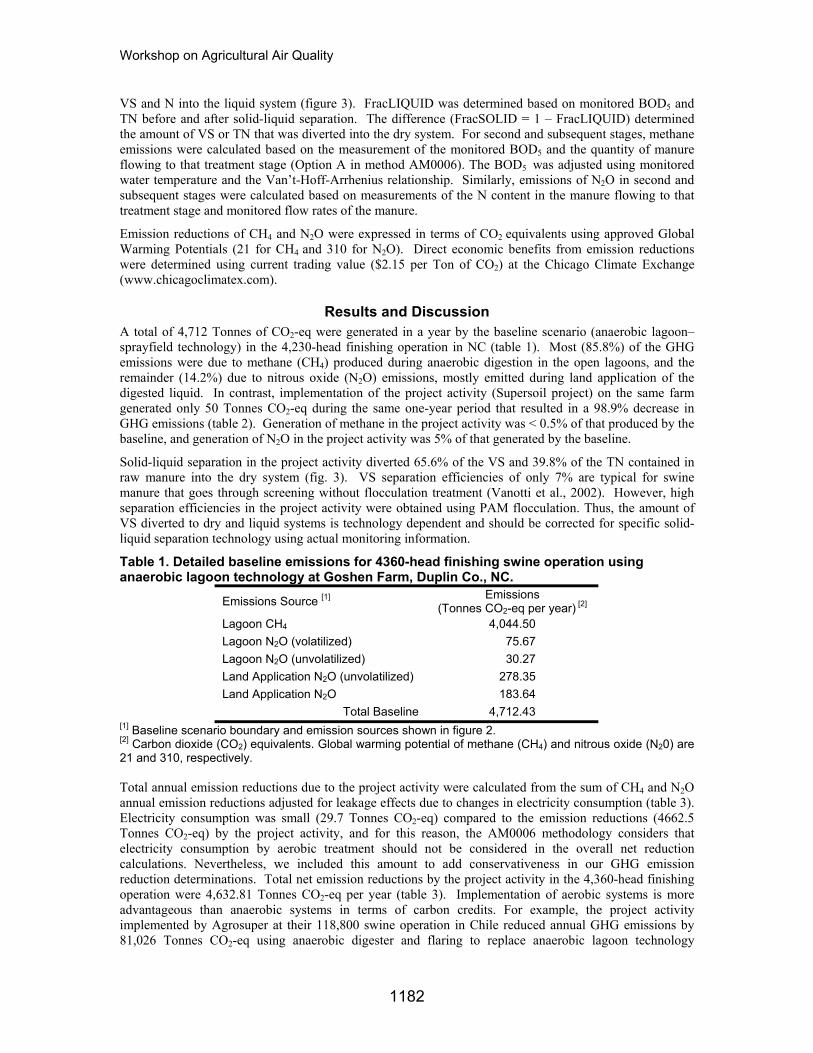
Results and Discussion A total of 4,712 Tonnes of CO2-eq were generated in a year by the baseline scenario (anaerobic lagoon–sprayfield technology) in the 4,230-head finishing operation in NC (table 1). Most (85.8%) of the GHG emissions were due to methane (CH4) produced during anaerobic digestion in the open lagoons, and the remainder (14.2%) due to nitrous oxide (N2O) emissions, mostly emitted during land application of the digested liquid. In contrast, implementation of the project activity (Supersoil project) on the same farm generated only 50 Tonnes CO2-eq during the same one-year period that resulted in a 98.9% decrease in GHG emissions (table 2). Generation of methane in the project activity was < 0.5% of that produced by the baseline, and generation of N2O in the project activity was 5% of that generated by the baseline.
Solid-liquid separation in the project activity diverted 65.6% of the VS and 39.8% of the TN contained in raw manure into the dry system (fig. 3). VS separation efficiencies of only 7% are typical for swine manure that goes through screening without flocculation treatment (Vanotti et al., 2002). However, high separation efficiencies in the project activity were obtained using PAM flocculation. Thus, the amount of VS diverted to dry and liquid systems is technology dependent and should be corrected for specific solid-liquid separation technology using actual monitoring information.
Table 1. Detailed baseline emissions for 4360-head finishing swine operation using anaerobic lagoon technology at Goshen Farm, Duplin Co., NC.
Emissions Source [1] Emissions (Tonnes CO2-eq per year) [2]
Lagoon CH4 4,044.50 Lagoon N2O (volatilized) 75.67 Lagoon N2O (unvolatilized) 30.27 Land Application N2O (unvolatilized) 278.35 Land Application N2O 183.64
Total Baseline 4,712.43 [1] Baseline scenario boundary and emission sources shown in figure 2. [2] Carbon dioxide (CO2) equivalents. Global warming potential of methane (CH4) and nitrous oxide (N20) are 21 and 310, respectively. Total annual emission reductions due to the project activity were calculated from the sum of CH4 and N2O annual emission reductions adjusted for leakage effects due to changes in electricity consumption (table 3). Electricity consumption was small (29.7 Tonnes CO2-eq) compared to the emission reductions (4662.5 Tonnes CO2-eq) by the project activity, and for this reason, the AM0006 methodology considers that electricity consumption by aerobic treatment should not be considered in the overall net reduction calculations. Nevertheless, we included this amount to add conservativeness in our GHG emission reduction determinations. Total net emission reductions by the project activity in the 4,360-head finishing operation were 4,632.81 Tonnes CO2-eq per year (table 3). Implementation of aerobic systems is more advantageous than anaerobic systems in terms of carbon credits. For example, the project activity implemented by Agrosuper at their 118,800 swine operation in Chile reduced annual GHG emissions by 81,026 Tonnes CO2-eq using anaerobic digester and flaring to replace anaerobic lagoon technology
1182
Workshop on Agricultural Air Quality
(baseline). In a second phase of the same project, they further reduced annual GHG emissions to a total of 116,993 Tonnes CO2-eq with the installation of aerobic post-treatment of the liquid before land application.
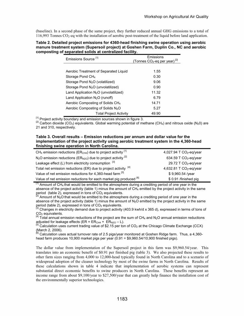
Table 2. Detailed project emissions for 4360-head finishing swine operation using aerobic manure treatment system (Supersoil project) at Goshen Farm, Duplin Co., NC and aerobic composting of separated solids at centralized facility.
Emissions Source [1] Emissions (Tonnes CO2-eq per year) [2]
Aerobic Treatment of Separated Liquid 1.55 Storage Pond CH4 0.30 Storage Pond N2O (volatilized) 9.06 Storage Pond N2O (unvolatilized) 0.90 Land Application N2O (unvolatilized) 11.32 Land Application N2O (runoff) 6.79 Aerobic Composting of Solids CH4 14.71 Aerobic Composting of Solids N2O 5.27
Total Project Activity 49.90 [1] Project activity boundary and emission sources shown in figure 3. [2] Carbon dioxide (CO2) equivalents. Global warming potential of methane (CH4) and nitrous oxide (N20) are 21 and 310, respectively.
Table 3. Overall results – Emission reductions per annum and dollar value for the implementation of the project activity using aerobic treatment system in the 4,360-head finishing swine operation in North Carolina. CH4 emission reductions (ERCH4) due to project activity [1] 4,027.94 T CO2-eq/year N2O emission reductions (ERN2O) due to project activity [2] 634.59 T CO2-eq/year Leakage effect (L) from electricity consumption [3] 29.72 T CO2-eq/year Total net emission reductions (ER) due to project activity [4] 4,632.81 T CO2-eq/year Value of net emission reductions for 4,360-head farm [5] $ 9,960.54 /year Value of net emission reductions for each market pig produced [6] $ 0.91 /finished pig [1] Amount of CH4 that would be emitted to the atmosphere during a crediting period of one year in the absence of the project activity (table 1) minus the amount of CH4 emitted by the project activity in the same period (table 2), expressed in tons of CO2 equivalents. [2] Amount of N2O that would be emitted to the atmosphere during a crediting period of one year in the absence of the project activity (table 1) minus the amount of N2O emitted by the project activity in the same period (table 2), expressed in tons of CO2 equivalents. [3] Changes in electricity demand due to project activity (403.9 kwh/d x 365 d), expressed in terms of tons of CO2 equivalents. [4] Total annual emission reductions of the project are the sum of CH4 and N2O annual emission reductions adjusted for leakage effects (ER = ERCH4 + ERN2O – L). [5] Calculation uses current trading value of $2.15 per ton of CO2 at the Chicago Climate Exchange (CCX) (March 2, 2006). [6] Calculation uses actual turnover rate of 2.5 pigs/year monitored at Goshen Ridge farm. Thus, a 4,360-head farm produces 10,900 market pigs per year (0.91 = $9,960.54/10,900 finished pigs).
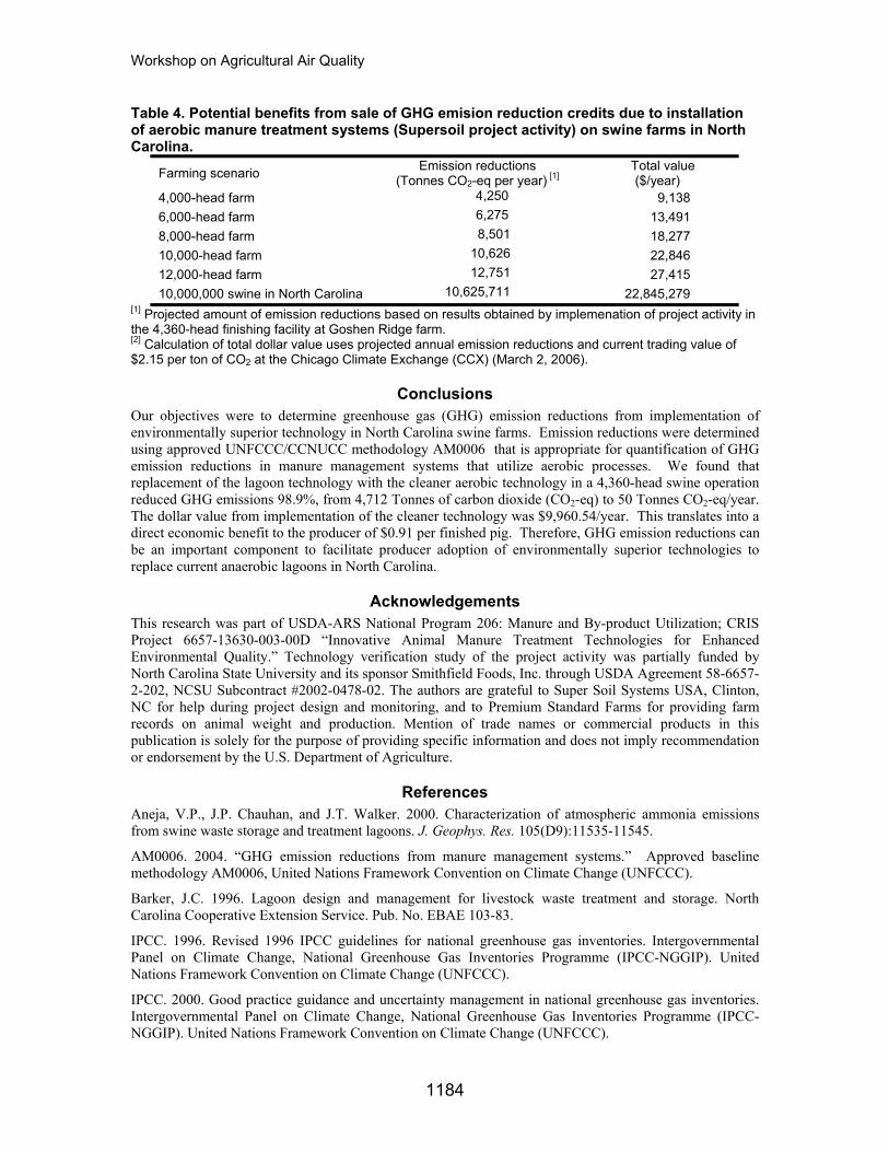
The dollar value from implementation of the Supersoil project in this farm was $9,960.54/year. This translates into an economic benefit of $0.91 per finished pig (table 3). We also projected these results to other farm sizes ranging from 4,000 to 12,000-head typically found in North Carolina and to a scenario of widespread adoption of the cleaner technology by most of the swine farms in North Carolina. Results of these calculations shown in table 4 indicate that implementation of aerobic systems can represent substantial direct economic benefits to swine producers in North Carolina. These benefits represent an income range from about $9,100/year to $27,500/year that can greatly help finance the installation cost of the environmentally superior technologies.
1183
Workshop on Agricultural Air Quality
Table 4. Potential benefits from sale of GHG emision reduction credits due to installation of aerobic manure treatment systems (Supersoil project activity) on swine farms in North Carolina.
Farming scenario Emission reductions (Tonnes CO2-eq per year) [1]
Total value ($/year)
4,000-head farm 4,250 9,138 6,000-head farm 6,275 13,491 8,000-head farm 8,501 18,277 10,000-head farm 10,626 22,846 12,000-head farm 12,751 27,415 10,000,000 swine in North Carolina 10,625,711 22,845,279
[1] Projected amount of emission reductions based on results obtained by implemenation of project activity in the 4,360-head finishing facility at Goshen Ridge farm. [2] Calculation of total dollar value uses projected annual emission reductions and current trading value of $2.15 per ton of CO2 at the Chicago Climate Exchange (CCX) (March 2, 2006).
Conclusions Our objectives were to determine greenhouse gas (GHG) emission reductions from implementation of environmentally superior technology in North Carolina swine farms. Emission reductions were determined using approved UNFCCC/CCNUCC methodology AM0006 that is appropriate for quantification of GHG emission reductions in manure management systems that utilize aerobic processes. We found that replacement of the lagoon technology with the cleaner aerobic technology in a 4,360-head swine operation reduced GHG emissions 98.9%, from 4,712 Tonnes of carbon dioxide (CO2-eq) to 50 Tonnes CO2-eq/year. The dollar value from implementation of the cleaner technology was $9,960.54/year. This translates into a direct economic benefit to the producer of $0.91 per finished pig. Therefore, GHG emission reductions can be an important component to facilitate producer adoption of environmentally superior technologies to replace current anaerobic lagoons in North Carolina.
Acknowledgements This research was part of USDA-ARS National Program 206: Manure and By-product Utilization; CRIS Project 6657-13630-003-00D “Innovative Animal Manure Treatment Technologies for Enhanced Environmental Quality.” Technology verification study of the project activity was partially funded by North Carolina State University and its sponsor Smithfield Foods, Inc. through USDA Agreement 58-6657-2-202, NCSU Subcontract #2002-0478-02. The authors are grateful to Super Soil Systems USA, Clinton, NC for help during project design and monitoring, and to Premium Standard Farms for providing farm records on animal weight and production. Mention of trade names or commercial products in this publication is solely for the purpose of providing specific information and does not imply recommendation or endorsement by the U.S. Department of Agriculture.
References Aneja, V.P., J.P. Chauhan, and J.T. Walker. 2000. Characterization of atmospheric ammonia emissions from swine waste storage and treatment lagoons. J. Geophys. Res. 105(D9):11535-11545.
AM0006. 2004. “GHG emission reductions from manure management systems.” Approved baseline methodology AM0006, United Nations Framework Convention on Climate Change (UNFCCC).
Barker, J.C. 1996. Lagoon design and management for livestock waste treatment and storage. North Carolina Cooperative Extension Service. Pub. No. EBAE 103-83.
IPCC. 1996. Revised 1996 IPCC guidelines for national greenhouse gas inventories. Intergovernmental Panel on Climate Change, National Greenhouse Gas Inventories Programme (IPCC-NGGIP). United Nations Framework Convention on Climate Change (UNFCCC).
IPCC. 2000. Good practice guidance and uncertainty management in national greenhouse gas inventories. Intergovernmental Panel on Climate Change, National Greenhouse Gas Inventories Programme (IPCC-NGGIP). United Nations Framework Convention on Climate Change (UNFCCC).
1184
Workshop on Agricultural Air Quality
Loughrin, J.H., A.A. Szogi, and M.B. Vanotti. 2006. Reduction of malodorous compounds from a treated swine anaerobic lagoon. J. Environ. Qual.35(1):194-199
Mallin, M.A. 2000. Impacts of industrial animal production on rivers and estuaries. American Scientist 88(1):26-37.
Sobsey, M.D., L.A.Khatib, V.R. Hill, E. Alocilja, and S. Pillai. 2001. Pathogens in animal wastes and the impacts of waste management practices on their survival, transport and fate. In: White Papers on animal agriculture and the environment. MidWest Plan Service (MWPS), Iowa State University, Ames, Iowa, (Chapter 17).
Szogi, A.A., M.B.Vanotti, and A.E. Stansbery. 2006. Reduction of ammonia emissions from treated anaerobic swine lagoons. Transactions of the ASABE (in press) Vanotti, M.B., D.M.C. Rashash, and P.G. Hunt. 2002. Solid-liquid separation of flushed swine manure with PAM: Effect of wastewater strength. Transactions of the ASAE 45(6):1959-1969.
Vanotti, M.B., A.A. Szogi, and P.G. Hunt. 2005. Wastewater treatment system. U.S. Patent 6,893,567. U.S. Patent Office.
Vanotti, M. B. 2005. Evaluation of Environmentally Superior Technology: Swine waste treatment system for elimination of lagoons, reduced environmental impact, and improved water quality (Centralized composting unit). Phase II: Final Report for Technology Determination per Agreements between NC Attorney General & Smithfield Foods, Premium Standard Farms, and Frontline Farmers. July 25, 2005. Available at: http://www.cals.ncsu.edu/waste_mgt/smithfield_projects/phase2report05/reports/A1.pdf
Vanotti, M.B., A.A. Szogi, P.G. Hunt, P.D. Millner, and F.J. Humenik. 2006. Development of environmentally superior treatment systems to replace anaerobic swine lagoons in the USA. Bioresource Technol. (in press).
Williams, C.M. 2005. Development of Environmentally Superior Technologies. Phase II Report for Technology Determination per Agreements Between the Attorney General of North Carolina and Smithfield Foods, Premium Standard Farms and Frontline Farmers. July 25, 2005. Available at: http://www.cals.ncsu.edu/waste_mgt/smithfield_projects/phase2report05/front.pdf
1185
Workshop on Agricultural Air Quality
Impact of Air Pollution on Agricultural Crops in India
C.K. Varshney Jawaharlal Nehru University, School of Environmental Sciences, New Delhi, 1110067, India
Abstract Effect of ground level ozone on plants is attracting much attention as it has been shown to reduce the crop yield. Buildup of ground level ozone is viewed as a growing threat to food security. Studies carried out at New Delhi have shown that the ambient ozone concentration varies between 20 and 273 ug m-3 and the WHO one hour ozone standard is violated on many occasions. Values of ground level ozone reported from nine other widely separated stations in the country suggest that the build up of ground level ozone is fairly widespread in the country. Growing industrialization, urbanization and rapidly rising consumption of fossil fuels will further contribute to the build up of ground level ozone in the country. Investigations were undertaken to study the effect of ozone on four important India crop species viz., Triticum, Phaseolus, Brassica and Spinacia was under taken at Delhi. Plants were exposed to ambient levels of ozone and at different sites as well as plants treated with EDU for comparison. Measurements were made on growth, biomass, seed set, seed weight and yield loss was determined. The average yield loss in these four crop species was 8.57, 8.58, 14.38, and 14.37 per cent, respectively. The paper provides evidence to show that the ambient level of ground level ozone can potentially undermine the crop yield. In future, air pollution especially ground level ozone is likely to increase and may become a serious challenge for increasing agricultural yield in the country.
1186
Workshop on Agricultural Air Quality
The ClearSky Field-Burning Decision Support System
J. K. Vaughan1, K. Heitkamp1, R. Jain2, B. K. Lamb1
1Laboratory for Atmospheric Research, Washington State University, Pullman, Washington 2Golder Associates Ltd., Calgary, Alberta, Canada
Abstract The ClearSky agricultural smoke dispersion modeling system was developed, beginning in 2002, as a decision support system for agricultural-burning smoke management in northern Idaho and eastern Washington. The ClearSky system features: 1) use of data from state burn-permitting programs to locate and characterize sources, 2) a web application giving authorized users the ability to submit potential burn scenarios for modeling, and 3) web-served graphics animations displaying burn scenario simulation air quality results. ClearSky is a NW-AIRQUEST (Northwest International Air Quality, Environmental Science and Technology Consortium) project and has developed in collaboration with the US Forest Service BlueSky/RAINS project for management of prescribed forest burning. The ClearSky modeling system uses a University of Washington MM5 forecast, at 4-km grid spacing, processed through CALMET to drive CALPUFF to simulate smoke dispersion from agricultural field burning. The emissions are simulated using a buoyant line source to represent an active flame front and a buoyant area source to represent the smoldering portion of a field. Parameters for the emissions and plume-rise modules were obtained from data collected during recent field studies and from sensitivity studies of the CALPUFF plume-rise modules. ClearSky was operated on a daily basis during the 2002 through 2005 burn seasons. An evaluation of the ClearSky system was conducted at the end of the 2002 season by re-running each burn day using actual burn data. Performance of the modeling system was analyzed by comparing 1) observed and MM5-predicted meteorology and 2) observed and ClearSky-predicted PM2.5 concentrations at the monitoring stations revealing a notable vulnerability to meteorological forecast errors. Consequently, a new Ensemble ClearSky System is being developed which utilizes a suite of parallel, conterminous MM5 meteorological forecasts to generate a probabilistic forecast of plume impacts.
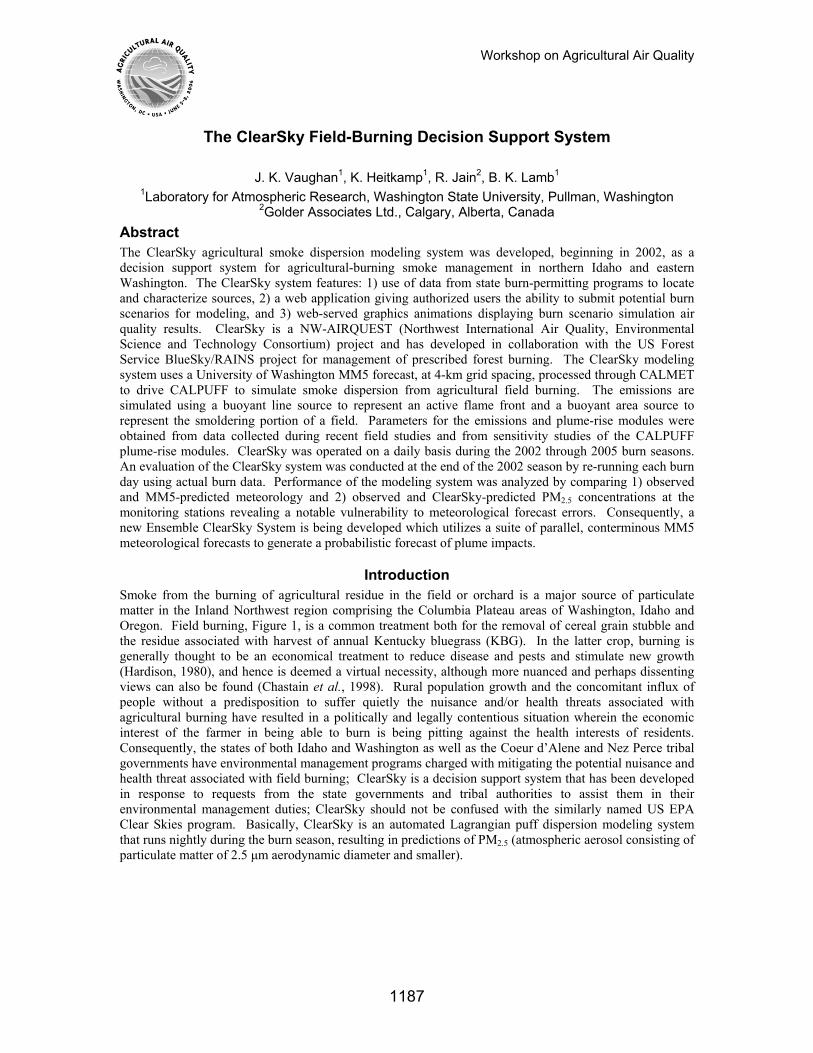
Introduction Smoke from the burning of agricultural residue in the field or orchard is a major source of particulate matter in the Inland Northwest region comprising the Columbia Plateau areas of Washington, Idaho and Oregon. Field burning, Figure 1, is a common treatment both for the removal of cereal grain stubble and the residue associated with harvest of annual Kentucky bluegrass (KBG). In the latter crop, burning is generally thought to be an economical treatment to reduce disease and pests and stimulate new growth (Hardison, 1980), and hence is deemed a virtual necessity, although more nuanced and perhaps dissenting views can also be found (Chastain et al., 1998). Rural population growth and the concomitant influx of people without a predisposition to suffer quietly the nuisance and/or health threats associated with agricultural burning have resulted in a politically and legally contentious situation wherein the economic interest of the farmer in being able to burn is being pitting against the health interests of residents. Consequently, the states of both Idaho and Washington as well as the Coeur d’Alene and Nez Perce tribal governments have environmental management programs charged with mitigating the potential nuisance and health threat associated with field burning; ClearSky is a decision support system that has been developed in response to requests from the state governments and tribal authorities to assist them in their environmental management duties; ClearSky should not be confused with the similarly named US EPA Clear Skies program. Basically, ClearSky is an automated Lagrangian puff dispersion modeling system that runs nightly during the burn season, resulting in predictions of PM2.5 (atmospheric aerosol consisting of particulate matter of 2.5 µm aerodynamic diameter and smaller).
1187
Workshop on Agricultural Air Quality
Figure 1. Wheat field stubble being burned in Eastern Washington
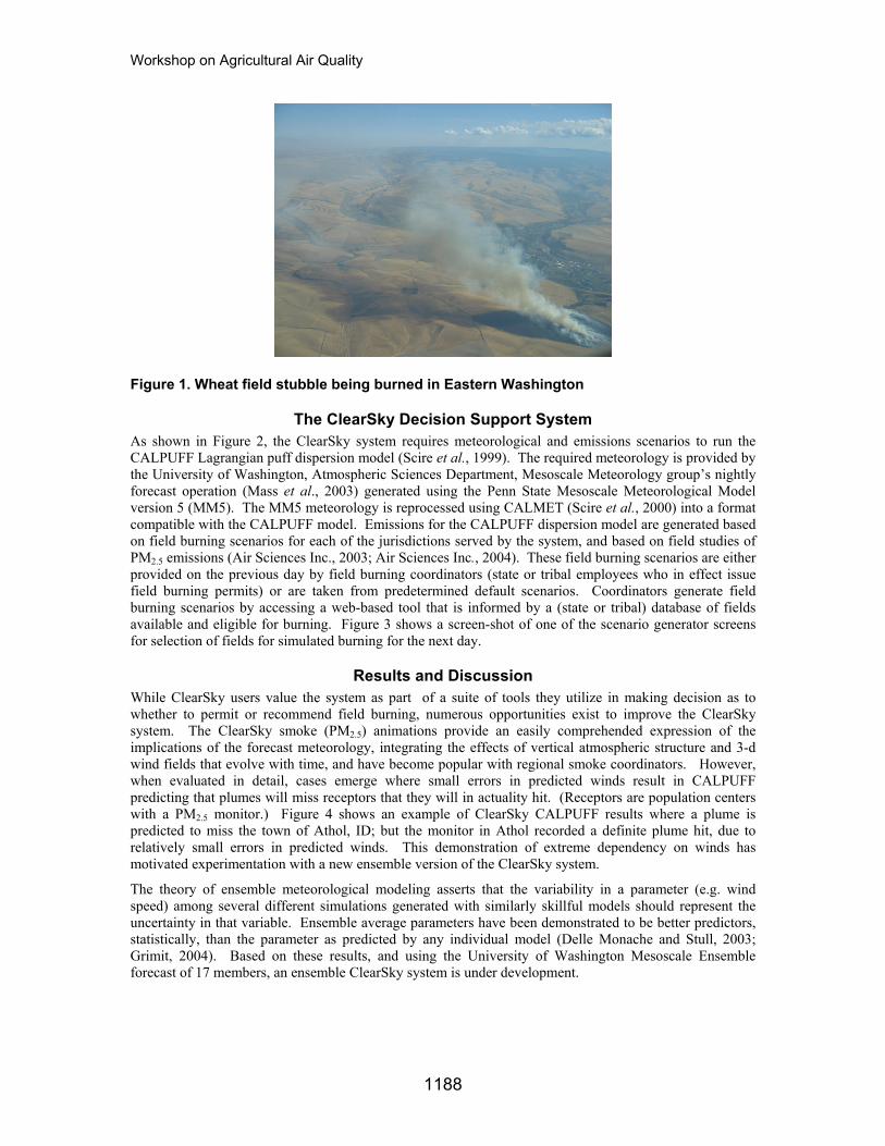
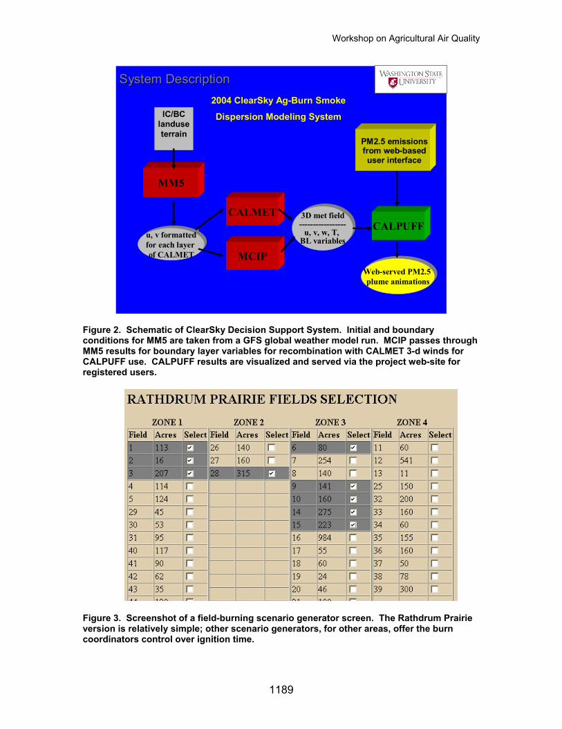
The ClearSky Decision Support System As shown in Figure 2, the ClearSky system requires meteorological and emissions scenarios to run the CALPUFF Lagrangian puff dispersion model (Scire et al., 1999). The required meteorology is provided by the University of Washington, Atmospheric Sciences Department, Mesoscale Meteorology group’s nightly forecast operation (Mass et al., 2003) generated using the Penn State Mesoscale Meteorological Model version 5 (MM5). The MM5 meteorology is reprocessed using CALMET (Scire et al., 2000) into a format compatible with the CALPUFF model. Emissions for the CALPUFF dispersion model are generated based on field burning scenarios for each of the jurisdictions served by the system, and based on field studies of PM2.5 emissions (Air Sciences Inc., 2003; Air Sciences Inc., 2004). These field burning scenarios are either provided on the previous day by field burning coordinators (state or tribal employees who in effect issue field burning permits) or are taken from predetermined default scenarios. Coordinators generate field burning scenarios by accessing a web-based tool that is informed by a (state or tribal) database of fields available and eligible for burning. Figure 3 shows a screen-shot of one of the scenario generator screens for selection of fields for simulated burning for the next day.
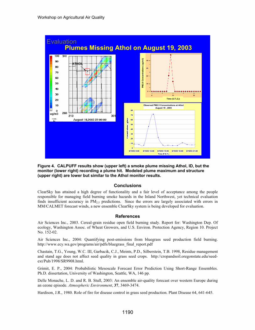
Results and Discussion While ClearSky users value the system as part of a suite of tools they utilize in making decision as to whether to permit or recommend field burning, numerous opportunities exist to improve the ClearSky system. The ClearSky smoke (PM2.5) animations provide an easily comprehended expression of the implications of the forecast meteorology, integrating the effects of vertical atmospheric structure and 3-d wind fields that evolve with time, and have become popular with regional smoke coordinators. However, when evaluated in detail, cases emerge where small errors in predicted winds result in CALPUFF predicting that plumes will miss receptors that they will in actuality hit. (Receptors are population centers with a PM2.5 monitor.) Figure 4 shows an example of ClearSky CALPUFF results where a plume is predicted to miss the town of Athol, ID; but the monitor in Athol recorded a definite plume hit, due to relatively small errors in predicted winds. This demonstration of extreme dependency on winds has motivated experimentation with a new ensemble version of the ClearSky system.
The theory of ensemble meteorological modeling asserts that the variability in a parameter (e.g. wind speed) among several different simulations generated with similarly skillful models should represent the uncertainty in that variable. Ensemble average parameters have been demonstrated to be better predictors, statistically, than the parameter as predicted by any individual model (Delle Monache and Stull, 2003; Grimit, 2004). Based on these results, and using the University of Washington Mesoscale Ensemble forecast of 17 members, an ensemble ClearSky system is under development.
1188
Workshop on Agricultural Air Quality
2004 ClearSky Ag-Burn Smoke
Dispersion Modeling System
MM5
CALMETCALPUFFu, v formatted
for each layer of CALMET
u, v formattedfor each layer of CALMET
3D met field-----------------
u, v, w, T, BL variables
3D met field-----------------
u, v, w, T, BL variables
Web-served PM2.5 plume animations
Web-served PM2.5 plume animations
IC/BClanduseterrain
MCIP
PM2.5 emissions from web-based user interface
System DescriptionSystem Description
Figure 2. Schematic of ClearSky Decision Support System. Initial and boundary conditions for MM5 are taken from a GFS global weather model run. MCIP passes through MM5 results for boundary layer variables for recombination with CALMET 3-d winds for CALPUFF use. CALPUFF results are visualized and served via the project web-site for registered users.
Figure 3. Screenshot of a field-burning scenario generator screen. The Rathdrum Prairie version is relatively simple; other scenario generators, for other areas, offer the burn coordinators control over ignition time.
1189
Workshop on Agricultural Air Quality
Plumes Missing Athol on August 19, 2003
Observed PM2.5 Concentrations at Athol August 19 , 2003
0
10
20
30
40
50
60
70
80
8/19/03 9:00 8/19/03 12:00 8/19/03 15:00 8/19/03 18:00 8/19/03 21:00Time (P.S.T.)
ATHOL
Time (U.T.Z.))
PM2.
5 Co
ncen
tratio
ns (u
g/m
3)
EvaluationEvaluation
Figure 4. CALPUFF results show (upper left) a smoke plume missing Athol, ID, but the monitor (lower right) recording a plume hit. Modeled plume maximum and structure (upper right) are lower but similar to the Athol monitor results.
Conclusions ClearSky has attained a high degree of functionality and a fair level of acceptance among the people responsible for managing field burning smoke hazards in the Inland Northwest, yet technical evaluation finds insufficient accuracy in PM2.5 predictions. Since the errors are largely associated with errors in MM/CALMET forecast winds, a new ensemble ClearSky system is being developed for evaluation.
References Air Sciences Inc., 2003. Cereal-grain residue open field burning study. Report for: Washington Dep. Of ecology, Washington Assoc. of Wheat Growers, and U.S. Environ. Protection Agency, Region 10. Project No. 152-02.
Air Sciences Inc., 2004: Quantifying post-emissions from bluegrass seed production field burning. http://www.ecy.wa.gov/programs/air/pdfs/bluegrass_final_report.pdf
Chastain, T.G., Young, W.C. III, Garbacik, C.J., Meints, P.D., Silberstein, T.B. 1998, Residue management and stand age does not affect seed quality in grass seed crops. http://cropandsoil.oregonstate.edu/seed-ext/Pub/1998/SR9908.html.
Grimit, E. P., 2004: Probabilistic Mesoscale Forecast Error Prediction Using Short-Range Ensembles. Ph.D. dissertation, University of Washington, Seattle, WA, 146 pp.
Delle Monache, L. D. and R. B. Stull, 2003: An ensemble air-quality forecast over western Europe during an ozone episode. Atmospheric Environment, 37, 3469-3474.
Hardison, J.R., 1980. Role of fire for disease control in grass seed production. Plant Disease 64, 641-645.
1190
Workshop on Agricultural Air Quality
Mass, C. F., Albright, M., Ovens, D., Steed, R., Grimit, E., Eckel, T., Lamb, B., Vaughan, J., Westrick, K., Storck, P., Colman, B., Hill, C., Maykut, N., Gilroy, M., Ferguson, S. A., Yetter, J., Sierchio, J. M., Bowman, C., Stender, R., Wilson, R. and Brown, W., 2003: Regional Environmental Prediction over the Pacific Northwest, Bull. Amer. Meteor. Soc., 84,1353-1366.
Scire, J.S., Robe, F.R., Fernau, M.E., Yamartino, R.J., 2000. A users guide for the CALMET meteorological model (Version 5). Earth Tech Inc.
Scire, J.S., Strimaitis, D.G., Yamartino, R.J., 1999. A users guide for the CALPUFF dispersion model (Version 5). Earth Tech Inc.
1191
Workshop on Agricultural Air Quality
Nitrogen Losses from Organic Housing Systems for Fattening Pigs
Hans von Wachenfelt and Knut-Håkan Jeppsson Department of Agricultural Biosystems and Technology, Swedish University of Agricultural
Sciences, P.O. Box 86, S- 230 53 Alnarp, Sweden. Phone: +46 40 415485. Fax: +46 40 415475. E-mail: [email protected]
Abstract In Sweden, organic pigs are generally produced according to the rules of the economic association KRAV. According to these rules, the pigs shall be held outdoors on pasture during summer period, whereas indoor housing with access to an outdoor pen is permitted only during winter period. The EU permitted systems for organic slaughter pig production with indoor housing and year round access to an outdoor pen with solid flooring and without additional access to plant covered soil are not common in Sweden. The aim of this project is to analyse and describe the consequences different production systems will have on manure management and nutrient balances for organic pig production. A research facility with four housing alternatives for organic fattening pig production has been built at the research farm Odarslöv situated in the south of Sweden. Inside, the housing alternatives are either deep litter or straw flow both combined with slatted floor area. Outside, two of the housing alternatives are based on access to only an outdoor pen with solid flooring, and the other two alternatives also have a yard with pasture during summer period. Nitrogen balances are calculated for the four housing alternatives. “Input“ nitrogen in the form of feed, roughage and straw are determined via feed utilisation, feed composition and straw usage, respectively. The “output“ nitrogen are determined by registration of pig growth, calculation of nitrogen contained in the pigs at slaughter, nitrogen in produced manure and urine, and the estimation of nitrogen accumulated on pasture. Each deep litter bed is weighed at cleaning and samples are analysed. Amount of manure from the slatted area is weighed each fortnight and analysed. Liquid manure from outdoor pens is weighed each fortnight and analysed. Soil tests to determine manure distribution and amounts in the yards are obtained before and after the growing period. For each housing alternative, the results will obtain a total picture of the nitrogen balance at pen level. The difference between “input” and “output” total nitrogen is mainly due to ammonia emission and nitrogen leaching. Preliminary results have shown that the pen balance method has a preliminary error of about ± 10%. The nitrogen loss from the pen alternatives is high, 2.5 - 3.0 kg per pig, probably depending on fodder nutrient constitution and large total pen area.
Introduction In Sweden, organic pigs are generally produced according to the standards of the economic association KRAV (Krav, 2006). According to these standards, the pigs shall be held outdoors on pasture during summer period, whereas indoor housing with access to an outdoor pen is permitted only during winter period. The EU permitted systems for organic slaughter pig production (CEC, 1999), with indoor housing and year round access to an outdoor pen with solid flooring and without additional access to plant covered soil, are not common in Sweden. The aim of this paper is to analyse and describe the consequences different organic production systems will have on manure management and nitrogen losses from organic pig production.
In Sweden 84% of the total ammonia emission origins from agriculture, whereof 58% from cattle/milk production, 14% from pig production, 6% from horses and 5% from poultry production. The animal production sources of ammonia can be divided in 22% from animal houses, 34% from manure storage, 36% from manure spreading and 8% from pastures (SCB, 2003). In 1999 the Swedish Government adopted a new policy setting 15 national environmental goals. Out of these, “Only natural acidification” deals with ammonia emission from the agricultural sector. The aim is to reduce the ammonia emission from agriculture by 15% in 2010 from the level of 1995 (Swedish Environmental Protection Agency, 2005).
During the past 20 years our knowledge about ammonia emissions from agriculture has improved. Many researchers have investigated factors affecting these emissions and measures to reduce emissions from livestock buildings, manure storage and spreading. In the literature, the following factors is presented to influence the ammonia emissions in livestock buildings; nitrogen content of the manure, adsorption of
1192
Workshop on Agricultural Air Quality
ammoniacal nitrogen, urease activity, pH of the manure, manure temperature, C/N ratio of the manure, manure surface area, air movements in the building, air velocity above the manure surface, ventilation rate through the building, air temperature and the availability of oxygen in the manure (Jeppsson, 2000). In organic pig production, the large pen area per animal due to the aim for better animal welfare could be in conflict with the aim to minimize the nutrient losses. An outside yard and a pasture may increase the ammonia emission. Furthermore, the content in the organic fodder may cause additional nitrogen content of the manure compared with conventional pig production.
Material and Methods A research facility with four housing alternatives for organic fattening pig production has been built at the research farm Odarslöv situated in the south of Sweden. Inside, the housing alternatives are either deep litter or straw flow both combined with a slatted floor area. Outside, the two inside housing alternatives have access to an outdoor pen with solid flooring. Furthermore, the outside housing alternatives have either access or no access to a yard with pasture during summer period.
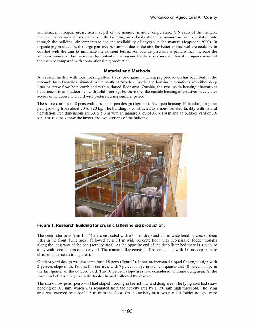
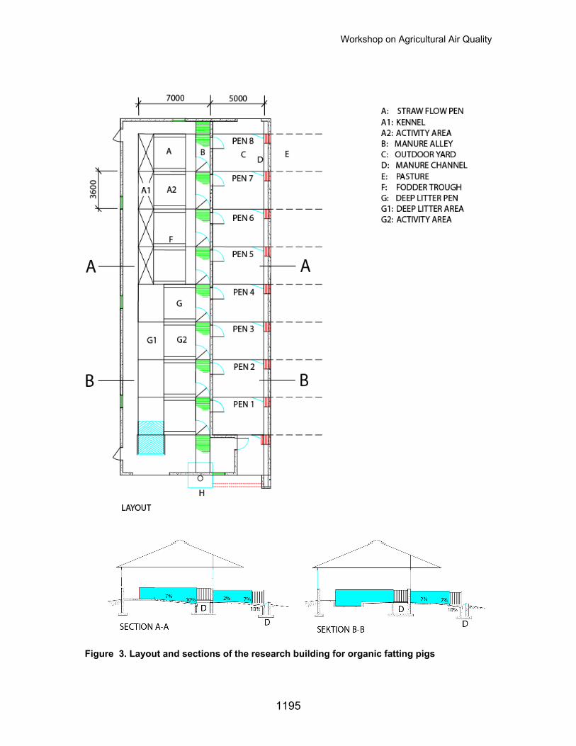
The stable consists of 8 pens with 2 pens per pen design (figure 1). Each pen housing 16 finishing pigs per pen, growing from about 20 to 120 kg. The building is constructed as a non-insulated facility with natural ventilation. Pen dimensions are 3.6 x 5.6 m with an manure alley of 3.6 x 1.4 m and an outdoor yard of 3.6 x 5.0 m. Figure 3 show the layout and two sections of the building.
Figure 1. Research building for organic fattening pig production.
The deep litter pens (pen 1 – 4) are constructed with a 0.4 m deep and 2.5 m wide bedding area of deep litter in the front (lying area), followed by a 3.1 m wide concrete floor with two parallel fodder troughs along the long way of the pen (activity area). At the opposite end of the deep litter bed there is a manure alley with access to an outdoor yard. The manure alley consists of concrete slats with 1,0 m deep manure channel underneath (dung area).
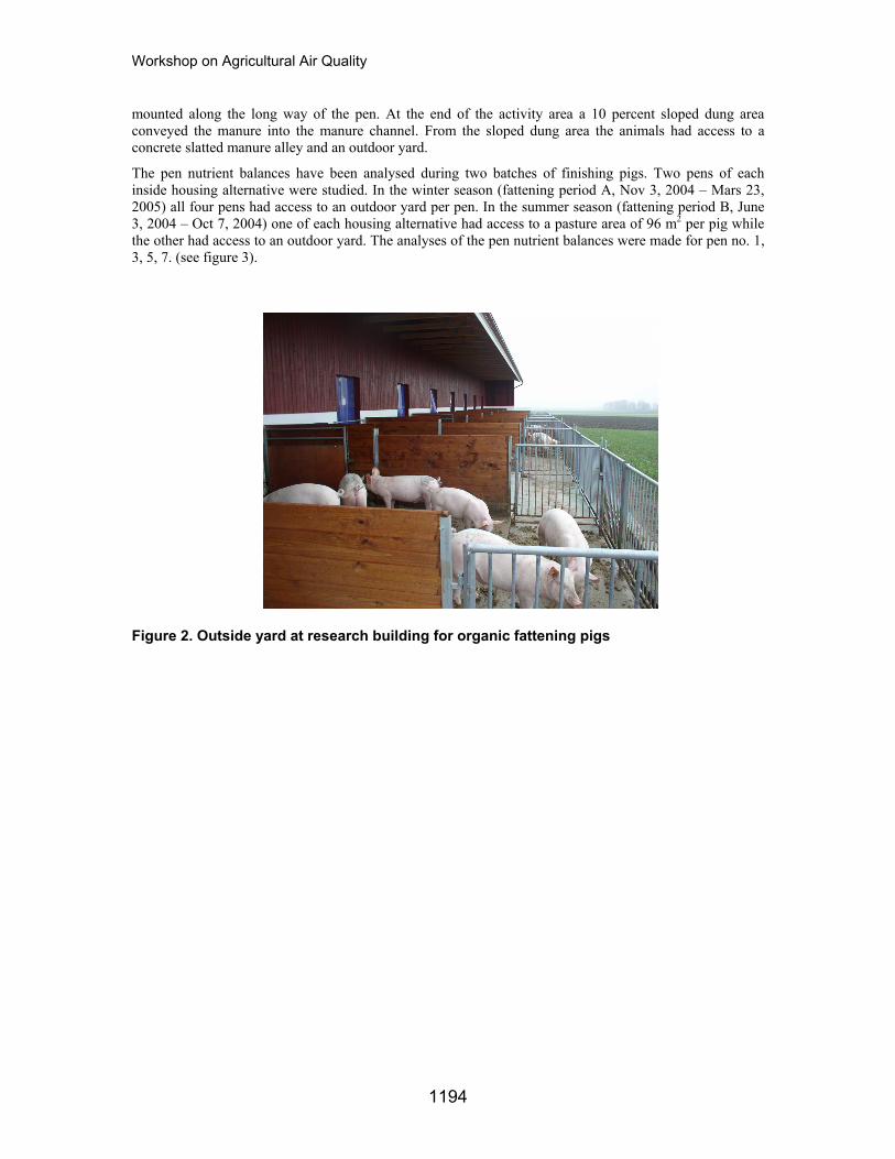
Outdoor yard design was the same for all 8 pens (figure 2). It had an increased sloped flooring design with 2 percent slope in the first half of the area, with 7 percent slope in the next quarter and 10 percent slope in the last quarter of the outdoor yard. The 10 percent slope area was considered as prime dung area. At the lower end of this dung area a flushable channel collected the manure.
The straw flow pens (pen 5 – 8) had sloped flooring in the activity and dung area. The lying area had straw bedding of 100 mm, which was separated from the activity area by a 150 mm high threshold. The lying area was covered by a roof 1,5 m from the floor. On the activity area two parallel fodder troughs were
1193
Workshop on Agricultural Air Quality
mounted along the long way of the pen. At the end of the activity area a 10 percent sloped dung area conveyed the manure into the manure channel. From the sloped dung area the animals had access to a concrete slatted manure alley and an outdoor yard.
The pen nutrient balances have been analysed during two batches of finishing pigs. Two pens of each inside housing alternative were studied. In the winter season (fattening period A, Nov 3, 2004 – Mars 23, 2005) all four pens had access to an outdoor yard per pen. In the summer season (fattening period B, June 3, 2004 – Oct 7, 2004) one of each housing alternative had access to a pasture area of 96 m2 per pig while the other had access to an outdoor yard. The analyses of the pen nutrient balances were made for pen no. 1, 3, 5, 7. (see figure 3).
Figure 2. Outside yard at research building for organic fattening pigs
1194
Workshop on Agricultural Air Quality
Figure 3. Layout and sections of the research building for organic fatting pigs
1195
Workshop on Agricultural Air Quality
Input Values of Pen Nutrient Balance Following parameters were regarded as significant input values in the nutrient balance for organic finishing pigs at pen level.
• Animal content of NPK (nitrogen, phosphorous, potassium) • Fodder content of NPK during finishing period • Grazing intake from pasture • Hay and silage content of NPK • Straw content of NPK
The input values of animal NPK per pen were based on entry date, weight, animal number, and the percentage NPK in body (Simonson, 1990). Fodder, hay, silage and straw values were all entered based on entry date, animal number, animal consumption, total solid content and NPK content from analysis.
Dry fodder pellets were given twice a day with time controlled water access. An all time access water nipple was situated in the manure alley in each pen. The fodder ration was volume metric measured and daily controlled by strain gauge sensors mounted at each leg of the fodder silo. Silage or hay was given at the top of the outdoor yard in a silage-hay bin. The amounts of straw and silage-hay were based on number of “loafs” of a bale per day, and regular measurements of loaf weights.
Output Values The output values were:
• Animal content of NPK • Liquid manure content of NPK, indoors and outdoors • Straw bedding content of NPK
The output animal NPK per pen value consisted of animal number, weight at slaughter and the percentage NPK in body (Simonson, 1990). The amounts of liquid manure and samples for NPK concentration were measured at a 14 day interval and as soon as the animals had left the building the amounts of the straw bedding were weighed and sampled for NPK analysis.
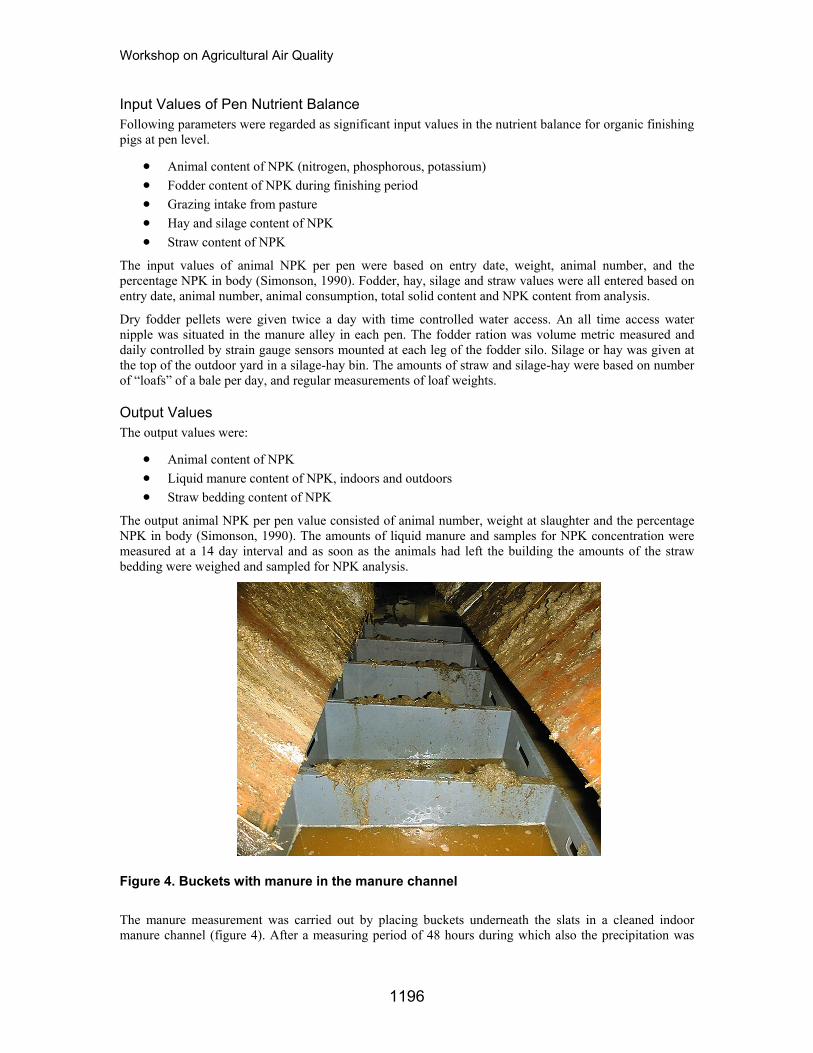
Figure 4. Buckets with manure in the manure channel
The manure measurement was carried out by placing buckets underneath the slats in a cleaned indoor manure channel (figure 4). After a measuring period of 48 hours during which also the precipitation was
1196
Workshop on Agricultural Air Quality
measured, all buckets per pen in the indoor manure channel were weighed on an electronic scale (Flint AB). The scale was calibrated by loading and unloading weights up to 230 kg and the fit of the regression curve was by a R2 = 0, 9983. The manure in the weighed buckets was emptied into a 100 litre barrel, thoroughly mixed and then sampled by intermittent sampling into one sample per pen when emptying the barrel. The same procedure was carried out for all four pens for the indoor manure channel.
In the outdoor yard both the manure channel and outdoor yard was cleaned before the buckets were put in place. After a measuring period of 48 hours, the outdoor yards were cleaned and the manure collected, measured and sampled together with the buckets from the outdoor manure channel following the same procedure as for the indoor manure channel.
Preliminary Results and Discussion The pen nutrient balances for fattening period A show good agreements for total-P and total-K (Table 1). The difference between input and output is between ± 3 kg except for P in pen 3. The small difference in total-P and total-K shows that the nutrient balance method have an error of about ± 10%. In fattening period B, the differences in total-P and total-K for the pens with no access to pasture (pen 3 and 7) is slightly higher than during fattening period A, between 2.7 and 3.5 kg for total-P and 3.4 and 4.7 kg for total-K. This could indicate a systematic error and will be further examined.
The difference in total-N is between 40.6 and 54.9 kg per pen, during fattening period A. The difference is mainly due to ammonia emission from the pen. Thus, between 48 and 68% of the total-N in the manure is lost. No statistical difference between the two types of pens can be made but the results indicate an N loss of 50 kg from the straw flow pen (pen 5 and 7). The N loss from the pen with deep litter as lying area is 40 kg with “clean” bedding (pen 3) and 55 kg with “dirtier” bedding.
The cleanliness of the lying area with deep litter is crucial for the ammonia emission. A pen with “clean” deep litter seems to have a lower ammonia emission than the straw flow pens but with a “dirty” deep litter the N loss is about 15 kg higher and exceeds the straw flow pen. The N loss of about 50 kg corresponds with an ammonia emission of about 10 – 12 g day-1 m-2 during the fattening period. The ammonia emission corresponds with the results by Ivanova-Peneva & Aarnink (2005) investigating the ammonia emission from Dutch organic pig production. The ammonia emission was 1.9 – 2.7 g day-1 m-2 from clean pen areas and 11.4 - 13.3 g day-1 m-2 from fouled areas. The ammonia emission also corresponds with results from deep litter beds for conventional growing pigs, average 10 g day-1 m-2, by Jeppsson (1998) and from outside yards for organic pig production, 9 – 12 g day-1 m-2 by von Wachenfelt (2002). The results show that the N loss is high, 3 kg per pig in average, probably depending on fodder nutrient constitution and large pen area per pig (2.6 m2 per pig).
During fattening period B (Table 2), the pigs in pen 3 and 7 had no access to pasture. The difference in total-N is just below 40 kg corresponding to about 60% loss of total-N in the manure. From these pens the difference in nitrogen is mainly the ammonia emission from the pens. The N loss is 2.5 kg per pig.
The measured amount of NPK in the manure from the pens with access to pasture, pen 1 and 5, are lower than from the pens without access (pen 3 and 7). This indicates that some of the faeces and urine land in the pasture. Calculations preliminary show that 43 and 17% of the manure land on the pasture corresponding to 12 and 4 kg total-N, 8 and 4 kg total-P, and 11 and 4 kg total-K, respectively. The N-loss is 43 kg corresponding to 60% loss of total-N in the manure for pen 1 and 5, respectively.
1197
Workshop on Agricultural Air Quality
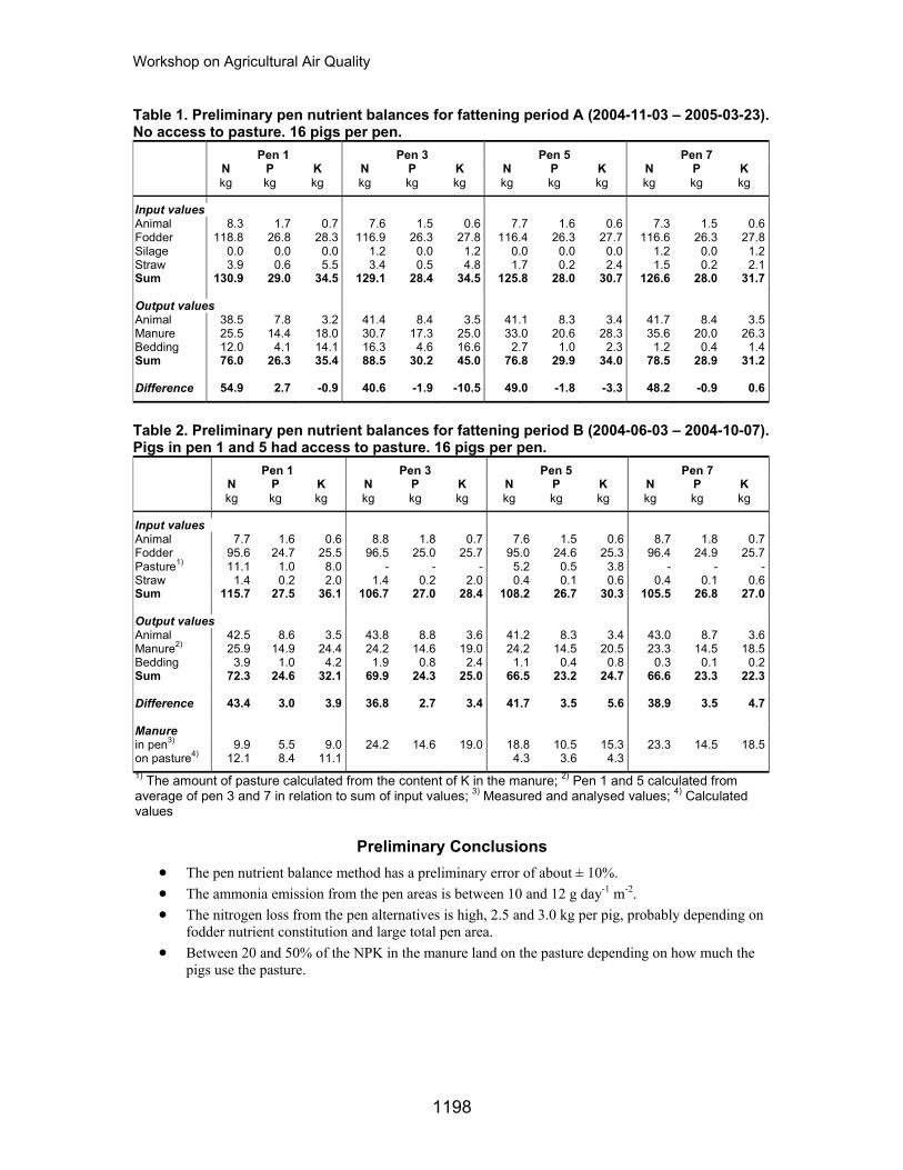
Table 1. Preliminary pen nutrient balances for fattening period A (2004-11-03 – 2005-03-23). No access to pasture. 16 pigs per pen.
Pen 1 Pen 3 Pen 5 Pen 7 N P K N P K N P K N P K kg kg kg kg kg kg kg kg kg kg kg kg
Input values Animal 8.3 1.7 0.7 7.6 1.5 0.6 7.7 1.6 0.6 7.3 1.5 0.6Fodder 118.8 26.8 28.3 116.9 26.3 27.8 116.4 26.3 27.7 116.6 26.3 27.8Silage 0.0 0.0 0.0 1.2 0.0 1.2 0.0 0.0 0.0 1.2 0.0 1.2Straw 3.9 0.6 5.5 3.4 0.5 4.8 1.7 0.2 2.4 1.5 0.2 2.1Sum 130.9 29.0 34.5 129.1 28.4 34.5 125.8 28.0 30.7 126.6 28.0 31.7 Output values Animal 38.5 7.8 3.2 41.4 8.4 3.5 41.1 8.3 3.4 41.7 8.4 3.5Manure 25.5 14.4 18.0 30.7 17.3 25.0 33.0 20.6 28.3 35.6 20.0 26.3Bedding 12.0 4.1 14.1 16.3 4.6 16.6 2.7 1.0 2.3 1.2 0.4 1.4Sum 76.0 26.3 35.4 88.5 30.2 45.0 76.8 29.9 34.0 78.5 28.9 31.2 Difference 54.9 2.7 -0.9 40.6 -1.9 -10.5 49.0 -1.8 -3.3 48.2 -0.9 0.6
Table 2. Preliminary pen nutrient balances for fattening period B (2004-06-03 – 2004-10-07). Pigs in pen 1 and 5 had access to pasture. 16 pigs per pen.
Pen 1 Pen 3 Pen 5 Pen 7 N P K N P K N P K N P K kg kg kg kg kg kg kg kg kg kg kg kg
Input values Animal 7.7 1.6 0.6 8.8 1.8 0.7 7.6 1.5 0.6 8.7 1.8 0.7Fodder 95.6 24.7 25.5 96.5 25.0 25.7 95.0 24.6 25.3 96.4 24.9 25.7Pasture1) 11.1 1.0 8.0 - - - 5.2 0.5 3.8 - - -Straw 1.4 0.2 2.0 1.4 0.2 2.0 0.4 0.1 0.6 0.4 0.1 0.6Sum 115.7 27.5 36.1 106.7 27.0 28.4 108.2 26.7 30.3 105.5 26.8 27.0 Output values Animal 42.5 8.6 3.5 43.8 8.8 3.6 41.2 8.3 3.4 43.0 8.7 3.6Manure2) 25.9 14.9 24.4 24.2 14.6 19.0 24.2 14.5 20.5 23.3 14.5 18.5Bedding 3.9 1.0 4.2 1.9 0.8 2.4 1.1 0.4 0.8 0.3 0.1 0.2Sum 72.3 24.6 32.1 69.9 24.3 25.0 66.5 23.2 24.7 66.6 23.3 22.3 Difference 43.4 3.0 3.9 36.8 2.7 3.4 41.7 3.5 5.6 38.9 3.5 4.7 Manure in pen3) 9.9 5.5 9.0 24.2 14.6 19.0 18.8 10.5 15.3 23.3 14.5 18.5on pasture4) 12.1 8.4 11.1 4.3 3.6 4.3 1) The amount of pasture calculated from the content of K in the manure; 2) Pen 1 and 5 calculated from average of pen 3 and 7 in relation to sum of input values; 3) Measured and analysed values; 4) Calculated values
Preliminary Conclusions • The pen nutrient balance method has a preliminary error of about ± 10%. • The ammonia emission from the pen areas is between 10 and 12 g day-1 m-2. • The nitrogen loss from the pen alternatives is high, 2.5 and 3.0 kg per pig, probably depending on
fodder nutrient constitution and large total pen area. • Between 20 and 50% of the NPK in the manure land on the pasture depending on how much the
pigs use the pasture.
1198
Workshop on Agricultural Air Quality
References CEC. 1999. Council Regulation on Organic Livestock Production 1804/1999 of 19 July 1999 Supplementing Regulation (EEC) No. 2092/1991. Commission of the European Communities, Brussels
Ivanova-Peneva, S.G. & Aarnink, A.J.A. 2005. Ammonia emissions in organic pig production. Bau, Technik und Umwelt in der landwirtschaftlichen Nutztierhaltung, Braunschweig
Jeppsson, K-H. 1998. Ammonia emission from different deep-litter materials for growing-finishing pigs. Swedish J. agric. Res. 28: 197-206
Jeppsson, K-H. 2000. Aerial Environment in Uninsulated Livestock Buildings - Release of ammonia, carbon dioxide and water vapour from deep litter and effect of solar heat load on the interior thermal environment. Doctoral thesis, Swedish University of Agricultural Sciences, Agraria 245. Alnarp.
Krav. 2006. Krav´s regler [Krav´s standards]. Krav, Uppsala (in Swedish)
Simonson, A. 1990. Omsättning av kväve, fosfor och kalium i svinproduktionen [Transformation of nitrogen, phosphorous and potassium in pig production] Sveriges lantbruksuniversitet. Fakta Husdjur nr. 1, 1990. Uppsala (in swedish)
Swedish Environmental Protection Agency. 2005. Swedens environmental objectives- for the sake of our children - deFacto 2005. (ISBN 91-620-1240-1)
http://www.miljomal.nu (February 14, 2006)
von Wachenfelt, H. 2002. Betesdrift och utomhusytor för ekologiska svin [Organic pig production on pasture and outdoor areas], Specialmeddelande 236. Inst f jordbrukets biosystem och teknologi, SLU, Alnarp (in Swedish with summary in English)
1199
Workshop on Agricultural Air Quality
Greenhouse Gas Emissions from Stored Animal Manure in Cold Climates
K.-H. Park1, C. Wagner-Riddle1, R. Gordon2, V. Glass2
1Department of Land Resource Science, University of Guelph, Guelph, ON, N1G 2W1, Canada 2Department of Engineering, Nova Scotia Agricultural College, Truro, NS, B2N 5E3, Canada
Abstract Current global warming has been linked to increases in greenhouse gas (GHG) concentrations. Animal manure is an important source of anthropogenic GHG, mostly of methane (CH4) and nitrous oxide (N2O), but environmental and animal factors affect and lend uncertainties to GHG emissions estimates from these sources. Country-specific emission estimates of these GHG can be obtained using IPCC 2000 guidelines, or suggested improvements, such as the USEPA approach for CH4 emissions, which is based on monthly air temperature (Tair). These approaches have not been validated against measured CH4 and N2O fluxes for liquid swine and dairy manure storage in cold climates due to the scarcity of year-round studies. A four-tower micrometeorological mass balance method was used at three swine farms and two dairy farms in Ontario, Canada (annual Tair <10°C), from July 2000 to July 2003. Methane and N2O concentrations were measured using two tunable diode laser trace gas analyzer. Mean N2O fluxes were not significantly different from zero. Mean CH4 fluxes obtained from half-hourly data varied between 4.6 x 10⁻³ to 1.05 mg m-2 s-1 for swine and 3.7 x 10⁻² to 0.1 mg m-2 s-1 for dairy. The methane conversion factor for liquid swine manure stored in concrete tanks derived from measured fluxes was 0.23, comparable to the USEPA derived values of 0.22 – 0.25, but much lower than the IPCC recommended value for cold climates (0.39).
Introduction Agricultural practices in Canada and globally have been identified as contributors to greenhouse gas emissions. In 1999, agriculture in Canada contributed 8.7% (or 61Mt) of total greenhouse gas emissions, an increase from 3.1% in 1990 (Government of Canada, 2001). The increased popularity of liquid manure handling systems at intensive livestock operations has raised environmental concerns regarding greenhouse gas emissions (Honeyman, 1996; Miner, 1999). Manure storage of this sort can occur for several months, leading to anaerobic decomposition and mostly the release of CH4. IPCC (2000) recommends non-invasive and year-round measurements of GHG emissions in production systems, in order to reduce the large uncertainties in emission factors used for calculating national GHG emission inventories. The Micrometeorological Mass Balance (MMB) method, a non-invasive measurement technique, is suitable for heterogeneous source distributions and/or elevated sources such as waste storage sites (Denmead et al., 1998).
The research reported here was carried out to address some of the uncertainties in greenhouse gas emissions from stored liquid swine and dairy manure. The objectives of this research were as follows: 1) to quantify N2O and CH4 emissions from manure storage systems in situ; 2) to convert measured greenhouse gas emissions to emission factors and compare these with IPCC emission factor estimates.
Materials and Method Three swine farms (Arkell, Jarvis, and Guelph) and one dairy farm (Bright) in Southern Ontario were chosen for this study. A mobile instrumentation trailer was moved between these sites to carry out measurements from June 2000 to July 2003. The micrometeorological mass balance method was used to measure CH4 and N2O fluxes at the four farms (Wagner-Riddle et al., 2006). This method requires gas concentration, wind speed and wind direction for calculations. The wind direction and wind speed were recorded using a mast mounted on the fence surrounding the manure tank. Each mast had four cup anemometers (F460, Climatronics Corp., Newton, PA) recording the wind speed at 25, 100, 200 and 350 cm above the concrete wall of the manure tanks. A wind vane (R.M. Young, Model 05102, Traverse, MI) was mounted on top of each mast (450 cm), to record the wind direction. Mean wind speed was recorded over 30 minutes, and mean wind direction was recorded over 5 minutes at Arkell and over 1 minute at the other sites. Four towers were placed around the tanks to ensure measurements of upwind and downwind air concentrations occurred during most periods. Each tower was equipped with four air sample intakes,
1200
Workshop on Agricultural Air Quality
placed at 25, 100, 200 and 350 cm above the manure tank wall. A vacuum pump (RA 0021, Busch, Virginia Beach, VA) was used to draw the samples from the intakes to the trailer. CH4 and N2O concentrations were quantified using two Tunable Diode Laser Trace Gas Analyzers (TDLTGA). Before reaching the TDLTGA the gas samples passed through a valve manifold unit (Campbell Scientific, Logan, Utah). This unit, capable of handling all 16 intakes, enabled the switching between the different sample intakes and the two analysers. As only one sample could be passed through each TDLTGA at any given time, the samples not going to the analysers were passed through a by-pass manifold and directed to the pump. CH4 and N2O fluxes were calculated using the mass balance method with the wind and concentration data as inputs. The mean fetch was calculated from 5- or 1-minute fetch values obtained from 5- or 1-minute mean wind direction data and averaged over 30 minutes.
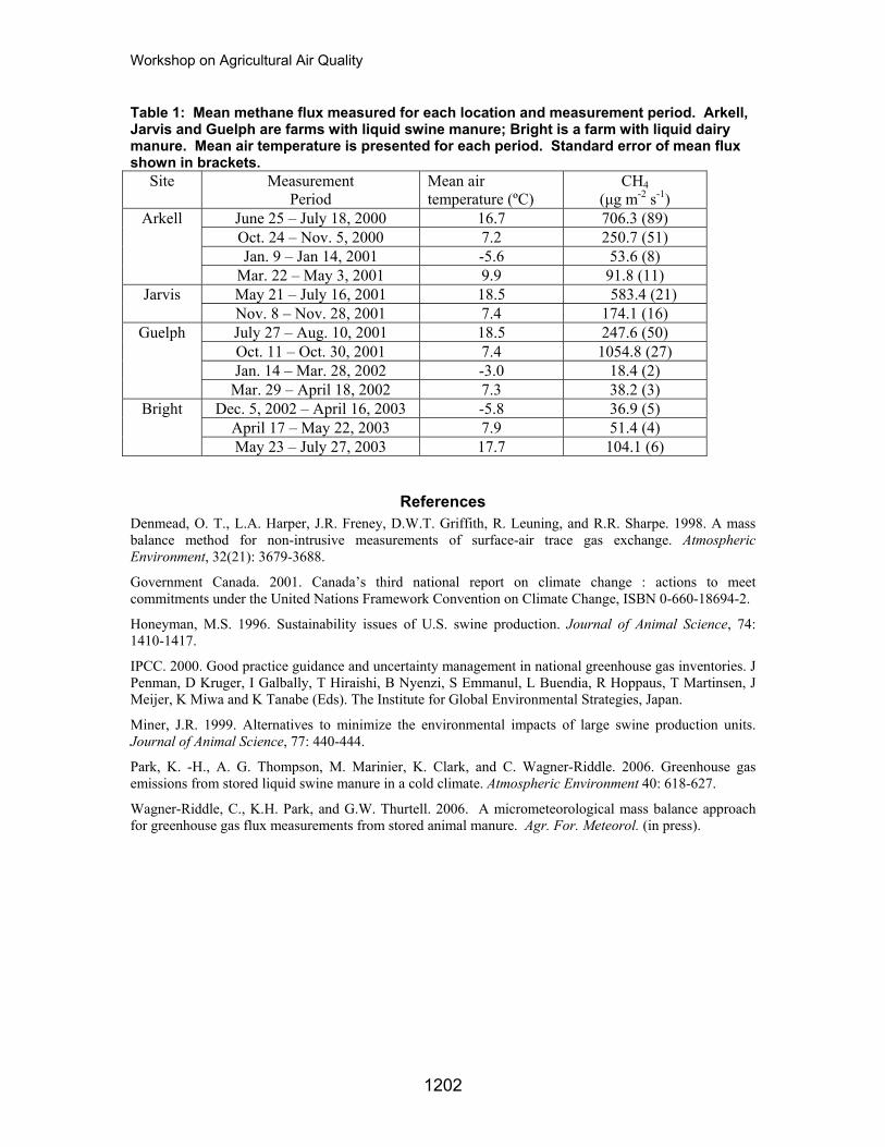
Results Nitrous oxide fluxes were small with mean value for several of the measurement period not significantly different from zero (P<0.05; data not shown). Methane fluxes at all of the sites were highly variable in time, a result of seasonal variation in temperature (Table 1). Methane fluxes from liquid swine manure were >0.5 mg m-2 s-1 during the warmest measurement periods, while fluxes from liquid dairy manure were much ~0.1 mg m-2 s-1, as expected due to the lower CH4 production potential of the latter.
As the measurements of CH4 fluxes from liquid swine manure at the three studied sites comprised a period > 1 year, comparison with annual emission factors using the IPCC and USEPA approaches was possible. Measured CH4 flux means were scaled using storage tank surface area and number of animals at each site. Consistent over-prediction of monthly CH4 emissions for the January to April period when using manure temperature in the USEPA approach were observed due to formation of an ice layer which suppressed emission (Park et al., 2006). However, for GHG inventory purposes the USEPA approach yielded quite acceptable results, with annual EF of 6.5, and 7.5 kg CH4 head-1 yr-1 with use of air temperature >7.5 oC, respectively, compared to the measured EF of 6.7 kg CH4 head-1 yr-1. Methane EF using IPCC Tier 2 for the three sites averaged 11.5 kg CH4 head-1 yr-1, an over-prediction consistent with the use of MCF = 0.39, when compared to the value derived from measurements (MCF = 0.23) and the USEPA derived values (MCF = 0.22 – 0.25).
Conclusions The micrometeorological mass balance method, a non-intrusive flux measurement method, was used in the quasi-continuous measurement of GHG fluxes from stored liquid manure over ~ 2 years. Nitrous oxide fluxes were negligible for most of the measurement period. The annual CH4 EF derived from our data was within ~10% of EF based on the USEPA approach. But, the measured EF was only ~60% of the EF derived using IPCC Tier 2. This discrepancy is due to an MCF factor (=0.39) recommended for climates with mean annual temperature <15 oC, which is clearly an over-estimate for cold climates (MCF<0.25).
1201
Workshop on Agricultural Air Quality
Table 1: Mean methane flux measured for each location and measurement period. Arkell, Jarvis and Guelph are farms with liquid swine manure; Bright is a farm with liquid dairy manure. Mean air temperature is presented for each period. Standard error of mean flux shown in brackets.
Site Measurement Period
Mean air temperature (ºC)
CH4(µg m-2 s-1)
June 25 – July 18, 2000 16.7 706.3 (89) Oct. 24 – Nov. 5, 2000 7.2 250.7 (51) Jan. 9 – Jan 14, 2001 -5.6 53.6 (8)
Arkell
Mar. 22 – May 3, 2001 9.9 91.8 (11) May 21 – July 16, 2001 18.5 583.4 (21) Jarvis Nov. 8 – Nov. 28, 2001 7.4 174.1 (16) July 27 – Aug. 10, 2001 18.5 247.6 (50) Oct. 11 – Oct. 30, 2001 7.4 1054.8 (27) Jan. 14 – Mar. 28, 2002 -3.0 18.4 (2)
Guelph
Mar. 29 – April 18, 2002 7.3 38.2 (3) Dec. 5, 2002 – April 16, 2003 -5.8 36.9 (5)
April 17 – May 22, 2003 7.9 51.4 (4) Bright
May 23 – July 27, 2003 17.7 104.1 (6)
References Denmead, O. T., L.A. Harper, J.R. Freney, D.W.T. Griffith, R. Leuning, and R.R. Sharpe. 1998. A mass balance method for non-intrusive measurements of surface-air trace gas exchange. Atmospheric Environment, 32(21): 3679-3688.
Government Canada. 2001. Canada’s third national report on climate change : actions to meet commitments under the United Nations Framework Convention on Climate Change, ISBN 0-660-18694-2.
Honeyman, M.S. 1996. Sustainability issues of U.S. swine production. Journal of Animal Science, 74: 1410-1417.
IPCC. 2000. Good practice guidance and uncertainty management in national greenhouse gas inventories. J Penman, D Kruger, I Galbally, T Hiraishi, B Nyenzi, S Emmanul, L Buendia, R Hoppaus, T Martinsen, J Meijer, K Miwa and K Tanabe (Eds). The Institute for Global Environmental Strategies, Japan.
Miner, J.R. 1999. Alternatives to minimize the environmental impacts of large swine production units. Journal of Animal Science, 77: 440-444.
Park, K. -H., A. G. Thompson, M. Marinier, K. Clark, and C. Wagner-Riddle. 2006. Greenhouse gas emissions from stored liquid swine manure in a cold climate. Atmospheric Environment 40: 618-627.
Wagner-Riddle, C., K.H. Park, and G.W. Thurtell. 2006. A micrometeorological mass balance approach for greenhouse gas flux measurements from stored animal manure. Agr. For. Meteorol. (in press).
1202
Workshop on Agricultural Air Quality
Aerobic Composting as a Strategy for Mitigation of Greenhouse Gas Emissions from Swine Manure
K.-H. Park1, K. A. Kumudinie1, C. Wagner-Riddle1, R. Fleming2, M. MacAlpine2
1Department of Land Resource Science, University of Guelph, Guelph, Ont., N1G 2W1, Canada 2Ridgetown College of Agricultural Technology, University of Guelph,
Ridgetown, Ont., N0P 2C0, Canada Abstract Agriculture has been recognized as a major contributor of greenhouse gases, releasing both nitrous oxide and methane. The collection and storage of livestock manure has been identified as a significant source of greenhouse gases. New strategies are being investigated as to their potential for reducing emissions of nitrous oxide and methane. Aerobic composting of the manure before storage is believed to have potential for mitigating the release of greenhouse gases, but research has not fully quantified emissions during the active and curing phases of this process. In addition, nitrous oxide emissions from soils after the field application of composted versus untreated liquid swine manure has not been considered in past studies. Here we report on two studies measuring: 1) methane and nitrous oxide emissions during the active in-vessel and curing phase of composting liquid swine manure with straw, and 2) nitrous oxide emissions after field application of untreated liquid swine manure in comparison to composted liquid swine manure, carried out in Ontario, Canada. A mega-chamber approach and eight large non-steady chambers were used to quantify CH4 and N2O fluxes during composting. A flux-gradient method was used to measure N2O fluxes from field plots after application of composted and untreated manure in fall 2004 until corn planting in spring 2005. A tunable diode laser trace gas analyzer was used in both studies to measure gas concentrations. An analysis comparing GHG emissions during manure treatment (aerobic composting) through field application vs. non-treatment will be presented.
Introduction Agriculture has been recognized as a major contributor of greenhouse gases (GHG), releasing both nitrous oxide and methane (Houghton et al., 2001; Mosier et al., 1998). The collection and storage of livestock manure has been identified as a significant source of methane and nitrous oxide (Rotmans et al., 1992; Khalil and Rasmussen, 1992). Treatment strategies, such as aerobic composting of the manure before storage, are being investigated as to their potential for stabilizing organic residuals and the fertilizer value for land application (Zeman et al., 2002). This treatment is also believed to have potential for mitigating the release of greenhouse gases (Thompson et al., 2004), but research has not fully quantified emissions during the active and curing phases of this process. In addition, nitrous oxide emissions from soils after the field application of composted versus untreated liquid swine manure have not been considered in past studies. The objectives of this study were: 1) to quantify methane (CH4) and nitrous oxide (N2O) fluxes during the active in-vessel and curing phase of composting liquid swine manure with straw, 2) to quantify N2O fluxes after field application of untreated liquid swine manure in comparison to composted liquid swine manure, and 3) to compare overall GHG emissions from treated and untreated liquid swine manure.
Materials and Method
Composting Measurements of CH4 and N2O fluxes were carried out at the composting facility of the Ridgetown College, Ontario. The facility utilized an in-vessel composting system, which consisted of three open-ended concrete channels (15.2 m long, 2.2 m wide and 1.6 m deep) housed in a covered building. The floors of the compost channels contained sub-channels connected to fans, which aerated the compost using a base level aeration regime coupled with a temperature feedback system (Fleming et al., 1999). Large round bales of wheat straw (a total of 1262 kg per channel) were placed in the channels, and manure was pumped from the holding tank to an hydraulic compost turner (Lagace System Corporation, Barrie, ON),
1203
Workshop on Agricultural Air Quality
which ran along steel tracks on the top of the channel walls, and dropped manure onto the straw while mixing both materials. Liquid swine manure was added three times over a 2 week period, each time at a rate of ~ 3.8 to 11.0 m3. Fluxes were monitored over two composting batches July 30 to August 19, and September 14 to October 1, 2004. The default aeration regime was 3 min per hour and aeration regimes ranging from 2 min every 10 min to 4 min every 10 min were set up for each channel, according to compost temperature feedback provided by six thermocouples installed in each channel.
Eight fiberglass chambers, which consisted of 120 cm-long, 60 cm-diameter semi-circular domes with flat ends, were used to measure fluxes. Polyethylene tubing (12.7 mm i.d., 15.9 mm o.d.) connected to the inlet of these open chambers, delivered air from a blower at 189.2 L min-1. At the same time, the compost building was used as a ‘mega-chamber’ by placing two fans with flow rate of 339.72 m3 min-1 at each end of the building as described by Thompson et al. (2004). Methane and N2O concentrations at the inlet and the outlet of fiberglass chambers and mega-chamber were quantified with two tunable diode laser Trace Gas Analyzer (TGA), one for CH4 and one for N2O (TGA100, Campbell Scientific Inc., Logan, UT). Mean gas concentrations over 10 min were recorded.
Curing The in-vessel composting process described above, results in material that is placed out-of-doors as curing piles for 3-6 months before application to fields. In order to characterize fluxes from these piles over time, materials produced between May 13 to October 1, 2004, were placed in separate piles as each of eight composting batches concluded. Measurement of CH4 and N2O fluxes from these curing piles, ranging in age between 1 and 123 days at the start of measurements, was conducted from Oct. 1 to Oct. 13, 2004. One fiberglass chamber was placed at the top of the each curing pile, and CH4 and N2O fluxes were measured as explained above.
Application of Liquid Manure and Composted Manure to Crop Fields The cured compost material was transported to the Arkell Research Farm, Ontario, for field application in November 2004. Three treatments were studied: application of composted swine manure, application of untreated liquid swine manure, and no manure application (control). Each treatment was applied to a 1-ha plot (100 m x 100 m). Untreated and treated manure were applied at a rate of 69 kg N ha-1 followed by chisel ploughing (80 % wheat stubble left on the field). Corn was planted in May 2005 and fertilized with urea and mono ammonium phosphate at a rate of 83kg N ha-1.
Nitrous oxide flux from each plot was measured using a micrometeorological flux gradient method, using a TGA and eddy diffusivity coefficient derived from a wind profile (Wagner-Riddle et al., 1996). Measurements were carried out from end of January to June 2005.
Comparison of Greenhouse Gas Emissions from Treated and Untreated Manure Methane and N2O fluxes during composting and after compost application to fields were compared to fluxes generated by untreated liquid swine manure. Since composting occurred over May to October, this ~6 month period was chosen for the comparison of effect of treatment on GHG emissions during manure storage. Values for mean methane and nitrous oxide fluxes for untreated liquid swine manure stored in a concrete tank were taken from Park et al. (2006). Fluxes from treated and untreated manure were expressed on a volume of manure basis, and also expressed in terms of CO2-equivalent by multiplying CH4 fluxes by 23 and N2O fluxes by 296, and adding these fluxes (IPCC, 2001). For the field application component, the time period considered was Nov. 2004 to Apr. 2005. Nitrous oxide fluxes measured for a 1-ha field were expressed in terms of volume of treated and untreated manure applied. Fluxes for November to January were estimated based on fluxes measured for February to April. Methane fluxes after field application of manure were considered negligible.
Results The mean CH4 and N2O fluxes measured during composting and curing periods, and after land application are shown in Table 1. Methane and N2O fluxes during composting quantified by the mega-chamber were 68.7 % and 157.5% of those quantified by the fiberglass chambers, respectively. This appears to be related to the spatial variability of compost temperature, and the placement of fiberglass chambers in the center of
1204
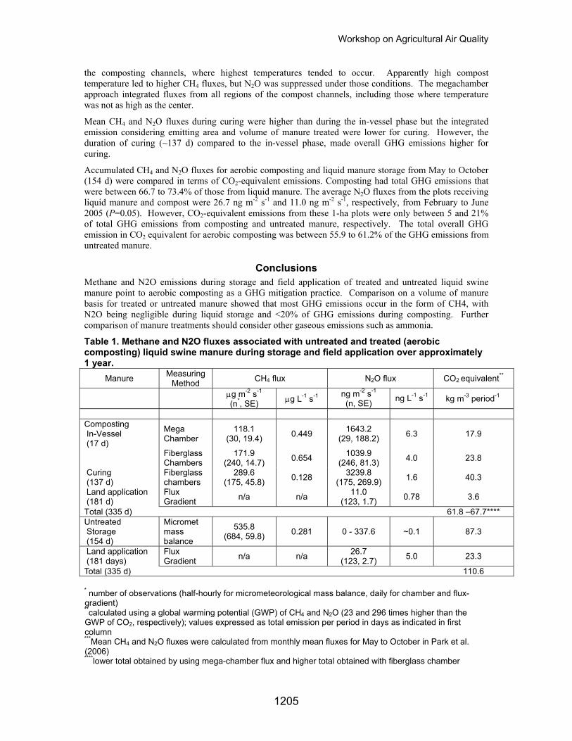
Workshop on Agricultural Air Quality
the composting channels, where highest temperatures tended to occur. Apparently high compost temperature led to higher CH4 fluxes, but N2O was suppressed under those conditions. The megachamber approach integrated fluxes from all regions of the compost channels, including those where temperature was not as high as the center.
Mean CH4 and N2O fluxes during curing were higher than during the in-vessel phase but the integrated emission considering emitting area and volume of manure treated were lower for curing. However, the duration of curing (~137 d) compared to the in-vessel phase, made overall GHG emissions higher for curing.
Accumulated CH4 and N2O fluxes for aerobic composting and liquid manure storage from May to October (154 d) were compared in terms of CO2-equivalent emissions. Composting had total GHG emissions that were between 66.7 to 73.4% of those from liquid manure. The average N2O fluxes from the plots receiving liquid manure and compost were 26.7 ng m-2 s-1 and 11.0 ng m-2 s-1, respectively, from February to June 2005 (P=0.05). However, CO2-equivalent emissions from these 1-ha plots were only between 5 and 21% of total GHG emissions from composting and untreated manure, respectively. The total overall GHG emission in CO2 equivalent for aerobic composting was between 55.9 to 61.2% of the GHG emissions from untreated manure.
Conclusions Methane and N2O emissions during storage and field application of treated and untreated liquid swine manure point to aerobic composting as a GHG mitigation practice. Comparison on a volume of manure basis for treated or untreated manure showed that most GHG emissions occur in the form of CH4, with N2O being negligible during liquid storage and <20% of GHG emissions during composting. Further comparison of manure treatments should consider other gaseous emissions such as ammonia.
Table 1. Methane and N2O fluxes associated with untreated and treated (aerobic composting) liquid swine manure during storage and field application over approximately 1 year.
Manure Measuring Method CH4 flux N2O flux CO2 equivalent**
µg m-2 s-1
(n*, SE) µg L-1 s-1 ng m-2 s-1
(n, SE) ng L-1 s-1 kg m-3 period-1
Composting In-Vessel (17 d)
Mega Chamber
118.1 (30, 19.4) 0.449 1643.2
(29, 188.2) 6.3 17.9
Fiberglass Chambers
171.9 (240, 14.7) 0.654 1039.9
(246, 81.3) 4.0 23.8
Curing (137 d)
Fiberglass chambers
289.6 (175, 45.8) 0.128 3239.8
(175, 269.9) 1.6 40.3
Land application (181 d)
Flux Gradient n/a n/a 11.0
(123, 1.7) 0.78 3.6
Total (335 d) 61.8 –67.7****
Untreated Storage (154 d)
Micromet mass balance
535.8(684, 59.8) 0.281 0 - 337.6 ~0.1 87.3
Land application (181 days)
Flux Gradient n/a n/a 26.7
(123, 2.7) 5.0 23.3
Total (335 d) 110.6 * number of observations (half-hourly for micrometeorological mass balance, daily for chamber and flux-gradient) **calculated using a global warming potential (GWP) of CH4 and N2O (23 and 296 times higher than the GWP of CO2, respectively); values expressed as total emission per period in days as indicated in first column ***Mean CH4 and N2O fluxes were calculated from monthly mean fluxes for May to October in Park et al. (2006) ****lower total obtained by using mega-chamber flux and higher total obtained with fiberglass chamber
1205
Workshop on Agricultural Air Quality
References Fleming, R., M. MacAlpine, and J. Morris. 1999. Final Report: Development of a Farm-Scale System to Compost Liquid Swine Manure, submitted to Ontario Pork. University of Guelph, Canada.
Houghton, J. T., Y. Ding, D. J. Griggs, M. Noguer, P. J. van der Linden, and D. Xiaosu. 2001. Climate Change 2001: The Scientific Basis Contribution of Working Group I to the Third Assessment Report of the Intergovernmental Panel on Climate Change (IPCC). Cambridge University Press, UK.
Khalil, M. A. K., and R. A. Rasmussen. 1992. The global source of nitrous oxide. Journal of Geophysical Research 97: 14651-14660.
Mosier, A., C. Kroeze, C. Nevison, O. Oenema, S. Seitzinger, and O. van Cleemput. 1998. Closing the global N2O budget: nitrous oxide emissions through the agricultural nitrogen cycle. Nutrient Cycling in Agroecosystems 52: 225-248.
Park, K. -H., A. G. Thompson, M. Marinier, K. Clark, and C. Wagner-Riddle. 2006. Greenhouse gas emissions from stored liquid swine manure in a cold climate. Atmospheric Environment 40: 618-627.
Rotmans, J., M. G. J. Den Elzen, M. S. Krol, R. J. Swart, and H. J. van der Woerd. 1992. Stabilizing atmospheric concentrations: towards international methane control. Ambio 21: 404-413.
Thompson, A.G., C. Wagner-Riddle, R. Fleming. 2004. Emissions of N2O and CH4 during the composting of liquid swine manure. Environmental Monitoring and Assessment 91: 87-104.
Wagner-Riddle , C., G. W. Thurtell, G. K. Kidd, and E. G. Beauchamp. 1996. Nitrous Oxide and Carbon Dioxide Fluxes from a Bare Soil Using a Micrometeorological Approach. Journal of Environmental Quality 25: 898-907.
Zeman, C., D. Depken, and M. Rich. 2002. Research on how the composting process impacts greenhouse gas emissions and global warming. Compost Science & Utilization 10: 72-86.
1206
Workshop on Agricultural Air Quality
Modeling Fugitive Dust Emissions in Pinal County, Arizona
J.P. Engelbrecht1 and K. Walch2
1Desert Research Institute, 2215 Raggio Parkway, Reno, NV 89512 2Pinal County Air Quality Control District, 31 N. Pinal Building F, Florence, AZ 85232
Abstract This paper presents the results from a source attribution modeling study conducted on aerosol samples collected in Pinal County, Arizona.
In October and November of 2003, the Pinal County Air Quality Control District (PCAQCD) in collaboration with the Desert Research Institute (DRI) performed an air quality study in Pinal County, Arizona, in order to identify and quantify the contributions by emission sources to elevated PM10 and PM2.5 particulate levels.
Low volume MiniVol samplers were operated on a US EPA one in three day 24-hour schedule, in parallel with existing Federal Reference Method (FRM) samplers. Five air quality monitoring sites located throughout the Pinal County agricultural basin were included in the study. The sites were located in the City of Casa Grande, the City of Coolidge, the Town of Stanfield, the Pinal County Housing Complex at Eleven Mile Corner, and a location locally known as Cowtown, which consists of several cattle feedlot companies. Additionally, three new fugitive dust samples were collected for re-suspension from a feedlot, dirt road and agricultural field.
Gravimetric analysis on the Teflon filters showed a substantial variation amongst the five sites with PM10 varying from 13 to 294 µg/m3 (US EPA 24 hr National Ambient Air Quality Standard for PM10 = 150 µg/m3) and for PM2.5 varying from 3 to 183 µg/m3 (US EPA 24 hr National Ambient Air Quality Standard for PM2.5 = 65 µg/m3)
A total of 130 ambient and 6 source filter pairs (Teflon and quartz fiber) were chemically analyzed by X-ray Fluorescence (XRF) spectrometry for 40 chemical elements, by Thermo Optical Reflectance (TOR) for 8 carbon species, by Ion Chromatography (IC) for 3 anions, by Atomic Absorption (AA) for 3 cations and automated colorimetry (AC) for ammonium.
The ambient samples together with the source profiles, including the new fugitive dust profiles and other profiles from the DRI’s database were modeled by the Chemical Mass Balance (CMB) receptor model. Modeled source attributions include largely soil and feedlot dust, with minor contributions from vegetative burning, motor vehicle emissions, coal fired power plants, as well as secondary ammonium nitrate, and in a few instances secondary ammonium sulfate.
Project Description This project (Walch and Gabrielson, 2005) was designed to identify the dominant sources of particulate matter in the Pinal County agricultural basin, which covers roughly the western third of the County. Low volume aerosol samplers capable of measuring particulate matter smaller than 2.5 microns (PM2.5) and particulate matter smaller than 10 microns (PM10) were used to collect ambient air samples at five existing monitoring sites. The Desert Research Institute (DRI) analyzed these filter samples for their mass and chemical species. These ambient results, together with measured source profiles, were modeled by the Chemical Mass Balance (CMB) receptor model to assess the source attributions within the Pinal County agricultural basin.
The ambient sampling was performed on a one in three day cycle, between October 1 and November 8, 2003. The ten individual days with the best data recovery were selected for chemical analysis. This sampling period was selected since elevated particulate matter concentrations have historically been recorded during the months of October and November. Several local sources contribute to elevated dust levels, the most notable one being cotton harvesting. Fall tillage is also taking place, and nine cotton gins throughout the agricultural basin are in full operation during this period. The cotton harvest also results in a substantial amount of traffic on agricultural field apron and other dirt roads, all contributing to elevated
1207
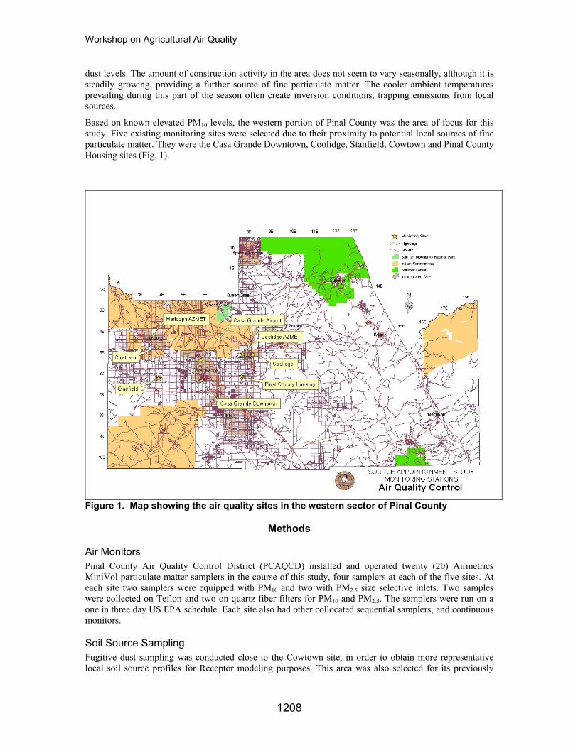
Workshop on Agricultural Air Quality
dust levels. The amount of construction activity in the area does not seem to vary seasonally, although it is steadily growing, providing a further source of fine particulate matter. The cooler ambient temperatures prevailing during this part of the season often create inversion conditions, trapping emissions from local sources.
Based on known elevated PM10 levels, the western portion of Pinal County was the area of focus for this study. Five existing monitoring sites were selected due to their proximity to potential local sources of fine particulate matter. They were the Casa Grande Downtown, Coolidge, Stanfield, Cowtown and Pinal County Housing sites (Fig. 1).
Figure 1. Map showing the air quality sites in the western sector of Pinal County
Methods
Air Monitors Pinal County Air Quality Control District (PCAQCD) installed and operated twenty (20) Airmetrics MiniVol particulate matter samplers in the course of this study, four samplers at each of the five sites. At each site two samplers were equipped with PM10 and two with PM2.5 size selective inlets. Two samples were collected on Teflon and two on quartz fiber filters for PM10 and PM2.5. The samplers were run on a one in three day US EPA schedule. Each site also had other collocated sequential samplers, and continuous monitors.
Soil Source Sampling Fugitive dust sampling was conducted close to the Cowtown site, in order to obtain more representative local soil source profiles for Receptor modeling purposes. This area was also selected for its previously
1208
Workshop on Agricultural Air Quality
recorded elevated PM10 concentrations and proximity to three major sources of particulate matter, feedlots, open field agriculture, and dirt roads. A significant additional source of particulate matter in the area is construction. The western portion of Pinal County where this study was focused is experiencing rapid development.
PCAQCD collected a surface soil grab sample from each of the potential major sources of fine particulate matter. The feedlot soil sample involved collecting one pound of fine surface material from each of five randomly selected feed pens, and combining these into one composite feedlot sample. Similarly the agricultural field soil samples involved collecting one pound of fine material from the surface of five randomly selected locations within an agricultural field immediately adjacent to the Cowtown ambient monitoring site, and combining these into one composite agricultural field sample. The dirt road soil samples involved collecting one pound of fine material from the road surface of five randomly selected locations along Hartman Road (a County dirt road bordering the site) and compositing these.
The DRI screened to minus 38 µm and re-suspended each composite sample, collecting filter sets of PM10 (minus 10 µm) and PM2.5 (minus 2.5 µm) source samples from each of the three soil samples. These source filters were analyzed by the same methods as the ambient samples and provided chemical fingerprints (source profiles) for feedlot soil emissions, agricultural soil emissions and dirt road soil emissions (Figs. 2 and 3). The feedlot chemical fingerprints were significantly different to the other two sources, in that they contained substantial amounts of the carbon species. There was no significant difference between the agricultural field and the dirt road sample fingerprints (chemical profiles).
Filter Analyses and Modeling The DRI weighed all Teflon filters and selected ten individual days for analysis by X-ray fluorescence spectrometry (XRF) for 40 elemental species. The number of Teflon filters chemically analyzed were as follows - ambient PM10 = 50, ambient PM2.5 = 50, source PM10 = 3, source PM2.5 = 3, field blanks = 10.
The DRI also analyzed the Pallflex quartz fiber filters for the cations Na+ and K+ by Atomic Absorption (AA) Spectroscopy, ammonium (NH4
+) by Automated Colorimetry (AC), the anions SO42-, NO3
-, Cl- by Ion Chromatography (IC), and the eight carbon species as well as carbonate (CO3
=) by Thermal/Optical Reflectance (TOR) carbon analysis. The number of quartz filters analyzed were as follows; ambient PM10 = 50, ambient PM2.5 = 50, source PM10 = 3, source PM2.5 = 3, blanks = 10.
The DRI thereafter performed a source apportionment on the chemically analyzed filter sets by the Chemical Mass Balance (CMB) Version 8 receptor model (Friedlander, 1973; Watson et al., 1997). This analysis involved using source profiles previously developed by DRI (Chow et .al., 2004) together with the three new profiles from the Cowtown area.
Gravimetric Results Summaries of the PM10 and PM2.5 MiniVol gravimetric results from the five sites are presented in Table 1. The PM10 concentrations recorded by the MiniVol samples compared well to the continuous and sequential samplers co-located at each monitoring site. The average percent difference between the MiniVol samplers and co-located filter based Federal Reference Method samplers was 14%. A scatter plot comparing the two methods resulted in a slope of 0.6 and an R2 value of 0.7. The average percent difference between the MiniVol samplers and co-located continuous Federal Equivalent Method samplers was elevated at 30%. Although a scatter plot comparing the two methods resulted in a slope of 0.9 and a R2 value of 0.9
The Casa Grande sampling site, had a collocated PM2.5 sequential FRM sampler. In this case the average Mini-Vol PM2.5/PM10 ratios listed in Table 1 were compared to the historical Casa Grande PM2.5/PM10 ratio of approximately 0.30. The average MiniVol PM2.5/PM10 ratios vary from 0.32 at the Stanfield site to 0.53 at the Coolidge and Cowtown sites. This comparison showed that the MiniVols likely overestimated the ambient PM2.5 concentrations at times.
1209
Workshop on Agricultural Air Quality
Table 1: PM10 and PM2.5 gravimetric averages and ratios Site Avg. Mini-Vol
PM10 (µg/m3) Avg. Mini-Vol PM2.5 (µg/m3)
Avg. Mini-Vol PM2.5/PM10 Ratio
Casa Grande 44 18 0.41 Coolidge 47 25 0.53 Cowtown 127 67 0.53 Pinal County Housing 60 25 0.42 Stanfield 55 18 0.32
Source Apportionment DRI performed a source apportionment modeling (CMB version 8) on the ten of the thirteen sampling dates selected for this project. The ten runs with the best data recovery were selected for the chemical speciation and CMB modeling study. The remaining three runs were not analyzed due to budgetary constraints and thus are not included in this report. The sampling days included were October 3, 9, 12, 15, 18, 21, 27 and 30, as well as November 5 and 8, 2003. The data recovery for these ten runs was 95.5%.
Chemical Fingerprints (Source Profiles) The chemical analyses of re-suspended filter samples provided chemical fingerprints for feedlot soil emissions, agricultural soil emissions and dirt road soil emissions (Figs. 2, 3). The PM10 and PM2.5 Feedlot Dust samples differ from the PM10 and PM2.5 Agricultural and Road Dust samples in that they contain a substantial amount of total carbon (TC).
1210
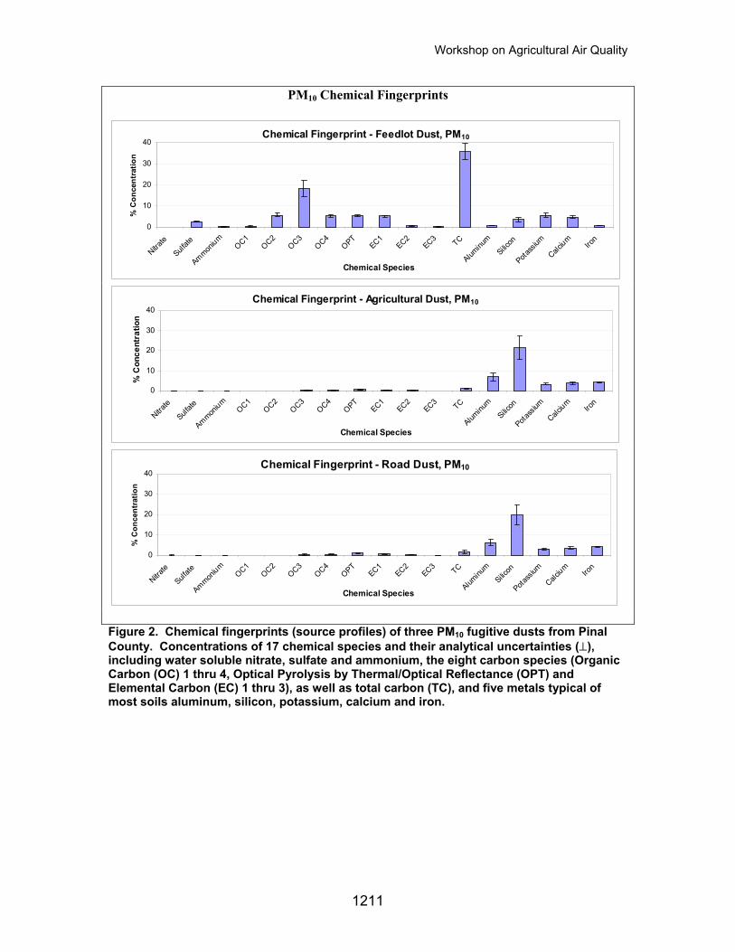
Workshop on Agricultural Air Quality
PM10 Chemical Fingerprints
Chemical Fingerprint - Feedlot Dust, PM10
0
10
20
30
40
Nitrate
Sulfate
Ammonium
OC1OC2
OC3OC4
OPTEC1
EC2EC3 TC
Aluminu
mSilic
on
Potass
ium
Calcium
Iron
Chemical Species
% C
once
ntra
tion
Chemical Fingerprint - Agricultural Dust, PM10
0
10
20
30
40
Nitrate
Sulfate
Ammonium
OC1OC2
OC3OC4
OPTEC1
EC2EC3 TC
Aluminu
m
Silicon
Potass
ium
Calcium
Iron
Chemical Species
% C
once
ntra
tion
Chemical Fingerprint - Road Dust, PM10
0
10
20
30
40
Nitrate
Sulfate
Ammonium
OC1OC2
OC3OC4
OPTEC1
EC2EC3 TC
Aluminu
mSilic
on
Potass
ium
Calcium
Iron
Chemical Species
% C
once
ntra
tion
Figure 2. Chemical fingerprints (source profiles) of three PM10 fugitive dusts from Pinal County. Concentrations of 17 chemical species and their analytical uncertainties (⊥), including water soluble nitrate, sulfate and ammonium, the eight carbon species (Organic Carbon (OC) 1 thru 4, Optical Pyrolysis by Thermal/Optical Reflectance (OPT) and Elemental Carbon (EC) 1 thru 3), as well as total carbon (TC), and five metals typical of most soils aluminum, silicon, potassium, calcium and iron.
1211
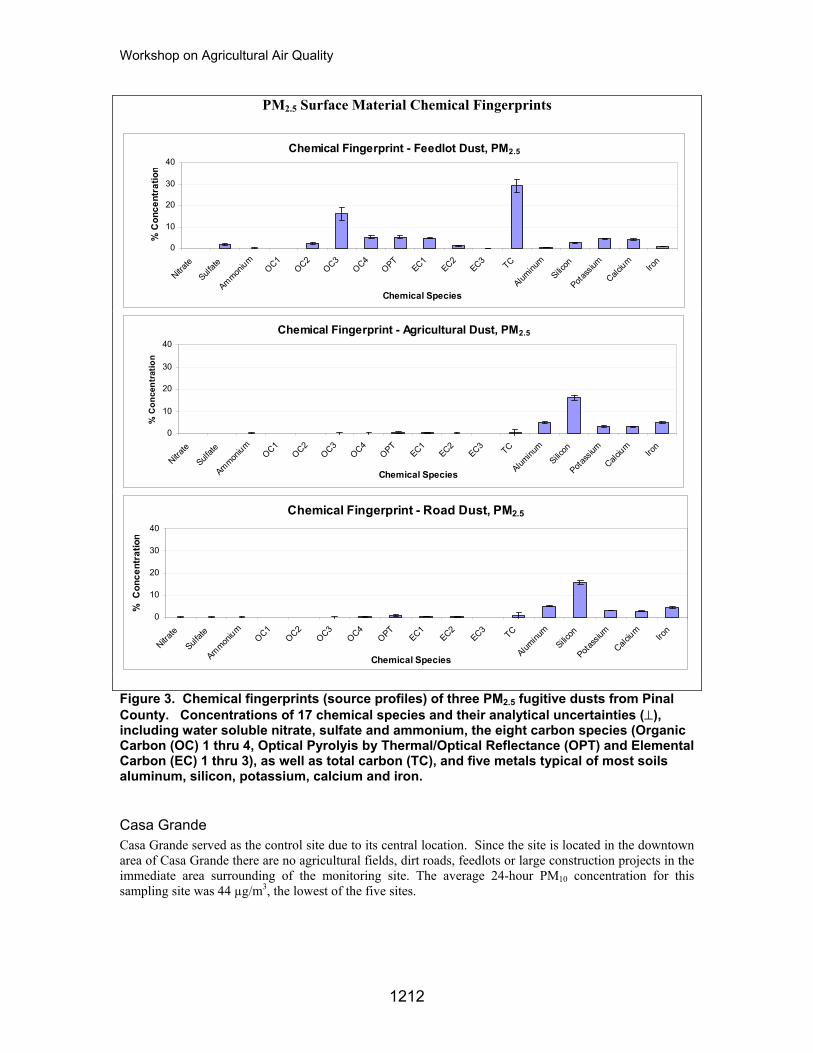
Workshop on Agricultural Air Quality
PM2.5 Surface Material Chemical Fingerprints
Chemical Fingerprint - Feedlot Dust, PM2.5
0
10
20
30
40
Nitrate
Sulfate
Ammonium
OC1OC2
OC3OC4
OPTEC1
EC2EC3 TC
Aluminu
mSilic
on
Potass
ium
Calcium
Iron
Chemical Species
% C
once
ntra
tion
Chemical Fingerprint - Agricultural Dust, PM2.5
0
10
20
30
40
Nitrate
Sulfate
Ammonium
OC1OC2
OC3OC4
OPTEC1
EC2EC3 TC
Aluminu
m
Silicon
Potass
ium
Calcium
Iron
Chemical Species
% C
once
ntra
tion
Chemical Fingerprint - Road Dust, PM2.5
0
10
20
30
40
Nitrate
Sulfate
Ammonium
OC1OC2
OC3OC4
OPTEC1
EC2EC3 TC
Aluminu
m
Silicon
Potass
ium
Calcium
Iron
Chemical Species
% C
once
ntra
tion
Figure 3. Chemical fingerprints (source profiles) of three PM2.5 fugitive dusts from Pinal County. Concentrations of 17 chemical species and their analytical uncertainties (⊥), including water soluble nitrate, sulfate and ammonium, the eight carbon species (Organic Carbon (OC) 1 thru 4, Optical Pyrolyis by Thermal/Optical Reflectance (OPT) and Elemental Carbon (EC) 1 thru 3), as well as total carbon (TC), and five metals typical of most soils aluminum, silicon, potassium, calcium and iron.
Casa Grande Casa Grande served as the control site due to its central location. Since the site is located in the downtown area of Casa Grande there are no agricultural fields, dirt roads, feedlots or large construction projects in the immediate area surrounding of the monitoring site. The average 24-hour PM10 concentration for this sampling site was 44 µg/m3, the lowest of the five sites.
1212
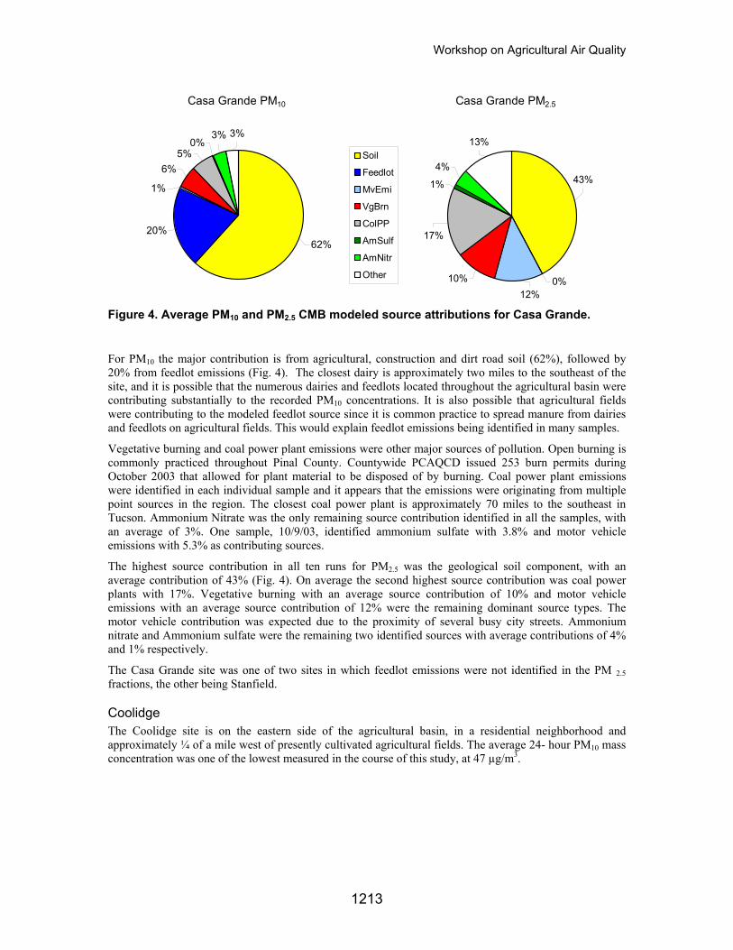
Workshop on Agricultural Air Quality
Casa Grande PM10
20%
6%
1%
62%
5%0%
3% 3%
Soil
Feedlot
MvEmi
VgBrn
ColPP
AmSulf
AmNitr
Other
Casa Grande PM2.5
1%
4%
13%
43%
0%10%
17%
12%
Figure 4. Average PM10 and PM2.5 CMB modeled source attributions for Casa Grande. For PM10 the major contribution is from agricultural, construction and dirt road soil (62%), followed by 20% from feedlot emissions (Fig. 4). The closest dairy is approximately two miles to the southeast of the site, and it is possible that the numerous dairies and feedlots located throughout the agricultural basin were contributing substantially to the recorded PM10 concentrations. It is also possible that agricultural fields were contributing to the modeled feedlot source since it is common practice to spread manure from dairies and feedlots on agricultural fields. This would explain feedlot emissions being identified in many samples.
Vegetative burning and coal power plant emissions were other major sources of pollution. Open burning is commonly practiced throughout Pinal County. Countywide PCAQCD issued 253 burn permits during October 2003 that allowed for plant material to be disposed of by burning. Coal power plant emissions were identified in each individual sample and it appears that the emissions were originating from multiple point sources in the region. The closest coal power plant is approximately 70 miles to the southeast in Tucson. Ammonium Nitrate was the only remaining source contribution identified in all the samples, with an average of 3%. One sample, 10/9/03, identified ammonium sulfate with 3.8% and motor vehicle emissions with 5.3% as contributing sources.
The highest source contribution in all ten runs for PM2.5 was the geological soil component, with an average contribution of 43% (Fig. 4). On average the second highest source contribution was coal power plants with 17%. Vegetative burning with an average source contribution of 10% and motor vehicle emissions with an average source contribution of 12% were the remaining dominant source types. The motor vehicle contribution was expected due to the proximity of several busy city streets. Ammonium nitrate and Ammonium sulfate were the remaining two identified sources with average contributions of 4% and 1% respectively.
The Casa Grande site was one of two sites in which feedlot emissions were not identified in the PM 2.5 fractions, the other being Stanfield.
Coolidge The Coolidge site is on the eastern side of the agricultural basin, in a residential neighborhood and approximately ¼ of a mile west of presently cultivated agricultural fields. The average 24- hour PM10 mass concentration was one of the lowest measured in the course of this study, at 47 µg/m3.
1213
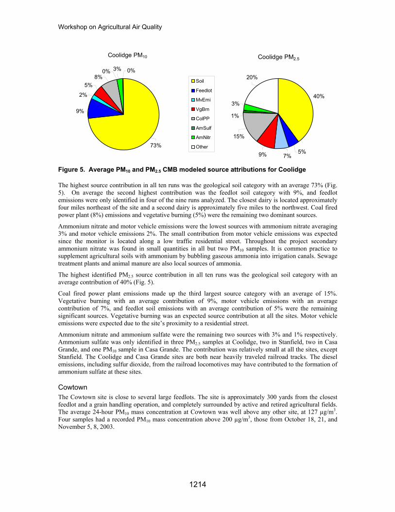
Workshop on Agricultural Air Quality
Coolidge PM2.5
3%
1%
5%7%9%
15%
20%
40%
Coolidge PM10
2%
5%
73%
3%0% 0%8%
9%
Soil
Feedlot
MvEmi
VgBrn
ColPP
AmSulf
AmNitr
Other
Figure 5. Average PM10 and PM2.5 CMB modeled source attributions for Coolidge The highest source contribution in all ten runs was the geological soil category with an average 73% (Fig. 5). On average the second highest contribution was the feedlot soil category with 9%, and feedlot emissions were only identified in four of the nine runs analyzed. The closest dairy is located approximately four miles northeast of the site and a second dairy is approximately five miles to the northwest. Coal fired power plant (8%) emissions and vegetative burning (5%) were the remaining two dominant sources.
Ammonium nitrate and motor vehicle emissions were the lowest sources with ammonium nitrate averaging 3% and motor vehicle emissions 2%. The small contribution from motor vehicle emissions was expected since the monitor is located along a low traffic residential street. Throughout the project secondary ammonium nitrate was found in small quantities in all but two PM10 samples. It is common practice to supplement agricultural soils with ammonium by bubbling gaseous ammonia into irrigation canals. Sewage treatment plants and animal manure are also local sources of ammonia.
The highest identified PM2.5 source contribution in all ten runs was the geological soil category with an average contribution of 40% (Fig. 5).
Coal fired power plant emissions made up the third largest source category with an average of 15%. Vegetative burning with an average contribution of 9%, motor vehicle emissions with an average contribution of 7%, and feedlot soil emissions with an average contribution of 5% were the remaining significant sources. Vegetative burning was an expected source contribution at all the sites. Motor vehicle emissions were expected due to the site’s proximity to a residential street.
Ammonium nitrate and ammonium sulfate were the remaining two sources with 3% and 1% respectively. Ammonium sulfate was only identified in three PM2.5 samples at Coolidge, two in Stanfield, two in Casa Grande, and one PM10 sample in Casa Grande. The contribution was relatively small at all the sites, except Stanfield. The Coolidge and Casa Grande sites are both near heavily traveled railroad tracks. The diesel emissions, including sulfur dioxide, from the railroad locomotives may have contributed to the formation of ammonium sulfate at these sites.
Cowtown The Cowtown site is close to several large feedlots. The site is approximately 300 yards from the closest feedlot and a grain handling operation, and completely surrounded by active and retired agricultural fields. The average 24-hour PM10 mass concentration at Cowtown was well above any other site, at 127 µg/m3. Four samples had a recorded PM10 mass concentration above 200 µg/m3, those from October 18, 21, and November 5, 8, 2003.
1214
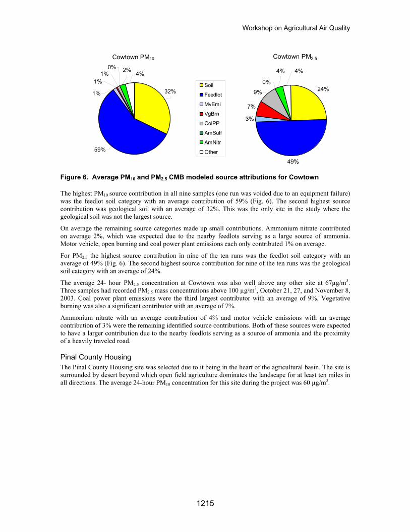
Workshop on Agricultural Air Quality
Cowtown PM2.5
24%
49%
3%
7%
9%
0%
4% 4%
Cowtown PM10
32%
59%
1%1%
1%
0% 2% 4%
Soil
Feedlot
MvEmi
VgBrn
ColPP
AmSulf
AmNitr
Other
Figure 6. Average PM10 and PM2.5 CMB modeled source attributions for Cowtown The highest PM10 source contribution in all nine samples (one run was voided due to an equipment failure) was the feedlot soil category with an average contribution of 59% (Fig. 6). The second highest source contribution was geological soil with an average of 32%. This was the only site in the study where the geological soil was not the largest source.
On average the remaining source categories made up small contributions. Ammonium nitrate contributed on average 2%, which was expected due to the nearby feedlots serving as a large source of ammonia. Motor vehicle, open burning and coal power plant emissions each only contributed 1% on average.
For PM2.5 the highest source contribution in nine of the ten runs was the feedlot soil category with an average of 49% (Fig. 6). The second highest source contribution for nine of the ten runs was the geological soil category with an average of 24%.
The average 24- hour PM2.5 concentration at Cowtown was also well above any other site at 67µg/m3. Three samples had recorded PM2.5 mass concentrations above 100 µg/m3, October 21, 27, and November 8, 2003. Coal power plant emissions were the third largest contributor with an average of 9%. Vegetative burning was also a significant contributor with an average of 7%.
Ammonium nitrate with an average contribution of 4% and motor vehicle emissions with an average contribution of 3% were the remaining identified source contributions. Both of these sources were expected to have a larger contribution due to the nearby feedlots serving as a source of ammonia and the proximity of a heavily traveled road.
Pinal County Housing The Pinal County Housing site was selected due to it being in the heart of the agricultural basin. The site is surrounded by desert beyond which open field agriculture dominates the landscape for at least ten miles in all directions. The average 24-hour PM10 concentration for this site during the project was 60 µg/m3.
1215
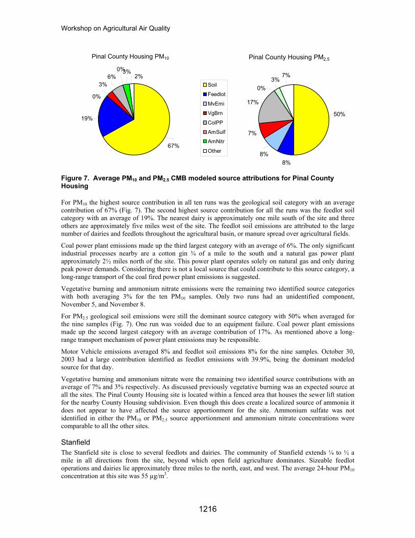
Workshop on Agricultural Air Quality
Pinal County Housing PM10
0%3%2%6%
3%
0%
19%
67%
Soil
Feedlot
MvEmi
VgBrn
ColPP
AmSulf
AmNitr
Other
Pinal County Housing PM2.5
50%
7%3%
0%
17%
7%
8%8%
Figure 7. Average PM10 and PM2.5 CMB modeled source attributions for Pinal County Housing For PM10 the highest source contribution in all ten runs was the geological soil category with an average contribution of 67% (Fig. 7). The second highest source contribution for all the runs was the feedlot soil category with an average of 19%. The nearest dairy is approximately one mile south of the site and three others are approximately five miles west of the site. The feedlot soil emissions are attributed to the large number of dairies and feedlots throughout the agricultural basin, or manure spread over agricultural fields.
Coal power plant emissions made up the third largest category with an average of 6%. The only significant industrial processes nearby are a cotton gin ¾ of a mile to the south and a natural gas power plant approximately 2½ miles north of the site. This power plant operates solely on natural gas and only during peak power demands. Considering there is not a local source that could contribute to this source category, a long-range transport of the coal fired power plant emissions is suggested.
Vegetative burning and ammonium nitrate emissions were the remaining two identified source categories with both averaging 3% for the ten PM10 samples. Only two runs had an unidentified component, November 5, and November 8.
For PM2.5 geological soil emissions were still the dominant source category with 50% when averaged for the nine samples (Fig. 7). One run was voided due to an equipment failure. Coal power plant emissions made up the second largest category with an average contribution of 17%. As mentioned above a long-range transport mechanism of power plant emissions may be responsible.
Motor Vehicle emissions averaged 8% and feedlot soil emissions 8% for the nine samples. October 30, 2003 had a large contribution identified as feedlot emissions with 39.9%, being the dominant modeled source for that day.
Vegetative burning and ammonium nitrate were the remaining two identified source contributions with an average of 7% and 3% respectively. As discussed previously vegetative burning was an expected source at all the sites. The Pinal County Housing site is located within a fenced area that houses the sewer lift station for the nearby County Housing subdivision. Even though this does create a localized source of ammonia it does not appear to have affected the source apportionment for the site. Ammonium sulfate was not identified in either the PM10 or PM2.5 source apportionment and ammonium nitrate concentrations were comparable to all the other sites.
Stanfield The Stanfield site is close to several feedlots and dairies. The community of Stanfield extends ¼ to ½ a mile in all directions from the site, beyond which open field agriculture dominates. Sizeable feedlot operations and dairies lie approximately three miles to the north, east, and west. The average 24-hour PM10 concentration at this site was 55 µg/m3.
1216
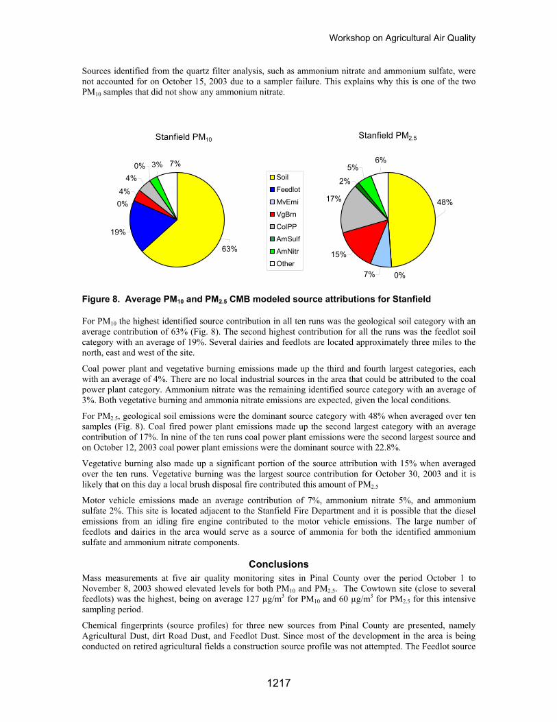
Workshop on Agricultural Air Quality
Sources identified from the quartz filter analysis, such as ammonium nitrate and ammonium sulfate, were not accounted for on October 15, 2003 due to a sampler failure. This explains why this is one of the two PM10 samples that did not show any ammonium nitrate.
Stanfield PM10
19%
63%
4%0%
4%0% 3% 7%
Soil
Feedlot
MvEmi
VgBrn
ColPP
AmSulf
AmNitr
Other
Stanfield PM2.5
2%
5%
17%
15%
7% 0%
48%
6%
Figure 8. Average PM10 and PM2.5 CMB modeled source attributions for Stanfield For PM10 the highest identified source contribution in all ten runs was the geological soil category with an average contribution of 63% (Fig. 8). The second highest contribution for all the runs was the feedlot soil category with an average of 19%. Several dairies and feedlots are located approximately three miles to the north, east and west of the site.
Coal power plant and vegetative burning emissions made up the third and fourth largest categories, each with an average of 4%. There are no local industrial sources in the area that could be attributed to the coal power plant category. Ammonium nitrate was the remaining identified source category with an average of 3%. Both vegetative burning and ammonia nitrate emissions are expected, given the local conditions.
For PM2.5, geological soil emissions were the dominant source category with 48% when averaged over ten samples (Fig. 8). Coal fired power plant emissions made up the second largest category with an average contribution of 17%. In nine of the ten runs coal power plant emissions were the second largest source and on October 12, 2003 coal power plant emissions were the dominant source with 22.8%.
Vegetative burning also made up a significant portion of the source attribution with 15% when averaged over the ten runs. Vegetative burning was the largest source contribution for October 30, 2003 and it is likely that on this day a local brush disposal fire contributed this amount of PM2.5
Motor vehicle emissions made an average contribution of 7%, ammonium nitrate 5%, and ammonium sulfate 2%. This site is located adjacent to the Stanfield Fire Department and it is possible that the diesel emissions from an idling fire engine contributed to the motor vehicle emissions. The large number of feedlots and dairies in the area would serve as a source of ammonia for both the identified ammonium sulfate and ammonium nitrate components.
Conclusions Mass measurements at five air quality monitoring sites in Pinal County over the period October 1 to November 8, 2003 showed elevated levels for both PM10 and PM2.5. The Cowtown site (close to several feedlots) was the highest, being on average 127 µg/m3 for PM10 and 60 µg/m3 for PM2.5 for this intensive sampling period.
Chemical fingerprints (source profiles) for three new sources from Pinal County are presented, namely Agricultural Dust, dirt Road Dust, and Feedlot Dust. Since most of the development in the area is being conducted on retired agricultural fields a construction source profile was not attempted. The Feedlot source
1217
Workshop on Agricultural Air Quality
profile differed significantly from the other two profiles in that it contained an elevated total carbon component. Since manure emissions could be distinctly identified a feedlot source profile was integrated into the modeling.
Source attribution modeling using the CMB receptor model showed that Soil (Agricultural + Dirt Road + Construction) was by far the greatest contributor to both PM10 and PM2.5 at four of the five sites. Feedlot dust was the second largest contributor for PM10 at four sites, the only exception was Cowtown where Feedlot dust was shown to be the greatest at 59% for PM10 and 49% for PM2.5. Minor modeled source types include Coal Fired Power Plant, Vegetative Burn, Motor Vehicle Emissions, Secondary Ammonium Nitrate and Secondary Ammonium Sulfate.
References Chow, J.C., J.G. Watson, H. Kuhns, V. Etyemezian, D.H. Lowenthal, D. Crow, S.D. Kohl, J.P. Engelbrecht, and M.C. Green (2004). Source profiles for industrial, mobile, and area sources in the Big Bend Regional Aerosol Visibility and Observational study. Chemosphere, 54(9), 185-208.
Friedlander, S.K. (1973). Chemical element balances and identification of air pollution sources. Environ.Sci.Technol. 7:235-40.
Walch, K.G., Gabrielson, D.G., (2005). Pinal County Air Quality Control District Source Apportionment Study, Pinal County Air Quality Control District Publication. http://www.co.pinal.az.us/AirQual/pdf/pinal_speciation_study.pdf (December 30, 2005)
Watson, J.G., Robinson, N.F., Lewis, C.W., Coulter, C.T., Chow, J.C., Fujita, E.M., Lowenthal, D.H., Corner, T.L., Henry, R.C., and Willis, R.D..(1997). Chemical mass balance receptor model version 8 (CMB) users manual, prepared for U.S. EPA, Research Triangle Park, NC, by Desert Research Institute, Reno, NV.
1218
Workshop on Agricultural Air Quality
Dry Deposition of Ammonia in the Vicinity of a Swine Production Facility
John T. Walker1 and Wayne Robarge2. 1US Environmental Protection Agency, Research Triangle Park, NC 27711, USA; 2North Carolina
State University, Department of Soil Science, Raleigh NC, 27695, USA. Abstract While animal production facilities have been identified as important sources of atmospheric NH3, there are no estimates of local NH3 dry deposition for U.S. sites. Such estimates are necessary to estimate net farm-scale emissions and for assessing the risk of neighboring ecosystems to nitrogen deposition. This project investigates the dry deposition of NH3 around a 5000 head swine production facility located in eastern North Carolina. Passive samplers are used to measure weekly-integrated NH3 concentrations along horizontal gradients from the lagoon/barn complex out to a distance of 500 m. Dry deposition is estimated using a canopy compensation point model. Here we present data for the period April, 2003 to August, 2005 with emphasis on modeling results and uncertainty. Dry deposition rates range from 200 kg NH3-N/ha/yr within 25 m of the lagoon/barn complex to 5 kg NH3-N/ha/yr at a distance of 500 m. Assuming a steady-state emission factor of 6.0 kg NH3/animal/yr, NH3 dry deposition over the nearest 500 m from the barn/lagoon complex accounted for 11.6 (± 3.5)% of emissions between July, 2003 and July, 2004.
1219
Workshop on Agricultural Air Quality
Study of Gas/Particle Partitioning Using Inorganic Thermodynamic Equilibrium Modules and Data from the
California Regional PM10/PM2.5 Air Quality Study
Kai Wang1, Yang Zhang1, Mark Z. Jacobson2, Jinyou Liang3, and Karen Magliano3
1North Carolina State University, Raleigh, NC 27695 2Stanford University, Stanford, CA 94305
3California Air Resources Board, Sacramento, CA 95812 Abstract Three thermodynamic equilibrium modules, ISORROPIA, AIM2, and EQUISOLV II are applied to simulate the gas/particle portioning for total amount of nitrate, ammonium, and chloride using observational data from the 1999-2001 California Regional PM10/PM25 Air Quality Studies (CRPAQS). The gas/PM partitioning predicted by ISORROPIA and EQUISOLV II with a bulk equilibrium approach is quite similar and both modules can generally reproduce the observed partitioning. The observed size distributions are reproduced by EQUISOLV II with a size-resolved equilibrium approach for some cases but large deviations exist for other cases, due in part to the uncertainties in the size-resolved aerosol measurements. The likely causes for the deviations are being identified through diagnostic and sensitivity studies.
Introduction Both the natural and anthropogenic particulate matter (PM) are known to play a significant role in many air pollution issues such as human heath problems, climate change, atmospheric visibility, stratospheric ozone depletion, acid deposition, and photochemical smog. Therefore, the knowledge of the physical and chemical properties, compositions, and processes of the aerosol particles is of great importance. The chemical compositions and formation mechanisms of PM are different for different size sections. Modeling the chemical composition and size distribution will improve our understanding of aerosol behavior and its impacts on air quality and climate change. In the past years, many inorganic and organic aerosol modules, most of which assume a thermodynamic equilibrium between the gas and aerosol phases for condensable species, have been developed to simulate the composition and phase state of PM. These include: EQUIL (Bassett and Seinfeld, 1983), MARS (Saxena et al., 1986), SEQUILIB (Pilinis and Seinfeld, 1987), AIM and AIM2 (Wexler and Seinfeld, 1991; Clegg et al., 1992, 1998), SCAPE and SCAPE2 (Kim et al., 1993a, b), EQUISOLV and EQUISOLV II (Jacobson et al., 1996; Jacobson, 1999), ISORROPIA (Nenes et al., 1998, 1999), and GFEMN (Ansari and Pandis, 1999a). These modules have been used in determining emission control strategies (e.g., Kumar et al., 1998), replicating ambient measurements (e.g., Fridlind and Jacobson, 2000; Moya et al., 2002; Campbell et al., 2002), and simulating PM in large-scale chemical transport models (e.g., Meng et al., 1998; Rodriguez and Dabdub, 2004; Zhang et al., 2004). A comprehensive review and performance evaluation of some of these modules have also been conducted in several studies (e.g., Ansari and Pandis, 1999b; Zhang et al., 2000).
In the present study, three aerosol equilibrium modules: ISORROPIA, AIM2, and EQUISOLV II are applied to study the gas/particle portioning of inorganic species using observational data from the 1999-2001 California Regional PM10/PM2.5 Air Quality Studies (CRPAQS). CRPAQS is a multi-year observational and modeling study that involves multiple organizations and is being conducted in northern California with a focus on the Central Valley, where the concentrations of PM frequently exceed the National Ambient Air Quality Standards, owing to the combination of mobile, industrial, agricultural, and residential sources (McDade, 2002). A comprehensive data analysis has been conducted using data from two CRPAQS sites (Angiola and Fresno) for the period of December 14, 2000 to January 18, 2001 during which PM concentrations (especially nitrate and ammonium) were the highest throughout the year. Two sets of observational data are used to set up inputs for model simulations for the two sites. The first set contains PM measurements (i.e., sulfate (SO4
2-), nitrate (NO3-), ammonium (NH4
+), chloride (Cl-), sodium (Na+), calcium (Ca+), potassium (K+), and magnesium (Mg2+)) that were obtained 5 times per day (3-8 hours average) using sequential filter sampler with Teflon/citric acid filter pack and corresponding gaseous
1220
Workshop on Agricultural Air Quality
measurements of nitric acid (HNO3) and ammonia (NH3) (referred to as episodic cases). The second set contains 24-hour average size-resolved PM measurements of the same species that were obtained using the Micro Orifice Uniform Deposit Impactor (MOUDI) samplers for nine stages over size range of 0.01-10 µm and corresponding gaseous HNO3 and NH3 (referred to as size-resolved cases). A total of 104 episodic cases (50 and 54 at Angiola and Fresno, respectively) and 8 size-resolved cases (4 at each site) are simulated.
In this paper, we compare the simulation results of ISORROPIA and EQUISOLV II against the observations. ISORROPIA simulates the partitioning using the bulk thermodynamic equilibrium approach only and it does not simulate equilibrium reactions involving Ca+, K+, and Mg2+. EQUISOLV II simulates the partitioning using both the bulk and the size-resolved thermodynamic equilibrium approaches (referred to as bulk EQUISOLV II and size-resolved EQUISOLV II). The inputs for ISORROPIA and bulk EQUISOLV II include temperature (T), relative humidity (RH), total amount of species in the gas and aerosol phases such as total sulfate (TSO4), total nitrate (TNO3 = HNO3 + NO3
-), total ammonium (TNH4 = NH3+NH4
+), and total chloride (TCl = HCl+Cl-). Total amounts of sodium (Na+), calcium (Ca+), potassium (K+), and magnesium (Mg2+) are also included in the inputs for the bulk EQUISOLV II simulations. The inputs for size-resolved EQUISOLV II include T, RH, TNO3, TNH4, and size-resolved SO4
2-, Cl-, Na+, Ca+, K+, and Mg2+. A comparison is also performed between the simulation results of ISORROPIA and bulk EQUISOLV II and the results of bulk vs. size-resolved EQUISOLV II. The simulations using AIM2 are being set up and the results will be compared with those of ISORROPIA and EQUISOLV II and the CRPAQS observations. The performance of these thermodynamic modules in reproducing observed PM concentrations, size distributions, and gas-PM partitioning will be evaluated.
Summary of the Simulation Results Three sets of simulations have been performed to simulate the partitioning of TNO3, TNH4, and TCl between the gas and aerosol phases: 1) bulk equilibrium simulations with ISORROPIA and bulk-EQUISOLV II for the 104 episodic cases; 2) bulk equilibrium simulations with ISORROPIA and bulk-EQUISOLV II for the 8 size-resolved cases with total amounts of species as inputs; and 3) size-resolved simulations with size-resolved EQUISOLV II for the 8 size-resolved cases with size-resolved PM composition as inputs except NO3
- and NH4+ which are inputted together with their corresponding gases as
TNO3 and TNH4.
For the bulk equilibrium simulations with ISORROPIA and bulk EQUISOLV II for the 104 episodic cases, ISORROPIA and bulk EQUISOLV II generally predict similar gas/PM partitioning of TNO3, TNH4, and TCl. Since all 104 cases are in sulfate-very poor (or ammonia-very rich) regime with the molar ratios of TNH4 to TSO4 (i.e., [TNH4]/[TSO4]) of 15-760 and more than 70% of those cases have high RHs (> 70%), this similarity is expected and is consistent with the findings of Ansari and Pandis (1999b) and Zhang et al. (2000). Some differences exist in the concentrations of H2O, HCl, and H+ predicted by both modules. At RH = 100%, both modules give extremely high H2O amount (> 105 µg m-3 for ISORROPIA and > 103 µg m-3 for EQUISOLV II), indicating the limitation of the activity coefficients at RH = 100% used in both modules. ISORROPIA predicts higher (by a factor up to 4) concentrations of HCl than EQUISOLV II for almost all cases. In most cases, the aqueous particle predicted by ISORROPIA is less acidic than that predicted by bulk EQUISOLV II (with an average pH value of 5.07 from ISORROPIA vs. 4.09 from EQUISOLV II for the 104 episodic cases). Those differences are mainly caused by the different sets of equilibrium reactions simulated in both modules. The module capability to reproduce the observed gas/PM partitioning differs from site to site, depending on chemical and meteorological conditions at the site. The average temperature for the 50 episodic cases at Angiola is 13.7 oC, which is higher than that (9.4 oC) for the 54 episodic cases at Fresno. The average RH at Angiola is 84%, which is also higher than that at Fresno (72%). The observed average [TNH4]/[TSO4] and [TNO3]/[TSO4] are 112.6 and 11.8 at Angiola and 52.3 and 18.5 at Fresno, indicating that both sites are in sulfate-very poor (or ammonia-very rich) and nitrate-rich condition. For aerosol NO3
-, 95% of predictions by ISORROPIA and bulk EQUISOLV II are within a factor of 1.5 of the observed values at both sites, with the correlation coefficient (r) of 0.8-0.81 at Angiola and 0.99 at Fresno. Both modules tend to slightly overpredict NO3
- at Fresno and may either overpredict or underpredict NO3
- at Angiola. For HNO3, less than 20% of predictions by both modules at both sites are within a factor of 1.5 of the observed values, with very low r values of 0.14 at Angiola and 0.25-0.26 at Fresno. For aerosol NH4
+, more than 95% of predictions by both modules at Fresno and only 70% of
1221
Workshop on Agricultural Air Quality
predictions at Angiola are within a factor of 1.5 of the observed values, with r values of 0.82 at Angiola and 0.96 at Fresno. Both modules reproduce well NH4
+ at Fresno but tend to significantly underpredict NH4+ at
Angiola. For NH3, more than 90% of predictions by both modules at both sites are within a factor of 1.5 of the observed values, with r values of 0.92 at Angiola and 0.69 at Fresno. Both modules reproduce well NH3 at Fresno but tend to overpredict NH3 at Angiola. For aerosol Cl-, both modules reproduce well with more than 95% of predictions within a factor of 1.5 of the observed values and an r value of nearly 1.0 at both sites.
For the bulk equilibrium simulations with ISORROPIA and bulk-EQUISOLV II for the 8 size-resolved cases, in most cases, the simulations and measurements are in excellent agreement for NH3 and Cl-, with a small overprediction by 0.9%, 2.7%, and 1.2% for NH3 and a small underprediction by 3.3%, 1.3%, 2.5% for Cl- for ISORROPIA, bulk EQUISOLV II, and size-resolved EQUISOLV II, respectively. ISORROPIA, bulk EQUISOLV II, and size-resolved EQUISOLV II also give good agreement for NO3
- and NH4
+, with a moderate overprediction by 13.8%, 14.1%, and 13.8% for NO3- and a moderate
underprediction by 11.8%, 35%, and 16.2% for NH4+, respectively. Similar to the episodic cases, all
modules fail to reproduce HNO3, with a significant underprediction by 95.4%, 97.5%, and 95.4% for ISORROPIA, bulk EQUISOLV II, and size-resolved EQUISOLV II, respectively. Overall, the performance of ISORROPIA and EQUISOLV II is similar, with the results of size-resolved EQUISOLV II slightly better than bulk EQUISOLV II.
For the size-resolved EQUISOLV II simulations for the 8 size-resolved cases, the module reproduces the observed size distributions of NO3
-, NH4+, and Cl- for some cases but with large deviations for other cases.
The observed NH4+ exists predominantly in the fine/accumulation modes and the observed NO3
- exists in the accumulation/coarse modes, which are generally reproduced by the module. The performance of the module is generally better in the fine/accumulation modes than the coarse mode, as the thermodynamic equilibrium assumption holds primarily for fine PM but not for coarse PM. The growth rate to small particles, multiplied by the number concentration of small particles, is greater than that to large particles, multiplied by the number concentration of large particles. The rate of mass transfer between gases and small particles is thus generally faster than that between gases and large particles, rendering the equilibrium assumption a valid simplification in many cases. The simulated size distributions of NO3
- are very similar to those of H2O and the predicted NO3
- concentrations are higher in the ammonia-rich size sections than those in the ammonia-poor size sections. One major factor leading to large deviations is likely associated with the large uncertainties in the size-resolved measurements. For example, some size bins (e.g., the first size bin (0.01 – 0.062 µm) and the second size bin (0.062 – 0.163 µm)) contain NH4
+ and Mg2+ but no SO4
2-, NO3-, and Cl- in some cases, causing unrealistic charge-imbalance in the observations. All 8 samples
contain excess cations that are not balanced. Other likely causes for the discrepancies between the simulated and observed size distributions are being identified through diagnostic and sensitivity studies.
Acknowledgements This work is performed under the National Science Foundation Career Award No. ATM-0348819 and the Environmental Protection Agency Contract No. 4-92U-9609 at NCSU. The authors thank Athanasios Nenes of Georgia Institute of Technology, for providing the ISORROPIA source code; Simon Clegg of the University of East Anglia, for providing the AIM2 executable files; and Gregory O’Brien of California Air Resources Board, for providing the CRPAQS observational data.
References Ansari, A.S., S.N. Pandis. 1999a. Prediction of multicomponent inorganic atmospheric aerosol behavior. Atmospheric Environment 33: 745-757.
Ansari, A.S., S.N. Pandis. 1999b. An analysis of four models predicting the partitioning of semi-volatile inorganic aerosol components. Aerosol Science and Technology 31: 129-153.
Bassett, M., J.H. Seinfeld. 1983. Atmospheric equilibrium model of sulfate and nitrate aerosol. Atmospheric Environment 17: 2237-2252.
1222
Workshop on Agricultural Air Quality
Campbell, S.W., M.C. Evans, N.D. Poor. 2002. Predictions of size-resolved aerosol concentrations of ammonium, chloride and nitrate at a bayside site using EQUISOLV II. Atmospheric Environment 36: 4299-4307.
Clegg, S.L., P. Brimblecombe, A.S. Wexler. 1998. A thermodynamic model of the system H+ -NH4+ -Na+ -
SO42- -NO3
- -Cl- -H2O at 298.15 K. Journal of Physical Chemistry 102: 2155-2171.
Clegg, S.L., K.S. Pitzer, P. Brimblecombe. 1992. Thermodynamics of multicomponent, miscible, ionic solutions. II. Mixture including unsymmetrical electrolytes. Journal of Physical Chemistry 96: 9470-9479.
Fridlind, A.M. and M.Z. Jacobson. 2000. A study of gas-aerosol equilibrium and aerosol pH in the remote marine boundary layer during the First Aerosol Characterization Experiment (ACE 1). Journal of Geophysical Research 105: 17325-17340.
Jacobson, M.Z., A. Tabazadeh, R.P. Turco, 1996. Simulating equilibrium within aerosols and nonequilibrium between gases and aerosols. Journal of Geophysical Research 101: 9079-9091.
Jacobson, M.Z. 1999. Studying the effects of calcium and magnesium on size-distributed nitrate and ammonium with EQUISOLV II. Atmospheric Environment 33:3635-3649.
Kim, Y.P., J.H. Seinfeld, P. Saxena, 1993a. Atmospheric gas-aerosol equilibrium I. Thermodynamic model. Aerosol Science and Technology 19: 157-181.
Kim, Y.P., J.H. Seinfeld, P. Saxena, 1993b. Atmospheric gas-aerosol equilibrium II. Analysis of common approximations and activity coefficients calculation methods. Aerosol Science and Technology 19: 181-198.
Kumar, N., F.W. Lurmann, S.N. Pandis, A.S. Ansari. 1998. Final Report: analysis of atmospheric chemistry during 1995 integrated monitoring study. Final Report Prepared for the California Air Resources Board, Sacramento, CA, by Sonoma Technology Inc., Santa Rosa, CA.
McDade, C.E. 2002. California Regional PM10/PM2.5 Air Quality Study (CRPAQS) Introduction to Site Documentation Reports. California Regional PM10/PM25 Air Quality Study Technical Committee c/o California Air Resources Board Sacramento, CA. by ENSR International Camarillo, CA.
Meng, Z., D., Dabdub, J.H. Seinfeld. 1998. Size-resolved and chemically resolved model of atmospheric aerosol dynamics. Journal of Geophysical Research 103: 3419-3435.
Moya, M., S.N. Pandis, and M.Z. Jacobson. 2002. Is the size distribution of urban aerosols determined by thermodynamic equilibrium?: An application to Southern California. Atmospheric Environment 36: 2349-2365.
Nenes, A., C. Pilinis, and S.N. Pandis. 1998. ISORROPIA: a new thermodynamic equilibrium model for multiphase multicomponent marine aerosols. Aquatic Geochemistry 4: 123-152.
Nenes, A., C. Pilinis, and S.N. Pandis. 1999. Continued development and testing of a new thermodynamic aerosol module for urban and regional air quality models. Atmospheric Environment 33: 1553-1560.
Pilinis, C., J.H. Seinfeld. 1987. Continued development of a general equilibrium model for inorganic multicomponent atmospheric aerosols. Atmospheric Environment 21: 2453-2466.
Rodriguez, M.A. and D. Dabdub. 2004. IMAGES-SCAPE2: A modeling study of size- and chemically resolved aerosol thermodynamics in a global chemical transport model. Journal of Geophysical Research 109: D02203.
Saxena, P., A.B. Hudischewskyj, C. Seigneur, J.H. Seinfeld. 1986. A comparative study of equilibrium approaches to the chemical characterization of secondary aerosols. Atmospheric Environment 20: 1471-1483
Wexler, A.S., J.H. Seinfeld. 1991. Second-generation inorganic aerosol model. Atmospheric Environment 25A: 2731-2748.
1223
Workshop on Agricultural Air Quality
Zhang, Y., C. Seigneur, J.H. Seinfeld, M. Jacobson, S L. Clegg, and F.S. Binkowski. 2000. A comparative review of inorganic aerosol thermodynamic equilibrium modules: similarities, differences, and their likely causes. Atmospheric Environment 34: 117-137.
Zhang, Y., B. Pun, K. Vijayaraghavan, S.-Y. Wu, C. Seigneur, S. Pandis, M. Jacobson, A. Nenes, and J. H. Seinfeld, 2004, Development and application of the model of aerosol dynamics, reaction, ionization and dissolution (MADRID), Journal of Geophysical Research 109, D01202, doi:10.1029/2003JD003501.
1224
Workshop on Agricultural Air Quality
Nitrogen Mass Balance for Spray Fields Fertilized with Liquid Swine Waste
S.C. Whalen1 and J.T. DeBerardinis2
1University of North Carolina, Department of Environmental Sciences and Engineering, Chapel Hill, NC 27599, USA
2North Carolina Department of Environment and Natural Resources, Division of Water Quality, Raleigh, NC 27607, USA
Abstract Increasingly, livestock is produced in the US in concentrated animal feeding operations (CAFOs), where large-scale confinement facilities house several thousand animals and collected waste is used as an organic fertilizer. In particular, eastern North Carolina has experienced the rapid proliferation of swine-producing CAFOs in the period 1980 to 2000 and stagnant growth thereafter. The current swine inventory in North Carolina stands at about 10 million animals concentrated in roughly 1500 production facilities. Waste at these facilities is collected in open-air lagoons and the liquid phase is land-applied by sprinkler irrigation. Accelerated eutrophication of coastal and inland waters and localized reports of groundwater contamination have centered attention on the fate of nitrogen in land-applied waste.
Although numerous investigations have focused on individual aspects of the fate and transport of nitrogenous liquid waste, none has attempted a detailed analysis of post-application transformations and losses of liquid waste-N. However, the post-application fate of N in land-applied liquid swine waste may involve several storage pools, transfers and transformations (Fig. 1). Nitrogenous material in anaerobic lagoonal swine waste consists of the inorganic reduced species NH3-N and NH4
+-N (=TAN; total ammoniacal nitrogen) as well as particulate and dissolved organic-N. The NH3 fraction of TAN is immediately available for loss to the atmosphere via volatilization. Organic-N can be microbially mineralized to NH4
+. Ammonium can engage in soil cation exchange reactions, volatilize to the atmosphere as NH3 under appropriate conditions of soil pH, or oxidize to NO3
--N through the action of nitrifying bacteria in aerobic soil zones. Nitrate can be reduced to N2 (and to a much lesser extent N2O) by denitrifying bacteria in anaerobic microzones, with the gaseous end products again lost to the atmosphere. Among other factors, rates of denitrification are dependent on microbial release of NH4
+-N from mineralization of organic materials and subsequent oxidation of NH4
+-N to NO3--N by nitrifying bacteria
(nitrification) in aerobic soil zones. Inorganic-N (NO3- and NH4
+) is available for consumption by microbes (immobilization) or plants and all organic and inorganic species are subject to export from the ecosystem via surface and ground waters, although NO3
- shows the most mobility. Our study was aimed at providing an event-based (single application) analysis of physicochemical and biological interactions involved in soil N cycling dynamics and soil-atmosphere exchange of gaseous N that are mediated by each spray event. A comprehensive understanding of the post-application fate of fertilizers is essential for the development of Best Management Practices (BMPs) that aim to minimize offsite transport and maximize nutrient availability to the host crop.
On three occasions, we experimentally applied liquid lagoonal swine waste at typical doses of 1.25 and 2.5 cm (40 to 130 kg N ha-2) to carefully defined plots in an active spray field on a on a corporate, farrow to half finish swine production facility located in eastern NC. A fifth, unfertilized plot served as a control. Waste collection and handling at the facility follow industry standards with the liquid phase applied by solid set sprinkler to a summer crop of coastal bermudagrass (Cynodon dactylon L.) that is overseeded with tall fescue (Festuca sp.) in the winter. Prior to experimentation, vegetation within each plot and the surrounding area was cut to a uniform height of 18 cm. Soil N pools and transformations were assessed for up to 19 d following waste addition. As necessary, soils were collected to a depth of 20 cm (“active soil zone”) within plots with standard coring devices and cores were replaced with similar size cores from adjoining nonexperimental plots. These companion plots were fertilized at rates consistent with the experimental plots and were used expressly for the purpose of replacing removed soils from experimental plots.
1225
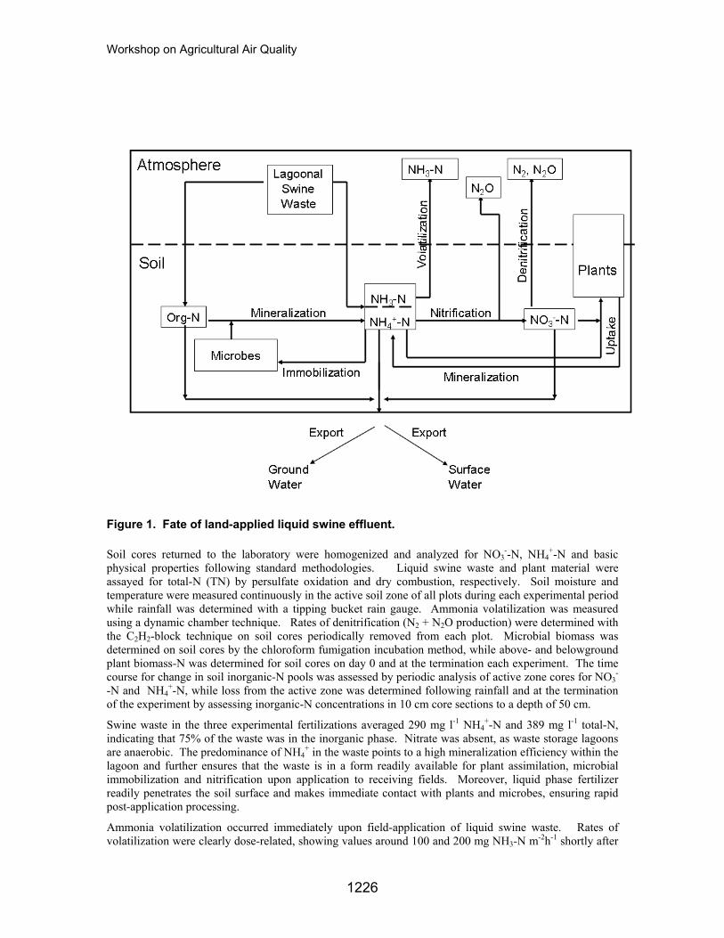
Workshop on Agricultural Air Quality
Figure 1. Fate of land-applied liquid swine effluent.
Soil cores returned to the laboratory were homogenized and analyzed for NO3
--N, NH4+-N and basic
physical properties following standard methodologies. Liquid swine waste and plant material were assayed for total-N (TN) by persulfate oxidation and dry combustion, respectively. Soil moisture and temperature were measured continuously in the active soil zone of all plots during each experimental period while rainfall was determined with a tipping bucket rain gauge. Ammonia volatilization was measured using a dynamic chamber technique. Rates of denitrification (N2 + N2O production) were determined with the C2H2-block technique on soil cores periodically removed from each plot. Microbial biomass was determined on soil cores by the chloroform fumigation incubation method, while above- and belowground plant biomass-N was determined for soil cores on day 0 and at the termination each experiment. The time course for change in soil inorganic-N pools was assessed by periodic analysis of active zone cores for NO3
-
-N and NH4+-N, while loss from the active zone was determined following rainfall and at the termination
of the experiment by assessing inorganic-N concentrations in 10 cm core sections to a depth of 50 cm.
Swine waste in the three experimental fertilizations averaged 290 mg l-1 NH4+-N and 389 mg l-1 total-N,
indicating that 75% of the waste was in the inorganic phase. Nitrate was absent, as waste storage lagoons are anaerobic. The predominance of NH4
+ in the waste points to a high mineralization efficiency within the lagoon and further ensures that the waste is in a form readily available for plant assimilation, microbial immobilization and nitrification upon application to receiving fields. Moreover, liquid phase fertilizer readily penetrates the soil surface and makes immediate contact with plants and microbes, ensuring rapid post-application processing.
Ammonia volatilization occurred immediately upon field-application of liquid swine waste. Rates of volatilization were clearly dose-related, showing values around 100 and 200 mg NH3-N m-2h-1 shortly after
1226
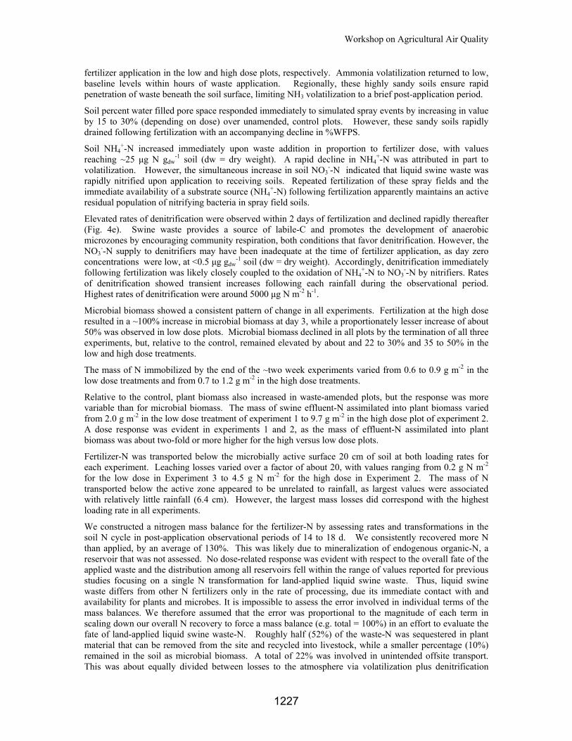
Workshop on Agricultural Air Quality
fertilizer application in the low and high dose plots, respectively. Ammonia volatilization returned to low, baseline levels within hours of waste application. Regionally, these highly sandy soils ensure rapid penetration of waste beneath the soil surface, limiting NH3 volatilization to a brief post-application period.
Soil percent water filled pore space responded immediately to simulated spray events by increasing in value by 15 to 30% (depending on dose) over unamended, control plots. However, these sandy soils rapidly drained following fertilization with an accompanying decline in %WFPS.
Soil NH4+-N increased immediately upon waste addition in proportion to fertilizer dose, with values
reaching ~25 µg N gdw-1 soil (dw = dry weight). A rapid decline in NH4
+-N was attributed in part to volatilization. However, the simultaneous increase in soil NO3
--N indicated that liquid swine waste was rapidly nitrified upon application to receiving soils. Repeated fertilization of these spray fields and the immediate availability of a substrate source (NH4
+-N) following fertilization apparently maintains an active residual population of nitrifying bacteria in spray field soils.
Elevated rates of denitrification were observed within 2 days of fertilization and declined rapidly thereafter (Fig. 4e). Swine waste provides a source of labile-C and promotes the development of anaerobic microzones by encouraging community respiration, both conditions that favor denitrification. However, the NO3
--N supply to denitrifiers may have been inadequate at the time of fertilizer application, as day zero concentrations were low, at <0.5 µg gdw
-1 soil (dw = dry weight). Accordingly, denitrification immediately following fertilization was likely closely coupled to the oxidation of NH4
+-N to NO3--N by nitrifiers. Rates
of denitrification showed transient increases following each rainfall during the observational period. Highest rates of denitrification were around 5000 µg N m-2 h-1.
Microbial biomass showed a consistent pattern of change in all experiments. Fertilization at the high dose resulted in a ~100% increase in microbial biomass at day 3, while a proportionately lesser increase of about 50% was observed in low dose plots. Microbial biomass declined in all plots by the termination of all three experiments, but, relative to the control, remained elevated by about and 22 to 30% and 35 to 50% in the low and high dose treatments.
The mass of N immobilized by the end of the ~two week experiments varied from 0.6 to 0.9 g m-2 in the low dose treatments and from 0.7 to 1.2 g m-2 in the high dose treatments.
Relative to the control, plant biomass also increased in waste-amended plots, but the response was more variable than for microbial biomass. The mass of swine effluent-N assimilated into plant biomass varied from 2.0 g m-2 in the low dose treatment of experiment 1 to 9.7 g m-2 in the high dose plot of experiment 2. A dose response was evident in experiments 1 and 2, as the mass of effluent-N assimilated into plant biomass was about two-fold or more higher for the high versus low dose plots.
Fertilizer-N was transported below the microbially active surface 20 cm of soil at both loading rates for each experiment. Leaching losses varied over a factor of about 20, with values ranging from 0.2 g N m-2 for the low dose in Experiment 3 to 4.5 g N m-2 for the high dose in Experiment 2. The mass of N transported below the active zone appeared to be unrelated to rainfall, as largest values were associated with relatively little rainfall (6.4 cm). However, the largest mass losses did correspond with the highest loading rate in all experiments.
We constructed a nitrogen mass balance for the fertilizer-N by assessing rates and transformations in the soil N cycle in post-application observational periods of 14 to 18 d. We consistently recovered more N than applied, by an average of 130%. This was likely due to mineralization of endogenous organic-N, a reservoir that was not assessed. No dose-related response was evident with respect to the overall fate of the applied waste and the distribution among all reservoirs fell within the range of values reported for previous studies focusing on a single N transformation for land-applied liquid swine waste. Thus, liquid swine waste differs from other N fertilizers only in the rate of processing, due its immediate contact with and availability for plants and microbes. It is impossible to assess the error involved in individual terms of the mass balances. We therefore assumed that the error was proportional to the magnitude of each term in scaling down our overall N recovery to force a mass balance (e.g. total = 100%) in an effort to evaluate the fate of land-applied liquid swine waste-N. Roughly half (52%) of the waste-N was sequestered in plant material that can be removed from the site and recycled into livestock, while a smaller percentage (10%) remained in the soil as microbial biomass. A total of 22% was involved in unintended offsite transport. This was about equally divided between losses to the atmosphere via volatilization plus denitrification
1227
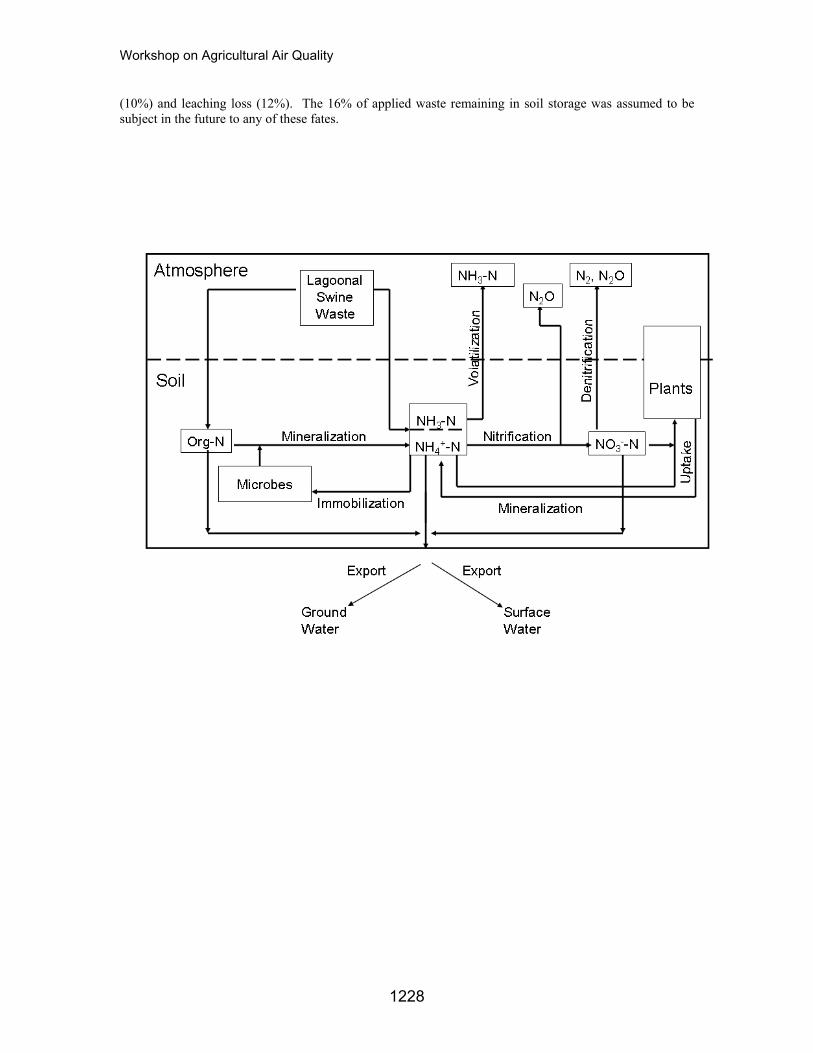
Workshop on Agricultural Air Quality
(10%) and leaching loss (12%). The 16% of applied waste remaining in soil storage was assumed to be subject in the future to any of these fates.
1228
Workshop on Agricultural Air Quality
Instrumentation Development for Monitoring Ammonia Emissions During Nutritional Trials in Dairy Freestall Housing
and Under Laboratory Conditions
Eileen F. Wheeler , Patrick A. Topper , Gabriella A. Varga , Neil Brown , Victoria Blanes-Vidal , A. Jud Heinrichs , Tom L. Richard , Robert E. Graves , Virginia Ishler , Geoffrey I. Zanton ,
Meghan L. Moody
1 1 2 2 3
2 1 1 2 2
2
1Agricultural & Biological Engineering, Pennsylvania State University, University Park, PA USA 2Dairy and Animal Science, Pennsylvania State University, University Park, PA USA 3Polytechnic University of Valencia, Department of Animal Science, Valencia, Spain
Overview A one-year study assessed ammonia gas emissions from dairy cattle housing during dietary trials that evaluated nutritional modifications that limit nitrogen excretion. These trials were conducted in freestall as well as individual feeding facilities, housing either lactating dairy cows or heifers. Results provide comparisons among dietary strategies that were expected to reduce ammonia emissions. In addition, the results provide essential baseline gas emission data from freestall dairy housing that is lacking in the USA. A sample of collected information is presented here.
Several dietary strategies were developed and their effects on nitrogen balance and ammonia emissions were studied. The nutritional strategy reported in this paper is an evaluation of forage source fed to mature Holstein lactating cows. Forage consisted of corn silage with alfalfa or fescue-orchard grass silage. Each forage contained either coarse or fine ground corn. Two trials with cows in a replicated 4 x 4 Latin square design were conducted. One trial had ten cows in a controlled environment barn. A concurrent second trial was a larger scale version in a freestall barn of 120 cows. Diets were formulated to closely meet the cow’s requirement for metabolizable protein such that rations contained 16.0 to 16.5% crude protein. The end result was more optimal nitrogen utilization efficiency, reduced ammonia emissions from housing, improved animal performance, and an indication of increased profits (reported elsewhere).
A mixture of feces and urine is necessary for ammonia formation and emission from dairy manure, with urease from the feces degrading the urea in the urine. In-barn measurements were completed to document the variability in emission rate from a barn environment that is partially dependent on incomplete mixing of feces and urine. To determine ammonia emissions under controlled conditions, experiments were also conducted within a laboratory with a set ratio of urine and feces from the 10 cows on dietary trial in the controlled environment barn.
Traditionally, ammonia emission from livestock housing has been estimated by measuring ventilation rate and ammonia concentration at the inlet and the outlet of the building. However, most dairy cattle are housed in naturally ventilated facilities where it is nearly impossible to accurately monitor emissions along large open sidewalls. Another approach to field measurement of gaseous emissions from animal houses lies in measuring the gas as it volatizes from the floor by means of enclosed flux chambers located over the manure.
Objectives This paper presents a sample of data from the forage dietary trials of mature cows with an emphasis on instrumentation development to evaluate ammonia gas emissions. The objectives of the gas emissions evaluation work were: (1) To develop a barn-rugged, portable non-steady state (static) flux chamber system and measurement procedure to determine ammonia emissions from naturally-ventilated freestall dairy barns; and (2) To validate this measuring system by comparing flux chamber emission rates from dairy cow manure with whole building emission rates, calculated from ammonia balance in an experimental room; and (3) To determine gas flux mechanisms under controlled laboratory conditions using steady-state flux (dynamic) chamber system for evaluation of a standardized mixture of urine and feces from cows on dietary trials.
1229
Workshop on Agricultural Air Quality
Materials and Methods Methods for Objective 1: Procedures were developed to measure ammonia emissions from curtain-sidewall, naturally-ventilated dairy housing by measuring ammonia as it volatilized in situ from the manure-covered floor. Over 80 locations were measured within the freestall environment during a 10-hour experimental period; fifteen experimental days were distributed evenly throughout a 10-month timeframe to capture the variety of weather conditions experienced in a cold-climate like Pennsylvania. During freestall evaluations, air temperature, manure/floor temperature, and air speed near the manure surface were recorded. Instrumentation for in-barn measurements included a non-steady state flux chamber technique (Hutchinson and Mosier, 1981; Livingston G.P. and Hutchinson G.L., 1995) with a photoacoustic multi-gas analyzer (Innova, Denmark) for rapid, accurate gas detection over a 5 to 10 minute interval.
Gas emission from the manure is closely related to the air velocity on its surface, as convective transfer plays an important role in this process (Ni, 1999). Various flux chamber designs have been used for relative comparisons of gas evolution from surfaces. To complete objective 1 of this project, a relative comparison among the diets was an appropriate first step for in situ field evaluation of dietary influence on ammonia gas release. In addition, this project sought to quantify actual emissions data.
Methods for Objective 2: For validation of technique, the non-steady state flux chamber methodology was applied to a mechanically-ventilated building, called the experimental test room, for comparison with traditional whole building emissions measurements. Building emission rates can be obtained from the ammonia balance in the building by Equation 1:
( )inletoutletroombalance CCQE −⋅= (1) where Ebalance is the ammonia emission rate from the building, calculated from the ammonia balance (in
); Q[ ] 13
−⋅ sNHg room is the ventilation flow rate in the building (in ); and C13 −⋅ sm inlet and Coutlet are the
ammonia concentrations (in ) measured at the inlet and the outlet, respectively. Validation experiments were carried out in a positive-pressure ventilated test room with a manure-covered floor. The ammonia flux rate was measured with the non-steady state flux chamber at eight coordinates uniformly placed over the floor. Ammonia emissions from the building calculated from flux chamber measurements (E
[ ] 33
−⋅mNHg
chamber) were obtained as the product of: the averaged measured ammonia flux rate from the floor and the area of the manured surface. Air temperature, manure temperature, and air speed near the manure surface were recorded along with a laboratory analysis of manure pH and nutrients. Evaluations were made with both static and recirculation flow in the chamber. Recirculation flow was set to match test room conditions according to a relationship between flow and surface velocity in the chamber that was previously determined. Ammonia flux rate from the manure covered by the chamber, , in , was calculated according to the model (Eqn 2) proposed by Hutchinson and Mosier (1981) for non-steady state chambers. This model calculates initial gas flux at the beginning of the sampling period.
f 12 −− ⋅⋅ smg
( )( ) 12
01
021
201
2 CCCC
LnCCCtA
CCVf
c
c
−−
−−−
= (2)
where: C0 is the background gas concentration (in [ ] 33
−⋅mNHg ); C1 is the gas concentration
(in ) at a time t after placing the chamber on the surface; C[ ] 33
−⋅mNHg 2 is the gas concentration
(in ) at a time 2t after placing the chamber on the surface; V[ ] 33
−⋅mNHg c is the volume of the chamber (in m3) and Ac is the area covered by the chamber (in m2). In this work, the time (t, in seconds) between measuring C0 and C1, was set at 120 seconds. This model is non-linear, as it assumes that the rate of gas exchange is not uniform over the measurement period, but decreases as the gas is accumulated inside of the chamber. It is essential to confirm for each flux measurement that this non-linear assumption is fulfilled, by verifying another simple relation (Eqn 3).
112
01 >−−
CCCC
(3)
1230
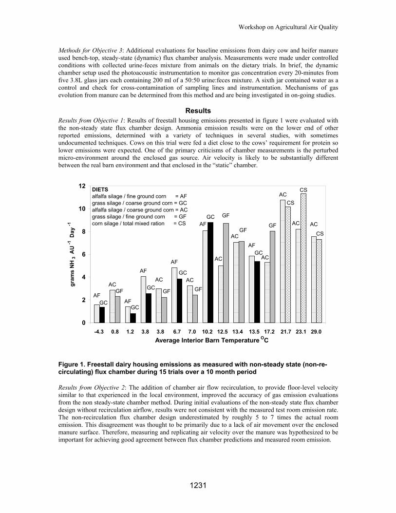
Workshop on Agricultural Air Quality
Methods for Objective 3: Additional evaluations for baseline emissions from dairy cow and heifer manure used bench-top, steady-state (dynamic) flux chamber analysis. Measurements were made under controlled conditions with collected urine-feces mixture from animals on the dietary trials. In brief, the dynamic chamber setup used the photoacoustic instrumentation to monitor gas concentration every 20-minutes from five 3.8L glass jars each containing 200 ml of a 50:50 urine:feces mixture. A sixth jar contained water as a control and check for cross-contamination of sampling lines and instrumentation. Mechanisms of gas evolution from manure can be determined from this method and are being investigated in on-going studies.
Results Results from Objective 1: Results of freestall housing emissions presented in figure 1 were evaluated with the non-steady state flux chamber design. Ammonia emission results were on the lower end of other reported emissions, determined with a variety of techniques in several studies, with sometimes undocumented techniques. Cows on this trial were fed a diet close to the cows’ requirement for protein so lower emissions were expected. One of the primary criticisms of chamber measurements is the perturbed micro-environment around the enclosed gas source. Air velocity is likely to be substantially different between the real barn environment and that enclosed in the “static” chamber.
AC
AF
AFAF
AC
GCGF
AC
AFGC
GF
GC
GCAC
GF
GC
GF
AF
AC
GF
ACGF
AFGC
AC
CS
AC
CS
AC
CS
0
2
4
6
8
10
12
gram
s N
H 3
AU
-1 D
ay -1
DIETSalfalfa silage / fine ground corn = AF grass silage / coarse ground corn = GCalfalfa silage / coarse ground corn = ACgrass silage / fine ground corn = GFcorn silage / total mixed ration = CS
-4.3 0.8 1.2 3.8 3.8 6.7 7.0 10.2 12.5 13.4 13.5 17.2 21.7 23.1 29.0 Average Interior Barn Temperature OC
Figure 1. Freestall dairy housing emissions as measured with non-steady state (non-re-circulating) flux chamber during 15 trials over a 10 month period Results from Objective 2: The addition of chamber air flow recirculation, to provide floor-level velocity similar to that experienced in the local environment, improved the accuracy of gas emission evaluations from the non steady-state chamber method. During initial evaluations of the non-steady state flux chamber design without recirculation airflow, results were not consistent with the measured test room emission rate. The non-recirculation flux chamber design underestimated by roughly 5 to 7 times the actual room emission. This disagreement was thought to be primarily due to a lack of air movement over the enclosed manure surface. Therefore, measuring and replicating air velocity over the manure was hypothesized to be important for achieving good agreement between flux chamber predictions and measured room emission.
1231
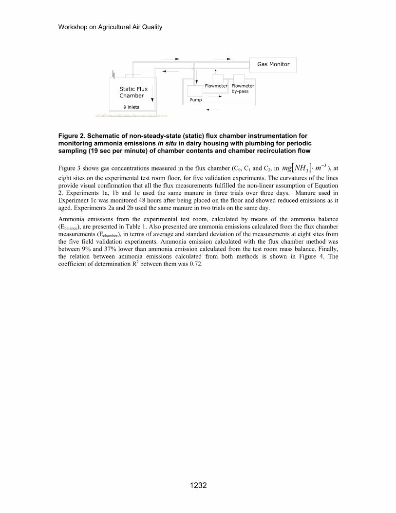
Workshop on Agricultural Air Quality
Gas Monitor
Pump
Flowmeter Flowmeterby-passStatic Flux
Chamber
9 inlets
Figure 2. Schematic of non-steady-state (static) flux chamber instrumentation for monitoring ammonia emissions in situ in dairy housing with plumbing for periodic sampling (19 sec per minute) of chamber contents and chamber recirculation flow Figure 3 shows gas concentrations measured in the flux chamber (C0, C1 and C2, in ), at eight sites on the experimental test room floor, for five validation experiments. The curvatures of the lines provide visual confirmation that all the flux measurements fulfilled the non-linear assumption of Equation 2. Experiments 1a, 1b and 1c used the same manure in three trials over three days. Manure used in Experiment 1c was monitored 48 hours after being placed on the floor and showed reduced emissions as it aged. Experiments 2a and 2b used the same manure in two trials on the same day.
[ ] 33
−⋅mNHmg
Ammonia emissions from the experimental test room, calculated by means of the ammonia balance (Ebalance), are presented in Table 1. Also presented are ammonia emissions calculated from the flux chamber measurements (Echamber), in terms of average and standard deviation of the measurements at eight sites from the five field validation experiments. Ammonia emission calculated with the flux chamber method was between 9% and 37% lower than ammonia emission calculated from the test room mass balance. Finally, the relation between ammonia emissions calculated from both methods is shown in Figure 4. The coefficient of determination R2 between them was 0.72.
1232
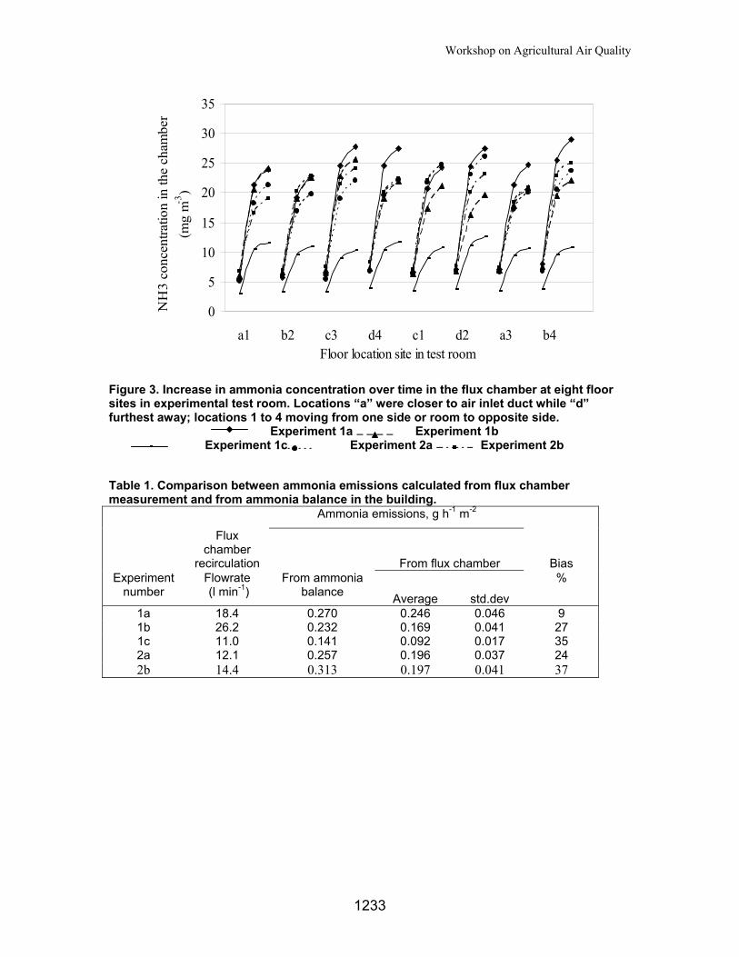
Workshop on Agricultural Air Quality
0
5
10
15
20
25
30
35
a1 b2 c3 d4 c1 d2 a3 b4 Floor location site in test room
NH
3 co
ncen
tratio
n in
the
cham
ber_
(mg
m-3)
Figure 3. Increase in ammonia concentration over time in the flux chamber at eight floor sites in experimental test room. Locations “a” were closer to air inlet duct while “d” furthest away; locations 1 to 4 moving from one side or room to opposite side.
Experiment 1a Experiment 1b Experiment 1c Experiment 2a Experiment 2b
Table 1. Comparison between ammonia emissions calculated from flux chamber measurement and from ammonia balance in the building. Ammonia emissions, g h-1 m-2
Flux chamber
recirculation
From flux chamber Bias Experiment
number Flowrate (l min-1)
From ammonia balance Average std.dev
%
1a 18.4 0.270 0.246 0.046 9 1b 26.2 0.232 0.169 0.041 27 1c 11.0 0.141 0.092 0.017 35 2a 12.1 0.257 0.196 0.037 24 2b 14.4 0.313 0.197 0.041 37
1233
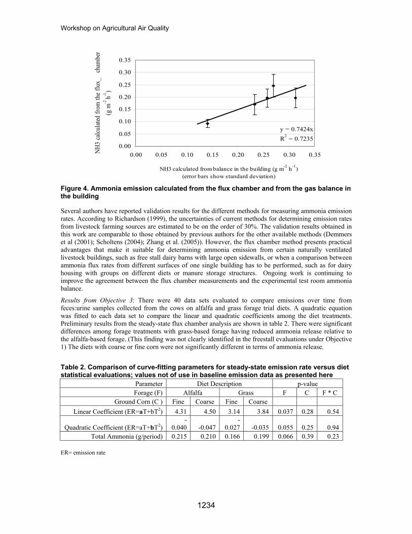
Workshop on Agricultural Air Quality
y = 0.7424xR2 = 0.7235
0.00
0.05
0.10
0.15
0.20
0.25
0.30
0.35
0.00 0.05 0.10 0.15 0.20 0.25 0.30 0.35
NH3 calculated from balance in the building (g m-2 h-1) (error bars show standard deviation)
NH3
calcu
lated
from
the f
lux_
ch
ambe
r (g
m-2
h-1)
Figure 4. Ammonia emission calculated from the flux chamber and from the gas balance in the building
Several authors have reported validation results for the different methods for measuring ammonia emission rates. According to Richardson (1999), the uncertainties of current methods for determining emission rates from livestock farming sources are estimated to be on the order of 30%. The validation results obtained in this work are comparable to those obtained by previous authors for the other available methods (Demmers et al (2001); Scholtens (2004); Zhang et al. (2005)). However, the flux chamber method presents practical advantages that make it suitable for determining ammonia emission from certain naturally ventilated livestock buildings, such as free stall dairy barns with large open sidewalls, or when a comparison between ammonia flux rates from different surfaces of one single building has to be performed, such as for dairy housing with groups on different diets or manure storage structures. Ongoing work is continuing to improve the agreement between the flux chamber measurements and the experimental test room ammonia balance.
Results from Objective 3: There were 40 data sets evaluated to compare emissions over time from feces:urine samples collected from the cows on alfalfa and grass forage trial diets. A quadratic equation was fitted to each data set to compare the linear and quadratic coefficients among the diet treatments. Preliminary results from the steady-state flux chamber analysis are shown in table 2. There were significant differences among forage treatments with grass-based forage having reduced ammonia release relative to the alfalfa-based forage. (This finding was not clearly identified in the freestall evaluations under Objective 1) The diets with coarse or fine corn were not significantly different in terms of ammonia release.
Table 2. Comparison of curve-fitting parameters for steady-state emission rate versus diet statistical evaluations; values not of use in baseline emission data as presented here
Parameter Diet Description p-value Forage (F) Alfalfa Grass F C F * C
Ground Corn (C ) Fine Coarse Fine Coarse Linear Coefficient (ER=aT+bT2) 4.31 4.50 3.14 3.84 0.037 0.28 0.54
Quadratic Coefficient (ER=aT+bT2) -
0.040 -0.047 -
0.027 -0.035 0.055 0.25 0.94 Total Ammonia (g/period) 0.215 0.210 0.166 0.199 0.066 0.39 0.23
ER= emission rate
1234
Workshop on Agricultural Air Quality
Conclusions A portable, non-steady state (static) flux chamber can be used to estimate ammonia emissions from natural ventilated buildings, being especially useful for measuring ammonia flux rates from different surfaces within one single building. The accuracy of the developed measurement method in the test room was comparable to those reported in literature for the other available gas emissions methods. Results of the dietary trials for mature cows and heifers will add to the ammonia emissions inventory from U.S. dairy farms while providing insight into potentially useful ammonia reduction strategies.
References Demmers T. G. M., Phillips V. R., Short L. S., Burgess L. R., Hoxey R. P., Wathes C. M.. 2001. Validation of Ventilation Rate Measurement Methods and the Ammonia Emission from Naturally Ventilated Dairy and Beef Buildings in the United Kingdom. J. of Agricultural Engineering Research, Vol 79(1). 107-116.
Hutchinson G. L.; Mosier A.R. 1981. Improved Soil Cover Method for Field Measurement of Nitrous Oxide Fluxes. Soil Sci. Soc. Am. J. 45:311-316.
Livingston G.P. and Hutchinson G.L. 1995. Chapter 2: Enclosure-based measurement of trace gas exchange: applications sources of error. In Biogenic Trace Gases: Measuring Emissions from Soil and Water, P.A. Matson and R.C. Harriss. Blackwell Science Ltd. Oxford, England.
Ni, J.Q. 1999. Mechanistic models of ammonia release from liquid manure: a review. Journal of Agricultural Engineering Research, 72, no.1, pp. 1-17.
Richardson S. 1999. Atmospheric emission inventory guidebook. EMEP/CORINAIR, second edition. Prepared by the EMEP Task Force on Emission Inventories. European Environment Agency, Copenhagen.
Scholtens R., Dore C.J., Jones B. M. R., Lee D. S., Phillips V. R. 2004. Measuring ammonia emission rates from livestock buildings and manure stores—part 1: development and validation of external tracer ratio, internal tracer ratio and passive flux sampling methods. Atmospheric Environment, Vol 38(19) 3003-3015.
Zhang G., Strøm J.S., Li B., Rom H.B., Morsing S., Dahl P., Wang C. 2005. Emission of ammonia and other contaminant gases from naturally ventilated dairy cattle buildings Biosystems Engineering, Vol 92(3) 355-364.
1235
Workshop on Agricultural Air Quality
Suits vs. Solutions: Incorporating Residents Perceptions into Optimal Air Quality Policy
Sara Whitmore, Jennie S. Popp, J. Martin Redfern University of Arkansas, Fayetteville, Arkansas
Abstract The Northwest Arkansas (NWAR) and Northeast Oklahoma (NEOK) area has a thriving economy that includes significant poultry production sector with numerous poultry grow-out houses in open-country, feed complexes, hatcheries, and processing plants. Major companies such as Wal-Mart, J.B. Hunt Transportation, and Tyson Foods have their corporate headquarters and expansive facilities in the region. From 1990 to 2000 the Northwest Arkansas area population grew 47%; since then it has grown another 22%. Many of the new residents are moving from urban areas, with little to no previous direct exposure to areas of production agriculture.
Currently, most environmental concerns in the region focus on water quality. However, as populations grow, concerns are turning towards air quality. Western Kentucky provides one example of this. A lawsuit against a poultry growing operation was filed by several residents near the facility, alleging that production management practices, designed to vent air in the poultry houses, led to degradated air for local residents. The court ruled in favor of the residents. Besides the general public looking at air quality, so are government agencies. Earlier this year, the EPA Animal Feeding Operations Consent Agreement recognized “…concerns raised regarding possible health impacts from Animal Feeding Operations (AFO) emissions”, such as ammonia, hydrogen sulfide, and particulate matter, and as a result, AFOs may be subject to the requirements of the Clean Air Act and notification process of CERCLA.
This research examines perceptions of residents in the growing NWAR and NEOK region regarding current air quality, the need (if any) to improve air quality and their willingness to pay for this improvement. For the first time, a representative sample of roughly 2000 urban, suburban and rural residents in the region will be interviewed through a mail survey regarding their perceptions about: 1) air quality in general, 2) negative impacts of air quality that may impact them, 3) and how agriculture and other industries impact air quality. This questionnaire will use the contingent valuation methods to determine residents’ willingness to pay for improved air quality. In addition to addressing the topics above it is expected that this survey will be able to highlight how differences in perceptions may be related to length of exposure to and knowledge of production agriculture. It is hoped that these results can be used as a catalyst to develop appropriate air quality policy in the region, before it is determined by the courts.
Introduction The Northwest Arkansas and Northeast Oklahoma area has a thriving economy that includes a significant poultry production sector with numerous poultry grow-out houses in open-country, along with the necessary feed complexes, hatcheries, and processing plants. Other major companies such as Wal-Mart, J.B. Hunt Transportation, and Tyson Foods have their corporate headquarters and other facilities in the area. From 1990 to 2000 the Northwest Arkansas area has grown 47% in population, and in past 5 years has grown 22% (Hawkins, 2005).
With this growth people are moving into the area that are not familiar with production agriculture and agribusiness operations, which can cause many problems between the rural and urban residents. The issue of air quality has become of greater concern to the general public in Northwest Arkansas and Northeast Oklahoma.
Importance of the Study Much of the concern about environmental issues in Northwest Arkansas and Northeast Oklahoma has been about water quality being impaired by phosphorous from point sources such as municipal waste water treatment plants, or runoff from non-point sources such as construction sites and farm fields. More recently air quality has become an issue of greater concern for governmental agencies as well as the general public.
1236
Workshop on Agricultural Air Quality
In western Kentucky a lawsuit against a poultry growing operation was recently resolved; several residents near the facility alleged that when the houses vented air to reduce the level of ammonia gas inside, the air quality outside the houses was reduced, and this reduced air quality impacted them negatively. The court ruled in favor of the residents.
A January 21, 2005, EPA news release stated “The emissions of air pollutants and hazardous substances from certain (animal) feeding operations may be subject to requirements of the Clean Air Act and the notification process of the Comprehensive Environmental Response, Compensation and Liability Act (CERCLA).” The January 31, 2005, Federal Register stated that the “EPA recognizes concerns raised regarding possible health impacts from AFO (Animal Feeding Operation) emissions”, such as ammonia, hydrogen sulfide, particulate matter, and volatile organic compounds. In 2001, John Sweeten of Texas A&M University, stated “Until recently, air quality from CAFOs has received only secondary consideration, notwithstanding recently-increased public concerns and policy attention. Water and air quality protection are inseparable, …”
As with the water quality issue, any major change regarding emissions from poultry houses could impose financial costs on poultry farm operators and negatively impact the industry. At the same time, the recreational and retirement industries, which are benefited by natural amenities in the area, might be adversely affected by poorer air quality.
Methodology and Expected Results The study area was chosen because it is believed that air quality will become a major issue in the next few years. The overall goal of the project is to measure area resident’s perceptions of air quality and to measure their willingness to pay for improved air quality. For the first time, a representative sample of roughly 2000 urban and rural residents in the region will be sent a mail survey regarding their perceptions about: 1) air quality in general, 2) negative impacts of air quality that may impact them, 3) how agriculture and other industries impact air quality. In addition, questionnaire will use the contingent valuation methods to determine residents’ willingness to pay for improved air quality.
It is also expected that this survey will be able to highlight how differences in perceptions may be related to length of exposure to and knowledge of production agriculture. This survey will provide valuable information that may be used not only to inform the general public, but may also be used as a catalyst to develop appropriate air quality policy in the region.
References Bergman, Cynthia. 2005: “EPA Announces Air Quality Compliance Agreement for Animal Feeding Operations” EPA Newsroom. http://www.epa.gov/newsroom/newsreleases.htm (January 23, 2005)
Environmental Protection Agency. January 31, 2005.Animal Feeding Operations Consent Agreement and Final Order. Federal Register, Vol. 70, No. 19.
Hawkins, J. Northwest Arkansas Planning Commission, Personal Communication, October 2005.
Sweeten, John. 2001. Animal Production and Air Quality. Agricultural Outlook Forum. Texas A&M University Agricultural Research and Extension Center, Amarillo Texas.
United States District Court for the Western district of Kentucky. 2005. Civil Action No.: 4:02 CV-073-M4, Consent Decree.
1237
Workshop on Agricultural Air Quality
AGLITE: A Multiwavelength Lidar for Aerosols
T.D. Wilkerson1, G.E. Bingham1, V.V. Zavyalov1, J. Swasey1, J.J. Hancock1, B.G. Crowther1, S.S. Cornelsen2, C. Marchant1, J.N. Cutts1, D.C. Huish3, C.L. Earl1, J.M. Andersen1, and M.L. Cox1
1Space Dynamics Laboratory, Research Division, North Logan, UT 84341, USA 2Campbell Scientific Inc., Logan, UT 84321, USA
3Utah State University, Mechanical Engineering Department, Logan, UT 84322, USA Abstract Agricultural operations produce a variety of particulates and gases that influence air quality. Agriculture, through wind erosion, tillage and harvest operations, burning, diesel-powered machinery and animal production operations, is a source of particulate matter that can enter human lungs and cause pulmonary problems. These emissions can negatively impact human health, property values, and the environment. The presence of buildings and other structures often make whole facility measurement capability a requirement for understanding the source strength and characteristics. The ability to use standoff methods to determine the movement and concentrations of emissions on a whole facility basis opens new capabilities for model development and verification. We report on the design, construction and operation of a new multiwavelength lidar developed with the Agricultural Research Service of the United States Department of Agriculture and its program on particle emissions from animal production facilities. The lidar incorporates a laser emitting simultaneous, pulsed NdYAG laser radiation at 355, 532 and 1064 nm at a pulse rate of 10 kHz. Lidar backscatter and extinction data are modeled to extract the aerosol information. All-reflective optics combined with dichroic and interferometric filters permit all the wavelength channels to be measured simultaneously, day or night, using photon counting by PMTs, an APD, and high speed data acquisition. The lidar is housed in a transportable trailer for all-weather operation at any accessible site. The laser beams are directed in both azimuth and elevation to targets of interest. We describe application of the lidar in a multidisciplinary atmospheric study at a swine production farm in Iowa. Aerosol plumes emitted from the facility were prominent phenomena, and their variations with temperature, turbulence, stability and feed cycle were studied, using arrays of particle samplers and turbulence detectors. Other lidar measurements focused on air motion as seen by long duration scans of the farm region. Successful operation of this lidar confirms the value of multiwavelength, eyesafe lidars for agricultural aerosol measurements.
The AGLITE Lidar System The AGLITE lidar instrument used in this study is a three-wavelength lidar system (infrared, visible and ultraviolet emissions) designed and built at the Space Dynamics Laboratory (SDL) under contract from the Agricultural Research Service (ARS) of the United States Department of Agriculture. Figure 1 shows a schematic layout of the lidar system.
The commercial laser unit indicated on the left has four components: (1) a laser diode pump that drives (2) a Nd:YAG crystal laser at 1064 nm, (3) a frequency-doubling crystal to generate 532 nm, and (4) a mixing crystal for frequency-tripled output at 355 nm. These frequencies are employed simultaneously to probe the optical scattering by particles in the atmosphere. The physical properties of particles are then inferred from the observed variation of scattering with wavelength.
Figure 2 shows AGLITE mounted in the trailer used for field work at agricultural sites. Adjustments and final calibrations were most conveniently carried out at night to establish baseline optical signals without daytime interference. An exterior view of the lidar trailer is shown in Figure 3. After final optical adjustment in Utah, the lidar trailer was hauled to Iowa for field trials at a swine production facility, where the lidar was put into operation without needing any further adjustment. Lidar measurements at the Iowa site are also described elsewhere in the Workshop proceedings (Bingham et al., 2006; Hipps et al. 2006; Martin et al., 2006; Silva et al., 2006; Zavyalov et al., 2006).
The AGLITE laser system produces short pulses of light (~10 nsec duration) that are elastically backscattered by atmospheric particles into the steerable telescope, which, along with the laser output, is scanned in elevation and azimuth using the beam director. The Newtonian telescope has a diameter of 28
1238
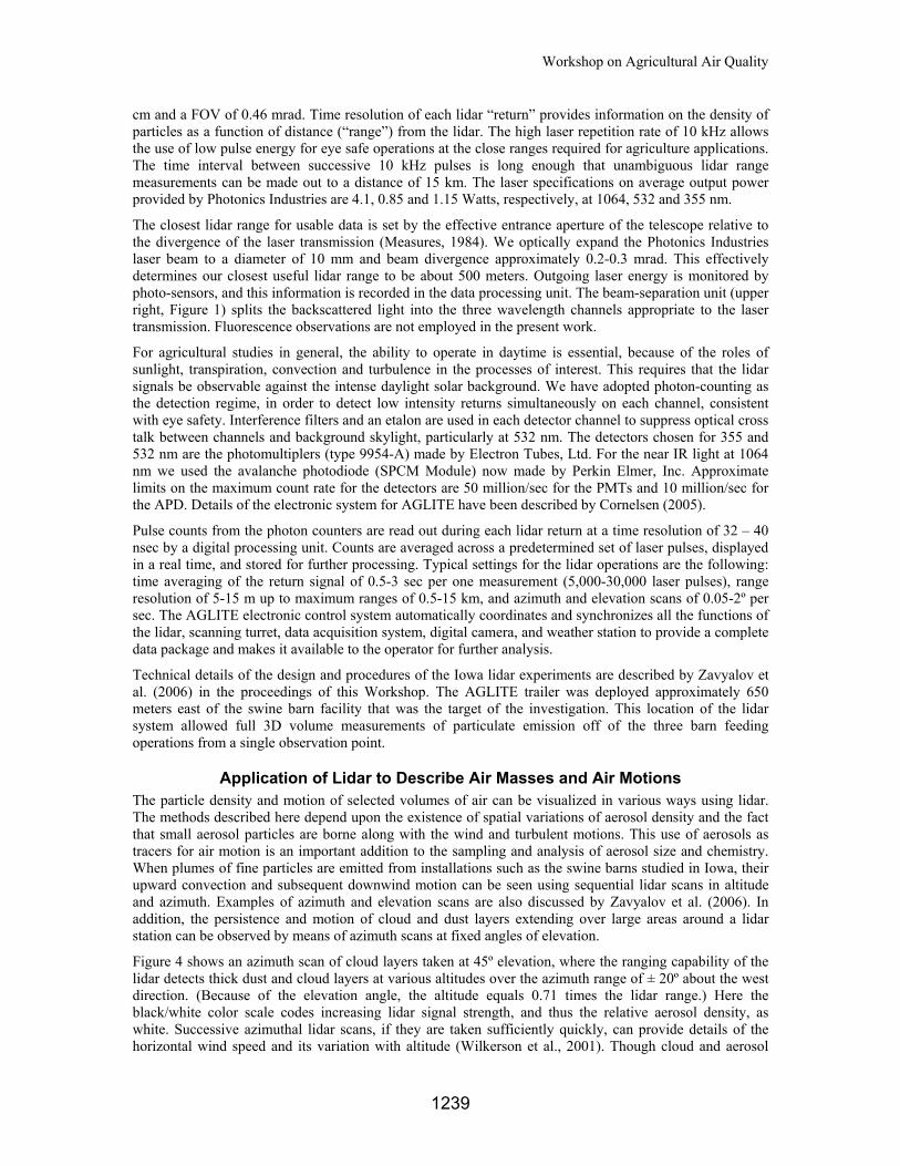
Workshop on Agricultural Air Quality
cm and a FOV of 0.46 mrad. Time resolution of each lidar “return” provides information on the density of particles as a function of distance (“range”) from the lidar. The high laser repetition rate of 10 kHz allows the use of low pulse energy for eye safe operations at the close ranges required for agriculture applications. The time interval between successive 10 kHz pulses is long enough that unambiguous lidar range measurements can be made out to a distance of 15 km. The laser specifications on average output power provided by Photonics Industries are 4.1, 0.85 and 1.15 Watts, respectively, at 1064, 532 and 355 nm.
The closest lidar range for usable data is set by the effective entrance aperture of the telescope relative to the divergence of the laser transmission (Measures, 1984). We optically expand the Photonics Industries laser beam to a diameter of 10 mm and beam divergence approximately 0.2-0.3 mrad. This effectively determines our closest useful lidar range to be about 500 meters. Outgoing laser energy is monitored by photo-sensors, and this information is recorded in the data processing unit. The beam-separation unit (upper right, Figure 1) splits the backscattered light into the three wavelength channels appropriate to the laser transmission. Fluorescence observations are not employed in the present work.
For agricultural studies in general, the ability to operate in daytime is essential, because of the roles of sunlight, transpiration, convection and turbulence in the processes of interest. This requires that the lidar signals be observable against the intense daylight solar background. We have adopted photon-counting as the detection regime, in order to detect low intensity returns simultaneously on each channel, consistent with eye safety. Interference filters and an etalon are used in each detector channel to suppress optical cross talk between channels and background skylight, particularly at 532 nm. The detectors chosen for 355 and 532 nm are the photomultiplers (type 9954-A) made by Electron Tubes, Ltd. For the near IR light at 1064 nm we used the avalanche photodiode (SPCM Module) now made by Perkin Elmer, Inc. Approximate limits on the maximum count rate for the detectors are 50 million/sec for the PMTs and 10 million/sec for the APD. Details of the electronic system for AGLITE have been described by Cornelsen (2005).
Pulse counts from the photon counters are read out during each lidar return at a time resolution of 32 – 40 nsec by a digital processing unit. Counts are averaged across a predetermined set of laser pulses, displayed in a real time, and stored for further processing. Typical settings for the lidar operations are the following: time averaging of the return signal of 0.5-3 sec per one measurement (5,000-30,000 laser pulses), range resolution of 5-15 m up to maximum ranges of 0.5-15 km, and azimuth and elevation scans of 0.05-2º per sec. The AGLITE electronic control system automatically coordinates and synchronizes all the functions of the lidar, scanning turret, data acquisition system, digital camera, and weather station to provide a complete data package and makes it available to the operator for further analysis.
Technical details of the design and procedures of the Iowa lidar experiments are described by Zavyalov et al. (2006) in the proceedings of this Workshop. The AGLITE trailer was deployed approximately 650 meters east of the swine barn facility that was the target of the investigation. This location of the lidar system allowed full 3D volume measurements of particulate emission off of the three barn feeding operations from a single observation point.
Application of Lidar to Describe Air Masses and Air Motions The particle density and motion of selected volumes of air can be visualized in various ways using lidar. The methods described here depend upon the existence of spatial variations of aerosol density and the fact that small aerosol particles are borne along with the wind and turbulent motions. This use of aerosols as tracers for air motion is an important addition to the sampling and analysis of aerosol size and chemistry. When plumes of fine particles are emitted from installations such as the swine barns studied in Iowa, their upward convection and subsequent downwind motion can be seen using sequential lidar scans in altitude and azimuth. Examples of azimuth and elevation scans are also discussed by Zavyalov et al. (2006). In addition, the persistence and motion of cloud and dust layers extending over large areas around a lidar station can be observed by means of azimuth scans at fixed angles of elevation.
Figure 4 shows an azimuth scan of cloud layers taken at 45º elevation, where the ranging capability of the lidar detects thick dust and cloud layers at various altitudes over the azimuth range of ± 20º about the west direction. (Because of the elevation angle, the altitude equals 0.71 times the lidar range.) Here the black/white color scale codes increasing lidar signal strength, and thus the relative aerosol density, as white. Successive azimuthal lidar scans, if they are taken sufficiently quickly, can provide details of the horizontal wind speed and its variation with altitude (Wilkerson et al., 2001). Though cloud and aerosol
1239
Workshop on Agricultural Air Quality
layers can also be detected using a lidar staring vertically above the lidar site, the simple zenith record is less informative about air motion patterns than the scans in azimuth and elevation.
Figure 5 is a set of elevation scans taken 5.79 minutes apart, showing large plumes of aerosol laden air in the atmospheric boundary layer out to distances of 2000 meters. An important aspect of these scans is the direction of the scan relative to the direction in which the plume is moving. For falling plumes of aerosols, a “down scan” follows the plume motion longer than for an “up scan”. Therefore the image of a falling plume is lengthened in the “down” case and compressed in the “up” case and, vice versa, is distorted oppositely for a rising plume. The resulting effects in the images of the top of the aerosol layer (~ 500 meters) are clearly illustrated by the alternating scans in Figure 5.
For well defined clouds of aerosols, these elevation scans enable us to measure both the size and vertical velocity of clouds. In Iowa, making such visual observations during nighttime lidar scans near the swine barns, we were able to estimate upward velocities of aerosol plumes to be about 0.5 – 1.0 meter/sec at a height of 5-10 meters above ground. For well defined plumes rising or falling as they are borne along with the wind, the elevation traces taken like those in Figure 5 display prominent tilts toward or away from the lidar origin depending on both the motion and scan directions, and thus provide information on the vertical and horizontal transport in the boundary layer.
Conclusions The three-wavelength AGLITE lidar has proved to be a fieldworthy, reliable and self contained system for monitoring and profiling the density and motion of aerosols in the air around agricultural installations. The use of three laser wavelengths has enabled us to observe significant variations in backscatter profiles depending on the particle origins. Time dependent records of vertical and horizontal motions have revealed both small scale and large scale motions of aerosol laden air masses originating from unpaved roads, large swine barn facilities, and ordinary atmospheric phenomena such as clouds and hazes.
In principle, atmospheric probing by lidar is able to obtain time dependent, three dimensional pictures of aerosol distributions in any region of interest such as the air space around animal feedlot and production facilities. Aerosols serve as valuable tracers of air motion. In practice, this faces limitations due to the time scale of atmospheric changes, such as turbulence versus the time required to make complete lidar scans of the region. In this paper and in companion papers in the Workshop, we illustrate that, by making the time dependent observations in two dimensions at a time, namely the lidar range versus a single geographic dimension (elevation or azimuth), one can obtain valuable information on the extent of clouds and on low altitude air motions both along and across the lidar beam direction. Then the synthesis of 3D interpretations of aerosol motion can follow from such 2D records as needed. We will continue to apply these lidar methods to the meteorological interpretation of aerosol motions seen in the emission of particulates from agricultural installations.
References Bingham G. E., J. Hatfield, J. H. Prueger, T. D. Wilkerson, V. V. Zavyalov, R. L. Pfeiffer, L. Hipps, R. Martin, P. Silva, W. Eichinger. 2006. An Integrated Approach to Measuring Emissions from Confined Animal Feeding Operations at the Whole Facility Scale. Proceedings of the Workshop on Agricultural Air Quality: June 5-8.
Cornelsen, S.S. 2005. Electronics Design of the AGLITE Instrument, SDL Document No.SDL/05-093 and Master of Science Thesis in Electrical Engineering, Utah State University, Logan, UT, 113 pp.
Hipps, L., J.H. Prueger, J. Hatfield, G.E. Bingham, W. Eichinger, T.D. Wilkerson, V.V. Zavyalov, R. Martin, P. Silva. 2006. Integrating Lidar and Atmospheric Boundary Layer Measurements to Determine Fluxes and Dynamics of Particulate Emissions from an Agriculture Facility. Proceedings of the Workshop on Agricultural Air Quality: June 5-8.
Measures, R. M. 1984. Laser remote sensing: Fundamentals and applications. John Willey & Sons, Inc., New York.
1240
Workshop on Agricultural Air Quality
Martin R.S., V. Doshi, and K. Moore. 2006. Determination of Particle (PM10 and PM2.5) and Gas-Phase Ammonia (NH3) Emissions from a Deep-Pit Swine Operation using Arrayed Field Measurements and Inverse Gaussian Plume Modeling. Proceedings of the Workshop on Agricultural Air Quality: June 5-8.
Silva, P., R.S. Martin, V. Doshi, K. Moore, and M. Erupe. 2006. Variations in Particle Composition and Size Distributions in and around a Deep Pit Swine Operation. Proceedings of the Workshop on Agricultural Air Quality: June 5-8.
Wilkerson, T.D., J.A. Sanders, I.Q. Andrus, G.K. Schwemmer, D.O. Miller, and D. Guerra. 2001. Horizontal Wind Measurements using the HARLIE Holographic Lidar. Proc.SPIE 4484, Lidar Remote Sensing for Industry and Environment Monitoring II, pp. 64 – 73.
Zavyalov, V.V., G.E. Bingham, T.D. Wilkerson, J. Swasey, C. Marchant, C. Rogers, R. Martin, P. Silva, and V. Doshi. 2006. Characterization of Particulate Emission from Animal Feeding Operations with Three-wavelength Lidar Using Simultaneous In-situ Point Measurements as Calibration Reference Sources. Proceedings of Workshop on Agricultural Air Quality: June 5-8.
Figure 1. Schematic of AGLITE lidar design and construction
1241
Workshop on Agricultural Air Quality
Figure 2. AGLITE lidar mounted vertically, viewed through open back door of trailer
Figure 3. Field deployment trailer for AGLITE lidar
1242
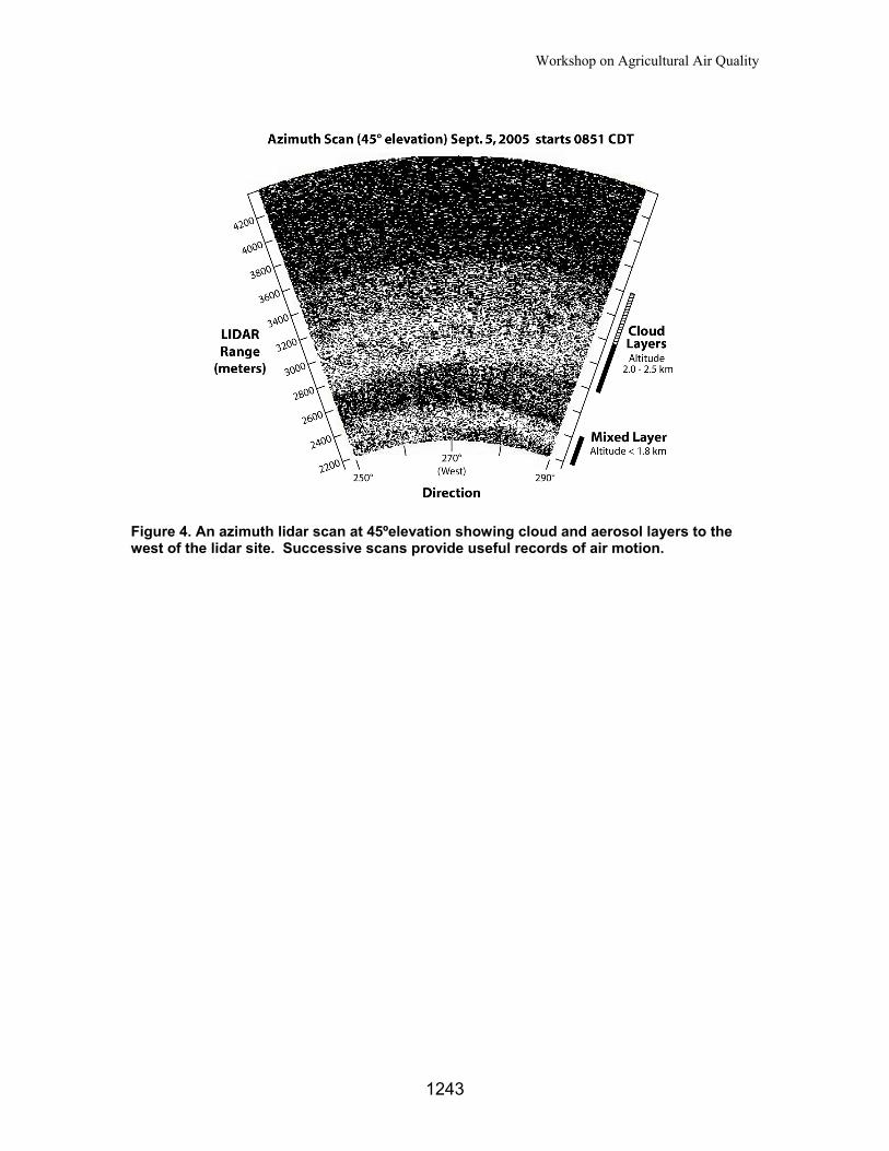
Workshop on Agricultural Air Quality
Figure 4. An azimuth lidar scan at 45ºelevation showing cloud and aerosol layers to the west of the lidar site. Successive scans provide useful records of air motion.
1243
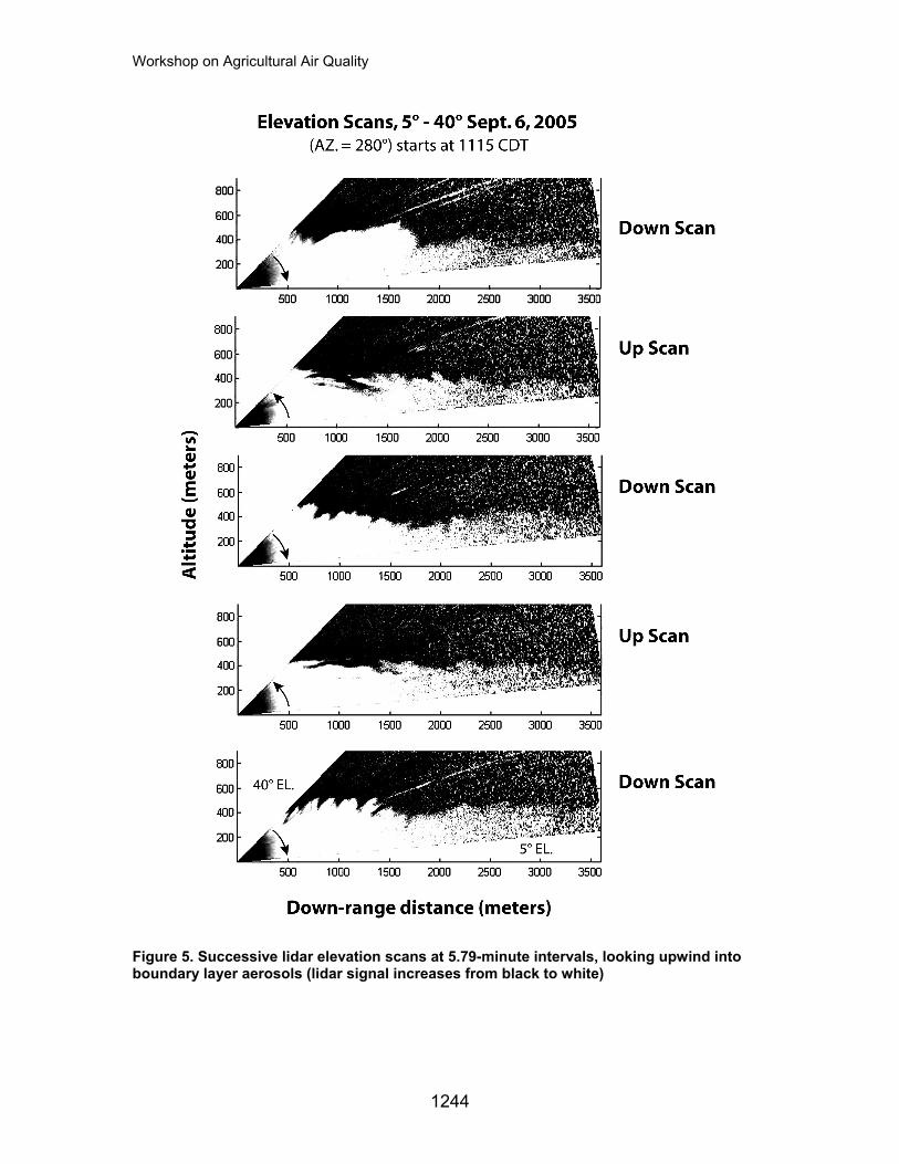
Workshop on Agricultural Air Quality
Figure 5. Successive lidar elevation scans at 5.79-minute intervals, looking upwind into boundary layer aerosols (lidar signal increases from black to white)
1244
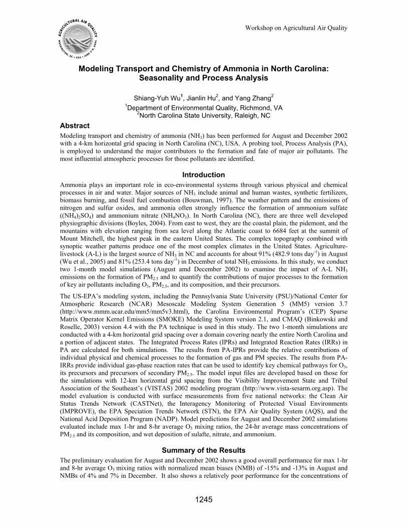
Workshop on Agricultural Air Quality
Modeling Transport and Chemistry of Ammonia in North Carolina: Seasonality and Process Analysis
Shiang-Yuh Wu1, Jianlin Hu2, and Yang Zhang2
1Department of Environmental Quality, Richmond, VA 2North Carolina State University, Raleigh, NC
Abstract Modeling transport and chemistry of ammonia (NH3) has been performed for August and December 2002 with a 4-km horizontal grid spacing in North Carolina (NC), USA. A probing tool, Process Analysis (PA), is employed to understand the major contributors to the formation and fate of major air pollutants. The most influential atmospheric processes for those pollutants are identified.
Introduction Ammonia plays an important role in eco-environmental systems through various physical and chemical processes in air and water. Major sources of NH3 include animal and human wastes, synthetic fertilizers, biomass burning, and fossil fuel combustion (Bouwman, 1997). The weather pattern and the emissions of nitrogen and sulfur oxides, and ammonia often strongly influence the formation of ammonium sulfate ((NH4)2SO4) and ammonium nitrate (NH4NO3). In North Carolina (NC), there are three well developed physiographic divisions (Boyles, 2004). From east to west, they are the coastal plain, the pidemont, and the mountains with elevation ranging from sea level along the Atlantic coast to 6684 feet at the summit of Mount Mitchell, the highest peak in the eastern United States. The complex topography combined with synoptic weather patterns produce one of the most complex climates in the United States. Agriculture-livestock (A-L) is the largest source of NH3 in NC and accounts for about 91% (482.9 tons day-1) in August (Wu et al., 2005) and 81% (253.4 tons day-1) in December of total NH3 emissions. In this study, we conduct two 1-month model simulations (August amd December 2002) to examine the impact of A-L NH3 emissions on the formation of PM2.5 and to quantify the contributions of major processes to the formation of key air pollutants including O3, PM2.5, and its composition, and their precursors.
The US-EPA’s modeling system, including the Pennsylvania State University (PSU)/National Center for Atmospheric Research (NCAR) Mesoscale Modeling System Generation 5 (MM5) version 3.7 (http://www.mmm.ucar.edu/mm5/mm5v3.html), the Carolina Environmental Program’s (CEP) Sparse Matrix Operator Kernel Emissions (SMOKE) Modeling System version 2.1, and CMAQ (Binkowski and Roselle, 2003) version 4.4 with the PA technique is used in this study. The two 1-month simulations are conducted with a 4-km horizontal grid spacing over a domain covering nearly the entire North Carolina and a portion of adjacent states. The Integrated Process Rates (IPRs) and Integrated Reaction Rates (IRRs) in PA are calculated for both simulations. The results from PA-IPRs provide the relative contributions of individual physical and chemical processes to the formation of gas and PM species. The results from PA-IRRs provide individual gas-phase reaction rates that can be used to identify key chemical pathways for O3, its precursors and precursors of secondary PM2.5. The model input files are developed based on those for the simulations with 12-km horizontal grid spacing from the Visibility Improvement State and Tribal Association of the Southeast’s (VISTAS) 2002 modeling program (http://www.vista-sesarm.org.asp). The model evaluation is conducted with surface measurements from five national networks: the Clean Air Status Trends Network (CASTNet), the Interagency Monitoring of Protected Visual Environments (IMPROVE), the EPA Speciation Trends Network (STN), the EPA Air Quality System (AQS), and the National Acid Deposition Program (NADP). Model predictions for August and December 2002 simulations evaluated include max 1-hr and 8-hr average O3 mixing ratios, the 24-hr average mass concentrations of PM2.5 and its composition, and wet deposition of sulafte, nitrate, and ammonium.
Summary of the Results The preliminary evaluation for August and December 2002 shows a good overall performance for max 1-hr and 8-hr average O3 mixing ratios with normalized mean biases (NMB) of -15% and -13% in August and NMBs of 4% and 7% in December. It also shows a relatively poor performance for the concentrations of
1245
Workshop on Agricultural Air Quality
24-hr average PM2.5 and its composition with NMBs of -72% to -18% for August and -59% to 107% for December for all networks. Overall the model underpredicts PM2.5 and all its composition for August and overpredicts PM2.5 and all its composition for December except SO4
2- at the CASTnet and STN sites, organic matters (OM) at the STN sites, and BC at the IMPROVE and STN sites.
17 locations are selected from the STN, IMPROVE, and CASTNet sites for a detail analysis with PA-IPRs. The preliminary analysis shows that the emission is the most important contributor to the production of PM2.5 and its major composition at the STN sites (primarily in urban areas) and the vertical transport is the largest contributor to their losses for both months. In general, the contribution of the PM processes to the mass change in PM2.5 is higher in December than August for PM2.5, NO3
-, and NH4+. At the IMPROVE
(remote locations) and CASTNet (suburban and rural) sites, the major processes are quite different from those at the STN sites. The vertical and horizontal transport dominate the production or loss of PM2.5, indicating the importance of meteorology in determining the concentrations of PM2.5 and its composition at those sites. Other important processes contributing to the production or loss of PM composition such as NO3
-, NH4+, and secondary organic aerosols include PM processes and dry deposition.
The results from PA-IRRs are being analyzed. Major chemical pathways for O3, its precursors, and precursors of secondary PM2.5 in August and December will be identified.
Acknowledgements This work is sponsored by the United States Department of Agriculture 2004-35112-14253, and the National Science Foundation Career Award No. ATM-0348819 at NCSU. Thanks are due to Mike Abraczinskas, George Bridgers, Wayne Cornelius, and Karen Harris of NCDENR for providing VISTAS’s emissions and CMAQ modeling results with a 12-km grid spacing; Don Olerud, BAMS, for providing VISTAS’s MM5 simulation results at a 12-km grid spacing.
References Binkowski, F.S. and S.J. Roselle, 2003. Models-3 community multiscale air quality (CMAQ) model aerosol component, 1. Model description. J. Geophys. Res., 108, 4183,
doi:10.1029/2001 JD001409.
Bouwman, A. F., D. S. Lee, W. A. H. Asman, F. J. Dentener, K. W. Van Der Hoek, and J. G. J Oliver, 1997. A global high resolution emission inventory for ammonia, Global Biogeochem. Cycl., 11, 561-587, 1997.
Boyles, R. P., 2004. North Carolina Climate: A summary of Climate Normals and Averages at 19 Agricultural Research Stations. The State Climate Office of North Carolina, Technical Bulletin 322, September 2004.
Wu, S.-Y., S. Krishnan, J.-L. Hu, C. Misenis, Y. Zhang, V. P. Aneja, and R. Mathur, 2005. Simulating atmospheric fate of ammonia in Southeast U.S. using CMAQ with a 4-km resolution, the 4th Annual CMAS Models-3 User’s Conference, Sep 26-28, 2005. Research Triangle Park, NC.
1246
Workshop on Agricultural Air Quality
Effect of Diet on Air Emissions from Laying Hens of Different Ages
W. Wu1, W. Powers1, R. Angel2, C.E. Hale, III3, and T. Applegate4
1Iowa State University, 109 Kildee Hall, Ames, IA 50011, USA 2University of Maryland, 4131 Animal Sciences Center, College Park, MD 20742, USA
3Rose Acre Farms, Seymour, IN 47274 and 4Purdue University, Lilly Hall of Life Sciences, West Lafayette, IN 47907, USA
Abstract Manure from poultry feeding operations is associated with diminished air quality. The objectives of the current study were to evaluate the effectiveness of feeding a reduced emission diet (R) containing 6.9% of a gypsum-zeolite mixture and a slightly reduced crude protein (CP) to 21-, 38-, and 59- wk old Hy-line W36 hens (trials 1, 2, and 3, respectively) on egg production and emissions of NH3, H2S, NO, NO2, CO2, CH4 and non-methane total hydrocarbon as compared to feeding a commercial diet (C). At each age, 640 hens (BW = 1.36, 1.47, and 1.52 kg in trials 1, 2, and 3, respectively) were allocated randomly to eight environmental chambers for a 3-wk period. On an analyzed basis, the C diet contained 18.0, 17.0, and 16.2% CP and 0.25, 0.20, and 0.20% S in trials 1, 2, and 3, respectively. The R diet contained 17.0, 15.5, and 15.6% CP and 0.99, 1.20, and 1.10% S in trials 1, 2, and 3, respectively. Diets were formulated to contain similar calcium and phosphorus content. Gaseous concentrations were monitored from each chamber in a sequential manner resulting in 10 to 11 daily observations per chamber. Average daily egg weight (ADEW; 57.4 g), average daily egg production (ADEP; 82.5%), average daily feed intake (ADFI; 92.6 g) and BW change (BWC; 24.3 g), across ages, were unaffected by diet (P>0.05). Age affected ADEW (52.1, 58.9, and 61.2 g), ADEP (86.7, 87.1, and 73.7%), ADFI (86.8, 96.2, and 94.6g) and BWC (65.2, 17.3, and -9.7 g) in trials 1, 2, and 3, respectively (P<0.01). Diet (P<0.01) and age (P<0.05) affected NH3 emissions. In trials 1, 2, and 3, daily NH3 emissions from hens fed the R diets (185.5, 312.2, and 333.5 mg bird-1) were less than those of hens fed the C diet (255.0, 560.5, and 616.3 mg bird-1). Daily emissions of H2S across trials from hens fed the R diet were 4.08 mg bird-1 compared to 1.32 mg bird-1 from hens fed the C diet (P<0.01). Diet (P<0.05) and age (P<0.05) affected emissions of CO2 and CH4. A diet effect (P<0.01) on NO emissions and an age effect on SO2 emissions (P<0.01) was observed. No diet or age effects (P>0.05) were observed for NO2 and non-methane total hydrocarbons. Results demonstrate that diet and laying age influence air emissions.
Introduction It is well documented that gaseous emissions from laying hen feeding operations can have potential negative impacts on the environment and on human and bird health. These emissions have been shown to be reduced through diet formulation. Feeding diets formulated to reduce excess crude protein inputs (Elwinger, et al, 1996) help to reduce nitrogen (N) excreted resulting in lower ammonia (NH3) emissions. Acidogenic materials reduce manure pH resulting in the protonation of NH3 to ammonium. Gypsum (calcium sulfate) is one of the acidogenic compounds that has been tested and can serve as a partial replacement for limestone as a calcium (Ca) source without reducing hen performance in laying hen diets (Keshavarz, 1991). Zeolite has been shown to be a beneficial feed additive that exhibits a strong preference for binding nitrogenous cations like ammonium resulting in lower NH3 concentration (Nakaue and Koelliker, 1981; Cabuk, et al (2004)). A study conducted by Hale (2005) showed that using a reduced crude protein (CP) diet in combination with acidogenic materials such as gypsum and nitrogenous binding compounds like zeolite decreased NH3 emission (as measured in vitro) from laying hen excreta. However, the effectiveness of feeding such a diet on all gaseous emissions has not been reported. The objective of the current study was to evaluate the effectiveness of feeding a reduced emissions diet (R) containing 6.9 % of a gypsum-zeolite mixture which replaced 35% of the limestone and slightly reduced CP to laying hens of different ages on egg production and emission of NH3, H2S, NO, NO2, CO2, CH4 and non-methane total hydrocarbon as compared to feeding a commercial diet (C).
1247
Workshop on Agricultural Air Quality
Materials and Methods The study consisted of three trials utilizing birds which were initially 21, 38, 59 wks old. During each trial, 640 Hy-line W36 hens (BW = 1.36, 1.47, and 1.52 kg in trials 1, 2, and 3, respectively) were randomly assigned to one of eight air emissions chambers for a 3-wk period. Between each trial, chambers were completely cleaned. In each chamber, eight cages of 10 birds per cage were used (355 cm2 per bird).
Feed, in mash form, and water were available for ad libitum consumption. On an analyzed basis, the C diet contained 18.0, 17.0, and 16.2% CP and 0.25, 0.20, and 0.20% S in trials 1, 2, and 3, respectively while the R diet contained 17.0, 15.5, and 15.6% CP and 0.99, 1.20, and 1.10% S in trials 1, 2, and 3, respectively. Diets were formulated to contain similar calcium and phosphorus concentrations. The R diet contained a 35% replacement of Ca with gypsum and clinoptilolite. All diets were formulated to meet National Research Council (1994) nutrient recommendations.
Gaseous concentration and air flow were monitored from each chamber in a sequential manner resulting in 10-11 daily observations per chamber. During each 15 minutes observation period, the concentration of NH3, H2S, NO, NO2, CO2, CH4 and non-methane total hydrocarbon were recorded through computer.
Data were analyzed using a mixed model with the day as random variable. (SAS v 8.0) Emission data were adjusted for number of birds. Significance was accepted at or below a P<0.05.
Results and Discussion Average daily egg weight (ADEW; 57.4 g), average daily egg production (ADEP; 82.5%), average daily feed intake (ADFI; 92.6 g) and BW change (BWC; 24.3 g), across ages, were unaffected by diet. Age affected ADEW (52.1, 58.9, and 61.2 g), ADEP (86.7, 87.1, and 73.7%), ADFI (86.8, 96.2, and 94.6g) and BWC (65.2, 17.3, and -9.7 g) in trials 1, 2, and 3, respectively.
In trials 1, 2, and 3, daily NH3 emissions from hens fed the R diets (185.5, 312.2, and 333.5 mg bird-1) were lower than those of hens fed the commercial diet (255.0, 560.5, and 616.3 mg bird-1). Age effects on daily NH3 emission were greater from older hens than from younger hens. Daily H2S emissions from hens fed the R diets (1.6, 7.1 and 3.7 mg bird-1) were lower than those of hens fed the commercial diet (0.5, 1.9 and 0.8 mg bird-1). Daily CO2 emissions from hens fed R diet (64626, 79799 and 80335 mg bird-1) were less than those of hens fed the commercial diet (65627, 86243 and 82694 mg bird-1). Additionally, age affected CO2 emissions. Daily methane emissions from hens fed R diet (138.5, 28.2 and 9.4 mg bird-1) were lower than those of hens fed the commercial diet (153.1, 43.8 and 11 mg bird-1). Age affected methane emission with younger birds producing more methane than older birds. Daily emissions of NO from hens fed R diets (0.71, 0.11 and 0.21 mg bird-1) were less than those from control diet (0.94, 0.2 and 0.28 mg bird-1). No diet or age effects were observed for NO2 non- methane total hydrocarbons.
Diet acidification, CP reduction and zeolite supplementation reduced the emissions of NH3 (by 39%), CO2 (by 5%), CH4 (by 17%) and NO (by 48%). Diet acidification increased the gaseous emissions of H2S mainly because of the high concentration of sulfate in the acidifying agent used. More research is needed to address the increased H2S emissions and to explore the impact of graded concentrations of the additive on emissions.
Implication Emergency Planning and Community Right-to-Know Act (EPCRA) and Comprehensive Environmental Response, Compensation, and Liability Act (CERCLA) reporting requirement allow daily emissions 100lb of both NH3 and H2S from poultry farms. The current study illustrated that feeding a reduced emission diet could increase hen population by 40% without exceeding the requirements. Even though gypsum addition increases H2S emissions considerably, these concentrations did not surpass reporting limits even for the larger laying hen complexes. Reporting requirements for laying hens operations for CERCLA/EPCRA, therefore, will be driven by NH3.
References Cabuk, M., A. Alcicek, M. Bozkurt, and S. Akkan, 2004. Effect of yucca schidigera and natural zeolite on broiler performance. Int. J. of Poultry Sci. 10:651-654.
1248
Workshop on Agricultural Air Quality
Hale III, E.C. 2005. Reduction of ammonia emission, phosphorus excretion, and potassium excretion in laying hen manure through feed manupulation. 2005 Animal Waste Management Symposium, Research Triangle Park, North Carolina
Keshavarz, K. 1991. The effect of calcium sulfate (gypsum) in combination with different sources and forms of calcium carbonate on acid-base balance and eggshell quality. Poultry Sci. 70:1723-1731.
McCrory, D. F. and P. J. Hobbs. 2001. Additives to Reduce Ammonia and Odor Emissions from Livestock Wastes: A Review. J. Environ. Qual. 30:345–355.
National Research Council. 1994. Nutrient Requirements of Poultry, 9th rev. ed. National Academy Press, Washington, DC.
H.S. Nakaue, J.K. Koelliker. 1981. Studies with clinoptilolite in poultry. I. Effect of feeding varying levels of clinoptilolite (zeolite) to dwarf single comb white leghorn pullets and ammonia production. Poultry Sci. 60:944-949
1249
Workshop on Agricultural Air Quality
Role of Leaf Surface Water in the Bi-Directional Ammonia Exchange Between the Atmosphere and Terrestrial Biosphere
Yihua Wu1, John Walker2, Christa Peters-Lidard1, Donna Schwede3, Robin Dennis3, Wayne Robarge4
1NASA/GSFC/HSB 2U.S.EPA/NRMRL
3NOAA/ARL/ASMD, in partnership with the USEPA 4NCSU/DSS
Abstract A field experiment was conducted to study the ammonia exchange between plants and the atmosphere in a soybean field in Duplin County, North Carolina during the summer of 2002. Measurements indicate that the net canopy-scale ammonia exchange is bi-directional and has a significant diurnal cycle. In general, ammonia concentrations peak a few hours after sunrise. Deposition occurs in the evening and early morning hours while emission occurs in the late morning and early afternoon. To investigate the mechanisms that control the exchange process, a new model is developed based on the Multi-Layer BioChemical deposition (MLBC) model (Wu et al., 2003) with additional parameterizations for the leaf ammonia compensation point (Wu et al., 2006) and leaf surface water effects. The MLBC model considers biochemical processes such as photosynthesis, respiration, and membrane passive transport through the cuticle. The leaf surface water thickness is based on a simple water budget equation. Model results suggest that while accurate prediction of the stomatal compensation point is critical, leaf surface water also plays an important role in the net canopy-scale ammonia flux.
1. Introduction It is well documented that leaf surface water influences the development of various foliar bacterial and fungal pathogens (Aston, 1979). Some studies suggest that leaf surface water plays a role in the deposition of pollutants on crops. Our field measurements of ammonia fluxes indicate that leaf surface water appears to enhance ammonia deposition to plants. The potential for the formation of free water on leaves is always present. Leaf surface water can originate from three sources: the air (dewfall and precipitation), the soil (dewrise) and the plant itself (guttation). Depending on environmental conditions, water on the leaf surface can be a thin film, discrete droplets, or a continuous liquid layer. Mikhail and Robens (1983) reported that a thin water film in the nanometer range was always present on surfaces at normal humidities in their investigation of a range of different hydrophilic materials. Leaf surface water can be a barrier for non-soluble gases (such as CO2), or an intermediate medium (i.e., temporary sink and source) for soluble gases (such as NH3 and SO2). Leaf surface water also plays an active role in chemical processes. Fowler and Unsworth (1979), and Schuepp (1989) found that the deposition velocity for SO2 was several times higher when the plant was covered by dew than for dry conditions. Weseley (1989) reported that dew increased the deposition of SO2 and decreased the deposition of O3. Observations by Finkelstein et al. (2000) also show that dew increases the deposition of SO2. Plant leaf surfaces exposed to the atmosphere are continuously exposed to water vapor, so the potential for the formation of molecular films is always present. According to Flechard et al. (1999), the sink strength of the leaf surface is largely dependent on surface humidity and temperature. Dry deposition to the leaf surface for most gas species is reversible. For example, thin water films on plant surfaces may behave as perfect sinks for NH3 for a limited period of time during wet periods after rain or during dewfall. However, as a dew layer or intercepted rainwater evaporates from the leaf surface, NH3 could be released from the evaporating water drops since the NH3 molecule is not immediately 'destroyed'. Therefore, it is very important to consider the role of water when investigating the exchange of ammonia between the atmosphere and biosphere. In this paper, we develop and evaluate a mechanistic model of ammonia uptake and emission from leaf surface water.
1250
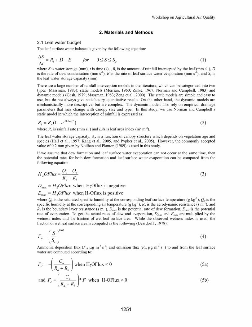
Workshop on Agricultural Air Quality
2. Materials and Methods
2.1 Leaf water budget The leaf surface water balance is given by the following equation:
ci SSforEDRtS
≤≤−+=∆∆ 0 (1)
where S is water storage (mm), t is time (s), , Ri is the amount of rainfall intercepted by the leaf (mm s-1), D is the rate of dew condensation (mm s-1), E is the rate of leaf surface water evaporation (mm s-1), and Sc is the leaf water storage capacity (mm).
There are a large number of rainfall interception models in the literature, which can be categorized into two types (Massman, 1983): static models (Merrian, 1960; Zinke, 1967; Norman and Campbell, 1983) and dynamic models (Gash, 1979; Massman, 1983; Zeng et al., 2000). The static models are simple and easy to use, but do not always give satisfactory quantitative results. On the other hand, the dynamic models are mechanistically more descriptive, but are complex. The dynamic models also rely on empirical drainage parameters that may change with canopy size and type. In this study, we use Norman and Campbell’s static model in which the interception of rainfall is expressed as:
)1( 5.0 LAIni eRR −−= (2)
where Rn is rainfall rate (mm s-1) and LAI is leaf area index (m2 m-2).
The leaf water storage capacity, Sc, is a function of canopy structure which depends on vegetation age and species (Hall et al., 1997; Kang et al., 2005, and Pypker et al., 2005). However, the commonly accepted value of 0.2 mm given by Noilhan and Planton (1989) is used in this study.
If we assume that dew formation and leaf surface water evaporation can not occur at the same time, then the potential rates for both dew formation and leaf surface water evaporation can be computed from the following equation:
ba
as
RRQQ
OFluxH+−
=2 (3)
OFluxHD 2max = when H2Oflux is negative OFluxHE 2max = when H2Oflux is positive
where Qs is the saturated specific humidity at the corresponding leaf surface temperature (g kg-1), Qa is the specific humidity at the corresponding air temperature (g kg-1), Ra is the aerodynamic resistance (s m-1), and Rb is the boundary layer resistance (s m-1), Dmax is the potential rate of dew formation, Emax is the potential rate of evaporation. To get the actual rates of dew and evaporation, Dmax and Emax are multiplied by the wetness index and the fraction of wet leaf surface area. While the observed wetness index is used, the fraction of wet leaf surface area is computed as the following (Deardorff , 1978):
67.0
⎟⎟⎠
⎞⎜⎜⎝
⎛=
cw S
SF (4)
Ammonia deposition flux (Fd, µg m-2 s-1) and emission flux (Fe, µg m-2 s-1) to and from the leaf surface water are computed according to:
⎟⎟⎠
⎞⎜⎜⎝
⎛+
−=ba
ad RR
CF when H2OFlux < 0 (5a)
and FRR
CFba
se *⎟⎟
⎠
⎞⎜⎜⎝
⎛+
= when H2OFlux > 0 (5b)
1251
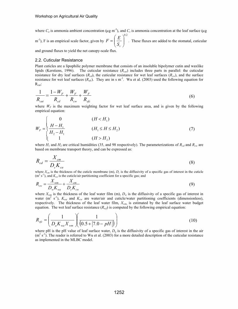
Workshop on Agricultural Air Quality
where Ca is ammonia ambient concentration (µg m-3), and Cs is ammonia concentration at the leaf surface (µg
m-3), F is an empirical scale factor, given by
2.0
⎟⎟⎠
⎞⎜⎜⎝
⎛=
cSEF . These fluxes are added to the stomatal, cuticular
and ground fluxes to yield the net canopy-scale flux.
2.2. Cuticular Resistance Plant cuticles are a lipophilic polymer membrane that consists of an insoluble bipolymer cutin and waxlike lipids (Kerstiens, 1996). The cuticular resistance (Rcut) includes three parts in parallel: the cuticular resistance for dry leaf surfaces (Rcd), the cuticular resistance for wet leaf surfaces (Rcw), and the surface resistance for wet leaf surfaces (Rsfc). They are in s m-1. Wu et al. (2003) used the following equation for Rcut:
sfc
F
cw
F
cd
F
cut RW
RW
RW
R++
−=
11 (6)
where WF is the maximum weighting factor for wet leaf surface area, and is given by the following empirical equation:
⎪⎪⎩
⎪⎪⎨
⎧
>
≤≤−−
<
=
)( 1
)(
)( 0
2
2112
1
1
HH
HHHHHHH
HH
WF (7)
where H1 and H2 are critical humidities (35, and 98 respectively). The parameterizations of Rcd and Rcw are based on membrane transport theory, and can be expressed as:
cac
cmcd KD
XR = (8)
where Xcm is the thickness of the cuticle membrane (m), Dc is the diffusivity of a specific gas of interest in the cuticle (m2 s-1), and Kca is the cuticle/air partitioning coefficient for a specific gas; and
cwc
cm
waw
wmcw KD
XKD
XR += (9)
where Xwm is the thickness of the leaf water film (m), Dw is the diffusivity of a specific gas of interest in water (m2 s-1), Kwa and Kcw are water/air and cuticle/water partitioning coefficients (dimensionless), respectively. The thickness of the leaf water film, Xwm, is estimated by the leaf surface water budget equation. The wet leaf surface resistance (Rscf) is computed by the following empirical equation:
( )⎟⎟⎠⎞
⎜⎜⎝
⎛
−+⎟⎟⎠
⎞⎜⎜⎝
⎛=
pHXKDR
wmwaasfc 0.75.0
11 (10)
where pH is the pH value of leaf surface water, Da is the diffusivity of a specific gas of interest in the air (m2 s-1). The reader is referred to Wu et al. (2003) for a more detailed description of the cuticular resistance as implemented in the MLBC model.
1252
Workshop on Agricultural Air Quality
2.3 Field Measurements The MLBC model was evaluated against ammonia fluxes measured over soybean (Walker et al., 2006). The experiment was conducted in Duplin County, NC between June 18 and August 22, 2002. The site is located in the state’s Upper Coastal Plain region which is characterized by relatively high ammonia emissions from animal production facilities and fertilizer application (Walker et al., 2000). Soil at this site is Norfolk series fine sandy loam. Ammonia concentrations showed considerable diurnal variability, reaching a maximum in the early morning and a minimum in the late evening. Deposition was observed at night and during the first few hours after sunrise, while emission typically occurred in the late morning and early afternoon (Figure 1). This diurnal cycle of ammonia flux is driven by at least three forces: diurnal variation of ambient ammonia concentration (Figure 1), diurnal variation of the plant ammonia compensation point, and diurnal variation of leaf surface water (Figure 1). Leaf surface water can affect ammonia exchange by: 1) acting as a temporary sink and source, and 2) modifying the plant cuticular resistance. As shown in Figure 1, there is a strong relationship between leaf surface wetness and ammonia flux: ammonia deposition increases with leaf surface wetness; ammonia emission occurs when leaf surface wetness drop to a threshold of 0.06. There appear to be two ammonia emission peaks: one at 11:00 AM (LT), and the other at about 14:00 PM (LT). The first peak is consistent with the evaporation of leaf surface water as indicated by the drop in leaf wetness between 7:00 and 11:00 AM. This suggests that the dissolved ammonia in leaf surface water is released back to the air. The second peak represents the diurnal maximum of the stomatal compensation point, which is a strong function of leaf temperature. Therefore, it is necessary to compute leaf surface water budget
3. Results and Discussion The leaf surface water budget model described above was incorporated into the MLBC model (Wu et al., 2003) with the addition of ammonia compensation point (Wu et al, 2006), which was then evaluated using data from the field experiment. Three model runs were conducted: RUN1 with a constant cuticular resistance (8000 s m-1) and without ammonia deposition and emission to and from leaf surface water; RUN2 with the parameterization for cuticular resistance and without ammonia deposition and emission to and from leaf surface water, and RUN3 with the parameterization for cuticular resistance and with ammonia deposition and emission to and from leaf surface water. Component fluxes (stomata, non-stomata [i.e., cuticle, leaf surface water and ground fluxes]) were also computed for RUN3. The average daily cycle of observed and modeled ammonia flux is shown in Figure 2. RUN1 and RUN2 have only one peak. The peak is around 15:00 PM (LT). RUN1 underestimated both deposition and emission most of the day while RUN2 overestimated deposition but underestimated emission. RUN3 has two peaks, one at 12:00 PM (LT), the other one at 15:00 PM (LT). The modeled peak values are close to the observed ones. RUN3 overestimated deposition. However, all runs are well within one standard deviation of the observations. The daily cycle of modeled component fluxes from RUN2 is shown in Figure 3. The figure clearly shows that the first peak is contributed by the release of the dissolved ammonia in leaf surface water when it evaporates, the second peak is contributed by stomatal emission. To further demonstrate this, the daily cycle of modeled stomatal and nonstomatal component fluxes is shown in Figure 4.
1253
Workshop on Agricultural Air Quality
-0 .1 5
-0 .1
-0 .0 5
0
0 .0 5
0
5
1 0
1 5
2 0
2 5
0 4 8 1 2 1 6 2 0 2 4
N H 3 F lu x
N H 3W e tn e s s
NH
3 ( g m-3) and W
etness (Obs*30)
T im e (H o u r )
NH
3 Flu
x (
g m
-2 s
-1)
µµ
Figure 1. Average diurnal variations of observed NH3 fluxes, leaf surface wetness and NH3 concentration for the entire experiment period. Leaf wetness represents the fraction of the 30-minute measurement period during which the leaf wetness sensor was wet, and is multiplied by 30 in order to show on the same figure.
-0 .2 5
-0 .2
-0 .1 5
-0 .1
-0 .0 5
0
0 .0 5
0 .1
0 .1 5
0 4 8 1 2 1 6 2 0 2 4
O b s
R u n 1
R u n 2
R u n 3
T im e (H o u r)
NH
3 Flu
x (
g m
-2 s
-1)
µ
Figure 2. Average diurnal variations of observed and modeled ammonia fluxes for the entire experiment period.
1254
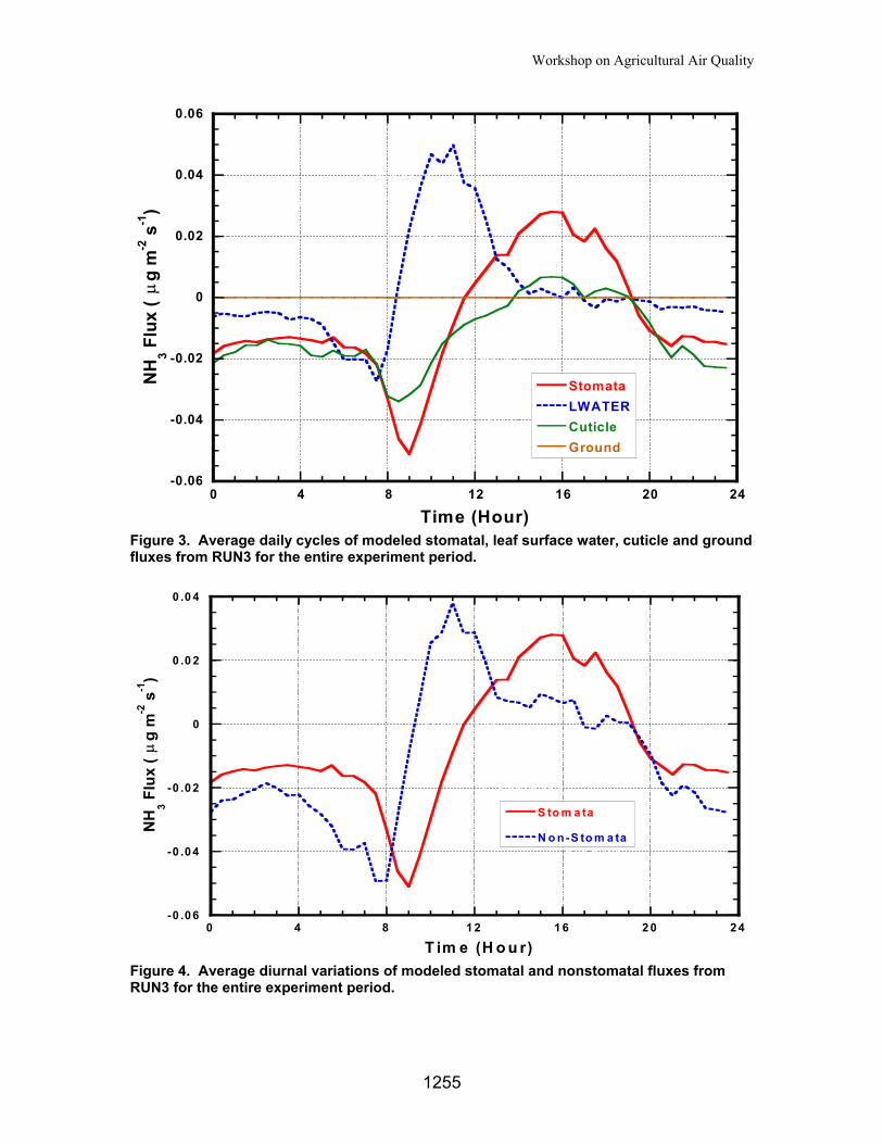
Workshop on Agricultural Air Quality
-0.06
-0.04
-0.02
0
0.02
0.04
0.06
0 4 8 12 16 20 24
StomataLWATERCuticleGround
Time (Hour)
NH
3 Flu
x (
g m
-2 s
-1)
µ
Figure 3. Average daily cycles of modeled stomatal, leaf surface water, cuticle and ground fluxes from RUN3 for the entire experiment period.
-0 .06
-0 .04
-0 .02
0
0 .0 2
0 .0 4
0 4 8 1 2 1 6 2 0 2 4
S to m a ta
N o n -S to m a ta
T im e (H o u r)
NH
3 Flu
x (
g m
-2 s
-1)
µ
Figure 4. Average diurnal variations of modeled stomatal and nonstomatal fluxes from RUN3 for the entire experiment period.
1255
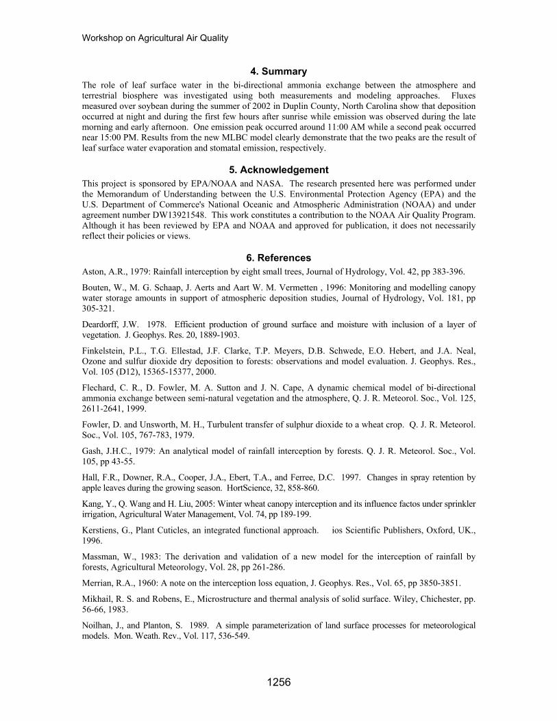
Workshop on Agricultural Air Quality
4. Summary The role of leaf surface water in the bi-directional ammonia exchange between the atmosphere and terrestrial biosphere was investigated using both measurements and modeling approaches. Fluxes measured over soybean during the summer of 2002 in Duplin County, North Carolina show that deposition occurred at night and during the first few hours after sunrise while emission was observed during the late morning and early afternoon. One emission peak occurred around 11:00 AM while a second peak occurred near 15:00 PM. Results from the new MLBC model clearly demonstrate that the two peaks are the result of leaf surface water evaporation and stomatal emission, respectively.
5. Acknowledgement This project is sponsored by EPA/NOAA and NASA. The research presented here was performed under the Memorandum of Understanding between the U.S. Environmental Protection Agency (EPA) and the U.S. Department of Commerce's National Oceanic and Atmospheric Administration (NOAA) and under agreement number DW13921548. This work constitutes a contribution to the NOAA Air Quality Program. Although it has been reviewed by EPA and NOAA and approved for publication, it does not necessarily reflect their policies or views.
6. References Aston, A.R., 1979: Rainfall interception by eight small trees, Journal of Hydrology, Vol. 42, pp 383-396.
Bouten, W., M. G. Schaap, J. Aerts and Aart W. M. Vermetten , 1996: Monitoring and modelling canopy water storage amounts in support of atmospheric deposition studies, Journal of Hydrology, Vol. 181, pp 305-321.
Deardorff, J.W. 1978. Efficient production of ground surface and moisture with inclusion of a layer of vegetation. J. Geophys. Res. 20, 1889-1903.
Finkelstein, P.L., T.G. Ellestad, J.F. Clarke, T.P. Meyers, D.B. Schwede, E.O. Hebert, and J.A. Neal, Ozone and sulfur dioxide dry deposition to forests: observations and model evaluation. J. Geophys. Res., Vol. 105 (D12), 15365-15377, 2000.
Flechard, C. R., D. Fowler, M. A. Sutton and J. N. Cape, A dynamic chemical model of bi-directional ammonia exchange between semi-natural vegetation and the atmosphere, Q. J. R. Meteorol. Soc., Vol. 125, 2611-2641, 1999.
Fowler, D. and Unsworth, M. H., Turbulent transfer of sulphur dioxide to a wheat crop. Q. J. R. Meteorol. Soc., Vol. 105, 767-783, 1979.
Gash, J.H.C., 1979: An analytical model of rainfall interception by forests. Q. J. R. Meteorol. Soc., Vol. 105, pp 43-55.
Hall, F.R., Downer, R.A., Cooper, J.A., Ebert, T.A., and Ferree, D.C. 1997. Changes in spray retention by apple leaves during the growing season. HortScience, 32, 858-860.
Kang, Y., Q. Wang and H. Liu, 2005: Winter wheat canopy interception and its influence factos under sprinkler irrigation, Agricultural Water Management, Vol. 74, pp 189-199.
Kerstiens, G., Plant Cuticles, an integrated functional approach. �ios Scientific Publishers, Oxford, UK., 1996.
Massman, W., 1983: The derivation and validation of a new model for the interception of rainfall by forests, Agricultural Meteorology, Vol. 28, pp 261-286.
Merrian, R.A., 1960: A note on the interception loss equation, J. Geophys. Res., Vol. 65, pp 3850-3851.
Mikhail, R. S. and Robens, E., Microstructure and thermal analysis of solid surface. Wiley, Chichester, pp. 56-66, 1983.
Noilhan, J., and Planton, S. 1989. A simple parameterization of land surface processes for meteorological models. Mon. Weath. Rev., Vol. 117, 536-549.
1256
Workshop on Agricultural Air Quality
Norman J.M., and Campbell, G. 1983. Application of a plant environment model to problems in the environment. Adv. Irrig. Vol. 2, pp 155-188.
Seinfeld, J. H. and S. N. Pandis, Atmospheric chemistry and physics: From air pollution to climate change, John Wiley & Sons, INC, New York, 1998.
Pypker, T.G., B.J. Bond, T.E. Link, D. Marks and M.H. Unsworth, 2005: The importance of canopy structure in controlling the interception loss of rainfall: Examples from a young and an old-growth Douglas-fir forest, Agricul. and Forest Meteorology, Vol. 130, pp 113-129.
Walker, J. T., Aneja, V. P., Dickey, D., 2000. Atmospheric Transport and Wet Deposition of Ammonium in North Carolina, USA. Atmospheric Environment, Vol. 34, 3407-3418.
Walker, J.T.,Wayne P. Robarge, Yihua Wu, Tilden Meyers, 2006. Measurement of bi-directional ammonia exchange over soybean using the modified Bowen-ratio technique. In press, Agricultural and Forest Meteorology.
Wesely, M.L, Parameterization of surface resistance to gaseous dry deposition in regional-scale numerical models. Atmospheric Environment, Vol. 23, 1293-1304, 1989.
Wu, Y., J. Walker, C. Peters-Lidard, Donna Schwede, Robin Dennis and Wayne Robarge and, 2006: Modeling Bi-directional ammonia gas exchanges between the atmosphere and biosphere, I. Parameterization of ammonia compensation point (To be submitted to Agricultural and Forest Meteorology).
Wu, Y., B. Brashers, P. L. Finkelstein and J. E. Pleim, 2003: A multiplayer biochemical dry deposition model, I. Model Formulation, JGR, Vol. 108 (2003), No. D1,
Zeng, M., J.W. Shuttleworth, J.H. Gash, 2000: Influence of temporal variability of rainfall on interception loss. Part I. Point analysis. Journal of Hydrology, Vol. 228, pp 228-241.
Zinke, P.J., 1967: Forest interception studies in the United States. In: W.E. Sopper and H.W. Hull (Editors), International Symposium on Forest Hydrology, Pregamon Press, Oxford, pp 823.
1257


