Assortative Mating and Female Labor Supply

DI

SC

US

SI

ON

P

AP

ER

S

ER

IE

S

Forschungsinstitut zur Zukunft der ArbeitInstitute for the Study of Labor

Assortative Mating and Female Labor Supply

IZA DP No. 5118

August 2010

Christian BredemeierFalko Juessen

Assortative Mating and Female Labor Supply

Christian Bredemeier University of Dortmund (TU)

and Ruhr Graduate School in Economics

Falko Juessen University of Dortmund (TU)

and IZA

Discussion Paper No. 5118 August 2010

IZA

P.O. Box 7240 53072 Bonn

Germany

Phone: +49-228-3894-0 Fax: +49-228-3894-180

E-mail: [email protected]

Any opinions expressed here are those of the author(s) and not those of IZA. Research published in this series may include views on policy, but the institute itself takes no institutional policy positions. The Institute for the Study of Labor (IZA) in Bonn is a local and virtual international research center and a place of communication between science, politics and business. IZA is an independent nonprofit organization supported by Deutsche Post Foundation. The center is associated with the University of Bonn and offers a stimulating research environment through its international network, workshops and conferences, data service, project support, research visits and doctoral program. IZA engages in (i) original and internationally competitive research in all fields of labor economics, (ii) development of policy concepts, and (iii) dissemination of research results and concepts to the interested public. IZA Discussion Papers often represent preliminary work and are circulated to encourage discussion. Citation of such a paper should account for its provisional character. A revised version may be available directly from the author.

IZA Discussion Paper No. 5118 August 2010

ABSTRACT

Assortative Mating and Female Labor Supply This paper investigates the pattern of wives’ hours disaggregated by the husband’s wage decile. In the US, this pattern has changed from downward-sloping to hump-shaped. We show that this development can be explained within a standard household model of labor supply when taking into account trends in assortative mating. We develop a model in which assortative mating determines the wage ratios within individual couples and thus the efficient time allocation of spouses. The economy-wide pattern of wives’ hours by the husband’s wage is downward-sloping for low degrees, hump-shaped for medium degrees, and upward-sloping for high degrees of assortative mating. A quantitative analysis of our model suggests that changes in the gender wage gap are responsible for the overall increase in hours worked by wives. By contrast, the fact that wives married to high-wage men experienced the most pronounced increase is a result of trends in assortative mating. JEL Classification: E24, J22, J16, D13 Keywords: female labor supply, assortative mating, gender wage gap Corresponding author: Falko Juessen Technische Universität Dortmund Wirtschafts- und Sozialwissenschaftliche Fakultät Volkswirtschaftslehre (Makroökonomie) D-44221 Dortmund Germany E-mail: [email protected]

1 Introduction

Hours worked of married women in the US increased substantially overthe second half of the last century. The most prominent explanationfor rising hours of wives is the closure of the gender wage gap, i.e. thecatching-up of female wages relative to men�s wages, see e.g. Galor andWeil (1996), Jones, Manuelli, and McGrattan (2003), Knowles (2007),and Attanasio, Low, and Sánchez-Marcos (2008). According to house-hold models of labor supply (see Chiappori 1988; Apps and Rees 1997;Blundell, Chiappori, Magnac, and Meghir 2007), labor supply of a wifedepends on both the wife�s and the husband�s characteristics. Manyempirical studies estimate cross-wage elasticities of female labor supplyand �nd a signi�cant in�uence of husbands�wages on working hours ofwives, see Blau and Kahn (1997), Blundell, Duncan, and Meghir (1998),Devereux (2004, 2007), and Morissette and Hou (2008).In this paper, we investigate wives�hours disaggregated by the hus-

band�s wage decile. Juhn and Murphy (1997) have performed an empir-ical strati�cation of wives�hours by the husband�s wage and documenta clearly downward sloping relation for the late 1960s and for the 1970s.Juhn and Murphy (1997) also �nd that the increase in hours workedof wives over time has been strongly non-uniform among all groups ofmarried women, with wives of middle- and high-wage men experiencingmore pronounced increases in hours than wives married to low-wage hus-bands. As a consequence, the pattern of wives�hours by the husband�swage has changed from negative to hump-shaped. Similar �ndings arereported by Morissette and Hou (2008) and Schwartz (2010).Thus, a view on disaggregated labor supply of married women re-

veals the following two stylized observations. First, the pattern of wives�hours by the husband�s wage has changed from downward-sloping tohump-shaped. Second, women married to men with high wages haveexperienced the strongest increases in hours worked. This paper aims atexplaining these two empirical observations.We highlight the role of assortative mating for understanding the

economy-wide pattern of wives�hours by the husband�s wage decile. As-sortative mating is the tendency of spouses with similar characteristicsto marry each other. The relevance of assortative mating for spouses�labor-supply decisions has been emphasized by Pencavel (1998) and De-vereux (2004) who stress that, when seeking to interpret the observed

2

relation between husbands�characteristics and wives�work decision, oneneeds to take into account that husbands�and wives�characteristics areusually correlated.In this paper, we demonstrate that a standard household model of

labor supply (Chiappori 1988; Apps and Rees 1997; Blundell, Chiappori,Magnac, and Meghir 2007) can generate the observed economy-wide pat-tern of wives�hours by the husband�s wage when one takes into accounttrends in assortative mating. We measure assortative mating in termsof wage potentials. For a low degree of assortative mating (i.e. mat-ing is almost random), our model generates a downward-sloping patternof wives� hours by the husband�s wage. By contrast, this pattern ishump-shaped for more pronounced assortative mating. Thus, when thedegree of assortative mating increases, this induces a non-uniform changein wives�hours worked by the husband�s wage decile. Speci�cally, theincrease in hours is most pronounced for women married to top-wagehusbands.The economy-wide pattern of wives�hours by the husband�s wage

can change due to two reasons: �rst, changes in the relation betweenthe husband�s wage and the wife�s labor supply at the household leveland, second, compositional e¤ects which may arise because the fractionsof spouses marrying in di¤erent ways changes. In our model, the relationat the micro level is stable but the aggregated pattern of wives�hoursby the husband�s wage depends on assortative mating.Speci�cally, patterns in hours in our model depend on the joint dis-

tribution of wages in marriages, i.e. on the marginal distributions ofgender-speci�c wages and the association between spouses�wages. Cou-ples face a specialization decision with respect to market work and homeproduction. Within a couple, the e¢ cient time allocation depends onthe wage ratio of the two spouses. Only when the wife�s relative wageis high enough, the couple opts for labor market participation of bothspouses. Conditional on participation, hours of the wife are an increasingfunction of her relative wage.To illustrate the e¤ects of assortative mating, consider �rst the ex-

treme cases of perfect sorting and random mating. Under random mat-ing, every husband is on average married to the wife earning the averagefemale wage independent of his own wage. Therefore, the relative wagesare on average lowest for wives married to top-wage husbands. As a con-sequence, these wives work the fewest hours and the pattern of wives�

3

hours by the husband�s wage is downward-sloping.Under perfect sorting, there exist only marriages where both wife

and husband are from the same quantile in the respective gender-speci�cwage distribution. Husband�s and wife�s wages are thus perfectly corre-lated though not necessarily identical. The pattern of wives�hours bythe husband�s wage will then also depend on the marginal distributionsof gender-speci�c wages. For example, with identical gender-speci�cdistributions and perfect sorting, the wage ratio is one in each couple.Consequently, all wives work the same and the pattern of wives�hoursby the husband�s wage is �at. By contrast, when there is a gender wagegap, the wife�s relative wage can also be increasing in the husband�swage. The reason is that an absolute wage gap is less important in rela-tive terms when absolute wages of the two spouses are high. In coupleswhere the husband�s wage is relatively low, the wage gap translates intopronounced relative wage di¤erences between husband and wife. Sincethe wife�s relative wage can be increasing in the husband�s wage, alsohours worked of the wife can be increasing in the husband�s wage.We can imagine intermediate sorting as a combination of the two

extreme cases, a fraction of the population marrying randomly and afraction marrying in a perfectly assortative way. The resulting pattern ofwives�hours worked by the husband�s wage decile is therefore a weightedaverage of the patterns in the two extreme cases.For the fraction of the population marrying in a random way, the pat-

tern of wives�hours by the husband�s wage decile is downward slopingindependent of the wage gap. By contrast, for the fraction of the popula-tion marrying in a perfectly assortative way, the pattern can be upwardsloping with the steepness depending on relative wage di¤erences be-tween husband and wife. The pattern is strongly increasing where wagesare low and relative wage di¤erences are thus pronounced. The patternis almost �at for couples with high absolute wages and thus low relativewage di¤erences. The resulting economy-wide pattern of wives�hours bythe husband�s wage decile can therefore be hump-shaped depending onthe relative sizes of the two population groups marrying randomly andperfectly assortatively, respectively. Trends in assortative mating thusalter the pattern of wives�hours by the husband�s wage decile observedin the aggregate and consequently lead to a non-uniform change in hoursworked by wives.From previous studies, there is much evidence that assortative mat-

4

ing in the US has indeed become stronger over time. Most studies haveinvestigated assortative mating in terms of educational attainment andfound that husband and wife have become more similar with respect toeducation over time, see Mare (1991), Kalmijn (1991a), Kalmijn (1991b),Qian and Preston (1993), Pencavel (1998), Qian (1998), Schwartz andMare (2005), Sánchez-Marcos (2008), and Schwartz (2010). Cancian andReed (1998) and Schwartz (2010) report increased assortative mating byincome. Sweeney and Cancian (2004) provide evidence for an increasingcorrelation between wife�s wage and husband�s income. Herrnstein andMurray (1994) report increased sorting by academic ability in highereducation and by intelligence. In this paper, we use data from the Cur-rent Population Survey (CPS) to measure trends in assortative matingin terms of wage potentials. We �nd strong evidence that assortativemating in terms of wages has increased substantially over time.To investigate whether empirically observed trends in the marginal

and joint distributions of wages imply patterns in hours that are consis-tent with the empirical developments, we feed the observed distributionsof wages into our model. We measure the association between spouses�wages in terms of the number of marriages that exist between di¤erentdeciles of the gender-speci�c marginal wage distributions. By measuringassortative mating in terms of wage deciles, we can disentangle changesin the marginal distributions of husbands�and wives�wages from changesin the association between spousal wages.The data shows a closure of the gender wage gap and a clear trend

towards stronger assortative mating in terms of wages. Our empiricalinvestigation suggests that trends in the marginal wage distributions areresponsible for the overall increase in hours worked by wives. By con-trast, the fact that wives married to high-wage men experienced the mostpronounced increase is primarily a result of trends in assortative matingrather than being due to changes in the marginal wage distributions.The remainder of this paper is organized as follows. In Section 2,

we present the empirical facts on married women�s labor supply we aimto explain as well as empirical evidence for increasing marital sortingin terms of wages. Section 3 presents the theoretical model that usesas an input the association between spousal wages to predict optimallabor supply decisions. Section 4 provides an quantitative analysis wherewe use the empirically observed joint distributions of wages. Section 5concludes and an appendix follows.

5

2 Wives�hours by the husband�s wage decile andtrends in assortative mating

In this section, we present the empirical facts we aim to explain. Thekey observation we address is that the increase in married women�s laborsupply has not been uniform among all wives. We also illustrate inthis section that assortative mating in terms of wages has increasedsubstantially over time.The non-uniform increase in women�s hours has been documented

by e.g. Juhn and Murphy (1997) and Schwartz (2010) and is illustratedin Figure 1. The data are from the Current Population Survey (CPS)in the US. The left panel shows average weekly hours worked of wivesmarried to men in the 10 deciles of the male wage distribution. The�gure compares two periods of time, 1975-1979 (darkly shaded bars)and 2000-2006 (white bars). We form subperiods of more than one yearto control for business cycle e¤ects. The sample consists of matchedhusband-wife pairs of ages 30-50. Details on the data employed can befound in Appendix A.During the 1970s, there has been a clear downward-sloping pattern of

wives�hours by the husband�s position in the wage distribution. Womenmarried to high-wage men tended to work less hours. In the more recentperiod, this relationship has changed with wives of men in the middleof the wage distribution working the most. Thus, the pattern of wives�hours by the husband�s wage has changed from downward-sloping tohump-shaped.1

The right panel in Figure 1 shows the change (between the two pe-riods) in weekly hours worked by married women disaggregated by thehusband�s wage decile. One can see that hours worked of wives in-creased substantially among all groups of married women over time.However, the increase has been strongly non-uniform across husband�swage deciles. Increases in hours have been largest for wives of middle-and high-wage men. By contrast, the increase in labor supply was rela-tively weak among wives of men in the low wage deciles.The empirical facts we aim to explain can thus be summarized as

follows:1A similar picture emerges when one considers changes in participation rates in-

stead of changes in hours worked (detailed results are available upon request).

6

Figure 1: Wives�weekly hours by the husband�s wage decile.

1 2 3 4 5 6 7 8 9 100

5

10

15

20

25

30

Husband's Wage Decile

Wiv

es' W

eekl

y H

ours

Wives' Weekly Hours by Husband's Wage Decile

197579200006

1 2 3 4 5 6 7 8 9 100

0.1

0.2

0.3

0.4

0.5

0.6

0.7

Change In Wives' Weekly Hours by Husband's Wage Decile, 197579 to 200006

Husband's Wage DecileC

hang

e in

Wiv

es' W

eekl

y H

ours

1. The aggregate pattern of wives�hours by the husband�s wage haschanged from downward-sloping to hump-shaped.

2. The increase in hours worked of wives has been strongly non-uniform among all groups of married women, with increases inhours of wives of middle- and high-wage men being more pro-nounced than for wives of men married to low-wage husbands.

In this paper, we seek to explain these developments as a result ofchanges in the wage structure in the economy. Speci�cally, the aggregatepattern of wives�hours by the husband�s wage predicted by our modelwill depend on the joint distribution of wages in marriages, i.e. onthe marginal distributions of gender-speci�c wages together with theassociation between spouses�wages.While most studies focused on assortative mating along education

levels (see e.g. Mare 1991, Fernández, Guner, and Knowles 2005,Schwartz and Mare 2005, and Schwartz 2010), we consider sorting interms of spousal wages. Thereby we face the problem that, in the data,we can observe an individual�s wage only if the person is participatingin the labor market. In our model, by contrast, wages are measures ofearnings potentials. To measure assortative mating in terms of potentialwages, we therefore have to impute wages for non-working individuals.Our model implies that the participation decision is not random.

We therefore need to predict wages for non-working wives that wouldbe observed in the absence of non-participation. To do so, we use a

7

Heckman (1976, 1979) selection model. The Heckmanmodel is estimatedseparately for the periods 1975-1979, 1980-1984, 1985-1989, 1990-1994,1995-1999, and 2000-2006.2 Appendix B presents details on the wageimputation.When measuring assortative mating, one has to take into account

that simple correlation coe¢ cients between the absolute levels of thevariable of interest can be poor measures for describing trends in assor-tative mating, see Mare (1991) and Hou and Myles (2007). The problemof correlation coe¢ cients is their inability to distinguish changes in themarginal distributions of husbands�and wives�wages from changes inthe association between spousal wages. For example, the correlation co-e¢ cient between absolute wages would change in response a change inthe marginal distributions even when the association between spousalwages were unchanged.We overcome this problem by calculating the correlation between

husband�s and wife�s position in the respective gender-speci�c wage dis-tribution, rather than between the absolute levels of their wages. Specif-ically, we consider the association between spouses�decile positions inthe gender-speci�c wage distributions. At each point in time, there are10% of individuals of a given gender in each wage decile independent ofthe wages earned in the speci�c decile. Thus, the distribution of decilepositions is by construction constant over time. Changes in the cor-relation between these relative positions of husband and wife thereforere�ect changes in assortative mating.3

Figure 2 shows the change in the correlation coe¢ cient between hus-band�s and wife�s wage decile positions over time for di¤erent approachesto handle the missing-data problem. Both for simple regression-basedand Heckman-based imputation, respectively, there is a pronounced andsteady increase in the correlation coe¢ cient between spousal wage decilepositions. In fact, the correlation coe¢ cient almost doubles from 1975-

2To check for robustness, we also consider alternative ways to handle the missing-data problem. A �rst strategy is to delete the entire couple from the sample if one ofthe spouses�wages is not observed. We refer to this speci�cation as �listwise deletion�.A second strategy is to use wage predictions from simple OLS estimates.

3An alternative approach to disentangle changes in the association from changesin the marginal wage distributions is to estimate a crossings model, see e.g. Mare(1991) and Schwartz (2010). An advantage of measuring assortative mating in termsof wage decile positions is that this association has a structural interpretation andcan be used directly as an input in our model later on.

8

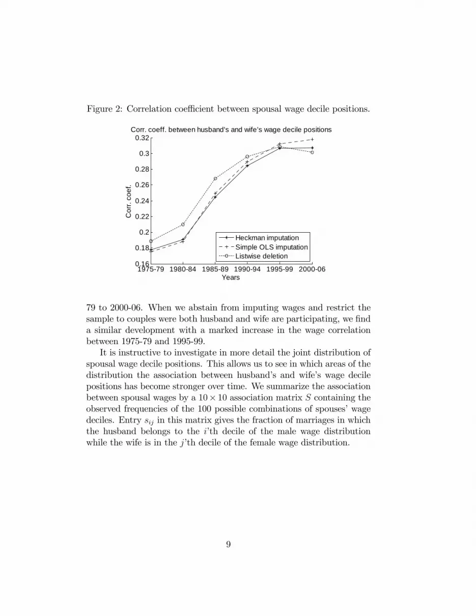
Figure 2: Correlation coe¢ cient between spousal wage decile positions.

197579 198084 198589 199094 199599 2000060.16

0.18

0.2

0.22

0.24

0.26

0.28

0.3

0.32Corr. coeff. between husband's and wife's wage decile positions

Years

Cor

r. co

ef.

Heckman imputationSimple OLS imputationListwise deletion

79 to 2000-06. When we abstain from imputing wages and restrict thesample to couples were both husband and wife are participating, we �nda similar development with a marked increase in the wage correlationbetween 1975-79 and 1995-99.It is instructive to investigate in more detail the joint distribution of

spousal wage decile positions. This allows us to see in which areas of thedistribution the association between husband�s and wife�s wage decilepositions has become stronger over time. We summarize the associationbetween spousal wages by a 10� 10 association matrix S containing theobserved frequencies of the 100 possible combinations of spouses�wagedeciles. Entry sij in this matrix gives the fraction of marriages in whichthe husband belongs to the i�th decile of the male wage distributionwhile the wife is in the j�th decile of the female wage distribution.

9

husb.�s

wife�swagedecile

decile

1st

2nd

3rd

4th

5th

6th

7th

8th

9th

10th

1st

46.0

11.5

-12.7

5.4

-1.4

1.0

-23.8

-38.5

-20.8

-32.2

2nd

27.0

16.7

-6.0

25.3

11.3

30.1

-27.3

-46.7

-15.6

-33.0

3rd

-3.8

5.9

1.4

19.6

17.8

50.6

-16.0

-37.0

-7.5

-26.4

4th

-4.2

1.7

1.2

22.1

-1.4

38.5

7.1

-20.2

-13.1

-31.2

5th

-16.0

1.1

6.5

9.6

2.5

9.7

3.2

-6.2

11.3

-21.2

6th

-15.2

-9.1

4.3

-5.4

5.2

3.8

8.6

-0.4

31.2

-19.8

7th

-20.3

-10.0

15.1

-9.6

-5.1

-8.4

13.1

1.9

27.6

-3.4

8th

-17.7

-14.2

-1.2

-19.5

-12.2

-16.2

11.6

23.2

20.4

18.7

9th

-29.0

-21.7

-1.3

-19.1

-8.3

-34.5

15.6

31.6

0.3

46.6

10th

-29.6

-18.8

5.9

-26.6

-2.7

-39.4

-1.8

69.0

-33.8

52.2

Table1:ChangeintheAssociationMatrixbetweenSpousalWages(percentagechangesinthedensityof

thedecilecombinationsfrom

1975-79to2000-06).

10

To highlight changes over time, Table 1 shows the relative changesof the frequencies of the di¤erent combinations of wage deciles from1975-79 to 2000-06,

�s2000�06ij � s1975�79ij

�=s1975�79ij , using the Heckman-

imputed wages for non-working wives.4 Positive values indicate that in2000-06 the number of couples with the speci�c combination of wagedeciles has increased relative to 1975-79. Tables 5 and 6 in Appendix Cshow the association matrices separately for the two periods of time.From Table 1 it can be seen that the number of couples where hus-

band and wife di¤er by much with respect to their relative positions inthe respective wage distributions has decreased substantially. For ex-ample, the number of couples where the husband is from the top decileof the male distribution and the wife is from the lowest decile of thefemale distribution has decreased by about 30%. In general, Table 1shows a clear pattern that most entries distant from the main diagonalare negative. By contrast, decile combinations on and close to the maindiagonal tend to be observed more often, highlighting that couples havebecome more similar in terms of gender-speci�c wage positions.These results show that assortative mating in terms of wages has

increased substantially over time. In the next section, we present atheoretical model that highlights the role of changes in the wage struc-ture for explaining the non-uniform increase in hours worked by marriedwomen and the resulting change in wives�hours worked disaggregatedby the husband�s wage decile.

3 The model

3.1 Decision problem of a coupleWe consider an economy populated by couples which di¤er by the wagesof the two spouses. First, we will present the decision process for indi-vidual couples. Thereafter, we will aggregate their decisions.A couple consists of two spouses. We denote spouses�wages by w1

and w2 and order spouses by these wages such that the index i = 1refers to the primary earner and i = 2 to the secondary earner. Notethat the index does not necessarily refer to the gender of the respectivespouse. For the decisions at the couple level, gender is not relevant. Forinstance, labor-force participation of the secondary earner will depend

4Results using OLS-imputed wages and from listwise deletion are very similar.

11

on his or her relative wage independent of gender.There are two commodities in the model, a private "market" con-

sumption good and a "home" consumption good that is public to thecouple. We assume that individuals�preferences over the two commodi-ties are characterized by the additively separable utility function

ui = ln ci + ln d , (1)

where ci denotes consumption of the market good and d stands for con-sumption of the home or domestic good. d does not wear an indexindicating an individual since the home good is public.Market goods can be earned through market labor by both spouses.

We denote the time spent on market work by ni. The couple�s budgetconstraint is thus given by

c1 + c2 = w1 � n1 + w2 � n2. (2)

Home goods are produced within the household using both spouses�labor (denoted by h1 and h2, respectively) as inputs with a productionfunction f (h1; h2) = (h1)

1=2 (h2)1=2. Correspondingly, the home con-

sumption constraint takes the form

d = (h1)1=2 (h2)

1=2 . (3)

We impose equal exponents on both labor inputs. A priori, there is there-fore no di¤erence between the two spouses�labor in home production.However, the household can decide to use the two inputs in di¤erentquantities depending on opportunity costs.Both spouses have a time endowment of 1 which can be used for

market work and home production, i.e.

ni + hi = 1; i = 1; 2. (4)

The couple chooses the time allocations of both spouses and thedistribution of the resulting consumption possibilities. Thus the couplechooses h1, h2, n1, n2, d, c1, and c2. Constraints are given by equations(2) to (4).While the distribution of market consumption is subject to the spe-

ci�c process of household bargaining, we can determine the time alloca-tions by e¢ ciency considerations alone. Since the focus of this paper is

12

on labor-supply decisions, we do not need to specify a household bar-gaining process. For our purposes, it is su¢ cient to assume that theoutcome of the bargaining process is e¢ cient.

3.2 Decision makingIn collective models of household behavior, households are assumed to al-locate their resources e¢ ciently (Chiappori 1988; Chiappori 1992). Con-sequently, given a desired amount of home consumption, the householdwill produce it with minimal opportunity costs. Given the desired levelof home consumption, the cost minimization determines time spent inhome production for both spouses. In our set-up, spouses spend theirremaining time on paid market work. Accordingly, we proceed by solv-ing for a family�s optimal level of home consumption and then deducelabor-supply decisions.For e¢ ciency, the marginal costs to produce the public home good

(in terms of foregone market consumption) has to be equal to the sumof both spouses marginal rates of substitution which corresponds toSamuelson�s (1955) rule for e¢ cient public-good provision,

MRS1 (c1; d) +MRS2 (c2; d) =MC (d) , (5)

where MRSi (ci; d) =@ui@ci=@ui@dis spouse i�s marginal rate of substitution

between home and market goods. MC (d) denotes the marginal costs ofhome production for the couple in terms of market goods. In order todetermine the optimal level of home consumption which satis�es (5), weneed to consider the couples�marginal costs of producing the home goodas well as spouses�marginal rates of substitution. Detailed derivationsof decisions at the couple level can be found in Appendix D.1.

Marginal costs of home consumption. The marginal cost functionMC (d) results from the production of d units of the home good withminimal costs. In this minimization problem, the household has to re-spect that no member can work more than one unit of time in homeproduction:

h1� 1 (6)

h2� 1 (7)

In e¢ cient allocations, total opportunity costs of home production as afunction of the consumption level d are the value function of the mini-

13

mization problemminh1;h2

w1h1 + w2h2

subject to the home production function (3) and the two time constraints(6) and (7). Technically, marginal costs are the derivative of this valuefunction.Due to the inequality restrictions (6) and (7), the marginal cost func-

tion is not globally di¤erentiable. In the range where (6) and (7) do notbind, production of the home good exhibits constant marginal costs dueto the constant returns to scale property of the production function.Marginal costs in this range are given by 2 � (w1)1=2 � (w2)1=2. The cost-minimal time inputs are h1 =

�w1w2

��1=2� d and h2 =

�w1w2

�1=2� d.

The couple can only produce with constant returns to scale and thuswith constant marginal costs as long as both spouses can still increasetheir time spent in home production. From the point where one spousespends her or his entire time endowment in home production, furtherincreases in home production can only be realized by increases in theother spouse�s time input. Since w1 > w2, the time constraint of thesecondary earner (7) will be binding �rst. This is at the point where

d =�w2w1

�1=2. From there on, marginal costs are given by the inverse

of the primary earner�s marginal productivity multiplied by his or herwage. Since h2 = 1 in this range, the marginal productivity of the

primary earner is given by 12(h1)

�1=2. For d >�w2w1

�1=2, the required

amount of h1 to produce d is h1 = d2. Marginal costs are therefore2 � w1 � d in this range. Since both spouses� time endowments are 1,the maximum quantity of home consumption is 1. The marginal costfunction (in terms of foregone market consumption) is thus given by

MC (d) =

8>>><>>>:2 � (w1)1=2 � (w2)1=2 ; d <

�w2w1

�1=22 � w1 � d;

�w2w1

�1=2< d < 1

1; d > 1.

(8)

14

The corresponding total (opportunity) cost function is

C (d) =

8>>><>>>:2 � (w1)1=2 � (w2)1=2 � d; d <

�w2w1

�1=2w2 + w1 � d2;

�w2w1

�1=2< d < 1

1; d > 1.

(9)

Sum of the marginal rates of substitution. We now turn to thespouses�marginal rates of substitution between market and home con-sumption. The marginal rates of substitution depend on spouses�indi-vidual marginal utility of market consumption. The couples�s marginalwillingness to pay will therefore in general depend on the intra-coupledistribution of private consumption which is subject to bargaining. Withlog utility, however, intra-household bargaining does not a¤ect the cou-ple�s willingness to pay for home consumption. Since the marginal ratesof substitution are linear with this speci�c formulation of utility and thehome good is public, marginal rates of substitution can be added upto a function of the couple�s total consumption levels of the two goodsindependent of the distribution across spouses. In particular, it holdsthat

MRS1 (c1; d) +MRS2 (c2; d) = � c1d+ � c2

d= � c

d, (10)

where c = c1 + c2. Redistributing private consumption lowers onespouses�s marginal rate of substitution but increases the other spouse�sone by the same amount. Changes in the distribution of private con-sumption within the couple therefore do not a¤ect the sum of the twomarginal rates of substitution.With e¢ cient production of the home good, the constraints (2), (3),

and (4) can be combined to

w1 + w2 = c+ C (d) .

Thus, the choice of either c or d determines the other as well. Thecouple�s total level of market consumption, c, can then be expressed asc = w1 + w2 � C (d). We can therefore express the sum of the twomarginal rates of substitution (10) as a function of the level of home

15

consumption only:

2Xi=1

MRSi =

8>>><>>>: w1+w2

d� 2 (w1)1=2 � (w2)1=2 ; d <

�w2w1

�1=2 w1 (d

�1 � d) ;�w2w1

�1=2< d < 1

�1; d > 1

(11)

3.3 Labor-supply decisionsBy the condition for e¢ cient provision of the public good (5), the optimallevel of home consumption is at the intersection of (8) and (11). Labor-market participation of the secondary earner will depend on whether ornot the couple wishes a level of home consumption that can be producedwithout using the entire time endowment of the secondary earner. Tech-nically, the secondary earner will participate if (5) is solved by a d that

falls below�w2w1

�1=2. We can thus derive a participation condition on

the secondary earner�s wage relative to the primary earner�s one. Theparticipation threshold for the secondary earner is

w2 >

2� w1. (12)

The secondary earner only participates in the labor market if his orher relative contribution to the couple�s potential income exceeds somethreshold value determined by the valuation of home consumption. Thehigher the wage of the primary earner, the higher the wage of the sec-ondary earner has to be for participation of both spouses.Conditional on participation of the secondary earner, her or his mar-

ket hours are

n2 =2

2 + �

2 + � w1w2

(13)

and the primary earner�s hours are

n1 =2

2 + �

2 + � w2w1. (14)

If the secondary earner does not participate, the primary earner worksconstant hours on the market, given by

n1 =2

2 + . (15)

16

Note that none of the labor-supply decisions described by equations(12) to (15) depend on the absolute wage of one of the two spouses.Instead, all decisions depend on the wage ratio between the two spouseswithin the couple.Now we consider a couple with a wife F and husbandM , whose wages

are denoted by wF and wM , respectively. The wife is the secondaryearner if wF < wM and vice versa. Summarizing labor-supply decisionsat the couple level as described by equations (12) to (15), we can expresshours worked by a wife F as a function of the wage ratio within thecouple, ! = wF

wM,

nF (!) =

8><>:0; ! <

22

2+ �

2+ � !�1;

2� ! < 2

2

2+ ; ! � 2

. (16)

We impose the parameter restriction

< 2

such that there are wage ratios for which both, husband and wife, par-ticipate in the labor market, see equation (16).

3.4 The role of assortative matingWe now illustrate the in�uence of the mating structure on the aggregatepattern of wives�labor supply. In the next section, we aggregate indi-vidual decisions formally to obtain the aggregate pattern of wives�hoursby the husband�s wage predicted by our model.Equation (16) describes the relation between the husband�s wage

and the wife�s labor supply at the household level. This relation isnegative and independent of the mating structure. By contrast, theaggregate pattern of wives�hours by the husband�s wage also dependson assortative mating because assortative mating a¤ects the aggregationof individual decisions.Figure 3 illustrates the relation between wife�s hours and the wages

of the two spouses in the couple given by equation (16). The �gureshows some selected iso-hours lines where darker colors correspond tomore hours of the wife. The dark gray area in the upper left part of the�gure contains couples who decide that only the wife works for pay. In

17

Figure 3: Wives�hours of market work for di¤erent husband-wife wagecombinations (iso-hours lines and areas, resp.; the darker, the morehours) and two joint distributions of wages with identical marginal dis-tributions (scenario 1: imperfect sorting (non-�lled circles); scenario 2:perfect sorting (�lled circles)).

wM

wF

woman 3

woman 2

woman 1

man 1 man 2 man 3

the light gray area in the lower right corner of the �gure, wives do notparticipate in the labor market. Between these two areas, hours of wivescontinuously decrease from the upper left to the lower right as the wife�srelative wage decreases.The circles in the �gure indicate couples with di¤erent husband-wife

wage combinations. We illustrate the role of assortative mating on theaggregate pattern of labor supply using these couples as examples. Weconsider three women and three men who are matched to each other intwo di¤erent ways. Across scenarios, the gender-speci�c marginal distri-butions of wages are identical but the joint distribution of spousal wagesdi¤ers. In scenario 1 (non-�lled circles), marital sorting is imperfectwhile it is perfect in scenario 2 (�lled circles). Marital sorting is perfectin the second scenario as the woman with the highest potential wage(woman 3) is married to the man with the highest wage (man 3), andso on.

18

First note that, in the example, the increase in assortative matingalters the aggregate participation rate. In scenario 1, the couple in thelower right of the �gure (woman 1 and man 3) decides against labor-market participation of the wife. Intra-household wage di¤erentials aresu¢ ciently pronounced that it is rational to use the wife�s time solelyin home production. In the other two couples, both spouses participateon the labor market. The aggregate participation rate of wives is 2/3 inthis scenario.In scenario 2 (�lled circles), although the marginal distributions of

wages have not changed, the aggregate participation rate is 1. Sortingis perfect in this scenario, i.e. the top-wage wife is matched with thetop-wage husband and so on. As a consequence, in the example, there isno more couple where intra-household wage di¤erentials are su¢ cientlylarge for husband-only participation.Changes in assortative mating a¤ect the aggregate pattern of wives�

hours worked by the husband�s wage positions. In scenario 1, the wifemarried to the husband with the highest wage (man 3) works the fewesthours while the other two women work the same. In scenario 2, thispattern is �ipped upside down with the wife married to the top-wagehusband supplying the most labor and the other two women workingthe same.

3.5 Aggregate pattern of wives�hours by the hus-band�s wage positions

We now use our model for a strati�cation analysis as performed in Sec-tion 2 for the CPS data. Speci�cally, we study the aggregate pattern ofwives�hours by the husband�s wage predicted by our model for di¤erentforms of assortative mating.We can use the joint distribution of wages in marriages as an input to

our model, i.e. the marginal distributions of gender-speci�c wages andthe association between spouses�wages. We allow for the possibility thatthe marginal distributions are not the same across genders. Speci�cally,we allow for a gender wage gap. To highlight the role of changes in theassociation between husband�s and wife�s wages, we consider uniformmarginal distributions in the theoretical part of the paper. In the nextsection, we feed the empirically observed marginal and joint distributionsof wages into our model.

19

In general, marginal distributions may di¤er by gender. With a gen-der wage gap, the wage of the representative man in the i�th decile of themale distribution, WM (i) ; is higher than the wage of the representativewoman in the i�th decile of the female distribution, WF (i). We denotethe absolute di¤erence between gender-speci�c wages by � and assumehere that this wage gap is constant across deciles.We normalize the marginal distribution of female wages so that its

support has length 1, i.e. female wages are distributed uniformly on(wmin; wmin + 1) with wmin � 0. Correspondingly, male wages are dis-tributed uniformly on (wmin + �;wmin + 1 + �). We apply the parameterrestriction

wminwmin + �

�

2,

which ensures that in a couple where both husband and wife earn thelowest gender-speci�c wages, respectively, the wife participates in the la-bor market. It furthermore implies that, whenever husband and wife areat the same quantile of the respective wage distributions, both spousesparticipate.We model assortative mating similar as in Kremer (1997). It is as-

sumed that a proportion � of agents marries a spouse from the samewage quantile whereas everyone else marries randomly. Perfect sortingand random mating are special cases where � = 1 or � = 0, respectively.For a husband with wage wM , the probability of being married to a wifewith wage wF = wM�� is � while all other wages of the wife are equallylikely with a total probability of 1� �.The economy-wide pattern of wives�hours by the husband�s wage

positions results from (i) the relation between the husband�s wage andthe wife�s labor supply at the household level described by equation(16) and (ii) the mating structure in the economy. To determine theaggregate pattern, we calculate average hours of wives married to hus-bands earning a certain wage wM . We do so by integrating individ-ual decisions (16) taking into account the density function of wages,

nF (wM) =RnF

�wFwM

�� f (wF j wM) dwF , where nF (wM) denotes aver-

age hours worked of wives married to husbands earning a wage wM . Thedensities f (wF j wM) depend on assortative mating. Given the marginaland joint distributions of wages, average hours of wives married to hus-

20

bands earning a wage wM are

nF (wM)= (1� �) �Z

2wM

wmin

0 dwF| {z }no participation of wife

+(1� �) �Z 2

wM

2wM

�2

2 + �

2 + � wMwF

�dwF| {z }

both spouses participate

(17)

+(1� �) �Z wmin+1

2 wM

2

2 + dwF| {z }

only wife participates

+ � ��

2

2 + �

2 + � wMwM � �

�| {z }

fraction marrying perfectly assortatively, both participate

which evaluates as (see Appendix D.2)

nF (wM) = + (1� �) � g (wM) + � � k (wM) , (18)

where = 22+

+ (1� �) � 22+

� wmin and

g (wM)=�

2 + ��1 + ln

4

2

�� wM

k (wM)=�

2 + � wMwM � �

.

Wives� hours by the husband�s wage are thus a constant plus theweighted sum of two functions of the husband�s wage. g (wM) is a down-ward sloping and linear function while k (wM) is an upward sloping andconcave function for � > 0 and a constant for � = 0. The weights forg (wM) and k (wM) are determined by the parameter � measuring thedegree of assortative mating. The pattern of wives�hours by the hus-band�s wage decile thus depends on the degree of assortative mating andthe gender wage gap.Figure 4 illustrates the pattern of wives�hours by the husband�s wage

deciles for six di¤erent scenarios. To illustrate the possible patterns, we

21

Figure 4: Patterns of wives�hours by husbands�wage deciles for di¤er-ent degrees of assortative mating (illustration using uniform marginaldistributions).

no wage gap, � = 0 wage gap, � > 0

perfectsorting

1 2 3 4 5 6 7 8 9 100

5

10

15

20

25

Wives' Weekly Hoursby Husband's Wage Decile


Wiv

es' W

eekl

y H

ours

1 2 3 4 5 6 7 8 9 100

5

10

15

20

25



Wiv

es' W

eekl

y H

ours

random

mating

1 2 3 4 5 6 7 8 9 100

5

10

15

20

25

30



Wiv

es' W

eekl

y H

ours

1 2 3 4 5 6 7 8 9 100

5

10

15

20

25



Wiv

es' W

eekl

y H

ours

intermediatesorting

1 2 3 4 5 6 7 8 9 100

5

10

15

20

25

30



Wiv

es' W

eekl

y H

ours

1 2 3 4 5 6 7 8 9 100

5

10

15

20



Wiv

es' W

eekl

y H

ours

22

use example parameter values.5 When we compare model predictionsto empirical observations in the next section, we use the empiricallyobserved marginal and joint distributions of wages.Here, we distinguish between two cases concerning the wage gap

(� = 0, � > 0) and three di¤erent degrees of assortative mating (� = 1 ,� = 0, 0 < � < 1). The left column in Figure 4 refers to the case of nowage gap (� = 0), while the right column shows the results when a wagegap is present (� > 0). The rows in Figure 4 refer to the three cases ofassortative mating (perfect sorting, random mating, intermediate sort-ing).Consider the case of perfect assortative mating, � = 1, which is

illustrated in the �rst row of Figure 4. In this situation, there exist onlymarriages where both wife and husband are from the same quantile inthe respective gender-speci�c wage distribution.Without a gender wage gap, � = 0, this implies that the wage ratio

in each couple is !j = 1. Consequently, all wives work the same, whichcan be seen from equation (18) for � = 1 and � = 0,

nF (wM) = � � �

2 + .

This case is illustrated in the upper left panel of Figure 4.By contrast, when there is a gender wage gap, � > 0, the average

wage ratio, (wM � �) =wM , is increasing in the husband�s wage. As aconsequence, with a gender wage gap and perfect assortative mating,average hours worked by wives are increasing in the husband�s wage.This is illustrated in the upper right panel of Figure 4 and can be seenfrom equation (18) for � = 1 and � > 0:

nF (wM) = � � �

2 + � wMwM � �

.

In the other extreme case, � = 0 , mating is completely random.Here, all possible combinations of wages within a marriage exist with

5For the �gure, the parameter measuring the valuation of home consumptionis set to 0:5 and the marginal distribution of female wages is uniform on [0:1; 1:1],thus wmin = 0:1. For the cases with a gender wage gap (right column), we set� = 0:3, otherwise � = 0. The parameter � measuring the degree of assortativemating is 1 (�rst row), 0 (second row), or 0:5 (third row), respectively. The weeklytime endowment is set to 40 hours.

23

same frequency. Hence, every husband is on average married to thewife earning the average female wage wF independent of his own wageposition. Therefore, the average wage ratio wF=wM is decreasing acrossthe male wage distribution. As can be seen from equation (18) for � =0, this results in a downward-sloping pattern of wives� hours by thehusband�s wage, independent of the wage gap,

nF (wM) = �

2 + ��1 + ln

4

2

�� wM .

This case is illustrated in the second row of Figure 4.The third row of Figure 4 represents an intermediate case of assor-

tative mating where � = 0:5. In this intermediate case, both functionsg (wM) and k (wM) are given non-zero weights in equation (18). For� = 0, wives�hours by the husband�s decile are then the sum of a down-ward sloping function and a constant,

nF (wM) = � (1� �) �

2 + ��1 + ln

4

2

�� wM � � �

2 + ,

and thus downward sloping in the male wage, see the lower left panel ofFigure 4. In the presence of a gender wage gap, � > 0, female hours bymale wage decile are the sum of a downward sloping linear function anda concave upward sloping function,

nF (wM) = � (1� �) �

2 + ��1 + ln

4

2

��wM � � �

2 + � wMwM � �

.

(19)The function nF (wM) is thus concave and can be hump-shaped, depend-ing on the speci�c value for �. In Appendix D.3, we show that for anycombination of the parameters , wmin, and � > 0, there exists a degreeof assortative mating, �, such that the pattern of wives�hours by thehusband�s wage is hump-shaped.The role of assortative mating for the pattern of wives�hours by the

husband�s wage becomes apparent when comparing the three panels inthe right column of Figure 4. In all three scenarios, the marginal distri-butions of gender-speci�c wages are identical. However, the patterns inwives�hours di¤er depending on the association between spouses�wages.

24

4 Quantitative analysis

The analysis in the previous section has shown that our model is ableto generate the empirical patterns documented in Section 2: The aggre-gate pattern of wives�hours by the husband�s wage has been downward-sloping in 1975-79 like in the middle row of Figure 4. In 2000-06 thispattern has changed to being hump-shaped as in the lower right panelof Figure 4.The patterns in hours predicted by the model depend on the joint

distribution of wages in marriages, i.e. on the marginal distributions ofgender-speci�c wages and the association between spouses�wages. Wenow feed the empirically observed joint distributions of wages into ourmodel and investigate whether observed trends in these distributionsimply patterns in hours that are consistent with the empirical develop-ments.As in Section 2, we measure the association in terms of the number

of marriages that exist between di¤erent deciles of the gender-speci�cmarginal wage distributions. The 10 � 10 association matrix S intro-duced in Section 2 contains the relative frequencies of the 100 possiblecombinations of deciles in a marriage. As discussed in Section 2, the as-sociation between husband�s and wife�s wage has changed towards morepronounced assortative mating.Since we consider deciles, all columns (and all rows) in S contain 10

percent of the overall population. By construction, our analysis in termsof wage deciles controls for changes in the marginal gender-speci�c wagedistributions that could otherwise distort the measurement of changesin assortative mating. Put di¤erently, by measuring assortative matingin terms of wage deciles, we can disentangle changes in the marginal dis-tributions of husband�s and wife�s wages from changes in the associationbetween spousal wages.The gender-speci�c mean wage levels associated with the deciles are

denoted by WF (i) and WM (i), respectively, where i is a decile number.Table 2 shows the marginal distributions of spousal wages for the twoperiods of time we consider, 1975-79 and 2000-06. For both genders,wages have increased over time whereas the increase has been strongerfor women. The gender wage gap closed by 12 percentage points onaverage over all deciles. The table also shows that changes in wages andthe gender wage gap have not been uniform across wage deciles.

25

mean

deciles

1st

2nd

3rd

4th

5th

6th

7th

8th

9th

10th

malewages1975-79

15.48

4.54

8.56

10.4612.0913.6915.3117.0819.2922.6631.10

femalewages1975-79

8.52

3.35

6.04

6.74

7.18

7.69

7.93

8.40

9.53

11.2117.18

wagegap1975-79

0.55

0.74

0.71

0.64

0.59

0.56

0.52

0.49

0.49

0.49

0.55

malewages2000-06

17.19

4.43

7.72

9.62

11.3613.1815.1817.6521.0426.5445.15

femalewages2000-06

11.54

3.51

5.64

6.98

7.77

8.89

10.2012.1713.5317.0029.75

wagegap2000-06

0.67

0.79

0.73

0.73

0.68

0.67

0.67

0.69

0.64

0.64

0.66

wage-gapclosure

0.12

0.06

0.02

0.08

0.09

0.11

0.15

0.20

0.15

0.15

0.11

Table2:MarginalDistributionsofSpousalWages1975-79and2000-06.

26

For both genders, wages in the upper deciles have grown stronger thanwages in the lower deciles. Similarly, the closure of the gender wage gaphas been strongest in the upper half of the wage distribution.Finally, we have to choose a value for the parameter measuring the

valuation of home consumption and a value for the weekly time endow-ment. We set the relative valuation of home consumption to = 0:5,a value in the range commonly used in the literature for comparableutility functions, see e.g. Jones, Manuelli, and McGrattan (2003). Thisvalue implies that the ratio of time spent on home production and timespent on market work is about 60%, which is in line with empirical �nd-ings. For instance, McGrattan, Rogerson, and Wright (1997) estimate ahousehold utility function with home production and their results implythat the ratio of home to market hours is 15=27. The weekly time en-dowment has a pure scaling e¤ect on labor supply and is set to 40 hours.The weekly time endowment is the total working time of agents in ourmodel since leisure is absent from the model.To calculate the economy-wide pattern of wives�hours by the hus-

band�s wage decile predicted by our model for a given joint distributionof wages fWF ;WM ; Sg, we proceed as follows. We �rst determine fe-male labor supply for all 100 possible combinations of decile positionsin a 10� 10 matrix H: To determine hours worked by the wife hij in aspeci�c cell ij we plug the ratio of gender-speci�c average wages in thiscell, !ij = WF (j) =WM (i), into equation (16). Average hours workedby wives married to men in decile i are then given by (hi � s0i) =

P10j=1 sij,

where hi is the i�th row of the female hours matrix H and si is thecorresponding row in the association matrix S.Figure 5 shows wives�hours by the husband�s wage decile predicted

by our model when we use the empirically observed marginal and jointdistributions of spousal wages in 1975-79 and 2000-06, respectively. Theright panel shows the relative change in married women�s hours by thehusband�s wage decile between the two periods. Thus, the �gure is themodel�s counterpart to the strati�cation analysis performed using CPShours displayed in Figure 1.For 1975-79, the model predicts a decreasing pattern of wives�hours

by the husband�s wage decile as observed in the data. For 2000-06, themodel predicts a higher level of hours worked by wives. From the rightpanel of the �gure, one can see that the predicted increase in hoursis not uniform across husband�s wage deciles. As in the data, wives

27

Figure 5: Predicted wife�s weekly hours by husband�s wage decile.

1 2 3 4 5 6 7 8 9 100

5

10

15

20

25

30


Pre

dict

ed W

ives

' Wee

kly

Hou

rs

Predicted Wives' Weekly Hours by Husband's Wage Decile

197579200006

1 2 3 4 5 6 7 8 9 100

0.05

0.1

0.15

0.2

0.25

0.3

0.35

Change In Predicted Wives' Weekly Hours by Husband's Wage Decile, 197579 to 200006

Husband's Wage DecileC

hang

e in

Pre

dict

ed W

ives

' Wee

kly

Hou

rs

married to high-wage men experience the strongest increases. However,the increase is not su¢ ciently non-uniform to change the pattern in theleft panel from downward sloping to hump-shaped.The patterns in Figure 5 result from e¤ects of changes in the mar-

ginal distributions of gender-speci�c wages as well as from e¤ects due tochanges in the association of spousal wages. To disentangle these e¤ects,we perform a series of counterfactual experiments. Figure 6 summarizesthe results. Each panel in the �gure corresponds to a di¤erent counter-factual setting and shows the change in wives�hours by the husband�sdecile (the �gures are thus the analogs to the right panel in Figure 5).In a �rst experiment, we hold constant the association matrix S at its

1975-79 level but allow the marginal distributions to change over time.This way, we shut down e¤ects of trends in assortative mating. From theupper left panel in Figure 6 it can be seen that, when we do not allow forchange in assortative mating, the model does predict an increase in hoursfor all groups of wives. Yet, in this scenario, the increase is strongest forwives married to medium-wage men. By contrast, the data show thatwives married to high-wage men have experienced the strongest increasesin hours worked.The upper right panel in Figure 6 refers to the other extreme case

where we allow for changes in the association between spousal wages buthold constant the gender-speci�c marginal wage distributions. In thisscenario, changes in wives�hours are increasing in the husband�s decile

28

Figure 6: Counterfactual experiments.

no change in assortative mating no change in marginal distributions

1 2 3 4 5 6 7 8 9 100

0.02

0.04

0.06

0.08

0.1

0.12

0.14

0.16



Cha

nge

in P

redi

cted

Wiv

es' W

eekl

y H

ours

1 2 3 4 5 6 7 8 9 100.05

0

0.05

0.1

0.15

0.2

0.25

0.3



Cha

nge

in P

redi

cted

Wiv

es' W

eekl

y H

ours

uniform wage-gap closure,no change in assortative mating

uniform wage-gap closure,change in assortative mating

1 2 3 4 5 6 7 8 9 100.1

0.05

0

0.05

0.1

0.15

0.2

0.25



Cha

nge

in P

redi

cted

Wiv

es' W

eekl

y H

ours

1 2 3 4 5 6 7 8 9 100

0.05

0.1

0.15

0.2

0.25

0.3

0.35



Cha

nge

in P

redi

cted

Wiv

es' W

eekl

y H

ours

29

position. Yet, not all groups of wives experience increasing hours in thisscenario.This evaluation of our model suggests that changes in the marginal

wage distributions are responsible for the overall increase in hours workedby wives. By contrast, the fact that wives married to high-wage menexperienced the most pronounced increase is a result of trends in assor-tative mating rather than being due to changes in the marginal distrib-utions.A potential source of the non-uniform increase in hours is that the

gender wage gap has closed in a non-uniform way. As we used the empir-ically observed marginal gender-speci�c wage distributions, our bench-mark results reported in Figure 5 include the e¤ects of the non-uniformwage-gap closure. In order to study the role of this development, we per-form two additional counterfactual experiments. In these experiments,we impose a uniform closure of the wage gap, i.e. we impose that thewage gap has closed by the same amount (measured in percentage points)across all deciles.The lower left panel in Figure 6 refers to the case where the wage

gap closes in such uniform way and the association is held constant atits 1975-79 level. The lower right panel also imposes a neutral wage-gapclosure but additionally allows for changes in assortative mating overtime. The e¤ects of the non-neutrality of the wage gap closure becomeapparent when comparing the upper left and the lower left panels in the�gure. With a uniform closure of the wage gap, the model predicts de-creasing hours for wives of top-wage men, opposed to what is observedin the data. However, one can see that accounting for trends in assorta-tive mating is key for understanding the non-uniform increase in wive�shours. Only when we allow the association matrix to change over time,our model predicts an increasing pattern in the change of hours workedby women as observed in the data.

5 Conclusion

This paper has investigated wives�hours disaggregated by the husband�swage decile. Speci�cally, we have addressed two empirical observationsthat have been documented for the US. First, the aggregate patternof wives� hours by the husband�s wage has changed from downward-sloping to hump-shaped. Second, over time, the increase in hours worked

30

of wives has been strongly non-uniform among all groups of marriedwomen, with increases in hours of wives of middle- and high-wage menbeing more pronounced than for wives of men married to low-wage hus-bands.We have presented a theoretical model that explicitly considers the

role of assortative mating in terms of wages for understanding thesedevelopments. Assortative mating determines the wage ratios within in-dividual couples. In our model, the intra-couple wage ratio determinesthe e¢ cient time allocation of the two spouses. Only when the wife�s rel-ative wage is high enough, the couple opts for labor-market participationof both spouses.Under random mating, every husband is on average married to the

wife earning the average female wage independent of his own wage.Therefore, the relative wages are lowest for wives married to top-wagehusbands. As a consequence, these wives work the fewest hours. Underrandom mating, the pattern of wives�hours by the husband�s wage decileis therefore negative.Under perfect sorting, by contrast, there exist only marriages where

both wife and husband are from the same quantile in the respectivegender-speci�c wage distribution. The pattern of wives�hours by thehusband�s wage will then also depend on the marginal distributions ofgender-speci�c wages. When there is a gender wage gap, the wife�srelative wage can be increasing in the husband�s wage. As a consequence,hours worked by the wife can be increasing in the husband�s wage.For intermediate sorting, the resulting pattern of wives�hours worked

by the husband�s wage decile is a weighted average of the patterns inthe two extreme cases of random and perfect mating, respectively. Theresulting economy-wide pattern of wive�s hours by the husband�s wagedecile can therefore be hump-shaped depending on the relative weightsof population groups marrying randomly and perfectly assortatively, re-spectively. Changes in assortative mating thus alter the pattern of wives�hours worked by the husband�s wage decile and consequently lead to anon-uniform change in hours worked by wives.The patterns in hours predicted by our model depend on the joint

distribution of wages in marriages. In a quantitative analysis, we havefed the empirically observed joint distributions of wages into our modeland have investigated whether observed changes in these distributionsimply patterns in hours that are consistent with the empirical develop-

31

ments.The data shows a closure of the gender wage gap and a clear trend

towards stronger assortative mating in terms of wages. For 1975-79, themodel predicts a decreasing pattern of wives�hours by the husband�swage decile as observed in the data. For 2000-06, the model predictsa higher overall level of hours worked by wives. In accordance withempirical developments, the model-predicted increase in hours is notuniform across husband�s wage deciles. As in the data, wives married tohigh-wage men experience the strongest increases. However, the increaseis not su¢ ciently non-uniform to change the pattern of wives�hours bythe husband�s wage from downward sloping to hump-shaped.A series of counterfactual experiments has shown that changes in

the marginal wage distributions are responsible for the overall increasein hours worked by wives. By contrast, the fact that wives married tohigh-wage men experienced the most pronounced increase is a result oftrends in assortative mating rather than being due to changes in themarginal wage distributions. Thus, accounting for trends in assortativemating is key for understanding the non-uniform increase in wives�hours.Only when we take into account trends in assortative mating, our modelpredicts an increasing pattern in the change of hours worked by womenas observed in the data.

References

Apps, P. F. and R. Rees (1997). Collective labor supply and householdproduction. Journal of Political Economy 105 (1), 178�90.

Attanasio, O., H. Low, and V. Sánchez-Marcos (2008). Explainingchanges in female labor supply in a life-cycle model. AmericanEconomic Review 98 (4), 1517�1552.

Blau, F. D. and L. M. Kahn (1997). Swimming upstream: Trendsin the gender wage di¤erential in 1980s. Journal of Labor Eco-nomics 15 (1), 1�42.

Blundell, R., P.-A. Chiappori, T. Magnac, and C. Meghir (2007). Col-lective labour supply: Heterogeneity and non-participation. Re-view of Economic Studies 74 (2), 417�445.

Blundell, R., A. Duncan, and C. Meghir (1998). Estimating laborsupply responses using tax reforms. Econometrica 66 (4), 827�861.

32

Cancian, M. and D. Reed (1998). Assessing the e¤ects of wives�earn-ings on family income inequality. The Review of Economics andStatistics 80 (1), 73�79.

Chiappori, P.-A. (1988). Rational household labor supply. Economet-rica 56 (1), 63�90.

Chiappori, P.-A. (1992). Collective labor supply and welfare. Journalof Political Economy 100 (3), 437�467.

Devereux, P. J. (2004). Changes in Relative Wages and Family LaborSupply. Journal of Human Resources 39 (3), 698�722.

Devereux, P. J. (2007). Small-sample bias in synthetic cohort modelsof labor supply. Journal of Applied Econometrics 22 (4), 839�848.

Fernández, R., N. Guner, and J. Knowles (2005). Love and money:A theoretical and empirical analysis of household sorting and in-equality. The Quarterly Journal of Economics 120 (1), 273�344.

Galor, O. and D. N. Weil (1996). The gender gap, fertility, and growth.American Economic Review 86 (3), 374�387.

Heckman, J. J. (1976). The common structure of statistical models oftruncation, sample selection and limited dependent variables anda simple estimator for such models. In Annals of Economic andSocial Measurement, Volume 5, number 4, NBER Chapters, pp.120�137. National Bureau of Economic Research.

Heckman, J. J. (1979). Sample selection bias as a speci�cation error.Econometrica 47 (1), 153�161.

Herrnstein, R. J. and C. Murray (1994). The Bell Curve: Intelligenceand Class Structure in American Life. New York: The Free Press.

Hou, F. and J. Myles (2007, May). The changing role of educationin the marriage market: Assortative marriage in canada and theunited states since the 1970s. Statistics Canada, Analytical StudiesBranch Research Paper 2007299e.

Jaeger, D. A. (1997). Reconciling the old and new census bureau ed-ucation questions: Recommendations for researchers. Journal ofBusiness & Economic Statistics 15 (3), 300�309.

33

Jones, L., R. Manuelli, and E. McGrattan (2003). Why are marriedwomen working so much? Federal Reserve Bank of Minneapolis,Sta¤ Report No. 317.

Juhn, C. and K. M. Murphy (1997). Wage inequality and family laborsupply. Journal of Labor Economics 15 (1), 72�97.

Kalmijn, M. (1991a). Shifting boundaries: Trends in religious andeducational homogamy. American Sociological Review 56 (6), 786�800.

Kalmijn, M. (1991b). Status homogamy in the united states. TheAmerican Journal of Sociology 97 (2), 496�523.

Knowles, J. (2007). Why are married men working so much? Themacroeconomics of bargaining between spouses. IZA DiscussionPaper 2909.

Kremer, M. (1997). How much does sorting increase inequality? Quar-terly Journal of Economics 112 (1), 115 �139.

Mare, R. D. (1991). Five decades of educational assortative mating.American Sociological Review 56 (1), 15 �32.

McGrattan, E. R., R. Rogerson, and R. Wright (1997). An equilibriummodel of the business cycle with household production and �scalpolicy. International Economic Review 38 (2), 267�290.

Morissette, R. and F. Hou (2008). Does the labour supply of wivesrespond to husbands�wages? Canadian evidence from micro dataand grouped data. Canadian Journal of Economics 41 (4), 1185�1210.

Pencavel, J. (1998). Assortative mating by schooling and the work be-havior of wives and husbands. American Economic Review 88 (2),326 �329.

Qian, Z. (1998). Changes in assortative mating: The impact of ageand education, 1970-1990. Demography 35 (3), 279�292.

Qian, Z. and S. H. Preston (1993). Changes in american marriage,1972 to 1987: Availability and forces of attraction by age andeducation. American Sociological Review 58 (4), 482�495.

34

Samuelson, P. A. (1955). Diagrammatic exposition of a theory of pub-lic expenditure. The Review of Economics and Statistics 37 (4),350�356.

Schwartz, C. R. (2010). Earnings inequality and the changing asso-ciation between spouses� earnings. American Journal of Sociol-ogy 115 (5), 1524�1557.

Schwartz, C. R. and R. D. Mare (2005). Trends in educational as-sortative marriage from 1940 to 2003. Demography 42 (4), 621 �646.

Sweeney, M. M. and M. Cancian (2004). The changing importance ofwhite women�s economic prospects for assortative mating. Journalof Marriage and Family 66 (4), 1015�1028.

Sánchez-Marcos, V. (2008). What accounts for the increase in collegeattainment of women? Applied Economics Letters 15 (1), 41�44.

Wooldridge, J. M. (2002). Econometric Analysis of Cross Section andPanel Data. MIT Press.

Appendix

A CPS data

The CPS data we use are in the format arranged by Unicon Research.6

The CPS is a monthly household survey conducted by the Bureau ofthe Census. Respondents are interviewed to obtain information aboutthe employment status of each member of the household 16 years of ageand older. Survey questions covering hours of work, earnings, gender,and marital status are covered in the Annual Social Economic Supple-ment, the so-called March Supplement Files. The sample of the CPS isrepresentative of the civilian non-institutional population.Data on hours and earnings is retrospective and refers to the previous

year. The CPS data we use covers the period 1975-2006. While the CPSprovides data on hours and earnings from 1963 onwards, the number ofchildren in family under age six is not available before 1975. Since thelatter variable is used as an instrument for imputing wages for non-working individuals, our analysis starts in 1975.

6See http://www.unicon.com/.

35

Our selected sample comprises civilians aged 30 to 50. In a set ofrobustness tests, we checked that our results are robust with respect tothe speci�c age range (detailed results are available on request). Wedrop people who derive their main income from self-employment andconsider only couples where both husband and wife are present in thesample. We identify spouses by the household identi�cation number. Tocontrol for outliers, we drop couples where either husband or wife fall inthe top 1% percentile of observed wages.In 1992, the educational-attainment question in the CPS changed

from years of education to degree receipt. Following Jaeger (1997), weharmonized both series and created a measure of educational attainmentthat takes on four categories: dropouts, high-school graduates, some col-lege, and college graduates.7

B Wage imputation

Since our dataset is very large, we use Heckman�s (1979) two-stepe¢ cient estimator instead of Maximum likelihood estimation (seeWooldridge 2002 for technical details). The Heckman two-step modelcan be described as follows. First, we estimate a binomial probit modelthat predicts the individual�s probability of participation in the labormarket (selection equation). Second, we use the estimated selectionmodel to construct the hazard rate for sample inclusion. Third, we in-clude the hazard rate as a regressor in the wage equation. When theerror term in the selection equation is correlated with the error termin the wage equation, standard regression techniques yield inconsistentestimates while the two-step Heckman procedure yields consistent esti-mates.To identify the Heckman model, we need to �nd factors that deter-

mine whether a wife participates in the labor market but are unrelated toa wife�s wage. We assume that the likelihood of working is a function ofthe number of preschool children at home (we code the number of kidsas dummy variables). Moreover, we include in the selection equationquadratic terms in age of wife and husband and the levels of educationof both partners. The number of preschool children and the characteris-tics of the husband are only included in the participation equation but

7This education variable has been created from the CPS variables _educ (1964-1991, 19 categories, Unicon recoded) and grdatn (1992-2007, 17 categories).

36

1975-1979 2000-2006Wage equation estimate std. err. estimate std. err.log(age wife/17) -0.054 0.149 1.182 0.116log(age wife/17) squared 0.038 0.103 -0.592 0.077education level 2 wife 0.156 0.011 0.385 0.014education level 3 wife 0.257 0.013 0.600 0.014education level 4 wife 0.495 0.014 0.975 0.014intercept 1.938 0.056 1.035 0.047year dummies includedParticipation equationlog(age wife/17) 0.105 0.280 0.338 0.235log(age wife/17) squared -0.390 0.193 -0.172 0.157log(age husband/17) -1.493 0.301 -0.797 0.256log(age husband/17) squared 0.843 0.198 0.416 0.164education level 2 wife 0.306 0.015 0.501 0.019education level 3 wife 0.451 0.020 0.712 0.019education level 4 wife 0.769 0.022 0.928 0.021education level 2 husband -0.051 0.015 0.190 0.018education level 3 husband -0.070 0.019 0.181 0.019education level 4 husband -0.232 0.019 -0.111 0.0202 kids younger than age 6 -0.655 0.013 -0.443 0.0113 kids younger than age 6 -1.041 0.020 -0.733 0.0154 kids younger than age 6 -1.332 0.051 -1.131 0.0375 kids younger than age 6 -1.765 0.173 -1.392 0.131intercept 0.626 0.090 0.215 0.088year dummies included

� (inv. Mills ratio) -0.017 0.018 0.295 0.018

Table 3: Two-step Estimates of Heckman Selection Model

Method Obs. Mean Std. Dev. Min Max1975-1979 Heckman 64090 2.070 0.158 1.790 2.419

OLS 64090 2.057 0.159 1.774 2.4082000-2006 Heckman 94352 2.183 0.307 1.376 2.618

OLS 94352 2.334 0.277 1.665 2.729

Table 4: Predictions of Heckman Selection Model vs. OLS imputation

37

are omitted from the wage equation. We also control for time e¤ects.In the wage equation, we include a quadratic term in the wife�s ageand dummy variables for the wife�s level of education. By including allvariables that determine the wage also in the participation equation, weallow the participation decision to depend implicitly on the wage.We �t the Heckman model separately for the periods 1975-1979 and

2000-2006. Table 3 summarizes the two-step estimates of the Heckmanselection model. The upper part of the table displays the estimatesfor the parameters in the wage equation while the lower part showsthe results for the participation equation. In both equations, we haveincluded time dummies but their point estimates are omitted from thetable to save on space.From the selection equation, it can be seen that more preschool chil-

dren in the household signi�cantly decrease the probability of participa-tion. The coe¢ cient of the selection term is reported at the bottom ofTable 1. While the selection term is found to be insigni�cant in 1975-1979 it turns highly signi�cant in the more recent period. This meansthat a standard regression not taking into account selection will produceinconsistent wage predictions for non-working women, which shows therelevance of incorporating selectivity in the estimation of the wage equa-tion.Table 4 compares predicted values from the Heckman model with an

ordinary regression model without selection adjustment. In the periodwhere the selection term has been found to be insigni�cant (1975-1979),wage predictions from the Heckman model and uncorrected OLS arefairly similar on average. During 2000-2006, by contrast, simple regres-sion yields predictions that are on average higher than the Heckman-corrected estimates. Speci�cally, wage predictions of the Heckman modelare on average about 6.87% lower than the regression-based ones. Onecan also see that the regression prediction shows less variation than theprediction based on the selection model.

38

C Association matrices

Table 5 shows the association matrix S between spouses�wage decilepositions for the period 1975-79. The association matrix for theperiod 2000-06 is presented in Table 6. The relative changes ofthe frequencies of the di¤erent combinations of the wage deciles,�s2000�06ij � s1975�79ij

�=s1975�79ij , can be found in Table 1 in the main text.

husb.�s wife�s wage deciledecile 1st 2nd 3rd 4th 5th 6th 7th 8th 9th 10th

1st 1.61 1.64 1.46 0.96 0.84 0.74 0.75 0.73 0.65 0.622nd 1.26 1.39 1.43 0.98 0.90 0.72 0.92 1.02 0.69 0.683rd 1.24 1.22 1.20 0.96 0.92 0.82 0.96 1.03 0.87 0.784th 1.04 1.06 1.10 0.96 0.98 0.95 0.96 0.97 1.03 0.935th 0.99 0.95 1.01 1.00 0.97 1.07 0.99 1.03 0.96 1.046th 0.92 0.92 0.94 1.08 0.98 1.07 0.97 0.96 0.97 1.187th 0.84 0.87 0.81 1.09 1.04 1.14 0.96 1.05 1.02 1.188th 0.77 0.77 0.80 1.13 1.13 1.10 1.03 0.97 1.15 1.159th 0.72 0.66 0.70 0.97 1.11 1.25 1.14 1.06 1.20 1.1910th 0.61 0.53 0.56 0.87 1.12 1.13 1.31 1.19 1.45 1.25

Table 5: Association Matrix S between Spousal Wages in 1975-79. (En-tries give percentage frequencies of di¤erent decile comibations.)

husb.�s wife�s wage deciledecile 1st 2nd 3rd 4th 5th 6th 7th 8th 9th 10th

1st 2.36 1.83 1.28 1.02 0.83 0.75 0.57 0.45 0.51 0.422nd 1.61 1.62 1.34 1.23 1.00 0.94 0.67 0.54 0.58 0.453rd 1.19 1.29 1.22 1.15 1.08 1.23 0.81 0.65 0.81 0.584th 1.00 1.08 1.12 1.17 0.96 1.32 1.03 0.78 0.90 0.645th 0.83 0.96 1.07 1.09 1.00 1.17 1.03 0.96 1.07 0.826th 0.78 0.84 0.98 1.02 1.03 1.11 1.05 0.96 1.28 0.957th 0.67 0.78 0.93 0.99 0.99 1.05 1.09 1.07 1.31 1.148th 0.64 0.66 0.79 0.91 0.99 0.92 1.15 1.20 1.38 1.379th 0.51 0.52 0.69 0.78 1.02 0.82 1.32 1.40 1.20 1.7410th 0.43 0.43 0.59 0.64 1.09 0.69 1.28 2.00 0.96 1.90

Table 6: Association Matrix S between Spousal Wages in 2000-06. (En-tries give percentage frequencies of di¤erent decile comibations.)

39

D Derivations and proofs

D.1 Decisions at the couple levelD.1.1 Marginal costs of home consumption

To �nd the marginal cost function of home consumption, we deter-mine the cost function �rst. Total opportunity costs are given byC = w1h1+w2h2 (home production involves labor only but each spousefaces opportunity costs of not working for pay). For the cost func-tion, we determine the quantities h1 and h2 to produce d units of thehome good with minimal costs. This cost minimization problem yieldsequivalent input combinations as the maximization of output for givencosts. The optimization problem involves the home production functionf (h1; h2) = (h1)

1=2 (h2)1=2, time constraints h1 � 1, h2 � 1, and the

total cost function C = h1w1 + h2w2. When solving the problem, onehas to distinguish whether the time constraints are binding or not.

1. If time constraints are not binding, the Lagrangean reads as

L = (h1)1=2 (h2)1=2 + � [h1w1 + h2w2 � C] .

The �rst-order conditions are

@L

@h1=1

2(h1)

�1=2 (h2)1=2 + �w1 = 0

@L

@h2=1

2(h1)

1=2 (h2)�1=2 + �w2 = 0

which can be simpli�ed to

h2 =w1w2h1: (20)

This gives a relation between both spouses�cost-minimal labor in-puts in home production. To determine each spouse�s time in homeproduction for a given level of home consumption d, substitute (20)into the home production function:

d = (h1)1=2

�w1w2h1

�1=2() h1 = d

�w1w2

��1=2.

40

For the secondary earner, one obtains

h2 =w1w2d

�w1w2

��1=2= d

�w1w2

�1=2.

When time constraints are not binding, total opportunity costs ofhome production are thus given by

C (d)=h1w1 + h2w2 = d

�w1w2

��1=2w1 + d

�w1w2

�1=2w2

=2 (w1)1=2 (w2)

1=2 d .

Marginal costs in this case are

MC (d) = 2 (w1)1=2 (w2)

1=2 .

2. Now we consider the case where the time constraint for the sec-ondary earner is binding. This is at the point where

h2 = d

�w1w2

�1=2= 1 () d =

�w2w1

�1=2.

The production function in this case is

f (h1; 1) = d = (h1)1=2 :

In this range, to produce d units of the home good, the primaryearner�s time in home production has to be

h1 = d2.

Total opportunity costs in this case are thus

C (d) = h1w1 + h2w2 = w1d2 + w2

and marginal costs are

MC (d) = 2w1d.

41

3. When both time constraints are binding, the household can notachieve a higher level of home consumption. The maximum levelof home consumption is

d = 11=2 � 11=2 = 1

In summary, the marginal cost function is de�ned piecewise, see equa-tion (8) in the main text. If time constraints are not binding, marginalcosts are constant. If the time constraint of the secondary earner binds,marginal costs are increasing linearly. If both time constraints bind,home production cannot be increased further.

D.1.2 Sum of the marginal rates of substitution

In general, the sum of the marginal rates of substitution will dependon the intra-household distribution of private consumption, since theindividual MRS depend on both consumption goods. However, with logutility (and thus linear marginal utility), the MRS can be simply addedup,

MRS1 (c1; d) +MRS2 (c2; d) = c1d+ c2d= c

d,

where c = c1 + c2. The sum of husband�s and wife�s MRS involvesthe couple�s total level of market consumption c; which is given by thedi¤erence between the couple�s full income and its expenditures for homeproduction

c = w1 + w2 � C (d) .

Using total costs of home consumption (9), this can be written as

c =

8>>><>>>:w1 + w2 � 2 � (w1)1=2 � (w2)1=2 � d; d <

�w2w1

�1=2w1 � (1� d2) ;

�w2w1

�1=2< d < 1

�1; d > 1.

.

Using this expression for c, the sum of the MRS can be written as inequation (11) in the main text.

D.1.3 Labor-supply decisions

To determine labor-supply decisions, we derive the household�s e¢ cientlevel of home consumption which is determined by the intersection of

42

equations (8) and (11). Since (8) and (11) are piecewise de�ned func-tions, one has to solve for the intersections of the di¤erent parts andcheck whether the intersection lies within the respective range.

1. The intersection of the �rst parts of (8) and (11) satis�es:

2 (w1)1=2 (w2)

1=2 = w1 + w2 � 2 � (w1)1=2 � (w2)1=2 � d

d

() d =

2 + � [w1 + w2]

(w1)1=2 � (w2)1=2

This level of d lies in the interval�0;�w2w1

�1=2�if

2 + � [w1 + wi;2]

(w1)1=2 � (w2)1=2

<

�w2w1

�1=2() w2 >

2w1,

which is condition (12) from the main text. If this condition is ful-�lled, the couple wishes a level of home consumption which can beproduced with both spouses working less than their full time en-dowment in home production. Then, both spouses also participatein the labor market. If the condition is ful�lled, the e¢ cient levelof home consumption determines the two spouses�time inputs inhome production:

h1= d ��w1w2

��1=2=

2 + � [w1 + w2]

(w1)1=2 � (w2)1=2

��w1w2

��1=2=

2 + � w1 + w2

w1

h2= d ��w1w2

�1=2=

2 + � [w1 + w2]

(w1)1=2 � (w2)1=2

��w1w2

�1=2=

2 + � w1 + w2

w2

The remaining time is spent on market work:

n1=1� h1 =2

2 + �

2 + � w2w1

n2=1� h2 =2

2 + �

2 + � w1w2

43

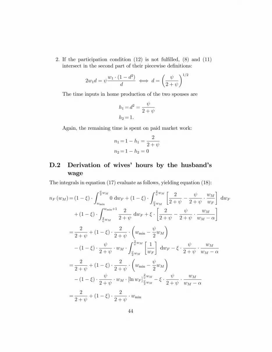
2. If the participation condition (12) is not ful�lled, (8) and (11)intersect in the second part of their piecewise de�nitions:

2w1d = w1 � (1� d2)

d() d =

�

2 +

�1=2The time inputs in home production of the two spouses are

h1= d2 =

2 + h2=1.

Again, the remaining time is spent on paid market work:

n1=1� h1 =2

2 + n2=1� h2 = 0

D.2 Derivation of wives� hours by the husband�swage

The integrals in equation (17) evaluate as follows, yielding equation (18):

nF (wM)= (1� �) �Z

2wM

wmin

0 dwF + (1� �) �Z 2

wM

2wM

�2

2 + �

2 + � wMwF

�dwF

+(1� �) �Z wmin+1

2 wM

2

2 + dwF + � �

�2

2 + �

2 + � wMwM � �

�

=2

2 + + (1� �) � 2

2 + ��wmin �

2wM

�� (1� �) �

2 + � wM �

Z 2 wM

2wM

�1

wF

�dwF � � �

2 + � wMwM � �

=2

2 + + (1� �) � 2

2 + ��wmin �

2wM

�� (1� �) �

2 + � wM � [lnwF ]

2 wM

2wM� � �

2 + � wMwM � �

=2

2 + + (1� �) � 2

2 + � wmin

44

� (1� �) �

2 + ��1 + ln

4

2

�� wM � � �

2 + � wMwM � �

D.3 Hump-shaped pattern of wives�hours by thehusband�s wage

For 0 < � < 1, the right hand side of equation (19) is a strictly concavefunction of wM . Thus, when there is a local extremum, it is a maximum.In this appendix, we show that for any combination of , wmin, and �,there is a � such that nF (wM) has a local extremum in the interior of thesupport of male wages. This is equivalent to the statement that, for allmarginal distributions of wages, there is a degree of assortative matingsuch the pattern of wives�hours by the husband�s wage is hump-shaped.The �rst derivative of equation (19) is

n0F (wM) = � (1� �) �

2 + ��1 + ln

4

2

�+� �

2 + � �

(wM � �)2. (21)

Since nF (wM) is concave, it is su¢ cient to show that there is a �� such

that n0F (wM) has a root on (wmin + �;wmin + �+ 1). A root w�M satis�es

(1� ��) ��1 + ln

4

2

�= ��

(w�M � �)2

() (w�M � �) =

s��

1� ��s

�

1 + ln 4 2

.

The root lies in the support of the male wage distribution when

wmin <

s��

1� ��s

�

1 + ln 4 2

< wmin + 1: (22)

Sinceq

�1+ln 4

2> 0 due to the restriction < 2 and

lim��!0

s�

1� �=0,

lim��!1

s�

1� �=1,

there is always a �� 2 (0; 1) such that (22) is ful�lled.

45

Documents

Assortative Mating and Female Labor Supply