Atmospheric boundary-layer height estimation by adaptive Kalman filtering of lidar data

Sergio Tomás*, Francesc Rocadenbosch, Michaël Sicard

Remote Sensing Lab (RSLAB), Dep. of Signal Theory and Communications (TSC), Univ. Politècnica de Catalunya (UPC)/IEEC CRAE, C/Jordi Girona, 1-3, 08034 Barcelona, SPAIN.

ABSTRACT

A solution based on a Kalman filter to trace the evolution of the atmospheric boundary layer (ABL) sensed by an elastic backscatter lidar is presented. An erf-like profile is used to model the mixing layer top and the entrainment zone thickness. The extended Kalman filter (EKF) enables to retrieve and track the ABL parameters based on simplified statistics of the ABL dynamics and of the observation noise present in the lidar signal. This adaptive feature permits to analyze atmospheric scenes with low signal-to-noise ratios without need to resort to long time averages or range-smoothing techniques, as well as to pave the way for an automated detection method. First EKF results based on synthetic lidar profiles are presented and compared with a typical least-squares inversion for different SNR scenarios.

Keywords: Atmospheric boundary layer height, Kalman filter, entrainment zone, least-squares, curve fitting, elastic lidar sensing, atmospheric boundary layer model

1. INTRODUCTION Elastic lidar techniques use the backscattered power from the atmospheric aerosols to profile the atmospheric structure in the troposphere. In the low troposphere, the atmospheric boundary layer (ABL) is marked by a transition interface known as the entrainment zone (EZ), where two different air masses, the mixing layer (ML) and the free troposphere (FT), merge and interact. Measurements in this transition region provide useful parameters such as the atmospheric boundary layer height or the entrainment-zone thickness. These parameters are highly valuable inputs to environmental models since they describe the extension and evolution of the transport of atmospheric constituents.

Despite the standard and well-known definition of the ABL as the part of the troposphere directly influenced by the ground for time scales of less than one hour1, there is no common definition among the numerous instruments that are able to measure its height. For example, radio-sounding measurements are based on its thermal properties looking for a temperature inversion height. In contrast, lidar measurements are based on the mixing and turbulent phenomena in the ABL. Though both thermal and mixing processes are related they are not one-to-one connected.

Among the ABL lidar-based methods there are different approaches in order to interpret and model the interface-mixing processes seen in the lidar signals. The statistical approach uses the high variability in the return signal caused by the mixing processes in the EZ between cells in the EZ and cells in the free troposphere above or in the mixing layer below. Another approach is the geometrical one which uses the fact that the EZ interfacial region usually appears in the individual lidar signal profiles as a sharp decrease between the two air masses (this is due to the lack of aerosols and moisture in the free troposphere), all of which causes a strong signature in the range-corrected backscatter lidar return.

Statistical methods such as the centroid –or variance– method2 and the cumulative probability density function (cdf) method3 require the analysis of a significant set of profiles to produce a statistically significant estimate of the mixing-layer depth, taken as the ABL height in average sense. While the centroid method is intended to give just a mean estimate for a certain period of time or over a certain sounding area without analyzing individual high-resolved profiles, the cdf method requires short-term structural parameters retrieved applying any of the methods explained below.

Geometrical methods are based on the detection of a meaningful transition be it by means of a threshold criterium4 or by gradient detection5,6 . They are applied with time-averaged profiles. As a further step, wavelet methods are multi-scale and feature local detection of transitions, which is intended to deal with small-scale features and noise fluctuations7.

*tomas.martinez@tsc.upc.edu; phone +34 93-401-60-85; fax +34 401-72-32

Remote Sensing of Clouds and the Atmosphere XV, edited by Richard H. Picard, Klaus Schäfer, Adolfo Comeron, Proc. of SPIE Vol. 7827, 782704 · © 2010 SPIE · CCC code: 0277-786X/10/$18 · doi: 10.1117/12.866477

Proc. of SPIE Vol. 7827 782704-1

Furthermore, another group of geometrical methods rely on a curve-fitting approach by applying some mathematical model to optimize the location of the ABL height. This is the case of the erf-function method, which fits the bulk of the range-corrected power curve transition8. When high temporal resolution is available, geometrical methods retrieve the individual profile parameters for a second step where some average is applied to obtain the mixing layer depth and the entrainment zone thickness9.

As a common trait, the nearly totality of the methods lack in some degree the requirements to operate in an automated, real-time basis to monitor the ABL. Thus, the centroid method does not benefit from the time resolution of the profiles obtained with a lidar instrument to trace the time evolution of the ABL while methods based on range-analysis do not assimilate in any way the estimates from previous lidar measurements in order to track the ABL. Complementarily, the ABL evolution can be traced in a second step by combining the individually processed profiles using some additional criteria10.

In practice, in scenarios with a well-mixed layer without stratifications and under high signal-to-noise ratios (SNRs) all the methods above perform reasonably well without ambiguous results. However, instrumental noise hampers to trace the ABL evolution with the high resolution capability in both range and time provided by the lidar instrument. The methods used to get a sufficient SNR generally require both range smoothing and time averaging, which often gives biased results and requires combined approaches and criteria11 and definitely a reduced resolution.

In this work, an Extended Kalman Filter (EKF) is used to adaptively fit an erf-like function modeling the EZ to the range-corrected (and noise-corrupted) lidar returns acquired with a backscatter lidar. The EKF is cross-examined with the classic least-squares (LSQ) solution, which suffers from the basic fault that a new estimation is carried out at each successive lidar return. In other words, neither the model parameters vary with time (non-memory estimation) nor LSQ parameter statistics are assimilated. As a result, the Kalman filter technique provides a convenient and generalized model with time-adaptive coefficients that is able to combine previous estimations in order to improve the actual one. It is expected that its future application to the ABL detection can provide real-time, automated tracking of the ABL parameters, chiefly its instantaneous height. This would permit to work with low signal-to-noise ratio (SNR) atmospheric scenes without excessively losing the temporal resolution of the lidar instrument.

2. THE ESTIMATION PROBLEM 2.1 Problem formulation

The erf-like transition model discussed in Sect. 1 is formally defined over the total (aerosol plus molecular) atmospheric backscatter profile following a similar formulation as that proposed by Steyn et al.8. Formally,

( ) 1 2( ; , , , ) 1 ( ) , 2bl blAh R R a A b erf a R R b R R R= − − + < <⎡ ⎤⎣ ⎦ , (1)

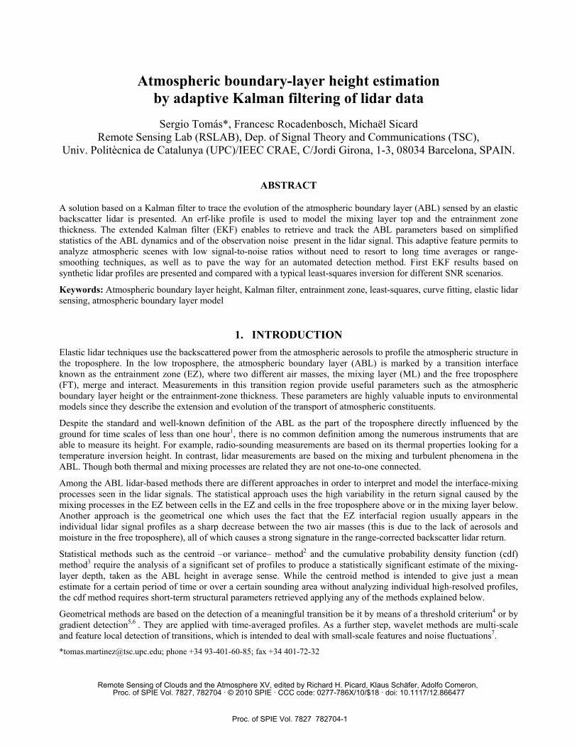
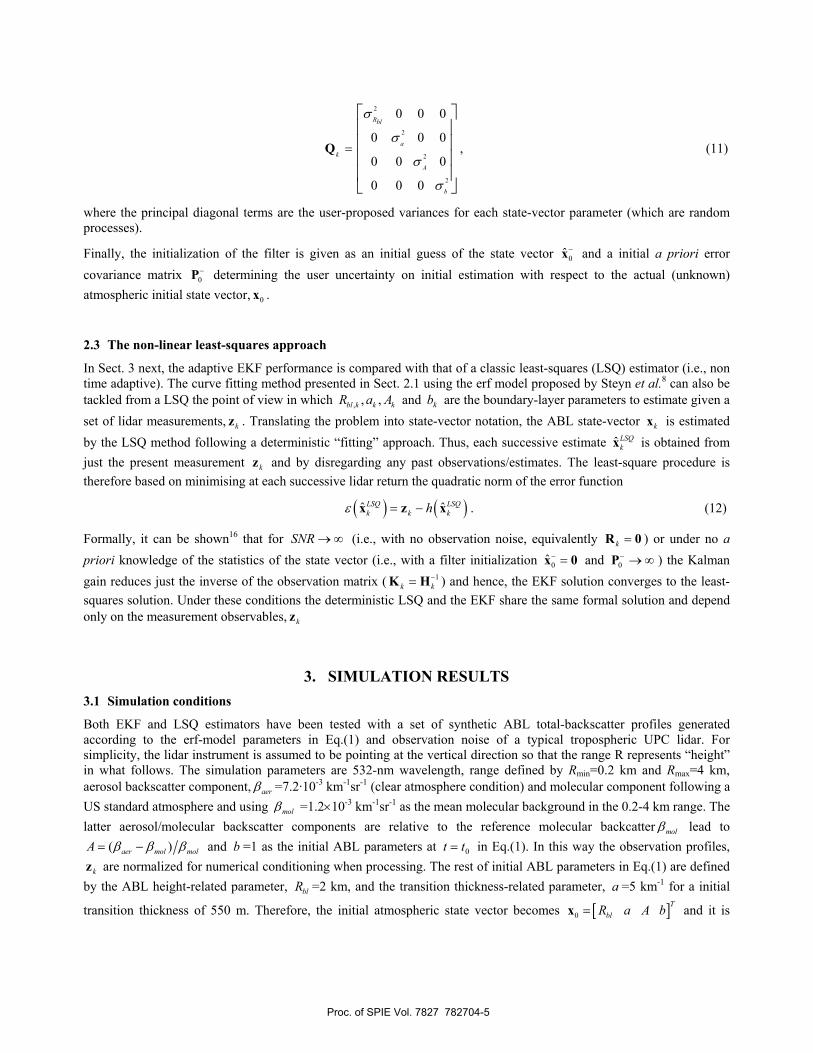
where R is the range, that is equivalent to height z by means of the scaling factor of the elevation angleθ of the lidar line-of-sight as sinz R θ= ; Rbl is the range that marks the height position of the interface, defined as the inflection point where the function h changes from convex to concave (equivalently, the point where h has minimum gradient), a is a scaling factor related to the transition thickness, A is the backscatter transition amplitude (equivalently, the difference between the upper and lower asymptotical level of h , or between the ML and FT backscatter values), and b is an offset term modeling the free-troposphere molecular backscatter level (Fig. 1). Eq.(1) profile models an idealized boundary-layer profile consisting of a single transition structure between the ML and the FT in the inversion range interval [ ]1 2,R R (to be assessed by the user).

At this point is it worth mentioning that in clear atmospheres the range-corrected backscatter lidar return is proportional to the total backscatter profile except for a proportionality factor being the product of the instrument constant and the two-way path transmissivity (approximately unity)12 so that range-corrected profiles can also be assimilated to Eq.(1) in the [ ]21, RR inversion interval. In the model of Eq.(1) the parameters of interest are blR and a for they are related to the measurement of the ML depth and to the EZ thickness9. The instantaneous ML top is identified as the minimum-gradient model parameter Rbl as seen in Flamant et al.5. For a Gaussian-based ABL transition, its derivative is a Gaussian curve whose full-width half maximum, blσ , is related to a as 1 2 bla σ− = (See Fig.1). Likewise, the transition thickness is

Proc. of SPIE Vol. 7827 782704-2

also defined8 as 2.77 1a− covering the interval that goes from the 95% to the 5% of the level in ( )h R . In the adaptive approach proposed, the EKF filter considers the four characteristic parameters of the backscatter profile of Eq.(1) as time-variant stochastic processes forming the state vector to be estimated at each time tk. Therefore, at each successive time kt a new model-backscatter profile is estimated. Formally, the 14× state vector at time kt is defined as

,T

k bl k k k kR a A b⎡ ⎤= ⎣ ⎦x , (2)

where subindex k is a reminder of the discrete time kt . The observation vector, kz is related to the state vector, kx , via the measurement model

( )k k kh= +z x v , (3)

where h is the backscatter model of Eq.(1) and kv is the observation noise at time kt (including modeling errors) with covariance matrix kR (see ref. 13 for details).

In Eq. (3) the observation vector kz is the noise-corrupted backscatter power profile which can be obtained after Klett’s (one component atmosphere)14 or Klett-Fernald-Sasano’s (two-component atmosphere) elastic inversion15 of the measured (i.e., noisy) lidar profiles. As mentioned before, for clear atmospheres, the observation vector can directly assimilated to the measured range-corrected lidar profiles in the interval of interest. Obviously, for data sufficiency the number of observation samples in the ABL transition must be 4≥N (4 being the order of the state vector to estimate). In practice, a much larger number of samples –as if always the case– conveys the extra benefit of enhanced robustness to noise for it is equivalent to an over-determined system of equations in classic algebra theory.

2.2 The Extended Kalman Filter (EKF) approach

The discrete Kalman filter is an adaptive linear estimator inherited from control system theory that operates recursively using a state-space model formulation. The filter is based on two models: The measurement model, which relates the state vector unknowns to the observation measurement (i.e., the backscatter or the range-corrected lidar measurements, Eq.(3)) and the state-vector model, which describes the temporal projection of the state vector and its associated statistics. However poor this a priori information about the atmospheric state vector and its statistics may be, this information is of advantage to the filter in order to improve its estimates by combining the actual estimation with an statistical reference from the past estimates. When as is the case in Eq.(1) the measurement model is not linear, a linearization is made around the state-vector trajectory, which is updated at each successive iteration once a new measurement kz is assimilated. Likewise, at each filter iteration, the state vector, kx , the estimated a priori and a posteriori error covariance matrices, k

−P and kP , respectively, and the Kalman gain, kK are recursively updated16. By this updating the filter corrects its projection trajectory and improves its estimation of the ABL parameters via a new state vector ˆ kx estimated. By means of this convenient adaptive behaviour tracking the state-vector components appears as a natural and desirable feature of the filter.

2.2.1 Measurement model.- In the EKF approach the filter compares the actual observables from the lidar measured backscattered profiles with a linearised observation model kH based on the partial derivatives of the measurement model function h (Eq.(1)) that is evaluated at the a priori estimation of the state vector, ˆ k

−x . The linearised measurement function takes the form

( ) (1 (2 (3 (4

4ˆ

( ) ( ) ( ) ( );k k k k k Nbl

k

h R h R h R h RRR a A b ×

−=

⎡ ⎤∂ ∂ ∂ ∂ ⎡ ⎤= =⎢ ⎥ ⎣ ⎦∂ ∂ ∂ ∂⎣ ⎦ x xH x H H H H , (4)

where

( ) ( ) ( )( ) [ ]2(1 21 2, exp , ,k bl bl

bl

h R Aaa R a R R R R RR π

∂′ ′= = − − ∈

∂H , (5)

Proc. of SPIE Vol. 7827 782704-3

( ) ( ) ( ) ( ) [ ](2 21 2, exp ( ) , ,k bl bl bl

h R Aa R R R a R R R R Ra π

∂′ ′= = − − − − ∈

∂H , (6)

( ) ( ) ( ) [ ) ]((31 1 2 2

1 1, , , ,2 2k bl

h RA b erf a R R R R R R R

A∂

′ ′= = − − ∈ ∪⎡ ⎤⎣ ⎦∂H , (7)

( ) ( ) [ ) ]((41 1 2 2, 1, , ,k

h RA b R R R R R

b∂

′ ′= = ∈ ∪∂

H , (8)

and where the range intervals [ ]211 , RRI ′′= and [ ) ]( 22112 ,, RRRRI ′∪′= respectively define the measurement-model “fitting” ranges inside and outside the transition (see Fig.1). The variables into brackets [ ( )blRa, and ( )bA, in (1 4

k−H ]

indicate the estimation variables inside each range interval. In Eqs. (4-8) above, (1 4k−H are N×1 vectors with N the

number of measurement samples in the observation record, kz . In Eq.(4), R is retained in continuous form for better clarity though in practice the range is discretised as min ( 1) ; 1..iR R + i R i N= − Δ = , with minR the minimum sounding/inversion range and RΔ the raw-data spatial resolution.

In relation to Eq.(3), the observation noise kv models both the instrumental noise and modeling errors affecting the observation vector, kz . The observation noise is modeled by its covariance matrix, kR , assuming white Gaussian

additive noise with range-dependent variance 2 ( )Rσ . Because the observations kz are the range-corrected lidar returns ( 2 ( )R P R , with R the range and ( )P R the elastic lidar return power) the noise covariance matrix takes the form

421 1

2 41 1

2 41

( ) 0 0

0

( ) 00 0 ( )

k

N N

N N

R R

R RR R

σ

σσ

− −

−

⎡ ⎤⎢ ⎥⎢ ⎥

= ⎢ ⎥⎢ ⎥⎢ ⎥⎢ ⎥⎣ ⎦

R

LO M

ML

. (9)

In Eq.(6) above, 2 ( )Rσ is computed from an estimate of the SNR in the lidar receiving channel.

2.2.2 State-vector atmospheric model.- The Kalman filter state-vector model is described by means of the recursive discrete model

1k k k k+ = +x Φ x w , (10)

where kΦ is the transition matrix from time kt to time 1+kt and kw is the state-noise vector with covariance matrix kQ modeling the statistics of the state vector, kx . In other words, kw is the “driving” noise vector of the filter affecting its nervousness. The model is initialized with a user input, 0ˆ −x , describing the approximate user-estimated initial value of

kx .

In atmospheric sciences and specifically for the ABL physical variables composing the state vector, the macroscopic fluctuations of these parameters are slowly varying with time and nearly constant over relatively large time scales (e.g., minutes or hours). A convenient model representing this situation is the random walk17 , which is characterized by a 4×4 transition matrix k =Φ I in Eq.(10) above. This enables , , ,bl k k kR a A and kb to evolve with time as random-walk independent processes. To shed more light in the issue, note that if k =w 0 in Eq. (10) above a constant state-vector is retrieved. Yet, very few things remain absolutely constant with time in the nature and that is why a non nil state-vector covariance matrix kQ must always be assumed to describe the expected 1-σ approximate variations of the state-vector variables. The proposed covariance matrix becomes

Proc. of SPIE Vol. 7827 782704-4

2

2

2

2

0 0 0

0 0 0

0 0 0

0 0 0

R

a

k

A

b

blσ

σ

σ

σ

=

⎡ ⎤⎢ ⎥⎢ ⎥⎢ ⎥⎢ ⎥⎣ ⎦

Q , (11)

where the principal diagonal terms are the user-proposed variances for each state-vector parameter (which are random processes).

Finally, the initialization of the filter is given as an initial guess of the state vector 0ˆ −x and a initial a priori error covariance matrix 0

−P determining the user uncertainty on initial estimation with respect to the actual (unknown) atmospheric initial state vector, 0x .

2.3 The non-linear least-squares approach

In Sect. 3 next, the adaptive EKF performance is compared with that of a classic least-squares (LSQ) estimator (i.e., non time adaptive). The curve fitting method presented in Sect. 2.1 using the erf model proposed by Steyn et al.8 can also be tackled from a LSQ the point of view in which , , ,bl k k kR a A and kb are the boundary-layer parameters to estimate given a set of lidar measurements, kz . Translating the problem into state-vector notation, the ABL state-vector kx is estimated by the LSQ method following a deterministic “fitting” approach. Thus, each successive estimate ˆ LSQ

kx is obtained from just the present measurement kz and by disregarding any past observations/estimates. The least-square procedure is therefore based on minimising at each successive lidar return the quadratic norm of the error function

( ) ( )ˆ ˆLSQ LSQk k khε = −x z x . (12)

Formally, it can be shown16 that for ∞→SNR (i.e., with no observation noise, equivalently k =R 0 ) or under no a priori knowledge of the statistics of the state vector (i.e., with a filter initialization 0ˆ − =x 0 and 0

− → ∞P ) the Kalman gain reduces just the inverse of the observation matrix ( 1

k k−=K H ) and hence, the EKF solution converges to the least-

squares solution. Under these conditions the deterministic LSQ and the EKF share the same formal solution and depend only on the measurement observables, kz

3. SIMULATION RESULTS 3.1 Simulation conditions

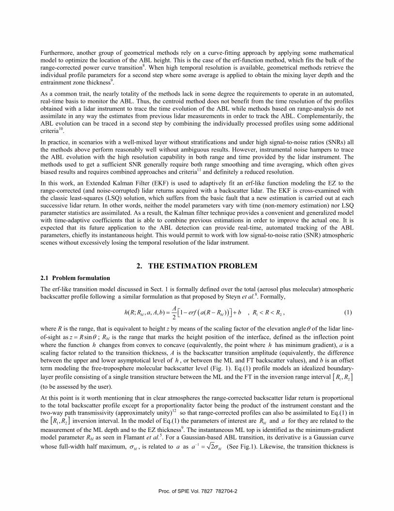
Both EKF and LSQ estimators have been tested with a set of synthetic ABL total-backscatter profiles generated according to the erf-model parameters in Eq.(1) and observation noise of a typical tropospheric UPC lidar. For simplicity, the lidar instrument is assumed to be pointing at the vertical direction so that the range R represents “height” in what follows. The simulation parameters are 532-nm wavelength, range defined by Rmin=0.2 km and Rmax=4 km, aerosol backscatter component, aerβ =7.2·10-3 km-1sr-1 (clear atmosphere condition) and molecular component following a US standard atmosphere and using molβ =1.2×10-3 km-1sr-1 as the mean molecular background in the 0.2-4 km range. The latter aerosol/molecular backscatter components are relative to the reference molecular backcatter molβ lead to

( )aer mol molA β β β= − and b =1 as the initial ABL parameters at 0tt = in Eq.(1). In this way the observation profiles,

kz are normalized for numerical conditioning when processing. The rest of initial ABL parameters in Eq.(1) are defined by the ABL height-related parameter, blR =2 km, and the transition thickness-related parameter, a =5 km-1 for a initial

transition thickness of 550 m. Therefore, the initial atmospheric state vector becomes [ ]0T

blR a A b=x and it is

Proc. of SPIE Vol. 7827 782704-5

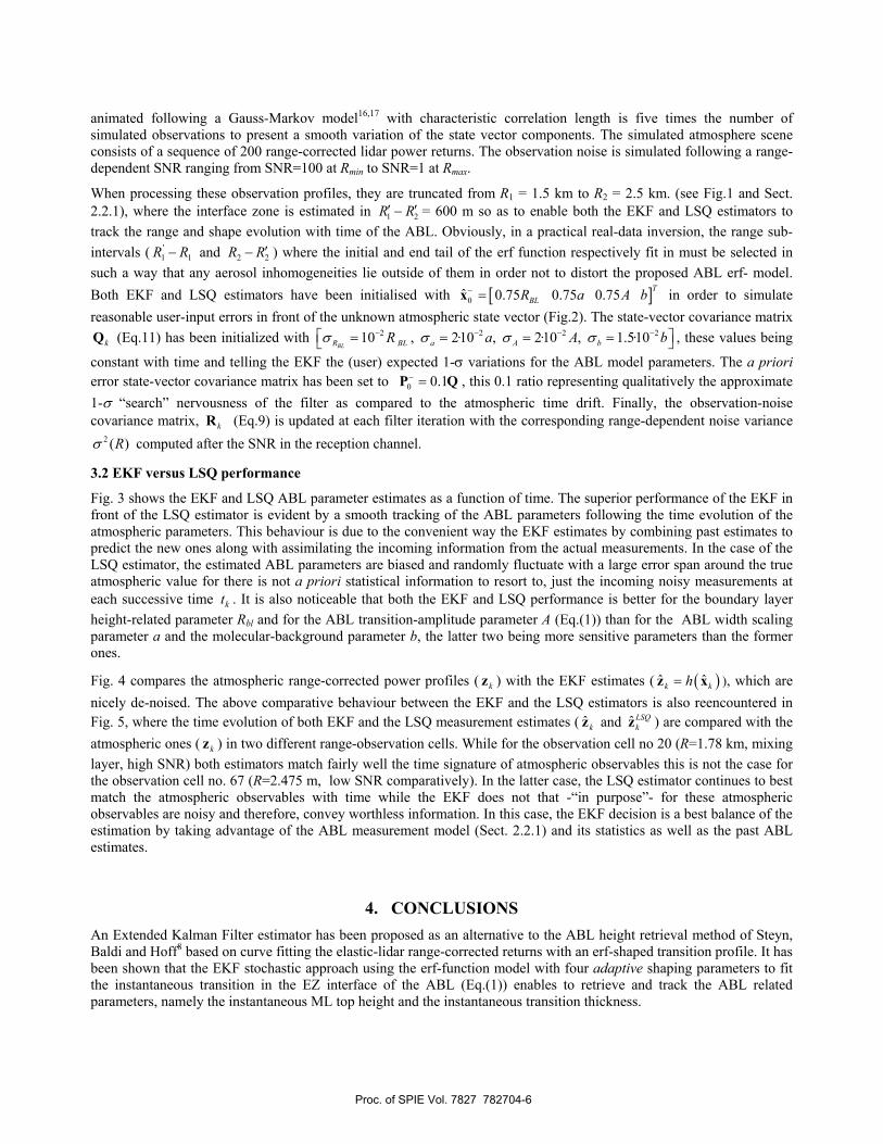
animated following a Gauss-Markov model16,17 with characteristic correlation length is five times the number of simulated observations to present a smooth variation of the state vector components. The simulated atmosphere scene consists of a sequence of 200 range-corrected lidar power returns. The observation noise is simulated following a range-dependent SNR ranging from SNR=100 at Rmin to SNR=1 at Rmax.

When processing these observation profiles, they are truncated from R1 = 1.5 km to R2 = 2.5 km. (see Fig.1 and Sect. 2.2.1), where the interface zone is estimated in 1 2R R′ ′− = 600 m so as to enable both the EKF and LSQ estimators to track the range and shape evolution with time of the ABL. Obviously, in a practical real-data inversion, the range sub-intervals ( 1

'1 RR − and 22 RR ′− ) where the initial and end tail of the erf function respectively fit in must be selected in

such a way that any aerosol inhomogeneities lie outside of them in order not to distort the proposed ABL erf- model. Both EKF and LSQ estimators have been initialised with [ ]0ˆ 0.75 0.75 0.75 T

BLR a A b− =x in order to simulate reasonable user-input errors in front of the unknown atmospheric state vector (Fig.2). The state-vector covariance matrix

kQ (Eq.11) has been initialized with 2 2 2 210 , 2·10 , 2·10 , 1.5·10BLR BL a A bR a A bσ σ σ σ− − − −⎡ ⎤= = = =⎣ ⎦ , these values being

constant with time and telling the EKF the (user) expected 1-σ variations for the ABL model parameters. The a priori error state-vector covariance matrix has been set to 0 0.1− =P Q , this 0.1 ratio representing qualitatively the approximate 1-σ “search” nervousness of the filter as compared to the atmospheric time drift. Finally, the observation-noise covariance matrix, kR (Eq.9) is updated at each filter iteration with the corresponding range-dependent noise variance

2 ( )Rσ computed after the SNR in the reception channel.

3.2 EKF versus LSQ performance

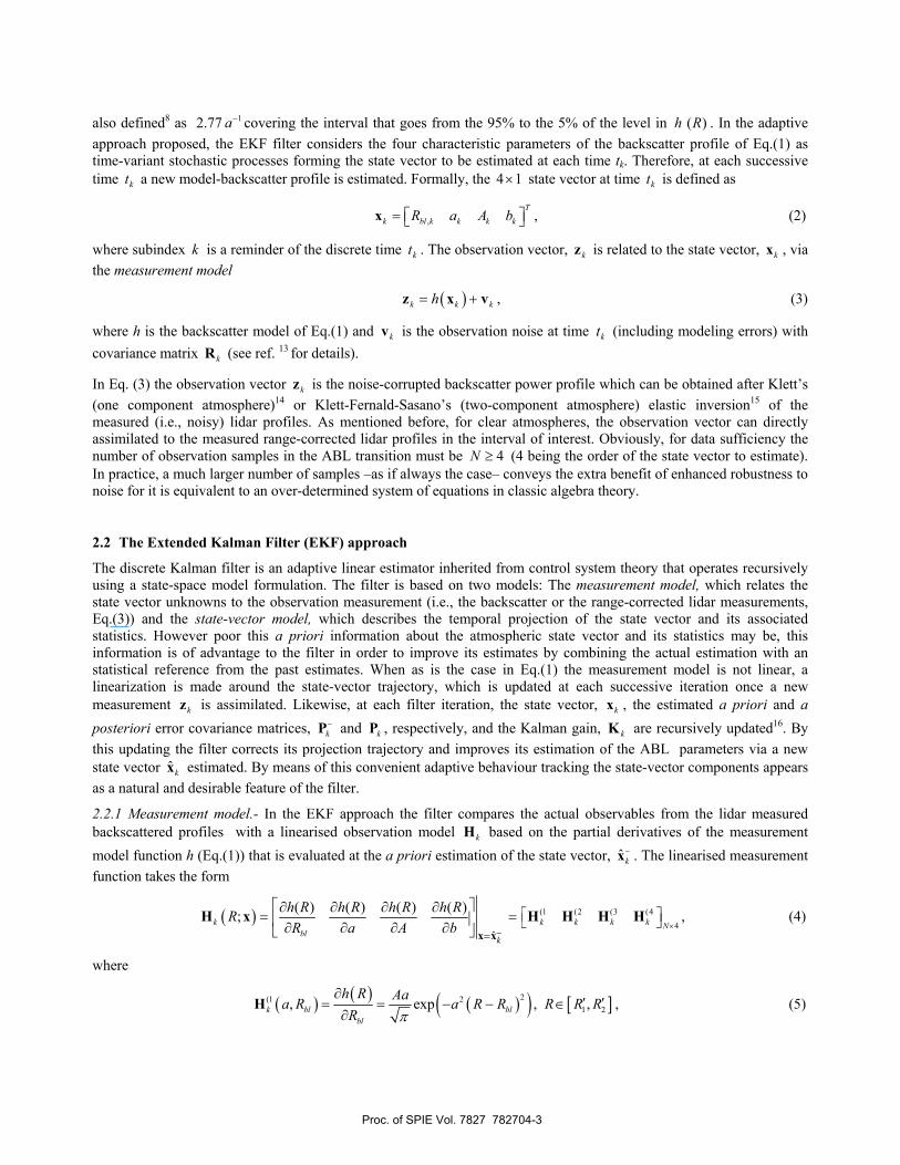
Fig. 3 shows the EKF and LSQ ABL parameter estimates as a function of time. The superior performance of the EKF in front of the LSQ estimator is evident by a smooth tracking of the ABL parameters following the time evolution of the atmospheric parameters. This behaviour is due to the convenient way the EKF estimates by combining past estimates to predict the new ones along with assimilating the incoming information from the actual measurements. In the case of the LSQ estimator, the estimated ABL parameters are biased and randomly fluctuate with a large error span around the true atmospheric value for there is not a priori statistical information to resort to, just the incoming noisy measurements at each successive time kt . It is also noticeable that both the EKF and LSQ performance is better for the boundary layer height-related parameter Rbl and for the ABL transition-amplitude parameter A (Eq.(1)) than for the ABL width scaling parameter a and the molecular-background parameter b, the latter two being more sensitive parameters than the former ones.

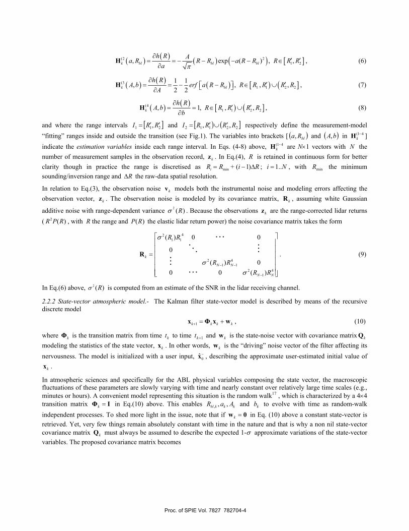
Fig. 4 compares the atmospheric range-corrected power profiles ( kz ) with the EKF estimates ( ( )ˆ ˆk kh=z x ), which are nicely de-noised. The above comparative behaviour between the EKF and the LSQ estimators is also reencountered in Fig. 5, where the time evolution of both EKF and the LSQ measurement estimates ( ˆ kz and ˆ LSQ

kz ) are compared with the atmospheric ones ( kz ) in two different range-observation cells. While for the observation cell no 20 (R=1.78 km, mixing layer, high SNR) both estimators match fairly well the time signature of atmospheric observables this is not the case for the observation cell no. 67 (R=2.475 m, low SNR comparatively). In the latter case, the LSQ estimator continues to best match the atmospheric observables with time while the EKF does not that -“in purpose”- for these atmospheric observables are noisy and therefore, convey worthless information. In this case, the EKF decision is a best balance of the estimation by taking advantage of the ABL measurement model (Sect. 2.2.1) and its statistics as well as the past ABL estimates.

4. CONCLUSIONS An Extended Kalman Filter estimator has been proposed as an alternative to the ABL height retrieval method of Steyn, Baldi and Hoff8 based on curve fitting the elastic-lidar range-corrected returns with an erf-shaped transition profile. It has been shown that the EKF stochastic approach using the erf-function model with four adaptive shaping parameters to fit the instantaneous transition in the EZ interface of the ABL (Eq.(1)) enables to retrieve and track the ABL related parameters, namely the instantaneous ML top height and the instantaneous transition thickness.

Proc. of SPIE Vol. 7827 782704-6

The superior EKF performance has also been corroborated in front of the usual deterministic approach of a least-squares estimator (lacking any adaptive capability) for the same ABL shape parameters by using an idealized Gauss-Markov process that simulates a random drift in these ABL parameters.

It has been shown that under high SNRs both EKF and LSQ solutions are similar. Nonetheless, for medium-to-low SNRs, the performance of the Kalman filter is much better than the rambling and biased estimation of the LSQ. In this respect, the most sensitive parameters for both estimators are the transition scaling width a and the free-troposphere offset term, b. On the contrary, the location of the minimum gradient range, often identified with the ABL instantaneous height is always well estimated and time tracked.

It is expected that future EKF implementations enable to deal with multilayer aerosol profiles rather than with single-transition ABL profiles as presented here along with a more accurate model for the two-component (aerosol + molecular) atmosphere. Run-time updating of the state-vector covariance matrix will also enable to follow non-stationary conditions in the ABL temporal evolution, such as the characteristic ones on a daily cycle.

ACKNOWLEDGEMENTS This work is supported by the European Union under the project EARLINET-ASOS (EU Coordination Action, contract nº 025991 (RICA)); by the MICINN (Spanish Ministry of Science and Innovation) and FEDER funds under the project TEC2009-09106/TEC, and the Complementary Actions CGL2008-01330-E/CLI and CGL2009-08031-E/CLI; and by the European Space Agency under the project 21487/08/NL/HE. MICINN is also thanked for Mr. Tomás’ FPI pre-doctoral fellowship BES-2007-17047.

REFERENCES

[1] Stull, R.B., [An Introduction to Boundary Layer Meteorology], Kluwer, Dordrecht, The Netherlands (1988). [2] Hooper, W.P. and Eloranta, E.W., " Lidar Measurements of Wind in the Planetary Bondary Layer: The Method,

Accuracy and Results from Joint Measurements with Radiosonde and Kytoon," J. Climate Appl. Meteor.,25, 990-1001 (1985).

[3] Deardorff, J.W., Willis, G.E., and Stockton, B.H.,"Laboratory Studies of the Entrainment Zone of a Convectively Mixed Layer", J. Fluid. Mech. 100, 41–64 (1980).

[4] Melfi, S. H., Spinhire J.D., Chou, S.-H. and Palm, S. P.,"Lidar observation of vertically organized convection in the planetary boundary layer over the ocean.," J. Climate Appl. Meteor.,24, 806–821 (1985).

[5] Flamant, C., Pelon, J., Flamant P.H. and Durand P., "Lidar Determination of the Entrainment Zone Thickness at the top of the Unstable Marine Atmospheric Boundary Layer," Boundary-Layer Meteorology 83, 247-284, (1997).

[6] Menut, L. Flamant, C., Pelon, J. and Flamant, P.H., "Urban Boundary-Layer Height Determination from Lidar Measurements over the Paris Area", Appl. Opt. 38, 945-954 (1999).

[7] Davis, K., Gamage, N., Hagelberg,C.R., Kiemle.C., Lenschow, D.H. and Sullivan, P.P., "An objective method for deriving atmospheric structure from airborne lidar observations", J. Atmos. Oceanic. Tech., 17,1455-1468 (2000).

[8] Steyn, D.G., Baldi, M. and Hoff, R.M., "The Detection of Mixing Layer Depth and Entrainment Zone Thickness from Lidar Backscatter Profiles", J. Atmos. Oceanic. Tech. 16(7), 953-959 (1999).

[9] Hägeli, P., Steyn, D.G., Strawbridge, K.B.,"Spatial and temporal variability of mixed layer depth and entrainment zone thickness", Boundary-Layer Meteorology, 97, 41-71 (2000).

[10] Endlich, R.M, Ludwig, F.L. and Uthe, E.E., "An Automatic Method for determining the Mixing Depth from Lidar Observations," Atmos. Environment 13, 1051-1056 (1979).

[11] Sicard, M., Perez,C. Rocadenbosch, F. Baldasano, J.M., Garcia-Vizcaino, D.,"Mixed-layer depth determination in the Barcelona coastal area from regular lidar measurements: Methods, results and limitations," Boundary-Layer Meteorology. 119(1),135-157 (2006).

[12] Rocadenbosch, F., ["Lidar-Aerosol Sensing" in Encyclopaedia of Optical Engineering], ed. D.D.Driggers, Marcel Dekker, New York, pp.1190 (2003).

Proc. of SPIE Vol. 7827 782704-7

[13] Rocadenbosch, F., Vazquez, G., Comeron, A. "Adaptive filter solution for processing lidar returns: optical parameter estimation", Appl. Opt. 37, 7019-7034 (1998).

[14] Klett, J.D., "Lidar Inversion with Variable Backscatter/Extinction Ratios", Appl. Opt. 24, 1638-1643 (1985). [15] Klett, J.D., "Stable Analytical Inversion Solution for Processing Lidar Returns", Appl. Opt. 20, 211-220 (1985). [16] Brown, R.G and Hwang, P.Y.C [Introduction to Random Signals and Applied Kalman filtering], Wiley, New

York, (1992) [17] Rocadenbosch, F., Sicard, M. Comeron, A. and Md.Reba, M.N., "Comparison between the Kalman and the

non-linear least-squares estimators in low signal-to-noise ratio lidar inversion", Proc. Geoscience and Remote Sensing Symposium, IGARSS 2008. IEEE International, 7-11 July, Boston, III-1083- III-1086 (2008).

Figure 1. Ideal instantaneous backscatter profile based in a erf curve showing the parameters that form the state vector: Rbl,

a, A and b. R1 and R2 are the boundaries to define the observation vector. The profile derivative shown below explain the scaling thickness parameter a, which is related to the standard deviation of this gaussian curve.

Figure 2. (a) Initial observable vector z0 . (b) Range-dependent signal-to-noise ratio of the observable vector.

Proc. of SPIE Vol. 7827 782704-8

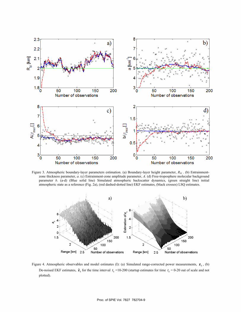
Figure 3. Atmospheric boundary-layer parameters estimation. (a) Boundary-layer height parameter, Rbl . (b) Entrainment-

zone thickness parameter, a. (c) Entrainment-zone amplitude parameter, A. (d) Free-troposphere molecular background parameter b. (a-d) (Blue solid line) Simulated atmospheric backscatter dynamics, (green straight line) initial atmospheric state as a reference (Fig. 2a), (red dashed-dotted line) EKF estimates, (black crosses) LSQ estimates.

Figure 4. Atmospheric observables and model estimates (I): (a) Simulated range-corrected power measurements, kz , (b)

De-noised EKF estimates, ˆ kz for the time interval kt =10-200 (startup estimates for time kt = 0-20 out of scale and not plotted).

Proc. of SPIE Vol. 7827 782704-9

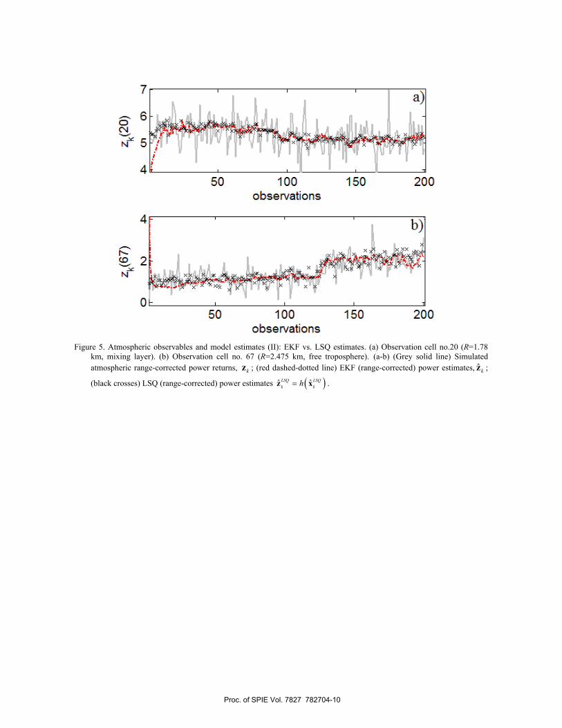
Figure 5. Atmospheric observables and model estimates (II): EKF vs. LSQ estimates. (a) Observation cell no.20 (R=1.78

km, mixing layer). (b) Observation cell no. 67 (R=2.475 km, free troposphere). (a-b) (Grey solid line) Simulated atmospheric range-corrected power returns, kz ; (red dashed-dotted line) EKF (range-corrected) power estimates, ˆ kz ;

(black crosses) LSQ (range-corrected) power estimates ( )ˆ ˆLSQ LSQk kh=z x .

Proc. of SPIE Vol. 7827 782704-10