Embed Size (px)
Citation preview

New Jersey Institute of Technology New Jersey Institute of Technology
Digital Commons @ NJIT Digital Commons @ NJIT
Dissertations Electronic Theses and Dissertations
Fall 1-27-2008
Automatic prediction of solar flares and super geomagnetic Automatic prediction of solar flares and super geomagnetic
storms storms
Hui Song New Jersey Institute of Technology
Follow this and additional works at: https://digitalcommons.njit.edu/dissertations
Part of the Other Physics Commons
Recommended Citation Recommended Citation Song, Hui, "Automatic prediction of solar flares and super geomagnetic storms" (2008). Dissertations. 854. https://digitalcommons.njit.edu/dissertations/854
This Dissertation is brought to you for free and open access by the Electronic Theses and Dissertations at Digital Commons @ NJIT. It has been accepted for inclusion in Dissertations by an authorized administrator of Digital Commons @ NJIT. For more information, please contact [email protected].

Copyright Warning & Restrictions
The copyright law of the United States (Title 17, United States Code) governs the making of photocopies or other
reproductions of copyrighted material.
Under certain conditions specified in the law, libraries and archives are authorized to furnish a photocopy or other
reproduction. One of these specified conditions is that the photocopy or reproduction is not to be “used for any
purpose other than private study, scholarship, or research.” If a, user makes a request for, or later uses, a photocopy or reproduction for purposes in excess of “fair use” that user
may be liable for copyright infringement,
This institution reserves the right to refuse to accept a copying order if, in its judgment, fulfillment of the order
would involve violation of copyright law.
Please Note: The author retains the copyright while the New Jersey Institute of Technology reserves the right to
distribute this thesis or dissertation
Printing note: If you do not wish to print this page, then select “Pages from: first page # to: last page #” on the print dialog screen

The Van Houten library has removed some ofthe personal information and all signatures fromthe approval page and biographical sketches oftheses and dissertations in order to protect theidentity of NJIT graduates and faculty.
ABSTRACT
AUTOMATIC PREDICTION OF SOLAR FLARESAND SUPER GEOMAGNETIC STORMS
byHui Song
Space weather is the response of our space environment to the constantly changing Sun.
As the new technology advances, mankind has become more and more dependent on space
system, satellite-based services. A geomagnetic storm, a disturbance in Earth's magne-
tosphere, may produce many harmful effects on Earth. Solar flares and Coronal Mass
Ejections (CMEs) are believed to be the major causes of geomagnetic storms. Thus, estab-
lishing a real time forecasting method for them is very important in space weather study.
The topics covered in this dissertation are: the relationship between magnetic gra-
dient and magnetic shear of solar active regions; the relationship between solar flare index
and magnetic features of solar active regions; based on these relationships a statistical
ordinal logistic regression model is developed to predict the probability of solar flare oc-
currences in the next 24 hours; and finally the relationship between magnetic structures
of CME source regions and geomagnetic storms, in particular, the super storms when the
Dst index decreases below -200 nT is studied and proved to be able to predict those super
storms.
The results are briefly summarized as follows: (1) There is a significant correlation
between magnetic gradient and magnetic shear of active region. Furthermore, compared
with magnetic shear, magnetic gradient might be a better proxy to locate where a large
flare occurs. It appears to be more accurate in identification of sources of X-class flares
than M-class flares; (2) Flare index, defined by weighting the SXR flares, is proved to have

positive correlation with three magnetic features of active region; (3) A statistical ordinal
logistic regression model is proposed for solar flare prediction. The results are much better
than those data published in the NASA/SDAC service, and comparable to the data provided
by the NOAA/SEC complicated expert system. To our knowledge, this is the first time that
logistic regression model has been applied in solar physics to predict flare occurrences; (4)
The magnetic orientation angle 0, determined from a potential field model, is proved to
be able to predict the probability of super geomagnetic storms (Dst ≤ -200nT). The results
show that those active regions associated with 0 < 90° are more likely to cause a super
geomagnetic storm.
AUTOMATIC PREDICTION OF SOLAR FLARESAND SUPER GEOMAGNETIC STORMS
byHui Song
A DissertationSubmitted to the Faculty of
New Jersey Institute of Technology andRutgers, the State University of New Jersey - Newark
in Partial Fulfillment of the Requirements for the Degree ofDoctor of Philosophy in Applied Physics
Federated Physics Department
January 2008

Copyright © 2007 by Hui Song
ALL RIGHTS RESERVED
APPROVAL PAGE
AUTOMATIC PREDICTION OF SOLAR FLARESAND SUPER GEOMAGNETIC STORMS
Hui Song
Dr. Haimin Wang, Dissertation Advisor -DateDistinguished Professor of Physics, Associate Director of the Center forSolar-Terrestrial Research and Big Bear Solar Observatory, NJIT
Dr. Dale Gary, Committee Member DateProfessor of Physics, Chair of Ph sics Department,Director of the Solar Array in wens Valley Radio Observatory, NJIT
Dr. Andrew Gerrard, Committee Member DateAssociate Prof sor of Physics, NJIT
Dr. Wenda Cao, Committee Member DateAssistant Professor of Physics, NJIT
Dr. Li Guo, Committee Member DateAssociate Professor of Mathematics & Computer Science,Rutgers University, Newark

BIOGRAPHICAL SKETCH
Author: Hui Song
Degree: Doctor of Philosophy
Date: January 2008
Undergraduate and Graduate Education:
• Doctor of Philosophy in Applied Physics,New Jersey Institute of Technology, Newark, New Jersey, 2008
• Master of Science in Computer Science,University of Bridgeport, Bridgeport, Connecticut, 2000
• Master of Science in Optics,Changchun Institute of Optics, Fine Mechanics and Physics,Chinese Academy of Science, Changchun, China, 1995
• Bachelor of Science in Electronic Engineering,Jilin University, Changchun, China, 1992
Major: Applied Physics
Publications in Refereed Journals:
Song, Hui; Yurchyshyn, Vasyl; Ju Jing; Changyi Tan; V. I. Abramenko and Haimin Wang,2007, Statistical Assessment of Photospheric Magnetic Features in Imminent SolarFlares Predictions, Solar Physics, submitted.
Song, Hui; Yurchyshyn, Vasyl; Yang, Guo; Tan, Changyi; Chen, Weizhong; Wang, Haimin,2006, The Automatic Predictability of Super Geomagnetic Storms from Halo CMEsassociated with Large Solar Flares, Solar Physics, 238, 141.
Jing, Ju; Song, Hui; Abramenko, Valentyna; Tan, Changyi; Wang, Haimin, 2006, The Sta-tistical Relationship between the Photospheric Magnetic Parameters and the FlareProductivity of Active Regions, Astrophysical Journal, 644., 1273.
Wang, Hai-Min; Song, Hui; Jing, Ju; Yurchyshyn, Vasyl; Deng, Yuan-Yong; Zhang, Hong-Qi; Falconer, David; Li, Jing, 2006, The Relationship between Magnetic Gradientand Magnetic Shear in Five Super Active Regions Producing Great Flares, ChineseJournal of Astronomy and Astrophysics, 6, 477.
Tan, Changyi; Jing, Ju; Abramenko, V. I.; Pevtsov, A. A.; Song, Hui; Park, Sung-Hong;Wang, Haimin, 2007 Statistical Correlations between Parameters of Photospheric
iv

Magnetic Fields and Coronal Soft X-Ray Brightness, Astrophysical Journal, 655,1460.
R.-S. Kim; K.-S. Cho; Y.-J. Moon; K.-H. Kim; Y.-D. Park; Y. Yi; J. Lee; H. Wang; H.Song; M. Dryer, 2007 CME earthward direction as an important geoeffectivenessindicator, Astrophysical Journal, submitted.

To
My Family
vi

ACKNOWLEDGMENT
I would like to express my gratitude to all those who gave me the possibility to complete
this thesis.
Firstly, I would like to thank my supervisor, Dr. Haimin Wang. I could not have
imagined having a better advisor and mentor for my PhD, and without his valuable guid-
ance, sound advice, encouragement, good teaching, and good company, I would never have
finished. His expertise in solar physics improved my research skills and prepared me for
future challenges. I also thank my other committee members, Dr. Dale Gary, Dr. Andrew
Gerrard, Dr. Wenda Cao and Dr. Li Guo, for their helpful suggestions and comments
during my study.
I am also grateful to many collaborators I've worked with, particularly to Dr. Vasyl
Yurchyshyn, who taught me the extrapolation model and helped me to publish my first pa-
per in Solar Physics. I would also like to thank all the rest of the academic and support staff
of the Center for Solar-Terrestrial Research and New Jersey Institute of Technology for pro-
viding resources and financial support for my research assistantship throughout this PhD.
Much respect to my officemates, and friends: Changyi, Ju, Zhiwei, Sipeng, Weizhong, Bin,
Hua, Peng, Jianjun, Zhaozhao, Yixuan, Shuli. Thank you for putting up with me for almost
four years, and having made these years enjoyable.
Especially, I would like to give my special thanks to my parents. They bore me,
raised me, supported me, taught me, and loved me. Lastly, and most importantly, I wish
to thank my wife Hongyu, whose patient love and encouragement enabled me to complete
this work. To them I dedicate this dissertation.
vii

TABLE OF CONTENTS
Chapter Page
1 INTRODUCTION 1
1.1 Elements of Space Weather 1
1.1.1 The Sun 1
1.1.2 The Interplanetary Space and Solar Wind 4
1.1.3 The Magnetosphere of the Earth 6
1.2 Solar Origins of Space Weather 10
1.2.1 Coronal Mass Ejections 10
1.2.2 Solar Flares 13
1.3 Consequences of Space Weather 14
1.3.1 Space Radiation Environment 14
1.3.2 Ionospheric Effects 15
1.3.3 Geomagnetic Effects 16
1.4 Space Weather Forecasting 17
1.5 The Goals and Structure of the Dissertation 19
2 THE RELATIONSHIP BETWEEN MAGNETIC GRADIENT AND MAGNETICSHEAR OF SOLAR ACTIVE REGIONS 23
2.1 Introduction 23
2.2 Observation 24
2.3 Results 27
2.3.1 Bastille Day Flare on 2000 July 14 27
2.3.2 Summary of the other Five Events 30
2.4 Summary and Discussion 34
viii
TABLE OF CONTENTS(Continued)
Chapter Page
3 THE RELATIONSHIP BETWEEN SOLAR FLARE INDEX AND MAGNETICFEATURES 42
3.1 Introduction 42
3.2 Magnetic Parameters and Flare Index 43
3.3 Data Sets and Analysis 46
3.4 Results 48
3.5 Conclusion 51
4 STATISTICAL ASSESSMENT OF MAGNETIC FEATURES IN IMMINENTSOLAR FLARES PREDICTION 55
4.1 Introduction 55
4.2 Methods 57
4.2.1 Data Collection 57
4.2.2 Definition of the Predictive and Response Variables 58
4.2.3 Flares Statistical Characteristics 67
4.3 Ordinal Logistic Regression Model 68
4.3.1 Model Specification 68
4.3.2 Testing for Ordinality Assumption 71
4.3.3 Estimation Procedures 72
4.4 Results 73
4.4.1 Quantifying Predictive Ability of Fitted Models 73
4.4.2 Validating the Fitted Models 78
4.4.3 Describing the Fitted Models 80
4.4.4 Comparison with NOAA/SEC and NASA Solar Monitor Predictions 84
4.5 Conclusions 87
ix
TABLE OF CONTENTS(Continued)
Chapter Page
5 THE RELATIONSHIP BETWEEN MAGNETIC ORIENTATION ANGLE ANDGEOMAGNETIC STORM 91
5.1 Introduction 91
5.2 Data Sets 92
5.3 Methods of Data Analysis 94
5.3.1 Identification of possible CME source regions from high gradientneutral lines 94
5.3.2 Orientation of CMEs 101
5.3.3 The effect of interplanetary CMEs 105
5.4 Results 110
5.4.1 Effectiveness of HGNL method on identification of flaring activeregions 110
5.4.2 Relationship between surface magnetic orientation 0, IMF B, andthe Dst index 115
5.5 Conclusions and Discussion 119
6 SUMMARY 121
REFERENCES 123
x

LIST OF TABLES
Table Page
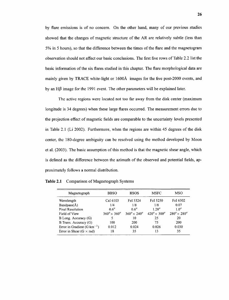
2.1 Comparison of Magnetograph Systems 26
2.2 Properties of Six Flares and the Active Regions 35
2.3 Effects of Projection Correction for the 2001 April 6 Flare 35
3.1 Correlation Coefficients between the Magnetic Parameters and the NaturalLogarithm of Flare Index 51
4.1 List of Active Regions Associated with Flares 60
4.2 Descriptive Statistics of Solar Flares Data 68
4.3 Regression models for Different Combination of Predictive Parameters . . . . 73
4.4 Indexes to Evaluate the Predictive Ability of Models 76
4.5 Validation of Model With Predictive Variables Lgni and Tflux 80
4.6 Validation Results of All Models 81
4.7 Effects of Lgni, Tflux on Response Variable Level 84
4.8 Comparison between Three Prediction Approaches 87
5.1 List of Halo CME Events Associated with Large Flares 98
5.2 Comparison of Magnetic Gradient Thresholds in Source Regions Identification 101
5.3 Magnetic Orientation of Solar Source Regions and Geomagnetic Storms . . . 117
xi
LIST OF FIGURES
Figure Page
1.1 Interior structure of the Sun. Courtesy of NASA 2
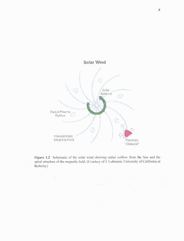
1.2 Schematic of the solar wind showing radial outflow from the Sun and the spi-ral structure of the magnetic field. (Courtesy of J. Luhmann, University ofCalifornia at Berkeley) 5
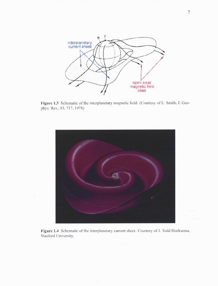
1.3 Schematic of the interplanetary magnetic field. (Courtesy of E. Smith, J. Geo-phys. Res., 83, 717, 1978) 7
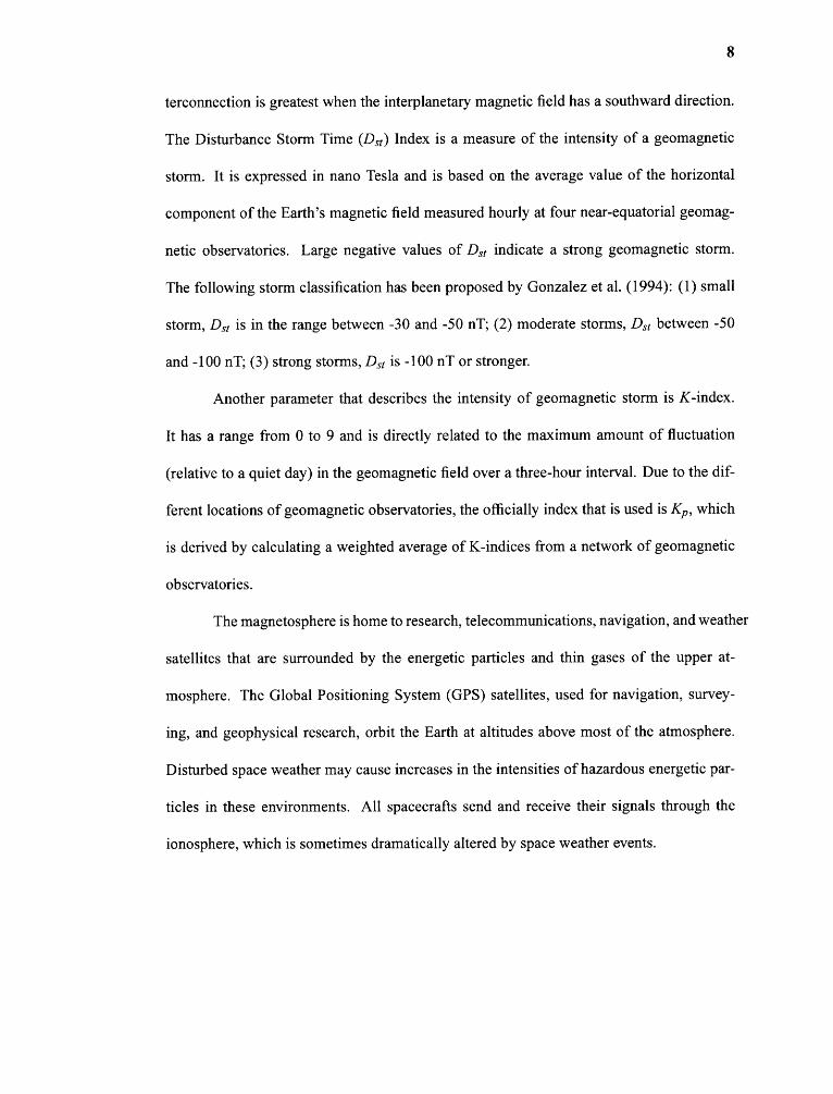
1.4 Schematic of the interplanetary current sheet. Courtesy of J. Todd Hoeksema,Stanford University. 7
1.5 Schematic of Earth's magnetosphere. The solar wind flows from left to right. 9
1.6 Coronal mass ejections sometimes reach out in the direction of Earth, SOHOimage and illustration. Courtesy: SOHO/LASCO/EIT (ESA and NASA). . . . 12
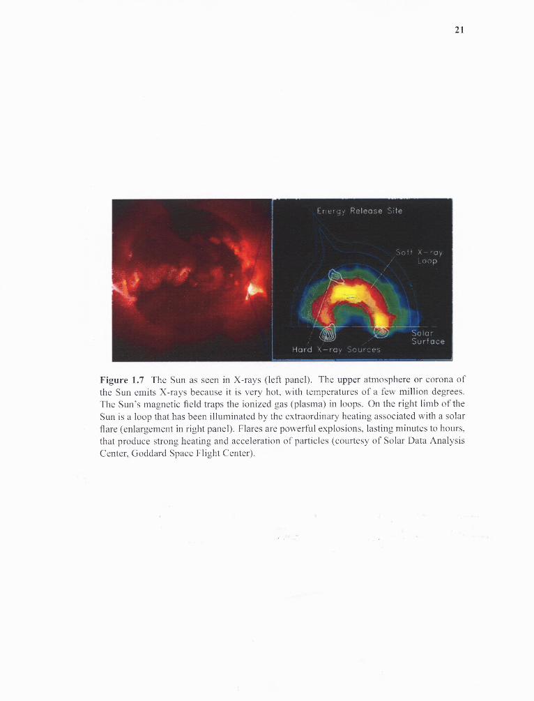
1.7 The Sun as seen in X-rays (left panel). The upper atmosphere or corona of theSun emits X-rays because it is very hot, with temperatures of a few milliondegrees. The Sun's magnetic field traps the ionized gas (plasma) in loops. Onthe right limb of the Sun is a loop that has been illuminated by the extraordi-nary heating associated with a solar flare (enlargement in right panel). Flaresare powerful explosions, lasting minutes to hours, that produce strong heatingand acceleration of particles (courtesy of Solar Data Analysis Center, GoddardSpace Flight Center) 21
1.8 Space weather hazards, courtesy Lou Lanzerotti, Bell Laboratories. 22
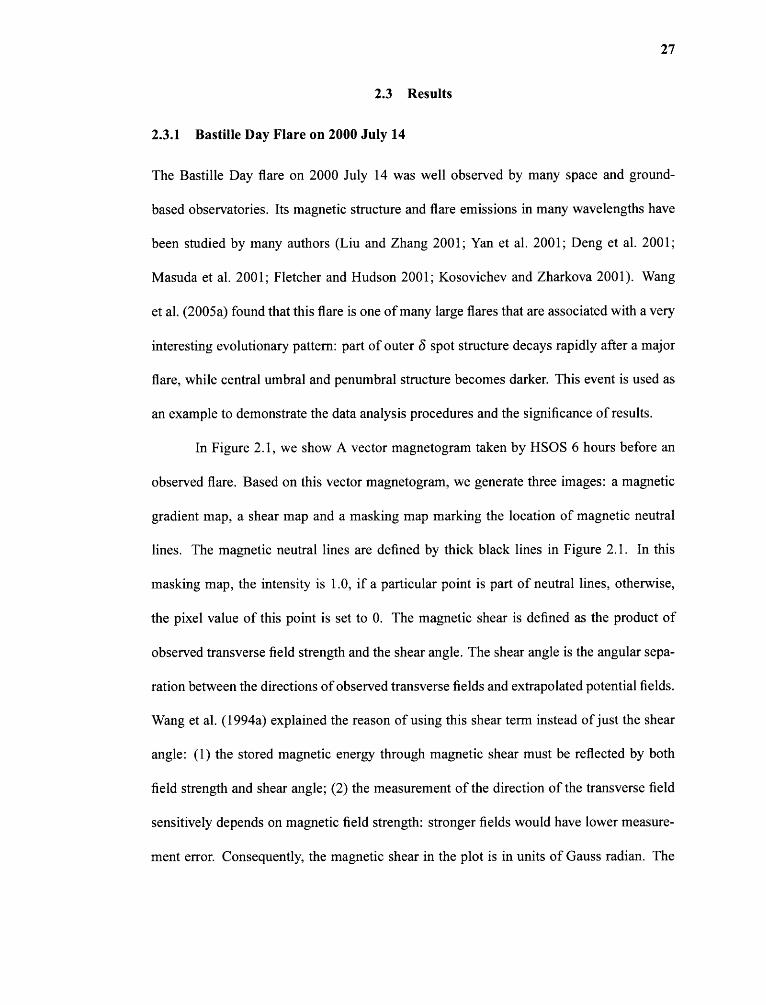
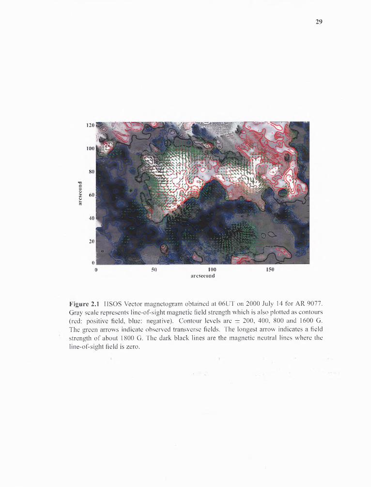
2.1 HSOS Vector magnetogram obtained at 06UT on 2000 July 14 for AR 9077.Gray scale represents line-of-sight magnetic field strength which is also plottedas contours (red: positive field, blue: negative). Contour levels are ± 200, 400,800 and 1600 G. The green arrows indicate observed transverse fields. Thelongest arrow indicates a field strength of about 1800 G. The dark black linesare the magnetic neutral lines where the line-of-sight field is zero. 29
xii
LIST OF FIGURES(Continued)
Figure Page
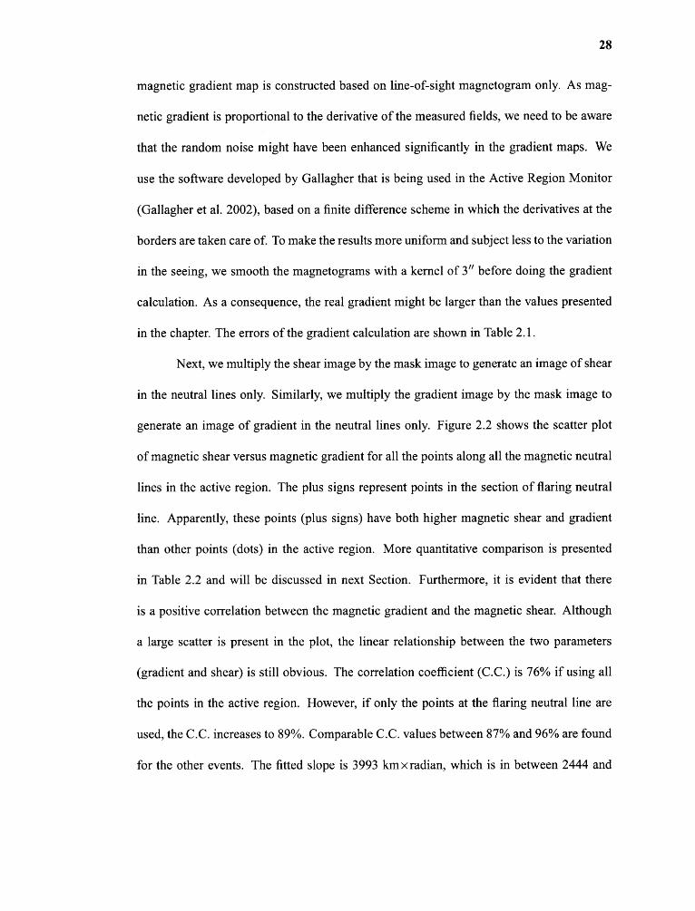
2.2 Top: Scatter plot of magnetic shear vs. magnetic gradient in all the points
along all the neutral lines identified for the active region 9077 on 2000 July 14.
Bottom: Plot of averaged magnetic shear vs. magnetic gradient with a linear
fit. The vertical bars present standard deviation of shear in each bin. 31
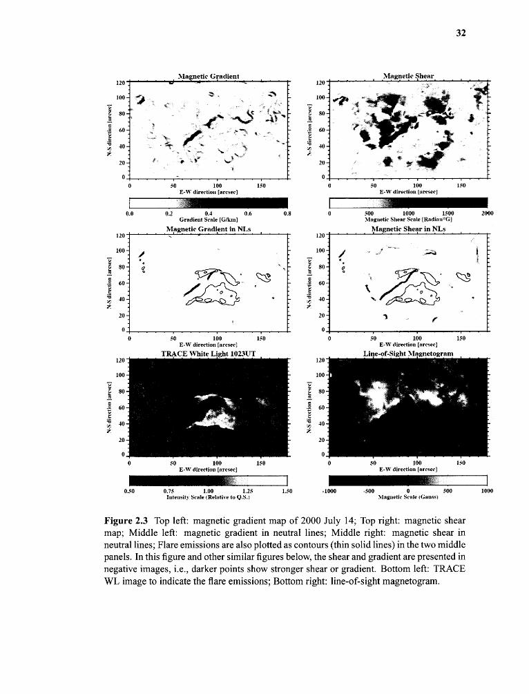
2.3 Top left: magnetic gradient map of 2000 July 14; Top right: magnetic shear
map; Middle left: magnetic gradient in neutral lines; Middle right: magnetic
shear in neutral lines; Flare emissions are also plotted as contours (thin solid
lines) in the two middle panels. In this figure and other similar figures below,
the shear and gradient are presented in negative images, i.e., darker points show
stronger shear or gradient. Bottom left: TRACE WL image to indicate the flare
emissions; Bottom right: line-of-sight magnetogram. 32
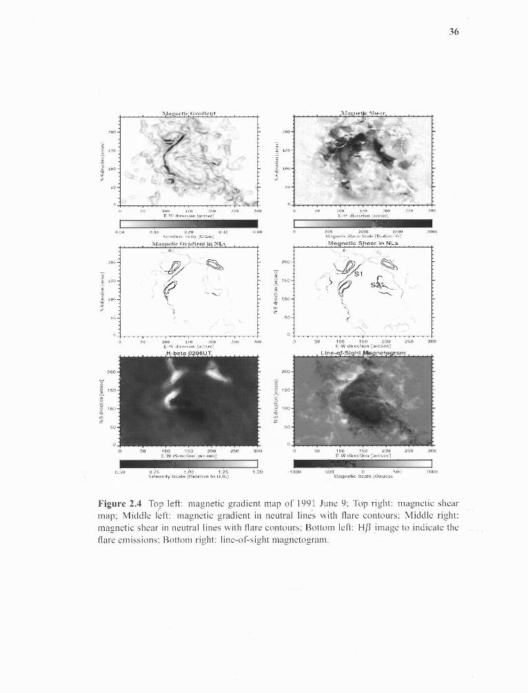
2.4 Top left: magnetic gradient map of 1991 June 9; Top right: magnetic shear
map; Middle left: magnetic gradient in neutral lines with flare contours; Mid-
dle right: magnetic shear in neutral lines with flare contours; Bottom left:
H/3 image to indicate the flare emissions; Bottom right: line-of-sight mag-
netogram 36
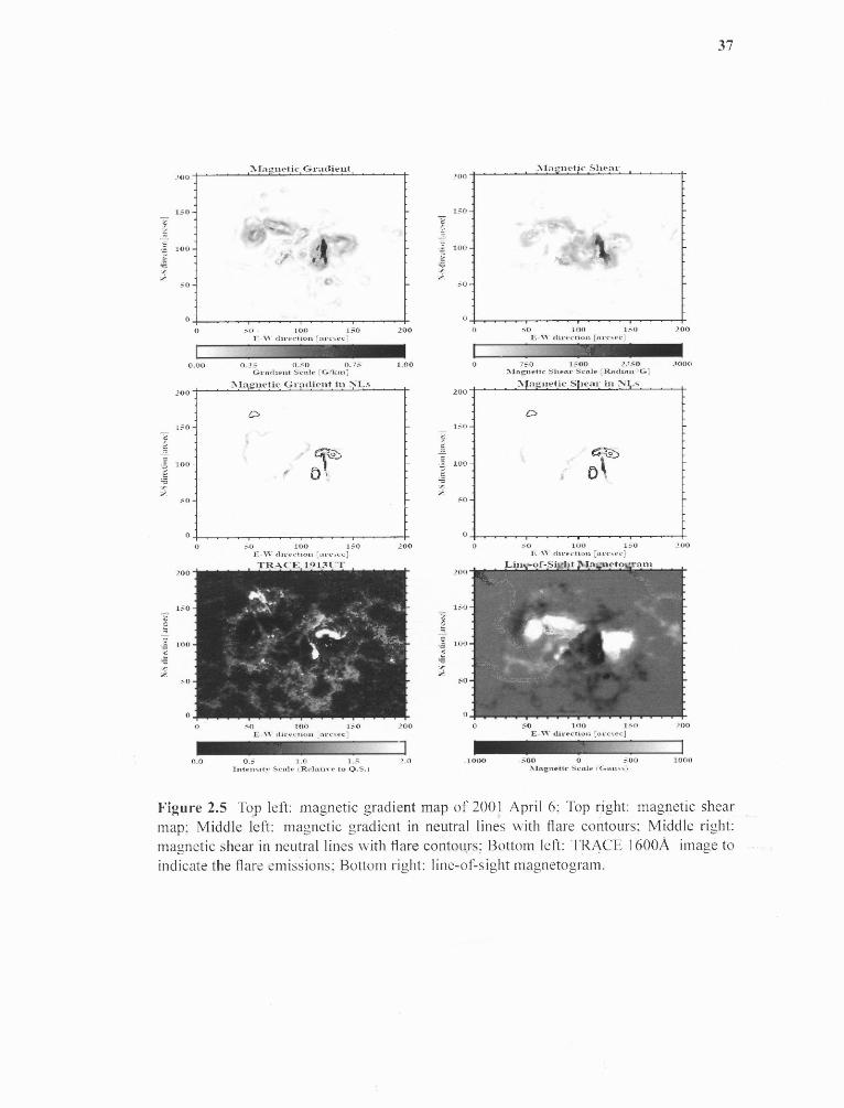
2.5 Top left: magnetic gradient map of 2001 April 6; Top right: magnetic shear
map; Middle left: magnetic gradient in neutral lines with flare contours; Mid-
dle right: magnetic shear in neutral lines with flare contours; Bottom left:
TRACE 1600A image to indicate the flare emissions; Bottom right: line-of-
sight magnetogram. 37
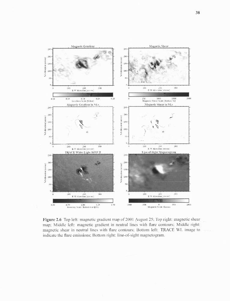
2.6 Top left: magnetic gradient map of 2001 August 25; Top right: magnetic shear
map; Middle left: magnetic gradient in neutral lines with flare contours; Mid-
dle right: magnetic shear in neutral lines with flare contours; Bottom left:
TRACE WL image to indicate the flare emissions; Bottom right: line-of-sight
magnetogram. 38
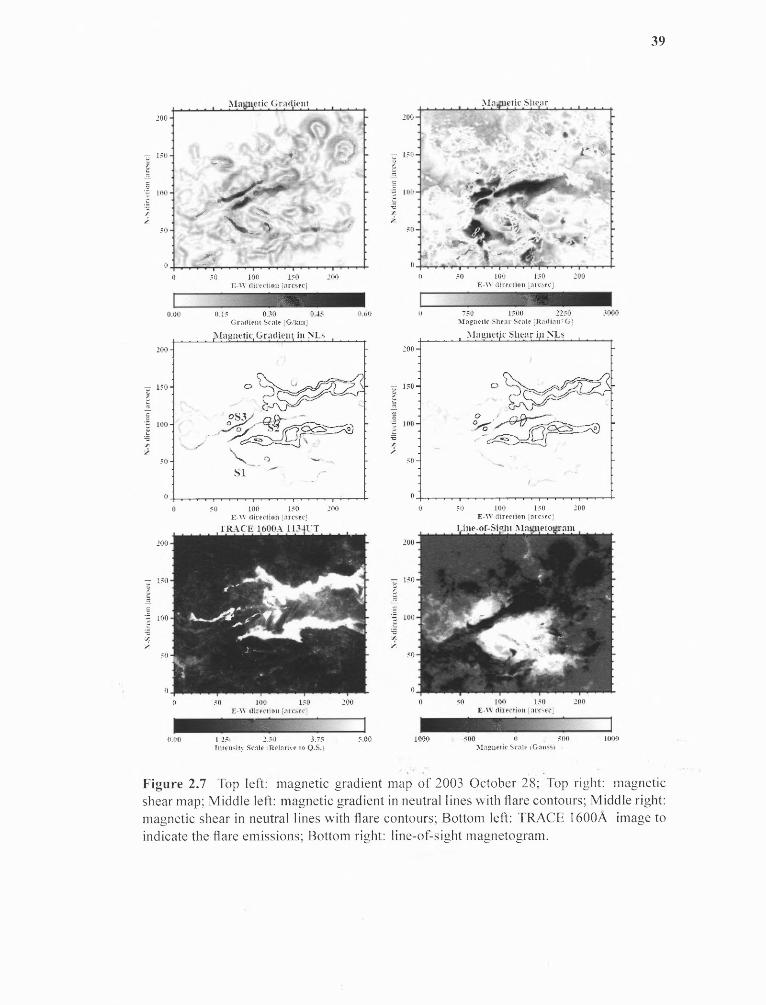
2.7 Top left: magnetic gradient map of 2003 October 28; Top right: magnetic
shear map; Middle left: magnetic gradient in neutral lines with flare contours;
Middle right: magnetic shear in neutral lines with flare contours; Bottom left:
TRACE 1600A image to indicate the flare emissions; Bottom right: line-of-
sight magnetogram. 39

LIST OF FIGURES(Continued)
Figure Page
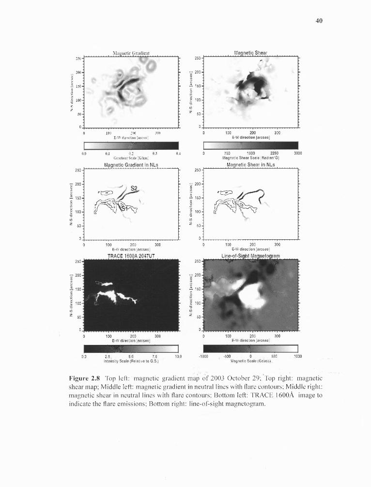
2.8 Top left: magnetic gradient map of 2003 October 29; Top right: magneticshear map; Middle left: magnetic gradient in neutral lines with flare contours;Middle right: magnetic shear in neutral lines with flare contours; Bottom left:TRACE 1600A image to indicate the flare emissions; Bottom right: line-of-sight magnetogram. 40
3.1 Left: the MDI line-of-sight magnetogram of active region NOAA9077 on 2000July 14; Middle: the gradient distribution along the neutral line; Right: themap of magnetic energy dissipation. The values of parameters at each pixelare indicated by the corresponding color bars 48
3.2 Scatter plots to compare flare index (in the form of logarithm) and magneticparameters. The left panels are based on flare index of entire disk passages ofactive regions, right is based on one-day flare index. The magnetic parameterspresented from top to bottom are: mean gradient on the magnetic neutral line;length of neutral lines with magnetic gradient larger than 50G Mm -1 ; andtotal magnetic energy dissipation. The solid lines show the least-squares linearregression line to the data points. The dashed lines show the 95 % confidenceintervals about the regression line. 50
3.3 Scatter plot of total magnetic energy dissipation vs. length of neutral lineswith magnetic gradient larger than 50G Mm -1 . The solid line shows the least-squares linear regression line to the data points. The dashed lines show the95% confidence intervals about the regression line. 52
4.1 Examination of the ordinality of Level for every magnetic parameter by access-ing how is the Level related to the mean value of each predictor, and whetherthe trend in each plot is monotonic. Solid lines connect the simple stratifiedmeans, and dashed lines connect the estimated expected value of X │Y=j giventhat PO holds. The extend of closeness of two curves indicates the perfectcondition to hold ordinal condition. 76
4.2 Checking PO assumptions separately for a series of predictive parameters. Thecircle, triangle, and plus sign correspond to Level > 1, 2, 3, respectively. POis checked by examining the vertical constancy of distances between any twoof these three symbols 77
xiv
LIST OF FIGURES(Continued)
Figure Page
4.3 Estimated logistic calibration curves obtained by bootstrapping using the cor-
rected intercept and slope. The logistic calibration model Pc = [1 + ex p — (yo +
γ1L))], where Pc is the bias-corrected probability. L is logit(P), and P is the pre-
dicted probabilities (labelled with 'Apparent'). The bisector line demonstrates
excellent validation on an absolute probability scale. 81
4.4 Distribution of predicted occurrence probability of solar flares. Panel (a), (b)
and (c) show the results when only Lgni, Tflux and Ediss as the predictive para-
meter, respectively. The probabilities for C, M and X class flares are displayed
by the black dots, red circles and green squares 88
4.5 Comparison of three predictive methods for each level of solar flares. The
results from Ordinal logistic method, NASA/SDAC and NOAA/SEC are in-
dicated by black diamonds, red squares and blue circles, respectively. For
comparison reasons, the actual probabilities of producing flares are shown by
green dots. The horizontal dot line is the probability of 50% (One more 25% in
X class panel). Vertical dot line represents the turning point of flare occurrence. 88
5.1 MDI high resolution magnetogram for AR 9077 taken on 2000 July 14 (top
panel). Black contours are magnetic neutral lines. The middle panel (b) shows
the corresponding magnetic gradient map. The bottom panel (c) is the gradient
distribution along the neutral line. Dark line is a gradient neutral line. 97
5.2 The comparison of magnetic field NLFF extrapolation before and after bastille
flare on July 14, 2000. (Courtesy of Thomas Weiglemann.) 103
5.3 The relationship between weighted mean shear angle and altitude. The blue
and red lines indicate the shear angles before and after solar flare, respectively.
Beyond 70,000 km, the magnetic field become potential. 104
5.4 Background is an MDI magnetogram taken at 0936UT on July 14 2000. Over
plotted are potential field lines. The segment of a thick blue line indicates the
position of the main magnetic neutral line. The field lines that cross the main
neutral line are displayed with red color 106
5.5 Definition of the magnetic orientation angle 0. Blue line N represents the
main neutral line. P'A' is projection of the field line L on the plane. Angle
between P'A' and the direction toward south pole is the orientation angle for
this particular field line. 107
xv
LIST OF FIGURES(Continued)
Figure Page
5.6 ACE measurements of IMF from July 26 to July 28 2004 (in GSE). From top tobottom are magnetic field strength (B), y and z component of magnetic fields(By , Be), the latitude (0) and longitude (0) angles, proton temperature (T),
density ratio (Nα/Np ), plasma pressure (f3) and the Dst index 111
5.7 ACE measurements of IMF from Nov. 07 to Nov. 09 2004 (in GSE). Fromtop to bottom are magnetic field strength (B), y and z component of magneticfields (By , Be), the latitude (0) and longitude (0) angles, proton temperature(T), density ratio (Nα /Np), plasma pressure (/3) and the Dst index. 112
5.8 Distribution of the calculated length of magnetic gradient neutral line of 73CME events. The width of the bar is 10 Mm. 114
5.9 Magnetic orientation angle, 0, versus the Dst index. The blue triangles rep-resent super storms, green stars show intense storms and red diamonds aremoderate storms. The label indicates the responsible interplanetary magneticstructure for the storm. 116
5.10 The magnetic orientation angle 0 versus corresponding IMF Be . In the case ofsuper geomagnetic storms produced by strong negative Be , the correspondingsource regions also had southward oriented magnetic fields. 118
xvi

CHAPTER 1
INTRODUCTION
Over the past decades, as new technology advances, mankind has become more dependent
on the space systems, satellite-based services, and other ground-based technologies than
ever before. Since these technologies are influenced by Sun-Earth interaction phenomena,
in recent years a new field, namely the Space Weather, which was formerly known as solar-
terrestrial physics has emerged. Space weather is the response of our space environment to
the constantly changing Sun.
1.1 Elements of Space Weather
The space weather is involved in the following stages: the Sun and its atmosphere as the
origin of the energy; the interplanetary space as the propagation medium; and the Earth's
magnetosphere and upper atmosphere as the destination of energy deposit.
1.1.1 The Sun
The Sun is the primary energy source of the Earth. All of the energy that we detect as light
and heat originates in nuclear reactions deep inside the Sun's high-temperature "core".
This core extends about one quarter of the way from the center of Sun to its surface where
the temperature is around 15 million kelvin (K). The Sun also gives off ultraviolet, X-ray,
gamma-ray, and radio emissions that are much more variable than its visible emissions.
The hot ionized gases in the interior of the Sun called radiative zone (Figure 1.1)
are constantly in motion as a result of the heat generated within, coupled with the Sun's
1
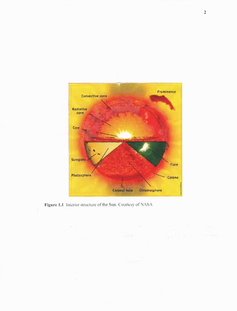
Figure 1.1 Interior structure of the Sun. Courtesy of NASA
2
3
rotation (one rotation every 27 days, approximately). In the outer regions, the high opacity
make it difficult for proton radiation to continue outward, then establish a steep tempera-
ture gradients and lead to convective equilibrium (Convective zone). Observationally, the
outer solar atmosphere following the convective zone has been divided into three spheri-
cally symmetric layers - the photosphere, chromosphere, and corona - lying successively
above one another (Zirin 1988). Solar magnetic fields are generated below the photosphere.
It plays a vital role in almost all kinds of solar activities. These fields are sometimes con-
centrated in sunspots, the largest compact magnetic concentrations on the surface of the
Sun. Sunspots are "dark" because they are colder than the areas around them. A large
sunspot might have a temperature of about 4,000 K, lower than the 5,800 K temperature of
the bright photosphere surrounding it. The magnetic field of sunspots decreases gradually
from the center, of about 3000 G, to the outer part, of about 800 G, and vanishes abruptly
outside in the photoshpere. Complexity of sunspots forms active regions. They are the
usual sites of solar activities, which may occur when their complicated magnetic fields are
suddenly rearranged.
Above the solar surface stretches the extended solar atmosphere, known as the solar
corona. Propagating waves and/or processes associated with the constant rearrangement of
the magnetic fields close to the Sun raise the temperature of the corona (to over 1,000,000
Kelvin), far above that of the solar surface (at about 6000 degrees Kelvin). Because of its
temperature, the coronal gas is highly ionized and so its structure is affected by the solar
magnetic field.
The Sun and its atmosphere are always changing, in a sense having weather of their
own. The Sun undergoes long-term (decade or more) variations such as the roughly 11-year
4
solar cycle (Mursula and Ulich 1998). This cycle showed itself in the number of sunspots
counted on the solar surface (above). The solar magnetic field evolves over the solar cycle
along with the sunspot number. The field is more complicated at solar maximum when the
simple solar minimum structure, which resembles Earth's field or that of a bar magnet, is
disrupted by the strong fields of many active regions. Processes related to this evolution of
the solar magnetic field are the ultimate causes of space weather.
1.1.2 The Interplanetary Space and Solar Wind
The high temperature of the solar upper atmosphere generates an outward flow of the ion-
ized coronal gas or plasma away from the Sun at typical speeds ranging from 400 to 800
kilometers per second. This outflow is known as the "solar wind" (Parker 1958, 1959). At
the Earth (1 astronomical unit (AU) or 150 million kilometers away from the Sun), 1 cubic
centimeter of solar wind contains about 7 protons and an equal number of electrons (so
there is no net electrical charge in the gas). Helium and heavier ions are also present in
the solar wind but in smaller numbers (Wolfe et al. 1966; Neugebauer and Snyder 1966;
Formisano et al. 1974; Barnes 1992).
The solar wind confines the magnetic field of Earth and governs phenomena such
as geomagnetic storms and aurorae. Coronal magnetic fields are constantly being carried
with the solar wind into interplanetary space. The solar rotation winds up the field into a
spiral resembling the water streams from a rotating garden sprinkler because the source of
the field keeps moving with the Sun (Figure 1.2).
At the Earth's distance from the Sun, the typical interplanetary magnetic field (IMF)
strength is about 5 nano teslas, or about 1/10,000 the strength of the Earth's magnetic field
Solar Wind
5
Figure 1.2 Schematic of the solar wind showing radial outflow from the Sun and thespiral structure of the magnetic field. (Courtesy of J. Luhmann, University of California atBerkeley)

6
at the surface. The "polarity" of the interplanetary magnetic field depends on the direction
of the coronal field at its roots. As illustrated in Figure 1.3, the interplanetary field is
typically organized into hemispheres of inward and outward field corresponding to the
North and South magnetic poles of the solar field. The two hemispheres are separated by a
sheet-like boundary carrying an electrical current (Smith et al. 1978). The sheet is not a flat
plane. As the Sun rotates, the sheet is shaped into swirls (see Figure 1.4) so that sometimes
the Earth is above the sheet and sometimes it is below it. The passage of this current sheet
is an important marker for space weather.
1.1.3 The Magnetosphere of the Earth
The magnetosphere is the region of space above the atmosphere that is dominated by the
Earth's magnetic field. Figure 1.5 shows the major structural features of this complex,
dynamical system derived from spacecraft observations in many different orbits.
The highly conducting solar wind gas is not able to penetrate Earth's magnetic field
at most locations, instead flowing around it. Before it is diverted, however, it slows down
at a (shock) wave called the "bow shock" that stands upstream of Earth in the solar wind.
It serves to slow the flowing ionized gas before it encounters the obstacle presented by
the Earth's magnetic field, analogous to air flow around a supersonic aircraft (Gold 1959;
Beard 1964).
Earth's magnetic field connects with the interplanetary magnetic field in the polar
caps. This interconnection allows transfer of energy from the solar wind to the magne-
tosphere and ionosphere, as well as entry of charged particles from interplanetary space.
This injection of energetic particles is known as geomagnetic storm. The amount of in-
7
Figure 1.3 Schematic of the interplanetary magnetic field. (Courtesy of E. Smith, J. Geo-phys. Res., 83, 717, 1978)
Figure 1.4 Schematic of the interplanetary current sheet. Courtesy of J. Todd Hoeksema,Stanford University.
8
terconnection is greatest when the interplanetary magnetic field has a southward direction.
The Disturbance Storm Time (Dst) Index is a measure of the intensity of a geomagnetic
storm. It is expressed in nano Tesla and is based on the average value of the horizontal
component of the Earth's magnetic field measured hourly at four near-equatorial geomag-
netic observatories. Large negative values of Dst indicate a strong geomagnetic storm.
The following storm classification has been proposed by Gonzalez et al. (1994): (1) small
storm, Dst is in the range between -30 and -50 nT; (2) moderate storms, Al between -50
and -100 nT; (3) strong storms, Dst is -100 nT or stronger.
Another parameter that describes the intensity of geomagnetic storm is K-index.
It has a range from 0 to 9 and is directly related to the maximum amount of fluctuation
(relative to a quiet day) in the geomagnetic field over a three-hour interval. Due to the dif-
ferent locations of geomagnetic observatories, the officially index that is used is Kp , which
is derived by calculating a weighted average of K-indices from a network of geomagnetic
observatories.
The magnetosphere is home to research, telecommunications, navigation, and weather
satellites that are surrounded by the energetic particles and thin gases of the upper at-
mosphere. The Global Positioning System (GPS) satellites, used for navigation, survey-
ing, and geophysical research, orbit the Earth at altitudes above most of the atmosphere.
Disturbed space weather may cause increases in the intensities of hazardous energetic par-
ticles in these environments. All spacecrafts send and receive their signals through the
ionosphere, which is sometimes dramatically altered by space weather events.
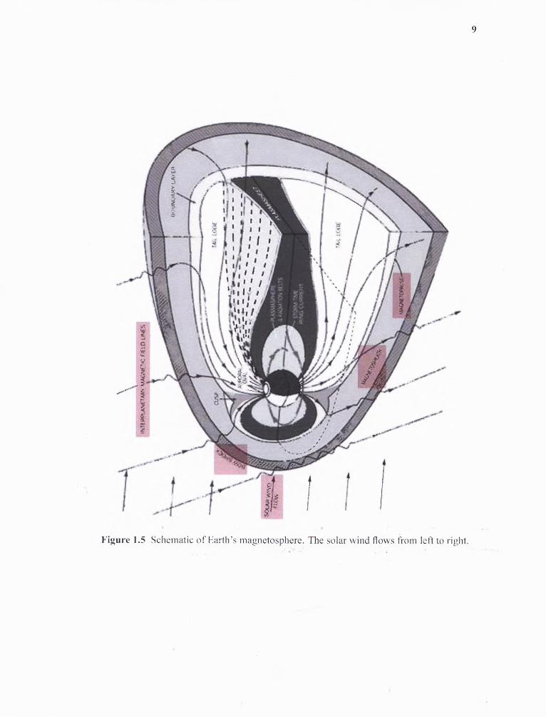
Figure 1.5 Schematic of Earth's magnetosphere. The solar wind flows from left to right.
9
10
1.2 Solar Origins of Space Weather
Most of the effects classified as space weather can ultimately be traced to changes occur-
ring at the Sun. These include variations in both the solar electromagnetic radiation and
the production of solar wind, plasma, and energetic particles. All of these are ultimately
related to the evolution of the solar magnetic field. Large disturbances in the space weather,
such as intense geomagnetic storms, shock waves and energetic particle events are mostly
associated with two solar activity transient phenomena: solar flares and coronal mass ejec-
tions (CMEs). These two events seem to be part of a single phenomenon, a solar magnetic
eruption. Nowadays it seems that neither one is the cause of the other (Gosling 1993).
1.2.1 Coronal Mass Ejections
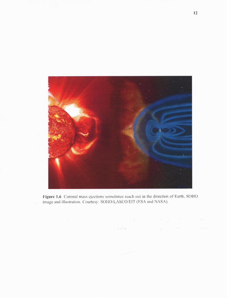
Figure 1.6 shows the release of a CME at the Sun. A large CME can contain 10 13 kg
of matter. The faster CMEs have outward speeds of up to 2000 kilometers per second,
considerably greater than the normal solar wind speeds of about 400 kilometers per second.
These produce large shock waves in the solar wind as they plow through it. Some of the
solar wind ions are accelerated by the shock, which then becomes a source of intense and
long-lasting energetic particle enhancements in interplanetary space. The rate of CMEs
depends on the phase of the solar cycle. Events occur at a rate of roughly 0.5 per day at
solar minimum and between two and three a day at solar maximum (Hundhausen 1993;
Webb and Howard 1994; St. Cyr et al. 2000).
CMEs are monitored using coronagraphs, which produce artificial eclipses on the
Sun by placing an "occulting disk" over the image of the Sun. CMEs directed along the
Sun-Earth line can be detected as "halos" around the occulting disk in a white-light coron-
11
agraph. A CME is a full halo when it extends 360° around the Sun and a partial halo if the
apparent width is greater than 120° (Howard et al. 1982).
Now it is well accepted that the front-side halo CMEs are the major causes for those
severe geomagnetic storms (e.g., Brueckner et al. 1998; Cane et al. 2000; Gopalswamy
et al. 2000; Webb et al. 2000; Wang et al. 2002; Zhang et al. 2003b). A halo CME may
head either toward the Earth if it arises on the front-side of the Sun, or away from the Earth
if it is on the backside. Cane et al. (2000) showed that only about half of front-side halo
CMEs encounter the Earth and their associated solar events typically occur at longitudes
ranging from 40° East to 40° West. According to Wang et al. (2002), about 45% of total
132 Earth-directed halo CMEs caused geomagnetic storms with Kp ≤ 5, and almost 83%
of events took place within +30° of the central meridian of the Sun.
The interplanetary counterparts of coronal mass ejections (ICMES) at the Sun have
been identified since the early years of solar wind observations. A subset of ICMEs are
the magnetic clouds (MC), which seem to constitute around 1/3 of all the ICMES. These
structures are identified, near 1 AU, by their high magnetic field intensity, low proton tem-
perature, low Beta (ratio between thermal and magnetic pressure), and a smooth and large
scale rotation in one of the magnetic field components. ICMEs present dimensions around
0.2-0.3 AU and cross the spacecrafts or Earth in r24 hours (Burlaga et al. 1981). Cur-
rent models of these magnetic clouds consider them as giant magnetic flux ropes with field
aligned currents. Other ICMEs are believed to be "complex ejecta", with a disordered
magnetic field (Burlaga et al. 2001). The geoeffectiveness of ICME ranges from 25%
(Vennerstroem 2001) up to 82% (Wu and Lepping 2002).
12
Figure 1.6 Coronal mass ejections sometimes reach out in the direction of Earth, SOHOimage and illustration. Courtesy: SOHO/LASCO/EIT (ESA and NASA).
13
1.2.2 Solar Flares
Short periods of explosive energy release, known as solar flares, more frequently occur in
active regions during the period around solar maximum. An example of a flare observed on
the limb of the Sun is shown below (Figure 1.7). Flares have lifetimes ranging from hours
for large gradual events down to tens of seconds for the most impulsive events. During a
very strong flare, the solar ultraviolet and X-ray emissions can increase by as much as 100
times above even active-region levels. During solar maximum, approximately one such
flare is observed every week. Flares heat the solar gas to tens of millions of degrees. The
heated gas then radiates strongly across the whole electromagnetic spectrum from radio to
gamma rays. The largest of these explosions are so bright that they can even be seen from
Earth in continuum visible light, so called white-light flares.
Flares are important to space weather mainly because they appear in connection to
some CMEs and also because they have an important role in particle acceleration. They
can accelerate protons and electrons that travel to Earth directly from the Sun along the
interplanetary magnetic field (which "channels" the charged particles). These contribute
to the high-energy particle environment in the vicinity of the magnetosphere if Earth's
location is magnetically connected to the flaring region by the interplanetary magnetic field.
Solar flares are classified according to its X-ray emission in the band 1-8 Ain emis-
sion classes B (with peak < 10 -6Wm-2 ), C (peak between 10 -6 and 10 -5Wm-2 ), M (with
peak between 10 -5 and 10 -4Wm -2 ) and X (with peak > 10 -4Wm-2 ). A number is also
indicated after the letter which gives the intensity of emission, each category having nine
subdivisions, e.g., C1-C9, C9 equivalent to a peak emission of 9 x 10 -5Wm-2 . Events of
the X type are big events that can cause planetary radio blackouts and long lasting radiation
14
storms. Events of the M type are of medium size, which can cause minor radiation storms
and brief radio-blackouts, mainly in the polar regions. Events of C and B types have very
little effect on Earth.
Park et al. (2002) reported that the geoeffectiveness of solar flares is about 30-45%.
Howard and Tappin (2005) performed a statistical analysis of CME/ICMEs events from
January 1998 to August 2004 and concluded that only around 40% of the shock/storms at
1AU were associated either with an X-class or M-class flares.
1.3 Consequences of Space Weather
Electromagnetic emission from the Sun can degrade systems in space and radio systems
on Earth. Changes in the spectrum and intensity of the radiation belts caused by high-
speed solar streams and CMEs have affected the operation of spacecraft through vehicle
damage, deterioration of solar cells, semiconductor damage, or through electric charg-
ing of the spacecraft. Changing fields in the magnetosphere can induce currents in the
ionosphere and, at ground level, in terrestrial power systems and long pipe lines that may
cause damage that is costly to industry. Variations in ionospheric conditions, subsequent
to magnetospheric changes, influence the operation of radio systems such as short wave
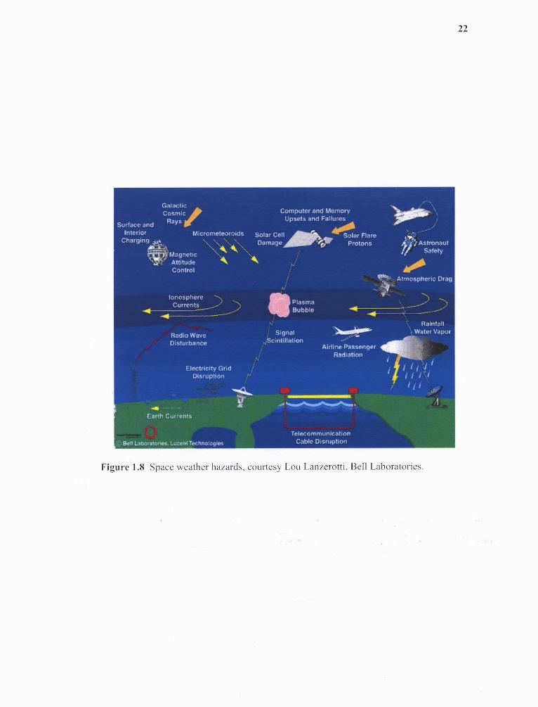
communications and radar. Figure 1.8 shows the numerous effects of space weather.
1.3.1 Space Radiation Environment
Geostationary satellites operate near the top of the outer radiation belt, low Earth orbit-
ing satellites operate within the inner radiation belt. Both environments are populated by
charged particles whose energy and number depend on space weather conditions.

15
Satellite systems can be impaired through direct penetration of the electronics by
high velocity solar protons, by deep or surface-charging or by surface damage. Surface
damage, such as degradation of solar cells, is caused by low energy particles and radiation.
Effects on satellite hardware have been reviewed by Baker (2001) and described by the
Geological Survey of Canada (2002).
Those working outside a space station or spacecraft beyond the protection of the
Earth's atmosphere can experience harmful radiation doses during major solar events un-
less protected. Radiation hazards are less for most aircraft but as general aviation develops
into the stratosphere, and to greater altitudes, the dosage experienced by passengers dur-
ing a major space event can become significant, particularly over polar routes, where the
protection of the Earth's magnetic field is lowest.
1.3.2 Ionospheric Effects
Shortwave radio communication at HF frequencies (3-30 megahertz), which is still exten-
sively used for overseas broadcasting in various countries, depends upon the reflection of
signals from Earth's ionosphere. These electromagnetic waves are attenuated as they pass
through the lower ionosphere (below 100 km), where collisions between the electrons and
air molecules are frequent. Ionosphere attenuation affects the usable radio communication
frequencies. If it becomes especially strong due to an increase in the local electron density,
it can cause a total communications blackout. Solar flare ultraviolet and X-ray bursts, solar
energetic particles, or intense aurora can all bring on this condition.
The deep ionization produced by the solar protons also alters the path taken by the
waves reflecting from the ionosphere. The ionospheric changes that occur during disturbed

16
times also increase the incidence of electron density irregularities, leading to sometimes
severe variations or scintillations in the phase strength of signals sent from the ground to
satellites at VHF and UHF frequencies (30 megahertz to 3 gigahertz).
Finally, solar radio bursts can directly interfere with communications in the fre-
quency range between 245 MHz and 2.7 GHz, which is widely used. In summary, space
weather-related disruptions to communication systems have wideranging effectsalfrom so-
cial interactions to economic transactions on a global level to intelligence and surveillance
activities.
Navigation systems, consisting of constellations of Earth-orbiting satellites, use the
propagation delay from satellite-to-receiver to measure the range from several satellites to
determine the position of the receiver. Unexpected changes in the ionospheric section of
the propagation path cause errors in range, and hence in position. Such changes in electron
density can be caused by a solar disturbance.
1.3.3 Geomagnetic Effects
A geomagnetic storm will induce electric currents in conductors at ground level. If power
lines, railway lines, steel pipelines or telecommunication cables, are long in terms of east-
west extent, the currents can be large enough to cause costly damage (Geological Survey
of Canada 2002).
Induced currents flowing through power transformers can trip relays and take out
power lines or burn out transformers. In heavily loaded systems it is possible to have a
failure of the whole system, as happened in the Canadian Hydro-Quebec system during a
magnetic storm in March 1989.

17
Long pipeline corrosion occurs through chemical reactions that take place through
current leakage between pipe and earth. To prevent the electro-chemical corrosion, a volt-
age between the pipe and ground is maintained. If the back emf is not altered to counter
the current induced by the geomagnetic storm, pipe corrosion is increased.
The principal space weather hazard to humans is radiation exposure to astronauts
and passengers in high-altitude aircraft. Although the residual atmosphere above an air-
craft provides a measure of protection from cosmic rays and solar energetic particles that
enter the magnetosphere, there is still concern for flights on polar routes during major solar
particle events. The primary means of reducing this hazard is to modify flight paths as
necessary and to limit the flight time of personnel on high-altitude aircraft like the super-
sonic transport. It is clear that in this case early warnings of solar energetic particles are
extremely desirable. While flares can be monitored at least on the visible disk of the Sun,
solar indications of the shockproducing fast CME toward Earth are less apparent.
1.4 Space Weather Forecasting
To avoid or reduce the above mentioned space weather induced hazards, there is a growing
request for reliable forecasts of hazardous space weather events for manned space activities,
for unmanned spacecrafts, for space and ground-based industry, for the public and insofar
for many aspect of daily life. The objective of space weather research is to understand in
theory and practice the stormy and hostile interplanetary environment, in order to make
possible procedures that turn it safe for human technological activities and for the human
presence in space (Hargreaves 1992; Cole 2003).
The warning of a potential threat from space weather on terrestrial and space sys-
18
tems can be provided a few hours ahead on the basis of observations of CMEs and verified
by in-situ data from spacecraft, but the specific severity of the effect requires further devel-
opment of models of the solar wind and magnetosphere.
Recent data from satellites have increased progress on space weather prediction.
The Advanced Composition Explorer (ACE) spacecraft, which orbits the L 1 Lagrangian
point of Earth-Sun gravitational equilibrium located about 1.5 million km from the Earth,
performs measurements of the direction and magnitude of IMF. This excellent position
enables ACE to conduct 24 hours monitoring of solar wind condition and to transmit inter-
planetary data in real time that can provide 1 hour advance warning of geomagnetic storms.
The Solar & Heliospheric Observatory (SOHO), containing twelve scientific instruments,
was launched in 1995. It currently becomes the main source of near-real time solar data for
space weather prediction.
There are now models specifying the magnetospheric environment with local ac-
curacy when used in conjunction with in-situ data; polar radars deliver realtime maps of
magnetospheric and ionospheric currents and magnetic fields; and networks of ionospheric
and geomagnetic monitors give constant information on ionospheric conditions. Much has
been achieved in the last few years but the ability to forecast the total Sun-Earth event
days, or even hours, ahead remains as a challenge. Some of other challenges are the au-
tomated definition, classification and representation of solar features and the establishing
of an accurate correlation between the occurrence of solar activities (e.g., solar flares and
CMEs) and solar features (e.g., sunspots, filaments and active regions) observed in various
wavelengths.

19
1.5 The Goals and Structure of the Dissertation
As mentioned, comprehensive study of the solar activities, especially solar flares and CMEs,
and the solar magnetic field is essential to space weather research. The goal of this study
is to explore the relation between solar surface activities, such as flares and CMEs and the
features of associated magnetic fields, e.g., magnetic orientation angle, length of magnetic
gradient neutral line, magnetic energy dissipation, total magnetic flux, and the relation be-
tween them and geomagnetic storms. Both case and statistical studies are carried out. The
dissertation is organized as follows:
Chapter 1: Introduction.
Chapter 2: The relationship between magnetic gradient and magnetic shear of solar active
regions.
In this chapter, the magnetic structure of five well-known active regions that pro-
duced great flares (X5 or larger) are studied. Magnetic gradient of active region could be a
better proxy than magnetic shear to predict where a major flare might occur.
Chapter 3: The relationship between solar flare index and magnetic features.
In this chapter, flare index, which characterizes the overall flare productivity of a
given active region, is found to have significant correlation with the mean spatial gradi-
ent on the neutral line, the length of magnetic gradient neutral line and the total energy
dissipation in a unit layer per a unit time.
Chapter 4: Statistical Assessment of Photospheric Magnetic Features in Imminent Solar
Flares Predictions.
In this chapter, the ordinal logistic regression model is first time introduced into
solar physics and proved to be a viable approach to the automated flare prediction. The

20
results are much better than those data published in NASA/SDAC service, and comparable
to the data provided by NOAA/SEC complicated expert system.
Chapter 5: The relationship between magnetic orientation angle and geomagnetic storm.
In this chapter, the relationship between magnetic structures of coronal mass ejec-
tion (CME) source regions and geomagnetic storms, in particular, the super storms is in-
vestigated. The magnetic orientation angle is derived and used to predicted those super
geomagnetic storms.
21
Figure 1.7 The Sun as seen in X-rays (left panel). The upper atmosphere or corona ofthe Sun emits X-rays because it is very hot, with temperatures of a few million degrees.The Sun's magnetic field traps the ionized gas (plasma) in loops. On the right limb of theSun is a loop that has been illuminated by the extraordinary heating associated with a solarflare (enlargement in right panel). Flares are powerful explosions, lasting minutes to hours,that produce strong heating and acceleration of particles (courtesy of Solar Data AnalysisCenter, Goddard Space Flight Center).
22
Figure 1.8 Space weather hazards, courtesy Lou Lanzerotti, Bell Laboratories.
CHAPTER 2
THE RELATIONSHIP BETWEEN MAGNETIC GRADIENT AND MAGNETIC
SHEAR OF SOLAR ACTIVE REGIONS
2.1 Introduction
Solar flares and CMEs are two related, and most important forms of explosive energy re-
lease from the Sun. It has been noticed long ago that non-potentiality of an active region's
magnetic structure is vitally important in storing energy and triggering flares (Hagyard
et al. 1984). The most notable indicator of non-potentiality is the 6 sunspot that is defined
as umbrae of opposite polarity lying in a common penumbra. For over three decades, the
morphological evolution of 8 configurations and their strong connection to intensive flare
activity have been widely studied by many authors (e.g., Tang 1983; Hagyard et al. 1984;
Zirin and Liggett 1987; Tanaka 1991). Using eighteen years of observations at Big Bear
Solar Observatory (BBSO), Zirin (1987) summarized the development of 6 spots and clas-
sified them in three categories, concluding that 3 groups are responsible for almost all great
flares.
Measurements of the global non-potentiality of an active region can be obtained
from a vector magnetogram of the region regardless of the chirality of global magnetic
shear or twist in chromospheric or coronal images. E.g., such a measurement has been used
to evaluate the potential of producing CMEs of particular active regions (Falconer 2001).
Zhang (2001) studied AR 6659 and found that the shear and gradient of the magnetic field
are important and reflect a part of the electric current in solar active regions. However, the
analysis of vector magnetograms has experienced great difficulties even as new instruments
23
24
have been developed. The most notable ones are calibration, resolution of 180 degree
ambiguity and correction of the projection effect when the region is not close to the solar
disk center.
From a sample of 17 vector magnetograms, Falconer et al. (2003) showed that there
is a viable proxy for non-potentiality that can be measured from a line-of-sight magne-
togram. This proxy is the strong magnetic gradient and it is correlated with active region
CME productivity. Because gradients can be measured from line-of-sight magnetograms
obtained from conventional magnetographs, it is a dependable substitute for magnetic shear
for use in operational CME forecasting. Prasad (2000) also used the similar parameter of
magnetic gradient to characterize the stressed magnetic fields in active regions. However,
no study has been carried out to have detailed comparison of gradient and shear in active
regions. In this chapter, two questions will be primary addressed: (1) Are magnetic shear
and gradient correlated? (2) Do flares tend to occur in the high gradient and/or high shear
locations?
2.2 Observation
The primary data sources are from four well-known vector magnetograph systems:
(1) Digital Magnetograph (DMG) at BBSO. The data were obtained by a filtergraph-
based system. It uses the Ca 1 6103 A. The bandpass of the birefringent filter is 1/4 A. The
field-of-view of the instrument is 360" x 360" and the spatial resolution is 0.6" per pixel
(Spirock 2005 ).
(2) Vector magnetograph at Huairou Solar Observing Station (HSOS) in China. The
data were obtained by a filtergraph-based system that was developed by Ai (1987). It uses
25
the Fe I 5324 A. The bandpass of the birefringent filter is 1/8 A. The field-of-view of the
instrument is 360" x 240" and the spatial resolution is 0.6" per pixel.
(3) Vector magnetograph at Marshall Space Flight Center (MSFC). The magneto-
graph is a filter-based instrument employing a tunable Zeiss birefringent filter with a 1/8 A
bandpass and an electro-optical modulator to obtain integrated Stokes profiles in the Fe I
5250 A absorption line. The field-of-view of the instrument is 420" x 300" and the spatial
resolution is 1.28" per pixel.
(4) Imaging Vector Magnetograph at Mees Solar Observatory: it consists of a 28-
cm telescope and a tunable Fabry-Perot system with a pixel resolution of 1 arsec, FOV of
280" x 280" and polarization precision of 0.1% (Mickey et al. 1996). The data analysis
procedures of IVM are more complicated then three other systems at BBSO, HSOS and
MSFC. It requires full Stokes Inversion (LaBonte et al. 1999).
Table 2.1 compares the basic parameters of these vector magnetograph systems.
According to the accuracy of each system, we estimated the probable errors when calcu-
lating the magnetic gradient and magnetic shear. The error in the azimuthal angle can only
be estimated by inter-comparison of multiple instruments (Zhang et al. 2003a; Wang et al.
1992). A 10-degree error is believed to be a reasonable value. Most measurement errors on
the various parameters are at least one order of magnitude smaller than the typical measured
physical quantities themselves.
The magnetograms presented in this chapter were obtained between 1 and 6 hours
before the flares, except that for the 2003 October 28 event, the first available magnetogram
on that day was taken 4 hours after the flare. Because there is a sufficient gap between the
time of observation and the time of the flare, possible contamination of magnetic signal
26
by flare emissions is of no concern. On the other hand, many of our previous studies
showed that the changes of magnetic structure of the AR are relatively subtle (less than
5% in 5 hours), so that the difference between the times of the flare and the magnetogram
observation should not affect our basic conclusions. The first five rows of Table 2.2 list the
basic information of the six flares studied in this chapter. The flare morphological data are
mainly given by TRACE white-light or 1600A images for the five post-2000 events, and
by an H/3 image for the 1991 event. The other parameters will be explained later.
The active regions were located not too far away from the disk center (maximum
longitude is 34 degrees) when these large flares occurred. The measurement errors due to
the projection effect of magnetic fields are comparable to the uncertainty levels presented
in Table 2.1 (Li 2002). Furthermore, when the regions are within 45 degrees of the disk
center, the 180-degree ambiguity can be resolved using the method developed by Moon
et al. (2003). The basic assumption of this method is that the magnetic shear angle, which
is defined as the difference between the azimuth of the observed and potential fields, ap-
proximately follows a normal distribution.
Table 2.1 Comparison of Magnetograph Systems
Magnetograph BBSO HSOS MSFC MSO
Wavelength Cal 6103 FeI 5324 FeI 5250 FeI 6302Bandpass(Å) 1/4 1/8 1/8 0.07
Pixel Resolution 0.6" 0.6" 1.28" 1.0"Field of View 360"x 360" 360"x 240" 420"x 300" 280"x 280"B Long. Accuracy (G) 5 10 25 20B Trans. Accuracy (G) 100 200 75 200Error in Gradient (G km -1 ) 0.012 0.024 0.026 0.030Error in Shear (G x rad) 18 35 13 35
27
2.3 Results
2.3.1 Bastille Day Flare on 2000 July 14
The Bastille Day flare on 2000 July 14 was well observed by many space and ground-
based observatories. Its magnetic structure and flare emissions in many wavelengths have
been studied by many authors (Liu and Zhang 2001; Yan et al. 2001; Deng et al. 2001;
Masuda et al. 2001; Fletcher and Hudson 2001; Kosovichev and Zharkova 2001). Wang
et al. (2005a) found that this flare is one of many large flares that are associated with a very
interesting evolutionary pattern: part of outer 3 spot structure decays rapidly after a major
flare, while central umbral and penumbral structure becomes darker. This event is used as
an example to demonstrate the data analysis procedures and the significance of results.
In Figure 2.1, we show A vector magnetogram taken by HSOS 6 hours before an
observed flare. Based on this vector magnetogram, we generate three images: a magnetic
gradient map, a shear map and a masking map marking the location of magnetic neutral
lines. The magnetic neutral lines are defined by thick black lines in Figure 2.1. In this
masking map, the intensity is 1.0, if a particular point is part of neutral lines, otherwise,
the pixel value of this point is set to 0. The magnetic shear is defined as the product of
observed transverse field strength and the shear angle. The shear angle is the angular sepa-
ration between the directions of observed transverse fields and extrapolated potential fields.
Wang et al. (1994a) explained the reason of using this shear term instead of just the shear
angle: (1) the stored magnetic energy through magnetic shear must be reflected by both
field strength and shear angle; (2) the measurement of the direction of the transverse field
sensitively depends on magnetic field strength: stronger fields would have lower measure-
ment error. Consequently, the magnetic shear in the plot is in units of Gauss radian. The
28
magnetic gradient map is constructed based on line-of-sight magnetogram only. As mag-
netic gradient is proportional to the derivative of the measured fields, we need to be aware
that the random noise might have been enhanced significantly in the gradient maps. We
use the software developed by Gallagher that is being used in the Active Region Monitor
(Gallagher et al. 2002), based on a finite difference scheme in which the derivatives at the
borders are taken care of To make the results more uniform and subject less to the variation
in the seeing, we smooth the magnetograms with a kernel of 3" before doing the gradient
calculation. As a consequence, the real gradient might be larger than the values presented
in the chapter. The errors of the gradient calculation are shown in Table 2.1.
Next, we multiply the shear image by the mask image to generate an image of shear
in the neutral lines only. Similarly, we multiply the gradient image by the mask image to
generate an image of gradient in the neutral lines only. Figure 2.2 shows the scatter plot
of magnetic shear versus magnetic gradient for all the points along all the magnetic neutral
lines in the active region. The plus signs represent points in the section of flaring neutral
line. Apparently, these points (plus signs) have both higher magnetic shear and gradient
than other points (dots) in the active region. More quantitative comparison is presented
in Table 2.2 and will be discussed in next Section. Furthermore, it is evident that there
is a positive correlation between the magnetic gradient and the magnetic shear. Although
a large scatter is present in the plot, the linear relationship between the two parameters
(gradient and shear) is still obvious. The correlation coefficient (C.C.) is 76% if using all
the points in the active region. However, if only the points at the flaring neutral line are
used, the C.C. increases to 89%. Comparable C.C. values between 87% and 96% are found
for the other events. The fitted slope is 3993 km x radian, which is in between 2444 and
29
Figure 2.1 HSOS Vector magnetogram obtained at 06UT on 2000 July 14 for AR 9077.Gray scale represents line-of-sight magnetic field strength which is also plotted as contours(red: positive field, blue: negative). Contour levels are ± 200, 400, 800 and 1600 G.The green arrows indicate observed transverse fields. The longest arrow indicates a fieldstrength of about 1800 G. The dark black lines are the magnetic neutral lines where theline-of-sight field is zero.

30
5769 km x radian for all the other events. The figure also includes an average plot with a
bin size of 0.04 G km -1 to show up the trend better. The fitted line is flatter due to the fact
that there are fewer points in the high shear/gradient area.
In Figure 2.3 we show maps of magnetic gradient, gradient at the neutral lines,
magnetic shear and shear at the neutral lines. In addition, the flare emissions are shown by
a TRACE WL image. Obviously, the flare neutral line has both strong magnetic gradient
and magnetic shear. Either the magnetic gradient or the magnetic shear can be used to
identify correctly the flaring neutral line.
2.3.2 Summary of the other Five Events
We present a comparison of shear and gradient maps in Figures 2.4-2.8 for the other five
events. The parameters concerning the shears and gradients are listed in Table 2.2. There
are four derived parameters for each: maximum value along all the neutral lines in the
active regions, maximum value along the flare neutral line, mean value along all the neutral
lines and mean value along the flare neutral line. The flare neutral line is defined by the
extent of flare ribbons at the emission maximum. From this table, it is obvious that for all
the six events, the maximum gradient along the flare neutral lines is the maximum gradient
for the entire active region; the ratio of mean gradient along the flare neutral line to that of
entire active region is between 2.3 and 8.0. The two lowest values of this ratio belong to the
2003 October 28 and 29 events. It is not difficult to explain such a low ratio for these two
events: two flares occurred in the same active region but at two different locations. Both
locations have high gradient (and shear as well). Therefore, either one of these two flare
neutral lines can not be uniquely dominant in having high mean gradient (or shear). Based
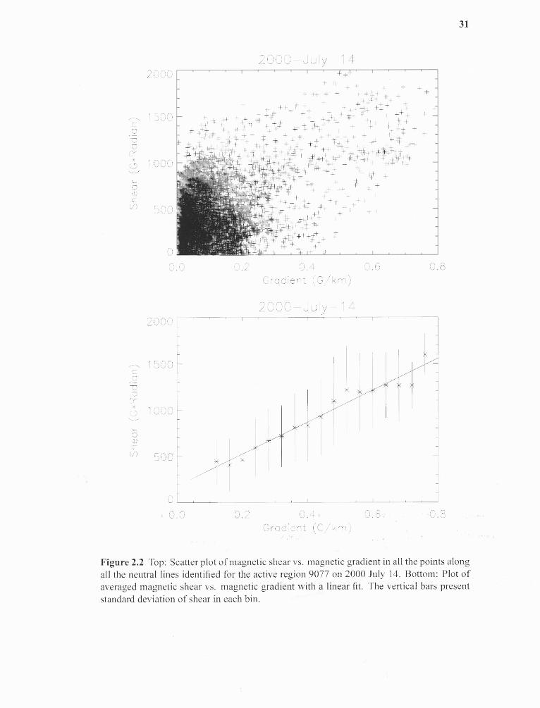
31
Figure 2.2 Top: Scatter plot of magnetic shear vs. magnetic gradient in all the points alongall the neutral lines identified for the active region 9077 on 2000 July 14. Bottom: Plot ofaveraged magnetic shear vs. magnetic gradient with a linear fit. The vertical bars presentstandard deviation of shear in each bin.
32
Figure 2.3 Top left: magnetic gradient map of 2000 July 14; Top right: magnetic shearmap; Middle left: magnetic gradient in neutral lines; Middle right: magnetic shear inneutral lines; Flare emissions are also plotted as contours (thin solid lines) in the two middlepanels. In this figure and other similar figures below, the shear and gradient are presented innegative images, i.e., darker points show stronger shear or gradient. Bottom left: TRACEWL image to indicate the flare emissions; Bottom right: line-of-sight magnetogram.

33
on this analysis, we can confidently conclude that the high magnetic gradient is a good
indicator of the location of these large flares. If we do a similar analysis for the magnetic
shear, then, maximum magnetic shear in active regions is not located at the flare neutral
lines for the 2001 August 25 and 2003 October 29 events. In general, all the events have
scatter plots similar to Figure 2.3: the shear and gradient are correlated, the flare neutral
line seems to have both higher gradient and shear. The measurement errors are at least one
order of magnitude smaller than the physical quantities presented here.
In Table 2, we also present three parameters describing the relationship between the
shear and gradient. If we consider all the neutral lines in the active regions, the correlation
coefficients are between 64% and 89%. However, if we only consider points along the
flare neutral lines, then, the coefficients are between 87% and 96%. Thus, the correlation
between shear and gradient is well established. For our data analysis procedures and results
presented in this chapter, it is natural to raise the following concern: since we did not
convert the data from the observed coordinate system to the heliographic coordinate system,
the neutral lines computed by the line-of-sight component of the magnetic field are not the
same as that calculated from the longitudinal fields measured in the heliographic system.
Consequently, the calculated gradient and shear angles from the observed transverse fields
would have limitations due to this projection effect. Ideally, we should correct these effects.
We did not do so for the following reasons:
1. As we stated earlier, Li (2002) simulated the projection effects, and found that they
would add about 10% to our uncertainty at the largest off-center position of the ob-
served regions.
2. We applied the coordinate conversion codes to the 2001 April 6 event, which had the
34
largest angular position away from the disk center. Table 2.3 compares the results
based on the corrected and uncorrected magnetograms. It is obvious that all the main
conclusions in the present chapter are still valid: maximum shear (or gradient) is
located in the flare neutral line; mean shear (or gradient) along the flare neutral line
is one order of magnitude larger than the mean value in the entire AR.
3. We noted a drop in the correlation coefficient from about 90% to 80% in the relation-
ship between the gradient and the shear. We believe that the projection correction
added noise to the gradient maps. From Table 2.1 it is evident that the transverse
fields' uncertainty is about an order of magnitude higher than that of the line-of-sight
fields. After we mix the measured line-of-sight and transverse fields, the differen-
tial operation to calculate the gradient would increase the noise significantly. This
error due to the random noise plus other errors, such as imperfect correction of the
180-degree uncertainty and calibration errors, will cause the results based on cor-
rected magnetograms to suffer a larger amount of uncertainty. Therefore, we only
selected events that are not too close to the solar limb and presented results based on
the analysis of magnetograms without correction of the projection effect.
2.4 Summary and Discussion
By analyzing vector magnetograms from four observatories for five well-known super-
active regions, we found significant correlation between magnetic gradient and magnetic
shear. Furthermore, we found that magnetic gradient might be even a better proxy to locate
where a large flare occurs: all six flares occurred in the neutral line with the maximum
gradient. If we use magnetic shear as the proxy, then the flaring neutral line of at least
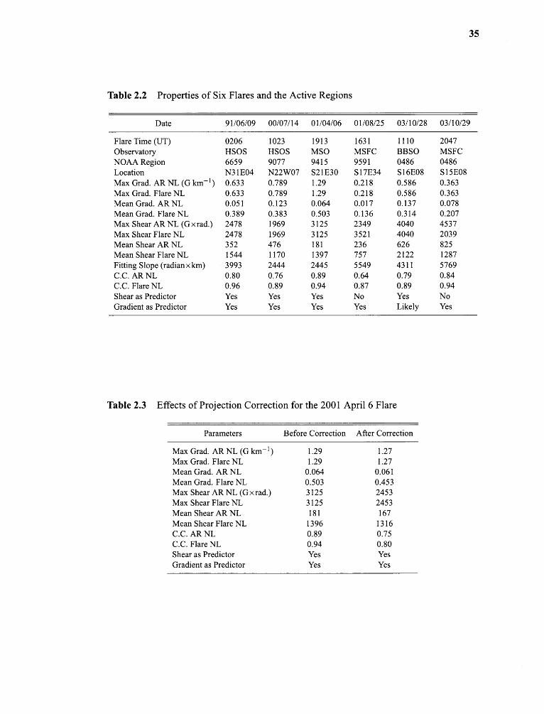
Table 2.2 Properties of Six Flares and the Active Regions
Date 91/06/09 00/07/14 01/04/06 01/08/25 03/10/28 03/10/29
Flare Time (UT) 0206 1023 1913 1631 1110 2047Observatory HSOS HSOS MSO MSFC BBSO MSFCNOAA Region 6659 9077 9415 9591 0486 0486Location N31E04 N22W07 S21E30 S17E34 S16E08 S15E08
Max Grad. AR NL (G km -1 ) 0.633 0.789 1.29 0.218 0.586 0.363Max Grad. Flare NL 0.633 0.789 1.29 0.218 0.586 0.363Mean Grad. AR NL 0.051 0.123 0.064 0.017 0.137 0.078Mean Grad. Flare NL 0.389 0.383 0.503 0.136 0.314 0.207Max Shear AR NL (G x rad.) 2478 1969 3125 2349 4040 4537Max Shear Flare NL 2478 1969 3125 3521 4040 2039Mean Shear AR NL 352 476 181 236 626 825Mean Shear Flare NL 1544 1170 1397 757 2122 1287Fitting Slope (radian x km) 3993 2444 2445 5549 4311 5769C.C. AR NL 0.80 0.76 0.89 0.64 0.79 0.84C.C. Flare NL 0.96 0.89 0.94 0.87 0.89 0.94Shear as Predictor Yes Yes Yes No Yes NoGradient as Predictor Yes Yes Yes Yes Likely Yes
Table 2.3 Effects of Projection Correction for the 2001 April 6 Flare
Parameters Before Correction After Correction
Max Grad. AR NL (G km -1 ) 1.29 1.27Max Grad. Flare NL 1.29 1.27Mean Grad. AR NL 0.064 0.061Mean Grad. Flare NL 0.503 0.453Max Shear AR NL (G x rad.) 3125 2453Max Shear Flare NL 3125 2453Mean Shear AR NL 181 167Mean Shear Flare NL 1396 1316C.C. AR NL 0.89 0.75C.C. Flare NL 0.94 0.80Shear as Predictor Yes YesGradient as Predictor Yes Yes
35
36
Figure 2.4 Top left: magnetic gradient map of 1991 June 9; Top right: magnetic shearmap; Middle left: magnetic gradient in neutral lines with flare contours; Middle right:magnetic shear in neutral lines with flare contours; Bottom left: HP image to indicate theflare emissions; Bottom right: line-of-sight magnetogram.
37
Figure 2.5 Top left: magnetic gradient map of 2001 April 6; Top right: magnetic shearmap; Middle left: magnetic gradient in neutral lines with flare contours; Middle right:magnetic shear in neutral lines with flare contours; Bottom left: TRACE 1600A image toindicate the flare emissions; Bottom right: line-of-sight magnetogram.
38
Figure 2.6 Top left: magnetic gradient map of 2001 August 25; Top right: magnetic shearmap; Middle left: magnetic gradient in neutral lines with flare contours; Middle right:magnetic shear in neutral lines with flare contours; Bottom left: TRACE WL image toindicate the flare emissions; Bottom right: line-of-sight magnetogram.
39
Figure 2.7 Top left: magnetic gradient map of 2003 October 28; Top right: magneticshear map; Middle left: magnetic gradient in neutral lines with flare contours; Middle right:magnetic shear in neutral lines with flare contours; Bottom left: TRACE 1600A image toindicate the flare emissions; Bottom right: line-of-sight magnetogram.
40
Figure 2.8 Top left: magnetic gradient map of 2003 October 29; Top right: magneticshear map; Middle left: magnetic gradient in neutral lines with flare contours; Middle right:magnetic shear in neutral lines with flare contours; Bottom left: TRACE 1600A image toindicate the flare emissions; Bottom right: line-of-sight magnetogram.

41
one (2001 August 25 event), and possibly two (2003 October 29 event), of the six events
would be misidentified. Please note that the weakness of using shear as a flare predictor
might be caused by the limitation of ground based vector magnetograms and the difficulty
in data analysis, such as the 180-degree ambiguity resolution and cross-talk among the
Stokes components. Clearer conclusions will be obtained when high quality space data
from Solar-B and SDO are available and data analysis methods are mature.
Magnetic gradient maps have been posted in the Active Region Monitor page daily
(Gallagher et al. 2002), they are being used as one of the parameters for solar flare predic-
tion. The results presented in this study have provided evidence that magnetic gradient is
important in real time activity monitoring and forecasting.
CHAPTER 3
THE RELATIONSHIP BETWEEN SOLAR FLARE INDEX AND MAGNETIC
FEATURES
3.1 Introduction
It is generally believed that nonpotential magnetic flux systems carry significant electric
currents and the relaxation of such magnetic configurations provides the energy for solar
energetic events such as flares, CMEs, etc. Although details of energy buildup and release
processes are not yet fully understood, from the observational point of view the frequency
and intensity of the activity observed in the solar corona correlate well with the size and
complexity of the host active region (e.g., Sawyer et al. 1986; McIntosh 1990; Falconer
2001; Falconer et al. 2003).
In an effort to advance our understanding of solar activity and identify a viable
proxy for its forecasting, numerous photospheric magnetic properties that describe the non-
potentiality of active regions have been explored. For example, based on 18 years of obser-
vations, Zirin and Liggett (1987) found that 6 sunspots are responsible for almost all great
flares. Temporal and spatial correspondence between the magnetic topological properties
of active regions and solar flares have been reported, supporting the idea that the presence
of strong electric current systems contributes to flare activity (Moreton and Severny 1968;
Abramenko et al. 1991; Leka et al. 1993; Wang et al. 1994b, 1996; Tian et al. 2002; Wang
et al. 2006). Falconer (2001); Falconer et al. (2003) measured the length of the strong-
sheared and the strong-gradient magnetic neutral lines, and found that they are strongly
correlated with each other and both might be prospective predictors of the CME productiv-
42

43
ity of active regions. Based on a systematic study of the temporal variations of photospheric
magnetic parameters related to solar flares, Leka and Barnes (2003a,b) demonstrated that
individually parameters have little ability to differentiate between flare-producing and flare-
quite regions, but with some combinations, two populations may be distinguished.
The magnetic shear and the vertical current in the photosphere are perhaps the most
commonly used measures of the magnetic nonpotentiality. However, these measurements
require vector magnetogram data, which are, compared to the line-of-sight magnetogram
data, less available and hindered by the 180° azimuthal ambiguity inherent to the trans-
verse component of magnetic fields. All published methods for this issue have certain
disadvantages. It is therefore desirable to find a measure that can be obtained directly from
line-of-sight magnetograms and that may reflect the nonpotentiality of active regions. This
is the central interest of this work, where we investigate and quantify the magnitude scal-
ing correlation between flare activity and photospheric magnetic parameters, which can be
derived from line-of-sight magnetograms.
This chapter is organized as follows: we introduce the magnetic measures and flare
index in Section 3.2. The data sets and the analysis method are described in Section 3.3.
Our results are presented and briefly discussed in Section 3.4 and Section 3.5, respectively.
3.2 Magnetic Parameters and Flare Index
Three magnetic parameters derivable from the line-of-sight magnetograms are adopted in
the present study. All of them contribute to the overall characterization of magnetic state
of active regions.
The first one is the mean spatial gradient of the magnetic fields on the neutral lines,
44
(▼Bz)NL• The spatial gradient quantifies the compactness of an active region and was
calculated as
where B, is the line-of-sight components of the magnetic field measured in the
plane (x,y). The spatial proximity of flare emission to neutral lines has been extensively
reported. In particular, the magnetic gradient on the neutral lines is found to be a good
proxy to predict where a major flare might occur (Wang et al. 2006).
The second parameter is the length of the magnetic neutral line with strong mag-
netic gradient in the context of certain threshold, Lgnl. To our knowledge, it was first elab-
orated by Falconer et al. (2003) as a measure of the nonpotentiality of active regions. Its
potential for CME forecasting has been explored (Falconer et al. 2003) and verified (Song
et al. 2006).
The third measure is the total energy dissipation of B, in a unit layer per a unit
time, ∫ ε(B,)dA, where the summation is done over the entire active region area A. This
parameter quantifies the energy dissipated at very small scales (2-3 Mm) due to the mag-
netic viscosity. The parameter can be calculated according to the following expression
(Abramenko et al. 2003):
that was derived from a more general formula (e.g., Monin and Yaglom 1975).
Assuming magnetic viscosity, vm , is spatially uniform and equal to unity (Abramenko et al.

45
2003), we calculated the magnetic energy dissipation rate ofBz component, ε(Bz ), over the
entire active region area.
The reason we adopt this measure is that the photospheric plasma is in a state of
highly developed turbulence and the Bz component of magnetic fields is known to be em-
bedded and diffusing in turbulent flows in the same way as a scalar field does (Parker 1979;
Petrovay and Szakaly 1993). As the large-scale magnetic flux tubes emerging from be-
neath the photosphere split into smaller ones, the magnetic energy of the tubes accordingly
cascades down to smaller scales. The power-law nature of magnetic power spectra in ac-
tive regions (Abramenko 2005) indicates that the energy of magnetic flux tubes is indeed
cascading from the scale of 10-20 Mm down to 2-3 Mm. Then the energy dissipates due
to magnetic viscosity. Thus, it is presumable that the more intensive random turbulent
motions lead to the higher energy dissipation rates of B.
In brief, (▼Bz)NL and Lgnl are quantitative measures of an active region's com-
plexity and nonpotentiality, while f ε(Bz )dA in some way conveys the information on the
amount of magnetic energy that dissipates (in lm layer per second) due to turbulent mo-
tions of magnetic flux tubes in the photosphere (Abramenko et al. 2003). The measurement
methods and errors will be discussed in Section 3.3.
On the other hand, overall flare productivity of a given active region can be quan-
tified by the soft X-ray (SXR) flare index (hereinafter abbreviated as FIsxR), as it was
proposed in Abramenko (2005). Note that a similar index quantifying the activity of the
entire Sun was first introduced by Antalova (1996) and was later applied by other authors
(e.g., Landi et al. 1998; Joshi and Joshi 2004). FIsxR (Abramenko 2005) is defined by
weighting the SXR flares of X-, M-, C- and B-class as 100, 10, 1 and 0.1, respectively (in
46
units of 10 -6 Wm -2):
where T is the length of time (measured in days) during which an active region is
visible on the solar disk, Ix, IM, /c and hi are GOES peak intensities of X-, M-, C- and
B-class flares produced by a given active region for the duration T. It is worthy mentioning
that, with the appropriate choice of time windows, we may evaluate the flare production for
the chosen time interval.
3.3 Data Sets and Analysis
Solar Geophysical Data (SGD) flare reports are a reliable source of the number and the
magnitude of SXR flares produced by an active region during its disk passage. In the
present study, 89 active regions showing a variety of FIsxR ranging from 0 to 500 were
analyzed. We used Michelson Doppler Imager (MDI) full disk magnetograms on board the
Solar and Heliospheric Observatory (SOHO) to measure the longitudinal component of the
magnetic fields, primarily because these data are routinely obtained, extensively archived
and free of the atmospheric seeing. To reduce the measurement errors due to projection
effect of magnetic fields, for each active region, we selected one MDI magnetogram ac-
cording to our criteria that the active region was viewed as close to disk center as possible.
That is, the analyzed magnetogram should be located between —10° to +10° in longitude
and —30° to +30° in latitude. We then manually cropped the full disk magnetogram such
that a small area containing the whole active region was left. Since the size of active regions
plays a role in flare production, the area size was not necessarily fixed.
47
The next step is to derive following three images for each active region: a magnetic
gradient map, a magnetic energy dissipation map and a mask map representing the location
of the magnetic neutral line. Then the gradient map was multiplied by the mask map in
order to generate an image of gradient distribution along the neutral line. Thus, L gnl is
the length of segments with strong gradient determined above certain threshold. Following
Falconer et al. (2003) and Song et al. (2006), we imposed a gradient threshold of 50 G
Mm-1 to determine the value of Lgnl. From a magnetic energy dissipation map, £(13z), we
calculated the total magnetic energy dissipation in a layer of 1 m, f ε(Bz )dA, by summing
over the entire field of view only for those regions above the 3o - level of ε(Bz ).
An example is illustrated in Figure 3.1 for active region NOAA 9077 on 2000 July
14. Left panel shows the MDI line-of-sight magnetogram of this flare prolific active region.
The daily FIsxR is as high as 90 (10 -6 W m -2 ), equivalent to a specific flare productivity
of one M9.0 flare per day. Middle and right panels show the gradient distribution along
the magnetic neutral line and structures of magnetic energy dissipation, respectively. The
values at each pixel are indicated by the corresponding color bars. Lgni is the total length of
the strong gradient segments (>50 G Mm -1 ) of the neutral line. Mean value of magnetic
gradient at the neutral line (▼Bz )NL and the total magnetic energy dissipation, ∫ ε (Bz )dA,
are also readily obtained.
Measurement errors mainly arise from the projection effect of the magnetic fields.
According to Gary and Hagyard (1990), the spherical geometry becomes apparent at 23°
heliocentric angle, and must be taken into consideration for those off-center regions with
heliocentric angles larger than 50°. Our sample of active regions were chosen primarily
because they were located near the center of solar disk, i.e., maximum longitude and lati-
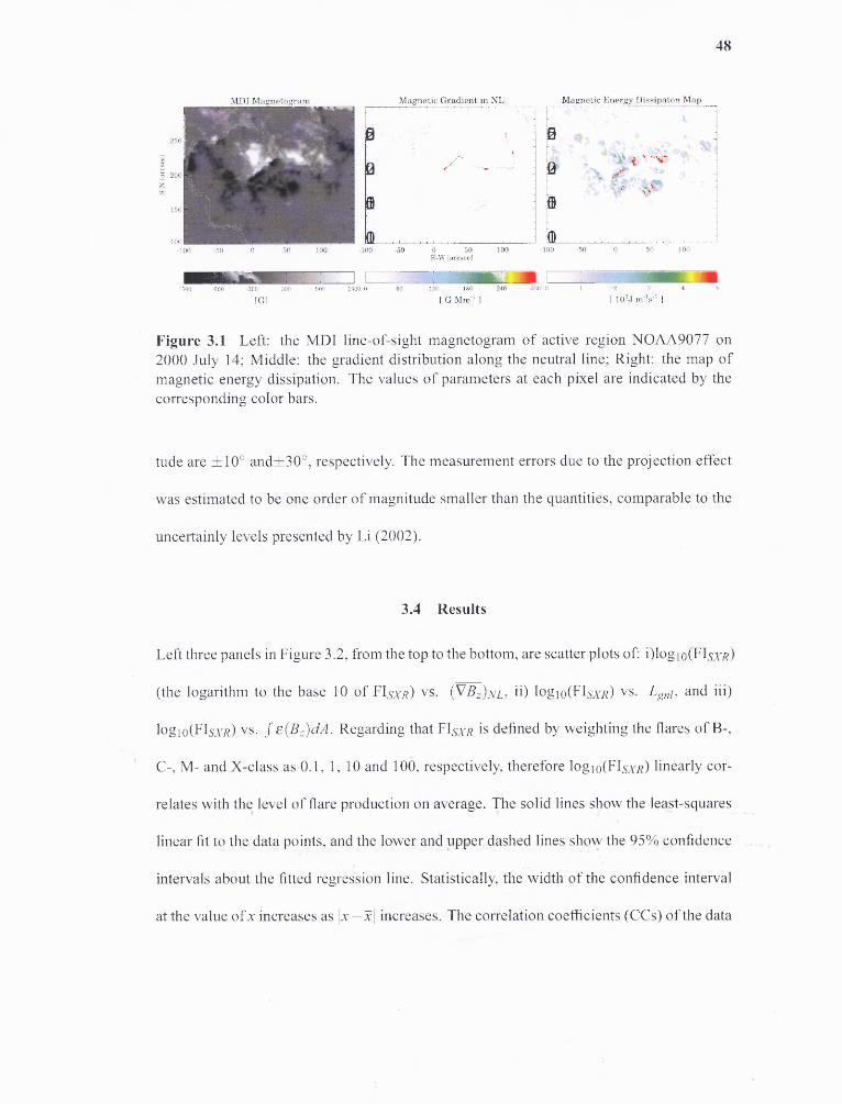
48
Figure 3.1 Left: the MDI line-of-sight magnetogram of active region NOAA9077 on2000 July 14; Middle: the gradient distribution along the neutral line; Right: the map ofmagnetic energy dissipation. The values of parameters at each pixel are indicated by thecorresponding color bars.
tude are ±10° and±30°, respectively. The measurement errors due to the projection effect
was estimated to be one order of magnitude smaller than the quantities, comparable to the
uncertainly levels presented by Li (2002).
3.4 Results
Left three panels in Figure 3.2, from the top to the bottom, are scatter plots of: i)log1o(FIsxR)
(the logarithm to the base 10 of FIsxR) vs. (▼Bz)NL, ii) log10(FIsXR) vs. Lgnl, and iii)
log10(FIsxR) vs. ∫ ε (B z )dA . Regarding that FIsxR is defined by weighting the flares of B-,
C-, M- and X-class as 0.1, 1, 10 and 100, respectively, therefore log10(FIsxR) linearly cor-
relates with the level of flare production on average. The solid lines show the least-squares
linear fit to the data points, and the lower and upper dashed lines show the 95% confidence
intervals about the fitted regression line. Statistically, the width of the confidence interval
at the value of x increases as Lx increases. The correlation coefficients (CCs) of the data
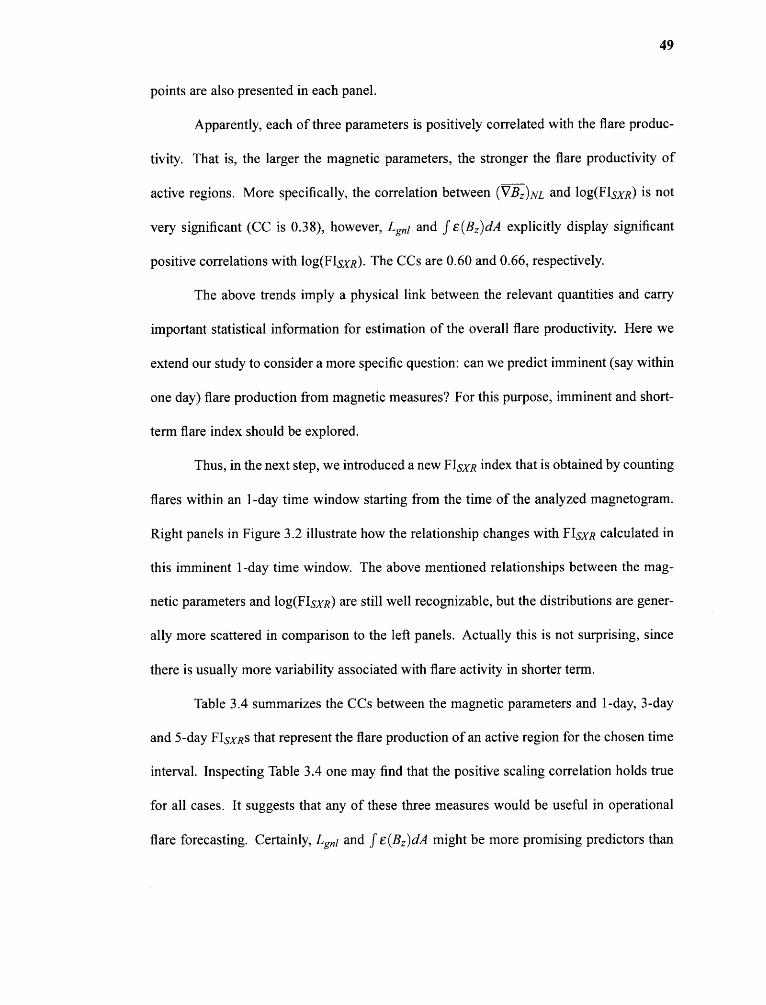
49
points are also presented in each panel.
Apparently, each of three parameters is positively correlated with the flare produc-
tivity. That is, the larger the magnetic parameters, the stronger the flare productivity of
active regions. More specifically, the correlation between (▼ BZ)NL and log(FIsxR) is not
very significant (CC is 0.38), however, Lgnl and ∫ ε(Bz )dA explicitly display significant
positive correlations with log(FIsxR). The CCs are 0.60 and 0.66, respectively.
The above trends imply a physical link between the relevant quantities and carry
important statistical information for estimation of the overall flare productivity. Here we
extend our study to consider a more specific question: can we predict imminent (say within
one day) flare production from magnetic measures? For this purpose, imminent and short-
term flare index should be explored.
Thus, in the next step, we introduced a new FIsxR index that is obtained by counting
flares within an 1-day time window starting from the time of the analyzed magnetogram.
Right panels in Figure 3.2 illustrate how the relationship changes with FIsxR calculated in
this imminent 1-day time window. The above mentioned relationships between the mag-
netic parameters and log(FIsxR) are still well recognizable, but the distributions are gener-
ally more scattered in comparison to the left panels. Actually this is not surprising, since
there is usually more variability associated with flare activity in shorter term.
Table 3.4 summarizes the CCs between the magnetic parameters and 1-day, 3-day
and 5-day FIsxRs that represent the flare production of an active region for the chosen time
interval. Inspecting Table 3.4 one may find that the positive scaling correlation holds true
for all cases. It suggests that any of these three measures would be useful in operational
flare forecasting. Certainly, Lgni and ∫ ε(Bz )dA might be more promising predictors than
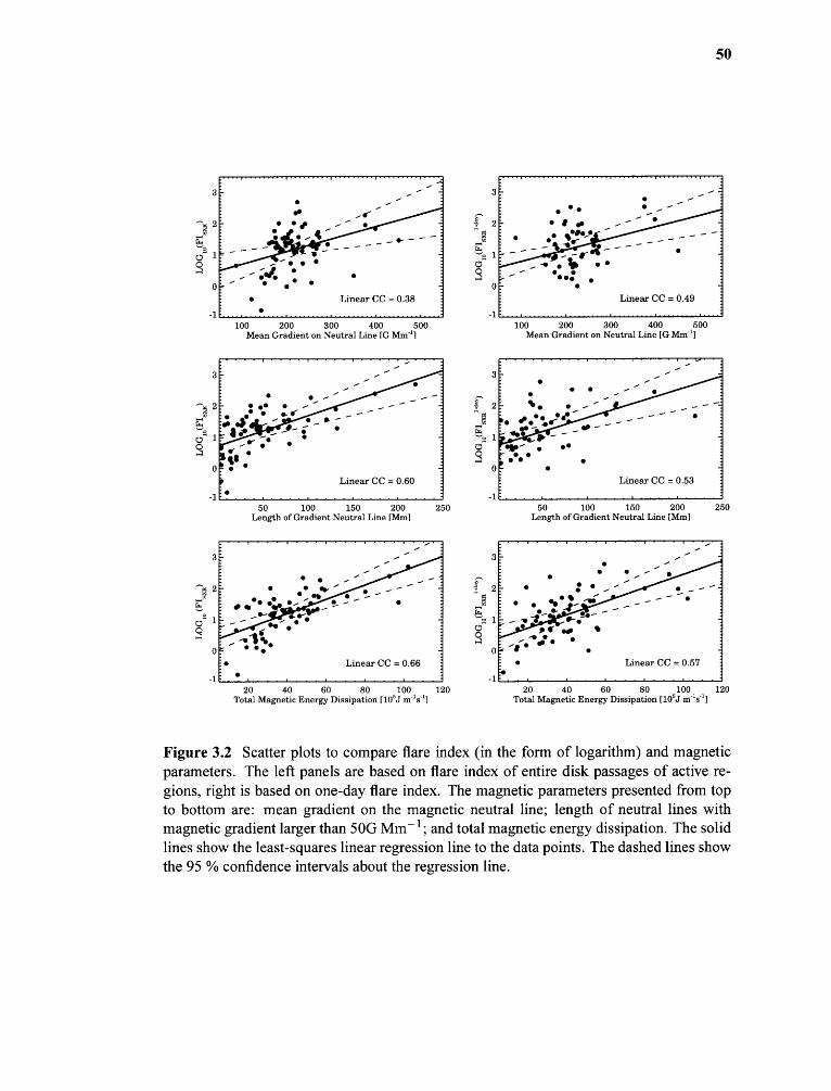
50
Figure 3.2 Scatter plots to compare flare index (in the form of logarithm) and magneticparameters. The left panels are based on flare index of entire disk passages of active re-gions, right is based on one-day flare index. The magnetic parameters presented from topto bottom are: mean gradient on the magnetic neutral line; length of neutral lines withmagnetic gradient larger than 50G Mm -1 ; and total magnetic energy dissipation. The solidlines show the least-squares linear regression line to the data points. The dashed lines showthe 95 % confidence intervals about the regression line.
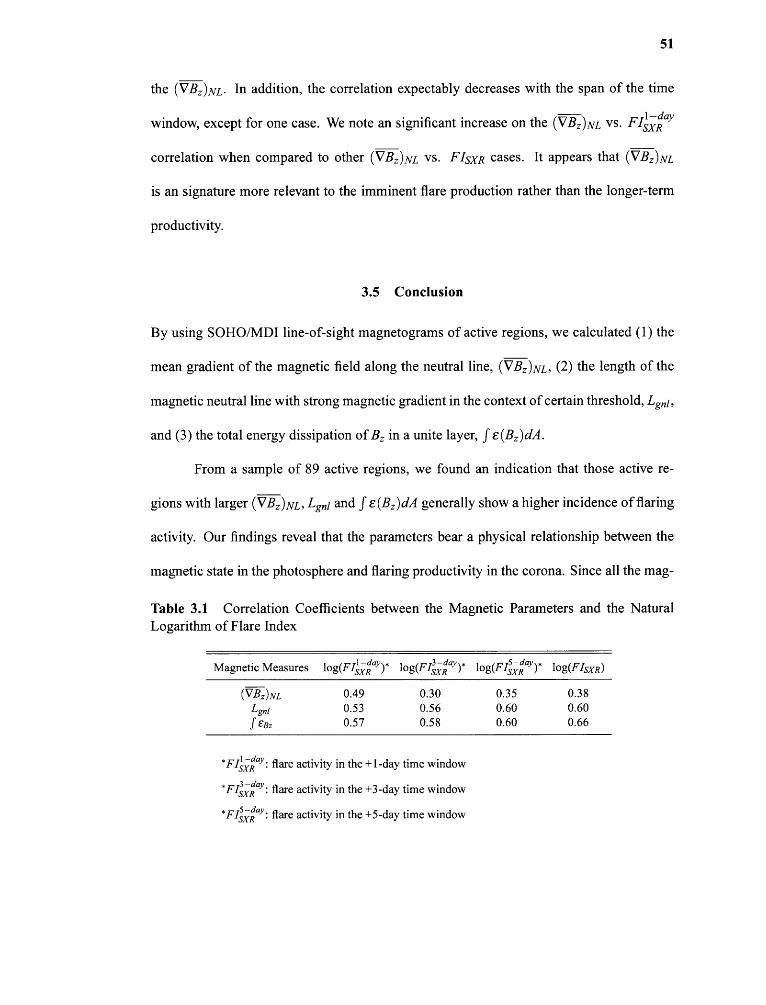
51
In addition, the correlation expectably decreases with the span of the time
window, except for one case. We note an significant increase on the
correlation when compared to other (▼Bz )nl vs. FIsxR cases. It appears that (▼BZ)NL
is an signature more relevant to the imminent flare production rather than the longer-term
productivity.
3.5 Conclusion
By using SOHO/MDI line-of-sight magnetograms of active regions, we calculated (1) the
mean gradient of the magnetic field along the neutral line, (▼Bz)NL, (2) the length of the
magnetic neutral line with strong magnetic gradient in the context of certain threshold, Lgnl,
and (3) the total energy dissipation of B Z in a unite layer, ∫ ε(Bz)dA .
From a sample of 89 active regions, we found an indication that those active re-
gions with larger (▼Bz )NL, Lgnl and ∫ ε(Bz )dA generally show a higher incidence of flaring
activity. Our findings reveal that the parameters bear a physical relationship between the
magnetic state in the photosphere and flaring productivity in the corona. Since all the mag-
Table 3.1 Correlation Coefficients between the Magnetic Parameters and the NaturalLogarithm of Flare Index
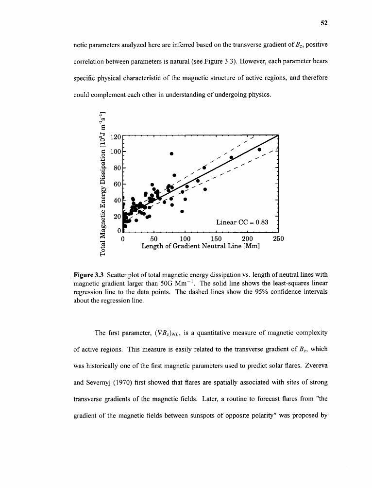
52
netic parameters analyzed here are inferred based on the transverse gradient of 13,, positive
correlation between parameters is natural (see Figure 3.3). However, each parameter bears
specific physical characteristic of the magnetic structure of active regions, and therefore
could complement each other in understanding of undergoing physics.
Figure 3.3 Scatter plot of total magnetic energy dissipation vs. length of neutral lines withmagnetic gradient larger than 50G Mm — I . The solid line shows the least-squares linearregression line to the data points. The dashed lines show the 95% confidence intervalsabout the regression line.
The first parameter, (▼ BZ)NL, is a quantitative measure of magnetic complexity
of active regions. This measure is easily related to the transverse gradient of Bz , which
was historically one of the first magnetic parameters used to predict solar flares. Zvereva
and Severnyj (1970) first showed that flares are spatially associated with sites of strong
transverse gradients of the magnetic fields. Later, a routine to forecast flares from "the
gradient of the magnetic fields between sunspots of opposite polarity" was proposed by

53
Severny et al. (1979). Recently, from a sample of 5 active regions that produced great
flares, Wang et al. (2006) verified that great flares occurred specifically in the neutral lines
with maximum gradient.
A generally accepted notion is that a nonpotential magnetic field configuration pro-
vides the energy for solar flares. As we mentioned in Introduction, the estimation of the
degree of nonpotentiality usually requires vector magnetograms. Falconer et al. (2003)
reported a strong correlation between our second parameter, Lgnl, and the the length of
the magnetic neutral lines with strong magnetic shear, L„/, which is derived from vector
magnetograms and can be qualified as a measure of nonpotentiality. This result, together
with the relationship found in the present study, leads to the conclusion that Lgni is also a
viable proxy for the active region's nonpotentiality, and the high level of flare productivity
is plausibly caused by strong deviations from the potential state and always accompanied
by the presence of strong electric currents in the photosphere.
We note that the relationship is most evident for the third parameter, the energy
dissipation. The value of f e(Bz )dA provides a clue as to the amount of magnetic energy
that dissipates due to the turbulent random motions of flux tubes in the photosphere. The
dissipation process is accompanied by the fragmentation of magnetic structure. In this
regard, the larger value of energy dissipation rate usually implies the higher fragmentation
rate and accordingly the more intensive turbulent motions in the photosphere. Recently,
Abramenko (2005) reported the relationship between the strong flaring productivity and
the high fragmentation rate of magnetic elements. Consistent with Abramenko (2005),
the observed correlation between ∫ ε(Bz)dA and FIsxR of active regions might support
the hypothesis that photospheric random motions of magnetic flux tubes contribute to the

54
energy build-up needed for flaring activity in the corona (e.g., Parker 1987; Longcope et al.
1996).
Finally, our study is of practical significance in flare forecasting. For example,
the empirical scaling correlation between magnetic parameters and 1-day flare production,
shown in the right panels of Figure 3.2, enables us a quick estimate of imminent flare
occurrence. We emphasize that all three parameters can be easily determined from near
real-time regime of MDI line-of-sight magnetograms and, therefore, they can be easily
applied in automatic flare forecasting.
CHAPTER 4
STATISTICAL ASSESSMENT OF MAGNETIC FEATURES IN IMMINENT
SOLAR FLARES PREDICTION
4.1 Introduction
One of the primary objectives in space weather research is to predict the occurrence of
solar flares and Coronal Mass Ejections (CMEs), which are believed to be the major causes
of geomagnetic disturbances (e.g., Brueckner et al., 1998; Cane et al., 2000; Gopalswamy
et al., 2000; Webb et al., 2000; Wang, et al., 2002; Zhang, et al., 2003). It has long
been known that solar flares tend to occur along magnetic polarity inversion lines where
the magnetic field lines are often highly sheared, with the transverse field directed nearly
parallel to the polarity inversion line (Svestka 1976; Hagyard et al. 1984; Sawyer et al.
1986). Canfield et al. (1999) showed that CMEs also tend to arise in connection with active
regions (ARs) exhibiting strong sheared and/or twisted coronal loops called sigmoid. The
twisting, tangling and shearing of magnetic loops lead to magnetic topological complexities
and build up a stressed flux system (and excess energy). Subsequent destabilizing events
such as local emergence of new magnetic flux from below the photosphere or changes in
magnetic connectivity due to magnetic field reorganization elsewhere on the Sun may result
in the release of energy (Hess 1964; Svestka 1976; Priest and Forbes 2000).
To date, various observational studies have explored the connection between pho-
tospheric magnetic fields and solar flares, supporting the hypothesis that solar flares are
driven by the nonpotentiality of magnetic fields (Moreton and Severny 1968; Abramenko
et al., 1991; Leka et al., 1993; Wang et al., 1994; Wang et al., 1996; Tian et al., 2002; Abra-
55
56
menko, 2005). Through five solar flares, Wang (2006a) found there are obvious changes of
the magnetic gradient occurred immediately and rapidly following the onset of each flare.
Falconer et al. (2001, 2003) measured the lengths of strong-sheared and strong-gradient
magnetic neutral line segments and found that they are strongly correlated with CME pro-
ductivity of an active region and both might be prospective predictors. In a study of 6 large
(X5 or larger) flares, Wang et al. (2006b) reported a positive linear relationship between
the magnetic shear and the magnetic gradient and that the latter seems to be a better tool
to predict the occurrence of flares and CMEs in an active region. According to Song et
al. (2006), the length of strong gradient neutral line, L01, was proved to be a viable tool to
locate source regions of either CMEs or flares. The overall accuracy of this method is about
75 % (55 out of 73 events). Jing et al. (2006) analyzed three magnetic parameters: i) mean
spatial magnetic field gradient at strong-gradient magnetic neutral line, (▼ BZ)NL; ii) length
of a strong-gradient magnetic neutral line, Lgnl; and iii) total magnetic energy dissipated in
a unit layer in 1 second over the active region's area, Ediss = f ε (B z ) d A and found that these
parameters have a positive correlation with the overall flare productivity of ARs. ARs with
larger (▼Bz )NL, Lgnl and Ediss generally show a higher incidence of flaring activity.
The purpose of this study is to find out whether statistical methods that are con-
ceptually simple, algorithmically fast are able to provide a feasible way to evaluate the
probability of an active region in producing solar flares. The ordinal logistic regression
model satisfies our criteria. The model describes the relationship between an ordered re-
sponse variable and a set of predictive variables. In our case, the ordered response variable
represents four different energy levels of solar flares. We assign numerical values 3, 2, 1
and 0 to represent X-, M-, C- and B-class flares, respectively. The predictive variables so
57
far include Ll, Ediss, that were used in Jing et al. (2006) study and total unsigned magnetic
flux, Tflux • Mathematically, what the ordinal regression model describes is not the value of
the response variable itself, but the probability, Prob, that it assumes the certain response
value (0, 1, 2 or 3). Thus, in this study, Prob represents the probability of certain class of
flare to occur. Since Prob ranges from 0 to 1, traditional linear regression is inappropriate
to predict its value directly.
We will study if the ordinal logistic regression model is able to predict the occur-
rence of solar flares in the next 1-day period. The reminder of this chapter proceeds as
follows. In Section 5.2 the data sets used to perform the statistical analysis are described.
Three magnetic measures are calculated based on the full disk Michelson Doppler Imager
(MDI) magnetograms. In Section 5.3, the ordinal logistic model is specified and estab-
lished. The results obtained from the statistical regression model are presented in Section
5.4, and Section 5.5 concludes this chapter with a discussion of key results.
4.2 Methods
4.2.1 Data Collection
Solar activity reports are available online from the US National Oceanic and Atmospheric
Administration (NOAA) space environment center (SEC) 1 . The reports include detailed in-
formation about solar flares, such as the coordinated universal time (UTC) of the beginning,
maximum and end of a flare, the X-ray flux at the flare peak and the location of the flare, if
available. Our study focuses on those flares occurred between 1996 to 2005. The criteria
for flares selection are: (1) the location of the flare is accurately indicated in the reports
I http://www.sec.noaa.gov/ftpmenu/indices.html

58
and as close to disk center as possible (±40° in longitude and ±30° in latitude), so the
project effects of magnetic fields can be avoided. In order to have enough events number of
X-class flares for our statistical study, the longitude was extended to ±40°, (2) Michelson
Doppler Imager (MDI) full disk magnetograms on board Solar and Heliospheric Obser-
vatory (SOHO) was available. These magnetograms were used to analyze photospheric
magnetic parameters. The reason that we use only MDI magnetograms is primarily be-
cause these data are routinely obtained, extensively achieved and free of the atmospheric
seeing. Total 230 solar flare events were chosen to be analyzed.
4.2.2 Definition of the Predictive and Response Variables
Detailed descriptions of how the photospheric magnetic parameters are calculated from the
MDI magnetograms was presented in detail in Jing et al. (2006). Thus, we will only briefly
list them here:
1. Total unsigned magnetic flux, Tflux , is a measure of the active region's size.
2. Length of the strong-gradient neutral line, Lgnl, describes the global non-potentiality
of an active region. The spatial gradient is calculated as
where B, is the line-of-sight components of the magnetic field measured in the plane
(x,y). The gradient threshold in this chapter was chosen to be 50 G Mm -1 (Falconer
et al. 2003; Song et al. 2006).
3. Total magnetic energy dissipation of Bz in a unit layer per unit time, Ediss = f ε(Bz)dA,
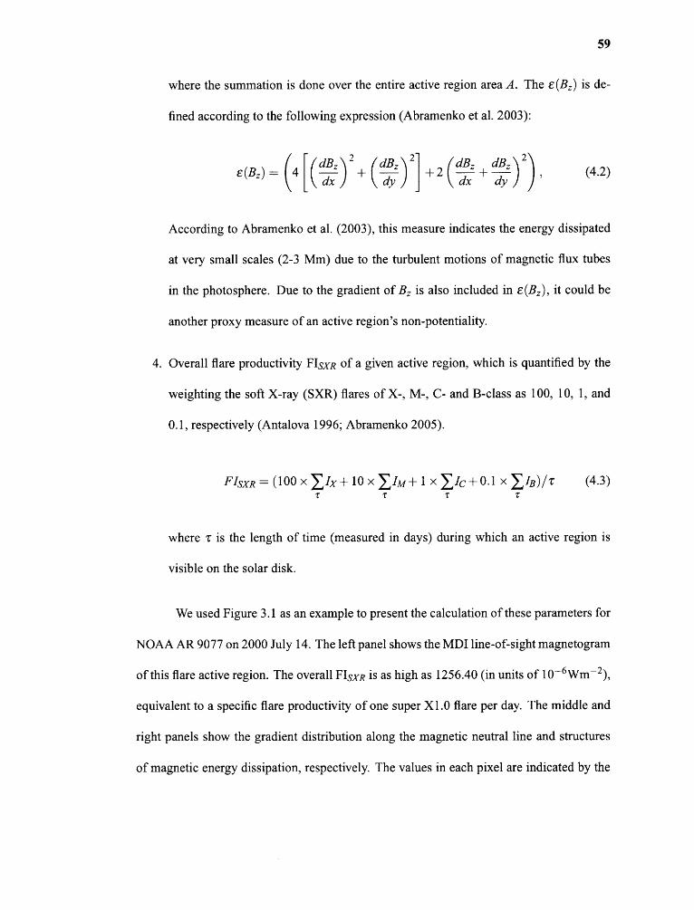
59
where the summation is done over the entire active region area A. The ε(Bz) is de-
fined according to the following expression (Abramenko et al. 2003):
According to Abramenko et al. (2003), this measure indicates the energy dissipated
at very small scales (2-3 Mm) due to the turbulent motions of magnetic flux tubes
in the photosphere. Due to the gradient of Bz is also included in ε(Bz), it could be
another proxy measure of an active region's non-potentiality.
4. Overall flare productivity FIsxR of a given active region, which is quantified by the
weighting the soft X-ray (SXR) flares of X-, M-, C- and B-class as 100, 10, 1, and
0.1, respectively (Antalova 1996; Abramenko 2005).
where t is the length of time (measured in days) during which an active region is
visible on the solar disk.
We used Figure 3.1 as an example to present the calculation of these parameters for
NOAA AR 9077 on 2000 July 14. The left panel shows the MDI line-of-sight magnetogram
of this flare active region. The overall FIsxR is as high as 1256.40 (in units of 10 -6Wm-2 ),
equivalent to a specific flare productivity of one super X1.0 flare per day. The middle and
right panels show the gradient distribution along the magnetic neutral line and structures
of magnetic energy dissipation, respectively. The values in each pixel are indicated by the
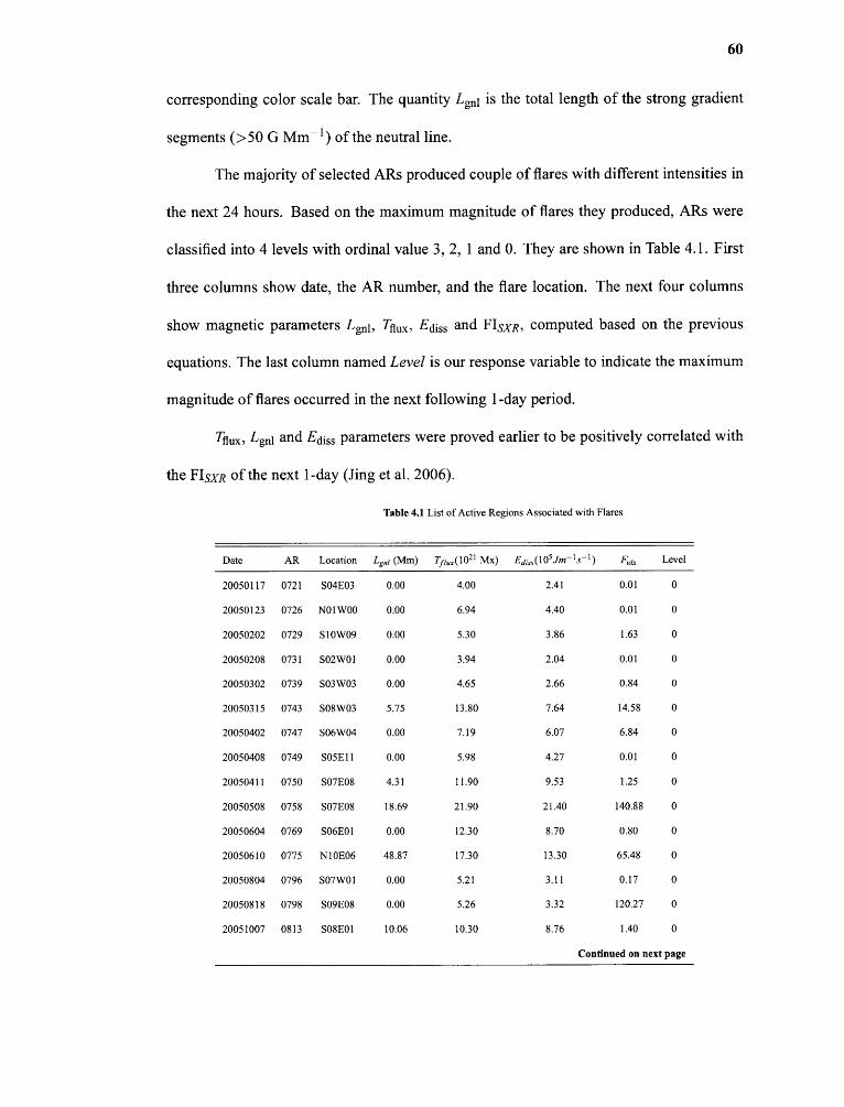
60
corresponding color scale bar. The quantity Lo is the total length of the strong gradient
segments (>50 G Mm-1 ) of the neutral line.
The majority of selected ARs produced couple of flares with different intensities in
the next 24 hours. Based on the maximum magnitude of flares they produced, ARs were
classified into 4 levels with ordinal value 3, 2, 1 and 0. They are shown in Table 4.1. First
three columns show date, the AR number, and the flare location. The next four columns
show magnetic parameters Lgnl, Tflux, Ediss and FIsxR, computed based on the previous
equations. The last column named Level is our response variable to indicate the maximum
magnitude of flares occurred in the next following 1-day period.
Tflux , Lgnl and Ediss parameters were proved earlier to be positively correlated with
the FIsxR of the next 1-day (Ding et al. 2006).
Table 4.1 List of Active Regions Associated with Flares
Date AR Location Lgnl (Mm) Tflux(1021 Mx)) Ediss(105 JM -1 s- I ) Fox Level
20050117 0721 SO4E03 0.00 4.00 2.41 0.01 0
20050123 0726 N01 W00 0.00 6.94 4.40 0.01 0
20050202 0729 S1OW09 0.00 5.30 3.86 1.63 0
20050208 0731 S02W01 0.00 3.94 2.04 0.01 0
20050302 0739 S03W03 0.00 4.65 2.66 0.84 0
20050315 0743 508W03 5.75 13.80 7.64 14.58 0
20050402 0747 S06W04 0.00 7.19 6.07 6.84 0
20050408 0749 SO5E11 0.00 5.98 4.27 0.01 0
20050411 0750 S07E08 4.31 11.90 9.53 1.25 0
20050508 0758 S07E08 18.69 21.90 21.40 140.88 0
20050604 0769 SO6E01 0.00 12.30 8.70 0.80 0
20050610 0775 N 10E06 48.87 17.30 13.30 65.48 0
20050804 0796 SO7W01 0.00 5.21 3.11 0.17 0
20050818 0798 509E08 0.00 5.26 3.32 120.27 0
20051007 0813 SO8E01 10.06 10.30 8.76 1.40 0
Continued on next page
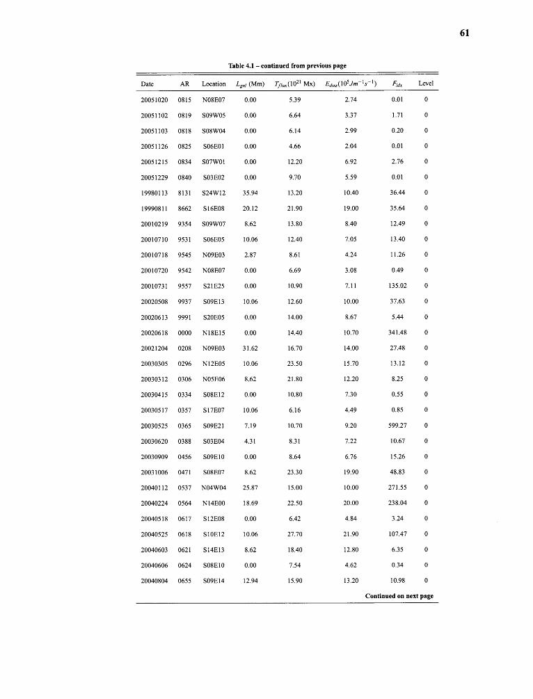
Table 4.1 - continued from previous page
Date AR Location 1,,,l (Mm) Tflux(1021 Mx)) Ediss(105Jm-1 S -1 ) Fax Level
20051020 0815 N08E07 0.00 5.39 2.74 0.01 0
20051102 0819 S09W05 0.00 6.64 3.37 1.71 0
20051103 0818 S08W04 0.00 6.14 2.99 0.20 0
20051126 0825 S06E01 0.00 4.66 2.04 0.01 0
20051215 0834 SO7W01 0.00 12.20 6.92 2.76 0
20051229 0840 S03E02 0.00 9.70 5.59 0.01 0
19980113 8131 S24W12 35.94 13.20 10.40 36.44 0
19990811 8662 S16E08 20.12 21.90 19.00 35.64 0
20010219 9354 S09W07 8.62 13.80 8.40 12.49 0
20010710 9531 S06E05 10.06 12.40 7.05 13.40 0
20010718 9545 N09E03 2.87 8.61 4.24 11.26 0
20010720 9542 N08E07 0.00 6.69 3.08 0.49 0
20010731 9557 S21E25 0.00 10.90 7.11 135.02 0
20020508 9937 S09E13 10.06 12.60 10.00 37.63 0
20020613 9991 S20E05 0.00 14.00 8.67 5.44 0
20020618 0000 N18E15 0.00 14.40 10.70 341.48 0
20021204 0208 N09E03 31.62 16.70 14.00 27.48 0
20030305 0296 N12E05 10.06 23.50 15.70 13.12 0
20030312 0306 N05E06 8.62 21.80 12.20 8.25 0
20030415 0334 S08E12 0.00 10.80 7.30 0.55 0
20030517 0357 S17E07 10.06 6.16 4.49 0.85 0
20030525 0365 S09E21 7.19 10.70 9.20 599.27 0
20030620 0388 S03E04 4.31 8.31 7.22 10.67 0
20030909 0456 SO9E10 0.00 8.64 6.76 15.26 0
20031006 0471 S08E07 8.62 23.30 19.90 48.83 0
20040112 0537 N04W04 25.87 15.00 10.00 271.55 0
20040224 0564 N14E00 18.69 22.50 20.00 238.04 0
20040518 0617 S12E08 0.00 6.42 4.84 3.24 0
20040525 0618 S1OE12 10.06 27.70 21.90 107.47 0
20040603 0621 S14E13 8.62 18.40 12.80 6.35 0
20040606 0624 SO8E10 0.00 7.54 4.62 0.34 0
20040804 0655 S09E14 12.94 15.90 13.20 10.98 0
Continued on next page
61
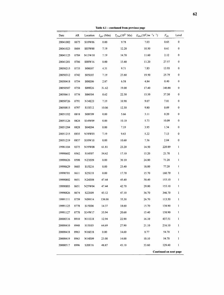
Table 4.1 - continued from previous page
Date AR Location Lgnl (Mm) Tflux (1021 Mx) Ediss(105 Jm- 1 s- 1 ) Fidx Level
20041002 0675 S10W06 0.00 9.78 7.03 0.65 0
20041023 0684 S03 W00 7.19 12.20 10.50 0.61 0
20041125 0704 N13W18 7.19 14.70 11.60 2.12 0
20041201 0706 S08W16 0.00 13.40 11.20 27.57 0
20050215 0735 S08E07 4.31 9.71 7.83 13.93 0
20050312 0742 S05E03 7.19 23.60 19.50 25.79 0
20050418 0754 S08E06 2.87 6.58 4.84 0.40 0
20050507 0758 S09E26 31.62 19.00 17.40 140.88 0
20050611 0776 S06E04 8.62 22.30 15.50 37.30 0
20050726 0791 N14E23 7.19 10.90 9.07 7.81 0
20050815 0797 S13E12 10.06 12.30 9.80 0.89 0
20051102 0818 S08E09 0.00 5.66 3.11 0.20 0
20051126 0824 S14W09 0.00 10.10 5.73 10.09 0
20051204 0828 SO4E04 0.00 7.19 3.95 1.34 0
20051215 0835 N19W03 7.19 9.63 5.22 7.13 0
20051219 0837 SlOW10 0.00 10.60 7.36 2.04 0
19981104 8375 N19W08 61.81 23.20 14.50 220.89 1
19990602 8562 S16E07 54.62 17.10 15.20 21.70 1
19990626 8598 N23E09 0.00 30.10 24.80 71.20 1
19990629 8603 S15E16 0.00 23.40 18.00 77.20 1
19990701 8611 S25E18 0.00 17.70 15.70 160.70 1
19990802 8651 N24E08 47.44 45.40 30.40 153.10 1
19990803 8651 N25W04 47.44 42.70 29.80 153.10 1
19990826 8674 S22E09 43.12 47.10 36.70 346.70 1
19991111 8759 N09E14 138.00 35.30 26.70 113.50 1
19991125 8778 S15E06 14.37 18.60 15.70 138.90 1
19991127 8778 S14W17 35.94 20.60 15.40 138.90 1
20000316 8910 N11E18 12.94 22.90 16.10 437.51 1
20000410 8948 S15E03 64.69 27.90 21.10 216.10 1
20000418 8963 N16E18 0.00 14.60 8.77 54.70 1
20000419 8963 N14E09 23.00 14.00 10.10 54.70 1
20000517 8996 S20E16 48.87 43.10 33.60 129.40 1
Continued on next page
62
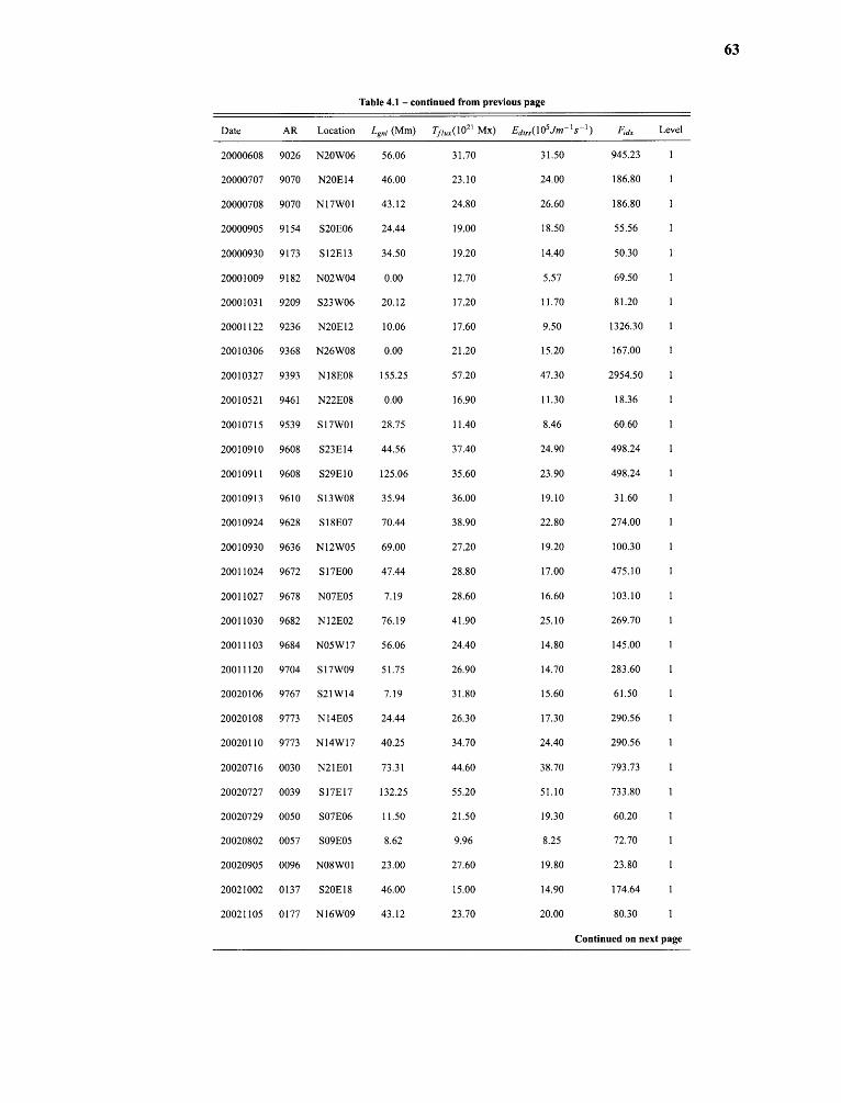
Table 4.1 - continued from previous page
Date AR Location Lgnl (Mm) Tflux(1021 Mx) Ediss(105 Jm- 1 s- 1) Fax Level
20000608 9026 N20W06 56.06 31.70 31.50 945.23 1
20000707 9070 N20E14 46.00 23.10 24.00 186.80 1
20000708 9070 N17W01 43.12 24.80 26.60 186.80 1
20000905 9154 S20E06 24.44 19.00 18.50 55.56 1
20000930 9173 S12E13 34.50 19.20 14.40 50.30 1
20001009 9182 NO2W04 0.00 12.70 5.57 69.50 1
20001031 9209 S23 W06 20.12 17.20 11.70 81.20 1
20001122 9236 N20E12 10.06 17.60 9.50 1326.30 1
20010306 9368 N26W08 0.00 21.20 15.20 167.00 1
20010327 9393 N18E08 155.25 57.20 47.30 2954.50 1
20010521 9461 N22E08 0.00 16.90 11.30 18.36 1
20010715 9539 S 1 7W01 28.75 11.40 8.46 60.60 1
20010910 9608 S23E14 44.56 37.40 24.90 498.24 1
20010911 9608 S29E10 125.06 35.60 23.90 498.24 1
20010913 9610 S 13W08 35.94 36.00 19.10 31.60 1
20010924 9628 S18E07 70.44 38.90 22.80 274.00 1
20010930 9636 N12W05 69.00 27.20 19.20 100.30 1
20011024 9672 S17E00 47.44 28.80 17.00 475.10 1
20011027 9678 N07E05 7.19 28.60 16.60 103.10 1
20011030 9682 N12E02 76.19 41.90 25.10 269.70 1
20011103 9684 N05W17 56.06 24.40 14.80 145.00 1
20011120 9704 S17W09 51.75 26.90 14.70 283.60 1
20020106 9767 S21W14 7.19 31.80 15.60 61.50 1
20020108 9773 N14E05 24.44 26.30 17.30 290.56 1
20020110 9773 N14W17 40.25 34.70 24.40 290.56 1
20020716 0030 N21E01 73.31 44.60 38.70 793.73 1
20020727 0039 S17E17 132.25 55.20 51.10 733.80 1
20020729 0050 S07E06 11.50 21.50 19.30 60.20 1
20020802 0057 S09E05 8.62 9.96 8.25 72.70 1
20020905 0096 NO8W01 23.00 27.60 19.80 23.80 1
20021002 0137 S20E18 46.00 15.00 14.90 174.64 1
20021105 0177 N16W09 43.12 23.70 20.00 80.30 1
Continued on next page
63

Table 4.1 - continued from previous page
Date AR Location Lgnl (Mm) T flux(1021 Mx) Ediss(105 Jm- 1 s- 1 ) Fidx Level
20021106 0180 S09W07 56.06 25.10 22.80 259.50 1
20030222 0290 N17W06 8.62 15.70 11.80 36.06 1
20030315 0314 S15W13 30.19 14.50 16.60 529.20 1
20030501 0349 S13E07 8.62 34.80 22.50 86.37 1
20030607 0375 N11E09 30.19 26.30 25.30 1358.62 1
20030608 0375 N11W03 43.12 31.80 29.70 1358.62 1
20030718 0410 S 12E09 0.00 2.27 0.70 91.71 1
20030815 0431 S 13W02 0.00 4.34 2.10 124.65 1
20031028 0488 N09W05 92.00 38.50 46.60 881.80 1
20040225 0564 N14W13 0.00 2.61 0.90 238.04 1
20040329 0582 N13E18 0.00 2.25 0.65 144.65 1
20040331 0582 N13W14 8.62 20.60 13.80 144.65 1
20040719 0649 SO9W00 0.00 4.10 2.12 1381.59 1
20040811 0656 S14E13 0.00 3.49 1.54 1260.24 1
20050604 0772 S18E09 7.19 10.90 11.10 98.41 1
20050702 0785 S17E04 0.00 3.87 1.86 15.56 1
20050914 0808 S11E02 92.00 44.70 45.60 4886.56 1
19980315 8179 S24W04 53.19 31.40 20.60 100.32 2
19980326 8185 S24E04 17.25 18.20 12.90 48.46 2
19980501 8210 S17E05 7.19 20.00 9.37 422.59 2
19990630 8603 S14W01 18.69 19.10 17.00 77.20 2
19990702 8611 S26E08 33.06 22.60 20.40 160.70 2
19990724 8636 N20W06 33.06 35.00 26.40 94.99 2
19990819 8672 N16W02 10.06 15.10 10.70 10.00 2
19990827 8674 S21W04 74.75 49.60 38.40 346.70 2
19991112 8759 N10E05 90.56 42.90 32.50 113.50 2
19991126 8778 S1 4W06 21.56 20.20 15.30 138.90 2
19991222 8806 N19E09 24.44 37.40 25.70 259.78 2
20000118 8831 S17E00 7.19 24.90 14.80 49.00 2
20000217 8872 S28E05 0.00 11.30 6.86 13.80 2
20000313 8906 S17E02 107.81 46.30 28.80 284.10 2
20000720 9087 S 1 2W02 34.50 36.70 30.20 443.60 2
Continued on next page
64
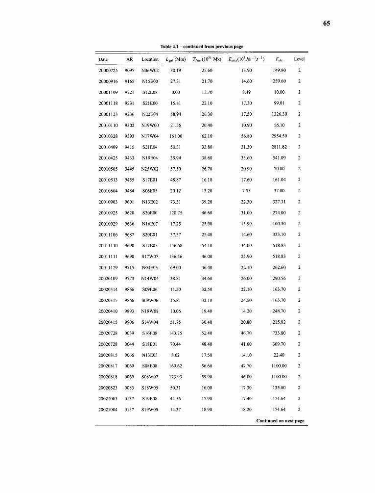
Table 4.1 - continued from previous page
Date AR Location Lgnl (Mm) TfIux(1021 Mx) Ediss(105Jm-1s-1 ) Fox Level
20000725 9097 N06W02 30.19 25.60 13.90 149.80 2
20000916 9165 N15E00 27.31 21.70 14.60 259.60 2
20001109 9221 S12E08 0.00 13.70 8.49 10.00 2
20001118 9231 S21E00 15.81 22.10 17.30 99.01 2
20001123 9236 N22E04 58.94 26.30 17.50 1326.30 2
20010110 9302 N19W00 21.56 20.40 10.90 56.10 2
20010328 9393 N17W04 161.00 62.10 56.80 2954.50 2
20010409 9415 S21E04 50.31 33.80 31.30 2811.82 2
20010425 9433 N19E04 35.94 38.60 35.60 541.09 2
20010505 9445 N25W02 57.50 26.70 20.90 70.80 2
20010513 9455 S1 7E01 48.87 16.10 17.60 161.04 2
20010604 9484 S06E05 20.12 13.20 7.55 37.00 2
20010903 9601 N13E02 73.31 39.20 22.30 327.31 2
20010925 9628 S20E00 120.75 46.60 31.00 274.00 2
20010929 9636 N16E07 17.25 25.90 15.90 100.30 2
20011106 9687 S20E01 37.37 25.40 14.60 333.10 2
20011110 9690 S17E05 156.68 54.10 34.00 518.83 2
20011111 9690 S 1 7W07 136.56 46.00 25.90 518.83 2
20011129 9715 N04E03 69.00 36.40 22.10 262.60 2
20020109 9773 N14W04 38.81 34.60 26.00 290.56 2
20020314 9866 S09E06 11.50 32.50 22.10 163.70 2
20020315 9866 S09W06 15.81 32.10 24.50 163.70 2
20020410 9893 N19W08 10.06 19.40 14.20 248.70 2
20020415 9906 S 1 4W04 51.75 30.40 20.80 215.82 2
20020728 0039 S16E08 143.75 52.40 46.70 733.80 2
20020728 0044 S18E01 70.44 48.40 41.60 309.70 2
20020815 0066 N13E03 8.62 17.50 14.10 22.40 2
20020817 0069 S08E08 169.62 56.60 47.70 1100.00 2
20020818 0069 S08W07 173.93 59.90 46.00 1100.00 2
20020823 0083 S 1 8W05 50.31 16.00 17.30 135.80 2
20021003 0137 S19E08 44.56 17.90 17.40 174.64 2
20021004 0137 S 1 9W05 14.37 18.90 18.20 174.64 2
Continued on next page
65
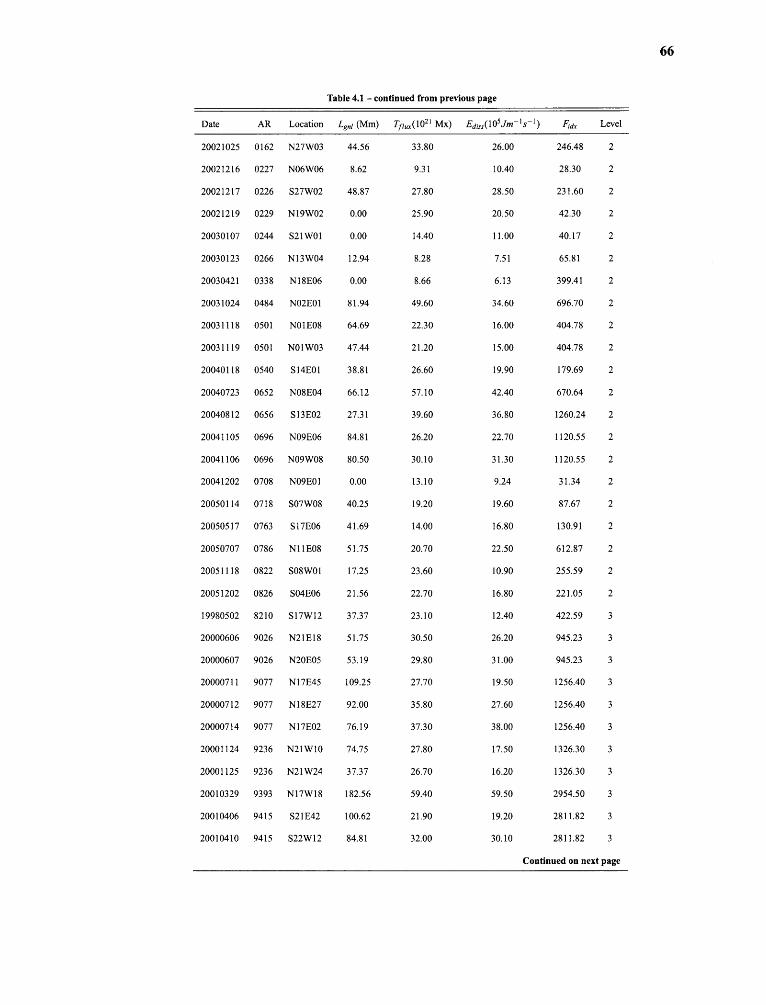
Table 4.1 - continued from previous page
Date AR Location Lgnl (Mm) Tflux(1021 Mx) Ediss(105Jm-1s-1 ) Fax Level
20021025 0162 N27W03 44.56 33.80 26.00 246.48 2
20021216 0227 N06W06 8.62 9.31 10.40 28.30 2
20021217 0226 S27W02 48.87 27.80 28.50 231.60 2
20021219 0229 N19W02 0.00 25.90 20.50 42.30 2
20030107 0244 S21W01 0.00 14.40 11.00 40.17 2
20030123 0266 N13W04 12.94 8.28 7.51 65.81 2
20030421 0338 N18E06 0.00 8.66 6.13 399.41 2
20031024 0484 NO2E01 81.94 49.60 34.60 696.70 2
20031118 0501 NO1E08 64.69 22.30 16.00 404.78 2
20031119 0501 N01 W03 47.44 21.20 15.00 404.78 2
20040118 0540 S14E01 38.81 26.60 19.90 179.69 2
20040723 0652 N08E04 66.12 57.10 42.40 670.64 2
20040812 0656 S13E02 27.31 39.60 36.80 1260.24 2
20041105 0696 N09E06 84.81 26.20 22.70 1120.55 2
20041106 0696 N09W08 80.50 30.10 31.30 1120.55 2
20041202 0708 NO9E01 0.00 13.10 9.24 31.34 2
20050114 0718 S07W08 40.25 19.20 19.60 87.67 2
20050517 0763 S17E06 41.69 14.00 16.80 130.91 2
20050707 0786 N11E08 51.75 20.70 22.50 612.87 2
20051118 0822 SO8W01 17.25 23.60 10.90 255.59 2
20051202 0826 SO4E06 21.56 22.70 16.80 221.05 2
19980502 8210 S1 7W12 37.37 23.10 12.40 422.59 3
20000606 9026 N21E18 51.75 30.50 26.20 945.23 3
20000607 9026 N20E05 53.19 29.80 31.00 945.23 3
20000711 9077 N17E45 109.25 27.70 19.50 1256.40 3
20000712 9077 N18E27 92.00 35.80 27.60 1256.40 3
20000714 9077 N17E02 76.19 37.30 38.00 1256.40 3
20001124 9236 N21W10 74.75 27.80 17.50 1326.30 3
20001125 9236 N21W24 37.37 26.70 16.20 1326.30 3
20010329 9393 N17W18 182.56 59.40 59.50 2954.50 3
20010406 9415 S21E42 100.62 21.90 19.20 2811.82 3
20010410 9415 522W12 84.81 32.00 30.10 2811.82 3
Continued on next page
66
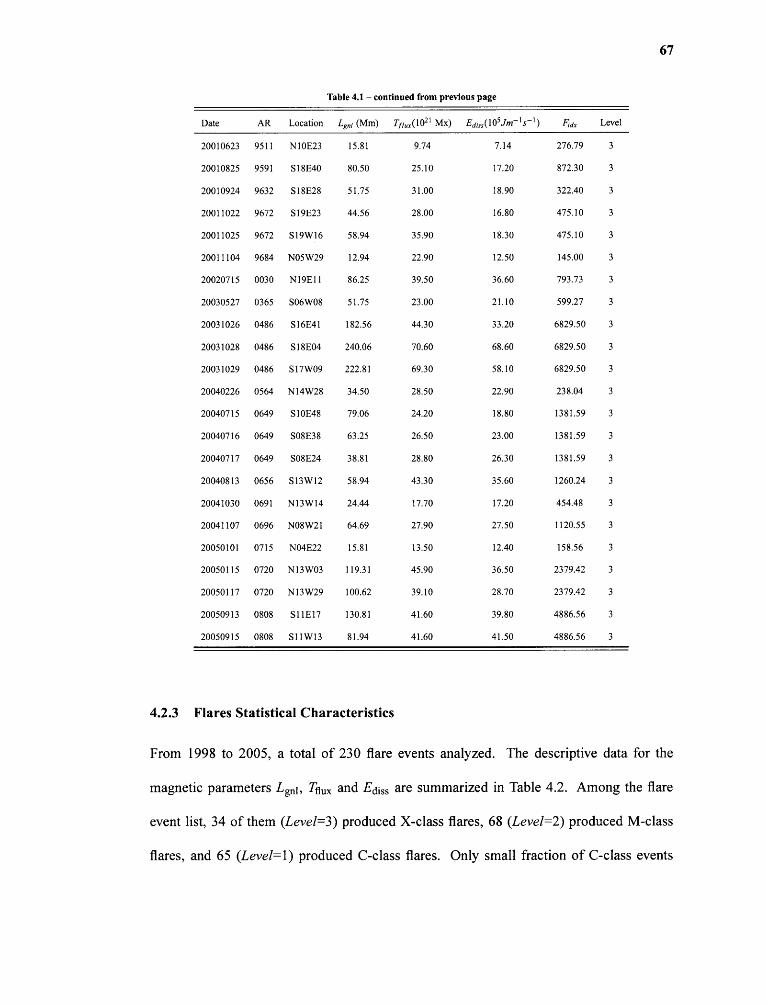
67
Table 4.1 - continued from previous page
Date AR Location Lgnl (Mm) Tflux(1021 Mx) Ediss(105 Jm-1 I s -1 ) Fidx Level
20010623 9511 N10E23 15.81 9.74 7.14 276.79 3
20010825 9591 S18E40 80.50 25.10 17.20 872.30 3
20010924 9632 518E28 51.75 31.00 18.90 322.40 3
20011022 9672 S19E23 44.56 28.00 16.80 475.10 3
20011025 9672 S19W16 58.94 35.90 18.30 475.10 3
20011104 9684 N05W29 12.94 22.90 12.50 145.00 3
20020715 0030 N19E11 86.25 39.50 36.60 793.73 3
20030527 0365 506W08 51.75 23.00 21.10 599.27 3
20031026 0486 S16E41 182.56 44.30 33.20 6829.50 3
20031028 0486 S18E04 240.06 70.60 68.60 6829.50 3
20031029 0486 S 1 7W09 222.81 69.30 58.10 6829.50 3
20040226 0564 N14W28 34.50 28.50 22.90 238.04 3
20040715 0649 S10E48 79.06 24.20 18.80 1381.59 3
20040716 0649 S08E38 63.25 26.50 23.00 1381.59 3
20040717 0649 S08E24 38.81 28.80 26.30 1381.59 3
20040813 0656 S13W12 58.94 43.30 35.60 1260.24 3
20041030 0691 N13W14 24.44 17.70 17.20 454.48 3
20041107 0696 N08W21 64.69 27.90 27.50 1120.55 3
20050101 0715 N04E22 15.81 13.50 12.40 158.56 3
20050115 0720 N13W03 119.31 45.90 36.50 2379.42 3
20050117 0720 N13W29 100.62 39.10 28.70 2379.42 3
20050913 0808 S11E17 130.81 41.60 39.80 4886.56 3
20050915 0808 S11W13 81.94 41.60 41.50 4886.56 3
4.2.3 Flares Statistical Characteristics
From 1998 to 2005, a total of 230 flare events analyzed. The descriptive data for the
magnetic parameters Lgnl, Tflux and Ediss are summarized in Table 4.2. Among the flare
event list, 34 of them (Level=3) produced X-class flares, 68 (Level=2) produced M-class
flares, and 65 (Level=1) produced C-class flares. Only small fraction of C-class events
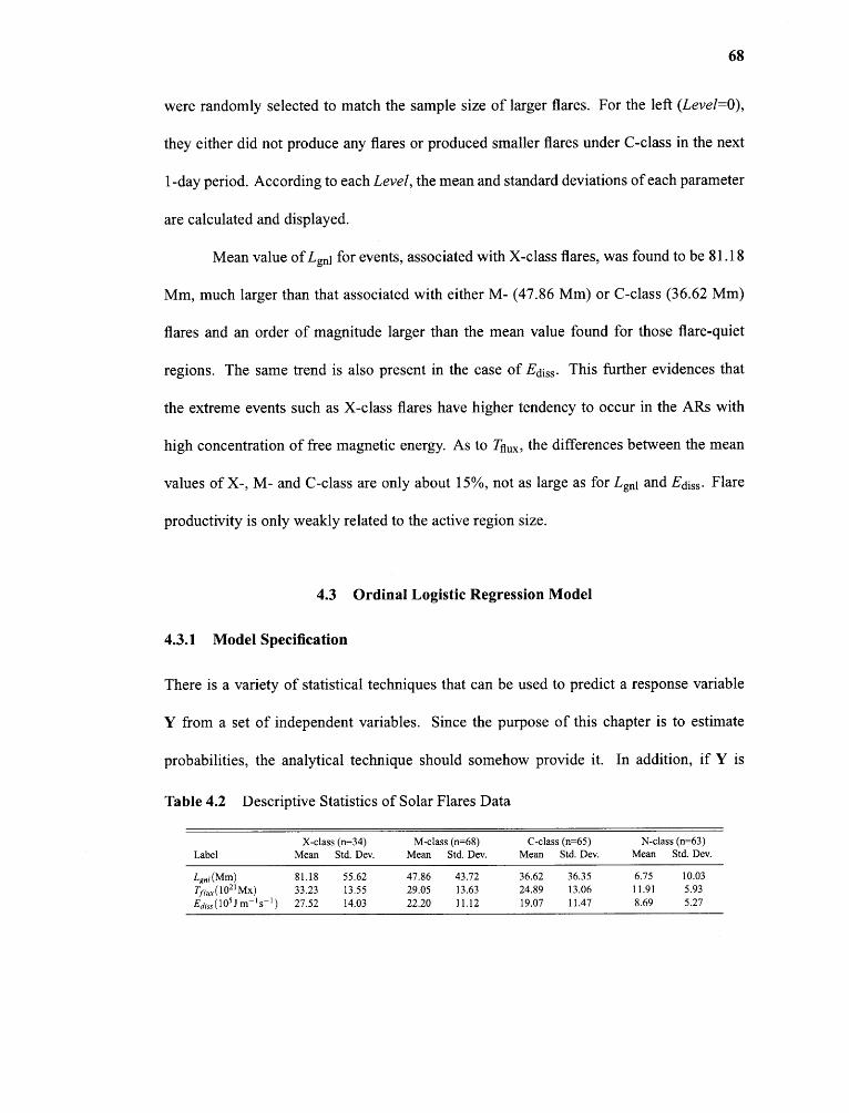
68
were randomly selected to match the sample size of larger flares. For the left (Level=0),
they either did not produce any flares or produced smaller flares under C-class in the next
1-day period. According to each Level, the mean and standard deviations of each parameter
are calculated and displayed.
Mean value of Lgnl for events, associated with X-class flares, was found to be 81.18
Mm, much larger than that associated with either M- (47.86 Mm) or C-class (36.62 Mm)
flares and an order of magnitude larger than the mean value found for those flare-quiet
regions. The same trend is also present in the case of Ediss . This further evidences that
the extreme events such as X-class flares have higher tendency to occur in the ARs with
high concentration of free magnetic energy. As to Tflux, the differences between the mean
values of X-, M- and C-class are only about 15%, not as large as for L gnl and Ediss . Flare
productivity is only weakly related to the active region size.
4.3 Ordinal Logistic Regression Model
4.3.1 Model Specification
There is a variety of statistical techniques that can be used to predict a response variable
Y from a set of independent variables. Since the purpose of this chapter is to estimate
probabilities, the analytical technique should somehow provide it. In addition, if Y is
Table 4.2 Descriptive Statistics of Solar Flares Data
LabelX-class (n=34)
Mean Std. Dev.M-class (n=68)
Mean Std. Dev.C-class (n=65)
Mean Std. Dev.N-class (n=63)
Mean Std. Dev.
Lgnl(Mm) 81.18 55.62 47.86 43.72 36.62 36.35 6.75 10.03
Tflux(1021Mx) 33.23 13.55 29.05 13.63 24.89 13.06 11.91 5.93Ediss (105 J m-I s-I ) 27.52 14.03 22.20 11.12 19.07 11.47 8.69 5.27
69
categorical, with more than two categories, such a response variable essentially rules out
usual regression analysis, including the variety of linear models. The major problem with
these techniques is that the linear function is inherently unbounded, while probabilities are
bounded by 0 and 1. This make the generalized (compared with binary) logistic method
the most obvious candidates for the regression analysis. It always returns values between 0
and 1. Depending on the scale of Y (ordinal or nominal), the model is further classified into
ordinal regression and nominal regression model. In our study, we use ordinal regression
model since Y here indicates the maximum magnitude of flares the given active region may
produce.
Suppose Y is the categorical response variable with k+1 ordered categories. For
example
Let X denotes the vector of predictive variables {xi , x2 , • • • ,xn} , and π j(x) = Prob(Y =
j │x=x) be the probability for the realization of Y =j,given X = x,j= 0,1,...,k.The
cumulative probabilities
70
where xβ stands for P0 + PiXi + • • • + βnxn. There are k intercepts (as). The regression
parameters a and s are estimated by the method of maximum likelihood (Agresti 1996),
which works by finding the value of p that returns the maximum value of the log-likelihood
function. Expression
is called the logistic function (logit). We can solve the above equation for αj + xβ
Thus the model becomes a linear regression model in the log odds that Y ≥ j. This is the
well-known proportional odds (PO) model (McCullagh 1980), also called ordinal logistic
model (Scott et al. 1997).
The logistic model formulated here for the solar flares study, contains a four-state
response variable. Level = 0 means the active region only produce microflares (Lower
than C-class flares) in the next 1-day period. Level = 1 means the active region at most
produce C-class flares. Level = 2 is for M- and Level = 3 is for X-class flares. Therefore,
the category number k = 3 and predictive variables are the some or all of three magnetic
parameters discussed earlier.
The model is computed with the statistical R software package (version 2.3.0 Linux
system), using a procedure that supports ordinal logistic regression model (lrm). For details
on the estimation procedure and the statistics in logistic regression models, see website 2 .
Ordinal logistic regression is not part of the standard R, but can be calculated via library
2 http://www.r-project.org/
71
Design 3 by using function lrm (Alzola and Harrell 2004).
4.3.2 Testing for Ordinality Assumption
A basic assumption of ordinal regression models is that the response variable behaves in
an ordinal fashion with respect to each predictive variable. Assuming that a predictor x
is linearly related to the log odds of some appropriate event, a simple way to check for
ordinality is to plot the mean of x stratified by levels of y. These means should be in a
consistent order. If for many of the xs, two adjacent categories of Y do not distinguish the
means, that is the evidence that those levels of Y should be pooled.
Figure 4.1 is such displays. Means of all three predictive variables are calculated for
each ordinal class of the response and plotted (solid) against it. In the ideal case, the dotted
line (PO model) should be superposed on the solid line if the PO assumptions hold. Ordi-
nality is satisfactorily verified for all three predictive variables (same monotonic trends).
Figure 4.2 shows another way to assess the PO assumption. Each predictive variable
is categorized into quartiles. Each quartile group is identified using the upper and lower
endpoints within that quartile. The logits of all proportions of the Level ≥ j, j = 1, 2, 3. is
computed. When proportional odds holds, the difference in logits between different values
of j should be the same at all levels of each parameter. This is because the model dictates
that logit(Level ≥ j x) - logit(Level > i │x) =αj - αi,for any constant x.
3http://biostat.mc.vanderbilt.edu/twiki/bin/view/main/design
72
4.3.3 Estimation Procedures
Before presenting the obtained results, we first describe three groups of models that were
used in our analysis. Table 4.3 shows products of different data generating models used
in the regression. In order to investigate the effects of each predictive parameter, every
possible combination is analyzed.
The models in group (a) contain only one predictive parameter. For prediction pur-
pose, these preliminary models may be too simple. However, their fitted results will help us
to understand which parameter may be more significant in producing solar flares. Models
in group (b) have three terms. The first two terms in each model are from our predictive
parameters. The third one is called the interaction term. It exists when the effect of one in-
dependent variable changes with different values of another independent variable. It is also
said that Variable 2 "moderates" the effect of Variable 1. In regression analysis, interaction
term is quantitatively represented by the product of Variable 1 and 2. Theoretically, interac-
tions among more than two variables, especially when these variables are continuous, can
be exceedingly complex. This is because there are many different combinations of two-
way interactions and the possibility of the order of interaction effects may be higher than
two, e.g. product of the square of one predictor and other predictor. Therefore, a good ap-
proach is to test for all such prespecified interaction effects with a single global test. Then,
unless interactions involving only one of the predictive variables is of special interest, we
can either drop all interactions or retain all of them (Harrell 2001). The models in group (c)
include all three predictive parameters, with and without corresponding interaction effect
terms.
The assumption of linearity in the logistic model need to be verified, especially
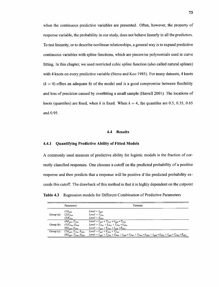
73
when the continuous predictive variables are presented. Often, however, the property of
response variable, the probability in our study, does not behave linearly in all the predictors.
To test linearity, or to describe nonlinear relationships, a general way is to expand predictive
continuous variables with spline functions, which are piecewise polynomials used in curve
fitting. In this chapter, we used restricted cubic spline function (also called natural splines)
with 4 knots on every predictive variable (Stone and Koo 1985). For many datasets, 4 knots
(k = 4) offers an adequate fit of the model and is a good compromise between flexibility
and loss of precision caused by overfitting a small sample (Harrell 2001). The locations of
knots (quantiles) are fixed, when k is fixed. When k = 4, the quantiles are 0.5, 0.35, 0.65
and 0.95.
4.4 Results
4.4.1 Quantifying Predictive Ability of Fitted Models
A commonly used measure of predictive ability for logistic models is the fraction of cor-
rectly classified responses. One chooses a cutoff on the predicted probability of a positive
response and then predicts that a response will be positive if the predicted probability ex-
ceeds this cutoff. The drawback of this method is that it is highly dependent on the cutpoint
Table 4.3 Regression models for Different Combination of Predictive Parameters
74
chosen for a positive prediction. In addition, it is presumptions to make one classification
rule from a probability model.
The test statistics allow us to test whether a predictive variable, or set of variables,
is related to the response. The generalized index Rif (Nagelkerke 1991; Cragg and Uhler
1970) can be useful for quantifying the predictive strength of a model. Let us assume that
the log likelihood (L.L.) of a model is represented by:
where Lc' = —2 x L.L, obtained under the null hypothesis that all regression coefficients
except for intercepts are zero. Likelihood ratio (LR) is then Li° — L, where L is -2 x L.L,
achieved from the fitted model. n is the size of dataset. For large enough datasets, LR
approximately follows X2 distribution. Index RN ranges from 0 to 1 and can be used to
assess how well the model compares to a "perfect" model.
A dimensionless index c indicates probability of concordance between the predicted
probability and the response. It has been shown that c is identical to a widely used measure
of diagnostic discrimination, which is the area under a "receiver operating characteristics"
(ROC) curve. A value of c 0.5 indicates random predictions, while c=1 indicates perfect
prediction. A model that has c near 0.8 has some reliability in predicting the responses of
individual events.
Another widely used index is 'Somers' index, D xy , that ranks the correlation be-
tween predicted probabilities and observed responses by the difference between concor-
75
dance and discordance probabilities.
When Dxy = 0, the model is making random predictions. When Lo x), = 1, the predictions
are perfectly discriminating.
Table 4.4 displays these indexes for every model listed in Table 4.3. For the mod-
els with only one predictive variable, they have comparable reliability in flare prediction
(nearly same indexes). The indexes of model (1) are slightly larger than that for model
(2) and (3). The larger indexes implies that the length of strong gradient neutral line is
relative more significant in prediction than the other two parameters. When we add one
more parameter to each model, then model (4) and (6) have larger indexes, indicating the
new parameter may improve the predictive strength. The worst result is for model (5) and
it confirms that Lgn1 plays the key role among three predictors. The nearly same results for
model (7) and (8) show that the ignorance of the interaction effects between predictors does
not reduce the predictive ability. Moreover, from the comparison of models (4) and (7), it
follows that parameter Ediss may be the least effective in flare prediction, while model (4),
namely the combination of Lgnl and 'hip( as predictors, seems to be the most effective tool
for predictions. This conclusion is consistent with the result that major flares of class M
or X are associated with pronounced high-gradient magnetic neutral line (Schrijver 2007).
According to Schrijver (2007), the measure of unsigned magnetic flux near the neutral line
is proved to be related with the probability of a active region to produce major flares.
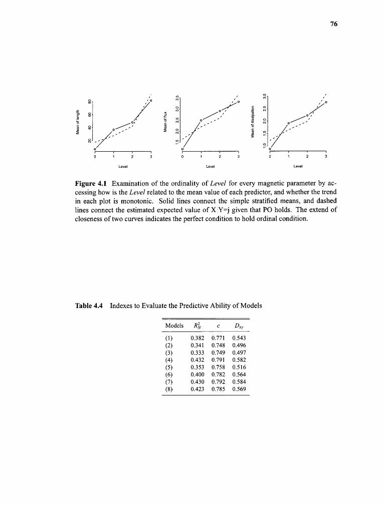
76
Figure 4.1 Examination of the ordinality of Level for every magnetic parameter by ac-cessing how is the Level related to the mean value of each predictor, and whether the trendin each plot is monotonic. Solid lines connect the simple stratified means, and dashedlines connect the estimated expected value of X Y=j given that PO holds. The extend ofcloseness of two curves indicates the perfect condition to hold ordinal condition.
Table 4.4 Indexes to Evaluate the Predictive Ability of Models
Models RN c Dxy
(1) 0.382 0.771 0.543(2) 0.341 0.748 0.496(3) 0.333 0.749 0.497(4) 0.432 0.791 0.582(5) 0.353 0.758 0.516(6) 0.400 0.782 0.564(7) 0.430 0.792 0.584(8) 0.423 0.785 0.569
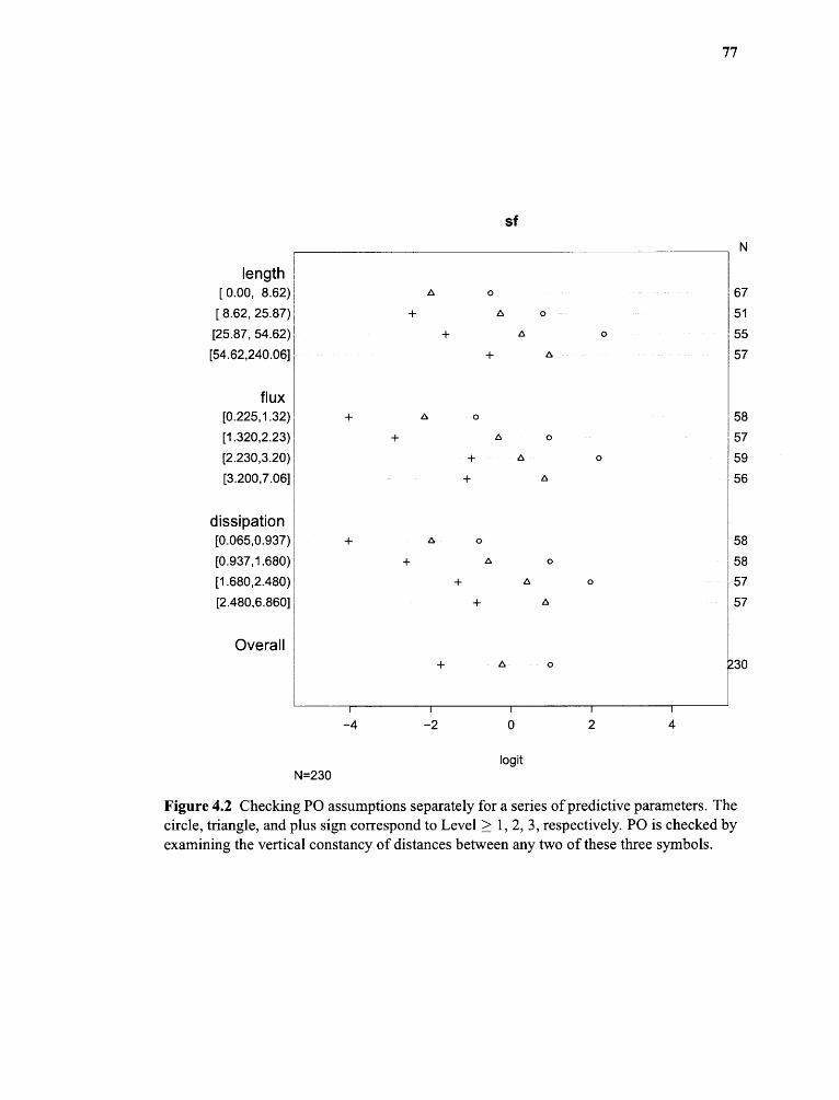
77
Figure 4.2 Checking PO assumptions separately for a series of predictive parameters. Thecircle, triangle, and plus sign correspond to Level ≥ 1, 2, 3, respectively. PO is checked byexamining the vertical constancy of distances between any two of these three symbols.
78
4.4.2 Validating the Fitted Models
Model validation is done to ascertain whether predicted values from the model are likely
to accurately predict responses on future events. The simplest validation method is one
time data-splitting. A dataset is split into training (model development) and test (vali-
dation) samples by a random process. The model's calibration are validated in the test
dataset. One disadvantage of data-splitting is that it greatly reduces the sample size for
both model development and model testing. The situation will become even worse when
the original dateset is not large enough, like our case in X-class flares. Bootstrapping can
be used to obtain nearly unbiased estimates of model performance without sacrificing sam-
ple size (Efron 1986; Breiman 1992). With bootstrapping, one repeatedly fits the model
in a bootstrap sample and evaluates the performance of the model on the original sample.
The estimate of the likely performance of the final model on future data is estimated by the
average of all of the indexes computed on the original sample. In general, the major cause
of unreliable models is overfitting the data. The amount of overfitting can be quantified by
the index of overoptimism. With bootstrapping we do not have a separate validation sample
for assessing calibration, but we can estimate the overoptimism in assuming that the final
model needs no calibration, that is, it has overall intercept and slope corrections of 0 and 1,
respectively. Refitting the model
where Pc denotes the actual calibrated probability, and the original predicted probability
is P = [1 + exp(-Xβ )] -1 in the original dataset will always result in y = (γe, γ1 ) = (0, 1 ),
79
since a logistic model will always fit when assessed overall. Thus, the bias-corrected esti-
mates of the true calibration can be obtained by the estimation of overoptimism in (0, 1).
An index of unreliability, Emax, that represents the maximum error in predicted probabili-
ties over the range a ≤ P ≤ b, follows immediately from this calibration:
As an example, we first validate model (4) shown in Table 4.3. The optimism-
corrected calibrations are in Table 4.5. The apparent Somers' D xy is 0.579, while the bias-
corrected Dxy is 0.559. The slope shrinkage factor is 0.933, indicating that this model
will validate on new data about 6.7% worse than on the current dataset. The maximum
absolute error in predicted probability is estimated to be about 0.017. A slight decrease in
R2 suggests some overfitting. Table 4.6 presents the validation results for all models. All
estimates of the maximum calibration error, Emax , are small, and quite satisfactory. After
the bias correction, model (4) still has the highest Dxy and R2 .
The estimated calibration curves for model (4) are displayed in Figure 4.3. They
are calculated as:
1
1 + exp[— (-0.009 + 0.933Lj)] 'Prob {Level > j} =
where Li is the logit of the predicted probability of Level j. The closeness of the calibra-
tion curves to the bisector line demonstrates excellent validation on the absolute probability
scale. The missing data in panel (a) and (c) cast some doubt on the validity of predictions
for C- and X-class flares. The shape of the calibration curve in panel (b) (slope < 1) implies
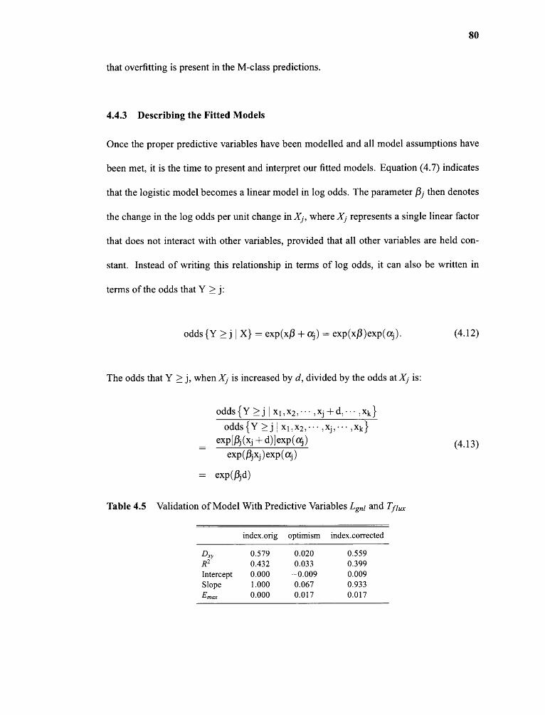
80
that overfitting is present in the M-class predictions.
4.4.3 Describing the Fitted Models
Once the proper predictive variables have been modelled and all model assumptions have
been met, it is the time to present and interpret our fitted models. Equation (4.7) indicates
that the logistic model becomes a linear model in log odds. The parameter βj then denotes
the change in the log odds per unit change in Xi , where Xi represents a single linear factor
that does not interact with other variables, provided that all other variables are held con-
stant. Instead of writing this relationship in terms of log odds, it can also be written in
terms of the odds that Y > j:
odds {Y j I X} = exp(xβ + αj) = exp(xβ )exp(αj) . (4. 1 2)
The odds that Y ≥ j, when X1 is increased by d, divided by the odds at Xi is:
Table 4.5 Validation of Model With Predictive Variables Lgnl and Tflux
index.orig optimism index.corrected
Dxy 0.579 0.020 0.559R2 0.432 0.033 0.399Intercept 0.000 —0.009 0.009Slope 1.000 0.067 0.933Emax 0.000 0.017 0.017
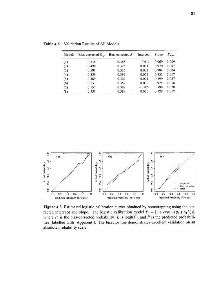
81
Table 4.6 Validation Results of All Models
Models Bias-corrected Dxy Bias-corrected R 2 Intercept Slope Erna:,
(1) 0.538 0.365 -0.011 0.969 0.009(2) 0.490 0.325 0.001 0.970 0.007(3) 0.501 0.326 0.002 0.984 0.004(4) 0.559 0.399 0.009 0.933 0.017(5) 0.489 0.309 0.021 0.899 0.027(6) 0.533 0.362 0.000 0.924 0.018(7) 0.557 0.382 -0.022 0.898 0.028(8) 0.551 0.389 0.000 0.928 0.017
Figure 4.3 Estimated logistic calibration curves obtained by bootstrapping using the cor-rected intercept and slope. The logistic calibration model Pc = [1 + exp(-(γ0 + γ1L))],where Pc is the bias-corrected probability. L is logit(P), and P is the predicted probabili-ties (labelled with 'Apparent'). The bisector line demonstrates excellent validation on anabsolute probability scale.
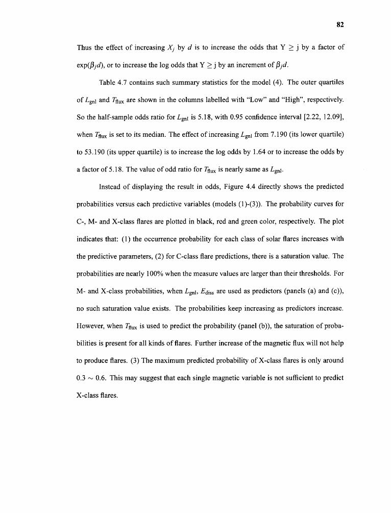
82
Thus the effect of increasing Xi by d is to increase the odds that Y ≥ j by a factor of
exp(βjd), or to increase the log odds that Y ≥ j by an increment of Ad.
Table 4.7 contains such summary statistics for the model (4). The outer quartiles
of Lo and Tflux are shown in the columns labelled with "Low" and "High", respectively.
So the half-sample odds ratio for Lgnl is 5.18, with 0.95 confidence interval [2.22, 12.09],
when Tflux is set to its median. The effect of increasing Lo from 7.190 (its lower quartile)
to 53.190 (its upper quartile) is to increase the log odds by 1.64 or to increase the odds by
a factor of 5.18. The value of odd ratio for Tflux is nearly same as Lgnl.
Instead of displaying the result in odds, Figure 4.4 directly shows the predicted
probabilities versus each predictive variables (models (1)-(3)). The probability curves for
C-, M- and X-class flares are plotted in black, red and green color, respectively. The plot
indicates that: (1) the occurrence probability for each class of solar flares increases with
the predictive parameters, (2) for C-class flare predictions, there is a saturation value. The
probabilities are nearly 100% when the measure values are larger than their thresholds. For
M- and X-class probabilities, when L Ediss are used as predictors (panels (a) and (c)),
no such saturation value exists. The probabilities keep increasing as predictors increase.
However, when Tflux is used to predict the probability (panel (b)), the saturation of proba-
bilities is present for all kinds of flares. Further increase of the magnetic flux will not help
to produce flares. (3) The maximum predicted probability of X-class flares is only around
0.3 ~ 0.6. This may suggest that each single magnetic variable is not sufficient to predict
X-class flares.
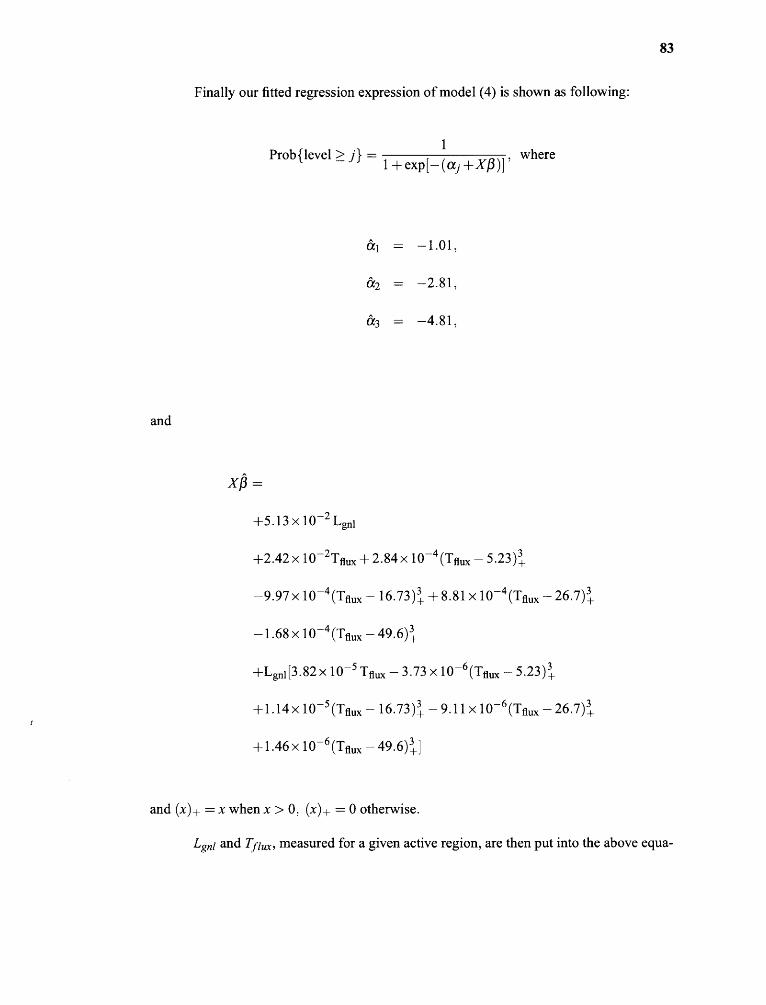
Finally our fitted regression expression of model (4) is shown as following:
α1
a2
a3
=
=
=
—1.01,
—2.81,
—4.81,
83
and
Lgnl and Tflux measured for a given active region, are then put into the above equa-
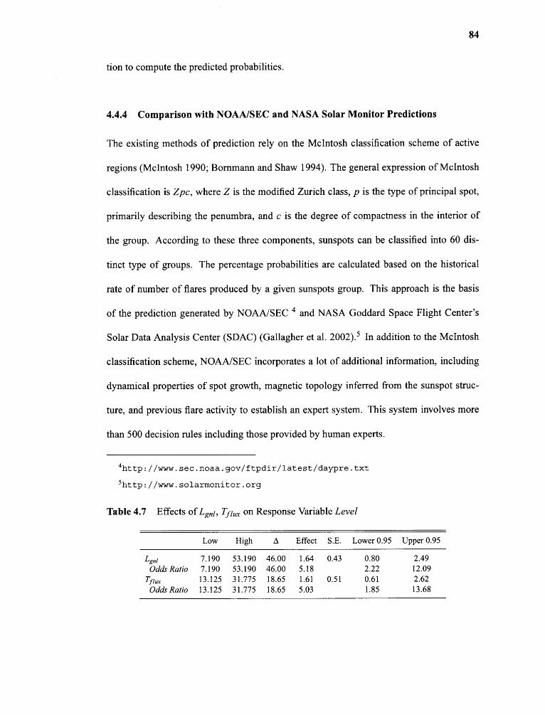
84
tion to compute the predicted probabilities.
4.4.4 Comparison with NOAA/SEC and NASA Solar Monitor Predictions
The existing methods of prediction rely on the McIntosh classification scheme of active
regions (McIntosh 1990; Bornmann and Shaw 1994). The general expression of McIntosh
classification is Zpc, where Z is the modified Zurich class, p is the type of principal spot,
primarily describing the penumbra, and c is the degree of compactness in the interior of
the group. According to these three components, sunspots can be classified into 60 dis-
tinct type of groups. The percentage probabilities are calculated based on the historical
rate of number of flares produced by a given sunspots group. This approach is the basis
of the prediction generated by NOAA/SEC 4 and NASA Goddard Space Flight Center's
Solar Data Analysis Center (SDAC) (Gallagher et al. 2002). 5 In addition to the McIntosh
classification scheme, NOAA/SEC incorporates a lot of additional information, including
dynamical properties of spot growth, magnetic topology inferred from the sunspot struc-
ture, and previous flare activity to establish an expert system. This system involves more
than 500 decision rules including those provided by human experts.
4http: //www. sec .noaa . gov/ftpdir/latest/daypre .txt
5 http : //www. solarmonitor .org
Table 4.7 Effects of Lgnl, Tflux on Response Variable Level
Low High A Effect S.E. Lower 0.95 Upper 0.95
LgnlOdds Ratio
T fluxOdds Ratio
7.1907.19013.12513.125
53.19053.19031.77531.775
46.0046.0018.6518.65
1.645.181.615.03
0.43
0.51
0.802.220.611.85
2.4912.092.6213.68
85
Disadvantages of the classification-based approaches are that the variation in flare
probability within a class is unavoidably ignored. The classification process is possibly
subjective because the McIntosh scheme with three parameters is an arbitrary construction.
Different observers may not agree with a given classification. The similar problems arise
with the additional information in the expert system since the choice of properties is essen-
tially arbitrary. Moreover, They might need human intervention, either in classification or
in prediction procedures, and therefore are not suitable for automated prediction.
In order to compare the predictability of the Logistic model and NASA/SDAC,
NOAA/SEC schemes, we studied our event list and found 55 events in the list were also
predicted by NOAA/SEC and NASA/SDAC. Their prediction results were plotted together
and shown in Figure 4.5. Every event (flare) is indexed in x-axis. Y axis represents the pre-
dicted probability. The results from different prediction approach are indicated by different
shapes of points. For comparison, the actual results (1 means occurred, 0 means not) are
also presented (green dots). We then used a contingency table, which has been widely used
in the meteorological forecasting literature, to evaluate the prediction capability of these
approaches. This table can provide us with information on the success or failure of the
forecasting experience in real time (Kim et al., 2005). We thus defined the probability of
>50% to be the "yes predicted", as shown by the points above horizontal dotted line. The
vertical dotted line indicates the actual start point of flare happening. Each graph in Figure
4.5 is divided into four regions (a-d). Region "a" contains the events with "yes predicted"
and "yes observed". The region "b" represents the number of false alarms that means "yes
predicted" but not observed. Similarly, "c" is the number of misses that means not pre-
dicted but "yes observed", and "d" is the number of correct nulls that means not predicted
86
or observed.
The indexes used by NOAA National Weather Service (NWS) were computed and
listed in Table 4.8. Probability of detection (POD) is the percentage of all flare events
which are predicted ( a/(a+c). A perfect score would be 100%). False alarm ratio (FAR)
measures how often we issue false alarm, or in other words, a measure of 'crying wolf'
(b/(a+b)). Ideally we want this number to be 0.0%. Critical success index (CSI) is the ratio
of predicted events a to the total number of (a + b + c) . In C-class flare prediction, the pre-
dicted probabilities computed from NASA/SDAC only distribute in the range of 0 and 55%.
The "yes predicted" is not as obvious as those from other two methods. Meanwhile, the
minimum probabilities predicted by Logistic method are larger than the results from both
NASA/SDAC and NOAA/SEC. This is probably due to the threshold (50 GMm -1 in this
study) for the gradient neutral lines. Those Lgnl with small values might still have enough
nonpotential energy to product weaker flares. For M- and X-class flares, such a problem is
eliminated. In M-class prediction, NASA/SDAC approach is no doubt incapable to satisfy
the prediction requirement. For X-class prediction, the results from all current methods are
not satisfactory. Thus, the indexes show that the method used by NOAA/SEC provide the
best prediction results. The low predictability in forecasting X class flares perhaps indicates
that the predictive parameters we applied so far may not have close enough correlation in
triggering stronger flares. The other possible reason for the incapability in prediction of X
class flares may be due to the insufficient data samples in logistic regression model.
The gap between NOAA/SEC and logistic regression model become smaller when
forecasting major solar flares. In Figure 4.5 the probabilities of X class flares prediction
obtained from ordinal logistic method and NOAA/SEC are higher in those active regions
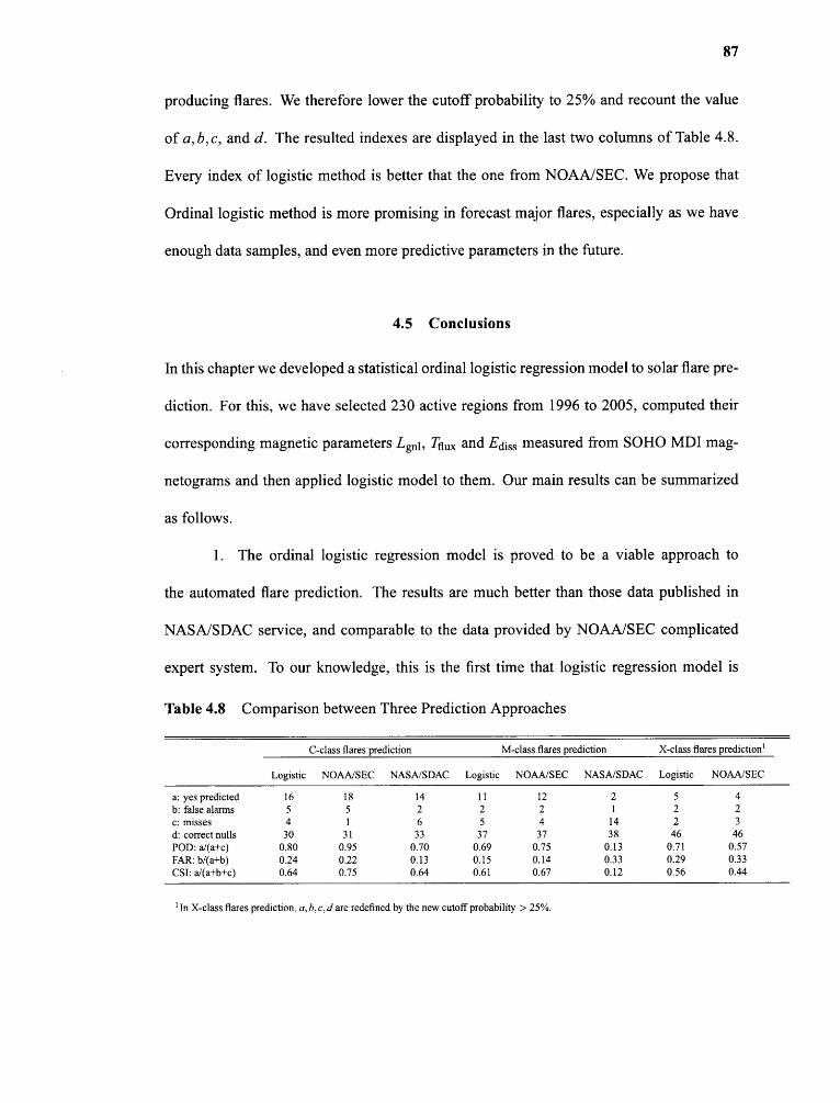
87
producing flares. We therefore lower the cutoff probability to 25% and recount the value
of a, b, c, and d. The resulted indexes are displayed in the last two columns of Table 4.8.
Every index of logistic method is better that the one from NOAA/SEC. We propose that
Ordinal logistic method is more promising in forecast major flares, especially as we have
enough data samples, and even more predictive parameters in the future.
4.5 Conclusions
In this chapter we developed a statistical ordinal logistic regression model to solar flare pre-
diction. For this, we have selected 230 active regions from 1996 to 2005, computed their
corresponding magnetic parameters Lo, Tfl ux and Ediss measured from SOHO MDI mag-
netograms and then applied logistic model to them. Our main results can be summarized
as follows.
1. The ordinal logistic regression model is proved to be a viable approach to
the automated flare prediction. The results are much better than those data published in
NASA/SDAC service, and comparable to the data provided by NOAA/SEC complicated
expert system. To our knowledge, this is the first time that logistic regression model is
Table 4.8 Comparison between Three Prediction Approaches
C-class flares prediction M-class flares prediction X-class flares prediction )
a: yes predictedb: false alarmsc: missesd: correct nullsPOD: a/(a+c)FAR: b/(a+b)CSI: a/(a+b+c)
Logistic NOAA/SEC NASA/SDAC Logistic NOAA/SEC NASA/SDAC Logistic NOAA/SEC
I6 I8 I4 II I2 2 5 45 5 2 2 2 I 2 24 I 6 5 4 14 2 330 3I 33 37 37 38 46 46
0.80 0.95 0.70 0.69 0.75 0.I3 0.7I 0.570.24 0.22 0.I3 0.I5 0.I4 0.33 0.29 0.330.64 0.75 0.64 0.61 0.67 0.I2 0.56 0.44
1In X-class flares prediction, a,b,c,d are redefined by the new cutoff probability > 25%.
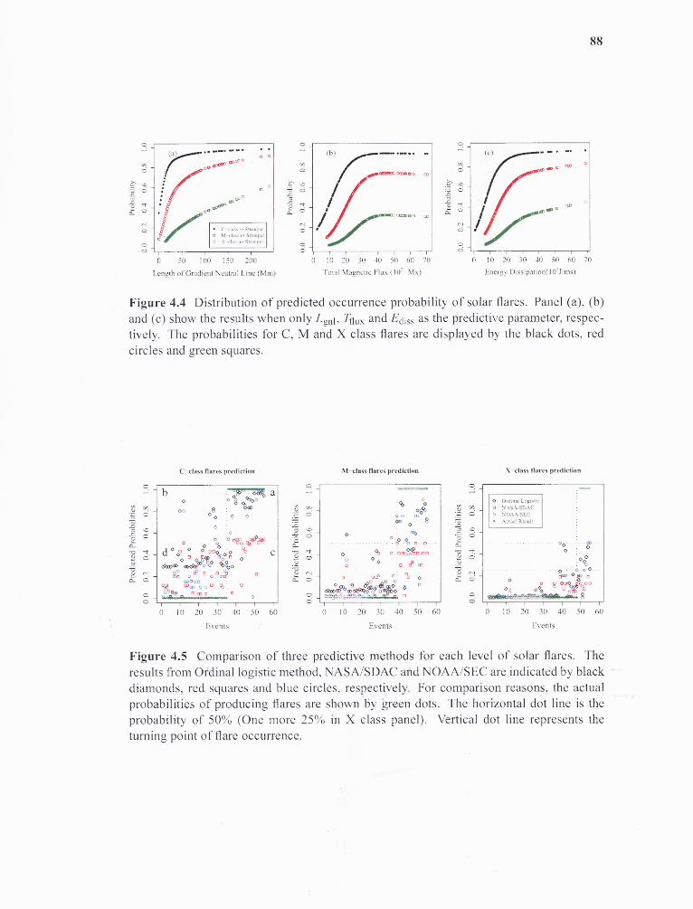
88
Figure 4.4 Distribution of predicted occurrence probability of solar flares. Panel (a), (b)and (c) show the results when only Lob TfluxandEdissas the predictive parameter, respec-tively. The probabilities for C, M and X class flares are displayed by the black dots, redcircles and green squares.
Figure 4.5 Comparison of three predictive methods for each level of solar flares. Theresults from Ordinal logistic method, NASA/SDAC and NOAA/SEC are indicated by blackdiamonds, red squares and blue circles, respectively. For comparison reasons, the actualprobabilities of producing flares are shown by green dots. The horizontal dot line is theprobability of 50% (One more 25% in X class panel). Vertical dot line represents theturning point of flare occurrence.
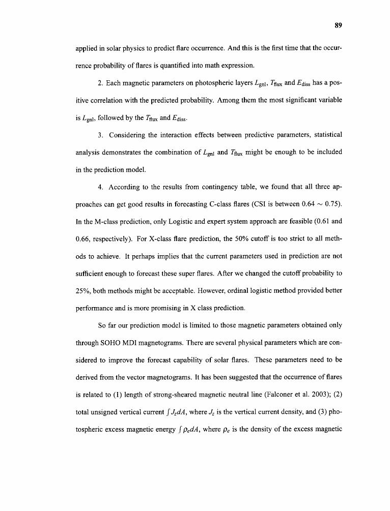
89
applied in solar physics to predict flare occurrence. And this is the first time that the occur-
rence probability of flares is quantified into math expression.
2. Each magnetic parameters on photospheric layers Lgnl , Tflux and Ediss has a pos-
itive correlation with the predicted probability. Among them the most significant variable
is Lgnl, followed by the Tflux and Ediss.
3. Considering the interaction effects between predictive parameters, statistical
analysis demonstrates the combination of Lo and Tflux might be enough to be included
in the prediction model.
4. According to the results from contingency table, we found that all three ap-
proaches can get good results in forecasting C-class flares (CSI is between 0.64 ~ 0.75).
In the M-class prediction, only Logistic and expert system approach are feasible (0.61 and
0.66, respectively). For X-class flare prediction, the 50% cutoff is too strict to all meth-
ods to achieve. It perhaps implies that the current parameters used in prediction are not
sufficient enough to forecast these super flares. After we changed the cutoff probability to
25%, both methods might be acceptable. However, ordinal logistic method provided better
performance and is more promising in X class prediction.
So far our prediction model is limited to those magnetic parameters obtained only
through SOHO MDI magnetograms. There are several physical parameters which are con-
sidered to improve the forecast capability of solar flares. These parameters need to be
derived from the vector magnetograms. It has been suggested that the occurrence of flares
is related to (1) length of strong-sheared magnetic neutral line (Falconer et al. 2003); (2)
total unsigned vertical current 1'4c/Á, where 4 is the vertical current density, and (3) pho-
tospheric excess magnetic energy ∫ pedA, where pe is the density of the excess magnetic

90
energy (Wang et al. 1996; Leka and Barnes 2003b,a). More extensive investigation is in
preparation as these parameters become readily available in the near future.
CHAPTER 5
THE RELATIONSHIP BETWEEN MAGNETIC ORIENTATION ANGLE AND
GEOMAGNETIC STORM
5.1 Introduction
One of the main objectives in space weather research is to predict the occurrence of geo-
magnetic storms based on real-time solar observations. A severe geomagnetic storm may
produce many harmful effects on the Earth, and usually is initiated when the energy is trans-
ferred from the Sun to the Earth's magnetosphere through CMEs. Normally, the Earth's
magnetosphere is a closed structure and no energy and particles can be injected into it.
Therefore, a geomagnetic storm can only occur when the IMF turns southward and re-
mains so for some period of time (e.g., Bothmer and Schwenn 1998; Tsurutani et al. 1988;
Tsurutani 2001). Reconnection between southward IMF and the northwardly directed geo-
magnetic field occurs at the day side magnetopause and this reconnection transports energy
from the solar wind into the magnetosphere (Dungey 1961).
A geomagnetic storm has three distinct phases of evolution: (1) initial phase, lasting
from minutes to hours, when Dst increases up to tens of nT; (2) main phase, lasting from
half an hour to several hours during which Dst drops below zero, down to minus hundreds
of nT; (3) recovery phase lasting tens of hours to days, when the D st index gradually returns
to the normal (undisturbed) level.
Previous studies had shown that filament chirality and the orientation of filament
magnetic fields correspond to the chirality and orientation of the magnetic field in the asso-
ciated MCs (Bothmer and Schwenn 1994; Rust 1994; Yurchyshyn et al. 2001, 2005). These
91
92
results suggest that immediately after the eruption one may be able to predict the orienta-
tion of the MC associated with the CME and, furthermore, the likelihood of a geomagnetic
storm.
In order to advance our current understanding of the relationship between CMEs
and geomagnetic storms we need a deeper knowledge of solar magnetic field that is the
main source of energy for solar eruptions. Because of lack of direct measurements of
the coronal magnetic field, extrapolation of the photospheric measurements upward into
the corona is the primary means to reconstruct coronal magnetic structure and analyze
magnetic connectivity. There are variety of extrapolation techniques such as potential,
force-free and non force-free field methods. For an automated, real-time magnetic field
simulations, we choose a potential field model, which requires least human intervention, a
minimum set of initial assumptions and boundary conditions and thus enables us to analyze
magnetic configuration of the CME source regions in the real time.
The objective of this chapter is to better understand the relationship between surface
magnetic structures and the geomagnetic index (Bz or Dst). In this chapter, observations are
described in Section 5.2, data analysis in Section 5.3. Statistical results are listed in Section
5.4. Finally, we present conclusions and discussions in Section 5.5.
5.2 Data Sets
Beginning from middle 1990s more advanced data on CMEs and IMF became available
from space observatories such as SOHO, ACE and WIND. They provide unprecedented
opportunity to study and forecast space weather. In this study we use the following data.
(1) Data from LASCO coronagraphs C2 and C3 that image Thomson-scattered vis-
93
ible light taken through a broadband filter onboard SOHO. The data allow us to determine
the occurrence of CMEs and their speeds. The CME Catalog, generated and maintained at
the CDAW data center and NASA, covers the period from 1996 to present (Yashiro et al.
2004). For each event it provides, among others, height-time plots, plane-of-sky speeds,
and CME onset time recorded by their first appearance in LASCO/C2, position angle, cor-
responding accelerations and so on. The CME speeds are determined from both linear and
quadratic fits to the height-time measurements. In our study we used the linear (constant
speed) fit. This choice is based on the study by MacQueen and Fisher (1983) who showed
that flare associated CMEs tend to display little or no acceleration beyond the edge of the
occulting disk (1.2 R0).
(2) Intensities of geomagnetic storms, measured by hourly equatorial Dst values
from the World Data Center for Geomagnetism in Kyoto'. Since the storms with D st ≤
-200nT are the most disastrous phenomena in space weather, for the purpose of this study
we regrouped geomagnetic storms as follows: moderate storms are in the range of -30 to
-100nT, intense storms are between -100 and -200nT and super storms are those with the
Dst index less than -200nT.
(3) Solar activity reports that are available online from the NOAA Space Environ-
ment Center2 . Solar flare reports include the Coordinated Universal Time (UTC) of the
beginning, maximum and end of a flare, the X-ray flux at the flare peak and the location of
the flare, if available. In our study we associated solar flares with the corresponding halo
CMEs by matching their onset times.
1http://swdcdb.kugi.kyoto-u.ac.jp/dstdir/
2http://www.sec.noaa.gov/ftpmenu/indices.html
94
(4) Magnetic Field Experiment (MAG) onboard ACE satellite provides one-hour
averages of magnetometer data, which are used to study structure of IMF. MAG mea-
surements, in particular the southward component, 13z, are used to forecast intensity of
geomagnetic storms.
(5) SOHO's Michelson Doppler Imager (MDI) provides full-disk line-of-sight mag-
netograms at the photospheric layer with a spatial resolution of 4 arc sec. These magne-
tograms were used to analyze the structure of magnetic fields in CME source regions.
5.3 Methods of Data Analysis
Halo CMEs are classified according to their angular width into either partial or full halo
CMEs. Here we concentrate only on full halo CMEs, which are defined as those having
360° span angle as indicated in the LASCO CME Catalog. Based on this criteria, we se-
lected 318 full halo CMEs that occurred during 1996 - 2004. The identification of the
geomagnetic storms, associated with these CMEs, was composed of two steps: 1) identifi-
cation of the active regions with high probability of CMEs/flares occurrence that is based
on full disk MDI magnetogram; 2) estimation of the range of intensity of geomagnetic
storms based on the observed CME data.
5.3.1 Identification of possible CME source regions from high gradient
neutral lines
There are variety of ways to identify the solar source of a front-side halo CME, such as EIT
dimming (Sheeley et al. 1983; Sterling and Hudson 1997; Webb et al. 2000; Wang et al.
2002), EIT and Moreton waves (Thompson et al. 1999; Warmuth et al. 2004), post-flare

95
loops (Hudson et al. 1998). All these methods, however, are based on the analysis of post-
event data. In this chapter we propose a gradient neutral line method that will enable us to
identify possible sources of CMEs/flares from solar data taken before the eruptive event.
Eruption of CME is accompanied by release of large amount of energy in a short
period of time. In order to store this energy, the magnetic field of the CME source region
must be in a stressed, distorted configuration as compared to the minimum-energy potential
field configuration. One signature of such a non-potential configuration is strong magnetic
shear seen along the active region main neutral line (NL) that divides two opposite polarity
magnetic regions. The extent to which the magnetic field is sheared along the main neutral
line is a measure of global non-potentiality of an active region (Falconer 2001; Zhang
2001). Magnetic shear can be quantitatively described by the angle between the observed
and potential transverse fields. Falconer et al. (2003) analyzed 17 vector magnetograms
and concluded that when the horizontal gradient of the line-of-sight field ( ▼Bll , herein,
magnetic gradient) is higher than a certain threshold (50 G Mm -1 in their study), the length
of a segment of the main NL with strong gradient, LSG, is significantly correlated with
CME productivity of an active region. In a study of 6 large (X5 or larger) flares , Wang
et al. (2006) reported on the positive linear relationship between the magnetic shear and the
magnetic gradient and that the latter seems to be a better tool to determine the probability of
the occurrence of flares and CMEs in an active region. In this work we further examine this
conclusion with more events. If this relationship is proved to be viable, then the magnetic
gradient method can be used as the first step in an automatic routine to locate the most
probable CME/flare source regions.
First, utilizing a full disk longitudinal MDI magnetogram obtained on the day of a

96
halo CME, we calculated a full disk magnetic gradient map and masked it with a neutral
line map. We then chose 50 G Mm -1 (Falconer et al. 2003) as the threshold to calculate the
length of high gradient neutral line (HGNL) at a point with the largest magnetic gradient in
the gradient map, and move along the NL in both directions away from the starting point.
According to Hagyard (1990), a sufficient condition for a large flare to occur is that the
length of the neutral line should be equal or exceed 8 ti 10 Mm. In our study we accepted
that if the length of HGNL is longer than ~ 7 Mm (approx. 10 arc sec), it indicates that the
region under study has a non-potential configuration and the probability of occurrence of
CMEs and/or flares is high. Otherwise, we proceed to the next largest gradient point in the
map and perform similar analysis again, until all neutral lines are evaluated. Then, using
the first qualified gradient point as center, we cropped the full disk MDI magnetogram into
a small map (Figure 5.1) with a field of view of about 300" x 200". This size can cover
a typical large active region. Both images are presented in negative, i.e., darker points
indicate stronger magnetic gradient. The dark thick line shown in the lower panel of Figure
5.1 is a HGNL and it represents the gradient distribution along the NL. The length of HGNL
depends on the gradient threshold values. It becomes shorter and only strongest parts are
left as we increase the threshold.
The locations identified by this method are shown in Table 5.1, column 2. The total
length of all intervals of HGNL in the identified source region is presented in column 8
as Lneu . Note that for several events listed in Table 5.1 the 50 G Mm -1 magnetic gradient
threshold was too large and therefore HGNL is zero.
To verify our identified locations, we used NOAA SEC reports on Hα flares, as-
sociated with the selected 318 halo CMEs. Please, note that only those halo CMEs that
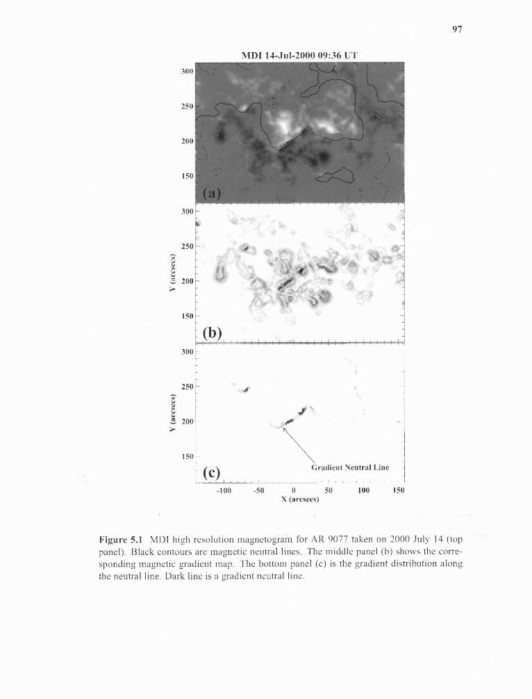
97
Figure 5.1 MDI high resolution magnetogram for AR 9077 taken on 2000 July 14 (toppanel). Black contours are magnetic neutral lines. The middle panel (b) shows the corre-sponding magnetic gradient map. The bottom panel (c) is the gradient distribution alongthe neutral line. Dark line is a gradient neutral line.
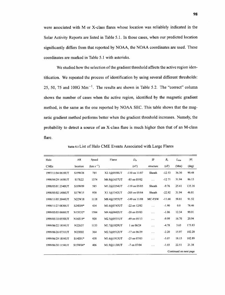
98
were associated with M or X-class flares whose location was reliablely indicated in the
Solar Activity Reports are listed in Table 5.1. In those cases, when our predicted location
significantly differs from that reported by NOAA, the NOAA coordinates are used. These
coordinates are marked in Table 5.1 with asterisks.
We studied how the selection of the gradient threshold affects the active region iden-
tification. We repeated the process of identification by using several different thresholds:
25, 50, 75 and 100G Mm -1 . The results are shown in Table 5.2. The "correct" column
shows the number of cases when the active region, identified by the magnetic gradient
method, is the same as the one reported by NOAA SEC. This table shows that the mag-
netic gradient method performs better when the gradient threshold increases. Namely, the
probability to detect a source of an X-class flare is much higher then that of an M-class
flare.
Table 5.1 List of Halo CME Events Associated with Large Flares
Halo AR Speed Flares Dst IP B, 1,„,„ 1191
CMEs location (km s -1 ) (nT) structure (nT) (Mm) (deg)
I997/11/04 06I0UT 519W28 785 X2.I@0558UT -110 on 11/07 Sheath -I2.53 36.30 90.48
I998/04/29 1658UT S17E22 I374 M6.8@1637UT -85 on 05/02 ... -12.7I 3I.94 86.I3
1998/05/01 2340UT 5I8W09 585 M1.2@2254UT -119 on 05/05 Sheath -9.76 25.41 135.16
I998/05/02 1406UT S17W15 938 X1.1@1342UT -205 on 05/04 Sheath -22.92 3I.94 46.8I
1998/11/05 2044UT N22W18 1118 M8.4@1955UT -149 on 11/08 MC-ESW -11.68 58.81 91.52
1998/11/27 0830UT S24E09* 434 M1.6@0743UT -22 on I2/02 ... -I.90 0.0 78.46
1999/05/03 0606UT N15E32* 1584 M4.4@0602UT -20 on 05/03 ... -1.06 12.34 90.01
1999/05/I0 0550UT N16EI9* 920 M2.5@0531UT -49 on 05/I3 ... -9.99 16.70 20.94
1999/06/22 I854UT N22E37 1133 M1.7@1829UT 1 on 06/24 ... -4.78 3.63 I73.83
I999/06/26 0731UT N23E02 364 M2.3@05I2UT -I7 on 06/29 ... -2.20 I5.97 I02.20
1999/06/29 I854UT 5I4E0I* 438 M1.6@1913UT -25 on 07/03 ... -5.07 18.15 I02.89
I999/06/30 1154UT S15W04* 406 M1.9@113OUT -7 on 07/04 ... -1.03 22.5I 2I.38
Continued on next page
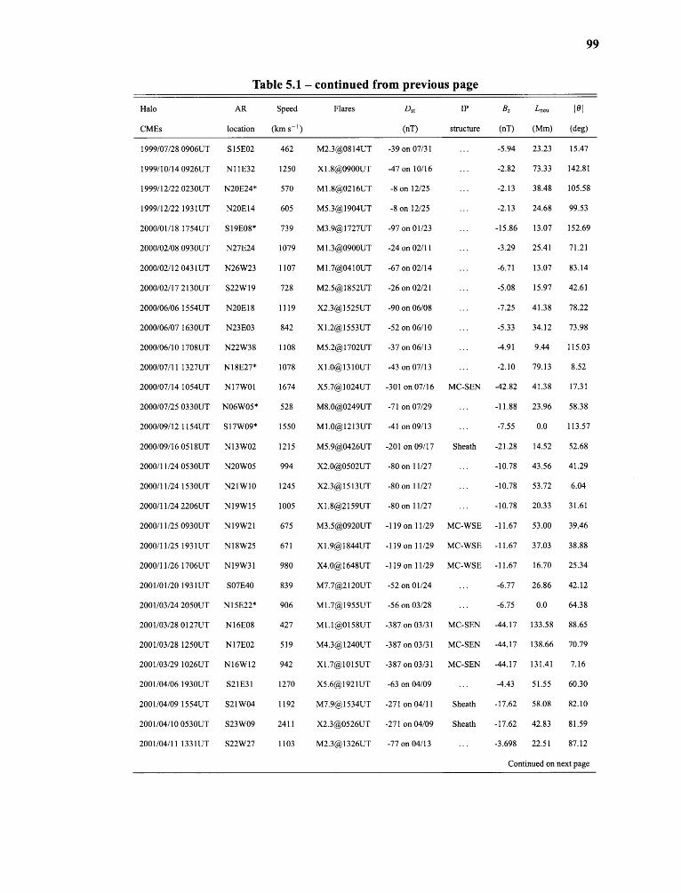
99
Table 5.1 - continued from previous page
Halo AR Speed Flares Dst IP B, Lneu lθl
CMEs location (km s -1 ) (nT) structure (nT) (Mm) (deg)
1999/07/28 0906UT S15E02 462 M2.3@0814UT -39 on 07/31 ... -5.94 23.23 15.47
1999/10/14 0926UT N11E32 1250 X1.8@0900UT -47 on 10/16 ... -2.82 73.33 142.81
1999/12/22 0230UT N20E24* 570 M1.8@0216UT -8 on 12/25 ... -2.13 38.48 105.58
1999/12/22 1931UT N20E14 605 M5.3@1904UT -8 on 12/25 ... -2.13 24.68 99.53
2000/01/18 1754UT S19E08* 739 M3.9@1727UT -97 on 01/23 ... -15.86 13.07 152.69
2000/02/08 0930UT N27E24 1079 M1.3@0900UT -24 on 02/11 ... -3.29 25.41 71.21
2000/02/12 0431UT N26W23 1107 M1.7@0410UT -67 on 02/14 ... -6.71 13.07 83.14
2000/02/17 2130UT S22W19 728 M2.5@1852UT -26 on 02/21 ... -5.08 15.97 42.61
2000/06/06 1554UT N20E18 1119 X2.3@1525UT -90 on 06/08 ... -7.25 41.38 78.22
2000/06/07 1630UT N23E03 842 X1.2@1553UT -52 on 06/10 ... -5.33 34.12 73.98
2000/06/10 1708UT N22W38 1108 M5.2@1702UT -37 on 06/13 ... -4.91 9.44 115.03
2000/07/11 1327UT N18E27* 1078 X1.0@1310UT -43 on 07/13 ... -2.10 79.13 8.52
2000/07/14 1054UT N17W01 1674 X5.7@1024UT -301 on 07/16 MC-SEN -42.82 41.38 17.31
2000/07/25 0330UT N06W05* 528 M8.0@0249UT -71 on 07/29 ... -11.88 23.96 58.38
2000/09/12 1154UT S1 7W09* 1550 M1.0@1213UT -41 on 09/13 ... -7.55 0.0 113.57
2000/09/16 0518UT N13W02 1215 M5.9@0426UT -201 on 09/17 Sheath -21.28 14.52 52.68
2000/11/24 0530UT N20W05 994 X2.0@0502UT -80 on 11/27 ... -10.78 43.56 41.29
2000/11/24 1530UT N21W10 1245 X2.3@1513UT -80 on 11/27 ... -10.78 53.72 6.04
2000/11/24 2206UT N19W15 1005 X1.8@2159UT -80 on 11/27 ... -10.78 20.33 31.61
2000/11/25 0930UT N19W21 675 M3.5@0920UT -119 on 11/29 MC-WSE -11.67 53.00 39.46
2000/11/25 1931UT N18W25 671 X1.9@1844UT -119 on 11/29 MC-WSE -11.67 37.03 38.88
2000/11/26 1706UT N19W31 980 X4.0@1648UT -119 on 11/29 MC-WSE -11.67 16.70 25.34
2001/01/20 1931UT S07E40 839 M7.7@2120UT -52 on 01/24 ... -6.77 26.86 42.12
2001/03/24 2050UT N15E22* 906 M1.7@1955UT -56 on 03/28 ... -6.75 0.0 64.38
2001/03/28 0127UT N16E08 427 M1.1@0158UT -387 on 03/31 MC-SEN -44.17 133.58 88.65
2001/03/28 1250UT N17E02 519 M4.3@1240UT -387 on 03/31 MC-SEN -44.17 138.66 70.79
2001/03/29 1026UT N16W12 942 X1.7@1015UT -387 on 03/31 MC-SEN -44.17 131.41 7.16
2001/04/06 1930UT S21E31 1270 X5.6@1921UT -63 on 04/09 ... -4.43 51.55 60.30
2001/04/09 1554UT S21W04 1192 M7.9@1534UT -271 on 04/11 Sheath -17.62 58.08 82.10
2001/04/10 0530UT S23W09 2411 X2.3@0526UT -271 on 04/09 Sheath -17.62 42.83 81.59
2001/04/11 1331UT 522W27 1103 M2.3@1326UT -77 on 04/13 ... -3.698 22.51 87.12
Continued on next page
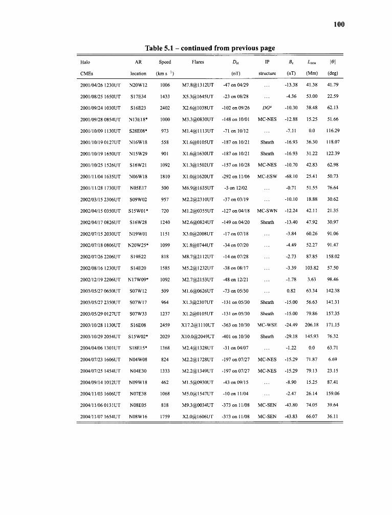
100
Table 5.1 - continued from previous page
Halo AR Speed Flares Dst IP B, Lneu lθl
CMEs location (km s -1 ) (nT) structure (nT) (Mm) (deg)
2001/04/26 1230UT N20W12 1006 M7.8@1312UT -47 on 04/29 ... -13.38 41.38 41.79
2001/08/25 1650UT 517E34 1433 X5.3@1645UT -23 on 08/28 ... -4.36 53.00 22.59
2001/09/24 1030UT 516E23 2402 X2.6@1038UT -102 on 09/26 DG° -10.30 38.48 62.13
2001/09/28 0854UT N13E18* 1000 M3.3@0830UT -148 on 10/01 MC-NES -12.88 15.25 51.66
2001/10/09 1130UT S28E08* 973 M1.4@1113UT -71 on 10/12 ... -7.11 0.0 116.29
2001/10/19 0127UT N16W18 558 X1.6@0105UT -187 on 10/21 Sheath -16.93 36.30 118.07
2001/10/19 1650UT N15W29 901 X1.6@1630UT -187 on 10/21 Sheath -16.93 31.22 122.39
2001/10/25 1526UT S16W21 1092 X1.3@1502UT -157 on 10/28 MC-NES -10.70 42.83 62.98
2001/11/04 1635UT N06W18 1810 X1.0@1620UT -292 on 11/06 MC-ESW -68.10 25.41 50.73
2001/11/28 1730UT N05E17 500 M6.9@1635UT -3 on 12/02 ... -0.71 51.55 76.64
2002/03/15 2306UT S09W02 957 M2.2@2310UT -37 on 03/19 ... -10.10 18.88 30.62
2002/04/15 0350UT S15W01* 720 M1.2@0355UT -127 on 04/18 MC-SWN -12.24 42.11 21.35
2002/04/17 0826UT S16W28 1240 M2.6@0824UT -149 on 04/20 Sheath -13.40 47.92 30.97
2002/07/15 2030UT N19W01 1151 X3.0@2008UT -17 on 07/18 ... -3.84 60.26 91.06
2002/07/18 0806UT N20W25* 1099 X1.8@0744UT -34 on 07/20 ... -4.49 52.27 91.47
2002/07/26 2206UT S19E22 818 M8.7@2112UT -14 on 07/28 ... -2.73 87.85 158.02
2002/08/16 1230UT S14E20 1585 M5.2@1232UT -38 on 08/17 ... -3.39 103.82 57.50
2002/12/19 2206UT N17W09* 1092 M2.7@2153UT -48 on 12/21 ... -1.78 3.63 98.46
2003/05/27 0650UT S07W 12 509 M1.6@0626UT -73 on 05/30 ... 0.82 63.34 142.38
2003/05/27 2350UT S07W17 964 X1.3@2307UT -131 on 05/30 Sheath -15.00 56.63 141.31
2003/05/29 0127UT 507W33 1237 X1.2@0105UT -131 on 05/30 Sheath -15.00 79.86 157.35
2003/10/28 1130UT S16E08 2459 X17.2@1110UT -363 on 10/30 MC-WSE -24.49 206.18 171.15
2003/10/29 2054UT S15W02* 2029 X10.0@2049UT -401 on 10/30 Sheath -29.18 145.93 76.32
2004/04/06 1301UT S18E15* 1368 M2.4@1328UT -31 on 04/07 ... -1.22 0.0 63.71
2004/07/23 1606UT N04W08 824 M2.2@1728UT -197 on 07/27 MC-NES -15.29 71.87 6.69
2004/07/25 1454UT N04E30 1333 M2.2@1349UT -197 on 07/27 MC-NES -15.29 79.13 23.15
2004/09/14 1012UT N09W18 462 M1.5@0930UT -43 on 09/15 -8.90 15.25 87.41
2004/11/03 1606UT N07E38 1068 M5.0@1547UT -10 on 11/04 ... -2.47 26.14 159.06
2004/11/06 0131UT N08E05 818 M9.3@0034UT -373 on 11/08 MC-SEN -43.80 74.05 39.64
2004/11/07 1654UT N08W16 1759 X2.0@1606UT -373 on 11/08 MC-SEN -43.83 66.07 36.11
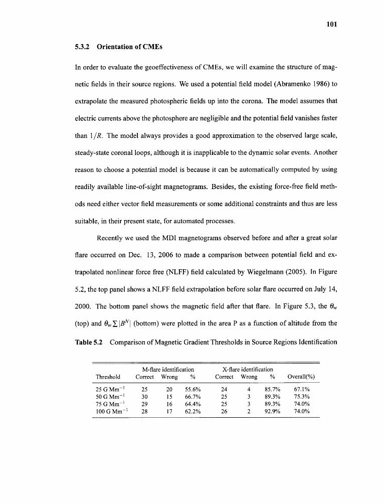
101
5.3.2 Orientation of CMEs
In order to evaluate the geoeffectiveness of CMEs, we will examine the structure of mag-
netic fields in their source regions. We used a potential field model (Abramenko 1986) to
extrapolate the measured photospheric fields up into the corona. The model assumes that
electric currents above the photosphere are negligible and the potential field vanishes faster
than 1 /R. The model always provides a good approximation to the observed large scale,
steady-state coronal loops, although it is inapplicable to the dynamic solar events. Another
reason to choose a potential model is because it can be automatically computed by using
readily available line-of-sight magnetograms. Besides, the existing force-free field meth-
ods need either vector field measurements or some additional constraints and thus are less
suitable, in their present state, for automated processes.
Recently we used the MDI magnetograms observed before and after a great solar
flare occurred on Dec. 13, 2006 to made a comparison between potential field and ex-
trapolated nonlinear force free (NLFF) field calculated by Wiegelmann (2005). In Figure
5.2, the top panel shows a NLFF field extrapolation before solar flare occurred on July 14,
2000. The bottom panel shows the magnetic field after that flare. In Figure 5.3, the 6,
(top) and 0,, BN (bottom) were plotted in the area P as a function of altitude from the
Table 5.2 Comparison of Magnetic Gradient Thresholds in Source Regions Identification
M-flare identification X-flare identificationThreshold Correct Wrong % Correct Wrong % Overall(%)
25 G Mm-1 25 20 55.6% 24 4 85.7% 67.1%50 G Mm -1 30 15 66.7% 25 3 89.3% 75.3%75 G Mm-1 29 16 64.4% 25 3 89.3% 74.0%100 G Mm -1 28 17 62.2% 26 2 92.9% 74.0%
102
photosphere boundary. In this case, 8,000 km appears to be a critical height, below which
the non-potentiality of the active region increases after the flare and above which to a height
of ~ 70,000 km the field is relaxed to a more potential state. Beyond 70,000 km, the fields
are potential both before and after the flare. It implies that the magnetic shear may increase
in a local area near flaring magnetic neutral lines, but, in the large scale, magnetic fields are
relaxed. When it is far enough from solar surface, the potential field model can provide us
with reliable extrapolated results.
Now let us illustrate how magnetic orientation of a CME can be quantified by using
the well studied July 14, 2000 eruption. A halo CME on July 14 2000, first appeared in
the LASCO/C2 FOV at 1054UT. Simultaneously, a great X5.7 solar flare was observed
near the disk center in active region NOAA 9077. The SOHO MDI full disk magnetogram
taken at 0936UT on July 14 2000 is shown in Figure 5.1a. The extrapolated potential field
is presented in Figure 5.4. The magnetic field lines are plotted in either red or green color,
depending on whether their projection is intersect with the HGNL (Figure 5.1c).
Figure 5.5 illustrates how the magnetic orientation angle 0 is defined and calculated
for a source region identified by the HGNL method. An extrapolated field line, L, is shown
by red color, while the gradient neutral line (N) is plotted in blue. Two arbitrary points on
the field line L are indicated with letters P and A. Projection of P and A on the horizontal
plane (photosphere) are P' and A', correspondingly. Hence, the line P'A' is the projection
of L on the surface and it intersects with the gradient neutral line N. The angle between
P'A' and the southward direction is defined as the orientation angle 0. In the entire active
region, numerous field lines have projections that intersect the HGNL and each of them
has its unique orientation angle. Thus, the average orientation angle determined for the
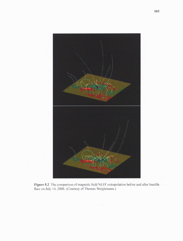
103
Figure 5.2 The comparison of magnetic field NLFF extrapolation before and after bastilleflare on July 14, 2000. (Courtesy of Thomas Weiglemann.)
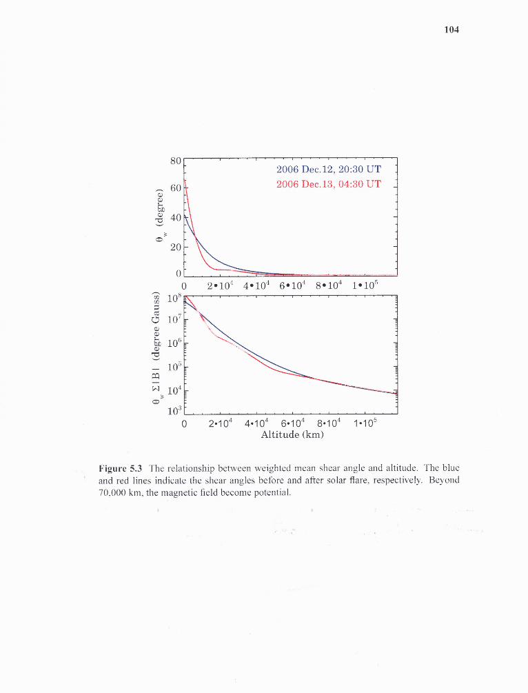
104
Figure 5.3 The relationship between weighted mean shear angle and altitude. The blueand red lines indicate the shear angles before and after solar flare, respectively. Beyond70,000 km, the magnetic field become potential.
105
entire active region is calculated as the median of individual O. In order to get an accurate
orientation angle 0, for each event we extrapolated over several thousands of field lines.
The number of intersected field lines to calculate the average angle are always more than
hundreds. The overall orientation angle of this particular event is about 11.65°, which
indicates southward magnetic field component associated with the neutral line.
5.3.3 The effect of interplanetary CMEs
ICME is the manifestation of a CME in interplanetary (IP) space. Depending on the mag-
netic orientation, an ICME may or may not trigger a large geomagnetic storm. There are
two magnetic structures in an ICME that can carry intense southward IMFs (Gonzalez et al.
1999): the sheath region behind the forward shock (Tsurutani et al. 1988; Tsurutani and
Gonzalez 1997) and an ICME body that can be often observed as a MC (Klein and Burlaga
1982). In the sheath region solar wind plasma is heated, compressed and piled up in front
of the ICME body. Magnetic fields with a rapidly fluctuating orientations are characteristic
for the sheath region. A MC is a large-scale and organized structure that can possess long
intervals of the southwardly directed fields, therefore it is expected to be more geoeffective
than sheath region (Zhang et al. 2004).
Generally, MCs could be modelled by a flux rope model (Mulligan and Russell
2001). The internal magnetic field configuration within a MC is cylindrically symmetric
and force-free, with constant α, where α is the magnitude of the magnetic helicity (Gold-
stein 1983; Burlaga et al. 1998). According to this model, Bothmer and Schwenn (1998)
described four types of MC structures: SWN, NES, SEN and NWS. In the GSE coordinate
system, these types of MCs will produce different magnetic signatures in the spacecraft
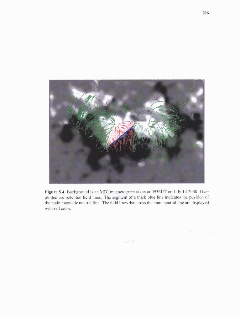
106
Figure 5.4 Background is an MDI magnetogram taken at 0936UT on July 14 2000. Overplotted are potential field lines. The segment of a thick blue line indicates the position ofthe main magnetic neutral line. The field lines that cross the main neutral line are displayedwith red color.
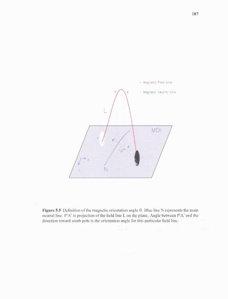
107
Figure 5.5 Definition of the magnetic orientation angle O. Blue line N represents the mainneutral line. P'A' is projection of the field line L on the plane. Angle between P'A' and thedirection toward south pole is the orientation angle for this particular field line.
108
measurements. Assuming that the axis of a MC lies in the ecliptic plane, the SEN type
clouds are those whose magnetic field vector turns from south (S, negative Bz) at the lead-
ing edge to east (E, positive By) at the cloud's axis and finally to the north (N, positive Bz) at
its trailing edge. Such a cloud is left handed (negative helicity). A SWN type cloud has its
axial field pointed westward, while the azimuthal field rotates from S to N direction. This
cloud is right handed (positive helicity). Similarly one can deduct the magnetic field rota-
tion in NES and NWS type clouds. Mulligan et al. (1998) introduced another four types of
MCs: ESW, ENW, WSE and WNE. The axes of these MC structures are perpendicular to
the ecliptic plane. Those MCs with an axes that lies approximately in the ecliptic plane are
called bipolar clouds because Bz can change its sign (rotate) during the passage of satellite.
Unipolar clouds have their axes nearly normal to the ecliptic plane and thus Bz component,
measured by a satellite, is of the same sign.
By studying 34 ICME events, Wu and Lepping (2002) found that geomagnetic
storms can be produced either by a sheath region, the leading or trailing field of a MC or
both the sheath field and the MC itself. In their study, when only bipolar MCs were consid-
ered a cloud's leading field is found to be the major driving force for storms (44.1%). Zhang
et al. (2004) examined the relationship between 271 storms and 104 magnetic clouds. It
is found that the leading field is the most geoeffective region and 72% of intense storms
were caused by MCs. Huttunen et al. (2005) examined 73 MCs observed by the WIND
and ACE instruments in solar cycle 23 and found that in 16 cases the storm was caused by
sheath region preceding the MC and for 21 events neither the sheath nor the MC triggered
the storm.
To determine the effect of magnetic topology of the CME source region on the Bz
109
of IMF and the D st index, we need to understand ICME's IP structures and distinguish be-
tween magnetic fields of the sheath region and a ICME body, and identify a storm driver.
Table 5.1, column 6 lists drivers of geomagnetic storms with D st ≤ -100 nT. They are iden-
tified based on either data from OMNI-data base 3 or obtained from several other studies
(Wang et al. 2003, 2005b; Zhang et al. 2004; Xue et al. 2005; Huttunen et al. 2005). Our
criteria to identify MC are: (1) smooth field rotation is required for all cases in this study;
(2) enhanced field is qualitatively compared with the ambient solar wind values. The refer-
ence field enhancement tended to be ≥ 50% with some exception; (3) The ratio of Nα /Np is
> 0.08-0.10 (Lynch et al. 2003; Xue et al. 2005); (4) The average values of plasma pressure
β is < 0.5 (Huttunen et al. 2005).
Figures 5.6 and 5.7 show ACE measurements data and D st index for two MCs in
observed in 2004. Panels from top to bottom are the total interplanetary magnetic field
B, east-west By and north-south Bz components of IMF (GSE system), latitude (0) and
longitude (0) of the solar wind magnetic field in RTN coordinates, proton temperature T,
ratio of Na /Np , magnetic plasma pressure β, and Dst index. The boundaries of each MCs
are indicated with vertical solid lines and the dashed lines indicate the beginning of sheath
regions. All data are 1-hour averages except the magnetic field data, which are 4-minute
averages.
In these two events, the D st index peaked at 1400UT on July 27 (-197nT) and at
0700UT on Nov 08 (-373nT). The cause of these two geomagnetic storms was the intense
southward IMF in the corresponding MCs. Figure 5.6 shows that southward IMF in the
July 27 MC lasted for about 12 hours and it attained the maximum value of -17.7nT. In
3 http://cdaweb.gsfc.nasa.gov/
110
this event, the field vector rotated from the northern direction (N) at the leading edge to
the southern (S) at the trailing edge and it was eastwardly directed at the cloud's axis (E,
positive Br). Such a MC is of the NES type and it was the trailing field (TF) that caused
the geomagnetic storm (Dst = -197 nT). Figure 5.7 shows a super geomagnetic storm (Dst =
-373nT) caused by another bipolar MC. The maximum southward Bz was -46.17nT, nearly
3 times stronger than that in Figure 5.6. The Bz duration was about 17 hours. The magnetic
field vector in this SEN MC changed from south (S) at the leading, to east (E) at the axis,
to north (N) at the trailing edge. Thus the geomagnetic storm was a result of the strong
southward leading field.
5.4 Results
In Table 5.1 we list results of our study for total of 73 halo CMEs. The first column shows
the date and time of the halo CMEs, the second column provides locations of the source
regions determined from the magnetic gradient method. The next columns are the linear
speed of a CME in the plane of the sky (POS), magnitude and time of associated solar
flares, the corresponding Dst index, the IP structures of ICME that caused the storm (only
for strong storms), the maximum southward component Bz, the length of main NL and the
orientation of magnetic structure in the source region.
5.4.1 Effectiveness of HGNL method on identification of flaring active
regions
Figure 5.8 shows the distribution of the number of events versus their calculated //rim.
For comparison, the events associated with X-class or M-class flares are separated and
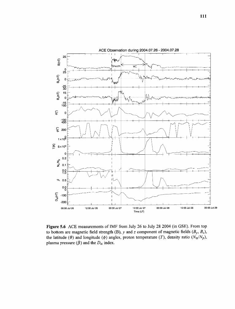
111
Figure 5.6 ACE measurements of IMF from July 26 to July 28 2004 (in GSE). From topto bottom are magnetic field strength (B), y and z component of magnetic fields (By , Br),the latitude (0) and longitude (0) angles, proton temperature (T), density ratio (Nα/Np),plasma pressure (β) and the Dst index.
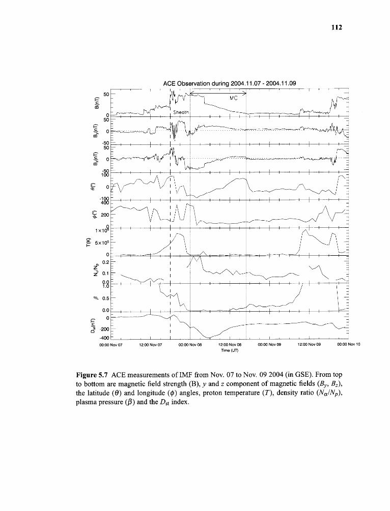
112
Figure 5.7 ACE measurements of IMF from Nov. 07 to Nov. 09 2004 (in GSE). From topto bottom are magnetic field strength (B), y and z component of magnetic fields (By , Br),the latitude (0) and longitude (0) angles, proton temperature (T), density ratio (Nα/Np ),plasma pressure (/3) and the Dst index.
113
displayed in panels (a) and (b). The median Lneu in panel (a) was in the range of 30-60
Mm, while it was much longer than that found in M-class events. Meanwhile, the range of
L. shown in panel (a) (up to 200 Mm) is also wider than that in panel (b). This is probably
because that X flares are extreme events and their tendency to occur at the location with
high concentration of free magnetic energy is much higher than that for the M-class flares.
In 25% of cases (18 out of 73, indicated by asterisks) the magnetic gradient method
produced wrong results and thus the location of source regions was different from that listed
in NOAA SEC reports. Furthermore, 11 out of these 18 events (61%) have Lneu shorter
than 20 Mm. Table 5.2 shows how the selection of the gradient threshold affects the source
identification. A sufficiently high threshold may improve the accuracy of identification
from 67% up to 75%. There is a limit on the gradient threshold, i.e., we can only improve
accuracy to a certain extent: further increase of the threshold value does not lead to a
significant increase in the accuracy. In this study the highest overall accuracy is about 75%
when the threshold was 50 G Mm -1 . When we divided events based on the magnitudes
of associated flares, the HGNL method produced better results for X-class flares (89%
success) as compared to the M-class flares (68% success).
The limitation of HGNL method could be due to the fact that several active regions
are in the same full disk MDI magnetogram. The region identified by HGNL method is
indeed 'active', however, it was not responsible for any CME eruptions. Such a limit might
be solved by the combination of LASCO information about CMEs, or the power spectra
method proposed by Abramenko (2005). Therefore, we conclude that the prediction on
the CME source region with the HGNL method is feasible, especially for those events
associated with X-class flares.
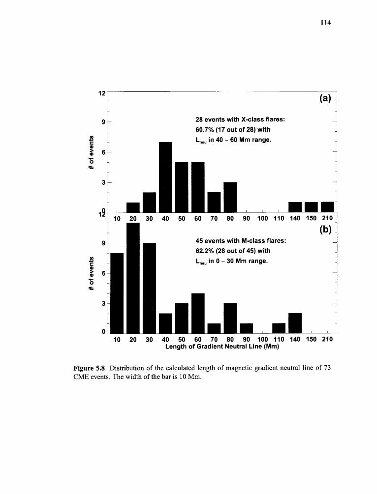
114
Figure 5.8 Distribution of the calculated length of magnetic gradient neutral line of 73CME events. The width of the bar is 10 Mm.
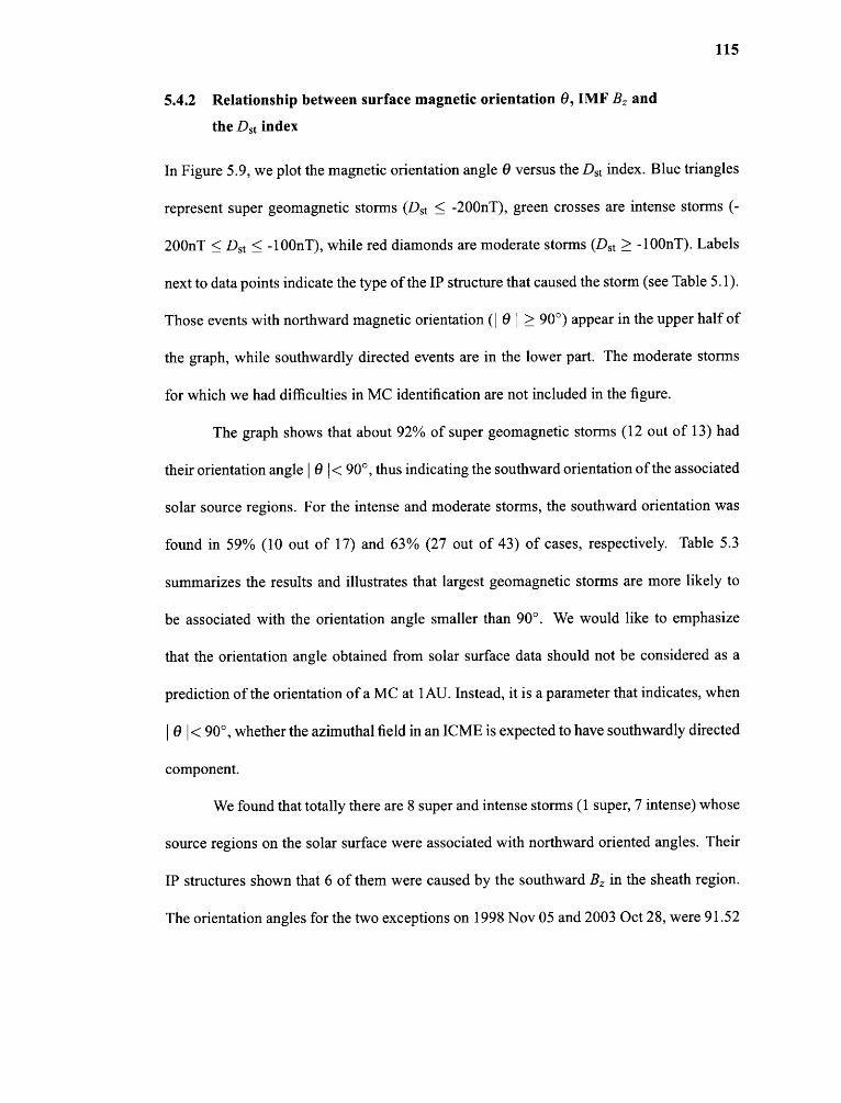
115
5.4.2 Relationship between surface magnetic orientation 0, IMF Bz and
the Dst index
In Figure 5.9, we plot the magnetic orientation angle 0 versus the Dst index. Blue triangles
represent super geomagnetic storms (D st < -200nT), green crosses are intense storms (-
200nT < Dst < -100nT), while red diamonds are moderate storms (D st > -100nT). Labels
next to data points indicate the type of the IP structure that caused the storm (see Table 5.1).
Those events with northward magnetic orientation (I θI≥90°) appear in the upper half of
the graph, while southwardly directed events are in the lower part. The moderate storms
for which we had difficulties in MC identification are not included in the figure.
The graph shows that about 92% of super geomagnetic storms (12 out of 13) had
their orientation angle I θ I< 90°, thus indicating the southward orientation of the associated
solar source regions. For the intense and moderate storms, the southward orientation was
found in 59% (10 out of 17) and 63% (27 out of 43) of cases, respectively. Table 5.3
summarizes the results and illustrates that largest geomagnetic storms are more likely to
be associated with the orientation angle smaller than 90°. We would like to emphasize
that the orientation angle obtained from solar surface data should not be considered as a
prediction of the orientation of a MC at 1AU. Instead, it is a parameter that indicates, when
0 < 90°, whether the azimuthal field in an ICME is expected to have southwardly directed
component.
We found that totally there are 8 super and intense storms (1 super, 7 intense) whose
source regions on the solar surface were associated with northward oriented angles. Their
IP structures shown that 6 of them were caused by the southward Bz in the sheath region.
The orientation angles for the two exceptions on 1998 Nov 05 and 2003 Oct 28, were 91.52
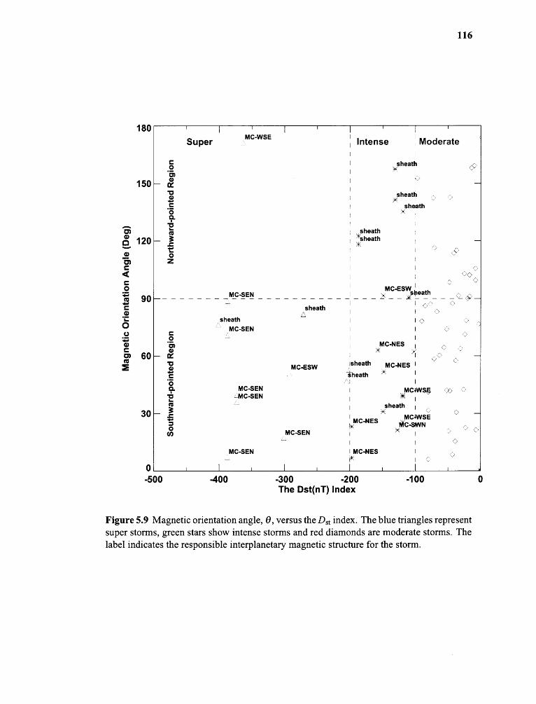
116
Figure 5.9 Magnetic orientation angle, 0, versus the Dst index. The blue triangles representsuper storms, green stars show intense storms and red diamonds are moderate storms. Thelabel indicates the responsible interplanetary magnetic structure for the storm.
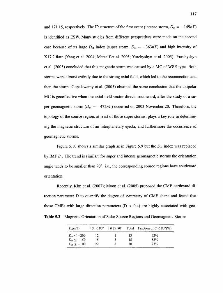
117
and 171.15, respectively. The IP structure of the first event (intense storm, D st = —149n T)
is identified as ESW. Many studies from different perspectives were made on the second
case because of its large Dst index (super storm, D st = —363nT) and high intensity of
X17.2 flare (Yang et al. 2004; Metcalf et al. 2005; Yurchyshyn et al. 2005). Yurchyshyn
et al. (2005) concluded that this magnetic storm was caused by a MC of WSE-type. Both
storms were almost entirely due to the strong axial field, which led to the reconnection and
then the storm. Gopalswamy et al. (2005) obtained the same conclusion that the unipolar
MC is geoeffective when the axial field vector directs southward, after the study of a su-
per geomagnetic storm (D st = —472nT) occurred on 2003 November 20. Therefore, the
topology of the source region, at least of those super storms, plays a key role in determin-
ing the magnetic structure of an interplanetary ejecta, and furthermore the occurrence of
geomagnetic storms.
Figure 5.10 shows a similar graph as in Figure 5.9 but the D st index was replaced
by IMF B. The trend is similar: for super and intense geomagnetic storms the orientation
angle tends to be smaller than 90°, i.e., the corresponding source regions have southward
orientation.
Recently, Kim et al. (2007); Moon et al. (2005) proposed the CME earthward di-
rection parameter D to quantify the degree of symmetry of CME shape and found that
those CMEs with large direction parameters (D > 0.4) are highly associated with geo-
Table 5.3 Magnetic Orientation of Solar Source Regions and Geomagnetic Storms
Dst (nT) I 0 I< 90° I 0 I> 90° Total Fraction of 0 < 90° (%)
Dst ≤ —200 12 1 13 92%Dst < —150 15 3 18 83%
Dst < —100 22 8 30 73%
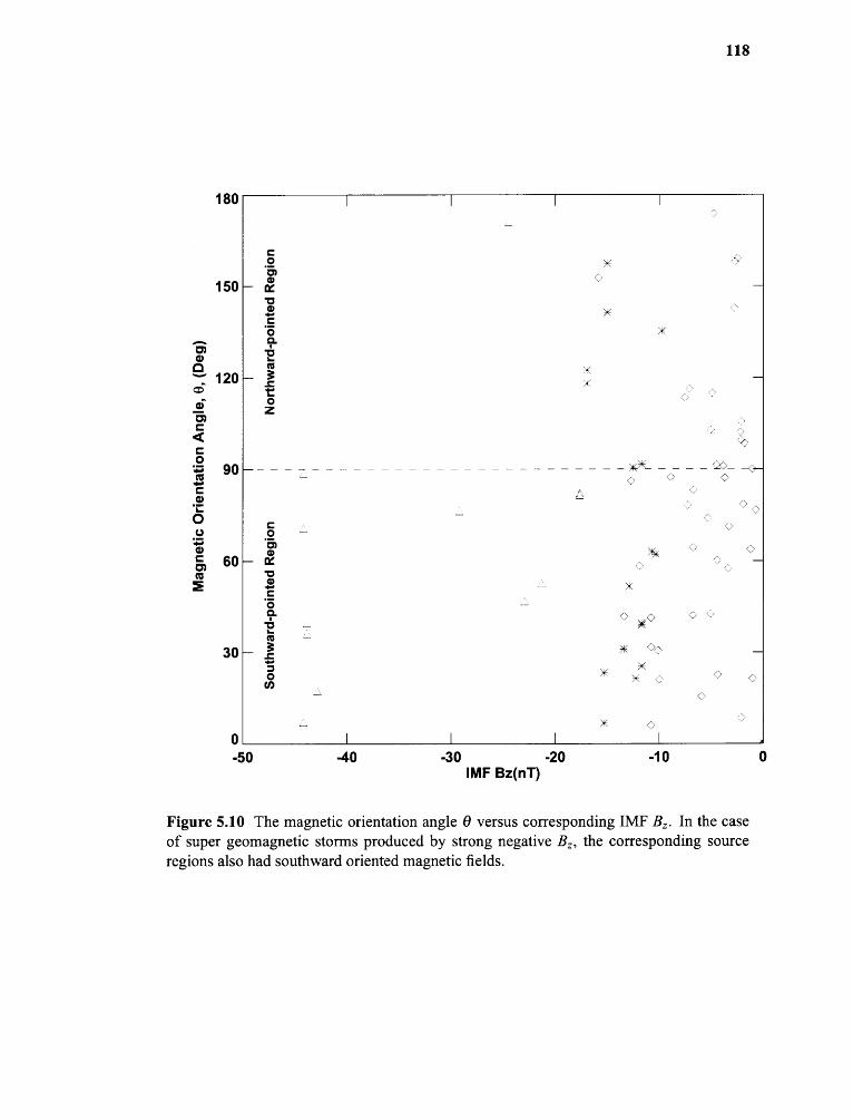
118
Figure 5.10 The magnetic orientation angle 0 versus corresponding IMF B. In the caseof super geomagnetic storms produced by strong negative Bz, the corresponding sourceregions also had southward oriented magnetic fields.
119
magnetic storms and their association probability rises from 52% to 84% as the direction
parameter increases from 0.4 to 1.0. Among the events listed in Table 5.1, they selected 64
CMEs whose direction parameters are well determined. They found that those six excep-
tional events that have northward magnetic field orientations but cause strong geomagnetic
storms (Dst < —100nT) all have large direction parameters (D < 0.6). The combination
of magnetic orientation angle 0 and direction parameter D might help us to improve the
accuracy of geomagnetic storms prediction.
5.5 Conclusions and Discussion
Automatic prediction of super geomagnetic storms (D st < -200nT) is an important task in
space weather programs. In our present work, the automatic prediction is performed in the
following procedures:
— identification of CME source regions: longitudinal magnetic gradient and gradient neutral
lines are calculated from full disk SOHO MDI magnetograms by using a suitable threshold
value (50 G Mm -1 ). The solar active regions most probable to launch a CME are located
on the solar disk by identifying locations with the largest length of the strongest HGNL.
Due to the projection effect on HGNL calculation, those active regions close to the limb of
solar disk might not be identified by HGNL method.
— potential field extrapolation: a potential field model is used to extrapolate coronal mag-
netic fields of the selected source region. Those extrapolated field lines that intersect with
the strongest HGNL are chosen to calculate the magnetic orientation angle 0.
— prediction: the magnetic orientation angle is used to predict the presence of southward
Bz in an ejecta: The events associated with 0 < 90° are more likely to cause a super

120
geomagnetic storm.
Based on a study of 73 halo CMEs associated with M and X class flares that oc-
curred between 1996 and 2004, we have reached the following conclusions:
1. Magnetic gradient method is proved to be a viable approach to locate the source
region of either CMEs or flares. The overall accuracy is about 75% (55 out of 73 events).
It appears to be more accurate in identification of sources of X-class flares (89%) than
M-class flares (68%).
2. The magnetic orientation angle 0, determined from a potential field model, can
be used to predict the probability of super geomagnetic storms (D st ≤ -200nT). About
92% of the super storms (12 out of 13 events) were associated with solar source regions
that had orientation angles 6 smaller than 90°, i.e. southward oriented magnetic fields.
Geomagnetic storms with northward oriented source region ( 0 > 90°) may be caused by
the sheath region and/or unipolar magnetic clouds.
3. The relationship between the Dst index and the orientation angle indicates that,
at least for super storms, the topology of the source region plays a key role in determining
the magnetic structure of an interplanetary ejecta.
CHAPTER 6
SUMMARY
This dissertation has covered a series of relationships between magnetic features of solar
active regions, solar activities such as solar flares, CMEs, etc. and the induced geomag-
netic storms in the interplanetary space. The following contributions to the space weather
forecasting have been made as part of this disseration:
1. The statistical ordinal logistic regression model is first time applied into solar
physics study and is proved to be a viable approach to automated predict the occurrance
probability of solar flares in next 24 hours. The predictive variables used in the model so
far are magnetic parameters obtained through SOHO MDI magnetograms. The model is
easy to extend to include other parameters, in order to improve the forecast ability. The
results are much better than those publised in NASA/SDAC service, and comparable to the
data provied by NOAA/SEC service. The major breakthrough is that solar flare might be
forecasted automatically and quantitively.
2. The magnetic orientation angle 0, determined from a potential field model, can
be used to predict the probability of super geomagnetic storms (D st ≤ -200nT). About 92%
of the super storms (12 out of 13 events) were associated with solar source regions that
had orientation angles 0 smaller than 90°, i.e. southward oriented magnetic fields. Ge-
omagnetic storms with northward oriented source region (1 0 1 > 90°) may be caused by
the sheath region and/or unipolar magnetic clouds. The relationship between D st index and
the orientation angle indicates that at least for super geomagnetic storms, the topology of
the source region plays a key role in determining the magnetic structure of an interplan-
121
122
etary ejecta. Meanwhile, the potential field extrapolation model is proved as accurate as
nonlinear extrapolation model, when the distance is far from solar surface.
3. Compared with magnetic shear, magnetic gradient might be a better proxy to
locate the source region of where a larger flare or CME occurs. Based on a study of 73
halo CMEs associated with larger flares, the overall identification accuracy is about 75%
(55 out of 73 events). It appears to be more accurate in identification of sources of X-class
flares (89%) than M-class flares (68%).
REFERENCES
Abramenko, V. I.: 1986, Solnechnye Dann. Bull. Akad. Nauk SSSR 8, 83.
Abramenko, V. I.: 2005, Astrophys. J. 629, 1141.
Abramenko, V. I., Gopasiuk, S. I., and Ogir', M. B.: 1991, Sol. Phys. 134, 287.
Abramenko, V. I., Yurchyshyn, V. B., Wang, H., Spirock, T. J., and Goode, P. R.: 2003,Astrophys. J. 597, 1135.
Agresti, A.: 1996, An introduction to categorical data analysis, New York:Wiley
Ai, G.-X.: 1987, Publications of the Beijing Astronomical Observatory 9, 27.
Alzola, A. and Harrell, F.: 2004, An Introduction to S and the Hmisc and Design Libraries,Free available electronic book.
Antalova, A.: 1996, Contributions of the Astronomical Observatory Skalnate Pleso 26, 98.
Baker, D. N.: 2001, in I. A. Daglis (ed.), Space Storms and Space Weather Hazards, p.285.
Barnes, A.: 1992, Reviews of Geophysics 30, 43.
Beard, D. B.: 1964, Reviews of Geophysics and Space Physics 2, 335.
Bornmann, P. L. and Shaw, D.: 1994, Sol. Phys. 150, 127.
Bothmer, V. and Schwenn, R.: 1994, Space Science Reviews 70, 215.
Bothmer, V. and Schwenn, R.: 1998, Ann. Geophys. 16, 1.
Breiman, L.: 1992, Journal of the American Statistical Association 87, 738.
Brueckner, G. E., Delaboudiniere, J.-P., Howard, R. A., Paswaters, S. E., St. Cyr, 0. C.,Schwenn, R., Lamy, P., Simnett, G. M., Thompson, B., and Wang, D.: 1998, Geo-phys. Res. Lett. 25, 3019.
Burlaga, L., Fitzenreiter, R., Lepping, R., Ogilvie, K., Szabo, A., Lazarus, A., Steinberg, J.,Gloeckler, G., Howard, R., Michels, D., Farrugia, C., Lin, R. P., and Larson, D. E.:1998, 1 Geophys. Res. 103, 277.
Burlaga, L., Sittler, E., Mariani, F., and Schwenn, R.: 1981, 1 Geophys. Res. 86, 6673.
Burlaga, L. F., Skoug, R. M., Smith, C. W., Webb, D. F., Zurbuchen, T. H., and Reinard,A.: 2001, J. Geophys. Res. 106, 20957.
Cane, H. V., Richardson, I. G., and Cyr, 0. C. S.: 2000, Geophys. Res. Lett. 27, 3591.
Cole, D. G.: 2003, Space Sci. Rev. 107, 295.
123
124
Cragg, J. and Uhler, R.: 1970, Canadian Journal of Economics 3, 386.
Deng, Y., Wang, J., Yan, Y., and Zhang, J.: 2001, Sol. Phys. 204, 11.
Dungey, J. W.: 1961, Phys. Rev. Lett. 6, 47.
Efron, B.: 1986, Journal of the American Statistical Association 81, 461.
Falconer, D. A.: 2001, J. Geophys. Res. 106, 25185.
Falconer, D. A., Moore, R. L., and Gary, G. A.: 2003, Journal of Geophysical Research(Space Physics) 108, 11.
Fletcher, L. and Hudson, H.: 2001, Sol. Phys. 204, 69.
Formisano, V., Moreno, G., and Amata, E.: 1974, 1 Geophys. Res. 79, 5109.
Gallagher, P. T., Moon, Y.-J., and Wang, H.: 2002, Sol. Phys. 209, 171.
Gary, G. A. and Hagyard, M. J.: 1990, Sol. Phys. 126, 21.
Geological Survey of Canada: 2002, Space Weather Effects on Technology, Technicalreport, http://www.spaceweather.gc.ca/effects_e.shtml.
Gold, T.: 1959, 1 Geophys. Res. 64, 1665.
Goldstein, H.: 1983, in M. Neugebauer (ed.), Solar Wind Conference, p. 731.
Gonzalez, W. D., Joselyn, J. A., Kamide, Y., Kroehl, H. W., Rostoker, G., Tsurutani, B. T.,and Vasyliunas, V. M.: 1994, 1 Geophys. Res. 99, 5771.
Gonzalez, W. D., Tsurutani, B. T., and Chia de Gonzalez, A. L.: 1999, Space Sci. Rev. 88,529.
Gopalswamy, N., Lara, A., Lepping, R. P., Kaiser, M. L., Berdichevsky, D., and St. Cyr,0. C.: 2000, Geophys. Res. Lett. 27, 145.
Gopalswamy, N., Yashiro, S., Michalek, G., Xie, H., Lepping, R. P., and Howard, R. A.:2005, Geophys. Res. Lett. 32, 12.
Gosling, J. T.: 1993, J. Geophys. Res. 98, 18937.
Hagyard, M. J.: 1990, Mem. Soc. Astron. Ital. 61, 337.
Hagyard, M. J., Teuber, D., West, E. A., and Smith, J. B.: 1984, Sol. Phys. 91, 115.
Hargreaves, J. K.: 1992, The solar-terrestrial environment, Cambridge atmospheric andspace science series, Cambridge: Cambridge University Press, 1992.
Harrell, F. E.: 2001, Regression Modeling Strategies With Application to Linear Models,Logistic Regression, and Survival Analysis , Springer.
125
Howard, R. A., Michels, D. J., Sheeley, Jr., N. R., and Koomen, M. J.: 1982, Astrophys.Lett. 263, L101.
Howard, T. A. and Tappin, S. J.: 2005, Astron. Astrophys. 440, 373.
Hudson, H. S., Lemen, J. R., St. Cyr, 0. C., Sterling, A. C., and Webb, D. F.: 1998,Geophys. Res. Lett. 25, 2481.
Hundhausen, A. J.: 1993, 1 Geophys. Res. 98, 13177.
Huttunen, K. E. J., Schwenn, R., Bothmer, V., and Koskinen, H. E. J.: 2005, Ann. Geophys.23, 625.
Jing, J., Song, H., Abramenko, V., Tan, C., and Wang, H.: 2006, Astrophys. J. 644, 1273.
Joshi, B. and Joshi, A.: 2004, Sol. Phys. 219, 343.
Kim, R.-S., Cho, K.-S., Moon, Y.-J., Kim, Y.-H., Park, Y. D., Yi, Y., Lee, J., Wang, H.,Song, H., and Dryer, M.: 2007, Astrophys. J., submitted.
Klein, L. W. and Burlaga, L. F.: 1982, 1 Geophys. Res. 87, 613.
Kosovichev, A. G. and Zharkova, V. V.: 2001, Astrophys. 1, Lett. 550, L105.
LaBonte, B. J., Mickey, D. L., and Leka, K. D.: 1999, Sol. Phys. 189, 1.
Landi, R., Moreno, G., Storini, M., and Antalová, A.: 1998, 1 Geophys. Res. 103, 20553.
Leka, K. D. and Barnes, G.: 2003a, Astrophys. J. 595, 1277.
Leka, K. D. and Barnes, G.: 2003b, Astrophys. J. 595, 1296.
Leka, K. D., Canfield, R. C., McClymont, A. N., de La Beaujardiere, J.-F., Fan, Y., andTang, F.: 1993, Astrophys. J. 411, 370.
Li, H.: 2002, Chinese Journal of Astronomy and Astrophysics 2, 174.
Liu, Y. and Zhang, H.: 2001, Astron. Astrophys. 372, 1019.
Longcope, D. W., Fisher, G. H., and Arendt, S.: 1996, Astrophys. J. 464, 999.
Lynch, B. J., Zurbuchen, T. H., Fisk, L. A., and Antiochos, S. K.: 2003, Journal of Geo-physical Research (Space Physics) 108, 6.
MacQueen, R. M. and Fisher, R. R.: 1983, Sol. Phys. 89, 89.
Masuda, S., Kosugi, T., and Hudson, H. S.: 2001, Sol. Phys. 204, 55.
McCullagh, P.: 1980, 1 Royal Statistical Society p. 109.
McIntosh, P. S.: 1990, Sol. Phys. 125, 251.
126
Metcalf, T. R., Leka, K. D., and Mickey, D. L.: 2005, Astrophys. J., Lett. 623, L53.
Mickey, D. L., Canfield, R. C., Labonte, B. J., Leka, K. D., Waterson, M. F., and Weber,H. M.: 1996, Sol. Phys. 168, 229.
Monin, G. and Yaglom, A.: 1975, Statistical Fluid Mechanics: Mechanics of Turbulence,Cambridge:MIT Press
Moon, Y.-J., Cho, K.-S., Dryer, M., Kim, Y.-H., Bong, S.-c., Chae, J., and Park, Y. D.:2005, Astrophys. J. 624, 414.
Moon, Y.-J., Wang, H., Spirock, T. J., Goode, P. R., and Park, Y. D.: 2003, Sol. Phys. 217,79.
Moreton, G. E. and Severny, A. B.: 1968, Sol. Phys. 3, 282.
Mulligan, T. and Russell, C. T.: 2001, J. Geophys. Res. 106, 10581.
Mulligan, T., Russell, C. T., and Luhmann, J. G.: 1998, Geophys. Res. Lett. 25, 2959.
Mursula, K. and Ulich, T.: 1998, Geophys. Res. Lett. 25, 1837.
Nagelkerke, N.: 1991, Biometrika 247, 205.
Neugebauer, M. and Snyder, C. W.: 1966, Average properties of the solar wind as deter-mined by Mariner II, Pasadena, Jet Propulsion Laboratory, California Institute ofTechnology, 1966.
Park, Y. D., Moon, Y.-J., Kim, I. S., and Yun, H. S.: 2002, Astrophys. Space. Sci. 279, 343.
Parker, E.: 1959, 1 Geophys. Res. 64, 1675.
Parker, E. N.: 1958, Astrophys. J 128, 664.
Parker, E. N.: 1979, Cosmical Magnetic Fields, Oxford: Clarendon Press
Parker, E. N.: 1987, Sol. Phys. 111, 297.
Petrovay, K. and Szakaly, G.: 1993, Astron. Astrophys. 274, 543.
Prasad, C.: 2000, Astrophys. Space. Sci. 274, 463.
Rust, D. M.: 1994, Geophys. Res. Lett. 21, 241.
Sawyer, C., Warwick, J. W., and Dennett, J. T.: 1986, Solar flare prediction, Researchsupported by Navy. Boulder, CO, Colorado Associated University Press, 1986, 191P.
Schrijver, C. J.: 2007, Astrophys. I Lett. 655, L117.
Scott, S., Goldberg, M. S., and Mayo, N. E.: 1997, I Clinical Epidemiology 50, 45.
127
Severny, A. B., Stepanyan, N. N., and Steshenko, N. V.: 1979, in R. F. Donnelly (ed.),NOAA Solar-Terrestrial Predictions Proceedings. Volume 1., Vol. 1, p. 72.
Sheeley, Jr., N. R., Howard, R. A., Koomen, M. J., and Michels, D. J.: 1983, Astrophys. J.272, 349.
Smith, E. J., Tsurutani, B. T., and Rosenberg, R. L.: 1978, J. Geophys. Res. 83, 717.
Song, H., Yurchyshyn, V., Yang, G., Tan, C., Chen, W., and Wang, H.: 2006, Sol. Phys.238, 141.
Spirock 2005, T., Ph.D. thesis
St. Cyr, 0. C., Plunkett, S. P., Michels, D. J., Paswaters, S. E., Koomen, M. J., Simnett,G. M., Thompson, B. J., Gurman, J. B., Schwenn, R., Webb, D. F., Hildner, E., andLamy, P. L.: 2000, J. Geophys. Res. 105, 18169.
Sterling, A. C. and Hudson, H. S.: 1997, Astrophys. J., Lett. 491, L55.
Stone, C. J. and Koo, C. Y.: 1985, in Proceedings of the Statistics Computing Section ASA,Washington, DC, p. 45.
Tanaka, K.: 1991, Sol. Phys. 136, 133.
Tang, F.: 1983, Sol. Phys. 89, 43.
Thompson, B. J., Gurman, J. B., Neupert, W. M., Newmark, J. S., Delaboudinière, J.-P.,St. Cyr, 0. C., Stezelberger, S., Dere, K. P., Howard, R. A., and Michels, D. J.:1999, Astrophys. J., Lett. 517, L151.
Tian, L., Liu, Y., and Wang, J.: 2002, Sol. Phys. 209, 361.
Tsurutani, B. and Gonzalez, W.: 1997, Geophysics Monography 98, 77.
Tsurutani, B. T.: 2001, in I. A. Daglis (ed.), Space Storms and Space Weather Hazards, p.103.
Tsurutani, B. T., Smith, E. J., Gonzalez, W. D., Tang, F., and Akasofu, S. I.: 1988, J.Geophys. Res. 93, 8519.
Vennerstroem, S.: 2001, J. Geophys. Res. 106, 29175.
Wang, H., Ewell, Jr., M. W., Zirin, H., and Ai, G.: 1994a, Astrophys. J. 424, 436.
Wang, H., Liu, C., Deng, Y., and Zhang, H.: 2005a, Astrophys. J. 627, 1031.
Wang, H., Varsik, J., Zirin, H., Canfield, R. C., Leka, K. D., and Wang, J.: 1992, Sol. Phys.142, 11.
Wang, H.-M., Song, H., Jing, J., Yurchyshyn, V., Deng, Y.-Y., Zhang, H.-Q., Falconer, D.,and Li, J.: 2006, Chinese Journal of Astronomy and Astrophysics 6, 477.
128
Wang, J., Shi, Z., Wang, H., and Lue, Y.: 1996, Astrophys. J. 456, 861.
Wang, T., Xu, A., and Zhang, H.: 1994b, Sol. Phys. 155, 99.
Wang, Y., Ye, P., Zhou, G., Wang, S., Wang, S., Yan, Y., and Wang, J.: 2005b, Sol. Phys.226, 337.
Wang, Y. M., Ye, P. Z., and Wang, S.: 2003, Journal of Geophysical Research (SpacePhysics) 108, 6.
Wang, Y. M., Ye, P. Z., Wang, S., Zhou, G. P., and Wang, J. X.: 2002, J. Geophys. Res.107, 2.
Warmuth, A., Vršnak, B., Magdalenić, J., Hanslmeier, A., and Otruba, W.: 2004, Astron.Astrophys. 418, 1117.
Webb, D. F., Cliver, E. W., Crooker, N. U., Cry, 0. C. S., and Thompson, B. J.: 2000, J.Geophys. Res. 105, 7491.
Webb, D. F. and Howard, R. A.: 1994, J. Geophys. Res. 99, 4201.
Wiegelmann, T.: 2005, in D. E. Innes, A. Lagg, and S. A. Solanki (eds.), Chromosphericand Coronal Magnetic Fields, Vol. 596 of ESA Special Publication
Wolfe, J. H., Silva, R. W., and Myers, M. A.: 1966, J. Geophys. Res. 71, 1319.
Wu, C.-C. and Lepping, R. P.: 2002, 1 Geophys. Res. 107, 19.
Xue, X. H., Wang, Y., Ye, P. Z., Wang, S., and Xiong, M.: 2005, Planet. Space Sci. 53,443.
Yan, Y., Deng, Y., Karlický, M., Fu, Q., Wang, S., and Liu, Y.: 2001, Astrophys. J. Lett.551, L115.
Yang, G., Xu, Y., Cao, W., Wang, H., Denker, C., and Rimmele, T. R.: 2004, Astrophys. J.,Lett. 617, L151.
Yashiro, S., Gopalswamy, N., Michalek, G., St. Cyr, 0. C., Plunkett, S. P., Rich, N. B., andHoward, R. A.: 2004, Journal of Geophysical Research (Space Physics) 109, 7105.
Yurchyshyn, V., Hu, Q., and Abramenko, V.: 2005, Space Weather 3, 8.
Yurchyshyn, V. B., Wang, H., Goode, P. R., and Deng, Y.: 2001, Astrophys. J. 563, 381.
Zhang, H.: 2001, Astrophys. 1, Lett. 557, L71.
Zhang, H., Labonte, B., Li, J., and Sakurai, T.: 2003a, Sol. Phys. 213, 87.
Zhang, J., Dere, K. P., Howard, R. A., and Bothmer, V.: 2003b, Astrophys. 1 582, 520.
Zhang, J., Liemohn, M. W., Kozyra, J. U., Lynch, B. J., and Zurbuchen, T. H.: 2004,Journal of Geophysical Research (Space Physics) 109, 9101.

129
Zirin, H.: 1988, Astrophysics of the Sun, Cambridge and New York, Cambridge UniversityPress, 1988, 440 p.
Zirin, H. and Liggett, M. A.: 1987, Sol. Phys. 113, 267.
Zvereva, A. M. and Severnyj, A. B.: 1970, Izvestiya Ordena Trudovogo Krasnogo ZnameniKrymskoj Astrofizicheskoj Observatorii 41, 97.


