Embed Size (px)
Citation preview
Bargaining versus Posted Price Competition in Customer Markets
Timothy N. Cason Department of Economics
Krannert School of Management Purdue University
West Lafayette, IN 47907-1310 [email protected]
Daniel Friedman and Garrett H. Milam
Department of Economics 217 Social Sciences I
University of California Santa Cruz, CA 95064
[email protected] and [email protected]
October 5, 2001
Abstract:
We compare posted price and bilateral bargaining (or “haggle”) market institutions in 12 pairs of laboratory market sessions. Each session runs for 50-75 periods in a customer market environment, where buyers incur a cost to switch sellers. Costs evolve following a random walk process. Coasian and New Institutionalist traditions provide competing conjectures on relative market performance. We find that efficiency is lower, sellers price higher, and prices are stickier under haggle than under posted offer. Acknowledgements: We thank the NSF for funding the work under grants SBR-9617917 and SBR-9709874; Brian Eaton for programming assistance, and Alessandra Cassar, Svetlana Pevnitskya and Sujoy Chakravarty for help in running the experimental sessions. We benefited from the comments of three anonymous referees, Flavio Menezes, John Morgan, Shyam Sunder, and participants at the March 2000 Tokyo Experimental Economics Conference, the September 2000 Tucson ESA workshop, the October 2000 Rio de Janeiro LACEA Conference and the January 2001 New Orleans ASSA meetings. We retain responsibility for any errors.
Bargaining versus Posted Price Competition in Customer Markets
1. Introduction
The ancient practice of price negotiation, or haggling, has largely been replaced in
industrialized societies by sellers posting prices. Posted prices save time, a tremendous advantage
in retail markets—imagine having to negotiate individual prices for every item you purchased at
the supermarket! However, haggling has not entirely disappeared and, beyond time costs, it is not
clear which institution better promotes efficiency. Nor is it clear how the two institutions
influence the division of surplus. Such questions become increasingly important as electronic
commerce transforms transaction costs, including time costs for negotiations, which can be
conducted now by “shop bots” (e.g., Eisenberg, 2000).
Laboratory comparison of market institutions has a history going back at least to Plott
and Smith (1978). The laboratory is especially appropriate for our questions because it allows
control of key features such as time costs that confound inferences from field data.
The present paper reports a laboratory experiment comparing the efficiency, the surplus
distribution and the price dynamics of two market institutions, the familiar seller posted offer
institution and a new bilateral bargaining institution called “haggle.” In the haggle institution, as
in the continuous double auction, each buyer and seller can continuously improve her own offer
or accept a counterparty offer at any moment during a trading period of known duration. In
haggle, but not in the continuous double auction, each offer is extended only to a single
counterparty, not to all possible counterparties. In the posted offer institution, sellers post a single
take-it-or-leave-it price each period, which buyers either accept or reject.
The laboratory environment we use is a “customer” market, a term coined by Okun
(1981). Each buyer is attached to a particular seller and must pay a switch cost to transact with
2
another seller. Switch costs are important in labor markets (where they include search, relocation
and retraining) and in many intermediate and wholesale markets, and are present even in retail
markets (think of the shopper’s extra time cost in an unfamiliar supermarket). Customer markets
are the natural habitat for haggle, since starting negotiations with a new counterparty normally
entails some setup cost. The posted offer institution is also common in customer markets and has
already been studied in the laboratory (e.g., Cason and Friedman, 2000).
No formal models are available for comparing market institutions in customer markets,1
but it is not hard to find cogent arguments with conflicting predictions. A strong oral tradition
rooted in Coase (1960) holds that parties will find ways to exhaust mutual gains unless artificial
barriers are imposed (De Meza, 1998). The continuous bargaining protocol in haggle imposes
fewer barriers than the unilateral, one-shot, take-it-or-leave-it offer allowed in the posted offer
institution, so haggle should be more efficient. Moreover, haggle permits first degree price
discrimination and thus should enhance efficiency while allowing sellers to capture a greater
share of the surplus.
New institutionalists might make the opposite predictions, based on incomplete
information considerations. The posted offer institution is a solution to the “fundamental problem
of commerce,” the tendency of buyers and sellers to underreveal their willingness to transact in
order to extract more favorable prices (e.g., Myerson and Satterthwaite, 1983; Milgrom and
Roberts, 1992; McKelvey and Page, 2000). Posted offer constrains these tendencies more than
haggle and hence should facilitate more efficient exchange. According to this view, sellers’
commitment technology in posted offer should allow them to extract a larger share of the surplus
than in haggle, where constraints and bargaining opportunities are more symmetric. 1 Formal comparisons in a static setting (i.e., no ongoing attachments or persistent cost shocks) include Julien et al. (2000) and Camera and Delacroix (2001).
3
The two market institutions are of special interest from an historical or evolutionary
perspective. Haggle spans the gap between pre-market gift exchange and early organized
marketplaces. Historically it has tended to be displaced by more complicated or structured forms
of exchange like posted offer (North, 1991), but it still holds a major share in modern economies
(e.g., procurement, car dealers, and wholesale transactions) as well as in traditional economies
like Morocco (Geertz et al., 1979). In the field, transactors’ time costs are higher for haggle than
for posted offer. Additionally, the expansion of retail from single proprietor "Mom and Pop"
outlets into chain stores leads to agency problems that favor posted prices. These factors account
for the shift into posted offer in modern economies, particularly for standardized, small ticket
items. The use of new information technology such as the Internet and automated 'price bots'
may overcome these obstacles. Indeed haggling is reemerging in e-commerce with such sites as
MakeUsAnOffer.com and Priceline.com, perhaps because sellers believe it will allow them to
extract a larger share of the surplus. In the laboratory we can remove agency problems and
equalize the time cost in order to test such conjectures and thus better understand the forces
driving the evolution of market institutions.2
The customer market environment also provides a non-trivial setting to study price
dynamics. Do transaction prices track competitive equilibrium prices when sellers’ production
costs change, or are transaction prices sticky? Early work by Scitovsky (1952) attributes price
stickiness to switch costs based on a modified kinked demand model. This and later models do
not clearly predict which market institution will have stickier prices. Do sellers price
discriminate between attached customers and new customers? Theoretical work by Klemperer
(1987) suggests that if sellers are unable to discriminate between attached vs. unattached 2 Kirchsteiger, Niederle and Potters (2001) employ a clever alternative laboratory research strategy to investigate the evolution of market institutions, by allowing traders to select their own information conditions and matching rules.
4
customers, they will compete vigorously early on and will raise prices once they achieve a base
of attached customers. Taylor (1999) examines subscription markets, such as banking and long-
distance telephone service, and shows in a variety of settings that firms will offer lower prices to
new customers. Although our laboratory environment is not closely adapted to either of these
theoretical analyses, it does provide evidence regarding the joint dynamics of price and
attachment, with and without the ability to price discriminate.
Laboratory researchers have studied the posted offer institution extensively; see Holt
(1995) for a survey of work from Plott and Smith (1978) and Ketcham et al. (1984) up through
the early 1990s. These studies confirm that the posted offer institution does allow sellers to
extract a greater share of the surplus than do more symmetric trading institutions such as the
continuous double auction. Efficiency also is lower in posted offer, but both effects tend to
decline over time in the repetitive stationary environments used in most of these studies. It is not
clear whether these results extend to customer market environments with switch costs and with
changing seller costs each period.
Laboratory studies of pairwise bargaining (e.g., Roth and Murnighan, 1982) also have a
long history, surveyed in Roth (1995). Almost no studies embed continuous bilateral bargaining
in a multilateral market context, as we do in the haggle institution. One exception is Hong and
Plott (1982). Motivated by a proposal that barge operators post prices at the Interstate Commerce
Commission, this experiment compared bilateral (telephone) negotiations with posted offer
trading. The same 33 subjects (22 sellers and 11 buyers) used both institutions in four sessions.
Hong and Plott find that relative to negotiation, price posting leads to collusive behavior
including higher prices, lower volume, and reduced efficiency. Our results are different, not
surprisingly given the many environmental and institutional differences, such as the number of
5
traders, demand shifts instead of variations in costs, no switch cost instead of positive switch
cost, and free-form verbal instead of computerized price-only negotiation.
A series of papers by Davis and Holt (1994, 1997, 1998) is also relevant, since they take a
step toward introducing negotiation in a standard posted offer, multilateral market context. Their
posted offer markets featured a single round of structured negotiation. Buyers could “request” a
discount, and sellers could offer a single, private discounted price. As in haggle, this allows
sellers to price discriminate. In order to limit buyers’ incentive to cycle through sellers
repeatedly, the authors introduce a small (5 or 10-cent) switching cost. Davis and Holt find that
the opportunity to offer secret discounts increased the variance of market outcomes (1994), did
not substantially improve market performance in a nonstationary environment (1997), and led to
the breakdown of explicit cartel agreements (1998).
The next section describes our experiment, a balanced panel design with twelve matched
pairs of sessions for the two trading institutions. Each session has two or three runs of 25 trading
periods. Sessions differ by switch cost (zero, low or high) and trader experience.
The following section presents the results. Posted offer proves to be (economically and
statistically) significantly more efficient than haggle. Decomposition of efficiency losses shows
that, consistent with the new institutionalist view, the dominant source of lower efficiency is low
volume; that is, traders in haggle more frequently fail to complete mutually beneficial
transactions. Market power, measured as seller markup over the competitive equilibrium price,
also varies across the two institutions. Contrary to the new institutionalist view, markups are
significantly higher in haggle than in posted offer. The data show consistently higher markups for
attached customers than new customers, consistent with the Taylor and Klemperer models, and
this effect is stronger in haggle in low switch cost sessions. Prices are also sticky, more so in
6
haggle than in posted offer markets. Finally, we find that buyers switch to new sellers less
frequently in haggle. The last section summarizes the results, offers some interpretations and
conjectures, and suggests new avenues of investigation.
2. The Experiment
The main treatment variable is the market institution. In the posted offer treatment each
seller enters a single take-it-or-leave-it price, and each buyer purchases at most one indivisible
unit from one seller at that seller’s posted price. In the haggle treatment each seller posts a “list”
price that serves as a starting point for negotiations with individual buyers. Each negotiating
buyer-seller pair sends binding price offers in a negotiation window. Only the two parties to the
negotiation see the window. Either party can send a better offer at any time, and either party can
accept the other’s offer at any time until the period ends. The message space is restricted to prices
in dollars and cents. Each seller begins at his list price and cannot withdraw or increase his offer
price to any attached buyer within the trading period, nor can any buyer reduce her bid price.
To create a customer market, we introduce attachments and switch costs. Each buyer
begins each period attached to some seller, whose posted or list price she observes costlessly. In
order to see other sellers’ prices or initiate negotiations with a new seller she must sink a switch
cost C≥0. If she does so she observes the offer or list prices for all sellers (who are not further
identified). In the posted offer treatment she can then accept any of these prices; in the haggle
treatment she can initiate negotiations with any one of the sellers. She enters the next period
attached to the seller she purchased from most recently. Thus the switch decision is a more
inclusive version of search. Switch cost C is constant across buyers and periods, and is publicly
announced before the first period. It is varied across sessions at three levels: zero (a baseline for
comparison), low (20 cents) and high (50 cents, over half of the median surplus in a transaction).
7
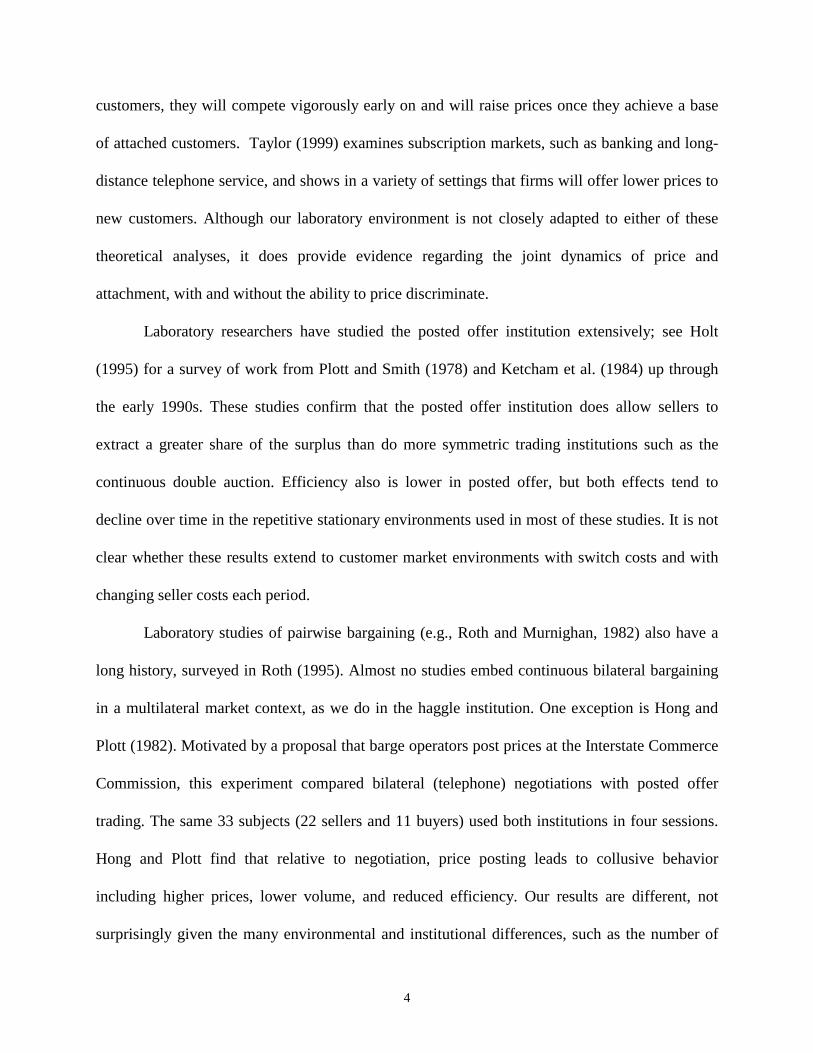
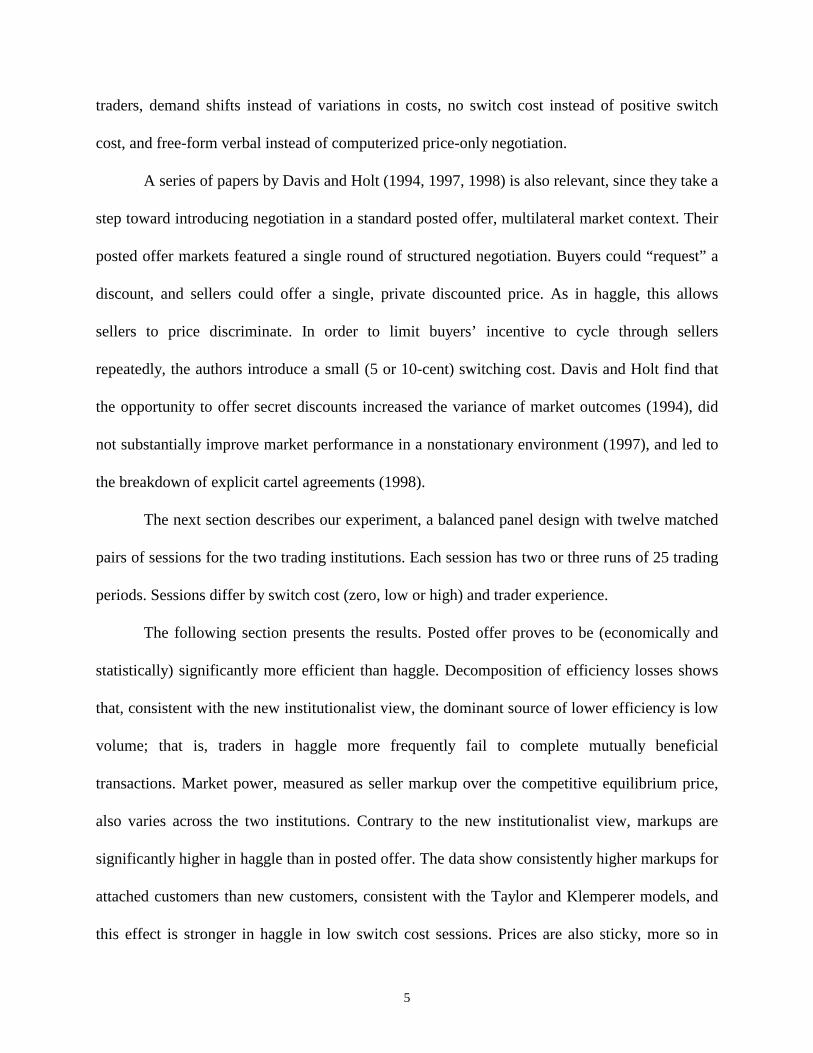
Customer markets feature long term but impermanent attachments. To discourage
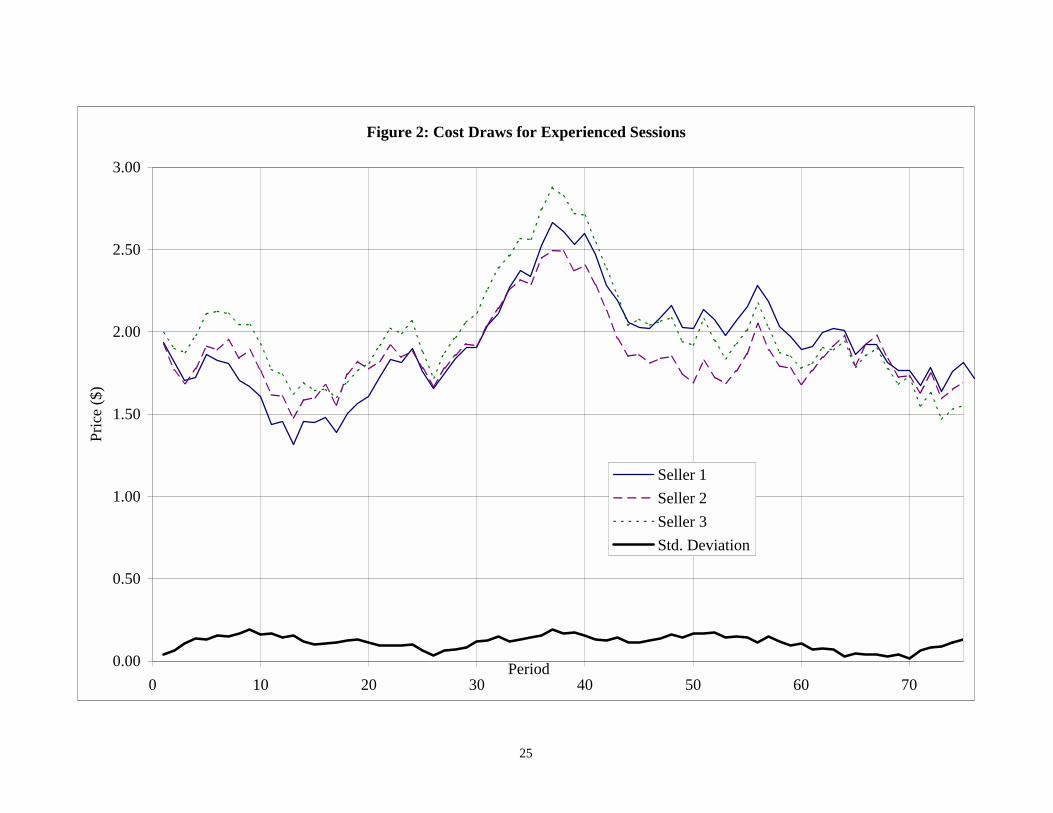
permanent attachments, the experiment introduces random production cost innovations. In each
session the production costs follow a random walk with a mean zero additive innovation to
marginal production cost each period. In particular, seller j’s cost in period t evolves randomly
according to cjt = cjt-1 + ejt, where the innovations ejt are the sum of two components, one common
to all sellers drawn from U(-15, 15) and one independent component drawn from U(-5, 5). The
larger correlated component keeps sellers’ costs closer together in later periods. To sharpen
comparisons across institutions and across switch costs, we used the same sequence of random
shocks ejt for all sessions with the same experience and cost process conditions. The realized cost
sequences are shown in Figures 1 and 2.
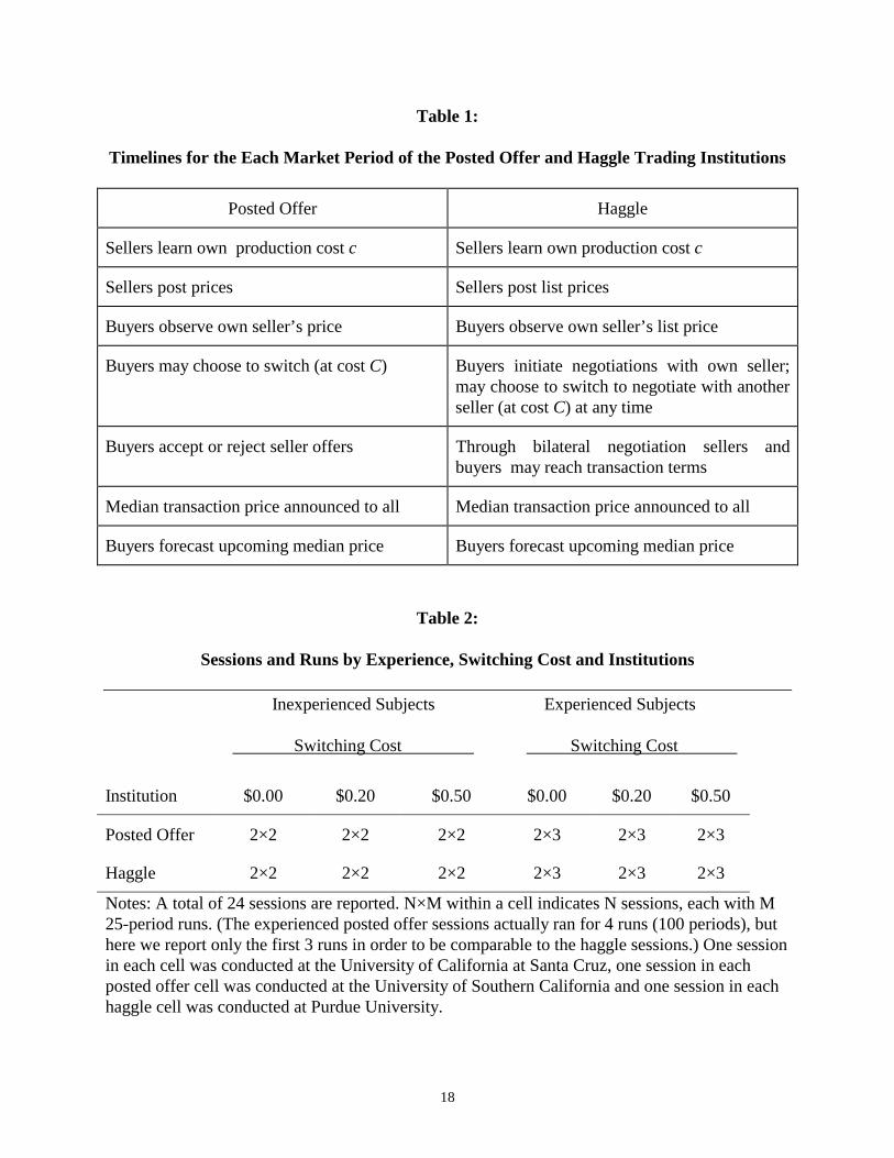
Table 1 summarizes the timelines for each trading period for the two market institutions.
In the posted offer treatment the period is over after each buyer has either rejected all available
price(s) or else accepted one of the posted prices she sees (that of “her seller” if she does not
switch, or all prices if she chose to switch). In the haggle treatment the period is over when the
60-second negotiation period ends.3 Then the sellers and buyers view interim screens that
summarize their own activity in that period and their own cumulative profit, as well as the
median transaction price (across all sellers) for that period.4 Buyers forecast the next period’s
median transaction price, at the same time that sellers are posting their prices for the period. The
buyer with smallest absolute forecast error totaled over all periods earns a modest prize ($5.00).
Each session is divided into runs of 25 periods, and buyers and sellers are randomly re- 3 We ran pilot sessions with periods lasting 180, 120, 90, 60 and 45 seconds. Except in the 45 second pilots we saw little impact on trade volume; after the first few periods most trades occur in the last 30 seconds. Therefore in the experiment we let the negotiation period run for 90 or 120 seconds in the first few periods and 60 seconds thereafter. 4 Cason and Friedman (2000) report sessions in the posted offer treatment with no feedback and with full (all transaction prices) feedback. Based their results, as well and Davis and Holt secret price discounts work mentioned earlier, we decided that reporting only the median price last period represents the most useful middle ground for our institutional comparison.

8
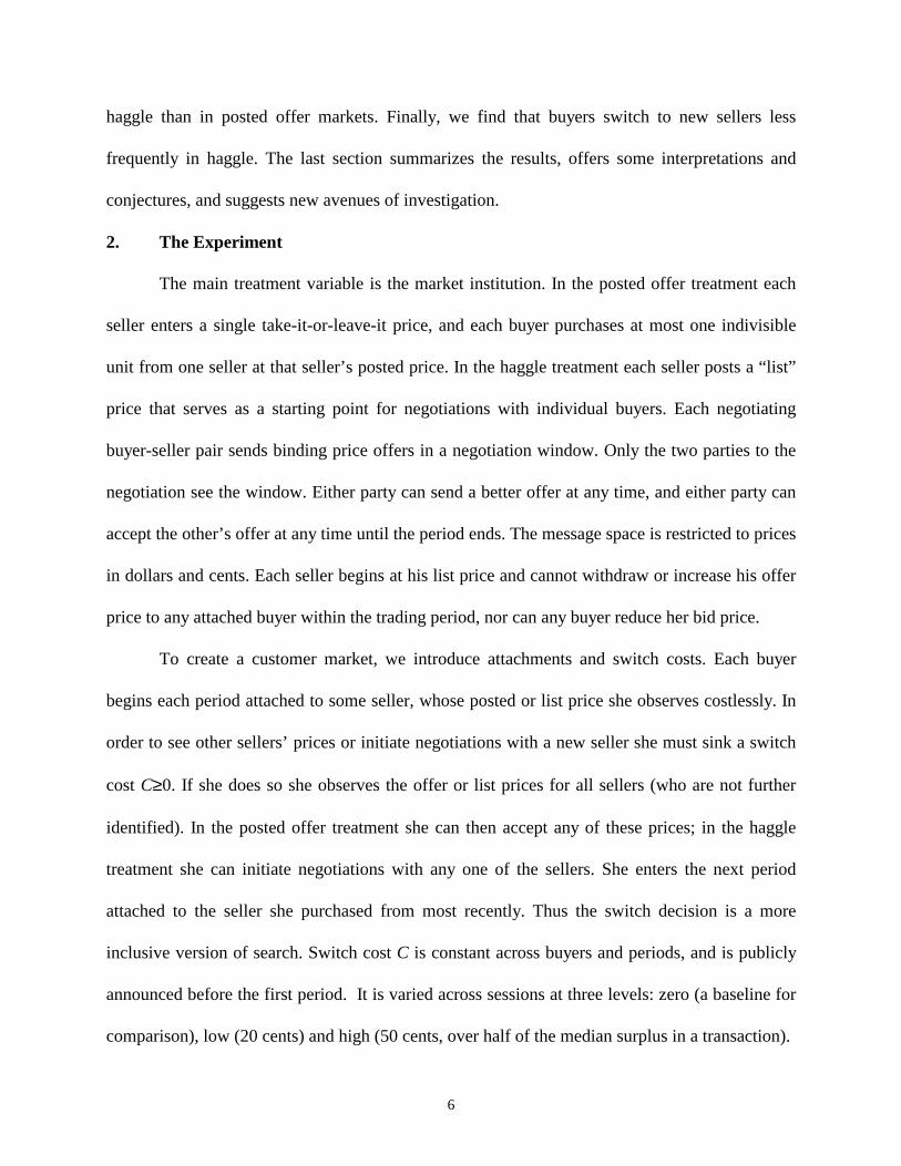
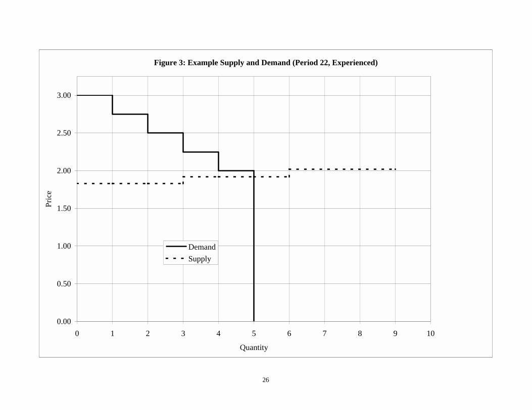
matched to new trading partners at the beginning of each run. Each session has three sellers who
produce to demand (i.e., no inventories) at a uniform (constant) marginal cost each period with
no fixed cost. Each seller’s capacity is 3 units, so the maximum quantity that sellers can supply
in total is 9 units per period. Five buyers each demand only one unit per period.5 Buyer values
are constant over each session at 300, 275, 250, 225, and 200 cents. At the end of each 25 period
run, assignments of buyers to these values are rotated and attachments are reinitialized randomly.
Figure 3 displays the supply and demand for an example period.
Table 2 presents the experimental design, which employs 24 sessions. The design is
balanced, with equal numbers of sessions in each trading institution and switch cost treatment.
Identical software was used at all sites. Experienced subjects participated in an earlier session
listed in the table, at the same site and in the same trading institution. We were able to complete
more periods in the experienced sessions because the experienced sessions required a
significantly shorter instructional period. Subjects typically earned between $20 and $30 per two
hour session (including instructions). Half of the data (the posted offer treatment) were reported
previously in Cason and Friedman (2000). This earlier paper focused on other research issues,
such as the market impact of information differences and changes in random cost sequences.
3. Results
This section begins with an overview of the data, and then compares relative market
efficiency, market power, and price stickiness. Our design allows for sharp matched pair
hypothesis tests for many of the comparisons because seller costs follow identical paths in the
two market institutions for each treatment. In testing for differences across market institutions,
5 If buyers try to accept more units than a specific seller has offered, then in the posted offer treatment the buyers who transacted most recently with that seller receive priority. Any remaining units are awarded first come first served, and in the haggle treatment all units are always awarded first come first served.
9
we also match experience, switch cost, and experimenter (UCSC versus [Purdue or USC]). In
testing for differences across any other treatment, we match market institution and the other
treatments.
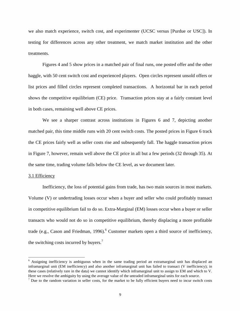
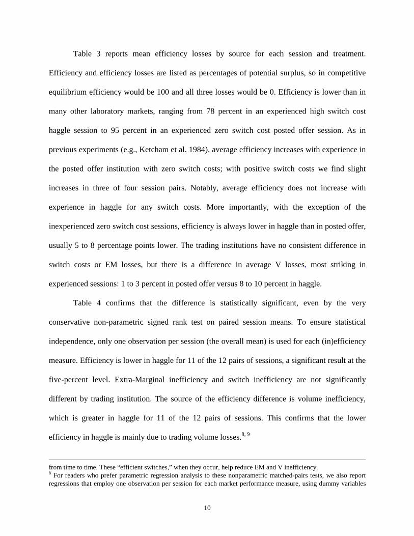
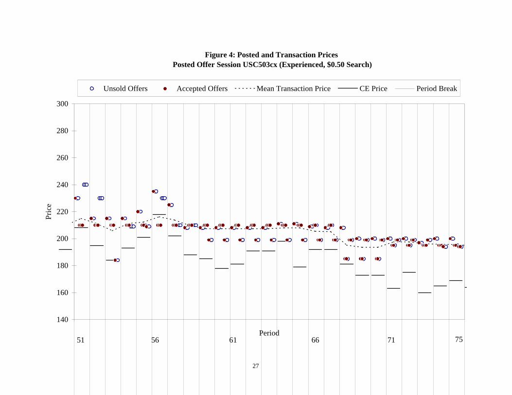
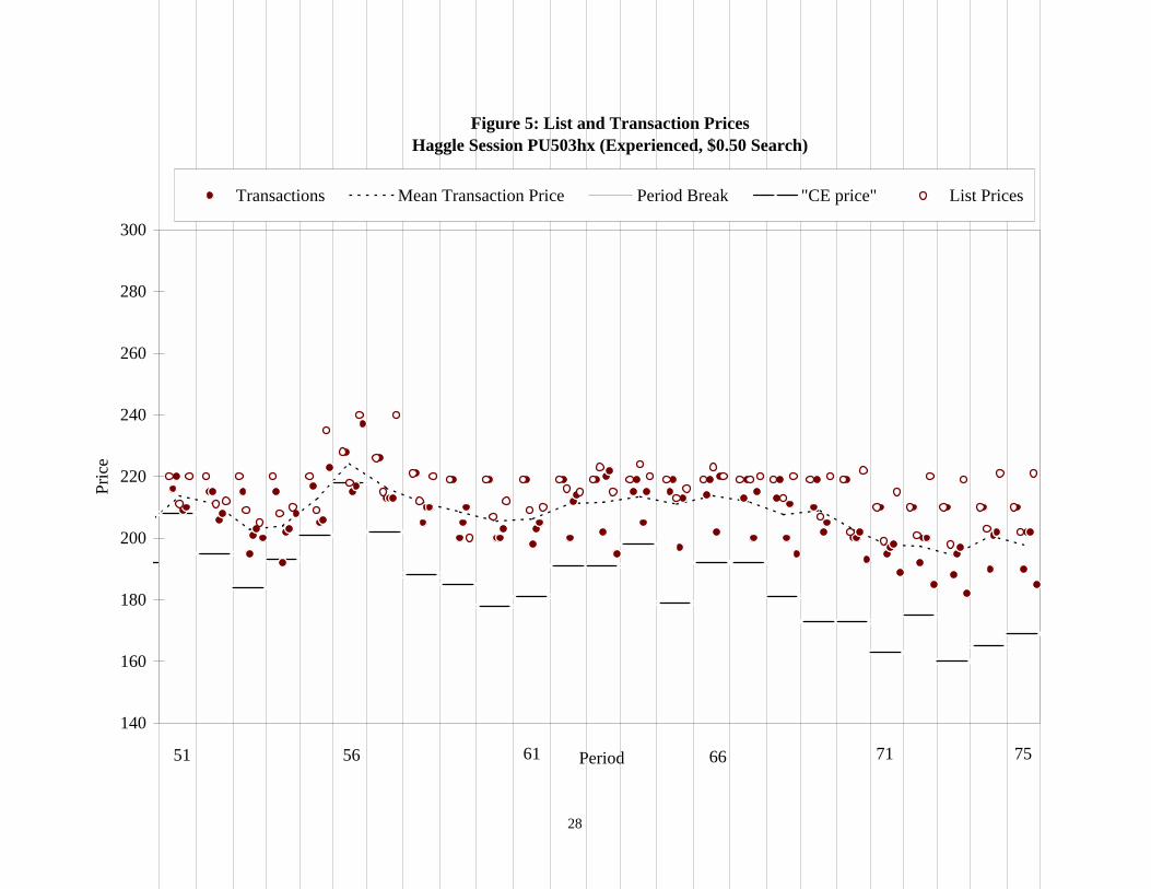
Figures 4 and 5 show prices in a matched pair of final runs, one posted offer and the other
haggle, with 50 cent switch cost and experienced players. Open circles represent unsold offers or
list prices and filled circles represent completed transactions. A horizontal bar in each period
shows the competitive equilibrium (CE) price. Transaction prices stay at a fairly constant level
in both cases, remaining well above CE prices.
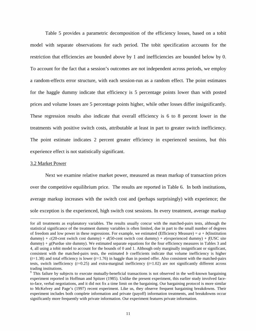
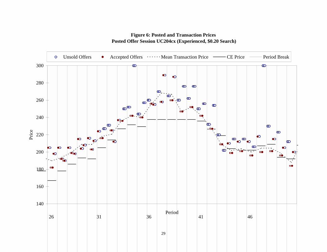
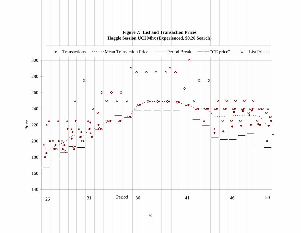
We see a sharper contrast across institutions in Figures 6 and 7, depicting another
matched pair, this time middle runs with 20 cent switch costs. The posted prices in Figure 6 track
the CE prices fairly well as seller costs rise and subsequently fall. The haggle transaction prices
in Figure 7, however, remain well above the CE price in all but a few periods (32 through 35). At
the same time, trading volume falls below the CE level, as we document later.
3.1 Efficiency
Inefficiency, the loss of potential gains from trade, has two main sources in most markets.
Volume (V) or undertrading losses occur when a buyer and seller who could profitably transact
in competitive equilibrium fail to do so. Extra-Marginal (EM) losses occur when a buyer or seller
transacts who would not do so in competitive equilibrium, thereby displacing a more profitable
trade (e.g., Cason and Friedman, 1996).6 Customer markets open a third source of inefficiency,
the switching costs incurred by buyers.7
6 Assigning inefficiency is ambiguous when in the same trading period an extramarginal unit has displaced an inframarginal unit (EM inefficiency) and also another inframarginal unit has failed to transact (V inefficiency); in these cases (relatively rare in the data) we cannot identify which inframarginal unit to assign to EM and which to V. Here we resolve the ambiguity by using the average value of the untraded inframarginal units for each source. 7 Due to the random variation in seller costs, for the market to be fully efficient buyers need to incur switch costs
10
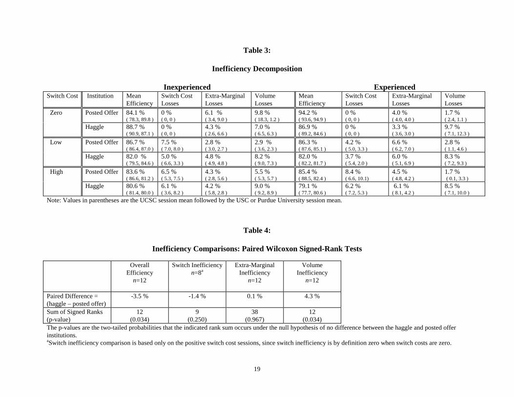
Table 3 reports mean efficiency losses by source for each session and treatment.
Efficiency and efficiency losses are listed as percentages of potential surplus, so in competitive
equilibrium efficiency would be 100 and all three losses would be 0. Efficiency is lower than in
many other laboratory markets, ranging from 78 percent in an experienced high switch cost
haggle session to 95 percent in an experienced zero switch cost posted offer session. As in
previous experiments (e.g., Ketcham et al. 1984), average efficiency increases with experience in
the posted offer institution with zero switch costs; with positive switch costs we find slight
increases in three of four session pairs. Notably, average efficiency does not increase with
experience in haggle for any switch costs. More importantly, with the exception of the
inexperienced zero switch cost sessions, efficiency is always lower in haggle than in posted offer,
usually 5 to 8 percentage points lower. The trading institutions have no consistent difference in
switch costs or EM losses, but there is a difference in average V losses, most striking in
experienced sessions: 1 to 3 percent in posted offer versus 8 to 10 percent in haggle.
Table 4 confirms that the difference is statistically significant, even by the very
conservative non-parametric signed rank test on paired session means. To ensure statistical
independence, only one observation per session (the overall mean) is used for each (in)efficiency
measure. Efficiency is lower in haggle for 11 of the 12 pairs of sessions, a significant result at the
five-percent level. Extra-Marginal inefficiency and switch inefficiency are not significantly
different by trading institution. The source of the efficiency difference is volume inefficiency,
which is greater in haggle for 11 of the 12 pairs of sessions. This confirms that the lower
efficiency in haggle is mainly due to trading volume losses.8, 9
from time to time. These “efficient switches,” when they occur, help reduce EM and V inefficiency. 8 For readers who prefer parametric regression analysis to these nonparametric matched-pairs tests, we also report regressions that employ one observation per session for each market performance measure, using dummy variables
11
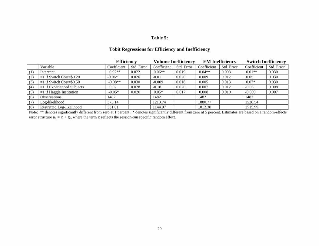
Table 5 provides a parametric decomposition of the efficiency losses, based on a tobit
model with separate observations for each period. The tobit specification accounts for the
restriction that efficiencies are bounded above by 1 and inefficiencies are bounded below by 0.
To account for the fact that a session’s outcomes are not independent across periods, we employ
a random-effects error structure, with each session-run as a random effect. The point estimates
for the haggle dummy indicate that efficiency is 5 percentage points lower than with posted
prices and volume losses are 5 percentage points higher, while other losses differ insignificantly.
These regression results also indicate that overall efficiency is 6 to 8 percent lower in the
treatments with positive switch costs, attributable at least in part to greater switch inefficiency.
The point estimate indicates 2 percent greater efficiency in experienced sessions, but this
experience effect is not statistically significant.
3.2 Market Power
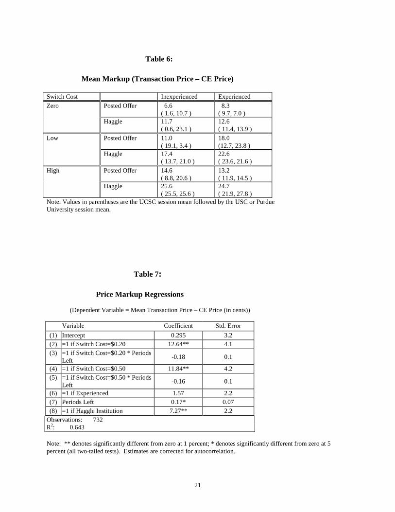
Next we examine relative market power, measured as mean markup of transaction prices
over the competitive equilibrium price. The results are reported in Table 6. In both institutions,
average markup increases with the switch cost and (perhaps surprisingly) with experience; the
sole exception is the experienced, high switch cost sessions. In every treatment, average markup for all treatments as explanatory variables. The results usually concur with the matched-pairs tests, although the statistical significance of the treatment dummy variables is often limited, due in part to the small number of degrees of freedom and low power in these regressions. For example, we estimated (Efficiency Measure) = a + b(Institution dummy) + c(20-cent switch cost dummy) + d(50-cent switch cost dummy) + e(experienced dummy) + f(USC site dummy) + g(Purdue site dummy). We estimated separate equations for the four efficiency measures in Tables 3 and 4, all using a tobit model to account for the bounds of 0 and 1. Although only marginally insignificant or significant, consistent with the matched-pairs tests, the estimated b coefficients indicate that volume inefficiency is higher (t=1.38) and total efficiency is lower (t=1.76) in haggle than in posted offer. Also consistent with the matched-pairs tests, switch inefficiency (t=0.25) and extra-marginal inefficiency (t=1.02) are not significantly different across trading institutions. 9 This failure by subjects to execute mutually-beneficial transactions is not observed in the well-known bargaining experiment reported in Hoffman and Spitzer (1985). Unlike the present experiment, this earlier study involved face-to-face, verbal negotiations, and it did not fix a time limit on the bargaining. Our bargaining protocol is more similar to McKelvey and Page’s (1997) recent experiment. Like us, they observe frequent bargaining breakdowns. Their experiment includes both complete information and private (payoff) information treatments, and breakdowns occur significantly more frequently with private information. Our experiment features private information.
12
is higher in haggle than in posted offer, usually by at least 50 percent. Figure 8 illustrates the
higher average transaction prices in haggle for the high switch cost treatment. This figure plots
the time series of the difference in mean transaction prices (haggle – posted offer) for each
period, for both the inexperienced (panel A) and experienced (panel B) sessions. Our
experimental design permits this direct period-by-period comparison, because we used the same
random cost sequence in each session (shown in Figures 1 and 2). Of the 50 inexperienced
periods for this high switch cost treatment, in only one period (period 38) did the mean posted
offer transaction price exceed the mean haggle transaction price. In the experienced sessions for
this treatment, transaction prices appear about equal in periods 31-60; but prices are
systematically higher in haggle in earlier and later periods.10 Another paired signed rank test
(again with each pair of matched sessions contributing one statistically independent observation)
confirms that markups are significantly higher in haggle (Wilcoxon sum of signed ranks=8,
n=12, p=0.012), controlling for switch cost, experimenter, and experience levels.11
Table 7 provides parametric decomposition of seller markup, with correction for
autocorrelated errors to account for possible price stickiness as discussed below. The dependent
variable is mean transaction price minus competitive equilibrium price. Both switch cost dummy
variables are highly significant, indicating markups roughly 12 cents higher for positive switch
cost treatments. The fact that the interaction terms are insignificant suggests that the impact of
switch costs does not decline significantly later in the run. The significant haggle dummy
confirms that markups are higher in this institution than in posted offer, by an average of 7 cents.
10 Recall from Figure 2 that seller costs increase very rapidly in periods 26-38 of the experienced sessions. We will later see that transaction prices are “stickier” in haggle, and this may account for the exceptional price comparison in periods 31-60. 11 An OLS regression of markups on the treatment dummy variables—analogous to the efficiency regressions described in footnote 8—provides a similar conclusion. Markups are higher in haggle, although only at marginal significance levels for this test (t=1.66; two-tailed p-value=0.115).
13
These higher observed markups coinciding with greater volume losses under haggle raise
the additional question of whether sellers see a net gain in profits due to these higher markups.
We examined seller profits using the paired test of signed ranks, with each session pair
contributing one observation, and found that they are significantly higher in haggle (sum of
signed ranks=9, n=12, p=0.016).12
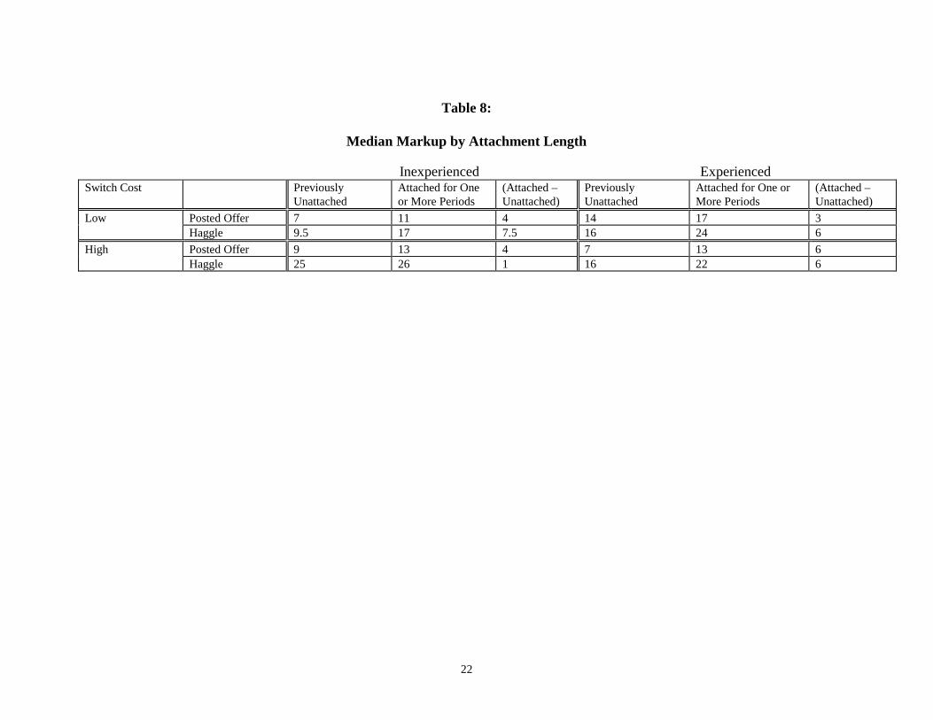
Are haggle markups higher because the institution allows sellers to price discriminate
between attached buyers and new customers? Table 8 shows median markup for new vs.
previously attached buyer-seller pairs in positive switch cost sessions.13 It shows that new
customers on average receive a discount in all relevant treatments, consistent with Taylor (1999).
In low switch cost sessions the discount is larger in haggle than in posted offer, with
inexperienced (7.5 vs. 4 cents) as well as experienced subjects (6 vs. 3 cents). In high cost
sessions it is not clear where the discount is larger.
Do markups for attached customers increase the longer they are attached? We looked at
the data in various ways and found little evidence for a systematic relationship in either
institution.
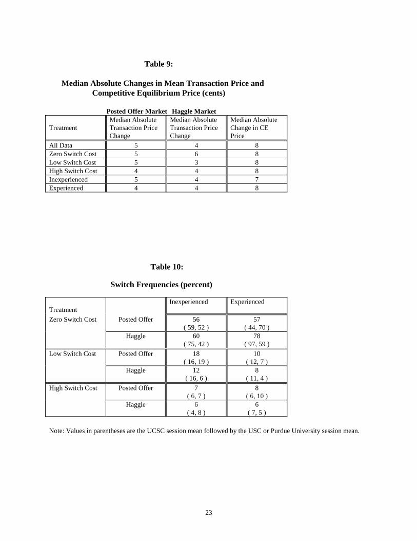
3.3 Sticky Prices
Cason and Friedman (2000) argue that price stickiness is best measured by comparing the
median change in period-to-period transaction prices to the corresponding change in competitive
equilibrium prices. To maintain comparability across the two trading institutions, here we look at
transaction prices for each continuing buyer-seller pair. Table 9 shows that prices are sticky in 12 The OLS regression of seller profits on treatment dummy variables indicates (insignificantly) higher profits in haggle (t=1.37; two-tailed p-value=0.190). 13 Since in haggle sellers negotiate individual transaction prices with each buyer, classifying transactions into “new” and “attached” categories is straightforward. In posted offer, by contrast, a particular offer price might be accepted both by new and attached customers, since the institution does not permit price discrimination. In these cases the price contributes observations to both the new and attached categories, with the number of observations determined by the number of accepting buyers of each type.
14
both institutions, since the median CE price change is always 7 or 8 cents while the median
transaction price change is 3 to 6 cents and is 4 or 5 in most treatments. This stickiness increases
with switch cost in all instances except for low switch cost in haggle. Median transaction price
changes are generally a bit smaller (and thus prices stickier) with haggle than with posted offer.
To sharpen the comparison, we classified an individual seller as “sticky” if her absolute
cost changes exceed her absolute price change in at least half of the periods. Overall, for the
posted offer market 24 of 36 sellers were “sticky” vs. 34 of 36 under haggle, a very significant
difference according to Fisher’s Exact Test (p-value<0.01).14
Although transaction prices vary less from period-to-period in haggle than in posted offer,
the list prices posted in haggle exhibit approximately the same variability as offer prices in the
posted offer sessions. For example, sellers’ median absolute change in list prices for haggle and
in posted prices for posted offer are both 5 cents. In posted offer 18 of 32 individual sellers have
a median absolute change in posted prices of 5 cents or less, and in haggle 20 of 32 individual
sellers have a median absolute change in list prices of 5 cents or less.
3.4 Buyer Behavior
Table 10 indicates that, not surprisingly, switch rates are lower in higher switch cost
sessions. More interestingly, switch rates seem lower for haggle when switch costs are positive—
for both inexperienced and experienced sessions and for both low and high switch costs. The
difference in switch rates is greatest when inexperienced subjects face low switch costs. More
formally, we form matched pairs of all 25-period runs with positive switch costs in the two
trading institutions and test whether the distribution of switch rate differences is centered on
zero. The test rejects the null hypothesis that switch rates are the same in the two institutions in 14 The breakdown by switch costs is 7/12, 7/12, and 10/12 sticky sellers for posted price and 10/12, 12/12, and 12/12 for haggle for the zero, 20 cent, and 50 cent switch cost cases, respectively.

15
favor of the alternative that switch rates are lower for haggle (Wilcoxon sum of signed ranks=39,
n=20, p=0.011).15 This lower observed switch rate is consistent with the earlier result that seller
market power is greater under haggle.
4. Discussion
Our laboratory results comparing haggle (bilateral bargaining) markets with posted offer
markets can be summarized as follows:
1. Haggle is less efficient at extracting potential gains from trade, mainly because mutually
beneficial trades are more often missed (“V losses”), and not because of inefficient customer
search or extramarginal trades. This result is consistent with the new institutionalist view and
inconsistent with the Coasian view. Unlike most other market institutions studied in the
laboratory, efficiency does not increase with experience in haggle.
2. Sellers obtain a larger share of realized gains with haggle than with posted offer. This is
contrary to the new institutionalist view that giving sellers the commitment technology in
posted offer should increase their share of the gains. It is consistent with the view that haggle
encourages classic market power with its deadweight (V) losses.
3. New buyers receive lower prices, consistent with the work of Taylor and (indirectly)
Klemperer. In low switch cost sessions, the effect is stronger in haggle, as one might expect
since haggle but not posted offer allows direct price discrimination.
4. Prices are sticky in both institutions, and especially in haggle. Sellers’ chosen prices dampen
15 A more conservative test that treats each pair of sessions (rather than each pair of runs) as the unit of observation marginally fails to reject this null hypothesis of no difference across institutions (p=0.117). This could be attributed in part to the small sample size of only 8 pairs of sessions with positive switch costs. Similarly, a tobit regression of each sessions’ switch rate on the treatment dummy variables does not indicate a significant difference in switch rates across trading institutions. This regression estimates six coefficients using only 16 session observations, and only the switch cost dummy variable is significantly different from zero.
16
the fluctuations in their production costs, and reflect only about half of the resulting
fluctuations in competitive equilibrium price.
5. In sessions with positive switch costs, buyers switch sellers less frequently with haggle than
with posted offer.
One might ask whether the V losses in haggle are due to insufficient time for negotiation.
We do not think so because these losses are not reduced either by longer negotiation periods in
early trials and in pilot experiments, or (as we have seen in the data reported above) by subjects’
experience. On the other hand, the V losses could be due to “deadline effects” in bargaining
(Roth et al., 1988). As in previous bilateral bargaining experiments, our subjects frequently
reached agreement within the last few seconds of the trading period, no matter how long it is and
no matter how experienced the subjects. Perhaps sometimes traders hold out for their
counterparty to concede in the last few seconds and that concession does not materialize. We
leave to another paper the real time dynamic analysis of haggling.
After thinking about our results we noticed a possible explanation for many of the
performance differences based on a subtle informational difference between the two market
institutions. A switching buyer in posted offer sees his actual alternative opportunities because
sellers are committed to their posted prices. By contrast, a switching buyer in haggle only sees a
weak signal of alternative opportunities because list prices are not committed, and so the switch
option is less valuable. Therefore in haggle buyers are less inclined to switch and sellers are
better able to exercise market power via larger markups and lower trading volume. Note that
these institutional switch value differences are also present in posted offer and haggle markets in
the field. For example, consider a procurement agent contemplating switching parts suppliers for
an assembly plant. This agent could estimate different values of switching depending on whether
17
she must negotiate terms with a new supplier, or whether she can simply accept or reject non-
negotiable seller offers.
More experiments are necessary to test this explanation and other possible theories. The
Coasian versus New Institutionalist theme was secondary in the present paper, but some
investigators might wish to pursue it further by simplifying the laboratory environment (e.g.,
draw private costs and values independently each period rather than random walks, and eliminate
attachments) and deriving explicit testable models. A different empirical project would be to
interpolate new market institutions with information and negotiation procedures between haggle
and posted offer, and study these new institutions in the laboratory. For example, subjects could
bargain by following a strict two or three round alternating offers protocol. The impact of
differing market information could also be studied, for example, by allowing switching buyers to
observe sellers’ transaction price history and/or their current production costs. Our current design
features a competitive equilibrium that tends to favor the buyers in terms of the division of
surplus. This asymmetry may be behind some of the divergence from the CE results that we find.
One interesting extension would be to remove or reverse this asymmetry and see if key results—
such as the higher prices in haggle compared to posted offer—continue to hold.
Another useful extension would allow sellers to choose which trading institution they
wish to employ. Our results suggest that sellers’ profits suffer when they adopt posted offer rules,
but as we discussed in the introduction there exist agency rationales for adopting this less flexible
pricing institution. It would be useful to include such agency complications in an experiment that
addresses the endogenous development of market institutions. It would also be valuable to
include new innovations such as bargaining bots and Priceline.com style haggling that offer the
opportunity for entirely new trading institutions.
18
Table 1:
Timelines for the Each Market Period of the Posted Offer and Haggle Trading Institutions
Posted Offer Haggle
Sellers learn own production cost c Sellers learn own production cost c
Sellers post prices Sellers post list prices
Buyers observe own seller’s price Buyers observe own seller’s list price
Buyers may choose to switch (at cost C) Buyers initiate negotiations with own seller; may choose to switch to negotiate with another seller (at cost C) at any time
Buyers accept or reject seller offers Through bilateral negotiation sellers and buyers may reach transaction terms
Median transaction price announced to all Median transaction price announced to all
Buyers forecast upcoming median price Buyers forecast upcoming median price
Table 2:
Sessions and Runs by Experience, Switching Cost and Institutions
Inexperienced Subjects Experienced Subjects
Switching Cost Switching Cost
Institution $0.00 $0.20 $0.50 $0.00 $0.20 $0.50
Posted Offer 2×2 2×2 2×2 2×3 2×3 2×3
Haggle 2×2 2×2 2×2 2×3 2×3 2×3
Notes: A total of 24 sessions are reported. N×M within a cell indicates N sessions, each with M 25-period runs. (The experienced posted offer sessions actually ran for 4 runs (100 periods), but here we report only the first 3 runs in order to be comparable to the haggle sessions.) One session in each cell was conducted at the University of California at Santa Cruz, one session in each posted offer cell was conducted at the University of Southern California and one session in each haggle cell was conducted at Purdue University.
19
Table 3:
Inefficiency Decomposition
Inexperienced Experienced Switch Cost Institution Mean
Efficiency Switch Cost Losses
Extra-Marginal Losses
Volume Losses
Mean Efficiency
Switch Cost Losses
Extra-Marginal Losses
Volume Losses
Zero Posted Offer 84.1 % ( 78.3, 89.8 )
0 % ( 0, 0 )
6.1 % ( 3.4, 9.0 )
9.8 % ( 18.3, 1.2 )
94.2 % ( 93.6, 94.9 )
0 % ( 0, 0 )
4.0 % ( 4.0, 4.0 )
1.7 % ( 2.4, 1.1 )
Haggle 88.7 % ( 90.9, 87.1 )
0 % ( 0, 0 )
4.3 % ( 2.6, 6.6 )
7.0 % ( 6.5, 6.3 )
86.9 % ( 89.2, 84.6 )
0 % ( 0, 0 )
3.3 % ( 3.6, 3.0 )
9.7 % ( 7.1, 12.3 )
Low Posted Offer 86.7 % ( 86.4, 87.0 )
7.5 % ( 7.0, 8.0 )
2.8 % ( 3.0, 2.7 )
2.9 % ( 3.6, 2.3 )
86.3 % ( 87.6, 85.1 )
4.2 % ( 5.0, 3.3 )
6.6 % ( 6.2, 7.0 )
2.8 % ( 1.1, 4.6 )
Haggle 82.0 % ( 79.5, 84.6 )
5.0 % ( 6.6, 3.3 )
4.8 % ( 4.9, 4.8 )
8.2 % ( 9.0, 7.3 )
82.0 % ( 82.2, 81.7 )
3.7 % ( 5.4, 2.0 )
6.0 % ( 5.1, 6.9 )
8.3 % ( 7.2, 9.3 )
High Posted Offer 83.6 % ( 86.6, 81.2 )
6.5 % ( 5.3, 7.5 )
4.3 % ( 2.8, 5.6 )
5.5 % ( 5.3, 5.7 )
85.4 % ( 88.5, 82.4 )
8.4 % ( 6.6, 10.1)
4.5 % ( 4.8, 4.2 )
1.7 % ( 0.1, 3.3 )
Haggle 80.6 % ( 81.4, 80.0 )
6.1 % ( 3.6, 8.2 )
4.2 % ( 5.8, 2.8 )
9.0 % ( 9.2, 8.9 )
79.1 % ( 77.7, 80.6 )
6.2 % ( 7.2, 5.3 )
6.1 % ( 8.1, 4.2 )
8.5 % ( 7.1, 10.0 )
Note: Values in parentheses are the UCSC session mean followed by the USC or Purdue University session mean.
Table 4:
Inefficiency Comparisons: Paired Wilcoxon Signed-Rank Tests Overall
Efficiency n=12
Switch Inefficiency n=8a
Extra-Marginal Inefficiency
n=12
Volume Inefficiency
n=12
Paired Difference = (haggle – posted offer)
-3.5 % -1.4 % 0.1 % 4.3 %
Sum of Signed Ranks (p-value)
12 (0.034)
9 (0.250)
38 (0.967)
12 (0.034)
The p-values are the two-tailed probabilities that the indicated rank sum occurs under the null hypothesis of no difference between the haggle and posted offer institutions. aSwitch inefficiency comparison is based only on the positive switch cost sessions, since switch inefficiency is by definition zero when switch costs are zero.
20
Table 5:
Tobit Regressions for Efficiency and Inefficiency
Efficiency Volume Inefficiency EM Inefficiency Switch Inefficiency Variable Coefficient Std. Error Coefficient Std. Error Coefficient Std. Error Coefficient Std. Error (1) Intercept 0.92** 0.022 0.06** 0.019 0.04** 0.008 0.01** 0.030 (2) =1 if Switch Cost=$0.20 -0.06* 0.026 -0.01 0.020 0.009 0.012 0.05 0.030 (3) =1 if Switch Cost=$0.50 -0.08** 0.030 -0.009 0.018 0.005 0.013 0.07* 0.030 (4) =1 if Experienced Subjects 0.02 0.028 -0.18 0.020 0.007 0.012 -0.05 0.008 (5) =1 if Haggle Institution -0.05* 0.020 0.05* 0.017 0.008 0.010 -0.009 0.007 (6) Observations 1482 1482 1482 1482 (7) Log-likelihood 373.14 1213.74 1880.77 1528.54 (8) Restricted Log-likelihood 331.01 1144.97 1812.30 1515.99 Note: ** denotes significantly different from zero at 1 percent , * denotes significantly different from zero at 5 percent. Estimates are based on a random-effects error structure uit = τi + εit, where the term τi reflects the session-run specific random effect.
21
Table 6:
Mean Markup (Transaction Price – CE Price)
Switch Cost Inexperienced Experienced Zero Posted Offer 6.6
( 1.6, 10.7 ) 8.3 ( 9.7, 7.0 )
Haggle 11.7 ( 0.6, 23.1 )
12.6 ( 11.4, 13.9 )
Low Posted Offer 11.0 ( 19.1, 3.4 )
18.0 (12.7, 23.8 )
Haggle 17.4 ( 13.7, 21.0 )
22.6 ( 23.6, 21.6 )
High Posted Offer 14.6 ( 8.8, 20.6 )
13.2 ( 11.9, 14.5 )
Haggle 25.6 ( 25.5, 25.6 )
24.7 ( 21.9, 27.8 )
Note: Values in parentheses are the UCSC session mean followed by the USC or Purdue University session mean.
Table 7:
Price Markup Regressions (Dependent Variable = Mean Transaction Price – CE Price (in cents))
Variable Coefficient Std. Error
(1) Intercept 0.295 3.2 (2) =1 if Switch Cost=$0.20 12.64** 4.1 (3) =1 if Switch Cost=$0.20 * Periods
Left -0.18 0.1
(4) =1 if Switch Cost=$0.50 11.84** 4.2 (5) =1 if Switch Cost=$0.50 * Periods
Left -0.16 0.1
(6) =1 if Experienced 1.57 2.2 (7) Periods Left 0.17* 0.07 (8) =1 if Haggle Institution 7.27** 2.2
Observations: 732 R2: 0.643 Note: ** denotes significantly different from zero at 1 percent; * denotes significantly different from zero at 5 percent (all two-tailed tests). Estimates are corrected for autocorrelation.
22
Table 8:
Median Markup by Attachment Length
Inexperienced Experienced Switch Cost Previously
Unattached Attached for One or More Periods
(Attached – Unattached)
Previously Unattached
Attached for One or More Periods
(Attached – Unattached)
Low Posted Offer 7 11 4 14 17 3 Haggle 9.5 17 7.5 16 24 6 High Posted Offer 9 13 4 7 13 6 Haggle 25 26 1 16 22 6
23
Table 9:
Median Absolute Changes in Mean Transaction Price and
Competitive Equilibrium Price (cents)
Posted Offer Market Haggle Market Treatment
Median Absolute Transaction Price Change
Median Absolute Transaction Price Change
Median Absolute Change in CE Price
All Data 5 4 8 Zero Switch Cost 5 6 8 Low Switch Cost 5 3 8 High Switch Cost 4 4 8 Inexperienced 5 4 7 Experienced 4 4 8
Table 10:
Switch Frequencies (percent) Treatment
Inexperienced Experienced
Zero Switch Cost Posted Offer 56 ( 59, 52 )
57 ( 44, 70 )
Haggle 60 ( 75, 42 )
78 ( 97, 59 )
Low Switch Cost Posted Offer 18 ( 16, 19 )
10 ( 12, 7 )
Haggle 12 ( 16, 6 )
8 ( 11, 4 )
High Switch Cost Posted Offer 7 ( 6, 7 )
8 ( 6, 10 )
Haggle 6 ( 4, 8 )
6 ( 7, 5 )
Note: Values in parentheses are the UCSC session mean followed by the USC or Purdue University session mean.

24
Figure 1: Cost Draws for Inexperienced Sessions
0.00
0.50
1.00
1.50
2.00
2.50
3.00
0 5 10 15 20 25 30 35 40 45 50Period
Cos
t ($)
Seller 1Seller 2Seller 3Std. Deviation
25
Figure 2: Cost Draws for Experienced Sessions
0.00
0.50
1.00
1.50
2.00
2.50
3.00
0 10 20 30 40 50 60 70Period
Pric
e ($
)
Seller 1Seller 2Seller 3Std. Deviation
26
Figure 3: Example Supply and Demand (Period 22, Experienced)
0.00
0.50
1.00
1.50
2.00
2.50
3.00
0 1 2 3 4 5 6 7 8 9 10
Quantity
Pric
e
DemandSupply
27
Figure 4: Posted and Transaction Prices Posted Offer Session USC503cx (Experienced, $0.50 Search)
140
160
180
200
220
240
260
280
300
Period
Pric
e
Unsold Offers Accepted Offers Mean Transaction Price CE Price Period Break
56 61 66 7151 75
28
Figure 5: List and Transaction PricesHaggle Session PU503hx (Experienced, $0.50 Search)
140
160
180
200
220
240
260
280
300
Period
Pric
e
Transactions Mean Transaction Price Period Break "CE price" List Prices
56 7551 61 66 71
29
Figure 6: Posted and Transaction Prices Posted Offer Session UC204cx (Experienced, $0.20 Search)
140
160
180
200
220
240
260
280
300
Period
Pric
e
Unsold Offers Accepted Offers Mean Transaction Price CE Price Period Break
31 36 41 4626
30
Figure 7: List and Transaction PricesHaggle Session UC204hx (Experienced, $0.20 Search)
140
160
180
200
220
240
260
280
300
Period
Pric
e
Transactions Mean Transaction Price Period Break "CE price" List Prices
36 5026 31 41 46
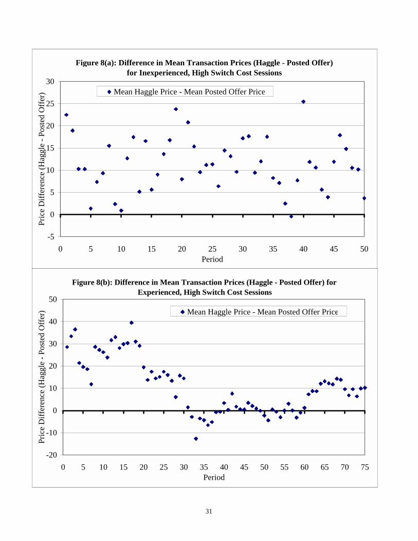
Figure 8(a): Difference in Mean Transaction Prices (Haggle - Posted Offer) for Inexperienced, High Switch Cost Sessions
-5
0
5
10
15
20
25
30
0 5 10 15 20 25 30 35 40 45 50Period
Pric
e D
iffer
ence
(Hag
gle
- Pos
ted
Off
er) Mean Haggle Price - Mean Posted Offer Price
Figure 8(b): Difference in Mean Transaction Prices (Haggle - Posted Offer) for Experienced, High Switch Cost Sessions
-20
-10
0
10
20
30
40
50
0 5 10 15 20 25 30 35 40 45 50 55 60 65 70 75Period
Pric
e D
iffer
ence
(Hag
gle
- Pos
ted
Off
er) Mean Haggle Price - Mean Posted Offer Price
31
32
References: Camera, Gabriele and Alain Delacroix (2001), “Bargaining or Price Posting?” Purdue University
working paper. Cason, Timothy and Daniel Friedman (1996), “Price Formation in Double Auction Markets,”
Journal of Economic Dynamics and Control 20, pp. 1307-1337. Cason, Timothy and Daniel Friedman (2000), “A Laboratory Study of Customer Markets,”
Purdue University working paper. Coase, Ronald (1960) “The Problem of Social Cost,” Journal of Law and Economics 3, pp. 1-44. Davis, Douglas and Charles Holt (1994), “The Effects of Discounting Opportunities in
Laboratory Posted Offer Markets,” Economics Letters 44, pp. 249-253. Davis, Douglas and Charles Holt (1997), “Price Rigidities and Institutional Variations in Markets
with Posted Prices,” Economic Theory 9, pp. 63-80. Davis, Douglas and Charles Holt (1998), “Conspiracies and Secret Discounts in Laboratory
Markets,” The Economic Journal 108, pp. 736-756. De Meza, David (1998), “The Coase Theorem,” in The New Palgrave Dictionary of Economics
and the Law, P. Newman, ed. (NY: Macmillan) pp. 270-281. Eisenberg, Anne (2000), “WHAT'S NEXT; In Online Auctions of the Future, It'll Be Bot vs. Bot
vs. Bot,” New York Times, August 17 (page 1 of a special section titled “Circuits”). Geertz, C., H. Geertz and L. Rosen (1979), Meaning and Order in Moroccan Society
(Cambridge: Cambridge University Press). Hoffman, Elizabeth and Matthew Spitzer (1985), “Entitlements, Rights, and Fairness – An
Experimental Examination of Subjects Concepts of Distributive Justice,” Journal of Legal Studies 14, pp. 259-297.
Holt, Charles (1995), “Industrial Organization: A Survey of Laboratory Research,” in The
Handbook of Experimental Economics, J. Kagel and A. Roth, eds. (Princeton, NJ: Princeton University Press), pp. 349-443.
Hong, James and Charles Plott (1982), “Rate Filing Policies for Inland Water Transportation: An
Experimental Approach,” Bell Journal of Economics 13, pp. 1-19. Julien, Benoît, John Kennes and Ian King (2000), “Matching Foundations,” University of
Auckland working paper.
33
Ketcham, Jon, Vernon Smith and Arlington Williams (1984), “A Comparison of Posted-Offer and Double-Auction Pricing Institutions,” Review of Economic Studies 51, pp. 595-614.
Kirchsteiger, Georg, Muriel Niederle and Jan Potters (2001), “Markets with Endogenous
Matching Structures,” University of Vienna working paper. Klemperer, Paul (1987), “Markets with Consumer Switching Costs,” Quarterly Journal of
Economics 102, pp. 375-394.
McKelvey, Richard and Talbot Page (1997), “An Experimental Study of Private Information in the Coase Theorem,” Caltech Working Paper 1018.
McKelvey, Richard and Talbot Page (2000), “Status Quo Bias in Bargaining: An Extension of the Myerson Satterthwaite Theorem with an Application to the Coase Theorem,” Caltech Working Paper 1035 (Revised).
Milgrom, Paul and John Roberts (1992), Economics, Organizations, and Management (Englewood Cliffs, NJ: Prentice-Hall, Inc.).
Myerson, Roger B. and Mark Satterthwaite (1983), "Efficient Mechanisms for Bilateral Trading," Journal of Economic Theory 29, pp. 265-281.
North, Douglass (1991), “Institutions,” Journal of Economic Perspectives 5, pp. 97-112. Okun, Arthur (1981), Prices and Quantities: A Macroeconomic Analysis (Washington, DC: The
Brookings Institution). Plott, Charles and Vernon Smith (1978), “An Experimental Examination of Two Exchange
Institutions,” Review of Economic Studies 45, pp. 133-153. Roth, Alvin (1995) “Bargaining Experiments,” in The Handbook of Experimental Economics, J.
Kagel and A. Roth, eds. (Princeton, NJ: Princeton University Press), pp. 253-348. Roth, Alvin and Keith Murnighan (1982), “The Role of Information in Bargaining: An
Experimental Study,” Econometrica 50, pp. 1123-42. Roth, Alvin, Keith Murnighan and Francoise Schoumaker (1988), “The Deadline Effect in
Bargaining: Some Experimental Evidence,” American Economic Review 78, 806-23. Scitovsky, Tibor (1952), Welfare and Competition: The Economics of a Fully Employed
Economy (London: Unwin University Books). Taylor, Curtis (1999), “Supplier Surfing: Competition and Consumer Behavior in Subscription
Markets,” Duke University working paper.


![[alt.fan.furry] A Furry Comic Book List Posted by infopage on](https://img.pdfslide.net/doc/110x75/63289cc121c8de96660032ab/altfanfurry-a-furry-comic-book-list-posted-by-infopage-on-.jpg)


