BAYES ESTIMATOR OF GENERALIZED-EXPONENTIAL PARAMETERS UNDER LINEX LOSS FUNCTION USING LINDLEY’S APPROXIMATION Rahul Singh1, Sanjay Kumar Singh2, Umesh Singh2, and Gyan Prakash Singh3* 1Department of Administrative Reforms, Govt. of Uttar Pradesh, Lucknow, India 2Department of Statistics, Banaras Hindu University, Varanasi-221005, India *3Division of Biostatistics, Institute of Medical Sciences, Banaras Hindu University, Varanasi-221005, India *Email: singhgpbhu@gmail.com

ABSTRACT

In this paper, we have obtained the Bayes Estimator of Generalized-Exponential scale and shape parameter using Lindley’s approximation (L-approximation) under asymmetric loss functions. The proposed estimators have been compared with the corresponding MLE for their risks based on simulated samples from the Generalized-Exponential distribution. 1 INTRODUCTION Exponential distribution is the most exploited distribution for life data analysis, but its suitability is restricted to constant hazard rate. For situations where the failure rate is monotonically increasing or decreasing, two-parameter Weibull and Gamma are the most popular distributions used for analyzing any lifetime data. Both distributions have increasing and decreasing hazard rates depending on the shape parameter. However, one of the major disadvantages of the gamma distribution is that its distribution and survival functions cannot be expressed in a closed form if the shape parameter is not an integer. Moreover, there are terms involving the incomplete gamma function, and thus, one needs to obtain distribution function, survival function, or hazard function by numerical integration. This makes the gamma distribution unpopular compared to a Weibull distribution, which has a nice closed form for the hazard and survival functions. On the other hand, the Weibull distribution has its own disadvantages. For example, Bain and Engelhardt (1991) have pointed out that the maximum likelihood estimators of a Weibull distribution might not behave properly for all parameter ranges. Recently a new distribution, called Generalized-Exponential distribution, has been introduced. This distribution can be used quite effectively in situations where a skewed distribution is needed. Gupta and Kundu (1999, 2002) and Raqab and Ahsanullah (2001) have investigated several properties of the two parameter generalized exponential distribution. The two-parameter Generalized-Exponential has a distribution function of the form

( ) ( )| , 1 xG EF x e

αλα λ −= − 0,; >λα (1)

` and hazard function given by

( ) ( )( )

11

| ,1 1

x x

x

e eh x

e

αλ λ

αλ

α λα λ

−− −

−

−=

− − . (2)

Here α is the shape parameter, and λ is the scale parameter. The two-parameter Generalized-Exponential has increasing and decreasing failure rates depending on the shape parameter. For any λ , the hazard function is increasing if 1>α , decreasing if 1<α , and constant if α =1. Gupta and Kundu (1999a) observed that because of the simple structure of the distribution and survival functions, the two-parameter Generalized-Exponential can be

Data Science Journal, Volume 7, 5 May 2008

65

used quite effectively in analyzing many lifetime data, particularly in place of two-parameter gamma and Weibull distributions. The estimation of parameters of the Generalized-Exponential distribution has been attempted by Gupta and Kundu (1999), but that work was only concerned with the maximum likelihood estimator or a Bayes estimator under a symmetric loss function. It is remarkable that most of the Bayesian inference procedures have been developed with the usual squared-error loss function, which is symmetrical and associates equal importance to the losses due to overestimation and underestimation of equal magnitude. However, such a restriction may be impractical in most situations of practical importance. For example, in the estimation of reliability and failure rate functions, an overestimation is usually much more serious than an underestimation. In this case, the use of symmetrical loss function might be inappropriate as also emphasized by Basu and Ebrahimi (1991). A useful asymmetric loss known as the LINEX loss function (linear-exponential) was introduced by Varian (1975) and has been widely used by several authors, Zellner (1986), Basu and Ebrahimi (1991), Calabria and Pulcini (1996), Soliman (2002), Singh et al. (2005), and Ahmadi et al. (2005). This function rises approximately exponentially on one side of zero and approximately linearly on the other side. It may also be noted here that the squared-error loss function can be obtained as a particular member of the LINEX loss function for a specific choice of the loss function parameter. However, Bayesian estimation under the LINEX loss function is not frequently discussed, perhaps, because the estimators under asymmetric loss function involve integral expressions, which are not analytically solvable. Therefore, one has to use the numerical quadrature techniques or certain approximation methods for the solutions. Lindley’s approximation technique is one of the methods suitable for solving such problems. Thus, our aim in this paper is to propose a Bayes estimator of the parameter of Generalized-Exponential distribution under the LINEX loss function using Lindley’s approximation technique. In Section 2, we discuss estimation of parameters. In Section 3 numerical results are presented, and Section 4 contains the conclusion. 2 ESTIMATION OF PARAMETERS Suppose x1,x2,…,xn is a random sample of size n from the density function defined in (2). The likelihood function of λ and α for the samples x1,x2,…,xn is

( ) ( )( ) ( )1 21

1, | 1 1 1 ex pn

nxx xn n

ii

L x e e e xαλλ λλ α α λ λ−

−− −

=

⎡ ⎤⎡ ⎤= − − − − − − − −⎢ ⎥⎣ ⎦ ⎣ ⎦∑ ;

0≥ix (3) 2.1 Maximum Likelihood Estimators of Generalized-Exponential Distributions The maximum likelihood estimate of parameters of the Generalized-Exponential distribution is obtained by differentiating the log of the likelihood and equating to zero. The two normal equations thus obtained are given below:

( ) ( ) 01

11log 1 1

1

=−−

⎟⎟⎟⎟

⎠

⎞

⎜⎜⎜⎜

⎝

⎛

+−

− ∑ ∑∑ = =

−

−

=

−

n

i

n

iix

xi

n

i

xx

eex

e

nni

i

i

λ

λ

λλ (4)

and

Data Science Journal, Volume 7, 5 May 2008

66

α̂ = -

( )1

1log 1 i

nx

i

n

e λ−

=

⎛ ⎞⎜ ⎟⎜ ⎟+⎜ ⎟−⎜ ⎟⎝ ⎠∑

(5)

But these normal equations are not solvable. Therefore the MLE does not exist in a nice closed form. However, the maximum likelihood estimator of two-parameter Generalized-Exponential distribution can be obtained by iterative procedures. We propose here to use a bisection method for solving the above-mentioned normal equations. 2.2 Bayes Estimator under LINEX loss The LINEX loss function with parameter k and 1c is given by

ˆ( , )L θ θ = k { ( ) ( )1ˆ

1ˆ 1ce cθ θ θ θ−

− − − } (6)

where θ̂ is the estimate of the parameter θ .

Under the above loss function, the Bayes estimator Lθ̂ of θ is given by

( )θθθ 1ln1ˆ

1

cL eE

c−−= (7)

where θE stands for posterior expectation.

The sign of shape parameter ( )1c reflects the direction of asymmetry, and its magnitude reflects the degree of asymmetry. For a Bayesian estimation, we need prior distribution for the parameters α andλ . It may be noted here that when the shape parameter is equal to one, the generalized exponential distribution reduces to exponential distribution. Hence, gamma prior may be taken as the prior distribution for the scale parameter of the Generalized-Exponential distribution. It is needless to mention that under the above-mentioned situation, the prior is a conjugate prior. On the other hand, if both the parameters are unknown, a joint conjugate prior for the parameters does not exist. In such a situation, there are a number of ways to choose the priors. We propose the use of piecewise independent priors for both the parameters, namely a non-informative prior for the shape parameter and a natural conjugate prior for the scale parameter (under the assumption that shape parameter is known). Thus the proposed priors for parameters α and λ may be taken as

( )11g αα

∝ , 0 α≤ < ∞ , (8)

and

( ) ( )1

2

e x p( )

c cm mg

cλ λ

λ− −

∝Γ

, 0≥λ ; 0, >cm (9)

respectively, to give the joint prior distribution for λ and α as:

( ) ( )1 exp,

( )

c cm mg

cλ λ

α λα

− −=

Γ, 0≥λ ; 0, >cm ∞<≤ α0 (10)

Data Science Journal, Volume 7, 5 May 2008

67

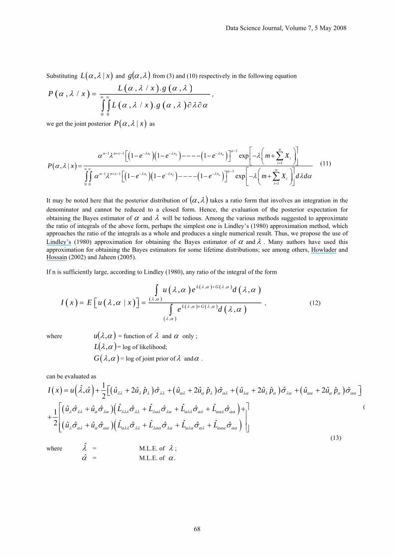
Substituting ( ), |L xα λ and ( )λα ,g from (3) and (10) respectively in the following equation

( ) ( ) ( )

( ) ( )0 0

, / . ,, /

, / . ,

L x gP x

L x g

α λ α λα λ

α λ α λ λ α∞ ∞=

∂ ∂∫ ∫,

we get the joint posterior ( ), |P xα λ as

( )( )( ) ( )

( )( ) ( )

1 2

1 2

11 1

1

11 1

10 0

1 1 1 exp, |

1 1 1 exp

n

n

nxx xn n c

ii

nxx xn n c

ii

e e e m XP x

e e e m X d d

αλλ λ

αλλ λ

α λ λα λ

α λ λ λ α

−−− −− + −

=∞ ∞ −

−− −− + −

=

⎡ ⎤⎛ ⎞⎡ ⎤− − − − − − − − +⎢ ⎥⎜ ⎟⎣ ⎦ ⎝ ⎠⎣ ⎦=⎡ ⎤⎛ ⎞⎡ ⎤− − − − − − − − +⎢ ⎥⎜ ⎟⎣ ⎦ ⎝ ⎠⎣ ⎦

∑

∑∫ ∫ (11)

It may be noted here that the posterior distribution of ( )λα , takes a ratio form that involves an integration in the denominator and cannot be reduced to a closed form. Hence, the evaluation of the posterior expectation for obtaining the Bayes estimator of α and λ will be tedious. Among the various methods suggested to approximate the ratio of integrals of the above form, perhaps the simplest one is Lindley’s (1980) approximation method, which approaches the ratio of the integrals as a whole and produces a single numerical result. Thus, we propose the use of Lindley’s (1980) approximation for obtaining the Bayes estimator of α and λ . Many authors have used this approximation for obtaining the Bayes estimators for some lifetime distributions; see among others, Howlader and Hossain (2002) and Jaheen (2005). If n is sufficiently large, according to Lindley (1980), any ratio of the integral of the form

( ) ( )( ) ( ) ( )

( )( )

( ) ( )

( )( )

, ,

,, ,

,

, ,

, |,

L G

L G

u e d

I x E u xe d

λ α λ α

λ α

λ α λ α

λ α

λ α λ α

λ αλ α

+

+= =⎡ ⎤⎣ ⎦

∫

∫ , (12)

where ( )αλ,u = function of λ and α only ;

( )αλ,L = log of likelihood;

( ),G λ α = log of joint prior ofλ andα .

can be evaluated as

( ) ( ) ( ) ( ) ( ) ( )

( ) ( )( ) ( )

1ˆ ˆ ˆ ˆ ˆ ˆ ˆ ˆ ˆ ˆ ˆ ˆ ˆ ˆ ˆ ˆ ˆ ˆ, 2 2 2 22

ˆ ˆ ˆ ˆˆ ˆ ˆ ˆ ˆ ˆ ˆ ˆ12 ˆ ˆ ˆ ˆˆ ˆ ˆ ˆ ˆ ˆ ˆ ˆ

I x u u u p u u p u u p u u p

u u L L L L

u u L L L L

λλ λ λ λλ αλ α λ αλ λα λ α λα αα α α αα

λ λλ α λα λλλ λλ λαλ λα αλλ αλ ααλ αα

λ αλ α αα αλλ λλ λαα λα αλα αλ ααα αα

λ α σ σ σ σ

σ σ σ σ σ σ

σ σ σ σ σ σ

= + + + + + + + +⎡ ⎤⎣ ⎦

⎡ + + + + +⎢+⎢ + + + +⎢⎣

⎤⎥⎥⎥⎦

(

(13) where λ̂ = M.L.E. of λ ; α̂ = M.L.E. of .α

Data Science Journal, Volume 7, 5 May 2008

68

( ) ( ) ( ) ( ) ( ) ( )2 2 2 2

2 2

ˆ ˆ ˆ ˆ ˆ ˆˆ ˆ ˆ ˆ ˆ ˆ, , , , , ,ˆ ˆ ˆ ˆ ˆ ˆ; ; ; ;

u u u u u uu u u u u uλ α λα αλ λλ αα

δ λ α δ λ α δ λ α δ λ α δ λ α δ λ α

δ λ δ α δ λδ α δ α δ λ δ λ δ α∧ ∧ ∧ ∧ ∧ ∧ ∧ ∧= = = = = =

( )

3 3 3 3 3

33

, , , , ,; ; ; ; ;

. . . . . . . . . .

,,;

. .

L L L L LL L L L L

LLL L

λλα λλλ λαλ ααλ αλλ

λλα ααα

δ λ α δ λ α δ λ α δ λ α δ λ α

δ λ δ λ δ α δ λ δ λ δ λ δ λ δ α δ λ δ α δ α δ λ δ α δ λ δ λ

δ λ αδ λ α

δ λ δ λ δ α

∧ ∧ ∧ ∧ ∧ ∧ ∧ ∧ ∧ ∧

∧ ∧ ∧ ∧ ∧

∧ ∧ ∧ ∧ ∧ ∧ ∧ ∧ ∧ ∧ ∧ ∧ ∧ ∧ ∧

∧ ∧

∧ ∧

∧ ∧ ∧

⎛ ⎞ ⎛ ⎞ ⎛ ⎞ ⎛ ⎞ ⎛ ⎞⎜ ⎟ ⎜ ⎟ ⎜ ⎟ ⎜ ⎟ ⎜ ⎟⎝ ⎠ ⎝ ⎠ ⎝ ⎠ ⎝ ⎠ ⎝ ⎠= = = = =

⎛⎝= =

3 , , ,; ; ; ;

. . .

L G GL P Pαλα α λ

δ λ α δ λ α δ λ α

δ α δ α δ α δ α δ λ δ α δ α δ λ

∧ ∧ ∧ ∧ ∧ ∧

∧ ∧ ∧

∧ ∧ ∧ ∧ ∧ ∧ ∧ ∧

⎞ ⎛ ⎞ ⎛ ⎞ ⎛ ⎞⎜ ⎟ ⎜ ⎟ ⎜ ⎟ ⎜ ⎟

⎠ ⎝ ⎠ ⎝ ⎠ ⎝ ⎠= = =

2.3 The Bayes estimator of λ under the LINEX loss function From (7), we see that the Bayes estimator of λ under the LINEX loss function is

1ˆ

1

1ˆ̂ log cE ec

λλ −⎡ ⎤= − ⎣ ⎦

where ( ) ( ) ( )1 1

( , ), | ,c cE e e p x dλ λ

λ λ αλ α λ α− −= ∫

After substituting the value of ( )x|,p αλ from (11), it may be written as:

( )( ) ( ) ( ) ( )

( ) ( ) ( )1

, ,

( , ), ,

( , )

, ,

,

L G

cL G

u e de

e dEλ α λ α

λ αλλ λ α λ α

λ α

λ α λ α

λ α

+

−+

=∫

∫ (14)

where ( ),u λ α = λ1ce− ;

( ),L λ α = ( ) ( ) ∑∑==

− −⎥⎦

⎤⎢⎣

⎡−−++

n

ii

n

i

x xenn i

11

1log1loglog λαλα λ

( ),G λ α = ( ) λλα mccmc −−+Γ−− log1logloglog

It may easily be verified that 1

1cu c e λ

λ−= − , 12

1cu c e λ

λ λ−= , 0u u uα λα αα= = = ,

1cp mλ λ

−= − ,

1pα α= − and

( ) ( )1 11

1

i

i

xn ni

ixi i

x enL xe

λ

λ λα

λ

−

−= =

⎡ ⎤⎢ ⎥= + − −

−⎢ ⎥⎣ ⎦∑ ∑ , ( )

1log 1 i

nx

i

nL e λα α

−

=

= + −∑ ,

Data Science Journal, Volume 7, 5 May 2008

69

( )( )

2

221

11 i

xni

xi

x enLe

λ

λλ λα

λ

−

−=

⎡ ⎤⎢ ⎥= − − −⎢ ⎥−⎣ ⎦∑ ,

( )1 1

i

i

xni

xi

x eLe

λ

λα λ

−

−=

=−

∑ , 2

nLαα α= − , 0L L Lλαα αλα ααλ= = =

3

2nLααα α= ,

( )2

21 1 i

xni

xi

x eLe

λ

λλα λ

−

−=

⎡ ⎤⎢ ⎥= −⎢ ⎥−⎣ ⎦∑ and ( ) ( )

( )

3

331

12 11

i i

i

x xni

xi

x e enLe

λ λ

λλλ λα

λ

− −

−=

+= + −

−∑ ,

Again, because λ and α are independent, 0λασ = ;1

Lλλλλ

σ = − ;1

Lαααα

σ = − .

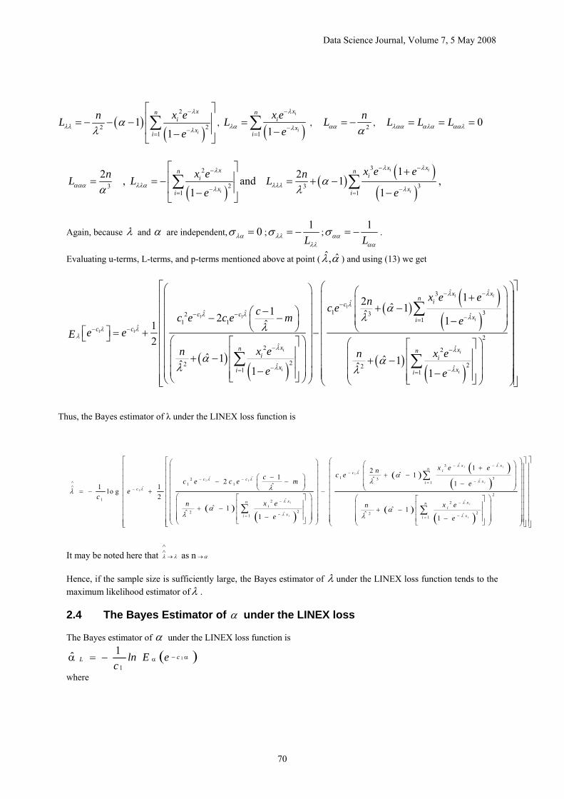
Evaluating u-terms, L-terms, and p-terms mentioned above at point ( αλ ˆ,ˆ ) and using (13) we get

( )( )

( )( )

( )

( )

1

1 1

1 1

ˆ ˆ3ˆ

1ˆ ˆ 332 ˆ11 1

ˆ

ˆ2 ˆ2

22 ˆ 21

12 ˆ 11 ˆ2 1ˆ12

ˆ 1 ˆ 1ˆ ˆ1

i i

i

i

i

x xn ic

c c xic c

xni i

xi

x e enc ecc e c e m ee eE

x en x ene

λ λ

λλ λ λ

λ λλ

λ

λ

αλ

λ

α αλ λ

− −

−

− − −=− −

− −

−=

⎛ ⎞ ⎛ ⎞+⎜ ⎟ ⎜ ⎟+ −⎜ ⎟−⎛ ⎞ ⎜ ⎟− −⎜ ⎟ ⎜ ⎟⎜ ⎟ −⎝ ⎠ ⎝ ⎠⎜ ⎟⎡ ⎤ = + −⎣ ⎦ ⎛ ⎞⎜ ⎟⎡ ⎤⎜ ⎟⎜ ⎟⎢ ⎥+ − + −⎜ ⎟⎜ ⎟⎢ ⎥

−⎜ ⎟⎜ ⎟⎢ ⎥⎣ ⎦⎝ ⎠⎝ ⎠

∑

∑( )

2

2ˆ1 1

i

i

xn

xi e

λ

λ−=

⎡ ⎤⎛ ⎞⎢ ⎥⎜ ⎟⎢ ⎥⎜ ⎟⎢ ⎥⎜ ⎟⎢ ⎥⎜ ⎟⎢ ⎥⎜ ⎟⎛ ⎞⎡ ⎤⎢ ⎥⎜ ⎟⎜ ⎟⎢ ⎥⎢ ⎥⎜ ⎟⎜ ⎟⎢ ⎥⎢ ⎥⎜ ⎟−⎜ ⎟⎜ ⎟⎢ ⎥⎣ ⎦⎢ ⎥⎝ ⎠⎝ ⎠⎣ ⎦

∑

Thus, the Bayes estimator of λ under the LINEX loss function is

( )( )

( )( )

( )

( )

1

1 1

1

ˆ ˆ3ˆ

1ˆ ˆ 332 ˆ11 1ˆ

1 ˆ2 2

22 ˆ 21

12 ˆ 11 ˆ2 1ˆ1 1l o g2

ˆ 1 ˆ 1ˆ ˆ1

i i

i

i

i

x xn ic

c c xic

xni i

xi

x e enc ecc e c e m ee

cx en xn

e

λ λ

λλ λ λ

λ

λ

λ

αλ

λλ

α αλ λ

− −

−

− − −∧ =∧

−

−

−=

⎛ ⎞ ⎛ ⎞+⎜ ⎟ ⎜ ⎟+ −⎜ ⎟ ⎜ ⎟−⎛ ⎞− −⎜ ⎟⎜ ⎟ ⎜ ⎟−⎝ ⎠ ⎝ ⎠⎜ ⎟= − + −⎜ ⎟⎛ ⎞⎡ ⎤⎜ ⎟⎜ ⎟⎢ ⎥⎜ ⎟+ −⎜ ⎟ + −⎢ ⎥⎜ ⎟⎜ ⎟−⎢ ⎥⎜ ⎟⎜ ⎟⎣ ⎦⎝ ⎠⎝ ⎠

∑

∑( )

2

ˆ

2ˆ1 1

i

i

xn

xi

e

e

λ

λ

−

−=

⎡ ⎤⎡ ⎤⎛ ⎞⎢ ⎥⎜ ⎟⎢ ⎥⎢ ⎥⎜ ⎟⎢ ⎥⎢ ⎥⎜ ⎟⎢ ⎥⎢ ⎥⎜ ⎟⎢ ⎥⎢ ⎥⎜ ⎟⎢ ⎥

⎛ ⎞⎡ ⎤⎢ ⎥⎜ ⎟⎢ ⎥⎜ ⎟⎢ ⎥⎢ ⎥⎜ ⎟⎢ ⎥⎜ ⎟⎢ ⎥⎢ ⎥⎜ ⎟⎢ ⎥⎜ ⎟−⎢ ⎥⎜ ⎟⎢ ⎥⎜ ⎟⎜ ⎟⎢ ⎥⎣ ⎦⎢ ⎥⎝ ⎠⎢ ⎥⎝ ⎠⎣ ⎦⎣ ⎦

∑

It may be noted here that λ λ

∧∧→ as n α→

Hence, if the sample size is sufficiently large, the Bayes estimator of λ under the LINEX loss function tends to the maximum likelihood estimator ofλ . 2.4 The Bayes Estimator of α under the LINEX loss The Bayes estimator of α under the LINEX loss function is

( )α−α−=α 1

1

1cL eEln

cˆ

where

Data Science Journal, Volume 7, 5 May 2008

70

( ) ( )( )

1 1

,, | ,c cE e e p x dα α

α λ αλ α λ α− −⎡ ⎤ =⎣ ⎦ ∫

After substituting the value of ( )x|,p αλ from (11), it may be expressed as:

( ) ( ) ( ) ( )( )

( ) ( ) ( )( )

1

, ,

,, ,

,

, ,

,

L G

cL G

u e dE e

e d

λ α λ α

λ ααα λ α λ α

λ α

λ α λ α

λ α

+

−+

⎡ ⎤ =⎣ ⎦∫

∫ (15)

where ( ),u λ α = α1ce− , ( )αλ,L and ( ),G λ α are the same as those given in (14).

Following the procedure as discussed above for the estimation of λ, we get after simplification

( )

( )( )

1 1 1

ˆ2

2ˆ12

ˆ ˆ1 1

ˆ2

22 ˆ1

1ˆ1 2 2ˆ ˆ2

ˆ 1ˆ 1

i

i

i

i

xni

xic c c

xni

xi

x e

eE e e c e c

nx en

e

λ

λ

α α αα

λ

λ

αα α

αλ

−

−=− − −

−

−=

⎡ ⎤⎛ ⎞⎢ ⎥⎜ ⎟⎢ ⎥⎜ ⎟⎢ ⎥⎜ ⎟−⎛ ⎞⎢ ⎥⎜ ⎟⎡ ⎤ = + + − −⎜ ⎟⎣ ⎦ ⎧ ⎫⎢ ⎥⎜ ⎟⎡ ⎤⎝ ⎠

⎪ ⎪⎢ ⎥⎜ ⎟⎢ ⎥+ −⎨ ⎬⎢ ⎥⎜ ⎟⎢ ⎥⎪ ⎪−⎜ ⎟⎢ ⎥⎢ ⎥⎣ ⎦⎩ ⎭⎝ ⎠⎣ ⎦

∑

∑

Thus, the Bayes estimator under the LINEX loss function is

( )

( )( )

1 1

ˆ2

2ˆ12

ˆ ˆ1 1

1 ˆ2

22 ˆ1

1ˆ1 1 2 2ˆ̂ logˆ ˆ2

ˆ 1ˆ 1

i

i

i

i

xni

xic c

xni

xi

x e

ee c e c

c nx en

e

λ

λ

α α

λ

λ

ααα α

αλ

−

−=− −

−

−=

⎡ ⎤⎧ ⎫⎧ ⎫⎢ ⎥⎪ ⎪⎪ ⎪⎢ ⎥⎪ ⎪⎪ ⎪⎢ ⎥⎪ ⎪⎪ ⎪−⎪ ⎪ ⎪⎪⎛ ⎞⎢ ⎥= − + + − −⎨ ⎨ ⎬⎬⎜ ⎟⎢ ⎥⎧ ⎫⎝ ⎠⎪ ⎪ ⎪⎪⎢ ⎥⎪ ⎪⎪ ⎪ ⎪⎪+ −⎨ ⎬⎢ ⎥⎪ ⎪ ⎪⎪⎪ ⎪−⎢ ⎥⎪ ⎪ ⎪⎪⎩ ⎭⎢ ⎥⎩ ⎭⎩ ⎭⎣ ⎦

∑

∑

It may be noted here that ˆ̂ ˆα α→ as ∞→n when sample size n is sufficiently large and the Bayes estimator of α under the LINEX loss function tends to the maximum likelihood estimator ofα . 3 NUMERICAL FINDINGS The estimators λ̂ and α̂ are maximum likelihood estimators of the parameters of the Generalized-Exponential

distribution; whereas λ̂̂ and α̂̂ are Bayes estimators obtained by using the L-approximation. As mentioned earlier, the maximum likelihood estimators and hence risks of the estimators cannot be put in a convenient closed form. Therefore, risks of the estimators are empirically evaluated based on a Monte-Carlo simulation study of 1000 samples. A number of values of unknown parameters are considered. Sample size is varied to observe the effect of small and large samples on the estimators. Changes in the estimators and their risks have been determined when changing the shape parameter of loss functions while keeping the sample size fixed. Different combinations of prior

Data Science Journal, Volume 7, 5 May 2008

71

parameters λ and α are considered in studying the change in the estimators and their risks. The results are summarized in Figures 1-10. It is easy to notice that the risk of the estimators will be the function of sample size, population parameters, parameters of the prior distribution (hyper parameters), and loss function parameters. In order to consider the wide variety of values, we have obtained the simulated risks for sample sizes N=10, 20, 30, and 40. The various values of parameters of the distribution considered are scale parameter λ =0.5 (.5) 3.0, shape parameter α =0.5 (.5) 3.0, and loss parameter 1c =± 0.5, ± 1.0 and ± 1.5. Prior parameters m and c are arbitrarily taken as 1.0. After an extensive study of the results thus obtained, conclusions are drawn regarding the behavior of the estimators, which are summarized below. It may be mentioned here that because of space restrictions, all results are not shown in the graphs. Only a few are presented here to demonstrate the effects found and the conclusion drawn. However, in most of the cases, the proposed Bayes estimator is better than the Maximum Likelihood Estimator (MLE). 3.1 The Effect of Sample Size It is noted that as sample size increases, the risk of the estimators decreases, and for a sample size greater than 25, the risk of the Bayes estimators and MLEs are more or less equal (see Figures 1-4). For small samples, the behaviors of risks of estimators depend on the values of c1, λ, and α. For positive values of c1 (i.e., when overestimation is more serious then underestimation), the risks of the Bayes estimator of λ are more or less equal to the MLE. However, the risk of the Bayes estimator of α is less than MLE, and the difference is larger for smaller sample sizes (see Figures 1 and 2).The trends of the risk of the estimators are reversed if c1 is negative (i.e., when underestimation is more serious then overestimation), see Figures 3 and 4. 3.2 Effect of Population Parameters λ and α The effect of variation of λ on the risks of the estimator of λ and α has also been studied. It has been noticed that for positive values of 1c , as λ increases, the risk of the estimator of λ first decreases, then increases. The same trend is also noticed forα . It is observed that in most of the cases, the risk of the Bayes estimator of α is less than the risk of the MLE estimator ofα , whereas the risk of the Bayes estimator of λ is same as the MLE for smaller values ofλ . When λ is large, however, it does not perform well (see Figures 5 and 6). For negative values of 1c , it is noted that as the value of λ increases, the risk of the estimator of bothλ and α , first increases then decreases. It is also noticed that the risk of the MLE estimator has a smaller value than the risk of the Bayes estimator ofλ . In the case ofα , there are very few data points for large samples and 1c =-0.5, where the risk of the Bayes estimator of α is less than risk of the MLE estimator of α (see Figures 7 and 8). 3.3 Effect of Loss Parameter 1c In studying the effect of variation in the values of 1c , i.e., the LINEX loss parameter, on risks of the estimator of λ

and α , it may be noted that the risks for negative values of 1c are less than the risks for positive values of 1c . As

the magnitude of 1c increases, the risks of the estimator of λ , as well as the risks of the estimator of α , increase,

which gives a bath-tub type curve, having minimum risks at 1c =-1.0. In most cases, for positive values of 1c , the risks of the Bayes estimator of α are less than the risks of the MLE estimator ofα , but this may not be true for negative values of 1c . The risks of the proposed Bayes estimator of λ are also not as good as the risks of the MLE estimator ofλ , which can be seen in Figures 9 and 10.

Data Science Journal, Volume 7, 5 May 2008

72

Figure 1. Risk of λ for overestimation (c1 positive) Figure 2. Risk of α for overestimation (c1 positive) as function of sample size as function of sample size Figure 3. Risk of λ for underestimation (c1 negative) Figure 4. Risk of α for underestimation (c1 negative) as function of sample size as function of sample size Figure 5. Risk of λ for overestimation (c1 positive) Figure 6. Risk of α for overestimation (c1 positive) as function of size of λ as function of size of α

Data Science Journal, Volume 7, 5 May 2008

73

Figure 7. Risk of λ for underestimation (c1 negative) Figure 8. Risk of α for underestimation (c1 negative) as function of size of λ as function of size of λ Figure 9. Risk of λ as function of loss parameter c1 Figure 10. Risk of α as function of loss parameter c1 5 CONCLUSION The performance of the proposed Bayes estimator under the LINEX loss has been compared to the maximum likelihood estimator in the previous section. On the basis of these results, we may conclude that for positive 1c , i.e., overestimation is more serious than underestimation, the proposed Bayes estimator of λ performs better than the maximum likelihood estimator of λ for large sample sizes and small values of λ and α respectively; whereas risks of the proposed Bayes estimator of α perform better than the maximum likelihood estimator of α for a large portion of parametric space. For negative 1c , i.e., underestimation is more serious than overestimation, the risks of the maximum likelihood estimator of λ perform better than the risks of the proposed Bayes estimator. The risks of the proposed Bayes estimator of α perform better than the maximum likelihood estimator of α for the whole parametric space. Thus, the use of the proposed estimator is to be recommended.

Data Science Journal, Volume 7, 5 May 2008

74

6 REFERENCES Ahmadi, J., Doostparast, M., & Parsian, A. (2005) Estimation and prediction in a two parameter exponential distribution based on k-record values under LINEX loss function. Commun. Statist. Theor. Meth. 34:795–805. Bain, L.J. & Engelhardt, M. (1991) Statistical Analysis of Reliability and Life Testing Models - Theory and Methods. New York: Marcel Dekker, Inc. Basu, A. P. & Ebrahimi, N. (1991) Bayesian approach to life testing and reliability estimation using asymmetric loss-function. J. Statist. Plann. Infer. 29:21–31. Calabria, R. & Pulcini, G. (1996) Point estimation under asymmetric loss functions for left truncated exponential samples. Commun. Statist. Theor. Meth. 25(3):585–600. Gupta, R.D. & Kundu, D. (1999) Generalised-Exponential Distribution, Australia and New Zealand Journal of Statistics, 41,173-188. Gupta, R.D. & Kundu, D. (2002) Generalised-Exponential Distribution, Journal of Applied Statistical Society. Gupta, R.D. & Kundu, D. (2004) Discriminating between Gamma and Generalised Exponential Distribution, Journal of Statistical Computation and Simulation Vol-74(2), 107-121. Jaheen, Z. F. (2005) On record statistics from a mixture of two exponential distributions. J. Statist. Computat. Simul. 75(1):1–11. Lieblein, J. & Zelen, M. (1956) Statistical investigation of the fatigue life of deep groove ball bearings. Jour. of Res. Natl. Bur. Std., 273-315. Lindley, D.V. (1980) Approximate Bayes methods. Bayesian Statistics, Valency. Raqab, M.Z. & Ahsanullah, M (2001) Estimation of location and scale parameter of Generalised-Exponential Distribution based on Order Statistics. Journal of Statistical Computation and Simulation, 69, 2, 109-124. Singh, U., Gupta, P. K., & Upadhyay, S. K. (2005) Estimation of parameters for exponentiated-Weibull family under Type-II censoring scheme. Omputat. Statist. DataAnal. 48(3):509–523. Soliman, A. A. (2002) Reliability estimation in a generalized life-model with application to the Burr-XII. IEEE Trans. Reliabil. 51:337–343. Tierny, L. & Kadane, J. B. (1986) Accurate approximations for posterior moments and marginal densities. J. Amer. Statist. Assoc. 81:82–86. Varian, H. R. (1975) A Bayesian approach to real state assessment. In: Stephen, E. F. & Zellner, A. ( Eds.) Studies in Bayesian Econometrics and Statistics in Honor of Leonard J. Savage, pp. 195–208. Amsterdam: North-Holland. Zellner, A. (1986) A Bayesian Estimation and Prediction using Asymmetric Loss function. JASA, 81, 446-451.

Data Science Journal, Volume 7, 5 May 2008

75