3766 IEEE TRANSACTIONS ON INFORMATION THEORY, VOL. 51, NO. 11, NOVEMBER 2005

Bayesian Bin Distribution Inference andMutual Information

Dominik Endres and Peter Földiák

Abstract—We present an exact Bayesian treatment of a simple,yet sufficiently general probability distribution model. We con-sider piecewise-constant distributions ( ) with uniform(second-order) prior over location of discontinuity points andassigned chances. The predictive distribution and the modelcomplexity can be determined completely from the data in acomputational time that is linear in the number of degrees offreedom and quadratic in the number of possible values of .Furthermore, exact values of the expectations of entropies andtheir variances can be computed with polynomial effort. Theexpectation of the mutual information becomes thus available, too,and a strict upper bound on its variance. The resulting algorithmis particularly useful in experimental research areas where thenumber of available samples is severely limited (e.g., neurophysi-ology). Estimates on a simulated data set provide more accurateresults than using a previously proposed method.

Index Terms—Bayesian inference, entropy, model selection, mu-tual information.

I. INTRODUCTION

THE small number of samples available in many areas ofexperimental science is a serious limitation in calculating

distributions and information. For instance, such limitations aretypical in the neurophysiological recording of neural activity.Computing entropies and mutual information from data of lim-ited sample size is a difficult task. A related problem is the es-timation of probability distributions and/or densities. In fact,once a good density estimate is available, one could also ex-pect the entropy estimates to be satisfactory. One of the sev-eral approaches proposed in the past is kernel-based estimation,having the advantage of being able to model virtually any den-sity, but suffering from a heavy bias, as reported by [1]. Anothercategory consists of parametrized estimation methods, whichchoose some class of density function and then determine a setof parameters that best fit the data by maximizing their likeli-hood. However, maximum-likelihood approaches are prone tooverfitting. A common remedy for this problem is cross vali-dation (see, e.g., [2]), which, while it appears to work in manycases, can at best be regarded as an approximation.

Overfitting occurs especially when the size of the data setis not large enough compared to the number of degrees offreedom of the chosen model. Thus, as a compromise betweenthe two aforementioned methods, mixture models have recently

Manuscript received August 16, 2004; revised May 12, 2005.The authors are with the School of Psychology, University of St.Andrews, St.

Andrews KY16 9JP, Scotland, U.K. (e-mail: dme2@st-andrews.ac.uk; pf2@st-andrews.ac.uk).

Communicated by P. L. Bartlett, Associate Editor for Pattern Recognition,Statistical Learning and Inference.

Digital Object Identifier 10.1109/TIT.2005.856954

attracted considerable attention (see, e.g., [3]). Here, a mixtureof simple densities (Gaussians are quite common) are usedto model the data. The most popular method for determiningits parameters is Expectation Maximization, first described by[4], which, while having nice convergence properties, is stillaiming at maximizing the likelihood. The question of howto determine the best number of model parameters thereforeremains unanswered in this framework.

This answer can be given by Bayesian inference. In fact, whenone is willing to accept some very natural consistency require-ments, it provides the only valid answer, as demonstrated by [5].The difficulty lies in carrying out the necessary computations.More specifically, the integrations involved in computing theposterior densities of the model parameters are hard to tackle.To date, only fairly simple and hence not very general densitymodels could be treated exactly. Thus, a variety of approxi-mation schemes have been devised, e.g., Laplace approxima-tion (where the true density is replaced by a Gaussian), MonteCarlo simulation, or variational Bayes (a good introduction canbe found in [6]). As is always the case with approximations,they will work in some cases and fail in others. Two other note-worthy approaches to dealing with the overfitting problem areminimum message length (MML) [7] and minimum descriptionlength (MDL) [8], which are similar to Bayesian inference.

In this paper, we will present an exactly tractable model.While still simple in construction, it is sufficiently general tomodel any distribution (or density). The model’s complexity isfully determined by the data, too. Moreover, it also yields exactexpectations of entropies and their variances. Thus, an exactexpectation of the mutual information and a strict upper boundon its variance can be computed as well.

II. BAYESIAN BINNING

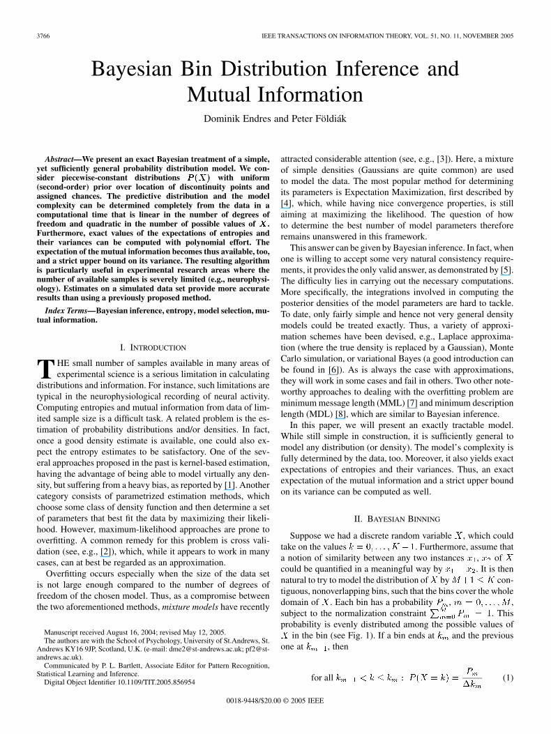
Suppose we had a discrete random variable , which couldtake on the values . Furthermore, assume thata notion of similarity between any two instances , ofcould be quantified in a meaningful way by . It is thennatural to try to model the distribution of by con-tiguous, nonoverlapping bins, such that the bins cover the wholedomain of . Each bin has a probability , ,subject to the normalization constraint . Thisprobability is evenly distributed among the possible values of

in the bin (see Fig. 1). If a bin ends at and the previousone at , then

for all (1)

0018-9448/$20.00 © 2005 IEEE

ENDRES AND FÖLDIÁK: BAYESIAN BIN DISTRIBUTION INFERENCE AND MUTUAL INFORMATION 3767

Fig. 1. An example configuration forK = 10 values ofX , three bins (M = 2interval boundaries), containing the probabilities P . Here, P (0) = P (1) =P (2) = , P (3) = � � � = P (8) = , P (9) = P . The points indicatewhich values of X belong to a bin. The algorithm iterates over all possibleconfigurations to find the expected probability distribution and other relevantaverages.

with , , and ,i.e., the first bin starts at and the last one includes

. Assume now we had a multisetof points drawn independently from the distribution whichwe would like to infer. Given the model parameterized byand , the probability of the data then is given (up toa factor) by a multinomial distribution

(2)

where is the number of points in bin . One might arguethat a multinomial factor should be inserted here, because thedata points are not ordered. This would, however, only amountto a constant factor that cancels out when averages (posteriors,expectations of variables, etc.) are computed. It will thereforebe dropped. The factors express the intention of mod-eling possible values of by the same probability. Froman information-theoretic perspective, we are trying to find a sim-pler coding scheme for the data while preserving the informa-tion present in them: The message “ ” for all

would be represented by a code element of the samelength . In contrast, were the absent, then themessage “ ” for each would berepresented by the same code element, i.e., an information re-duction transformation would have been applied to the data.

We now want to compute the evidence of a model withbins, i.e., . It is obtained by multiplying the likeli-hood (see (2)) with a suitable prior to yield

. This density is then marginalized withrespect to (w.r.t.) and , which is done by integrationand summation, respectively. The summation boundaries forthe have to be chosen so that each bin covers at least onepossible value of . Since the bins may not overlap,

, , etc. Because therepresent probabilities, their integrations run from to

subject to the normalization constraint, which can be enforcedvia a Dirac function

(3)

where

(4)

and

(5)

Note that the prior is a probability density,because the are real numbers.

III. COMPUTING THE PRIOR

We shall make a noninformative prior assumption, namely,that all possible configurations of are equally likelyprior to observing the data. The prior can be written as

(6)

Note that the second factor on the right-hand side (RHS) is nota probability density, because there is only a finite number ofconfigurations for the . We now make the assumption thatthe probability contained in a bin is independent of the bin size,i.e.,

This is certainly not the only possible choice, but a commonone: in the absence of further prior information, independenceassumptions can be justified, since they maximize the prior’sentropy. Thus, (6) becomes

(7)

Since all models are to be equally likely, the prior is constant(denoted by ) w.r.t. and , and normalized

(8)

Carrying out the integrals is straightforward (see, e.g., [9]) andyields the normalization constant of a Dirichlet distribution. Thevalue of the sums is given by

(9)

This is, of course, just the number of possibilities of distributingordered bin boundaries across places. Due to the as-

sumed independence between and , we can write

(10)

(11)

3768 IEEE TRANSACTIONS ON INFORMATION THEORY, VOL. 51, NO. 11, NOVEMBER 2005

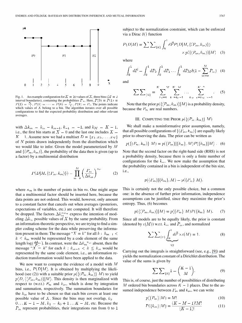
Fig. 2. After all the evidence contributions a( ~M; ~K) have been evaluated to compute the evidence of a model with ~M intersections, they can be reused tocompute the a( ~M + 1; ~K). The arrows indicate which a( ~M; ~K) enter into the calculation for an a( ~M + 1; ~K).

and thus, the prior is

(12)

IV. COMPUTING THE EVIDENCE

To compute (3), we rewrite it as

(13)

where

(14)Given a configuration of the , the are fixed, and thusthe integrals can be carried out (see, e.g., [9]) to yield

(15)

i.e., the normalization integral of a Dirichlet distribution again.Thus,

(16)

For a speedy evaluation of the sums in (13), we suggest thefollowing iterative scheme:

let

(17)

where is the total number of data points for which(i.e., the number of points in the current bin ). Furthermore,define

(18)

where is the total number of data points for which(i.e., the number of points in the current bin ).

In other words, to compute the contribution to (13) which hasbin boundaries in the interval , let boundarymove between position (because the previous

boundaries must at least occupy the positions )and (because bin must at least have width ).For each of these positions, multiply the factor for bin(which ranges from to ) with the contribution for binboundaries in the interval and add.

By induction, we hence obtain

(19)

Inserting (16) into (13) and using (11) yields

(20)

This way of organizing the calculation is computationallysimilar to the sum–product algorithm [10], the messages beingpassed from one -level to the next are the , whereaswithin one level, a sum over the messages from the previouslevel (times a factor) is performed.

To compute , we need all the ,(see Fig. 2). While we are at it, we can

just as well evaluate , which does not increasethe overall computation complexity. Thus, we get the evidencesfor models with less than intersections with little extra ef-fort. Moreover, in an implementation it is sufficient to store the

in a one-dimensional array of length that is over-written in reverse order as one proceeds from to (be-cause is no longer needed once iscomputed, etc.). In pseudocode (where func-tion returns the number of observed points for which

):

ENDRES AND FÖLDIÁK: BAYESIAN BIN DISTRIBUTION INFERENCE AND MUTUAL INFORMATION 3769

1) Initialize ,2) for to do

a)b)

3)4) for to do

a) if then elseb) for downto lb do

i)ii) for to do

A)B)

c)

Step 4a) is not essential, but it saves some computational ef-fort: once the main loop 4 reaches , only needsto be calculated. The would only be necessaryif the evidence for bin boundaries were to be evaluated.

In a real-world implementation, it might be advisable to con-struct a lookup table for

since these quantities would otherwise be evaluated multipletimes in step 4b)ii)B), as soon as .

A look at the main loop 4) shows that the computational com-plexity of this algorithm is (provided that ,i.e., the number of bins is much smaller than the number of pos-sible values of ), or more generally, (because

). This is significantly faster than the naïve approachof simply trying all possible configurations, which would yield

.

V. EVALUATING THE MODEL POSTERIOR , THE

DISTRIBUTION , AND ITS VARIANCE

Once the evidence is known, we can proceed to determine therelative probabilities of different , the model posterior

(21)

where is the model prior and

The sum over includes all models which we choose to includeinto our inference process, therefore, the conditioning on a par-ticular is marginalized. It is thus customary to refer toas “the probability of the data.” This is somewhat misleading,because is still not only conditioned on the set of wechose, but also on the general model class we consider (here:probability distributions that consist of a number of bins).

The predictive distribution of can be calculated via theevidence as well. Note that

(22)

i.e., the joint predictive probability of is the ex-pectation of the product of their probabilities given and .Thus, if we want the value of the predictive distribution of ata particular , we can simply add this to the multiset . Callthis extended multiset , then

(23)

The choice of will usually be noninformative (e.g., uni-form), unless we have reasons to prefer certain models overothers.

Likewise, to obtain the variance, add twice:. Then

(24)

VI. INFERRING PROBABILITY DENSITIES

The algorithm can also be used to estimate probability densi-ties. To do so, replace all occurrences of with ,where is the interval between and . This yields a dis-cretized approximation to the density. The discretization is justanother model parameter which can be determined from the data

(25)

where runs over all possible values of which wechoose to include. is computed in the same fashionas in (21) for a given , except that the data are nowassumed to be continuous, hence, the probability turns into adensity.

The dependence of on is through (see(3)): if one tries to find a suitable discretization of the interval

, then .

VII. MODEL SELECTION VERSUS MODEL AVERAGING

Once is determined, we could use it to select an. However, making this decision involves “contriving” in-

formation, namely, nats. Thus, unless one isforced to do so, one should refrain from it and rather averageany predictions over all possible . Since , com-puting such an average has a computational cost of . Ifthe structure of the data allows for it, it is possible to reduce thiscost by finding a range of that does not increase linearly with

, without a high risk of not including a model even though itprovides a good description of the data. In analogy to the sig-nificance levels of orthodox statistics, we shall call this risk .If the posterior of is unimodal (which it has been in mostobserved cases, see, e.g., Seection IX), we can then choose thesmallest interval of s around the maximum of suchthat

(26)

and carry out the averages over this range of .

3770 IEEE TRANSACTIONS ON INFORMATION THEORY, VOL. 51, NO. 11, NOVEMBER 2005

VIII. COMPUTING THE ENTROPY AND ITS VARIANCE

To evaluate the entropy of the distribution , we firstcompute the entropy of (1)

(27)

where is the natural logarithm. This expression mustnow be averaged over the posterior distributions ofand possibly to obtain the expectation of . In-stead of carrying this out for (27) as a whole, it is easier to doit term-by-term, i.e., we need to calculate the expectations of

and . Generally speaking, ifwe want to compute the average of any quantity that is a func-tion of the probability in a bin for a given , we can proceedin the following fashion: call this function . Its expecta-tion w.r.t. the is then

(28)where, by virtue of (14) and (15)

(29)

because is a constant, otherwise it would have to beincluded in the integrations. Note that, as far as the counts in thebins are concerned, depends onlyon (and possibly , the total number of data points). Thiscan be verified by integrating the numerator of (28) over all ,

. Therefore,

(30)

When (29) is inserted here, it becomes apparent that this ex-pectation has the same form as (13) after inserting (16). Com-bined with the fact that depends onlyon , this means that the above described iterative computa-tion scheme ((17) and (18)) can be employed for its evaluation.All one needs to do is to substitute

i.e., (18) is replaced by

(31)

where and . The forare the same as before. Note that (31) can also be used ifdepends not only on , but also on the boundaries of bin(i.e., and ). Generally speaking, (31) can be employedwhenever the expectation of a function (given and ) is tobe evaluated, if this function depends only on the parameters ofone bin.

For fixed , some of these expectations have been com-puted before in [9].

A. Computing

Using (1) and defining , we obtain

(32)

To compute the integrals, note that

(33)

which is

(34)

where is the beta function (see, e.g., [11] for details onits derivatives and other properties), and

(35)

is the difference between the partial sums of the harmonic serieswith upper limits and . The first part of (34) is the normal-ization integral of the density of the . Hence, their entropyfor fixed is given by (34) divided by (15)

(36)which is a rational number. In other words, entropy changes inrational increments as we observe new data points.

Thus,

(37)

ENDRES AND FÖLDIÁK: BAYESIAN BIN DISTRIBUTION INFERENCE AND MUTUAL INFORMATION 3771

B. Computing

Here

(38)

and by using the same identities as above

(39)

C. Computing the Variance

To compute the variance, we need the square of the entropy

(40)

Hence, we need to evaluate the expectations of

1) . See Section VIII-D.2) . See Section VIII-E.3) . Can be evaluated along the same lines

as (39) and yields

(41)

4) . Follows from (15) byreplacing with , with , and yields

(42)5) . Can be evaluated along the

same lines as (37) and yields

(43)

6) . Can be evaluated alongthe same lines as (37) and yields

(44)In an actual implementation, steps 1), 3), and 5) can becomputed in one run, because they contain only terms thatrefer to the bin . Likewise, the remaining three steps canbe evaluated together. However, since they depend on theparameters of two distinct bins, the iteration over the binconfiguration has to be adapted: assume . This isno restriction, since and can always be exchangedto satisfy this constraint. As we will show later, the quanti-ties of interest can be expressed as products of expectations

. The itera-tion rule (18) then is

(45)

and

(46)

D. Computing

Since

(47)

we can use the same method of calculation as above. Thus, weobtain

(48)

where

(49)

E. Computing

To compute this expectation, we need to evaluate

(50)

and then divide it by a normalization constant. The integralsin the last expression can be rewritten, using beta functions, toyield

(51)

3772 IEEE TRANSACTIONS ON INFORMATION THEORY, VOL. 51, NO. 11, NOVEMBER 2005

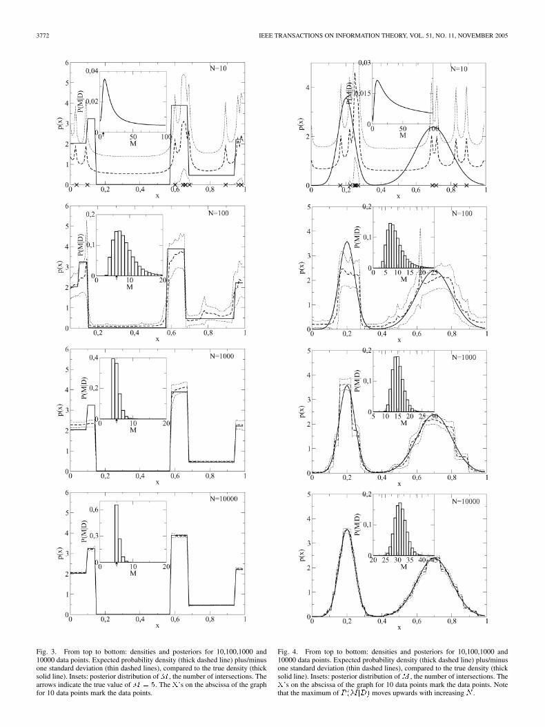
Fig. 3. From top to bottom: densities and posteriors for 10,100,1000 and10000 data points. Expected probability density (thick dashed line) plus/minusone standard deviation (thin dashed lines), compared to the true density (thicksolid line). Insets: posterior distribution ofM , the number of intersections. Thearrows indicate the true value ofM = 5. The X’s on the abscissa of the graphfor 10 data points mark the data points.

Fig. 4. From top to bottom: densities and posteriors for 10,100,1000 and10000 data points. Expected probability density (thick dashed line) plus/minusone standard deviation (thin dashed lines), compared to the true density (thicksolid line). Insets: posterior distribution ofM , the number of intersections. TheX’s on the abscissa of the graph for 10 data points mark the data points. Notethat the maximum of P (M jD) moves upwards with increasing N .

ENDRES AND FÖLDIÁK: BAYESIAN BIN DISTRIBUTION INFERENCE AND MUTUAL INFORMATION 3773

where and is the part that does notdepend upon and and, thus, is not affected by the dif-ferentiation

(52)

We then obtain

(53)

The desired expectation can thus be computed in two runs of theiteration: first, let

(54)

(55)

and divide the result by .Second, let

(56)

(57)

and multiply the result with .

IX. EXAMPLES

Fig. 3 shows examples of the predictive density andits variance, compared to the density from which the datapoints were drawn ( , , data point abscissaswere rounded to the next lower discretization point), as well asthe model posteriors . The prior was chosenuniform over the maximum range of , here .Inference was conducted with (see (26)).1 Note thatthe curves that represent the expected density plus/minus onestandard deviation are not densities any more. The data wereproduced by first drawing uniform random numbers with thegenerator sran2() from [12], those were then transformed bythe inverse cumulative density (a method also described in[12]) to be distributed according to the desired density. For verysmall data sets, only the largest structures of the distributioncan vaguely be seen (such as the valley between and

). Furthermore, the density peaks at each data point (at ,two points were observed very close to each other). One mighttherefore imagine the process by which the density comes aboutas similar to kernel-based density estimates. It does, however,differ from a kernel-based procedure insofar as that the numberof degrees of freedom does not necessarily grow with the dataset, but is determined by the data’s structure. The model poste-rior is very broad, reflecting the large remaining uncertaintiesdue to the small data set. Models with wereincluded in the predictions.

With 100 data points, more structures begin to emerge (e.g.,the high plateau between and ), and the variance de-creases, as one would expect. The model posterior exhibits a

1On a 2.6-GHz Pentium 4 system running SuSE Linux 8.2, computing the ev-idence took � 0.26 s (without initializations). The algorithm was implementedin C++ and compiled with the GnU compiler.

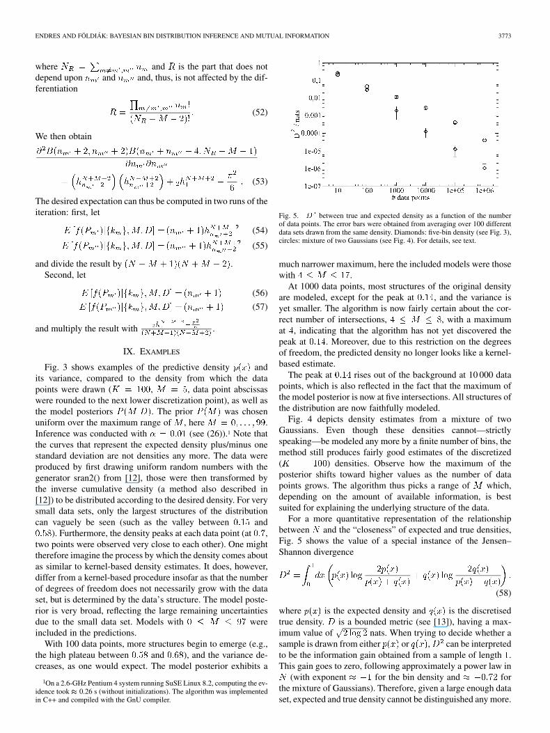
Fig. 5. D between true and expected density as a function of the numberof data points. The error bars were obtained from averaging over 100 differentdata sets drawn from the same density. Diamonds: five-bin density (see Fig. 3),circles: mixture of two Gaussians (see Fig. 4). For details, see text.

much narrower maximum, here the included models were thosewith .

At 1000 data points, most structures of the original densityare modeled, except for the peak at , and the variance isyet smaller. The algorithm is now fairly certain about the cor-rect number of intersections, , with a maximumat , indicating that the algorithm has not yet discovered thepeak at . Moreover, due to this restriction on the degreesof freedom, the predicted density no longer looks like a kernel-based estimate.

The peak at rises out of the background at 10 000 datapoints, which is also reflected in the fact that the maximum ofthe model posterior is now at five intersections. All structures ofthe distribution are now faithfully modeled.

Fig. 4 depicts density estimates from a mixture of twoGaussians. Even though these densities cannot—strictlyspeaking—be modeled any more by a finite number of bins, themethod still produces fairly good estimates of the discretized( ) densities. Observe how the maximum of theposterior shifts toward higher values as the number of datapoints grows. The algorithm thus picks a range of which,depending on the amount of available information, is bestsuited for explaining the underlying structure of the data.

For a more quantitative representation of the relationshipbetween and the “closeness” of expected and true densities,Fig. 5 shows the value of a special instance of the Jensen–Shannon divergence

(58)

where is the expected density and is the discretisedtrue density. is a bounded metric (see [13]), having a max-imum value of nats. When trying to decide whether asample is drawn from either or , can be interpretedto be the information gain obtained from a sample of length .This gain goes to zero, following approximately a power law in

(with exponent for the bin density and forthe mixture of Gaussians). Therefore, given a large enough dataset, expected and true density cannot be distinguished any more.

3774 IEEE TRANSACTIONS ON INFORMATION THEORY, VOL. 51, NO. 11, NOVEMBER 2005

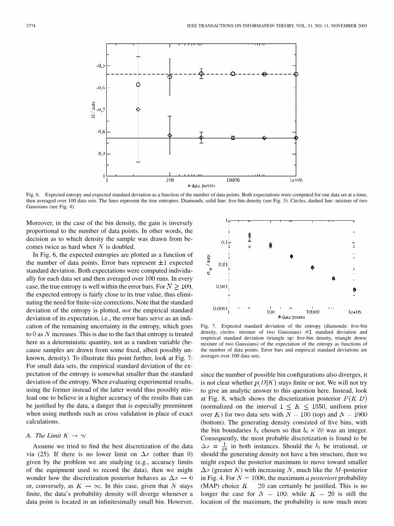
Fig. 6. Expected entropy and expected standard deviation as a function of the number of data points. Both expectations were computed for one data set at a time,then averaged over 100 data sets. The lines represent the true entropies. Diamonds, solid line: five-bin density (see Fig. 3). Circles, dashed line: mixture of twoGaussians (see Fig. 4).

Moreover, in the case of the bin density, the gain is inverselyproportional to the number of data points. In other words, thedecision as to which density the sample was drawn from be-comes twice as hard when is doubled.

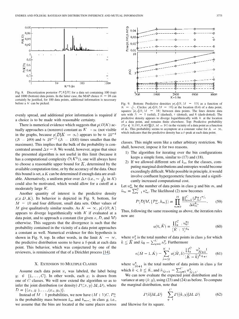
In Fig. 6, the expected entropies are plotted as a function ofthe number of data points. Error bars represent expectedstandard deviation. Both expectations were computed individu-ally for each data set and then averaged over 100 runs. In everycase, the true entropy is well within the error bars. For ,the expected entropy is fairly close to its true value, thus elimi-nating the need for finite-size corrections. Note that the standarddeviation of the entropy is plotted, not the empirical standarddeviation of its expectation, i.e., the error bars serve as an indi-cation of the remaining uncertainty in the entropy, which goesto as increases. This is due to the fact that entropy is treatedhere as a deterministic quantity, not as a random variable (be-cause samples are drawn from some fixed, albeit possibly un-known, density). To illustrate this point further, look at Fig. 7:For small data sets, the empirical standard deviation of the ex-pectation of the entropy is somewhat smaller than the standarddeviation of the entropy. When evaluating experimental results,using the former instead of the latter would thus possibly mis-lead one to believe in a higher accuracy of the results than canbe justified by the data, a danger that is especially preeminentwhen using methods such as cross validation in place of exactcalculations.

A. The Limit

Assume we tried to find the best discretization of the datavia (25). If there is no lower limit on (other than )given by the problem we are studying (e.g., accuracy limitsof the equipment used to record the data), then we mightwonder how the discretization posterior behaves asor, conversely, as . In this case, given that staysfinite, the data’s probability density will diverge whenever adata point is located in an infinitesimally small bin. However,

Fig. 7. Expected standard deviation of the entropy (diamonds: five-bindensity, circles: mixture of two Gaussians) �1 standard deviation andempirical standard deviation (triangle up: five-bin density, triangle down:mixture of two Gaussians) of the expectation of the entropy as functions ofthe number of data points. Error bars and empirical standard deviations areaverages over 100 data sets.

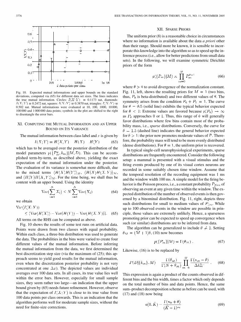
since the number of possible bin configurations also diverges, itis not clear whether stays finite or not. We will not tryto give an analytic answer to this question here. Instead, lookat Fig. 8, which shows the discretization posterior(normalized on the interval , uniform priorover ) for two data sets with (top) and(bottom). The generating density consisted of five bins, withthe bin boundaries chosen so that was an integer.Consequently, the most probable discretization is found to be

in both instances. Should the be irrational, orshould the generating density not have a bin structure, then wemight expect the posterior maximum to move toward smaller

(greater ) with increasing , much like the -posteriorin Fig. 4. For , the maximum a posteriori probability(MAP) choice can certainly be justified. This is nolonger the case for : while is still thelocation of the maximum, the probability is now much more

ENDRES AND FÖLDIÁK: BAYESIAN BIN DISTRIBUTION INFERENCE AND MUTUAL INFORMATION 3775

Fig. 8. Discretization posterior P (KjD) for a data set containing 100 (top)and 1000 (bottom) data points. In the latter case, the MAP choice K = 20 cancertainly be justified, for 100 data points, additional information is necessarybefore a K can be picked.

evenly spread, and additional prior information is required ifa choice is to be made with reasonable certainty.

There is numerical evidence which suggests that ac-tually approaches a (nonzero) constant as (not visiblein the graphs, because appears to be( ) and ( ) times smaller than themaximum). This implies that the bulk of the probability is con-centrated around . We would, however, argue that sincethe presented algorithm is not useful in this limit (because ithas a computational complexity ), one will always haveto choose a reasonable upper bound for , determined by theavailable computation time, or by the accuracy of the data. Oncethis bound is set, a can be determined if enough data are avail-able. Alternatively, a uniform prior over (i.e., in )could also be motivated, which would allow for a cutoff at amoderately large .

Another quantity of interest is the predictive density. Its behavior is depicted in Fig. 9, bottom, forand four different, small data sets. Other values of

give qualitatively similar results. As ,appears to diverge logarithmically with if evaluated at adata point, and to approach a constant (for given , , and )otherwise. This suggests that the divergence is such that theprobability contained in the vicinity of a data point approachesa constant as well. Numerical evidence for this hypothesis isshown in Fig. 9, top. In other words, in the limit ,the predictive distribution seems to have a -peak at each datapoint. This behavior, which was conjectured by one of thereviewers, is reminiscent of that of a Dirichlet process [14].

X. EXTENSION TO MULTIPLE CLASSES

Assume each data point was labeled, the label being. In other words, each is drawn from

one of classes. We will now extend the algorithm so as toinfer the joint distribution (or density) , where

.Instead of probabilities, we now have .

is the probability mass between and in class , i.e.,we assume that the bins are located at the same places across

Fig. 9. Bottom: Predictive densities p(xjD;M = 10) as a function ofK = . Circles: p(xjD;M = 10) at the location (0.4) of a data point,squares: p(xjD;M = 10) between data points. The lines denote datasets with N = 1 (solid), 2 (dashed), 4 (dotted), and 8 (dash-dotted). Thepredictive density appears to diverge logarithmically with K at the locationof a data point, and remains finite elsewhere. Top: Predictive probabilityP (x 2 [0:395; 0:405]jD;M = 10) in the vicinity of a data point as a functionof K . This probability seems to asymptote at a constant value for K ! 1,which indicates that the predictive density has a �-peak at each data point.

classes. This might seem like a rather arbitrary restriction. Weshall, however, impose it for two reasons.

1) The algorithm for iterating over the bin configurationskeeps a simple form, similar to (17) and (18).

2) If we allowed different sets of for the classes, com-puting marginal distributions and entropies would becomeexceedingly difficult. While possible in principle, it wouldinvolve confluent hypergeometric functions and a signifi-cantly increased computational cost.

Let be the number of data points in class and bin , and. The likelihood (2) now becomes

(59)

Thus, following the same reasoning as above, the iteration rulesnow are

(60)

where is the total number of data points in class for whichand . Furthermore

(61)

where is the total number of data points in class for

which , and .We can now evaluate the expected joint distribution and its

variance at any , using (23) and (24) as before. To computethe marginal distribution, note that

(62)

and likewise for its square.

3776 IEEE TRANSACTIONS ON INFORMATION THEORY, VOL. 51, NO. 11, NOVEMBER 2005

Fig. 10. Expected mutual informations and upper bounds on the standarddeviations, computed via (65) for different data set sizes. The lines indicatesthe true mutual information. Circles: I(X;Y ) = 0.1173 nat, diamonds:I(X;Y ) = 0.2472 nat, squares: I(X;Y ) = 0.3870 nat, triangles: I(X;Y ) =0.502 nat. Mutual informations were evaluated at 10, 100, 1000, 10 000,100 000 and 1 000 000 data points; symbols in the plot are shifted to the rightto disentangle the error bars.

XI. COMPUTING THE MUTUAL INFORMATION AND AN UPPER

BOUND ON ITS VARIANCE

The mutual information between class label and is given by

(63)

which has to be averaged over the posterior distribution of themodel parameters . This can be accom-plished term-by-term, as described above, yielding the exactexpectation of the mutual information under the posterior.The evaluation of its variance is somewhat more difficult, dueto the mixed terms , ,and . For the time being, we shall thus becontent with an upper bound. Using the identity

(64)

we obtain

(65)

All terms on the RHS can be computed as above.Fig. 10 shows the results of some test runs on artificial data.

Points were drawn from two classes with equal probability.Within each class, a three-bin distribution was used to generatethe data. The probabilities in the bins were varied to create fourdifferent values of the mutual information. Before inferringthe mutual information from the data, we first determined thebest discretization step size (via the maximum of (25); this ap-proach seems to yield good results for the mutual information,even when the discretization posterior probability is not veryconcentrated at one ). The depicted values are individualaverages over 100 data sets. In all cases, its true value lies wellwithin the error bars. However, especially for small samplesizes, they seem rather too large—an indication that the upperbound given by (65) needs future refinement. However, observethat the expectation of is close to its true value from100 data points per class onwards. This is an indication that thealgorithm performs well for moderate sample sizes, without theneed for finite-size corrections.

XII. SPARSE PRIORS

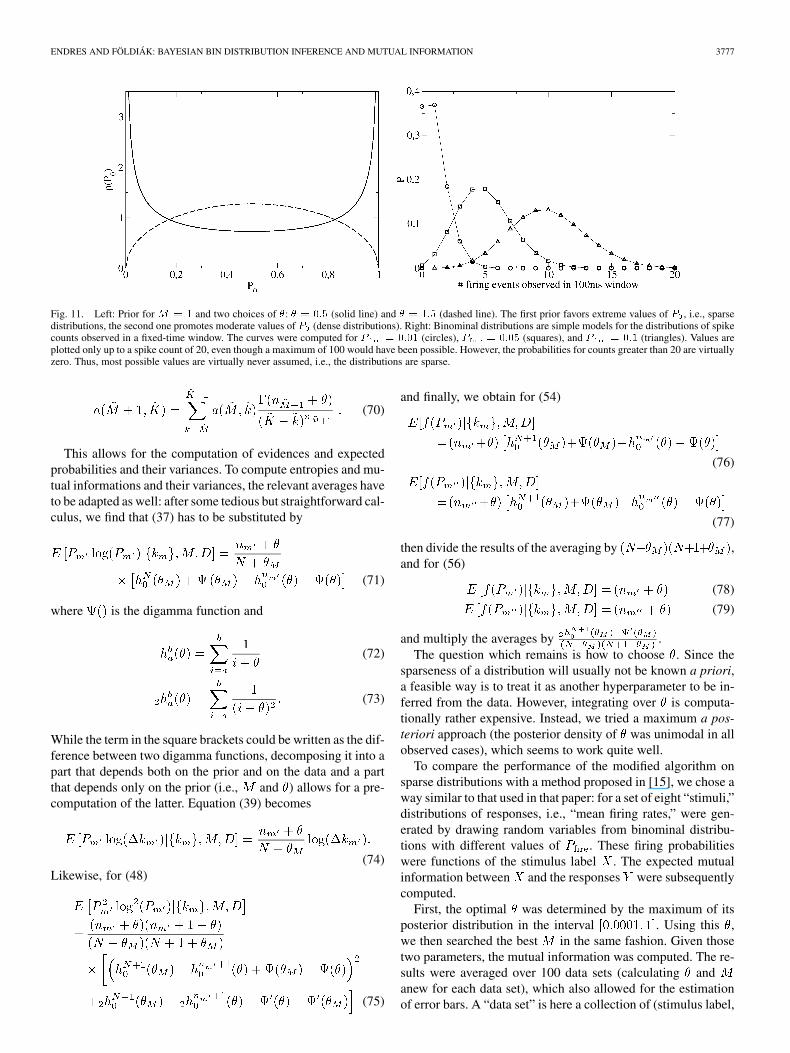
The uniform prior (8) is a reasonable choice in circumstanceswhere no information is available about the data a priori otherthan their range. Should more be known, it is sensible to incor-porate this knowledge into the algorithm so as to speed up the in-ference process (i.e., allow for better predictions from small datasets). In the following, we will examine symmetric Dirichletpriors of the form

(66)

where to avoid divergence of the normalization constant.Fig. 11, left, shows the resulting priors for (two bins,thus, is beta-distributed) and two different values of . Thesymmetry arises from the condition . The curvefor (solid line) exhibits the typical behavior expectedfor : Extreme values are favored becauseas approaches or . Thus, this range of will generallyfavor distributions where few bins contain most of the proba-bility mass, i.e., sparse distributions. Conversely, the curve for

(dashed line) indicates the general behavior expectedfor : the prior now promotes moderate values of . There-fore, the probability mass will tend to be more evenly distributed(dense distributions). For , the uniform prior is recovered.

In typical single-cell neurophysiological experiments, sparsedistributions are frequently encountered. Consider the followingsetup: a mammal is presented with a visual stimulus and thefiring events produced by one of its visual cortex neurons arerecorded in some suitably chosen time window. Assume thatthe temporal resolution of the recording equipment was 1 msand the window width 100 ms. A simple model for the firing be-havior is the Poisson process, i.e., a constant probability ofobserving an event at any given time within the window. The ex-pected distribution of the number of observed events is then gov-erned by a binominal distribution. Fig. 11, right, depicts threesuch distributions for small to medium values of . Whileup to 100 observed events in the window are possible in prin-ciple, those values are extremely unlikely. Hence, a sparsenesspromoting prior can be expected to speed up convergence whensuch (or similar) distributions are to be inferred from data.

The algorithm can be generalized to include . Setting, (10) now becomes

(67)

Likewise, (16) is to be replaced by

(68)

This expression is again a product of the counts observed in dif-ferent bins and the bin width, times a factor which only dependson the total number of bins and data points. Hence, the samesum–product decomposition scheme as before can be used, with(17) and (18) now being

(69)

ENDRES AND FÖLDIÁK: BAYESIAN BIN DISTRIBUTION INFERENCE AND MUTUAL INFORMATION 3777

Fig. 11. Left: Prior for M = 1 and two choices of �: � = 0:5 (solid line) and � = 1:5 (dashed line). The first prior favors extreme values of P , i.e., sparsedistributions, the second one promotes moderate values of P (dense distributions). Right: Binominal distributions are simple models for the distributions of spikecounts observed in a fixed-time window. The curves were computed for P = 0:01 (circles), P = 0:05 (squares), and P = 0:1 (triangles). Values areplotted only up to a spike count of 20, even though a maximum of 100 would have been possible. However, the probabilities for counts greater than 20 are virtuallyzero. Thus, most possible values are virtually never assumed, i.e., the distributions are sparse.

(70)

This allows for the computation of evidences and expectedprobabilities and their variances. To compute entropies and mu-tual informations and their variances, the relevant averages haveto be adapted as well: after some tedious but straightforward cal-culus, we find that (37) has to be substituted by

(71)

where is the digamma function and

(72)

(73)

While the term in the square brackets could be written as the dif-ference between two digamma functions, decomposing it into apart that depends both on the prior and on the data and a partthat depends only on the prior (i.e., and ) allows for a pre-computation of the latter. Equation (39) becomes

(74)Likewise, for (48)

(75)

and finally, we obtain for (54)

(76)

(77)

then divide the results of the averaging by ,and for (56)

(78)

(79)

and multiply the averages by .The question which remains is how to choose . Since the

sparseness of a distribution will usually not be known a priori,a feasible way is to treat it as another hyperparameter to be in-ferred from the data. However, integrating over is computa-tionally rather expensive. Instead, we tried a maximum a pos-teriori approach (the posterior density of was unimodal in allobserved cases), which seems to work quite well.

To compare the performance of the modified algorithm onsparse distributions with a method proposed in [15], we chose away similar to that used in that paper: for a set of eight “stimuli,”distributions of responses, i.e., “mean firing rates,” were gen-erated by drawing random variables from binominal distribu-tions with different values of . These firing probabilitieswere functions of the stimulus label . The expected mutualinformation between and the responses were subsequentlycomputed.

First, the optimal was determined by the maximum of itsposterior distribution in the interval . Using this ,we then searched the best in the same fashion. Given thosetwo parameters, the mutual information was computed. The re-sults were averaged over 100 data sets (calculating andanew for each data set), which also allowed for the estimationof error bars. A “data set” is here a collection of (stimulus label,

3778 IEEE TRANSACTIONS ON INFORMATION THEORY, VOL. 51, NO. 11, NOVEMBER 2005

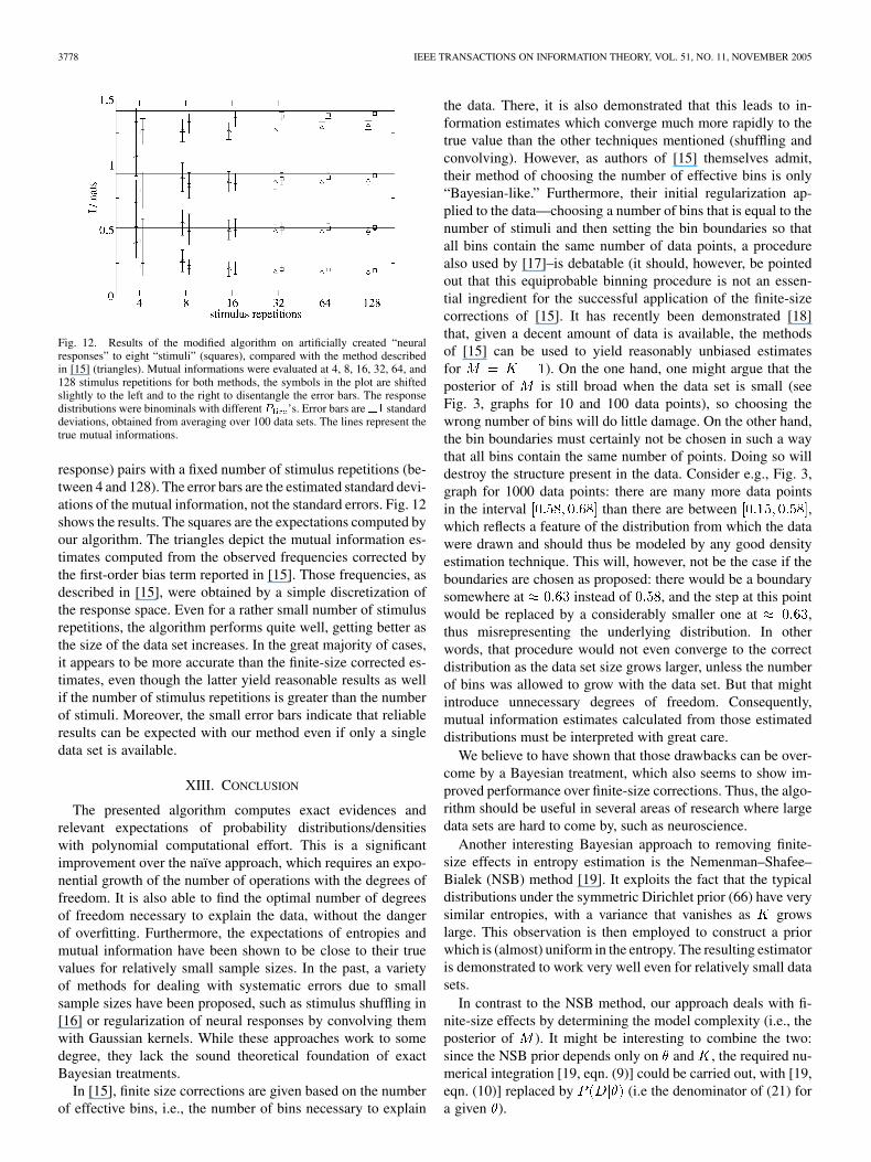
Fig. 12. Results of the modified algorithm on artificially created “neuralresponses” to eight “stimuli” (squares), compared with the method describedin [15] (triangles). Mutual informations were evaluated at 4, 8, 16, 32, 64, and128 stimulus repetitions for both methods, the symbols in the plot are shiftedslightly to the left and to the right to disentangle the error bars. The responsedistributions were binominals with different P ’s. Error bars are�1 standarddeviations, obtained from averaging over 100 data sets. The lines represent thetrue mutual informations.

response) pairs with a fixed number of stimulus repetitions (be-tween 4 and 128). The error bars are the estimated standard devi-ations of the mutual information, not the standard errors. Fig. 12shows the results. The squares are the expectations computed byour algorithm. The triangles depict the mutual information es-timates computed from the observed frequencies corrected bythe first-order bias term reported in [15]. Those frequencies, asdescribed in [15], were obtained by a simple discretization ofthe response space. Even for a rather small number of stimulusrepetitions, the algorithm performs quite well, getting better asthe size of the data set increases. In the great majority of cases,it appears to be more accurate than the finite-size corrected es-timates, even though the latter yield reasonable results as wellif the number of stimulus repetitions is greater than the numberof stimuli. Moreover, the small error bars indicate that reliableresults can be expected with our method even if only a singledata set is available.

XIII. CONCLUSION

The presented algorithm computes exact evidences andrelevant expectations of probability distributions/densitieswith polynomial computational effort. This is a significantimprovement over the naïve approach, which requires an expo-nential growth of the number of operations with the degrees offreedom. It is also able to find the optimal number of degreesof freedom necessary to explain the data, without the dangerof overfitting. Furthermore, the expectations of entropies andmutual information have been shown to be close to their truevalues for relatively small sample sizes. In the past, a varietyof methods for dealing with systematic errors due to smallsample sizes have been proposed, such as stimulus shuffling in[16] or regularization of neural responses by convolving themwith Gaussian kernels. While these approaches work to somedegree, they lack the sound theoretical foundation of exactBayesian treatments.

In [15], finite size corrections are given based on the numberof effective bins, i.e., the number of bins necessary to explain

the data. There, it is also demonstrated that this leads to in-formation estimates which converge much more rapidly to thetrue value than the other techniques mentioned (shuffling andconvolving). However, as authors of [15] themselves admit,their method of choosing the number of effective bins is only“Bayesian-like.” Furthermore, their initial regularization ap-plied to the data—choosing a number of bins that is equal to thenumber of stimuli and then setting the bin boundaries so thatall bins contain the same number of data points, a procedurealso used by [17]–is debatable (it should, however, be pointedout that this equiprobable binning procedure is not an essen-tial ingredient for the successful application of the finite-sizecorrections of [15]. It has recently been demonstrated [18]that, given a decent amount of data is available, the methodsof [15] can be used to yield reasonably unbiased estimatesfor ). On the one hand, one might argue that theposterior of is still broad when the data set is small (seeFig. 3, graphs for 10 and 100 data points), so choosing thewrong number of bins will do little damage. On the other hand,the bin boundaries must certainly not be chosen in such a waythat all bins contain the same number of points. Doing so willdestroy the structure present in the data. Consider e.g., Fig. 3,graph for 1000 data points: there are many more data pointsin the interval than there are between ,which reflects a feature of the distribution from which the datawere drawn and should thus be modeled by any good densityestimation technique. This will, however, not be the case if theboundaries are chosen as proposed: there would be a boundarysomewhere at instead of , and the step at this pointwould be replaced by a considerably smaller one at ,thus misrepresenting the underlying distribution. In otherwords, that procedure would not even converge to the correctdistribution as the data set size grows larger, unless the numberof bins was allowed to grow with the data set. But that mightintroduce unnecessary degrees of freedom. Consequently,mutual information estimates calculated from those estimateddistributions must be interpreted with great care.

We believe to have shown that those drawbacks can be over-come by a Bayesian treatment, which also seems to show im-proved performance over finite-size corrections. Thus, the algo-rithm should be useful in several areas of research where largedata sets are hard to come by, such as neuroscience.

Another interesting Bayesian approach to removing finite-size effects in entropy estimation is the Nemenman–Shafee–Bialek (NSB) method [19]. It exploits the fact that the typicaldistributions under the symmetric Dirichlet prior (66) have verysimilar entropies, with a variance that vanishes as growslarge. This observation is then employed to construct a priorwhich is (almost) uniform in the entropy. The resulting estimatoris demonstrated to work very well even for relatively small datasets.

In contrast to the NSB method, our approach deals with fi-nite-size effects by determining the model complexity (i.e., theposterior of ). It might be interesting to combine the two:since the NSB prior depends only on and , the required nu-merical integration [19, eqn. (9)] could be carried out, with [19,eqn. (10)] replaced by (i.e the denominator of (21) fora given ).

ENDRES AND FÖLDIÁK: BAYESIAN BIN DISTRIBUTION INFERENCE AND MUTUAL INFORMATION 3779

It was proven in [20] that uniformly (over all possible dis-tributions) consistent entropy estimators can be constructed fordistributions comprised of any number of bins , even if

. The above presented results (Fig. 6) suggest that the ex-pected entropies computed with our algorithm are asymptoti-cally unbiased and consistent. Furthermore, the true entropy wasusually found within the expected standard deviation. It remainsto be determined how the algorithm performs if .

Since the upper bound (65) on the variance of the mutualinformation is rather large for small sample sizes, it might beinteresting to invest some more work into computing the exactvariance of the mutual information. This, however, turns out tobe difficult.

ACKNOWLEDGMENT

The authors would like to thank Johannes Schindelin formany stimulating discussions. Furthermore, they are alsograteful to the anonymous reviewers for their helpful sugges-tions and references.

REFERENCES

[1] M. Rosenblatt, “Remarks on some nonparametric estimates of a densityfunction,” Ann. Math. Statist., vol. 27, pp. 832–837, 1956.

[2] M. Stone, “Cross-validatory choice and assessment of statistical predic-tions,” J. Roy. Statist. Soc., Ser. B, vol. 36, no. 1, pp. 111–147, 1974.

[3] N. Ueda, R. Nakano, Z. Ghahramani, and G. E. Hinton, “SMEM algo-rithm for mixture models,” Neur. Comput., vol. 12, no. 9, pp. 2109–2128,2000.

[4] A. Dempster, N. Laird, and D. Rubin, “Maximum likelihood for incom-plete data via the EM algorithm,” J. Roy. Statist. Soc., Ser, B, vol. 39, no.1, pp. 1–38, 1977.

[5] R. Cox, “Probability, frequency and reasonable expectation,” Amer. J.Phys., vol. 14, no. 1, pp. 1–13, 1946.

[6] M. Jordan, Z. Ghahramani, T. Jaakkola, and L. Saul, “An introductionto variational methods for graphical models,” Mach. Learn., vol. 37, no.2, pp. 183–233, 1999.

[7] C. Wallace and D. Boulton, “An information measure for classification,”Comput. J., vol. 11, pp. 185–194, 1968.

[8] J. Rissanen, “Modeling by shortest data description,” Automatica, vol.14, pp. 465–471, 1978.

[9] M. Hutter, “Distribution of mutual information,” in Advances in NeuralInformation Processing Systems. Cambridge, MA: MIT Press, 2002,vol. 14, pp. 339–406.

[10] F. Kschischang, B. Frey, and H.-A. Loeliger, “Factor graphs and thesum-product algorithm,” IEEE Trans. Inf. Theory, vol. 47, no. 2, pp.498–519, Feb. 2001.

[11] P. Davis, “Gamma function and related functions,” in Handbook ofMathematical Functions, M. Abramowitz and I. Stegun, Eds. NewYork: Dover, 1972.

[12] W. Press, B. Flannery, S. Teukolsky, and W. Vetterling, NumericalRecipes in C: The Art of Scientific Computing. New York: CambridgeUniv. Press, 1986.

[13] D. Endres and J. Schindelin, “A new metric for probability distribu-tions,” IEEE Trans. Inf. Theory, vol. 49, no. 7, pp. 1858–1860, Jul. 2003.

[14] T. S. Ferguson, “Prior distributions on spaces of probability measures,”Ann. Statist., vol. 2, no. 4, pp. 615–629, 1974.

[15] S. Panzeri and A. Treves, “Analytical estimates of limited sampling bi-ases in different information measures,” Network: Comp. Neur. Syst.,vol. 7, pp. 87–107, 1996.

[16] L. Optican, T. Gawne, B. Richmond, and P. Joseph, “Unbiased measuresof transmitted information and channel capacity from multivariate neu-ronal data,” Biol. Cybern., vol. 65, pp. 305–310, 1991.

[17] E. Rolls, H. Critchley, and A. Treves, “The representation of olfactoryinformation in the primate orbitofrontal cortex,” J. Neurophys., vol. 75,pp. 1982–1996, 1995.

[18] E. Arabzadeh, S. Panzeri, and M. Diamond, “Whisker vibration infor-mation carried by rat barrel cortex neurons,” J. Neurosci., vol. 24, no.26, pp. 6011–6020, 2004.

[19] I. Nemenman, W. Bialek, and R. van Steveninck, “Entropy and infor-mation in neural spike trains: Progress on the sampling problem,” Phys.Rev. E, vol. 69, no. 5, 2004.

[20] L. Paninski, “Estimating entropy on m bins given fewer than m sam-ples,” IEEE Trans. Inf. Theory, vol. 50, no. 9, pp. 2200–2203, Sep. 2004.