Embed Size (px)
Citation preview

faculteit Wiskunde en
Natuurwetenschappen
BBP-numbers and
normality
Bacheloronderzoek Wiskunde
Augustus 2008
Student: J.M. Heegen
Studentnummer: 1056484
Begeleiders: Prof.dr. J. Top en Prof.dr. H. Waalkens

Contents
Introduction 21. Normal numbers 32. The Bailey-Borwein-Plouffe formula 43. Using BBP-type formulae to compute individual digits of arithmetical constants 74. Computing digits in Mathematica 95. Generating correct base-b expansions for BBP-numbers 126. Normality of BBP-numbers 167. Rational BBP-numbers 188. Conclusion 22Bibliography 24
1

Introduction
One of the many unsolved problems in mathematics is the question whether the digits of variousarithmetical constants exhibit a certain randomness, that is, if one randomly picks a string of somelength out of the expansion of the constant, each possible string of that length is equally likely tocome up. This is the notion of a so-called normal number.To take a first step in the direction of a possible solution for this problem, we will introduce avery special class of numbers that do not only possess a method to generate digit expansions withincreasing accuracy, and in some cases, even exactly; but also, under a certain hypothesis, areprovably normal. This class of numbers include some fundamental, naturally occurring constants,most notably the fascinating number π.
2

1. Normal numbers
Definition 1.1. Let α be a real number and b ≥ 2 an integer. The number α is called normal tobase b if every string of k digits occurs in the base-b expansion of α with a limiting frequency ofb−k.If α is normal to every integer base b ≥ 2, it is called absolutely normal.
For example, if α is normal to base 2, the digits 0 and 1 will both appear in the binary ex-pansion of α with an equal frequency of 1
2 ; the strings 00, 01, 10 and 11 will all appear with anequal frequency of 1
4 , and so on.
In the case of a number that is normal to base 10, every digit 0, 1, 2, ..., 9 will appear one-tenth ofthe time in its decimal expansion. A randomly picked string of five digits will have a probabilityof 1
100000 to be ”07817”, and so on.For a number that is normal to base 16, in its hexadecimal expansion (with a ’digit alphabet’consisting of the integers 0 through 9 and the capital letters A through F) the probabilities for arandomly picked 6-digit string to be ”1CACA0” or ”C0FFEE” are both equal to 16−6.
The expansion of a rational number is eventually periodic, i.e. from some position in the ex-pansion, a particular string of digits is repeated infinitely often. This means that there are stringsof digits that never appear, so the number cannot be normal. Hence, every normal number mustbe irrational.
There are uncountably many numbers that are not normal. This is easily seen by the fact that, forinstance, there are uncountably many numbers without a 0 in their decimal expansion, and theseare obviously not normal.
Some important properties of normal numbers are the following [Kuipers & Niederreiter, 1974]:
• Let b, k,m ∈ N, b ≥ 2 and α ∈ R, such that α is normal to base bk. Then α is also normal tobase bm.
• Let q, r be rational numbers with r 6= 0. If α is normal to base b, then rα+ q is also normalto base b. Furthermore, α is normal to base c = br, in case c is an integer.
An important result by Emile Borel, who first introduced the concept of normality in the beginningof the 20th century, is that almost all real numbers are absolutely normal; that is, the set of allreal numbers that are not absolutely normal has a Lebesgue measure of zero.
Despite the abundance of such numbers, it has turned out to be very difficult to prove the normalityof a given irrational number. Even though empirical data strongly seems to suggest that constantslike π, e, log 2,
√2, the golden mean 1
2(1 +√
5) (and in fact all irrational algebraic numbers) andnumerous others are absolutely normal, yet no proof nor disproof of normality in any base has everbeen given for any of these numbers.
Normality has been established for some numbers that have been specifically constructed for thesepurposes. An example is the Champernowne constant, which is obtained by concatenating (i.e.
3

putting behind one another in ascending order) the positive integers:
C10 = 0.123456789101112131415 . . .
This number has been shown to be normal to base 10. Similarly, the binary Champernowne con-stant C2 = 0.11011100101110111 . . . is known to be normal to base 2, the ternary Champernowneconstant C3 = 0.12101112202122 . . . is normal to base 3, etcetera.Another artificially constructed number, the Copeland-Erdos constant, which is obtained by con-catenating all primes: 0.2357111317192329 . . ., is normal to base 10.
A fairly recent result [Bailey, 2005] is that all constants of the form
αp,q =∞∑k=1
1pqkqk
in which p and q are relatively prime, the so-called Stoneham numbers, are normal to base p.
However, it has long been a desire to prove the widely conjectured normality of the aforemen-tioned ”naturally occurring” constants (π, e, log 2,
√2, ...). An important new direction in the
quest for these proofs has been initiated by the discovery of a formula known as the Bailey-Borwein-Plouffe formula.
2. The Bailey-Borwein-Plouffe formula
The Bailey-Borwein-Plouffe formula (shortly: BBP) is a formula for computing π. It is named afterSimon Plouffe, who discovered it in 1995, and David Bailey and Peter Borwein, the co-authors ofthe paper in which it was first published. It states that
π =∞∑i=0
116i
(4
8i+ 1− 2
8i+ 4− 1
8i+ 5− 1
8i+ 6
)(1)
More generally, a BBP-type formula is a convergent series of the form
α =∞∑k=0
p(k)bkq(k)
where b ≥ 2 is an integer and p, q are polynomials with integer coefficients. The BBP-fomula for πis of this type, because we can combine the four fractions into one. A real number α that can berepresented in this way is called a BBP-number.
Proof of the BBP formula for π.
For any k < 8,∫ 1/√
2
0
xk−1
1− x8dx =
∫ 1/√
2
0xk−1 · 1
1− x8dx =
∫ 1/√
2
0xk−1
( ∞∑i=0
(x8)i)dx
4

(we can substitute the geometric series here, because |x8| < 1 for 0 ≤ x ≤ 1√2)
=∫ 1/
√2
0
( ∞∑i=0
xk−1+8i
)dx =
∞∑i=0
(∫ 1/√
2
0xk−1+8idx
)=∞∑i=0
[1
k + 8ixk+8i
]x=1/√
2
x=0
=∞∑i=0
1k + 8i
(1√2
)k+8i
=∞∑i=0
1k + 8i
· 12k/2
· 116i
=1
2k/2
∞∑i=0
116i(8i+ k)
.
Now define
Tk :=∞∑i=0
116i(8i+ k)
, so that Tk = 2k/2∫ 1/
√2
0
xk−1
1− x8dx. Then
∞∑i=0
116i
(4
8i+ 1− 2
8i+ 4− 1
8i+ 5− 1
8i+ 6
)= 4T1 − 2T4 − T5 − T6
= 4 · 21/2
∫ 1/√
2
0
11− x8
dx − 2 · 24/2
∫ 1/√
2
0
x3
1− x8dx
− 25/2
∫ 1/√
2
0
x4
1− x8dx − 26/2
∫ 1/√
2
0
x5
1− x8dx
=∫ 1/
√2
0
4√
2− 8x3 − 4√
2x4 − 8x5
1− x8dx.
We now substitute y :=√
2x, so that x = 1√2y and dx = 1√
2dy, and the above expression becomes
∫ 1
0
4√
2− 8 · 12√
2y3 − 4
√2 · 1
4y4 − 8 · 1
4√
2y5
1− 116y
8· 1√
2dy
=∫ 1
016 · 4− 2y3 − y4 − y5
16− y8dy = 16
∫ 1
0
y5 + y4 + 2y3 − 4y8 − 16
dy
= 16∫ 1
0
(y − 1)(y4 + 2y3 + 4y2 + 4y + 4)(y4 − 2y3 + 4y − 4)(y4 + 2y3 + 4y2 + 4y + 4)
dy
= 16∫ 1
0
(y − 1)y4 − 2y3 + 4y − 4
dy = 16∫ 1
0
y − 1(y2 − 2)(y2 − 2y + 2)
dy.
To evaluate this integral, we will first decompose the integrand into partial fractions. We need tofind A,B,C,D ∈ R such that
y − 1(y2 − 2)(y2 − 2y + 2)
=Ay +B
y2 − 2+
Cy +D
y2 − 2y + 2.
This means that
y − 1 = (Ay +B)(y2 − 2y + 2) + (Cy +D)(y2 − 2)= (A+ C)y3 + (−2A+B +D)y2 + (2A− 2B − 2C)y + (2B − 2D)
5
=⇒
A+ C = 0−2A+B +D = 02A− 2B − 2C = 1
2B − 2D = −1
=⇒
A = 14
B = 0C = −1
4D = 1
2
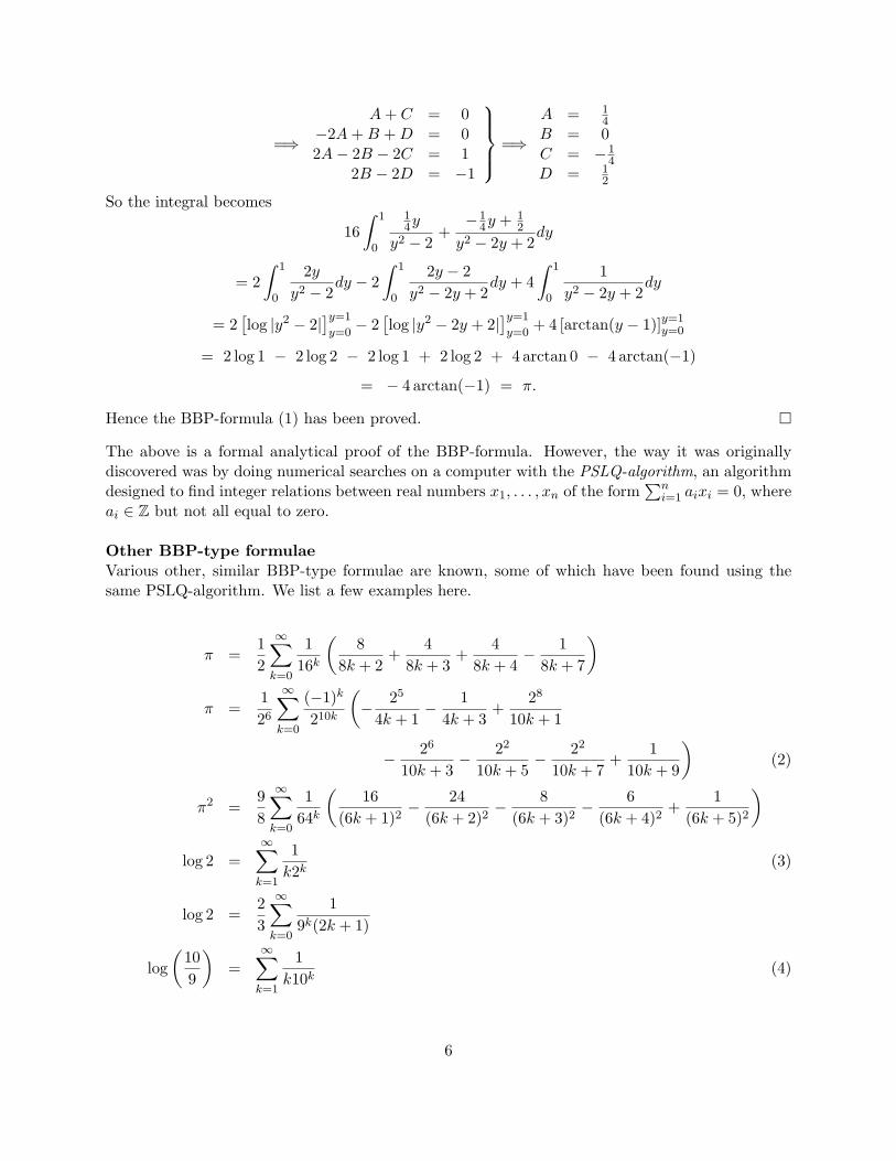
So the integral becomes
16∫ 1
0
14y
y2 − 2+−1
4y + 12
y2 − 2y + 2dy
= 2∫ 1
0
2yy2 − 2
dy − 2∫ 1
0
2y − 2y2 − 2y + 2
dy + 4∫ 1
0
1y2 − 2y + 2
dy
= 2[log |y2 − 2|
]y=1
y=0− 2
[log |y2 − 2y + 2|
]y=1
y=0+ 4 [arctan(y − 1)]y=1
y=0
= 2 log 1 − 2 log 2 − 2 log 1 + 2 log 2 + 4 arctan 0 − 4 arctan(−1)
= − 4 arctan(−1) = π.
Hence the BBP-formula (1) has been proved. �
The above is a formal analytical proof of the BBP-formula. However, the way it was originallydiscovered was by doing numerical searches on a computer with the PSLQ-algorithm, an algorithmdesigned to find integer relations between real numbers x1, . . . , xn of the form
∑ni=1 aixi = 0, where
ai ∈ Z but not all equal to zero.
Other BBP-type formulaeVarious other, similar BBP-type formulae are known, some of which have been found using thesame PSLQ-algorithm. We list a few examples here.
π =12
∞∑k=0
116k
(8
8k + 2+
48k + 3
+4
8k + 4− 1
8k + 7
)
π =126
∞∑k=0
(−1)k
210k
(− 25
4k + 1− 1
4k + 3+
28
10k + 1
− 26
10k + 3− 22
10k + 5− 22
10k + 7+
110k + 9
)(2)
π2 =98
∞∑k=0
164k
(16
(6k + 1)2− 24
(6k + 2)2− 8
(6k + 3)2− 6
(6k + 4)2+
1(6k + 5)2
)
log 2 =∞∑k=1
1k2k
(3)
log 2 =23
∞∑k=0
19k(2k + 1)
log(
109
)=
∞∑k=1
1k10k
(4)
6

log 3 =∞∑k=0
14k(2k + 1)
arctan(
13
)=
∞∑k=0
116k
(1
8k + 1− 1
8k + 2− 1/2
8k + 4− 1/4
8k + 5
)
252
log
781256
(57− 5
√5
57 + 5√
5
)√5 =
∞∑k=0
155k
(5
5k + 2+
15k + 3
)Many other constants for which BBP-type formulae are known can be found in the literature. Theseinclude many rather exotic numbers and formulae with very large numbers of terms.
Note that the equalities (3) and (4) have actually been well-known for centuries. Another ex-ample are the polylogarithms Lis(1
b ), which have BBP-type formulae by definition:
Lis(1b
) =∞∑k=1
1bkks
.
3. Using BBP-type formulae to compute individual digits of arith-metical constants
We will use the following notations:
Let b·c denote the floor function, that is, for x ∈ R, bxc is the greatest integer less than or equal to x.
For x, y ∈ R, y 6= 0, let the modulo operator be defined as
x mod y := x− bxycy.
That is, the smallest nonnegative number representing x + Z · y that lies in a certain interval oflength y.
The fractional part of a number x ∈ R is defined as frac(x) := x− bxc = x mod 1.
Now consider the sums
Tj =∞∑k=0
116k(8k + j)
as used in the derivation of the BBP-formula. Note that the hexadecimal digits of these sums (i.e.the digits in the base-16 expansion), starting at position d+ 1 after the hexadecimal point, can beobtained from the fractional part of 16dTj . Now
frac(16dTj) =∞∑k=0
16d−k
8k + jmod 1 =
d∑k=0
16d−k
8k + jmod 1 +
∞∑k=d+1
16d−k
8k + jmod 1
7

=d∑
k=0
(16d−k
8k + j− b 16d−k
8k + jc)
mod 1 +∞∑
k=d+1
16d−k
8k + jmod 1
=d∑
k=0
16d−k − b16d−k
8k+j c(8k + j)
8k + jmod 1 +
∞∑k=d+1
16d−k
8k + jmod 1
=d∑
k=0
16d−k mod (8k + j)8k + j
mod 1 +∞∑
k=d+1
16d−k
8k + jmod 1
The second summation can be evaluated using floating-point arithmetic. It has only negative expo-nents of 16 and is rapidly converging. Only a few terms are needed, just until it is ensured that theremaining terms add up to less than the ”machine epsilon” of the floating-point arithmetic used.The first summation can be evaluated efficiently using a scheme known as the Binary Exponentia-tion Algorithm, reduced modulo an integer.
The Binary Exponentiation AlgorithmTo compute xn, where n is a nonnegative integer, first note that n can be represented uniquely asn =
∑Ni=0 bi2
i, where N = blog2(n)c and each bi ∈ {0, 1}. Then
xn = x∑N
i=0 bi2i
=N∏i=0
xbi2i
in which there are at most N multiplications of powers of x. (For bi = 0, no multiplication isnecessary.) Now for all i,
x2i= (x2i−1
)2 = ((x2i−2)2)2 = . . . = (· · · ((x2)2)2 · · ·)2
in which there are i−1 pairs of parentheses, corresponding to i−1 multiplications. So in total, thenumber of multiplications needed will not be greater than N +N , so it will never exceed 2 log2(n),which is of an order far less than if one would naively multiply x with itself n− 1 times.
The corresponding Binary Exponentiation Algorithm (shortly BEA) can be written as
Pow(x, n)
1 , n = 0
Pow(x2, n2 ) , n ∈ N evenx · Pow(x2, n−1
2 ) , n ∈ N odd
In case of the BEA modulo an integer m, each multiplication result is reduced modulo m. A simpleprogram that would compute r = bn mod c in this manner can be represented as follows:
t := max{2i | 2i ≤ n};r := 1;
A if n ≥ t then r := br mod c; n := n− t; endif;t := t/2;if t ≥ 1 then r := r2 mod c; go to A; endif;
This computation can be entirely performed with integers no greater than c2.
8

The above method can be applied to compute each of the four sums Tj . Combining these us-ing the BBP-formula, this allows us to correctly compute the (d + 1)-th hexadecimal digit of πwithout the need to know the first d digits.We can now also compute individual binary digits of π: for every d, the hexadecimal digit at posi-tion d corresponds to the four binary digits at positions 4d− 3 till 4d.It is clear that these methods can be easily generalized to extract individual digits in base b for anyconstant α that has a BBP-type formula
α =∞∑k=0
p(k)bckq(k)
where p, q are polynomials with integer coefficients and b, c ∈ N, b ≥ 2. For example, formula (3)can be used to obtain individual binary digits of log 2 and (4) to obtain individual decimal digits oflog(10
9 ). Formula (2), known as Bellard’s formula, is used in the currently fastest known and mostwidely used method for computing individual binary digits of π.
4. Computing digits in Mathematica
Using the methods described in the previous section, we can efficiently compute digits of variousarithmetical constants with a software package such as Mathematica. We will start here with thesimple BBP-type formula (4).
Recall that
log(
109
)=∞∑k=1
110kk
so that the decimal digits of log(109 ) beginning at position d+1 can be obtained from the fractional
part
frac
(10d
∞∑k=1
110kk
)=
(10d
∞∑k=1
110kk
)mod 1 =
d∑
k=1
(10d−kmod k
k
)mod 1︸ ︷︷ ︸
=:Sd+1
+∞∑
k=d+1
10d−k
k
mod 1
It is easily seen that if we multiply the above expression by 10 and then take the largest integerbelow that, the result will be equal to the d+ 1-th decimal digit of log(10
9 ).Now we look at the first part of the sum, Sd+1, ignoring the tail sum starting at d + 1. We willconsider the sequence sd := (b10Sdc). This sequence will be used in the computation of the decimaldigits from position 2 onwards. We can define this in Mathematica in the following way:
In[1]:= S[d_] := FractionalPart[ Sum [ Mod [10^(d - k), k]/k, {k, 1, d}]]
In[2]:= s[d_] := IntegerPart[10 S[d - 1]]
9

We want to see if these computations, in which the tail sums are not considered yet, already produceaccurate digits. To do this we generate two tables of 1000 digits, one for the digits obtained by theabove method and the other for the actual decimal digits of log(10
9 ), respectively:
In[3]:= stable := Table[s[d], {d, 2, 1001}]
In[4]:= srealdigits := RealDigits[Log[10/9], 10, 1001][[1]]
In[5]:= stableoftruedigits := Table[srealdigits[[d]], {d, 2, 1001}]
We compare these tables and count the number of matching digits:
In[6]:= sdifftable := stableoftruedigits - stable
In[7]:= Count[sdifftable, 0]
Out[7]= 991
We see that there are only 9 differences between the digits produced by sd and the correct digitsof log(10
9 ).
In the same way, we can look at the polylogarithm Li2( 110), which is defined as
Li2(110
) =∞∑k=1
110kk2
.
Notice that this formula is very similar to the one for log(109 ), the only difference being k2 in the
denominator instead of k. Its decimal digits beginning at position d+ 1 can be obtained from thefractional part
(10d
∞∑k=1
110kk2
)mod 1 =
d∑
k=1
(10d−kmod k2
k2
)mod 1︸ ︷︷ ︸
=:Td+1
+∞∑
k=d+1
10d−k
k2
mod 1
Multiplying this expression by 10 and taking the largest integer below the result, we get the d+1-thdecimal digit of Li2( 1
10).We ignore the tail sum again and only look at the first part of the sum, Td+1. We now use thesequence td := (b10Tdc) in the computation of the decimal digits from position 2 onwards. InMathematica:
In[8]:= T[d_] := FractionalPart[ Sum [ Mod [10^(d - k), k^2]/k^2, {k, 1, d}]]
In[9]:= t[d_] := IntegerPart[10 T[d - 1]]
10

Again we want to check if this already produces accurate digits. We generate two tables again, onefor the digits computed this way and the other for the actual decimal digits of Li2( 1
10):
In[10]:= ttable := Table[t[d], {d, 2, 1001}]
In[11]:= trealdigits := RealDigits[PolyLog[2, 1/10], 10, 1001][[1]]
In[12]:= ttableoftruedigits := Table[trealdigits[[d]], {d, 2, 1001}]
We compare the number of matching digits in these tables again:
In[13]:= tdifftable := ttableoftruedigits - ttable
In[14]:= Count[tdifftable, 0]
Out[14]= 999
Actually, all 1000 digits match here; the one discrepancy is due to rounding. (The actual 1001-stand 1002-nd digits are 2 and 9, respectively. This causes the function RealDigits to return a 3 asthe 1001-st and last digit in this computation.)
In a similar way, we can use the BBP-formula
π =∞∑k=0
116k
(4
8k + 1− 2
8k + 4− 1
8k + 5− 1
8k + 6
)to perform a computation of hexadecimal digits of π. For computational convenience, we gatherall four terms under the same denominator and then shift the summation index by 1. We get
π =∞∑k=1
116k−1
p(k)q(k)
wherep(k) = 120k2 − 89k + 16q(k) = 512k4 − 1024k3 + 712k2 − 206k + 21
The hexadecimal digits starting at the d+ 1-th position can be obtained from
(16d+1
∞∑k=1
p(k)16kq(k)
)mod 1 =
d∑
k=1
(16d+1−kp(k)mod q(k)
q(k)
)mod 1︸ ︷︷ ︸
=:Ud+1
+∞∑
k=d+1
16d+1−kp(k)q(k)
mod 1
Again, we only look at the first part of this sum, Ud+1, and define the sequence ud := (b16Udc).
In[15]:= p[k_] := 120k^2 - 89k + 16
In[16]:= q[k_] := 512k^4 - 1024k^3 + 712k^2 - 206k + 21
11

In[17]:= U[d_] := FractionalPart[ Sum[ Mod[ 16^(d - k + 1)p[k], q[k]]/q[k],{k, 1, d}]]
In[18]:= u[d_] := IntegerPart[16 U[d - 1]]
To get an indication of the accuracy of the digits produced this way, we generate two tables of 1000digits again, one for the computed digits and one for the actual hexadecimal digits of π.
In[19]:= utable := Table[u[d], {d, 3, 1002}]
In[20]:= urealdigits := RealDigits[Pi, 16, 1002, -2][[1]]
In[21]:= utableoftruedigits := Table[urealdigits[[d]], {d, 2, 1001}]
Comparing these tables, we get
In[22]:= udifftable := utableoftruedigits - utable
In[23]:= Count[udifftable, 0]
Out[23]= 1000
Again we observe no differences between our computed digits and the true hexadecimal digits of π.In fact, in various researches, millions of hexadecimal digits have been computed in this manner,none of these showing any differences.
5. Generating correct base-b expansions for BBP-numbers
Lemma 5.1. Let (xn) be the sequence defined by
x0 = 0 and xn =(bxn−1 +
p(n)q(n)
)mod 1, n = 1, 2, . . . (5)
Then for all n = 1, 2, . . . the following holds:
xn =
(n∑k=1
bn−kp(k) mod q(k)q(k)
)mod 1.
Proof. We will prove this equality by induction. For n = 1 we have
x1 =(bx0 +
p(1)q(1)
)mod 1 =
p(1)q(1)
mod 1 =b1−1p(1)mod q(1)
q(1)mod 1
=
(1∑
k=1
b1−kp(k) mod q(k)q(k)
)mod 1
12

so the equality holds for n = 1.
Now suppose that for some n ≥ 1,
xn =(bxn−1 +
p(n)q(n)
)mod 1 =
n∑k=1
(bn−kp(k) mod q(k)
q(k)
)mod 1.
Then (bxn +
p(n+ 1)q(n+ 1)
)mod 1 =
(b
(bxn−1 +
p(n)q(n)
)mod 1 +
p(n+ 1)q(n+ 1)
)mod 1
=
(b
(n∑k=1
(bn−kp(k) mod q(k)
q(k)
)mod 1
)mod 1 +
p(n+ 1) mod q(n+ 1)q(n+ 1)
mod 1
)mod 1
=
(b
(n∑k=1
(bn−kp(k) mod q(k)
q(k)
)mod 1
)mod 1 + b · b
n−(n+1)p(n+ 1) mod q(n+ 1)q(n+ 1)
mod 1
)mod 1
=
(bn+1∑k=1
(bn−kp(k) mod q(k)
q(k)
)mod 1
)mod 1 =
n+1∑k=1
(bn+1−kp(k) mod q(k)
q(k)
)mod 1
which means that the equality also holds for n+ 1. �
For a real number α ∈ [0, 1), we can define the norm ‖α‖ = min(α, 1 − α). In this way, ‖α − β‖measures the shortest distance between α and β on a circle with circumference 1.
Lemma 5.2. Let α be a real number with BBP-type formula
α =∞∑k=1
p(k)bkq(k)
where p, q are integer polynomials with 0 ≤ deg(p) < deg(q) such that q has no zeros for the positiveintegers. Define the sequence (xn) as in (5) and let αn denote the part of the base-b expansion ofα starting at position n+ 1 after the base-b ”decimal” point. Then
‖xn − αn‖ −→ 0 for n −→∞.
Proof. For all n ∈ N we have that
αn = (bnα) mod 1 =
( ∞∑k=1
bn−kp(k)q(k)
)mod 1
=
((n∑k=1
bn−kp(k) mod q(k)q(k)
)mod 1 +
∞∑k=n+1
bn−kp(k)q(k)
)mod 1
=
(xn +
∞∑k=n+1
bn−kp(k)q(k)
)mod 1.
13

Furthermore, since 0 ≤ deg(p) < deg(q), we have∣∣∣p(k)q(k)
∣∣∣ ↘ 0, that is, for all ε > 0, there is an
N = N(ε) such that∣∣∣p(k)q(k)
∣∣∣ < ε for all k ≥ N . Hence, if n is large enough,
‖xn − αn‖ ≤
∣∣∣∣∣∞∑
k=n+1
bn−kp(k)q(k)
∣∣∣∣∣ < ε
∞∑k=n+1
bn−k = ε
∞∑j=1
1bj
= ε1
b− 1≤ ε.
This means that ‖xn − αn‖ −→ 0 for n −→∞. �
Lemma 5.2 shows us that the sequence (xn) is a good approximation of the sequence (αn) of shifteddigit expansions of α.In the previous section we saw that for some BBP-numbers
α =∞∑k=1
1bkp(k)q(k)
the sequence (yn) := (bbxnc), where xn is the fractional part of a finite summation,
xn =
(n∑k=1
bn−kp(k) mod q(k)q(k)
)mod 1,
produces digits of the base-b expansion of α quite accurately, regardless of the tail summation; forsome of these BBP-numbers, the produced digits even appear to exactly match the true digits.Note that the sequence (xn) is precisely the one used in Lemmas 5.1 and 5.2. Hence, another wayof stating this is that the sequence (yn) = (bbxnc), where (xn) is defined as
x0 = 0 and xn =(bxn−1 +
p(n)q(n)
)mod 1, n = 1, 2, . . .
very accurately (and in some cases exactly) appears to produce digits of the base-b expansion of α,regardless of the tail sequence
tn =∞∑
k=n+1
bn−kp(k)q(k)
.
For instance, in the BBP-type formula (3) for α = log 2, we have p(k) ≡ 1 and q(k) = k and thiscorresponds to the sequence (xn) where
x0 = 0 and xn =(
2xn−1 +1n
)mod 1.
The digit sequence (yn) = (b2xnc) generates the binary digits of log 2 quite accurately. In the sameway, in the formula (4) for α = log(10
9 ), we also have p(k) ≡ 1 and q(k) = k, corresponding to thesequence (xn) with
x0 = 0 and xn =(
10xn−1 +1n
)mod 1.
14

Here the digit sequence (yn) = (b10xnc) quite accurately produces the decimal digits of log(109 ).
For α = Li2( 110), we have p(k) ≡ 1 and q(k) = k2, with its corresponding sequence (xn), where
x0 = 0 and xn =(
10xn−1 +1n2
)mod 1,
the digit sequence (yn) = (b10xnc) appears to correctly produce the decimal digits of Li2( 110).
In the same way, the BBP-formula gives us p(k) = 120k2 − 89k + 16 and q(k) = 512k4 −1024k3 + 712k2 − 206k + 21 and the sequence
x0 = 0 and xn =(
16xn−1 +p(k)q(k)
)mod 1.
Here, the digit sequence (yn) = (b16xnc) appears to correctly produce hexadecimal digits of π.
We quickly observe that for log 2 and log(109 ), we have deg(q) = deg(p) + 1 and for Li2( 1
10) andπ, we have deg(q) = deg(p) + 2. In fact, computations for various other BBP-numbers all seemto suggest that whenever deg(q) ≥ deg(p) + 2, the correct digits are generated, whereas errors areexpected to occur if this is not the case. This leads to the following conjecture:
Conjecture 5.3. If a real number α can be written as a BBP-type formula
α =∞∑k=1
1bkp(k)q(k)
,
with deg(q) ≥ deg(p) + 2, the sequence (bbxnc), where (xn) is defined as
x0 = 0 and xn =(bxn−1 +
p(n)q(n)
)mod 1, n = 1, 2, . . .
generates the correct base-b expansion of α.
Note that when deg(q) ≥ deg(p) + 2, the expression p(k)q(k) is summable. If the conjecture is true, the
tail sequence
tn =∞∑
k=n+1
bn−kp(k)q(k)
,
which can be seen as the error term for the prediction of the digit at place n+ 1, never changes adigit. For Li2( 1
10), the tail sequence is given by
tn =∞∑
k=n+1
10n−k
k2.
This is approximately equal to the first summand (k = n + 1). For the sum of all tail sequences(i.e. the sum of all prediction errors) we have
∞∑n=1
tn ≈ 0.0644934 . . .
15

Multiplied by 10, this number can be regarded as the expected total number of errors in thegenerated digit sequence; it is a number smaller than 1. Similarly, for π, we have the tail sequence
tn =∞∑
k=n+1
16n−k(120k2 − 89k + 16)512k4 − 1024k3 + 712k2 − 206k + 21
and∞∑n=1
tn ≈ 0.0157946 . . .
Multiplied by 16, this number gives us an indication of the expected total number of errors in thegenerated digit sequence for π; again it is smaller than 1, meaning no errors are expected to occur.Obviously, the corresponding tail sequences for log 2 and log(10
9 ), where p(k)q(k) = 1
k , are not summable.This indicates that errors are expected to occur infinitely often. However, it is difficult to be precisehere; no proof of Conjecture 5.3 is known, nor of a concrete relation between the sums of the tailsequences and the number of errors that occur in our digit computations.
6. Normality of BBP-numbers
We now return to the concept of normality. If Conjecture 5.3 is true, we have a way to correctlyrepresent individual digits of a certain class of BBP-numbers by means of the sequence (bbxnc).Even under the weaker (but proven) statement Lemma 5.2, we know that for all BBP-numbers,the sequence at least eventually agrees quite well with the true base-b expansions. This leads to thehope that statements can be made about the distribution of the digits of BBP-numbers, or evenprovide a way to establish normality for these numbers.
Definition 6.1. A sequence (xn) in [0, 1) is called equidistributed if for all 0 ≤ c < d < 1,
limN→∞
#{xi ∈ [c, d) | i < N}N
= d− c.
Definition 6.2. A sequence (xn) in [0, 1) has a finite attractor W = (w0, w1, . . . wP−1) if for allε > 0 there exists a K = K(ε) such that ‖xK+k−wt(k)‖ < ε for all k ≥ 0, where t is some functiont : N→ {0, . . . P − 1}.
This is used in the following important hypothesis formulated by [Bailey & Crandall, 2001]:
Hypothesis 6.3. Let p, q be polynomials with integer coefficients, such that 0 ≤ deg(p) < deg(q),with q having no zeros on N, and let rn = p(n)
q(n) . Then the sequence (xn), defined by
x0 = 0 and xn = (bxn−1 + rn) mod 1, n = 1, 2, . . .
is either equidistributed in [0, 1) or has a finite attractor.
We now state some important results that will be used to show the consequence of Hypothesis
16

6.3 for the normality of BBP-numbers.
Theorem 6.4. If (xn) is an equidistributed sequence and (yn) a sequence for whichlimn→∞(yn mod 1) = L, then the sequence ((xn + yn) mod 1) is also equidistributed.
Theorem 6.5. If (yn) is a sequence in [0, 1) that has a limit point limn→∞ yn = L, then a sequence(xn) in [0, 1) has a finite attractor if and only if the sequence ((xn+yn) mod 1) has a finite attractor.
Theorem 6.6. A number α ∈ R is normal to base-b if and only if the sequence ((bnα) mod 1)n∈Nis equidistributed.
Theorem 6.7. A number α ∈ R is rational if and only if the sequence ((bnα) mod 1)n∈N hasa finite attractor.
It would go too far to prove these results here; full proofs have been given in [Kuipers & Niederre-iter, 1974] and [Bailey & Crandall, 2001], respectively.
Theorem 6.8. Let α be a BBP-number of the form
α =∞∑k=1
p(k)bkq(k)
(6)
where p, q are polynomials with integer coefficients, 0 ≤ deg(p) < deg(q), q having no zeros forpositive integers, and b ≥ 2 an integer. Then α is rational if and only if the sequence defined by
x0 = 0 and xn =(bxn−1 +
p(n)q(n)
)mod 1, n = 1, 2, . . . (7)
has a finite attractor.
Proof. From Lemma 5.2, we know that the sequence (xn − αn), where αn = (bnα) mod 1, has alimit (which is 0). Because of Theorem 6.5, this means that (xn) has a finite attractor if and onlyif (αn) has a finite attractor, and from Theorem 6.7, this is the case if and only if α is rational. �
Theorem 6.9. Let α and (xn) be defined as in Theorem 6.8. If (xn) is equidistributed, thenα is normal to base b.
Proof. Suppose that (xn) is equidistributed. Let (αn) be as in the proof of the previous theorem.We know that (xn−αn) converges to 0, so from Theorem 6.4, (αn) must also be equidistributed. Be-cause of Theorem 6.6, αmust be normal to base b. �
The previous two theorems lead to an interesting result about the normality of BBP-numbers,assuming Hypothesis 6.3 is true.
Theorem 6.10. Under Hypothesis 6.3, a BBP-number is either rational or normal to base b.
Proof. Every BBP-number α of the form (6) has a corresponding sequence (xn) of the form
17

(7). Under the hypothesis, this sequence either has a finite attractor or is equidistributed. If it hasa finite attractor, then by Theorem 6.8 α is rational. If it is equidistributed, then by Theorem 6.9 αis normal to base b. �
Obviously, this means that if Hypothesis 6.3 is valid, every irrational number that has a BBP-type formula as in (6) is normal to base b. For example, this would imply that log 2 is normal tobase 2, log(10
9 ) and Li2( 110) are normal to base 10 and π is normal to base 16 (and hence also to
base 2).
7. Rational BBP-numbers
Of course, the question arises whether rational examples of BBP-numbers actually exist. Theanswer is yes; several BBP-type formulae are known that evaluate to the rational number 0. Welist some examples here, found by David Bailey using the PSLQ-algorithm. [Bailey, 2004]
0 =∞∑k=0
116k
(−8
8k + 1+
88k + 2
+4
8k + 3+
88k + 4
+2
8k + 5+
28k + 6
− 18k + 7
)
0 =∞∑k=0
164k
(16
6k + 1− 24
6k + 2− 8
6k + 3− 6
6k + 4+
16k + 5
)
0 =∞∑k=0
1729k
(81
12k + 2− 162
12k + 3+
2712k + 5
+36
12k + 6
+9
12k + 8+
612k + 9
+4
12k + 10− 1
12k + 11
)These BBP zero relations are relevant for finding new BBP-type formulae with algorithms likePSLQ. Of course, these formulae can be rewritten in the familiar form (6) by gathering all termsunder the same denominator (and shifting the index of summation). For instance, the secondformula above yields
0 =∞∑k=1
164k
6804k4 − 14256k3 + 9891k2 − 2664k + 224(−1944k5 + 4860k4 − 4590k3 + 2025k2 − 411k + 30)
By Theorem 6.8 this means that the sequence (xn) given by x0 = 0 and
xn+1 =(
64xn +6804n4 − 14256n3 + 9891n2 − 2664n+ 224
−1944n5 + 4860n4 − 4590n3 + 2025n2 − 411n+ 30
)mod 1
has a finite attractor. Since every digit in the base-64 expansion is 0, this finite attractor is ofcourse equal to zero.
However, in an attempt to further investigate Hypothesis 6.3, we would like to find some nonzerorational BBP-numbers. We observe that BBP-numbers can be considered as special cases of hy-pergeometric functions:
18

Definition 7.1. The standard hypergeometric function 2F1 is given by
2F1(a, b; c; z) =∞∑n=0
(a)n(b)n(c)n
zn
n!
where (a)n denotes the Pochhammer symbol, (a)n = a(a+ 1) · · · (a+ n− 1).
For instance,
12 2F1(1, 1; 2;
12
) =12
∞∑n=0
(1)n(1)n(2)nn!
(12
)n =12
∞∑n=0
(1 · 2 · 3 · · ·n)(1 · 2 · 3 · · ·n)(2 · 3 · · ·n · (n+ 1))(1 · 2 · 3 · · ·n)
(12
)n
=12
∞∑n=0
1n+ 1
12n
=∞∑m=1
1m2m
= log 2.
Another relevant example is, for j = 1, . . . 8,
1j
2F1
(j
8, 1;
j
8+ 1;
116
)=
1j
∞∑n=0
( j8)n(1)n( j8 + 1)nn!
(116
)n
=1j
∞∑n=0
j8( j8 + 1)( j8 + 2) · · · ( j8 + n− 1)(1 · 2 · · ·n)
( j8 + 1)( j8 + 2) · · · ( j8 + n− 1)( j8 + n)(1 · 2 · · ·n)(
116
)n
=1j
∞∑n=0
j8
j8 + n
116n
=∞∑n=0
18n+ j
116n
=: Tj
in which we recognize the series used in the original BBP formula π = 4T1 − 2T4 − T5 − T6.
This makes us hopeful that possible nonzero rational examples of hypergeometric function evalua-tions will lead to nonzero rational examples of BBP-numbers. Now for some particular points, thehypergeometric function is known to assume rational values. For example,
2F1
(13,23
;56
;2732
)=
85
and 2F1
(14,12
;34
;8081
)=
95
corresponding to
∞∑n=0
(13)n(2
3)n(56)nn!
(2732
)n =85
and∞∑n=0
(14)n(1
2)n(34)nn!
(8081
)n =95
and even
2F1
(13,23
;32
;274x2(1− x2)2
)=
11− x2
for 0 ≤ x ≤ 13
√3.
However, these examples do not correspond to BBP-type formulae; not enough terms in the nu-merator and denominator of the summands cancel.
19

An interesting theorem along these lines, dealing with the (ir)rationality of a class of numberscontaining the BBP-numbers, is the following [Lagarias, 2001]:
Theorem 7.2. Let p, q ∈ Q[X] such that q has no zeros for the nonnegative integers and pand q have no common factors. Let
f(z) =∞∑n=0
p(n)q(n)
zn.
If q(x) splits into distinct linear factors over Q, then for each r ∈ Q that is in the open disk ofconvergence of f(z) around z = 0, the value f(r) is either rational or transcendental.
The proof of this theorem relies on results about irrationality and transcendence for linear combi-nations of logarithms. We will illustrate this for the case of π.
Take a look at the function
f1(x) =∞∑n=0
xn
8n+ 1.
Setting x = y8, we get
f1(x) =∞∑n=0
y8n
8n+ 1=
1y
∞∑n=0
y8n+1
8n+ 1=
1yg1(y) where g1(y) :=
∞∑n=0
y8n+1
8n+ 1.
Then, assuming |y| < 1,
g′1(y) =∞∑n=0
y8n =1
1− y8and g1(0) = 0 (8)
We know that 1− y8 = 0 if and only if y ∈ {ζk8 | k = 1, . . . , 8}, where the ζk8 = e2πik/8 are the 8thcomplex roots of unity:
1− y8 =8∏
k=1
(1− ζk8 y).
Now we want to find constants ak such that
11− y8
=8∑
k=1
ak
1− ζk8 y
from which it follows with (8) that
g1(y) =8∑
k=1
−akζ−k8 log(1− ζk8 y).
We know that for each k = 1, . . . , 8
ak
1− ζk8 y=ak∏8m=1,m 6=k(1− ζm8 y)
1− y8.
20

Summing over all k, we get
11− y8
=8∑
k=1
ak
1− ζk8 y=
11− y8
8∑k=1
ak 8∏m=1,m 6=k
(1− ζm8 y)
and from this we are able to calculate ak, k = 1, . . . , 8. This rather lengthy calculation, which ismost easily done in Mathematica, is equivalent to solving the system of linear equations
Z a = (1, 0, 0, 0, 0, 0, 0, 0)T , in which a = (a1, . . . , a8)T and
Z =
ζ88 ζ8
8 ζ88 ζ8
8 ζ88 ζ8
8 ζ88 ζ8
8
ζ18 ζ2
8 ζ38 ζ4
8 ζ58 ζ6
8 ζ78 ζ8
8
ζ28 ζ4
8 ζ68 ζ8
8 ζ28 ζ4
8 ζ68 ζ8
8
ζ38 ζ6
8 ζ18 ζ4
8 ζ78 ζ2
8 ζ58 ζ8
8
ζ48 ζ8
8 ζ48 ζ8
8 ζ48 ζ8
8 ζ48 ζ8
8
ζ58 ζ2
8 ζ78 ζ4
8 ζ18 ζ6
8 ζ38 ζ8
8
ζ68 ζ4
8 ζ28 ζ8
8 ζ68 ζ4
8 ζ28 ζ8
8
ζ78 ζ6
8 ζ58 ζ4
8 ζ38 ζ2
8 ζ18 ζ8
8
Its solution is a = 1
8(1, 1, 1, 1, 1, 1, 1, 1)T . This means that
g1(y) = −18
8∑k=1
ζ−k8 log(1− ζk8 y).
In the same way, we look at the function
f4(x) =∞∑n=0
xn
8n+ 4.
Again setting x = y8, we get
f4(x) =∞∑n=0
y8n
8n+ 4=
1y4
∞∑n=0
y8n+4
8n+ 4=
1y4g4(y) where g4(y) :=
∞∑n=0
y8n+4
8n+ 4.
Assuming |y| < 1, we have
g′4(y) =∞∑n=0
y8n+3 =y3
1− y8and g4(0) = 0
Solving a similar system of linear equations, we get
g4(y) = −18
8∑k=1
(−1)k log(1− ζk8 y).
Likewise (omitting details for brevity),
f5(x) =∞∑n=0
xn
8n+ 5=
1y5g5(y) where g5(y) :=
∞∑n=0
y8n+5
8n+ 5
21
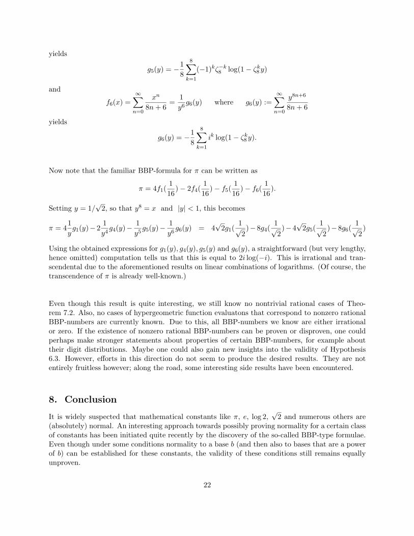
yields
g5(y) = −18
8∑k=1
(−1)kζ−k8 log(1− ζk8 y)
and
f6(x) =∞∑n=0
xn
8n+ 6=
1y6g6(y) where g6(y) :=
∞∑n=0
y8n+6
8n+ 6
yields
g6(y) = −18
8∑k=1
ik log(1− ζk8 y).
Now note that the familiar BBP-formula for π can be written as
π = 4f1(116
)− 2f4(116
)− f5(116
)− f6(116
).
Setting y = 1/√
2, so that y8 = x and |y| < 1, this becomes
π = 41yg1(y)− 2
1y4g4(y)− 1
y5g5(y)− 1
y6g6(y) = 4
√2g1(
1√2
)− 8g4(1√2
)− 4√
2g5(1√2
)− 8g6(1√2
)
Using the obtained expressions for g1(y), g4(y), g5(y) and g6(y), a straightforward (but very lengthy,hence omitted) computation tells us that this is equal to 2i log(−i). This is irrational and tran-scendental due to the aforementioned results on linear combinations of logarithms. (Of course, thetranscendence of π is already well-known.)
Even though this result is quite interesting, we still know no nontrivial rational cases of Theo-rem 7.2. Also, no cases of hypergeometric function evaluatons that correspond to nonzero rationalBBP-numbers are currently known. Due to this, all BBP-numbers we know are either irrationalor zero. If the existence of nonzero rational BBP-numbers can be proven or disproven, one couldperhaps make stronger statements about properties of certain BBP-numbers, for example abouttheir digit distributions. Maybe one could also gain new insights into the validity of Hypothesis6.3. However, efforts in this direction do not seem to produce the desired results. They are notentirely fruitless however; along the road, some interesting side results have been encountered.
8. Conclusion
It is widely suspected that mathematical constants like π, e, log 2,√
2 and numerous others are(absolutely) normal. An interesting approach towards possibly proving normality for a certain classof constants has been initiated quite recently by the discovery of the so-called BBP-type formulae.Even though under some conditions normality to a base b (and then also to bases that are a powerof b) can be established for these constants, the validity of these conditions still remains equallyunproven.
22

Despite numerous efforts, no proof of normality for any of these constants has ever been given, noteven to one particular base. In fact, every attempt to gain more insight into the distribution of digitsseems to give rise to an whole new class of problems, and the discovery of some interesting prop-erties along the way, that may or may not seem directly useful for solving the question of normality.
Even if one would be able to make statements about the normality of BBP-numbers, there area lot of other constants, for instance
√2 and e, for which a BBP-type formula is not even known.
Perhaps some day, more hidden knowledge about normality can be uncovered, but for now, it re-mains one of the most intriguing unsolved problems in mathematics.
23

Bibliography
[Bailey, 2004] D.H. Bailey, “A Compendium of BBP-Type Formulas for Mathematical Constants”,2004. (At the author’s webpage, http://crd.lbl.gov/~dhbailey/dhbpapers/)
[Bailey, 2005] D.H. Bailey, “A “Hot-Spot” Proof of Normality for the Alpha Constants”, 2005.(At the author’s webpage, http://crd.lbl.gov/~dhbailey/dhbpapers/)
[Bailey, Borwein, Borwein & Plouffe, 1997] D.H. Bailey, J.M. Borwein, P.B. Borwein and S. Plouffe,“The Quest for Pi”, Mathematical Intelligencer, vol. 19, no. 1 , 1997.
[Bailey, Borwein & Plouffe, 1997] D.H. Bailey, P.B. Borwein and S. Plouffe, “On the Rapid Com-putation of Various Polylogarithmic Constants”, Mathematics of Computation, vol. 66, no. 218.
[Bailey & Crandall, 2001] D.H. Bailey and R.E. Crandall, “On the Random Character of Fun-damental Constant Expansions”, Experimental Mathematics vol. 10, no. 2, 2001.
[Kuipers & Niederreiter, 1974] L. Kuipers and H. Niederreiter, Uniform distribution of sequences,Wiley-Interscience, New York, 1974.
[Lagarias, 2001] J.C. Lagarias, “On the Normality of Arithmetical Constants”, Experimental Math-ematics vol. 10, no. 3, 2001.
24

Addendum
The derivation on pages 22-24 is NOT intended to be a transcendence proof for π, nor should itbe read as such. We merely restated the fact that π = 2i log(−i) using the BBP-formula. This istranscendental, using a result by Baker 1 which tells us that finite sums of linear forms in logarithmswith algebraic coefficients, evaluated at algebraic points, are transcendental if and only if the sumof the logarithmic terms is nonzero.
1A. Baker, Transcendental number theory, Cambridge University Press, London, 1975


