Beam Emittance Measurements at Fermilab

Manfred Wendt*, Nathan Eddy, Martin Hu, Victor Scarpine, Mike Syphers, Gianni Tassotto, Randy Thurman-Keup, Ming-JenYang, James Zagel

Fermi National Accelerator Laboratory, Batavia, IL 60510, U.S.A.1

INTRODUCTION

Abstract. We give short overview of various beam emittance measurement methods, currently applied at different machine locations for the Run II collider physics program at Fermilab. All these methods are based on beam profile measurements, and we give some examples of the related instrumentation techniques. At the end we introduce a multi-megawatt proton source project, currently under investigation at Fermilab, with respect to the beam instrumentation challenges.

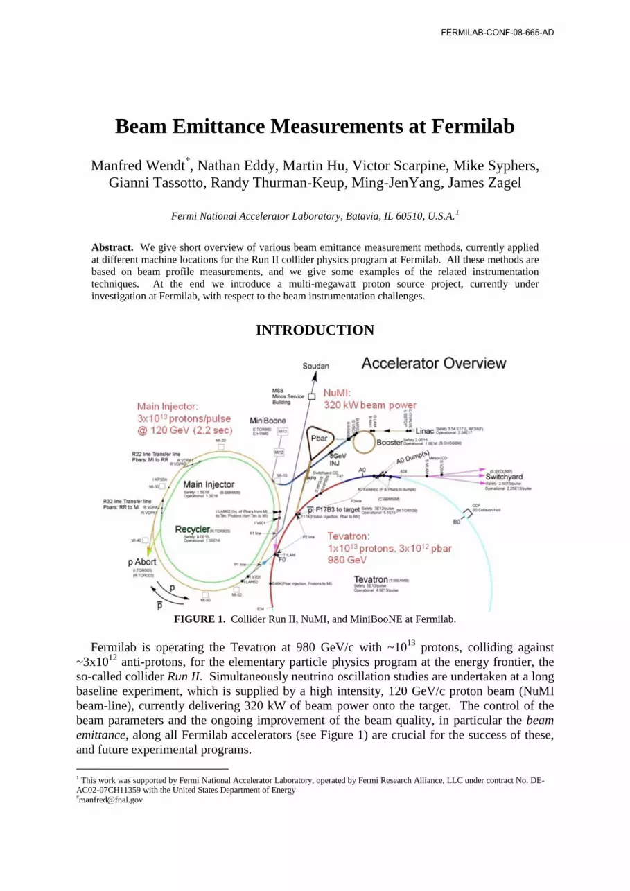
FIGURE 1. Collider Run II, NuMI, and MiniBooNE at Fermilab.

Fermilab is operating the Tevatron at 980 GeV/c with ~1013 protons, colliding against

~3x1012 anti-protons, for the elementary particle physics program at the energy frontier, the so-called collider Run II. Simultaneously neutrino oscillation studies are undertaken at a long baseline experiment, which is supplied by a high intensity, 120 GeV/c proton beam (NuMI beam-line), currently delivering 320 kW of beam power onto the target. The control of the beam parameters and the ongoing improvement of the beam quality, in particular the beam emittance, along all Fermilab accelerators (see Figure 1) are crucial for the success of these, and future experimental programs. 1 This work was supported by Fermi National Accelerator Laboratory, operated by Fermi Research Alliance, LLC under contract No. DE-AC02-07CH11359 with the United States Department of Energy #manfred@fnal.gov

FERMILAB-CONF-08-665-AD

Beam Emittance

The transverse motion of a single particle along a linear guide field is given by: [ ]δψβ += )(cos)()( ssAsx (1)

where x(s) denotes either the horizontal or the vertical coordinate. The functions β(s) and ψ(s) are the usual twiss parameters and A and δ are constants of motion. Using Eq.(1) and its derivative one finds

πεβαγ ==′+′+ 222 2 Axxxx (2)

with: )(21)( ss βα ′−≡ ,

βαγ

21+≡

A single particle follows an ellipse in the transverse phase space (Figure 2, right) given by Eq. (2), in which the area is defined as transverse emittance ε in π mm mrad.

Figure 2. Single particle motion and emittance.

Each particle in the beam follows its own ellipse. At Fermilab we define the beam

emittance as the area in the x-x’ phase space occupied by 95 % of the particles (Figure 3), assuming a Gaussian stationary density distribution:

dxedxxn x 22 2/

21)( σ

σπ−= (3)

Figure 3. Fermilab 95 % beam emittance definition.

The particle motion of Eq. (1) gives circles of radius a in an x-(αx+βx’) phase space, which allows for a mathematical simplification to compute the beam emittance:

( )F−−= 1ln2 2

βσπε (4)

with: ∫ −=a

r drreF0

22/ 22

σσ

The fraction F of particles, considered in the x-x’ phase space for a Gaussian beam of transverse rms beam size σ, varies among laboratories and institutions for defining the beam emittance ε. At Fermilab we are interested in the total beam size, setting F = 0.95 (95 %), which defines the transverse normalized emittance in presence of

dispersion D to: ( )

−=

2226

PdpDrel σ

ββγπ

ε (5)

Typically, the measurement of the beam emittance is based on the measurement of the transverse beam profile, i.e. the projection of the x-x’ phase space on the x-axis (Fig. 3). From this beam profile measurement we evaluate the rms beam width σ. In presence of dispersion D, also the longitudinal beam profile needs to be measured, from which we find the momentum spread dp/P. Finally, the determination of the beam emittance relies on the knowledge of the lattice parameters β and D, as well as on the beam energy related parameter (βγ)rel.

FLYING WIRE PROFILE MONITOR

The Tevatron Flying Wire Monitor System

Figure 4. The Tevatron Flying Wire profile monitoring system (left: TeV location E11, right: schematic).

The Tevatron Flying Wire (TFW) system consists of a horizontal and a vertical wire at

location E11 (Figure 4) and another horizontal wire at location E17. The wire is actually a carbon filament of 5 µm diameter. A typical wire fly travels 540 degrees starting at a park position sufficiently away from the first pass through beam to allow the wire to accelerate to full speed, maintain a constant speed through the beam twice, and decelerate to stop at the second park position well out of the beam aperture. Constant speed is not an absolute requirement, as the beam loss data is correlated to position and not time in the final analysis;

it is desired though so that no vibrations are induced in the wire or motion control system during data acquisition. Figure 5. Flying Wire beam profile before and during scraping.

By capturing the time between losses on an oscilloscope we can calculate the wire speed as a cross check on the reported value from the motion control hardware. The radius of the wire about the center of rotation is 96.5 mm; the time measured on the oscilloscope is 35.6 msec, resulting in a circumferential wire speed of 6.6 meters/sec.

Looking at beam losses before, during, and after scraping shows the reduced beam width as expected in a shot setup (Figure 5).

Figure 6. Pre-tension setup for the 5 µm diameter carbon filament in the Flying Wire fork.

The carbon filament is mounted by pre-tensioning the the filament to well below its

breaking stress but tight enough to withstand the acceleration and deceleration force without deformation. Each end is captured in am aluminum clamp that is buffered by kapton on one side and soft copper on the other end. The buffering material allows for a slight flexing of the filament during acceleration but ensures no sharp edges will allow educed high stress points. One end is conducting to drain any residual charge build up on the filament. The opposite end is insulated to retard any circulation current in the fork (Figure 6).

FLYING WIRE VS. IPM BEAM PROFILE MEASUREMENTS

0

0.1

0.2

0.3

0.4

0.5

0.6

0.7

0.8

0.9

1 4 7 10 13 16 19 22 25 28 31 34

Bunch

Bea

m s

ize

(mm

)

Flying wireIPM

Figure 7. Comparison of Flying Wire vs. Ionization Profile Monitor (IPM) measurements.

y = 1.0089x

0

0.5

1

0 0.5 1

Flying wire

IPM

In the Tevatron there is a flying wire system and an Ionization Profile Monitor (IPM) in the E sector. While the flying wire builds a profile over many turns, the IPM is making bunch-by-bunch measurements on a turn-by-turn basis for all 72 bunches. The IPM can be set to very precisely measure a single bunch by averaging many turns. Shown Figure 7 is a comparison for one store with beam intensity of 1011 particles per bunch at a vacuum of 10-9

torr. Good IPM measurements of P-Bar bunches at 1010 particles per bunch require a local gas bump bringing the vacuum to 10-8 torr.

Tevatron Beam Emittance Measurements based on Flying Wire Profiles

In the Tevatron, the beam profiles from the flying wire monitors are used to compute the transverse emittance of each proton and anti-proton bunch as shown in Eq. (5). The Beta Function, β, and Dispersion Function, D, are given by the machine lattice and are measured independently [1]. For the vertical flying wire, the Dispersion Function is nearly zero so that the vertical emittance is calculated from the measured beam profile and the Beta Function at the wire location. For the horizontal flying wire the Dispersion Function is not zero so the beam profile is also dependent upon the momentum spread of the beam. The simple technique is to measure the horizontal profile at two different locations with different Dispersion and solve for the momentum spread. In the Tevatron, there are horizontal wires located at E11 (low Dispersion) and E17 (high Dispersion). In practice this technique does not work well in the Tevatron due to uncertainties, especially at E17, on the actual value of the Dispersion Function at the wire locations. Currently, the horizontal emittance is calculated using the momentum spread directly measured for each bunch from the Tevatron Longitudinal Profile Monitor described in the next section.

Figure 8. The calculated emittances and momentum spread for the first proton bunch injected into the Tevatron for each wire fly. The protons are injected at 150GeV then put on a helical orbit for anti-proton injection. The beams are then ramped to 980GeV and brought into collision.

The momentum spread and emittances calculated for the first proton bunch from the

vertical wire at E11 and the horizontal wires at E11 and E17 are shown in Fig. 8. Each point represents one fly from the wires as each proton and anti-proton is loaded into the Tevatron at 150GeV and then accelerated up to 980GeV. Note that the machine optics and lattice functions change during this process. Ideally, the emittance for each bunch remains constant throughout this process. In practice, the emittance for each bunch is slowly increasing due to vacuum and beam-beam interactions. The calculated vertical emittance shifts when the beam is ramped from 150GeV to 980GeV and is in fact smaller at 980GeV. As this is not physically possible, this effect is due to uncertainties on the different Beta Functions used at 150GeV and 980GeV. The effects are more pronounced in the horizontal emittance calculations were the Dispersion plays a significant role. One expects round beam in the Tevatron and hence the horizontal and vertical emittances should be approximately equal. There is reasonable agreement for the low Dispersion wire at E11, but there is a large discrepancy at the high Dispersion E17 wire. This suggests the E17 calcuation is dominated by the uncertainty on the Dispersion. The horizontal emittance calculated from the E11 wire also shifts from 150GeV to 980GeV but it is similar to the shift observed from the vertical wire. Operationally, the emittance measurements from the E11 horizontal and vertical wires are used to monitor the store to store performance. They are also now used to estimate the expected luminosity for each Tevatron store. This has prompted closer scrutiny on the accuracy of the emittance calculations and understanding of the lattice parameter uncertainties.

SYNCHROTRON RADIATION PROFILE MONITOR

The synchrotron radiation profile monitor utilizes synchrotron emissions from the edge of a Tevatron superconducting dipole magnet. The light is intercepted by a small mirror in the beampipe and directed out a quartz vacuum window into a light-tight box where it is focused onto a combination image intensifier and CID camera. There are separate systems for the protons and antiprotons (Figure 9).

Figure 9. The Tevatron SyncLight beam profile monitor setup.

The Tevatron dipole magnets have a cutoff wavelength near 1 µm; however, light emitted

near the edges of the dipole magnets is enhanced at shorter wavelengths (Figure 10, left) [2]. Thus before entering the intensifier, the light is bandpass filtered around 400 nm to keep the depth of field short. Ideally, only light originating near the edge of the magnet would be allowed into the intensifier.

The image intensifier is gated and used to image only a single bunch at a time, albeit over many revolutions. The acquired image is processed in a PC running LabVIEW where the horizontal and vertical projections are performed (Fig. 10, right).

Protons

Proton Box

Antiproton Box

Proton light Antiproton light

Dipole Dipole

Half-Dipole

Pickoff Mirrors Antiprotons

Figure 10. Left: Proton beam image. Right: Horizontal and Vertical projections of beam image. The projections are fit with Gaussian plus linear background functions and the fitted

widths are corrected for camera non-linearities, diffraction effects (100-200 µm out of a 300-800 µm beam size), and the non-Gaussian parts resulting from the longitudinal extent of the source as well as the multiple sources edges in the antiproton case. The corrections other than the camera non-linearities were obtained from the Synchrotron Radiation Workshop [3] simulation.

The emittance is obtained using these fitted and corrected beam widths together with the lattice parameters and the momentum spread from a longitudinal profile device. The results are presented approximately once every minute which is the time it takes to perform the measurements on all 72 proton and anti-proton bunches in the Tevatron.

Longitudinal Profile and Emittance Monitor

The longitudinal emittance measurements in the Tevatron and the Main Injector are accomplished via a wall current monitor, fast oscilloscope, and processing software which records the time profile of a particle bunch. The time profile is converted to longitudinal emittance using a fitting algorithm wherein the fitting function is a superposition of projections of phase space contours, ∑ ii Fa (Fig. 11).

Figure 11. Left: Phase space contours which are solutions to constRE =∆−∆ φcos2 where R depends on various machine parameters. Right: Projections of successive phase space annuli onto the Δϕ axis. These projections form a set of functions, Fi, for fitting to the time (Δϕ) profile.

The coefficients, ai, are determined by solving the matrix equation, ∑ ∆=∆ )()( φφ ii FaI , where I(Δϕ) is the discrete time profile (Δϕ and t are interchangeable). Once the ai are

-2 0 20

0.1

0.2

0.3

0.4Fitting Functions (Projections on ∆φ axis)

∆φ (rad)Pha

se S

pace

Are

a (a

rbitr

ary

units

-2 0 2-1.5

-1

-0.5

0

0.5

1

1.5Contours in phase space

∆φ (rad)

∆E

(ar

bitra

ry u

nits

)

known, then the emittance can be calculated since the ai are effectively the particle density in each annulus.

The underlying assumption in this is that the density along any one phase space trajectory is constant. This implies that the time distribution should be symmetric. For beam that has been in the ring for many synchrotron periods, this is certainly true. But for accelerator rings such as the Main Injector, where beam is there only for a few seconds and is undergoing various RF manipulations, phase space is not very uniform (Fig. 12).

0 4 8 12 16 20 24-100

-50

0

50

Time (ns)

Remnants of coalescing during proton injections to the Tevatron

Tevatron is very uniform

Tevatron

Main Injector

Figure 12. Time distributions from the Tevatron (left) and Main Injector (right) showing the non-uniformity in the Main Injector resulting from the various RF manipulations leading up to the injection to the Tevatron.

One way the non-uniform phase space can be accommodated is by averaging over samples evenly spaced throughout a synchrotron period. This serves to smooth out the lumpiness and delivers an emittance number that is representative of what the emittance would be if the beam were left in the ring for an extended period.

The emittance results are available about once a second in the Tevatron. In the Main Injector, each type of acceleration cycle has a unique set of predefined acquisition times corresponding to important events in the cycle (such as before and after acceleration, before and after coalescing, etc…). These results are made available after each cycle (from a few seconds to minutes, depending on the cycle type).

SEM MULTIWIRE BEAM PROFILE MONITOR

NuMI is the highest intensity beamline presently running at Fermilab, with >300 kW beam power (Table 1). The profile monitors that are in use are Secondary Emission Monitors, (SEM), also called multiwires. Because of the beam loss that SEMs generate they are typically only used during tuning periods except for the target SEM which is always in the beam.

NuMI Beam Parameters Beam energy (GeV) 120 Intensity (particles / spill) 4e13 Spill time (µsec) 8.56 Cycle time (sec) 2.2 Power / spill (kJ) 140

Table 1. NuMI beam parameters

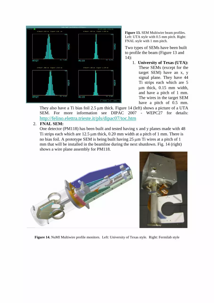
Figure 13. SEM Multiwire beam profiles. Left: UTA style with 0.5 mm pitch. Right: FNAL style with 1 mm pitch. Two types of SEMs have been built to profile the beam (Figure 13 and 14):

1. University of Texas (UTA): These SEMs (except for the target SEM) have an x, y signal plane. They have 44 Ti strips each which are 5 µm thick, 0.15 mm width, and have a pitch of 1 mm. The wires in the target SEM have a pitch of 0.5 mm.

They also have a Ti bias foil 2.5 µm thick. Figure 14 (left) shows a picture of a UTA SEM. For more information see DIPAC 2007 - WEPC27 for details: http://felino.elettra.trieste.it/pls/dipac07/toc.htm

2. FNAL SEM: One detector (PM118) has been built and tested having x and y planes made with 48 Ti strips each which are 12.5 µm thick, 0.20 mm width at a pitch of 1 mm. There is no bias foil. A prototype SEM is being built having 25 µm Ti wires at a pitch of 1 mm that will be installed in the beamline during the next shutdown. Fig. 14 (right) shows a wire plane assembly for PM118.

Figure 14. NuMI Multiwire profile monitors. Left: University of Texas style. Right: Fermilab style

Beam Losses

Figure 15. Orbit / beam losses in the NuMI beamline. Left: PM118 out of the beam. Right: PM118 in the beam.

Calculations to estimate beam losses have been done both at UTA and FNAL. For a typical UTA SEM it was estimated 2.6 x 10-6 interaction lengths. For PM118, presently under test, the estimate is for 1.78 x 10-5 interaction lengths and for the newly built SEM having 25 µm Ti wires will estimate 3.56 x 10-6 interaction lengths. This will enable an operator to set a SEM IN/OUT of the beam without tripping the radiation detector set at 5 Rad/sec. Figure 15 (left) shows the radiation level with PM118 out of the beam and Figure 15 (right) shows the loss monitors response as PM118 is in the beam.

Thermal Simulations

Figure 16. Thermal simulation of a 5 µm strip, 3x1013 protons.

UTA simulated the temperature raise of various materials: see report NuMI-B-926. For a 5 µm thick Ti foil the temperature increase is almost 300 C (Fig. 16). For a 25 µm Ti wire the expected temperature raise is 1.64 x 1014 protons before the wire fails. It is possible to increase the beam intensity by selecting other materials, particularly C which has a high melting temperature (3500 C.), low density, 2.2 g/cm3, (versus 4.54 g/cm3 for Ti) and high emissivity (8 times greater than Ti). This will enable C

filaments to survive much higher intensities while generating manageable beam losses.

Temperature raise of 25 µm Ti wire have been estimated using MARS15. Experts in the mechanical group are now estimating fail conditions using ANSYS program. The results of MARS calculation are shown in Figure 17, which indicate that the wire will survive NOνA beam parameters, but not those of Project-X.

Figure 17. Temperature raise simulations (MARS).

Emittance Measurements

Multi-wire profile monitors are important tools for beam diagnostics. They can be used as beam position monitors and, unlike the electro-static Beam Position Monitors, need no gain calibrations. However, their most unique function is to provide lattice diagnostics. Typically a beam line is instrumented with a number of multi-wire profile monitors at strategic locations to measure beam widths, which should reflect the design beta functions. During Numi beam line commissioning the beam width pattern was found not to match that of design. After a systematic study of the beam line optics it was realized that power supply current calibration for the very first quadrupole magnet was off by almost 50 % and was not providing necessary focusing. Figure 18 (left) shows the observed beam width data along with a calculation that took into account this error in the magnet current. Figure 18 (right) shows the updated measurements and design calculation, after error was corrected.

Figure 18. MuMI beam-line: Beam sigma with Q101 error (left), and after error correction (right).

Another example of usage can be found in the Main Injector 8-GeV transfer line where profile monitors are being used actively to monitors beam emittances. The present implementation uses two horizontal plane profile data to calculate horizontal plane emittance and the momentum spread ∆p/P, and one vertical profile to calculate vertical plane emittance.

The calculation assumes that lattice functions at the profile monitors have being verified previously. Figure 19 shows examples of two horizontal and one vertical profiles along with the equations used in the calculation. Emittance results are logged continuously and can be examined at any time later. Figure 20 is an example plot of the logged data which shows a jump in the vertical emittance. In this case the change was believed to be caused by a change in the vertical position at the extraction septum magnet, which has been known to exhibit large normal and skew sextupole field components.

Figure 19. Multiwire beam profiles, measured in the MI-8 beam-line.

Figure 20. Multiwire-based emittance data logging of the MI-8 beam-line during a vertical beam position jump.

As mentioned, this emittance monitor implementation uses only a minimal set of profiles with no redundancy. Consequently, any up-stream lattice function change will result in values that are not reflective of the actually emittances. A more elaborated scheme is currently being considered such that it will detect unexpected lattice function change as well.

OPTICAL TRANSITION RADIATION (OTR) DETECTORS FOR HIGH INTENSITY HADRON BEAMS

Optical transition radiation is generated when a charged particle transits the interface of two media with different dielectric constants (e.g., vacuum to dielectric or vice versa) [4][5]. Eq. (6) gives the expression for the single-particle spectral angular distribution of the number of photons, N, per unit frequency (dω) and solid angle (dΩ) is given by [5, 6],

222

222

)(2

θγθ

ωπω +=

Ω −che

ddNd

(6)

where e is the electron charge, h is Planck’s constant, c is the speed of light, γ is the Lorentz factor of the charged particle, and θ is the angle from the OTR emission axis. For the forward OTR this axis is the same as the particle beam while for the backward OTR this axis is the specular reflection axis. In addition, the intensity of the backward OTR is proportional to the reflectivity of the surface. This expression shows that the angular distribution is maximum at θ ~ 1/γ.

OTR detectors have been used extensively to measure transverse beam shape in electron accelerators. Recently, CERN incorporated OTR detectors in various transfer lines to measure proton bunches used for operation of the LHC [7]. As part of the Run II collider plan and the NuMI neutrino program, a series of OTR detectors were designed, constructed and installed in various beamlines at Fermilab. Previous near-field OTR images, from other

Fermilab beamlines, of lower-intensity 120 GeV and 150 GeV protons with larger transverse beam size have been presented [8] [9] [10]. An OTR detector has been installed in the Fermilab NuMI proton beamline, which operates at beam powers of up to ~350 kW, to obtain real-time, spill-by-spill beam profiles for neutrino production. NuMI OTR images of 120 GeV protons for beam intensities up to 4.1x1013 at a spill rate of 0.5 Hz and small transverse beam size of ~1 mm (sigma) have been measured [11]. A detailed description of the OTR detector can be found in reference [12]. Figure 21. NuMI OTR beam images and horizontal and vertical projections with Gaussian fits for 2.4x1013 and 4.1x1013

protons per bunch.

Figure 21 shows OTR images for bunch intensities of ~2.4x1013 and ~4.1x1013protons. This figure also shows the beam projections with Gaussian fits. The images show the increase in beam size with increase in beam intensity. The images also show an increase in the beam ellipticity with higher intensities. This shows the advantage of a two-dimensional beam shape monitor, such as an OTR detector, over other standard one-dimensional profile monitors.

OTR detectors for lower intensity proton beams have been shown to operate over extended periods of time. Issues of foil lifetime for high beam intensity are not well understood but it is assumed that the foil properties will change over time. The choice of a 6 micron thick, aluminized Kapton foil for the NuMI OTR was made to minimize the scatter of the NuMI beam. The detector is equipped with two foils, a primary foil for continuous operation and a calibration foil for temporary use to monitor changes in the primary foil. Figure 22 shows a comparison of the OTR signal from the primary foil after ~6.5e19 120 GeV protons to the secondary calibration foil. The primary shows signs of aging with a ~25% reduction in OTR signal. Figure 23 shows the change to the NuMI OTR primary Kapton foil after ~3 months of continuous operation. The figure clearly shows the reduction of reflectivity to a cloudy appearance and an uneven stretching of the foil.

The extended use of OTR detectors as potential profile monitors for future intense proton beams will primarily depend on the survivability of the OTR foil. However, non-continuous use of OTR detectors in an intense proton beamline is an option for transverse profile measurements.

Figure 22. Comparison of the NuMI OTR response for primary foil and calibration foils after ~6.5e19 120 GeV protons through primary foil.

Figure 23. Photograph of the NuMI OTR 6 micron aluminized Kapton primary foil after ~6.5e19 120 GeV protons with σ ~1 mm beam size.

SCHOTTKY DETECTOR BASED EMITTANCE MEASUREMENTS

In the 8 GeV Recycler storage ring we use a 1.7 GHz Schottky detection system for the characterization of various beam parameters:

Figure 24. 1.7 GHz Schottky detector in the Recycler

• Momentum spread • Longitudinal emittance • Transverse emittance • Betatron tunes

The Schottky monitor offers also the potential to measure:

• Chromaticities • Beam intensity • Beam-gas scattering

(asymmetry in energy spectra of the DC beam signal)

Figure 25. Schematics of the Schottky detection system. Left: Schottky pickup. Right: RF electronics.

Characteristics of the Schottky monitor are: • Operation frequency: 1.75 GHz • High impedance narrow-band directional coupler style pickups (h ~ 20,000) • One system per plane; looks at both, difference signals (transverse domain), and sum

signals (longitudinal domain) • Down-conversion to a few MHz (IF) for signal transmission and analysis with VSA • Built-in calibration system for system gain monitoring • Provides continues longitudinal and transverse emittance monitoring for the Recycler • Crucial tool for monitoring of beam stability, transfer efficiency, and potential

luminosity in the Tevatron.

Figure 26. Calibration using beam scarpers for transverse emittance measurement with the Schottky monitor.

Figure 26 shows how a beam scraper is used to calibrate the Schottky monitor for the 95 % emittance definition in the x-x’ or y-y’ plane. The method is destructive and uses a beam intensity signal, as well as a high sensitive BLM to evaluate the scraper jaws setting.

Figure 27. Upper and lower side-band Schottky signals for evaluation of horizontal (left) and vertical (right) emittance, and the longitudinal emittance signal (center).

PROJECT X

A multi megawatt proton source is currently under investigation at Fermilab [13]. It will provide:

• A 2 MW proton beam @ 50-120 GeV for neutrino physics at the intensity frontier o 1.6e14 protons / 1.4 sec at 122 GeV: 2.1 MW o 20 mA, 1.25 msec, 5 Hz from a SCRF H- linac (8 GeV). o ~100 turns stripped into the Recycler o Single turn transfer into the Main Injector

• Kaon and Muon physics at 8 GeV, simultaneously o 3 transfers from the Recycler to the Accumulator o 7e13 protons / 1.4 (0.7) sec at 8 GeV: 70 (140) MW for µ-to-e experiments o 3 (6) time more beam power than during the NOνA era o Need to investigate slow spill extraction

• A path toward a neutrino factory, and possibly a muon collider o Upgrade path to 10 Hz, an longer pulse length

Figure 28. Schematic layout of the Project X multi-megawatt proton source at Fermilab.

Linac Main Injector Recycler

Particle Type H- Particle Type protons Particle Type protons

Beam Kinetic Energy 8 GeV Beam Kinetic Energy (maximum)

120 GeV Beam Kinetic Energy 8 GeV

Particles per pulse 1.6x1014 Cycle Time 1.4 sec Cycle Time 0.2 sec

Pulse rate 5 Hz Particles per cycle from Recycler

1.6x1014 Particles per cycle to Main Injector

1.6x1014

Beam Power 1000 kW Beam Power at 120 GeV 2100 kW Beam power to Main Injector

140 kW

Av. Pulse Beam Current 20 mA Additional Beam Power available

860 kW

Beam Pulse Length 1.25 msec Table 2. Project X beam parameters

A list of basic beam parameters of Project X is summarized in Table 2. As of the high beam intensity and power, it will force the development of new, predominantly non-invasive beam diagnostics, as well as a very reliable beam loss monitors for the machine protection system[14]:

• Transverse beam size / emittance o Physical (intercepting) wires, e.g. scanners, multiwires (harp) / slits, etc. o Laser wire, laser emittance (only H- beams) o Ionization profile monitors o E-beam scanner o Allison scanner (at low energies)

• Beam halo characterization o Crawling wire o Mode-locked laser wire o Vibrating wire

• Longitudinal Diagnostics o Microwave Faraday cup o Bunch shape monitor (wire-based)

References [1] V. Lebedev, et. al., “Measurement and Correction of Linear Optics and Coupling at the Tevatron

Complex,” Nucl. Instrum. Methods A 558, p. 299 (2006). [2] R. Coïsson, “Angular-spectral distribution and polarization of synchrotron radiation from a ‘short’ magnet,”

Phys. Rev. A20 (1979) 524. [3] O. Chubar and P. Elleaume, “Accurate and Efficient Computation of Synchrotron Radiation in the Near

Field Region,” in the proceedings of 1998 European Particle Accelerator Conference, 22-26 June 1998, Stockholm, Sweden.

[4] J. Bosser, J. Mann, G. Ferioli and L. Wartski, “Optical Transition Radiation Proton Beam Profile Monitor,” CERN/SPS 84-17.

[5] L. Wartski, J. Marcou and S. Roland, “Detection of Optical Transition Radiation and it’s Application to Beam Diagnostics,” IEEE Trans. Nucl. Sci., vol. 20, no. 3, pp. 544-548 (1973).

[6] D. W. Rule et al., “The Effect of Detector Bandwidth on Microbunch Length Measurements made with Coherent Transition Radiation,” Advanced Accelerator Concepts: Eighth Workshop, W. Lawson, C. Bellamy, and D. Brosius, eds., AIP 472, p.745-754, 1999.

[7] C. Fischer, "Results with LHC Beam Instrumentation Prototypes," Proc. DIPAC, Grenoble, France (2001). [8] V. E. Scarpine, A. H. Lumpkin, W. Schappert and G. R. Tassotto, "Optical Transition Radiation Imaging of

Intense Proton Beams at FNAL," IEEE Trans. Nucl. Sci. 51, 1529-1532 (2004). [9] V. E. Scarpine, A. H. Lumpkin and G. R. Tassotto, "Initial OTR Measurements of 150 GeV Protons in the

Tevatron at FNAL," Beam Instrumentation Workshop, May 2006, AIP Conf. Proc 868, p. 473. [10] G. R. Tassotto, V. E. Scarpine, A. H. Lumpkin and R. M. Thurman-Keup , "Optical Transition Radiation

Imaging of 120 GeV Protons Used for Antiproton Production at FNAL," presented at the 2006 IEEE Nucl. Sci. Symp., San Diego, CA.

[11] V. E. Scarpine, G. R. Tassotto and A. H. Lumpkin, "OTR Imaging of Intense 120 GeV Protons in the NuMI Beamline at FNAL," Proc. of Particle Accelerator Conference, Albuquerque, NM, 2639-2641 (2007)

[12] V. E. Scarpine, C. Lindenmeyer, A. H. Lumpkin and G. R. Tassotto, "Development of an Optical Transition Radiation Detector for Profile Monitoring of Antiproton and Proton Beams at FNAL," Proc. of Particle Accelerator Conference, Knoxville, TN, 2381-2383 (2005).

[13] G. Apollinari, "Project X as a Way to Intensity Frontier Physics," Proc. of 42nd ICFA Advanced Beam Dynamics Workshop on High-Intensity, High-Brightness Hadron Beams, HB 2008, August 25-29, 2008, Nashville, TN, USA.

[14] M. Wendt, "Beam Instrumentation for Future High Intensity Hadron Accelerators at Fermilab," Proc. of 42nd ICFA Advanced Beam Dynamics Workshop on High-Intensity, High-Brightness Hadron Beams, HB 2008, August 25-29, 2008, Nashville, TN, USA.