Behavioral Responses of Wildlife to Snowmobiles and Coaches in Yellowstone

P.J. White1, Troy Davis1, John J. Borkowski2, Robert A. Garrott2, Daniel P. Reinhart1, and D. Craig McClure1

1 National Park Service, Yellowstone National Park, Wyoming 82190 USA 2 Montana State University, Bozeman, Montana 59717 USA

October 17, 2006

Abstract. Managers of Yellowstone National Park are charged with protecting some of our nation’s most

important natural resources, while providing for their use and enjoyment by visitors. Over 100,000 visitors entered

the park by over-snow, motorized means on snowmobiles (94%) or coaches (6%) during 2003-2006. Most vehicles

toured the central portion of the park where bald eagles (Haliaeetus leucocephalus), bison (Bison bison), coyotes

(Canis latrans), elk (Cervus elaphus), and trumpeter swans (Olor buccinator) wintered in areas close to roads. We

sampled 5688 interactions between groups of these species and groups of snowmobiles and coaches during 2003-

2006 and used multinomial logits models, odds ratios, and predicted probabilities to identify conditions leading to

behavioral responses. Bison responded less frequently (20%) to snowmobiles and coaches than swans (43%), elk

(52%), coyotes (61%), or bald eagles (83%) due to fewer vigilance responses. However, the frequency of higher-

intensity movement responses was similar among species (8-10%), with the exception of coyotes (24%). The

likelihood of vigilance and movement responses by these species increased significantly if animals were on or near

roads, animals groups were smaller, humans approached animals on foot, interaction time increased, or the numbers

of snowmobiles and coaches in a group increased. There were thresholds on the odds of eliciting a response by

wildlife for several of these covariates. We did not detect significant increases or decreases in the odds of

movement responses for any wildlife species as cumulative over-snow vehicle traffic increased through the winter.

However, the likelihood of a vigilance response by bison decreased within the winter having the largest visitation,

suggesting some habituation to snowmobiles and coaches. In contrast, there was a significant increase in the odds of

vigilance responses by elk as the cumulative visitation increased through the winter. Human disturbance did not

appear to be a primary factor influencing the distribution and movements of the wildlife species we studied. The

risk of vehicle-related mortality from snowmobiles was quite low and observed behavioral responses were

apparently short-term changes that were later reversed. Bison, elk, and swans in Yellowstone used the same core

winter ranges during the past three decades despite large winter-to-winter variability in cumulative exposure to

OSVs. There was no evidence that snowmobile use during the past 35 years adversely affected the demography or

population dynamics of bald eagles, bison, elk, or trumpeter swans (no data was available for coyotes). Thus, we

suggest regulations restricting levels and travel routes of OSVs were effective at reducing disturbances to these

wildlife species below a level that would cause measurable fitness effects. We recommend park managers consider

maintaining OSV traffic levels at or below those observed during our study. Regardless, differing interpretations of

the behavioral and physiological response data will continue to exist because of the diverse values and beliefs of the

many constituencies of Yellowstone.

INTRODUCTION

Human disturbance of wildlife is widely considered a serious conservation problem when animals demonstrate

strong, negative responses to human presence (Boyle and Sampson 1985, Klein et al. 1995, Knight and Gutzwiller

1995, Olliff et al. 1999). If humans significantly alter the activities or distributions of animals, then there may be

increased vigilance and movement levels, reduced foraging rates, and reduced levels of parental care; each of which

could reduce reproduction, survival, and population size (Stalmaster and Kaiser 1998, Duchesne et al. 2000, Steidl

and Anthony 2000, Gonza lez et al. 2006). However, behavioral responses and apparent avoidance may not reduce

the number of animals supported in an area because animals displaced from disturbed sites in the short term may

return later, resulting in the overall use of these sites being unchanged (Gill et al. 2001a). Thus, studies of

disturbance need to identify major factors influencing the behavior, distribution, and forage selection of affected

species and assess the role of disturbance in altering these relationships (Gill et al. 1996, Wisdom 2005). Studies

also need to address whether responses to disturbance affect reproduction, survival, and abundance (Gill and

Sutherland 2000, Gill et al. 2001b).

′

Yellowstone National Park (Yellowstone) protects some of our nation's most important natural resources that,

in turn, attract millions of visitors annually for recreational activities. Thus, park managers are essentially charged

with conserving resources, while providing for their use and/or enjoyment by people (National Park Service Organic

Act of 1916; 16 USC 1, 2-4). Recreation may disrupt ecological processes by disturbing wildlife and resulting in

altered distributions, increased energetic costs, changes in behavior and fitness, and avoidance of otherwise suitable

habitat (Boyle and Sampson 1985, Knight and Gutzwiller 1995). Thus, management policies must address the

effects of recreation on wildlife and other resources to ensure that the integrity of the resources, and ecosystem

processes on which they depend, are not harmed. The use of reliable science to obtain an understanding of the

resources, ecological processes, and human-related effects is a prerequisite for developing these policies (Parsons

2004).

The history of winter recreation in Yellowstone illustrates the difficulty of balancing the trade-off between

access and recreation-related effects. Snow coaches and snowmobiles were used in the park for the first time during

1955 and 1963, respectively, and park staff began grooming (i.e., packing) snow-covered roads in 1971 to facilitate

their safe passage (Aune 1981, Yochim 1998). Winter recreation and snowmobile use increased dramatically in the

following decades and more than 100,000 riders per year entered Yellowstone during the early 1990s (Yochim

1998, Gates et al. 2005). Not surprisingly, a conflict arose between protecting park resources and the desires of

many visitors to experience the park via snowmobile. During the severe winter of 1997, more than 1,000 bison

(Bison bison) left the park and were killed to prevent the potential spread of brucellosis to livestock. Some of these

bison left the park by traveling along roads groomed for over-snow use. This event prompted several plaintiffs to

file suit, alleging that the National Park Service failed to adequately consider the effects of road grooming on bison

distribution and movements and the effects of snowmobiling on the behavior, distribution, and demography of

wildlife (National Park Service, U.S. Department of the Interior 2000). A lack of rigorous empirical studies to

evaluate the merits of these claims (District of Columbia 2003) resulted in conflicting legal decisions and

2

corresponding reactive changes in winter recreation regulations (National Park Service, U.S. Department of the

Interior 2004).

The effects of road grooming on bison distribution and movements have been addressed by Bruggeman (2006),

Bruggeman et al. (2006), and Fuller (2006). We sampled the behavioral responses of bald eagles (Haliaeetus

leucocephalus), bison, coyotes (Canis latrans), elk (Cervus elaphus), and trumpeter swans (Olor buccinator) to

snowmobiles and coaches (collectively referred to as over-snow vehicles; OSVs) during 2003-2006. We focused on

these species (collectively referred to as wildlife) because of their proximity and/or perceived sensitivity to OSVs

and associated human activities during winter. Our specific objectives were to determine if behavioral responses of

wildlife related to the: 1) number of snowmobiles and coaches present during a human/wildlife encounter; 2) type

of human activity exhibited during a human/wildlife encounter; 3) length of the human/wildlife interaction; and 4)

cumulative numbers of OSVs within a winter season. We also assessed the effects of human disturbance on the

distribution and demography of bison and elk by evaluating the results of companion studies conducted during

2003-2006 (Messer 2003, Garrott et al. 2006, Bruggeman 2006, Fuller 2006).

STUDY AREA

We conducted our study along road segments throughout the central portion of Yellowstone in the northern

Rocky Mountains of Montana and Wyoming of the United States. However, >90% of observed interactions

between groups of OSVs and groups of wildlife occurred in the upper Madison River drainage in the west-central

portion of the park. Thus, we focused the study area description on the winter range for bison and elk in this area, as

defined by rigorous ground and aerial surveys during 1991-2004 (Bjornlie and Garrott 2001, Garrott et al. 2003,

Hess 2002). This range encompassed 27,000 ha along the Firehole, Gibbon, and Madison rivers between the Norris

geyser basin, Old Faithful, and West Yellowstone, Montana. Our study area also included a movement corridor for

bison between Norris and Mammoth (Gates et al. 2005). Physiography was dominated by the river drainages, with

extensive meadows along the valley bottoms (Despain 1990). Large-scale fires during 1988 burned 55% of these

drainages, creating a complex mosaic of burned and unburned forests at different stages of succession (Romme and

Despain 1989). Major geyser basins at Midway, Norris, and Old Faithful, along with many smaller geothermal

areas interspersed, produced warm ice-free rivers, creeks, and pockets where the severity of winter was reduced,

allowing photosynthesizing plant communities to grow throughout the winter (Meagher 1973, Despain 1990).

Elevations ranged from 2250-2800 m and snow depths often exceeded 91 centimeters in non-geothermal areas.

These deep snows drastically reduced food availability and produced severe energetic bottlenecks for herbivores

during the winter (Craighead et al. 1973, Garrott et al. 2003). Snow pack typically began to accumulate in

November, peaked in April, and melted off in May.

The west-central Yellowstone system had a relatively simple faunal complex during winter, with only two

abundant ungulate species and two large predators. Approximately 900-1,200 bison from the migratory central

Yellowstone herd wintered in the area. The nonmigratory central Yellowstone elk population consisted of

approximately 230-400 elk during our study (Garrott et al. 2006) and remained within the borders of the park

throughout the year (Craighead et al. 1973). Grizzly bears (Ursus arctos) were seasonally common during spring

and autumn. The number of wolves (Canis lupus) using the study area ranged between 3-4 packs totaling 30-40

3

animals in 2005 to 2 packs totaling 11 wolves in 2006. Black bears (U. americanus) and coyotes also occurred in

the area, but were not significant predators on adult bison or elk (Garrott et al. 2003).

Nesting, migrating, and wintering bald eagles and trumpeter swans occurred in Yellowstone during our study,

including 32-34 nesting pairs of bald eagles and 18 resident swans (McEneaney 2006). Resident eagles and swans

displayed strong fidelity to breeding areas and nest sites, and winter habitat was generally associated with areas of

ice-free, open water (Olliff et al. 1999). Nest building by bald eagles occurred during October-April, while

incubation occurred during February-March. Swans generally returned to their breeding territories between

February and late May, with young hatching in late June (Olliff et al. 1999).

Human activity in the upper Madison River drainage occurred in a predictable pattern. Vehicular travel was

restricted to paved, 2-lane roads that were closed in early November each year, and wheeled traffic was limited to

park staff. Once sufficient snow accumulated, traffic on the roads transitioned from wheeled vehicles to OSVs.

Roads were groomed (i.e., snow packing) at least every other night and the park was open to public OSV traffic

during mid-December through mid-March. Over-snow vehicle traffic each winter consisted of commercially guided

groups of OSVs, unguided groups of snowmobiles, and administrative OSVs operated by park staff and

concessionaires. Most groups of snowmobiles were unguided during 2003, but in winter 2004 (beginning in

December 2003 in response to a court ruling) the park initiated regulations requiring all groups of recreational

snowmobiles to be guided by a trained operator, limited daily snowmobile numbers, and moved towards requiring

most sleds to be the cleanest and quietest commercially available. To prepare the park for the summer, roads were

plowed from early March through early April, after which they were only open to wheeled vehicles operated by park

staff or concessionaires. Roads were opened to public wheeled vehicles during the last week of April for the

summer season.

METHODS

We examined the behavioral responses of wildlife to OSVs during December-March of winters 2003-2006 (i.e.,

December 2004-March 2005 = winter 2005). Surveys were conducted at least twice a week by a pair of observers

snowmobiling <50 km/h along the following 9 road segments: 1) Madison to West Yellowstone (22 km); 2)

Madison to Old Faithful (26 km); 3) Madison to Norris (23 km); 4) Norris to Mammoth (26 km); 5) Canyon Village

to Lake Butte (26 km); 6) Fishing Bridge to West Thumb (34 km); 7) Canyon Village to Norris (19 km); 8) Old

Faithful to West Thumb (27 km); and 9) South Entrance to West Thumb (43 km). High OSV use segments 1-4 were

surveyed during all winters. Lower-use segments 5-6 were surveyed during 2003-2005 winters. Segment 7 was

only surveyed in 2003, while segments 8 and 9 were only surveyed in 2004. Survey times were randomly chosen

during daylight hours to capture daily and weekly variation in OSV traffic and activities of wildlife. Observers

traveled a given road segment until a group (i.e., ≥1 animal) of wildlife was detected. The observers stopped at a

location where approaching OSVs could be observed without disturbing the animals. For each group of wildlife,

observers recorded group size and habitat and measured perpendicular distance to the road using laser rangefinders.

Habitats were aquatic, burned forest, unburned forest, meadow, or geothermal. We also generated an indicator

variable recording whether or not a bison, coyote, or elk group was on the road.

4

Our sampling unit was an interaction between a group of OSVs and associated humans and a group of wildlife

within 500 meters of the road. For each interaction, observers recorded the most extreme human group activity as:

1) no visible reaction; 2) stopped to observe animals; 3) dismounted or exited the OSV; 4) approached animals on

foot; or 5) impeded or hastened movement by chasing animals or by forcing animals ahead of vehicles. The

approach and impede/hasten categories were combined for all animals except bison because of low frequencies of

impede/hasten activities.

Observers recorded the response behaviors of wildlife as: 1) no visible reaction to vehicles or humans; 2)

looked at OSVs or humans and then resumed their behavior; 3) alarm/attention posture, including rising from bed or

agitation; 4) traveled away from OSVs or humans; 5) flight (i.e., quick movement away); or 6) defense (i.e.,

attacked or charged). They also recorded the number of snowmobiles and coaches and if the OSV group was

administrative or guided. Once an interaction was complete, the observers continued the survey along the road

segment to locate the next group of wildlife. Wildlife group responses resulting from a reaction to the observer were

excluded from the analyses.

We obtained daily measurements of snow water equivalent from the Natural Resources Conservation Service’s

automated SNOTEL site at West Yellowstone (2,042 meters). We summed the daily snow water equivalent

measurements from 1 October through 31 April for each winter to obtain a daily cumulative value (Garrott et al.

2003). We also summed the daily number of OSVs entering the west, south, or east gates for each day of the winter

recreation season to obtain a daily cumulative number of OSVs. Data was not available from the north entrance

gate.

The survey variable we modeled was wresp, the most common wildlife group response (n = 5,688) observed

during a human/wildlife interaction. We combined the travel, flight, and defense responses into a single

“movement” category because their frequencies were low, but represent activities requiring the greatest amount of

energy expenditure. We combined the attention/alarm and look-and-resume responses into a single “vigilance”

category because they involved increased alertness, but required less energy than a movement response. If the

wildlife group did not respond to the human activity, then it was categorized as “none.” Thus, we modeled three

response categories for each species – none (n = 3,646), vigilance (n = 1,556), and movement (n = 486) –

corresponding to activities requiring an increasing amount of energy expenditure.

Model formulation

Candidate sets of models were formulated prior to analyzing the survey data (Appendix A). We developed a

base model with terms that were included in every a priori model based on their importance in previous analyses

(Borkowski et al. 2006). Base model terms included: 1) year (year); 2) animal group size (sppnum); 3) distance

from road (dist); 4) human group activity (hact); 5) human/wildlife interaction time (intxn); 6) number of

snowmobiles (sb); 7) number of coaches (coach); 8) sppnum*dist interaction (bison, elk, and swans only due to

sample size constraints); and 9) an on-road indicator for the wildlife group (onroad; non-avian species only). We

then added combinations of the following covariate effects to this base model: 1) habitat (hab); 2) cumulative OSV

visitation (cumvis); and 3) interactions sppnum*hab, year*cumvis, dist*hact, sppnum*hact, intxn*dist, and/or

5

intxn*sppnum. There was only 1 habitat for swans (aquatic). Also, only 2 interactions (year*cumvis and intxn*dist)

could be estimated for bald eagles and coyotes because of the limited number of observations.

The covariate estimates for the quantitative variables group size, distance from road, and cumulative visitation

were hypothesized to be negative for the movement logit L0(x) and vigilance logit L1(x), while the estimates for

interaction time and number of snowmobiles and coaches were hypothesized to be positive. In other words, these

logits (or, equivalently, the odds) were expected to decrease as group size, distance to the road, or cumulative

number of OSVs increased. The logits were also expected to decrease as the human/wildlife interaction time,

number of snowmobiles or coaches decreased.

Estimated effects for the categorical on-road indicator covariate were hypothesized to be positive for the two

logits when bison, coyote, or elk groups were on the road. Formulating a priori hypotheses for the categorical

covariates human activity and habitat were more complicated because the multiple parameter estimates were

constrained to sum to zero. We expected animals to respond more frequently and intensively as human activity

became more directed and pronounced towards the wildlife group. Thus, we hypothesized the parameter estimate

for the movement and vigilance logits would be positive if humans approached wildlife on foot and negative if

humans did nothing. For habitat, we expected estimates to be negative when wildlife groups were in cover (e.g.,

forest) and positive when wildlife groups were in open habitats (i.e., meadow, thermal, aquatic). Habitat was not

considered for coyotes and only forest, burned forest, and meadow habitats were considered for bald eagles because

of the limited numbers of observations across the habitat categories.

Given the complexity of the Yellowstone ecological system and potential recreational effects, it would be

surprising for an additive effects model to adequately represent the relationship between the covariates and the

wildlife group response. In other words, there is no reason to assume that the effect of one covariate on the response

is independent of the levels of another covariate. Hence, we also formulated predictions for 7 interactions between

covariates. We hypothesized: 1) the effects of cumulative OSV visitation on the wildlife response would vary

across winters (cumvis*year) because of differences in visitation numbers across years; 2) the negative effect of

distance would be smaller for larger wildlife groups (sppnum*dist) because group size would no longer be a large

mitigating factor when groups were far enough away from the road (i.e., the magnitude of the reduction in the odds

due to increasing the group size becomes smaller the farther the group is from the road); 3) the negative effect of

distance would be larger for longer interaction times (dist*intxn) because interaction time would no longer be a large

mitigating factor when groups were far enough away from the road; 4) the negative effect of group size would be

larger for longer interaction times (sppnum*intxn) because interaction time would no longer be a large mitigating

factor when groups were larger; 5) the effects of distance to mitigate a wildlife response would vary based on the

human activity (dist*hact) because the odds of eliciting a response when approaching wildlife should be smaller the

further animals were from humans and OSVs; 6) the effects of group size to mitigate a wildlife response would vary

based on the human activity (sppnum*hact) because the odds of eliciting a response when humans approach animals

should be smaller as group size increases.; and 7) the effects of group size to mitigate a wildlife response would vary

based on the habitat (sppnum*hab) because the odds of eliciting a response when humans approach animals should

be smaller for less open habitats (e.g., forest).

6

Multinomial logits regression (Stokes et al. 1996, Hosmer and Lemeshow 2000, Allison 2003) was used to fit

each model for each species because there were three response categories (N, V, and M). Two logits La(x) = log

[πa(x)/ π2(x)] (a = 0, 1) were modeled where π0(x), π1(x), and π2(x) are, respectively, the probabilities of an M

response, V response, and N response given x = (x1, x2,…, xp) is a vector of model covariates. The ratio πa(x)/ π2(x)

is called an odds. We treated no response as the baseline response by selecting π2(x) to be in the denominator of

each odds. For example, if π0(x)/ π2(x) = 2, then the probability of an M response is twice the probability of an N

response given covariate conditions x. We modeled the logarithm of the odds (i.e., the logit) rather than the odds

themselves because the parameter estimates under this transformation are approximately normally distributed for

large samples. The logit parameters were fit using the SAS LOGISTIC procedure (SAS Institute 2002). Model AIC

(Akaike information criterion) statistics were also output from which AICC values were computed.

Three forms of logit model effects for quantitative covariate xi were also postulated a priori: linear, moderated,

and threshold. The logit model effect is denoted βixi* where (i) xi

* = xi for the linear form, (ii) xi* = √xi for the

moderated form, and (iii) xi* = xi for xi ≤ Ti and xi

* = Ti for xi > Ti for the threshold form. The linear form assumes a

fixed-rate increase or decrease per unit increase in xi, the moderated form assumes an increasing or decreasing effect

per unit increase in xi, and the threshold form assumes a fixed-value increase or decrease per unit increase in xi up to

some threshold value Ti. The linear or moderated forms imply a continual increasing or decreasing covariate effect

while the threshold form implies that the maximum effect of that covariate has been reached. For example,

increasing the wildlife group size from 2 to 4 may reduce the odds of observing a movement response, while

increasing the group size from 15 to 20 may have no effect. In this case, a threshold would be more appropriate than

the linear or moderated form.

We created a candidate set of 86 multinomial logit models for bison and elk, 36 models for swans, 12 models

for bald eagles, and 6 models for coyotes that were judiciously formulated to cover a wide assortment of covariate

combinations and contain a sufficient number of effects to represent the complexity of underlying ecological

processes (Appendix B). The general form for each fitted logit model from the a priori model set having main

and/or interaction effects is:

***i0a )(ˆ

jii j ijajiaa xxbxbbL ∑∑∑ ++=x (a = 0, 1).

For the categorical variables year, on-road, habitat, and human activity, the xi* (or xj

* ) in each multinomial logits

model were indicator variables corresponding to categorical levels of that variable. For a categorical variable or an

interaction involving a categorical and a quantitative variable, the number of estimated parameters was one less than

the number of categorical levels per logit. There was only one estimated parameter per logit for a quantitative

variable or an interaction involving two quantitative variables.

For each model there were 36 = 729 possible combinations of quantitative covariate effect forms because group

size, distance from road, number of snowmobiles, number of coaches, interaction time, or cumulative visitation

could each assume one of three forms. To address a problem of such high dimensionality, we used a sequential

model selection process consistent with the a priori model and covariate form specifications (Borkowski et al. 2006,

Appendix C). We began the process by fitting all a priori models with linear forms for the quantitative covariates

and then selecting the “best” models for each species having the smallest AICC values. The number of “best”

7

models varied across species because they were based on cutoffs where large gaps in AICC values occurred. For

example, the AICC values for the 24th and 25th best models for bison were 8.46 and 9.95, respectively, indicating

that only the 24 best a priori models should be studied. For elk, however, the AICC values for the 32nd and 33rd

best models were 10.57 and 11.10, respectively, indicating that the 32 best a priori models should be studied. We

did not select fewer models because it was possible to observe a large improvement in an AICC value after covariate

transformation. Thus, we advise observing the effect of covariate transformations on more than just the initial

models differing in AIC from the best initial model by less than 2 units or by selecting a predetermined number of

top models.

Next, we replaced the linear form of one covariate with its moderated form yielding a new set of models that

preserved each model’s structure. AICC values were calculated for these models. Similarly, the same linear effect

was replaced with a threshold form and the AICC values of the resulting models were calculated. We estimated the

threshold value by checking a set of potential threshold values and retaining the one that yielded the lowest AICC

value. Increments or decrements of 5 meters for distance from road, 1 animal for group size, 500 OSVs for

cumulative visitation, 6 seconds for interaction time, and 1 vehicle for snowmobiles and coaches were used to select

a threshold. The greatest improvements in AICC occurred with a group size threshold for bison, elk, and swans and

an interaction time threshold for bald eagles and coyotes. There were also large improvements in AICC with a

distance from road threshold for bison, bald eagles, and coyotes and a moderated form for swans.

Once AICC values corresponding to the best models for linear, moderated, and threshold forms of the first

covariate were determined, variable forms yielding models with the best AICC values were selected and the

sequential assessment process was repeated for the second quantitative covariate, yielding another set of AICC

values. The variable forms yielding the models with the best AICC values were retained. This process was repeated

until all quantitative covariates were examined with linear, moderated, and threshold forms. The final models were

assessed to determine relationships between covariates, interactions, and the wildlife group responses. The

covariates were examined in order of distance from road, group size, interaction time, cumulative visitation, and

numbers of snowmobiles and coaches during this sequential process.

We conducted post hoc analyses to see if a model existed whose effects were consistent with the a priori

hypotheses but yielded a significantly improved AICC value. We removed any model main effects or interactions

that improved the current best AICC value. This step generally corresponded to the removal of main effects or

interactions with large P-values. We also attempted to simplify models by combining 2 levels of a categorical

covariate having similar parameter estimates. We replaced cumulative visitation with the quantitative covariate

cumulative snow water equivalent because of a strong correlation between these covariates. We retained cumulative

snow water equivalent if the current best AICC value was improved. In addition, we included the categorical

covariate human group type (gtype) indicating whether OSVs were driven by staff or visitors.

Odds Ratios and Predicted Probabilities

Parsimonious post-hoc models consistent with the assessment results for the a priori models were used to

generate predicted probability plots and odds ratios from the logit estimates. For covariate vectors x1 and x , the 2

8

odds of a wildlife group response requiring energy expenditure for vigilance and a wildlife group response requiring

negligible or no energy expenditure under condition x1 to that under condition x2 is denoted

)(π̂)/(π̂)(π̂)/(π̂

),(2220

1210211 xx

xxxx =OR . The odds of a wildlife group response requiring energy expenditure for

movement (M) and a wildlife group response requiring negligible or no energy expenditure under condition x1 to

that under condition x)(π̂)/(π̂)(π̂)/(π̂ ),(

2221

1211212 xx

xxxx =OR2 is denoted . For each quantitative variable, x1 and x2 are

selected so the odds ratio was calculated for a one unit of measurement increase. For each categorical variable, x1

and x2 were selected so the odds ratio was calculated for a categorical change from its baseline (i.e., on the road for

the on-road indicator, no response for human activity, and meadow for habitat. For quantitative covariate estimates,

or interaction estimates between two quantitative covariates, the odds ratio (OR) associated with a one-unit increase

were found by exponentiation of the parameter estimate (i.e., OR = eestimate). We took the reciprocal (1/OR) to get

the odds ratio associated with a one-unit decrease (i.e., 1/OR = 1/eestimate = e-estimate). For categorical variable

estimates, or for interaction estimates between quantitative and categorical covariates, the odds ratios were found by

exponentiation of the difference in estimates between the effect of interest and the baseline (i.e., OR = eeffect - baseline or

1/OR = ebaseline-effect). The OR value represents the odds ratio for comparing an effect to the baseline while the 1/OR

value represents the odds ratio for comparing a baseline to the effect. In all analyses, no response is the baseline

group response.

Though odds ratios provide useful information regarding odds, they do not directly provide information

regarding the probabilities associated with each response category. It is very useful for interpretation if patterns in

the predicted probabilities can be determined for different covariate x vectors because

predicted response probabilities can be directly compared, while odds ratios comparisons are relative to a baseline

response. Fortunately, for any x, estimates of the predicted probabilities can be

calculated from the predicted logits.

)(π̂ and ),(π̂ ),(π̂ 210 xxx

)(π̂ and ),(π̂ ),(π̂ 210 xxx

Because there were an infinite number of possible covariates conditions, scenarios for predicted response

probabilities for bison, elk, and swans were calculated using the fitted logit models by judiciously selecting sets of

covariate levels. The scenarios reflect varying levels of distance from road, group size, and cumulative number of

OSVs at specific within-season dates, while allowing examination of all human activity and habitat effects on the

bison or elk group response. The mean interaction times for the human activity categories were calculated from the

data for each species and used as the values of interaction time in each scenario. For bison and elk, separate mean

interaction times for each human activity category were calculated for both on-road indicator categories (i.e.,

animals on or off the road). Predicted probability plots were not generated for bald eagles and for coyote because of

the small number of observations.

For each scenario, we evaluated the potential for habituation to cumulative OSV traffic by comparing response

probabilities at the start of the winter season, on January 31, and on February 28. The respective cumulative OSVs

for January 31 and February 28 were 15,330 and 29,532 in 2003, 10,657 and 19,529 in 2004, 8,691 and 17,069 in

9

2005, and 11,671 and 20,453 in 2006. Probability estimates were averaged over the four winter seasons. The

responses of bison and elk during human/wildlife interactions were examined at distances of 50 meters and near the

road (at 5 meters or on the road), and for group sizes of 4 and 8 bison or elk. The number of OSVs was set to 4

snowmobiles. For bison, the mean on-road and off-road interaction times for each level of human group activity,

respectively, were 2.1 and 2.0 minutes for impede/hasten, 3.0 and 2.7 minutes for approach, 2.7 and 2.5 minutes for

dismount, 2.4 and 2.1 minutes for stop but not dismount, and 1.1 and 0.7 minutes for no reaction. For elk, the mean

on-road and off-road interaction times, respectively, were 3.1 and 3.9 minutes for approach, 4.3 and 3.8 minutes for

dismount, 3.3 and 3.0 minutes for stop but not dismount, and 2.1 and 1.0 minutes for no reaction. The responses of

swans during human/wildlife interactions were examined for two OSV cases (1 snowmobile or 1 coach) and group

sizes of 1 and 7 swans. The mean interaction times for swans were 5.8 minutes for approach, 4.6 minutes for

dismount, 2.9 minutes for stop but not dismount, and 0.9 minutes for no reaction. Because the only habitat for

swans was aquatic, the covariate for habitat was replaced by distance from road in the predicted probability plots.

Distances of 25, 50, 100, and 200 meters were considered in each plot, in addition to human group activity.

Predicted probability plots were generated for each of the combinations.

Abundance, Demography, and Displacement of Wildlife

To evaluate if responses to human disturbance during winter adversely affected the demography of bison and

elk, we obtained estimates of abundance, removals, calf ratios, and cause-specific mortality for bison and elk in

central Yellowstone from Fuller (2006) and Garrott et al. (2006), respectively. Elk in the west-central portion of

Yellowstone are non-migratory and, as a result, not subject to human harvests or management removals (Garrott et

al. 2003). Thus, we regressed estimates of elk abundance directly on cumulative visitation each year during 1967-

2006. Conversely, there were large, irregularly spaced management removals of central Yellowstone bison that

significantly influenced their population trend during this period (Fuller 2006). We removed the effects of these

culls from the population trend before considering the possible effects of other variables such as human visitation by

calculating annual growth rates (rt) as rt = ln(countt) – ln(countt-1 – removalst-1). In other words, we used the number

of bison remaining to reproduce at time t-1 after the removals to estimate rt and regressed these growth rates on

cumulative visitation each year during 1966-2006. We also regressed bison counts directly on cumulative visitation.

For elk in central Yellowstone, there is a significant negative relationship between spring calf:cow ratios, which

are considered an index of annual recruitment, and the severity of snow pack conditions as indexed by cumulative

snow water equivalent at the Madison Plateau SNOTEL site (April calf:cow ratio = 350 x exp(-SWEACC x 0.00046,

R2 = 0.91, Garrott et al. 2003:41). Likewise, spring calf ratios for central Yellowstone bison are significantly and

negatively related to cumulative snow water equivalent at the Canyon SNOTEL site (spring calf:cow ratio = 0.27 +

(-0.000022 x SWEACC), R2 = 0.20, Fuller 2006). We used these relationships to remove the effects of snow water

equivalent from the spring calf ratios for bison and elk before considering the possible effects of cumulative

visitation on calf survival. We calculated differences between predicted and observed calf ratios across the range of

observed cumulative snow water equivalents and regressed these residuals, for which the effects of snow water

equivalent were removed, on cumulative visitation. We also regressed calf ratios directly on cumulative visitation.

10

To evaluate if responses to human disturbance during winter adversely affected the demography of bald eagles

and trumpeter swans, we regressed counts of nesting eagles, fledgling eagles, resident swans, and cygnets

(McEneaney 2006) on cumulative visitation. We also monitored the distribution of swans in and near Yellowstone

during winter 2003 by conducting weekly swan surveys on road segments along the Madison River, Firehole River,

Yellowstone River, and Yellowstone Lake. Also, the Avian Ecology and Management Program in Yellowstone

conducted aerial surveys for swans in and near Yellowstone each month during November through April.

RESULTS

The public OSV season lasted 72 days in 2003, 89 days in 2004, 72 days in 2005, and 82 days in 2006. The

mean and standard deviation (SD) of daily OSVs entering the West Entrance Station were 320 + 114 in 2003, 178 +

59 in 2004, 156 + 70 in 2005, and 181 + 56 in 2006. Maximum daily numbers were 573 on February 20, 2003, 330

on February 15, 2004, 324 on February 23, 2005, and 338 on December 30, 2005 (winter 2005-06). Peak visitation

typically occurred on weekends and holidays, while fewer vehicles entered the park on weekdays. Cumulative

OSVs entering the West Entrance Station totaled 23,073 in 2003, 15,846 in 2004, 11,199 in 2005, and 14,856 in

2006. Peak snow water equivalents (centimeters) at the West Yellowstone SNOTEL site were 20.8 in 2003, 30.7 in

2004, 25.7 in 2005, and 36.1 in 2006. Thus, snow pack during our study was lower than the 37-year average of 26.6

centimeters in 2003 and above average in 2006 (Figure 1). Ambient temperatures were moderate in winters 2003-

2006, with minimum daily temperatures during December through April ranging from -32 to 3oC at the Madison

Plateau SNOTEL site and -41 to 3oC at the West Yellowstone SNOTEL site.

We observed 5,688 interactions between groups of wildlife and OSVs. Sixty-six percent of humans on OSVs

that observed groups of wildlife showed no visible reaction and did not stop, 19% stopped to observe but remained

on or inside their OSV, 8% stopped and dismounted their OSV, and 7% approached, impeded, or hastened the

movement of bison, elk, or coyotes with the OSVs. For bison, 80% of responses to OSVs and associated human

activities were characterized as no apparent response, 12% vigilance (i.e., 9% look/resume, 3% attention/alarm), and

8% movement (i.e., 5% travel, 2% flight, and <1% defensive). For elk, 48% of responses were characterized as no

response, 44% vigilance (i.e., 27% look/resume, 17% attention/alarm), and 8% movement (i.e., 5% travel, 2% flight,

and <1% defensive). For swans, 57% of responses were characterized as no response, 33% vigilance (i.e., 21%

look/resume, 12% attention/alarm), and 10% movement (i.e., 9% travel, and 1% flight). For bald eagles, 17% of

responses were characterized as no response, 73 vigilance (i.e., 64% look/resume, 9% attention/alarm), and 10%

movement (i.e., 4% travel, and 6% flight). For coyotes, 39% of responses were characterized as no response, 37%

vigilance (i.e., 29% look/resume, 8% attention/alarm), and 24% movement (i.e., 14% travel, 9% flight, and 1%

defensive).

For bison, the 2 best models resulting from the sequential model selection process had AICC values of 2,460 and

2,462, with Akaike model weights of wk = 0.45 and 0.17. All other models had ∆AICC >2.7 (Table 1). The 6 best

AICC–based models included year, group size, distance from road, on-road indicator, human activity, interaction

time, number of snowmobiles and coaches, habitat, and cumulative visitation, with threshold values of 8 bison for

group size, 85 meters for distance, 3.0 minutes for interaction time, 8 snowmobiles, 3 coaches, and 28,500 OSVs for

cumulative visitation. The 6 best models also included the following interactions with Akaike predictor weights

11

(wp): sppnum*dist (1), dist*hact (0.69), intxn*dist (0.16), intxn*sppnum (1), sppnum*hab (0.22), and year*cumvis

(0.97); though the dist*hact interaction was not statistically significant (P = 0.15). The estimated odds of responses

by bison decreased with increasing group size and with distance to road, but increased with increasing numbers of

snowmobiles and coaches or when bison groups were on the road (Table 2). The odds of observing no response

relative to a movement response were 17 times greater for each additional 10 animals in the group and 912 times

greater for each 100-meter increase in distance from the road. However, the effect of increasing distance from roads

at reducing the odds of a movement response decreased as bison groups got larger (sppnum*dist). The odds of

observing a movement response were 1.1 times greater for each additional snowmobile, 1.5 times greater for each

additional coach, 2 times greater when humans approached on foot, 7 times greater when OSVs impeded or hastened

bison, 17 times greater when bison were on the road, and 17 and 1.6 times greater in aquatic or thermal habitat,

respectively.

For elk, the 3 best models resulting from the sequential model selection process had AICC values of 1,825,

1,825, and 1,826, with Akaike model weights of wk = 0.27, 0.22, and 0.16. All other models had ∆AICC >2.0 (Table

1). The 6 best AICC–based models included year, group size, distance from road, on-road indicator, human activity,

interaction time, number of snowmobiles and coaches, habitat, and cumulative visitation, with a moderated form for

distance and threshold values of 8 elk for group size, 5.7 minutes for interaction time, and 1 snow coach (Table 2).

The 6 best models also included the following interactions with Akaike predictor weights (wp): sppnum*dist (1),

sppnum*hact (1), intxn*dist (0.80), intxn*sppnum (1), sppnum*hab (0.49), and year*cumvis (0.30). The estimated

odds of responses by elk increased with increasing interaction time and when elk groups were on the road (Table 3).

The odds of observing vigilance or movement responses relative to no response were 3-4 times greater for each 1-

minute increase in interaction time. However, the effect of increasing interaction time at increasing the odds of a

movement response decreased as elk groups got larger (intxn*sppnum) or the elk groups were farther from the road

(intxn*dist). The odds of observing a movement response were 31 times greater when elk were on the road. The

effects of human activities and habitat on elk were highly dependent on elk group size (sppnum*hact, sppnum*hab),

with larger groups magnifying the odds of observing a vigilance or movement response when humans approached

elk on foot or the habitat was aquatic or unburned forest. Conversely, the odds of observing a movement response

decreased with larger groups in thermal habitat.

For trumpeter swans, the 2 best models resulting from the sequential model selection process had AICC values

of 1,873 and 1,874, with Akaike model weights of wk = 0.30 and 0.17. All other models had AICC >2.1 (Table 1).

The 6 best AICC–based models included year, group size, distance from road, human activity, interaction time,

number of snowmobiles and coaches, and cumulative visitation, with a moderated form for distance and threshold

values of 7 swans for group size, 8.0 minutes for interaction time, and 1 snow coach. The 6 best models also

included the following interactions with Akaike predictor weights (wp): dist*hact (0.24), intxn*dist (0.59),

intxn*sppnum (0.52), and year*cumvis (0.71). The estimated odds of responses by trumpeter swans decreased with

increasing group size and distance to road, but increased with increasing interaction time and numbers of

snowmobiles (Table 4). The odds of observing no response relative to movement responses were 6 times greater for

each additional 10 birds in the group and 8 times greater for each 100-meter increase in distance from the road. The

12

odds of observing a movement response were 1.2 times greater for each 1-minute increase in interaction time, 1.1

times greater for each additional snowmobile, and 3 times greater when humans approached on foot.

For bald eagles, the 2 best models resulting from the sequential model selection process had AICC values of

412 and 414, with Akaike model weights of wk = 0.61 and 0.24. All other models had ∆AICC >3.5 (Table 1). The 6

best AICC–based models included year, group size, distance from road, human activity, interaction time, number of

snowmobiles and coaches, habitat, and cumulative visitation, with a threshold values of 250 meters for distance, 1.4

minutes for interaction time, 18 snowmobiles, and 1 snow coach. The 6 best models also included the intxn*dist and

year*cumvis effects, with Akaike predictor weights (wp) of 0.85 and 0.01, respectively. The estimated odds of

responses by bald eagles decreased with distance to road, but increased with numbers of snowmobiles (Table 5).

The odds of observing no response relative to a movement response were 4 times greater for each 100-meter

increase in distance from the road. The odds of observing a vigilance response were 60 times greater for each 1-

minute increase in interaction time and 54 times greater when they were in burned forest than meadow habitat. The

odds of observing a movement response were 1.3 times greater for each additional snowmobile and 5 times greater

when humans approached on foot.

For coyotes, the best model was the general model with an AICC value of 275.5 and Akaike model weight of wk

= 0.85. All other models had ∆AICC >4.2 (Table 1). The 6 best AICC–based models included year, group size,

distance from road, on-road indicator, human activity, interaction time, number of snowmobiles and coaches, and

cumulative visitation, with threshold values of 2 coyotes for group size, 65 meters for distance, 1.1 minutes for

interaction time, 7 snowmobiles, and 1 snow coach. The 6 best models also included the intxn*dist and year*cumvis

effects, with Akaike predictor weights (wp) of 0.05 and 0.10, respectively. The estimated odds of responses by

coyotes decreased with distance to road, but increased with increasing interaction time and when humans

approached on foot (Table 6). The odds of observing no response relative to a movement response were 163 times

greater for each 100-meter increase in distance from the road. The odds of observing a movement response were 25

times greater for each 1-minute increase in interaction time and 10 times greater when humans approached.

There were no significant increases or decreases in the odds of movement responses for any wildlife species as

cumulative OSV traffic increased through the winter. However, we observed significant decreases in the odds of

vigilance responses by bison and swans as cumulative OSV traffic increased (Tables 2-6). The odds of observing a

no response relative to a vigilance response by bison and swans were 1.04 and 1.08 times greater, respectively, for

each additional 1,000 OSVs. In contrast, there was a significant increase in the odds of vigilance responses by elk as

the cumulative number of OSVs increased through the winter. The odds of observing a vigilance response relative

to no response by elk was 1.03 times greater for each additional 1,000 OSVs. The cumvis*year interaction indicated

the effects of cumulative OSV traffic varied across winters for groups of bison and trumpeter swans. The odds of

observing a movement response by bison as cumulative visitation increased were greater during winters 2003-2005

compared to winter 2006. In contrast, the odds of observing a movement response by swans decreased as

cumulative visitation increased during winters 2003-2005 compared to winter 2006.

The post hoc exploratory analyses did not result in any improvement when cumulative visitation was replaced

with cumulative snow water equivalent or human group type was added to the models. Also, the exploratory model

13

for bison was the same as the a priori model (Appendices D and I). The best a priori model for elk (AICC = 1824.7)

was improved by removing distance to road (P = 0.14), human activity (P = 0.15), number of snowmobiles (P =

0.70), and sppnum*dist (P = 0.06), and replacing group size (P = 0.36) and habitat (P = 0. 0004) with sppnum*hab

(AICC = 1808.0; Appendices E and J). The best a priori model for trumpeter swans (AICC = 1872.7) was improved

by removing sppnum*dist (P = 0.70) and dist*intxn (P = 0.26; AICC = 1866.6; Appendices F and K). The best a

priori model for bald eagles (AICC = 412.4) was improved by removing group size (P = 0.31; AICC = 403.7;

Appendices G and L). The best a priori model for coyotes (AICC = 275.5) was improved by removing the group

size (P = 0.20), on-road indicator (P = 0.91), snowmobile (P = 0.25), and coach (P = 0.94) covariates (AICC = 249.7;

Appendices H and M).

Changes in predicted movement response probabilities of bison as visitation increased across winter for each

human activity were: negligible in unburned forest, burned forest, and meadow habitats; decreased slightly in

thermal habitats; and increased slightly in aquatic habitat or when bison were on the road and impeded or hastened

by OSVs (Figures 2-5). Predicted vigilant response probabilities decreased across the winter for each covariate

combination. For increasing bison group size, predicted movement probabilities increased slightly for all covariate

combinations when distance was 50 meters. The largest increases occurred in aquatic habitats. When distance was

reduced to 5 meters, however, predicted movement probabilities decreased slightly in thermal and burned forest

habitats, while changes were negligible in aquatic and meadow habitats. These predictions were consistent with the

significant sppnum*dist and dist*hact interaction estimates in the final bison model. Predicted vigilance response

probabilities decreased with increasing group size for each covariate combination. For human activities, predicted

movement probabilities were highest for all covariate combinations when OSVs impeded or hastened the bison

group and lowest when humans did nothing. The probability profiles across human activity categories were similar

in unburned forest, burned forest, and thermal habitats, while vigilance and movement response probabilities were

smaller in meadow habitats.

Changes in predicted movement response probabilities of elk as visitation increased across winter for each

human activity were negligible for all covariate combinations, while predicted vigilant response probabilities

decreased across the winter (Figures 6-9). These predictions were consistent with the insignificant effect of

cumulative visitation on the movement response logit and the significant positive cumulative visitation effect on the

vigilance logit. There was a small decrease in both predicted movement and vigilance probabilities for all covariate

combinations as distance of elk groups from the road increased. Predicted movement probabilities decreased

slightly as elk group size increased in burned forest and thermal habitats, but were negligible in forest and meadow

habitats. The only increases in predicted movement probabilities with increasing group size occurred in aquatic

habitats and when humans approached elk on foot. These predictions are consistent with the significant

sppnum*hact and sppnum*hab interaction estimates in the final elk model. Predicted vigilance response

probabilities decreased with increasing group size for each covariate combination. Predicted movement

probabilities were highest for all covariate combinations when humans approached elk and decreased as the level of

human interaction decreased to dismount, stop but not dismount, and no reaction. Vigilance and movement

probability profiles across human activities were similar for unburned forest, burned forest, and thermal habitats, but

14

smaller in meadow habitats. For all covariate combinations, predicted movement probabilities were highest in

aquatic habitats, followed by forest, meadow, burned forest, and thermal habitats.

Changes in predicted movement response probabilities of trumpeter swans decreased from the start of winter to

January 31st, but then increased slightly from January 31st to February 28th for all covariate combinations (Figures

10-13). Predicted vigilance response probabilities decreased through winter for all covariate combinations.

Predicted movement and vigilance probabilities decreased for all covariate combinations as group size and distance

from road increased. Predicted movement probabilities were highest and similar for all covariate combinations

when humans approached on foot and decreased as the level of human interaction decreased to stop but not

dismount and no reaction. The predicted movement probabilities were slightly higher for one snow coach compared

to one snowmobile under all covariate combinations.

Abundance, Demography, and Displacement of Wildlife

Estimates of elk abundance were positively correlated with cumulative winter visitation during 1967-2006 (R2 =

0.21, df = 18, F = 4.5, P = 0.05). Elk numbers fluctuated around a stable attractor of 500-550 elk during 1967-2002

despite a 20-fold increase in cumulative visitation (Figure 14). Numbers then decreased with cumulative visitation

during 2002-2006; though this later relationship was likely due to the effects of restored wolves on elk population

dynamics (Garrott et al. 2006). Elk calf ratios were positively correlated with cumulative visitation during 1992-

2006 (R2 = 0.25, df = 14, F = 4.3, P = 0.06). However, this relationship was not significant once the effects of snow

water equivalent on calf ratios were removed (R2 = 0.02, df = 14, F = 0.3, P = 0.60). Bison counts increased

exponentially with cumulative visitation during 1966-1994 (Figure 15), but then decreased and varied irregularly

after management removals increased during 1995-2006 (R2 = 0.63, df = 26, F = 41.8, P < 0.001). Bison population

growth rates, for which the effects of management culls were removed, were not significantly related to cumulative

visitation during 1966-2006 (R2 = 0.01, df = 27, F = 0.1, P = 0.78). Bison calf ratios were not significantly

correlated with cumulative visitation (R2 = 0.01, df = 17, F = 0.2, P = 0.68).

Numbers of nesting and fledgling bald eagles in Yellowstone increased incrementally during 1987-2005

(McEneaney 2006) and were not significantly correlated with cumulative visitation (Figure 16; R2 < 0.05, df = 18, F

< 0.8, P > 0.40). Numbers of resident adult/subadult and cygnet trumpeter swans decreased during 1961-2005

(McEneaney 2006) and were negatively correlated with cumulative visitation (Figure 17; adults: R2 = 0.37, df = 23,

F = 13.0, P = 0.002; cygnets: R2 = 0.13, df = 23, F = 3.1, P = 0.09). Counts of trumpeter swans on the north and

west shores of Yellowstone Lake and along the Yellowstone River peaked in late November 2002 at 496 swans,

then decreased through late February 2003 as open water sections of the Yellowstone River diminished (Figure 18).

Conversely, counts of trumpeter swans along the Madison and Firehole Rivers increased during late December

2002, peaked at 47 swans in mid-January 2003, and remained relatively high through early February. As winter

progressed and open water areas in the park diminished, the proportion of the swan population counted within

Yellowstone decreased compared to areas outside the park (Table 7).

DISCUSSION

Bald eagles, bison, coyotes, elk, and trumpeter swans in Yellowstone behaviorally responded to OSVs and

associated human activities with increased vigilance (i.e., look/respond, alert/attention), travel (i.e., walking away)

15

and, occasionally, flight or defense. The likelihood and intensity of these responses differed by species, with bison

responding less frequently (20%) than swans (43%), elk (52%), coyotes (61%), or bald eagles (83%). This

difference was due to increased vigilance responses by swans (33%), elk (44%), coyotes (37%), and bald eagles

(73%) compared to bison (12%). The frequency of higher-intensity movement responses was similar (8-10%)

among bison, bald eagles, elk, and swans, but higher (24%) for coyotes. Similar to other studies, we found that the

odds of a movement response significantly increased when humans stopped, dismounted, and approached wildlife

on foot (Stalmaster and Kaiser 1998, Steidl and Anthony 2000, Papouchis et al. 2001, Gonza lez et al. 2006). Also,

the likelihood and intensity of responses by these wildlife species increased significantly if animals were on or near

roads, animal groups were smaller, interaction time increased, or numbers of snowmobiles and coaches increased.

There were thresholds on the odds of eliciting a response by wildlife for several of these covariates. For example,

the effects of group size at reducing the odds of a response reached a maximum at 7-8 animals for bison, elk, and

swans. Conversely, the effects of interaction time at increasing the odds of a response were reached at quite

different thresholds, including 1 minute for coyotes and eagles, 3 minutes for bison, 6 minutes for elk, and 8 minutes

for swans. The odds of eliciting a movement response by wildlife were higher for coaches than snowmobiles, but

the maximum effect was reached at a threshold of

′

<3 coaches. In contrast, there was no threshold for elk and swans

with each additional snowmobile and the threshold was 7-18 snowmobiles for bison, coyotes, and eagles.

Borkowski et al. (2006) sampled interactions between groups of bison and elk and OSVs in Yellowstone during

1999-2003 when visitation was 2-3 times higher than during 2004-2006. Similar to our study, they found elk

responded 3 times more (52%) than bison (19%) during interactions with OSVs due to increased vigilance responses

(elk: 44%; bison: 10%). In addition, the frequency of higher-intensity movement responses by bison and elk were

similar (8-9%) and relatively low compared to other studies reporting substantially higher degrees of avoidance and

responses to snowmobiles by bison (Fortin and Andruskiw 2003), moose (Alces alces; Colescott and Gillingham

1998), mule deer (O. hemionus; Freddy et al. 1986), reindeer (Rangifer tarandus; Tyler 1991, Reimers et al. 2003),

and white-tailed deer (Odocoileus virginianus; Dorrance et al. 1975; Richens and Lavigne 1978; Eckstein et al.

1979). For example, Fortin and Andruskiw (2003) reported that in Prince Albert National Park, Saskatchewan,

Canada, 3% of bison reacted to human presence by approaching, 46% by looking while remaining in place, and 51%

by fleeing the area. Bison were as likely to flee from a person on foot as a snowmobile and the probability of flight

by groups that included bison less than a year old increased as the snowmobile approached, reaching 50% at 257

meters.

The responses of bald eagles in our study (9% attention/alarm, 6% flight) were similar to those (3-17%

alert/flight) of nesting eagle in Voyageurs National Park, Minnesota to watercraft passing within 800 meters of their

nests (Grubb et al. 2002). However, Shea (1979) reported swans at Harriman State Park in Idaho had more

pronounced reactions to human disturbance than swans in Yellowstone. Swans in Idaho took flight when

approached by a person on skis or snowmobile and often moved several kilometers to another stretch of river (Shea

1979). Conversely, swans on the Yellowstone and Madison Rivers generally reacted to humans by swimming

farther away while continuing to feed (Shea 1979). Several studies concluded eagle response rates were affected by

distance, number of vehicles/event, interaction duration and rates, and time of day (Grubb et al. 2002, Gonza′lez et

16

al. 2006). Thus, buffer zones 400-800 meters wide, where watercraft or vehicles are not permitted to stop, have

been recommended for sensitive foraging areas and nesting sites of eagles elsewhere (Stalmaster and Kaiser 1998,

Grubb et al. 2002, Gonza′lez et al. 2006). During our study, however, there were few responses by eagles when the

distance to OSVs and associated humans was >250 meters. Thus, the buffer zone that prohibits stopping within 400

meters of the eagle nest between West Yellowstone and Madison Junction has likely been somewhat effective at

reducing disturbances to this pair. However, the majority of OSVs entering the park still drive approximately 55

meters from the nest and it is impossible for visitors to keep >250 meters from eagles in the Firehole and Madison

drainages because, even at their widest points, the rivers are often <250 meters from the road.

The comparatively less frequent and lower intensity responses by the wildlife species we studied in

Yellowstone suggest there is a certain level of habituation to OSVs and associated human activities. Also, we

observed a decrease in the odds of vigilance responses by bison and swans as cumulative OSV traffic increased

through the winter. Furthermore, the effect of increased cumulative visitation at increasing the odds of movement

by bison was less in the high visitation year of 2003 (72,560 visitors) compared to relatively low visitation years of

2004-2006 (<49,000 visitors). Habituation occurs when an animal learns to refrain from responding to repeated

stimuli that are not biologically meaningful (Eibl-Eibesfeldt 1970). Wildlife may become conditioned to human

activity when the activity is controlled, predictable, and not harmful to the animals (Schultz and Bailey 1978,

Thompson and Henderson 1998). Aune (1981) and Hardy (2001) concluded bison and elk habituated to the

presence and patterns of human activity in Yellowstone. Also, Borkowski et al. (2006) reported the likelihood of an

active response by bison during 1999-2004 in Yellowstone decreased within winters having the highest visitation,

suggesting some further habituation to OSV recreation with increasing exposure to vehicles during the season. Shea

(1979) reported swans wintering within 55 meters of the road along the Madison River, which had high snowmobile

traffic, showed more tolerance to winter visitors than swans on the Yellowstone River where levels of traffic were

lower. Likewise, Aune (1981) reported swans in Yellowstone appeared to habituate to moving snowmobiles, but

often flew or swam away if vehicles stopped and/or humans approached on foot or skis. Several studies have

reported the responses of eagles to recreation activities decreased over the course of a day or season (Stalmaster and

Kaiser 1998, Steidl and Anthony 2000, Grubb et al. 2002, Gonza′lez et al. 2006).

There are several characteristics of winter recreation in Yellowstone that likely facilitate behavioral habituation

by wintering animals to OSV traffic (Aune 1981, Hardy 2001). All OSVs traveled through our study area in

predictable ways, remaining confined to roads and typically without humans threatening or harassing wildlife. Few

people ventured far from roads, established trails, or areas of concentrated human activities (e.g., warming huts,

geyser basin trails). Also, the minimal risk of mortality associated with human presence may reduce avoidance

responses by these species (Gill et al. 2001a). Hunting is illegal in the park (National Park Service Protective Act of

1894; 16 USC 1, 5§26) and few animals were hit and killed by OSVs each winter. Gunther et al. (1999) reported 10

bison, 3 elk, 2 coyotes, and 1 moose were killed by snowmobiles in Yellowstone during 1989-1998. For

comparison, 98 bison, 427 elk, 75 coyotes, 84 moose, and 406 other large mammals (e.g., bears, bighorn sheep Ovis

canadensis, deer Odocoileus sp., pronghorn Antilocapra americana, wolves) were killed by wheeled vehicles in

Yellowstone during these years. The road-kill attributed to wheeled vehicles was significantly greater than

17

snowmobiles across all road segments after standardizing the data to account for open road days per vehicle type

(Gunther et al. 1999). Likewise, 7 of 7 vehicle strikes that killed radio-collared elk, and 3 of 4 vehicle strikes that

killed radio-collared bison, in central Yellowstone during 1991-2006 occurred outside the winter recreation season

(R. Garrott, Montana State University, and K. Aune, Montana Fish, Wildlife, and Parks, unpublished data).

However, there are complex species-specific differences and interactions among covariates that affect the

degree of habituation by wildlife in Yellowstone and which complicate interpretation of recreation effects. For

example, elk exhibited a significant increase in the odds of vigilance responses as OSV traffic increased through

winter. Also, the effect of increased cumulative visitation at increasing the odds of movement by trumpeter swans

was less in 2006 than 2003-2005, perhaps due to the reduced availability of ice-free areas during the hard winter of

2006. Animals can probably only habituate to particular types and levels of human disturbance up to some threshold

(Steidl and Anthony 2000), above-which a change in the amount or type of disturbance may drastically alter the

likelihood and intensity of their responses (Stalmaster and Newman 1978, White and Thurow 1985). Hence, winter

recreational activities in Yellowstone should continue to be conducted in a predictable manner.

Similar to predation risk, an animal’s decision of whether to move away from a disturbed area is influenced by

factors such as the quality of the occupied site, the distance to and quality of other suitable sites, the relative risk of

predation or competition at alternate sites, the investment the individual has made in a site (e.g., energy

expenditure), and the individual’s nutritional condition (Gill et al. 2001b). Animals should move away from

disturbed sites if fitness costs of disturbance are high or, alternatively, fitness costs of disturbance are low, but there

is a high availability of alternate habitat elsewhere for animals to relocate. For example, Stalmaster and Kaiser

(1998) reported some bald eagles were displaced to secluded areas during disturbances along the Skagit River in

Washington. However, there may be little change in numbers with increasing disturbance if there is little alternate

habitat where animals can move (Gill et al. 2001b). There is some evidence animals were displaced away from

roads with OSV traffic in Yellowstone. Aune (1981) and Hardy (2001) indicated elk were temporarily displaced

about 60 meters from busy road segments (e.g., Madison to Old Faithful) as cumulative traffic increased, while Shea

(1979) reported swans in Yellowstone often retreated by swimming away from visitors that stopped. Also, Bjornlie

and Garrott (2001) reported 60% of encounters between bison and OSVs when bison were traveling on groomed

roads resulted in negative responses, with animals being moved by vehicles along extended distances of road or

diverted into snow off the road.

Human disturbance did not appear to be a primary factor influencing the distribution and movements of the

wildlife species we studied, suggesting behavioral responses and apparent avoidance of humans in the vicinity of the

road were apparently short-term changes that were later reversed. Bison, elk, and swans in Yellowstone used the

same core winter ranges during the past three decades despite large winter-to-winter variability in cumulative

exposure to OSVs (Craighead et al. 1973, Shea 1979, Aune 1981, Hardy 2001, Bruggeman 2006). Bruggeman

(2006) found that factors influencing resource availability—including snow pack, population density, and drought—

provided the primary impetus for variability in the distribution, movements, and foraging behavior of central

Yellowstone bison during winter. Similarly, Messer (2003) reported the distribution of elk in central Yellowstone

during winter was primarily influenced by snow mass and heterogeneity. During 2002-2006, a pair of bald eagles

18

took up residence in a large tree nest located 55 meters from the road approximately 10 kilometers east of West

Yellowstone (McEneaney 2006). Despite high OSV and wheeled-vehicle traffic, this pair maintained the territory

throughout the year and fledged 1-2 eaglets in 2002-2003 and 2005 (McEneaney 2006). Furthermore, the area

located <100 meters from the road along the Madison River approximately 11 kilometers east of West Yellowstone

has been a traditional nesting area for decades and at least 23 cygnets have fledged from this site since 1983, making

it one of the more productive nesting areas in Yellowstone (McEneaney 2006).

We did not conduct detailed energetics measurements or modeling to evaluate the relative energy costs to

wildlife from interactions with OSVs in relation to their total daily energy expenditures because numerous

assumptions are required and poorly defined parameter estimates could strongly affect model output (Beissinger and

Westphal 1998). As Creel et al. (2002) suggested, however, it is still logical to ask if the behavioral responses we

observed to OSV recreation in Yellowstone are adversely affecting the population dynamics or demography of bison

and elk. Over-snow vehicle recreation increased exponentially from 5,000 to >100,000 riders during 1968-1994

(Gates et al. 2005). Counts of central Yellowstone bison increased exponentially over this same period from

approximately 400 to 3,400 and annual survival of adult females was high and constant during 1995-2001 (Fuller

2006). Also, population estimates for central Yellowstone elk fluctuated around a dynamic equilibrium of

approximately 500-550 elk during 1968-2004 (λ = 0.99-1.01; Garrott et al. 2006). The annual survival of adult

female elk in this population exceeded 90% and early winter calf ratios indicated healthy reproductive rates prior to

the restoration of wolves in 1998 (Garrott et al. 2003). In addition, numbers of nesting bald eagles and fledglings in

Yellowstone increased incrementally during 1987-2005 and a pair successfully nested and fledged young 55 meters

from the most intensively used road segment for OSV traffic (McEneaney 2006). Thus, any adverse behavioral and

energetic effects of OSV recreation to these populations have apparently been compensated for at the population

level. Fortin and Andruskiw (2003) reached a similar conclusion for bison in Prince Albert National Park,

Saskatchewan, Canada. They found no evidence that the frequency of disturbance imposed on bison by

snowmobiles, trucks, or foot traffic had an important effect on resource use or bison density among meadows.

The significant, negative correlation between swan counts and OSV traffic was likely spurious because numbers

of swans decreased regionally throughout the Greater Yellowstone Area during the past several decades, including

the productive Centennial Valley of Montana (Olliff et al. 1999, McEneaney 2006). Decreases in reproductive rates

have been detected in eagles exposed to increased recreational activity (Stalmaster and Kaiser 1998, Steidl and

Anthony 2000, Gonza lez et al. 2006). However, it is unlikely that poor regional production by swans in

Yellowstone resulted from winter recreation; especially when swans generally incubate eggs in May and hatch

young in late June (Olliff et al. 1999) – which is well after the OSV recreation period. Also, as winter progresses

and open water areas in the park diminish, the proportion of the swan population within Yellowstone decreases

compared to areas outside the park. Thus, relatively few swans were exposed to motorized winter use in the park.

Moreover, the area located <100 meters from the road along the Madison River approximately 11 kilometers east of

West Yellowstone has been a traditional nesting area for decades and at least 23 cygnets have fledged from this site

since 1983, making it one of the more productive nesting areas in Yellowstone (McEneaney 2006).

′

19

Resolution of the debate regarding winter recreation in Yellowstone depends, in part, on quantitative

evaluations of the effects of OSVs on wildlife. If disturbances have serious fitness effects, then managers are

justified in restricting access to wildlife areas. If human presence alters behavior but has no other effects, however,

then such measures are not important from a conservation perspective and represent an unnecessary dissipation of

effort and funds (Gill et al. 2001a). However, science cannot resolve issues where policy is advocated due to values

judgments and perceptions about what is appropriate in national parks (Sarewitz 2004). As Creel et al. (2002)

discussed, various constituencies have strong values and beliefs about the primary purpose of the park (i.e.,

recreation vs. conservation) and acceptable levels of impact (i.e., behavioral vs. physiological vs. population). At

one extreme, it is argued that ungulate responses to activities associated with OSVs are minor and of little

consequence given the absence of a measurable decrease in abundance. At the other extreme, it is argued that

human activities that induce behavioral and stress responses should be curtailed. The wildlife species we studied are

acutely aware of their surroundings and any human activity in close proximity will likely elicit some response, even

if it is not detectable by an observer. Thus, it is unrealistic to expect winter recreation or administrative travel by

park staff to be totally benign, regardless of whether the activity is skiing, snowshoeing, snowmobiling, or driving

an automobile (e.g., Aune 1981, Cassirer et al. 1992, Hardy 2001). As a result, park managers must seek ways to

minimize, to the greatest degree practicable, adverse effects to park resources and values (National Park Service

2000).

Monitoring during 1999-2006 in Yellowstone documented the vast majority of winter visitors traveling on

OSVs remained on groomed roads, behaved appropriately when viewing wildlife, and rarely approached wildlife

except when animals were on or immediately adjacent to the road. These attributes have allowed wildlife in

Yellowstone to habituate somewhat to OSV recreation; commonly demonstrating no observable response, and rarely

displaying “fight or flight” responses when animals were off road. Further, available data provides no evidence that

levels and patterns of OSV traffic during the past 35 years adversely affected the demography or population

dynamics of the wildlife we studied. Thus, we suggest regulations restricting the levels and travel routes of OSVs

during recent years were effective at reducing disturbances to wildlife below a level that would cause measurable

fitness effects. We acknowledge the potential for fitness effects to develop if OSVs or other stressors become more

severe or prolonged. Thus, we recommend park managers consider maintaining OSV traffic levels at or below those

observed during our monitoring. Regardless, numerous studies have shown that scientific findings rarely persuade

people to alter their values or beliefs (e.g., Meadow et al. 2005). Thus, we suspect that varying interpretations of the

behavioral and physiological response data will continue to exist because of the diverse values and beliefs of the

many constituencies of Yellowstone.

RECOMMENDATIONS

• Continue to conduct winter recreational activities in a in predictable manner with OSV traffic levels at or below

those observed during the last 3 years of our study (i.e., <50,000 over-snow visitors).

• Convey information about factors that increase the likelihood of responses by wildlife (e.g., humans dismount

and approach animals, animals on or near roads, longer interaction times, larger groups of snowmobiles and

coaches) to guides so that they may take actions to minimize wildlife disturbance by visitors under their control.

20

• Collect additional data over subsequent winters for bald eagles to increase sample sizes and statistical power for

detecting effects not included in the models. The absence of potential group size effects in the exploratory

models for bald eagles does not prove this covariate was insignificant regarding responses due to the small

number of observations. It is possible the statistical tests were not powerful enough to detect true effects that

were smaller in magnitude.

• Continue to collect data on the proportions of wildlife group responses that fall into each of the possible

response category so that a finer analysis of the response structure within groups and their relation to study

covariates can be analyzed. This type of data was not available for the first two years of this study (2003-2004),

but is available for the last two years (2005-2006). Many of the potential main effects and interaction effects

did not appear in our current models, suggesting either (a) the effects were not truly significant, (b) sizes of the

effects were too small to be detected as significant given the variability in the data, or (c) some effects did not

appear in the final models as an artifact of the response that was analyzed (i.e., most common response

occurring in a wildlife group).

• Use telemetry and/or ground distribution data for bison and elk in Firehole, Madison, and Gibbon drainages to

investigate the prediction that selection of habitats increases with increasing distance away from open roads

and, also, intensity of OSV traffic, during the winter use season (Rowland et al. 2004, Wisdom et al. 2005).

These analyses should consider potential individual heterogeneity in responses of bison and elk to human

recreation to evaluate if some animals live closer to the road corridor (i.e., habituation), while others avoid the

road corridor (Papouchis et al. 2001).

• Use data on the pregnancy and survival rates of bison and elk to investigate if responses to human disturbance

during winter adversely affected these rates. We also recommend examining indices of nutrition (e.g.,

allantoin:creatinine; Garrott et al. 1998) for elk, from which the effects of snow water equivalent have been

removed, to investigate if responses to human disturbance during winter adversely affected the quantity and/or

quality of diet.

ACKNOWLEDGEMENTS

Funding for this project was provided by Montana State University, National Park Service, National Science

Foundation grants DEB-9806266 and DEB-0074444, and Rocky Mountains Cooperative Ecosystem Studies Unit

Cooperative Agreement #1200-99-007 to Montana State University. Special thanks to K. Aune, J. Bruggeman, J.

Fuller, T. McEneaney, K. Gunther, and R. Wallen for avian, bison, elk, and road-killed wildlife data. We also thank

B. Adams, A. Black, B. Buchanan, A. Dimmick, M. Donovan, D. Elwood, J. Garton, C. Hendrix, J. Hoff, S. Jawors,

C. McClure, M. McKinney, T. Olliff, J. Perius, P. Perrotti, G. Plumb, T. Reese, J. Sacklin, J. Smith, D. Swanke, B.

Teets, K. Tonnessen, B. Weselmann, B. Wyman, M. Yochim, and D. Young for assistance with data collection,

funding, logistics, and planning. The views and opinions in this report are those of the authors and should not be

construed to represent any views, determinations, or policies of the National Park Service.

LITERATURE CITED

Allison, P. D. 2003. Logistic Regression using the SAS System: Theory and Applications. SAS Institute, Cary,

North Carolina, USA.

21

Aune, K. E. 1981. Impacts of winter recreationists on wildlife in a portion of Yellowstone National Park,

Wyoming. Thesis, Montana State University, Bozeman, Montana, USA.

Beissinger, S. R., and M. I. Westphal. 1998. On the use of demographic models of population viability in

endangered species management. Journal of Wildlife Management 62:821-841.

Bjornlie, D. D., and R.A. Garrott. 2001. Ecological effects of winter road grooming on bison in Yellowstone

National Park. Journal of Wildlife Management 65:423-435.

Borkowski, J. J., P. J. White, R. A. Garrott, T. Davis, A. R. Hardy, and D. J. Reinhart. 2006. Behavioral responses

of bison and elk in Yellowstone to snowmobiles and snow coaches. Ecological Applications, in press.

Boyle, S. A., and F. B. Sampson. 1985. Effects of nonconsumptive recreation on wildlife: a review. Wildlife

Society Bulletin 13:110-116.

Bruggeman, J. E. 2006. Spatio-temporal dynamics of the central bison herd in Yellowstone National Park.

Dissertation, Montana State University, Bozeman, Montana, USA.

Bruggeman, J. E., R. A. Garrott, P. J. White, F. G. R. Watson, and J. Borkowski. 2006. Temporal variability in

winter travel patterns of Yellowstone bison: the effects of road grooming. Ecological Applications 16:1539-

1554.

Cassirer, E. F., D. J. Freddy, and E. D. Ables. 1992. Elk responses to disturbance by cross-country skiers in

Yellowstone National Park. Wildlife Society Bulletin 20:375-381.

Colescott, J. H., and M. P. Gillingham. 1998. Reaction of moose (Alces alces) to snowmobile traffic in the Greys

River Valley, Wyoming. Alces 34:120-125.

Craighead, J. J., F. C. Craighead, Jr., R. L. Ruff, and B. W. O'Gara. 1973. Home ranges and activity patterns of

nonmigratory elk of the Madison drainage herd as determined by biotelemetry. Wildlife Monographs 33.

Creel, S., J. E. Fox, A. Hardy, J. Sands, B. Garrott, and R. O. Peterson. 2002. Snowmobile activity and

glucocorticoid stress responses in wolves and elk. Conservation Biology 16:809-814.

Despain, D. G. 1990. Yellowstone vegetation: consequences of environment and history in a natural setting.

Roberts Rhinehart, Boulder, Colorado, USA.

District of Columbia. 2003. The Fund for Animals v. Norton, 294 F. Supp. 2d 92, 115. December 16, 2003, U.S.

District Court, Washington, D.C., USA.

Dorrance, M. J., P. J. Savage, and D. E. Huff. 1975. Effects of snowmobiles on white-tailed deer. Journal of

Wildlife Management 39:563-569.

Duchesne, M., S. D. C o t , and C. Barrette. 2000. Responses of woodland caribou to winter ecotourism in the

Charlevoix Biosphere Reserve, Canada. Biological Conservation 96:311-317.

e′ˆ

Eckstein, R. G., T. F. O’Brien, O. J. Rongstad, and J. G. Bollinger. 1979. Snowmobile effects on movements of

white-tailed deer: a case study. Environmental Conservation 6:45-51.

Eibl-Eibesfeldt, I. 1970. Ethology: The Biology of Behavior. Holt, Rinehart, and Winston, New York, New York,

USA.

Fortin, D., and M. Andruskiw. 2003. Behavioral response of free-ranging bison to human disturbance. Wildlife

Society Bulletin 31:804-813.

22

Freddy, D. J., M. B. Whitcomb, and M. C. Fowler. 1986. Responses of mule deer to disturbances by persons afoot

and snowmobiles. Wildlife Society Bulletin 14:63-68.

Fuller, J.A. 2006. Population demography of the Yellowstone National Park bison herds. Thesis, Montana State

University, Bozeman, Montana, USA.

Garrott, R.A., J.G. Cook, J.G. Berardinelli, P. J. White, S. Cherry, and D.B. Vagnoni. 1998. Evaluation of the

urinary allantoin:creatinine ratio as a nutritional index for elk. Canadian Journal of Zoology 75:1519-1525.

Garrott, R. A., L. L. Eberhardt, P. J. White, and J. Rotella. 2003. Climate-induced variation in vital rates of an

unharvested large-herbivore population. Canadian Journal of Zoology 81:33-45.

Garrott, R. A., J. A. Gude, E. J. Bergman, C. Gower, P. J. White, and K. L. Hamlin. 2006. Generalizing wolf

effects across the greater Yellowstone area: a cautionary note. Wildlife Society Bulletin 33:1245-1255.

Gates, C. C., B. Stelfox, T. Muhly, T. Chowns, and R. J. Hudson. 2005. The ecology of bison movements and

distribution in and beyond Yellowstone National Park. University of Calgary, Alberta, Canada.

Gill, J. A., K. Norris, and W. J. Sutherland. 2001a. The effects of disturbance on habitat use by black-tailed

godwits Limosa limosa. Journal of Applied Ecology 38:846-856.

Gill, J. A., K. Norris, and W. J. Sutherland. 2001b. Why behavioural responses may not reflect the population

consequences of human disturbance. Biological Conservation 97:265-268.

Gill, J. A., and W. J. Sutherland. 2000. Predicting the consequences of human disturbance from behavioural

decisions. Pages 51-64 in L. M. Gosling and W. J. Sutherland, editors. Behavior and Conservation.

Cambridge University Press, Cambridge, UK.

Gill, J. A., W. J. Sutherland, and A. R. Watkinson. 1996. A method to quantify the effects of human disturbance for

animal populations. Journal of Applied Ecology 33:786-792.

a′Gonz lez, L. M., B. E. Arroyo, A. Margalida, R. Sa′ nchez, and J. Oria. 2006. Effect of human activities on the

behaviour of breeding Spanish imperial eagles (Aquila adalberti): management implications for the

conservation of a threatened species. Animal Conservation 9: 85-93.

Grubb, T. G., W. L. Robinson, and W. W. Bowerman. 2002. Effects of watercraft on bald eagles nesting in

Voyageurs National Park, Minnesota. Wildlife Society Bulletin 30:156-161.

Gunther, K. A., M. J. Biel, R. A. Renkin, and H. N. Zachary. 1999. Influence of season, park visitation, and mode

of transportation on the frequency of road-killed wildlife in Yellowstone National Park. Yellowstone National

Park, Mammoth, Wyoming, USA.

Hardy, A. R. 2001. Bison and elk responses to winter recreation in Yellowstone National Park. Thesis, Montana

State University, Bozeman, Montana, USA.

Hess, S. C. 2002. Aerial survey methodology for bison population estimation in Yellowstone National Park.

Dissertation, Montana State University, Bozeman, Montana, USA.

Hosmer, D. W., and S. Lemeshow. 2000. Applied Logistic Regression. Wiley, New York, New York, USA.

Klein, M. L., S. R. Humphrey, and H. F. Percival. 1995. Effects of ecotourism on distribution of waterbirds in a

wildlife refuge. Conservation Biology 9:1454-1465.

23

Knight, R. L., and K. J. Gutzwiller, editors. Wildlife and recreationists: coexistence through management and

research. Island Press, Washington, D.C., USA.

McEneaney, T. 2006. Yellowstone bird report, 2005. YCR-2006-2, National Park Service, Yellowstone Center for

Resources, Yellowstone National Park, Wyoming, USA.

Meadow, R., R. P. Reading, M. Phillips, M. Mehringer, and B. J. Miller. 2005. The influence of persuasive

arguments on public attitudes toward a proposed wolf restoration in the southern Rockies. Wildlife Society

Bulletin 33:154-163.

Meagher, M. 1973. The bison of Yellowstone National Park. National Park Service Scientific Monograph Series

Number 1, Washington, D.C., USA.

Messer, M. A. 2003. Identifying large herbivore distribution mechanisms through application of fine-scale snow

modeling. Thesis, Montana State University, Bozeman, Montana, USA.

Millspaugh, J. J., and B. E. Washburn. 2004. Use of fecal glucocorticoid metabolite measures in conservation

biology research: considerations for application and interpretation. General and Comparative Endocrinology

138:189-199.

Munck, A., P. Guyre, and N. Holbrook. 1984. Physiological functions of glucocorticoids in stress and their relation

to pharmacological actions. Endocrine Reviews 5:25-48.

National Park Service, U.S. Department of the Interior. 2000. Winter Use Plans Final Environmental Impact

Statement, Volume I, for the Yellowstone and Grand Teton National Parks and John D. Rockefeller, Jr.,

Memorial Parkway. National Park Service Intermountain Regional Office, Lakewood, Colorado, USA.

National Park Service. 2000. Management policies 2001. NPS D1416, National Park Service, U.S. Department of

the Interior, Washington, D. C., USA.

National Park Service, U.S. Department of the Interior. 2004. Special regulations, areas of the national park

system, final rule. Federal Register 69:65348-65366.

Olliff, T., K. Legg, and B. Kaeding, editors. 1999. Effects of winter recreation on wildlife of the Greater

Yellowstone Area: a literature review and assessment. Report to the Greater Yellowstone Coordinating

Committee. Yellowstone National Park, Mammoth, Wyoming, USA.

Papouchis, C. M., F. J. Singer, and W. B. Sloan. 2001. Responses of desert bighorn sheep to increased human

recreation. Journal of Wildlife Management 65:573-582.

Parsons, D. J. 2004. Supporting basic ecological research in U.S. national parks: challenges and opportunities.

Ecological Applications 14:5-13.

Reimers, E., S. Eftestol, and J.E. Colman. 2003. Behavior responses of wild reindeer to direct provocation by a

snowmobiler or skier. Journal of Wildlife Management 67:747-754.

Richens, V. B., and G. R. Lavigne. 1978. Response of white-tailed deer to snowmobiles and snowmobile trails in

Maine. Canadian Field Naturalist 92:334-344.

Romero, L. M. 2004. Physiological stress in ecology: lessons from biomedical research. Trends in Ecology and

Evolution 19:249-255.

24

Romme, W. H., and D. G. Despain. 1989. Historical perspective on the Yellowstone fires of 1988. BioScience

39:695-699.

Rowland, M. M., M. J. Wisdom, B. K. Johnson, and J. G. Kie. 2000. Elk distribution and modeling in relation to

roads. Journal of Wildlife Management 64:672-684.

Sapolsky, R. 1992. Neuroendocrinology of the stress response. Pages 287-324 in J. B. Becker, S. M. Breedlove,

and D. Crews, editors. Behavioral endocrinology. MIT Press, Cambridge Massachusetts, USA.

Sarewitz, D. 2004. How science makes environmental controversies worse. Environmental Science & Policy

7:385-403.

SAS Institute. 2002. SAS help and documentation, version 9.00. SAS Institute, Cary, North Carolina, USA.

Schultz, R. D., and J. A. Bailey. 1978. Responses of national park elk to human activity. Journal of Wildlife

Management 42:91-100.

Shea, R. 1979. The ecology of the trumpeter swan in Yellowstone National Park and vicinity. Thesis, University

of Montana, Missoula, Montana, USA.

Stalmaster, M. V., and J. L. Kaiser. 1998. Effects of recreational activity on wintering bald eagles. Wildlife

Monographs 137.

Stalmaster, M. V., and J. R. Newman. 1978. Behavioral responses of wintering bald eagles to human activity.

Journal of Wildlife Management 42:506-513.

Steidl, R. J., and R. G. Anthony. 1996. Responses of bald eagles to human activity during the summer in interior

Alaska. Ecological Applications 6:482-491.

Steidl, R. J., and R. G. Anthony. 2000. Experimental effects of human activity on breeding bald eagles. Ecological

Applications 10:258-268.

Stokes, M. E., Davis, C. S., and G. G. Koch. 1996. Categorical data analysis using the SAS System. SAS Institute,

Cary, North Carolina, USA.

Taylor, A. R., and R. L. Knight. 2003. Wildlife responses to recreation and associated visitor perceptions.

Ecological Applications 13:951-963.

Thompson, M. J., and R. E. Henderson. 1998. Elk habituation as a credibility challenge for wildlife professionals.

Wildlife Society Bulletin 26:477-483.

Tyler, N. C. 1991. Short-term behavioural responses of Svalbard reindeer Rangifer tarandus to direct provocation

by a snowmobile. Biological Conservation 56:179-194.

White, C. M., and T. L. Thurow. 1985. Reproduction of ferruginous hawks exposed to controlled disturbance.

Condor 87:14-22.

Wisdom, M. J. 2005. The Starkey Project: a synthesis of long-term studies of elk and mule deer. Alliance

Communications Group, Lawrence, Kansas, USA.

Wisdom, M. J., A. A. Ager, H. K. Preisler, N. J. Cimon, and B. K. Johnson. 2005a. Effects of off-road recreation

on mule deer and elk. Pages 67-80 in M. J. Wisdom, technical editor. The Starkey Project: a synthesis of long-

term studies of elk and mule deer. Reprinted from the 2004 Transactions of the North American Wildlife and

Natural Resource Conference, Alliance Communications Group, Lawrence, Kansas, USA.

25

26

Wisdom, M. J., N. J. Cimon, B. K. Johnson, E. O. Garton, and J. W. Thomas. 2005b. Spatial partitioning by mule

deer and elk in relation to traffic. Pages 53-66 in M. J. Wisdom, technical editor. The Starkey Project: a

synthesis of long-term studies of elk and mule deer. Reprinted from the 2004 Transactions of the North

American Wildlife and Natural Resource Conference, Alliance Communications Group, Lawrence, Kansas,

USA.

Yochim, M. J. 1998. The development of snowmobile policy in Yellowstone National Park. Thesis, University of

Montana, Missoula, Montana, USA.

Table 1. Model selection results for the top 6 a priori models for bison, elk, trumpeter swans, bald eagles, and coyotes. Each model for a given species contains

the base model and the terms indicated. Abbreviations are: year (year of study); dist (distance from road in meters); sppnum (group size); onroad (on or off road

indicator); hact (human activity); intxn (interaction time in minutes); sb (number of snowmobiles); coach (number of coaches); cumvis (cumulative daily number

of over-snow vehicles); hab (habitat); T (variable threshold); K (number of model parameters); ΔAICc (AIC corrected for small sample size); and wk (AIC model

weight).

Bison Model = year + sppnum (T = 8) + dist (T = 85 m) + onroad + hact + intxn (T= 3.0) + sb(T = 8) + coach (T = 3) + sppnum*dist K wΔAICc k

hab + cumvis (T = 28500) + dist*hact + intxn*sppnum + year*cumvis 1 56 0.00 0.45

hab + cumvis (T = 28500) + intxn*sppnum + year*cumvis 2 48 1.98 0.1

hab + cumvis (T = 28500) + dist*hact + intxn*sppnum + sppnum*hab + year*cumvis 3 64 2.71 0.1

hab + cumvis (T = 28500) + dist*hact + intxn*dist + intxn*sppnum + year*cumvis 4 58 3.31 0.0

hab + cumvis (T = 28500) + intxn*sppnum + sppnum*hab + year*cumvis 5 56 3.64 0.07

hab + cumvis (T = 28500) + intxn*dist + intxn*sppnum + year*cumvis 6 50 4.81 0.04

Elk K wModel = year + sppnum (T = 8) + √dist + onroad + hact + intxn (T= 5.7) + sb + coach (T = 1) + sppnum*dist ΔAICc k

hab + cumvis + sppnum*hact + intxn*dist + intxn*sppnum 1 48 0.00 0.27

hab + cumvis + sppnum*hact + intxn*dist + intxn*sppnum + sppnum*hab + year*cumvis 2 56 0.39 0.22

hab + cumvis + sppnum*hact + intxn*dist + intxn*sppnum + year*cumvis 3 54 1.08 0.16

hab + cumvis + sppnum*hact + intxn*dist + intxn*sppnum + sppnum*hab + year*cumvis 4 62 2.08 0.10

hab + cumvis + sppnum*hact + intxn*sppnum + sppnum*hab 5 54 2.81 0.67

hab + cumvis + sppnum*hact + intxn*sppnum 6 46 2.95 0.06

Swan K wModel = year + sppnum (T = 7) + √dist + hact + intxn (T= 8.0) + sb + coach (T = 1) + sppnum*dist ΔAICc k

cumvis + intxn*dist + year*cumvis 1 36 0.00 0.30

cumvis + intxn*sppnum + year*cumvis 2 36 1.14 0.17

cumvis + dist*hact + intxn*sppnum + year*cumvis 3 42 2.14 0.10

cumvis + intxn*dist 4 30 2.22 0.10

cumvis + intxn*dist + intxn*sppnum + year*cumvis 5 38 2.56 0.08

27

28

6 cumvis + intxn*sppnum 30 2.77 0.08

Eagle Model = year + sppnum + dist (T = 250) + hact + intxn (T= 1.4) + sb (T = 18) + coach (T = 1) K ΔAICc wk

1 hab + intxn*dist + year*cumvis 30 0.00 0.61

2 hab + cumvis + intxn*dist 32 1.89 0.24

3 hab 28 3.52 0.10

4 hab + cumvis 30 5.27 0.04

5 hab + cumvis + intxn*dist + year*cumvis 38 9.04 0.01

6 hab + cumvis + year*cumvis 36 12.31 0.00

Coyote Model = year + sppnum (T = 2) + dist (T = 65) + onroad + hact + intxn (T= 1.1) + sb (T = 7) + coach (T = 1) K ΔAICc wk

1 26 0.00 0.85

2 year*cumvis 28 4.24 0.10

3 intxn*dist 28 5.75 0.05

4 cumvis + intxn*dist 30 10.13 0.01

5 cumvis + year*cumvis 34 18.66 0.00

6 cumvis + intxn*dist + year*cumvis 36 25.41 0.00

Table 2. Estimates, standard errors, and P-values for the movement logit and vigilance logit from the a priori model

for bison best supported by the data. Abbreviations are: year (year of study); dist (distance of group from road);

sppnum (group size); onroad (on or off road); hact (human activity); intxn (interaction time); sb (number of

snowmobiles); coach (number of coaches); hab (habitat), cumvis (cumulative daily number of over-snow vehicles);

IH (impeded/hastened animal movement); AP (approached animals on foot); D (dismounted or exited OSVs); S

(stopped to observe animals); N (no visible reaction); ON (animals on the road); OFF (animals off the road); A

(aquatic); BF (burned forest); F (unburned forest); TH (thermal); and M (meadow). For each categorical variable,

results are presented relative to the baseline level (i.e., 2006 for year, N for hact, ON for onroad, and M for hab) and

each estimate represents a departure from zero (i.e., no effect).

Movement logit Vigilance logit

Effect Estimate SE P P Estimate SE

intercept -0.23 0.63 0.776 0.82 0.42 0.055

year = 2003 2.20 0.42 <0.0001 0.74 0.25 0.003

= 2004 -0.08 0.40 0.839 -0.03 0.27 0.912

= 2005 -0.08 0.48 0.545 0.21 0.30 0.478

= 2006 -1.83 0.63 0.004 -0.92 0.31 0.003

sppnum -2.9 0.72 <0.0001 1.53 0.54 0.004

dist -6.82 2.61 0.009 -2.32 0.81 0.004

hact = IH 1.41 0.33 <.0001 1.12 0.31 <0.001

= AP 0.33 0.65 0.608 -0.53 0.49 0.282

= D -1.47 0.50 0.003 0.08 0.30 0.782

= S 0.20 0.27 0.456 -0.07 0.22 0.738

= N -0.47 0.30 0.112 -0.60 0.23 0.009

intxn 0.27 0.21 0.206 0.49 0.14 <0.001

onroad = OFF -1.43 0.20 <0.0001 -0.50 0.12 <0.0001

= ON 1.43 0.20 <0.0001 0.50 0.12 <0.0001

sb 0.11 0.04 0.002 0.08 0.03 0.002

coach 0.41 0.15 0.009 0.32 0.12 0.009

hab = A 1.90 0.53 <0.001 1.28 0.34 <0.001

= BF -0.37 0.27 0.161 -0.27 0.19 0.156

= F -0.11 0.21 0.588 0.08 0.14 0.581

= TH -0.47 0.24 0.047 -0.66 0.17 <0.0001

= M -0.95 0.22 <0.0001 -0.43 0.14 0.002

cumvis 0.00 0.02 0.825 -0.04 0.01 0.001

sppnum*dist 4.85 1.25 <0.001 -0.74 0.72 0.305

29

dist*hact = IH 1.06 3.77 0.779 -2.10 2.47 0.395

= AP -11.62 8.87 0.190 -0.11 1.29 0.935

= D 5.38 2.47 0.029 0.70 0.84 0.406

= S 2.59 2.39 0.279 0.85 0.75 0.256

= N 2.59 2.38 0.277 0.66 0.72 0.364

intxn* sppnum 0.01 0.32 0.966 -0.66 0.22 0.003

cumvis*year = 2003 -0.07 0.02 0.005 0.03 0.02 0.095

= 2004 0.07 0.03 0.786 -0.03 0.02 0.110

= 2005 0.03 0.04 0.496 -0.01 0.03 0.656

= 2006 0.03 0.04 0.399 0.02 0.02 0.392

30

Table 3. Estimates, standard errors, and P-values for the movement logit and vigilance logit from the a priori model

for elk best supported by the data. Abbreviations are: year (year of study); dist (distance of group from road);

sppnum (group size); onroad (on or off road); hact (human activity); intxn (interaction time); sb (number of

snowmobiles); coach (number of coaches); hab (habitat), cumvis (cumulative daily number of over-snow vehicles);

AP (approached animals on foot); D (dismounted or exited OSVs); S (stopped to observe animals); N (no visible

reaction); ON (animals on the road); OFF (animals off the road); A (aquatic); BF (burned forest); F (unburned

forest); TH (thermal); and M (meadow). For each categorical variable, results are presented relative to the baseline

level (i.e., 2006 for year, N for hact, ON for onroad, and M for hab) each estimate represents a departure from zero

(i.e., no effect).

Movement logit Vigilance logit

Effect Estimate SE P P Estimate SE

Intercept -2.59 0.84 0.002 -0.73 0.55 0.185

year = 2003 0.41 0.31 0.193 0.37 0.16 0.019

= 2004 0.23 0.22 0.300 -0.03 0.11 0.741

= 2005 1.12 0.30 <0.001 0.63 0.15 <0.0001

= 2006 -1.76 0.36 <0.0001 -0.96 0.15 <0.0001

sppnum 2.03 1.53 0.184 0.94 0.93 0.310

dist -1.18 0.73 0.108 0.19 0.32 0.559

hact = AP 0.69 0.64 0.283 0.42 0.53 0.422

= D -0.83 0.77 0.281 0.31 0.51 0.548

= S -0.64 0.50 0.201 -0.55 0.31 0.077

= N 0.78 0.49 0.111 -0.18 0.31 0.574

intxn 1.45 0.24 <0.0001 0.90 0.17 <0.0001

onroad = OFF -1.29 0.36 <0.001 0.00 0.30 0.987

= ON 1.29 0.36 <0.001 -0.00 0.30 0.987

sb 0.00 0.02 0.862 -0.01 0.01 0.526

coach 0.63 0.33 0.054 -0.06 0.17 0.714

hab = A 0.62 0.31 0.043 0.44 0.15 0.003

= BF -0.36 0.28 0.199 -0.09 0.12 0.452

= F 0.91 0.28 0.001 0.41 0.15 0.007

= TH -1.25 0.51 0.015 -0.54 0.19 0.006

= M 0.08 0.33 0.818 -0.22 0.14 0.124

cumvis 0.03 0.02 0.224 0.03 0.01 0.007

sppnum*dist 0.87 1.20 0.467 -1.21 0.64 0.057

sppnum*hact = AP 0.65 1.11 0.556 -0.45 0.87 0.608

31

= D 1.90 1.32 0.150 -0.69 0.89 0.438

= S 1.23 0.94 0.192 1.43 0.57 0.012

= N -3.78 1.08 <0.001 -0.29 0.59 0.622

intxn*dist -0.28 0.18 0.127 -0.31 0.12 0.009

intxn* sppnum -1.62 0.33 <0.0001 -0.74 0.21 <0.001

32

Table 4. Estimates, standard errors, and P-values for the movement logit and vigilance logit from the a priori model

for trumpeter swans best supported by the data. Abbreviations are: year (year of study); dist (distance of group

from road); sppnum (group size); hact (human activity); intxn (interaction time); sb (number of snowmobiles); coach

(number of coaches); cumvis (cumulative daily number of over-snow vehicles); AP (approached animals on foot); D

(dismounted or exited OSVs); S (stopped to observe animals); and N (no visible reaction). For each categorical

variable, results are presented relative to the baseline level (i.e., 2006 for year and N for hact) and each estimate

represents a departure from zero (i.e., no effect).

Movement logit Vigilance logit

Effect Estimate SE P P Estimate SE

intercept 0.64 1.03 0.534 2.40 0.65 <0.001

year = 2003 1.42 0.56 0.011 0.29 0.39 0.467

= 2004 0.73 0.77 0.343 1.46 0.48 0.002

= 2005 -2.01 0.97 0.038 0.05 0.45 0.917

= 2006 -0.14 0.64 0.824 -1.79 0.51 <0.001

sppnum -3.10 1.73 0.073 -2.78 1.15 0.016

dist -2.12 1.09 0.052 -2.50 0.65 <0.001

hact = AP 0.31 0.35 0.376 0.32 0.32 0.307

= D 0.38 0.28 0.180 -0.31 0.27 0.252

= S 0.10 0.22 0.668 0.23 0.18 0.210

= N -0.78 0.23 <0.001 -0.24 0.18 0.201

intxn 0.38 0.15 0.013 -0.04 0.13 0.776

sb 0.08 0.03 0.012 0.07 0.02 0.004

coach 0.53 0.18 0.004 0.46 0.14 0.001

cumvis -0.10 0.07 0.141 -0.08 0.04 0.062

sppnum*dist 1.58 2.12 0.455 0.78 1.42 0.580

intxn* dist -0.22 0.18 0.211 0.08 0.14 0.578

cumvis*year = 2003 -0.10 0.09 0.252 0.01 0.06 0.928

= 2004 -0.08 0.12 0.497 -0.18 0.07 0.016

= 2005 0.39 0.15 0.010 0.08 0.07 0.268

= 2006 -0.20 0.11 0.062 0.09 0.08 0.240

33

Table 5. Estimates, standard errors, and P-values for the movement logit and vigilance logit from the a priori model

for bald eagles best supported by the data. Abbreviations are: year (year of study); dist (distance of group from

road); sppnum (group size); hact (human activity); intxn (interaction time); sb (number of snowmobiles); coach

(number of coaches); hab (habitat); AP (approached animals on foot); D (dismounted or exited OSVs); S (stopped to

observe animals); N (no visible reaction); BF (burned forest); F (unburned forest); and M (meadow). For each

categorical variable, results are presented relative to the baseline level (i.e., 2006 for year, N for hact, and M for

hab) and each estimate represents a departure from zero (i.e., no effect).

Movement logit Vigilance logit

Effect Estimate SE P P Estimate SE

intercept 0.37 1.40 0.791 -3.11 1.31 0.017

year = 2003 1.04 0.45 0.022 0.05 0.38 0.895

= 2004 -0.24 0.51 0.633 0.77 0.34 0.023

= 2005 0.66 0.45 0.141 0.38 0.37 0.297

= 2006 -1.46 0.56 0.009 -1.20 0.35 <0.001

sppnum -0.18 0.17 0.296 -0.43 0.33 0.190

dist -1.21 0.72 0.094 0.67 0.55 0.229

hact = AP 0.80 0.85 0.346 -0.27 0.75 0.715

= D 0.13 0.55 0.812 -0.72 0.51 0.158

= S -0.14 0.49 0.774 -0.32 0.42 0.444

= N -0.79 0.66 0.232 1.32 0.54 0.014

intxn 0.19 1.27 0.883 4.40 1.17 <0.001

sb 0.23 0.08 0.003 0.19 0.07 0.005

coach 1.41 0.67 0.036 0.56 0.51 0.267

hab = BF 0.34 0.37 0.363 2.06 0.34 <0.0001

= F -0.81 0.40 0.045 -0.39 .33 0.232

= M 0.47 0.49 0.338 -1.67 0.50 <0.001

intxn*dist 0.15 0.67 0.822 -1.37 0.59 0.019

34

Table 6. Estimates, standard errors, and P-values for the movement logit and vigilance logit from the a priori model

for coyotes best supported by the data. Abbreviations are: year (year of study); dist (distance of group from road);

sppnum (group size); onroad (on or off road); hact (human activity); intxn (interaction time); sb (number of

snowmobiles); coach (number of coaches); AP (approached animals on foot); D (dismounted or exited OSVs); S

(stopped to observe animals); and N (no visible reaction). For each categorical variable, results are presented

relative to the baseline level (i.e., 2006 for year, N for hact, and ON for onroad) and each estimate represents a

departure from zero (i.e., no effect).

Movement logit Vigilance logit

Effect Estimate SE P P Estimate SE

intercept -1.46 1.80 .417 -1.13 1.27 .376

year = 2003 .93 .68 .170 1.28 .49 .009

= 2004 -.48 .61 .429 -.32 .43 .454

= 2005 .41 .57 .479 .70 .39 .075

= 2006 -.86 .60 .153 -1.66 .49 <.001

sppnum .72 .70 .302 -.49 .51 .339

dist -6.22 1.96 .001 -1.78 1.57 .256

hact = AP 1.64 .90 .068 -.62 1.12 .581

= D -.34 .73 .647 -.12 .62 .848

= S -.39 .54 .467 .50 .51 .327

= N -.92 .67 .174 .24 .56 .669

intxn 2.78 1.53 .070 2.31 .90 .010

onroad = OFF .27 .63 .668 .10 .62 .872

= ON -.27 .63 .668 -.10 .62 .872

sb .05 .16 .764 .17 .11 .105

coach .07 .91 .935 -.19 .69 .796

35

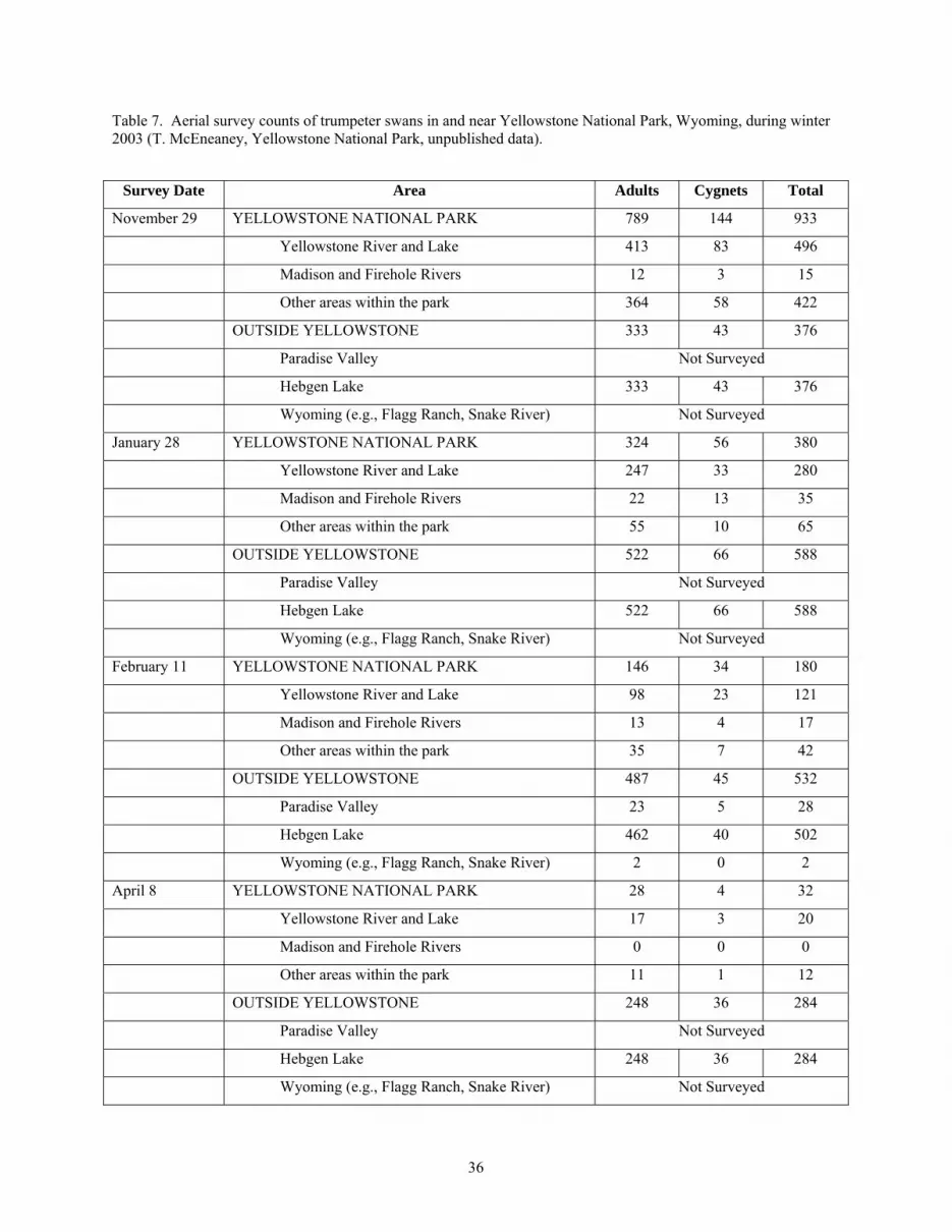
Table 7. Aerial survey counts of trumpeter swans in and near Yellowstone National Park, Wyoming, during winter 2003 (T. McEneaney, Yellowstone National Park, unpublished data).

Survey Date Area Adults Cygnets Total

November 29 YELLOWSTONE NATIONAL PARK 789 144 933

Yellowstone River and Lake 413 83 496

Madison and Firehole Rivers 12 3 15

Other areas within the park 364 58 422

OUTSIDE YELLOWSTONE 333 43 376

Paradise Valley Not Surveyed

Hebgen Lake 333 43 376

Wyoming (e.g., Flagg Ranch, Snake River) Not Surveyed

January 28 YELLOWSTONE NATIONAL PARK 324 56 380

Yellowstone River and Lake 247 33 280

Madison and Firehole Rivers 22 13 35

Other areas within the park 55 10 65

OUTSIDE YELLOWSTONE 522 66 588

Paradise Valley Not Surveyed

Hebgen Lake 522 66 588

Wyoming (e.g., Flagg Ranch, Snake River) Not Surveyed

February 11 YELLOWSTONE NATIONAL PARK 146 34 180

Yellowstone River and Lake 98 23 121

Madison and Firehole Rivers 13 4 17

Other areas within the park 35 7 42

OUTSIDE YELLOWSTONE 487 45 532

Paradise Valley 23 5 28

Hebgen Lake 462 40 502

Wyoming (e.g., Flagg Ranch, Snake River) 2 0 2

April 8 YELLOWSTONE NATIONAL PARK 28 4 32

Yellowstone River and Lake 17 3 20

Madison and Firehole Rivers 0 0 0

Other areas within the park 11 1 12

OUTSIDE YELLOWSTONE 248 36 284

Paradise Valley Not Surveyed

Hebgen Lake 248 36 284

Wyoming (e.g., Flagg Ranch, Snake River) Not Surveyed

36