Beiträge zur angewandten Wirtschaftsforschung

Nr. 10 (2005)

Combination Versus Competition - The Welfare Trade-offs Revisited

Tholen Eekhoff

Tholen Eekhoff Institut für Genossenschaftswesen

Centrum für angewandte Wirtschaftsforschung Münster (CAWM) Am Stadtgraben 9, D-48143 Münster

www.cawm.de

2

TABLE OF CONTENTS

1 INTRODUCTION ..................................................................................................... 3

2 ASSUMPTIONS....................................................................................................... 3

3 EFFICIENCY EFFECTS VERSUS SYNERGY EFFECTS OF A COMBINATION... 4

3.1 Scenario 1: Reduction of variable costs........................................................................................................... 4

3.2 Introducing fixed costs into the model............................................................................................................. 7

3.3 Scenario 2: Reduction of fixed costs.............................................................................................................. 10

3.4 Scenario 3: Product innovation ..................................................................................................................... 13

4 CONCLUSIONS .................................................................................................... 16

REFERENCES ......................................................................................................... 21

3

1 Introduction1

With the Eastern enlargement of the European Union, integration of the European economies

takes a substantial step forward. As a consequence, the decrease of barriers motivates and

facilitates mergers and acquisitions as well as cooperations among firms. Primarily, this de-

velopment has a favorable effect on economic welfare. Most combinations of firms are driven

by the motivation to realize synergy effects. However, a horizontal cooperation or merger

between firms tends to increase market concentration and can hence have a negative impact

on competition. These two effects comprise the challenge to competition authorities as they

have to evaluate the total effect on economic welfare.

The paper is organized as follows. In section 2, the assumptions of the framework that is de-

veloped in this paper will be explained. In the main part of the paper (sections 3), three sce-

narios are analyzed in which the efficiency effect of a combination is weighed against the

concentration effect. Within these scenarios, several constellations can be differentiated by

assumptions about the market structure and barriers to market entry. Section 4 concludes.

2 Assumptions

In his article from 1969, Williamson introduced the idea of a trade-off between the efficiency

effect and the concentration effect due to a combination of firms. He assumes a combination,

i.e. a merger or cooperation, of two firms forming a cartel or monopoly. The efficiency effect

of the combination is a cost reduction of the combined firms as compared to the situation be-

fore the concentration. The concentration effect implies that the firms are now able to set a

monopoly price. If the (positive) efficiency effect has a greater impact on total surplus (made

up of producer and consumer surplus) than the concentration effect, welfare increases and

competition authorities should approve the combination. Contrarily, if the concentration effect

is larger the combination should be prohibited.2

1 I would like to thank Dirk Lamprecht (University of Muenster) and Johann Eekhoff (University of Cologne) for their valuable comments. Many thanks also to Burkhard Kesting for valuable support work. I finally owe thanks to the Volkswagen Foundation for their support of this research project. 2 See Williamson (1969).

4

The model that is developed in this paper changes some of the assumptions of the Williamson

model in order to make it more realistic and to attain a broader application. Instead of a hori-

zontal cost curve, as presumed by Williamson, an upward sloping cost curve is assumed. As

synergy effects due to a combination should materialize within a few years, a short run per-

spective is adequate. In the short run, marginal costs can be assumed to rise and therefore the

cost curve is upward sloping. This assumption, however, introduces the necessity to differen-

tiate between fixed and variable costs. This problem will be solved in this paper using a new

approach to include fixed costs into a market analysis.

A second assumption is the possibility of no barriers to entry. Finally, synergy effects can not

only be realized by saving costs. An alternative efficiency effect of a combination is the inno-

vation of a product (which includes the invention of a new product).

In the following, alternative scenarios for a welfare trade-off due to a combination of firms

will be developed. In scenario 1, a combination is analyzed where a reduction of variable

costs is weighed against the concentration effect. With the introduction of fixed costs to the

model, the reduction thereof can be regarded in scenario 2. It was noted above that a synergy

effect can also take the form of a product innovation. Scenario 3 is concerned with this possi-

bility.

3 Efficiency effects versus synergy effects of a combination

3.1 Scenario 1: Reduction of variable costs

In this scenario the Williamsonian model will only be modified such that the cost curve is

upward sloping and barriers to entry are taken into account. As the reduction of variable costs

is regarded, fixed costs can be ignored.

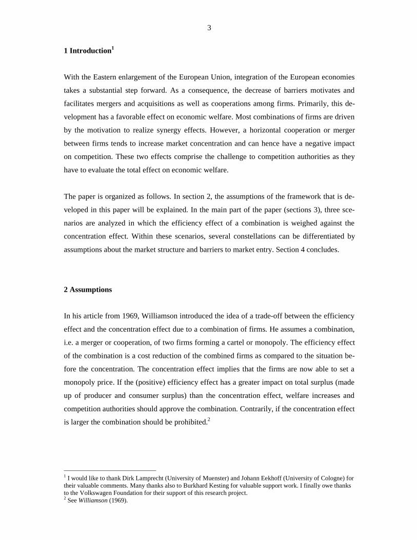
Let us assume an equilibrium in point A with a competitive market structure in figure 1 where

an average benefit is attained, as compared to other sectors of the economy. The marginal cost

curve is MC0 and the demand curve D so that p0 and x0 are the equilibrium price and quan-

5

tity.3 Now assume for simplicity that all the firms in the market decide to cooperate or to form

a monopoly. This combination yields two effects. The efficiency effect is assumed to be a

reduction of variable costs shifting MC0 downward to MC1. As the firms are now able to exert

greater market power they are assumed to charge the monopoly price p1 which leads to a sold

quantity of x1.4 The new equilibrium is described by the points B and R. Due to the described

effects, consumer surplus is reduced by the area p0ABp1. Producer surplus increases by the

areas p0GBp1 and ERCF, where the latter describes the efficiency gain; it decreases by the

area CAG. The net effect on producer surplus has to be positive because both the efficiency

effect and the concentration effect have a positive impact on producer surplus.5 Total surplus

rises by the area ERCF and decreases by the area CAB (which is the dead-weight loss due to

monopoly pricing).6 If the first area is larger than the second, i.e. the efficiency effect is big-

ger than the concentration effect, the impact of the combination on total welfare is positive

and it should be approved by the competition authorities.

Figure 1: Reduction of variable costs

3 For a definition and the properties of a competitive equilibrium see Frank (2000), pp. 363-364 or Wied-Nebbeling/Schott (1998), pp. 174-178. 4 The monopoly equilibrium is determined by the optimization condition that marginal cost (MC) is to equal marginal revenue (MR). See Frank (2000) pp. 394-410, or Varian (1995), pp. 387-390. 5 The efficiency effect is equal to area EDCF. The concentration effect is positive for producers because they the gain from setting the monopoly price p1 is higher than the gain from charging the competitive price p0. 6 For the concept of producer, consumer and total surplus see Frank (2000), pp. 364-367, or Varian (1995), pp. 236-252.

M

N Q

MC2

B

G

p1 p2

p0

p3 p4

E

F K

L

R

C J

I

H MC1

P

x1 x2 x0 x3 x4 X

D

MR

A

MC0

6

However, the higher gains that are realized by producers in the market attract additional firms.

The equilibrium described above (points B and R) can only be the final equilibrium in the

case of a non-competitive market. If the market is completely competitive the incumbent

firms are forced to set a price equal to marginal cost, i.e. p3. However, as firms attained an

average gain in the initial equilibrium, the firms receive a higher benefit after the combination

due to the cost saving. Therefore, new firms have an incentive to enter the market. In order to

be able to compete this has to be an efficient entry, i.e. the new firms have to realize the same

efficiency gains as the incumbent firms did by the means of the combination. Entry is worth-

while until benefits in the market are equal to the average benefit in the economy. Due to the

entry of firms the marginal cost curve shifts to the right (from MC1 to MC2). The final equi-

librium is somewhere below point L, say point Q, where p4 is the equilibrium price and x4 is

the equilibrium quantity. As compared to the initial equilibrium, consumer surplus rises by the

area p4QAp0. Producer surplus increases MQNE by but decreases by p4NAp0. After the com-

bination of the firms producer surplus is positive even though price is set equal to marginal

cost because only part of the efficiency gain is redistributed to consumers.7 As new firms en-

ter the market this higher producer surplus is distributed to a higher number of firms until an

average benefit is reached. Therefore, the benefit for each producer is constant in the medium

term and long run if the market is completely competitive. Total surplus increases by MQAF

which is equal to the efficiency gain.

An alternative situation in this scenario is that only some of the firms in the market decide to

work together in a cooperation or monopoly. This would lead to an oligopoly where a price

between p0 and p1 would be charged, for example p2.8 Like the monopoly case there would

have to be barriers to entry, otherwise this price could not be charged. The effect on welfare

would tend to be more positive than if a monopoly price is set (because of the smaller concen-

tration effect) but more negative than a situation with a completely competitive market (where

no concentration effect exists and price equals marginal cost).

Furthermore, the initial equilibrium may be oligopolistic. If there are barriers to entry, which

is usually the case in an oligopolistic market, the price will be between p0 and p1, say p2, and

quantity would then equal x2. A combination will then lead to a more concentrated oligopoly

7 A full redistribution would only take place if the demand curve was completely inelastic, which in reality will rarely be the case. 8 An oligopolistic price will usually lie between the competitive (marginal cost) price and the monopoly price. See for example Borchert/Grossekettler (1985), pp. 13-111.

7

or even a monopoly with the price p1 and the quantity x1. As before, the marginal cost curve

will shift downward to MC1. The results will be similar to those described above with barriers

to entry.

3.2 Introducing fixed costs into the model

In a lot of situations, cost savings are realized by reducing the fixed costs of the combined

firms rather than variable costs. This is the case if the firms use the same assets for their pro-

duction and, probably more importantly, if the same support functions such as controlling or

marketing are used by all entities that are involved in the combination. All the mentioned

forms of fixed costs have to be borne before the first unit can be produced. Therefore they

could be interpreted as marginal costs of the first unit. However, a more realistic interpreta-

tion can be attained by taking a firm’s investment rationale into consideration. In the case of

substantial fixed costs, a minimum quantity is necessary in order to regain at least part of

these costs. Whereas the exact quantity that will be sold as a result of an investment is not

known ex ante, a firm will usually calculate with this minimum quantity.

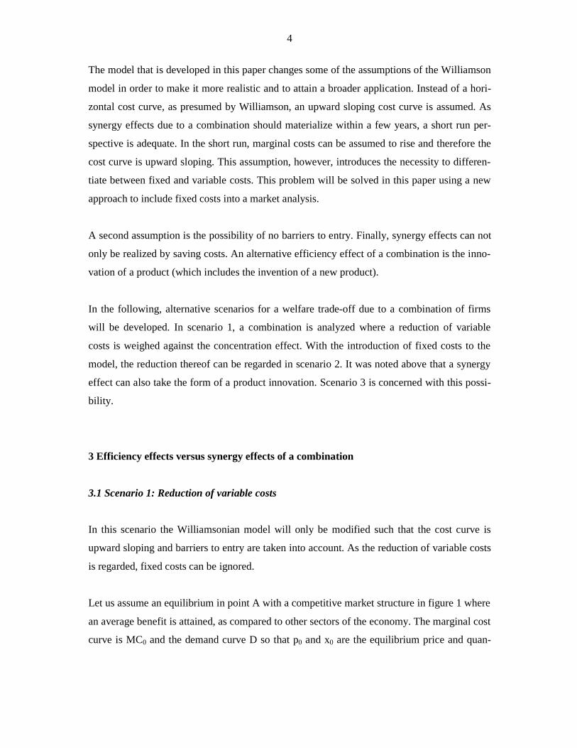
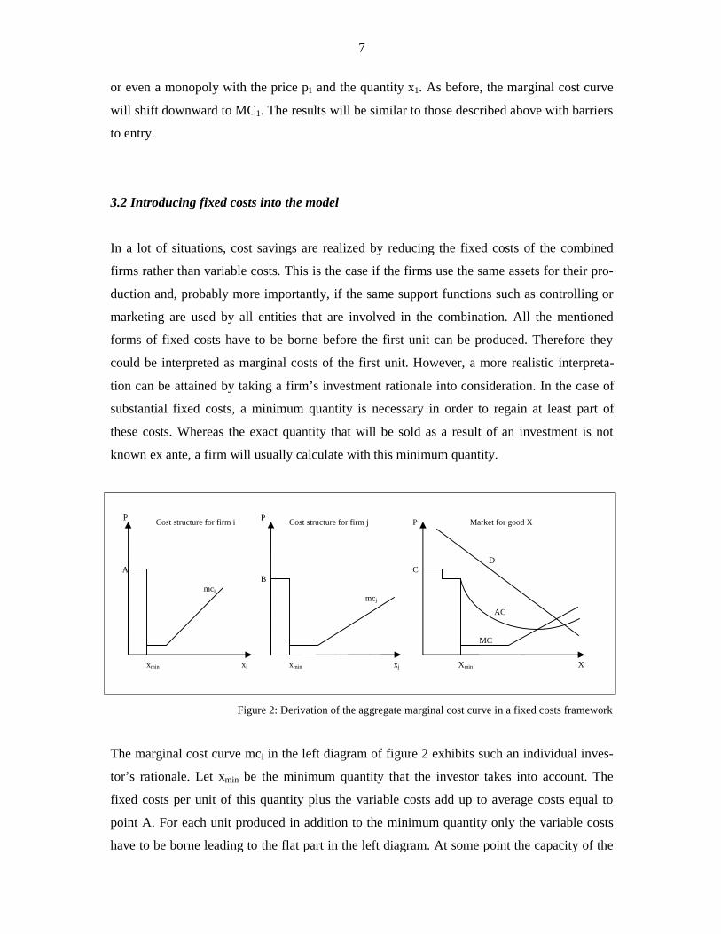
Figure 2: Derivation of the aggregate marginal cost curve in a fixed costs framework

The marginal cost curve mci in the left diagram of figure 2 exhibits such an individual inves-

tor’s rationale. Let xmin be the minimum quantity that the investor takes into account. The

fixed costs per unit of this quantity plus the variable costs add up to average costs equal to

point A. For each unit produced in addition to the minimum quantity only the variable costs

have to be borne leading to the flat part in the left diagram. At some point the capacity of the

A

P P P

C B

mcj

mci

Xmin xmin xmin xi xj X

MC

AC

D

Cost structure for firm i Cost structure for firm j Market for good X

8

fixed assets that are used in the production process will be fully employed and a re-investment

will be necessary. Realistically, not all fixed assets will have the same capacity so that they

will full employment occurs at different quantities. This phenomenon is approximated by the

rising part of the individual marginal cost function in the left panel. Once this point is

reached, it can be regarded as a new investment situation, like the one explained above. The

diagram in the middle of figure 2 describes another investor’s individual situation similar to

the first investor.9 Capacities of the two investors are assumed to be different (the flat parts

have different lengths), and so are the fixed costs that have to be borne in order to create these

capacities. In order to derive the market curve of marginal costs, the individual marginal cost

curves are aggregated horizontally. This results in the marginal cost curve MC in the right

diagram of figure 2.10

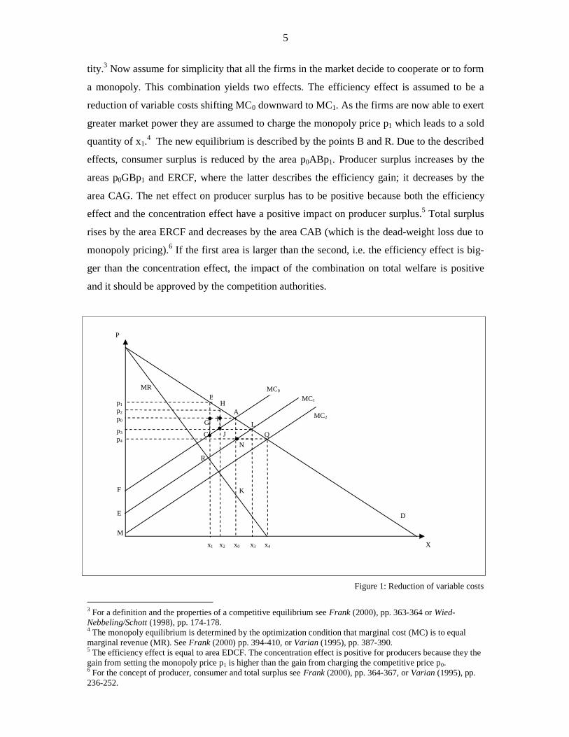
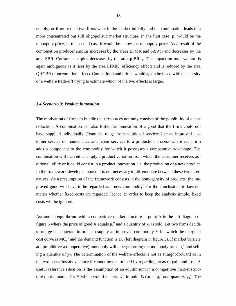
For the functioning of market processes in this framework consider figure 3. The firms’ cost

structures were aggregated as explained above.11 Assume an initial equilibrium in point A

with price p0, quantity x0 and an aggregate minimum quantity of x0min. As fixed costs per unit

of X are higher than the price firms bear a loss of (L-p0) per unit adding up to a total loss

equal to area p0SKL. Whether this is a stable equilibrium depends on the firms’ profits. Let us

assume that the marginal cost curve MC0 contains the economy’s average return in the form

of opportunity costs. Then firms receive an equilibrium profit if the loss borne over the mini-

mum quantity x0min is compensated by the surplus over the other units (x0-x0

min). In other

words, firms receive the economy’s average profit if the area of the loss (p0SKL) is equal to

the area of the surplus (SUHA). Let us denote this situation a “medium term equilibrium”. If

the market is competitive, i.e. barriers to entry are not prohibitively high, the market will al-

ways return to such a medium term equilibrium.

Consider what happens if positive profits are earned, i.e. if in the initial equilibrium in point A

(p0, x0, x0min) the area SUHA is larger than the area p0SKL. In this case new firms would be

attracted. Due to the additional capacities let the new minimum quantity equal x1min increasing

the fixed cost block to equal the area x0min,x1

min,F,K. The flat part of the marginal costs will

also increase, say by the distance HJ. The horizontal aggregation of the individual marginal

9 For simplicity, minimum quantities of the two investors are assumed to be the same. The analysis would not yield different results if this assumption was altered. 10 For the horizontal aggregation of individual marginal cost curves see for example Wied-Nebbeling/Schott (1998), pp. 166-167. 11 In order to simplify the analysis the fixed costs are shown in one block disregarding different individual levels. They were added and then divided by the aggregate minimum quantity. This simplification does not lead to dif-ferent results than the aggregation procedure described above.

9

cost curves results in a flatter aggregate cost curve MC2. Price will decrease to p2 and the

quantity sold will rise to x2. The new aggregate loss due to the fixed costs increases, now

equalling area p2IFL whereas aggregate surplus also increases to equal area IGJR. As the new

(short-term) equilibrium in point R is further away from the monopoly equilibrium (point C)

than the initial equilibrium (point A) each individual firm’s profits will decrease. This process

will continue until profits in this market are equal to the economy’s average profits. This is

true where the average cost curve AC intersects the demand curve (the average cost curves are

not depicted in figure 3).

Figure 3: Market process in a fixed cost framework

On the other hand, a medium-term equilibrium where firms bear a loss on average cannot

materialize besides the situation of a natural monopoly. In order to prove this hypothesis con-

sider the right diagram in figure 2 once again. The marginal cost curve will always intersect

the average cost curve in its minimum. Equilibria to the left of this intersection fall into the

area of a natural monopoly. At the same time, an equilibrium in this area will imply an aver-

age loss as the demand curve and the marginal cost curve will have their intersection below

the average cost curve. If average costs are higher than the price firms on average bear a loss.

The case of a natural monopoly, i.e. an equilibrium to the left of the intersection of D and MC

shall be disregarded in this paper, because in this case a monopoly is always the most efficient

solution with no need for a trade-off. Hence, for a medium-term equilibrium that does not lie

MR

F

E

G

xM

pM

p1

R

MC2

x2

MC1

M

C

H

I

L K

Q J

B

p2

x1

A

x0min x1

min x0

p0

P

X

MC0

D

S

T

U

10

within the area of a natural monopoly price will always be higher than (or at least equal to)

average costs.

However, the market does not necessarily remain in a medium-term equilibrium. The fact that

an average return is earned in the market does not necessarily imply that each individual firm

receives an average profit. If cost structures and hence their productivities differ yields will

also be different. Therefore it is possible that the economy’s average return is earned in the

market but some firms make profits and others incur losses. Let us assume an equilibrium in

point A in figure 3 with price p0 and quantity x0. Let the minimum quantity now be x1min. In

this medium-term equilibrium let the average profit be zero, i.e. the areas p0EFL and GHAE

are equal. Yet, some firms earn profits higher than the economies average return and others

bear losses due to different productivities of the firms’ assets. Those firms that incur losses

will leave the market eventually.12 Hence, the minimum quantity will decrease, assumably to

x0min and therefore the block of fixed costs become smaller by the area x0

min,x1min,F,K. The

flat part of the marginal cost curve shortens and the curve will become steeper (MC1). As the

new equilibrium in point B is now closer to the monopolistic equilibrium C and since fixed

costs have decreased, market profits will increase. These higher than average profits attract

new firms will enter the market, which they are only able to if they employ efficient assets of

production until an equilibrium is reached where all firms receive the economy’s average re-

turn. Let us denote such a situation a long-term equilibrium. However, as a medium-term

equilibrium is stable for a while (until re-investment in inefficient firms is necessary) and

since competition policy should regard short and medium-term developments, it is sufficient

to regard medium-term equilibria.

3.3 Scenario 2: Reduction of fixed costs

Synergy effects reducing the fixed costs of the partners are the more relevant part of a cost

reduction as compared to the reduction of variable costs. They include the mutual use of new

or existing assets, transport or service facilities, management capacities etc.

12 If all marginal costs are lower than the price, as assumed here, it is worthwile to produce with the existing capacities which in this case are sunk costs. Firms will exit the market as soon as their assets have depreciated and a re-investment would be necessary.

11

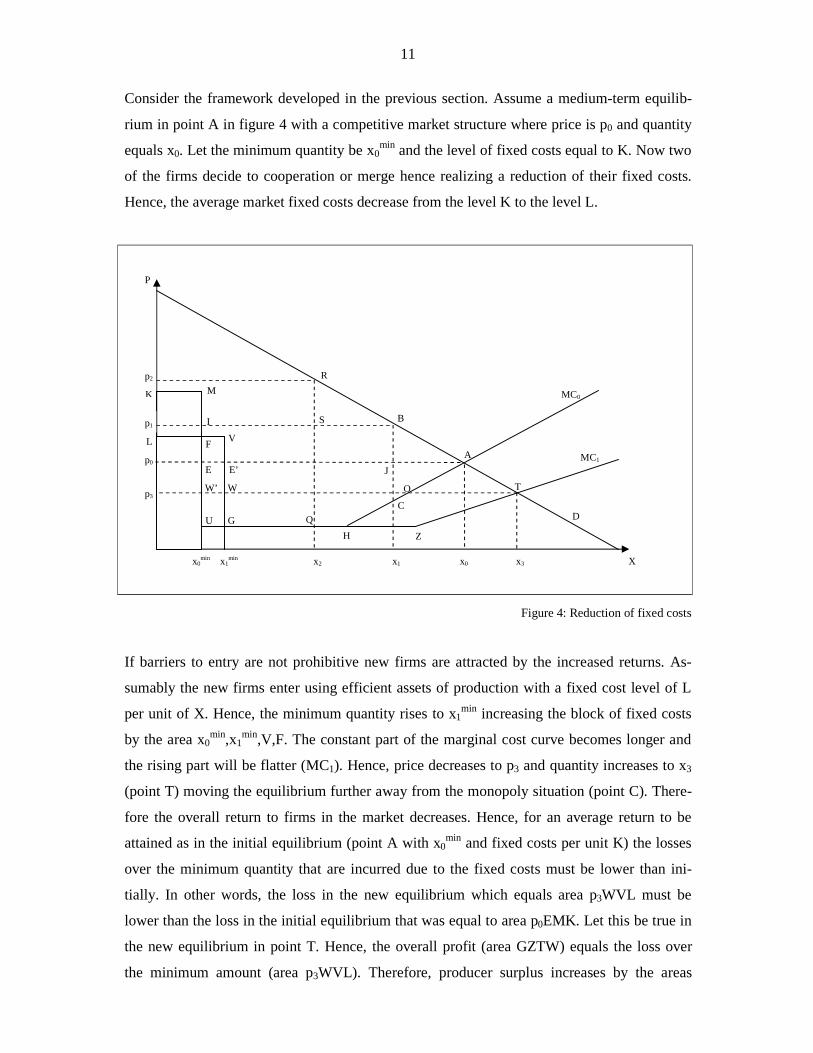
Consider the framework developed in the previous section. Assume a medium-term equilib-

rium in point A in figure 4 with a competitive market structure where price is p0 and quantity

equals x0. Let the minimum quantity be x0min and the level of fixed costs equal to K. Now two

of the firms decide to cooperation or merge hence realizing a reduction of their fixed costs.

Hence, the average market fixed costs decrease from the level K to the level L.

Figure 4: Reduction of fixed costs

If barriers to entry are not prohibitive new firms are attracted by the increased returns. As-

sumably the new firms enter using efficient assets of production with a fixed cost level of L

per unit of X. Hence, the minimum quantity rises to x1min increasing the block of fixed costs

by the area x0min,x1

min,V,F. The constant part of the marginal cost curve becomes longer and

the rising part will be flatter (MC1). Hence, price decreases to p3 and quantity increases to x3

(point T) moving the equilibrium further away from the monopoly situation (point C). There-

fore the overall return to firms in the market decreases. Hence, for an average return to be

attained as in the initial equilibrium (point A with x0min and fixed costs per unit K) the losses

over the minimum quantity that are incurred due to the fixed costs must be lower than ini-

tially. In other words, the loss in the new equilibrium which equals area p3WVL must be

lower than the loss in the initial equilibrium that was equal to area p0EMK. Let this be true in

the new equilibrium in point T. Hence, the overall profit (area GZTW) equals the loss over

the minimum amount (area p3WVL). Therefore, producer surplus increases by the areas

V

W’ W

Z

O T p3

x3

MC1

S

R

H

M

I

F L

K

E E’

U G Q C

J

B

p2

p1

x2 x1

A

x0min x1

min x0

p0

P

X

MC0

D

12

LFMK and HZTO and decreases by the areas UGVF and p3OAp0. Consumer surplus rises by

p3TAp0. Total surplus clearly increases because both consumer and producer surplus increase

(recall that each firm receives average profits but as firms have entered the market producer

surplus has grown). The individual producers are no better or worse off than initially because

they earn average profits. Only in the short run those firms that have realized the efficiency

increase earn more temporarily. As total surplus rises (by the areas LFMK and HZTA minus

UGVF) this scenario does not pose a problem to competition authorities. This result is owed

to the fact of the free entry of firms.

Results change fundamentally if barriers to entry are prohibitive. Let point A again be the

initial equilibrium with fixed costs per unit of K and a minimum quantity x0min. Due to the

combination of two firms the aggregate fixed cost level is reduced to L. The higher market

profits form an incentive for other incumbent firms to realize similar synergies by the means

of a combination. Assume these processes to lead to an increased market concentration and

hence an oligopolistic market structure. Hence, firms will be able to set a higher price, say p1

leading to a decrease in the quantity sold of x1. Producer surplus rises by the areas LFMK,

LFIp1 and EJBI and decreases by the area CAJ. Consumer surplus is reduced by the area

p0ABp1. The effect on total surplus is ambiguous. It rises by LFMK (efficiency effect) and

decreases by CAB (concentration effect). In this situation a welfare trade-off becomes neces-

sary where competition authorities have to estimate which effect is larger. In case of a combi-

nation that solely produces cost synergies a good indicator for the welfare effect is the price.

If it rises the concentration effect is likely to be larger than the efficiency effect. However,

this indicator ignores quantity effects. Furthermore, it cannot be employed if quality changes

play a role, which will be shown later.

As in scenario 1 it is possible that the initial equilibrium exhibits an oligopolistic market

structure where price p1 is higher than the marginal cost price (p0). Quantity would then equal

x1. A price above the p0 would have to be protected by market barriers against the entry of

potential competitors. Assume the aggregate minimum quantity again to be x0min and the level

of fixed costs per unit of this quantity to equal K. A combination of two firms assumably

leads to fixed cost savings represented by the area LFMK. Due to the increased market con-

centration firms will be able to set a higher price (say p2) and hence quantity sold decreases to

x2. For further analysis it is not important whether the oligopoly in the initial equilibrium con-

sisted of two firms that now form a monopoly (or in case of a cooperation a collective mo-

13

nopoly) or if more than two firms were in the market initially and the combination leads to a

more concentrated but still oligopolistic market structure. In the first case, p2 would be the

monopoly price, in the second case it would be below the monopoly price. As a result of the

combination producer surplus increases by the areas LFMK and p1SRp2 and decreases by the

area SBR. Consumer surplus decreases by the area p1BRp2. The impact on total welfare is

again ambiguous as it rises by the area LFMK (efficiency effect) and is reduced by the area

QHCBR (concentration effect). Competition authorities would again be faced with a necessity

of a welfare trade-off trying to estimate which of the two effects is larger.

3.4 Scenario 3: Product innovation

The motivation of firms to bundle their resources not only consists of the possibility of a cost

reduction. A combination can also foster the innovation of a good that the firms could not

have supplied individually. Examples range from additional services like an improved cus-

tomer service or maintenance and repair services to a production process where each firm

adds a component to the commodity for which it possesses a comparative advantage. The

combination will then either imply a product variation from which the consumer receives ad-

ditional utility or it could consist in a product innovation, i.e. the production of a new product.

In the framework developed above it is not necessary to differentiate between these two alter-

natives. As a presumption of the framework consists in the homogeneity of products, the im-

proved good will have to be regarded as a new commodity. For the conclusions it does not

matter whether fixed costs are regarded. Hence, in order to keep the analysis simple, fixed

costs will be ignored.

Assume an equilibrium with a competitive market structure in point A in the left diagram of

figure 5 where the price of good X equals px0 and a quantity of x0 is sold. Let two firms decide

to merge or cooperate in order to supply an improved commodity Y for which the marginal

cost curve is MCy1 and the demand function is Dy (left diagram in figure 5). If market barriers

are prohibitive a (cooperative) monopoly will emerge setting the monopoly price py2 and sell-

ing a quantity of y2. The determination of the welfare effects is not as straight-forward as in

the two scenarios above since it cannot be determined by regarding areas of gain and loss. A

useful reference situation is the assumption of an equilibrium in a competitive market struc-

ture on the market for Y which would materialize in point B (price py1 and quantity y1). The

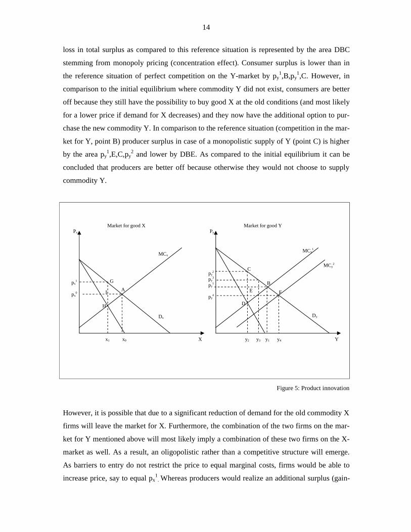
14

loss in total surplus as compared to this reference situation is represented by the area DBC

stemming from monopoly pricing (concentration effect). Consumer surplus is lower than in

the reference situation of perfect competition on the Y-market by py1,B,py

1,C. However, in

comparison to the initial equilibrium where commodity Y did not exist, consumers are better

off because they still have the possibility to buy good X at the old conditions (and most likely

for a lower price if demand for X decreases) and they now have the additional option to pur-

chase the new commodity Y. In comparison to the reference situation (competition in the mar-

ket for Y, point B) producer surplus in case of a monopolistic supply of Y (point C) is higher

by the area py1,E,C,py

2 and lower by DBE. As compared to the initial equilibrium it can be

concluded that producers are better off because otherwise they would not choose to supply

commodity Y.

Figure 5: Product innovation

However, it is possible that due to a significant reduction of demand for the old commodity X

firms will leave the market for X. Furthermore, the combination of the two firms on the mar-

ket for Y mentioned above will most likely imply a combination of these two firms on the X-

market as well. As a result, an oligopolistic rather than a competitive structure will emerge.

As barriers to entry do not restrict the price to equal marginal costs, firms would be able to

increase price, say to equal px1

. Whereas producers would realize an additional surplus (gain-

H

I

G

F

MCy2

C

D

E

py2

py3

py1

py

4

B A

Y X y2 y3 y1 y4

px

1

px

0

x1 x0

MCy1

MCx

Dy

Dx

Py Px

Market for good X Market for good Y

15

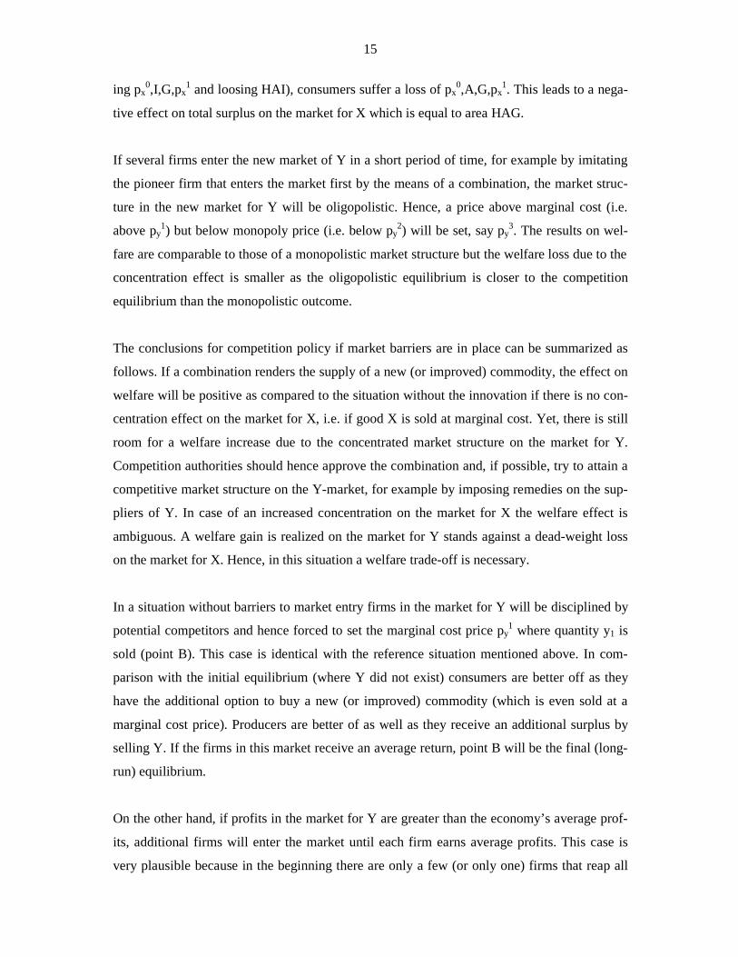
ing px0,I,G,px

1 and loosing HAI), consumers suffer a loss of px0,A,G,px

1. This leads to a nega-

tive effect on total surplus on the market for X which is equal to area HAG.

If several firms enter the new market of Y in a short period of time, for example by imitating

the pioneer firm that enters the market first by the means of a combination, the market struc-

ture in the new market for Y will be oligopolistic. Hence, a price above marginal cost (i.e.

above py1) but below monopoly price (i.e. below py

2) will be set, say py3. The results on wel-

fare are comparable to those of a monopolistic market structure but the welfare loss due to the

concentration effect is smaller as the oligopolistic equilibrium is closer to the competition

equilibrium than the monopolistic outcome.

The conclusions for competition policy if market barriers are in place can be summarized as

follows. If a combination renders the supply of a new (or improved) commodity, the effect on

welfare will be positive as compared to the situation without the innovation if there is no con-

centration effect on the market for X, i.e. if good X is sold at marginal cost. Yet, there is still

room for a welfare increase due to the concentrated market structure on the market for Y.

Competition authorities should hence approve the combination and, if possible, try to attain a

competitive market structure on the Y-market, for example by imposing remedies on the sup-

pliers of Y. In case of an increased concentration on the market for X the welfare effect is

ambiguous. A welfare gain is realized on the market for Y stands against a dead-weight loss

on the market for X. Hence, in this situation a welfare trade-off is necessary.

In a situation without barriers to market entry firms in the market for Y will be disciplined by

potential competitors and hence forced to set the marginal cost price py1 where quantity y1 is

sold (point B). This case is identical with the reference situation mentioned above. In com-

parison with the initial equilibrium (where Y did not exist) consumers are better off as they

have the additional option to buy a new (or improved) commodity (which is even sold at a

marginal cost price). Producers are better of as well as they receive an additional surplus by

selling Y. If the firms in this market receive an average return, point B will be the final (long-

run) equilibrium.

On the other hand, if profits in the market for Y are greater than the economy’s average prof-

its, additional firms will enter the market until each firm earns average profits. This case is

very plausible because in the beginning there are only a few (or only one) firms that reap all

16

the profits from selling Y. The entry of additional firms shifts the aggregate marginal cost

curve from MCy1 to MCy

2. Hence, price decreases to py4 and quantity rises to y4. As compared

to the initial situation, consumer utility rises even further. Additional consumer surplus due to

the market entry of new firms equals area py4,F,B,py

1. Producers are worse off as compared to

the situation before the entry of new firms, however, after some temporary returns above av-

erage they receive the economy’s average return. As both groups are (at least slightly) better

off, welfare rises in comparison with the initial equilibrium before Y was supplied. In case of

free market entry, the supply of a new (or improved) commodity clearly improves overall

welfare.

4 Conclusions

The Eastern Enlargement is another step in the integration process of the European econo-

mies. The mergers and acquisitions as well as cooperations that are facilitated due to this de-

velopment can have a positive and a negative effect on welfare. Primarily, the combination of

firms is driven by the motivation to realize synergy effects. However, this efficiency effect

must be weighed against the increased concentration which can be a consequence of the com-

bination as well. In this paper, different scenarios were analyzed with or without barriers to

market entry, with different synergy effects and market structures. The Synergy effects result-

ing from a combination can take the form of a cost reduction and alternatively of a product

innovation. The results for the scenarios analyzing a variable and a fixed cost reduction are

summarized in table 1.

In constellation a) of each scenario the results for a transition from competition to a monopoly

are analyzed. Alternatively, the increased market concentration may merely lead to an oligop-

oly (constellation b). In constellation c) an oligopolistic market structure is assumed in the

initial equilibrium and the transition to a collective monopoly is regarded. The transition from

competition to a very concentrated market structure can happen if other firms try to attain the

same synergy effects by forming a combination, following the example of the pioneering

firms. Each constellation can be differentiated as to whether barriers to market entry are in

place, besides constellation c). That is because it seems likely that barriers to entry have been

in place in the initial oligopolistic market structure. While only the results of prohibitive and

no barriers to entry have been analyzed, constellations with moderate barriers to entry will

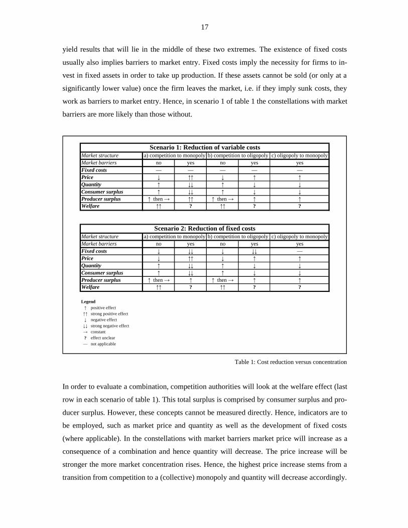
17

yield results that will lie in the middle of these two extremes. The existence of fixed costs

usually also implies barriers to market entry. Fixed costs imply the necessity for firms to in-

vest in fixed assets in order to take up production. If these assets cannot be sold (or only at a

significantly lower value) once the firm leaves the market, i.e. if they imply sunk costs, they

work as barriers to market entry. Hence, in scenario 1 of table 1 the constellations with market

barriers are more likely than those without.

Market structure c) oligopoly to monopolyMarket barriers no yes no yes yesFixed costs — — — — —Price ↓ ↑↑ ↓ ↑ ↑Quantity ↑ ↓↓ ↑ ↓ ↓Consumer surplus ↑ ↓↓ ↑ ↓ ↓Producer surplus ↑ then → ↑↑ ↑ then → ↑ ↑Welfare ↑↑ ? ↑↑ ? ?

Market structure c) oligopoly to monopolyMarket barriers no yes no yes yesFixed costs ↓ ↓↓ ↓ ↓↓ —Price ↓ ↑↑ ↓ ↑ ↑Quantity ↑ ↓↓ ↑ ↓ ↓Consumer surplus ↑ ↓↓ ↑ ↓ ↓Producer surplus ↑ then → ↑ ↑ then → ↑ ↑Welfare ↑↑ ? ↑↑ ? ?

Legend↑ positive effect↑↑ strong positive effect↓ negative effect↓↓ strong negative effect→ constant? effect unclear— not applicable

a) competition to monopoly b) competition to oligopoly

Scenario 1: Reduction of variable costs

Scenario 2: Reduction of fixed costs

a) competition to monopoly b) competition to oligopoly

Table 1: Cost reduction versus concentration

In order to evaluate a combination, competition authorities will look at the welfare effect (last

row in each scenario of table 1). This total surplus is comprised by consumer surplus and pro-

ducer surplus. However, these concepts cannot be measured directly. Hence, indicators are to

be employed, such as market price and quantity as well as the development of fixed costs

(where applicable). In the constellations with market barriers market price will increase as a

consequence of a combination and hence quantity will decrease. The price increase will be

stronger the more market concentration rises. Hence, the highest price increase stems from a

transition from competition to a (collective) monopoly and quantity will decrease accordingly.

18

Hence, consumer surplus will be reduced and producer surplus increases. As the effect on

total welfare is ambiguous, a welfare trade-off is necessary taking into account the specific

circumstances of the situation.

Results change substantially if no barriers to market entry are in place. While price rises at

first due to the combination, new competitors entering the market will exert a downward

pushing the price below its initial level. Accordingly, quantity decreases at first and then rises

above its initial level. Incumbent producers’ profits are increased initially and then reduced to

an average return due to the entry of new firms. Consumer surplus increases. Therefore, wel-

fare increases in all constellations without market barriers. This result underlines the impor-

tance of free market entry.

Synergy effects due to a combination can also arise from a product innovation. Both forms of

synergy effects, cost reductions and product innovations, oftentimes go hand in hand. How-

ever, an isolated analysis seems reasonable in order to determine the result of each form. The

consequences of a combination with synergy effects taking the form of a product innovation

are summarized in table 2. In constellation a) a monopoly on the market for the new commod-

ity Y is assumed whereas in constellation b) an oligopolistic market structure will presumably

materialize. In constellation c) a market structure change on the market for the old good “X”

is assumed, i.e. a transition from competition to monopoly (presuming a monopoly on the

market for the new commodity Y as well).

As we are now looking at two markets, the parameters of both can be regarded. The price for

the newly developed good Y is measured against the price of the old good X, as these goods

are very similar and substitutable. As a product innovation implies the addition to new proper-

ties to an existing commodity, it can be assumed that consumers are willing to pay more for

the new than for the old good. Contrarily, the comparison of quantities for the new and the old

good do not make sense if the commodities are not homogeneous. The changes in the quantity

of Y are hence measured against its initial quantity after the market for the new commodity is

created.

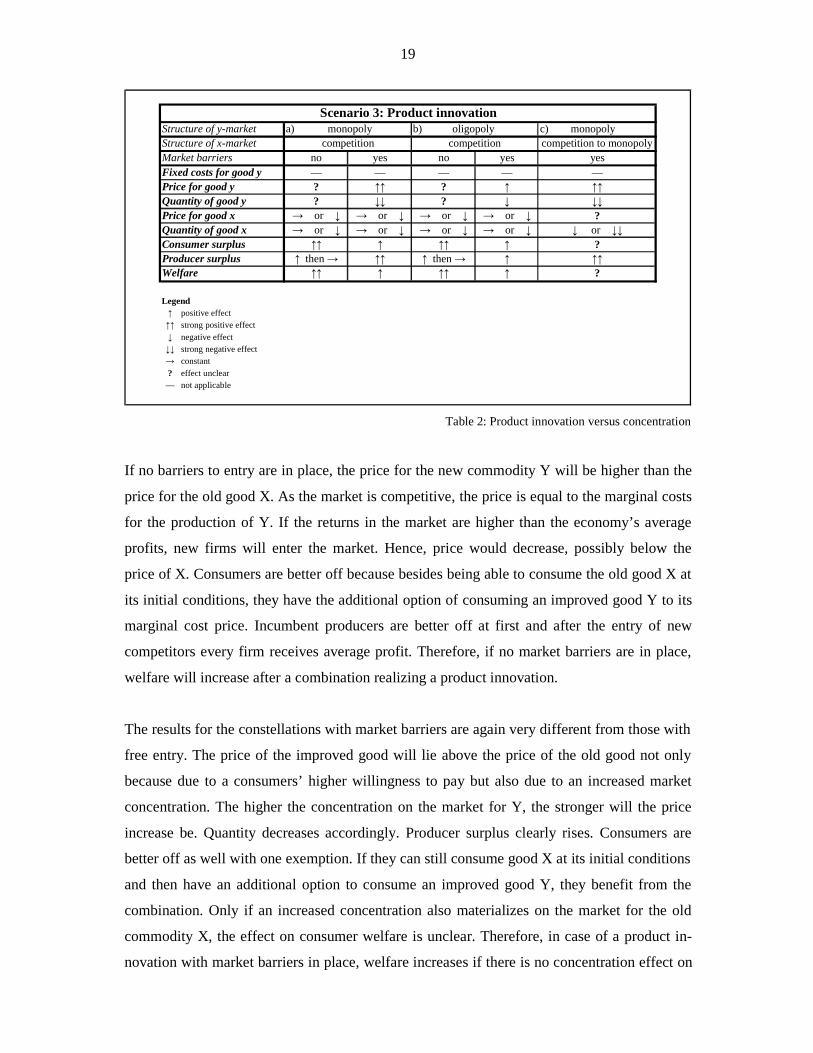
19

Structure of y-market c) monopolyStructure of x-market competition to monopolyMarket barriers no yes no yes yesFixed costs for good y — — — — —Price for good y ? ↑↑ ? ↑ ↑↑Quantity of good y ? ↓↓ ? ↓ ↓↓Price for good x → or ↓ → or ↓ → or ↓ → or ↓ ?Quantity of good x → or ↓ → or ↓ → or ↓ → or ↓ ↓ or ↓↓Consumer surplus ↑↑ ↑ ↑↑ ↑ ?Producer surplus ↑ then → ↑↑ ↑ then → ↑ ↑↑Welfare ↑↑ ↑ ↑↑ ↑ ?

Legend↑ positive effect↑↑ strong positive effect↓ negative effect↓↓ strong negative effect→ constant? effect unclear— not applicable

competition competition

Scenario 3: Product innovationa) monopoly b) oligopoly

Table 2: Product innovation versus concentration

If no barriers to entry are in place, the price for the new commodity Y will be higher than the

price for the old good X. As the market is competitive, the price is equal to the marginal costs

for the production of Y. If the returns in the market are higher than the economy’s average

profits, new firms will enter the market. Hence, price would decrease, possibly below the

price of X. Consumers are better off because besides being able to consume the old good X at

its initial conditions, they have the additional option of consuming an improved good Y to its

marginal cost price. Incumbent producers are better off at first and after the entry of new

competitors every firm receives average profit. Therefore, if no market barriers are in place,

welfare will increase after a combination realizing a product innovation.

The results for the constellations with market barriers are again very different from those with

free entry. The price of the improved good will lie above the price of the old good not only

because due to a consumers’ higher willingness to pay but also due to an increased market

concentration. The higher the concentration on the market for Y, the stronger will the price

increase be. Quantity decreases accordingly. Producer surplus clearly rises. Consumers are

better off as well with one exemption. If they can still consume good X at its initial conditions

and then have an additional option to consume an improved good Y, they benefit from the

combination. Only if an increased concentration also materializes on the market for the old

commodity X, the effect on consumer welfare is unclear. Therefore, in case of a product in-

novation with market barriers in place, welfare increases if there is no concentration effect on

20

the market for the old good X. In case of a concentration in this market, the effect on welfare

is unclear and a trade-off is necessary taking into account the specific circumstances of the

situation. Furthermore, it should be noted that there is still room for an additional welfare in-

crease if a more competitive market structure can be attained in the Y-market.

To sum up, one of the main conclusions of this paper is that barriers to entry play a very im-

portant role. If a market is competitive, welfare is increased in all three scenarios. In case of a

product innovation, the effect on welfare is positive as well, unless there is a negative concen-

tration effect on the market for the old good, i.e. the good without the properties that were

added in the innovation process. However, there usually is still room for a welfare increase

due to a concentrated market structure on the market for the innovated commodity. If synergy

effects take the form of a cost reduction, the effect on welfare is always unclear if high barri-

ers to entry are in place. Hence, a trade-off is necessary between the efficiency and the con-

centration effect by taking a closer look at the specific circumstances.

21

References

Borchert, Manfred / Grossekettler, Heinz (1985): Preis- und Wettbewerbstheorie. Verlag W.

Kohlhammer; Stuttgart, Berlin, Köln, Mainz; 1985.

Frank, Robert H. (2000): Microeconomics and Behaviour. McGraw-Hill, 4th Edition; Boston,

Burr Ridge, Dubuque u. a.; 2000.

Varian, Hal R. (1995): Grundzüge der Mikroökonomik. Oldenbourg Verlag, 3. Aufl., Mün-

chen, 1995.

Wied-Nebbeling, Susanne / Schott, Hartmut (1998): Grundlagen der Mikroökonomik. Sprin-

ger, 1. Aufl., Berlin, 1998.

Williamson, Oliver E. (1969): Economies as an Antitrust Defense: The Welfare Tradeoffs. In:

The American Economic Review, Vol. 58, Stanford, 1969.