Aalto University

School of Science

Degree Programme of Computer Science and Engineering

Vlad Mihai MIREL

Benchmarking Big Data SQL Frame-works

Master’s ThesisEspoo, 16.6.2016

Supervisor: Associate Prof. Heljanko KeijoInstructors: D.Sc. (Tech.) Khalid Latif

D.Sc. (Tech.) Olli Luukkonen

Aalto UniversitySchool of ScienceDegree Programme of Computer Science and Engineering

ABSTRACT OFMASTER’S THESIS

Author: Vlad Mihai MIREL

Title:Benchmarking Big Data SQL Frameworks

Date: 16.6.2016 Pages: 76

Supervisor: Associate Prof. Heljanko Keijo

Instructors: D.Sc. (Tech.) Khalid LatifD.Sc. (Tech.) Olli Luukkonen

The amount of data being generated on a daily basis is constantly increasing,pushing the limits of traditional data processing technologies. A consequenceof this increase is the rise to new distributed Big Data engines. This thesisis focused on benchmarking Big Data SQL frameworks, both open-source orproprietary.

The Big Data frameworks are compared with each other from three points ofview: performance (total job execution time), feature availability and integrationwith other services. In order to provide an unbiased comparison, a similarunderlying infrastructure was employed for each framework. More precisely,experiments were conducted on different Big Data SQL platforms hosted on twopublic cloud infrastructures: Microsoft Azure and Google Cloud Platform. Inthe case of Azure, SQL queries were executed on HDInsight, a PaaS solutionfor Big Data SQL clusters like Spark SQL, HiveQL, Apache Drill and ApacheImpala. Experiments were also conducted on SaaS solutions offered by theboth vendors, Microsoft Azure Data Lake Analytics and Google BigQuery. Theworkloads comprised from several GBs up to 250 GBs in Parquet format. In thecase of SaaS platforms, 44.8 GBs of .csv files were employed.

The results obtained from conducting the experiments on both PaaS and SaaSplatforms are meant to shed some light on the benefits that emerge when choosingone technology. Furthermore, based on these insights, existing Big Data enginescould be further improved.

Keywords: Big Data, SQL, Cloud Computing, Performance

Language: English

2

Acknowledgements

I want to thank Associate Professor Heljanko Keijo and my instructors KhalidLatif and Olli Luukkonen for their guidance.

Espoo, 16.6.2016

Vlad Mihai MIREL

3

Abbreviations and Acronyms

ADIC Atomicity, Consistency, Isolation, DurabilityBLOB Binary Large ObjectHDFS Hadoop Distributed File SystemIaaS Infrastructure as a ServiceLLVM Low Level Virtual MachineMPP Masively Parallel ProcessingOLAP Online Analytical ProcessingOLTP Online transaction processingORC Optimized Row ColumnarPaaS Platform as a ServicePOS Point of SaleRDBMS Relational database management systemSaaS Software as a ServiceSSD Solid State DriveVM Virtual MachineWAS Windows Azure Storage

4

Contents

Abbreviations and Acronyms 4

1 Introduction 6

2 Background 122.1 Big Data Engines . . . . . . . . . . . . . . . . . . . . . . . . . 122.2 Data Storage Formats . . . . . . . . . . . . . . . . . . . . . . 162.3 Big Data SQL Frameworks . . . . . . . . . . . . . . . . . . . . 20

2.3.1 Hive SQL . . . . . . . . . . . . . . . . . . . . . . . . . 212.3.2 Spark SQL . . . . . . . . . . . . . . . . . . . . . . . . . 232.3.3 Apache Drill . . . . . . . . . . . . . . . . . . . . . . . . 272.3.4 Facebook Presto . . . . . . . . . . . . . . . . . . . . . 292.3.5 Apache Impala . . . . . . . . . . . . . . . . . . . . . . 32

2.4 Azure . . . . . . . . . . . . . . . . . . . . . . . . . . . . . . . 34

3 Technical contributions 393.1 Big Data SQL frameworks - Platform as a Service . . . . . . . 393.2 Big Data SQL frameworks - Software as a Service . . . . . . . 45

4 Experiments 50

5 Results 56

6 Conclusions 636.1 Achievements . . . . . . . . . . . . . . . . . . . . . . . . . . . 636.2 Future development . . . . . . . . . . . . . . . . . . . . . . . . 65

A Queries 73A.1 HiveQL queries . . . . . . . . . . . . . . . . . . . . . . . . . . 73A.2 Cross Big Data SQL set of queries . . . . . . . . . . . . . . . . 75

5

Chapter 1

Introduction

This chapter provides an overview of Big Data. The topic is then integratedto the concept of analytic workloads, which can be of two kinds: OLAP (On-line Analytical Processing) or OLTP (Online transaction processing).

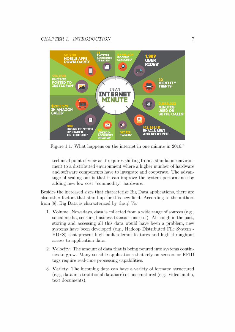
The amount of data generated on a daily basis is increasing rapidly [24],with large portions of it being created by the end users1. Every minute,Google registers 2.4 million search queries, over 547000 tweets are posted andFacebook registers more than 700000 user logins. A more detailed picture ofthe main data traffic providers is presented in Figure 1.1.

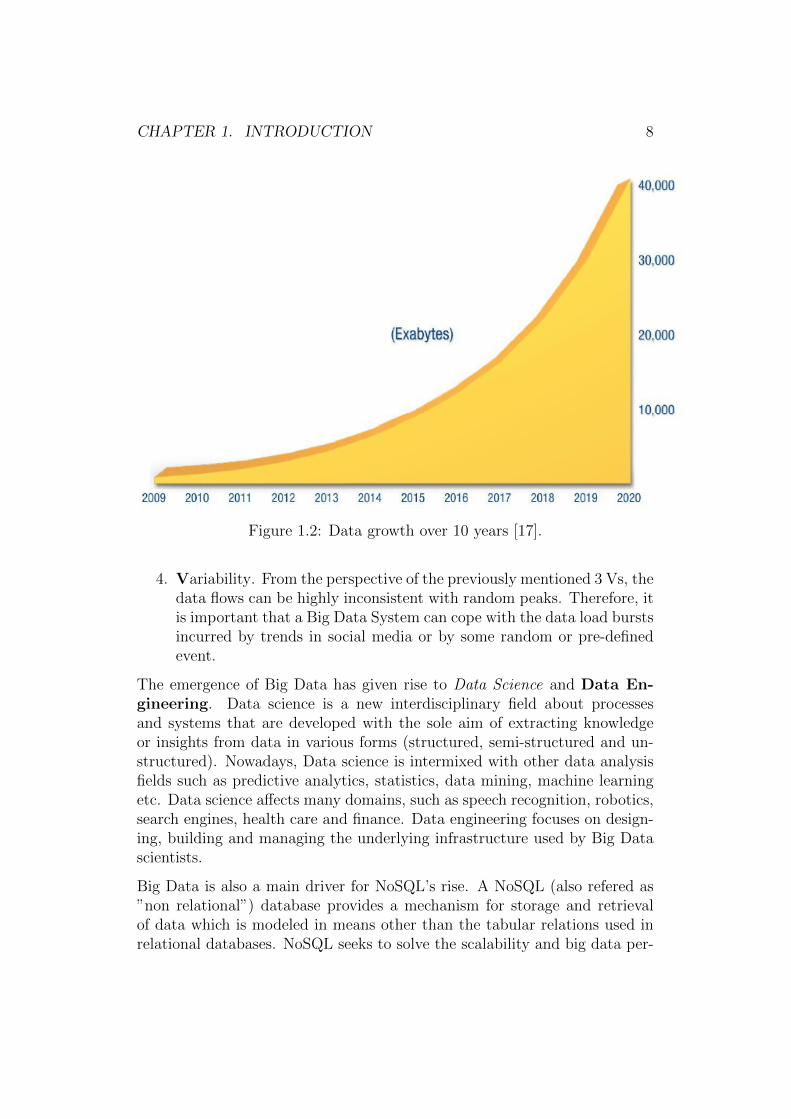
Following this trend, it is expected that by 2020, the amount of data storedon the Internet will be 50 times larger than the amount stored in 2010 [17].The graph depicted in Figure 1.2 highlights this scenario.

These large data sets (often called Big Data) can no longer be analyzedefficiently using traditional analytic methods. Thus, novel ways for per-forming efficient analyses using the available computing resources have tobe employed. The performance of such a system can be improved in twoways:

1. Scaling Up, upgrading the single computer responsible for processingthe provided tasks. Scaling up is usually considered not to be a costeffective way of increasing performance [24].

2. Scaling Out, where multiple computers are added to process the al-located tasks concurrently. Scaling out is difficult to implement from a

1http://techcrunch.com/2010/08/04/schmidt-data2http://www.excelacom.com/resources/blog/one-internet-minute

6

CHAPTER 1. INTRODUCTION 7

Figure 1.1: What happens on the internet in one minute in 2016.2

technical point of view as it requires shifting from a standalone environ-ment to a distributed environment where a higher number of hardwareand software components have to integrate and cooperate. The advan-tage of scaling out is that it can improve the system performance byadding new low-cost ”commodity” hardware.

Besides the increased sizes that characterize Big Data applications, there arealso other factors that stand up for this new field. According to the authorsfrom [8], Big Data is characterized by the 4 Vs :

1. Volume. Nowadays, data is collected from a wide range of sources (e.g.,social media, sensors, business transactions etc.). Although in the past,storing and accessing all this data would have been a problem, newsystems have been developed (e.g., Hadoop Distributed File System -HDFS) that present high fault-tolerant features and high throughputaccess to application data.

2. Velocity. The amount of data that is being poured into systems contin-ues to grow. Many sensible applications that rely on sensors or RFIDtags require real-time processing capabilities.

3. Variety. The incoming data can have a variety of formats: structured(e.g., data in a traditional database) or unstructured (e.g., video, audio,text documents).

CHAPTER 1. INTRODUCTION 8

Figure 1.2: Data growth over 10 years [17].

4. Variability. From the perspective of the previously mentioned 3 Vs, thedata flows can be highly inconsistent with random peaks. Therefore, itis important that a Big Data System can cope with the data load burstsincurred by trends in social media or by some random or pre-definedevent.

The emergence of Big Data has given rise to Data Science and Data En-gineering. Data science is a new interdisciplinary field about processesand systems that are developed with the sole aim of extracting knowledgeor insights from data in various forms (structured, semi-structured and un-structured). Nowadays, Data science is intermixed with other data analysisfields such as predictive analytics, statistics, data mining, machine learningetc. Data science affects many domains, such as speech recognition, robotics,search engines, health care and finance. Data engineering focuses on design-ing, building and managing the underlying infrastructure used by Big Datascientists.

Big Data is also a main driver for NoSQL’s rise. A NoSQL (also refered as”non relational”) database provides a mechanism for storage and retrievalof data which is modeled in means other than the tabular relations used inrelational databases. NoSQL seeks to solve the scalability and big data per-

CHAPTER 1. INTRODUCTION 9

formance issues that relational databases are facing. NoSQL embeds a widerange of technologies and architectures, making it useful for applications thatneed to access and analyze massive amount of data stored on multiple serverinstances. Designed as a modern web-scale database [35], the main char-acteristics through which NoSQL databases differ from relational databasesare:

1. Schema-free.

2. Easy replication support.

3. Simple API.

4. BASE properties (basically available, soft state, eventually consistent)are replacing the ACID properties (atomicity, consistency, isolation,durability).

Nowadays, according to a report3, there are more than 225 NoSQL databases.The differences arise from the above mentioned features which allowed sys-tems to specialize against different data sets with different formats and pro-cessing requirements. These characteristics can be labelled as follows:

1. Wide Column Store / Column Families:

1.1. HBase [18] is an open source, non-relational, distributed databasewritten in Java. It was modeled after Google’s BigTable and runson top of HDFS.

1.2. Cassandra [13] is a popular NoSQL database initially developed byFacebook. It was released as open source in 2008. It is massivelyscalable, partitioned row store, has a masterless architecture, andpresents linear scale performance with no single points of failure.

1.3. Amazon SimpleDB [6] is suitable for less complex database envi-ronments where users need to access data in non-relational databases.Its strengths rely on providing high availability and flexibility toits customers.

2. Document Store:

2.1. MongoDB [9] is a free and open-source cross-platform document-oriented database. It detaches itself from table-based relationdatabases through JSON documents with dynamic schemas.

3http://nosql-database.org/

CHAPTER 1. INTRODUCTION 10

2.2. Elasticsearch [25] is a distributed text search engine developed inJava. It provides an HTTP web interface and schema-free JSONdocuments.

3. Key Value / Tuple Store:

3.1. Amazon Dynamo Database [42] is known for extremely low laten-cies and high scalability. All data items are stored on Solid StateDrives (SSDs), and are replicated across three Availability Zonesfor high availability and durability.

3.2. Azure Table Storage [6] is a service offered by Microsoft to storestructured NoSQL data on Azure. The storage is based on key/attributepairs with a schemaless design.

3.3. Redis [28] is an open-source, networked, in-memory data structurestore, used as database, cache and message broker.

3.4. Voldemort [44] is an open-source implementation of Amazon Dy-namo DB.

3.5. MemcacheDB [14] is a distributed, fast and reliable key-value stor-age and retrieval system designed for persistence.

4. Graph Databases:

4.1. Neo4J [45] is a graph database that uses its own query languageCypher to execute queries on data organized as a graph.

4.2. Titan [12] is a distributed graph database over a cluster of ma-chines. The cluster can elastically scale to support a growingdataset and user base. Titan has a pluggable storage architecturewhich allows it to build on proven database technology such asApache Cassandra, or Apache HBase.

5. Object Databases

5.1. Versant [46] is an object database which facilitates the storage andretrieval of complex object models. It does not rely on mappingcode to store or retrieve objects. Thus, schema modifications canbe handled without application downtime.

5.2. Starcounter4 is entirely written in C# and provides ACID prop-erties for each query. It supports SQL-like queries and providesfull checkpoint recovery.

4http://starcounter.com/

CHAPTER 1. INTRODUCTION 11

All these databases have applications related to business intelligence, as theyare able to provide (to different degrees) analytical processing. Due to thecloud environment in which they reside, these computations are often per-formed online. IT systems can be divided into transactional (OLTP) andanalytical (OLAP).

On the one hand, OLTP is characterized by a large number of short on-line transactions (INSERT, UPDATE, DELETE). The focus here is on fastquery processing, maintaining data integrity in multi-access environmentsand an effectiveness measured by number of transactions per second. Exam-ples of systems using OLTP include: online banking, online reserverations,or transactions that take place when dealing with ATMs and POS (Pointof Sale). In general, OLTP systems are considered data providers to datawarehouses.

On the other hand, in an OLAP system, the volume of transactions is low.However, the queries are more complex than in the previous case and in-volve aggregations. Thus, OLAP systems are suitable for data mining or thediscovery of previously undiscerned relationships between data items.

Chapter 2

Background

This chapter presents an overview of existing scalable cloud storage systems,newly proposed enhancements in the area of Big Data storage formats as wellas a comparative analysis of Big Data SQL engines. Section 2.1 provides anoverview of the engines used in Big Data systems. In Section 2.2 formatspopular in the area of Big Data are described. Next, Section 2.3 presentsSQL frameworks developed for Big Data processing. Finally, Section 2.4presents features related to data storage, data encoding and processing clus-ter belonging to a public cloud vendor.

2.1 Big Data Engines

MapReduce [16] has been the mainstay on Hadoop for batch jobs for along time. However, two very promising technologies have recently emerged:Apache Drill [43] and Spark [37]. Apache Drill is a columnar SQL enginefor self-service data exploration. Spark is a general-purpose compute enginethat can run both batch, interactive and streaming jobs on the cluster usingthe same unified frame.

Spark can be described through its three big concepts: RDDs (resilient dis-tributed data sets) [49], transformations and actions. RDDs are a representa-tion of the data that is coming into the system in an object format and allowsperforming computations on top of it. They are called resilient because oftheir lineage which allow them to recompute themselves whenever there is afailure in the system just by using the prior information. Transformationsallow creating of RDDs from other RDDs. Opening a file and creating an

12

CHAPTER 2. BACKGROUND 13

RDD from its contents is such an example. The third and final concept isrepresented by the actions. Actions occur whenever asking the system for ananswer that it needs to provide. For example, counting or asking whether thefirst line contains a certain word. Spark treats transformations lazily, whichmeans that the RDDs are not loaded and pushed into the system when anRDD is encountered, but they are only done when there actually is an ac-tion to be performed. Due to this, unlike Hadoop, which was constrainedto the MapReduce status, Spark can place a complex RDD graph in themost optimized manner on a Hadoop cluster. Spark also differs itself fromMapReduce through the consistency specific to RDDs. In distributed-sharedmemories check-pointing at different intervals is used to handle failures. Inthe case of RDDs, a lineage graph is built, and upon encountering an erroror a failure, they can go back and recompute based on that graph and regen-erate the missing RDDs. RDDs allow the engine to do some simple queryoptimizations, such as pipelining operations.

Released in 2015, ”DataFrames” [37] extend the API provided by Spark,making it easier to program, and at the same time improve performancethrough intelligent optimizations and code-generation. A DataFrame is adistributed collection of data organized into named columns. It is similar to atable in a relational database or a data frame in R/Python, but benefits fromricher optimizations occuring under the hood. Moreover, DataFrames can becreated from different sources such as: structured data files, tables in Hive,external databases, or existing RDDs. DataFrame supports reading fromlocal file systems, distributed file systems (e.g., HDFS), cloud storage (S3 orAzure Blob Storage), and external relational database systems via JDBC. Inaddition, through Spark SQL’s external data source API, DataFrames can beextended to support any third-party data formats or sources. Existing third-party extensions already include Avro, CSV, ElasticSearch, and Cassandra.Users can now pass DataFrames between Scala, Java or Python functions,breaking up their code into smaller parts and building a logical plan, and stillbenefiting from optimizations across the whole plan when they run an outputoperation. It is now easier to structure computations and debug intermediatesteps. Last but not least, the exposed API for DataFrames analyzes theplans in an eagerly fashion. For example, it can identify whether the columnnames used in expressions exist in the underlying tables, and whether theirdata types are appropriate. This is in contrast with the query results whichare computed lazily.

The impact of all these features is analyzed by the researchers in [41]. Theirexperiments prove that Spark is about 2.5x, 5x, and 5x faster than MapRe-duce, for Word Count, k-means, and PageRank respectively. The identified

CHAPTER 2. BACKGROUND 14

reasons for this speedup are the efficiency of the hash-based aggregation com-ponent for combine, as well as reduced CPU and disk overheads due to RDDcaching in Spark. However, the experiments have also shown that MapRe-duce is 2x faster than Spark when performing sort operations. This is due toMapReduce’s execution model which is more efficient than Spark at shufflingdata.

Spark was developed as an in-memory processing engine upgrade over Hadoop(which relies solely on map reduce operations over disk). Furthermore, newimprovements are being added on a regular basis. These improvements usu-ally arise as a solution to an identified bottleneck in the performance of thesystem. Some solutions ([5, 7, 15]) target the network infrastructure insidethe data centers, suggesting improvements in the area of network IO band-width as well as reducing the number of hops between data nodes. Theauthors in [19] present a network architecture that can scale to support datacenters with uniform high capacity between servers, whilst at the same timeoffer performance isolation between services, and Ethernet layer-2 seman-tics. Their model, called VL2, makes use of flat addressing to allow serviceinstances to be placed anywhere in the network. Moreover, the traffic is uni-formly spread across the network through a Valiant Load Balancer1. Thesefeatures combined together help skip the complex work that would haveotherwise been requested to the network control plane. The experimentsconducted on the VL2 prototype involved shuffling 2.7 TB of data among75 servers. The shuffling operation took 395 seconds in total. During thisoperation the flows were evenly distributed (with an efficiency of 94% andhigh TCP fairness was achieved (fairness index of 0.995).

Other solutions improve the disk efficiency2 and some are based on the re-search done by the authors in [3, 29, 49] on caching data in memory. Anotherpaper [31] brings contributions to the efficiency of RAM memories within adata center, from an energy perspective. Here, the research is based on thefact that the servers from within a datacenter use DDR3 memory, which is de-signed for high bandwidth also consumes a lot of energy. More precisely, sucha system which uses only 20% of the peak DDR3 bandwidth consumes 2.3xmore energy per bit than the energy consumed when the memory bandwidthis fully utilized. The solution envisaged by the authors is to use a technologyoriginally designed for mobile platforms, called LPDDR2. LPDDR2 is a ver-sion of the SDRAM (synchronous DRAM), which provides the same capacityper chip as DDR3 and similar access latency but at lower peak bandwidth.

1randomized scheme for communication among interconnected parallel processors2https://issues.apache.org/jira/browse/SPARK-5645

CHAPTER 2. BACKGROUND 15

By employing these type of memories, they obtain a 3-5x lower memorypower and small performance penalties for datacenter workloads. A differentangle is approached by the authors in [21, 27]. Here, the identification ofstraggler tasks3 caused by data skew and popularity skew [2] has promotednew ways of creating and distributing tasks among workers.

Last but not least, a deep analysis of the main bottlenecks in big data en-gines such as Spark and Hadoop is presented in [34]. The authors have ana-lyzed Spark’s performance on two industry benchmarks and one productionworkload. The aforementioned benchmarks are designed to model multipleusers running queries of different types: reporting, interactive, OLAP (On-line Analytical Processing), and data mining. For these benchmarks, thedata is stored on disk using Parquet file format, but with different scalingfactors (100x and 5000x). The latter workload is a production workload fromDatabricks. However, in this case, due to confidentiality reasons, further de-tails are not disclosed. The benchmarks were performed on two clustersof Amazon EC2 m2.4x large instances, one with 20 virtual machines andone with 9 virtual machines, and each VM had 68.4GB RAM, two disks,and eight cores. The clusters were running Apache Spark version 1.2.1 andHadoop version 2.0.2. The results obtained through their experiments haveshed light on the performance improvement factor brought by different hard-ware upgrades:

1. Network optimizations can reduce job completion time by an aver-age of 2%. Although the m2.4x large instances had a low bandwidth(1Gbps) network link, much less data was being sent over the networkthan what was being transferred to and from the disk. This was due tothe nature of the analytic queries that often shuffle and output muchless data than they read.

2. Disk accesses optimization can reduce the job completion time byan average of 19%. Moreover, throughout their experiments, the CPUI/O utilization was much higher than the disk I/O utilization. Onereason behind this was the format of the compressed stored data (Par-quet), which kept the CPU busy most of the time for complicatedserialization and compression techniques. The conducted experimentshave also pointed out that, when executing the same queries againstuncompressed data, the system incurred disk I/O bound. Their resultshint the fact that that for some queries, as much as half of the CPUtime is spent to deserialize and decompress the data. Another reasonbehind the CPU bottleneck can be attributed to the fact that Spark

3tasks that prolong job completion times

CHAPTER 2. BACKGROUND 16

was written Scala, as opposed to a lower-level language such at C++.The CPU time was reduced by a factor of 2x when the analytic querieswere rewritten in C++.

3. Optimizing stragglers can reduce job completion time by an averageof at most 10%. The stragglers were mainly created by Java’s garbagecollection or due to the increased time to transfer data to and from thedisk. For example, their experiments have revealed the fact that thedefault file system of the EC2 instance (ext3) performed poorly in thecase of workloads with large number of parallel reads and writes. Byreplacing the file system with ext4, some query runtimes were reducedby up to 58%. Last but not least, allocating fewer Java objects reducedthe number of stragglers induced by the Garbage Collector.

The results obtained by the authors in [34] highlight that whereas the shifttowards more sophisticated serialization and compression formats has de-creased the I/O, at the same time, it has increased the CPU requirements ofanalytics frameworks. The use of flash storage and the storage of in-memoryserialized data have improved the job completion time. However, it is ex-pected that by caching deserialized data (and therefore by eliminating thedeserialization time and the stress on the CPU), the yielded performance willbe much higher that that of the systems that focus solely on improving thefile compression level.

2.2 Data Storage Formats

One popular file format used by Big Data applications is the Text, or moreconcisely, files with raw text data such as .csv files.

One of the first file formats developed for improving the performance of BigData systems is Sequence4. This format represents the default MapReduceoutput and it is optimized for KeyValue pairs.

Dremel [32] stores data in its columnar storage, which means it separatesa record into column values and stores each value on different storage vol-ume, whereas traditional databases normally store the whole record on onevolume.

Another efficient storage format for Hadoop like engines is Parquet5. De-

4https://wiki.apache.org/hadoop/SequenceFile5https://parquet.apache.org

CHAPTER 2. BACKGROUND 17

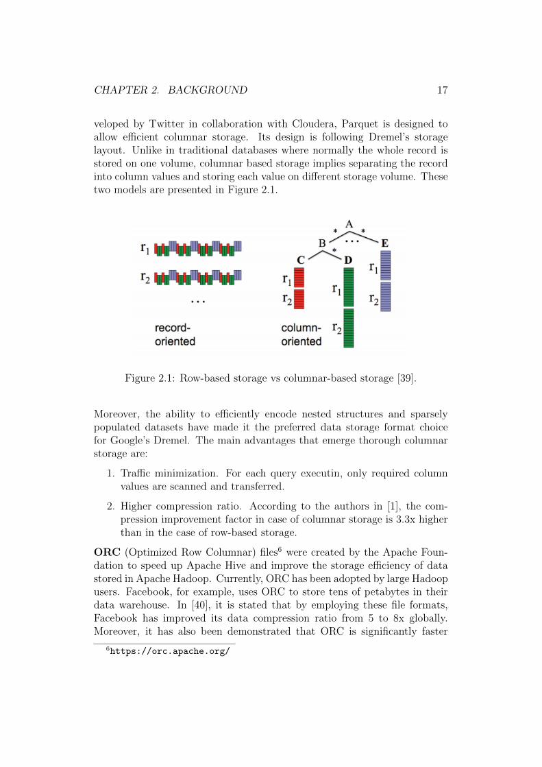
veloped by Twitter in collaboration with Cloudera, Parquet is designed toallow efficient columnar storage. Its design is following Dremel’s storagelayout. Unlike in traditional databases where normally the whole record isstored on one volume, columnar based storage implies separating the recordinto column values and storing each value on different storage volume. Thesetwo models are presented in Figure 2.1.

Figure 2.1: Row-based storage vs columnar-based storage [39].

Moreover, the ability to efficiently encode nested structures and sparselypopulated datasets have made it the preferred data storage format choicefor Google’s Dremel. The main advantages that emerge thorough columnarstorage are:

1. Traffic minimization. For each query executin, only required columnvalues are scanned and transferred.

2. Higher compression ratio. According to the authors in [1], the com-pression improvement factor in case of columnar storage is 3.3x higherthan in the case of row-based storage.

ORC (Optimized Row Columnar) files6 were created by the Apache Foun-dation to speed up Apache Hive and improve the storage efficiency of datastored in Apache Hadoop. Currently, ORC has been adopted by large Hadoopusers. Facebook, for example, uses ORC to store tens of petabytes in theirdata warehouse. In [40], it is stated that by employing these file formats,Facebook has improved its data compression ratio from 5 to 8x globally.Moreover, it has also been demonstrated that ORC is significantly faster

6https://orc.apache.org/

CHAPTER 2. BACKGROUND 18

than traditional RC (Row Columnar) or Parquet files [40]. These resultscome in contrast with the experiments conducted by Matti Niemenmaa onsequencing DNA data [33]. The results obtained in his thesis showed thatthe ORC file format does not ensure the fastest execution times. Otherimportant ORC features include:

1. ACID Support. Includes support for atomic, consistent, isolated,durable transactions and snapshot isolation.

2. Built-in Indexes. Jumps to the right row with indexes includingminimum, maximum, and bloom filters for each column.

3. Complex Types. Supports all of Hive’s types including the compoundtypes: structs, lists, maps, and unions.

A performance evaluation benchmark of column-oriented database systems[40] on the 200GB TCP-DS has shown that ORC provides a data compressionratio of up to 3.4x, whereas Parquet is limited to 2.8x.

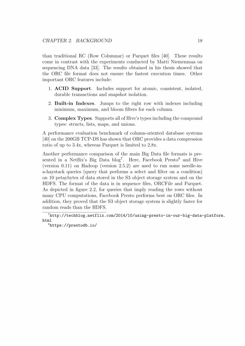
Another performance comparison of the main Big Data file formats is pre-sented in a Netflix’s Big Data blog7. Here, Facebook Presto8 and Hive(version 0.11) on Hadoop (version 2.5.2) are used to run some needle-in-a-haystack queries (query that performs a select and filter on a condition)on 10 petaybytes of data stored in the S3 object storage system and on theHDFS. The format of the data is in sequence files, ORCFile and Parquet.As depicted in figure 2.2, for queries that imply reading the rows withoutmany CPU computations, Facebook Presto performs best on ORC files. Inaddition, they proved that the S3 object storage system is slightly faster forrandom reads than the HDFS.

7http://techblog.netflix.com/2014/10/using-presto-in-our-big-data-platform.html

8https://prestodb.io/

CHAPTER 2. BACKGROUND 19

Figure 2.2: Presto read performance for different file formats.7

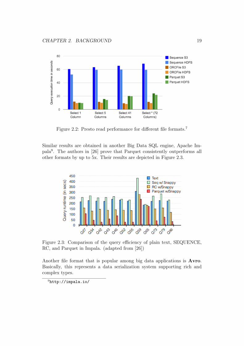
Similar results are obtained in another Big Data SQL engine, Apache Im-pala9. The authors in [26] prove that Parquet consistently outperforms allother formats by up to 5x. Their results are depicted in Figure 2.3.

Figure 2.3: Comparison of the query efficiency of plain text, SEQUENCE,RC, and Parquet in Impala. (adapted from [26])

Another file format that is popular among big data applications is Avro.Basically, this represents a data serialization system supporting rich andcomplex types.

9http://impala.io/

CHAPTER 2. BACKGROUND 20

2.3 Big Data SQL Frameworks

During the last couple of years, several new frameworks have been developedwhich allow to execute SQL like queries on large datasets. Initially, theframeworks used to rely on Map-Reduce algorithm to do the actual work.Nowadays, several new data abstractions have been devised such as Dremel[32] and Resilient Distributed Datasets [49] which are especially targeted forinteractive usage and in-memory processing.

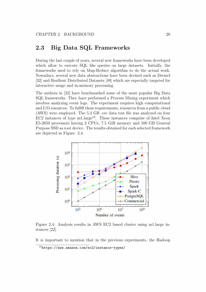
The authors in [22] have benchmarked some of the most popular Big DataSQL frameworks. They have performed a Process Mining experiment whichinvolves analyzing event logs. The experiment requires high computationaland I/O resources. To fulfill these requirements, resources from a public cloud(AWS) were employed. The 5.3 GB .csv data test file was analyzed on fourEC2 instances of type m1.large10. These instances comprise of Intel XeonE5-2650 processors having 2 CPUs, 7.5 GiB memory and 100 GB GeneralPurpose SSD as root device. The results obtained for each selected frameworkare depicted in Figure 2.4.

Figure 2.4: Analysis results in AWS EC2 based cluster using m1.large in-stances [22].

It is important to mention that in the previous experiments, the Hadoop

10https://aws.amazon.com/ec2/instance-types/

CHAPTER 2. BACKGROUND 21

based systems use three way replication, whilst there is no replication forRDBMSs. The obtained results conclude that RDBMS systems (PostgreSQLand the commercial one) are competitive for small data sets. However, theyare overpaced by distributed disk based systems when dealing with massivedata sets.

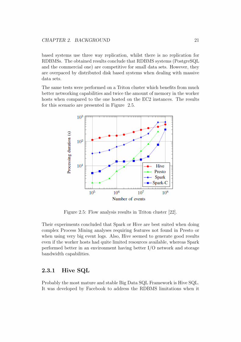
The same tests were performed on a Triton cluster which benefits from muchbetter networking capabilities and twice the amount of memory in the workerhosts when compared to the one hosted on the EC2 instances. The resultsfor this scenario are presented in Figure 2.5.

Figure 2.5: Flow analysis results in Triton cluster [22].

Their experiments concluded that Spark or Hive are best suited when doingcomplex Process Mining analyses requiring features not found in Presto orwhen using very big event logs. Also, Hive seemed to generate good resultseven if the worker hosts had quite limited resources available, whereas Sparkperformed better in an environment having better I/O network and storagebandwidth capabilities.

2.3.1 Hive SQL

Probably the most mature and stable Big Data SQL Framework is Hive SQL.It was developed by Facebook to address the RDBMS limitations when it

CHAPTER 2. BACKGROUND 22

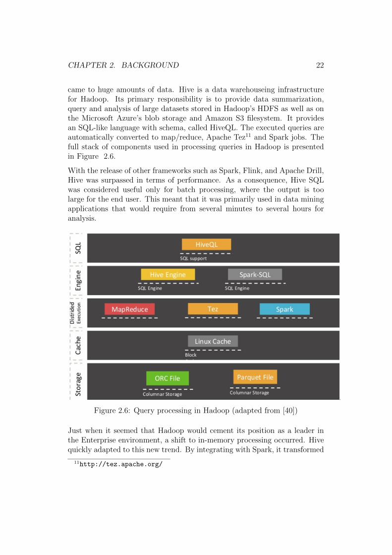
came to huge amounts of data. Hive is a data warehouseing infrastructurefor Hadoop. Its primary responsibility is to provide data summarization,query and analysis of large datasets stored in Hadoop’s HDFS as well as onthe Microsoft Azure’s blob storage and Amazon S3 filesystem. It providesan SQL-like language with schema, called HiveQL. The executed queries areautomatically converted to map/reduce, Apache Tez11 and Spark jobs. Thefull stack of components used in processing queries in Hadoop is presentedin Figure 2.6.

With the release of other frameworks such as Spark, Flink, and Apache Drill,Hive was surpassed in terms of performance. As a consequence, Hive SQLwas considered useful only for batch processing, where the output is toolarge for the end user. This meant that it was primarily used in data miningapplications that would require from several minutes to several hours foranalysis.

Figure 2.6: Query processing in Hadoop (adapted from [40])

Just when it seemed that Hadoop would cement its position as a leader inthe Enterprise environment, a shift to in-memory processing occurred. Hivequickly adapted to this new trend. By integrating with Spark, it transformed

11http://tez.apache.org/

CHAPTER 2. BACKGROUND 23

itself from a batch-only, high-latency system into a modern SQL engine capa-ble of both batch and interactive queries over large datasets. The authors in[40] have shown that by moving past map / reduce, and by mixing columnarstorage with a vectorized SQL engine and by applying distributed execution(Tez), Hive became 100x faster. In a performance evaluation benchmarkon the 200GB TCP-DS, Hive on Tez performed 77% faster than Hive onSpark and 10% faster than Spark SQL. A similar test was conducted on30TB TCP-DS. Here, Hive on Tez outperformed Spark SQL by 18x. Theconducted experiments have shown that Hive is CPU bound, while Sparkconsumes more CPU, Disk, Network IO. Moreover, Hive on Spark spendstoo much time translating from RDDs to Hive’s ”Row Containers”. SparkSQL was faster than Hive on Tez and Hive on Spark only in the case of MapJoins.

For future improvements and releases of Hive, the focus is on creating a betterintegration with Spark as a distributed computing engine and developing anLLAP system, responsible for persisting server cache vectors and startingqueries instantly.

2.3.2 Spark SQL

The first attempt at building a relational interface on Spark was Shark [48].At that time, Shark was a modified version of Apache Hive which imple-mented RDBMS optimizations, such as columnar processing, over the Sparkengine. Shark was limited in various aspects, such as it could query externaldata stored only in the Hive catalog making it useless for relational querieson data which resides inside a Spark program. Moreover, the Hive optimizerwas tailored for MapReduce and difficult to extend [48], making it hard tointegrate new features such as data types for machine learning or support fornew data sources.

One of the main features of Spark are its ability to run programs both inmemory and on disk. Built on the earlier SQL-on-Spark, called Shark, SparkSQL is a schema-free SQL Query Engine. It is schema free because it lever-ages advanced query compilation and re-compilation techniques to maximizeperformance without requiring up-front schema knowledge. Spark SQL of-fers users the possibility to intermix relational and procedural processing,through a declarative DataFrame API that integrates with procedural Sparkcode.

In most cases, DataFrames are considered to be more efficient than Spark’s

CHAPTER 2. BACKGROUND 24

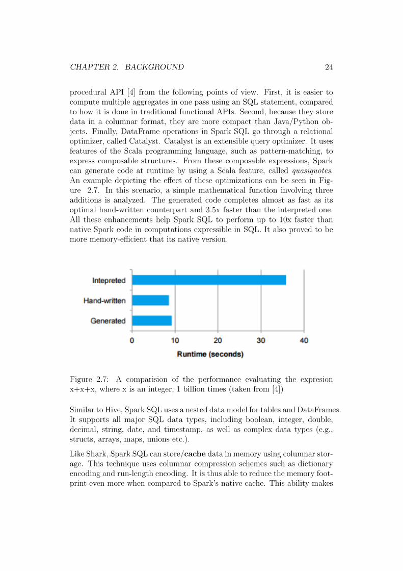
procedural API [4] from the following points of view. First, it is easier tocompute multiple aggregates in one pass using an SQL statement, comparedto how it is done in traditional functional APIs. Second, because they storedata in a columnar format, they are more compact than Java/Python ob-jects. Finally, DataFrame operations in Spark SQL go through a relationaloptimizer, called Catalyst. Catalyst is an extensible query optimizer. It usesfeatures of the Scala programming language, such as pattern-matching, toexpress composable structures. From these composable expressions, Sparkcan generate code at runtime by using a Scala feature, called quasiquotes.An example depicting the effect of these optimizations can be seen in Fig-ure 2.7. In this scenario, a simple mathematical function involving threeadditions is analyzed. The generated code completes almost as fast as itsoptimal hand-written counterpart and 3.5x faster than the interpreted one.All these enhancements help Spark SQL to perform up to 10x faster thannative Spark code in computations expressible in SQL. It also proved to bemore memory-efficient that its native version.

Figure 2.7: A comparision of the performance evaluating the expresionx+x+x, where x is an integer, 1 billion times (taken from [4])

Similar to Hive, Spark SQL uses a nested data model for tables and DataFrames.It supports all major SQL data types, including boolean, integer, double,decimal, string, date, and timestamp, as well as complex data types (e.g.,structs, arrays, maps, unions etc.).

Like Shark, Spark SQL can store/cache data in memory using columnar stor-age. This technique uses columnar compression schemes such as dictionaryencoding and run-length encoding. It is thus able to reduce the memory foot-print even more when compared to Spark’s native cache. This ability makes

CHAPTER 2. BACKGROUND 25

it useful for applications counting on interactive queries. These applicationscomprise of iterative algorithms common in machine learning.

In order to address the Big Data challenges, three features were added toSpark SQL. One of these challenges refers to the veracity of the data, whichcomes in many forms and is mostly unstructured. Spark SQL solves this byincluding a schema inference algorithm for JSON and other semi-structureddata that allows users to query the data right away. Another problem comesfrom the need of deeper analytics (operations that are more complex thansimple aggregations and joins). This issue is tackled by integrating SparkSQL into a new high-level API for Spark’s machine learning library [47]. Lastbut not least, Spark SQL allows a single program query disparate sources, atechnique known as query federation.

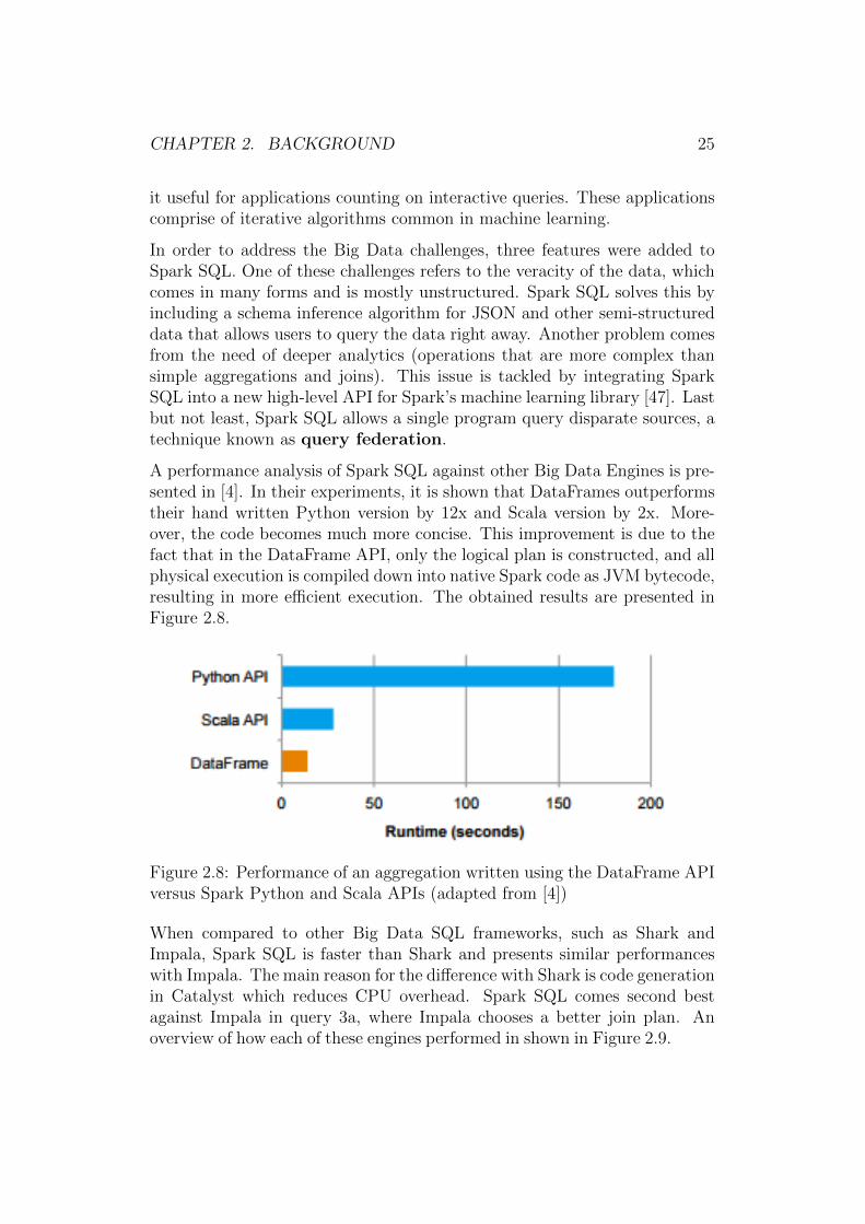
A performance analysis of Spark SQL against other Big Data Engines is pre-sented in [4]. In their experiments, it is shown that DataFrames outperformstheir hand written Python version by 12x and Scala version by 2x. More-over, the code becomes much more concise. This improvement is due to thefact that in the DataFrame API, only the logical plan is constructed, and allphysical execution is compiled down into native Spark code as JVM bytecode,resulting in more efficient execution. The obtained results are presented inFigure 2.8.

Figure 2.8: Performance of an aggregation written using the DataFrame APIversus Spark Python and Scala APIs (adapted from [4])

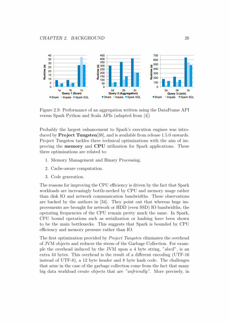
When compared to other Big Data SQL frameworks, such as Shark andImpala, Spark SQL is faster than Shark and presents similar performanceswith Impala. The main reason for the difference with Shark is code generationin Catalyst which reduces CPU overhead. Spark SQL comes second bestagainst Impala in query 3a, where Impala chooses a better join plan. Anoverview of how each of these engines performed in shown in Figure 2.9.

CHAPTER 2. BACKGROUND 26

Figure 2.9: Performance of an aggregation written using the DataFrame APIversus Spark Python and Scala APIs (adapted from [4])

Probably the largest enhancement to Spark’s execution engines was intro-duced by Project Tungsten[38], and is available from release 1.5.0 onwards.Project Tungsten tackles three technical optimizations with the aim of im-proving the memory and CPU utilization for Spark applications. Thesethree optimizations are related to:

1. Memory Management and Binary Processing.

2. Cache-aware computation.

3. Code generation.

The reasons for improving the CPU efficiency is driven by the fact that Sparkworkloads are increasingly bottle-necked by CPU and memory usage ratherthan disk IO and network communication bandwidths. These observationsare backed by the authors in [34]. They point out that whereas huge im-provements are brought for network or HDD (even SSD) IO bandwidths, theoperating frequencies of the CPU remain pretty much the same. In Spark,CPU bound operations such as serialization or hashing have been shownto be the main bottlenecks. This suggests that Spark is bounded by CPUefficiency and memory pressure rather than IO.

The first optimization provided by Project Tungsten eliminates the overheadof JVM objects and reduces the stress of the Garbage Collection. For exam-ple the overhead induced by the JVM upon a 4 byte string, ”abcd”, is anextra 44 bytes. This overhead is the result of a different encoding (UTF-16instead of UTF-8), a 12 byte header and 8 byte hash code. The challengesthat arise in the case of the garbage collection come from the fact that manybig data workload create objects that are ”unfriendly”. More precisely, in

CHAPTER 2. BACKGROUND 27

order for the Garbage Collector to efficiently operate, it needs to reliablyestimate the life cycle of objects. This, in turn, would involve the hassle toparametrize the JVM with more information about the life cycle of objects.Both these two problems are tackled by a memory manager that allows Sparkoperations to run directly against binary data rather than Java objects. Thememory manager makes use of unsafe methods in order to manipulate mem-ory without safety checks and to build data structures in on or off heapmemory.

The second optimization relies on algorithms and data structures to exploitthe memory hierarchy. The goal here is to improve the data processingspeed through a more effective use of L1/L2/L3 CPU caches, which areorders of magnitude faster than the main memory. Last but not least, thefinal optimization reduces the boxing of primitive data types and avoidsexpensive polymorphic function calls. More precisely, in order to eliminatethese overflows, the generic evaluation of logical expressions on the JVM isreplaced with generated custom bytecode. This custom code is generatedwith the Janino12 compiler in order to further reduce the code generationtime.

Although these three directions for performance improvement have alreadybeen tackled, Project Tungsten plans to further add on to these by investi-gating the compilation to LLVM or OpenCL. This should help leverage theSSE/SIMD instructions of modern CPUs and the high parallelism offeredby GPUs to speed up applications relying on machine learning and graphcomputations.

2.3.3 Apache Drill

Similar to Spark SQL, Apache Drill provides a schema-free SQL Query En-gine for Hadoop, NoSQL and Cloud Storage systems. It basically helpsdevelopers avoid the hassle of loading the data, creating and maintainingschemes, or transform the data before it can be processed. Just like in Face-book Presto or Spark SQL, in Drill one only has to include the path to thedata repository in the SQL query.

A single Drill query can join data from sources such as HBase, MongoDB,MapR-DB, HDFS, MapR-FS, Amazon S3, Azure Blob Storage, Google CloudStorage, Swift, NAS or even local files. These data sources can contains com-plex / nested data structures. Drill’s query engine features an in-memory

12http://unkrig.de/w/Janino

CHAPTER 2. BACKGROUND 28

shredded columnar representation for complex data, thus allowing it to suc-cessfully parse such structures at a columnar speed. Drill’s internal pro-cessing capabilities leverage advanced runtime query compilation throughautomatically restructured query plans, thus maximizing the performancewithout requiring upfront schema knowledge.

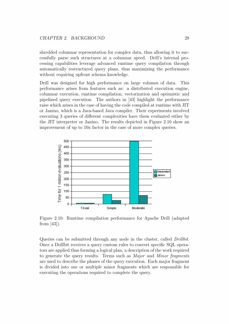
Drill was designed for high performance on large volumes of data. Thisperformance arises from features such as: a distributed execution engine,columnar execution, runtime compilation, vectorization and optimistic andpipelined query execution. The authors in [43] highlight the performanceraise which arises in the case of having the code compiled at runtime with JITor Janino, which is a Java-based Java compiler. Their experiments involvedexecuting 3 queries of different complexities have them evaluated either bythe JIT interpreter or Janino. The results depicted in Figure 2.10 show animprovement of up to 10x factor in the case of more complex queries.

Figure 2.10: Runtime compilation performance for Apache Drill (adaptedfrom [43]).

Queries can be submitted through any node in the cluster, called Drillbit.Once a Drillbit receives a query custom rules to convert specific SQL opera-tors are applied thus forming a logical plan, a description of the work requiredto generate the query results. Terms such as Major and Minor fragmentsare used to describe the phases of the query execution. Each major fragmentis divided into one or multiple minor fragments which are responsible forexecuting the operations required to complete the query.

CHAPTER 2. BACKGROUND 29

Vectorization allows Drill to operate on more than one record at a time. Thespeedup that comes with this is due to modern chip technology that makesuse of heavily pipelined CPU designs. Moreover, logic vectorization avoidCPU branching thus speeding the CPU pipeline.

2.3.4 Facebook Presto

Similar to the previous frameworks, Presto is a SQL query engine for runninginteractive analytic queries. It has been strongly popularized by Facebookdue to is speed performance which is in the range of commercial data ware-houses and massive scaling. Presto allows querying data stored on differ-ent systems, such as Hive, Cassandra, relational databases or even propri-etary data stores. It differentiates itself from Spark by running in memoryonly.

When executing a query, Presto translates it into a pipeline execution ratherthan a MapReduce workload. It uses memory much more aggressively thanHive, keeping the intermediate data in memory, rather than using disk. How-ever, Hive is still necessary for some operations, like loading data in.

One of the first benchmarkings that included Presto alongside other Big DataSQL engines was developed by Qubole13, a company specializing in acceleratecloud-scale data processing. Their technical report14 on this matter involvesexecuting a set of six queries on a 75GB set of data stored in a RCFileformat. The queries were run on two clusters, one with Hive and anotherone with Presto, each comprising of 10 m1.large instances hosted by Amazon.Because at the time they were conducting the experiments, Presto did notdo join ordering, the queries had to be rewritten so as to impose a ”good”join order. Their results show a speedup between 2x and 7.5x in favour ofPresto for that set of queries. However, although Presto is faster, it requiredrewriting the queries with the right join order. Had the queries not beenrewritten, the performance might have been drastically reduced as a badjoin order could have slowed down a query while creating the hash table onthe bigger table. Moreover, if the bigger table does not fit in memory, out ofmemory exceptions will been thrown. Last but not least, the authors of thereport, propose to remake the experiments against ORC files, and suggestthat improvements shall arise from an optimizer that is expected to producebetter query plans.

13https://www.qubole.com/14https://www.qubole.com/blog/product/presto-performance/

CHAPTER 2. BACKGROUND 30

A software blog post15 on Big Data that compares Presto against Hive ispresented by Facebook. The underlying hardware used for the experimentscarried out here comprises of a 14-machine cluster, each containing:

1. CPU : Dual 8-core Intel Xeon CPU (32 Hyper-Threads), E5-2660 @2.20GHz

2. Memory : 64 GB

3. Disk : 15 x 3 TB (JBOD configuration)

4. Network : 10 gigabit with full bandwidth between machines

The experiments highlight the performance improvement factor (in favour ofPresto) that emerge when storing data in ORC format. This improvement ismainly attributed to the release of three new features: predicate pushdown,columnar reads and lazy reads. In ORC, the minimum and maximum valuesof each column are recorded per file, per stripe (approximately every 1Mrows), and every 10,000 rows. Similar with Hive ORC reader, which hasSearchArgument to filter segments, Presto’s reader can now skip any segmentthat could not possibly match the query predicate. The results obtained aresimilar with the ones obtained by the researchers from Qubole. However,in the case of queries that can take advantage of lazy reads and predicatepushdown, the speedups varies from 18x to 80x, respectively. However, thisspeedup was considered unfair, due to lack of support for those features inthe built-in Hive reader. Another experiment presented in this paper targetsthe speedup in case of using ORC files against RC binary files. They startby first defining the wall time as the speedup in end-to-end query latency.Next, through the carried experiments, they show an improvement in boththe wall time and the CPU time. More precisely, a 2-4x wall time and CPUtime speedup over the RCFile-binary reader is found when employing ORCfile formats. Last but not least, the last set of experiments described in theblog post compares the performance difference of running Presto with ORCfiles against Apache Impala with the data stored in Parquet format. Here,a wall time speedup (and comparable CPU time) between 1.3x to 5.8x overImpala are identified in favour of Presto.

In the light of all these features, Facebook Presto has become widely used bybig multinational companies for their big data processing, such as AirBnb16,DropBox17 and Netflix18. In the case of the latter, Presto became the main

15https://code.facebook.com/posts/faster-data-speed-of-presto-orc/16https://www.airbnb.com/17https://www.dropbox.com/18https://www.netflix.com/

CHAPTER 2. BACKGROUND 31

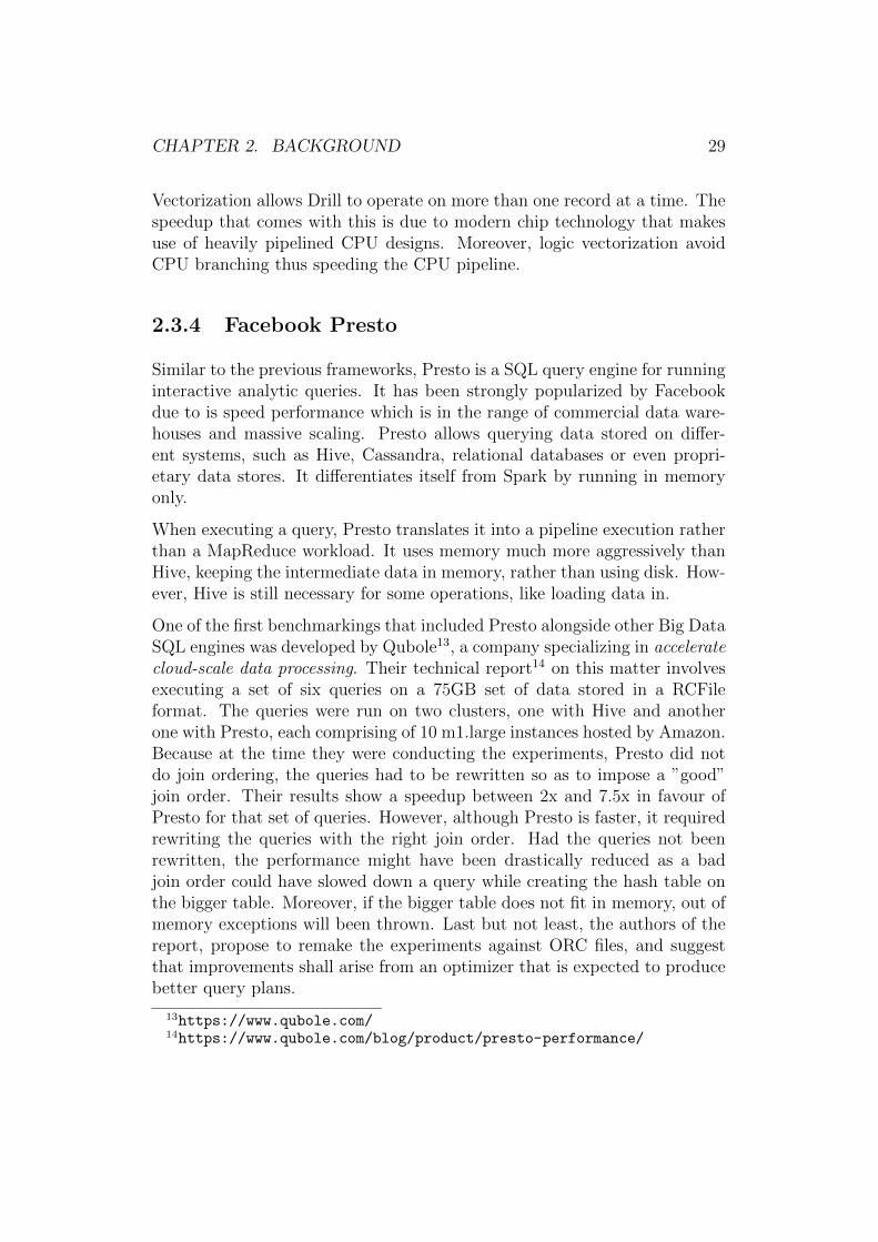
choice when looking for an wanted an open source project that could handleand scale their data and processing needs. Moreover, it benefited from agreat integration with the Hive metastore, and provided an easy way tointegrate with their data warehouse hosted on Amazon’s S3 storage service.The report created by the Big Data Platform Team at Netflix presents theirexperiments conducted on Presto and Hive, the resulted benchmarks andtheir contributions to the Facebook’s Big Data SQL engine. The experimentsinvolved querying a 10 petabyte data warehouse on S3 with 40 m2.4xlargeEC2 worker instances. The data queries was in Parquet format, and eachquery processed the same data set with varying data sizes between 140GB to210GB depending on the file format. In addition, due to performance reasons,only RAM memory is used and no disk. The results obtained through theirexperiments are depicted in Figure 2.11.

Figure 2.11: Presto vs. Hive performance.19

Basically, the experiments have shown that the queries ran in Presto benefitfrom a speedup varying from 10x to 100x then when executed by Hive. Thespeedup in Presto grows linearly, i.e. directly proportional with the numberof MR jobs involved. Among the the contributions brought by the Big DataPlatform Team from Netflix to the Presto open source project, probablythe most important and vital to their success, was creating the integrationbetween the SQL engine and the S3 object storage system..

19http://techblog.netflix.com/using-presto-in-our-big-data-platform.html

CHAPTER 2. BACKGROUND 32

2.3.5 Apache Impala

Part of the Apache Incubator, Impala is an open source, native analyticdatabase for Apache Hadoop. Unlike Apache Hive, which is a batch frame-work, Impala is a query engine designed for performance, real time, lowlatency and high concurrency processing. With Impala, one can query datastored in HDFS or Apache HBase by employing the same SQL or HiveQLsintax.

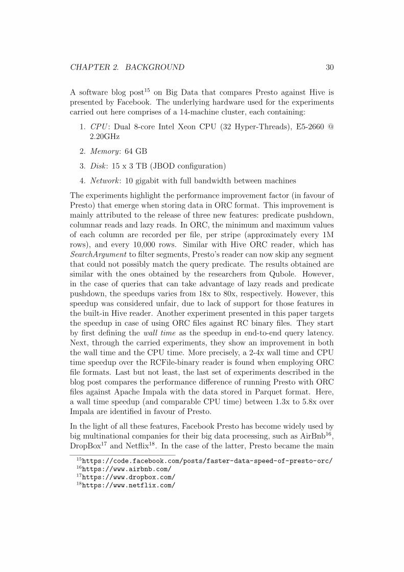
Impala differs itself from Hive through a specialized distributed query enginethat can directly access the data. Although it runs directly in Hadoop, dueto its sql engine, it can bypass the MapReduce paradigm. According to theauthors in [26], Impala is suitable for performing analytics workloads and run-ning thousands of concurrent queries. It is also stated as being able to scalelinearly, i.e., the time for performing the same amount of work decreasingdirectly proportional with each new node that is added to the system. Thearchitecture of the system presented in [26] depicts the reasons for the highperformance obtained by Impala. More precisely, Impala’s backend, writtenentirely in C++, acts a as MPP (Masively Parallel Processing) Query Engineand is responsible for runtime code generation using LLVM IR20. Throughthis technique efficient codepaths (with respect to instruction count) andsmall memory overhead are produced. The impact on the performance whenemploying this technique is depicted in Figure 2.12.

Figure 2.12: Impact in performance of run-time code generation in Impala(adapted from [26]).

From a user perspective, each node with data runs an Impala Daemon and

20low-level programming language, similar to assembly

CHAPTER 2. BACKGROUND 33

can accept queries. Queries are distributed towards the nodes with relevantdata. Impala supports the following file formats: Parquet, RCFile, Avro,Sequence and Text (e.g. .csv). It also supports Snappy, GZIP, BZIP2 andLZO compressions. Despite adopting the SQL-92 revision, due to the limita-tions of HDFS as a storage manager, Impala does not support UPDATE orDELETE statements. Emerging issues could however be bypassed throughbulk insertions (e.g., INSERT INTO ... SELECT ..).

An Impala deployment comprises of three services. The first one is a daemonthat runs as a distributed service and is responsible for receiving, orchestrat-ing and executing user queries. Impala daemons have a symmetric characterin the sense that they can act in all roles, thus improving the fault-toleranceand load-balancing of the system. The second service is called ”statestoredaemon” and represents a central system state repository. It contains Meta-data about the nodes and the data to be processed and periodically sendshearbeats to check for liveness or push new data. Finally, the last service, thecatalog daemon stores metadata about the hive metastore and the HDFS.The catalog daemon automatically propagates changes and is able to performatomic updates.

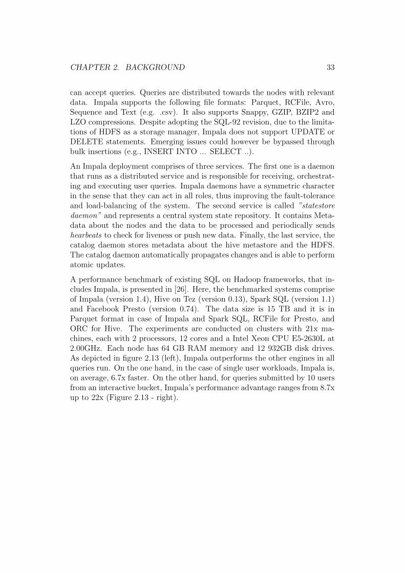
A performance benchmark of existing SQL on Hadoop frameworks, that in-cludes Impala, is presented in [26]. Here, the benchmarked systems compriseof Impala (version 1.4), Hive on Tez (version 0.13), Spark SQL (version 1.1)and Facebook Presto (version 0.74). The data size is 15 TB and it is inParquet format in case of Impala and Spark SQL, RCFile for Presto, andORC for Hive. The experiments are conducted on clusters with 21x ma-chines, each with 2 processors, 12 cores and a Intel Xeon CPU E5-2630L at2.00GHz. Each node has 64 GB RAM memory and 12 932GB disk drives.As depicted in figure 2.13 (left), Impala outperforms the other engines in allqueries run. On the one hand, in the case of single user workloads, Impala is,on average, 6.7x faster. On the other hand, for queries submitted by 10 usersfrom an interactive bucket, Impala’s performance advantage ranges from 8.7xup to 22x (Figure 2.13 - right).

CHAPTER 2. BACKGROUND 34

((a)) Single user workloads ((b)) Multi user workloads

Figure 2.13: Comparison of query response times for on single and multi userruns (adapted from [26]).

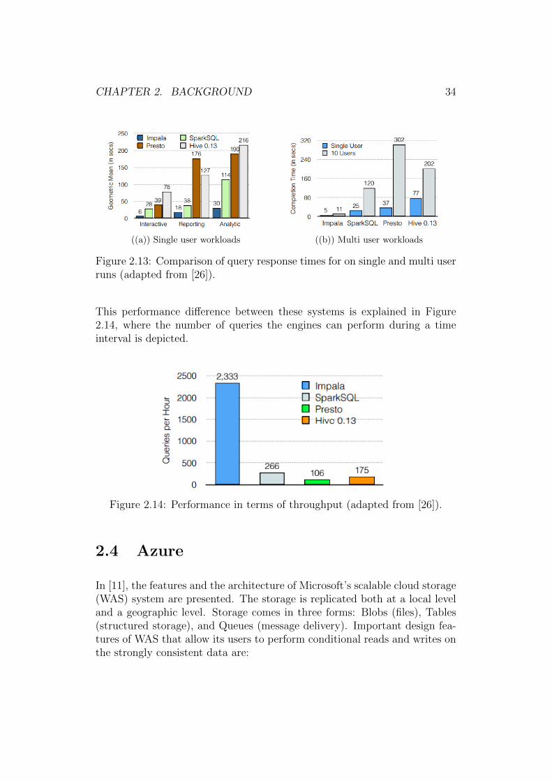
This performance difference between these systems is explained in Figure2.14, where the number of queries the engines can perform during a timeinterval is depicted.

Figure 2.14: Performance in terms of throughput (adapted from [26]).

2.4 Azure

In [11], the features and the architecture of Microsoft’s scalable cloud storage(WAS) system are presented. The storage is replicated both at a local leveland a geographic level. Storage comes in three forms: Blobs (files), Tables(structured storage), and Queues (message delivery). Important design fea-tures of WAS that allow its users to perform conditional reads and writes onthe strongly consistent data are:

CHAPTER 2. BACKGROUND 35

1. Strong Consistency. This is achieved by satisfying three proper-ties that are difficult to achieve at the same time, as claimed by theCAP theorem [10]: strong consistency, high availability, and partitiontolerance.

2. Global and Scalable Namespace/Storage. Stored data can beaccessed in a consistent manner from any location in the world due toa global namespace.

3. Disaster Recovery. By storing the data across multiple data cen-ters, WAS provides protection against hazards such as earthquakes,tornadoes, nuclear reactor meltdown, etc.

4. Multi-tenancy and Cost of Storage. By serving multiple customersfrom the same shared storage infrastructure, the total storage cost isreduced.

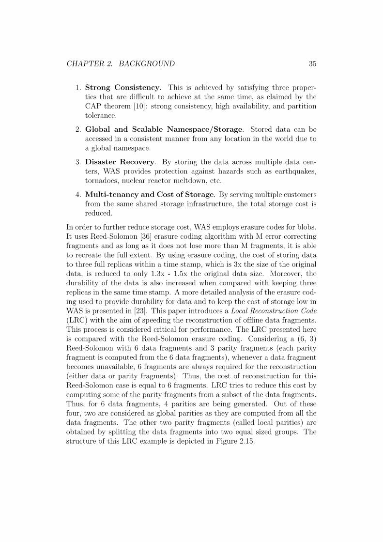
In order to further reduce storage cost, WAS employs erasure codes for blobs.It uses Reed-Solomon [36] erasure coding algorithm with M error correctingfragments and as long as it does not lose more than M fragments, it is ableto recreate the full extent. By using erasure coding, the cost of storing datato three full replicas within a time stamp, which is 3x the size of the originaldata, is reduced to only 1.3x - 1.5x the original data size. Moreover, thedurability of the data is also increased when compared with keeping threereplicas in the same time stamp. A more detailed analysis of the erasure cod-ing used to provide durability for data and to keep the cost of storage low inWAS is presented in [23]. This paper introduces a Local Reconstruction Code(LRC) with the aim of speeding the reconstruction of offline data fragments.This process is considered critical for performance. The LRC presented hereis compared with the Reed-Solomon erasure coding. Considering a (6, 3)Reed-Solomon with 6 data fragments and 3 parity fragments (each parityfragment is computed from the 6 data fragments), whenever a data fragmentbecomes unavailable, 6 fragments are always required for the reconstruction(either data or parity fragments). Thus, the cost of reconstruction for thisReed-Solomon case is equal to 6 fragments. LRC tries to reduce this cost bycomputing some of the parity fragments from a subset of the data fragments.Thus, for 6 data fragments, 4 parities are being generated. Out of thesefour, two are considered as global parities as they are computed from all thedata fragments. The other two parity fragments (called local parities) areobtained by splitting the data fragments into two equal sized groups. Thestructure of this LRC example is depicted in Figure 2.15.

CHAPTER 2. BACKGROUND 36

Figure 2.15: A (6, 2, 2) LRC Example. (k = 6 data fragments, l = 2 localparities and r = 2 global parities.) (taken from [23])

Next, they compared LRC (12, 2, 2) with Reed-Solomon (12, 4). Althoughboth codes present the same storage overhead (of 1.33x), LRC decreseasesmore the number of I/O operations and bandwidth during reconstruction.The experiments have concluded the fact that for small (4KB) I/O recon-structions, the latency induced by LRC is around 91 ms, whereas for Reed-Solomon averages 305 ms. In the case of large (4MB) I/O reconstructions,the latency induced by Reed-Solomon is 9 times higher than the one inducedby LRC (893 ms versus 99 ms).

Azure blobs can store structured or unstructured data. It is a general-purpose storage solution which can integrate with different cloud servicessuch as virtual machines, containers and other PaaS services. Azure blobsreside in storage accounts21, which are of 2 types:

1. Standard storage accounts. These are suitable for applications thatrequire bulk storage or where data is accessed infrequently. They arebacked by magnetic drives and provide the lowest cost per GB.

2. Premium storage accounts. These are suitable for I/O-intensiveapplications. They are backed by SSDs, thus providing low-latencyperformance. Here, the data is replicated 3 times, but within the sameregion. It is thus impossible to enable Read-Access Geo-RedundantStorage (RAGRS) on this storage.

21https://azure.microsoft.com/en-us/documentation/articles/storage-introduction

CHAPTER 2. BACKGROUND 37

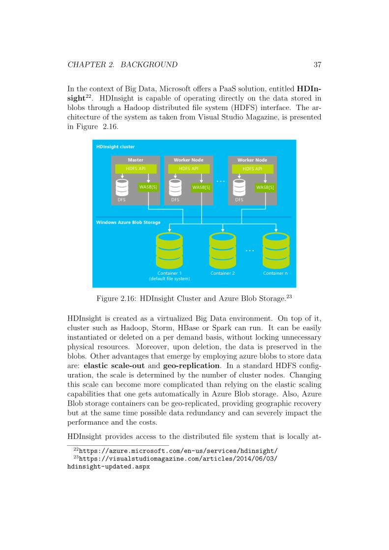
In the context of Big Data, Microsoft offers a PaaS solution, entitled HDIn-sight22. HDInsight is capable of operating directly on the data stored inblobs through a Hadoop distributed file system (HDFS) interface. The ar-chitecture of the system as taken from Visual Studio Magazine, is presentedin Figure 2.16.

Figure 2.16: HDInsight Cluster and Azure Blob Storage.23

HDInsight is created as a virtualized Big Data environment. On top of it,cluster such as Hadoop, Storm, HBase or Spark can run. It can be easilyinstantiated or deleted on a per demand basis, without locking unnecessaryphysical resources. Moreover, upon deletion, the data is preserved in theblobs. Other advantages that emerge by employing azure blobs to store dataare: elastic scale-out and geo-replication. In a standard HDFS config-uration, the scale is determined by the number of cluster nodes. Changingthis scale can become more complicated than relying on the elastic scalingcapabilities that one gets automatically in Azure Blob storage. Also, AzureBlob storage containers can be geo-replicated, providing geographic recoverybut at the same time possible data redundancy and can severely impact theperformance and the costs.

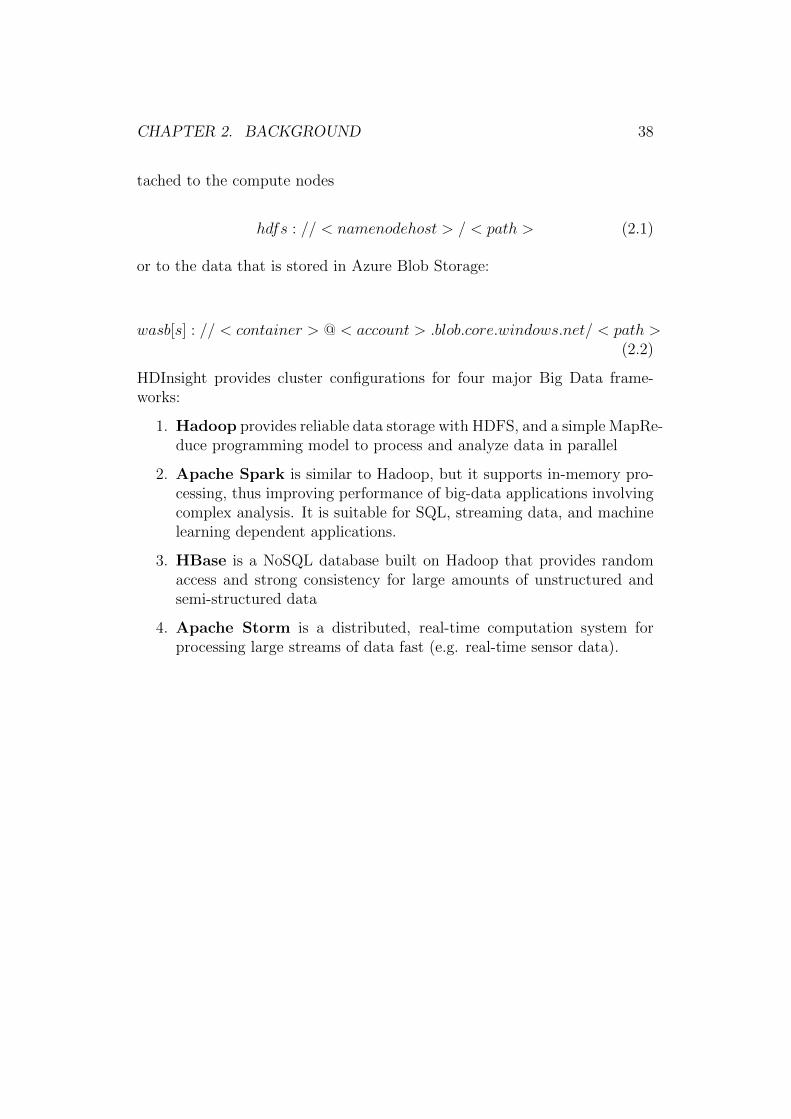
HDInsight provides access to the distributed file system that is locally at-

22https://azure.microsoft.com/en-us/services/hdinsight/23https://visualstudiomagazine.com/articles/2014/06/03/

hdinsight-updated.aspx

CHAPTER 2. BACKGROUND 38

tached to the compute nodes

hdfs : // < namenodehost > / < path > (2.1)

or to the data that is stored in Azure Blob Storage:

wasb[s] : // < container > @ < account > .blob.core.windows.net/ < path >(2.2)

HDInsight provides cluster configurations for four major Big Data frame-works:

1. Hadoop provides reliable data storage with HDFS, and a simple MapRe-duce programming model to process and analyze data in parallel

2. Apache Spark is similar to Hadoop, but it supports in-memory pro-cessing, thus improving performance of big-data applications involvingcomplex analysis. It is suitable for SQL, streaming data, and machinelearning dependent applications.

3. HBase is a NoSQL database built on Hadoop that provides randomaccess and strong consistency for large amounts of unstructured andsemi-structured data

4. Apache Storm is a distributed, real-time computation system forprocessing large streams of data fast (e.g. real-time sensor data).

Chapter 3

Technical contributions

This chapter lies the foundation for the conducted experiments. It presentsthe underlying systems and environment enhancements that were configuredor added to in order to successfully run the experiments from Chapter 4.This chapter is divided into two subsections: Section 3.1 deals with the BigData options from a PaaS perspective, whereas Section 3.2 tackles them froma SaaS point of view.

All the experiments were conducted on Microsoft’s and Google’s public cloudoffering, Azure and Google Cloud Platform respectively. In the case of Azure,the experiments were based on the PaaS Big Data solution, HDInsight withSpark (currently in preview) or the PaaS offered by Cloudera Enterprise DataHub1. Experiments were also run against Microsoft and Google’s Big DataSaaS solutions.

3.1 Big Data SQL frameworks - Platform as

a Service

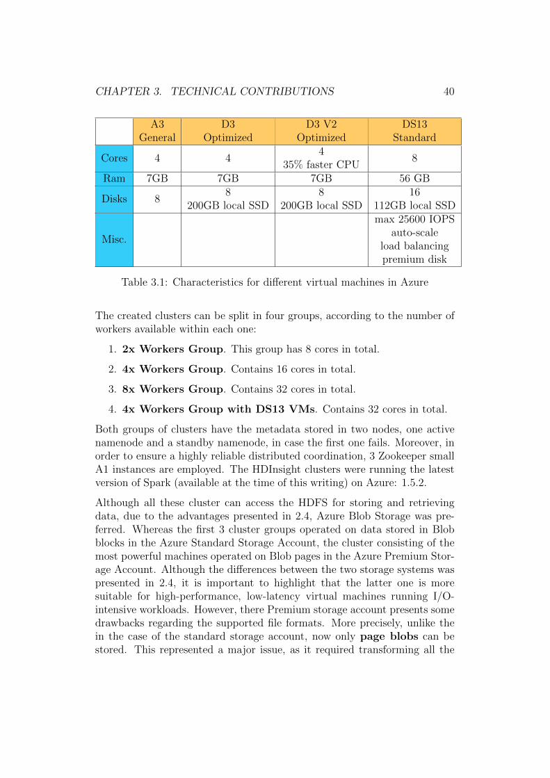
The created clusters were based on virtual resources, consisting of A3, D3, D3V2 and DS13 Standard machines. These can be described via the followingparameters in table 3.1. A more enhanced comparison between the A andD VM family is provided in [30]. The experiments conducted here show thatD VMs benefit from a 58% faster VCPU, 65% more memory bandwidth and6.3x more IOPS.

1https://www.cloudera.com/products.html

39

CHAPTER 3. TECHNICAL CONTRIBUTIONS 40

A3General

D3Optimized

D3 V2Optimized

DS13Standard

Cores 4 44

35% faster CPU8

Ram 7GB 7GB 7GB 56 GB

Disks 88

200GB local SSD8

200GB local SSD16

112GB local SSD

Misc.

max 25600 IOPSauto-scale

load balancingpremium disk

Table 3.1: Characteristics for different virtual machines in Azure

The created clusters can be split in four groups, according to the number ofworkers available within each one:

1. 2x Workers Group. This group has 8 cores in total.

2. 4x Workers Group. Contains 16 cores in total.

3. 8x Workers Group. Contains 32 cores in total.

4. 4x Workers Group with DS13 VMs. Contains 32 cores in total.

Both groups of clusters have the metadata stored in two nodes, one activenamenode and a standby namenode, in case the first one fails. Moreover, inorder to ensure a highly reliable distributed coordination, 3 Zookeeper smallA1 instances are employed. The HDInsight clusters were running the latestversion of Spark (available at the time of this writing) on Azure: 1.5.2.

Although all these cluster can access the HDFS for storing and retrievingdata, due to the advantages presented in 2.4, Azure Blob Storage was pre-ferred. Whereas the first 3 cluster groups operated on data stored in Blobblocks in the Azure Standard Storage Account, the cluster consisting of themost powerful machines operated on Blob pages in the Azure Premium Stor-age Account. Although the differences between the two storage systems waspresented in 2.4, it is important to highlight that the latter one is moresuitable for high-performance, low-latency virtual machines running I/O-intensive workloads. However, there Premium storage account presents somedrawbacks regarding the supported file formats. More precisely, unlike thein the case of the standard storage account, now only page blobs can bestored. This represented a major issue, as it required transforming all the

CHAPTER 3. TECHNICAL CONTRIBUTIONS 41

blob blocks into pages upon transferring the data to the clusters employingDS13 VMs.

The main advantage of these storage systems over HDFS was that uponcluster deletion, the data remains preserved in the blobs. The format of thestored data was Parquet, thus providing efficient columnar storage and ac-cess. The data used in the experiments was made public by HSL, or HelsinkiPublic Transport. It comprised of several hundreds of .csv files, which weremerged together (via a Spark script) into one big Parquet file of 8.4 GB.In order to reach Big Data volumes, this file was further processed (dupli-cated and concatenated) into another Parquet file with a size of 52 GBand of 259 GB. These two final files were used throughout the queries fromChapter 4.

The software stack running on top of the HDInsight Cluster, on which theexperiments were performed, can be divided into 3 groups:

1. Spark SQL.

2. Hive on Tez.

3. Apache Drill.

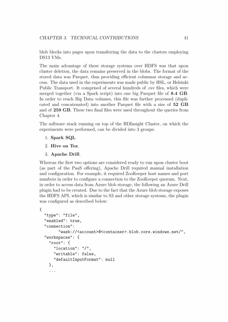
Whereas the first two options are considered ready to run upon cluster boot(as part of the PaaS offering), Apache Drill required manual installationand configuration. For example, it required ZooKeeper host names and portnumbers in order to configure a connection to the ZooKeeper quorum. Next,in order to access data from Azure blob storage, the following an Azure Drillplugin had to be created. Due to the fact that the Azure blob storage exposesthe HDFS API, which is similar to S3 and other storage systems, the pluginwas configured as described below:

{

"type": "file",

"enabled": true,

"connection":

"wasb://<account>@<container>.blob.core.windows.net/",

"workspaces": {

"root": {

"location": "/",

"writable": false,

"defaultInputFormat": null

},

...

CHAPTER 3. TECHNICAL CONTRIBUTIONS 42

}}

In the above code snippet, account name stands for the Azure Storage ac-count, which ensures that the data is preserved upon cluster disposal. con-tainer name is the name of the container hosting our blob files that we wishto access and process.

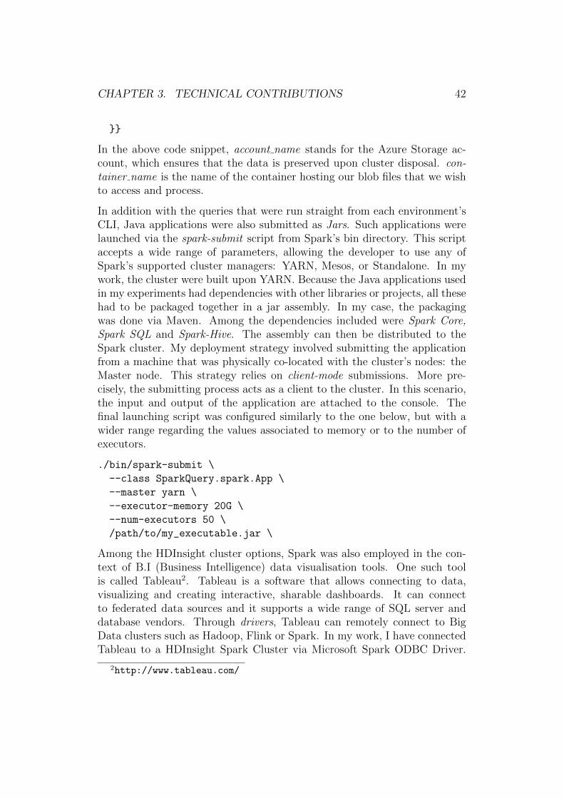
In addition with the queries that were run straight from each environment’sCLI, Java applications were also submitted as Jars. Such applications werelaunched via the spark-submit script from Spark’s bin directory. This scriptaccepts a wide range of parameters, allowing the developer to use any ofSpark’s supported cluster managers: YARN, Mesos, or Standalone. In mywork, the cluster were built upon YARN. Because the Java applications usedin my experiments had dependencies with other libraries or projects, all thesehad to be packaged together in a jar assembly. In my case, the packagingwas done via Maven. Among the dependencies included were Spark Core,Spark SQL and Spark-Hive. The assembly can then be distributed to theSpark cluster. My deployment strategy involved submitting the applicationfrom a machine that was physically co-located with the cluster’s nodes: theMaster node. This strategy relies on client-mode submissions. More pre-cisely, the submitting process acts as a client to the cluster. In this scenario,the input and output of the application are attached to the console. Thefinal launching script was configured similarly to the one below, but with awider range regarding the values associated to memory or to the number ofexecutors.

./bin/spark-submit \

--class SparkQuery.spark.App \

--master yarn \

--executor-memory 20G \

--num-executors 50 \

/path/to/my_executable.jar \

Among the HDInsight cluster options, Spark was also employed in the con-text of B.I (Business Intelligence) data visualisation tools. One such toolis called Tableau2. Tableau is a software that allows connecting to data,visualizing and creating interactive, sharable dashboards. It can connectto federated data sources and it supports a wide range of SQL server anddatabase vendors. Through drivers, Tableau can remotely connect to BigData clusters such as Hadoop, Flink or Spark. In my work, I have connectedTableau to a HDInsight Spark Cluster via Microsoft Spark ODBC Driver.

2http://www.tableau.com/

CHAPTER 3. TECHNICAL CONTRIBUTIONS 43

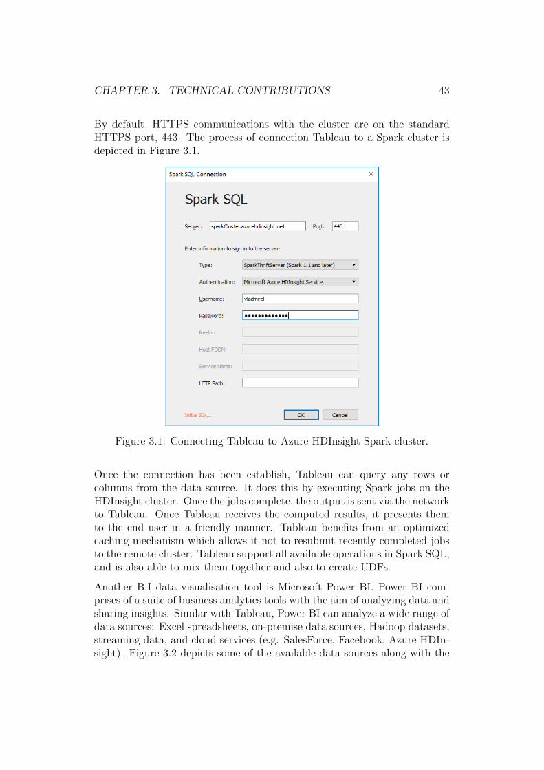
By default, HTTPS communications with the cluster are on the standardHTTPS port, 443. The process of connection Tableau to a Spark cluster isdepicted in Figure 3.1.

Figure 3.1: Connecting Tableau to Azure HDInsight Spark cluster.

Once the connection has been establish, Tableau can query any rows orcolumns from the data source. It does this by executing Spark jobs on theHDInsight cluster. Once the jobs complete, the output is sent via the networkto Tableau. Once Tableau receives the computed results, it presents themto the end user in a friendly manner. Tableau benefits from an optimizedcaching mechanism which allows it not to resubmit recently completed jobsto the remote cluster. Tableau support all available operations in Spark SQL,and is also able to mix them together and also to create UDFs.

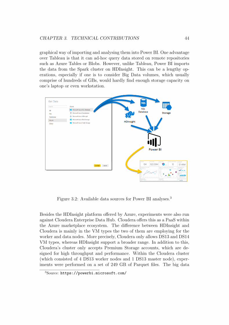
Another B.I data visualisation tool is Microsoft Power BI. Power BI com-prises of a suite of business analytics tools with the aim of analyzing data andsharing insights. Similar with Tableau, Power BI can analyze a wide range ofdata sources: Excel spreadsheets, on-premise data sources, Hadoop datasets,streaming data, and cloud services (e.g. SalesForce, Facebook, Azure HDIn-sight). Figure 3.2 depicts some of the available data sources along with the

CHAPTER 3. TECHNICAL CONTRIBUTIONS 44

graphical way of importing and analysing them into Power BI. One advantageover Tableau is that it can ad-hoc query data stored on remote repositoriessuch as Azure Tables or Blobs. However, unlike Tableau, Power BI importsthe data from the Spark cluster on HDInsight. This can be a lengthy op-erations, especially if one is to consider Big Data volumes, which usuallycomprise of hundreds of GBs, would hardly find enough storage capacity onone’s laptop or even workstation.

Figure 3.2: Available data sources for Power BI analyses.3

Besides the HDInsight platform offered by Azure, experiments were also runagainst Cloudera Enterprise Data Hub. Cloudera offers this as a PaaS withinthe Azure marketplace ecosystem. The difference between HDInsight andCloudera is mainly in the VM types the two of them are employing for theworker and data nodes. More precisely, Cloudera only allows DS13 and DS14VM types, whereas HDInsight support a broader range. In addition to this,Cloudera’s cluster only accepts Premium Storage accounts, which are de-signed for high throughput and performance. Within the Cloudera cluster(which consisted of 4 DS13 worker nodes and 1 DS13 master node), exper-iments were performed on a set of 249 GB of Parquet files. The big data

3Source: https://powerbi.microsoft.com/

CHAPTER 3. TECHNICAL CONTRIBUTIONS 45

frameworks that run the queries were SparkSQL version 1.5.0 and Impalaversion 2.4.0. The 249 GB set of Parquet files was obtained from the pre-vious set of 259 GB. The difference is represented by the files for which themetadata was considered as stale by the Impala engine. These files wereremoved from the hdfs as any queries against the data set would result inwarnings and no output.

3.2 Big Data SQL frameworks - Software as

a Service

Last but not least, experiments were conducted on Microsoft Azure DataLake Analytics4, which is a SaaS for processing big volumes of data with-out the hassle of managing distributed infrastructure, deploying, configuringor tuning hardware. This service allows developers to focus on their queriesto transform data and extract valuable insights. The system can be scaledaccording to developer’s needs and provides a new SQL like language, calledU-SQL. Although Hive queries are expected in the near future, U-SQL postsitself as an impressive language that unifies the benefits of SQL with theexpressive power of user code. It can integrate APIs from .net libraries (i.e.inside queries we can call functions written in one of the languages men-tioned below) and can be intermixed with other programming languages:C#, Java, Python, C++, Nodejs. Azure Data Lake Analytics can run feder-ated queries, performing aggregations or joins on data from different storagesystems such as SQL Servers in Azure, Azure SQL Database and Azure SQLData Warehouse. Another main feature of this service is its affordability andcost effectiveness. By paying only on a per-job basis when data is processed,no hardware, physical or virtual resources, or licenses are required. It mightthus be cheaper to run queries only when needed vs maintaining a cluster24/7. Moreover, the system automatically scales up or down as the job startsand completes, thus charging only for used resources. The data processed bythis engine was in .csv format and accumulated 44.8 GB.

For my experiments I have decided to create a simple console applicationin Visual Studio. The entire code logic was written in U-SQL which I haveintermixed with some C# function calls. Through this IDE, I then usedMicrosoft’s Azure Data Lake plugin for submitting jobs to their cloud infras-tructure. This plugin manages the authentication against Microsoft Azure

4https://azure.microsoft.com/en-us/services/data-lake-analytics/

CHAPTER 3. TECHNICAL CONTRIBUTIONS 46

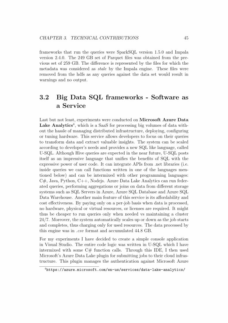
and sets the correct parameters for the job to be run. In my case, I haveset the parallelism level to 4 and 8 workers. Next, via this plugin, a POSTrequest is sent which contains the assembly of the program written by me.Once the request arrives on Microsoft’s servers, it is then processed by AzureData Lake Analytics. This processing involves querying the data stored in-side Azure Data Lake Store. Once all the aggregations have finished, Azuresends the computed output back to client’s console application. The entireflow of actions is depicted in Figure 3.3.

Figure 3.3: Azure Data Lake Analytics action flow.

The same set of experiments were run against Google BigQuery5. Big-Query is Google’s SaaS for querying massive datasets. This services frees thedeveloper from the hassle of installing and maintaining the right hardwareand infrastructure and allows him / her to tap in the full power (or somepart of it as it will be explained soon) of Google’s infrastructure. The un-derlying engine behind BigQuery is Dremel [39]. More precisely, BigQuery

5https://cloud.google.com/bigquery/

CHAPTER 3. TECHNICAL CONTRIBUTIONS 47

provides the core set of features available in Dremel to third party devel-opers via different interfaces: REST API, command line interface Web Uietc. When using BigQuery, there are main three concepts that build up thisservice:

1. Datasets - allow one to organize and control access to his or her ta-bles. At least one dataset has to be created before loading data intoBigQuery.

2. Tables - these are contained in datasets. Each table has a schema thatdescribes field names, types, and other information. External tables aretables defined over data stored in other source (e.g. Cloud Storage).

3. Jobs - these are actions (executed by BigQuery) that involve operationssuch as data loading, exporting, or querying. Since jobs can potentiallytake a long time to complete, they execute asynchronously and can bepolled for their status.

The first step that has to be completed before launching BigQuery jobs is tocreate a dataset. Once a dataset has been created, the next step is to addsome tables to it. Tables can be created in 3 ways:

1. Uploading a local file.

2. Using the files stored in Google Cloud Storage.

3. Using the files stored in Google Drive.

For my experiments, I have uploaded the same 44.8 GB .csv files into aGoogle Cloud Storage bucket. The employed bucket is of type ”Standard”, asit presents the best performance in terms of latency and is the recommendedsolution for storing data that is frequently accessed.

Note: BigQuery can only analyze data that resides within the same GEN-ERAL region as the Dataset. Thus, if your Dataset was created in EU, makesure the bucket also resides in EU, and not somewhere else (like EUROPE-WEST1). More information of the matter can be dug up here6.

Regarding the software development part, I have developed a simple consoleapplication in Visual Studio. The entire code logic was written C#. Thecommunication with Google’s Cloud Platform was done through their C#SDK, which provides a wrapper for some REST interfaces. The SDK exposesAPIs that allow developers to authenticate against GCP, access services suchas BigQuery and perform different tasks on Google’s infrastructure. In order

6https://code.google.com/p/google-bigquery/issues/detail?id=443

CHAPTER 3. TECHNICAL CONTRIBUTIONS 48

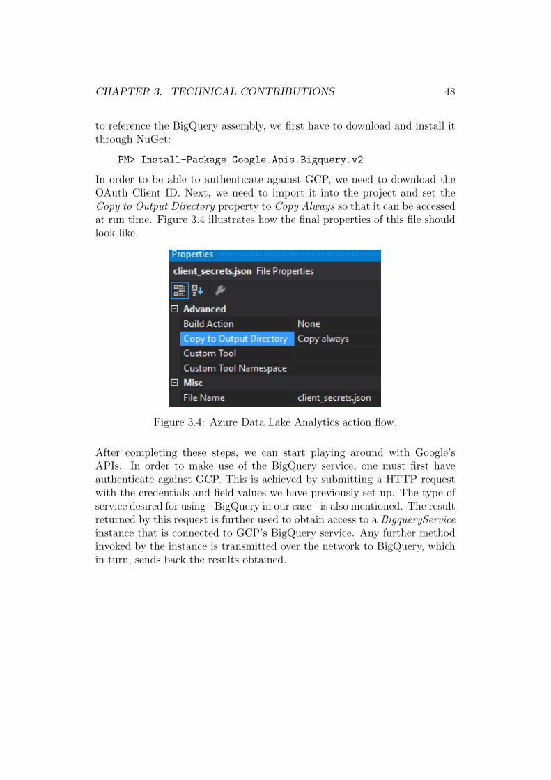
to reference the BigQuery assembly, we first have to download and install itthrough NuGet:

PM> Install-Package Google.Apis.Bigquery.v2

In order to be able to authenticate against GCP, we need to download theOAuth Client ID. Next, we need to import it into the project and set theCopy to Output Directory property to Copy Always so that it can be accessedat run time. Figure 3.4 illustrates how the final properties of this file shouldlook like.

Figure 3.4: Azure Data Lake Analytics action flow.

After completing these steps, we can start playing around with Google’sAPIs. In order to make use of the BigQuery service, one must first haveauthenticate against GCP. This is achieved by submitting a HTTP requestwith the credentials and field values we have previously set up. The type ofservice desired for using - BigQuery in our case - is also mentioned. The resultreturned by this request is further used to obtain access to a BigqueryServiceinstance that is connected to GCP’s BigQuery service. Any further methodinvoked by the instance is transmitted over the network to BigQuery, whichin turn, sends back the results obtained.

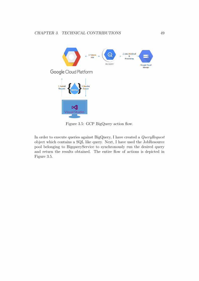
CHAPTER 3. TECHNICAL CONTRIBUTIONS 49

Figure 3.5: GCP BigQuery action flow.

In order to execute queries against BigQuery, I have created a QueryRequestobject which contains a SQL like query. Next, I have used the JobResourcepool belonging to BigqueryService to synchronously run the desired queryand return the results obtained. The entire flow of actions is depicted inFigure 3.5.

Chapter 4

Experiments

The queries from this chapter were performed on the systems described inChapter 3. They can be split into 2 parts: one that makes use of standartSQL statement (denoted by the letter A), and another one which is morefocused towards applying mathematical, statistical and analytical functions(denoted by the letter B). The aim of the first set of queries is to analyzeand retrieve some information from the HSL data1 on public transport. Theset consists of three queries (named from 1A to 3A), and their description isas follows:

1. Query 1A. For each existing route calculate five basic measures for theduration: Maximum value, upper quartile, median, lower quartile andminimum value. This query aims to show the performance for simplestatistical functions that require sorting of the whole data set.

2. Query 2A. Scenario where each service provider has the ability toget the data from their own provided service for a given time period.Service provider gets the results for Query 1 (above), with a WHEREclause identifying the service provider and a time period. Purpose forthis query is to see the impact to the performance when introducingsimple where clauses.

3. Query 3A. Each service provider must have some sub-organizationsthat have restricted access to the data. For example service provider 12might have two subcontractors sub1 and sub2. sub1 operates route 36and sub2 operates route 1. Each subcontractor can query the data fortheir own operations only (WHERE clause includes the subcontractor

1http://dev.hsl.fi/ajoaika_gps/

50

CHAPTER 4. EXPERIMENTS 51

identifier, not the service provider or the route). Note that it shouldpossible that the subcontractors can operate multiple routes for mul-tiple service provider (e.g., sub1 can access data for service provider12 on route 36 AND for service provider 22 and route 1). The queryresults are as in Query 1 and 2, but the query needs to do a lookupor join to a separate table that maintains the relations between thesubcontractors, service providers and the routes operated by the sub-contractors. For this query we need to create some sub-organizationstructure in a separate operational lookup/reference table, as the na-ture of this data is not stable. The subcontractors change over time andfor the sake of improved business all new subcontractors need to see theprevious operators’ metrics for the same routes (and service provider)for comparison. Purpose for this query is to introduce an operationallookup/join table that is expected to have a dramatic performance im-pact to the above queries, but is necessary to restrict data access sothat the query cannot be tampered with by the user (Assume that asystem is developed where the organization / role / subcontractor idis taken automatically based on the login information and provided tothe query in the back-end, not manually entered by the user).

Whereas Spark SQL is able to create the schema of the data at runtime andthen process the queries on the fly, HiveSQL needs to know the structureof the data beforehand. A complete list of column names of the data canbe found on HSL’s public domain2. The following code snippet in Scalahighlights the structure of Query 1A used for launching the Spark jobs:

// Read in the parquet file.

// Parquet files are self-describing so the schema is preserved.

// The result of loading a Parquet file is a DataFrame.

val parquetData =

sqlContext.parquetFile("wasb:///hsldata/hsl_data.parquet")

// register it into a in-memory table

parquetData.registerTempTable("parquetDataTable")

// apply sql queries and fetch the results

sqlContext.sql("select linja as bus_line,max(ajoaika)

as max_duration,

min(ajoaika) as min_duration,

percentile(cast(ajoaika as bigint), 0.75)

2http://datasciencehackathon.aalto.fi/?page_id=108

CHAPTER 4. EXPERIMENTS 52

as upper_quartile,

percentile(cast(ajoaika as bigint), 0.5)

as median,

percentile(cast(ajoaika as bigint), 0.25)

as lower_quartile

from parquetDataTable

group by linja

order by linja desc")

.show()

The above Spark Scala code contains two actions and two transformations.On one hand, the actions, corresponding to the lines responsible for loadingthe file and printing the results to the console, are executed on the spot.On the other hand, the transformations (corresponding to the part of coderesponsible for registering the temporary table and applying the SQL queries)allow for a lazy evaluation, thus bringing the Spark engine more chances ofoptimizing our job.

The second query (Query 2A) differs from the Query 1A only by a ”WHERE”clause.

[... code is the same with the one from Query 1A...]

sqlContext.sql("select palveluntuottaja as service_provider,

linja as bus_line,max(ajoaika) as max_duration,

min(ajoaika) as min_duration,

percentile(cast(ajoaika as bigint), 0.75)

as upper_quartile,

percentile(cast(ajoaika as bigint), 0.5)

as median,

percentile(cast(ajoaika as bigint), 0.25)

as lower_quartile

from parquetDataTable

WHERE palveluntuottaja=’36’

group by palveluntuottaja,linja

order by palveluntuottaja,linja desc")

.show()

Finally, the third query (3A), is slightly more complicated as it builds onquery 2A and extends it by joining results with a different table.

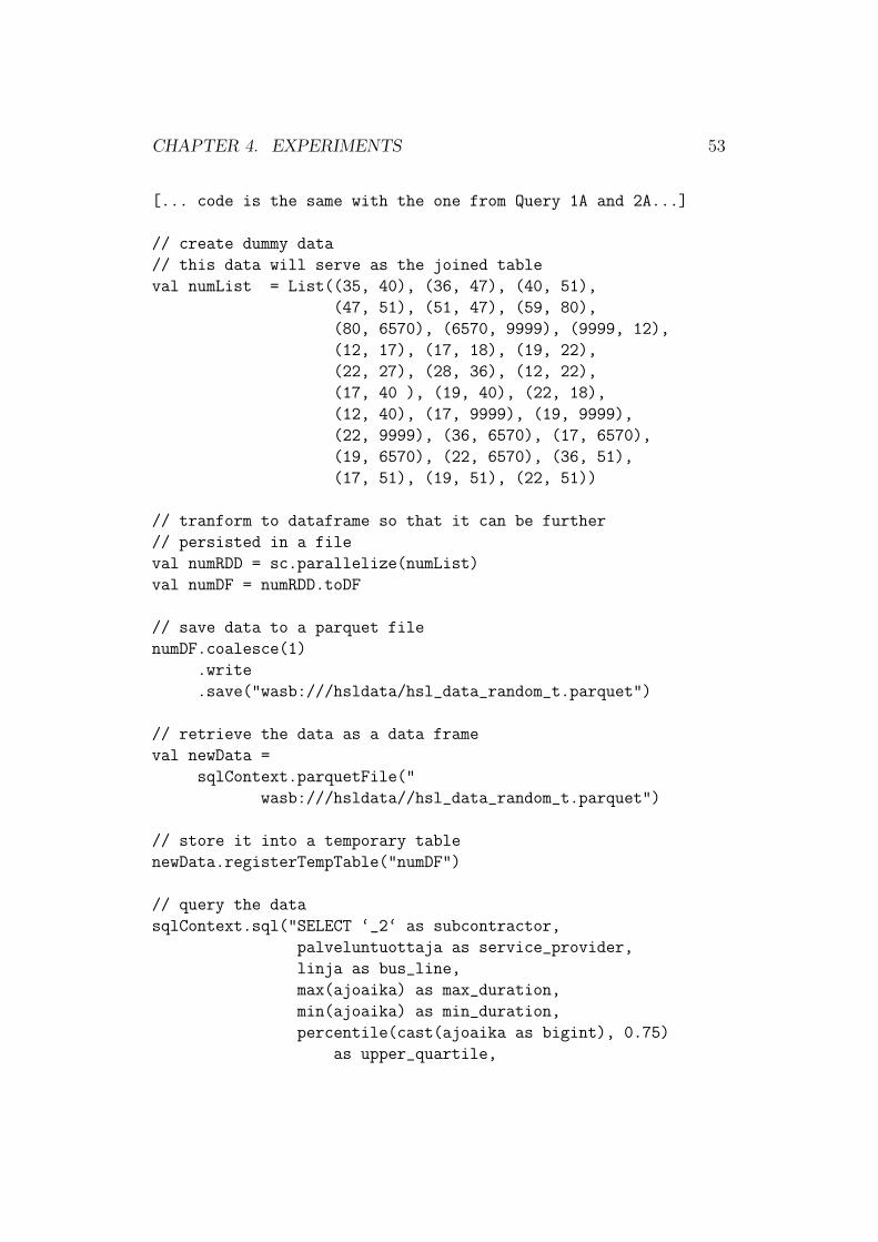
CHAPTER 4. EXPERIMENTS 53

[... code is the same with the one from Query 1A and 2A...]

// create dummy data

// this data will serve as the joined table

val numList = List((35, 40), (36, 47), (40, 51),

(47, 51), (51, 47), (59, 80),

(80, 6570), (6570, 9999), (9999, 12),

(12, 17), (17, 18), (19, 22),

(22, 27), (28, 36), (12, 22),

(17, 40 ), (19, 40), (22, 18),

(12, 40), (17, 9999), (19, 9999),

(22, 9999), (36, 6570), (17, 6570),

(19, 6570), (22, 6570), (36, 51),

(17, 51), (19, 51), (22, 51))

// tranform to dataframe so that it can be further

// persisted in a file

val numRDD = sc.parallelize(numList)

val numDF = numRDD.toDF

// save data to a parquet file

numDF.coalesce(1)

.write

.save("wasb:///hsldata/hsl_data_random_t.parquet")

// retrieve the data as a data frame

val newData =

sqlContext.parquetFile("

wasb:///hsldata//hsl_data_random_t.parquet")

// store it into a temporary table

newData.registerTempTable("numDF")

// query the data

sqlContext.sql("SELECT ‘_2‘ as subcontractor,

palveluntuottaja as service_provider,

linja as bus_line,

max(ajoaika) as max_duration,

min(ajoaika) as min_duration,

percentile(cast(ajoaika as bigint), 0.75)

as upper_quartile,

CHAPTER 4. EXPERIMENTS 54

percentile(cast(ajoaika as bigint), 0.5)

as median,

percentile(cast(ajoaika as bigint), 0.25)

as lower_quartile

FROM parquetData initData

JOIN numDF ndf

ON initData.palveluntuottaja = ‘_1‘

WHERE palveluntuottaja=’36’

GROUP BY ‘_2‘, palveluntuottaja,linja

ORDER BY ‘_2‘, palveluntuottaja,linja desc")

.show()

As mentioned before, in order to parse the data, Hive requires prior knowl-edge about its structure, called metadata. Thus, in order to be able to runthe same queries against Hive on Tez, we must first create a table with theschema emulated on the data columns. Next, the table must be populatedwith the data from the parquet file. Finally, we can execute queries basedon this table.

The second set of queries (denoted by the capital letter B) differs from thefirst one by replacing some statistical functions (e.g. percentile) with others.This is due to the fact that engines such as Apache Drill and Impala donot support some operations, that are otherwise supported in Spark SQLand Hive. Additional mathematical and statistical functions are also addedto this set of queries, thus making it more CPU intensive. These functionsinclude: SUM, AVG, COUNT and DISTINCT.

In the case of Google BigQuery, the queries were all executed from theWEB UI provided by Google. The first query that was executed once thefiles had been uploaded to the bucket involved loading all that data into atable. The following images depict the required steps for launching the jobresponsible for loading the data into a new table.

Figure 4.1: Loading multiple .csv files from Google Cloud Storage to a table.

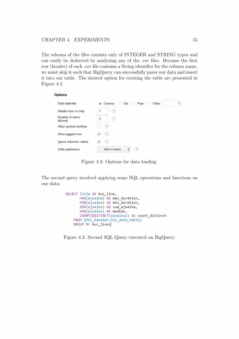
CHAPTER 4. EXPERIMENTS 55

The schema of the files consists only of INTEGER and STRING types andcan easily be deducted by analyzing any of the .csv files. Because the firstrow (header) of each .csv file contains a String identifier for the column name,we must skip it such that BigQuery can successfully parse our data and insertit into our table. The desired option for creating the table are presented inFigure 4.2.

Figure 4.2: Options for data loading.

The second query involved applying some SQL operations and functions onour data:

Figure 4.3: Second SQL Query executed on BigQuery.

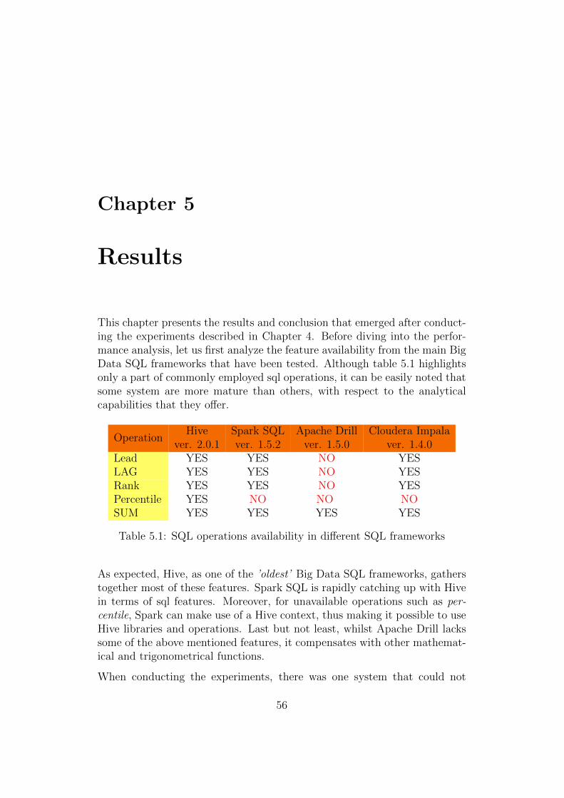
Chapter 5

Results

This chapter presents the results and conclusion that emerged after conduct-ing the experiments described in Chapter 4. Before diving into the perfor-mance analysis, let us first analyze the feature availability from the main BigData SQL frameworks that have been tested. Although table 5.1 highlightsonly a part of commonly employed sql operations, it can be easily noted thatsome system are more mature than others, with respect to the analyticalcapabilities that they offer.

OperationHive

ver. 2.0.1Spark SQLver. 1.5.2

Apache Drillver. 1.5.0

Cloudera Impalaver. 1.4.0

Lead YES YES NO YESLAG YES YES NO YESRank YES YES NO YESPercentile YES NO NO NOSUM YES YES YES YES

Table 5.1: SQL operations availability in different SQL frameworks

As expected, Hive, as one of the ’oldest’ Big Data SQL frameworks, gatherstogether most of these features. Spark SQL is rapidly catching up with Hivein terms of sql features. Moreover, for unavailable operations such as per-centile, Spark can make use of a Hive context, thus making it possible to useHive libraries and operations. Last but not least, whilst Apache Drill lackssome of the above mentioned features, it compensates with other mathemat-ical and trigonometrical functions.

When conducting the experiments, there was one system that could not

56

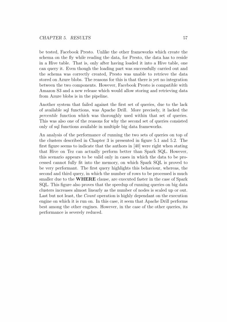
CHAPTER 5. RESULTS 57

be tested, Facebook Presto. Unlike the other frameworks which create theschema on the fly while reading the data, for Presto, the data has to residein a Hive table. That is, only after having loaded it into a Hive table, onecan query it. Even though the loading part was successfully carried out andthe schema was correctly created, Presto was unable to retrieve the datastored on Azure blobs. The reasons for this is that there is yet no integrationbetween the two components. However, Facebook Presto is compatible withAmazon S3 and a new release which would allow storing and retrieving datafrom Azure blobs is in the pipeline.

Another system that failed against the first set of queries, due to the lackof available sql functions, was Apache Drill. More precisely, it lacked thepercentile function which was thoroughly used within that set of queries.This was also one of the reasons for why the second set of queries consistedonly of sql functions available in multiple big data frameworks.

An analysis of the performance of running the two sets of queries on top ofthe clusters described in Chapter 3 is presented in figure 5.1 and 5.2. Thefirst figure seems to indicate that the authors in [40] were right when statingthat Hive on Tez can actually perform better than Spark SQL. However,this scenario appears to be valid only in cases in which the data to be pro-cessed cannot fully fit into the memory, on which Spark SQL is proved tobe very performant. The first query highlights this behaviour, whereas, thesecond and third query, in which the number of rows to be processed is muchsmaller due to the WHERE clause, are executed faster in the case of SparkSQL. This figure also proves that the speedup of running queries on big dataclusters increases almost linearly as the number of nodes is scaled up or out.Last but not least, the Count operation is highly dependant on the executionengine on which it is run on. In this case, it seem that Apache Drill performsbest among the other engines. However, in the case of the other queries, itsperformance is severely reduced.

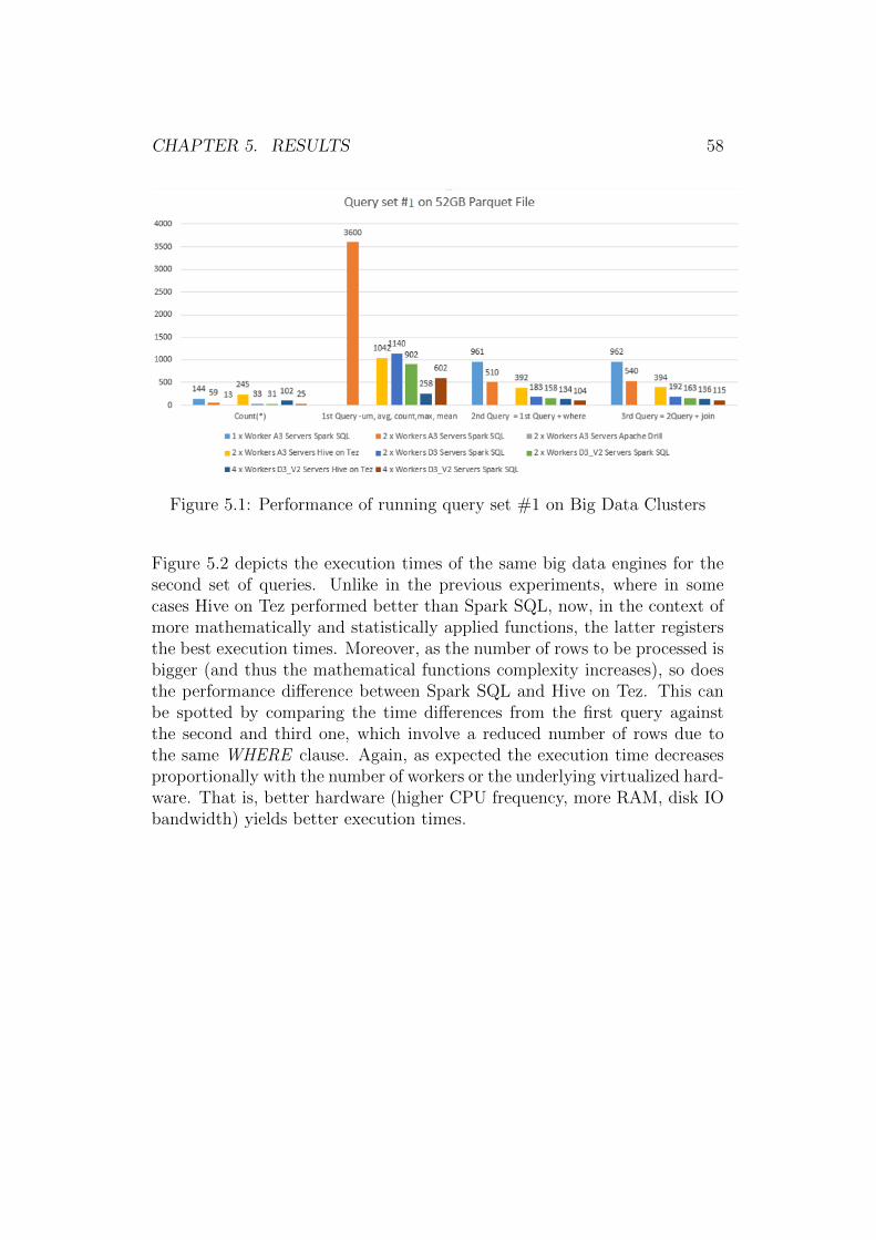
CHAPTER 5. RESULTS 58

Figure 5.1: Performance of running query set #1 on Big Data Clusters

Figure 5.2 depicts the execution times of the same big data engines for thesecond set of queries. Unlike in the previous experiments, where in somecases Hive on Tez performed better than Spark SQL, now, in the context ofmore mathematically and statistically applied functions, the latter registersthe best execution times. Moreover, as the number of rows to be processed isbigger (and thus the mathematical functions complexity increases), so doesthe performance difference between Spark SQL and Hive on Tez. This canbe spotted by comparing the time differences from the first query againstthe second and third one, which involve a reduced number of rows due tothe same WHERE clause. Again, as expected the execution time decreasesproportionally with the number of workers or the underlying virtualized hard-ware. That is, better hardware (higher CPU frequency, more RAM, disk IObandwidth) yields better execution times.

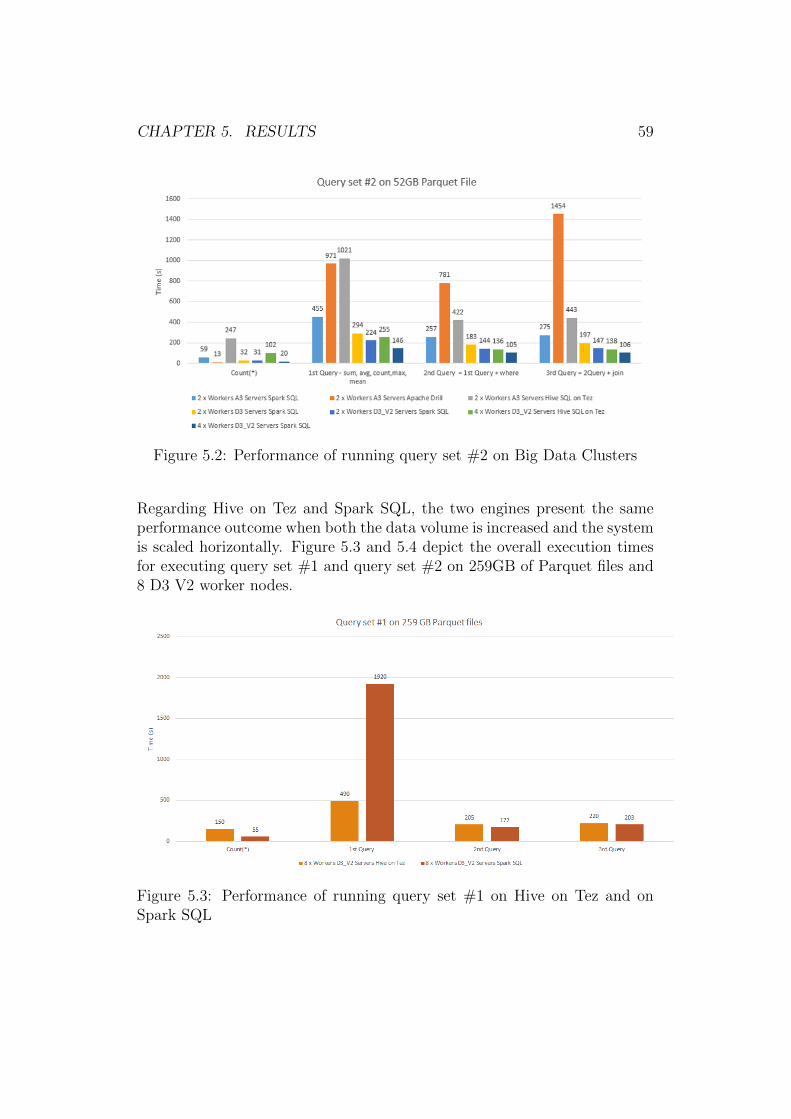
CHAPTER 5. RESULTS 59

Figure 5.2: Performance of running query set #2 on Big Data Clusters

Regarding Hive on Tez and Spark SQL, the two engines present the sameperformance outcome when both the data volume is increased and the systemis scaled horizontally. Figure 5.3 and 5.4 depict the overall execution timesfor executing query set #1 and query set #2 on 259GB of Parquet files and8 D3 V2 worker nodes.

Figure 5.3: Performance of running query set #1 on Hive on Tez and onSpark SQL

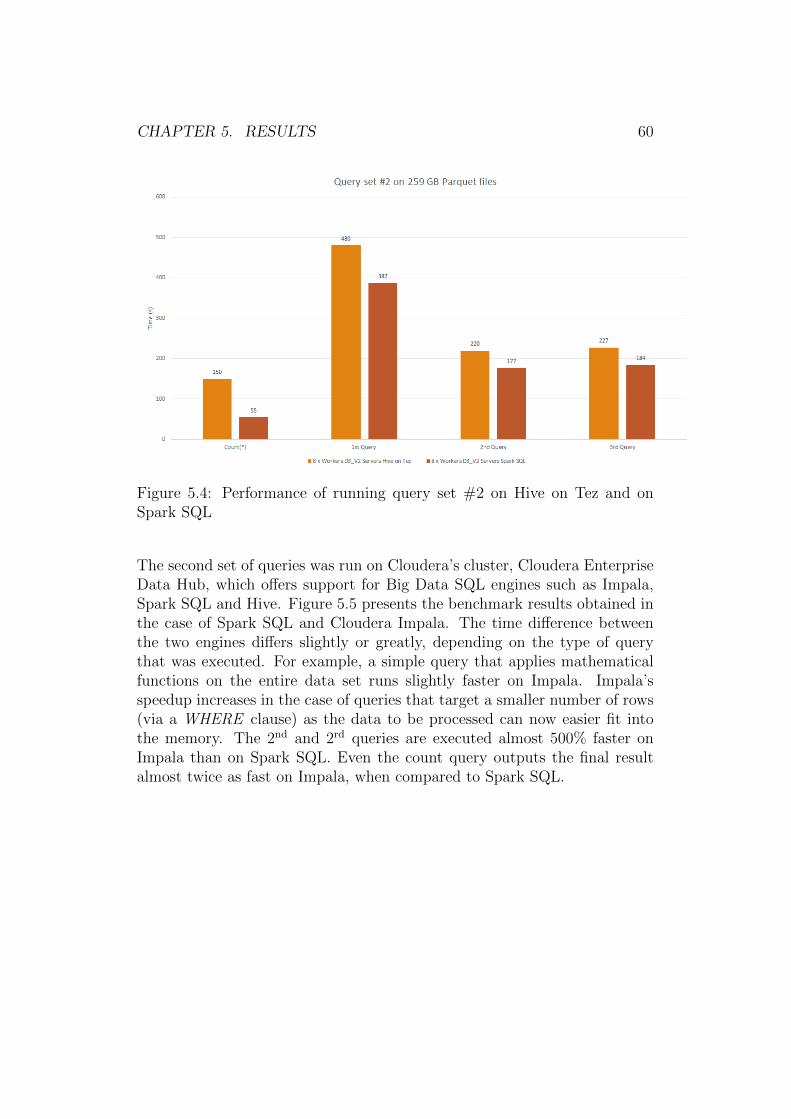
CHAPTER 5. RESULTS 60

Figure 5.4: Performance of running query set #2 on Hive on Tez and onSpark SQL

The second set of queries was run on Cloudera’s cluster, Cloudera EnterpriseData Hub, which offers support for Big Data SQL engines such as Impala,Spark SQL and Hive. Figure 5.5 presents the benchmark results obtained inthe case of Spark SQL and Cloudera Impala. The time difference betweenthe two engines differs slightly or greatly, depending on the type of querythat was executed. For example, a simple query that applies mathematicalfunctions on the entire data set runs slightly faster on Impala. Impala’sspeedup increases in the case of queries that target a smaller number of rows(via a WHERE clause) as the data to be processed can now easier fit intothe memory. The 2nd and 2rd queries are executed almost 500% faster onImpala than on Spark SQL. Even the count query outputs the final resultalmost twice as fast on Impala, when compared to Spark SQL.

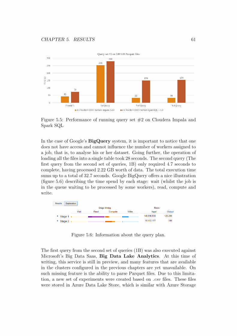
CHAPTER 5. RESULTS 61

Figure 5.5: Performance of running query set #2 on Cloudera Impala andSpark SQL

In the case of Google’s BigQuery system, it is important to notice that onedoes not have access and cannot influence the number of workers assigned toa job, that is, to analyse his or her dataset. Going further, the operation ofloading all the files into a single table took 28 seconds. The second query (Thefirst query from the second set of queries, 1B) only required 4.7 seconds tocomplete, having processed 2.22 GB worth of data. The total execution timesums up to a total of 32.7 seconds. Google BigQuery offers a nice illustration(figure 5.6) describing the time spend by each stage: wait (whilst the job isin the queue waiting to be processed by some workers), read, compute andwrite.

Figure 5.6: Information about the query plan.

The first query from the second set of queries (1B) was also executed againstMicrosoft’s Big Data Saas, Big Data Lake Analytics. At this time ofwriting, this service is still in preview, and many features that are availablein the clusters configured in the previous chapters are yet unavailable. Onsuch missing feature is the ability to parse Parquet files. Due to this limita-tion, a new set of experiments were created based on .csv files. These fileswere stored in Azure Data Lake Store, which is similar with Azure Storage

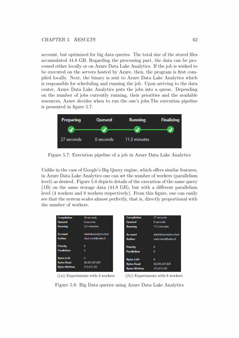
CHAPTER 5. RESULTS 62

account, but optimized for big data queries. The total size of the stored filesaccumulated 44.8 GB. Regarding the processing part, the data can be pro-cessed either locally or on Azure Data Lake Analytics. If the job is wished tobe executed on the servers hosted by Azure, then, the program is first com-piled locally. Next, the binary is sent to Azure Data Lake Analytics whichis responsible for scheduling and running the job. Upon arriving to the datacenter, Azure Data Lake Analytics puts the jobs into a queue. Dependingon the number of jobs currently running, their priorities and the availableresources, Azure decides when to run the one’s jobs.The execution pipelineis presented in figure 5.7.

Figure 5.7: Execution pipeline of a job in Azure Data Lake Analytics

Unlike in the case of Google’s Big Query engine, which offers similar features,in Azure Data Lake Analytics one can set the number of workers (parallelismlevel) as desired. Figure 5.8 depicts details of the execution of the same query(1B) on the same storage data (44.8 GB), but with a different parallelismlevel (4 workers and 8 workers respectively). From this figure, one can easilysee that the system scales almost perfectly, that is, directly proportional withthe number of workers.

((a)) Experiments with 4 workers ((b)) Experiments with 8 workers

Figure 5.8: Big Data queries using Azure Data Lake Analytics

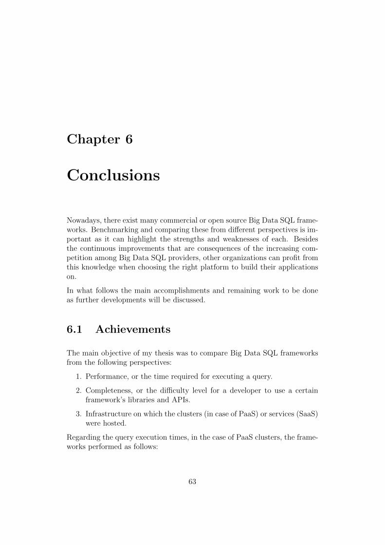
Chapter 6

Conclusions

Nowadays, there exist many commercial or open source Big Data SQL frame-works. Benchmarking and comparing these from different perspectives is im-portant as it can highlight the strengths and weaknesses of each. Besidesthe continuous improvements that are consequences of the increasing com-petition among Big Data SQL providers, other organizations can profit fromthis knowledge when choosing the right platform to build their applicationson.

In what follows the main accomplishments and remaining work to be doneas further developments will be discussed.

6.1 Achievements

The main objective of my thesis was to compare Big Data SQL frameworksfrom the following perspectives:

1. Performance, or the time required for executing a query.

2. Completeness, or the difficulty level for a developer to use a certainframework’s libraries and APIs.

3. Infrastructure on which the clusters (in case of PaaS) or services (SaaS)were hosted.

Regarding the query execution times, in the case of PaaS clusters, the frame-works performed as follows:

63

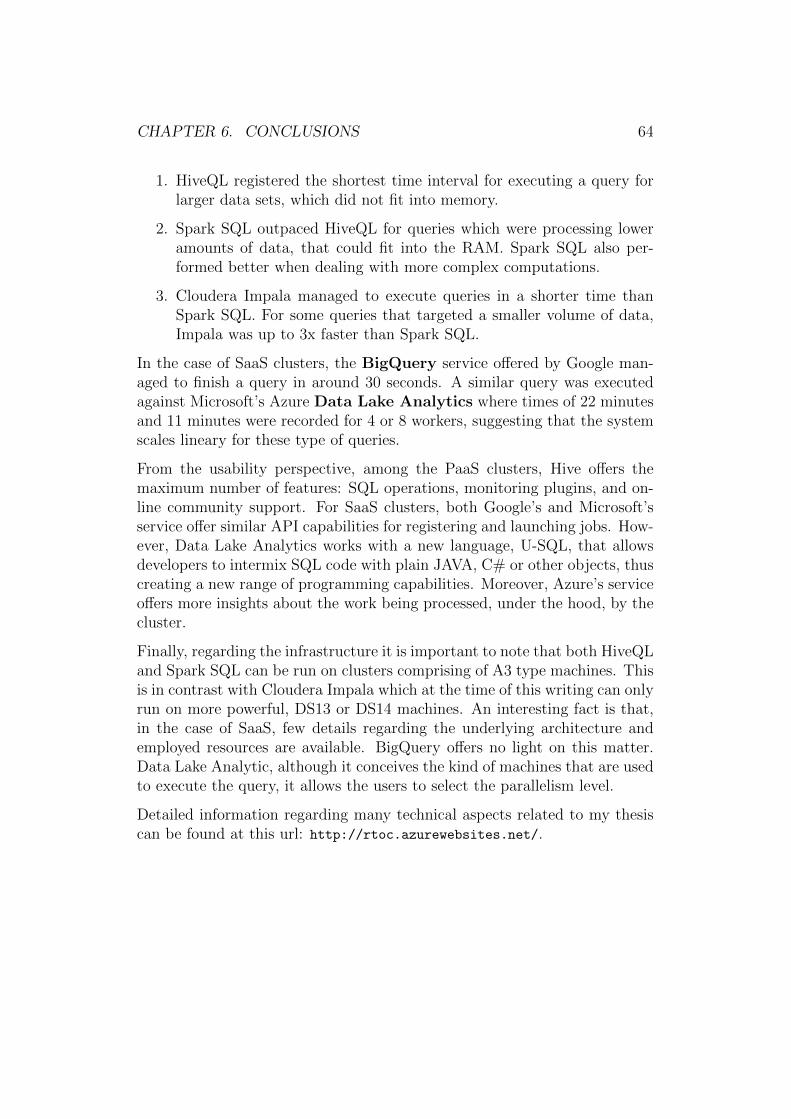
CHAPTER 6. CONCLUSIONS 64

1. HiveQL registered the shortest time interval for executing a query forlarger data sets, which did not fit into memory.

2. Spark SQL outpaced HiveQL for queries which were processing loweramounts of data, that could fit into the RAM. Spark SQL also per-formed better when dealing with more complex computations.

3. Cloudera Impala managed to execute queries in a shorter time thanSpark SQL. For some queries that targeted a smaller volume of data,Impala was up to 3x faster than Spark SQL.

In the case of SaaS clusters, the BigQuery service offered by Google man-aged to finish a query in around 30 seconds. A similar query was executedagainst Microsoft’s Azure Data Lake Analytics where times of 22 minutesand 11 minutes were recorded for 4 or 8 workers, suggesting that the systemscales lineary for these type of queries.

From the usability perspective, among the PaaS clusters, Hive offers themaximum number of features: SQL operations, monitoring plugins, and on-line community support. For SaaS clusters, both Google’s and Microsoft’sservice offer similar API capabilities for registering and launching jobs. How-ever, Data Lake Analytics works with a new language, U-SQL, that allowsdevelopers to intermix SQL code with plain JAVA, C# or other objects, thuscreating a new range of programming capabilities. Moreover, Azure’s serviceoffers more insights about the work being processed, under the hood, by thecluster.

Finally, regarding the infrastructure it is important to note that both HiveQLand Spark SQL can be run on clusters comprising of A3 type machines. Thisis in contrast with Cloudera Impala which at the time of this writing can onlyrun on more powerful, DS13 or DS14 machines. An interesting fact is that,in the case of SaaS, few details regarding the underlying architecture andemployed resources are available. BigQuery offers no light on this matter.Data Lake Analytic, although it conceives the kind of machines that are usedto execute the query, it allows the users to select the parallelism level.

Detailed information regarding many technical aspects related to my thesiscan be found at this url: http://rtoc.azurewebsites.net/.

CHAPTER 6. CONCLUSIONS 65

6.2 Future development

For future work, more experiments are to be performed with different datasets, in different formats and on various types of cluster.

One technical question that is currently puzzling is why some Parquet filescan be successfully analysed by Spark’s execution engine, whilst Impala can-not. A potential investigation on the matter should focus on the Parquetparser implementation used by both engines.

The development of SaaS platforms for analyzing Big Data would create newways for developers and scientist to gain valuable insights without the hassleof configuring and maintaining their own hardware infrastructure. Moreover,improvements in the area of supported languages for Big Data SaaS servicesare also expected. For example, HiveQL is expected to be part of the nextrelease of Azure Data Lake Analytics.

Bibliography

[1] Abadi, D., Boncz, P. A., Harizopoulos, S., Idreos, S., andMadden, S. The Design and Implementation of Modern Column-Oriented Database Systems. Foundations and Trends in Databases 5, 3(2013), 197–280.

[2] Ananthanarayanan, G., Agarwal, S., Kandula, S., Green-berg, A. G., Stoica, I., Harlan, D., and Harris, E. Scarlett:Coping with Skewed Content Popularity in MapReduce Clusters. In Eu-ropean Conference on Computer Systems, Proceedings of the Sixth Eu-ropean conference on Computer systems, EuroSys 2011, Salzburg, Aus-tria, April 10-13, 2011 (2011), C. M. Kirsch and G. Heiser, Eds., ACM,pp. 287–300.

[3] Ananthanarayanan, G., Ghodsi, A., Warfield, A.,Borthakur, D., Kandula, S., Shenker, S., and Stoica,I. PACMan: Coordinated Memory Caching for Parallel Jobs. InGribble and Katabi [20], pp. 267–280.

[4] Armbrust, M., Xin, R. S., Lian, C., Huai, Y., Liu, D.,Bradley, J. K., Meng, X., Kaftan, T., Franklin, M. J., Gh-odsi, A., and Zaharia, M. Spark SQL: Relational Data Processingin Spark. In Proceedings of the 2015 ACM SIGMOD International Con-ference on Management of Data, Melbourne, Victoria, Australia, May31 - June 4, 2015 (2015), T. K. Sellis, S. B. Davidson, and Z. G. Ives,Eds., ACM, pp. 1383–1394.

[5] Ballani, H., Costa, P., Karagiannis, T., and Rowstron, A.I. T. Towards Predictable Datacenter Networks. In Proceedings ofthe ACM SIGCOMM 2011 Conference on Applications, Technologies,Architectures, and Protocols for Computer Communications, Toronto,ON, Canada, August 15-19, 2011 (2011), S. Keshav, J. Liebeherr, J. W.Byers, and J. C. Mogul, Eds., ACM, pp. 242–253.

66

BIBLIOGRAPHY 67

[6] Benefico, S., Gjeci, E., Gomarasca, R. G., Lever, E., Lom-bardo, S., Ardagna, D., and Nitto, E. D. Evaluation of theCAP Properties on Amazon SimpleDB and Windows Azure Table Stor-age. In 14th International Symposium on Symbolic and Numeric Algo-rithms for Scientific Computing, SYNASC 2012, Timisoara, Romania,September 26-29, 2012 (2012), A. Voronkov, V. Negru, T. Ida, T. Je-belean, D. Petcu, S. M. Watt, and D. Zaharie, Eds., IEEE ComputerSociety, pp. 430–435.

[7] Bharti, S., and Pattanaik, K. K. Dynamic Distributed FlowScheduling for Effective Link Utilization in Data Center Networks. J.High Speed Networks 20, 1 (2014), 1–10.

[8] Birke, R., Bjorkqvist, M., Chen, L. Y., Smirni, E., and En-gbersen, T. (Big) Data in a Virtualized World: Volume, Velocity,and Variety in Cloud Datacenters. In Proceedings of the 12th USENIXconference on File and Storage Technologies, FAST 2014, Santa Clara,CA, USA, February 17-20, 2014 (2014), B. Schroeder and E. Thereska,Eds., USENIX, pp. 177–189.

[9] Botoeva, E., Calvanese, D., Cogrel, B., Rezk, M., and Xiao,G. A Formal Presentation of MongoDB (Extended Version). CoRRabs/1603.09291 (2016).

[10] Brewer, E. A. Towards robust distributed systems (abstract). InProceedings of the Nineteenth Annual ACM Symposium on Principlesof Distributed Computing, July 16-19, 2000, Portland, Oregon, USA.(2000), G. Neiger, Ed., ACM, p. 7.

[11] Calder, B., Wang, J., Ogus, A., Nilakantan, N., Skjolsvold,A., McKelvie, S., Xu, Y., Srivastav, S., Wu, J., Simitci, H.,Haridas, J., Uddaraju, C., Khatri, H., Edwards, A., Be-dekar, V., Mainali, S., Abbasi, R., Agarwal, A., ul Haq,M. F., ul Haq, M. I., Bhardwaj, D., Dayanand, S., Adusumilli,A., McNett, M., Sankaran, S., Manivannan, K., and Rigas,L. Windows Azure Storage: A Highly Available Cloud Storage Servicewith Strong Consistency. In Proceedings of the 23rd ACM Symposiumon Operating Systems Principles 2011, SOSP 2011, Cascais, Portugal,October 23-26, 2011 (2011), T. Wobber and P. Druschel, Eds., ACM,pp. 143–157.

[12] Chang, C., Moon, B., Acharya, A., Shock, C., Sussman,A., and Saltz, J. H. Titan: A High-Performance Remote Sensing

BIBLIOGRAPHY 68

Database. In Proceedings of the Thirteenth International Conference onData Engineering, April 7-11, 1997 Birmingham U.K. (1997), W. A.Gray and P. Larson, Eds., IEEE Computer Society, pp. 375–384.

[13] Chebotko, A., Kashlev, A., and Lu, S. A Big Data Model-ing Methodology for Apache Cassandra. In 2015 IEEE InternationalCongress on Big Data, New York City, NY, USA, June 27 - July 2,2015 (2015), B. Carminati and L. Khan, Eds., IEEE, pp. 238–245.

[14] Chen, Q., Hsu, M., and Wu, R. MemcacheSQL A Scale-Out SQLCache Engine. In Enabling Real-Time Business Intelligence - 5th Inter-national Workshop, BIRTE 2011, Held at the 37th International Confer-ence on Very Large Databases, VLDB 2011, Seattle, WA, USA, Septem-ber 2, 2011, Revised Selected Papers (2011), M. Castellanos, U. Dayal,and W. Lehner, Eds., vol. 126 of Lecture Notes in Business InformationProcessing, Springer, pp. 23–37.

[15] Chowdhury, M., Kandula, S., and Stoica, I. Leveraging End-point Flexibility in Data-Intensive Clusters. In ACM SIGCOMM 2013Conference, SIGCOMM’13, Hong Kong, China, August 12-16, 2013(2013), D. M. Chiu, J. Wang, P. Barford, and S. Seshan, Eds., ACM,pp. 231–242.

[16] Dean, J., and Ghemawat, S. MapReduce: Simplified Data Process-ing on Large Clusters. Commun. ACM 51, 1 (2008), 107–113.

[17] Gantz, J., and Reinsel, D. THE DIGITAL UNIVERSE IN 2020:Big Data, Bigger Digital Shadows, and Biggest Growth in the Far East.Tech. rep.

[18] George, L. HBase - The Definitive Guide: Random Access to YourPlanet-Size Data. O’Reilly, 2011.

[19] Greenberg, A. G., Hamilton, J. R., Jain, N., Kandula, S.,Kim, C., Lahiri, P., Maltz, D. A., Patel, P., and Sengupta,S. VL2: A Scalable and Flexible Data Center Network. Commun. ACM54, 3 (2011), 95–104.

[20] Gribble, S. D., and Katabi, D., Eds. Proceedings of the 9thUSENIX Symposium on Networked Systems Design and Implementa-tion, NSDI 2012, San Jose, CA, USA, April 25-27, 2012 (2012),USENIX Association.

BIBLIOGRAPHY 69

[21] Gufler, B., Augsten, N., Reiser, A., and Kemper, A. LoadBalancing in MapReduce Based on Scalable Cardinality Estimates. InIEEE 28th International Conference on Data Engineering (ICDE 2012),Washington, DC, USA (Arlington, Virginia), 1-5 April, 2012 (2012),A. Kementsietsidis and M. A. V. Salles, Eds., IEEE Computer Society,pp. 522–533.

[22] Hinkka, M., Lehto, T., and Heljanko, K. Assessing Big DataSQL Frameworks for Analyzing Event Logs. In 24th Euromicro Interna-tional Conference on Parallel, Distributed, and Network-Based Process-ing, PDP 2016, Heraklion, Crete, Greece, February 17-19, 2016 (2016),IEEE Computer Society, pp. 101–108.

[23] Huang, C., Simitci, H., Xu, Y., Ogus, A., Calder, B.,Gopalan, P., Li, J., and Yekhanin, S. Erasure Coding in WindowsAzure Storage. In 2012 USENIX Annual Technical Conference, Boston,MA, USA, June 13-15, 2012 (2012), G. Heiser and W. C. Hsieh, Eds.,USENIX Association, pp. 15–26.

[24] Jacobs, A. The Pathologies of Big Data. ACM Queue 7, 6 (2009), 10.

[25] Kononenko, O., Baysal, O., Holmes, R., and Godfrey, M. W.Mining Modern Repositories with Elasticsearch. In 11th Working Con-ference on Mining Software Repositories, MSR 2014, Proceedings, May31 - June 1, 2014, Hyderabad, India (2014), P. T. Devanbu, S. Kim,and M. Pinzger, Eds., ACM, pp. 328–331.

[26] Kornacker, M., Behm, A., Bittorf, V., Bobrovytsky, T.,Ching, C., Choi, A., Erickson, J., Grund, M., Hecht, D., Ja-cobs, M., Joshi, I., Kuff, L., Kumar, D., Leblang, A., Li,N., Pandis, I., Robinson, H., Rorke, D., Rus, S., Russell,J., Tsirogiannis, D., Wanderman-Milne, S., and Yoder, M.Impala: A Modern, Open-Source SQL Engine for Hadoop. In CIDR2015, Seventh Biennial Conference on Innovative Data Systems Re-search, Asilomar, CA, USA, January 4-7, 2015, Online Proceedings(2015), www.cidrdb.org.

[27] Kwon, Y., Balazinska, M., Howe, B., and Rolia, J. A. Skew-Tune in Action: Mitigating Skew in MapReduce Applications. PVLDB5, 12 (2012), 1934–1937.

[28] Lerner, R. M. At the Forge: Redis. Linux J. 2010, 197 (Sept. 2010).

BIBLIOGRAPHY 70

[29] Li, H., Ghodsi, A., Zaharia, M., Shenker, S., and Stoica,I. Tachyon: Reliable, Memory Speed Storage for Cluster ComputingFrameworks. In Proceedings of the ACM Symposium on Cloud Comput-ing, Seattle, WA, USA, November 03 - 05, 2014 (2014), E. Lazowska,D. Terry, R. H. Arpaci-Dusseau, and J. Gehrke, Eds., ACM, pp. 6:1–6:15.

[30] Liu, A. Q. Generational Performance Comparison: Microsoft Azure’sA-Series and D-Series. Tech. rep.

[31] Malladi, K. T., Nothaft, F. A., Periyathambi, K., Lee, B. C.,Kozyrakis, C., and Horowitz, M. Towards Energy-ProportionalDatacenter Memory with Mobile DRAM. In 39th International Sympo-sium on Computer Architecture (ISCA 2012), June 9-13, 2012, Port-land, OR, USA (2012), IEEE Computer Society, pp. 37–48.

[32] Melnik, S., Gubarev, A., Long, J. J., Romer, G., Shivakumar,S., Tolton, M., and Vassilakis, T. Dremel: Interactive Analysisof Web-Scale Datasets. Commun. ACM 54, 6 (2011), 114–123.

[33] Niemenmaa, M. Analysing Sequencing Data in Hadoop: The road toInteractivity via SQL. Master’s Thesis, Aalto University, 2013.

[34] Ousterhout, K., Rasti, R., Ratnasamy, S., Shenker, S., andChun, B. Making Sense of Performance in Data Analytics Frame-works. In 12th USENIX Symposium on Networked Systems Design andImplementation, NSDI 15, Oakland, CA, USA, May 4-6, 2015 (2015),USENIX Association, pp. 293–307.

[35] Pokorny, J. NoSQL Databases: A Step to Database Scalability inWeb Environment. In Proceedings of the 13th International Conferenceon Information Integration and Web-based Applications and Services(New York, NY, USA, 2011), iiWAS ’11, ACM, pp. 278–283.

[36] Reed, I., and Solomon, G. Polynomial Codes Over Certain FiniteFields. Journal of the Society of Industrial and Applied Mathematics 8,2 (06/1960 1960), 300–304.

[37] Reynold Xin, M. A., and Liu, D. IntroducingDataFrames in Spark for Large Scale Data Science. Tech.rep. Available at https://databricks.com/blog/2015/02/17/

introducing-dataframes-in-spark-for-large-scale-data-science.

html.

BIBLIOGRAPHY 71

[38] Rosen, J. Deep Dive into Project Tungsten: Bringing Spark Closer toBare Metal. Tech. rep., Databricks, A Session at Spark Summit, June2016.

[39] Sato, K. An Inside Look at Google BigQuery. Tech. rep. Available athttps://cloud.google.com/files/BigQueryTechnicalWP.pdf.

[40] Shanklin, C., and Mokhtar, M. Hive on Spark is Blaz-ing Fast... or is it? In Strata + Hadoop World, San Jose, 21February 2015. Available at http://www.slideshare.net/hortonworks/

hive-on-spark-is-blazing-fast-or-is-it-final.

[41] Shi, J., Qiu, Y., Minhas, U. F., Jiao, L., Wang, C., Reinwald,B., and Ozcan, F. Clash of the Titans: MapReduce vs. Spark forLarge Scale Data Analytics. PVLDB 8, 13 (2015), 2110–2121.

[42] Sivasubramanian, S. Amazon DynamoDB: A Seamlessly ScalableNon-Relational Database Service. In Proceedings of the ACM SIG-MOD International Conference on Management of Data, SIGMOD2012, Scottsdale, AZ, USA, May 20-24, 2012 (2012), K. S. Candan,Y. Chen, R. T. Snodgrass, L. Gravano, and A. Fuxman, Eds., ACM,pp. 729–730.

[43] Srivas, M. Apache Drill: Building Highly Flexible, High PerformanceQuery Engines. Tech. rep. Available at http://www.slideshare.net/

HiveData/apache-drilltalk-thehive.

[44] Sumbaly, R., Kreps, J., Gao, L., Feinberg, A., Soman, C.,and Shah, S. Serving Large-Scale Batch computed Data with ProjectVoldemort. In Proceedings of the 10th USENIX conference on File andStorage Technologies, FAST 2012, San Jose, CA, USA, February 14-17,2012 (2012), W. J. Bolosky and J. Flinn, Eds., USENIX Association,p. 18.

[45] Webber, J. A Programmatic Introduction to Neo4j. In Conferenceon Systems, Programming, and Applications: Software for Humanity,SPLASH ’12, Tucson, AZ, USA, October 21-25, 2012 (2012), G. T.Leavens, Ed., ACM, pp. 217–218.

[46] Wietrzyk, V. I., and Orgun, M. A. VERSANT Architecture:Supporting High - Performance Object Databases. In Proceedings of the1998 International Database Engineering and Applications Symposium,

BIBLIOGRAPHY 72

IDEAS 1998, Cardiff, Wales, U.K., July 8-10, 1998 (1998), B. Eagle-stone, B. C. Desai, and J. Shao, Eds., IEEE Computer Society, pp. 141–149.

[47] Xiangrui Meng, Joseph Bradley, E. S., and Venkatara-man, S. ML Pipelines: A New High-Level API for MLlib.Tech. rep. Available at https://databricks.com/blog/2015/01/07/

ml-pipelines-a-new-high-level-api-for-mllib.html.

[48] Xin, R. S., Rosen, J., Zaharia, M., Franklin, M. J., Shenker,S., and Stoica, I. Shark: SQL and Rich Analytics at Scale. InProceedings of the ACM SIGMOD International Conference on Man-agement of Data, SIGMOD 2013, New York, NY, USA, June 22-27,2013 (2013), K. A. Ross, D. Srivastava, and D. Papadias, Eds., ACM,pp. 13–24.

[49] Zaharia, M., Chowdhury, M., Das, T., Dave, A., Ma, J.,McCauly, M., Franklin, M. J., Shenker, S., and Stoica, I.Resilient Distributed Datasets: A Fault-Tolerant Abstraction for In-Memory Cluster Computing. In Gribble and Katabi [20], pp. 15–28.

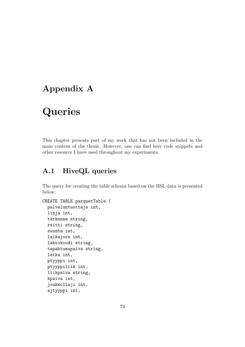
Appendix A

Queries

This chapter presents part of my work that has not been included in themain content of the thesis. However, one can find here code snippets andother resource I have used throughout my experiments.

A.1 HiveQL queries

The query for creating the table schema based on the HSL data is presentedbelow:

CREATE TABLE parquetTable (

palveluntuottaja int,

linja int,

tarkenne string,

reitti string,

suunta int,

laikajore int,

lahtokoodi string,

tapahtumapaiva string,

laika int,

ptyyppi int,

ptyyppiliik int,

liikpaiva string,

kpaiva int,

joukkollaji int,

ajtyyppi int,

73

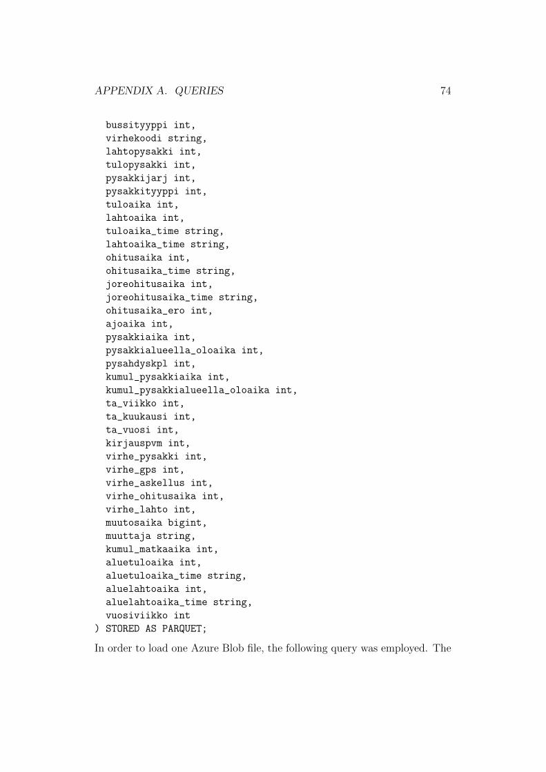
APPENDIX A. QUERIES 74

bussityyppi int,

virhekoodi string,

lahtopysakki int,

tulopysakki int,

pysakkijarj int,

pysakkityyppi int,

tuloaika int,

lahtoaika int,

tuloaika_time string,

lahtoaika_time string,

ohitusaika int,

ohitusaika_time string,

joreohitusaika int,

joreohitusaika_time string,

ohitusaika_ero int,

ajoaika int,

pysakkiaika int,

pysakkialueella_oloaika int,

pysahdyskpl int,

kumul_pysakkiaika int,

kumul_pysakkialueella_oloaika int,

ta_viikko int,

ta_kuukausi int,

ta_vuosi int,

kirjauspvm int,

virhe_pysakki int,

virhe_gps int,

virhe_askellus int,

virhe_ohitusaika int,

virhe_lahto int,

muutosaika bigint,

muuttaja string,

kumul_matkaaika int,

aluetuloaika int,

aluetuloaika_time string,

aluelahtoaika int,

aluelahtoaika_time string,

vuosiviikko int

) STORED AS PARQUET;

In order to load one Azure Blob file, the following query was employed. The

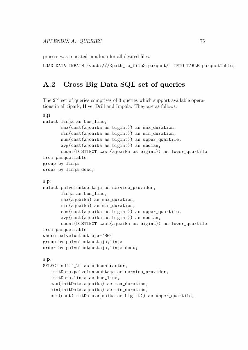
APPENDIX A. QUERIES 75

process was repeated in a loop for all desired files.

LOAD DATA INPATH ’wasb:///<path_to_file>.parquet/’ INTO TABLE parquetTable;

A.2 Cross Big Data SQL set of queries

The 2nd set of queries comprises of 3 queries which support available opera-tions in all Spark, Hive, Drill and Impala. They are as follows:

#Q1

select linja as bus_line,

max(cast(ajoaika as bigint)) as max_duration,

min(cast(ajoaika as bigint)) as min_duration,

sum(cast(ajoaika as bigint)) as upper_quartile,

avg(cast(ajoaika as bigint)) as median,

count(DISTINCT cast(ajoaika as bigint)) as lower_quartile

from parquetTable

group by linja

order by linja desc;

#Q2

select palveluntuottaja as service_provider,

linja as bus_line,

max(ajoaika) as max_duration,

min(ajoaika) as min_duration,

sum(cast(ajoaika as bigint)) as upper_quartile,

avg(cast(ajoaika as bigint)) as median,

count(DISTINCT cast(ajoaika as bigint)) as lower_quartile

from parquetTable

where palveluntuottaja=’36’

group by palveluntuottaja,linja

order by palveluntuottaja,linja desc;

#Q3

SELECT ndf.‘_2‘ as subcontractor,

initData.palveluntuottaja as service_provider,

initData.linja as bus_line,

max(initData.ajoaika) as max_duration,

min(initData.ajoaika) as min_duration,

sum(cast(initData.ajoaika as bigint)) as upper_quartile,

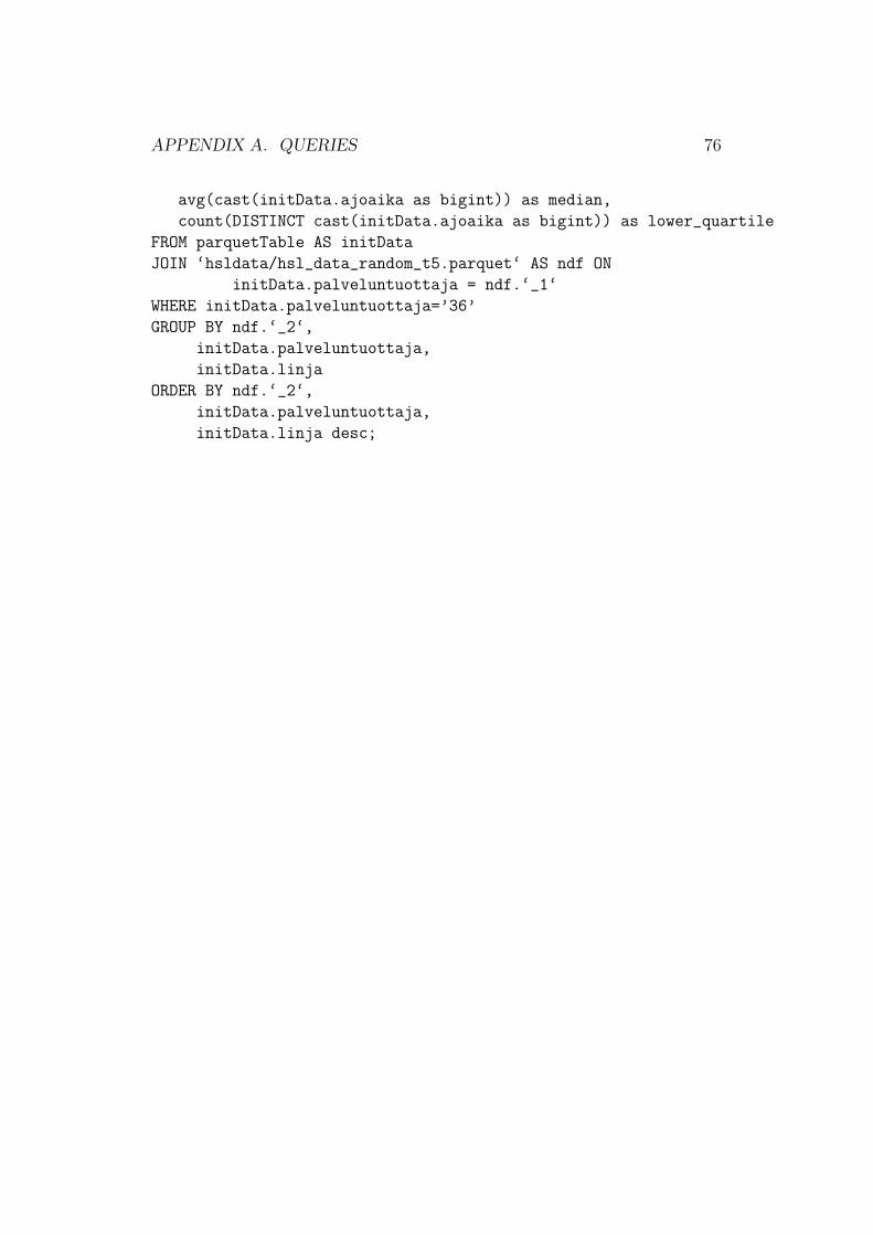
APPENDIX A. QUERIES 76

avg(cast(initData.ajoaika as bigint)) as median,

count(DISTINCT cast(initData.ajoaika as bigint)) as lower_quartile

FROM parquetTable AS initData

JOIN ‘hsldata/hsl_data_random_t5.parquet‘ AS ndf ON

initData.palveluntuottaja = ndf.‘_1‘

WHERE initData.palveluntuottaja=’36’

GROUP BY ndf.‘_2‘,

initData.palveluntuottaja,

initData.linja

ORDER BY ndf.‘_2‘,

initData.palveluntuottaja,

initData.linja desc;