Embed Size (px)
Citation preview
arX
iv:1
309.
7560
v1 [
mat
h.C
A]
29
Sep
2013
LECTURE NOTES
BERNOULLI POLYNOMIALS
AND APPLICATIONS
OMRAN KOUBA†
Abstract. In this lecture notes we try to familiarize the audience with the theory of Bernoulli poly-nomials; we study their properties, and we give, with proofs and references, some of the most relevantresults related to them. Several applications to these polynomials are presented, including a unifiedapproach to the asymptotic expansion of the error term in many numerical quadrature formulæ, andmany new and sharp inequalities, that bound some trigonometric sums.
Contents
1. Introduction 22. Properties of Bernoulli polynomials 33. Fourier series and Bernoulli polynomials 94. Bernoulli polynomials on the unit interval [0, 1] 125. Asymptotic behavior of Bernoulli polynomials 166. The generating function of Bernoulli polynomials 187. The von Staudt-Clausen theorem 238. The Euler-Maclaurin’s formula 259. Asymptotic expansions for numerical quadrature formulæ 29
9.1. Riemann sums. 299.2. The trapezoidal rule. 309.3. Simpson’s rule. 339.4. The two point Gauss rule. 349.5. Romberg’s rule. 34
10. Asymptotic expansions for the sum of certain series related to harmonic numbers 3711. Asymptotic expansions for certain trigonometric sums 4212. Endnotes 47References 47
2010 Mathematics Subject Classification. 11B68, 11L03, 30D10, 32B05, 43E05, 42A16, 65D32.Key words and phrases. Fourier series, analytic functions, power series expansion, Bernoulli polynomials, Bernoulli
numbers, harmonic numbers, asymptotic expansion, numerical quadrature, Riemann sum, trapezoidal rule, Simpson’s rule,Gauss quadrature rule, Romberg’s rule, sum of cosecants, sum of cotangents.
† Department of Mathematics, Higher Institute for Applied Sciences and Technology.
1
2 OMRAN KOUBA
1. Introduction
There are many ways to introduce Bernoulli polynomials and numbers. We opted for the algebraicapproach relying on the difference operator. But first, let us introduce some notation.
Let the real vector space of polynomials with real coefficients be denoted by R[X ]. For a nonnegativeinteger n, let Rn[X ] be the subspace of R[X ] consisting of polynomials of degree smaller or equal to n.
If P is a polynomial from R[X ], we define ∆Pdef= P (X + 1)− P (X), and we denote by ∆ the linear
operator, defined on R[X ], by P 7→ ∆P .
Lemma 1.1. The linear operator Φ defined by
Φ : R[X ]−→R[X ]× R, P 7→(∆P,
∫ 1
0
P (t) dt
)(1.1)
is bijective.
Proof. Consider P ∈ kerΦ, then P ∈ ker∆ and∫ 1
0P (t) dt = 0. Now, if we considerQ(X) = P (X)− P (0),
then clearly we have
Q(X + 1) = P (X + 1)− P (0) = P (X)− P (0) = Q(X)
This implies by induction that Q(n) = 0 for every nonnegative integer n, so Q = 0, since it has infinitely
many zeros. Thus, P (X) = P (0), but we have also∫ 1
0 P (t) dt = 0, so P (0) = 0, and consequently P = 0.This proves that Φ is injective.
Clearly, for a nonnegative integer n we have deg∆(Xn+1) = n. Thus
P ∈ Rn+1[X ] =⇒ ∆P ∈ Rn[X ]
Therefore,∀n ∈ N, Φ(Rn+1[X ]) ⊂ Rn[X ]× R.
But the fact that Φ is injective implies that
dimΦ(Rn+1[X ]) = dimRn+1[X ] = 1 + dimRn[X ] = dim(Rn[X ]× R),
and consequently∀n ∈ N, Φ(Rn+1[X ]) = Rn[X ]× R
This, proves that Φ is surjective, and the lemma follows. �
Let us consider the basis E = (en)n∈N of R[X ]× R defined by e0 = (0, 1) and en = (nXn−1, 0) forn ∈ N∗. We can define the Bernoulli polynomials, In terms of this basis and of the isomorphism Φ ofLemma 1.1 as follows:
Definition 1.2. The sequence of Bernoulli polynomials (Bn)n∈N is defined by
Bn = Φ−1 (en) for n ≥ 0.
According to Lemma 1.1, this definition takes a more practical form as follows :
Corollary 1.3. The sequence of Bernoulli polynomials (Bn)n∈N is uniquely defined by the conditions:
1© B0(X) = 1.
2© ∀n ∈ N∗, Bn(X + 1)−Bn(X) = nXn−1. (1.2)
3© ∀n ∈ N∗,
∫ 1
0
Bn(t) dt = 0.
For instance, it is straightforward to see that
B1(X) = X − 1
2, and B2(X) = X2 −X +
1
6.
BERNOULLI POLYNOMIALS AND APPLICATIONS 3
2. Properties of Bernoulli polynomials
In the next proposition, we summarize some simple properties of Bernoulli polynomials :
Proposition 2.1. The sequence of Bernoulli polynomials (Bn)n∈N satisfies the following properties:
i. For every positive integer n we have B′n(X) = nBn−1(X).
ii. For every positive integer n we have Bn(1 −X) = (−1)nBn(X).iii. For every nonnegative integer n and every positive integer p we have
1
p
p−1∑
k=0
Bn
(X + k
p
)=
1
pnBn(X).
Proof. (i ) Consider the sequence of polynomials (Qn)n∈N defined byQn = 1n+1B
′n+1. It is straightforward
to see that Q0(X) = 1 and for n ≥ 1 :
∆Qn =1
n+ 1(∆Bn+1)
′ =1
n+ 1((n+ 1)Xn)′ = nXn−1
and ∫ 1
0
Qn(t) dt =1
n+ 1
∫ 1
0
B′n+1(t) dt =
∆Bn+1(0)
n+ 1= 0.
This proves that the sequence of (Qn)n∈N satisfies the conditions 1©, 2© and 3© of Corollary 1.3, and (i )follows because of the unicity assertion.
(ii) Consider again the sequence (Qn)n∈N defined by Qn(X) = (−1)nBn(1−X). Clearly Q0(X) = 1 andfor n ≥ 1 :
∆Qn = (−1)n(Bn(−X)−Bn(1−X)) = (−1)n−1∆Bn(−X)
= (−1)n−1n(−X)n−1 = nXn−1.
Moreover, for n ≥ 1,∫ 1
0 Qn(t) dt = (−1)n∫ 1
0 Bn(1 − t) dt = 0. This proves that the sequence of (Qn)n∈N
satisfies the conditions 1©, 2© and 3© of Corollary 1.3, and (ii ) follows from the unicity assertion.
(iii) Similarly, consider the sequence of polynomials (Qn)n∈N defined by
Qn(X) = pn−1
p−1∑
k=0
Bn
(X + k
p
)
Clearly Q0(X) = 1 and for n ≥ 1 :
∆Qn = pn−1
p−1∑
k=0
Bn
(X + k + 1
p
)− pn−1
p−1∑
k=0
Bn
(X + k
p
)
= pn−1
(p∑
k=1
Bn
(X + k
p
)−
p−1∑
k=0
Bn
(X + k
p
))
= pn−1
(Bn
(X + p
p
)−Bn
(X
p
))= pn−1∆Bn
(1
pX
)= nXn−1.
Moreover, for n ≥ 1,∫ 1
0
Qn(t)dt = pn−1
p−1∑
k=0
∫ 1
0
Bn
(t+ k
p
)dt
= pn−1
p−1∑
k=0
∫ (k+1)/p
k/p
Bn(t) dt = pn−1
∫ 1
0
Bn(t) dt = 0.
This proves that the sequence of (Qn)n∈N satisfies the conditions 1©, 2© and 3© of Corollary 1.3, and (iii )follows by unicity. The proof of Proposition 2.1 is complete. �
4 OMRAN KOUBA
Definition 2.2. The sequence of Bernoulli Numbers (bn)n∈N is defined by
bn = Bn(0) for n ≥ 0.
The following proposition summarizes some properties of Bernoulli numbers.
Proposition 2.3. The sequence of Bernoulli numbers (bn)n∈N satisfies the following properties:
i. For every positive integer n we have b2n+1 = 0 and b2n = B2n(1).ii. For every nonnegative integer n we have Bn
(12
)= (21−n − 1)bn.
iii. For every nonnegative integer n we have
Bn(X) =
n∑
k=0
(n
k
)bn−kX
k.
iv. For every positive integer n we have
bn = − 1
n+ 1
n−1∑
k=0
(n+ 1
k
)bk.
Proof. (i) Using Proposition 2.1(i ) we have, for n ≥ 2 :
Bn(1)−Bn(0) =
∫ 1
0
B′n(t) dt = n
∫ 1
0
Bn−1(t)dt = 0
and according to Proposition 2.1(ii ) we have Bn(1) = (−1)nBn(0) for every n ≥ 1. This proves thatbn = 0 if n is an odd integer greater than 2, and that B2n(1) = b2n for n ≥ 1. This is (i ).
(ii) According to Proposition 2.1(iii ) with p = 2 we see that, for every nonnegative integer n we have
Bn
(X
2
)+Bn
(X + 1
2
)= 21−nBn(X)
Substituting X = 0 we obtain (ii ).
(iii) Consider n ∈ N, according Now, we use again Proposition 2.1(i ) to conclude that
B(k)n = n(n− 1) . . . (n− k + 1)Bn−k, for 0 < k ≤ n.
It follows that
B(k)n (Y )
k!=
(n
k
)Bn−k(Y ), for 0 < k ≤ n
and using Taylor’s formula for polynomials we conclude that
Bn(X + Y ) =
n∑
k=0
(n
k
)Bn−k(Y )Xk
Finally, substituting Y = 0, we obtain (iii ).
(iv) Let n be an integer such that n ≥ 2. We have shown that Bn(1) = bn, and using the preceding point
we conclude that Bn(1) =∑n
k=0
(nk
)bn−k, that is bn =
∑nk=0
(nk
)bn−k or
∑n−1k=0
(nk
)bk = 0. So
∀n ≥ 1,n∑
k=0
(n+ 1
k
)bk = 0
which is equivalent to (iv ). �
BERNOULLI POLYNOMIALS AND APPLICATIONS 5
Application 1. In Proposition 2.3 (iii ), Bernoulli polynomials are expressed in terms of the canonicalbasis (Xk)k∈N of R[X ]. In fact, we have proved that
Bn(X + Y ) =
n∑
k=0
(n
k
)Bn−k(X)Y k (2.1)
and this can be used to, conversely, express the canonical basis (Xk)k∈N of R[X ] in terms of Bernoullipolynomials.
Indeed, substituting Y = 1 in (2.1) we obtain
Bn+1(X + 1) =n+1∑
k=0
(n+ 1
k
)Bn+1−k(X),
but according to Corollary 1.3 we have also Bn+1(X + 1) = Bn+1(X) + (n+ 1)Xn. Thus
(n+ 1)Xn =
n+1∑
k=1
(n+ 1
k
)Bn+1−k(X) =
n∑
k=0
(n+ 1
k
)Bk(X)
Finally,
Xn =1
n+ 1
n∑
k=0
(n+ 1
k
)Bk(X)
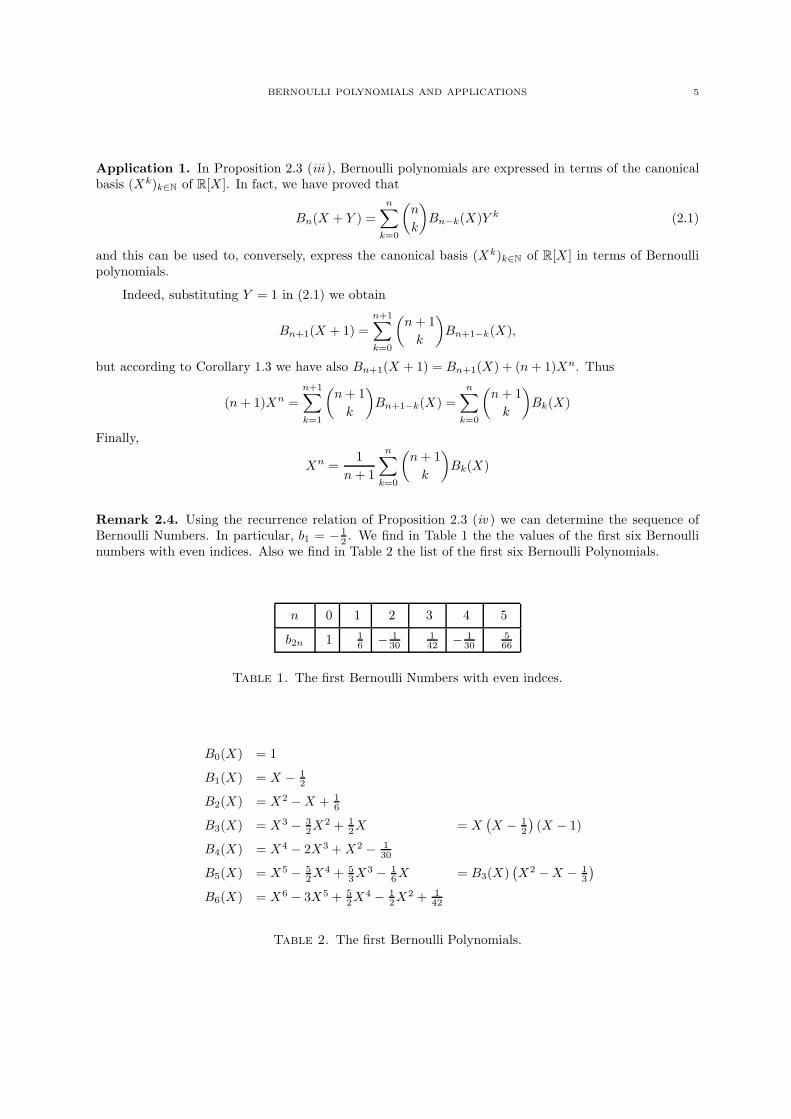
Remark 2.4. Using the recurrence relation of Proposition 2.3 (iv ) we can determine the sequence ofBernoulli Numbers. In particular, b1 = − 1
2 . We find in Table 1 the the values of the first six Bernoullinumbers with even indices. Also we find in Table 2 the list of the first six Bernoulli Polynomials.
n 0 1 2 3 4 5
b2n 1 16 − 1
30142 − 1
30566
Table 1. The first Bernoulli Numbers with even indces.
B0(X) = 1
B1(X) = X − 12
B2(X) = X2 −X + 16
B3(X) = X3 − 32X
2 + 12X = X
(X − 1
2
)(X − 1)
B4(X) = X4 − 2X3 +X2 − 130
B5(X) = X5 − 52X
4 + 53X
3 − 16X = B3(X)
(X2 −X − 1
3
)
B6(X) = X6 − 3X5 + 52X
4 − 12X
2 + 142
Table 2. The first Bernoulli Polynomials.
6 OMRAN KOUBA
Application 2. For a nonnegative integer n and a positive integer m, we define Sn(m) to be the sum
Sn(m) = 1n + 2n + · · ·+mn =
m∑
k=1
kn.
Noting that
kn =1
n+ 1(Bn+1(k + 1)−Bn+1(k))
we see that
Sn(m) =1
n+ 1(Bn+1(m+ 1)−Bn+1(0)) .
In Table 3 we have listed the first values of these sums using the results from Table 2.
1 + 2 + · · ·+m =m(m+ 1)
2
12 + 22 + · · ·+m2 =m(m+ 1)(2m+ 1)
6
13 + 23 + · · ·+m3 =m2(m+ 1)2
4
14 + 24 + · · ·+m4 =m(m+ 1)(2m+ 1)(3m2 +m− 1)
30Table 3. The sum of consecutive powers.
It was on studying these sums that Jacob Bernoulli introduced the numbers named after him.
�����
��
�
�
�
�
�
�
��
�
��
�
��
��
���
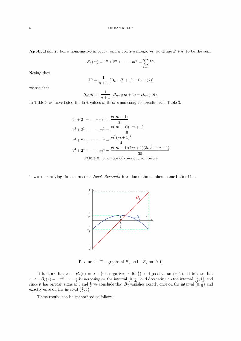
Figure 1. The graphs of B1 and −B2 on [0, 1].
It is clear that x 7→ B1(x) = x − 12 is negative on
(0, 1
2
)and positive on
(12 , 1). It follows that
x 7→ −B2(x) = −x2 +x− 16 is increasing on the interval
[0, 12], and decreasing on the interval
[12 , 1], and
since it has opposit signs at 0 and 12 we conclude that B2 vanishes exactly once on the interval
(0, 12)and
exactly once on the interval(12 , 1).
These results can be generalized as follows:
BERNOULLI POLYNOMIALS AND APPLICATIONS 7
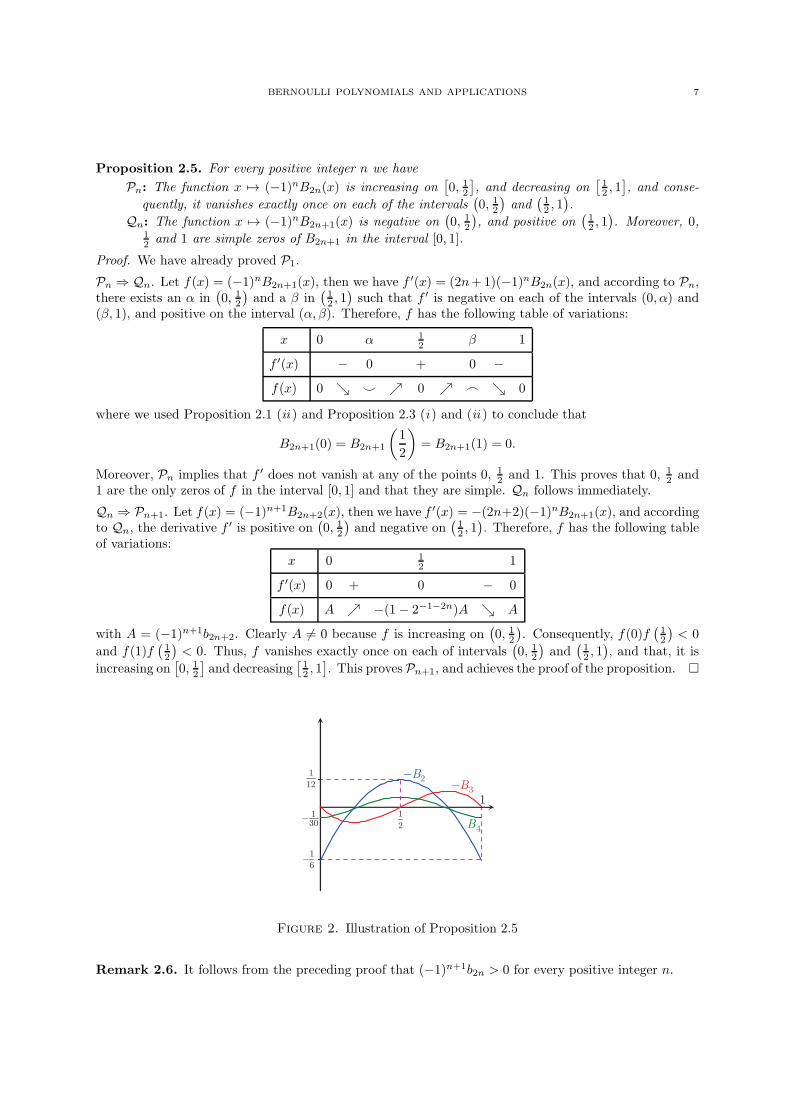
Proposition 2.5. For every positive integer n we have
Pn: The function x 7→ (−1)nB2n(x) is increasing on[0, 12], and decreasing on
[12 , 1], and conse-
quently, it vanishes exactly once on each of the intervals(0, 12)and
(12 , 1).
Qn: The function x 7→ (−1)nB2n+1(x) is negative on(0, 1
2
), and positive on
(12 , 1). Moreover, 0,
12 and 1 are simple zeros of B2n+1 in the interval [0, 1].
Proof. We have already proved P1.
Pn ⇒ Qn. Let f(x) = (−1)nB2n+1(x), then we have f ′(x) = (2n+1)(−1)nB2n(x), and according to Pn,there exists an α in
(0, 1
2
)and a β in
(12 , 1)such that f ′ is negative on each of the intervals (0, α) and
(β, 1), and positive on the interval (α, β). Therefore, f has the following table of variations:
x 0 α 12 β 1
f ′(x) − 0 + 0 −f(x) 0 ց ⌣ ր 0 ր ⌢ ց 0
where we used Proposition 2.1 (ii ) and Proposition 2.3 (i ) and (ii ) to conclude that
B2n+1(0) = B2n+1
(1
2
)= B2n+1(1) = 0.
Moreover, Pn implies that f ′ does not vanish at any of the points 0, 12 and 1. This proves that 0, 1
2 and1 are the only zeros of f in the interval [0, 1] and that they are simple. Qn follows immediately.
Qn ⇒ Pn+1. Let f(x) = (−1)n+1B2n+2(x), then we have f ′(x) = −(2n+2)(−1)nB2n+1(x), and accordingto Qn, the derivative f ′ is positive on
(0, 12)and negative on
(12 , 1). Therefore, f has the following table
of variations:
x 0 12 1
f ′(x) 0 + 0 − 0
f(x) A ր −(1− 2−1−2n)A ց A
with A = (−1)n+1b2n+2. Clearly A 6= 0 because f is increasing on(0, 12
). Consequently, f(0)f
(12
)< 0
and f(1)f(12
)< 0. Thus, f vanishes exactly once on each of intervals
(0, 12)and
(12 , 1), and that, it is
increasing on[0, 12
]and decreasing
[12 , 1]. This provesPn+1, and achieves the proof of the proposition. �
��
��
�
�
�
�
���
�
��
�
�����
���
��
Figure 2. Illustration of Proposition 2.5
Remark 2.6. It follows from the preceding proof that (−1)n+1b2n > 0 for every positive integer n.
8 OMRAN KOUBA
Corollary 2.7. For every positive integer n we have
supx∈[0,1]
|B2n(x)| = |b2n| and supx∈[0,1]
|B2n+1(x)| ≤2n+ 1
4|b2n|
Proof. In fact, we conclude from Proposition 2.5 that
supx∈[0,1]
|B2n(x)| = max
(|B2n(0)| ,
∣∣∣∣B2n
(1
2
)∣∣∣∣)
= max
(|b2n| ,
(1− 1
22n−1
)|b2n|
)= |b2n|
In order to show the second inequality we consider several cases:
• If x ∈[0, 1
4
], then we have
B2n+1(x) = B2n+1(x)−B2n+1(0) =
∫ x
0
B2n(t) dt
So
|B2n+1(x)| ≤ (2n+ 1)
∫ x
0
|B2n(t)| dt
≤ (2n+ 1) |b2n|x ≤2n+ 1
4|b2n|
• If x ∈[14 ,
12
], then we have
B2n+1(x) = B2n+1(x)−B2n+1
(1
2
)=
∫ x
1/2
(2n+ 1)B2n(t) dt
Thus
|B2n+1(x)| ≤ (2n+ 1)
∫ 1/2
x
|B2n(t)| dt
≤ (2n+ 1) |b2n|(1
2− x
)≤ 2n+ 1
4|b2n|
• Finally, when x ∈[12 , 1], we recall that B2n+1(x) = −B2n+1(1− x) according to Proposition 2.1
(ii ). Thus, in this case we have also
|B2n+1(x)| ≤ sup0≤t≤ 1
2
|B2n+1(t)| ≤2n+ 1
4|b2n|
and the second part of the proposition follows. �
Remark 2.8. We will show later in these notes that
supx∈[0,1]
|B2n+1(x)| ≤2n+ 1
2π|b2n|
which is, asymptotically, the best possible result. That is, we have also
limn→∞
2π
(2n+ 1) |b2n|· supx∈[0,1]
|B2n+1(x)| = 1
BERNOULLI POLYNOMIALS AND APPLICATIONS 9
3. Fourier series and Bernoulli polynomials
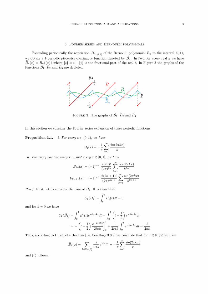
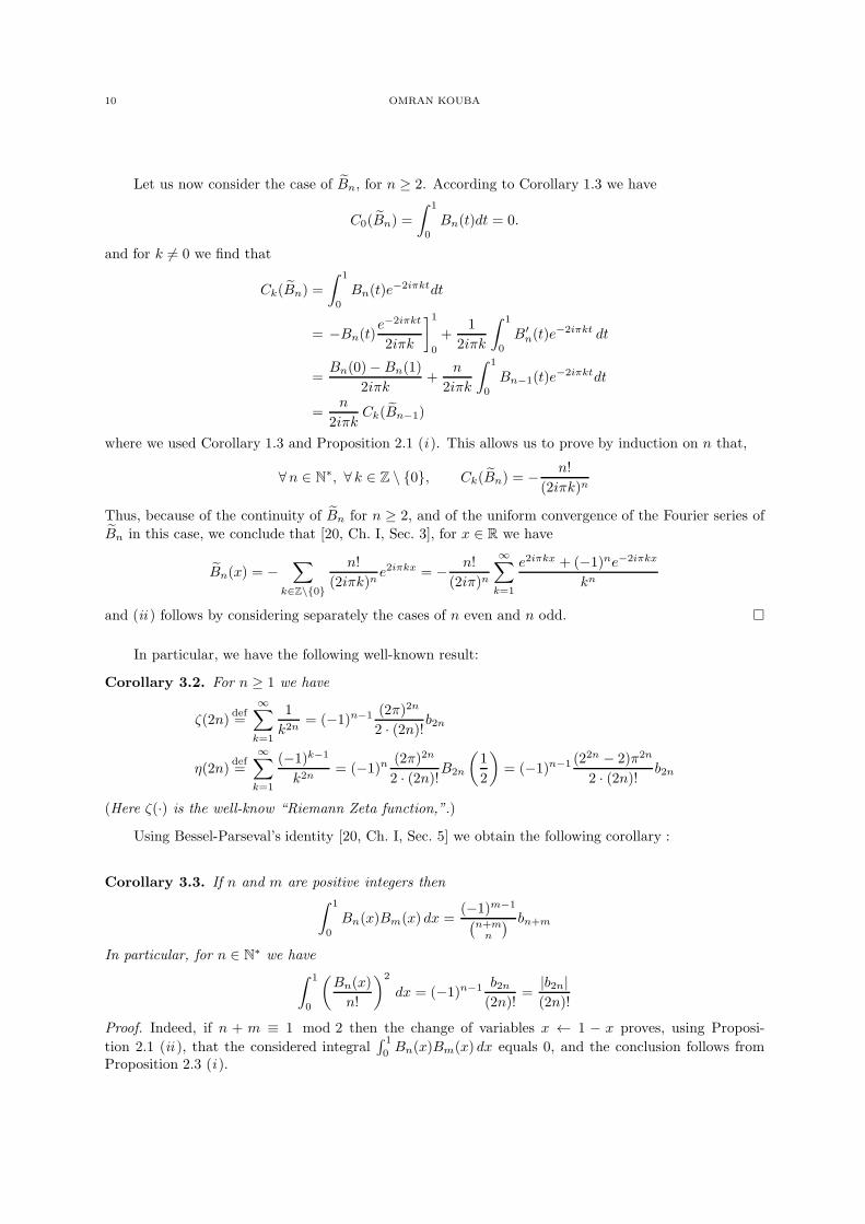
Extending periodically the restriction Bn|[0,1) of the Bernoulli polynomial Bn to the interval [0, 1),
we obtain a 1-periodic piecewise continuous function denoted by Bn. In fact, for every real x we have
Bn(x) = Bn({x}) where {t} = t − ⌊t⌋ is the fractional part of the real t. In Figure 3 the graphs of the
functions B1, B2 and B3 are depicted.
��
��
�
�
��
�
���
���
���
Figure 3. The graphs of B1, B2 and B3
In this section we consider the Fourier series expansion of these periodic functions.
Proposition 3.1. i. For every x ∈ (0, 1), we have
B1(x) = −1
π
∞∑
k=1
sin(2πkx)
k
ii. For every positive integer n, and every x ∈ [0, 1], we have
B2n(x) = (−1)n+1 2(2n)!
(2π)2n
∞∑
k=1
cos(2πkx)
k2n
B2n+1(x) = (−1)n+1 2(2n+ 1)!
(2π)2n+1
∞∑
k=1
sin(2πkx)
k2n+1
Proof. First, let us consider the case of B1. It is clear that
C0(B1) =
∫ 1
0
B1(t)dt = 0.
and for k 6= 0 we have
Ck(B1) =
∫ 1
0
B1(t)e−2iπktdt =
∫ 1
0
(t− 1
2
)e−2iπktdt
= −(t− 1
2
)e−2iπkt
2iπk
]1
0
+1
2iπk
∫ 1
0
e−2iπkt dt =i
2πk
Thus, according to Dirichlet’s theorem [14, Corollary 3.3.9] we conclude that for x ∈ R \ Z we have
B1(x) =∑
k∈Z\{0}
i
2πke2iπkx = − 1
π
∞∑
k=1
sin(2πkx)
k
and (i ) follows.
10 OMRAN KOUBA
Let us now consider the case of Bn, for n ≥ 2. According to Corollary 1.3 we have
C0(Bn) =
∫ 1
0
Bn(t)dt = 0.
and for k 6= 0 we find that
Ck(Bn) =
∫ 1
0
Bn(t)e−2iπktdt
= −Bn(t)e−2iπkt
2iπk
]1
0
+1
2iπk
∫ 1
0
B′n(t)e
−2iπkt dt
=Bn(0)− Bn(1)
2iπk+
n
2iπk
∫ 1
0
Bn−1(t)e−2iπktdt
=n
2iπkCk(Bn−1)
where we used Corollary 1.3 and Proposition 2.1 (i ). This allows us to prove by induction on n that,
∀n ∈ N∗, ∀ k ∈ Z \ {0}, Ck(Bn) = −n!
(2iπk)n
Thus, because of the continuity of Bn for n ≥ 2, and of the uniform convergence of the Fourier series of
Bn in this case, we conclude that [20, Ch. I, Sec. 3], for x ∈ R we have
Bn(x) = −∑
k∈Z\{0}
n!
(2iπk)ne2iπkx = − n!
(2iπ)n
∞∑
k=1
e2iπkx + (−1)ne−2iπkx
kn
and (ii ) follows by considering separately the cases of n even and n odd. �
In particular, we have the following well-known result:
Corollary 3.2. For n ≥ 1 we have
ζ(2n)def=
∞∑
k=1
1
k2n= (−1)n−1 (2π)2n
2 · (2n)!b2n
η(2n)def=
∞∑
k=1
(−1)k−1
k2n= (−1)n (2π)2n
2 · (2n)!B2n
(1
2
)= (−1)n−1 (2
2n − 2)π2n
2 · (2n)! b2n
(Here ζ(·) is the well-know “Riemann Zeta function,”.)
Using Bessel-Parseval’s identity [20, Ch. I, Sec. 5] we obtain the following corollary :
Corollary 3.3. If n and m are positive integers then∫ 1
0
Bn(x)Bm(x) dx =(−1)m−1
(n+mn
) bn+m
In particular, for n ∈ N∗ we have∫ 1
0
(Bn(x)
n!
)2
dx = (−1)n−1 b2n(2n)!
=|b2n|(2n)!
Proof. Indeed, if n + m ≡ 1 mod 2 then the change of variables x ← 1 − x proves, using Proposi-
tion 2.1 (ii ), that the considered integral∫ 1
0 Bn(x)Bm(x) dx equals 0, and the conclusion follows fromProposition 2.3 (i ).
BERNOULLI POLYNOMIALS AND APPLICATIONS 11
So, let us suppose that n ≡ m mod 2. In this case, by Bessel-Parseval’s identity, we have∫ 1
0
Bn(x)Bm(x) dx =∑
k∈Z
Ck(Bn)Ck(Bm)
= (−1)m n!m!
(2iπ)n+m
∑
k∈Z\{0}
1
kn+m
and the desired conclusion follows by Corollary 3.2. �
Application 3. One more formula for Bernoulli polynomials.
Let us consider the polynomial Tn defined by
Tn(X) =1
n+ 1
n∑
k=0
Bk(X)Bn−k(X).
Clearly, for n ≥ 1, we have
(n+ 1)T ′n(X) =
n∑
k=1
kBk−1(X)Bn−k(X) +
n−1∑
k=0
(n− k)Bk(X)Bn−k−1(X)
=
n−1∑
k=0
(k + 1)Bk(X)Bn−k−1(X) +
n−1∑
k=0
(n− k)Bk(X)Bn−k−1(X)
= (n+ 1)
n−1∑
k=0
Bk(X)Bn−1−k(X) =n+ 1
nTn−1
That is T ′n = nTn−1. Now, since Tn is a polynomial of degree n there are (λ
(n)k )0≤k≤n such that
Tn(X) =∑n
k=0 λ(n)k Bk, and from T ′
n = nTn−1 we conclude that
n−1∑
k=0
(k + 1)λ(n)k+1Bk =
n−1∑
k=0
nλ(n−1)k Bk.
Thus (k + 1)λ(n)k+1 = nλ
(n−1)k for 0 ≤ k ≤ n − 1. It follows that λ
(n)k =
(nk
)λ(n−k)0 for 0 ≤ k ≤ n. So, we
have proved that
1
n+ 1
n∑
k=0
Bk(X)Bn−k(X) =
n∑
k=0
(n
k
)λ(k)0 Bn−k
Integrating on [0, 1], and using Corollaries 1.3 and 3.3 , we obtain λ(0)0 = 1, λ
(1)0 = 0, and for n ≥ 2:
λ(n)0 =
1
n+ 1
n∑
k=0
∫ 1
0
Bk(t)Bn−k(t) dt =bn
n+ 1
n−1∑
k=1
(−1)k−1
(nk
)
= bn
n−1∑
k=1
(−1)k−1 k!(n− k)!
(n+ 1)!= −bn
∫ 1
0
(n−1∑
k=1
tn−k(t− 1)k
)dt
= −bn∫ 1
0
(tn+1 − (t− 1)n+1 − tn − (t− 1)n
)dt =
1 + (−1)n(n+ 2)(n+ 1)
bn.
That is λ(2m+1)0 = 0 and λ
(2m)0 = 1
(m+1)(2m+1)b2m. Therefore, we have proved that
1
n+ 1
n∑
k=0
Bk(X)Bn−k(X) =
⌊n/2⌋∑
k=0
(n
2k
)b2k
(k + 1)(2k + 1)Bn−2k(X).
12 OMRAN KOUBA
In particular, taking n = 2m and x = 0 we find, for m 6= 1, that
m∑
k=0
b2kb2m−2k =1
m+ 1
m∑
k=0
(2m+ 2
2k + 2
)b2kb2m−2k.
or equivalently, for m 6= 2 :
m∑
k=1
b2(k−1)b2(m−k) =1
m
m∑
k=1
(2m
2k
)b2(k−1)b2(m−k).
This is an unusual formula since it combines both convolution and binomial convolution.
4. Bernoulli polynomials on the unit interval [0, 1]
Our first result concerns the sequence of Bernoulli numbers and it follows immediately from Corollary3.2:
Proposition 4.1. The sequence of Bernoulli numbers (b2n)n≥1 satisfies the following:
i. For every positive integer n, we have |b2n| < 2
(1 +
3
22n
)(2n)!
(2π)2n< 4
(2n)!
(2π)2n.
ii. Asymptotically, for n in the neighborhood of +∞, we have |b2n| ∼+∞ 2(2n)!
(2π)2n.
Proof. Noting that, for t ∈ [k − 1, k], we have k−2n ≤ t−2n we conclude that
∞∑
k=3
1
k2n≤
∞∑
k=3
∫ k
k−1
dt
t2n=
∫ ∞
2
dt
t2n=
2
2n− 1· 1
22n
Thus, for every n ≥ 1 we have
1 < ζ(2n) =
∞∑
k=1
1
k2n≤ 1 +
1
22n+
2
2n− 1· 1
22n
or, equivalently
1 < ζ(2n) ≤ 1 +2n+ 1
2n− 1· 1
22n≤ 1 +
3
22n≤ 1 +
3
4< 2
Hence, we have proved that 1 < ζ(2n) < 2 for every n ≥ 1 and that limn→∞
ζ(2n) = 1. This implies the
desired conclusion using Corollary 3.2. �
Remark 4.2. Using Stirling’s Formula [1, pp. 257] we see that for large n we have
|b2n| ∼+∞ 4√πn( n
eπ
)2n
It is clear, according to Proposition 2.5 that the function x 7→ |B2n(x)| attains its maximum on theinterval [0, 1] at x = 0. Thus, for n ≥ 1 we have
supx∈[0,1]
|B2n(x)| = |B2n(0)| = |b2n|
Determining the maximum of x 7→ |B2n+1(x)| on the interval [0, 1] is more difficult. In this regard,we have the following result.
BERNOULLI POLYNOMIALS AND APPLICATIONS 13
Proposition 4.3. For every positive integer n we have
i. supx∈[0,1]
|B2n+1(x)| <2n+ 1
2π|b2n|.
ii.
∣∣∣∣B2n+1
(1
4
)∣∣∣∣ ≥(1− 4
22n
)2n+ 1
2π|b2n|.
Proof. In fact, using Proposition 3.1 (ii ) we see that
supx∈[0,1]
|B2n+1(x)| ≤2(2n+ 1)!
(2π)2n+1·
∞∑
k=1
1
k2n+1<
2(2n+ 1)!
(2π)2n+1·
∞∑
k=1
1
k2n.
Thus, according to Corollary 3.2 we conclude that
supx∈[0,1]
|B2n+1(x)| <2(2n+ 1)!
(2π)2n+1· (2π)2n
2 · (2n)! |b2n| =2n+ 1
2π|b2n| .
which is (i ).
On the other hand, for n ∈ N, using Proposition 3.1 (ii ) once more, we obtain
B2n+1
(1
4
)= (−1)n+1 2(2n+ 1)!
(2π)2n+1
∞∑
k=0
(−1)k(2k + 1)2n+1
,
but the series above is alternating, so∞∑
k=0
(−1)k(2k + 1)2n+1
> 1− 1
32n+1
Thus
(−1)n+1B2n+1
(1
4
)>
(1− 1
32n+1
)2(2n+ 1)!
(2π)2n+1.
Now, using Proposition 4.1 (i ) we see that
(−1)n+1B2n+1
(1
4
)>
(1− 3−2n−1
1 + 3 · 2−2n
)2n+ 1
2π|b2n| ,
and since
∀n ∈ N∗,1− 3−2n−1
1 + 3 · 2−2n≥ 1− 4
22n
we obtain (ii ). �
Remark 4.4. Combining Corollary 2.7 and Propositions 4.1 and 4.3 we see that, for large n we have
supx∈[0,1]
|Bn(x)| ∼+∞2 · n!(2π)n
.
Next, we will study the behavior of the unique zero of B2n in the interval (0, 1/2).
Proposition 4.5. For a positive integer n, let αn be the unique zero of B2n that belongs to the interval(0, 1/2). Then the sequence (αn)n≥1 satisfies the following inequality:
1
4− 1
π · 22n < αn < αn+1 <1
4.
Proof. First, note that α1 = 12 − 1
2√3so 1
4
(1− 1
π
)< α1 < 1
4 . On the other hand, since α1(1 − α1) =16
and B4(X) = X2(1−X)2 − 130 we conclude that
B4(α1) = −1
180< 0 and B4
(1
4
)=
269
7680> 0.
This proves the desired inequality for n = 1.
14 OMRAN KOUBA
Now, let us suppose that n ≥ 2. Using Proposition 2.1 (iii ) with p = 4 and X = 0 we obtain
B2n(0) +B2n
(1
4
)+B2n
(1
2
)+B2n
(3
4
)=
1
42n−1B2n(0).
But, according to Proposition 2.1 (ii ), B2n
(14
)= B2n
(34
), and using Proposition 2.3 (ii ), we have also
B2n
(12
)= (21−2n − 1)b2n. Hence
B2n
(1
4
)=
1
22n(21−2n − 1
)b2n =
1
22nB2n
(1
2
).
This proves that B2n
(14
)B2n
(12
)> 0 and B2n
(14
)B2n(0) < 0. It follows that 0 < αn < 1
4 .
Now, let us define the function hn by
hn(x) =∞∑
k=1
cos(2πkx)
k2n.
Also, let xn = 14 − 1
π·22n . Clearly we have
hn(xn) = cos
(π
2− 2
22n
)+
∞∑
k=2
cos(2πkxn)
k2n
≥ sin
(2
22n
)−
∞∑
k=2
1
k2n> sin
(2
22n
)− 2n+ 1
2n− 1· 1
22n
where we used the inequality ζ(2n)− 1 < 2n+12n−12
−2n from Proposition 4.1.
Finally, using the inequality sinx ≥ x− x3
6 which is valid for x ≥ 0, and recalling that n ≥ 2 we concludethat
hn(xn) >1
22n
(2− 2n+ 1
2n− 1− 4
3 · 24n)
hn(xn) >1
22n
(2n− 3
2n− 1− 4
3 · 24n)≥ 1
3 · 22n(1− 1
26
)> 0
This proves, according to Proposition 3.1 (ii ), that B2n(xn)B2n(0) > 0 and consequently xn < αn.
Next, let us show that hn+1(αn) > 0, because this implies, according to Proposition 3.1 (ii ), thatB2n+2(αn)B2n+2(0) > 0 and consequently αn < αn+1.
First, on one hand, we have
0 = hn(αn) =
∞∑
k=1
cos(2πkαn)
k2n= cos(2παn) +
∞∑
k=2
cos(2πkαn)
k2n
and on the other
hn+1(αn) =
∞∑
k=1
cos(2πkαn)
k2n+2= cos(2παn) +
∞∑
k=2
cos(2πkαn)
k2n+2.
Hence
hn+1(αn) = −∞∑
k=2
(1− 1
k2
)cos(2πkαn)
k2n
= −3
4· cos(4παn)
22n−
∞∑
k=3
(1− 1
k2
)cos(2πkαn)
k2n.
But, from 14 − 1
π·22n < αn < 14 we conclude that π − 4
22n < 4παn < π, and consequently
1− 8
24n≤ 1− 2 sin2
(4
22n
)= cos
(4
22n
)< − cos(4παn),
BERNOULLI POLYNOMIALS AND APPLICATIONS 15
Thus, using the estimate∑∞
k=31
k2n < 23·22n obtained on the occasion of proving Proposition 4.1, we get
hn+1(αn) ≥3
22n+2− 6
26n−
∞∑
k=3
(1− 1
k2
)1
k2n
>3
22n+2− 6
26n−
∞∑
k=3
1
k2n>
3
22n+2− 8
26n− 2
3 · 22n
≥ 1
22n
(1
12− 8
24n
)≥ 1
22n
(1
12− 1
32
)> 0
This concludes the proof of the desired inequality. �
Remark 4.6. The better inequality: αn > 14 − 1
2π 2−2n, is proved in [26], but the increasing behaviourof the sequence is not discussed there. Concerning the rational zeros of Bernoulli polynomials, it wasproved in [18] that the only possible rational zeros for a Bernoulli polynomial are 0, 1
2 and 1. A detailedaccount of the complex zeros of Bernoulli polynomials can be found in [10].
In the next proposition, we will show how to estimate the “L1-norm”∫ 1
0|Bn| in terms of the “L∞-
norm” sup[0,1] |Bn+1|.
Proposition 4.7. The following two properties hold:
i. For every positive integer n, we have∫ 1
0
|Bn(x)| dx < 16n!
(2π)n+1.
ii. Asymptotically, for large n, we have∫ 1
0
|Bn(x)| dx ∼+∞ 8n!
(2π)n+1
Proof. According to Proposition 2.1 (ii ) we have |Bn(x)| = |Bn(1− x)|. Thus∫ 1
0
|Bn(x)| = 2
∫ 1/2
0
|Bn(x)| dx.
So, we consider two cases:
(a) The case n = 2m. We have seen (Proposition 2.5) that x 7→ (−1)mB2m(x) is increasing on [0, 1/2]and has a unique zero αm in this interval. Hence
∫ 1/2
0
|Bn(x)| dx = (−1)m(−∫ αm
0
Bn(x) dx +
∫ 1/2
αm
Bn(x) dx
)
= (−1)m(−Bn+1(x)
n+ 1
]αm
0
+Bn+1(x)
n+ 1
] 12
αm
)
= 2(−1)m+1B2m+1(αm)
n+ 1=
2
n+ 1sup
x∈[0,1]
|Bn+1(x)| .
Thus, if n is even, we have∫ 1
0
|Bn(x)| dx =4
n+ 1sup
x∈[0,1]
|Bn+1(x)| (†)
16 OMRAN KOUBA
(b) The case n = 2m+ 1. Using again Proposition 2.5, we see that the function x 7→ (−1)m+1B2m+1(x)is nonnegative on [0, 1/2], thus
∫ 1/2
0
|Bn(x)| dx = (−1)m+1
∫ 1/2
0
Bn(x) dx = (−1)m+1Bn+1(x)
n+ 1
]1/2
0
=(−1)m+1
n+ 1
(B2m+2
(1
2
)−B2m+2(0)
)
=(−1)m+1
n+ 1
((1
22m+1− 1
)b2m+2 − b2m+2
)
=
(2− 1
2n
) |bn+1|n+ 1
.
So, according to Corollary 2.7, if n is odd, we have
∫ 1
0
|Bn(x)| dx =4− 21−n
n+ 1sup
x∈[0,1]
|Bn+1(x)| (‡)
Thus, combinning (†), (‡) and Remark 4.4 we obtain
∫ 1
0
|Bn(x)| dx ∼+∞4
n+ 1sup
x∈[0,1]
|Bn+1(x)| ∼+∞8 · n!
(2π)n+1
Also, using Propositions 4.1 and 4.3 we obtain
∫ 1
0
|Bn(x)| dx <16 · n!(2π)n+1
which is the desired conclusion. �
5. Asymptotic behavior of Bernoulli polynomials
Proposition 3.1 shows that, for x ∈ [0, 1], we have
∣∣∣∣(−1)n+1 (2π)2n
2 · (2n)!B2n(x)− cos(2πx)
∣∣∣∣ ≤∞∑
k=2
1
k2n= ζ(2n)− 1 <
3
22n
and ∣∣∣∣(−1)n+1 (2π)2n+1
2 · (2n+ 1)!B2n+1(x)− sin(2πx)
∣∣∣∣ ≤∞∑
k=2
1
k2n+1= ζ(2n+ 1)− 1 <
3
22n+1
where we used the following simple inequality, valid for m ≥ 2:
ζ(m)− 1 <1
2m+
∫ ∞
2
dt
tm=
m+ 1
m− 1
1
2m<
3
2m
Thus, the sequence((−1)n+1 (2π)2n
2(2n)! B2n
)
n≥1converges uniformly on the interval [0, 1] to cos(2π ·), and
similarly, the sequence((−1)n+1 (2π)2n+1
2(2n+1)!B2n+1
)
n≥1converges uniformly on the interval [0, 1] to sin(2π ·).
In fact, this conclusion is a particular case of a more general result proved by K. Dilcher [9].
BERNOULLI POLYNOMIALS AND APPLICATIONS 17
Let us first introduce some notation. Let (Tn)n∈N be the sequence of polynomials defined by theformula :
Tn(z) = (−1)⌊n/2⌋⌊n/2⌋∑
k=0
(−1)k (2πz)n−2k
(n− 2k)!.
So that
T2n(z) =
n∑
k=0
(−1)k (2πz)2k
(2k)!,
T2n+1(z) =
n∑
k=0
(−1)k (2πz)2k+1
(2k + 1)!.
With this notation we have:
Proposition 5.1. For every integer n, with n ≥ 2, and every complex number z we have∣∣∣∣(−1)
⌊n/2⌋ (2π)n
2 · n! Bn
(z +
1
2
)− Tn(z)
∣∣∣∣ <e4π|z|
2n
Proof. Note that B2k+1
(12
)= 0 for every k ≥ 0, and according to Corollary 3.2 we have
B2k
(12
)= (−1)k 2 · (2k)!
(2π)2kη(2k), for k ≥ 1
where η(2k) =∑∞
m=1(−1)m−1/m2k. Thus, using Taylor’s expansion we have
Bn
(z +
1
2
)= zn +
n∑
k=1
(n
k
)Bk
(1
2
)zn−k
= zn +∑
1≤k≤n/2
(n
2k
)B2k
(1
2
)zn−2k
= zn +2 · n!(2π)n
∑
1≤k≤n/2
(−1)kη(2k) (2πz)n−2k
(n− 2k)!
Thus
(2π)n
2 · n! Bn
(z +
1
2
)− (−1)⌊n/2⌋Tn(z) = −
(2πz)n
2 · n! +∑
1≤k≤n/2
(−1)k(η(2k)− 1)(2πz)n−2k
(n− 2k)!
and consequently, since 0 < 1− η(2k) < 2−2k, we get∣∣∣∣(−1)
⌊n/2⌋ (2π)n
2 · n! Bn
(z +
1
2
)− Tn(z)
∣∣∣∣ ≤(2π |z|)n2 · n! +
∑
1≤k≤n/2
(1− η(2k))(2π |z|)n−2k
(n− 2k)!
≤ 1
2n
(4π |z|)n2 · n! +
∑
1≤k≤n/2
(4π |z|)n−2k
(n− 2k)!
≤ 1
2n
∑
0≤k≤n/2
(4π |z|)n−2k
(n− 2k)!
≤ e4π|z|
2n
and the desired inequality follows. �
Clearly, the sequences of polynomial functions (T2n)n∈N and (T2n+1)n∈N converge uniformly on everycompact subset of C to z 7→ cos(2πz) and z 7→ sin(2πz) respectively. So, the next corollary is obtainedon replacing z by z − 1/2 in Proposition 5.1.
18 OMRAN KOUBA
Corollary 5.2. The following two properties hold:
i. The sequence((−1)n+1 (2π)2n
2(2n)! B2n
)
n≥1converges uniformly on every compact subset of C to the
function cos(2π ·).ii. The sequence
((−1)n+1 (2π)2n+1
2(2n+1)!B2n+1
)
n≥1converges uniformly on every compact subset of C to the
function sin(2π ·).
6. The generating function of Bernoulli polynomials
In what follows, we will write D(a, r) to denote the open disk of center a and radius r in the complexplane C:
D(a, r) ={z ∈ C : |z − a| < r
}.
The next result gives the generating function of the sequence of Bernoulli polynomials.
Proposition 6.1. For every (z, w) ∈ C×D(0, 2π), the series
∞∑
n=0
Bn(z)
n!wn is convergent and
∀ (z, w) ∈ C×D(0, 2π),∞∑
n=0
Bn(z)
n!wn =
wezw
ew − 1
Proof. Using Proposition 4.1 (i ), and the facts that b0 = 1, b1 = −1/2 we see that
∀n ∈ N, |bn| ≤ 4n!
(2π)n.
So, using Proposition 2.3 (iii ), we see that for every nonnegative integer n and complex number z wehave:
|Bn(z)| ≤n∑
k=0
(n
k
)|bn−k| |z|k
≤ 4
n∑
k=0
(n
k
)(n− k)!
(2π)n−k|z|k
= 4n!
(2π)n
n∑
k=0
(2π |z|)kk!
≤ 4n!
(2π)ne2π|z|.
Hence, for every (z, w) ∈ C×D(0, 2π) and every nonnegative integer n we have
|Bn(z)|n!
|w|n ≤ 4e2π|z|( |w|2π
)n
This implies the convergence of the series∑∞
n=0Bn(z)
n! wn. Therefore, we can define
F : C×D(0, 2π)−→C, F (z, w) =
∞∑
n=0
Bn(z)
n!wn
Moreover, for w ∈ D(0, 2π), the normal convergence of the series∑∞
n=0Bn(·)n! wn on every compact subset
of C, implies, using Proposition 2.1 (i ), the normal convergence of the series∑∞
n=0B′
n(·)
n! wn on everycompact subset of C. So, the function F (·, w) has a derivative on C and
∂F
∂z(z, w) =
∞∑
n=0
B′n(z)
n!wn
=
∞∑
n=1
nBn−1(z)
n!wn = wF (z, w)
BERNOULLI POLYNOMIALS AND APPLICATIONS 19
Thus, there exists a function f : D(0, 2π)−→C such that F (z, w) = ezwf(w) for every (z, w) in
C×D(0, 2π). Now, since the series∑∞
n=0Bn(·)n! wn is normally convergent on the compact set [0, 1],
and using Corollary 1.3, we obtain
∫ 1
0
F (t, w) dt =
∞∑
n=0
wn
n!
∫ 1
0
Bn(t) dt = 1
But, on the other hand, we have
∫ 1
0
F (t, w) dt = f(w)
∫ 1
0
etw dt = f(w)ew − 1
w
Hence, f(w) = w/(ew−1), and consequently F (z, w) = wezw/(ew−1), which is the desired conclusion. �
The above result allows us to find the power series expansion of some well-known functions.
Proposition 6.2. The functions z 7→ z cot z, z 7→ tan z and z 7→ z/ sin z have the following power seriesexpansions in the neighbourhood of zero:
i. ∀ z ∈ D(0, π), z cot z =
∞∑
n=0
22n(−1)nb2n(2n)!
z2n.
ii. ∀ z ∈ D(0,
π
2
), tan z =
∞∑
n=1
22n(22n − 1)(−1)n+1b2n(2n)!
z2n−1.
iii. ∀ z ∈ D(0, π),z
sin z=
∞∑
n=0
(22n − 2)(−1)n+1b2n(2n)!
z2n.
Proof. Indeed, choosing z = 0 in Proposition 6.1 and using Proposition 2.3 (i ) we obtain
∀w ∈ D(0, 2π), −1
2w +
∞∑
n=0
b2n(2n)!
w2n =w
ew − 1.
Thus
∀w ∈ D(0, 2π),∞∑
n=0
2b2n(2n)!
w2n = w
(ew + 1
ew − 1
).
Substituting w = 2iz we obtain
∀ z ∈ D(0, π),
∞∑
n=0
22n(−1)nb2n(2n)!
z2n = iz
(e2iz + 1
e2iz − 1
)= z cot z.
This proves (i ).On the other hand. Noting that
tan z = cot z − 2 cot(2z)
1
sin z= cot
(z2
)− cot z
we obtain (ii ) and (iii ). �
Remark 6.3. Recalling Corollary 3.2 we see that for z ∈ D(0, 1) we have
πz cot(πz) = 1− 2∞∑
n=1
ζ(2n)z2n (6.1)
20 OMRAN KOUBA
Interchanging the signs of summation we find that
πz cot(πz) = 1− 2
∞∑
n=1
∞∑
k=1
(zk
)2n= 1− 2
∞∑
k=1
z2
k2 − z2
= 1 + z∞∑
k=1
(1
z − k+
1
z + k
)
This yields the following simple fraction expansion of the cotangent function:
π cot(πz) =1
z+
∞∑
k=1
(1
z − k+
1
z + k
)= lim
n→∞
n∑
k=−n
1
z − k(6.2)
Note that we have proved this for z ∈ D(0, 1) but the result is valid for every z ∈ C \ Z using analyticcontinuation [2, Chap. 8, § 1]. Similarly, for z ∈ D(0, 1) we have
πz
sin(πz)= 1− 2
∞∑
n=1
η(2n)z2n (6.3)
Interchanging the signs of summation we find that
πz
sin(πz)= 1− 2
∞∑
n=1
∞∑
k=1
(−1)k−1(zk
)2n= 1− 2
∞∑
k=1
(−1)k−1 z2
k2 − z2
= 1 + z
∞∑
k=1
(−1)k(
1
z − k+
1
z + k
)
This yields the following simple fraction expansion of the cosecant function:
π
sin(πz)=
1
z+
∞∑
k=1
(−1)k(
1
z − k+
1
z + k
)= lim
n→∞
n∑
k=−n
(−1)kz − k
(6.4)
This is also valid for every z ∈ C \ Z using analytic continuation.
Application 4. Using the power series expansion of z 7→ tan z obtained in the previous result, we seethat for every positive integer n we have
tan(2n−1)(0) =22n(22n − 1)
2n(−1)n+1b2n
So, let us define an = tan(n)(0). We note that a2n = 0 for every n ≥ 0 since “tan” is an odd function. Ifwe use tan′ = 1 + tan2 and the Leibniz formula, we obtain,
tan(2n+1)(z) =(1 + tan2 z
)(2n)=
2n∑
k=0
(2n
k
)tan(k)(z) tan(2n−k)(z)
for every positive integer n. Thus
∀n ≥ 1, a2n+1 =
n−1∑
k=0
(2n
2k + 1
)a2k+1a2(n−k)−1
But, a1 = 1 and the above formula shows inductively that a2n+1 is an integer for every n. This provesthat
∀n ≥ 1,22n(22n − 1)
2nb2n ∈ Z
and considering the separate case of b1 we see that
∀n ≥ 1,2n(2n − 1)
nbn ∈ Z.
This result is to be compared with Corollary 7.5.
BERNOULLI POLYNOMIALS AND APPLICATIONS 21
Application 5. Let f(z) = z cot z. Since f(z)− zf ′(z) = z2 + f2(z) we conclude from Proposition 6.2(i ) that
∞∑
n=0
22n(1− 2n)(−1)nb2n(2n)!
z2n = z2 +∞∑
n=0
22n(−1)n(2n)!
(n∑
k=0
(2n
2k
)b2kb2n−2k
)z2n
Comparing the coefficients of z2n we see that the sequence (b2n)n≥1 can be defined recursively by theformula
b2 =1
6, ∀n ≥ 2, b2n = − 1
2n+ 1
n−1∑
k=1
(2n
2k
)b2kb2n−2k.
Application 6. A multiplication formula for Bernoulli polynomials. Consider an integer q, withq ≥ 2, clearly we have
eqw − 1
ew − 1=
q−1∑
k=0
ekw = 1 +
∞∑
n=0
(q−1∑
k=1
kn
)wn
n!,
= 1 +∞∑
n=0
Sn(q − 1)wn
n!= 1 +
∞∑
n=0
Bn+1(q)−Bn+1(0)
n+ 1· w
n
n!,
= q +
∞∑
n=1
Bn+1(q)− bn+1
n+ 1· w
n
n!.
Where we used the notation of Application 2. Noting the identity
q · we(qz)w
ew − 1=
(qw)ez(qw)
eqw − 1· e
qw − 1
ew − 1
we conclude that∞∑
n=0
qBn(qz)wn
n!=
( ∞∑
n=0
qnBn(z)wn
n!
)(q +
∞∑
n=1
Bn+1(q)− bn+1
n+ 1· w
n
n!
)
=
∞∑
n=0
Gn(q, z)wn
n!
where
Gn(q, z) = qn+1Bn(z) +1
n+ 1
n−1∑
j=0
qj(n+ 1
j
)Bj(z)(Bn+1−j(q)− bn+1−j).
But, because a power series expansion is unique, we have qBn(qz) = Gn(q, z) for every n. Now, fix z inC and consider the polynomial
Q(X) = Bn(zX)−
XnBn(z) +
1
n+ 1
n−1∑
j=0
(n+ 1
j
)Bj(z)(Bn+1−j(X)− bn+1−j)X
j−1
(Note that X |(Bn+1−j(X)−bn+1−j).) Clearly degQ ≤ n, and Q has infinitely many zeros, (namely, everyinteger q greater than 1.) Thus Q(X) = 0 and we have proved the following “Multiplication Formula”,valid for every complex numbers z and w:
Bn(zw) = wnBn(z) +1
n+ 1
n−1∑
j=0
(n+ 1
j
)Bj(z)w
j−1(Bn+1−j(w) − bn+1−j) (6.5)
For example, taking w = 2 and z = 0 we obtain, the following recurrence
bn =1
2(1− 2n)
n−1∑
j=0
2j(n
j
)bj
22 OMRAN KOUBA
since Bn+1−j(2)−Bn+1−j(0) = n+ 1− j for 0 ≤ j < n according to Corollary 1.3. This recurrence wasobtained in [27], and was generalized in [8]. All these generalizations follow from (6.5).
Application 7. More formulæ for Bernoulli numbers. The function w 7→ ew−1w is entire, and has
a power series expansion, that converges in the whole complex plane. Let ρ be defined by
1
ρ= sup
w∈D(0,1)
∣∣∣∣ew − 1
w
∣∣∣∣ > 1.
Now, for the disk w ∈ D(0, ρ) we have |ew − 1| < 1 and consequently
w = Log(1− (1 − ew)) = −∞∑
n=1
1
n(1− ew)n.
Thus, for every m ≥ 1 we have
w
ew − 1=
m∑
n=0
(1 − ew)n
n+ 1+ gm(w)
where gm(w) =∑∞
n=m+11
n+1 (1 − ew)n. Clearly, w = 0 is a zero of gm of order greater than m. Thus
g(m)m (0) = 0. But, using Proposition 6.1 the Bernoulli number bm is the mth derivative of w 7→ w
ew−1 at0 so
bm =
m∑
n=0
1
n+ 1
((1− ew)n
)(m)]
w=0
But (1− ew)n =∑n
k=0
(nk
)(−1)kekw. Thus,
bm =m∑
n=0
1
n+ 1
(n∑
k=0
(n
k
)(−1)kkm
), for m ≥ 1. (6.6)
This is quite an old formula for Bernoulli numbers (see [12] and the references therein.) Noting that
m∑
n=1
(1− x)n
n=
∫ 1−x
0
(m∑
n=1
tn−1
)dt =
∫ 1−x
0
tm − 1
t− 1dt
=
∫ x
1
(1− u)m − 1
udu =
∫ x
1
(m∑
n=1
(m
n
)(−1)nun−1
)du
=
m∑
n=1
(m
n
)(−1)nx
n − 1
n,
we can rearrange our previous calculation, as follows
m∑
n=1
(1− ew)n−1
n=
m∑
n=1
(m
n
)(−1)nn
enw − 1
ew − 1=
m∑
n=1
(m
n
)(−1)nn
(n−1∑
k=0
ekw
).
Hence, taking as before the mth derivative at 0, another formula is obtained [5]:
bm =m∑
n=1
(m
n
)(−1)nn
(n−1∑
k=1
km
), for m ≥ 1. (6.7)
BERNOULLI POLYNOMIALS AND APPLICATIONS 23
7. The von Staudt-Clausen theorem
In this section we give the proof of a famous theorem that determines the fractional part of a Bernoullinumber. First, let us introduce some notation, the reader is invited to take a look at [19, Chapter 15], andthe references therein, for a deeper insight on the role played by Bernoulli numbers in Number Theory.
Let us denote by A the set of functions f that are analytic in the neighborhood of 0 and such thatf (n)(0) is an integer for every nonnegative integer n. Let f and g be two members of A, and let m bea positive integer. We will write f ≡ g (mod m) if f (n)(0) ≡ g(n)(0) (mod m) for every nonnegativeinteger n. Finally, for two functions f and g that are analytic functions in the neighborhood of 0, wewrite f ≡ g (mod A) if f − g ∈ A.
Lemma 7.1. The following properties hold:
i. If f belongs to A, then both f ′ and z 7→∫ z
0f(t) dt belong to A.
ii. If f and g belong to A, then fg belongs also to A.iii. If f belongs to A and f(0) = 0, then 1
m!fm belongs also to A for every positive integer m.
Proof. Consider f ∈ A. There is a sequence of integers (an)n∈N such that f(z) =∑∞
n=0an
n! zn in a
neighbourhood of 0. But then
f ′(z) =∞∑
n=0
an+1
n!zn, and
∫ z
0
f(t)dt =
∞∑
n=1
an−1
n!zn.
and consequently both f ′ and z 7→∫ z
0 f(t) dt belong to A. This proves (i ).Property (ii ) follows from Leibniz formula.
Property (iii ) is proved by mathematical induction. It is true for m = 1, and if we suppose that1
(m−1)!fm−1 belongs to A, then according to (i ) and (ii ) the function 1
(m−1)!fm−1f ′ belongs also to A,
and using (i ) once more we conclude that
z 7→ 1
m!fm(z) =
1
(m− 1)!
∫ z
0
fm−1(t)f ′(t)dt
also belongs A. This achieves the proof of the lemma. �
Lemma 7.2. If m is a composite positive number such that m > 4 then
(m− 1)! ≡ 0 (mod m).
Proof. Let p be the smallest prime that divides m, and let q = m/p. Since m is composite we concludethat q ≥ p so, there are two cases:
• q > p. In this case 1 < p < q < m and consequently m = pq divides (m− 1)!.• q = p. That is m = p2, but m > 4, implies that p > 2 and consequently 1 < p < 2p < m. Itfollows that 2m = p× (2p) divides (m− 1)!.
and the lemma follows. �
Proposition 7.3. The function g defined by g(z) = ez − 1 belongs to A and it satisfies the followingproperties:
i. If m is composite and greater than 4 then gm−1 ≡ 0 (mod m).
ii. If m = 4 then gm−1(z) ≡ 2
∞∑
k=0
z2k+1
(2k + 1)!(mod m).
iii. If m is prime then gm−1(z) ≡ −∞∑
k=1
zk(m−1)
(km− k)!(mod m).
24 OMRAN KOUBA
Proof. The fact that g ∈ A is immediate.
Suppose that m is a composite integer greater than 4. Using Lemma 7.1 (iii ) we see that gm−1
(m−1)! ∈ A,
and (i ) follows from Lemma 7.2.Consider the case m = 4. Noting that g3(z) = e3z − 3e2z + 3ez − 1 we conclude that g3(z) =∑
n=3an
n! zn with
an = 3n − 3 · 2n + 3.
But, for n ≥ 3 we have an ≡ (−1)n− 1 (mod 4) so a2k ≡ 0 (mod 4) and a2k+1 ≡ 2 (mod 4). This proves(ii )
Finally, suppose that m is a prime. Here
gm−1(z) =
m−1∑
k=0
(m− 1
k
)(−1)m−k−1ekz ,
and consequently gm−1(z) =∑
n=m−1bnn! z
n with
b0 = b1 = . . . = bm−2 = 0, bm−1 = (m− 1)!,
and for n ≥ m− 1
bn =
m−1∑
k=1
(m− 1
k
)(−1)m−k−1kn
But according to Fermat’s Little Theorem [16, Theorem 71] we have km−1 ≡ 1 (mod m) for 1 ≤ k ≤ m−1,and consequently bn+m−1 ≡ bn (mod m) for every n. Thus, bn ≡ 0 (mod m) if n is not a multiple ofm− 1, and if n is a multiple of m− 1 then
bn ≡ (m− 1)! ≡ −1 (mod m)
where the last congruence follows from Wilson’s Theorem [16, Theorem 80], and (iii ) follows. �
Theorem 7.4 (von Staudt-Clausen Theorem). For a given positive integer n, let the set of primes psuch that p− 1 divides 2n be denoted by pn. Then
b2n +∑
p∈pn
1
p∈ Z.
Proof. Indeed, consider the function g of Proposition 7.3. Note that
z = Log(1 + g(z)) =
∞∑
m=1
(−1)m−1
mgm(z)
Thus
z
ez − 1=
∞∑
m=1
(−1)m−1
mgm−1(z) = 1− g(z)
2− g3(z)
4+
∑
p>2p prime
gp−1(z)
p(mod A)
= 1− 1
2
∞∑
k=1
z2k+1
(2k + 1)!−
∑
p≥2p prime
1
p
∞∑
k=1
zk(p−1)
(kp− k)!(mod A)
But, since z/(ez − 1) =∑∞
n=0bnn! z
n according to Proposition 6.1, the desired conclusion follows from the
above equality, on comparing the coefficients of z2n. �
For instance, p1 = {2, 3} and b2+12 +
13 = 1. Also, p2 = {2, 3, 5}, and b4 +
12 +
13 +
15 = 1. Generally,
for a positive integer n, we have {2, 3} ⊂ pn and consequently the denominator of b2n is always a multipleof 6.
BERNOULLI POLYNOMIALS AND APPLICATIONS 25
Corollary 7.5. For every positive integer m and every nonnegative integer k the quantity m(mk − 1)bkis an integer.
Proof. We only need to consider the case k = 2n for some positive integer n because the other cases aretrivial.
Consider a prime p such that p− 1 divides 2n, (i.e. p ∈ pn.) Consider also a positive integer m.
• If p | m then clearly p | m(mk − 1).• If p ∤ m then, according to Fermat’s Little Theorem [16, Theorem 71] we have mp−1 ≡ 1 (mod p),and since (p− 1) | k we conclude that mk ≡ 1 (mod p). Thus p | m(mk − 1) also in this case.
It follows that m(mk − 1) is a multiple of every prime p ∈ pn, and the result follows according toProposition 7.4. �
Corollary 7.6. For every positive integer n there are infinitely many integers m such that B2m − B2n
is an integer.
Proof. Consider τ = lcm(d+ 1 : d | (2n)); (the least common multiple of the numbers d+ 1 where d is adivisor of 2n,) and let q be a prime number such that q ≡ 1 (mod τ).
Now, if m = nq then pm = pn. Indeed, if p′ ∈ pm then p′ − 1 divides 2nq, so, there are two cases:
• If p′ − 1 divides 2n then clearly p′ ∈ pn since p′ is prime.• If p′ − 1 = dq for some d | 2n, then
p′ = 1 + dq = (d+ 1)q + 1− q = (d+ 1)q − λτ, for some integer λ,
so, p′ is a multiple of d+ 1, and since it is a prime, we conclude that p′ = d+ 1 which is absurdsince q 6= 1.
Thus, we have proved that pm ⊂ pn. But, the inverse inclusion is trivially true, and pm = pn, orequivalently B2m −B2n is an integer.
Finally, using Dirichlet’s Theorem [19, Chapter 16], we know that there are infinitely many primesq such that q ≡ 1 (mod τ), and the corollary follows. �
8. The Euler-Maclaurin’s formula
For a function g defined on the interval [0, 1] we introduce the notation δg to denote the difference
g(1)− g(0). Also we recall the notation Bn for the 1-periodic function that coincides with x 7→ Bn(x) onthe interval [0, 1], or equivalently,
∀x ∈ R, Bn(x) = Bn({x})where {t} = t− ⌊t⌋ is the fractional part of t.
Proposition 8.1. Consider a positive integer m and a function f : [0, 1]−→C having a continuous mth
derivative. For every x in [0, 1] we have
∫ 1
0
f(t) dt− f(x) +
m−1∑
k=0
Bk+1(x)
(k + 1)!δf (k) =
1
m!
∫ 1
0
Bm(x− t)f (m)(t) dt
Proof. For an integer k with 0 ≤ k ≤ m we define Fk(x) by the formula
Fk(x) =1
k!
∫ 1
0
Bk(x− t)f (k)(t) dt.
Clearly we have
F0(x) =
∫ 1
0
B0(x− t)f(t) du =
∫ 1
0
f(t) dt.
26 OMRAN KOUBA
Also, for 0 ≤ k < m and x ∈ [0, 1], we have
Fk+1(x) =
∫ 1
0
Bk+1(x− t)
(k + 1)!f (k+1)(t) dt
=
∫ x
0
Bk+1(x− t)
(k + 1)!f (k+1)(t) dt+
∫ 1
x
Bk+1(1 + x− t)
(k + 1)!f (k+1)(t) dt
=Bk+1(x − t)
(k + 1)!f (k)(t)
]t=x
t=0
+
∫ x
0
Bk(x− t)
k!f (k)(t) dt+
Bk+1(1 + x− t)
(k + 1)!f (k)(t)
]t=1
t=x
+
∫ 1
x
Bk(1 + x− t)
k!f (k)(t) dt
=Bk+1(0)−Bk+1(1)
(k + 1)!f (k)(x) +
Bk+1(x)
(k + 1)!δf (k)+
∫ x
0
Bk(x − t)
k!f (k)(t) dt+
∫ 1
x
Bk(x− t)
k!f (k)(t) dt
=Bk+1(0)−Bk+1(1)
(k + 1)!f (k)(x) +
Bk+1(x)
(k + 1)!δf (k) + Fk(x)
Hence, we have proved that
F0(x) =
∫ 1
0
f(t) dt
F1(x) = −f(x) +B1(x)δf + F0(x)
Fk+1(x) =Bk+1(x)
(k + 1)!δf (k) + Fk(x) for 1 ≤ k < m
Adding these equalities as k varies from 0 to m− 1 we obtain the desired formula. �
The next corollary corresponds to the particular case x = 1.
Corollary 8.2. Consider a positive integer m, and a function f that has a continuous (2m−1)st derivativeon [0, 1]. If f (2m−1) is decreasing, then
∫ 1
0
f(t) dt =f(1) + f(0)
2−
m−1∑
k=1
b2k(2k)!
δf (2k−1) + (−1)m+1Rm
with
Rm =
∫ 1/2
0
|B2m−1(t)|(2m− 1)!
(f (2m−1)(t)− f (2m−1)(1 − t)
)dt
and
0 ≤ Rm ≤6
(2π)2m
(f (2m−1)(0)− f (2m−1)(1)
).
Proof. Indeed, choosing x = 1 in Proposition 8.1 with 2m− 1 for m, we obtain∫ 1
0
f(t) dt− f(1) +
2m−2∑
k=0
Bk+1(1)
(k + 1)!δf (k) =
1
(2m− 1)!
∫ 1
0
B2m−1(1− t)f (2m−1)(t) dt
Now, using Proposition 2.1 (ii ), Proposition 2.3 (i ) and the fact that B1(1) = 1/2, we see that∫ 1
0
f(t) dt− f(1) + f(0)
2+
m−1∑
k=1
b2k(2k)!
δf (2k−1) = − rm(2m− 1)!
with
rm =
∫ 1
0
B2m−1(t)f(2m−1)(t) dt
BERNOULLI POLYNOMIALS AND APPLICATIONS 27
But,
rm =
∫ 1/2
0
B2m−1(t) f(2m−1)(t) dt+
∫ 1
1/2
B2m−1(t) f(2m−1)(t) dt
=
∫ 1/2
0
B2m−1(t) f(2m−1)(t) dt+
∫ 1/2
0
B2m−1(1 − t) f (2m−1)(1 − t) dt
=
∫ 1/2
0
B2m−1(t)(f (2m−1)(t)− f (2m−1)(1− t)
)dt
Now, according to Proposition 2.5, we know that (−1)mB2m−1 is positive on (0, 1/2). Thus
rm = (−1)m∫ 1/2
0
|B2m−1(t)|(f (2m−1)(t)− f (2m−1)(1− t)
)dt,
and the expression of Rm follows.
In particular, when f (2m−1) is decreasing, the maximum on the interval [0, 1/2] of the quantityf (2m−1)(t)− f (2m−1)(1− t) is −δf (2m−1), attained at t = 0, and its minimum on the same interval is 0and it is attained at t = 1/2. Consequently, using Proposition 4.1, we have
0 ≤ Rm ≤ (−1)m+1
(∫ 1/2
0
B2m−1(t)
(2m− 1)!dt
)δf (2m−1)
≤ (−1)m+1B2m(1/2)−B2m(0)
(2m)!δf (2m−1)
≤ (2 − 21−2m)|b2m|(2m)!
∣∣∣δf (2m−1)∣∣∣
≤ 4
(1− 1
22m
)(1 +
3
22m
)1
(2π)2n
∣∣∣δf (2m−1)∣∣∣
≤ 41 + 21−2m
(2π)2m
∣∣∣δf (2m−1)∣∣∣ ≤ 6
(2π)2m
∣∣∣δf (2m−1)∣∣∣
and the desired conclusion follows. �
Before proceeding to the next result, we will prove the following property that generalises the well-known “Riemann Lebesgue’s lemma”.
Lemma 8.3. Consider an integrable function h : [0, 1]−→C, and a piecewise continuous 1-periodicfunction g : R−→C. Then
limp→∞
∫ 1
0
g(pt)h(t) dt =
(∫ 1
0
g(t) dt
)·(∫ 1
0
h(t) dt
)
Proof. First, suppose that∫ 1
0 g = 0. This implies that x 7→ G(x) =∫ x
0 g(t)dt is a continuous 1-periodicfunction. Particularly G is bounded, and we can define M = supR |G|.
Now, assume that h = χ[α,β); the characteristic function of an interval [α, β). In this case∫ 1
0
g(pt)h(t) dt =
∫ β
α
g(pt) dt =G(pβ)−G(pα)
p
So ∣∣∣∣∫ 1
0
g(pt)h(t) dt
∣∣∣∣ ≤2M
p
and consequently limp→∞
∫ 1
0g(pt)h(t) dt = 0.
28 OMRAN KOUBA
Using linearity, we see that the same conclusion holds if h is a step function. Finally, the density of
the space of step functions in L1([0, 1]) implies that limp→∞
∫ 1
0 g(pt)h(t) dt = 0 for every integrable function
h : [0, 1]−→C.
Applying the preceding case to the function g = g −∫ 1
0g, that satisfies
∫ 1
0g(t)dt = 0, we conclude
that
limp→∞
∫ 1
0
g(pt)h(t) dt = 0
for every h ∈ L1([0, 1]). Which is the desired conclusion. �
The next theorem is the main result of this section.
Theorem 8.4. For a positive integer p, and a function f having at least a continuous mth derivative onthe interval [0, 1], we define the quantities Hp(f ;x) and E(p,m, f ;x) for x ∈ [0, 1] by
Hp(f ;x) =1
p
p−1∑
k=0
f
(k + x
p
)
and
E(p,m, f ;x) =
∫ 1
0
f(t) dt−Hp(f ;x) +
m∑
k=1
Bk(x)
k!· δf
(k−1)
pk.
Then,
i. The quantity E(p,m, f ;x) has the following expression in terms of Bm:
E(p,m, f ;x) =1
pm
∫ 1
0
Bm(x − pt)
m!f (m)(t) dt.
ii. It satisfies also the following inequality:
|E(p,m, f ;x)| ≤ 8
π· 1
(2πp)m· sup[0,1]
∣∣∣f (m)∣∣∣ .
iii. Moreover,limp→∞
pm · E(p,m, f ;x) = 0.
Proof. Applying Proposition 8.1 to the function x 7→ Hp(f ;x) we obtain
∫ 1
0
Hp(f ; t) dt−Hp(f ;x) +
m−1∑
k=0
Bk+1(x)
(k + 1)!δH(k)
p (f ; ·) = 1
m!
∫ 1
0
Bm(x− t)H(m)p (f ; t) dt. (∗)
But ∫ 1
0
Hp(f ; t) dt =1
p
p−1∑
k=0
∫ 1
0
f
(k + t
p
)dt =
p−1∑
k=0
∫ (k+1)/p
k/p
f(u)du =
∫ 1
0
f(u) du.
Also,
H(k)p (f ;x) =
1
pk+1
p−1∑
k=0
f (k)
(k + x
p
)=
1
pkHp(f
(k);x).
Thus
δH(k)p (f ; ·) = 1
pk+1
(p−1∑
k=0
f (k)
(k + 1
p
)−
p−1∑
k=0
f (k)
(k
p
)),
=f (k)(1)− f (k)(0)
pk+1=
1
pk+1δf (k).
BERNOULLI POLYNOMIALS AND APPLICATIONS 29
Replacing the above results in (∗) we conclude that
E(p,m, f ;x) =1
m! · pm∫ 1
0
Bm(x− t)Hp(f(m); t) dt,
and (i ) follows, since
∫ 1
0
Bm(x − t)Hp(f(m); t) dt =
1
p
p−1∑
k=0
∫ 1
0
Bm(x − t)f (m)
(k + t
p
)dt
=
p−1∑
k=0
∫ (k+1)/p
k/p
Bm(x+ k − pt)f (m)(t) dt
=
p−1∑
k=0
∫ (k+1)/p
k/p
Bm(x− pt)f (m)(t) dt
=
∫ 1
0
Bm(x− pt)f (m)(t) dt
Using (i ), and recalling that Bm is 1-periodic, we see that
|E(p,m, f ;x)| ≤ 1
m! · pm∫ 1
0
∣∣∣Bm(x− pt)∣∣∣ ·∣∣∣f (m)(t)
∣∣∣ dt
≤ 1
m! · pm supt∈[0,1]
∣∣∣f (m)(t)∣∣∣ ·∫ 1
0
∣∣∣Bm(x − pt)∣∣∣ dt
≤ 1
m! · pm supt∈[0,1]
∣∣∣f (m)(t)∣∣∣ · 1
p
∫ p
0
∣∣∣Bm(x− u)∣∣∣ du
=1
m! · pm supt∈[0,1]
∣∣∣f (m)(t)∣∣∣ ·∫ 1
0
∣∣∣Bm(t)∣∣∣ dt,
and (ii ) follows using Proposition 4.7 (i ).
Finally, applying Lemma 8.3 to the 1-periodic function u 7→ g(t) = Bm(x − t) and the integrable
function t 7→ h(t) = f (m)(t) we obtain (iii ) because∫ 1
0g = 0 in this case. �
9. Asymptotic expansions for numerical quadrature formulæ
In this section we only consider functions defined on the intervall [0, 1]. The more general case ofa functions defined on [a, b] can be obtained by applying the results after using the change of variablet 7→ a+ t(b − a).
We consider a function f : [0, 1]−→C, having a continuous mth derivative, with m ≥ 2, and we willuse freely the notation of the previous section.
9.1. Riemann sums. The Riemann sum of f obtained by taking the values of the function f at thelower bound of each subdivision interval, is given by
RLp (f) =
1
p
p−1∑
k=0
f
(k
p
). (9.1)
According to Theorem 8.4 we have RLp (f) = Hp(f, 0), so
∫ 1
0
f(t)dt = RLp (f) +
δf
2p−
∑
1≤k≤m
2
b2k(2k)! · p2k · δf
(2k−1) + E(p,m, f ; 0) (9.2)
30 OMRAN KOUBA
Similarly, the Riemann sum of f obtained by taking the values of the function f at the upper boundof each subdivision interval, is given by
RRp (f) =
1
p
p∑
k=1
f
(k
p
)(9.3)
And again using Theorem 8.4 we have RRp (f) = Hp(f, 1), so
∫ 1
0
f(t)dt = RRp (f)−
δf
2p−
∑
1≤k≤m
2
b2k(2k)! · p2k · δf
(2k−1) + E(p,m, f ; 0) (9.4)
where we noted that E(p,m, f ; 1) = E(p,m, f ; 0), since Bm is 1-periodic.
Also, the Riemann sum of f obtained by taking the values of the function f at the midpoint of eachsubdivision interval, is given by
RMp (f) =
1
p
p−1∑
k=0
f
(2k + 1
2p
)(9.5)
This is the “Midpoint Quadrature Rule”. By Theorem 8.4 we have RMp (f) = Hp
(f, 1
2
), so
∫ 1
0
f(t)dt = RMp (f)−
∑
1≤k≤m
2
(21−2k − 1)b2k(2k)! · p2k · δf (2k−1) + E
(p,m, f ;
1
2
)(9.6)
For example, taking m = 2, we obtain from Theorem 8.4 (iii):
limp→∞
p2(∫ 1
0
f(t)dt−RMp (f)
)=
f ′(1)− f ′(0)
24. (9.7)
Thus, the midpoint quadrature rule is a second order rule.
9.2. The trapezoidal rule. Taking the half sum of RLp (f) and RR
p (f) we obtain the trapesoidal rulethat corresponds to approximating f linearly on each interval of the subdivision.
Tp(f) =1
2
(RL
p (f) +RRp (f)
)=
f(0) + f(1)
2p+
1
p
p−1∑
k=1
f
(k
p
)(9.8)
Using (9.2) and (9.4) we see that
∫ 1
0
f(t)dt = Tp(f)−∑
1≤k≤m
2
b2k(2k)! · p2k · δf
(2k−1) + E(p,m, f ; 0) (9.9)
In particular, choosing m = 2, we obtain from Theorem 8.4 (iii):
limp→∞
p2(∫ 1
0
f(t)dt− Tp(f))
= −f ′(1)− f ′(0)
12. (9.10)
Thus, the trapezoidal quadrature rule is a second order rule.
In fact, for the case of the trapezoidal rule we have a more refined result in some cases. This is theobject of the following proposition.
BERNOULLI POLYNOMIALS AND APPLICATIONS 31
Proposition 9.1. Consider a positive integer m, and a function f that has a continuous (2m − 1)st
derivative on [0, 1]. If f (2m−1) is decreasing, then, for every positive integer p we have
∫ 1
0
f(t) dt = Tp(f)−m−1∑
k=1
b2k(2k)! · p2k · δf
(2k−1) + (−1)m+1Rm,p
with
0 ≤ Rm,p ≤6
(2πp)2m
(f (2m−1)(0)− f (2m−1)(1)
).
Proof. Our starting point will be Corollary 8.2 applied to the function x 7→ f(
j+xp
), with 0 ≤ j < p. It
follows that
p
∫ (j+1)/p
j/p
f(t) dt =1
2
(f(
j+1p
)+ f
(jp
))
−m−1∑
k=1
b2k(2k)!p2k−1
(f (2k−1)
(j+1p
)− f (2k−1)
(jp
))+ (−1)m+1Rm,p,j
with
0 ≤ Rm,p,j ≤6
(2π)2mp2m−1
(f (2m−1)
(jp
)− f (2m−1)
(j+1p
)). (*)
Adding these inequalities, for 0 ≤ j < p, and recalling (9.8) we see that
∫ 1
0
f(t) dt = Tp(f)−m−1∑
k=1
b2k(2k)!p2k
δf (2k−1) + (−1)m+1Rm,p
with Rm,p = 1p
∑p−1j=0 Rm,p,j. Now, using (*) we get
0 ≤ Rm,p ≤6
(2πp)2m
(f2m−1(0)− f (2m−1(1)
)
which is the desired conclusion. �
Application 8. An asymptotic expansion for a trigonometric sum. For a positive integer p,
we consider the trigonometric sum
Jp =
p−1∑
j=1
j cot
(jπ
p
).
This sum will be studied in detail later, but we want here to illustrate the use of the Proposition 9.1.
Proposition 9.2. For every positive integers p and m, there is a real number θp,m such that
Jp = − 1
πp2Hp +
ln(2π)
πp2 − p
2π−
m−1∑
k=1
b2k(1 + 2ζ(2k))
2πk · p2k−2+
(−1)mp2m−2
θp,m
and
0 < θp,m <|b2m| (1 + 2ζ(2m))
2πm,
where Hp =∑p
j=1 1/j is the pth harmonic number.
Proof. Indeed, let ϕ be the function defined by
ϕ(x) = πx cot(πx) +1
1− x.
32 OMRAN KOUBA
According to formula (6.2) we know that
ϕ(x) = 2 +x
x+ 1+
∞∑
n=2
(x
x− n+
x
x+ n
).
Thus, ϕ is defined and analytic on the interval (−1, 2). Let us show that, for every positive integer k,the derivative ϕ(2k) is negative on the interval [0, 1]. To this end, we note, using (6.1), that
ϕ(x) = πx cot(πx) +2
1− x2− 1
1 + x
= 3− 1
1 + x− 2
∞∑
n=1
(ζ(2n)− 1)x2n.
Hence,
ϕ(2k)(x)
(2k)!= − 1
(1 + x)2k+1− 2
∞∑
n=k
(2n
2k
)(ζ(2n)− 1)x2n−2k,
which is clearly negative on [0, 1].
Now, we can apply Proposition 9.1 to ϕ. We only need to calculate δϕ(2k−1) for every k. Note that
ϕ(x) + ϕ(1− x) =1− π cot(πx)
x+ 2πx cot(πx) +
1
1− x
Thus, using (6.1) again we obtain, for |x| < 1,
ϕ(x) + ϕ(1− x) = 3 +
∞∑
n=1
(2ζ(2n) + 1)x2n−1 +
∞∑
n=1
(1 − 4ζ(2n))x2n
Taking the (2k − 1)st derivative at x = 0, we get
δϕ2k−1
(2k − 1)!= −1− 2ζ(2k).
So, applying Proposition 9.1, we obtain
∫ 1
0
ϕ(t) dt = Tp(ϕ) +m−1∑
k=1
b2k(1 + 2ζ(2k))
2k · p2k + (−1)m+1Rm,p (*)
with
0 ≤ Rm,p ≤6(2m− 1)! · (1 + 2ζ(2m))
(2πp)2m
But
Tp(ϕ) =ϕ(0) + ϕ(1)
2p+
1
p
p−1∑
j=1
ϕ
(j
p
)
=3
2p+
π
p2
p−1∑
j=1
j cot
(πj
p
)+
p−1∑
j=1
1
p− j= Hp +
1
2p+
π
p2Jp
Also, for x ∈ [0, 1), we have∫ x
0
ϕ(t) dt = − ln(1− x) + x ln sin(πx) −∫ x
0
ln sin(πt) dt
and, letting x tend to 1 we obtain∫ 1
0
ϕ(t) dt = ln(π)−∫ 1
0
ln sin(πt) dt = ln(2π)
BERNOULLI POLYNOMIALS AND APPLICATIONS 33
where we used the fact∫ 1
0ln sin(πt) dt = − ln 2, (see [13, 4.224 Formula 3.]. Thus (*) is equivalent to
ln(2π) = Hp +1
2p+
π
p2Jp +
m−1∑
k=1
b2k(1 + 2ζ(2k))
2k · p2k + (−1)m+1Rm,p
orπ
p2Jp = ln(2π)−Hp −
1
2p−
m−1∑
k=1
b2k(1 + 2ζ(2k))
p2k+ (−1)mRm,p
Thus, we have shown that for every nonnegative integer m we have
π
p2Jp < ln(2π)−Hp −
1
2p−
2m∑
k=1
b2k(1 + 2ζ(2k))
2k · p2k
and
π
p2Jp > ln(2π)−Hp −
1
2p−
2m+1∑
k=1
b2k(1 + 2ζ(2k))
2k · p2k
So, for every positive integer m we have,
0 < (−1)m(Jp −
p2
π(ln(2π)−Hp) +
p
2π+
m−1∑
k=1
b2k(1 + 2ζ(2k))
2πk · p2k−2
)<|b2m| (1 + 2ζ(2m))
2πm · p2m−2.
Which is the desired conclusion. �
The result of this proposition is not completely satisfactory, because of the sum Hp. That is why itis just the beginning of the story! It will be pursued in a later section.
9.3. Simpson’s rule. Comparing (9.10) and (9.7) we see that
limp→∞
p2
(∫ 1
0
f −Tp(f) + 2RM
p (f)
3
)= 0,
so the quantity 13
(Tp(f) + 2RM
p (f))is a better quarature rule than the second order ones. Hence, let us
define the “Simpson quadrature rule” by
Sp(f) =1
3
(T Lp (f) + 2RM
p (f))
=1
6p
p−1∑
k=1
(f
(2k
2p
)+ f
(2k + 1
2p
)+ f
(2k + 2
2p
))(9.11)
Using (9.9) and (9.6) we see that∫ 1
0
f(t)dt = Sp(f) +∑
2≤k≤m
2
(1− 41−k)b2k3(2k)! · p2k · δf (2k−1) + ES(p,m, f) (9.12)
with
ES(p,m, f) =1
3
(E(p,m, f ; 0) + 2E
(p,m, f ;
1
2
))
Using Theorem 8.4 we see that
ES(p,m, f) ≤ 8
π· 1
(2p)2m· sup[0,1]
∣∣∣f (2m)∣∣∣ and lim
p→∞p2m · ES(p,m, f) = 0
In particular, choosing m = 4, we obtain :
limp→∞
p4(∫ 1
0
f(t)dt− Sp(f))
= −f (3)(1)− f (3)(0)
2880. (9.13)
Thus, the Simpson quadrature rule is a forth order rule.
34 OMRAN KOUBA
9.4. The two point Gauss rule. Applying Theorem 8.4 at x and 1− x and using Proposition 2.1 (ii ),we obtain after taking the half sum:
∫ 1
0
f(t)dt =1
2p
p−1∑
k=0
(f(
k+xp
)+ f
(k+1−x
p
))−
∑
1≤k≤m
2
B2k(x)
(2k)! p2kδf (2k−1) + E(p,m, f ;x)
with
E(p,m, f ;x) =1
2(E(p,m, f ;x) + E(p,m, f ; 1− x)) .
Here E satisfies the same properties as E in Theorem 8.4. The case x = 0 corresponds to the trapezoidalrule, and the case x = 1
2 corresponds the midpoint point rule. But the best choice for x is when
x = α = 12 − 1√
12which is a zero of B2. Then, we obtain “the two point Gauss quadrature rule”:
Gp(f) =1
2p
p−1∑
k=0
(f
(k + 1
2 − 1√12
p
)+ f
(k + 1
2 + 1√12
p
))(9.14)
with ∫ 1
0
f(t)dt = Gp(f)−∑
2≤k≤m
2
B2k(α)
(2k)! p2kδf (2k−1) + E(p,m, f ;α) (9.15)
For example, with m = 4 we find that
limp→∞
p4(∫ 1
0
f(t)dt− Gp(f))
=f (3)(1)− f (3)(0)
4320(9.16)
Thus, the two point Gauss quadrature rule is a forth order rule.
9.5. Romberg’s rule. Let us consider again the case of the trapezoidal rule (9.8), and the error asymp-totic expansion:
∫ 1
0
f(t)dt = Tp(f)−∑
1≤k≤m
2
b2k(2k)! · p2k · δf
(2k−1) + E(p,m, f ; 0) (9.17)
We define T (0)p (f) = Tp(f) and for simplicity we write E(0)m (p) for E(p,m, f ; 0). Next, we define inductively
T (ℓ)p (f) =
4ℓ T (ℓ−1)2p (f)− T (ℓ−1)
p (f)
4ℓ − 1
E(ℓ)m (p) =4ℓ E(ℓ−1)
m (2p)− E(ℓ−1)m (p)
4ℓ − 1
for ℓ = 1, 2, . . ..
It is easy to prove by induction, starting from (9.17) that∫ 1
0
f(t)dt = T (1)p (f)−
∑
1≤k≤m
2
(41−k − 1
4− 1
)b2k
(2k)! · p2k δf (2k−1) + E(1)m (p)
∫ 1
0
f(t)dt = T (2)p (f)−
∑
1≤k≤m
2
(41−k − 1
4− 1
)(42−k − 1
42 − 1
)b2k
(2k)! · p2k δf (2k−1) + E(2)m (p)
... =...
...
∫ 1
0
f(t)dt = T (ℓ)p (f)−
∑
1≤k≤m
2
ℓ∏
j=1
(4j−k − 1
4j − 1
)b2k
(2k)! · p2k δf (2k−1) + E(ℓ)m (p)
BERNOULLI POLYNOMIALS AND APPLICATIONS 35
Note thatℓ∏
j=1
(4j−k − 1
4j − 1
)= 0 for k = 1, 2, . . . , ℓ,
so, in fact, we have
∫ 1
0
f(t)dt = T (ℓ)p (f)−
∑
ℓ<k≤m
2
ℓ∏
j=1
(4j−k − 1
4j − 1
)b2k
(2k)! · p2k δf (2k−1) + E(ℓ)m (p) (9.18)
In order to simplfy a little bit the notation we recall that the finite q-Pochhammer (z; q)n symbol isdefined as the product
(z; q)n =n∏
k=1
(1− zqk−1
).
The limit as n tend to +∞ defines the q-Pochhammer symbol (z; q)∞ when |q| < 1. Also, we define theq-binomial coefficient
(nm
)qby the formula
(n
m
)
q
=(q; q)n
(q; q)n−m(q; q)m, for 0 ≤ m ≤ n. (9.19)
With this notation we see that for k > ℓ and q = 1/4, we have
ℓ∏
j=1
(4j−k − 1
4j − 1
)=
(−1)ℓ2ℓ(1+ℓ)
ℓ∏
j=1
(1− qk−j
1− qj
)
=(−1)ℓ2ℓ(1+ℓ)
(q; q)k−1
(q; q)k−1−ℓ(q; q)ℓ=
(−1)ℓ2ℓ(1+ℓ)
(k − 1
ℓ
)
q
Thus, we can write (9.18) as follows
∫ 1
0
f(t)dt = T (ℓ)p (f)− (−1)ℓ
2ℓ(1+ℓ)
∑
ℓ<k≤m
2
(k − 1
ℓ
)
14
b2k(2k)! · p2k δf (2k−1) + E(ℓ)m (p) (9.20)
Also, since according to Theorem 8.4 (iii ), we have limp→∞
pm E(0)m (p) = 0, we conclude by induction on ℓ
that we have
limp→∞
pm E(ℓ)m (p) = 0, for ℓ = 0, 1, 2, . . ..
In particular, when m ≥ 2ℓ+ 2 we have
limp→∞
p2ℓ+2
(∫ 1
0
f(t)dt− T (ℓ)p (f)
)= − |b2ℓ+2|
2ℓ(1+ℓ) (2ℓ+ 2)!δf (2ℓ+1).
On the other hand, using Theorem 8.4 (ii ) we have
∣∣∣ E(0)m (p)∣∣∣ ≤ 8
(2πp)m· sup[0,1]
∣∣∣f (m)∣∣∣
and, for ℓ = 1, 2, . . . we have
∣∣∣ E(ℓ)m (p)∣∣∣ ≤
4ℓ∣∣∣ E(ℓ−1)
m (2p)∣∣∣ +∣∣∣ E(ℓ−1)
m (p)∣∣∣
4ℓ − 1
36 OMRAN KOUBA
So∣∣∣ E(1)m (p)
∣∣∣ ≤ 8
(2πp)m
(1 + 4/2m
4− 1
)· sup[0,1]
∣∣∣f (m)∣∣∣
∣∣∣ E(2)m (p)∣∣∣ ≤ 8
(2πp)m
(1 + 4/2m
4− 1
)(1 + 42/2m
42 − 1
)· sup[0,1]
∣∣∣f (m)∣∣∣
......
∣∣∣ E(ℓ)m (p)∣∣∣ ≤ 8
(2πp)m
ℓ∏
j=1
(1 + 4j/2m
4j − 1
)· sup[0,1]
∣∣∣f (m)∣∣∣ (9.21)
But, for m ≥ 2ℓ+ 2 we have
ℓ∏
j=1
(1 + 4j/2m
)≤
ℓ∏
j=1
(1 + 4−(ℓ−j+1)
)=
ℓ∏
j=1
(1 + 4−j
)
Soℓ∏
j=1
(1 + 4j/2m
4j − 1
)≤ 1
2ℓ(1+ℓ)
ℓ∏
j=1
1 + 4−j
1− 4−j(9.22)
Now, since x 7→ ln(
1+x1−x
)is convex on the interval [0, 1/4] we conclude that for x ∈ [0, 1/4] we have
ln
(1 + x
1− x
)≤ 4 ln
(1 + 4−1
1− 4−1
)x = 4 ln
(5
3
)x
Thusℓ∑
j=1
ln
(1 + 4−j
1− 4−j
)< 4 ln
(5
3
) ∞∑
j=1
1
4j=
4
3ln
(5
3
)
Finally, since (5/3)4/3 < 2 we obtain from (9.22) that
∀m ≥ 2ℓ+ 2,ℓ∏
j=1
(1 + 4j/2m
4j − 1
)≤ 2
2ℓ(1+ℓ)
Thus, (9.21) implies the following more appealing form∣∣∣ E(ℓ)m (p)
∣∣∣ ≤ 16
π· 1
2ℓ(1+ℓ)(2πp)msup[0,1]
∣∣∣f (m)∣∣∣ (9.23)
We have proved the following result:
Proposition 9.3. Let m be a positive integer, and let f be a function having a continuous mth derivative
on [0, 1]. For a positive p, let T (0)p (f) be the trapezoidal quadrature rule applied to f defined by (9.8).
Next, for ℓ ≥ 1, define inductively the Romberg’s rule of order ℓ by
T (ℓ)p (f) =
4ℓ T (ℓ−1)2p (f)− T (ℓ−1)
p (f)
4ℓ − 1
Then ∫ 1
0
f(t)dt = T (ℓ)p (f)− (−1)ℓ
2ℓ(1+ℓ)
∑
ℓ<k≤m
2
(k − 1
ℓ
)
14
b2k(2k)! · p2k δf (2k−1) + E(ℓ)m (p)
with limp→∞
pm E(ℓ)m (p) = 0, (where the q-binomial is defined by (9.19).) Moreover, for m ≥ 2ℓ+ 2 we have
∣∣∣ E(ℓ)m (p)∣∣∣ ≤ 16
π· 1
2ℓ(1+ℓ)(2πp)msup[0,1]
∣∣∣f (m)∣∣∣ .
BERNOULLI POLYNOMIALS AND APPLICATIONS 37
Consider the particular case where m = 2ℓ+ 2. In this case, Proposition 9.3 implies∣∣∣∣∫ 1
0
f(t)dt− T (ℓ)p (f)
∣∣∣∣ ≤1
2ℓ(1+ℓ)(2πp)2ℓ+2
((2π)2ℓ+2 |b2ℓ+2|
(2ℓ+ 2)!
∣∣∣δf (2ℓ+1)∣∣∣+
16
πsup[0,1]
∣∣∣f (2ℓ+2)∣∣∣)
≤ 1
2ℓ(ℓ+1)(2πp)2ℓ+2
(4∣∣∣δf (2ℓ+1)
∣∣∣+16
πsup[0,1]
∣∣∣f (2ℓ+2)∣∣∣)
≤ 4 + 16/π
2ℓ(ℓ+1)(2πp)2ℓ+2sup[0,1]
∣∣∣f (2ℓ+2)∣∣∣
≤ 10
2(ℓ+2)(ℓ+1)(πp)2ℓ+2sup[0,1]
∣∣∣f (2ℓ+2)∣∣∣
where we used Proposition 4.1 (i ), and the fact that∣∣δf (2ℓ+1)
∣∣ ≤ sup[0,1]∣∣f (2ℓ+2)
∣∣.
Note that the Romberg’s rule T (ℓ)p subdivides the interval [0, 1] into 2ℓp equal subintervals. In the
particular case p = 1, we obtain∣∣∣∣∫ 1
0
f(t)dt− T (ℓ)1 (f)
∣∣∣∣ ≤10
2(ℓ+2)(ℓ+1) π2ℓ+2sup[0,1]
∣∣∣f (2ℓ+2)∣∣∣ .
10. Asymptotic expansions for the sum of certain series related to harmonic numbers
Recall that the sequence of harmonic numbers (Hn)n∈N is defined by Hn =∑n
k=1 1/k (with theconvention H0 = 0). It is well-known that lim
n→∞(Hn − lnn) = γ, where γ ≈ 0.57721 56649 is the so called
Euler-Mascheroni Constant.
In the next proposition, the asymptotic expansion of (Hn)n∈N is presented.
Proposition 10.1. For every positive integer n and nonnegative integer m, we have
Hn = lnn+ γ +1
2n−
m−1∑
k=1
b2k2k· 1
n2k+ (−1)mRn,m,
with
Rn,m =
∫ 1/2
0
|B2m−1(t)|∞∑
j=n
(1
(j + t)2m− 1
(j + 1− t)2m
)dt
Moreover, 0 < Rn,m <|b2m|
2m · n2m.
Proof. Note that for j ≥ 1 we have
1
j− ln
(1 +
1
j
)=
∫ 1
0
(1
j− 1
j + t
)dt =
∫ 1
0
t
j(j + t)dt
Adding these equalities as j varies from 1 to n− 1 we conclude that
Hn − lnn− 1
n=
∫ 1
0
n−1∑
j=1
t
j(j + t)
dt.
Thus, letting n tend to∞, and using the monotone convergence theorem [4, Corollary 2.3.5], we conclude
γ =
∫ 1
0
∞∑
j=1
t
j(j + t)
dt.
38 OMRAN KOUBA
It follows that
γ + lnn−Hn +1
n=
∫ 1
0
∞∑
j=n
t
j(j + t)
dt.
So, let us consider the function fn : [0, 1]−→R defined by
fn(t) =
∞∑
j=n
t
j(j + t)
Note that fn(0) = 0, fn(1) = 1/n, and that fn is infinitely continuously derivable with
f(k)n (t)
k!= (−1)k+1
∞∑
j=n
1
(j + t)k+1, for k ≥ 1.
In particular,
f(2k−1)n (t)
(2k − 1)!=
∞∑
j=n
1
(j + t)2k, for k ≥ 1.
So, f(2m−1)n is decreasing on the interval [0, 1], and
δf(2k−1)n
(2k − 1)!=
∞∑
j=n
1
(j + 1)2k−
∞∑
j=n
1
j2k= − 1
n2k
Applying Corollary 8.2 to fn, and using the above data, we get
γ + lnn−Hn +1
2n=
m−1∑
k=1
b2k2k n2k
+ (−1)m+1Rn,m
with
Rn,m =
∫ 1/2
0
|B2m−1(t)|∞∑
j=n
(1
(j + t)2m− 1
(j + 1− t)2m
)dt
and
0 < Rn,m <6 · (2m− 1)!
(2π)2mn2m.
What is important in this estimate is the lower bound, i.e. Rn,m > 0. In fact, considering separately thecases m odd and m even, we obtain, for every nonnegative integer m′:
Hn < lnn+ γ +1
2n−
2m′∑
k=1
b2k2k· 1
n2k,
and
Hn > lnn+ γ +1
2n−
2m′+1∑
k=1
b2k2k· 1
n2k.
This yields the following more precise estimate for the error term:
0 < (−1)m(Hn − lnn− γ − 1
2n+
m−1∑
k=1
b2k2k · n2k
)<
|b2m|2m · n2m
(10.1)
which is valid for every positive integer m. (see [15, Chapter 9].) �
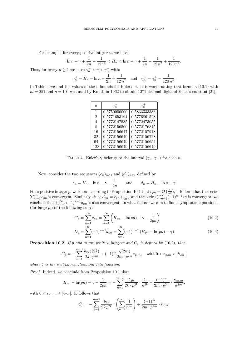
BERNOULLI POLYNOMIALS AND APPLICATIONS 39
For example, for every positive integer n, we have
lnn+ γ +1
2n− 1
12n2< Hn < lnn+ γ +
1
2n− 1
12n2+
1
120n4.
Thus, for every n ≥ 1 we have γ−n < γ < γ+
n with:
γ+n = Hn − lnn− 1
2n+
1
12n2and γ−
n = γ+n −
1
120n4.
In Table 4 we find the values of these bounds for Euler’s γ. It is worth noting that formula (10.1) withm = 251 and n = 104 was used by Knuth in 1962 to obtain 1271 decimal digits of Euler’s constant [21].
n γ−n γ+
n
1 0.5750000000 0.58333333332 0.5771653194 0.57768615284 0.5772147535 0.57724730558 0.5772156500 0.577217684516 0.5772156647 0.577215791832 0.5772156649 0.577215672864 0.5772156649 0.5772156654128 0.5772156649 0.5772156649
Table 4. Euler’s γ belongs to the interval (γ−n , γ+
n ) for each n.
Now, consider the two sequences (cn)n≥1 and (dn)n≥1 defined by
cn = Hn − lnn− γ − 1
2nand dn = Hn − lnn− γ
For a positive integer p, we know according to Proposition 10.1 that cpn = O(
1n2
), it follows that the series∑∞
n=1 cpn is convergent. Similarly, since dpn = cpn+1
2pn and the series∑∞
n=1(−1)n−1/n is convergent, we
conclude that∑∞
n=1(−1)n−1dpn is also convergent. In what follows we aim to find asymptotic expansions,(for large p,) of the following sums:
Cp =
∞∑
n=1
cpn =
∞∑
n=1
(Hpn − ln(pn)− γ − 1
2pn
)(10.2)
Dp =
∞∑
n=1
(−1)n−1dpn =
∞∑
n=1
(−1)n−1 (Hpn − ln(pn)− γ) (10.3)
Proposition 10.2. If p and m are positive integers and Cp is defined by (10.2), then
Cp = −m−1∑
k=1
b2kζ(2k)
2k · p2k + (−1)m ζ(2m)
2m · p2m εp,m, with 0 < εp,m < |b2m|,
where ζ is the well-known Riemann zeta function.
Proof. Indeed, we conclude from Proposition 10.1 that
Hpn − ln(pn)− γ − 1
2pn= −
m−1∑
k=1
b2k2k · p2k ·
1
n2k+
(−1)m2m · p2m ·
rpn,mn2m
.
with 0 < rpn,m ≤ |b2m|. It follows that
Cp = −m−1∑
k=1
b2k2k p2k
·( ∞∑
n=1
1
n2k
)+
(−1)m2m · p2m · rp,m.
40 OMRAN KOUBA
where rp,m =∑∞
n=1rpn,m
n2m .
Hence,
0 < rp,m =
∞∑
n=1
rpn,mn2m
< |b2m|∞∑
n=1
1
n2m= |b2m| ζ(2m)
and the desired conclusion follows with εp,m = rp,m/ζ(2m). �
For example, when m = 3, we obtain∞∑
n=1
(Hpn − ln(pn)− γ − 1
2pn
)= − π2
72p2+
π4
10800p4+O
(1
p6
).
Similarly, in the next proposition we have the analogous result corresponding to Dp.
Proposition 10.3. If p and m are positive integers and Dp is defined by (10.3), then
Dp =ln 2
2p−
m−1∑
k=1
b2kη(2k)
2k · p2k + (−1)m η(2m)
2m · p2m ε′p,m, with 0 < ε′p,m < |b2m|,
where η(2k) is defined in Corollary 3.2.
Proof. Indeed, let us define an,m by the formula
an,m = Hn − lnn− γ − 1
2n+
m−1∑
k=1
b2k2k · n2k
with empty sum equal to 0. We have shown in the proof of Proposition 10.1 that
(−1)man,m =
∫ 1/2
0
|B2m−1(t)| gn,m(t) dt
where gn,m is the positive decreasing function on [0, 1/2] defined by
gn,m(t) =
∞∑
j=n
(1
(j + t)2m− 1
(j + 1− t)2m
).
Now, for every t ∈ [0, 1/2] the sequence (gnp,m(t))n≥1 is positive and decreasing to 0. So, Using thealternating series criterion [3, Theorem 7.8, and Corollary 7.9] we see that, for everyN ≥ 1 and t ∈ [0, 1/2],
∣∣∣∣∣
∞∑
n=N
(−1)n−1gnp,m(t)
∣∣∣∣∣ ≤ gNp,m(t) ≤ gNp,m(0) =1
(Np)2m.
This proves the uniform convergence on [0, 1/2] of the series
Gp,m(t) =
∞∑
n=1
(−1)n−1gnp,m(t).
Consequently
(−1)m∞∑
n=1
(−1)n−1apn,m =
∫ 1/2
0
|B2m−1(t)|Gp,m(t) dt.
Now using the properties of alternating series, we see that for t ∈ (0, 1/2) we have
0 < Gp,m(t) < gp,m(t) < gp,m(0) =
∞∑
j=p
(1
j2m− 1
(j + 1)2m
)=
1
p2m
Thus,∞∑
n=1
(−1)n−1apn,m =(−1)mp2m
ρp,m
BERNOULLI POLYNOMIALS AND APPLICATIONS 41
with 0 < ρp,m <∫ 1/2
0 |B2m−1(t)| dt.
On the other hand we have
∞∑
n=1
(−1)n−1apn,m = Dp −1
2p
∞∑
n=1
(−1)n−1
n+
m−1∑
k=1
b2k2k p2k
∞∑
n=1
(−1)n−1
n2k
= Dp −ln 2
2p+
m−1∑
k=1
b2kη(2k)
2k · p2k .
Thus
Dp =ln 2
2p−
m−1∑
k=1
b2kη(2k)
2k · p2k +(−1)mp2m
ρp,m
Now, the important estimate for ρp,m is the lower bound, i.e. ρp,m > 0. In fact, considering separatelythe cases m odd and m even, we obtain, for every nonnegative integer m′:
Dp <ln 2
2p−
2m′∑
k=1
b2kη(2k)
2k · p2k ,
and
Dp >ln 2
2p−
2m′+1∑
k=1
b2kη(2k)
2k · p2k .
This yields the following more precise estimate for the error term:
0 < (−1)m(Dp −
ln 2
2p+
m−1∑
k=1
b2kη(2k)
2k p2k
)<|b2m| η(2m)
2m · p2m ,
and the desired conclusion follows. �
In the next lemma, we will show that there are other alternating series that can be expressed interms of Dp, This lemma will be helpful in § 11.
Lemma 10.4. For a positive integer p, we have
Epdef=
∞∑
n=0
(−1)n(Hp(n+1) −Hpn) = ln p+ γ − ln(π2
)+ 2Dp, (10.4)
where Dp is the sum defined by (10.3).
42 OMRAN KOUBA
Proof. Indeed
2Dp = dp +∞∑
n=2
(−1)n−1dpn +∞∑
n=1
(−1)n−1dpn
= dp +
∞∑
n=1
(−1)ndp(n+1) +
∞∑
n=1
(−1)n−1dpn
= dp +
∞∑
n=1
(−1)n−1(dpn − dp(n+1))
= dp +
∞∑
n=1
(−1)n(Hp(n+1) −Hpn) +
∞∑
n=1
(−1)n−1 ln
(n+ 1
n
)
= − ln p− γ +
∞∑
n=0
(−1)n(Hp(n+1) −Hpn) +
∞∑
n=1
(−1)n−1 ln
(n+ 1
n
)
Using Wallis formula for π [13, Formula 0.262], we have
∞∑
n=1
(−1)n−1 ln
(n+ 1
n
)=
∞∑
n=1
ln
(2n
2n− 1· 2n
2n+ 1
)
= − ln
∞∏
n=1
(1− 1
4n2
)= ln
(π2
)
and the desired formula follows. �
11. Asymptotic expansions for certain trigonometric sums
In this section we aim to exploit the results of the previous sections to study the following trigono-metric sums defined for a positive integer p by the formulæ:
Ip =
p−1∑
j=1
1
sin(kπ/p)=
p−1∑
j=1
csc
(kπ
p
)(11.1)
Jp =
p−1∑
j=1
k cot
(kπ
p
)(11.2)
with empty sums interpreted as 0.
While there is a of favourable result [24] concerning the sum∑p
k=1 sec(
2kπ2p+1
), and many favourable
results [6] concerning the power sums∑p−1
k=1 csc2n(kπ/p), it seems that there is no known closed form for
Ip, and the same can be said about the sum Jp. Therefore, we will look for asymptotic expansions forthese sums and will give some tight inequalities that bound Ip and Jp. This investigation complementsthe work of H. Chen in [7, Chapter 7.], and answers an open question raised there.
In the next lemma we give some equivalent forms for the trigonometric sums under consideration.
BERNOULLI POLYNOMIALS AND APPLICATIONS 43
Lemma 11.1. For a positive integer p let
Kp =
p−1∑
k=1
tan
(kπ
2p
), Kp =
p−1∑
j=1
cot
(kπ
2p
),
Lp =
p−1∑
k=1
k
sin(kπ/p), Mp =
p−1∑
k=0
(2k + 1) cot
((2k + 1)π
2p
)
Then,
i. Kp = Kp = Ip.ii. Lp = (p/2) Ip.iii. Mp = (p/2)J2p − 2Jp = −p Ip.
Proof. First, note that the change of summation variable j ← p− j proves that Kp = Kp. So, using thetrigonometric identity tan θ + cot θ = 2 csc(2θ) we obtain
2Kp = Kp + Kp =
p−1∑
k=1
(tan
(kπ
2p
)+ cot
(kπ
2p
))
= 2
p−1∑
k=1
csc
(kπ
p
)= 2Ip
This proves (i).
Similarly, (ii) follows from the change of summation variable j ← p− j in Lp:
Lp =
p−1∑
j=1
p− k
sin(kπ/p)= pIp − Lp
Also,
Mp =∑
1≤k<2pk odd
k cot
(kπ
2p
)=
2p−1∑
k=1
k cot
(kπ
2p
)−
∑
1≤k<2pk even
k cot
(kπ
2p
)
=
2p−1∑
k=1
k cot
(kπ
2p
)− 2
p−1∑
k=1
k cot
(kπ
p
)= J2p − 2Jp.
But
J2p =
p−1∑
k=1
k cot
(kπ
2p
)+
2p−1∑
k=p+1
k cot
(kπ
2p
)
=
p−1∑
k=1
k cot
(kπ
2p
)−
p−1∑
k=1
(2p− k) cot
(kπ
2p
)
= 2
p−1∑
k=1
k cot
(kπ
2p
)− 2pKp
Thus, using (i) and the trigonometric identity cot(θ/2)− cot θ = csc θ we obtain
Mp = J2p − 2Jp = 2
p−1∑
k=1
k
(cot
(kπ
2p
)− cot
(kπ
p
))− 2pIp
= 2
p−1∑
k=1
k csc
(kπ
p
)− 2pIp = 2Lp − 2pIp = −pIp
This concludes the proof of (iii). �
44 OMRAN KOUBA
Proposition 11.2. For p ≥ 2, let Ip be the sum of cosecants defined by the (11.1). Then
Ip = −2 ln 2
π+
2p
πEp,
= −2 ln 2
π+
2p
π(ln p+ γ − ln(π/2)) +
4p
πDp,
where Dp and Ep are defined by formulæ (10.3) and (10.4) respectively.
Proof. Indeed, our starting point will be the “simple fractions” expansion (6.4) of the cosecant function:
π
sin(πα)=∑
n∈Z
(−1)nα− n
=1
α+
∞∑
n=1
(−1)n(
1
α− n+
1
α+ n
)
which is valid for α ∈ C \ Z. Using this formula with α = k/p for k = 1, 2, . . . , p − 1 and adding, weconclude that
π
pIp =
p−1∑
k=1
1
k+
∞∑
n=1
(−1)np−1∑
k=1
(1
k − np+
1
k + np
)
=
p−1∑
k=1
1
k+
∞∑
n=1
(−1)n−
pn−1∑
j=p(n−1)+1
1
j+
p(n+1)−1∑
j=pn+1
1
j
,
and this result can be expressed in terms of the Harmonic numbers as follows
π
pIp = Hp−1 +
∞∑
n=1
(−1)n(−Hpn−1 +Hp(n−1) +Hp(n+1)−1 −Hpn
)
= Hp−1 +
∞∑
n=1
(−1)n(Hp(n+1) − 2Hpn +Hp(n−1)
)+
1
p
∞∑
n=1
(−1)n(1
n− 1
n+ 1
)
= Hp−1 +∞∑
n=1
(−1)n(Hp(n+1) − 2Hpn +Hp(n−1)
)+
1
p
( ∞∑
n=1
(−1)nn
+∞∑
n=2
(−1)nn
)
= Hp +
∞∑
n=1
(−1)n(Hp(n+1) − 2Hpn +Hp(n−1)
)− 2
p
∞∑
n=1
(−1)n−1 1
n
= Hp −2 ln 2
p+
∞∑
n=1
(−1)n(Hp(n+1) − 2Hpn +Hp(n−1)
).
Thus
π
pIp +
2 ln 2
p= Hp +
∞∑
n=1
(−1)n(Hp(n+1) −Hpn
)+
∞∑
n=1
(−1)n(Hp(n−1) −Hpn
)
=
∞∑
n=0
(−1)n(Hp(n+1) −Hpn
)+
∞∑
n=1
(−1)n(Hp(n−1) −Hpn
)
= Ep + Ep = 2Ep,
and the desired formula follows according to Lemma 10.4. �
Combining Proposition 11.2 and Proposition 10.3, we obtain:
Proposition 11.3. For p ≥ 2 and m ≥ 1, we have
πIp = 2p ln p+ 2(γ − ln(π/2))p−m−1∑
k=1
2b2kη(2k)
k · p2k−1+ (−1)m 2η(2m)
m · p2m−1ε′p,m
with 0 < ε′p,m < |b2m|.
BERNOULLI POLYNOMIALS AND APPLICATIONS 45
Using the values of the η(2k)’s from Corollary 3.2, and considering separately the cases m even andm odd we obtain the following corollary.
Corollary 11.4. For every positive integer p and every nonnegative integer n, the sum of cosecants Ipdefined by (11.1) satisfies the following inequalities:
Ip <2p
π(ln p+ γ − ln(π/2)) +
2n∑
k=1
(−1)k (22k − 2)b22kk · (2k)!
(π
p
)2k−1
,
and
Ip >2p
π(ln p+ γ − ln(π/2)) +
2n+1∑
k=1
(−1)k (22k − 2)b22kk · (2k)!
(π
p
)2k−1
.
As an example, for n = 0 we obtain the following inequality, valid for every p ≥ 1 :
2p
π(ln p+ γ − ln(π/2))− π
36p< Ip <
2p
π(ln p+ γ − ln(π/2)).
This answers positively the open problem proposed in [7, Section 7.4].
Remark 11.5. The asymptotic expansion of Ip was proposed as an exercise in [17, Exercise 13, p. 460],and it was attributed to P. Waldvogel, but the result there is less precise than Corollary 11.4
Now we turn our attention to the other trigonometric sum Jp. Next we find an analogous result toProposition 11.2.
Proposition 11.6. For a positive integer p, let Jp be the sum of cotangents defined by the (11.2). Then
πJp = −p2 ln p+ (ln(2π)− γ)p2 − p+ 2p2Cp
where Cp is defined by the formula (10.2).
Proof. Recall that cn = Hn − lnn− γ − 12n satisfies cn = O(1/n2). Thus, both series
Cp =
∞∑
n=1
cpn and Cp =
∞∑
n=1
(−1)n−1cpn
are convergent. Further, we note that Cp = Dp − ln 22p where Dp is defined by (10.3).
According to Remark 11.10 we have
Cp =ln(π/2)− γ − ln p
2+
π
4pIp. (11.3)
Now, noting that
Cp =∑
n≥1n odd
cpn +∑
n≥1n even
cpn =∑
n≥1n odd
cpn +
∞∑
n=1
c2pn
Cp =∑
n≥1n odd
cpn −∑
n≥1n even
cpn =∑
n≥1n odd
cpn −∞∑
n=1
c2pn
we conclude that Cp − Cp = 2C2p, or equivalently
Cp − 2C2p = Cp (11.4)
On the other hand, for a positive integer p let us define Fp by
Fp =ln p+ γ − ln(2π)
2+
1
2p+
π
2p2Jp. (11.5)
46 OMRAN KOUBA
It is easy to check, using Lemma 11.1 (iii), that
Fp − 2F2p =ln(π/2)− ln p− γ
2− π
4p2(J2p − 2Jp)
=ln(π/2)− ln p− γ
2+
π
4pIp (11.6)
We conclude from (11.4) and (11.6) that Cp − 2C2p = Fp − 2F2p, or equivalently
Cp − Fp = 2(C2p − F2p).
Hence,
∀m ≥ 1, Cp − Fp = 2m(C2mp − F2mp) (11.7)
Now, using Proposition 10.1 to replace Hp in Proposition 9.2, we obtain
π
p2Jp = ln(2π)−Hp −
1
2p+O
(1
p2
)
= ln(2π)− ln p− γ − 1
p+O
(1
p2
)
Thus Fp = O(
1p2
). Similarly, from the fact that cn = O
(1n2
)we conclude also that Cp = O
(1p2
).
Consequently, there exists a constant κ such that, for large values of p we have |Cp − Fp| ≤ κ/p2. So,from (11.7), we see that for large values of m we have
|Cp − Fp| ≤κ
2mp2
and letting m tend to +∞ we obtain Cp = Fp, which is equivalent to the announced result. �
Combining Proposition 11.6 and Proposition 10.2, we obtain:
Proposition 11.7. For p ≥ 2 and m ≥ 1, we have
πJp = −p2 ln p+ (ln(2π)− γ)p2 − p−m−1∑
k=1
b2kζ(2k)
k · p2k−2+ (−1)m ζ(2m)
m · p2m−2εp,m,
with 0 < εp,m < |b2m|, where ζ is the well-known Riemann zeta function.
Using the values of the ζ(2k)’s from Corollary 3.2, and considering separately the cases m even andm odd we obtain the next corollary.
Corollary 11.8. For every positive integer p and every nonnegative integer n, the sum of cotangents Jpdefined by (11.2) satisfies the following inequalities:
Jp <1
π
(−p2 ln p+ (ln(2π)− γ)p2 − p
)+ 2π
2n∑
k=1
(−1)k b22kk · (2k)!
(2π
p
)2k−2
,
and
Jp >1
π
(−p2 ln p+ (ln(2π)− γ)p2 − p
)+ 2π
2n+1∑
k=1
(−1)k b22kk · (2k)!
(2π
p
)2k−2
.
As an example, for n = 0 we obtain the following double inequality, which is valid for p ≥ 1 :
0 <1
π
(−p2 ln p+ (ln(2π)− γ)p2 − p
)− Jp <
π
36
BERNOULLI POLYNOMIALS AND APPLICATIONS 47
Remark 11.9. It is not clear that one can prove Proposition 11.7 by combining Propositions 9.2 and10.1 directly.
Remark 11.10. Note that we have proved the following results. For a postive integer p:
∞∑
n=1
(−1)n−1(Hpn − ln(pn)− γ) =ln(π/2)− γ − ln p
2+
ln 2
2p+
π
4p
p−1∑
k=1
csc
(kπ
p
).
∞∑
n=0
(−1)n(Hp(n+1) −Hpn) =ln 2
p+
π
2p
p−1∑
k=1
csc
(kπ
p
).
∞∑
n=1
(Hpn − ln(pn)− γ − 1
2pn
)=
ln p+ γ − ln(2π)
2+
1
2p+
π
2p2
p−1∑
k=1
k cot
(kπ
p
).
These results are to be compared with those in [22], see also [23].
12. Endnotes
Bernoulli numbers appeared in the work Jacob Bernoulli (1654-1705, Basel, Switzerland) in connec-tion with evaluating the sums of the form
∑ni=1 i
k. They appear in Bernoulli’s most original work Ars
Conjectandi, (“The Art of Conjecturing”,) published by his nephew in Basel in 1713, eight years after hisdeath. They also appear independantly in the work of the Japanese Mathematician Seki Takakazu (SekiKowa) (1642-1708). Bernoulli numbers are related to Fermat’s Last Theorem by Kummer’s theorem [25],this opened a very large and furctuous field of investigation (see [19, Chapter 15].)
The Euler-Maclaurin’s Summation Formula was developed independantly by Leonhard Euler (1736)and Colin MacLaurin (1742). The aim was to provide a powerful tool for the computation of severalsums like the harmonic numbers.
Finally, a thorough bibliography on Bernoulli numbers and their applications that contains morethan 3000 entries can be found on the web [11].
References
[1] Abramowitz, M. and Stegan, I. A., Handbook of Mathematical Functions, with Formulas, Graphs, and MathematicalTables, Dover Books on Mathematics, Dover Publication, Inc., New York, (1972).
[2] Ahlfors, L. V., Complex Analysis, McGraw-Hill, Inc. (1979).
[3] Amann, H. and Escher, J., Analysis I, Birkhauser Verlag, Basel -Boston-Berlin. (2005).
[4] Athreya, K. B. and Lahiri, S. N., Measure Theory and Probability Theory, Springer Science+Business Media, LLC.(2006).
[5] Bergmann, H., Eine explizite Darstellung der Bernoullischen Zahlen, Math. Nachr., 34, (1967), pp.377-378.
[6] Chen, H., On some trigonometric power sums, Internat. J. Math. Math. Sci, 30, (2002), 185–191.
[7] , Excursions in Classical Analysis, Mathematical Association of America, Inc. (2010).
[8] Deeba, E. Y. and Rodrigues, D. M., Stirling’s Series and Bernoulli Numbers, The American Mathematical Monthly,98, 5 (1991), pp.423–426.
[9] Dilcher, K., Asymptotic Behaviour of Bernoulli, Euler, and Generalized Bernoulli Polynomials, Journal of Approxima-tion Theory, 49, (1987), 321–330.
[10] , Zeros of Bernoulli, generalized Bernoulli and Euler polynomials, Mem. Amer. Math. Soc., Number 386, (1988).
[11] Dilcher, K. and Slavutskii, I. Sh., A Bibliography of Bernoulli Numbers (1713-2007).[ONLINE : http://http://www.mathstat.dal.ca/∼dilcher/bernoulli.html].
[12] Gould. H. W., Explicit formulas for Bernoulli numbers, The American Mathematical Monthly, 79, 1 (1972), pp.44–51.
[13] Gradshteyn, I. and Ryzhik, I., Tables of Integrals, Series and Products, 7th ed., Academic Press, (2007).
[14] Grafakos, L., Classical Fourier Analysis, Second edition., Graduate Texts in Mathemetics, Springer Science+BusinessMedia, LLC. (2008).
48 OMRAN KOUBA
[15] Graham, R. L., Knuth, D. E., and Patashnik, O. Concrete Mathematics : a foundation for computer science, 2nd ed.Addison-Wesley Publishing Company, Inc, (1994).
[16] Hardy, G. H. and Wright, E. M., An introduction to the theory of numbers, 6th ed., Oxford University Press, (2007).
[17] Henrici, P., Applied and Computational Complex Analysis, Vol. 2, John Wiley & Sons, New York, (1977).
[18] Inkeri, K., The real roots of Bernoulli polynomials, Ann. Univ. Turku. Ser. A I37 (1959), 20pp.
[19] Ireland, K. and Rosen, M., A Classical Introduction to Modern Number Theory, 2nd ed., Springer-Verlag, New York,Inc, (1990).
[20] Katznelson, Y., Introduction To Harmonic Analysis, 3rd ed., Cambridge University Press, (2004).
[21] Knuth, D. E., Eulers constant to 1271 places, Math. Comput., 16, (1962), pp. 275–281.
[22] Kouba, O., The sum of certain series related to harmonic numbers, Octogon Mathematical Magazine, 19, No. 1 (2011),pp.3–18.[ONLINE : http://www.uni-miskolc.hu/∼matsefi/Octogon/].
[23] , Proposed Problem 11499, The American Mathematical Monthly, 117, 7 (2010), p.371.
[24] Kouba, O., and Andreescu, T., Solution to Problem U207, Mathematical Reflections, Issue 5, (2011), p.16.
[ONLINE : http://www.awesomemath/home].
[25] Kummer E. E.,Allgemeiner Beweis des Fermat’schen Satzes, dass die Gleichung xλ + yλ = zλ durch ganze Zahlenunlosbar ist, fur alle diejenigen Potenz-Exponenten λ, welche ungerade Primzahlen sind und in den Zahlern der ersten(λ− 3)/2 Bernoulli’schen Zahlen als Factoren nicht vorkommen, J. Reine Angew. Math. 40 (1850), pp.131–138.
[26] Lehmer, D. H., On the maxima and minima of Bernoulli Polynomials, The American Mathematical Monthly, 47, 8(1940). pp, 533–358.
[27] Namias, V., A simple Derivation of Stirling’s Asymptotic Series, The American Mathematical Monthly, 93, 1 (1986).pp, 25–29.
Department of Mathematics, Higher Institute for Applied Sciences and Technology, P.O. Box 31983, Damascus,
Syria.
E-mail address: omran [email protected]


