Embed Size (px)
Citation preview

Beyond the Power Law: Uncovering Stylized Facts in Interbank Networks
Benjamin Vandermarliere∗
Department of Physics and Astronomy,Department of General Economics,
Ghent University, Belgium
Alexei Karas†
University College Roosevelt,Utrecht University School of Economics,
The Netherlands
Jan Ryckebusch‡
Department of Physics and Astronomy,Ghent University, Belgium
Koen Schoors§
Department of General Economics,Ghent University, Belgium
(Dated: September 17, 2014)
We use daily data on bilateral interbank exposures and monthly bank balance sheets to studynetwork characteristics of the Russian interbank market over Aug 1998 - Oct 2004. Specifically,we examine the distributions of (un)directed (un)weighted degree, nodal attributes (bank assets,capital and capital-to-assets ratio) and edge weights (loan size and counterparty exposure). Wesearch for the theoretical distribution that fits the data best and report the “best” fit parameters.We observe that all studied distributions are heavy tailed. The fat tail typically contains 20% ofthe data and can be systematically described by a truncated power law. In most cases, however,separating the bulk and tail parts of the data is hard, so we proceed to study the full range of theevents. We find that the stretched exponential and the log-normal distributions fit the full rangeof the data best. These conclusions are robust to 1) whether we aggregate the data over a week,month, quarter or year; 2) whether we look at the “growth” versus “maturity” phases of interbankmarket development; and 3) with minor exceptions, whether we look at the “normal” versus “crisis”operation periods. In line with prior research, we find that the network topology changes greatly asthe interbank market moves from a “normal” to a “crisis” operation period.
PACS numbers: 89.65.Gh, 89.75.Fb, 89.75.Hc
I. INTRODUCTION
The frequency of an event follows a power law whenthat frequency varies as a power of some attribute of thatevent (e.g. its size). Power-law distributions have beenclaimed to occur in an extraordinarily diverse range ofphenomena from the sizes of wars, earthquakes and com-puter files to the numbers of papers scientists write andcitations those papers receive [1]. In economics and fi-nance, power laws have been documented for income andwealth [2], the size of cities and firms, stock market re-turns, trading volume, international trade, and executivepay [3]. Most relevant to this paper, the tail parts of in-terbank network characteristics, such as degree distribu-tion, have been shown to follow a power law too (see [4]
∗Electronic address: [email protected]†Electronic address: [email protected]‡Electronic address: [email protected]§Electronic address: [email protected]
for Brazil, [5, 6] for Austria, [7] for the US Fedwire sys-tem, and [8] for the commercial banks in the US). Thisubiquituous presence of power laws has resulted in anextensive search for universal dynamics that can explaintheir existence (see [9, 10] for examples of such search ininterbank networks).
Recently, however, Clauset et. al. [11] (followed by[12]) call these findings into question. In particular,they critisize the commonly used methods for analyzingpower-law data, such as least-squares fitting, which canproduce inaccurate estimates of parameters for power-law distributions or provide no indication of whether thedata obey a power law at all. Clauset et. al. propose a sta-tistical framework for discerning and quantifying power-law behavior in empirical data and apply that frame-work to twenty-four real-world data sets, each of whichhas been conjectured to follow a power law. For mostdatasets they find moderate to weak evidence in favor ofpower laws.
This debate about the potential of power laws to cap-ture the underlying network dynamics is important foreconomic policy. For example, current research on con-
arX
iv:1
409.
3738
v1 [
q-fi
n.G
N]
12
Sep
2014

2
tagion in interbank markets often relies on a scale-freetopology to simulate the interbank network [13, 14].This choice likely affects the outcome of conducted stresstests (as is explicitly confirmed by [14]) and, therefore,the policy implications stemming from them. Yet theevidence supporting this choice is not ironclad.
This paper contributes to the debate by providinga detailed analysis of the network characteristics of areal interbank network over an extended period of time.We use daily data on bilateral interbank exposures andmonthly bank balance sheets to study network character-istics of the Russian interbank market over Aug 1998 -Oct 2004. We focus on measures that represent essentialinput for most of the interbank contagion simulations.Specifically, we examine the distributions of (un)directed(un)weighted degree, nodal attributes (bank assets, cap-ital and capital-to-assets ratio) and edge weights (loansize and counterparty exposure). Using the methodologyof [11] we set up a horse race between the different the-oretical distributions to find one that fits the data best.We then study the time evolution of the best-fit param-eters.
We observe that all studied distributions are heavytailed. The fat tail typically contains 20% of the dataand can be systematically described by a truncated powerlaw. In most cases, however, separating the bulk and tailparts of the data is hard, so we proceed to study the fullrange of the events. We find that the stretched exponen-tial and the log-normal distributions fit the full range ofthe data best. Our conclusions turn out to be robust towhether we aggregate the data over a week, month, quar-ter or year. Further, we find no qualitative differencebetween the “growth” and “maturity” phases of inter-bank market development and little difference betweenthe “crisis” and “non-crisis” periods.
Sec. II describes our data, defines the network mea-sures we study, and summarizes the conclusions fromprevious studies of those measures. Sec. III and IV, re-spectively, describe and illustrate the methodology weuse to find the theoretical distribution that fits the databest. Sec. V reports the results. Sec. VI concludes.
II. DATA AND DEFINITIONS
A. Data Source
Mobile, a private financial information agency, pro-vided us with two datasets for the period Aug 1998 -Oct 2004. [29] The information in the datasets is a partof standard disclosure requirements and is supplied tothe regulator on a monthly basis. The first dataset, de-scribed in [15], contains monthly bank balances for mostRussian banks. From this dataset we take two variables:total assets and capital. The second dataset containsmonthly reports “On Interbank Loans and Deposits” (of-ficial form’s code 0409501) and represents a register of allinterbank loans issued in the Russian market. For each
loan we know its size, interest rate, issuer, receiver, re-porting date and maturity date.
On average, about half of the Russian banks are activeon the interbank market. Consequently, the analysis ofinterbank network measures includes fewer banks thanthe analysis of balance sheet indicators.
B. Network Measures
We use the two aforementioned datasets to constructan interbank network with banks as nodes and mutualcontracts representing edges. This procedure is per-formed for aggregated data covering various time inter-vals. In every situation, we construct three versions ofthe interbank network, which differ in the level of detailin quantifying the edges. In the undirected version, anundirected unweighted edge is established between banksif they exchange money on the interbank market duringthe considered time period. For the directed versions, wediscriminate between the issuer and the receiver of theinterbank loan. A directed edge, which points from is-suer to receiver, is established if the issuer has lent moneyto the receiver in the considered period. In the multidi-rected version, every interbank loan is represented by adirected edge pointing from issuer to receiver. This im-plies there can be several edges between pairs of nodes.
In this paper we focus on network characteristics thatrepresent essential input for typical interbank contagionsimulations [13, 16–18]. We distinguish three types ofnetwork characteristics: nodal attributes, edge weightsand various measures of a node’s centrality.
We consider three nodal attributes: bank capital, totalassets and leverage. Total assets proxy for bank size.Capital measures its financial buffer. Leverage is definedas capital divided by total assets. We exclude banks withnegative assets (data errors) or negative capital (banksin effective default) from our sample.
Edge weights are measured separately for the directedand the multidirected network. For the former, the edgeweight equals counterparty exposure, that is, the totalamount of money the issuer has lent to the receiver inthe considered time period.
For the multidirected network, the edge weight equalsthe size of the issued loan.
We consider various measures of a node’s centrality.For an undirected network, we define the degree of anode as the number of edges connected to that node.It measures the number of counterparties a bank has onthe interbank market. For the directed network, an in-degree (out-degree) of a node is the number of incoming(outgoing) edges; it measures the number of interbanklenders (borrowers) a bank has. For the multidirectednetwork, an in-degree (out-degree) is the number of re-ceived (issued) loans. Finally, for each bank we definethe total in-exposure (out-exposure) as the total amountof money borrowed from (lent to) the market.
The interbank network characteristics we consider in

3
this paper have already been studied for a number ofcountries. Here we summarize the main findings of thosestudies.
The majority of studies find numerous heavy tailedvariables in the interbank network. In addition, manyauthors propose a power law as the best-fit candidateto (at least the tail of) the empirical distribution. Inparticular, Goddard et al. [8] find that the asset size dis-tribution of U.S. commercial banks is well described bya truncated lognormal, while the tail part is well fittedwith a power law. Cont et al. [4] obtain fair fits to thetails of the in-degree, out-degree, total degree, and expo-sure size distributions of the Brazilian interbank networkwith power laws. Soramaki et al. [7] put forward a powerlaw to describe the out-degree distribution, as well asthe number of transactions between pairs of banks in theUS Fedwire system. In the Austrian interbank marketthe loan size distribution is well described by a powerlaw [5, 6]. That same study also examines the degreedistribution of the undirected network and the in- andout-degree distribution of the directed alternative. Eachof these three distributions is seemingly well described bytwo power laws, one for the low-degree region and one forthe tail part. Finally, Iori et al. [19] investigate the distri-butions of the in-degree, out-degree and exposure of theindividual banks in the Italian market. The authors donot attempt to fit their data with some theoretical distri-bution. They do find, however, a structural difference inthe network topology between the months of the globalfinancial crisis of 2008 and normal operating months.
Few studies, however, consider alternate theoreticaldistributions as candidates to describe their data. Theones that do [20], in fact, cast doubt on the ability ofpower laws to provide the best empirical fit. In whatfollows, we too consider an extensive list of alternativetheoretical distributions and identify those that describeboth the tail and the entire distribution better than thepower law. Along the way, we apply a criterion whichallows us to discriminate between the tail and the bulkparts of the data.
C. Descriptive Statistics
Different phases of the interbank market development(for example, growth versus maturity, or crisis versusnon-crisis) may be guided by a different data generat-ing mechanism. For example, Iori et al. [19] find a struc-tural difference in the Italian interbank network topologybefore versus during the 2008 financial crisis. This find-ing suggests that the choice of the distribution that bestfits the data may vary over time, and in particular maydiffer between crisis and non-crisis periods. In Sect. Vwe check whether such variation exists. In this section,we provide evidence that the Russian interbank market,indeed, went through some distinct development phases.
Fig. 1 shows the time series of the number of banksactive on the interbank market and of the number of is-
1998 1999 2000 2001 2002 2003 2004 2005Time (year)
2
4
6
8
10
Num
ber o
f Ban
ks (x
100)
Crisis 1 Crisis 2
8
16
24
32
Num
ber o
f Loa
ns (x
1000
)
FIG. 1: (Color online) The time dependence of the numberof active banks (solid line) and the number of interbank loans(dashed line) in the Russian interbank network between 1998and 2005. Data are aggregated over a month. The arrowsindicate the start of the two “crises”.
sued loans. For this figure we use data aggregated overa month. Over 1998-2002 the interbank network expe-riences growth: we observe a steady and comparable in-crease in the number of active banks and of issued loans.After 2002, the interbank network gradually matures: thenumber of active banks flattens out while the number ofloans per bank grows. Note, however, the strong varia-tion in the number of issued loans from the second halfof 2003 onwards.
As is clearly indicated in Fig. 1, our sample period in-cludes two crises: one in August 1998 and one in the sum-mer of 2004. Both crises resulted in a partial meltdownof the Russian interbank market. They coincide with theedges of the sample period and are clearly marked by a re-duction in the number of active banks and issued loans.The first crisis got triggered on August 17, 1998 whenRussia abandoned its exchange rate regime, defaulted onits domestic public debt and declared a moratorium on allprivate foreign liabilities. The second crisis was ignitedby an investigation of banks accused of money launder-ing and sponsorship of terrorism. This gave rise to awave of distrust among banks and a consequent liquiditydrought.
Fig. 2 illustrates the impact of Aug 1998 crisis on theRussian interbank network. Nodes are banks, and di-rected edges represent issued loans. The first panel showsthe activity in the market in the two weeks leading upto the seizure, whereas the second panel covers the twoweeks after the collapse. Evidently, we see a decrease inthe number of active banks, from 87 to 65, and in thenumber of loans granted, from 507 to 96. When consid-ering the structure in this unweighted multidirected net-work we can find a clear distinction between the “normal”and “crisis” periods. The technique of Ref. [21] can be

4
FIG. 2: (Color online) The activity on the interbank marketin the two weeks leading up to August 17, 1998 (top panel)and the two consecutive weeks (bottom panel). A bank isrepresented as node and each link represents an issued loan.Nodes are colored per block as defined in Ref. [21].
used to uncover groups of nodes, called blocks, which ful-fil similar roles in the network. In the two weeks leadingup to the crisis we get an interbank market with 5 blocks(and two isolated banks). After the crisis the number ofidentified blocks goes down to 3. Notably, the identifiedblocks interact with each other before the crisis but notafter. So the crisis disintegrates the network and recon-figures banks’ role in it.
We can also see evidence of different developmentphases by studying the time evolution of two basic net-work measures: the average local clustering coefficientand the average shortest path length. For an undirectednetwork, the local clustering coefficient 0 ≤ cu ≤ 1 of anode u is the number of the edges between the nodes ofthe neighborhood of u divided by the maximum amountthat could possibly exist between them. It can be conve-niently defined as in [22]
cu =2T (u)
deg(u) (deg(u)− 1), (1)
where T (u) is the number of triangles (a subgraph withthree nodes and three edges) attached to u and deg(u)is the degree of u. The average of this local clustering
coefficient is
C =1
n
∑u∈G
cu, (2)
where n is the number of nodes in the network G [23].The average shortest path length D is defined as
D =∑u,v∈V
d(u, v)
n(n− 1)(3)
where V is the set of nodes in the network G, and d(u, v)is the length of the shortest path from node u to v [24].In a disconnected graph D can only be computed for thelargest connected component.
Fig. 3 shows the time evolution of C and D computedper month for the largest connected component of theundirected interbank network. First, note that the localclustering coefficient averaged over all nodes and time pe-riods (C = 0.198) is nearly identical to the one reportedby [4] for the Brazilian interbank market (C = 0.2). Incontrast, the average shortest path length (D ≈ 3) isnotably higher compared to Austrian (D = 2) [5] andMexican (D = 1.7) [25] interbank networks.C and D tend to move in the opposite direction: three
months after the first crisis hits C drops while D spikes;during the growing phase of the network (1999-2002) Cgrows while D falls; during the mature phase (2002-2004)both measures stabilize at C ≈ 0.22 and D ≈ 3; finally,during the 2004 crisis C drops while D spikes again. Theaverage local clustering coefficient C, however, tends tohave bigger fluctuations from period to period. In con-trast, the time series of the average shortest path lengthis very smooth, and the only two obvious spikes occuraround the two crises. Clearly, those crises disrupted theoverall network structure: the liquidity drought, whichis equivalent to the pruning of links, caused a significantincrease in the average shortest path length. Even thedecrease in the number of nodes, and hence shrinking ofthe network, could not offset this effect. The 1998 spikein D is particularly remarkable given we only consider thelargest connected component, that is, about one third ofthe nodes (see Fig. 2). We thus conclude that the averageshortest path length has some potential to discriminatebetween the “normal” and the “crisis” operation periodsof the interbank market.
III. METHODOLOGY
For each network measure we test whether the powerlaw or an alternate fat-tailed distribution fits the databest. First, we fit distributions to the tail, then to theentire data range. Along the way, we apply a criterionwhich allows us to discriminate between the tail and thebulk parts of the data.
To study the tail we adopt the methodology ofRef. [11]. First, we fit a power law (PL) to the data to

5
1998 1999 2000 2001 2002 2003 2004 2005Time (year)
0.1
0.2
0.3Av
erag
e C
lust
erin
g C
oeffi
cien
t
3
4
5
Aver
age
Shor
test
Pat
h Le
ngth
FIG. 3: (Color online) The time dependence of the averageclustering coefficient (solid line) and the average shortest pathlength (dashed line) calculated for the most connected com-ponent of the undirected version of the Russian interbanknetwork between 1998 and 2005. Data are aggregated over amonth.
TABLE I: Definition of the normalized distributions used inthis work. The constant C is defined by the normalizationcondition
∫∞xmin
f(x)dx = 1.
Distribution f(x)
Power law (PL) Cx−α
Truncated power law (TPL) Cx−αe−λx
Exponential (Exp) Ce−λx
Stretched exponential (SExp) Cxβ−1e−(λx)β
Log-normal (LN) Cx
exp[− (ln x−µ)2
2σ2
]
determine the starting point of the tail part (the so-calledcut-off xmin of the scaling range). Then we fit each ofthe theoretical distributions to the tail using maximumlikelihood (ML). Finally, we use a relative goodness-of-fittest to select the distribution that fits the data best. Weconsider the same selection of theoretical distributions asin Ref. [11]. Their functional forms are listed in Table Iand involve one or two free parameters.
For completeness and to introduce the notation webriefly sketch the methodology of Ref. [11]. Considera given ordered data set {xj , j = 1, . . . , N}. Every entryxj is a potential xmin and for each of those we computethe ML estimate of the power-law exponent α
α (xj = xmin) = 1 + (N − j + 1)
N∑i=j
lnxixmin
. (4)
We then use the Kolmogorov-Smirnov test to selectthe optimum xmin. It is defined as the cut-off which
minimizes the quantity
Z = maxx≥xmin
| S(x)− P (x) | . (5)
Here, S(x) is the cumulative distribution function (CDF)of the observed values for xj ≥ xmin, and P (x) =C−α+1
(x−α+1 − x−α+1
min
)is the CDF of the power-law fit
to the tail part of the data.In the next step, for given xmin, we perform ML fits
to the data with the other four candidate distributionsof Table I. As argued by Ref. [11], it is more usefulto know which distribution is the best possible fit can-didate, rather than the goodness of fit for each distribu-tion individually. To compare the relative goodness ofthe different fits, we compute the likelihood ratios R forthe pairs of probability density functions (PDFs) p1(xi)and p2(xi)
R (p1, p2) =L1
L2=
N∏i=j
p1(xi)
p2(xi). (6)
The corresponding normalized loglikelihood ratiosR (p1, p2) read
R (p1, p2) =1
σ12√N − j + 1
N∑i=j
[lnp1(xi)
p2(xi)
]
=1
σ12√N − j + 1
N∑i=j
[l(1)i − l
(2)i
], (7)
where l(k)i = ln pk(xi) and σ12 is defined as
σ212 =
1
N − j + 1
N∑i=j
[(l(1)i − l
(2)i
)−(l(1) − l(2)
)]2.
(8)The R (p1, p2) is positive (negative) if the data is morelikely in the p1 (p2) distribution.
In order to guarantee that the value of R is not merelya product of fluctuations and that the true expectationvalue of R is zero, we compute the probability that themeasured normalized log likelihood ratio has a magnitudeas large or larger than the observed value |R|. This so-called p-value is defined as
p (R) =1√2π
[∫ −|R|−∞
e−t2
2 dt+
∫ ∞|R|
e−t2
2 dt
]. (9)
The distribution pk with the highest value of
g (pk) =∑l 6=k
R (pk, pl) , (10)
is considered as the most suitable distribution amongthe different candidates {pi}. Bootstrapping and theKolmogorov-Smirnov test are alternate methods to com-pute the p values. Both methods, however, are subjectto some pitfalls as outlined in Ref. [26].

6
10-1 100 101 102 103 104 105
Out-Exposure (106 Rb)
10-3
10-2
10-1
100C
CD
F
(a)
PLTPLExpSExpLNData
103 104
Out-Exposure (106 Rb)
10-3
10-2
10-1
100
CC
DF
(b)
PLTPLExpSExpLNData
FIG. 4: (Color online) The complementary cumulative distri-bution functiom (CCDF) of the entire (a) and tail part (b)of the monthly-aggregated out-exposure distribution for Jan-uary 2002. Also shown are the ML fits to the CCDFs for thefive distributons of Table I.
A drawback of the above mentioned procedure is thatthe cut-off xmin is determined by a power-law fit. Thisintroduces a bias toward a PL as the best fit candidatedistribution.
We stress that the above-sketched methodology ofRef. [11] can not only be applied to the analysis of thetail part of the data but also to the full range of the databy setting xmin = x1. When considering the full rangeof data it is natural to select a set of theoretical distri-butions that encompass a Gaussian-like regime (thermalor bulk part) supplemented with a fat tail (superther-mal part). Examples of such distributions include thestretched exponential and the log-normal.
IV. ILLUSTRATION OF METHODOLOGY FOROUT-EXPOSURE DISTRIBUTION
As a prototypical example of the methodology sketchedin Sec. III, we explore the out-exposure distribution forthe monthly aggregated data. The data for the out-exposure distribution of January 2002 shown in Fig. 4 areexemplary for all considered 70 months (January 1999 -October 2004). The considered values for the out expo-sure extend over more than five orders of magnitude andthe distribution can be labelled as heavy-tailed [30].
Using the methodology outlined in Sec. III we iden-tify the tail part of the data. From Fig. 4(b) it is clearthat fits to the tail part of the considered data withthe two-parameter log-normal (LN), stretched exponen-tial (SExp) and truncated power law (TPL) distributionsoutperform those with the one-parameter exponential(Exp) and power law (PL) distributions. The parameterλ in the TPL accounts for the finite-size effects near theupper edge of the out-exposure distribution. For eachof the 70 months in our sample we compute the ratiosR (p1, p2) of Eq. (7) for all pair combinations out of thelist of five distributions of Table I. In Fig. 5 we display thetime series of the R (TPL, p2) for p2 =PL, Exp, SExp,and LN. We observe that R (TPL, p2) is mostly positive,which indicates that the TPL offers the best overall de-scription of the tail of the out-exposure data. In order totest the significance of this observation, we evaluate the pvalues. If the normalized ratio for a pair of distributionsin a given month is significant at a one percent level, thedata points in Fig. 5 are dotted. The figure indicates thatthe two-parameter TPL is a significantly better fit to thetail of the monthly-aggregated out-exposure distributionthan a power law and an exponential. The TPL, how-ever, does not provide a significantly better fit than theLN or SExp for most of the months.
Fig. 6(b) shows the time evolution of the TPL param-eters. Whereas α fluctuates around the same averagevalue, λ falls over time. Hence, as time proceeds, the ex-ponential cutoff to the power law shifts to larger valuesof the out-exposure.
To weigh the relative performance of the different dis-tributions we compute their monthly g (pi) scores (seeEq. (10)). We dub pi as the “best” overall fit candidatewhen its g (pi) score is highest for the largest fraction ofthe 70 months in our sample. As can be seen in Table II,the truncated power law is the best-fit candidate in 94%of the considered months. Nevertheless, R (TPL,SExp)is not significantly different from zero in 94% of the con-sidered months as is the case with R (TPL,PL) in 59%and with R (TPL,LN) in 83% of the months. So we listthe SExp as well as PL and LN as alternate best-fit can-didates. In general, if a distribution is not significantlyworse than the best-fit candidate in more than half ofthe months, it is mentioned in the last column of Ta-ble II. We conclude that although the tail is describedbest by a TPL, the fit is not significantly better than thepower-law, stretched-exponential and log-normal fits.

7
1999 2000 2001 2002 2003 2004 2005Time (year)
0
5
10
15
20
25
R(p
1=LN,p
2)
(a)p2 =PL
p2 =TPL
p2 =Exp
p2 =SExp
1999 2000 2001 2002 2003 2004 2005Time (year)
0
1
2
3
4
5
6
7
R(p
1=TPL,p
2)
(b)p2 =PL
p2 =Exp
p2 =SExp
p2 =LN
FIG. 5: (Color online) (a) The time series of the normalized loglikelihood ratios R (p1 = LN, p2) of Eq. (7) for the different fitsto the total distribution of the monthly-aggregated out-exposure. (b) The time series of R (p1 = TPL, p2) for the fit to the tailof the monthly-aggregated out-exposure distribution.
1999 2000 2001 2002 2003 2004 20052
3
4
5
6
µ
(a)
1.75
2.00
2.25
2.50
2.75
σ
1999 2000 2001 2002 2003 2004 20051
2
3
4
α
(b)
0
1
2
3
4
λ(1
0−4)
FIG. 6: (Color online) The time evolution of the parameters for the best fit to the total (a) and tail (b) part of the out-exposuredistributions. The total data range is fitted with a log-normal distribution with parameters µ (solid line) and σ (dashed line).The tail part is fitted with a truncated power-law distribution with parameters α (solid line) and λ (dashed line).
8
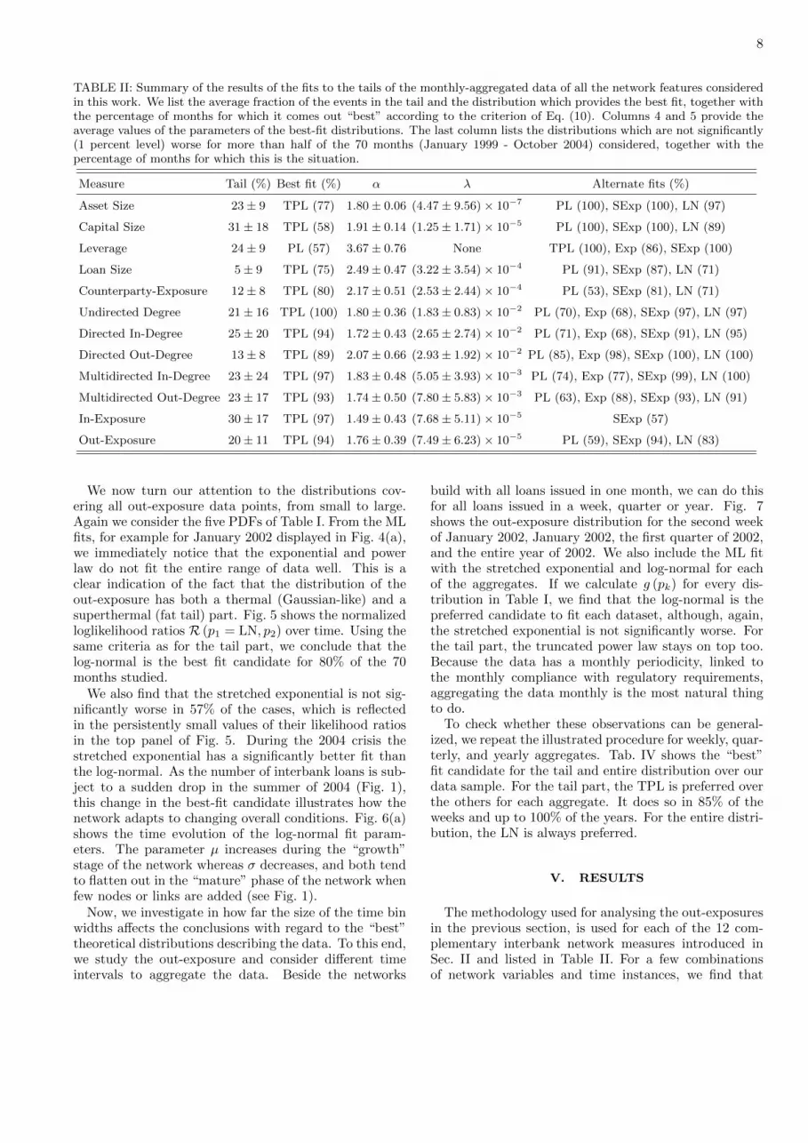
TABLE II: Summary of the results of the fits to the tails of the monthly-aggregated data of all the network features consideredin this work. We list the average fraction of the events in the tail and the distribution which provides the best fit, together withthe percentage of months for which it comes out “best” according to the criterion of Eq. (10). Columns 4 and 5 provide theaverage values of the parameters of the best-fit distributions. The last column lists the distributions which are not significantly(1 percent level) worse for more than half of the 70 months (January 1999 - October 2004) considered, together with thepercentage of months for which this is the situation.
Measure Tail (%) Best fit (%) α λ Alternate fits (%)
Asset Size 23± 9 TPL (77) 1.80± 0.06 (4.47± 9.56)× 10−7 PL (100), SExp (100), LN (97)
Capital Size 31± 18 TPL (58) 1.91± 0.14 (1.25± 1.71)× 10−5 PL (100), SExp (100), LN (89)
Leverage 24± 9 PL (57) 3.67± 0.76 None TPL (100), Exp (86), SExp (100)
Loan Size 5± 9 TPL (75) 2.49± 0.47 (3.22± 3.54)× 10−4 PL (91), SExp (87), LN (71)
Counterparty-Exposure 12± 8 TPL (80) 2.17± 0.51 (2.53± 2.44)× 10−4 PL (53), SExp (81), LN (71)
Undirected Degree 21± 16 TPL (100) 1.80± 0.36 (1.83± 0.83)× 10−2 PL (70), Exp (68), SExp (97), LN (97)
Directed In-Degree 25± 20 TPL (94) 1.72± 0.43 (2.65± 2.74)× 10−2 PL (71), Exp (68), SExp (91), LN (95)
Directed Out-Degree 13± 8 TPL (89) 2.07± 0.66 (2.93± 1.92)× 10−2 PL (85), Exp (98), SExp (100), LN (100)
Multidirected In-Degree 23± 24 TPL (97) 1.83± 0.48 (5.05± 3.93)× 10−3 PL (74), Exp (77), SExp (99), LN (100)
Multidirected Out-Degree 23± 17 TPL (93) 1.74± 0.50 (7.80± 5.83)× 10−3 PL (63), Exp (88), SExp (93), LN (91)
In-Exposure 30± 17 TPL (97) 1.49± 0.43 (7.68± 5.11)× 10−5 SExp (57)
Out-Exposure 20± 11 TPL (94) 1.76± 0.39 (7.49± 6.23)× 10−5 PL (59), SExp (94), LN (83)
We now turn our attention to the distributions cov-ering all out-exposure data points, from small to large.Again we consider the five PDFs of Table I. From the MLfits, for example for January 2002 displayed in Fig. 4(a),we immediately notice that the exponential and powerlaw do not fit the entire range of data well. This is aclear indication of the fact that the distribution of theout-exposure has both a thermal (Gaussian-like) and asuperthermal (fat tail) part. Fig. 5 shows the normalizedloglikelihood ratios R (p1 = LN, p2) over time. Using thesame criteria as for the tail part, we conclude that thelog-normal is the best fit candidate for 80% of the 70months studied.
We also find that the stretched exponential is not sig-nificantly worse in 57% of the cases, which is reflectedin the persistently small values of their likelihood ratiosin the top panel of Fig. 5. During the 2004 crisis thestretched exponential has a significantly better fit thanthe log-normal. As the number of interbank loans is sub-ject to a sudden drop in the summer of 2004 (Fig. 1),this change in the best-fit candidate illustrates how thenetwork adapts to changing overall conditions. Fig. 6(a)shows the time evolution of the log-normal fit param-eters. The parameter µ increases during the “growth”stage of the network whereas σ decreases, and both tendto flatten out in the “mature” phase of the network whenfew nodes or links are added (see Fig. 1).
Now, we investigate in how far the size of the time binwidths affects the conclusions with regard to the “best”theoretical distributions describing the data. To this end,we study the out-exposure and consider different timeintervals to aggregate the data. Beside the networks
build with all loans issued in one month, we can do thisfor all loans issued in a week, quarter or year. Fig. 7shows the out-exposure distribution for the second weekof January 2002, January 2002, the first quarter of 2002,and the entire year of 2002. We also include the ML fitwith the stretched exponential and log-normal for eachof the aggregates. If we calculate g (pk) for every dis-tribution in Table I, we find that the log-normal is thepreferred candidate to fit each dataset, although, again,the stretched exponential is not significantly worse. Forthe tail part, the truncated power law stays on top too.Because the data has a monthly periodicity, linked tothe monthly compliance with regulatory requirements,aggregating the data monthly is the most natural thingto do.
To check whether these observations can be general-ized, we repeat the illustrated procedure for weekly, quar-terly, and yearly aggregates. Tab. IV shows the “best”fit candidate for the tail and entire distribution over ourdata sample. For the tail part, the TPL is preferred overthe others for each aggregate. It does so in 85% of theweeks and up to 100% of the years. For the entire distri-bution, the LN is always preferred.
V. RESULTS
The methodology used for analysing the out-exposuresin the previous section, is used for each of the 12 com-plementary interbank network measures introduced inSec. II and listed in Table II. For a few combinationsof network variables and time instances, we find that

9
101 102 103 104 105 106
Out-Exposure (106 Rb)
10-3
10-2
10-1
100C
CD
F LNSExpweekmonthquarteryear
FIG. 7: (Color online) The CCDF of the out-exposure distri-bution from a network aggregated with data from one week(week 2 of January 2002), from one month (January 2002),from one quarter (first quarter of 2002), and one year (2002).We also show the respective stretched exponential and log-normal fits.
the xmin, which marks the lower boundary of the tailparts of the distributions and results from minimizingthe quantity Z of Eq. (5), is close to the upper edge ofthe distribution. Under those circumstances the identi-fied tail does not hold a sufficient amount of datapointsto perform a meaningful fit. This is particularly commonduring the 1998 interbank network collapse. For this rea-son, we only study the best-fit parameters from January1999 onwards.
A prototypical example of a data set for which thefit with the functions of Table I is not fully satisfactoryis shown in Fig. 8. The figure includes the loan sizeand counterparty-exposure measures for January 2004.Whereas the TPL is a good match for the tail parts ofthe data, the “best” fit to the entire range of the datawith a LN distribution clearly underestimates the prob-ablility of events in the tail. Fig. 9 displays for January2004 the “tail” and “bulk+tail” parts of the 10 otherinterbank network measures considered. It is clear thatthe data can be reasonably well described by the adoptedprocedure and proposed theoretical distributions.
Table II reports our findings on the tail parts of theempirical distributions. The second column shows thepercentage of data points assigned to the tail via theKolmogorov-Smirnov criterion of Eq. (5). This numberaverages to about 20% across the considered networkmeasures but varies a lot. In particular, the loan size,counterparty exposure, and directed out-degree have rel-atively few events in the tail. For most of the 70 monthsincluded in the analysis, the truncated power law outper-forms, according to our methodology, the other four can-didates for every measure. In Table II the time-averagedvalues for the α and λ parameters are also reported. The
102 103 104
size (106 Rb)
10-4
10-3
10-2
10-1
100
CC
DF
(a)
loancp-exposure
10-2 10-1 100 101 102 103 104
size (106 Rb)
10-5
10-4
10-3
10-2
10-1
100
CC
DF
(b)
FIG. 8: (Color online) The CCDF for the loan-size and thecounterparty(cp)-exposure for January 2004. Panel (a) showsthe tail part of the data together with a PL (grey) and TPL(green) fit. Panel (b) shows the data over the entire rangetogether with LN fit. For illustrative reasons, the data forthe cp-exposure have been scaled by a factor of 0.1.
power α is consistently of the order of two. It emergesfrom our studies that a fat tail is a characteristic featureof the measurable quantities of an interbank system. Wenotice that λ is very volatile.
Upon evaluating the last column of Table II, we findthat although the truncated power law systematicallyprovides the best fit, the other candidates are hardly sig-nificantly worse at the 1 percent level. This observationis particularly true for the unweighted degree measureswhich are discrete. In fact, for the degree measures, noneof the five distribution candidates can be conclusively la-beled as representing the best fit to the data. We notethat the fraction of events located in the tail fluctuates alot. This hints that a more integrated approach wherebythe bulk and the tail parts of the data are simultane-ously fitted with a non-Gaussian distribution may leadto a more stable description of the network features.

10
103 104 105 106 107
Asset and Capital (mln Rb)
10-3
10-2
10-1
100
CC
DF
(a)
assetscapital
101
Leverage
(b)102 103 104 105
Exposure (mln Rb)
(c)
inout
102
Undirected degree
10-3
10-2
10-1
100
CC
DF
(d)102
Directed degree
(e)
inout
102
Multidirected degree
(f)
inout
100 101 102 103 104 105 106 107
Asset and Capital (mln Rb)
10-3
10-2
10-1
100
CC
DF
(g)
assetcapital
100 101
Leverage
(h)100 101 102 103 104 105
Exposure (mln Rb)
(i)
inout
100 101 102
Undirected degree
10-3
10-2
10-1
100
CC
DF
(j)100 101 102
Directed degree
(k)
inout
100 101 102
Multidirected degree
(l)
inout
FIG. 9: (Color online) The CCDF for 10 interbank network measures for the montly aggregated data in January 2004. Panels(a-f) display the tails parts of the data together with the PL (grey) and TPL (green) fits. Panels (g-l) contain the data overthe entire range together with the ”best” fit from Table III. For illustrative reasons, in those panels with two measures, thedata of the second measure have been shifted vertically by multiplying them by a scaling factor of 0.5.

11
Table III summarizes our fits to the entire distribu-tions of all 12 network measures over all 70 months usingmonthly-aggregated data. The asset, capital, leverage,loan sizes, as well as the counterparty-exposure and in-exposure distributions are described significantly best bya log-normal. The various degree distributions prefer thestretched exponential, which is on average not signifi-cantly better than the log-normal and/or the truncatedpower law. For those network measures for which thestretched exponential represents the best fit, we observethat the parameter λ is very volatile. It is worth not-ing that the stretched exponential has been put forwardas a natural fat tail distribution for many physical andeconomic phenomena which cannot be satisfactorily de-scribed by a power law [27]. In general, the parametersentering the fits to the tail parts are subject to largerfluctuations than those entering the distributions for thecomplete data set.
Our results compare well with some of the existingstudies of interbank networks, but differ from others.Specifically, our findings are in line with Goddard etal. [8] who study U.S. banks: the log-normal distribu-tion fits the bulk part of the asset-size data well, whilethe power law does the same for the tail part. Our find-ings are not too different from those of Cont et al. [4]for the Brazilian interbank network: while our TPL fitsto the tails of various degree distributions (see Table II)deliver values of α between 1.7 and 2.2, Cont et al. [4] re-port power-law exponents between 2.2 and 2.8 (α = 2.54for total degree, α = 2.46 for in-degree, α = 2.83 for out-degree, and α = 2.27 for out-exposure size). Finally, incontrast to [5] studying the Austrian interbank marketwe do not find that the power law provides a good fitto the entire loan-size distribution ([5] report α = 1.87).Their power-law exponents reported for the tails of totaland in-degree distributions (resp. α = 2.0 and α = 3.11)are comparable to the TPL values in Table II, while theirout-degree α = 1.72 differs substantially.
The most extensive study of interbank distributionswas performed for the e-mid market [20]. In line with thiswork, the authors consider both the complete and tailparts of the distributions and report results for daily andquarterly time aggregates. For the quarterly aggregatesof the in-, out- and total degree distribution, a stretchedexponential emerged as the best fit to the entire distri-bution. This confirms our findings. A log normal wasreported as a best fit to the tail parts of the data. Wealso find that the LN can reasonably account for the tailparts. It is slightly outperformed by the truncated powerlaw (which was not included in the set of possible distri-butions in the work of Ref. [20]) and flags as not signif-icantly worse in our table. For the quarterly aggregatednumber of transactions, a network feature comparable tothe multidirected degree considered here, they also findsimilar results as for the regular degrees.
Upon scrutiny of the time evolution of the fitted distri-butions and their parameters, we do not find any system-atic changes in the distributions which emerge as best fit
to the data, between the “growth” phase (1999-2002) andthe “mature” phase (2002-2004). In line with the expec-tations, however, the extracted parameters are subject tosmaller variations as the network grows and the numberof nodes and edges increases.
As already mentioned, our data set covers two crises,the first in August 1998 and the second in the summerof 2004. We would like to know if the best-fit candidatesfor the crisis periods are different than the ones for thenormal operation periods.
As a consequence of the moratorium in August 1998,the interbank market collapsed in September, and thenagain in December 1998 (see Fig. 1). Due to this col-lapse, the network is too small and their are too fewtransactions to gather proper statistics. Fits to the datain this period are inconclusive for most of the measures,and hence are not included in the overall discussion.
During the second crisis period, the network does staylarge enough to have proper statistics. From Fig. 5 it isclear that the stretched exponential distribution is sig-nificantly better than the log-normal from mid 2004 on-wards. Thus, for the out-exposure (as well as the in-exposure), there is a difference between pre- and post-crisis best-fit candidates. For the other measures, how-ever, we find that the same distributions are preferred in”crisis” as in ”normal” operation periods.
To end this section, we test the qualitative robustnessof the obtained results using different time windows. Thisis particulary important in view of the fact that a recentstudy has shown that the interbank network propertiesdepend on the aggregation period [28]. To check if thesame distribution is preferred for different aggregates, werepeat the monthly procedure for weekly, quarterly, andyearly aggregates. Tab. IV shows the “best” fit for eachmeasure-aggregate pair and the percentage of the bins itis considered so. For the tail parts, we find that the TPLcan be considered as the best overall fit candidate. Wenotice that in general the TPL becomes more preferred asthe bin width increases. For each measure, the favouredfits to the entire distribution stay the same for differentbin widths.
VI. CONCLUSION
In this paper we use daily data on bilateral interbankexposures and monthly bank balance sheets to study net-work characteristics of the Russian interbank market overAug 1998 - Oct 2004. Specifically, we examine the dis-tributions of (un)directed (un)weighted degree, nodal at-tributes (bank assets, capital and capital-to-assets ratio)and edge weights (loan size and counterparty exposure).Using the methodology of [11] we set up a horse race be-tween the different theoretical distributions to find onethat fits the data best.
In line with the existing literature, we observe thatall studied distributions are heavy tailed with the tailtypically containing 20% of the data. The tail is best

12
TABLE III: Summary of the results of the fits to the monthly-aggregated data of all the network features considered in thiswork. We list the distribution which provides the best fit to the full range of the data (”bulk”+”tail”)), together with thepercentage of months for which it comes out “best” according to the criterion of Eq. (10). Columns 3 and 4 provide theaverage values of the parameters of the best-fit distribution. The last column list the distributions which are not significantly(at the 1 percent level) worse for more than half of the 70 months (January 1999 - October 2004) considered, together with thepercentage of months for which this is the situation.
Measure Best fit (%) Parameter 1 Parameter 2 Alternative fit (%)
Asset Size LN (100) µ = 5.45± 0.63 σ = 1.91± 0.02 None
Capital Size LN (100) µ = 4.64± 0.53 σ = 1.51± 0.03 None
Leverage LN (99) µ = 1.57± 0.05 σ = 0.74± 0.01 None
Loan Size LN (100) µ = 2.54± 0.34 σ = 1.27± 0.08 None
Counterparty-exposure LN (99) µ = 3.33± 0.31 σ = 1.56± 0.13 None
Undirected Degree SExp (54) λ = 0.29± 0.20 β = 0.55± 0.06 LN (94)
Directed In-Degree SExp (66) λ = 0.41± 0.27 β = 0.46± 0.07 TPL (91), LN (71)
Directed Out-Degree SExp (83) λ = 0.43± 0.39 β = 0.60± 0.05 TPL (51), LN (97)
Multidirected In-Degree SExp (80) λ = 0.29± 0.35 β = 0.43± 0.07 TPL (90)
Multidirected Out-Degree SExp (73) λ = 0.19± 0.26 β = 0.53± 0.09 LN (80)
In-Exposure LN (83) µ = 4.26± 0.83 σ = 2.37± 0.09 None
Out-Exposure LN (80) µ = 4.55± 0.65 σ = 2.13± 0.10 SExp (57)
TABLE IV: Robustness of the “best” fits for different aggregates. This table shows for each measure-aggregate pair the preferredfit candidate as well as the percentage of the bins it was considered so. This is done for fit of tail as well as total.
Tail Bulk+Tail
Measure Week Month Quarter Year Week Month Quarter Year
Loan Size TPL (70) TPL (75) TPL (78) TPL (80) LN (95) LN (100) LN (100) LN (100)
Counterparty-exposure TPL (82) TPL (80) TPL (83) TPL (80) LN (94) LN (99) LN (100) LN (100)
Undirected Degree TPL (94) TPL (100) TPL (90) TPL (100) SExp (66) SExp (54) SExp (52) SExp (80)
Directed In-Degree TPL (93) TPL (94) TPL (90) TPL (100) SExp (58) SExp (66) SExp (65) SExp (60)
Directed Out-Degree TPL (83) TPL (89) TPL (95) TPL (100) SExp (64) SExp (83) SExp (87) SExp (100)
Multidirected In-Degree TPL (92) TPL (97) TPL (95) TPL (100) SExp (78) SExp (80) SExp (87) SExp (100)
Multidirected Out-Degree TPL (79) TPL (93) TPL (90) TPL (100) SExp (67) SExp (73) SExp (87) SExp (100)
In-Exposure TPL (94) TPL (97) TPL (100) TPL (100) LN (74) LN (83) LN (74) LN (60)
Out-Exposure TPL (85) TPL (94) TPL (100) TPL (100) LN (83) LN (80) LN (57) LN (80)
described by a truncated power law, although the fit ofother candidate distributions is only marginally worse.
In most cases, separating the bulk and tail parts of thedata turns out to be hard, and the proportion of obser-vations assigned to the tail varies a lot. More stable fitsto the data are obtained in an integrated approach thataccounts for both the Gaussian and the non-Gaussianparts of the distributions. We find two distributions thatfit the full range of the data best: the stretched exponen-tial for measures related to unweighted degree and thelog-normal for everything else. In case of the former, thelog-normal performs only marginally worse.
Our conclusions turn out to be robust to whether weaggregate the data over a week, month, quarter or year.Further, we find no qualitative difference between the“growth” and “maturity” phases of interbank market de-velopment and little difference between the “crisis” and“non-crisis” periods.
Our findings support the recent call [11, 12] for morerigorous statistical tests to detect power-law behavior inempirical data. While for most variables we find that thepower law fits the tail of the distribution reasonably well,it is:
1. almost never the best candidate to describe the tail;

13
2. typically not a good candidate to describe the wholedistribution.
Our findings echo those of Ref. [20] who also find that thepower law provides an inferior fit, compared to alterna-tive distributions, to their overnight money market datacoming from the e-MID trading platform. We thus tendto conclude that the evidence on power laws is not (yet)strong enough to warrant their widespread use in pol-icy simulations. From the study presented in this workwe provide alternate distributions and corresponding pa-rameters which can systematically and robustly capturethe interbank network measures. We deem that those
distributions represent a more realistic account of the in-terbank network structure than the widely used powerlaws and could facilitate more realistic contagion model-ing.
Acknowledgments
This work is supported by the Research Founda-tion Flanders (FWO-Flanders), the Research Founda-tion of Ghent University (BOF) and the Bank of Finland(BOFIT).
[1] M. E. Newman, Contemp. Phys. 46, 323 (2005).[2] V. M. Yakovenko and J. B. Rosser Jr, Rev. Mod. Phys.
81, 1703 (2009).[3] X. Gabaix, Working Paper 14299, NBER (2008).[4] R. Cont, A. Moussa, E. B. Santos, et al., Network struc-
ture and systemic risk in banking systems (2013).[5] M. Boss, H. Elsinger, M. Summer, and S. Thurner 4,
Quant. Finance 4, 677 (2004).[6] D. O. Cajueiro and B. M. Tabak, Physica A 387, 6825
(2008).[7] K. Soramaki, M. L. Bech, J. Arnold, R. J. Glass, and
W. E. Beyeler, Physica A 379, 317 (2007).[8] J. Goddard, H. Liu, D. Mckillop, and J. O. Wilson, IJEB
21, 139 (2014).[9] G. De Masi, G. Iori, and G. Caldarelli, Phys. Rev. E 74,
066112 (2006).[10] G. Iori, R. Reno, G. De Masi, and G. Caldarelli, Physica
A 376, 467 (2007).[11] A. Clauset, C. R. Shalizi, and M. E. Newman, SIAM
Rev. 51, 661 (2009).[12] M. P. Stumpf and M. A. Porter, Science 335, 665 (2012).[13] A. Krause and S. Giansante, J. Econ. Behav. Organ. 83,
583 (2012).[14] T. Roukny, H. Bersini, H. Pirotte, G. Caldarelli, and
S. Battiston, Sci. Rep. 3 (2013).[15] A. Karas and K. Schoors, Working Paper 327, Ugent
(2005).[16] P. Gai, A. Haldane, and S. Kapadia, J. Monetary Econ.
58, 453 (2011).[17] E. Nier, J. Yang, T. Yorulmazer, and A. Alentorn, J.
Econ. Dyn. Control 31, 2033 (2007).[18] S. Battiston, D. D. Gatti, M. Gallegati, B. Greenwald,
and J. E. Stiglitz, J. Fin. Stability 8, 138 (2012).[19] G. Iori, G. De Masi, O. V. Precup, G. Gabbi, and G. Cal-
darelli, J. Econ. Dyn. Control 32, 259 (2008).[20] D. Fricke and T. Lux, Working Paper 1819, IfW (2013).[21] T. P. Peixoto, Phys. Rev. X 4, 011047 (2014).[22] D. J. Watts and S. H. Strogatz, Nature (London) 393,
440 (1998).[23] J. Saramaki, M. Kivela, J.-P. Onnela, K. Kaski, and
J. Kertesz, Phys. Rev. E 75, 027105 (2007).[24] M. Newman, SIAM Rev. 45, 167 (2003).[25] S. Martinez-Jaramillo, B. Alexandrova-Kabadjova,
B. Bravo-Benitez, and J. P. Solorzano-Margain, J. Econ.Dyn. Control 40, 242 (2014).
[26] J. Alstott, E. Bullmore, and D. Plenz, PloS one 9, e85777(2014).
[27] J. Laherrere and D. Sornette, EPJ B 2, 525 (1998).[28] K. Finger, D. Fricke, and T. Lux, Comput. Manag. Sci.
10, 187 (2013).[29] For more information on the data provider see its website
at www.mobile.ru.[30] A distribution is defined as heavy-tailed if it is not expo-
nentially bounded [26].


