Biases and Implicit Knowledge!

Tom Cunningham†

First Version: September 2012

Current Version: September 2013

Abstract

A common explanation for biases in judgment and choice has been to postulate two

separate processes in the brain: a “System 1” that generates judgments automatically,

but using only a subset of the information available, and a “System 2” that uses the entire

information set, but is only occasionally activated. This theory faces two important

problems: that inconsistent judgments often persist even with high incentives, and that

inconsistencies often disappear in within-subject studies. In this paper I argue that

these behaviors are due to the existence of “implicit knowledge”, in the sense that our

automatic judgments (System 1) incorporate information which is not directly available

to our reflective system (System 2). System 2 therefore faces a signal extraction problem,

and information will not always be e!ciently aggregated. The model predicts that

biases will exist whenever there is an interaction between the information private to

System 1 and that private to System 2. Additionally it can explain other puzzling

features of judgment: that judgments become consistent when they are made jointly,

that biases diminish with experience, and that people are bad at predicting their own

!Among many others I thank for their comments Roland Benabou, Erik Eyster, Scott Hirst, DavidLaibson, Vanessa Manhire, Arash Nekoei, José Luis Montiel Olea, Alex Peysakhovich, Ariel Rubinstein,Benjamin Schoefer, Andrei Shleifer, Rani Spiegler, Dmitry Taubinsky, Matan Tsur, Michael Woodford, andseminar participants at Harvard, Tel Aviv, Princeton, HHS, the IIES, and Oxford.

†IIES, Stockholm University, tom.cunningham@iies.su.se.

1

future judgments. Because System 1 and System 2 have perfectly aligned preferences,

welfare is well-defined in this model, and it allows for a precise treatment of eliciting

preferences in the presence of framing e"ects.

2

1 Introduction

A common explanation of anomalies in judgment is that people sometimes make judgments

automatically, using only superficial features of the case, ignoring more abstract or high-level

information. Variations on this type of explanation are widespread in the studies of biases

in perception, judgment, and decision-making:

• In perception the most common explanation of optical illusions is that, although the

visual system generally makes correct inferences from the information available, those

inferences are based only on local information. Pylyshyn (1999) says “a major portion

of vision . . . does its job without the intervention of [high-level] knowledge, beliefs or

expectations, even when using that knowledge would prevent it from making errors.”1

• In psychology two of the dominant paradigms, “heuristics and biases” and “dual sys-

tems”, both explain biases as due to people making judgments which are correct on av-

erage, but which use only a subset of the information (Tversky and Kahneman (1974),

Sloman (1996)).

• Within economics an important explanation of biases has been “rational inattention”

(Sims (2005), Chetty et al. (2007), Woodford (2012)). In these models people make

optimal decisions relative to some set of information, but they use only a subset of all

the information available, because they must pay a cognitive cost which is increasing

in the amount of information used.

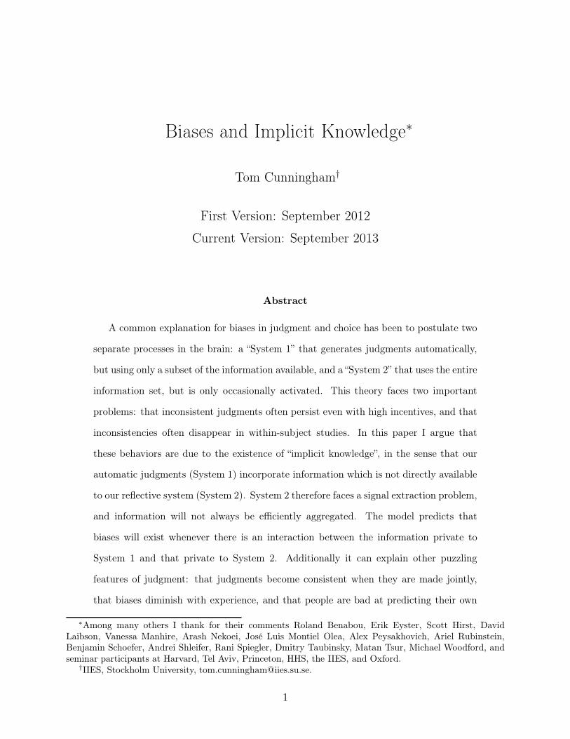
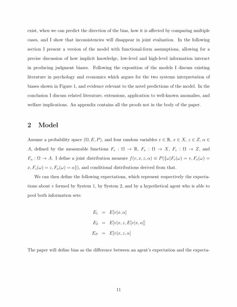
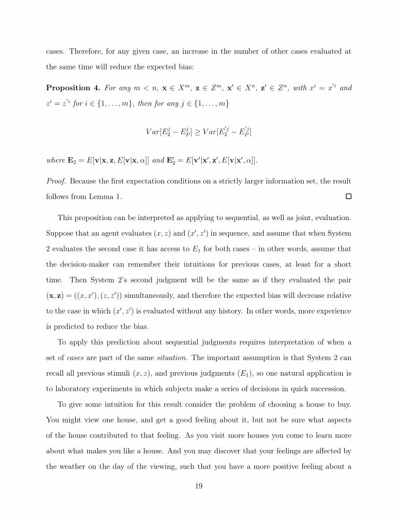
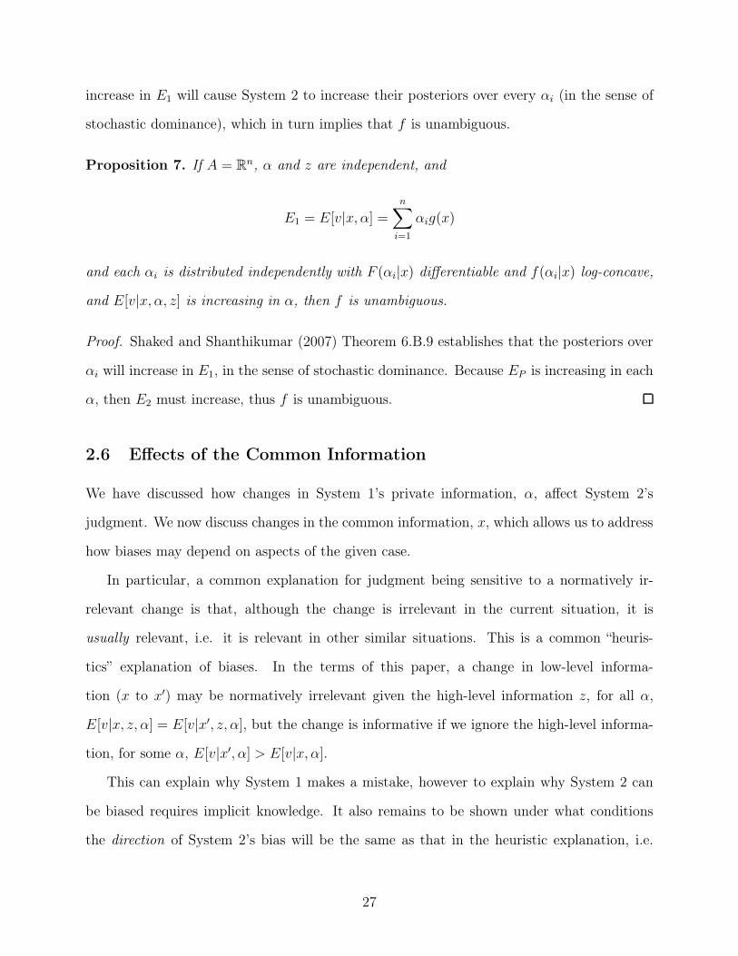
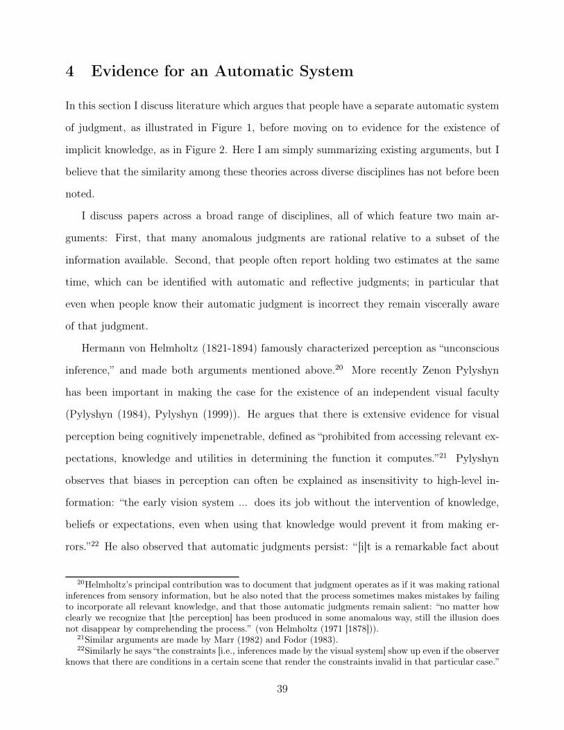
A simple version of this type of model is illustrated in Figure 1: when making judgments

we can either use an automatic system (System 1), which only uses part of the information

available, or a reflective system (System 2), which uses all the information, but is costly to

1Feldman (2013) says “there is a great deal of evidence ... that perception is singularly uninfluenced bycertain kinds of knowledge, which at the very least suggests that the Bayesian model must be limited in scopeto an encapsulated perception module walled o! from information that an all-embracing Bayesian accountwould deem relevant.”

3

activate.2 The names “System 1” and “System 2” are taken from Stanovich and West (2000).

In this model biases will occur when System 2 is not activated, and the nature of biases can

be understood as due to ignoring the high-level information available only to System 2.3

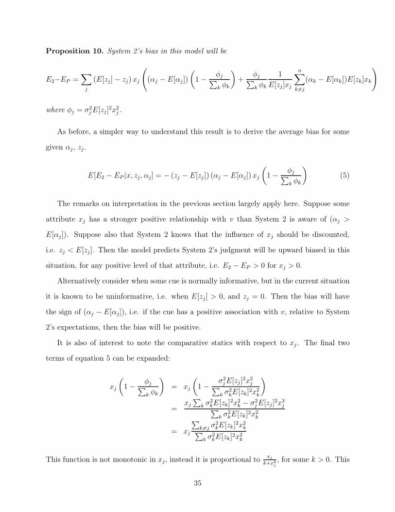
!"#$%&'(1E[v|x]

!!

v

x

""!!!

!!!!

!!!

!!!!

!!!

!!!!

x,z

##""""

""""

"""

""""

"""

"""

!"#$%&'(2E[v|x,z]

!!

Figure 1: A simple representation of a two-systems model: System 1 is above, System2 is below. Both systems form rational expectations about the unobserved variable v,however System 1 receives only x (low-level information), while System 2 additionallyreceives z (high-level information).

Although this class of models has been used to give persuasive analyses of individual bi-

ases, they su!er from two important empirical problems: the response of biases to incentives,

and the response of biases to joint evaluation.

First, the model predicts that biases will disappear when System 2 is activated, which

should occur whenever time and incentives are su"ciently high. Although incentives do tend

to reduce the magnitude of biases, it is commonly observed that many biases remain even

when the stakes become quite high. Camerer and Hogarth (1999) say “no replicated study

has made rationality violations disappear purely by raising incentives.” Similarly, behavior

outside the laboratory often seems to be influenced by irrelevant information even with very

high stakes (Post et al. (2008), Thaler and Benartzi (2004)). A similar point is true for

perceptual illusions: spending a longer time staring at the illusion may reduce the magnitude

of the bias, but it rarely eliminates it (Predebon et al. (1998)). Thus it becomes a puzzle

2Although the theories listed all share the same basic diagnosis of why biases occur, they di!er on anumber of other important dimensions, discussed later in the paper. More recently the System 1 / System 2terminology has been used to refer to di!erences in preference (e.g. short-run vs long-run preferences), ratherthan di!erences in information, but in this paper I just consider di!erences in information.

3Within economics the terms “dual systems” and “dual selves” often refer to models in which the systemshave di!erent preferences (Fudenberg and Levine (2006), Brocas and Carrillo (2008)). In this paper I consideronly the case in which the systems di!er in information, and have aligned preferences.

4

why people should still be relying on their imperfect automatic judgments when there are

high incentives to not make mistakes.

Second, many experiments find that inconsistencies among judgments disappear when

those judgments are made jointly, and the two-system model gives no reason to expect this

e!ect. Many biases were originally identified using between-subject studies, and when tested

in within-subject studies their magnitude is generally much smaller (Kahneman and Frederick

(2005)). When valuing gambles, people often place a higher value on a dominated gamble,

but they almost never directly choose a dominated gamble (Hey (2001)). And willingness

to pay for a product can be a!ected by changing an irrelevant detail, but when the two

products are valued side-by-side people usually state the same willingness to pay for each

product (Mazar et al. (2010)). Overall people seem to be consistent within situations, but

their standards of evaluation change between situations.

These two generalizations - that inconsistencies are insensitive to incentives, but sensitive

to joint presentation - suggest that our reflective judgments obey principles of consistency,

but are distorted by the same biases that distort our automatic system. This could occur if

System 2’s judgment takes into account the judgments that System 1 makes. And this, in

turn, would be rational if System 1’s judgments incorporated information not accessible to

System 2.

This paper proposes that the reason we make inconsistent judgments when using our full

reflective judgment is that in di!erent situations we receive di!erent signals from System 1 (or

intuitions), and it is rational to take into account those signals because they contain valuable

information. I call the underlying assumption implicit knowledge, because it is knowledge

that is private to our automatic system, and thus available to our reflective system only

indirectly, through observing the automatic system’s judgments.

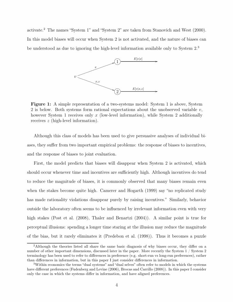
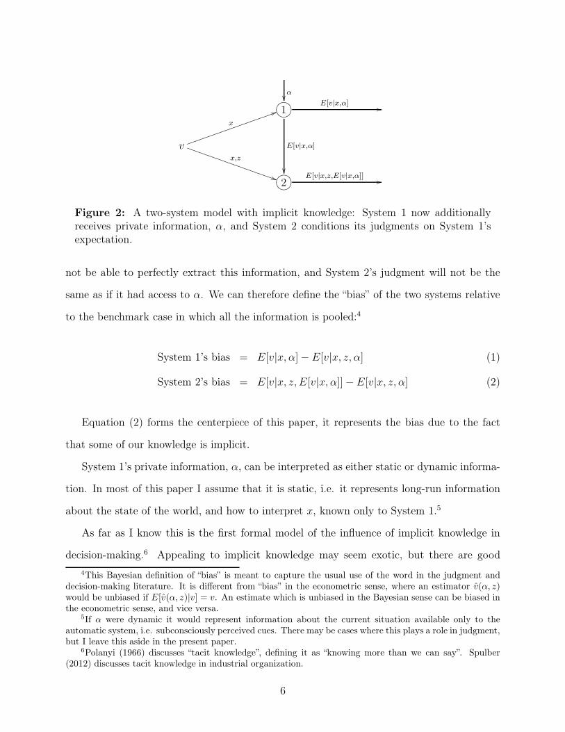
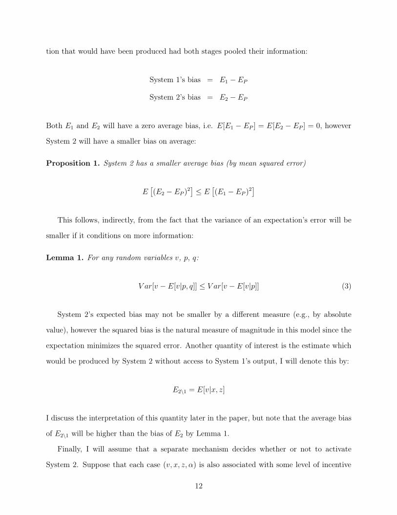
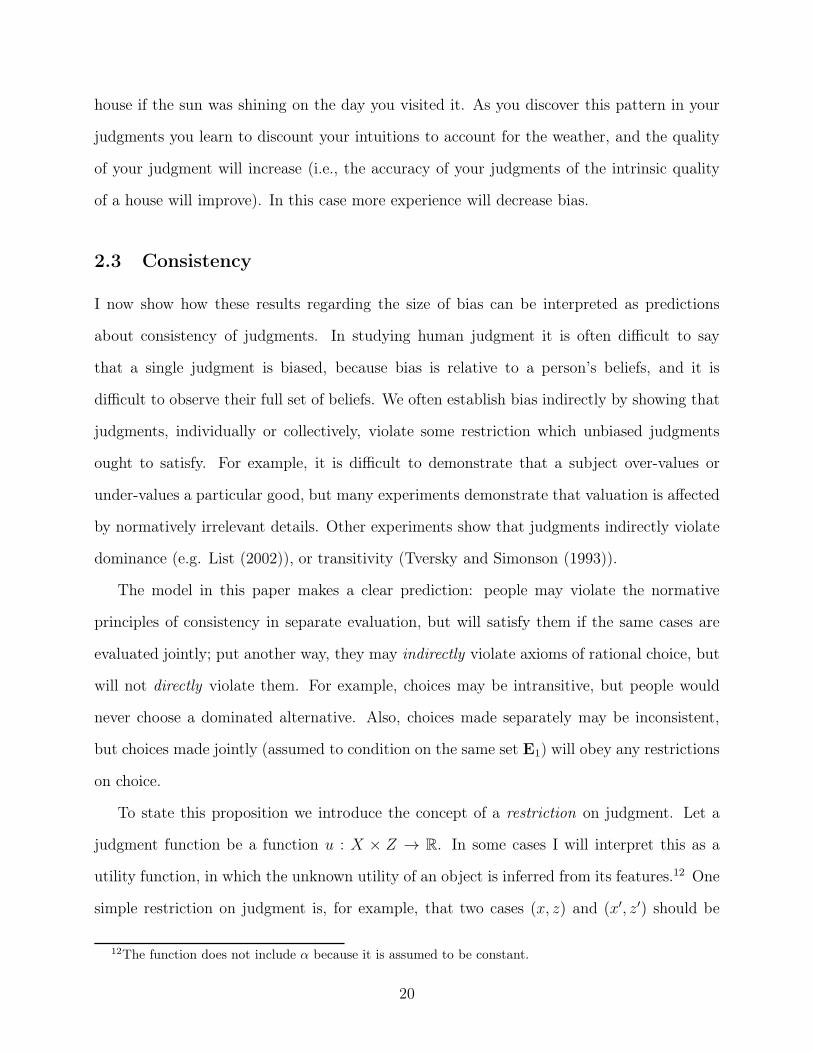
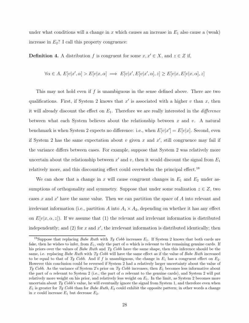
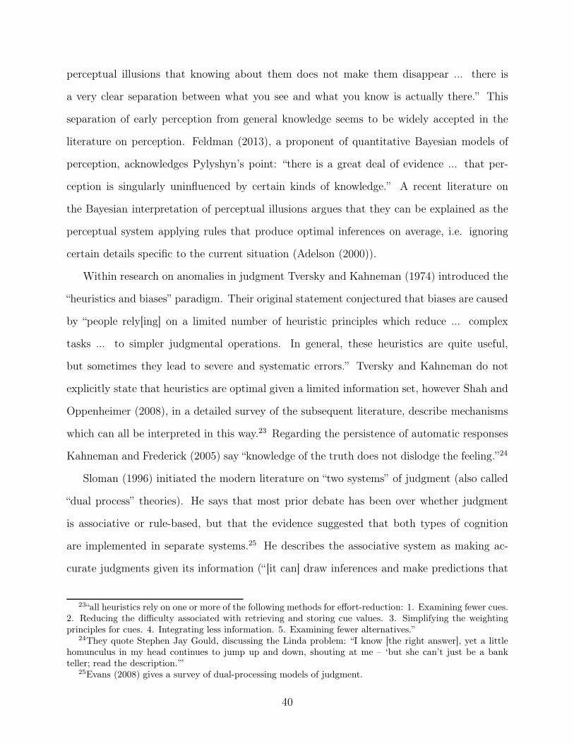
Figure 2 shows how the formal analysis di!ers: System 1 now has access to private

information, !, and System 2 can observe System 1’s posterior judgment (E[v|x,!]). System

2 faces a signal extraction problem in inferring ! from E[v|x,!]. In many cases System 2 will

5

!$$

!"#$%&'(1E[v|x,!]

!!

E[v|x,!]

$$

v

x

""!!!!

!!!!

!!!

!!!!

!!!!!

!

x,z

##"""""

"""

""""

"""

""""

""

!"#$%&'(2E[v|x,z,E[v|x,!]]

!!

Figure 2: A two-system model with implicit knowledge: System 1 now additionallyreceives private information, !, and System 2 conditions its judgments on System 1’sexpectation.

not be able to perfectly extract this information, and System 2’s judgment will not be the

same as if it had access to !. We can therefore define the “bias” of the two systems relative

to the benchmark case in which all the information is pooled:4

System 1’s bias = E[v|x,!]" E[v|x, z,!] (1)

System 2’s bias = E[v|x, z, E[v|x,!]]" E[v|x, z,!] (2)

Equation (2) forms the centerpiece of this paper, it represents the bias due to the fact

that some of our knowledge is implicit.

System 1’s private information, !, can be interpreted as either static or dynamic informa-

tion. In most of this paper I assume that it is static, i.e. it represents long-run information

about the state of the world, and how to interpret x, known only to System 1.5

As far as I know this is the first formal model of the influence of implicit knowledge in

decision-making.6 Appealing to implicit knowledge may seem exotic, but there are good

4This Bayesian definition of “bias” is meant to capture the usual use of the word in the judgment anddecision-making literature. It is di!erent from “bias” in the econometric sense, where an estimator v(!, z)would be unbiased if E[v(!, z)|v] = v. An estimate which is unbiased in the Bayesian sense can be biased inthe econometric sense, and vice versa.

5If ! were dynamic it would represent information about the current situation available only to theautomatic system, i.e. subconsciously perceived cues. There may be cases where this plays a role in judgment,but I leave this aside in the present paper.

6Polanyi (1966) discusses “tacit knowledge”, defining it as “knowing more than we can say”. Spulber(2012) discusses tacit knowledge in industrial organization.

6

reasons to believe that large parts of our knowledge are only accessible in limited ways. In

perception the evidence is overwhelming: our eyes are able to make very accurate inferences

from the light they receive, but it has taken psychologists a centuries to understand how those

inferences are made, and the best computers remain inferior to a small child in interpreting

photographs. In more general knowledge a striking pattern is that we are far better at

recognizing certain patterns than reproducing them. As a simple example, most people find

it di"cult to answer the question “is there an English word which contains five consecutive

vowels?”, but instantly recognize that the statement is true when they are reminded of a word

that fits the pattern.7 Most people can easily recognize whether a sentence is grammatical,

but have di"culty making generalizations about the set of grammatical sentences.8 These

distinctions in accessibility would not exist if our knowledge was explicit, i.e. stored as a

distribution over possible states of the world. This paper proposes that the knowledge we

use in making economic decisions is stored in a similarly implicit form: that people are able

to make confident snap judgments about the value of di!erent alternatives, but they have

limited insight into how those judgments are formed. This separation of knowledge between

systems can explain why our decisions often violate normative principles that we reflectively

endorse.

The model makes a variety of predictions about human judgment: (1) biases will occur

when there is an interaction between implicit knowledge and high-level information in infer-

ring v (i.e., between ! and z); (2) judgments will appear inconsistent to an outside observer

because in di!erent situations the reflective system will have di!erent information about !;

(3) biases will be systematic, such that it will appear as if people are using simple heuris-

tics; (4) however when making multiple judgments jointly then judgments will be consistent,

because they will condition on the same beliefs about !; (5) the magnitude of biases will

7“queueing”.8Fernandez and Cairns (2010) say “Linguistic competence constitutes knowledge of language, but that

knowledge is tacit, implicit. This means that people do not have conscious access to the principles and rulesthat govern the combination of sounds, words, and sentences; however, they do recognize when those rulesand principles have been violated.”

7

decrease when a person is given more cases to judge, because with a larger set they can

learn more of the information that is private to their automatic system; and (6) people will

not be able to accurately predict their future judgments, because they cannot anticipate the

estimates that System 1 will produce in future situations.

I discuss evidence relevant to these predictions from perception, judgment, and economic

decision-making. In particular I emphasize the interpretation of framing e!ects: the reason

that we can be influenced by irrelevant features of the situation (anchors, reference points,

decoy alternatives, salience) is because those features are ordinarily relevant, and therefore

influence our automatic judgments. Even when we know a feature to be irrelevant in the

current case, it nevertheless can a!ect our reflective judgment indirectly because its influence

on automatic judgment is combined with other influences that are relevant, therefore we

often cannot completely decontaminate our automatic judgments to get rid of the irrelevant

influence.

Framing e!ects are often interpreted as evidence that true preferences do not exist, or

that preferences are labile, posing an important challenge to welfare economics (Ariely et al.

(2003), Bernheim and Rangel (2009)). The interpretation of this paper is that framing e!ects

reflect problems with aggregation of knowledge, and therefore true preferences do exist, and

can be recovered from choices. The model makes predictions about how true preferences can

be recovered: in particular, it predicts that judgments can be debiased by presenting subjects

with comparisons that vary the aspects that are irrelevant, allowing subjects to isolate the

cause of their bias.

The model in this paper di!ers qualitatively from existing models of imperfect attention

or imperfect memory, in fact it is the interaction of these two mechanisms that generates

biases (System 1 has imperfect attention, System 2 has imperfect memory). The model is

most related to the literature on social learning and herding, in which each agent learns from

observing prior agents’ actions. This paper makes three significant formal contributions.

First, it establishes new results in 2-agent social learning relating the bias to the nature of

8

the distribution of information between agents. Second, under the assumption that the first

agent’s private information is static, it shows under what conditions judgments and decisions

will be consistent when made jointly. Third, it presents an analytic solution for the bias under

linear-Gaussian assumptions, allowing for a clear intuitive characterization of how implicit

and explicit knowledge interact to a!ect judgment.

The interpretive contribution of this paper is to argue that many biases - in percep-

tion, judgment, and choice - are best understood as being due to the existence of implicit

knowledge.

1.1 Metaphor

A simple metaphor can be used to illustrate all of the principal e!ects in the model: the

model predicts that behavior will be as if you had access to an oracle who had superior

memory (i.e., which knows !), but which also has inferior perception of the situation (i.e.,

they do not observe z).

To be more concrete, suppose that you were attending an auction of baseball cards, and

suppose that you were accompanied by your sister, who will represent System 1. Suppose

that your sister has superior memory, meaning that she has a superior knowledge of the value

of individual baseball cards. However suppose that she has inferior perception, which will

mean that she cannot discriminate between genuine and fake cards.

When confronted with a packet of cards your sister will announce the expected value

of those cards, according to her experience, but without knowing whether any of the cards

are fake. Because you know which cards are fake you will wish to adjust her estimate to

incorporate your own information, however because her estimate is of the value of an entire

packet you cannot exactly back out her estimates of the values of individual cards. Your

final judgment will therefore be influenced by your sister’s knowledge, but it will not be an

optimal aggregation of your own information with your sister’s.

To an outside observer your behavior will appear to be systematically biased. In partic-

9

ular, your bids will be a!ected by information that you know to be irrelevant. Consider two

packets which are identical except for the final card: one contains a forged Babe Ruth card,

and the other contains a forged Ty Cobb. In each case the sister would give the packets di!er-

ent estimates because she is not aware that they di!er only in cards which are fake. Because

you are not able to infer your sister’s knowledge of the values of the individual cards, the

value of the fake card will indirectly influence your judgment in each case, and you would

produce di!erent bids in each of the two situations.

The outside observer would conclude that your judgment is biased: your behavior is as

if you are following a heuristic, i.e. ignoring whether or not cards are genuine. However

the observer would also notice a striking fact: that your judgments will obey principles

of consistency when multiple packets are considered simultaneously. Suppose that the two

packets described above are encountered at the same time. The sister will give two di!erent

estimates. However upon hearing these two estimates you will update your beliefs about the

values of all of the cards, and your two bids will be identical, because they reflect the same

beliefs about card values.

Two more of the predictions can be illustrated with this metaphor. First, exposure to a

larger set of cases will tend to reduce biases: if you are presented with a set of packets, and

you can hear your sister’s estimates for each packet, then you will be able to infer more of

your sister’s knowledge, and your bias will decline, converging towards a situation in which

you learn all of your sister’s knowledge. Second, the model predicts that people will not be

able to accurately forecast their future judgments. For example, suppose you were asked to

choose a set of 3 cards worth exactly $100, and you made this choice without your sister’s help

(i.e., your sister refuses to share her knowledge, apart from stating her estimates of individual

packets). You may choose a set of cards which you believe is worth $100 under your current

knowledge, but when you present that packet to your sister, and hear her estimate, your

estimate is likely to change.

In the next section I state the general model, and give conditions under which a bias will

10

exist, when we can predict the direction of the bias, how it is a!ected by comparing multiple

cases, and I show that inconsistencies will disappear in joint evaluation. In the following

section I present a version of the model with functional-form assumptions, allowing for a

precise discussion of how implicit knowledge, low-level and high-level information interact

in producing judgment biases. Following the exposition of the models I discuss existing

literature in psychology and economics which argues for the two systems interpretation of

biases shown in Figure 1, and evidence relevant to the novel predictions of the model. In the

conclusion I discuss related literature, extensions, application to well-known anomalies, and

welfare implications. An appendix contains all the proofs not in the body of the paper.

2 Model

Assume a probability space (!, E, P ), and four random variables v # R, x # X, z # Z, ! #

A, defined by the measurable functions Fv : ! $ R, Fx : ! $ X, Fz : ! $ Z, and

F! : ! $ A. I define a joint distribution measure f(v, x, z,!) % P ({"|Fv(") = v, Fx(") =

x, Fz(") = z, F!(") = !}), and conditional distributions derived from that.

We can then define the following expectations, which represent respectively the expecta-

tions about v formed by System 1, by System 2, and by a hypothetical agent who is able to

pool both information sets:

E1 = E[v|x,!]

E2 = E[v|x, z, E[v|x,!]]

EP = E[v|x, z,!]

The paper will define bias as the di!erence between an agent’s expectation and the expecta-

11

tion that would have been produced had both stages pooled their information:

System 1’s bias = E1 "EP

System 2’s bias = E2 "EP

Both E1 and E2 will have a zero average bias, i.e. E[E1 " EP ] = E[E2 " EP ] = 0, however

System 2 will have a smaller bias on average:

Proposition 1. System 2 has a smaller average bias (by mean squared error)

E!

(E2 " EP )2"

& E!

(E1 " EP )2"

This follows, indirectly, from the fact that the variance of an expectation’s error will be

smaller if it conditions on more information:

Lemma 1. For any random variables v, p, q:

V ar[v " E[v|p, q]] & V ar[v " E[v|p]] (3)

System 2’s expected bias may not be smaller by a di!erent measure (e.g., by absolute

value), however the squared bias is the natural measure of magnitude in this model since the

expectation minimizes the squared error. Another quantity of interest is the estimate which

would be produced by System 2 without access to System 1’s output, I will denote this by:

E2\1 = E[v|x, z]

I discuss the interpretation of this quantity later in the paper, but note that the average bias

of E2\1 will be higher than the bias of E2 by Lemma 1.

Finally, I will assume that a separate mechanism decides whether or not to activate

System 2. Suppose that each case (v, x, z,!) is also associated with some level of incentive

12

# # R. Then we can define a final expectation which is used for decision-making:

EF =

#

$

$

%

$

$

&

E1 # < #

E2 # ' #

where # # R is a constant. This describes the behavior of a person who activates System 2

only when the incentive is su"ciently high. This will be a rational strategy for an agent who

faces a loss function which is quadratic in (EF " v), and who must pay a cost when System

2 is activated.9

In practice mental e!ort may lie on a continuum, rather than being binary. What is

important for this model is that even with maximum mental e!ort, not all information is

e"ciently aggregated.

In the rest of the paper I concentrate mainly on the properties of System 2’s bias, E2"EP ,

i.e. the bias which survives in a person’s reflective judgment. When I say that judgment is

unbiased I will mean that for all x # X,! # A, z # Z,

E[v|x, z, E[v|x,!]] = E[v|x, z,!]

2.1 Conditions for a Bias in Reflective Judgment

A simple su"cient condition for unbiasedness is that E[v|x,!] is a one-to-one function of !.

If it was then System 2 would simply be able to invert E1 to infer !. However this condition

is not necessary, because in many cases System 2 can extract all the information it needs

from E1 without knowing !. We are able to give more interesting conditions below.

The relationship between E1, E2, and EP can be illustrated in the following table:

9A more sophisticated model would allow this decision to condition on more information (x, z, andperhaps !), but for the purposes of this paper it is only important that there is some level of incentives abovewhich System 2 will be activated.

13

! !! !!!

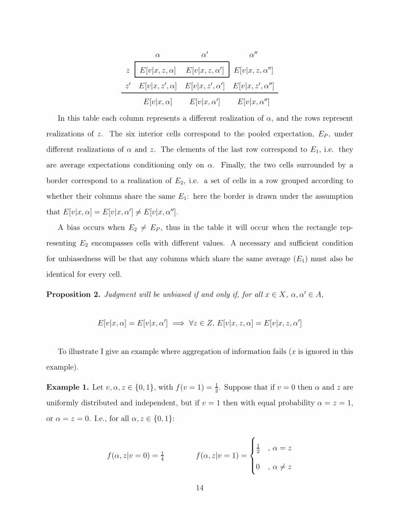
z E[v|x, z,!] E[v|x, z,!!] E[v|x, z,!!!]

z! E[v|x, z!,!] E[v|x, z!,!!] E[v|x, z!,!!!]

E[v|x,!] E[v|x,!!] E[v|x,!!!]

In this table each column represents a di!erent realization of !, and the rows represent

realizations of z. The six interior cells correspond to the pooled expectation, EP , under

di!erent realizations of ! and z. The elements of the last row correspond to E1, i.e. they

are average expectations conditioning only on !. Finally, the two cells surrounded by a

border correspond to a realization of E2, i.e. a set of cells in a row grouped according to

whether their columns share the same E1: here the border is drawn under the assumption

that E[v|x,!] = E[v|x,!!] (= E[v|x,!!!].

A bias occurs when E2 (= EP , thus in the table it will occur when the rectangle rep-

resenting E2 encompasses cells with di!erent values. A necessary and su"cient condition

for unbiasedness will be that any columns which share the same average (E1) must also be

identical for every cell.

Proposition 2. Judgment will be unbiased if and only if, for all x # X, !,!! # A,

E[v|x,!] = E[v|x,!!] =) *z # Z, E[v|x, z,!] = E[v|x, z,!!]

To illustrate I give an example where aggregation of information fails (x is ignored in this

example).

Example 1. Let v,!, z # {0, 1}, with f(v = 1) = 12 . Suppose that if v = 0 then ! and z are

uniformly distributed and independent, but if v = 1 then with equal probability ! = z = 1,

or ! = z = 0. I.e., for all !, z # {0, 1}:

f(!, z|v = 0) = 14 f(!, z|v = 1) =

#

$

$

%

$

$

&

12 , ! = z

0 , ! (= z

14

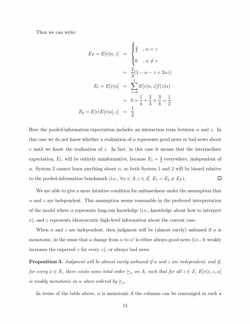
Then we can write:

EP = E[v|!, z] =

#

$

$

%

$

$

&

23 , ! = z

0 , ! (= z

=2

3(1" !" z + 2!z)

E1 = E[v|!] =1'

z=0

E[v|!, z]f(z|!)

= 0+1

4+

2

3+

3

4=

1

2

E2 = E[v|E[v|!], z] =1

2

Here the pooled-information expectation includes an interaction term between ! and z. In

this case we do not know whether a realization of ! represents good news or bad news about

v until we know the realization of z. In fact, in this case it means that the intermediate

expectation, E1, will be entirely uninformative, because E1 =12 everywhere, independent of

!. System 2 cannot learn anything about !, so both System 1 and 2 will be biased relative

to the pooled-information benchmark (i.e., *! # A, z # Z, E1 = E2 (= EP ).

We are able to give a more intuitive condition for unbiasedness under the assumption that

! and z are independent. This assumption seems reasonable in the preferred interpretation

of the model where ! represents long-run knowledge (i.e., knowledge about how to interpret

x), and z represents idiosyncratic high-level information about the current case.

When ! and z are independent, then judgment will be (almost surely) unbiased if ! is

monotonic, in the sense that a change from ! to !! is either always good news (i.e., it weakly

increases the expected v for every z), or always bad news.

Proposition 3. Judgment will be almost surely unbiased if ! and z are independent, and if,

for every x # X, there exists some total order ,x on A, such that for all z # Z, E[v|x, z,!]

is weakly monotonic in ! when ordered by ,x.

In terms of the table above, ! is monotonic if the columns can be rearranged in such a

15

way that the elements in every row are weakly increasing.

A natural case in which bias will occur is if ! represents a vector of continuous parameters,

and z represents information on how much weight to put on each element in the vector (these

are the assumptions used in the Gaussian model discussed below). Because ! is a vector,

E[v|x,!] may not be invertible. And because the relative importance of di!erent elements

of ! depends on the realization of z, then ! will not be monotonic, i.e. !! may be better or

worse than ! (in terms of v) depending on the realization of z.

It follows from proposition 3 that bias will not occur when EP is a separable function of

! and z, i.e. there must be some interaction between the two pieces of information for bias

to occur.

Corollary 1. Judgment will be unbiased if ! and z are independent, and there exist functions

g : X + A $ R, h : X + Z $ R, and i : R $ R, such that

EP = E[v|x, z,!] = i(g(x,!) + h(x, z))

and i is strictly monotonic.

Proof. In this case for any x there exists an ordering of A such that EP is monotonic in !,

for any z (i.e., the ordering according to g(x,!)). Judgment will therefore be unbiased, by

the previous proposition.

The existence of bias is sensitive to the distribution of knowledge: for example, no bias

would occur if your sister knew everything about the half of the baseball cards that are

alphabetically first, A-M, and you knew everything about the second half of baseball cards,

N-Z. If your sister knows both the values of her cards, and how to spot a fake, then changes

in your sister’s knowledge would then be monotonic: a change would be unambiguously good

or unambiguously bad news, independent of System 2’s knowledge, and therefore there would

be no bias, i.e. E2 = EP .

16

In a related paper Arieli and Mueller-Frank (2013) show that there will be no bias if the

signals ! and z are conditionally independent (given v and x), and if System 2 can infer from

E1 the entire posterior of System 1, not just their expectation (i.e. if they can infer f(v|x,!),

not just E[v|x,!]). They also show that E1 will almost always reveal the entire posterior, in

a probabilistically generic sense. The latter fact will hold in the Gaussian examples below:

System 2 always will be able to infer System 1’s entire posterior distribution over v. However

in most examples of interest to this paper ! and z will not be conditionally independent, and

for this reason Arieli and Mueller-Frank’s theorem will not apply, and a bias will remain.

2.2 Multiple Evaluations

An important distinctive prediction of this model is regarding judgments made jointly.

Most models of judgment and choice assume that each case is evaluated separately, inde-

pendent of other cases that may be under consideration at the same time.10 However I will

assume that when a set of cases is is encountered jointly then the reflective system receives

a corresponding set of automatic judgments, and that it can use the information from the

entire set to learn more about !, and therefore more about each individual case. To represent

joint evaluations I consider vectors of m # N+ elements, v = Rm, x = Xm, ! = Am, z = Zm,

with the joint distribution,

fm(v,x, z,!)

I will refer to a pair of vectors (x, z) as a situation, and an element (xi, zi) as a case. I

assume that System 1 forms their expectations about each case as before, and that System 2

conditions each of their judgments on the entire set of expectations received from System 1,

10Exceptions include theories of choice with menu-dependent preferences, e.g. Bordalo et al. (2012),K"szegi and Szeidl (2011), or where inferences are made from the composition of the choice set, Kamenica(2008).

17

E1 = E[v|x,!]

E2 = E[v|x, z,E1]

EP = E[v|x, z,!]

As written, this setup allows many channels of inference, so I introduce further assumptions

in order to concentrate just on the channels of interest.

First, as discussed, our principal interpretation is that System 1’s private information

represents long-run knowledge, so I assume that all elements of ! are identical, and therefore

simply refer to it as !.

Second, I will assume that each case (xi, zi) is distributed independently of !. If the

elements of x were informative about ! then we would expect joint and separate judgment

to di!er even without any signal from System 1.11

Finally, we will also assume that all observable information about each object is idiosyn-

cratic, i.e. xi and zi are informative only about vi, not about vj for j (= i.

These three points are incorporated into the following assumption about the distribution

of information:

fm(v,x, z,!) =

(

m)

i=1

f(vi|xi, zi,!)

*

f(z|x)f(x)f(!) (A1)

We can first note that, within this framework, neither System 1’s expectation nor the

pooled-information expectation will di!er between joint and separate evaluation, i.e.:

Ei1 = E[v|xi,!]

EiP = E[v|xi, zi,!]

However when System 2 observes a vector E1, it can learn about ! from the entire set of

11For example with baseball cards, you might infer that more common cards are less valuable, and thiscould cause separate and joint evaluation to di!er for another reason.

18

cases. Therefore, for any given case, an increase in the number of other cases evaluated at

the same time will reduce the expected bias:

Proposition 4. For any m < n, x # Xm, z # Zm, x! # Xn, z! # Zn, with xi = x!i and

zi = z!i for i # {1, . . . , m}, then for any j # {1, . . . , m}

V ar[Ej2 "Ej

P ] ' V ar[E!j2 "E

!jP ]

where E2 = E[v|x, z, E[v|x,!]] and E!2 = E[v!|x!, z!, E[v|x!,!]].

Proof. Because the first expectation conditions on a strictly larger information set, the result

follows from Lemma 1.

This proposition can be interpreted as applying to sequential, as well as joint, evaluation.

Suppose that an agent evaluates (x, z) and (x!, z!) in sequence, and assume that when System

2 evaluates the second case it has access to E1 for both cases – in other words, assume that

the decision-maker can remember their intuitions for previous cases, at least for a short

time. Then System 2’s second judgment will be the same as if they evaluated the pair

(x, z) = ((x, x!), (z, z!)) simultaneously, and therefore the expected bias will decrease relative

to the case in which (x!, z!) is evaluated without any history. In other words, more experience

is predicted to reduce the bias.

To apply this prediction about sequential judgments requires interpretation of when a

set of cases are part of the same situation. The important assumption is that System 2 can

recall all previous stimuli (x, z), and previous judgments (E1), so one natural application is

to laboratory experiments in which subjects make a series of decisions in quick succession.

To give some intuition for this result consider the problem of choosing a house to buy.

You might view one house, and get a good feeling about it, but not be sure what aspects

of the house contributed to that feeling. As you visit more houses you come to learn more

about what makes you like a house. And you may discover that your feelings are a!ected by

the weather on the day of the viewing, such that you have a more positive feeling about a

19

house if the sun was shining on the day you visited it. As you discover this pattern in your

judgments you learn to discount your intuitions to account for the weather, and the quality

of your judgment will increase (i.e., the accuracy of your judgments of the intrinsic quality

of a house will improve). In this case more experience will decrease bias.

2.3 Consistency

I now show how these results regarding the size of bias can be interpreted as predictions

about consistency of judgments. In studying human judgment it is often di"cult to say

that a single judgment is biased, because bias is relative to a person’s beliefs, and it is

di"cult to observe their full set of beliefs. We often establish bias indirectly by showing that

judgments, individually or collectively, violate some restriction which unbiased judgments

ought to satisfy. For example, it is di"cult to demonstrate that a subject over-values or

under-values a particular good, but many experiments demonstrate that valuation is a!ected

by normatively irrelevant details. Other experiments show that judgments indirectly violate

dominance (e.g. List (2002)), or transitivity (Tversky and Simonson (1993)).

The model in this paper makes a clear prediction: people may violate the normative

principles of consistency in separate evaluation, but will satisfy them if the same cases are

evaluated jointly; put another way, they may indirectly violate axioms of rational choice, but

will not directly violate them. For example, choices may be intransitive, but people would

never choose a dominated alternative. Also, choices made separately may be inconsistent,

but choices made jointly (assumed to condition on the same set E1) will obey any restrictions

on choice.

To state this proposition we introduce the concept of a restriction on judgment. Let a

judgment function be a function u : X + Z $ R. In some cases I will interpret this as a

utility function, in which the unknown utility of an object is inferred from its features.12 One

simple restriction on judgment is, for example, that two cases (x, z) and (x!, z!) should be

12The function does not include ! because it is assumed to be constant.

20

given the same evaluation; this can be expressed as a subset of the set of possible judgment

functions, {u : u(x, z) = u(x!, z!)}. We will be interested only in convex restrictions, i.e.:

Definition 1. A restriction on judgment U - RX"Z is convex if and only if, for any u, v # U ,

and 0 < ! < 1,

!u+ (1" !)v # U

If a restriction is convex then it means that any linear mixture of judgment functions which

each satisfy a constraint will itself satisfy the constraint. Most common restrictions satisfy

this definition, e.g. indi!erence between pairs of alternatives, dominance between pairs, or

separability of arguments.13 It is convenient to define judgment functions corresponding to

the the three types of expectation:

u!1 (x, z) = E[v|x,!]

u!2 (x, z) = E[v|x, z, E[v|x,!]]

u!P (x, z) = E[v|x, z,!]

It will also be convenient to define a joint judgment function for System 2, which conditions

on a set of cases, x,14

u!,x2 (x, z) = E[v|x, z, E[v|x,!]].

Now suppose that the pooled-information judgment function u!P satisfies some convex

restriction U . Clearly u!1 may violate that restriction, because it ignores z. However for u2

the result will be mixed: when evaluations are made separately (i.e., when conditioning on

di!erent sets x), then the restriction may be violated, but when evaluations are made jointly,

with the same conditioning set x, they will always satisfy the restriction.

13For example, the indi!erence restriction {u : u(x, z) = u(x", z")} is convex because any mixture betweenpairs of utility functions which satisfy this indi!erence will itself satisfy indi!erence. An example of a non-convex restriction is that u(x, z) # {0, 1}.

14This represents the evaluation of x conditioning on some other set x. In practice we may only observejudgments when x # x, i.e. the current case must always be a member of the conditioning set.

21

Proposition 5. For any convex restriction on judgment U - RX"Z with, for all ! # A,

u!P (x, z) # U

then for all ! # A, x # Xm, m > 1,

u!,x2 (x, z) # U

For example consider how people will respond to irrelevant di!erences. Suppose that

our restriction is, as above, that for some x, x! # X, z, z! # Z, {u : u(x, z) = u(x!, z!)}.

Proposition 5 implies that people evaluating (x, z) and (x!, z!) jointly will evaluate them to

have the same worth, though they may give di!erent judgments when evaluated separately.

A natural corollary exists in choice behavior. Usually we assume that choice from a choice

set (D # D, D = 2X"Z\!) is generated by maximizing a utility function:

c(D) = arg max(x,z)#D

u(x, z)

and restrictions on the utility function can be translated into restrictions (or axioms) on

the choice correspondence. Choice correspondences can be defined corresponding to each

evaluation function defined above (i.e. c!P , c!1 , c!2 , c!,x2 pick out the maximal elements of the

choice set according to the functions u!P , u!

1 , u!2 , and u!,x

2 ). In the case of c!,x2 I make the

further assumption that the conditioning set x is formed by elements of the choice set, D, i.e.

that when choosing from a choice set, System 2 receives signals from System 1 about each of

the alternatives in the choice set. Proposition 5 will imply that, if EP satisfies some convex

restriction U , then System 2’s choices will obey any axioms implied by that restriction.

Corollary 2. For any convex restriction on judgment, U - RX"Z , and corresponding choice

restriction CU - DD,15 if pooled-information judgment satisfies U (*! # A, u!P # U) then

15c # CU i! .u # U , c(A) = argmax(x,z)#A u(x, z).

22

individual System 2 choices will satisfy CU .

Proof. By the proposition, each u!,x2 belongs to U , therefore it must satisfy the choice re-

strictions implied by U .

Decisions made by System 1 may violate restrictions axioms on choice, because those

decisions will fail to condition on z (put another way, inattentive decisions may violate

axioms of choice). Proposition 5 implies that System 2’s decisions will never violate an

axiom in a given choice set, although decisions made separately can collectively violate those

axioms. If the underlying restriction U entirely rules out certain choices, then those choices

will never be made by System 2. For example if U included a dominance restriction, so

that for some (x, z), (x!, z) # X + Z, U = {u : u(x, z) > u(x!, z)}, then a decision-maker

with implicit knowledge would never choose a dominated option ((x!, z) # c({(x, z), (x!, z)})),

however they might still make intransitive choices (e.g. (x, z) = c({(x, z), (x!, z)}), (x!, z) =

c({(x!, z), (x!!, z)}), (x!!, z) = c({(x!!, z), (x, z)})).

This can be extended to choices which are made jointly. Joint decision-making is a

common protocol used in experiments (Hsee et al. (1999), Mazar et al. (2010)). Subjects

are typically instructed to consider all choice sets before making their several decisions,

and are told that a single decision will be randomly chosen to be implemented. If choices

obey the independence axiom of expected utility theory, and subjects infer nothing from the

composition of the choice set, then choice from each given choice set should be una!ected by

the other choices being considered simultaneously.

The corollary above implies that choices made jointly will not violate any axioms of choice,

under the assumption that when presented with joint choices people make judgments which

condition on all the alternatives available. To be precise, if they are confronted with a set of

choice sets D1, .., Dn, then I assume that they form judgments using E!,x2 , with x now being

the union of all the choice sets (i.e., x # x i! x # D1 / . . . /Dn).

It is important to emphasize that although the model predicts that joint evaluations

and choices will be consistent, it does not predict that they will be be unbiased (i.e., that

23

E2 = EP ). In terms of baseball cards, consistency implies giving two packets the same

bid when they di!er only in a counterfeit card. Though consistent, these judgments may

still have bias: even in joint evaluation you will not necessarily be able to back out perfect

knowledge of ! from your sister’s reports, so your judgments may still be biased relative to

the pooled-information benchmark.

It is also worth mentioning that choices taken sequentially need not be consistent with

each other.16 Later choices will have access to larger sets of E1 judgments, and therefore

di!erent beliefs about !, thus sequential decisions need not be consistent.

2.4 Learnability

In its current form the model allows for the existence of knowledge held by System 1 which

could never be discovered by System 2. Suppose there exist a pair !,!! # A such that, for

every x # X, E[v|x,!] = E[v|x,!!]. Then System 2 could never discover whether ! or !!

holds, even though it may be relevant, i.e. .z # Z, E[v|x, z,!] (= E[v|x, z,!!].

In this section I note that if ! is learnable by System 1 (in a particular sense) then !

can also be inferred by System 2, from observing System 1’s responses. Therefore there will

be no bias when System 2 observes all of System 1’s judgments, i.e. its judgments for every

possible x.

Definition 2. A distribution f(v, x, z,!) is learnable if *!,!! # A, .x # X,

E[v|x,!] (= E[v|x,!!]

Learnability is a natural restriction if we think of System 1 as a naive learner: i.e., if

System 1 simply stores the average observed v for a given x. Given an unlearnable distribu-

tion, there will always exist a coarsening of A that is learnable (because, at worst, if A is a

16Sometimes “within-subjects” is used to mean experimental conditions in which decisions are made se-quentially. Here I use it to refer to simultaneous choices.

24

singleton, then it is learnable).17

The following proposition states that if System 2 can observe System 1’s judgment for

every element in X, and f is learnable, then judgment will be unbiased.

Proposition 6. If f is learnable then for all ! # A, z # Z, x # X, m # N, x # Xm, with

x! # x 0) x! # X,

E!,x2 (x, z) = E!

P (x, z)

Proof. Because x contains every element in X, then E1 will contain E[v|x,!] for every x # X.

Because f is learnable, there is only a single ! # A that is consistent with this pattern, thus

E[!|x,E1] = !. Therefore E2 = E[v|x, z,E1] = E[v|x, z,!] = EP .

2.5 Comparative Statics

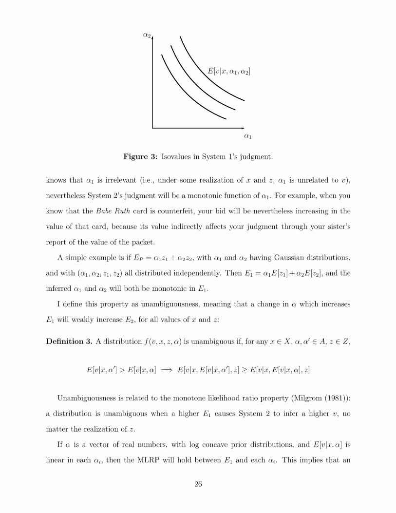
Next we consider what can be said about the direction of the bias. An illustration of the

nature of the problem is given in Figure 3, in which System 1’s private information is a

point in a two-dimensional space ((!1,!2) # A = R2), and E[v|x, z,!1,!2] is assumed to

be increasing in both !1 and !2. System 1 observes (!1,!2) and calculates an expectation,

E1 = E[v|x,!1,!2]. System 2 observes that expectation, and therefore learns that !1 and

!2 lie on a certain curve, which leads him to update his posterior over (!1,!2). A natural

assumption will be that, when System 2 observes a higher E1, his posteriors over both !1

and !2 increase, in the sense of having higher expected values. If this is true then there will

be a “spillover” e!ect: an increase in !1 will cause an increase in System 2’s estimate of !2.

Thus in situations where !1 is known to be irrelevant, it will nevertheless a!ect System 2’s

judgment, and the direction of influence will be predictable.

If this property holds we can tell an intuitive story about biases: even when System 2

17There is a simple example of a non-learnable distribution for the baseball-cards example. Suppose thedistribution of cards is such that two cards P and Q only ever appear together, i.e. every pack containseither both cards or neither. Then someone who observes x and v will not be able to learn ! (the values ofthe cards). In particular for any assignment of values to P and Q which is consistent with the observed xand v, it would also be consistent if those values were switched. So in this case we would expect System 1only to learn the value of P +Q; i.e., a coarsening of A would be learnable.

25

!

"!1

!2

E[v|x,!1,!2]

Figure 3: Isovalues in System 1’s judgment.

knows that !1 is irrelevant (i.e., under some realization of x and z, !1 is unrelated to v),

nevertheless System 2’s judgment will be a monotonic function of !1. For example, when you

know that the Babe Ruth card is counterfeit, your bid will be nevertheless increasing in the

value of that card, because its value indirectly a!ects your judgment through your sister’s

report of the value of the packet.

A simple example is if EP = !1z1 + !2z2, with !1 and !2 having Gaussian distributions,

and with (!1,!2, z1, z2) all distributed independently. Then E1 = !1E[z1] +!2E[z2], and the

inferred !1 and !2 will both be monotonic in E1.

I define this property as unambiguousness, meaning that a change in ! which increases

E1 will weakly increase E2, for all values of x and z:

Definition 3. A distribution f(v, x, z,!) is unambiguous if, for any x # X, !,!! # A, z # Z,

E[v|x,!!] > E[v|x,!] =) E[v|x, E[v|x,!!], z] ' E[v|x, E[v|x,!], z]

Unambiguousness is related to the monotone likelihood ratio property (Milgrom (1981)):

a distribution is unambiguous when a higher E1 causes System 2 to infer a higher v, no

matter the realization of z.

If ! is a vector of real numbers, with log concave prior distributions, and E[v|x,!] is

linear in each !i, then the MLRP will hold between E1 and each !i. This implies that an

26

increase in E1 will cause System 2 to increase their posteriors over every !i (in the sense of

stochastic dominance), which in turn implies that f is unambiguous.

Proposition 7. If A = Rn, ! and z are independent, and

E1 = E[v|x,!] =n'

i=1

!ig(x)

and each !i is distributed independently with F (!i|x) di!erentiable and f(!i|x) log-concave,

and E[v|x,!, z] is increasing in !, then f is unambiguous.

Proof. Shaked and Shanthikumar (2007) Theorem 6.B.9 establishes that the posteriors over

!i will increase in E1, in the sense of stochastic dominance. Because EP is increasing in each

!, then E2 must increase, thus f is unambiguous.

2.6 E!ects of the Common Information

We have discussed how changes in System 1’s private information, !, a!ect System 2’s

judgment. We now discuss changes in the common information, x, which allows us to address

how biases may depend on aspects of the given case.

In particular, a common explanation for judgment being sensitive to a normatively ir-

relevant change is that, although the change is irrelevant in the current situation, it is

usually relevant, i.e. it is relevant in other similar situations. This is a common “heuris-

tics” explanation of biases. In the terms of this paper, a change in low-level informa-

tion (x to x!) may be normatively irrelevant given the high-level information z, for all !,

E[v|x, z,!] = E[v|x!, z,!], but the change is informative if we ignore the high-level informa-

tion, for some !, E[v|x!,!] > E[v|x,!].

This can explain why System 1 makes a mistake, however to explain why System 2 can

be biased requires implicit knowledge. It also remains to be shown under what conditions

the direction of System 2’s bias will be the same as that in the heuristic explanation, i.e.

27

under what conditions will a change in x which causes an increase in E1 also cause a (weak)

increase in E2? I call this property congruence:

Definition 4. A distribution f is congruent for some x, x! # X, and z # Z if,

*! # A, E[v|x!,!] > E[v|x,!] =) E[v|x!, E[v|x!,!], z] ' E[v|x, E[v|x,!], z]

This may not hold even if f is unambiguous in the sense defined above. There are two

qualifications. First, if System 2 knows that x! is associated with a higher v than x, then

it will already discount the e!ect on E1. Therefore we are really interested in the di!erence

between what each System believes about the relationship between x and v. A natural

benchmark is when System 2 expects no di!erence: i.e., when E[v|x!] = E[v|x]. Second, even

if System 2 has the same expectation about v given x and x!, still congruence may fail if

the variance di!ers between cases. For example, suppose that System 2 was relatively more

uncertain about the relationship between x! and v, then it would discount the signal from E1

relatively more, and this discounting e!ect could overwhelm the principal e!ect.18

We can show that a change in x will cause congruent changes in E1 and E2 under as-

sumptions of orthogonality and symmetry. Suppose that under some realization z # Z, two

cases x and x! have the same value. Then we can partition the space of A into relevant and

irrelevant information (i.e., partition A into A1 +A2, depending on whether it has any e!ect

on E[v|x,!, z]). If we assume that (1) the relevant and irrelevant information is distributed

independently; and (2) for x and x!, the irrelevant information is distributed identically; then

18Suppose that replacing Babe Ruth with Ty Cobb increases E1. If System 2 knows that both cards arefake, then he wishes to infer, from E1, only the part of ! which is relevant to the remaining genuine cards. Ifhis priors over the values of Babe Ruth and Ty Cobb have the same shape, then this inference should be thesame, i.e. replacing Babe Ruth with Ty Cobb will have the same e!ect as if the value of Babe Ruth increasedto be equal to that of Ty Cobb. And if f is unambiguous, the change in E1 has a congruent e!ect on E2.However this conclusion could be reversed if System 2 had a relatively larger uncertainty about the value ofTy Cobb. As the variance of System 2’s prior on Ty Cobb increases, then E1 becomes less informative aboutthe part of ! relevant to System 2 (i.e., the part of ! relevant to the genuine cards), and System 2 will putrelatively more weight on his prior, and relatively less weight on E1. In the limit, as System 2 becomes moreuncertain about Ty Cobb’s value, he will eventually ignore the signal from System 1, and therefore even whenE1 is greater for Ty Cobb than for Babe Ruth, E2 could exhibit the opposite pattern; in other words a changein x could increase E1 but decrease E2.

28

the changes in E1 and E2 will be congruent (if f is unambiguous).

Proposition 8. For any x, x! # X, and z # Z, if

(i) under z, the di!erence between x and x! is irrelevant, i.e. *! # A, E[v|x, z,!] =

E[v|x!, z,!]

(ii) A can be divided into two parts, distributed independently of each other and of x, i.e.

A = A1 +A2, with f(!1,!2, x) = f(!1)f(!2)f(x)

(iii) under z, !2 is irrelevant, i.e. E[v|x!!, z,!1,!2] = E[v|x!!, z,!1,!!2] for all x!! # X,

!1 # A1, !2,!!2 # A2

(iv) given !1, x and x! have the same information about v, i.e. *!1 # A1, f(v|x,!1) =

f(v|x!,!1)

(v) f is unambiguous

then the distribution f will be congruent for x and x!.

This result allows us to derive an important prediction: if we observe bias to go in a

particular direction, then we should expect the world to also move in that direction. I.e., if

x! induces a higher judgment than x, even when people know that the di!erence is norma-

tively irrelevant, then, under the assumptions above, this implies that E[v|x!,!] > E[v|x,!],

i.e. that on average (ignoring z) x! is associated with higher v, though people may not be

consciously aware of this association. I discuss evidence for this prediction in a later section.

3 Gaussian Model

In this section I assume a specific distribution for f(v, x, z,!), and solve explicitly for the bias.

Under this distribution System 2’s problem can be seen as reweighting a weighted average.

System 1’s estimate, E1, will be a weighted average of their private information (!1, . . . ,!n),

with weights given by the public information (x1, . . . , xn). System 2 wishes to reweight that

information, but cannot perfectly infer the underlying data, and so their estimate, E2, will

incorporate systematic biases when seen from the perspective of a third party. This allows

29

us to make quite precise statements about how low-level information, high-level information,

and implicit knowledge interact to produce biases.

I first present the model without any low-level information (i.e., ignoring x), then intro-

duce x, and finally introduce multiple objects of consideration (x). I assume that ! and z

are n-vectors of reals, !, z # Rn, and are independently distributed, i.e.,

f(v,!, z) = f(v|!, z)

(

n)

j=1

f(!i)

*(

n)

j=1

f(zj)

*

and that the pooled-information expectation is separable in each dimension, and multiplica-

tive in the elements of ! and z:

EP = E[v|!, z] =n'

j=1

!jzj

We can therefore express each System’s expectation as:

E1 =n'

j=1

!jE[zj ]

E2 =n'

j=1

E[!j |E1]zj

and it is convenient to define:

E0 =n'

j=1

E[!j ]E[zj ]

Finally I assume that System 2 has independent Gaussian priors over the distribution of !j:

!j 1 N(E[!j ], $2j )

Given the normality assumption, System 2 will update each !j by attributing to it a share

30

of E1 proportional to its variance:

E[!j |E1] = E[!j ] +E[zj ]2$2

j+

k E[zk]2$2k

E1 "E0

E[zj ]

We can now write out the full solution to System 2’s problem, defining %j = E[zj ]2$2j :

E2 =n'

j=1

E[!j |E1]zj

=n'

j=1

E[!j ]zj +n'

j=1

%j+

k %k

E1 "E0

E[zj ]zj

Now we wish to derive the bias, i.e. compare E1 and E2 to the full information case. First

note how E1 di!ers from EP :

E1 "EP ='

!j(E[zj]" zj)

If zj < E[zj ] (i.e., if System 2 knows that dimension !j should be given less weight than

usual), then System 1 will tend to over-react to feature j, and vice versa.

We can write System 2’s final bias as:

E2 " EP =n'

j=1

E[!j ]zj +n'

j=1

%j+

k %k

E1 " E0

E[zj ]zj "

n'

j=1

!jzj

=n'

j=1

(E[!j]" !j)zj + (E1 " E0) +n'

j=1

zj " E[zj ]

E[zj ]

%j+

k %k(E1 " E0)

=n'

j=1

(E[!j]" !j)zj +n'

j=1

(!j " E[!j ])E[zj ] +n'

j=1

zj " E[zj ]

E[zj ]

%j+

k %k(E1 " E0)

=n'

j=1

(E[zj ]" zj)

(

(!j " E[!j ])"1

E[zj ]

%j+

k %k(

n'

k=1

(!k "E[!k])E[zk])

*

The first term inside the large brackets can be thought of as the direct bias, due to the

31

di!erence between the expected and actual outcomes. The second term represents the loss

of accuracy due to the discounting which System 2 applies to the information coming from

System 1.

Proposition 9. The overall bias can be expressed as

E2 " EP =n'

j=1

(E[zj]" zj)

(

,

1"%j

+

k %k

-

(!j "E[!j ])"%j

+

k %k

'

k $=j

E[zk]

E[zj ](!k " E[!k])

*

The intuition can be better understood with a further simplified version, conditioning

just on some pair !j, zj ,

E[E1 " EP |!j, zj ] = " (zj "E[zj ])!j

E[E2 " EP |!j, zj ] = "

,

1"%j

+

k %k

-

(zj " E[zj ]) (!j " E[!j])

The term (1" "j!k "k

), is always between 0 and 1, so the direction of the bias is determined by

the deviations of ! and z from their expected values. We can make a number of observations

about the nature of the biases:

1. A bias requires that both ! and z are not at their expected values, i.e. there exists some

j, k with !j (= E[!j] and zk (= E[zk] (it does not need to be the case that j = k, though

the following discussion focuses on that case). In other words, bias occurs only when

both the implicit knowledge and the high-level information depart from their expected

values.

2. The sign of System 2’s bias depends on the interaction of the two deviation terms,

!j " E[!j ] and zj " E[zj ]. Suppose that zj < E[zj ] and !j > E[!j ], this will cause

people to overestimate v. Intuitively, the second System discounts the signal, because

!j is less important than usual. But !j is bigger than expected, so the reflective system

does not discount enough.

3. The size of System 2’s bias is decreasing in %j = $2jE[zj ]2. A higher $j represents more

32

uncertainty about !j , and so a larger part of (E1 " E0) will be attributed to !j, and

therefore the bias will be smaller because the discount applied to E1 will be greater. In

other words, if System 2 is less sure about the e!ect of !j , then it will be less influenced

by changes in !j.

This model has a simple interpretation as the reweighting of a weighted average. For example

the US EPA’s “combined MPG” for new cars is calculated as a weighted average of city MPG

(55%) and highway MPG (45%). Each car buyer may have their own preferred weights. If

I observe only the EPA’s combined MPG for a car, I will then have to infer the underlying

data in order to construct my preferred weighting. If my priors about the car’s underlying

MPG variables are Gaussian, then the model in this section is an exact description of the

problem I face, with System 1 representing the EPA and System 2 representing me. My

posterior can be described by the expression above for E2, and my bias relative to the case

in which I knew the underlying data as E2 " EP (here n = 2, ! will represent the city and

highway MPG variables, z are my idiosyncratic weightings, and the EPA’s weights could be

interpreted as E[z], i.e. the average weights used by car buyers).

The predictions will apply to buying a car: if my weights di!er from the EPA’s weights,

and if the car’s attributes di!er from their expected values, then my judgment will be biased

in a predictable way. In some cases my judgment will be a!ected by information I know to

be irrelevant: if I put a 0% weight on highway MPG, nevertheless I will value more highly a

car which has a higher highway MPG, everything else equal (because highway MPG a!ects

the EPA’s combined MPG, which in turn a!ects my beliefs about city MPG).

3.1 Judging Alternatives with Attributes

I now extend the Gaussian model to include public information which can be interpreted as

a set of attributes (x # Rn) which are observable to both System 1 and System 2. I assume

that the interpretation of these attributes is a!ected both by information private to System

33

1, !, and by information private to System 2, z, with the functional form:

EP = E[v|x, z,!] =n'

j=1

xjzj!j (4)

As before, in order to achieve an analytical solution, I assume that each element in ! is drawn

from a normal distribution, i.e. !j 1 N(E[!j ], $2j ), each !j is independent of the others, and

of x and z.

The attributes xi should be interpreted as cues which are used as inputs to judgments. For

example when judging the distance of an object then the cues, (x1, . . . , xn), could include

the object’s size, shape, color, etc. When judging the value of a product, then the cues

could include its price, color, quality, and contextual features such as whether it is the most

expensive product, or whether you have observed someone else buying this product. Finally

the model in this section can be applied directly to the baseball-card metaphor used in the

introduction: if there is a universe of n cards, !i represents the value of card i, xi # {0, 1}

represents whether card i is in the current packet, and zi # {0, 1} represents whether the

card is genuine or not.

Because xj is a commonly-known weighting variable, the solution is essentially the same

as in the model without attributes, substituting in xjzj for zj , and xjE[zj ] for E[zj ]. The

solutions are therefore:

E1 = E[v|!, x] =n'

j=1

!jxjE[zj ]

E1 " EP =n'

j=1

!jxj(E[zj ]" zj)

E[!j |x, z, E1] = E[!j] +E[zj ]2x2

j$2!j

+

k E[zk]2x2k$

2!k

E1 "E0

xjE[zj ]

34

Proposition 10. System 2’s bias in this model will be

E2"EP ='

j

(E[zj ]" zj)xj

(

(!j "E[!j ])

,

1"&j

+

k &k

-

+&j

+

k &k

1

E[zj ]xj

n'

k $=j

(!k "E[!k])E[zk]xk

*

where &j = $2jE[zj ]2x2

j .

As before, a simpler way to understand this result is to derive the average bias for some

given !j , zj .

E[E2 " EP |x, zj ,!j] = " (zj " E[zj ]) (!j " E[!j]) xj

,

1"&j

+

k &k

-

(5)

The remarks on interpretation in the previous section largely apply here. Suppose some

attribute xj has a stronger positive relationship with v than System 2 is aware of (!j >

E[!j]). Suppose also that System 2 knows that the influence of xj should be discounted,

i.e. zj < E[zj ]. Then the model predicts System 2’s judgment will be upward biased in this

situation, for any positive level of that attribute, i.e. E2 "EP > 0 for xj > 0.

Alternatively consider when some cue is normally informative, but in the current situation

it is known to be uninformative, i.e. when E[zj ] > 0, and zj = 0. Then the bias will have

the sign of (!j " E[!j]), i.e. if the cue has a positive association with v, relative to System

2’s expectations, then the bias will be positive.

It is also of interest to note the comparative statics with respect to xj . The final two

terms of equation 5 can be expanded:

xj

,

1"&j

+

k &k

-

= xj

,

1"$2jE[zj ]2x2

j+

k $2kE[zk]2x2

k

-

=xj

+

k $2kE[zk]2x2

k " $2jE[zj ]2x3

j+

k $2kE[zk]2x2

k

= xj

+

k $=j $2kE[zk]2x2

k+

k $2kE[zk]2x2

k

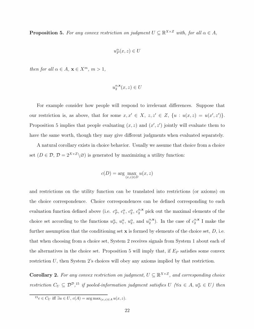
This function is not monotonic in xj , instead it is proportional to xj

k+x2j, for some k > 0. This

35

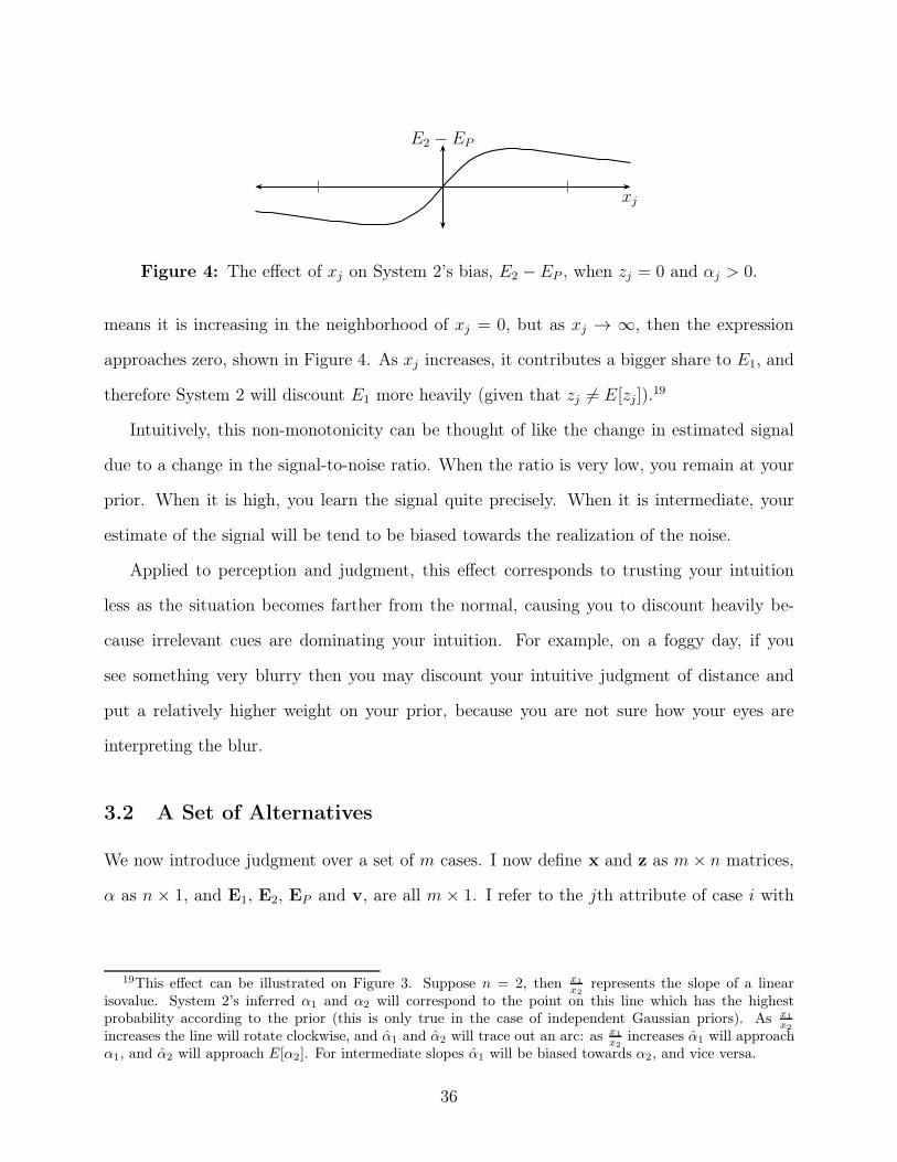
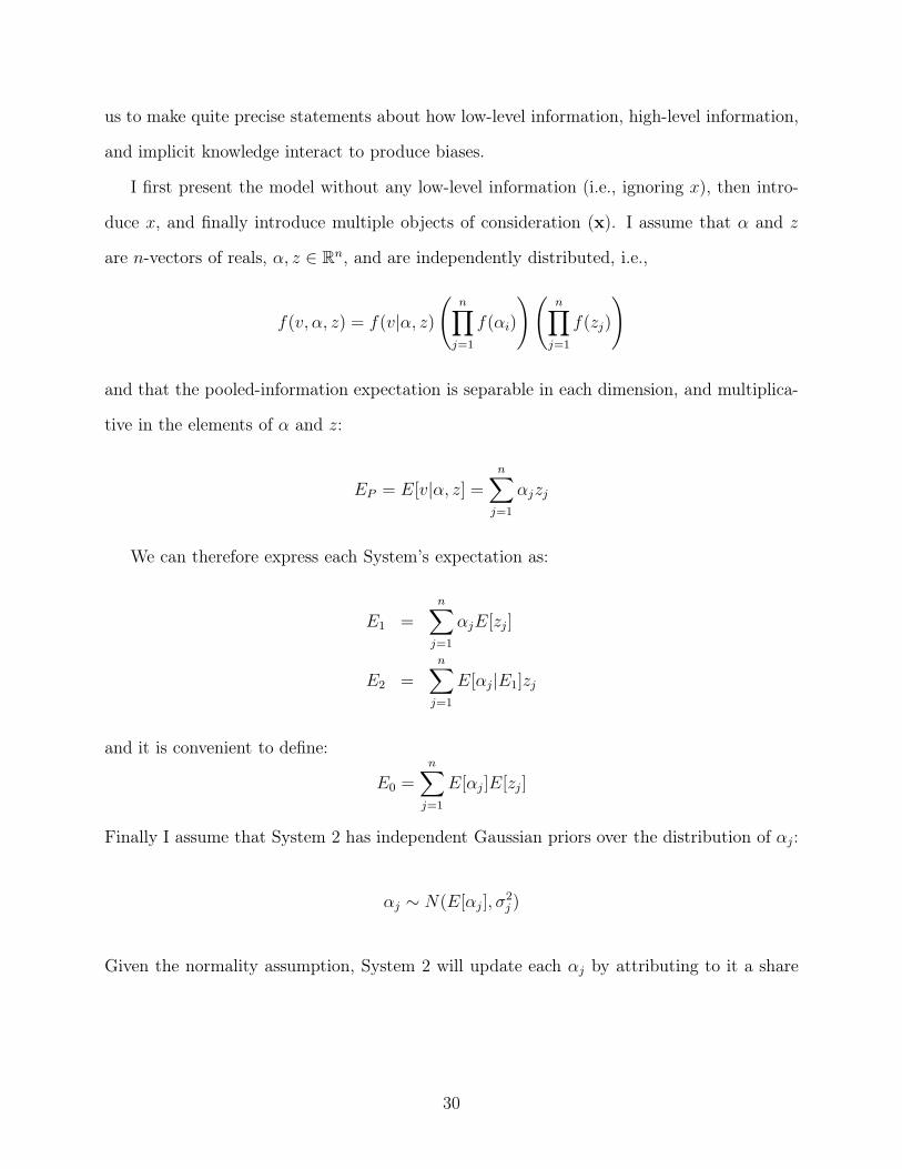
E2 " EP

xj

Figure 4: The e!ect of xj on System 2’s bias, E2 "EP , when zj = 0 and !j > 0.

means it is increasing in the neighborhood of xj = 0, but as xj $ 2, then the expression

approaches zero, shown in Figure 4. As xj increases, it contributes a bigger share to E1, and

therefore System 2 will discount E1 more heavily (given that zj (= E[zj ]).19

Intuitively, this non-monotonicity can be thought of like the change in estimated signal

due to a change in the signal-to-noise ratio. When the ratio is very low, you remain at your

prior. When it is high, you learn the signal quite precisely. When it is intermediate, your

estimate of the signal will be tend to be biased towards the realization of the noise.

Applied to perception and judgment, this e!ect corresponds to trusting your intuition

less as the situation becomes farther from the normal, causing you to discount heavily be-

cause irrelevant cues are dominating your intuition. For example, on a foggy day, if you

see something very blurry then you may discount your intuitive judgment of distance and

put a relatively higher weight on your prior, because you are not sure how your eyes are

interpreting the blur.

3.2 A Set of Alternatives

We now introduce judgment over a set of m cases. I now define x and z as m+ n matrices,

! as n + 1, and E1, E2, EP and v, are all m + 1. I refer to the jth attribute of case i with

19This e!ect can be illustrated on Figure 3. Suppose n = 2, then x1

x2represents the slope of a linear

isovalue. System 2’s inferred !1 and !2 will correspond to the point on this line which has the highestprobability according to the prior (this is only true in the case of independent Gaussian priors). As x1

x2

increases the line will rotate clockwise, and !1 and !2 will trace out an arc: as x1

x2increases !1 will approach

!1, and !2 will approach E[!2]. For intermediate slopes !1 will be biased towards !2, and vice versa.

36

xij , and likewise for the other variables. The expectations can be defined as:

E1 = E[v|x,!]

E2 = E[v|x,E1, z]

EP = E[v|x,!, z]

System 1 is assumed to form independent judgments of each case:

Ei1 = E[vi|!, xi] =

n'

j=1

!jxijE[zj ]

In matrix notation this can be written,

E1 = x(! 3 E[z])

where (P 3 Q)ij = P ij + Qi

j. For compactness, and without loss of generality, I set E[zj ] = 1

for all j. As before System 2 wishes to infer ! from E1, but he now has more information.

Because the elements of ! are distributed independently and normally, the expectation of !,

!, will maximize the likelihood function,

"(! "E[!])T"(!" E[!])

subject to the above constraint, where " is a diagonal matrix, with elements $%21 , . . . , $%2

n ,

and P T is the transpose of P . The first-order condition of a Lagrangian can be written (Boyd

and Vandenberghe (2004), p304):

2(!" E[!])T" = 'x

! = E[!] +1

2"%1

xT'T

37

Where ' is an n + 1 vector of Lagrangian multipliers. Substituting into the constraint, we

get (with E[z] a vector of 1s):

E1 = xE[!] +1

2x"%1

xT'T

(x"%1xT )%1(E1 " xE[!]) =

1

2'T

This can be substituted back into the first-order condition to get:

! = E[!] + "%1xT (x"%1

xT )%1(E1 " xE[!])

Proposition 11. System 2’s bias can be expressed as

E2 "EP = (x 3 z)E[!|E1,x]" (x 3 z)!

= (x 3 z).

E[!] + "%1x!(x"%1

x!)%1

x(!" E[!])" !/

As before, if every zij = E[zij ], then there will be no bias, even though System 2 will not

know the true value of ! (in this case every element of z would be 1, and the expression

above would collapse to E2 " Ep = 0). Likewise, if every !j = E[!j ], then E2 = EP .

In this case, if you observe a su"cient number of objects you can infer all of System 1’s

information, and therefore bias will go to zero. In particular if there are n dimensions in !,

then observing n di!erent objects will be su"cient (as long as no objects are collinear), i.e.

if rank(x) ' n, then E2 = EP.

In practice there may be so many characteristics influencing automatic judgment that

System 2 will never realistically infer all of System 1’s information. Bias would also never go

to zero if there is noise in observing E1; this could be represented by dummy-variables in x

which are non-zero for individual cases, to represent idiosyncratic qualities.

38

4 Evidence for an Automatic System

In this section I discuss literature which argues that people have a separate automatic system

of judgment, as illustrated in Figure 1, before moving on to evidence for the existence of

implicit knowledge, as in Figure 2. Here I am simply summarizing existing arguments, but I

believe that the similarity among these theories across diverse disciplines has not before been

noted.

I discuss papers across a broad range of disciplines, all of which feature two main ar-

guments: First, that many anomalous judgments are rational relative to a subset of the

information available. Second, that people often report holding two estimates at the same

time, which can be identified with automatic and reflective judgments; in particular that

even when people know their automatic judgment is incorrect they remain viscerally aware

of that judgment.

Hermann von Helmholtz (1821-1894) famously characterized perception as “unconscious

inference,” and made both arguments mentioned above.20 More recently Zenon Pylyshyn

has been important in making the case for the existence of an independent visual faculty

(Pylyshyn (1984), Pylyshyn (1999)). He argues that there is extensive evidence for visual

perception being cognitively impenetrable, defined as “prohibited from accessing relevant ex-

pectations, knowledge and utilities in determining the function it computes.”21 Pylyshyn

observes that biases in perception can often be explained as insensitivity to high-level in-

formation: “the early vision system ... does its job without the intervention of knowledge,

beliefs or expectations, even when using that knowledge would prevent it from making er-

rors.”22 He also observed that automatic judgments persist: “[i]t is a remarkable fact about

20Helmholtz’s principal contribution was to document that judgment operates as if it was making rationalinferences from sensory information, but he also noted that the process sometimes makes mistakes by failingto incorporate all relevant knowledge, and that those automatic judgments remain salient: “no matter howclearly we recognize that [the perception] has been produced in some anomalous way, still the illusion doesnot disappear by comprehending the process.” (von Helmholtz (1971 [1878])).

21Similar arguments are made by Marr (1982) and Fodor (1983).22Similarly he says “the constraints [i.e., inferences made by the visual system] show up even if the observer

knows that there are conditions in a certain scene that render the constraints invalid in that particular case.”

39

perceptual illusions that knowing about them does not make them disappear ... there is

a very clear separation between what you see and what you know is actually there.” This

separation of early perception from general knowledge seems to be widely accepted in the

literature on perception. Feldman (2013), a proponent of quantitative Bayesian models of

perception, acknowledges Pylyshyn’s point: “there is a great deal of evidence ... that per-

ception is singularly uninfluenced by certain kinds of knowledge.” A recent literature on

the Bayesian interpretation of perceptual illusions argues that they can be explained as the

perceptual system applying rules that produce optimal inferences on average, i.e. ignoring

certain details specific to the current situation (Adelson (2000)).

Within research on anomalies in judgment Tversky and Kahneman (1974) introduced the

“heuristics and biases” paradigm. Their original statement conjectured that biases are caused

by “people rely[ing] on a limited number of heuristic principles which reduce ... complex

tasks ... to simpler judgmental operations. In general, these heuristics are quite useful,

but sometimes they lead to severe and systematic errors.” Tversky and Kahneman do not

explicitly state that heuristics are optimal given a limited information set, however Shah and

Oppenheimer (2008), in a detailed survey of the subsequent literature, describe mechanisms

which can all be interpreted in this way.23 Regarding the persistence of automatic responses

Kahneman and Frederick (2005) say “knowledge of the truth does not dislodge the feeling.”24

Sloman (1996) initiated the modern literature on “two systems” of judgment (also called

“dual process” theories). He says that most prior debate has been over whether judgment

is associative or rule-based, but that the evidence suggested that both types of cognition

are implemented in separate systems.25 He describes the associative system as making ac-

curate judgments given its information (“[it can] draw inferences and make predictions that

23“all heuristics rely on one or more of the following methods for e!ort-reduction: 1. Examining fewer cues.2. Reducing the di#culty associated with retrieving and storing cue values. 3. Simplifying the weightingprinciples for cues. 4. Integrating less information. 5. Examining fewer alternatives.”

24They quote Stephen Jay Gould, discussing the Linda problem: “I know [the right answer], yet a littlehomunculus in my head continues to jump up and down, shouting at me – ‘but she can’t just be a bankteller; read the description.’”

25Evans (2008) gives a survey of dual-processing models of judgment.

40

approximate those of a sophisticated statistician”), whereas the rule-based system “is rela-

tively complex and slow,” but dominant, meaning that it can “suppress the response of the

associative system in the sense that it can overrule it.” Sloman has two principal arguments

for the existence of two systems. First, that biases in judgment can often be explained as

due to misapplied associative reasoning: “[r]easoning performance is accurately predicted

by judgments of similarity taken out of the problem context in the absence of any further

assumptions about the knowledge that people bring to bear on the task.”26 Second, that

association-based judgments persist; he gives examples of reasoning problems which “cause

people to believe believe two contradictory responses simultaneously ...[in which] the first

response continues to be compelling irrespective of belief in the second answer, irrespective

even of certainty in the second answer.”

Stanovich and West (2000) introduced the “System 1” and “System 2” terminology, and

additionally argued that Sloman’s dual-system model could give a good account of interper-

sonal di!erences in susceptibility to bias. Daniel Kahneman has since adopted the System

1 / 2 terminology as a foundation for the “heuristics and biases” program (Kahneman and

Frederick (2005), Kahneman (2011)).

Each of these writers uses di!erent words to describe the knowledge which the automatic

does not have access to (in the language of this paper, z). Helmholtz says that perception

will make incorrect inferences when “the modes of stimulation of the organs of sense are

unusual,” or when “we recognize that [stimuli] ha[ve] been produced in some anomalous

way,” i.e. he assumes that the perceptual system does not have access to knowledge about

unusual stimulation. Pylyshyn says that vision is prohibiting from accessing “global” or

“high-level” information. Sloman says that System 1 relies on associations, and does not

use the “problem context” or “further knowledge.” Kahneman and Tversky do not explicitly

26One example is performance in the Wason selection task, where subjects choose which cards to turn overin order to test a proposition about what is on the faces of the cards. A common finding is that performanceis influenced strongly by the associative features of the proposition being tested, even when subjects areaware that those associative features are irrelevant in the current task. Interpreted in the language of thispaper, some associative cue xi may be normally relevant, but irrelevant in the current situation (i.e., whetheror not it is relevant is determined by zi, something that is not observed by System 1).

41

talk about what kind of information heuristics exclude, but they discuss what information

heuristics do have access to, which are “natural assessments includ[ing] computations of

similarity and representativeness, attributions of causality, and evaluations of the availability

of associations and exemplars.”

I will use “high-level information” as a term to capture the common element in these

di!erent theories of what information is not available to the automatic system; “low-level

information” refers to the information available to both systems. To expand on the definition,

we could say that “low-level” refers to local, superficial, or salient aspects of a case, and

“high-level” refers to global or abstract information about the case. In perception common

examples of high-level information are knowledge about transformations of the sensory data,

for example our ability to recognize faces is much lower when an image is turned upside down,

or inverted (i.e., black and white are reversed), and this is commonly taken as evidence for

the encapsulation of the perceptual system, because it does not e"ciently integrate this

high-level information (Sinha et al. (2006)). In economic decision-making one example of

high-level information could be the set of statements that experimenters typically give to

subjects, such as “only one choice will be implemented,” or “the price has been randomly

generated,” or “you will never interact with this participant again.” These statements are

important to the interpretation of the current situation, but our automatically-produced

intuitions may not take them into consideration.

Finally turning to economics a number of recent models have proposed that people make

rational decisions but using only a subset of the available information; this literature is often

called “inattention” or “rational inattention” (Sims (2005), Chetty et al. (2007), Woodford

(2012), Caplin and Martin (2011), Gabaix (2012)). These theories put less emphasis on the

existence of two separate systems, and instead assume that the amount of information can

vary continuously, though in practice they often emphasize that the choice of information

may be made once, ex ante, for a series of subsequent decisions.27 The partition between

27Chetty et al. say “the agent will presumably solve the problem of whether to compute tax-inclusiveprices for a particular class of goods (e.g. items in a grocery store) once, and then apply that rule whenever

42

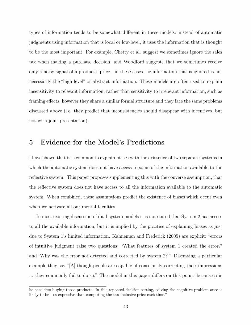
types of information tends to be somewhat di!erent in these models: instead of automatic

judgments using information that is local or low-level, it uses the information that is thought

to be the most important. For example, Chetty et al. suggest we sometimes ignore the sales

tax when making a purchase decision, and Woodford suggests that we sometimes receive

only a noisy signal of a product’s price - in these cases the information that is ignored is not

necessarily the “high-level” or abstract information. These models are often used to explain

insensitivity to relevant information, rather than sensitivity to irrelevant information, such as

framing e!ects, however they share a similar formal structure and they face the same problems

discussed above (i.e. they predict that inconsistencies should disappear with incentives, but

not with joint presentation).

5 Evidence for the Model’s Predictions

I have shown that it is common to explain biases with the existence of two separate systems in

which the automatic system does not have access to some of the information available to the

reflective system. This paper proposes supplementing this with the converse assumption, that

the reflective system does not have access to all the information available to the automatic

system. When combined, these assumptions predict the existence of biases which occur even

when we activate all our mental faculties.

In most existing discussion of dual-system models it is not stated that System 2 has access

to all the available information, but it is implied by the practice of explaining biases as just

due to System 1’s limited information. Kahneman and Frederick (2005) are explicit: “errors

of intuitive judgment raise two questions: ‘What features of system 1 created the error?’

and ‘Why was the error not detected and corrected by system 2?” ’ Discussing a particular

example they say “[A]lthough people are capable of consciously correcting their impressions

... they commonly fail to do so.” The model in this paper di!ers on this point: because ! is

he considers buying those products. In this repeated-decision setting, solving the cognitive problem once islikely to be less expensive than computing the tax-inclusive price each time.”

43

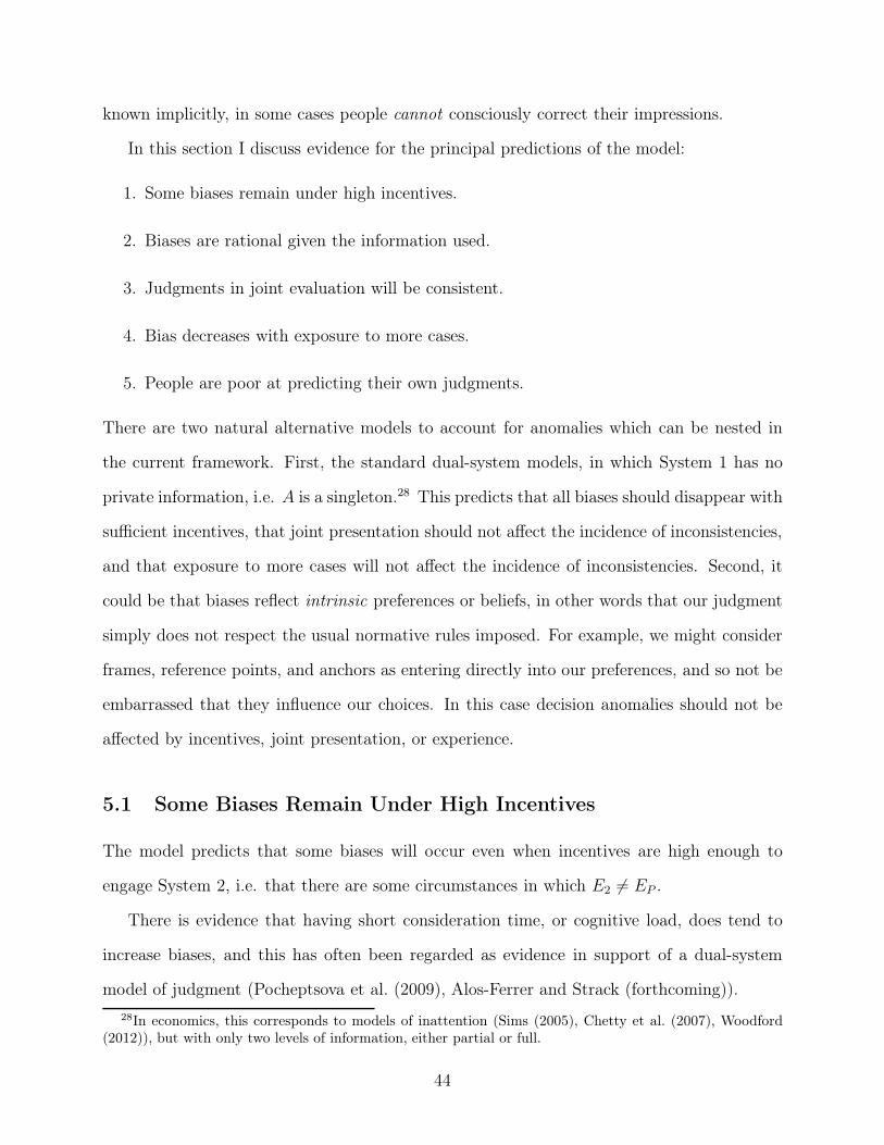
known implicitly, in some cases people cannot consciously correct their impressions.

In this section I discuss evidence for the principal predictions of the model:

1. Some biases remain under high incentives.

2. Biases are rational given the information used.

3. Judgments in joint evaluation will be consistent.

4. Bias decreases with exposure to more cases.

5. People are poor at predicting their own judgments.

There are two natural alternative models to account for anomalies which can be nested in

the current framework. First, the standard dual-system models, in which System 1 has no

private information, i.e. A is a singleton.28 This predicts that all biases should disappear with

su"cient incentives, that joint presentation should not a!ect the incidence of inconsistencies,

and that exposure to more cases will not a!ect the incidence of inconsistencies. Second, it

could be that biases reflect intrinsic preferences or beliefs, in other words that our judgment

simply does not respect the usual normative rules imposed. For example, we might consider

frames, reference points, and anchors as entering directly into our preferences, and so not be

embarrassed that they influence our choices. In this case decision anomalies should not be

a!ected by incentives, joint presentation, or experience.

5.1 Some Biases Remain Under High Incentives

The model predicts that some biases will occur even when incentives are high enough to

engage System 2, i.e. that there are some circumstances in which E2 (= EP .

There is evidence that having short consideration time, or cognitive load, does tend to

increase biases, and this has often been regarded as evidence in support of a dual-system

model of judgment (Pocheptsova et al. (2009), Alos-Ferrer and Strack (forthcoming)).

28In economics, this corresponds to models of inattention (Sims (2005), Chetty et al. (2007), Woodford(2012)), but with only two levels of information, either partial or full.

44

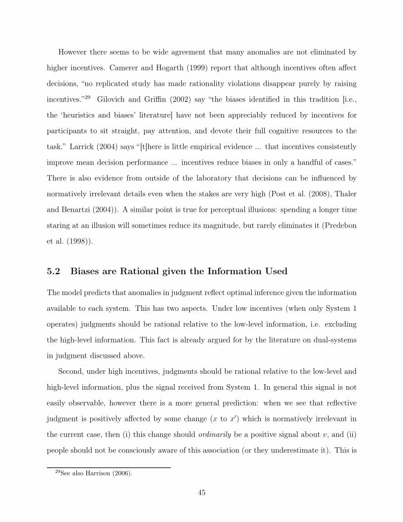
However there seems to be wide agreement that many anomalies are not eliminated by

higher incentives. Camerer and Hogarth (1999) report that although incentives often a!ect

decisions, “no replicated study has made rationality violations disappear purely by raising

incentives.”29 Gilovich and Gri"n (2002) say “the biases identified in this tradition [i.e.,

the ‘heuristics and biases’ literature] have not been appreciably reduced by incentives for

participants to sit straight, pay attention, and devote their full cognitive resources to the

task.” Larrick (2004) says “[t]here is little empirical evidence ... that incentives consistently

improve mean decision performance ... incentives reduce biases in only a handful of cases.”

There is also evidence from outside of the laboratory that decisions can be influenced by

normatively irrelevant details even when the stakes are very high (Post et al. (2008), Thaler

and Benartzi (2004)). A similar point is true for perceptual illusions: spending a longer time

staring at an illusion will sometimes reduce its magnitude, but rarely eliminates it (Predebon

et al. (1998)).

5.2 Biases are Rational given the Information Used

The model predicts that anomalies in judgment reflect optimal inference given the information

available to each system. This has two aspects. Under low incentives (when only System 1

operates) judgments should be rational relative to the low-level information, i.e. excluding

the high-level information. This fact is already argued for by the literature on dual-systems

in judgment discussed above.

Second, under high incentives, judgments should be rational relative to the low-level and

high-level information, plus the signal received from System 1. In general this signal is not

easily observable, however there is a more general prediction: when we see that reflective

judgment is positively a!ected by some change (x to x!) which is normatively irrelevant in

the current case, then (i) this change should ordinarily be a positive signal about v, and (ii)

people should not be consciously aware of this association (or they underestimate it). This is

29See also Harrison (2006).

45

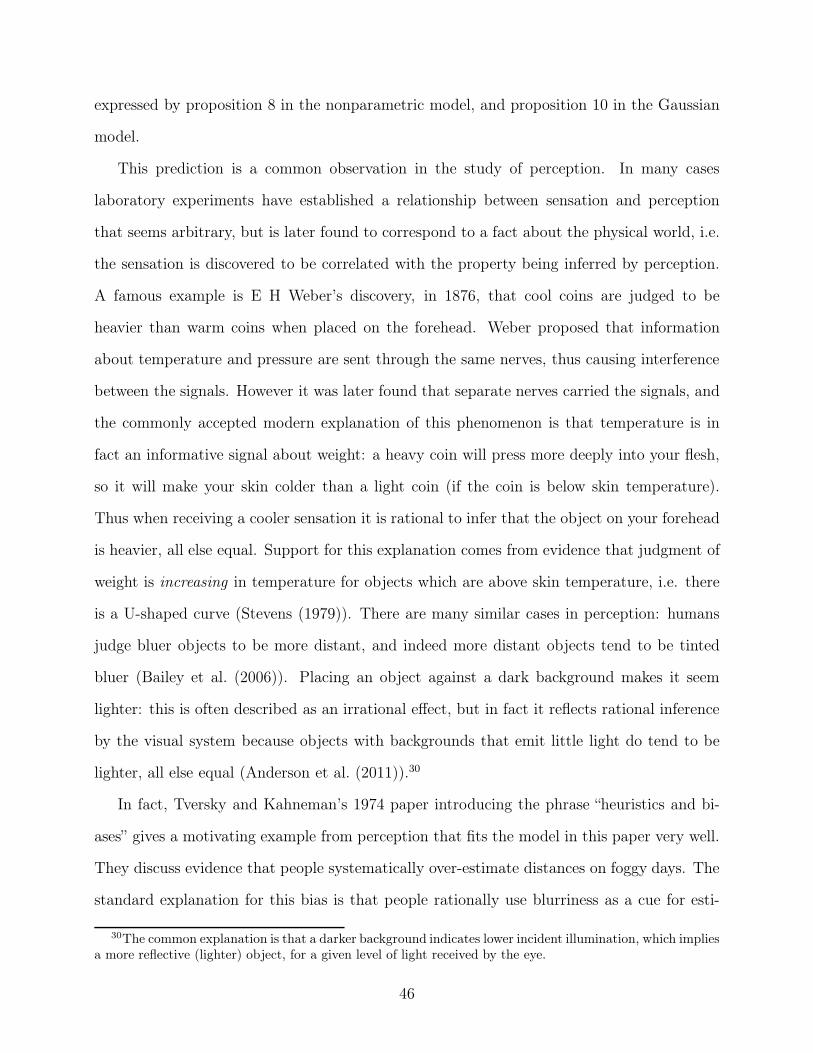
expressed by proposition 8 in the nonparametric model, and proposition 10 in the Gaussian

model.

This prediction is a common observation in the study of perception. In many cases

laboratory experiments have established a relationship between sensation and perception

that seems arbitrary, but is later found to correspond to a fact about the physical world, i.e.

the sensation is discovered to be correlated with the property being inferred by perception.

A famous example is E H Weber’s discovery, in 1876, that cool coins are judged to be

heavier than warm coins when placed on the forehead. Weber proposed that information

about temperature and pressure are sent through the same nerves, thus causing interference

between the signals. However it was later found that separate nerves carried the signals, and

the commonly accepted modern explanation of this phenomenon is that temperature is in

fact an informative signal about weight: a heavy coin will press more deeply into your flesh,

so it will make your skin colder than a light coin (if the coin is below skin temperature).

Thus when receiving a cooler sensation it is rational to infer that the object on your forehead

is heavier, all else equal. Support for this explanation comes from evidence that judgment of

weight is increasing in temperature for objects which are above skin temperature, i.e. there

is a U-shaped curve (Stevens (1979)). There are many similar cases in perception: humans

judge bluer objects to be more distant, and indeed more distant objects tend to be tinted

bluer (Bailey et al. (2006)). Placing an object against a dark background makes it seem

lighter: this is often described as an irrational e!ect, but in fact it reflects rational inference

by the visual system because objects with backgrounds that emit little light do tend to be

lighter, all else equal (Anderson et al. (2011)).30

In fact, Tversky and Kahneman’s 1974 paper introducing the phrase “heuristics and bi-

ases” gives a motivating example from perception that fits the model in this paper very well.

They discuss evidence that people systematically over-estimate distances on foggy days. The

standard explanation for this bias is that people rationally use blurriness as a cue for esti-

30The common explanation is that a darker background indicates lower incident illumination, which impliesa more reflective (lighter) object, for a given level of light received by the eye.

46

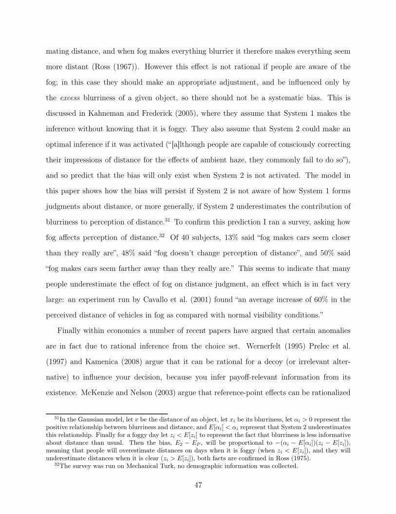
mating distance, and when fog makes everything blurrier it therefore makes everything seem

more distant (Ross (1967)). However this e!ect is not rational if people are aware of the

fog; in this case they should make an appropriate adjustment, and be influenced only by

the excess blurriness of a given object, so there should not be a systematic bias. This is

discussed in Kahneman and Frederick (2005), where they assume that System 1 makes the

inference without knowing that it is foggy. They also assume that System 2 could make an

optimal inference if it was activated (“[a]lthough people are capable of consciously correcting

their impressions of distance for the e!ects of ambient haze, they commonly fail to do so”),

and so predict that the bias will only exist when System 2 is not activated. The model in

this paper shows how the bias will persist if System 2 is not aware of how System 1 forms

judgments about distance, or more generally, if System 2 underestimates the contribution of

blurriness to perception of distance.31 To confirm this prediction I ran a survey, asking how

fog a!ects perception of distance.32 Of 40 subjects, 13% said “fog makes cars seem closer

than they really are”, 48% said “fog doesn’t change perception of distance”, and 50% said

“fog makes cars seem farther away than they really are.” This seems to indicate that many

people underestimate the e!ect of fog on distance judgment, an e!ect which is in fact very

large: an experiment run by Cavallo et al. (2001) found “an average increase of 60% in the

perceived distance of vehicles in fog as compared with normal visibility conditions.”

Finally within economics a number of recent papers have argued that certain anomalies

are in fact due to rational inference from the choice set. Wernerfelt (1995) Prelec et al.

(1997) and Kamenica (2008) argue that it can be rational for a decoy (or irrelevant alter-

native) to influence your decision, because you infer payo!-relevant information from its

existence. McKenzie and Nelson (2003) argue that reference-point e!ects can be rationalized

31In the Gaussian model, let v be the distance of an object, let xi be its blurriness, let !i > 0 represent thepositive relationship between blurriness and distance, and E[!i] < !i represent that System 2 underestimatesthis relationship. Finally for a foggy day let zi < E[zi] to represent the fact that blurriness is less informativeabout distance than usual. Then the bias, E2 " EP , will be proportional to "(!i " E[!i])(zi " E[zi]),meaning that people will overestimate distances on days when it is foggy (when zi < E[zi]), and they willunderestimate distances when it is clear (zi > E[zi]), both facts are confirmed in Ross (1975).

32The survey was run on Mechanical Turk, no demographic information was collected.

47

by inference. Armstrong and Chen (2012) argue that reference-price and anchoring e!ects

can occur because of rational inference. However these models all predict that if the feature

which influences judgment is randomized, and known by the subjects to be randomized, then

it should no longer have an e!ect on choice. Yet a variety of studies show that many fram-

ing e!ects do persist under explicit randomization (Fudenberg et al. (2010), Jahedi (2011),

Mazar et al. (2010)). Thus these papers can be thought of as explaining the direction of

bias under the assumption that subjects ignore whether or not the attribute is randomized,

and the survival of the bias under randomization can be justified by the existence of implicit

knowledge, as assumed in this paper.

5.3 Judgments in Joint Evaluation will be Consistent

The model predicts that when reflective judgment is activated then judgments elicited sepa-

rately may violate rules of consistency, but judgments elicited jointly will always be consistent.

Note again that jointly-elicited judgments need not be unbiased, just consistent relative to

some normative constraint. Note also that testing this prediction does not require knowing

how information is partitioned between low-level high-level aspects of the case (x and z).

Evidence from a wide variety of sources seems to confirm the prediction.33

The simplest case is of framing e!ects, where an irrelevant change in the context a!ects

evaluation.34 The model predicts that when the two cases are presented side by side, the

discrepancy will disappear. Presenting two frames simultaneously while adequately control-

ling for information e!ects is relatively rare.3536 A good example is reported in Mazar et al.

(2010). They asked subjects to state their willingness to pay (WTP) for a mug, using the

33Tversky and Kahneman (1986) make a similar point, saying “the axioms of rational choice are generallysatisfied in transparent situations and often violated in non-transparent ones.”

34These can be treated as cases, (x, z) and (x", z"), where *! # A, E[v|x, z,!] = E[v|x", z",!], butE[v|x, z, E[v|x,!]] (= E[v|x", z", E[v|x",!]].

35Some framing e!ects cannot be easily be presented jointly: for example, choice is often a!ected bymanipulations of reference point (as in Kahneman and Tversky (1979)), however a joint presentation mayinduce a common reference point for both choices, instead of two separate reference points for each choiceset.

36LeBoeuf and Shafir (2003) find that framing e!ects in Tversky and Kahneman’s “Asian disease” casereduce markedly in sequential presentation.

48

incentive-compatible Becker-DeGroot-Marschack mechanism, with a distribution over the

prices at which the mug could be sold. They varied the probabilities of prices in the dis-

tribution: in one condition there was a 50% chance of drawing $0, in the other there was

a 50% chance of drawing $10, and in both cases the remaining probability was distributed

uniformly between $0 and $10. The distribution of probabilities is normatively irrelevant, by

our usual standards, yet the subjects in each condition stated a significantly di!erent WTP.

The result was replicated when the subjects were shown both distributions beforehand, with

their distribution being chosen by coin flip, to eliminate the possibility that subjects were in-

ferring something from the shape of the distribution. In that version the di!erence in average

bids was large ($2.42 for the left-skewed distribution, $5.08 for the right-skewed distribution).

Finally, the subjects were presented with both distributions and asked to submit two bids,

one for each scenario, and the actual distribution used was subsequently chosen by coin flip.

In this version the di!erence in bids shrank dramatically: the average bids were $3.09 and

$3.38, respectively. This experiment has a clear interpretation in terms of this paper’s model:

the distributions of prices are salient features (x and x!), but in each case high-level infor-

mation (z and z!) tells us that the distribution is normatively irrelevant (i.e., these represent

information that the distributions are randomly drawn). Judgment is nevertheless a!ected –

implying that System 1 believes there is a positive association between price and value, and

that System 2 does not appreciate how strong this association is. Finally, in a joint situation,

System 2 submits equal bids for both cases, because it is aware that they are normatively

identical.

A separate literature has identified a number of situations where the WTP for one object

is higher than that for another, even when the second object dominates the first. Birnbaum

(1992) finds this for gambles.37 Hsee (1998) finds this in WTP for products, e.g. people

state a higher WTP for 7oz of ice cream in a 5oz cup, than for 8oz in a 10oz cup. John

List has found similar e!ects in field settings (List (2002), Gneezy et al. (2006)), for example

37Birnbaum finds that (($0,10%; $96 otherwise) is given a higher WTP than ($24,10%; $96 otherwise)).See also Slovic et al. (2007).

49

that people will generally bid more for a packet of 10 high-quality baseball cards than for a

packet which is identical except for additionally containing 3 low-quality cards. In each of

these cases, when WTP judgments are made jointly, the dominating object is given a higher

value, consistent with the prediction of implicit knowledge.

Another line of evidence come from experiments which have attempted to calibrate models

of preference over gambles. Subjects very often reverse their preferences when they encounter

an identical problem twice: Starmer (2000) reports, in a survey, that “between one-quarter

and one-third of subjects ’switch’ preferences on repeated questions.” However a striking fact

is that, despite this volatility, subjects very rarely choose a stochastically dominated option

(Carbone and Hey (1995), Loomes and Sugden (1998), Hey (2001)).38 This is a paradox for

models of attention: people are inattentive enough to make inconsistent choices, but attentive

enough to never choose a dominated alternative. However this pattern matches a model, as

in this paper, in which subjects have normative preferences, but receive a di!erent signal

about the nature of those preferences in each situation.39

Kahneman and Frederick (2005) discuss the di!erences between separate and joint judg-

ment.40 They note that many judgment anomalies were first discovered in between-subject

experiments (i.e., in separate evaluation), but some were also found to survive in joint evalu-

ation.41 They acknowledge that subsequent research has shown the existence of bias in joint

evaluation to be fragile,42 and they emphasize that most biases remain robust in between-

subject experiment with more careful controls, and that the existence of biases in separate

evaluation remains important in studying real-world behavior.

38Carbone and Hey (1995) say “[w]hat is startling ... are the results of the satisfaction or violation ofdominance ... [with a] mean violation rate of just 0.3 percent. In contrast the average inconsistency rate ofthe repeated pairs was 12 percent.”

39The fact that people often reverse their preferences could be due to any of the other noise picked up bySystem 1: the history of prior cases, or the time of day, or a feeling of fatigue.

40In their terminology, the di!erence between “coherence rationality” (satisfying rationality in separateevaluation) and “reasoning rationality” (satisfying rationality in joint evaluation, or in a single task).

41“[Tversky and Kahneman] were ... shocked to discover that more than 80% of undergraduates committeda conjunction error even when asked point blank whether Linda was more likely to be ’a bank teller’ or ’abank teller who is active in the feminist movement’.”

42“[w]e suspect that most of [the criticisms] have some validity and that they identified mechanisms thatmay have made the results in the engineer–lawyer and Linda studies exceptionally strong.”

50

A corollary of the consistency result is that money pumps will not survive repeated

presentation. Define a money pump as a set of choice sets, such that some option is indirectly

revealed to be preferred to another option which strictly dominates it. For example, in

pairwise choice, preferences such that p 4 q 4 p!, where p! dominates p. These choices

are allowed by the model in this paper, but it predicts that the pump will run out if the

decisions are made sequentially, i.e. after being exposed to all three alternatives (p, p!, q)

subjects will make subsequent decisions with the same beliefs about !, so will make consistent

decisions. This prediction is supported by Chu and Chu (1990), who find that classical

preference reversals (Lichtenstein and Slovic (1971)) decrease significantly after choices are

made sequentially, such that subjects come to face the possibility of a money pump.

Finally, when applied to perceptual biases, the theory makes the counterfactual prediction

that inconsistencies will disappear in joint presentations. This problem can be resolved if

we additionally assume that people do not have direct reflective access to their own raw

sensations, a common observation in the literature on perception. Take the common illusion

that an object appears brighter when placed against a dark background, even when the

background color is known to be irrelevant.43 This can be explained if System 1 treats the

background color as an informative signal about the color of the foreground object (Adelson

(2000)), and if System 2 is unaware of this association. Then the background color can

influence judgment even in cases where people are aware that it is objectively uninformative

(as long as E1 is not invertible). This analysis predicts that the inconsistency will not occur

in joint evaluation for a pair of cases which are identical except for the background color.44

Yet manifestly the illusion does occur in side-by-side presentation, in fact this is the most

common way of presenting this kind of illusion. This implication will not hold if System

1 observes additional case-specific information which is not accessible to System 2: then

System 2 will not know that the di!erence between the two reports (E1 and E !1) is due

only to the background color. This assumption seems reasonable: that people do not have

43Similar contrast e!ect illusions occur for perception of color, size, and other perceptual dimensions.44In particular, if illumination is known to be constant across all of the objects.

51

direct conscious access to their raw sensory data is a common conclusion in the study of

perception.4546

5.4 Bias Decreases with Exposure to More Cases

Proposition 4 states the bias will be smaller when more cases are judged simultaneously.

There seems to be strong evidence that experience tends to reduce the magnitude of biases.

Plott (1996) discusses evidence that biases tend to decrease with experience in experiments,

and proposes a “discovered preference hypothesis” that has a similar spirit to the model

proposed in this paper: “[b]ehavior seems to go through stages of rationality that begin with

a type of myopia when faced with unfamiliar tasks. With incentives and practice, which take

the form of repeated decisions in the experimental work ... the myopia gives way to what

appears to be a stage of more considered choices that reflect stable attitudes or preferences

(as opposed to the labile attitudes identified by psychologists).”

John List and coauthors, in a series of papers (List (2003), Alevy et al. (2007), Harrison

and List (2008)), have found, for a series of laboratory biases, that they can be reproduced

in field experiments but they are greatly diminished with experience of that type of decision,

whether it is prior professional experience, or longer experience in the experiment.

5.5 People are Poor at Predicting their own Judgments

Finally, the model predicts that reflective judgments will typically be di!erent when the

automatic system is not available, i.e. that E2\1 (= E2. Additionally, that bias will tend to

be higher in this case: V ar[E2\1 " EP ] ' V ar[E2 " EP ]. This result is more di"cult to

interpret, but there are some situations in which people seem to make reflective judgments

without access to their automatic system.

Within perception this seems to fit the fact that we are much better at recognizing certain

45A fuller discussion of this illusion can be found in Cunningham (2012).46von Helmholtz (1971 [1878]) says “we are not in the habit of observing our sensations accurately ... in

most cases some special assistance and training are needed in order to observe these ... subjective sensations.”

52

stimuli than reproducing them. For example, without training it is extremely di"cult to paint

a scene accurately, but we can easily recognize an accurate painting. Lawson (2006) finds

that when people are asked to draw a bicycle, they produce a drawing which is recognizably

not a bicycle.

Within economics one interpretation of decision without access to System 1 is the ex-

perimental protocol of “matching”, where subjects are asked to choose a parameter value for

one alternative (e.g., an amount of money or probability) which would make them indif-

ferent between that and another alternative. The classic preference reversal finding shows

that the results of matching are systematically di!erent from those of direct choice (Grether

and Plott (1979)), and Tversky et al. (1990) give some reasons for thinking that matching

protocol tends to produce larger biases.

Finally, Loewenstein et al. (2003) discuss further evidence that people are poor judges of

their future preferences (“projection bias”).

6 Discussion

6.1 Related Literature

The model in this paper is similar to existing dual-agent models within economics (e.g., Fu-

denberg and Levine (2006), Brocas and Carrillo (2008)) in that behavior results from the

interaction of two agents within the decision-maker. However the results in those models

are driven by the conflict of preferences, this paper di!ers in having perfectly aligned pref-

erences.47 The two classes of model are complementary if, as seems likely, mental processes

di!er in both information and preferences.

There are a number of models of decision-making with imperfect memory which have

similarities to the model in this paper. Many share the feature that memory is aggregated in

47In Fudenberg and Levine (2006) there is no asymmetry of information. In Brocas and Carrillo (2008)there is some asymmetry, but the short-run agent (the decision-maker) knows strictly more than the long-runagent, so if their preferences were aligned (as in this paper) there would be no bias.

53

some way that produces biases in behavior, relative to an agent that has access to all their

past experiences. In Shapiro (2006) consumers are uncertain if they have positive memories

about a product because of a good experience, or because of seeing advertisements, and thus

they may be influenced by uninformative advertising. In Baliga and Ely (2011) investors

do not remember why they started a project, so may exhibit sensitivity to costs which are

sunk. In Wilson (2002) agents have a limited number of states they can use in memory, so

sometimes rationally ignore new information, and react di!erently to a stream of information

depending on the order in which it is received.48 These models all can explain decisions

being a!ected by irrelevant information, but only irrelevant information in the past, because

the irrelevant information a!ects current behavior through being aggregated together with

relevant information into coarse memories. These models do not predict judgment being

influenced by contemporaneous irrelevant information, as in the framing e!ects that motivate

this paper.

The model in this paper could be thought of as a combination of limited-attention and

limited-memory models: System 1 has limited attention, System 2 has limited memory. This

allows it to reproduce the qualitative biases in limited attention models, but it can also

explain why those biases remain with higher incentives.

Formally this paper is most similar to models of social learning (Chamley (2003)), in

that each agent receives a private signal, one agent observes another agent’s action, and we

solve for the conditions under which information is e"ciently aggregated. The model in this

paper di!ers in a few ways: in having a continuous action space (most herding models have a

discrete action, to prevent the action being a su"cient statistic for the information); in having

a many-to-one mapping between signal and the expectation of the underlying variable (which

prevents E1 from revealing !); and in having just two agents, and thus being interested in

perfect aggregation, not aggregation in the limit. An important pair of related papers are

48Mullainathan (2002) and Schwartzstein (2012) are similar but additionally assume that agents are naiveabout how memories are retrieved.

54

Mueller-Frank and Arieli (2012) and Arieli and Mueller-Frank (2013), discussed earlier.49

One important related paper is the Mullainathan et al. (2008) model of “coarse thinking”

which can be interpreted as a reduced-form version of the model in this paper. In that paper

decision-makers observe a message and a situation, and from these form a judgment of value.

However subjects are assumed to conflate some set of situations, thus their reaction to the

message can be biased relative to the case in which they discriminated perfectly between

situations.50 In particular, subjects may be a!ected by a message which is uninformative in

the current situation when that message is informative in other situations. In an example

from the paper, putting silk in a shampoo bottle can cause consumers to value it more

highly, despite it being objectively worthless, because consumers co-categorize this situation

with one in which silkiness is a positive signal about the quality of shampoo (e.g. if it

was silkiness of the hair being treated by the shampoo).51 In terms of the model of implicit

knowledge, the situation is z, the message is x, and the interpretation of the messages (E[q|m]

in their paper) is !. Mullainathan et al. (2008) assumes that people are fundamentally

non-Bayesian. Interpreted using the model in this paper, people are Bayesian, but they

have access to an automatic system, and it is this which causes their judgment to respond

to irrelevant information. The implicit knowledge interpretation of coarse thinking makes

additional predictions about their examples: most particularly, it predicts that subjects

will not be influenced by an irrelevant attribute in joint evaluation: willingness to pay for

shampoo will be influenced by the presence of silk in a between-subjects experiment, but not

in a within-subjects experiment, in which both products are evaluated simultaneously.52

49Example 2 in Mueller-Frank and Arieli (2012) fits the assumptions of the model in this paper: althoughagent 2 can infer agent 1’s posterior over v, agent 2’s posterior is not equal to the pooled-information posterior,because agent 2’s private information is not conditionally independent of agent 1’s private information.

50“the coarse thinker ... reacts to an uninformative message in situation s = 0 because it is informative inthe co-categorized situation.” This describes the “transference” mechanism in that paper, they also describea separate “framing” e!ect.

51“’looks silky’ is informative in situation s=“evaluating hair” ... but ’contains silk’ is always uninformativein situation s=’evaluating a shampoo” ’

52These predictions rely on the assumption that the cues are known to be uninformative in the currentcase. If people believe that silk in the bottle is in fact a good proxy for the quality of shampoo then thedi!erence may not disappear in joint evaluation, and in fact the behavior would not be irrational, so therewould be no bias to explain.

55

6.2 Implications for Anomalies in Economic Decision-Making

The model of implicit knowledge can be used to interpret the framing e!ects and related

anomalies often found in economic decision-making.

Some of the well-known anomalous e!ects on economic decision-making are (i) that peo-

ple have excess sensitivity to losses, defined relative to some reference point (Kahneman

and Tversky (1979)); (ii) that willingness to pay for a good can be a!ected by a randomly-

generated anchor-price (Ariely et al. (2003), Fudenberg et al. (2010)); (iii) that adding an

extreme option to a choice set can cause people to substitute towards an intermediate op-

tion (Kamenica (2008)); and (iv) that people have excess sensitivity to larger proportional

di!erences (Bordalo et al. (2011)).

This kind of e!ect can be explained within the framework of this paper if the feature

that a!ects valuation is usually informative. I.e., if reference points, price anchors, decoy

alternatives, and relative magnitudes are usually informative proxies for value. This case has

been made explicitly by some previous papers, discussed above. Thus these papers can be

thought of as explaining the direction of bias for System 1, and the survival of the bias under

randomization could be justified if System 2 is not aware of how System 1 uses this cue.

If the inconsistency of laboratory judgments and choices is due to implicit knowledge, this

has some implications about how everyday economic decisions are made. First, it implies

that economic decisions are heavily influenced by subtle environmental cues, and that this is

not irrational, i.e. those cues are informative.

Second, it implies that we have poor insight into which features a!ect our automatic

judgment, or what e!ect each feature has. This is common in everyday vernacular: people

say their decision is based on a “hunch”, “intuition”, “gut feeling”, or “instinct”, and so they

cannot fully express their reasons for the choice they made. This is also true of other areas of

human judgment: humans remain superior to computers in various tasks, such as recognizing

written text (Holley (2009)), in recognizing faces (Sinha et al. (2006)), in playing Go, and

56

in forecasting weather.53 The fact that we cannot teach these skills to computers (who have

more processing power, and larger training sets, in each of these cases) suggests we have

limited insight into our own knowledge. This paper’s interpretation is that we are in a

similar situation with respect to economic decisions: people have well calibrated judgments

about economic decisions, but little insight into how those decisions are made.

6.3 Implications for Debiasing and Inferring Preferences from Choices

The model in this paper can be used to help identify unbiased judgments, EP . This is

related to two separate literatures: that on finding situations in which bias is minimized

(“debiasing”, see Larrick (2004) and Milkman and Bazerman (2008)), and the literature on

inferring true preferences in the face of inconsistent decision-making (Bernheim and Rangel

(2009), Beshears et al. (2008)).

Bernheim and Rangel (2009) propose a partial solution to the problem of inferring true

preferences: although preferences cannot be exactly identified with choices, they propose

that preferences can be bounded within the range of choices elicited under di!erent frames.

This seems reasonable, however the bounds are often very large, and discovering the bounds

requires us knowing the full distribution of possible frames.

The model presented in this paper has the advantage that welfare is well-defined, and can

in principle be inferred from decisions.

I will note five predictions, and leave a fuller analysis to future work: judgments can be

improved either by (1) increasing incentives; (2) putting people in more familiar situations; (3)

providing a wider range of cases; (4) providing comparison cases which isolate the dimensions

which are unusual; or (5) directly informing people about !.

First, as already noted, raising incentives will reveal E2 but not EP . Larrick (2004),

who organizes a discussion of debiasing around a dual-system model, notes that contrary to

53For weather forecasting the human superiority is just in modifying an existing computer forecast. Silver(2012) says “humans improve the accuracy of precipitation forecasts by about 25 percent over the computerguidance alone. They improve the temperature forecasts by about 10 percent.”

57

that model’s predictions, incentives are not generally very e!ective in debiasing: “[t]here is

little empirical evidence ... that incentives consistently improve mean decision performance

... incentives reduce biases in only a handful of cases.”

Second, the Gaussian model predicts that bias will be lower when z is closer to E[z], i.e.

when the high-level information is close to its average values. This could be interpreted as

meaning that people tend to make better judgments and choices in “ordinary” or “familiar”

situations. This seems to be true for perception: for example, our ability to recognize faces

is significantly worse when we are upside down (Sinha et al. (2006)). This could also be

true of laboratory tests of economic preferences: because we are in an unusual situation, our

judgments are less well calibrated, and so we will tend to make less accurate judgments of

preference.

Third, as shown in Proposition 4, bias will tend to diminish when subjects are exposed

to a larger set of cases. This has a natural interpretation in the case of the bias induced by

fog discussed above: you can improve your judgment about the distance of any one object

by looking at other objects. For example if you notice that your hood ornament looks far

o!, though you know it to be only 4 feet away, this observation allows you to learn that the

fog is causing your automatic judgment to overestimate the distance of objects (i.e., in the

Gaussian model System 2 will updates to increase its estimate of !i, where xi is blurriness),

and therefore that other objects may also be closer than they appear. For decision-making,

this implies that exposing subjects to more alternatives will decrease bias, and therefore raise

welfare.54 There are some recent studies which argue the opposite - that people tend to make

worse choices from larger choice sets (Iyengar and Kamenica (2010)) - though they propose

an independent and complementary mechanism.

Fourth, the model predicts that not all comparisons are equal: certain comparisons can

improve judgment more than others. Intuitively, we can help a person make better decisions

by giving them cases which isolate the elements which contribute to the bias. Consider the

54Larrick (2009) argues that judgments are generally improved by “broadening the decision frame”, byconsidering multiple objectives, multiple alternatives and multiple outcomes.

58

Gaussian model, and suppose we have some case (x, z) for which we are concerned there

is a bias, because the high-level circumstances are unusual, zi (= E[zi]. If there is only

one dimension that is unusual, i.e. for which zi (= E[zi], then we can give the subject a

comparison case, (x!, z!), which is identical except for dimension i, i.e. xj = x!j for j (= i.

Providing this comparison will allow System 2 to exactly identify !i (!i = E!

1%E1

x!

i%xi), and

therefore to exactly infer EP .55 In everyday scenarios, this could be interpreted as trying to

consider a case from a di!erent angle, varying the aspects which you believe to be irrelevant

or unusual. For example, you may wish to visit a house on both a sunny day and a cloudy

day, to isolate the e!ect of weather, and therefore debias your judgment.56 In experiments,

if we are concerned that an irrelevant detail is a!ecting choice (i.e., a framing e!ect), then

this theory recommends presenting subjects with multiple versions of the same case, varying

the irrelevant detail.

Finally, the model predicts that biases could be eliminated if subjects were directly told

the contents of !: i.e., if they knew the information that their intuitions used. In practice the

entire set of information is probably too large to teach to people, though it may be e!ective

to teach subjects about some typical e!ects. This is common with visual illusions, e.g. an

Airbus training manual warns “[f]lying in light rain, fog, haze, mist, smoke, dust, glare or

darkness usually create an illusion of being too high” (Airbus (2011)).

7 Conclusion

This paper argues that many puzzles of human judgment can be explained by a simple model:

that when we form judgments we take advice from a separate dedicated system, which has

55EP = E2 " !ixiE[zi] + !ixizi.56In fact, in general we can provide a single comparison case which will exactly reveal EP : denote the

comparison case (x", z") and set x"i = xiziE[zi]$1, and z"i = E[zi]zi, then E"

1 =+

x"i!iE[zi] =

+

xi!izi = EP ,and E"

2 = E"1 = EP . The subject’s judgment of this comparison case will be equal to the pooled-information

judgment of the original case. This has a simple interpretation in the baseball-cards example: to get anaccurate estimate of the value of a packet, simply give the subject a packet with all the fake cards removed,and take their estimate of that packet. Recall that xi = 1 if the packet contains that card, and zi = 1 if it isgenuine; so the theory proposes setting x"

i = 0 wherever zi = 0. It also implies setting x"i = E[zi]$1 for the

other cards, but if E[zi] is constant for all cards then this can be ignored.

59

superior information about prior experiences with similar cases, but which fails to take into

account high-level or abstract information about the current case.

This model predicts a number of facts that match human behavior in many situations:

(1) we make inconsistent judgments, as if we are following simple heuristics; however (2) our

judgments are consistent when made jointly; (3) our biases decreases with experience; and

(4) we are poor at forecasting our future judgments.

There are a number of interesting issues raised that I leave for future work. One is why

our brain should be structured in such a modular way (Fodor (1983)). Another is a more

precise model for how information is partitioned between systems, i.e. what information is

“low level” and “high level”. A third is which value, v, is inferred: from a given set of cues,

there are multiple di!erent underlying values a System 1 could wish to infer.57 Finally, it

may be of interest is how this form of judgment will a!ect persuasion: a strategic player who

has superior knowledge about ! (such as a firm) will choose x to maximize E2, not EP .

57For example we might wish to infer either the size or distance of an object; similarly we might get anintuition about either the likelihood or the representativeness of a case.

60

References

Adelson, Edward H (2000), “Lightness perception and lightness illusions.” In The New Cog-

nitive Neurosciences (M. Gazzinaga, ed.), 339–351, The MIT Press.

Airbus (2011), “Flight operations briefing notes: Human performance: Visual illusions aware-

ness.” Technical report, Airbus.

Alevy, JE, CE Landry, and JA List (2007), “Anchors away: A field experiment on anchor-

ing of consumer valuations.” University of Nevada, East Carolina State University, and

University of Chicago Working Paper.

Alos-Ferrer, Carlos and Fritz Strack (forthcoming), “From dual processes to multiple selves:

Implications for economic behavior.” Journal of Economic Psychology.

Anderson, B.L., B.G. Khang, and J. Kim (2011), “Using color to understand perceived light-

ness.” Journal of Vision, 11.

Arieli, Itai and Manuel Mueller-Frank (2013), “Inferring beliefs from actions.” Available at

SSRN 2208083.

Ariely, D., G. Loewenstein, and D. Prelec (2003), “Coherent arbitrariness: Stable demand

curves without stable preferences.” The Quarterly Journal of Economics, 118, 73–106.

Armstrong, M. and Y. Chen (2012), “Discount pricing.”

Bailey, R., C. Grimm, and C. Davoli (2006), “The real e!ect of warm-cool colors.” In Inter-

national Conference on Computer Graphics and Interactive Techniques.

Baliga, Sandeep and Je!rey C Ely (2011), “Mnemonomics: the sunk cost fallacy as a memory

kludge.” American Economic Journal: Microeconomics, 3, 35–67.

61

Bernheim, B Douglas and Antonio Rangel (2009), “Beyond revealed preference: choice-

theoretic foundations for behavioral welfare economics.” The Quarterly Journal of Eco-

nomics, 124, 51–104.

Beshears, John, James J Choi, David Laibson, and Brigitte C Madrian (2008), “How are

preferences revealed?” Journal of Public Economics, 92, 1787–1794.

Birnbaum, M.H. (1992), “Violations of monotonicity and contextual e!ects in choice-based

certainty equivalents.” Psychological Science, 3, 310.

Bordalo, P., N. Gennaioli, and A. Shleifer (2011), “Salience and consumer choice.” Working

Paper.

Bordalo, Pedro, Nicola Gennaioli, and Andrei Shleifer (2012), “Salience and consumer choice.”

Technical report, National Bureau of Economic Research.

Boyd, Stephen Poythress and Lieven Vandenberghe (2004), Convex optimization. Cambridge

university press.

Brocas, I. and J.D. Carrillo (2008), “The brain as a hierarchical organization.” The American

Economic Review, 98, 1312–1346.

Camerer, C.F. and R.M. Hogarth (1999), “The e!ects of financial incentives in experiments:

A review and capital-labor-production framework.” Journal of risk and uncertainty, 19,

7–42.

Caplin, A. and D. Martin (2011), “A testable theory of imperfect perception.” Technical

report, National Bureau of Economic Research.

Carbone, Enrica and John D Hey (1995), “A comparison of the estimates of eu and non-eu

preference functionals using data from pairwise choice and complete ranking experiments.”

Geneva Papers on Risk and Insurance Theory, 20, 111–133.

62

Cavallo, V., M. Colomb, and J. Doré (2001), “Distance perception of vehicle rear lights in

fog.” Human Factors: The Journal of the Human Factors and Ergonomics Society, 43,

442–451.

Chamley, C.P. (2003), Rational herds: Economic models of social learning. Cambridge Uni-

versity Press.

Chetty, Raj, Adam Looney, and Kory Kroft (2007), “Salience and taxation: Theory

and evidence.” Working Paper 13330, National Bureau of Economic Research, URL

http://www.nber.org/papers/w13330.

Chu, Yun-Peng and Ruey-Ling Chu (1990), “The subsidence of preference reversals in sim-

plified and marketlike experimental settings: A note.” The American Economic Review,

80, 902–911.

Cunningham, T.E. (2012), “Comparisons and choice.” Working Paper.

Evans, Jonathan St BT (2008), “Dual-processing accounts of reasoning, judgment, and social

cognition.” Annu. Rev. Psychol., 59, 255–278.

Feldman, Jacob (2013), “Bayesian models of perceptual organization.” In Oxford Handbook

of Perceptual Organization (Johan Wagemans, ed.), Oxford University Press.

Fernandez, Eva M and Helen Smith Cairns (2010), Fundamentals of Psycholinguistics. Wiley-

Blackwell.

Fodor, Jerry A (1983), The Modularity of Mind: An Essay on Faculty Psycholgy. The MIT

Press.

Fudenberg, D. and D.K. Levine (2006), “A dual-self model of impulse control.” The American

Economic Review, 1449–1476.

Fudenberg, D., D.K. Levine, and Z. Maniadis (2010), “Reexamining coherent arbitrariness

for the evalution of common goods and lotteries.” Levine’s Working Paper Archive.

63

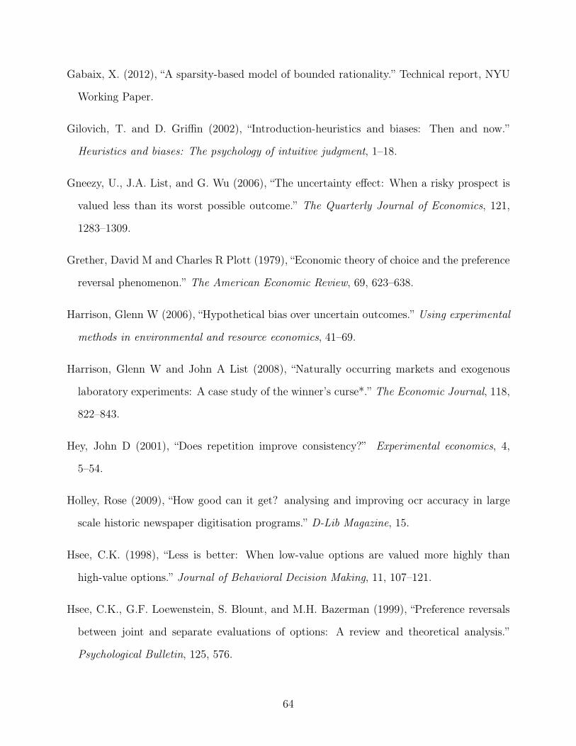
Gabaix, X. (2012), “A sparsity-based model of bounded rationality.” Technical report, NYU

Working Paper.

Gilovich, T. and D. Gri"n (2002), “Introduction-heuristics and biases: Then and now.”

Heuristics and biases: The psychology of intuitive judgment, 1–18.

Gneezy, U., J.A. List, and G. Wu (2006), “The uncertainty e!ect: When a risky prospect is

valued less than its worst possible outcome.” The Quarterly Journal of Economics, 121,

1283–1309.

Grether, David M and Charles R Plott (1979), “Economic theory of choice and the preference

reversal phenomenon.” The American Economic Review, 69, 623–638.

Harrison, Glenn W (2006), “Hypothetical bias over uncertain outcomes.” Using experimental

methods in environmental and resource economics, 41–69.

Harrison, Glenn W and John A List (2008), “Naturally occurring markets and exogenous

laboratory experiments: A case study of the winner’s curse*.” The Economic Journal, 118,

822–843.

Hey, John D (2001), “Does repetition improve consistency?” Experimental economics, 4,

5–54.

Holley, Rose (2009), “How good can it get? analysing and improving ocr accuracy in large

scale historic newspaper digitisation programs.” D-Lib Magazine, 15.

Hsee, C.K. (1998), “Less is better: When low-value options are valued more highly than

high-value options.” Journal of Behavioral Decision Making, 11, 107–121.

Hsee, C.K., G.F. Loewenstein, S. Blount, and M.H. Bazerman (1999), “Preference reversals

between joint and separate evaluations of options: A review and theoretical analysis.”

Psychological Bulletin, 125, 576.

64

Iyengar, S.S. and E. Kamenica (2010), “Choice proliferation, simplicity seeking, and asset

allocation.” Journal of Public Economics, 94, 530–539.

Jahedi, S. (2011), “A taste for bargains.” Unpublished Manuscript, University of Arkansas.

Kahneman, D. (2011), Thinking, fast and slow. Farrar, Straus and Giroux.

Kahneman, D. and S. Frederick (2005), “A model of heuristic judgment.” The Cambridge

handbook of thinking and reasoning, 267–293.

Kahneman, D. and A. Tversky (1979), “Prospect theory: An analysis of decision under risk.”

Econometrica: Journal of the Econometric Society, 263–291.

Kamenica, E. (2008), “Contextual inference in markets: On the informational content of

product lines.” The American Economic Review, 98, 2127–2149.

K#szegi, B. and A. Szeidl (2011), “A model of focusing in economic choice.” Working Paper.

Larrick, Richard P (2004), “Debiasing.”

Larrick, RICHARD P (2009), “Broaden the decision frame to make e!ective decisions.” Hand-

book of principles of organizational behavior, 461–80.

Lawson, Rebecca (2006), “The science of cycology: Failures to understand how everyday

objects work.” Memory & cognition, 34, 1667–1675.

LeBoeuf, Robyn A and Eldar Shafir (2003), “Deep thoughts and shallow frames: On the

susceptibility to framing e!ects.” Journal of Behavioral Decision Making, 16, 77–92.

Lichtenstein, Sarah and Paul Slovic (1971), “Reversals of preference between bids and choices

in gambling decisions.” Journal of experimental psychology, 89, 46.

List, J.A. (2002), “Preference reversals of a di!erent kind: The ’more is less’ phenomenon.”

The American Economic Review, 92, 1636–1643.

65

List, J.A. (2003), “Does market experience eliminate market anomalies?” The Quarterly

Journal of Economics, 118, 41–71.

Loewenstein, George, Ted O’Donoghue, and Matthew Rabin (2003), “Projection bias in pre-

dicting future utility.” The Quarterly Journal of Economics, 118, 1209–1248.

Loomes, Graham and Robert Sugden (1998), “Testing di!erent stochastic specificationsof

risky choice.” Economica, 65, 581–598.

Marr, David (1982), Vision: A computational investigation into the human representation

and processing of visual information. Henry Holt and Co Inc., New York, NY.

Mazar, N., B. Koszegi, and D. Ariely (2010), “Price-sensitive preferences.” Available at SSRN

1665017.

McKenzie, Craig R. M. and Jonathan D. Nelson (2003), “What a speaker’s choice of frame

reveals: Reference points, frame selection, and framing e!ects.” Psychonomic Bulletin and

Review, 10, 596–602.

Milgrom, Paul R (1981), “Good news and bad news: Representation theorems and applica-

tions.” The Bell Journal of Economics, 380–391.

Milkman, Chugh and M.H. Bazerman (2008), “How decision-making can be improved.” Hbs

working paper, Harvard Business School.

Mueller-Frank, Manuel and Itai Arieli (2012), “Generic outcomes of observational learning.”

Available at SSRN 2101661.

Mullainathan, S. (2002), “A memory-based model of bounded rationality.” The Quarterly

Journal of Economics, 117, 735–774.

Mullainathan, S., J. Schwartzstein, and A. Shleifer (2008), “Coarse thinking and persuasion.”

The Quarterly Journal of Economics, 123, 577–619.

66

Plott, C.R. (1996), “Rational individual behaviour in markets and social choice processes:

the discovered preference hypothesis.” In The rational foundations of economic behavior

(K. Arrow, E. Colombatto, M. Perlaman, and C. Schmidt, eds.), 225–250, Macmillan,

London.

Pocheptsova, A., O. Amir, R. Dhar, and R.F. Baumeister (2009), “Deciding without resources:

Resource depletion and choice in context.” Journal of Marketing Research, 46, 344–355.

Polanyi, Michael (1966), The Tacit Dimension. Doubleday and Co.

Post, Thierry, Martijn J Van den Assem, Guido Baltussen, and Richard H Thaler (2008),

“Deal or no deal? decision making under risk in a large-payo! game show.” The American

economic review, 38–71.

Predebon, J. et al. (1998), “Decrement of the brentano müller-lyer illusion as a function of

inspection time.” PERCEPTION-LONDON-, 27, 183–192.

Prelec, D., B. Wernerfelt, and F. Zettelmeyer (1997), “The role of inference in context e!ects:

Inferring what you want from what is available.” Journal of Consumer research, 24, 118–

126.

Pylyshyn, Zenon (1999), “Is vision continuous with cognition? the case for cognitive impen-

etrability of visual perception.” Behavioral and brain sciences, 22, 341–365.

Pylyshyn, Zenon W (1984), Computation and cognition. Cambridge Univ Press.

Ross, H.E. (1967), “Water, fog and the size-distance invariance hypothesis.” British Journal

of Psychology, 58, 301–313.

Ross, Helen (1975), “Mist, murk and visual perception.” New Scientist, 66.

Schwartzstein, J. (2012), “Selective attention and learning.” Unpublished Manuscript, Dart-

mouth University.

67

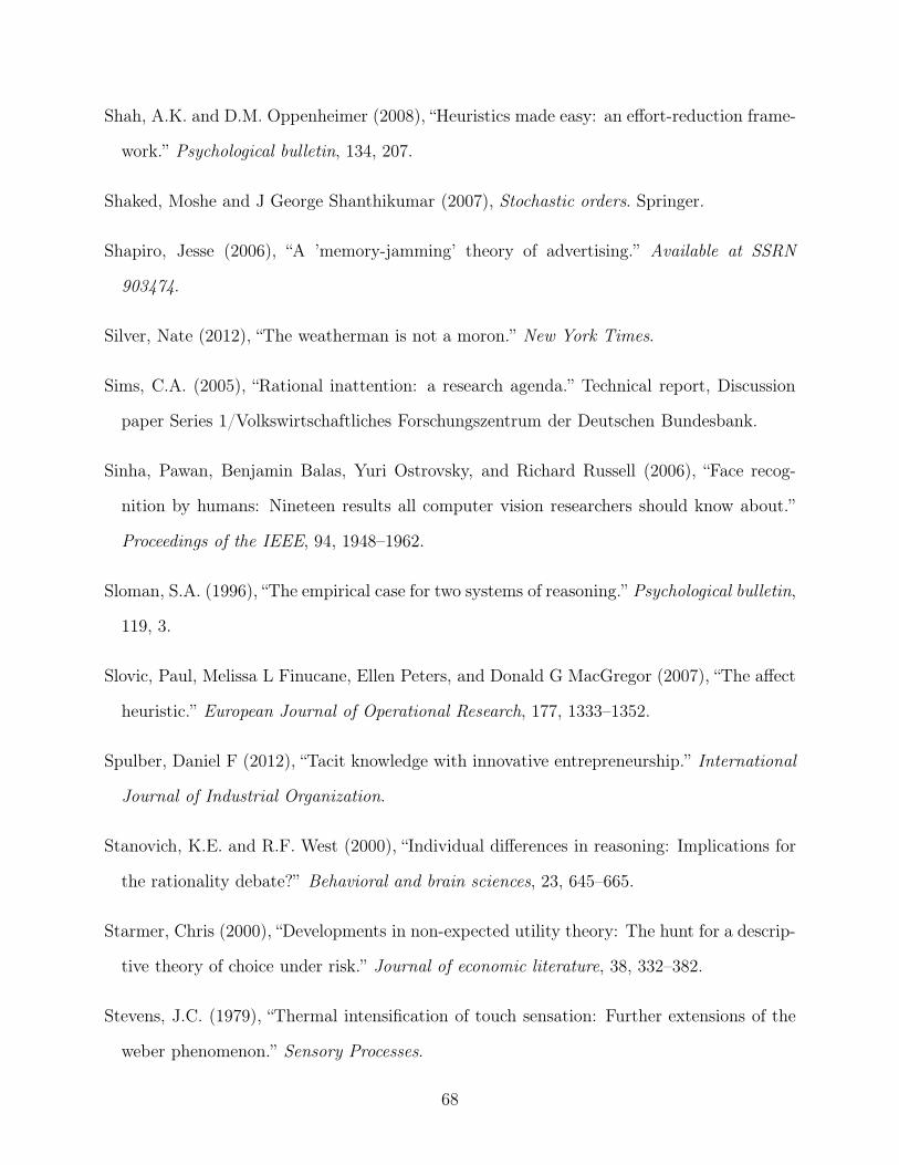
Shah, A.K. and D.M. Oppenheimer (2008), “Heuristics made easy: an e!ort-reduction frame-

work.” Psychological bulletin, 134, 207.

Shaked, Moshe and J George Shanthikumar (2007), Stochastic orders. Springer.

Shapiro, Jesse (2006), “A ’memory-jamming’ theory of advertising.” Available at SSRN

903474.

Silver, Nate (2012), “The weatherman is not a moron.” New York Times.

Sims, C.A. (2005), “Rational inattention: a research agenda.” Technical report, Discussion

paper Series 1/Volkswirtschaftliches Forschungszentrum der Deutschen Bundesbank.

Sinha, Pawan, Benjamin Balas, Yuri Ostrovsky, and Richard Russell (2006), “Face recog-

nition by humans: Nineteen results all computer vision researchers should know about.”

Proceedings of the IEEE, 94, 1948–1962.

Sloman, S.A. (1996), “The empirical case for two systems of reasoning.” Psychological bulletin,

119, 3.

Slovic, Paul, Melissa L Finucane, Ellen Peters, and Donald G MacGregor (2007), “The a!ect

heuristic.” European Journal of Operational Research, 177, 1333–1352.

Spulber, Daniel F (2012), “Tacit knowledge with innovative entrepreneurship.” International

Journal of Industrial Organization.

Stanovich, K.E. and R.F. West (2000), “Individual di!erences in reasoning: Implications for

the rationality debate?” Behavioral and brain sciences, 23, 645–665.

Starmer, Chris (2000), “Developments in non-expected utility theory: The hunt for a descrip-

tive theory of choice under risk.” Journal of economic literature, 38, 332–382.

Stevens, J.C. (1979), “Thermal intensification of touch sensation: Further extensions of the

weber phenomenon.” Sensory Processes.

68

Thaler, Richard H and Shlomo Benartzi (2004), “Save more tomorrow: Using behavioral

economics to increase employee saving.” Journal of political Economy, 112, S164–S187.

Tversky, A. and D. Kahneman (1974), “Judgment under uncertainty: Heuristics and biases.”

science, 185, 1124–1131.

Tversky, A. and D. Kahneman (1986), “Rational choice and the framing of decisions.” The

Journal of Business, 59, 251–278.

Tversky, A. and I. Simonson (1993), “Context-dependent preferences.” Management science,

39, 1179–1189.

Tversky, Amos, Paul Slovic, and Daniel Kahneman (1990), “The causes of preference rever-

sal.” The American Economic Review, 204–217.

von Helmholtz, H. (1971 [1878]), “The facts of perception.” In Selected writings of Hermann

von Helmholtz, Wesleyan Univ Pr.

Wernerfelt, B. (1995), “A rational reconstruction of the compromise e!ect: Using market

data to infer utilities.” Journal of Consumer Research, 627–633.

Wilson, A. (2002), “Bounded memory and biases in information processing.” NAJ Economics,

5.

Woodford, M. (2012), “Inattentive valuation and reference-dependent choice.” Unpublished

Manuscript, Columbia University.

69

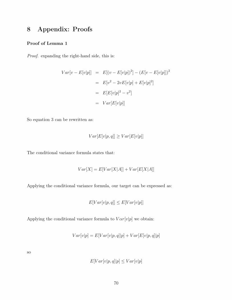
8 Appendix: Proofs

Proof of Lemma 1

Proof. expanding the right-hand side, this is:

V ar[v " E[v|p]] = E[(v " E[v|p])2]" (E[v "E[v|p]])2

= E[v2 " 2vE[v|p] + E[v|p]2]

= E[E[v|p]2 " v2]

= V ar[E[v|p]]

So equation 3 can be rewritten as:

V ar[E[v|p, q]] ' V ar[E[v|p]]

The conditional variance formula states that:

V ar[X ] = E[V ar[X|A]] + V ar[E[X|A]]

Applying the conditional variance formula, our target can be expressed as:

E[V ar[v|p, q]] & E[V ar[v|p]]

Applying the conditional variance formula to V !r[v|p] we obtain:

V ar[v|p] = E[V ar[v|p, q]|p] + V ar[E[v|p, q]|p]

so

E[V ar[v|p, q]|p] & V ar[v|p]

70

then taking expectations and applying the law of iterated expectations, we get, as required:

E[V ar[v|p, q]] & E[V ar[v|p]]

Proof of Proposition 1:

Proof. We wish to show that System 2’s bias is always weakly smaller, i.e.

V ar[E[v|x, z, E[v|x,!]]] & V ar[v " E[v|x,!]]

this follows directly from the Lemma if we note that, by the law of iterated expectations,

E[v|x,!] = E[v|x, E[v|x,!]]

thus E2 can be written as conditioning on a strictly larger information set than E1.

Proof of Proposition 2:

Proof. A bias exists if and only if there is some x # X, ! # A, z # Z, such that E[v|x, z,!] (=

E[v|x, z, E[v|x,!]]. We can express E2 as

E2 = E[v|x, z, E[v|x,!]]

=

ˆ

!#A

E[v|x, z, !]f(d!|x, z, E[v|x,!])

If the assumed condition holds, then for any ! # A such that f(!|x, z, E[v|x,!]) > 0 then

71

E[v|x, z, !] = E[v|x, z,!], therefore:

=

ˆ

!#A

E[v|x, z,!]f(d!|x, z, E[v|x, z])

= E[v|x, z,!]

= EP

Now suppose the condition did not hold, then there would exist some x # X, !,!! # A,

z # Z such that:

E[v|x, z,!] (= E[v|x, z,!!]

E[v|x, z, E[v|x,!]] = E[v|x, z, E[v|x,!!]]

Both cases give rise to the same E2, but have di!erent EP , thus one case must be biased, i.e.

either for ! or !!, E2 (= EP .

Proof of Proposition 3.

Suppose that there existed some x and !, such that there was a non-zero probability of

bias, i.e.:

ˆ

z#Z

1{E[v|x, z,!] > E[v|x, z, E[v|x,!]]}f(dz|x) > 0 ,

This implies thatˆ

z#Z

f(dz|x) +

ˆ

z#Z

f(dz|x) > 0

where Z = {z # Z : EP < E2} and Z = {z # Z : EP > E2}. Now consider the element

!! which is highest ranked among those which have the same E1, i.e. !! # sup&xA, where

72

A = {! # A : E[v|x, !] = E[v|x,!]}. We know that for all z # Z,

E[v|x, z,!!] ' E[v|x, z,!]

E[v|x, z,!!] '

ˆ

!#A

E[v|x, z, !]f(d!|x, z)

= E[v|x, z, E[v|x,!]]

so for Z,

*z # Z, E[v|x, z,!] < E[v|x, z,!!]

meaning that if´

z#Z f(dz|x) > 0 then

ˆ

z#Z

(E[v|x, z,!!]" E[v|x, z,!]) f(dz|x) > 0

ˆ

z#Z

(E[v|x, z,!!]" E[v|x, z,!]) f(dz|x) > 0,

however this contradicts our assumption that ! and !! both yield the same E1, i.e. that:

ˆ

z#Z

E[v|x, z,!!]f(dz|x) =

ˆ

z#Z

E[v|x, z,!]f(dz|x)

A symmetric argument will also deliver a contradiction if´

z#Z f(dz|x) > 0 (using the infinum

of A instead of its supremum). Thus for any given x and ! the probability of bias must be

zero, therefore the unconditional probability of bias must be zero.

Proof of Proposition 5:

Proof. The final expectation can be written as an integral over expectations at di!erent

73

values of !:

u!,x2 (x, z) = E[v|x, z,E1]

=

ˆ

vf(dv|x, z,E1)

=

ˆ

,ˆ

vf(dv|x, z, !)

-

f(d!|x, z,E1)

=

ˆ

E[v|x, z, !]f(d!|x, z,E1)

=

ˆ

u!P (x, z)f(d!|x, z,E1)

and by the convexity of U , u!,x2 (x, z) must therefore belong to U .

Proof of Proposition 8.

Proof. We first wish to show that x and x! will induce the same posteriors over !1, given the

same E1. Expanding,

f(!1|x, E1) =f(E1, x|!1)f(!1)´

f(E1, x|!1)df(!1)

=f(E1|x,!1)f(x|!1)f(!1)´

f(E1|x, !1)f(x|!1)f(d!1)

=f(E1|x!,!1)f(x!|!1)f(!1)´

f(E1|x!, !1)f(x!|!1)f(d!1)

= f(!1|x!, E1)

where the substitutions of x! for x invoke assumptions (iii) and (iv). Having established that

the mapping is the same, we can write E2 as:

E[v|x, z, E1] =

´

E[v|x, z, !]f(E1|x, !)f(d!)´

f(E1|x, !)f(d!)

74

by assumption we can replace ! with !1 for this realization of z,

E[v|x, z, E1] =

´

E[v|x, z, !1]f(E1|x, !1)f(d!1)´

f(E1|x, !1)f(d!1)

=

´

E[v|x!, z, !1]f(E1|x!, !1)f(d!1)´

f(E1|x!, !1)f(d!1)

= E[v|x!, z, E1]

and because f is assumed to be unambiguous, an increase in E1 must also weakly increase

E2, and the conclusion is direct.

75