Bio Jour Bioequivalence2001TLS

The Total Least Squares Methodin Individual Bioequivalence Evaluation

Vladimir Dragalin and Valerii Fedorov

Research Statistics Unit, Biomedical and Data SciencesGlaxo SmithKline

Summary

We propose a simple method for comparison of series of matched observations. While in all our exam-ples we address “individual bioequivalence” (IBE), which is the subject of much discussion in pharma-ceutical statistics, the methodology can be applied to a wide class of cross-over experiments, includingcross-over imaging. From the statistical point of view the considered models belong to the class of the“error-in-variables” models. In computational statistics the corresponding optimization method is re-ferred to as the “least squares distance” and the “total least squares” method. The derived confidenceregions for both intercept and slope provide the basis for formulation of the IBE criteria and methodsfor its assessing. Simple simulations show that the proposed approach is very intuitive and transparent,and, at the same time, has a solid statistical and computational background.

Key words and phrases: Average bioequivalence; Comparison of matched observa-tions; Comparison of pharmacokinetic characteristics;Cross-over experiment; Error-in-variables model; Indivi-dual bioequivalence; Population bioequivalence; Totalleast squares method.

1. Introduction

Bioequivalence trials, in which a test (T) and a reference (R) drug are being com-pared, usually are run as double-blind TR=RT cross-over designs. The referencedrug is usually an innovator drug while the test drug is either a generic or a newformulation produced by the same innovator pharmaceutical company. Blood sam-ples are taken at regular intervals and the area under the concentration curve(AUC), perhaps the maximum concentration (Cmax) and occasionally the time tomaximum concentration (Tmax) are compared. According to the present standardsin the assessment of bioequivalence, the test formulation may be regarded asequivalent to the reference if the 90% confidence interval for the ratio of AUCslies between 0.8 and 1.25 (so called average bioequivalence –– ABE). Recently,FDA (Guidance, 1999) issued a draft guideline for implementation of new stand-ards in evaluating bioequivalence (population and individual bioequivalence ––

Biometrical Journal 43 (2001) 4, 399–420

# WILEY-VCH Verlag Berlin GmbH, 13086 Berlin, 2001 0323-3847/01/0407-0399 $ 17.50þ.50/0

PBE and IBE) in which new concepts of prescribability and switchability are pro-posed. Two formulations could have the same average bioavailability and not beequally prescribable because one could be more variable than another. Two formula-tions could be equally prescribable for a new patient, but they might not be switch-able because a patient currently on the reference formulation might notice a differ-ence when switched to a new formulation. Many different bioequivalence criteriahave been suggested that encompass the average bioavailability, prescribability andswitchability aspects (see e.g. Anderson and Hauck (1990), Shall and Luus

(1993), Hyslop et al. (2000), Gould (2000), Dragalin and Fedorov (1999)).In the simplest case, the observations in such a trial are matched pairs

ðxTj; xRjÞ; j ¼ 1; . . . ; n, of the responses to the test and reference drug given to n(usually 20–25) healthy volunteers on particular days well separated by a wash-out period. A number of different models can be considered for these data. Re-gression with error-in-variables, also known as the measurement error model, is amodel of the form

xTj ¼ mTj þ eTj ; xRj ¼ mRj þ eRj ;ð1Þ

mTj ¼ q0 þ qmRj j ¼ 1; . . . ; n ;

where eTj and eRj are independent random variables with mean zero and variancess2T and s2

R, respectively. The case when eTj and eRj are dependent variables andtheir covariance matrix ~SS ¼ s2S, where S is known, can be obviously reduced tothe previous case. It is also assumed that observations from different individualsare independent. The variables mTj and mRj are sometimes called latent variables, aterm that refers to quantities that cannot be directly measured.

There are two different versions of this model. Under the linear functional mod-el, we observe pairs ðxTj; xRjÞ, according to (1), where the mRj’s are fixed, unknownparameters. The parameters of main interest are q0 and q and inference on theseparameters is made using the joint distribution of ððxT1; xR1Þ; . . ., ðxTn; xRnÞÞ, condi-tional on ðmR1; . . . ; mRnÞ.

The linear structural model can be thought of as an extension of the functionalrelationship model, extended through the following hierarchy. As in the functionalmodel we have random variables XTj and XRj, with EðXTj j mTjÞ ¼ mTj andEðXRj j mRjÞ ¼ mRj and we assume the functional relationship mTj ¼ q0 þ qmRj, butnow we assume that the parameters ðmR1; . . . ;mRnÞ are themselves a random sam-ple from a common normal population, i.e. mRj � NðmR; s

*2Þ: Consequently,

mTj � Nðq0 þ qmR; q2s*2Þ: As in the functional model, the parameters of main

interest are q0 and q. Here, however, the inference on these parameters may bemade using the joint distribution of ððxT1; xR1Þ; . . . ; ðxTn; xRnÞÞ, unconditional onðmR1; . . . ;mRnÞ additionally to the inferences conditional on ðmR1; . . . ; mRnÞ.

In usual linear regression, when it is assumed that one variable in the pair ismeasured without error, say xR ¼ mR, the least squares solution for estimating q0

and q is usually considered by minimization of the sum of squared vertical dis-tances (residuals). Similarly if the xT ¼ mT , then the minimization of horizontal dis-

400 V. Dragalin and V. Fedorov: The Total Least Squares Method

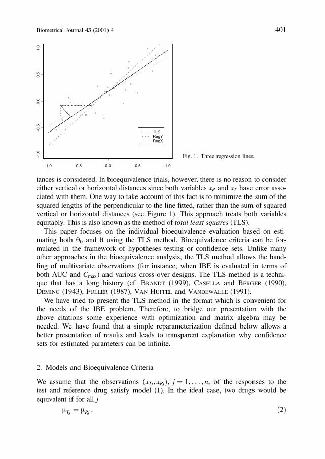
tances is considered. In bioequivalence trials, however, there is no reason to considereither vertical or horizontal distances since both variables xR and xT have error asso-ciated with them. One way to take account of this fact is to minimize the sum of thesquared lengths of the perpendicular to the line fitted, rather than the sum of squaredvertical or horizontal distances (see Figure 1). This approach treats both variablesequitably. This is also known as the method of total least squares (TLS).

This paper focuses on the individual bioequivalence evaluation based on esti-mating both q0 and q using the TLS method. Bioequivalence criteria can be for-mulated in the framework of hypotheses testing or confidence sets. Unlike manyother approaches in the bioequivalence analysis, the TLS method allows the hand-ling of multivariate observations (for instance, when IBE is evaluated in terms ofboth AUC and Cmax) and various cross-over designs. The TLS method is a techni-que that has a long history (cf. Brandt (1999), Casella and Berger (1990),

Deming (1943), Fuller (1987), Van Huffel and Vandewalle (1991).We have tried to present the TLS method in the format which is convenient for

the needs of the IBE problem. Therefore, to bridge our presentation with theabove citations some experience with optimization and matrix algebra may beneeded. We have found that a simple reparameterization defined below allows abetter presentation of results and leads to transparent explanation why confidencesets for estimated parameters can be infinite.

2. Models and Bioequivalence Criteria

We assume that the observations ðxTj; xRjÞ; j ¼ 1; . . . ; n, of the responses to thetest and reference drug satisfy model (1). In the ideal case, two drugs would beequivalent if for all j

mTj ¼ mRj : ð2Þ

Biometrical Journal 43 (2001) 4 401

-1.0 -0.5 0.0 0.5 1.0

-1.0

-0.5

0.0

0.5

1.0

TLSRegYRegX

Fig. 1. Three regression lines

But even in this case, the presence of the time trend noticeable in the intervalbetween T and R type observations can make (2) too restrictive. For practicalneeds, the inequality

max1�j�n

jmTj mRjj < D ; ð3Þ

where D is a prespecified positive constant, appears to be a more satisfactorydefinition of bioequivalence. However, even such a liberal restriction (3) does notassure that for some new patient j0 the absolute difference jmTj0 mRj0 j will be lessthan D. Another way is to assume a functional relationship between mTj and mRj,say mTj ¼ f ðmRjÞ, and to prove that this function is close to identity, i.e. f ðxÞ � x.For simplicity and practical purposes, a simple linear approximation to the func-tion f might suffice:

mTj ¼ q0 þ qmRj

for any patient (either participating or not in the experiment), and then to imposesome constraints on both q0 and q, treating them as unknown “population” param-eters. For instance, one can declare the IBE of T and R if q0 is close (in units ofstandard deviation of xR) to 0 and q is close to 1. Consequently, the main focus inthis situation is on estimation of the unknown parameters q0 and q and on verifi-cation of the (statistical) fulfillment of the imposed constraints, which are mathe-matical formulations of “close to”. Accepting model (1) as a model for the obser-vations, we have an opportunity to develop the IBE criteria which are defined bysome goalpost sets in the plane ðq0;qÞ.

In traditional settings, the aggregate criteria are usually recommended. For ex-ample, Anderson and Hauck (1990) propose to use

EðmTj mRjÞ2 ¼ ðmT mRÞ

2 þ Var ðmTj mRjÞ : ð4Þ

In the framework of the linear structural model

EðmTj mRjÞ2 ¼ ½q0 þ ðq 1Þ mR

2 þ ðq 1Þ2 s*2 :

For the reference treatment R it is plausible to assume that mR and s*2 are known.

In this case, after proper selection of the origin

EðmTj mRjÞ2 ¼ q2

0 þ ðq 1Þ2 s*2 ð5Þ

and any IBE admissibility set generates an admissibility ellipse in the ðq0; qÞplane. Notice that the major axis of this ellipse (with respect to q) is propor-tional to variance s2

� of the reference treatment mean mRj, i.e. larger the as-sumed variability of R, larger will be the goalpost region for IBE. Similarly, alarger goalpost value for the aggregate criterion corresponds to a larger goalpostregion for the proposed criterion, the former goalpost being a scale factor forthe latter.


Similarly, the KL-distance for IBE introduced in Dragalin and Fedorov

(1999) is

1

2fq2

0 þ ðq 1Þ2 s*2 þ s2

T þ s2Rg

1

s2T

þ 1

s2R

� � 2 :

Here again, the IBE goalpost region is an ellipse in the ðq0; qÞ plane, but nowboth ellipse axes are scaled by s2

T and s2R also.

In the linear functional model setting one may be interested in the “closeness”of mTj and mRj on some interval ða; bÞ. Then, a similar to (5) criterion is

maxa�mRj�b

jmTj mRjj ¼ max fjq0 þ ðq 1Þ aj; jq0 þ ðq 1Þ bjg :

In our opinion, model (1) provides flexibility in the meaningful selection of theIBE criteria and adjusting that selection to the practitioner’s understanding of thedrug comparison problem. Of course, the latter might not coincide with the FDAunderstanding of the same problem. Note that the FDA (1999) proposed criterionfor IBE is:

EðxTj xRjÞ2 2 Var ðeRÞ ¼ ðmT mRÞ2 þ Var ðmTj mRjÞ þ s2

T s2R ;

ð6Þwhere eR and eT are assumed to be independent. Under very reasonable assump-tion that Var ðeRÞ ¼ Var ðeTÞ, criterion (6) coincides with (4). Otherwise, one hasto estimate Var ðeRÞ and Var ðeTÞ and this will require cross-over designs withmore than two periods. Interestingly, that in the FDA (1999) criterion it is boldlyassumed that EðeRjeTjÞ ¼ 0, i.e. the random errors in observing two subsequentresponses on the same subject are independent. At the same time, the assumptions2R ¼ s2

T , which is not more restrictive, is rejected. Moreover, it is not clear whycriterion (6) is better than criterion

EðxTj xRjÞ2 Var ðeTÞ Var ðeRÞ;which in the case of independent eT and eR coincides with (4).

Model (1) can be generalized in various directions. For instance, one may con-sider a more complicated functional relationships between mT and mR. Frequently,at each experiment several pharmacokinetic characteristics such as AUC, Cmax,Tmax, etc. are measured. In this case

x ¼xT

xR

!¼

x1T. . .

xkT

x1R. . .

xkR

0BBBBBBBB@

1CCCCCCCCA¼

mT

mR

!þ

ETER

!: ð7Þ


If the washout period between administrations of the two formulations is longenough then

EðEETÞ ¼EðETET

TÞ EðETETRÞ

EðERETTÞ EðERET

RÞ

!¼

ST 0

0 SR

!: ð8Þ

As in the univariate case, it is reasonable to assume that ST ¼ SR ¼ S, but unlikein the former we have to gain additional information about the matrix S.

Another generalization may be in the direction of more complicated cross-overdesigns. For instance, one may introduce arbitrary sequences of T and R likeðRRTT . . .Þ1; ðTRTR . . .Þ2; . . . ; ðTTRR . . .Þn which may be different for different pa-tients. Besides the obvious and straightforward complexity arising in all formulas,in this case one has to be more cautious about the assumption of independence ofconsequent observations. Autoregressive types of models might be possible candi-dates to describe dependence inside a long series of cross-over observations, i.e.matrix (8) will include some off-diagonal blocks. Thus, in general, the followingmodel should be considered:

xj ¼ mj þ Ej and ATðqÞ mj ¼ bðqÞ ; ð9Þ

EðEjÞ ¼ 0; EðEjETj Þ ¼ s2S ; ð10Þ

where AðqÞ is a q� k matrix and bðqÞ is a k � 1 vector, xj are observations andthe matrix S is assumed to be known. In the simplest, and probably, practicallythe most important case (1):

xT ¼ ðxT ; xRÞ; mT ¼ ðmT ; mRÞATðqÞ ¼ ð1;qÞ; bðqÞ ¼ q0;

and the matrix S ¼ s2T 00 s2

R

� �.

3. Total Least Squares Method: Simple Linear Model

Main optimization problemOne of the most popular methods to analyze model (9) and (10) is based on mini-mization of sum of squared distances of observations from a fitted planeATðqÞ m ¼ bðqÞ. The corresponding estimator of q is defined as

qq ¼ arg minq;mj

Pnj¼1

ðxj mjÞT S1ðxj mjÞ ; ð11Þ

such that ATðqÞ mj ¼ bðqÞ. Let

v2ðqÞ ¼ minmj

Pnj¼1

ðxj mjÞT S1ðxj mjÞ ; ð12Þ


then, the estimator ss2 of s2 from (10) is defined as

ss2 ¼ ðknÞ1 v2ðqqÞ ; ð13Þwhere k ¼ dim ðxÞ ¼ dim ðmÞ.

Minimization of (12) with respect to m yields

v2ðqÞ ¼Pni¼1

½ATðqÞ xj bðqÞ T ½ATðqÞ S1AðqÞ 1 ½ATðqÞ xj bðqÞ : ð14Þ

Here and whenever inverse matrices are used, their existence is assumed. If thedimensions of q, AðqÞ and bðqÞ are large, then the minimization of v2ðqÞ withrespect to q is a difficult, but well studied numerical problem; cf. van Huffel andVandewalle (1991), Ch. 3–5. However, in bioequivalence studies the number ofunknown parameters, i.e. the dimension of the vector q, is relatively small and thenumerical aspects of the TLS method are not that important and are not discussedin this paper.

In the case of normally distributed E, vector (11) coincides with the maximumlikelihood estimator. The variance estimator (13) however is different from themaximum likelihood estimator kss2, which is not consistent, while the former oneit is.

Simple linear modelTo understand the statistical properties of TLS estimators we start with the simplelinear model (1) and the additional assumption that s2

T ¼ s2R ¼ s2. For this model,

the function v2ðqÞ looks rather simple:

v2ðqÞ ¼ 1

s2ð1þ q2ÞPnj¼1

ðxTj q0 qxRjÞ2 : ð15Þ

Note that only the denominator s2ð1þ q2Þ in (15) makes v2ðqÞ different from thesum of the least squares. The solution minimizing (15) can be found analytically:

qq0 ¼ �xxT qq�xxR;

qq ¼STT SRR þ

ffiffiffiffiffiffiffiffiffiffiffiffiffiffiffiffiffiffiffiffiffiffiffiffiffiffiffiffiffiffiffiffiffiffiffiffiffiffiffiffiðSTT SRRÞ2 þ 4S2TR

q2STR

; ð16Þ

where �xxT and �xxR are sample means of fxTjgn1 and fxRjgn1 and STT ¼Pnj¼1

ðxTj �xxTÞ2,SRR ¼

Pnj¼1

ðxRj �xxRÞ2 and STR ¼Pnj¼1

ðxTj �xxTÞ ðxRj �xxRÞ.

Referring to Figure 1, where scatter plot of 24 such pairs ðxTj; xRjÞ (generatedunder the scenario q0 ¼ 0:1, q ¼ 1:2, mRj equally spaced from 0:5 to 0:5 andeTj; eRj normally distributed with means zero and variances s2

T ¼ s2R ¼ 0:1), to-

gether with three fitted linear regression lines are displayed, we see that the TLSline always lies between the ordinary regression of xT on xR (RegY) and the ordin-ary regression of xR on xT (RegX). All three lines pass through ð�xxR; �xxTÞ.


Brown’s methodExplicit formulas (16) allow the derivation of the distribution of the estimators qq0

and qq and the construction of confidence sets for them or their transforms. As inmost publications on this topic (cf. Cheng and Van Ness (1994)), we assume thateTj and eRj are normally distributed. Consequently, the random variables

uj ¼ xTj q0 qxRj ; j ¼ 1; . . . ; n ;

are normally distributed with zero means and variance Var ðujÞ ¼ s2ð1þ q2Þ. Inde-pendence of eTj; eRj and eTj0 ; eRj0 implies the independence of uj and uj0 . Observing that

v2ðq0; qÞ ¼Pnj¼1

u2j

s2ð1þ q2Þ; ð17Þ

we may conclude that v2ðq0; qÞ has a c2 distribution with n degrees of freedom. If

Prðv2ðq0; qÞ � c21aðnÞÞ ¼ 1 a ;

then the inequality

v2ðq0; qÞ � c21aðnÞ ð18Þ

enables the construction of a ð1 aÞ100 per cent confidence set for qT ¼ ðq0; qÞ(cf. Brown (1957)). Here and in the sequel c2

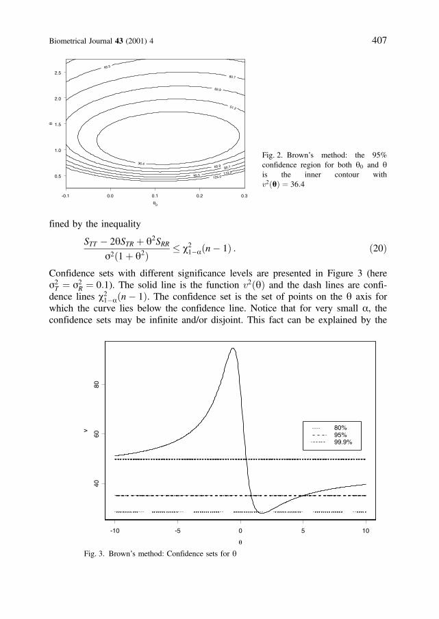
1aðnÞ is the 1 a upper percentileof the c2 distribution with n degrees of freedom. A typical confidence set is pre-sented in Figure 2. Data were generated under the same scenario as for Figure 1except that now s2

T ¼ s2R ¼ 0:01. The confidence set defined by (18) may have

different widths for different samples and even may be zero or infinite with posi-tive probability; see Gleser and Hwang (1987). To understand this phenomenonand its practical consequences, we consider the behaviour of the unconditionalconfidence intervals for the slope q. The presence of q in the denominator ofv2ðq0; qÞ causes most of the peculiarities in the TLS analysis.

Minimization of v2ðq0; qÞ in (17) with respect to q0 yields

v2ðqÞ ¼ 1

s2ð1þ q2ÞPnj¼1

½ðxTj �xxTÞ qðxRj �xxRÞ 2

¼ 1

s2ð1þ q2Þ½STT 2qSTR þ q2SRR : ð19Þ

Combining (1) and (19), we have

v2ðqÞ ¼Pnj¼1

½ðeTj qeRjÞ ðeT qeRÞ 2

s2ð1þ q2Þ;

where eTj qeRj are normally distributed with zero means, variance s2ð1þ q2Þand eT qeR ¼ n1

Pnj¼1

ðeTj qeRjÞ. Thus, v2ðqÞ has c2 distribution with ðn 1Þdegrees of freedom, and the ð1 aÞ100 per cent confidence interval for q is de-


fined by the inequality

STT 2qSTR þ q2SRR

s2ð1þ q2Þ� c2

1aðn 1Þ : ð20Þ

Confidence sets with different significance levels are presented in Figure 3 (heres2T ¼ s2

R ¼ 0:1). The solid line is the function v2ðqÞ and the dash lines are confi-dence lines c2

1aðn 1Þ. The confidence set is the set of points on the q axis forwhich the curve lies below the confidence line. Notice that for very small a, theconfidence sets may be infinite and/or disjoint. This fact can be explained by the


-0.1 0.0 0.1 0.2 0.3

θ0

0.5

1.0

1.5

2.0

2.5

θ

36.4

51.2

65.9

65.9

80.7

80.7

95.5

95.5

110.2

125.0

Fig. 2. Brown’s method: the 95%confidence region for both q0 and qis the inner contour withv2ðqÞ ¼ 36:4

-10 -5 0 5 10

θ

4060

80

v 80%95%99.9%

Fig. 3. Brown’s method: Confidence sets for q

boundness (from above) of v2ðqÞ as a function of q for any given n andfxTj; xRjgn1. We recall that in the least squares method the corresponding confi-dence interval is defined by the function

~vv2ðqÞ ¼Pnj¼1

½ðxTj �xxTÞ qðxRj �xxRÞ 2 ;

which infinitely increases when q ! �1. Note that in the least squares method itis assumed that Var xRj ¼ Var eRj ¼ 0.

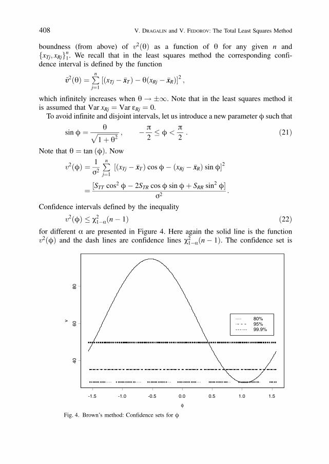
To avoid infinite and disjoint intervals, let us introduce a new parameter f such that

sin f ¼ qffiffiffiffiffiffiffiffiffiffiffiffiffi1þ q2

p ; p

2� f <

p

2: ð21Þ

Note that q ¼ tan ðfÞ. Now

v2ðfÞ ¼ 1

s2

Pnj¼1

½ðxTj �xxTÞ cos f ðxRj �xxRÞ sin f 2

¼ ½STT cos2 f 2STR cos f sin f þ SRR sin2 f s2

:

Confidence intervals defined by the inequality

v2ðfÞ � c21aðn 1Þ ð22Þ

for different a are presented in Figure 4. Here again the solid line is the functionv2ðfÞ and the dash lines are confidence lines c2

1aðn 1Þ. The confidence set is


-1.5 -1.0 -0.5 0.0 0.5 1.0 1.5

φ

4060

80

v 80%95%99.9%

Fig. 4. Brown’s method: Confidence sets for f

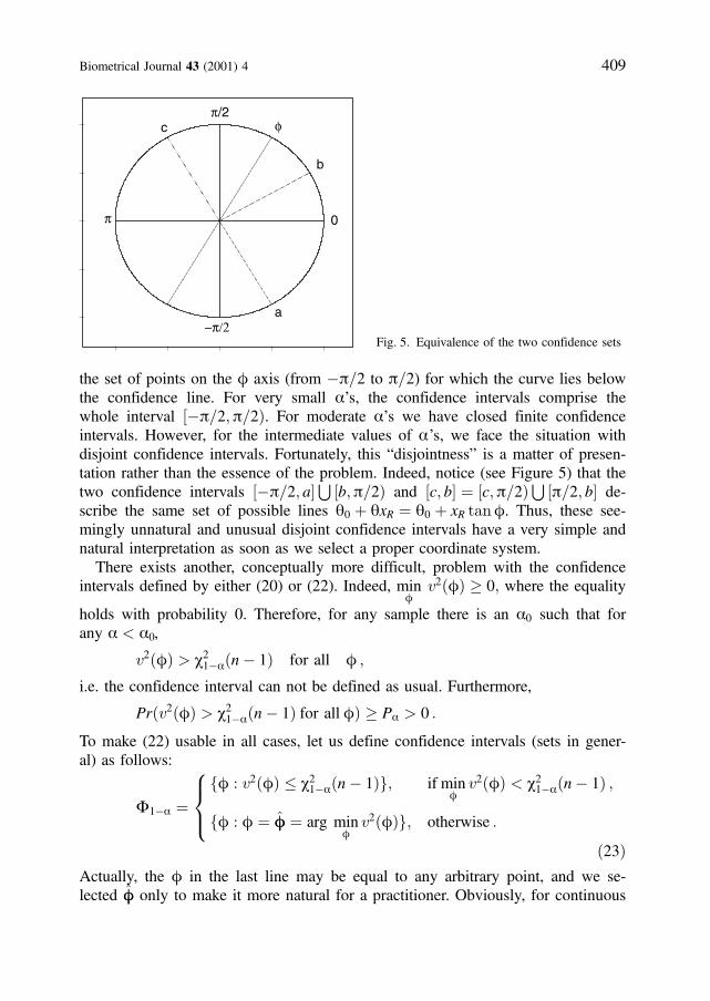
the set of points on the f axis (from p=2 to p=2) for which the curve lies belowthe confidence line. For very small a’s, the confidence intervals comprise thewhole interval ½p=2;p=2Þ. For moderate a’s we have closed finite confidenceintervals. However, for the intermediate values of a’s, we face the situation withdisjoint confidence intervals. Fortunately, this “disjointness” is a matter of presen-tation rather than the essence of the problem. Indeed, notice (see Figure 5) that thetwo confidence intervals ½p=2; a

S½b;p=2Þ and ½c; b ¼ ½c;p=2Þ

S½p=2; b de-

scribe the same set of possible lines q0 þ qxR ¼ q0 þ xR tanf. Thus, these see-mingly unnatural and unusual disjoint confidence intervals have a very simple andnatural interpretation as soon as we select a proper coordinate system.

There exists another, conceptually more difficult, problem with the confidenceintervals defined by either (20) or (22). Indeed, min

fv2ðfÞ � 0; where the equality

holds with probability 0. Therefore, for any sample there is an a0 such that forany a < a0,

v2ðfÞ > c21aðn 1Þ for all f ;

i.e. the confidence interval can not be defined as usual. Furthermore,

Prðv2ðfÞ > c21aðn 1Þ for all fÞ � Pa > 0 :

To make (22) usable in all cases, let us define confidence intervals (sets in gener-al) as follows:

F1a ¼ff : v2ðfÞ � c2

1aðn 1Þg; if minf

v2ðfÞ < c21aðn 1Þ ;

ff : f ¼ ff ¼ arg minf

v2ðfÞg; otherwise :

8><>:ð23Þ

Actually, the f in the last line may be equal to any arbitrary point, and we se-lected ff only to make it more natural for a practitioner. Obviously, for continuous


−π/2

π/2

0π

φ

b

c

a

Fig. 5. Equivalence of the two confidence sets

ff, the event fff ¼ the true value of fg has zero probability and in this sense allconfidence intervals with zero width are useless (non-informative). However, ifone repeats the sampling of fxTj; xRjgn1 infinitely many times, then the frequencythat F1a covers the true value of f will tend to 1 a.

In this subsection, it was assumed that the parameter s2 is known. To relax thisassumption, replicates are needed. Let m > 1 be the number of replicates for boththe T and R formulations (for simplicity, we assume here the same number ofreplicates per formulation, but the general case can be considered similarly) andthe observations fxTji; xRjigmi¼1 on subject j be summarized by

xTj ¼1

m

Pmi¼1

xTji ; s2Tj ¼

1

m 1

Pmi¼1

ðxTji xTjÞ2 ;

xRj ¼1

m

Pmi¼1

xRji ; s2Rj ¼

1

m 1

Pmi¼1

ðxRji xRjÞ2 :

Since s2Tj and xTj (and similarly s2

Rj and xRj) are independent, the pooled estimator

ss2 ¼ 1

2n

Pnj¼1

ðs2Tj þ s2

RjÞ

will be independent of fxTj; xRjgnj¼1. Moreover, under the assumption thats2T ¼ s2

R ¼ s2; the statistic 2nðm 1Þ ss2=s2 will have a c2-distribution with2nðm 1Þ degrees of freedom. Therefore, one can replace the unknown s2 in (17)by its pooled estimator ss2 and conclude that

m

nvv2ðq0; qÞ ¼ m

n

Pnj¼1

ðxTj q0 qxRjÞ2

ss2ð1þ q2Þ

has an F-distribution with n and 2nðm 1Þ degrees of freedom. The ð1 aÞ100per cent confidence set for ðq0; qÞ is given then by the inequality

m

nvv2ðq0; qÞ � F1aðn; 2nðm 1ÞÞ :

The confidence set for q under unknown s2 can be obtained generalizing (20) insimilar way. Details are omitted.

Creasy’s methodIt is known that the random variable

T ¼ ðn 2Þ q2

ð1 q2Þ

� �1=2

; ð24Þ

where q ¼ STR=ffiffiffiffiffiffiffiffiffiffiffiffiffiffiSTTSRR

p, has a t distribution with n 2 degrees of freedom if the

vector XTR ¼ ðxR1; . . . ; xRnÞ has a n-variate spherical distribution with

PrðXR ¼ 0Þ ¼ 0 and XTT ¼ ðxT1; . . . ; xTnÞ has any distribution with

PrðXT 2 f1gÞ ¼ 0 (cf. Muirhead (1982), Ch. 5); vectors XR and XT must be in-


dependent. Obviously, both functional and structural models satisfy the above con-dition if ET and ER are normally distributed N nð0; s2

TIÞ and N nð0; s2RIÞ respec-

tively. Note that in our problem XR and XT are independent when q ¼ 0. Creasy(1956) observed that when s2

T ¼ s2R, the TLS estimator qq (16) of the q (which is

also the maximum likelihood estimator in this case) satisfies the equality

tan 2ff ¼ 2STRjSTT SRRj

: ð25Þ

Combining (24) and (25), one can verify that

T2 ¼ ðn 2Þ ðSTT SRRÞ2 þ 4S2TR4ðSTTSRR S2TRÞ

sin2 2ff : ð26Þ

To derive (26) we have assumed that q ¼ 0 ðf ¼ 0Þ. The general case can bedealt with using an orthogonal transform and it can be verified that

T ¼ ðn 2Þ ðSTT SRRÞ2 þ 4S2TR4ðSTTSRR S2TRÞ

sin2 2ðff fÞ( )1=2

has a t distribution with n 2 degrees of freedom. Thus, we have identified apivotal quantity and we conclude that

f : sin2 2ðff fÞ � 4ðSTTSRR S2TRÞðn 2Þ ½ðSTT SRRÞ2 þ 4S2TR

t21a=2ðn 2Þ( )

ð27Þ

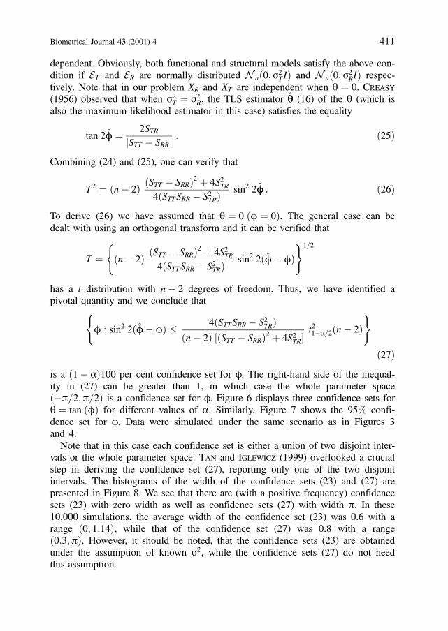
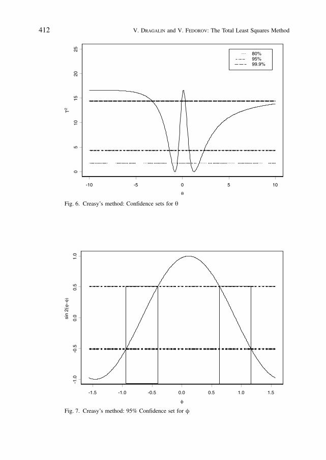
is a ð1 aÞ100 per cent confidence set for f. The right-hand side of the inequal-ity in (27) can be greater than 1, in which case the whole parameter spaceðp=2;p=2Þ is a confidence set for f. Figure 6 displays three confidence sets forq ¼ tan ðfÞ for different values of a. Similarly, Figure 7 shows the 95% confi-dence set for f. Data were simulated under the same scenario as in Figures 3and 4.

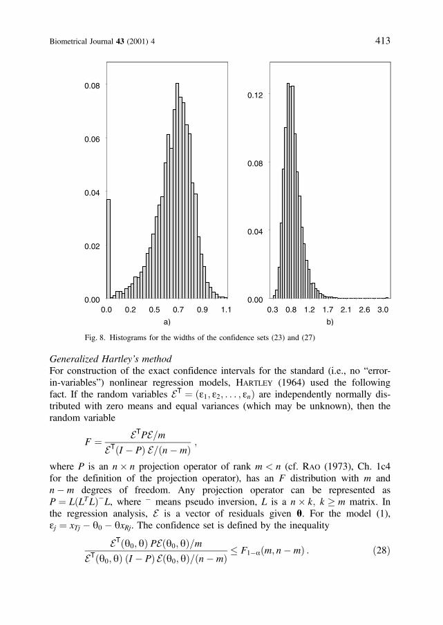
Note that in this case each confidence set is either a union of two disjoint inter-vals or the whole parameter space. Tan and Iglewicz (1999) overlooked a crucialstep in deriving the confidence set (27), reporting only one of the two disjointintervals. The histograms of the width of the confidence sets (23) and (27) arepresented in Figure 8. We see that there are (with a positive frequency) confidencesets (23) with zero width as well as confidence sets (27) with width p. In these10,000 simulations, the average width of the confidence set (23) was 0.6 with arange ð0; 1:14Þ, while that of the confidence set (27) was 0.8 with a rangeð0:3;pÞ. However, it should be noted, that the confidence sets (23) are obtainedunder the assumption of known s2, while the confidence sets (27) do not needthis assumption.



-1.5 -1.0 -0.5 0.0 0.5 1.0 1.5

φ

-1.0

-0.5

0.0

0.5

1.0

sin

2(ϕ−

φ)

Fig. 6. Creasy’s method: Confidence sets for q

-10 -5 0 5 10

θ

05

1015

2025

T2

80%95%99.9%

Fig. 7. Creasy’s method: 95% Confidence set for f

Generalized Hartley’s methodFor construction of the exact confidence intervals for the standard (i.e., no “error-in-variables”) nonlinear regression models, Hartley (1964) used the followingfact. If the random variables ET ¼ ðe1; e2; . . . ; enÞ are independently normally dis-tributed with zero means and equal variances (which may be unknown), then therandom variable

F ¼ ETPE=mETðI PÞ E=ðn mÞ

;

where P is an n� n projection operator of rank m < n (cf. Rao (1973), Ch. 1c4for the definition of the projection operator), has an F distribution with m andn m degrees of freedom. Any projection operator can be represented asP ¼ LðLTLÞL, where means pseudo inversion, L is a n� k; k � m matrix. Inthe regression analysis, E is a vector of residuals given q. For the model (1),ej ¼ xTj q0 qxRj. The confidence set is defined by the inequality

ETðq0; qÞ PEðq0; qÞ=mETðq0; qÞ ðI PÞ Eðq0; qÞ=ðn mÞ

� F1aðm; n mÞ : ð28Þ


Fig. 8. Histograms for the widths of the confidence sets (23) and (27)

0.0 0.2 0.5 0.7 0.9 1.1

a)

0.00

0.02

0.04

0.06

0.08

0.3 0.8 1.2 1.7 2.1 2.6 3.0

b)

0.00

0.04

0.08

0.12

The size (area) of confidence set defined by (28) depends crucially on the choiceof P. In the standard linear regression, P ¼ XðXXTÞ1 X, where X is the designmatrix. To mimic this choice, we have to select

LT ¼ 1; 1; . . . ; 1mR1; mR2; . . . ; mRn

� �:

Unfortunately mRj are unknown. We can not replace mRj by xRj because it makes La random matrix and F is not any more F-distributed. However, F will still be F-distributed if L is independent of E, i.e. independent of the observational errors eTjand eRj. This is a useful fact for the structural model case where mRj are random.

The lack of knowledge of mRj ’s can be partly overcome if one can find a covari-ate z such that z ¼ yðmRÞ, where either y is known or some of its properties(e.g., linearity, monotonicity, etc) are assumed known. For instance, if y is mono-tone increasing function then one can choose

LT ¼ 1; 1; . . . ; 1r1; r2; . . . ; rn

� �;


-0.1 0.0 0.1 0.2 0.3

θ0

0.5

1.0

1.5

2.0

2.5

θ

3.47.8

16.7

25.6

30.0

a)

-0.1 0.0 0.1 0.2 0.3

θ0

0.5

1.0

1.5

2.0

2.5

θ

3.4

12.0

20.6

29.2

29.229.2

37.8

46.455.0

b)

-0.1 0.0 0.1 0.2 0.3

θ0

0.5

1.0

1.5

2.0

2.5

θ

3.4

12.3

16.7

30.0

c)

-0.1 0.0 0.1 0.2 0.3

θ0

0.5

1.0

1.5

2.0

2.5

θ

3.4

12.0

20.6

29.2

37.846.455.0

d)

30.025.621.1

21.1 25.6 30.0

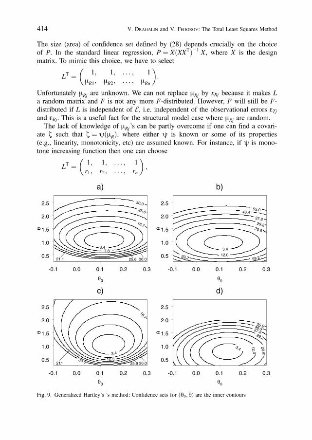
Fig. 9. Generalized Hartley’s ’s method: Confidence sets for ðq0; q) are the inner contours

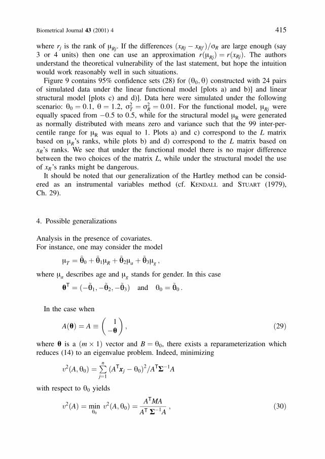
where rj is the rank of mRj. If the differences ðxRj xRj0 Þ=sR are large enough (say3 or 4 units) then one can use an approximation rðmRjÞ ¼ rðxRjÞ. The authorsunderstand the theoretical vulnerability of the last statement, but hope the intuitionwould work reasonably well in such situations.

Figure 9 contains 95% confidence sets (28) for ðq0; qÞ constructed with 24 pairsof simulated data under the linear functional model [plots a) and b)] and linearstructural model [plots c) and d)]. Data here were simulated under the followingscenario: q0 ¼ 0:1, q ¼ 1:2, s2

T ¼ s2R ¼ 0:01. For the functional model, mRj were

equally spaced from 0:5 to 0:5, while for the structural model mR were generatedas normally distributed with means zero and variance such that the 99 inter-per-centile range for mR was equal to 1. Plots a) and c) correspond to the L matrixbased on mR’s ranks, while plots b) and d) correspond to the L matrix based onxR’s ranks. We see that under the functional model there is no major differencebetween the two choices of the matrix L, while under the structural model the useof xR ’s ranks might be dangerous.

It should be noted that our generalization of the Hartley method can be consid-ered as an instrumental variables method (cf. Kendall and Stuart (1979),Ch. 29).

4. Possible generalizations

Analysis in the presence of covariates.For instance, one may consider the model

mT ¼ ~qq0 þ ~qq1mR þ ~qq2ma þ ~qq3mg ;

where ma describes age and mg stands for gender. In this case

qT ¼ ð~qq1;~qq2;~qq3Þ and q0 ¼ ~qq0 :

In the case when

AðqÞ ¼ A � 1q

� �; ð29Þ

where q is a ðm� 1Þ vector and B ¼ q0, there exists a reparameterization whichreduces (14) to an eigenvalue problem. Indeed, minimizing

v2ðA; q0Þ ¼Pnj¼1

ðATxj q0Þ2=ATS1A

with respect to q0 yields

v2ðAÞ ¼ minq0

v2ðA; q0Þ ¼ATMA

AT S1A; ð30Þ


where M ¼Pnj¼1

ðxj �xxÞ ðxj �xxÞT and �xx ¼ n1Pnj¼1

xj. Note that

qq0 ¼ arg minq0

v2ðA; q0Þ ¼ AT�xx :

Let

g ¼ S1=2A=ffiffiffiffiffiffiffiffiffiffiffiffiffiffiffiffiATS1A

p; gTg ¼ 1 ; ð31Þ

and

v2ðgÞ ¼ gTS1=2MS1=2g :

Then (cf. Rao (1973), Ch. 1f)

minA

v2ðAÞ ¼ ming

v2ðgÞ ¼ lmin ; ð32Þ

where lmin is the smallest eigenvalue of the matrix M ¼ S1=2MS1=2. The TLSestimator of the introduced parameter g is defined as the eigenvector of the matrixM corresponding to lmin, i.e. it is defined by the following equation

lmingg ¼ Mgg: ð33ÞComputation of eigenvalues and eigenvectors of positive definite matrices is a wellestablished area in numerical analysis and the corresponding tools may be foundin many statistical software packages. Note that

qi ¼ xi=x0 ; i ¼ 1; . . . ;m ; ð34Þwhere ðx0; x1; . . . ; xmÞT ¼ S1=2g. Formulas (29)–(34) provide an effective solutionof the TLS problem in bioequivalence evaluation in presence of covariates.

In general, the parameterization (31) (which corresponds to q=ffiffiffiffiffiffiffiffiffiffiffiffiffi1þ q2

p¼ sin f

in the one-dimensional case) is useful not only in computations but in statisticalanalysis as well. The set of all possible values of the unknown parameters g isfinite and therefore one can avoid infinitely large confidence intervals which wealready observed in the simpler one-dimensional case.

To construct confidence regions for q0 and q one may use either Brown’s meth-od or the generalized Hartley’s method. In the first case, it is assumed that thematrix S is known while in the second one it is assumed that S ¼ s2S0, where S0

is known, but s2 is unknown.For instance, Brown’s confidence set for q (compare with (23)) is defined as

G1a ¼fg : gTS1=2MS1=2g � c2

1aðn 1Þg ; if lmin < c21aðn 1Þ ;

fg : g ¼ ggg ; otherwise :

(Note that for any given n and a

Prðlmin < c21aðn 1ÞÞ � Pl > 0 ;

Prðlmin > c21aðn 1ÞÞ � Pu > 0 ;


i.e. the confidence sets may, with positive probabilities, consist of either a singlepoint or the whole parameter space.

Multivariate bioequivalenceWe return now to the multivariate bioequivalence model (7)–(10) where severalpharmacokinetics characteristics (say k of them) are measured. In this case

ATðqÞ ¼

1 0 . . . 0 q1 0 . . . 00 1 . . . 0 0 q2 . . . 0. . . . . . . . . . . . . . . . . . . . . . . .0 0 . . . 1 0 0 . . . qk

0BB@1CCA ¼ I;Qð Þ ;

bðqÞT ¼ q01;q02; . . . ; q0kð Þ ¼ Q0 ; mT ¼ mT1; . . . ; mTk; mR1; . . . ; mRkð Þ ;and q ¼ 2k. (14) is now

v2ðQ0;QÞ ¼Pnj¼1

ðxTj Q0 QxRjÞT eSS1ðxTj Q0 QxRjÞ;

where eSS ¼ ST þ ATðqÞ SRAðqÞ. Minimizing it with respect to Q0 yields

v2ðQÞ ¼Pnj¼1

½ðxTj �xxTÞ QðxRj �xxRÞ T eSS1½ðxTj �xxTÞ QðxRj �xxRÞ :

One can verify (compare with (18) and (20)) that v2ðQ0;QÞ has a c2-distributionwith kn degrees of freedom and v2ðQÞ has a c2-distribution with kðn 1Þ degreesof freedom. Thus, we can use the generalized Brown’s method in this case aswell. We have not explored the generalization of the Creasy’s method to the multi-variate case. As for generalization of the Hartley’s method, everything is straight-forward.

Parametric comparison of pharmacokinetics curvesThe use of AUC or Cmax in evaluating bioequivalence can be considered as anonparametric approach in comparing the pharmacokinetic (PK) curves. The pro-posed method may improve the current approach allowing the combination ofinformation about AUC, Cmax and Tmax in a very natural way. Actually, the meth-od could be extended to allow the parametric comparison of PK curves. As anexample, let us consider the first-order one-compartment model:

yðtiÞ ¼ x3�ex1ti ex2ti

�þ wi ¼ hðx; tiÞ þ wi ; ð35Þ

where x1; x2 and x3 are unknown parameters and wi are observational errors, suchthat EðwiÞ ¼ 0 and Eðw2Þ ¼ D2 for all i. If one has N observationsyðt1Þ; yðt2Þ; . . . ; yðtNÞ, then in the case of independent and homogeneous errors wi,the least squares estimator

xx ¼ arg minx

PNi¼1

½yðtiÞ hðx; tiÞ 2


is a consistent estimator and asymptotically

xx x*ffiffiffiffiN

p � Nð0;XÞ ;

where x* is the vector of the true values and the matrix NX can be approximatedas follows

NX ’ MM1 ¼ SS ;

with

MM1 ¼ D2 PNi¼1

f ðxx; tiÞ f Tðxx; tiÞ ;

f ðx; tÞ ¼ @hðx; tÞ@x

;

(cf. Atkinson et al. (1993)).If the PK analysis was performed for both treatment and reference formulations,

then one can compute xxT ; SST and xxR; SSR correspondingly. Note that AUC andCmax in the “nonparametric” setting have variances of order D2 while the compo-nents of the vectors xx have variances of order D2=N.

IBE can be evaluated now using the TLS method based on vectors xxT and xxR ofobservations on the two formulations governed by the model (7) with covariancestructure (8) (with ST ¼ SST and SR ¼ SSR) and the assumption (9) about the linearrelationship. As usual, application of the “physical“ model helps to improve preci-sion through the use of information about absorption-elimination process (withobvious concern about validity of the selected model).

5. Conclusion

The traditional least squares analysis of testing a null intercept and unit slope isnot appropriate for individual bioequivalence evaluation because both xR and xTare observed with random errors. On the other hand, the TLS estimators treat bothvariables equally. The total least squares technique allows us to clarify and gener-alize the concept of individual bioequivalence in cross-over designs. Simultaneousconsideration of several pharmacokinetic characteristics such as AUC, Cmax, andTmax is straightforward using the TLS method. Moreover, more advanced evalua-tion of the bioequivalence of two formulations in terms of more natural pharmaco-kinetic characteristics such as absorption and elimination rates is possible.

We discussed three groups of confidence sets for the structural parameters ofthe linear functional and structural models. Two formulations are declared bioequi-valent if the confidence set of a given significance level is inside of the goalpostregion. Consequently, our main focus was on the analysis of such confidence sets.


These three methods of constructing confidence sets are complementary to eachother. No one was proved to be statistically the most efficient. However, our simu-lations showed that Hartley’s method leads on average to smaller size confidencesets.

We would like to emphasize that the size of the confidence sets in any of theconsidered approaches varies significantly from sample to sample. Therefore, inpractice one should be concerned not merely with the size of the observed confi-dence set, but rather with the average size of such confidence sets.

The results were illustrated with simulated data showing that the TLS methodcan be an alternative tool for the IBE evaluation.

Acknowledgement

We are grateful to our colleagues from SmithKline Beecham Byron Jones, MarkHeise, Scott Patterson and Sergei Leonov for a very constructive discussions ofthe results and their comments on practical aspects of the approach. We wish tothank the Editor and the referee for their comments that have improved this arti-cle.

References

Anderson, S. and Hauck, W. W., 1990: Consideration of individual bioequivalence. Journal of Phar-macokinetics and Biopharmaceutics 18, 259–273.

Atkinson, A. C., Chaloner, K., and Herzberg, A. M., 1993: Optimum experimental designs forproperties of a compartmental model. Biometrics 49, 325–337.

Berger, R. L. and Hsu, J. C., 1996: Bioequivalence trials, intersection-union tests and equivalenceconfidence sets (with discussion). Statistical Sciences 11, 283–319.

Brandt, S., 1999: Data Analysis: Statistical and Computational Methods for Scientists and Engineers,3rd edition. Springer, New York.

Brown, R. L., 1957: Bivariate structural relation. Biometrika 44, 84–86.Cheng, C.-L. and Van Ness, J. W., 1994: On estimating linear relationships when both variables are

subject to errors. J. R. Statist. Soc. B 56, 167–183.Casella, G. and Berger, R. L., 1990: Statistical Inference. Pacific Grove, CA: Wadsworth.Creasy, M. A., 1956: Confidence limits for the gradient in the linear functional relationship. J.R.

Statist. Soc. B 18, 65–69.Dragalin, V. and Fedorov, V. 1999: Kullback–Leibler distance for evaluating bioequivalence: I. Cri-

teria and models. SB BDS Technical Report # 03, November, 1999. Presented at ENAR 2000Spring Meeting, March 19–24, 2000, Chicago, USA

Fieller, E. C., 1954: Some problems in interval estimation. J. R. Statist. Soc. B 16, 175–185.Fuller, W. A., 1987: Measurement Error Models. John Wiley & Sons, New York.Gleser, L. J., 1981: Estimation in a multivariate “errors in variables“ regression model: large sample

results. Ann. Statist. 9, 24–44.Gleser, L. J. and Hwang, J. T., 1987: The nonexistence of 100ð1 aÞ% confidence sets of finite

expected diameter in errors-in-variables and related models. Ann. Statist. 15, 1351–1362.


Gould, A., 2000: A practical approach for evaluating population and individual bioequivalence. Statis-tics in Medicine, 19, 2721–2740.

Guidance for Industry: Average, Population, and Individual Approaches to Establishing Bioequiva-lence. Food and Drug Administration, August, 1999.

Hyslop, T. F., Holder, D. J., and Hsuan, F., 2000: A small-sample confidence interval approach toassess individual bioequivalence. Statistics in Medicine, 19, 2885–2897.

Kendall, M. G. and Stuart, A. (1979) The Advanced Theory of Statistics, 4th edn, vol 2, LondonGriffin.

Muirhead, R. J., 1982: Aspects of Multivariate Statistical Theory Wiley, New York.PhRMA Perspective on Population and Individual Bioequivalence, To appear in Journal of Clinical

Pharmacology, 1999.Rao, C. R., 1973: Linear Statistical Inference and Its Applications, 2nd ed. John Wiley & Sons, New

York.Schall, R. and Luus, G. H., 1993: On population and individual bioequivalence. Statistics in Medi-

cine 12,1009–1124.Tan, C. Y. and Iglewicz, B., 1999: Measurement-methods comparisons and linear statistical relation-

ship. Technometrics, 41, 192–201.Van Huffel, S. and Vandewalle, J., 1991: The Total Least Squares Problem: Computational Aspects

and Analysis. SIAM, Philadelphia.Zariffa, N. M.-D., Patterson, S. D., Boyle, D., and Hyneck, M., 2000: Case studies, practical

issues and observations on population and individual bioequivalence. Statistics in Medicine, 19,2811–2820.

Prof. Valerii Fedorov Received, December 1999Smith Kline Beecham Pharmaceuticals Revised, October 20001250 S. Collegeville Road, PO Box 5089 Accepted, January 2001Collegeville, PA 19426-0989USA


Documents

Bio Jour Bioequivalence2001TLS