Bioenergetics of mixotrophic metabolisms: A theoretical analysis

Bioenergetics of mixotrophic metabolisms: A theoretical analysis

by

Stephanie Slowinski

A thesis

presented to the University of Waterloo

in fulfillment of the

thesis requirement for the degree of

Master of Science

in

Earth Sciences (Water)

Waterloo, Ontario, Canada, 2019

© Stephanie Slowinski 2019

ii

Author’s Declaration

This thesis consists of material all of which I authored or co-authored: see Statement of Contributions

included in the thesis. This is a true copy of the thesis, including any required final revisions, as

accepted by my examiners.

I understand that my thesis may be made electronically available to the public.

iii

Statement of Contributions

This thesis consists of two co-authored chapters.

I contributed to the study design and execution in chapters 2 and 3. Christina M. Smeaton (CMS) and

Philippe Van Cappellen (PVC) provided guidance during the study design and analysis. I co-authored

both of these chapters with CMS and PVC.

iv

Abstract

Many biogeochemical reactions controlling surface water and groundwater quality, as well as

greenhouse gas emissions and carbon turnover rates, are catalyzed by microorganisms. Representing the

thermodynamic (or bioenergetic) constraints on the reduction-oxidation reactions carried out by

microorganisms in the subsurface is essential to understand and predict how microbial activity affects

the environmental fate and transport of chemicals. While organic compounds are often considered to be

the primary electron donors (EDs) in the subsurface, many microorganisms use inorganic EDs and are

capable of autotrophic carbon fixation. Furthermore, many microorganisms and communities are likely

capable of mixotrophy, switching between heterotrophic and autotrophic metabolisms according to the

environmental conditions and energetic substrates available to them. The potential for switching

between metabolisms has important implications for representing microbially-mediated reaction kinetics

in environmental models. In this thesis, I integrate existing bioenergetic and kinetic formulations into a

general modeling framework that accounts for the switching between metabolisms driven by either an

organic ED, an inorganic ED, or both.

In Chapter 2, I introduce a conceptual model for mixotrophic growth. The conceptual model

combines the carbon and energy balances of a cell by accounting for the allocation of an organic ED

between incorporation into biomass growth and the generation of energy in catabolism. I select

experimental datasets from the literature in which mixotrophic growth of pure culture organisms is

assessed in chemostats. These experiments employ biochemical methods that allow one to estimate the

contributions of the possible end-member metabolisms under variable supply rates of organic and

inorganic EDs. Using the conceptual model, I develop a quantitative modeling framework that explicitly

accounts for the substrate utilization kinetics and the energetics of the catabolic and anabolic reactions. I

then compare the model predictions to the experimental data.

v

While in Chapter 2 datasets collected in controlled laboratory settings are considered, in Chapter

3 I apply my modeling framework for mixotrophic growth to a lake sediment geochemistry dataset. I

focus on the activity of a nitrate reducing, acetate and iron(II) oxidizing mixotrophic microbial

community in the suboxic zone of the lake sediment. I demonstrate the application of the modeling

framework to this natural system, based on the reported concentration profiles of the relevant EDs (i.e.,

acetate and iron(II)), electron acceptors (EAs) (i.e., nitrate), and other reactants and products to calculate

the depth distributions of the energetic and kinetic constraints in the model calculations. The predicted

fractions of the metabolic end-members are in general agreement with the relative distributions of the

different microbial functional groups reported in the original study. I also assess the sensitivity of the

model’s predictions on the kinetic parameter values used to simulate the net utilization rates of the two

EDs. The results of the analysis provide new insights into the role of mixotrophy in the coupled cycling

of nitrogen, iron(II), and dissolved inorganic carbon in the nitrate-reducing zone of lake sediments.

The conceptual model and modeling framework presented in this thesis can be used to account

for mixotrophic activity in environmental reactive transport models. That is, in the future, this modeling

framework could be incorporated into models that simulate the interactions of mixotrophy with other

geochemical, geomicrobial, and transport processes. The work presented in this thesis is thus a valuable

step towards building realistic theoretical representations of microbial activity in earth’s near surface

environments.

vi

Acknowledgements

Thank you to Philippe Van Cappellen, my supervisor, for your enthusiasm for bioenergetics and

geochemistry, encouraging words, and support.

Thank you to Christina Smeaton, my co-supervisor, for your open-door policy, patient teaching, and

encouragement. My completion of this thesis would not have been possible without your support.

Thank you to my committee members, Carol Ptacek and Laura Hug, for your words of advice on my

research and meeting deadlines, and for sharing encouraging words.

Thank you to Marianne Vandergriendt for her support during my time in the lab. Thank you to Greg

Friday, Elodie Passeport, Catherine Landesman, Adrian Mellage, Samantha Burke, and Leslie Bragg for

taking the time to discuss the details of potential experimental work with me. Thank you to Shannon

Oliphant for her work developing lab methods that I used. Thank you to Chris Parsons for answering my

chemistry questions on the fly in the lab at times.

Thank you to everyone else in the Ecohydrology research group and Earth Sciences department who has

offered me research and/ or academic support.

I am unable to thank all the people that have been present in my life during this degree. Thank you to

everyone who has: shared a hello or a wave in the hallway, shared encouraging words, shared in

intramural games, or discussed biogeochemistry, experimental, coding, or modeling concepts with me.

Thank you especially to everyone who has taken the time to discuss the big picture with me and helped

me to refocus my perspective. These conversations have meant so much to me.

(And a special shout-out to my roommates, Wynona, Rachel, Christine, and sometimes Camille!)

Thank you to my Mom and Dad for so much support in so many ways (it’s hard to express and there’s

no way to quantify it!) Thanks also to Kathy, Don, James, Erika, Ellie, Nathalie, Evelyn and Sophia for

your support.

vii

Table of Contents

Author’s Declaration ................................................................................................................................... ii Statement of Contributions ........................................................................................................................ iii Abstract ...................................................................................................................................................... iv Acknowledgements .................................................................................................................................... vi List of Figures ............................................................................................................................................ ix

List of Tables .............................................................................................................................................. x List of Abbreviations ................................................................................................................................. xi Chapter 1 General Introduction .................................................................................................................. 1

1.1 Chemosynthetic microbial activity in the terrestrial subsurface ....................................................... 1 1.2 Chemosynthetic microbial metabolisms ........................................................................................... 1

1.2.1 Bioenergetics: How chemical energy limits microbial activity .................................................. 5

1.3 Mixotrophy ........................................................................................................................................ 7

1.3.1 Environmental occurrence and controls on mixotrophy ............................................................. 7

1.4 Representing microbial activity in biogeochemical models ............................................................. 8

1.4.1 Bioenergetics and the microbial growth yield ............................................................................ 9 1.4.2 Geomicrobial kinetics ............................................................................................................... 12

1.5 Biogeochemical implications of mixotrophy .................................................................................. 15

1.5.1 Accounting for mixotrophy in environmental models (RTMs)................................................ 18

1.6 Thesis objectives ............................................................................................................................. 19

Chapter 2 Mathematically representing chemosynthetic mixotrophy in biogeochemical models ........... 20

2.1 Introduction ..................................................................................................................................... 20 2.2 Conceptual model ............................................................................................................................ 22

2.2.1 Carbon and energy balances ..................................................................................................... 25

2.2.2 Representing energetic constraints: Defining reaction stoichiometries ................................... 27

2.3 Literature experimental data compilation ....................................................................................... 31

2.3.1 Calculating the net ED utilization and growth rates ................................................................. 35

2.3.2 Calculating the MEM fractions ................................................................................................ 35 2.3.3 Comparing data-derived and GEDYM-predicted growth yields .............................................. 37 2.3.4 Bioenergetic controls on Y values ............................................................................................ 39 2.3.5 Trends in the data-derived MEM fractions, fh, fa and forg

assim ................................................... 42 2.3.6 Bioenergetic controls on the upper and lower bounds to forg

assim ............................................. 42

2.4 Applying the conceptual model: A modeling framework for mixotrophy...................................... 45

2.4.1 System of equations .................................................................................................................. 45 2.4.2 Implementation ......................................................................................................................... 47 2.4.3 Implementation: Matlab ........................................................................................................... 48 2.4.4 Comparing actual versus predicted MEMs .............................................................................. 48

2.5 Discussion ....................................................................................................................................... 53

2.5.1 Combined kinetic and energetic constraints regulate metabolic flexibility ............................. 53

viii

2.5.2 Implications for predicting carbon and energy cycling ............................................................ 53

2.6 Conclusions ................................................................................................................................ 55

Chapter 3 Application of a bioenergetic-kinetic model: Predicting mixotrophic nitrate-dependent iron

oxidation in a lake sediment ..................................................................................................................... 57

3.1 Introduction ................................................................................................................................ 57

3.1.2 Lake Constance background ..................................................................................................... 61

3.2 Methods ...................................................................................................................................... 61

3.2.1 Geochemical dataset compilation and synthesis ...................................................................... 61 3.2.2 Applying the bioenergetic-kinetic modeling framework .......................................................... 63 3.2.3 Sensitivity analysis ................................................................................................................... 69

3.3 Results and Discussion ............................................................................................................... 69

3.3.1 Nitrate, inorganic carbon, and iron(II) turnover rates predicted ............................... 69

3.3.2 MEM fractions predicted .......................................................................................... 70

3.3.3 Implications of mixotrophy for predicting NO3- reduction rates .............................. 75

3.3.4 Implications of mixotrophy for the coupling of C, N and Fe cycles ........................ 76

3.3.5 Limitations of the modeling approach ...................................................................... 79

3.4 Conclusions ................................................................................................................................ 80

Chapter 4 Conclusions and Perspectives .................................................................................................. 82

4.1 Summary of key findings ........................................................................................................... 82 4.2 Research perspectives and future directions .............................................................................. 83

4.2.1 Implementation of the modeling framework into a kinetic reaction model .............. 85

4.2.2 Accounting for changes in chemical variables ......................................................... 85 4.2.3 Accounting for changes in temperature .................................................................... 86

4.2.5 The potential to predict “the priming effect” in soils ............................................... 87

Bibliography ............................................................................................................................................. 89 Appendix A: Supplementary Information for Chapter 2 .......................................................................... 99

Appendix B: Supplementary Information for Chapter 3 ........................................................................ 112

ix

List of Figures

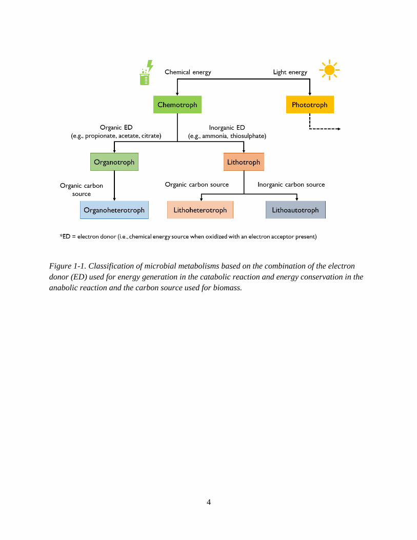
Figure 1-1. Classification of microbial metabolisms based on the combination of the electron donor

(ED) used for energy generation in the catabolic reaction and energy conservation in the anabolic

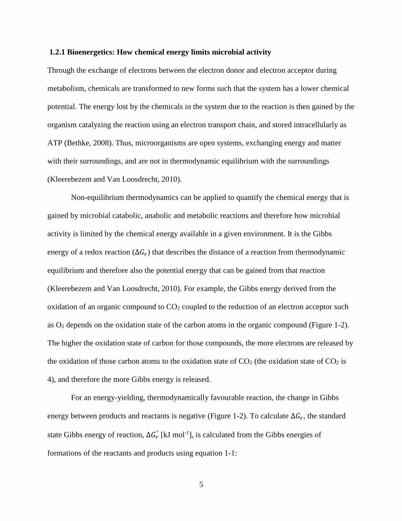
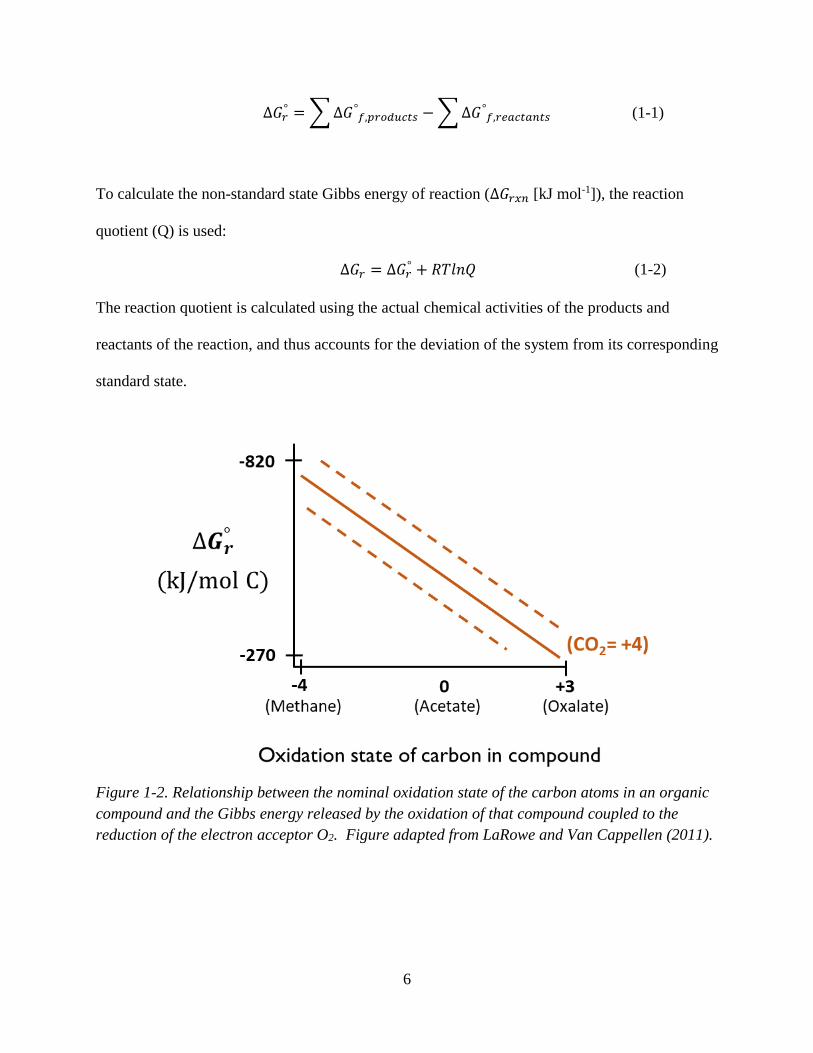
reaction and the carbon source used for biomass........................................................................................ 4 Figure 1-2. Relationship between the nominal oxidation state of the carbon atoms in an organic

compound and the Gibbs energy released by the oxidation of that compound coupled to the reduction of

the electron acceptor O2. ............................................................................................................................. 6 Figure 1-3. Conceptual diagram illustrating the significance of the growth yield, Y. ............................. 11 Figure 1-4. Hypothetical specific growth rates versus the ED substrate concentration for three different

combinations of Monod-type kinetic parameters. .................................................................................... 14 Figure 1-5. Conceptual diagram illustrating the implications of mixotrophic metabolisms for the

biogeochemical cycling of redox-active compounds. ............................................................................... 17

Figure 2-1. Illustration of conceptual model of mixotrophic growth. ...................................................... 24 Figure 2-2. Parity plots of observed and predicted yields in C-mol biomass/ mol ED for the 3 individual

MEMs as indicated by subplot header (where LA= lithoautotrophy, LH= lithoheterotrophy, OH=

organoheterotrophy), and for the total yield calculated as the sum of the three predicted yields, in units

of C-mol biomass/ mol O2. ....................................................................................................................... 40

Figure 2-3. Total calculated mixotrophic growth yield, Y, and MEM-specific growth yields versus the

fraction of inorganic electron equivalents consumed ............................................................................... 41 Figure 2-4. Data-derived fractions of three MEMs observed (xik), fh and forg

assim as a function of the

fraction of inorganic electron equivalents consumed ............................................................................... 44 Figure 2-5. Predicted versus observed fractions of three end member metabolisms (xik) and fraction of

the organic ED substrate assimilated (fassimorg) during growth of Paracoccus versutus on mixtures of

acetate and thiosulfate. .............................................................................................................................. 50 Figure 2-6. Predicted versus observed fractions of three end member metabolisms (xik) and fraction of

the organic ED substrate assimilated (fassimorg) during growth of Pseudomonas oxalaticus on mixtures of

acetate and formate, .................................................................................................................................. 51 Figure 2-7. Predicted versus observed fractions of three end member metabolisms (xik) and fraction of

the organic ED substrate assimilated (fassimorg) during growth of Pseudomonas oxalaticus on mixtures of

oxalate and formate ................................................................................................................................... 52 Figure 3-1. Depth profiles of concentration data taken from Melton et al. (2014) and predicted rates. .. 68

Figure 3-2. Fractions of all 3 MEMs predicted with depth (left panel), and fraction of heterotrophy (fh)

predicted (dotted line) and observed ((fh obs via MPN counts, pink symbols) with depth (right panel). .. 73 Figure 3-3. Total NO3

- reduction rate (indicated by bar length), and MEM-specific NO3- reduction rate

(colour of bar segments) predicted with depth in the sediment. ............................................................... 74 Figure 3-4. Simulated NO3

- reduction rates and predicted implicit maximum rates. ............................... 77

Figure 3-5.Predicted ratios of coupling of NO3-:Fe2+, DIC: Fe2+, and DIC:NO3

- as a function of the

fraction of autotrophic activity.................................................................................................................. 78

x

List of Tables

Table 2-1. Description of experimental datasets available that examined mixotrophic growth on variable

ratios of organic and inorganic ED substrate. ........................................................................................... 34 Table 3-1. Summary of electron donor, electron acceptor, and carbon source used by each metabolic end

member reaction (MEM) during potential mixotrophic NDFO. .............................................................. 59 Table 3-2. Most Probable Number data from Melton et al. (2014) .......................................................... 66

Table 3-3. Monod kinetic parameters used to calculate the rates of iron oxidation and acetate oxidation

in the sediments......................................................................................................................................... 67

xi

List of Abbreviations

Abbreviation Description Units

ATP Adenosine triphosphate - - -

ED Electron donor substrate mol ED

EA Electron acceptor substrate mol EA

MEM Metabolic end member - - -

OH Organoheterotrophy - - -

LH Lithoheterotrophy - - -

LA Lithoautotrophy - - -

SWI Sediment-water interface - - -

Redox Reduction-oxidation - - -

eeq

Electron equivalents, number of electrons transferred during a

reduction or oxidation half reaction.

Used in this thesis to normalize ED utilization rates to a

common unit, and thus represents the number of electrons that

would be released by the complete oxidation of that ED.

- - -

𝑛𝑒𝑒𝑞𝑆

Number of moles of electron equivalents in some compound,

S (electrons released by the complete oxidation of a

compound)

mol eeq (mol S)-1

𝑟𝐸𝐷

Rate of utilization of inorganic or organic ED substrate for use

as ED by metabolic reaction (denoted by subscript inorg ED

or org ED)

mol ED (L h)-1

𝑟𝑒𝑒𝑞 Rate of utilization of inorganic or organic ED substrate for use

as ED by metabolic reaction in units of mol eeq (L h)-1

(denoted by subscript inorg eeq or org eeq)

mol eeq (L h)-1

𝑥𝑖𝑘

Fraction of metabolic end member reaction used to build

biomass, where the subscript 𝑖 denotes the electron donating

reaction used by the catabolism and anabolism, and 𝑘 denotes

the carbon source

- - -

𝑥𝑜ℎ Fraction of organoheterotrophy (MEM/ biomass fraction) - - -

𝑥𝑙ℎ Fraction of lithoheterotrophy (MEM/ biomass fraction) - - -

𝑥𝑙𝑎 Fraction of lithoautotrophy (MEM/ biomass fraction) - - -

𝑟𝑥 Total biomass growth rate C-mol biomass (L

h)-1

𝑟𝑥,ℎ𝑒𝑡 Rate of heterotrophic biomass growth C-mol biomass (L

time)-1

xii

𝑟𝑥,𝑎𝑢𝑡𝑜 Rate of autotrophic biomass growth C-mol biomass (L

time)-1

𝑓𝑎𝑠𝑠𝑖𝑚𝑜𝑟𝑔

Fraction of electron equivalents from the organic ED/ carbon

source substrate that is used as a carbon source

- - -

𝑓𝑑𝑖𝑠𝑠𝑖𝑚𝑜𝑟𝑔

Fraction of electron equivalents from the organic ED/ carbon

source substrate that is used as an electron donor

- - -

𝑓𝑘 Fraction of metabolism that is either heterotrophic or

autotrophic

- - -

𝑓ℎ

Fraction of biomass carbon that is derived from organic

carbon source/ ED (fraction of total mixotrophic

biomass/metabolism that is heterotrophic)

- - -

𝑓𝑎

Fraction of biomass carbon that is derived from inorganic

carbon (fraction of total mixotrophic biomass/metabolism that

is autotrophic)

- - -

𝜙𝑖

Fraction of total electrons donated to metabolism (for energy

conservation and generation in both catabolism and

anabolism) that is either organotrophic or lithotrophic

- - -

𝜙𝑜 Fraction of electrons donated for oxidation that are from the

organic ED substrate, “fraction of organotrophy”

- - -

𝜙𝑙 Fraction of electrons donated for oxidation that are from the

inorganic ED substrate, “fraction of lithotrophy”

- - -

∆𝐺𝑟 Gibbs energy of a reaction under non-standard state

conditions

kJ (mol ED)-1 or kJ

(C-mol biomass)-1

Δ𝐺𝑟°

Gibbs energy of a reaction under standard state conditions

(25 °C, and unit activities for all chemical species)

kJ (mol ED)-1 or kJ

(C-mol biomass)-1

ΔG𝑟°′

Gibbs energy of a reaction under biochemical standard state

conditions (25 °C, pH 7 and unit activities for all chemical

species, except H+)

kJ (mol ED)-1 or kJ

(C-mol biomass)-1

𝑚𝑒𝑡 Subscript used to denote metabolic reaction - - -

𝑐𝑎𝑡 Subscript used to denote catabolic reaction - - -

𝑎𝑛 Subscript used to denote anabolic reaction - - -

𝑟𝑚𝑎𝑥 Biomass-, yield-, and maximum specific growth rate-implicit

maximum rate used in Monod-type kinetics

mol ED (L time)-1

𝐾𝐸𝐷 Half-saturation constant used in Monod-type kinetics mol ED (L)-1

1

Chapter 1

General Introduction

1.1 Chemosynthetic microbial activity in the terrestrial subsurface

In the dark terrestrial subsurface, life and biogeochemical activity is dominated by

chemosynthetic prokaryotic microorganisms which derive their energy from the oxidation of

electron donors during chemical reduction-oxidation reactions (Whitman et al., 1998; Newman

and Banfield, 2002). These environments include aquifers, wetland and hydric soils, peatlands,

and aquatic sediments. Globally, the terrestrial subsurface reservoir contains one fifth of the

earth’s organic carbon, and the production of carbon dioxide by soil respiration is an important

flux in the carbon balance of terrestrial ecosystems (Anantharaman et al., 2016). Microbial

activity and its associated chemical transformations in these environments controls the

speciation, toxicity, and mobility of important nutrients and contaminants (Hunter et al., 1998;

Thullner et al., 2007), including for example perchlorate (Hubbard et al., 2014), nitrate (Rivett et

al., 2008), uranium (Williams et al., 2011), and trace metals (Torres et al., 2015). Through the

hydrological connections between the subsurface and surface water ecosystems, subsurface

microbial activity has the potential to mediate nutrient fluxes that fuel harmful algal blooms, as

well as other water quality issues (Bouwman et al., 2013). The subsurface is also connected to

the atmosphere via the soil interface, and many microbial activities produce greenhouse gases

such as nitrous oxide (N2O), carbon dioxide (CH4), and carbon dioxide (CO2) (Long et al.,

2016). In short, the activity of subsurface microorganisms contributes many societally-relevant

ecosystem functions.

1.2 Chemosynthetic microbial metabolisms

During growth, microorganisms carry out two distinct reduction-oxidation (redox) reactions:

they couple a reaction for the creation of biomass (the anabolic reaction) to the reaction from

2

which they derive energy (the catabolic reaction). The energy produced during the catabolic

redox reaction is required by microorganisms to survive and grow. Redox reactions are those

which involve the exchange of electrons between a reduced chemical species (the electron

donor) and an oxidized species (the electron acceptor). The overall reaction, or the metabolic

reaction, represents the combination of the catabolic and anabolic reactions.

Microbial metabolic reactions can be classified based on the identities of the electron

donor (ED) and carbon source. In chemosynthetic microbial growth reactions, the ED is used as

both an energy source by its reaction with an electron acceptor in catabolism, and for energy

conservation in the anabolic redox reaction. Organoheterotrophic metabolisms use organic

compounds for both energy generation (i.e., as an electron donor) and as a carbon source.

Lithoheterotrophic metabolisms use organic carbon compounds as their carbon source, while

using an inorganic compound as their catabolic energy source. Lithoautotrophic metabolisms

also use an inorganic energy source, while using inorganic carbon (e.g., CO2) as their carbon

source. Figure 1-1 is a flow chart that shows the classification and relatedness of these different

types of metabolisms. Chemotrophic metabolisms are also distinguished from phototrophic

metabolisms in Figure 1-1.

The organic compounds that are commonly used as EDs and/or carbon sources in the

subsurface include short chain organic acids (e.g., propionate, lactate, or citrate) generated by the

hydrolysis or fermentation of plant-derived polymeric organic molecules (Roden and Jin, 2011).

Inorganic compounds that are commonly used as EDs in the subsurface include methane (CH4),

ammonia (NH4+), nitrite (NO2

-), sulfide (S2-), thiosulfate (S2O32-), iron(II) (Fe2+), and dihydrogen

(H2). These reduced inorganic compounds are generated by many different processes. For

example, weathering of the mineral pyrite produces S2- (Bosch and Meckenstock, 2012), and the

3

breakdown of organic matter by fermentation and nitrogen fixation by rhizobacterium produce

H2 (Lovley and Chapelle, 1995; Miltner et al., 2005; Piché-Choquette and Constant, 2019).

Microbial reduction of oxidized forms of the electron donor is also an important source of

reduced compounds, such as iron(III) reduction producing Fe2+ (Weber et al., 2006; Schmidt et

al., 2010; Berg et al., 2016). Anthropogenic input of NH4+ or S0 via fertilizers is also possible

(Lawrence et al., 1988; He et al., 2007). In the deep subsurface, additional processes can

generate reduced inorganic compounds, including the serpentization of igneous rocks (e.g., H2)

and Fischer-Tropsch type reactions (e.g., CH4) (Sherwood-Lollar et al., 2008; Kieft, 2016).

The most common electron acceptors in anoxic subsurface environments are nitrate

(NO3-), sulfate (SO4

2-), iron(III) (Fe3+), manganese(IV) (Mn4+) and carbon dioxide (CO2) (Bethke

et al., 2011; Burgin et al., 2011). These electron acceptors can be used by both organotrophic

and lithotrophic catabolic reactions. Microbial activity significantly influences the cycling of the

common redox-active elements carbon (C), nitrogen (N), iron (Fe), sulfur (S), and manganese

(Mn) in subsurface environments, which is evident given the use of different forms of these

elements as both electron acceptors and electron donors. The extent of coupling between these

elements can be captured by writing out the metabolic reactions that are occurring in any given

environment. This microbial control of the cycling of these redox-active elements is well

discussed in the biogeochemical literature (e.g., Burgin et al., 2011), and is a major theme of this

thesis.

4

Figure 1-1. Classification of microbial metabolisms based on the combination of the electron

donor (ED) used for energy generation in the catabolic reaction and energy conservation in the

anabolic reaction and the carbon source used for biomass.

5

1.2.1 Bioenergetics: How chemical energy limits microbial activity

Through the exchange of electrons between the electron donor and electron acceptor during

metabolism, chemicals are transformed to new forms such that the system has a lower chemical

potential. The energy lost by the chemicals in the system due to the reaction is then gained by the

organism catalyzing the reaction using an electron transport chain, and stored intracellularly as

ATP (Bethke, 2008). Thus, microorganisms are open systems, exchanging energy and matter

with their surroundings, and are not in thermodynamic equilibrium with the surroundings

(Kleerebezem and Van Loosdrecht, 2010).

Non-equilibrium thermodynamics can be applied to quantify the chemical energy that is

gained by microbial catabolic, anabolic and metabolic reactions and therefore how microbial

activity is limited by the chemical energy available in a given environment. It is the Gibbs

energy of a redox reaction (∆𝐺𝑟) that describes the distance of a reaction from thermodynamic

equilibrium and therefore also the potential energy that can be gained from that reaction

(Kleerebezem and Van Loosdrecht, 2010). For example, the Gibbs energy derived from the

oxidation of an organic compound to CO2 coupled to the reduction of an electron acceptor such

as O2 depends on the oxidation state of the carbon atoms in the organic compound (Figure 1-2).

The higher the oxidation state of carbon for those compounds, the more electrons are released by

the oxidation of those carbon atoms to the oxidation state of CO2 (the oxidation state of CO2 is

4), and therefore the more Gibbs energy is released.

For an energy-yielding, thermodynamically favourable reaction, the change in Gibbs

energy between products and reactants is negative (Figure 1-2). To calculate ∆𝐺𝑟, the standard

state Gibbs energy of reaction, ∆𝐺𝑟° [kJ mol-1], is calculated from the Gibbs energies of

formations of the reactants and products using equation 1-1:

6

∆𝐺𝑟° = ∑ ∆𝐺°

𝑓,𝑝𝑟𝑜𝑑𝑢𝑐𝑡𝑠 − ∑ ∆𝐺°𝑓,𝑟𝑒𝑎𝑐𝑡𝑎𝑛𝑡𝑠 (1-1)

To calculate the non-standard state Gibbs energy of reaction (∆𝐺𝑟𝑥𝑛 [kJ mol-1]), the reaction

quotient (Q) is used:

∆𝐺𝑟 = ∆𝐺𝑟° + 𝑅𝑇𝑙𝑛𝑄 (1-2)

The reaction quotient is calculated using the actual chemical activities of the products and

reactants of the reaction, and thus accounts for the deviation of the system from its corresponding

standard state.

Figure 1-2. Relationship between the nominal oxidation state of the carbon atoms in an organic

compound and the Gibbs energy released by the oxidation of that compound coupled to the

reduction of the electron acceptor O2. Figure adapted from LaRowe and Van Cappellen (2011).

7

1.3 Mixotrophy

Organisms that are metabolically flexible and capable of switching between organoheterotrophy,

lithoheterotrophy and lithoautotrophy are called facultative chemolithoautotrophs or,

alternatively, mixotrophs (Rittenberg, 1972; Kelly, 1981). These microorganisms possess the

genes to carry out all three metabolisms, and can regulate which metabolism they use according

to which one is most optimal under the given conditions (Rittenberg, 1972). This metabolic

flexibility has been recognized in pure cultures for some time and is likely also a community-

level attribute in a variety of environments.

Recognition of the widespread capacity for metabolic flexibility across many genera of

bacteria and archaea is growing, especially with the increased use of omics techniques for

analyzing laboratory cultures and environmental samples (Long, Williams, Hubbard, & Banfield,

2016). For example, the bacteria Leptothrix ochracea, one of the first lithotrophic organisms

discovered by Winogradsky, was previously thought to be a strict lithoautotroph. When grown in

an enrichment culture with different concentrations of iron(II), L. ochracea was able to

assimilate both organic and inorganic carbon, revealing that it is capable of mixotrophy

(Rittenberg, 1972; Fleming et al., 2018).

1.3.1 Environmental occurrence and controls on mixotrophy

In the environment, mixotrophy can be identified using metagenomic methods by the coincident

occurrence of genes for carbon fixation and genes for assimilating organic compounds (Probst et

al., 2017), by stable isotope probing (Bellini et al., 2018), by tracing natural carbon isotope

fractionation (Probst et al., 2018), or by Most Probable Number (MPN) approaches that employ

mixotroph-specific media (Hauck et al., 2001; Melton et al., 2014).

8

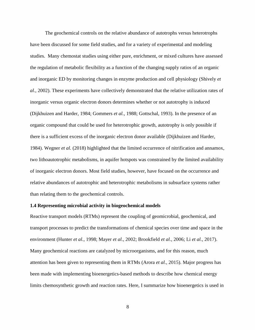
The geochemical controls on the relative abundance of autotrophs versus heterotrophs

have been discussed for some field studies, and for a variety of experimental and modeling

studies. Many chemostat studies using either pure, enrichment, or mixed cultures have assessed

the regulation of metabolic flexibility as a function of the changing supply ratios of an organic

and inorganic ED by monitoring changes in enzyme production and cell physiology (Shively et

al., 2002). These experiments have collectively demonstrated that the relative utilization rates of

inorganic versus organic electron donors determines whether or not autotrophy is induced

(Dijkhuizen and Harder, 1984; Gommers et al., 1988; Gottschal, 1993). In the presence of an

organic compound that could be used for heterotrophic growth, autotrophy is only possible if

there is a sufficient excess of the inorganic electron donor available (Dijkhuizen and Harder,

1984). Wegner et al. (2018) highlighted that the limited occurrence of nitrification and annamox,

two lithoautotrophic metabolisms, in aquifer hotspots was constrained by the limited availability

of inorganic electron donors. Most field studies, however, have focused on the occurrence and

relative abundances of autotrophic and heterotrophic metabolisms in subsurface systems rather

than relating them to the geochemical controls.

1.4 Representing microbial activity in biogeochemical models

Reactive transport models (RTMs) represent the coupling of geomicrobial, geochemical, and

transport processes to predict the transformations of chemical species over time and space in the

environment (Hunter et al., 1998; Mayer et al., 2002; Brookfield et al., 2006; Li et al., 2017).

Many geochemical reactions are catalyzed by microorganisms, and for this reason, much

attention has been given to representing them in RTMs (Arora et al., 2015). Major progress has

been made with implementing bioenergetics-based methods to describe how chemical energy

limits chemosynthetic growth and reaction rates. Here, I summarize how bioenergetics is used in

9

RTMs by introducing how microbially-controlled reaction rates are represented in RTMs and

then how bioenergetics can be integrated into these rate expressions to improve their realism.

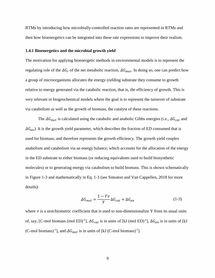
1.4.1 Bioenergetics and the microbial growth yield

The motivation for applying bioenergetic methods in environmental models is to represent the

regulating role of the 𝛥𝐺𝑟 of the net metabolic reaction, 𝛥𝐺𝑚𝑒𝑡. In doing so, one can predict how

a group of microorganisms allocates the energy-yielding substrate they consume to growth

relative to energy generated via the catabolic reaction, that is, the efficiency of growth. This is

very relevant in biogeochemical models where the goal is to represent the turnover of substrate

via catabolism as well as the growth of biomass, the catalyst of these reactions.

The 𝛥𝐺𝑚𝑒𝑡 is calculated using the catabolic and anabolic Gibbs energies (i.e., 𝛥𝐺𝑐𝑎𝑡 and

𝛥𝐺𝑎𝑛). It is the growth yield parameter, which describes the fraction of ED consumed that is

used for biomass, and therefore represents the growth efficiency. The growth yield couples

anabolism and catabolism via an energy balance, which accounts for the allocation of the energy

in the ED substrate to either biomass (or reducing equivalents used to build biosynthetic

molecules) or to generating energy via catabolism to build biomass. This is shown schematically

in Figure 1-3 and mathematically in Eq. 1-3 (see Smeaton and Van Cappellen, 2018 for more

details):

𝛥𝐺𝑚𝑒𝑡 =1 − 𝑌𝑣

𝑌∆𝐺𝑐𝑎𝑡 + ∆𝐺𝑎𝑛 (1-3)

where 𝑣 is a stoichiometric coefficient that is used to non-dimensionalize Y from its usual units

of, say, [C-mol biomass (mol ED)-1], 𝛥𝐺𝑐𝑎𝑡 is in units of [kJ (mol ED)-1], ∆𝐺𝑎𝑛 is in units of [kJ

(C-mol biomass)-1], and 𝛥𝐺𝑚𝑒𝑡 is in units of [kJ (C-mol biomass)-1].

10

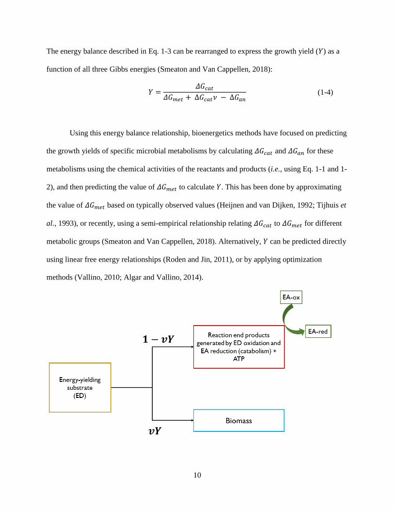
The energy balance described in Eq. 1-3 can be rearranged to express the growth yield (𝑌) as a

function of all three Gibbs energies (Smeaton and Van Cappellen, 2018):

𝑌 =𝛥𝐺𝑐𝑎𝑡

𝛥𝐺𝑚𝑒𝑡 + ∆𝐺𝑐𝑎𝑡𝜈 − ∆𝐺𝑎𝑛 (1-4)

Using this energy balance relationship, bioenergetics methods have focused on predicting

the growth yields of specific microbial metabolisms by calculating 𝛥𝐺𝑐𝑎𝑡 and 𝛥𝐺𝑎𝑛 for these

metabolisms using the chemical activities of the reactants and products (i.e., using Eq. 1-1 and 1-

2), and then predicting the value of 𝛥𝐺𝑚𝑒𝑡 to calculate 𝑌. This has been done by approximating

the value of 𝛥𝐺𝑚𝑒𝑡 based on typically observed values (Heijnen and van Dijken, 1992; Tijhuis et

al., 1993), or recently, using a semi-empirical relationship relating 𝛥𝐺𝑐𝑎𝑡 to 𝛥𝐺𝑚𝑒𝑡 for different

metabolic groups (Smeaton and Van Cappellen, 2018). Alternatively, 𝑌 can be predicted directly

using linear free energy relationships (Roden and Jin, 2011), or by applying optimization

methods (Vallino, 2010; Algar and Vallino, 2014).

11

Figure 1-3. Conceptual diagram illustrating the significance of the growth yield, Y. The diagram

shows the allocation of an ED substrate to be oxidized by catabolism, or allocated to biomass.

12

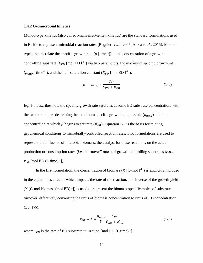
1.4.2 Geomicrobial kinetics

Monod-type kinetics (also called Michaelis-Menten kinetics) are the standard formulations used

in RTMs to represent microbial reaction rates (Regnier et al., 2005; Arora et al., 2015). Monod-

type kinetics relate the specific growth rate (𝜇 [time-1]) to the concentration of a growth-

controlling substrate (𝐶𝐸𝐷 [mol ED l-1]) via two parameters, the maximum specific growth rate

(𝜇𝑚𝑎𝑥 [time-1]), and the half-saturation constant (𝐾𝐸𝐷 [mol ED l-1]):

𝜇 = 𝜇𝑚𝑎𝑥 ∗𝐶𝐸𝐷

𝐶𝐸𝐷 + 𝐾𝐸𝐷 (1-5)

Eq. 1-5 describes how the specific growth rate saturates at some ED substrate concentration, with

the two parameters describing the maximum specific growth rate possible (𝜇𝑚𝑎𝑥) and the

concentration at which 𝜇 begins to saturate (𝐾𝐸𝐷). Equation 1-5 is the basis for relating

geochemical conditions to microbially-controlled reaction rates. Two formulations are used to

represent the influence of microbial biomass, the catalyst for these reactions, on the actual

production or consumption rates (i.e., “turnover” rates) of growth-controlling substrates (e.g.,

𝑟𝐸𝐷 [mol ED (L time)-1]).

In the first formulation, the concentration of biomass (𝑋 [C-mol l-1]) is explicitly included

in the equation as a factor which impacts the rate of the reaction. The inverse of the growth yield

(𝑌 [C-mol biomass (mol ED)-1]) is used to represent the biomass-specific moles of substrate

turnover, effectively converting the units of biomass concentration to units of ED concentration

(Eq. 1-6):

𝑟𝐸𝐷 = 𝑋 ∗𝜇𝑚𝑎𝑥

𝑌

𝐶𝐸𝐷


where 𝑟𝐸𝐷 is the rate of ED substrate utilization [mol ED (L time)-1].

13

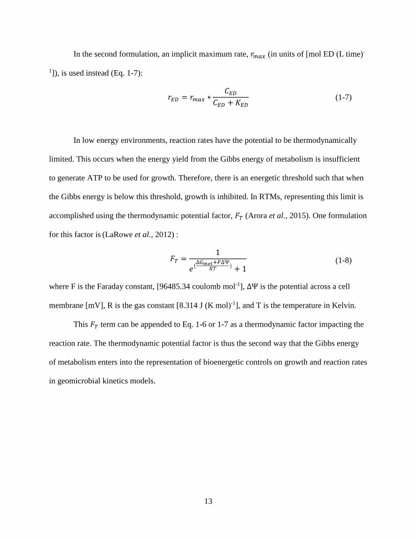
In the second formulation, an implicit maximum rate, 𝑟𝑚𝑎𝑥 (in units of [mol ED (L time)-

1]), is used instead (Eq. 1-7):

𝑟𝐸𝐷 = 𝑟𝑚𝑎𝑥 ∗𝐶𝐸𝐷


In low energy environments, reaction rates have the potential to be thermodynamically

limited. This occurs when the energy yield from the Gibbs energy of metabolism is insufficient

to generate ATP to be used for growth. Therefore, there is an energetic threshold such that when

the Gibbs energy is below this threshold, growth is inhibited. In RTMs, representing this limit is

accomplished using the thermodynamic potential factor, 𝐹𝑇 (Arora et al., 2015). One formulation

for this factor is (LaRowe et al., 2012) :

𝐹𝑇 =1

𝑒(∆𝐺𝑚𝑒𝑡+𝐹∆Ψ

𝑅𝑇) + 1

(1-8)

where F is the Faraday constant, [96485.34 coulomb mol-1], ∆Ψ is the potential across a cell

membrane [mV], R is the gas constant [8.314 J (K mol)-1], and T is the temperature in Kelvin.

This 𝐹𝑇 term can be appended to Eq. 1-6 or 1-7 as a thermodynamic factor impacting the

reaction rate. The thermodynamic potential factor is thus the second way that the Gibbs energy

of metabolism enters into the representation of bioenergetic controls on growth and reaction rates

in geomicrobial kinetics models.

14

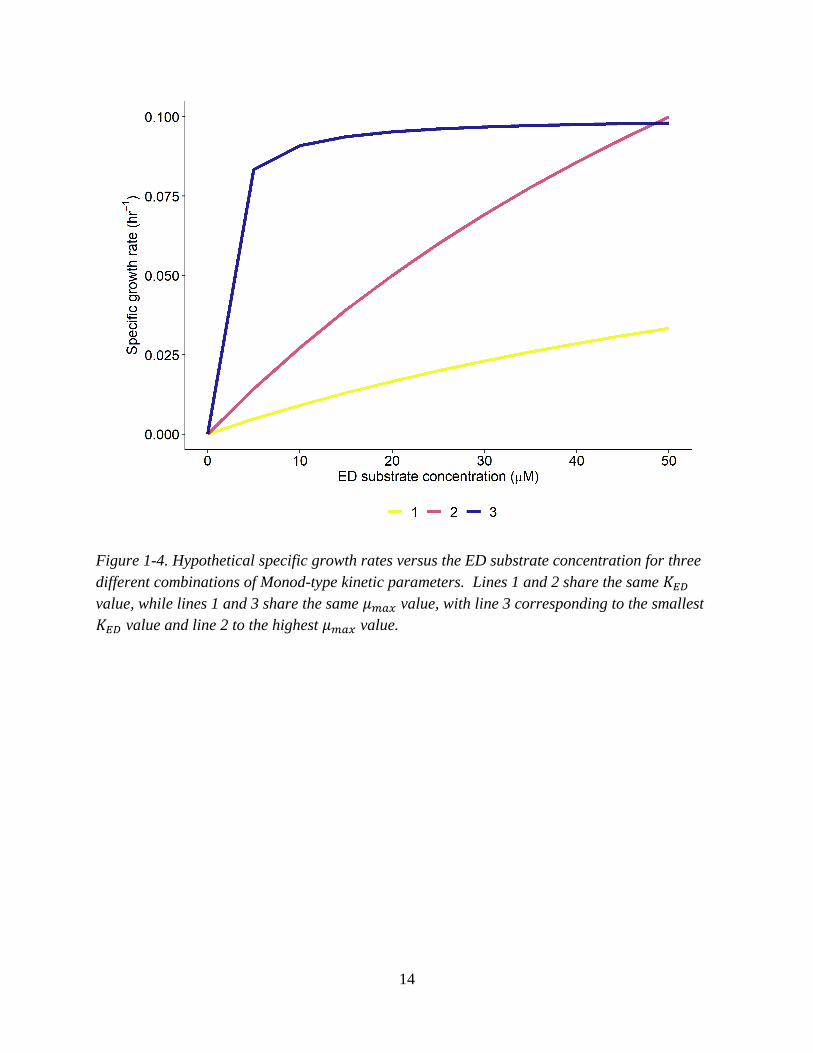
Figure 1-4. Hypothetical specific growth rates versus the ED substrate concentration for three

different combinations of Monod-type kinetic parameters. Lines 1 and 2 share the same 𝐾𝐸𝐷

value, while lines 1 and 3 share the same 𝜇𝑚𝑎𝑥 value, with line 3 corresponding to the smallest

𝐾𝐸𝐷 value and line 2 to the highest 𝜇𝑚𝑎𝑥 value.

15

1.5 Biogeochemical implications of mixotrophy

Typically, carbon cycling in subsurface environments is assumed to be unidirectional, with

microbial “soil respiration” degrading the organic carbon previously fixed by terrestrial plants

and microorganisms to inorganic carbon, which can be returned to the atmosphere as carbon

dioxide (CO2). Under this assumption, subsurface microbial growth and activity is assumed to be

organoheterotrophic. There is growing evidence in many environments that indicates that

lithoautotrophic and mixotrophic metabolisms play a prominent role in subsurface ecosystems in

terms of their relative abundance and contribution to ecosystem function (Kellermann et al.,

2012; Griebler and Avramov, 2015; Jewell et al., 2016). With this metabolic capacity, subsurface

prokaryotic communities are not only catalysts of carbon degradation, but are capable of

inorganic carbon fixation and therefore they close the carbon cycle in the subsurface (Hutchins et

al., 2016).

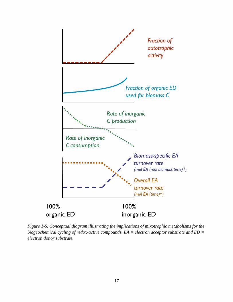
Figure 1-5 illustrates the implications of mixotrophy for biogeochemical reaction

dynamics. This conceptual diagram is largely informed by pure culture experiments that studied

the metabolic flexibility of mixotrophs. The changes in carbon cycle fluxes, biomass assimilation

of organic carbon, and electron acceptor turnover rates are shown as a function of the relative

proportions of the organic and inorganic ED substrates that a mixotrophic organism consumes.

With increasing relative utilization of the inorganic compound, autotrophic activity does not

occur immediately, but instead begins at some threshold (as discussed in section 1.3.1). Prior to

this threshold, microbial activity is heterotrophic (i.e., uses only organic carbon for biomass

synthesis). This sustained heterotrophic activity is matched by an increased assimilation of the

organic compound for biomass C compared to growth on the organic compound alone.

Consequently, the rate of inorganic C production decreases because the inorganic ED is being

16

oxidized for energy generation rather than the organic ED. At some point following the onset of

autotrophic activity, there is a net consumption of inorganic C.

Mixotrophy impacts the overall turnover rate of electron acceptors such as nitrate, sulfate

and iron(III) due to the different energetic efficiencies of autotrophic and heterotrophic

metabolisms. Heterotrophic metabolisms require less energy to form organic biosynthetic

molecules from existing organic compounds compared to autotrophic metabolisms which must

fix inorganic C into organic molecules (Heijnen and van Dijken, 1992). Per unit of biomass

produced, autotrophic metabolisms therefore need to run their catabolic reaction more times

relative to heterotrophic metabolisms, making growth less efficient in terms of the total energy-

yielding substrate (i.e., electron donor or electron acceptor) that is consumed. Consequently, the

biomass-specific electron acceptor turnover rates by autotrophic metabolisms are higher, that is,

the amount of the electron acceptor consumed by catabolism per amount of biomass formed is

higher. The overall turnover rates, however, are lower due to the impact of the less efficient

growth of autotrophs on the overall turnover rate (i.e., 𝑟𝑚𝑎𝑥 in Eq. 1-7 is the overall turnover rate,

and can be compared to Eq. 1-6 to see the three parameters that are lumped into 𝑟𝑚𝑎𝑥, including

the growth yield Y, which represents the growth efficiency) (Koenig and Liu, 2001; Watson et

al., 2003; Cardoso et al., 2006; Handley et al., 2013).

17

Figure 1-5. Conceptual diagram illustrating the implications of mixotrophic metabolisms for the

biogeochemical cycling of redox-active compounds. EA = electron acceptor substrate and ED =

electron donor substrate.

18

1.5.1 Accounting for mixotrophy in environmental models (RTMs)

Newman and Banfield (2002) summarize the major questions motivating research that seeks to

improve representation of geomicrobial reactions using models:

“How do organisms self-organize in response to changes in their environment

(both biological and chemical)? In turn, how does their organization affect the

chemistry of their environment? What are the metabolic and genetic networks

that link the members of the community to one another? And how robust are

these networks in the face of environmental perturbations?”

Mixotrophy involves important changes to the chemistry of an environment compared to

organotrophy. In turn, the availability of alternative EDs in the environment determines whether

mixotrophy is energetically desirable (Figure 1-5). This thesis seeks to build a modeling

framework based on the “metabolic network” involved, in order to be able to represent the

chemical controls on the metabolic flexibility of mixotrophy. This modeling framework can then

be used to predict the response of mixotrophy to changes in environmental conditions, and to

predict the turnover of environmentally-relevant chemicals.

Progress has been made in RTMs by using bioenergetics to more accurately represent

growth yields and energetic limitations of reaction kinetics (i.e., the FT term) (Arora et al., 2015).

A major challenge remaining in RTMs is accounting for when reactions are energetically

favourable (∆𝐺𝑐𝑎𝑡 < 0 , ∆𝐺𝑚𝑒𝑡 < 0, and 𝐹𝑇 > 0), but are not occurring, because some reaction

is even more favourable. In a sense, this challenge represents a form of competition between

multiple reactions for EA reduction, ED oxidation, or carbon source utilization reactions.

Modelling frameworks that integrate thermodynamic (i.e., bioenergetic) and kinetic

constraints using the formulations outlined in sections 1.4.1 and 1.4.2 have been successful in

19

more systematically representing switching between types of metabolisms other than those

involved in mixotrophy. For example, Algar and Vallino (2014) used a bioenergetic-kinetic

approach to predict the competition between nitrate reducing processes. Payn et al. (2014) used a

bioenergetic-kinetic approach to represent the different energetic efficiencies (i.e., growth yields)

of autotrophic and heterotrophic metabolisms. However, these authors did not explicitly

represent the progressive switching between all the metabolisms involved in mixotrophy.

1.6 Thesis objectives

The overall objective of this thesis is to describe the competition between heterotrophic versus

autotrophic, and organotrophic versus lithotrophic metabolic activities in metabolically flexible

chemotrophic microbial communities using a combined bioenergetic and kinetic approach. This

approach is compatible with the formulations and level of detail typically implemented in

reactive transport models. The specific objectives of the thesis are to (1) develop a conceptual

model of mixotrophic growth informed by experimental datasets that describes the constraints on

energy and carbon allocation among end member metabolisms, (2) apply this conceptual model

into a bioenergetic-kinetic modeling framework that incorporates the existing Gibbs Energy

Dynamic Yield Method (GEDYM, Smeaton and Van Cappellen, 2018) bioenergetics framework

to predict the relative abundances of heterotrophy and autotrophy at steady state in experimental

chemostat systems, and (3) apply the framework to predict the relative contribution of

autotrophic and heterotrophic metabolisms to iron, nitrogen, and carbon cycling in a lake

sediment.

20

Chapter 2

Mathematically representing chemosynthetic mixotrophy in

biogeochemical models

2.1 Introduction

Chemosynthetic microorganisms play major roles in biogeochemical elemental cycling, thereby

influencing nutrient and metal cycling and greenhouse gas fluxes (Long et al., 2016). Outside the

photic zone, organic compounds are typically assumed to be the primary carbon sources and

electron donors (EDs) supporting microbial activity. That is, the metabolic activity of

chemosynthetic communities is often closely regulated (or limited) by the supply and energy

content of low molecular weight organic acids (e.g. acetate) (Gottschal and Dijkhuizen, 1988;

Vallino et al., 1996). In addition to serving as energy substrates, these organic compounds can

also provide the carbon atoms needed for the synthesis of new biomass. Alternatively, inorganic

carbon sources, most often CO2, can be used for growth by autotrophic microorganisms. Carbon

in CO2, however, has an oxidation state greater than that of carbon in biomass, making it

energetically costlier to incorporate into biomass.

Although chemoorganotrophs are usually assumed to dominate non-photosynthetic

microbial communities, there is growing evidence of the significance of chemolithoautotrophy,

sometimes called dark carbon fixation, in the biogeochemical reaction systems controlling the

cycling of elements such as iron and sulfur (Alfreider et al., 2003; Kellermann et al., 2012;

Griebler and Avramov, 2015; Herrmann et al., 2015; Francois et al., 2016; Jewell et al., 2016).

The corresponding chemolithoautotrophic metabolisms incorporate CO2 into biomass using a

variety of fixation pathways (Sato and Atomi, 2010), while acquiring energy from the oxidation

of an inorganic ED, for example, methane (CH4), ammonium (NH4+), nitrite (NO2

-), sulfide (S2-),

thiosulfate (S2O32-), and dihydrogen (H2). These inorganic compounds are generated by

21

processes such as mineral weathering (Yabusaki et al., 2017; Dwivedi et al., 2018) and organic

matter fermentation (Lovley and Chapelle, 1995). The inclusion of autotrophic metabolisms in

reactive transport models of subsurface environments has demonstratably improved the

predictions of reaction rates associated with carbon, sulfur, iron and nitrogen cycling (Arora et

al., 2017; Yabusaki et al., 2017; Dwivedi et al., 2018). In environments where low

concentrations of organic and inorganic electron EDs are available, the microbial community is

likely to simultaneously utilize more than one carbon source, including CO2, for growth, and

more than one ED for energy generation. That is, these environments may support mixotrophic

or facultative chemolithoautotrophic communities (Rittenberg, 1972; Matin, 1978; Dijkhuizen

and Harder, 1984).

The chemical and biological controls on mixotrophic metabolisms have been fairly well

studied in pure cultures by measurement of enzyme production, substrate utilization rates (e.g.,

carbon fixation rates), and biomass concentrations, as examples. These experiments have

demonstrated that during growth on mixtures of organic and inorganic ED substrates, growth is

enhanced compared to growth on the organic substrate alone. This growth is related to the

enhanced incorporation of the organic ED substrate into biomass. Accordingly, there is a

threshold for the onset of autotrophy, where autotrophy is only possible once the relative rate of

utilization of the inorganic ED is in sufficient excess that the metabolism is organic carbon-

limited (Dijkhuizen and Harder, 1984). This behaviour highlights the importance of the

competition between heterotrophic and autotrophic modes of metabolism during mixotrophic

growth.

The regulation of metabolic functions and rates is closely linked to the generation and use

of catabolic energy by cells, which forms the field of research known as bioenergetics. There are

22

only a few studies in which bioenergetic models have been applied in environmental simulations

to account for the thermodynamic limitations on biogeochemical reaction rates (Payn et al.,

2014; Arora et al., 2015). The potential co-occurrence of autotrophic and heterotrophic

metabolisms as a function of (variable) environmental conditions needs to be acknowledged and

more systematically represented in a bioenergetics framework. While it is possible to quantify

the thermodynamic driving forces of metabolic reactions, many reactions may be

thermodynamically favourable at the same time, but they may not all occur, because cells and

communities strive to optimize the allocation of limiting resources, whether an electron donor or

acceptor, an essential nutrient, or even habitat space (Arora et al., 2015). In other words, we

cannot assume that a community uses only organic carbon compounds for energy production and

biomass growth, or that a given combination of carbon sources and energy substrates remains

unchanging over time.

In this chapter, I develop a bioenergetics-based mathematical framework for representing

mixotrophy in biogeochemical reaction systems. The derivation of this framework is inspired by

recent work on the prediction of dynamic growth yields of microorganisms, the so-called Gibbs

Energy Dynamic Yield method (Smeaton and Van Cappellen, 2018). It takes into account kinetic

and thermodynamic constraints on the rates of the possible metabolic end members, under

imposed chemo-static conditions.

2.2 Conceptual model

Chemosynthetic mixotrophic growth can be conceptualized as the combination of a set of three

metabolic end member (MEM) reactions occurring simultaneously (Wood and Kelly, 1980;

Gottschal and Thingstad, 1982; Perez and Matin, 1982; Lee et al., 1985; Von Stockar et al.,

2011). These end member reactions represent unique combinations of an ED (and energy source)

and carbon source used for growth. They are: organoheterotrophy (OH), lithoautotrophy (LA),

23

and lithoheterotrophy (LH). As section 2.2 described, OH uses organic carbon substrates as both

an energy and carbon source, and LA uses inorganic substrates as an energy source and inorganic

carbon for its carbon. LH, then uses an inorganic substrate for its energy, while using an organic

carbon source.

The relative rates of these MEMs undertaken by a population of organisms at any time

during growth on a mixture of an organic ED and inorganic ED are regulated by the relative

utilization rates of the two EDs (𝑟𝑖𝑛𝑜𝑟𝑔 𝐸𝐷 and 𝑟𝑜𝑟𝑔 𝐸𝐷). The relative expression of the three

MEMs can be described as a fraction of the total mixotrophic biomass, 𝑥𝑖𝑘, where 𝑖 is either 𝑜 or

𝑙 and used to represent organotrophy or lithotrophy, respectively, and 𝑘 is either ℎ or 𝑎 to

represent heterotrophy or autotrophy, respectively. These MEM fractions can be related to

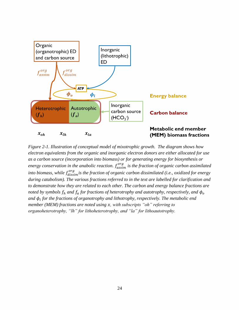
𝑟𝑖𝑛𝑜𝑟𝑔 𝐸𝐷 and 𝑟𝑜𝑟𝑔 𝐸𝐷 using expressions for the energy and carbon balances of the population.

Figure 2-1 illustrates the conceptual model, showing the relationship between the utilization rates

of the two EDs and the carbon and energy balances.

24

Figure 2-1. Illustration of conceptual model of mixotrophic growth. The diagram shows how

electron equivalents from the organic and inorganic electron donors are either allocated for use

as a carbon source (incorporation into biomass) or for generating energy for biosynthesis or

energy conservation in the anabolic reaction. 𝑓𝑎𝑠𝑠𝑖𝑚𝑜𝑟𝑔

is the fraction of organic carbon assimilated

into biomass, while 𝑓𝑑𝑖𝑠𝑠𝑖𝑚𝑜𝑟𝑔

is the fraction of organic carbon dissimilated (i.e., oxidized for energy

during catabolism). The various fractions referred to in the text are labelled for clarification and

to demonstrate how they are related to each other. The carbon and energy balance fractions are

noted by symbols 𝑓ℎ and 𝑓𝑎 for fractions of heterotrophy and autotrophy, respectively, and 𝜙𝑜

and 𝜙𝑙 for the fractions of organotrophy and lithotrophy, respectively. The metabolic end

member (MEM) fractions are noted using 𝑥, with subscripts “oh” referring to

organoheterotrophy, “lh” for lithoheterotrophy, and “la” for lithoautotrophy.

25

2.2.1 Carbon and energy balances

Here, I outline the energy and carbon balance expressions for mixotrophic growth which

describe the allocation of the two EDs and two carbon sources to the energy-requiring processes

of biosynthesis and energy conservation, plus the carbon requirement for biosynthesis. The

energy balance fractions represent the proportions of the overall metabolism that use the organic

(i.e., organotrophy) and inorganic (i.e., lithotrophy) EDs for energy, while the carbon balance

fractions represent the proportion of the biomass that is formed using organic (i.e., heterotrophy)

and inorganic (i.e., autotrophy) carbon.

To compare the ED utilization rates in terms of the energy available, it is necessary to

convert the rates from units of mole of ED to units of moles of electron equivalents (eeq).

Electron equivalents represent the number of electrons (e-) released during complete oxidation of

the ED. For example, during the oxidation half reaction of thiosulfate (𝑆2𝑂32−), 8 e- are released:

𝑆2𝑂32− → 2𝑆𝑂4

2− + 8𝑒− (2-1)

An eeq factor (𝑛𝑒𝑒𝑞𝐸𝐷 ) [mol eeq (mol ED)-1] can be used to convert ED utilization rate units. For

example, 𝑟𝑜𝑟𝑔 𝐸𝐷 [mol org ED (L time)-1] can be converted to 𝑟𝑜𝑟𝑔 𝑒𝑒𝑞 [mol org eeq (L time)-1]

using Eq. 2-2. These two notations for distinguishing rates in units of mol ED and mol eeq will

be used throughout this thesis.

𝑟𝑜𝑟𝑔 𝑒𝑒𝑞 = 𝑟𝑜𝑟𝑔 𝐸𝐷 ∗ 𝑛𝑒𝑒𝑞𝐸𝐷 (2-2)

The total rate of ED utilization of the inorganic and organic substrates for processes

requiring electron donation in both catabolism and anabolism (𝑟𝑒𝑒𝑞)[mol eeq (L time)-1] is the

sum of the rates of consumption of the two EDs where the organic ED utilization rate is

multiplied by the electron equivalents fraction of the organic ED dissimilated, 𝑓𝑑𝑖𝑠𝑠𝑖𝑚𝑜𝑟𝑔

:

26

𝑟𝑒𝑒𝑞 = 𝑓𝑑𝑖𝑠𝑠𝑖𝑚𝑜𝑟𝑔

∗ 𝑟𝑜𝑟𝑔 𝑒𝑒𝑞 + 𝑟𝑖𝑛𝑜𝑟𝑔 𝑒𝑒𝑞 (2-3)

The fraction of the total metabolic reaction that is organotrophic (𝜙𝑜𝑟𝑔𝑚𝑒𝑡) and lithotrophic (𝜙𝑙𝑖𝑡ℎ𝑜

𝑚𝑒𝑡 )

can be calculated using each of the terms on the right side of Eq. 2-3 as the numerator and the

total eeq utilization rate for energy production as the denominator:

𝜙𝑜𝑟𝑔 =𝑓𝑑𝑖𝑠𝑠𝑖𝑚

𝑜𝑟𝑔∗ 𝑟𝑜𝑟𝑔 𝑒𝑒𝑞

𝑟𝑒𝑒𝑞 (2-4)

𝜙𝑙𝑖𝑡ℎ𝑜 =𝑟𝑖𝑛𝑜𝑟𝑔 𝑒𝑒𝑞

𝑟𝑒𝑒𝑞 (2-5)

The carbon balance fractions are calculated using units of C-mol rather than units of mol eeq, as

with the energy balance fractions. The total biomass production rate (𝑟𝑥) [C-mol biomass (L

time)-1] reflects the use of organic (i.e., heterotrophic) and inorganic (i.e., autotrophic) carbon to

build biomass and can therefore be expressed as the sum of the two rates of consumption of these

carbon sources:

𝑟𝑥 = 𝑟𝑥,ℎ𝑒𝑡 + 𝑟𝑥,𝑎𝑢𝑡𝑜 (2-6)

whereby the total rate of heterotrophic microbial growth (i.e., the OH and LH MEMs) (𝑟𝑥,ℎ𝑒𝑡)

[C-mol biomass (L time)-1] is:

𝑟ℎ𝑒𝑡,𝑥 = 𝑓𝑎𝑠𝑠𝑖𝑚𝑜𝑟𝑔

∗ 𝑟𝑜𝑟𝑔 𝐸𝐷 ∗ 𝑛𝐶𝑜𝑟𝑔 𝐸𝐷

(2-7)

where 𝑛𝐶𝑜𝑟𝑔

is the number of moles of carbon in one mole of organic substrate, and is used to

convert the organic ED utilization units to C-mol units, and 𝑓𝑎𝑠𝑠𝑖𝑚𝑜𝑟𝑔

is the fraction of the organic

substrate assimilated for biomass synthesis (and is equal to 1-𝑓𝑑𝑖𝑠𝑠𝑖𝑚𝑜𝑟𝑔

).

27

All inorganic carbon uptake is allocated to biomass synthesis and, given the 1:1 ratio of

carbon in CO2 and in a C-mol of biomass, the rate of biomass production attributed to autotrophy

(𝑟𝑥,𝑎𝑢𝑡𝑜) [C-mol biomass (L h)-1] is equal to the rate of carbon dioxide uptake (𝑟𝐶𝑂2) [C-mol (L

h)-1]:

𝑟𝑥,𝑎𝑢𝑡𝑜 = 𝑟𝐶𝑂2 (2-8)

The fraction of the total metabolism that is heterotrophic (𝑓ℎ) and autotrophic (𝑓𝑎) is described

using:

𝑓ℎ =𝑟𝑥,ℎ𝑒𝑡

𝑟𝑥 (2-9)

𝑓𝑎 =𝑟𝑥,𝑎𝑢𝑡𝑜

𝑟𝑥 (2-10)

These metabolic carbon and energy balance fractions can be used to calculate the relative

proportions of the MEMs. These MEM fractions represent the fraction of biomass, and therefore

also total metabolic activity, that uses that MEM reaction. Given that there are three MEMs

representing the unique combination of a carbon and energy source, the fraction of each MEM

will be the product of a metabolic energy balance fraction (𝜙𝑖𝑚𝑒𝑡) and a carbon balance fraction

(𝑓𝑘):

𝑥𝑖𝑘 = 𝜙𝑖𝑚𝑒𝑡 ∗ 𝑓𝑘 (2-11)

2.2.2 Representing energetic constraints: Defining reaction stoichiometries

To apply this conceptual framework using a bioenergetic-kinetic approach, and represent the

energetic constraints on each MEM, the Gibbs Energy Dynamic Yield Method (GEDYM) is

used. This method uses the Gibbs energies of the anabolic (i.e., biomass forming) and catabolic

(i.e., energy generating) reactions that make up the metabolic reaction to predict how they are

28

combined to yield the metabolic reaction. The details of deriving catabolic and anabolic reactions

are described by Smeaton and Van Cappellen (2018). By calculating the bioenergetics-predicted

metabolic reaction stoichiometry, the specific turnover rates of reactants and products can be

calculated for each MEM.

As examples, the catabolic and anabolic reactions during lithoheterotrophic growth using

thiosulfate (𝑆2𝑂32−) as an ED/ energy source, oxygen (𝑂2) as an electron acceptor, and acetate

(𝐶2𝐻3𝑂2−) as a carbon source are outlined here. The catabolic reaction describing the oxidation

of 𝑆2𝑂32− 𝑡𝑜 𝑆𝑂4

2− coupled to the reduction of 𝑂2 to 𝐻2𝑂, called lithotrophy would be:

𝑆2𝑂32− + 2𝑂2 + 𝐻2𝑂 → 2𝑆𝑂4

2− + 2𝐻+ (2-12)

For the anabolic reactions describing the formation of biomass, the generic formula,

𝐶𝐻1.8𝑂0.5𝑁0.2, is used to represent one carbon mole of biomass. The anabolic reaction here

involves the reduction of 𝐶2𝐻3𝑂2 to the oxidation state of biomass coupled to the oxidation of

𝑆2𝑂32− 𝑡𝑜 𝑆𝑂4

2−:

0.15𝑆2𝑂3−2 + 0.5𝐶2𝐻3𝑂2

− + 0.2𝑁𝐻4+ + 0.27𝐻2𝑂 →

0.3𝑆𝑂4−2 + 0.05𝐻𝐶𝑂3

− + 0.06𝐻+ + 𝐶𝐻1.8𝑂0.5𝑁0.2 (2-13)

These reactions can be used to calculate the standard state Gibbs energies, ∆𝐺𝑎𝑛° and ∆𝐺𝑐𝑎𝑡

°

(using Eq. 1-1, and Eq. A-16 (Appendix A) to correct for temperature), and subsequently ∆𝐺𝑎𝑛

and ∆𝐺𝑐𝑎𝑡 (using Eq. 1-2) given the chemical activities in the environment being simulated.

Smeaton and Van Cappellen (2018) present the principle equation of the GEDYM that is

used to calculate growth yields and the energetic limitations to metabolic reactions. Its derivation

29

is reproduced in Appendix A. The method uses linear regressions specific to different metabolic

groups with different energetic costs. Here, I use the linear regression parameters from the fit to

the “majority of metabolisms” for heterotrophic metabolisms (i.e., for the OH and LH MEMs).

For autotrophic metabolisms, I use an unpublished linear regression that is meant to represent the

energetic costs of reverse electron transport and inorganic carbon fixation. Reverse electron

transport is used by many lithoautotrophs to generate the reducing equivalents necessary to

reduce CO2 to the oxidation state of biomass. The linear regression parameters for these two

metabolic groups are given in Table A-4 (Appendix A). In addition to being able to calculate the

growth yield (Y) for a metabolism given the energy available from the specific chemical

activities in a given environment, the maximum potential growth yield can also be calculated

using bioenergetics. The calculation for this maximum potential growth yield (𝑌𝑚𝑎𝑥) is also

described in Appendix A.

MEM-specific rates of reactant or product turnover, including growth rates, can be

calculated using these MEM-specific growth yields. The anabolic and catabolic reactions can be

added together to yield the metabolic reaction using the energy balance relationship described by

Eq. 1-3. This metabolic reaction describes the stoichiometric coefficients in front of all reactants

and products and thus facilitates the conversion of ED utilization rates to the rate of interest. For

example, to account for the total potential MEM-specific turnover rate of a substrate S (𝑟𝑆,𝑀𝐸𝑀),

the general equation 2-14 can be used:

𝑟𝑆,𝑀𝐸𝑀 = 𝑟𝐸𝐷 ∗𝑛𝑆

𝑚𝑒𝑡

𝑛𝐸𝐷𝑚𝑒𝑡 (2-14)

where 𝑛𝑆𝑚𝑒𝑡 is the stoichiometric coefficient in front of a substrate, S in the metabolic reaction

for that MEM [mol S (C-mol biomass)-1], and 𝑛𝐸𝐷𝑚𝑒𝑡 is the stoichiometric coefficient in front of

the ED in the metabolic reaction [mol ED (C-mol biomass)-1].

30

To account for the limitation of MEM turnover rates by their competition with other

MEMs, I scale the total potential MEM-specific rate by energy balance or carbon balance

fractions. For the OH MEM, the total potential rate is scaled by 𝜙𝑜, the fraction of organotrophy,

to represent the fact that not all the 𝑟𝑜𝑟𝑔 𝐸𝐷 consumed is used for organotrophic growth:

𝑟𝑆,𝑂𝐻 = 𝜙𝑜 ∗ 𝑟𝑜𝑟𝑔 𝐸𝐷 ∗𝑛𝑆

𝑚𝑒𝑡


where 𝑟𝑆,𝑂𝐻 is the OH-specific turnover rate of substrate S.

For LH, and LA, the two lithotrophic metabolisms, all of the inorganic ED consumed is used for

donating electrons, so to describe the partitioning of the ED to either of the two MEMs, the

carbon balance fractions (𝑓𝑘) can be used to scale the total potential rates of each MEM:

𝑟𝑆,𝑀𝐸𝑀 = 𝑓𝑘 ∗ 𝑟𝐸𝐷 ∗𝑛𝑆

𝑚𝑒𝑡


Therefore, for LH, Eq. A-28 becomes:

𝑟𝑆,𝐿𝐻 = 𝑓ℎ ∗ 𝑟𝑖𝑛𝑜𝑟𝑔 𝐸𝐷 ∗𝑛𝑆

𝑚𝑒𝑡


And for LA, Eq. A-28 becomes:

𝑟𝑆,𝐿𝐴 = 𝑓𝑎 ∗ 𝑟𝑖𝑛𝑜𝑟𝑔 𝐸𝐷 ∗𝑛𝑆

𝑚𝑒𝑡


To calculate MEM-specific growth rates (i.e., 𝑟𝑥,𝑂𝐻, 𝑟𝑥,𝐿𝐻, and 𝑟𝑥,𝐿𝐴) , the same equations can be

used, with 𝑛𝑆

𝑚𝑒𝑡

𝑛𝐸𝐷𝑚𝑒𝑡 replaced by 𝑌𝑖𝑘, the potential growth yield (in units of [C-mol biomass (mol ED)-

1] for that specific MEM. The total mixotrophic substrate turnover rate or growth rate can then be

calculated as the sum of these MEM-specific rates:

𝑟𝑥 = 𝜙𝑜 ∗ 𝑟𝑜𝑟𝑔 𝐸𝐷 ∗ 𝑌𝑜ℎ + 𝑟𝑖𝑛𝑜𝑟𝑔 𝐸𝐷 ∗ (𝑓ℎ ∗ 𝑌𝑙ℎ + 𝑓𝑎 ∗ 𝑌𝑙𝑎) (2-19)

31

To validate my modeling framework for predicting the relative abundances of the MEMs

expressed as a function of the relative utilization of the two EDs, I collected data from chemostat

studies identified in the literature which directly traced the fraction of the organic ED/ carbon

source assimilated (𝑓𝑎𝑠𝑠𝑖𝑚𝑜𝑟𝑔

), enabling the calculation of the MEM fractions using the conceptual

model illustrated in Figure 2-1.

2.3 Literature experimental data compilation

Chemostats are ideal experimental systems to study mixotrophy, because they allow organisms

to grow under stable, steady state conditions, simulating environmental conditions.

Consequently, organisms grow in a constant physiological state, such that growth yields and

kinetic parameters (such as 𝑟𝑥) are more precise and reproducible than those extracted from batch

experiments (Kovarova-Kovar and Egli, 1998). Moreover, the supply rates of different ED and

carbon source mixtures can be tightly controlled in chemostats.

In chemostats, sterile growth medium is supplied at a constant volumetric flow rate (F) to

a culture vessel containing microorganisms (e.g., Esteve-Núñez et al., 2005). Biomass-

containing effluent is removed from the vessel at the same flow rate to maintain a constant

culture volume (V). The residence time of the cells in the reactor is given by the dilution rate (D)

[time-1] (Herbert et al, 1956) (Eq. 2-20). At steady state, the specific growth rate of the

organisms, µ, is equal to 𝐷.

𝐷 = 𝐹

𝑉 (2-20)

Literature chemostat studies were chosen that used biochemical techniques (e.g., isotopic

labelling, tracking CO2 gas production, and measurement of specific CO2 fixation rates) to track

32

the proportion of organic substrate assimilated and used for biosynthetic molecules (𝑓𝑎𝑠𝑠𝑖𝑚𝑜𝑟𝑔

)

versus the fraction dissimilated for biomass synthesis and energy conservation (𝑓𝑑𝑖𝑠𝑠𝑖𝑚 𝑜𝑟𝑔

). These

studies also reported measurements that could be used to calculate 𝑟𝑜𝑟𝑔 𝐸𝐷, 𝑟𝑖𝑛𝑜𝑟𝑔 𝐸𝐷, and 𝑟𝑥.

While studies that fit all the above criteria are sparse, these data enable fully constraining the

energy and carbon balances described in section 2.2.1 to calculate the fraction of each MEM.

Three published chemostat studies which investigated mixotrophic pure cultures grown on

mixtures of organic and inorganic EDs were identified. Table 2 summarizes the experimental

conditions of each study.

Briefly, all chosen studies used O2 as the sole electron acceptor. Study 1 examined

mixotrophic growth of Paracoccus versutus (formerly known as Thiobacillus A2 and

Thiobacillus versutus) (Katayama et al., 1995) on the organic ED acetate and the inorganic ED

thiosulfate (Gottschal and Kuenen, 1980). The catabolic and anabolic reactions for study 1 are in

Table A-1 (Appendix A). In study 2, Pseudomonas oxalaticus was grown on mixtures of acetate

and formate. While formate is an organic compound, it is treated as an “inorganic” substrate for

the purposes of this synthesis since P. oxalaticus is unable to use formate as a C source for

biomass, and its growth on formate is therefore exclusively autotrophic (Dijkhuizen et al.,

1977b). In other words, no formate is assimilated for forming biomass, which is the same for

lithoautotrophic growth using a true inorganic compound such as H2. While some papers have

called autotrophic growth where formate or other one carbon acids such as methanol are used as

the ED either organoautotrophic or methylotrophic (Dijkhuizen and Harder, 1984; Bowien et al.,

1996), it is herein referred to as lithoautotrophic. Studies 2 and 3 are nearly identical (i.e., same

organism, inorganic ED and electron acceptor), with the only difference being that in study 3 the

33

organic ED substrate is oxalate. The anabolic and catabolic reactions corresponding to studies 2

and 3 are found in Appendix A, Tables A-2 and A-3.

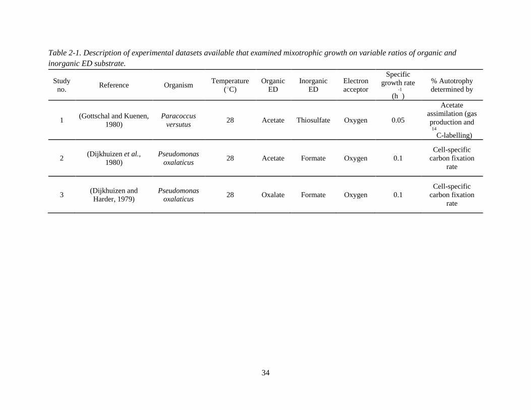
34

Table 2-1. Description of experimental datasets available that examined mixotrophic growth on variable ratios of organic and

inorganic ED substrate.

Study

no. Reference Organism

Temperature

(○C)

Organic

ED

Inorganic

ED

Electron

acceptor

Specific

growth rate

(h-1

)

% Autotrophy

determined by

1 (Gottschal and Kuenen,

1980)

Paracoccus

versutus 28 Acetate Thiosulfate Oxygen 0.05

Acetate

assimilation (gas

production and 14

C-labelling)

2 (Dijkhuizen et al.,

1980)

Pseudomonas

oxalaticus 28 Acetate Formate Oxygen 0.1

Cell-specific

carbon fixation

rate

3 (Dijkhuizen and

Harder, 1979)

Pseudomonas

oxalaticus 28 Oxalate Formate Oxygen 0.1

Cell-specific

carbon fixation

rate

35

2.3.1 Calculating the net ED utilization and growth rates

The concentrations of ED substrates supplied (𝐶𝐸𝐷𝑠𝑢𝑝𝑝𝑙𝑖𝑒𝑑

) [mol ED (L)-1] and the steady state

residual concentrations (𝐶𝐸𝐷𝑟𝑒𝑠𝑖𝑑𝑢𝑎𝑙) [mol ED (L)-1] of ED substrates in the chemostat studies are

used to calculate the net rates of organic and inorganic ED utilization (𝑟𝐸𝐷 ) [mol ED (L time)-1]

using Eq. 2-21. As described in Eq. 2-2, this rate can be converted to units of mol eeq using the

eeq factor, 𝑛𝑒𝑒𝑞𝐸𝐷 .

𝑟𝐸𝐷 = 𝐷 ∙ (𝐶𝐸𝐷𝑠𝑢𝑝𝑝𝑙𝑖𝑒𝑑 − 𝐶𝐸𝐷

𝑟𝑒𝑠𝑖𝑑𝑢𝑎𝑙) (2-21)

For the studies considered here, the residual concentrations were reported as not detectable, so

that the ED utilization rates are equivalent to rate of ED supply at the chemostat inlet. For

energetic calculations, the residual concentrations of the EDs were estimated using calculations

that are outlined in Appendix A.

The total biomass concentrations (𝑋𝑡𝑜𝑡) measured at the outlet of the chemostat and

reported in the studies in either [g of biomass C (L)-1] or [g of dry weight biomass (L)-1] were

converted to units of [C-mol biomass (L)-1] by multiplying them by the molecular weight of

carbon (12.01 g (mol)-1) or the average molecular weight of biomass (24.6 g (C-mol biomass)-1

(Smeaton and Van Cappellen, 2018)), respectively. The total biomass production rate (𝑟𝑥) [C-

mol biomass (L time)-1] was determined using:

𝑟𝑥 = 𝑋𝑡𝑜𝑡 ∗ 𝐷 (2-22)

2.3.2 Calculating the MEM fractions

In the selected studies, two different approaches were used to monitor inorganic carbon fixation

activity versus heterotrophic organic carbon use. In study 1, 𝑓𝑎𝑠𝑠𝑖𝑚𝑜𝑟𝑔

was measured directly by

36

either tracing the CO2 produced by organic substrate oxidation or by tracing the carbon allocated

to biomass using an isotopic label (Gottschal and Kuenen, 1980). Along with the calculated

growth rates and ED substrate utilization rates (described in section 2.31), this enabled the

calculation of the carbon and energy balances as described in section 2.2.1, and therefore the

calculation of the MEM fractions (using Eq. 2-9).

While 𝑓𝑎𝑠𝑠𝑖𝑚𝑜𝑟𝑔

was not directly measured in studies 2 and 3, the carbon fixation rate was

measured and could be used to determine the fractions of autotrophy (𝑓𝑎) and heterotrophy (𝑓ℎ).

This is accomplished by comparing the biomass production (𝑟𝑡𝑜𝑡 𝑥100) and carbon fixation

(𝑟𝐶𝑂2100) rates under 100% autotrophic conditions (i.e., no added organic carbon) to the biomass

production (𝑟𝑡𝑜𝑡 𝑥) and carbon fixation (𝑟𝐶𝑂2) rates of chemostat experiments containing organic

carbon using:

𝑓𝑎

𝑓𝑎100

=

𝑟𝐶𝑂2

𝑟𝑥𝑟𝐶𝑂2100

𝑟𝑥100

(2-23)

At 100% autotrophy, 𝑓𝑎100 = 1, therefore:

𝑓𝑎 =𝑟𝐶𝑂2/ 𝑟𝑥

𝑟𝐶𝑂2100/ 𝑟𝑥100

(2-24)

The fraction of heterotrophy, 𝑓ℎ can thus be determined given that 𝑓ℎ = 1 − 𝑓𝑎.

Given that biomass-specific carbon fixation rates were reported in studies 2 and 3 (i.e., per units

biomass; [nmol-CO2 min-1 mg dry weight-1]), this effectively accounts for normalizing the rate

by biomass, and thus Eq. 2-25 was used:

𝑓𝑎 =𝑞𝐶𝑂2

𝑞𝐶𝑂2100

(2-25)

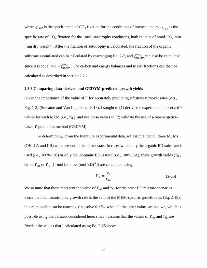
37

where 𝑞𝐶𝑂2 is the specific rate of CO2 fixation for the conditions of interest, and 𝑞𝐶𝑂2100 is the

specific rate of CO2 fixation for the 100% autotrophy conditions, both in units of nmol-CO2 min-

1 mg dry weight-1. After the fraction of autotrophy is calculated, the fraction of the organic

substrate assimilated can be calculated by rearranging Eq. 2-7, and 𝑓𝑑𝑖𝑠𝑠𝑖𝑚𝑜𝑟𝑔

can also be calculated

since it is equal to 1 – 𝑓𝑎𝑠𝑠𝑖𝑚𝑜𝑟𝑔

. The carbon and energy balances and MEM fractions can then be

calculated as described in section 2.2.1.

2.3.3 Comparing data-derived and GEDYM-predicted growth yields

Given the importance of the value of 𝑌 for accurately predicting substrate turnover rates (e.g.,

Fig. 1-3) (Smeaton and Van Cappellen, 2018), I sought to (1) derive the experimental observed 𝑌

values for each MEM (i.e., 𝑌𝑖𝑘), and use these values to (2) validate the use of a bioenergetics-

based 𝑌 prediction method (GEDYM).

To determine 𝑌𝑖𝑘 from the literature experimental data, we assume that all three MEMs

(OH, LA and LH) were present in the chemostats. In cases when only the organic ED substrate is

used (i.e., 100% OH) or only the inorganic ED is used (i.e., 100% LA), these growth yields (𝑌𝑖𝑘,

either 𝑌𝑜ℎ or 𝑌𝑙𝑎 [C-mol biomass (mol ED)-1]) are calculated using:

𝑌𝑖𝑘 =𝑟𝑥

𝑟𝐸𝐷 (2-26)

We assume that these represent the value of 𝑌𝑜ℎ and 𝑌𝑙𝑎 for the other ED mixture scenarios.

Since the total mixotrophic growth rate is the sum of the MEM-specific growth rates (Eq. 2-19),

this relationship can be rearranged to solve for 𝑌𝑙ℎ when all the other values are known, which is

possible using the datasets considered here, since I assume that the values of 𝑌𝑜ℎ and 𝑌𝑙𝑎 are

fixed at the values that I calculated using Eq. 2-25 above:

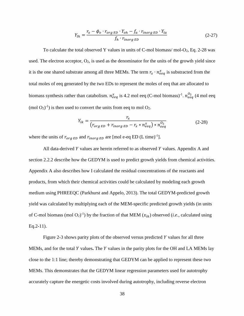
38

𝑌𝑙ℎ =𝑟𝑥 − 𝜙𝑜 ∙ 𝑟𝑜𝑟𝑔 𝐸𝐷 ∙ 𝑌𝑜ℎ − 𝑓𝑎 ∙ 𝑟𝑖𝑛𝑜𝑟𝑔 𝐸𝐷 ∙ 𝑌𝑙𝑎

𝑓ℎ ∙ 𝑟𝑖𝑛𝑜𝑟𝑔 𝐸𝐷 (2-27)

To calculate the total observed Y values in units of C-mol biomass/ mol-O2, Eq. 2-28 was

used. The electron acceptor, O2, is used as the denominator for the units of the growth yield since

it is the one shared substrate among all three MEMs. The term 𝑟𝑥 ∙ 𝑛𝑒𝑒𝑞𝑥 is substracted from the

total moles of eeq generated by the two EDs to represent the moles of eeq that are allocated to

biomass synthesis rather than catabolism. 𝑛𝑒𝑒𝑞𝑥 is 4.2 mol eeq (C-mol biomass)-1. 𝑛𝑒𝑒𝑞

𝑂2 (4 mol eeq

(mol O2)-1) is then used to convert the units from eeq to mol O2.

𝑌𝑖𝑘 =𝑟𝑥

(𝑟𝑜𝑟𝑔 𝐸𝐷 + 𝑟𝑖𝑛𝑜𝑟𝑔 𝐸𝐷 − 𝑟𝑥 ∗ 𝑛𝑒𝑒𝑞𝑥 ) ∗ 𝑛𝑒𝑒𝑞

𝑂2 (2-28)

where the units of 𝑟𝑜𝑟𝑔 𝐸𝐷 and 𝑟𝑖𝑛𝑜𝑟𝑔 𝐸𝐷 are [mol e-eq ED (L time)-1].

All data-derived 𝑌 values are herein referred to as observed 𝑌 values. Appendix A and

section 2.2.2 describe how the GEDYM is used to predict growth yields from chemical activities.

Appendix A also describes how I calculated the residual concentrations of the reactants and

products, from which their chemical activities could be calculated by modeling each growth

medium using PHREEQC (Parkhurst and Appelo, 2013). The total GEDYM-predicted growth

yield was calculated by multiplying each of the MEM-specific predicted growth yields (in units

of C-mol biomass (mol O2)-1) by the fraction of that MEM (𝑥𝑖𝑘) observed (i.e., calculated using

Eq.2-11).

Figure 2-3 shows parity plots of the observed versus predicted 𝑌 values for all three

MEMs, and for the total 𝑌 values. The 𝑌 values in the parity plots for the OH and LA MEMs lay

close to the 1:1 line; thereby demonstrating that GEDYM can be applied to represent these two

MEMs. This demonstrates that the GEDYM linear regression parameters used for autotrophy

accurately capture the energetic costs involved during autotrophy, including reverse electron

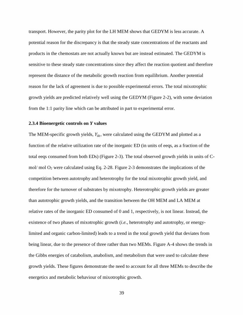
39

transport. However, the parity plot for the LH MEM shows that GEDYM is less accurate. A

potential reason for the discrepancy is that the steady state concentrations of the reactants and

products in the chemostats are not actually known but are instead estimated. The GEDYM is

sensitive to these steady state concentrations since they affect the reaction quotient and therefore

represent the distance of the metabolic growth reaction from equilibrium. Another potential

reason for the lack of agreement is due to possible experimental errors. The total mixotrophic

growth yields are predicted relatively well using the GEDYM (Figure 2-2), with some deviation

from the 1:1 parity line which can be attributed in part to experimental error.

2.3.4 Bioenergetic controls on Y values

The MEM-specific growth yields, 𝑌𝑖𝑘, were calculated using the GEDYM and plotted as a

function of the relative utilization rate of the inorganic ED (in units of eeqs, as a fraction of the

total eeqs consumed from both EDs) (Figure 2-3). The total observed growth yields in units of C-

mol/ mol O2 were calculated using Eq. 2-28. Figure 2-3 demonstrates the implications of the

competition between autotrophy and heterotrophy for the total mixotrophic growth yield, and

therefore for the turnover of substrates by mixotrophy. Heterotrophic growth yields are greater

than autotrophic growth yields, and the transition between the OH MEM and LA MEM at

relative rates of the inorganic ED consumed of 0 and 1, respectively, is not linear. Instead, the

existence of two phases of mixotrophic growth (i.e., heterotrophy and autotrophy, or energy-

limited and organic carbon-limited) leads to a trend in the total growth yield that deviates from

being linear, due to the presence of three rather than two MEMs. Figure A-4 shows the trends in

the Gibbs energies of catabolism, anabolism, and metabolism that were used to calculate these

growth yields. These figures demonstrate the need to account for all three MEMs to describe the

energetics and metabolic behaviour of mixotrophic growth.

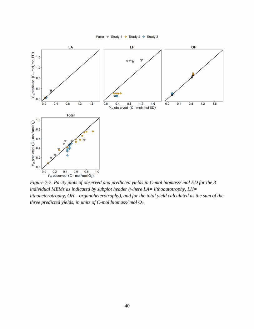
40

Figure 2-2. Parity plots of observed and predicted yields in C-mol biomass/ mol ED for the 3

individual MEMs as indicated by subplot header (where LA= lithoautotrophy, LH=

lithoheterotrophy, OH= organoheterotrophy), and for the total yield calculated as the sum of the

three predicted yields, in units of C-mol biomass/ mol O2.

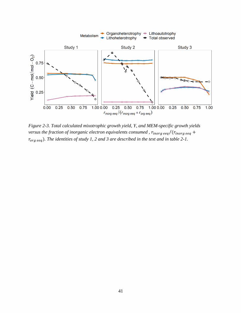
41

Figure 2-3. Total calculated mixotrophic growth yield, Y, and MEM-specific growth yields

versus the fraction of inorganic electron equivalents consumed , 𝑟𝑖𝑛𝑜𝑟𝑔 𝑒𝑒𝑞 (𝑟𝑖𝑛𝑜𝑟𝑔 𝑒𝑒𝑞⁄ +

𝑟𝑜𝑟𝑔 𝑒𝑒𝑞). The identities of study 1, 2 and 3 are described in the text and in table 2-1.

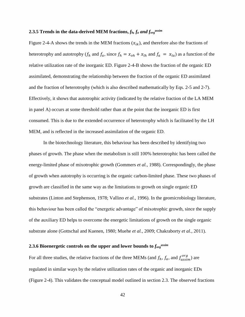
42

2.3.5 Trends in the data-derived MEM fractions, fh, fa and forgassim

Figure 2-4-A shows the trends in the MEM fractions (𝑥𝑖𝑘), and therefore also the fractions of

heterotrophy and autotrophy (𝑓ℎ and 𝑓𝑎, since 𝑓ℎ = 𝑥𝑜ℎ + 𝑥𝑙ℎ and 𝑓𝑎 = 𝑥𝑙𝑎) as a function of the

relative utilization rate of the inorganic ED. Figure 2-4-B shows the fraction of the organic ED

assimilated, demonstrating the relationship between the fraction of the organic ED assimilated

and the fraction of heterotrophy (which is also described mathematically by Eqs. 2-5 and 2-7).

Effectively, it shows that autotrophic activity (indicated by the relative fraction of the LA MEM

in panel A) occurs at some threshold rather than at the point that the inorganic ED is first

consumed. This is due to the extended occurrence of heterotrophy which is facilitated by the LH

MEM, and is reflected in the increased assimilation of the organic ED.

In the biotechnology literature, this behaviour has been described by identifying two

phases of growth. The phase when the metabolism is still 100% heterotrophic has been called the

energy-limited phase of mixotrophic growth (Gommers et al., 1988). Correspondingly, the phase

of growth when autotrophy is occurring is the organic carbon-limited phase. These two phases of

growth are classified in the same way as the limitations to growth on single organic ED

substrates (Linton and Stephenson, 1978; Vallino et al., 1996). In the geomicrobiology literature,

this behaviour has been called the “energetic advantage” of mixotrophic growth, since the supply

of the auxiliary ED helps to overcome the energetic limitations of growth on the single organic

substrate alone (Gottschal and Kuenen, 1980; Muehe et al., 2009; Chakraborty et al., 2011).

2.3.6 Bioenergetic controls on the upper and lower bounds to forgassim

For all three studies, the relative fractions of the three MEMs (and 𝑓ℎ, 𝑓𝑎, and 𝑓𝑎𝑠𝑠𝑖𝑚𝑜𝑟𝑔

) are

regulated in similar ways by the relative utilization rates of the organic and inorganic EDs

(Figure 2-4). This validates the conceptual model outlined in section 2.3. The observed fractions

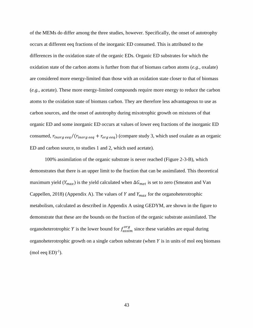
43

of the MEMs do differ among the three studies, however. Specifically, the onset of autotrophy

occurs at different eeq fractions of the inorganic ED consumed. This is attributed to the

differences in the oxidation state of the organic EDs. Organic ED substrates for which the

oxidation state of the carbon atoms is further from that of biomass carbon atoms (e.g., oxalate)

are considered more energy-limited than those with an oxidation state closer to that of biomass

(e.g., acetate). These more energy-limited compounds require more energy to reduce the carbon

atoms to the oxidation state of biomass carbon. They are therefore less advantageous to use as

carbon sources, and the onset of autotrophy during mixotrophic growth on mixtures of that

organic ED and some inorganic ED occurs at values of lower eeq fractions of the inorganic ED

consumed, 𝑟𝑖𝑛𝑜𝑟𝑔 𝑒𝑒𝑞 (𝑟𝑖𝑛𝑜𝑟𝑔 𝑒𝑒𝑞⁄ + 𝑟𝑜𝑟𝑔 𝑒𝑒𝑞) (compare study 3, which used oxalate as an organic

ED and carbon source, to studies 1 and 2, which used acetate).

100% assimilation of the organic substrate is never reached (Figure 2-3-B), which

demonstrates that there is an upper limit to the fraction that can be assimilated. This theoretical

maximum yield (𝑌𝑚𝑎𝑥) is the yield calculated when ∆𝐺𝑚𝑒𝑡 is set to zero (Smeaton and Van

Cappellen, 2018) (Appendix A). The values of 𝑌 and 𝑌𝑚𝑎𝑥 for the organoheterotrophic

metabolism, calculated as described in Appendix A using GEDYM, are shown in the figure to

demonstrate that these are the bounds on the fraction of the organic substrate assimilated. The

organoheterotrophic 𝑌 is the lower bound for 𝑓𝑎𝑠𝑠𝑖𝑚𝑜𝑟𝑔

since these variables are equal during

organoheterotrophic growth on a single carbon substrate (when 𝑌 is in units of mol eeq biomass

(mol eeq ED)-1).

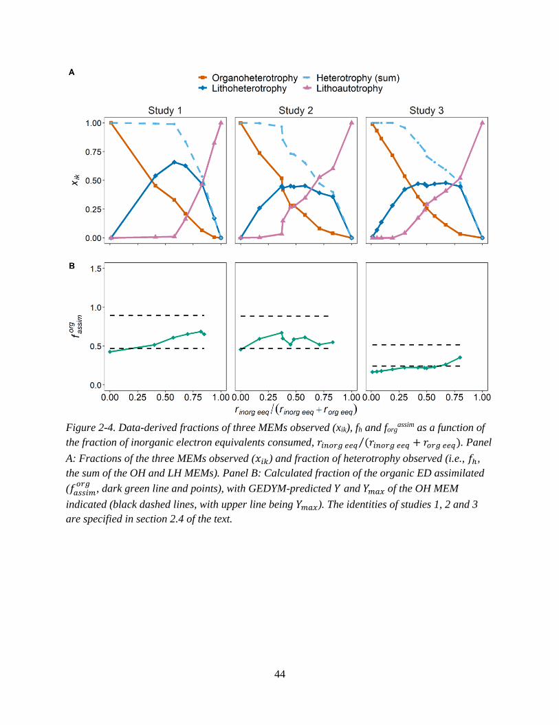
44

Figure 2-4. Data-derived fractions of three MEMs observed (xik), fh and forg

assim as a function of

the fraction of inorganic electron equivalents consumed, 𝑟𝑖𝑛𝑜𝑟𝑔 𝑒𝑒𝑞 (𝑟𝑖𝑛𝑜𝑟𝑔 𝑒𝑒𝑞⁄ + 𝑟𝑜𝑟𝑔 𝑒𝑒𝑞). Panel

A: Fractions of the three MEMs observed (𝑥𝑖𝑘) and fraction of heterotrophy observed (i.e., 𝑓ℎ,

the sum of the OH and LH MEMs). Panel B: Calculated fraction of the organic ED assimilated

(𝑓𝑎𝑠𝑠𝑖𝑚𝑜𝑟𝑔

, dark green line and points), with GEDYM-predicted 𝑌 and 𝑌𝑚𝑎𝑥 of the OH MEM

indicated (black dashed lines, with upper line being 𝑌𝑚𝑎𝑥). The identities of studies 1, 2 and 3

are specified in section 2.4 of the text.

45

2.4 Applying the conceptual model: A modeling framework for mixotrophy

A system of governing equations to predict the MEM fractions was developed using the

conceptual framework built in the preceding sections. The system of equations relates the MEM

fractions, 𝑥𝑜ℎ, 𝑥𝑙ℎ and 𝑥𝑙𝑎, and the fraction of the organic ED/ carbon source dissimilated, 𝑓𝑑𝑖𝑠𝑠𝑖𝑚𝑜𝑟𝑔

to the utilization rates of the EDs (𝑟𝑖𝑛𝑜𝑟𝑔 𝑒𝑒𝑞 and 𝑟𝑜𝑟𝑔 𝑒𝑒𝑞), and the GEDYM-predicted growth

yields of the three MEMs (𝑌𝑖𝑘) for a steady state chemostat system. The equations effectively

represent the kinetic (i.e., ED utilization rates) and thermodynamic (i.e., growth yields)

constraints on the expression of the three MEMs. The purpose of developing this modeling

framework is that it can be implemented in larger kinetic reaction models where the MEM

fractions can be calculated at each time step as a function of the changing utilization rates of the

two EDs, changes in the growth yields, and/ or other limitations. The inputs are the net

utilization rates of the two ED substrates, and the chemical environment-specific growth yields

of the three MEMs.

2.4.1 System of equations

The first constraint describes how the three MEM fractions must sum to unity:

𝑥𝑜ℎ + 𝑥𝑙ℎ + 𝑥𝑙𝑎 = 1 (2-29)

The second constraint is derived from the energy balance expression for the fraction of

lithotrophy. It specifies that the two lithotrophic MEMs, 𝑥𝑙ℎ and 𝑥𝑙𝑎, must combine to equal the

fraction of the total metabolic reaction that is lithotrophic (𝜙𝑙𝑖𝑡ℎ𝑜𝑚𝑒𝑡 ) by imposing:

𝜙𝑙𝑖𝑡ℎ𝑜𝑚𝑒𝑡 = 𝑥𝑙ℎ + 𝑥𝑙𝑎 (2-30)

This can be expressed in terms of ED utilization rates and MEM fractions only by substituting

Eqs. 2-5 and 2-3 into Eq. 2-30:

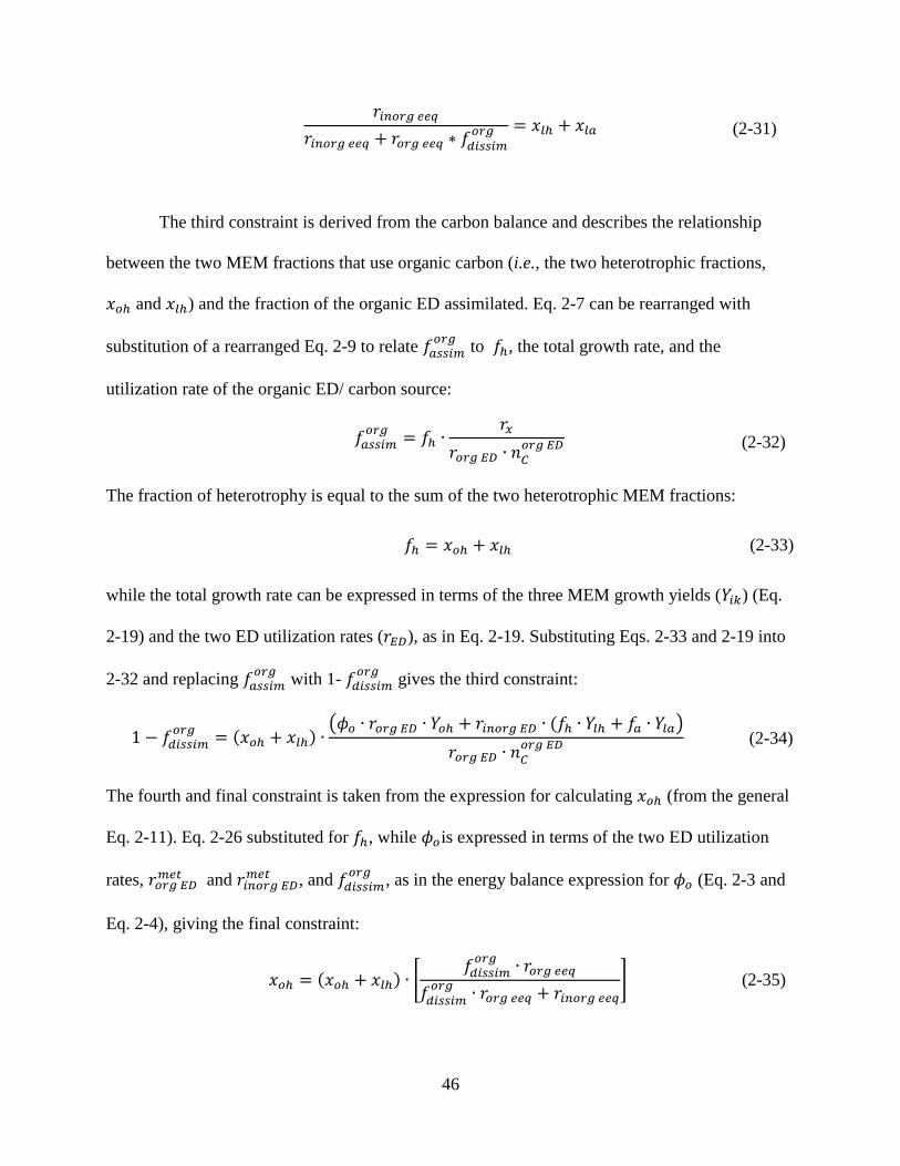
46

𝑟𝑖𝑛𝑜𝑟𝑔 𝑒𝑒𝑞

𝑟𝑖𝑛𝑜𝑟𝑔 𝑒𝑒𝑞 + 𝑟𝑜𝑟𝑔 𝑒𝑒𝑞 ∗ 𝑓𝑑𝑖𝑠𝑠𝑖𝑚𝑜𝑟𝑔 = 𝑥𝑙ℎ + 𝑥𝑙𝑎 (2-31)

The third constraint is derived from the carbon balance and describes the relationship

between the two MEM fractions that use organic carbon (i.e., the two heterotrophic fractions,

𝑥𝑜ℎ and 𝑥𝑙ℎ) and the fraction of the organic ED assimilated. Eq. 2-7 can be rearranged with

substitution of a rearranged Eq. 2-9 to relate 𝑓𝑎𝑠𝑠𝑖𝑚𝑜𝑟𝑔

to 𝑓ℎ, the total growth rate, and the

utilization rate of the organic ED/ carbon source:

𝑓𝑎𝑠𝑠𝑖𝑚𝑜𝑟𝑔

= 𝑓ℎ ∙𝑟𝑥

𝑟𝑜𝑟𝑔 𝐸𝐷 ∙ 𝑛𝐶𝑜𝑟𝑔 𝐸𝐷 (2-32)

The fraction of heterotrophy is equal to the sum of the two heterotrophic MEM fractions:

𝑓ℎ = 𝑥𝑜ℎ + 𝑥𝑙ℎ (2-33)

while the total growth rate can be expressed in terms of the three MEM growth yields (𝑌𝑖𝑘) (Eq.

2-19) and the two ED utilization rates (𝑟𝐸𝐷), as in Eq. 2-19. Substituting Eqs. 2-33 and 2-19 into

2-32 and replacing 𝑓𝑎𝑠𝑠𝑖𝑚𝑜𝑟𝑔

with 1- 𝑓𝑑𝑖𝑠𝑠𝑖𝑚𝑜𝑟𝑔

gives the third constraint:

1 − 𝑓𝑑𝑖𝑠𝑠𝑖𝑚𝑜𝑟𝑔

= (𝑥𝑜ℎ + 𝑥𝑙ℎ) ∙(𝜙𝑜 ∙ 𝑟𝑜𝑟𝑔 𝐸𝐷 ∙ 𝑌𝑜ℎ + 𝑟𝑖𝑛𝑜𝑟𝑔 𝐸𝐷 ∙ (𝑓ℎ ∙ 𝑌𝑙ℎ + 𝑓𝑎 ∙ 𝑌𝑙𝑎)

𝑟𝑜𝑟𝑔 𝐸𝐷 ∙ 𝑛𝐶𝑜𝑟𝑔 𝐸𝐷 (2-34)

The fourth and final constraint is taken from the expression for calculating 𝑥𝑜ℎ (from the general

Eq. 2-11). Eq. 2-26 substituted for 𝑓ℎ, while 𝜙𝑜is expressed in terms of the two ED utilization

rates, 𝑟𝑜𝑟𝑔 𝐸𝐷𝑚𝑒𝑡 and 𝑟𝑖𝑛𝑜𝑟𝑔 𝐸𝐷

𝑚𝑒𝑡 , and 𝑓𝑑𝑖𝑠𝑠𝑖𝑚𝑜𝑟𝑔

, as in the energy balance expression for 𝜙𝑜 (Eq. 2-3 and

Eq. 2-4), giving the final constraint:

𝑥𝑜ℎ = (𝑥𝑜ℎ + 𝑥𝑙ℎ) ∙ [𝑓𝑑𝑖𝑠𝑠𝑖𝑚

𝑜𝑟𝑔∙ 𝑟𝑜𝑟𝑔 𝑒𝑒𝑞


∙ 𝑟𝑜𝑟𝑔 𝑒𝑒𝑞 + 𝑟𝑖𝑛𝑜𝑟𝑔 𝑒𝑒𝑞

] (2-35)

47

These constraints (Eqs. 2-29, 2-31, 2-34, 2-35) describe how energy is allocated within

mixotrophic populations as a function of the utilization rates of the two EDs and the growth

yields of the three MEMs on their respective EDs.

In addition to the constraints, the solver used to implement the system of equations

allows for the specification of lower and upper bounds to the unknown variables. These bounds

describe the range of values that the solver guesses for, and therefore represent the range of

values that are possible for that variable. Values of 0 and 1 are imposed as the lower and upper

bounds, respectively, of the variables 𝑥𝑜ℎ, 𝑥𝑙ℎ, and 𝑥𝑙𝑎. As discussed in section 2.3.6, the lower

and upper bounds for the value of 𝑓𝑑𝑖𝑠𝑠𝑖𝑚𝑜𝑟𝑔

can be described using the values of 𝑌𝑜ℎ and 𝑌𝑚𝑎𝑥 of

the OH MEM calculated using the GEDYM. Therefore, for the variable 𝑓𝑑𝑖𝑠𝑠𝑖𝑚𝑜𝑟𝑔

, the lower and

upper bounds specified are 1-𝑌𝑚𝑎𝑥 and 1-𝑌𝑜ℎ. These values can both be calculated using the

GEDYM for the specific chemical conditions and organic compound.

2.4.2 Implementation

The ability of the four constraints, or the non-linear system of governing equations, to accurately

predict MEM fractions (𝑥𝑜ℎ, 𝑥𝑙ℎ, and 𝑥𝑙𝑎) and the fraction of the organic ED/carbon source

assimilated (𝑓𝑎𝑠𝑠𝑖𝑚𝑜𝑟𝑔

) were tested using the three compiled literature datasets. During computation

(see Section 2.4.3 for more details), 𝑥𝑜ℎ, 𝑥𝑙ℎ, 𝑥𝑙𝑎 and 𝑓𝑑𝑖𝑠𝑠𝑖𝑚𝑜𝑟𝑔

are the only unknowns and the rest

of the parameters are calculated as described in the previous sections. Accordingly, the values of

the net ED utilization rates (𝑟𝑜𝑟𝑔 𝐸𝐷 and 𝑟𝑖𝑛𝑜𝑟𝑔 𝐸𝐷) were determined using Eq. 2-21.

The values of 𝑌𝑜ℎ, 𝑌𝑙ℎ, and 𝑌𝑙𝑎, and the upper and lower bounds of 𝑓𝑑𝑖𝑠𝑠𝑖𝑚𝑜𝑟𝑔

were provided to the

system of equations by predicting them using GEDYM (as described in section 2.2.2 and

Appendix A).

48

2.4.3 Implementation: Matlab

I used the fmincon solver in Matlab to apply the system of equations to the datasets described in

section 2.4. fmincon is a general constrained optimization algorithm available in the MATLAB

Optimization Toolbox (MathWorks, 2016). Typically, this solver is used to minimize an

objective function that is a function of the variables being solved for, given some constraints on

the variables. In this case, it was used to solve for the non-linear system of equations, and thus no

objective function was needed since the number of constraints is equal to the number of variables

and the system of equations is completely defined. In this way, the root finding algorithms built

into fmincon were used to solve the system of equations. fmincon uses the Newton-Raphson

method as a first approach to solving the system of equations. If the Newton-Raphson method

does not work, it uses a Conjugate Gradient step method instead (MathWorks, 2016). This local

optimization method was implemented within a global search algorithm, which is also available

in the MATLAB Optimization Toolbox (MathWorks, 2016). The global search algorithm uses a

stochastic method to generate many starting points from which to run fmincon to identify which

of the local solutions is the global solution (MathWorks, 2016).

2.4.4 Comparing actual versus predicted MEMs

Figures 2-5, 2-6, and 2-7 are parity plots comparing the observed versus the predicted MEM

fractions (i.e.,xik). Agreement between the data is compared using the root mean squared error

(RMSE) which is calculated using:

𝑅𝑀𝑆𝐸 = √1

𝑁∗ ∑(𝑥𝑖𝑘,𝑝𝑟𝑒𝑑 − 𝑥𝑖𝑘,𝑜𝑏𝑠)2

𝑁

1

(2-36)

49

where 𝑥𝑖𝑘,𝑝𝑟𝑒𝑑 is the value of 𝑥𝑖𝑘 predicted by the modeling framework and 𝑥𝑖𝑘,𝑜𝑏𝑠 is the value of

𝑥𝑖𝑘 “observed” in the experimental dataset (calculated using Eq. 2-11), and N is the number of

observations/ predictions.

The solutions predict the MEM fractions relatively well, with a maximum RMSE of 0.16

when predicting the 3 MEM fractions, and of 0.30 when predicting the fraction of the organic

ED dissimilated (forgdissim) One reason for the deviation from the parity line between the observed

and predicted fractions is the experimental error that is likely to occur during the measurement

methods used to trace the carbon fixation activities. This error would be further propagated when

these measurements were used to calculate the data-derived carbon and energy balance fractions,

and subsequently, the MEM fractions.

The deviation from the parity line that is observed for the values of xik is matched by

deviation of the forgdissim value from the parity line. This is because the accuracy of the prediction

of the values of xik depends on the accuracy of predicting forgdissim, which is evident in the

governing equations. The value of forgdissim controls to what extent heterotrophy or organotrophy

occurs and therefore plays a role in predicting OH and LH, and LA indirectly since the value of

LA is codependent on the value of LH predicted (Eq. 2-31). The predicted values of xla are

systematically overpredicted for study 1 and underpredicted for study 3, which can be attributed

to the inaccurate prediction of the value of forgdissim (Figures 2-4 and 2-7). This is also matched by

the deviation of another MEM fraction other than xla, either xlh or xoh, from the parity line, since

the MEM fraction values predicted are not independent of each other. The predictions of the

growth yields, which are used in Eq. 2-34 of the governing equations, and therefore of the MEM

fractions, could be improved by more accurate geochemical data for the steady state conditions

in the chemostats, since energetics calculations using the GEDYM are very sensitive to the

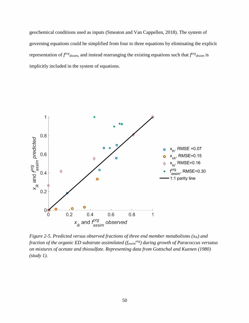
https://www.statisticshowto.datasciencecentral.com/wp-content/uploads/2016/10/root-mean-square-error.png

https://www.statisticshowto.datasciencecentral.com/wp-content/uploads/2016/10/root-mean-square-error.png

50

geochemical conditions used as inputs (Smeaton and Van Cappellen, 2018). The system of

governing equations could be simplified from four to three equations by eliminating the explicit

representation of forgdissim, and instead rearranging the existing equations such that forg

dissim is

implicitly included in the system of equations.

Figure 2-5. Predicted versus observed fractions of three end member metabolisms (xik) and

fraction of the organic ED substrate assimilated (fassimorg) during growth of Paracoccus versutus

on mixtures of acetate and thiosulfate. Representing data from Gottschal and Kuenen (1980)

(study 1).

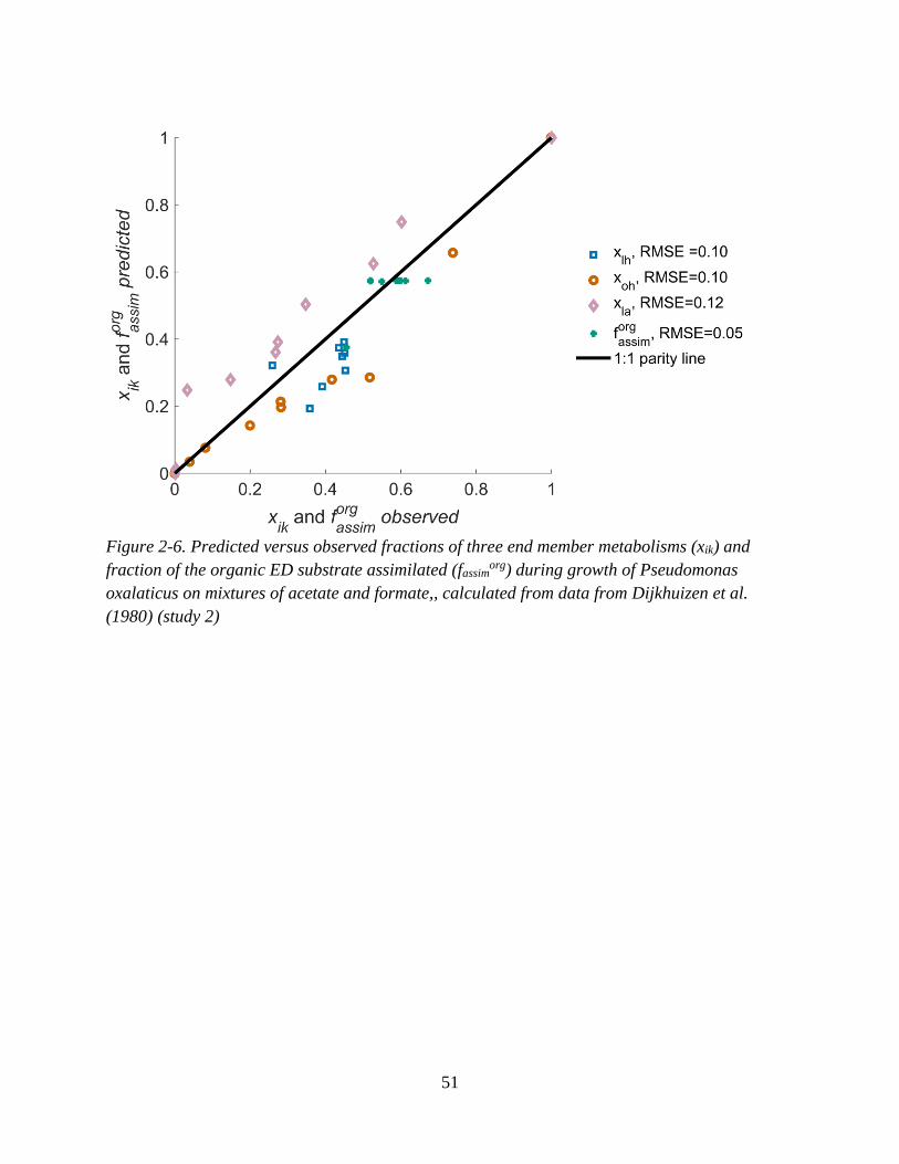
51


fraction of the organic ED substrate assimilated (fassimorg) during growth of Pseudomonas

oxalaticus on mixtures of acetate and formate,, calculated from data from Dijkhuizen et al.

(1980) (study 2)

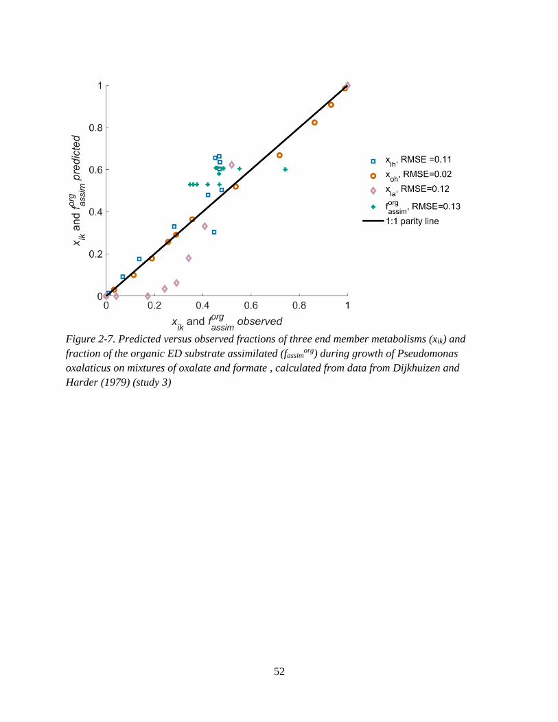
52


fraction of the organic ED substrate assimilated (fassimorg) during growth of Pseudomonas

oxalaticus on mixtures of oxalate and formate , calculated from data from Dijkhuizen and

Harder (1979) (study 3)

53

2.5 Discussion

2.5.1 Combined kinetic and energetic constraints regulate metabolic flexibility

The ability of the system of equations to predict the relative abundances of the 3 MEMs and


demonstrates that it is the combination of thermodynamic (e.g., bioenergetic) and kinetic

constraints that regulates the combination of MEMs expressed under different ED supply

scenarios. The role of the 2 ED utilization rates (𝑟𝐸𝐷) in regulating the relative proportions of the

3 MEMs is evident in the carbon and energy balance expressions that represent the constraints on

the metabolism. The utilization rates of either one of or both of the 2 EDs are present in all 4

equations. These equations work to predict the MEM fractions because the “energy available” to

an organism is primarily determined by the utilization rate of EDs, the kinetic constraints. The

system of equations describes how each of the 2 ED substrates are required by 2 MEMs, and

therefore how their utilization rates constrain whether these MEMs are possible. The second

control on the “energy available” is the energetic constraints of the growth substrates, which are

represented by the growth yields of the 3 MEMs, and the upper and lower bounds provided to the

solver for predicting the value of 𝑓𝑑𝑖𝑠𝑠𝑖𝑚𝑜𝑟𝑔

. The equations also represent the dual role of the

organic compound as an ED and carbon source using the 𝑓𝑑𝑖𝑠𝑠𝑖𝑚𝑜𝑟𝑔

variable.

2.5.2 Implications for predicting carbon and energy cycling

The system of equations predicts the expression of autotrophy versus heterotrophy, two

metabolic regimes with distinct energetic costs and growth efficiencies (i.e. growth yields). This

has significant implications for the prediction of reaction rates for carbon and other elements

associated with energy cycling in subsurface environments (Jin and Bethke, 2003).

The ability of this system of equations to predict the fractions of MEMs in ED-limited

chemostats where mixed organic and inorganic EDs are present and consumed at low

54

concentrations explains the pervasiveness of autotrophy in aquifer and other terrestrial

subsurface environments. The occurrence of autotrophy in these environments demonstrates that

subsurface communities do not necessarily rely on carbon produced at the surface by

photosynthesis for their energy or carbon (Griebler and Lueders, 2009; Probst et al., 2014;

Emerson et al., 2016). For example, inorganic carbon trends and fluxes in the Colorado River

aquifer were best reproduced when lithoautotrophy was included in the model (Arora et al.,

2017).

Therefore, predicting the occurrence of autotrophy and heterotrophy for whole

communities in real environments using the system of equations proposed here has the potential

to improve the representation of soil carbon cycling in models (Wieder et al., 2015; Bradford et

al., 2016; Buchkowski et al., 2017; Li et al., 2017). Figures 2-3 and 1-5 highlight the

significance of the LH MEM in controlling whether carbon dioxide fixation occurs, and to what

extent, when an inorganic ED is being oxidized that can be used by lithotrophic MEMs (and

when there is coincident utilization of an organic ED). LH is likely under underrepresented in

current models and should be considered when representing lithotrophy in environmental

models.

Autotrophic biomass-specific nitrate reduction rates can be ten times slower than those of

heterotrophic denitrification (based on implicit maximum rate (i.e., 𝑟𝑚𝑎𝑥 in Eq. 1-7) parameters

collected by Handley et al. (2013)) due to the differences in growth yields between the

heterotrophic and autotrophic MEMs (Figure 2-3). Consequently, omitting lithoautotrophic and

lithoheterotrophic processes from a community’s microbial reaction network would fail to

account for potential denitrification pathways and could either over- or under- predict nitrate

reduction rates. For example, including chemolithoautotrophic metabolic reactions in

55

geochemical models of the Colorado River aquifer is essential for predicting “hot spots” and hot

moments” of nitrate removal (Dwivedi et al., 2018). In section 3.3.4 of Chapter 3, I also

demonstrate the sensitivity of nitrate cycling rates to the relative abundance of autotrophic

activity.

Including these lithotrophic MEMs in reaction networks is not only important for

predicting the turnover rates of electron acceptors, but also for predicting the oxidative cycling of

reduced geochemical species (i.e., EDs). ED oxidation reactions regenerate oxidized species

which can be used as electron acceptors, closing the redox cycling of redox active elements such

as C, N, Fe and S. For example, Yabusaki et al.(2017) showed that including

chemolithoautotrophic pathways improved the predictions of S and Fe cycling in a Colorado

River aquifer model.

While in this chapter I have only demonstrated the applicability of this framework at the

population scale, I believe that the same kinetic and energetic constraints could potentially be

applied at the community scale. At this scale, the goal of applying this framework would be to

predict the relative functional abundances of metabolisms and their contributions to geochemical

rates rather than specific biological species. This is also the typical goal in trait-based and

dynamic energy allocation approaches, which this framework is similar to (Arora et al., 2015).

However, I acknowledge that representing community scale microbial processes is an ongoing

challenge due to the need to account for facilitative, predative and competitive interactions (Hug

and Co, 2018).

2.6 Conclusions

In this chapter, I present a modeling framework for predicting the competition between, and

relative contributions of, autotrophic and heterotrophic metabolisms. Literature data collected

from ED-limited chemostat studies were used to validate a system of governing equations that is

56

used to calculate the fractions of MEMs. With these equations, I show mathematically how the

relative utilization rates of the organic and inorganic ED regulate the combination of MEMs

expressed by the microorganisms grown in the chemostat experiments. Moreover, I show that the

threshold at which inorganic carbon fixation (i.e., autotrophy) is initiated is dependent on the

energy contents of the two EDs. These findings highlight the key role of the ED supply rates in

regulating autotrophy and heterotrophy in natural geomicrobial systems, as a direct consequence

of the distinct energetic costs of the two end-member metabolisms. The occurrence of

mixotrophy in the environment has important implications for the turnover of redox-active

elements including N, S, Fe, Mn, H and especially C, since the relative utilization rates of

organic versus inorganic EDs directly impacts carbon fixation versus mineralization.

57

Chapter 3

Application of a bioenergetic-kinetic model: Predicting mixotrophic

nitrate-dependent iron oxidation in a lake sediment

3.1 Introduction

Lake sediments are a large reactive interface and reservoir, acting as either a source or sink of

carbon, nutrients (e.g., phosphorus and silicon), and metals (e.g., arsenic and selenium) to the

overlying water column (Hunter et al., 1998; Pace and Prairie, 2005; Couture et al., 2010;

Omoregie et al., 2013; Liu et al., 2015; Orihel et al., 2017). Sediment biogeochemistry is

characterized by distinct vertical stratification of redox processes with depth from the sediment-

water interface (SWI) (Van Cappellen et al., 1993; Thullner et al., 2007). Consequently,

characterizing both the abiotic and biotic reactions occurring in sediments is essential for

predicting the fate of carbon, nutrients and metals.

Iron (Fe) and nitrogen (N) are especially prominent in lake sediment energy cycling since

manganese and sulfur concentrations are quite low, especially in Lake Constance, for which the

sediment geochemistry is used in this chapter to predict the occurrence of a mixotrophic

metabolism (Melton et al., 2014). Nitrate and ferric iron (Fe(III)) are used as terminal electron

acceptors for microbial respiration of organic carbon compounds in the absence of oxygen.

While these reduction reactions link both the iron Fe and N cycles to the carbon cycle in

sediments, the Fe and N cycles are directly linked by microbially mediated iron(II) (Fe2+)

oxidation coupled to nitrate (NO3-) reduction, also called nitrate dependent iron oxidation

(NDFO). This lithotrophic catabolic reaction is given by reaction 3-1:

𝐹𝑒2+ + 0.2𝑁𝑂3− + 1.4𝐻2𝑂 → 𝐹𝑒(𝑂𝐻)2

+ + 0.1𝑁2 + 0.8𝐻+ (3-1)

NDFO closes the Fe cycle in dark anoxic sediments where Fe2+ oxidation using oxygen (O2) or

by phototrophic iron oxidizers is not possible (Roden 2012).

58

Found in sediments and groundwater at neutral pH, NDFO bacteria and archaea are well

studied (Straub et al., 1996). These organisms are suspected to be mixotrophs that are capable of

coupling NO3- reduction to the oxidation of either Fe2+ or an organic ED substrate as their energy

source, and of using both inorganic and organic carbon sources (Bryce et al., 2018; Jamieson et

al., 2018). The proposed ED, EA, and C sources that would be used by the MEM reactions

during NDFO-driven mixotrophy are summarized in Table 3-1. However, the exact

mechanism(s) responsible for the net NDFO process observed in laboratory cultures, sediments

and groundwater remains unknown. It is unclear if Fe2+ oxidation is abiotic or biotic (Bryce et

al., 2018; Jamieson et al., 2018). Furthermore, should NDFO be a lithotrophic metabolism where

Fe2+ oxidation is biotic, it is unknown if all strains can grow autotrophically (Bryce et al., 2018).

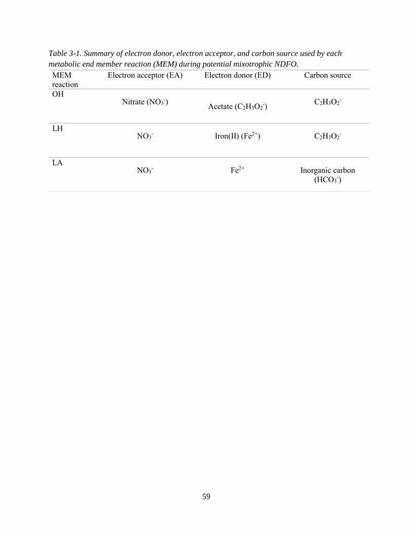
59

Table 3-1. Summary of electron donor, electron acceptor, and carbon source used by each

metabolic end member reaction (MEM) during potential mixotrophic NDFO.

MEM

reaction

Electron acceptor (EA) Electron donor (ED) Carbon source

OH Nitrate (NO3

-) Acetate (C2H3O2

-) C2H3O2

-

LH NO3

- Iron(II) (Fe2+) C2H3O2-

LA NO3

- Fe2+ Inorganic carbon

(HCO3-)

60

Evidence of the capacity for lithoheterotrophy during NDFO includes enhanced growth

of pure cultures grown with NO3- as their EA on mixtures of Fe2+ and an organic ED substrate

such as acetate (e.g., Muehe et al., 2009) over those grown on the organic ED alone (Muehe et

al., 2009; Chakraborty et al., 2011; Bryce et al., 2018). However, mechanisms that could

explain this enhanced growth that do not involve enzyme-catalyzed Fe2+ oxidation have been

proposed. One proposed mechanism is that the enzymatic reduction of NO3- reduction to nitrite

(NO2-) using an organic ED/ C source (organoheterotrophy) induces chemodenitrification, the

abiotic reduction of NO2- by Fe2+ oxidation. Chemodenitrification could confer an energetic

advantage to NDFO organisms by acting as a detoxification mechanism for dealing with nitrite

(Carlson et al., 2013). Enhanced growth could also be explained by a high demand for nutrient

iron in some organisms (Klueglein and Kappler, 2013).

Various studies have demonstrated that certain NDFO organisms may be unable to carry

out NDFO-driven lithoautotrophy (Byrne-Bailey et al., 2012; Ishii et al., 2016), while studies of

other organisms have demonstrated the opposite (Hallbeck and Pedersen, 1991; Straub et al.,

1996; Oshiki et al., 2013). The capacity for NDFO-driven lithoautotrophy is likely present in

whole communities of organisms, since it has been demonstrated in sediment incubations and

enrichment cultures (Blöthe and Roden, 2009; Laufer et al., 2016). These two unknown aspects

of NDFO (i.e., the relative contributions of biotic versus abiotic and heterotrophic versus

autotrophic reactions) are related, since organoheterotrophy-driven NO3- reduction to NO2

- and

subsequent Fe2+-driven chemodenitrification means that populations growing via that mechanism

are not capable of either lithotrophic MEMs (neither lithoheterotrophy nor lithoautotrophy).

To investigate the bioenergetic constraints on the potential mixotrophic biotic

contribution to NDFO, I apply the modeling framework developed for mixotrophy in Chapter 2,

61

representing the competition between NO3- reducing, Fe2+- or acetate- oxidizing autotrophic and

heterotrophic metabolisms in lake sediments. I apply it to literature geochemical and microbial

datasets collected in the profundal sediments of Lake Constance (Schulz and Conrad, 1995;

Melton et al., 2014). NDFO is identified as a likely mixotrophic metabolism occurring in these

sediments (Hauck et al., 2001; Muehe et al., 2009; Melton et al., 2012; Melton et al., 2014).

3.1.2 Lake Constance background

Lake Constance is a large (over 500 km2) freshwater lake located at the border of Switzerland,

Germany, and Austria at an elevation of 385 m above sea level (Altermatt et al., 2014). L.

Constance is a monomictic lake, experiencing stratified conditions between the months of May

and September, and fully mixed conditions otherwise (Wahl and Peeters, 2014). The depth of

water in the profundal zone of L. Constance ranges from 60-254 m, with a mean depth of 100 m

(Hauck et al., 2001; Wahl and Peeters, 2014). The sediment geochemistry in L. Constance is

quite well characterized. In terms of electron accepting half reactions, there are prominent O2-,

NO3--, iron(III)-, and CO2- reducing zones at different depths in L. Constance sediments (Schulz

and Conrad, 1995; Schulz and Conrad, 1996; Melton et al., 2014). In terms of electron donors,

Fe2+, NH4+, and organic acids are commonly used (with the organic acids also being used as

carbon sources) (Melton et al., 2014).

3.2 Methods

3.2.1 Geochemical dataset compilation and synthesis

Reported high resolution in situ porewater profiles of O2, NO3-, ammonium (NH4

+), and pH in

Lake Constance from Fig. 2 in Melton et al. (2014) were digitized using WebPlotDigitizer

(Rohatgi, 2019). Concentrations of poorly crystalline (0.5 M HCl extractions) and crystalline

solid phase Fe2+ and Fe3+ (6 M HCl extractions) with depth were digitized from Fig. 3, MPN

counts were taken from Table 1, and functional gene copy numbers were digitized from Fig. 8 in

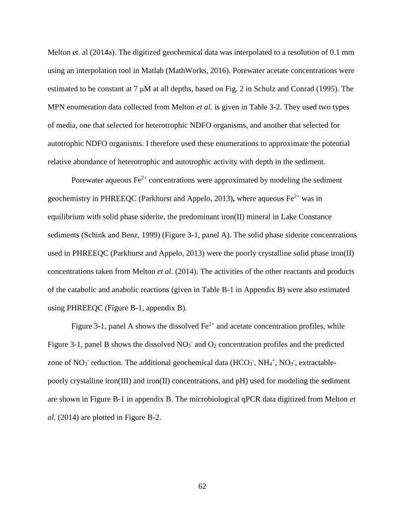
62

Melton et. al (2014a). The digitized geochemical data was interpolated to a resolution of 0.1 mm

using an interpolation tool in Matlab (MathWorks, 2016). Porewater acetate concentrations were

estimated to be constant at 7 μM at all depths, based on Fig. 2 in Schulz and Conrad (1995). The

MPN enumeration data collected from Melton et al. is given in Table 3-2. They used two types

of media, one that selected for heterotrophic NDFO organisms, and another that selected for

autotrophic NDFO organisms. I therefore used these enumerations to approximate the potential

relative abundance of heterotrophic and autotrophic activity with depth in the sediment.

Porewater aqueous Fe2+ concentrations were approximated by modeling the sediment

geochemistry in PHREEQC (Parkhurst and Appelo, 2013), where aqueous Fe2+ was in

equilibrium with solid phase siderite, the predominant iron(II) mineral in Lake Constance

sediments (Schink and Benz, 1999) (Figure 3-1, panel A). The solid phase siderite concentrations

used in PHREEQC (Parkhurst and Appelo, 2013) were the poorly crystalline solid phase iron(II)

concentrations taken from Melton et al. (2014). The activities of the other reactants and products

of the catabolic and anabolic reactions (given in Table B-1 in Appendix B) were also estimated

using PHREEQC (Figure B-1, appendix B).

Figure 3-1, panel A shows the dissolved Fe2+ and acetate concentration profiles, while

Figure 3-1, panel B shows the dissolved NO3- and O2 concentration profiles and the predicted

zone of NO3- reduction. The additional geochemical data (HCO3

-, NH4+, NO3

-, extractable-

poorly crystalline iron(III) and iron(II) concentrations, and pH) used for modeling the sediment

are shown in Figure B-1 in appendix B. The microbiological qPCR data digitized from Melton et

al. (2014) are plotted in Figure B-2.

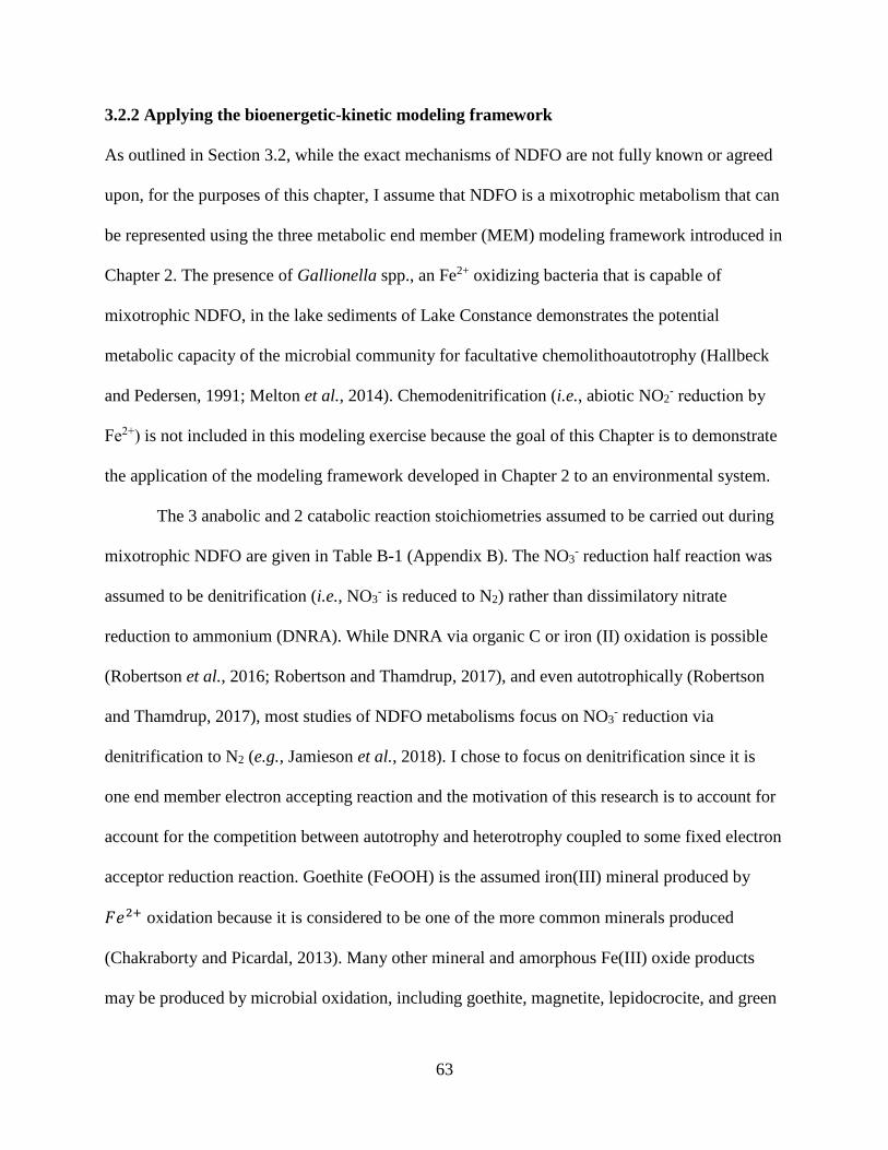
63

3.2.2 Applying the bioenergetic-kinetic modeling framework

As outlined in Section 3.2, while the exact mechanisms of NDFO are not fully known or agreed

upon, for the purposes of this chapter, I assume that NDFO is a mixotrophic metabolism that can

be represented using the three metabolic end member (MEM) modeling framework introduced in

Chapter 2. The presence of Gallionella spp., an Fe2+ oxidizing bacteria that is capable of

mixotrophic NDFO, in the lake sediments of Lake Constance demonstrates the potential

metabolic capacity of the microbial community for facultative chemolithoautotrophy (Hallbeck

and Pedersen, 1991; Melton et al., 2014). Chemodenitrification (i.e., abiotic NO2- reduction by

Fe2+) is not included in this modeling exercise because the goal of this Chapter is to demonstrate

the application of the modeling framework developed in Chapter 2 to an environmental system.

The 3 anabolic and 2 catabolic reaction stoichiometries assumed to be carried out during

mixotrophic NDFO are given in Table B-1 (Appendix B). The NO3- reduction half reaction was

assumed to be denitrification (i.e., NO3- is reduced to N2) rather than dissimilatory nitrate

reduction to ammonium (DNRA). While DNRA via organic C or iron (II) oxidation is possible

(Robertson et al., 2016; Robertson and Thamdrup, 2017), and even autotrophically (Robertson

and Thamdrup, 2017), most studies of NDFO metabolisms focus on NO3- reduction via

denitrification to N2 (e.g., Jamieson et al., 2018). I chose to focus on denitrification since it is

one end member electron accepting reaction and the motivation of this research is to account for

account for the competition between autotrophy and heterotrophy coupled to some fixed electron

acceptor reduction reaction. Goethite (FeOOH) is the assumed iron(III) mineral produced by

𝐹𝑒2+ oxidation because it is considered to be one of the more common minerals produced

(Chakraborty and Picardal, 2013). Many other mineral and amorphous Fe(III) oxide products

may be produced by microbial oxidation, including goethite, magnetite, lepidocrocite, and green

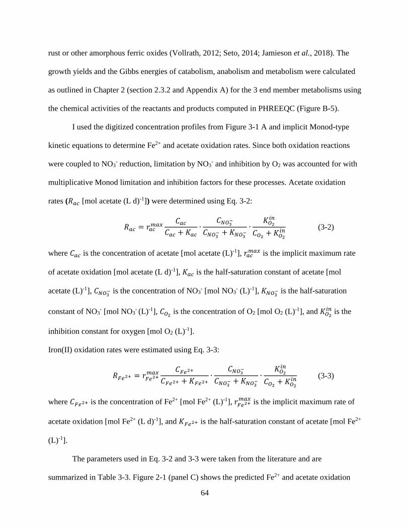
64

rust or other amorphous ferric oxides (Vollrath, 2012; Seto, 2014; Jamieson et al., 2018). The

growth yields and the Gibbs energies of catabolism, anabolism and metabolism were calculated

as outlined in Chapter 2 (section 2.3.2 and Appendix A) for the 3 end member metabolisms using

the chemical activities of the reactants and products computed in PHREEQC (Figure B-5).

I used the digitized concentration profiles from Figure 3-1 A and implicit Monod-type

kinetic equations to determine Fe2+ and acetate oxidation rates. Since both oxidation reactions

were coupled to NO3- reduction, limitation by NO3

- and inhibition by O2 was accounted for with

multiplicative Monod limitation and inhibition factors for these processes. Acetate oxidation

rates (𝑅𝑎𝑐 [mol acetate (L d)-1]) were determined using Eq. 3-2:

𝑅𝑎𝑐 = 𝑟𝑎𝑐𝑚𝑎𝑥

𝐶𝑎𝑐

𝐶𝑎𝑐 + 𝐾𝑎𝑐∙

𝐶𝑁𝑂3−

𝐶𝑁𝑂3− + 𝐾𝑁𝑂3

−∙

𝐾𝑂2

𝑖𝑛

𝐶𝑂2+ 𝐾𝑂2

𝑖𝑛 (3-2)

where 𝐶𝑎𝑐 is the concentration of acetate [mol acetate (L)-1], 𝑟𝑎𝑐𝑚𝑎𝑥 is the implicit maximum rate

of acetate oxidation [mol acetate (L d)-1], 𝐾𝑎𝑐 is the half-saturation constant of acetate [mol

acetate (L)-1], 𝐶𝑁𝑂3− is the concentration of NO3

- [mol NO3- (L)-1], 𝐾𝑁𝑂3

− is the half-saturation

constant of NO3- [mol NO3

- (L)-1], 𝐶𝑂2 is the concentration of O2 [mol O2 (L)-1], and 𝐾𝑂2

𝑖𝑛 is the

inhibition constant for oxygen [mol O2 (L)-1].

Iron(II) oxidation rates were estimated using Eq. 3-3:

𝑅𝐹𝑒2+ = 𝑟𝐹𝑒2+𝑚𝑎𝑥 𝐶𝐹𝑒2+

𝐶𝐹𝑒2+ + 𝐾𝐹𝑒2+∙

𝐶𝑁𝑂3−

𝐶𝑁𝑂3− + 𝐾𝑁𝑂3

−∙

𝐾𝑂2

𝑖𝑛

𝐶𝑂2+ 𝐾𝑂2

𝑖𝑛 (3-3)

where 𝐶𝐹𝑒2+ is the concentration of Fe2+ [mol Fe2+ (L)-1], 𝑟𝐹𝑒2+𝑚𝑎𝑥 is the implicit maximum rate of

acetate oxidation [mol Fe2+ (L d)-1], and 𝐾𝐹𝑒2+ is the half-saturation constant of acetate [mol Fe2+

(L)-1].

The parameters used in Eq. 3-2 and 3-3 were taken from the literature and are

summarized in Table 3-3. Figure 2-1 (panel C) shows the predicted Fe2+ and acetate oxidation

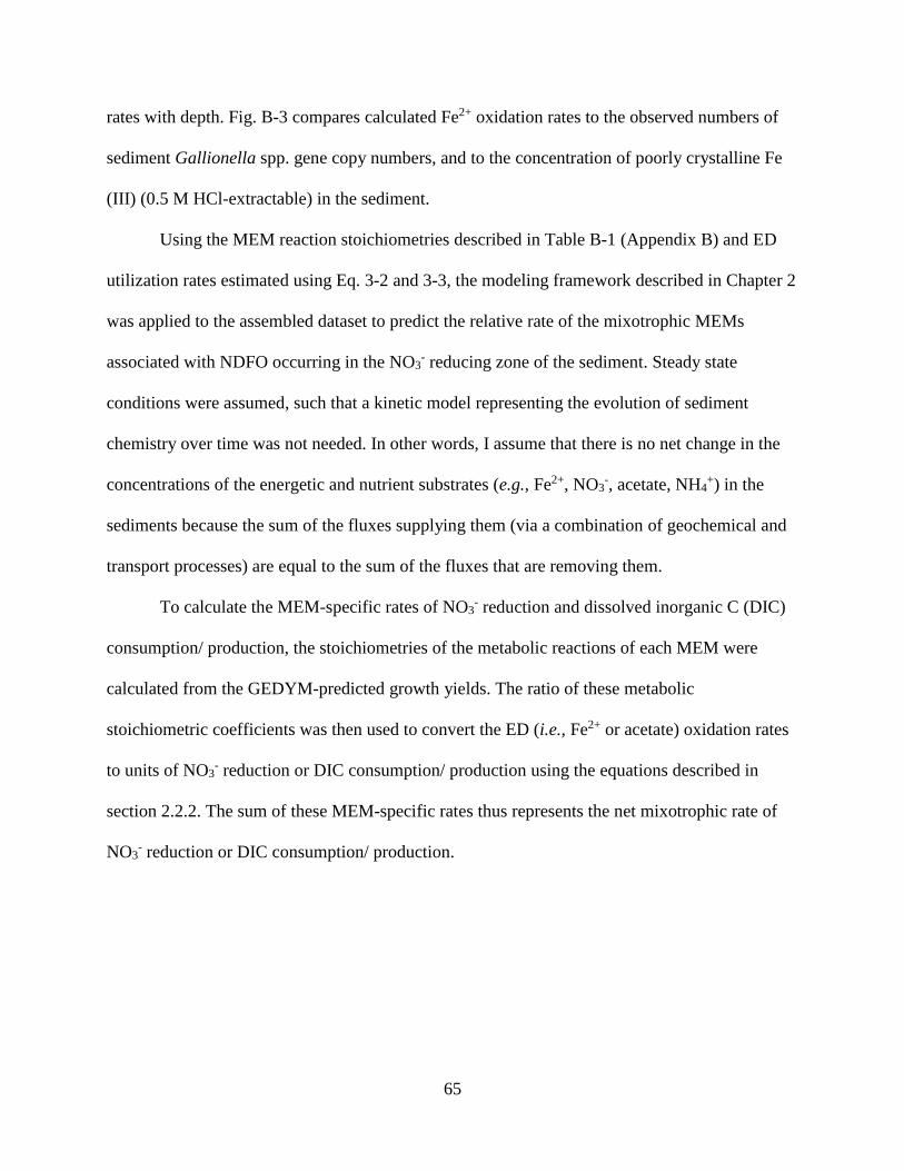
65

rates with depth. Fig. B-3 compares calculated Fe2+ oxidation rates to the observed numbers of

sediment Gallionella spp. gene copy numbers, and to the concentration of poorly crystalline Fe

(III) (0.5 M HCl-extractable) in the sediment.

Using the MEM reaction stoichiometries described in Table B-1 (Appendix B) and ED

utilization rates estimated using Eq. 3-2 and 3-3, the modeling framework described in Chapter 2

was applied to the assembled dataset to predict the relative rate of the mixotrophic MEMs

associated with NDFO occurring in the NO3- reducing zone of the sediment. Steady state

conditions were assumed, such that a kinetic model representing the evolution of sediment

chemistry over time was not needed. In other words, I assume that there is no net change in the

concentrations of the energetic and nutrient substrates (e.g., Fe2+, NO3-, acetate, NH4

+) in the

sediments because the sum of the fluxes supplying them (via a combination of geochemical and

transport processes) are equal to the sum of the fluxes that are removing them.

To calculate the MEM-specific rates of NO3- reduction and dissolved inorganic C (DIC)

consumption/ production, the stoichiometries of the metabolic reactions of each MEM were

calculated from the GEDYM-predicted growth yields. The ratio of these metabolic

stoichiometric coefficients was then used to convert the ED (i.e., Fe2+ or acetate) oxidation rates

to units of NO3- reduction or DIC consumption/ production using the equations described in

section 2.2.2. The sum of these MEM-specific rates thus represents the net mixotrophic rate of

NO3- reduction or DIC consumption/ production.

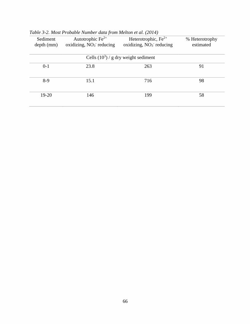
66

Table 3-2. Most Probable Number data from Melton et al. (2014)

Sediment

depth (mm)

Autotrophic Fe2+

oxidizing, NO3- reducing

Heterotrophic, Fe2+

oxidizing, NO3- reducing

% Heterotrophy

estimated

Cells (103) / g dry weight sediment

0-1 23.8 263 91

8-9 15.1 716 98

19-20 146 199 58

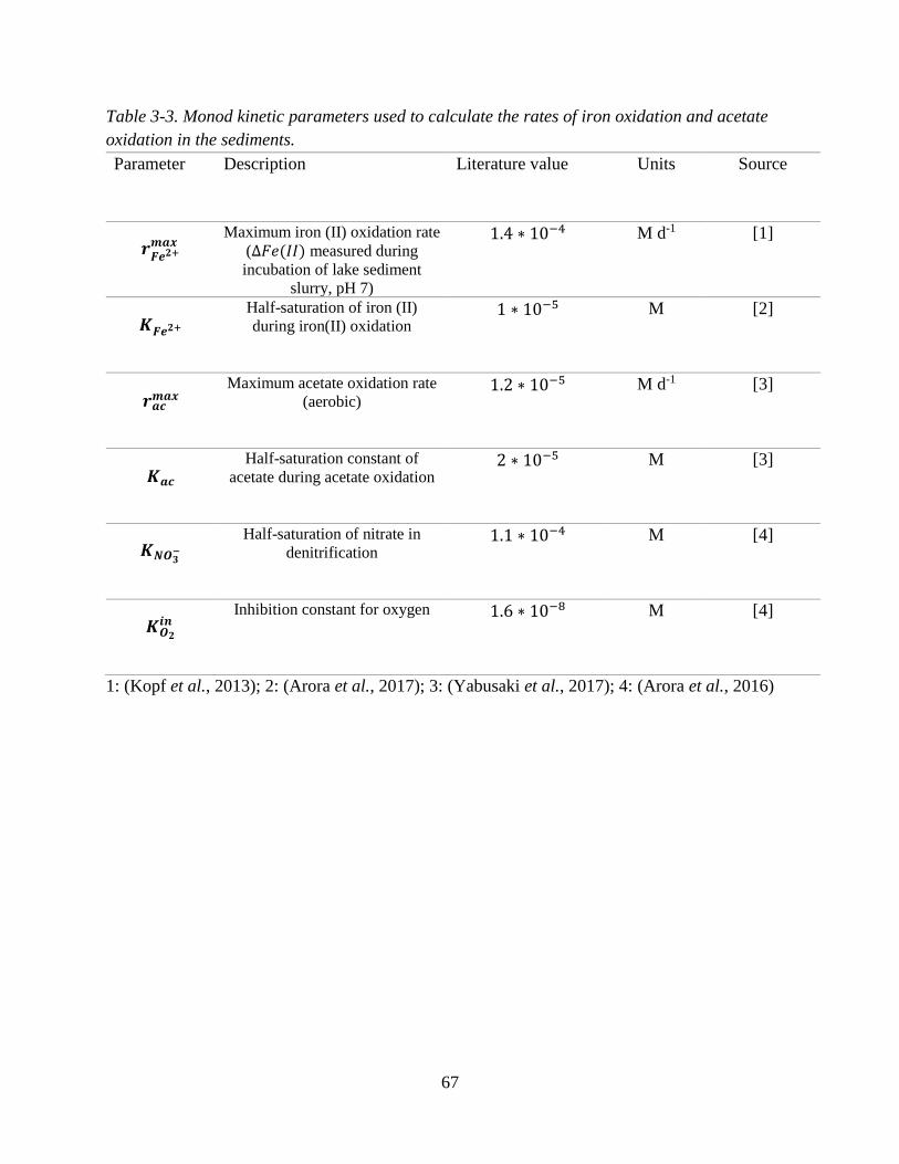
67

Table 3-3. Monod kinetic parameters used to calculate the rates of iron oxidation and acetate

oxidation in the sediments.

Parameter Description Literature value Units Source

𝒓𝑭𝒆𝟐+𝒎𝒂𝒙

Maximum iron (II) oxidation rate

(∆𝐹𝑒(𝐼𝐼) measured during

incubation of lake sediment

slurry, pH 7)

1.4 ∗ 10−4 M d-1 [1]

𝑲𝑭𝒆𝟐+ Half-saturation of iron (II)

during iron(II) oxidation 1 ∗ 10−5 M [2]

𝒓𝒂𝒄𝒎𝒂𝒙

Maximum acetate oxidation rate

(aerobic) 1.2 ∗ 10−5 M d-1 [3]

𝑲𝒂𝒄 Half-saturation constant of

acetate during acetate oxidation 2 ∗ 10−5 M [3]

𝑲𝑵𝑶𝟑−

Half-saturation of nitrate in

denitrification 1.1 ∗ 10−4 M [4]

𝑲𝑶𝟐

𝒊𝒏 Inhibition constant for oxygen 1.6 ∗ 10−8 M [4]

1: (Kopf et al., 2013); 2: (Arora et al., 2017); 3: (Yabusaki et al., 2017); 4: (Arora et al., 2016)

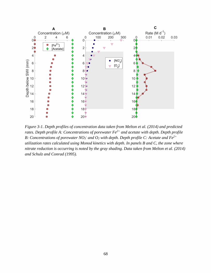
68

Figure 3-1. Depth profiles of concentration data taken from Melton et al. (2014) and predicted

rates. Depth profile A: Concentrations of porewater Fe2+ and acetate with depth. Depth profile

B: Concentrations of porewater NO3- and O2 with depth. Depth profile C: Acetate and Fe2+

utilization rates calculated using Monod kinetics with depth. In panels B and C, the zone where

nitrate reduction is occurring is noted by the gray shading. Data taken from Melton et al. (2014)

and Schulz and Conrad (1995).

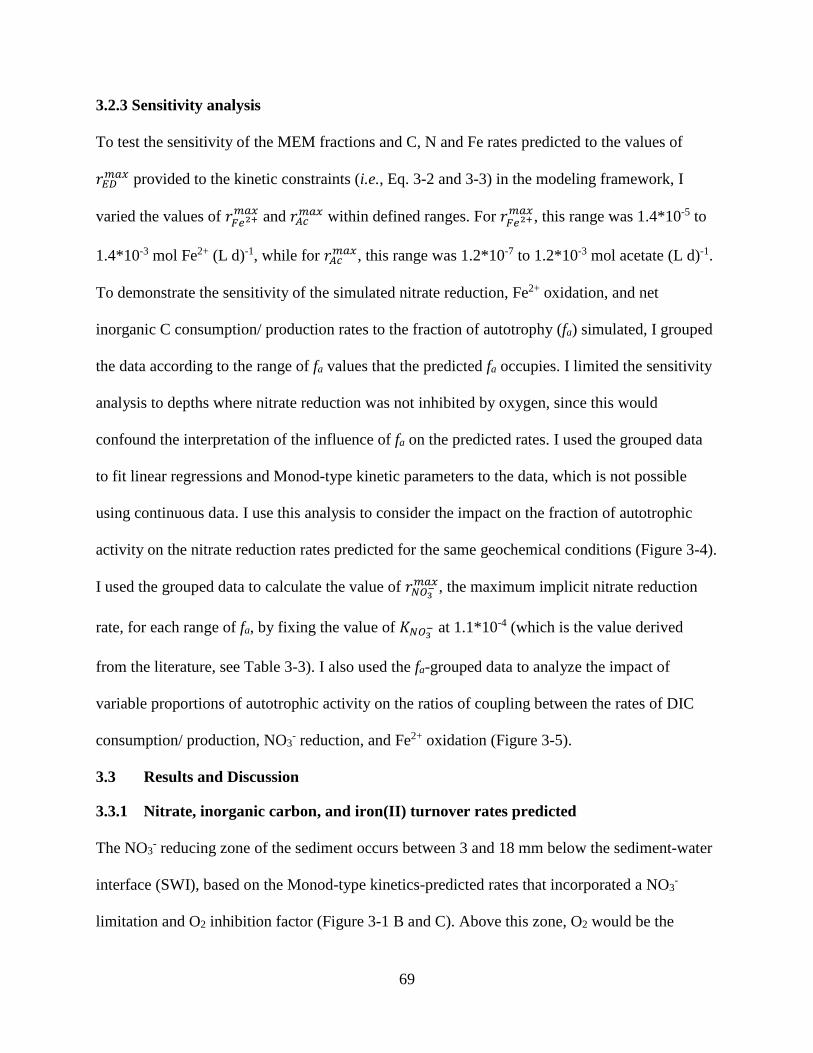
69

3.2.3 Sensitivity analysis

To test the sensitivity of the MEM fractions and C, N and Fe rates predicted to the values of

𝑟𝐸𝐷𝑚𝑎𝑥 provided to the kinetic constraints (i.e., Eq. 3-2 and 3-3) in the modeling framework, I

varied the values of 𝑟𝐹𝑒2+𝑚𝑎𝑥 and 𝑟𝐴𝑐

𝑚𝑎𝑥 within defined ranges. For 𝑟𝐹𝑒2+𝑚𝑎𝑥, this range was 1.4*10-5 to

1.4*10-3 mol Fe2+ (L d)-1, while for 𝑟𝐴𝑐𝑚𝑎𝑥, this range was 1.2*10-7 to 1.2*10-3 mol acetate (L d)-1.

To demonstrate the sensitivity of the simulated nitrate reduction, Fe2+ oxidation, and net

inorganic C consumption/ production rates to the fraction of autotrophy (fa) simulated, I grouped

the data according to the range of fa values that the predicted fa occupies. I limited the sensitivity

analysis to depths where nitrate reduction was not inhibited by oxygen, since this would

confound the interpretation of the influence of fa on the predicted rates. I used the grouped data

to fit linear regressions and Monod-type kinetic parameters to the data, which is not possible

using continuous data. I use this analysis to consider the impact on the fraction of autotrophic

activity on the nitrate reduction rates predicted for the same geochemical conditions (Figure 3-4).

I used the grouped data to calculate the value of 𝑟𝑁𝑂3−

𝑚𝑎𝑥, the maximum implicit nitrate reduction

rate, for each range of fa, by fixing the value of 𝐾𝑁𝑂3− at 1.1*10-4 (which is the value derived

from the literature, see Table 3-3). I also used the fa-grouped data to analyze the impact of

variable proportions of autotrophic activity on the ratios of coupling between the rates of DIC

consumption/ production, NO3- reduction, and Fe2+ oxidation (Figure 3-5).

3.3 Results and Discussion

3.3.1 Nitrate, inorganic carbon, and iron(II) turnover rates predicted

The NO3- reducing zone of the sediment occurs between 3 and 18 mm below the sediment-water

interface (SWI), based on the Monod-type kinetics-predicted rates that incorporated a NO3-

limitation and O2 inhibition factor (Figure 3-1 B and C). Above this zone, O2 would be the

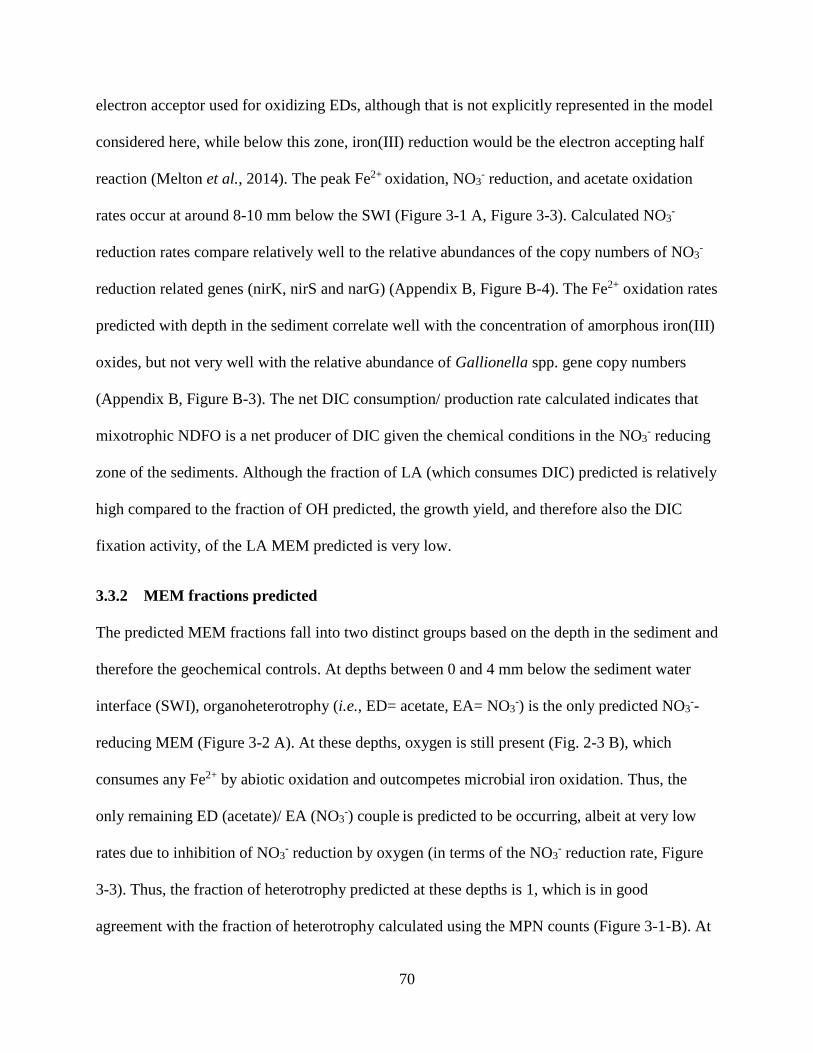
70

electron acceptor used for oxidizing EDs, although that is not explicitly represented in the model

considered here, while below this zone, iron(III) reduction would be the electron accepting half

reaction (Melton et al., 2014). The peak Fe2+ oxidation, NO3- reduction, and acetate oxidation

rates occur at around 8-10 mm below the SWI (Figure 3-1 A, Figure 3-3). Calculated NO3-

reduction rates compare relatively well to the relative abundances of the copy numbers of NO3-

reduction related genes (nirK, nirS and narG) (Appendix B, Figure B-4). The Fe2+ oxidation rates

predicted with depth in the sediment correlate well with the concentration of amorphous iron(III)

oxides, but not very well with the relative abundance of Gallionella spp. gene copy numbers

(Appendix B, Figure B-3). The net DIC consumption/ production rate calculated indicates that

mixotrophic NDFO is a net producer of DIC given the chemical conditions in the NO3- reducing

zone of the sediments. Although the fraction of LA (which consumes DIC) predicted is relatively

high compared to the fraction of OH predicted, the growth yield, and therefore also the DIC

fixation activity, of the LA MEM predicted is very low.

3.3.2 MEM fractions predicted

The predicted MEM fractions fall into two distinct groups based on the depth in the sediment and

therefore the geochemical controls. At depths between 0 and 4 mm below the sediment water

interface (SWI), organoheterotrophy (i.e., ED= acetate, EA= NO3-) is the only predicted NO3

--

reducing MEM (Figure 3-2 A). At these depths, oxygen is still present (Fig. 2-3 B), which

consumes any Fe2+ by abiotic oxidation and outcompetes microbial iron oxidation. Thus, the

only remaining ED (acetate)/ EA (NO3-) couple is predicted to be occurring, albeit at very low

rates due to inhibition of NO3- reduction by oxygen (in terms of the NO3

- reduction rate, Figure

3-3). Thus, the fraction of heterotrophy predicted at these depths is 1, which is in good

agreement with the fraction of heterotrophy calculated using the MPN counts (Figure 3-1-B). At

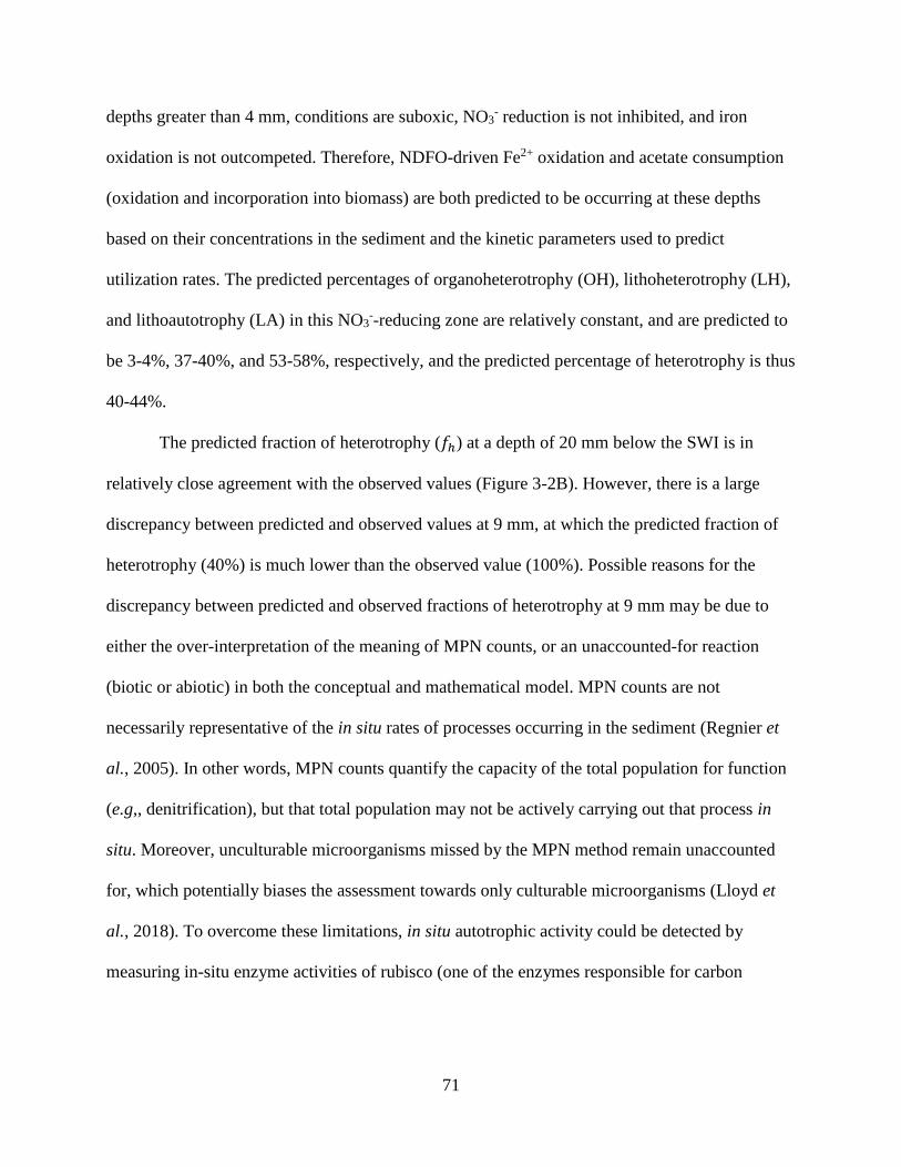
71

depths greater than 4 mm, conditions are suboxic, NO3- reduction is not inhibited, and iron

oxidation is not outcompeted. Therefore, NDFO-driven Fe2+ oxidation and acetate consumption

(oxidation and incorporation into biomass) are both predicted to be occurring at these depths

based on their concentrations in the sediment and the kinetic parameters used to predict

utilization rates. The predicted percentages of organoheterotrophy (OH), lithoheterotrophy (LH),

and lithoautotrophy (LA) in this NO3--reducing zone are relatively constant, and are predicted to

be 3-4%, 37-40%, and 53-58%, respectively, and the predicted percentage of heterotrophy is thus

40-44%.

The predicted fraction of heterotrophy (𝑓ℎ) at a depth of 20 mm below the SWI is in

relatively close agreement with the observed values (Figure 3-2B). However, there is a large

discrepancy between predicted and observed values at 9 mm, at which the predicted fraction of

heterotrophy (40%) is much lower than the observed value (100%). Possible reasons for the

discrepancy between predicted and observed fractions of heterotrophy at 9 mm may be due to

either the over-interpretation of the meaning of MPN counts, or an unaccounted-for reaction

(biotic or abiotic) in both the conceptual and mathematical model. MPN counts are not

necessarily representative of the in situ rates of processes occurring in the sediment (Regnier et

al., 2005). In other words, MPN counts quantify the capacity of the total population for function

(e.g,, denitrification), but that total population may not be actively carrying out that process in

situ. Moreover, unculturable microorganisms missed by the MPN method remain unaccounted

for, which potentially biases the assessment towards only culturable microorganisms (Lloyd et

al., 2018). To overcome these limitations, in situ autotrophic activity could be detected by

measuring in-situ enzyme activities of rubisco (one of the enzymes responsible for carbon

72

fixation, e.g., Kellermann et al. (2012)), by omics methods (e.g., Probst et al. (2017)), or by

stable isotope fractionation (e.g., Preuß et al. (1989)).

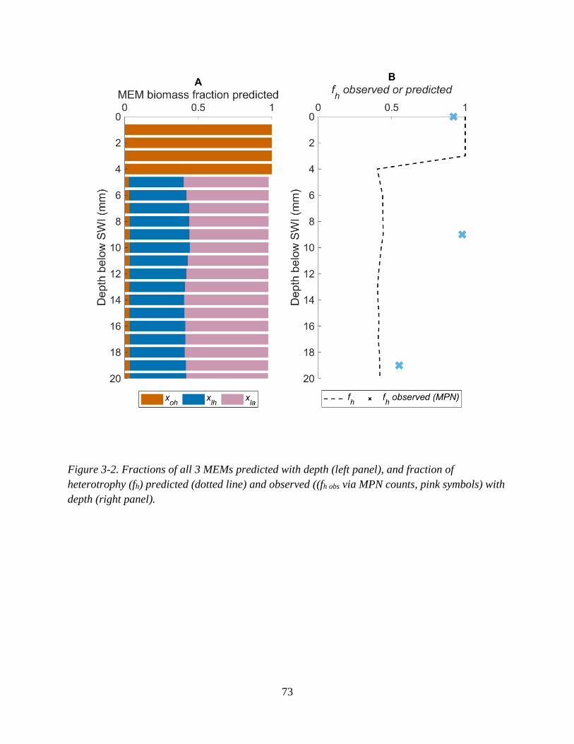
73

Figure 3-2. Fractions of all 3 MEMs predicted with depth (left panel), and fraction of

heterotrophy (fh) predicted (dotted line) and observed ((fh obs via MPN counts, pink symbols) with

depth (right panel).

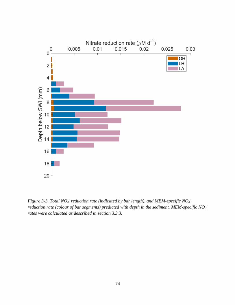
74

Figure 3-3. Total NO3- reduction rate (indicated by bar length), and MEM-specific NO3

-

reduction rate (colour of bar segments) predicted with depth in the sediment. MEM-specific NO3-

rates were calculated as described in section 3.3.3.

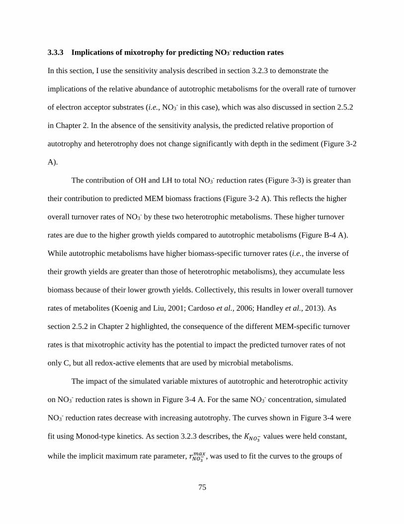
75

3.3.3 Implications of mixotrophy for predicting NO3- reduction rates

In this section, I use the sensitivity analysis described in section 3.2.3 to demonstrate the

implications of the relative abundance of autotrophic metabolisms for the overall rate of turnover

of electron acceptor substrates (i.e., NO3- in this case), which was also discussed in section 2.5.2

in Chapter 2. In the absence of the sensitivity analysis, the predicted relative proportion of

autotrophy and heterotrophy does not change significantly with depth in the sediment (Figure 3-2

A).

The contribution of OH and LH to total NO3- reduction rates (Figure 3-3) is greater than

their contribution to predicted MEM biomass fractions (Figure 3-2 A). This reflects the higher

overall turnover rates of NO3- by these two heterotrophic metabolisms. These higher turnover

rates are due to the higher growth yields compared to autotrophic metabolisms (Figure B-4 A).

While autotrophic metabolisms have higher biomass-specific turnover rates (i.e., the inverse of

their growth yields are greater than those of heterotrophic metabolisms), they accumulate less

biomass because of their lower growth yields. Collectively, this results in lower overall turnover

rates of metabolites (Koenig and Liu, 2001; Cardoso et al., 2006; Handley et al., 2013). As

section 2.5.2 in Chapter 2 highlighted, the consequence of the different MEM-specific turnover

rates is that mixotrophic activity has the potential to impact the predicted turnover rates of not

only C, but all redox-active elements that are used by microbial metabolisms.

The impact of the simulated variable mixtures of autotrophic and heterotrophic activity

on NO3- reduction rates is shown in Figure 3-4 A. For the same NO3

- concentration, simulated

NO3- reduction rates decrease with increasing autotrophy. The curves shown in Figure 3-4 were

fit using Monod-type kinetics. As section 3.2.3 describes, the 𝐾𝑁𝑂3− values were held constant,

while the implicit maximum rate parameter, 𝑟𝑁𝑂3−

𝑚𝑎𝑥, was used to fit the curves to the groups of

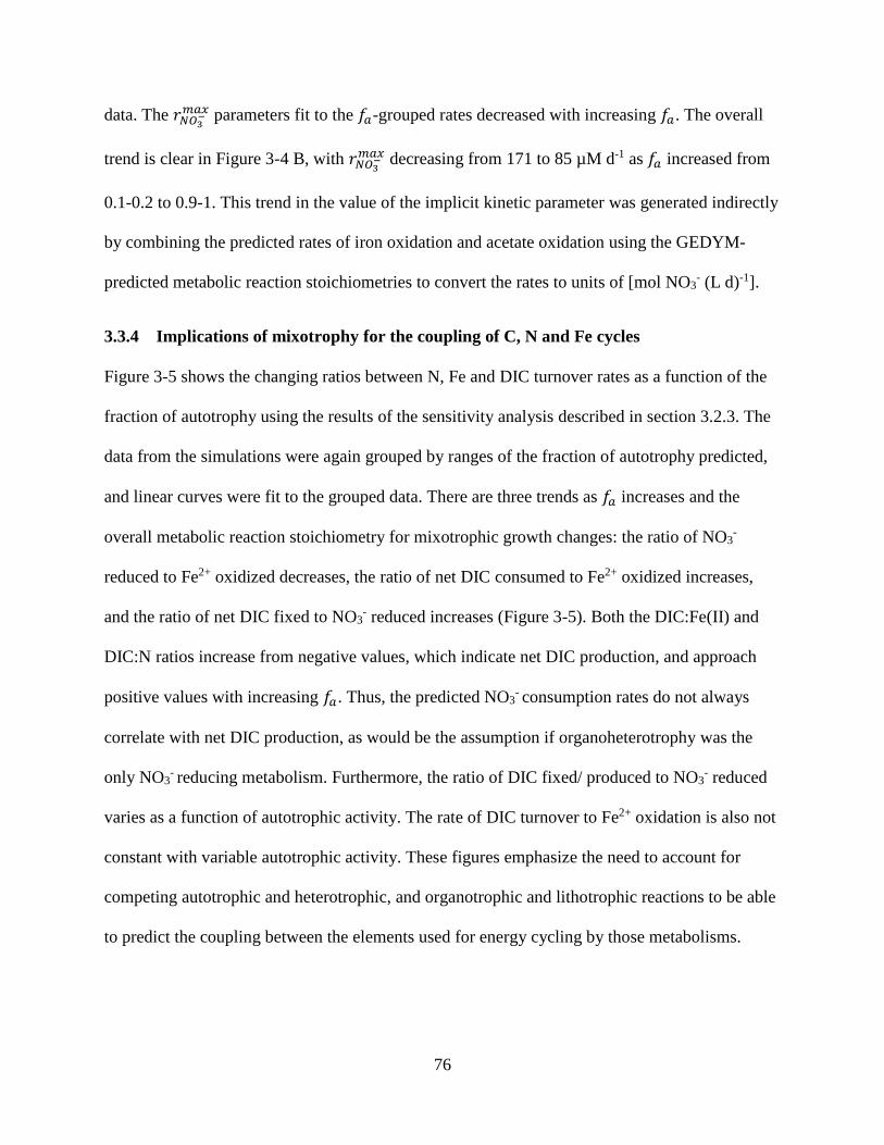
76

data. The 𝑟𝑁𝑂3−

𝑚𝑎𝑥 parameters fit to the 𝑓𝑎-grouped rates decreased with increasing 𝑓𝑎. The overall

trend is clear in Figure 3-4 B, with 𝑟𝑁𝑂3−

𝑚𝑎𝑥 decreasing from 171 to 85 µM d-1 as 𝑓𝑎 increased from

0.1-0.2 to 0.9-1. This trend in the value of the implicit kinetic parameter was generated indirectly

by combining the predicted rates of iron oxidation and acetate oxidation using the GEDYM-

predicted metabolic reaction stoichiometries to convert the rates to units of [mol NO3- (L d)-1].

3.3.4 Implications of mixotrophy for the coupling of C, N and Fe cycles

Figure 3-5 shows the changing ratios between N, Fe and DIC turnover rates as a function of the

fraction of autotrophy using the results of the sensitivity analysis described in section 3.2.3. The

data from the simulations were again grouped by ranges of the fraction of autotrophy predicted,

and linear curves were fit to the grouped data. There are three trends as 𝑓𝑎 increases and the

overall metabolic reaction stoichiometry for mixotrophic growth changes: the ratio of NO3-

reduced to Fe2+ oxidized decreases, the ratio of net DIC consumed to Fe2+ oxidized increases,

and the ratio of net DIC fixed to NO3- reduced increases (Figure 3-5). Both the DIC:Fe(II) and

DIC:N ratios increase from negative values, which indicate net DIC production, and approach

positive values with increasing 𝑓𝑎. Thus, the predicted NO3- consumption rates do not always

correlate with net DIC production, as would be the assumption if organoheterotrophy was the

only NO3- reducing metabolism. Furthermore, the ratio of DIC fixed/ produced to NO3

- reduced

varies as a function of autotrophic activity. The rate of DIC turnover to Fe2+ oxidation is also not

constant with variable autotrophic activity. These figures emphasize the need to account for

competing autotrophic and heterotrophic, and organotrophic and lithotrophic reactions to be able

to predict the coupling between the elements used for energy cycling by those metabolisms.

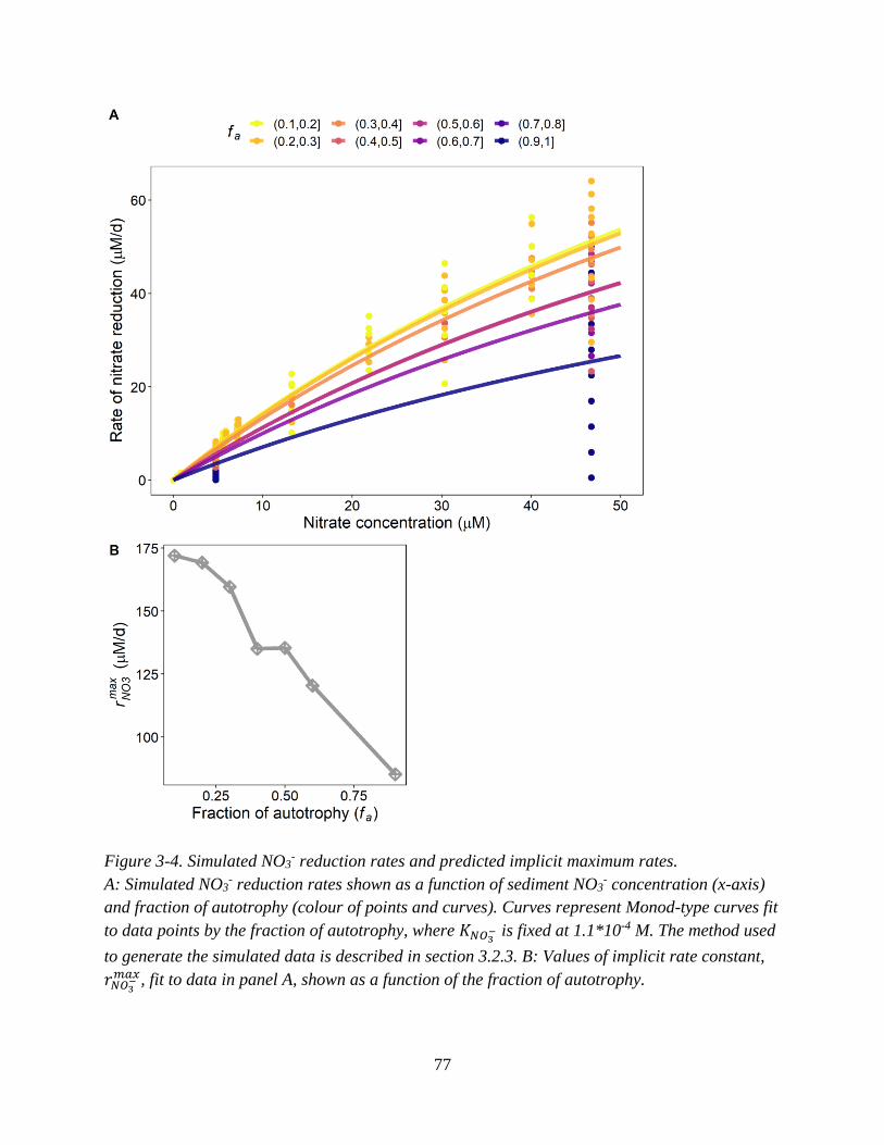
77

Figure 3-4. Simulated NO3- reduction rates and predicted implicit maximum rates.

A: Simulated NO3- reduction rates shown as a function of sediment NO3

- concentration (x-axis)

and fraction of autotrophy (colour of points and curves). Curves represent Monod-type curves fit

to data points by the fraction of autotrophy, where 𝐾𝑁𝑂3− is fixed at 1.1*10-4 M. The method used

to generate the simulated data is described in section 3.2.3. B: Values of implicit rate constant,

𝑟𝑁𝑂3−

𝑚𝑎𝑥, fit to data in panel A, shown as a function of the fraction of autotrophy.

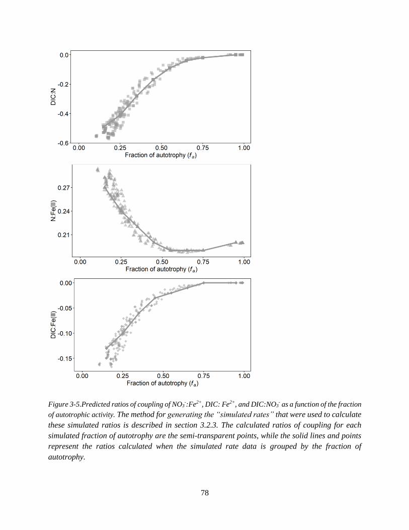
78

Figure 3-5.Predicted ratios of coupling of NO3-:Fe2+, DIC: Fe2+, and DIC:NO3

- as a function of the fraction

of autotrophic activity. The method for generating the “simulated rates” that were used to calculate

these simulated ratios is described in section 3.2.3. The calculated ratios of coupling for each

simulated fraction of autotrophy are the semi-transparent points, while the solid lines and points

represent the ratios calculated when the simulated rate data is grouped by the fraction of

autotrophy.

79

3.3.5 Limitations of the modeling approach

For the purposes of demonstrating the application of the modeling framework developed

in Chapter 2, the scope of sediment biogeochemical processes that are represented is limited

compared to what occurs in natural sediments. Many other microbially controlled reactions that

impact C, Fe, and N cycling directly and indirectly occur in sediments including NH4+ oxidation,

sulfide oxidation, and/ or acetate (or other organic acid) oxidation, coupled to iron(III) reduction,

sulfate reduction, and/ or O2 reduction. The C, N and Fe balances calculated represent only the

processes that are predicted to be occurring in the NO3- reducing zone of the sediment. In Lake

Constance, mixotrophic NH4+ oxidation coupled to iron(III) reduction is likely present below the

zone of NO3- reduction (Melton et al., 2014). In the oxic zone of the sediment, microaerophilic

mixotrophic or autotrophic metabolisms such as sulfide oxidation are possible, as are

photoautotrophic metabolisms such as phototrophic iron oxidation (Geelhoed et al., 2009;

Melton et al., 2012). Mineral precipitation and dissolution reactions (e.g., pyrite dissolution and

precipitation) or abiotic reactions (e.g. chemodenitrification, sulfide oxidation by O2) are also not

represented.

Other limitations to the modeling approach are related to the lack of fundamental

knowledge regarding the energetics and stoichiometries of microbial Fe2+ oxidation and NO3-

reduction reactions. A largely unknown aspect of the bioenergetics of Fe2+ oxidation is what

chemical species of Fe2+ organisms interact with in terms of both the Fe2+ species used as the

reactant and the Fe3+ species generated as the oxidation product (Bird et al., 2011). The

speciation of Fe2+ and Fe3+ can impact both the kinetic and the energetic constraints. In aqueous

solutions, Fe2+ can be present as free Fe2+ ions, or in carbonate or hydroxide complexes (Whitney

King, 1998; Jolivet et al., 2004). In lake sediments, Fe2+ could be chelated by organic acids such

80

as citrate and humic acids, which are present at low concentrations (Peng et al., 2019) . The

presence of chelators could inhibit or accelerate microbial iron oxidation rates (Peng et al., 2018;

Peng et al., 2019). Fe2+ is also present in minerals that are accessible by microbial oxidation

(Shelobolina et al., 2012). The speciation of Fe2+ and Fe3+ impact the Gibbs energy available

from the Fe2+ oxidation reaction and can therefore impact the bioenergetics-predicted growth

yields of lithoheterotrophy and lithoautotrophy (Bird et al., 2011). Similarly, the relative

proportions of DNRA versus denitrification during NO3- reduction used in bioenergetic

calculations would impact the catabolic energy yields of both the organotrophic and lithotrophic

reactions and could impact the predicted outcome of competition between the three MEMs.

3.4 Conclusions

Applying the modeling framework developed in Chapter 2 to high resolution sediment

geochemical data that are available for Lake Constance predicts that there is simultaneous iron

and acetate oxidation, and auto- and heterotrophy occurring in the NO3- reducing zone. These

predictions agree with MPN data and the presence of Gallionella spp. in the sediment. I also

showed how the NO3- reduction rate depends on the fraction of autotrophic NO3

- reducers, using

the GEDYM-predicted MEM-specific metabolic reaction stoichiometries. This reinforces the

fact that the competition between heterotrophic and autotrophic metabolisms impacts not only C

cycling, but also the cycling of N in the sediments. The stoichiometries of how the Fe2+

oxidation, NO3- reduction, and DIC turnover rates are coupled depends on the fraction of

autotrophic versus heterotrophic activity, demonstrating the importance of accounting for

mixotrophy in models of real environments. In this chapter, therefore, I have demonstrated the

utility of the modeling framework developed in Chapter 2 for better constraining chemical

reaction rates in subsurface environments like lake sediments.

81

This modeling framework could be incorporated into models that simulate the

interactions of mixotrophy with other sediment processes to be able to predict the response of

NDFO-driven mixotrophy to changes in geochemical conditions. Some examples of

environmental forcings that could impact the balance of heterotrophic and autotrophic nitrate

reducing MEMs, and therefore also the relative net turnover rates of N, Fe, and C could include:

seasonal changes in the discharge of Fe2+-rich groundwater through the sediment, for example. If

implemented in an advection-diffusion-reaction (i.e., reactive transport) model, the role of the

cycling of other elements could also be incorporated. For example, an influx of sulfide to the

sediment could increase Fe2+ removal by iron sulfide mineral precipitation and decrease Fe(III)

reduction rates by increasing the bioavailable sulfur pool in the sediment and increasing the

extent of the zone of sulfate reduction. This modeling framework accounts for the role of

potential mixotrophic biotic activity in the net process of NDFO. The framework could thus

serve as the basis for predicting the biotic contribution in a modeling effort that aims to elucidate

the relative roles of mixotrophic Fe2+ oxidation and abiotic chemodenitrification.

82

Chapter 4

Conclusions and Perspectives

4.1 Summary of key findings

In terrestrial subsurface environments, the turnover of many geochemical species is regulated by

microorganisms (i.e., bacteria and archaea). These organisms are chemosynthetic, relying on

reduction-oxidation reactions rather than photosynthetic reactions for their growth. Subsurface

microbial activity is therefore limited by the chemical energy available in the energetic substrates

that are present. Many organisms inhabiting the subsurface possess the capacity to switch

between heterotrophic (i.e., the source of biomass carbon is organic carbon compounds) and

autotrophic (i.e., the source of biomass carbon is inorganic carbon) modes of metabolism. In

addition to directly impacting the balance between the mineralization of organic carbon to

inorganic carbon and the fixation of inorganic carbon into biomass, autotrophic and

heterotrophic metabolisms have different energetic costs that impact the net turnover rates of

other elements in addition to carbon. Therefore, representing this metabolic flexibility is essential

for predicting the functions carries out by microbial activities in the subsurface.

This thesis outlines the development and demonstrates the application of a modeling

framework for predicting the metabolic flexibility observed in chemosynthetic mixotrophs. This

modeling framework consists of a deterministic system of governing equations that describes the

allocation of the carbon and energy in a microbial system during growth on a mixture of an

organic ED/ carbon source and an inorganic ED. The equations incorporate the utilization rates

of the EDs and the growth yields of the different metabolisms that are co-occurring during

mixotrophy. These can also be described as the “kinetic and energetic constraints,” respectively.

The growth yields of each of the potential metabolisms are calculated a priori for the

geochemical conditions using the bioenergetic-based Gibbs Energy Dynamic Yield Method.

83

These “end member metabolisms” represent the potential unique combinations of the two carbon

source and two energy sources that are possible in chemosynthetic mixotrophs.

In Chapter 2, the system of governing equations describing mixotrophy is developed and

validated using literature datasets of chemostat experiments where the incorporation of the

organic carbon source into biomass carbon was tracked using biochemical methods. Along with

measurements of the biomass growth rate and the utilization rates of the two EDs, this enabled

the calculation of the observed relative abundances of autotrophic and heterotrophic

metabolisms. The system of governing equations describing mixotrophic growth were developed

and validated using these experimental results. Application of the calculation method yields

relatively good agreement between the observed and predicted relative abundances of the

metabolisms.

In Chapter 3, the modeling framework was applied to a geochemical dataset collected

from the profundal sediments of Lake Constance, taken from Melton et al. (2014). The results of

applying the modeling framework to this dataset were consistent with the relative numbers of

different metabolic groups in the sediment that were determined by Most Probable Number

enumerations, data which were also collected by Melton et al. (2014). This dataset was also used

to explore the impact of mixotrophic metabolisms on the coupling of the C, N and Fe cycles, by

demonstrating the variability of the ratios of their turnover rates with changing relative

abundances of autotrophic and heterotrophic metabolisms. The impact of variable fractions of

autotrophy on the kinetic parameters describing nitrate (i.e., electron acceptor) turnover was also

explored using this dataset.

4.2 Research perspectives and future directions

84

This thesis reinforces that it is the combined kinetic and energetic limitations to microbial

activity that control the relative functional abundances of microbial groups in the subsurface.

Since these energetic limitations are determined by the combination of electron donor and

acceptor used for the catabolic reaction, it is the supply (via the interaction of the generation and

transport of these substrates) of energetic substrates that determines the energetic efficiency of

microbial growth and activity. The widespread occurrence of autotrophy in subsurface

environments is justified by the modeling framework, which mathematically describes when a

chemosynthetic microbial system becomes organic carbon-limited. Thus, it predicts ecological

niches of heterotrophic and autotrophic metabolisms.

The experimental datasets used in Chapter 2 were collected in controlled chemostat

systems that monitored the organic carbon assimilated into biomass and enzyme activities in

addition to traditional geomicrobial metrics such as biomass and chemical species. Similarly, the

field dataset used in chapter 3 collected genomic data, MPN data, and geochemical data.

Targeted experiments and field studies like these which combine geomicrobial measurements

with tools for tracking microbial physiology, activity, and energetics are critical to building and

validating bioenergetics-based modeling frameworks. These include tools such as calorimetry

(e.g., Von Stockar et al. 2011; Robador et al. 2018), stable isotope probing (e.g., Glaubitz et al.

2009), tracing the incorporation and fractionation of natural abundance isotopes (e.g., Vlasceanu,

Popa, and Kinkle 1997; Probst et al. 2018)), omics techniques (e.g., Dyksma et al. 2016; Kusian

and Bowien 1997; Li et al. 2017). Other tools for tracking microbial physiology and activity

could include autofluorescence as a proxy for intracellular redox activity (Yang et al. 2012), or

spectral induced polarization (Mellage et al. 2018).

85

With the modeling framework outlined in this thesis able to describe chemostat and lake

sediment systems that are at steady state (i.e., the supply rates of EDs is unchanging), the

sensitivity of mixotrophy to environmental perturbations can be tested. To do this, the modeling

framework could be implemented in a kinetic reaction model.

4.2.1 Implementation of the modeling framework into a kinetic reaction model

Implementing the modeling framework into a truly kinetic reaction model that describes the

evolution of a system over time (i.e., a numerical model that solves a system of governing

differential equations that describe the rates of turnover of relevant geochemical species) is the

logical next step. Doing so may provide new insights into the dynamic environmental controls on

mixotrophy. In addition to the overarching kinetic and energetic controls (i.e., the relative

utilization rates of the 2 EDs and the oxidation state of the organic carbon source) on mixotrophy

that the modeling framework demonstrates, other environmental forcings could impact the

balance between autotrophy and heterotrophy. These could include changes in chemical

variables such as pH and pCO2, or changes in temperature. I will briefly outline how the impact

of these environmental variables could be accounted for below.

4.2.2 Accounting for changes in chemical variables

Both the energetic and kinetic constraints in the mixotrophic modeling framework could respond

to changes in chemical variables like pH or pCO2. pH modifies the chemical speciation, and

therefore the chemical activity of substrates, which can modify the amount of the bioavailable

fraction of a substrate (i.e., the kinetic constraint), while also modifying the Gibbs energy of

redox reactions (i.e., the energetic constraints) (Jin and Kirk, 2018a; Jin and Kirk, 2018b). For

example, bioenergetic-kinetic modeling approaches have been used to demonstrate how pH

controls the balance between the use of iron(III) and methane (Marquart et al., 2018), and sulfate

86

and iron(III) (Kirk et al., 2016) as electron acceptors coupled to organic carbon oxidation. In the

case of mixotrophy, the influence of pH depends on the identity of the mixture of organic ED/

carbon source and inorganic substrates being used by the metabolism. pH is likely to modify the

energetics constraints on mixotrophy when protons are present as a product in one and reactant

in the other of the two catabolic reactions. Both autotrophic and heterotrophic anabolic reactions

typically use protons as reactants (see reactions in Appendix A), but that is also dependent on the

ED oxidation reaction required to balance the anabolic reaction.

The impact of pCO2 on the competition between autotrophy and heterotrophy could be

important, since one anabolic reaction requires dissolved inorganic carbon species (i.e., CO2,

HCO3-, and/ or H2CO3) as reactants, while the other generates them as products. The sensitivity

of any reaction to changes in the activity of a reactant or product does depend on the

stoichiometric coefficient in front of that reactant/product (Jin and Kirk, 2018a). At low pCO2

levels, limitation of autotrophy by the availability of inorganic carbon limitation could be an

important constraint, which could be accounted for by incorporating a kinetic limitation factor

for inorganic carbon.

4.2.3 Accounting for changes in temperature

Temperature would impact the kinetic parameters 𝜇 𝑚𝑎𝑥 and 𝐾𝑠 (Ratkowsky et al., 1982; Price

and Sowers, 2004; Schaum et al., 2018). The response of 𝜇𝑚𝑎𝑥 to changes in temperature is

proposed to be an asymmetric curve (Price and Sowers, 2004). There is some temperature at

which the maximum specific growth rate is at a maximum, and this temperature lies somewhere

in the range of temperatures at which the organism can grow. Alternatively, temperature

sensitivity can be represented using an Arrhenius-inspired Q10 factor that is used to modify 𝜇𝑚𝑎𝑥

(Dale et al., 2006). Interestingly, the metabolic theory of ecology posits that the 𝜇𝑚𝑎𝑥 of

87

photosynthetic autotrophic metabolisms are less sensitive to temperature than heterotrophic

metabolisms, and therefore that systems will become more heterotrophic with increasing

temperature (Allen et al., 2005).

The sensitivity of the Gibbs energies of metabolism and therefore also growth yields to

temperature can be accounted for using the van’t Hoff equation (Dale et al., 2006). According to

the van’t Hoff equation, exothermic reactions which produce heat to in the forward direction

should become less energy-yielding with increased temperature. Both chemoautotrophic and

chemoheterotrophic metabolisms are typically exothermic, although chemoheterotrophic

metabolisms tend to be more exothermic. Changes in temperature could therefore impact the

energetic constraints on autotrophic and heterotrophic metabolisms to different extents.

4.2.5 The potential to predict “the priming effect” in soils

A kinetic-bioenergetic framework could be used to describe the “priming” of organic ED

substrates in the presence of other organic ED substrates. The “priming effect” describes the

enhanced degradation of a less “labile” ED in the presence of another, more labile ED (Guenet et

al., 2010). The concept of “lability” effectively describes the amount of chemical energy released

by the oxidation of an organic ED, and thus its favourability to be used for microbial

metabolism. Lability is therefore related to the degree of reduction of an organic ED. The degree

of lability is also related to the energetic costs of breaking the substrate down for energy use

(e.g., cellulose and other polymers are considered less labile). In addition to the enhanced

degradation of the less labile ED, the priming effect is also associated with increased microbial

growth efficiency using the more labile ED. The priming effect has been proposed as a key

mechanism for soil C retention in biomass and potential storage (Fontaine, Mariotti, & Abbadie,

2003; Qiao et al., 2014) The relative lability of the two ED substrates could be represented using

88

bioenergetics, making the bioenergetic-kinetic modeling framework an ideal framework for

representing the priming effect.

89

Bibliography

Adams D. D. and Baudo R. (2001) Gases (CH4, CO2 and N2) and pore water chemistry in the

surface sediments of Lake Orta, Italy: Acidification effects on C and N gas cycling. J.

Limnol. 60, 79–90.

Alfreider A., Vogt C., Hoffmann D. and Babel W. (2003) Diversity of ribulose-1,5-bisphosphate

carboxylase/oxygenase large-subunit genes from groundwater and aquifer microorganisms.

Microb. Ecol. 45, 317–328.

Algar C. K. and Vallino J. J. (2014) Predicting microbial nitrate reduction pathways in coastal

sediments. Aquat. Microb. Ecol. 71, 223–238.

Allen A. P., Gillooly J. F. and Brown J. H. (2005) Linking the global carbon cycle to individual

metabolism. Funct. Ecol. 19, 202–213.

Altermatt F., Alther R., Fišer C., Jokela J., Konec M., Küry D., Mächler E., Stucki P. and

Westram A. M. (2014) Diversity and distribution of freshwater amphipod species in

Switzerland (Crustacea: Amphipoda). PLoS One.

Anantharaman K., Brown C. T., Hug L. A., Sharon I., Castelle C. J., Probst A. J., Thomas B. C.,

Singh A., Wilkins M. J., Karaoz U., Brodie E. L., Williams K. H., Hubbard S. S. and

Banfield J. F. (2016) Thousands of microbial genomes shed light on interconnected

biogeochemical processes in an aquifer system. Nat. Commun. 7, 1–11.

Arora B., Cheng Y., King E., Bouskill N. and Brodie E. (2015) Modeling microbial energetics

and community dynamics. In Handbook of Metal-Microbe Interactions and Bioremediation

(eds. S. Das and H. R. Dash). CRC Press, Boca Raton. pp. 445–454.

Arora B., Dwivedi D., Spycher N. and Steefel C. (2017) On modeling CO2 dynamics in a flood

plain aquifer. Procedia Earth Planet. Sci. 17, 408–411. Available at:

http://linkinghub.elsevier.com/retrieve/pii/S1878522016301370.

Arora B., Spycher N. F., Steefel C. I., Molins S., Bill M., Conrad M. E., Dong W., Faybishenko

B., Tokunaga T. K., Wan J., Williams K. H. and Yabusaki S. B. (2016) Influence of

hydrological, biogeochemical and temperature transients on subsurface carbon fluxes in a

flood plain environment. Biogeochemistry 127, 367–396.

Bellini M. I., Kumaresan D., Tarlera S., Murrell J. C. and Fernández-Scavino A. (2018)

Identification of active denitrifiers by DNA-stable isotope probing and amplicon sequencing

reveals Betaproteobacteria as responsible for attenuation of nitrate contamination in a low

impacted aquifer. FEMS Microbiol. Ecol. 94, 1–13.

Berg J. S., Michellod D., Pjevac P., Martinez-Perez C., Buckner C. R. T., Hach P. F., Schubert

C. J., Milucka J. and Kuypers M. M. M. (2016) Intensive cryptic microbial iron cycling in

the low iron water column of the meromictic Lake Cadagno. Environ. Microbiol. 18, 5288–

5302.

Bethke C. M. (2008) Geochemical and Biogeochemical Reaction Modeling. Second. ed. C. M.

Bethke, Cambridge University Press, Cambridge.

Bethke C. M., Sanford R. A., Kirk M. F., Jin Q. and Flynn T. M. (2011) The thermodynamic

ladder in geomicrobiology. Am. J. Sci. 311, 183–210.

Bird L. J., Bonnefoy V. and Newman D. K. (2011) Bioenergetic challenges of microbial iron

metabolisms. Trends Microbiol. 19, 330–340.

Blöthe M. and Roden E. E. (2009) Composition and activity of an autotrophic Fe(II)-oxidizing,

nitrate-reducing enrichment culture. Appl. Environ. Microbiol. 75, 6937–6940.

90

Bosch J. and Meckenstock R. U. (2012) Rates and potential mechanism of anaerobic nitrate-

dependent microbial pyrite oxidation. Biochem. Soc. Trans. 40, 1280–1283.

Bouwman A. F., Bierkens M. F. P., Griffioen J., Hefting M. M., Middelburg J. J., Middelkoop H.

and Slomp C. P. (2013) Nutrient dynamics, transfer and retention along the aquatic

continuum from land to ocean: Towards integration of ecological and biogeochemical

models. Biogeosciences 10, 1–23.

Bowien B., Friedebold J., Kusian D., Bommer D. and Schaferjohann J. (1996) Biochemistry and

genetics of organoautotrophy in Alcaligenes eutrophus. In Microbial growth on C1

compounds (eds. M. E. Lidstrom and F. R. Tabita). Kluwer Academic Publishers,

Dordrecht, The Netherlands.

Bradford M. A., Wieder W. R., Bonan G. B., Fierer N., Raymond P. A. and Crowther T. W.

(2016) Managing uncertainty in soil carbon feedbacks to climate change. Nat. Clim. Chang.

6, 751–758. Available at: http://dx.doi.org/10.1038/nclimate3071.

Brookfield A. E., Blowes D. W. and Mayer K. U. (2006) Integration of field measurements and

reactive transport modelling to evaluate contaminant transport at a sulfide mine tailings

impoundment. J. Contam. Hydrol. 88, 1–22.

Bryce C., Blackwell N., Schmidt C., Otte J., Huang Y., Kleindienst S., Tomaszewski E., Schad

M., Warter V., Peng C., Byrne J. and Kappler A. (2018) Microbial anaerobic Fe(II)

oxidation - ecology, mechanisms and environmental implications. Environ. Microbiol. 20,

3462–3483. Available at: http://doi.wiley.com/10.1111/1462-2920.14328.

Buchkowski R. W., Bradford M. A., Grandy A. S., Schmitz O. J. and Wieder W. R. (2017)

Applying population and community ecology theory to advance understanding of

belowground biogeochemistry. Ecol. Lett. 20, 231–245.

Burgin A. J., Yang W. H., Hamilton S. K. and Silver W. L. (2011) Beyond carbon and nitrogen:

How the microbial energy economy couples elemental cycles in diverse ecosystems. Front.

Ecol. Environ. 9, 44–52.

Byrne-Bailey K. G., Weber K. A. and Coates J. D. (2012) Draft genome sequence of the

anaerobic, nitrate-dependent, Fe(II)-oxidizing bacterium Pseudogulbenkiania ferrooxidans

strain 2002. J. Bacteriol. 194, 2400–2401.

Van Cappellen P., Gaillard J.-F. and Rabouille C. (1993) Biogeochemical transformations in

sediments: Kinetic models of early diagenesis. In Interactions of C, N, P and S

Biogeochemical Cycles and Global Change. Volume 4 of NATO advanced science institutes

series: Global environmental change. (eds. R. Wollast, F. T. Mackenzie, and L. Chou).

Springer Berlin Heidelberg. pp. 401–445.

Cardoso R. B., Sierra-Alvarez R., Rowlette P., Flores E. R., Gómez J. and Field J. A. (2006)

Sulfide oxidation under chemolithoautotrophic denitrifying conditions. Biotechnol. Bioeng.

95, 1148–1157.

Carlson H. K., Clark I. C., Blazewicz S. J., Iavarone A. T. and Coates J. D. (2013) Fe(II)

oxidation is an innate capability of nitrate-reducing bacteria that involves abiotic and biotic

reactions. J. Bacteriol. 195, 3260–3268.

Chakraborty A. and Picardal F. (2013) Induction of nitrate-dependent Fe(II) oxidation by Fe(II)

in Dechloromonas sp. strain UWNR4 and Acidovorax sp. strain 2AN. Appl. Environ.

Microbiol. 79, 748–752.

Chakraborty A., Roden E. E., Schieber J. and Picardal F. (2011) Enhanced growth of Acidovorax

sp. strain 2AN during nitrate-dependent Fe(II) oxidation in batch and continuous-flow

systems. Appl. Environ. Microbiol. 77, 8548–8556.

91

Couture R. M., Gobeil C. and Tessier A. (2010) Arsenic, iron and sulfur co-diagenesis in lake

sediments. Geochim. Cosmochim. Acta 74, 1238–1255.

Dale A., Regnier P. and Van Cappellen P. (2006) Bioenergetic controls of anaerobic oxidation

of methane in organic-rich marine sediments: A sensitivity analysis. Am. J. Sci. 306, 246–

294.

Dijkhuizen L., Groen L., Harder W. and Konings W. N. (1977a) Active transport of oxalate by

Pseudomonas oxalaticus OX1. Arch. Microbiol. 115, 223–227.

Dijkhuizen L. and Harder W. (1984) Current views on the regulation of autotrophic carbon

dioxide fixation via the Calvin cycle in bacteria. Antonie Van Leeuwenhoek 50, 473–487.

Dijkhuizen L. and Harder W. (1979) Regulation of autotrophic and heterotrophic metabolism in

Pseudomonas oxalaticus OX1. Arch. Microbiol. 123.

Dijkhuizen L., van der Werf B. and Harder W. (1980) Metabolic regulation in Pseudomonas

oxalaticus OX1. Diauxic growth on mixtures of oxalate and formate or acetate. Arch.

Microbiol. 124, 261–268.

Dijkhuizen L., Wiersma M. and Harder W. (1977b) Energy production and growth of

Pseudomonas oxalaticus OX1 on oxalate and formate. Arch. Microbiol. 115, 229–236.

Dwivedi D., Arora B., Steefel C. I., Dafflon B. and Versteeg R. (2018) Hot spots and hot

moments of nitrogen in a riparian corridor. Water Resour. Res. 54, 205–222.

Emerson J. B., Thomas B. C., Alvarez W. and Banfield J. F. (2016) Metagenomic analysis of a

high carbon dioxide subsurface microbial community populated by chemolithoautotrophs

and bacteria and archaea from candidate phyla. Environ. Microbiol. 18, 1686–1703.

Esteve-Núñez A., Rothermich M., Sharma M. and Lovley D. (2005) Growth of Geobacter

sulfurreducens under nutrient-limiting conditions in continuous culture. Environ. Microbiol.

7, 641–648.

Fleming E. J., Woyke T., Donatello R., Kuypers M., Sczyrba A., Littmann S. and Emerson D.

(2018) Insights into the fundamental physiology of the uncultured Fe-oxidizing bacteria

Leptothrix ochracea. Appl. Environ. Microbiol. 84, 1–15.

Fontaine S., Mariotti A. and Abbadie L. (2003) The priming effect of organic matter: A question

of microbial competition? Soil Biol. Biochem. 35, 837–843.

Francois C. M., Mermillod-Blondin F., Malard F., Fourel F., Lécuyer C., Douady C. J. and

Simon L. (2016) Trophic ecology of groundwater species reveals specialization in a low-

productivity environment. Funct. Ecol. 30, 262–273.

Geelhoed J. S., Sorokin D. Y., Epping E., Tourova T. P., Banciu H. L., Muyzer G., Stams A. J.

M. and Van Loosdrecht M. C. M. (2009) Microbial sulfide oxidation in the oxic-anoxic

transition zone of freshwater sediment: Involvement of lithoautotrophic Magnetospirillum

strain J10. FEMS Microbiol. Ecol. 70, 54–65.

Gommers P. J. F., Van Schie B. J., Van Dijken J. P. and Kuenen J. G. (1988) Biochemical limits

to microbial growth yields: An analysis of mixed substrate utilization. Biotechnol. Bioeng.

32, 86–94.

Gottschal J. C. (1993) Growth kinetics and competition - some contemporary comments. Antonie

Van Leeuwenhoek 63, 299–313.

Gottschal J. C. and Dijkhuizen L. (1988) The place of continuous culture in ecological research.

In CRC Handbook of Laboratory Model Systems for Microbial Ecosystems (ed. J.

Wimpenny). CRC Press, Inc., Boca Raton, Florida. pp. 19–31.

Gottschal J. C. and Kuenen G. (1980) Mixotrophic growth of Thiobacillus A2 on acetate and

thiosulfate as growth limiting substrates in the chemostat. Arch. Microbiol. 126, 33–42.

92

Gottschal J. C. and Thingstad T. F. (1982) Mathematical description of competition between two

and three bacterial species under dual substrate limitation in the chemostat: A comparison

with experimental data. Biotechnol. Bioeng. 24, 1403–1418.

Griebler C. and Avramov M. (2015) Groundwater ecosystem services: A review. Freshw. Sci.

34, 355–367.

Griebler C. and Lueders T. (2009) Microbial biodiversity in groundwater ecosystems. Freshw.

Biol. 54, 649–677.

Guenet B., Danger M., Abbadie L. and Lacroix G. (2010) Priming effect: Bridging the gap

between terrestrial and aquatic ecology. Ecology 91, 2850–2861.

Hallbeck L. and Pedersen K. (1991) Autotrophic and mixotrophic growth of Gallionella

ferruginea. J. Gen. Microbiol. 137, 2657–2661.

Handley K. M., Verberkmoes N. C., Steefel C. I., Williams K. H., Sharon I., Miller C. S.,

Frischkorn K. R., Chourey K., Thomas B. C., Shah M. B., Long P. E., Hettich R. L. and

Banfield J. F. (2013) Biostimulation induces syntrophic interactions that impact C, S and N

cycling in a sediment microbial community. ISME J. 7, 800–816. Available at:

http://dx.doi.org/10.1038/ismej.2012.148.

Hauck S., Benz M., Brune A. and Schink B. (2001) Ferrous iron oxidation by denitrifying

bacteria in profundal sediments of a deep lake (Lake Constance). FEMS Microbiol. Ecol.

37, 127–134.

He J. Z., Shen J. P., Zhang L. M., Zhu Y. G., Zheng Y. M., Xu M. G. and Di H. (2007)

Quantitative analyses of the abundance and composition of ammonia-oxidizing bacteria and

ammonia-oxidizing archaea of a Chinese upland red soil under long-term fertilization

practices. Environ. Microbiol. 9, 2364–2374.

Heijnen J. J. and van Dijken J. P. (1992) In search of a thermodynamic description of biomass

yields for the chemotrophic growth of microorgansims. Biotechnol. Bioengeneering 39,

833–852.

Herrmann M., Rusznyák A., Akob D. M., Schulze I., Opitz S., Totsche K. U. and Küsel K.

(2015) Large fractions of CO2-fixing microorganisms in pristine limestone aquifers appear

to be involved in the oxidation of reduced sulfur and nitrogen compounds. Appl. Environ.

Microbiol. 81, 2384–2394.

Hubbard C. G., Cheng Y., Engelbrekston A., Druhan J. L., Li L., Ajo-franklin J. B., Coates J. D.,

Conrad M. E., Miller L. G., States U., Conrad M. E. and Berkeley L. (2014) Isotopic

insights into microbial sulfur cycling in oil reservoirs. Front. Microbiol. 5, 1–12.

Hug L. A. and Co R. (2018) It takes a village: Microbial communities thrive through interactions

and metabolic handoffs. mSystems 3, e00152-17.

Huitema C. and Horsman G. (2018) Analyzing enzyme kinetic data using the powerful statistical

capabilities of R. bioRxiv Biochem. 10. Available at:

http://biorxiv.org/cgi/content/short/316588v1.

Hunter K. S., Wang Y. and Van Cappellen P. (1998) Kinetic modeling of microbially-driven

redox chemistry of subsurface environments: coupling transport, microbial metabolism and

geochemistry. J. Hydrol. 209, 53–80.

Hutchins B. T., Engel A. S., Howlin W. H. and Schwartz B. F. (2016) Chemolithoautotrophy

supports macroinvertebrate food webs and affects diversity and stability in groundwater

communities. Ecology 97, 1530–1542.

Ishii S., Joikai K., Otsuka S., Senoo K. and Okabe S. (2016) Denitrification and nitrate-

dependent Fe(II) oxidation in various Pseudogulbenkiania strains. Microbes Environ. 31,

93

293–298.

Jamieson J., Prommer H., Kaksonen A. H., Sun J., Siade A. J., Yusov A. and Bostick B. (2018)

Identifying and quantifying the intermediate processes during nitrate-dependent iron(II)

oxidation. Environ. Sci. Technol. 52, 5771–5781.

Jewell T. N. M., Karaoz U., Brodie E. L., Williams K. H. and Beller H. R. (2016)

Metatranscriptomic evidence of pervasive and diverse chemolithoautotrophy relevant to C,

S, N and Fe cycling in a shallow alluvial aquifer. ISME J. 10, 2106–2117.

Jin Q. and Bethke C. M. (2003) A new rate law describing microbial respiration. Appl. Environ.

Microbiol. 69, 2340–2348.

Jin Q. and Kirk M. F. (2018a) pH as a primary control in environmental microbiology: 1.

Thermodynamic perspective. Front. Environ. Sci. 6, 1–15.

Jin Q. and Kirk M. F. (2018b) pH as a primary control in environmental microbiology: 2. Kinetic

perspective. Front. Environ. Sci. 6, 1–16.

Jolivet J.-P., Chanéac C. and Tronc E. (2004) Iron oxide chemistry. From molecular clusters to

extended solid networks. Chem. Commun., 477–483.

Katayama Y., Hiraishi A. and Kuraishi H. (1995) Paracoccus thiocyanatus sp. nov., a new

species of thiocyanate-utilizing facultative chemolithotroph, and transfer of Thiobacillus

versutus to the genus Paracoccus as Paracoccus versutus comb. nov. with emendation of

the genus. Microbiology 141, 1469–1477.

Kellermann C., Selsi D., Lee N., Hugler M., Esperchutz J., Hartmann A. and Griebler C. (2012)

Microbial CO2 fixation potential in a tar-oil-contaminated porous aquifer. FEMS Microbiol.

Ecol 81, 172–187.

Kelly D. P. (1981) Introduction to chemolithotrophic bacteria. In The Prokaryotes Volume 1

(eds. M. Starr, H. Stolp, H. Truper, A. Balows, and H. Schlegel). Springer-Verlag Berlin

Heidelberg, New York. pp. 997–1004.

Kieft T. L. (2016) Microbiology of the deep continental biosphere. In Their World: A Diversity

of Microbial Environments (ed. C. J. Hurst). Spring International Publishing, Switzerland.

pp. 225–250.

Kirk M. F., Jin Q. and Haller B. R. (2016) Broad-scale evidence that pH influences the balance

between microbial iron and sulfate reduction. Groundwater 54, 406–413.

Kleerebezem R. and Van Loosdrecht M. C. M. (2010) A generalized method for thermodynamic

state analysis of environmental systems. Crit. Rev. Environ. Sci. Technol. 40, 1–54.

Klueglein N. and Kappler A. (2013) Abiotic oxidation of Fe(II) by reactive nitrogen species in

cultures of the nitrate-reducing Fe(II) oxidizer Acidovorax sp. BoFeN1 - questioning the

existence of enzymatic Fe(II) oxidation. Geobiology 11, 180–190.

Koenig A. and Liu L. H. (2001) Kinetic model of autotrophic denitrification in sulphur packed-

bed reactors. Water Res. 35, 1969–1978.

Kopf S. H., Henny C. and Newman D. K. (2013) Ligand-enhanced abiotic iron oxidation and the

effects of chemical versus biological iron cycling in anoxic environments. Environ. Sci.

Technol. 47, 2602–2611.

Kovarova-Kovar K. and Egli T. (1998) Growth kinetics of suspended microbial cells: From

single-substrate-controlled growth to mixed-substrate kinetics. Microbiol. Mol. Biol. Rev.

62, 646–666.

LaRowe D. E. and Van Cappellen P. (2011) Degradation of natural organic matter: A

thermodynamic analysis. Geochim. Cosmochim. Acta 75, 2030–2042. Available at:

http://dx.doi.org/10.1016/j.gca.2011.01.020.

94

LaRowe D. E., Dale A. W., Amend J. P. and Van Cappellen P. (2012) Thermodynamic

limitations on microbially catalyzed reaction rates. Geochim. Cosmochim. Acta 90, 96–109.

Available at: http://dx.doi.org/10.1016/j.gca.2012.05.011.

Laufer K., Røy H. and Jørgensen B. (2016) Evidence for the existence of autotrophic nitrate-

reducing Fe(II) - oxidizing bacteria in marine coastal sediment. Appl. Environ. Microbiol.

82, 6120–6131.

Lawrence J. R., Gupta R. and Germida J. J. (1988) Impact of elemental sulfur fertilization on

agricultural soils. II. Effects on sulfur-oxidizing populations and oxidation rates. Can. J.

Soil Sci. 68, 475–483.

Lee H. Y., Erickson L. E. and Yang S. S. (1985) Analysis of bioenergetic yield and maintenance

parameters associated with mixotrophic and photoheterotrophic growth. Biotechnol. Bioeng.

27, 1640–1651.

Li L., Maher K., Navarre-Sitchler A., Druhan J., Meile C., Lawrence C., Moore J., Perdrial J.,

Sullivan P., Thompson A., Jin L., Bolton E. W., Brantley S. L., Dietrich W. E., Mayer K.

U., Steefel C. I., Valocchi A., Zachara J., Kocar B., Mcintosh J., Tutolo B. M., Kumar M.,

Sonnenthal E., Bao C. and Beisman J. (2017) Expanding the role of reactive transport

models in critical zone processes. Earth-Science Rev. 165, 280–301.

Linton J. D. and Stephenson R. J. (1978) A preliminary study on growth yields in relation to the

carbon and energy content of various organic growth substrates. FEMS Microb. Ecol. Lett.

3, 95–98.

Liu K., Wu L., Couture R. M., Li W. and Van Cappellen P. (2015) Iron isotope fractionation in

sediments of an oligotrophic freshwater lake. Earth Planet. Sci. Lett. 423, 164–172.

Lloyd K. G., Steen A. D., Ladau J., Yin J. and Crosby L. (2018) Phylogenetically novel

uncultured microbial cells dominate Earth microbiomes. mSystems 3, 1–12.

Long P. E., Williams K. H., Hubbard S. S. and Banfield J. F. (2016) Microbial metagenomics

reveals climate-relevant subsurface biogeochemical processes. Trends Microbiol. 24, 600–

610.

Lovley D. R. and Chapelle F. H. (1995) Deep subsurface microbial processes. Rev. Geophys. 33,

365–381.

Marquart K. A., Haller B. R., Paper J. M., Flynn T. M., Boyanov M. I., Shodunke G., Gura C.,

Jin Q. and Kirk M. F. (2018) Influence of pH on the balance between methanogenesis and

iron reduction. Geobiology, 1–14.

MathWorks (2016) MATLAB and Statistics Toolbox 2016b.

Matin A. (1978) Organic nutrition of chemolithotrophic bacteria. Annu. Rev. Microbiol. 32, 433–

468.

Mayer K. U., Frind E. O. and Blowes D. W. (2002) Multicomponent reactive transport modeling

in variably saturated porous media using a generalized formulation for kinetically controlled

reactions. Water Resour. Res. 38, 1–20.

Melton E. D., Schmidt C. and Kappler A. (2012) Microbial iron(II) oxidation in littoral

freshwater lake sediment: The potential for competition between phototrophic vs. nitrate-

reducing iron(II)-oxidizers. Front. Microbiol. 3, 1–12.

Melton E., Stief P., Behrens S., Kappler A. and Schmidt C. (2014) High spatial resolution of

distribution and interconnections between Fe- and N-redox processes in profundal lake

sediments. Environ. Microbiol. 16, 3287–3303.

Miltner A., Kopinke F.-D., Kindler R., Selesi D., Hartmann A. and Kästner M. (2005) Non-

phototrophic CO2 fixation by soil microorganisms. Plant Soil 269, 193–203.

95

Muehe E. M., Gerhardt S., Schink B. and Kappler A. (2009) Ecophysiology and the energetic

benefit of mixotrophic Fe(II) oxidation by various strains of nitrate-reducing bacteria.

FEMS Microbiol. Ecol. 70, 335–343.

Newman D. K. and Banfield J. F. (2002) Geomicrobiology: How molecular-scale interactions

underpin biogeochemical systems. Science (80-. ). 296, 1071–1077.

Omoregie E. O., Couture R. M., Van Cappellen P., Corkhill C. L., Charnock J. M., Polya D. A.,

Vaughan D., Vanbroekhoven K. and Lloyd J. R. (2013) Arsenic bioremediation by biogenic

iron oxides and sulfides. Appl. Environ. Microbiol. 79, 4325–4335.

Orihel D. M., Baulch H. M., Casson N. J., North R. L., Parsons C. T., Seckar D. C. M. and

Venkiteswaran J. J. (2017) Internal phosphorus loading in Canadian fresh waters: a critical

review and data analysis. Can. J. Fish. Aquat. Sci. 74, 2005–2029.

Oshiki M., Ishii S., Yoshida K., Fujii N., Ishiguro M., Satoh H. and Okabe S. (2013) Nitrate-

dependent ferrous iron oxidation by anaerobic ammonium oxidation (anammox) bacteria.

Appl. Environ. Microbiol. 79, 4087–4093.

Pace M. L. and Prairie Y. T. (2005) Respiration in lakes. In Respiration in Aquatic Ecosystems

(eds. P. del Giorgio and P. Williams). Oxford University Press Inc., Oxford. pp. 103–121.

Parkhurst D. L. and Appelo C. A. J. (2013) PHREEQC (Version 3)-A Computer Program for

Speciation, Batch-Reaction, One-Dimensional Transport, and Inverse Geochemical

Calculations. U.S. Geological Survey Techniques and Methods, book 6, chap. A43, 497 p.,

available only at https://pubs.usgs.gov/tm/06/a43/.

Payn R. A., Helton A. M., Poole G. C., Izurieta C., Burgin A. J. and Bernhardt E. S. (2014) A

generalized optimization model of microbially driven aquatic biogeochemistry based on

thermodynamic, kinetic, and stoichiometric ecological theory. Ecol. Modell. 294, 1–18.

Peng C., Bryce C., Sundman A., Borch T. and Kappler A. (2019) Organic matter complexation

promotes Fe(II) oxidation by the photoautotrophic Fe(II)-oxidizer Rhodopseudomonas

palustris TIE-1. ACS Earth Sp. Chem. 3, 531–536.

Peng C., Sundman A., Bryce C., Catrouillet C., Borch T. and Kappler A. (2018) Oxidation of

Fe(II)-organic matter complexes in the presence of the mixotrophic nitrate-reducing Fe(II)-

oxidizing bacterium Acidovorax sp. BoFeN1. Environ. Sci. Technol. 52, 5753–5763.

Perez R. C. and Matin A. (1982) Carbon dioxide assimilation by Thiobacillus novellus under

nutrient-limited mixotrophic conditions. J. Bacteriol. 150, 46–51.

Piché-Choquette S. and Constant P. (2019) Molecular hydrogen, a neglected key driver of soil

biogeochemical processes. Appl. Environ. Microbiol. Available at:

http://aem.asm.org/lookup/doi/10.1128/AEM.02418-18.

Preuß A., Schauder R., Fuchs G. and Stichler W. (1989) Carbon isotope fractionation by

autotrophic bacteria with three different CO2 fixation pathways. Zeitschrift fur Naturforsch.

- Sect. C J. Biosci. 44, 397–402.

Price P. B. and Sowers T. (2004) Temperature dependence of metabolic rates for microbial

growth, maintenance, and survival. Proc. Natl. Acad. Sci. 101, 4631–4636.

Probst A. J., Castelle C. J., Singh A., Brown C. T., Anantharaman K., Sharon I., Hug L. A.,

Burstein D., Emerson J. B., Thomas B. C. and Banfield J. F. (2017) Genomic resolution of a

cold subsurface aquifer community provides metabolic insights for novel microbes adapted

to high CO2concentrations. Environ. Microbiol. 19, 459–474.

Probst A. J., Elling F. J., Castelle C. J., Zhu Q., Elvert M., Birarda G., Holman H.-Y., Lane K.

R., Ladd B., Ryan M. C., Woyke T., Hinrichs K.-U. and Banfield J. F. (2018) Lipid analysis

of CO2-rich subsurface aquifers suggests an autotrophy-based deep biosphere with

96

lysolipids enriched in CPR bacteria. bioRxiv Prepr., 1–24.

Probst A. J., Weinmaier T., Raymann K., Perras A., Emerson J. B., Rattei T., Wanner G., Klingl

A., Berg I. A., Yoshinaga M., Viehweger B., Hinrichs K. U., Thomas B. C., Meck S.,

Auerbach A. K., Heise M., Schintlmeister A., Schmid M., Wagner M., Gribaldo S.,

Banfield J. F. and Moissl-Eichinger C. (2014) Biology of a widespread uncultivated

archaeon that contributes to carbon fixation in the subsurface. Nat. Commun. 5, 1–13.

Available at: http://dx.doi.org/10.1038/ncomms6497.

Qiao N., Schaefer D., Blagodatskaya E., Zou X., Xu X. and Kuzyakov Y. (2014) Labile carbon

retention compensates for CO2 released by priming in forest soils. Glob. Chang. Biol. 20,

1943–54. Available at: http://www.ncbi.nlm.nih.gov/pubmed/24293210.

Ratkowsky D., Olley J., McMeekin T. and Ball A. (1982) Relationship between temperature and

growth rate of bacterial cultures. J. Bacteriol. 149, 1–5.

Regnier P., Dale A., Pallud C., van Lith Y., Bonneville S., Hyacinthe C., Thullner M. and Van

Cappellen P. (2005) Incorporating geomicrobial processes in reactive transport models of

subsurface environments. In Reactive Transport in Soil and Groundwater (eds. G.

Nutzmann, P. Viotti, and P. Aagaard). Berlin, Germany. pp. 109–125.

Rittenberg S. C. (1972) The obligate autotroph - the demise of a concept. Antonie Van

Leeuwenhoek 38, 457–478.

Rivett M. O., Buss S. R., Morgan P., Smith J. W. N. and Bemment C. D. (2008) Nitrate

attenuation in groundwater: A review of biogeochemical controlling processes. Water Res.

42, 4215–4232.

Robertson E. K., Roberts K. L., Burdorf L. D. W., Cook P. and Thamdrup B. (2016)

Dissimilatory nitrate reduction to ammonium coupled to Fe(II) oxidation in sediments of a

periodically hypoxic estuary. Limnol. Oceanogr. 61, 365–381.

Robertson E. K. and Thamdrup B. (2017) The fate of nitrogen is linked to iron(II) availability in

a freshwater lake sediment. Geochim. Cosmochim. Acta 205, 84–99. Available at:

http://dx.doi.org/10.1016/j.gca.2017.02.014.

Roden E. E. and Jin Q. (2011) Thermodynamics of microbial growth coupled to metabolism of

glucose, ethanol, short-chain organic acids, and hydrogen. Appl. Environ. Microbiol. 77,

1907–1909.

Rohatgi A. (2019) WebPlotDigitizer. Available at: https://automeris.io/WebPlotDigitizer.

Sato T. and Atomi H. (2010) Microbial inorganic carbon fixation. Encycl. Life Sci., 1–12.

Schaum C.-E., Pawar S., Yvon-Durocher G., Bestion E. and García-Carreras B. (2018)

Metabolic traits predict the effects of warming on phytoplankton competition. Ecol. Lett.,

655–664.

Schink B. and Benz M. (1999) Microbial metabolism of iron species in freshwater lake

sediments. In Redox: Fundamentals, Processes and Applications (eds. J. Schüring, H. D.

Schulz, W. R. Fischer, J. Böttcher, and W. H. M. Duijnisveld). Springer, Berlin. pp. 228–

234.

Schmidt C., Behrens S. and Kappler A. (2010) Ecosystem functioning from a geomicrobiological

perspective - a conceptual framework for biogeochemical iron cycling. Environ. Chem. 7,

399–405.

Schulz S. (2002) Influence of temperature on pathways to methane production in the

permanently cold profundal sediment of Lake Constance. FEMS Microbiol. Ecol. 20, 1–14.

Schulz S. and Conrad R. (1995) Effect of algal deposition on acetate and methane concentrations

in the profundal sediment of a deep lake (Lake Constance). FEMS Microbiol. Ecol. 16,

97

251–260.

Schulz S. and Conrad R. (1996) Influence of temperature on pathways to methane production in

the permanently cold profundal sediment of Lake Constance. FEMS Microbiol. Ecol.

Seto M. (2014) The Gibbs free energy threshold for the invasion of a microbial population under

kinetic constraints. Geomicrobiol. J. 31, 645–653.

Shelobolina E., Xu H., Konishi H., Kukkadapu R., Wu T., Blöthe M. and Roden E. (2012)

Microbial lithotrophic oxidation of structural Fe(II) in biotite. Appl. Environ. Microbiol. 78,

5746–5752.

Sherwood-Lollar B., Lacrampe-Couloume G., Voglesonger K., Onstott T. C., Pratt L. M. and

Slater G. F. (2008) Isotopic signatures of CH4 and higher hydrocarbon gases from

Precambrian Shield sites: A model for abiogenic polymerization of hydrocarbons. Geochim.

Cosmochim. Acta 72, 4778–4795.

Shively J. M., van Keulen G. and Meijer W. G. (2002) Something from almost nothing: Carbon

dioxide fixation in chemoautotrophs. Annu. Rev. Microbiol. 52, 191–230.

Smeaton C. M. and Van Cappellen P. (2018) Gibbs Energy Dynamic Yield Method (GEDYM):

Predicting microbial growth yields under energy-limiting conditions. Geochim. Cosmochim.

Acta 241, 1–16.

Von Stockar U., Marison I., Janssen M. and Patiño R. (2011) Calorimetry and thermodynamic

aspects of heterotrophic, mixotrophic, and phototrophic growth. J. Therm. Anal. Calorim.

104, 45–52.

Straub K. L., Benz M., Schink B. and Widdel F. (1996) Anaerobic, nitrate-dependent microbial

oxidation of ferrous iron. Appl. Environ. Microbiol. 62, 1458–1460.

Thullner M., Regnier P. and Van Cappellen P. (2007) Modeling microbially induced carbon

degradation in redox-stratified subsurface environments: Concepts and open questions.

Geomicrobiol. J. 24, 139–155.

Tijhuis L., van Loosdrecht M. C. M. and Heijnen J. J. (1993) A thermodynamically based

correlation for maintenance Gibbs energy requirements in anaerobic and aerobic

chemotrophic growth. Biotechnol. Bioeng. 42, 509–519.

Torres E., Couture R. M., Shafei B., Nardi A., Ayora C. and Cappellen P. Van (2015) Reactive

transport modeling of early diagenesis in a reservoir lake affected by acid mine drainage:

Trace metals, lake overturn, benthic fluxes and remediation. Chem. Geol. 419, 75–91.

Vallino J. J. (2010) Ecosystem biogeochemistry considered as a distributed metabolic network

ordered by maximum entropy production. Philos. Trans. R. Soc. B Biol. Sci. 365, 1417–

1427.

Vallino J. J., Hopkinson C. S. and Hobbie J. E. (1996) Modeling bacterial utilization of dissolved

organic matter: Optimization replaces Monod growth kinetics. Limnol. Oceanogr. 41,

1591–1609.

Vollrath S. (2012) Microbial Fe(II) oxidation at circumneutral pH: Reaction kinetics, mineral

products, and distribution of neutrophilic iron oxidizers in wetland soils. Utrecht University.

Available at: http://igitur-archive.library.uu.nl/dissertations/2012-0110-

200347/vollrath.pdf%5Cnpapers2://publication/uuid/6806E599-E2FB-4202-8A7A-

EB0FB70B251C.

Wahl B. and Peeters F. (2014) Effect of climatic changes on stratification and deep-water

renewal in Lake Constance assessed by sensitivity studies with a 3D hydrodynamic model.

Limnol. Oceanogr.

Watson I. A., Oswald S. E., Mayer K. U., Wu Y. and Banwart S. A. (2003) Modeling kinetic

98

processes controlling hydrogen and acetate concentrations in an aquifer-derived microcosm.

Environ. Sci. Technol. 37, 3910–3919.

Weber K. A., Urrutia M. M., Churchill P. F., Kukkadapu R. K. and Roden E. E. (2006)

Anaerobic redox cycling of iron by freshwater sediment microorganisms. Environ.

Microbiol. 8, 100–113.

Wegner C.-E., Gaspar M., Geesink P., Herrmann M., Küsel K. and Marz M. (2018)

Biogeochemical regimes in shallow aquifers reflect the metabolic coupling of elements of

nitrogen, sulfur and carbon. Appl. Environ. Microbiol. 85, 1–18.

Whitman W. B., Coleman D. C. and Wiebe W. J. (1998) Prokaryotes: The unseen majority.

Proc. Natl. Acad. Sci. 95, 6578–6583.

Whitney King D. (1998) Role of carbonate speciation on the oxidation rate of Fe(II) in aquatic

systems. Environ. Sci. Technol. 32, 2997–3003.

Wieder W. R., Allison S. D., Davidson E. A., Georgiou K., Hararuk O., He Y., Hopkins F., Luo

Y., Smith M. J., Sulman B., Todd-Brown K., Wang Y. P., Xia J. and Xu X. (2015) Global

biogeochemical cycles in Earth system models. Global Biogeochem. Cycles 29, 1–19.

Williams K. H., Long P. E., Davis J. A., Wilkins M. J., Guessan A. L. N., Steefel C. I., Yang L.,

Newcomer D., Frank A., Kerkhof L. J., Mcguinness L., Dayvault R. and Lovley D. R.

(2011) Acetate availability and its influence on sustainable bioremediation of uranium-

contaminated groundwater. Geomicrobiol. J. 28, 519–539.

Wood A. and Kelly D. (1980) Carbohydrate degradation pathways in Thiobacillus A2 grown on

various sugars. J. Gen. Microbiol. 120, 333–345.

Yabusaki S. B., Wilkins M. J., Fang Y., Williams K. H., Arora B., Bargar J., Beller H. R.,

Bouskill N. J., Brodie E. L., Christensen J. N., Conrad M. E., Danczak R. E., King E.,

Soltanian M. R., Spycher N. F., Steefel C. I., Tokunaga T. K., Versteeg R., Waichler S. R.

and Wainwright H. M. (2017) Water table dynamics and biogeochemical cycling in a

shallow, variably-saturated floodplain. Environ. Sci. Technol. 51, 3307–3317.

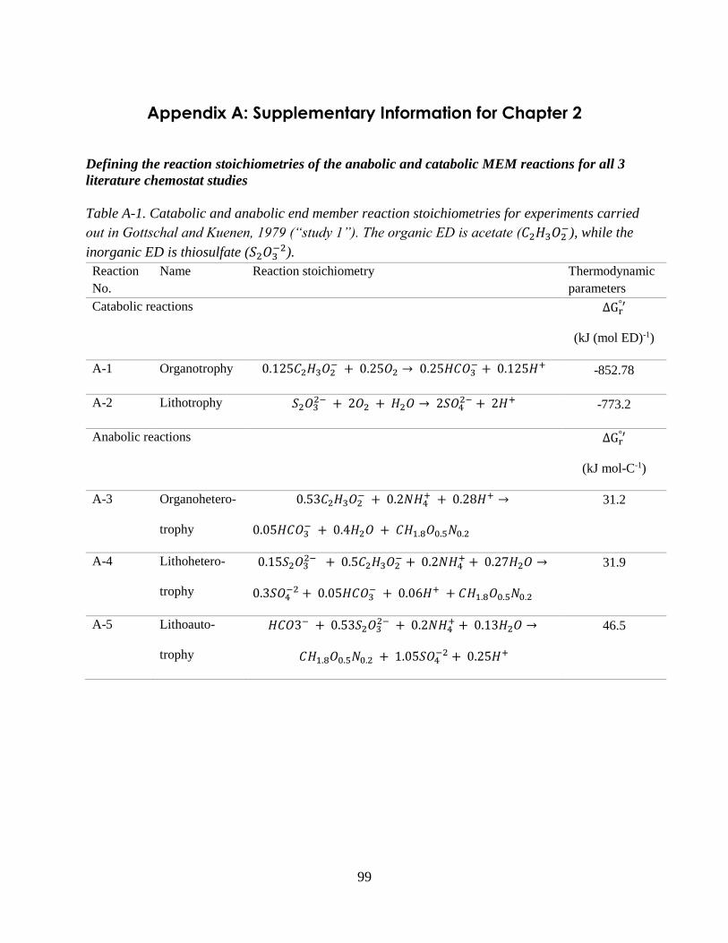
99

Appendix A: Supplementary Information for Chapter 2

Defining the reaction stoichiometries of the anabolic and catabolic MEM reactions for all 3

literature chemostat studies

Table A-1. Catabolic and anabolic end member reaction stoichiometries for experiments carried

out in Gottschal and Kuenen, 1979 (“study 1”). The organic ED is acetate (𝐶2𝐻3𝑂2−), while the

inorganic ED is thiosulfate (𝑆2𝑂3−2).

Reaction

No.

Name Reaction stoichiometry Thermodynamic

parameters

Catabolic reactions ∆Gr°′

(kJ (mol ED)-1)

A-1 Organotrophy 0.125𝐶2𝐻3𝑂2− + 0.25𝑂2 → 0.25𝐻𝐶𝑂3

− + 0.125𝐻+ -852.78

A-2 Lithotrophy 𝑆2𝑂32− + 2𝑂2 + 𝐻2𝑂 → 2𝑆𝑂4

2− + 2𝐻+ -773.2

Anabolic reactions ∆Gr°′

(kJ mol-C-1)

A-3 Organohetero-

trophy

0.53𝐶2𝐻3𝑂2− + 0.2𝑁𝐻4

+ + 0.28𝐻+ →

0.05𝐻𝐶𝑂3− + 0.4𝐻2𝑂 + 𝐶𝐻1.8𝑂0.5𝑁0.2

31.2

A-4 Lithohetero-

trophy

0.15𝑆2𝑂32− + 0.5𝐶2𝐻3𝑂2

− + 0.2𝑁𝐻4+ + 0.27𝐻2𝑂 →

0.3𝑆𝑂4−2 + 0.05𝐻𝐶𝑂3

− + 0.06𝐻+ + 𝐶𝐻1.8𝑂0.5𝑁0.2

31.9

A-5 Lithoauto-

trophy

𝐻𝐶𝑂3− + 0.53𝑆2𝑂32− + 0.2𝑁𝐻4

+ + 0.13𝐻2𝑂 →

𝐶𝐻1.8𝑂0.5𝑁0.2 + 1.05𝑆𝑂4−2 + 0.25𝐻+

46.5

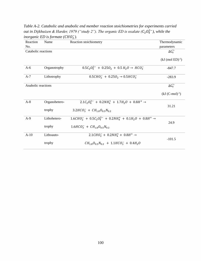
100


out in Dijkhuizen & Harder, 1979 (“study 2”). The organic ED is oxalate (𝐶2𝑂42−), while the

inorganic ED is formate (𝐶𝐻𝑂2−).

Reaction

No.


parameters


(kJ (mol ED)-1)

A-6 Organotrophy 0.5𝐶2𝑂42− + 0.25𝑂2 + 0.5 𝐻2𝑂 → 𝐻𝐶𝑂3

− -847.7

A-7 Lithotrophy 0.5𝐶𝐻𝑂2− + 0.25𝑂2 → 0.5𝐻𝐶𝑂3

− -283.9


(kJ (C-mol)-1)

A-8 Organohetero-

trophy

2.1𝐶2𝑂42− + 0.2𝑁𝐻4

+ + 1.7𝐻2𝑂 + 0.8𝐻+ →

3.2𝐻𝐶𝑂3− + 𝐶𝐻1.8𝑂0.5𝑁0.2

31.21

A-9 Lithohetero-

trophy

1.6𝐶𝐻𝑂2− + 0.5𝐶2𝑂4

2− + 0.2𝑁𝐻4+ + 0.1𝐻2𝑂 + 0.8𝐻+ →

1.6𝐻𝐶𝑂3− + 𝐶𝐻1.8𝑂0.5𝑁0.2

24.9

A-10 Lithoauto-

trophy

2.1𝐶𝐻𝑂2− + 0.2𝑁𝐻4

+ + 0.8𝐻+ →

𝐶𝐻1.8𝑂0.5𝑁0.2 + 1.1𝐻𝐶𝑂3− + 0.4𝐻2𝑂

-101.5

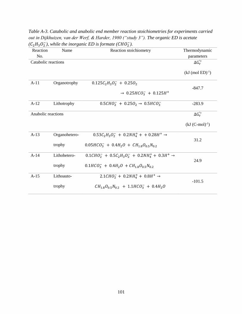
101


out in Dijkhuizen, van der Werf, & Harder, 1980 (“study 3”). The organic ED is acetate

(𝐶2𝐻3𝑂2−), while the inorganic ED is formate (𝐶𝐻𝑂2

−).

Reaction

No.


parameters


(kJ (mol ED)-1)

A-11 Organotrophy 0.125𝐶2𝐻3𝑂2− + 0.25𝑂2

→ 0.25𝐻𝐶𝑂3− + 0.125𝐻+

-847.7

A-12 Lithotrophy 0.5𝐶𝐻𝑂2− + 0.25𝑂2 → 0.5𝐻𝐶𝑂3

− -283.9


(kJ (C-mol)-1)

A-13 Organohetero-

trophy

0.53𝐶2𝐻3𝑂2− + 0.2𝑁𝐻4

+ + + 0.28𝐻+ →

0.05𝐻𝐶𝑂3− + 0.4𝐻2𝑂 + 𝐶𝐻1.8𝑂0.5𝑁0.2

31.2

A-14 Lithohetero-

trophy

0.1𝐶𝐻𝑂2− + 0.5𝐶2𝐻3𝑂2

− + 0.2𝑁𝐻4+ + 0.3𝐻+ →

0.1𝐻𝐶𝑂3− + 0.4𝐻2𝑂 + 𝐶𝐻1.8𝑂0.5𝑁0.2

24.9

A-15 Lithoauto-

trophy

2.1𝐶𝐻𝑂2− + 0.2𝑁𝐻4

+ + 0.8𝐻+ →

𝐶𝐻1.8𝑂0.5𝑁0.2 + 1.1𝐻𝐶𝑂3− + 0.4𝐻2𝑂

-101.5

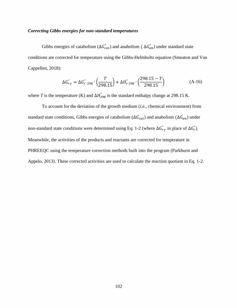
102

Correcting Gibbs energies for non-standard temperatures

Gibbs energies of catabolism (∆𝐺𝑐𝑎𝑡° ) and anabolism ( ∆𝐺𝑎𝑛

° ) under standard state

conditions are corrected for temperature using the Gibbs-Helmholtz equation (Smeaton and Van

Cappellen, 2018):

∆𝐺𝑟°

𝑇= ∆𝐺𝑟 298

° ∙ (𝑇

298.15) + ∆𝐻𝑟 298

° ∙ (298.15 − 𝑇

298.15) (A-16)

where T is the temperature (K) and ∆𝐻298° is the standard enthalpy change at 298.15 K.

To account for the deviation of the growth medium (i.e., chemical environment) from

standard state conditions, Gibbs energies of catabolism (∆𝐺𝑐𝑎𝑡) and anabolism (∆𝐺𝑎𝑛) under

non-standard state conditions were determined using Eq. 1-2 (where ∆𝐺𝑟°

𝑇 in place of ∆𝐺𝑟

°).

Meanwhile, the activities of the products and reactants are corrected for temperature in

PHREEQC using the temperature correction methods built into the program (Parkhurst and

Appelo, 2013). These corrected activities are used to calculate the reaction quotient in Eq. 1-2.

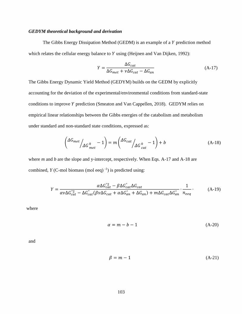
103

GEDYM theoretical background and derivation

The Gibbs Energy Dissipation Method (GEDM) is an example of a 𝑌 prediction method

which relates the cellular energy balance to 𝑌 using (Heijnen and Van Dijken, 1992):

𝑌 =∆𝐺𝑐𝑎𝑡

∆𝐺𝑚𝑒𝑡 + 𝜈∆𝐺𝑐𝑎𝑡 − ∆𝐺𝑎𝑛 (A-17)

The Gibbs Energy Dynamic Yield Method (GEDYM) builds on the GEDM by explicitly

accounting for the deviation of the experimental/environmental conditions from standard-state

conditions to improve 𝑌 prediction (Smeaton and Van Cappellen, 2018). GEDYM relies on

empirical linear relationships between the Gibbs energies of the catabolism and metabolism

under standard and non-standard state conditions, expressed as:

(𝛥𝐺𝑚𝑒𝑡

𝛥𝐺 𝑚𝑒𝑡0⁄ − 1) = 𝑚 (

𝛥𝐺𝑐𝑎𝑡

𝛥𝐺 𝑐𝑎𝑡0⁄ − 1) + 𝑏 (A-18)

where m and b are the slope and y-intercept, respectively. When Eqs. A-17 and A-18 are

combined, Y (C-mol biomass (mol eeq) -1) is predicted using:

𝑌 =𝛼∆𝐺𝑐𝑎𝑡

°2 − 𝛽∆𝐺𝑐𝑎𝑡° ∆𝐺𝑐𝑎𝑡

𝛼𝜈∆𝐺𝑐𝑎𝑡°2 − ∆𝐺𝑐𝑎𝑡

° (𝛽𝜈∆𝐺𝑐𝑎𝑡 + 𝛼∆𝐺𝑎𝑛° + ∆𝐺𝑎𝑛) + 𝑚∆𝐺𝑐𝑎𝑡∆𝐺𝑎𝑛

°∙

1

𝑛𝑒𝑒𝑞∙ (A-19)

where

𝛼 = 𝑚 − 𝑏 − 1 (A-20)

and

𝛽 = 𝑚 − 1 (A-21)

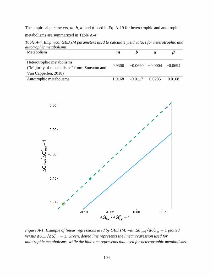
104

The empirical parameters, 𝑚, 𝑏, 𝛼, and 𝛽 used in Eq. A-19 for heterotrophic and autotrophic

metabolisms are summarized in Table A-4:

Table A-4. Empirical GEDYM parameters used to calculate yield values for heterotrophic and

autotrophic metabolisms

Metabolism 𝒎 𝒃 𝜶 𝜷

Heterotrophic metabolisms

("Majority of metabolisms" from: Smeaton and

Van Cappellen, 2018)

0.9306 −0.0690 −0.0004 −0.0694

Autotrophic metabolisms 1.0168 -0.0117 0.0285 0.0168

Figure A-1. Example of linear regressions used by GEDYM, with ∆𝐺𝑚𝑒𝑡 ∆𝐺𝑚𝑒𝑡°⁄ − 1 plotted

versus ∆𝐺𝑐𝑎𝑡 ∆𝐺𝑐𝑎𝑡°⁄ − 1. Green, dotted line represents the linear regression used for

autotrophic metabolisms, while the blue line represents that used for heterotrophic metabolisms.

105

Maximum theoretical growth yield (𝒀𝒎𝒂𝒙)

A maximum theoretical growth yield (𝑌𝑚𝑎𝑥) can be determined which corresponds to the 𝑌 value

when ∆𝐺𝑚𝑒𝑡 = 0, yet the catabolic reaction remains thermodynamically favorable (i.e., 𝛥𝐺𝑐𝑎𝑡 <

0):

𝑌𝑚𝑎𝑥 =𝛥𝐺𝑐𝑎𝑡

∆𝐺𝑐𝑎𝑡𝜈 − ∆𝐺𝑎𝑛 (A-22)

Knowledge of this theoretical maximum growth yield can be used in models to prevent a

metabolic reaction from occurring when it is not thermodynamically possible. When 𝛥𝐺𝑚𝑒𝑡

calculated using the GEDYM is greater than 0, 𝑌 is set to 𝑌𝑚𝑎𝑥, and the reaction is not permitted

to occur until the geochemical conditions changes such that 𝛥𝐺𝑚𝑒𝑡 value becomes

thermodynamically favourable (i.e., 𝛥𝐺𝑚𝑒𝑡< 0) (Smeaton and Van Cappellen, 2018).

106

Calculating steady state concentrations in the chemostat

The net utilization rates of the two ED substrates and biomass concentration in the chemostat are

known and can be used to calculate the steady state ED concentration using Monod kinetics:

𝑟𝐸𝐷𝑚𝑒𝑡 =

𝑋

𝑌𝜇𝑚𝑎𝑥(

𝐶𝐸𝐷

𝐶𝐸𝐷 + 𝐾𝐸𝐷) (A-23)

Re-arranging reaction A16 gives reaction A17, which expresses the steady state concentration of

the ED as a function of the ED utilization rate:

𝐶𝐸𝐷 =𝑟𝐸𝐷

𝑚𝑒𝑡 ∙ 𝑌 ∙ 𝐾𝐸𝐷

𝑓𝐸𝐷𝑒𝑒𝑞 ∙ 𝑋 ∙ 𝜇𝑚𝑎𝑥 − 𝑟𝐸𝐷

𝑚𝑒𝑡 ∙ 𝑌 (A-24)

The values of 𝜇𝑚𝑎𝑥 and 𝐾𝐸𝐷 used for the EDs used in all three studies are summarized in

Table A5. Mixotroph-specific 𝜇𝑚𝑎𝑥 and 𝐾𝐸𝐷 parameters can be calculated from the parameters

of obligate organisms using the relationship proposed by Gottschal and Thingstad (1982). The

𝜇𝑚𝑎𝑥 values are 25% lower, while the 𝐾𝐸𝐷 values are also around 25% lower for mixotrophs

(i.e., facultative organisms) compared to the value for organisms capable of growing only on the

single ED (i.e., obligate organisms). This how the parameters for the growth of P. versutus on

thiosulfate and acetate were calculated.

Most of the 𝜇𝑚𝑎𝑥 and 𝐾𝐸𝐷 values in Table A5 were taken from studies where mixotrophs

were grown on the single substrates, so these adjustments to the parameters were not required.

The calculation of these parameters is described in the next section.

The ED utilization rates and steady state ED concentrations in all three studies are summarized

in Figure A-2.

107

Table A-5. Monod kinetic parameters calculated for the growth of P. versutus on acetate and

thiosulfate and P. oxalaticus on acetate, oxalate and formate

Substrate (Organism) 𝝁𝒎𝒂𝒙

(h-1)

𝑲𝑬𝑫

Source

Acetate (P. versutus) 0.145 1 µM [1]

Thiosulfate (P. versutus) 0.085 1 µM [1]

Acetate (P. oxalaticus) 0.432 1.4 mM [2], fitted

Oxalate (P. oxalaticus) 0.095 0.71 mM [2], fitted

Formate (P. oxalaticus) 0.208 9.3∗ 10−2 mM [2], fitted

1: (Gottschal and Thingstad, 1982), 2: (Dijkhuizen et al., 1980)

Figure A-2. ED utilization rates (top panel) and steady state concentration of the two EDs

(bottom panel) as a function of the fraction of inorganic electron equivalents consumed for all

three studies.

108

Calculating the kinetic parameters for the growth of P. oxalaticus on formate, oxalate and

acetate

To calculate the values of the maximum specific growth rate (𝜇𝑚𝑎𝑥) and the half-

saturation constant (𝐾𝑠) kinetic parameters for the growth of P. oxalaticus on the electron donor

(ED) substrates formate, acetate and oxalate, experimental data for these organisms growing in

batch culture was used.

The data used came from Dijkhuizen et al. (1980). In this study, P. oxalaticus was grown

on mixtures of two EDs. The optical density of the cells was measured over time, along with the

residual concentration of each ED in the culture. Given these data, the specific growth rate can

be calculated and related to the residual ED concentration.

In batch culture, specific growth rates are higher, and growth on two substrates is diauxic,

meaning that each ED is used one at a time for growth rather than simultaneously. I therefore

identified phases where the ED of interest was being used for growth and used those data for

calculating the kinetic parameters since I was interested in the kinetic parameters that

represented growth on single ED substrates.

The specific growth rate of the cells in batch culture was calculated using the method

described in Smeaton and Van Cappellen (2018). Briefly, the doubling time (𝑡𝑑) of the culture at

any point during its growth in batch phase was calculated using Eq. A-25:

𝑡𝑑 =0.301(𝑡2 − 𝑡1)

log 𝑋2 − log 𝑋1 (A-25)

where 𝑋1 and 𝑋2 are cell concentrations (as optical density) measured at times 𝑡1 and 𝑡2,

respectively. Using the doubling time, the specific growth rate (μ) was calculated using Eq. A-

26:

𝜇 =ln 2

𝑡𝑑 (A-26)

To calculate the parameters 𝜇𝑚𝑎𝑥 and 𝐾𝑠, the Monod-type equation was fit to the data using a

non-linear least squares fitting procedure, using the method and base script outlined by Huitema

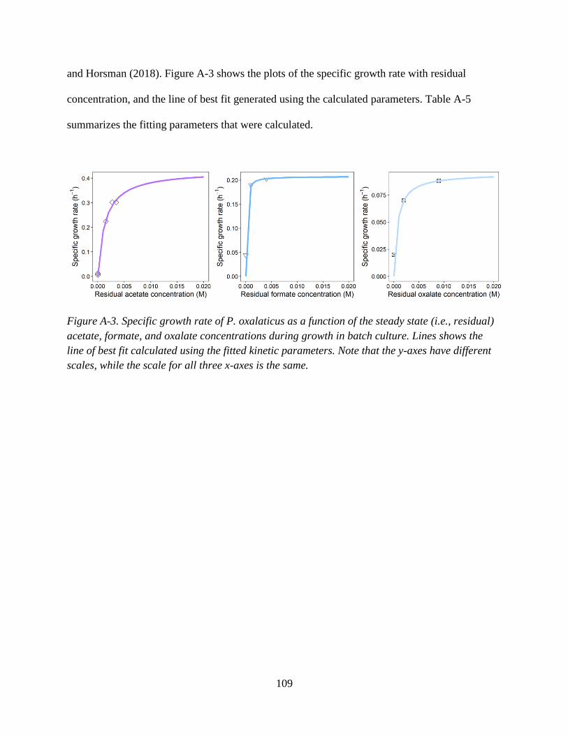
109

and Horsman (2018). Figure A-3 shows the plots of the specific growth rate with residual

concentration, and the line of best fit generated using the calculated parameters. Table A-5

summarizes the fitting parameters that were calculated.

Figure A-3. Specific growth rate of P. oxalaticus as a function of the steady state (i.e., residual)

acetate, formate, and oxalate concentrations during growth in batch culture. Lines shows the

line of best fit calculated using the fitted kinetic parameters. Note that the y-axes have different

scales, while the scale for all three x-axes is the same.

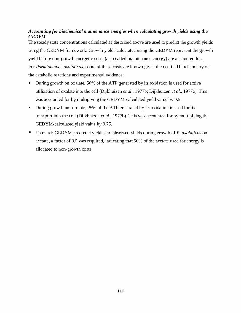
110

Accounting for biochemical maintenance energies when calculating growth yields using the

GEDYM

The steady state concentrations calculated as described above are used to predict the growth yields

using the GEDYM framework. Growth yields calculated using the GEDYM represent the growth

yield before non-growth energetic costs (also called maintenance energy) are accounted for.

For Pseudomonas oxalaticus, some of these costs are known given the detailed biochemistry of

the catabolic reactions and experimental evidence:

▪ During growth on oxalate, 50% of the ATP generated by its oxidation is used for active

utilization of oxalate into the cell (Dijkhuizen et al., 1977b; Dijkhuizen et al., 1977a). This

was accounted for by multiplying the GEDYM-calculated yield value by 0.5.

▪ During growth on formate, 25% of the ATP generated by its oxidation is used for its

transport into the cell (Dijkhuizen et al., 1977b). This was accounted for by multiplying the

GEDYM-calculated yield value by 0.75.

▪ To match GEDYM predicted yields and observed yields during growth of P. oxalaticus on

acetate, a factor of 0.5 was required, indicating that 50% of the acetate used for energy is

allocated to non-growth costs.

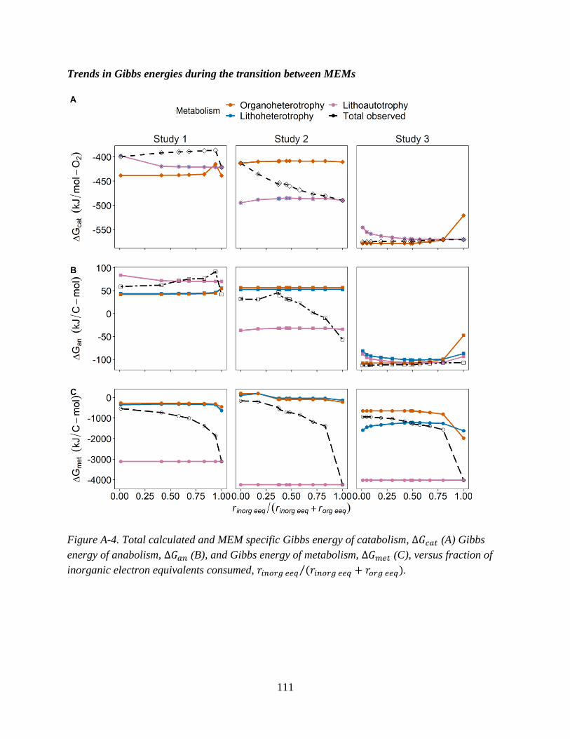
111

Trends in Gibbs energies during the transition between MEMs

Figure A-4. Total calculated and MEM specific Gibbs energy of catabolism, ∆𝐺𝑐𝑎𝑡 (A) Gibbs

energy of anabolism, ∆𝐺𝑎𝑛 (B), and Gibbs energy of metabolism, ∆𝐺𝑚𝑒𝑡 (C), versus fraction of

inorganic electron equivalents consumed, 𝑟𝑖𝑛𝑜𝑟𝑔 𝑒𝑒𝑞 (𝑟𝑖𝑛𝑜𝑟𝑔 𝑒𝑒𝑞⁄ + 𝑟𝑜𝑟𝑔 𝑒𝑒𝑞).

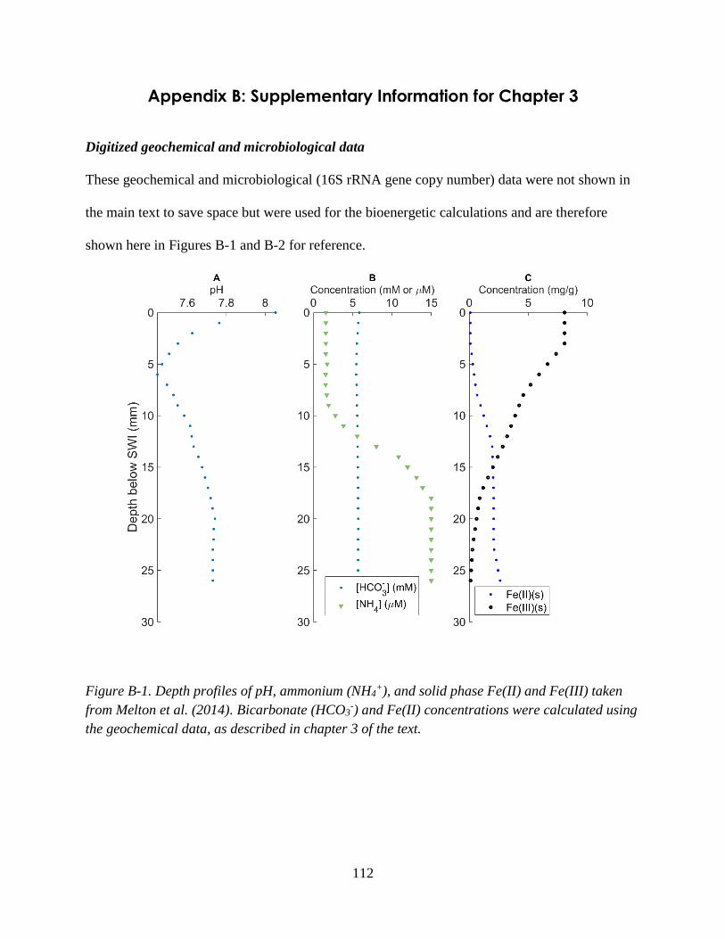
112

Appendix B: Supplementary Information for Chapter 3

Digitized geochemical and microbiological data

These geochemical and microbiological (16S rRNA gene copy number) data were not shown in

the main text to save space but were used for the bioenergetic calculations and are therefore

shown here in Figures B-1 and B-2 for reference.

Figure B-1. Depth profiles of pH, ammonium (NH4+), and solid phase Fe(II) and Fe(III) taken

from Melton et al. (2014). Bicarbonate (HCO3-) and Fe(II) concentrations were calculated using

the geochemical data, as described in chapter 3 of the text.

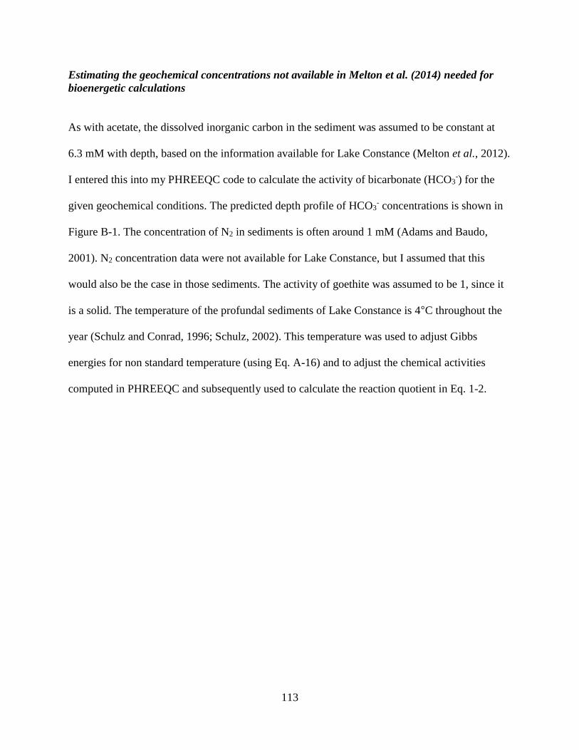
113

Estimating the geochemical concentrations not available in Melton et al. (2014) needed for

bioenergetic calculations

As with acetate, the dissolved inorganic carbon in the sediment was assumed to be constant at

6.3 mM with depth, based on the information available for Lake Constance (Melton et al., 2012).

I entered this into my PHREEQC code to calculate the activity of bicarbonate (HCO3-) for the

given geochemical conditions. The predicted depth profile of HCO3- concentrations is shown in

Figure B-1. The concentration of N2 in sediments is often around 1 mM (Adams and Baudo,

2001). N2 concentration data were not available for Lake Constance, but I assumed that this

would also be the case in those sediments. The activity of goethite was assumed to be 1, since it

is a solid. The temperature of the profundal sediments of Lake Constance is 4°C throughout the

year (Schulz and Conrad, 1996; Schulz, 2002). This temperature was used to adjust Gibbs

energies for non standard temperature (using Eq. A-16) and to adjust the chemical activities

computed in PHREEQC and subsequently used to calculate the reaction quotient in Eq. 1-2.

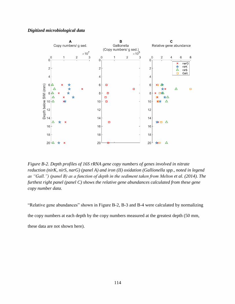
114

Digitized microbiological data

Figure B-2. Depth profiles of 16S rRNA gene copy numbers of genes involved in nitrate

reduction (nirK, nirS, narG) (panel A) and iron (II) oxidation (Gallionella spp., noted in legend

as “Gall.”) (panel B) as a function of depth in the sediment taken from Melton et al. (2014). The

furthest right panel (panel C) shows the relative gene abundances calculated from these gene

copy number data.

“Relative gene abundances” shown in Figure B-2, B-3 and B-4 were calculated by normalizing

the copy numbers at each depth by the copy numbers measured at the greatest depth (50 mm,

these data are not shown here).

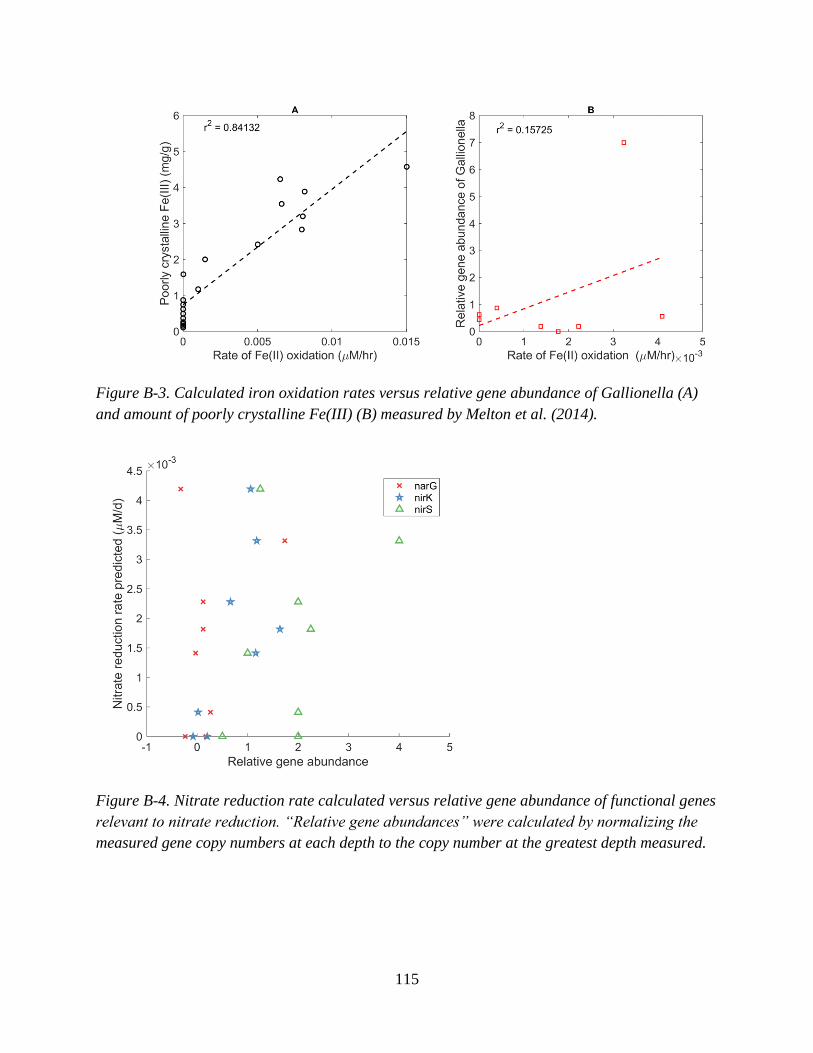
115

Figure B-3. Calculated iron oxidation rates versus relative gene abundance of Gallionella (A)

and amount of poorly crystalline Fe(III) (B) measured by Melton et al. (2014).

Figure B-4. Nitrate reduction rate calculated versus relative gene abundance of functional genes

relevant to nitrate reduction. “Relative gene abundances” were calculated by normalizing the

measured gene copy numbers at each depth to the copy number at the greatest depth measured.

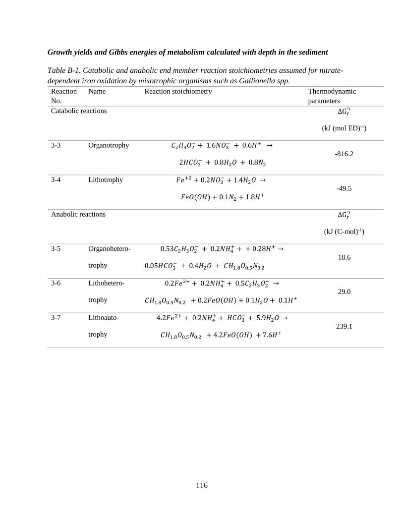
116

Growth yields and Gibbs energies of metabolism calculated with depth in the sediment

Table B-1. Catabolic and anabolic end member reaction stoichiometries assumed for nitrate-

dependent iron oxidation by mixotrophic organisms such as Gallionella spp.

Reaction

No.


parameters


(kJ (mol ED)-1)

3-3 Organotrophy 𝐶2𝐻3𝑂2− + 1.6𝑁𝑂3

− + 0.6𝐻+ →

2𝐻𝐶𝑂3− + 0.8𝐻2𝑂 + 0.8𝑁2

-816.2

3-4 Lithotrophy 𝐹𝑒+2 + 0.2𝑁𝑂3− + 1.4𝐻2𝑂 →

𝐹𝑒𝑂(𝑂𝐻) + 0.1𝑁2 + 1.8𝐻+ -49.5


(kJ (C-mol)-1)

3-5 Organohetero-

trophy

0.53𝐶2𝐻3𝑂2− + 0.2𝑁𝐻4

+ + + 0.28𝐻+ →

0.05𝐻𝐶𝑂3− + 0.4𝐻2𝑂 + 𝐶𝐻1.8𝑂0.5𝑁0.2

18.6

3-6 Lithohetero-

trophy

0.2𝐹𝑒2+ + 0.2𝑁𝐻4+ + 0.5𝐶2𝐻3𝑂2

− →

𝐶𝐻1.8𝑂0.5𝑁0.2 + 0.2𝐹𝑒𝑂(𝑂𝐻) + 0.1𝐻2𝑂 + 0.1𝐻+ 29.0

3-7 Lithoauto-

trophy

4.2𝐹𝑒2+ + 0.2𝑁𝐻4+ + 𝐻𝐶𝑂3

− + 5.9𝐻2𝑂 →

𝐶𝐻1.8𝑂0.5𝑁0.2 + 4.2𝐹𝑒𝑂(𝑂𝐻) + 7.6𝐻+ 239.1

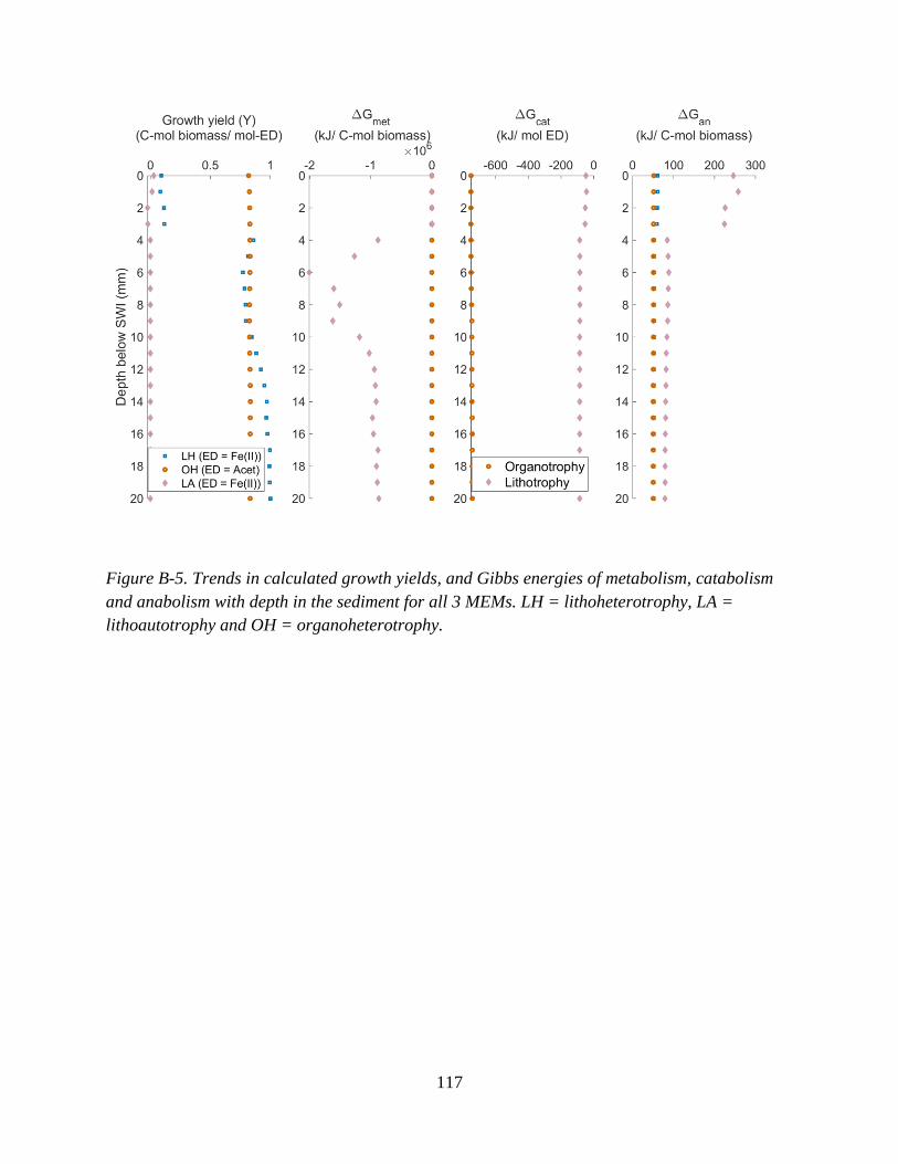
117

Figure B-5. Trends in calculated growth yields, and Gibbs energies of metabolism, catabolism

and anabolism with depth in the sediment for all 3 MEMs. LH = lithoheterotrophy, LA =

lithoautotrophy and OH = organoheterotrophy.

Documents

Bioenergetics of mixotrophic metabolisms: A theoretical analysis