Embed Size (px)
Citation preview

APPRAISING RESPONSE OF ADDITIVES IN SOIL
STABILIZATION FOR PAVEMENT
A PROJECT REPORT
Submitted by
CHAKSHU KOUL 16CE202
MAKADIA DHRUV 17CE317
PATEL BHAVIN 17CE319
AGARIYA HARDIK 17CE326
VOHRA ALMAS 17CE332
VHORA ABRAR 17CE333
in fully fulfilment for the award of the degree of
B. TECH. (CIVIL ENGINEERING)
Under the subject of
CE444: PROJECT-II
BIRLA VISHVAKARMA MAHAVIDYALAYA
(ENGINEERING COLLEGE)
(An Autonomous Institution)
VALLABH VIDYANAGAR
Affiliated to
GUJARAT TECHNOLOGICAL UNIVERSITY, AHMEDABAD
Academic Year: 2019 – 2020

Birla Vishwakarma Mahavidyalaya College of Engg., Anand
2
APPROVAL SHEET
This project report “Appraising response of additives in soil stabilization for pavement”
is carried out by:
CHAKSHU KOUL 16CE202
MAKADIA DHRUV 17CE317
PATEL BHAVIN 17CE319
AGARIYA HARDIK 17CE326
VOHRA ALMAS 17CE332
VHORA ABRAR 17CE333
is approved for the submission as a project report under the subject CE444: Project-II for
the submission for the award of the degree of B. Tech. (Civil Engineering).
Name and Signature of Supervisor
Date:
Place:
Name and Signature of Examiner
Date:
Place:

Birla Vishwakarma Mahavidyalaya College of Engg., Anand
3
DEPARTMENT OF CIVIL ENGINEERING
B. V. M. ENGINEERING COLLEGE, VALLABH VIDYANAGAR-
388120
BONAFIDE CERTIFICATE
Certified that this project report “Appraising Response of Additives in Soil Stabilization
for Pavement” is the bonafide and original work of
CHAKSHU KOUL 16CE202
MAKADIA DHRUV 17CE317
PATEL BHAVIN 17CE319
AGARIYA HARDIK 17CE326
VOHRA ALMAS 17CE332
VHORA ABRAR 17CE333
who carried out the project work under my supervision.
Prof. C. B Mishra
(Associate Professor of Civil Engg. Department)
BVM Engg. College, Vallabh Vidyanagar
Dr. L. B. Zala
(Head of Civil Engg. Department)
BVM Engg. College, Vallabh Vidyanagar

Birla Vishwakarma Mahavidyalaya College of Engg., Anand
4
ACKNOWLEDGEMENTS
Sometime word falls short to show gratitude the same is happening with us during his project. The
immense help and support received from the faculties and friend overwhelmed us during the project.
The project work has been the most exciting part of our learning experience, which would be assert us
for our future carrier.
We earnestly express our sincere thanks and sense of gratitude to Dr. Indrajit N. Patel, Principle of
Birla Vishwakarma Mahavidyalaya and Dr. L.B. Zala, HOD of Civil engineering department who has
given us an opportunity to work on such project development by providing all facilities that were
required.
We are highly indebted to Prof. C.B. Mishra (internal project guide) who has provided us with the
necessary information and his valuable suggestions on bringing out this project in the best possible
way.

5
Birla Vishvakarma Mahavidyalaya College of Engg., Anand
ABSTRACT
Stability of underlying soil affects the short term and long-term performance of pavement structure.
In situ sub grades often do not provide the support required to achieve acceptable performance
under traffic loading and environmental demands. However, construction of roads in rural areas is
always restrained by geographic limitation and often can be costly and energy inefficient. Hence it
causes more adverse impact on the environment.
The amount of waste generated from varied sources has increased in recent years due to increase
in population, industrialization, social as well as economic activities. It has become the need of the
hour to utilize this waste in the best manner yet to encourage the concept of reusing in waste
management and thus reduce the cost of waste disposal. One such method of reusing is that by using
it in the process of soil stabilization.
Roadways designed for low-volume traffic are constructed of local soils containing high
percentages of fines and high indices of plasticity. These soils may not have characteristics
appropriate for use in soil road construction, but can often be upgraded with soil stabilization
technology to successfully recondition and strengthen existing road base and sub-base materials
for extended life and heavier traffic duty.
In this thesis, an effort has been made to decrease the thickness of pavement by utilizing innovative
materials like Waste marble powder and wooden dust for sub-grade soil stabilization. The tests
such as Grain size analysis, Atterberg’s limits, CBR and UCS values along with Free swell index
which is performed to analysis the engineering properties of soil such as classification of soil, OMC,
and MDD, the strength of soil and properties.
The CBR and UCS tests are studied for untreated and treated soils with optimum dosages and the
readings are recorded for 3 days, 7 days, 14 days, and 21 days. Comparison of soil treated with
Marble powder, wooden dust and combine (marble powder + wooden dust) are evaluated and also
the flexible pavement thickness based on IRC 37-2012 is carried out based on CBR values and the
cost saving is also computed.
Also, utilizing field emission microscopy (FESEM) and an energy dispersive x-beam spectrometry
(EDAX) strategy on ordinary soil balanced out with an optimum dosage of marble powder and
wooden dust to have a superior comprehension of changes in atomic structure contributing towards
upgraded quality.

6
Birla Vishvakarma Mahavidyalaya College of Engg., Anand
Index
CHAPTER 1 INTRODUCTION ............................................................................................................. 13
1.1 Introduction .......................................................................................................................................................... 13
1.2 General ................................................................................................................................................................. 13
1.3 Problem identification .......................................................................................................................................... 15
1.4 Aims and Objectives .............................................................................................................................................. 15
1.5 Scope of work ....................................................................................................................................................... 16
1.6 Methodology Framework...................................................................................................................................... 16
CHAPTER 2 LITERATURE REVIEW...................................................................................................... 17
2.1 Soil Stabilization.................................................................................................................................................... 17
2.2 Basic Soil Stabilization Process .............................................................................................................................. 22
2.3 Industrial waste .................................................................................................................................................... 23
2.4 Materials............................................................................................................................................................... 33
2.5 Review of research paper on Waste Marble powder ............................................................................................ 39
2.6 Review of research paper on Saw dust.................................................................................................................. 42
CHAPTER 3 LABORATORY TESTS AND RESULTS ................................................................................. 45
3.1 Laboratory Tests for Soil (As Per Indian Standards) ............................................................................................... 45
CHAPTER 4 THICKNESS OF PAVEMENT DESIGN .............................................................................. 109
4.1 Pavement design................................................................................................................................................. 109
4.2 Different layer thickness by referring IRC: 37-2012 ............................................................................................. 109
4.3 Summary of cost analysis .................................................................................................................................... 115
CHAPTER 5 LABORATORY TEST BY USING SAW DUST ..................................................................... 116
5.1 Laboratory Tests for Soil (As Per Indian Standards) ............................................................................................. 116
CHAPTER 6 PAVEMENT DESIGN USING SAW DUST ......................................................................... 173
6.1 Pavement design ............................................................................................................................................. 173
6.2 Different layer thickness by referring IRC: 37-2012 .......................................................................................... 173

7
Birla Vishvakarma Mahavidyalaya College of Engg., Anand
6.3 Summary of cost analysis ................................................................................................................................. 179
CHAPTER 7 CONCLUSION ............................................................................................................... 180
7.1 Conclusion based on Saw Dust ............................................................................................................................ 180
7.2 Conclusion based on Marble Powder .................................................................................................................. 180
7.3 Conclusion based on both the additives .............................................................................................................. 180
# REFRENCES ................................................................................................................................. 181

8
Birla Vishvakarma Mahavidyalaya College of Engg., Anand
LISTS OF FIGURES
FIGURE 1.1 SOIL STABILIZATION (SOURCE WWW.WIRTGEN.DE) ................................................................................... 14 FIGURE 1.2 CRACK PATTERNS IN BLACK COTTON SOIL (SOURCE CIVILBLOG.ORG) ......................................................... 15 FIGURE 2.1 MECHANICAL STABILIZATION (SOURCE – SLIDESHARE.NET) ....................................................................... 17 FIGURE 2.2 CHEMICAL STABILIZATION (SOURCE- PROJECTTUNNEL.COM) ..................................................................... 18 FIGURE 2.3 LIME STABILIZATION (SOURCE-HAPPHO.COM) ........................................................................................... 20 FIGURE 2.4 TOTAL WASTE GENERATIONS (SOURCE-RESEARCHGATE.COM) .................................................................. 24 FIGURE 2.5 COLLECTION VS DUMPED STATISTICS (NUMBERS IN MILLION MT PER ANNUM) ......................................... 24 FIGURE 2.6 COLLECTION OF SOIL SAMPLE (SOURCE –GOOGLE MAPS .COM)................................................................. 34 FIGURE 2.7 MARBLE DUST (SOURCE –INDIAMART.COM) .............................................................................................. 34 FIGURE 2.7 SAWDUST (SOURCE –SCIALERT.COM) ........................................................................................................ 38 FIGURE 3.1 PLASTICITY CHART (I.S. SOIL CLASSIFICATION) ............................................................................................ 47 FIGURE 3.2 OMC AND MDD FOR NATURAL SOIL........................................................................................................... 54 FIGURE 3.3 OMC AND MDD FOR NATURAL SOIL + 5% MP ............................................................................................ 55 FIGURE 3.3 OMC AND MDD FOR NATURAL SOIL + 5% MP ............................................................................................ 56 FIGURE 3.4 OMC AND MDD FOR NATURAL SOIL + 10% MP .......................................................................................... 57 FIGURE 3.4 OMC AND MDD FOR NATURAL SOIL + 10% MP .......................................................................................... 58 FIGURE 3.6 OMC AND MDD FOR NATURAL SOIL + 20% MP .......................................................................................... 59 FIGURE 3.7 CBR EQUIPMENT ....................................................................................................................................... 61 FIGURE 3.8 CORRECTION LOAD PENETRATION CURVES ................................................................................................ 62 FIGURE 3.9 CBR TESTING SAMPLE ................................................................................................................................ 63 FIGURE 3.10 CBR GRAPH FOR BC SOIL .......................................................................................................................... 64 FIGURE 3.11 CBR GRAPH FOR BC SOIL + 5% MP ........................................................................................................... 65 FIGURE 3.12 CBR GRAPH FOR BC SOIL + 5% MP (7 DAYS) ............................................................................................. 66 FIGURE 3.13 CBR GRAPH FOR BC SOIL + 5% MP (14 DAYS)............................................................................................ 67 FIGURE 3.14 CBR GRAPH FOR BC SOIL + 5% MP (21 DAYS)............................................................................................ 68 FIGURE 3.15 CBR GRAPH FOR BC SOIL + 10% MP.......................................................................................................... 70 FIGURE 3.16 CBR GRAPH FOR BC SOIL + 10% MP (7 DAYS) ........................................................................................... 71 FIGURE 3.17 CBR GRAPH FOR BC SOIL + 10% MP (14 DAYS).......................................................................................... 72 FIGURE 3.18 CBR GRAPH FOR BC SOIL + 10% MP (21 DAYS).......................................................................................... 73 FIGURE 3.19 CBR GRAPH FOR BC SOIL + 15% MP.......................................................................................................... 74 FIGURE 3.20 CBR GRAPH FOR BC SOIL + 15% MP (7 DAYS)............................................................................................ 76 FIGURE 3.21 CBR GRAPH FOR BC SOIL + 15% MP (14 DAYS).......................................................................................... 77 FIGURE 3.22 CBR GRAPH FOR BC SOIL + 15% MP (21 DAYS).......................................................................................... 78 FIGURE 3.23 CBR GRAPH FOR BC SOIL + 20% MP.......................................................................................................... 79 FIGURE 3.24 CBR GRAPH FOR BC SOIL + 20% MP (7 DAYS)............................................................................................ 80 FIGURE 3.25 CBR GRAPH FOR BC SOIL + 20% MP (14 DAYS).......................................................................................... 81 FIGURE 3.26 CBR GRAPH FOR BC SOIL + 20% MP (21 DAYS).......................................................................................... 83 FIGURE 3.27 UCS SOIL TESTING .................................................................................................................................... 84 FIGURE 3.28 STRESS V/S STRAIN FOR BC SOIL .............................................................................................................. 85 FIGURE 3.29 STRESS VS STRAIN FOR CLAY SOIL (3 DAYS) .............................................................................................. 87 FIGURE 3.29 UCS GRAPH FOR BC SOIL (7 DAYS) ............................................................................................................ 88 FIGURE 3.30 UCS GRAPH FOR BC SOIL (14 DAYS) .......................................................................................................... 89 FIGURE 3.31 UCS GRAPH FOR BC SOIL + 5% MP ........................................................................................................... 90 FIGURE 3.32 UCS GRAPH FOR BC SOIL + 5% MP (3 DAYS) ............................................................................................. 91 FIGURE 3.33 UCS GRAPH FOR BC SOIL + 5% MP (7 DAYS) ............................................................................................. 92 FIGURE 3.34 UCS GRAPH FOR BC SOIL + 5% MP (14 DAYS) ........................................................................................... 94 FIGURE 3.35 UCS GRAPH FOR BC SOIL + 10% MP ......................................................................................................... 95 FIGURE 3.36 UCS GRAPH FOR BC SOIL + 10% MP (3 DAYS) ........................................................................................... 96 FIGURE 3.37 UCS GRAPH FOR BC SOIL + 10% MP (7 DAYS) ........................................................................................... 97 FIGURE 3.38 UCS GRAPH FOR BC SOIL + 10% MP (14 DAYS).......................................................................................... 98 FIGURE 3.39 UCS GRAPH FOR BC SOIL + 15% MP ....................................................................................................... 100 FIGURE 3.40 UCS GRAPH FOR BC SOIL + 10% MP ....................................................................................................... 101 FIGURE 3.41 UCS GRAPH FOR BC SOIL + 15% MP (7 DAYS) ......................................................................................... 102

9
Birla Vishvakarma Mahavidyalaya College of Engg., Anand
FIGURE 3.43 UCS GRAPH FOR BC SOIL + 15% MP (14 DAYS)........................................................................................ 103 FIGURE 3.44 UCS GRAPH FOR BC SOIL + 20% MP ....................................................................................................... 104 FIGURE 3.44 UCS GRAPH FOR BC SOIL + 20% MP (3 DAYS) ......................................................................................... 105 FIGURE 3.45 UCS GRAPH FOR BC SOIL + 20% MP (7 DAYS) ......................................................................................... 107 FIGURE 3.46 UCS GRAPH FOR BC SOIL + 20% MP (21 DAYS)........................................................................................ 108 FIGURE 4.1 COMPOSITION OF LAYERS OF BC SOIL ...................................................................................................... 110 FIGURE 4.2 COMPOSITION OF LAYERS OF BC SOIL + 5% MP ....................................................................................... 111 FIGURE 4.3 COMPOSITION OF LAYERS OF BC SOIL + 10% MP...................................................................................... 112 FIGURE 4.4 COMPOSITION OF LAYERS OF BC SOIL + 15% MP...................................................................................... 113 FIGURE 4.5 COMPOSITION OF LAYERS OF BC SOIL + 20% MP...................................................................................... 114 FIGURE 5.1 OMC AND MDD FOR NATURAL SOIL......................................................................................................... 120 FIGURE 5.2 OMC AND MDD FOR NATURAL SOIL + 3 % SAW DUST .............................................................................. 121 FIGURE 5.3 OMC AND MDD FOR NATURAL SOIL + 6 % SAW DUST .............................................................................. 122 FIGURE 5.4 OMC AND MDD FOR NATURAL SOIL + 9 % SAW DUST .............................................................................. 123 FIGURE 5.5 OMC AND MDD FOR NATURAL SOIL + 12 % SAW DUST ............................................................................ 124 FIGURE 5.6 CBR GRAPH FOR BC SOIL .......................................................................................................................... 128 FIGURE 5.7 CBR GRAPH FOR BC SOIL + 3% SD............................................................................................................. 129 FIGURE 5.8 CBR GRAPH FOR BC SOIL + 6% SD............................................................................................................. 130 FIGURE 5.9 CBR GRAPH FOR BC SOIL + 9% SD............................................................................................................. 131 FIGURE 5.10 GRAPH FOR BC SOIL + 12% SD ................................................................................................................ 132 FIGURE 5.11 GRAPH FOR BC SOIL + 3% SD (7 DAY) ..................................................................................................... 133 FIGURE 5.12 GRAPH FOR BC SOIL + 6% SD (7 DAY ...................................................................................................... 134 FIGURE 5.13 GRAPH FOR BC SOIL + 9% SD (7 DAY) ..................................................................................................... 135 FIGURE 5.14 GRAPH FOR BC SOIL + 12% SD (7 DAY) ................................................................................................... 136 FIGURE 5.15 CBR GRAPH FOR BC SOIL + 3% SD (14 DAYS) ........................................................................................... 137 FIGURE 5.16 CBR GRAPH FOR BC SOIL + 6% SD (14 DAYS) ........................................................................................... 138 FIGURE 5.17 CBR GRAPH FOR BC SOIL + 9% SD (14 DAYS) ........................................................................................... 139 FIGURE 5.18 CBR GRAPH FOR BC SOIL + 12% SD (14 DAYS) ......................................................................................... 140 FIGURE 5.19 CBR GRAPH FOR BC SOIL + 3% SD (21 DAYS) ........................................................................................... 141 FIGURE 5.20 CBR GRAPH FOR BC SOIL + 6% SD (21 DAYS) ........................................................................................... 142 FIGURE 5.21 CBR GRAPH FOR BC SOIL + 9% SD(21 DAYS) ........................................................................................... 143 FIGURE 5.22 CBR GRAPH FOR BC SOIL + 12% SD (21 DAYS) ......................................................................................... 144 FIGURE 5.23 UCS SOIL TESTING .................................................................................................................................. 145 FIGURE 5.24 GRAPH OF BC SOIL ................................................................................................................................. 147 FIGURE 5.25 GRAPH OF BC SOIL + 3% SD .................................................................................................................... 148 FIGURE 5.26 GRAPH OF BC SOIL + 6% SD .................................................................................................................... 149 FIGURE 5.27 GRAPH OF BC SOIL + 9% SD .................................................................................................................... 151 FIGURE 5.28 GRAPH OF BC SOIL + 12% SD .................................................................................................................. 152 FIGURE 5.29 GRAPH OF BC SOIL (3 DAY) .................................................................................................................... 153 FIGURE 5.30 BC SOIL +3% SAW DUST (3 DAYS) ........................................................................................................... 154 FIGURE 5.31 GRAPH BC SOIL +6% SAW DUST (3 DAYS) ............................................................................................... 156 FIGURE 5.33 GRAPH BC SOIL + 12% SAW DUST (3 DAYS) ............................................................................................ 159 FIGURE 5.34 GRAPH BC SOIL (7 DAYS) ....................................................................................................................... 160 FIGURE 5.34 GRAPH BC SOIL + 3% SAW DUST (7 DAYS) .............................................................................................. 162 FIGURE 5.35 GRAPH BC SOIL + 6% SAW DUST (7 DAYS) .............................................................................................. 163 FIGURE 5.36 GRAPH BC SOIL + 9% SAW DUST (7 DAYS) .............................................................................................. 164 FIGURE 5.37 GRAPH BC SOIL + 12% SAW DUST (7 DAYS) ............................................................................................ 166 FIGURE 5.38 GRAPH BC SOIL (14 DAYS) ...................................................................................................................... 167 FIGURE 5.39 GRAPH OF BC SOIL +3% SD (14 DAYS)..................................................................................................... 168 FIGURE 5.40 GRAPH OF BC SOIL +6% SD (14 DAYS)..................................................................................................... 170 FIGURE 5.41 GRAPH OF BC SOIL +9% SD (14 DAYS)..................................................................................................... 171 FIGURE 5.42 GRAPH OF BC SOIL +12% SD (14 DAYS) ................................................................................................... 172 FIGURE 6.1 COMPOSITION OF LAYERS OF BC SOIL ...................................................................................................... 174 FIGURE 6.3 COMPOSITION OF LAYERS OF BC SOIL + 6% SD ......................................................................................... 176

10
Birla Vishvakarma Mahavidyalaya College of Engg., Anand
FIGURE 6.4 COMPOSITION OF LAYERS OF BC SOIL + 9% SD ......................................................................................... 177 FIGURE 6.5 COMPOSITION OF LAYERS OF BC SOIL + 12% SD ....................................................................................... 178
LISTS OF TABLES
TABLE 2.1 TYPES OF WASTES AND THEIR IMPACTS (SOURCE –SLIDESHARE.COM) ......................................................... 33 TABLE 2.2 CHEMICAL PROPERTIES OF MARBLE DUST (SOURCE –SLIDESHARE.COM) ..................................................... 36 TABLE 2.3 PHYSICAL PROPERTIES OF MARBLE DUST (SOURCE –SLIDESHARE.COM) ....................................................... 36 TABLE 2.4 PROPERTIES OF WOODEN DUST (SOURCE –CHEGG.COM) ............................................................................ 38 TABLE 3.1 GRAIN SIZE ANALYSIS .................................................................................................................................. 46 TABLE 3.2 SOIL CLASSIFICATION, FSI AND ATTERBERG’S LIMIT...................................................................................... 46 TABLE 3.3 LIQUID LIMIT FOR RAW SOIL ........................................................................................................................ 48 TABLE 3.4 LIQUID LIMIT WITH 5% MP .......................................................................................................................... 48 TABLE 3.5 LIQUID LIMIT WITH 10% MP ........................................................................................................................ 49 TABLE 3.6 LIQUID LIMIT WITH 15% MP ........................................................................................................................ 49 TABLE 3.7 LIQUID LIMIT WITH 20% MP ........................................................................................................................ 49 TABLE 3.8 PLASTIC LIMIT FOR RAW SOIL ...................................................................................................................... 50 TABLE 3.9 PLASTIC LIMIT WITH 5% MP......................................................................................................................... 50 TABLE 3.10 PLASTIC LIMIT WITH 10% MP ..................................................................................................................... 50 TABLE 3.11 PLASTIC LIMIT WITH 15% MP ..................................................................................................................... 51 TABLE 3.12 LL, PL AND FREE SWELL INDEX WITH 20% MP ............................................................................................ 51 TABLE 3.13 FREE SWELL INDEX .................................................................................................................................... 51 TABLE 3.14 RESULTS OF OMC AND MDD FOR NATURAL SOIL ....................................................................................... 54 TABLE 3.15 RESULTS OF OMC AND MDD WITH 5% MP ................................................................................................. 55 TABLE 3.15 RESULTS OF OMC AND MDD WITH 5% MP ................................................................................................. 56 TABLE 3.16 RESULTS OF OMC AND MDD WITH 10% MP ............................................................................................... 57 TABLE 3.17 RESULTS OF OMC AND MDD WITH 15% MP ............................................................................................... 58 TABLE 3.18 RESULTS OF OMC AND MDD WITH 20% MP ............................................................................................... 59 TABLE 3.19 CORRECTION LOAD PENETRATION VALUE .................................................................................................. 62 TABLE 3.20 RESULT FOR CBR TEST FOR CLAY SOIL ........................................................................................................ 63 TABLE 3.21 RESULT FOR CBR TEST FOR BC SOIL + 5% MP ............................................................................................. 65 TABLE 3.22 RESULT FOR CBR TEST FOR BC SOIL + 5% MP (7 DAYS) ............................................................................... 66 TABLE 3.23 RESULT FOR CBR TEST FOR BC SOIL + 5% MP (14 DAYS).............................................................................. 67 TABLE 3.24 RESULT FOR CBR TEST FOR BC SOIL + 5% MP (21 DAYS).............................................................................. 68 TABLE 3.25 RESULT FOR CBR TEST FOR BC SOIL + 10% MP............................................................................................ 69 TABLE 3.26 RESULT FOR CBR TEST FOR BC SOIL + 10% MP (7 DAYS).............................................................................. 71 TABLE 3.27 RESULT FOR CBR TEST FOR BC SOIL + 10% MP (14 DAYS) ............................................................................ 72 TABLE 3.28 RESULT FOR CBR TEST FOR BC SOIL + 10% MP (21 DAYS) ............................................................................ 73 TABLE 3.29 RESULT FOR CBR TEST FOR BC SOIL + 15% MP............................................................................................ 74 TABLE 3.30 RESULT FOR CBR TEST FOR BC SOIL + 15% MP (7 DAYS).............................................................................. 75 TABLE 3.31 RESULT FOR CBR TEST FOR BC SOIL + 15% MP (14 DAYS) ............................................................................ 77 TABLE 3.32 RESULT FOR CBR TEST FOR BC SOIL + 15% MP (21 DAYS) ............................................................................ 78 TABLE 3.33 RESULT FOR CBR TEST FOR BC SOIL + 20% MP............................................................................................ 79 TABLE 3.34 RESULT FOR CBR TEST FOR BC SOIL + 20% MP (7 DAYS).............................................................................. 80 TABLE 3.35 RESULT FOR CBR TEST FOR BC SOIL + 20% MP (14 DAYS) ............................................................................ 81 TABLE 3.36 RESULT FOR CBR TEST FOR BC SOIL + 20% MP (21 DAYS) ............................................................................ 82 TABLE 3.37 RESULT FOR UCS TEST FOR BC SOIL ............................................................................................................ 85 TABLE 3.38 RESULT FOR UCS TEST FOR CLAY SOIL (3 DAYS) .......................................................................................... 86 TABLE 3.39 RESULT FOR UCS TEST FOR CLAY SOIL (7 DAYS) .......................................................................................... 88 TABLE 3.40 RESULT FOR UCS TEST FOR CLAY SOIL (14 DAYS) ........................................................................................ 89 TABLE 3.41 RESULT FOR UCS TEST FOR CLAY SOIL + 5% MP .......................................................................................... 90 TABLE 3.42 RESULT FOR UCS TEST FOR CLAY SOIL + 5% MP (3 DAYS) ............................................................................ 91 TABLE 3.43 RESULT FOR UCS TEST FOR CLAY SOIL + 5% MP (7 DAYS) ............................................................................ 92

11
Birla Vishvakarma Mahavidyalaya College of Engg., Anand
TABLE 3.44 RESULT FOR UCS TEST FOR CLAY SOIL + 5% MP (14 DAYS) .......................................................................... 93 TABLE 3.45 RESULT FOR UCS TEST FOR CLAY SOIL + 10% MP ........................................................................................ 95 TABLE 3.46 RESULT FOR UCS TEST FOR CLAY SOIL + 10% MP (3 DAYS) .......................................................................... 96 TABLE 3.47 RESULT FOR UCS TEST FOR CLAY SOIL + 10% MP (7 DAYS) .......................................................................... 97 TABLE 3.48 RESULT FOR UCS TEST FOR CLAY SOIL + 10 % MP (14 DAYS) ....................................................................... 98 TABLE 3.49 RESULT FOR UCS TEST FOR CLAY SOIL + 15% MP ........................................................................................ 99 TABLE 3.50 RESULT FOR UCS TEST FOR CLAY SOIL + 15% MP (3 DAYS) ........................................................................ 101 TABLE 3.51 RESULT FOR UCS TEST FOR CLAY SOIL + 15% MP (7 DAYS) ....................................................................... 102 TABLE 3.52 RESULT FOR UCS TEST FOR CLAY SOIL + 15% MP (14 DAYS) ...................................................................... 103 TABLE 3.53 RESULT FOR UCS TEST FOR CLAY SOIL + 20% MP ...................................................................................... 104 TABLE 3.54 RESULT FOR UCS TEST FOR CLAY SOIL + 20% MP (3 DAYS) ........................................................................ 105 TABLE 3.55 RESULT FOR UCS TEST FOR CLAY SOIL + 20% MP (7 DAYS) ........................................................................ 106 TABLE 3.56 RESULT FOR UCS TEST FOR CLAY SOIL + 20% MP (14 DAYS) ...................................................................... 108 TABLE 4.1 RESULT FOR CBR TEST ............................................................................................................................... 109 TABLE 4.2 DIFFERENT LAYER THICKNESS .................................................................................................................... 109 TABLE 4.3 COST ESTIMATION FOR RAW SOIL ............................................................................................................. 110 TABLE 4.4 COST ESTIMATION FOR RAW SOIL +5% MP ................................................................................................ 111 TABLE 4.5 COST ESTIMATION FOR RAW SOIL +10% MP .............................................................................................. 112 TABLE 4.6 COST ESTIMATION FOR RAW SOIL +15% MP .............................................................................................. 113 TABLE 4.7 COST ESTIMATION FOR RAW SOIL +20% MP .............................................................................................. 114 TABLE 5.1 LIQUID LIMIT FOR RAW SOIL ...................................................................................................................... 117 TABLE 5.2 LIQUID LIMIT BC SOIL + 3% SD ................................................................................................................... 117 TABLE 5.3 LIQUID LIMIT BC SOIL + 6% SD ................................................................................................................... 117 TABLE 5.4 LIQUID LIMIT BC SOIL + 9% SD ................................................................................................................... 118 TABLE 5.5 LIQUID LIMIT BC SOIL + 12% SD ................................................................................................................. 118 TABLE 5.6 PLASTIC LIMIT FOR RAW SOIL .................................................................................................................... 118 TABLE 5.7 PLASTIC LIMIT OF BLACK COTTON SOIL + 3% SD ...................................................................................... 119 TABLE 5.8 PLASTIC LIMIT OF BLACK COTTON SOIL +6% SD ....................................................................................... 119 TABLE 5.9 PLASTIC LIMIT OF BLACK COTTON SOIL + 9% SD ...................................................................................... 119 TABLE 5.10 PLASTIC LIMIT OF BLACK COTTON SOIL + 12% SD .................................................................................. 119 TABLE 5.11 RESULTS OF OMC AND MDD FOR NATURAL SOIL ..................................................................................... 120 TABLE 5.12 RESULT OF OMC & MDD FOR NATURAL SOIL + 3% SAW DUST .................................................................. 121 TABLE 5.13 RESULT OF OMC & MDD FOR NATURAL SOIL + 6% SAW DUST .................................................................. 122 TABLE 5.14 RESULT OF OMC & MDD FOR NATURAL SOIL + 9% SAW DUST .................................................................. 123 TABLE 5.15 RESULT OF OMC & MDD FOR NATURAL SOIL + 12% SAW DUST ................................................................ 124 TABLE 5.16 RESULT FOR CBR TEST FOR BC SOIL .......................................................................................................... 128 TABLE 5.17 RESULT FOR CBR TEST FOR BC SOIL + 3% SAW DUST ................................................................................ 129 TABLE 5.18 RESULT FOR CBR TEST FOR BC SOIL + 6% SAW DUST ................................................................................ 130 TABLE 5.19 RESULT FOR CBR TEST FOR BC SOIL + 9% SAW DUST ................................................................................ 131 TABLE 5.20 RESULT FOR CBR TEST FOR BC SOIL + 12% SAW DUST .............................................................................. 132 TABLE 5.21 RESULT FOR CBR TEST FOR BC SOIL + 3% SD (7 DAYS)............................................................................... 133 TABLE 5.22 RESULT FOR CBR TEST FOR BC SOIL + 6% SD (7 DAYS)............................................................................... 134 TABLE 5.23 RESULT FOR CBR TEST FOR BC SOIL + 9% SD (7 DAYS)............................................................................... 135 TABLE 5.24 RESULT FOR CBR TEST FOR BC SOIL + 12% SD (7 DAYS) ............................................................................. 136 TABLE 5.25 RESULT FOR CBR TEST FOR BC SOIL + 3% SD (14 DAYS) ............................................................................. 137 TABLE 5.26 RESULT FOR CBR TEST FOR BC SOIL + 6% SD (14 DAYS) ............................................................................. 138 TABLE 5.27 RESULT FOR CBR TEST FOR BC SOIL + 9% SD (14 DAYS) ............................................................................. 139 TABLE 5.28 RESULT FOR CBR TEST FOR BC SOIL + 12% SD (14 DAYS) ........................................................................... 140 TABLE 5.29 RESULT FOR CBR TEST FOR BC SOIL + 3% SD (21 DAYS) ............................................................................. 141 TABLE 5.30 RESULT FOR CBR TEST FOR BC SOIL + 6% SD (21 DAYS) ............................................................................. 142 TABLE 5.31 RESULT FOR CBR TEST FOR BC SOIL + 9% SD (21 DAYS) ............................................................................. 143 TABLE 5.32 RESULT FOR CBR TEST FOR BC SOIL + 12% SD (21 DAYS) ........................................................................... 144 TABLE 5.33 RESULT FOR UCS TEST FOR BC SOIL ......................................................................................................... 146 TABLE 5.34 RESULT FOR UCS TEST FOR CLAY SOIL + 3% SD ......................................................................................... 148

12
Birla Vishvakarma Mahavidyalaya College of Engg., Anand
TABLE 3.35 RESULT FOR UCS TEST FOR CLAY SOIL + 6% SD ......................................................................................... 149 TABLE 5.36 RESULT FOR UCS TEST FOR CLAY SOIL + 9% SD ......................................................................................... 150 TABLE 5.37 RESULT FOR UCS TEST FOR CLAY SOIL +12% SD ........................................................................................ 152 TABLE 5.38 RESULT FOR UCS TEST FOR CLAY SOIL (3 DAYS) ........................................................................................ 153 TABLE 5.39 RESULT FOR UCS TEST FOR CLAY SOIL + 3% SD (3 DAYS) ........................................................................... 154 TABLE 5.40 RESULT FOR UCS TEST FOR CLAY SOIL + 6% SD (3 DAYS) ........................................................................... 155 TABLE 5.41 RESULT FOR UCS TEST FOR CLAY SOIL + 9% SD (3 DAYS) ........................................................................... 157 TABLE 5.43 RESULT FOR UCS TEST FOR CLAY SOIL (7 DAYS) ........................................................................................ 160 TABLE 5.44 RESULT FOR UCS TEST FOR CLAY SOIL + 3% SD (7 DAYS) ........................................................................... 161 TABLE 5.45 RESULT FOR UCS TEST FOR CLAY SOIL + 6% SD (7 DAYS) ........................................................................... 163 TABLE 5.46 RESULT FOR UCS TEST FOR CLAY SOIL + 9% SD (7 DAYS) ........................................................................... 164 TABLE 5.47 RESULT FOR UCS TEST FOR CLAY SOIL + 12% SD (7 DAYS) ......................................................................... 165 TABLE 5.48 RESULT FOR UCS TEST FOR CLAY SOIL (14 DAYS) ...................................................................................... 167 TABLE 5.49 RESULT FOR UCS TEST FOR CLAY SOIL + 3% SD(14 DAYS) .......................................................................... 168 TABLE 5.50 RESULT FOR UCS TEST FOR CLAY SOIL + 6 % SD (14 DAYS) ........................................................................ 169 TABLE 5.51 RESULT FOR UCS TEST FOR CLAY SOIL + 9% SD (14 DAYS) ......................................................................... 171 TABLE 5.52 RESULT FOR UCS TEST FOR CLAY SOIL + 12% SD (14 DAYS) ....................................................................... 172 TABLE 6.1 RESULT FOR CBR TEST ............................................................................................................................... 173 TABLE 6.2 DIFFERENT LAYER THICKNESS .................................................................................................................... 173 TABLE 6.3 COST ESTIMATION FOR RAW SOIL ............................................................................................................. 174 TABLE 6.4 COST ESTIMATION FOR RAW SOIL +3% SD ................................................................................................. 175 TABLE 6.176 COST ESTIMATION FOR RAW SOIL + 6% SD ............................................................................................ 176 TABLE 6.6 COST ESTIMATION FOR RAW SOIL + 9% SD ................................................................................................ 177 TABLE 6.7 COST ESTIMATION FOR RAW SOIL +12% SD ............................................................................................... 178 TABLE 6.8 COST ANALYSIS.......................................................................................................................................... 179

13
Birla Vishvakarma Mahavidyalaya College of Engg., Anand
CHAPTER 1 INTRODUCTION
1.1 Introduction
Soil Stabilization is the alteration of soils to enhance their physical properties. Stabilization can
increase the shear strength of a soil and/or control the shrink-swell properties of a soil, thus improving
the load bearing capacity of a sub-grade to support pavements. In this study, industrial wastes like
Marble dust and wooden dust are used to improve engineering properties of a soil.
1.2 General
Before taking any geotechnical projects, site feasibility study is far most beneficial. Before the design
process site survey is usually carry out to understand the characteristics of subsoil upon which the
decision on location of the project can be made. The following geotechnical design criteria have to be
considered during site selection like: Design load and function of the structure, type of foundation to
be used and bearing capacity of subsoil.
From the above stated criteria bearing capacity of soil played an important role in decision making of
site selection. If the bearing capacity of soil was poor then the following option are taken:
• Relocate the construction project
• Remove and replace the in-situ soil.
• Consolidation / Compaction by surcharge load
• Dynamic Compaction of soil
• Vibration of ground surface
However, in most projects, it is not possible to obtain a construction site that will meet the design
requirements without ground modification. So, the current practice is to modify the engineering
properties of the native problematic soils to meet the design specifications.
Nowadays, soils such as, soft clays and organic soils can be improved to the civil engineering
requirements. Therefore, for improvement of the soil one of the methods used is soil stabilization.
Soil stabilization aims at improving soil strength and increasing resistance to softening by water
through bonding the soil particles together, water proofing the particles or combination of the two.
Usually, the technology provides an alternative provision structural solution to a practical problem.
The simplest stabilization processes are compaction and drainage (if water drains out of wet soil it
becomes stronger). The other process is by improving gradation of particle size and further
improvement can be achieved by adding binders to the weak soils.
Soil stabilization can be accomplished by several methods. All these methods fall into two broad
categories namely: -
• Mechanical stabilization
• Chemical stabilization

14
Birla Vishvakarma Mahavidyalaya College of Engg., Anand
Mechanical stabilization
Under this category, soil stabilization can be achieved through physical process by altering the physical
nature of native soil particles by either induced vibration or compaction or by incorporating other
physical properties such as barriers and nailing.
Chemical stabilization
Under this category, soil stabilization depends mainly on chemical reactions between stabilizer
(cementations’ material) and soil minerals (pozzolanic materials) to achieve the desired effect.
The method can be achieved in two ways, namely:
• in situ stabilization
• ex-situ stabilization
Soil stabilization can be achieved by various methods such as mechanical method, soil - fly ash
stabilization, soil - cement stabilization, soil – lime stabilization and chemical stabilization.
Industrial waste
Industrial waste refers to the solid, liquid, and gaseous emissions, residuals and unwanted wastes from
industrial operations. Industrial wastes are hazardous since they are corrosive, reactive, genitive and
toxic hence leading to an extensive pollution. It can be reduced through recycling, treatment before
release and utilizing bio friendly methods of manufacturing.
Presently in India, about 960 million tonnes of solid waste is being generated annually as by-products
during industrial, mining, municipal, agricultural and other processes. Of these 350 million tonnes are
organic wastes from agricultural sources, 290 million tonnes are inorganic waste of industrial and
mining sectors and 4.5 million tonnes are hazardous in nature.
In this thesis we have used industrial waste (marble dust and wooden dust) as an additive for soil
stabilization. India is the largest producer of waste marble dust. India is estimated to have 3,172
thousand tons of marble dust was produced in year 2009-10.
Figure 1.1 Soil Stabilization (Source www.wirtgen.de)

15
Birla Vishvakarma Mahavidyalaya College of Engg., Anand
1.3 Problem identification
Black cotton soils are weak soils exhibiting high swell and shrinkage characteristics when exposed to
changes in moisture content and hence have been found to be most troublesome from engineering
considerations. It exhibits low bearing capacity, low permeability and high-volume change with
variation in environment.
If the road pavement is constructed on this type of soil, not only the maintenance of roads will be
expansive but also difficult and the pavements show early signs of failures. Following are the problems
with black cotton soil.
• The variation in the volume of the soil is to the extent of 20-30% of the original volume.
• In the rainy season, these soils become very soft by filling up of water in the cracks and fissures.
These soft soils reduce the bearing capacity of the soils.
• In saturated conditions, these soils have high consolidation settlements.
• These soils have high swelling nature which causes structure damages.
• When loads are applied on these soils in wet conditions. This soil gets shrink.
In the field, black cotton soil can be easily recognized in the dry season by the deep cracks, in roughly
polygonal patterns, in the ground surface as shown in figure 2.
Therefore, it is necessary to improve the properties of black cotton soil to avoid damage to the
pavement structures. In India, Black Cotton Soils cover nearly 20% of the landmass and include almost
the entire Deccan plateau, Western Madhya Pradesh, parts of Gujarat, Andhra Pradesh, Uttar Pradesh,
Karnataka, and Maharashtra.
1.4 Aims and Objectives
The main aim of this project is to stabilize the available sub-grade soil by using additives (marble dust
and sawdust) as industrial waste.
The objectives are:
• To study the basic properties of soil before and after addition of the marble dust powder and
wooden dust waste in suitable dosages.
• To carry out a study of the CBR values and to design the flexible pavement thickness using the
optimum value of CBR with and without additives.
• To investigate the changes in the structure of natural soil and with stabilizers utilizing field
emission microscopy (FESEM) and an energy dispersive x-beam spectrometry (EDAX).
Figure 1.2 Crack patterns in Black Cotton Soil (Source civilblog.org)
16
Birla Vishvakarma Mahavidyalaya College of Engg., Anand
1.5 Scope of work
Our further study is focusing on identifying the soil mixture, laboratory investigations is carried out
for finding the initial engineering property for classification of sub-grade soil. Also, to determine the
engineering characteristics of soil with additives (marble dust powder and wooden dust) to find out
whether it is suitable for use in terms of economically, suitability and environmentally. The main
testing is carried out to compare the strength and characteristic of soft soil before and after treating
with different concentration of additives. Standard Proctor test was applied to determine the maximum
dry unit weight and the optimum moisture content of the soils. CBR value is obtained and
correspondingly thickness design of flexible pavement as per IRC: 37 – 2012 and IRC: 37 – 2018 is
worked out. Also, molecular structure is determined using spectrometry test.
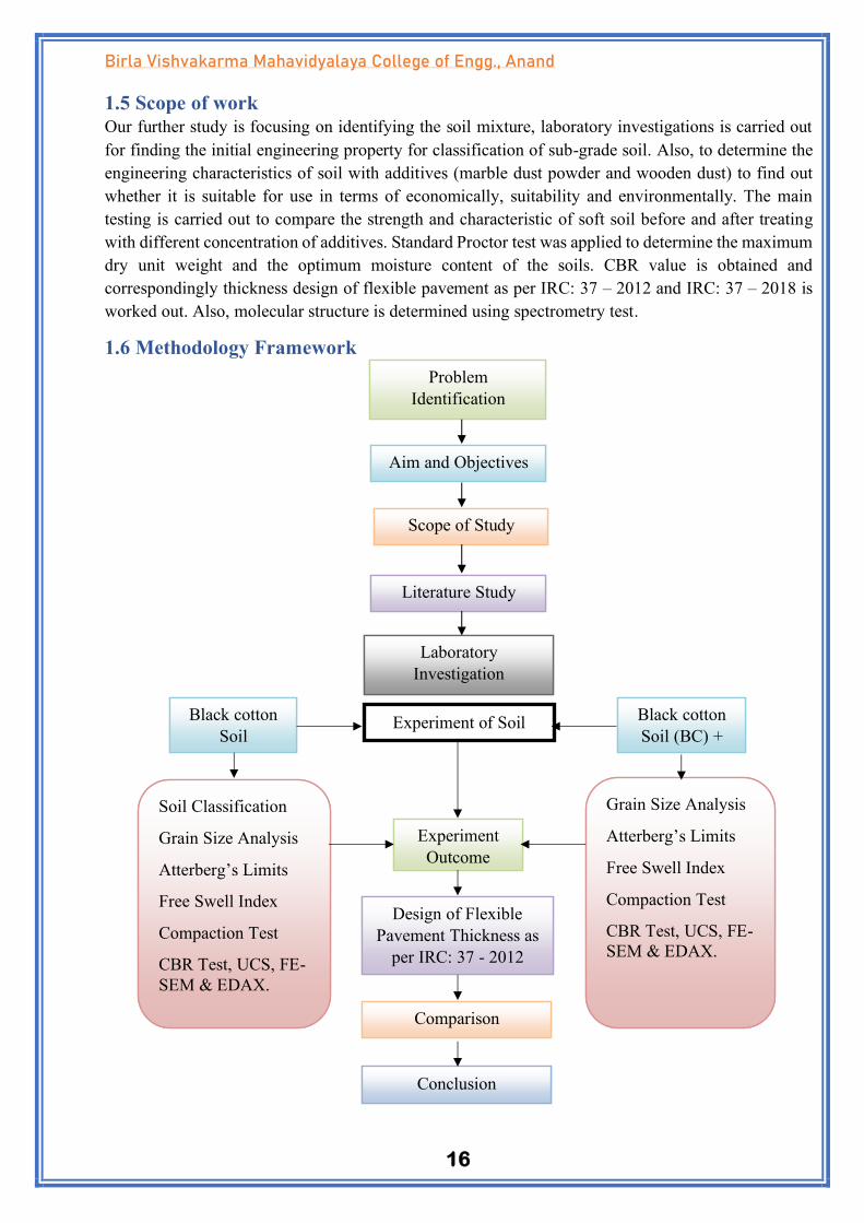
1.6 Methodology Framework
Problem
Identification
Aim and Objectives
Scope of Study
Literature Study
Laboratory
Investigation
Experiment of Soil Black cotton
Soil
Black cotton
Soil (BC) +
Additives
Experiment
Outcome
Soil Classification
Grain Size Analysis
Atterberg’s Limits
Free Swell Index
Compaction Test
CBR Test, UCS, FE-
SEM & EDAX.
Grain Size Analysis
Atterberg’s Limits
Free Swell Index
Compaction Test
CBR Test, UCS, FE-
SEM & EDAX.
Design of Flexible
Pavement Thickness as
per IRC: 37 - 2012
Comparison
Conclusion

17
Birla Vishvakarma Mahavidyalaya College of Engg., Anand
CHAPTER 2 LITERATURE REVIEW
2.1 Soil Stabilization
Soil stabilization means the improvement of the stability or bearing capacity of the soil by the
controlled compaction, proportioning and addition of suitable admixtures or stabilizers.
2.1.1 General
Soil stabilization is the process of improving the engineering properties of the soil and thus making it
more stable. In its broadest sense stabilization include compaction pre consolidation drainage and
many other processes.
Soil stabilization is used to reduce the permeability and compressibility of the soil mass in earth
structure and to increase the shear strength.
However, the main use of stabilization is to improve the natural soil for the construction of highways
and make an area trafficable within a short period of time for military and other emergency purposes.
In India, the modern era of soil stabilization began in early 1970’s with a general shortage of petroleum
and aggregates; it became necessary for engineers to look at means to improve soil other than replacing
the poor soil at the building sites.
Need for soil stabilization
• It is needed for strength improvement and for controlling of shrink- swell properties of soil.
• For improving the load bearing capacity of a sub grade soil and foundation soil to support
pavements and structures.
• Lower the compressibility of soil and therefore reduce the settlement when structures are built on
it
• It is needed for Soil waterproofing
The soil stabilization methods are broadly classified into two categories: Mechanical and Chemical
stabilization.
Figure 2.1 Mechanical stabilization (Source – slideshare.net)

18
Birla Vishvakarma Mahavidyalaya College of Engg., Anand
2.1.2 Mechanical Stabilization
In this method stability of soil is increased by blending the available soil with imported soil or
aggregate so as to obtain a desired particle size distribution, and by compacting the mixture to the
desired density.
The methodologies are as follows, compaction, blasting, dynamic compaction, preloading, sand drains,
etc.
• Application of mechanical stabilization
• Soil - aggregate mixture
• Sand - clay mixture
• Sand – gravel mixture
• Stabilization of soil with soft aggregate
2.1.3 Chemical Stabilization
Stability of granular soil lacks when they are too dry. If their moisture content is stabilized by the
addition of some chemicals then these soils can be used successfully.
It involves treatment of the soil with some kind of chemical compound, which when added to the soil,
would result in a chemical reaction. Addition of chemicals with the soil helps to retain moisture and
to impart some cohesion and thus retain the stability. These chemicals also reduce the dust nuisance in
un-surfaced roads.
The chemical reaction modifies or enhances the physical and engineering properties of a soil, such
asvolume stability and strength. It can increase their strength, bearing capacity, and improve their
shrink/swell and freeze/thaw characteristics. Lime stabilization and cement stabilization are two most
commonly used method in chemical stabilization.
Chlorides of calcium and sodium are the most popular salts used for this purpose. A number of other
chemicals/materials such as sodium silicate, lignin, resins, molasses etc., are used for chemical
stabilization of soils.
Figure 2.2 Chemical stabilization (Source- projecttunnel.com)
19
Birla Vishvakarma Mahavidyalaya College of Engg., Anand
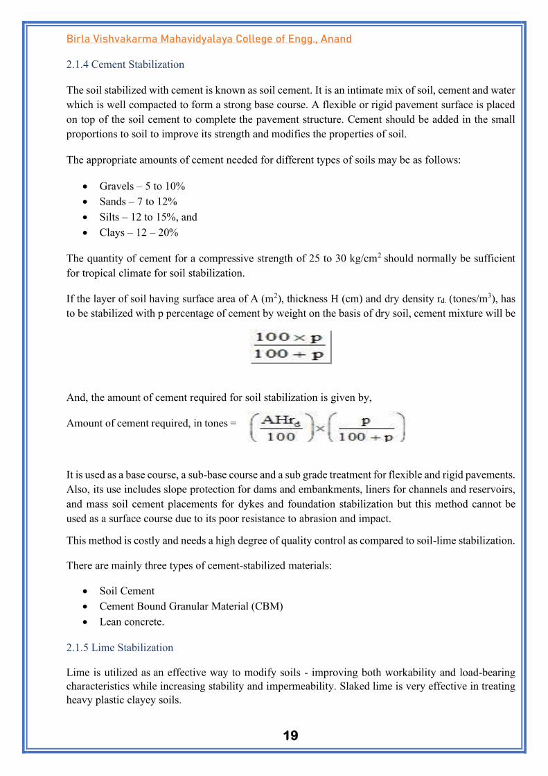
2.1.4 Cement Stabilization
The soil stabilized with cement is known as soil cement. It is an intimate mix of soil, cement and water
which is well compacted to form a strong base course. A flexible or rigid pavement surface is placed
on top of the soil cement to complete the pavement structure. Cement should be added in the small
proportions to soil to improve its strength and modifies the properties of soil.
The appropriate amounts of cement needed for different types of soils may be as follows:
• Gravels – 5 to 10%
• Sands – 7 to 12%
• Silts – 12 to 15%, and
• Clays – 12 – 20%
The quantity of cement for a compressive strength of 25 to 30 kg/cm2 should normally be sufficient
for tropical climate for soil stabilization.
If the layer of soil having surface area of A (m2), thickness H (cm) and dry density rd. (tones/m3), has
to be stabilized with p percentage of cement by weight on the basis of dry soil, cement mixture will be
And, the amount of cement required for soil stabilization is given by,
Amount of cement required, in tones =
It is used as a base course, a sub-base course and a sub grade treatment for flexible and rigid pavements.
Also, its use includes slope protection for dams and embankments, liners for channels and reservoirs,
and mass soil cement placements for dykes and foundation stabilization but this method cannot be
used as a surface course due to its poor resistance to abrasion and impact.
This method is costly and needs a high degree of quality control as compared to soil-lime stabilization.
There are mainly three types of cement-stabilized materials:
• Soil Cement
• Cement Bound Granular Material (CBM)
• Lean concrete.
2.1.5 Lime Stabilization
Lime is utilized as an effective way to modify soils - improving both workability and load-bearing
characteristics while increasing stability and impermeability. Slaked lime is very effective in treating
heavy plastic clayey soils.

20
Birla Vishvakarma Mahavidyalaya College of Engg., Anand
Lime-Soil stabilization is the process of adding lime to the soil to improve its properties like density,
bearing capacity etc. Various factors affecting lime-soil stabilization are soil type, lime type, lime
content used, compaction, curing period and additives. Lime may be used alone or in combination with
cement, bitumen or fly ash. When clayey soil with high plasticity is treated with lime, the plasticity
index is decreased and the soil becomes brittle and easy to be pulverized having less attraction with
water.
Lime-Soil stabilized mixes are useful to construct sub-base and base course for pavement. But this
method cannot be used as a surface course due to its poor resistance to abrasion and impact. This
method is quite suitable in warm regions, but not very suitable under freezing temperature.
Types of limes available are:
• Hydrated lime (Ca (OH) 2)
• Quick lime (CaO)
• Mono dehydrated dolomite lime (Ca (OH)2. MgO).
• Dolomite quick lime (Ca (OH) 2Mg (OH) 2).
Normally 2 to 8% of lime may be required for coarse grained soils and 5 to 8% of lime may be required
for plastic soils. The amount of fly ash as admixture may vary from 8 to 20% of the weight of the soil.
2.1.6 Fly Ash Stabilization
Fly ash is a byproduct from burning pulverized coal in electric power generating plants. From these
power generating plants, it generates different types of ash residues and discharge a huge amount of
particulate matter and gases.
Class C fly ash and Class F-lime product blends can be used in numerous geotechnical applications
common with highway construction:
• To enhance strength properties
• Stabilize embankments
• To control shrink swell properties of expansive soils
• Drying agent to reduce soil moisture contents to permit compaction
Its disposal not only needs enormous land, water, and power resources but it also causes serious
environmental hazards.
Figure 2.3 Lime stabilization (Source-happho.com)

21
Birla Vishvakarma Mahavidyalaya College of Engg., Anand
Fly ash is classified into two classes, F and C. Class C fly ash can be used as a stand-alone material
because of its self-cementitious properties. Class F fly ash can be used in soil stabilization applications
with the addition of a cementitious agent. The self-cementitious behavior of fly ashes is determined by
ASTM D 5239.
This test provides a standard method for determining the compressive strength of cubes made with fly
ash and water (water/fly ash weight ratio is 0.35), tested at seven days with standard moist curing.
The use of fly ash in soil stabilization and soil modification may be subject to local environmental
requirements pertaining to leaching and potential interaction with ground water and adjacent water
courses.
2.1.7 Bitumen stabilization
The basic principles in bituminous stabilization are waterproofing and binding. Generally, both the
binding and waterproofing actions are provided to the soil by adding bituminous material. Asphalts
and tars are bituminous materials which are used for stabilization of soil, generally for pavement
construction. Bituminous materials when added to a soil, it imparts both cohesion and reduced water
absorption. Most commonly used bituminous materials are cutback and emulsion.
Bituminous stabilized layer can be used as a sub-base or base course of ordinary roads and even as a
surface course for roads with low traffic in low rainfall region.
Depending upon the above actions and the nature of soils, bitumen stabilization is classified in
following four types:
• Sand bitumen stabilization
• Soil Bitumen stabilization
• Water proofed mechanical stabilization, and
• Oiled earth.
2.1.8 Soil stabilization by grouting
Among other techniques of soil stabilization, the grouting is one of the most expensive methods where
some kind of stabilizing agent inserted into the soil mass under pressure.
In this method, stabilizers are introduced by injection into the soil. The pressure forces the agent into
the soil voids in a limited space around the injection tube. The agent reacts with the soil and /or itself
to form a stable mass. This method is not useful for clayey soils because of their low permeability.
The most common grout is an admixture of cement and water, with or without sand. It has a large
number of applications such as:
• Control of water problems by filling cracks and pores.
• Prevention of sand densification beneath adjacent structures due to pile driving.
• Underpinning using compaction (displacement) grouting.
• Reducing vibrations by stiffening the soil.
• Reducing settlements by filling voids and cementing the soil structure more firmly.

22
Birla Vishvakarma Mahavidyalaya College of Engg., Anand
Generally, grout can be used if the permeability of the deposit is greater than 10 -5 m/s. This method is
suitable for stabilizing buried zones of relatively limited extent.
The grouting techniques can be classified as following:
• Clay grouting
• Chemical grouting
• Chrome lignin grouting
• Polymer grouting, and
• Bituminous grouting
2.2 Basic Soil Stabilization Process
Proper design and testing are an important component of any stabilization project. This testing will
establish proper design criteria in determining the proper additive and admixture rate to be used to
achieve the desired engineering properties. The following process is generally practiced.
• Assessment & Testing
The soils of the site are thoroughly tested to determine the existing conditions. Based on analysis of
existing conditions, additives are selected and specified. Generally, a target chemical percentage by
weight and a design mix depth are defined for the sub base contractor. The selected additives are
subsequently mixed with soil samples and allowed to cure. The cured sample is then tested to ensure
that the additives will produce the desired results.
• Site Preparation
The existing materials on site, including existing pavement if it is being reclaimed, is pulverized
utilizing a rotary mixer. The material is brought to the optimal moisture content by drying overly wet
soil or adding water to overlay dry soil.
• Introduce Additives
Cement, lime or fly ash can be applied dry or wet. When applied dry, it is typically spread at a required
amount per square meter or station utilizing a cyclone spreader or other device.
When lime is applied as slurry, it is either spread with tanker truck or through the rotary mixers on
board water spray system. Calcium chloride is usually applied by a tanker truck equipped with a spray
bar.
• Mixing
To fully incorporate the additives with the soil, a rotary mixer makes several mixing passes until the
materials are homogenous and well graded. It is crucial that the rotary mixer maintains optimal mixing
depths, as mixing depth, as mixing too shallow or too deep will create undesirable proportions of soil
and additive will decrease the load bearing properties of the cured layer.
• Compaction & Shaping/Trimming

23
Birla Vishvakarma Mahavidyalaya College of Engg., Anand
Compaction usually follows immediately after mixing, especially when the additive is cement or fly
ash. Some bituminous additive s requires a delay between mixing and compaction to allow for certain
chemical changes to occur. Compaction is accomplished through several passes using different
machines. Initial compaction is begun utilizing a vibratory pad foot compactor.
The surface is then shaped and trimmed to remove pad marks and provide a more suitable profile.
Intermediate compaction follows utilizing a pneumatic compactor, which provides certain kneading
action that further increase soil density. A tandem drum roller is used on the finishing pass to provide
a smooth surface.
• Curing
Sufficient curing will allow the additive to fully achieve its engineering potential. For cement, lime
and fly ash stabilization, weather and moisture are critical factors, as the curing can have a direct
bearing on the strength of the stabilized base. Generally, a minimum of seven days is required to ensure
proper curing. During the curing period, samples taken from the stabilized base will reveal when the
moisture content is appropriate for surfacing.
2.3 Industrial waste
2.3.1 General
Industrial waste refers to the solid, liquid and gaseous emissions, residual and unwanted wastes from
an industrial operation. It is produced by industrial activity which includes any material that is rendered
useless during a manufacturing process such as that of factories, industries, mills, and mining
operations.
Industrial wastes are hazardous since they are corrosive, reactive, genitive and toxic hence leading to
an extensive pollution. Industrial waste can be reduced through recycling, treatment before release and
utilizing bio friendly methods of manufacturing.
The main sources of industrial waste are:
• It caused by the emission of industrial waste into water bodies. It is the main source of water
pollution.
• Organic chemical industries which includes paints, dyes, detergents etc.
• Industrial waste includes organic pollutants and toxic chemicals i.e. heavy metals.
Waste Management is the collection, transport, processing or disposal, managing and monitoring of
waste materials. The term usually relates to materials produced by human activity, and the process is
generally undertaken to reduce their effect on health, the environment or aesthetics.
Waste management is a distinct practice from resource recovery which focuses on delaying the rate of
consumption of natural resources. All waste materials, whether they are solid, liquid, gaseous or
radioactive fall within the remit of waste management.

24
Birla Vishvakarma Mahavidyalaya College of Engg., Anand
2.3.2 Total industrial waste in India
India alone generate more than 1, 00,000 metric tonnes of solid waste every day which is higher than
many countries. Large metropolis such as Mumbai and Delhi generate around 9000 metric tonnes and
8300 metric tonnes of waste per day, respectively.
India generates 62 million tonnes of waste (mixed waste containing both recyclable and non-recyclable
waste) every year with an average annual growth rate of 4%. From the total waste generated of which
less than 60% is collected and around 15% processed.
With landfills ranking third in terms of greenhouse gas emissions in India, and increasing pressure
from the public, the Government of India revised the Solid Waste Management after 16 years.
The generated waste can be divided into three major categories:
• Organic (all kinds of biodegradable waste)
• Dry (or recyclable waste)
• Biomedical (or sanitary and hazardous waste).
As shown in Figure 6, nearly 50% of the total waste is organic with the volumes of recyclables and
biomedical/hazardous waste growing each year as India becomes more urbanized.
Figure 2.4 Total Waste Generations (Source-researchgate.com)
Figure 2.5 Collection vs dumped statistics (numbers in million MT per annum)

25
Birla Vishvakarma Mahavidyalaya College of Engg., Anand
As shown in Figure 7, less than 60% of waste is collected from households and only 15% of urban
India’s waste is processed in a country 12 times as dense as that of the United States (US) (PIB 2016)
While the collection rate needs to be improved to avoid illegal dumping and burning waste at street
corners and unoccupied lands, what happens to the waste post-collection is the subject matter of focus
of this section.
In India, the marble processing is one of the most flourishing industry. Marble industries in India grow
more than 3500 metric tons of marble powder per day.
The Indian marble industry has been growing steadily at an annual rate of around 10% per year. 20 to
30% of marble blocks are converted into powder. 3,172 M tons of marble dust were produced in year
2009-10.
In India, Rajasthan alone accounted for 94% output value followed by Gujarat and Madhya Pradesh.
Production value was less than 1% in Odisha, Andhra Pradesh, Jammu & Kashmir and Jharkhand in
2009-10.
2.3.3 Types of industrial waste
1. Solid waste
In industrial services, solid waste includes a variety of different materials, including paper, cardboard,
plastics, packaging materials, wood, and scrap metal. Some of these materials can be reused and
recycled by a recycling centre.
Solid waste means any garbage, refuse, sludge from a wastewater treatment plant, water supply
treatment plant, or air pollution control facility and other discarded materials including solid, liquid,
semi-solid, or contained gaseous material, resulting from industrial, commercial, mining and
agricultural operations, and from community activities, but does not include solid or dissolved
materials in domestic sewage.
Solid wastes include the following materials when discarded:
• waste tires, scrap metal, latex paints
• furniture and toys
• garbage
• appliances and vehicles
• oil and anti-freeze
• construction and demolition debris, asbestos
A material is discarded if it is abandoned by being:
• disposed of;

26
Birla Vishvakarma Mahavidyalaya College of Engg., Anand
• burned or incinerated, including being burned as a fuel for the purpose of recovering usable energy;
or
• Accumulated, stored or physically, chemically or biologically treated (other than burned or
incinerated) instead of or before being disposed of.
2. Chemical Waste
Chemical waste is any type of waste that is composed of noxious, potentially hazardous chemicals.
Harmful chemicals and solvents that are the by-products of large-scale laboratories and manufacturing
plants serve as the most common examples of industrial chemical waste.
Chemical waste is typically generated by factories, processing centres, warehouses, and plants. This
waste may include harmful or dangerous chemicals and chemical residue, and waste disposal must
adhere to careful guidelines.
However, certain household refrigerants, batteries and cleaning products qualify as chemical waste,
too. Depending on the potency of certain chemicals and solvents, as well as the potential safety hazards
they present, they may fall under the category of hazardous waste. Because of the safety hazards
associated with this type of waste, most chemical waste must be disposed of in a special manner.
For industrial forms of chemical waste, the disposal process typically involves sealing the waste in
securely sealed chemical-resistant drums or barrels, then transporting the safely stored waste to a
special landfill.
For household forms of chemical waste, many municipal landfills feature areas specifically designated
for this type of waste.
3. Toxic waste
Toxic waste is any unwanted material in all forms that can cause harm (e.g. by being inhaled,
swallowed, or absorbed through the skin). Many of today's household products such as televisions,
computers and phones contain toxic chemicals that can pollute the air and contaminate soil and water.
Disposing of such waste is a major public health issue.
Toxic materials are poisonous by-products as a result of industries such as manufacturing, farming,
construction, automotive, laboratories, and hospitals which may contain heavy metals, radiation,
dangerous pathogens, or other toxins. Toxic waste has become more abundant since the industrial
revolution, causing serious global health issues.
4. Hazardous waste
Hazardous waste is comprised of materials that can cause serious health and safety problems if waste
disposal is not handled correctly. This type of waste typically includes dangerous by-products
materials generated by factories, farms, construction sites, laboratories, garages, hospitals, and certain
production and manufacturing plants. The EPA and state departments regulate toxic and hazardous
waste disposal. This waste disposal is only legal at special designated facilities around the country.
6. Electronic waste

27
Birla Vishvakarma Mahavidyalaya College of Engg., Anand
Electronic Waste (e-waste) is one of the fastest growing segments of our nation’s waste stream. It
encompasses all broken, unusable, or outdated/obsolete electronic devices, components, and materials.
Used electronics which are destined for refurbishment, reuse, resale, salvage recycling through
material recovery, or disposal are also considered e-waste.
2.3.4 Impact of industrial waste on environment
Factories and power plants are typically located near bodies of water due to the need for large amounts
of water as an input to the manufacturing process, or for equipment cooling.
Metals, chemicals and sewage released into bodies of water directly affect marine ecosystems and the
health of those who depend on the waters as food or drinking water sources.
Air Pollution
Another obvious effect of industrial waste is air pollution resulting from fossil fuel burning. This
affects the lives of many people because this spreads illnesses.
This also affects the quality of soil because farmers have to try and deal with this massive issue. In
addition, nitrogen dioxide is a common air pollutant found in the air. Air pollutants have a devastating
effect on the human population because it causes sicknesses.
Water Pollution
One of the most devastating effects of industrial waste is water pollution. For most industrial processes,
heavy amount of water is used which comes in contact with harmful chemicals. These chemicals are
usually metals or radioactive material.
This heavily effects the environment because most of waste ends up in oceans, lakes, or rivers. As a
result, water becomes polluted posing as health hazard to everyone.
Industry is a huge source of water pollution; it produces pollutants that are extremely harmful to people
and the environment. Many industrial facilities use freshwater to carry away waste from the plant and
into rivers, lakes and oceans.
Pollutants from industrial sources include: Asbestos, lead, mercury, nitrates, Sulphur, phosphates,
petrochemicals etc.
Global Warming
Global warming is among the most serious outcome of industrial pollution, witnessed on the account
of the steady rise of industrial activities. Industries release into the atmosphere a variety of greenhouse
gases including carbon dioxide (CO2) and methane (CH4). These gases absorb thermal radiation from
the sun thereby increasing the general temperature of the earth, leading to global warming.
Global warming has several severe effects on human health and the environment. Rise in water levels,
melting of glaciers, extinction of polar species, tsunamis, flooding, and hurricanes are some of the dire
effects of global warming. Furthermore, global warming has threatened human survival and presented
health risks such as the increased incidences of diseases like cholera, plague, malaria, Lyme disease
and so on.

28
Birla Vishvakarma Mahavidyalaya College of Engg., Anand
Other impacts on environment:
• Decomposition of organic waste is a major source of escaping gases which contributes to global
warming
• Even with controlled land filling, only 45% methane can be utilized, the rest escapes to the
atmosphere, together with other harmful gases
• Global warming potential of methane is significantly higher than CO2
2.3.5 Impact of industrial waste on human health
The world Health Organization (WHO) revealed that outdoor air pollution accounts for about 2% of
all lung and heart diseases. WHO also underscores, around 5% of all lung cancers and 1% of all chest
infections are implications of outdoor air pollution.
Industrial toxic and chemical wastes that are disposed into water bodies or landfills are also responsible
for cancers and human cell poisoning. For instance, exposure to inorganic arsenic causes tumours to
form. Above all, industrial pollutants are responsible for thousands of illnesses and premature deaths
across the globe.
For the general public, the main risks to health are indirect and arise from the breeding of disease
vectors, primarily flies and rats. Uncontrolled hazardous wastes from industries mixing up with
municipal wastes create potential risks to human health.
Some other types of problem are as follows
• Chemical poisoning through chemical inhalation
• Uncollected waste can obstruct the storm
• water runoff resulting in flood Low birth weight
• Cancer
• Congenital malformations
• Neurological disease
• Nausea and vomiting
• Mercury toxicity from eating fish with high
• levels of mercury Plastic found in oceans ingested by birds
• Resulted in high algal population in rivers and sea.
• Degrades water and soil quality

29
Birla Vishvakarma Mahavidyalaya College of Engg., Anand
INDUS
TRIAL
WAST
E
SOURCE
ENVIRONME
NTAL
IMPACT
IMPACT
ON
HEALT
H
CONCLUSION
MARBL
E DUST
Mineral
waste
Soil damage,
Ecological impact,
Air pollution,
Water pollution,
Water clogging
Silicosis,
Eye
irritation,
Scleroderm
a,
Respiratory
disorder
• It gives maximum improvement
in the swelling and linear
shrinkage properties of BC soil.
• Increase in percentage of
marble dust decreases liquid
limit, plasticity index and
plastic limit and swelling
potential.
SAWDU
ST
Wood
industry
Impact on wildlife,
Harmful leachates
Lung
disease,
Asthma,
Eye
irritation,
ulceration
of the skin
• With increase in Sawdust
content a general reduction in
maximum dry unit weight was
observed.
• The OMC shows increase with
increase in Sawdust content.
• Reduce construction cost of the
roads particularly in the rural
areas.
FLYASH Thermal
power plant
Reduction in
recharge of ground
water,
Air & Water
pollution
kidney
disease,
hearing
impairment
,
high blood
pressure,
Lung
disease
• It is used to stabilize the soil in
different civil work such as in
road construction by reducing
the layer thickness, in
development of low
permeability.
INDUST
RIAL
WASTE
SOU
RCE
ENVIRON
MENTAL
IMPACT
IMPACT
ON
HEALTH
CONCLUSION

30
Birla Vishvakarma Mahavidyalaya College of Engg., Anand
MARBL
E DUST
Mineral
waste
Soil damage,
Ecological impact,
Air pollution,
Water pollution,
Water clogging
Silicosis,
Eye
irritation,
Scleroderm
a,
Respiratory
disorder
• It gives maximum improvement
in the swelling and linear
shrinkage properties of BC soil.
• Increase in percentage of
marble dust decreases liquid
limit, plasticity index and
plastic limit and swelling
potential.
SAWDU
ST
Wood
industry
Impact on wildlife,
Harmful leachates
Lung
disease,
Asthma,
Eye
irritation,
ulceration
of the skin
• With increase in Sawdust
content a general reduction in
maximum dry unit weight was
observed.
• The OMC shows increase with
increase in Sawdust content.
• Reduce construction cost of the
roads particularly in the rural
areas.
FLYASH
Thermal
power plant
Reduction in
recharge of ground
water,
Air & Water
pollution
kidney
disease,
hearing
impairment
,
high blood
pressure,
Lung
disease
• It is used to stabilize the soil in
different civil work such as in
road construction by reducing
the layer thickness, in
development of low
permeability
LIME
Limestone
Kankar,
Shells of sea
animals
It increases the pH
of acidic soil,
Global warming
When lime
comes in
contact
with skin it
can cause
serious
irritation
• Lime acts immediately and
improves various property of
soil such as carrying capacity of
soil, resistance to shrinkage
during moist conditions,
reduction in plasticity index,
and increase in CBR value and
subsequent increase in the
compression resistance with the
increase in time.

31
Birla Vishvakarma Mahavidyalaya College of Engg., Anand
CRUSH
ED
GLASS
Glass
Water pollution,
Production of solid
waste,
Volatile organic
compounds
Glass is
considered
a risk in
areas of
low-level
glazing.
• By adding a (%) of crushed
glass, some mechanical
properties of soil in
embankments as a viable
alternative material,
transportation, &
redevelopment in urban
environments can be improved.
BAGASS
E ASH Sugar mills
Open field burning
or land filling,
soil and water
pollution
Nervous
system
disorders,
Asthma,
Birth
defects
• Bagasse ash has effectively
stabilized black cotton soil and
has led to tremendous increase
in compressive strength of the
soil.
• BA is found to influence the
index and engineering
properties of BC soil making it
suitable for construction as a
foundation material for
structures built over it.
WASTE
PAPER
SLUDGE
Paper
Industry
Water pollution
Paper waste
Asthma
COPD
(Chronic
Obstructive
Pulmonary
Disease)
• When soil is treated with waste
paper sludge an increase in
OMC and decrease in MDD is
observed
• Ratio of decrease in density and
increase in OMC with increase
in percentage of additive waste
paper sludge.
GROUN
D
GRANU
LATED
BLAST
FURNA
CE
SLAG
By product
of iron and
steel
making
Air pollution,
Emission of CO2
Eye
irritation,
Respiratory
system
• With the increases of GGBS
(%) optimum moisture content
goes on decreasing while
maximum dry density goes on
increasing, hence compatibility
of soil increases and making the
soil denser and harder.

32
Birla Vishvakarma Mahavidyalaya College of Engg., Anand
RICE
HUSK
ASH
Agriculture
waste
Air pollution,
RHA are disposed
of into landfills or
improperly burned,
which can cause
severe
environmental
impacts in air,
water, and soil
Asthma,
Nervous
system
disorders
• The LL and the free swell index
of the soil decreased steeply
with the increase in the % of
RHA.
• Silica present in RHA is
capable to replace the
exchangeable ion present in
clay mineral thus can reduce
shrinkage and swelling property
of clay minerals.
LIME
Limestone
Kankar,
Shells of sea
animals
It increases the pH
of acidic soil,
Global warming
When lime
comes in
contact
with skin it
can cause
serious
irritation
• Lime acts immediately and
improves various property of
soil such as carrying capacity of
soil, resistance to shrinkage
during moist conditions,
reduction in plasticity index,
and increase in CBR value and
subsequent increase in the
compression resistance with the
increase in time.
CRUSH
ED
GLASS
Glass
Water pollution,
Production of solid
waste,
Volatile organic
compounds
Glass is
considered
a risk in
areas of
low-level
glazing.
• By adding a (%) of crushed
glass, some mechanical
properties of soil in
embankments as a viable
alternative material,
transportation. &
redevelopment in urban
environments can be improved
BAGASS
E ASH
Sugar mills
Open field burning
or land filling,
soil and water
pollution
Nervous
system
disorders,
Asthma,
Birth
defects
• Bagasse ash has effectively
stabilized black cotton soil and
has led to tremendous increase
in compressive strength of the
soil.
• BA is found to influence the
index and engineering
properties of BC soil making it
suitable for construction as a
foundation material for
structures built over it.
WASTE
PAPER
SLUDGE
Paper
Industry
Water pollution
Paper waste
Asthma
COPD
(Chronic
• When soil is treated with waste
paper sludge an increase in

33
Birla Vishvakarma Mahavidyalaya College of Engg., Anand
Obstructive
Pulmonary
Disease)
OMC and decrease in MDD is
observed
• Ratio of decrease in density and
increase in OMC with increase
in percentage of additive waste
paper sludge.
GROUN
D
GRANU
LATED
BLAST
FURNA
CE
SLAG
By product
of iron and
steel
making
Air pollution,
Emission of CO2
Eye
irritation,
Respirator
y system
• With the increases of GGBS
(%) optimum moisture
content goes on decreasing
while maximum dry density
goes on increasing, hence
compatibility of soil increases
and making the soil denser and
harder.
RICE
HUSK
ASH
Agriculture
waste
Air pollution,
RHA are disposed
of into landfills or
improperly burned,
which can cause
severe
environmental
impacts in air,
water, and soil
Asthma,
Nervous
system
disorders
• The LL and the free swell
index of the soil decreased
steeply with the increase in the
% of RHA.
• Silica present in RHA is
capable to replace the
exchangeable ion present in
clay mineral thus can reduce
shrinkage and swelling
property of clay minerals.
Table 2.1 Types of wastes and their impacts (Source –slideshare.com)
2.4 Materials
2.4.1 Black cotton soil
In this thesis, soil is collected from Surat city near Sachin railway station. Black cotton soils possess
low strength and undergo excessive volume changes, making their use in constructions very difficult.
Test according to Indian Standards are performed on the soil to check the properties of untreated and
treated the soil with stabilizer.
These soils cause more extensive damage than even natural disasters. So, we must increase the
compressive strength of black cotton soil by utilizing of additives such as marble dust and wooden
dust. Black cotton soil possesses low strength. If the soil is weak, then the thickness of the pavements
increases. So, for such problematic soil, it is essential to stabilize them in the most economic and
affective way.
Following are the problems with Black cotton soil.
• In the rainy season, these soils become very soft by filling up of water in the cracks and
fissures. These soft soils reduce the bearing capacity of the soils.

34
Birla Vishvakarma Mahavidyalaya College of Engg., Anand
• In saturated conditions, these soils have high consolidation settlements.
• These soils have high swelling nature. Due to this structure causes damages.
• When lands are applied on these soils in wet conditions. These soils get Shrinkage.
2.4.2 Marble dust
In terms of geological definition ‘Marble is metamorphosed limestone produced by re-crystallization
under thermal condition and also regional metamorphism.’ Marble is a rock resulting from
metamorphism of sedimentary carbonate rocks, most commonly limestone or dolomite rock. The
purest calcite (CaCO3) marble is white in colour.
The purity of marble is responsible for its colour and appearance; it is white if the limestone is
composed solely of calcite.
Marble is used for construction and decoration; marble is durable, has a noble appearance, and is
consequently in great demand. Chemically, marbles are crystalline rocks composed predominantly of
calcite, dolomite or serpentine minerals.
Figure 2.6 Collection of soil sample (Source –Google maps .com)
Figure 2.7 Marble Dust (Source –indiamart.com)

35
Birla Vishvakarma Mahavidyalaya College of Engg., Anand
The other mineral constituents vary from origin to origin. Quartz, muscovite, tremolite, actinolite,
micro line, talc, garnet, osterie and biotite are the major mineral impurities whereas SiO2, limonite,
Fe2O3, manganese, 3H2O and FeS2 are the major chemical impurities associated with marble.
The marble dusts were generated from cutting and polishing of marble stones. The major constituent
of marble dust is calcium carbonate (88.5%) which aids in the stabilization of the soil.
The solid waste is produced on the mine sites or at the processing units and slurry is in the semi-
liquid form generates during sawing and polishing operations. The generation of waste marble dust is
approximately 30-40% of the total marble handled per year. It makes relevance because every year
about 68 million ton of marble is manufactured all over the world.
The main states of India at which the marble is found are Rajasthan, Haryana, Gujarat, Jammu &
Kashmir, Madhya Pradesh, Uttar Pradesh, Maharashtra, Andhra Pradesh, Sikkim and West Bengal.
❖ Advantages of Marble dust
• Marble powder can be used as filler in concrete and paving materials it helps to reduce total
void content in concrete.
• Marble powder can be used as an admixture in concrete, so that strength of the concrete can be
increased.
• We can reduce the environmental pollution by utilizing this marble powder for producing the
other products.
• Marble dust is mixed with concrete, cement or synthetic resins to make counters, building
stones, sculptures, floors and many other objects.
• Marble dust is also used to make paint primer for canvas paintings, and as paint filler.
• The marble powder is also used to create carbonic acid gases which are used in the bottling of
beverages.
❖ Disadvantages of Marble dust
• Marble powder is not available in all the places.
• Only 20% of the final product is obtained from stone industry.
❖ Production of Waste Marble Dust
The production of fine particles (<2mm) while cutting is one of the major problems for the marble
industry. When 1 m3 marble block is cut into 2 cm thick slab, the proportion of the particle production
is approximately 25%. While cutting of marble block water is used as cooler. But the fine particle can
be easily dispersed after losing humidity, under atmospheric condition, such as wind and rain. Thus,
fine particle can pollute more than other forms of marble waste.
❖ Percentage of waste Generated
The slurry generated during processing can be estimate at about 10% of the total stone quarried (20%
to 25% of the block as received from the quarries) and during polishing as 5% to 7%
Chemical Properties of marble dust
Sr. No. Materials Marble powder (%)
1. Loss of ignition (LOI) 43.63

36
Birla Vishvakarma Mahavidyalaya College of Engg., Anand
2. CaO (calcium oxide) 43.20
3. Fe2O3 (iron oxide) 1.90
4. Al2O3 (Aluminium oxide) 2.50
5. SiO2 (Silicon dioxide) 13.8
6. MgO (Magnesium oxide) 2.70
7. SO3 (Sulphur trioxide) 0.07
8. K2O (Potassium oxide) 0.60
9. Na2O (Sodium oxide) 0.90
10. CL (chlorine) 0.03
Table 2.2 Chemical properties of marble dust (Source –slideshare.com)
Table 2.3 physical properties of marble dust (Source –slideshare.com)
2.4.2.1 Impact of marble dust on environment
• The waste in the water does not completely sink into the ground and much of it remains on the
surface. As the water evaporates the liquid wastes solidify. Subsequently wet marble wastes
subjected to rain will carry seepage down into the ground.
• Generally, wastes are dumped on the roads outside city and the dust is airborne by the wind and
scrap.
• The fine particles can cause more pollution than other form of marble waste unless stored properly
in sedimentation tanks and further utilized.
• The white dust particles usually contain CaCo3 and can cause visual pollution.
• The marble slurry in the long run could lead into water clogging of the soil, to increase soil
alkalinity and to disruption of photosynthesis and transportation. The net effect is soil fertility and
plant productivity.
• Many animal species are exclusively herbivores. Again, if plants did not out, their internal
chemistry will have been altered and their nutritional value poisoned by gases emitted by the
industries.
• It should also be emphasized that animal health like human health, can be adversely affected by
inferior environment quality
COLOUR WHITE
FORM POWDER
ODOR ODORLESS
MOISTURE CONTENT (%) 1.59

37
Birla Vishvakarma Mahavidyalaya College of Engg., Anand
• Soil damage: -The waste in the water does not completely sink into the ground and much of it
remains on the surface. As the water evaporates the liquid wastes solidify. Subsequently wet
marble wastes subjected to rain will carry seepage down into the ground.
• Ecological impact: - Reduced porosity & permeability of the topsoil along with the increasing
alkalinity have tremendously affected the soil fertility. The percolation rate of rain water due to
clogging of pores of top soil has also increased surface run-off which reduced recharging of ground
water.
• Air Pollution: - Deposition of particulate/fugitive dust on roads up to 2.5 cm causes
solid particles and liquid droplets found in the air due to vehicular activities and strong wind
currents.
• Water Pollution: - Disposing the slurry waste near to water bodies, road side areas can deteriorate
the surface & ground water quality by increasing turbidity, suspended solids, and calcium and
magnesium hardness.
2.4.2.2 Impact of marble dust on human health
• Silicosis
Stone carving of a hard stone like marble requires the use of power tools such as saws, drills, grinders
and sanders. Inhaling marble dust causes toxic effects on the respiratory system. Workers and residents
living in areas adjacent to stone quarries are prone to a disease called silicosis, whereby inhaled marble
dust damages the cells of the respiratory system. Symptoms include a chronic cough and shortness of
breath. There is no specific treatment other than supportive treatment such as cough medicine,
bronchodilators and oxygen. People with silicosis have a higher risk of developing tuberculosis.
Wearing a protective respirator may decrease risk of inhaling marble dust.
• Eye Irritation
Grinding and polishing marble releases small particles of stone and dust into the air. Exposure to the
eyes with airborne marble dust causes irritation because of the abrasiveness of the product.
Recommended first-aid measures include flushing the eyes with water thoroughly for 15 minutes,
gently lifting the eyelids and rinsing under the eyelids and avoid scrubbing or rubbing the eyes. Seek
medical attention if irritation and discomfort persist. Wearing eye protection may decrease risk of eye
irritation when working with marble.
• Scleroderma
Marble dust is abrasive and causes irritation to the skin. Stonemasons who have long-term exposure
to marble dust have a high risk of developing scleroderma. This is a rare and progressive disease that
involves the hardening and tightening of the skin and connective tissue. It results from the
overproduction and accumulation of collagen in the body tissues. Exposure to silica, which is a
component found in marble dust, is one risk factor for developing scleroderma
2.4.3 Wooden dust
Also known as Saw dust which is actually by-products of sawmills generated by sawing timber. It is
the loose particles or wood chippings obtained by sawing wood into useable sizes. After collection,
clean saw dust not having much bark and so not much organic content was air dried and burnt at the

38
Birla Vishvakarma Mahavidyalaya College of Engg., Anand
room temperature. Sawdust insulation is probably the most cost-effective insulating material. Sawdust
is composed of fine particles of wood.
Figure 2.7 Sawdust (Source –scialert.com)
It is the by-product of cutting, drilling, grinding, sanding wood. It is produced as a small irregular chip
or small garbage of wood during sawing of logs of timber into different sizes. Sawdust absorbs water
from soil. It can also increase plasticity of soil and reduce swelling pressure of soil.
• Properties of wooden dust
Constituent Composition (%)
Silicon Dioxide 19.30
Aluminium Oxide 10.04
Calcium Oxide 35.63
Potassium Oxide 9.21
Magnesium Oxide 7.30
Ferric Oxide 2.52
Sodium Oxide 3.60
Loss on Ignition 12.40
Table 2.4 Properties of wooden dust (Source –chegg.com)
2.4.3.1 Impact of wooden dust on environment
At sawmills, unless reprocessed into particleboard, burned in a sawdust burner or used to make heat
for other milling operations, sawdust may collect in piles and add harmful lichgates into local water
systems, creating an environmental hazard. This has placed small sawyers and environmental agencies
in a deadlock.
Technical advisors have reviewed some of the environmental studies, but say most lack standardized
methodology or evidence of a direct impact on wildlife. They don’t take into account large drainage

39
Birla Vishvakarma Mahavidyalaya College of Engg., Anand
areas, so the amount of material that is getting into the water from the site in relation to the total
drainage area is extremely small.
The decomposition of a tree in a forest is similar to the impact of sawdust, but the difference is of
scale. Sawmills may be storing thousands of cubic meters of wood residues in one place, so the issue
becomes one of concentration.
But of larger concern are substances such as lignin’s and fatty acids that protect trees from predators
while they are alive, but can leach into water and poison wildlife.
2.4.3.2 Impact of wooden dust on human health
• Inhaling dust into the lungs can cause breathing problems and lead to lung diseases such as
occupational asthma and lung cancer. Breathing in dust is the most common type of exposure to
wood dust.
• Swallowing wood dust can affect the intestines, bloodstream and vital organs and make people ill.
• Getting dust in the eyes can cause irritation and damage.
• Skin contact with wood dust can cause ulceration of the skin, irritation and dermatitis.
2.5 Review of research paper on Waste Marble powder
[01] B. B. Patel, C. B. Mishra, Dr. H. R. Varia, H. B. Thakar (2017). “Use of Waste Marble
Powder to Improve the Characteristics of Black Cotton Soil.” Earthquake International Journal of
Engineering Research & Technology (IJERT), Vol. 6, Issue 4.
Research Paper Materials Tests Outcome
Use of Waste
Marble Powder to
Improve the
Characteristics of
Black Cotton Soil
Soil: black cotton
soil
Additives: waste
marble dust
Grain Size Analysis,
Atterberg’s Limit,
Free Swell Index of
Soils, Compaction,
California Bearing
Ratio, Unconfined
Compressive Strength,
Water Content
• Soil + 20% Marble
powder PI- 11.57, FSI-
34.44
• Soil + 30% Marble
powder PI- 11.2, FSI-
32.81
• Soil + 40% Marble
powder PI- 9.66, FSI-
30.77
• Soil + 60% Marble
powder PI-4.35, FSI-
29.78
[02] Krichphon Singh, V.K. Arora (2017). “Stabilization of non-plastic silt using marble dust”
International journal of advance research in science and engineering, Vol. 6, Issue 4.

40
Birla Vishvakarma Mahavidyalaya College of Engg., Anand
[03] Krichphon Singh, V.K. Arora (2018). “Pursuance of waste marble powder to improve soil
stabilization” International Research Journal of Engineering and Technology (IRJET), Vol. 5, Issue 5.
Research Paper Materials Tests Outcome
Pursuance of waste
marble powder to
improve soil
stabilization
Soil: highly
clayey soil
Additives: waste
marble powder
MDD & OMC,
California Bearing
Ratio, Unconfined
Compressive
Strength
• The OMC of 12.97% is
reached at 45% of waste
marble powder.
• The increase in CBR for
45% additive is 2.76
times that of ordinary
soil.
• The UCS vale for soil
with 45% additive is 1.5
times more compared to
ordinary soil.
[04] C. B. Mishra, Nandan Patel, Riddhi Choksi (2018). “Soil stabilization using marble dust”
International Research Journal of Engineering and Technology (IRJET), Vol. 5, Issue 5.
Research Paper Materials Tests Outcome
Soil stabilization
using marble dust
Soil: black
cotton soil
Additives:
waste marble
dust
Free swell Index
Liquid limit Plastic
Limit, Plasticity index,
Shrinkage Limit,
Specific gravity,
MDD.
• The liquid Limit of soil
sample is 61%. Soil sample
is classified as Highly
Compressible clay
Research Paper Materials Tests Outcome
Stabilization of non-
plastic silt using
marble dust
Soil: Silt soil
Additives: waste
marble dust
Unconfined
Compression
Strength test,
Standard proctor
test
• Optimum value of marble
dust -15% by weight of
dry soil.
• Maximum UCS of sample
is = 1.032 for 15% marble
dust addition.
• Samples turned brittle on
higher percentage of
marble dust.
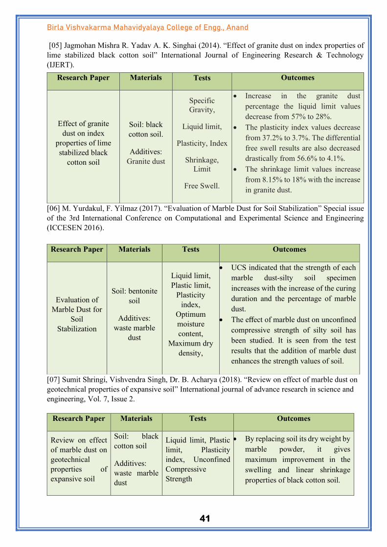
41
Birla Vishvakarma Mahavidyalaya College of Engg., Anand
[05] Jagmohan Mishra R. Yadav A. K. Singhai (2014). “Effect of granite dust on index properties of
lime stabilized black cotton soil” International Journal of Engineering Research & Technology
(IJERT).
[06] M. Yurdakul, F. Yilmaz (2017). “Evaluation of Marble Dust for Soil Stabilization” Special issue
of the 3rd International Conference on Computational and Experimental Science and Engineering
(ICCESEN 2016).
[07] Sumit Shringi, Vishvendra Singh, Dr. B. Acharya (2018). “Review on effect of marble dust on
geotechnical properties of expansive soil” International journal of advance research in science and
engineering, Vol. 7, Issue 2.
Research Paper Materials Tests Outcomes
Effect of granite
dust on index
properties of lime
stabilized black
cotton soil
Soil: black
cotton soil.
Additives:
Granite dust
Specific
Gravity,
Liquid limit,
Plasticity, Index
Shrinkage,
Limit
Free Swell.
• Increase in the granite dust
percentage the liquid limit values
decrease from 57% to 28%.
• The plasticity index values decrease
from 37.2% to 3.7%. The differential
free swell results are also decreased
drastically from 56.6% to 4.1%.
• The shrinkage limit values increase
from 8.15% to 18% with the increase
in granite dust.
Research Paper Materials Tests Outcomes
Evaluation of
Marble Dust for
Soil
Stabilization
Soil: bentonite
soil
Additives:
waste marble
dust
Liquid limit,
Plastic limit,
Plasticity
index,
Optimum
moisture
content,
Maximum dry
density,
• UCS indicated that the strength of each
marble dust-silty soil specimen
increases with the increase of the curing
duration and the percentage of marble
dust.
• The effect of marble dust on unconfined
compressive strength of silty soil has
been studied. It is seen from the test
results that the addition of marble dust
enhances the strength values of soil.
Research Paper Materials Tests Outcomes
Review on effect
of marble dust on
geotechnical
properties of
expansive soil
Soil: black
cotton soil
Additives:
waste marble
dust
Liquid limit, Plastic
limit, Plasticity
index, Unconfined
Compressive
Strength
• By replacing soil its dry weight by
marble powder, it gives
maximum improvement in the
swelling and linear shrinkage
properties of black cotton soil.
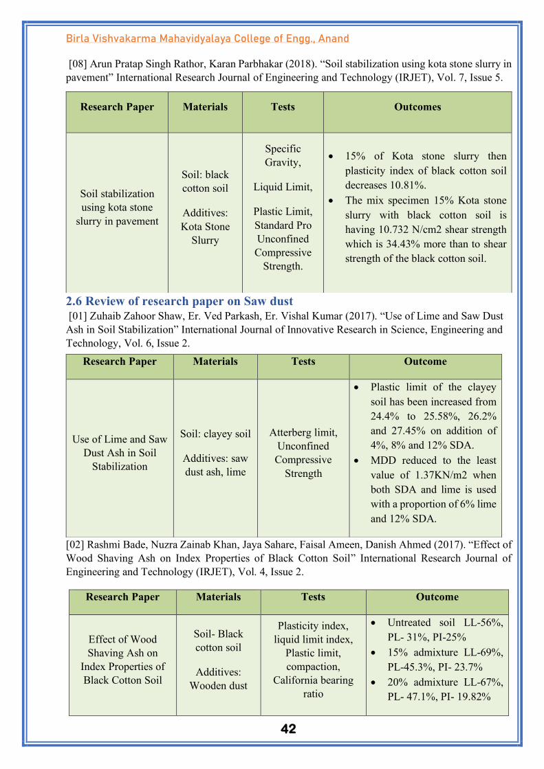
42
Birla Vishvakarma Mahavidyalaya College of Engg., Anand
[08] Arun Pratap Singh Rathor, Karan Parbhakar (2018). “Soil stabilization using kota stone slurry in
pavement” International Research Journal of Engineering and Technology (IRJET), Vol. 7, Issue 5.
2.6 Review of research paper on Saw dust
[01] Zuhaib Zahoor Shaw, Er. Ved Parkash, Er. Vishal Kumar (2017). “Use of Lime and Saw Dust
Ash in Soil Stabilization” International Journal of Innovative Research in Science, Engineering and
Technology, Vol. 6, Issue 2.
[02] Rashmi Bade, Nuzra Zainab Khan, Jaya Sahare, Faisal Ameen, Danish Ahmed (2017). “Effect of
Wood Shaving Ash on Index Properties of Black Cotton Soil” International Research Journal of
Engineering and Technology (IRJET), Vol. 4, Issue 2.
Research Paper Materials Tests Outcome
Effect of Wood
Shaving Ash on
Index Properties of
Black Cotton Soil
Soil- Black
cotton soil
Additives:
Wooden dust
Plasticity index,
liquid limit index,
Plastic limit,
compaction,
California bearing
ratio
• Untreated soil LL-56%,
PL- 31%, PI-25%
• 15% admixture LL-69%,
PL-45.3%, PI- 23.7%
• 20% admixture LL-67%,
PL- 47.1%, PI- 19.82%
Research Paper Materials Tests Outcomes
Soil stabilization
using kota stone
slurry in pavement
Soil: black
cotton soil
Additives:
Kota Stone
Slurry
Specific
Gravity,
Liquid Limit,
Plastic Limit,
Standard Pro
Unconfined
Compressive
Strength.
• 15% of Kota stone slurry then
plasticity index of black cotton soil
decreases 10.81%.
• The mix specimen 15% Kota stone
slurry with black cotton soil is
having 10.732 N/cm2 shear strength
which is 34.43% more than to shear
strength of the black cotton soil.
Research Paper Materials Tests Outcome
Use of Lime and Saw
Dust Ash in Soil
Stabilization
Soil: clayey soil
Additives: saw
dust ash, lime
Atterberg limit,
Unconfined
Compressive
Strength
• Plastic limit of the clayey
soil has been increased from
24.4% to 25.58%, 26.2%
and 27.45% on addition of
4%, 8% and 12% SDA.
• MDD reduced to the least
value of 1.37KN/m2 when
both SDA and lime is used
with a proportion of 6% lime
and 12% SDA.

43
Birla Vishvakarma Mahavidyalaya College of Engg., Anand
[03] A. G. Patil, K. P. Patil, N. P. Patil, P. S. Joshi, S. S. Chavan, Dr. V.R. Saraf (2017). “Eco-
friendly stabilization of black cotton soil” International Journal of Innovative Research in Science,
Engineering and Technology, Vol. 3, Issue 3.
[04] T. Deepika (2019). “Experimental Study on Behavior of Black Cotton Soil using Wood Ash as
Stabilizer” International Research Journal of Engineering and Technology (IRJET), Vol. 5, Issue 3.
[5] Berjees Anisa Ikra, Tamanna Kabir, Anika Nowshin Mowrin, Ahsan Habib (2018). “Stabilization
of Clay Soil Mixed with Wood Ash” International Journal of Scientific & Engineering Research, Vol.
9, Issue 10.
Research paper Materials Tests Outcomes
Eco-friendly
stabilization of
black cotton soil
Soil: Black
cotton soil
Additives:
Wooden Ash
Quarry Dust
Specific gravity
Liquid limit
Plastic limit
Plasticity index
Optimum moisture
index
Unconfined
compressive
strength.
California bearing
ratio
• Wood ash and quarry dust are
the industrial wastes which can
be efficiently used as the eco-
friendly stabilizers.
• According to the various tests
conducted on black cotton soil
with and without stabilizers, to
the use of 10% wood ash as a
stabilizer.
Research Paper Materials Tests Outcome
Experimental
Study on Behavior
of Black Cotton
Soil using Wood
Ash as Stabilizer
Soil: Black
cotton soil
Additives:
Wood ash
liquid limit, plastic
limit, compaction,
California bearing
ratio, Unconfined
compressive strength
test
• The properties such as LL and
PL decreases with increase in
percentage of wood ash added.
• CBR of the soil attained its
highest value at 8% addition of
wood ash
• Differential FSI decreases with
increase in− percentage of
wood ash added
Research Paper Materials Tests Outcomes
Strength behavior
of clayey soil
stabilized with
saw dust ash’
Clay soil
Additive
Saw dust
Specific gravity, Liquid
limit,
Plastic limit, Plasticity
index, Optimum
moisture content,
Unconfined compressive
strength,
California bearing ratio
• The CBR value increases by
103.11 % and unconfined
compressive strength
increases by 26.35 at 4 % SDA
content which is taken as
optimum
• With increase in SDA content
a general reduction in
maximum dry unit weight was
observed.

44
Birla Vishvakarma Mahavidyalaya College of Engg., Anand
[06] A. Venkatesh and Dr. G. Sreenivasa Reddy (2016). “Effect of Waste Saw Dust Ash on
Compaction and Permeability Properties of Black Cotton Soil” International Journal of Civil
Engineering Research, Vol. 7, Issue 1
[07] M. Usha Rani, J. Martina Jenifer (2016). “Analysis of strength characteristics of black cotton
soil using wood ash as stabilizer” International Journal of Research in Science and Technology, Vol.
6, Issue 1.
Conclusion based on research papers
The research reviewed the use of industrial waste in improving pavement interlayer material. Marble
and saw dust f industrial wastes were reviewed in a bid to improve sustainability and make road
construction affordable in developing nations. From the review, it can be concluded that:
In any project-based work the study of various research papers is important in determining the various
aspects of predetermined knowledge of any study. On the basis of that study we are able to know how
the material would behave on account of various tests performed on it Those research papers also help
us to determine what are the most suitable tests that would carried on the material .In our case we were
able to evaluate that CBR and UCS tests would be the main spine of our projects and on the basis of
those tests only we would be able to design the pavement and find out its cost afterwards. Those
research papers also helped us in finding out the required amount of stimulating dosage between any
tests and find out the required optimum value of the given sample taken. Hence the study of research
papers is important field in any project related study to know its historical background or predict its
future outcome.
Research Paper Materials Tests Outcomes
Effect of Waste
Saw Dust Ash on
Compaction and
Permeability
Properties of Black
Cotton Soil
Soil: black
cotton
Additive:
saw dust
Liquid limit, Plastic
limit, plasticity index,
Optimum moisture
content by Standard
proctor test, Maximum
dry density, Free swell
index, Sieve analysis,
Specific gravity
• At 2% of WSDA was added to
the soil the dry density was
increased from 1. 40 gm/cc to 1.
46 gm/cc. With further increase
of WSDA to the soil the density
starts decreasing.
• With increase in percentages of
WSDA to the soil the
coefficient of permeability was
reduced from 0. 18 to 0. 08.
Research Paper Materials Tests Outcomes
Analysis of strength
characteristics of
black cotton soil
using wood ash as
stabilizer
Soil: black
cotton
Additive:
saw dust
Liquid limit, Plastic
limit, plasticity index,
MDD, OMC, Free
swell index, CBR,
Thickness of flexible
pavement
• The maximum dry density of
the soil increases with increase
in percentage of wood ash.
Irrespective of their
percentages.
• The soaked CBR of the soil
increases with increase in
percentage wood ash content.

45
Birla Vishvakarma Mahavidyalaya College of Engg., Anand
CHAPTER 3 LABORATORY TESTS AND RESULTS
3.1 Laboratory Tests for Soil (As Per Indian Standards)
To identify the engineering properties as per Indian Standard provision, various tests were performed
which are enlisted as follows.
▪ Determination of Grain Size Analysis (IS: 2720 (Part IV) – 1985)
▪ Determination of Liquid & Plastic Limit (IS: 2720 (Part V) – 1986)
▪ Determination of Free Swell Index of Soils (IS: 2720 (Part XL) – 1977)
▪ Determination of Water Content - Dry Density Relation Using Heavy Compaction (IS: 2720 (Part
VIII) – 1997)
▪ Laboratory Determination of California Bearing Ratio (IS: 2720 (Part XVI) – 1987)
▪ Determination of Unconfined Compressive Strength (IS: 2720 (Part X) – 1991)
3.1.1 Determination of Grain Size Analysis (IS: 2720 (Part 4) – 1985)
Scope: This standard covers the method for the quantitative determination of grain size distribution of
grain size distribution soils.
Apparatus: Balance, Sieve, Rubber Pestle Mortar
Procedure: The portion of the soil sample retained on 4.75-mm IS Sieve, selected as given in the
preparation of the sample, shall be weighed and the mass recorded as the mass of the sample
uncorrected for hygroscopic moisture. The quantity of the soil sample taken shall depend on the
maximum particle size contained in the soil which is shown in Table 3.1.
The sample shall be separated into various fractions by sieving through the Indian Standard Sieves
specified in apparatus. Other sieves may be introduced between the sieves mentioned in rubber pestle
and mortar depending upon the additional information that may be desired to be obtained from the
analysis. While sieving through each sieve, the sieve shall be agitated so that the sample rolls in
irregular motion over the Sieve. Any particles may be tested to see if they will fall through but they
shall not be pushed through.
The material from the sieve may be rubbed, if necessary, with the rubber pestle in the mortar taking
care to see t individual soil particle are not broken and re-sieved to make sure that only individual
particles are retained.
The quantity taken each time for sieving on each sieve shall be such that the maximum weight of
material retained on each sieve at the completion of sieving does not exceed the values given in Table
3.1.
Depending upon the maximum size of material present in substantial quantities in the soil, the mass of
soil sample taken for analysis may be as follows.

46
Birla Vishvakarma Mahavidyalaya College of Engg., Anand
Sieve size (mm) Wt. of retained
soil (grams)
Cumulative wt.
of retained soil
% Retained % Passing
4.75 30 30 3.0 97
2.36 11 41 4.1 95.9
1.18 14 55 5.5 94.5
0.600 17 72 7.2 92.8
0.300 19 91 9.1 90.9
0.150 23 114 11.4 88.6
0.075 36 150 15.0 85
PAN 850 1000 100 0
Table 3.1 Grain size analysis
Results: IS: 1498 – 1970 describes the Indian Standard on Classification and Identification of soils for
general engineering purposes. To determine the classification of soil, data for gradation, Atterberg’s
limits are required which were performed in the laboratory as per Indian Standards. Following are the
results for the given soil.
Soil
Grain Size Distribution Atterberg's Limit Free
Swell
Index
(FSI)
IS
Classificat
ion
Gravel
(%)
Sand
(%)
Clay
(%)
L. L
(%)
P. L.
(%)
P. I.
(%)
Black cotton Soil 3 12 85 68 33 35 56.56% CH
Table 3.2 Soil classification, Fsi and Atterberg’s limit
From fig. 3.1 in X – axis represents liquid limit and Y – axis represents plasticity index. And at which
plasticity (low, intermediate, high, very high, extremely high) of soil can be found. For black cotton
soil point, P is shown in fig. where P represents Liquid Limit = 56 on X – axis and Plasticity Index
represents = 24 on Y – axis. And the point is above a point. Soil is intermediate plastic. In flow diagram,
dark portion represents black cotton soil and from that flow diagram, it can be concluded that given
Clay soil type is CH.

47
Birla Vishvakarma Mahavidyalaya College of Engg., Anand
3.1.2 Determination of Liquid Limit, Plastic Limit (IS: 2720 (Part V) – 1986)
Scope: The basic principle is to observe depths of penetrations of soils at various initial moisture
contents of a metal cone of acertain weight and apex angle with the point barely touching the surface
is allowed to drop into the surface. The standardization has been to identify liquid limit water content
for a specified depth of penetration.
Apparatus: Balance -Sensitive to 0.01 g.
Containers - non-corrodible and air-tight for moisture determination.
Soil Sample: A soil sample weighing about 150 g from thoroughly mixed portion of the soil passing
425 microns IS Sieve obtained in accordance to IS 2720 (Part 1)-19837.
Procedure: About 150 g of soil sample obtained as in 4.3 shall be worked well into a paste with the
addition of distilled water. In the case of highly clayey soils, to ensure uniform moisture distribution,
it is recommended that the soil in the mixed state is left for sufficient time (24 hours) in an air-tight
container. The wet soil paste shall then be transferred to the cylindrical cup of cone penetrometer
apparatus, ensuring that no air is trapped in this process. Finally, the wet soil is levelled up to the top
of the cup and placed on the base of the cone penetrometer apparatus.
The penetrometer shall be so adjusted that the cone point just touches the surface of the soil paste in
the cup clamped in this position. The initial reading is either adjusted to zero or noted down as is shown
on the graduated scale. The vertical clamp is then released allowing the cone to penetrate into the soil
paste under its own weight. The penetration of the cone after 5 seconds shall be noted to the nearest
millimetre. If the difference in penetration lies between 14 and 28 mm the test is repeated with suitable
Figure 3.1 Plasticity Chart (I.S. Soil Classification)

48
Birla Vishvakarma Mahavidyalaya College of Engg., Anand
adjustments to moisture either by the addition of more water or exposure of the spreading paste on a
glass plate for a reduction in moisture content.
The test shall then be repeated at least to have four sets of values of penetration in the range of 14 to
28 mm. The exact moisture content of each trial shall be determined in accordance with IS: 2720 (Part
2)-1973.
Determination of Liquid Limit:
A graph representing later content on the y-axis and the cone penetration on the x-axis shall be
prepared. The best fitting straight line is then drawn. The moisture content corresponding to cone
penetration of 20 mm shall be taken as the liquid limit of the soil and shall be expressed to the nearest
first decimal place.
3.1.2.1 Test Results for Atterberg’s Limit and FSI
Liquid Limit for Raw Soil
Can
No.
Wt. of
Can
(gm)
Number
of blows
Can + Wet
Sample
(gm)
Can + Dry
Sample
(gm)
Wt. of
Water
(gm)
Wt. of Dry
Sample
(gm)
Moisture
Content
(%)
140 15 19 35 26 9 11 81.81
154 27 21 38 33 5 6 83.33
574 30 24 54 44 10 14 71.42
Liquid Limit of black cotton Soil 68.0%
Table 3.3 Liquid limit for raw soil
Table 3.4 Liquid limit with 5% MP
Liquid Limit of black cotton Soil + 5% MP
Sample Condition: Passing through 425-micron sieve
Can
No.
No of
blows
Wt. of
Can
(gm)
Can + Wet
Sample
(gm)
Can + Dry
Sample
(gm)
Wt. of
Water
(gm)
Wt. of Dry
Sample
(gm)
Moisture
Content
(%)
108 21 9.25 33.45 25.38 8.07 16.13 50
175 27 8.25 32.53 24.19 8.38 15.94 52.57
553 32 9.1 35.67 25.5 10.17 16.40 62
Liquid Limit of black cotton Soil 56.98%

49
Birla Vishvakarma Mahavidyalaya College of Engg., Anand
Liquid Limit of black cotton Soil + 10% MP
Sample Condition: Passing through 425-micron sieve
Can
No.
No of
blows
Wt. of
Can
(gm)
Can + Wet
Sample
(gm)
Can + Dry
Sample
(gm)
Wt. of
Water
(gm)
Wt. of Dry
Sample
(gm)
Moisture
Content
(%)
530 14 10.18 54.37 39.73 14.64 29.55 49.54
505 19 10.82 58.62 41.99 16.63 31.17 53.35
510 27 9.59 45.98 33.29 13.69 23.70 57.76
Liquid Limit of black cotton Soil 51.78%
Table 3.5 Liquid limit with 10% MP
Liquid Limit of black cotton Soil + 15% MP
Sample Condition: Passing through 425-micron sieve
Can
No.
No of
blows
Wt. of
Can
(gm)
Can + Wet
Sample
(gm)
Can + Dry
Sample
(gm)
Wt. of
Water
(gm)
Wt. of Dry
Sample
(gm)
Moisture
Content
(%)
530 14 15.47 38 30.75 7.25 15.2 47.75
505 19 17.29 45.11 35.88 9.23 18.59 49.65
510 27 13.12 53.95 39.90 14.05 26.78 52.46
Liquid Limit of black cotton Soil 50.2%
Table 3.6 Liquid limit with 15% MP
Liquid Limit of black cotton Soil + 20 % MP
Sample Condition: Passing through 425-micron sieve
Can
No.
No of
blows
Wt. of
Can
(gm)
Can + Wet
Sample
(gm)
Can + Dry
Sample
(gm)
Wt. of
Water
(gm)
Wt. of Dry
Sample
(gm)
Moisture
Content
(%)
174 14 30.5 36.5 34.5 2 4 50
205 21 32.5 39 37 2 4.5 44.44
536 29 33 41 38.5 2 5.5 36.36
Liquid Limit of black cotton Soil + 20% MP 43%
Table 3.7 Liquid limit with 20% MP

50
Birla Vishvakarma Mahavidyalaya College of Engg., Anand
Plastic Limit for Raw Soil
Can
No.
Wt. of
Can (gm)
Can + Wet
Sample (gm)
Can + Dry
Sample (gm)
Wt. of
Water
(gm)
Wt. of Dry
Sample (gm)
Moisture
Content
(%)
534 15 21.47 19.8 1.67 4.8 34.8
548 14 19 17.81 1.19 3.81 31.2
Average Plastic Limit 33.00%
Plasticity Index 35%
Table 3.8 Plastic limit for raw soil
Plastic Limit of black cotton Soil + 5% MP
Can
No.
Wt. of
Can (gm)
Can + Wet
Sample (gm)
Can + Dry
Sample (gm)
Wt. of
Water
(gm)
Wt. of Dry
Sample
(gm)
Moisture
Content
(%)
140 15 21.8 20.17 1.63 5.17 31.5
538 14 19.21 18.02 1.19 4.02 29.5
Average Plastic Limit 30.5%
Plasticity Index 2.48%
Table 3.9 Plastic limit with 5% MP
Plastic Limit of black cotton soil + 10% MP
Can
No.
Wt. of
Can (gm)
Can + Wet
Sample (gm)
Can + Dry
Sample (gm)
Wt. of
Water
(gm)
Wt. of Dry
Sample (gm)
Moisture
Content
(%)
157 14.5 22.16 20.4 1.76 5.9 29.8
148 15 23.55 21.7 1.85 6.7 27.5
Average Plastic Limit 28.65%
Plasticity Index 23.13%
Table 3.10 Plastic limit with 10% MP

51
Birla Vishvakarma Mahavidyalaya College of Engg., Anand
Table 3.11 Plastic limit with 15% MP
Table 3.12 LL, PL and Free Swell Index with 20% MP
Free Swell Index
Mass of Dry
Soil
Volume of Soil In
water
Volume of Soil In
kerosene
% Free Swell
Index Avg. FSI
10 16 10.5 52.38 56.56%
10 17.2 10.7 60.74
Table 3.13 Free Swell Index
3.1.3 Determination of Water Content - Dry Density Relation Using Heavy Compaction (IS: 2720
(Part 8) – 1983)
Scope: This standard lays down the method for the determination of the relation between the water
content and the dry density of soil using light compaction. In this test, 2.6 kg rammer falling through
a height of 310 mm is used.
Apparatus: Cylindrical metal mould, Sample extruder, Balances, Oven, Container, Steel straightedge,
Sieve, Mixing Tools, Metal rammer.
Procedure: A 5-kg sample of air-dried soil passing the 20 mm IS test sieve shall be taken. The sample
shall be mixed thoroughly with a suitable amount of water depending on the soil type. The mould, with
base plate attached, shall be weighed to the nearest 1 gmm1).The mould shall be placed on a solid base,
such as a concrete floor or plinth and the moist soil shall be compacted into the mould, with the
Plastic Limit of black cotton soil + 15% MP
Can
No.
Wt. of
Can
(gm)
Can + Plastic
Wet Sample (gm)
Can + Dry
Sample (gm)
Wt. of
Water
(gm)
Wt. of Dry
Sample
(gm)
Moisture
Content
(%)
1 20 24.95 24 0.95 4 23.5
2 18 21.69 21 0.69 3 23
Average Plastic Limit 23.25%
Plasticity Index 26.95%
Plastic Limit of black cotton soil + 20% MP
Can
No.
Wt. of
Can (gm)
Can + Wet
Sample (gm)
Can + Dry
Sample (gm)
Wt. of
Water
(gm)
Wt. of Dry
Sample (gm)
Moisture
Content
(%)
1 24 30.3415 29 1.3415 5 26.83
2 22 27.0068 26 1.0068 4 25.17
Average Plastic Limit 26%
Plasticity Index 17%

52
Birla Vishvakarma Mahavidyalaya College of Engg., Anand
extension attached, in three layers of approximately equal mass, each layer being given 25 blows from
the 4.9-kg rammer dropped from a height of 450 mm above the soil. The blows shall be distributed
uniformly over the surface of each layer. The operator shall ensure that the tube of the rammer is kept
clear of soil so that the rammer always falls freely. The amount of soil used shall be sufficient to fill
the mould, leaving not more than about 6 mm to be struck off when the extension is removed. The
extension shall be removed and the compacted soil shall be levelled off carefully to the top of the
mould by means of the straightedge. The mould and soil shall then be weighed to 1gm (m2). The
compacted soil specimen shall be removed from the mould and placed on the mixing tray. The water
content of a representative sample of the specimen shall be determined as in IS: 2720 (Part II) – 1973.
The remainder of the soil specimen shall be broken up, rubbed through the 20 mm IS test sieve, and
then mixed with the remainder of the original sample. Suitable increments of water shall be added
successively and mixed into the sample, and the above procedure from operations shall be repeated for
each increment of water added. The total number of determinations made shall he at least five, and the
range of moisture contents should be such that the optimum moisture content, at which the maximum
dry density occurs, is within that range. Soil Susceptible to Crushing during Compaction: The
procedure is as follows:
a) Five or more 2.5-kg samples of air-dried soil passing the 20 mm are test sieve, shall be taken.
The samples shall each be mixed thoroughly with different amounts of water to give a suitable
range of moisture contents. The range of moisture content, at which the maximum dry density
occurs, is within that range.
b) Each sample shall be treated as in given in procedure.
c) Each compacted specimen shall be treated as given in procedure.
d) The remainder of each soil specimen shall be discarded.
Compaction in Large size Mould - For compacting soil containing coarse material up to 40 mm size,
the 2 250 ml mould should be wed. A sample weighing about 6 kg and passing the 40-mm IS sieve is
used for the test. Soil is compacted in three/five layers, each layer being given 55 blows of the 4.9-kg
rammer. The rest of the procedure is the same as given.
Calculations: Bulk Density: in g/cm3, of each compacted specimen shall be calculated from the
equation:
=
Where,
m1 = Mass in gm of mould and base
m2 = Mass in gm of mould, base, and soil
Vm = Volume in ml of mould
The dry density, in gm/cm3, shall be calculated from the equation:

53
Birla Vishvakarma Mahavidyalaya College of Engg., Anand
Where,
w = Moisture content of soil in the present
The dry densities, obtained in a series of determinations shall be plotted against the corresponding
moisture contents w.
3.1.3.1 Proctor Test Result for soil by using Standard Procter Test
Proctor Test is to be performed as per IS: 2720 (Part VIII) – 1987. From this test Moisture, Dry Density
(MDD) & Optimum Moisture Content (OMC) can be computed. The Modified Proctor test method
for the determination of the relation between the water content and the dry density of soils use heavy
compaction. In this test 4.9 kg, hammer falling through a height of 450 mm is used. The sample is
compacted in five layers of approximately equal mass, each layer being given 25 blows from the 4.9
kg rammer dropped from a height of 450 mm above the soil. The blows should be distributed uniformly
over the surface of each layer.

54
Birla Vishvakarma Mahavidyalaya College of Engg., Anand
Result of OMC & MDD for Natural Soil
Volume of Mould = 981.74
Weight of Mould in gram = 4855gm
Wt. of
Mould
+ Wet
Soil
(gm)
Wt.
of
Wet
Soil
(gm)
Bulk
Density
(gm/cc)
Wt. of
Container
(gm)
Wt. of
Container
+ Wet
Sample
(gm)
Wt. of
Container
+ Dry
Sample
(gm)
Wt. of
Water
(gm)
Wt. of
Dry
Sample
(gm)
Moisture
Content
(%)
Dry
Density
(gm/cc)
6487 1619 1.67 13.23 28.22 25.88 2.34 12.65 18.5 1.41
6516 1648 1.70 13.66 25.72 23.74 1.98 10.08 19.6 1.423
6642 1774 1.83 14.31 34.41 30.92 3.49 16.61 21 1.51
6661 1793 1.85 12.87 26.02 23.58 2.44 10.71 22.7 1.50
6642 1774 1.83 16.83 44.98 39.62 5.36 22.79 23.5 1.48
6612 1757 1.79 16.45 49.41 43.15 6.26 26.70 23.44 1.45
Table 3.14 Results of OMC and MDD for Natural soil
1.41
1.423
1.51
1.5
1.48
1.45
1.4
1.42
1.44
1.46
1.48
1.5
1.52
0 5 10 15 20 25
Dry
Den
sity
(gm
/cc)
Moisture Content (%)
Figure 3.2 OMC and MDD for Natural soil

55
Birla Vishvakarma Mahavidyalaya College of Engg., Anand
Table 3.15 Results of OMC and MDD with 5% MP
Result of OMC & MDD for Natural Soil + 5% Marble powder
Volume of Mould = 981.74cc
Weight of Mould in gram = 4855gm
Wt. of
Mould
+ Wet
Soil
(gm)
Wt. of
Wet
Soil
(gm)
Bulk
Densit
y
(gm/cc
)
Wt. of
Conta
iner
(gm)
Wt. of
Contain
er +
Wet
Sample
(gm)
Wt. of
Contain
er +
Dry
Sample
(gm)
Wt. of
Water
(gm)
Wt. of
Dry
Sampl
e (gm)
Moisture
Content
(%)
Dry
Density
(gm/cc)
3145.79 1709.21 1.741 36.45 63.43 59.54 3.89 23.086 16.85 1.490
3106.52 1748.48 1.781 14.07 34.99 31.92 3.07 17.849 17.20 1.520
2996.57 1858.43 1.893 27.19 50.44 46.78 3.66 19.593 18.68 1.595
2953.37 1901.63 1.937 11.44 38.07 33.78 4.29 22.344 19.20 1.625
3042.71 1812.29 1.846 10.50 39.71 34.87 4.84 24.371 19.86 1.540
3106.52 1748.48 1.781 8.49 41.14 35.61 5.53 27.161 20.36 1.480
1.49
1.52
1.595
1.625
1.54
1.48
1.46
1.48
1.5
1.52
1.54
1.56
1.58
1.6
1.62
1.64
0 5 10 15 20 25
Dry
Den
sity
(gm
/cc)
Moisture Content (%)
Figure 3.3 OMC and MDD for Natural soil + 5% MP

56
Birla Vishvakarma Mahavidyalaya College of Engg., Anand
Table 3.15 Results of OMC and MDD with 5% MP
Result of OMC & MDD for Natural Soil + 5% Marble powder
Volume of Mould = 981.74cc
Weight of Mould in gram = 4855gm
Wt. of
Mould
+ Wet
Soil
(gm)
Wt. of
Wet
Soil
(gm)
Bulk
Densit
y
(gm/cc
)
Wt. of
Conta
iner
(gm)
Wt. of
Contain
er +
Wet
Sample
(gm)
Wt. of
Contain
er +
Dry
Sample
(gm)
Wt. of
Water
(gm)
Wt. of
Dry
Sampl
e (gm)
Moisture
Content
(%)
Dry
Density
(gm/cc)
3145.79 1709.21 1.741 36.45 63.43 59.54 3.89 23.086 16.85 1.490
3106.52 1748.48 1.781 14.07 34.99 31.92 3.07 17.849 17.20 1.520
2996.57 1858.43 1.893 27.19 50.44 46.78 3.66 19.593 18.68 1.595
2953.37 1901.63 1.937 11.44 38.07 33.78 4.29 22.344 19.20 1.625
3042.71 1812.29 1.846 10.50 39.71 34.87 4.84 24.371 19.86 1.540
3106.52 1748.48 1.781 8.49 41.14 35.61 5.53 27.161 20.36 1.480
1.49
1.52
1.595
1.625
1.54
1.48
1.46
1.48
1.5
1.52
1.54
1.56
1.58
1.6
1.62
1.64
0 5 10 15 20 25
Dry
Den
sity
(gm
/cc)
Moisture Content (%)
Figure 3.3 OMC and MDD for Natural soil + 5% MP

57
Birla Vishvakarma Mahavidyalaya College of Engg., Anand
Result of OMC & MDD for Natural Soil + 10 % Marble powder
Volume of Mould = 981.74cc
Weight of Mould in gram = 4855 gm
Wt. of
Mould +
Wet Soil
(gm)
Wt. of
Wet Soil
(gm)
Bulk
Densi
ty
(gm/c
c)
Wt. of
Container
(gm)
Wt. of
Contai
ner +
Wet
Sampl
e (gm)
Wt. of
Contain
er +
Dry
Sample
(gm)
Wt. of
Wate
r (gm)
Wt. of
Dry
Sampl
e (gm)
Moist
ure
Conte
nt
(%)
Dry
Densit
y
(gm/cc
)
3227.27 1627.73 1.658 38.07 58.57 54.27 4.30 26.54 16.20 1.427
4612.51 242.49 0.247 24.89 50.63 41.87 8.76 51.59 16.98 1.456
4582.08 272.92 0.278 37.5 60.64 55.18 5.46 30.88 17.68 1.538
4564.41 290.59 0.296 26.58 49.58 45.18 4.40 23.65 18.60 1.590
4559.5 295.50 0.301 10.77 33.94 30.22 3.72 19.13 19.45 1.546
4553.61 301.39 0.307 8.67 33.44 29.35 4.09 19.78 20.68 1.487
Table 3.16 Results of OMC and MDD with 10% MP
1.427
1.456
1.538
1.59
1.546
1.487
1.4
1.42
1.44
1.46
1.48
1.5
1.52
1.54
1.56
1.58
1.6
0 5 10 15 20 25
Dry
De
nsi
ty (
gm/c
c
Moisture Content (%)
Figure 3.4 OMC and MDD for Natural soil + 10% MP

58
Birla Vishvakarma Mahavidyalaya College of Engg., Anand
Result of OMC & MDD for Natural Soil + 15 % Marble powder
Volume of Mould = 981.74cc
Weight of Mould in gram = 4855 gm
Wt. of
Mould +
Wet Soil
(gm)
Wt. of
Wet Soil
(gm)
Bulk
Dens
ity
(gm/
cc)
Wt. of
Contai
ner
(gm)
Wt. of
Contai
ner +
Wet
Sampl
e (gm)
Wt. of
Containe
r + Dry
Sample
(gm)
Wt. of
Water
(gm)
Wt. of
Dry
Sampl
e (gm)
Moistu
re
Conte
nt (%)
Dry
Density
(gm/cc)
6709.5 1854.50 1.889 11.68 35.98 32.49 3.49 20.81 16.77 1.6185
6806.69 1951.69 1.988 8.73 37.38 33.2 4.18 24.47 17.08 1.698
6825.35 1970.35 2.007 9.3 31.56 28.26 3.30 18.96 17.40 1.710
6801.79 1946.79 1.983 12.01 41.99 36.98 5.01 24.97 20.06 1.6518
6804.74 1949.74 1.986 11.62 40.96 35.79 5.17 24.17 21.39 1.6366
6765.46 1910.46 1.946 10.53 44.62 38.42 6.20 27.89 22.23 1.5920
Table 3.17 Results of OMC and MDD with 15% MP
1.6185
1.698
1.71
1.6518
1.6366
1.5921.58
1.6
1.62
1.64
1.66
1.68
1.7
1.72
0 5 10 15 20 25
Dry
Den
sity
(gm
/cc
Moisture Content (%)
Figure 3.4 OMC and MDD for Natural soil + 10% MP

59
Birla Vishvakarma Mahavidyalaya College of Engg., Anand
Result of OMC & MDD for Natural Soil + 20 % Marble powder
Volume of Mould = 981.74cc
Weight of Mould in gram = 4855 gm
Wt. of
Mould
+ Wet
Soil
(gm)
Wt. of
Wet
Soil
(gm)
Bulk
Densit
y
(gm/cc
)
Wt. of
Conta
iner
(gm)
Wt. of
Conta
iner +
Wet
Sampl
e (gm)
Wt. of
Contain
er +
Dry
Sample
(gm)
Wt. of
Water
(gm)
Wt. of
Dry
Sampl
e (gm)
Moist
ure
Conte
nt (%)
Dry
Density
(gm)
3078.1 1776.9 1.810 21.82 60.68 55.89 55.89 34.068 14.06 1.5869
3025.1 1829.9 1.864 21.31 49.78 45.9 45.9 24.588 15.78 1.610
2980.9 1874.1 1.909 12.78 36.48 33 33 20.221 17.21 1.6289
2949.4 1905.6 1.941 23.2 53.22 48.88 48.88 25.680 16.90 1.660
2957.3 1897.7 1.933 21.71 59.80 54.05 54.05 32.339 17.78 1.6408
2997.4 1857.6 1.892 7.95 35.57 31.22 31.22 23.274 18.69 1.5941
Table 3.18 Results of OMC and MDD with 20% MP
3.1.4 Laboratory Determination of California Bearing Ratio (IS: 2720 (Part 16) 1987))
Scope:
Standard Load:
The load which has been obtained from the test on the crushed stone which was defined as having a
California Bearing Ratio of 100 percent.
1.5869
1.61
1.6289
1.66
1.6408
1.5941
1.58
1.59
1.6
1.61
1.62
1.63
1.64
1.65
1.66
1.67
0 2 4 6 8 10 12 14 16 18 20
Dry
Den
sity
(gm
/cc
Moisture Content (%)
Figure 3.6 OMC and MDD for Natural soil + 20% MP

60
Birla Vishvakarma Mahavidyalaya College of Engg., Anand
California Bearing Ratio (CBR):
The Ratio expressed in percentage of force per unit area required to penetrate a soil mass with a circular
plunger of 50 mm diameter at the rate of 1.25 mm/min to that required for corresponding penetration
of a standard material. The ratio is usually determined for penetration of 2.5 mm and 5 mm, the ratio
at 5 mm is used.
Apparatus: Modulus with base plate, Stay rod and wing nut, Collar, Spacer Disc, Metal Rammer,
Expansion Measuring Apparatus, Weights, Loading Machine, Penetration Plunger, Dial Gauges: Two
dial gauges reading to 0.01 mm, Sieves: 47.5 mm IS Sieve and 19 mm IS Sieve, Other general
apparatus, such as a mixing bowl, straightedge, scales, soaking tank or pan, drying oven, filter paper,
dishes and calibrated measuring jar.
Soil Sample: The material used in the remoulded specimen shall pass a 19-mm IS Sieve. Allowance
for larger material shall be made by replacing it with an equal amount of material which passes a 19
mm IS Sieve but is retained on 4.75 mm IS Sieve.
Procedure: The mould containing the specimen, with the base plate in position but the top face exposed,
shall be placed on the lower plate of the testing machine. Surcharge weights, sufficient to produce an
intensity of loading equal to the weight of the base material and pavement shall be placed on the
specimen. If the specimen has been soaked previously, the surcharge shall be equal to that used during
the soaking period. To prevent upheaval of soil into the hole of the surcharge weights, 2.5 kg annular
weight shall be placed on the soil surface prior to seating the penetration plunger after which the
remainder of the surcharge weights shall be placed. The plunger shall be seated under a load of 4 kg
so that full contact is established between the surface of the specimen and the plunger. The load and
deformation gauges shall then be set to zero (In other words, the initial load applied to the plunger
shall be considered as zero when determining the load penetration relation). The load shall be applied
to the plunger into the soil at the rate of 1.25 mm per minute. Reading of the load shall be taken at
penetrations of 0.5, 1.0, 1.5, 2.0, 2.5, 4.0, 5.0, 7.5, 10.0 and 12.5 mm (The maximum load and
penetration shall be recorded if it occurs for a penetration of less than 12.5 mm). The plunger shall be
raised and the mould detached from the loading equipment. About 20 to 50 g of soil shall be collected
from the top 30 mm layer of the specimen and the water content determined according to IS: 2720
(Part 2)-1973. If the average water content of the whole specimen is desired, water content sample
shall be taken from the entire depth of the specimen. The undisturbed specimen for the test should be
carefully examined after the test is completed for the presence of any oversize soil particles which are

61
Birla Vishvakarma Mahavidyalaya College of Engg., Anand
likely to affect the results if they happen to be located directly below the penetration plunger. The
penetration test may be repeated as a check test for the rear end of the sample.
Calculations:
Load Penetration Curve:
The load penetration curve shall be plotted. This curve is usually convex upwards although the initial
portion of the curve may be convex downwards due to surface irregularities. A correction shall then
be applied by drawing a tangent to the point of greatest slope and then transposing the axis of the load
so that zero penetration is taken as the point where the tangent cuts the axis of penetration. The
corrected load-penetration curve would then consist of the tangent from the new origin to the point of
tangency on the re-sited curve and then the curve itself.
California Bearing Ratio:
The CBR values are usually calculated for penetrations of 2.5 mm and 5 mm. corresponding to the
penetration values at which the CBR values are desired, corrected load value shall be taken from the
load penetration curve and the CBR calculated as follows.
California Bearing Ratio = x 100
Where,
PT = Corrected unit (or total) test load corresponding to the chosen penetration from the load
penetration curve.
Figure 3.7 CBR Equipment

62
Birla Vishvakarma Mahavidyalaya College of Engg., Anand
PS = Unit (or total) standard load for the sample depth of penetration as for PT taken from the table.
Penetration Depth
(mm)
Unit Standard Load
(Kg/cm2)
Total Standard Load
(kgf)
2.5 70 1.370
5.0 105 2.055
Table 3.19 Correction Load Penetration Value
Generally, the CBR value at 2.5 mm penetration will be greater than that at 5 mm penetration and in
such a case; the former shall be taken as the CBR value for design purposes. If the CBR value
corresponding to a penetration of 5 mm exceeds that for 2.5 mm, the test shall be repeated. If
identical results follow, the CBR corresponding to 5 mm penetration shall be taken for design.
3.1.4.1 CBR test results for soil
The results obtained by these tests are used with the empirical curves to determine the thickness of
pavement and its component layers. This is the most widely used method for the design of flexible
pavement. The CBR value of the specimen reflects on the strength of the specimen in soaked
Figure 3.8 Correction Load Penetration Curves

63
Birla Vishvakarma Mahavidyalaya College of Engg., Anand
condition as tested in the laboratory. The soak CBR test is carried out after the submergence of the
sample in water for 96 hours in accordance to IS 2720 (part 16) 1987.
Sample Condition: Remolded at OMC & MDD
Test Condition: Soaked Soaking for 96 Hours
Penetration Rate: 1.25 mm/minute Surcharge Weight: 5.0 kg
Penetration (mm) Proving ring Load (kg)
0.5 7 13.74
1.0 9 17.62
1.5 12 23.42
2.0 14 27.54
2.5 16 31.38
4.0 22 43.12
5.0 26 50.94
7.5 29 56.84
10.0 31 60.76
12.5 33 64.68
Table 3.20 Result for CBR Test for Clay Soil
Figure 3.9 CBR Testing Sample

64
Birla Vishvakarma Mahavidyalaya College of Engg., Anand
CBR = X 100
CBR at 2.5 mm = X 100
CBR at 2.5 mm = 2.2905 % And, CBR at 5.0 mm = X 100
CBR at 5.0 mm = 2.478 %
By the result of test CBR value is 2.478% at 5 mm penetration
Result for CBR Test BC Soil + 5% Marble Powder
Sample Condition: Remolded at OMC & MDD
Test Condition: Soaked Soaking for 96 Hours
Penetration Rate: 1.25 mm/minute Surcharge Weight: 5.0 kg
Penetration (mm) Proving Ring Reading Load (kg)
0.5 13 25.38
1.0 21 41.26
1.5 27 52.86
2.0 31 60.47
2.5 41 80.01
4.0 52 101.72
5.0 60 117.09
7.5 67 131.67
10.0 70 137.15
2.5, 31.38
5.0, 50.94
0.00
10.00
20.00
30.00
40.00
50.00
60.00
70.00
0.0 2.0 4.0 6.0 8.0 10.0 12.0 14.0
Load
(k
g)
Penetration (mm)
Figure 3.10 CBR Graph for BC soil

65
Birla Vishvakarma Mahavidyalaya College of Engg., Anand
12.5 73 143.08
Table 3.21 Result for CBR Test for BC Soil + 5% MP
CBR = 𝑪𝒐𝒓𝒓𝒆𝒄𝒕𝒆𝒅 𝒕𝒆𝒔𝒕 𝒍𝒐𝒂𝒅 𝒇𝒓𝒐𝒎 𝒈𝒓𝒂𝒑𝒉
𝑺𝒕𝒂𝒏𝒅𝒂𝒓𝒅 𝒍𝒐𝒂𝒅 𝒇𝒓𝒐𝒎 𝒔𝒂𝒎𝒆 𝒑𝒆𝒏𝒆𝒕𝒓𝒂𝒕𝒊𝒐𝒏 X 100
CBR at 2.5 mm = 80.01
1370 X 100
CBR at 2.5 mm = 5.84 %
And,
CBR at 5.0 mm = 117.09
2055 X 100
CBR at 5.0 mm = 5.69 %
By the result of test CBR value is 5.84% at 2.5 mm penetration.
Result for CBR Test BC Soil + 5% Marble Powder (7 Days)
Sample Condition: Remolded at OMC & MDD
Test Condition: Soaked Soaking for 96 Hours
Penetration Rate: 1.25 mm/minute Surcharge Weight: 5.0 kg
Penetration (mm) Proving Ring Reading Load (kg)
0.5 16 31.36
2.5, 80.01
5.0,117. 09
0.00
20.00
40.00
60.00
80.00
100.00
120.00
140.00
160.00
0.0 2.0 4.0 6.0 8.0 10.0 12.0 14.0
Load
(kg
)
Penetration (mm)
Figure 3.11 CBR Graph for BC soil + 5% MP

66
Birla Vishvakarma Mahavidyalaya College of Engg., Anand
1.0 27 52.92
1.5 38 74.48
2.0 47 92.12
2.5 60 117.60
4.0 75 147.00
5.0 83 162.68
7.5 91 178.36
10.0 101 197.96
12.5 110 215.60
Table 3.22 Result for CBR Test for BC Soil + 5% MP (7 days)
CBR = 𝐶𝑜𝑟𝑟𝑒𝑐𝑡𝑒𝑑 𝑡𝑒𝑠𝑡 𝑙𝑜𝑎𝑑 𝑓𝑟𝑜𝑚 𝑔𝑟𝑎𝑝ℎ
𝑆𝑡𝑎𝑛𝑑𝑎𝑟𝑑 𝑙𝑜𝑎𝑑 𝑓𝑟𝑜𝑚 𝑠𝑎𝑚𝑒 𝑝𝑒𝑛𝑒𝑡𝑟𝑎𝑡𝑖𝑜𝑛 X 100
CBR at 2.5 mm = 117.60
1370 X 100
CBR at 2.5 mm = 8.58 %
And, CBR at 5.0 mm = 162.68
2055 X 100
CBR at 5.0 mm = 7.92 %
By the result of test CBR value is 8.58% at 2.5 mm penetration.
2.5, 117.60
5.0, 162.68
0.00
50.00
100.00
150.00
200.00
250.00
0.0 2.0 4.0 6.0 8.0 10.0 12.0 14.0
Loa
d (
kg
)
Penetration (mm)
Figure 3.12 CBR Graph for BC soil + 5% MP (7 days)

67
Birla Vishvakarma Mahavidyalaya College of Engg., Anand
Result for CBR Test BC Soil + 5% Marble Powder (14 Days)
Sample Condition: Remolded at OMC & MDD
Test Condition: Soaked Soaking for 96 Hours
Penetration Rate: 1.25 mm/minute Surcharge Weight: 5.0 kg
Penetration (mm) Proving Ring Reading Load (kg)
0.5 18 35.28
1.0 35 68.60
1.5 49 96.04
2.0 57 111.72
2.5 72 141.12
4.0 89 174.44
5.0 98 192.08
7.5 110 215.60
10.0 119 233.24
12.5 127 248.92
Table 3.23 Result for CBR Test for BC Soil + 5% MP (14 days)
CBR = 𝑪𝒐𝒓𝒓𝒆𝒄𝒕𝒆𝒅𝒕𝒆𝒔𝒕𝒍𝒐𝒂𝒅𝒇𝒓𝒐𝒎𝒈𝒓𝒂𝒑𝒉
𝑺𝒕𝒂𝒏𝒅𝒂𝒓𝒅𝒍𝒐𝒂𝒅𝒇𝒓𝒐𝒎𝒔𝒂𝒎𝒆𝒑𝒆𝒏𝒆𝒕𝒓𝒂𝒕𝒊𝒐𝒏 X 100
CBR at 2.5 mm = 141.12
1370 X 100
CBR at 2.5 mm = 10.30 %
2.5, 141.12
5.0, 192.08
0.00
50.00
100.00
150.00
200.00
250.00
300.00
0.0 2.0 4.0 6.0 8.0 10.0 12.0 14.0
Loa
d (
kg
)
Penetration (mm)
Figure 3.13 CBR Graph for BC soil + 5% MP (14 days)

68
Birla Vishvakarma Mahavidyalaya College of Engg., Anand
And, CBR at 5.0 mm = 192.80
2055 X 100
CBR at 5.0 mm = 9.35 %
By the result of test CBR value is 10.30% at 2.5 mm penetration.
Result for CBR Test BC Soil + 5% Marble Powder (21 Days)
Sample Condition: Remolded at OMC & MDD
Test Condition: Soaked Soaking for 96 Hours
Penetration Rate: 1.25 mm/minute Surcharge Weight: 5.0 kg
Penetration (mm) Proving Ring Reading Load (kg)
0.5 21 41.16
1.0 39 76.44
1.5 54 105.84
2.0 66 129.36
2.5 79 154.84
4.0 93 182.28
5.0 109 213.64
7.5 122 239.12
10.0 136 266.56
12.5 141 276.36
Table 3.24 Result for CBR Test for BC Soil + 5% MP (21 days)
2.5, 154.84
5.0, 213.64
0.00
50.00
100.00
150.00
200.00
250.00
300.00
0.0 2.0 4.0 6.0 8.0 10.0 12.0 14.0
Load
(k
g)
Penetration (mm)
Figure 3.14 CBR Graph for BC soil + 5% MP (21 days)

69
Birla Vishvakarma Mahavidyalaya College of Engg., Anand
CBR = 𝑪𝒐𝒓𝒓𝒆𝒄𝒕𝒆𝒅𝒕𝒆𝒔𝒕𝒍𝒐𝒂𝒅𝒇𝒓𝒐𝒎𝒈𝒓𝒂𝒑𝒉
𝑺𝒕𝒂𝒏𝒅𝒂𝒓𝒅𝒍𝒐𝒂𝒅𝒇𝒓𝒐𝒎𝒔𝒂𝒎𝒆𝒑𝒆𝒏𝒆𝒕𝒓𝒂𝒕𝒊𝒐𝒏 X 100
CBR at 2.5 mm = 154.84
1370 X 100
CBR at 2.5 mm = 11.30 %
And,
CBR at 5.0 mm = 213.64
2055 X 100
CBR at 5.0 mm = 10.40 %
By the result of test CBR value is 11.30% at 2.5 mm penetration.
Result for CBR Test BC Soil + 10% Marble Powder
Sample Condition: Remolded at OMC & MDD
Test Condition: Soaked Soaking for 96 Hours
Penetration Rate: 1.25 mm/minute Surcharge Weight: 5.0 kg
Penetration (mm) Proving Ring Reading Load (kg)
0.5 12 23.52
1.0 23 45.08
1.5 30 58.80
2.0 39 76.44
2.5 49 96.04
4.0 62 121.52
5.0 71 139.16
7.5 76 148.96
10.0 82 160.72
12.5 86 168.56
Table 3.25 Result for CBR Test for BC Soil + 10% MP

70
Birla Vishvakarma Mahavidyalaya College of Engg., Anand
CBR = 𝑪𝒐𝒓𝒓𝒆𝒄𝒕𝒆𝒅𝒕𝒆𝒔𝒕𝒍𝒐𝒂𝒅𝒇𝒓𝒐𝒎𝒈𝒓𝒂𝒑𝒉
𝑺𝒕𝒂𝒏𝒅𝒂𝒓𝒅𝒍𝒐𝒂𝒅𝒇𝒓𝒐𝒎𝒔𝒂𝒎𝒆𝒑𝒆𝒏𝒆𝒕𝒓𝒂𝒕𝒊𝒐𝒏 X 100
CBR at 2.5 mm = 96.04
1370 X 100
CBR at 2.5 mm = 7.01 %
And, CBR at 5.0 mm = 139.16
2055 X 100
CBR at 5.0 mm = 6.77 %
By the result of test CBR value is 7.01% at 2.5 mm penetration
Result for CBR Test BC Soil + 10% Marble Powder (7 Days)
Sample Condition: Remolded at OMC & MDD
Test Condition: Soaked Soaking for 96 Hours
Penetration Rate: 1.25 mm/minute Surcharge Weight: 5.0 kg
Penetration (mm) Proving Ring Reading Load (kg)
0.5 19 37.24
1.0 35 68.60
1.5 42 82.32
2.0 56 109.76
2.5 67 131.32
4.0 92 180.32
2.5, 96.04
5.0, 139.16
0.00
20.00
40.00
60.00
80.00
100.00
120.00
140.00
160.00
180.00
0.0 2.0 4.0 6.0 8.0 10.0 12.0 14.0
Loa
d (
kg
)
Penetration (mm)
Figure 3.15 CBR Graph for BC soil + 10% MP

71
Birla Vishvakarma Mahavidyalaya College of Engg., Anand
5.0 101 197.96
7.5 119 233.24
10.0 127 248.92
12.5 135 264.60
Table 3.26 Result for CBR Test for BC Soil + 10% MP (7 days)
CBR = 𝐶𝑜𝑟𝑟𝑒𝑐𝑡𝑒𝑑 𝑡𝑒𝑠𝑡 𝑙𝑜𝑎𝑑 𝑓𝑟𝑜𝑚 𝑔𝑟𝑎𝑝ℎ
𝑆𝑡𝑎𝑛𝑑𝑎𝑟𝑑 𝑙𝑜𝑎𝑑 𝑓𝑟𝑜𝑚 𝑠𝑎𝑚𝑒 𝑝𝑒𝑛𝑒𝑡𝑟𝑎𝑡𝑖𝑜𝑛 X 100
CBR at 2.5 mm = 131.32
1370 X 100
CBR at 2.5 mm = 9.59 %
And,
CBR at 5.0 mm = 197.96
2055 X 100
CBR at 5.0 mm = 9.63 %
By the result of test, CBR value is 9.63% at 5 mm penetration.
Result for CBR Test BC Soil + 10% Marble Powder (14 Days)
Sample Condition: Remolded at OMC & MDD
Test Condition: Soaked Soaking for 96 Hours
Penetration Rate: 1.25 mm/minute Surcharge Weight: 5.0 kg
Penetration (mm) Proving Ring Reading Load (kg)
2.5, 131.32
5.0, 197.96
0.00
50.00
100.00
150.00
200.00
250.00
300.00
0.0 2.0 4.0 6.0 8.0 10.0 12.0 14.0
Load
(k
g)
Penetration (mm)
Figure 3.16 CBR Graph for BC soil + 10% MP (7 days)

72
Birla Vishvakarma Mahavidyalaya College of Engg., Anand
0.5 19 37.24
1.0 35 68.60
1.5 55 107.80
2.0 68 133.28
2.5 77 150.92
4.0 104 203.84
5.0 114 223.44
7.5 131 256.76
10.0 147 288.12
12.5 161 315.56
Table 3.27 Result for CBR Test for BC Soil + 10% MP (14 days)
CBR = 𝐶𝑜𝑟𝑟𝑒𝑐𝑡𝑒𝑑𝑡𝑒𝑠𝑡𝑙𝑜𝑎𝑑𝑓𝑟𝑜𝑚𝑔𝑟𝑎𝑝ℎ
𝑆𝑡𝑎𝑛𝑑𝑎𝑟𝑑𝑙𝑜𝑎𝑑𝑓𝑟𝑜𝑚𝑠𝑎𝑚𝑒𝑝𝑒𝑛𝑒𝑡𝑟𝑎𝑡𝑖𝑜𝑛 X 100
CBR at 2.5 mm = 150.92
1370 X 100
CBR at 2.5 mm = 11.02 %
And, CBR at 5.0 mm = 223.44
2055 X 100
CBR at 5.0 mm = 10.87 %
By the result of test CBR value is 11.02% at 2.5 mm penetration.
2.5, 150.92
5.0, 223.44
0.00
50.00
100.00
150.00
200.00
250.00
300.00
350.00
0.0 2.0 4.0 6.0 8.0 10.0 12.0 14.0
Loa
d (
kg
)
Penetration (mm)
Figure 3.17 CBR Graph for BC soil + 10% MP (14 days)

73
Birla Vishvakarma Mahavidyalaya College of Engg., Anand
Result for CBR Test BC Soil + 10% Marble Powder (21 Days)
Sample Condition: Remolded at OMC & MDD
Test Condition: Soaked Soaking for 96 Hours
Penetration Rate: 1.25 mm/minute Surcharge Weight: 5.0 kg
Penetration (mm) Proving Ring Reading Load (kg)
0.5 19 37.24
1.0 35 68.60
1.5 55 107.80
2.0 68 133.28
2.5 87 170.52
4.0 104 203.84
5.0 121 237.16
7.5 143 280.28
10.0 155 303.80
12.5 167 327.32
Table 3.28 Result for CBR Test for BC Soil + 10% MP (21 days)
CBR = 𝐶𝑜𝑟𝑟𝑒𝑐𝑡𝑒𝑑𝑡𝑒𝑠𝑡𝑙𝑜𝑎𝑑𝑓𝑟𝑜𝑚𝑔𝑟𝑎𝑝ℎ
𝑆𝑡𝑎𝑛𝑑𝑎𝑟𝑑𝑙𝑜𝑎𝑑𝑓𝑟𝑜𝑚𝑠𝑎𝑚𝑒𝑝𝑒𝑛𝑒𝑡𝑟𝑎𝑡𝑖𝑜𝑛 X 100
CBR at 2.5 mm = 170.52
1370 X 100
CBR at 2.5 mm = 12.45 %
And, CBR at 5.0 mm = 237.16
2055 X 100
2.5, 170.52
5.0, 237.16
0.00
50.00
100.00
150.00
200.00
250.00
300.00
350.00
0.0 2.0 4.0 6.0 8.0 10.0 12.0 14.0
Loa
d (
kg
)
Penetration (mm)
Figure 3.18 CBR Graph for BC soil + 10% MP (21 days)
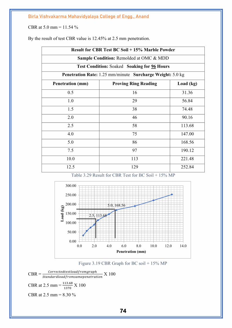
74
Birla Vishvakarma Mahavidyalaya College of Engg., Anand
CBR at 5.0 mm = 11.54 %
By the result of test CBR value is 12.45% at 2.5 mm penetration.
Result for CBR Test BC Soil + 15% Marble Powder
Sample Condition: Remolded at OMC & MDD
Test Condition: Soaked Soaking for 96 Hours
Penetration Rate: 1.25 mm/minute Surcharge Weight: 5.0 kg
Penetration (mm) Proving Ring Reading Load (kg)
0.5 16 31.36
1.0 29 56.84
1.5 38 74.48
2.0 46 90.16
2.5 58 113.68
4.0 75 147.00
5.0 86 168.56
7.5 97 190.12
10.0 113 221.48
12.5 129 252.84
Table 3.29 Result for CBR Test for BC Soil + 15% MP
CBR = 𝐶𝑜𝑟𝑟𝑒𝑐𝑡𝑒𝑑𝑡𝑒𝑠𝑡𝑙𝑜𝑎𝑑𝑓𝑟𝑜𝑚𝑔𝑟𝑎𝑝ℎ
𝑆𝑡𝑎𝑛𝑑𝑎𝑟𝑑𝑙𝑜𝑎𝑑𝑓𝑟𝑜𝑚𝑠𝑎𝑚𝑒𝑝𝑒𝑛𝑒𝑡𝑟𝑎𝑡𝑖𝑜𝑛 X 100
CBR at 2.5 mm = 113.68
1370 X 100
CBR at 2.5 mm = 8.30 %
2.5, 113.68
5.0, 168.56
0.00
50.00
100.00
150.00
200.00
250.00
300.00
0.0 2.0 4.0 6.0 8.0 10.0 12.0 14.0
Loa
d (
kg
)
Penetration (mm)
Figure 3.19 CBR Graph for BC soil + 15% MP

75
Birla Vishvakarma Mahavidyalaya College of Engg., Anand
And, CBR at 5.0 mm = 168.56
2055 X 100
CBR at 5.0 mm = 8.20 %
By the result of test CBR value is 8.30% at 2.5 mm penetration.
Result for CBR Test BC Soil + 15% Marble Powder (7 Days)
Sample Condition: Remolded at OMC & MDD
Test Condition: Soaked Soaking for 96 Hours
Penetration Rate: 1.25 mm/minute Surcharge Weight: 5.0 kg
Penetration (mm) Proving Ring Reading Load (kg)
0.5 20 39.20
1.0 35 68.60
1.5 47 92.12
2.0 63 123.48
2.5 74 145.04
4.0 92 180.32
5.0 110 215.60
7.5 119 233.24
10.0 125 245.00
12.5 138 270.48
Table 3.30 Result for CBR Test for BC Soil + 15% MP (7 days)

76
Birla Vishvakarma Mahavidyalaya College of Engg., Anand
CBR = 𝐶𝑜𝑟𝑟𝑒𝑐𝑡𝑒𝑑𝑡𝑒𝑠𝑡𝑙𝑜𝑎𝑑𝑓𝑟𝑜𝑚𝑔𝑟𝑎𝑝ℎ
𝑆𝑡𝑎𝑛𝑑𝑎𝑟𝑑𝑙𝑜𝑎𝑑𝑓𝑟𝑜𝑚𝑠𝑎𝑚𝑒𝑝𝑒𝑛𝑒𝑡𝑟𝑎𝑡𝑖𝑜𝑛 X 100
CBR at 2.5 mm = 145.04
1370 X 100
CBR at 2.5 mm = 10.59 %
And, CBR at 5.0 mm = 215.60
2055 X 100
CBR at 5.0 mm = 10.49 %
By the result of test CBR value is 10.59% at 2.5 mm penetration.
Result for CBR Test BC Soil + 15% Marble Powder (14 Days)
Sample Condition: Remolded at OMC & MDD
Test Condition: Soaked Soaking for 96 Hours
Penetration Rate: 1.25 mm/minute Surcharge Weight: 5.0 kg
Penetration (mm) Proving Ring Reading Load (kg)
0.5 21 41.16
1.0 31 60.76
1.5 45 88.20
2.0 62 121.52
2.5 85 166.60
4.0 101 197.96
5.0 116 227.36
2.5, 145.04
5.0, 215.60
0.00
50.00
100.00
150.00
200.00
250.00
300.00
0.0 2.0 4.0 6.0 8.0 10.0 12.0 14.0
Load
(k
g)
Penetration (mm)
Figure 3.20 CBR Graph for BC soil + 15% MP (7 days)

77
Birla Vishvakarma Mahavidyalaya College of Engg., Anand
7.5 125 245.00
10.0 136 266.56
12.5 149 292.04
Table 3.31 Result for CBR Test for BC Soil + 15% MP (14 days)
CBR = 𝐶𝑜𝑟𝑟𝑒𝑐𝑡𝑒𝑑𝑡𝑒𝑠𝑡𝑙𝑜𝑎𝑑𝑓𝑟𝑜𝑚𝑔𝑟𝑎𝑝ℎ
𝑆𝑡𝑎𝑛𝑑𝑎𝑟𝑑𝑙𝑜a𝑑𝑓𝑟𝑜𝑚𝑠𝑎𝑚𝑒𝑝𝑒𝑛𝑒𝑡𝑟𝑎𝑡𝑖𝑜𝑛 X 100
CBR at 2.5 mm = 166.60
1370 X 100
CBR at 2.5 mm = 12.16 %
And, CBR at 5.0 mm = 227.36
2055 X 100
CBR at 5.0 mm = 11.06 %
By the result of test CBR value is 12.16% at 2.5 mm penetration.
Result for CBR Test BC Soil + 15% marble powder (21 Days)
Sample Condition: Remolded at OMC & MDD
Test Condition: Soaked Soaking for 96 Hours
Penetration Rate: 1.25 mm/minute Surcharge Weight: 5.0 kg
Penetration (mm) Proving Ring Reading Load (kg)
0.5 32 62.72
1.0 49 96.04
1.5 61 119.56
2.5, 166.60
5.0, 227.36
0.00
50.00
100.00
150.00
200.00
250.00
300.00
350.00
0.0 2.0 4.0 6.0 8.0 10.0 12.0 14.0
Load
(k
g)
Penetration (mm)
Figure 3.21 CBR Graph for BC soil + 15% MP (14 days)

78
Birla Vishvakarma Mahavidyalaya College of Engg., Anand
2.0 79 154.84
2.5 91 178.36
4.0 120 235.20
5.0 132 258.72
7.5 145 284.20
10.0 157 307.72
12.5 163 319.48
Table 3.32 Result for CBR Test for BC Soil + 15% MP (21 days)
CBR = 𝐶𝑜𝑟𝑟𝑒𝑐𝑡𝑒𝑑𝑡𝑒𝑠𝑡𝑙𝑜𝑎𝑑𝑓𝑟𝑜𝑚𝑔𝑟𝑎𝑝ℎ
𝑆𝑡𝑎𝑛𝑑𝑎𝑟𝑑𝑙𝑜𝑎𝑑𝑓𝑟𝑜𝑚𝑠𝑎𝑚𝑒𝑝𝑒𝑛𝑒𝑡𝑟𝑎𝑡𝑖𝑜𝑛 X 100
CBR at 2.5 mm = 178.36
1370 X 100
CBR at 2.5 mm = 13.02 %
And,
CBR at 5.0 mm = 258.72
2055 X 100
CBR at 5.0 mm = 12.59 %
By the result of test CBR value is 13.02% at 2.5 mm penetration.
Result for CBR Test BC Soil + 20% Marble Powder
Sample Condition: Remolded at OMC & MDD
Test Condition: Soaked Soaking for 96 Hours
2.5, 178.36
5.0, 258.72
0.00
50.00
100.00
150.00
200.00
250.00
300.00
350.00
0.0 2.0 4.0 6.0 8.0 10.0 12.0 14.0
Loa
d (
kg)
Penetration (mm)
Figure 3.22 CBR Graph for BC soil + 15% MP (21 days)

79
Birla Vishvakarma Mahavidyalaya College of Engg., Anand
Penetration Rate: 1.25 mm/minute Surcharge Weight: 5.0 kg
Penetration (mm) Proving Ring Reading Load (kg)
0.5 10 19.60
1.0 18 35.28
1.5 28 54.88
2.0 37 72.52
2.5 43 84.28
4.0 52 101.92
5.0 64 125.44
7.5 71 139.16
10.0 78 152.88
12.5 82 160.72
Table 3.33 Result for CBR Test for BC Soil + 20% MP
CBR = 𝐶𝑜𝑟𝑟𝑒𝑐𝑡𝑒𝑑𝑡𝑒𝑠𝑡𝑙𝑜𝑎𝑑𝑓𝑟𝑜𝑚𝑔𝑟𝑎𝑝ℎ
𝑆𝑡𝑎𝑛𝑑𝑎𝑟𝑑𝑙𝑜𝑎𝑑𝑓𝑟𝑜𝑚𝑠𝑎𝑚𝑒𝑝𝑒𝑛𝑒𝑡𝑟𝑎𝑡𝑖𝑜𝑛 X 100
CBR at 2.5 mm = 84.28
1370 X 100
CBR at 2.5 mm = 6.15 %
And, CBR at 5.0 mm = 125.44
2055 X 100
CBR at 5.0 mm = 6.10 %
By the result of test CBR value is 6.15% at 2.5 mm penetration.
2.5, 84.28
5.0, 125.44
0.00
20.00
40.00
60.00
80.00
100.00
120.00
140.00
160.00
180.00
0.0 2.0 4.0 6.0 8.0 10.0 12.0 14.0
Loa
d (
kg
)
Penetration (mm)
Figure 3.23 CBR Graph for BC soil + 20% MP

80
Birla Vishvakarma Mahavidyalaya College of Engg., Anand
Result for CBR Test BC Soil + 20% marble powder (7 Days)
Sample Condition: Remolded at OMC & MDD
Test Condition: Soaked Soaking for 96 Hours
Penetration Rate: 1.25 mm/minute Surcharge Weight: 5.0 kg
Penetration (mm) Proving Ring Reading Load (kg)
0.5 21 41.16
1.0 29 56.84
1.5 36 70.56
2.0 41 80.36
2.5 49 96.04
4.0 68 133.28
5.0 74 145.04
7.5 86 168.56
10.0 97 190.12
12.5 107 209.72
Table 3.34 Result for CBR Test for BC Soil + 20% MP (7 days)
CBR = 𝐶𝑜𝑟𝑟𝑒𝑐𝑡𝑒𝑑𝑡𝑒𝑠𝑡𝑙𝑜𝑎𝑑𝑓𝑟𝑜𝑚𝑔𝑟𝑎𝑝ℎ
𝑆𝑡𝑎𝑛𝑑𝑎𝑟𝑑𝑙𝑜𝑎𝑑𝑓𝑟𝑜𝑚𝑠𝑎𝑚𝑒𝑝𝑒𝑛𝑒𝑡𝑟𝑎𝑡𝑖𝑜𝑛 X 100
CBR at 2.5 mm = 96.04
1370 X 100
CBR at 2.5 mm = 7.01 %
And,
2.5, 96.04
5.0, 145.04
0.00
50.00
100.00
150.00
200.00
250.00
0.0 2.0 4.0 6.0 8.0 10.0 12.0 14.0
Loa
d (
kg
)
Penetration (mm)
Figure 3.24 CBR Graph for BC soil + 20% MP (7 days)

81
Birla Vishvakarma Mahavidyalaya College of Engg., Anand
CBR at 5.0 mm = 145.04
2055 X 100
CBR at 5.0 mm = 7.06 %
By the result of test CBR value is 7.06% at 5 mm penetration.
Result for CBR Test BC Soil + 20% marble powder (14 Days)
Sample Condition: Remolded at OMC & MDD
Test Condition: Soaked Soaking for 96 Hours
Penetration Rate: 1.25 mm/minute Surcharge Weight: 5.0 kg
Penetration (mm) Proving Ring Reading Load (kg)
0.5 19 37.24
1.0 35 68.60
1.5 52 101.92
2.0 61 119.56
2.5 69 135.24
4.0 83 162.68
5.0 91 178.36
7.5 99 194.04
10.0 105 205.80
12.5 112 219.52
Table 3.35 Result for CBR Test for BC Soil + 20% MP (14 days)
CBR = 𝐶𝑜𝑟𝑟𝑒𝑐𝑡𝑒𝑑𝑡𝑒𝑠𝑡𝑙𝑜𝑎𝑑𝑓𝑟𝑜𝑚𝑔𝑟𝑎𝑝ℎ
𝑆𝑡𝑎𝑛𝑑𝑎𝑟𝑑𝑙𝑜𝑎𝑑𝑓𝑟𝑜𝑚𝑠𝑎𝑚𝑒𝑝𝑒𝑛𝑒𝑡𝑟𝑎𝑡𝑖𝑜𝑛 X 100
2.5, 135.24
5.0, 178.36
0.00
50.00
100.00
150.00
200.00
250.00
0.0 2.0 4.0 6.0 8.0 10.0 12.0 14.0
Load
(k
g)
Penetration (mm)
Figure 3.25 CBR Graph for BC soil + 20% MP (14 days)
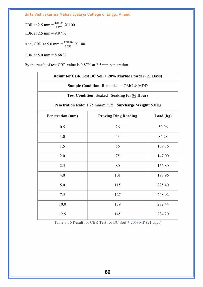
82
Birla Vishvakarma Mahavidyalaya College of Engg., Anand
CBR at 2.5 mm = 135.24
1370 X 100
CBR at 2.5 mm = 9.87 %
And, CBR at 5.0 mm = 178.36
2055 X 100
CBR at 5.0 mm = 8.68 %
By the result of test CBR value is 9.87% at 2.5 mm penetration.
Result for CBR Test BC Soil + 20% Marble Powder (21 Days)
Sample Condition: Remolded at OMC & MDD
Test Condition: Soaked Soaking for 96 Hours
Penetration Rate: 1.25 mm/minute Surcharge Weight: 5.0 kg
Penetration (mm) Proving Ring Reading Load (kg)
0.5 26 50.96
1.0 43 84.28
1.5 56 109.76
2.0 75 147.00
2.5 80 156.80
4.0 101 197.96
5.0 115 225.40
7.5 127 248.92
10.0 139 272.44
12.5 145 284.20
Table 3.36 Result for CBR Test for BC Soil + 20% MP (21 days)

83
Birla Vishvakarma Mahavidyalaya College of Engg., Anand
CBR = 𝐶𝑜𝑟𝑟𝑒𝑐𝑡𝑒𝑑𝑡𝑒𝑠𝑡𝑙𝑜𝑎𝑑𝑓𝑟𝑜𝑚𝑔𝑟𝑎𝑝ℎ
𝑆𝑡𝑎𝑛𝑑𝑎𝑟𝑑𝑙𝑜𝑎𝑑𝑓𝑟𝑜𝑚𝑠𝑎𝑚𝑒𝑝𝑒𝑛𝑒𝑡𝑟𝑎𝑡𝑖𝑜𝑛 X 100
CBR at 2.5 mm = 156.80
1370 X 100
CBR at 2.5 mm = 11.45 %
And, CBR at 5.0 mm = 225.40
2055 X 100
CBR at 5.0 mm = 10.97 %
By the result of test CBR value is 11.45% at 2.5 mm penetration
3.1.5 Determination of Unconfined Compressive Strength (IS: 2720 (Part 10) 1991))
Scope: This method describes the m method for determining the unconfined compressive strength of
clayey soil, undisturbed, remolded or compacted, using controlled rate of strain.
Unconfined Compressive Strength qu: It is the load per unit area at which an unconfined cylindrical
specimen of soil will fail in the axial compression test.
Apparatus: Hydraulic loading device, Screw jack with a providing ring, Proving ring, deformation
dial gauge, Vernier calipers, oven, weighing balances, Specimen trimming, and carving tools,
remoulding apparatus, water content cans, data sheets, etc. as required.
Procedure:
1. Extrude the soil sample from Shelby tube sampler. Cut a soil specimen so that the ratio (L/d) is
approximately between 2 and 2.5. Where L and d, are the length and diameter of soil specimen,
respectively.
2. Measure the exact length of the specimen at three locations 120° apart, and then average the
measurements and record the average as the length of the data sheet.
2.5, 156.80
5.0, 225.40
0.00
50.00
100.00
150.00
200.00
250.00
300.00
0.0 2.0 4.0 6.0 8.0 10.0 12.0 14.0
Load
(k
g)
Penetration (mm)
Figure 3.26 CBR Graph for BC soil + 20% MP (21 days)

84
Birla Vishvakarma Mahavidyalaya College of Engg., Anand
3. Weigh the sample and record the mass on the data sheet.
4. Calculate the deformation (DL) corresponding to 15% strain (e).
Strain (e) =
Where L0 = Original specimen length (as measured in step 3).
5. Carefully place the specimen in the compression device and center it on the bottom plate. Adjust
the device so that the upper plate just makes contact with the specimen and set the load and
deformation dials to zero.
6. Apply the load so that the device produces an axial strain at a rate of 0.5% to 2.0% per minute, and
then record the load and deformation dial readings on the data sheet at every 20 to 50 divisions on
deformation the dial.
7. Keep applying the load until (1) the load (load dial) decreases on the specimen significantly, (2)
the load holds constant for at least four deformation dial readings, or (3) the deformation is
significantly past the 15% strain that was determined in step 5.
Remove the sample from the compression device and obtain a sample for water content determination.
3.1.5.1 UCS Test Results for Soil
UCS Test: Clay Soil
Axial
Deformation
(cm)
Proving ring
Reading
Axial Strain
(%) (e)
Area (A)
(cm2)
Axial Force
(kg)
Compressive
Stress
(kg/cm2)
0 0 0 19.625 0 0
0.05 9 0.472 19.718 17.64 0.8946
0.1 13 0.944 19.812 25.48 1.2860
Figure 3.27 UCS Soil Testing

85
Birla Vishvakarma Mahavidyalaya College of Engg., Anand
0.15 15 1.415 19.906 29.4 1.4769
0.2 17 1.886 20.002 33.32 1.6658
0.25 18 2.358 20.098 35.28 1.7553
0.3 20 2.830 20.196 39.2 1.9409
0.35 21 3.301 20.294 41.16 2.0281
0.4 21 3.773 20.394 41.16 2.0182
0.45 21 4.245 20.495 41.16 2.0082
0.5 22 4.716 20.596 43.12 2.0936
0.55 23 5.188 20.698 45.08 2.1779
0.6 23 5.660 20.802 45.08 2.1670
0.65 24 6.132 20.907 47.04 2.2499
0.7 24 6.603 20.012 47.04 2.350
0.75 23 7.075 21.119 45.08 2.1345
0.8 23 7.547 21.227 45.08 2.1237
0.85 21 8.018 21.335 41.16 1.9292
0.9 21 8.490 21.445 41.16 1.9193
Table 3.37 Result for UCS Test for BC Soil
0
0.5
1
1.5
2
2.5
0 1 2 3 4 5 6 7 8 9
Co
mp
ress
ive
Stre
ss (
kg/c
m2 )
Axial strain (%) (e)
Figure 3.28 Stress v/s Strain for BC Soil

86
Birla Vishvakarma Mahavidyalaya College of Engg., Anand
UCS Test: Clay Soil (3 Days)
Axial
Deformation
(cm)
Proving ring
Reading
Axial
Strain
(%) (e)
Area (A)
(cm2)
Axial Force
(kg)
Compressiv
e Stress
(kg/cm2)
0 0 0 19.625 0 0
0.05 18 0.472 19.718 35.28 1.789228
0.1 24 0.944 19.812 47.04 2.374319
0.15 28 1.415 19.906 54.88 2.756958
0.2 30 1.886 20.002 58.8 2.939706
0.25 31 2.358 20.098 60.76 3.023186
0.3 32 2.830 20.196 62.72 3.105565
0.35 33 3.301 20.294 64.68 3.187149
0.4 35 3.773 20.394 68.6 3.363734
0.45 37 4.245 20.495 72.52 3.538424
0.5 38 4.716 20.596 74.48 3.616236
0.55 40 5.188 20.698 78.4 3.787806
0.6 42 5.660 20.802 82.32 3.957312
0.65 42 6.132 20.907 82.32 3.937437
0.7 41 6.603 20.012 80.36 4.015591
0.75 41 7.075 21.119 80.36 3.805104
0.8 41 7.547 21.227 80.36 3.785745
0.85 40 8.018 21.335 78.4 3.674713
0.9 40 8.490 21.445 78.4 3.655864
Table 3.38 Result for UCS Test for Clay Soil (3 Days)
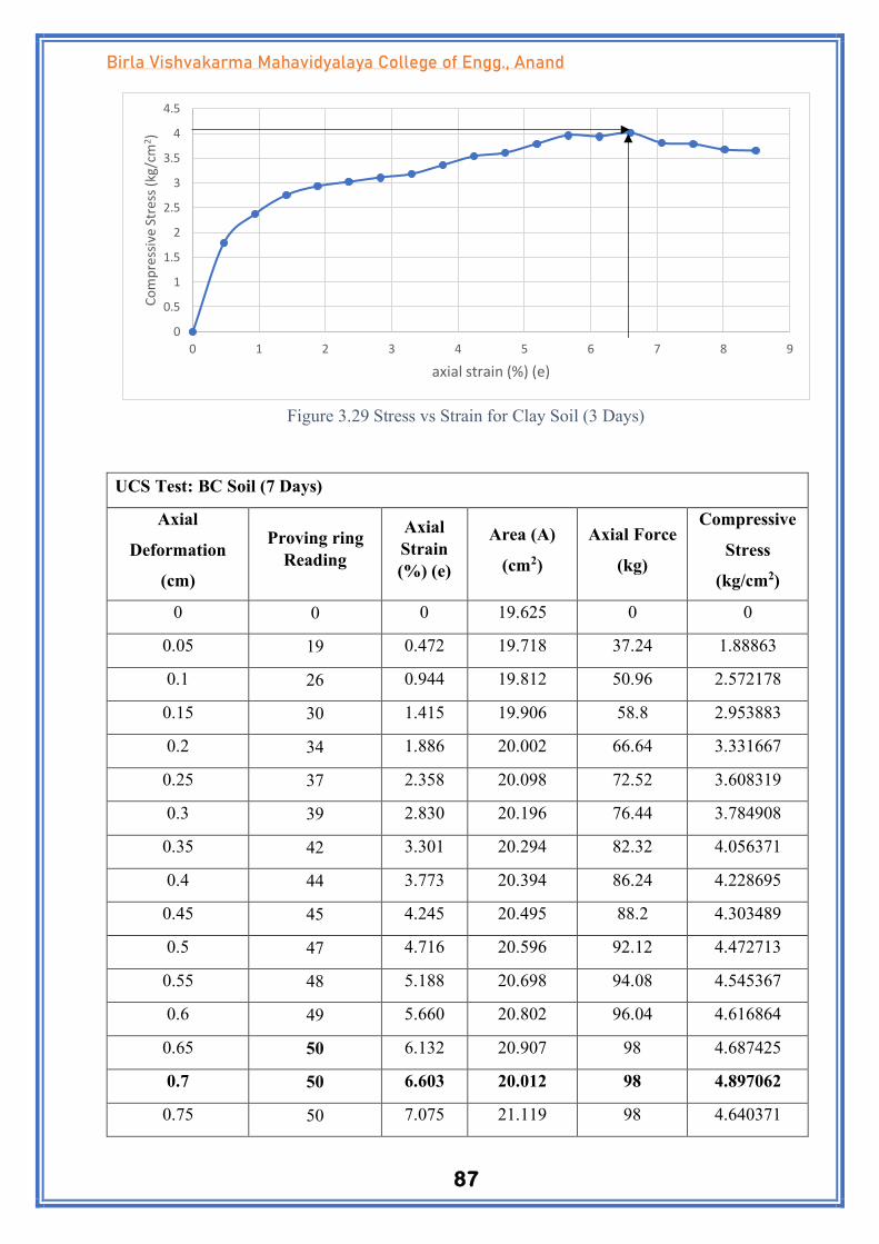
87
Birla Vishvakarma Mahavidyalaya College of Engg., Anand
UCS Test: BC Soil (7 Days)
Axial
Deformation
(cm)
Proving ring
Reading
Axial
Strain
(%) (e)
Area (A)
(cm2)
Axial Force
(kg)
Compressive
Stress
(kg/cm2)
0 0 0 19.625 0 0
0.05 19 0.472 19.718 37.24 1.88863
0.1 26 0.944 19.812 50.96 2.572178
0.15 30 1.415 19.906 58.8 2.953883
0.2 34 1.886 20.002 66.64 3.331667
0.25 37 2.358 20.098 72.52 3.608319
0.3 39 2.830 20.196 76.44 3.784908
0.35 42 3.301 20.294 82.32 4.056371
0.4 44 3.773 20.394 86.24 4.228695
0.45 45 4.245 20.495 88.2 4.303489
0.5 47 4.716 20.596 92.12 4.472713
0.55 48 5.188 20.698 94.08 4.545367
0.6 49 5.660 20.802 96.04 4.616864
0.65 50 6.132 20.907 98 4.687425
0.7 50 6.603 20.012 98 4.897062
0.75 50 7.075 21.119 98 4.640371
0
0.5
1
1.5
2
2.5
3
3.5
4
4.5
0 1 2 3 4 5 6 7 8 9
Co
mp
ress
ive
Stre
ss (
kg/c
m2 )
axial strain (%) (e)
Figure 3.29 Stress vs Strain for Clay Soil (3 Days)

88
Birla Vishvakarma Mahavidyalaya College of Engg., Anand
0.8 50 7.547 21.227 98 4.616762
0.85 49 8.018 21.335 96.04 4.501523
0.9 49 8.490 21.445 96.04 4.478433
Table 3.39 Result for UCS Test for Clay Soil (7 Days)
UCS Test: Clay Soil Clay Soil (14 Days)
Axial
Deformation
(cm)
Proving ring
Reading
Axial Strain
(%) (e)
Area
(A)
(cm2)
Axial
Force (kg)
Compressive
Stress (kg/cm2)
0 0 0 19.625 0 0
0.05 19 0.472 19.718 37.24 1.88863
0.1 26 0.944 19.812 50.96 2.572178
0.15 29 1.415 19.906 56.84 2.85542
0.2 34 1.886 20.002 66.64 3.331667
0.25 36 2.358 20.098 70.56 3.510797
0.3 38 2.830 20.196 74.48 3.687859
0.35 42 3.301 20.294 82.32 4.056371
0.4 44 3.773 20.394 86.24 4.228695
0.45 46 4.245 20.495 90.16 4.399122
0.5 49 4.716 20.596 96.04 4.663041
0.55 50 5.188 20.698 98 4.734757
0.6 51 5.660 20.802 99.96 4.805307
0.65 51 6.132 20.907 99.96 4.781174
0.7 51 6.603 20.012 99.96 5.0125
00.5
11.5
22.5
33.5
44.5
55.5
0 1 2 3 4 5 6 7 8 9
com
pp
ress
ive
stre
ss
()kg
/cm
20
axial strain (%) (e)
Figure 3.29 UCS Graph for BC soil (7 days)

89
Birla Vishvakarma Mahavidyalaya College of Engg., Anand
0.75 50 7.075 21.119 98 4.640371
0.8 50 7.547 21.227 98 4.616762
0.85 50 8.018 21.335 98 4.593391
0.9 49 8.490 21.445 96.04 4.478433
Table 3.40 Result for UCS Test for Clay Soil (14 Days)
UCS Test: BC Soil Clay Soil +5% marble Powder
Axial
Deformation
(cm)
Proving ring
Reading
Axial
Strain
(%) (e)
Area (A)
(cm2)
Axial Force
(kg)
Compressive
Stress
(kg/cm2)
0 0 0 19.625 0 0
0.05 7 0.472 19.718 13.72 0.695811
0.1 11 0.944 19.812 21.56 1.088229
0.15 15 1.415 19.906 29.4 1.476942
0.2 18 1.886 20.002 35.28 1.763824
0.25 20 2.358 20.098 39.2 1.950443
0.3 21 2.830 20.196 41.16 2.038027
0.35 23 3.301 20.294 45.08 2.221346
0.4 25 3.773 20.394 49 2.402667
0.45 26 4.245 20.495 50.96 2.48646
0.5 28 4.716 20.596 54.88 2.664595
0
1
2
3
4
5
6
0 1 2 3 4 5 6 7 8 9
Co
mp
ress
ive
Stre
ss (
kg/c
m2 )
Axial Strain (%) (e)
Figure 3.30 UCS Graph for BC soil (14 days)

90
Birla Vishvakarma Mahavidyalaya College of Engg., Anand
0.55 29 5.188 20.698 56.84 2.746159
0.6 30 5.660 20.802 58.8 2.826651
0.65 30 6.132 20.907 58.8 2.812455
0.7 30 6.603 20.012 58.8 2.938237
0.75 29 7.075 21.119 56.84 2.691415
0.8 29 7.547 21.227 56.84 2.677722
0.85 28 8.018 21.335 54.88 2.572299
0.9 28 8.490 21.445 54.88 2.559105
Table 3.41 Result for UCS Test for Clay Soil + 5% MP
V
UCS Test: BC Soil +5% marble Powder (3 Days)
Axial
Deformation
(cm)
Proving ring
Reading
Axial
Strain
(%) (e)
Area (A)
(cm2)
Axial Force
(kg)
Compressive
Stress
(kg/cm2)
0 0 0 19.625 0 0
0.05 29 0.472 19.718 56.84 2.882645
0.1 39 0.944 19.812 76.44 3.858268
0.15 45 1.415 19.906 88.2 4.430825
0.2 49 1.886 20.002 96.04 4.80152
0.25 53 2.358 20.098 103.88 5.168673
0.3 56 2.830 20.196 109.76 5.43474
0.35 58 3.301 20.294 113.68 5.601656
0
0.5
1
1.5
2
2.5
3
3.5
0 1 2 3 4 5 6 7 8 9
com
pp
ress
ive
stre
ss (
)kg/
cm20
axial strain (%) (e)
Figure 3.31 UCS Graph for BC soil + 5% MP

91
Birla Vishvakarma Mahavidyalaya College of Engg., Anand
Table 3.42 Result for UCS Test for Clay Soil + 5% MP (3 Days)
UCS Test: BC Soil +5% marble Powder (7 Days)
Axial
Deformation
(cm)
Proving ring
Reading
Axial
Strain
(%) (e)
Area (A)
(cm2)
Axial Force
(kg)
Compressive
Stress (kg/cm2)
0 0 0 19.625 0 0
0.05 29 0.472 19.718 56.84 2.882645
0.1 44 0.944 19.812 86.24 4.352917
0.4 60 3.773 20.394 117.6 5.766402
0.45 61 4.245 20.495 119.56 5.833618
0.5 62 4.716 20.596 121.52 5.900175
0.55 63 5.188 20.698 123.48 5.965794
0.6 63 5.660 20.802 123.48 5.935968
0.65 64 6.132 20.907 125.44 5.999904
0.7 64 6.603 20.012 125.44 6.268239
0.75 64 7.075 21.119 125.44 5.939675
0.8 63 7.547 21.227 123.48 5.81712
0.85 63 8.018 21.335 123.48 5.787673
0.9 63 8.490 21.445 123.48 5.757986
0
0.5
1
1.5
2
2.5
3
3.5
4
4.5
5
5.5
6
6.5
7
0 1 2 3 4 5 6 7 8 9
Co
mp
ress
ive
Stre
ss (
kg/c
m2 )
Axial Strain (%) (e)
Figure 3.32 UCS Graph for BC soil + 5% MP (3 days)
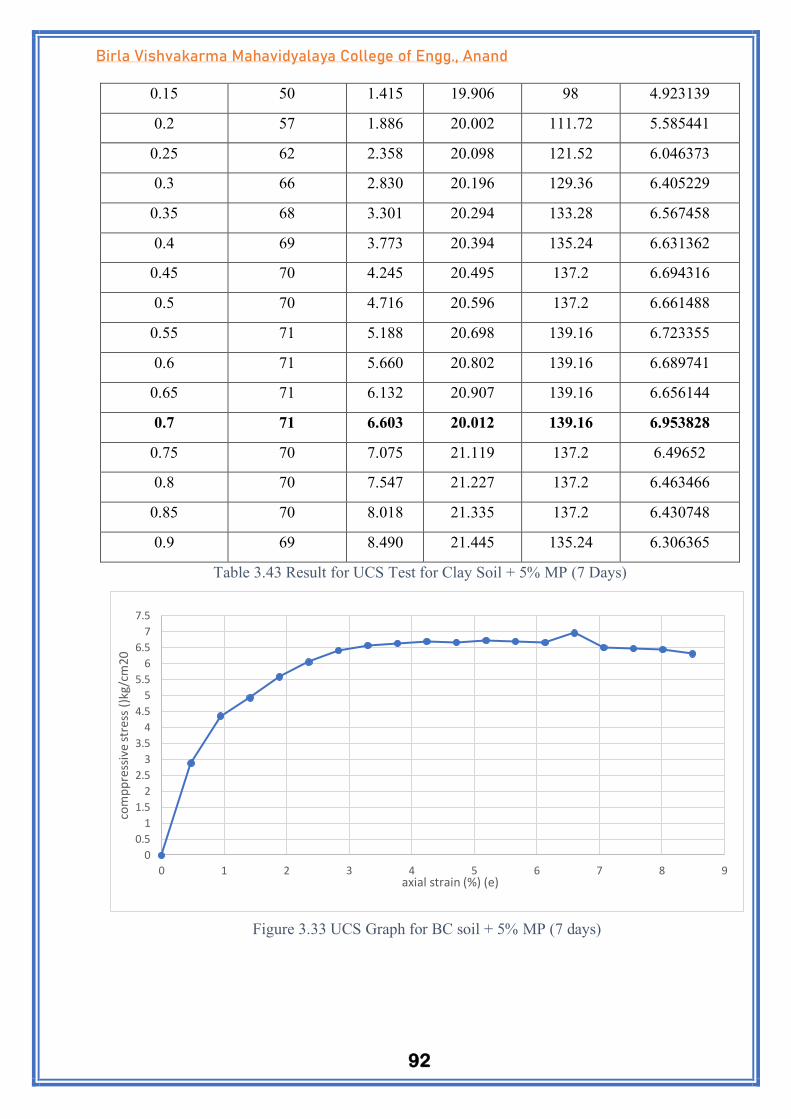
92
Birla Vishvakarma Mahavidyalaya College of Engg., Anand
0.15 50 1.415 19.906 98 4.923139
0.2 57 1.886 20.002 111.72 5.585441
0.25 62 2.358 20.098 121.52 6.046373
0.3 66 2.830 20.196 129.36 6.405229
0.35 68 3.301 20.294 133.28 6.567458
0.4 69 3.773 20.394 135.24 6.631362
0.45 70 4.245 20.495 137.2 6.694316
0.5 70 4.716 20.596 137.2 6.661488
0.55 71 5.188 20.698 139.16 6.723355
0.6 71 5.660 20.802 139.16 6.689741
0.65 71 6.132 20.907 139.16 6.656144
0.7 71 6.603 20.012 139.16 6.953828
0.75 70 7.075 21.119 137.2 6.49652
0.8 70 7.547 21.227 137.2 6.463466
0.85 70 8.018 21.335 137.2 6.430748
0.9 69 8.490 21.445 135.24 6.306365
Table 3.43 Result for UCS Test for Clay Soil + 5% MP (7 Days)
0
0.5
1
1.5
2
2.5
3
3.5
4
4.5
5
5.5
6
6.5
7
7.5
0 1 2 3 4 5 6 7 8 9
com
pp
ress
ive
stre
ss (
)kg/
cm20
axial strain (%) (e)
Figure 3.33 UCS Graph for BC soil + 5% MP (7 days)

93
Birla Vishvakarma Mahavidyalaya College of Engg., Anand
UCS Test: BC Soil + 5% marble powder (14 Days)
Axial
Deformation
(cm)
Proving ring
Reading
Axial Strain
(%) (e)
Area
(A)
(cm2)
Axial
Force (kg)
Compressive
Stress (kg/cm2)
0 0 0 19.625 0 0
0.05 32 0.472 19.718 62.72 3.18085
0.1 47 0.944 19.812 92.12 4.649707
0.15 54 1.415 19.906 105.84 5.31699
0.2 61 1.886 20.002 119.56 5.977402
0.25 67 2.358 20.098 131.32 6.533983
0.3 69 2.830 20.196 135.24 6.696376
0.35 71 3.301 20.294 139.16 6.857199
0.4 72 3.773 20.394 141.12 6.919682
0.45 73 4.245 20.495 143.08 6.981215
0.5 73 4.716 20.596 143.08 6.94698
0.55 74 5.188 20.698 145.04 7.00744
0.6 74 5.660 20.802 145.04 6.972406
0.65 74 6.132 20.907 145.04 6.937389
0.7 73 6.603 20.012 143.08 7.14971
0.75 73 7.075 21.119 143.08 6.774942
0.8 73 7.547 21.227 143.08 6.740472
0.85 72 8.018 21.335 141.12 6.614483
0.9 72 8.490 21.445 141.12 6.580555
Table 3.44 Result for UCS Test for Clay Soil + 5% MP (14 Days)

94
Birla Vishvakarma Mahavidyalaya College of Engg., Anand
UCS Test: BC Soil +10% marble Powder
Axial
Deformation (cm)
Proving ring
Reading
Axial
Strain
(%) (e)
Area (A)
(cm2)
Axial Force
(kg)
Compressive
Stress
(kg/cm2)
0 0 0 19.625 0 0
0.05 16 0.472 19.718 31.36 1.590425
0.1 21 0.944 19.812 41.16 2.077529
0.15 25 1.415 19.906 49 2.461569
0.2 28 1.886 20.002 54.88 2.743726
0.25 30 2.358 20.098 58.8 2.925664
0.3 31 2.830 20.196 60.76 3.008517
0.35 33 3.301 20.294 64.68 3.187149
0.4 33 3.773 20.394 64.68 3.171521
0.45 34 4.245 20.495 66.64 3.251525
0.5 34 4.716 20.596 66.64 3.23558
0.55 35 5.188 20.698 68.6 3.31433
0.6 35 5.660 20.802 68.6 3.29776
0.65 35 6.132 20.907 68.6 3.281198
0.7 34 6.603 20.012 66.64 3.330002
0
0.5
1
1.5
2
2.5
3
3.5
4
4.5
5
5.5
6
6.5
7
7.5
8
0 1 2 3 4 5 6 7 8 9
com
pp
ress
ive
stre
ss (
kg/c
m2
)
axial strain (%) (e)
Figure 3.34 UCS Graph for BC soil + 5% MP (14 days)

95
Birla Vishvakarma Mahavidyalaya College of Engg., Anand
0.75 34 7.075 21.119 66.64 3.155452
0.8 33 7.547 21.227 64.68 3.047063
0.85 33 8.018 21.335 64.68 3.031638
0.9 33 8.490 21.445 64.68 3.016088
Table 3.45 Result for UCS Test for Clay Soil + 10% MP
UCS Test: BC Soil +10% marble Powder (3 Days)
Axial
Deformation
(cm)
Proving ring
Reading
Axial
Strain
(%) (e)
Area (A)
(cm2)
Axial Force
(kg)
Compressive
Stress
(kg/cm2)
0 0 0 19.625 0 0
0.05 25 0.472 19.718 49 2.485
0.1 38 0.944 19.812 74.48 3.7593
0.15 50 1.415 19.906 98 4.9231
0.2 58 1.886 20.002 113.68 5.6834
0.25 66 2.358 20.098 129.36 6.4365
0.3 70 2.830 20.196 137.2 6.7934
0.35 74 3.301 20.294 145.04 7.1469
0.4 75 3.773 20.394 147 7.208
0.45 76 4.245 20.495 148.96 7.2681
0.5 77 4.716 20.596 150.92 7.3276
0.55 78 5.188 20.698 152.88 7.3862
0
0.5
1
1.5
2
2.5
3
3.5
0 1 2 3 4 5 6 7 8 9
com
pp
ress
ive
stre
ss (
)kg/
cm20
axial strain (%) (e)
Figure 3.35 UCS Graph for BC soil + 10% MP

96
Birla Vishvakarma Mahavidyalaya College of Engg., Anand
0.6 78 5.660 20.802 152.88 7.3493
0.65 78 6.132 20.907 152.88 7.3124
0.7 78 6.603 20.012 152.9 7.639
0.75 78 7.075 21.119 152.88 7.239
0.8 77 7.547 21.227 150.92 7.1098
0.85 77 8.018 21.335 150.92 7.0738
0.9 77 8.490 21.445 150.92 7.0375
Table 3.46 Result for UCS Test for Clay Soil + 10% MP (3 Days)
UCS Test: BC Soil +10% marble Powder (7 Days)
Axial
Deformation
(cm)
Proving ring
Reading
Axial
Strain
(%) (e)
Area (A)
(cm2)
Axial Force
(kg)
Compressive
Stress
(kg/cm2)
0 0 0 19.625 0 0
0.05 28 0.472 19.718 54.88 2.783244
0.1 39 0.944 19.812 76.44 3.858268
0.15 52 1.415 19.906 101.92 5.120064
0.2 70 1.886 20.002 137.2 6.859314
0.25 79 2.358 20.098 154.84 7.704249
0.3 85 2.830 20.196 166.6 8.249158
0.35 90 3.301 20.294 176.4 8.692224
0.4 97 3.773 20.394 190.12 9.32235
00.5
11.5
22.5
33.5
44.5
55.5
66.5
77.5
88.5
0 1 2 3 4 5 6 7 8 9
com
pp
ress
ive
stre
ss ()
kg/c
m2 )
axial strain (%) (e)
Figure 3.36 UCS Graph for BC soil + 10% MP (3 days)

97
Birla Vishvakarma Mahavidyalaya College of Engg., Anand
0.45 101 4.245 20.495 197.96 9.658941
0.5 105 4.716 20.596 205.8 9.992232
0.55 106 5.188 20.698 207.76 10.03768
0.6 108 5.660 20.802 211.68 10.17594
0.65 108 6.132 20.907 211.68 10.12484
0.7 107 6.603 20.012 209.72 10.47971
0.75 107 7.075 21.119 209.72 9.930394
0.8 106 7.547 21.227 207.76 9.787535
0.85 106 8.018 21.335 207.76 9.737989
0.9 106 8.490 21.445 207.76 9.688039
Table 3.47 Result for UCS Test for Clay Soil + 10% MP (7 Days)
UCS Test: BC Soil + 10% marble powder (14 Days)
Axial
Deformation
(cm)
Proving ring
Reading
Axial Strain
(%) (e)
Area
(A)
(cm2)
Axial
Force (kg)
Compressive
Stress (kg/cm2)
0 0 0 19.625 0 0
0.05 30 0.472 19.718 58.8 2.982047
0.1 40 0.944 19.812 78.4 3.957198
0.15 54 1.415 19.906 105.84 5.31699
0.2 70 1.886 20.002 137.2 6.859314
0.25 81 2.358 20.098 158.76 7.899293
00.5
11.5
22.5
33.5
44.5
55.5
66.5
77.5
88.5
99.510
10.511
11.5
0 1 2 3 4 5 6 7 8 9
com
pp
ress
ive
stre
ss (
)kg/
cm20
axial strain (%) (e)
Figure 3.37 UCS Graph for BC soil + 10% MP (7 days)

98
Birla Vishvakarma Mahavidyalaya College of Engg., Anand
0.3 87 2.830 20.196 170.52 8.443256
0.35 93 3.301 20.294 182.28 8.981965
0.4 103 3.773 20.394 201.88 9.89899
0.45 105 4.245 20.495 205.8 10.04147
0.5 106 4.716 20.596 207.76 10.0874
0.55 107 5.188 20.698 209.72 10.13238
0.6 107 5.660 20.802 209.72 10.08172
0.65 109 6.132 20.907 213.64 10.21859
0.7 109 6.603 20.012 213.64 10.67559
0.75 108 7.075 21.119 211.68 10.0232
0.8 107 7.547 21.227 209.72 9.87987
0.85 106 8.018 21.335 207.76 9.737989
0.9 106 8.490 21.445 207.76 9.688039
Table 3.48 Result for UCS Test for Clay Soil + 10 % MP (14 Days)
10.67559
00.5
11.5
22.5
33.5
44.5
55.5
66.5
77.5
88.5
99.510
10.511
11.5
0 1 2 3 4 5 6 7 8 9
com
pp
ress
ive
str
ess
(kg
/cm
2)
axial strain (%) (e)
Figure 3.38 UCS Graph for BC soil + 10% MP (14 days)

99
Birla Vishvakarma Mahavidyalaya College of Engg., Anand
UCS Test: Clay Soil Clay Soil +15% marble Powder
Axial
Deformation
(cm)
Proving ring
Reading
Axial
Strain
(%) (e)
Area
(A)
(cm2)
Axial Force
(kg)
Compressive
Stress (kg/cm2)
0 0 0 19.625 0 0
0.05 17 0.472 19.718 33.32 1.689827
0.1 22 0.944 19.812 43.12 2.176459
0.15 26 1.415 19.906 50.96 2.560032
0.2 29 1.886 20.002 56.84 2.841716
0.25 31 2.358 20.098 60.76 3.023186
0.3 32 2.830 20.196 62.72 3.105565
0.35 34 3.301 20.294 66.64 3.283729
0.4 34 3.773 20.394 66.64 3.267628
0.45 35 4.245 20.495 68.6 3.347158
0.5 35 4.716 20.596 68.6 3.330744
0.55 36 5.188 20.698 70.56 3.409025
0.6 36 5.660 20.802 70.56 3.391982
0.65 36 6.132 20.907 70.56 3.374946
0.7 35 6.603 20.012 68.6 3.427943
0.75 35 7.075 21.119 68.6 3.24826
0.8 34 7.547 21.227 66.64 3.139398
0.85 34 8.018 21.335 66.64 3.123506
0.9 34 8.490 21.445 66.64 3.107484
Table 3.49 Result for UCS Test for Clay Soil + 15% MP

100
Birla Vishvakarma Mahavidyalaya College of Engg., Anand
UCS Test: BC Soil +15% marble Powder (3 Days)
Axial
Deformation
(cm)
Proving
ring
Reading
Axial Strain
(%) (e)
Area
(A)
(cm2)
Axial
Force (kg)
Compressive
Stress (kg/cm2)
0 0 0 19.625 0 0
0.05 26 0.472 19.718 50.96 2.5844
0.1 38 0.944 19.812 74.48 3.7593
0.15 49 1.415 19.906 96.04 4.8247
0.2 57 1.886 20.002 111.72 5.5854
0.25 68 2.358 20.098 133.28 6.6315
0.3 73 2.830 20.196 143.08 7.0846
0.35 86 3.301 20.294 168.56 8.3059
0.4 90 3.773 20.394 176.4 8.6496
0.45 94 4.245 20.495 184.24 8.9895
0.5 97 4.716 20.596 190.12 9.2309
0.55 99 5.188 20.698 194.04 9.3748
0.6 100 5.660 20.802 196 9.4222
0.65 100 6.132 20.907 196 9.3749
0.7 100 6.603 20.012 196 9.794
0.75 99 7.075 21.119 194.04 9.1879
0
0.5
1
1.5
2
2.5
3
3.5
4
0 1 2 3 4 5 6 7 8 9
com
pp
ress
ive
stre
ss (
)kg/
cm2)
axial strain (%) (e)
Figure 3.39 UCS Graph for BC soil + 15% MP

101
Birla Vishvakarma Mahavidyalaya College of Engg., Anand
0.8 99 7.547 21.227 194.04 9.1412
0.85 99 8.018 21.335 194.04 9.0949
0.9 99 8.490 21.445 194.04 9.0483
Table 3.50 Result for UCS Test for Clay Soil + 15% MP (3 Days)
UCS Test: BC Soil +15% Marble Powder (7 Days)
Axial
Deformation
(cm)
Proving
ring
Reading
Axial
Strain (%)
(e)
Area (A)
(cm2)
Axial
Force (kg)
Compressive Stress
(kg/cm2)
0 0 0 19.625 0 0
0.05 28 0.472 19.718 54.88 2.783244
0.1 50 0.944 19.812 98 4.946497
0.15 64 1.415 19.906 125.44 6.301618
0.2 75 1.886 20.002 147 7.349265
0.25 79 2.358 20.098 154.84 7.704249
0.3 83 2.830 20.196 162.68 8.05506
0.35 86 3.301 20.294 168.56 8.305903
0.4 89 3.773 20.394 174.44 8.553496
0.45 91 4.245 20.495 178.36 8.70261
0.5 93 4.716 20.596 182.28 8.850262
0.55 94 5.188 20.698 184.24 8.901343
00.5
11.5
22.5
33.5
44.5
55.5
66.5
77.5
88.5
99.510
10.5
0 1 2 3 4 5 6 7 8 9
com
pp
ress
ive
str
ess
()kg
/cm
2)
axial strain (%) (e)
Figure 3.40 UCS Graph for BC soil + 10% MP

102
Birla Vishvakarma Mahavidyalaya College of Engg., Anand
0.6 95 5.660 20.802 186.2 8.951062
0.65 95 6.132 20.907 186.2 8.906108
0.7 95 6.603 20.012 186.2 9.304417
0.75 95 7.075 21.119 186.2 8.816705
0.8 95 7.547 21.227 186.2 8.771847
0.85 94 8.018 21.335 184.24 8.635575
0.9 94 8.490 21.445 184.24 8.59128
Table 3.51 Result for UCS Test for Clay Soil + 15% MP (7 Days)
UCS Test: BC Soil +15% Marble Powder (14 Days)
Axial
Deformatio
n (cm)
Proving ring
Reading
Axial Strain
(%) (e)
Area (A)
(cm2)
Axial Force
(kg)
Compressive Stress
(kg/cm2)
0 0 0 19.625 0 0
0.05 31 0.472 19.718 60.76 3.081448
0.1 41 0.944 19.812 80.36 4.056128
0.15 55 1.415 19.906 107.8 5.415453
0.2 71 1.886 20.002 139.16 6.957304
0.25 82 2.358 20.098 160.72 7.996816
0.3 88 2.830 20.196 172.48 8.540305
0.35 94 3.301 20.294 184.24 9.078545
0.4 104 3.773 20.394 203.84 9.995097
0.45 106 4.245 20.495 207.76 10.13711
00.5
11.5
22.5
33.5
44.5
55.5
66.5
77.5
88.5
99.510
0 1 2 3 4 5 6 7 8 9
com
pp
ress
ive
str
ess
(kg
/cm
2)
axial strain (%) (e)
Figure 3.41 UCS Graph for BC soil + 15% MP (7 days)

103
Birla Vishvakarma Mahavidyalaya College of Engg., Anand
0.5 107 4.716 20.596 209.72 10.18256
0.55 108 5.188 20.698 211.68 10.22708
0.6 108 5.660 20.802 211.68 10.17594
0.65 110 6.132 20.907 215.6 10.31234
0.7 110 6.603 20.012 215.6 10.77354
0.75 109 7.075 21.119 213.64 10.11601
0.8 108 7.547 21.227 211.68 9.972205
0.85 107 8.018 21.335 209.72 9.829857
0.9 107 8.490 21.445 209.72 9.779436
Table 3.52 Result for UCS Test for Clay Soil + 15% MP (14 Days)
UCS Test : BC Soil +20% Marble Powder
Axial
Deformation (cm)
Proving ring
Reading
Axial Strain
(%) (e)
Area
(A)
(cm2)
Axial Force
(kg)
Compressive Stress
(kg/cm2)
0 0 0 19.625 0 0
0.05 14 0.472 19.718 27.44 1.391622
0.1 18 0.944 19.812 35.28 1.780739
0.15 22 1.415 19.906 43.12 2.166181
0.2 25 1.886 20.002 49 2.449755
0.25 28 2.358 20.098 54.88 2.73062
0.3 28 2.830 20.196 54.88 2.71737
0.35 31 3.301 20.294 60.76 2.993988
00.5
11.5
22.5
33.5
44.5
55.5
66.5
77.5
88.5
99.510
10.511
11.5
0 1 2 3 4 5 6 7 8 9
com
pp
ress
ive
str
ess
(kg
/cm
2)
axial strain (%) (e)
Figure 3.43 UCS Graph for BC soil + 15% MP (14 days)

104
Birla Vishvakarma Mahavidyalaya College of Engg., Anand
0.4 33 3.773 20.394 64.68 3.171521
0.45 33 4.245 20.495 64.68 3.155892
0.5 34 4.716 20.596 66.64 3.23558
0.55 34 5.188 20.698 66.64 3.219635
0.6 35 5.660 20.802 68.6 3.29776
0.65 35 6.132 20.907 68.6 3.281198
0.7 34 6.603 20.012 66.64 3.330002
0.75 33 7.075 21.119 64.68 3.062645
0.8 33 7.547 21.227 64.68 3.047063
0.85 32 8.018 21.335 62.72 2.93977
0.9 31 8.490 21.445 60.76 2.833294
Table 3.53 Result for UCS Test for Clay Soil + 20% MP
UCS Test: BC Soil +20% Marble Powder (3 Days)
Axial
Deformation (cm)
Proving ring
Reading
Axial Strain
(%) (e)
Area (A)
(cm2)
Axial Force
(kg)
Compressive Stress
(kg/cm2)
0 0 0 19.625 0 0
0.05 20 0.472 19.718 39.2 1.988031
0.1 23 0.944 19.812 45.08 2.275389
0.15 32 1.415 19.906 62.72 3.150809
0.2 46 1.886 20.002 90.16 4.507549
0
0.5
1
1.5
2
2.5
3
3.5
4
0 1 2 3 4 5 6 7 8 9
com
pp
ress
ive
str
ess
(kg
/cm
2)
axial strain (%) (e)
Figure 3.44 UCS Graph for BC soil + 20% MP

105
Birla Vishvakarma Mahavidyalaya College of Engg., Anand
0.25 58 2.358 20.098 113.68 5.656284
0.3 62 2.830 20.196 121.52 6.017033
0.35 68 3.301 20.294 133.28 6.567458
0.4 71 3.773 20.394 139.16 6.823576
0.45 73 4.245 20.495 143.08 6.981215
0.5 74 4.716 20.596 145.04 7.042144
0.55 76 5.188 20.698 148.96 7.196831
0.6 76 5.660 20.802 148.96 7.16085
0.65 76 6.132 20.907 148.96 7.124886
0.7 77 6.603 20.012 150.92 7.541475
0.75 76 7.075 21.119 148.96 7.053364
0.8 75 7.547 21.227 147 6.925143
0.85 75 8.018 21.335 147 6.890087
0.9 74 8.490 21.445 145.04 6.763348
Table 3.54 Result for UCS Test for Clay Soil + 20% MP (3 Days)
0
0.5
1
1.5
2
2.5
3
3.5
4
4.5
5
5.5
6
6.5
7
7.5
8
0 1 2 3 4 5 6 7 8 9
com
pp
ress
ive
str
ess
(kg
/cm
2)
axial strain (%) (e)
Figure 3.44 UCS Graph for BC soil + 20% MP (3 days)
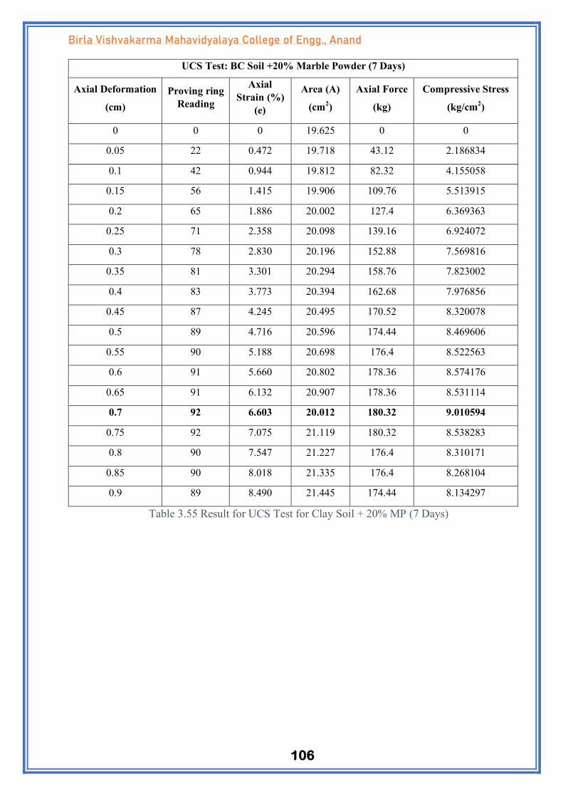
106
Birla Vishvakarma Mahavidyalaya College of Engg., Anand
UCS Test: BC Soil +20% Marble Powder (7 Days)
Axial Deformation
(cm)
Proving ring
Reading
Axial
Strain (%)
(e)
Area (A)
(cm2)
Axial Force
(kg)
Compressive Stress
(kg/cm2)
0 0 0 19.625 0 0
0.05 22 0.472 19.718 43.12 2.186834
0.1 42 0.944 19.812 82.32 4.155058
0.15 56 1.415 19.906 109.76 5.513915
0.2 65 1.886 20.002 127.4 6.369363
0.25 71 2.358 20.098 139.16 6.924072
0.3 78 2.830 20.196 152.88 7.569816
0.35 81 3.301 20.294 158.76 7.823002
0.4 83 3.773 20.394 162.68 7.976856
0.45 87 4.245 20.495 170.52 8.320078
0.5 89 4.716 20.596 174.44 8.469606
0.55 90 5.188 20.698 176.4 8.522563
0.6 91 5.660 20.802 178.36 8.574176
0.65 91 6.132 20.907 178.36 8.531114
0.7 92 6.603 20.012 180.32 9.010594
0.75 92 7.075 21.119 180.32 8.538283
0.8 90 7.547 21.227 176.4 8.310171
0.85 90 8.018 21.335 176.4 8.268104
0.9 89 8.490 21.445 174.44 8.134297
Table 3.55 Result for UCS Test for Clay Soil + 20% MP (7 Days)

107
Birla Vishvakarma Mahavidyalaya College of Engg., Anand
UCS Test: Clay Soil Clay Soil +20% Marble Powder (14 Days)
Axial
Deformation (cm)
Proving ring
Reading
Axial Strain
(%) (e)
Area
(A)
(cm2)
Axial Force
(kg)
Compressive Stress
(kg/cm2)
0 0 0 19.625 0 0
0.05 25 0.472 19.718 49 2.485039
0.1 30 0.944 19.812 58.8 2.967898
0.15 39 1.415 19.906 76.44 3.840048
0.2 48 1.886 20.002 94.08 4.70353
0.25 55 2.358 20.098 107.8 5.363718
0.3 69 2.830 20.196 135.24 6.696376
0.35 73 3.301 20.294 143.08 7.05036
0.4 95 3.773 20.394 186.2 9.130136
0.45 98 4.245 20.495 192.08 9.372042
0.5 101 4.716 20.596 197.96 9.611575
0.55 102 5.188 20.698 199.92 9.658904
0.6 102 5.660 20.802 199.92 9.610614
0.65 104 6.132 20.907 203.84 9.749845
0.7 104 6.603 20.012 203.84 10.18589
00.5
11.5
22.5
33.5
44.5
55.5
66.5
77.5
88.5
99.5
0 1 2 3 4 5 6 7 8 9
com
pp
ress
ive
str
ess
(kg
/cm
2)
axial strain (%) (e)
Figure 3.45 UCS Graph for BC soil + 20% MP (7 days)

108
Birla Vishvakarma Mahavidyalaya College of Engg., Anand
0.75 103 7.075 21.119 201.88 9.559165
0.8 102 7.547 21.227 199.92 9.418194
0.85 101 8.018 21.335 197.96 9.27865
0.9 101 8.490 21.445 197.96 9.231056
Table 3.56 Result for UCS Test for Clay Soil + 20% MP (14 Days)
00.5
11.5
22.5
33.5
44.5
55.5
66.5
77.5
88.5
99.510
10.511
0 1 2 3 4 5 6 7 8 9
com
pp
ress
ive
stre
ss (
kg/c
m2)
axial strain (%) (e)
Figure 3.46 UCS Graph for BC soil + 20% MP (21 days)

109
Birla Vishvakarma Mahavidyalaya College of Engg., Anand
CHAPTER 4 THICKNESS OF PAVEMENT DESIGN
4.1 Pavement design
Comparative table for California Bearing Ratio is given below.
S. No. Samples C. B. R. Values
1. Raw Soil 2.47
2. Raw Soil +5% MP 5.84
3. Raw Soil +10% MP 7.01
4. Raw Soil + 15%MP 8.30
5. Raw soil +20%MP 6.15
Table 4.1 Result for CBR test
Considered Pavement Design Data:
• State Highway of 6 lane
• Design Traffic(A)= 1000 CVPD
• Lane Distribution Factor(D) = 60% (three lane carriage way road)
• Vehicle damage factor (F) = 3.5 (For Plain Terrain)
• Design Life (n) = 15 years
• Annual Growth Rate(r) = 7.5% (assumed)
• Width = 10.5m + 10.5m (10.5m of single side)
• N = [(365 x {(1+ r)n-1})/ r}]AFD
N = [(365 x {(1+0.075)15-1})/0.075] x 1000 x 0.6 x 3
N= 20 msa
4.2 Different layer thickness by referring IRC: 37-2012
Material CBR
GSB
(mm)
G. BASE
(mm)
DBM
(mm)
BC
(mm)
TOTAL
(mm)
RAW SOIL 2.47 380 250 120 40 790
R.S.+5% MP 5.84 260 250 90 40 640
R.S.+10%MP 7.01 200 250 85 40 575
R.S.+15%MP 8.3 260 250 90 40 640
R.S.+20%MP 6.15 200 250 85 40 575
Table 4.2 Different layer thickness

110
Birla Vishvakarma Mahavidyalaya College of Engg., Anand
4.2.1 Total Pavement Thickness for BC Soil
• Total Pavement Thickness = 790 mm
• Granular Sub base = 380 mm = 200mm + 180 mm
• Granular Base Course = 250 mm = 125 mm +125 mm
• Dense Bound Macadam = 120 mm
• Bituminous Course = 40 mm
Quantity for BC Soil (1 km)
• Quantity for GSB = 0.380 * 10.5 * 1000 = 3990 m3
• Quantity for WMM = 0.125 * 10.5 * 1000 = 1312.5m3
• Quantity for WBM = 0.125 * 10.5 * 1000 = 1312.5m3
• Quantity for Prime Coat = 10.5 * 1000 = 10500m2
• Quantity for DBM = 0.120 * 10.5* 1000 = 1260 m3
• Quantity for BC = 0.040 * 10.5 * 1000 = 420 m3
Item No. Item Name Total Quantity Unit Rate Rs. Total cost Rs.
1 GSB 3990 Cum 1200 4788000
3 WMM 1312.5 Cum 1600 2100000
4 WBM 1312.5 Cum 1600 2100000
5 Prime Coat 10500 Sq. m 35 367500
6 DBM 1260 Cum 7400 9324000
7 BC 420 Cum 9000 3780000
Total Amount Rs. 22459500
Table 4.3 Cost estimation for raw soil
Figure 4.1 Composition of layers of BC soil

111
Birla Vishvakarma Mahavidyalaya College of Engg., Anand
4.2.2 Total Pavement Thickness for BC Soil +5% MP
• Total Pavement Thickness = 640 mm
• Granular Sub base = 260 mm
• Granular Base Course = 250 mm = 125 mm +125 mm
• Dense Bound Macadam = 90 mm
• Bituminous Course = 40 mm
Quantity for BC Soil + 5 % MP (1 km)
• Quantity for GSB = 0.260 * 10.5 * 1000 = 2730 m3
• Quantity for WMM = 0.125 * 10.5 * 1000 = 1312.5m3
• Quantity for WBM = 0.125 * 10.5 * 1000 = 1312.5m3
• Quantity for Prime Coat = 10.5 * 1000 = 10500m2
• Quantity for DBM = 0.090 * 10.5* 1000 = 945 m3
• Quantity for BC = 0.040 * 10.5 * 1000 = 420 m3
Item No. Item Name Total Quantity Unit Rate Rs. Total cost Rs.
1 GSB 2730 Cum 1200 3276000
3 WMM 1312.5 Cum 1600 2100000
4 WBM 1312.5 Cum 1600 2100000
5 Prime Coat 10500 Sq. m 35 367500
6 DBM 945 Cum 7400 6993000
7 BC 420 Cum 9000 3780000
Total Amount Rs. 18616500
Table 4.4 Cost estimation for raw soil +5% MP
Figure 4.2 Composition of layers of BC soil + 5% MP
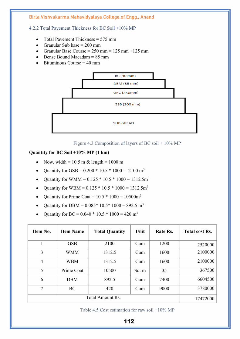
112
Birla Vishvakarma Mahavidyalaya College of Engg., Anand
4.2.2 Total Pavement Thickness for BC Soil +10% MP
• Total Pavement Thickness = 575 mm
• Granular Sub base = 200 mm
• Granular Base Course = 250 mm = 125 mm +125 mm
• Dense Bound Macadam = 85 mm
• Bituminous Course = 40 mm
Quantity for BC Soil +10% MP (1 km)
• Now, width = 10.5 m & length = 1000 m
• Quantity for GSB = 0.200 * 10.5 * 1000 = 2100 m3
• Quantity for WMM = 0.125 * 10.5 * 1000 = 1312.5m3
• Quantity for WBM = 0.125 * 10.5 * 1000 = 1312.5m3
• Quantity for Prime Coat = 10.5 * 1000 = 10500m2
• Quantity for DBM = 0.085* 10.5* 1000 = 892.5 m3
• Quantity for BC = 0.040 * 10.5 * 1000 = 420 m3
Table 4.5 Cost estimation for raw soil +10% MP
Item No. Item Name Total Quantity Unit Rate Rs. Total cost Rs.
1 GSB 2100 Cum 1200 2520000
3 WMM 1312.5 Cum 1600 2100000
4 WBM 1312.5 Cum 1600 2100000
5 Prime Coat 10500 Sq. m 35 367500
6 DBM 892.5 Cum 7400 6604500
7 BC 420 Cum 9000 3780000
Total Amount Rs. 17472000
Figure 4.3 Composition of layers of BC soil + 10% MP

113
Birla Vishvakarma Mahavidyalaya College of Engg., Anand
4.2.2 Total Pavement Thickness for BC Soil +15% MP
• Total Pavement Thickness = 640 mm
• Granular Sub base = 260 mm
• Granular Base Course = 250 mm = 125 mm +125 mm
• Dense Bound Macadam = 90 mm
• Bituminous Course = 40 mm
Quantity for BC Soil 15 % MP (1 km)
• Now, width = 10.5 m & length = 1000 m
• Quantity for GSB = 0.260 * 10.5 * 1000 = 2730 m3
• Quantity for WMM = 0.125 * 10.5 * 1000 = 1312.5m3
• Quantity for WBM = 0.125 * 10.5 * 1000 = 1312.5m3
• Quantity for Prime Coat = 10.5 * 1000 = 10500m2
• Quantity for DBM = 0.090 * 10.5* 1000 = 945 m3
• Quantity for BC = 0.040 * 10.5 * 1000 = 420 m3
Item No. Item Name Total Quantity Unit Rate Rs. Total cost Rs.
1 GSB 2730 Cum 1200 3276000
3 WMM 1312.5 Cum 1600 2100000
4 WBM 1312.5 Cum 1600 2100000
5 Prime Coat 10500 Sq. m 35 367500
6 DBM 945 Cum 7400 6993000
7 BC 420 Cum 9000 3780000
Total Amount Rs. 18616500
Table 4.6 Cost estimation for raw soil +15% MP
Figure 4.4 Composition of layers of BC soil + 15% MP

114
Birla Vishvakarma Mahavidyalaya College of Engg., Anand
4.2.2 Total Pavement Thickness for BC Soil +20% MP
• Total Pavement Thickness = 575 mm
• Granular Sub base = 200 mm
• Granular Base Course = 250 mm = 125 mm +125 mm
• Dense Bound Macadam = 85 mm
• Bituminous Course = 40 mm
Quantity for BC Soil +20% MP (1 km)
• Now, width = 10.5 m & length = 1000 m
• Quantity for GSB = 0.200 * 10.5 * 1000 = 2100 m3
• Quantity for WMM = 0.125 * 10.5 * 1000 = 1312.5m3
• Quantity for WBM = 0.125 * 10.5 * 1000 = 1312.5m3
• Quantity for Prime Coat = 10.5 * 1000 = 10500m2
• Quantity for DBM = 0.085* 10.5* 1000 = 892.5 m3
• Quantity for BC = 0.040 * 10.5 * 1000 = 420 m3
Item No. Item Name Total Quantity Unit Rate Rs. Total cost Rs.
1 GSB 2100 Cum 1200 2520000
3 WMM 1312.5 Cum 1600 2100000
4 WBM 1312.5 Cum 1600 2100000
5 Prime Coat 10500 Sq. m 35 367500
6 DBM 892.5 Cum 7400 6604500
7 BC 420 Cum 9000 3780000
Total Amount Rs. 17472000
Table 4.7 Cost estimation for raw soil +20% MP
Figure 4.5 Composition of layers of BC soil + 20% MP

115
Birla Vishvakarma Mahavidyalaya College of Engg., Anand
4.3 Summary of cost analysis
Materials Cost (Rs.)
BC Soil 22459500
BC Soil + 5% MP 18616500
BC Soil + 10% MP 17472000
BC Soil + 15% MP 18616500
BC Soil + 20% MP 17472000

116
Birla Vishvakarma Mahavidyalaya College of Engg., Anand
CHAPTER 5 LABORATORY TEST BY USING SAW DUST
5.1 Laboratory Tests for Soil (As Per Indian Standards)
To identify the engineering properties as per Indian Standard provision, various tests were performed
which are enlisted as follows.
▪ Determination of Liquid & Plastic Limit (IS: 2720 (Part V) – 1986)
▪ Determination of Free Swell Index of Soils (IS: 2720 (Part XL) – 1977)
▪ Determination of Water Content - Dry Density Relation Using Heavy Compaction (IS: 2720 (Part
VIII) – 1997)
▪ Laboratory Determination of California Bearing Ratio (IS: 2720 (Part XVI) – 1987)
▪ Determination of Unconfined Compressive Strength (IS: 2720 (Part X) – 1991)
5.1.1 Determination of Liquid Limit, Plastic Limit (IS: 2720 (Part V) – 1986)
Scope: The basic principle is to observe depths of penetrations of soils at various initial moisture
contents of a metal cone of acertain weight and apex angle with the point barely touching the surface
is allowed to drop into the surface. The standardization has been to identify liquid limit water content
for a specified depth of penetration.
Apparatus: Balance -Sensitive to 0.01 g.
Containers - non-corrodible and air-tight for moisture determination.
Soil Sample: A soil sample weighing about 150 g from thoroughly mixed portion of the soil passing
425 microns IS Sieve obtained in accordance to IS 2720 (Part 1)-19837.
Procedure: About 150 g of soil sample obtained as in 4.3 shall be worked well into a paste with the
addition of distilled water. In the case of highly clayey soils, to ensure uniform moisture distribution,
it is recommended that the soil in the mixed state is left for sufficient time (24 hours) in an air-tight
container. The wet soil paste shall then be transferred to the cylindrical cup of cone penetrometer
apparatus, ensuring that no air is trapped in this process. Finally, the wet soil is levelled up to the top
of the cup and placed on the base of the cone penetrometer apparatus.
The penetrometer shall be so adjusted that the cone point just touches the surface of the soil paste in
the cup clamped in this position. The initial reading is either adjusted to zero or noted down as is shown
on the graduated scale. The vertical clamp is then released allowing the cone to penetrate into the soil
paste under its own weight. The penetration of the cone after 5 seconds shall be noted to the nearest
millimetre. If the difference in penetration lies between 14 and 28 mm the test is repeated with suitable
adjustments to moisture either by the addition of more water or exposure of the spreading paste on a
glass plate for a reduction in moisture content.
The test shall then be repeated at least to have four sets of values of penetration in the range of 14 to
28 mm. The exact moisture content of each trial shall be determined in accordance with IS: 2720 (Part
2)-1973.
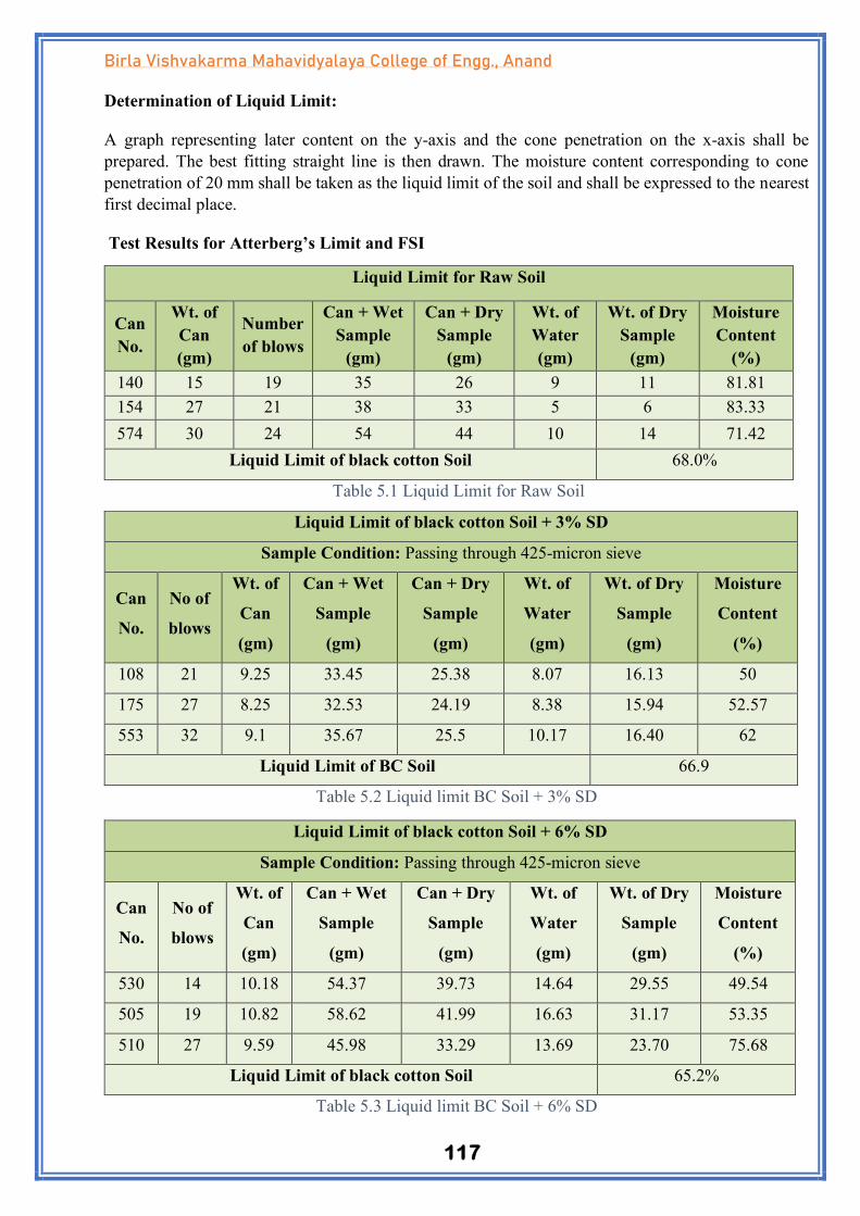
117
Birla Vishvakarma Mahavidyalaya College of Engg., Anand
Determination of Liquid Limit:
A graph representing later content on the y-axis and the cone penetration on the x-axis shall be
prepared. The best fitting straight line is then drawn. The moisture content corresponding to cone
penetration of 20 mm shall be taken as the liquid limit of the soil and shall be expressed to the nearest
first decimal place.
Test Results for Atterberg’s Limit and FSI
Liquid Limit for Raw Soil
Can
No.
Wt. of
Can
(gm)
Number
of blows
Can + Wet
Sample
(gm)
Can + Dry
Sample
(gm)
Wt. of
Water
(gm)
Wt. of Dry
Sample
(gm)
Moisture
Content
(%)
140 15 19 35 26 9 11 81.81
154 27 21 38 33 5 6 83.33
574 30 24 54 44 10 14 71.42
Liquid Limit of black cotton Soil 68.0%
Table 5.1 Liquid Limit for Raw Soil
Table 5.2 Liquid limit BC Soil + 3% SD
Liquid Limit of black cotton Soil + 6% SD
Sample Condition: Passing through 425-micron sieve
Can
No.
No of
blows
Wt. of
Can
(gm)
Can + Wet
Sample
(gm)
Can + Dry
Sample
(gm)
Wt. of
Water
(gm)
Wt. of Dry
Sample
(gm)
Moisture
Content
(%)
530 14 10.18 54.37 39.73 14.64 29.55 49.54
505 19 10.82 58.62 41.99 16.63 31.17 53.35
510 27 9.59 45.98 33.29 13.69 23.70 75.68
Liquid Limit of black cotton Soil 65.2%
Table 5.3 Liquid limit BC Soil + 6% SD
Liquid Limit of black cotton Soil + 3% SD
Sample Condition: Passing through 425-micron sieve
Can
No.
No of
blows
Wt. of
Can
(gm)
Can + Wet
Sample
(gm)
Can + Dry
Sample
(gm)
Wt. of
Water
(gm)
Wt. of Dry
Sample
(gm)
Moisture
Content
(%)
108 21 9.25 33.45 25.38 8.07 16.13 50
175 27 8.25 32.53 24.19 8.38 15.94 52.57
553 32 9.1 35.67 25.5 10.17 16.40 62
Liquid Limit of BC Soil 66.9

118
Birla Vishvakarma Mahavidyalaya College of Engg., Anand
Liquid Limit of black cotton Soil + 9%SD
Sample Condition: Passing through 425-micron sieve
Can
No.
No of
blows
Wt. of
Can
(gm)
Can + Wet
Sample
(gm)
Can + Dry
Sample
(gm)
Wt. of
Water
(gm)
Wt. of Dry
Sample
(gm)
Moisture
Content
(%)
530 14 15.47 38 30.75 7.25 15.2 47.75
505 19 17.29 45.11 35.88 9.23 18.59 70.50
510 27 13.12 53.95 39.90 14.05 26.78 52.46
Liquid Limit of black cotton Soil 63.82%
Table 5.4 Liquid limit BC Soil + 9% SD
Liquid Limit of black cotton Soil + 12% SD
Sample Condition: Passing through 425-micron sieve
Can
No.
No of
blows
Wt. of
Can
(gm)
Can + Wet
Sample
(gm)
Can + Dry
Sample
(gm)
Wt. of
Water
(gm)
Wt. of Dry
Sample
(gm)
Moisture
Content
(%)
174 14 30.5 36.5 34.5 2 4 50
205 21 32.5 39 37 2 4.5 65.9
536 29 33 41 38.5 2 5.5 66.36
Liquid Limit of black cotton Soil + 20% SD 64.9%
Table 5.5 Liquid limit BC Soil + 12% SD
Plastic Limit for Raw Soil
Can
No.
Wt. of
Can (gm)
Can + Wet
Sample (gm)
Can + Dry
Sample (gm)
Wt. of
Water
(gm)
Wt. of Dry
Sample (gm)
Moisture
Content
(%)
534 15 21.47 19.8 1.67 4.8 34.8
548 14 19 17.81 1.19 3.81 31.2
Average Plastic Limit 33.00%
Plasticity Index 35%
Table 5.6 Plastic Limit for Raw Soil

119
Birla Vishvakarma Mahavidyalaya College of Engg., Anand
Plastic Limit of black cotton Soil + 3% SD
Can
No.
Wt. of
Can
(gm)
Can + Wet
Sample (gm)
Can + Dry
Sample (gm)
Wt. of
Water
(gm)
Wt. of Dry
Sample (gm)
Moisture
Content
(%)
16 14.9 21.49 20.00 1.49 5.10 29.22
27 15.6 20.50 19.28 1.22 3.68 33.15
Average Plastic Limit 30.50%
Plasticity Index 36.6%
Table 5.7 Plastic Limit of black cotton Soil + 3% SD
Plastic Limit of black cotton soil + 6% SD
Can
No.
Wt. of
Can
(gm)
Can + Wet
Sample (gm)
Can + Dry
Sample (gm)
Wt. of
Water
(gm)
Wt. of Dry
Sample (gm)
Moisture
Content
(%)
12 14.5 22.16 20.4 1.76 5.9 30.83
21 15 23.56 21.6 1.96 6.6 29.70
Average Plastic Limit 28.65%
Plasticity Index 36.55%
Table 5.8 Plastic Limit of black cotton Soil +6% SD
Table 5.9 Plastic Limit of black cotton Soil + 9% SD
Table 5.10 Plastic Limit of black cotton Soil + 12% SD
Plastic Limit of black cotton soil + 9% SD
Can
No.
Wt. of
Can
(gm)
Can + Wet
Sample (gm)
Can + Dry
Sample (gm)
Wt. of
Water
(gm)
Wt. of Dry
Sample (gm)
Moisture
Content
(%)
16 16 22.5 21.1 1.4 5.1 27.45
11 15.5 24.6 22.6 2 7.1 28.17
Average Plastic Limit 23.25
Plasticity Index 40.55%
Plastic Limit of black cotton soil + 12% SD
Can
No.
Wt. of
Can (gm)
Can + Wet
Sample (gm)
Can + Dry
Sample (gm)
Wt. of
Water
(gm)
Wt. of Dry
Sample (gm)
Moisture
Content
(%)
140 14 21.49 19.8 1.69 5.8 29.14
538 15 22.67 20.8 1.87 5.8 32.24
Average Plastic Limit 26.00%
Plasticity Index 38.90%

120
Birla Vishvakarma Mahavidyalaya College of Engg., Anand
5.1.2 Proctor Test Result for soil by using Standard Procter Test
Result of OMC & MDD for Natural
Soil
Volume of Mould = 981.74
Weight of Mould in gram = 4855gm
Wt. of Wt. Wt. of Wt. of Wt. of
Dry
Sample
(gm)
Mould of Bulk Wt. of Container Container Wt. of Moisture Dry
+ Wet Wet Density Container + Wet + Dry Water Content Density
Soil Soil (gm/cc) (gm) Sample Sample (gm) (%) (gm/cc)
(gm) (gm) (gm) (gm)
6487
1619
1.67
13.23
28.22
25.88
2.34
12.65
18.5
1.41
6516
1648
1.70
13.66
25.72
23.74
1.98
10.08
19.6
1.423
6642 1774 1.83 14.31 34.41 30.92 3.49 16.61 21 1.51
6661 1793 1.85 12.87 26.02 23.58 2.44 10.71 22.7 1.50
6642 1774 1.83 16.83 44.98 39.62 5.36 22.79 23.5 1.48
6612 1757 1.79 16.45 49.41 43.15 6.26 26.70 23.44 1.45
Table 5.11 Results of OMC and MDD for Natural soil
Dry
Den
sity
(gm
/cc)
1.52
1.51
1.5 1.5
1.48 1.48
1.46
1.45
1.44
1.42 1.423
1.41
1.4
0 5 10 15 20 25
Moisture Content (%)
Figure 5.1 OMC and MDD for Natural soil
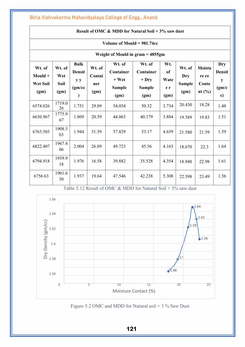
121
Birla Vishvakarma Mahavidyalaya College of Engg., Anand
1.66
1.64
1.62
1.6
1.58
1.56
0 5 10 15 20 25
Moisture Contact (%)
Result of OMC & MDD for Natural Soil + 3% saw dust
Volume of Mould = 981.74cc
Weight of Mould in gram = 4855gm
Wt. of
Mould +
Wet Soil
(gm)
Wt. of
Wet
Soil
(gm)
Bulk
Densit
y y
(gm/cc
)
Wt. of
Contai
ner
(gm)
Wt. of
Container
+ Wet
Sample
(gm)
Wt. of
Container
+ Dry
Sample
(gm)
Wt.
of
Wate
r r
(gm)
Wt. of
Dry
Sample
(gm)
Moistu
re re
Conte
nt (%)
Dry
Densit
y
(gm/c
c)
6574.026 1719.0
26 1.751 29.89 54.054 50.32 3.734 20.430 18.28 1.48
6630.967 1775.9
67 1.809 20.59 44.063 40.179 3.884 19.589 19.83 1.51
6763.503 1908.5
03 1.944 31.59 57.829 53.17 4.659 21.580 21.59 1.59
6822.407 1967.4
06 2.004 26.89 49.723 45.56 4.163 18.670 22.3 1.64
6794.918 1939.9
18 1.976 16.58 39.882 35.528 4.354 18.948 22.98 1.61
6756.63 1901.6
30 1.937 19.64 47.546 42.238 5.308 22.598 23.49 1.56
Table 5.12 Result of OMC & MDD for Natural Soil + 3% saw dust
1.64
1.61
1.59
1.56
1.51
1.48
Figure 5.2 OMC and MDD for Natural soil + 3 % Saw Dust
Dry
Den
sity
(gm
/cc)

122
Birla Vishvakarma Mahavidyalaya College of Engg., Anand
1.8
1.75
1.7
1.65
1.6
1.55
0 5 10 15
Moisture Contact (%)
20 25 30
Result of OMC & MDD for Natural Soil + 6% saw
dust
Volume of Mould = 981.74
Weight of Mould in gram = 4855gm
Wt. of
Mould
+ Wet
Soil
(gm)
Wt. of
Wet
Soil
(gm)
Bulk
Densit
y
(gm/cc
)
Wt. of
Containe
r (gm)
Wt. of
Containe
r + Wet
Sample
(gm)
Wt. of
Containe
r + Dry
Sample
(gm)
Wt.
of
Wate
r
(gm)
Wt. of
Dry
Sampl
e (gm)
Moistu
r e
Conten
t (%)
Dry
Den
sit y
(gm/
cc
)
6714.41
6
1859.41
6
1.894
12.38
29.9
26.94
2.96
14.56
20.38
1.573
6839.09
7
1984.09
7
2.021
14.84
30.12
27.4
2.72
12.56
21.65
1.661
6981.44
9
2126.44
9 2.166 11.58 33.65 29.41 4.24 17.83 23.8 1.750
6891.12 9
2036.12 9
2.074 17.96 31.41 28.81 2.60 10.85 23.97 1.673
6750.74 1895.74 1.931 18.64 43.02 38.18 4.84 19.54 24.81 1.547
6658.45
6
1803.45
6 1.837 12.61 40.93 35.27 5.66 22.66 24.99 1.467
Table 5.13 Result of OMC & MDD for Natural Soil + 6% saw dust
1.75
1.673
1.661
1.5 73
1.54
7
1.46 7
Dry
Den
sity
(gm
/cc)
Figure 5.3 OMC and MDD for Natural soil + 6 % Saw Dust

123
Birla Vishvakarma Mahavidyalaya College of Engg., Anand
1.9 1.891
1.85
1.8
1.75
1.7
1.65 0 5 10 15
Moisture Content (%)
20 25 30
Result of OMC & MDD for Natural Soil + 9% saw
dust
Volume of Mould = 981.74cc
Weight of Mould in gram = 4855 gm
Wt. of
Mould +
Wet Soil
(gm)
Wt. of
Wet
Soil
(gm)
Bulk
Densit
y
(gm/cc
)
Wt. of
Contai
ner
(gm)
Wt. of
Container
+ Wet
Sample
(gm)
Wt. of
Container
+ Dry
Sample
(gm)
Wt.
of
Wate
r
(gm)
Wt.
of
Dry
Sam
ple
(gm)
Mois
tu re
Cont
e nt
(%)
Dry
Densit
y
(gm/c
c)
6810.608 1777.9
31 1.811 25.67 52.996 48.56 4.436 22.89 19.38 1.517
6811.608 1956.6
08 1.993 30.38 67.384 60.99 6.394 30.61 20.89 1.649
6991.266 2136.2
66 2.176 33.72 67.569 61.28 6.289 27.56 22.82 1.772
7141.472 2286.4
72 2.329 19.51 59.784 52.2 7.584 32.69 23.2 1.891
7033.481 2178.4
81 2.219 21.38 44.655 40.16 4.495 18.78 23.94 1.791
6901.928 2046.9
28 2.085 23.67 67.493 58.83 8.663 35.16 24.64 1.673
Table 5.14 Result of OMC & MDD for Natural Soil + 9% saw dust
1.791 1.772
1.673
1.649
1.517
Dry
Den
sity
(gm
/cc)
Figure 5.4 OMC and MDD for Natural soil + 9 % Saw Dust

124
Birla Vishvakarma Mahavidyalaya College of Engg., Anand
Result of OMC & MDD for Natural Soil + 12% saw dust
Volume of Mould = 981.74cc
Weight of Mould in gram = 4855 gm
Wt. of
Mould +
Wet Soil
(gm)
Wt. of
Wet
Soil
(gm)
Bulk
Densit
y
(gm/cc
)
Wt. of
Contai
ner
(gm)
Wt. of
Container +
Wet Sample
(gm)
Wt. of
Container
+ Dry
Sample
(gm)
Wt.
of
Wat
e r
(gm)
Wt. of
Dry
Sampl
e (gm)
Mois
tu re
Cont
e nt
(%)
Dry
Dens
i ty
(gm)
6589.735 1734.7
35 1.767 12.01 55.646 48.63 7.01
6
36.6
2
19.1
6
1.483
6691.836 1836.8
36 1.871 11.62 48.257 42.2 6.05
7
30.5
8 19.8
1
1.562
6776.265 1921.2
65 1.957 10.53 43.649 37.92 5.72
9
27.3
9 20.9
2
1.619
6855.786 2000.7
86 2.038 13.23 62.778 53.9 8.87
8
40.6
7 21.8
3
1.673
6943.161 2088.1
61 2.127 13.66 67.199 57.33 9.86
9
43.6
7 22.6
0
1.735
6833.206 1978.2
06 2.015 14.31 43.312 37.88 5.43
2
23.5
7 23.0
5
1.638
Table 5.15 Result of OMC & MDD for Natural Soil + 12% saw dust
1.673
1.638
1.619
1.56 2
1.483
5.1.3 Laboratory Determination of California Bearing Ratio (IS: 2720 (Part 16) 1987))
Scope: Standard Load:
1.75 1.735
1.7
1.65
1.6
1.55
1.5
1.45 0 5 10 15 20 25
Moisture Content (%)
Dry
Den
sity
(gm
/cc)
Figure 5.5 OMC and MDD for Natural soil + 12 % Saw Dust

125
Birla Vishvakarma Mahavidyalaya College of Engg., Anand
The load which has been obtained from the test on the crushed stone which was defined as having a
California Bearing Ratio of 100 percent.
California Bearing Ratio (CBR):
The Ratio expressed in percentage of force per unit area required to penetrate a soil mass with a circular
plunger of 50 mm diameter at the rate of 1.25 mm/min to that required for corresponding penetration
of a standard material. The ratio is usually determined for penetration of 2.5 mm and 5 mm, the ratio
at 5 mm is used.
Apparatus: Modulus with base plate, Stay rod and wing nut, Collar, Spacer Disc, Metal Rammer,
Expansion Measuring Apparatus, Weights, Loading Machine, Penetration Plunger, Dial Gauges: Two
dial gauges reading to 0.01 mm, Sieves: 47.5 mm IS Sieve and 19 mm IS Sieve, Other general
apparatus, such as a mixing bowl, straightedge, scales, soaking tank or pan, drying oven, filter paper,
dishes and calibrated measuring jar.
Soil Sample: The material used in the remolded specimen shall pass a 19-mm IS Sieve. Allowance for
larger material shall be made by replacing it with an equal amount of material which passes a 19 mm
IS Sieve but is retained on 4.75 mm IS Sieve.
Procedure: The mould containing the specimen, with the base plate in position but the top face
exposed, shall be placed on the lower plate of the testing machine. Surcharge weights, sufficient to
produce an intensity of loading equal to the weight of the base material and pavement shall be placed
on the specimen. If the specimen has been soaked previously, the surcharge shall be equal to that used
during the soaking period. To prevent upheaval of soil into the hole of the surcharge weights, 2.5 kg
annular weight shall be placed on the soil surface prior to seating the penetration plunger after which
the remainder of the surcharge weights shall be placed. The plunger shall be seated under a load of 4
kg so that full contact is established between the surface of the specimen and the plunger. The load
and deformation gauges shall then be set to zero (In other words, the initial load applied to the plunger
shall be considered as zero when determining the load penetration relation). The load shall be applied
to the plunger into the soil at the rate of 1.25 mm per minute. Reading of the load shall be taken at
penetrations of 0.5, 1.0, 1.5, 2.0, 2.5, 4.0, 5.0, 7.5, 10.0 and 12.5 mm (The maximum load and
penetration shall be recorded if it occurs for a penetration of less than 12.5 mm). The plunger shall be
raised and the mould detached from the loading equipment. About 20 to 50 g of soil shall be collected
from the top 30 mm layer of the specimen and the water content determined according to IS: 2720
(Part 2)-1973. If the average water content of the whole specimen is desired, water content sample

126
Birla Vishvakarma Mahavidyalaya College of Engg., Anand
shall be taken from the entire depth of the specimen. The undisturbed specimen for the test should be
carefully examined after the test is completed for the presence of any oversize soil particles which are
likely to affect the results if they happen to be located directly below the penetration plunger. The
penetration test may be repeated as a check test for the rear end of the sample.
Load Penetration Curve:
The load penetration curve shall be plotted. This curve is usually convex upwards although the initial
portion of the curve may be convex downwards due to surface irregularities. A correction shall then
be applied by drawing a tangent to the point of greatest slope and then transposing the axis of the load
so that zero penetration is taken as the point where the tangent cuts the axis of penetration. The
corrected load-penetration curve would then consist of the tangent from the new origin to the point of
tangency on the re-sited curve and then the curve itself.
California Bearing Ratio:
The CBR values are usually calculated for penetrations of 2.5 mm and 5 mm. corresponding to the
penetration values at which the CBR values are desired, corrected load value shall be taken from the
load penetration curve and the CBR calculated as follows.
California Bearing Ratio = x 100 Where,

127
Birla Vishvakarma Mahavidyalaya College of Engg., Anand
PT = Corrected unit (or total) test load corresponding to the chosen penetration from the load
penetration curve.
PS = Unit (or total) standard load for the sample depth of penetration as for PT taken from the table.
Generally, the CBR value at 2.5 mm penetration will be greater than that at 5 mm penetration and in
such a case; the former shall be taken as the CBR value for design purposes. If the CBR value
corresponding to a penetration of 5 mm exceeds that for 2.5 mm, the test shall be repeated. If identical
results follow, the CBR corresponding to 5 mm penetration shall be taken for design.
CBR test results for soil
The results obtained by these tests are used with the empirical curves to determine the thickness of
pavement and its component layers. This is the most widely used method for the design of flexible
pavement. The CBR value of the specimen reflects on the strength of the specimen in soaked condition
as tested in the laboratory. The soak CBR test is carried out after the submergence of the sample in
water for 96 hours in accordance to IS 2720 (part 16) 1987.

128
Birla Vishvakarma Mahavidyalaya College of Engg., Anand
Sample Condition: Remolded at OMC & MDD
Test Condition: Soaked Soaking for 96 Hours
Penetration Rate: 1.25 mm/minute Surcharge Weight: 5.0 kg
Penetration (mm) Proving Ring Reading Load
(kg)
0.5 7 13.74
1.0 9 17.62
1.5 12 23.42
2.0 14 27.54
2.5 16 31.38
4.0 22 43.12
5.0 26 50.94
7.5 29 56.84
10.0 31 60.76
12.5 33 64.68
Table 5.16 Result for CBR Test for BC Soil
CBR = X 100
Load
(k
g)
70.00
5.0, 50.94
50.00
2.5, 31.38
30.00
20.00
10.00 0.0 2.0 4.0 6.0 8.0 10.0 12.0 14.0
Penetration (mm)
Figure 5.6 CBR Graph for BC soil

129
Birla Vishvakarma Mahavidyalaya College of Engg., Anand
CBR at 2.5 mm = X 100
CBR at 2.5 mm = 2.478 % And, CBR at 5.0 mm = X
100 CBR at 5.0 mm = 2.22 %
By the result of test CBR value is 2.47% at 5 mm penetration.
Result for CBR Test BC Soil+3% SD
Sample Condition: Remolded at OMC & MDD
Test Condition: Soaked Soaking for 96 Hours
Penetration Rate: 1.25 mm/minute Surcharge Weight: 5.0
kg
Penetration (mm) Proving Ring Reading Load
(kg)
0.5 7 12.72
1.0 9 17.64
1.5 12 23.52
2.0 14 27.44
2.5 16 31.38
4.0 22 42.12
5.0 26 49.02
7.5 29 56.84
10.0 31 60.76
12.5 33 64.68
Table 5.17 Result for CBR Test for BC Soil + 3% Saw Dust
CBR = 𝐶𝑜𝑟𝑟𝑒𝑐𝑡𝑒𝑑 𝑡𝑒𝑐𝑡 𝑆𝑜𝑎𝑑 𝑓𝑟𝑜𝑚 𝐺𝑟𝑎𝑝ℎ
𝑆𝑡𝑎𝑛𝑑𝑎𝑟𝑑 𝐿𝑜𝑎𝑑𝑓𝑟𝑜𝑚 𝑠𝑎𝑚𝑒 𝑝𝑒𝑛𝑒𝑡𝑟𝑎𝑡𝑖𝑜𝑛𝑋 100
70
60
50
40
30 0 . 5 1 1 . 5 2 2 . 5 4 5 7 . 5 1 0 1 2 . 5
PENETRATION (MM)
Figure 5.7 CBR Graph for BC soil + 3% SD
LOA
D (
KG)

130
Birla Vishvakarma Mahavidyalaya College of Engg., Anand
CBR at 2.5 mm =2.38 %
CBR at 5.0 mm = 2.20 %
By the result of test CBR value is 2.38% at 2.5 mm penetration
Result for CBR Test BC Soil + 6% SD
Sample Condition: Remolded at OMC & MDD
Test Condition: Soaked Soaking for 96 Hours
Penetration Rate : 1.25 mm/minute Surcharge Weight : 5.0 kg
Penetration (mm) Proving Ring Reading Load (kg)
0.5 13 18.56
1.0 21 23.48
1.5 27 31.92
2.0 31 42.76
2.5 41 53.36
4.0 52 73.92
5.0 60 79.60
7.5 67 92.32
10.0 70 97.20
12.5 73 103.08
Table 5.18 Result for CBR Test for BC Soil + 6% Saw Dust
Figure 5.8 CBR Graph for BC soil + 6% SD
CBR = 𝐶𝑜𝑟𝑟𝑒𝑐𝑡𝑒𝑑 𝑡𝑒𝑐𝑡 𝑆𝑜𝑎𝑑 𝑓𝑟𝑜𝑚 𝐺𝑟𝑎𝑝ℎ
𝑆𝑡𝑎𝑛𝑑𝑎𝑟𝑑 𝐿𝑜𝑎𝑑𝑓𝑟𝑜𝑚 𝑠𝑎𝑚𝑒 𝑝𝑒𝑛𝑒𝑡𝑟𝑎𝑡𝑖𝑜𝑛𝑋 100

131
Birla Vishvakarma Mahavidyalaya College of Engg., Anand
CBR at 2.5 mm =3.89 %
CBR at 5.0 mm = 2.50 %
By the result of test CBR value is 3.89 % at 2.5 mm penetration
Result for CBR Test BC Soil + 9% SD
Sample Condition: Remolded at OMC & MDD
Test Condition: Soaked Soaking for 96 Hours
Penetration Rate: 1.25 mm/minute Surcharge Weight: 5.0 kg
Penetration (mm) Proving Ring Reading Load (kg)
0.5 10 19.60
1.0 18 35.28
1.5 28 54.88
2.0 37 49.52
2.5 43 61.28
4.0 52 78.92
5.0 64 102.5
7.5 71 109.16
10.0 78 116.88
12.5 82 126.72
Table 5.19 Result for CBR Test for BC Soil + 9% SAW DUST
CBR = 𝐶𝑜𝑟𝑟𝑒𝑐𝑡𝑒𝑑 𝑡𝑒𝑐𝑡 𝑆𝑜𝑎𝑑 𝑓𝑟𝑜𝑚 𝐺𝑟𝑎𝑝ℎ
𝑆𝑡𝑎𝑛𝑑𝑎𝑟𝑑 𝐿𝑜𝑎𝑑𝑓𝑟𝑜𝑚 𝑠𝑎𝑚𝑒 𝑝𝑒𝑛𝑒𝑡𝑟𝑎𝑡𝑖𝑜𝑛𝑋 100
CBR at 2.5 mm = 4.98 %
140
120
100
80
60
0.5 1 1.5 2 2.5 4 5 7.5 10 12.5
PENETRATION (MM)
Figure 5.9 CBR Graph for BC Soil + 9% SD

132
Birla Vishvakarma Mahavidyalaya College of Engg., Anand
CBR at 5.0 mm = 4.80 %
By the result of test CBR value is 4.98% at 2.5 mm penetration.
Table 5.20 Result for CBR Test for BC Soil + 12% SAW DUST
Figure 5.10 Graph for BC Soil + 12% SD
CBR = 𝐶𝑜𝑟𝑟𝑒𝑐𝑡𝑒𝑑 𝑡𝑒𝑐𝑡 𝑆𝑜𝑎𝑑 𝑓𝑟𝑜𝑚 𝐺𝑟𝑎𝑝ℎ
𝑆𝑡𝑎𝑛𝑑𝑎𝑟𝑑 𝐿𝑜𝑎𝑑𝑓𝑟𝑜𝑚 𝑠𝑎𝑚𝑒 𝑝𝑒𝑛𝑒𝑡𝑟𝑎𝑡𝑖𝑜𝑛𝑋 100
CBR at 2.5 mm = 3.94 %
Result for CBR Test BC Soil + 12% SD
Sample Condition: Remolded at OMC & MDD
Test Condition: Soaked Soaking for 96 Hours
Penetration Rate: 1.25 mm/minute Surcharge Weight: 5.0 kg
Penetration (mm) Proving Ring Reading Load (kg)
0.5 12 19.57
1.0 23 24.38
1.5 30 31.90
2.0 39 42.77
2.5 49 54.04
4.0 62 73.92
7.5 71 75.61
10.0 76 82.32
12.5 86 101.08
120
100
80
60
40
20
0 0.5 1 1.5 2 2.5 4 5 7.5 10 12.5
PENETRATION (MM)

133
Birla Vishvakarma Mahavidyalaya College of Engg., Anand
CBR at 5.0 mm = 3.67 %
By the result of test CBR value is 3.94% at 2.5 mm penetration.
Table 5.21 Result for CBR Test for BC Soil + 3% SD (7 days)
CBR = 𝐶𝑜𝑟𝑟𝑒𝑐𝑡𝑒𝑑 𝑡𝑒𝑐𝑡 𝑆𝑜𝑎𝑑 𝑓𝑟𝑜𝑚 𝐺𝑟𝑎𝑝ℎ
𝑆𝑡𝑎𝑛𝑑𝑎𝑟𝑑 𝐿𝑜𝑎𝑑𝑓𝑟𝑜𝑚 𝑠𝑎𝑚𝑒 𝑝𝑒𝑛𝑒𝑡𝑟𝑎𝑡𝑖𝑜𝑛𝑋 100
Result for CBR Test BC Soil + 3% saw dust (7 Days)
Sample Condition: Remolded at OMC & MDD
Test Condition: Soaked Soaking for 96 Hours
Penetration Rate: 1.25 mm/minute Surcharge Weight: 5.0 kg
Penetration (mm) Proving Ring Reading Load (kg)
0.5 16 12.74
1.0 27 17.82
1.5 38 23.56
2.0 47 27.48
2.5 60 32.87
4.0 75 42.20
5.0 83 46.50
7.5 91 56.84
10.0 101 60.76
12.5 110 64.68
LOA
D (
KG
)
70
60
50
40
30
0.5 1 1.5 2 2.5 4 5 7.5 10 12.5
PENETRATION (MM)
Figure 5.11 Graph for BC Soil + 3% SD (7 day)

134
Birla Vishvakarma Mahavidyalaya College of Engg., Anand
CBR at 2.5 mm = 3.43 %
CBR at 5.0 mm = 2.261
By the result of test CBR value is 3.43 % at 2.5 mm penetration.
Result for CBR Test BC Soil + 6% SAW DUST (7 Days)
Sample Condition: Remolded at OMC & MDD
Test Condition: Soaked Soaking for 96 Hours
Penetration Rate: 1.25 mm/minute Surcharge Weight: 5.0 kg
Penetration (mm) Proving Ring Reading Load (kg)
0.5 19 18.45
1.0 35 23.48
1.5 42 31.92
2.0 56 42.76
2.5 67 52.36
4.0 92 74.98
5.0 101 81.42
7.5 119 90.31
10.0 127 98.20
12.5 135 102.08
Table 5.22 Result for CBR Test for BC Soil + 6% SD (7 days)
70
60
50
40
0.5 1 1.5 2 2.5 4 5 7.5 10 12.5
PENETRATION (MM)
Figure 5.12 Graph for BC Soil + 6% SD (7 day)

135
Birla Vishvakarma Mahavidyalaya College of Engg., Anand
CBR = 𝐶𝑜𝑟𝑟𝑒𝑐𝑡𝑒𝑑 𝑡𝑒𝑐𝑡 𝑆𝑜𝑎𝑑 𝑓𝑟𝑜𝑚 𝐺𝑟𝑎𝑝ℎ
𝑆𝑡𝑎𝑛𝑑𝑎𝑟𝑑 𝐿𝑜𝑎𝑑𝑓𝑟𝑜𝑚 𝑠𝑎𝑚𝑒 𝑝𝑒𝑛𝑒𝑡𝑟𝑎𝑡𝑖𝑜𝑛𝑋 100
CBR at 2.5 mm = 3.821 %
CBR at 5.0 mm = 3.96 %
By the result of test, CBR value is 3.96 % at 5 mm penetration
Table 5.23 Result for CBR Test for BC Soil + 9% SD (7 days)
Result for CBR Test BC Soil + 9% SAW DUST (7 Days)
Sample Condition: Remolded at OMC & MDD
Test Condition: Soaked Soaking for 96 Hours
Penetration Rate: 1.25 mm/minute Surcharge Weight: 5.0 kg
Penetration (mm) Proving Ring Reading Load (kg)
0.5 20 23.47
1.0 35 39.28
1.5 47 55.88
2.0 63 62.52
2.5 74 71.13
4.0 92 84.92
5.0 110 98.71
7.5 119 109.16
10.0 125 116.88
12.5 138 126.72
140
120
100
80
60
40
20
0 0.5 1 1.5 2 2.5 4 5 7.5 10 12.5
PENETRATION (MM)
LOA
D (
KG
)
Figure 5.13 Graph for BC Soil + 9% SD (7 day)

136
Birla Vishvakarma Mahavidyalaya College of Engg., Anand
CBR = 𝐶𝑜𝑟𝑟𝑒𝑐𝑡𝑒𝑑 𝑡𝑒𝑐𝑡 𝑆𝑜𝑎𝑑 𝑓𝑟𝑜𝑚 𝐺𝑟𝑎𝑝ℎ
𝑆𝑡𝑎𝑛𝑑𝑎𝑟𝑑 𝐿𝑜𝑎𝑑𝑓𝑟𝑜𝑚 𝑠𝑎𝑚𝑒 𝑝𝑒𝑛𝑒𝑡𝑟𝑎𝑡𝑖𝑜𝑛𝑋 100
CBR at 2.5 mm = 5.18 %
CBR at 5.0 mm = 4.80 %
By the result of test CBR value is 5.18% at 2.5 mm penetration.
Result for CBR Test BC Soil + 12% SAW DUST (7 Days)
Sample Condition: Remolded at OMC & MDD
Test Condition: Soaked Soaking for 96 Hours
Penetration Rate: 1.25 mm/minute Surcharge Weight: 5.0 kg
Penetration (mm) Proving Ring Reading Load (kg)
0.5 21 21.67
1.0 29 29.28
1.5 36 41.88
2.0 41 49.52
2.5 49 55.68
4.0 68 71.92
5.0 74 84.92
7.5 86 99.16
10.0 97 106.88
12.5 107 116.72
Table 5.24 Result for CBR Test for BC Soil + 12% SD (7 days)
LOA
D (
KG
)
140
120
100
80
60
40
20
0.5 1 1.5 2 2.5 4 5 7.5 10 12.5
PENETRATION (MM)
Figure 5.14 Graph for BC Soil + 12% SD (7 day)
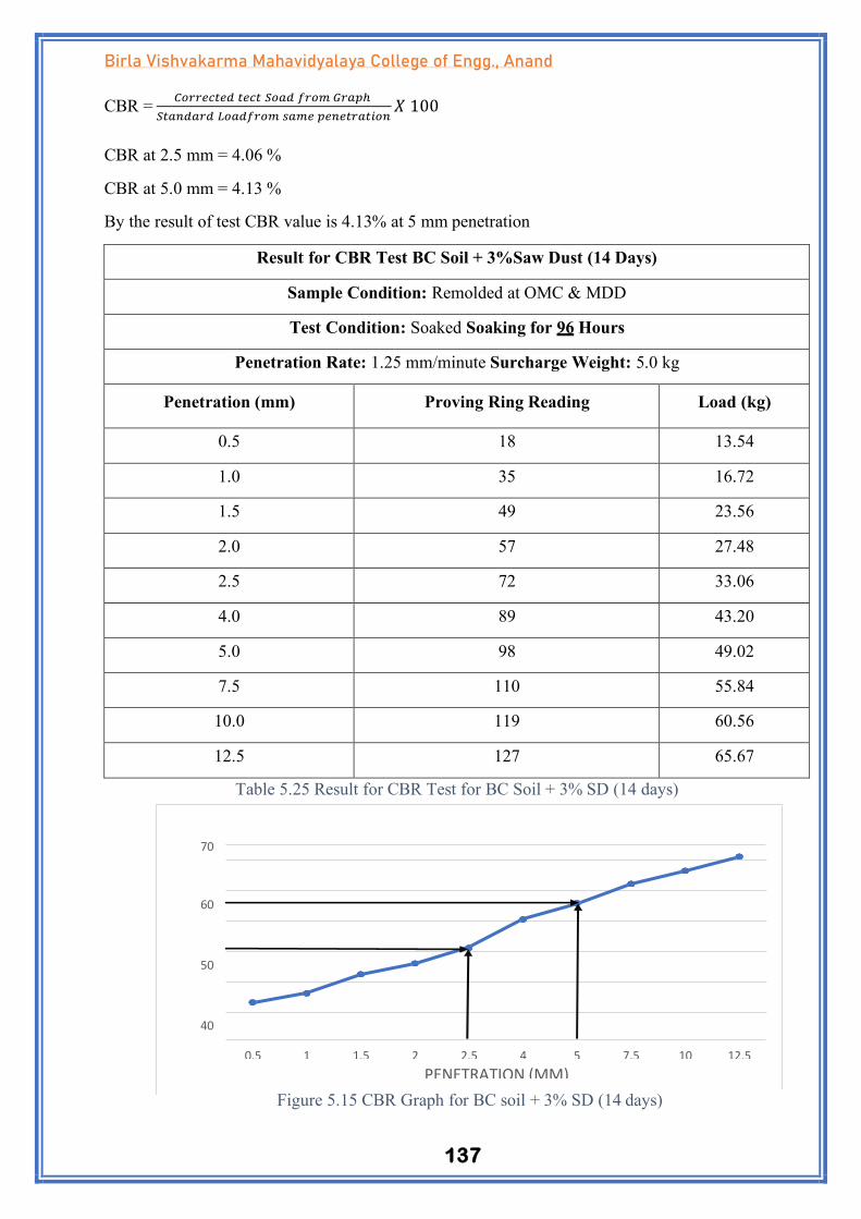
137
Birla Vishvakarma Mahavidyalaya College of Engg., Anand
CBR = 𝐶𝑜𝑟𝑟𝑒𝑐𝑡𝑒𝑑 𝑡𝑒𝑐𝑡 𝑆𝑜𝑎𝑑 𝑓𝑟𝑜𝑚 𝐺𝑟𝑎𝑝ℎ
𝑆𝑡𝑎𝑛𝑑𝑎𝑟𝑑 𝐿𝑜𝑎𝑑𝑓𝑟𝑜𝑚 𝑠𝑎𝑚𝑒 𝑝𝑒𝑛𝑒𝑡𝑟𝑎𝑡𝑖𝑜𝑛𝑋 100
CBR at 2.5 mm = 4.06 %
CBR at 5.0 mm = 4.13 %
By the result of test CBR value is 4.13% at 5 mm penetration
Result for CBR Test BC Soil + 3%Saw Dust (14 Days)
Sample Condition: Remolded at OMC & MDD
Test Condition: Soaked Soaking for 96 Hours
Penetration Rate: 1.25 mm/minute Surcharge Weight: 5.0 kg
Penetration (mm) Proving Ring Reading Load (kg)
0.5 18 13.54
1.0 35 16.72
1.5 49 23.56
2.0 57 27.48
2.5 72 33.06
4.0 89 43.20
5.0 98 49.02
7.5 110 55.84
10.0 119 60.56
12.5 127 65.67
Table 5.25 Result for CBR Test for BC Soil + 3% SD (14 days)
70
60
50
40
0.5 1 1.5 2 2.5 4 5 7.5 10 12.5
PENETRATION (MM)
Figure 5.15 CBR Graph for BC soil + 3% SD (14 days)

138
Birla Vishvakarma Mahavidyalaya College of Engg., Anand
CBR = 𝐶𝑜𝑟𝑟𝑒𝑐𝑡𝑒𝑑 𝑡𝑒𝑐𝑡 𝑆𝑜𝑎𝑑 𝑓𝑟𝑜𝑚 𝐺𝑟𝑎𝑝ℎ
𝑆𝑡𝑎𝑛𝑑𝑎𝑟𝑑 𝐿𝑜𝑎𝑑𝑓𝑟𝑜𝑚 𝑠𝑎𝑚𝑒 𝑝𝑒𝑛𝑒𝑡𝑟𝑎𝑡𝑖𝑜𝑛𝑋 100
CBR at 2.5 mm = 3.43%
CBR at 5.0 mm = 2.38 %
By the result of test CBR value is 3.43% at 2.5 mm penetration.
Table 5.26 Result for CBR Test for BC Soil + 6% SD (14 days)
Figure 5.16 CBR Graph for BC soil + 6% SD (14 days)
Result for CBR Test BC Soil + 6% SAW DUST (14 Days)
Sample Condition: Remolded at OMC & MDD
Test Condition: Soaked Soaking for 96 Hours
Penetration Rate: 1.25 mm/minute Surcharge Weight: 5.0 kg
Penetration (mm) Proving Ring Reading Load (kg)
0.5 19 20.60
1.0 35 29.28
1.5 55 41.88
2.0 68 49.52
2.5 77 57.43
4.0 104 74.92
5.0 114 83.67
7.5 131 99.16
10.0 147 106.88
12.5 161 116.72
140
120
100
80 0.5 1 1.5 2 2.5 4 5 7.5 10 12.5
PENETRATION (MM)
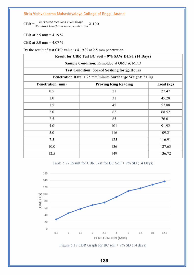
139
Birla Vishvakarma Mahavidyalaya College of Engg., Anand
CBR = 𝐶𝑜𝑟𝑟𝑒𝑐𝑡𝑒𝑑 𝑡𝑒𝑐𝑡 𝑆𝑜𝑎𝑑 𝑓𝑟𝑜𝑚 𝐺𝑟𝑎𝑝ℎ
𝑆𝑡𝑎𝑛𝑑𝑎𝑟𝑑 𝐿𝑜𝑎𝑑𝑓𝑟𝑜𝑚 𝑠𝑎𝑚𝑒 𝑝𝑒𝑛𝑒𝑡𝑟𝑎𝑡𝑖𝑜𝑛𝑋 100
CBR at 2.5 mm = 4.19 %
CBR at 5.0 mm = 4.07 %
By the result of test CBR value is 4.19 % at 2.5 mm penetration.
Table 5.27 Result for CBR Test for BC Soil + 9% SD (14 Days)
Figure 5.17 CBR Graph for BC soil + 9% SD (14 days)
Result for CBR Test BC Soil + 9% SAW DUST (14 Days)
Sample Condition: Remolded at OMC & MDD
Test Condition: Soaked Soaking for 96 Hours
Penetration Rate: 1.25 mm/minute Surcharge Weight: 5.0 kg
Penetration (mm) Proving Ring Reading Load (kg)
0.5 21 27.47
1.0 31 45.28
1.5 45 57.88
2.0 62 68.52
2.5 85 76.01
4.0 101 91.92
5.0 116 109.21
7.5 125 116.91
10.0 136 127.63
12.5 149 136.72

140
Birla Vishvakarma Mahavidyalaya College of Engg., Anand
CBR = 𝐶𝑜𝑟𝑟𝑒𝑐𝑡𝑒𝑑 𝑡𝑒𝑐𝑡 𝑆𝑜𝑎𝑑 𝑓𝑟𝑜𝑚 𝐺𝑟𝑎𝑝ℎ
𝑆𝑡𝑎𝑛𝑑𝑎𝑟𝑑 𝐿𝑜𝑎𝑑𝑓𝑟𝑜𝑚 𝑠𝑎𝑚𝑒 𝑝𝑒𝑛𝑒𝑡𝑟𝑎𝑡𝑖𝑜𝑛𝑋 100
CBR at 2.5 mm = 5.54 %
CBR at 5.0 mm = 5.30 %
By the result of test CBR value is 5.54% at 2.5 mm penetration
Table 5.28 Result for CBR Test for BC Soil + 12% SD (14 Days)
Figure 5.18 CBR Graph for BC soil + 12% SD (14 days)
Result for CBR Test BC Soil + 12% SAW DUST (14 Days)
Sample Condition: Remolded at OMC & MDD
Test Condition: Soaked Soaking for 96 Hours
Penetration Rate: 1.25 mm/minute Surcharge Weight: 5.0 kg
Penetration (mm) Proving Ring Reading Load (kg)
0.5 19 24.62
1.0 35 32.28
1.5 52 44.88
2.0 61 55.52
2.5 69 64.60
4.0 83 71.92
5.0 91 95.24
7.5 99 104.16
10.0 105 116.80
12.5 112 127.72

141
Birla Vishvakarma Mahavidyalaya College of Engg., Anand
CBR = 𝐶𝑜𝑟𝑟𝑒𝑐𝑡𝑒𝑑 𝑡𝑒𝑐𝑡 𝑆𝑜𝑎𝑑 𝑓𝑟𝑜𝑚 𝐺𝑟𝑎𝑝ℎ
𝑆𝑡𝑎𝑛𝑑𝑎𝑟𝑑 𝐿𝑜𝑎𝑑𝑓𝑟𝑜𝑚 𝑠𝑎𝑚𝑒 𝑝𝑒𝑛𝑒𝑡𝑟𝑎𝑡𝑖𝑜𝑛𝑋 100
CBR at 2.5 mm = 4.715%
CBR at 5.0 mm = 4.63 %
By the result of test CBR value is 4.715% at 2.5 mm penetration.
Result for CBR Test BC Soil + 3% Sawdust (21 Days)
Sample Condition: Remolded at OMC & MDD
Test Condition: Soaked Soaking for 96 Hours
Penetration Rate: 1.25 mm/minute Surcharge Weight: 5.0 kg
Penetration (mm) Proving Ring Reading Load (kg)
0.5 21 14.54
1.0 39 19.72
1.5 54 24.56
2.0 66 28.78
2.5 79 33.38
4.0 93 43.20
5.0 109 49.74
7.5 122 56.84
10.0 136 60.93
12.5 141 65.46
Table 5.29 Result for CBR Test for BC Soil + 3% SD (21 days)
Figure 5.19 CBR Graph for BC soil + 3% SD (21 days)
CBR Graph for BC soil + 3% SD(21days)
70
60
50
40
30
20
10
0.5 1 1.5 2 2.5 4 5 7.5 10 12.5
PENETRATION (MM)

142
Birla Vishvakarma Mahavidyalaya College of Engg., Anand
CBR = 𝐶𝑜𝑟𝑟𝑒𝑐𝑡𝑒𝑑 𝑡𝑒𝑐𝑡 𝑆𝑜𝑎𝑑 𝑓𝑟𝑜𝑚 𝐺𝑟𝑎𝑝ℎ
𝑆𝑡𝑎𝑛𝑑𝑎𝑟𝑑 𝐿𝑜𝑎𝑑𝑓𝑟𝑜𝑚 𝑠𝑎𝑚𝑒 𝑝𝑒𝑛𝑒𝑡𝑟𝑎𝑡𝑖𝑜𝑛𝑋 100
CBR at 2.5 mm = 3.89 %
CBR at 5.0 mm = 2.420 %
By the result of test CBR value is 3.89 % at 2.5 mm penetration.
Result for CBR Test BC Soil + 6% SAW DUST (21 Days)
Sample Condition: Remolded at OMC & MDD
Test Condition: Soaked Soaking for 96 Hours
Penetration Rate: 1.25 mm/minute Surcharge Weight: 5.0 kg
Penetration (mm) Proving Ring Reading Load (kg)
0.5 19 22.70
1.0 35 31.28
1.5 55 41.88
2.0 68 49.52
2.5 87 61.95
4.0 104 74.92
5.0 121 86.97
7.5 143 101.16
10.0 155 112.88
12.5 167 123.72
Table 5.30 Result for CBR Test for BC Soil + 6% SD (21 days)
Figure 5.20 CBR Graph for BC soil + 6% SD (21 days)
CBR Graph for BC soil + 6% SD(21 days) 140
120
100
80
0.5 1 1.5 2 2.5 4 5 7.5 10 12.5
PENETRATION (MM)

143
Birla Vishvakarma Mahavidyalaya College of Engg., Anand
CBR = 𝐶𝑜𝑟𝑟𝑒𝑐𝑡𝑒𝑑 𝑡𝑒𝑐𝑡 𝑆𝑜𝑎𝑑 𝑓𝑟𝑜𝑚 𝐺𝑟𝑎𝑝ℎ
𝑆𝑡𝑎𝑛𝑑𝑎𝑟𝑑 𝐿𝑜𝑎𝑑𝑓𝑟𝑜𝑚 𝑠𝑎𝑚𝑒 𝑝𝑒𝑛𝑒𝑡𝑟𝑎𝑡𝑖𝑜𝑛𝑋 100
CBR at 2.5 mm = 4.52 %
CBR at 5.0 mm = 4.23 %
By the result of test CBR value is 4.52 % at 2.5 mm penetration.
Result for CBR Test by Soil +9 % SAW DUST (21 Days)
Sample Condition: Remolded at OMC & MDD
Test Condition: Soaked Soaking for 96 Hours
Penetration Rate: 1.25 mm/minute Surcharge Weight: 5.0 kg
Penetration (mm) Proving Ring Reading Load (kg)
0.5 32 29.59
1.0 49 47.28
1.5 61 59.88
2.0 79 72.47
2.5 91 81.61
4.0 120 101.92
5.0 132 120.19
7.5 145 129.34
10.0 157 137.63
12.5 163 146.72
Table 5.31 Result for CBR Test for BC Soil + 9% SD (21 Days)
Figure 5.21 CBR Graph for BC Soil + 9% SD(21 Days)
160
140
120
100
80
0.5 1 1.5 2 2.5 4 5 7.5 10 12.5
PENETRATION (MM)

144
Birla Vishvakarma Mahavidyalaya College of Engg., Anand
CBR = 𝐶𝑜𝑟𝑟𝑒𝑐𝑡𝑒𝑑 𝑡𝑒𝑐𝑡 𝑆𝑜𝑎𝑑 𝑓𝑟𝑜𝑚 𝐺𝑟𝑎𝑝ℎ
𝑆𝑡𝑎𝑛𝑑𝑎𝑟𝑑 𝐿𝑜𝑎𝑑𝑓𝑟𝑜𝑚 𝑠𝑎𝑚𝑒 𝑝𝑒𝑛𝑒𝑡𝑟𝑎𝑡𝑖𝑜𝑛𝑋 100
CBR at 2.5 mm = 5.95 %
CBR at 5.0 mm = 5.84 %
By the result of test CBR value is 5.95% at 2.5 mm penetration.
Table 5.32 Result for CBR Test for BC Soil + 12% SD (21 Days)
Figure 5.22 CBR Graph for BC Soil + 12% SD (21 Days)
Result for CBR Test BC Soil + 12% SAW DUST (21 Days)
Sample Condition: Remolded at OMC & MDD
Test Condition: Soaked Soaking for 96 Hours
Penetration Rate: 1.25 mm/minute Surcharge Weight: 5.0 kg
Penetration (mm) Proving Ring Reading Load (kg)
0.5 26 34.64
1.0 43 42.24
1.5 56 53.62
2.0 75 62.26
2.5 80 71.40
4.0 101 89.94
5.0 115 105.86
7.5 127 114.16
10.0 139 126.51
12.5 145 137.75
160
140
120
100
80
0.5 1 1.5 2 2.5 4 5 7.5 10 12.5
PENETRATION (MM)

145
Birla Vishvakarma Mahavidyalaya College of Engg., Anand
CBR = 𝐶𝑜𝑟𝑟𝑒𝑐𝑡𝑒𝑑 𝑡𝑒𝑐𝑡 𝑆𝑜𝑎𝑑 𝑓𝑟𝑜𝑚 𝐺𝑟𝑎𝑝ℎ
𝑆𝑡𝑎𝑛𝑑𝑎𝑟𝑑 𝐿𝑜𝑎𝑑𝑓𝑟𝑜𝑚 𝑠𝑎𝑚𝑒 𝑝𝑒𝑛𝑒𝑡𝑟𝑎𝑡𝑖𝑜𝑛𝑋 100
CBR at 2.5 mm = 5.21 %
CBR at 5.0 mm = 5.15 %
By the result of test CBR value is 5.21% at 2.5 mm penetrations.
5.1.4 Determination of Unconfined Compressive Strength (IS: 2720 (Part 10) 1991))
Scope: This method describes the m method for determining the unconfined compressive strength of
clayey soil, undisturbed, remolded or compacted, using controlled rate of strain.
Unconfined Compressive Strength Qu: It is the load per unit area at which an unconfined
cylindrical specimen of soil will fail in the axial compression test.
Apparatus: Hydraulic loading device, Screw jack with a providing ring, proving ring, deformation
dial gauge, Vernier callipers, oven, weighing balances, Specimen trimming, and carving tools,
remoulding apparatus, water content cans, data sheets, etc. as required.
Procedure:
1. Extrude the soil sample from Shelby tube sampler. Cut a soil specimen so that the ratio (L/d)
is approximately between 2 and 2.5. Where L and d, are the length and diameter of soil
specimen, respectively.
2. Measure the exact length of the specimen at three locations 120° apart, and then average the
measurements and record the average as the length of the data sheet.
3. Weigh the sample and record the mass on the data sheet
4. Calculate the deformation (DL) corresponding to 15% strain (e).
5. Strain (e) =
6. Where L0 = Original specimen length (as measured in step 3).
7. Carefully place the specimen in the compression device and center it on the bottom plate.
Adjust the device so that the upper plate just makes contact with the specimen and set the
load and deformation dials to zero.
8. Apply the load so that the device produces an axial strain at a rate of 0.5% to 2.0% per minute,
and then record the load and deformation dial readings on the data sheet at every 20 to 50
divisions on deformation the dial.
Figure 5.23 UCS Soil
Testing

146
Birla Vishvakarma Mahavidyalaya College of Engg., Anand
9. Keep applying the load until (1) the load (load dial) decreases on the specimen significantly,
(2) the load holds constant for at least four deformation dial readings, or (3) the deformation
is significantly past the 15% strain that was determined in step 5.
Remove the sample from the compression device and obtain a sample for water content
determination.
UCS Test Results for Soil
Table 5.33 Result for UCS Test for BC Soil
UCS Test: Clay Soil
Axial
Deformation
(cm)
Proving ring
Reading
Axial Strain
(%) (e)
Area (A)
(cm2)
Axial Force
(kg)
Compressive
Stress
(kg/cm2)
0 0 0 19.625 0 0
0.05 9 0.472 19.718 17.64 0.8946
0.1 13 0.944 19.812 25.48 1.2860
0.15 15 1.415 19.906 29.4 1.4769
0.2 17 1.886 20.002 33.32 1.6658
0.25 18 2.358 20.098 35.28 1.7553
0.3 20 2.830 20.196 39.2 1.9409
0.35 21 3.301 20.294 41.16 2.0281
0.4 21 3.773 20.394 41.16 2.0182
0.45 21 4.245 20.495 41.16 2.0082
0.5 22 4.716 20.596 43.12 2.0936
0.55 23 5.188 20.698 45.08 2.1779
0.6 23 5.660 20.802 45.08 2.1670
0.65 24 6.132 20.907 47.04 2.2499
0.7 24 6.603 20.012 47.04 2.350
0.75 23 7.075 21.119 45.08 2.1345
0.8 23 7.547 21.227 45.08 2.1237
0.85 21 8.018 21.335 41.16 1.9292
0.9 21 8.490 21.445 41.16 1.9193
Co
mp
ress
ive
stre
ss (
kg/c
m2)

147
Birla Vishvakarma Mahavidyalaya College of Engg., Anand
UCS Test: BC Soil Clay Soil +3% Saw Dust
Axial
Deformation
(cm)
Proving ring
Reading
Axial
Strain
(%) (e)
Area (A)
(cm2)
Axial Force
(kg)
Compressive
Stress
(kg/cm2)
0
0
0
0
0
0
0.05
7
0.472
25.12821
13.72
0.546
0.1
11
0.944
21.82186
21.56
0.988
0.15
15
1.415
22.20544
29.4
1.324
0.2
18
1.886
21.03757
35.28
1.677
0.25
20
2.358
20.65332
39.2
1.898
0.3
21
2.830
20.37624
41.16
2.02
0.35
23
3.301
20.50955
45.08
2.198
0.4
25
3.773
20.6229
49
2.376
0.45
26
4.245
21.3311
50.96
2.389
2.5 2.35
2
1.5
1
0.5
0
0 1 2 3 4 5 6 7 8 9
Axial strain (%) €
Figure 5.24 Graph of BC Soil

148
Birla Vishvakarma Mahavidyalaya College of Engg., Anand
0.5
28
4.716
22.48259
54.88
2.441
0.55
29
5.188
22.84566
56.84
2.488
0.6
30
5.660
23.30559
58.8
2.523
0.65
30
6.132
22.72025
58.8
2.588
0.7
30
6.603
22.18031
58.8
2.651
0.75
29
7.075
21.87837
56.84
2.598
0.8
29
7.547
22.28146
56.84
2.551
0.85
28
8.018
21.96078
54.88
2.499
0.9
28
8.490
22.23663
54.88
2.468
Table 5.34 Result for UCS Test for Clay Soil + 3% SD
Figure 5.25 Graph of BC Soil + 3% SD
UCS Test: BC Soil +6% Saw Dust
Axial
Deformation
(cm)
Proving ring
Reading
Axial
Strain (%)
(e)
Area (A)
(cm2)
Axial Force
(kg)
Compressive
Stress
(kg/cm2)
0
0
0
0
0
0
0.05
16
0.472
21.03286
31.36
1.491
0.1
21
0.944
26.69261
41.16
1.542

149
Birla Vishvakarma Mahavidyalaya College of Engg., Anand
0.15
25
1.415
31.79753
49
1.541
0.2
28
1.886
31.16411
54.88
1.761
0.25
30
2.358
29.57746
58.8
1.988
0.3
31
2.830
28.37926
60.76
2.141
0.35
33
3.301
29.16141
64.68
2.218
0.4
33
3.773
28.14621
64.68
2.298
0.45
34
4.245
28.57633
66.64
2.332
0.5
34
4.716
27.30029
66.64
2.441
0.55
35
5.188
26.40493
68.6
2.598
0.6
35
5.660
26.27346
68.6
2.611
0.65
35
6.132
24.95453
68.6
2.749
0.7
34
6.603
23.20334
66.64
2.872
0.75
34
7.075
24.22392
66.64
2.751
0.8
33
7.547
23.85835
64.68
2.711
0.85
33
8.018
24.49072
64.68
2.641
0.9
33
8.490
25.86166
64.68
2.501
Table 3.35 Result for UCS Test for Clay Soil + 6% SD
Figure 5.26 Graph of BC Soil + 6% SD

150
Birla Vishvakarma Mahavidyalaya College of Engg., Anand
UCS Test: Clay Soil Clay Soil +9% Saw Dust
Axial
Deformation
(cm)
Proving
ring
Reading
Axial
Strain (%)
(e)
Area (A)
(cm2)
Axial
Force
(kg)
Compressive
Stress (kg/cm2)
0
0
0
0
0
0
0.05
17
0.472
20.64436
33.32
1.614
0.1
22
0.944
26.00724
43.12
1.658
0.15
26
1.415
29.61069
50.96
1.721
0.2
29
1.886
28.59155
56.84
1.988
0.25
31
2.358
28.91956
60.76
2.101
0.3
32
2.830
26.14423
62.72
2.399
0.35
34
3.301
26.21558
66.64
2.542
0.4
34
3.773
25.52279
66.64
2.611
0.45
35
4.245
25.42624
68.6
2.698
0.5
35
4.716
25.29499
68.6
2.712
0.55
36
5.188
24.83633
70.56
2.841
0.6
36
5.660
23.61446
70.56
2.988
0.65
36
6.132
22.60814
70.56
3.121
0.7
35
6.603
21.16631
68.6
3.241
0.75
35
7.075
21.98013
68.6
3.121
0.8
34
7.547
22.31001
66.64
2.987
0.85
34
8.018
25.12821
66.64
2.652
0.9
34
8.490
27.10045
66.64
2.459
Table 5.36 Result for UCS Test for Clay Soil + 9% SD

151
Birla Vishvakarma Mahavidyalaya College of Engg., Anand
Figure 5.27 Graph of BC Soil + 9% SD
UCS Test : BC Soil +12% Saw Dust
Axial
Deformatio
n
(cm)
Proving ring
Reading
Axial
Strain
(%) (e)
Area (A)
(cm2)
Axial
Force (kg)
Compressive
Stress (kg/cm2)
0
0
0
0
0
0
0.05
14
0.472
19.41967
27.44
1.413
0.1
18
0.944
24.08191
35.28
1.465
0.15
22
1.415
26.07013
43.12
1.654
0.2
25
1.886
26.54388
49
1.846
0.25
28
2.358
28.17248
54.88
1.948
0.3
28
2.830
24.97952
54.88
2.197
0.35
31
3.301
26.83746
60.76
2.264
0.4
33
3.773
26.77152
64.68
2.416
0.45
33
4.245
24.65879
64.68
2.623
0.5
34
4.716
24.54512
66.64
2.715
0.55
34
5.188
23.70687
66.64
2.811

152
Birla Vishvakarma Mahavidyalaya College of Engg., Anand
0.6
35
5.660
23.85257
68.6
2.876
0.65
35
6.132
23.3254
68.6
2.941
0.7
34
6.603
22.57453
66.64
2.952
0.75
33
7.075
22.06755
64.68
2.931
0.8
33
7.547
22.72663
64.68
2.846
0.85
32
8.018
22.75762
62.72
2.756
0.9
31
8.490
22.37113
60.76
2.716
Table 5.37 Result for UCS Test for Clay Soil +12% SD
Figure 5.28 Graph of BC Soil + 12% SD
UCS Test: Clay Soil (3 Days)
Axial
Deformation
(cm)
Proving ring
Reading
Axial
Strain
(%) (e)
Area (A)
(cm2)
Axial Force
(kg)
Compressiv
e e Stress
(kg/cm2)
0
0
0
19.625
0
0
0.05
18
0.472
19.718
35.28
1.789228
0.1
24
0.944
19.812
47.04
2.374319
0.15
28
1.415
19.906
54.88
2.756958
0.2
30
1.886
20.002
58.8
2.939706
0.25
31
2.358
20.098
60.76
3.023186

153
Birla Vishvakarma Mahavidyalaya College of Engg., Anand
0.3
32
2.830
20.196
62.72
3.105565
0.35
33
3.301
20.294
64.68
3.187149
0.4
35
3.773
20.394
68.6
3.363734
0.45
37
4.245
20.495
72.52
3.538424
0.5
38
4.716
20.596
74.48
3.616236
0.55
40
5.188
20.698
78.4
3.787806
Table 5.38 Result for UCS Test for Clay Soil (3 Days)
Figure 5.29 Graph of BC Soil (3 day)
UCS Test: BC Soil +3% Saw Dust (3 Days)
Axial
Deformation
(cm)
Proving ring
Reading
Axial
Strain
(%) (e)
Area (A)
(cm2)
Axial Force
(kg)
Compressive
Stress
(kg/cm2)
0
0
0
0
0
0
0.05
29
0.472
26.93839
56.84
2.11
0.1
39
0.944
34.77707
76.44
2.198
0.15
45
1.415
39.74763
88.2
2.219
0.2
49
1.886
40.88548
96.04
2.349

154
Birla Vishvakarma Mahavidyalaya College of Engg., Anand
0.25
53
2.358
43.01449
103.88
2.415
0.3
56
2.830
41.45015
109.76
2.648
0.35
58
3.301
39.94378
113.68
2.846
0.4
60
3.773
39.93209
117.6
2.945
0.45
61
4.245
36.06637
119.56
3.315
0.5
62
4.716
35.13154
121.52
3.459
0.55
63
5.188
33.57259
123.48
3.678
0.6
63
5.660
31.22914
123.48
3.954
0.65
64
6.132
29.8809
125.44
4.198
0.7
64
6.603
28.672
125.44
4.375
0.75
64
7.075
29.41149
125.44
4.265
0.8
63
7.547
29.41401
123.48
4.198
0.85
63
8.018
30.15385
123.48
4.095
0.9
63
8.490
31.30038
123.48
3.945
Table 5.39 Result for UCS Test for Clay Soil + 3% SD (3 Days)
Figure 5.30 BC Soil +3% Saw Dust (3 Days)
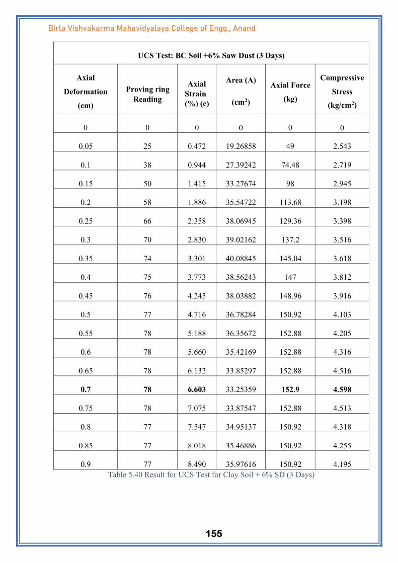
155
Birla Vishvakarma Mahavidyalaya College of Engg., Anand
UCS Test: BC Soil +6% Saw Dust (3 Days)
Axial
Deformation
(cm)
Proving ring
Reading
Axial
Strain
(%) (e)
Area (A)
(cm2)
Axial Force
(kg)
Compressive
Stress
(kg/cm2)
0
0
0
0
0
0
0.05
25
0.472
19.26858
49
2.543
0.1
38
0.944
27.39242
74.48
2.719
0.15
50
1.415
33.27674
98
2.945
0.2
58
1.886
35.54722
113.68
3.198
0.25
66
2.358
38.06945
129.36
3.398
0.3
70
2.830
39.02162
137.2
3.516
0.35
74
3.301
40.08845
145.04
3.618
0.4
75
3.773
38.56243
147
3.812
0.45
76
4.245
38.03882
148.96
3.916
0.5
77
4.716
36.78284
150.92
4.103
0.55
78
5.188
36.35672
152.88
4.205
0.6
78
5.660
35.42169
152.88
4.316
0.65
78
6.132
33.85297
152.88
4.516
0.7
78
6.603
33.25359
152.9
4.598
0.75
78
7.075
33.87547
152.88
4.513
0.8
77
7.547
34.95137
150.92
4.318
0.85
77
8.018
35.46886
150.92
4.255
0.9
77
8.490
35.97616
150.92
4.195
Table 5.40 Result for UCS Test for Clay Soil + 6% SD (3 Days)

156
Birla Vishvakarma Mahavidyalaya College of Engg., Anand
Figure 5.31 Graph BC Soil +6% Saw Dust (3 Days)
UCS Test: BC Soil +9% Saw Dust (3 Days)
Axial
Deformation
(cm)
Proving ring
Reading
Axial
Strain
(%) (e)
Area (A)
(cm2)
Axial
Force (kg)
Compressive
Stress (kg/cm2)
0
0
0
19.625
0
0
0.05
26
0.472
19.718
50.96
2.815
0.1
38
0.944
19.812
74.48
2.954
0.15
49
1.415
19.906
96.04
3.126
0.2
57
1.886
20.002
111.72
3.349
0.25
68
2.358
20.098
133.28
3.429
0.3
73
2.830
20.196
143.08
3.519
0.35
86
3.301
20.294
168.56
3.715
0.4
90
3.773
20.394
176.4
3.975
0.45
94
4.245
20.495
184.24
4.197

157
Birla Vishvakarma Mahavidyalaya College of Engg., Anand
0.5
97
4.716
20.596
190.12
4.315
0.55
99
5.188
20.698
194.04
4.428
0.6
100
5.660
20.802
196
4.615
0.65
100
6.132
20.907
196
4.759
0.7
100
6.603
20.012
196
4.822
0.75
99
7.075
21.119
194.04
4.765
0.8
99
7.547
21.227
194.04
4.691
0.85
99
8.018
21.335
194.04
4.565
0.9
99
8.490
21.445
194.04
4.416
Table 5.41 Result for UCS Test for Clay Soil + 9% SD (3 Days)
Figure 5.32 Graph BC Soil +9% Saw Dust (3 Days)
UCS Test: BC Soil +12% Saw Dust (3 Days)
Axial
Deformation
(cm)
Proving ring
Reading
Axial Strain
(%) (e)
Area (A)
(cm2)
Axial
Force
(kg)
Compressiv
e Stress
(kg/cm2)
0
0
0
0
0
0

158
Birla Vishvakarma Mahavidyalaya College of Engg., Anand
0.05
20
0.472
13.9254
39.2
2.815
0.1
23
0.944
14.95191
45.08
3.015
0.15
32
1.415
19.01759
62.72
3.298
0.2
46
1.886
27.173
90.16
3.318
0.25
58
2.358
33.18155
113.68
3.426
0.3
62
2.830
33.65273
121.52
3.611
0.35
68
3.301
35.86652
133.28
3.716
0.4
71
3.773
36.47706
139.16
3.815
0.45
73
4.245
36.54662
143.08
3.915
0.5
74
4.716
35.36698
145.04
4.101
0.55
76
5.188
34.72261
148.96
4.29
0.6
76
5.660
33.73188
148.96
4.416
0.65
76
6.132
32.99225
148.96
4.515
0.7
77
6.603
32.26165
150.92
4.678
0.75
76
7.075
32.97034
148.96
4.518
0.8
75
7.547
33.21283
147
4.426
0.85
75
8.018
34.03566
147
4.319
0.9
74
8.490
34.82353
145.04
4.165
Table 5.42 Result for UCS Test for Clay Soil + 12% SD (3 Days)
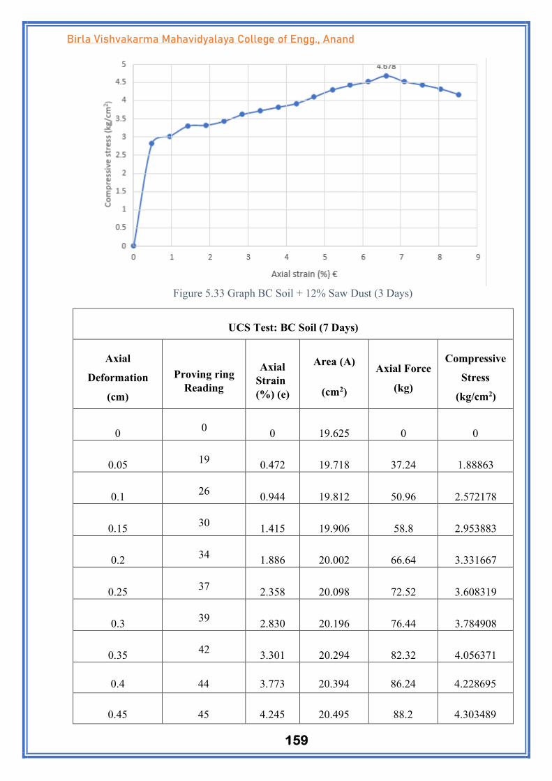
159
Birla Vishvakarma Mahavidyalaya College of Engg., Anand
Figure 5.33 Graph BC Soil + 12% Saw Dust (3 Days)
UCS Test: BC Soil (7 Days)
Axial
Deformation
(cm)
Proving ring
Reading
Axial
Strain
(%) (e)
Area (A)
(cm2)
Axial Force
(kg)
Compressive
Stress
(kg/cm2)
0
0
0
19.625
0
0
0.05
19
0.472
19.718
37.24
1.88863
0.1
26
0.944
19.812
50.96
2.572178
0.15
30
1.415
19.906
58.8
2.953883
0.2
34
1.886
20.002
66.64
3.331667
0.25
37
2.358
20.098
72.52
3.608319
0.3
39
2.830
20.196
76.44
3.784908
0.35
42
3.301
20.294
82.32
4.056371
0.4
44
3.773
20.394
86.24
4.228695
0.45
45
4.245
20.495
88.2
4.303489

160
Birla Vishvakarma Mahavidyalaya College of Engg., Anand
0.5
47
4.716
20.596
92.12
4.472713
0.55
48
5.188
20.698
94.08
4.545367
0.6
49
5.660
20.802
96.04
4.616864
0.65
50
6.132
20.907
98
4.687425
0.7
50
6.603
20.012
98
4.897062
0.75
50
7.075
21.119
98
4.640371
0.8
50
7.547
21.227
98
4.616762
0.85
49
8.018
21.335
96.04
4.501523
0.9
49
8.490
21.445
96.04
4.478433
Table 5.43 Result for UCS Test for Clay Soil (7 Days)
Figure 5.34 Graph BC Soil (7 Days)

161
Birla Vishvakarma Mahavidyalaya College of Engg., Anand
UCS Test: BC Soil +3% Saw Dust (7 Days)
Axial
Deformation
(cm)
Proving ring
Reading
Axial
Strain
(%) (e)
Area (A)
(cm2)
Axial Force
(kg)
Compressiv
e Stress
(kg/cm2)
0
0
0
0
0
0
0.05
29
0.472
23.05882
56.84
2.465
0.1
44
0.944
22.97283
86.24
3.754
0.15
50
1.415
24.6355
98
3.978
0.2
57
1.886
25.09941
111.72
4.4511
0.25
62
2.358
26.43463
121.52
4.597
0.3
66
2.830
27.80739
129.36
4.652
0.35
68
3.301
27.77824
133.28
4.798
0.4
69
3.773
28.4596
135.24
4.752
0.45
70
4.245
28.43523
137.2
4.825
0.5
70
4.716
28.20144
137.2
4.865
0.55
71
5.188
28.25584
139.16
4.925
0.6
71
5.660
28.0791
139.16
4.956
0.65
71
6.132
26.98991
139.16
5.156
0.7
71
6.603
26.4161
139.16
5.268
0.75
70
7.075
26.51208
137.2
5.175
0.8
70
7.547
27.5005
137.2
4.989
0.85
70
8.018
27.88051
137.2
4.921
0.9
69
8.490
27.74154
135.24
4.875
Table 5.44 Result for UCS Test for Clay Soil + 3% SD (7 Days)

162
Birla Vishvakarma Mahavidyalaya College of Engg., Anand
Figure 5.34 Graph BC Soil + 3% Saw Dust (7 Days)
UCS Test: BC Soil +6% Saw Dust (7 Days)
Axial
Deformation
(cm)
Proving ring
Reading
Axial
Strain
(%) (e)
Area (A)
(cm2)
Axial Force
(kg)
Compressive
Stress
(kg/cm2)
0
0
0
0
0
0
0.05
28
0.472
19.92738
54.88
2.754
0.1
39
0.944
22.68923
76.44
3.369
0.15
52
1.415
29.53347
101.92
3.451
0.2
70
1.886
36.12428
137.2
3.798
0.25
79
2.358
36.02606
154.84
4.298
0.3
85
2.830
34.74453
166.6
4.795
0.35
90
3.301
36.37113
176.4
4.85
0.4
97
3.773
37.06765
190.12
5.129
0.45
101
4.245
36.4433
197.96
5.432
0.5
105
4.716
36.78284
205.8
5.595

163
Birla Vishvakarma Mahavidyalaya College of Engg., Anand
0.55
106
5.188
35.90736
207.76
5.786
0.6
108
5.660
36.33368
211.68
5.826
0.65
108
6.132
35.53467
211.68
5.957
0.7
107
6.603
37.96524
209.72
5.524
0.75
107
7.075
40.92896
209.72
5.124
0.8
106
7.547
42.83711
207.76
4.85
0.85
106
8.018
43.30138
207.76
4.798
0.9
106
8.490
45.0477
207.76
4.612
Table 5.45 Result for UCS Test for Clay Soil + 6% SD (7 Days)
Figure 5.35 Graph BC Soil + 6% Saw Dust (7 Days)
UCS Test: BC Soil +9% Saw Dust (7 Days)
Axial
Deformation
(cm)
Proving ring
Reading
Axial
Strain
(%) (e)
Area (A)
(cm2)
Axial Force
(kg)
Compressive
Stress
(kg/cm2)
0
0
0
0
0
0
0.05
28
0.472
20.67822
54.88
2.654
0.1
39
0.944
33.80476
76.44
2.899

164
Birla Vishvakarma Mahavidyalaya College of Engg., Anand
0.15
52
1.415
38.37259
101.92
3.269
0.2
70
1.886
43.93305
137.2
3.346
0.25
79
2.358
44.37948
154.84
3.489
0.3
85
2.830
44.05091
166.6
3.693
0.35
90
3.301
44.84171
176.4
3.759
0.4
97
3.773
43.79613
190.12
3.983
0.45
101
4.245
41.2012
197.96
4.329
0.5
105
4.716
37.99083
205.8
4.798
0.55
106
5.188
37.93288
207.76
4.857
0.6
108
5.660
36.30337
211.68
5.129
0.65
108
6.132
35.12545
211.68
5.301
0.7
107
6.603
32.38824
209.72
5.749
0.75
107
7.075
35.71155
209.72
5.214
0.8
106
7.547
38.66279
207.76
4.816
0.85
106
8.018
38.95961
207.76
4.729
0.9
106
8.490
39.74973
207.76
4.635
Table 5.46 Result for UCS Test for Clay Soil + 9% SD (7 Days)
Figure 5.36 Graph BC Soil + 9% Saw Dust (7 Days)

165
Birla Vishvakarma Mahavidyalaya College of Engg., Anand
UCS Test: BC Soil +12% Saw Dust (7 Days)
Axial
Deformation
(cm)
Proving ring
Reading
Axial Strain
(%) (e)
Area (A)
(cm2)
Axial
Force
(kg)
Compressive
Stress
(kg/cm2)
0
0
0
0
0
0
0.05
22
0.472
15.64586
43.12
2.756
0.1
42
0.944
25.36044
82.32
3.246
0.15
56
1.415
31.73171
109.76
3.459
0.2
65
1.886
33.66808
127.4
3.784
0.25
71
2.358
35.6912
139.16
3.899
0.3
78
2.830
36.52174
152.88
4.186
0.35
81
3.301
37.47875
158.76
4.236
0.4
83
3.773
36.64789
162.68
4.439
0.45
87
4.245
37.32108
170.52
4.569
0.5
89
4.716
36.16836
174.44
4.823
0.55
90
5.188
35.45016
176.4
4.976
0.6
91
5.660
34.19479
178.36
5.216
0.65
91
6.132
33.64648
178.36
5.301
0.7
92
6.603
32.13115
180.32
5.612
0.75
92
7.075
35.19813
180.32
5.123
0.8
90
7.547
36.34116
176.4
4.854
0.85
90
8.018
37.72455
176.4
4.676
0.9
89
8.490
38.36376
174.44
4.547
Table 5.47 Result for UCS Test for Clay Soil + 12% SD (7 Days)

166
Birla Vishvakarma Mahavidyalaya College of Engg., Anand
Figure 5.37 Graph BC Soil + 12% Saw Dust (7 Days)
UCS Test: Clay Soil Clay Soil (14 Days)
Axial
Deformation
(cm)
Proving ring
Reading
Axial Strain
(%) (e)
Area
(A)
(cm2)
Axial
Force (kg)
Compressive
Stress (kg/cm2)
0
0
0
19.625
0
0
0.05
19
0.472
19.718
37.24
1.88863
0.1
26
0.944
19.812
50.96
2.572178
0.15
29
1.415
19.906
56.84
2.85542
0.2
34
1.886
20.002
66.64
3.331667
0.25
36
2.358
20.098
70.56
3.510797
0.3
38
2.830
20.196
74.48
3.687859
0.35
42
3.301
20.294
82.32
4.056371
0.4
44
3.773
20.394
86.24
4.228695
0.45
46
4.245
20.495
90.16
4.399122
0.5
49
4.716
20.596
96.04
4.663041
0.55
50
5.188
20.698
98
4.734757
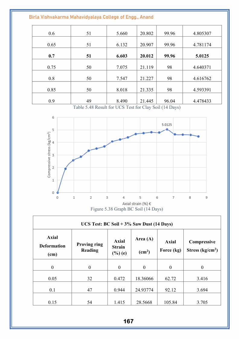
167
Birla Vishvakarma Mahavidyalaya College of Engg., Anand
0.6
51
5.660
20.802
99.96
4.805307
0.65
51
6.132
20.907
99.96
4.781174
0.7
51
6.603
20.012
99.96
5.0125
0.75
50
7.075
21.119
98
4.640371
0.8
50
7.547
21.227
98
4.616762
0.85
50
8.018
21.335
98
4.593391
0.9
49
8.490
21.445
96.04
4.478433
Table 5.48 Result for UCS Test for Clay Soil (14 Days)
Figure 5.38 Graph BC Soil (14 Days)
UCS Test: BC Soil + 3% Saw Dust (14 Days)
Axial
Deformation
(cm)
Proving ring
Reading
Axial
Strain
(%) (e)
Area (A)
(cm2)
Axial
Force (kg)
Compressive
Stress (kg/cm2)
0
0
0
0
0
0
0.05
32
0.472
18.36066
62.72
3.416
0.1
47
0.944
24.93774
92.12
3.694
0.15
54
1.415
28.5668
105.84
3.705

168
Birla Vishvakarma Mahavidyalaya College of Engg., Anand
0.2
61
1.886
30.53895
119.56
3.915
0.25
67
2.358
31.98246
131.32
4.106
0.3
69
2.830
31.40734
135.24
4.306
0.35
71
3.301
30.81488
139.16
4.516
0.4
72
3.773
29.92366
141.12
4.716
0.45
73
4.245
29.71547
143.08
4.815
0.5
73
4.716
29.11089
143.08
4.915
0.55
74
5.188
27.9784
145.04
5.184
0.6
74
5.660
27.37637
145.04
5.298
0.65
74
6.132
27.12042
145.04
5.348
0.7
73
6.603
26.49139
143.08
5.401
0.75
73
7.075
26.73893
143.08
5.351
0.8
73
7.547
27.69648
143.08
5.166
0.85
72
8.018
28.70627
141.12
4.916
0.9
72
8.490
29.64706
141.12
4.76
Table 5.49 Result for UCS Test for Clay Soil + 3% SD(14 Days)
Figure 5.39 Graph of BC Soil +3% SD (14 Days)

169
Birla Vishvakarma Mahavidyalaya College of Engg., Anand
UCS Test: BC Soil + 6% Saw Dust (14 Days)
Axial
Deformation
(cm)
Proving ring
Reading
Axial Strain
(%) (e)
Area (A)
(cm2)
Axial
Force
(kg)
Compressive
Stress (kg/cm2)
0
0
0
0
0
0
0.05
30
0.472
26.08696
58.8
2.254
0.1
40
0.944
33.23442
78.4
2.359
0.15
54
1.415
44.00832
105.84
2.405
0.2
70
1.886
48.22496
137.2
2.845
0.25
81
2.358
51.11397
158.76
3.106
0.3
87
2.830
48.74786
170.52
3.498
0.35
93
3.301
51.99087
182.28
3.506
0.4
103
3.773
52.76529
201.88
3.826
0.45
105
4.245
49.02334
205.8
4.198
0.5
106
4.716
46.11765
207.76
4.505
0.55
107
5.188
43.55556
209.72
4.815
0.6
107
5.660
41.07325
209.72
5.106
0.65
109
6.132
38.9073
213.64
5.491
0.7
109
6.603
37.39541
213.64
5.713
0.75
108
7.075
37.69902
211.68
5.615
0.8
107
7.547
38.14478
209.72
5.498
0.85
106
8.018
39.91547
207.76
5.205
0.9
106
8.490
41.73564
207.76
4.978
Table 5.50 Result for UCS Test for Clay Soil + 6 % SD (14 Days)

170
Birla Vishvakarma Mahavidyalaya College of Engg., Anand
Figure 5.40 Graph of BC Soil +6% SD (14 Days)
UCS Test: BC Soil +9% Saw Dust (14 Days)
Axial
Deformation
(cm)
Proving ring
Reading
Axial
Strain
(%) (e)
Area (A)
(cm2)
Axial
Force (kg)
Compressive
Stress (kg/cm2)
0
0
0
0
0
0
0.05
31
0.472
21.25219
60.76
2.859
0.1
41
0.944
25.47876
80.36
3.154
0.15
55
1.415
33.01685
107.8
3.265
0.2
71
1.886
39.81688
139.16
3.495
0.25
82
2.358
44.58252
160.72
3.605
0.3
88
2.830
45.19916
172.48
3.816
0.35
94
3.301
46.66667
184.24
3.948
0.4
104
3.773
49.68072
203.84
4.103
0.45
106
4.245
48.26016
207.76
4.305
0.5
107
4.716
42.41052
209.72
4.945
0.55
108
5.188
38.37563
211.68
5.516
0.6
108
5.660
37.47875
211.68
5.648

171
Birla Vishvakarma Mahavidyalaya College of Engg., Anand
0.65
110
6.132
36.861
215.6
5.849
0.7
110
6.603
34.97729
215.6
6.164
0.75
109
7.075
35.91796
213.64
5.948
0.8
108
7.547
37.03937
211.68
5.715
0.85
107
8.018
37.43663
209.72
5.602
0.9
107
8.490
38.39619
209.72
5.462
Table 5.51 Result for UCS Test for Clay Soil + 9% SD (14 Days)
Figure 5.41 Graph of BC Soil +9% SD (14 Days)
UCS Test: Clay Soil Clay Soil +12% Saw Dust (14 Days)
Axial
Deformation
(cm)
Proving ring
Reading
Axial
Strain (%)
(e)
Area (A)
(cm2)
Axial
Force (kg)
Compressive
Stress (kg/cm2)
0
0
0
0
0
0
0.05
25
0.472
21.25813
49
2.305
0.1
30
0.944
23.27791
58.8
2.526
0.15
39
1.415
28.86707
76.44
2.648

172
Birla Vishvakarma Mahavidyalaya College of Engg., Anand
0.2
48
1.886
31.59167
94.08
2.978
0.25
55
2.358
32.61725
107.8
3.305
0.3
69
2.830
38.11725
135.24
3.548
0.35
73
3.301
38.40043
143.08
3.726
0.4
95
3.773
45.80566
186.2
4.065
0.45
98
4.245
43.50623
192.08
4.415
0.5
101
4.716
42.89491
197.96
4.615
0.55
102
5.188
40.07216
199.92
4.989
0.6
102
5.660
37.3822
199.92
5.348
0.65
104
6.132
36.97442
203.84
5.513
0.7
104
6.603
35.71754
203.84
5.707
0.75
103
7.075
36.59898
201.88
5.516
0.8
102
7.547
36.84482
199.92
5.426
0.85
101
8.018
45.41409
197.96
4.359
0.9
101
8.490
48.21237
197.96
4.106
Table 5.52 Result for UCS Test for Clay Soil + 12% SD (14 Days)
Figure 5.42 Graph of BC Soil +12% SD (14 Days)

173
Birla Vishvakarma Mahavidyalaya College of Engg., Anand
CHAPTER 6 PAVEMENT DESIGN USING SAW DUST
6.1 Pavement design
Comparative table for California Bearing Ratio is given below.
S. No. Samples C. B. R. Values
1. Raw Soil 2.47
2. Raw Soil +3% SD 2.38
3. Raw Soil +6% SD 3.89
4. Raw Soil + 9%SD 4.98
5. Raw soil +12%SD 3.94
Table 6.1 Result for CBR test
Considered Pavement Design Data:
• State Highway of 6 lane
• Design Traffic(A)= 1000 CVPD
• Lane Distribution Factor(D) = 60% (three lane carriage way road)
• Vehicle damage factor (F) = 3.5 (For Plain Terrain)
• Design Life (n) = 15 years
• Annual Growth Rate(r) = 7.5% (assumed)
• Width = 10.5m + 10.5m (10.5m of single side)
• N = [(365 x {(1+ r)n-1})/ r}]AFD
• N = [(365 x {(1+0.075)15-1})/0.075] x 1000 x 0.6 x 3.5
• N= 20 msa
6.2 Different layer thickness by referring IRC: 37-2012
Material
CBR
GSB
(mm)
G. BASE
(mm)
DBM
(mm)
BC
(mm)
TOTAL
(mm)
RAW SOIL 2.47 380 250 120 40 790
R.S.+3% SD 2.38 380 250 120 40 790
R.S.+6%SD 3.89 330 250 110 40 730
R.S.+9%SD 4.98 300 250 100 40 690
R.S.+12%SD 3.94 300 250 110 40 730
Table 6.2 Different layer thickness
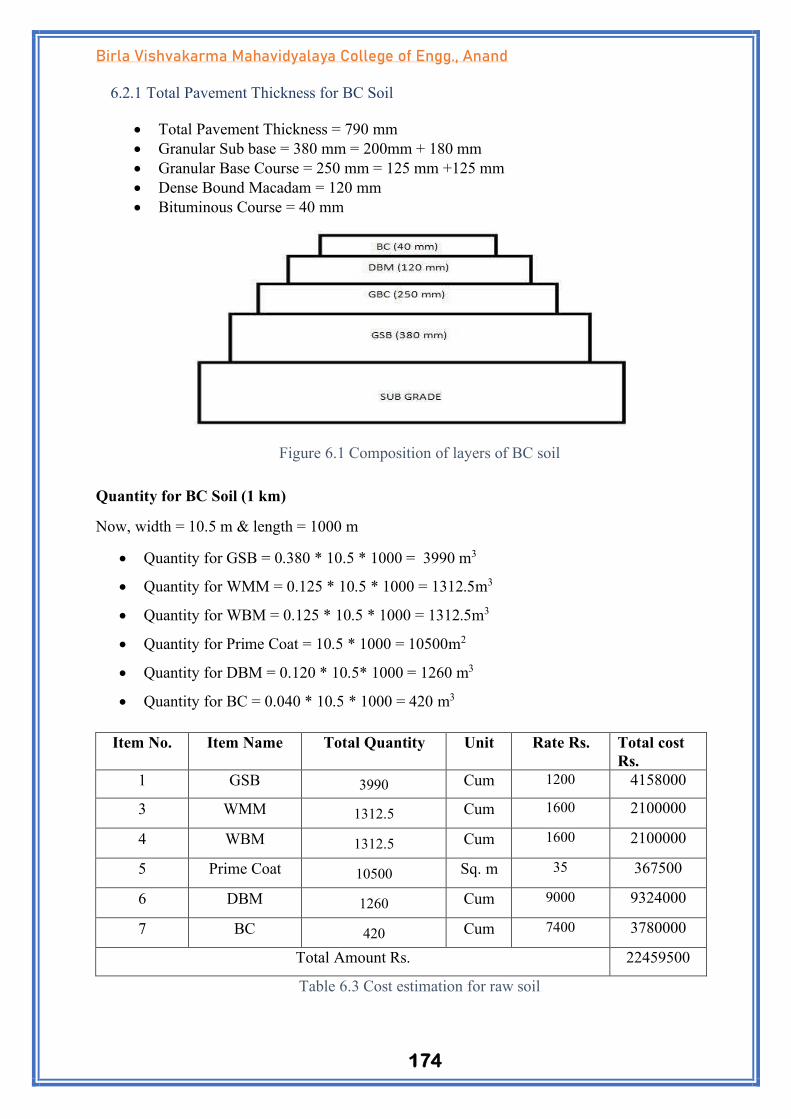
174
Birla Vishvakarma Mahavidyalaya College of Engg., Anand
6.2.1 Total Pavement Thickness for BC Soil
• Total Pavement Thickness = 790 mm
• Granular Sub base = 380 mm = 200mm + 180 mm
• Granular Base Course = 250 mm = 125 mm +125 mm
• Dense Bound Macadam = 120 mm
• Bituminous Course = 40 mm
Quantity for BC Soil (1 km)
Now, width = 10.5 m & length = 1000 m
• Quantity for GSB = 0.380 * 10.5 * 1000 = 3990 m3
• Quantity for WMM = 0.125 * 10.5 * 1000 = 1312.5m3
• Quantity for WBM = 0.125 * 10.5 * 1000 = 1312.5m3
• Quantity for Prime Coat = 10.5 * 1000 = 10500m2
• Quantity for DBM = 0.120 * 10.5* 1000 = 1260 m3
• Quantity for BC = 0.040 * 10.5 * 1000 = 420 m3
Item No. Item Name Total Quantity Unit Rate Rs. Total cost
Rs.
1 GSB 3990 Cum 1200 4158000
3 WMM 1312.5 Cum 1600 2100000
4 WBM 1312.5 Cum 1600 2100000
5 Prime Coat 10500 Sq. m 35 367500
6 DBM 1260 Cum 9000 9324000
7 BC 420 Cum 7400 3780000
Total Amount Rs. 22459500
Table 6.3 Cost estimation for raw soil
Figure 6.1 Composition of layers of BC soil

175
Birla Vishvakarma Mahavidyalaya College of Engg., Anand
6.2.2 Total Pavement Thickness for BC Soil +3% SD
• Total Pavement Thickness = 790 mm
• Granular Sub base = 380 mm = 200mm + 180 mm
• Granular Base Course = 250 mm = 125 mm +125 mm
• Dense Bound Macadam = 120 mm
• Bituminous Course = 40 mm
Quantity for BC Soil + 3% SD (1 km)
• Now, width = 10.5 m & length = 1000 m
• Quantity for GSB = 0.380 * 10.5 * 1000 = 3990 m3
• Quantity for WMM = 0.125 * 10.5 * 1000 = 1312.5m3
• Quantity for WBM = 0.125 * 10.5 * 1000 = 1312.5m3
• Quantity for Prime Coat = 10.5 * 1000 = 10500m2
• Quantity for DBM = 0.120 * 10.5* 1000 = 1260 m3
• Quantity for BC = 0.040 * 10.5 * 1000 = 420 m3
Item No. Item Name Total Quantity Unit Rate Rs. Total cost Rs.
1 GSB 3990 Cum 1200 4158000
3 WMM 1312.5 Cum 1600 2100000
4 WBM 1312.5 Cum 1600 2100000
5 Prime Coat 10500 Sq. m 35 367500
6 DBM 1260 Cum 9000 9324000
7 BC 420 Cum 7400 3780000
Total Amount Rs. 22459500
Table 6.4 Cost estimation for Raw Soil +3% SD
Figure 6.2 Composition of layers of BC soil + 3% SD

176
Birla Vishvakarma Mahavidyalaya College of Engg., Anand
6.2.3 Total Pavement Thickness for BC Soil +6% SD
• Total Pavement Thickness = 730 mm
• Granular Sub base = 330mm
• Granular Base Course = 250 mm = 125 mm +125 mm
• Dense Bound Macadam = 110 mm
• Bituminous Course = 40 mm
Quantity for BC Soil +6% SD (1 km)
Now, width = 10.5 m & length = 1000 m
• Quantity for GSB = 0.330 * 10.5 * 1000 = 3465 m3
• Quantity for WMM = 0.125 * 10.5 * 1000 = 1312.5m3
• Quantity for WBM = 0.125 * 10.5 * 1000 = 1312.5m3
• Quantity for Prime Coat = 10.5 * 1000 = 10500m2
• Quantity for DBM = 0.110* 10.5* 1000 = 1155m3
• Quantity for BC = 0.040 * 10.5 * 1000 = 420 m3
Item No. Item Name Total Quantity Unit Rate Rs. Total cost Rs.
1 GSB 3465 Cum 1200 4158000
3 WMM 1312.5 Cum 1600 2100000
4 WBM 1312.5 Cum 1600 2100000
5 Prime Coat 10500 Sq. m 35 367500
6 DBM 1155 Cum 7400 8547000
7 BC 420 Cum 9000 3780000
Table 6.176 Cost estimation for raw soil + 6% SD
6.2.4 Total Pavement Thickness for BC Soil + 9% SD
• Total Pavement Thickness = 690mm
Figure 6.3 Composition of layers of BC soil + 6% SD
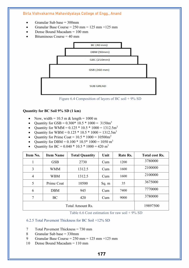
177
Birla Vishvakarma Mahavidyalaya College of Engg., Anand
• Granular Sub base = 300mm
• Granular Base Course = 250 mm = 125 mm +125 mm
• Dense Bound Macadam = 100 mm
• Bituminous Course = 40 mm
Quantity for BC Soil 9% SD (1 km)
• Now, width = 10.5 m & length = 1000 m
• Quantity for GSB = 0.300* 10.5 * 1000 = 3150m3
• Quantity for WMM = 0.125 * 10.5 * 1000 = 1312.5m3
• Quantity for WBM = 0.125 * 10.5 * 1000 = 1312.5m3
• Quantity for Prime Coat = 10.5 * 1000 = 10500m2
• Quantity for DBM = 0.100 * 10.5* 1000 = 1050 m3
• Quantity for BC = 0.040 * 10.5 * 1000 = 420 m3
Item No. Item Name Total Quantity Unit Rate Rs. Total cost Rs.
1 GSB 2730 Cum 1200 3780000
3 WMM 1312.5 Cum 1600 2100000
4 WBM 1312.5 Cum 1600 2100000
5 Prime Coat 10500 Sq. m 35 3675000
6 DBM 945 Cum 7400 7770000
7 BC 420 Cum 9000 3780000
Total Amount Rs. 19897500
Table 6.6 Cost estimation for raw soil + 9% SD
6.2.5 Total Pavement Thickness for BC Soil +12% SD
Total Pavement Thickness = 730 mm
Granular Sub base = 330mm
Granular Base Course = 250 mm = 125 mm +125 mm
Dense Bound Macadam = 110 mm
Figure 6.4 Composition of layers of BC soil + 9% SD

178
Birla Vishvakarma Mahavidyalaya College of Engg., Anand
Bituminous Course = 40 mm
•
Quantity for BC Soil +12% SD (1 km)
• Now, width = 10.5 m & length = 1000 m
• Quantity for GSB = 0.200 * 10.5 * 1000 = 2100 m3
• Quantity for WMM = 0.125 * 10.5 * 1000 = 1312.5m3
• Quantity for WBM = 0.125 * 10.5 * 1000 = 1312.5m3
• Quantity for Prime Coat = 10.5 * 1000 = 10500m2
• Quantity for DBM = 0.085* 10.5* 1000 = 892.5 m3
• Quantity for BC = 0.040 * 10.5 * 1000 = 420 m3
Item No. Item Name Total Quantity Unit Rate Rs. Total cost
Rs.
1 GSB 3465 Cum 1200 4158000
3 WMM 1312.5 Cum 1600 2100000
4 WBM 1312.5 Cum 1600 2100000
5 Prime Coat 10500 Sq. m 35 367500
6 DBM 1155 Cum 7400 7770000
7 BC 420 Cum 9000 3780000
Total Amount Rs. 21052500
Table 6.7 Cost estimation for raw soil +12% SD
Figure 6.5 Composition of layers of BC soil + 12% SD

179
Birla Vishvakarma Mahavidyalaya College of Engg., Anand
6.3 Summary of cost analysis
Materials Cost (Rs.)
BC Soil 22459500
BC Soil + 3% SD 22459500
BC Soil + 6% SD 21052500
BC Soil + 9% SD 19897500
BC Soil + 12% SD 21052500
Table 6.8 Cost Analysis

180
Birla Vishvakarma Mahavidyalaya College of Engg., Anand
CHAPTER 7 CONCLUSION
7.1 Conclusion based on Saw Dust
From the above results of test, it can be concluded that the impact of saw dust on BC soil is positive.
By replacing soil its dry weight by saw dust it gives maximum improvement in the swelling and linear
shrinkage properties of black cotton soil. The presence of Holocellulose (83.8%) in Saw Dust are
responsible for improve the performance of black cotton soil. The MDD of black cotton soil varies
from 1.510 g/cc to 1.891 g/cc and the OMC increase from 21% to 23.2% for increase of saw dust from
0% to 12%. With increase in saw dust a general increase in maximum dry unit weight was observed.
So, use of saw dust is preferable for stabilization because it gives positive results as stabilizer and also
it is a waste utilization. Use of saw dust in highway construction must provide a clear advantage in
term of improvement of the geotechnical properties of the foundation subgrade, sub base and
embankment material.
7.2 Conclusion based on Marble Powder
The results showed positive response of marble powder on BC soil. The C.B.R. value of black cotton
soil varies from 5.80% to 8.30%, M.D.D. is found to increase by 1.510gm/cc to 1.710 gm/cc, O.M.C.
changes from 1.8 to 4.1%. The presence of CaCo3 in Marble Powder is responsible for improve the
performance of black cotton soil. With increase in marble powder as general increase in maximum dry
unit weight was observed. So, we can clearly see that the marble powder is a good stabilizing agent
for weak black cotton soil and can be used to drastically change its properties which could be better
and helpful in several construction process related to subgrade, sub base and embankment.
7.3 Conclusion based on both the additives
This study concludes that addition of waste material can prove out to be a good stabilizing agent for
weaker soils. Some results showed marble dust was better where as some favoured saw dust but overall
results of both the tests were positive. But usage of saw dust can be recommended more than that of
use of marble dust as saw dust is generated from wooden derived products and can be found out
everywhere in the world but whereas marble dust can be found out on the selective areas only.

181
Birla Vishvakarma Mahavidyalaya College of Engg., Anand
# REFRENCES
JOURNALS [1] A. G. Patil, K. P. Patil, N. P. Patil, P. S. Joshi, S. S. Chavan, Dr. V.R. Saraf (2017). “Eco-friendly
stabilization of black cotton soil” International Journal of Innovative Research in Science,
Engineering and Technology, Vol. 3, Issue 3.
[2] Arun Pratap Singh Rather, Karan Parbhakar (2018). “Soil stabilization using kota stone slurry in
pavement” International Research Journal of Engineering and Technology (IRJET), Vol. 7, Issue 5.
[3] A. Venkatesh and Dr. G. Sreenivasa Reddy (2016). “Effect of Waste Saw Dust Ash on
Compaction and Permeability Properties of Black Cotton Soil” International Journal of Civil
Engineering Research, Vol. 7, Issue 1
[4] B. B. Patel, C. B. Mishra, Dr. H. R. Varia, H. Thakar (2017). “Use of Waste Marble Powder to
Improve the Characteristics of Black Cotton Soil.” Earthquake International Journal of Engineering
Research & Technology (IJERT), Vol. 6, Issue 4
[5] Berjees Anisa Ikra, Tamanna Kabir, Anika Nowshin Mowrin, Ahsan Habib (2018). “Stabilization
of Clay Soil Mixed with Wood Ash” International Journal of Scientific & Engineering Research, Vol.
9, Issue 10.
[06] Berjees Anisa Ikra, Tamanna Kabir, Anika Nowshin Mowrin, Ahsan Habib (2016).
[7] C. B. Mishra, Nandan Patel, Riddhi Choksi (2018). “Soil stabilization using marble dust”
International Research Journal of Engineering and Technology (IRJET), Vol. 5, Issue 5
[8] Jagmohan Mishra, R K Yadav and A K Singhai (2018). “Effect of granite dust on index
properties of lime stabilized black cotton soil” International Research Journal of Engineering and
Technology (IRJET), Vol. 3, Issue 1
[9] Krichphon Singh, V.K. Arora (2018). “Pursuance of waste marble powder to improve soil
stabilization” International Research Journal of Engineering and Technology (IRJET), Vol. 5, Issue 5
[10] Krichphon Singh, V.K. Arora (2017). “Stabilization of non-plastic silt using marble dust”
International journal of advance research in science and engineering, Vol. 6, Issue 4
[11] M. Usha Rani, J. Martina Jenifer (2016). “Analysis of strength characteristics of black cotton soil
using wood ash as stabilizer” International Journal of Research in Science
[12] M. Yurdakul, F. Yilmaz (2017). “Evaluation of Marble Dust for Soil Stabilization” Special issue
of the 3rd International Conference on Computational and Experimental Science and Engineering
(ICCESEN 2016).
[13] Rashmi Bade, Nuzra Zainab Khan, Jaya Sahare, Faisal Ameen, Danish Ahmed (2017). “Effect of
Wood Shaving Ash on Index Properties of Black Cotton Soil” International Research Journal of
Engineering and Technology (IRJET), Vol. 4, Issue 2.
[14] Sumit Shringi, Vishvendra Singh, Dr. B. Acharya (2018). “Review on effect of marble dust on
geotechnical properties of expansive soil” International journal of advance research in science and
engineering, Vol. 7, Issue 2

182
Birla Vishvakarma Mahavidyalaya College of Engg., Anand
[14] T. Deepika (2019). “Experimental Study on Behavior of Black Cotton Soil using Wood Ash as
Stabilizer” International Research Journal of Engineering and Technology (IRJET), Vol. 5
[15] Zuhaib Zahoor Shaw, Er. Ved Parkash, Er. Vishal Kumar (2017). “Use of Lime and Saw Dust
Ash in Soil Stabilization” International Journal of Innovative Research in Science, Engineering and
Technology, Vol. 6, Issue 2
IS Codes [1] IS: 1498-1970, “Soil Classification”
[2] IS: 2720 (Part 4) – 1985, “Determination of Grain Size Analysis”
[3] IS: 2720 (Part 5) – 1985, “Determination of Liquid and Plastic Limit”
[4] IS: 2720 (Part 7) – 1980, “Determination of Water Content – Dry Density Relation Using
Standard Proctor Compaction test”
[5] IS: 9143 – 1979, “Laboratory Determination of UCS”
[6] IS: 2720 (Part 40) – 1977, “Determination of Free swell index”