Embed Size (px)
Citation preview

Foundations and TrendsR© insampleVol. xx, No xx (xxxx) 1–144c© xxxx xxxxxxxxxDOI: xxxxxx
Bit-Interleaved Coded Modulation
Albert Guillen i Fabregas1, AlfonsoMartinez2 and Giuseppe Caire3
1 Department of Engineering, University of Cambridge, Trumpington Street,Cambridge, CB2 1PZ, United Kingdom, [email protected]
2 Centrum Wiskunde & Informatica (CWI), Kruislaan 413, Amsterdam,1098 SJ, The Netherlands, [email protected]
3 Electrical Engineering Department, University of Southern California, 3740McClintock Av., Los Angeles, 90080 CA, USA, [email protected]
Abstract
The principle of coding in the signal space follows directly from Shan-non’s analysis of waveform Gaussian channels subject to an input con-straint. The early design of communication systems focused separatelyon modulation, namely signal design and detection, and error correct-ing codes, which deal with errors introduced at the demodulator ofthe underlying waveform channel. The correct perspective of signal-space coding, although never out of sight of information theorists, wasbrought back into the focus of coding theorists and system design-ers by Imai’s and Ungerbock’s pioneering work on coded modulation.More recently, powerful families of binary codes with a good tradeoffbetween performance and decoding complexity have been (re-) discov-ered. Bit-Interleaved Coded Modulation (BICM) is a pragmatic ap-proach combining the best out of both worlds: it takes advantage ofthe signal-space coding perspective, whilst allowing for the use of pow-erful families of binary codes with virtually any modulation format.

BICM avoids the need for the complicated and somewhat less flexi-ble design typical of coded modulation. As a matter of fact, most oftoday’s systems that achieve high spectral efficiency such as DSL, Wire-less LANs, WiMax and evolutions thereof, as well as systems based onlow spectral efficiency orthogonal modulation, feature BICM, makingBICM the de-facto general coding technique for waveform channels.The theoretical characterization of BICM is at the basis of efficient cod-ing design techniques and also of improved BICM decoders, e.g., thosebased on the belief propagation iterative algorithm and approximationsthereof. In this monograph, we review the theoretical foundations ofBICM under the unified framework of error exponents for mismatcheddecoding. This framework allows an accurate analysis without any par-ticular assumptions on the length of the interleaver or independencebetween the multiple bits in a symbol. We further consider the sensi-tivity of the BICM capacity with respect to the signal-to-noise ratio(SNR), and obtain a wideband regime (or low-SNR regime) character-ization. We review efficient tools for the error probability analysis ofBICM that go beyond the standard approach of considering infinite in-terleaving and take into consideration the dependency of the coded bitobservations introduced by the modulation. We also present boundsthat improve upon the union bound in the region beyond the cutoffrate, and are essential to characterize the performance of modern ran-domlike codes used in concatenation with BICM. Finally, we turn ourattention to BICM with iterative decoding, we review extrinsic infor-mation transfer charts, the area theorem and code design via curvefitting. We conclude with an overview of some applications of BICMbeyond the classical coherent Gaussian channel.

Contents
List of Abbreviations, Acronyms and Symbols iii
1 Introduction 1
2 Channel Model and Code Ensembles 5
2.1 Channel Model: Encoding and Decoding 5
2.2 Coded Modulation 8
2.3 Bit-Interleaved Coded Modulation 9
2.A Continuous- and Discrete-Time Gaussian Channels 12
3 Information-Theoretic Foundations 16
3.1 Coded Modulation 17
3.2 Bit-Interleaved Coded Modulation 23
3.3 Comparison with Multilevel Coding 29
3.4 Mutual Information Analysis 36
3.5 Concluding Remarks and Related Work 46
i

ii Contents
4 Error Probability Analysis 49
4.1 Error Probability and the Union Bound 50
4.2 Pairwise Error Probability for Infinite Interleaving 58
4.3 Pairwise Error Probability for Finite Interleaving 71
4.4 Bounds and Approximations Above the Cutoff Rate 81
4.5 Concluding Remarks and Related Work 84
4.A Saddlepoint Location 86
4.B Asymptotic Analysis with Nakagami Fading 87
5 Iterative Decoding 89
5.1 Factor Graph Representation and Belief Propagation 91
5.2 Density Evolution 95
5.3 EXIT Charts 100
5.4 The Area Theorem 104
5.5 Improved Schemes 108
5.6 Concluding Remarks and Related Work 118
5.A Density Evolution Algorithm for BICM-ID 119
6 Applications 122
6.1 Non-Coherent Demodulation 122
6.2 Block-Fading 124
6.3 MIMO 127
6.4 Optical Communication: Discrete-Time Poisson Channel 129
6.5 Additive Exponential Noise Channel 130
7 Conclusions 133
References 136

List of Abbreviations, Acronyms and Symbols
APP A posteriori probabilityAWGN Additive white Gaussian noiseBEC Binary erasure channelBICM Bit-interleaved coded modulationBICM-ID Bit-interleaved coded modulation with iterative decodingBIOS Binary-input output-symmetric (channel)BP Belief propagationCM Coded modulationEXIT Extrinsic information transferFG Factor graphGMI Generalized mutual informationISI Inter-symbol interferenceLDPC Low-density parity-check (code)MAP Maximum a posterioriMIMO Multiple-input multiple-outputMLC Multi-level codingMMSE Minimum mean-squared errorMSD Multi-stage decodingPSK Phase-shift keying
iii

iv Contents
QAM Quadrature-amplitude modulationRA Repeat-accumulate (code)SNR Signal-to-noise ratioTCM Trellis-coded modulationTSB Tangential sphere boundAd Weight enumerator at Hamming distance dAd,ρN
Weight enumerator at Hamming distance d and pattern ρN
A′d Bit weight enumerator at Hamming distance db Bit in codewordb Binary complement of bit bbj(x) Inverse labeling (mapping) functionC Channel capacityCbicmX BICM capacity over set X
Cbpsk BPSK capacityCcmX Coded modulation capacity over set XC Binary codec1 First-order Taylor capacity series coefficientc2 Second-order Taylor capacity series coefficientd Hamming distanced Scrambling (randomization) sequencedv Average variable degree (LDPC code)dc Average check node degree (LDPC code)∆P Power expansion ratio∆W Bandwidth expansion ratioE[U ] Expectation (of a random variable U)Eb Average bit energyEbN0
Ratio between average bit energy and noise spectral densityEbN0 lim
EbN0
at vanishing SNREs Average signal energyE(R) Reliability function at rate REbicm
0 (ρ, s) BICM random coding exponentEcm
0 (ρ) CM random coding exponentEq
0(ρ, s) Generalized Gallager functionEq
r (R) Random coding exponent with mismatched decodingexitdec(y) Extrinsic information at decoder

Contents v
exitdem(x) Extrinsic information at demapperhk Fading realization at time kI(X;Y ) Mutual information between variables X and YIcm(X;Y ) Coded modulation capacity (Ccm
X )Igmi(X;Y ) Generalized mutual informationIgmis (X;Y ) Generalized mutual information (function of s)I ind(X;Y ) BICM capacity with independent-channel modelK Number of bits per codeword log2 |M|κ(s) Cumulant transformκ′′(s) Second derivative of cumulant transformκ1(s) Cumulant transform of bit scoreκv(s) Cumulant transform of symbol score with weight vκpw(s) Cumulant transform of pairwise scoreκpw(s, ρN ) Cumulant transform of pairwise score for pattern ρN
M Input set (constellation) X cardinalitym Number of bits per modulation symbolmf Nakagami fading parameterµ Labeling (mapping) ruleM Message setm Messagem Message estimatemmse(snr) MMSE of estimating input X (Gaussian channel)N Number of channel usesN0 Noise spectral density (one-sided)N (·) Neighborhood around a node (in factor graph)νf→ϑ Function-to-variable messageνϑ→f Variable-to-function messageO(f(x)
)Term vanishing as least as fast as af(x), for a > 0
o(f(x)
)Term vanishing faster than af(x), for a > 0
P Signal powerPb Average probability of bit errorPe Average probability of message errorPj(y|b) Transition probability of output y for j-th bitPj(y|b) Output transition probability for bits b at j positionsPBj |Y (b|y) j-th a posteriori marginal

vi Contents
P·· Probability distributionPY |X(y|x) Channel transition probability (symbol)PY |X(y|x) Channel transition probability (sequence)PEP(d) Pairwise error probabilityPEP1(d) Pairwise error probability (infinite interleaving)PEP(xm′ ,xm) Pairwise error probabilityπn Interleaver of size nPrdec→dem(b) Bit probability (from the decoder)Prdem→dec(b) Bit probability (from the demapper)Q(·) Gaussian tail functionq(x, y) Symbol decoding metricq(x,y) Codeword decoding metricqj(b, y) Bit decoding metric of j-th bitR Code rate, R = log2 |M|/Nr Binary code rate, r = log2 |C|/n = R/m
R0 Cutoff rateRav
0 Cutoff rate for average-channel modelRind
0 Cutoff rate for independent-channel modelRq
0 Generalized cutoff rate (mismatched decoding)ρN Bit distribution pattern over codeword∑
∼x Summary operator —excluding x—s Saddlepoint valueσ2
X Variance
σ2X Pseudo-variance, σ2
X∆= E
[|X|2
]− |E[X]|2
ζ0 Wideband slopesnr Signal-to-noise ratioW Signal bandwidthX Input signal set (constellation)X j
b Set of symbols with bit b at j-th labelX ji1
,...,jiv
bi1,...,biv
Set of symbols with bits bi1 , . . . , biv at positions ji1 , . . . , jivxk Channel input at time kx Vector of all channel inputs; input codewordxm Codeword corresponding to message m
Ξm(k−1)+j Bit log-likelihood of j-th bit in k-th symbolyk Channel output at time k

Contents vii
y Vector of all channel outputsY Output signal setzk Noise realization at time kΞpw Pairwise scoreΞs
k Symbol score for k-th symbolΞb
k,j Bit score at j-th label of k-th symbolΞb
1 Symbols score with weight 1 (bit score)Ξdec→dem
m(k−1)+j Decoder LLR for j-th bit of k-th symbolΞdec→dem Decoder LLR vectorΞdec→dem∼i Decoder LLR vector, excluding the i-th component
Ξdem→decm(k−1)+j Demodulator LLR for j-th bit of k-th symbol
Ξdem→dec Demodulator LLR vectorΞdem→dec∼i Demodulator LLR vector, excluding the i-th component
1
Introduction
Since Shannon’s landmark 1948 paper [105], approaching the capacityof the Additive White Gaussian Noise (AWGN) channel has been oneof the more relevant topics in information theory and coding theory.Shannon’s promise that rates up to the channel capacity can be reliablytransmitted over the channel comes together with the design challengeof effectively constructing coding schemes achieving these rates withlimited encoding and decoding complexity.
The complex baseband equivalent model of a bandlimited AWGNchannel is given by
yk =√
snr xk + zk, (1.1)
where yk, xk, zk are complex random variables and snr denotes theSignal-to-Noise Ratio (SNR), defined as the signal power over the noisepower. The capacity C (in nats per channel use) of the AWGN channelwith signal-to-noise ratio snr is given by the well-known
C = log(1 + snr). (1.2)
The coding theorem shows the existence of sufficiently long codesachieving error probability not larger than any ε > 0, as long as thecoding rate is not larger than C. The standard achievability proof of
1

2 Introduction
(1.2) considers a random coding ensemble generated with i.i.d. compo-nents according to a Gaussian probability distribution.
Using a Gaussian code is impractical, as decoding would require anexhaustive search over the whole codebook for the most likely candi-date. Instead, typical signaling constellations like Phase-Shift Keying(PSK) or Quadrature-Amplitude Modulation (QAM) are formed by afinite number of points in the complex plane. In order to keep the mod-ulator simple, the set of elementary waveforms that the modulator cangenerate is a finite set, preferably with small cardinality. A practicalway of constructing codes for the Gaussian channel consists of fixingthe modulator signal set, and then considering codewords obtained assequences over the fixed modulator signal set, or alphabet. These codedmodulation schemes are designed for the equivalent channel resultingfrom the concatenation of the modulator with the underlying waveformchannel. The design aims at endowing the coding scheme with justenough structure such that efficient encoding and decoding is possiblewhile, at the same time, having a sufficiently large space of possiblecodes so that good codes can be found.
Driven by Massey’s consideration on coding and modulation as asingle entity [79], Ungerbock in 1982 proposed Trellis-Coded Modula-tion (TCM), based on the combination of trellis codes and discrete sig-nal constellations through set partitioning [130] (see also [15]). TCMenables the use of the efficient Viterbi algorithm for optimal decod-ing [138] (see also [35]). An alternative scheme is multilevel codedmodulation (MLC), proposed by Imai and Hirakawa in 1977 [56] (seealso [140]). MLC uses several binary codes, each protecting a single bitof the binary label of modulation symbols. At the receiver, instead ofoptimal joint decoding of all the component binary codes, a suboptimalmulti-stage decoding, alternatively termed successive interference can-cellation, achieves good performance with limited complexity. Althoughnot necessarily optimal in terms of minimizing the error probability, themulti-stage decoder achieves the channel capacity [140].
The discovery of turbo codes [11] and the re-discovery of low-densityparity-check (LDPC) codes [38, 69] with their corresponding iterativedecoding algorithms marked a new era in Coding Theory. These modern

3
codes [96] approach the capacity of binary-input channels with lowcomplexity. The analysis of iterative decoding also led to new methodsfor their efficient design [96]. At this point, a natural development ofcoded modulation would have been the extension of these powerfulcodes to non-binary alphabets. However, iterative decoding of binarycodes is by far simpler.
In contrast to Ungerbock’s findings, Zehavi proposed bit-interleavedcoded modulation (BICM) as a pragmatic approach to coded modula-tion. BICM separates the actual coding from the modulation throughan interleaving permutation [142]. In order to limit the loss of infor-mation arising in this separated approach, soft information about thecoded bits is propagated from the demodulator to the decoder in theform of bit-wise a posteriori probabilities or log-likelihood ratios. Ze-havi illustrated the performance advantages of separating coding andmodulation. Later, Caire et al. provided in [29] a comprehensive analy-sis of BICM in terms of information rates and error probability, show-ing that in fact the loss incurred by the BICM interface may be verysmall. Furthermore, this loss can essentially be recovered by using iter-ative decoding. Building upon this principle, Li and Ritcey [64] andten Brink [122] proposed iterative demodulation for BICM, and il-lustrated significant performance gains with respect to classical non-iterative BICM decoding [29, 142] when certain binary mappings andconvolutional codes are employed. However, BICM designs based onconvolutional codes and iterative decoding cannot approach the codedmodulation capacity, unless the number of states grows large [139].Improved constructions based on iterative decoding and on the use ofpowerful families of modern codes can, however, approach the channelcapacity for a particular signal constellation [120,121,127].
Since its introduction, BICM has been regarded as a pragmatic yetpowerful scheme to achieve high data rates with general signal constel-lations. Nowadays, BICM is employed in a wide range of practical com-munications systems, such as DVB-S2, Wireless LANs, DSL, WiMax,the future generation of high data rate cellular systems (the so-called4th generation). BICM has become the de-facto standard for codingover the Gaussian channel in modern systems.

4 Introduction
In this monograph, we provide a comprehensive study of BICM. Inparticular, we review its information theoretic foundations, and reviewits capacity, cutoff rate and error exponents. Our treatment also cov-ers the wideband regime. We further examine the error probability ofBICM, and we focus on the union bound and improved bounds to theerror probability. We then turn our attention to iterative decoding ofBICM; we also review the underlying design techniques and introduceimproved BICM schemes in a unified framework. Finally, we describea number of applications of BICM not explicitly covered in our treat-ment. In particular, we consider the application of BICM to orthogonalmodulation with non-coherent detection, to the block-fading channel,to the multiple-antenna channel as well as to less common channelssuch as the exponential-noise or discrete-time Poisson channels.

2
Channel Model and Code Ensembles
This chapter provides the reference background for the remainder ofthe monograph, as we review the basics of coded modulation schemesand their design options. We also introduce the notation and describethe Gaussian channel model used throughout this monograph. Chap-ter 6 briefly describes different channels and modulations not explicitlycovered by the Gaussian channel model.
2.1 Channel Model: Encoding and Decoding
Consider a memoryless channel with input xk and output yk, respec-tively drawn from the alphabets X and Y. Let N denote the numberof channel uses, i. e. k = 1, . . . , N . A block codeM⊆ XN of length Nis a set of |M| vectors x = (x1, . . . , xN ) ∈ XN , called codewords. Thechannel output is denoted by y
∆= (y1, . . . , yN ), with yk ∈ Y.We consider memoryless channels, for which the channel transition
probability PY |X(y|x) admits the decomposition
PY |X(y|x) =N∏
k=1
PY |X(yk|xk), (2.1)
5

6 Channel Model and Code Ensembles
With no loss of generality, we limit our attention to continuous outputand identify PY |X(y|x) as a probability density function. We denoteby X,Y the underlying random variables. Similarly, the correspondingrandom vectors are
X∆= (X1, . . . , XN ) and Y
∆= (Y1, . . . , YN ), (2.2)
respectively drawn from the sets XN and YN .At the transmitter, a message m drawn with uniform probability
from a message set is mapped onto a codeword xm, according to theencoding schemes described in Sections 2.2 and 2.3. We denote thisencoding function by φ, i. e. φ(m) = xm. Often, and unless strictlynecessary, we drop the subindex m in the codeword xm and simplywrite x. Whenever |X | <∞, we respectively denote the cardinality ofX and the number of bits required to index a symbol by M and m,
M∆= |X |, m
∆= log2M. (2.3)
The decoder outputs an estimate of the message m according to agiven codeword decoding metric, denoted by q(x,y), so that
m = ϕ(y) = arg maxm∈{1,...,|M|}
q(xm,y). (2.4)
The decoding metrics considered in this work are given as products ofsymbol decoding metrics q(x, y), for x ∈ X and y ∈ Y, namely
q(x,y) =N∏
k=1
q(xk, yk). (2.5)
For equally likely codewords, this decoder finds the most likely code-word as long as the metric q(x, y) is a bijective (thus strictly increas-ing) function of the transition probability PY |X(y|x) of the memory-less channel. Instead, if the decoding metric q(x, y) is not a bijectivefunction of the channel transition probability, we have a mismatcheddecoder [41, 59,84].
2.1.1 Gaussian Channel Model
A particularly interesting, yet simple, case is that of complex-planesignal sets (X ⊂ C, Y = C) in AWGN with fully-interleaved fading,
yk = hk
√snr xk + zk, k = 1, . . . , N (2.6)

2.1. Channel Model: Encoding and Decoding 7
where hk are fading coefficients with unit variance, zk are the zero-mean, unit-variance, circularly symmetric complex Gaussian samples,and snr is the signal-to-noise ratio (SNR). In Appendix 2.A we relatethis discrete-time model to an underlying continuous-time model withadditive white Gaussian noise. We denote the fading and noise randomvariables by H and Z, with respective probability density functionsPH(h) and PZ(z). Examples of input set X are unit energy PSK orQAM signal sets.1
With perfect channel state information (coherent detection), thechannel coefficient hk is part of the output, i. e. it is given to the re-ceiver. From the decoder viewpoint, the channel transition probabilityis decomposed as PY,H|X(y, h|x) = PY |X,H(y|x, h)PH(h), with
PY |X,H(y|x, h) =1π
e−|y−h√
snr x|2 . (2.7)
Under this assumption, the phase of the fading coefficient becomes ir-relevant and we can assume that the fading coefficients are real-valued.In our simulations, we will consider Nakagami-mf fading, with density
PH(h) =2mmf
f h2mf−1
Γ(mf )e−mf h2
. (2.8)
Here Γ(x) is Euler’s Gamma function, Γ(x) =∫∞0 tx−1e−t dt, and mf >
0. In this fading model, we recover the AWGN (h = 1) with mf → +∞,the Rayleigh fading by letting mf = 1 and the Rician fading withparameter K by setting mf = (K + 1)2/(2K + 1).
Other cases are possible. For example, hk may be unknown to thereceiver (non-coherent detection), or only partially known, i. e. the re-ceiver knows hk such that (H, H) are jointly distributed random vari-ables. In this case, (2.7) generalizes to
PY |X, bH(y|x, h) = E
[1π
e−|y−H√
snr x|2∣∣∣H = h
](2.9)
1 We consider only one-dimensional complex signal constellations X ⊂ C, such as QAM orPSK signal sets (alternatively referred to as two-dimensional signal constellations in the
real domain). The generalization to “multidimensional” signal constellations X ⊂ CN′,
for N ′ > 1, follows immediately, as briefly reviewed in Chapter 6.

8 Channel Model and Code Ensembles
Encoder Decoderm m
φ ϕ
Channelxm
y
PY |X(y|xm)
Fig. 2.1 Channel model with encoding and decoding functions.
The classical non-coherent channel where h = ejθ, with θ denoting auniformly distributed random phase, is a special case of (2.9) [16,95].
For simplicity of notation, we shall denote the channel transitionprobability simply as PY |X(y|x), where the possible conditioning withrespect to h or any other related channel state information h, is im-plicitly understood and will be clear from the context.
2.2 Coded Modulation
In a coded modulation (CM) scheme, the elements xk ∈ X of the code-word xm are in general non-binary. At the receiver, a maximum metricdecoder ϕ (as in Eq. (2.4)) generates an estimate of the transmittedmessage, ϕ(y) = m. The block diagram of a coded modulation schemeis illustrated in Figure 2.1.
The rate R of this scheme in bits per channel use is given by R =KN , where K ∆= log2 |M| denotes the number of bits per informationmessage. We define the average probability of a message error as
Pe∆=
1|M|
|M|∑m=1
Pe(m) (2.10)
where Pe(m) is the conditional error probability when message m wastransmitted. We also define the probability of bit error as
Pb∆=
1K|M|
K∑k=1
|M|∑m=1
Pe(k,m) (2.11)
where Pe(k,m) ∆= Pr{k-th bit in error | message m was transmitted} isthe conditional bit error probability when message m was transmitted.

2.3. Bit-Interleaved Coded Modulation 9
Binary Encoder
Interleaving
Permutation
Binary Labeling
C
c
π µ
m
φ
c xm
Fig. 2.2 BICM encoder model.
2.3 Bit-Interleaved Coded Modulation
2.3.1 BICM Encoder and Decoders
In a bit-interleaved coded modulation scheme, the encoder is restrictedto be the serial concatenation of a binary code C of length n ∆= mN andrate r = log2 |C|
n = Rm , a bit interleaver, and a binary labeling function
µ : {0, 1}m → X which maps blocks of m bits to signal constellationsymbols. The codewords of C are denoted by c. The block diagram ofthe BICM encoding function is shown in Figure 2.2.
We denote the inverse mapping function for labeling position j asbj : X → {0, 1}, that is, bj(x) is the j-th bit of symbol x. Accordingly,we now define the sets
X jb
∆= {x ∈ X : bj(x) = b} (2.12)
as the set of signal constellation points x whose binary label has valueb ∈ {0, 1} in its j-th position. More generally, we define the setsX ji1
,...,jiv
bi1,...,biv
as the sets of constellation points having the v binary labelsbi1 , . . . , biv in positions ji1 , . . . , jiv ,
X ji1,...,jiv
bi1,...,biv
∆= {x ∈ X : bji1(x) = bi1 , . . . , bjiv
(x) = biv}. (2.13)
For future reference, we define the random variables B,Xjb as a ran-
dom variables taking values on {0, 1} or X jb with uniform probability,
respectively. The bit b = b ⊕ 1 denotes the binary complement of b.The above sets prove key to analyze the BICM system performance.For reference, Figure 2.3 depicts the sets X 1
b and X 4b for a 16-QAM
signal constellation with the Gray labeling described in Section 2.3.3.

10 Channel Model and Code EnsemblesQ
I
1110 1010 0010 0110
1111 1011 0011 0111
1101 1001 0001 0101
1100 1000 0000 0100
(a) X 10 and X 1
1 .
Q
I
1110 1010 0010 0110
1111 1011 0011 0111
1101 1001 0001 0101
1100 1000 0000 0100
(b) X 40 and X 4
1 .
Fig. 2.3 Binary labeling sets X 1b and X 4
b for 16-QAM with Gray mapping. Thin dots cor-respond to points in X i
0 while thick dots correspond to points in X i1.
The classical BICM decoder proposed by Zehavi [142] treats eachof the m bits in a symbol as independent and uses a symbol decod-ing metric proportional to the product of the a posteriori marginalsPBj |Y (b|y). More specifically, we have the (mismatched) symbol metric
q(x, y) =m∏
j=1
qj(bj(x), y
), (2.14)
where the j-th bit decoding metric qj(b, y) is given by
qj(bj(x) = b, y
)=∑
x′∈X jb
PY |X(y|x′). (2.15)
We will refer to this metric as BICM Maximum A Posteriori (MAP)metric. This metric is proportional to the transition probability of theoutput y given the bit b at position j, which we denote for later use byPj(y|b),
Pj(y|b)∆= PY |Bj
(y|b) =1∣∣X jb
∣∣ ∑x′∈X j
b
PY |X(y|x′). (2.16)
In practice, due to complexity limitations, one might be interestedin the following lower-complexity version of (2.15),
qj(b, y) = maxx∈X j
b
PY |X(y|x). (2.17)
2.3. Bit-Interleaved Coded Modulation 11
Binary
Encoder
C
mc
Channel
m
.
.
.
Channelj
Channel
1 .
.
.
Ξ1
Ξj
Ξm
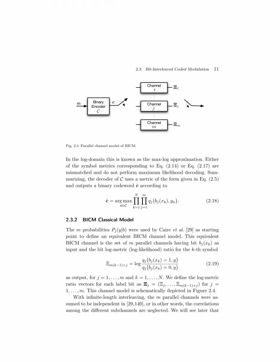
Fig. 2.4 Parallel channel model of BICM.
In the log-domain this is known as the max-log approximation. Eitherof the symbol metrics corresponding to Eq. (2.14) or Eq. (2.17) aremismatched and do not perform maximum likelihood decoding. Sum-marizing, the decoder of C uses a metric of the form given in Eq. (2.5)and outputs a binary codeword c according to
c = arg maxc∈C
N∏k=1
m∏j=1
qj(bj(xk), yn
). (2.18)
2.3.2 BICM Classical Model
The m probabilities Pj(y|b) were used by Caire et al. [29] as startingpoint to define an equivalent BICM channel model. This equivalentBICM channel is the set of m parallel channels having bit bj(xk) asinput and the bit log-metric (log-likelihood) ratio for the k-th symbol
Ξm(k−1)+j = logqj(bj(xk) = 1, y
)qj(bj(xk) = 0, y
) (2.19)
as output, for j = 1, . . . ,m and k = 1, . . . , N . We define the log-metricratio vectors for each label bit as Ξj = (Ξj , . . . ,Ξm(k−1)+j) for j =1, . . . ,m. This channel model is schematically depicted in Figure 2.4.
With infinite-length interleaving, the m parallel channels were as-sumed to be independent in [29,140], or in other words, the correlationsamong the different subchannels are neglected. We will see later that

12 Channel Model and Code Ensembles
this “classical” representation of BICM as a set of parallel channelsgives a good model, even though it can sometimes be optimistic. Thealternative model which uses the symbol mismatched decoding metricachieves a higher accuracy at a comparable modeling complexity.
2.3.3 Labeling Rules
As evidenced in the results of [29], the choice of binary labeling is criti-cal to the performance of BICM. For the decoder presented in previoussections, it was conjectured [29] that binary reflected Gray mappingwas optimum, in the sense of having the largest BICM capacity. Thisconjecture was supported by some numerical evidence, and was furtherrefined in [2, 109] to possibly hold only for moderate-to-large values ofSNR. Indeed, Stierstorfer and Fischer [110] have shown that a differentlabeling —strictly regular set partitioning— is significantly better forsmall values of SNR. A detailed discussion on the different merits ofthe various forms of Gray labeling can be found in [2].
Throughout the monograph, we use for our simulations the labelingrules depicted in Figure 2.5, namely binary reflected Gray labeling [95]and set partitioning labeling [130]. Recall that the binary reflected Graymapping for m bits may be generated recursively from the mapping form− 1 bits by prefixing a binary 0 to the mapping for m− 1 bits, thenprefixing a binary 1 to the reflected (i. e. listed in reverse order) map-ping for m− 1 bits. For QAM modulations, the symbol mapping is theCartesian product of Gray mappings over the in-phase and quadraturecomponents. For PSK modulations, the mapping table is wrapped sothat the first and last symbols are contiguous.
2.A Continuous- and Discrete-Time Gaussian Channels
We follow closely the review paper by Forney and Ungerbock [36]. Inthe linear Gaussian channel, the input x(t), additive Gaussian noisecomponent z(t), and output y(t) are related as
y(t) =∫h(t; τ)x(τ − t) dτ + z(t), (2.20)

2.A. Continuous- and Discrete-Time Gaussian Channels 13
Q
I
1011
01 00
(a) QPSK, Gray.
Q
I
10
01 11
00
(b) QPSK, set partitioning.
Q
I
001
010
100
011
101
110
111
000
(c) 8-PSK, Gray.
Q
I
001
110
101
100
011
111
010
000
(d) 8-PSK, set partitioning.
Q
I
1110 1010 0010 0110
1111 1011 0011 0111
1101 1001 0001 0101
1100 1000 0000 0100
(e) 16-QAM, Gray.
Q
I
0000
0010 0011
0101
0111
1100 1101 10001001
1110 1011 1010
0001 0100
0110
1111
(f) 16-QAM, set partitioning.
Fig. 2.5 Binary labeling rules (Gray, set partitioning) for QPSK, 8-PSK and 16-QAM.
where h(t; τ) is a (possibly time-varying) channel impulse response.Since all functions are real, their Fourier transforms are Hermitian and

14 Channel Model and Code Ensembles
we need consider only the positive-frequency components.We constrain the signal x(t) to have power P and a frequency con-
tent concentrated in an interval (fmin, fmax), with the bandwidth W
given by W = fmax − fmin. Additive noise is assumed white in thefrequency band of interest, i. e. noise has a flat power spectral densityN0 (one-sided). If the channel impulse response is constant with unitenergy in (fmin, fmax), we define the signal-to-noise ratio snr as
snr =P
N0W. (2.21)
In this case, it is also possible to represent the received signal by itsprojections onto an orthonormal set,
yk = xk + zk, (2.22)
where there are only WT effective discrete-time components when thetransmission time lasts T seconds (T � 1) [39]. The signal componentsxk have average energy Es, which is related to the power constraint asP = EsW . The quantities zk are circularly-symmetric complex Gaus-sian random variables of variance σ2
Z = N0. We thus have snr = Es/σ2Z .
Observe that we recover the model in Eq. (2.6) (with hk = 1) by divid-ing all quantities in Eq. (2.22) by σZ and incorporating this coefficientin the definition of the channel variables.
Another channel of interest we use in the monograph is thefrequency-nonselective, or flat fading channel. Its channel responseh(t; τ) is such that Eq. (2.20) becomes
y(t) = h(t)x(t) + z(t). (2.23)
The channel makes the signal x(t) fade following a coefficient h(t).Under the additional assumption that the coefficient varies quickly, werecover a channel model similar to Eq. (2.6),
yk = hkxk + zk. (2.24)
With the appropriate normalization by σZ we obtain the model inEq. (2.6). Throughout the monograph, we use the Nakagami-mf fadingmodel in Eq. (2.8), whereby coefficients are statistically independent

2.A. Continuous- and Discrete-Time Gaussian Channels 15
from one another for different values of k. The squared fading coefficientg = |h|2 has density
PG(g) =m
mf
f gmf−1
Γ(mf )e−mf g. (2.25)

3
Information-Theoretic Foundations
In this chapter, we review the information-theoretic foundations ofBICM. As suggested in the previous chapter, BICM can be viewed asa coded modulation scheme with a mismatched decoding metric. Westudy the achievable information rates of coded modulation systemswith a generic decoding metric [41, 59, 84] and determine the so-calledgeneralized mutual information. We also provide a general coding the-orem based on Gallager’s analysis of the error probability by means ofthe random coding error exponent [39], thus giving an achievable rateand a lower bound to the random coding error exponent.
We compare these results (in particular, the mutual information,the cutoff rate and the overall error exponent) with those derived fromthe classical BICM channel model as a set of independent parallel chan-nels [29,140]. Whereas the BICM mutual information coincides for bothmodels, the error exponent of the mismatched-decoding model is alwaysupper bounded by that of coded modulation, a condition which is notverified in the independent parallel-channel model mentioned in Sec-tion 2.3. We complement our analysis with a derivation of the errorexponents of other variants of coded modulation, namely multi-levelcoding with successive decoding [140] and with independent decoding
16

3.1. Coded Modulation 17
of all the levels. As is well known, the mutual information attained bymulti-level constructions can be made equal to that of coded modula-tion. However, this equality is attained at a non negligible cost in errorexponent, as we will see later.
For Gaussian channels with binary reflected Gray labeling, the mu-tual information and the random coding error exponent of BICM areclose to those of coded modulation for medium-to-large signal-to-noiseratios. For low signal-to-noise ratios —or low spectral efficiency— wegive a simple analytic expression for the loss in mutual information orreceived power compared to coded modulation. We determine the min-imum energy per bit necessary for reliable communication when BICMis used. For QAM constellations with binary reflected Gray labeling,this energy is at most 1.25 dB from optimum transmission methods.BICM is therefore a suboptimal, yet simple transmission method validfor a large range of signal-to-noise ratios. We also give a simple ex-pression for the first derivative of the BICM mutual information withrespect to the signal-to-noise ratio, in terms of Minimum Mean-EquareError (MMSE) for estimating the input of the channel from its output,and we relate this to the findings of [51,67].
3.1 Coded Modulation
3.1.1 Channel Capacity
A coding rate1 R is said achievable if, for all ε > 0 and all sufficientlylarge N there exists codes of length N with rate not smaller than R
(i. e. with at least deRNe messages) and error probability Pe < ε [31].The capacity C is the supremum of all achievable rates. For memorylesschannels, Shannon’s theorem yields the capacity formula:
Theorem 3.1 (Shannon 1948). The channel capacity C is given by
C = supPX(·)
I(X;Y ), (3.1)
where I(X;Y ) denotes the mutual information of between X and Y ,
1 Capacities and information rates will be expressed using a generic logarithm, typically thenatural logarithm. However, all charts in this monograph are expressed in bits.
18 Information-Theoretic Foundations
defined
I(X;Y ) = E[log
PY |X(Y |X)PY (Y )
]. (3.2)
For the maximum-likelihood decoders considered in Section 2.12
Gallager studied the average error probability of randomly generatedcodes [39, Chapter 5]. Specifically, he proved that the error probabilitydecreases exponentially with the block length according to a parametercalled the reliability function. Denoting the error probability attainedby a coded modulation scheme M of length N and rate R by Pe(M),we define the reliability function E(R) as
E(R) ∆= limN→∞
− 1N
log infMPe(M), (3.3)
where the optimization is carried out over all possible coded modu-lation schemes M. Since the reliability function is often not knownexactly [39], upper and lower bounds to it are given instead. We arespecially interested in a lower bound, known as the random coding errorexponent, which gives an accurate characterization of the average errorperformance of the ensemble of random codes for sufficiently high rates.Furthermore, this lower bound is known to be tight for rates above acertain threshold, known as the critical rate [39, Chapter 5].
When the only constraint to the system is E[|X|2] ≤ 1, then thechannel capacity of the AWGN channel described in (2.6) (letting H =1 with probability 1) is given by [31,39,105]
C = log (1 + snr) . (3.4)
In this case, the capacity given by (3.4) is achieved by Gaussian code-books [105], i. e. randomly generated codebooks with components inde-pendently drawn according to a Gaussian distribution, X ∼ NC(0, 1).
From a practical point of view, it is often more convenient to con-struct codewords as sequences of points from a signal constellation Xof finite cardinality, such as PSK or QAM [95], with a uniform input
2 Decoders with a symbol decoding metric q(x, y) that is a bijective (increasing) functionof the channel transition probability PY |X(y|x).

3.1. Coded Modulation 19
distribution, PX(x) = 12m for all x ∈ X . While a uniform distribution
is only optimal for large snr, it is simpler to implement and usuallyleads to more manageable analytical expressions. In general, the prob-ability distribution PX(x) that maximizes the mutual information for agiven signal constellation depends on snr and on the specific constella-tion geometry. Optimization of this distribution has been termed in theliterature as signal constellation shaping (see for example [34, 36] andreferences therein). Unless otherwise stated, we will always consider theuniform distribution throughout this monograph.
For a uniform input distribution, we refer to the corresponding mu-tual information between channel input X and output Y as the codedmodulation capacity, and denote it by Ccm
X or Icm(X;Y ), that is
CcmX = Icm(X;Y ) ∆= E
[log
PY |X(Y |X)1
2m
∑x′∈X PY |X(Y |x′)
]. (3.5)
Observe that the finite nature of these signal sets implies that they canonly convey a finite number of bits per channel use, i. e. Ccm
X ≤ m bits.Figure 3.1 shows the coded modulation capacity for multiple signal
constellations in the AWGN channel, as a function of snr.
3.1.2 Error Probability with Random Codes
Following in the footsteps of Gallager [39, Chapter 5], this section pro-vides an achievability theorem for a general decoding metric q(x, y)using random coding arguments. The final result, concerning the errorprobability, can be found in Reference [59].
We consider an ensemble of randomly generated codebooks, forwhich the entries of the codewords x are i. i. d. realizations of a ran-dom variable X with probability distribution PX(x) over the set X , i.e. PX(x) =
∏Nk=1 PX(xk). We denote by Pe(m) the average error prob-
ability over the code ensemble when message m is transmitted and byPe the error probability averaged over the message choices. Therefore,
Pe =1|M|
|M|∑m=1
Pe(m). (3.6)
The symmetry of the code construction makes Pe(m) independent of

20 Information-Theoretic Foundations
−20 −10 0 10 20 300
1
2
3
4
5
6
7
snr (dB)
Ccm
X(b
its/
channel
use
)
64−QAM
32−QAM
16−QAM
8−PSK
QPSK
BPSK
Fig. 3.1 Coded modulation capacity in bits per channel use for multiple signal constella-tions with uniform inputs in the AWGN channel. For reference, the channel capacity withGaussian inputs (3.4) is shown in thick lines.
the index m, and hence Pe = Pe(m) for any m ∈M. Averaged over therandom code ensemble, we have that
Pe(m) =∑xm
PX(xm)∫
yPY |X(y|xm) Pr {ϕ(y) 6= m|xm,y}dy, (3.7)
where Pr {ϕ(y) 6= m|xm,y} is the probability that, for a channel outputy, the decoder ϕ selects a codeword other than the transmitted xm.
The decoder ϕ, as defined in (2.4), chooses the codeword xbm withlargest metric q(xbm,y). The pairwise error probability Pr{ϕ(y) =m′|xm,y} of wrongly selecting message m′ when message m has beentransmitted and sequence y has been received is given by
Pr{ϕ(y) = m′|xm,y} =∑
xm′ : q(xm′ ,y)≥ q(xm,y)
PX(xm′). (3.8)
Using the union bound over all possible codewords, and for all 0 ≤ρ ≤ 1, the probability Pr {ϕ(y) 6= m|xm,y} can be bounded by [39, p.

3.1. Coded Modulation 21
136]
Pr {ϕ(y) 6= m|xm,y} ≤ Pr
⋃m′ 6=m
{ϕ(y) = m′|xm,y}
(3.9)
≤
∑m′ 6=m
Pr{ϕ(y) = m′|xm,y}
ρ
. (3.10)
Since q(xm′ ,y) ≥ q(xm,y) and the sum over all xm′ upper boundsthe sum over the set {xm′ : q(xm′ ,y) ≥ q(xm,y)}, for any s > 0, thepairwise error probability in Eq. (3.8) can bounded by
Pr{ϕ(y) = m′|xm,y} ≤∑xm′
PX(xm′)(q(xm′ ,y)q(xm,y)
)s
. (3.11)
As m′ is a dummy variable, for any s > 0 and 0 ≤ ρ ≤ 1 it holds that
Pr {ϕ(y) 6= m|xm,y} ≤
(|M| − 1) ∑
xm′
PX(xm′)(q(xm′ ,y)q(xm,y)
)sρ
.
(3.12)Therefore, Eq. (3.7) can be written as
Pe ≤(|M| − 1
)ρ E
∑xm′
PX(xm′)(q(xm′ ,Y )q(Xm,Y )
)sρ . (3.13)
For memoryless channels, we have a per-letter characterization [39]
Pe ≤ (|M| − 1)ρ (E
[(∑x′
PX(x′)(q(x′, Y )q(X,Y )
)s)ρ])N
. (3.14)
Hence, for any input distribution PX(x), 0 ≤ ρ ≤ 1 and s > 0,
Pe ≤ e−N(Eq0(ρ,s)−ρR) (3.15)
where
Eq0(ρ, s)
∆= − log E
[(∑x′
PX(x′)(q(x′, Y )q(X,Y )
)s)ρ]
(3.16)

22 Information-Theoretic Foundations
is the generalized Gallager function. The expectation is carried outaccording to the joint distribution PX,Y (x, y) = PY |X(y|x)PX(x).
We define the mismatched random coding exponent as
Eqr (R) ∆= max
0≤ρ≤1maxs>0
(Eq
0(ρ, s)− ρR). (3.17)
This procedure also yields a lower bound on the reliability function,E(R) ≥ Eq
r (R). Further improvements are possible by optimizing overthe input distribution PX(x).
According to (3.15), the average error probability Pe goes to zero ifEq
0(ρ, s) > ρR for a given s. In particular, as ρ vanishes, rates below
limρ→0
Eq0(ρ, s)ρ
(3.18)
are achievable. Using that Eq0(ρ, s) = 0 for ρ = 0, and in analogy to the
mutual information I(X;Y ), we define the quantity Igmis (X;Y ) as
Igmis (X;Y ) ∆=
∂Eq0(ρ, s)∂ρ
∣∣∣∣ρ=0
= limρ→0
Eq0(ρ, s)ρ
(3.19)
= −E
[log∑x′
PX(x′)(q(x′, Y )q(X,Y )
)s]
(3.20)
= E[log
q(X,Y )s∑x′∈X PX(x′)q(x′, Y )s
]. (3.21)
By maximizing over the parameter s we obtain the generalized mutualinformation for a mismatched decoder using metric q(x, y) [41,59,84],
Igmi(X;Y ) = maxs>0
Igmis (X;Y ). (3.22)
The preceding analysis shows that any rate R < Igmi(X;Y ) is achiev-able, i. e. we can transmit at rate R < Igmi(X;Y ) and have Pe → 0.
For completeness and symmetry with classical random coding anal-ysis, we define the generalized cutoff rate as
R0∆= Eq
r (R = 0) = maxs>0
Eq0(1, s). (3.23)
For a maximum likelihood decoder, Eq0(ρ, s) is maximized by letting

3.2. Bit-Interleaved Coded Modulation 23
s = 11+ρ [39], and we have
E0(ρ)∆= − log E
(∑x′
PX(x′)(PY |X(Y |x′)PY |X(Y |X)
) 11+ρ
)ρ (3.24)
= − log∫
y
(∑x
PX(x)PY |X(y|x)1
1+ρ
)1+ρ
dy, (3.25)
namely the coded modulation exponent. For uniform inputs,
Ecm0 (ρ) ∆= − log
∫y
(1
2m
∑x
PY |X(y|x)1
1+ρ
)1+ρ
dy. (3.26)
Incidentally, the argument in this section proves the achievability ofthe rate Ccm
X = Icm(X;Y ) with random codes and uniform inputs, i.e. there exist coded modulation schemes with exponentially vanishingerror probability for all rates R < Ccm
X .Later, we will use the following data-processing inequality, which
shows that the generalized Gallager function of any mismatched de-coder is upperbounded by the Gallager function of a maximum likeli-hood decoder.
Proposition 3.1 (Data-Processing Inequality [59,77]). For s > 0,0 ≤ ρ ≤ 1, and a given input distribution we have that
Eq0(ρ, s) ≤ E0(ρ) (3.27)
The necessary condition for equality to hold is that the metric q(x, y)is proportional to a power of the channel transition probability,
PY |X(y|x) = c′q(x, y)s′ for all x ∈ X (3.28)
for some constants c′ and s′.
3.2 Bit-Interleaved Coded Modulation
In this section, we study the BICM decoder and determine the general-ized mutual information and a lower bound to the reliability function.Special attention is given to the comparison with the classical analysisof BICM as a set of m independent parallel channels (see Section 2.3).

24 Information-Theoretic Foundations
3.2.1 Achievable Rates
We start with a brief review of the classical results on the achievablerates for BICM. Under the assumption of an infinite-length interleaver,capacity and cutoff rate were studied in [29]. This assumption (see Sec-tion 2.3) yields a set of m independent parallel binary-input channels,for which the corresponding mutual information and cutoff rate are thesum of the corresponding rates of each subchannel, and are given by
I ind(X;Y ) ∆=m∑
j=1
E
[log
∑x′∈X j
BPY |X(Y |x′)
12
∑x′∈X PY |X(Y |x′)
], (3.29)
and
Rind0
∆= m log 2−m∑
j=1
log
1 + E
√√√√∑x′∈X j
B
PY |X(Y |x′)∑x′∈X j
BPY |X(Y |x′)
, (3.30)
respectively. An underlying assumption behind Eq. (3.30) is that the mindependent channels are used the same number of times. Alternatively,the parallel channels may be used with probability 1
m , and the cutoffrate is then m times the cutoff rate of an averaged channel [29],
Rav0
∆= m
log 2− log
1 +1m
m∑j=1
E
√√√√√∑
x′∈X j
Bj
PY |X(Y |x′)∑x′∈X j
Bj
PY |X(Y |x′)
.
(3.31)
The expectations are over the joint probability PBj ,Y (b, y) = 12Pj(y|b).
From Jensen’s inequality one easily obtains that Rav0 ≤ Rind
0 .We will use the following shorthand notation for the BICM capacity,
CbicmX
∆= I ind(X;Y ). (3.32)
The following alternative expression [26,76,140] for the BICM mutualinformation turns out to be useful,
CbicmX =
m∑j=1
12
1∑b=0
(CcmX − Ccm
X jb
)(3.33)

3.2. Bit-Interleaved Coded Modulation 25
where CcmA is the mutual information for coded modulation over a gen-
eral signal constellation A.We now relate this BICM capacity with the generalized mutual
information introduced in the previous section.
Theorem 3.2 ( [77]). The generalized mutual information of theBICM decoder is given by the sum of the generalized mutual informa-tions of the independent binary-input parallel channel model of BICM,
Igmi(X;Y ) = sups>0
m∑j=1
E
[log
qj(b, Y )s
12
∑1b′=0 qj(b′, Y )s
]. (3.34)
There are a number of interesting particular cases of the above theorem.
Corollary 3.1 ( [77]). For the metric in Eq. (2.15),
Igmi(X;Y ) = CbicmX . (3.35)
Expression (3.35) coincides with the BICM capacity above, eventhough we have lifted the assumption of infinite interleaving. Whenthe suboptimal metrics (2.17) are used, we have the following.
Corollary 3.2 ( [77]). For the metric in Eq. (2.17),
Igmi(X;Y ) = sups>0
m∑j=1
E
log
(maxx∈XB
jp(y|x)
)s12
∑1b=0
(max
x′∈X jbp(y|x′)
)s . (3.36)
The information rates achievable with this suboptimal decoder havebeen studied by Szczecinski et al. [112]. The fundamental differencebetween their result and the generalized mutual information given in(3.36) is the optimization over s. Since both expressions are equal whens = 1, the optimization over s may induce a larger achievable rate.
Figure 3.2 shows the BICM mutual information for some signalconstellations, different binary labeling rules and uniform inputs for

26 Information-Theoretic Foundations
−20 −10 0 10 20 300
1
2
3
4
5
snr (dB)
Cbicm
X(b
its/
channel
use
)
16−QAM
8−PSK
QPSK
Fig. 3.2 Coded modulation and BICM capacities (in bits per channel use) for multiplesignal constellations with uniform inputs in the AWGN channel. Gray and set partitioninglabeling rules correspond to dashed and dashed-dotted lines respectively. In thick solid lines,the capacity with Gaussian inputs (3.4); with thin solid lines the CM channel capacity.
the AWGN channel, as a function of snr. For the sake of illustrationsimplicity, we have only plotted the information rate for the Gray andset partitioning binary labeling rules from Figure 2.5. Observe thatbinary reflected Gray labeling pays a negligible penalty in informationrate, being close to the coded modulation capacity.
3.2.2 Error Exponents
Evaluation of the generalized Gallager function in Eq. (3.16) for BICMwith a bit metric qj(b, y) yields a function Ebicm
0 (ρ, s) of ρ and s,
Ebicm0 (ρ, s) ∆= − log E
12m
∑x′∈X
m∏j=1
qj(bj(x′), Y )s
qj(bj(X), Y )s
ρ . (3.37)

3.2. Bit-Interleaved Coded Modulation 27
Moreover, the data processing inequality for error exponents in Propo-sition 3.1 shows that the error exponent (and in particular the cutoffrate) of the BICM decoder is upperbounded by the error exponent (andthe cutoff rate) of the ML decoder, that is Ebicm
0 (ρ, s) ≤ Ecm0 (ρ).
In their analysis of multilevel coding and successive decoding,Wachsmann et al. provided the error exponents of BICM modeled as aset of independent parallel channels [140]. The corresponding Gallager’sfunction, which we denote by Eind
0 (ρ), is given by
Eind0 (ρ) ∆= −
m∑j=1
log E
[(1∑
b′=0
PBj (b′)Pj(Y |b′)
11+ρ
Pj(Y |B)1
1+ρ
)ρ]. (3.38)
This quantity is the random coding exponent of the BICM decoderif the channel output y admits a decomposition into a set of paralleland independent subchannels. In general, this is not the case, sinceall subchannels are affected by the same noise —and possibly fading—realization, and the parallel-channel model fails to capture the statisticsof the channel.
Figures 3.3(a), 3.3(b) and 3.4 show the error exponents for codedmodulation (solid), BICM with independent parallel channels (dashed),BICM using metric (2.15) (dash-dotted), and BICM using metric (2.17)(dotted) for 16-QAM with the Gray labeling in Figure 2.5, Rayleighfading and snr = 5, 15,−25 dB, respectively. Dotted lines labeled withs = 1
1+ρ correspond to the error exponent of BICM using metric (2.17)letting s = 1
1+ρ . The parallel-channel model gives a larger exponentthan the coded modulation, in agreement with the cutoff rate resultsof [29]. In contrast, the mismatched-decoding analysis yields a lowerexponent than coded modulation. As mentioned in the previous section,both BICM models yield the same capacity.
In most cases, BICM with a max-log metric (2.17) incurs a marginalloss in the exponent for mid-to-large SNR. In this SNR range, theoptimized exponent and that with s = 1
1+ρ are almost equal. For lowSNR, the parallel-channel model and the mismatched-metric modelwith (2.15) have the same exponent, while we observe a larger penaltywhen metrics (2.17) are used. As we observe, some penalty is incurredat low SNR for not optimizing over s. We denote with crosses the

28 Information-Theoretic Foundations
0 0.5 1 1.5 20
0.2
0.4
0.6
0.8
1
R
Er(R
)
(a) snr = 5 dB.
0 0.5 1 1.5 2 2.5 3 3.50
0.5
1
1.5
2
2.5
3
R
Er(R
)
(b) snr = 15 dB.
Fig. 3.3 Error exponents for coded modulation (solid), BICM with independent parallelchannels (dashed), BICM using metric (2.15) (dash-dotted), and BICM using metric (2.17)(dotted) for 16-QAM with Gray labeling, Rayleigh fading.

3.3. Comparison with Multilevel Coding 29
0 1 2 3 4 5
x 10−3
0
0.5
1
1.5
2
2.5x 10
−3
R
Er(R
)
s = 1
1+ρ
Fig. 3.4 Error exponents for coded modulation (solid), BICM with independent parallelchannels (dashed), BICM using metric (2.15) (dash-dotted), and BICM using metric (2.17)(dotted) for 16-QAM with Gray labeling, Rayleigh fading and snr = −25 dB. Crossescorrespond to (from right to left) coded modulation, BICM with metric (2.15), BICM withmetric (2.17) and BICM with metric (2.17) and s = 1.
corresponding achievable information rates.An interesting question is whether the error exponent of the parallel-
channel model is always larger than that of the mismatched-decodingmodel. The answer is negative, as illustrated in Figure 3.5, which showsthe error exponents for coded modulation (solid), BICM with inde-pendent parallel channels (dashed), BICM using metric (2.15) (dash-dotted), and BICM using metric (2.17) (dotted) for 8-PSK with Graylabeling in the AWGN channel.
3.3 Comparison with Multilevel Coding
Multilevel codes (MLC) combined with multistage decoding (MSD)have been proposed [56,140] as an efficient method to attain the channelcapacity by using binary codes. In this section, we compare BICM with

30 Information-Theoretic Foundations
0 0.5 1 1.5 20
0.5
1
1.5
R
Er(R
)
Fig. 3.5 Error exponents for coded modulation (solid), BICM with independent parallelchannels (dashed), BICM using metric (2.15) (dash-dotted), and BICM using metric (2.17)(dotted) for 8-PSK with Gray labeling, AWGN and snr = 5 dB.
MLC in terms of error exponents and achievable rates. In particular, weelaborate on the analogy between MLC and the multiple-access channelto present a general error exponent analysis of MLC with MSD. Theerror exponents of MLC have been studied in a somewhat different wayin [12,13,140].
For BICM, a single binary code C is used to generate a binary code-word, which is used to select modulation symbols by a binary labelingfunction µ. A uniform distribution over the channel input set inducesa uniform distribution over the input bits bj , j = 1, . . . ,m. In MLC,the input binary code C is the Cartesian product of m binary codes oflength N , one per modulation level, i. e. C = C1 × . . . × Cm, and theinput distribution for the symbol x(b1, . . . , bj) has the form
PX(x) = PB1,...,BM(b1, . . . , bm) =
m∏j=1
PBj (bj). (3.39)
Denoting the rate of the j-th level code by Rj , the resulting total rate

3.3. Comparison with Multilevel Coding 31
Binary
Labeling
µ
xm1,...,mm
Binary
EncoderC1
Binary
EncoderCm
m
m1
mm
.
.
.
{
c1
cm
Fig. 3.6 Block diagram of a multi-level encoder.
of the MLC scheme is R =∑m
j=1Rj . We denote the codewords of Cjby cj . The block diagram of MLC is shown in Figure 3.6.
The multi-stage decoder operates by decoding the m levels sepa-rately. The symbol decoding metric is thus of the form
q(x, y) =m∏
j=1
qj(bj(x), y). (3.40)
A crucial difference with respect to BICM is that the decoders are al-lowed to pass information from one level to another. Decoding operatessequentially, starting with code C1, feeding the result to this decoderto C2, and proceeding across all levels. We have that the j-th decodingmetric of MLC with MSD is given by
qj(bj(x) = b, y
)=
1∣∣∣X 1,...,jb1,...,bj−1,b
∣∣∣∑
x′∈X 1,...,jb1,...,bj−1,b
PY |X(y|x′). (3.41)
Conditioning on the previously decoded levels reduces the number ofsymbols remaining at the j-th level, so that only 2m−j symbols remainat the j-th level in Eq. (3.41). Figure 3.7 depicts the operation of anMLC/MSD decoder.
The MLC construction is very similar to that of a multiple-accesschannel, as noticed by [140]. An extension of Gallager’s random codinganalysis to the multiple-access channel was carried out by Slepian andWolf in [108] and Gallager [40], and we now review it for a simple 2-levelcase. Generalization to a larger number of levels is straightforward.

32 Information-Theoretic Foundations
Decoder of
C1
Decoder of
Decoder of
Cm
C2
y m1
m2
mm
mm−1
.
.
.
Fig. 3.7 Block diagram of a multi-stage decoder for MLC.
As in our analysis of Section 3.1.2, we denote by Pe the error prob-ability averaged over an ensemble of randomly selected codebooks,
Pe =1
|C1||C2|
|C1|∑m1=1
|C2|∑m2=1
Pe(m1,m2), (3.42)
where Pe(m1,m2) denotes the average error probability over the codeensemble when messages m1 and m2 are chosen by codes C1 andC2, respectively. Again, the random code construction makes the er-ror probability independent of the transmitted message and hencePe = Pe(m1,m2) for any messages m1,m2. If m1,m2 are the selectedmessages, then xm1,m2 denotes the sequence of modulation symbolscorresponding to these messages.
For a given received sequence y, the decoders ϕ1 and ϕ2 choosethe messages m1, m2 with largest metric q(xm1,m2 ,y). Let (1, 1) be theselected message pair. In order to analyze the MSD decoder, it provesconvenient to separately consider three possible error events,
(1) the decoder for C1 fails (ϕ1(y) 6= 1), but that for C2 is suc-cessful (ϕ2(y) = 1): the decoded codeword is xm1,1, m1 6= 1;
3.3. Comparison with Multilevel Coding 33
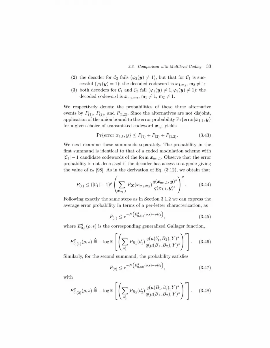
(2) the decoder for C2 fails (ϕ2(y) 6= 1), but that for C1 is suc-cessful (ϕ1(y) = 1): the decoded codeword is x1,m2 , m2 6= 1;
(3) both decoders for C1 and C2 fail (ϕ1(y) 6= 1, ϕ2(y) 6= 1): thedecoded codeword is xm1,m2 , m1 6= 1, m2 6= 1.
We respectively denote the probabilities of these three alternativeevents by P(1), P(2), and P(1,2). Since the alternatives are not disjoint,application of the union bound to the error probability Pr{error|x1,1,y}for a given choice of transmitted codeword x1,1 yields
Pr{error|x1,1,y} ≤ P(1) + P(2) + P(1,2). (3.43)
We next examine these summands separately. The probability in thefirst summand is identical to that of a coded modulation scheme with|C1| − 1 candidate codewords of the form xm1,1. Observe that the errorprobability is not decreased if the decoder has access to a genie givingthe value of c2 [98]. As in the derivation of Eq. (3.12), we obtain that
P(1) ≤ (|C1| − 1)ρ
∑xm1,1
PX(xm1,m2)q(xm1,1,y)s
q(x1,1,y)s
ρ
. (3.44)
Following exactly the same steps as in Section 3.1.2 we can express theaverage error probability in terms of a per-letter characterization, as
P(1) ≤ e−N“Eq
0,(1)(ρ,s)−ρR1
”, (3.45)
where Eq0,1(ρ, s) is the corresponding generalized Gallager function,
Eq0,(1)(ρ, s)
∆= − log E
∑b′1
PB1(b′1)q(µ(b′1, B2), Y )s
q(µ(B1, B2), Y )s
ρ . (3.46)
Similarly, for the second summand, the probability satisfies
P(2) ≤ e−N“Eq
0,(2)(ρ,s)−ρR2
”, (3.47)
with
Eq0,(2)(ρ, s)
∆= − log E
∑b′2
PB2(b′2)q(µ(B1, b
′2), Y )s
q(µ(B1, B2), Y )s
ρ . (3.48)

34 Information-Theoretic Foundations
As for the third summand, there are (|C1| − 1)(|C2| − 1) alternativecandidate codewords of the form xm1,m2 , which give the upper bound
P(1,2) ≤ e−N“Eq
0,(1,2)(ρ,s)−ρ(R1+R2)
”, (3.49)
with the corresponding Gallager function,
Eq0,(1,2)(ρ, s)
∆= − log E
∑b′1,b′2
PB1(b′1)PB2(b
′2)q(µ(b′1, b
′2), Y )s
q(µ(B1, B2), Y )s
ρ .(3.50)
Summarizing, the overall average error probability is bounded by
Pe ≤ e−N“Eq
0,(1)(ρ,s)−ρR1
”+ e−N
“Eq
0,(2)(ρ,s)−ρR2
”
+ e−N“Eq
0,(1,2)(ρ,s)−ρ(R1+R2)
”. (3.51)
For any choice of ρ, s, input distribution and R1, R2 ≥ 0 such thatR1 + R2 = R, we obtain a lower bound to the reliability function ofMLC at rate R. For sufficiently large N , the error probability (3.51) isdominated by the minimum exponent. In other words,
E(R) ≥ Eqr (R) ∆= max
R1,R2R1+R2=R
min{Eq
r,(1)(R1) , Eqr,(2)(R2) , E
qr,(1,2)(R)
}(3.52)
where
Eqr,(1)(R1)
∆= max0≤ρ≤1
maxs>0
(Eq
0,(1)(ρ, s)− ρR1
)(3.53)
Eqr,(2)(R2)
∆= max0≤ρ≤1
maxs>0
(Eq
0,(2)(ρ, s)− ρR2
)(3.54)
Eqr,(1,2)(R) ∆= max
0≤ρ≤1maxs>0
(Eq
0,(1,2)(ρ, s)− ρR). (3.55)
Since C1, C2 are binary, the exponents Eqr,(1)(R) and Eq
r,(2)(R) are alwaysupper bounded by 1. Therefore, the overall exponent of MLC with MSDis smaller than one.
As we did in Section 3.1.2, analysis of Eq. (3.51) yields achievablerates. Starting the decoding at level 1, we obtain
R1 < I(B1;Y ) (3.56)
R2 < I(B2;Y |B1). (3.57)

3.3. Comparison with Multilevel Coding 35
R1
R2
I(B1;Y ) I(B1;Y |B2)
I(B2;Y |B1)
I(B2;Y )
R1 + R2 < I(X;Y )
R1 + R2 < I(B1;Y ) + I(B2;Y )
Fig. 3.8 Rate regions for MLC/MSD and BICM.
Generalization to a larger number of levels gives
Rj < I(Bj ;Y |B1, . . . , Bj−1). (3.58)
The chain rule of mutual information proves that MLC and MSDachieve the coded modulation capacity [56,140],
∑mj=1Rj < Icm(X;Y ).
When MLC is decoded with the standard BICM decoder, i. e. withoutMSD, then the rates we obtain are
R1 < I(B1;Y ) (3.59)
R2 < I(B2;Y ). (3.60)
Figure 3.8 shows the resulting rate region for MLC. The Figure alsocompares with MLC with BICM decoding (i. e. without MSD), showingthe corresponding achievable rates.
While MLC with MSD achieves the coded modulation capacity, itdoes not achieve the coded modulation error exponent. This is due tothe MLC (with or without MSD) error exponent always being givenby the minimum of the error exponents of the various levels, whichresults in an error exponent smaller than 1. While BICM suffers froma non-zero, yet small, capacity loss compared to CM and MLC/MSD,

36 Information-Theoretic Foundations
BICM attains a larger error exponent, whose loss with respect to CM issmall. This loss may be large for an MLC construction. In general, thedecoding complexity of BICM is larger than that of MLC/MSD, sincethe codes of MLC are shorter. One such example is a code where onlya few bits out of the m are coded while the rest are left uncoded. Inpractice, however, if the decoding complexity grows linearly with thenumber of bits in a a codeword, e. g. with LDPC or turbo codes, theoverall complexity of BICM becomes comparable to that of MLC/MSD.
3.4 Mutual Information Analysis
In this section, we focus on AWGN channels with and without fadingand study some properties of the mutual information as a function ofsnr. Building on work by Guo, Shamai and Verdu [51], we first providea simple expression for the first derivative of the mutual informationwith respect to snr. This expression is of interest for the optimizationof power allocation across parallel channels, as discussed by Lozano etal. [67] in the context of coded modulation systems.
Then, we study the BICM mutual information at low snr, that is inthe wideband regime recently popularised by Verdu [134]. For a givenrate, BICM with Gray labeling loses at most 1.25 dB in received power.
3.4.1 Derivative of Mutual Information
A fundamental relationship between the input-output mutual informa-tion and the minimum mean-squared error (MMSE) in estimating theinput from the output in additive Gaussian channels was discovered byGuo, Shamai and Verdu in [51]. It is worth noting that, beyond its ownintrinsic theoretical interest, this relationship has proved instrumentalin optimizing the power allocation for parallel channels with arbitraryinput distributions and in obtaining the minimum bit-energy-to-noise-spectral-density ratio for reliable communication [67].
For a scalar model Y =√
snrX + Z, it is shown in [51] that
dC(snr)d snr
= mmse(snr) (3.61)

3.4. Mutual Information Analysis 37
where C(snr) = I(X;Y ) is the mutual information expressed in nats,
mmse(snr) ∆= E[|X − X|2
](3.62)
is the MMSE of estimating the input X from the output Y of the givenGaussian channel model, and where
X∆= E[X|Y ] (3.63)
is the MMSE estimate of the channel input X given the output Y . ForGaussian inputs we have that
mmse(snr) =1
1 + snr
while for general discrete signal constellations X we have that [67]
mmseX (snr) = E[|X|2
]− E
∣∣∣∣∣∑
x′∈X x′ e−|
√snr(X−x′)+Z|2∑
x′∈X e−|√
snr(X−x′)+Z|2
∣∣∣∣∣2 . (3.64)
Figure 3.9 shows the function mmse(snr) for Gaussian inputs and var-ious coded modulation schemes.
For BICM, obtaining a direct relationship between the BICM ca-pacity and the MMSE in estimating the coded bits given the out-put is a challenging problem. However, the combination of Eqs. (3.33)and (3.61) yields a simple relationship between the first derivative ofthe BICM mutual information and the MMSE of coded modulation:
Theorem 3.3 ( [49]). The derivative of the BICM mutual informationis given by
dCbicmX (snr)d snr
=m∑
j=1
12
1∑b=0
(mmseX (snr)−mmseX j
b(snr)
)(3.65)
where mmseA(snr) is the MMSE of an arbitrary input signal constella-tion A defined in (3.64).
Hence, the derivative of the BICM mutual information with respect tosnr is a linear combination of MMSE functions for coded modulation.

38 Information-Theoretic Foundations
0 5 10 15 200
0.2
0.4
0.6
0.8
1
snr
mm
se
Fig. 3.9 MMSE for Gaussian inputs (thick solid line), BPSK (dotted line), QPSK (dash-dotted line), 8-PSK (dashed line) and 16-QAM (solid line).
Figure 3.10 shows an example (16-QAM modulation) of the computa-tion of the derivative of the BICM mutual information. For comparison,the values of the MMSE for Gaussian inputs and for coded modulationand 16-QAM are also shown. At high snr we observe a very good matchbetween coded modulation and BICM with binary reflected Gray la-beling (dashed line). As for low snr, we notice a small loss, whose valueis determined analytically from the analysis in the next section.
3.4.2 Wideband Regime
At very low signal-to-noise ratio snr, the energy of a single bit is spreadover many channel degrees of freedom, leading to the wideband regimerecently discussed at length by Verdu [134]. Rather than studying theexact expression of the channel capacity, one considers a second-orderTaylor series in terms of snr,
C(snr) = c1snr + c2snr2 + o(snr2
), (3.66)

3.4. Mutual Information Analysis 39
0 5 10 15 200
0.2
0.4
0.6
0.8
1
snr
dC
bicm
X(snr)
dsnr
Fig. 3.10 Derivative of the mutual information for Gaussian inputs (thick solid line), 16-QAM coded modulation (solid line), 16-QAM BICM with Gray labeling (dashed line) and16-QAM BICM with set partitioning labeling (dotted line).
where c1 and c2 depend on the modulation format, the receiver design,and the fading distribution. The notation o(snr2) indicates that theremaining terms vanish faster than a function asnr2, for a > 0 and smallsnr. Here the capacity may refer to the coded modulation capacity, orthe BICM capacity.
In the following, we determine the coefficients c1 and c2 in the Tay-lor series (3.66) for generic constellations, and use them to derive thecorresponding results for BICM. Before proceeding along this line, wenote that [134, Theorem 12] covers the effect of fading. The coefficientsc1 and c2 for a general fading distribution are given by
c1 = E[|H|2
]cawgn1 , c2 = E
[|H|4
]cawgn2 , (3.67)
where the coefficients cawgn1 and cawgn
2 are in absence of fading. Hence,even though we focus only on the AWGN channel, all results are validfor general fading distributions.
Next to the coefficients c1 and c2, Verdu also considered an equiv-

40 Information-Theoretic Foundations
alent pair of coefficients, the energy per bit to noise power spectraldensity ratio at zero snr and the wideband slope [134]. These param-eters are obtained by transforming Eq. (3.66) into a function of theEbN0
= snrC log2 e , so that one obtains
C
(Eb
N0
)= ζ0
(Eb
N0− Eb
N0 lim
)+ O
((∆Eb
N0
)2)
(3.68)
where ∆EbN0
∆= EbN0− Eb
N0 limand
ζ0∆= − c31
c2 log2 2,
Eb
N0 lim
∆=log 2c1
. (3.69)
The notation O(x2) indicates that the remaining terms decay at leastas fast as a function ax2, for a > 0 and small x. The parameter ζ0is Verdu’s wideband slope in linear scale [134]. We avoid using theword minimum for Eb
N0 lim, since there exist communication schemes with
a negative slope ζ0, for which the absolute minimum value of EbN0
isachieved at non-zero rates. In these cases, the expansion at low poweris still given by Eq. (3.68).
For Gaussian inputs, we have c1 = 1 and c2 = −12 . Prelov and Verdu
determined c1 and c2 in [94] for proper-complex constellations, previ-ously introduced by Neeser and Massey in [86]. These constellationssatisfy E[X2] = 0, where E[X2] is a second-order pseudo-moment [86].We similarly define a pseudo-variance, denoted by σ2
X , as
σ2X
∆= E[X2]− E[X]2. (3.70)
Analogously, we define the constellation variance as σ2X
∆= E[|X|2
]−
|E[X]|2. The coefficients for coded modulation schemes with arbitraryfirst and second moments are given by the following result:
Theorem 3.4 ( [76,94]). Consider coded modulation schemes over ageneral signal set X used with probabilities PX(x) in the AWGN chan-nel described by (2.6). Then, the first two coefficients of the Taylorexpansion of the coded modulation capacity C(snr) around snr = 0 are
c1 = σ2X (3.71)
c2 = −12
((σ2
X
)2 +∣∣σ2
X
∣∣2). (3.72)

3.4. Mutual Information Analysis 41
For zero-mean unit-energy signal sets, we obtain the following
Corollary 3.3 ( [76]). Coded modulation schemes over a signal set Xwith E[X] = 0 (zero mean) and E[|X|2] = 1 (unit energy) have
c1 = 1, c2 = −12
(1 +
∣∣E[X2]∣∣2). (3.73)
Alternatively, the quantity c1 can be simply obtained as c1 = mmse(0).Observe also that Eb
N0 lim= log 2.
Plotting the mutual information curves as a function of EbN0
(shownin Figure 3.11) reveals the suboptimality of the BICM decoder. In par-ticular, even binary reflected Gray labeling is shown to be informationlossy at low rates. Based on the expression (3.33), one obtains
Theorem 3.5 ( [76]). The coefficients c1 and c2 of CbicmX for a constel-
lation X with zero mean and unit average energy are given by
c1 =m∑
j=1
12
1∑b=0
∣∣∣E[Xjb ]∣∣∣2, (3.74)
c2 =m∑
j=1
14
1∑b=0
((σ2
Xjb
)2+∣∣∣σ2
Xjb
∣∣∣2 − 1−∣∣E[X2]
∣∣2). (3.75)
Table 3.1 reports the numerical values for c1, c2, EbN0 lim
, and ζ0 forvarious cases, namely QPSK, 8-PSK and 16-QAM with binary reflectedGray and Set Partitioning (anti-Gray for QPSK) mappings.
In Figure 3.12, the approximation in Eq. (3.68) is compared with thecapacity curves. As expected, a good match for low rates is observed.We use labels to identify the specific cases: labels 1 and 2 are QPSK,3 and 4 are 8-PSK and 5 and 6 are 16-QAM. Also shown is the linearapproximation to the capacity around Eb
N0 lim, given by Eq. (3.68). Two
cases with Nakagami fading (with density in Eq. (2.8)) are also includedin Figure 3.12, which also show good match with the estimate, taking

42 Information-Theoretic Foundations
0 5 10 15 200
1
2
3
4
5
Eb
N0
(dB)
Cbicm
X(b
its/
channel
use
)
16−QAM
8−PSK
QPSK
Fig. 3.11 Coded modulation and BICM capacities (in bits per channel use) for multiplesignal constellations with uniform inputs in the AWGN channel. Gray and set partitioninglabeling rules correspond to thin dashed and dashed-dotted lines respectively. For reference,the capacity with Gaussian inputs (3.4) is shown in thick solid lines and the CM channelcapacity with thin solid lines.
into account that E[|H|2] = 1 and E[|H|4] = 1 + 1/mf for Nakagami-mf fading [95]. An exception is 8-PSK with set-partitioning, where thelarge slope limits the validity of the approximation to very low rates.
It seems hard to make general statements for arbitrary labelingsfrom Theorem 3.5. An important exception is the strictly regular setpartitioning labeling defined by Stierstorfer and Fischer [110], whichhas c1 = 1 for 16-QAM and 64-QAM. In constrast, for binary reflectedGray labeling (see Section 2.3) we have:
Theorem 3.6 ( [76]). ForM -PAM andM2-QAM and binary-reflectedGray labeling, the coefficient c1 is
c1 =3 ·M2
4(M2 − 1), (3.76)

3.4. Mutual Information Analysis 43
Table 3.1 EbN0 lim
and wideband slope coefficients c1, c2 for BICM in AWGN.
Modulation and Labeling
QPSK 8-PSK 16-QAM
GR A-GR GR SP GR SP
c1 1.000 0.500 0.854 0.427 0.800 0.500EbN0 lim
(dB) -1.592 1.419 -0.904 2.106 -0.627 1.419
c2 -0.500 0.250 -0.239 0.005 -0.160 -0.310ζ0 4.163 -1.041 5.410 -29.966 6.660 0.839
and the minimum EbN0 lim
is
Eb
N0 lim=
4(M2 − 1)3 ·M2
log 2. (3.77)
As M →∞, EbN0 lim
approaches 43 log 2 ' −0.3424dB. from below.
The results for BPSK, QPSK (2-PAM×2-PAM), and 16-QAM (4-PAM×4-PAM), as presented in Table 3.1, match with the Theorem.
It is somewhat surprising that the loss incurred by binary reflectedGray labeling with respect to coded modulation is bounded at low snr.The loss for large M represents about 1.25 dB with respect to the clas-sical CM limit, namely Eb
N0 lim= −1.59 dB. Using a single modulation
for all signal-to-noise ratio values, adjusting the transmission rate bychanging the code rate using a suboptimal non-iterative demodulator,needs not result in a large loss with respect to optimal schemes, whereboth the rate and modulation can change. Another low-complexity so-lution is to change the mapping only (not the modulation) accordingto SNR, switching between Gray and the mappings of [110]. This haslow-implementation complexity as it is implemented digitally.
3.4.2.1 Bandwidth and Power Trade-off
In the previous section we computed the first coefficients of the Taylorexpansion of the CM and BICM capacities around snr = 0. We now

44 Information-Theoretic Foundations
−2 0 2 4 6 80
0.5
1
1.5
2
2.5
3
Eb
N0
(dB)
Cbicm
X(b
its/
channel
use
)
1
1f 2
3
45
6 6f
Fig. 3.12 BICM channel capacity (in bits per channel use). Labels 1 and 2 are QPSK, 3 and4 are 8-PSK and 5 and 6 are 16-QAM. Gray and set partitioning labeling rules correspondto dashed (and odd labels) and dashed-dotted lines (and even labels) respectively. Dottedlines are cases 1 and 6 with Nakagami-0.3 and Nakagami-1 (Rayleigh) fading (an ‘f’ is
appended to the label index). Solid lines are linear approximation around EbN0 lim
.
use these coefficients to determine the trade-off between power andbandwidth in the low-power regime. We will see how to trade off part ofthe power loss incurred by BICM against a large bandwidth reduction.
As discussed in Section 2.A, the data rate transmitted across awaveform Gaussian channel is determined by two physical variables: thepower P , or energy per unit time, and the bandwidth W , or number ofchannel uses per unit time. In this case, the signal-to-noise ratio snr isgiven by snr = P/(N0W ), where N0 is the noise power spectral density.Then, the capacity measured in bits per unit time is the natural figureof merit for a communications system. With only a constraint on snr,this capacity is given by W log(1+snr). For low snr, we have the Taylor

3.4. Mutual Information Analysis 45
series expansion
W log(
1 +P
N0W
)=
P
N0− P 2
2N20W
+ O(
P 3
N30W
2
). (3.78)
Similarly, for coded modulation systems with capacity CcmX , we have
CcmX W = c1
P
N0+ c2
P 2
N20W
+ O
(P 5/2
N5/20 W 3/2
). (3.79)
Following Verdu [134], we consider the following scenario. Let twoalternative transmission systems with respective powers Pi and band-widths Wi, i = 1, 2, achieve respective capacities per channel use Ci.The corresponding first- and second-order Taylor series coefficients aredenoted by c11, c21 for the first system, and c12, c22 for the second. Anatural comparison is to fix a power ratio ∆P = P2/P1 and then solvefor the corresponding bandwidth ratio ∆W = W2/W1 so that the datarate is the same, that is C1W1 = C2W2. For instance, option 1 can beQPSK and option 2 use of a high-order modulation with BICM.
When the capacities C1 and C2 can be evaluated, the exact trade-offcurve ∆W (∆P ) can be computed. For low power, a good approxima-tion is obtained by keeping the first two terms in the Taylor series.Under this approximation, we have the following result.
Theorem 3.7 ( [76]). Around snr1 = 0, and neglecting terms o(snr1),the capacities in bits per second, C1W1 and C2W2 are equal when thepower and bandwidth expansion ratios ∆P and ∆W are related as
∆W ' c22snr1(∆P )2
c11 + c21snr1 − c12∆P, (3.80)
for ∆W as a function of ∆P and, if c12 6= 0,
∆P ' c11c12
+(c21c12− c22c
211
c312∆W
)snr1, (3.81)
for ∆P as a function of ∆W .
The previous theorem leads to the following derived results.

46 Information-Theoretic Foundations
Corollary 3.4. For ∆P = 1, we obtain
∆W ' c22snr1c11 + c21snr1 − c12
, (3.82)
and for the specific case c11 = c12, ∆W ' c22/c21.
As noticed in [134], the loss in bandwidth may be significant when∆P = 1. But this point is just one of a curve relating ∆P and ∆W .For instance, with no bandwidth expansion we have
Corollary 3.5. For c11 = c12 = 1, choosing ∆W = 1 gives ∆P '1 +
(c21 − c22
)snr1.
For signal-to-noise ratios below −10 dB, the approximation in Theo-rem 3.7 seems to be very accurate for “reasonable” power or bandwidthexpansion ratios. A quantitative definition would lead to the problemof the extent to which the second order approximation to the capacityis correct, a question on which we do not dwell further.
Figure 3.13 depicts the trade-off for between QPSK and BICM over16-QAM (with Gray labeling) for two values of signal-to-noise ratio.The exact result, obtained by using the exact formulas for Ccm
X andCbicmX , is plotted along the result by using Theorem 3.7. As expected
from the values of c1 and c2, use of 16-QAM incurs in a non-negligiblepower loss. On the other hand, this loss may be accompanied by asignificant reduction in bandwidth, which might be of interest in someapplications. For signal-to-noise ratios larger than those reported inthe figure, the assumption of low snr loses its validity and the resultsderived from the Taylor series are no longer accurate.
3.5 Concluding Remarks and Related Work
In this Chapter, we have reviewed the information-theoretic founda-tions of BICM and we have compared them with those of coded mod-ulation. In particular, we have re-developed Gallager’s analysis for theaverage error probability of the random coding ensemble for a genericmismatched decoding metric, of which BICM is a particular case. We

3.5. Concluding Remarks and Related Work 47
0.5 1 1.5 2 2.5 310
−2
10−1
100
101
∆P (dB)
∆W
snr1 = −8 dB
snr1 = −18 dB
Fig. 3.13 Trade-off between ∆P and ∆W between QPSK and 16-QAM with Gray labeling.Exact tradeoff in solid lines, dashed lines for the low-SNR tradeoff.
have shown that the resulting error exponent cannot be larger than thatof coded modulation and that the loss in error exponent with respect tocoded modulation is small for binary reflected Gray labeling. We haveshown that the largest rate achievable by the random coding construc-tion, i. e. the generalized mutual information, coincides with the BICMcapacity of [29], providing an achievability proof without resorting tothe independent parallel channel model. We have compared the errorexponents of BICM with those of multilevel coding with multi-stagedecoding [56, 140]. We have shown that the error exponent of multi-level coding cannot be larger than one, while the error exponent ofBICM does not show this restriction, and can hence be larger. Build-ing upon these considerations, we have analyzed the BICM capacity inthe wideband regime, or equivalently, when the SNR is very low. Wehave determined the minimum energy-per-bit-to-noise-power-spectral-density-ratio for BICM as well as the wideband slope with arbitrarylabeling. We have also shown that, with binary reflected Gray labeling,the loss in minimum energy per bit to noise power spectral density

48 Information-Theoretic Foundations
ratio with respect to coded modulation is at most 1.25 dB. We havealso given a simple and general expression for the first derivative of theBICM capacity with respect to SNR.
A number of works have studied various aspects related to the BICMcapacity and its application. An aspect of particular relevance is theimpact of binary labeling on the BICM capacity. Based on the calcula-tion of the BICM capacity, Caire et al. conjectured that Gray labelingmaximizes the BICM capacity. As shown in [109], binary reflected Graylabeling for square QAM constellations maximizes the BICM capacityfor medium-to-large signal-to-noise ratios, while different Gray label-ings might show a smaller BICM capacity. A range of labeling ruleshave been proposed in the literature. However, there has been no at-tempt to systematically classify and enumerate all labeling rules for aparticular signal constellation. Reference [26] provides an exhaustivelabeling classification for 8-PSK based on bit-wise distance spectra forthe BICM decoding metric.
Determination of the best labeling rule is thus an open problem.More generally, an analytic determination of the reason why the CMand BICM capacities (and error exponents) are very close for Gaussianchannels, and whether this closeness extends to more general channelsis also open. In Chapter 6 we review some applications of BICM toother channels. Also, in Chapter 5 we give an overview of the currentinformation-theoretic characterization of iterative decoding of BICMvia density evolution and EXIT charts.

4
Error Probability Analysis
In this Chapter, we present several bounds and approximations to theerror probability of BICM. Our presentation incorporates fundamentaltraits from [29, 74, 104, 141]. As we mentioned in Chapter 2, specialattention is paid to the union bound and the Gaussian-noise channelwith and without fully-interleaved fading.
We first introduce a general method for estimating the pairwise er-ror probability of a generic maximum-metric decoder, where the metricneed not necessarily be the likelihood. As we saw in the previous chap-ter, BICM is a paramount example of such mismatched decoding, andour analysis is therefore directly applicable. The presentation is builtaround the concept of decoding score, a random variable whose positivetail probability yields the pairwise error probability. Our discussion ofthe computation of the pairwise error probability is similar to the anal-ysis in Sections 5.3 and 5.4 of [39], or to the presentation of Chapters 2and 3 of [139]. Exact expressions for the pairwise error probability aredifficult to obtain, and we resort to bounds and approximations to es-timate it. In particular, we will study the Chernoff and Bhattacharyyabounds, and the saddlepoint and Gaussian approximations, and showthat these are simple to compute in practice. As we shall see, the sad-
49

50 Error Probability Analysis
dlepoint approximation often yields a good approximation.Section 4.2 follows the path proposed by Caire et al. in [29], namely,
modeling the BICM channel as a set of parallel binary-input output-symmetric channels. This analysis leads to a first approximation of thepairwise error probability, which we denote by PEP1(d), d being theHamming distance between the competing and reference codewords ofthe underlying binary code C.
We then use the analysis of Yeh et al. [141] to derive general expres-sions for the error probability using a uniform interleaver, namely, theaverage over all possible interleavers, as done in [8, 9] for turbo-codes.In Section 4.3 we present this general expression, denoted by PEP(d),and discuss the extent to which it can be accurately approximated byPEP1(d). We put forward the idea that the operation of BICM withuniform interleaving is close to that of Berrou’s turbo codes in the fol-lowing sense. In the context of fading channels, a deep fade affects allthe m bits in the label. Consider now a pairwise error event. As noticedby Zehavi and Caire et al. [29,142], thanks to the interleaver, BICM isable to achieve a larger diversity than that of standard coded modu-lation, since the bits corresponding to bad error events may be spreadover different modulation symbols. We shall argue that these bad errorevents remain, but they are subtly weighted by a low error probability,remaining thus hidden for most practical purposes. We give a quantita-tive description of this behaviour by first focussing on the simple caseof QPSK modulation with Gray labeling and fully-interleaved fading,and then extending the results to more general constellations.
Finally, we conclude this chapter with a brief section outlining pos-sible extensions of the union bound for BICM to the region beyond thecutoff rate. We chiefly use the results reported in Sason and Shamai’smonograph on improved bounds beyond the cutoff rate [101].
4.1 Error Probability and the Union Bound
In Chapter 2, we expressed the message error probability as
Pe =1|M|
|M|∑m=1
Pe(m) (4.1)

4.1. Error Probability and the Union Bound 51
where Pe(m) is the probability of message error when message m wastransmitted. As we saw in Chapter 3, obtaining exact expressions forPe can be difficult. Instead, we commonly resort to bounds. From thestandard union bound technique, we obtain that
Pe ≤1|M|
|M|∑m=1
∑m′ 6=m
PEP(xm′ ,xm) (4.2)
where
PEP(xm′ ,xm) ∆=Pr{q(xm′ ,y) > q(xm,y)} (4.3)
is the pairwise error probability, i. e. the probability that the maxi-mum metric decoder decides in favor of xm′ when xm was the trans-mitted codeword. In the analysis of BICM we quite often concentrateon the codewords of the underlying binary code cm ∈ C instead ofthe modulated codewords xm ∈ M. Let cm = (c1, . . . , cn) denote thereference codeword (corresponding to the transmitted message m) andcm′ = (c′1, . . . , c
′n) denote the competing codeword (corresponding to
the transmitted message m′). Since there is a one-to-one correspon-dence with the binary codewords cm and the modulated codewordsxm, with some abuse of notation we write that
Pe ≤1|M|
|M|∑m=1
∑m′ 6=m
PEP(cm′ , cm) (4.4)
where
PEP(cm′ , cm) ∆=Pr{q(cm′ ,y) > q(cm,y)}. (4.5)
Since the symbol xk is selected as xk = µ(b1(xk), . . . , bm(xk)), we canwrite the decoder metric as
q(x,y) =N∏
k=1
q(xk, yk) (4.6)
=N∏
k=1
m∏j=1
qj(bj(xk), yk
), (4.7)

52 Error Probability Analysis
and we can define the pairwise score as
Ξpw ∆=N∑
k=1
m∑j=1
logqj(c′m(k−1)+j , yk)
qj(cm(k−1)+j , yk). (4.8)
The pairwise score can be expressed as
Ξpw =N∑
k=1
Ξsk =
N∑k=1
m∑j=1
Ξbk,j (4.9)
where
Ξsk
∆=m∑
j=1
logqj(c′m(k−1)+j , yk)
qj(cm(k−1)+j , yk)(4.10)
is the k-th symbol score and
Ξbk,j
∆= logqj(c′m(k−1)+j , yk)
qj(cm(k−1)+j , yk)(4.11)
is the bit score corresponding to the j-th bit of the k-th symbol. Clearly,only the bit indices in which the codewords cm′ and cm differ have anon-zero bit score. Since some of these bit indices might be modulatedin the same constellation symbol, we have m classes of symbol scores,each characterized by a different number of wrong bits (that is, theHamming weight of the binary labels). Then, we have the following
Proposition 4.1. The pairwise error probability PEP(cm′ , cm) betweena reference codeword cm and the competing codeword cm′ is given by
PEP(cm′ , cm) = Pr{Ξpw > 0
}, (4.12)
where Ξpw is the pairwise decoding score.
These scores are random variables whose density function dependson all the random elements in the channel, as well as the transmittedbits, their position in the symbol and the bit pattern. In order to avoidthis dependence, we will use the random coset code method used in [60]to analyze LDPC codes for the Inter-Symbol Interference (ISI) channeland in [10] to analyze nonbinary LDPC codes. This method consists of
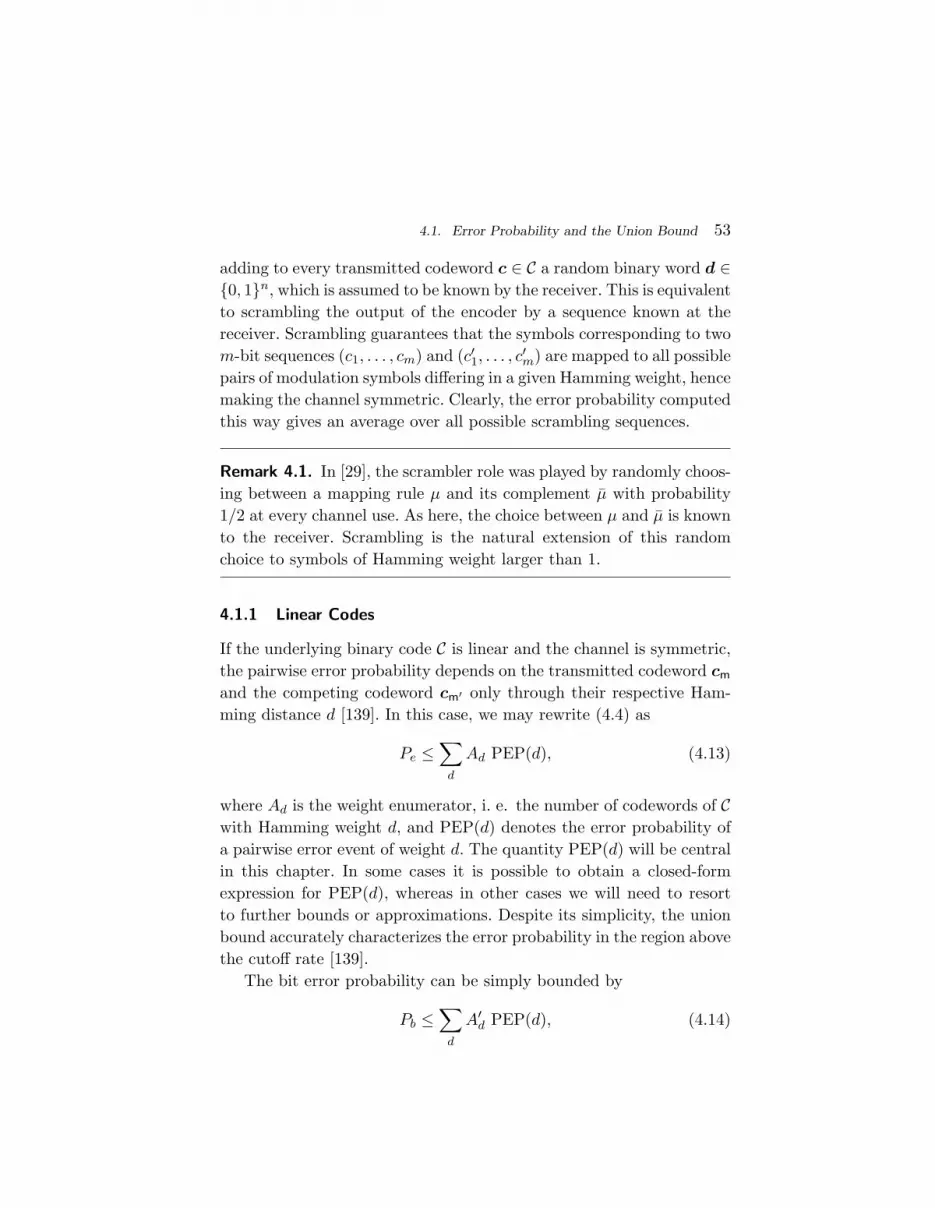
4.1. Error Probability and the Union Bound 53
adding to every transmitted codeword c ∈ C a random binary word d ∈{0, 1}n, which is assumed to be known by the receiver. This is equivalentto scrambling the output of the encoder by a sequence known at thereceiver. Scrambling guarantees that the symbols corresponding to twom-bit sequences (c1, . . . , cm) and (c′1, . . . , c
′m) are mapped to all possible
pairs of modulation symbols differing in a given Hamming weight, hencemaking the channel symmetric. Clearly, the error probability computedthis way gives an average over all possible scrambling sequences.
Remark 4.1. In [29], the scrambler role was played by randomly choos-ing between a mapping rule µ and its complement µ with probability1/2 at every channel use. As here, the choice between µ and µ is knownto the receiver. Scrambling is the natural extension of this randomchoice to symbols of Hamming weight larger than 1.
4.1.1 Linear Codes
If the underlying binary code C is linear and the channel is symmetric,the pairwise error probability depends on the transmitted codeword cm
and the competing codeword cm′ only through their respective Ham-ming distance d [139]. In this case, we may rewrite (4.4) as
Pe ≤∑
d
Ad PEP(d), (4.13)
where Ad is the weight enumerator, i. e. the number of codewords of Cwith Hamming weight d, and PEP(d) denotes the error probability ofa pairwise error event of weight d. The quantity PEP(d) will be centralin this chapter. In some cases it is possible to obtain a closed-formexpression for PEP(d), whereas in other cases we will need to resortto further bounds or approximations. Despite its simplicity, the unionbound accurately characterizes the error probability in the region abovethe cutoff rate [139].
The bit error probability can be simply bounded by
Pb ≤∑
d
A′d PEP(d), (4.14)

54 Error Probability Analysis
whereA′d
∆=∑
i
i
nAi,d, (4.15)
where Ai,d is the input-output weight enumerator, i. e. number of code-words of C of Hamming weight d generated with information messagesof Hamming weight i.
4.1.2 Cumulant Transforms of Symbol Scores
In this section, we introduce the definition of the cumulant transformand apply it to the symbol scores. The cumulant transform of the sym-bol and bit scores, compared to other equivalent representations suchas the characteristic function of the moment generating function, willshow particularly convenient in accurately approximating the pairwiseerror probability with the saddlepoint approximation [28,57].
Let U be a random variable. Then, for s ∈ C we define its cumulanttransform as [28,57]
κ(s) ∆= log E[esU]. (4.16)
The cumulant transform is an equivalent representation of the proba-bility density function. Whenever needed, the density can be recoveredby an inverse Fourier transform.
The derivatives of the cumulant transform are respectively denotedby κ′(s), κ′′(s), κ′′′(s), and κ(ν)(s) for ν > 3.
In Eq. (4.9) we expressed the pairwise decoding score as a sum ofnon-zero symbol scores, each of them corresponding to a symbol wherethe codewods differ in at least 1 bit. Since there are m bits in the binarylabel, there are m classes of symbol scores, one for each of the possibleHamming weigths. Consider a symbol score of weight v, 1 ≤ v ≤ m.
Definition 4.1. The cumulant transform of a symbol score Ξs withHamming weight v, denoted by κv(s), is given by
κv(s) = log E[es Ξs]
= log
(1(mv
) ∑j=(j1,...,jv)
12v
∑b∈{0,1}v
E
[∏vi=1 qji(bji , Y )s∏vi=1 qji(bji , Y )s
]), (4.17)
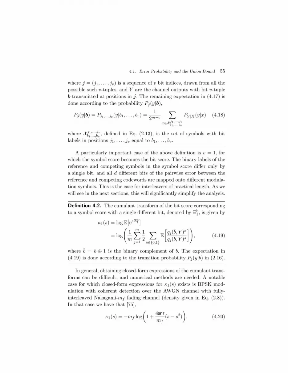
4.1. Error Probability and the Union Bound 55
where j = (j1, . . . , jv) is a sequence of v bit indices, drawn from all thepossible such v-tuples, and Y are the channel outputs with bit v-tupleb transmitted at positions in j. The remaining expectation in (4.17) isdone according to the probability Pj(y|b),
Pj(y|b) = Pj1,...,jv(y|b1, . . . , bv) =1
2m−v
∑x∈X j1,...,jv
b1,...,bv
PY |X(y|x) (4.18)
where X j1,...,jv
b1,...,bv, defined in Eq. (2.13), is the set of symbols with bit
labels in positions j1, . . . , jv equal to b1, . . . , bv.
A particularly important case of the above definition is v = 1, forwhich the symbol score becomes the bit score. The binary labels of thereference and competing symbols in the symbol score differ only bya single bit, and all d different bits of the pairwise error between thereference and competing codewords are mapped onto different modula-tion symbols. This is the case for interleavers of practical length. As wewill see in the next sections, this will significantly simplify the analysis.
Definition 4.2. The cumulant transform of the bit score correspondingto a symbol score with a single different bit, denoted by Ξb
1 , is given by
κ1(s) = log E[es Ξb
1]
= log
(1m
m∑j=1
12
∑b∈{0,1}
E[qj(b, Y )s
qj(b, Y )s
]), (4.19)
where b = b ⊕ 1 is the binary complement of b. The expectation in(4.19) is done according to the transition probability Pj(y|b) in (2.16).
In general, obtaining closed-form expressions of the cumulant trans-forms can be difficult, and numerical methods are needed. A notablecase for which closed-form expressions for κ1(s) exists is BPSK mod-ulation with coherent detection over the AWGN channel with fully-interleaved Nakagami-mf fading channel (density given in Eq. (2.8)).In that case we have that [75],
κ1(s) = −mf log(
1 +4snr
mf(s− s2)
). (4.20)

56 Error Probability Analysis
As mf →∞, we have that κ1(s)→ −4snr(s−s2), which corresponds tothe cumulant transform of a Gaussian random variable of mean −4snr
and variance 8snr, the density of a log-likelihood ratio in this channel[119]. Another exception, although significantly more complicated thanthe above, is BICM over the Gaussian and fully-interleaved channelswith max-log metric. In this case, as shown in [112] and referencestherein, the probability density function of Ξb
1 can be computed inclosed-form. As we will see, only the cumulant transform is neededto accurately approximate the error probability. Moreover, we can useefficient numerical methods based on Gaussian quadratures to computeit.
As we shall see in the coming sections, the error events that domi-nate the error probability for large SNR are those that assign multipledifferent bits to the same symbol, i. e. v > 1. For large SNR the curveschange slope accordingly. Fortunately, this effect shows in error proba-bility values of interest only for short interleaver lengths, and assumingsymbols of weight 1 is sufficient for most practical purposes. Whereshort lengths are required, random interleaving can cause performancedegradation due to these effects and an interleaving must be designedto allocate all different bits in the the smaller distance pairwise errorsto different constellation symbols.
Figure 4.1 shows the computer-simulated density of Ξb1 for BICM
using the MAP metric, 16-QAM with Gray mapping in the AWGNand fully-interleaved Rayleigh fading channels, respectively, both withsnr = 10 dB. For the sake of comparison, we also show with dashedlines the distribution of a Gaussian random variable with distributionN (−4snreq, 8snreq), where snreq = −κ1(s) is the equivalent signal-to-noise ratio. This Gaussian approximation is valid in the tail of thedistribution, rather than at the mean as would be the case for thestandard Gaussian approximation (dash-dotted lines) with the samemean and variance as that of Ξb
1 , i. e. N(E[Ξb
1 ],E[(Ξb1)
2]−E[Ξb1 ]
2). For
AWGN, the tail of Ξb1 is close to the Gaussian approximation, and re-
mains similar for Rayleigh fading. Since the tail gives the pairwise errorprobability, this Gaussian approximation gives a good approximation tothe latter. This Gaussian approximation, which will be properly intro-

4.1. Error Probability and the Union Bound 57
−40 −30 −20 −10 0 1010
−4
10−3
10−2
10−1
100
Ξb
1
(a) No fading.
−40 −30 −20 −10 0 1010
−4
10−3
10−2
10−1
100
Ξb
1
(b) Fully-interleaved Rayleigh fading.
Fig. 4.1 Simulated density of Ξb1 for BICM with MAP metric, 16-QAM with Gray map-
ping with snr = 10 dB. The solid lines correspond to the simulated density, dashed linescorrespond to the Gaussian approximation N (−4snreq, 8snreq), with snreq = −κ1(s), anddash-dotted lines correspond to the Gaussian approximation N
`E[Ξb
1 ], E[(Ξb1)2]− E[Ξb
1 ]2´.

58 Error Probability Analysis
duced in the next section, illustrates the benefits of using the cumulanttransform to compute the pairwise error probability.
4.2 Pairwise Error Probability for Infinite Interleaving
In this section, we study the pairwise error probability assuminginfinite-length interleaving [29]. As we saw in the previous chapter,this channel model does not fully characterize the fundamental limitsof BICM. While the model yields the same capacity, the error expo-nent is in general different. In this and the following sections, we shallsee that this model characterizes fairly accurately the error probabilityfor medium-to-large signal-to-noise ratios when the union bound is em-ployed. However, as shown in Section 4.3, for very large signal-to-noiseratio this model does not capture the overall error behavior, and moregeneral techniques must be sought. Infinite-length interleaving impliesthat all d different bits in a pairwise error event are mapped onto d dif-ferent symbols, i. e. there are no symbols with label-Hamming-weightlarger than 1. We will first review expressions, bounds and approxima-tions to the pairwise error probability, and we will then apply them tocompute the union bound.
4.2.1 Exact Formulas, Bounds, and Approximations
We denote the pairwise error probability for infinite interleaving asPEP1(d). We first relate it to the pairwise score Ξpw. We denote thecumulant transform of the pairwise score by
κpw(s) ∆= log E[es Ξpw]. (4.21)
Under the assumption that bit scores are independent and identicallydistributed, we have that
κpw(s) = d κ1(s). (4.22)
Since the pairwise error probability is the tail probability of the pairwisescore, we have that,
PEP1(d) = Pr
{d∑
i=1
Ξbi > 0
}(4.23)

4.2. Pairwise Error Probability for Infinite Interleaving 59
where the variables Ξbi are bit scores corresponding to the d different
bits in the pairwise error.The above pairwise tail probability can be evaluated by complex-
plane integration of the cumulant transform of κpw(s) = dκ1(s), amethod advocated by Biglieri et al. [18, 19]. We have that
Proposition 4.2. The pairwise error probability PEP1(d) is given by
PEP1(d) =1
2πj
∫ s0+j∞
s0−j∞
1s
ed κ1(s) ds, (4.24)
where s0 ∈ R belongs to region where the cumulant transform κ1(s) iswell defined.
In [18], the numerical evaluation of the above complex-plane integrationusing Gaussian quadrature rules was proposed.
As we next review, the tail probability of the pairwise or the symbolscores is to a large extent determined by the form of the cumulanttransform around a special value of s, the saddlepoint s.
Definition 4.3. The saddlepoint s is the value of s that makes the firstderivative of the cumulant transform, κ′(s) equal to zero.
An expression often used is the Chernoff bound, which gives thefollowing upper bound to the pairwise error probability.
Proposition 4.3 (Chernoff Bound). The Chernoff bound to the pair-wise error probability is
PEP1(d) ≤ edκ1(s), (4.25)
where s, the saddlepoint, is the root of the equation κ′1(s) = 0.
In general, one needs to find the saddlepoint either analytically or nu-merically. As we shall see in Section 4.2.2, the choice s = 1
2 is optimumfor the MAP BICM metric. We also note that the optimum value ofs for the random coding error exponent at vanishing rate (or equiva-lently at the cutoff rate) is s = 1
2 (for s = 1/(1 + ρ) and ρ = 1). This

60 Error Probability Analysis
is not surprising since the error exponent analysis and our pairwiseerror probability are closely related. A somewhat looser version of theChernoff bound for general metrics is the Bhatthacharyya bound, forwhich one replaces s in (4.25) by 1
2 , as if the saddlepoint was s = 12 (we
remark that for general metrics and channels s 6= 12).
The Chernoff bound gives a true bound and is moreover easy tocompute. It is further known to correctly give the asymptotic expo-nential decay of the error probability for large d and snr [74, 95]. Insome cases, such as the AWGN or fully interleaved fading channels,the Chernoff bound is not tight. This looseness can be compensatedfor in practice by using the saddlepoint approximation.
Theorem 4.1. The pairwise error probability can be approximated tofirst-order by
PEP1(d) '1√
2πdκ′′1(s) sed κ1(s) (4.26)
where κ′′1(s) is the second derivative of κ(s), and s is the saddlepoint.
The saddlepoint approximation may also be seen as an approxima-tion of the complex-plane integration of Proposition 4.2. Essentially,the function κ1(s) is approximated by a second-order Taylor expansionat the saddlepoint, neglecting higher order terms, and the resultingintegral is explicitly computed.
Alternatively, the saddlepoint approximation extends the Chernoffbound by including a multiplicative coefficient to obtain an expressionof the form α · edκ1(s). Higher-order expansions have a correction factorα, polynomial in inverse powers of
(dκ′′1(s)
)−1. For instance, for thesecond-order approximation we have
α = 1 +1
dκ′′1(s)
(− 1s2− κ′′′1 (s)
2sκ′′1(s)+κ
(4)1 (s)
8κ′′1(s)− 15
72
(κ′′′1 (s)κ′′1(s)
))2
. (4.27)
In general, and for the purpose of evaluating the error probability ofBICM, the effect of the higher-order correction terms is found to benegligible and the formula in Eq. (4.26) gives a good approximation.
For the sake of completeness, we also mention two additional ap-

4.2. Pairwise Error Probability for Infinite Interleaving 61
proximations. First, the Lugannani-Rice formula [68] (see also [78]),
PEP1(d) ' Q(√−2dκ1(s)
)(4.28)
+1√2π
edκ1(s)
(1√
dκ′′1(s)s− 1√
−2dκ1(s)
), (4.29)
Finally, we have a Gaussian approximation
PEP1(d) ' Q(√−2dκ(s)
). (4.30)
This approximation equals the zero-th order term in the Lugannani-Rice formula and the error probability of a BPSK AWGN channel withequivalent signal-to-noise ratio snreq = −κ(s). This approximation washeuristically introduced in [50], and is precisely the Gaussian approxi-mation depicted in Figure 4.1.
In the following, we particularize the above results to the MAP andmax-log metrics in Eqs. (2.15) and (2.17) respectively.
4.2.2 MAP Demodulator
In this section, we study the MAP metric, i. e.
qj(bj(x) = b, y
)=∑
x′∈X jb
PY |X(y|x′). (4.31)
First, we relate the BICM channel with MAP metric to the familyof binary-input output-symmetric channels. Recall that the standarddefinition of BIOS channels starts with the posterior log-likelihood ratio
Λ = logPC|Y (c = 1|y)PC|Y (c = 0|y)
. (4.32)
Then, a channel with binary input is said output-symmetric [96] if thefollowing relation between the densities of the posterior log-likelihoodratios, seen as function the channel input, holds:
PΛ|C(Λ|c = 1) = PΛ|C(−Λ|c = 0). (4.33)
By construction, bit score and posterior log-likelihood ratio coincidewhen the transmitted bit is zero, i. e. Λ = Ξb. Similarly, we have thatΛ = −Ξb when the transmitted bit is one.

62 Error Probability Analysis
Proposition 4.4. The classical BICM model with infinite interleavingand MAP metric is a binary-input output-symmetric (BIOS) channel.
In addition, we have the following result.
Proposition 4.5. The saddlepoint is located at s = 12 , i. e. κ′1
(12
)= 0.
The following higher-order derivatives of the cumulant transform verify
κ′′1(s) =E[(Ξb)2esΞb]E[esΞb
] ≥ 0, κ′′′1 (s) =E[(Ξb)3esΞb]E[esΞb
] = 0. (4.34)
Proof. See Appendix 4.A.
Using Definition 4.2 and Theorem 4.1 we can write the saddlepointapproximation to PEP1(d) for BICM with infinite interleaving in thefully-interleaved AWGN fading channel:
PEP1(d) '2√
2πdE[e
12Ξb(Ξb)2
] (E[e12Ξb
])d+ 1
2 , (4.35)
where Ξb is the bit score. In the fully-interleaved AWGN fading channel,we have that
Ξb = logqj(b,√
snrhx+ z)
qj(b,√
snrhx+ z) (4.36)
= log
∑x′∈X j
b
e−|√
snrh(x−x′)+z|2∑x′∈X j
be−|
√snrh(x−x′)+z|2 . (4.37)
The expectation of a generic function f(·) of the bit score Ξb is doneaccording to
E[f(Ξb)] =1
m2m
1∑b=0
m∑j=1
∑x∈X j
b
∫∫f(Ξb) pdH(h)PZ(z) dzdh. (4.38)
This expectation can be easily evaluated by numerical integration usingthe appropriate quadrature rules. Unfortunately, there seems to be no

4.2. Pairwise Error Probability for Infinite Interleaving 63
tractable, simple expression for the final result. The only case in which(4.35) admits a closed form is the case of binary BPSK modulationwith Nakagami-mf fading for which using (4.20) we obtain [75],
PEP1(d) '1
2√πd snr
(1 +
snr
mf
)−mf d+ 12
. (4.39)
The exact expression of PEP1(d) from Proposition 4.2 or the Cher-noff bound in Proposition 4.3 admits a form similar to (4.35). In partic-ular, since in this case s = 1
2 , the Chernoff and Bhattacharyya boundscoincide. This Bhattacharyya union bound was first proposed in [29].
We next compare the estimate of PEP1(d) with the BICM expur-gated bound of [29]. The expurgated bound can be seen as the positivetail probability of the random variable with sample value
logPY |X(y|x)PY |X(y|x)
, (4.40)
where x is the transmitted symbol and x is its nearest neighbour in X j
b,
i. e., with complementary bit b in label index j. Compared with theMAP metric there is only one term in each summation, rather than thefull set X j
b . For some metrics and/or labelings, Eq. (4.40) may not beaccurate. For example, for the set-partitioning mapping considered in[29], the bound was not close to the simulation results. This inaccuracywas solved in [74] by using the saddlepoint approximation with the fullMAP metric given in (4.35). The inaccuracy of the expurgated boundwas also remarked by Sethuraman [104] and Yeh al. [141] who noticedthat this “bound” is actually not a bound in general. A further pointis discussed in Section 4.3.4, where we analyze the effect of consideringonly Hamming weight 1.
We next show some examples to illustrate the accuracy of thesebounds and approximations for convolutional and repeat-accumulate(RA) codes [32]. In particular, we show the Chernoff/Bhattacharyyaunion bound (dash-dotted lines), the saddlepoint approximation (4.35)union bound (solid lines), the Gaussian approximation union bound(dashed lines) and the simulations. In the case of RA codes, we use theuniform interleaver [8,9] and an iterative decoder with 20 decoding iter-

64 Error Probability Analysis
ations. The assumption of uniform interleaver allows for the analyticalcalculation of the weight enumerator coefficients (see [32]).
Figure 4.2 shows the bit error rate as a function of EbN0
for theaforementioned methods with 16-QAM in the AWGN channel withno fading. In Figure 4.2(a) we use the optimum 64-state and rate-1/2 convolutional code with Gray and set partitioning mappings andin Figure 4.2(b) an RA code of rate 1/4 with Gray mapping. As weobserve, the Chernoff/Bhattacharyya bound is loose when comparedwith the saddlepoint or Gaussian approximations, which are close tothe actual simulations for large Eb
N0. We notice that the saddlepoint
and Gaussian approximations are close to each other for the convolu-tional code. However, for RA codes, the Gaussian approximation yieldsa slightly optimistic estimate of the error floor region. As we will see inthe following examples, this effect is more visible in fading channels.
Figure 4.3 shows the estimates of the bit error rate for convolu-tional and RA codes respectively in a fully-interleaved AWGN channelwith Rayleigh fading. Figure 4.3(a) shows two cases, a rate-2/3, 8-statecode over 8-PSK, and the rate-1/2, 64-state code over 16-QAM bothwith Gray mapping (both codes have largest Hamming distance). Fig-ure 4.3(b) shows the performance of a RA code of rate 1/4 with Graymapping and 16-QAM modulation. All approximations are close to thesimulated value, but now only the saddlepoint approximation gives anaccurate estimate of the error probability. As we saw in Section 4.1.2,and in Figure 4.1(b) to be more precise, the tail of the bit score in thefully-interleaved Rayleigh fading channel is approximately exponential,rather than Gaussian, and this shape is not accurately tracked by theGaussian approximation. As evidenced by the results of 16-QAM withthe 64-state convolutional code, this effect becomes less apparent forcodes with large minimum distance, since the pairwise score containsmore terms and its tail is closer to a Gaussian. For RA codes, wherethe minimum distance is low, we appreciate the differences betweensaddlepoint and Gaussian approximations.
In the following section, we discuss in more detail the slope of decayof the error probability for large snr, by studying the asymptotic be-havior of the cumulant transform and its second derivative evaluated atthe saddlepoint. This analysis reveals that BICM mimics the behavior
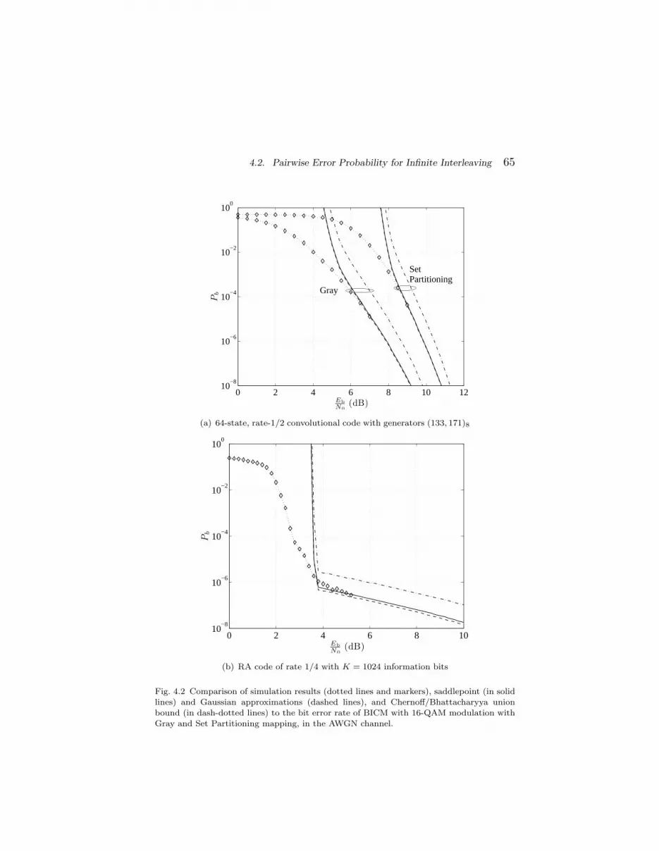
4.2. Pairwise Error Probability for Infinite Interleaving 65
0 2 4 6 8 10 1210
−8
10−6
10−4
10−2
100
Eb
N0
(dB)
Pb Gray
SetPartitioning
(a) 64-state, rate-1/2 convolutional code with generators (133, 171)8
0 2 4 6 8 1010
−8
10−6
10−4
10−2
100
Eb
N0
(dB)
Pb
(b) RA code of rate 1/4 with K = 1024 information bits
Fig. 4.2 Comparison of simulation results (dotted lines and markers), saddlepoint (in solidlines) and Gaussian approximations (dashed lines), and Chernoff/Bhattacharyya unionbound (in dash-dotted lines) to the bit error rate of BICM with 16-QAM modulation withGray and Set Partitioning mapping, in the AWGN channel.

66 Error Probability Analysis
0 2 4 6 8 10 12 14 16 1810
−8
10−6
10−4
10−2
100
Eb
N0
(dB)
Pb
16−QAM
8−PSK
(a) 64-state, rate-1/2 convolutional code with generators (133, 171)8over 16-QAM modulation with Gray labeling and optimum 8-staterate-2/3 convolutional code with 8-PSK and Gray labeling
0 2 4 6 8 10
10−6
10−4
10−2
100
Eb
N0
(dB)
Pb
(b) RA code of rate 1/4 with K = 512 information bits over 16-QAMmodulation with Gray mapping
Fig. 4.3 Comparison of simulation results (dotted lines and markers), saddlepoint (in solidlines) and Gaussian approximations (dashed lines), and Chernoff union bound (in dash-dotted lines) to the bit error rate of BICM in the fully-interleaved Rayleigh fading channel.

4.2. Pairwise Error Probability for Infinite Interleaving 67
of binary modulation, preserving the properties of the binary code.
4.2.3 Cumulant transform asymptotic analysis
Inspection of Figures 4.2 and 4.3 suggests that the bounds and approx-imations considered in the previous section yield the same asymptoticbehavior of the error probability for large snr. Indeed, BICM mimicsthe behavior of binary modulation, preserving the properties of thebinary code:
Proposition 4.6 ( [74]). The cumulant transform of the bit scores ofBICM transmitted over the AWGN with no fading and its secondderivative have the following limits for large snr
limsnr→∞
κ1(s)snr
= −d2X ,min
4(4.41)
limsnr→∞
κ′′1(s)snr
= 2d2X ,min, (4.42)
where d2X ,min
∆= minx,x′ |x − x′|2 is the minimum squared Euclideandistance of the signal constellation X .
For large snr, BICM behaves like a binary modulation with distanced2X ,min, regardless of the mapping. This result confirms that BICM
preserves the properties of the underlying binary code C, and that forlarge snr the error probability decays exponentially with snr as
PEP1(d) ' K e−14snr d2
X ,min (4.43)
Here K may depend on the mapping (see for example Figure 4.2(a)),but the exponent is not affected by it. To illustrate this point, Fig-ure 4.4 shows −κ(s)
snr (thick lines) and κ′′(s)snr (thin lines) for 16-QAM
with Gray (solid lines) and set partitioning (dashed lines) mappings inthe AWGN channel. As predicted by Proposition 4.6, the asymptoticvalue of −κ(s)
snr is −14d
2X ,min = 0.1 (recall that we consider signal constel-
lations X normalized in energy, and that d2X ,min = 0.4 for 16-QAM).
In the Gaussian approximation introduced in [50], the quantity −κ(s)snr
can be interpreted as a scaling in snr due to BICM; the asymptotic

68 Error Probability Analysis
−20 −10 0 10 20 3010
−2
10−1
100
101
snr (dB)
Fig. 4.4 Cumulant transform limits in the AWGN channel −κ(s)snr
(thick lines) andκ′′(s)
snr(thin lines) for 16-QAM with Gray (solid lines) and set partitioning (dashed lines) mappings.For fully-interleaved Rayleigh fading channel, in dash-dotted lines κ′′(s) for 16-QAM andin dotted lines for 8-PSK.
scaling depends only on the signal constellation, but not on the binarylabeling. Figure 4.4 also shows κ′′(s)
snr for the same setup (thin lines).Again, the limit coincides with (4.42).
In the case of Nakagami-mf fading (density in Eq. (2.8)), we have asimilar result. All curves in Figures 4.3(a) and 4.3(b) show an asymp-totic slope of decay, which is characterized by the following proposition.
Proposition 4.7 ( [74]). The cumulant transform of BICM transmit-ted over the AWGN with fully-interleaved Nakagami-mf fading and itssecond derivative have the following limits for large snr
limsnr→∞
κ1(s)log snr
= −mf (4.44)
limsnr→∞
κ′′1(s) = 8mf . (4.45)

4.2. Pairwise Error Probability for Infinite Interleaving 69
The proof of this result is a straightforward extension of the proofin [74] for Rayleigh fading. The above result does not depend on themodulation nor the binary labeling, and confirms that BICM indeedbehaves as a binary modulation and thus, the asymptotic performancedepends on the Hamming distance of the the binary code C rather thanon the Euclidean distance. Figure 4.4 also shows κ′′(s) for 16-QAM(dash-dotted line) and 8-PSK (dotted line), both with Gray labeling inthe Rayleigh channel. As expected, the limit value is 8, which does notdepend on the modulation.
A finer approximation to the exponent of the error probability isgiven by the the following result.
Proposition 4.8. The cumulant transform of the BICM bit score forthe AWGN channel with fully-interleaved Nakagami-mf fading behavesfor large snr as
limsnr→∞
eκ1(s)
snr−mf= EX,J
[4mf
d2(x, x)
]mf
(4.46)
where x is the closest symbol in the constellation X j
bto x, d2(x, x) =
|x− x|2 is the Euclidean distance between two symbols and the expec-tation EX,J [·] is with respect to X uniform over X and J uniform overthe the label bit index j = 1, . . . ,m.
Proof. See Appendix 4.B.
The above expectation over the symbols is proportional to a formof harmonic distance d2
h,
1d2
h
=
(1
m 2m
1∑b=0
m∑j=1
∑x∈X j
b
(1
d2(x, x′)
)mf) 1
mf
, (4.47)
where x′ is the closest symbol in the constellation X j
bto x and d2(x, x′)
is the Euclidean distance between two symbols.The asymptotic results given by Propositions 4.7 and 4.8 can be
combined with the saddlepoint approximation (4.35) to produce a

70 Error Probability Analysis
heuristic approximation of PEP1(d) for large snr as,
PEP1(d) '1
2√πdmf
(4mf
d2hsnr
)dmf
. (4.48)
A similar harmonic distance was used by Caire et al. [29] to approxi-mate the Chernoff bound for Rician fading.
4.2.4 Numerical Results with Max-Log Metric
In this section, we study the error probability of BICM with the max-log metric in Eq. (2.17),
qj(bj(x) = b, y
)= max
x′∈X jb
PY |X(y|x′). (4.49)
As for the MAP metric, the saddlepoint approximation with infiniteinterleaving in the fully-interleaved AWGN fading channel is given by
PEP1(d) '2√
2πdE[esΞb(Ξb)2
] (E[esΞb])d+ 1
2 , (4.50)
where Ξb is the bit score, in turn given by
Ξb = minx′∈X j
b
|√
snrh(x− x′) + z|2 − minx′∈X j
b
|√
snrh(x− x′) + z|2. (4.51)
The saddlepoint s now needs to be found numerically, since in general,it will be different from that of the MAP metric, i. e. 1
2 . To any extent,as snr→∞ the saddlepoint approaches 1
2 , since the MAP and the max-log metrics become indistinguishable. This result builds on the proofsof Propositions 4.6 and 4.7 [74], where only the dominant term in theMAP metric is kept for large snr.
For this metric, Sczeszinski et al. [112] have derived closed expres-sions for the density of the bit score Ξb. This expression allows for thecalculation of the cumulant transform, however, it does not allow forthe direct evaluation of PEP1(d) and numerical methods are neededto either perform the numerical integration in (4.24) or compute thesaddlepoint, and hence the saddlepoint approximation (4.50).
Figure 4.5 shows the comparison between MAP and max-log metricsfor BICM with an RA code and 16-QAM. As we observe, the perfor-mance is with the max-log metric is marginally worse than that with

4.3. Pairwise Error Probability for Finite Interleaving 71
0 2 4 6 8 10
10−6
10−4
10−2
100
Eb
N0
(dB)
Pb
Fig. 4.5 Comparison of simulation results and saddlepoint approximations on the bit errorrate of BICM with a rate-1/4 RA code with K = 512 information bits, 16-QAM modulationwith Gray mapping, in the fully-interleaved Rayleigh fading channel using MAP (diamonds)and max-log (circles) metrics. In solid lines, saddlepoint approximation union bound.
the MAP metric. Note that we are using perfectly coherent detection.It should be remarked, though, that more significant penalties mightbe observed for larger constellations, in presence of channel estimationerrors, or in non-coherent detection (see Chapter 6).
4.3 Pairwise Error Probability for Finite Interleaving
4.3.1 Motivation
So far we have assumed, as it was done in [29], that the bit inter-leaver has infinite length. For this case, all symbol scores have Hammingweight 1 and are thus bit scores. Moreover, since the channel is mem-oryless, the bit scores with infinite interleaving are independent. Forfinite interleaving, however, some of the d bits in which the two code-words in the pairwise error event differ belong to the same symbol withnonzero probability. Therefore, they are affected by the same realiza-

72 Error Probability Analysis
tion of the channel noise and possibly fading, and are thus statisticallydependent. As we mentioned in Section 4.1, a general characterizationof the error probability requires the whole set of possible symbol scoresΞs, for all the valid Hamming weights v, 1 ≤ v ≤ min(m, d).
Since the task of determining the exact distribution of the d pairwisedifferent bits onto the N symbols can be hard, we follow the resultsof [141] and compute an average pairwise error probability by averagingover all possible distributions of d bits onto N symbols, equivalent touniform interleaving for turbo-codes [8, 9]. In Section 4.3.2 we presenta general expression for the pairwise error probability, as well as itscorresponding saddlepoint approximation.
In Section 4.3.3 we apply the theory to what is arguably the simplestcase of BICM, QPSK under Nakagami fading. We discuss the extent towhich QPSK can be modeled by two independent BPSK modulationseach with half signal-to-noise ratio. We show that the slope of thepairwise error probability is reduced at sufficiently high snr due to thesymbol scores of Hamming weight 2. An estimate of the snr at whichthis “floor” appears is given. Finally, we extend the main elements ofthe QPSK analysis to higher-order modulations in Section 4.3.4, wherewe discuss the presence of a floor in the error probabilities and give amethod to estimate the snr at which it appears.
4.3.2 A General Formula for the Pairwise Error Probability
In this section, we closely follow Yeh et al. [141] to give a generalcharacterization of the error probability. We distinguish the possibleways of allocating d bits on N modulation symbols, by counting thenumber of symbols with weight v, where 0 ≤ v ≤ w? and
w? ∆= min(m, d). (4.52)
Herem is the number of bits in the binary label of a modulation symbol.Denoting the number of symbols of weight v by Nv, we have that
w?∑v=0
Nv = N and d =w?∑v=1
vNv. (4.53)

4.3. Pairwise Error Probability for Finite Interleaving 73
We further denote the symbol pattern by ρN∆= (N0, . . . , Nw?). For
finite interleaving, every possible pattern corresponds to a (possibly)different conditional pairwise error probability, denoted by PEP(d, ρN ).Then, we can write the following union bound
Pe ≤∑
d
∑ρN
Ad,ρNPEP(d, ρN ) (4.54)
where Ad,ρNis the number of codewords of C of Hamming weight d
that are mapped onto the constellation symbols following patter ρN ,i. e. mapped onto Nv symbols of Hamming weight v, for 0 ≤ v ≤w?. In some cases where the exact location of the d different bits isdifficult to obtain, it might be interesting and convenient to study theaverage performance over all possible ways of choosing d locations in acodeword. In this case we have the following union bound
Pe ≤∑
d
Ad
∑ρN
P (ρN )PEP(d, ρN ) (4.55)
=∑
d
AdPEP(d) (4.56)
where P (ρN ) is the probability of a particular pattern ρN andPEP(d) ∆=
∑ρNP (ρN )PEP(d, ρN ) is the average pairwise error prob-
ability over all possible patterns. A counting argument [141] gives theprobability of the pattern ρN as
P (ρN ) ∆= Pr(ρN = (N0, . . . , Nw?)
)(4.57)
=
(m1
)N1(m2
)N2 · · ·(
mw?
)Nw?(mN
d
) N !N0!N1!N2! . . . Nw? !
. (4.58)
In general, the pairwise score depends on the pattern ρN ; ac-cordingly, we denote the cumulant transform of the symbol score byκpw(s, ρN ), to make the dependence on ρN explicit. We have that
κpw(s, ρN ) =w?∑v=1
Nvκv(s), (4.59)
since the symbol scores are independent. For infinite interleaving, wehave ρ∗N = (N−d, d, 0, . . . , 0), and we therefore recover the result shown

74 Error Probability Analysis
in the previous section, i. e. κpw(s, ρ∗N ) = dκ1(s). When N → ∞ andm > 1 the probability that the bit scores are dependent tends to zero,but does so relatively slowly, as proved by the following result.
Proposition 4.9 ( [73]). The probability that all d bits are indepen-dent, i. e. the probability of ρN = (N − d, d, 0, . . . ) is
Pind∆= Pr
(ρN = (N − d, d, 0, . . . )
)=md(N/m
d
)(Nd
) . (4.60)
Further, for large N , we have that
Pind ' e−d(d−1)(m−1)
2N ' 1− d(d− 1)(m− 1)2N
(4.61)
where the second approximation in (4.61) assumes that N � d.
For BPSK, or m = 1, there is no dependence, as it should be. How-ever, for m > 1 the probability of having symbol scores independent isnonzero. As we shall see in the following, this effect will induce a changein the slope of the error probability. It is important to remark that thisis an average result over the ensemble of all possible interleavers.
The conditional pairwise error probability is of fundamental impor-tance for this analysis, and we devote the rest of the section to its study.In particular we have a result analogous to Proposition 4.2 [141].
Proposition 4.10. The conditional pairwise error probability for a par-ticular pattern ρN can be computed as
PEP(d, ρN ) =1
2πj
∫ s0+j∞
s0−j∞
1s
eκpw(s,ρN ) ds (4.62)
where s0 ∈ R belongs to region where the cumulant transforms κv(s)are well defined.
Sethuraman et al. [104] pointed out that Caire’s union bound forBICM (which assumes infinite interleaving, that is our PEP1(d)), wasnot a true bound. Taking into account all possible patterns ρN solvesthis inconsistency and yields a true bound to the average pairwise errorprobability with a uniform interleaver.
A looser bound given by the following result.

4.3. Pairwise Error Probability for Finite Interleaving 75
Proposition 4.11 (Chernoff Bound). The Chernoff bound to the con-ditional pairwise error probability is
PEP(d, ρN ) ≤ edκpw(s,ρN ). (4.63)
where s, the saddlepoint, is the root of the equation κ′pw(s, ρN ) = 0.
Again, we can use the saddlepoint approximation to obtain a resultsimilar to that shown in Theorem 4.1.
Theorem 4.2. The conditional pairwise error probability can be ap-proximated to first-order by
PEP(d, ρN ) ' 1√2πκ′′pw(s, ρN )s
eκpw(s,ρN ). (4.64)
The saddlepoint s depends in general on the specific pattern ρN .In the following, we particularize the above analysis to QPSK with
Gray labeling in the fully-interleaved Nakagami-mf channel. This ispossibly the simplest case of dependency between the bit sub-channels,with symbol scores of Hamming weight 2.
4.3.3 QPSK with Gray Labeling as BICM
In this section, we analyze QPSK in fully interleaved Nakagami-mf
fading (for the density, see Eq. (2.8)) for finite block lengths. The sad-dlepoint approximation was evaluated in [73].
Theorem 4.3 ( [73]). The saddlepoint approximation correspondingto the average pairwise error probability PEP(d) of QPSK with code-word length N in Nakagami-mf fading is
PEP(d) '∑
N1,N2
P (ρN )
(1 + snr
2mf
)−mf N1(1 + snr
mf
)−mf N2√2π(N1
snr1+ snr
2mf
+N22snr
1+ snrmf
) (4.65)

76 Error Probability Analysis
where
P (ρN ) =2N1(2Nd
) N !(N − d+N2)!(d− 2N2)!N2!
(4.66)
and max(0, d−N) ≤ N2 ≤ bd/2c, N1 + 2N2 = d.
For the AWGN channel, as mf →∞, we have that
PEP(d) '∑
N1,N2
P (ρN )e−
snr2
(N1+2N2)√2πsnr(N1 + 2N2)
(4.67)
=e−d snr
2
√2πdsnr
, (4.68)
the usual exponential approximation to the error probability of BPSKat half signal-to-noise ratio. In the presence of fading, however, thesymbols of Hamming weight 2 have an important effect. The slope ofthe pairwise error probability changes at sufficiently large signal-to-noise ratio. The approximate signal-to-noise ratio at which the errorprobability changes slope, denoted by snrth, was estimated in [73],
snrth =
4m(
2Ne
81d d
) 1m
d even
4m(2Ne)1m
(e2
) 2m(d−1) (d−1)
dm(d−1) (d+1)
1m(d−1)
d2(d+1)m(d−1)
d odd.(4.69)
A coarse approximation to the bit error probability at the thresholdis derived by keeping only the term at minimum distance d and the twosummands with N2 = 0 and N2 = bd2c. We have then
Pb ' 2A′dPEP(d) ' A′d1√πmfd
(snrth2m
)−mf d
. (4.70)
Figure 4.6 depicts the bit error rate of QPSK with the (5, 7)8 con-volutional code for n = 40, 200 (N = 20, 100) and mf = 0.5. In allcases, the saddlepoint approximation to the union bound (solid lines)is accurate for large SNR. In particular, we observe the change in slopewith respect to the union bound using N2 = max{0, d−N} (the upperone corresponds to n = 200), i. e. assuming that all bits of the differ-ent codewords are mapped over different symbols (independent binary

4.3. Pairwise Error Probability for Finite Interleaving 77
0 10 20 30 40 50 6010
−12
10−10
10−8
10−6
10−4
10−2
100
Eb
N0
(dB)
Pb
N = 20
N = 100
Fig. 4.6 Bit error rate of the (5, 7)8 convolutional code over QPSK in a fully interleavedfading channel with mf = 0.5; uniform interleaver of length n = 40, 200 (N = 20, 100).Diamonds for the simulation, solid lines for the union bound, dashed lines for the unionbound assuming N2 = Nmin
2 = max{0, d−N} (the upper one corresponds to N = 100) anddotted lines for the union bound for N2 = b d
2c.
channels). The approximated thresholds (4.69) computed with the min-imum distance, namely snrth = 22 dB for N = 20 and snrth = 36 dBfor N = 100, are very close to the points where dashed and dottedlines cross. In the next section we generalize this result to higher ordermodulations.
Figure 4.7 depicts the approximate value of Pb (assuming A′d = 1)at the threshold signal-to-noise ratio for several values of mf and ` asa function of the minimum Hamming distance d. The error probabilityat the crossing rapidly becomes small, at values typically below theoperating point of common communication systems.
4.3.4 High-order Modulations: Asymptotic Analysis
In this section, we closely follow the analysis in [73] for general constel-lations and mappings, and estimate the signal-to-noise ratio at which

78 Error Probability Analysis
2 4 6 8 10 12 14 16 18 2010
−40
10−30
10−20
10−10
100
d
Pb
Fig. 4.7 Bit error probability of QPSK at the threshold signal-to-noise ratio snrth accordingto (4.70) as a function of the minimum Hamming distance d for several values of mf andn. The solid line corresponds to mf = 0.5, n = 100, the dashed line to mf = 0.5, n = 1000,the dash-dotted to mf = 3, n = 100 and the dotted to mf = 3, n = 1000.
the slope of the error probability changes.First, and in a similar vein to the asymptotic analysis presented in
Section 4.2.3 for v = 1, for sufficiently large snr, we can approximatethe Chernoff bound to the error probability in the AWGN channel by
eκv(s) ' e−14d2m(v)snr, (4.71)
where d2m(v) is given by
d2m(v) ∆= min
x∈X
(∑vi=1 |x− x′i|2
)2|∑v
i=1(x− x′i)|2 , x′i
∆= arg minx′∈X i
bi(x)
|x− x′|2. (4.72)
For v = 1, we recover d2m(1) = d2
X ,min.For the fully-interleaved Nakagami-mf fading channel, we have
eκv(s) '
(d2
h(v)snr
4mf
)−mf
, (4.73)

4.3. Pairwise Error Probability for Finite Interleaving 79
where d2h(v) is a generalization of the harmonic distance given by
1d2
h(v)=
(1(
mv
)2m
∑b
∑j
∑x∈X b
j
(|∑v
i=1(x− x′i)|2
(∑v
i=1 |x− x′i|2)2
)mf) 1
mf
. (4.74)
For a given x, x′i is the i-th symbol in the sequence of v symbols(x′1, . . . , x
′v) which have binary label cji at position ji and for which
the ratio |Pv
i=1(x−x′i)|Pvi=1 |x−x′i|2
is minimum among all possible such sequences.
For mf = 1, v = 1 we recover the harmonic distance d2h in Section 4.2.3.
As it happened with the bit score and PEP1(d), Eq. (4.73) may bein the saddlepoint approximation to obtain a heuristic approximationto the pairwise error probability for large snr, namely
PEP(d, ρn) ' PEPH(d, ρn) ∆=1
2√πmf
∑v≥1 nv
m∏v=1
(4mf
d2h(v)
1snr
)nvmf
.
(4.75)We use Eq. (4.75) to estimate the threshold SNR. For the sake
of simplicity, consider d ≥ m, that is w? = m in our definitions atthe beginning of this Section. Then, since d =
∑mv=1Nvv by con-
struction, we can view the pattern ρN = (N0, N1, . . . , Nm) as a (non-unique) representation of the integer d as a weighted sum of the integers{0, 1, 2, . . . ,m}. By construction, the sum
∑v Nv is the number of non-
zero Hamming weight symbols in the candidate codeword. The lowestvalue of
∑v Nv gives the worst (flattest) pairwise error probability in
the presence of fading. As found in [73], a good approximation to thethreshold is given by
snrth ' 4mf
( ∑ρn:min
Pv nv
P (ρn)(d2
h(1))d
P (ρ0)∏
v
(d2
h(v))nv
)− 1mf (d−
Pv nv)
. (4.76)
For QPSK with Gray mapping, computation of this value of snrth(d2
h(1) = 2, d2h(2) = 4) gives a result which is consistent with the result
derived in Section 4.3.3, namely Eq. (4.69), with the minor differencethat we use now the Chernoff bound whereas the saddlepoint approxi-mation was used in the QPSK case.

80 Error Probability Analysis
10 15 20 25 30 35 4010
−12
10−10
10−8
10−6
10−4
10−2
100
N = 30
N = 100
N = 1000
N = ∞
Eb
N0
(dB)
Pb
Fig. 4.8 Bit error probability union bounds and bit-error rate simulations of 8-PSK withthe 8-state rate-2/3 convolutional code in a fully-interleaved Rayleigh fading channel. In-terleaver length N = 30 (circles) and N = 1000 (diamonds). In solid lines, the saddlepointapproximation union bounds for N = 30, N = 100, N = 1000 and for infinite interleaving,with PEP1(d). In dashed, dashed-dotted, and dotted lines, the heuristic approximationswith weight v = 1, 2, 3 respectively.
Figure 4.8 shows the error performance of 8-PSK with Rayleighfading and Gray labeling; the code is the optimum 8-state rate-2/3convolutional code, with dmin = 4. Again, an error floor appears dueto the probability of having symbol scores of Hamming weight largerthan 1. The figure depicts simulation results (for interleaver sizes n =90, 1000) together with the saddlepoint approximations for finite N (forN = 30, 100, 1000), infinite interleaving (with PEP1(d)), and with theheuristic approximation PEPH(d, ρn) (only for n = 90 and d = 4).
For 8-PSK with Gray mapping, evaluation of Eq. (4.74) givesd2
h(1) = 0.7664, d2h(2) = 1.7175, and d2
h(3) = 2.4278. Table 4.1 givesthe values of P (ρn) for the various patterns ρn. Table 4.1 also gives thethreshold snrth given in Eq. (4.76) for all possible values of
∑v≥1 nv,

4.4. Bounds and Approximations Above the Cutoff Rate 81
Table 4.1 Asymptotic analysis for 8-PSK with varying interleaver length n = 3N andminimum distance d = 4.
Pattern ρn n P (ρn) Threshold EbN0
(dB)
(N − 4, 4, 0, 0) n = 90 0.8688 N/An = 300 0.9602 N/An = 3000 0.9960 N/A
(N − 3, 2, 1, 0) n = 90 0.1287 16.0n = 300 0.0396 21.5n = 3000 0.0040 31.6
(N − 2, 0, 2, 0), n = 90 0.0015 20.5(N − 1, 1, 0, 1) n = 300 0.0002 26.0
n = 3000 2 · 10−6 39.1
not only for the worst case. We observe that the main flattening of theerror probability takes place at high snr. This effect essentially disap-pears for interleavers of practical length: for n = 100 (resp. n = 1000)the error probability at the first threshold is about 10−8 (resp. 10−12).The saddlepoint approximation is remarkably precise; the heuristic ap-proximation PEPH(dmin, ρn) also gives very good results.
4.4 Bounds and Approximations Above the Cutoff Rate
Spurred by the appearance of turbo-codes [11] and the rediscovery ofLDPC codes [69], there has been renewed interest in the past decadein the derivation of improved bounds for a region above the cutoff rate.A comprehensive review can be found in the monograph by Sason andShamai [101]. In this section, we briefly discuss such bounds for BICM.
Of the available improved bounds, two are of special importance: thesecond Duman-Salehi (DS2) bound and the tangential sphere bound(TSB). The first bound, valid for general decoding metrics and chan-nels, is directly applicable to BICM. The TSB is known to be thetightest bound in binary-input AWGN channels, and will be combinedwith the Gaussian approximation introduced in Section 4.2.
The error probability was analyzed in Section 3.1.2 for an ensemble

82 Error Probability Analysis
of random codes. For a fixed binary code C, we consider the averageover all possible interleavers πn of length n and over all the scramblingsequences d described in Section 4.1. We denote the joint probabilityof the interleaver and the scrambling by P (πn,d). For a fixed messagem (and binary codeword cm), the transmitted codeword xm dependson the interleaver πn and on the scrambling sequence d. The condi-tional error probability Pe(m), when message m and codeword cm aretransmitted, can be derived from Eqs. (3.7) and (3.11), to obtain
Pe(m) ≤∑πn,d
P (πn,d)∫
yPY |X(y|xm)
∑m′ 6=m
(q(xm′ ,y)q(xm,y)
)sρ
dy
(4.77)
for 0 ≤ ρ ≤ 1 and s > 0.The Duman-Salehi bound is derived by introducing a normalized
measure ψ(y) (possibly dependent on the codeword cm), and trans-forming the integral in Eq. (4.77) as
∫yPY |X(y|xm)
ψ(y)ψ(y)
∑m′ 6=m
(q(xm′ ,y)q(xm,y)
)sρ
dy (4.78)
=∫
yψ(y)
∑m′ 6=m
PY |X(y|xm)1ρ
ψ(y)1ρ
(q(xm′ ,y)q(xm,y)
)sρ
dy.
(4.79)
Now, applying Jensen’s inequality we obtain
Pe(m) ≤
∑m′ 6=m
∑πn,d
P (πn,d)∫
y
PY |X(y|xm)1ρ
ψ(y)1ρ−1
(q(xm′ ,y)q(xm,y)
)s
dy
ρ
.
(4.80)
Next, we consider a decomposition ψ(y) =∏N
n=1 ψ(yn). We alsoassume that the all-zero binary codeword is transmitted, and groupthe summands m′ having the same Hamming weight d together. Recallthat Ad denotes the number of codewords with Hamming weight d andthat ρN = (N0, . . . , Nw?), with w? = min(m, d), denotes the pattern

4.4. Bounds and Approximations Above the Cutoff Rate 83
representing the allocation of d bits onto the N modulation symbols.The average over all possible patterns is equivalent to the average overall possible interleavers πn. We thus have
∑πn,d
P (πn,d)∫
y
PY |X(y|xm)1ρ
ψ(y)1ρ−1
(q(xm′ ,y)q(xm,y)
)s
dy =∑ρN
P (ρN )w?∏v=0
Ps(v)ρN (v),
(4.81)
where Ps(v) is defined as
Ps(v)∆=
1(mv
)2m
∑j
∑b
∑x∈X b
j
∫y
PY |X(y|x)1ρ
ψ(y)1ρ−1
(v∏
i=1
qji(bji , y)qji(bji , y)
)s
dy.
(4.82)
In particular, for v = 0 (for which the metrics q(xm, y) and q(xm′ , y)coincide) and v = 1 (for which the metrics differ in only 1 bit), we have
Ps(0) =1
2m
∑x∈X
∫y
PY |X(y|x)1ρ
ψ(y)1ρ−1
dy (4.83)
Ps(1) =1
m2m
m∑j=1
∑b∈{0,1}
∑x∈X b
j
∫y
PY |X(y|x)1ρ
ψ(y)1ρ−1
(qj(b, y)qj(b, y)
)s
dy. (4.84)
Finally, since the computation does not depend on the transmittedmessage, we have that the average error probability is bounded as
Pe ≤
(∑d
Ad
∑ρN
P (ρN )w?∏v=0
Ps(v)ρN (v)
)ρ
, (4.85)
for all possible choices of ρ and ψ. For the specific choice ρ = 1, thefunction ψ is inactive, and the functions Ps(v) are simply a Chernoffbound to the symbol score Ξs of weight v (see Definition 4.1).
As for the tangential sphere bound, the Gaussian approximation tothe bit score discussed in Section 4.2 was used in [50] to give an approx-imation to the average error probability in the AWGN channel (see alsoEq. (4.30)) . This analysis involves two approximations. First, all thesymbol decoding scores of weight larger than 1 are neglected. Secondly,

84 Error Probability Analysis
the bit score is assumed to be Gaussian with equivalent signal-to-noiseratio snreq = −κ1(s) for all values of the score, not only the tail, sothat distances between codewords follow a chi-square distribution. Theresulting approximation is then given by
Pe ≤ Q(√−2nκ1(s)
)+∫ ∞
−∞
dΞb
√2π
e−(Ξb)2
2
(1− Γ
(n− 1
2,r2
2
))+∑
d
Ad
∫ ∞
−∞
dΞb
√2π
e−(Ξb)2
2 Γ(n− 2
2,r2 − β2
d
2
)(Q(βd
)−Q(r)
),
(4.86)
where n = mN , and we have used that
r∆=(√−2nκ1(s)− Ξb
)tan θ, (4.87)
βd∆=(√−2nκ1(s)− Ξb
)tanφ, (4.88)
where tanφ =√
dn−d and tan θ is the solution of
∑d
Ad
∫ arccos tan φtan θ
0sinn−3 θ dθ =
√πΓ(
n−22
)Γ(
n−12
) , (4.89)
and the coefficients Ad are Ad = Ad if βd < r and Ad = 0 otherwise.Figure 4.9 shows the comparison between the simulation, saddle-
point approximation and the TSB with the Gaussian approximation foran RA code with 16-QAM with Gray mapping in the fully-interleavedRayleigh fading channel. As we observe, the TSB with the Gaussian ap-proximation yields an underestimation of the error floor, and gives anestimate of the error probability for low SNR. Unfortunately, validatingthe tightness of this approximation at low SNR is difficult, chiefly be-cause of the use of approximations and of the suboptimality of iterativedecoding compared to maximum-metric decoding.
4.5 Concluding Remarks and Related Work
In this Chapter, we have reviewed the error probability analysis ofBICM. After considering the traditional error probability analysis ofBICM based on the independent parallel channel model [29], we have

4.5. Concluding Remarks and Related Work 85
0 2 4 6 8 10
10−6
10−4
10−2
100
Eb
N0
(dB)
Pe
Fig. 4.9 Comparison of simulation results and saddlepoint (solid line) and TSB Gaussianapproximations (dash-dotted line) on the bit error rate of BICM with an RA code of rate1/4 with K = 512 information bits, 16-QAM modulation with Gray mapping, in the fully-interleaved AWGN Rayleigh fading channel.
presented a number of bounds and approximations to the error proba-bility based on a union bound approach. In particular, we have shownthat the saddlepoint approximation yields accurate results and is sim-ple to compute. In passing, we have also seen why the expurgatedbound proposed in [29] is not a true bound [104]. Next, and basedon [141], we have considered the average over all possible interleavers(the uniform interleaver from turbo codes [8, 9]), and have shown thatfor interleavers of short length, the error probability is dominated bythe symbols with Hamming weight larger than 1. This effect translatesinto a reduced rate of decay of the error probability with SNR. Wehave then reviewed improved bounds to the error probability like theDuman-Salehi and the tangential-sphere bound [101]. We have giventhe expression of the former for a general decoding metric, while thelatter is an approximate bound based on the Gaussian approximationof the tail of the decoding score distribution.

86 Error Probability Analysis
Bounding techniques similar to those presented in this Chapter havebeen applied to the determination of the error floor of BICM withiterative decoding for convolutional codes or turbo-like codes [30, 63,103,113]. In these analyses, the bit decoding score has access to perfectextrinsic side information on the values of the decoded bits.
4.A Saddlepoint Location
Since the metric qj(b, y) is proportional to Pj(y|b), we have that
E[esΞb] =
∫ (12P 1−s
j (y|0)P sj (y|1) +
12P 1−s
j (y|1)P sj (y|0)
)dy. (4.90)
This quantity is symmetric around s = 12 , since it remains unchanged
if we replace s by 1 − s. This also shows that the density of the bitscore is independent of the value of the transmitted bit.
The first derivative of κ1(s), κ′1(s) =E[ΞbesΞb
]E[esΞb] , is zero when
E[ΞbesΞb]
= 0. We concentrate on E[ΞbesΞb]
, readily computed as∫12
(Pj(y|0)
(Pj(y|1)Pj(y|0)
)s
− Pj(y|1)(Pj(y|1)Pj(y|0)
)s)
logPj(y|1)Pj(y|0)
dy,
(4.91)
which is zero at s = 12 thanks to the symmetry.
The other derivatives, evaluated at the saddlepoint, are given by
κ′′1(s) =E[(Ξb)2esΞb]E[esΞb
] , κ′′′1 (s) =E[(Ξb)3esΞb]E[esΞb
] . (4.92)
We thus find that the second derivative is proportional to
12
∫ (Pj(y|0)
(Pj(y|1)Pj(y|0)
)s
+ Pj(y|1)(Pj(y|1)Pj(y|0)
)s)
log2 Pj(y|1)Pj(y|0)
dy,
(4.93)
which is positive at s = 12 . Also, the third derivative is proportional to
12
∫ (Pj(y|0)
(Pj(y|1)Pj(y|0)
)s
− Pj(y|1)(Pj(y|1)Pj(y|0)
)s)
log3 Pj(y|1)Pj(y|0)
dy,
(4.94)

4.B. Asymptotic Analysis with Nakagami Fading 87
which is zero at s = 12 , thanks to the symmetry.
4.B Asymptotic Analysis with Nakagami Fading
We wish to compute the limit `v∆= limsnr→∞
eκv(s)
snr−mf
, given by
`v = limsnr→∞
1snr−mf
12v(mv
)∑j,b
E[∏v
i=1 qji(bji , Y )s∏vi=1 qji(bji , Y )s
] . (4.95)
As done in [74], only the dominant terms need to be kept in the bitscores qji(·, y), which allows us to rewrite the expression inside theexpectation as
e−Pv
i=1 s(snr|H|2|X−X′i|2+2
√snr Re(H(X−X′
i)Z∗)), (4.96)
where x′i is the closest symbol (in Euclidean distance) to the transmit-ted symbol x differing in the i-th bit label.
We now carry out the expectation over Z. Completing squares, andusing that the formula for the density of Gaussian noise, we have that∫
1π
e−|z|2e−
Pvi=1 s(snr|H|2|X−X′
i|2+2√
snr Re(H(X−X′i)z
∗)) dz =
= e−snr|H|2“s
Pvi=1 |X−X′
i|2−s2|Pvi=1(X−X′
i)|2
”. (4.97)
In turn, the expectation over h of this quantity yields [75]1 +
s v∑i=1
|X −X ′i|2 − s2
∣∣∣∣∣v∑
i=1
(X −X ′i)
∣∣∣∣∣2 snr
mf
−mf
. (4.98)
We next turn back to the limit `v. For large snr, we have that
`v =m
mf
f
2m(mv
)∑j,b
∑x∈X j
b
s v∑i=1
|x− x′i|2 − s2∣∣∣∣∣
v∑i=1
(x− x′i)
∣∣∣∣∣2−mf
.
(4.99)
For each summand, the optimizing s is readily computed to be
s =∑v
i=1 |x− x′i|2
2 |∑v
i=1(x− x′i)|2 , (4.100)

88 Error Probability Analysis
which gives
`v =1
2m(mv
)∑j,b
∑x∈X j
b
(4mf |
∑vi=1(x− x′i)|
2
(∑v
i=1 |x− x′i|2)2
)mf
. (4.101)
In particular, for v = 1, we have
`1 =1
m2m
∑j,b
∑x∈X j
b
(4mf
|x− x′1|2
)mf
. (4.102)

5
Iterative Decoding
In this Chapter, we study BICM with iterative decoding (BICM-ID).Inspired by the advent of turbo-codes and iterative decoding [11],BICM-ID was originally proposed by Li and Ritcey and ten Brink[64–66,122] in order to improve the performance of BICM by exchang-ing messages between the demodulator and the decoder of the underly-ing binary code. As shown in [64–66,122] and illustrated in Figure 5.1,BICM-ID can provide some performance advantages using convolu-tional codes combined with mappings different from Gray. With morepowerful codes, the gains are even more pronounced [120,121].
In BICM-ID, a message-passing decoding algorithm [96] is appliedto the factor graph (FG) [62] representing the BICM scheme and thechannel. In particular, we focus our attention on the Belief Propaga-tion (BP) message-passing algorithm. The BP algorithm often yieldsexcellent performance, even when it is not optimal, or if optimalitycannot be shown. We describe a numerical analysis technique, knownas density evolution, that is able to characterize the behavior of theiterative decoder for asymptotically large block length. Since densityevolution is computationally demanding, we focus on a simpler, yet ac-curate, approximate technique based on extrinsic information transfer
89

90 Iterative Decoding
0 1 2 3 4 5 6 710
−6
10−5
10−4
10−3
10−2
10−1
100
Eb
N0
(dB)
Pb
1
23451020
Fig. 5.1 Bit error rate for BICM-ID in the AWGN channel with the (5, 7)8 convolutionalcode, 16-QAM with set partitioning mapping, for n = 20000. Curve labels denote theiteration number. Upper curve corresponds to iteration 1, decreasing down to iteration 5.In dashed line, results for Gray mapping.
(EXIT) charts [116, 117, 119]. This technique is particularly useful forthe optimization of BICM-ID schemes.
We also discuss the so-called area theorem that yields a condition(within the limits of the EXIT approximation) for which a BICM-IDscheme can approach the corresponding coded modulation capacity.Due to the shape of the EXIT curves and despite the good performanceshown in Figure 5.1, standard convolutional codes with BICM-ID can-not achieve vanishing error probability as the block length increases. Weparticularize the area theorem to a number of improved constructionsbased on LDPC and RA codes and illustrate the impact of the designparameters (degree distributions). We will finally show how to designcapacity-approaching BICM schemes using curve fitting. Simulationsshow that EXIT analysis is highly accurate.
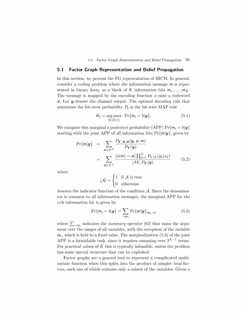
5.1. Factor Graph Representation and Belief Propagation 91
5.1 Factor Graph Representation and Belief Propagation
In this section, we present the FG representation of BICM. In general,consider a coding problem where the information message m is repre-sented in binary form, as a block of K information bits m1, . . . ,mK .The message is mapped by the encoding function φ onto a codewordx. Let y denote the channel output. The optimal decoding rule thatminimizes the bit-error probability Pb is the bit-wise MAP rule
mi = arg maxb∈{0,1}
Pr{mi = b|y}. (5.1)
We compute this marginal a posteriori probability (APP) Pr{mi = b|y}starting with the joint APP of all information bits Pr{m|y}, given by
Pr{m|y} =∑
x∈XN
PY ,X,M(y,x,m)PY (y)
=∑
x∈XN
[φ(m) = x]∏N
k=1 PY |X(yk|xk)|M| PY (y)
(5.2)
where
[A] =
{1 if A is true
0 otherwise
denotes the indicator function of the condition A. Since the denomina-tor is common to all information messages, the marginal APP for thei-th information bit is given by
Pr{mi = b|y} =∑∼mi
Pr{m|y}|mi=b (5.3)
where∑
∼miindicates the summary operator [62] that sums the argu-
ment over the ranges of all variables, with the exception of the variablemi, which is held to a fixed value. The marginalization (5.3) of the jointAPP is a formidable task, since it requires summing over 2K−1 terms.For practical values of K this is typically infeasible, unless the problemhas some special structure that can be exploited.
Factor graphs are a general tool to represent a complicated multi-variate function when this splits into the product of simpler local fac-tors, each one of which contains only a subset of the variables. Given a

92 Iterative Decoding
factorization, the corresponding Factor Graph (FG) is a bipartite graphwith two sets of nodes, the variable nodes V and the function nodesF . The set of edges E in the FG contains all edges (ϑ, f) for whichthe variable ϑ ∈ V is an argument of the factor (function) f ∈ F [62].We use circles and squares in order to represent variable and functionnodes in the FGs, respectively. As an example, Figure 5.2 shows theFG of a BICM scheme of rate R = 1, using a rate-1/3 binary convolu-tional code and an 8-ary modulation (m = 3). On the right side of theFG we see the convolutional structure of the binary code, with boxesrepresenting the encoder state equation, black circles representing theencoder state variables, and white circles representing the encoder in-put and output variables. On the left, we notice the modulator part,where white boxes represent the modulation mapping µ (from binarylabels to signal points), taking labels of three bits each and producingthe corresponding signal point. In between, separating the code andthe modulator, we have an interleaver, i. e. a permutation of the codedbits on the right-hand side to the label bits on the left-hand side. Theseconnections are included into a big box for the sake of clarity.
A general method for computing or approximating the marginalAPPs consists of applying the BP algorithm to a FG corresponding tothe joint APP. If the FG is a tree, then BP computes the marginal APPexactly [62]. If the FG contains loops, then the BP algorithm becomesiterative in nature, and gives rise to a variety of iterative decoding algo-rithms. These algorithms are distinguished by the underlying FG usedfor decoding, by the scheduling of the local computation at the nodes,and by the approximations used in the computations, that sometimesare necessary in order to obtain low complexity algorithms. Generallyspeaking, the BP algorithm is a message passing algorithm that propa-gates messages between adjacent nodes in the FG. For any given node,the message output on a certain edge is a function of all the messagesreceived on all other edges.
The BP general computation rules are given as follows [62]. Considera variable node ϑ, connected to function nodes {f ∈ N (ϑ)}, whereN (ϑ) denotes the set of neighbors of node ϑ in the FG. The variable-

5.1. Factor Graph Representation and Belief Propagation 93
Interleaver
.
.
.
Cc1
cn
Demapper
nodes
y1
yN
variable
bit nodes
.
.
.
y2
cn
c1
Fig. 5.2 Factor graph representation of a BICM scheme of rate R = 1. In this case, C is abinary convolutional code of rate r = 1
3and m = 3, i. e., 8-PSK or 8-QAM.
to-function message from ϑ to f ∈ N (ϑ) is given by
νϑ→f =∏
g∈N (ϑ)g 6=f
νg→v. (5.4)
Messages are functions of the variable node they come from or are sentto, i. e., both νf→ϑ and νϑ→f are functions of the single variable ϑ.Consider a function node f , connected to variable nodes {ϑ ∈ N (f)},where N (f) denotes the set of neighbors of node f in the FG. Thefunction-to-variable message from f to ϑ ∈ N (f) is given by
νf→ϑ =∑∼ϑ
f({η ∈ N (f)})∏
η∈N (f)η 6=ϑ
νη→f . (5.5)
where∑
∼ϑ indicates summation of the argument inside over the rangesof all variables, with the exception of ϑ.
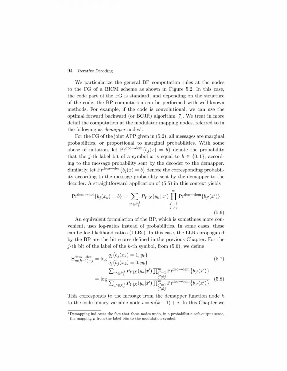
94 Iterative Decoding
We particularize the general BP computation rules at the nodesto the FG of a BICM scheme as shown in Figure 5.2. In this case,the code part of the FG is standard, and depending on the structureof the code, the BP computation can be performed with well-knownmethods. For example, if the code is convolutional, we can use theoptimal forward backward (or BCJR) algorithm [7]. We treat in moredetail the computation at the modulator mapping nodes, referred to inthe following as demapper nodes1.
For the FG of the joint APP given in (5.2), all messages are marginalprobabilities, or proportional to marginal probabilities. With someabuse of notation, let Prdec→dem{bj(x) = b} denote the probabilitythat the j-th label bit of a symbol x is equal to b ∈ {0, 1}, accord-ing to the message probability sent by the decoder to the demapper.Similarly, let Prdem→dec{bj(x) = b} denote the corresponding probabil-ity according to the message probability sent by the demapper to thedecoder. A straightforward application of (5.5) in this context yields
Prdem→dec{bj(xk) = b} =∑
x′∈X jb
PY |X(yk |x′)m∏
j′=1j′ 6=j
Prdec→dem{bj′(x′)}
(5.6)An equivalent formulation of the BP, which is sometimes more con-
venient, uses log-ratios instead of probabilities. In some cases, thesecan be log-likelihood ratios (LLRs). In this case, the LLRs propagatedby the BP are the bit scores defined in the previous Chapter. For thej-th bit of the label of the k-th symbol, from (5.6), we define
Ξdem→decm(k−1)+j = log
qj(bj(xk) = 1, yk
)qj(bj(xk) = 0, yk
) (5.7)
= log
∑x′∈X j
1PY |X(yk|x′)
∏mj′=1j′ 6=j
Prdec→dem{bj′(x′)
}∑
x′∈X j0PY |X(yk|x′)
∏mj′=1j′ 6=j
Prdec→dem{bj′(x′)
} (5.8)
This corresponds to the message from the demapper function node kto the code binary variable node i = m(k − 1) + j. In this Chapter we
1 Demapping indicates the fact that these nodes undo, in a probabilistic soft-output sense,the mapping µ from the label bits to the modulation symbol.

5.2. Density Evolution 95
Demapper
Decoder of
C
π
π−1
Ξdem→dec
Ξdec→dem
Fig. 5.3 Block diagram of BICM-ID.
will consider the analysis of BICM-ID using an infinite interleaver. Wehence drop the superscript b in the bit scores to simplify the notation.Instead, we have added a superscript to indicate the direction of themessage, i. e., from demapper to decoder or from decoder to demapper.We denote the vector of bit scores by
Ξdem→dec ∆= (Ξdem→dec1 , . . . ,Ξdem→dec
n ) (5.9)
and the vector of all bit scores but the i-th by
Ξdem→dec∼i
∆= (Ξdem→dec1 , . . . ,Ξdem→dec
i−1 ,Ξdem→deci+1 , . . . ,Ξdem→dec
n ).(5.10)
We further denote the a priori log-messages as
Ξdec→demm(k−1)+j = log
Prdec→dem{bj(xk) = 1
}Prdec→dem
{bj(xk) = 0
} . (5.11)
Similarly, we define the vectors
Ξdec→dem ∆= (Ξdec→dem1 , . . . ,Ξdec→dem
n ) (5.12)
and the vector of all log a priori messages but the i-th by
Ξdec→dem∼i
∆= (Ξdec→dem1 , . . . ,Ξdec→dem
i−1 ,Ξdec→demi+1 , . . . ,Ξdec→dem
n ).(5.13)
Figure 5.3 shows the block diagram of the basic BICM-ID decoder.
5.2 Density Evolution
In this section, we discuss a method to characterize the asymptoticperformance of BICM in the limit of large interleaver size. This method,

96 Iterative Decoding
named density evolution, describes how the densities of the messagespassed along the graph evolve through the iterations.
In particular, we consider a random ensemble of BICM schemesdefined by a random interleaver πn, generated with uniform probabil-ity over the set of permutations of n elements, and a random binaryscrambling sequence d ∈ {0, 1}n generated i.i.d. with uniform prob-ability. The random interleaver and the random scrambling sequencewere respectively introduced in Sections 4.3 and 4.4, and in Sections 4.1and 4.4. As already mentioned in Section 4.1, these elements used tosymmetrize the system with respect to the transmitted codewords. Inorder to transmit a binary codeword c ∈ C, the BICM encoder producesc⊕d, interleaves the result and maps the interleaved scrambled binarycodeword over a sequence of modulation symbols. The receiver knowsd, such that the modulo-2 scrambling can be undone at the receiver.
Let us denote the coded bit error probability at iteration ` wheninterleaver πn and scrambling sequence d are used by P (`)
c (πn,d). Wewish to compute the averaged coded bit error probability Pc at iteration`, given by
P (`)c
∆=∑πn,d
P (πn)P (d)P (`)c (πn,d), (5.14)
where P (πn) and P (d) respectively denote the probabilities of the in-terleaver and the scrambling sequence.
For given interleaver and scrambling sequence, the message vec-tors Ξdem→dec and Ξdec→dem are random vectors, function of the chan-nel noise and fading and of the transmitted information message. TheBICM-ID decoder behavior can be characterized by studying the jointprobability density of Ξdem→dec (or, equivalently, of Ξdec→dem) as afunction of the decoder iterations. This can be a highly complicatedtask due to n being large and to the statistical dependence between themessages passed along the FG. Moreover, the joint probability densityof the message vector at a given iteration is a function of the (random)interleaver and of the (random) scrambling sequence. Fortunately, apowerful set of rather general results come to rescue [22, 60, 96, 97].As we will state more precisely later, the marginal probability densityof a message sent over a randomly chosen edge in the FG converges

5.2. Density Evolution 97
almost surely to a deterministic probability density that depends onthe BICM ensemble parameters for large block lengths, provided thatthe FG is sufficiently local (e.g., the maximum degree of each node isbounded). The proof of this concentration result for BICM-ID closelyfollows the footsteps of analogous proofs for LDPC codes over BIOSchannels [96, 97], for LDPC codes over binary-input ISI channels [60],and for linear codes in multiple access Gaussian channels [22].
By way of illustration, consider a BICM ensemble based on theconcatenation of a binary convolutional code with a modulation signalset through an interleaver, whose FG is shown in Figure 5.2. We focuson a randomly chosen coded symbol ci. Also, we let i = m(k−1)+j suchthat the coded symbol i corresponds to the k-th modulation symbol,in label position j. We wish to compute the limiting density of themessage Ξdem→dec
i , from the demapper node µk to the variable node ci,at the `-th iteration.
We define the oriented neighborhood N `(µk → ci) of depth 2` asthe subgraph formed by all paths of length 2` starting at node µk andnot containing the edge (µk → ci). As done in [22, 60], we decode theconvolutional code using a windowed BCJR algorithm. This algorithmproduces the extrinsic information output for symbol ci by operatingover a trellis finite window centered around the symbol position i. Thetrellis states at the window edges are assumed to be uniformly dis-tributed. It is well-known that if the window size is much larger thanthe code constraint length, then the windowed BCJR approaches theexact (optimal) BCJR algorithm that operates over the whole trellis.Figure 5.4 shows an example of oriented neighborhood of depth 4.
In general, the neighbourhood N `(µk → ci) has cycles, or loops, bywhich we mean that some node of the FG appears more than once inN `(µk → ci). As n → ∞, however, one can show that the probabilitythat the neighborhood N `(µk → ci) is cycle-free for finite ` can bemade arbitrarily close to 1. Averaged over all possible interleavers, theprobability that the neighborhood has cycles is bounded as [22,60]
Pr{N `(µk → ci) has cycles
}≤ α
n, (5.15)
as n→∞ and for some positive α independent of n. The key elementin the proof is the locality of the FG, both for the code and for the
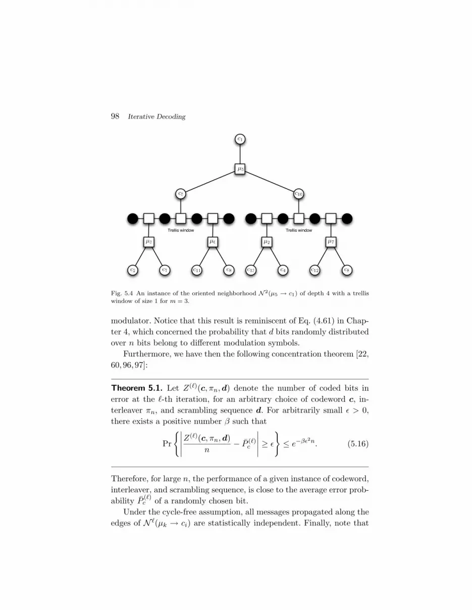
98 Iterative Decoding
c1
µ5
c5 c10
µ3 µ6 µ2 µ7
c2 c7 c11 c8 c13 c4 c12 c8
Trellis window Trellis window
Fig. 5.4 An instance of the oriented neighborhood N 2(µ5 → c1) of depth 4 with a trelliswindow of size 1 for m = 3.
modulator. Notice that this result is reminiscent of Eq. (4.61) in Chap-ter 4, which concerned the probability that d bits randomly distributedover n bits belong to different modulation symbols.
Furthermore, we have then the following concentration theorem [22,60,96,97]:
Theorem 5.1. Let Z(`)(c, πn,d) denote the number of coded bits inerror at the `-th iteration, for an arbitrary choice of codeword c, in-terleaver πn, and scrambling sequence d. For arbitrarily small ε > 0,there exists a positive number β such that
Pr
{∣∣∣∣∣Z(`)(c, πn,d)n
− P (`)c
∣∣∣∣∣ ≥ ε}≤ e−βε2n. (5.16)
Therefore, for large n, the performance of a given instance of codeword,interleaver, and scrambling sequence, is close to the average error prob-ability P (`)
c of a randomly chosen bit.Under the cycle-free assumption, all messages propagated along the
edges of N `(µk → ci) are statistically independent. Finally, note that

5.2. Density Evolution 99
−30 −20 −10 0 100
0.05
0.1
0.15
0.2
0.25
Ξ
(a) Density of Ξdem→dec.
−30 −20 −10 0 100
0.02
0.04
0.06
0.08
0.1
0.12
Ξ
(b) Density of Ξdec→dem.
Fig. 5.5 Density evolution of messages Ξdem→dec and Ξdec→dem with the (5, 7)8 convolu-
tional code with 16-QAM and Gray mapping at EbN0
= 3.5 dB. Solid lines correspond to thefirst iteration; dashed lines correspond to iteration 5.
the coded bit error probability is simply the tail probability of themessage Ξdec→dem
i , from the variable node ci to the demapper nodeµk
2. Density evolution tracks precisely the density of this message.Note also that by construction, the message Ξdem→dec
i is the the bitscore Ξb introduced in Chapter 4.
A detailed DE algorithm, for arbitrary modulation constellationand labeling, arbitrary (memoryless stationary) channel and arbitrarybinary convolutional code, can be found in Appendix 5.A.
Figures 5.5 and 5.6 illustrate the density evolution method for the(5, 7)8 convolutional code, 16-QAM with Gray and set-partitioningmapping, respectively. Note that the Eb
N0= 3.5 dB is above the water-
fall, which from Figure 5.1 occurs at approximately EbN0
= 3 dB. Figure5.5 shows that the positive tail of the message densities does not changemuch with the iterations, resulting in a nearly equal error probability.On the other hand, Figure 5.6, illustrates the improvement achievedwith iterative decoding, which reduces the tail of the distribution. No-tice, however, that there is an irreducible tail, which results in an error
2 This probability corresponds to decisions based on extrinsic information. Usually, decisionsare based on APP information for which the corresponding error probability is given bythe tail of the APP message Ξdec→dem
i + Ξdem→deci .

100 Iterative Decoding
−30 −20 −10 0 100
0.05
0.1
0.15
0.2
0.25
0.3
0.35
0.4
Ξ
110, 20 5
(a) Density of Ξdem→dec.
−30 −20 −10 0 100
0.2
0.4
0.6
0.8
1
1.2
1.4
Ξ
10, 20 5 1
(b) Density of Ξdec→dem.
Fig. 5.6 Density evolution of messages Ξdem→dec and Ξdec→dem with the (5, 7)8 convo-
lutional code with 16-QAM and set-partitioning mapping at EbN0
= 3.5 dB. Solid linescorrespond to iterations 1, 10 and 20; dashed lines correspond to iterations 2, 3, 4 and 5.
floor. As opposed to turbo-like and LDPC codes, this error floor occurseven for infinite interleaving. As shown in [30], this floor matches theperformance with perfect side information on the transmitted bits. Theresults match with the error probability simulations shown in Figure5.1. Note that the densities would not evolve significantly through theiterations if Eb
N0< 3 dB.
5.3 EXIT Charts
In the previous section, we have described density evolution as amethod that characterizes the message-passing process exactly in thelimit for infinite interleavers. Density evolution is computationally de-manding, since the whole density of the messages needs to be tracked.Unfortunately, density evolution does not yield simple criteria to op-timize the BICM-ID scheme. However, there are a number of one-dimensional approximate methods that only track one parameter ofthe density. These methods are simpler to compute and yield good andaccurate criteria to design efficient BICM-ID schemes. Among the pos-sible one-dimensional parameters, the mutual information functionalyields accurate approximations as well as analytical insight into thedesign of iteratively decodable systems [6,129].

5.3. EXIT Charts 101
Extrinsic information transfer (EXIT) charts are a tool for pre-dicting the behavior of iterative detection and decoding systems likeBICM-ID, and where first proposed by ten Brink in [116, 117, 119].EXIT charts are a convenient and accurate single-parameter approxi-mation of density evolution that plots the mutual information betweenbits and their corresponding messages in the iterative decoder. In par-ticular, let
x∆=
1n
n∑k=1
I(Ck; Ξdec→demk ), (5.17)
y∆=
1n
n∑k=1
I(Ck; Ξdem→deck ) (5.18)
respectively denote the average mutual information between the codedbits Ck, k = 1, . . . , n, and the decoder-to-demapper messages Ξdec→dem
k
and the demapper-to-decoder messages Ξdem→deck . Note that x and y
respectively correspond to the extrinsic informations at the decoder(demapper) output (input) and input (output). EXIT charts representthe extrinsic information as a function of a priori information,
y = exitdem(x), (5.19)
x = exitdec(y), (5.20)
and thus represent the transfer of extrinsic information in the demapperand decoder blocks. Since we deal with binary variables, the EXITcharts are represented in the axis [0, 1]×[0, 1]. The fixed point of BICM-ID, where further decoding iterations do not improve the performance,is the leftmost intersection of the EXIT curves.
EXIT-chart analysis is based on the simplifying assumption that thea priori information, i. e., x for y = exitdem(x) and y for x = exitdec(y),comes from an independent extrinsic channel. Figures 5.7(a) and 5.7(b)show the EXIT decoding model and extrinsic channels for a priori in-formation for the demapper and decoder blocks, respectively.
In the original EXIT charts proposed by ten Brink [116, 117, 119],the extrinsic channel was modeled as a binary-input AWGN channelwith an equivalent SNR given by
snrdemap = C−1
bpsk(x) (5.21)

102 Iterative Decoding
DemapperΞ
dem→dec
Ξdec→dem
CommunicationChannelEncoder
Extrinsic Channel
m xmy
Pext
Ξ|X(Ξdec→dem|xm)
PY |X(y|xm)
(a) Demapper
DecoderΞ
dem→decΞ
dec→dem
EncoderExtrinsic Channel
m
Pext
Ξ|X(Ξdem→dec|xm)
(b) Decoder
Fig. 5.7 Extrinsic channel models in BICM-ID.
for the demapper EXIT chart, and
snrdecap = C−1
bpsk(y) (5.22)
for the decoder EXIT chart, where Cbpsk(snr) is the capacity curve forBPSK modulation over the AWGN channel. In this model, the a priorimessages are modeled as normal distributed. In practice, the AWGNmodel for the extrinsic channel predicts the convergence behavior ofBICM-ID accurately, although not exactly, since the real messages ex-changed in the iterative process are not Gaussian. Another particu-larly interesting type of extrinsic channel is the binary erasure channel(BEC), for which the EXIT chart analysis is exact.
Different mappings might behave differently in BICM-ID [117]. Thisis shown in Figure 5.8(a), where we show the EXIT curves for Gray,set-partitioning and the optimized maximum squared Euclidean weight(MSEW) [113] for 16-QAM. In particular, Gray mapping has an almostflat curve. This implies that not much will be gained through iterations,since as the input extrinsic information x increases, the output extrinsicinformation y virtually stays the same, i. e., when decoding a given la-bel position, the knowledge of the other positions of the label does not

5.3. EXIT Charts 103
0 0.2 0.4 0.6 0.8 10
0.2
0.4
0.6
0.8
1
x
y
GraySP
MSEW
(a) Mapping comparison.
0 0.2 0.4 0.6 0.8 10
0.2
0.4
0.6
0.8
1
x
y 64 states
4 states
(b) Convolutional code comparison.
Fig. 5.8 (a) EXIT curves for Gray, set partitioning and MSEW are shown at snr = 6 dBwith an AWGN (solid) and a BEC (dashed) extrinsic channel. (b) Exit curves for 4 and 64states convolutional codes with an AWGN (solid) and a BEC (dashed) extrinsic channel.
help. Instead, set partitioning and MSEW show better EXIT curves.An important observation is that even with perfect extrinsic side in-formation (see the point x = 1 in the Figure), the mappings cannotperfectly recover the bit for which the message is being computed, i.e., these mappings cannot reach the (x, y) = (1, 1) point in the EXITchart. Notice that the AWGN and BEC EXIT curves are close to eachother. Figure 5.8(b) shows the EXIT curves for 4- and 64-state convolu-tional codes; the more powerful the code becomes, the flatter its EXITcurve. The differences between BEC and AWGN extrinsic informationare slightly more significant in this case.
Figures 5.9(a) and 5.9(b) show the EXIT chart of a BICM-IDscheme with a convolutional code, 16-QAM with set partitioning map-ping, and with AWGN and BEC extrinsic channels respectively. Wealso show the simulated trajectory of the information exchange be-tween demapper and decoder through the iterations as well as the fixedpoint (circle). The trajectory matches well the predictions made by theAWGN EXIT analysis, while it is not as accurate with the BEC EXIT,which predicts a fixed point not achieved in reality. Note that thismatches with the results of Figure 5.1, where a waterfall is observed at

104 Iterative Decoding
0 0.2 0.4 0.6 0.8 10
0.2
0.4
0.6
0.8
1
x
y
exit−1
dec(x)
exitdem(x)
1
mCbicm
X
(a) AWGN EXIT vs Trajectory.
0 0.2 0.4 0.6 0.8 10
0.2
0.4
0.6
0.8
1
x
y
exit−1
dec(x)
exitdem(x)
1
mCbicm
X
(b) BEC EXIT vs Trajectory.
Fig. 5.9 EXIT chart and simulated trajectory for BICM-ID with the (5, 7)8 convolutionalcode with 16-QAM with set partitioning mapping with snr = 6 dB, and AWGN (a) and BEC(b) extrinsic information. The normalized BICM capacity 1
mCbicmX is plotted for reference.
Dashed lines correspond to the EXIT curve of the demapper, solid lines correspond to theEXIT curve of the decoder while circles denote the fixed point.
EbN0≈ 3 dB (snr ≈ 6 dB). This waterfall corresponds to the tunnel of the
EXIT chart being open with a fixed point close to (1, y) point. The iter-ative process starts at the normalized BICM capacity 1
mCbicmX and stalls
when approaching the fixed point. Since the mapping cannot reach the(x, y) = (1, 1) point in the EXIT chart, the iterative decoder will notconverge to vanishing error probability. Although it can significantlyimprove the performance, it will therefore not have a threshold [96].The underlying reason is that the demodulator treats the bits as ifthey were uncoded. Figure 5.1 confirms the above discussion, namelya threshold behavior at low snr together with an irreducible error floorat large snr.
5.4 The Area Theorem
As discovered by Ashikhmin et al. EXIT charts exhibit a fundamentalproperty when the extrinsic channel is a BEC [6]: the area under theEXIT curve with a BEC extrinsic channel is related to the rate of theiterative decoding element we are plotting the EXIT chart of. Consider
5.4. The Area Theorem 105
Decoder
Ξext
Ξa
Communication
ChannelEncoder 1
Extrinsic Channel
m x y
Encoder 2
v
PY |X(y|x)
Pext
Ξ|V (Ξa|v)
Fig. 5.10 General decoding model for a given component of the iterative decoding process.
the general decoding model for a given component shown in Figure 5.10[6], where Ξa and Ξext denote the a priori and extrinsic messages,respectively. The input of the extrinsic channel is denoted by v =(v1, . . . , vn), and its associated random vector is denoted by V . Then,
Theorem 5.2 ( [6]). The area under the EXIT curve y(x) of the de-coding model described in Figure 5.10 with a BEC extrinsic channelsatisfies
A =∫ 1
0y(x)dx = 1− 1
nH(V |Y ) (5.23)
where H(V |Y ) denotes the conditional entropy of the random vectorV given Y .
Figure 5.10 encompasses the decoding models shown in Fig-ures 5.7(a) and 5.7(b) for the demapper and decoder of BICM-ID,respectively. In particular, we recover the decoding model of the de-coder shown in Figure 5.7(b) by having no communication channeland letting v = x, Ξa = Ξdem→dec and Ξext = Ξdec→dem. ApplyingTheorem 5.2 to the decoder extrinsic model yields the following result.
Corollary 5.1 ( [6]). Consider the EXIT curve of the decoder of the bi-nary code C of length n and rate r in a BICM-ID scheme, x = exitdec(y).Then, ∫ 1
0x(y)dy = 1− r (5.24)

106 Iterative Decoding
and
Adec =∫ 1
0y(x)dx = r. (5.25)
An example of the above result with the (5, 7)8 convolutional code isshown in Figure 5.11 (left). From Figure 5.10, we also recover the decod-ing model of the demapper shown in Figure 5.7(a) by letting Encoder2 be equal to Encoder 1, v = x, Ξa = Ξdec→dem and Ξext = Ξdem→dec.Applying Theorem 5.2 to the demapper case yields the following result.
Corollary 5.2. Consider the EXIT curve of the demapper in a BICM-ID scheme, y = exitdem(x). Then,
Adem =∫ 1
0y(x)dx =
1m
CcmX . (5.26)
Proof. From Figure 5.7(a), since the encoder is a one-to-one mapping,we can replace V by X to obtain that [6, p. 2662]
Adem =∫ 1
0y(x)dx (5.27)
= 1− 1nH(X|Y ) (5.28)
=1m
(m− 1
NH(X|Y )
)(5.29)
=1m
CcmX . (5.30)
An example of the above result with a set partitioning demapper inthe AWGN channel is shown in Figure 5.11 (right).
5.4.1 Code Design Considerations
The practical significance of the area theorem lies in the following ob-servation. As mentioned earlier, as long as the demapper EXIT curveis above the code EXIT curve, i. e.,
exitdem(x) > exit−1dec(x), (5.31)

5.4. The Area Theorem 107
0 0.2 0.4 0.6 0.8 10
0.2
0.4
0.6
0.8
1
x
y
∫1
0
y(x)dx = r
∫1
0
x(y)dy = 1 − r
(a) Convolutional code.
0 0.2 0.4 0.6 0.8 10
0.2
0.4
0.6
0.8
1
x
y
∫1
0
y(x)dx =1
m
Ccm
X
(b) Demapper.
Fig. 5.11 Area theorem for the convolutional code (5, 7)8 (left) and for a set partitioningdemapper in an AWGN channel with snr = 6 dB (right).
the decoder improves its performance with iterations eventually yield-ing vanishing error probability. This implies that as long as Adem >
Adec BICM-ID will improve its performance with iterations. Combin-ing the results of Corollaries 5.1 and 5.2 we see that this happens if
CcmX > rm = R. (5.32)
which is a satisfying result. Furthermore, this result suggests that anyarea gap between the two EXIT curves translates in a rate loss withrespect to the capacity Ccm
X [6]. The implications for code design areclear: one should design codes and mappers so that the EXIT curveof the code matches (fits) with that of the demapper. This matchingcondition was illustrated in [82,83,96] for binary LDPC codes.
For the demapper EXIT curve, it is not difficult to show that
exitdem(x = 1) < 1 (5.33)
for any binary labeling µ and finite snr. As discussed earlier, this impliesthat, even with perfect extrinsic side information the demapper is notable to correctly infer the value of the bit i. e., the demapper EXITcurve cannot reach the point (1, 1). This is due to the fact that thedemapper treats the bits as if they were uncoded. As (1, 1) cannot be a

108 Iterative Decoding
fixed point, the demapper and code curves will cross at some point andthere is no threshold effect. Also, since the area is fixed, the higher thepoint (1, y) is, the lower the point (0, y), i. e., BICM capacity Cbicm
X .
5.5 Improved Schemes
In this section, we discuss some BICM-ID schemes whose demapperEXIT curve does not treat the bits as uncoded. In particular, we con-sider LDPC and RA-based constructions and show that significantgains can be achieved. These constructions use in one way or anothercoded mappers, i. e., mappers with memory. The underlying memoryin the mapping will show to be the key to achieve the (1, 1) point. Thefollowing result lies at the heart of improved constructions.
Proposition 5.1 (Mixing property, [6, 120,128]). Suppose that en-coder 1 in Figure 5.10 consists of the direct product of multiple codes,i. e., C = C1 × . . .× Cdmax each of length ni, i. e.,
∑dmaxi=1 ni = n. Then,
y(x) =dmax∑i=1
ni
nyi(x) (5.34)
where yi(x) is the EXIT curve of code Ci.
The EXIT curve of a code mixture is the sum of the individual EXITcurves, appropriately weighted by the length fractions corresponding toeach code. The above result is usually employed to design irregular codeconstructions by optimizing the code parameters [96,100,120,121,128].
5.5.1 Standard concatenated codes with BICM-ID
A possibility to improve over the above BICM-ID is to use a powerfulbinary code like a turbo code or an LDPC code. The correspondingblock diagram for this scheme is shown in Figure 5.12. The decodingof this scheme involves message passing between the mapper and innercode, as well as between the inner and outer codes. This typically resultsin 3-dimensional EXIT charts and multiple scheduling algorithms, i. e.,how decoding iterations of each type are scheduled [25,27,55]. Hence thedesign of such schemes based on curve fitting is potentially complicated.

5.5. Improved Schemes 109
Outer
Code
Inner
CodeInterleaver Interleaver
Binary
Labeling
C
µ
Binary Encoder
m xm
Fig. 5.12 Block diagram of concatenated codes with BICM-ID.
Although suboptimal, another way of looking at the problem consid-ers a scheduling that allows the decoder of the powerful code to performas many iterations as required, followed by a demapping iteration. Inthis case the EXIT curve of the code becomes a step function [111]and hence, due to the shape of the demapper EXIT curve (see e.g. Fig-ure 5.9), the BICM-ID scheme would yield vanishing error probabilityas long as R < exitdem(x = 0) = Cbicm
X , i. e., the leftmost point of thedemapper EXIT curve.
Since the largest CbicmX is achieved for Gray mapping, it seems nat-
ural to design powerful binary codes for Gray mapping. As Gray map-ping does not improve much its EXIT transfer characteristics throughiterations, we could simplify the scheme —and reduce the decodingcomplexity— by not performing iterations at the demapper, e. g. theBICM decoding described in Chapter 3. This construction can be ad-vantageous for high rates, where the BICM capacity is close to thecoded modulation capacity. The FG is shown in Figure 5.13.
Our next example is a binary irregular RA codes [58, 100] withgrouping factor a, for which a single-parity-check code of rate a is in-troduced before the accumulator. In Figure 5.14 we show the resultsfor grouping factor a = 2, no demapping iterations, and 16-QAM withGray mapping. A number of optimization methods are possible andwe here use standard linear programming [100, 120, 121, 127]. Since noiterations are performed at the demapper, the observation messagescorrespond the classical BICM decoder, without extrinsic side infor-mation. Observe that the simulated error probability in Figure 5.15(N = 125000 and 100 decoding iterations) matches well the EXITanalysis predictions, especially the threshold, which the EXIT analysis

110 Iterative Decoding
Interleaver
Demapper
nodes
y1
yN
variable
bit nodes.
.
.
y2
Accumulator
with grouping
.
.
.
Repetition Code
Interleaver
Fig. 5.13 Regular rate rrep = 13
RA BICM-ID factor graph with regular grouping withfactor a = 2 and m = 3. The overall transmission rate is R = 2.
locates at 0.2157 dB from the BICM capacity.
5.5.2 LDPC BICM-ID
Let us first consider the concatenation of an LDPC code with the binarylabeling. The FG of this construction is shown in Figure 5.16 for aregular (3, 6) LDPC code. In general, we consider irregular ensembleswith left and right degree distributions respectively given by [96]
λ(z) =∑
i
λizi−1 and ρ(z) =
∑i
ρizi−1, (5.35)
where λi (resp. ρi) is the fraction of edges in the LDPC graph connectedto variable (resp. check) nodes of degree i. With this notation, theaverage variable and check node degrees are given by
dv∆=
1∫ 10 λ(z)dz
and dc∆=
1∫ 10 ρ(z)dz
, (5.36)

5.5. Improved Schemes 111
0 0.2 0.4 0.6 0.8 10
0.2
0.4
0.6
0.8
1
x
y
λ2 = 0.2158
λ3 = 0.2115
λ8 = 0.5727
r =1
4
(a) BICM BEC extrinsic channel.
0 0.2 0.4 0.6 0.8 10
0.2
0.4
0.6
0.8
1
x
y
λ2 = 0.1103
λ3 = 0.4015
λ8 = 0.4882
r ≈1
4
(b) BICM AWGN extrinsic channel.
Fig. 5.14 EXIT chart fit with an irregular RA code a with BEC (upper left) and AWGN(upper right) extrinsic channel, for 16-QAM with Gray mapping in the AWGN channelwith snr = 6 dB using a = 2. Binary accumulator; no iterations at the demapper. In dashedlines the accumulator-demapper curve; in solid lines the irregular repetition code. Codesare at 0.2157 dB from the BICM capacity.
2 2.2 2.4 2.6 2.8 310
−6
10−5
10−4
10−3
10−2
10−1
100
Eb
N0
(dB)
Pb
Fig. 5.15 Error probability for optimal AWGN code with N = 125000 and 100 decodingiterations. In solid, dash-dotted, and dashed vertical lines the coded modulation capacity,BICM capacity, and code threshold, respectively. Dotted line with diamonds is the simula-tion of the optimal AWGN code.

112 Iterative Decoding
+
+
+
LDPC variable
bit nodes
LDPC check
nodes
Demapper
nodes
y1
yN
.
.
.
.
.
.
Interleavery2
Fig. 5.16 Regular (3, 6) LDPC BICM-ID factor graph with m = 3.
respectively. The design rate of this LDPC code ensemble is thus
r = 1− dv
dc, (5.37)
and the overall rate of the construction is R = mr. The interest of thisimproved BICM-ID construction is the lack of interleaver between theLDPC and the mapping. The decoding algorithm decodes the variablenode bits from the LDPC directly and passes the messages along tothe check node decoder [121]. The corresponding EXIT area result forthis construction is given in the following.
Corollary 5.3 ( [6]). Consider the joint EXIT curve of the demapperand LDPC variable nodes y = exitldpc
dem,v(x) in a BICM-ID scheme withan LDPC code with left and right edge degree distributions given by

5.5. Improved Schemes 113
λ(z) and ρ(z), respectively. Then
Aldpcdem,v = 1− dv
(1− 1
mCcmX
). (5.38)
Furthermore, the area under the check node decoder EXIT curve x =exitldpc
dec,c(y) is given by ∫ 1
0x(y)dy =
1dc. (5.39)
Then we have that
Aldpcdec,c =
∫ 1
0y(x)dx = 1− 1
dc. (5.40)
Since we need that the areas Aldpcdem,v > Aldpc
dec,c to ensure convergenceto vanishing error probability, the above result implies that
CcmX > m
(1− dv
dc
)= mr = R (5.41)
where r denotes here the design rate of the LDPC code. That is, againwe recover a matching condition, namely, that the overall design spec-tral efficiency should be less than the channel capacity.
Bennatan and Burshtein [10] proposed a similar construction basedon non-binary LDPC codes, where the variable nodes belong to FM , fol-lowed by a mapping over a signal constellation of size M . The messagespassed along the edges of the graph correspond to M -ary variables. Therandom coset technique described in Section 4.1 enabled them to con-sider i.i.d. messages and define density evolution and EXIT charts.
5.5.3 RA BICM-ID
Similarly to the LDPC BICM-ID construction, we can design an im-proved BICM-ID scheme based on RA codes [93,120,127]. In particular,we consider the accumulator shown in Figure 5.17 of rate m
m . In order todesign a more powerful code, we incorporate grouping, i. e., introducea check node of degree a before the accumulator. As an outer code, weconsider irregular repetition code. We use the same notation to refer

114 Iterative Decoding
Delay
+
.
.
.
Modulator
xk
+
+
+
Grouping
a1
m− 1
m
.
.
.
.
.
.
.
.
.
a
a
Fig. 5.17 Accumulator of rate racc = a mm
, with grouping factor a.
to the degree distributions of the code: λ(z) denotes the edge degreedistribution of the irregular repetition code while ρ(z) denotes the edgedegree distribution of the accumulators with grouping. Let also
drep∆=
1∫ 10 λ(z)dz
and dacc∆=
1∫ 10 ρ(z)dz
, (5.42)
denote the average degrees of the repetition code and accumulator, re-spectively. The rate of the outer repetition code is rrep = drep. The rateof the accumulator is racc = mdacc. The overall rate of the constructionis hence R = mdrep dacc. The overall FG is shown in Figure 5.18 for aregular repetition code and regular grouping.
Figure 5.19 shows the EXIT curves for the accumulator in Fig-ure 5.17 with 8-PSK and various grouping factors. The curves not onlyreach the (1, 1) point, but also start at the point (0, 0) when a > 1, anditerative decoding would not start. In order to overcome this problem,we can introduce a small fraction of bits of degree one [120] or use codedoping [118], i. e., introduce a small fraction of pilot bits known to thereceiver.
Following [6, Example 26], we have the following area property.

5.5. Improved Schemes 115
Interleaver
Demapper
nodes
y1
yN
variable
bit nodes.
.
.
y2
Accumulator
with grouping
.
.
.
Repetition Code
Fig. 5.18 Regular rate rrep = 13
RA BICM-ID factor graph with regular grouping withfactor a = 2 and m = 3. The overall transmission rate is R = 2.
Corollary 5.4 ( [6]). Consider the EXIT curve y = exitradem,acc(x) of theaccumulator shown in Figure 5.17 combined with irregular groupingwith edge degree distribution ρ(z). Then
Aradem,acc =
1mdacc
CcmX . (5.43)
Furthermore, the area under the EXIT curve of the outer irregularrepetition code with edge degree distribution λ(z) is given by
Aradec,rep = drep. (5.44)
Since we again require the areas Aradem,acc > Ara
dec,rep to ensure con-vergence to vanishing error probability, we have the matching condition
CcmX > m daccdrep = R. (5.45)

116 Iterative Decoding
0 0.2 0.4 0.6 0.8 10
0.2
0.4
0.6
0.8
1
x
y 2 3 4
15
(a) Repetition codes.
0 0.2 0.4 0.6 0.8 10
0.2
0.4
0.6
0.8
1
x
y
1
2 3
(b) Accumulators.
Fig. 5.19 EXIT curves for repetition codes with repetition factors 2, 3, 4, 15 (left) and theaccumulator shown in Figure 5.17 with 8-PSK and grouping factors 1, 2, 3 (right). Solid anddashed lines correspond to AWGN and BEC extrinsic channels, respectively.
We now show a design example of RA-BICM-ID with 8-PSK. Forsimplicity, we consider regular grouping with a = 2, although irregulargrouping would lead to improved codes with a better threshold. We usea curve-fitting approach to optimize the irregular code distribution andmatch it to that corresponding to the accumulator. As in Section 5.5.1,we optimize the design by using standard linear programming. Fig-ure 5.20 shows the results of the curve fitting design at snr = 6 dB,which is close to the capacity for a transmission rate R = 2. Resultswith AWGN and BEC extrinsic channels are shown. The rate of theoverall schemes with a BEC extrinsic channel is R = 1.98 while forAWGN is R = 1.9758, which are respectively at 0.34 dB and 0.36 dBfrom capacity. The corresponding error probability simulation is shownin Figure 5.21. As we observe, the error probability matches well theEXIT predictions. Also, the code designed with a BEC extrinsic chan-nel is 0.1 dB away from that designed for the AWGN channel. Hence,using the BEC as a design channel yields good codes in a similar wayto [92] for LDPC codes.

5.5. Improved Schemes 117
0 0.2 0.4 0.6 0.8 10
0.2
0.4
0.6
0.8
1
x
y
λ2 = 0.1219
λ3 = 0.6559
λ4 = 0.1942
λ15 = 0.0280
r = 0.33
(a) BICM-ID BEC extrinsic channel.
0 0.2 0.4 0.6 0.8 10
0.2
0.4
0.6
0.8
1
x
y
λ2 = 0.1094
λ3 = 0.6234
λ4 = 0.2672
r ≈ 0.3293
(b) BICM-ID AWGN extrinsic channel.
Fig. 5.20 EXIT chart fit with an irregular RA code a with BEC (left) and AWGN (right)extrinsic channel, for 8-PSK with Gray mapping in the AWGN channel with snr = 6 dB.Grouping factor a = 2 and non-binary accumulator from Figure 5.17. In dashed lines theaccumulator-demapper curve; in solid lines the irregular repetition code.
2.5 3 3.510
−6
10−5
10−4
10−3
10−2
10−1
100
Eb
N0
(dB)
Pb
Fig. 5.21 Error probability for optimal AWGN code with N = 100000 and 100 decod-ing iterations. In solid and dashed vertical lines the coded modulation capacity and codethreshold, respectively; actual simulation in dotted line with diamonds.

118 Iterative Decoding
5.6 Concluding Remarks and Related Work
In this Chapter, we have reviewed iterative decoding of BICM. In par-ticular, we have studied the properties of BICM-ID when the interleaverlength is large. In this case, we have shown that the correspondinganalysis tool to characterize the error probability of BICM-ID is den-sity evolution, i. e., the characterization of how the density of the bitscores evolve through the iterations. A more compact and graphical,yet not exact, method for understanding the behavior of BICM-ID isEXIT chart analysis. A particularly interesting property of EXIT chartanalysis is the area theorem for BEC extrinsic side information, whichrelates the area under the EXIT curve of a given component to the itsrate. We have shown how to particularize this property to BICM-ID,and we have illustrated how the area property leads to the efficientdesign of capacity-approaching BICM-ID schemes. The optimized RA-BICM-ID codes could be further improved by introducing irregularityat the accumulator side, and by possibly optimizing the connectionsat the accumulator and the constellation mapping. A number of im-proved BICM-ID code constructions have been proposed in the litera-ture [93,120,121,127]. Based on the concepts illustrated in this Chapter,turbo-coded modulation schemes [99] can also be put into the BICM-IDframework. Furthermore, a number of optimized MLC have also beenproposed [54, 102]. We argue, however, that the optimization processand decoding is simpler for BICM-ID than for MLC, since there is onlyone code to be optimized.
Since the discovery of the improved performance of BICM-ID withmappings different from Gray, a number of works have focused on find-ing good mappings under a variety of criteria [26, 103, 113, 125, 131].Further, multidimensional mappings have been shown to provide per-formance advantages with BICM-ID [106, 107, 124]. A popular map-ping design criterion has been to optimize the perfect extrinsic sideinformation point of the EXIT chart (1, y), in order to make y aslarge as possible. Note that, according to the area theorem, larger y
in the (1, y) point, which corresponds to a lower error floor, implieslower y in the (0, y) point, which implies a larger convergence SNR.A number of works, using bounding techniques similar to those pre-

5.A. Density Evolution Algorithm for BICM-ID 119
sented in Chapter 4 using a metric with perfect extrinsic side infor-mation, have predicted the error floor of BICM-ID with convolutionalcodes [30,63,103,113].
Recall that the area theorem yields exact results only when theextrinsic side information comes from a BEC channel, and only ap-proximate results when the extrinsic channel is an AWGN. In [14], anMSE-based transfer chart was proposed. Building on the fundamen-tal relationship between mutual information and MMSE [51], Bhattadand Narayanan showed that the area property holds exactly for theMSE-based chart when the extrinsic channel is an AWGN. Althoughthe analysis that one might obtain in this case is still approximate,it seems reasonable to assume that it might be more accurate thanthe BEC analysis in terms of thresholds. Finally, generalized EXIT(GEXIT) charts were proposed in [82] as an EXIT chart where thearea property is imposed by definition. GEXIT charts therefore ex-actly characterize the iterative decoding process. The slight drawbackof GEXIT charts is that computing them is potentially demanding.
In this Chapter, we have only touched upon infinite-length analysisof BICM-ID. Finite-length analysis of BICM-ID is an open problemwhich is of significant interest due to the fact that practical systems,especially those meant to transmit real-time data, do not usually em-ploy such large interleavers. Successful finite-length analysis techniquesfor LDPC codes, such as finite-length scaling [3,4,96], find BICM-ID asa natural application. The analysis of the finite-length case, could alsobe performed by employing improved bounds to the error probability,like the Duman-Salehi or the tangential-sphere bound. The tangential-sphere bound was used in [44] to characterize the error probability offinite-length binary RA codes with grouping.
5.A Density Evolution Algorithm for BICM-ID
Since the message Ξdem→deci is a function of the messages propagated
upwards (from bottom to top) in the oriented neighborhood N `(µk →ci), it follows that the limiting probability density of Ξdem→dec
i can berecursively computed as follows. First, initialize the pdf of the messagesΞdec→dem (we drop the time index for simplicity of notation) to a single
120 Iterative Decoding
mass-point at zero. This represents the fact that, at the beginning ofthe BICM-ID process, no information is available from the decoderto the demapper. Then, alternatively, compute the pdf of the messagesΞdem→dec given the pdf of the messages Ξdec→dem and then compute thepdf of the messages Ξdec→dem given the pdf of the messages Ξdem→dec
obtained at the previous step until the exit condition is met.Several criteria for the exit condition are possible and have been con-
sidered in the literature. A common criterion is to exit if the resultingerror probability does not change significantly through the iterations.
Generally, it is much more convenient to work with cumulative dis-tribution functions rather than with pdfs (we refer to pdfs here sincethe algorithm is called density evolution). In fact, the calculation ofthe empirical cdf of a data set can easily be accomplished, and also thesampling from a distribution with given cdf is well-known and simpleto implement.
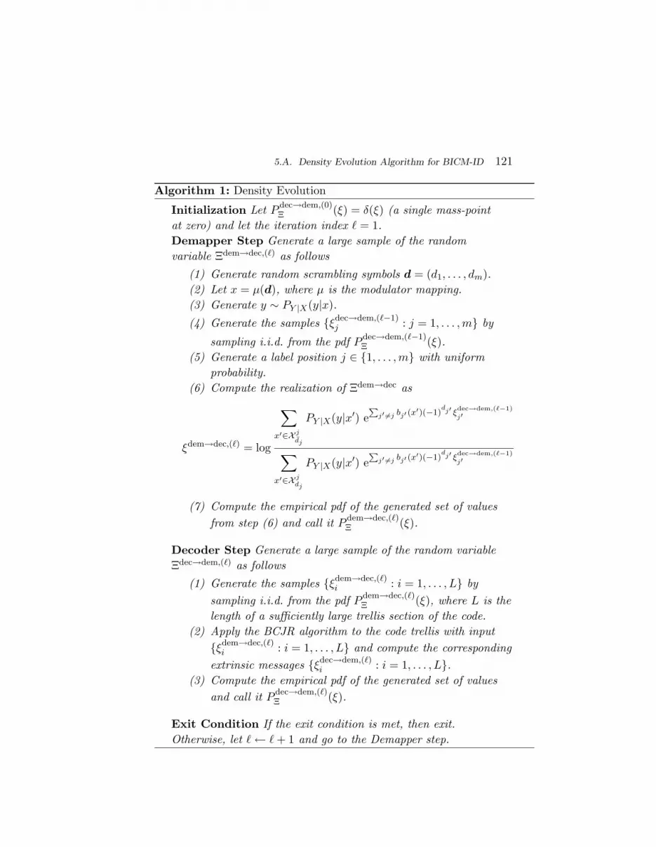
5.A. Density Evolution Algorithm for BICM-ID 121
Algorithm 1: Density Evolution
Initialization Let P dec→dem,(0)Ξ (ξ) = δ(ξ) (a single mass-point
at zero) and let the iteration index ` = 1.Demapper Step Generate a large sample of the randomvariable Ξdem→dec,(`) as follows
(1) Generate random scrambling symbols d = (d1, . . . , dm).(2) Let x = µ(d), where µ is the modulator mapping.(3) Generate y ∼ PY |X(y|x).(4) Generate the samples {ξdec→dem,(`−1)
j : j = 1, . . . ,m} by
sampling i.i.d. from the pdf P dec→dem,(`−1)Ξ (ξ).
(5) Generate a label position j ∈ {1, . . . ,m} with uniformprobability.
(6) Compute the realization of Ξdem→dec as
ξdem→dec,(`) = log
∑x′∈X j
dj
PY |X(y|x′) eP
j′ 6=j bj′ (x′)(−1)
dj′ ξdec→dem,(`−1)
j′
∑x′∈X j
dj
PY |X(y|x′) eP
j′ 6=j bj′ (x′)(−1)
dj′ ξdec→dem,(`−1)
j′
(7) Compute the empirical pdf of the generated set of valuesfrom step (6) and call it P dem→dec,(`)
Ξ (ξ).
Decoder Step Generate a large sample of the random variableΞdec→dem,(`) as follows
(1) Generate the samples {ξdem→dec,(`)i : i = 1, . . . , L} by
sampling i.i.d. from the pdf P dem→dec,(`)Ξ (ξ), where L is the
length of a sufficiently large trellis section of the code.(2) Apply the BCJR algorithm to the code trellis with input{ξdem→dec,(`)
i : i = 1, . . . , L} and compute the correspondingextrinsic messages {ξdec→dem,(`)
i : i = 1, . . . , L}.(3) Compute the empirical pdf of the generated set of values
and call it P dec→dem,(`)Ξ (ξ).
Exit Condition If the exit condition is met, then exit.Otherwise, let `← `+ 1 and go to the Demapper step.

6
Applications
In this Chapter we briefly discuss some applications of BICM to casesof practical relevance not explicitly included in our presentation. Inparticular, we review current work and outline how to extend the re-sults we presented throughout the monograph to non-coherent detec-tion, block-fading, multiple-input multiple-output (MIMO) channelsand non-standard channels such as the exponential-noise channel.
6.1 Non-Coherent Demodulation
Orthogonal modulation with non-coherent detection is a practicalchoice for situations where the received signal phase cannot be reli-ably estimated and/or tracked. Important examples include militarycommunications using fast frequency hopping, airborne communica-tions with high Doppler shifts due to significant relative motion of thetransmitter and receiver, and high phase noise scenarios, due to the useof inexpensive or unreliable local oscillators. Common choices of imple-mentation for the modulator are pulse-position modulation (PPM) orfrequency-shift keying (FSK) [95].
BICM with orthogonal modulation was first studied by Caire et al.
122

6.1. Non-Coherent Demodulation 123
in [29]. The study in [29] included BICM capacity, cutoff rate as well aserror probability considerations. Valenti and Cheng applied BICM-IDtechniques to orthogonal modulation with non-coherent detection withturbo-codes [132]. In [48], the design of capacity approaching codesis considered using the improved construction based on RA codes.Capacity-approaching codes within tenths of dB of capacity were found,also with suboptimal decoding metrics.
The application of our main results to orthogonal modulationis straightforward. Symbols x ∈ RM belong now to an orthogo-nal modulation constellation, i. e., x ∈ X ∆= {e1, . . . , eM}, whereek = (0, . . . , 0︸ ︷︷ ︸
k−1
, 1, 0, . . . , 0︸ ︷︷ ︸M−k−1
) is a vector has all zeros except in the k-th
position, where there is a one. The received signal over a fading channelcan still be expressed by (2.6), where now y, z ∈ CM , i. e., they arevectors of dimension M . The channel transition probability becomes
PY |X,H(y|x, h) =1πM
e−‖y−h√
snr x‖2 . (6.1)
Depending on the knowledge of the channel coefficients at the receiver,the decoding metric might vary. In particular, for coherent detection thesymbol decoding metric for hypothesis x = ek satisfies q(x = ek, y) ∝PY |X,H(y|x, h). When no knowledge of the carrier phase is available atthe receiver, then the symbol decoding metric for hypothesis x = ekwith coded modulation becomes [95]
q(x = ek, y) ∝ I0(2√
snr|h|yk
)(6.2)
where I0(.) is the zero-th order Bessel function of the first kind [1] andwith some abuse of notation we let yk denote the k-th entry of thereceived signal vector y. The bit metrics are
qj(bj(x) = b, y
)=∑
k′∈X jb
I0(2√
snr|h|yk′). (6.3)
where now X jb is the set of indices from {0, . . . ,M−1} with bit b in the
j-th position. All general results from the previous chapters can be ap-plied to orthogonal modulation by properly adapting the metric. Also,all integrals over y are now M -dimensional integrals. As an example,

124 Applications
−10 −5 0 5 10 15 200
1
2
3
4
5
snr (dB)
Cbicm
X(b
its/
channel
use
)
16−PPM/FSK
8−PPM/FSK
4−PPM/FSK
2−PPM/FSK
Fig. 6.1 Coded modulation capacity (solid lines), BICM capacity (dash-dotted lines) fororthogonal modulation (PPM/FSK) with non-coherent detection in the AWGN channel.
Figures 6.1 and 6.2 show the coded modulation and BICM capacities forthe AWGN channel and the fully-interleaved Rayleigh fading channelwith non-coherent detection, respectively. As we observe, the capacityloss of BICM with respect to coded modulation is somewhat largerthan in the QAM/PSK modulation case with coherent-detection.
Another common choice for systems where the carrier phase cannotbe reliably estimated and/or tracked is differential modulation wherea reference symbol is included. Common choices for practical imple-mentations in this case include differential PSK or block-differentialPSK [53,88–91].
6.2 Block-Fading
The block-fading channel [16, 87] is a useful channel model for a classof time- and/or frequency-varying fading channels where the durationof a block-fading period is determined by the product of the channel

6.2. Block-Fading 125
−10 0 10 20 30 400
1
2
3
4
5
snr (dB)
Cbicm
X(b
its/
channel
use
)
16−PPM/FSK
8−PPM/FSK
4−PPM/FSK
2−PPM/FSK
Fig. 6.2 Coded modulation capacity (solid lines), BICM capacity (dash-dotted lines) fororthogonal modulation (PPM/FSK) with non-coherent detection in the fully-interleavedRayleigh fading channel.
coherence bandwidth and the channel coherence time [95]. Within ablock-fading period, the channel fading gain remains constant. In thissetting, transmission typically extends over multiple block-fading peri-ods. Frequency-hopping schemes as encountered in the Global Systemfor Mobile Communication (GSM) and the Enhanced Data GSM Envi-ronment (EDGE), as well as transmission schemes based on OFDM, canalso conveniently be modeled as block-fading channels. The simplifiedmodel is mathematically tractable, while still capturing the essentialfeatures of the practical transmission schemes over fading channels.
Denoting the number of block per codeword by B, the codewordtransition probability in a block-fading channel can be expressed as
PY |X,H(y|x,h) =B∏
i=1
N∏k=1
PYi|Xi,Hi(yi,k|xi,k, hi), (6.4)
where xi,k, yi,k ∈ C are respectively the transmitted and received sym-

126 Applications
bols at block i and time k, and hi ∈ C is the channel coefficient corre-sponding to block i. The symbol transition probability is given by
PYi|Xi,Hi(yi,k|xi,k, hi) ∝ e−|yi,k−hi
√snrxi,k| (6.5)
The block-fading channel is equivalent to a set of parallel channels,each used a fraction 1
B of the time. The block-fading channel is notinformation stable [135] and its channel capacity is zero [16, 87]. Thecorresponding information-theoretic limit is the outage probability, andthe design of efficient coded modulation schemes for the block-fadingchannel is based on approaching the outage probability. In [46] it wasproved that the outage probability for sufficiently large snr behaves as
Pout(snr) = K snr−dsb , (6.6)
where dsb is the slope of the outage probability in a log-log scale andis given by the Singleton bound [61,70]
dsb∆= 1 +
⌊B
(1− R
m
)⌋. (6.7)
Hence, the error probability of efficient coded modulation schemes inthe block-fading channel must have slope equal to the Singleton bound.Furthermore, this diversity is achievable by coded modulation as wellas BICM [46]. As observed in Figure 6.3, the loss in outage probabilitydue to BICM is marginal. While the outage probability curves withGaussian, coded modulation and BICM inputs have the same slopedsb = 2 when B = 2, we note a change in the slope with coded modula-tion and BICM for B = 4. This is due to the fact that while Gaussianinputs yield slope 4, the Singleton bound gives dsb = 3.
In [46] the family of blockwise concatenated codes based on BICMwas introduced. Improved binary codes for the block-fading channel [23,24] can be combined with blockwise bit interleaving to yield powerfulBICM schemes.
In order to apply our results on error exponents and error probabil-ity, we need to follow Malkamaki’ and Leib’s approach [70] and derivethe error exponent for a particular channel realization. Then, the errorprobability (and not the error exponent) is averaged over the channelrealizations. Similarly, in order to characterize the error probability for

6.3. MIMO 127
−5 0 5 10 15 20 2510
−4
10−3
10−2
10−1
100
Eb
N0
(dB)
Pout
B = 2B = 4
Fig. 6.3 Outage probability with 16-QAM for R = 2 in a block-fading channel with B = 2, 4.Solid lines correspond to coded modulation and dash-dotted lines correspond to BICM. Theoutage probability with Gaussian inputs is also shown for reference with thick solid lines.
particular code constructions, we need to calculate the error proba-bility (or a bound) for each channel realization, and average over therealizations. Unfortunately, the union bound averaged over the channelrealizations diverges, and improved bounds must be used. A simple, yetvery powerful technique, was proposed by Malkamaki and Leib in [71],where the average over the fading is performed once the union boundhas been truncated at 1.
6.3 MIMO
Multiple antenna or MIMO channels model transmission systems whereeither the transmitter, the receiver or both, have multiple antennasavailable for transmission/reception. Multiple antenna transmission hasemerged as a key technology to achieve high spectral and power effi-ciency in wireless communications ever since the landmark works byTelatar [115] and Foschini and Gans [37] (see also [126]), which illus-trate significant advantages from an information theoretic perspective.

128 Applications
Coded modulation schemes that are able to exploit the available degreesof freedom in both space and time are named space-time codes [114].Design criteria based on the worst case PEP were proposed in [45,114]for quasi-static and fully-interleaved MIMO fading channels.
The design of efficient BICM space-time codes has been studied ina number of works [17,20,21,42,43,47,52,80,81,85,123]. The design ofBICM for MIMO channels fundamentally depends on the nature of thechannel (quasi-static, block-fading, fully-interleaved) and the numberof antennas available at the transmitter/receiver. An important featureof the design of BICM for MIMO channels is decoding complexity. Inthe case of MIMO, we have a transition probability
PY |X,H(y|x,H) ∝ e−‖y−√
snrHx‖2 , (6.8)
where y ∈ Cnr is the received signal vector, x ∈ Cnt is the transmittedsignal vector and H ∈ Cnr×nt is the MIMO channel matrix. In thiscase, the BICM decoding metric is
qj,t(bj,t(x) = b,y) =∑
x′∈X j,tb
e−‖y−√
snrHx‖2 , (6.9)
where X j,tb denotes the set of vectors with bit b in the j-th position at
the t-th antenna. In the fully-interleaved MIMO channel, this metriccan be used to characterize the mismatched decoding error exponents,capacity and error probability. In the quasi-static channel, we wouldneed to compute the error exponent using the metric (6.9) at everychannel realization, and derive the corresponding error probability asdone in [70] in block-fading channels. Note, however, that the size ofX j,t
b is exponential with the number of transmit antennas, which canmake decoding very complex.
For BICM-ID, similarly to what we discussed in Chapter 5, the apriori probabilities need to be incorporated in the metric (6.9). Spheredecoding and linear filtering techniques have been successfully appliedto limit the decoding complexity [20,47,52,136,137]. Figure 6.4 showsthe ergodic capacities for coded modulation and BICM in a MIMOchannel with nt = 2, nr = 2 and Rayleigh fading. A larger penalty,due to the impact of the BICM decoding metric that treats the bits

6.4. Optical Communication: Discrete-Time Poisson Channel 129
−20 −10 0 10 20 300
1
2
3
4
5
6
7
8
9
snr (dB)
Cbicm
X(b
its/
channel
use
)16−QAM
8−PSK
QPSK
BPSK
Fig. 6.4 Coded modulation capacity (solid lines), BICM capacity (dash-dotted lines) inMIMO channel with nt = nr = 2 and independent Rayleigh fading. The channel capacity(thick solid line) is shown for reference.
corresponding to a given vector symbol as independent, than in single-antenna channels is apparent. In particular, the BPSK capacities differ.When the number of antennas grows, the capacity computation be-comes more complex. As illustrated in [20] sphere decoding techniquescan also be employed to accurately estimate the coded modulation andBICM capacities.
6.4 Optical Communication: Discrete-Time Poisson Channel
The channel models we have mainly considered so far are variationsof the additive Gaussian noise channel, which provide an accuratecharacterization for communication channels operating at radio andmicrowave frequencies. For optical frequencies, however, the familyof Poisson channels is commonly considered a more accurate channelmodel. In particular, the so-called discrete-time Poisson (DTP) channel

130 Applications
with pulse-energy modulations (PEM) constitutes a natural counter-part to the PSK and QAM modulations considered throughout themonograph [72].
More formally, the input alphabet of the DTP channel is a set ofM non-negative real numbers X = {x1, . . . , xM}, normalized to unitenergy, 1
M
∑Mk=1 xk = 1. The output alphabet is the set of non-negative
integers, Y = {0, 1, 2, . . . }. The output at time n is distributed accord-ing to a Poisson random variable with mean εsxk + z0, where εs is theaverage energy constraint and z0 a background noise component. Thesymbol transition probability PY |X(y|x) is thus given by
PY |X(y|x) = e−(εsx+z0) (εsx+ z0)y
y!(6.10)
and therefore the symbol decoding metric can be written as
q(x, y) = e−εsx(εsx+ z0)y. (6.11)
It is clear that BICM schemes can be used in the DTP channel. Inparticular, the bitwise BICM metric can be written as
qj(bj(x) = b, y
)=∑
x′∈X jb
e−εsx′(εsx′ + z0)y. (6.12)
Figure 6.5 depicts the CM capacity attained by constellation pointsplaced at points 6(k−1)2
(2M−1)(M−1) , for k = 1, . . . ,M , as well BICM capac-ity Cbicm
X for BICM with binary reflected Gray mapping for severalmodulations. In all cases, z0 = 0 is considered. This spacing betweenconstellation points was proved in [33] to minimize the pairwise er-ror probability in the DTP channel at high signal energy levels. Asit happened in the Gaussian channel, BICM performs close to codedmodulation in the DTP channel when Gray labeling is used [72].
6.5 Additive Exponential Noise Channel
Channels with additive exponential noise (AEN) have been consideredin the context of queueing systems [5], and then in their own right [133]because their analytical characterization closely follows that of theGaussian channel. For instance, the capacity of such channels with

6.5. Additive Exponential Noise Channel 131
−10 0 10 20 30 400
1
2
3
4
5
εs (dB)
Cbicm
X(b
its/
channel
use
)
16−PEM
8−PEM
4−PEM
2−PEM
Fig. 6.5 Coded modulation capacity (solid lines), BICM capacity (dash-dotted lines) forPEM modulation in the DTP channel. Upper (thick solid line) and lower bounds (thickdashed line) to the capacity are shown for reference.
average signal-to-noise ratio snr is given by log(1 + snr) [133]. In theAEN channel, inputs are non-negative real numbers X = {x1, . . . , xM},xk ≥ 0, with average unit energy, 1
M
∑Mk=1 xk = 1. The output alpha-
bet is the set of non-negative real numbers, Y = [0,∞). The symboltransition probability PY |X(y|x) is given by
PY |X(y|x) = e−(y−snr x)u(y − snr x), (6.13)
where u(t) is the unit step function. For the symbol decoding metric,a simple expression can be used, namely
q(x, y) = esnr xu(y − snr x). (6.14)
The bitwise BICM metric can be written as
qj(bj(x) = b, y
)=∑
x′∈X jb
esnr x′u(y − snr x′). (6.15)

132 Applications
−10 0 10 20 300
1
2
3
4
5
snr (dB)
Cbicm
X(b
its/
channel
use
)
16−PEM
8−PEM
4−PEM
2−PEM
Fig. 6.6 Coded modulation capacity (solid lines), BICM capacity (dash-dotted lines) forPEM modulation in the AEN channel. The channel capacity (thick solid line) is shown forreference.
Figure 6.6 shows the CM capacity CcmX and the BICM capacity Cbicm
Xof uniformly spaced, equiprobable constellation sets placed at locations2(k−1)M−1 . Gray mapping is used for BICM. As it happened in the Gaussian
channel, BICM performs rather well in the AEN channel, although theloss in capacity with respect to Ccm
X is somewhat larger than the onein the Gaussian channel [72].
7
Conclusions
Coding in the signal space is dictated directly by Shannon capacity for-mula and suggested by the random coding achievability proof. In earlydays of digital communications, modulation and coding were kept sepa-rated because of complexity. Modulation and demodulation treated thephysical channel, waveform generation, parameter estimation (e.g., fre-quency, phase and timing) and symbol-by-symbol detection. Error cor-recting codes were used to undo the errors introduced by the physicalmodulation/demodulation process. This paradigm changed radicallywith the advent of Coded Modulation. Trellis-coded modulation was atopic of significant research activities in the 80’s, for approximately adecade. In the early 90’s, new families of powerful random-like codes,such as turbo codes, LDPC codes and Repeat-Accumulate codes werediscovered (or re-discovered), along with very efficient low-complexityBelief Propagation iterative decoding algorithms which allowed un-precedented performance close to capacity, at least for binary-inputchannels. Roughly at the same time, Bit-Interleaved Coded Modula-tion emerged as a very simple yet powerful tool to concatenate virtu-ally any binary code to any modulation constellation, with only minorpenalty with respect to the traditional joint modulation and decoding
133

134 Conclusions
paradigm. Therefore, BICM and modern powerful codes with itera-tive decoding were a natural marriage, and today virtually any mod-ern telecommunication system that seeks high spectral efficiency andhigh performance, including DSL, Digital TV and Audio Broadcast-ing, Wireless LANs, WiMax, and next generation cellular systems useBICM as the central component of their respective physical layers.
In this monograph, we have presented a comprehensive review of thefoundations of BICM in terms of information-theoretic, error probabil-ity and iterative decoding analysis. In particular, we have shown thatBICM is a paramount example of mismatched decoding where the de-coding metric is obtained as the product of bitwise metrics. Using thisdecoder, we have presented the derivation of the average error proba-bility of the random coding ensemble and obtained the resulting errorexponents, generalized mutual information and cutoff rate. We haveshown that the error exponent —and hence the cutoff rate— of theBICM mismatched decoder is upper bounded by that of coded mod-ulation and may thus be lower than in the infinite-interleaved modelthat was previously proposed and generally accepted for the analysisof BICM. Nevertheless, for binary reflected Gray mapping in Gaussianchannels the loss in error exponent is small. We have also consideredBICM in the wideband, or low SNR, regime and we have character-ized the suboptimality of the BICM decoder in terms of minimum bitenergy to noise ratio and wideband slope.
We have reviewed the error probability analysis of BICM with ageneric decoding metric with finite and infinite interleavers and we havegiven exact formulas and tight approximations, such as the saddlepointapproximation. We have seen that a short uniform interleaver resultsin a performance loss that in a fading channel translates into a diver-sity loss. We have also reviewed the application of improved bounds toBICM, which are central to analyze the performance of modern codessuch as turbo and LDPC codes with BICM, since these typically oper-ates beyond the cutoff rate and the standard union bound fails to givemeaningful results.
We have reviewed iterative decoding of BICM. In particular, wehave shown that perfect extrinsic information closes the gap betweenthe error exponents of BICM and that of coded modulation. We have
135
reviewed the density evolution analysis of BICM-ID and the applicationof the area theorem to BICM. We have finally shown how to designvery powerful BICM-ID structures based on LDPC or RA codes. Theanalysis reviewed here is valid for infinitely large block lengths, which isanyway a meaningful assumption when modern random-like codes areconsidered, since the latter yield competitive performance at moderateto large block length. The analysis of BICM with iterative decodingand short block lengths remains an open problem.
Overall, this monograph casts BICM in a unified common frame-work, and we believe it provides analysis and code design tools valuablefor both researchers and system designers.
References
[1] M. Abramowitz and I. A. Stegun, Handbook of mathematical funcions. DoverPublications, 1964.
[2] E. Agrell, J. Lassing, E. G. Strom, and T. Ottoson, “On the optimality ofthe binary reflected Gray code,” IEEE Trans. Inf. Theory, vol. 50, no. 12,pp. 3170–3182, 2004.
[3] A. Amraoui, Asymptotic and finite-length optimization of LDPC codes. PhDthesis, Ecole Polytechnique Federale de Lausanne, 2006.
[4] A. Amraoui, A. Montanari, T. Richardson, and R. Urbanke, “Finite-LengthScaling for Iteratively Decoded LDPC Ensembles,” submitted to IEEE Trans.Inf. Theory. Arxiv preprint cs/0406050, 2004.
[5] V. Anantharam and S. Verdu, “Bits through queues,” IEEE Trans. Inf. The-ory, vol. 42, no. 1, pp. 4–18, 1996.
[6] A. Ashikhmin, G. Kramer, and S. Brink, “Extrinsic information transferfunctions: model and erasure channel properties,” IEEE Trans. Inf. Theory,vol. 50, no. 11, pp. 2657–2673, 2004.
[7] L. Bahl, J. Cocke, F. Jelinek, and J. Raviv, “Optimal decoding of linear codesfor minimizing symbol error rate,” IEEE Trans. Inf. Theory, vol. 20, no. 2,pp. 284–287, 1974.
[8] S. Benedetto, D. Divsalar, G. Montorsi, and F. Pollara, “Serial concatenationof interleaved codes: performance analysis, design, and iterative decoding,”IEEE Trans. Inf. Theory, vol. 44, no. 3, pp. 909–926, 1998.
[9] S. Benedetto and G. Montorsi, “Unveiling turbo codes: some results on par-allel concatenated coding schemes,” IEEE Trans. Inf. Theory, vol. 42, no. 2,pp. 409–428, 1996.
136

References 137
[10] A. Bennatan and D. Burshtein, “Design and analysis of nonbinary LDPCcodes for arbitrary discrete-memoryless channels,” IEEE Trans. Inf. Theory,vol. 52, no. 2, pp. 549–583, 2006.
[11] C. Berrou, A. Glavieux, and P. Thitimajshima, “Near Shannon limit error-correcting coding and decoding: Turbo-codes.,” in IEEE Int. Conf. Commun.,Geneva, 1993.
[12] G. Beyer, K. Engdahl, and K. S. Zigangirov, “Asymptotical analysis and com-parison of two coded modulation schemes using PSK signaling - Part I,” IEEETrans. Inf. Theory, vol. 47, no. 7, pp. 2782–2792, 2001.
[13] G. Beyer, K. Engdahl, and K. S. Zigangirov, “Asymptotical analysis and com-parison of two coded modulation schemes using PSK signaling - Part II,” IEEETrans. Inf. Theory, vol. 47, no. 7, pp. 2793–2806, 2001.
[14] K. Bhattad and K. R. Narayanan, “An MSE-based transfer chart for analyzingiterative decoding schemes using a gaussian approximation,” IEEE Trans. Inf.Theory, vol. 53, no. 1, p. 22, 2007.
[15] E. Biglieri, D. Divsalar, M. K. Simon, and P. J. McLane, Introduction toTrellis-Coded Modulation with Applications. Prentice-Hall, 1991.
[16] E. Biglieri, J. Proakis, and S. Shamai, “Fading channels: information-theoreticand communications aspects,” IEEE Transactions on Information Theory,vol. 44, no. 6, pp. 2619–2692, 1998.
[17] E. Biglieri, G. Taricco, and E. Viterbo, “Bit-interleaved space–time codes forfading channels,” in Proc. Conf. Inf. Sci. and Sys., 2000.
[18] E. Biglieri, G. Caire, and G. Taricco, “Error probability over fading channels:a unified approach,” Europ. Trans. Commun., January 1998.
[19] E. Biglieri, G. Caire, G. Taricco, and J. Ventura-Traveset, “Simple method forevaluating error probabilities,” Electron. Lett., vol. 32, pp. 191–192, February1996.
[20] J. Boutros, N. Gresset, L. Brunel, and M. Fossorier, “Soft-input soft-outputlattice sphere decoder for linear channels,” in Global Telecommun. Conf., 2003.
[21] J. J. Boutros, F. Boixadera, and C. Lamy, “Bit-interleaved coded modulationsfor multiple-input multiple-output channels,” in IEEE Int. Symp. Spread Spec-trum Tech. App., 2000.
[22] J. J. Boutros and G. Caire, “Iterative multiuser joint decoding: unified frame-work and asymptotic analysis,” IEEE Trans. Inf. Theory, vol. 48, pp. 1772–1793, May 2002.
[23] J. J. Boutros, E. Calvanese Strinati, and A. Guillen i Fabregas, “Turbo codedesign for block fading channels,” Proc. 42nd Annual Allerton Conference onCommunication, Control and Computing, Allerton, IL, Sept.-Oct. 2004.
[24] J. Boutros, A. Guillen i Fabregas, E. Biglieri, and G. Zemor, “Low-densityparity-check codes for nonergodic block-fading channels,” submitted to IEEETrans. Inf. Theory. Available from http://arxiv.org/abs/0710.1182, 2007.
[25] F. Brannstrom, Convergence Analysis and Design of Multiple ConcatenatedCodes. PhD thesis, Department of Computer Engineering, Chalmers Univer-sity of Technology, 2004.
[26] F. Brannstrom and L. K. Rasmussen, “Classification of 8PSK mappings forBICM,” in 2007 IEEE Int. Symp. Inf. Theory, Nice, France, June, 2007.

138 References
[27] F. Brannstrom, L. K. Rasmussen, and A. J. Grant, “Convergence Analysisand Optimal Scheduling for Multiple Concatenated Codes,” IEEE Trans. Inf.Theory, vol. 51, no. 9, pp. 3354–3364, 2005.
[28] R. W. Butler, Saddlepoint Approximations with Applications. Cambridge Uni-versity Press, 2007.
[29] G. Caire, G. Taricco, and E. Biglieri, “Bit-interleaved coded modulation,”IEEE Trans. Inf. Theory, vol. 44, no. 3, pp. 927–946, 1998.
[30] A. Chindapol and J. A. Ritcey, “Design, analysis, and performance evaluationfor BICM-ID with square QAM constellations in Rayleigh fading channels,”IEEE J. Select. Areas Commun., vol. 19, no. 5, pp. 944–957, 2001.
[31] T. M. Cover and J. A. Thomas, Elements of information theory. Wiley NewYork, 2nd ed., 2006.
[32] D. Divsalar, H. Jin, and R. J. McEliece, “Coding theorems for turbo-likecodes,” Proc. 1998 Allerton Conference on Communication, Control and Com-puting, pp. 201–210, 1998.
[33] G. H. Einarsson, Principles of lightwave communications. Wiley New York,1996.
[34] R. F. Fischer, Precoding and Signal Shaping for Digital Transmission. JohnWiley & Sons, Inc. New York, NY, USA, 2002.
[35] G. D. Forney Jr, “The Viterbi algorithm,” Proc. of the IEEE, vol. 61, no. 3,pp. 268–278, 1973.
[36] G. D. Forney Jr and G. Ungerbock, “Modulation and coding for linear Gaus-sian channels,” IEEE Transactions on Information Theory, vol. 44, no. 6,pp. 2384–2415, 1998.
[37] G. J. Foschini and M. J. Gans, “On Limits of Wireless Communications ina Fading Environment when Using Multiple Antennas,” Wireless PersonalCommunications, vol. 6, no. 3, pp. 311–335, 1998.
[38] R. G. Gallager, “Low-density parity-check codes,” IEEE Trans. Inf. Theory,vol. 8, no. 1, pp. 21–28, 1962.
[39] R. G. Gallager, Information Theory and Reliable Communication. John Wiley& Sons, Inc. New York, NY, USA, 1968.
[40] R. G. Gallager, “A perspective on multiaccess channels,” IEEE Trans. Inf.Theory, vol. 31, pp. 124–142, Mar. 1985.
[41] A. Ganti, A. Lapidoth, and I. E. Telatar, “Mismatched decoding revisited:general alphabets, channels with memory, and the wideband limit,” IEEETrans. Inf. Theory, vol. 46, no. 7, pp. 2315–2328, 2000.
[42] N. Gresset, J. J. Boutros, and L. Brunel, “Multidimensional mappings foriteratively decoded bicm on multiple-antenna channels,” IEEE Trans. Inf.Theory., vol. 51, no. 9, pp. 3337–3346, 2005.
[43] N. Gresset, L. Brunel, and J. J. Boutros, “Space-time coding techniques withbit-interleaved coded modulations for MIMO block-fading channels,” IEEETrans. Inf. Theory, vol. 54, pp. 2156–2178, May 2008.
[44] S. Guemghar, Advanced Coding Techniques and Applications to CDMA. PhDthesis, Ecole Nationale des Telecommunications, Paris, 2004.

References 139
[45] J. C. Guey, M. P. Fitz, M. R. Bell, and W. Y. Kuo, “Signal design for transmit-ter diversity wireless communicationsystems over Rayleigh fading channels,”IEEE Trans. Commun., vol. 47, no. 4, pp. 527–537, 1999.
[46] A. Guillen i Fabregas and G. Caire, “Coded modulation in the block-fadingchannel: coding theorems and code construction,” IEEE Trans on Inf. Theory,vol. 52, pp. 91–114, Jan. 2006.
[47] A. Guillen i Fabregas and G. Caire, “Impact of signal constellation expansionon the achievable diversity of pragmatic bit-interleaved space-time codes,”IEEE Trans. Wireless Commun., vol. 5, no. 8, pp. 2032–2037, 2006.
[48] A. Guillen i Fabregas and A. Grant, “Capacity approaching codes for non-coherent orthogonal modulation,” IEEE Trans. Wireless Commun., vol. 6,pp. 4004–4013, Nov. 2007.
[49] A. Guillen i Fabregas and A. Martinez, “Derivative of BICM mutual informa-tion,” IET Electronics Letters, vol. 43, pp. 1219–1220, Oct. 2007.
[50] A. Guillen i Fabregas, A. Martinez, and G. Caire, “Error probability of bit-interleaved coded modulation using the gaussian approximation,” in Proceed-ings of the Conf. on Inform. Sciences and Systems (CISS-04), (Princeton,USA), March 2004.
[51] D. Guo, S. Shamai, and S. Verdu, “Mutual information and minimummean-square error in Gaussian channels,” IEEE Trans. Inf. Theory, vol. 51,pp. 1261–1282, Apr. 2005.
[52] B. M. Hochwald and S. ten Brink, “Achieving near-capacity on a multiple-antenna channel,” IEEE Trans. Commun., vol. 51, no. 3, pp. 389–399, 2003.
[53] P. Hoeher and J. Lodge, ““Turbo DPSK”: iterative differential PSK demodu-lationand channel decoding,” IEEE Trans. Commun., vol. 47, no. 6, pp. 837–843, 1999.
[54] J. Hou, P. H. Siegel, L. B. Milstein, and H. D. Pfister, “Capacity-approachingbandwidth-efficient coded modulation schemes based on low-density parity-check codes,” IEEE Trans. Inf. Theory, vol. 49, no. 9, pp. 2141–2155, 2003.
[55] S. Huettinger and J. Huber, “Design of “multiple-turbo-codes” with transfercharacteristics of component codes,”,” Proc. Conf. Inf. Sciences and Systems(CISS), 2002.
[56] H. Imai and S. Hirakawa, “A new multilevel coding method using error-correcting codes,” IEEE Trans. Inf. Theory, vol. 23, pp. 371–377, May 1977.
[57] J. L. Jensen, Saddlepoint Approximations. Oxford University Press, USA,1995.
[58] H. Jin, A. Khandekar, and R. McEliece, “Irregular repeat-accumulate codes,”in 2nd Int. Symp. Turbo Codes and Related Topics, pp. 1–8, 2000.
[59] G. Kaplan and S. Shamai, “Information rates and error exponents of com-pound channels with application to antipodal signaling in a fading environ-ment,” AEU. Archiv fur Elektronik und Ubertragungstechnik, vol. 47, no. 4,pp. 228–239, 1993.
[60] A. Kavcic, X. Ma, and M. Mitzenmacher, “Binary intersymbol interferencechannels: Gallager codes, density evolution, and code performance bounds,”IEEE Trans. Inf. Theory, vol. 49, no. 7, pp. 1636–1652, 2003.

140 References
[61] R. Knopp and P. A. Humblet, “On coding for block fading channels,” IEEETrans. Inf. Theory, vol. 46, no. 1, pp. 189–205, 2000.
[62] F. R. Kschischang, B. J. Frey, and H. A. Loeliger, “Factor graphs and thesum-product algorithm,” IEEE Trans. Inf. Theory, vol. 47, no. 2, pp. 498–519, 2001.
[63] X. Li, A. Chindapol, and J. A. Ritcey, “Bit-interleaved coded modulation withiterative decoding and 8 PSK signaling,” IEEE Trans. Commun., vol. 50, no. 8,pp. 1250–1257, 2002.
[64] X. Li and J. A. Ritcey, “Bit-interleaved coded modulation with iterative de-coding,” IEEE Commun. Letters, vol. 1, pp. 169–171, Nov. 1997.
[65] X. Li and J. A. Ritcey, “Bit-interleaved coded modulation with iterative de-coding using soft feedback,” Electronics Letters, vol. 34, no. 10, pp. 942–943,1998.
[66] X. Li and J. A. Ritcey, “Trellis-coded modulation with bit interleaving anditerative decoding,” IEEE Journal on Selected Areas in Communications,vol. 17, no. 4, pp. 715–724, 1999.
[67] A. Lozano, A. M. Tulino, and S. Verdu, “Opitmum power allocation for par-allel Gaussian channels with arbitrary input distributions,” IEEE Trans. Inf.Theory, vol. 52, pp. 3033–3051, Jul. 2006.
[68] R. Lugannani and S. O. Rice, “Saddle point approximation for the distribu-tion of the sum of independent random variables,” Adv. Appl. Prob., vol. 12,pp. 475–490, 1980.
[69] D. J. C. MacKay and R. M. Neal, “Near Shannon limit performance of lowdensity parity check codes,” IEE Electronics Letters, vol. 33, no. 6, pp. 457–458, 1997.
[70] E. Malkamaki and H. Leib, “Coded diversity on block-fading channels,” IEEETrans. Inf. Theory, vol. 45, no. 2, pp. 771–781, 1999.
[71] E. Malkamaki and H. Leib, “Evaluating the performance of convolutionalcodes over block fading channels,” IEEE Trans. Inf. Theory, vol. 45, no. 5,pp. 1643–1646, 1999.
[72] A. Martinez, Information-theoretic analysis of a family of additive energychannels. PhD thesis, Technische Universiteit Eindhoven, 2008.
[73] A. Martinez and A. Guillen i Fabregas, “Large-snr error probability analysis ofbicm with uniform interleaving in fading channels,” submitted to IEEE Trans.Wireless Commun., Nov. 2008.
[74] A. Martinez, A. Guillen i Fabregas, and G. Caire, “Error probability anal-ysis of bit-interleaved coded modulation,” IEEE Trans. Inf. Theory, vol. 52,pp. 262–271, Jan. 2006.
[75] A. Martinez, A. Guillen i Fabregas, and G. Caire, “A closed-form approxima-tion for the error probability of BPSK fading channels,” IEEE Trans. WirelessCommun., vol. 6, pp. 2051–2056, Jun. 2007.
[76] A. Martinez, A. Guillen i Fabregas, G. Caire, and F. Willems, “Bit-interleavedcoded modulation in the wideband regime,” accepted for publication in IEEETrans. Inf. Theory, 2008.

References 141
[77] A. Martinez, A. Guillen i Fabregas, G. Caire, and F. Willems, “Bit-interleavedcoded modulation revisited: a mismatched decoding perspective,” submittedto IEEE Trans. Inf. Theory. arXiv:0805.1327, 2008.
[78] A. Martinez, A. Guillen i Fabregas, and G. Caire, “New simple evaluationof the error probability of bit-interleaved coded modulation using the saddle-point approximation,” in Proc. 2004 International Symposium on InformationTheory and its Applications (ISITA 2004), (Parma (Italy)), October 2004.
[79] J. L. Massey, “Coding and modulation in digital communications,” in Int.Zurich Seminar Digital Commun., Zurich, Switzerland, 1974.
[80] M. McKay and I. Collings, “Capacity and performance of MIMO-BICM withzero-forcing receivers,” IEEE Trans. Commun., vol. 53, no. 1, pp. 74–83, 2005.
[81] M. McKay and I. Collings, “Error performance of MIMO-BICM with zero-forcing receivers in spatially-correlated Rayleigh channels,” IEEE Trans.Wireless Commun, vol. 6, no. 3, pp. 787–792, 2005.
[82] C. Measson, Conservation laws for coding. PhD thesis, Ecole PolytechniqueFederale de Lausanne, 2006.
[83] C. Measson, A. Montanari, and R. Urbanke, “Why we can not surpass capac-ity: The matching condition,” in 43rd Annual Allerton Conference on Com-munication, Control and Computing, Monticello, IL, Oct. 2005.
[84] N. Merhav, G. Kaplan, A. Lapidoth, and S. Shamai Shitz, “On informationrates for mismatched decoders,” IEEE Trans. Inf. Theory, vol. 40, no. 6,pp. 1953–1967, 1994.
[85] S. H. Muller-Weinfurtner, “Coding approaches for multiple antenna transmis-sion in fast fading and OFDM,” IEEE Trans. Signal Process., vol. 50, no. 10,pp. 2442–2450, 2002.
[86] F. D. Neeser and J. L. Massey, “Proper complex random processes with ap-plications to information theory,” IEEE Trans. Inf. Theory, vol. 39, no. 4,pp. 1293–1302, 1993.
[87] L. H. Ozarow, S. Shamai, and A. D. Wyner, “Information theoretic consider-ations for cellular mobile radio,” IEEE Transactions on Vehicular Technology,vol. 43, no. 2, pp. 359–378, 1994.
[88] V. Pauli, L. Lampe, and R. Schober, ““Turbo DPSK” Using Soft Multiple-Symbol Differential Sphere Decoding,” IEEE Trans. Inf. Theory, vol. 52,pp. 1385–1398, Apr. 2006.
[89] M. Peleg, I. Sason, S. Shamai, and A. Elia, “On interleaved, differentially en-coded convolutional codes,” IEEE Trans. Inf. Theory, vol. 45, no. 7, pp. 2572–2582, 1999.
[90] M. Peleg and S. Shamai, “On the capacity of the blockwise incoherent MPSKchannel,” IEEE Trans. Commun., vol. 46, no. 5, pp. 603–609, 1998.
[91] M. Peleg, S. Shamai, and S. Galan, “Iterative decoding for coded noncoherentMPSK communications overphase-noisy AWGN channel,” IEE Proc. Com-mun., vol. 147, no. 2, pp. 87–95, 2000.
[92] F. Peng, W. Ryan, and R. Wesel, “Surrogate-Channel Design of UniversalLDPC Codes,” IEEE Commun. Letters, vol. 10, no. 6, p. 480, 2006.

142 References
[93] S. Pfletschinger and F. Sanzi, “Error floor removal for bit-interleaved codedmodulation with iterative detection,” IEEE Trans. Wireless Commun., vol. 5,no. 11, pp. 3174 – 3181, 2006.
[94] V. Prelov and S. Verdu, “Second order asymptotics of mutual information,”IEEE Trans. Inf. Theory, vol. 50, pp. 1567–1580, Aug. 2004.
[95] J. G. Proakis, “Digital Communications,” McGraw-Hill USA, 4th edition,2001.
[96] T. Richardson and R. Urbanke, Modern Coding Theory. Cambridge UniversityPress, Cambridge, UK, 2008.
[97] T. Richardson and R. Urbanke, “The capacity of low-density parity-checkcodes under message-passing decoding,” IEEE Trans. Inf. Theory, vol. 47,no. 2, pp. 599–618, 2001.
[98] B. Rimoldi and R. Urbanke, “A rate-splitting approach to the gaussianmultiple-access channel,” IEEE Trans. Inf. Theory, vol. 42, pp. 364–375, Mar.1996.
[99] P. Robertson and T. Worz, “Bandwidth-efficient turbo trellis-coded modu-lation using puncturedcomponent codes,” IEEE J. Select. Areas Commun.,vol. 16, no. 2, pp. 206–218, 1998.
[100] A. Roumy, S. Guemghar, G. Caire, and S. Verdu, “Design methods for ir-regular repeat-accumulate codes,” IEEE Trans. Inf. Theory, vol. 50, no. 8,pp. 1711–1727, 2004.
[101] I. Sason and S. Shamai, Performance Analysis of Linear Codes UnderMaximum-likelihood Decoding: A Tutorial. Vol. 3, Now Publishers Inc, 2006.
[102] H. E. Sawaya and J. J. Boutros, “Multilevel coded modulations based onasymmetric constellations,” in IEEE Int. Symp. Inf. Theory, Washington,DC, USA, June, 2001.
[103] F. Schreckenbach, N. Gortz, J. Hagenauer, and G. Bauch, “Optimized symbolmappings for bit-interleaved coded modulation with iterative decoding,” IEEECommun. Letters, vol. 7, pp. 593 – 595, Dec. 2003.
[104] V. Sethuraman and B. Hajek, “Comments on Bit-Interleaved Coded Modula-tion,” IEEE Trans. Inf. Theory, vol. 52, no. 4, pp. 1795–1797, 2006.
[105] C. E. Shannon, “A Mathematical Theory of Communication,” Bell SystemTechnical Journal, vol. 27, pp. 379–423 and 623–656, 1948.
[106] F. Simoens, H. Wymeersch, H. Bruneel, and M. Moeneclaey, “Multidimen-sional mapping for bit-interleaved coded modulation with BPSK/QPSK sig-naling,” IEEE Commun. Letters, vol. 9, no. 5, pp. 453–455, 2005.
[107] F. Simoens, H. Wymeersch, and M. Moeneclaey, “Linear Precoders for Bit-Interleaved Coded Modulation on AWGN Channels: Analysis and Design Cri-teria,” IEEE Trans. Inf. Theory., vol. 54, pp. 87–99, Jan. 2008.
[108] D. Slepian and J. K. Wolf, “A coding theorem for multiple access channelswith correlated sources,” Bell Syst. Tech. J, vol. 52, no. 7, pp. 1037–1076,1973.
[109] C. Stierstorfer and R. F. H. Fischer, “(Gray) mappings for bit-interleavedcoded modulation,” in 65th IEEE Vehic. Techn. Conf., Dublin, Ireland, April2007.

References 143
[110] C. Stierstorfer and R. F. H. Fischer, “Mappings for BICM in UWB scenar-ios,” in Proc. 7th Intl ITG Conf. Source and Channel Coding (SCC), Ulm,Germany, January 2008.
[111] I. Sutskover, S. Shamai, and J. Ziv, “Extremes of information combining,”IEEE Trans. Inf. Theory, vol. 51, no. 4, pp. 1313–1325, 2005.
[112] L. Szczecinski, A. Alvarado, R. Feick, and L. Ahumada, “On the distributionof L-values in gray-mapped M2-QAM signals: Exact expressions and simpleapproximations,” in IEEE Global Commun. Conf, 26-30 November, Washing-ton, DC, USA, 2007.
[113] J. Tan and G. Stuber, “Analysis and Design of Symbol Mappers for IterativelyDecoded BICM,” IEEE Trans. Wireless Commun., vol. 4, no. 2, pp. 662–672,2005.
[114] V. Tarokh, N. Seshadri, and A. Calderbank, “Space-time codes for high datarate wireless communication: performance criterion and code construction,”IEEE Trans. Inf. Theory, vol. 44, no. 2, pp. 744–765, 1998.
[115] I. E. Telatar, “Capacity of multi-antenna Gaussian channels,” EuropeanTransactions on Telecommunications, vol. 10, no. 6, pp. 585–595, 1999.
[116] S. ten Brink, “Convergence of iterative decoding,” Electronics Letters, vol. 35,p. 806, 1999.
[117] S. ten Brink, “Designing iterative decoding schemes with the extrinsic in-formation transfer chart,” AEU Int. J. Electron. Commun, vol. 54, no. 6,pp. 389–398, 2000.
[118] S. ten Brink, “Code doping for triggering iterative decoding convergence,” inIEEE Int. Symp. Inf. Theory, Washington, DC, USA, June, 2001.
[119] S. ten Brink, “Convergence behavior of iteratively decoded parallel concate-nated codes,” IEEE Trans. Commun., vol. 49, pp. 1727–1737, Oct. 2001.
[120] S. ten Brink and G. Kramer, “Design of repeat-accumulate codes for itera-tive detection and decoding,” IEEE Trans. Signal Process., vol. 51, no. 11,pp. 2764–2772, 2003.
[121] S. ten Brink, G. Kramer, and A. Ashikhmin, “Design of low-density parity-check codes for modulation and detection,” IEEE Trans. Commun., vol. 52,no. 4, pp. 670–678, 2004.
[122] S. ten Brink, J. Speidel, and R. H. Yan, “Iterative demapping for QPSKmodulation,” Electronics Letters, vol. 34, no. 15, pp. 1459–1460, 1998.
[123] A. M. Tonello, “Space-time bit-interleaved coded modulation with an iterativedecoding strategy,” in 52nd Vehic. Tech. Conf., 2000.
[124] N. Tran and H. Nguyen, “Design and performance of BICM-ID systems withhypercube constellations,” IEEE Trans. Wireless Commun., vol. 5, no. 5,pp. 1169–1179, 2006.
[125] N. Tran and H. Nguyen, “Signal mappings of 8-ary constellations for bit inter-leaved coded modulation with iterative decoding,” IEEE Trans. Broadcasting,vol. 52, no. 1, pp. 92–99, 2006.
[126] D. Tse and P. Viswanath, Fundamentals of Wireless Communication. Cam-bridge University Press, 2005.
[127] M. Tuchler, “Design of serially concatenated systems depending on the blocklength,” IEEE Trans. Commun., vol. 52, no. 2, pp. 209–218, 2004.

144 References
[128] M. Tuchler and J. Hagenauer, “EXIT charts of irregular codes,” in Conf. Inf.Sciences and Systems, pp. 748–753, 2002.
[129] M. Tuchler, J. Hagenauer, and S. ten Brink, “Measures for Tracing Conver-gence of Iterative Decoding Algorithms,” in Proc. 4th Intern. ITG Conf. onSource and Channel Coding, Berlin, Germany, pp. 53–60, Jan. 2002.
[130] G. Ungerbock, “Channel Coding With Multilevel/Phase Signals.,” IEEETrans. Inf. Theory, vol. 28, no. 1, pp. 55–66, 1982.
[131] M. Valenti, R. Doppalapudi, and D. Torrieri, “A genetic algorithm for de-signing constellations with low error floors,” Proc. Conf. Inf. Sciences andSystems (CISS), 2008.
[132] M. Valenti and S. Cheng, “Iterative demodulation and decoding of turbo-coded M -ary noncoherent orthogonal modulation,” IEEE J. Select. AreasCommun., vol. 23, no. 9, pp. 1739–1747, 2005.
[133] S. Verdu, “The exponential distribution in information theory,” Problemyperedachi informatsii, vol. 32, no. 1, pp. 100–111, 1996.
[134] S. Verdu, “Spectral efficiency in the wideband regime,” IEEE Trans. Inf. The-ory, vol. 48, pp. 1319–1343, Jun. 2002.
[135] S. Verdu and T. S. Han, “A general formula for channel capacity,” IEEETrans. Inf. Theory, vol. 40, no. 4, pp. 1147–1157, 1994.
[136] H. Vikalo, Sphere Decoding Algorithms for Digital Communications. PhDthesis, Stanford University, 2003.
[137] H. Vikalo, B. Hassibi, and T. Kailath, “Iterative decoding for MIMO channelsvia modified sphere decoding,” IEEE Trans. Wireless Commun., vol. 3, no. 6,pp. 2299–2311, 2004.
[138] A. J. Viterbi, “Error bounds for convolutional codes and an asymptotically op-timum decoding algorithm,” IEEE Trans. Inf. Theory, vol. 13, no. 2, pp. 260–269, 1967.
[139] A. J. Viterbi and J. K. Omura, Principles of Digital Communication andCoding. McGraw-Hill, Inc. New York, NY, USA, 1979.
[140] U. Wachsmann, R. F. H. Fischer, and J. B. Huber, “Multilevel codes: theo-retical concepts and practical design rules,” IEEE Trans. Inf. Theory, vol. 45,pp. 1361–1391, Jul. 1999.
[141] P. Yeh, S. Zummo, and W. Stark, “Error probability of bit-interleaved codedmodulation in wireless environments,” IEEE Transactions on Vehicular Tech-nology, vol. 55, no. 2, pp. 722–728, 2006.
[142] E. Zehavi, “8-PSK trellis codes for a Rayleigh channel,” IEEE Trans. Com-mun., vol. 40, no. 5, pp. 873–884, 1992.


