Embed Size (px)
Citation preview

Blind deconvolution for thin layered confocal imaging
Praveen Pankajakshan, Bo Zhang, Laure Blanc-Feraud, Zvi Kam,
Jean-Christophe Olivo-Marin, Josiane Zerubia
To cite this version:
Praveen Pankajakshan, Bo Zhang, Laure Blanc-Feraud, Zvi Kam, Jean-Christophe Olivo-Marin, et al.. Blind deconvolution for thin layered confocal imaging. Applied Optics, OpticalSociety of America, 2009, 48 (22). <inria-00395523>
HAL Id: inria-00395523
https://hal.inria.fr/inria-00395523
Submitted on 15 Jun 2009
HAL is a multi-disciplinary open accessarchive for the deposit and dissemination of sci-entific research documents, whether they are pub-lished or not. The documents may come fromteaching and research institutions in France orabroad, or from public or private research centers.
L’archive ouverte pluridisciplinaire HAL, estdestinee au depot et a la diffusion de documentsscientifiques de niveau recherche, publies ou non,emanant des etablissements d’enseignement et derecherche francais ou etrangers, des laboratoirespublics ou prives.

On blind deconvolution for thin layered confocal
imaging
Praveen Pankajakshan,1,∗ Bo Zhang,2 Laure Blanc-Feraud,1 Zvi Kam,3
Jean-Christophe Olivo-Marin,2 and Josiane Zerubia1
1ARIANA Project-team, INRIA/I3S,
2004 Route des lucioles, BP 93, 06902 Sophia-Antipolis Cedex, France
2Quantitative Image Analysis Unit,
Institut Pasteur, 25-28 rue du Docteur Roux, 75015 Paris, France
3Department of Molecular Cell Biology,
Weizmann Institute of Science, Rehovot, Israel 76100.
∗Corresponding author: [email protected]
1

In this paper, we have proposed an Alternate Minimization (AM) algorithm
for estimating the Point-Spread Function (PSF) of a Confocal Laser Scanning
Microscope (CLSM) and the specimen fluorescence distribution. A 3-D
separable Gaussian model is used to restrict the PSF solution space and
a constraint on the specimen is used so as to favor the stabilization and
convergence of the algorithm. The results obtained from the simulation show
that the PSF can be estimated to a high degree of accuracy, and those on real
data show better deconvolution as compared to a full theoretical PSF model.
c© 2009 Optical Society of America
OCIS codes: 100.1455, 180.1790, 100.3190.
1. Introduction
Most of the fluorescence microscopes that image a uniformly illuminated three-
dimensional (3-D) object by the optical sectioning technique, are affected by some
out-of-focus fluorescence contributions. Secondary fluorescence from the sections away
from the region of interest often interferes with the contrast and resolution of those
features that are in focus. Let us take the case of a single-photon (1-p) fluorescence
microscope like the Widefield Microscope (WFM) and the Confocal Laser Scanning
Microscope (CLSM) [1]. For the sake of simplicity, if we assume that the detectors
are the same, then a WFM could be seen as a CLSM but with a fully-open pinhole.
The WFM can collect more light even from the deeper sections of a specimen but the
2

data are sometimes rendered useless as there is a significant amount of out-of-focus
blur. The maximum intensity in each plane decreases as z−2, with z being the ax-
ial distance from the source. A completely closed pinhole (diameter < 1 Airy Units
(AU); 1AU= 1.22λex/Numerical Aperture) on the other hand, confines the light de-
tected only to the in-focus plane but at the expense of imaging low-contrast, highly
noisy (signal dependant noise) images. The intensity from a point source in this case
decreases as z−4 and the loss of in-focus intensity inhibits imaging of weakly fluo-
rescent specimens. Even with a useable pinhole diameter of 1AU, 30% of the light
collected is from the out-of-focus regions. In addition, the microscope is inherently
diffraction-limited [1, 2] and the image of a point source (the Point-Spread Function
(PSF)) displays a lateral diffractive ring pattern (expanding with defocus) introduced
by the finite-lens aperture.
Let O(Ω) = {o = (oxyz) : Ω ⊂ N3 → R} denote all possible observable objects on
the discrete spatial domain Ω = {(x, y, z) : 0 ≤ x ≤ Nx − 1, 0 ≤ y ≤ Ny − 1, 0 ≤
z ≤ Nz − 1} and h : Ω �→ R the microscope PSF. If we assume that the imaging
system is linear and shift-invariant, then the interaction between h and o is a “3-D
convolution”: (h ∗ o)(x) =∑
x′∈Ω
h(x−x′)o(x′). From the perspective of computational
methods, this could be inverted with the knowledge of the scanning system proper-
ties and also by information about the object being scanned. It is for this reason that
the knowledge of the PSF h is of fundamental importance. The nature of the PSF
for fluorescence microscope has been studied extensively [3–5]. We will introduce the
3

reader in Section 2.B to one such theoretical model based on the scalar diffraction
theory and its parametric approximation in Section 3.B.
1.A. Problem Formulation
Restoration by deconvolution could be achieved by using either a non-blind or blind
approach. For the non-blind case, the most common approach is an experimental
procedure [6, 7] that obtains the PSF by imaging a small fluorescent bead (so as to
approximate a point object) positioned in the cover slide. Although such a PSF should
have been an ideal choice for a deconvolution algorithm, it suffers from low contrast
(can be recorded only at finite defocus ranges) and is contaminated by noise. A way
to suppress the noise would be to either acquire several bead data sets and then av-
erage them [8, 9] or reconstruct them using Zernike polynomial moments [10]. This
approach is however handicapped by alignment problems and also the whole process
could take a long time. The alternative would be to use an analytical model of the
PSF [11,12] that takes into account the acquisition system’s physical information as
parameters. This information however might not be available or might change during
the course of the experiment (for example, due to heating of live samples).
We hence arrive at the blind deconvolution approach of estimating the specimen
and the unknown PSF parameters using a single observation of the specimen volume.
The problem of blind deconvolution is thus reduced to answering the following ques-
tion:
4

“How does one estimate the original object and the PSF, given only a single observa-
tion?”
If we forget the effect of noise and consider the observation model (h ∗ o) in the
Fourier space as: F(i) = F(h) · F(o), several solutions for o and h answer this prob-
lem. For example, if (h, o) is a solution, then the trivial case is that h is a Dirac
function and o = i or vice versa. If h is not irreducible, there exists h1 and h2 such
that h = h1∗h2, and the couples (h1∗h2, o) and (h1, h2∗o) are also solutions. Another
ambiguity is in the scaling factor. If (h, o) is a solution, then (τh, 1/τo) ∀τ > 0 are
solutions too. This last ambiguity can be waived for example by imposing a forced
normalization on h. Thus broadly speaking, a way of reducing the space of possible
solutions and to regularize the problem is to introduce constraints on h and o. If the
problem of deconvolution is ill-posed, that of blind deconvolution is under-determined
as the number of unknowns to be estimated is increased without any increase in the
input observation data.
Many methods use an iterative approach to estimate the PSF and the object with
no prior information on the object [13, 14]. Markham and Conchello [15] worked on
a parametric form for the PSF and developed an estimation method utilizing this
model. The difficulty in using this model for our application is that the number of
free parameters to estimate is large and the algorithm is computationally expensive.
Hom et al. [16] proposed a myopic deconvolution algorithm that alternates between
iteration to deconvolve the object and estimate the PSF. In order to myopically recon-
5

struct the PSF, they introduce a constraint on the Optical Transfer Function (OTF)
(the OTF and the PSF are Fourier Transform pairs).
This paper is organized in the following manner: we first discuss the nature of the
noise, its mathematical modeling and handling in Section 2.A. The PSF modeling is
introduced in the Section 2.B. Section 3 is dedicated to the proposed joint restoration
and estimation of the imaged object and the microscope PSF using a Bayesian frame-
work. Direct restoration from the observation data is very difficult, and hence it is
necessary to define an underlying model for both the object and the PSF respectively.
An Alternate Minimization (AM) algorithm is then proposed to solve this particular
problem. This AM algorithm was then tested on images of degraded phantom objects
and real data; the results obtained are presented in Section 4. We then conclude in
Section 5 with a discussion and proposed future work. The scope of this paper is
restricted to restoring images from a CLSM given the spatial invariance nature of the
diffraction-limited PSF.
2. Sources of distortion and their modeling
2.A. Poissonian Assumption
In digital microscopy, the source of noise is either the signal itself (so-called ‘pho-
ton shot noise’), or the digital imaging system. By tracking the photon to electron
conversion at the detector, we can observed that the signal and the dependent noise
follows an underlying distribution which is Poissonian [17]. Conversely, the imaging
6

noise isolated in the absence of any fluorescence source follows a Gaussian distribu-
tion [18,19]. The interested reader may refer to [1,20] for more details on this subject.
In this paper, we have assumed that there is no readout or dark noise as the Photo-
multiplier Tube is operating in the photon-counting mode. When the imaging system
has been a priori calibrated, there is almost negligible offset in the detector and the
illumination is uniform. Thus if {i(x) : x ∈ Ω} (assumed to be bounded and pos-
itive) denotes the observed intensity of the volume, for the Poissonian assumption,
the observation model can be expressed as:
γi(x) = P(γ([h ∗ o](x) + b(x))), x ∈ Ω, (1)
where, P(·) denotes voxel-wise noise function modeled as a Poissonian process. b :
Ω �→ R is a uniformly distributed intensity that models the low-frequency background
signal caused by scattered photons and auto-fluorescence from the sample. 1/γ is
known as the photon conversion factor, and γi(x) is the observed photon at the
detector.
2.B. Theoretical diffraction-limited PSF Model
Among the enormous literature available on PSF modeling, we highlight the work
of P. A. Stokseth [11] who obtained the OTF for an aberration-free optical system
especially for large defocus. This model was used to study the PSFs under different
microscope settings, and also in validating the algorithm.
If we consider a converging spherical wave in the object space from the objec-
7

tive lens, the near-focus amplitude distribution hA can be written in terms of the
amplitude optical transfer function OTFA as: hA(x) =∫kOTFA(k)exp(jk · x)dk,
where, j2 = −1, and x and k are the 3-D coordinates in the image and the Fourier
space respectively. By making the axial Fourier space coordinate kz a function of
lateral coordinates, kz = (k2 − (k2x + k2
y))1/2, the 3-D Fourier transform is reduced
to: hA(x, y, z) :=∫
kx
∫kyP (kx, ky, z)exp(j(kxx+kyy))dkydkx, where, k = 2πμ/λ is the
wave number of an illumination wave with a wavelength λ in vacuum and in a medium
of refractive index μ, and P (·, ·) describes the overall complex field distribution in the
pupil of an non-aberrated objective lens [2, 11].
For an aberration-free microscope, the pupil function can be written as:
P (kx, ky, z) =
⎧⎪⎪⎪⎪⎨
⎪⎪⎪⎪⎩
A(φ)exp(jkψ), if√k2
x + k2y < k sinφmax
0, otherwise
(2)
where, ψ is the optical distance between the wavefront emerging from the exit pupil
and the reference sphere measured along the extreme ray, φ = sin−1(k2x+k2
y)1/2/k, and
φmax is the maximum semi-aperture angle of the objective. The intensity projected
from an isotropically illuminating point source such as a fluorophore, on a (flat)
pupil plane is bound to be energy conservation constraint. Therefore, the amplitude
A(φ) in the pupil plane for detection should vary as (cosφ)−1/2 and the energy as
(cosφ)−1 [21]. Conversely, for the illumination case, A(φ) varies as (cosφ)1/2. Also for
small defocus, ψ in (2) could be approximated as [11]: ψ = z(1− cosφ). To derive the
8

intensity distribution of a point source in the image space of a CLSM, we make use of
the Helmholtz reciprocity theorem. Since in induced fluorescence, the excitation (λex)
and the emission wavelengths (λem) are different, the confocal PSF can be written
as [22]:
h(x) = C|hA(x;λex)|2 ·∫
x21+y2
1≤D2
4
|hA(x− x1, y − y1, z;λem)|2dx1dy1, (3)
where C is a scaling factor and D is the back-projected diameter of the circular
pinhole. This theoretical model of the PSF does not take into account aberrations
and assumes that diffraction effect predominates the aberrations. However, this scalar
model could be extended for other aberrations by modifying the pupil function ex-
pression in (2) to also include the additional phase term due to aberrations [20].
3. Bayesian framework for the Alternate Minimization (AM) blind de-
convolution algorithm
In this section we will use the Bayesian framework to describe the method for the
blind deconvolution.
3.A. Deconvolution
Since the advent of the nearest neighbor deconvolution algorithm [3], there have been
numerous techniques proposed [23–26] for image restoration applied to microscopy.
These however assume that the noise is Gaussian and are valid only for images with
high SNR. Statistical methods [27,28] on the other hand are extremely effective when
9

the noise in the acquired 3-D image is fairly strong. We propose here one such non-
linear iterative algorithm which although slightly computationally expensive (in com-
parison to linear methods), can better restore the lost higher frequencies.
If we accept the Poissonian model approximation of (1), then the image i can be
interpreted as the realization of independent Poison processes at each voxel. Hence
the likelihood can be written as:
Pr(i|o, h) =∏
x∈Ω
[h ∗ o](x)i(x)e−[h∗o](x)
i(x)!, (4)
where, the mean of the Poisson process is given by [h ∗ o](x). In all the derivations
used henceforth, the background term has been excluded but the algorithm can be
modified by changing the above mean to [h ∗ o+ b](x). The background fluorescence
can be determined from the smoothed histogram of a single “specimen-independent”
slice, and it is subsequently added to the mean at every iteration of the Maximum
Likelihood (ML) algorithm (4) for o [20]. As iterative ML methods do not ensure any
smoothness constraints, if unchecked, they evolve to a solution that displays many
artifacts from noise amplification (for examples see [29]). There are many remedies
like terminating the iteration (manually or by using a statistical criterion) before
the deterioration begins or pre-filtering the observation data. One might argue that
by applying a low-pass filter as a pre-processing step before deconvolution (as in
[30]), the results are improved in comparison to the deconvolved images with no pre-
filtering. The deconvolution algorithm applied after denoising is less influenced by the
10

prior term of the object [31]. However, such pre-filtering operations might influence
the blind deconvolution algorithm as it is not clear how the resulting filtered data
is eventually mapped to the original object. The number of iterations for eventual
convergence of the deconvolution algorithm also increases and the final result need
not be optimum. Such interventions are thus a post hoc method of regularizing the
ill-posed problem as it is a way of bringing some knowledge about the solution o. The
Maximum a Posteriori (MAP) algorithm proposed in this paper uses the prior model
on the specimen and the PSF but within the Bayesian framework. We are hence able
to simultaneously denoise and deconvolve the observation data without making any
modifications whatsoever.
By using the Bayes theorem and assuming that o and h are independent, the
posterior joint probability is:
Pr(o, h|i) =Pr(i|o, h) Pr(o) Pr(h)
Pr(i)(5)
where, Pr(o) is the global prior probability on the object and Pr(h) is the global prior
on the PSF. The nature of the prior terms and their expressions are discussed in the
Sections 3.A.1 and 3.B. The estimates for o and h can be obtained by simultaneously
maximizing the joint probability as:
(o, h) = arg max(o,h)
{Pr(o, h|i)}
= arg min(o,h)
{− log[Pr(o, h|i)]}. (6)
11

As Pr(i) does not depend on o or h, it shall hereafter be excluded from all the esti-
mation procedures that involve either o or h. The minimization of the cologarithm
of Pr(o, h|i) in (6) can be rewritten as the minimization of the following energy func-
tional:
J (o, h|i) ≡ Jobs(i|o, h) + (λoJreg,o(o) + λhJreg,h(h)). (7)
Jobs : Ω �→ R is a measure of fidelity to the data and it corresponds to the term
Pr(i|o, h) which is given from the noise distribution. It has the role of pulling the
solution towards the observed data. While, Jreg,o : Ω �→ R and Jreg,h : Ω �→ R are the
prior terms on the object and the PSF which ensure smoothness of the solutions. λo
and λh are positive parameters which measures the trade off between goodness of fit
and the regularity of the solutions. For the Bayesian interpretation of regularization
problems, we refer the reader to the paper [32] by Demoment.
Practically, simultaneous estimation of o and h from (6) is a difficult task. A way
to overcome this difficulty is to alternatively maximize the posterior first with respect
to o while assuming that the PSF function h is known and fixed, and then update
the PSF using the previous object estimate. This joint optimization algorithm is
summarized as:
o(n+1) = arg maxo{Pr(i|o, h(n)) Pr(o)},
h(n+1) = arg maxh{Pr(i|o(n+1), h) Pr(h)}. (8)
12

The implementation strategy of this blind deconvolution schema has been shown in
Algorithm 1 on Section 4.A and the discussion follows in the subsequent Sections.
3.A.1. A priori object models
The ensemble model of an object class refers to any probability distribution Pr(o) on
the object space O of the following form:
Pr(o) = Z−1λoe−λoE(o), (9)
where, E(o) is a generalized energy and 1/λo (with λo > 0) is the Gibbs parameter
for the prior term. We associate with each site (x, y, z) ∈ Ω of the object a unique
neighborhood ηxyz ⊆ Ω \ (x, y, z), and we denote the collection of all neighbors η =
{ηxyz|(x, y, z) ∈ Ω} as the neighborhood system. If we assume that the random field
(O = o) on a domain Ω is Markovian with respect to the neighborhood system η,
then, Pr(oxyz|oΩ\x,y,z) = Pr(oxyz|oηxyz). o is a Markov Random Field (MRF) on (Ω, η),
if o denotes a Gibbs ensemble on Ω and the energy is a superposition of potentials
associated to the cliques (a set of connected pixels). Hence, E(o) =∑
C∈C VC(o).
We use in this paper, the following first-order, homogeneous, isotropic MRF, over
a 6 member neighborhood ηx ∈ η (see Fig. 1) of the site x ∈ Ω,
Pr[O = o(x)] = Z−1λoe−λo
∑
x|∇o(x)|
(10)
where, |∇o(x)| is the potential function and λo is the regularization parameter de-
scribed above. The estimation of this parameter is dealt with in Section 4.A.
13

From a numerical point of view, |∇o(x)| is not straightforward to minimize, since it
is not differentiable in zero. An approach to circumvent this problem is to regularize
it, and instead to consider the (isotropic) discrete definition as:
|∇o(x, y, z)|ε = ((o(x+ 1, y, z)− o(x, y, z))2 + (o(x, y + 1, z)− o(x, y, z))2
+(o(x, y, z + 1)− o(x, y, z))2 + ε2)12 , (11)
where, ε is an arbitrarily small value (< 10−3). For the partition function Zλo =
∑o∈O(Ω) exp(−λo
∑x |∇o(x)|ε) to be finite, we restrict the possible values of o(x) so
that the numerical gradient of ∇o(x) is also bounded. When this model is used as a
prior for the object, we have the following smoothed regularization functional:
Jreg,o(o(x)) = λo
∑
x
|∇o(x)|ε. (12)
For numerical calculations, we will use the above smoothed approximation, and
|∇o(x)|ε will henceforth be simply written as |∇o(x)|. From (10) and (12), it can
be inferred that sites with very high total gradient intensities are more penalized and
those with low total gradients are less penalized. This is because it is more likely that
high gradients correspond to the case where there is less similarity between the site
of interest and their closest neighbors.
Tikhonov-Miller [33,34] introduced a regularization based on the 2 norm of the gra-
dient of the image. However, we have used the Total Variation (TV) regularization (see
Rudin-Osher-Fatemi (ROF) [35]) as it is able to better preserve discontinuities [28].
A direct 3-D extension of this TV algorithm for CLSM is described in [29] and [36].
14

3.A.2. Estimation of the object
For the time being let us assume that either the PSF or its parameters θ ∈ Θ are
known (either by initialization or from previous estimates) and hence h is determinate.
From (4), (5) and (10) we get:
Pr(o, h|i) = Z−1λoe−λo
∑
x|∇o(x)| ·
∏
x∈Ω
[h ∗ o](x)i(x)e−[h∗o](x)
i(x)!. (13)
As in (6), by applying −log operator to the a posteriori above, the cost function
J (o, h|i) to be minimized with respect to o becomes:
J (o, h|i) ≡(∑
x∈Ω
[h ∗ o](x)−∑
x∈Ω
i(x) log[h ∗ o](x) +∑
x∈Ω
log(i(x)!))
+ (14)
λo
∑
x∈Ω
|∇o(x)|+ log[Zλo ].
Richardson-Lucy (RL) algorithm with TV regularization The Euler-
Lagrange equation for minimizing J (o, h|i) in (14) with respect to o is:
1− h(−x) ∗( i(x)
(h ∗ o)(x)
)− λo div
( ∇o(x)
|∇o(x)|)
= 0 (15)
where, h(−x) is the Hermitian adjoint operation on h(x) and div stands for the
divergence (see [28] for details). Inspired by the RL algorithm [37, 38], (15) can be
solved for the object o by the following fixed-point iterative algorithm:
o(n+1)(x) =
[i(x)
(o(n) ∗ h)(x)∗ h(−x)
]
· o(n)(x)
1− λo div(
∇o(n)(x)
|∇o(n)(x)|
) (16)
where, (·) denotes the Hadamard multiplication (component wise) and n the iter-
ation number for the deconvolution algorithm. (16) is similar to the Expectation-
15

Maximization (EM) algorithm [39] with an underlying statistical model of the pro-
cess, and can be used for obtaining the MAP estimate of the object. The term
div(∇o(n)(x)/|∇o(n)(x)|
)can be numerically implemented with the use of central-
differences and the minmod scheme [29].
Positivity and flux constraint for the object estimate The deconvolution al-
gorithm that was described above suffers from an inherent weakness. For large values
of λo, even when the starting guess o(n) (with n = 0) is positive, the successive esti-
mates need not necessarily have positive intensities. We know that the true intensity
of the object o(x) is always non-negative. Most algorithms often truncate these neg-
ative intensities to zero or a small positive value. This however is a crude manner to
handle the estimated intensities as it can lead to loss of some essential information
and sometimes also introduce bias into the calculations.
So how else can the problems associated with negative intensity estimates be han-
dled? Fortunately, the problem is entirely due to poor statistical methodology. The
modification that we suggest is to include this knowledge of non-negative true inten-
sities into the prior term of (10). The distribution that would express precisely this
condition is:
Pr[o(x)] :=
⎧⎪⎪⎪⎪⎨
⎪⎪⎪⎪⎩
Z−1λoe−λo
∑
x|∇o(x)|
, if o(x) ≥ 0
0, otherwise.
(17)
16

For the sake of numerical differentiability we approximate the prior (17) using a
sigmoid function as:
Pr[o(x)] := Z−1new,λo
e−λo
∑
x|∇o(x)| ·
(1
(1 + exp(βo(ε− o(x))))
)
(18)
where, ε is a small value close to zero, and βo is a value that specifies the steepness
of the sigmoid curve. Typically the values of βo and ε are chosen to be very large
and small respectively as precision allows. Their values do not individually affect the
algorithm and hence need not be known accurately. The cost function (14), the Euler-
Lagrange equation (15) and the multiplicative algorithm (16) are thus modified as
follows:
J (o, h|i) ≡(∑
x∈Ω
[h ∗ o](x)−∑
x∈Ω
i(x) log[h ∗ o](x))
+ λo
∑
x∈Ω
|∇o(x)|+ log[Znew,λo ]
− log
(1
(1 + exp(βo(ε− o(x))))
)
,(19)
1− h(−x)( i(x)
(h ∗ o)(x)
)− λo div
( ∇o(x)
|∇o(x)|)− βo
exp(βo(ε− o(x)))
1 + exp(βo(ε− o(x)))= 0, (20)
o(n+1)(x) =
[i(x)
(o(n) ∗ h)(x)∗ h(−x)
]
· o(n)(x)
1− λo div(
∇o(n)(x)
|∇o(n)(x)|
)− βo
exp(βo(ε−o(x)))1+exp(βo(ε−o(x)))
.
(21)
Intuitively, the cost function in (19) ensures that the energy for negative intensity
pixels (o(x) < ε) is very high and hence is not reachable (or is not a possible solution)
during the iteration procedure.
17

If PSF is normalized such that ||h(x)||1 = 1, in the absence of a background signal,
it is simple to show that for each iteration of the RL algorithm (see (16) with λo = 0),
the following property is true: s =∑
x∈Ω i(x) =∑
x∈Ω o(x). This property is known
as the flux or global photometry conservation and it guarantees that the total number
of counts of the reconstructed object is the same as the total number of observation
counts. However, this property is lost with regularization and can be incorporated
by modifying the cost function (14) to an additive form or by enforcing it in the
following manner after every iteration: o(n+1)new (x) = (s(0) × o
(n+1)old (x))/s(n+1), where,
s(n+1) =∑
x∈Ω o(n+1)old (x), and s(0) =
∑x∈Ω o
(0)(x) =∑
x∈Ω i(x).
3.B. Parametrization of the Point-Spread Function
When λo = 0 in (14), theoretically speaking the estimation method on the object and
PSF should be the same as h and o play a symmetric role. When no constraint is
imposed on the PSF, the solution is not always unique. Some reason that a regular-
ization model on the PSF (Jreg,h(h)) could also be argued along the same lines as the
constraints introduced earlier for o [14, 40]. Firstly, a Total Variation (TV) [35] kind
of regularization cannot model the continuity and regularity in the PSF. A 1 kind of
norm is suitable only for PSFs that have edges, like motion blur [41]. Secondly, in such
cases the recovered PSF will be very much dependent on the object/specimen [42].
Separation of the PSF and the object in this case becomes difficult as they have the
same or similar solution space. Finally, the regularization parameter λh for such a
18

model is highly dependent on the amount of defocus, and varies drastically from one
image sample to another. It is for these reasons that we are proposing to intrinsically
regularize the PSF through a parametric model.
Due to the invariance property of ML estimation, we can say: hML(x) = h(x; θML)
is the MLE of the PSF. θ ∈ Θ ⊂ R+ is the set of parameters that defines the PSF.
In a more general manner, any PSF can be written as the decomposition on a set of
basis functions Φ as: h(x) ≈ ∑Nb
l=1wlΦl(x) = 〈w,Φ(x)〉,∀x ∈ Ω, where, wl denotes
the corresponding weights, and Nb denotes the number of the basis functions. The
imperfections in an image formation system normally act as passive operations on
the data, i.e. they neither absorb nor generate energy. Thus, when an object goes
out of focus it is blurred, but the volume’s total intensity remains constant. Conse-
quently, all energy arising from a specific point in the fluorescent specimen should
be preserved and ‖h(x)‖1 =∑
x∈Ω |h(x)| = 1. From (3), it is clear that the intensity
distribution of a point source will always be positive and so h(x) ≥ 0,∀x ∈ Ω. To
satisfy the above defined conditions, and an additional criterion of circular symmetry
(i.e. h(−x,−y) = h(x, y),∀(x, y) ∈ R2 ), the Gaussian kernel is chosen as the basis
(see [43] for the 2-D case). This drastically reduces the number of free parameters to
estimate and yet retain a reasonable fit to the actual PSF. It was demonstrated by
Zhang et al. [5] that for a CLSM, a 3-D separable Gaussian model gives a Relative
Squared Error (RSE)< 9% for a pinhole diameter D < 3AU and when the PSF peaks
being matched (i.e. ‖h(x)‖∞ = 1). Where we say RSE := ‖PSF − h‖22/‖PSF‖22.
19

Thus the diffraction-limited PSF (with restrictions on the pinhole diameter D) can
be approximated as:
h(x) = (2π)−32 |Σ|− 1
2 exp(−1
2(x− μ)T Σ−1(x− μ)). (22)
where, μ = (μx, μy, μz)T is the mean vector, Σ = [σij]1≤i,j≤3 is the covariance matrix,
and μ(·), σ(·,·) ∈ Θ. As a first approximation, for thin-layered specimen imaging with
no aberrations, the PSF is spatially invariant and μ = {0}. A mirror symmetry about
the central xy-plane results in a diagonal covariance matrix and hence its determinant
is |Σ| = σ4rσ
2z , where σ11(= σ22) = σr and σ33 = σz are the lateral and axial spreads
respectively. It can be shown that the parameters that we are interested in estimating
θ = {σr, σz}, are dependant on the following settings: wavelength λex, refractive index
μ and the numerical aperture NA [5].
PSF parameter estimation on the complete data
The method outlined in Section 3.A.2 requires the knowledge of the PSF h(x) or
h(x; θ). From (4), (6), (8), and with the invariance property of ML estimation de-
scribed earlier, minimizing the energy function with respect to the PSF (J (o, h|i))
or the parameters (J (o, θ|i)) are equivalent. Thus:
J (o, θ|i) = −∑
x∈Ω
(i(x) log[h(θ) ∗ o](x)) +∑
x∈Ω
[h(θ) ∗ o](x). (23)
If the true object o is assumed to be known a priori as o, then estimation of the true
parameters of the PSF is straight forward as the cost function (23) is convex in the
20

neighborhood of optimal θ ∈ Θ (see Fig. 2). The parameters of the PSF can hence be
obtained by a Gradient-Descent (GD) kind of algorithm [44]. Analytically minimizing
(23) with respect to the parameters leads us to the following:
θl
(n+1)= θl
(n) − α(n)∇θlJ (o, θl
(n)|i); θ = {σr, σz}, (24)
where, α(n) and ∇θlJ (o, θl
(n)|i) are the step size and the search direction at iteration
n. The gradient of the cost function with respect to the parameters can be calculated
as:
∇θlJ (o, θl|i) =
∑
x∈Ω
[∂
∂θl
h(θ) ∗ o](x)−∑
x∈Ω
i(x)
[h(θ) ∗ o](x)· [ ∂∂θl
h(θ) ∗ o](x), (25)
∀θl > 0 ∈ Θ.
If we assume that the PSF is axially and radially centered i.e μ = 0,
[∂h(θ)/∂θl
]
θl=σr
=(−2/σr + r2/σ3
r
)h(θ), and
[∂h(θ)/∂θl
]
θl=σz
=(−1/σz +
z2/σ3z
)h(θ). The separable nature of the Gaussian distribution reduces the complexity
of the algorithm, as the convolution with the 3-D Gaussian PSF can be implemented
as three successive 1D multiplications in the Fourier domain. Only a single FFT of
the object estimate o needs to be performed as an analytical closed form expression
for the Fourier transform of the Gaussian and its derivative exists and can hence be
numerically calculated. We stop the computation if the difference measure between
two successive iterations is smaller than ε (in practice 10−3 or 10−4), and use the last
estimate as the best one.
21

4. Results
In this section, we validate the proposed AM algorithm on some synthetic and real
data.
4.A. Algorithm analysis
The global procedure alternatively minimizes the cost function (14) first with respect
to o (16) while keeping the PSF function h fixed and then update the PSF (24) using
the previous object estimate o. Since the iterative algorithm requires an initial guess
for the true object, we use the mean of the observed image (i.e. every site is assumed
to have a uniform intensity and is hence equally likely) for the initialization. For
the PSF, as there are no constraints on its spread or support, initialization of the
parameters to small values cannot guarantee its convergence to the desired size (due
to the Dirac trivial solution). To avoid this problem, we choose the initial parameters
to be utmost 2κ−1 Resels and 6κ−1 Resels (1 Resel= 0.61λex/NA; NA: Numerical
Aperture; κ = 2.35) for the lateral and axial case respectively, and descend down to
the optimal value. Both Jobs(i|o, h) and Jreg,o(o) in (19) are convex though not in
the strict sense. Although the convergence of the algorithm to the optimal solution
is theoretically difficult to prove, numerical experiments indicate that the global
procedure does converge when the initialization is carried out as described above.
A delicate situation is in the choice of the regularization parameter λo; too small
values yield overly oscillatory estimates owing to noise or discontinuities, while
22

too large values yield overly smooth estimates. The selection or estimation of the
regularization parameter is thus a critical issue on which there have been several
proposed approaches [45]. However, we are looking for a simple technique that
could be combined with the AM algorithm and also fits well with the Bayesian
framework. The difficulty in performing marginalization with respect to λo is that
the partition function is not easily computed. An approach to circumvent this
problem is by approximating the partition function Znew,λo as λ−NxNyNzo [46]. By
assuming a uniform hyperprior on λo and maximizing (19) with respect to λo leads
to the optimal λo at iteration (n + 1) as, λ(n+1)o = (NxNyNz)/
∑x∈Ω |∇o(n)(x)|.
23

begin1
Input: Observed volume i ∈ N3.
Data: Initial parameters θ(0)
(Section 4.A), convergence criterion ε.
Output: Deconvolved volume o ∈ N3, PSF parameters θ ∈ Θ ⊂ R2+.
Initialization: n← 0, o(n)(x)← Mean(i(x)), h(n)(x)← h(x; θ(n)
) (22).2
Estimate the background term b from the image histogram (Section 3.A).3
while |θ(n) − θ(n−1)|/θ(n) ≥ ε do4
Hyperparameter λo estimation: λ(n)o ← 1/Mean(|∇on(x)|).5
Using the minmod scheme [29], calculate div(∇on(x)/|∇on(x)|).6
Deconvolution: Calculate o(n+1) from (21).7
Projection Operation: Scale o(n+1) for preserving the flux (3.A.2).8
Parameter estimation: Calculate θ(n+1)
from (24), (25).9
Assign: h(n+1)(x)← h(x; θ(n+1)
) and n← (n+ 1).10
end11
end12
Algorithm 1: Schema for the proposed blind deconvolution algorithm.
4.B. Numerical experiments
For the numerical experiments in Fig. 3, we have used a 3-D simulated test object
of dimension 128 × 128 × 64, with XY and Z pixel sizes of 20nm and 50nm respec-
tively. The observed data was then generated by using an analytical model of the
24
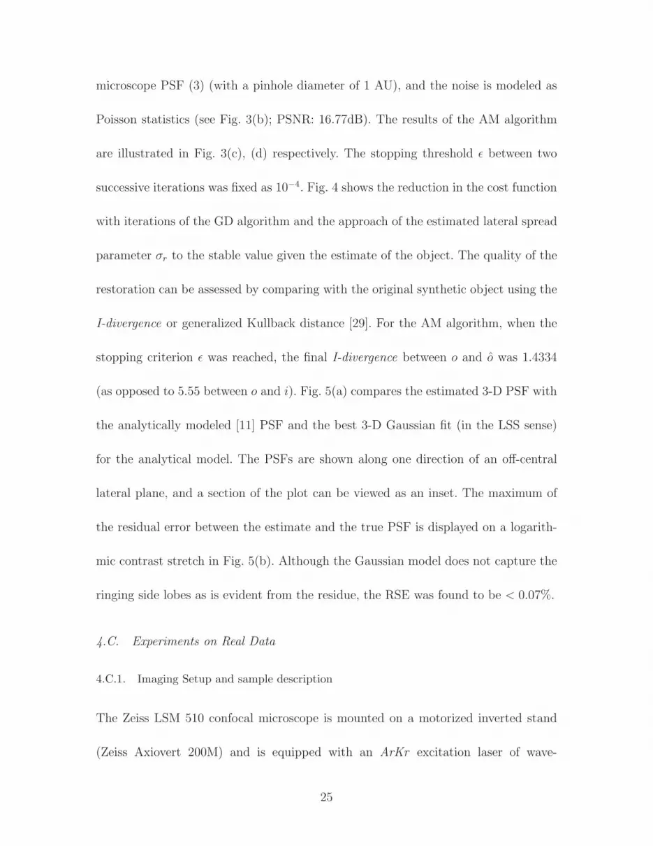
microscope PSF (3) (with a pinhole diameter of 1 AU), and the noise is modeled as
Poisson statistics (see Fig. 3(b); PSNR: 16.77dB). The results of the AM algorithm
are illustrated in Fig. 3(c), (d) respectively. The stopping threshold ε between two
successive iterations was fixed as 10−4. Fig. 4 shows the reduction in the cost function
with iterations of the GD algorithm and the approach of the estimated lateral spread
parameter σr to the stable value given the estimate of the object. The quality of the
restoration can be assessed by comparing with the original synthetic object using the
I-divergence or generalized Kullback distance [29]. For the AM algorithm, when the
stopping criterion ε was reached, the final I-divergence between o and o was 1.4334
(as opposed to 5.55 between o and i). Fig. 5(a) compares the estimated 3-D PSF with
the analytically modeled [11] PSF and the best 3-D Gaussian fit (in the LSS sense)
for the analytical model. The PSFs are shown along one direction of an off-central
lateral plane, and a section of the plot can be viewed as an inset. The maximum of
the residual error between the estimate and the true PSF is displayed on a logarith-
mic contrast stretch in Fig. 5(b). Although the Gaussian model does not capture the
ringing side lobes as is evident from the residue, the RSE was found to be < 0.07%.
4.C. Experiments on Real Data
4.C.1. Imaging Setup and sample description
The Zeiss LSM 510 confocal microscope is mounted on a motorized inverted stand
(Zeiss Axiovert 200M) and is equipped with an ArKr excitation laser of wave-
25

length of 488nm. The Band Pass (BP) filter transmits emitted light within the band
505− 550nm.
The specimen that was chosen for the first experiment is an embryo of the
Drosophila Melanogaster (see Fig. 6(a)). It was mounted and tagged with the Green
Fluorescence Protein (GFP). This preparation is used for studying the sealing of the
epithelial sheets (Dorsal Closure) midway during the embryogenesis. The objective
lens is a Plan-Neofluar with 40X magnification having a NA of 1.3 and immersed
in oil (ImmersolTM518F, Zeiss, refractive index μ = 1.518). The pinhole size was
67μm. The images ( c© Institute of Signaling, Development Biology & Cancer, Nice
UMR6543/CNRS/UNSA) were acquired with a XY pixel size of 50nm and a Z step
size of 170nm, and the size of the volume imaged is 25.59× 25.59× 2.55μm.
The second set of images ( c© INRA, Sophia-Antipolis) are the root apex of the
plant Arabidopsis Thaliana immersed in water (see Fig. 7). The dissected roots of
the Arabidopsis Thaliana plant were directly put on a microscope slide in approxi-
mately 100μl of water and this was then gently covered with a coverslip. This simple
set up works very well when the image acquisition recording times are not too long
(about 30 minutes). The microscope specifications are the same as that used for ac-
quiring the first data set but the objective is a C-Apochromat water immersion lens
with 63X magnification, 1.2 NA. The lateral pixel dimensions are 113nm and the Z
step is 438nm. The pinhole was fixed at 110μm. This preparation was used to study
Nematode infection at the center of the root in the vascular tissue.
26

4.C.2. Deconvolution Results
A rendered sub-volume of the observed and restored data for the Drosophila
Melanogaster is shown in Fig. 6. The deconvolution algorithm was stopped when
the difference between subsequent estimates was lower than ε = 0.002. The AM algo-
rithm converged after 40 iterations of the joint RL-TV and GD algorithm. The PSF
parameters were initialized to 300nm and 600nm for the lateral and the axial case re-
spectively, and the GD algorithm estimated them to be 257.9 and 477.9nm [47]. These
are larger (by about 16% and 14.5% for the lateral and the axial case respectively)
than their corresponding theoretically calculated values [5]. These results are fully in
line with also an experimental study performed earlier [48] with sub-resolution beads
which indicated a large deviation between theoretical aberration-free PSF models and
empirically determined PSFs.
Fig. 8(a) shows a rendered sub-volume (as indicated in Fig. 7) of the observed root-
apex and the corresponding restored result is shown in Fig. 8(b). It is evident from
these results that the microtubules (as identified by their specific binding proteins-
Microtubules binding domain (MBD)) are much easily discerned in the restoration
than in the original data. It was verified from the experiments on synthetic data [47]
that the proposed algorithm can not only estimate the actual PSF, but also provide
much better deconvolution result [49] in comparison to theoretical microscope PSF’s
(generated using the microscope settings). Validation is very important as in some
27

situations artifacts might arise in the restored image. These artifacts would be hard
to distinguish from biological structures unless some knowledge about the true image
is available. However, the results on real data are difficult to be validated unless a
higher resolution image of the same sample is available. Hence, we tested our decon-
volution algorithm on images of spherical fluorescent shells (see [36]) whose thickness
was measured after deconvolution and found closer to the true value specified by
Molecular Probes R©.
5. Conclusions and future work
In this paper we have proposed and validated an “Alternate Minimization (AM)”
algorithm for the joint estimation of the microscope PSF and the specimen source
distribution for a CLSM. We choose the RL algorithm for the deconvolution process
as it is best suited for the Poisson data, and TV as the regularization model. A
separable 3-D Gaussian model best describes the diffraction-limited confocal PSF, and
is chosen as the a priori model for the PSF. We are able to achieve blind deconvolution
by constraining the solution of the object and the PSF to different spaces. The PSF
approximation that is given in this paper is currently relevant to imaging thin samples.
However, it could also be extended to encompass any PSF that can be decomposed
in a similar manner. We have experimented on simulated and real data, and the
method gives very good deconvolution results and a PSF estimation close to the true
value [29, 47]. However, it should be noted that, all of the out-of-focus light cannot
28

be rejected and some noticeable haze and axial smearing remains in the images. This
could be improved by adding a Gamma prior on the PSF parameters.
Acknowledgement
This research was partially funded by the P2R Franco-Israeli Collaborative Research
Program. The authors gratefully acknowledge Dr. Caroline Chaux (Universite Paris-
Est, France) and Prof. Arie Feuer (Technion, Israel) for several interesting discus-
sions. We would also like to thank INRIA for supporting the Ph.D. of the first author
through a CORDI fellowship and CNRS for supporting the Ph.D. of the second au-
thor. Additionally, our sincere gratitude goes to Dr. Stephane Noselli, Mrs. Fanny
Serman (Ph.D. candidate) from the Institute of Signaling, Development Biology &
Cancer UMR 6543/CNRS/UNSA and Dr. Gilbert Engler (INRA Sophia-Antipolis,
France) for painstakingly preparing the images presented in Section 4.C, and for the
useful comments on their validation.
References
1. J. B. Pawley, editor. Handbook of biological confocal microscopy. Springer, 3rd
edition, 2006.
2. M. Born and E. Wolf. Principles of Optics. Cambridge Press, Cambridge, 1999.
3. D. A. Agard. Optical sectioning microscopy: Cellular architecture in three dimen-
sions. Ann. Rev. Biophys. Bioeng., 13:191–219, 1984.
29

4. R. Hudson, J. N. Aarsvold, C.-T. Chen, J. Chen, P. Davies, T. Disz, I. Foster,
M. Griem, M. K. Kwong, and B. Lin. Optical microscopy system for 3D dynamic
imaging. In C. J. Cogswell, G. S. Kino, and T. Wilson, editors, Proc. SPIE,
volume 2655, pages 187–198, 1996.
5. B. Zhang, J. Zerubia, and J. C. Olivo-Marin. Gaussian approximations of fluo-
rescence microscope point-spread function models. Appl. Opt., 46(10):1819–1829,
2007.
6. J. G. McNally, C. Preza, J.-A. Conchello, and L. J. Thomas Jr. Artifacts in
computational optical-sectioning microscopy. J. Opt. Soc. Am. A, 11:1056–1067,
March 1994.
7. J. W. Shaevitz and D. A. Fletcher. Enhanced three-dimensional deconvolution
microscopy using a measured depth-varying point-spread function. J. Opt. Soc.
Am. A, 24(9):2622–2627, 2007.
8. P. J. Shaw and D. J. Rawlins. The point-spread function of a confocal microscope:
its measurement and use in deconvolution of 3-D data. Journal of Microscopy,
163(2):151–165, 1991.
9. P. J. Shaw. Deconvolution in 3-D optical microscopy. The Histochemical Journal,
26(9):687–694, Sept. 1994.
10. A. Dieterlen, M. Debailleul, A. De Meyer, B. Simon, V. Georges, B. Colicchio,
O. Haeberle, and V. Lauer. Recent advances in 3-D fluorescence microscopy:
30

tomography as a source of information. In M. Kujawinska and O. V. Angelsky,
editors, Proc. SPIE, volume 7008, pages 70080S1–8. SPIE, 2008.
11. P. A. Stokseth. Properties of a Defocused Optical System. J. Opt. Soc. Am. A,
59:1314–1321, October 1969.
12. S.F. Gibson and F. Lanni. Diffraction by a circular aperture as a model for
three-dimensional optical microscopy. J. Opt. Soc. Am. A, A6:1357–1367, 1989.
13. O. V. Michailovich and D. R. Adam. Deconvolution of medical images from
microscopic to whole body images. In P. Campisi and K. Egiazarian, editors,
Blind Image Deconvolution: Theory and Applications, pages 169–237. CRC Press,
2007.
14. T. J. Holmes. Blind deconvolution of quantum-limited incoherent imagery:
maximum-likelihood approach. J. Opt. Soc. Am. A, 9:1052–1061, July 1992.
15. J. Markham and J.-A. Conchello. Parametric blind deconvolution: a robust
method for the simultaneous estimation of image and blur. J. Opt. Soc. Am.
A, 16(10):2377–2391, 1999.
16. E. F. Y. Hom, F. Marchis, T. K. Lee, S. Haase, D. A. Agard, and J. W. Sedat.
AIDA: an adaptive image deconvolution algorithm with application to multi-
frame and three-dimensional data. J. Opt. Soc. Am. A, 24(6):1580–1600, 2007.
17. L. Mandel. Sub-Poissonian photon statistics in resonance fluorescence. Opt. Lett.,
4:205–207, July 1979.
31

18. D. A. Agard, Y. Hiraoka, P. Shaw, and J. W. Sedat. Fluorescence microscopy in
three dimensions. Methods Cell Biology, 30:353–377, 1989.
19. G. B. Avinash. Data-driven, simultaneous blur and image restoration in 3-D
fluorescence microscopy. Journal of Microscopy, 183(2):145–157, August 1996.
20. P. Pankajakshan, L. Blanc-Feraud, Z. Kam, and J. Zerubia. Point-Spread Func-
tion retrieval in Fluorescence Microscopy. In Proceedings of IEEE International
Symposium on Biomedical Imaging, July 2009. Accepted for publication.
21. B. M. Hanser, M. G. Gustafsson, D. A. Agard, and J. W. Sedat. Phase retrieval for
high-numerical-aperture optical systems. Opt. Lett., 28(10):801–803, May 2003.
22. C. J. R. Sheppard and C. J. Cogswell. Three-dimensional image formation in
confocal microscopy. Journal of Microscopy, 159(2):179–194, 1990.
23. A. Erhardt, G. Zinser, D. Komitowski, and J. Bille. Reconstructing 3-D light-
microscopic images by digital image processing. Appl. Opt., 24:194–200, 1985.
24. W.A. Carrington, K. E. Fogarty, and F. S. Fay. 3D Fluorescence Imaging of Single
Cells Using Image Restoration, pages 53–72. Wiley-Liss, 1990.
25. C. Preza, M. I. Miller, L. J. Thomas Jr., and J. G. McNally. Regularized linear
method for reconstruction of three-dimensional microscopic objects from optical
sections. J. Opt. Soc. Am. A, 9(2):219–228, 1992.
26. T. Tommasi, A. Diaspro, and B. Bianco. 3-D reconstruction in optical microscopy
by a frequency-domain approach. Signal Processing, 32(3):357–366, 1993.
32

27. T. J. Holmes. Maximum-likelihood image restoration adapted for noncoherent
optical imaging. J. Opt. Soc. Am. A, 5:666–673, May 1988.
28. N. Dey, L. Blanc-Feraud, C. Zimmer, Z. Kam, P. Roux, J.C. Olivo-Marin, and
J. Zerubia. Richardson-Lucy Algorithm with Total Variation Regularization for
3D Confocal Microscope Deconvolution. Microscopy Research Technique, 69:260–
266, 2006.
29. P. Pankajakshan, B. Zhang, L. Blanc-Feraud, Z. Kam, J.C. Olivo-Marin, and
J. Zerubia. Parametric Blind Deconvolution for Confocal Laser Scanning Mi-
croscopy (CLSM)-Proof of Concept. Research Report 6493, INRIA Sophia-
Antipolis, France, March 2008.
30. G. M. P. Van Kempen, L. J. Van Vliet, P. J. Verveer, and H. T. M. Van Der Voort.
A quantitative comparison of image restoration methods for confocal microscopy.
Journal of Microscopy, 12:354–365, March 1997.
31. A. Dieterlen, C. Xu, O. Haeberle, N. Hueber, R. Malfara, B. Colicchio, and
S. Jacquey. Identification and restoration in 3D fluorescence microscopy. In
Oleg V. Angelsky, editor, Proc. SPIE, volume 5477, pages 105–113. SPIE, 2004.
32. G. Demoment. Image reconstruction and restoration: overview of common es-
timation structures and problems. IEEE Trans. Acoustics, Speech and Signal
Processing, 37(12):2024–2036, Dec 1989.
33. A. N. Tikhonov and V. A. Arsenin. Solution of Ill-posed Problems. Winston &
33

Sons, 1977.
34. K. Miller. Least Squares Methods for Ill-Posed Problems with a Prescribed Bound.
SIAM Journal on Mathematical Analysis, 1(1):52–74, 1970.
35. L. I. Rudin, S. Osher, and E. Fatemi. Nonlinear total variation based noise
removal algorithms. Physica D., 60:259–268, 1992.
36. N. Dey, L. Blanc-Feraud, C. Zimmer, P. Roux, Z. Kam, and J.C. Olivo-Marin. 3D
Microscopy Deconvolution using Richardson-Lucy Algorithm with Total Variation
Regularization. Research Report 5272, INRIA, France, July 2004.
37. L. B. Lucy. An iterative technique for the rectification of observed distributions.
Astron. J., 79:745–754, 1974.
38. W. H. Richardson. Bayesian-Based Iterative Method of Image Restoration. J.
Opt. Soc. Am. A, 62(1):55–59, January 1972.
39. A. P. Dempster, N. M. Laird, and D. B. Rubin. Maximum Likelihood from
Incomplete Data via the EM Algorithm. Journal of the Royal Statistical Society
B, 39(1):1–38, 1977.
40. M. Jiang and G. Wang. Development of blind image deconvolution and its appli-
cations. Journal of X-Ray Science and Technology, 11:13–19, 2003.
41. T. F. Chan and C.-K. Wong. Total variation blind deconvolution. IEEE Trans.
Image Processing, 7(3):370–375, Mar 1998.
42. L. Bar, N. A. Sochen, and N. Kiryati. Variational Pairing of Image Segmenta-
34

tion and Blind Restoration. In T. Pajdla and J. Matas, editors, Proc. ECCV,
volume II, pages 166–177. Springer, May 2004.
43. A. Santos and I. T. Young. Model-Based Resolution: Applying the Theory in
Quantitative Microscopy. Appl. Opt., 39(17):2948–2958, 2000.
44. K. E. Atkinson. An introduction to Numerical Analysis. John Wiley and Sons,
2nd edition, 1989.
45. A. Jalobeanu, L. Blanc-Feraud, and J. Zerubia. Hyperparameter estimation for
satellite image restoration using a MCMC Maximum Likelihood method. Pattern
Recognition, 35(2):341–352, 2002.
46. A. Mohammad-Djafari. A full Bayesian approach for inverse problems. In K. Han-
son and R. N. Silver, editors, Maximum entropy and Bayesian methods, volume 79,
pages 135–143. Kluwer Academic Publisher, 1996.
47. P. Pankajakshan, B. Zhang, L. Blanc-Feraud, Z. Kam, J.C. Olivo-Marin, and
J. Zerubia. Parametric Blind Deconvolution for Confocal Laser Scanning Mi-
croscopy. In Proceedings of IEEE International Conference of EMBS, pages 6531–
6534, Lyon, France, August 2007.
48. M. de Moraes Marim, B. Zhang, J.-C. Olivo-Marin, and C. Zimmer. Improv-
ing single particle localization with an empirically calibrated Gaussian kernel.
In Proceedings of IEEE International Symposium on Biomedical Imaging, pages
1003–1006, May 2008.
35

49. P. Pankajakshan, B. Zhang, L. Blanc-Feraud, Z. Kam, J.C. Olivo-Marin, and
J. Zerubia. Blind deconvolution for diffraction-limited fluorescence microscopy.
In Proceedings of IEEE International Symposium on Biomedical Imaging, pages
740–743, Paris, May 2008.
36

List of Figure Captions
Fig. 1. The MRF over a 6 member neighborhood ηx.
Fig. 2. Variation of the energy function J (o, θ|i) with respect to (a) lateral (σr)
and (b) with axial PSF parameter (σz). For this experiment, the true object o
is known and the observation is generated using a known 3-D Gaussian model.
The axial PSF parameter σz is varied by a factor ±ε to monitor its effect on
the estimated parameter σr and vice versa. σ(·,true) is the true parameter value.
Fig. 3. 3-D (a) phantom object (with false coloring), (b) observed image
blurred by the PSF model (3) and Poisson noise (PSNR: 16.77dB, I-divergence:
5.55), (c) restoration after RL+TV deconvolution with the estimated PSF (I-
divergence: 1.43), (d) estimated PSF. The intensities of the object, observation
and the restoration are on a linear scale while the PSF is on a logarithmic scale.
Fig. 4. Convergence of the cost function and lateral parameter by the GD
method (when the original object is known). The Y axis is left-scaled for the
cost function J (θ, o|i) and right-scaled for the PSF parameter respectively.
Fig. 5. (a) The full model (dash), estimated (continuous) and the best Gaussian
fit (dash-dot) PSFs are displayed for one direction (off-central plane); the inset
shows a section of the plot, (b) X-Z projection of the residual (RSE < 0.07%)
between the estimated and full PSF model is displayed on a log scale.
Fig. 6. (a) Rendered sub-volume of the original specimen ( c© Institute of
37

Signaling, Developmental Biology & Cancer UMR6543/CNRS/UNSA), and
(b) restored image ( c© Ariana-INRIA/I3S). The intensity is scaled between
[0 130] for display.
Fig. 7. Observed root apex of an Arabidopsis Thaliana with a volume
146.448μm × 146.448μm × 30.222μm ( c© INRA). The sub-volume chosen
for restoration is emphasized.
Fig. 8. Rendered sub-volume of the (a) observed image slices in Fig. 7 ( c©
INRA) and (b) volume rendering of the restored image slices ( c© Ariana-
INRIA/I3S). ε = 0.0001.
38

Fig. 1. The MRF over a 6 member neighborhood ηx. fig1.eps.
39

50 60 70 80 90 100
Radial spread parameter σr (in nm)
Ene
rgy
Func
tionJ(
θ,o|i)
ε = 0%
ε=−11%
ε=−5%
ε=+5%
ε=+11%
σr,true
σr,true
(a)
180 190 200 210 220 230 240 250 260 270 280
Axial spread parameter σz (in nm)
Ene
rgy
Func
tionJ(
θ,o|i)
ε=0%
ε=−11%
ε=−2%
ε=+2%
ε=+11%
σz,true
σz,true
(b)
Fig. 2. Variation of the energy function J (o, θ|i) with respect to (a) lateral (σr)
and (b) with axial PSF parameter (σz). For this experiment, the true object o
is known and the observation is generated using a known 3-D Gaussian model.
The axial PSF parameter σz is varied by a factor ±ε to monitor its effect on
the estimated parameter σr and vice versa. σ(·,true) is the true parameter value.
fig2a.eps fig2b.eps.
40
X-Y
X-Z
(a) (b)
X-Y
X-Z
(c) (d)
Fig. 3. 3-D (a) phantom object (with false coloring), (b) observed image
blurred by the PSF model (3) and Poisson noise (PSNR: 16.77dB, I-divergence:
5.55), (c) restoration after RL+TV deconvolution with the estimated PSF (I-
divergence: 1.43), (d) estimated PSF. The intensities of the object, observation
and the restoration are on a linear scale while the PSF is on a logarithmic
scale. fig3axy.eps fig3bxy.eps fig3scale.eps fig3axz.eps fig3bxz.eps fig3cxy.eps
fig3dxy.eps fig3scalepsf.eps fig3cxz.eps fig3dxz.eps.
41

5
10x 10
6
J(θ,
o|i)
2 4 6 8 10 12 14 16 18 200
506.9
Iterations
σr
(in
nm)
σr estimate
Cost Function
σr,true
Fig. 4. Convergence of the cost function and lateral parameter by the GD
method (when the original object is known). The Y axis is left-scaled for the
cost function J (θ, o|i) and right-scaled for the PSF parameter respectively.
fig4.eps.
42

−880 −480 −80 320 720 11200
0.2
0.4
0.6
0.8
1
x (in nm)
h(x
)/‖h
(x)‖
∞
Analytical PSF model
Estimated PSF using AM
Analytical PSF data fitted
0
0.01
0.02
0.03
0.04
0.05
Z
X
(a) (b)
Fig. 5. (a) The full model (dash), estimated (continuous) and the best Gaussian
fit (dash-dot) PSFs are displayed for one direction (off-central plane); the inset
shows a section of the plot, (b) X-Z projection of the residual (RSE < 0.07%)
between the estimated and full PSF model is displayed on a log scale. fig5a.eps
fig5b.eps.
43

(a) (b)
Fig. 6. (a) Rendered sub-volume of the original specimen ( c© Institute of Sig-
naling, Developmental Biology & Cancer UMR6543/CNRS/UNSA), and (b)
restored image ( c© Ariana-INRIA/I3S). The intensity is scaled between [0 130]
for display. fig6a.eps fig6b.eps.
44

Fig. 7. Observed root apex of an Arabidopsis Thaliana with a volume
146.448μm × 146.448μm × 30.222μm ( c© INRA). The sub-volume chosen
for restoration is emphasized. fig7.eps.
45
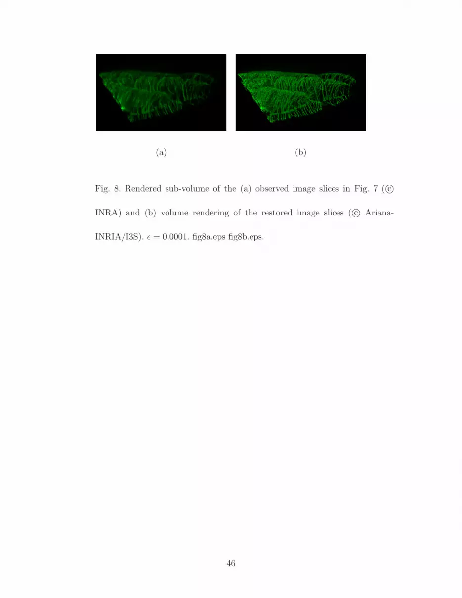
(a) (b)
Fig. 8. Rendered sub-volume of the (a) observed image slices in Fig. 7 ( c©
INRA) and (b) volume rendering of the restored image slices ( c© Ariana-
INRIA/I3S). ε = 0.0001. fig8a.eps fig8b.eps.
46


