Blind prediction of HIV integrase bindingfrom the SAMPL4 challenge

David L. Mobley • Shuai Liu • Nathan M. Lim • Karisa L. Wymer •

Alexander L. Perryman • Stefano Forli • Nanjie Deng • Justin Su •

Kim Branson • Arthur J. Olson

Received: 27 January 2014 / Accepted: 28 January 2014

� Springer International Publishing Switzerland 2014

Abstract Here, we give an overview of the protein-

ligand binding portion of the Statistical Assessment of

Modeling of Proteins and Ligands 4 (SAMPL4) challenge,

which focused on predicting binding of HIV integrase

inhibitors in the catalytic core domain. The challenge

encompassed three components—a small ‘‘virtual screen-

ing’’ challenge, a binding mode prediction component, and

a small affinity prediction component. Here, we give

summary results and statistics concerning the performance

of all submissions at each of these challenges. Virtual

screening was particularly challenging here in part because,

in contrast to more typical virtual screening test sets, the

inactive compounds were tested because they were thought

to be likely binders, so only the very top predictions per-

formed significantly better than random. Pose prediction

was also quite challenging, in part because inhibitors in the

set bind to three different sites, so even identifying the

correct binding site was challenging. Still, the best methods

managed low root mean squared deviation predictions in

many cases. Here, we give an overview of results, highlight

some features of methods which worked particularly well,

and refer the interested reader to papers in this issue which

describe specific submissions for additional details.

Keywords HIV integrase � Binding mode � Virtual

screening � Pose prediction � Affinity � SAMPL4

Introduction

Accurate protein-ligand binding predictions could impact

many areas of science. An ideal computational method

which could quickly and reliably predict binding free ener-

gies and bound structures for small molecules of interest to

arbitrary receptors would have far reaching applications,

including in virtual screening, drug lead optimization, and

even further afield, to help enzyme design, systems biology,

and in a variety of other applications. However, most sys-

tematic tests of methods for predicting binding strengths and

binding modes indicate that these still need substantial

improvement to be of routine use in discovery applications.

While methods can be improved based on existing

Electronic supplementary material The online version of thisarticle (doi:10.1007/s10822-014-9723-5) contains supplementarymaterial, which is available to authorized users.

D. L. Mobley (&) � S. Liu � N. M. Lim � K. L. Wymer � J. Su

Department of Pharmaceutical Sciences and Department of

Chemistry, University of California, Irvine, 147 Bison Modular,

Irvine, CA 92697, USA

e-mail: dmobley@mobleylab.org

D. L. Mobley

Department of Chemistry, University of New Orleans,

2000 Lakeshore Drive, New Orleans, LA 70148, USA

A. L. Perryman � S. Forli � A. J. Olson

Department of Integrative Structural and Computational

Biology, The Scripps Research Institute, La Jolla, CA 92037,

USA

Present Address:

A. L. Perryman

Department of Medicine, Division of Infectious Diseases,

Rutgers University-NJ Medical School, Newark, NJ, USA

N. Deng

Department of Chemistry and Chemical Biology Rutgers, The

State University of New Jersey, A203, 610 Taylor Road,

Piscataway, NJ 08854, USA

K. Branson

Hessian Informatics, LLC. 609 Lakeview Way, Emerald Hills,

CA, USA

123

J Comput Aided Mol Des

DOI 10.1007/s10822-014-9723-5

experimental data, methodological improvements need to be

tested in a predictive setting to determine how well they work

prospectively, and especially so for methods involving

empirical parameters which are tuned to fit previously

known values. Thus, we need recurring prediction chal-

lenges to help test and advance computational methods. The

Statistical Assessment of Modeling of Proteins and Ligands

(SAMPL) challenge we discuss here provides one such test.

SAMPL protein-ligand binding background

The SAMPL challenge focuses on testing computational

methods for predicting thermodynamic properties of small

drug-like or fragment-like molecules, including solvation free

energies, host-guest binding affinities, and protein-ligand

binding. The challenge started informally in 2007 at one of

OpenEye Software’s Customers, Users, and Programmers

(CUP) meetings [40], and then was formalized as the SAMPL

challenge beginning in 2008. Here, we discuss the results of

the protein-ligand binding component of SAMPL4, the 4th

iteration of the SAMPL challenge, which took place in 2013.

Protein-ligand binding has not been a feature of every

SAMPL challenge, featuring previously only in SAMPL1 and

SAMPL3. SAMPL1 included a pose prediction test on kinases,

which proved extremely challenging. The system which

proved most interesting for analysis was JNK3 kinase, where

the best performing predictions were from two participants

who used software-assisted visual modeling to generate and

select poses. Essentially, pose predictions were generated and

filtered using expert knowledge of related ligands or related

systems. The two experts applying this strategy substantially

outperformed all pure algorithmic approaches [47]. Affinity

prediction results in some cases were reasonable, however [49].

The SAMPL3 protein-ligand challenge involved predicting

binding of a series of fragments to trypsin [39], and a number of

groups participated [2, 30, 31, 49, 50], in some cases achieving

rather good enrichment for screening [49, 50] and good cor-

relations between predicted binding strength and measured

affinity [50], though the test was still challenging [31].

The current SAMPL4 challenge focused on predicting

binding of a series of ligands to multiple binding sites in

HIV integrase.

HIV integrase background

According to the World Health Organizations data (http://

UNAIDS.org), over 33.3 million people are currently liv-

ing with an HIV infection. Approximately 2.3–2.8 million

people become infected with HIV annually, and 1.7 million

people die from HIV-related causes each year. Throughout

the AIDS epidemic, over 32 million people have died of

HIV-related causes, which makes HIV the deadliest virus

plaguing humanity.

HIV integrase and the drugs that target it

HIV integrase (IN) is one of three virally encoded

enzymes. It performs two distinct catalytic functions called

‘‘3’ processing’’ (which cleaves two nucleotides off of the

end of the viral cDNA in a sequence-specific manner to

generate reactive CAOH�30 termini) and the ‘‘strand transfer

reaction’’ (which covalently attaches, or integrates, the

cleaved viral cDNA into human genomic DNA, in a non-

sequence-specific manner). Two drugs that target the active

site of IN have been approved by the FDA for the treatment

of HIV/AIDS: Raltegravir was approved in 2007, and El-

vitegravir was approved in 2012 [46]. These two drugs are

called INSTIs (for Integrase Strand Transfer Inhibitors). A

third INSTI, Dolutegravir, is currently in late-phase clinical

trials [46].

HIV integrase is an enzyme that is part of a large family

of recombinases that all contain the ‘‘DDE’’ motif (or D,D-

35-E motif) within the active site. The two Asps and one

Glu are used to chelate two magnesium ions, using

monodentate interactions between each carboxylate group

and a magnesium [44]. This active site region is where the

30 processing and strand transfer reactions occur. One

monomer of HIV IN contains three different domains: the

N-terminal domain (NTD), catalytic core domain (CCD),

and the C-terminal domain (CTD) (Fig. 1). When per-

forming catalysis (or when bound to DNA immediately

before catalysis occurs), IN is a tetramer (i.e., a dimer of

three-domain dimers). The NTD is an HH-CC zinc-binding

domain (for the His,His-Cys,Cys motif that chelates the

Zn). The CTD displays the SH3 fold and binds DNA non-

specifically (to likely help position, or scaffold, the DNA

and direct it towards a CCD). The CCD displays the

RnaseH fold, and two monomers of the CCD form a

spherical dimer. The CCD dimer contains two active site

regions (i.e., one active site per monomer), which is where

the advanced INSTIs all bind (i.e., they bind to the com-

plex of the CCD with DNA). But in the full 3-domain

tetramer of HIV IN bound to both viral cDNA and human

genomic DNA, it is likely that only one active site per CCD

dimer is involved in catalysis (due to geometric con-

straints). All of the crystal structures of HIV IN used in this

challenge contained dimers of only the CCD. Although

there are many crystal structures of HIV IN, the only

structures available in the PDB contain only one or 2

domains of the full 3 domain monomer of IN, and none of

the HIV IN crystal structures include any DNA. However,

a similar recombinase from Prototype Foamy Virus, called

PFV integrase, was recently crystallized in many different

complexes by Peter Cherepanov et al. These PFV IN

crystal structures often contain DNA and one of the three

aforementioned advanced INSTIs (see Fig. 1) [19, 20, 21,

34, 36].

J Comput Aided Mol Des

123

Although the three advanced INSTIs were only recently

developed, multi-drug-resistant mutants against which

these inhibitors lose their potency have already appeared in

clinical settings [1, 17, 45, 46, 55]. There are three main,

independent pathways resulting in INSTI resistance, which

involve mutations at positions Tyr143, Asn155, and

Gln148 [55], all of which are within the catalytic active site

region. Mutations at these positions, especially when

combined with additional secondary mutations at other

positions, cause extensive cross-resistance to both Ralte-

gravir and Elvitegravir, and mutations involving Gln148

significantly decrease the susceptibility of HIV to all three

advanced INSTIs [1, 17, 55]. The fact that HIV can quickly

evolve drug resistance against these strand transfer active

site inhibitors of IN highlights the urgent need to discover

and develop new classes of drugs that bind to different sites

and display new mechanisms of action.

Utility of allosteric inhibitors

Combinations of two different classes of inhibitors that

act on the same enzyme have been shown to inhibit

broad panels of many different multi-drug-resistant

mutants and to also decrease the probability of the

emergence of new drug-resistant mutants, as exemplified

by the combination of an active site inhibitor and an

allosteric inhibitor of Bcr-Abl, a kinase target for cancer

chemotherapy [25, 58]. This also appears to be the case

for HIV treatment. When a Nucleoside Reverse Trans-

criptase Inhibitor (NRTI; NRTIs target the active site of

HIV reverse transcriptase, or RT) is combined with an

allosteric Non-Nucleoside Reverse Transcriptase Inhibitor

(NNRTI; NNRTIs target a non-active site region of HIV

RT), the evolution of drug resistance to both classes of

drugs is impeded [10].

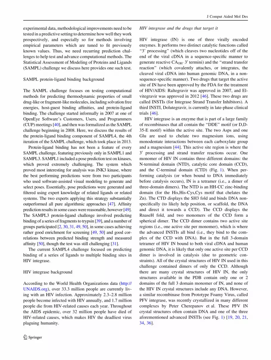
Fig. 1 Integrase (IN) functional structure and architecture. The three

domain structure of a monomer of IN is displayed. The PFV IN

crystal structure (from 3OS1.pdb) of the ‘‘target capture complex’’

with DNA is displayed in surface mode, with the C-Terminal Domain

in yellow, the N-Terminal Domain in light blue, and the human DNA

in salmon. The 3NF8 reference structure of the HIV IN Catalytic Core

Domain dimer was superimposed onto this PFV IN crystal structure,

and its CCD is shown in ribbon mode (with one monomer in green

and the other in cyan). The ‘‘CDQ’’ allosteric fragment from 3NF8 is

displayed as sticks with white carbons to highlight the three allosteric

sites of HIV IN that were part of the SAMPL4 challenge: LEDGF,

Y3, and FBP. A black outline and the label RLT show the location of

the active site of IN. Raltegravir (labeled as RLT) was extracted by

superimposing the PFV IN crystal structure from 3OYA.pdb onto the

3OS1.pdb structure of PFV IN. During catalysis, HIV IN is present as

a tetramer (i.e., a dimer of dimers)

J Comput Aided Mol Des

123

LEDGF inhibitors

One new class of inhibitors that seem particularly prom-

ising in the fight against AIDS are the subset of ALLosteric

INtegrase Inhibitors (ALLINIs) called LEDGINs [7],

which bind to the LEDGF site at the dimer interface of the

CCD [12, 28]. LEDGF (for Lens Epithilial-Derived

Growth Factor) is a human protein that HIV exploits: when

IN interacts with LEDGF/p75, it guides the integration of

the viral genome into the regions of our chromosomes

where the actively expressed genes are located [4], which

increases the probability of the subsequent production of

viral proteins that can then help spread the infection. The

LEDGINs use a carboxylate group to mimic a key inter-

action that LEDGF utilizes to bind to the backbone amino

groups of Glu170 and His171, which are located in the

LEDGF site of IN [28]. When LEDGINs bind the LEDGF

site, they promote and stabilize higher-order multimers of

IN and inhibit the catalytic process [6, 26, 27, 53].

Before the challenge began, the participants were

informed that most of the SAMPL4 compounds were

known to bind to (at least) the LEDGF site of IN, but some

of the compounds were known to bind to at least one of the

two additional allosteric sites of IN, which were referred to

as the ‘‘FBP’’ site (for Fragment Binding Pocket) and the

‘‘Y3’’ site (see Fig. 1). Like the LEDGF site, the FBP site

is also located at the dimer interface of the CCD of IN.

There are two LEDGF sites per IN CCD dimer, two FBP

sites per IN CCD dimer, and also two Y3 sites per IN CCD

dimer. But the Y3 site is entirely contained within each

monomer of the core domain and is located underneath the

very flexible 140s loop (i.e., Gly140-Gly149). The top of

the 140s loop flanks the active site region, and the com-

position, conformation, and flexibility of the 140s loop is

known to be critical to IN activity [11, 18, 44]. Participants

in the pose prediction challenge were given the hint that, if

they were concerned about trying to predict the binding

site, they might wish to focus their efforts on the LEDGF

site, though most chose not to do so. This could have led to

successful binding mode predictions in *52 of 55 cases

considered.

SAMPL challenge preparation and logistics

The experimental data for the IN portion of SAMPL4 is

described in detail elsewhere in this issue [42]. It includes a

set of inactive compounds which were not observed to bind

via both crystallography and surface plasmon resonance

(SPR), and a set of actives; together, these were used for

the virtual screening component of SAMPL4. Additionally,

crystal structures for some 57 of the actives were used for

the pose prediction challenge. Accurate affinities were

measured via SPR for 8 of these compounds, and these

were used for the affinity prediction challenge.

For each portion of the challenge, participants were

provided with a PDF of introductory material on the system

prepared by Thomas S. Peat, which included a brief

overview of the biological relevance, the different binding

sites, and some references to previous published work from

the same discovery project. This PDF is provided in the

Supporting Information. In addition to this PDF, partici-

pants in each individual component received a further set

of calculation inputs which will be described below.

The integrase portion of SAMPL4 was staged, so that

participants must either complete or opt-out of virtual

screening before going on to pose prediction, and complete

or opt-out of pose prediction before going on to affinity

prediction. This was done because inputs for the sub-

sequent portions of the challenge would reveal all or part of

the results from the earlier challenge components. In some

cases, participants opted to conduct the whole challenge

using only the inputs for the virtual screening challenge,

and thus had no information about the identities of actual

binders and/or structures when working on the affinity

prediction and pose prediction challenges. This was pri-

marily the case for submission IDs 535-540.

The SAMPL4 challenge was advertised via the SAMPL

website (http://sampl.eyesopen.com) and e-mails to past

participants, others in the field, and the computational

chemistry list (CCL), beginning in January, 2013. The

virtual screening portion of the challenge was made

available via the SAMPL website April 1, 2013, and par-

ticipants moved on to the other components once their

screening results were submitted, or once they opted out.

Submissions for all challenge components were due Friday,

August 16. The challenge wrapped up with the SAMPL4

workshop on September 20 at Stanford University. Sub-

missions were allowed to be anonymous, though we1

received only three anonymous submissions from this

portion of the challenge. Because of this, however, we

typically refer to submissions by their submission ID (a

three digit number) rather than by the authors’ names.

Pre-challenge preparation

The challenge organizers were provided with three main

inputs to prepare the SAMPL4 challenge. First, we

received a disk with raw crystallography data and refined

structures for the majority of the compounds which were

crystallized. Second, we received a spreadsheet describing

1 The SAMPL4 challenge was designed, run and evaluated by the

Mobley lab with some help from Kim Branson, so when this report

uses the word ‘‘we’’ to refer to an action relating to challenge design,

logistics, and analysis, it refers to these authors—specifically,

Mobley, Branson, Su, Lim, Wymer, and Liu.

J Comput Aided Mol Des

123

the active compounds, with SMILES strings, 2D structures,

information about the density, and the location of the data

on the disk. Third, we received a document containing

images of the chemical structures of many inactive com-

pounds. Fourth, we received a list of the molecules for

which affinities were being measured precisely via SPR.

Our pre-challenge preparation mainly involved turning this

information into suitable inputs for predictions, and

checking the data. Here, we used OpenEye unified Python

toolkits [41] unless otherwise noted.

Preparing inactives

For the list of non-binders, since we had only compound

identifiers and images of the 2D structures, we re-drew 2D

structures of all of the non-binding compounds in Marvin

Sketch [35] and then stored SMILES of these which were

subsequently canonicalized and turned into 3D structures

using the OpenEye toolkits [41] and Omega [22, 23]. Since

this step involved manually drawing the structures, all

structures drawn were inspected by two different people to

check for accuracy.

Preparing actives

We also needed SMILES strings and 3D structures for all

of the binders. SMILES strings were available both in the

spreadsheet we were provided and on the disk, but these

were not always consistent, and typically omitted stereo-

chemistry information. We found that the most reliable

route to getting this information was to pull the 3D ligand

structures from the protein structures we were provided,

then add protons and perceive stereochemistry information

based on these structures. However, strain or other issues in

the structures on occasion resulted in incorrect assignment

of stereochemistry.

To deal with incorrect assignment of stereochemistry,

we used OpenEye’s Flipper module to enumerate all ster-

eoisomers for each ligand, and with the Shape toolkit

overlaid these onto the ligand structures pulled from the

refined PDB files, automatically selecting the best-scoring

shape overlay as the correct stereoisomer for cases with

high shape similarity. Any alternate stereoisomer case

where the shape Tanimoto score was within 0.1 of the best

scoring shape overlay was flagged for additional manual

inspection, although ultimately all structures were inspec-

ted manually. Based on manual examination of the shape

overlays and electron densities in cases where there was

any ambiguity, we concluded that the automatically

assigned stereochemistry information was correct in every

case except AVX17587, 38673, 38741, 38742, 38747,

38748, 38749, 38782, 38789, 101124, and GL5243-84.

This seemed primarily to be because of poor-quality shape

overlays in these cases, possibly due to ligand strain. Once

we finished applying this procedure, we saved 3D struc-

tures of the correct stereoisomer of every ligand, as well as

the isomeric SMILES string specifying stereochemistry

information. In some cases our shape overlay work here

actually resulted in a re-evaluation and potentially a re-

refinement of the crystal structure, as discussed elsewhere

[42].

Stereoisomer enumeration

In general, chiral compounds were tested as a mix of

stereoisomers, so treating isomers as distinct compounds

provides an opportunity to expand the list of inactive

compounds. This is especially true for the inactive com-

pounds, but even for the active compounds, if a given

stereoisomer is not observed to bind, it means either that it

does not bind, or it is much weaker than the stereoisomer

which is observed to bind. Thus, for all compounds we

enumerated all stereoisomers using Flipper and assigned

them an isomer ID which was added to their ID. For

example, for AVX38670, with two stereoisomers, these

were labeled AVX38670_0 and AVX38670_1 and treated

separately for the virtual screening and (when applicable)

pose prediction challenges. The issue of whether or not to

treat alternate (apparently non-binding) stereoisomers of

actives as inactives will be discussed further below.

After generating or reading in isomeric SMILES strings

for all compounds, we also cross-checked for duplicate

compounds under the same or different identifiers and

removed a number of such duplicates. In the OpenEye

toolkits, there is a 1:1 correspondence between an isomeric

SMILES string and a particular compound in its standard

representation, so we expected that this would catch all

duplicates. However, because of differences in how

bonding was assigned prior to generating isomeric

SMILES strings, some SMILES strings were generated

from the Kekule representation of molecules and some

were not. These forms result in different isomeric SMILES

strings, so some duplicates remained when we conducted

the challenge and were only removed when we discovered

this in post-analysis, as discussed below.

Protonation state assignment

By default, protonation/tautomer states for provided 3D

structures for all compounds were assigned via the Open-

Eye toolkits using their ‘‘neutral pH model’’ predictor,

though we did some additional investigation for pose pre-

diction and affinity prediction, as noted below.

J Comput Aided Mol Des

123

Molecular dynamics re-refinement

In the process of preparing for SAMPL, several structures

were re-refined and in several cases resulted in substantial

changes. We were concerned that we might miss other

problem cases, and sought an automated procedure to

identify cases where the binding mode might be ques-

tionable. Therefore, we took all refined structures and

simulated them in the AMBER99SB-ILDN protein force

field [33] with the AMBER GAFF [56] in GROMACS

4.6.2 for 110 ps of equilibration and another 100 ps of

production, using protein protonation states assigned by

MCCE. Equilibration was done gradually releasing

restraints on the protein?ligand. Following this, we mon-

itored root mean squared deviation (RMSD) over the

course of the short production simulations and looked for

cases where the ligand moved substantially away from its

starting binding mode, by more than 3 A *RMSD. This

flagged several cases as potentially problematic—

AVX17558, AVX38749, and AVX38747. All three have a

somewhat-floppy alkyl tail which in at least two of the

cases has fairly poor density, which may be part of the

issue. Re-refinement from our final structures from MD did

not result in substantial improvement. Still, to us this

suggests that closer scrutiny of these three may still be

warranted. Particularly, in AVX17558 and AVX38747,

there is some question as to the chirality. For AVX17558,

there is some evidence in the density that both stereoiso-

mers bind [43], while for AVX38747, it is not completely

clear which stereoisomer fits the density best [43]. The

remaining cases remained quite close to the crystallo-

graphic structure.

Virtual screening

In addition to the IN background PDF noted above, virtual

screening participants were provided with a README file,

a template for submitting their predictions, isomeric

SMILES strings and 3D structures (in MOL2 and SDF

format) for all stereoisomers of all compounds, and a ref-

erence protein/ligand structure in the form of a

3NF8_reference.pdb file—essentially, the PDB 3NF8

structure, aligned to the frame of reference we had chosen

for the challenge. This 3NF8 structure was selected in part

because it contains a bound ligand from the series studied

here, and in part because this ligand is observed in all six

binding sites (both copies of the LEDGF, Y3, and FBP

sites). The README file contained information on what

they were to submit, notes about the reference structure and

the locations of the three sites, and a substantial hint—that

‘‘many (though by no means all) of the ligands bind in the

LEDGF site, so if you like, you can focus on just that site

and still do relatively well.’’ We also included a disclaimer

that the ligand protonation/tautomer states are provided ‘‘as

is’’ and participants might wish to investigate these on their

own. Submissions included a rank for each compound, a

field indicating whether or not it was predicted to bind

(‘‘yes’’ or ‘‘no’’) and a confidence level ranging from 1

(low confidence) to 5 (very confident). These files are

provided in the Supporting Information.

After the challenge, we found some issues with dupli-

cate or incorrect compounds included in the virtual

screening set. Specifically, we had to remove AVX17684m

(or AVX17684-mod) because it was present in only some

of the files which were distributed, and AVX17268_1

because it was incorrect. And only one member of each

given set of duplicates was considered in analysis. Dupli-

cates/replicates included (AVX17556, AVX17561, and

GL5243-84), (AVX17557 and AVX17587), (AVX101125

and AVX62777), (AVX17285 and AVX16980), and

(AVX17557 and AVX17587).

Pose prediction

In addition to the IN background PDF, pose prediction

participants were provided with a README file, the ref-

erence structure described above, and SMILES strings and

3D structures (in MOL2 and SDF format) for all ligands, as

in the case of the virtual screening challenge. The main

differences here were that in this case, the compound list

included only active compounds, and additional informa-

tion in the README file. Particularly, the README file

additionally added some additional pointers concerning

protonation/tautomerization states. For this challenge por-

tion, we used Epik, from Schrodinger, to enumerate pos-

sible protonation and tautomer states, and cross-compared

the Epik predictions with those from OpenEye’s QuacPac

[41]. As a result, we highlighted compounds AVX17715,

AVX58741, AVX38779-38789, and AVX-101118 to

101119 as having possible uncertainty in their protonation

states, and GL5243-102 as having two possible tautomers

on its five-membered ring, so these notes were provided in

the README. The input files are provided in the Sup-

porting Information.

Depending on the nature of their method, participants

submitted either a 3D structure of the ligand in its predicted

binding mode (relative to the 3NF8_reference.pdb structure

provided), omitting the protein; or a 3D structure of the

ligand-protein complex. In this challenge, our analysis

focused only on the predicted binding modes relative to a

static structure, so in cases where the full protein structure

was submitted (i.e. for flexible protein methods), we scored

binding modes based on an alignment onto the static ref-

erence structure.

For pose prediction, participants received SMILES

strings for 58 compounds but 3D structures for 65

J Comput Aided Mol Des

123

compounds because of a scripting error which resulted in

some extra isomers being included in the 3D structures

directory. So participants should have predicted binding

modes for 58 compounds. However, several additional

compounds had to be removed prior to analysis. Specifi-

cally, AVX17680 was removed because participants were

provided with the wrong SMILES string and 3D structure

because of a scripting error. Additionally, AVX101121 had

a discrepancy between its SMILES string and its structure

(differing by a methyl) apparently due to confusion about

the original identity of the compound in the experiments,

so this was removed prior to analysis. A similar thing

happened with AVX-17543 on the computational end—

participants were given an incorrect ligand SMILES and

structure, and this had to be removed prior to analysis.

Finally, AVX-17557 and AVX-17587 are actually the

same compound, prepared as different salts. Thus the final

number of compounds analyzed was 54.

Affinity prediction

In addition to the IN background PDF, affinity prediction

participants were provided with 3D structures of all 8

ligands (in MOL2 and SDF format), a README file, the

refined crystal structures PDB format, MTZ format density

files for the crystal structures, shape overlays of the ligands

onto the crystallographic ligands (generated by the Open-

Eye Shape toolkit [41]), the refined crystal structure and

ligand for the compound from the 3ZSQ structure, which

was used as the control compound in SPR, and a text file

template for submissions, which contained fields for the

compound ID, the predicted binding free energy, the pre-

dicted statistical uncertainty, and the predicted model

uncertainty. In this case, the README file highlighted

minor issues with the electron density for AVX-17557 and

for the aliphatic amino in AVX-38780, and an alternate

rotamer for Leu102 in AVX40811 and AVX40812, as well

as uncertainty in the protonation state of AVX38780.

SAMPL analysis methods

In general, analysis was done using OpenEye’s Python

toolkits for working with molecules and structures, and

Python/NumPy for numerical data. Matplotlib was used for

plots.

Virtual screening

Virtual screening performance was analyzed by a variety of

relatively standard metrics, including area under the curve

(AUC) and enrichment factor at 10 % of the database

screened (EF10), as well as the newer Boltzmann-enhanced

discrimination of receiver operating characteristic (BED-

ROC) [52]. We also made enrichment and ROC plots for

all submissions. These were done using our own Python

implementation of the underlying routines.

Pose prediction

Here, we focused primarily on judging pose predictions via

RMSD. We used two different evaluation schemes

depending on how we handled cases with multiple copies

of the ligand bound. Since IN is a dimer, there are two

essentially symmetric copies of each binding site, for a

total of 6 binding sites. These ‘‘symmetric’’ sites exhibit

non-crystallographic symmetry (sequence symmetry) and

are in some cases not quite symmetric. Typically, they in

fact were refined separately. This introduced some com-

plexities for judging pose prediction. Even if a ligand only

occupied the LEDGF site, and a participant only predicted

one binding mode, two RMSD scores were possible

depending on how the prediction was superimposed onto

the crystallographic structure. To compute both values, we

rotate the crystal structure to the alternate possible align-

ment onto the reference structure (thus handling the non-

crystallographic symmetry). Then, we compute the RMSD

based on both the original alignment and the new align-

ment, and retain the best value as the score for this sub-

mission. This scenario of only a single predicted binding

mode applied to the majority of submissions, though a

minority of participants predicted multiple binding modes

for some ligands, and a minority of ligands bound in other

binding sites or exhibited multiple site binding. In these

cases, additional RMSD values were possible. For exam-

ple, if a participant predicted a ligand to bind to the

LEDGF site, and actual binding was observed in both

LEDGF sites and the Y3 site, we would obtain four dif-

ferent RMSD values. To handle this ambiguity, we chose

to use two different scoring schemes, which we call ‘‘by

ligand’’ and ‘‘by pose’’. In the ‘‘by ligand’’ scheme, we

choose each submission’s best RMSD value for each

ligand, resulting in a total of 54 RMSD values. In the ‘‘by

pose’’ scheme, each experimental binding site and mode

(LEDGF, Y3, FBP) is scored separately and the best

RMSD value is retained for each, resulting in a total of 112

RMSD values. Since most participants predicted only one

binding mode per compound, this latter scheme penalizes

submissions which miss binding to the additional sites in

the case of multiple-site binding, while the former does not.

Our analysis here focuses only on scoring the best RMSD

value of each submission for each ligand or pose. In general

one might also be interested in knowing the worst RMSD.

But since all but two participants here submitted only a single

binding mode for each compound, the best and worst values

are essentially identical for most submissions here.

J Comput Aided Mol Des

123

To evaluate RMSD scores, we used a maximal common

substructure search to match predicted ligand binding

modes onto the crystallographic binding modes since this

matching was not always obvious. Particularly, submis-

sions used a variety of file formats, and not all submissions

included ligand hydrogen atoms. Some submissions also

altered atom naming conventions, meaning that the most

straightforward approach of simply matching atoms by

their names would not always work. Additionally, some

ligands had internal symmetries (for example, a symmetric,

rotatable ring) and participants should not be penalized for

flipping symmetric groups. So, for each ligand or pose

considered, we evaluated multiple maximum common

substructure matches using the OpenEye Python toolkits,

and took the match yielding the lowest RMSD. This

approach simultaneously handled the issue of internal

symmetry, together with variations in atom naming and

protonation state.

In some cases, portions of ligands were relatively flex-

ible and had only weak electron density. For example, a

number of ligands had a floppy alkyl tail which was rela-

tively poorly resolved but still included in the refined

structures. We wanted to avoid penalizing participants for

predictions which did not fit the model well in regions of

weak density. Therefore, we manually inspected the elec-

tron density for all ligands and built a list of ligand heavy

atoms which did not fall within the 2Fo - Fc density when

contoured at 1r. This included C54 and N57 for AVX-

17557; C42, C48, and N51 for AVX-17558; C18 for

AVX17684m; C18 and O29 for AVX38672; N30, N31,

C24 and C6 for AVX38741; N23, O30, C17, O27 and O25

for AVX38742; C25, C26, and O28 for AVX38743; C22

for AVX38747; C14, O31, C22, C25, and C26 for

AVX38748; O32 for AVX38749; O1, O25, and O26 for

AVX101140; and C20, C21, C22, and C23 for GL5243-84.

These atoms were excluded from RMSD calculation, so in

these cases only the portions of the ligands which did have

good electron density were counted for scoring. In this

case, since most submissions did relatively poorly at pre-

dicting binding modes, this consideration did not substan-

tially alter RMSD values. However, we believe this

procedure is in general good practice to avoid a scenario

where one method appears better than another simply

because it gives binding modes more consistent with those

from refinement, even when there is no difference in how

well they fit the electron density.

We had originally planned to also calculate the dif-

fraction-component precision index (DPI), and thus the

coordinate error, for each of the structures [3]. This would

provide a mechanism to compute the best achievable

RMSD values. For example, two methods can be consid-

ered equally good whenever they yield the lowest RMSD

which can be obtained given the coordinate error. Or, to put

it another way, RMSD comparisons are useful only for

RMSD values above the fundamental limit imposed by the

precision in the coordinates. Experimental structures with

very precise coordinates can permit RMSD comparisons

down to very low values, while less precise structures

provide less information about which predictions are the

most accurate. This could be dealt with in analysis by

assigning a DPI-adjusted RMSD to any submission which

coincidentally obtained an RMSD value lower than the best

possible value expected given the coordinate error. In

general, we believe this approach is the correct one to take

in comparing binding mode predictions by RMSD. How-

ever, we ran out of time to conduct this analysis prior to

SAMPL, and here, so many binding modes proved very

difficult to predict that small adjustments to the RMSD

values for a few submissions on a few ligands would not

have substantially affected the overall analysis.

One other metric commonly used to assess binding

mode prediction is the fraction of ligands correctly pre-

dicted. However, ‘‘correct’’ is typically defined with

respect to an arbitrary cutoff—for example, ligands pre-

dicted better than 2 A *RMSD might be said to be cor-

rectly predicted, while another practitioner might use a

different cutoff. To avoid this ambiguity here, for each

submission, we plotted the fraction of ligands correctly

predicted as a function of RMSD cutoff x and evaluated the

area under the curve (AUC). These plots and the AUC were

provided to participants and are discussed below. In gen-

eral, a method will predict no binding modes correctly at a

cutoff of 0 A *RMSD, and all binding modes correctly at

a cutoff larger than the size of the receptor, with the

fraction correct varying in between these. A reasonable

AUC can be achieved in multiple ways—for example, by

having many very accurate predictions but also many very

wrong predictions, or by having all predictions achieve

modest accuracy.

As noted above in Section 2.1.5, there may still be

questions about the true ligand binding mode or bound

structure in a handful of cases. However, the set is large

enough that these cases do not substantially affect the

conclusions of the analysis here, and so our overall analysis

includes these cases.

It is worth noting that the vast majority of the ligands in

this series bind exclusively in the LEDGF site, with a

smaller number exhibiting multiple site binding, and a few

binding only in alternate sites. Specifically, AVX-15988,

AVX-17389, and AVX-17679 bind FBP exclusively; and

AVX-17631 binds both the LEDGF site and the FBP. pC2-

A03 binds just one of the Y3 sites, and AVX-17258 and

AVX-101140 bind both Y3 and the LEDGF site. A few

structures are annotated with other possibilities—AVX-

17260 is noted to have some density in the FBP, but is only

modeled in the LEDGF site; and AVX-17285 is suggested

J Comput Aided Mol Des

123

to perhaps have multiple conformations but only one is

modeled.

This analysis focused on ligand binding mode prediction

essentially in the absence of protein motion, and even in

cases where participants used a flexible protein and sub-

mitted a protein structure along with the ligand binding

mode, this was used only to align their protein structure

onto the reference structure used for judging. We made this

choice primarily because protein motion here was quite

minor, with side-chain rearrangements only appearing in a

handful of cases (for example, LEU102 for AVX-17377,

AVX-40811, and AVX-40812) and GLU157 in pC2-A03

and AVX-17377), and more substantial protein motion

appeared to in general be absent. Thus it seemed appro-

priate to focus this SAMPL primarily on ligand binding

mode prediction within an essentially static protein

structure.

Because binding site prediction was a substantial chal-

lenge which was here convoluted with binding mode pre-

diction, we recomputed all metrics for each submission for

the fraction of poses which were placed ‘‘in’’ the correct

binding site. For the purposes of this analysis, we consid-

ered compounds in the correct binding site when they were

placed so that the predicted center-of-mass (COM) location

is nearer the COM of a ligand in that binding site in the

3NF8 structure than the COM of the ligand in any other

binding site. In other words, each ligand was considered to

be in the binding site its center-of-mass was nearest to.

We also computed an interaction fingerprint metric to

look at whether predicted binding modes made the correct

contacts with the protein. Interaction fingerprints were

computed using Van der Waals (VdW) interactions from

the DOCK 3.5 scoring function [13], and the hydrogen

bonding term from SCORE [57]. For each atom in the

protein the VdW and hydrogen bonding interactions were

checked against every atom in the ligand. A bit string was

constructed for each atom in the protein. Protein atoms

with a favorable VdW or hydrogen bonding interactions

had their bits set to 1 otherwise 0. A bit string was calcu-

lated for the crystallographic ligand coordinates (the ref-

erence string) and the docked poses. The Tanimoto

coefficient was used to assess the similarity in protein

contacts between the reference and docked poses.

Several minor changes were made to structures after the

SAMPL challenge and all analysis was completed, during

the process of deposition to the PDB. Because these

changes were made at such a late date, when many SAMPL

manuscripts were already in review and/or accepted for

publication, our analysis was left as is and these updates

are only noted here. Specifically, further work on AVX-

38743 determined that a mixed regio-isomer is actually a

better fit to the density, as seen in the final structure (PDB

4CF9). And for AVX-38741, it was determined that a ring

which had been thought to have formed within the mole-

cule in fact did not form, altering the compound identity

(PDB 4CF8).

Affinity prediction

Of the actual binders observed here by crystallography,

only a small number were strong enough to obtain accurate

affinities via surface plasmon resonance (SPR). Affinities

measured by SPR were provided for 8 compounds by Peat

et al. [42]. These were provided as Kd values with uncer-

tainties and converted to DG� for analysis. A couple of

additional compounds were also available, but due to

questions about the stoichiometry of binding and other

issues these were excluded from the analysis. Final

Table 1 Calculated metrics for SAMPL4 virtual screening

submissions

ID BEDROC AUC EF (10 %)

007 0.20 ± 0.07 0.53 ± 0.04 1.07 ± 0.37

008 0.37 ± 0.09 0.63 ± 0.04 1.97 ± 0.48

133 0.13 ± 0.05 0.59 ± 0.04 1.07 ± 0.39

134 0.20 ± 0.07 0.62 ± 0.04 1.25 ± 0.40

135 0.37 ± 0.09 0.64 ± 0.04 2.21 ± 0.51

136 0.27 ± 0.08 0.65 ± 0.04 1.47 ± 0.43

146 0.20 ± 0.07 0.56 ± 0.04 1.25 ± 0.39

147 0.28 ± 0.08 0.55 ± 0.05 1.79 ± 0.46

148 0.36 ± 0.09 0.59 ± 0.04 1.61 ± 0.45

157 0.14 ± 0.07 0.45 ± 0.04 0.72 ± 0.32

164 0.56 ± 0.09 0.71 ± 0.04 3.22 ± 0.49

165 0.20 ± 0.06 0.55 ± 0.04 1.43 ± 0.44

171 0.38 ± 0.10 0.60 ± 0.04 1.25 ± 0.41

172 0.24 ± 0.07 0.54 ± 0.04 1.43 ± 0.42

173 0.18 ± 0.06 0.49 ± 0.05 1.25 ± 0.41

174 0.20 ± 0.07 0.49 ± 0.05 1.07 ± 0.39

175 0.11 ± 0.05 0.45 ± 0.04 0.72 ± 0.32

176 0.10 ± 0.05 0.46 ± 0.05 0.36 ± 0.26

198 0.13 ± 0.06 0.52 ± 0.04 0.72 ± 0.34

200 0.14 ± 0.07 0.48 ± 0.04 0.54 ± 0.29

238 0.14 ± 0.07 0.50 ± 0.04 0.72 ± 0.34

239 0.19 ± 0.07 0.56 ± 0.04 1.07 ± 0.38

240 0.20 ± 0.07 0.53 ± 0.04 1.25 ± 0.41

241 0.16 ± 0.06 0.54 ± 0.04 0.89 ± 0.36

242 0.16 ± 0.06 0.56 ± 0.04 0.89 ± 0.38

524 0.11 ± 0.05 0.48 ± 0.04 0.72 ± 0.34

546 0.20 ± 0.07 0.56 ± 0.04 1.25 ± 0.41

547 0.20 ± 0.07 0.57 ± 0.04 1.25 ± 0.39

Also shown are control or null models 007 and 008. For each sub-

mission ID, we computed the area under the enrichment curve (AUC),

the Boltzmann-enhanced discrimination of receiver operating char-

acteristic (BEDROC), and the enrichment factor at 10 %. For this set,

the maximum enrichment factor at 10 % is 305/56 = 5.45

J Comput Aided Mol Des

123

affinities are all fairly weak, spanning from 200 to

1,460 lM, unfortunately giving a rather narrow range of

binding free energies.

All submissions were analyzed by a variety of standard

metrics, including average error, average unsigned error,

RMS error, Pearson correlation coefficient (R), and Ken-

dall tau, as well as the slope of a best linear fit of calculated

to predicted values. Additionally, we compared the median

Kullback–Leibler (KL) divergence for all methods, adjus-

ted to avoid penalizing for predicted uncertainties that are

smaller than the experimental error when the calculated

value is close to the experimental value, as discussed in

more detail elsewhere in this issue [37]. Because KL

divergences are difficult to average when performance is

poor, we also looked at the expected loss, given by

L = \1 - e-(KL)[ where KL is the KL divergence [37].

We also examined one additional metric, what we call

the error slope, which evaluates how well submissions

predicted uncertainties. This looks at the fraction of

experimental values (resampled with noise drawn from the

experimental distribution) falling within a given multiple

of a submissions assigned statistical uncertainty, and

compares it to the fraction expected (a Q–Q plot), as dis-

cussed elsewhere in this issue [37]. A line is fit to this, and

a slope of 1 corresponds to accurate uncertainty estimation;

a slope higher than 1 means uncertainty estimates were too

high on average, and a slope lower than 1 means uncer-

tainty estimates were too low on average.

Error analysis

For all sections of the challenge, we computed uncertainty

estimates in all numerical values as the standard deviation

measured over a bootstrapping procedure as explained in

more detail elsewhere in this issue [37]. Some additional

detail is warranted for the virtual screening analysis, where

bootstrapping consisted of constructing ‘‘new’’ datasets by

selecting a new set of compounds of the same length at

random from the original set, with replacement, and pairing

these with the corresponding predicted values. This new set

typically contained multiple entries of some compounds

and omitted others, allowing assessment of the dependence

of the computed results on the set. As usual, the uncertainty

was reported as the standard deviation over 1,000 bootstrap

trials.

Integrase screening results

SAMPL analysis focused on the full set

For the binding prediction portion of the challenge, we

received 26 submissions from nine different research

groups. Overall statistics for these are shown in Table 1

and Fig. 2. We also show statistics for two control or null

models, 007 and 008, described below. In general, this

portion of the challenge was extremely challenging, and

even the best methods enriched actives only slightly better

than random over the entire set of 305 compounds (with

249 non-binders).2 We attribute this to several factors.

First, participants did not know the actual binding site,

increasing the potential for false positives. Second, the

inactive compounds here are available precisely because

they were thought to be good candidate binders and

therefore were tested experimentally. That is, they are part

of the same series as the active compounds and resemble

the active compounds in essentially every respect. Third,

many (116) of the inactives are in fact alternate stereo-

isomers of active compounds, further increasing their

resemblance to actives. The challenging nature of this test

can be observed by noting that only five submissions

(submission IDs 134, 135, 136, 164, and 171) achieved an

(a) BEDROC (b) AUC (c) EF 10%

Fig. 2 Calculated metrics for SAMPL4 virtual screening statistics, graphed in ranked order. The statistics are as given in Table 1. Note that

many submissions have overlapping error bars, so ranked order is not necessarily indicative of significantly better performance

2 The challenge began with 322 compounds, 260 non-binders, and 62

binders, but due to errors and redundancies, final analysis was run on

305 compounds and 56 binders.

J Comput Aided Mol Des

123

AUC of 0.6 or higher (predicting active compounds at

random would be expected to yield an AUC of 0.5), and

only six (IDs 135, 136, 147, 148, 164, and 172) achieved an

enrichment factor at 10 % (EF) more than one standard

error better than random (1.0). Enrichment plots for two of

the top submissions (164, which is top by every metric, and

135, which is consistently among the top) are shown in

Fig. 3, along with an enrichment plot for a more typical

submission (198).

Submission 164 was the top performer by every metric,

and really stood out from the pack, especially in terms of

early enrichment, so it is worth examining the approach in

slightly more detail, but we refer the reader elsewhere for a

full description [54]. In brief, this submission came from a

human expert with more than 10 years experience working

on this specific target. The specific procedure used docking

with GOLD, then a pharmacophore search done in MOE

using many crystallographic structures of LEDGF ligands

to generate the query. MOE and an electrostatic similarity

search were used for filtering. The correct stereochemistry

of binders was assigned manually after electrostatic simi-

larity comparison and binding mode examination. Overall,

screening via this approach involved substantial manual

intervention and expert knowledge. It is worth highlighting

that this approach did especially well at early enrichment,

with an enrichment factor of 3.2 ± 0.5. The maximum EF

at 10 % on this set is 5.2. The observation that the top

performing submission used substantial manual interven-

tion and human expertise echoes the conclusion of

SAMPL2, where human experts outperformed automated

methods at pose prediction [47].

Submission 135 was also particularly interesting, in that

it began from essentially the same inputs as 133 and 134—

AutoDock/Vina docking calculations—but used BEDAM

alchemical binding free energy calculations [5, 16] to score

predictions. This appears to have been remarkably suc-

cessful at improving recognition of LEDGF binders, and

was hampered by time constraints—not all molecules

could be analyzed in this way, so apparently many of the

actives which were still missed lacked binding free energy

estimates. We refer the reader elsewhere in this issue for

additional discussion of this submission [15].

Overall, we saw submissions using a fairly wide range

of other methods, though in general most of these were

relatively rapid methods (with the exception of 135)

involving at least some component of docking. A variety of

submissions used simple docking with various packages

and different target protein structures (133, 157, 198, 200,

238, 239–242, 524, 546–547) and most others used docking

plus something else (i.e. rescoring, scoring function mod-

ifications, etc.). For example, as discussed, 135 used

docking plus alchemical free energy calculations, while

136 used a consensus score of 133–135, 146–148 used

WILMA docking plus SIE re-scoring, 165 used protein-

specific charges, and so on. 172–176 stood out from other

approaches because they used a pharmacophore docking

approach. However, in general among these methods, we

do not see an approach which clearly stands out from the

rest.

We also ran two control or null models, submissions 007

and 008, which were not formally SAMPL submissions. ID

007 is based on molecular weight alone—compounds are

ranked simply based on molecular weight, with heavier

compounds predicted to bind best. ID 008 is based on

ligand shape similarity, computing using OpenEye’s

ROCS, with reference ligand CDQ 225 from the 3NF8

(a) Enrichment, 164 (b) Enrichment, 135 (c) Enrichment, 198

Fig. 3 Enrichment plots for two of the best-performing virtual

screening submissions, and one for which performance is close to

random. Submission 164 was the top performer by all metrics, and

135 was one of the other top performers. 198 is shown here as

representative of more typical performance for comparison. Error

bars are shown in red and give an idea of the expected variation with

the composition of the set

J Comput Aided Mol Des

123

reference structure. This approach, shape similarity to a

known ligand, is actually quite reasonable and should be

thought of as a control rather than a null model. Indeed, we

find that many methods outperform 007, which does not do

significantly better than random at recognizing actives. On

the other hand, 008, based on shape similarity to a known

ligand, performs quite well, and indeed is among the top

methods in terms of early enrichment and is one of the

approaches achieving an AUC over 0.6.

Post-SAMPL: alternate isomers may not be non-binders

We constructed the virtual screening set with the assump-

tion that alternate isomers of binders are in fact non-

binders, but this may in fact be an oversimplification. This

approach seemed reasonable initially, since SPR and

crystallography were typically run on mixtures of isomers,

so isomers which were not observed to bind crystallo-

graphically are at least much weaker binders than the

binding isomer. But this does not guarantee that they are

actually non-binders. Consider a hypothetical molecule

A with isomers A0 and A1, where A0 has a dissociation

constant of 5 lM and A1 has a dissociation constant of

100 lM. Binding of A1 is sufficiently weaker than A0 that it

would be extremely difficult to detect in an assay on an

equal mixture of the two isomers, and hence would be

labeled a ‘‘non-binder’’. Hence, it would perhaps be more

appropriate to divide our virtual screening set into three

categories: ‘‘actives’’, ‘‘inactives’’, and ‘‘inactives or very

weak actives’’. Success in the last category would require a

method to rank these compounds lower than the corre-

sponding alternate isomers which are in the ‘‘actives’’

category. In any case, this analysis suggests that a re-ana-

lysis of the SAMPL results may be needed.

In view of this uncertainty, we ran a re-analysis of the

virtual screening challenge on a new set which dropped all

alternate isomers of active compounds, effectively

excluding the ‘‘inactive or very weak active’’ category and

retaining only true actives and inactives. This reduced the

number of compounds analyzed from 305 to 189, while

retaining the same 56 actives. Full statistics and plots for

this subset are provided in the Supporting Information.

Overall, the ranking of methods by our different metrics

stayed somewhat similar in many cases, though the best

BEDROC values rose very substantially, indicating better

early enrichment. Also, submission 547, which had been

essentially in the middle by every metric instead jumped to

second place by every metric, in some cases within error of

our best submission, 164. In our view the marked change in

performance here suggests that some fraction of the inac-

tive compounds may in fact be weak actives. Additionally,

this observation has obvious implications for future

experimental design and design of SAMPL challenges,

since it means additional information is needed to distin-

guish between very weak actives which are tested together

with stronger actives, versus true non binders.

Table 2 Statistics for SAMPL4 pose prediction

ID By ligand By pose Correct site, by ligand

RMSD Med. RMSD AUC RMSD Med. RMSD AUC RMSD Med. RMSD AUC

143 6.5 ± 1.0 3.8 ± 0.4 93.4 ± 1.0 7.2 ± 0.8 4.1 ± 0.4 92.7 ± 0.8 3.4 ± 1.0 3.4 ± 0.4 96.5 ± 1.0

154 12.2 ± 1.7 4.4 ± 4.7 87.7 ± 1.7 13.0 ± 1.2 4.9 ± 4.7 86.9 ± 1.2 2.3 ± 1.7 1.5 ± 4.7 97.6 ± 1.7

155 15.4 ± 1.5 17.2 ± 5.5 84.5 ± 1.5 15.8 ± 1.1 20.0 ± 4.1 84.1 ± 1.1 3.8 ± 1.5 1.8 ± 5.5 96.1 ± 1.5

156 7.8 ± 0.9 5.8 ± 1.0 92.1 ± 0.9 8.6 ± 0.7 6.2 ± 0.8 91.3 ± 0.7 6.7 ± 0.9 5.2 ± 1.0 93.2 ± 0.9

177 5.6 ± 0.9 4.0 ± 0.4 94.3 ± 0.9 6.4 ± 0.7 4.1 ± 0.2 93.5 ± 0.7 3.3 ± 0.9 3.7 ± 0.4 96.6 ± 0.9

300 20.4 ± 1.1 18.7 ± 0.4 79.5 ± 1.1 20.4 ± 0.7 18.9 ± 0.3 79.5 ± 0.7 23.2 ± 1.1 17.5 ± 0.4 76.7 ± 1.1

301 4.3 ± 0.8 2.8 ± 0.4 95.6 ± 0.8 5.3 ± 0.7 2.8 ± 0.3 94.6 ± 0.7 2.8 ± 0.8 2.5 ± 0.4 97.1 ± 0.8

535 22.6 ± 0.8 24.0 ± 0.3 77.3 ± 0.8 22.7 ± 0.5 24.0 ± 0.2 77.2 ± 0.5 3.4 ± 0.8 3.3 ± 0.3 96.5 ± 0.8

536 6.3 ± 0.7 4.8 ± 0.4 93.6 ± 0.7 7.2 ± 0.6 4.9 ± 0.3 92.7 ± 0.6 5.0 ± 0.7 4.7 ± 0.4 94.9 ± 0.7

537 26.7 ± 0.9 28.8 ± 0.6 73.2 ± 0.9 26.9 ± 0.6 28.6 ± 0.4 73.0 ± 0.6 6.3 ± 0.9 6.3 ± 0.6 93.5 ± 0.9

538 26.1 ± 1.1 28.1 ± 0.5 73.8 ± 1.1 26.3 ± 0.7 28.1 ± 0.3 73.6 ± 0.7 5.2 ± 1.1 5.1 ± 0.5 94.7 ± 1.1

539 27.3 ± 1.0 29.2 ± 0.5 72.6 ± 1.0 27.4 ± 0.6 29.0 ± 0.3 72.5 ± 0.6 5.5 ± 1.0 6.2 ± 0.5 94.4 ± 1.0

540 27.0 ± 0.9 29.1 ± 0.4 72.9 ± 0.9 27.2 ± 0.6 29.0 ± 0.3 72.7 ± 0.6 5.5 ± 0.9 6.2 ± 0.4 94.4 ± 0.9

583 25.7 ± 1.6 24.3 ± 2.7 74.2 ± 1.6 26.0 ± 1.1 25.3 ± 1.8 73.9 ± 1.1 13.5 ± 1.6 14.1 ± 2.7 86.4 ± 1.6

1,000 20.7 ± 1.4 24.4 ± 0.8 79.2 ± 1.4 20.9 ± 0.9 24.4 ± 0.4 79.0 ± 0.9 4.0 ± 1.4 4.5 ± 0.8 95.9 ± 1.4

Statistics by ligand (where the lowest RMSD prediction is taken for each ligand), by pose (where the lowest RMSD prediction is considered

separately for each experimental binding mode), and by ligand for only the fraction of ligands placed into (or nearest) the correct binding site

J Comput Aided Mol Des

123

(a) RMSD (b) RMSD, correct site

(c) AUC (d) Fingerprint Tanimoto

(e) Site identification

Fig. 4 Ranked performance on pose prediction, by various metrics.

a, b, box/whisker plots showing performance by ligand as judged by

RMSD; b focuses only on the subset of ligands placed within the

correct site. c performance judged by AUC, by ligand; and

d performance by ligand as judged by interaction fingerprint

Tanimoto scores. e The number of ligands placed into the correct

binding site for each submission. For bar plots, normal submissions

are shown in blue, while control models (300, 301) are shown in gray,

as discussed in the text

J Comput Aided Mol Des

123

Integrase pose prediction results

Pose prediction participation was, from our perspective,

surprisingly light. We received 12 submissions from five

research groups. While in principle participants could

submit multiple predicted binding modes for each ligand

(since some ligands bound in multiple sites, completely

successful predictions would have needed to do so), only

three submissions did so, and in only a few cases. As noted

above, we score each method both by the best predicted

pose for each ligand, and by the best predicted pose for

each experimental binding mode. Since a number of

ligands have multiple binding modes, the latter is a sub-

stantially longer set.

Our initial analysis focused primarily on examining the

RMSD for each submission, as shown in Table 2 and

Fig. 4. Because RMSD is unbounded, a simple mean is not

necessarily a good metric overall, so we also looked at the

median RMSD. As discussed in the analysis section above,

we also wanted to look at how often binding modes were

predicted successfully, but without an arbitrary ‘‘success’’

RMSD threshold. So instead, we computed the area under

the curve (AUC) for the fraction of poses predicted cor-

rectly at a given cutoff level; here, a higher number is

better.

As Fig. 4 shows, each method had substantial variability

in performance. While the top methods tended to predict

more poses correctly, no method predicted all binding

modes to high accuracy, as seen by RMSD. The figure

focuses on the best predictions for each ligand, but a

similar conclusion holds for predictions when judged by

pose, as shown in the Supporting Information. Still, by a

variety of metrics, submissions 177, 536, 143, and 154

were typically among the top performers. Test submission

301 also did quite well, and is a reference model we ran

internally and will be discussed below. ID 177 used XP

Glide [14] with rescoring via DrugScore and MM-PB/SA

[29], and 143 used AutoDock Vina [51], while ID 154 used

Wilma docking and SIE re-scoring [38, 48]. ID 536 used

DOCK 3.7. All of these except submission 536 considered

binding to multiple sites.

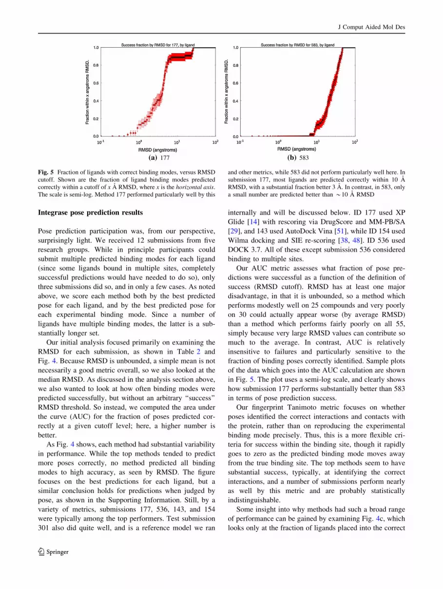
Our AUC metric assesses what fraction of pose pre-

dictions were successful as a function of the definition of

success (RMSD cutoff). RMSD has at least one major

disadvantage, in that it is unbounded, so a method which

performs modestly well on 25 compounds and very poorly

on 30 could actually appear worse (by average RMSD)

than a method which performs fairly poorly on all 55,

simply because very large RMSD values can contribute so

much to the average. In contrast, AUC is relatively

insensitive to failures and particularly sensitive to the

fraction of binding poses correctly identified. Sample plots

of the data which goes into the AUC calculation are shown

in Fig. 5. The plot uses a semi-log scale, and clearly shows

how submission 177 performs substantially better than 583

in terms of pose prediction success.

Our fingerprint Tanimoto metric focuses on whether

poses identified the correct interactions and contacts with

the protein, rather than on reproducing the experimental

binding mode precisely. Thus, this is a more flexible cri-

teria for success within the binding site, though it rapidly

goes to zero as the predicted binding mode moves away

from the true binding site. The top methods seem to have

substantial success, typically, at identifying the correct

interactions, and a number of submissions perform nearly

as well by this metric and are probably statistically

indistinguishable.

Some insight into why methods had such a broad range

of performance can be gained by examining Fig. 4c, which

looks only at the fraction of ligands placed into the correct

(a) 177 (b) 583

Fig. 5 Fraction of ligands with correct binding modes, versus RMSD

cutoff. Shown are the fraction of ligand binding modes predicted

correctly within a cutoff of x A RMSD, where x is the horizontal axis.

The scale is semi-log. Method 177 performed particularly well by this

and other metrics, while 583 did not perform particularly well here. In

submission 177, most ligands are predicted correctly within 10 A

RMSD, with a substantial fraction better 3 A. In contrast, in 583, only

a small number are predicted better than *10 A RMSD

J Comput Aided Mol Des

123

binding site. Since most methods considered all three

binding sites, many of the high RMSD predictions were a

result of predicting the wrong binding site. Thus, perfor-

mance seems more comparable across methods when

considering only poses within the correct site. However, it

is worth noting that the same submissions are still among

the top performers. This is further highlighted by looking at

the number of ligands placed into the correct site, in

Fig. 4f. Despite the hint given participants that they could

focus primarily on the LEDGF site, most chose to include

both the Y3 and FBP sites when making predictions, as

well, and so the majority of submissions typically selected

the incorrect binding site. However, of the top submissions,

most did include multiple sites in their analysis. The fact

that several submissions were thus fairly successful at

identifying the correct binding site is encouraging.

Submissions 300 and 301 are an attempt at generating

null or comparison models. Thus, these are not discussed

above because these are test cases not formally submitted

for SAMPL, but some discussion is warranted. Both of

these submissions were done in a blind manner, just as the

rest of the SAMPL, and submission 300 (but not 301) was

done prior to the submission deadline. Submission 300 was

a control run in which a beginning high school student in

the Mobley laboratory predicted binding modes using

AutoDock simply by following online tutorials and docu-

mentation, with no separate instruction and with minimal

background reading on IN and on this particular series. It

appears that one major challenge for 300 was the definition

of and identification of the binding site region. Very few

ligands were placed nearest the correct site, and even of

those, none came close to the correct binding modes.

Table 3 Statistics for IN

affinity prediction

The average error, RMS error,

AUE, Kendall tau, and Pearson

R

ID Avg. Err. RMS AUE Tau R

012 -18.0 ± 0.1 18.0 ± 0.1 18.0 ± 0.1 -0.2 ± 0.0 -0.2 ± 0.0

013 -41.6 ± 2.5 42.2 ± 2.8 41.6 ± 2.5 -0.4 ± 0.0 -0.6 ± 0.0

182 -3.8 ± 0.3 3.9 ± 0.3 3.8 ± 0.3 -0.4 ± 0.3 -0.7 ± 0.3

183 -3.2 ± 0.3 3.3 ± 0.3 3.3 ± 0.3 -0.6 ± 0.2 -0.8 ± 0.2

184 -1.2 ± 0.5 1.8 ± 0.4 1.3 ± 0.4 -0.1 ± 0.3 -0.3 ± 0.3

190 -2.2 ± 0.8 3.1 ± 0.5 2.7 ± 0.5 -0.1 ± 0.2 -0.2 ± 0.3

191 -3.8 ± 0.3 4.0 ± 0.3 3.8 ± 0.3 0.2 ± 0.3 0.4 ± 0.3

199 -22.2 ± 4.2 25.1 ± 2.8 23.0 ± 3.6 0.6 ± 0.3 0.6 ± 0.4

201 -25.1 ± 5.0 28.8 ± 2.8 27.1 ± 3.4 0.5 ± 0.3 0.6 ± 0.4

233 -24.6 ± 4.8 28.1 ± 2.6 26.6 ± 3.3 0.4 ± 0.3 0.5 ± 0.4

234 -25.6 ± 4.4 28.5 ± 2.8 26.5 ± 3.7 0.2 ± 0.3 0.5 ± 0.4

235 -17.4 ± 3.6 20.1 ± 2.5 18.2 ± 3.1 0.5 ± 0.3 0.6 ± 0.3

236 -17.5 ± 3.4 20.0 ± 1.9 18.9 ± 2.4 0.4 ± 0.3 0.6 ± 0.4

237 -27.0 ± 3.4 28.6 ± 2.7 27.0 ± 3.4 0.2 ± 0.3 0.5 ± 0.4

549 -7.8 ± 1.3 8.6 ± 1.3 7.8 ± 1.3 -0.2 ± 0.3 -0.3 ± 0.3

(a) Ranked AUE (b) Ranked R

Fig. 6 Representative statistics for the integrase affinity challenge. Shown are the Pearson correlation coefficient, R, and the average unsigned

error (AUE). Normal submissions are shown in blue; control models are shown in gray, as discussed in the text

J Comput Aided Mol Des

123

Primarily, this probably serves to illustrate that some

expertise in docking and some knowledge of likely binding

sites is still needed for successful pose prediction.

ID 301 provides a more challenging benchmark. This

applied a different approach than most participants, and

took all six bound ligands out of the 3NF8 reference

structure. Each ligand was then shape-overlaid onto the

3NF8 ligands using OpenEye’s ROCS, and bumping poses

were removed. Each pose was then energy minimized with

MMFF, and the remaining pose with the best MMFF

energy was then submitted. This actually would have ended

up being the top submission by most metrics, and does

extremely well. This is partly because this is precisely the

type of challenge where a ligand-based approach such as

this one ought to do well—where there are structures of

related ligands bound in all the binding sites of interest—

and partly because the LEDGF site seems to have typically

resulted in the best MMFF energy.

We examined median error across different ligands in

the set to try and understand whether particular classes of

ligand were especially difficult to predict. However, almost

every ligand is well predicted by at least some methods.

Median errors across all methods do fluctuate substantially

from ligand-to-ligand, but we did not immediately observe

patterns where particular classes or groups of ligands were

particularly difficult to predict. We did observe a slight

correlation between increasing molecular weight and

median RMSD, but some correlation between RMSD and

molecular weight is to be expected regardless. We also find

(as did Coleman et al. [8]) a slight trend that more highly

charged ligands (charge -2, or zwitterions with charge -2

? 1) may have higher median RMSDs, but the test set is

small enough it is hard to be sure this is statistically

significant.

Integrase affinity results

The integrase affinity challenge received 15 submissions

from four groups. Statistics are shown in Table 3 and

Fig. 6. We used the Kendall W statistic to see whether

there was a clear leader and arrived at a value of

W = 0.80 ± 0.08, indicating that almost all affinities are

better predicted by one submission than any other. This

submission was 184 (Fig. 7), which used the SIE scoring

function [38, 48] with the FiSH [9] hydration model, but

even this suffered from rather poor performance overall.

While this submission’s RMS error, 1.83 ± 0.41 kcal/mol,

and the AUE 1.33 ± 0.44 kcal/mol seem acceptable, the

experimental data spans only a 1 kcal/mol range, so the

error is larger than the signal. Thus, for ID 184, the Pearson

R and Kendall tau are actually negative, indicating incor-

rect ranking. Interestingly, one group of compounds seems

well predicted, while the rest are very poorly predicted.

The authors suggest that some of this noise can be reduced

by using a common protein structure instead of the cognate

crystallographic structures [24].

In this challenge component, most submissions actually

used docking to try and predict affinities. And submission

IDs 199, 201, and 233–237 actually submitted scores from

the DOCK package as ‘‘affinity’’ predictions. Since these

scores are not normalized, the hope was that these would

provide some correlation with experiment, rather than

actually provide reasonable affinity estimates, hence the

very large errors for these submissions. One notable

exception to the typical docking approach here was sub-

missions 190–191, which used an MM-PB/SA approach.

Submission IDs 012 and 013 were a null model based on

the classic work of Kuntz [32], where affinities were pre-

dicted based on the number of heavy atoms with a value of

1.5 kcal/mol per heavy atom up to a plateau value, and

then were a constant beyond that (ID 012). Because all of

these ligands are large enough to have reached the plateau,

this resulted in a constant prediction for all ligands, so

model 013 removes the plateau. These were provided by

Coleman et al. [8]. It is worth noting that a variety of other

methods substantially outperform these null models here,

despite the limited nature of this test.

Overall, given the very narrow range of experimental

binding free energies for these few relatively weak ligands,

it is difficult to draw any strong conclusions from this

portion of the challenge.

Fig. 7 Performance of submission 184 in the integrase affinity

challenge. While one group of compounds was well predicted,

another group was not. 184 was essentially the top submission in the

challenge

J Comput Aided Mol Des

123

Conclusions

Overall, the HIV integrase portion of the SAMPL4 chal-

lenge proved extremely challenging. The virtual screening

component was difficult apparently because the inactive

compounds are true inactives and were so similar to active

compounds, and indeed were tested precisely because they

were thought to bind. Thus, it proved extremely difficult to

substantially enrich compounds in this portion of the

challenge. Likewise, the binding mode prediction of the

challenge was difficult, partly because of the several

binding sites participants had to deal with. And the narrow

range of relatively weak affinities in the affinity prediction

challenge made it challenging to achieve any correlation

between calculated and experimental values—though sev-

eral methods did have reasonably low errors.

However, it was encouraging that some methods were

able to significantly enrich actives in the virtual screening

portion of the challenge. Here, one method in particular

stood out from the pack, and interestingly, it involved

substantial manual intervention from a human expert in the

screening process. Apparently, human expertise still pays

off. To us, this is actually somewhat encouraging, in that it

means that there is still more we can teach our binding

prediction algorithms.

For binding mode prediction, all methods performed

poorly on at least some ligands, but one major source of

large errors was placement of ligands into the incorrect

binding site (since three binding sites were possible).

Interestingly, however, placing ligands into the correct

binding site was not a guarantee of success, and some of

the top methods actually considered binding to all three

sites. This suggests that, at least in some cases, binding site

identification may be possible with today’s methods.

Interestingly, a control model we ran using a ligand-based

approach actually performed quite well at this portion of

the challenge, suggesting that in the future, participants

may want to consider alternate approaches such as this to

help their structure-based efforts. A similar (control)

ligand-based approach also performed well in the virtual

screening test, further supporting this line of thinking.

Possibly in future challenges the best approach may

involve a combination of methods.

Overall, we believe the integrase component of the

SAMPL4 challenge was a valuable test, and we are con-

vinced that blind tests like this are a helpful way to gain

insight into how methods may perform in a real-world

discovery setting. Expert knowledge does seem to continue

to play an important role, but it does not guarantee success,

nor does the lack of expert knowledge guarantee failure.

Much depends on both the practitioner and the details of

the approach.

Supporting information

We provide Supporting Information in the form of a sup-

porting archive file which contains the majority of the

challenge inputs, outputs, and analysis and plots generated.

Specifically, it contains the intro PDF file which was pro-

vided to participants, and all challenge inputs as provided

to participants. Additional files are provided indicating

changes which were made (in the form of molecules

removed) prior to analysis, and experimental results are

provided. We provide all statistics computed, and the full

set of plots generated for all submissions in all challenge

components. Additionally, for participants who consented,

we provide the contents of their submissions, including

method descriptions and other metadata.

Acknowledgments We acknowledge the financial support of the

National Institutes of Health (1R15GM096257-01A1 to DLM and

R01 GM073087 and P50 GM103368 to AJO), and computing support

from the UCI GreenPlanet cluster, supported in part by NSF Grant

CHE-0840513. We are also grateful to OpenEye Scientific Software

for support for SAMPL, including for the meeting and for logistical

help with the website, and in particular would like to thank Matt

Geballe for help with the website and submissions and for helpful

discussions, and Paul Hawkins, Greg Warren, and Geoff Skillman for

helpful discussions and pointers on analysis. We are also thankful to

Tom Peat (CSIRO) and colleagues for the experimental data which

made the integrase portion of SAMPL possible, and helped initiate

SAMPL4.

References

1. Abram ME, Hluhanich RM, Goodman DD, Andreatta KN,

Margot NA, Ye L, Niedziela-Majka A, Barnes TL, Novikov N,

Chen X, Svarovskaia ES, McColl DJ, White KL, Miller MD

(2013) Impact of primary Elvitegravir resistance-associated

mutations in HIV-1 integrase on drug susceptibility and viral

replication fitness. Antimicrob Agents Chemother 57(6):

2654–2663

2. Benson ML, Faver JC, Ucisik MN, Dashti DS, Zheng Z, Merz

KM Jr (2012) Prediction of trypsin/molecular fragment binding

affinities by free energy decomposition and empirical scores.

J Comput Aided Mol Des 26(5):647–659

3. Blow DM (2002) Rearrangement of Cruickshank’s formulae for

the diffraction-component precision index. Acta Crystallogr Sect

D Biol Crystallogr 58(5):792–797

4. Cherepanov P, Ambrosio ALB, Rahman S, Ellenberger T, Eng-

elman A (2005) Structural basis for the recognition between HIV-

1 integrase and transcriptional coactivator p75. Proc Natl Acad

Sci USA 102(48):17,308–17,313

5. Chodera JD, Mobley DL, Shirts MR, Dixon RW, Branson K,

Pande VS (2011) Alchemical free energy methods for drug dis-

covery: progress and challenges. Curr Opin Struct Biol 21(2):

150–160

6. Christ F, Shaw S, Demeulemeester J, Desimmie BA, Marchand

A, Butler S, Smets W, Chaltin P, Westby M, Debyser Z, Pickford

C (2012) Small-molecule inhibitors of the LEDGF/p75

binding site of integrase block HIV replication and modulate

J Comput Aided Mol Des

123

integrase multimerization. Antimicrob Agents Chemother 56(8):

4365–4374

7. Christ F, Voet A, Marchand A, Nicolet S, Desimmie BA,

Marchand D, Bardiot D, Vander Veken NJ, Van Remoortel B,

Strelkov SV, De Maeyer M, Chaltin P, Debyser Z (2010)

Rational design of small-molecule inhibitors of the LEDGF/p75-

integrase interaction and HIV replication. Nat Meth 6(6):442–448

8. Coleman RG, Sterling T, Weiss DR (2014) SAMPL4 &

DOCK3.7: lessons for automated docking procedures. J Comput

Aided Mol Des. doi:10.1007/s10822-014-9722-6

9. Corbeil CR, Sulea T, Purisima EO (2010) Rapid prediction of

solvation free energy. 2. The first-shell hydration (FiSH) con-

tinuum model. J Chem Theory Comput 6(5):1622–1637

10. De Clercq E (1999) Perspectives of non-nucleoside reverse

transcriptase inhibitors (NNRTIs) in the therapy of HIV-1

infection. Il Farmaco 54(1–2):26–45

11. Dewdney TG, Wang Y, Kovari IA, Reiter SJ, Kovari LC (2013)

Reduced HIV-1 integrase flexibility as a mechanism for ralte-

gravir resistance. J Struct Biol 184:245–250

12. Engelman A, Cherepanov P (2012) The structural biology of

HIV-1: mechanistic and therapeutic insights. Nat Rev Microbiol

10(4):279–290

13. Ewing TJ, Makino S, Skillman AG, Kuntz ID (2001) DOCK 4.0:

search strategies for automated molecular docking of flexible

molecule databases. J Comput Aided Mol Des 15(5):411–428

14. Friesner RA, Murphy RB, Repasky MP, Frye LL, Greenwood JR,

Halgren TA, Sanschagrin PC, Mainz DT (2006) Extra precision

glide: docking and scoring incorporating a model of hydrophobic

enclosure for proteinligand complexes. J Med Chem 49(21):

6177–6196

15. Gallicchio E, Deng N, He P, Perryman AL, Santiago DN, Forli S,

Olson AJ, Levy RM (2014) Virtual screening of integrase

inhibitors by large scale binding free energy calculations.

J Comput Aided Mol Des. doi:10.1007/s10822-014-9711-9

16. Gallicchio E, Lapelosa M, Levy RM (2010) The binding energy

distribution analysis method (BEDAM) for the estimation of

protein-ligand binding affinities. J Chem Theory Comput 6(9):

2961–2977

17. Geretti AM, Armenia D, Ceccherini-Silberstein F (2012)

Emerging patterns and implications of HIV-1 integrase inhibitor

resistance. Curr Opin Infect Dis 25(6):677–686. doi:10.1097/

QCO.0b013e32835a1de7

18. Greenwald J, Le V, Butler SL, Bushman FD, Choe S (1999) The

mobility of an HIV-1 integrase active site loop is correlated with

catalytic activity. Biochemistry 38(28):8892–8898

19. Hare S, Maertens GN, Cherepanov P (2012) 3[prime]-Processing

and strand transfer catalysed by retroviral integrase in crystallo.

EMBO J 31(13):3020–3028

20. Hare S, Smith SJ, Metifiot M, Jaxa-Chamiec A, Pommier Y,

Hughes SH, Cherepanov P (2011) Structural and functional

analyses of the second-generation integrase strand transfer

inhibitor dolutegravir (S/GSK1349572). Mol Pharmacol 80(4):

565–572

21. Hare S, Vos AM, Clayton RF, Thuring JW, Cummings MD,

Cherepanov P (2010) Molecular mechanisms of retroviral in-

tegrase inhibition and the evolution of viral resistance. Proc Natl

Acad Sci 107(46):20,057–20,062

22. Hawkins PCD, Nicholls A (2012) Conformer generation with

OMEGA: learning from the data set and the analysis of failures.

J Chem Inf Model 52(11):2919–2936

23. Hawkins PCD, Skillman AG, Warren GL, Ellingson BA, Stahl

MT (2010) Conformer generation with OMEGA: algorithm and

validation using high quality structures from the Protein Data-

bank and Cambridge Structural Database. J Chem Inf Model

50(4):572–584

24. Hogues H, Sulea T, Purisima EO (2014) Exuastive docking and

solvated interaction energy scoring: lessons learned from the

SAMPL4 challenge. J Comput Aided Mol Des. doi:10.1007/

s10822-014-9715-5

25. Japrung D, Leartsakulpanich U, Chusacultanachai S, Yuthavong

Y (2007) Conflicting requirements of Plasmodium falciparum

dihydrofolate reductase mutations conferring resistance to pyri-

methamine-WR99210 combination. Antimicrob Agents Chemo-

ther 51(12):4356–4360

26. Jurado KA, Wang H, Slaughter A, Feng L, Kessl JJ, Koh Y,

Wang W, Ballandras-Colas A, Patel PA, Fuchs JR, Kvaratskhelia

M, Engelman A (2013) Allosteric integrase inhibitor potency is

determined through the inhibition of HIV-1 particle maturation.

Proc Natl Acad Sci 110(21):8690–8695

27. Kessl JJ, Jena N, Koh Y, Taskent-Sezgin H, Slaughter A, Feng L,

de Silva S, Wu L, Le Grice SFJ, Engelman A, Fuchs JR, Kva-

ratskhelia M (2012) Multimode, cooperative mechanism of action

of allosteric HIV-1 integrase inhibitors. J Biol Chem 287(20):

16,801–16,811

28. Krishnan L, Engelman A (2012) Retroviral integrase proteins and

HIV-1 DNA integration. J Biol Chem 287(49):40,858–40,866

29. Kuhn B, Kollman PA (2000) Binding of a diverse set of ligands

to avidin and streptavidin: an accurate quantitative prediction of

their relative affinities by a combination of molecular mechanics

and continuum solvent models. J Med Chem 43(20):3786–3791

30. Kulp JL, Blumenthal SN, Wang Q, Bryan RL, Guarnieri F (2012)

A fragment-based approach to the SAMPL3 challenge. J Comput

Aided Mol Des 26(5):583–594

31. Kumar A, Zhang KYJ (2012) Computational fragment-based

screening using RosettaLigand: the SAMPL3 challenge. J Com-

put Aided Mol Des 26(5):603–616

32. Kuntz ID, Chen K, Sharp KA, Kollman PA (1999) The maximal

affinity of ligands. Proc Natl Acad Sci 96(18):9997–10,002

33. Lindorff-Larsen K, Piana S, Palmo K, Maragakis P, Klepeis JL,

Dror RO, Shaw DE (2010) Improved side-chain torsion potentials

for the Amber ff99SB protein force field. Proteins pp NA–NA

78(8):1950–1958

34. Maertens GN, Hare S, Cherepanov P (2010) The mechanism of

retroviral integration from X-ray structures of its key intermedi-

ates. Nature 468(7321):326–329

35. MarvinSketch version 5.8.2 (2013)ChemAxon. http://www.che

maxon.com/products/marvin/marvinsketch/

36. Metifiot M, Maddali K, Johnson BC, Hare S, Smith SJ, Zhao XZ,

Marchand C, Burke TR, Hughes SH, Cherepanov P, Pommier Y

(2013) Activities, crystal structures, and molecular dynamics of

dihydro-1H-isoindole derivatives, inhibitors of HIV-1 integrase.

ACS Chem Biol 8(1):209–217

37. Mobley DL, Wymer KL, Lim NM (2014) Blind prediction of

solvation free energies from the SAMPL4 challenge. J Comput

Aided Mol Des

38. Naım M, Bhat S, Rankin KN, Dennis S, Chowdhury SF, Siddiqi

I, Drabik P, Sulea T, Bayly CI, Jakalian A (2007) Solvated

interaction energy (SIE) for scoring protein-ligand binding

affinities. 1. Exploring the parameter space. J Chem Inf Model

47(1):122–133

39. Newman J, Dolezal O, Fazio V, Caradoc-Davies T, Peat TS

(2012) The DINGO dataset: a comprehensive set of data for the

SAMPL challenge. J Comput Aided Mol Des 26(5):497–503

40. Nicholls A, Mobley DL, Guthrie JP, Chodera JD, Bayly CI,

Cooper MD, Pande VS (2008) Predicting small-molecule solva-

tion free energies: an informal blind test for computational

chemistry. J Med Chem 51(4):769–779

41. OpenEye Python Toolkits. http://www.eyesopen.com (2013)

42. Peat TS, Dolezal O, Newman J, Mobley DL, Deadman JJ (2014)

Interrogating HIV integrase for compounds that bind—a

J Comput Aided Mol Des

123

SAMPL4 challenge. J Comput Aided Mol Des. doi:10.1007/

s10822-014-9721-7

43. Peat TS, Warren G (2013) Personal Communication. E-mail

exchange

44. Perryman AL, Forli S, Morris GM, Burt C, Cheng Y, Palmer MJ,

Whitby K, McCammon JA, Phillips C, Olson AJ (2010) A

dynamic model of HIV integrase inhibition and drug resistance.

J Mol Biol 397(2):600–615

45. Quashie PK, Mesplede T, Han YS, Veres T, Osman N, Hassou-

nah S, Sloan R, Xu HT, Wainberg MA (2013) Biochemical

analysis of the role of G118R-linked dolutegravir drug resistance

substitutions in HIV-1 integrase. Antimicrob Agents Chemother

57(12):6223–6235

46. Quashie PK, Mesplede T, Wainberg MA (2013) Evolution of

HIV integrase resistance mutations. Curr Opin Infect Dis

26(1):43–49. doi:10.1097/QCO.0b013e32835ba81c

47. Skillman AG, Warren GL, Nicholls A (2008) SAMPL at first

glance: So much data, so little time…. http://www.eyesopen.com/

2008_cup_presentations/CUP9_Skillman.pdf

48. Sulea T, Cui Q, Purisima EO (2011) Solvated interaction energy

(SIE) for scoring protein–ligand binding affinities. 2. Benchmark

in the CSAR-2010 scoring exercise. J Chem Inf Model 51(9):

2066–2081

49. Sulea T, Hogues H, Purisima EO (2012) Exhaustive search and

solvated interaction energy (SIE) for virtual screening and affinity

prediction. J Comput Aided Mol Des 26(5):617–633

50. Surpateanu G, Iorga BI (2012) Evaluation of docking perfor-

mance in a blinded virtual screening of fragment-like trypsin

inhibitors. J Comput Aided Mol Des 26(5):595–601

51. Trott O, Olson AJ (2010) AutoDock Vina: improving the speed

and accuracy of docking with a new scoring function, efficient

optimization, and multithreading. J Comput Chem 31(2):455–461

52. Truchon J, Bayly CI (2007) Evaluating virtual screening meth-

ods: good and bad metrics for the ‘‘early recognition’’ problem.

J Chem Inf Model 47(2):488–508

53. Tsiang M, Jones GS, Niedziela-Majka A, Kan E, Lansdon EB,

Huang W, Hung M, Samuel D, Novikov N, Xu Y, Mitchell M,

Guo H, Babaoglu K, Liu X, Geleziunas R, Sakowicz R (2012)

New class of HIV-1 integrase (IN) inhibitors with a dual mode of

action. J Biol Chem 287(25):21,189–21,203

54. Voet ARD, Kumar A, Berenger F, Zhang KYJ (2014) Combining

in cerebra and in silico approaches for virtual screening and pose

prediction in SAMPL4. J Comput Aided Mol Des. doi:10.1007/

s10822-013-9702-2

55. Wainberg MA, Mesplede T, Quashie PK (2012) The develop-

ment of novel HIV integrase inhibitors and the problem of drug

resistance. Curr Opin Virol 2(5):656–662

56. Wang J, Wolf R, Caldwell J, Kollman P, Case D (2004) Devel-

opment and testing of a general amber force field. J Comput

Chem 25(9):1157–1174

57. Wang R, Liu L, Lai L, Tang Y (1998) SCORE: a new empirical

method for estimating the binding affinity of a protein-ligand

complex. J Mol Model 4(12):379–394

58. Zhang J, Adrian FJ, Jahnke W, Cowan-Jacob SW, Li AG, Iacob

RE, Sim T, Powers J, Dierks C, Sun F, Guo GR, Ding Q, Okram

B, Choi Y, Wojciechowski A, Deng X, Liu G, Fendrich G,

Strauss A, Vajpai N, Grzesiek S, Tuntland T, Liu Y, Bursulaya B,

Azam M, Manley PW, Engen JR, Daley GQ, Warmuth M, Gray

NS (2010) Targeting Bcr-Abl by combining allosteric with ATP-

binding-site inhibitors. Nature 463(7280):501–506

J Comput Aided Mol Des

123