Forest Ecology and Management 325 (2014) 74–89

Contents lists available at ScienceDirect

Forest Ecology and Management

journal homepage: www.elsevier .com/ locate/ foreco

Branch models for white spruce (Picea glauca (Moench) Voss) innaturally regenerated stands

http://dx.doi.org/10.1016/j.foreco.2014.03.0510378-1127/� 2014 Elsevier B.V. All rights reserved.

⇑ Corresponding author. Tel.: +1 780 492 6472; fax: +1 780 492 4323.E-mail addresses: dsattler@ualberta.ca (D.F. Sattler), pcomeau@ualberta.ca

(P.G. Comeau), alexis.achim@sbf.ulaval.ca (A. Achim).

Derek F. Sattler a,⇑, Philip G. Comeau b, Alexis Achim c

a Department of Renewable Resources, University of Alberta, 751 General Services Building, Edmonton, AB T6G 2H1, Canadab Department of Forest Resources Management, University of Alberta, 751 General Services Building, Edmonton, AB T6G 2H14, Canadac Département des sciences du bois et de la forêt, Faculté de foresterie, de géographie et de géomatique, Université Laval, 2425, rue de la Terrasse, Pavillon Gene-H.-Kruger, Québec,QC G1V 0A6, Canada

a r t i c l e i n f o a b s t r a c t

Article history:Received 21 January 2014Received in revised form 27 March 2014Accepted 28 March 2014

Keywords:Branch characteristicsWhite spruceNaturally regenerated standsGeneralized mixed models

To describe the branching characteristics of white spruce trees (Picea glauca [Moench] Voss) in naturallyregenerated, pure and mixed-species stands of the Canadian boreal forest, predictive models were devel-oped for: (1) the number of branches (P5 mm diameter), (2) maximum branch diameter, (3) the diam-eter of all other branches, and (4) the angle of branch insertion (P5 mm diameter). An additional set ofequations were developed for models (1) and (4) for branches P12.5 mm in diameter in order to evaluatethe factors affecting the recovery of No 1 grade cut lumber. Tree and stand-level variables common todistance independent growth and yield simulators were tested in the models and a generalized hierarchi-cal mixed-effect approach was used to estimate the parameters. Estimates for the branch characteristicwere obtained for 1 m sections of the live crown since distinct branch whorls were unidentifiable. Therelative or absolute depth into the crown (m) were significant variables in all the models, reflectingthe importance of branch age and diminishing light levels with increasing crown depth. Increasing socialposition within a stand, measured by the basal area of larger trees (Bal), was positively related to anincrease in the number of branches P5 mm per section but did not significantly influence the numberof branches P12.5 mm, which was more strongly related to crown length and tree slenderness (ratioof height to diameter at breast height). Crown length was a significant variable affecting maximumbranch diameters, whereas tree slenderness was important for the diameter of all other branches. Therank of a branch relative to the largest branch within a 1 m stem section was related to the diameterof smaller branches, angle of insertion for branches P5 mm as well as branches P12.5 mm. No speciescomposition or explicit stand-level variables (other than Bal) were significant in any of the models.Within many of the models, the presence of tree-level variables which are known to be sensitive tochanges in competition and tree social status suggest that branch characteristics for white spruce withinpure and mixed-species stands of the boreal forest are affected by local changes in light availability.

� 2014 Elsevier B.V. All rights reserved.

1. Introduction

The link between branching characteristics and wood qualityhas been recognized for several tree species including black spruce(Benjamin et al., 2009), Norway spruce (Picea abies) (Colin andHoullier, 1992), Sitka spruce [Picea sitchensis (Bong.) Carr.](Achim et al., 2006), Scots pine (Pinus sylvestris L.) (Mäkinen andColin, 1999) and Douglas-fir [Pseudotsuga mensziesii (Mirb.) Franco](Maguire et al., 1994). This has motivated the development of arange of predictive models for different branch characteristics for

several commercially important species. Many of these modelsuse simple stand and tree-level measurements to make predictionsof branching characteristics, and can therefore be incorporated intotree growth simulators which use the same set of measurements.The refinement of existing branch models is ongoing, includingwork by Hein et al. (2007) on Norway spruce and Auty et al.(2012) on Sitka spruce among others, and is an indication of theimportance of these models. White spruce (Picea glauca [Moench]Voss), which is located throughout much of the Canadian borealforest region, is a commercially important species whose woodquality is known to be affected by branching characteristics, asdemonstrated by Tong et al. (2013) through the use of computedtomography images. Predictive models relating stand and externaltree characteristics to specific branch characteristics in white

D.F. Sattler et al. / Forest Ecology and Management 325 (2014) 74–89 75

spruce, however, are few. The works by Groot and Schneider(2011) and Nemec et al. (2012) being the only recently publishedstudies to present white spruce-specific branch characteristicmodels using external tree traits. Thus, despite its economicimportance, there remains a need to develop models of branchcharacteristics for white spruce from stand-level and external treecharacteristics, and in turn, integrate these models into growthsimulators.

Groot and Schneider (2011) examined maximum branch diam-eter for white spruce, and developed regression-based equationsusing independent variables measured using remotely sensed data(e.g., LiDAR). The response variable was the average of the largestthree branches within the crown (MBD). For white spruce, theyfound that when only tree-level variables were used, MDBincreased with increasing tree height at a rate lower than mostother species examined, although similar to that of black spruce.Furthermore, MBD in white spruce displayed the highest positiveresponse to increasing crown length indicating a strong age-related effect given that crown length is positively correlated withtotal tree age. MBD in white spruce also displayed a strong sensi-tivity to competition relative to the other species tested. Ratherthan predict a single-tree average for maximum branch diameter,Nemec et al. (2012) describe a method which provides estimatesof average branch diameter for branches within clusters, nestedwithin shoots of different age classes which are in turn nestedwithin trees. Using the same hierarchical structure, Nemec et al.(2012) also present models for the number of clusters and thenumber of branches per cluster. For white spruce, branch diame-ters were found to increase with increasing distance from the treeapex and with increasing relative distance along an annual shoot.Additionally, two distance-dependent measures related to theproximity of neighbouring trees were significant, indicating thesensitivity of branch diameters to the effects of local competition.Their model for the number of branch clusters along annual shootsof all ages showed that there was a positive correlation betweenshoot age and branch shedding.

The studies by Groot and Schneider (2011) and Nemec et al.(2012) provide useful information with regards to white sprucebranch characteristics; however, each address a specific need andprovide estimates on different scales. The former makes use ofremotely sensed data and provides a single estimate of MBD pertree. The latter provides estimates of branch traits at the level ofannual shoots, and requires a considerable amount of detailedinformation, including the age of shoots and the distance to thepoint of crown contact with neighbouring trees. The models pre-sented by Nemec et al. (2012) also employed a compound distribu-tion under the assumption that branches grow in distinct clustersalong shoots. However, the clustering of first order branches inmature white spruce grown in unmanaged stands is erratic, whilenodal and internal branches are not easily distinguished. This leadsto a further important distinction. Most of the data utilized byGroot and Schneider (2011) were from single species density man-agement experiments. The white spruce data used by Nemec et al.(2012) appear to be from single species stands, though it is unclearwhether samples were from plantations, naturally regeneratedstands, or both.

The majority of white spruce currently being harvested withinthe Canadian boreal forest are from natural regeneration. Further-more, a large proportion of the harvested volume is from mixed-species stands. Therefore, branch models for white spruce devel-oped using data from these types of stands are required. Consider-ation for the effect of species mixtures on branching patterns washighlighted by Garber and Maguire (2005), who reported largermaximum branch diameters for trees in mixed stands when com-pared to the same species, but from pure stands. They attributedthese differences to changes in the light environment between

mixed and pure stands, which were the result of different growthstrategies exhibited by the shade tolerant and shade intoleranttrees present in the stand. Detection of these effects was througha simple stand-level species composition index; however, the sam-pled stands were evenly spaced, whereas naturally regenerated,mixed-species stands in the boreal forest have complex spatialarrangements of trees. Thorpe et al. (2010) noted that for interiorspruce (Picea glauca � engelmanii), crown size decreased at a fasterrate with increasing local density when the nearest competitorswere composed of both shade tolerate and shade intolerant speciesversus conspecific competitors. Like Nemec et al. (2012), the studyby Thorpe et al. (2010) used distance-dependent measures of localcompetition, indicating that crown dynamics in boreal forests areaffected by ‘‘neighbourhood’’ conditions. For naturally regeneratedwhite spruce, it is currently unknown if branching characteristicsare affected by different levels of aspen content and if these effectscan be captured by stand-level measures of species composition.This information would be useful in assessing the potential qualityof lumber derived from spruce harvested from mixed or purestands.

Therefore, the outstanding needs pertaining to white sprucebranching models are to: (1) develop branch models for use in nat-urally regenerated stands, and (2) examine if species-specificstand-level competition affects white spruce branching traits. Thegoal of the present study was to address these needs, subject toconstraints and specifications which are now described. First, giventhe predominant use of distance independent growth models inthe western Canadian boreal forest [e.g., mixedwood growth model(MGM) (Bokalo et al., 2010)], the stand- and tree-level predictorvariables considered when developing branch models were thosethat are available within most distance independent growth simu-lators and which are collected during standard forest inventories. Afurther objective of this study was to evaluate the contribution ofvariables derived from the measurement of height to live crownon the overall performance of the branch models being presented,as these measures are not always collected in forest inventories. Afinal specification during model development was to provide anexplicit link between the branch models and wood quality assess-ment guidelines. The factors affecting overall crown structure maydiffer from the factors affecting branches whose knot size isdirectly linked to specific grades of wood quality (Duchateauet al., 2013; Tong et al., 2013). Models for branches of a specificknot size class, which are linked to specific grades of lumber wouldgreatly improve the practical applicability of such models. The lit-erature for models developed with this intent, however, is sparse.Colin and Houllier (1992) developed separate models for branches>10 mm and those >5 mm for Norway spruce; however, it was notexplicitly stated if the selection of these size classes was tied tolumber grading rules. For white spruce, lumber grading rules indi-cate a maximum knot size of 12.5 mm for a 50 mm-wide No. 1grade cut (NLGA, 2003; Tong et al., 2013). Thus, an additional setof models was developed for branch frequency and branch inser-tion angle using only branches with diameters P12.5 mm at thepoint of insertion.

2. Materials and methods

2.1. Site description and measurements

Branch characteristics were determined for 65 white sprucetrees located adjacent to 15 permanent sample plots (PSP). ThePSPs, which had been installed by Alberta Sustainable ResourceDevelopment (ASRD, 2005), were situated within unmanagedstands that had established through natural regeneration.Although the selected PSPs spanned approximately 500 km from

Table 1Symbol and associated description of tree and stand-level variables tested in themodels. Natural log transformations of the variables were also tested and are denotedin the text with the prefix ‘ln’.

Variable symbol Description

DBH Diameter at 1.3 mTotalHt Total tree height (m)Cl Length of live crown (m)Cr Crown ratioHtlcrn Height to base of live crown (m)Slc Height (m)/DBH (cm) (i.e., slenderness)ScHt Height to top of each 1 m section (m) from

base of treeDist Difference between tree apex and top of 1 m

section (TotalHt – ScHt) (m)RDist Relative position of section in live crown

(Dist/Cl)Rank Rank of the diameter of a branch relative to

the largest branch within a 1 m sectionBal Basal area of larger trees (m2 ha�1)Baha�1 Basal area of the stand (m2 ha�1)PctSwBaha�1 PctAwBaha�1 Percent of stand basal area that is white

spruce (Sw) and trembling aspen (Aw)hL Lorey’s height; tree height weighted by basal

area (m)SwTopHt, AwTopHt Top height for white spruce (Sw) and

trembling aspen (Aw); calculated as theaverage height of the largest 100 trees ha�1

by DBH

76 D.F. Sattler et al. / Forest Ecology and Management 325 (2014) 74–89

east to west, climatic conditions over this region are reported to besimilar (Beckingham and Archibald, 1996). All the sites sampledwere classified to the ‘reference’ ecosite-type (i.e., upland forestswith moderately well-drained, othic-gray luvisolic soils, whichgenerally transition from an aspen to white spruce overstory) ofthe central mixedwood natural subregion of Alberta, Canada(Beckingham and Archibald, 1996). Given the common ecosite-type, site index values were assumed to be relatively similar. Interms of total basal area ha�1 (Ba ha�1), the sampled PSPs rangedfrom 25 to 56 m2 ha�1 and included spruce dominated stands(>70% of stand Ba ha�1), mixtures of spruce and aspen (between30% and 70% Ba ha�1 of each species), and aspen dominated stands(>70% of stand Ba ha�1) with a white spruce understory (see Sup-plementary material). The mean BH age of overstory trees withinthe PSPs ranged from 52 to 153 years, although the ages amongwhite spruce trees within a PSP often varied by 10 or more years.

Selected trees were no more than 100 m from the adjacent PSPboundary and located within the same forest ecosite-type as thatfound within the PSP. The process of tree selection first involveddefining the quartiles of the DBH range for white spruce treeswithin each PSP. This was done using measurements of DBH col-lected during the most recent inventory of the PSPs. A minimumof two trees with a DBH between the 2nd and 3rd quartile werethen selected. Additionally, at least one other tree was selectedwhich was larger than the DBH limit defined by the 3rd quartile.All sampled trees were free of major stem defects (e.g., missingtops, excessive lean); however, minor stem defects (e.g., leader-whip damage) were unavoidable. Following the measurement ofDBH, trees were felled and branch measurements collected withinthe live crown. The base of the live crown was defined by the low-est living branch which was separated from the next living branchby no more than one whorl containing only dead branches. Totaltree height was also recorded on the felled trees.

Measurements were collected for all live branches with a diam-eter P5 mm at the base of the branch (see Supplementary mate-rial). To maintain consistency, measurements of branch diameterwere taken at a distance from the main tree stem equal to thediameter of the branch at the point of stem insertion. Calipers wereused to record branch diameters <50 mm while a diameter tapewas used on larger branches. All measurements were taken tothe nearest millimeter. The angle of branch insertion, measuredwith a protractor and taken to the nearest degree (�), was definedas the angle between the main stem and the branch (0� represent-ing a vertical branch pointing toward the tree apex).

2.2. Model building

Due to the nature of the sampling methods used when measur-ing branch-level variables, a hierarchical approach is oftenemployed when fitting models of branch characteristics (Heinet al., 2007). Typically, branches are nested within whorls, whorlsnested within trees and trees nested within plots. While the datastructure for the current study includes trees within plots, it wasnot possible to clearly distinguish branch whorls for the whitespruce trees sampled. Furthermore, a consistently clear distinctioncould not be made between nodal and internodal branches. There-fore, for modelling purposes the live crown was divided into 1 msections, starting from crown base. Since full crown lengths didnot necessarily divide exactly into 1 m sections, stem sections atthe crown apex which were less than 1 m were discarded fromthe model datasets.

For predictions of the number of branches per section, two setof models were developed. The first model was constructed to pro-vide estimates of the total number of living branches with a diam-eter P5 mm. The second model was constructed to provideestimates of the total number of living branches per section with

a diameter P12.5 mm (maximum allowable knot size for No 1grade lumber for 50 mm wide white spruce structural lumber).Within each 1 m section, all live branches P5 mm in diameterwere ranked in terms of their diameter relative to the largest (i.e.second largest branch per section had rank = 1, 3rd largest hadrank = 2, etc.). This ranking was then tested as an independent var-iable in the branch-level models (i.e., relative diameter of smallerbranches and branch angle). As was done for the number of branchesper section, two models were developed for branch angle; one usingall branches P5 mm and a second for all branches P12.5 mm.

Guiding the development of the models was the intention thatthey would eventually be incorporated into growth and yield sim-ulators such to the mixedwood growth model (MGM) (Bokalo et al.2010, 2013), which is currently used in Alberta for the types ofstands that were sampled. The covariates considered for inclusion,therefore, were those that are typically collected during standardforest inventories and which are used as input variables to initiatea growth cycle within simulators such as MGM (see Table 1 for var-iable symbols and descriptions). The variable selection processbegan by fitting the models using only tree-level variables andno random effects. The ‘drop1’ function in the glm package for R(R Core Team, 2013), was used to evaluate the marginal contribu-tion of a given covariate given the presence of the other covariatesin the model. When a pair of covariates were significant (assessedat a = 0.05) but also highly correlated (r2 > 0.8), only the covariatewhich provided the greatest improvement to the model (assessedusing Akaike’s information criterion [aic]; Akaike, 1974) wasretained. Stand-level variables were then progressively added,with the covariates in the models re-evaluated upon each addition.

With the fixed effect covariates selected, the models were thenrefit with random intercepts included for the hierarchical levelsappropriate for the given dependent variable. For example, themodel for maximum branch diameter (i.e., with a single estimateper section) included plot (p) and tree (t) -level random effects,while the model for the relative diameter of smaller branches(i.e., with a single estimate for each branch (l)) included, plot, tree,and section (s) -level random effects.

For models fit to count or binomial data (i.e., branch frequencyand relative branch diameter), the final set of fixed-effect covariates

D.F. Sattler et al. / Forest Ecology and Management 325 (2014) 74–89 77

retained in the mixed-model were all significant at alpha = 0.05level. For the models fit to continuous data (i.e., maximum branchdiameter and branch angle), significance tests of the individualcovariates are considered to be unreliable (Bolker et al., 2009). Thus,the decision to retain a variable was assessed using the leave-one-variable-out approach. Following Auty et al. (2012), a givencovariate was dropped when aic values between the full model(all covariates, plus fixed and random effects) and the reducedmodel (single covariate removed, plus fixed and random effects)differed by P10 (Burnham and Anderson, 2002). If the final modelfor a given branch characteristic contained covariates derived fromthe measured crown length, then the model was refit without thesevariables in order to evaluate the contribution to the respectivemodel. Evaluation of the models fit with and without crown-derived measurements was done though the comparison of errorstatistics. Since the models were fit using datasets that included awide range of tree sizes and ages, the need to extrapolate beyondthe range of data tested was not a significant concern.

For each of the models, an index of fit (Pseudo-R2) for estimatesprovided by the fixed effect component was calculated usingEq. (1a), while Eq. (1b) was used to calculate the index forestimates provided from fixed and random effects.

Pseudo-R2f ¼ 1� ssef

ssyð1aÞ

Pseudo-R2fþr ¼ 1� ssefþr

ssyð1bÞ

where ssef is the error sums of squares resulting from estimates ofthe fixed effects and ssef+r is the error sums of squares resultingfrom estimates from the fixed and random effects. The ssy, is thesum of squares of the dependent variable (y). These calculationswere performed following conversion of predicted values from thescale of the pseudo-data to the original scale. The amount of vari-ability partitioned to each of the random effects was assessed visu-ally through the use of normal probability plots of the conditionalmeans and associated prediction intervals (referred to as caterpillarplots). An examination of the residuals resulting from preliminarymixed-effect models indicated that autocorrelation was not signifi-cant for the branch characteristics being tested. Therefore, covari-ance structures appropriate for correlated data were not specified.The lmer function in the lme4 package (Bates and Maechler,2009) for R which fits generalized linear mixed-effect models(GLMMs) was used for this stage of model fitting.

The error statistics used to evaluate the performance of thefixed effect component of the models were calculated on the scaleof the original data and included:

RMSE ¼

ffiffiffiffiffiffiffiffiffiffiffiffiffiffiffiffiffiffiffiffiffiffiffiffiffiPðyi � yiÞ2

n

sðRoot mean square errorÞ ð2aÞ

E ¼Pðyi � yiÞ

nðMean errorÞ ð2bÞ

jEj ¼Pjyi � yij

nðMean absolute errorÞ ð2cÞ

REð%Þ ¼P jyi�yi j

yi

� �n

� 100 ðRelative errorÞ ð2dÞ

where yi is the observed value and yi is the predicted value on theoriginal scale for the ith observation (i = 1,2, . . .,n), and n is the totalnumber of observations used when fitting a given model. The RMSEprovides a measure of the average magnitude of error and is in theunits of measure of the dependent variable, while E is the mean pre-diction bias. jEj is an unweighted measure of precision and when

compared to RMSE is used to assess the variance of the errors, whileRE% is scale-independent measure used to evaluate the relative pre-cision of the predictions. In addition, plots of the residuals againstpredicted values and the individual covariates included in the mod-els were used to examine for possible prediction bias.

3. Results

3.1. Number of branches per stem section

Frequency plots of the number of branches per section revealedclear differences in the distribution of the number of sections con-taining branches P5 mm and branches P12.5 mm (Fig. 1a and b).The models for all branches P5 mm and those P12.5 mm wereboth fit using a Poisson distribution with a log-link function. Noadjustment for overdispersion was needed as an examination ofthe Pearson residuals resulting from the two models showed thatthe estimated dispersion parameter was close to the assumedvalue of 1 (1.39 for Eq. (3a) and 1.31 for Eq. (3b)) (Venables andRipley, 2002).

The model to predict the number of branches with a diameterP5 mm per section (NBrTot) was:

lnðNBrTotptsÞ ¼ a0 þ a1Distpts þ a2Balpt þ ap þ apt ð3aÞ

where a0 is the population-average intercept, a1 and a2 are fixedeffect parameters, and ap, apt, are the random effects at the plotand tree level, respectively. Distance from the tree apex showed anegative relationship with the total number of live branches andprovided a large improvement in model performance when com-pared to relative distance (model aic with Dist = 1460, withRDist = 1730). The number of branches was also negatively relatedto the basal area of larger trees. The estimated variation explainedby the fixed-effect component of the model was 60% and increasedto 73% with the addition of plot and tree-level random effects. Theoverall mean bias calculated from the residuals was small (Table 2);however, there was a large bias (underestimate) when the numberof observed branches P5 mm per 1 m section exceeded 30 (Fig. 2a).Plots of the residuals against the distance from tree apex revealedthat this bias occurred mainly within the top 5 m of the crown (fig-ures not shown). No obvious bias in the residuals was observedwith respect to Bal. Model predictions indicated that stem sectionswith 12–14 branches displayed the greatest range in terms of theirrelative location within the crown (Fig. 2b). Only one of the plots(Plot 379; see Supplementary material for plot summary statistics)appeared to have a conditional mean significantly different thanzero (Fig. 2c). Tree-to-tree differences in the conditional modesappeared to be significant and the variability was larger than fromplot-to-plot (Fig. 2d).

For the prediction of the number of branches P12.5 mm persection (NBrNo1Grd), the model selected was:

lnðNBrNo1GrdptsÞ ¼ b0 þ b1Distpts þ b2lnRDistpts þ b3Clpt

þ b4Slcpt þ bp þ bpt ð3bÞ

where b0 to b4 are the parameters to be estimated for the givencovariates, while bp and bpt are the random effects. Initially, themodel was fit without lnRDist to avoid including a variable highlycorrelated (r2 > 0.9) with distance from apex. The residuals, how-ever, showed a curvilinear trend and lnRDist was, therefore,included in the model to take this trend into account. Based on pre-dictions from the final model, the number of branches P12.5 mmper 1 m section first increased and then decreased with increasingdistance from crown apex, peaking at a relative distance of approx-imately 20% from the tree top (Fig. 4a). There was a decrease in thenumber of branches P12.5 mm per section with increasing slender-ness, while longer crowns produced 1 m sections with more

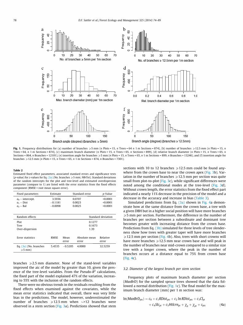
Fig. 1. Frequency distributions for (a) number of branches P5 mm (n Plots = 15, n Trees = 64 n 1 m Sections = 874), (b) number of branches P12.5 mm (n Plots = 15, nTrees = 64, n 1 m Sections = 874), (c) maximum branch diameter (n Plots = 15, n Trees = 65, n Sections = 899), (d) relative branch diameter (n Plots = 15, n Trees = 65, nSections = 864, n Branches = 12101), (e) insertion angle for branches P5 mm (n Plots = 15, n Trees = 65, n 1 m Sections = 899, n Branches = 13246), and (f) insertion angle forbranches P12.5 mm (n Plots = 15, n Trees = 65, n 1 m Sections = 874, n Branches = 7301).

Table 2Estimated fixed effect parameters, associated standard errors and significance tests(p-value) for z-values for Eq. (3a) (No. branches P5 mm; NBrTot). Standard deviationsof the random intercepts for the plot and tree-level and estimated overdispersionparameter (compare to 1) are listed with the error statistics from the fixed effectscomponent (RMSE = root mean square error).

Fixed parameters Estimate Standard error p-Value

a0 – intercept. 3.5936 0.0707 <0.0001a1 – Dist �0.1181 0.0023 <0.0001a2 – Bal �0.0098 0.0025 <0.0001

Random effects Standard deviation

Plot 0.1277Tree 0.1673Over-dispersion 1.39

Error statistics RMSE Meanerror

Absolute meanerror

Relativeerror

Eq. (3a) (No. branchesP5 mm)

5.4535 �0.5205 4.0000 32.5259

78 D.F. Sattler et al. / Forest Ecology and Management 325 (2014) 74–89

branches P2.5 mm diameter. None of the stand-level variablesimproved the aic of the model by greater than 10, given the pres-ence of the tree-level variables. From the Pseudo-R2 calculations,the fixed part of the model explained 47% of the variation, increas-ing to 55% with the inclusion of the random effects.

There were no obvious trends in the residuals resulting from thefixed effects when examined against the covariates, while themean error statistics indicated that overall, there was very littlebias in the predictions. The model, however, underestimated thenumber of branches P12.5 mm when �>12 branches wereobserved in a stem section (Fig. 3a). Predictions showed that stem

sections with 10 to 12 branches P12.5 mm could be found any-where from the crown base to near the crown apex (Fig. 3b). Var-iation in the number of branches P12.5 mm per section was quitesmall from plot-to-plot (Fig. 3c), while significant differences werenoted among the conditional modes at the tree-level (Fig. 3d).Without crown length, the error statistics from the fixed effect partindicated a nearly 11% decrease in the precision of the model and adecrease in the accuracy and increase in bias (Table 3).

Simulated predictions from Eq. (3a) shown in Fig. 4a demon-strate how at the same distance from the crown base, a tree witha given DBH but in a higher social position will have more branchesP5 mm per section. Furthermore, the difference in the number ofbranches per section between a subordinate and dominant treebecomes greater with increasing distance from the crown base.Predictions from Eq. (3b) simulated for three levels of tree slender-ness show how trees with greater taper will have more branchesP12.5 mm per section (Fig. 4b). Also, trees with short crowns willhave more branches P12.5 mm near crown base and will peak inthe number of branches near mid-crown compared to a similar sizetree with a longer crown, where the peak in the number ofbranches occurs at a distance equal to 75% from crown base(Fig. 4c).

3.2. Diameter of the largest branch per stem section

Frequency plots of maximum branch diameter per section(MaxBrD) for the sampled spruce trees showed that the data fol-lowed a normal distribution (Fig. 1c). The final model for the max-imum branch diameter (mm) per 1 m section was:

lnðMaxBrDptsÞ ¼ c0 þ c1RDistpts þ c2 ln RDistpts þ c3Clpt

þ c4Slcpt þ c5Htlcrnpt þ vp þ vpt þ epts ð4aÞ

Fig. 2. One-to-one line (solid line) overlaid with observed versus fitted values (circles) for the number of branches P5 mm (a); boxplots showing the distribution of thepredicted number of branches per section using fixed effects (boxes identify the 1st and 3rd quartiles and the median, whiskers show 1.5 interquartile range (IQR) and circlesshow outliers) versus relative distance from crown base (b); and caterpillar plots of the plot-level (c) and tree-level (d) random effects (dots are the conditional means for thewithin-group levels and lines represent the 95% confidence intervals).

Fig. 3. One-to-one line (solid line) overlaid with observed versus fitted values (circles) for the number of branches P12.5 mm (a); boxplots showing the distribution of thepredicted number of branches per section using fixed effects (boxes identify the 1st and 3rd quartiles and the median, whiskers show 1.5 IQR and circles show outliers) versusrelative distance from crown base (b); and caterpillar plots of the plot-level (c) and tree-level (d) random effects (dots are the conditional means for the within-group levelsand lines represent the 95% confidence intervals).

D.F. Sattler et al. / Forest Ecology and Management 325 (2014) 74–89 79

Fig. 4. Predicted number of branches for: (a) all branches P5 mm and for four different levels of basal area of larger trees (Bal) using Eq. (3a), (b) branches P12.5 mm usingEq. (3b) for three different levels of slenderness (Slc), and (c) branches P12.5 mm using for four crown lengths (Cl). Simulated values for Bal, Slc and Cl represent the range fora tree with DBH = 30 cm.

80 D.F. Sattler et al. / Forest Ecology and Management 325 (2014) 74–89

which was fit using a Gaussian distribution with a log-link functionand where c0 to c5 were the parameters to be estimated, vp and vpt

were the plot and tree random effects and epts the residual error(Table 4). Maximum branch diameter was positively related tocrown length and height to live crown. Tree slenderness, on theother hand, showed a negative relationship to the diameter of thelargest branch. Boxplots of the predictions show that maximumbranch diameters from 20 mm to 34 mm are most often estimatedto occur within 20–70% of the crown base, while maximum branchdiameters P36 mm are restricted to the lower 40% of the crown(Fig. 5b).

Residuals from the fixed part of the model showed little to nobias along the full range of predicted values. The same was truewhen the residuals were plotted against the covariates in themodel. The fixed-effect part of the model explained 61% of the var-iability, while the addition of random effects only explained anadditional 4% of the variability. Plot-to-plot variability for maxi-mum branch diameter was low as indicated in Fig. 5c. Tree-to-treevariability was larger; however, differences in the random effectsbetween trees did not appear to be significant. When the modelwas refit without the variables for crown length and height to live

crown, there was a large drop in the precision and accuracyof the estimates from the fixed effect component. Furthermore,without the crown size related variables, the model showedgreater bias and tended to underestimate maximum branchdiameter (Table 4).

Simulated predictions (Fig. 6a–c) from Eq. (4a) show that forcrown length, height to live crown, and tree slenderness, maxi-mum branch diameter follows the same overall trend with increas-ing relative distance from the tree apex. That is, maximumdiameters increase rapidly descending from the tree apex untilroughly 60% from crown base, after which point they increase ata slower rate until they peak at about 25% from the crown base.For all simulated scenarios, the greatest differences in maximumbranch diameter are observed over the lower half of the crown.

3.3. Diameter of branches smaller than the largest

Given the distribution of relative branch diameters (RelBrD)(Fig. 1d) and that the dependent variable was in the form of pro-portional data, a binomial distribution with a logit link functionwas used to fit the model. The model selected was:

Table 3Estimated fixed effect parameters, associated standard errors and significance tests(p-value) for z-values for Eq. (3b) (No. branches P12.5 mm; NoBrNo1Grd). Standarddeviations of the random intercepts for the plot and tree-level and estimatedoverdispersion parameter (compare to 1) are listed with the error statistics from thefixed effects component (RMSE = root mean square error).

Fixed parameters Estimate Standard error p-Value

b0 – intercept 4.1546 0.19058 <0.0001b1 – Dist �0.1924 0.00756 <0.0001b2 – lnRDist 0.8367 0.04727 <0.0001b3 – Cl 0.06295 0.00559 <0.0001b4 – Slc �0.8296 0.1828 <0.0001

Random effects Standard deviation

Plot 0.02668Tree 0.1205Over-dispersion 1.31

Error statistics RMSE Meanerror

Absolute meanerror

Relativeerror

Eq. (3b) (No. branchesP12.5 mm)

3.7456 0.06169 2.9169 34.4410

Eq. (3b) without crownlength

4.4354 0.2392 3.3737 43.6521

Table 4Estimated fixed effect parameters and associated standard errors (significance testsnot calculated) for Eq. (4a) (MaxBrD). Standard deviations of the random effects (Plot,Tree and Residuals) are listed with the error statistics from the fixed effectscomponent (RMSE = root mean square error).

Fixed parameters Estimate Standard error

c0 – intercept 4.1404 0.6374c1 – Rdist �0.7344 0.0749n 0.5641 0.0353c3 – Cl 0.0282 0.0164c4 – Slc �0.9052 0.6107c5 - Htlcrn 0.0281 0.0152

Random effects Standard deviation

Plot 0.2185Tree 0.4749Residuals 4.5796

Error statistics RMSE Meanerror

Absolute meanerror

Relativeerror

Eq. (4a) (MaxBrD) 5.5503 �0.0468 4.2193 16.3426Eq. (4a) minus crown

length vars.7.5212 1.9049 5.9159 24.9252

D.F. Sattler et al. / Forest Ecology and Management 325 (2014) 74–89 81

lnBrDptsl=MaxBrDpts

1� ðBrDptsl=MaxBrDptsÞ

� �¼ d0 þ d1RDistpts þ d2Rankptsb

þ d3Slcpts þ dp þ dpt þ dpts ð5aÞ

The fixed effect parameters to be estimated were d0 to d3, whilethe random effects for the plot, tree and section level were dp, dpt,and dpts, respectively (Table 5). Among the covariates in the model,the rank of the branch appeared to be the most important in termsof explaining the relative diameter. Relative branch diameters

Fig. 5. One-to-one line (solid line) overlaid with observed versus fitted values (circles)predicted branch diameters (mm) using fixed effects (boxes identify the 1st and 3rd quartdistance from crown base (b); and caterpillar plots of the plot-level (c) and tree-level (d)represent the 95% confidence intervals).

increased as the rank of the branch increased (e.g., from rank 8to rank 1). Also, the relative diameter of branches per sectionincreased with increasing relative distance from the tree apexwhile more slenderness trees had smaller relative branch diame-ters per 1 m section. Although overall mean error was quite small(Table 5), residuals from the fitted fixed effect part of the modelshowed that the model tended to overestimate at small relativebranch diameters and underestimate at relative branch diameters>70%. The greatest difference between fitted and observed valuesoccurred for branches that were �<40% of the maximum branch

for the maximum branch diameter (a); boxplots showing the distribution of theiles and the median, whiskers show 1.5 IQR and circles show outliers) versus relativerandom effects (dots are the conditional means for the within-group levels and lines

Fig. 6. Predicted values for maximum branch diameter using Eq. (4a), for (a) three values of crown length (slenderness = 0.85, height to live crown = 15 m), (b) three values ofslenderness (crown length = 10 m, height to live crown = 15 m), and (c) three values of height to live crown (crown length = 10 m, slenderness = 0.85). 0 = crown base and1 = crown apex. Simulated values for crown length and slenderness represent the range for a tree with DBH = 30 cm.

82 D.F. Sattler et al. / Forest Ecology and Management 325 (2014) 74–89

diameter within a 1 m section (Fig. 7a). Boxplots of the predictionsin Fig. 7b were calculated by multiplying the estimated relativebranch size by the maximum branch size for the given stem sectionand indicated that branch diameters >18 mm could be found any-where from near the crown apex to the crown base.

Caterpillar plots showed that most of the variability in therandom effects was between sections within trees, followed bytree-to-tree and plot-to-plot variability (Fig. 7c–e). Using only thefixed effects part of the model, the Pseudo-R2 was 59%, whileadding plot, tree and section random effects increased thisvalue to 81%.

Predictions from Eq. (5a) simulated for four branch ranks andthree levels of tree slenderness (Fig. 8a, and b, respectively) showsimilar general trends as those for maximum branch diameter.That is, there is a rapid decrease in branch diameter from about60% relative crown depth to crown apex. The difference in diame-ter between a branch of rank 2 and one of rank 8 is greatest overthe bottom half of the crown, and becomes less towards the crownapex. Also, given a similar DBH, a more slender tree will haveslightly smaller branch diameters than one which is less slender.

Like branch rank, this difference is most notable over the bottomhalf of the crown.

3.4. Branch angle

The model selected to provide estimates of branch angle for alllive branches P5 mm diameter (BrAngTot) was:

BrAngTotptsl ¼ e0 þ e1RDistpts þ e2Rankptsb þup þupt þupts þ eptsl

ð6aÞ

where e0 to e2 were the fixed effect parameters to be estimated andup, upt, upts, and eptsl were the random effects (Table 6). The samemodel structure was used for estimates of insertion angle forbranches P12.5 mm (BrAngNo1Grd):

BrAngNo1Grdptsl ¼ f0 þ f1RDistpts þ f2Rankptsb þ/p þ/pt þ/pts þ eptsl

ð6bÞwhere f0 to f2 were the fixed effect parameters and /p, /pt, /pts, andeptsl were the random effects (Table 7). Frequency plots of branch

Table 5Estimated fixed effect parameters, associated standard errors and significance tests(p-value) for z-values for Eq. (5a) (RelBrD). Standard deviations of the randomintercepts for the plot, tree, and section-level are listed with the error statistics fromthe fixed effects component (RMSE = root mean square error).

Fixed Parameters Estimate Standard error p-Value

d0 – intercept 2.5819 0.2527 <0.0001d1 – RDist �0.2134 0.0667 <0.0001d2 – Rank �0.1421 0.0009 <0.0001d3 – Slc �0.7590 0.2956 <0.0102

Random effects Standard deviation

Plot 0.1200Tree 0.1917Section 0.4861

Error statistics RMSE Meanerror

Absolute meanerror

Relativeerror

Eq. (5a) (proportionscale)

0.1403 0.0093 0.1106 43.8917

Eq. (5a) (diameter scale(mm))

3.9350 �0.4106 2.8145 42.6869

D.F. Sattler et al. / Forest Ecology and Management 325 (2014) 74–89 83

angle were similar for the two dependent variables (Fig. 1e and f)and both models were fit using a Gaussian distribution with anidentity link function. As was the case for estimates of relativebranch diameter, branch rank was the most important coefficientfor estimates of branch angle, regardless of branch size. The esti-mated fixed-effect coefficients from Eqs. (6a) and (6b) indicatedthat branch angle decreased as the branch rank increased. Withincreasing distance from tree apex branch angles decreased at asimilar rate for both branches P5 mm and those P12.5 mm. Themean error of the fitted residuals indicated that the model forbranches with a diameter P5 mm showed a small tendency tooverestimate branch angles (Table 6). This was most notable atbranch angles >90�. Also, when the rank of the branch exceeded�30% of the maximum branch diameter, the model tended to over-estimate angles. Some prediction bias was also noted in relation tothe relative distance into the crown (RDist), where angles wereoverestimated for branches located within 15% crown base as wellas for those located within 15% of the crown apex. The overall biasin the model for branches with a diameter P12.5 mm was small(Table 7) but showed a slight tendency to underestimate branchangles that were >90�. Unlike the previous model, there was nonoticeable bias across relative distance into the crown or branchrank.

The fixed effect part of the model for all branches P5 mmexplained 29% of the variability in branch angle, while the modelfor branches P12.5 mm explained 32% of the variability. The addi-tion of the random effects to each of the models had a similar effectin terms of the additional variance explained, increase by 28% and32%, respectively. Partitioning of the random variability was nearlyidentical for the two equations. Among the random effects, tree-to-tree variability was the highest, followed between section andbetween plot variability (Figs. 9c–e and 10c–e).

Simulations for four different branch ranks resulting from Eqs(6a) and (6b) show how for a given relative height in the crown,branch angles are smaller for a branch whose diameter is closerto the maximum branch diameter for the given 1 m stem section(Fig. 11a and b). The predicted rate of increase in branch angle withincreasing relative distance from the tree top was nearly the samefor branches P5 mm and those P12.5 mm. Similarly, the differ-ence between a lower ranked branch and a higher ranked branchat a given relative height is nearly the same.

4. Discussion

4.1. Number of branches per section

Stand and tree-level variables used in branch frequency modelsfor species where this characteristic is under strong genetic controloften have poor explanatory capabilities. For example, Hein et al.(2007) cited moderate genetic control in Norway spruce as a pos-sible reason why only a low percentage (<6%) of the total variancefor the number of branches (P5 mm) in a whorl could beexplained using a mixed effect model. In contrast, the fixed compo-nents of the model presented here explained 60% of the total var-iance using only distance from tree apex (Dist) and tree socialstatus (Bal). This suggests a weaker genetic control over branchfrequency within white spruce, implying that positional andstand-level effects have a greater impact on branch initiation andself-pruning. This would be consistent with Merrill and Mohn (1985),who found low heritability for the number of branches per whorlwithin an open-pollinated 20 year old plantation of white spruce.

For the current study, there was a large decrease in AIC (1730–1460) when relative position within the crown was replaced byabsolute distance within the crown. Within the model dataset,the longest crowns were measured on large, old (>125 years) over-story trees. Thus, the oldest branches within the dataset are foundat large absolute distances from the crown apex of these trees. Age-related effects such as reduced photosynthesis and diminished sto-matal conductance (Bond, 2000) are likely to have a strong impacton branch loss at these distances. Conversely, for the same dataset,large relative distances from the crown apex will not only includevery old branches from large trees with long crowns, but alsoyounger branches on smaller, understory trees. However, for theyounger trees, age-related effects on branch loss will be less prom-inent (Ishii and McDowell, 2002). Therefore, for the range of crownlengths and branch ages included in the model dataset, absolutedistance into the crown seems to be a better proxy to describethe gamut of effects (e.g., branch age, shading, damage from con-tact with neighbouring trees) causing branch loss. In comparison,the model used by Nemec et al. (2012) to explain the frequencyof branch clusters along older annual shoots (>5 years) in whitespruce included both a relative and absolute measure of shootheight, with no distinction made between the effects attributableto these two variables. Their model for branch number per cluster,however, included no positional effects; rather, shoot age was citedas a minor factor.

Among the suite of models presented in this study, branch fre-quency (for diameters P5 mm) was the only one to include a mea-sure of competition derived from a stand-level measurement. Theinclusion of the basal area of larger trees (Bal) in the model seemsto confirm our earlier interpretation that local stand conditionshave a large effect on branch frequency relative to effects relatedto heritability. The negative relationship between the number ofbranches and Bal indicates that trees in a dominant position havea greater number of branches per stem section than suppressedtrees. This can be attributed to increased levels of light receivedby dominant trees, which in turn increases the development ofnew branches (Maguire et al., 1994; Weiskittel et al., 2010). Simu-lated predictions from the models showed that these differencesare greatest at the tops of trees and become negligible near thebase of the crown. Nemec et al. (2012) did not test the inclusionof stand-level derived measures of competition in their modelsfor cluster and branch frequency, presumably because theyassumed that the effects of competition would be captured bythe tree and shoot-level predictor variables they tested. For forestgrowth simulators where only stand and tree-level variables areprovided, the basal area of larger trees has been recommended as

Fig. 7. One-to-one line (solid line) overlaid with observed versus fitted values (circles) for relative branch diameters (a); boxplots showing the distribution of predictedbranch diameters using fixed effects (boxes identify the 1st and 3rd quartiles and the median, notches identify confidence intervals for the median and circles show outliers)versus relative distance from crown base (b); and caterpillar plots of the plot-level (c), tree-level (d) and section-level (e) random effects (dots are the conditional means forthe within-group levels and lines represent the 95% confidence intervals).

84 D.F. Sattler et al. / Forest Ecology and Management 325 (2014) 74–89

an appropriate competition index, particularly for complex stands(Wykoff et al., 1982; Wykoff, 1986; Temesgen et al., 2005). The factthat Bal, and not a species-specific competition index, was found tosignificantly affect branch frequency suggests that this characteris-tic is not strongly influenced by the type (e.g., deciduous or conif-erous) of species in the stand.

Like the model for branches P5 mm, the frequency of branchesP12.5 mm was most strongly related to absolute distance fromcrown apex. The initial increase in the frequency for branchesP12.5 mm moving down from the crown apex is mainly a reflec-tion of the time required for braches to attain at least 12.5 mm.The subsequent decrease in frequency from roughly 20% of crownlength to crown base reflects the increasing effects of branch ageand shading (either self-shading or from competitors) on branchloss. The frequency of branches P12.5 mm was also positively cor-related to crown length and negatively related to tree slenderness.For range of tree ages and crown lengths in the model dataset,crown length seemed to capture both shade and age-related effectson branch frequency better than crown ratio. The differences in

branch frequency between slender trees and trees with large taperwas most notable at around 20% from the crown apex. For Norwayspruce, Hein et al. (2007) also found tree slenderness to be a signif-icant predictor for the frequency of branches P5 mm, whileWeiskittel et al. (2007) reported a similar increase in the branchfrequency (also for branches P5 mm) with increasing crownlength for Douglas fir.

4.2. Diameter of the largest branch per section

There were strong positional effects acting on maximum branchdiameter given that relative distance into the crown was the mostimportant variable in the model. Although Nemec et al. (2012) didnot specifically model maximum branch diameters in whitespruce, positional effects were also important when predictingthe diameter of live branches. Two of the five within-crown posi-tional variables they included were based on distance dependentmeasures of neighbouring competitors, indicating that bothshelf-shading and shading from competitors had an effect on light

Fig. 8. Predicted values for relative branch diameter using Eq. (5a). for (a) four levels of branch rank (rank = 2, 4, 6, 8) (slenderness = 0.85 m) and (b) for three levels ofslenderness (Branch rank = 3). Simulated values for slenderness are representative of a tree with DBH = 30 cm.

Table 6Estimated fixed effect parameters and associated standard errors for Eq. (6a)(BrAngTot). Standard deviations of the random components (Plot, Tree, Section andResiduals) are listed with the error statistics for the fixed effects component(RMSE = root mean square error).

Fixed parameters Estimate Standard error

e0 – intercept 45.7100 1.5658e1 – RDist 50.3424 1.0766e2 – Rank 1.1050 0.0214

Random effects Standard deviation

Plot 4.1951Tree 7.1154Section 6.9460Residuals 13.9605

Error statistics RMSE Meanerror

Absolutemean error

Relativeerror

Eq. (6a) angle forbranches P5 mm

17.4867 �0.7239 13.3320 17.6227

Table 7Estimated fixed effect parameters and associated standard errors for Eq. (6a)(BrAngNo1Grd). Standard deviations of the random components (Plot, Tree,Section and Residuals) are listed with the error statistics for the fixed effectscomponent (RMSE = root mean square error).

Fixed parameters Estimate Standard error

f0 – intercept 46.1606 1.6539f1 – RDist 49.4716 1.0353f2 – Rank 0.9298 0.0408

Random effects Standard deviation

Plot 4.4171Tree 7.6760Section 6.1483Residuals 11.9578

Error statistics RMSE Meanerror

Absolutemean error

Relativeerror

Eq. (6b) angle for branchesP12.5 mm

15.8205 0.5927 11.9130 16.0385

D.F. Sattler et al. / Forest Ecology and Management 325 (2014) 74–89 85

availability, which in turn limited branch diameter growth. Tree-level variables, however, were not important in their models, indi-cating that the positional effects were the same regardless of treesize. In contrast, the results here indicate that crown length (Cl),height to live crown (Htlcrn) and tree slenderness (Slc) were allrelated to maximum branch diameter even after within-crownpositional effects were taken into account. The difference in find-ings may at least partially be attributable to the two distance-dependent measures of competition used by Nemec et al. (2012).In the absence of distance-dependent, branch-level measures ofinter-tree competition, tree-level variables that are sensitive tostand density appear to be able to account for some of the compe-tition-related variability in maximum branch diameters. In addi-tion to being sensitive to stand density, large values for crownlength and height to live crown were associated with some ofthe oldest trees in the model dataset. Thus, these two variablesmay also reflect the effects of branch age on maximum branchdiameters. Although positional effects were not investigated byGroot and Schneider (2011), they did find that the average maxi-mum branch diameter (MDB) per tree increased with increasingcrown length on white spruce trees. MDB in white spruce was alsomore sensitive to changes in stand density than the other speciesthey tested.

For a given DBH, differences in maximum branch diameterbetween trees with short and long crowns was greatest over thelower half of the crown. Although the correlation between thefixed effects for crown length and height to live crown was <0.8,trees with long crowns tended to have larger heights to live crown.This explains why trees with small values for height to live crownalso had smaller branches in the lower half when compared totrees with large values for the height to live crown. The greatestdifference in maximum branch diameters for slender trees versustrees with greater taper was also over the lower half of the crown.This is important information for forest managers since this indi-cates that silvicultural practices that affect crown length and treetaper can have a large impact on knot size, particularly withinthe merchantable portion of the crown. Wang et al. (2000) foundthat tree slenderness for white spruce within boreal mixedwoodforests was positively correlated with stand density and site index.This suggests that silviculturalists could control maximum branchdiameters by planting spruce at higher densities within areas withhigh site index.

Fig. 9. One-to-one line (solid line) overlaid with observed versus fitted values (circles) for angle of insertion for branches P5 mm (a); boxplots showing the distribution of thepredicted branch angles using fixed effects (boxes identify the 1st and 3rd quartiles and the median, notches identify confidence intervals for the median and circles showoutliers) versus relative distance from crown base (b); and caterpillar plots of the plot-level (c), tree-level (d) and section-level (e) random effects (dots are the conditionalmeans for the within-group-levels and lines represent the 95% confidence intervals).

86 D.F. Sattler et al. / Forest Ecology and Management 325 (2014) 74–89

4.3. Branch diameter other than the largest branch

The relative distance into the crown and the branch rank hadthe strongest influence on relative branch diameter. The fact thatwithin-crown and within-section variables accounted for most ofthe variability in relative branch diameters is in agreement withthe findings from Nemec et al. (2012). When predictions of relativebranch diameter were transformed into absolute branch diame-ters, there was a general pattern of increasing branch diameterwith increasing distance from the tree top, which followed closelyto the patterns displayed by maximum branch diameter. That is,there was rapid increase moving down from the tree top untilabout 35% into the crown, followed by a more gradual increasedownward, peaking at about 25% from the crown base. The low

crown position for the peak in relative branch diameters may beindicative of the moderate to high shade-tolerance exhibited bywhite spruce. Previous studies on other shade-tolerant specieshave also reported peaks in branch diameter at low crown posi-tions (e.g., Hein et al. (2007) for Norway spruce and Benjaminet al. (2009) for black spruce). The inclusion of tree slendernessindicates that stand density has a minor effect on smaller branches,but not as strong as with maximum branch size. Overall, the modelfor relative branch diameter had the highest relative error andtended to overestimate branch diameters that were small relativeto the largest branch per 1 m section. The addition of randomeffects greatly improved the model, however, this implies thatlocal calibration of the model will likely be required if it is to beused over a wider area.

Fig. 10. One-to-one line (solid line) overlaid with observed versus fitted values (circles) for angle of insertion for branches P12.5 mm (a); boxplots showing the distributionof the predicted branch angles using fixed effects (boxes identify the 1st and 3rd quartiles and the median, notches identify confidence intervals for the median and circlesshow outliers) versus relative distance from crown base (b); and caterpillar plots of the plot-level (c), tree-level (d) and section-level (e) random effects (dots are theconditional means for the within-group-levels and lines represent the 95% confidence intervals).

D.F. Sattler et al. / Forest Ecology and Management 325 (2014) 74–89 87

4.4. Branch angle

The angle of branches P5 mm and those P12.5 mm appearedto be under the influence of the same factors given that the modelsincluded the same variables and only showed minor differences inthe estimated coefficients. Similar to relative branch diameter,within-crown and within section positioning effects had the great-est influence on branch angles, regardless of branch size. Since novariables that would indicate the presence of tree-age relatedeffects were included in the model (e.g., DBH, Cl), the trendsobserved for branch angle appear to be the same for both youngand old trees. Nemec et al. (2012) did not model branch anglesfor white spruce, and no other studies for branch angle on naturallyregenerated white spruce could be found. However, for Sitkaspruce, Achim et al. (2006) also found that tree-size related effectsdid not influence branch insertion angle.

For white spruce, the larger branches within a section (i.e.,smaller rank) displayed the smallest angles (i.e., they pointed moretowards tree apex) and is consistent with the findings from Sitkaspruce reported by Auty et al. (2012). This has significant implica-tions in terms of appearance grading of structural lumber, sincesmall angles on branches with large diameters will produce a largeknot surface area. No stand-level variables or tree-level variablesthat are sensitive to changes in stand density were included inthe model, suggesting that prescribed thinning or changes in plant-ing densities will have little effect over the control of branchangles. The positive relationship between relative distance intothe crown and branch angle observed here was also observed onNorway spruce (Colin and Houllier, 1992). The trend may berelated to the increase in branch mass with age. Yamamoto et al.(2002) concluded that higher amounts of biomass carried by largerbranches pulled the branches downward. Thus, as successive

Fig. 11. Predicted values for branch angle using Eq. (6a) for four levels of branch rank (rank = 2, 4, 6, 8) for (a) branches P5 mm diameter, and (b) for branches P12.5 mmdiameter.

88 D.F. Sattler et al. / Forest Ecology and Management 325 (2014) 74–89

growth rings are added to the main stem of the tree, branch inser-tion angle on the main stem will increase while the relative dis-tance of the branch from the tree apex also increases.

5. Model applications and conclusions

The models here represent an important addition to the toolsrequired to manage stands with wood quality objectives in mind.Existing branch models for white spruce included: (1) those pre-sented by Groot and Schneider (2011) which uses LiDAR dataand provide a single average estimate of maximum branch diame-ter per tree; and (2) those provided by Nemec et al. (2012), whichprovide estimates of cluster frequency, branch frequency per clus-ter, and branch diameter and which require detailed measure-ments of shoot age and distance to the nearest competitor. Thecurrent suite of models differ from these existing models sincethey were explicitly developed to be used within distance-inde-pendent growth simulators. Furthermore, model datasets wereexclusively from naturally regenerated, unmanaged stands, whichwas not the case for the existing branch models. Their develop-ment using data from both mixed and pure species stands meansthat they should be suitable for use in the mixedwood growthmodel (MGM) simulator. The models, in their current form, areapplicable to the ‘reference’ (i.e., modal) ecosite of the centralmixedwood subregion of Alberta (Natural Regions Committee,2006). The ‘reference’ ecosite within this subregion is associatedwith deep, moderately-fine textured soils of average moistureand nutrient status. Spruce harvested from these sites representsa large proportion of the total volume of harvested timber. Sinceplot-level random effects were important in several of the models,calibration of the parameters to specific areas (e.g., other naturalsubregions within the Boreal forest) is likely required. Validationof the models will also be necessary before they can be usedoperationally.

The results of the models appear to largely confirm our limitedknowledge of crown architecture for white spruce and are, for themost part, in line with results from other coniferous species. Manyof the explanatory variables used in the models presented herehave been previously used to predict branch characteristics forother conifers. However, most of the pre-existing knowledge ofbranch characteristics has been derived using data from spacing

trials or from single species stands. The data collected for the cur-rent study presented an opportunity to test these assumptions innaturally regenerated, mixed species stands. Our finding that onlytree-level variables were required for most of the models is, there-fore, interesting since it suggests that species composition effectson the branching characteristics of individual white spruce cannotbe easily detected at the stand-level. Thorpe et al. (2010) foundthat crown size for interior spruce was highly sensitive to local,inter-tree competition; crown radius decreased more rapidly withan increasing number of local competitors when competitors werecomposed of both shade-tolerant and shade intolerant species ver-sus only conspecifics. Although the tree-level variables included inthe current models do not capture species-specific effects, they aregood proxies for the effects of local competition. Thus, their pres-ence in the models here are in agreement with the more generalfindings by Thorpe et al. (2010) that crown architecture is affectedby local ‘‘neighbourhood’’ conditions.

Acknowledgements

The work presented in this paper was completed while the leadauthor was a member of the Forest Value Network/Projet ForêtValeur. We gratefully acknowledge the Natural Sciences and Engi-neering Research Council of Canada, who provided financial sup-port for this research project through funding of ForValueNetStategic Network. Furthermore, we wish to thank the numerousfield and lab assistants who contributed to the collection of dataused in the analyses.

Appendix A. Supplementary material

Supplementary data associated with this article can befound, in the online version, at http://dx.doi.org/10.1016/j.foreco.2014.03.051.

References

Achim, A., Gardiner, B.A., Leban, J.-M., Daquitane, R., 2006. Predicting the branchingproperties of Sitka spruce grown in Great Britain. NZ J. For. Sci. 36, 246–264.

Akaike, H., 1974. A new look at the statistical model identification. IEEE Trans.Autom. Control 19, 716–723.

D.F. Sattler et al. / Forest Ecology and Management 325 (2014) 74–89 89

Alberta Sustainable Resource Development (ASRD), 2005. Permanent sample plotfield procedures manual. Public Lands and Forest Division, Forest ManagementBranch, Edmonton, Alberta, 30p.

Auty, D., Weiskittel, A.R., Achim, A., Moore, J.R., Gardiner, B.A., 2012. Influence ofearly re-spacing on Sitka spruce branch structure. Ann. For. Sci. 69, 93–104.

Bates D, Maechler M., 2009. Package ‘lme4’ <http://lme4.r-forge.r-project.org/>.Beckingham, J.D., Archibald, J.H., 1996. Field guide to ecosites of northern Alberta.

Northern Forestry Centre, Forestry Canada, Northwest Region. Spec. Rep. 5.Benjamin, J.G., Kershaw Jr., J.A., Weiskittel, A.R., Chui, Y.H., Zhang, S.Y., 2009.

External knot size and frequency in black spruce trees from an initial spacingtrial in Thunder Bay, Ontario. For. Chron. 85, 618–624.

Bokalo, M., Stadt, K.J., Comeau, P.G., Titus, S.J., 2010. Mixedwood Growth Model(MGM) (version MGM2010.xls). University of Alberta, Edmonton, Alberta, Canada.2010. <http://www.rr.ualberta.ca/Research/MixedwoodGrowthModel.aspx>(accessed 07.07.11).

Bokalo, M., Stadt, K.J., Comeau, P.G., Titus, S.J., 2013. The validation of themixedwood growth model (MGM) for use in forest management decisionmaking. Forests 4, 1–27.

Bolker, B.M., Brooks, M.E., Clark, C.J., Geange, S.W., Poulsen, J.R., Stevens, M.H.H.,White, J.S., 2009. Generalized linear mixed models: a practical guide for ecologyand evolution. Trends Ecol. Evol. 24, 127–135.

Bond, B.J., 2000. Age-related changes in photosynthesis of woody plants. Trends inplant science. Reviews 5 (8), 349–353.

Burnham, K.P., Anderson, D.R., 2002. Model Selection and Multimodel Inference: APractical Information-theoretic Approach. Springer, New York.

Colin, F., Houllier, F., 1992. Branchiness of Norway Spruce in Northeastern France –predicting the main crown characteristics from usual tree measurements. Ann.Sci. For. 49, 511–538.

Duchateau, E., Longuetaud, F., Mothe, F., Ung, C., Auty, D., Achim, A., 2013. Modellingknot morphology as a function of external tree and branch attributes. Can. J. For.Res. 43, 266–277.

Garber, S., Maguire, D., 2005. Vertical trends in maximum branch diameter in twomixed-species spacing trials in the central Oregon Cascades. Can. J. For. Res. 35,295–307.

Groot, A., Schneider, R., 2011. Predicting maximum branch diameter from crowndimensions, stand characteristics and tree species. For. Chron. 87, 542–551.

Hein, S., Mäkinen, H., Yue, C., Kohnle, U., 2007. Modelling branch characteristics ofNorway spruce from wide spacings in Germany. For. Ecol. Manage. 242, 155–164.

Ishii, H., McDowell, N., 2002. Age-related development of crown structure in coastalDouglas-fir trees. For. Ecol. Manage. 169, 257–270.

Maguire, D., Moeur, M., Bennett, W., 1994. Models for describing basal diameter andvertical-distribution of primary branches in Young Douglas-Fir. For. Ecol.Manage. 63, 23–55.

Mäkinen, H., Colin, F., 1999. Predicting the number, death, and self-pruning ofbranches in Socts pine. Can. J. For. Res. 29, 1225–1236.

Merrill, R., Mohn, C., 1985. Heritability and genetic correlations for stem diameterand branch characteristics in white spruce. Can. J. For. Res. 15, 494–497.

Natural Regions Committee, 2006. Natural Regions and Subregions of Alberta.Compiled by D.J. Downing and W.W. Pettapiece. Government of Alberta. Pub.No. T/852.

Nemec, A.F.L., Parish, R., Goudie, J.W., 2012. Modelling number, vertical distribution,and size of live branches on coniferous tree species in British Columbia. Can. J.For. Res. 42, 1072–1090.

NLGA, 2003. Standard grading rules for Canadian lumber. National Lumber GradesAuthority, New Westminster, British Columbia, Canada.

R Core Team, 2013. R: A language and environment for statistical computing. RFoundation for Statistical Computing, Vienna, Austria. <http://www.R-project.org/> (accessed 27.07.13).

Temesgen, H., LeMay, V., Mitchell, S., 2005. Tree crown ratio models for multi-species and multi-layered stands of southeastern British Columbia. For. Chron.81, 133–141.

Tong, Q., Duchesne, I., Belley, D., Beaudoin, M., Swift, E., 2013. Characterization ofknots in plantation white spruce. Wood Fiber Sci. 45, 84–97.

Thorpe, H.C., Astrup, R., Trownbridge, A., Coates, K.D., 2010. Competition and treecrowns: a neighborhood analysis of three boreal tree species. For. Ecol. Manage.259, 1586–1596.

Venables, W.N., Ripley, B.D., 2002. Modern Applied Statistics with S, fourth ed.Springer, New York.

Wang, Y., Titus, S.J., LeMay, V.M., 2000. Relationships between tree slendernesscoefficients and tree or stand characteristics for major species in borealmixedwood forests. Can. J. For. Res. 28, 1171–1183.

Weiskittel, A.R., Maguire, D.A., Monserud, R.A., 2007. Response of branch growthand mortality to silvicultural treatments in coastal Douglas-fir plantations:implications for predicting tree growth. For. Ecol. Manage. 251, 182–194.

Weiskittel, A.R., Seymour, R.S., Hofmeyer, P.V., Kershaw Jr., J.A., 2010. Modellingprimary branch frequency and size for five conifer species in Maine, USA. For.Ecol. Manage. 259, 1912–1921.

Wykoff, W.R., Crookston, N.L., Stage, A.R., 1982. User’s guide to the stand prognosismodel. USDA For. Serv. Gen. Tech. Rep. INT-133.

Wykoff, W.R., 1986. Supplement to the User’s Guide for the Stand Prognosis Model –Version 5.0. Gen. Tech. Rep. INT-208. USDA For. Serv., Ogden, UT. 36 p.

Yamamoto, H., Yoshida, M., Okuyama, T., 2002. Growth stress controls negativegravitropism in woody plant stems. Planta 216, 280–292.