Breathless: Schools, Air Toxics, and Environmental Justice in California

Breathless: Schools, Air Toxics, and EnvironmentalJustice in California

Manuel Pastor Jr., Rachel Morello-Frosch, and James L. Sadd

The exposure of children to environmental disamenities has emerged as a key policy concern in recentyears, with some analysts and activists suggesting that minority children are disproportionatelyimpacted. Utilizing a dataset that combines air toxics at the census tract level with school-baseddemographic and other information, this article indicates disparate exposures for students of color inCalifornia schools and suggests that there may be negative impacts on one measure of academicperformance, even after controlling for other factors usually associated with test scores. Policyimplications include a special focus on school remediation and strengthening overall efforts to reduceemissions “hot spots.”

KEY WORDS: environmental justice, air toxics, academic performance, racial disparity, fixed effectsregression

Introduction

In recent years, the intersection between environmental justice, children’shealth, and schools has attracted the interest of many researchers and activists.Part of the concern is caused by a growing body of scientific evidence thatindicates that children are more susceptible than adults to the adverse effects ofenvironmental pollution (see Bearer, 1995; Crom, 1994; Guzelian, Henry, & Olin,1992; Landrigan & Garg, 2002; Wiley, 1991). The problems may even begin beforebirth: Studies have linked air pollution exposures to adverse health effects includ-ing preterm birth, low birth weight, and birth defects (Bobak, 2000; Ha et al., 2001;Ritz & Yu, 1999; Ritz, Yu, Chapa, & Fruin, 2000; Ritz et al., 2002; Wang, Ding,Louise, & Xu, 1997), and a recent study by Chay and Greenstone (2003) found thatair pollution had a significant impact on infant mortality.

There have also been concerns about disparities in exposures by race, partlybecause some diseases that appear later in childhood and are potentially related toair pollution (e.g. respiratory illnesses such as asthma) also seem to be particularlyon the rise in minority populations (Leikauf et al., 1995; Mannino, Homa, &Pertowski, 1998; Mathieu-Nolf, 2002). A landmark multidisciplinary study trackednearly 1,800 children over eight years in Southern California communities and

The Policy Studies Journal, Vol. 34, No. 3, 2006

337

0190-292X © 2006 The Policy Studies JournalPublished by Blackwell Publishing. Inc., 350 Main Street, Malden, MA 02148, USA, and 9600 Garsington Road, Oxford, OX4 2DQ.

found that air pollution can adversely impact lung function and development(Gauderman et al., 2004). More detailed work in the heavily Latino HuntingtonPark area of Southern California showed significant negative effects from pollutionon the asthma symptoms for children aged 10–16 years (Delfino et al., 2003).

While many of these studies have looked at the impacts of children in thecommunities where they live, children also spend much of their day atschool—and their schools may or may not be located near their home, particularlygiven magnet programs and cross-town busing in major urban areas. Air qualityin and near schools is often problematic, partly because of poor outdoor ambientair quality and partly because of inadequate filtering and other systems (seeShendell et al., 2004). Several studies have also suggested that schools with higherminority populations are more likely to be located in areas with lower qualityambient air, indicating potential environmental justice implications (see Greenet al., 2004; Morello-Frosch, Pastor, & Sadd, 2002; Pastor, Sadd, & Morello-Frosh,2002). And such proximity can have real health consequences: A children’srespiratory health study looking at more than 1,000 children in the San FranciscoBay Area found that living and going to school near busy roads was correlatedwith exacerbation of asthma and chronic bronchitis (Kim et al., 2004).

Moreover, children’s respiratory problems from air pollution have been asso-ciated directly and indirectly with lower academic performance (Fowler,Davenport, & Garg, 1992; Bener, Abdulrazzaq, Debuse, & Abdin 1994; Pastor,Sadd, & Morello-Frosh, 2004). In some communities, parents have complained ofdiminished school performance among their children because of health effectsassociated with outdoor and other pollution (Diette et al., 2000; Kaplan & Morris,2000), and one “meta-study” of the field (Wong et al., 2004) suggests that airpollution reduction could have broad benefits for children, such as reductions inschool absences and improved academic performance.

The issue of children’s environmental health in schools is particularly chal-lenging in California because over 10 percent of the state’s schools are designatedas overcrowded. The majority of new school sites will be located in dense urbanareas where local air quality is relatively poor (Pastor & Reed, 2004; Pastor, Sadd,& Morello-Frosch, 2005). For example, Los Angeles County, with about twentypercent of the students in the state, has over 60 percent of the overcrowdedschools; San Francisco, with around 1 percent of the state’s students, has morethan 10 percent of the overcrowded schools. Given that many of the students inthese schools already face severe socioeconomic challenges, assessing the poten-tial health impacts of poor air quality is particularly salient in terms of high-lighting potential ways for improving children’s health, and possibly schoolperformance.

This article builds on a series of earlier research efforts focused on Los Angeles(Morello-Frosch, Pastor, & Sadd, 2002; Pastor et al., 2002; Pastor et al., 2004) to lookat the intersection of environmental justice, ambient air quality, and schoolperformance in the state of California. Results indicate that students of colordisproportionately attend schools with higher respiratory hazards from air toxics.There also seems to be a relationship between respiratory hazards and school

338 Policy Studies Journal, 34:3

performance, even when proper controls are introduced to account for otherfactors associated with academic success. We begin below with a description of ourdata and methods, and then offer regression analyses that suggest an associationof air pollution with respiratory issues and subsequently with test scores. Weconclude by drawing some implications for policy.

Data and Methods

To understand the relationship between local air quality, environmentaljustice, and academic performance, we combined several data sources. Annualaverage air toxics concentration estimates were compiled from the U.S. Environ-mental Protection Agency’s (U.S. EPA, 2004) National Air Toxics Assessment(NATA) for 1996, which estimates concentrations for diesel particulates and 32 ofthe 188 air toxics listed under the 1990 Clean Air Act Amendments.1 To developnationwide estimates of annual average ambient concentrations of air toxics, theAssessment System for Population Exposure Nationwide (ASPEN) model, devel-oped and used in U.S. EPA’s Cumulative Exposure Project, was employed.2 Themodeling approach was applied to U.S. EPA’s National Toxics Inventory (NTI)which is compiled using five primary information sources including state and localtoxic air pollutant inventories, existing databases related to U.S. EPA’s air toxicsregulatory program, U.S. EPA’s Toxic Release Inventory (TRI) database, estimatesusing mobile source methodology (developed by U.S. EPA’s Office of Transpor-tation and Air Quality), and emission estimates generated from emission factorsand activity data. Using the emissions data as inputs, the ASPEN air dispersionmodel then estimates the annual average ambient concentration of each air toxicpollutant at the centroid of each census tract, after taking into account the impactsof atmospheric processes (winds, temperature, atmospheric stability, etc.) onpollutants.

We then utilized this data to calculate a respiratory hazard index associatedwith outdoor air toxics exposures in which we divided each pollutant concentra-tion estimate by its corresponding reference concentration (RfC) to derive a hazardratio. A RfC for chronic respiratory effects is defined as the amount of toxicantbelow which long-term exposure to the general population of humans, includingsensitive subgroups, is not anticipated to result in any adverse effects (Dourson &Stara, 1983). The actual respiratory hazard ratios for each pollutant in each censustract were calculated using the following formula:

HR C RfCij ij j= (1)

where HRij is the hazard ratio for pollutant j in tract i, Cij is the concentration inug/m3 of pollutant j in census tract i, and RfCj is the reference concentration forpollutant j in ug/m3. An indicator of total respiratory hazard was calculated bysumming together the hazard ratios for each pollutant to derive a total respiratoryhazard index:

Pastor/Morello-Frosch/Sadd: Schools, Air Toxics, and Environmental Justice in California 339

HI HRi j ij= Σ (2)

where HIi is the sum of the hazard ratios for all pollutants (j) in census tract i. Thismeasure assumes that multiple subthreshold exposures may result in an adversehealth effect.3

Because the 1996 NATA risk values are calculated for 1990 census tracts, weused geoprocessing in ArcGIS to apply these risk estimates to the 2000 census tractpolygons. We specifically intersected the two census polygon data layers, usingstandard conflation routines to ensure common tract boundaries and verticeswhere the intent of the census was to retain the same boundary in 1990 and 2000.To allow accurate measurement of area, tract polygons from both years wereprojected into an equivalent map projection. Hazard ratios were then calculated asattributes of the 2000 tract polygons based on the proportion of common area with1990 tract polygons.4

We then mapped all public schools included in both the California BasicEducational Data System (CBEDS) and Academic Performance Index (API) for theyear 2000 by geocoding school addresses using Geographic Data TechnologyDynamap street network and correspondence files; addresses receiving a geocod-ing match score of less than 80 percent were checked for errors and rematchedinteractively.5 All school locations were then linked to their respective API data sothat we could have both school demographics and school performance data.

Mandated by the State of California under the Public Schools AccountabilityAct of 1999, the API is a summary score of overall school performance based onthe Stanford 9 achievement test given as part of the state’s testing program; wespecifically used the results for the test administered in spring of 2000.6 Tocontextualize measures of school performance, the state includes in this databasea limited set of school-level variables, including student demography, a proxy forpoverty, a measure of teacher quality, and other factors.7 Because such measureshave been shown in other research to have an effect on school performance, wemade use of those additional variables in our regressions below, linking them tothe tract-level information on the air toxics health hazard. Schools for which noAPI or demographic data were available were excluded from the analysis.

We also examined the association between the respiratory hazard data andasthma hospitalizations for the period 1998 to 2000. Our theory based on theepidemiological literature, is that higher respiratory hazards caused by poor airquality is linked to asthma which could lead to lower scores, perhaps throughincreased absenteeism, which adversely affects learning capacity and school per-formance. The asthma data were made available to us by California’s CommunityAction to Fight Asthma,8 and the data utilized hospitalization rates from the Officeof Statewide Health Planning and Development (OSHPD) to calculate three-yearaveraged, age-adjusted, asthma hospitalization rates by ZIP Code Tabulation Area(ZCTA) for selected regions of California (specifically for portions of the Bay Areaand the San Joaquin Valley as well as Los Angeles County, San Diego and ImperialCounties, a total area that includes about two-thirds of the state’s overall popu-lation).9 In our analysis, we aggregated our underlying tract-based respiratory


hazard data using a similar area-weighted calculation to fit the 2000 ZCTApolygons.

Results

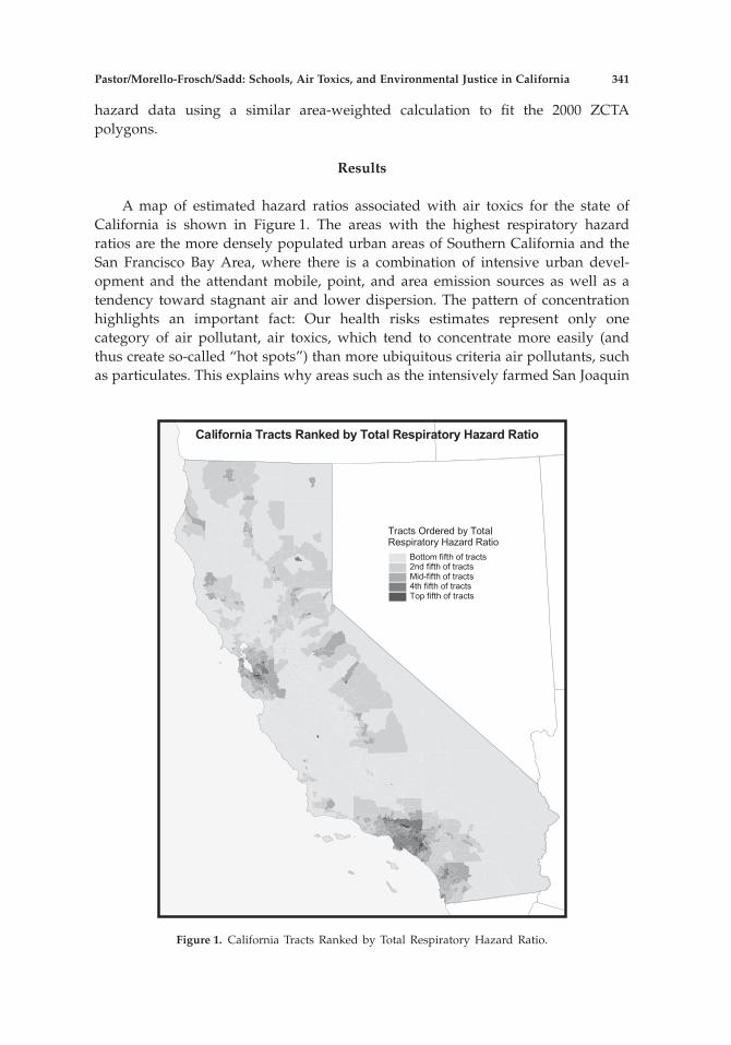
A map of estimated hazard ratios associated with air toxics for the state ofCalifornia is shown in Figure 1. The areas with the highest respiratory hazardratios are the more densely populated urban areas of Southern California and theSan Francisco Bay Area, where there is a combination of intensive urban devel-opment and the attendant mobile, point, and area emission sources as well as atendency toward stagnant air and lower dispersion. The pattern of concentrationhighlights an important fact: Our health risks estimates represent only onecategory of air pollutant, air toxics, which tend to concentrate more easily (andthus create so-called “hot spots”) than more ubiquitous criteria air pollutants, suchas particulates. This explains why areas such as the intensively farmed San Joaquin

Figure 1. California Tracts Ranked by Total Respiratory Hazard Ratio.


Valley of California, now acknowledged to be among the most polluted areas inthe United States in terms of particulate air pollutants, do not appear to have highrespiratory hazard ratios. Indeed, while the heavily urbanized San Francisco, LosAngeles, Orange, Santa Clara, Alameda, and San Mateo Counties are among thetop six when California’s counties are ranked by the air toxics hazard ratio, the topsix in terms of criteria air pollutants are Los Angeles and five primarily agricul-tural counties—San Bernardino, Riverside, Kern, Fresno, and Tulare.10 However,such particulate air pollution is monitored at select locations and the resultingconcentration estimates are not generally available at the geographic resolutionneeded for the analysis undertaken here.

Respiratory Hazards and Health End Points

Are the air toxics risk estimates related to patterns of respiratory problems? Toconsider this, we utilized the asthma hospitalization data discussed above: Thecorrelation between our respiratory hazard ratio and the reported rates of hospi-talization for asthma was positive and highly significant with a Pearson correlationcoefficient of 0.297.11 Of course, hospitalization is only one possible outcome forasthma, because many affected individuals are able to effectively manage theircondition through medication and preventive health care. To consider the relation-ship between asthma and our respiratory hazard ratio, we therefore needed to takea multivariate approach that would also include factors (such as income, whichmight be associated with access to preventive health care) that might explain thedifference between asthma sufferers who are hospitalized and those who are not.

In considering multivariate techniques, it is important to note the truncatednature of the data: When there are fewer than five hospitalization cases per ZCTA,the actual number is not given to protect confidentiality.12 Because of this, anordinary least squares regression would tend to fit the line inappropriately and sowe used a Tobit technique designed specifically for truncated data; we also useda log-transformation of the hazard ratio when entered as an independent variable,a process that yielded a normal distribution that was consistent with the logspecification utilized in the school regressions.13 Finally, because the ZIP codes aremuch less uniform in total population than census tracts, we ran all regressionsweighted by the ZIP code population.14

Our additional variables are meant to control for both other factors that mightpredict asthma and factors, such as income, that would predict where asthmasufferers might land on the continuum of care. We therefore included populationdensity, the percent of the tract population in poverty, and the median value ofoccupied housing units: Population density is associated with crowding, whichencourages transmission of respiratory tract infections (Madrid, Mennie, &Newton, 2006), poverty indirectly measures access to quality health care, andmedian house value proxies the quality of the housing stock (older and lessexpensive houses often have worse indoor air quality regardless of the level ofoutdoor air quality, and so this would mediate the effect of our respiratory hazardmeasure on respiratory health). We also include education because higher levels of


education seem to be associated with lower levels of asthma hospitalizations,presumably because of more knowledge on the part of patients and/or theirparents about how to manage the disease (Chen, Bloomberg, Fisher, & Strunk,2003). Finally, we include tract-level measures of racial or ethic make-up to reflectany patterns of asthma hospitalization that seem to persist by race, even aftersocioeconomic conditions are taken into account.

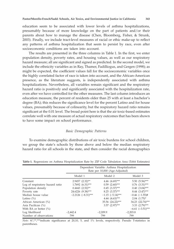
The results are presented in the three columns in Table 1. In the first, we enterpopulation density, poverty rates, and housing values, as well as our respiratoryhazard measure; all are significant and signed as predicted. In the second model, weinclude the ethnicity variables as in Ray, Thamer, Fadilliogus, and Gergen (1998); asmight be expected, the coefficient values fall for the socioeconomic variables oncethe highly correlated factor of race is taken into account, and the African-Americanpresence, as the literature suggests, is independently associated with asthmahospitalizations. Nevertheless, all variables remain significant and the respiratoryhazard ratio is positively and significantly associated with the hospitalization rate,even after we have controlled for the other measures. The last column introduces aneducation measure, the percent of residents older than 25 with at least a bachelor’sdegree (BA); this reduces the significance level for the percent Latino and for housevalues, presumably because of colinearity, but the respiratory hazard ratio remainssignificant at the 0.01 level. The broad point here is that the air toxic-based estimatescorrelate well with one measure of actual respiratory outcomes that has been shownto have some impact on school performance.

Basic Demographic Patterns

To examine demographic distributions of air toxic burdens for school children,we group the state’s schools by those above and below the median respiratoryhazard ratio for all schools in the state, and then consider the racial demographics

Table 1. Regressions on Asthma Hospitalization Rate by ZIP Code Tabulation Area (Tobit Estimates)

Dependent Variable: Asthma HospitalizationRate per 10,000 (Age-Adjusted)

Model 1 Model 2 Model 3

Constant 2.9457 (2.32)** 4.46 (4.69)*** 5.50 (5.56)***Log of respiratory hazard ratio 1.7692 (6.31)*** 0.59 (2.60)*** 0.76 (3.31)***Population density 0.4443 (2.52)** 0.45 (3.37)*** 0.40 (3.04)***Poverty rate 24.6226 (9.38)*** 8.25 (3.37)*** 8.44 (3.47)***Median house value -2.2126 (-8.31)*** -1.15 (-5.14)*** -0.46 (-1.55)#Latino (%) 4.44 (4.63)*** 2.04 (1.75)*African American (%) 35.56 (24.22)*** 34.23 (22.74)***Asia Pacifican (%) 3.57 (2.97)*** 3.33 (2.79)***With BA or better (%) -6.61 (-3.51)***Log likelihood -2,442.4 -2,209.9 -2,203.8Number of observations 799 799 799

Note: #,*,**,***indicate significance at 20,10, 5, and 1% levels, respectively. Pseudo T-statistics inparentheses.


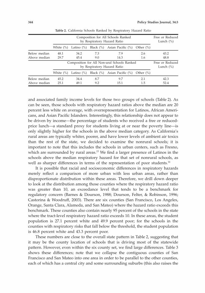
and associated family income levels for those two groups of schools (Table 2). Ascan be seen, those schools with respiratory hazard ratios above the median are 20percent less white on average, with overrepresentation for Latinos, African Ameri-cans, and Asian Pacific Islanders. Interestingly, this relationship does not appear tobe driven by income—the percentage of students who received a free or reduced-price lunch—a standard proxy for students living at or near the poverty line—isonly slightly higher for the schools in the above median category. As California’srural areas are typically whiter, poorer, and have lower levels of ambient air toxicsthan the rest of the state, we decided to examine the nonrural schools; it isimportant to note that this includes the schools in urban centers, such as Fresno,which are surrounded by rural areas.15 We find a larger presence of Latinos in theschools above the median respiratory hazard for that set of nonrural schools, aswell as sharper differences in terms of the representation of poor students.16

It is possible that racial and socioeconomic differences in respiratory hazardsmerely reflect a comparison of more urban with less urban areas, rather thandisproportionate distribution within these areas. Therefore, we drill down deeperto look at the distribution among those counties where the respiratory hazard ratiowas greater than 10, an exceedance level that tends to be a benchmark forregulatory concern (Barnes & Dourson, 1988; Dourson, Felter, & Robinson, 1996;Castorina & Woodruff, 2003). There are six counties (San Francisco, Los Angeles,Orange, Santa Clara, Alameda, and San Mateo) where the hazard ratio exceeds thisbenchmark. These counties also contain nearly 95 percent of the schools in the statewhere the tract-level respiratory hazard ratio exceeds 10. In these areas, the studentpopulation is 27.1 percent white and 49.9 percent poor; for the schools in thecounties with respiratory risks that fall below the threshold, the student populationis 46.8 percent white and 43.3 percent poor.

These numbers are close to the overall state pattern in Table 2, suggesting thatit may be the county location of schools that is driving most of the statewidepattern. However, even within the six county set, we find large differences. Table 3shows these differences; note that we collapse the contiguous counties of SanFrancisco and San Mateo into one area in order to be parallel to the other counties,each of which has a central city and some surrounding suburbs (this also raises the

Table 2. California Schools Ranked by Respiratory Hazard Ratio

Composition for All Schools Rankedby Respiratory Hazard Ratio

Free or ReducedLunch (%)

White (%) Latino (%) Black (%) Asian Pacific (%) Other (%)

Below median 48.1 34.2 7.3 7.9 2.6 43.2Above median 29.7 45.4 9.0 14.3 1.6 48.8

Composition for All Non-ural Schools Rankedby Respiratory Hazard Ratio

Free or ReducedLunch (%)

White (%) Latino (%) Black (%) Asian Pacific (%) Other (%)

Below median 45.2 34.4 8.7 9.7 2.1 42.3Above median 25.1 49.1 9.2 15.1 1.5 52.4


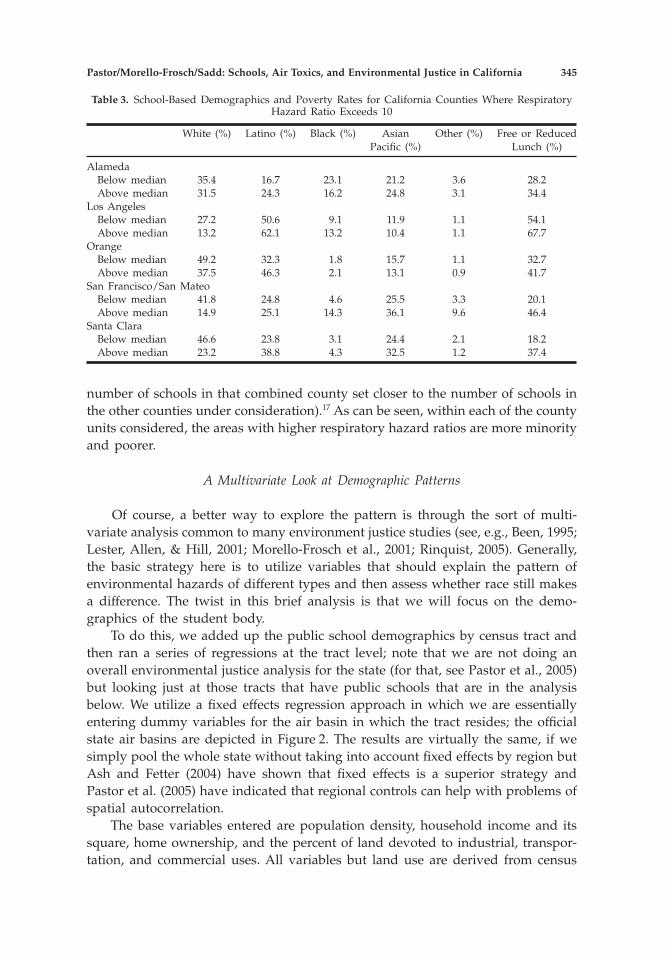
number of schools in that combined county set closer to the number of schools inthe other counties under consideration).17 As can be seen, within each of the countyunits considered, the areas with higher respiratory hazard ratios are more minorityand poorer.

A Multivariate Look at Demographic Patterns

Of course, a better way to explore the pattern is through the sort of multi-variate analysis common to many environment justice studies (see, e.g., Been, 1995;Lester, Allen, & Hill, 2001; Morello-Frosch et al., 2001; Rinquist, 2005). Generally,the basic strategy here is to utilize variables that should explain the pattern ofenvironmental hazards of different types and then assess whether race still makesa difference. The twist in this brief analysis is that we will focus on the demo-graphics of the student body.

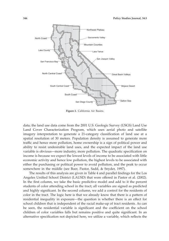
To do this, we added up the public school demographics by census tract andthen ran a series of regressions at the tract level; note that we are not doing anoverall environmental justice analysis for the state (for that, see Pastor et al., 2005)but looking just at those tracts that have public schools that are in the analysisbelow. We utilize a fixed effects regression approach in which we are essentiallyentering dummy variables for the air basin in which the tract resides; the officialstate air basins are depicted in Figure 2. The results are virtually the same, if wesimply pool the whole state without taking into account fixed effects by region butAsh and Fetter (2004) have shown that fixed effects is a superior strategy andPastor et al. (2005) have indicated that regional controls can help with problems ofspatial autocorrelation.

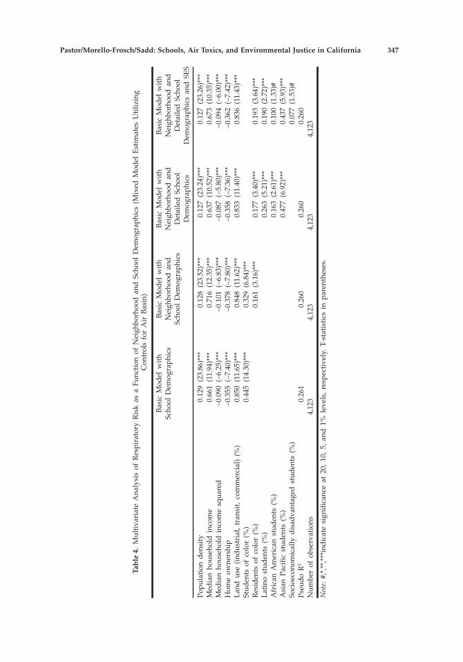
The base variables entered are population density, household income and itssquare, home ownership, and the percent of land devoted to industrial, transpor-tation, and commercial uses. All variables but land use are derived from census

Table 3. School-Based Demographics and Poverty Rates for California Counties Where RespiratoryHazard Ratio Exceeds 10

White (%) Latino (%) Black (%) AsianPacific (%)

Other (%) Free or ReducedLunch (%)

AlamedaBelow median 35.4 16.7 23.1 21.2 3.6 28.2Above median 31.5 24.3 16.2 24.8 3.1 34.4

Los AngelesBelow median 27.2 50.6 9.1 11.9 1.1 54.1Above median 13.2 62.1 13.2 10.4 1.1 67.7

OrangeBelow median 49.2 32.3 1.8 15.7 1.1 32.7Above median 37.5 46.3 2.1 13.1 0.9 41.7

San Francisco/San MateoBelow median 41.8 24.8 4.6 25.5 3.3 20.1Above median 14.9 25.1 14.3 36.1 9.6 46.4

Santa ClaraBelow median 46.6 23.8 3.1 24.4 2.1 18.2Above median 23.2 38.8 4.3 32.5 1.2 37.4


data; the land use data come from the 2001 U.S. Geologic Survey (USGS) Land UseLand Cover Characterization Program, which uses aerial photo and satelliteimagery interpretation to generate a 21-category classification of land use at aspatial resolution of 30 meters. Population density is assumed to generate moretraffic and hence more pollution, home ownership is a sign of political power andability to resist undesirable land uses, and the expected impact of the land usevariable is obvious—more industry, more pollution. The quadratic specification onincome is because we expect the lowest levels of income to be associated with littleeconomic activity and hence low pollution, the highest levels to be associated witheither the purchasing or political power to avoid pollution, and the peak to occursomewhere in the middle (see Boer, Pastor, Sadd, & Snyder, 1997).

The results of this analysis are given in Table 4 and parallel findings for the LosAngeles Unified School District (LAUSD) that were offered in Pastor et al. (2002).In the first column, we take the basic predictive model and add to it the percentstudents of color attending school in the tract; all variables are signed as predictedand highly significant. In the second column, we add a control for the residents ofcolor in the tract. The logic here is that we already know that there is a pattern ofresidential inequality in exposure—the question is whether there is an effect forschool children that is independent of the racial make-up of tract residents. As canbe seen, the residential variable is significant and the coefficient on the schoolchildren of color variables falls but remains positive and quite significant. In analternative specification not depicted here, we utilize a variable, which reflects the

Figure 2. California Air Basins.


Tab

le4.

Mul

tiva

riat

eA

naly

sis

ofR

espi

rato

ryR

isk

asa

Func

tion

ofN

eigh

borh

ood

and

Scho

olD

emog

raph

ics

(Mix

edM

odel

Est

imat

esU

tiliz

ing

Con

trol

sfo

rA

irB

asin

)

Bas

icM

odel

wit

hSc

hool

Dem

ogra

phic

sB

asic

Mod

elw

ith

Nei

ghbo

rhoo

dan

dSc

hool

Dem

ogra

phic

s

Bas

icM

odel

wit

hN

eigh

borh

ood

and

Det

aile

dSc

hool

Dem

ogra

phic

s

Bas

icM

odel

wit

hN

eigh

borh

ood

and

Det

aile

dSc

hool

Dem

ogra

phic

san

dSE

S

Popu

lati

ond

ensi

ty0.

129

(23.

86)*

**0.

128

(23.

52)*

**0.

127

(23.

24)*

**0.

127

(23.

26)*

**M

edia

nho

useh

old

inco

me

0.66

1(1

1.94

)***

0.71

6(1

2.35

)***

0.63

7(1

0.52

)***

0.67

3(1

0.35

)***

Med

ian

hous

ehol

din

com

esq

uare

d-0

.090

(-6.

25)*

**-0

.101

(-6.

83)*

**-0

.087

(-5.

80)*

**-0

.094

(-6.

00)*

**H

ome

owne

rshi

p-0

.355

(-7.

40)*

**-0

.378

(-7.

80)*

**-0

.358

(-7.

36)*

**-0

.362

(-7.

42)*

**L

and

use

(ind

ustr

ial,

tran

sit,

com

mer

cial

)(%

)0.

850

(11.

65)*

**0.

848

(11.

62)*

**0.

833

(11.

40)*

**0.

836

(11.

43)*

**St

uden

tsof

colo

r(%

)0.

445

(14.

30)*

**0.

329

(6.8

4)**

*R

esid

ents

ofco

lor

(%)

0.16

1(3

.16)

***

0.17

7(3

.40)

***

0.19

3(3

.64)

***

Lat

ino

stud

ents

(%)

0.26

3(5

.21)

***

0.19

0(2

.72)

***

Afr

ican

Am

eric

anst

uden

ts(%

)0.

163

(2.6

1)**

*0.

100

(1.3

3)#

Asi

anPa

cific

stud

ents

(%)

0.47

7(6

.92)

***

0.43

7(5

.93)

***

Soci

oeco

nom

ical

lyd

isad

vant

aged

stud

ents

(%)

0.07

7(1

.53)

#Ps

eud

oR

20.

261

0.26

00.

260

0.26

0N

umbe

rof

obse

rvat

ions

4,12

34,

123

4,12

34,

123

Not

e:#,

*,**

,***

ind

icat

esi

gnifi

canc

eat

20,

10,

5,an

d1%

leve

ls,

resp

ecti

vely

.T-

stat

isti

csin

pare

nthe

ses.


difference between the student demographics and the residential demographics,with higher values signaling a more minority student body; it is also positive andhighly significant.18

The third column of Table 4 breaks up the different ethnic groups of stu-dents attending school in the tracts while the fourth column adds to that thepercent of students receiving free or reduced price lunches, a usual sign offamily poverty. All the variables in both columns are signed as expected andnearly all are highly significant. The exception is the percent African-Americanstudents and students on free and reduced lunch in column four, in which thetwo are collinear and so compete for significance This may suggest that theenvironmental disparities for African American students are related to familyincome while the disparities for Latinos and Asian Pacific Americans persistacross income bands. In any case, this sort of multivariate mapping suggeststhat there are disparities by ethnicity in the exposures facing schoolchildren inthe state of California.

Test Scores

Is there a relationship between pollution-related respiratory risk and aca-demic performance? To get at this, we needed, as with asthma hospitalizationsand the overall pattern of demographic disparity, to nest the correlation in abroader multivariate model of school outcomes. Fortunately, there is a thrivingliterature on education production functions (see, for example, Hanushek, 1992;Krueger, 1999); unfortunately, much of this is based on utilizing individualstudent performance as the unit of analysis. By contrast, our regressions below areecological in nature and focus on aggregate school performance. However, suchschool-level studies are increasingly common because of the way in which statesand districts evaluate schools as the unit of accountability, and regression modelsof this ecological sort are becoming more common (Fowler & Walberg, 1991;Bickel & Howley, 2000).

What are the other variables thought to impact school outcomes? The mostimportant of these is parental income which we proxy with the percent ofchildren receiving free and reduced price school lunches. While this is an imper-fect measure of family poverty, it is the best available in the data at hand andis quite standard in the literature (see Krueger, 1999).19 We also use the percentof teachers with emergency credentials as a proxy for teaching quality (seeDarling-Hammond, 2000). Furthermore, we introduce the percent of students justlearning English (because these students score less on an exam that is admin-istered in English),20 and likewise enter a measure of student mobility (thenumber of students new to the school that year) on the grounds that continualchanges in school registration could produce lower performance. We also intro-duce a measure of school size because previous research indicates that largerschool size can adversely affect academic performance (Fowler, 1995).21

The statistical literature on student performance also suggests that parents’educational background matters greatly for school performance (see Hanushek,


1992).22 We operationalize this measure as the percent of parents lacking a highschool degree, with the expectation that this will negatively affect school perfor-mance. We also introduce a dummy variable for whether the school has ayear-round or traditional academic calendar, because this factor may possiblyaffect overall school performance (Campbell, 1994; Naylor, 2001; Weaver, 1992). Wealso include variables indicating the percent Latino, African American, and AsianPacific in the school. We do this mostly because of the idea that such ethnicvariables can pick up unexplained differences in performance and have beenshown to be important, even in regressions with the sort of socioeconomicvariables that we have here (see Krueger, 1999). However, it has the added benefitof making it harder to find significance on our respiratory risk variable—becausethe latter is correlated with race—which is exactly the sort of challenge to place onour hypotheses. Therefore, these measures of race/ethnicity are modeled aspotential confounding variables in our analysis. Finally, we are also introducingour respiratory hazard measure; note that the dependent variable (the academicperformance index) and all nondummy variables, including the respiratorymeasure, are entered as natural logs, both to reflect diminishing returns and forreasons of standardization.23

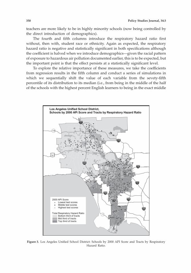
We first focus on a single district, LAUSD, which is both the largest in the state(with approximately 12 percent of all students) and is located in a part of the statewhere the county-level respiratory hazard ratio exceeds 10. Respiratory hazardratios and school scores for LAUSD are shown in Figure 3; the map shows a visualcorrelation between scores and the respiratory hazards but sorting out all the otherfactors driving those scores requires multivariate analysis.24

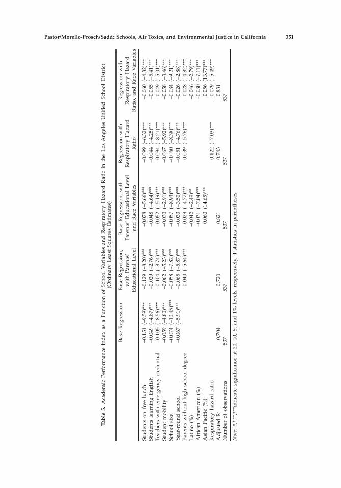
Regression results are shown in Table 5; all regressions are weighted by thenumber of students. The first specification includes the key variables usuallyassociated with school performance (percent of poorer students, percent of stu-dents learning English, percent of teachers with an emergency credential, thedegree of student mobility in the school, school size, and a dummy for having ayear-round calendar); we find a negative and significant coefficient for all thesevariables as well as a reasonable fit (as measured by the R2). Our second columnintroduces the measure for parents’ education level; this is done in a separate runbecause not all parents respond to questions about their education level and thusthe measure, while important, may be less reliable than other variables.25 Asexpected, the measure is statistically significant, the fit of the regression improves,and several other variables that may have been correlated with parental education(such as students receiving free or reduced price lunch) see their coefficientsdecline. The third specification introduces student race or ethnicity, with Latinosand African Americans associated with lower scores (even controlling for all theother schools measures) and the Asian Pacific presence contributing to higherscores. Note also the interactions: In particular, the coefficient and T-statistics forthe percent poorer students decline, suggesting that race was one of the factors“buried” in the poverty measure, and the coefficient and T-statistics for teacherswith an emergency credential also declines, again pointing to the fact that such


teachers are more likely to be in highly minority schools (now being controlled bythe direct introduction of demographics).

The fourth and fifth columns introduce the respiratory hazard ratio firstwithout, then with, student race or ethnicity. Again as expected, the respiratoryhazard ratio is negative and statistically significant in both specifications althoughthe coefficient is halved when we introduce demographics—given the racial patternof exposure to hazardous air pollution documented earlier, this is to be expected, butthe important point is that the effect persists at a statistically significant level.

To explore the relative importance of these measures, we take the coefficientsfrom regression results in the fifth column and conduct a series of simulations inwhich we sequentially shift the value of each variable from the sevety-fifthpercentile of its distribution to its median (i.e., from being in the middle of the halfof the schools with the highest percent English learners to being in the exact middle

Figure 3. Los Angeles Unified School District: Schools by 2000 API Score and Tracts by RespiratoryHazard Ratio.


Tab

le5.

Aca

dem

icPe

rfor

man

ceIn

dex

asa

Func

tion

ofSc

hool

Var

iabl

esan

dR

espi

rato

ryH

azar

dR

atio

inth

eL

osA

ngel

esU

nifie

dSc

hool

Dis

tric

t(O

rdin

ary

Lea

stSq

uare

sE

stim

ates

)

Bas

eR

egre

ssio

nB

ase

Reg

ress

ion,

wit

hPa

rent

s’E

duc

atio

nal

Lev

el

Bas

eR

egre

ssio

n,w

ith

Pare

nts’

Ed

ucat

iona

lL

evel

and

Rac

eV

aria

bles

Reg

ress

ion

wit

hR

espi

rato

ryH

azar

dR

atio

Reg

ress

ion

wit

hR

espi

rato

ryH

azar

dR

atio

,an

dR

ace

Var

iabl

es

Stud

ents

onfr

eelu

nch

-0.1

51(-

9.59

)***

-0.1

29(-

8.20

)***

-0.0

78(-

5.66

)***

-0.0

99(-

6.32

)***

-0.0

60(-

4.32

)***

Stud

ents

lear

ning

Eng

lish

-0.0

49(-

4.87

)***

-0.0

29(-

2.76

)***

-0.0

48(-

4.64

)***

-0.0

44(-

4.25

)***

-0.0

55(-

5.41

)***

Teac

hers

wit

hem

erge

ncy

cred

enti

al-0

.105

(-8.

56)*

**-0

.104

(-8.

74)*

**-0

.052

(-5.

19)*

**-0

.094

(-8.

21)*

**-0

.049

(-5.

01)*

**St

uden

tm

obili

ty-0

.059

(-4.

80)*

**-0

.062

(-5.

23)*

**-0

.030

(-2.

91)*

**-0

.067

(-5.

92)*

**-0

.058

(-3.

46)*

**Sc

hool

size

-0.0

74(-

10.4

5)**

*-0

.058

(-7.

82)*

**-0

.057

(-8.

93)*

**-0

.060

(-8.

38)*

**-0

.034

(-9.

21)*

**Ye

ar-r

ound

scho

ol-0

.067

(-5.

91)*

**-0

.065

(-5.

87)*

**-0

.033

(-3.

50)*

**-0

.051

(-4.

76)*

**-0

.026

(-2.

88)*

**Pa

rent

sw

itho

uthi

ghsc

hool

deg

ree

-0.0

40(-

5.64

)***

-0.0

29(-

4.77

)***

-0.0

39(-

5.76

)***

-0.0

28(-

4.82

)***

Lat

ino

(%)

-0.0

42(-

2.49

)**

-0.0

46(-

2.79

)***

Afr

ican

Am

eric

an(%

)-0

.031

(-7.

04)*

**-0

.030

(-7.

11)*

**A

sian

Paci

fic(%

)0.

060

(14.

65)*

**0.

056

(13.

77)*

**R

espi

rato

ryha

zard

rati

o-0

.122

(-7.

03)*

**-0

.079

(-5.

49)*

**A

dju

sted

R2

0.70

40.

720

0.82

10.

743

0.83

1N

umbe

rof

obse

rvat

ions

537

537

537

537

537

Not

e:#,

*,**

,***

ind

icat

esi

gnifi

canc

eat

20,

10,

5,an

d1%

leve

ls,

resp

ecti

vely

.T-

stat

isti

csin

pare

nthe

ses.


of the whole distribution).26 Although we experiment with all the variables, severalare generally beyond the influence of district-level policy: reducing students on freelunch has more to do with broad sociodemographics as does the extent of studentmobility, and increasing parent education levels may help student scores but thistype of change is well beyond the control of school administrators.27

On the other hand, the model suggests that moving from the sevety-fifthpercentile to the median in terms of school size could lead to a 3.4 percentimprovement in scores. This helps explain the significant interest in more schoolconstruction but it is also important to note the scale of what is required: If onewanted to ensure that the most populated schools in LAUSD had a studentattendance average of the current district median (without affecting the size of thesmaller schools below the median), the number of schools would need to grow bynearly 70 percent. If one was willing to backfill the schools below the median size,a new level of crowding that is likely impossible because of both facility size andparent resistance, one would need 50 percent more schools. Of course, some of thisschool size adjustment can be accomplished by having multiple small schools ona single site, a goal of the so-called “Small Schools Movement,” but even this raisesimportant costs of reconfiguration.

As for other changes, moving from the seventy-fifth percentile to the medianfor percent English learners (which might be accomplished by more effectivelanguage transition programs) would yield about a modest 2.4 percent increase intest scores; this is slightly less than twice what we would expect to see from thesame change (from the seventy-fifth percentile to the median) in either the shareof teachers with emergency credentials (which might be achieved through incen-tives for more qualified teachers and improved teacher training) or from a similarimprovement in the respiratory hazard ratio (perhaps through emissions sourcereduction, careful consideration of air quality when siting new schools, and otherstrategies that will be discussed subsequently).

While the test scores gains might seem modest, the reader should recall thatgiven the nature of the regression technique, the estimates offered here essentiallydescribe how to shift ranks within the cross-section of schools in any particularyear. As it turns out, changes in academic performance year-to-year are usuallydriven not so much by changes in the underlying variables as by gains inefficiency—schools figure out how to achieve better results with the same re-sources. Still, the cross-sectional estimates do provide some direction as to whereto focus resources and environmental improvement might be one part of a muchlarger package for school reform.

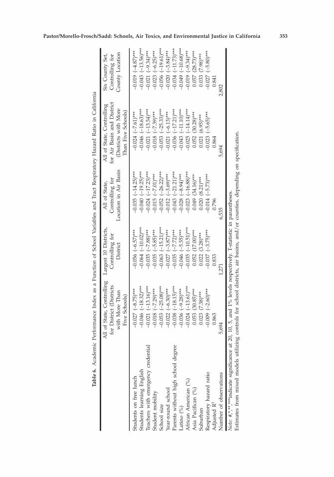
Table 6 shows the results when the analysis is scaled up statewide. To do this,we implement a series of fixed effects regression procedures that alternativelycontrol for school district, air basin, county, or some combination. In the simplestof the cases, that of district fixed effects, we are assuming that the impacts onacademic performance of variables of interest (such as the respiratory hazard ratio,teacher quality, or percent students on free lunch) are the same across all districtsbut that districts may have some systematic differences in their baseline levels ofperformance; the actual regression thus allows the intercept to vary for each


Tab

le6.

Aca

dem

icPe

rfor

man

ceIn

dex

asa

Func

tion

ofSc

hool

Var

iabl

esan

dTr

act

Res

pira

tory

Haz

ard

Rat

ioin

Cal

ifor

nia

All

ofSt

ate,

Con

trol

ling

for

Dis

tric

t(D

istr

icts

wit

hM

ore

Tha

nFi

veSc

hool

s)

Lar

gest

10D

istr

icts

,C

ontr

ollin

gfo

rD

istr

ict

All

ofSt

ate,

Con

trol

ling

for

Loc

atio

nin

Air

Bas

in

All

ofSt

ate,

Con

trol

ling

for

Air

Bas

inan

dD

istr

ict

(Dis

tric

tsw

ith

Mor

eT

han

Five

Scho

ols)

Six

Cou

nty

Set,

Con

trol

ling

for

Cou

nty

Loc

atio

n

Stud

ents

onfr

eelu

nch

-0.0

27(-

8.75

)***

-0.0

56(-

6.57

)***

-0.0

35(-

14.2

5)**

*-0

.024

(-7.

61)*

**-0

.019

(-4.

87)*

**St

uden

tsle

arni

ngE

nglis

h-0

.046

(-18

.32)

***

-0.0

64(-

10.0

2)**

*-0

.040

(-19

.25)

***

-0.0

46(-

18.6

3)**

*-0

.043

(-13

.56)

***

Teac

hers

wit

hem

erge

ncy

cred

enti

al-0

.021

(-13

.16)

***

-0.0

35(-

7.88

)***

-0.0

24(-

17.2

3)**

*-0

.021

(-13

.54)

***

-0.0

21(-

9.34

)***

Stud

ent

mob

ility

-0.0

18(-

7.29

)***

-0.0

35(-

5.85

)***

-0.0

15(-

7.01

)***

-0.0

18(-

7.39

)***

-0.0

23(-

6.25

)***

Scho

olsi

ze-0

.053

(-25

.08)

***

-0.0

63(-

15.2

1)**

*-0

.052

(-26

.22)

***

-0.0

53(-

25.3

3)**

*-0

.056

(-19

.61)

***

Year

-rou

ndsc

hool

-0.0

22(-

6.30

)***

-0.0

27(-

3.87

)***

-0.0

12(-

3.69

)***

-0.0

21(-

6.13

)***

-0.0

20(-

3.84

)***

Pare

nts

wit

hout

high

scho

old

egre

e-0

.038

(-18

.15)

***

-0.0

35(-

7.72

)***

-0.0

43(-

21.2

1)**

*-0

.036

(-17

.21)

***

-0.0

34(-

11.7

3)**

*L

atin

o(%

)-0

.036

(-9.

28)*

**-0

.046

(-5.

55)*

**-0

.028

(-8.

94)*

**-0

.043

(-11

.10)

***

-0.0

49(-

10.6

8)**

*A

fric

anA

mer

ican

(%)

-0.0

24(-

13.6

1)**

*-0

.035

(-10

.51)

***

-0.0

23(-

16.8

8)**

*-0

.025

(-14

.14)

***

-0.0

19(-

9.34

)***

Asi

aPa

cific

an(%

)0.

053

(30.

85)*

**0.

052

(17.

00)*

**0.

049

(34.

16)*

**0.

052

(30.

28)*

**0.

057

(28.

73)*

**Su

burb

an0.

023

(7.3

8)**

*0.

022

(3.2

8)**

*0.

020

(8.2

1)**

*0.

021

(6.9

5)**

*0.

033

(7.9

8)**

*R

espi

rato

ryha

zard

rati

o-0

.009

(-2.

60)*

**-0

.037

(-3.

75)*

**-0

.014

(-5.

73)*

**-0

.023

(-5.

65)*

**-0

.027

(-5.

80)*

**A

dju

sted

R2

0.86

30.

833

0.79

60.

864

0.84

1N

umbe

rof

obse

rvat

ions

5,69

41,

271

6,53

55,

694

2,80

2

Not

e:#,

*,**

,***

ind

icat

esi

gnifi

canc

eat

20,

10,

5,an

d1%

leve

lsre

spec

tive

ly.

T-st

atis

tic

inpa

rant

hese

s.E

stim

ates

from

mix

edm

odel

sut

ilizi

ngco

ntro

lsfo

rsc

hool

dis

tric

ts,

air

basi

ns,

and

/or

coun

ties

,d

epen

din

gon

spec

ifica

tion

.


district. This approach is similar to the fixed effects for schools introduced in theliterature on individual student performance (see Krueger, 1999).

Given our focus on air quality, it is also useful to assume fixed effects by airbasin—that is, to assume that the impact of air quality on academic outcomes isthe same across air basins regardless of which district a school is in but that theremight be a difference in the baseline respiratory measure. The most completespecification, however, is a mixed approach in which the intercept varies depen-dent on both the air basin and the district, and this is a specification we highlight.Finally, we also fix the effects by county when we focus on the six most affectedcounties profiled in the tables above. We should stress that when the fixed effectprocedure uses district controls, we set a minimum number of schools per districtfor inclusion in the sample to five because we need enough observations to havevariance within district; this lets us include slightly over 90 percent of the studentsin the state. When we introduce controls just for air basins or counties, we areunder no such constraint in terms of number of schools per district; hence, thenumber of observations is higher in, say, the third column of Table 6.

The first column in Table 6 offers a broad overview of the state, with controlsentered for each school district. Note that we enter a new variable in this regressionand the others in this table: an identifier for whether a school is suburban (as suchschools appear to exhibit higher performance than schools in either central cities orrural areas).28 As can be seen, all variables are signed as expected and significant atthe 0.01 level; the explanatory power, as given by a pseudo R2 calculated directlyfrom the regression residuals, is nearly 90 percent. Our second column focuses in onthe most populous 10 districts in the state, all of which are in major urban areas andtogether account for about 19 percent of the schools and almost 23 percent of thestudents in the state. Our idea was that this was a representative sample thatinvolved fewer district controls. As can be seen, all variables are signed as expectedand significant at the 0.01 level, although the respiratory hazard ratio, as in thestatewide sample, has one of the lower T-scores. The third column considers thewhole state again but this time introduces controls for the air basin location. As inthe other specification, all variables are signed as expected and significant.

Column 4 reflects what is likely to be the most sensible specification: controlsare introduced for both districts and air basins simultaneously. Note that thepseudo R2 is quite high and, while nearly all coefficients are lower than in our fullspecification for LAUSD, the pattern is quite similar and the significance levels aremuch higher, likely because of the larger sample size. We also run the regressionsfor the six counties where the respiratory hazard ratio exceeds 10. One of thoseruns is shown in the last column of Table 6; utilizing controls for the counties, allvariables are signed appropriately and significant. When we utilize controls forboth county and district, the respiratory hazard ratio is significant and all othervariables remain appropriately signed and significant (although the percent ofpoor students declines in significance to 0.05 level).

We also ran a regression not shown in the table for the counties with at least50 schools where the respiratory hazard ratio is less than 10. Utilizing controls forboth counties and districts, we find that the respiratory hazard measure is


negatively signed, but the results are only marginally significant. As the countiesare rather small, we tried instead to utilize air basins as the control in addition todistricts; in that run, the respiratory hazard measure was negative with a T-scoreof 1.966, which is significant at the 0.05 level. It seems that the effects of therespiratory hazard ratio might be more pronounced in the areas with a higher baselevel of respiratory hazards.

Finally, we explored possible interaction effects between race and our respi-ratory hazard variable. Such interactions are more appropriate with tests onindividual test scores in which the ethnicity of a student can be tagged and theninteracted with other variables to see the impact on academic performance; this isnot possible with the ecological approach we are taking here. Instead, we createda variable that was set to one if the school population made up of over 50 percentstudents of color; this variable was then interacted with the respiratory hazardmeasure to see if the slope of the effect increased or decreased for predominantlyminority schools. We implemented this across the specifications but the mostrelevant is the preferred regression in the fourth column of Table 6 in which wecontrol for both district and air basin. In that run, which we do not report in thetable itself, both the respiratory risk variable and the interaction variable werenegative and significant, with the coefficients suggesting that the effects of respi-ratory hazards on academic performance were slightly more pronounced inschools with a larger proportion of minority students. This raises environmentaljustice concerns about the potentially disparate impact of respiratory hazards onthe school performance of predominantly minority schools.

Conclusions and Policy Implications

This cross-sectional study indicates that schools located in areas with higherrespiratory hazards associated with air toxics also tend to have higher proportionsof both poor students and students of color. Multivariate analysis suggests acorrelation of such respiratory risk with lower academic performance, even aftercontrolling for student socio-economic status, teacher quality, parent education,and other measures, as well as district, air basin, and county characteristics. Takentogether, these results suggest that attention to environmental quality at andaround schools may be important issues for regulators and policymakers who areconcerned about educational achievement in public schools, environmental justice,and children’s environmental health.

The challenge for public policymakers is that it is exactly those highly pollutedurban school districts where the need for new school construction is greatest.29

Seventeen percent of public school students in California are in what the stateterms “critically overcrowded” schools, but the problem is severely racialized—1in 20 White students attend critically overcrowded schools versus 1 in 4 African-American and Latino students. In LAUSD, almost 80 percent of students are incritically overcrowded schools (see Pastor & Reed, 2004), and some students maybe bearing additional pollution burdens because of long bus rides to distantschools, (Solomon et al., 2001; see also Fitz, Winer, & Colome, 2003; Wargo &


Brown, 2002). Crowding has also led to an excessive use of portable classrooms,with indoor air quality of particular concern because noisy ventilation systems inportable classrooms are sometimes turned off by teachers seeking a quieterclassroom (see CARB/CDHS, 2003).

There is, in short, no escaping the need to build new schools in older, relativelypolluted urban areas. Fortunately, the state’s Department of Toxic SubstancesControl (DTSC) has been actively reviewing proposals for new school constructionwith an eye toward appropriate remediation or removal of tainted soil as neces-sary. However, the DTSC acknowledges that there are also issues for existingschools that may unknowingly be near hazardous locations (Oudiz, Booze, &Pollock, 2003). Moreover, the research here goes beyond toxic soil straight to toxicair. California has responded to the situation with a law that prevents new schoolsfrom being built within 500 feet of busy roads to address air quality problems—butit has not established a program to go back and assess and remediate those schoolsthat are currently located within these no-build zones.

To move policy forward for both new sites and remediation of current schoollocations, we need to improve the data for assessing air quality in Californiaschools. Better-localized measures of criteria pollutants, many of which havebeen linked to adverse health effects, would improve both the assessment of bothenvironmental equity and the impact of pollution exposures on academic per-formance. This would involve more extensive and reliable air monitoring, bettermodeling of air dispersion, and spatial data with higher resolution to takeadvantage of local topography and meteorological information in interpolation.

Policy should also recognize the connection between outdoor and indoor air(Sexton et al., 2004) and establish better ventilation and filtration strategies(Shendell, Barnett, & Boese, 2004). The U.S. EPA has offered a new set of “Tools forSchools” to assess indoor air quality, which includes significant details aboutventilation and other strategies (see http://www.epa.gov/iaq/schools/). In addi-tion, clean-up may not be just about stationary sources: Recognizing the harmfuleffects of diesel emissions, California has recently passed regulations to limit busidling near schools and some districts are retrofitting or replacing bus fleets withcleaner burning vehicles.

Although promoting site remediation, better ventilation, bus retrofitting, andother measures are useful stopgap measures for schools, emission source reductionremains the only permanent strategy for protecting children’s environmentalhealth. Mounting evidence points to the potentially positive effects of mobile andpoint source reduction, combining both the positive impact of air pollutionreduction on children’s health with potentially significant savings in health andother costs (Wong et al., 2004; see also AAP, 2004). In some sense, schools are abarometer for society as a whole: Improving air quality with kids in mind canimprove air quality for everyone.


http://www.epa.gov/iaq/schools

Manuel Pastor, Jr. is a professor of Latin American and Latino Studies andco-director of the Center for Justice, Tolerance and Community at the Universityof California, Santa Cruz.Rachel Morello-Frosch is Carney assistant professor at the Center for Environ-mental Studies and the Department of Community Health, School of Medicine,Brown University, Providence, Rhode Island.James L. Sadd is a professor of geology and environmental science at OccidentalCollege in Los Angeles.

Notes

We thank the California Wellness Foundation for providing the main funding and support for thisresearch. We also thank Justin Scoggins as well as Marium Lange, Breana George, and Julie Jacobs forable research assistance, Martha Matsuoka for coordinating community sessions on this work, andmembers of the environmental health and justice communities in Los Angeles and the Bay Area fortheir comments on earlier expositions of this research. We also thank two anonymous reviewers fortheir very useful comments. All views in this work are those of the authors and do not necessarilyreflect the perspectives of the California Wellness Foundation or our respective organizations.

1. Clean Air Act Amendments of 1990. §112 Hazardous Air Pollutants.

2. For information on the modeling algorithm, see Rosenbaum et al. (1999).

3. The methods for deriving a respiratory hazard index comply with recommendations for conductingscreening-level noncancer risk assessments for multiple pollutants under the Superfund Guidance,California’s AB2588 “Hot Spots” Guidelines, and the U.S. EPA’s Chemical Mixtures Guidelines.

4. For more details on the geoprocessing and conflation, see Pastor et al. (2005). We employ areaweighting of intersected polygons; Pastor and Scoggins (2004) provide a discussion of alternativemethods, and area weighting is most appropriate for reworking this risk surface.

5. There are 25 California schools which we could not successfully geocode. In aggregate, theseschools report 7,534 students, and have a median student population of 301.

6. Scores for magnet programs are not reported separately when these programs are physically partof a larger campus; in these cases, the magnet scores are averaged in with the rest of the schoolpopulation.

7. Another source for school-level demographics is California Basic Educational Data System(CBEDS) database, an annual data collection program administered by the California Departmentof Education Demographic Research Unit. The demographics from this database do not alwayssquare perfectly with the API demographics, partly because the latter records only those whotook the tests. We use the CBEDS numbers when simply comparing school demographics in thetables below as they best reflect the school population; however, when we enter demographicvariables in a regression on the determinants of the API we utilize the figures for those whoactually took the test.

8. http://www.csusm.edu/nlrc/projects/CAFA/CAFA.html

9. ZIP Code Tabulation Areas are very similar and sometimes identical to the more commonly knownU.S. Postal Service ZIP Codes, but were created in the year 2000 by the U.S. Census Bureau as aseparate geography for tabulating block-level data. For a more detailed explanation of thedifference between ZIP codes and ZCTAs, see http://www.census.gov/geo/ZCTA/zcta.html.

10. We draw the county level measure for person-days exceeding National Ambient Air QualityStandards from http://www.scorecard.org for the year 2002, then divide by the 2000 population asrecorded in the census. While the numbers are slightly inflated given the lower population in 2000,the ranks are similar, and removing the population weighting from the person-days measure movesone area (Sacramento) out of the top six and surfaces Tulare, a switch still in keeping with ournotion that our own measure is biased toward urban areas. Ranking by the hazard ratio is donewith the data base used in this article; these six counties surface as the top regardless of whetherwe use simple averages or averages weighted by land area or population.


http://www.csusm.edu/nlrc/projects/CAFA/CAFA.html

http://www.census.gov/geo/ZCTA/zcta.html

http://www.scorecard.org

11. This is the unweighted correlation coefficient; a correlation coefficient in which we weight eachobservation by the population in the ZIP code (similar to the procedure we use for the regressionsbelow) is 0.25161; again, this is statistically significant at the 0.001 level.

12. We specifically set the rate to 1.92 hospitalizations per 10,000 people, the minimum rate amongZCTAs for which there were five or more hospitalizations. Note that the rate of 1.92 probablyunderstates, on average, the true rates for ZCTAs with less than five asthma hospitalizations overallbecause many of these areas have such small populations that even one hospitalization couldtranslate into a very high rate per 10,000. When we ran the regression with the dependent variablefigured as a number instead of a rate and implemented appropriate left-censoring, setting all of theunknown (less than five) values to five, we obtained essentially the same results shown in Table 1with a slightly lower level of significance attached to our respiratory risk variable, and a much lesssignificant result (0.107) for population density (not surprising because we had to include also thenumber of people in the ZIP code as a control). We think the rate approach is more appropriate andwhen we tried filling in unknown asthma hospitalization rates with values higher than 1.92 and ranthe Tobit model, we obtained higher levels of significance for our respiratory risk variable as wedid for most other variables on the right side of the regression. Given the data, the approach wetake to left-censoring, including the selection of a low base rate as the truncated value, is designedto work least favorably in our direction, an appropriate bias compared to the alternative.

13. We first multiplied the respiratory hazard ratio by 10 to ensure that every observation would beabove one so that we could avoid creating negative values. A linear specification of the hazard ratioperformed quite similarly, with significance falling slightly: For our full model in column two ofTable 4, in the log specification, the significance level is 0.009, and in the linear specification, it is0.0132.

14. Weights were normalized so that the total equaled the number of observations. The population ofthe tracts for which we had hospitalization data was 22,164,915 out of a total California populationof 33,871,648. For five of the ZIP codes for which we had hospitalization data, we lacked povertydata (because the population was either too small or, in two cases, consisted entirely of groupquarters populations (entirely institutionalized in one zip code and mostly in another). For nine ZIPcodes, we lacked data on housing values. Dropping all 14 of these observations caused us to lose10,674 people, less than one-tenth of one percent of the total.

15. The rural specification is not available at the whole tract level for which this and most environ-mental justice analyses are done but it is available at a block group level where the chain ofgeographic levels is such that groups may be split by jurisdiction. We calculated the “urban” areafor each of the state’s block groups, summed that up to the tract level, and then called a tract ruralor nonrural depending on whether more than 50 percent of the calculated area was not designatedas “urban.” As we make clear in the text, urban in this case can also refer to suburban areas; hence,we are essentially just distinguishing between rural and nonrural areas.

16. The measures in the tables are not simply averages but rather averages weighted by the relevantschool population; hence, we are essentially comparing one sort of population to another.

17. San Francisco is a single city, county, and school district. The latter is another reason why we coupleSan Francisco and San Mateo, so that we can be more comparable to the other counties, which havemultiple districts as well as a central city and a suburb.

18. This is consistent with our notion that the school bodies may be somewhat different than the tractpopulations—and with a pattern in which white parents in minority tracts may be more likely tobe sending their children away from home school boundaries.

19. One reason that the measure is flawed is that a child is eligible for a lunch subsidy as long as familyincome is below 185 percent of the poverty level—and this is thought to be hardly indicative ofpoverty. However, California is such a high-price state that the national poverty level is consideredinadequate and many analysts are increasingly using 150 percent of the poverty level as a basicbenchmark; this is right between the 130 percent poverty rate needed for a free lunch and the 185percent mark for a reduced-price lunch. More important, recall that this is an ecological and not anindividual study: The percent of students meeting the 185 percent mark is likely correlated withthose meeting the 100 percent or 150 percent mark, and so the measure is likely adequate forschool-level comparison no matter what objection might be raised to utilizing the measure inregression on individual student performance.


20. The underlying exams used to calculate the API are administered in English because of the passagein California of a 1998 statewide initiative that limits bilingual instruction and testing.

21. Interestingly, class size, the subject of recent heated debate between a series of researchers andpolicymakers (see Hanushek, 2000; Krueger, 2000), does not have a significant impact on theschoolscore in our regressions; while we tested to find this out, we drop it from the regressionspresented here because of the insignificance.

22. In California, the data quality on this variable is somewhat poor—in 2000, about 15 percent ofschools receive replies from less than a 50 percent of parents—but the variable is so important thatwe construct a reasonable measure and utilize it in the regressions.

23. In addition, log values were more normally distributed. To prevent missing values, we added toall percent values the sum of 1.01 (so that we never log anything below one or equal to zero). Wealso multiplied the hazard ratio by 10 to avoid the same problem. We take a similar approach tospecification in Pastor et al. (2005).

24. We carried out a similar analysis of LAUSD using an older version of the air toxics and API datain Pastor et al. (2005); the innovation here is the extension to the whole state of California but weundertook this exercise focused on Los Angeles partly to ensure that we were able to square thepattern with the earlier results before extending to the state.

25. Indeed, some schools do not have recorded levels of parent education. To maintain comparabilityacross results, even regressions that do not include the parent education variable include onlyschools for which the data are available; if we were to expand the sample in those regressions toinclude those schools lacking the variable, the pattern would be the same but we impose theconstraint so that we can more clearly see the effect of the variable and not the effect of changingsample size when we introduce the parent education measure.

26. The logic for this approach rather than utilizing percentage increases in each variable is that thiswould allow us to better take account of the underlying distribution of the independent variables.

27. Schools could also alter school demographics through redrawing boundaries and bussing arrange-ments but this does not alter the demographics of the district—the other changes we stress suchas school size reduction, improving teaching, and cleaning the air can affect overall districtperformance.

28. A school is tagged as suburban if it is in an area of the state designated as urban but not in oneof the following central cities: Bakersfield, Fresno, Long Beach, Los Angeles, Oakland, Riverside,Sacramento, San Bernardino, San Diego, San Francisco, San Jose, and Santa Ana.

29. Moreover, building outside these areas simply encourages further sprawl, which has its own costsin terms of environmental and economic sustainability. See Wolch et al. (2004).

References

American Academy of Pediatrics (AAP). 2004. “Ambient Air Pollution: Health Hazards for Children.”Pediatrics 114 (December): 1699–707.

Ash, Michael, and T. Robert Fetter. 2004. “Who Lives on the Wrong Side of the Environmental Tracks?Evidence from the EPA’s Risk-Screening Environmental Indicators Model.” Social Science Quarterly85 (2): 441–62.

Barnes, Donald G., and Michael L. Dourson. 1988. “Reference Dose (RfD): Description and Use inHealth Risk Assessments.” Regulatory Toxicology and Pharmacology 8 (4): 471–86.

Bearer, Cynthia. 1995. “Environmental Health Hazards: How Children are Different from Adults.”Critical Issues for Children and Youths 5 (Summer/Fall): 11–26.

Been, Vicki. 1995. “Analyzing Evidence of Environmental Justice.” Journal of Land Use and EnvironmentalLaw 11 (Fall): 1–37.

Bener, Abdulbari, Yousef Mohamed Abdulrazzaq, Peter Debuse, and A. H. Abdin. 1994. “Asthma andWheezing as the Cause of School Absence.” Journal of Asthma 31 (2): 93–98.


Bickel, Richard, and Craig Howley. 2000. “The Influence of Scale on School Performance: A Multi-LevelExtension of the Matthew Principle.” Education Policy Analysis Archives 8 (22) [Online]. http://epaa.asu.edu/epaa/v8n22/. Accessed March 3, 2006.

Bobak, Martin. 2000. “Outdoor Air Pollution, Low Birth Weight, and Prematurity.” Environmental HealthPerspectives 108: 173–76.

Boer, Joel T., Manuel Pastor, James L. Sadd, and Lori D. Snyder. 1997. “Is There Environmental Racism?The Demographics of Hazardous Waste in Los Angeles County.” Social Science Quarterly 78 (4):793–810.

California Air Resources Board and California Department of Health Services (CARB/CDHS). 2003.Environmental Health Conditions in California’s Portable Classrooms. November. Sacramento,CA: California Air Resources Board.

Campbell, Wallace. 1994. “Year-Round Schooling for Academically At-Risk Students: Outcomes andPerceptions of Participants in an Elementary Program” ERS-Spectrum 12: 20–24.

Castorina, Rosemary, and Tracey J. Woodruff. 2003. “Assessment of Potential Risk Levels Associatedwith U.S. Environmental Protection Agency Reference Values.” Environmental Health Perspectives111 (10): 1318–25.

Chay, Kenneth Y., and Michael Greenstone. 2003. “The Impact of Air Pollution on Infant Mortality:Evidence from Geographic Variation in Pollution Shocks Induced by a Recession.” The QuarterlyJournal of Economics 118 (3): (August): 1121–67.

Chen, Edith, Gordon R. Bloomberg, Edwin B. Fisher Jr., and Robert C. Strunk. 2003. “Predictors ofRepeat Hospitalizations in Children with Asthma: The Role of Psychosocial and Socio-environmental Factors.” Health Psychology 22: 12–18.

Crom, William R. 1994. “Pharmacokinetics in the Child.” Environmental Health Perspectives 102 (Suppl.):111–17.

Darling-Hammond, Linda. 2000. “Teacher Quality and Student Achievement: A Review of State PolicyEvidence.” Educational Policy Analysis Archives 8 (1) [Online]. http://epaa.asu.edu/epaa/v8n1.Accessed March 3, 2006.

Delfino, Ralph J., Henry Gong Jr., William S. Linn, Edo D. Pellizzari, and Ye Hu. 2003. “AsthmaSymptoms in Hispanic Children and Daily Ambient Exposures to Toxic and Criteria Air Pollut-ants.” Environmental Health Perspectives 111 (4): 647–56.

Diette, Gregory B., Leona Markson, Elizabeth A. Skinner, Theresa T. Nguyen, Pamela Algatt-Bergstrom,and Albert W. Wu. 2000. “Nocturnal Asthma in Children Affects School Attendance, SchoolPerformance, and Parents’ Work Attendance.” Archives of Pediatrics and Adolescent Medicine 154 (9):923–29.

Dourson, Michael L., and Jerry F. Stara. 1983. “Regulatory History and Experimental Support ofUncertainty (Safety) Factors.” Regulatory Toxicology and Pharmacology 3 (3): 224–38.

Dourson, Michael L., Susan P. Felter, and Denise Robinson. 1996. “Evolution of Science-basedUncertainty Factors in Noncancer Risk Assessment.” Regulatory Toxicology and Pharmacology 24 (2):108–20.

Fitz, Dennis R., Arthur M. Winer, and Steven Colome. 2003. “Characterizing the Range of Children’sPollutant Exposure during School Bus Commutes.” Final Report to the California Air ResourcesBoard, October [Online]. http://www.ftp.arb.ca.gov/research/schoolbus/schoolbus.htm. AccessedMarch 3, 2006.

Fowler, William J. Jr. 1995. “School Size and Student Outcomes.” Advances in Educational Productivity 5:3–26.

Fowler, William J. Jr., and Herbert J. Walberg. 1991. “School Size, Characteristics, and Outcomes.’Educational Evaluation and.” Policy Analysis 13 (2): 189–202.

Fowler, Mary Glenn, Marsha G. Davenport, and Rekha Garg. 1992. “School Functioning of US Childrenwith Asthma.” Pediatrics 90 (6): 939–44.

Gauderman, W. James, Edward Avol, Frank Gilliland, Hita Vora, Duncan Thomas, Kiros Berhane, RobMcConnell, Nino Kuenzli, Fred Lurmann, Edward Rappaport, Helene Margolis, David Bates, andJohn Peters. 2004. “The Effect of Air Pollution on Lung Development from 10 to 18 Years of Age.”New England Journal of Medicine 351 (September 9): 1057–67.


http://epaa.asu.edu/epaa/v8n22



http://www.ftp.arb.ca.gov/research/schoolbus/schoolbus.htm.Accessed

Green, Rochelle, Svetlana Smorodinsky, Janice Kim Jr., Robert McLaughlin, and Bart Ostro. 2004.“Proximity of California Public Schools to Busy Roads.” Environmental Health Perspectives 112 (1):61–66.

Guzelian, Philip, Carol Henry, and Stephen Olin. 1992. Similarities and Differences between Children andAdults: Implications for Risk Assessment. Washington, DC: ILSI Press.

Ha, Eun-Hee, Yun-Chul Hong, Boeun Lee, Bock-Hi Woo, Joel Schwartz, and David Christiani. 2001. “IsAir Pollution a Risk Factor for Low Birth Weight in Seoul?” Epidemiology 12: 643–48.

Hanushek, Eric A. 2000. Evidence, Politics, and the Class Size Debate. The Class Size Policy Debate.Working paper no. 121, The Economic Policy Institute, Washington, DC.

———. 1992. “The Trade-Off between Child Quantity and Quality.” Journal of Economic Literature 24 (3):1141–77.

Kaplan, Sheila, and Jim Morris 2000. “Kids at Risk: Chemicals in the Environment Come UnderScrutiny as the Number of Childhood Learning Problems Soars.” U.S. News and World Report, 128(4): 47–53.

Kim, Janice J., Svetlana Smorodinsky, Michael Lipsett, Brett C. Singer, Alfred T. Hodgson, and BartOstro. 2004. “Traffic-Related Air Pollution near Busy Roads: The East Bay Children’s RespiratoryHealth Study.” American Journal of Respiratory and Critical Care Medicine 170: 520–26.

Krueger, Alan B. 1999. “Experimental Estimates of Educational Production Functions.” Quarterly Journalof Economics 114 (2): 497–532.

———. 2000. “Understanding the Magnitude and Effect of Class Size on Student Achievement.” TheClass Size Policy Debate. Working paper no. 121, The Economic Policy Institute, Washington, DC.

Landrigan, Phillip, and Anjali Garg. 2002. “Chronic Effects of Toxic Environmental Exposure onChildren’s Health.” Clinical Toxicology 40 (4): 449–56.

Leikauf, George D., Sharon Line, Roy E. Albert, C. Stuart Baxter, David I. Bernstein, and C. RalphBuncher. 1995. “Evaluation of a Possible Association of Urban Air Toxics and Asthma.” Environ-mental Health Perspectives 103 (Suppl. 6): 253–71.

Lester, James P., David W. Allen, and Kelly M. Hill. 2001. Environmental Injustice In the United States:Myths and Realities. Boulder, CO: Westview Press.

Madrid, Eric, Greg W. Mennie, and Patricia L. Newton. 2006. “Asthma: Challenges in VulnerablePopulations.’ Journal of the American Academy of Physicians.” Assistants 19 (2): 41–46.

Mannino, David, David Homa, and Carol Pertowski. 1998. “Surveillance for Asthma—United States,1960–1995.” MMWR 47 (SS-1): 1–28.

Mathieu-Nolf, Monique. 2002. “Poisons in the Air: A Cause of Chronic Disease in Children.” ClinicalToxicology 40 (4): 483–91.

Morello-Frosch, Rachel, Manuel Pastor, and James Sadd. 2001. “Environmental Justice and SouthernCalifornia’s ‘Riskscape’: The Distribution of Air Toxics Exposures and Health Risks AmongDiverse Communities.” Urban Affairs Review 36 (4): 551–78.

———. 2002. “Integrating Environmental Justice and the Precautionary Principle in Research andPolicy-Making: The Case of Ambient Air Toxics Exposures and Health Risks among SchoolChildren in Los Angeles.” Annals of the American Academy of Political and Social Science 584: 47–68.

Naylor, Charlie. 2001. “Do Year-Round Schools Improve Student Learning? An Annotated Bibliographyand Synthesis of the Research.” British Columbia Teachers’ Federation. October 22 [Online].http://www.betf.ca/researchreports/g5ei03/ Accessed March 3, 2006.

Oudiz, Deborah, Thomas Booze, and Gerald Pollock 2003. Emerging Issues: Existing Schools. Humanand Ecological Risk Division, Department of Toxic Substances Control [Online]. http://dtsc.ca.gov/assessingrisk/upload/emergingissues-existingschools.pdf. Accessed March 3, 2006.

Pastor, Manuel, and Debbie Reed. 2004. Understanding Equitable Infrastructure Investment forCalifornia. Working paper, Public Policy Institute of California.

Pastor, Manuel, and Justin Scoggins. 2004. Income Forecasting at the Small Area Level for SouthernCalifornia: Issues, Methods, and Projections. Final report to the Southern California Association ofGovernments. Santa Cruz, CA: Center for Justice, Tolerance, and Community, March 29.


http://www.betf.ca/researchreports/g5ei03

http://dtsc.ca.gov/assessingrisk/upload/emergingissues-existingschools.pdf

http://dtsc.ca.gov/assessingrisk/upload/emergingissues-existingschools.pdf

Pastor, Manuel, James Sadd, and Rachel Morello-Frosh. 2002. “Who’s Minding the Kids? Pollution,Public Schools, and Environmental Justice in Los Angeles.” Social Science Quarterly Special Issue:Social Science and the Environment 83 (1): 263–80.

———. 2004. “Reading, Writing, and Toxics: Children’s Health, Academic Performance, and Environ-mental Justice in Los Angeles.” Environment and Planning C: Government and Policy 22: 271–90.

———. 2005. “The Air is Always Cleaner on the Other Side: Race, Space, and Air Toxics Exposures inCalifornia.” Journal of Urban Affairs 27 (2): 127–48.

Ray, Nancy, May Thamer, Bahar Fadilliogus, and Peter Gergen. 1998. “Race, Income, Urbanicity, andAsthma Hospitalization in California: A Small Area Analysis.” Chest 113 (5): 1277–84.

Rinquist, Evan J. 2005. “Assessing Evidence of Environmental Inequities: A Meta-Analysis.” Journal ofPolicy Analysis and Management 24 (2): 223–47.

Ritz, Beate, and Fei Yu. 1999. “The Effect of Ambient Carbon Monoxide on Low Birth Weight amongChildren Born in Southern California between 1989 and 1993.” Environmental Health Perspectives107 (1): 17–25.

Ritz, Beate, Fei Yu, Guadalupe Chapa, and Scott Fruin. 2000. “Effect of Air Pollution on Preterm Birthamong Children Born in Southern California between 1989 and 1993.” Epidemiology 11 (5): 502–11.

Ritz, Beate, Fei Yu, Scott Fruin, Guadalupe Chapa, Gary M. Shaw, and John A. Harris. 2002. “AmbientAir Pollution and Risk of Birth Defects in Southern California.” American Journal of Epidemiology155 (1): 17–25.

Rosenbaum, Arlene S., Daniel A. Axelrad, Tracey J. Woodruff, Yi-Hua Wei, Mary Ligocki, and JonathanP. Cohen. 1999. “National Estimates of Outdoor Air Toxics Concentrations.” Journal of the Air &Waste Management Association 49: 1138–52.

Sexton, Ken, John L. Adgate, Gurumurthy Ramachandran, Gregory C. Pratt, Steven J. Mongin, ThomasH. Stock, and Maria T. Morandi. 2004. “Comparison of Personal, Indoor, and Outdoor Exposuresto Hazardous Air Pollutants in Three Urban Communities.” Environmental Science Technology 38:423–30.

Shendell, Derek G., Arthur M. Winer, Thomas H. Stock, Lin Zhang, Junfeng (Jim) Zhang, Silvia Maberti,and Steven D. Colome. 2004. “Air Concentrations of VOCs in Portable and Traditional Classrooms:Results of a Pilot Study in Los Angeles County.” Journal of Exposure Analysis and EnvironmentalEpidemiology 14: 44–59.

Shendell, Derek G., Claire Barnett, and Stephen Boese. 2004. “Science-Based Recommendations toPrevent or Reduce Potential Exposure to Biological, Chemical, and Physical Agents in Schools.”Journal of School Health 74 (10): 390–96.

Solomon, Gina M., Todd R. Campbell, Gail Ruderman Feuer, Julie Masters, Artineh Samkian, andKavita Ann Paul. 2001. No Breathing in the Aisles: Diesel Exhaust Inside School Buses. New York:National Resource Defense Council and Coalition for Clean Air.

U.S. Environmental Protection Agency (U.S. EPA). 2004. National Air Toxics Assessment [Online].http://www.epa.gov/ttn/atw/nata/natsaov.html. Accessed March 3, 2006.

Wang, Xiaobin, Hui Ding, Ryan Louise, and Xiping Xu. 1997. “Association Between Air Pollution andLow Birth Weight: A Community-Based Study.” Environmental Health Perspectives 105: 514–20.

Wargo, John, and David Brown. 2002. Children’s Exposure to Diesel Exhaust on School Buses. NorthHaven, CT: Environment and Human Health Inc.

Weaver, Tyler. 1992. Year-Round Education. Washington, DC: Office of Educational Research andImprovement. ERIC document: ED 342107.

Wiley, James. 1991. Study of Children’s Activity Patterns. Final report to the California Air ResourcesBoard. Survey Research Center, University of California, Berkeley, CA.

Wolch, Jennifer, Manuel Pastor, Jr., and Peter Dreier. 2004. Up Against the Sprawl: Public Policy and TheMaking of Southern California. Minneapolis, MN: University of Minnesota Press.

Wong, Eva Y., Julia Gohlke, William C. Griffith, Scott Farrow, and Elaine M. Faustma. 2004. “Assessingthe Health Benefits of Air Pollution Reduction for Children.” Environmental Health Perspectives 112(2): 226–32.


http://www.epa.gov/ttn/atw/nata/natsaov.html

Documents

Breathless: Schools, Air Toxics, and Environmental Justice in California