Provided by the author(s) and University College Dublin Library in accordance with publisher policies. Please

cite the published version when available.

Downloaded 2012-04-25T06:40:20Z

Some rights reserved. For more information, please see the item record link above.

Title Bridge roughness index as an indicator of bridge dynamicamplification

Author(s) O'Brien, Eugene J.; Li, Yingyan; González, Arturo

PublicationDate 2006-05

Publicationinformation Computers and Structures, 84 (12): 759-769

Publisher Elsevier

Link topublisher's

versionhttp://dx.doi.org/10.1016/j.compstruc.2006.02.008

This item'srecord/moreinformation

http://hdl.handle.net/10197/2532

Rights All rights reserved.

1

Bridge Roughness Index as an Indicator of Bridge Dynamic

Amplification

Eugene OBrien, Yingyan Li and Arturo González

Department of Civil Engineering, University College Dublin, Earlsfort Terrace, Dublin

2, Ireland

ABSTRACT

The concept of a road roughness index for bridge dynamics is developed. The

International Roughness Index (IRI) is shown to be very poorly correlated with bridge

dynamic amplification as it takes no account of the location of individual road surface

irregularities. It is shown in this paper that a Bridge Roughness Index (BRI) is possible

for a given bridge span which is a function only of the road surface profile and truck

fleet statistical characteristics. The index is a simple linear combination of the changes

in road surface profile; the coefficients are specific to the load effect and span of

interest. The BRI is well correlated with bridge dynamic amplification for bending

moment due to 2-axle truck crossing events. A similar process can be used to develop a

BRI for trucks with other numbers of axles or combinations of trucks meeting on a

bridge.

Keywords: DAF, DAE, BRI, dynamic, roughness, bridge, vehicle.

Corresponding author: Li Yingyan

E-mail: yingyan.li@ucd.ie

Tel: +353-1-716-7281

Fax: +353-1-716-7399

2

1. Introduction

The Dynamic Amplification Factor (DAF) for a bridge is defined as the maximum total

(dynamic plus static) load effect divided by the maximum static load effect. DAF is

influenced by many factors. Speed is particularly important, as noted by many authors

[1-6] and in particular the ratio of speed to bridge 1st natural frequency [7]. Road

roughness is also a key factor [3-4, 8], particularly for short bridges.

In the highway industry, indices for the evaluation of pavement surface evenness have

been developed since the 1960s. The most popular parameters are the International

Roughness Index (IRI) [9-11] which was developed and recommended by the World

Bank to evaluate pavement roughness, and the Power Spectral Density (PSD) [12].

[Li – can you fix up the ref numbering please]

Olsson (1985), Lin (1997), Henchi et al. (1997), Liu et al. (2002) and Majumder and

Manohar (2003) are just some of the authors that use finite element analysis with six

degrees of freedom per node to model bridges dynamically. Olsson (1985) compared

the results of finite element analysis with an Euler-Bernoulli beam model [Li – did he

compare them?]. Green and Cebon (1994) modelled two bridges in the U.K. with finite

elements and compared the results to field measurements. [Li – I think this is true – is

it?] Chompooming and Yener (1995) present a finite element model of a beam and slab

bridge. This type of section is also modeled by Kou and Dewolf (1997) who use plate

elements for the deck and beam elements for the girders. González (2001) couples

displacements and velocities at the bridge/vehicle contact points at each time step in an

iterative formulation. Yau and Yang (2004) allow for instability and inertial effects in a

finite element model of a cable stayed bridge.

3

The effect of road surface irregularities on bridge vibration has been examined by

DIVINE [1], Green et al. [4], Lay and Zhu [13], Kou and Dewolf [14], Lei and Noda

[15] and Chatterjee et al. [16]. Vehicle and bridge models have been used to simulate

the vehicle-bridge interaction system and to determine the effect of profile unevenness.

However, these papers investigate the influence of different PSD levels. It has been

found by Li et al. [17] that there are substantial differences in dynamic amplification

between road profiles with the same PSD level and the same IRI value.

Michaltsos [18] and Pesterev et al. [19, 20] have shown that the position of an

irregularity is important for bridge dynamic amplification. In a previous paper [17], the

authors confirm this and show that if bridge deflections are negligible [20], the principle

of superposition applies for the dynamic response to individual road surface

irregularities. This makes possible the estimation of dynamic amplification by adding

together the DAFs due to each irregularity that makes up the road surface profile. Very

good agreement with critical DAF values is reported for a range of 'good' road surface

profiles. A significant problem is that the resulting dynamic amplification estimate is

specific to the properties (spring stiffness etc.) of that vehicle.

Yang et al. [12], Zhu & Law [21] and Brady & OBrien [22] examine cases of two

following loads and compare the effects to single load crossings. Axle spacing is

identified as being particularly important [22, 23] and it quickly becomes clear that an

amplification factor derived from a 1-axle vehicle model is of limited value as an

indicator of DAF for multiple-axle vehicles.

4

The goal of this paper is to develop the concept of a Bridge Roughness Index (BRI)

which can be used as an estimator of DAF for a given vehicle class, and in particular in

this paper, a BRI for 2-axle vehicles. The BRI will be a function of the road profile

only; it will not be dependent on the speeds or properties of particular vehicles. A BRI

potentially constitutes an extremely useful measure of road surface roughness that could

be used by bridge maintenance managers as an indicator of the level of dynamic

amplification that might be expected on a bridge.

2. BRIDGE VIBRATION

2.1. Vehicle-bridge interaction model

A half-car model crossing a simply supported Bernoulli-Euler beam at a constant speed

is used to simulate 2-axle vehicle events (Fig. 1). The motion controlling this system is

defined by the ordinary differential equations [24]:

2

2

( )( 1) ( ( ) ( )) 0i

i i bi

d tI D Z t Z t

dt

ϕ− + − + =

(1a)

2 23

3 21

( )[ ( ) ( )] 0

i bi

i

d y tm Z t Z t

dt =

− − + =∑ (1b)

2

3 2

( )( ) ( ) ( ) 0+ − + + − =i

i i i i bi i

d y tm g m g m Z t Z t R t

dt i=1,2

(1c)

4 2 2

4 21

( , ) ( , ) ( , )2 ( ) ( )

b i i i

i

v x t v x t v x tEJ x x R t

x t tµ µω ε δ

=

∂ ∂ ∂+ + = −

∂ ∂ ∂∑

(1d)

where I and φ(t) are the mass moment of inertia and rotational degree of freedom of the

body mass respectively; Di is the horizontal distance between the centroid of sprung

mass and unsprung mass i; m1, m2, m3 are masses of the front axle, rear axle and vehicle

5

body respectively and y1(t), y2(t) and y3(t) are the corresponding vertical displacement of

their centers of gravity; g is acceleration of gravity; v(x,t) is the displacement of the

bridge at location x and time t; E, J, µ and ωb are modulus of elasticity, inertia of the

cross-section, mass per unit length and circular frequency of damping of the bridge

respectively; εi.= 1 if axle i is present on the bridge and εi.= 0 if not; δ(x-xi) is the Dirac

function. Therefore,

[ ]3( ) ( ) ( )i s i i

Z t K y t y t= − (2a)

is the force in the spring between the ith axle and the vehicle body, where Ks is the

suspension spring stiffness.

3 ( ) ( )( ) i i

bi s

dy t dy tZ t C

dt dt

= −

(2b)

is the damping force between the ith axle and the vehicle body, where Cs is a suspension

linear damper.

3 3( ) ( ) ( 1) ( )i

i iy t y t D tϕ= − − (2c)

is the displacement of the contact point between the ith axle and the vehicle body.

231 3

1 2

132 3

1 2

=+

=+

Dm m

D D

Dm m

D D

(2d)

are the masses of the sprung part of the vehicle by axle.

[ ]( ) ( ) ( , ) ( ) 0i t i i i i

R t K y t v x t r xε= − − ≥ (2e)

is the tire force imparted to the bridge by the ith axle, where Kt is tire stiffness and r(xi)

is height of road profile at location of axle i. No allowance has been made for separation

6

of the tire from the road. Based on the work of Frýba [24], numerical results are found

in the time domain through the Runge-Kutta-Nyström method [25].

2.2. Dynamic Amplification due to 2-axle vehicle

In a previous study [17], the authors have proven that the effect of individual road

irregularities can be superposed for a quarter-car model traveling on a short-span bridge

with a good road profile. Bending moment is found by adding the moment due to the

vehicle traveling on a perfectly smooth surface and the moment due to each individual

irregularity that exists on the surface. The approach is accurate for negligible bridge

deflections and a good approximation when bridge deflections are small compared to

the road irregularities. Based on this assumption of superposition, the total normalized

midspan bending moment, M(c,t), for a vehicle speed, c, and position of 1st axle x1, can

be calculated as

1 0 1 1 0 11

( , ) ( , ) ( , , ) ( , ) ( )N

u

i

M c x M c x M c i x M c x s i=

= + − × ∑ (3)

where 0M is the normalized midspan bending moment caused by the vehicle on a

smooth profile and u

M is the normalized midspan moment due to a unit ramp at

location i. The profile is discretized into N ramps each 100 mm long and the measured

fall in the ith ramp in mm is s(i). All bending moments are normalized by dividing them

by the maximum static bending moment. The calculation procedure is illustrated in

Fig.2 for a road profile made of two ramps of heights H1 and -H2 located at -0.1 and 0 m

respectively. The total moment M due to a vehicle of given mechanical parameters and

speed (Fig.2(a)) is the result of adding three moments: (1) M0 corresponding to a

smooth profile (Fig.2(b)), (2) [s(1)×(Mu(x=-0.1)-M0)], or moment due to a unit ramp at x =

7

-0.1 (Fig.2(c)) scaled by the height of the first ramp (s(1) = H1/0.001), and (3)

[s(2)×(Mu(x=0)-M0)], or moment due to a unit ramp at x = 0 (Fig.2(d)) scaled by its height

(s(2) = -H2/0.001). This approach involves the addition of bending moment values

corresponding to different critical points near the centre of the bridge. Then, the

dynamic amplification factor due to a vehicle traveling at speed c can be estimated from

the maximum normalized total moment for any location x1 while the vehicle is near the

center of the bridge:

[ ]1

10.4 0.8

( ) ( , )maxL x L

DAE c M c x≤ ≤

= (4)

It becomes clear that the nature of a given road profile relating bridge dynamics, can

only be characterized as ‘good’ or ‘poor’ linked to a given vehicle type.

Unfortunately, while DAE provides an excellent estimate of dynamic amplification for a

particular vehicle, it is only accurate for that vehicle. For example, on the road profiles

described as Fig. 3, the 2-axle estimator is illustrated for three vehicles with axle

spacings D (=5 m), 0.7D and 1.3D in Fig. 4. Clearly the spacing used to generate the

terms, 0 ( )M c and ( , )u

M c i in Eq. (3), has a most significant influence on the result.

Further, there is no one spacing for a 2-axle vehicle that will provide good estimates of

dynamic amplification for other vehicle spacings.

DAF and DAE are also strongly influenced by vehicle speed. The normalized bending

moment due to the two-axle vehicle defined by parameters in Table 1 and traveling on a

smooth road profile, 0 1( , )M c x , is illustrated in Fig. 5(a) for x1= 0.5L, i.e., front axle at

8

the center of the bridge. The corresponding normalized moments for unit ramp

excitations of the vehicle, 0( , ,0.5 ) ( ,0.5 )u

M c i L M c L− , are given in Fig. 5(b). This

graph provides a valuable insight into the source of the total bending moment. It can be

seen that particular locations on the bridge are especially important. For example a ramp

at -0.4L is highly significant while a ramp at -0.2L makes no contribution. It can also be

seen that there are positive and negative effects – light and dark zones in the figure.

Hence the effects of some ramps will cancel out while others will be additive and there

will be particular combinations of ramps that will result in very high bending moment.

A section through Fig. 5(b) corresponding to a speed of 80 km/h is illustrated in Fig.

6(a). The product of this graph and the road profile of Fig. 3 is illustrated in Fig. 6(b).

The sum of all ordinates in the latter graph represents the total contribution of the road

profile to the normalized bending moment (see Eq. (3)). It can be seen that bending and

hence dynamic amplification is highly sensitive to the location of road surface

irregularities. The corresponding graph for a speed of 120 km/h, illustrated in Fig. 6(c),

shows the sensitivity to speed.

3. MONTE CARLO SIMULATION

It has been shown that dynamic amplification and the estimate of dynamic amplification

provided by DAE for a given vehicle, is strongly influenced by the inter-axle spacing

and speed of that vehicle. Similar variability in results can be shown for other vehicle

properties such as the ratio of the axle weights. A BRI does not need to be accurate but

9

must provide an indication of DAF for the range of vehicles and speeds that are likely to

occur on the bridge.

To overcome the problem of multiple parameters, statistical data is used to determine

the properties of 'typical' vehicles from a truck fleet. For this paper, truck fleet statistics

were obtained from a Weigh-in-Motion station on the A1 road near Ressons in France.

Data was collected over a period of 105 hours for 9498 trucks. Only 2-axle trucks of

more than 15 tonne gross vehicle weight were considered. The histograms for gross

vehicle weight, spacing, axle weight ratio and speed are illustrated in Fig. 7.

Monte Carlo simulation [26] is used to generate 2-axle truck properties representative of

the measured data. This is achieved by a simple bootstrapping from the measured data,

i.e., frequency is selected by generating a random number between zero and i

i

f∑ ,

where fi is the frequency of interval i; the property from the corresponding interval in

the histogram is then used in the simulation. While there may be some correlation

between vehicle properties, all properties are assumed to be independent in this study.

For each of 21 values of x1 in the interval 0.4L ≤ x1 ≤ 0.8L, 500 sets of property values

were generated and the mean and standard deviation for 0 1( )M x calculated. The results

are illustrated in Fig. 8(a) and Fig. 8(c). Fig. 8(a) corresponds to some extent to a truck

fleet equivalent of Fig. 5(a) – it represents the mean normalized moment on a smooth

road profile for 500 trucks with speeds, axle spacings etc. that are typical of the fleet.

However, while Fig. 5(a) provides the maximum normalized moment for a range of

speeds and front axle at midspan, Fig. 8(a) provides the vehicle at all points, averaged

over many speeds and other vehicle parameters. Hence it gives an indication of the

10

mean dynamic amplification that might be expected of 2-axle vehicles, if the road

profile were smooth. For example, when the front axle is located at the center of the

bridge (x1 = 0.5L), the mean normalized midspan moment, (0.5 )M L , is 0.8501, which

means that the mean midspan moment from the 500 trucks/speeds considered is 0.8501

of the static value.

Fig. 8(b) is in some sense the truck fleet equivalent of Fig. 5(b). It gives the mean

moment due to a unit ramp only at a given point from a representative sample of 500

trucks/speeds for a range x1 of vehicle locations. Figs. 8(c) and (d) give the

corresponding standard deviations of normalized bending moment: 0 1( )SDM x and

1 0 1[ ( ) ( )]− SD

uM x M x respectively.

Fig. 8 is used to evaluate the Bridge Roughness Index, BRI, for a given vehicle class,

defined as:

11 1

0.4 0.8max ( ) ( )SD

L x LBRI M x M x

≤ ≤ = + (5)

where,

1 1 0 1( , ) ( , ) ( )= −r u

M i x M i x M x (6a)

1 0 1 11

( ) ( ) ( , ) ( )N

r

i

M x M x M i x s i=

= + × ∑ (6b)

[ ]{ }2 2 2

1 0 1 11

( ) ( ) ( , ) ( )N

SD SD SD

r

i

M x M x M i x s i=

= + × ∑ (6c)

The BRI represents a kind of mean estimate of dynamic amplification for vehicle

properties and speeds representative of site measurements of key vehicle properties. Of

course, considerable inaccuracy is introduced by taking the maximum of many averaged

11

components instead of averaging the maxima. However, this is necessary as it is only in

this way that the BRI can be evaluated directly from a knowledge of Fig. 8 and the road

profile, s(i).

4. APPLICATION AND ASSESSMENT OF BRI

The application of the BRI is illustrated using the road profile of Fig. 3. The

contribution of the different vehicles on a smooth profile can be seen to be varying from

about 0.85 to 0.99 in the range of 0.5L to 0.75L as described in Fig. 8(a). The influence

of the road profile roughness is illustrated in Fig. 9(a), which gives a positive

contribution of up to 0.02 at the critical position of 0.68L, and the negative contribution

at the position of 0.6L. Fig. 9(b) provides a breakdown of the contributions of the ramps

that make up the profile to the mean normalized moment, namely, 1( , ) ( )×r

M i x s i . It is

interesting to note that for this particular road profile, irregularities in the approach and

at the start of the bridge are not significant (this would of course be different if there

were large irregularities due to damage at a joint). The most important contributions of

the road profile to bending moment occur in the range of 0.3L to 0.6L and depend on the

location of the critical moment. At the time when x1 = 0.68L, the critical point for this

example, the contributions are illustrated in Fig. 9(c). Taking into account the standard

deviation of the normalized bending moment, the dynamic amplification in Equ. 5 is

described as Fig. 9(d), where the maximum value of 1.04 at the critical position of 0.7L

represents BRI.

12

The accuracy of the BRI as a measure of profile roughness is assessed through

comparison with DAF for 500,000 vehicle/speed/profile combinations. For this purpose,

one thousand random road profiles are simulated with the Class ‘B’ [27, 28]. Together,

the profiles represent a wide range of conditions with different positions of the ramps.

For each road profile, 500 sets of vehicle properties are generated by Monte Carlo

simulation. In all cases, the exact dynamic amplification, DAF, is calculated for

comparison. The DAF is related to IRI in Fig. 10(a). Each point in this figure

corresponds to one road profile, the mean of DAF plus the standard deviation is plotted

against the IRI. It can be seen that there is no discernable correlation between IRI and

DAF. (However, it is of note that better correlation is evident if a wider range of road

roughnesses is considered). The coefficient of correlation for this set of Class ‘B’

profiles is 0.185. The ratio of DAF to BRI is illustrated in Fig. 10(b). While there is

considerable scatter, there is a clear correlation and the correlation coefficient is 0.762.

The effect of road roughness is strongly influenced by the span of bridge considered.

Figs. 11(a) and (b) give the mean normalized moment on a smooth profile and due to a

unit ramp for a 15 m bridge respectively (equivalent of Figs. 8(a) and (b)). While Fig.

11(a) is similar to Fig. 8(a), considerable differences are evident in Figs. 8(b) and 11(b)

in the magnitudes of the effects of unit ramps. The corresponding standard deviation of

normalized moment caused by the 2-axle truck fleet when ignoring and taking into

count the road roughness are shown in Figs. 11(c) and (d) respectively. Nevertheless,

the principle of superposition still applies and the BRI has a good correlation with DAF

as can be seen in Fig. 12.

13

5. DISCUSSION AND CONCLUSIONS

The concept of a bridge roughness indes, BRI, is developed in this paper. It is shown

that IRI is poorly correlated with dynamic amplification for roads of average roughness.

While there is considerable scatter in the relationship between the proposed BRI and

dynamic amplification, this index is well correlated and considerably more so than IRI.

The index is independent of individual vehicle properties such as speed and axle

spacing but is a function of the vehicle fleet properties, represented by histograms (Fig.

8). For a given bridge, it is calculated from the profile information only using factors

derived from the fleet histograms, represented here by Fig. 7. Once the fleet-specific

factors are known, the calculation of the BRI is quite simple (Eq. (5)).

The BRI factors developed here are applicable to 2-axle vehicles over 15 tonnes and to

mid-span bending moment in 25 m simply supported bridges. It is shown that the

corresponding factors for a 15 m bridge are quite different. Clearly the same procedure

can be used to develop similar factors for other fleets, spans and load effects. For

example, it would be straightforward to develop factors for 5-axle trucks representative

of Western European highway traffic. This could be repeated for a number of spans and

load effects. However, this would still only represent an indicator of dynamic

amplification for a single truck crossing event and would not be accurate for two or

more trucks meeting or passing on the bridge. The great variety of combinations of

truck speeds, properties and other parameters is such that there appears to be no simple

roughness measure of a road surface that is universally applicable and has a strong

correlation with dynamic amplification. Nevertheless, the BRI is valuable in that it gives

insight into the contribution that road roughness makes to dynamics. The importance of

14

irregularity location and the sensitivity of dynamic amplification to irregularities at

particular points both on and in the approach to the bridge are identified.

15

REFERENCES

[1] DIVINE Programme, OECD, Dynamic Interaction of Heavy Vehicles with Roads

and Bridges. DIVINE Concluding Conference. Ottawa, Canada, 1997.

[2] Olsson M. On the Fundamental Moving Load Problem. J Sound Vib 1991;

154(2):299-307.

[3] Liu C, Huang D, Wang TL. Analytical dynamic impact study Based on Correlated

Road Roughness. Computers & Structures 2002; 80:1639-1650.

[4] Green MF, Cebon D, Cole DJ. Effects of Vehicle Suspension Design on Dynamics

of Highway Bridges. J Struct Eng, ASCE, 1995; 121(2):272-282.

[5] Greco A, Santini. Dynamic Response of a Flexural non-classically Damped

Continuous Beam Under Moving Loadings. Computers & Structures 2002; 80:1945-

1953.

[6] Fafard M, Bennur M, Savard M. A General Multi-Axle Vehicle Model to Study the

Bridge-Vehicle Interaction. Eng Comput 1997; 15(5):491-508.

[7] Brady SP, OBrien EJ, Žnidarič A. The Effect of Vehicle Velocity on the Dynamic

Amplification of a Vehicle crossing a Simply Supported Bridge. J Bridge Eng, ASCE,

2005; accepted for publication.

[8] Coussy O, Said M, Van Hoove JP. The influence of Random Surface Irregularities

on the Dynamic Response of Bridges under Suspended Moving Loads, J Sound Vib

1989; 130(2):313-320.

[9] Gillespie TD, Sayers MW, Segel L. Calibration of response-type pavement

roughness measuring systems. National Cooperative Highway Research Program. Res.

16

Rep. No. 228, Transportation Research Board. National Research Council. Washington

DC, 1980.

[10] Gillespie TD, Karimihas SM, Cebon D, Sayers M, Nasim MA, Hansen W, Ehsan

N. Effects of heavy-vehicle characteristics on pavement response and performance.

National Cooperative Highway Research Program. Res. Rep. No. 353, Transportation

Research Board, National Research Council. Washington DC, 1993.

[11] Marcondes JA, Snyder MB, Singh SP. Predicting vertical acceleration in vehicles

through pavement roughness. J Transport Eng, ASCE, 1992; 118(1):33-49.

[12] Yang YB and Lin BH. Vehicle-Bridge Analysis by Dynamic Condensation Method.

J Struct Eng, ASCE, 1995; 121(11):1636-1643.

[13] Law SS, Zhu XQ. Bridge dynamic responses due to road surface roughness and

braking of vehicle. J Sound Vib 2005; 282(3-5):805-830.

[14] Kou JW, Dewolf JT. Vibration Behavior of continuous span highway bridge-

influencing variables. J Struct Eng, ASCE, 1997;123(3):333-344.

[15] Lei X, Noda NA. Analyses of Dynamic Response of Vehicle and Track Coupling

System with Random Irregularity of Track Vertical Profile. J Sound Vib 2002;

258(1):147-165.

[16] Chatterjee PK, Datta TK, Surana CS. Vibration of Continuous Bridges Under

Moving Vehicles. J Sound Vib 1994; 169(5):619-632.

[17] Li YY, OBrien EJ, González A. The Development of a Dynamic Amplification

Estimator for Bridges with Good Road Profiles. J Sound Vib, in press, 2005.

[18] Michaltsos GT. Parameters Affecting the Dynamic Response of Light (Steel)

Bridges. Facta Universitatis, Series Mechanics, Automatic Control and Robotics 2000;

2(10):1203-1218.

17

[19] Pesterev AV, Bergman LA, Tan CA. A novel approach to the calculation of

pothole-induced contact forces in MDOF vehicle models. J Sound Vib 2004; 275(1-

2):127-149.

[20] Pesterev AV, Bergman LA, Tan CA, Yang B. Assessing tire forces due to roadway

unevenness by the pothole dynamic amplification factor method. J Sound Vib 2005;

279(3-5): 817-841.

[21] Zhu XQ, Law SS. Dynamic Load on Continuous Multi-Lane Bridge Deck From

Moving Vehicles. J Sound Vib 2002; 251(4):697-716.

[22] Brady SP, OBrien EJ. The Effect of Vehicle Velocity on the Dynamic

Amplification of Two Vehicles crossing a Simply Supported Bridge. J Bridge Eng,

ASCE, 2005; accepted for publication.

[23] Yang YB, Yau JD, Wu YS. Vehicle-Bridge Interaction Dynamics With

Applications to High-Speed Railways. Singapore: World Scientific Publishing Co. Pte.

Ltd, 2004.

[24] Frýba L. Vibration of Solids and Structures under Moving Loads. Noordhoff

International Publishing. Groningen. The Netherlands. 1972.

[25] Kreyszig E. ADVANCED ENGINEERING MATHEMATICS. New York: John

Wiley & Sons Inc, 1983.

[26] Metcalfe AV. Statistics in Civil Engineering. New York: John Wiley & Sons Inc,

1997.

[27] ISO 8608. Mechanical vibration-Road surface profiles-reporting of measure data,

1995.

[28] González A, Development of Accurate Methods of Weighing Trucks in Motion,

PhD. Thesis, Department of Civil Engineering, Trinity College, Dublin, Ireland, 2001.

18

Fig. 1 Schematic of the two-axle vehicle and bridge interaction system Fig. 2 Concept of superposition of unit ramps: (a) Total moment. (b) Moment due to a smooth profile. (c) Moment due to a unit ramp at the first location. (d) Moment due to a unit ramp at the second location. Fig. 3 Road Profile adjacent to and on the bridge (0 corresponds to the start of the bridge) Fig. 4 Influence of axle spacing on dynamic amplification Fig. 5 (a) Normalised moment for smooth surface and a range of speeds (front axle at mid-span). (b) Normalised moment for a range of unit ramp locations and speeds (front axle at mid-span) Fig. 6 (a) Contribution to dynamic amplification due to a range of unit ramp locations for vehicle travelling at 80 km/h. (b) Contribution to dynamic amplification due to each road irregularity in 3(a) for vehicle at 80 km/h. (c) Contribution to dynamic amplification due to each road irregularity in 3(a) for vehicle at 90 km/h. Fig. 7 Histograms of gross vehicle weights, axle spacings, axle weight distribution and speeds for a two-axle truck fleet. Fig. 8 Normalized mid-span moments in a 25 m bridge due to a truck fleet: (a) Mean normalized moment for smooth surface and a range of vehicle locations. (b) Mean normalized moment for a range of vehicle and unit ramp locations. (c) Standard deviation of normalized moment for smooth surface and a range of vehicle locations. (d) Standard deviation of normalised moment for a range of vehicle and unit ramp locations. Fig. 9 (a) Mean contribution to dynamic amplification due to road profile in Fig. 3 for a range of vehicle locations. (b) Mean contribution to dynamic amplification due to each road irregularity for a range of vehicle locations. (c) Mean contribution to dynamic amplification due to each road irregularity when front axle is at 0.68L. (d) Total mean plus the standard deviation normalised moment due to the road profile. Fig. 10 (a) DAF versus IRI for a 25 m bridge. (b) DAF versus BRI for a 25 m bridge Fig. 11 Normalized mid-span moments in a 15 m bridge due to a truck fleet: (a) Mean normalized moment for smooth surface and a range of vehicle locations. (b) Mean normalized moment for a range of vehicle and unit ramp locations. (c) Standard deviation of normalized moment for smooth surface and a range of vehicle locations. (d) Standard deviation of normalised moment for a range of vehicle and unit ramp locations. Fig. 12 (a) DAF versus IRI for a 15 m bridge. (b) DAF versus BRI for a 15 m bridge

19

CsKs

Kt

m3, I

y1(t)y2(t)

y3(t)

ϕ (t)

m2 m1

Ks Cs

Kt

D1D2

v(x,t)

x1

x2

E, J, u

r(x1)r(x2)

Fig. 1

20

0.1m0.1m

CsKs

Kt

mt

ms Speed

H2H1

x

-5 0 5 10 15 20 25-0.2

0

0.2

0.4

0.6

0.8

1

1.2

x

M

(a)

x

CsKs

Kt

mt

ms Speed

-5 0 5 10 15 20 25-0.2

0

0.2

0.4

0.6

0.8

1

1.2

x

M0

(b)

21

0.001m

0.1m

x

CsKs

Kt

mt

ms Speed

-5 0 5 10 15 20 25-6

-4

-2

0

2

4

6x 10

-3

x

Mu

(x=

-0.1

) - M

0

(c)

0.001m

0.1m

x

CsKs

Kt

mt

ms Speed

-5 0 5 10 15 20 25-6

-4

-2

0

2

4

6x 10

-3

x

Mu

(x=

0) -

M0

(d)

Fig. 2

22

-25 -20 -15 -10 -5 0 5 10 15 20 25

0

5

10

15

20

25

Distance along the bridge (m)

Ele

va

tio

n (

mm

)

Fig. 3

23

50 60 70 80 90 100 110 120 130 140 1500.95

1

1.05

1.1

1.15

1.2

1.25

Speed (km/h)

DA

E0.7DD 1.3D

Fig. 4

24

50 60 70 80 90 100 110 120 130 140 1500.85

0.9

0.95

1

1.05

1.1

Speed (km/h)

M0(0

.5L

)

(a)

Position of ramp / Length of bridge

Sp

ee

d (

km

/h)

-1 -0.8 -0.6 -0.4 -0.2 050

60

70

80

90

100

110

120

130

140

150

-8

-6

-4

-2

0

2

4

6

8

x 10-3

(b)

Fig. 5

25

-1 -0.5 0 0.5 1-8

-6

-4

-2

0

2

4

6

8x 10

-3

Position of ramp / Length of bridge

Dyn

am

ic A

mp

lifica

tio

n

(a)

-1 -0.5 0 0.5 1-6

-4

-2

0

2

4

6

8x 10

-3

Position of ramp / Length of bridge

Dyn

am

ic A

mp

lifica

tio

n

(b)

26

-1 -0.5 0 0.5 1-5

-4

-3

-2

-1

0

1

2

3

4x 10

-3

Position of ramp / Length of bridge

Dyn

am

ic A

mp

lifica

tio

n

(c)

Fig. 6

27

0 0.5 1 1.50

100

200

300

Axle weight ratio

Num

be

r

20 40 60 80 1000

100

200

300

Speed (km/h)

Num

be

r

15 20 25 300

50

100

150

200

250

Total weight (tonne)

Num

ber

2 4 6 80

100

200

300

400

500

Spacing (m)

Num

ber

Fig. 7

28

0.4 0.45 0.5 0.55 0.6 0.65 0.7 0.75 0.80.65

0.7

0.75

0.8

0.85

0.9

0.95

1

x1

(a)

Position of ramp / Length of bridge

x1

-1 -0.5 0 0.5 10.4

0.45

0.5

0.55

0.6

0.65

0.7

0.75

0.8

-4

-2

0

2

4

6

x 10-3

(b)

29

0.4 0.45 0.5 0.55 0.6 0.65 0.7 0.75 0.80.04

0.045

0.05

0.055

0.06

0.065

0.07

0.075

0.08

0.085

x1

M0S

D

(c)

Position of ramp / Length of bridge

x1

-1 -0.5 0 0.5 10.4

0.45

0.5

0.55

0.6

0.65

0.7

0.75

0.8

1

2

3

4

5

6

x 10-3

(d)

Fig. 8

30

0.4 0.45 0.5 0.55 0.6 0.65 0.7 0.75 0.8-0.04

-0.03

-0.02

-0.01

0

0.01

0.02

x1

Dyn

am

ic A

mp

lifica

tio

n

(a)

Position of ramp / Length of bridge

x1

-1 -0.5 0 0.5 10.4

0.45

0.5

0.55

0.6

0.65

0.7

0.75

0.8

-6

-4

-2

0

2

4

6

8

10

x 10-3

(b)

31

-1 -0.5 0 0.5 1-4

-2

0

2

4

6

8

10

12x 10

-3

Position of ramp / Length of bridge

Dyn

am

ic A

mp

lifica

tio

n

(c)

0.4 0.45 0.5 0.55 0.6 0.65 0.7 0.75 0.80.7

0.75

0.8

0.85

0.9

0.95

1

1.05

x1

Dyn

am

ic A

mp

lifica

tio

n

(d)

Fig. 9

32

(a)

(b)

Fig. 10

33

0.3 0.4 0.5 0.6 0.7 0.8 0.9 10.3

0.4

0.5

0.6

0.7

0.8

0.9

1

x1

(a)

Position of ramp / Length of bridge

x1

-1 -0.5 0 0.5 1

0.4

0.5

0.6

0.7

0.8

0.9

1

-0.015

-0.01

-0.005

0

0.005

0.01

0.015

(b)

34

0.3 0.4 0.5 0.6 0.7 0.8 0.9 10.04

0.05

0.06

0.07

0.08

0.09

0.1

0.11

0.12

0.13

0.14

x1

M0S

D

(c)

Position of ramp / Length of bridge

x1

-1 -0.5 0 0.5 1

0.4

0.5

0.6

0.7

0.8

0.9

1

0

0.005

0.01

0.015

0.02

(d)

Fig. 11

35

(a)

(b)

Fig. 12

Vehicle Properties Beam Properties

Physical description symbol Value Physical description symbol Value

Sprung mass m3 18000 kg Mass per unit length µ 18358 kg/m

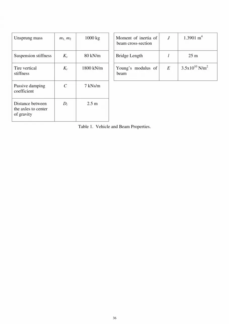
36

Unsprung mass m1, m2 1000 kg Moment of inertia of beam cross-section

J 1.3901 m4

Suspension stiffness Ks 80 kN/m Bridge Length l 25 m

Tire vertical stiffness

Kt 1800 kN/m Young’s modulus of beam

E 3.5x1010 N/m2

Passive damping coefficient

C 7 kNs/m

Distance between the axles to center of gravity

Di 2.5 m

Table 1. Vehicle and Beam Properties.