Building an Application - Generation of �?Items Tree’ Based on Transactional Data

Building an application - generation of ‘items tree’ based on transactional data 109

Building an application - generation of ‘items tree’ based on transactional data

Mihaela Vranić, Damir Pintar and Zoran Skočir

x

Building an application - generation of ‘items tree’ based on transactional data

Mihaela Vranić, Damir Pintar and Zoran Skočir

University of Zagreb, Faculty of Electrical Engineering and Computing

Croatia

1. Introduction

Association rules method is a commonly known and frequently used technique of undirected data mining. One of the commonly known drawbacks of this technique is that it often discovers a very large number of rules, many of which are trivial, uninteresting or simply variations of each other. Domain experts have to go through many of these rules to draw a meaningful conclusion which could be acted upon. Another issue that may arise is that investigation of obtained association ruleswhich cannot provide information about actual distances between items that transactions include (distances being a term describing how often items show up together in same transactions). In this particular case the actual absolute distances are not as important as the relative ones. A feature such as a compact presentation of such distances between items could be used by some business environments to quickly and dynamically produce usable business decisions. Realizing the problem of great quantity of association rules, investigations on redundancy elimination were done and results are presented in (Pasquier et al., 2005) and (Xu, Li, 2007). Here described approach is different from those – final goal is different and acquired structure should be interpreted in specific way. Driven by issues described above, we have created an application that goes trough presented transactional data multiple times and creates association rules on various levels. The final outcome of created rules is a table that reflects relative distances between items. Chapter is arranged as follows: Firstly, in paragraph 2, motivation and problem description is elaborated upon in more detail. Also, some examples of possible usages are given. Short introduction to the main method used in this article (method of association rules) is given in paragraph 3. Basic terms, measurements used in this method along with examples of its usage are addressed here and certain strengths and weaknesses are elaborated upon. Paragraph 4 introduces tools bearing relevant connections to the one this chapter deals with. Chosen technologies for the application realization are discussed in paragraph 5. Application functionality is described in detail in paragraph 6. This paragraph also deals with many issues that emerged with corresponding solutions.

7

https://www.researchgate.net/publication/27473170_Mining_Non-redundant_Association_Rules_based_on_Concise_Bases?el=1_x_8&enrichId=rgreq-331509a7-04de-4952-8e12-af3bb82b42ee&enrichSource=Y292ZXJQYWdlOzIyMTkwNzUyMztBUzoyMDc2OTkyMzQwMzc3NjhAMTQyNjUzMDc2NDQ4OQ==

https://www.researchgate.net/publication/43309353_Generating_a_Condensed_Representation_for_Association_Rules?el=1_x_8&enrichId=rgreq-331509a7-04de-4952-8e12-af3bb82b42ee&enrichSource=Y292ZXJQYWdlOzIyMTkwNzUyMztBUzoyMDc2OTkyMzQwMzc3NjhAMTQyNjUzMDc2NDQ4OQ==

Application of Machine Learning110

The application was applied on a real life dataset. Its functionality and performance parameters are depicted in paragraph 7. This performance, of course, depends on dataset characteristics, so information about dataset origin is also included. Insight on how certain characteristics of dataset can affect application performance will be given. There are some fields where the application can be improved. That is left for further investigation and described in paragraph 8. Finally, paragraph 9 provides concluding thoughts. Work presented in this chapter concentrates on issues of developing the application core – an algorithm which would in reasonable time provide data which reflects connections between items based on their co-occurrence in same transactions. In subsequent chapters this final data will be referred to as the ‘tree data’. However, visual presentation of the ‘tree data’ describing the generated tree was also considered. There are some available open source tree presentations based on XML. Even though the application doesn’t recognize our generated ‘tree data’ as input, transformation between our tree data and required XML document should be simple and straightforward.

2. Motivation and Problem Definition

Retail industry, telecommunication industry, insurance companies and other various industries produce and store great quantities of transactional data. For example, in medicine data about patients, therapies, patient reactions etc. is being recorded on daily basis. In this great quantity of data many patterns that could be acted upon are often hidden. If we take retail industry as an example then visual presentation of the distance between items found in the store depending on actual market basket contents could be very helpful. This data could help not only to ensure more effective placement of products on the shelves, but also to provide assistance for customers who could find products they are interested in with more ease. Mentioned findings could also be used to discover some connections which could lead to revelations of hidden causalities. Transactional data can reveal which items often show up together in some transactions. Certain measure (i.e. aforementioned distance) between items could be introduced. Items that very often show up together in same transactions should be considered as close ones, and items that relatively rarely show up together transactions should express greater distance between each other. Based on that distance between items graphical tree presentation containing items could be formed. Close items should be connected very early in a tree (near the tree leaves), while distanced items should connect to each other in a part of a tree closer to the tree root. Our goal was to find a way to generate data clearly depicting ‘closeness’ of items with following characteristics:

data has to be transferable to the graphical tree representation, items should be connected if certain proportion of recorded transactions suggests

their ‘closeness’, the number of tree levels must be reasonable in order to be manageable by a

human analyst (this prerequisite is necessary because of the large number of expected items to be found in transactions).

Certain technologies and available techniques were chosen to construct a solution for the presented problem. Some guidance for that matter is given in (Campos et al., 2005). Decision

was made to use a widely known data mining method of association rules generation. This method has already developed certain measures that could be used to determine item closeness. However, multiple usages of that method will be necessary to construct multiple tree levels. Attribute distance algorithms were also considered. However, requirement for the application to take into account some measures that reflect ratio in which items appear together and on that bases stop further growth of the item tree encouraged us to use the association rules method instead.

3. General Idea and Theoretical Base of Association Rules

For introduction of association rules and for various explanations (Agrawal et al., 1993) and (Hand et al., 2001) were used.

3.1 Basic terms Association rules represent local patterns in data. This descriptive data mining method results in a set of probabilistic statements that discover co-occurrence of certain attributes (items). Some basic terms that will be used further on will now be introduced:

Let I={i1, i2,..., in} be a set of n binary attributes called items. Let T={t1, t2, ..., tm} be a set of transactions. Each transaction tj has a unique ID and contains a subset of attributes in I. A rule has a simple form: if A then B (or simply A B), where A, BI and AB=Ø. A and B are sets of items (shortly itemsets). A is called antecedent, and B is called consequent of the rule.

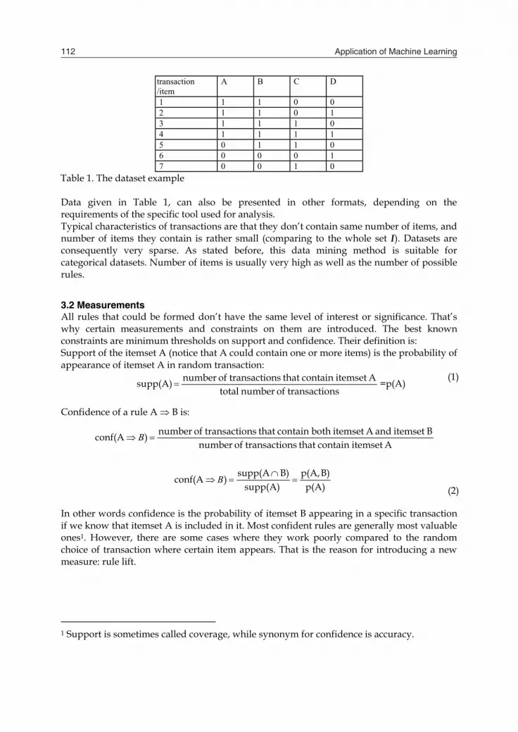
The idea of this widely used and explored method could be easily explained on transactional data concerning purchases in retail - supermarket. In that case I represents a collection of products (items) that could be bought in the store, and every tj collects some of available products depending on the realized transactions by customers. By analyzing accomplished transactions through a certain time period, some regularities will emerge – for example: transactions that contain bread very often contain milk (bread and milk are items that co-occur in same transactions). Association rule for this relationship looks like: bread milk. Example given here depicts one of the most common usages of association rules method – so-called Market Basket Analysis. However, depending of the data at hand, association rules could bring to surface various types of regularities. I could be set of binary attributes that depict some entities or cases of some interest to us. In that case, association rules give us insight that existence of some attribute (attributes) often implicates appearance of some other attribute (attributes). Dataset example is given in Table 1. Rows present transactions, while columns present binary attributes-items. Data should be read like this: items A and B are included in the first transaction.


The application was applied on a real life dataset. Its functionality and performance parameters are depicted in paragraph 7. This performance, of course, depends on dataset characteristics, so information about dataset origin is also included. Insight on how certain characteristics of dataset can affect application performance will be given. There are some fields where the application can be improved. That is left for further investigation and described in paragraph 8. Finally, paragraph 9 provides concluding thoughts. Work presented in this chapter concentrates on issues of developing the application core – an algorithm which would in reasonable time provide data which reflects connections between items based on their co-occurrence in same transactions. In subsequent chapters this final data will be referred to as the ‘tree data’. However, visual presentation of the ‘tree data’ describing the generated tree was also considered. There are some available open source tree presentations based on XML. Even though the application doesn’t recognize our generated ‘tree data’ as input, transformation between our tree data and required XML document should be simple and straightforward.

2. Motivation and Problem Definition

Retail industry, telecommunication industry, insurance companies and other various industries produce and store great quantities of transactional data. For example, in medicine data about patients, therapies, patient reactions etc. is being recorded on daily basis. In this great quantity of data many patterns that could be acted upon are often hidden. If we take retail industry as an example then visual presentation of the distance between items found in the store depending on actual market basket contents could be very helpful. This data could help not only to ensure more effective placement of products on the shelves, but also to provide assistance for customers who could find products they are interested in with more ease. Mentioned findings could also be used to discover some connections which could lead to revelations of hidden causalities. Transactional data can reveal which items often show up together in some transactions. Certain measure (i.e. aforementioned distance) between items could be introduced. Items that very often show up together in same transactions should be considered as close ones, and items that relatively rarely show up together transactions should express greater distance between each other. Based on that distance between items graphical tree presentation containing items could be formed. Close items should be connected very early in a tree (near the tree leaves), while distanced items should connect to each other in a part of a tree closer to the tree root. Our goal was to find a way to generate data clearly depicting ‘closeness’ of items with following characteristics:

data has to be transferable to the graphical tree representation, items should be connected if certain proportion of recorded transactions suggests

their ‘closeness’, the number of tree levels must be reasonable in order to be manageable by a

human analyst (this prerequisite is necessary because of the large number of expected items to be found in transactions).

Certain technologies and available techniques were chosen to construct a solution for the presented problem. Some guidance for that matter is given in (Campos et al., 2005). Decision

was made to use a widely known data mining method of association rules generation. This method has already developed certain measures that could be used to determine item closeness. However, multiple usages of that method will be necessary to construct multiple tree levels. Attribute distance algorithms were also considered. However, requirement for the application to take into account some measures that reflect ratio in which items appear together and on that bases stop further growth of the item tree encouraged us to use the association rules method instead.

3. General Idea and Theoretical Base of Association Rules

For introduction of association rules and for various explanations (Agrawal et al., 1993) and (Hand et al., 2001) were used.

3.1 Basic terms Association rules represent local patterns in data. This descriptive data mining method results in a set of probabilistic statements that discover co-occurrence of certain attributes (items). Some basic terms that will be used further on will now be introduced:

Let I={i1, i2,..., in} be a set of n binary attributes called items. Let T={t1, t2, ..., tm} be a set of transactions. Each transaction tj has a unique ID and contains a subset of attributes in I. A rule has a simple form: if A then B (or simply A B), where A, BI and AB=Ø. A and B are sets of items (shortly itemsets). A is called antecedent, and B is called consequent of the rule.

The idea of this widely used and explored method could be easily explained on transactional data concerning purchases in retail - supermarket. In that case I represents a collection of products (items) that could be bought in the store, and every tj collects some of available products depending on the realized transactions by customers. By analyzing accomplished transactions through a certain time period, some regularities will emerge – for example: transactions that contain bread very often contain milk (bread and milk are items that co-occur in same transactions). Association rule for this relationship looks like: bread milk. Example given here depicts one of the most common usages of association rules method – so-called Market Basket Analysis. However, depending of the data at hand, association rules could bring to surface various types of regularities. I could be set of binary attributes that depict some entities or cases of some interest to us. In that case, association rules give us insight that existence of some attribute (attributes) often implicates appearance of some other attribute (attributes). Dataset example is given in Table 1. Rows present transactions, while columns present binary attributes-items. Data should be read like this: items A and B are included in the first transaction.


transaction/item

A B C D

1 1 1 0 0 2 1 1 0 1 3 1 1 1 0 4 1 1 1 1 5 0 1 1 0 6 0 0 0 1 7 0 0 1 0

Table 1. The dataset example Data given in Table 1, can also be presented in other formats, depending on the requirements of the specific tool used for analysis. Typical characteristics of transactions are that they don’t contain same number of items, and number of items they contain is rather small (comparing to the whole set I). Datasets are consequently very sparse. As stated before, this data mining method is suitable for categorical datasets. Number of items is usually very high as well as the number of possible rules.

3.2 Measurements All rules that could be formed don’t have the same level of interest or significance. That’s why certain measurements and constraints on them are introduced. The best known constraints are minimum thresholds on support and confidence. Their definition is: Support of the itemset A (notice that A could contain one or more items) is the probability of appearance of itemset A in random transaction:

nstransactio of number totalAitemset contain that nstransactio of numbersupp(A) =p(A)

(1)

Confidence of a rule A B is:

Aitemset contain that nstransactio of numberBitemset and Aitemset thcontain bothat nstransactio of number) conf(A B

p(A)B)p(A,

supp(A)B)supp(A) conf(A

B

(2)

In other words confidence is the probability of itemset B appearing in a specific transaction if we know that itemset A is included in it. Most confident rules are generally most valuable ones1. However, there are some cases where they work poorly compared to the random choice of transaction where certain item appears. That is the reason for introducing a new measure: rule lift.

1 Support is sometimes called coverage, while synonym for confidence is accuracy.

ntransactio randomin B of appearance of yprobabilit

confidence rule) lift(A B

p(B)1

p(A)B)p(A) lift(A

,B

(3)

Association rules are required to satisfy a user-specified minimum support and minimum confidence. Algorithms first find all itemsets that satisfy given support, and then rules that could be formed from this itemsets are examined to satisfy minimum confidence. Real issue in terms of processing time and capacity is the first step since number of candidate itemsets grows exponentially with number of items. Many algorithms for generating association rules were presented over time. One of the most used one is Apriory algorithm, which is also implemented in the tools that are to be used in application described in this book chapter.

3.3 Common usage, strengths and weaknesses Rule structure is quite simple and interpretable. However, one has to be careful since these rules don’t have to describe causal relationships but only state the fact of co-occurrence of items in transactions. As stated before, this descriptive data mining method lets data tell its own story. Depending on the adapted parameters, rules with support and confidence greater that specified minimum are generated. Previous knowledge and some experimentation is required to tweak the parameters in such manner so the algorithm yields the best possible results – so not to end up with an extremely low number of rules or to get thousands of them. Furthermore, it is common to get a large number of rules that present fairly obvious facts (like connecting certain attributes which is predetermined before and not really a revelation), and special attention has to be taken to distinct such results apart from the new, potentially useful information. It is often hard for the analyst to get a clear picture of connections between items (attributes) since one connection is expressed with many rules (e.g. A B; B A; A,C B; B,C A...). Furthermore, it is often difficult to distinguish which connections are stronger than others. Application described in this chapter resulted from seeking a way to present rules in a manner which would enable better understanding and faster reaction of business analyst responsible for rule interpretation and forming of actable business decisions.

4. Available Viewer Applications

The problem of interpreting high quantities of association rules emerged early with usage of given method and algorithms. Many tools tried to resolve this issue by providing various graphical representations of constructed rules. Some tools enable the analyst to pick an antecedent or consequent which results in rules that satisfy this condition being displayed (e.g. Oracle Data Miner). Other tools incorporate modules like ‘Association Rules Tree Viewer’ (e.g. Orange - component-based data mining software). Those applications enable tree-like association rules presentation. Rules antecedents appear as tree roots while


transaction/item

A B C D

1 1 1 0 0 2 1 1 0 1 3 1 1 1 0 4 1 1 1 1 5 0 1 1 0 6 0 0 0 1 7 0 0 1 0

Table 1. The dataset example Data given in Table 1, can also be presented in other formats, depending on the requirements of the specific tool used for analysis. Typical characteristics of transactions are that they don’t contain same number of items, and number of items they contain is rather small (comparing to the whole set I). Datasets are consequently very sparse. As stated before, this data mining method is suitable for categorical datasets. Number of items is usually very high as well as the number of possible rules.

3.2 Measurements All rules that could be formed don’t have the same level of interest or significance. That’s why certain measurements and constraints on them are introduced. The best known constraints are minimum thresholds on support and confidence. Their definition is: Support of the itemset A (notice that A could contain one or more items) is the probability of appearance of itemset A in random transaction:

nstransactio of number totalAitemset contain that nstransactio of numbersupp(A) =p(A)

(1)

Confidence of a rule A B is:

Aitemset contain that nstransactio of numberBitemset and Aitemset thcontain bothat nstransactio of number) conf(A B

p(A)B)p(A,

supp(A)B)supp(A) conf(A

B

(2)

In other words confidence is the probability of itemset B appearing in a specific transaction if we know that itemset A is included in it. Most confident rules are generally most valuable ones1. However, there are some cases where they work poorly compared to the random choice of transaction where certain item appears. That is the reason for introducing a new measure: rule lift.

1 Support is sometimes called coverage, while synonym for confidence is accuracy.

ntransactio randomin B of appearance of yprobabilit

confidence rule) lift(A B

p(B)1

p(A)B)p(A) lift(A

,B

(3)

Association rules are required to satisfy a user-specified minimum support and minimum confidence. Algorithms first find all itemsets that satisfy given support, and then rules that could be formed from this itemsets are examined to satisfy minimum confidence. Real issue in terms of processing time and capacity is the first step since number of candidate itemsets grows exponentially with number of items. Many algorithms for generating association rules were presented over time. One of the most used one is Apriory algorithm, which is also implemented in the tools that are to be used in application described in this book chapter.

3.3 Common usage, strengths and weaknesses Rule structure is quite simple and interpretable. However, one has to be careful since these rules don’t have to describe causal relationships but only state the fact of co-occurrence of items in transactions. As stated before, this descriptive data mining method lets data tell its own story. Depending on the adapted parameters, rules with support and confidence greater that specified minimum are generated. Previous knowledge and some experimentation is required to tweak the parameters in such manner so the algorithm yields the best possible results – so not to end up with an extremely low number of rules or to get thousands of them. Furthermore, it is common to get a large number of rules that present fairly obvious facts (like connecting certain attributes which is predetermined before and not really a revelation), and special attention has to be taken to distinct such results apart from the new, potentially useful information. It is often hard for the analyst to get a clear picture of connections between items (attributes) since one connection is expressed with many rules (e.g. A B; B A; A,C B; B,C A...). Furthermore, it is often difficult to distinguish which connections are stronger than others. Application described in this chapter resulted from seeking a way to present rules in a manner which would enable better understanding and faster reaction of business analyst responsible for rule interpretation and forming of actable business decisions.

4. Available Viewer Applications

The problem of interpreting high quantities of association rules emerged early with usage of given method and algorithms. Many tools tried to resolve this issue by providing various graphical representations of constructed rules. Some tools enable the analyst to pick an antecedent or consequent which results in rules that satisfy this condition being displayed (e.g. Oracle Data Miner). Other tools incorporate modules like ‘Association Rules Tree Viewer’ (e.g. Orange - component-based data mining software). Those applications enable tree-like association rules presentation. Rules antecedents appear as tree roots while


consequents form branches. If multiple antecedent elements are present then second antecedent element forms a new branch. This branch is further expanded to leaves (consequents) or more complex branches (further antecedent elements). Main goal of the existing software solutions is to enable better representation of rules generated in one step – algorithm applied once and producing rules satisfying thresholds of minimal support and confidence. One drawback of such presentation is that the same rule – connection between two attributes appears in more than one place in a tree which results in basic problem of difficult readability not being resolved by those applications and/or tools. Our main goal is to form a tree where an item will always appear only once.

5. Technologies and Tools

Association rules as a data mining technique is pretty demanding when it comes to processing time and power. We wanted to distance our application from the ETL process and enable it to work with the data that is already in the database. That is why we decided to use database inbuilt data mining functionalities. Those functionalities are available in Oracle Database 11g Enterprise Edition and known as ODM (Oracle Data Mining). Choice of this technology brought us certain important advantages: data mining models are treated as objects inside the database and data mining processes use database inbuilt functions to maximize scalability and time efficiency. Furthermore, security is resolved by the database which makes it relatively simple to update the data (this usually depends on actual data sources, organization business rules, etc.). ODM offers a few application programming interfaces which could be used to develop the final application, such as PL/SQL and Java API. Decision to use PL/SQL and direct access to database objects that keep various information on final association rules model was made, due to flexibility it offers and opportunity to tweak the finally developed algorithm to best suit our needs. Algorithm was stored as a script containing both PL/SQL blocks and DDL instructions. Java was chosen to further develop the aforementioned developed algorithm and tweak parameters for every step of tree level generation.

6. Application Functionality

6.1 ‘Tree representation’ data For better understanding of following steps a clarification of the goal and its data representation must be presented. As stated before, final goal of the application is to generate a tree-like structure that reflects co-occurrence of items in the same transactions (or co-occurrence of attributes in the observations). A presentation that corresponds to structure is presented in Fig. 1 (on the left). This tree-like structure has to be mapped to the data in some way. Expected characteristics of the data model are:

to be straightforward and easily transferable to the tree-like structure to be easily readable preference that every algorithm step (which generates one tree level) corresponds

to one data structure (for example column in a relational table).

Decision to adopt the data model corresponding to the one presented in Fig. 1 (on the right) was made. Final data model consist of one relational table where every row presents one item (making the column of item ID necessary), and other columns which reflect item’s belonging to certain groups on various levels.

Fig. 1. Final tree-like structure and its data representation Level column interpretation works like this: items having the same number in a certain column belong to the same group on that level and are connected in a tree structure (in that level). If there are items that on a certain level don’t have items to be grouped with (on certain criteria) then they have a unique group number in that column – i.e. there are no other items to share their group number with (in Fig. 1 – Item 3 on level 1 has a unique group number 2). Numbers (group marks) N1, N2... depend on number of group identification on certain level and identified groups on previous levels. If a binary tree is created formulas for N1 and general Nj are provided below:

21G

N1N

2jG

NjN 1j

Where: N – total number of items Nj – maximum group number on level j Gj – number of formed groups on level j

It is important to emphasize that some groups consist of only one element from previous level (e.g. G1-2). The existence of this group is not necessary and in final graphical representation it doesn’t have to be displayed.

6.2 Overall algorithm To generate the tree representation data described in the previous paragraph, multiple level data generation (further called one step creation) must be preformed and acceptably saved to the whole model. Items present the tree leaves of the final model. Data mining method of association rules will be used for generation of each level – one model per tree level. Generation of each level will further in the text be addressed as one step creation – or ‘OSC’. Level 1 will capture items that are most closely related (closest in the terms described in paragraph 2 of this chapter). For every following level parameters of association rules generation will be loosened to the extent permitted by the analyst. Depending on the

...

Item 1

Item 2

Item 3

G1-1

G2-1

...

G2-N2 Item N

G1-2

G1-N1

...

ITEM Level 1 Level2 Item 1 1 1 Item 2 1 1 Item 3 2 1 ... ... ... Item N N1 N2


consequents form branches. If multiple antecedent elements are present then second antecedent element forms a new branch. This branch is further expanded to leaves (consequents) or more complex branches (further antecedent elements). Main goal of the existing software solutions is to enable better representation of rules generated in one step – algorithm applied once and producing rules satisfying thresholds of minimal support and confidence. One drawback of such presentation is that the same rule – connection between two attributes appears in more than one place in a tree which results in basic problem of difficult readability not being resolved by those applications and/or tools. Our main goal is to form a tree where an item will always appear only once.

5. Technologies and Tools

Association rules as a data mining technique is pretty demanding when it comes to processing time and power. We wanted to distance our application from the ETL process and enable it to work with the data that is already in the database. That is why we decided to use database inbuilt data mining functionalities. Those functionalities are available in Oracle Database 11g Enterprise Edition and known as ODM (Oracle Data Mining). Choice of this technology brought us certain important advantages: data mining models are treated as objects inside the database and data mining processes use database inbuilt functions to maximize scalability and time efficiency. Furthermore, security is resolved by the database which makes it relatively simple to update the data (this usually depends on actual data sources, organization business rules, etc.). ODM offers a few application programming interfaces which could be used to develop the final application, such as PL/SQL and Java API. Decision to use PL/SQL and direct access to database objects that keep various information on final association rules model was made, due to flexibility it offers and opportunity to tweak the finally developed algorithm to best suit our needs. Algorithm was stored as a script containing both PL/SQL blocks and DDL instructions. Java was chosen to further develop the aforementioned developed algorithm and tweak parameters for every step of tree level generation.

6. Application Functionality

6.1 ‘Tree representation’ data For better understanding of following steps a clarification of the goal and its data representation must be presented. As stated before, final goal of the application is to generate a tree-like structure that reflects co-occurrence of items in the same transactions (or co-occurrence of attributes in the observations). A presentation that corresponds to structure is presented in Fig. 1 (on the left). This tree-like structure has to be mapped to the data in some way. Expected characteristics of the data model are:

to be straightforward and easily transferable to the tree-like structure to be easily readable preference that every algorithm step (which generates one tree level) corresponds

to one data structure (for example column in a relational table).

Decision to adopt the data model corresponding to the one presented in Fig. 1 (on the right) was made. Final data model consist of one relational table where every row presents one item (making the column of item ID necessary), and other columns which reflect item’s belonging to certain groups on various levels.

Fig. 1. Final tree-like structure and its data representation Level column interpretation works like this: items having the same number in a certain column belong to the same group on that level and are connected in a tree structure (in that level). If there are items that on a certain level don’t have items to be grouped with (on certain criteria) then they have a unique group number in that column – i.e. there are no other items to share their group number with (in Fig. 1 – Item 3 on level 1 has a unique group number 2). Numbers (group marks) N1, N2... depend on number of group identification on certain level and identified groups on previous levels. If a binary tree is created formulas for N1 and general Nj are provided below:

21G

N1N

2jG

NjN 1j

Where: N – total number of items Nj – maximum group number on level j Gj – number of formed groups on level j

It is important to emphasize that some groups consist of only one element from previous level (e.g. G1-2). The existence of this group is not necessary and in final graphical representation it doesn’t have to be displayed.

6.2 Overall algorithm To generate the tree representation data described in the previous paragraph, multiple level data generation (further called one step creation) must be preformed and acceptably saved to the whole model. Items present the tree leaves of the final model. Data mining method of association rules will be used for generation of each level – one model per tree level. Generation of each level will further in the text be addressed as one step creation – or ‘OSC’. Level 1 will capture items that are most closely related (closest in the terms described in paragraph 2 of this chapter). For every following level parameters of association rules generation will be loosened to the extent permitted by the analyst. Depending on the

...

Item 1

Item 2

Item 3

G1-1

G2-1

...

G2-N2 Item N

G1-2

G1-N1

...

ITEM Level 1 Level2 Item 1 1 1 Item 2 1 1 Item 3 2 1 ... ... ... Item N N1 N2


starting dataset and enforced parameters certain number of levels will be created. Level presenting the tree root doesn’t have to be reached. Data has to be adjusted for each OSC activity (except for the first one where certain characteristics of input data are presumed). After performing each OSC, model results have to be extracted and tree representation data has to be updated. OSC activity is realized by SQL script containing both PL/SQL blocks and SQL DDL commands (further referred as OSC script). Because of the necessary DDL commands, OSC can’t be encapsulated in a PL/SQL procedure. Therefore a custom Java class was used for creation of user interface and orchestration of the entire process, taking into account parameter inputs made by the user (analyst). Java class is the one responsible for running the OSC script (of course depending on certain conditions). Fig. 2 presents the overall application functionality. One can notice that the process of data input (with all checkups that go with it) is left in care of other applications. User is only required to name the table containing input transactional data. Java class functionality is presented by functional blocks in red colour, while the basic functionalities of OSC script are presented in green. Final result of the main Java class method is development of tree representation data. Graphical presentation of developed data model is not the focus of this text and is left for further investigation. Technology to present it is left to final user preferences. However, researches on this matter were also made. There are some open-source solutions that enable interactive graphical presentations of tree-like structures through Internet browsers (e.g. Google Interactive Treeview). Transformation of the generated relational tree representation data into a (for example) XML file – which mentioned tool uses as its input - is rather straightforward.

Fig. 2. Developed algorithm shown through main functionality blocks Input data parameters and its adjustment through algorithm should be elaborated in more detail. At algorithm start-up, analyst is required to specify the following boundaries: top and bottom support and confidence (measures used in association rules methods) together with acceptable number of tree levels (L). Top boundaries are used to form the first level of item tree. All items included in generated association rules with support and confidence greater than parameters used as input for certain step are connected. Through following

steps those starting measures are being lowered until they reach bottom support and confidence. The actual purpose of bottom support and confidence is based on the fact that analyst is not interested in connections between items which are not supported by certain proportions of transactions. If analyst wants to utilize even minimal number of transactions supporting certain connections (so no item is left unconnected except the ones that appear in transactions containing only one item) than bottom support and confidence should be set to value near zero. At this moment, algorithm that adjusts parameters between OSC steps in linear way is developed (distance between bottom and top parameters is divided by (L-1) and parameters through whole process are tweaked to reach from top levels to bottom ones through (L-1) steps). It is possible for the algorithm to reach the tree root even earlier – but that depends on the actual data being analyzed.

6.3 Generation of one tree level – recurring step in detail This paragraph will present the developed OSC script in more detail and elaborate the decisions made during its construction. Decision to use some database structures directly (i.e. tables which keep data about generated model in the specific step) was made. Usage of PL/SQL data mining API when forming groups of items would slow the whole process down. The most important parts of OSC script are: A) view creation

Database inbuilt data mining functions require certain presentation of transactional data.

B) setup of model parameters For this, a special table is created. This table is named settings table.

C) model generation PL/SQL data mining API is used to perform model generation. Input parameters are:

a. model name b. mining function (association rules with only one available algorithm –

Apriory) c. data table name (view in our case) d. column which identifies each transaction specification e. settings table name.

D) created database structures As a consequence of the previous step certain tables that keep information about generated model (association rules) are created. This step is implicit and doesn't require custom coding. Most important tree tables are:

T1: encloses information of antecedent and consequent itemsets IDs along with measurements connected with the rule

T2: reflects structure of each itemset T3: presents all items in separated rows.


starting dataset and enforced parameters certain number of levels will be created. Level presenting the tree root doesn’t have to be reached. Data has to be adjusted for each OSC activity (except for the first one where certain characteristics of input data are presumed). After performing each OSC, model results have to be extracted and tree representation data has to be updated. OSC activity is realized by SQL script containing both PL/SQL blocks and SQL DDL commands (further referred as OSC script). Because of the necessary DDL commands, OSC can’t be encapsulated in a PL/SQL procedure. Therefore a custom Java class was used for creation of user interface and orchestration of the entire process, taking into account parameter inputs made by the user (analyst). Java class is the one responsible for running the OSC script (of course depending on certain conditions). Fig. 2 presents the overall application functionality. One can notice that the process of data input (with all checkups that go with it) is left in care of other applications. User is only required to name the table containing input transactional data. Java class functionality is presented by functional blocks in red colour, while the basic functionalities of OSC script are presented in green. Final result of the main Java class method is development of tree representation data. Graphical presentation of developed data model is not the focus of this text and is left for further investigation. Technology to present it is left to final user preferences. However, researches on this matter were also made. There are some open-source solutions that enable interactive graphical presentations of tree-like structures through Internet browsers (e.g. Google Interactive Treeview). Transformation of the generated relational tree representation data into a (for example) XML file – which mentioned tool uses as its input - is rather straightforward.

Fig. 2. Developed algorithm shown through main functionality blocks Input data parameters and its adjustment through algorithm should be elaborated in more detail. At algorithm start-up, analyst is required to specify the following boundaries: top and bottom support and confidence (measures used in association rules methods) together with acceptable number of tree levels (L). Top boundaries are used to form the first level of item tree. All items included in generated association rules with support and confidence greater than parameters used as input for certain step are connected. Through following

steps those starting measures are being lowered until they reach bottom support and confidence. The actual purpose of bottom support and confidence is based on the fact that analyst is not interested in connections between items which are not supported by certain proportions of transactions. If analyst wants to utilize even minimal number of transactions supporting certain connections (so no item is left unconnected except the ones that appear in transactions containing only one item) than bottom support and confidence should be set to value near zero. At this moment, algorithm that adjusts parameters between OSC steps in linear way is developed (distance between bottom and top parameters is divided by (L-1) and parameters through whole process are tweaked to reach from top levels to bottom ones through (L-1) steps). It is possible for the algorithm to reach the tree root even earlier – but that depends on the actual data being analyzed.

6.3 Generation of one tree level – recurring step in detail This paragraph will present the developed OSC script in more detail and elaborate the decisions made during its construction. Decision to use some database structures directly (i.e. tables which keep data about generated model in the specific step) was made. Usage of PL/SQL data mining API when forming groups of items would slow the whole process down. The most important parts of OSC script are: A) view creation

Database inbuilt data mining functions require certain presentation of transactional data.

B) setup of model parameters For this, a special table is created. This table is named settings table.

C) model generation PL/SQL data mining API is used to perform model generation. Input parameters are:

a. model name b. mining function (association rules with only one available algorithm –

Apriory) c. data table name (view in our case) d. column which identifies each transaction specification e. settings table name.

D) created database structures As a consequence of the previous step certain tables that keep information about generated model (association rules) are created. This step is implicit and doesn't require custom coding. Most important tree tables are:

T1: encloses information of antecedent and consequent itemsets IDs along with measurements connected with the rule

T2: reflects structure of each itemset T3: presents all items in separated rows.


E) rules ordering Multiple connections among few items may appear. To ensure that the most significant ones are presented in level groupings, rules are ordered and confidence is chosen as an order criteria. In the future only one PL/SQL instruction has to be altered to change this criterion (if the analyst needs such a change).

F) elimination of itemsets and rules To take into account only those rules which only concern two-way connections, all itemsets containing more than one item are eliminated together with the corresponding rules. There are a few reasons for that step: final tree is intended to present structure where relative distance between two items can be compared with a distance between other two items. Rules which have more elements in antecedent or consequent can’t be properly depicted in intended tree structure.

G) formation of item groups Items that are not already occupied by some group in a certain level are grouped together on the basis of sequential reading of ordered rules. They are being assigned the next unused number - group mark.

H) population of group column A certain number of items is expected not to take part in any groups on specific level. They will have NULL values in certain table cells. Group column must be populated with unused numbers – group marks.

I) storing of the tree level information Finally, useful information about performed groupings is saved to the special table which is to be used outside of the OSC step.

J) transactional data modulation To be able to perform the next level generation, transactional data needs to be altered. In the next step association rule modelling must be performed on groups formed on previous level.

K) index creation On certain phases of the OSC step indexes have to be created to speed up the whole process (without them required time for some steps may exceed required time for model generation).

L) cleansing of some structures Every OSC step generates structures that are to be used in the next OSC step. For that reason cleansing of those structures must be preformed.

6.4 Possible issues Major issues and questions that emerged during OSC script creation are described in this chapter. (A) TRANSACTIONAL DATA MODULATION AND ITS CONSEQUENCES First issue is the one concerning the changes of transactional data. Data is changed to enable performing each consecutive step and to avoid losing information about item ‘connections’. The real question is whether the final measures (produced by models after transactional data change) are acceptable and how the tree structure should be interpreted. Implemented algorithm in each transaction replaces original item ID with the newly assigned group mark. Since association rules measures are important for the next level of

tree structure generation, a question may arise regarding the consequence of replacing a group of items with one sole item which will represent the entire group. To best depict the problem, transactional data presented in Table 1 is used as an example to make a tree structure model. Certain measures for the input data can be calculated (equations (2) and (3)). Support of items and item pairs is presented in Table 2. This table is orthogonally symmetric since supp(A,B)=supp(B,A) which is a consequence of a support definition.

A B C D A 4/7 4/7 2/7 2/7 B 4/7 5/7 3/7 2/7 C 2/7 3/7 4/7 1/7 D 2/7 2/7 1/7 3/7

Table 2. Calculated support for dataset example Table 3 presents calculated confidence of possible binary rules for the same example data. Items presented at row beginnings represent antecedents and columns present consequents (e.g. conf(BA)=4/5). Since generally conf(AA)=1, these measures were not marked in the table.

consequent antecedent\

A B C D

A 1 1/2 1/2 B 4/5 3/5 2/5 C 1/2 3/4 1/4 D 2/3 2/3 1/3

Table 3. Calculated confidence for possible binary rules If parameters for first level creation are set in such a way that only items A and B are connected in a group called X (conf(AB)=1), than one of the possible representations of final model is depicted on Fig.3.

Fig. 3. Possible formation of a tree structure based on example data Two important questions may arise concerning the replacement of A and B with a group/item named X:

- what happens to the relationships of items unaffected by this new group? - what happens to the measures of possible rules which include ‘new item’ X?

Regarding relationships between items unaffected by formed group, the following facts stand:

- support of those items remains the same - support of itemsets that don’t contain X remains the same (e.g. supp(C,D))

A

B

C

X


E) rules ordering Multiple connections among few items may appear. To ensure that the most significant ones are presented in level groupings, rules are ordered and confidence is chosen as an order criteria. In the future only one PL/SQL instruction has to be altered to change this criterion (if the analyst needs such a change).

F) elimination of itemsets and rules To take into account only those rules which only concern two-way connections, all itemsets containing more than one item are eliminated together with the corresponding rules. There are a few reasons for that step: final tree is intended to present structure where relative distance between two items can be compared with a distance between other two items. Rules which have more elements in antecedent or consequent can’t be properly depicted in intended tree structure.

G) formation of item groups Items that are not already occupied by some group in a certain level are grouped together on the basis of sequential reading of ordered rules. They are being assigned the next unused number - group mark.

H) population of group column A certain number of items is expected not to take part in any groups on specific level. They will have NULL values in certain table cells. Group column must be populated with unused numbers – group marks.

I) storing of the tree level information Finally, useful information about performed groupings is saved to the special table which is to be used outside of the OSC step.

J) transactional data modulation To be able to perform the next level generation, transactional data needs to be altered. In the next step association rule modelling must be performed on groups formed on previous level.

K) index creation On certain phases of the OSC step indexes have to be created to speed up the whole process (without them required time for some steps may exceed required time for model generation).

L) cleansing of some structures Every OSC step generates structures that are to be used in the next OSC step. For that reason cleansing of those structures must be preformed.

6.4 Possible issues Major issues and questions that emerged during OSC script creation are described in this chapter. (A) TRANSACTIONAL DATA MODULATION AND ITS CONSEQUENCES First issue is the one concerning the changes of transactional data. Data is changed to enable performing each consecutive step and to avoid losing information about item ‘connections’. The real question is whether the final measures (produced by models after transactional data change) are acceptable and how the tree structure should be interpreted. Implemented algorithm in each transaction replaces original item ID with the newly assigned group mark. Since association rules measures are important for the next level of

tree structure generation, a question may arise regarding the consequence of replacing a group of items with one sole item which will represent the entire group. To best depict the problem, transactional data presented in Table 1 is used as an example to make a tree structure model. Certain measures for the input data can be calculated (equations (2) and (3)). Support of items and item pairs is presented in Table 2. This table is orthogonally symmetric since supp(A,B)=supp(B,A) which is a consequence of a support definition.

A B C D A 4/7 4/7 2/7 2/7 B 4/7 5/7 3/7 2/7 C 2/7 3/7 4/7 1/7 D 2/7 2/7 1/7 3/7

Table 2. Calculated support for dataset example Table 3 presents calculated confidence of possible binary rules for the same example data. Items presented at row beginnings represent antecedents and columns present consequents (e.g. conf(BA)=4/5). Since generally conf(AA)=1, these measures were not marked in the table.

consequent antecedent\

A B C D

A 1 1/2 1/2 B 4/5 3/5 2/5 C 1/2 3/4 1/4 D 2/3 2/3 1/3

Table 3. Calculated confidence for possible binary rules If parameters for first level creation are set in such a way that only items A and B are connected in a group called X (conf(AB)=1), than one of the possible representations of final model is depicted on Fig.3.

Fig. 3. Possible formation of a tree structure based on example data Two important questions may arise concerning the replacement of A and B with a group/item named X:

- what happens to the relationships of items unaffected by this new group? - what happens to the measures of possible rules which include ‘new item’ X?

Regarding relationships between items unaffected by formed group, the following facts stand:

- support of those items remains the same - support of itemsets that don’t contain X remains the same (e.g. supp(C,D))

A

B

C

X


- previous two entries result in no effect on the possible rules not containing X. Depicted features are desirable and welcome.

Regarding possible rules which include ‘new item’ X, measure calculations show the following:

- supp(X)>=max(supp(A), supp(B))

- supp(X)<supp(A)+supp(B)

- support of itemsets that include X increases: (supp(X,C)=supp((AvB),C)>= max(supp(A,C), supp(B,C))

- confidence of rules that incorporate X as an antecedent will fall somewhere between conf(AC) and conf(BC).

- confidence of rules that incorporate X as a consequent will be greater than conf(CA) and conf(CB) (support of (X,C) is equal or greater than supp(A,C) or supp(B,C) while support of antecedent remains the same).

From these observations, following reasoning could be made: item X will display closeness to some other item (e.g. item C) in the case that both of its components (A and B) display closeness to C. If A is ‘close’ to C but B isn’t, than the appearance frequency of A and B in transactional data has to be taken into account. If appearance of A is frequent, while B is rare, than measure of closeness (conf(XC)) will be more influenced by item A and X would be relatively close to C. That means that X (as antecedent) exposes more average (or tenderer) features than its components with the number of supporting transactions also affecting the outcome. Explained and depicted features of grouping item X are also desirable and acceptable. When examining X as a consequent, it can be stated that it can more easily be connected to other items than can solely items A and B, which is also logical consequence of grouping. Final tree representation should be interpreted in the following way: based on transactional data, items A and B are close i.e. connected. If X is further connected to C then we can say that item group of A and B exposes closeness to C. However, direct connection between A and C cannot be stated (likewise for items B and C). (B) ELIMINATION OF TRANSACTIONS CONTAINING ONLY ONE ITEM In real life datasets which the authors have encountered many transactions exist which contain only one item. These cases also emerge in our application usage. After making certain groups and modulating transactional data for the new step, it is possible that some transactions exist which include only one item which is result of grouping (e.g. first transaction in Table 1, after replacing A and B with X, contains only one item). Such transactions seemingly do not contribute to further analysis and could potentially be eliminated. However, it is worth to consider the impact of these eliminations on further rules development. To demonstrate consequences of transaction elimination, first example is used and then ratios are generalized. Example of transactional data presented in Table 1 is used, where on level 1 of a tree structure items A and B are connected and form ‘new item’ X. Renewed transactional data is presented in Table 4.

transaction/item

X C D

1 1 0 0 2 1 0 1 3 1 1 0 4 1 1 1 5 1 1 0 6 0 0 1 7 0 1 0

Table 4. Example - transformed data after first level creation For analysis, three general cases are recognized. All possible combinations of item relationships belong to one of them:

- rules where X is antecedent - rules where X is consequent - rules not containing X;

where X is the single item in eliminated transaction. Measures for given example:

- before elimination of first transaction:

75)supp( X ;

74)supp( C ;

73)supp( D ;

7

3supp(X,C) ;7

1 supp(C,D)

53conf(X )C ;

43conf(C )X ;

41conf(C )D

- after elimination of the first transaction:

64)(supp' X ;

64)(supp' C ;

63)(supp' D ;

63C)(X,supp' ; '

6

1 supp(C,D)

43(Xconf' )C ;

43(Cconf' )X ;

41(Cconf' )D

To generalize - if m transactions are eliminated because they contained only one item, measures change in the following way:


td)supp(

tc)supp(

tx)supp(

D

C

X

t

t

gsupp(X,C)

h supp(C,D)


- previous two entries result in no effect on the possible rules not containing X. Depicted features are desirable and welcome.

Regarding possible rules which include ‘new item’ X, measure calculations show the following:

- supp(X)>=max(supp(A), supp(B))

- supp(X)<supp(A)+supp(B)

- support of itemsets that include X increases: (supp(X,C)=supp((AvB),C)>= max(supp(A,C), supp(B,C))

- confidence of rules that incorporate X as an antecedent will fall somewhere between conf(AC) and conf(BC).

- confidence of rules that incorporate X as a consequent will be greater than conf(CA) and conf(CB) (support of (X,C) is equal or greater than supp(A,C) or supp(B,C) while support of antecedent remains the same).

From these observations, following reasoning could be made: item X will display closeness to some other item (e.g. item C) in the case that both of its components (A and B) display closeness to C. If A is ‘close’ to C but B isn’t, than the appearance frequency of A and B in transactional data has to be taken into account. If appearance of A is frequent, while B is rare, than measure of closeness (conf(XC)) will be more influenced by item A and X would be relatively close to C. That means that X (as antecedent) exposes more average (or tenderer) features than its components with the number of supporting transactions also affecting the outcome. Explained and depicted features of grouping item X are also desirable and acceptable. When examining X as a consequent, it can be stated that it can more easily be connected to other items than can solely items A and B, which is also logical consequence of grouping. Final tree representation should be interpreted in the following way: based on transactional data, items A and B are close i.e. connected. If X is further connected to C then we can say that item group of A and B exposes closeness to C. However, direct connection between A and C cannot be stated (likewise for items B and C). (B) ELIMINATION OF TRANSACTIONS CONTAINING ONLY ONE ITEM In real life datasets which the authors have encountered many transactions exist which contain only one item. These cases also emerge in our application usage. After making certain groups and modulating transactional data for the new step, it is possible that some transactions exist which include only one item which is result of grouping (e.g. first transaction in Table 1, after replacing A and B with X, contains only one item). Such transactions seemingly do not contribute to further analysis and could potentially be eliminated. However, it is worth to consider the impact of these eliminations on further rules development. To demonstrate consequences of transaction elimination, first example is used and then ratios are generalized. Example of transactional data presented in Table 1 is used, where on level 1 of a tree structure items A and B are connected and form ‘new item’ X. Renewed transactional data is presented in Table 4.

transaction/item

X C D

1 1 0 0 2 1 0 1 3 1 1 0 4 1 1 1 5 1 1 0 6 0 0 1 7 0 1 0

Table 4. Example - transformed data after first level creation For analysis, three general cases are recognized. All possible combinations of item relationships belong to one of them:

- rules where X is antecedent - rules where X is consequent - rules not containing X;

where X is the single item in eliminated transaction. Measures for given example:


75)supp( X ;

74)supp( C ;

73)supp( D ;

7

3supp(X,C) ;7

1 supp(C,D)

53conf(X )C ;

43conf(C )X ;

41conf(C )D

- after elimination of the first transaction:

64)(supp' X ;

64)(supp' C ;

63)(supp' D ;

63C)(X,supp' ; '

6

1 supp(C,D)

43(Xconf' )C ;

43(Cconf' )X ;

41(Cconf' )D

To generalize - if m transactions are eliminated because they contained only one item, measures change in the following way:


td)supp(

tc)supp(

tx)supp(

D

C

X

t

t

gsupp(X,C)

h supp(C,D)


chconf(C

cg

conf(C

xg

conf(X

)

)

)

D

X

C

(4)

(5)

(6) - after elimination of m transaction:

m-td)(supp'

m-tc)(supp'

m-tm-x)(supp'

D

C

X

'

t-m

't-m

gsupp(X,C)

h supp(C,D)

ch(Cconf'

cg

(Cconf'

m-xg

(Xconf'

)

)

)

D

X

C

(7) (8) (9)

Comparing (4), (5) and (6) with (7), (8) and (9) the following conclusion can be made: confidence of rules containing X as consequent and confidence of rules not containing X remains the same but confidence of rules containing X as antecedent increases. Therefore elimination of transactions containing only one item on various levels should not be performed since it could skew the real relationships between items. This decision could also be supported by an extreme case example where item X is the only item appearing in many transactions, with only one transaction where it appears with another item - C. If we eliminate transactions which include only one item then conf(XC) would be 1, which is very far from the true relationship. (C) DIFFERENT TREE STRUCTURES DEPICTING THE SAME TRANSACTIONAL DATA AS A CONSEQUENCE OF DIFFERENT PARAMETER INPUT For the same transactional data, various final tree presentations could be made depending on parameter input. Two extremes would be:

- very loose parameters - strict parameters with slight changes from one step to another.

Fig. 4 presents two outcomes depending on the input parameters.

Fig. 4. Two tree-like structure outcomes depending on input parameters

A

B

C

D

G1 G2

G3

A

B

C

D

G1

What is loose and what is strict usually depends on characteristics of the input dataset. This is an issue best left to analyst’s discretion; analyst should tweak the parameters to get the structure he/she feels is the most informative and could most easily be acted upon.

7. Results on Real-life Dataset

7.1 Data set Characteristics Datasets can vary in great extent when their various characteristics are in question. These characteristics influence overall performance of the generated application. Therefore some characteristics of dataset at hand used for verification of application performance will be presented first. Number of transactions and number of items are the most obvious characteristics of dataset and usually the most important ones. Example dataset presented in Table 1 includes 7 transactions and 4 items. Data density could be presented by a ratio between realized appearances of items in transactions compared to the case where every transaction includes all items. Density is for the most datasets very low and therefore is often multiplied by 100 to form ‘modified data density’ (i.e. if average transaction includes every hundredth item the density results in 1). Data density for example data is 15/(7*4)=0,53 (53% of table cells are populated with value ‘1’). It could be useful to notice the most frequently appearing item and what is number of transactions where it could be found (e.g. item B appears in most transactions, 5 of them). Average number of items per transaction gives a good insight on the input dataset (for given example this ratio is 2,29). Application performance was examined on few real-life datasets. The one which clearly demonstrates the performance of generated application was chosen. It holds data of market basket contents in one computer store. Characteristics of chosen dataset are given in Table 5.

Dataset characteristic ValueNumber of transactions 940 Number of items 14 Data density 0,21 Number of transactions where the most frequently appearing item appeared

303 (32%)

Average number of items per transaction 2,98 Table 5. Characteristics of examined real-life dataset First step is the most critical one, so it will be examined in more detail. 12 rules were found with parameters set to values:

- minimal support: 0,1 - minimal confidence: 0,1.

Those rules resulted in 2 item groups: one containing 4 items and one containing 2 items (Table 6). Two groups that satisfied first setting chosen by the analyst resulted in a pretty good score comparing to 12 association rules those groups stemmed from and which analyst doesn’t have to read. Of course, this concise presentation resulted in some information loss, but it happened in accordance with analyst decision of parameter setting.


chconf(C

cg

conf(C

xg

conf(X

)

)

)

D

X

C

(4)

(5)

(6) - after elimination of m transaction:

m-td)(supp'

m-tc)(supp'

m-tm-x)(supp'

D

C

X

'

t-m

't-m

gsupp(X,C)

h supp(C,D)

ch(Cconf'

cg

(Cconf'

m-xg

(Xconf'

)

)

)

D

X

C

(7) (8) (9)

Comparing (4), (5) and (6) with (7), (8) and (9) the following conclusion can be made: confidence of rules containing X as consequent and confidence of rules not containing X remains the same but confidence of rules containing X as antecedent increases. Therefore elimination of transactions containing only one item on various levels should not be performed since it could skew the real relationships between items. This decision could also be supported by an extreme case example where item X is the only item appearing in many transactions, with only one transaction where it appears with another item - C. If we eliminate transactions which include only one item then conf(XC) would be 1, which is very far from the true relationship. (C) DIFFERENT TREE STRUCTURES DEPICTING THE SAME TRANSACTIONAL DATA AS A CONSEQUENCE OF DIFFERENT PARAMETER INPUT For the same transactional data, various final tree presentations could be made depending on parameter input. Two extremes would be:

- very loose parameters - strict parameters with slight changes from one step to another.

Fig. 4 presents two outcomes depending on the input parameters.

Fig. 4. Two tree-like structure outcomes depending on input parameters

A

B

C

D

G1 G2

G3

A

B

C

D

G1

What is loose and what is strict usually depends on characteristics of the input dataset. This is an issue best left to analyst’s discretion; analyst should tweak the parameters to get the structure he/she feels is the most informative and could most easily be acted upon.

7. Results on Real-life Dataset

7.1 Data set Characteristics Datasets can vary in great extent when their various characteristics are in question. These characteristics influence overall performance of the generated application. Therefore some characteristics of dataset at hand used for verification of application performance will be presented first. Number of transactions and number of items are the most obvious characteristics of dataset and usually the most important ones. Example dataset presented in Table 1 includes 7 transactions and 4 items. Data density could be presented by a ratio between realized appearances of items in transactions compared to the case where every transaction includes all items. Density is for the most datasets very low and therefore is often multiplied by 100 to form ‘modified data density’ (i.e. if average transaction includes every hundredth item the density results in 1). Data density for example data is 15/(7*4)=0,53 (53% of table cells are populated with value ‘1’). It could be useful to notice the most frequently appearing item and what is number of transactions where it could be found (e.g. item B appears in most transactions, 5 of them). Average number of items per transaction gives a good insight on the input dataset (for given example this ratio is 2,29). Application performance was examined on few real-life datasets. The one which clearly demonstrates the performance of generated application was chosen. It holds data of market basket contents in one computer store. Characteristics of chosen dataset are given in Table 5.

Dataset characteristic ValueNumber of transactions 940 Number of items 14 Data density 0,21 Number of transactions where the most frequently appearing item appeared

303 (32%)

Average number of items per transaction 2,98 Table 5. Characteristics of examined real-life dataset First step is the most critical one, so it will be examined in more detail. 12 rules were found with parameters set to values:

- minimal support: 0,1 - minimal confidence: 0,1.

Those rules resulted in 2 item groups: one containing 4 items and one containing 2 items (Table 6). Two groups that satisfied first setting chosen by the analyst resulted in a pretty good score comparing to 12 association rules those groups stemmed from and which analyst doesn’t have to read. Of course, this concise presentation resulted in some information loss, but it happened in accordance with analyst decision of parameter setting.


After updating transactional data2, a number of items are represented as one item in further analysis. Therefore there are some duplicate entries of items belonging to certain transactions that could be eliminated. For example, let items A and B belong to transaction ti, and they are grouped and their group is presented by ‘item X’, then duplicate recording of item X belonging to transaction ti is not necessary. Immediate benefit is that data for transaction representation is reduced from 2804 rows to 2345 rows. In the following steps this reduction is reiterated resulting in shorter execution time for every subsequent level creation. Application performance could be demonstrated by setting following input parameters:

- minimal support: 0,1-0,08; - minimal confidence=0,1 - expected levels=3.

Resulting model is presented in Table 6. As it can be observed, there are some items that relatively rarely show up together with any other item in transactions and they stay as solitary leaves. If we take a look at the real items that are connected, some combinations of items are quite logical, for instance: External 8X CD-ROM and CD-RW, High Speed Pack of 5. Final model data presentation, given in Table 6, shows that our data representation can easily be converted to a graphical tree-like structure. Readability can be improved simply by sorting the columns data – going from the levels closest to the root towards those nearer to the leaves.

Item_id Name Level_1 Level_2 Level_3 12 18" Flat Panel Graphics

Monitor3 2 1

9 SIMM- 16MB PCMCIAII card

3 2 1

8 Keyboard Wrist Rest 8 2 1 7 External 8X CD-ROM 2 3 1 10 CD-RW, High Speed

Pack of 5 2 3 1

11 Multimedia speakers- 3" cones

9 3 1

3 Standard Mouse 1 1 4 Extension Cable 1 1 14 Model SM26273 Black

Ink Cartridge 4 1

2 Mouse Pad 4 1 1 Y Box 5 5 Envoy Ambassador 6 6 Envoy 256MB - 40GB 7 13 O/S Documentation Set -

English10

Table 6. Resulting model for real-life dataset Each following step data characteristics change: number of items decreases, data density increases and number of items per transaction decreases.

2 Every realization of item’s appearance in transaction is presented in a separate row.

Application testing showed that not only data characteristics influenced final model structure (number of groupings per level and level numbers) but also the nature of data in question. For the optimal use of application analyst should be closely acquainted with business problem, available data and usability of final model.

8. Further work

There are some areas in application functioning that could be improved. The most important one concerns parameter adjusting since it has great effect on application functionality and final outcome. Dataset characteristics play the most important role here so in the future application should give the analyst suggestions for parameter setup based on input dataset. It would prevent analyst from straying and would offer him a priori guidance on what choices could potentially be the most effective. Some researches regarding usage of data density in mining association rules have already been undertaken. Its usage is even further investigated in (Cheung et al., 2007) where new measures of data density for quantitative attributes are introduced. In some cases analysts will want to investigate on how some specific item groups are connected to other items, for example illness symptoms that are somehow connected to diseases or other symptoms.Insight in belonging tree structure could bring upon some new notions. For that matter a feature to bundle some items in advance will be offered by application. The bottleneck of implemented algorithm is the need for repeated creation of association rules in each step. However, some time improvements could be made by optimizations of SQL commands and PL/SQL blocks.

9. Conclusion

New approach to well known data mining method of association rules is developed and elaborated. In a nutshell, an application was created which generates a tree-like structure representing an interpretation of relationship between items based on their co-occurrence in transactional data.Survey of existing applications’ functionalities using association rules is presented, along with motivation to make rather different solution. Way of interpretation of developed solution is clearly elaborated. Application was realized with Java technology and uses database in-built data mining functions. This technology bundle gave us both flexibility and advantages of optimizations through direct in-base data structure manipulation. One more benefit of such approach is that data doesn’t have to be transferred from its original source. Although association rules are quite resource exhausting method, with reasonable parameters input for specific dataset, good performance characteristics were accomplished. During application development some issues emerged. They were examined and most important decisions along with reasoning are presented in this chapter. There are many possible usages of developed tool and data model. It is quite easy to interpret it and exploit it. However, like with every data mining method, final functionality and benefits depend on quality of input data and analyst acquaintance with business problem, the data and application itself.


After updating transactional data2, a number of items are represented as one item in further analysis. Therefore there are some duplicate entries of items belonging to certain transactions that could be eliminated. For example, let items A and B belong to transaction ti, and they are grouped and their group is presented by ‘item X’, then duplicate recording of item X belonging to transaction ti is not necessary. Immediate benefit is that data for transaction representation is reduced from 2804 rows to 2345 rows. In the following steps this reduction is reiterated resulting in shorter execution time for every subsequent level creation. Application performance could be demonstrated by setting following input parameters:

- minimal support: 0,1-0,08; - minimal confidence=0,1 - expected levels=3.

Resulting model is presented in Table 6. As it can be observed, there are some items that relatively rarely show up together with any other item in transactions and they stay as solitary leaves. If we take a look at the real items that are connected, some combinations of items are quite logical, for instance: External 8X CD-ROM and CD-RW, High Speed Pack of 5. Final model data presentation, given in Table 6, shows that our data representation can easily be converted to a graphical tree-like structure. Readability can be improved simply by sorting the columns data – going from the levels closest to the root towards those nearer to the leaves.

Item_id Name Level_1 Level_2 Level_3 12 18" Flat Panel Graphics

Monitor3 2 1

9 SIMM- 16MB PCMCIAII card

3 2 1

8 Keyboard Wrist Rest 8 2 1 7 External 8X CD-ROM 2 3 1 10 CD-RW, High Speed

Pack of 5 2 3 1

11 Multimedia speakers- 3" cones

9 3 1

3 Standard Mouse 1 1 4 Extension Cable 1 1 14 Model SM26273 Black

Ink Cartridge 4 1

2 Mouse Pad 4 1 1 Y Box 5 5 Envoy Ambassador 6 6 Envoy 256MB - 40GB 7 13 O/S Documentation Set -

English10

Table 6. Resulting model for real-life dataset Each following step data characteristics change: number of items decreases, data density increases and number of items per transaction decreases.

2 Every realization of item’s appearance in transaction is presented in a separate row.

Application testing showed that not only data characteristics influenced final model structure (number of groupings per level and level numbers) but also the nature of data in question. For the optimal use of application analyst should be closely acquainted with business problem, available data and usability of final model.

8. Further work

There are some areas in application functioning that could be improved. The most important one concerns parameter adjusting since it has great effect on application functionality and final outcome. Dataset characteristics play the most important role here so in the future application should give the analyst suggestions for parameter setup based on input dataset. It would prevent analyst from straying and would offer him a priori guidance on what choices could potentially be the most effective. Some researches regarding usage of data density in mining association rules have already been undertaken. Its usage is even further investigated in (Cheung et al., 2007) where new measures of data density for quantitative attributes are introduced. In some cases analysts will want to investigate on how some specific item groups are connected to other items, for example illness symptoms that are somehow connected to diseases or other symptoms.Insight in belonging tree structure could bring upon some new notions. For that matter a feature to bundle some items in advance will be offered by application. The bottleneck of implemented algorithm is the need for repeated creation of association rules in each step. However, some time improvements could be made by optimizations of SQL commands and PL/SQL blocks.

9. Conclusion

New approach to well known data mining method of association rules is developed and elaborated. In a nutshell, an application was created which generates a tree-like structure representing an interpretation of relationship between items based on their co-occurrence in transactional data.Survey of existing applications’ functionalities using association rules is presented, along with motivation to make rather different solution. Way of interpretation of developed solution is clearly elaborated. Application was realized with Java technology and uses database in-built data mining functions. This technology bundle gave us both flexibility and advantages of optimizations through direct in-base data structure manipulation. One more benefit of such approach is that data doesn’t have to be transferred from its original source. Although association rules are quite resource exhausting method, with reasonable parameters input for specific dataset, good performance characteristics were accomplished. During application development some issues emerged. They were examined and most important decisions along with reasoning are presented in this chapter. There are many possible usages of developed tool and data model. It is quite easy to interpret it and exploit it. However, like with every data mining method, final functionality and benefits depend on quality of input data and analyst acquaintance with business problem, the data and application itself.


10. References

Agrawal, R.; Imielinski, T. & Swami, A. (1993).: Mining Association Rules Between Sets of Items in Large Databases, Proceedings of the 1993 ACM SIGMOD international conference on Management of data, pp 207-216, 0-89791-592-5, May 25-28, 1993, Washington, D.C., United States

Campos, M.M.; Stengard, P.J.& Milenova, B.L. (2005).: Data-centric automated data mining, Proceedings of the Fourth International Conference on Machine Learning and Applications, pp. 97-104, 0-7695-2495-8, December 15-17 2005, IEEE Computer Society, Washington, DC

Cheung, D. W. ; Wang, L.; Yiu, S. M. & Zhou B. (2007). Density-Based Mining of Quantitative Association Rules, In: Knowledge Discovery and Data Mining. Current Issues and New Applications, 257-268, Springer Berlin/Heidelberg, 978-3-540-67382-8, Germany

Hand, D.; Mannila, H.; Smyth, P. (2001). Principles of Data Mining, The MIT Press, ISBN: 026208290, USA

Orange – component-based data mining software Available: http://www.ailab.si/orange/ (accessed on 20.05.2009.)

Pasquier, N.; Taouil, R.; Bastide, Y.; Stumme, G. & Lakhal, L. (2005).: Generating a condensed representation for association rules. Journal of Intelligent Information Systems, Vol. 24, No. 1. (January 2005), pp 29-60, 0925-9902

Xu, Y. & Li, Y. (2007).: Mining Non-Redundant Association Rules Based on Concise Bases. International Journal of Pattern Recognition and Artificial Intelligence, Vol. 21, No. 4. (June 2007), pp 659-675, 0218-0014

Documents

Building an Application - Generation of �?Items Tree’ Based on Transactional Data