Building Thermal Network Model

and Application to Temperature Regulation

Qi Luo and Kartik B. Ariyur

Abstract— Residential and commercial facilities account forover 40% of energy consumption in the US. Our work showshow fine grain modeling and sensing of this consumption canlead to substantial savings. We construct a thermal networkmodel of a building with the temperatures of the various roomsas states; with the room thermal capacitances and thermalresistances between the rooms as parameters; the externalor ambient temperatures as uncontrolled input and heatingand cooling loads as control inputs. We show the effects onenergy consumption of the random opening and closing ofdoors or windows. We show that active management of roomtemperature set points saves up to 20% of energy costs . Wealso demonstrate the substantial savings–up to 30%–throughstrategies of keeping certain doors and windows closed.

I. INTRODUCTION

Heating and cooling of both residences and commercial fa-

cilities accounts for the lion’s share of energy consumption–

over 40%–in the United States. Utilities building the Smart

Grid [1], [2] on the one hand and consumers switching to

Smart Appliances [3] on the other hand raise the possibility

of significant savings of energy in a variety of applications.

The availability of real time cost and consumption infor-

mation from smart meters and measurements [4] opens up

several avenues for savings. The utilities can save through

monitoring vulnerability, [5] and electrical [6] or gas loads

in real time; the integration of renewable energy sources

into the grid; and the integration of distributed generation

into the grid. Consumers can save through use of real-time

pricing information and schedule their energy consumption

for intervals of relatively lower prices; they can also use

smart appliances and sensors to keep track of their patterns

of energy use and systematically cut waste.

In this context, we develop a higher fidelity model of

building heat consumption (or equivalently cooling load) that

uses the distributed sensing and data logging expected to be

available, and can account for human habits. The building

is modeled as a thermal network–a passive circuit with room

heaters as heat sources and the ambient environment as the

heat sink. The thermal resistances between rooms or that

between rooms and the ambient can change randomly if

doors or windows are opened or closed. Thus, we have a

stochastic hybrid system that can have any of a finite number

of system dynamics. Our model renders some strategies of

energy savings explicit and gives means to quantify them.

Qi Luo is with the School of Mechanical Engineering, , Purdue Univer-sity, West Lafayette, IN 47906, USA luoq@purdue.edu

Kartik B. Ariyur is with the School of Mechanical Engineering, , PurdueUniversity, West Lafayette, IN 47906, USA kariyur@purdue.edu

It also opens up several possibilities–such as helping con-

sumers track their consumption precisely and craft strategies

to cut their energy costs. We show that a simple strategy of

closing doors in a building can lead to a saving of 30%in energy costs–which runs counter to the current trend of

cubicle farms in commercial facilities.

The paper is organized as follows: Section II introduces

the thermal network model of the building, Section III details

the thermal connectivity matrix for a building, Section IV

supplies a simple distributed energy saving control strategy

for the building, Section V shows illustrative results from

using the model for temperature regulation for facilities, and

Section VI supplies concluding remarks.

II. THERMAL NETWORK MODEL

In prior work [7], which used a lumped building thermal

model, we showed the potential of energy savings via active

energy management. Here we posit a higher fidelity model

to enable better quantification of those benefits. The model

relates the environmental conditions of a building to its

heating and cooling loads. The model is obtained through

combining convective and conductive heat transfer between

the building and its surroundings. Overall, we have, for a

single room,

miCp

dθi

dt=

m∑

j=1

1

( 1

hini

Aij+

Lij

kijAij+ 1

houtj

Aij)(θout − θi)

+

n∑

k=1

1

( 1

hini

Aik+ Lik

kikAik+ 1

hikAik)(θk − θi) + Qi (1)

where, typically,

m + n = 6 (2)

because a cuboidal (typical room) has only six faces. The

parameters and variables in the differential equations are

room thermal mass mi, specific heat capacity Cp, which

is approximately constant because of small temperature

range, the air temperature inside the room θi, the ambient

temperature θout, the conduction coefficient of the brick

connecting jth wall of room i with ambient environment kij ,

the area of the jth wall connecting room i and the ambient

environment Aij , the thickness of the jth wall connecting

room i and the ambient environment Lij , the convection

coefficient between the outside air and the jth wall houtj ,

the convection coefficient between the inside air and the

wall hini , and in the second part of the equation, kik is the

2010 IEEE International Conference on Control ApplicationsPart of 2010 IEEE Multi-Conference on Systems and ControlYokohama, Japan, September 8-10, 2010

978-1-4244-5363-4/10/$26.00 ©2010 IEEE 2190

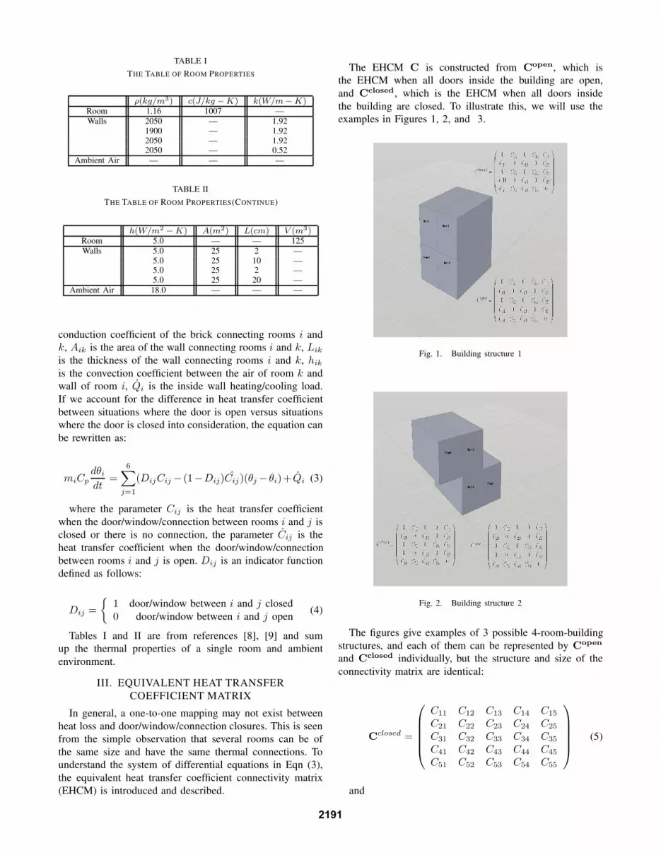
TABLE I

THE TABLE OF ROOM PROPERTIES

ρ(kg/m3) c(J/kg − K) k(W/m − K)Room 1.16 1007 —

Walls 2050 — 1.921900 — 1.922050 — 1.922050 — 0.52

Ambient Air — — —

TABLE II

THE TABLE OF ROOM PROPERTIES(CONTINUE)

h(W/m2− K) A(m2) L(cm) V (m3)

Room 5.0 — — 125

Walls 5.0 25 2 —5.0 25 10 —5.0 25 2 —5.0 25 20 —

Ambient Air 18.0 — — —

conduction coefficient of the brick connecting rooms i and

k, Aik is the area of the wall connecting rooms i and k, Lik

is the thickness of the wall connecting rooms i and k, hik

is the convection coefficient between the air of room k and

wall of room i, Qi is the inside wall heating/cooling load.

If we account for the difference in heat transfer coefficient

between situations where the door is open versus situations

where the door is closed into consideration, the equation can

be rewritten as:

miCp

dθi

dt=

6∑

j=1

(DijCij − (1−Dij)Cij)(θj −θi)+ Qi (3)

where the parameter Cij is the heat transfer coefficient

when the door/window/connection between rooms i and j is

closed or there is no connection, the parameter Cij is the

heat transfer coefficient when the door/window/connection

between rooms i and j is open. Dij is an indicator function

defined as follows:

Dij =

{

1 door/window between i and j closed

0 door/window between i and j open(4)

Tables I and II are from references [8], [9] and sum

up the thermal properties of a single room and ambient

environment.

III. EQUIVALENT HEAT TRANSFER

COEFFICIENT MATRIX

In general, a one-to-one mapping may not exist between

heat loss and door/window/connection closures. This is seen

from the simple observation that several rooms can be of

the same size and have the same thermal connections. To

understand the system of differential equations in Eqn (3),

the equivalent heat transfer coefficient connectivity matrix

(EHCM) is introduced and described.

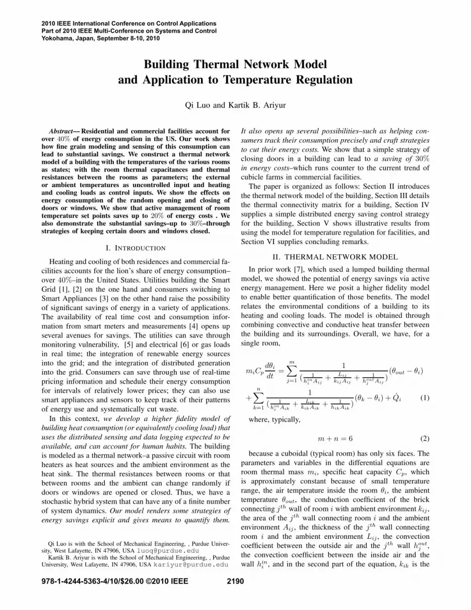
The EHCM C is constructed from Copen, which is

the EHCM when all doors inside the building are open,

and Cclosed, which is the EHCM when all doors inside

the building are closed. To illustrate this, we will use the

examples in Figures 1, 2, and 3.

Fig. 1. Building structure 1

Fig. 2. Building structure 2

The figures give examples of 3 possible 4-room-building

structures, and each of them can be represented by Copen

and Cclosed individually, but the structure and size of the

connectivity matrix are identical:

Cclosed =

C11 C12 C13 C14 C15

C21 C22 C23 C24 C25

C31 C32 C33 C34 C35

C41 C42 C43 C44 C45

C51 C52 C53 C54 C55

(5)

and

2191

Fig. 3. Building structure 3

Copen =

C11 C12 C13 C14 C15

C21 C22 C23 C24 C25

C31 C32 C33 C34 C35

C41 C42 C43 C44 C45

C51 C52 C53 C54 C55

(6)

where the indices 1−4 represent rooms 1−4, and index 5

represents ambient environment. Cij and Cij are constructed

according to the following rules.

Connection: If the rooms i and j (or ambient envi-

ronment) are directly connected, Cij and Cij represents

respectively the equivalent heat transfer coefficient between

rooms i and j (or ambient environment) when the door is

closed or open, Cij and Cij are equation (3). And Cii is

defined to be zero for all i.Non-Connection: If rooms i and j (or ambient environ-

ment) are not directly connected, the equivalent heat transfer

coefficient is zero. The physical meaning is that there is no

direct heat transfer between these regions.

In prior work, we neglected the effect of the open or

closed status of the doors on the building thermal model.

Nevertheless, in a real building, some of the doors are open

and some of them are closed, and the EHCM of the building

C is a combination of elements of Copen and C

closed. We

use the a priori probability of a door being open Popen to

help build up the C matrix for simulation.

Bernoulli distribution of door/window open (closed):

We assume that each door is open (closed) at any time

according to a constant probability Pij (1 − Pij ). Thus,

the doors are either open or closed according to the prob-

abilities in a matrix P, each of whose elements pro-

vides probability of an individual connection being open.

In the frequency interpretation of probability, popenij refers

to the proportion of time in a day in which the door

is open. This also lends itself to simulation, in that we

perform a Monte-Carlo simulation of the building with

C matrices chosen according to the probability matri-

ces and then averaging them to estimate the expected

bill. In doing so, we are assuming ergodicity of stochas-

tic process, i.e., time average, limT→∞

1

T

∫ T

0

∑

Qi dt =

phase space average, E <∑

∫

Qidt >.

In our simulations, we explore the simplest case: Each

room has at most one door and all of them have the same

probability of being open, i.e., all nonzero Pij=Popen, which

can be acquired from the empirical data and used to generate

a random connectivity matrix between the rooms:

Cij =

0 room i and j not directly connected

Cclosedij door between i and j is closed/no door

Copenij open door connecting i and j

(7)

For commercial facilities, some doors open and close more

often and their open probabilities may need to be estimated

individually from data. For residences, however, the C matrix

does not change very often.

IV. CONTROL FOR ENERGY MANAGEMENT

In current building thermal control, the set point of indoor

temperature is always adjusted manually, so it is always the

case that the heater in the room is still on while no one is in

during a specific time period, or the temperature set point can

be relatively high when the real time gas price is at a high

level. Our control goal is to reduce the energy cost of these

situations. The model shows that minimization of heat loss is

equivalent to maximization of energy saving: In steady state,

i.e.

dθi

dt= 0 (8)

for ∀i and

min∑

∫

Qidt ⇔ min∑ ∑

∫

Cij(θi − θj)dt (9)

We assume that temperature control is performed by a

standard on-off controller in the thermostat. The switching

is performed as follows

Qin =

{

Qmax when θseti − θi(t) exceeds δ

0 when θi(t) − θseti exceeds δ

(10)

where δ is the deadzone parameter. In order to maintain

human comfort, we assume that the temperature set-point

θset will lie between a suitable Tmin and Tmax.

Tmin < θset < Tmax (11)

The adaptation of the set-point is performed to reactively

reduce the cost of gas used.

θset = θset + min(0, 1/UA/Pgas(VgasPgas −Cgas)) (12)

The parameters in the above equations are as follows: the

cost of gas per second Cgas; the volume of gas expected

to be consumed Vgas per second; and the cost per volume

2192

unit of gas Pgas, and weighted heat transfer coefficient UA,

which is defined as:

UA =6

∑

i=1

(DijCij − (1 − Dij)Cij) (13)

From these equations, we can set different expected volumes

based on instant gas prices to maintain the bill at a low level.

V. EXAMPLE OF BUILDING THERMAL

NETWORK MODEL

A. An Example of Four Room Building

We first illustrate the advantages of active management for

the 4 room building model in Figure 4. We assume that δ =0.5K in Eqn (10) and Tmin = 288.5K(60F ) and Tmax =300K(80F ) in Eqn (11).

Fig. 4. A simple four room building model

This structure has four rooms with thermal interactions

denoted as Room1-Room4, and have four doors denoted as

Door1-Door4, where Door1 connects Room1 and ambi-

ent, Door2 connects Room2 and Room3, Door3 connects

Room3 and Room4, Door4 connects Room4 and ambient.

If we take into consideration the thermal effect of the

open and closed status of the doors within the building, we

will have the element C15 within the C matrix affected by

the open/closed status of Door1, C12 within the C matrix

affected by the open/closed status of Door2, C35 within the

C matrix affected by the open/closed status of Door3, and

C34 within the C matrix affected by the open/closed status

of Door4. For the purpose of simulation, we assume an

a priori probability Popen = 0.3 that a door is open. We

generate fifty C matrices satisfying the probability condition

and calculate the consumption profile for each of them. We

then calculate the expected consumption profile by averaging

these trajectories. Figures 5 through 8, show the simulation

results. Specifically, Figures 5 and 6 show the building indoor

temperature and gas cost when all doors are closed. Figures 7

and 8 show the building indoor temperature and gas cost

when all doors are open. It can be seen that the thermal

0 100 200 300 400 500 600240

250

260

270

280

290

300

Time, s

T, K

Temperautres of building model (type one) without active control

T(1)T(2)T(3)T(4)T(out)

Fig. 5. Temperatures of building model (all doors closed) without activecontrol

0 100 200 300 400 500 6000

2

4

6

8x 10

4

Time,sH

eat

Com

sum

ption,J

Heat consumption of building model (type one) without active control

0 100 200 300 400 500 6000

1

2

3x 10

−3

Time,s

Bill,$

Bill of advanced building model(type one) with active temperature control

Fig. 6. Heat consumption of building model (all doors closed) withoutactive control

properties of the building have a significant change from all

doors inside closed to all doors inside open. The main reason

is that when the doors open, especially Door1 and Door3,

the major heat exchange method changes from convection

and conduction to diffusion, and the heat loss rate to the

ambient environment increases greatly. Figures 9 and 10

show the building indoor temperature in an instance and

average gas cost when the probability of any door being

open is given by Popen = 0.3.

Figures 11 and 12 show an instance of the inside

temperature of this four room building with active control,

its average heat consumption and gas cost respectively. The

set point is adapted according to Equation (12). Figure 12

shows a cost saving of some 20% compared to Figure 10.

B. Energy Cost vs Number of Open Doors Inside the Build-

ing

In order to analyze the relationship between the energy

cost and the number of open doors inside the building, we

2193

0 100 200 300 400 500 600245

250

255

260

265

270

275

280

285

290

Time, s

T,

K

Temperautres of building model (type two) without active control

T(1)T(2)T(3)T(4)T(out)

Fig. 7. Temperatures of building model (all doors open) without activecontrol

0 100 200 300 400 500 6007.9999

8

8

8

8.0001x 10

4

Time,s

He

at

Co

msu

mp

tio

n,J

Heat consumption of building model (type two) without active control

0 100 200 300 400 500 6000

0.001

0.002

0.003

Time,s

Bill,$

Bill of advanced building model (type two) without active temperature control

Fig. 8. Heat consumption of building model (all doors open) without activecontrol

0 100 200 300 400 500 600240

250

260

270

280

290

300

Time,s

T,

K

Building temperautre without active control

T(1)T(2)T(3)T(4)T(out)

Fig. 9. Building temperature without active control with Popen = 0.3

0 100 200 300 400 500 6000

2

4

6

8x 10

4

Time,s

He

at

Co

msu

mp

tio

n,J

Heat Consumption of Building Without Active Temperature Control

0 100 200 300 400 500 6000

1

2

3x 10

−3

Time,s

Bill,$

Bill of the Building Without Active Temperature Control

Fig. 10. Building heat consumption and bill without active control withPopen = 0.3

0 100 200 300 400 500 600245

250

255

260

265

270

275

280

285

290

295

Time, s

T,

K

Temperautres of advanced building model with active control

T(1)T(2)T(3)T(4)T(out)

Fig. 11. Building temperature with active control with Popen = 0.3

0 100 200 300 400 500 6000

2

4

6

8x 10

4

Time,s

He

at

Co

msu

mp

tio

n,J

Heat consumption of advanced building model with active control

0 100 200 300 400 500 6000

1

2

3x 10

−3

Time,s

Bill,$

Bill of advanced building model with active temperature control

Fig. 12. Building heat consumption and bill with active control withPopen = 0.3

2194

Fig. 13. Building with fifteen Rooms and sixteen Doors

0 2 4 6 8 10 12 14 160.006

0.0065

0.007

0.0075

0.008

0.0085

0.009

Number of doors open

En

erg

y c

ost

$/s

The energy cost vs number of opening doors

Fig. 14. Energy cost vs number of open doors inside the building

simulate a building of fifteen rooms with the structure shown

in Figure 13.

The building has fourteen regular rooms and one corridor

which is treated as the fifteenth room. We plot the energy

cost versus the number of open doors inside the building

in Figure 14. It is clear from the plot that energy cost

increases as the number of doors increases-a whopping 30%in this illustrative example. This is a problem in many

large buildings with a constant traffic at the outside doors,

including the Purdue Mechanical Engineering building. The

specific fast changes of room temperature and overall heater

outputs following door openings and closures, if logged by

a smart building environment control system, will permit

tracking of consumer habits, and indeed specific actions such

as the opening/closing of doors.

VI. CONCLUSIONS AND FUTURE WORK

We have shown how better modeling and more sensors can

help reduce building energy consumption more than 20%.

Our modeling framework, implemented in SIMULINK can

handle arbitrary structures of connectivity within buildings.

It is usable as an optimization tool in smart HVAC systems.

In conjunction with real-time pricing of electricity or gas,

and the temperature preferences of the consumer, the model

can help derive which doors and windows in a building must

be left open or closed.

There are several avenues where we plan to use this model.

The first is to model consumer demand and demand response

of consumers to utility pricing; the second is in identifying

habits of consumption, keeping doors open or closed, from

real-time energy consumption data that may come from smart

metering. The latter will be useful for utilities trying to

balance their loads through the day and night.

However, our assumption of steady state where maximiza-

tion of energy saving is equivalent to minimization of heat

losses may not be valid for commercial facilities where the

EHCM changes randomly and often. That is, commercial

building will always be in a transient; another assumption

we may evaluate is the absence of mass flows and pressure

differences between rooms and between the building and

the ambient, and this becomes important when temperature

differences are large; further analysis needs to be done to

evaluate the building thermal network model in this case.

In the case of central residential heating, flue gas from the

furnace often sent directly into rooms. Hence we may have

to account better for these mass flows.

VII. ACKNOWLEDGMENTS

We wish to acknowledge discussions with Anoop K.

Mathur of Terrafore.

REFERENCES

[1] H. Farhangi, ”The path of the smart grid,” IEEE Power and Energy

Magazine, vol. 8, pp. 18–28, January-February 2010.

[2] Stan M. K., Fred S., Amy A., Jon W., Suedeen G. K., and James J.H., Smart Grid, first edition, The Capitol 2009.

[3] C-Y. Chen, Y-P. Tsou, S-C. Liao, C-T. Lin, ”Implementing thedesign of smart home and achieving energy conservation,” 7th IEEE

International Conference on Industrial Informatics, pp. 273–276,June 23–26, 2009.

[4] R. V. Gerwen, S. Jaarsma and R. W., KEMA, ”SmartMetering”,available at Leonardo Energy Orgnization, July 2006.

[5] Anurag S. and Alexander F., Contingency Screening Techniques And

Electric Grid Vulnerabalities, first edition, VDM Verlag Dr. Muller2008.

[6] Reynaldo N., Electric Power Monitoring with Synchronized Power

Measurements, first edition, VDM Verlag Dr. Muller 2009.

[7] Q. Luo, K. B. Ariyur and A. K. Mathur, ”Real Time EnergyManagement : Cutting the Carbon Footprint and Energy Costs viaHedging, Local Sources and Active Control”, Proceedings of theASME Dynamic Systems and Control Conference, Hollywood, CA,October 2009.

[8] N. Mendes, G. H. C. Oliveira, H. X. Arajo and L. S. Coelho, ”AMATLAB based simulation tool for thermal performance analysis,”8th International IBPSA Conference, pp. 855–862, Eindhoven,Netherlands, August 2003.

[9] M. G. Davies, ”Building Heat Transfer”, John Wiley & Sons,Hoboken, NJ, 2004

2195