Embed Size (px)
Citation preview
Bushfire Surveillance Using DynamicPriority Maps and Swarming Unmanned
Aerial Vehicles
David John Howden,
DipInfTech, BSc(Computer Science andSoftware Engineering)
Swinburne University of Technology2012
A dissertation submitted in fulfilment of the requirements of the degree of
Doctor of Philosophy.

Abstract
Bushfires are large or destructive conflagrations that occur in areas of wilderness, their
remote location serving as a barrier to rapid detection or response. As a result of their
inaccessibility, these fires can grow to unsuppressible proportions and not only cause
significant economic damage to an area, but also endanger the lives of communities and
their fire fighters.
Fast and effective detection is a key factor in bushfire fighting, however fire managers
often have to rely on archaic methods such as humans physically patrolling the fire’s
perimeter. Having accurate knowledge of the status of a bushfire is indispensable for
enabling accurate fire prediction modelling, maintaining the safety of fire fighting crews
and allowing efforts to be focused on areas of the highest risk such as urban areas with
strong human presence.
This problem is ideal for the application of multiple, small unmanned aerial vehicles
(UAVs). For deployment of multiple UAVs to be practical, a method for controlling
their actions autonomously and cooperatively is required. The field of swarm intelligence
deals with systems of multiple agents which can collaborate on tasks without need for
a centralised controller or group-wide coordination. Inspiration for these systems, and
name of the field, is from animal swarms found in nature such as ant colonies or flocks
of birds.
The advantages of deploying UAVs as a swarm include massive scalability, low commu-
nication overheads, reduced need for human supervision, and resilience against individ-
ual failure. A promising branch of inquiry into swarm control algorithms is biomimicry,
specifically the use of artificial pheromone.
Using digital pheromone maps to represent the environment a swarm occupies allows
the combination of information sharing and collective decision making elements of swarm
behaviour into a single intuitive concept. With the problem of detecting and then
monitoring bushfires in an area without the infrastructure needed to provide long range
communication, individual pheromone maps need to be stored on-board. Maps can then
be communicated via short range broadcasts to synchronising environment knowledge
i
and direct further surveillance.
This dissertation presents a swarm intelligence approach to exhaustive and continuous
surveillance of large areas. Using priority maps, a technique inspired by pheromone,
landmarks and features can be assigned priorities relative to their value or risk, either
on deployment or dynamically in reaction to observations. Due to the remoteness and
volatility of bushfires, the algorithm is resilient against loss of vehicles and does not
require established communication infrastructure.
ii
Acknowledgements
Professional
With sincere and profound gratitude, I thank my advisor and friend, Professor Tim
Hendtlass. Without Tim’s, frankly, extraordinary advocacy and support, this thesis
would not exist, and I would not be where I am today. As an undergraduate, Tim’s
childlike wonder and boundless enthusiasm inspired the same from us, his students. Even
then, his door was always open and he, without exception, made time to humour my
eager but undirected interest in artificial intelligence and postgraduate research. It was
during one of these chats, while Tim was off on one of his famous tangents, that the
problem which was to become my thesis topic first came up.
As a graduate advisor Tim was nothing short of exemplary. When I was inexplicably
disqualified from receiving a scholarship due to bureaucratic oversight, he went to bat
on my behalf, appealing the decision at every level. After all avenues at had been
exhausted and Swinburne Research reasserted their intention to deny me the ability
to even apply for funding (despite using my work, and I, in multiple public relation
campaigns as an example of the “excellent research being done at Swinburne”) Tim
took the extraordinary step of assuming complete responsibility for my sponsorship.
Tim’s hands-off style of advising helped me grow as a confident, independent academic,
while his eagerness to listen to any problem I may have had, or even just to idly chat
while clearing my mind, meant at the same time I never felt lost or without a safety net.
Going forward from this point into my career as an academic, I have a duty to treat any
student who may come to me looking for advice or support with the same patience and
generosity that was afforded to me.
Dr. James Montgomery, you are an outstanding advisor, and an even better drinking
buddy. Some of my fondest memories of Swinburne involve hallway to office conversa-
tions long after everyone else had left for the night, where we still felt like we should
actually get some work done, or us drinking, resigned to the fact that it just wasn’t
going to happen. Your almost inhuman ability to locate and correct grammatical flaws
iii
in my work, over the course of what feels like a dozen drafts, has resulted in a standard
of quality I would not have achieved in a lifetime working alone.
Dr. Clinton Woodward, perhaps unknowingly, you’ve taught me as much about how
to teach and engage students as you did about the subject matter itself. Working with
you as a teaching assistant was always genuinely fun, and is a significant part of how
I realised that teaching could be satisfying, and not just a chore to be suffered so one
could get back to research. On the topic of research, your ability to simultaneously
see extensions to the big picture while keeping an eye for detail was invaluable. I am
specifically grateful for your advice and suggestions when it came to visualising concepts
I was struggling to describe in words alone.
Dr. Jason Brownlee, while I don’t think I will ever be able to match your almost
machine like motivation, dedication, and personal drive, it gives me a goal to aim for.
Your insight into problems I’ve had along the way (as often over drinks as not) was
always invaluable, and allowing me opportunities to collaborate on your endless personal
projects has always felt like it was more of a boon to me than you.
On a personal note...
My mother, Karen Fraser, who, despite our continued disagreement over how long in
front of a computer is too long (never, it’s never too long), did everything in her power
to push me to succeed. It was through your countless trips to museums, availability
of educational media, and enrolment in various extension classes and extracurricular
activities that my interest in science first developed.
Finally, I would like to express gratitude to, and appreciation of, my father, Kevin
Howden. I have lost count of the number of times you have pulled my chestnuts out
of the fire during the course of my postgraduate experience. Knowing that you were
there, proud and in the background, in case I ever got myself in too far over my head,
allowed me to take risks and push myself further than would have been possible alone.
While Tim made the work possible, the knowledge that I had your support, if and when
I needed it, allowed me to enjoy the ride.
iv
Declaration of Originality
I hereby declare that this dissertation contains no material which has been accepted for
the award of any other degree or diploma, except where due reference is made; that to
the best of the my knowledge this dissertation contains no material previously published
or written by another person except where due reference is made; and that where work
is based on joint research or publications, the relative contributions of the respective
authors has been disclosed.
David John Howden
v

Contents
1. Introduction 1
1.1. Bushfires . . . . . . . . . . . . . . . . . . . . . . . . . . . . . . . . . . . . 1
1.2. Unmanned Aerial Vehicles . . . . . . . . . . . . . . . . . . . . . . . . . . 2
1.3. Swarm Intelligence . . . . . . . . . . . . . . . . . . . . . . . . . . . . . . 5
1.4. Flocking and Stigmergy . . . . . . . . . . . . . . . . . . . . . . . . . . . 8
1.5. Summary . . . . . . . . . . . . . . . . . . . . . . . . . . . . . . . . . . . 9
2. Existing Work 11
2.1. Potential Fields . . . . . . . . . . . . . . . . . . . . . . . . . . . . . . . . 11
2.2. Pheromone . . . . . . . . . . . . . . . . . . . . . . . . . . . . . . . . . . 12
2.3. Realised Swarm Robotics . . . . . . . . . . . . . . . . . . . . . . . . . . . 15
2.3.1. Beckers . . . . . . . . . . . . . . . . . . . . . . . . . . . . . . . . 15
2.3.2. Pherobots . . . . . . . . . . . . . . . . . . . . . . . . . . . . . . . 15
2.3.3. I-SWARM . . . . . . . . . . . . . . . . . . . . . . . . . . . . . . . 16
2.3.4. iRobot SwarmBots . . . . . . . . . . . . . . . . . . . . . . . . . . 16
2.3.5. PheGMot . . . . . . . . . . . . . . . . . . . . . . . . . . . . . . . 17
2.4. Implementation Issues with UAV Swarms . . . . . . . . . . . . . . . . . . 17
2.4.1. Spatial Awareness . . . . . . . . . . . . . . . . . . . . . . . . . . . 18
2.4.2. Control . . . . . . . . . . . . . . . . . . . . . . . . . . . . . . . . 19
2.5. Summary . . . . . . . . . . . . . . . . . . . . . . . . . . . . . . . . . . . 19
3. Distributed Priority Maps 21
3.1. Proposed Algorithm . . . . . . . . . . . . . . . . . . . . . . . . . . . . . 21
3.1.1. Detailed Description . . . . . . . . . . . . . . . . . . . . . . . . . 22
3.2. Algorithm Concepts and Modifications . . . . . . . . . . . . . . . . . . . 23
3.2.1. Diversity . . . . . . . . . . . . . . . . . . . . . . . . . . . . . . . . 23
3.2.2. Heuristics . . . . . . . . . . . . . . . . . . . . . . . . . . . . . . . 24
3.3. Pheromone Map versus Priority-Time Map . . . . . . . . . . . . . . . . . 25
vii
Contents
3.4. Summary . . . . . . . . . . . . . . . . . . . . . . . . . . . . . . . . . . . 26
4. Simulation Setup 27
4.1. Environmental Representation and Perception . . . . . . . . . . . . . . . 27
4.2. Node Spacing . . . . . . . . . . . . . . . . . . . . . . . . . . . . . . . . . 28
4.3. UAV Specifications . . . . . . . . . . . . . . . . . . . . . . . . . . . . . . 29
4.4. Simulator Limitations: Granularity and Abstractions . . . . . . . . . . . 29
4.5. Fire Simulation . . . . . . . . . . . . . . . . . . . . . . . . . . . . . . . . 30
4.6. Summary . . . . . . . . . . . . . . . . . . . . . . . . . . . . . . . . . . . 32
5. Performance Baselines 33
5.1. Baseline Calculation . . . . . . . . . . . . . . . . . . . . . . . . . . . . . 33
5.2. Scaling with Swarm Size . . . . . . . . . . . . . . . . . . . . . . . . . . . 34
5.3. Stable States . . . . . . . . . . . . . . . . . . . . . . . . . . . . . . . . . 36
5.4. Patterns . . . . . . . . . . . . . . . . . . . . . . . . . . . . . . . . . . . . 37
5.5. Summary . . . . . . . . . . . . . . . . . . . . . . . . . . . . . . . . . . . 39
6. Varied Priority Levels 41
6.1. Complex Environments . . . . . . . . . . . . . . . . . . . . . . . . . . . . 43
6.2. Null Priority and No-Fly Zones . . . . . . . . . . . . . . . . . . . . . . . 46
6.3. Summary . . . . . . . . . . . . . . . . . . . . . . . . . . . . . . . . . . . 49
7. Target detection and tracking 51
7.1. Fire location . . . . . . . . . . . . . . . . . . . . . . . . . . . . . . . . . . 51
7.2. Fire tracking . . . . . . . . . . . . . . . . . . . . . . . . . . . . . . . . . . 52
7.3. Secondary Fire Detection . . . . . . . . . . . . . . . . . . . . . . . . . . . 55
7.4. Discreet Mobile Targets . . . . . . . . . . . . . . . . . . . . . . . . . . . 58
7.5. Summary . . . . . . . . . . . . . . . . . . . . . . . . . . . . . . . . . . . 61
8. Communication 63
8.1. Scaling with Communication . . . . . . . . . . . . . . . . . . . . . . . . . 63
8.2. Information Flow . . . . . . . . . . . . . . . . . . . . . . . . . . . . . . . 65
8.2.1. Data Synchronisation . . . . . . . . . . . . . . . . . . . . . . . . . 66
8.3. Not All Communication Is Good . . . . . . . . . . . . . . . . . . . . . . 69
8.3.1. Deterministic versus Stochastic Behaviours . . . . . . . . . . . . . 73
8.4. Communication Failure . . . . . . . . . . . . . . . . . . . . . . . . . . . . 74
8.5. Summary . . . . . . . . . . . . . . . . . . . . . . . . . . . . . . . . . . . 76
viii
Contents
9. Comparative Results 77
9.1. Exhaustive Swarming Search Strategy . . . . . . . . . . . . . . . . . . . . 77
9.2. Uniform Map . . . . . . . . . . . . . . . . . . . . . . . . . . . . . . . . . 79
9.3. Lake Map . . . . . . . . . . . . . . . . . . . . . . . . . . . . . . . . . . . 80
9.4. No-Fly Zone Map . . . . . . . . . . . . . . . . . . . . . . . . . . . . . . . 82
9.5. Analysis of Comparative Results . . . . . . . . . . . . . . . . . . . . . . . 84
9.6. Summary . . . . . . . . . . . . . . . . . . . . . . . . . . . . . . . . . . . 85
10.Conclusions and Final Remarks 87
10.1. Summary . . . . . . . . . . . . . . . . . . . . . . . . . . . . . . . . . . . 87
10.2. Research Contributions . . . . . . . . . . . . . . . . . . . . . . . . . . . . 88
10.3. Future Work . . . . . . . . . . . . . . . . . . . . . . . . . . . . . . . . . . 89
Appendices 99
A. Glossary 103
B. Comparison of Currently Deployed Unmanned Aircraft Systems 105
C. Publications Arising from this Study 107
ix

List of Figures
1.1. Collection of small US Navy unmanned aerial vehicles . . . . . . . . . . . 3
1.2. Local, and consensus, autonomy levels . . . . . . . . . . . . . . . . . . . 5
2.1. Pheromone maps for swarm robotics overlay a digital grid over the envi-
ronment. . . . . . . . . . . . . . . . . . . . . . . . . . . . . . . . . . . . . 13
4.1. Calculation of optimal node separation . . . . . . . . . . . . . . . . . . . 28
4.2. Anatomy of a bushfire: head, back, and flank fires . . . . . . . . . . . . . 31
4.3. Satellite view of Wilson’s Promontory, an Australian national park . . . . 32
5.1. Method for approximating the maximum survey speed of a UAV . . . . . 34
5.2. Decrease in average survey time with increased UAVs . . . . . . . . . . . 35
5.3. Average survey time of the algorithm as a percentage of baseline . . . . . 35
5.4. Increase in pheromone and subsequent levelling off at a stable state . . . 36
5.5. UAVs exhibiting edge following behaviour on the first pass of a uniform
map . . . . . . . . . . . . . . . . . . . . . . . . . . . . . . . . . . . . . . 37
5.6. Scale representation of the path a UAV follows when all non-surveyed
nodes have the same pheromone level . . . . . . . . . . . . . . . . . . . . 38
5.7. Typical sequence of moves for a UAV . . . . . . . . . . . . . . . . . . . . 38
5.8. Diagonal movement when node spacing is smaller than the survey radius 39
5.9. An example of diagonal moves leading to interesting, yet unstable, spi-
ralling behaviour. . . . . . . . . . . . . . . . . . . . . . . . . . . . . . . . 40
6.1. Priority map with two priority levels . . . . . . . . . . . . . . . . . . . . 41
6.2. Average survey period of the baseline and simulation results using the
two priority map . . . . . . . . . . . . . . . . . . . . . . . . . . . . . . . 42
6.3. Average survey period on the two priority map as a proportion of the
baseline value . . . . . . . . . . . . . . . . . . . . . . . . . . . . . . . . . 42
6.4. Priority map with four priority levels . . . . . . . . . . . . . . . . . . . . 43
xi
List of Figures
6.5. Priority map with eight priority levels . . . . . . . . . . . . . . . . . . . . 44
6.6. Average survey period of the eight priority level environment, broken
down into individual priority zones. . . . . . . . . . . . . . . . . . . . . . 44
6.7. Effect of UAV density on survey ratios . . . . . . . . . . . . . . . . . . . 45
6.8. Increasing severity of priority levels on identically sized environments to
increase local agent density . . . . . . . . . . . . . . . . . . . . . . . . . . 46
6.9. Heat maps generated using the eight priority map . . . . . . . . . . . . . 47
6.10. Comparison of heat maps after the priority map is rearranged into a more
difficult to survey arrangement . . . . . . . . . . . . . . . . . . . . . . . . 48
6.11. Comparison of the three different priority map configurations proportion-
ate to baseline performance . . . . . . . . . . . . . . . . . . . . . . . . . 49
7.1. Average detection time of targets based on location . . . . . . . . . . . . 51
7.2. Average detection time of targets in a map with two priority levels . . . . 52
7.3. Average detection time of fires at the edge of the search space using a
scaled priority map . . . . . . . . . . . . . . . . . . . . . . . . . . . . . . 53
7.4. Progressive images of the simulation in progress . . . . . . . . . . . . . . 54
7.5. Comparison of the percentage of fire area discovered using two different
classes of UAVs . . . . . . . . . . . . . . . . . . . . . . . . . . . . . . . . 55
7.6. Progressive images of the secondary fire simulation in progress. . . . . . . 56
7.7. Percentage of fires found using the secondary fire simulation with grass
and forest fires . . . . . . . . . . . . . . . . . . . . . . . . . . . . . . . . 57
7.8. Forest fire: difference in detection between the primary waypointed and
secondary unknown fire for various priority levels . . . . . . . . . . . . . 57
7.9. Grass fire: difference in detection between the primary waypointed and
secondary unknown fire for various priority levels . . . . . . . . . . . . . 58
7.10. Elapsed time before initial detection of targets in a square 22.5 km envi-
ronment . . . . . . . . . . . . . . . . . . . . . . . . . . . . . . . . . . . . 59
7.11. Percentage of time during the simulation that the swarm knew the target’s
location . . . . . . . . . . . . . . . . . . . . . . . . . . . . . . . . . . . . 60
7.12. Average pheromone of the nodes directly under targets . . . . . . . . . . 60
8.1. Communication effects on average survey period . . . . . . . . . . . . . . 64
8.2. Diminishing returns on communication range over large environments . . 64
8.3. Convergence of environment pheromone level and pheromone level of
nodes which are synchronised . . . . . . . . . . . . . . . . . . . . . . . . 67
xii
List of Figures
8.4. Effect of communication period on synchronisation level and environment
pass time . . . . . . . . . . . . . . . . . . . . . . . . . . . . . . . . . . . 68
8.5. Percentage of synchronised nodes given varying communication periods . 68
8.6. Average search time, scaled relative to a swarm with zero communication 70
8.7. Communication period scaled by environment size and communication
range . . . . . . . . . . . . . . . . . . . . . . . . . . . . . . . . . . . . . . 70
8.8. Communication period scaled by environment size and swarm size . . . . 71
8.9. Agent density divided by communication range . . . . . . . . . . . . . . 72
8.10. Variance in pheromone levels when adding random noise to the pheromone
map in a sparsely populated environment . . . . . . . . . . . . . . . . . . 73
8.11. Time between surveys of high priority nodes as a function of how fre-
quently one UAV broadcasts random pheromone information . . . . . . . 74
8.12. The time between surveys of medium priority nodes as a function of how
frequently one UAV broadcasts random pheromone information . . . . . 75
8.13. The time between surveys of low priority nodes as a function of how
frequently one UAV broadcasts random pheromone information. . . . . . 75
9.1. Flowchart for the behaviour of Erginac’s algorithm . . . . . . . . . . . . 78
9.2. An example of emergent contour following observed during the execution
of Algorithm E using a uniform map. . . . . . . . . . . . . . . . . . . . . 79
9.3. Comparative average mean times of Algorithms E and H, since cell’s last
visit . . . . . . . . . . . . . . . . . . . . . . . . . . . . . . . . . . . . . . 80
9.4. Lake map featuring four priority levels, inclusive of null priority areas . . 81
9.5. Comparative average survey times using the lake map . . . . . . . . . . . 81
9.6. Mean time since visit for highest priority areas using the lake map . . . . 82
9.7. No-fly zone map featuring four priority levels, inclusive of no-fly areas . . 83
9.8. Mean time since visit for highest priority areas using the no-fly zone map 83
9.9. Heatmaps of node surveys for the no-fly zone map . . . . . . . . . . . . . 84
xiii

1. Introduction
1.1. Bushfires
Bushfires are conflagrations that start in remote undeveloped areas of the environment,
and have the potential to spread out of control causing immense damage. Bushfires, also
know as wildfires or forest fires in different parts of the world, differ from other fires in
that the wooded areas they originate in serve as an abundant source of fuel. As bushfires
more often occur during summer months, and with greater frequency during droughts,
fuel is often desiccated and extremely combustible, allowing an unmanaged fire to turn
into a firestorm. During a firestorm, a bushfire generates its own self-sustaining weather
system: hot deoxygenated air evacuates upwards fast enough to draw in fresh air from
surrounding areas, serving to feed the fire with yet more oxygen. The radiant heat
(infrared radiation) of a firestorm is great enough to ignite fuel at a significant distance
ahead of the fire front itself (Cheney and Sullivan 2008). Under such circumstances
bushfires can result not only in property and environmental damage but severe loss of
human life.
Due to its unique environment, Australia is one of the most bushfire prone countries in
the world, disaster-level bushfires1 alone causing an average of A$77,000,000 of damage
a year (Bureau of Transport Economics 2001; Ganewatta and Handmer 2006). The most
significant reason that bushfires so frequently result in this level of destruction is due to
the limited accessibility of the ‘undeveloped’ forested or mountainous regions in which
ignition often occurs. Before fire management can fully mobilise an incident can already
be at an unmanageable size, at which point it can easily spread and threaten nearby
populated areas.
The way that fires spread can be modelled with a damage-time function showing the
amount of damage caused increasing exponentially the longer the fire is allowed to burn
(Restas 2006a). With this in mind, the speed with which fire management can begin is
1The Bureau of Transport Economics (2001) defines disaster-level bushfires as those with a totalinsurance cost of more than A$10,000,000.
1
Chapter 1: Introduction
often the decisive factor in how much much damage a fire causes. To begin fire fighting in
earnest, fire management requires three things. First, the fire manager needs to discover
that there is a fire in progress. Second, men and equipment need to reach the fire and,
third, preliminary reconnaissance needs to be performed.
Reconnaissance is the most important initial activity by fire fighters arriving on the
scene. Knowledge of the fire’s extent and status is necessary both for the safety of
personnel on the ground and for accurate fire modelling for use in efficiently allocating
resources. The problem with this is that reconnaissance too often requires actually
touring the affected area and the terrain is unlikely to allow for ground vehicles to
be used effectively. The cost of manned aircraft is prohibitive so they are not usually
deployed until after the initial reconnaissance suggests that it is necessary. Satellite fire
imaging may seem like a promising alternative, but because of the polar orbit used by
weather satellites and current technological limitations, they are best used for strategic
observations.2
Strategic observations provide a regional view of the fire’s progress, a mission often
best suited to weather satellites equipped with radiometers and fire detection algorithms
(Kant et al. 2000). Tactical observations on the other hand are ideally localised, frequent
and more detailed (Ambrosia et al. 2003), being traditionally performed by fire fighters
on the ground. However, even assuming conditions allow for fire fighters to arrive while
the fire is still contained within an optimistic 150 metre radius, there will already exist
a perimeter of over a kilometre which needs to be surveyed. This process takes time,
and as described the longer a fire is allowed to burn uncontrolled, the faster it spreads.
Additionally, as observations are performed manually by individual fire commanders,
subjectivity can become a factor, distorting the information the fire manager has to
work with.
1.2. Unmanned Aerial Vehicles
Fire managers are interested in possible applications of unmanned aerial vehicles (UAVs)
for use reconnoitring fires which are in progress, as well as the initial detection of igni-
tions. A UAV is essentially any vehicle that can fly without a human pilot on board,
ranging from the remote controlled helicopters purchasable from toy stores to the General
Atomics MQ-9 Reaper, a four and a half tonne semi-autonomous war plane. Generally
speaking however, the most common type of UAVs are aeroplanes with an approxi-
2A satellite on a polar orbit has a round trip time of nine hours.
2
Chapter 1: Introduction
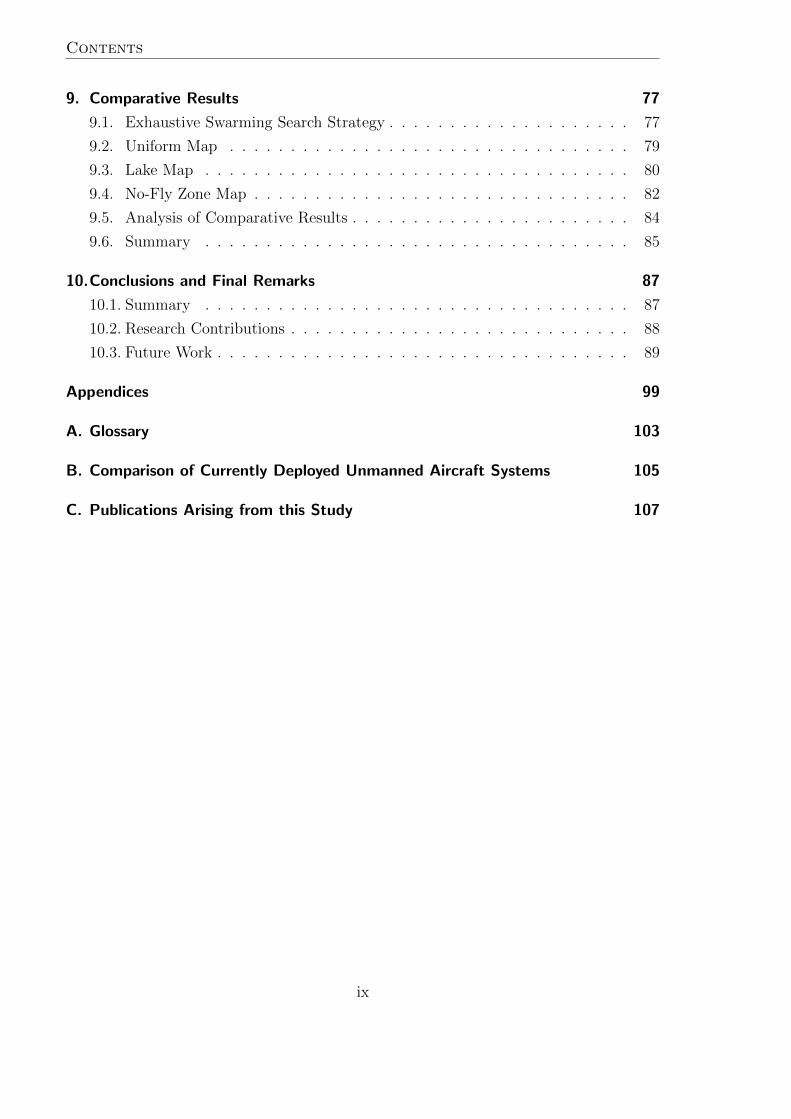
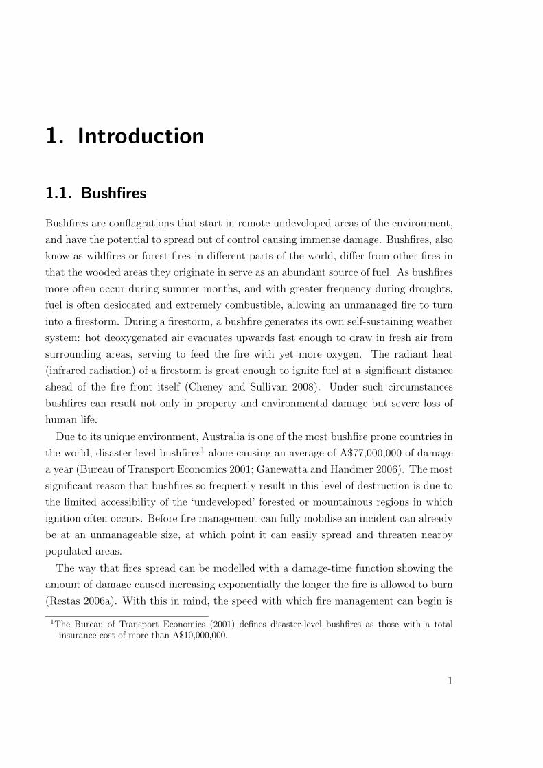
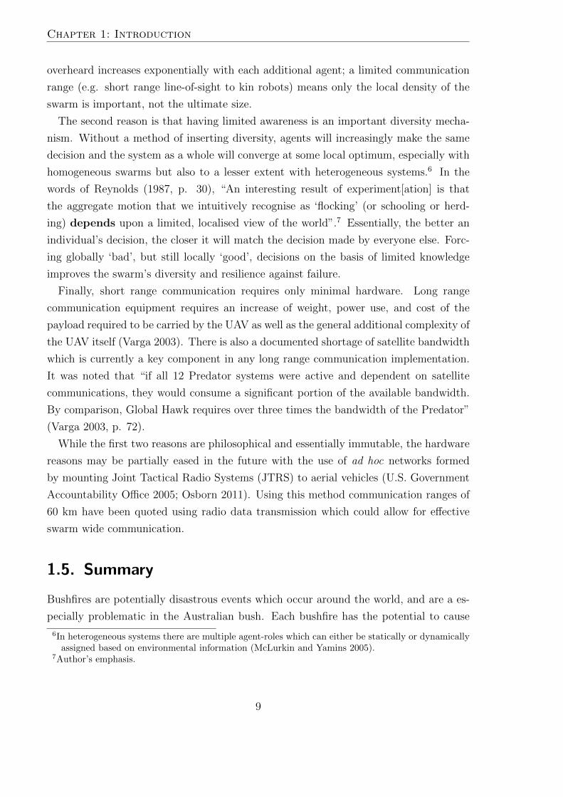
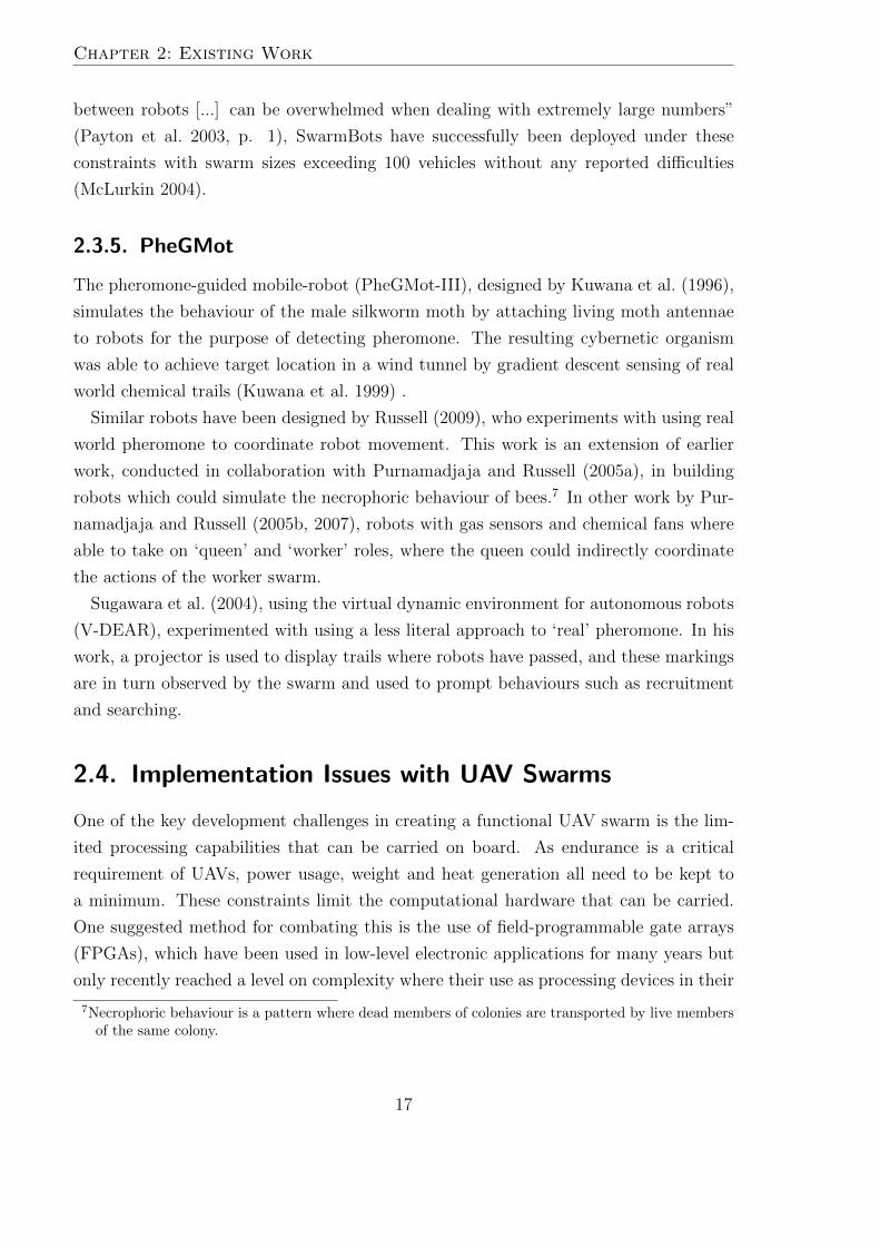
Figure 1.1.: Collection of small US Navy unmanned aerial vehicles, the largest of whichbeing the RQ-2B Pioneer with a wingspan of 5 metres (Source: public do-main image from http://www.navy.mil, 2005)
mate wingspan of three meters, with partial autonomy, a number of which are shown in
Figure 1.1.
Autonomy, in reference to UAVs, is the ability for the vehicle to fly itself through
application of on-board artificial intelligence algorithms. Due to technological limitations
and safety regulations, even UAVs which are capable of fully autonomous operation
have historically been limited to use as remote controlled platforms piloted by humans.
This state of affairs is slowly changing with initiatives like the ASTRAEA programme,
which has brought together a consortium of major aerospace companies for the purpose
of developing UAV certification, and the UK’s document CAP 722–Unmanned Aerial
Vehicle Operations in UK Airspace: Guidance which for the first time provides guidelines
for verifying autonomous vehicles for use in unrestricted airspaces (Hutchings et al. 2007;
United Kingdom Central Authority 2004).
There are many reasons for interest in UAVs as both a replacement for traditional
aeroplanes, as well as in entirely new domains. The main advantages for UAVs come
from a value standpoint: small UAVs can be purchased for A$5,000 to A$10,000, while
traditional light aircraft start at A$100,000. These values do not factor in the costs
of hiring certified commercial pilots and maintaining the vehicle to meet the additional
safety regulations required for carrying humans. This reduced cost and lack of human
presence is what leads UAVs to be ideal for tasks which are “Dull, Dirty (or) Dangerous”
(Barber et al. 2006, p. 1).
In most cases the missions that UAVs would be used for, when abstracted, have the
unifying goal of searching a bounded problem space. Work in this field has so far been
3
Chapter 1: Introduction
mostly focused on discrete searches, where one or more targets exist within an area, and
once they are located the search is complete. The discrete search approach is sensible for
missions such as search and rescue, mapping a static area such as in agricultural survey-
ing, battle damage assessment (BDA), and for short duration Intelligence, Surveillance
and Reconnaissance (ISR) missions (Sauter et al. 2005). Continuous state-space explo-
ration (i.e. surveillance), such as would be required for problems such as fire spotting,
border surveillance, or long duration ISR missions, is a research area with a smaller
body of published work.
The idea of utilising aerial surveillance to reconnoitre wildfires is an old one, as replac-
ing ground crews in reconnaissance would mean the effect of rugged terrain on survey
time was negated. However, getting a manned aeroplane to the scene of a wildfire both
takes too long for the initial survey and is not cost effective for monitoring the progress
of the fire if the initial survey showed it to be a minor event.3 At the other extreme,
where a wildfire has grown out of control and generates a firestorm, the use of a manned
aircraft is warranted though the environment posses an inherent danger to the vehicle
and pilot. It is apparent then that depending on the state of the fire, this reconnaissance
can fall into either the previously mentioned “dull” or “dangerous” category, making fire
reconnaissance an ideal application for UAVs.
Preparatory work for the first deployment of a UAV for fire monitoring in operational
service was done by Restas (2006a). Of the more interesting things found by getting
the equipment into the hands of actual fire fighters was that not only were black and
white images of the fire’s progress sufficient, it was even claimed that black and white
was preferable to coloured images for the sake of clarity. The online experiments also
proved the utility of having a UAV for fire spotting when an unknown secondary fire was
discovered while using the UAV to observe a current fire which was in progress. Benefits
aside, Restas also pointed out the limitations of a single UAV in that it is insufficient
for large fires, and that while fire monitoring was accomplished, it was unsuccessful at
conducting fire spotting patrols.
The advantages of using multiple UAVs over a single platform are similar to the
original advantages of using a UAV instead of a manned vehicle; namely that if there
is danger involved, having multiple vehicles is preferable due to redundancy, so that
the loss of an individual does not have an inordinate effect on mission performance.
Secondly the response time issue, where an on-site UAV is able to reach a fire quicker
3Wildfires are reasonably frequent, and the extinction of a medium-sized forest fire generally takesfrom a couple of hours to a day (Restas 2006b).
4
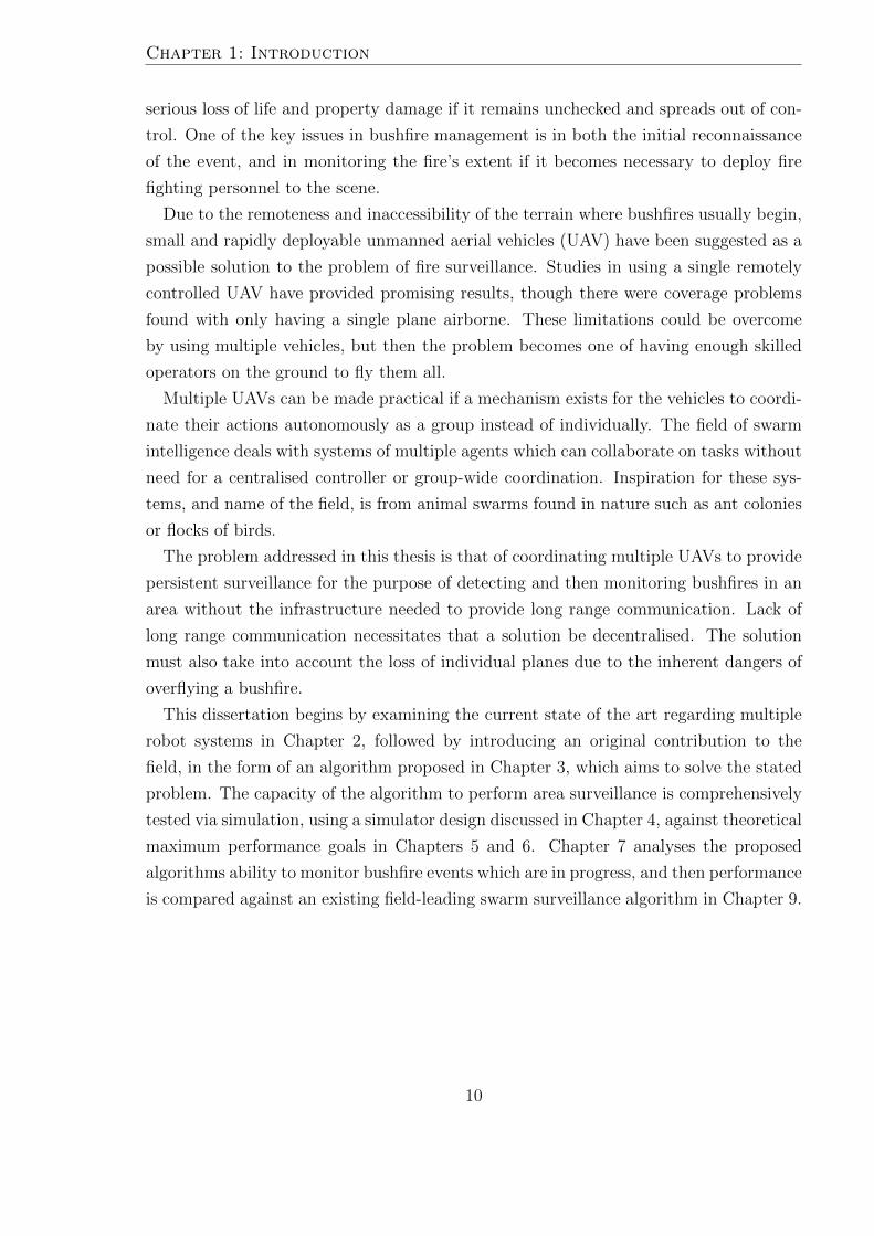
Chapter 1: Introduction
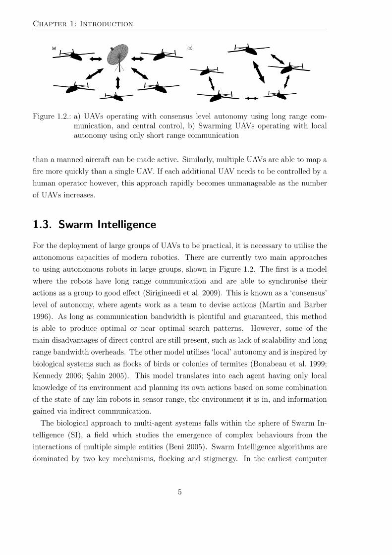
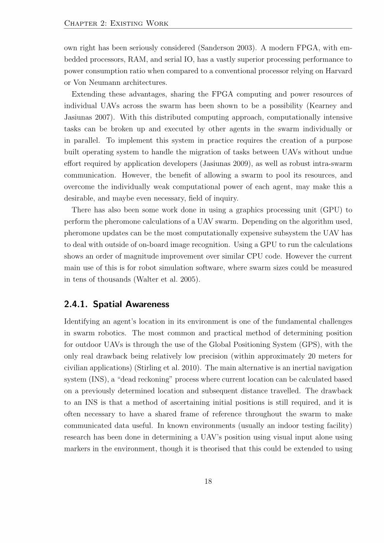
Figure 1.2.: a) UAVs operating with consensus level autonomy using long range com-munication, and central control, b) Swarming UAVs operating with localautonomy using only short range communication
than a manned aircraft can be made active. Similarly, multiple UAVs are able to map a
fire more quickly than a single UAV. If each additional UAV needs to be controlled by a
human operator however, this approach rapidly becomes unmanageable as the number
of UAVs increases.
1.3. Swarm Intelligence
For the deployment of large groups of UAVs to be practical, it is necessary to utilise the
autonomous capacities of modern robotics. There are currently two main approaches
to using autonomous robots in large groups, shown in Figure 1.2. The first is a model
where the robots have long range communication and are able to synchronise their
actions as a group to good effect (Sirigineedi et al. 2009). This is known as a ‘consensus’
level of autonomy, where agents work as a team to devise actions (Martin and Barber
1996). As long as communication bandwidth is plentiful and guaranteed, this method
is able to produce optimal or near optimal search patterns. However, some of the
main disadvantages of direct control are still present, such as lack of scalability and long
range bandwidth overheads. The other model utilises ‘local’ autonomy and is inspired by
biological systems such as flocks of birds or colonies of termites (Bonabeau et al. 1999;
Kennedy 2006; Sahin 2005). This model translates into each agent having only local
knowledge of its environment and planning its own actions based on some combination
of the state of any kin robots in sensor range, the environment it is in, and information
gained via indirect communication.
The biological approach to multi-agent systems falls within the sphere of Swarm In-
telligence (SI), a field which studies the emergence of complex behaviours from the
interactions of multiple simple entities (Beni 2005). Swarm Intelligence algorithms are
dominated by two key mechanisms, flocking and stigmergy. In the earliest computer
5
Chapter 1: Introduction
simulations of flocking (Heppner and Grenander 1990; Reynolds 1987), it was demon-
strated that complex behaviours exhibited by groups of individually simple creatures
could be replicated via very simple rule-based algorithms. In Reynold’s seminal work on
Boids4 the flocking behaviour of birds was simulated, fundamentally, by simply having
each individual Boid agent try to maintain an optimal distance from its neighbours. Go-
ing a little deeper, this optimal distance was calculated through three interacting forces:
separation, alignment, and cohesion. Separation pushes the Boid away from its closest
neighbour, alignment steers the Boid’s heading to try and match that of its neighbours,
and cohesion pulls the Boid towards the flock’s centre of mass. It is the interaction of
these rules with each other from which the desired flocking behaviour emerges. While
originally designed as an exercise in computer graphics, it would later serve as inspira-
tion for algorithms in other fields, including the well known Particle Swarm Optimisation
(PSO) (Kennedy and Eberhart 1995).
PSO exists at the other end of the swarm intelligence abstraction spectrum; a meta-
heuristic which uses a swarm of particles to ‘fly’ through a fitness landscape and converge
on a good solution. Each particle is initialised with a random position and velocity, and
‘remembers’ the its best found value and position which had resulted in that value.
Upon each update of the algorithm, particles accelerate towards the best position they
have personally seen, as well as the best position seen by any particle in the swarm. The
algorithm, while extremely simple, is surprisingly effective at optimising a wide range of
functions. Unifying these two examples, along with other algorithms in the field of SI,
are certain traits (Parunak 1997):
• Small Agents - Individual agents are not a large or irreplaceable part of the
whole, giving rise to resilience and resistance to loss.
• Short Sighted - Agents make decisions predominantly based on knowledge of
their immediate surroundings. They do not make long term plans or individually
keep detailed histories.5
• Decentralised - Decisions are made by the individual, on an agent-by-agent basis.
Swarms never have a centralised control structure.
These traits on their own suffice to produce a collection of simple, independent indi-
viduals but will not result in the emergent behaviours which are symbolic of a swarm.
4The name Boids refers to Bird-like objects.5This does not preclude modification of the environment to collectively store information as this is
communal rather than individual.
6
Chapter 1: Introduction
The following additional traits, also suggested by Parunak, are what enable emergent
behaviour:
• Ability to Share Information - For agents to interact with each other, there
needs to be some mechanism to spread information. This can be as simple as an
agent observing where a peer is in relation to itself and the environment, to the
pheromone trails left by ant colonies or the waggle dance done by bees (Frisch
1967).
• Diversity Mechanism - A homogeneous collection of individuals, sharing knowl-
edge and behavioural rules, is prone to rapid convergence. To counteract this, a
method of injecting diversity is a vital yet subtle element to emergent behaviours.
At a minimum this usually means the presence of a stochastic process (i.e. a
random element).
While “small, simple, decentralised individuals” describes what a swarm is, the hidden
complexity and emergent behaviours are the result of communal information flow and
counteracting diversity processes. Broadly speaking there are two main types of swarm:
flocks, and colonies. Reynolds (1987) put forward that, at a minimum, to be considered
a flock, agents need to know the relative direction and distance to at least some of their
neighbours. This spatial awareness of kin agents is all the information spread that is
required for a flock to function, however some colony type swarms are able to function
without even this basic information. In colonies, communication is most often done
through modifying the environment itself, a mechanism known as stigmergy.
Stigmergy as a term was first coined by Grasse in 1959 in relation to the nest building
behaviour of termite colonies (Grasse 1959). Termites will occasionally scoop up a ball of
earth which is then coated with pheromone and dropped at random. However if there is
already a pheromone coated mud ball nearby, there is an increased chance that the second
will be placed alongside. As this stack increases in size and the corresponding quantity
of pheromone grows, so does the chance it will be further added to, which eventually
results in a structured termite mound, complete with arches and chambers. This first
action of placing a mud ball which cascades into a full termite mound is an example of a
positive feedback loop, a frequent result of stigmergic communication (Izquierdo-Torres
2004). Thus while a colony is made up of individual termites seemingly pursuing their
own interests, the shape and state of their surrounding environment influences their
actions and enables swarm wide coordination.
7
Chapter 1: Introduction
Positive feedback behaviours are often beneficial in the short term but must be bal-
anced by a diversity mechanism (negative feedback) to enable the system as a whole to
continue to function over the long term. In the termite example the pheromone which
was added to the mud balls evaporates over time, eventually disappearing entirely. Other
common diversity mechanisms are repulsion from other agents, limiting the agent’s scope
to a local subset of the environment, and stochastic elements in the control algorithms
(e.g. the ‘random’ nature of the termite’s actions).
As with the Boids/PSO flocking example, stigmergic systems were abstracted to in-
spire algorithm design. The earliest work on ant based systems was by Ebling et al.
(1989), with the most commonly cited algorithm in this sub-category being Ant Colony
Optimisation (ACO) described by Dorigo et al. (1996). In ACO the behaviour of forag-
ing ants finding an optimal path between nest and food source is emulated. The basic
concept is that foraging ants wander randomly, leaving a constant stream of pheromone,
and when food is found they head back to the nest. As with termites, the random nature
of their wandering is influenced by pheromone quantity, and the pheromone evaporates
over time.
The more circuitous the route taken back to the nest, the weaker the average phero-
mone as it will have had more time to evaporate. Therefore an ant that wanders off
this trail and ends up finding a shortcut will leave a stronger pheromone trail than the
ant travelling by the original route. Over time, the long route will disappear and only
the short one will remain. Effectively what ants solved in nature, and ACO through
biomimicry, is the Shortest Path Problem.
1.4. Flocking and Stigmergy
The two concepts of flocking and stigmergy are central in the implementation of UAV
swarms as they both represent mechanisms for indirect communication and subsequently
self-organisation. Communication within a swarm in general, and especially in robotic
swarms, is almost inherently via one-to-many communication. In addition, the prevailing
opinion in published research is that robotic swarms will require, or at the least only
be practical with, low range, local communication (McLurkin and Demaine 2009; Schill
2007).
Broadly speaking there are three reasons for this, the first being maintaining scala-
bility. Robots should be able to be added and removed from a swarm with no dispro-
portionate effect on performance. If communication is global, then the communication
8
Chapter 1: Introduction
overheard increases exponentially with each additional agent; a limited communication
range (e.g. short range line-of-sight to kin robots) means only the local density of the
swarm is important, not the ultimate size.
The second reason is that having limited awareness is an important diversity mecha-
nism. Without a method of inserting diversity, agents will increasingly make the same
decision and the system as a whole will converge at some local optimum, especially with
homogeneous swarms but also to a lesser extent with heterogeneous systems.6 In the
words of Reynolds (1987, p. 30), “An interesting result of experiment[ation] is that
the aggregate motion that we intuitively recognise as ‘flocking’ (or schooling or herd-
ing) depends upon a limited, localised view of the world”.7 Essentially, the better an
individual’s decision, the closer it will match the decision made by everyone else. Forc-
ing globally ‘bad’, but still locally ‘good’, decisions on the basis of limited knowledge
improves the swarm’s diversity and resilience against failure.
Finally, short range communication requires only minimal hardware. Long range
communication equipment requires an increase of weight, power use, and cost of the
payload required to be carried by the UAV as well as the general additional complexity of
the UAV itself (Varga 2003). There is also a documented shortage of satellite bandwidth
which is currently a key component in any long range communication implementation.
It was noted that “if all 12 Predator systems were active and dependent on satellite
communications, they would consume a significant portion of the available bandwidth.
By comparison, Global Hawk requires over three times the bandwidth of the Predator”
(Varga 2003, p. 72).
While the first two reasons are philosophical and essentially immutable, the hardware
reasons may be partially eased in the future with the use of ad hoc networks formed
by mounting Joint Tactical Radio Systems (JTRS) to aerial vehicles (U.S. Government
Accountability Office 2005; Osborn 2011). Using this method communication ranges of
60 km have been quoted using radio data transmission which could allow for effective
swarm wide communication.
1.5. Summary
Bushfires are potentially disastrous events which occur around the world, and are a es-
pecially problematic in the Australian bush. Each bushfire has the potential to cause
6In heterogeneous systems there are multiple agent-roles which can either be statically or dynamicallyassigned based on environmental information (McLurkin and Yamins 2005).
7Author’s emphasis.
9
Chapter 1: Introduction
serious loss of life and property damage if it remains unchecked and spreads out of con-
trol. One of the key issues in bushfire management is in both the initial reconnaissance
of the event, and in monitoring the fire’s extent if it becomes necessary to deploy fire
fighting personnel to the scene.
Due to the remoteness and inaccessibility of the terrain where bushfires usually begin,
small and rapidly deployable unmanned aerial vehicles (UAV) have been suggested as a
possible solution to the problem of fire surveillance. Studies in using a single remotely
controlled UAV have provided promising results, though there were coverage problems
found with only having a single plane airborne. These limitations could be overcome
by using multiple vehicles, but then the problem becomes one of having enough skilled
operators on the ground to fly them all.
Multiple UAVs can be made practical if a mechanism exists for the vehicles to coordi-
nate their actions autonomously as a group instead of individually. The field of swarm
intelligence deals with systems of multiple agents which can collaborate on tasks without
need for a centralised controller or group-wide coordination. Inspiration for these sys-
tems, and name of the field, is from animal swarms found in nature such as ant colonies
or flocks of birds.
The problem addressed in this thesis is that of coordinating multiple UAVs to provide
persistent surveillance for the purpose of detecting and then monitoring bushfires in an
area without the infrastructure needed to provide long range communication. Lack of
long range communication necessitates that a solution be decentralised. The solution
must also take into account the loss of individual planes due to the inherent dangers of
overflying a bushfire.
This dissertation begins by examining the current state of the art regarding multiple
robot systems in Chapter 2, followed by introducing an original contribution to the
field, in the form of an algorithm proposed in Chapter 3, which aims to solve the stated
problem. The capacity of the algorithm to perform area surveillance is comprehensively
tested via simulation, using a simulator design discussed in Chapter 4, against theoretical
maximum performance goals in Chapters 5 and 6. Chapter 7 analyses the proposed
algorithms ability to monitor bushfire events which are in progress, and then performance
is compared against an existing field-leading swarm surveillance algorithm in Chapter 9.
10
2. Existing Work
Currently, two major branches of swarm robotic research are behaviour design and com-
munication, both of which are heavily influenced by biologically inspired collective intelli-
gence (Bayindir and Sahin 2007). It was recognised early on that behaviour design using
traditional methods when dealing with groups of autonomous agents was a difficult prob-
lem, that can be made tractable to the simple and mathematically elegant approaches
found in nature (Yamaguchi and Arai 1994). The related challenge in implementing this
type of behaviour design “lies in developing a suitable medium for interaction between
elements and in deriving the appropriate modes of information exchange” (Payton et al.
2005, p. 1).
2.1. Potential Fields
The two of most common techniques for communication between vehicles in swarm
robotics are artificial pheromone and artificial potential fields (Parunak et al. 2002a).
The artificial potential field, first applied in the field of robotics in the mid 1980s (Hogan
1984; Khatib 1986; Krogh 1984), “is a temporary structure created over an analogical
representation of the world. The structure consists of vector fields which can either
attract or repell robot movement” (Steels 1993, p. 47). Compared to earlier work which
required movement to be preplanned inside pre-mapped static environments, potential
fields allowed robots to autonomously plan paths in real time even inside dynamic en-
vironments (Freund and Hoyer 1988). While their initial design was mathematically
inspired, the technique was found to be useful in emulating biological concepts.
The main use of artificial potential fields, as with pheromone based algorithms, is
pathfinding. Navigation of dynamic environments is made possible by assigning repul-
sion vectors from the edges of found objects and attraction vectors at target destinations.
Providing the path does not get stuck at a local optimum,1 robots can generate plans on-
line (i.e. reactively) by iteratively summing surrounding vectors and performing gradient
1There exist many common methods for avoiding this pitfall.
11
Chapter 2: Existing Work
descent. The similarities between potential fields and pheromone can be seen in work
done by Mei et al. (2006) where a combination of pheromone2 and artificial potential
fields were used for global and local pathfinding, respectively.
A contemporary example of pathfinding with potential fields is in communication re-
lays. In communication relay problems groups of hetrogenous robots are required to
form communication relays between a ground station and some target receiver, opti-
mising point to point data throughput (Horner 2004; Deok-Jin and Richard 2010). By
utilising various gradient descent methods and heuristics, a stable relay emerges in a
distributed fashion with minimal computational overhead. It is in problems of this na-
ture, where robots move from their initial location to a final environmental equilibrium
state, that potential fields excel. When the environment changes, such as through a
robot becoming non-functional or a receiver moving, the individual robots simply fall
into the new equilibrium.
2.2. Pheromone
There are two prevailing methods or representing pheromone within pheromone based
systems: pheromone maps, where pheromone originates from the environment, and direct
communication, where pheromone originates from swarm members to form gradients.
Of the two, the method seen most often in robot swarms that have been physically
assembled (as opposed to simulated) has individual swarm members using peer-to-peer
communication to transmit pheromone values which represent signal strength at their
current position. The robot who initiates these messages usually does so in response
to stimulus, such as target detection or boundary discovery. By having peers, which
receive this data, propagate the message at decreased strength (in relation to distance),
potential fields can be built up without any prior knowledge of the size or shape of the
environment. In effect, each robot becomes a mobile waypoint or node in a dynamic
map. The term pheromone robotics is sometimes used when combining swarm robotics
and this type of pheromone communication (Payton et al. 2001).
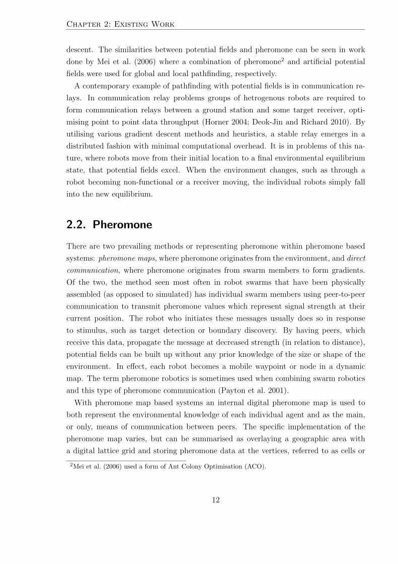
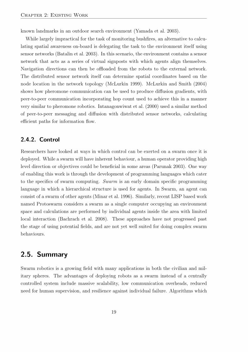
With pheromone map based systems an internal digital pheromone map is used to
both represent the environmental knowledge of each individual agent and as the main,
or only, means of communication between peers. The specific implementation of the
pheromone map varies, but can be summarised as overlaying a geographic area with
a digital lattice grid and storing pheromone data at the vertices, referred to as cells or
2Mei et al. (2006) used a form of Ant Colony Optimisation (ACO).
12
Chapter 2: Existing Work
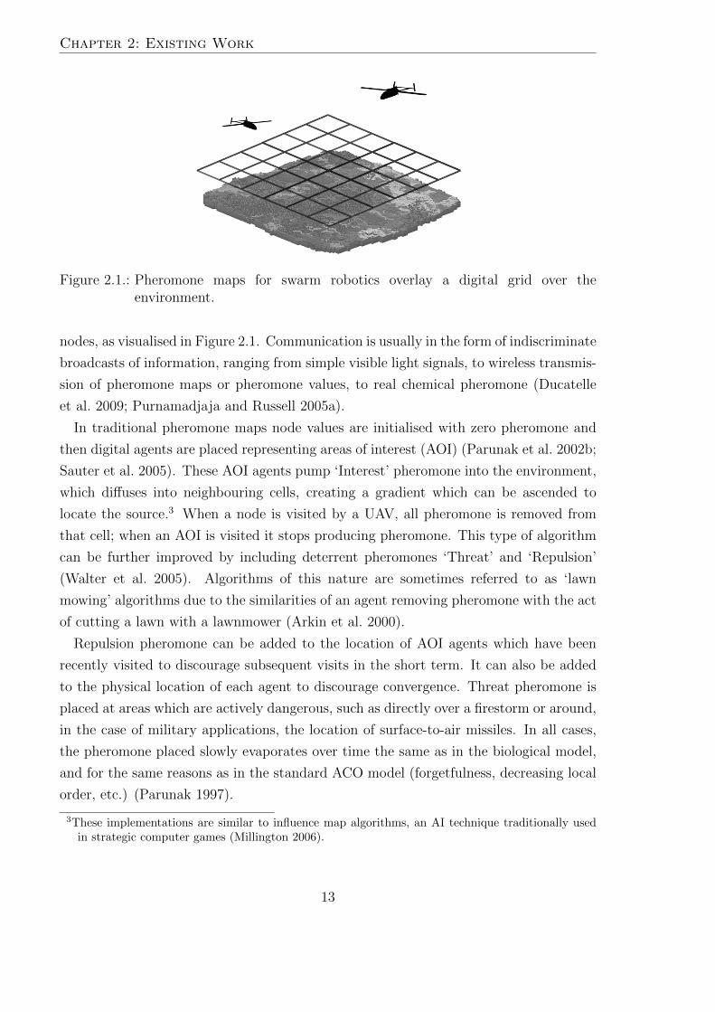
Figure 2.1.: Pheromone maps for swarm robotics overlay a digital grid over theenvironment.
nodes, as visualised in Figure 2.1. Communication is usually in the form of indiscriminate
broadcasts of information, ranging from simple visible light signals, to wireless transmis-
sion of pheromone maps or pheromone values, to real chemical pheromone (Ducatelle
et al. 2009; Purnamadjaja and Russell 2005a).
In traditional pheromone maps node values are initialised with zero pheromone and
then digital agents are placed representing areas of interest (AOI) (Parunak et al. 2002b;
Sauter et al. 2005). These AOI agents pump ‘Interest’ pheromone into the environment,
which diffuses into neighbouring cells, creating a gradient which can be ascended to
locate the source.3 When a node is visited by a UAV, all pheromone is removed from
that cell; when an AOI is visited it stops producing pheromone. This type of algorithm
can be further improved by including deterrent pheromones ‘Threat’ and ‘Repulsion’
(Walter et al. 2005). Algorithms of this nature are sometimes referred to as ‘lawn
mowing’ algorithms due to the similarities of an agent removing pheromone with the act
of cutting a lawn with a lawnmower (Arkin et al. 2000).
Repulsion pheromone can be added to the location of AOI agents which have been
recently visited to discourage subsequent visits in the short term. It can also be added
to the physical location of each agent to discourage convergence. Threat pheromone is
placed at areas which are actively dangerous, such as directly over a firestorm or around,
in the case of military applications, the location of surface-to-air missiles. In all cases,
the pheromone placed slowly evaporates over time the same as in the biological model,
and for the same reasons as in the standard ACO model (forgetfulness, decreasing local
order, etc.) (Parunak 1997).
3These implementations are similar to influence map algorithms, an AI technique traditionally usedin strategic computer games (Millington 2006).
13
Chapter 2: Existing Work
Dasgupta (2006) discusses algorithms for distributed automatic target recognition
(ATR). The proposed application is one where a swarm is performing surveillance and the
task of target identification is improved by using multiple platforms to take and compare
images of a target from different angles. As is the trend with swarm applications, a
pheromone based implementation is used with individual pheromone maps4 distributed
via stigmergic broadcasts. Initial target detection is via a simple dispersion algorithm,
but once target information is known a mixture of attractive (at known target locations)
and repulsive (at previous target locations) pheromone is coupled with a hill climbing
algorithm to saturate target locations with agents (Chen et al. 2007). Good results are
shown even with simulated environmental effects which add noise to the images.
Area coverage using pheromone essentially creates an optimisation landscapes, and
as such it can be appropriate to use optimisation terminology when describing the be-
haviour of algorithms in these environments. Specifically, the problem with heuristics
based on diffusion is that agents can become stuck in local minima, the diffusion and
evaporation rates need to be precisely calibrated to minimise wandering (usually using
an offline method) and, most significantly, they cannot guarantee exhaustive coverage
(Erignac 2007). A way of getting around these issues is by taking a less literal inter-
pretation of nature and using raw Euclidean distance to cells that need to be observed,
rather than pheromone diffusion and evaporation. Using this method cells are either
‘explored’ or ‘unexplored’, with explored cells containing the Euclidean distance to the
closest unexplored cell. The heuristic presented by Erignac (2007) is essentially a greedy
hill descent method, but using a representation of the environment more similar to a
potential field than one strictly pheromone based. If there is an adjacent unexplored
cell, move to it; if all adjacent cells are explored, move into the one that has the lowest
distance to an unexplored cell.
While fire surveillance requires a persistent presence, the algorithms described so far
are primarily designed to perform a discrete search, where the mission is considered
complete once the environment has been fully searched and targets have been located.
The standard way of modifying these approaches to accommodate continuous search
is to switch nodes from an inert/explored state to an active/unexplored state after an
arbitrary period (Altshuler et al. 2005). The critical problem with this approach is that
the interval is too short then exhaustive coverage is not guaranteed: nodes will reactivate
for their second pass before all nodes have been seen on their first pass. Alternatively,
if the interval is too long, then the environment becomes very sparse and the swarm
4Dasgupta (2006) refers to these pheromone maps as ‘pheromone landscapes’.
14
Chapter 2: Existing Work
takes straight, long distance routes to newly active nodes instead of efficiently winding
through local nodes.
An additional problem lies in the distinction between monitoring a known fire which
is in progress, and detecting new fires. While long term surveillance for new fires is a
problem which can be calibrated for known variables (size of the environment, num-
ber of active UAVs, etc.) transitioning into active fire surveillance means the problem
space becomes highly dynamic. Pheromone dispersion algorithms can transition be-
tween surveillance and monitoring through the addition of artificial point of interest
(POI) agents, however algorithms which require a priori target knowledge will be lim-
ited in their usefulness for this particular domain (Flint et al. 2002).
2.3. Realised Swarm Robotics
2.3.1. Beckers
Beckers (1994) was one of the first projects to take the theoretical idea of stigmergic
robots and build a real swarm. The swarm of five robots were equipped with grippers
for picking up pucks, and two IR sensors. In his work the behaviour of termite nest
building was replicated, where, without direct communication, the swarm was able to
collect a scattered collection of objects and stack them together. This was achieved with
purely stigmergic communication (moving the pucks) and a very small set of simple rules
encoded into a finite state machine (FSM).
2.3.2. Pherobots
Another swarm robotic system used for research purposes is the Pherobot swarm, de-
signed by Payton et al. (2005) Pherobots use an infrared communications ring that is
used for both navigation as well as communication. One interesting advantage of in-
frared communication is that it approximates real world pheromone, in that its strength
decreases over distance providing a natural gradient for peer robots to interact with.
With Pherobots, the pheromone analogue used is peer-to-peer messaging which in-
cludes hop count, pheromone type, and a multi-purpose data field. Typically when a
Pherobot receives a pheromone message, it increases the hop count and resends the
message in all directions. In the (almost guaranteed) event of multiple pheromone mes-
sages being received, only the strongest signal is propagated. In this way, each Pherobot
acts as a node in a pheromone map. A typical application of this approach is robotic
15
Chapter 2: Existing Work
mapping, where the swarm can spread incrementally and individual agents can maintain
position indefinitely.
2.3.3. I-SWARM
I-SWARM was a project funded by the European Commission to build a large scale
robot swarm of up to 1,000 vehicles (Seyfried et al. 2005). Using optical communication,
early results of this project allowed for multiple types of pheromone messages to be
sent optically via LEDs to enable dynamic task allocation (Woern et al. 2006). The
inspiration for this particular robot Swarm was “collective perception” in honeybees:
By evaluating trophallactic5 contacts forager bees can indirectly assess the current ratio
of brood demand to pollen supply in the colony without inspecting brood area and pollen
stores individually” (Camazine 1993; Schmickl and Crailsheim 2004).
Simulating the I-SWARM using the LaRoSim (Large Robotswarm Simulator) plat-
form, Schmickl et al. (2007) are able to utilise collective perception to measure and
compare the sizes of two distant targets without long distance communication or sens-
ing (Valdastri et al. 2006). As with the previously mentioned Pherobots, communication
is via peer-to-peer communication which incorporates hop count data, where only the
strongest signal is propagated in the case of multiple messages. Similar approaches have
also been used with this system to perform pathfinding and lawn-cutting algorithms
(Schmickl and Crailsheim 2006; Valdastri et al. 2006).6
2.3.4. iRobot SwarmBots
The SwarmBot is a four-wheeled, 12 cm cube with spatial location capability, infrared
and radio communication incorporating unique ID chips (McLurkin and Dwight 2008).
Primarily used by McLurkin and Smith (2004) in work on distributed algorithms, appli-
cations have ranged from simple swarm dispersal behaviour to complex environmental
boundary detection by using the swarm as a mobile sensor network (McLurkin and De-
maine 2009). Work by Shaw et al. (2010) used the SwarmBot platform as a test case to
show the efficiency of the input-based consensus algorithm in addressing the problem of
communication failure in collective perception.
While Pherobots were designed with the view that “coordination schemes that require
unique identities for each robot [and] explicit routing of point-to-point communication
5Trophallaxis is the transfer of fluid food among members of a colony through orifice to mouth feeding.6In I-SWARM publications the synonym collective floor cleaning is used for lawn-cutting, and optimal
route finding for pathfinding.
16
Chapter 2: Existing Work
between robots [...] can be overwhelmed when dealing with extremely large numbers”
(Payton et al. 2003, p. 1), SwarmBots have successfully been deployed under these
constraints with swarm sizes exceeding 100 vehicles without any reported difficulties
(McLurkin 2004).
2.3.5. PheGMot
The pheromone-guided mobile-robot (PheGMot-III), designed by Kuwana et al. (1996),
simulates the behaviour of the male silkworm moth by attaching living moth antennae
to robots for the purpose of detecting pheromone. The resulting cybernetic organism
was able to achieve target location in a wind tunnel by gradient descent sensing of real
world chemical trails (Kuwana et al. 1999) .
Similar robots have been designed by Russell (2009), who experiments with using real
world pheromone to coordinate robot movement. This work is an extension of earlier
work, conducted in collaboration with Purnamadjaja and Russell (2005a), in building
robots which could simulate the necrophoric behaviour of bees.7 In other work by Pur-
namadjaja and Russell (2005b, 2007), robots with gas sensors and chemical fans where
able to take on ‘queen’ and ‘worker’ roles, where the queen could indirectly coordinate
the actions of the worker swarm.
Sugawara et al. (2004), using the virtual dynamic environment for autonomous robots
(V-DEAR), experimented with using a less literal approach to ‘real’ pheromone. In his
work, a projector is used to display trails where robots have passed, and these markings
are in turn observed by the swarm and used to prompt behaviours such as recruitment
and searching.
2.4. Implementation Issues with UAV Swarms
One of the key development challenges in creating a functional UAV swarm is the lim-
ited processing capabilities that can be carried on board. As endurance is a critical
requirement of UAVs, power usage, weight and heat generation all need to be kept to
a minimum. These constraints limit the computational hardware that can be carried.
One suggested method for combating this is the use of field-programmable gate arrays
(FPGAs), which have been used in low-level electronic applications for many years but
only recently reached a level on complexity where their use as processing devices in their
7Necrophoric behaviour is a pattern where dead members of colonies are transported by live membersof the same colony.
17
Chapter 2: Existing Work
own right has been seriously considered (Sanderson 2003). A modern FPGA, with em-
bedded processors, RAM, and serial IO, has a vastly superior processing performance to
power consumption ratio when compared to a conventional processor relying on Harvard
or Von Neumann architectures.
Extending these advantages, sharing the FPGA computing and power resources of
individual UAVs across the swarm has been shown to be a possibility (Kearney and
Jasiunas 2007). With this distributed computing approach, computationally intensive
tasks can be broken up and executed by other agents in the swarm individually or
in parallel. To implement this system in practice requires the creation of a purpose
built operating system to handle the migration of tasks between UAVs without undue
effort required by application developers (Jasiunas 2009), as well as robust intra-swarm
communication. However, the benefit of allowing a swarm to pool its resources, and
overcome the individually weak computational power of each agent, may make this a
desirable, and maybe even necessary, field of inquiry.
There has also been some work done in using a graphics processing unit (GPU) to
perform the pheromone calculations of a UAV swarm. Depending on the algorithm used,
pheromone updates can be the most computationally expensive subsystem the UAV has
to deal with outside of on-board image recognition. Using a GPU to run the calculations
shows an order of magnitude improvement over similar CPU code. However the current
main use of this is for robot simulation software, where swarm sizes could be measured
in tens of thousands (Walter et al. 2005).
2.4.1. Spatial Awareness
Identifying an agent’s location in its environment is one of the fundamental challenges
in swarm robotics. The most common and practical method of determining position
for outdoor UAVs is through the use of the Global Positioning System (GPS), with the
only real drawback being relatively low precision (within approximately 20 meters for
civilian applications) (Stirling et al. 2010). The main alternative is an inertial navigation
system (INS), a “dead reckoning” process where current location can be calculated based
on a previously determined location and subsequent distance travelled. The drawback
to an INS is that a method of ascertaining initial positions is still required, and it is
often necessary to have a shared frame of reference throughout the swarm to make
communicated data useful. In known environments (usually an indoor testing facility)
research has been done in determining a UAV’s position using visual input alone using
markers in the environment, though it is theorised that this could be extended to using
18
Chapter 2: Existing Work
known landmarks in an outdoor search environment (Yamada et al. 2003).
While largely impractical for the task of monitoring bushfires, an alternative to calcu-
lating spatial awareness on-board is delegating the task to the environment itself using
sensor networks (Batalin et al. 2003). In this scenario, the environment contains a sensor
network that acts as a series of virtual signposts with which agents align themselves.
Navigation directions can then be offloaded from the robots to the external network.
The distributed sensor network itself can determine spatial coordinates based on the
node location in the network topology (McLurkin 1999). McLurkin and Smith (2004)
shows how pheromone communication can be used to produce diffusion gradients, with
peer-to-peer communication incorporating hop count used to achieve this in a manner
very similar to pheromone robotics. Intanagonwiwat et al. (2000) used a similar method
of peer-to-peer messaging and diffusion with distributed sensor networks, calculating
efficient paths for information flow.
2.4.2. Control
Researchers have looked at ways in which control can be exerted on a swarm once it is
deployed. While a swarm will have inherent behaviour, a human operator providing high
level direction or objectives could be beneficial in some areas (Parunak 2003). One way
of enabling this work is through the development of programming languages which cater
to the specifics of swarm computing. Swarm is an early domain specific programming
language in which a hierarchical structure is used for agents. In Swarm, an agent can
consist of a swarm of other agents (Minar et al. 1996). Similarly, recent LISP based work
named Protoswarm considers a swarm as a single computer occupying an environment
space and calculations are performed by individual agents inside the area with limited
local interaction (Bachrach et al. 2008). These approaches have not progressed past
the stage of using potential fields, and are not yet well suited for doing complex swarm
behaviours.
2.5. Summary
Swarm robotics is a growing field with many applications in both the civilian and mil-
itary spheres. The advantages of deploying robots as a swarm instead of a centrally
controlled system include massive scalability, low communication overheads, reduced
need for human supervision, and resilience against individual failure. Algorithms which
19
Chapter 2: Existing Work
are designed to work in a swarm environment are still in their infancy, yet a promising
branch of inquiry has been biomimicry, specifically the use of artificial pheromone.
Using pheromone maps to represent the environment a swarm occupies allows algo-
rithms to combine the information sharing and collective decision making elements of
swarm behaviour into a single intuitive concept. The problem with pheromone as a
concept, however, is that the analogy only holds so long as the information is stored in
the environment itself. With the problem of detecting and then monitoring bushfires in
an area without the infrastructure needed to provide long range communication there is
no immediately apparent medium to store this information.
The next chapter will present an algorithm which solves this problem by storing a
unique pheromone map within each individual agent and then broadcasting the phero-
mone map locally as a means of synchronising with other agents’ internal model.
20
3. Distributed Priority Maps
The goal of the algorithm presented in this dissertation is to enable a swarm of UAVs to
cooperatively engage in aerial surveillance, primarily for bushfires, in a way which only
uses short range communication and is resilient to vehicle loss. Areas of interest should
be specifiable, so that high risk areas can be given an appropriate level of attention.
3.1. Proposed Algorithm
The proposed algorithm uses a pheromone map, where pheromone is used to quantify
the need for a survey of a particular location: the higher the pheromone level the greater
the need. Pheromone increases automatically over time by an amount that is propor-
tional to the required survey frequency, and is reset to zero when a survey is made.
Survey frequency, or priority, of a location can be set a priori or changed in response to
environmental observations depending on the mission. UAVs are attracted to the cell
most due for survey while taking into account distance from their current location.1
Each UAV keeps its own internal pheromone map, resetting the pheromone on each
point it visits. This map information is broadcast periodically, which allows any UAVs
within communication range of the transmission to set the pheromone level of all cells on
their own pheromone map to the lower of their current or received value. UAVs in close
proximity are repelled from each other if their location becomes known via a broadcast
which, together with the information shared, discourages multiple UAVs surveying the
same point shortly after each other.
The net effect of this is that the UAVs spread out rather than converge, surveying
locations with the highest pheromone levels preferentially so that all areas on the map
are surveyed as frequently as possible and in the required frequency ratio.
1The terms cell and node are used interchangeably as synonyms in this, and other, published work.
21
Chapter 3: Distributed Priority Maps
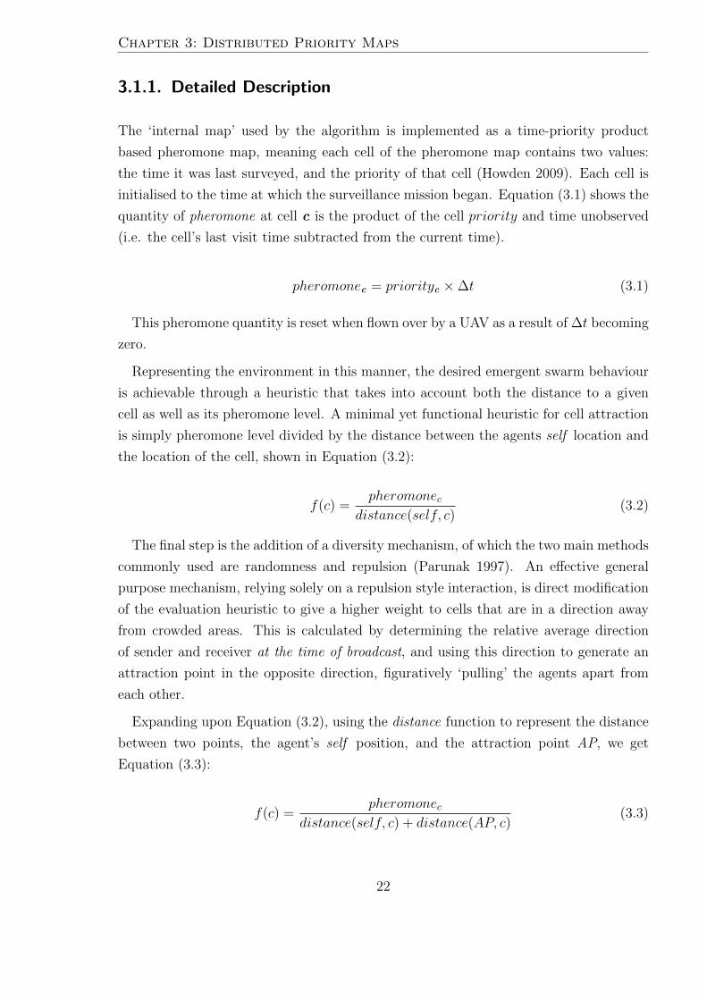
3.1.1. Detailed Description
The ‘internal map’ used by the algorithm is implemented as a time-priority product
based pheromone map, meaning each cell of the pheromone map contains two values:
the time it was last surveyed, and the priority of that cell (Howden 2009). Each cell is
initialised to the time at which the surveillance mission began. Equation (3.1) shows the
quantity of pheromone at cell c is the product of the cell priority and time unobserved
(i.e. the cell’s last visit time subtracted from the current time).
pheromonec = priorityc ×∆t (3.1)
This pheromone quantity is reset when flown over by a UAV as a result of ∆t becoming
zero.
Representing the environment in this manner, the desired emergent swarm behaviour
is achievable through a heuristic that takes into account both the distance to a given
cell as well as its pheromone level. A minimal yet functional heuristic for cell attraction
is simply pheromone level divided by the distance between the agents self location and
the location of the cell, shown in Equation (3.2):
f(c) =pheromonec
distance(self, c)(3.2)
The final step is the addition of a diversity mechanism, of which the two main methods
commonly used are randomness and repulsion (Parunak 1997). An effective general
purpose mechanism, relying solely on a repulsion style interaction, is direct modification
of the evaluation heuristic to give a higher weight to cells that are in a direction away
from crowded areas. This is calculated by determining the relative average direction
of sender and receiver at the time of broadcast, and using this direction to generate an
attraction point in the opposite direction, figuratively ‘pulling’ the agents apart from
each other.
Expanding upon Equation (3.2), using the distance function to represent the distance
between two points, the agent’s self position, and the attraction point AP, we get
Equation (3.3):
f(c) =pheromonec
distance(self, c) + distance(AP, c)(3.3)
22
Chapter 3: Distributed Priority Maps
3.2. Algorithm Concepts and Modifications
One of the key concepts in swarm algorithms is scalability. As this thesis investigates
and presents the strengths and weaknesses of the proposed algorithm over a wide range
of scenarios, some time was spent focusing on the algorithm’s general purpose func-
tionality. This means that instead of adjusting for the best possible performance in a
specific scenario, good performance should be possible over most scenarios using default
parameters. The method that will be presented to make this possible involves a small in-
crease in complexity, however the increase in performance makes this a worthwhile trade
off. This optimised version of the algorithm is the one used to generate the majority of
results presented in this dissertation.
3.2.1. Diversity
A critical factor in maintaining steady performance over a range of scenarios is the
diversity mechanism. As repulsion and randomness are, at their most fundamental,
methods of forcing agents to make sub-optimal individual decisions for the sake of the
swarm as a whole, the force should only be as strong as it needs to be, but no stronger.
The force required either in time spent under the direct effect of the diversity mechanism,
or in the severity of effect itself, increases in proportion to the local density of agents.
What works well at 1000 agents may be ineffective or catastrophic for 10 agents.
As previously described, diversity is handled in the algorithm through application of
an attraction force to a point away from other agents. While this may seem synonymous
with standard repulsion, in practice pushing an agent away from a ‘poor’ area (from the
standpoint of swarm performance as a whole) requires more force to ensure satisfactory
dispersal as well as potentially moving the UAV to yet another bad area. Pulling the
agent directly towards a good area requires less force due to being focused instead of
dispersed as well as negating the second problem, of ending up in another poor area,
entirely.
The choice to have repulsion act directly on the heuristic, instead of as a steering be-
haviour, is also based on the concept of being light handed. While a steering force based
repulsion would take effect immediately, pushing the UAV off course, by incorporating
repulsion into the heuristic evaluation the UAV can still head directly for specific loca-
tions. Repulsion was also designed to be a constant value, rather than what is typical in
swarm algorithms which is to inversely scale the force of the push based on the distance
between agents. While inverse scaling can be necessary for ‘push’ style mechanisms, it
23
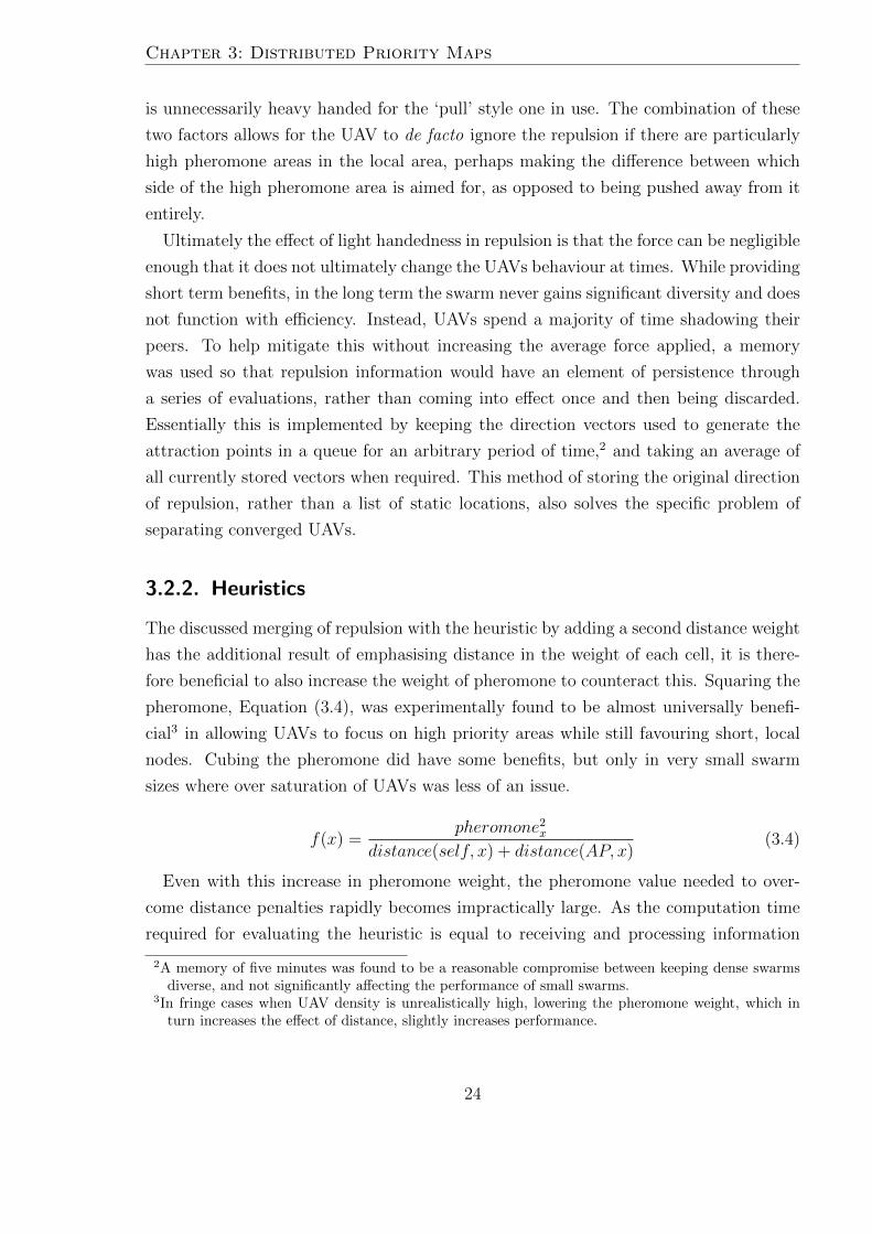
Chapter 3: Distributed Priority Maps
is unnecessarily heavy handed for the ‘pull’ style one in use. The combination of these
two factors allows for the UAV to de facto ignore the repulsion if there are particularly
high pheromone areas in the local area, perhaps making the difference between which
side of the high pheromone area is aimed for, as opposed to being pushed away from it
entirely.
Ultimately the effect of light handedness in repulsion is that the force can be negligible
enough that it does not ultimately change the UAVs behaviour at times. While providing
short term benefits, in the long term the swarm never gains significant diversity and does
not function with efficiency. Instead, UAVs spend a majority of time shadowing their
peers. To help mitigate this without increasing the average force applied, a memory
was used so that repulsion information would have an element of persistence through
a series of evaluations, rather than coming into effect once and then being discarded.
Essentially this is implemented by keeping the direction vectors used to generate the
attraction points in a queue for an arbitrary period of time,2 and taking an average of
all currently stored vectors when required. This method of storing the original direction
of repulsion, rather than a list of static locations, also solves the specific problem of
separating converged UAVs.
3.2.2. Heuristics
The discussed merging of repulsion with the heuristic by adding a second distance weight
has the additional result of emphasising distance in the weight of each cell, it is there-
fore beneficial to also increase the weight of pheromone to counteract this. Squaring the
pheromone, Equation (3.4), was experimentally found to be almost universally benefi-
cial3 in allowing UAVs to focus on high priority areas while still favouring short, local
nodes. Cubing the pheromone did have some benefits, but only in very small swarm
sizes where over saturation of UAVs was less of an issue.
f(x) =pheromone2x
distance(self, x) + distance(AP, x)(3.4)
Even with this increase in pheromone weight, the pheromone value needed to over-
come distance penalties rapidly becomes impractically large. As the computation time
required for evaluating the heuristic is equal to receiving and processing information
2A memory of five minutes was found to be a reasonable compromise between keeping dense swarmsdiverse, and not significantly affecting the performance of small swarms.
3In fringe cases when UAV density is unrealistically high, lowering the pheromone weight, which inturn increases the effect of distance, slightly increases performance.
24
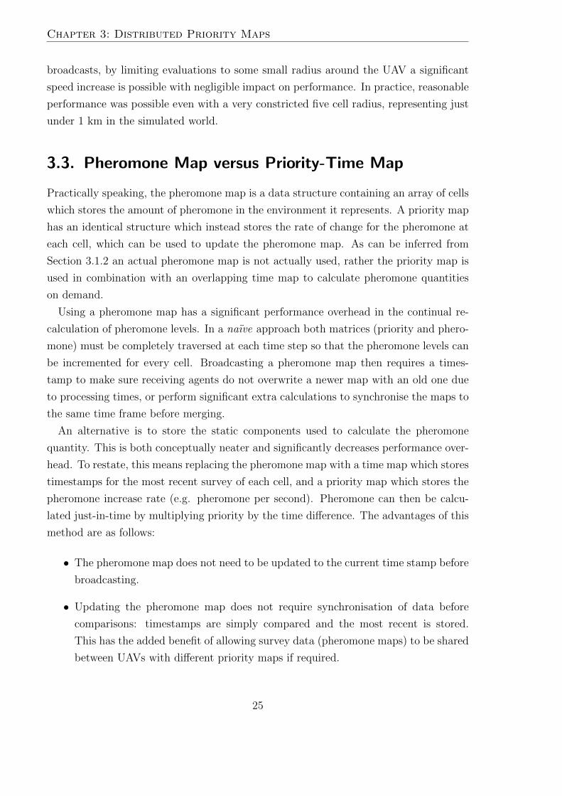
Chapter 3: Distributed Priority Maps
broadcasts, by limiting evaluations to some small radius around the UAV a significant
speed increase is possible with negligible impact on performance. In practice, reasonable
performance was possible even with a very constricted five cell radius, representing just
under 1 km in the simulated world.
3.3. Pheromone Map versus Priority-Time Map
Practically speaking, the pheromone map is a data structure containing an array of cells
which stores the amount of pheromone in the environment it represents. A priority map
has an identical structure which instead stores the rate of change for the pheromone at
each cell, which can be used to update the pheromone map. As can be inferred from
Section 3.1.2 an actual pheromone map is not actually used, rather the priority map is
used in combination with an overlapping time map to calculate pheromone quantities
on demand.
Using a pheromone map has a significant performance overhead in the continual re-
calculation of pheromone levels. In a naıve approach both matrices (priority and phero-
mone) must be completely traversed at each time step so that the pheromone levels can
be incremented for every cell. Broadcasting a pheromone map then requires a times-
tamp to make sure receiving agents do not overwrite a newer map with an old one due
to processing times, or perform significant extra calculations to synchronise the maps to
the same time frame before merging.
An alternative is to store the static components used to calculate the pheromone
quantity. This is both conceptually neater and significantly decreases performance over-
head. To restate, this means replacing the pheromone map with a time map which stores
timestamps for the most recent survey of each cell, and a priority map which stores the
pheromone increase rate (e.g. pheromone per second). Pheromone can then be calcu-
lated just-in-time by multiplying priority by the time difference. The advantages of this
method are as follows:
• The pheromone map does not need to be updated to the current time stamp before
broadcasting.
• Updating the pheromone map does not require synchronisation of data before
comparisons: timestamps are simply compared and the most recent is stored.
This has the added benefit of allowing survey data (pheromone maps) to be shared
between UAVs with different priority maps if required.
25
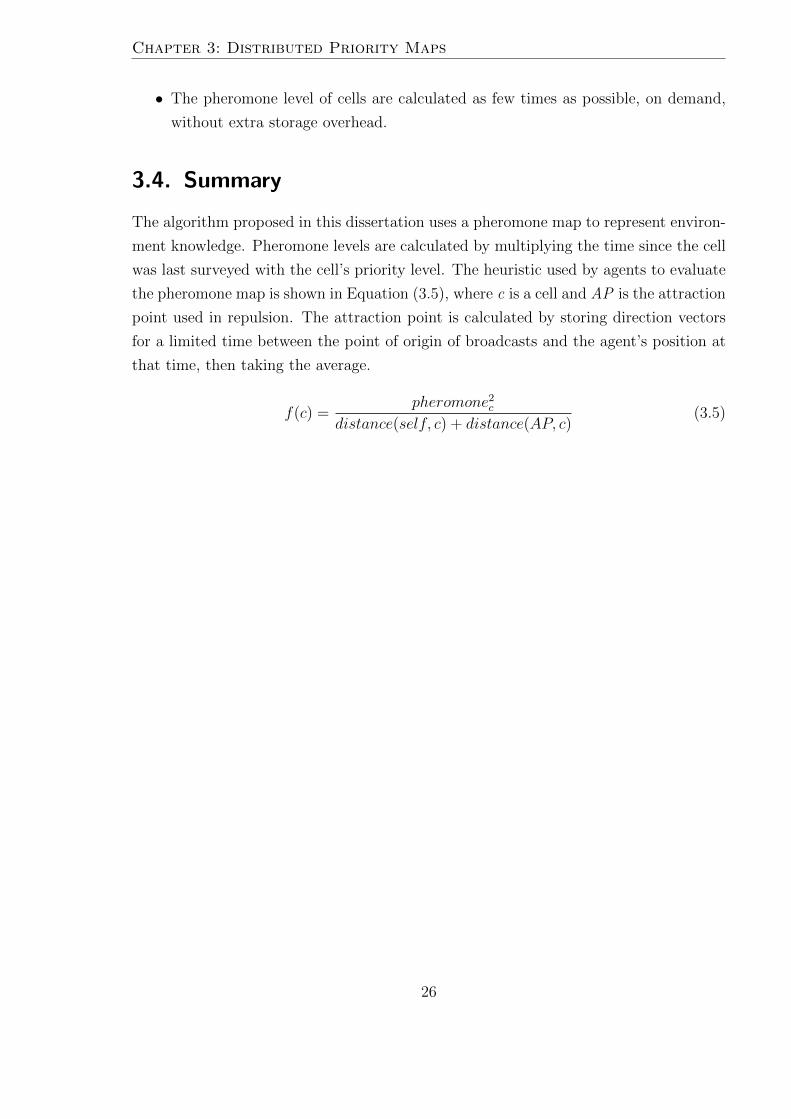
Chapter 3: Distributed Priority Maps
• The pheromone level of cells are calculated as few times as possible, on demand,
without extra storage overhead.
3.4. Summary
The algorithm proposed in this dissertation uses a pheromone map to represent environ-
ment knowledge. Pheromone levels are calculated by multiplying the time since the cell
was last surveyed with the cell’s priority level. The heuristic used by agents to evaluate
the pheromone map is shown in Equation (3.5), where c is a cell and AP is the attraction
point used in repulsion. The attraction point is calculated by storing direction vectors
for a limited time between the point of origin of broadcasts and the agent’s position at
that time, then taking the average.
f(c) =pheromone2c
distance(self, c) + distance(AP, c)(3.5)
26
4. Simulation Setup
The proposed algorithm is evaluated by simulating swarms of UAVs. This approach is
also used to explore and describe properties of the algorithm by varying parameters and
environments. To this end, this chapter describes the most important elements of the
simulator as well as the decisions and assumptions behind them.
4.1. Environmental Representation and Perception
Agents perceive the environment as a pheromone map in the form of a lattice graph, with
quantities of pheromone accumulating at the nodes. Node arrangement is in a square
grid pattern to streamline map storage and representation, and evaluation functions. In
a real world deployment a hexagonal representation would allow for a slight increase in
mission performance at the cost of an increase in code complexity.
The agents can sense their own position in the simulated environment as a Cartesian
coordinate via GPS. Positions of peer agents are ‘sensed’ indirectly through Cartesian
coordinates attached to periodic information broadcasts. It is assumed that the agents
have additional sensors required to handle emergency collision avoidance with other
objects, as this is outside the scope of the algorithm presented.
Fire detection is done through use of a low power visible CMOS camera (Kearney
and Jasiunas 2007). When a possible target is identified the UAV switches to a high
powered thermographic camera, also known as a forward looking infrared (FLIR) camera.
The camera’s specifications are based on current and common off-the-shelf components:
640×480 resolution, field of view of 60◦ and optical 10× zoom. Using these specifications,
and adding a requirement for high resolution 5 cm2 pixel clarity, the UAV has a 176m
footprint radius when using the FLIR camera.
Speed of search is a factor of UAV speed the specifications of the cameras used: a larger
footprint allows UAVs to travel a shorter distance to attain coverage. For this reason,
along with the swarm principle of individuals being simple and cheap, the specifications
of the camera are consciously conservative.
27
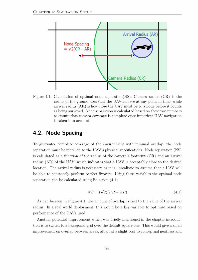
Chapter 4: Simulation Setup
Figure 4.1.: Calculation of optimal node separation(NS). Camera radius (CR) is theradius of the ground area that the UAV can see at any point in time, whilearrival radius (AR) is how close the UAV must be to a node before it countsas being surveyed. Node separation is calculated based on these two numbersto ensure that camera coverage is complete once imperfect UAV navigationis taken into account.
4.2. Node Spacing
To guarantee complete coverage of the environment with minimal overlap, the node
separation must be matched to the UAV’s physical specifications. Node separation (NS)
is calculated as a function of the radius of the camera’s footprint (CR) and an arrival
radius (AR) of the UAV, which indicates that a UAV is acceptably close to the desired
location. The arrival radius is necessary as it is unrealistic to assume that a UAV will
be able to constantly perform perfect flyovers. Using these variables the optimal node
separation can be calculated using Equation (4.1).
NS = (√
2)(FR− AR) (4.1)
As can be seen in Figure 4.1, the amount of overlap is tied to the value of the arrival
radius. In a real world deployment, this would be a key variable to optimise based on
performance of the UAVs used.
Another potential improvement which was briefly mentioned in the chapter introduc-
tion is to switch to a hexagonal grid over the default square one. This would give a small
improvement on overlap between areas, albeit at a slight cost to conceptual neatness and
28
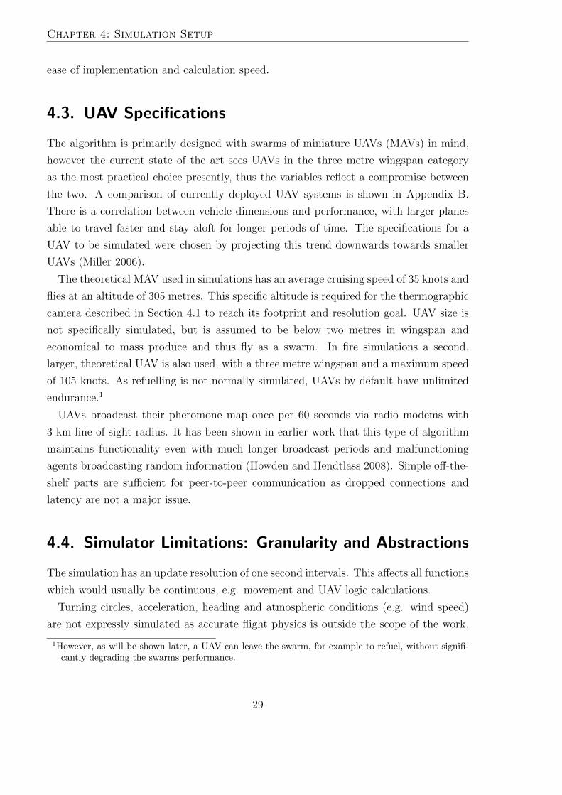
Chapter 4: Simulation Setup
ease of implementation and calculation speed.
4.3. UAV Specifications
The algorithm is primarily designed with swarms of miniature UAVs (MAVs) in mind,
however the current state of the art sees UAVs in the three metre wingspan category
as the most practical choice presently, thus the variables reflect a compromise between
the two. A comparison of currently deployed UAV systems is shown in Appendix B.
There is a correlation between vehicle dimensions and performance, with larger planes
able to travel faster and stay aloft for longer periods of time. The specifications for a
UAV to be simulated were chosen by projecting this trend downwards towards smaller
UAVs (Miller 2006).
The theoretical MAV used in simulations has an average cruising speed of 35 knots and
flies at an altitude of 305 metres. This specific altitude is required for the thermographic
camera described in Section 4.1 to reach its footprint and resolution goal. UAV size is
not specifically simulated, but is assumed to be below two metres in wingspan and
economical to mass produce and thus fly as a swarm. In fire simulations a second,
larger, theoretical UAV is also used, with a three metre wingspan and a maximum speed
of 105 knots. As refuelling is not normally simulated, UAVs by default have unlimited
endurance.1
UAVs broadcast their pheromone map once per 60 seconds via radio modems with
3 km line of sight radius. It has been shown in earlier work that this type of algorithm
maintains functionality even with much longer broadcast periods and malfunctioning
agents broadcasting random information (Howden and Hendtlass 2008). Simple off-the-
shelf parts are sufficient for peer-to-peer communication as dropped connections and
latency are not a major issue.
4.4. Simulator Limitations: Granularity and Abstractions
The simulation has an update resolution of one second intervals. This affects all functions
which would usually be continuous, e.g. movement and UAV logic calculations.
Turning circles, acceleration, heading and atmospheric conditions (e.g. wind speed)
are not expressly simulated as accurate flight physics is outside the scope of the work,
1However, as will be shown later, a UAV can leave the swarm, for example to refuel, without signifi-cantly degrading the swarms performance.
29
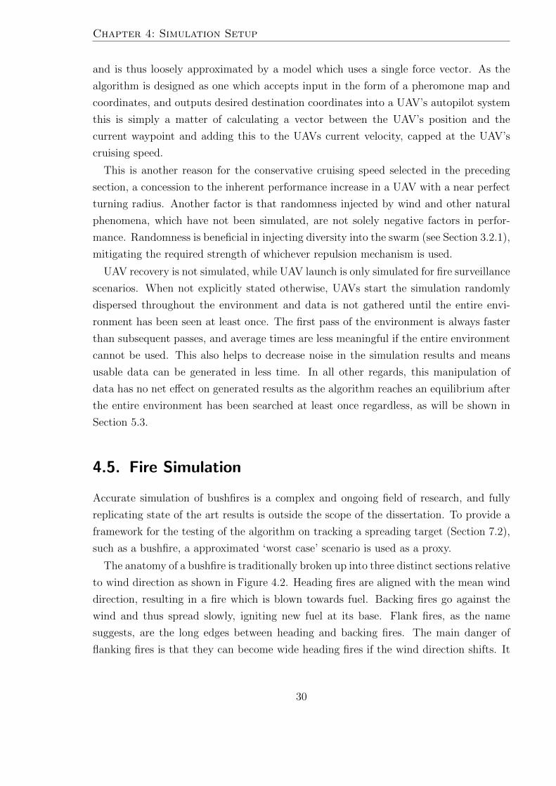
Chapter 4: Simulation Setup
and is thus loosely approximated by a model which uses a single force vector. As the
algorithm is designed as one which accepts input in the form of a pheromone map and
coordinates, and outputs desired destination coordinates into a UAV’s autopilot system
this is simply a matter of calculating a vector between the UAV’s position and the
current waypoint and adding this to the UAVs current velocity, capped at the UAV’s
cruising speed.
This is another reason for the conservative cruising speed selected in the preceding
section, a concession to the inherent performance increase in a UAV with a near perfect
turning radius. Another factor is that randomness injected by wind and other natural
phenomena, which have not been simulated, are not solely negative factors in perfor-
mance. Randomness is beneficial in injecting diversity into the swarm (see Section 3.2.1),
mitigating the required strength of whichever repulsion mechanism is used.
UAV recovery is not simulated, while UAV launch is only simulated for fire surveillance
scenarios. When not explicitly stated otherwise, UAVs start the simulation randomly
dispersed throughout the environment and data is not gathered until the entire envi-
ronment has been seen at least once. The first pass of the environment is always faster
than subsequent passes, and average times are less meaningful if the entire environment
cannot be used. This also helps to decrease noise in the simulation results and means
usable data can be generated in less time. In all other regards, this manipulation of
data has no net effect on generated results as the algorithm reaches an equilibrium after
the entire environment has been searched at least once regardless, as will be shown in
Section 5.3.
4.5. Fire Simulation
Accurate simulation of bushfires is a complex and ongoing field of research, and fully
replicating state of the art results is outside the scope of the dissertation. To provide a
framework for the testing of the algorithm on tracking a spreading target (Section 7.2),
such as a bushfire, a approximated ‘worst case’ scenario is used as a proxy.
The anatomy of a bushfire is traditionally broken up into three distinct sections relative
to wind direction as shown in Figure 4.2. Heading fires are aligned with the mean wind
direction, resulting in a fire which is blown towards fuel. Backing fires go against the
wind and thus spread slowly, igniting new fuel at its base. Flank fires, as the name
suggests, are the long edges between heading and backing fires. The main danger of
flanking fires is that they can become wide heading fires if the wind direction shifts. It
30
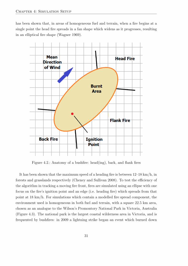
Chapter 4: Simulation Setup
has been shown that, in areas of homogeneous fuel and terrain, when a fire begins at a
single point the head fire spreads in a fan shape which widens as it progresses, resulting
in an elliptical fire shape (Wagner 1969).
Figure 4.2.: Anatomy of a bushfire: head(ing), back, and flank fires
It has been shown that the maximum speed of a heading fire is between 12–18 km/h, in
forests and grasslands respectively (Cheney and Sullivan 2008). To test the efficiency of
the algorithm in tracking a moving fire front, fires are simulated using an ellipse with one
focus on the fire’s ignition point and an edge (i.e. heading fire) which spreads from that
point at 18 km/h. For simulations which contain a modelled fire spread component, the
environment used is homogeneous in both fuel and terrain, with a square 22.5 km area,
chosen as an analogue to the Wilson’s Promontory National Park in Victoria, Australia
(Figure 4.3). The national park is the largest coastal wilderness area in Victoria, and is
frequented by bushfires: in 2009 a lightning strike began an event which burned down
31
Chapter 4: Simulation Setup
over 250 km2 (50% of the park’s area).
Figure 4.3.: a) Satellite view of Wilson’s Promontory, an Australian national park lo-cated at 39◦02′S 146◦23′E. b) A corresponding priority map, where each pixelcorresponds to a node. Higher priority levels are represented by brightercolours.
4.6. Summary
The simulator presented is primarily concerned with allowing evaluation of the waypoint
selection heuristic in the proposed algorithm. Due to this focus, low level aerodynamic
and bushfire mechanics have been abstracted. Where abstractions will result in artifi-
cially increasing the apparent performance of the underlying algorithm, measures have
been taken to mitigate this, such as consciously conservative UAV speeds and worst-case
fire velocities.
32
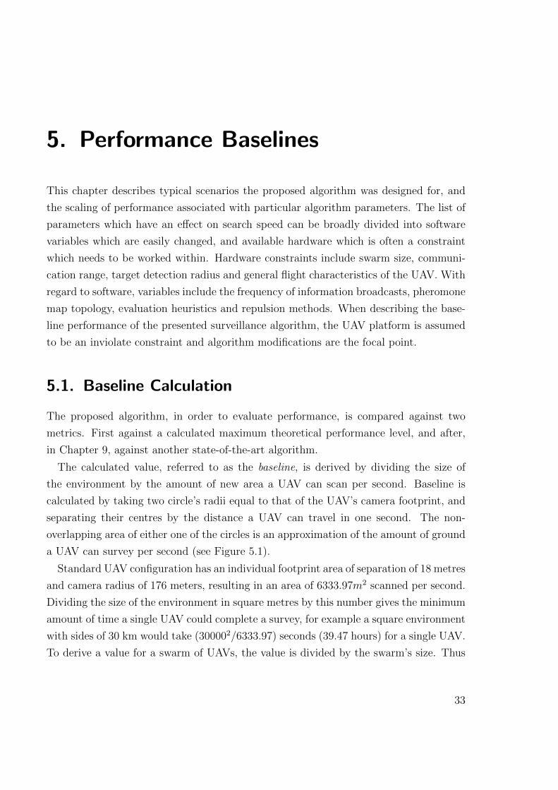
5. Performance Baselines
This chapter describes typical scenarios the proposed algorithm was designed for, and
the scaling of performance associated with particular algorithm parameters. The list of
parameters which have an effect on search speed can be broadly divided into software
variables which are easily changed, and available hardware which is often a constraint
which needs to be worked within. Hardware constraints include swarm size, communi-
cation range, target detection radius and general flight characteristics of the UAV. With
regard to software, variables include the frequency of information broadcasts, pheromone
map topology, evaluation heuristics and repulsion methods. When describing the base-
line performance of the presented surveillance algorithm, the UAV platform is assumed
to be an inviolate constraint and algorithm modifications are the focal point.
5.1. Baseline Calculation
The proposed algorithm, in order to evaluate performance, is compared against two
metrics. First against a calculated maximum theoretical performance level, and after,
in Chapter 9, against another state-of-the-art algorithm.
The calculated value, referred to as the baseline, is derived by dividing the size of
the environment by the amount of new area a UAV can scan per second. Baseline is
calculated by taking two circle’s radii equal to that of the UAV’s camera footprint, and
separating their centres by the distance a UAV can travel in one second. The non-
overlapping area of either one of the circles is an approximation of the amount of ground
a UAV can survey per second (see Figure 5.1).
Standard UAV configuration has an individual footprint area of separation of 18 metres
and camera radius of 176 meters, resulting in an area of 6333.97m2 scanned per second.
Dividing the size of the environment in square metres by this number gives the minimum
amount of time a single UAV could complete a survey, for example a square environment
with sides of 30 km would take (300002/6333.97) seconds (39.47 hours) for a single UAV.
To derive a value for a swarm of UAVs, the value is divided by the swarm’s size. Thus
33
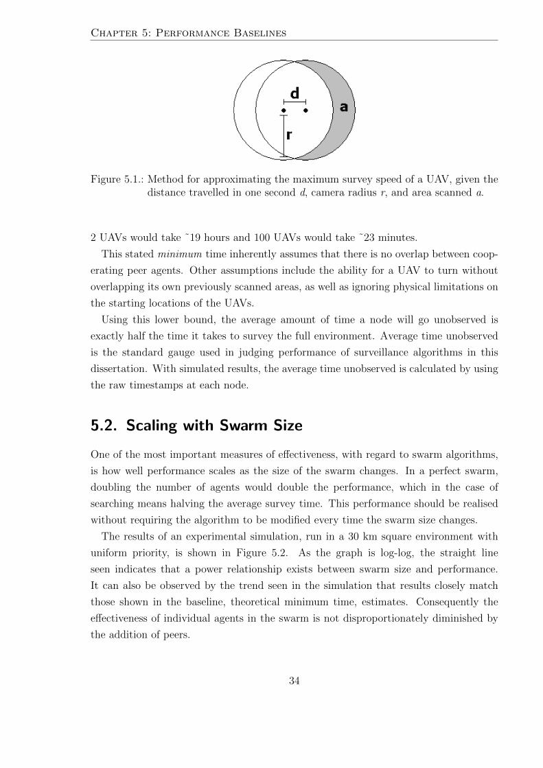
Chapter 5: Performance Baselines
Figure 5.1.: Method for approximating the maximum survey speed of a UAV, given thedistance travelled in one second d, camera radius r, and area scanned a.
2 UAVs would take ˜19 hours and 100 UAVs would take ˜23 minutes.
This stated minimum time inherently assumes that there is no overlap between coop-
erating peer agents. Other assumptions include the ability for a UAV to turn without
overlapping its own previously scanned areas, as well as ignoring physical limitations on
the starting locations of the UAVs.
Using this lower bound, the average amount of time a node will go unobserved is
exactly half the time it takes to survey the full environment. Average time unobserved
is the standard gauge used in judging performance of surveillance algorithms in this
dissertation. With simulated results, the average time unobserved is calculated by using
the raw timestamps at each node.
5.2. Scaling with Swarm Size
One of the most important measures of effectiveness, with regard to swarm algorithms,
is how well performance scales as the size of the swarm changes. In a perfect swarm,
doubling the number of agents would double the performance, which in the case of
searching means halving the average survey time. This performance should be realised
without requiring the algorithm to be modified every time the swarm size changes.
The results of an experimental simulation, run in a 30 km square environment with
uniform priority, is shown in Figure 5.2. As the graph is log-log, the straight line
seen indicates that a power relationship exists between swarm size and performance.
It can also be observed by the trend seen in the simulation that results closely match
those shown in the baseline, theoretical minimum time, estimates. Consequently the
effectiveness of individual agents in the swarm is not disproportionately diminished by
the addition of peers.
34
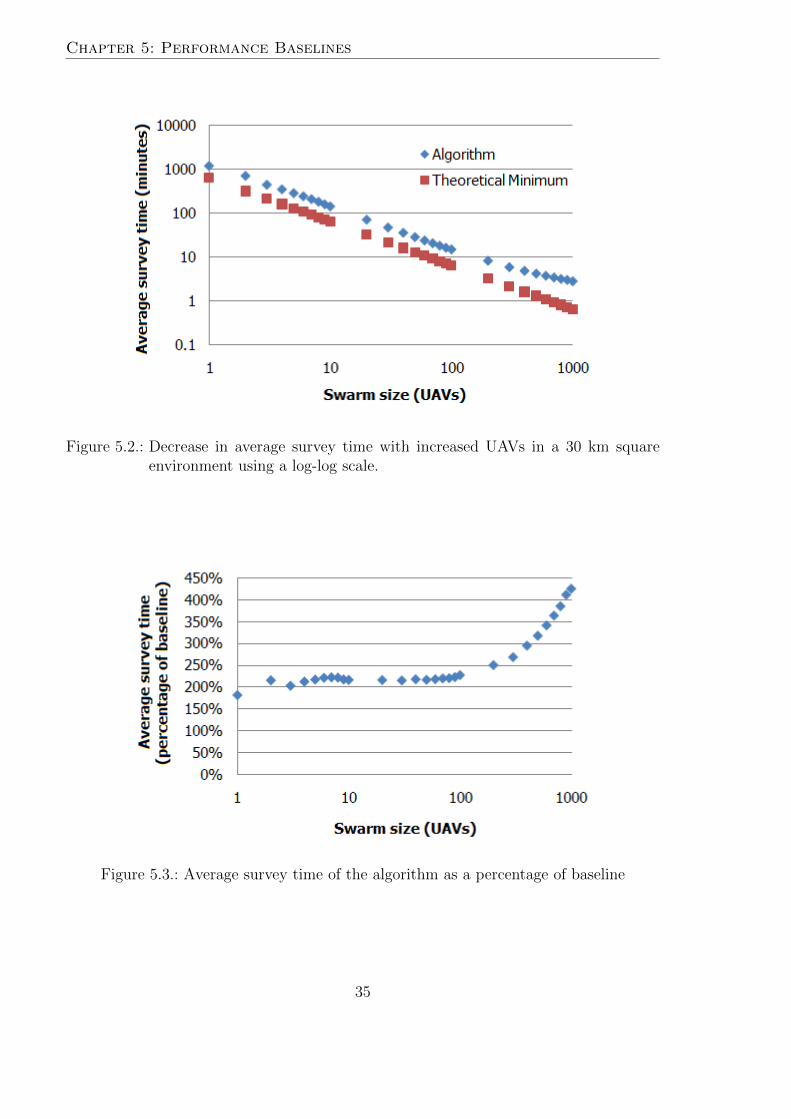
Chapter 5: Performance Baselines
Figure 5.2.: Decrease in average survey time with increased UAVs in a 30 km squareenvironment using a log-log scale.
Figure 5.3.: Average survey time of the algorithm as a percentage of baseline
35
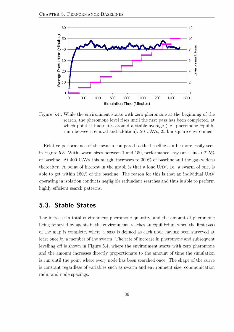
Chapter 5: Performance Baselines
Figure 5.4.: While the environment starts with zero pheromone at the beginning of thesearch, the pheromone level rises until the first pass has been completed, atwhich point it fluctuates around a stable average (i.e. pheromone equilib-rium between removal and addition). 20 UAVs, 25 km square environment
Relative performance of the swarm compared to the baseline can be more easily seen
in Figure 5.3. With swarm sizes between 1 and 150, performance stays at a linear 225%
of baseline. At 400 UAVs this margin increases to 300% of baseline and the gap widens
thereafter. A point of interest in the graph is that a lone UAV, i.e. a swarm of one, is
able to get within 180% of the baseline. The reason for this is that an individual UAV
operating in isolation conducts negligible redundant searches and thus is able to perform
highly efficient search patterns.
5.3. Stable States
The increase in total environment pheromone quantity, and the amount of pheromone
being removed by agents in the environment, reaches an equilibrium when the first pass
of the map is complete, where a pass is defined as each node having been surveyed at
least once by a member of the swarm. The rate of increase in pheromone and subsequent
levelling off is shown in Figure 5.4, where the environment starts with zero pheromone
and the amount increases directly proportionate to the amount of time the simulation
is run until the point where every node has been searched once. The shape of the curve
is constant regardless of variables such as swarm and environment size, communication
radii, and node spacings.
36
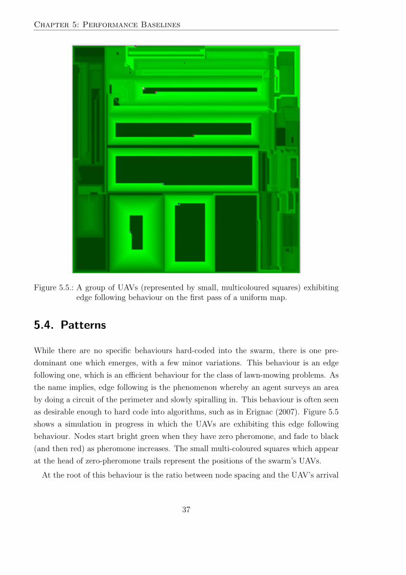
Chapter 5: Performance Baselines
Figure 5.5.: A group of UAVs (represented by small, multicoloured squares) exhibitingedge following behaviour on the first pass of a uniform map.
5.4. Patterns
While there are no specific behaviours hard-coded into the swarm, there is one pre-
dominant one which emerges, with a few minor variations. This behaviour is an edge
following one, which is an efficient behaviour for the class of lawn-mowing problems. As
the name implies, edge following is the phenomenon whereby an agent surveys an area
by doing a circuit of the perimeter and slowly spiralling in. This behaviour is often seen
as desirable enough to hard code into algorithms, such as in Erignac (2007). Figure 5.5
shows a simulation in progress in which the UAVs are exhibiting this edge following
behaviour. Nodes start bright green when they have zero pheromone, and fade to black
(and then red) as pheromone increases. The small multi-coloured squares which appear
at the head of zero-pheromone trails represent the positions of the swarm’s UAVs.
At the root of this behaviour is the ratio between node spacing and the UAV’s arrival
37
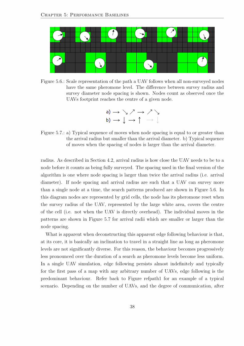
Chapter 5: Performance Baselines
Figure 5.6.: Scale representation of the path a UAV follows when all non-surveyed nodeshave the same pheromone level. The difference between survey radius andsurvey diameter node spacing is shown. Nodes count as observed once theUAVs footprint reaches the centre of a given node.
Figure 5.7.: a) Typical sequence of moves when node spacing is equal to or greater thanthe arrival radius but smaller than the arrival diameter. b) Typical sequenceof moves when the spacing of nodes is larger than the arrival diameter.
radius. As described in Section 4.2, arrival radius is how close the UAV needs to be to a
node before it counts as being fully surveyed. The spacing used in the final version of the
algorithm is one where node spacing is larger than twice the arrival radius (i.e. arrival
diameter). If node spacing and arrival radius are such that a UAV can survey more
than a single node at a time, the search patterns produced are shown in Figure 5.6. In
this diagram nodes are represented by grid cells, the node has its pheromone reset when
the survey radius of the UAV, represented by the large white area, covers the centre
of the cell (i.e. not when the UAV is directly overhead). The individual moves in the
patterns are shown in Figure 5.7 for arrival radii which are smaller or larger than the
node spacing.
What is apparent when deconstructing this apparent edge following behaviour is that,
at its core, it is basically an inclination to travel in a straight line as long as pheromone
levels are not significantly diverse. For this reason, the behaviour becomes progressively
less pronounced over the duration of a search as pheromone levels become less uniform.
In a single UAV simulation, edge following persists almost indefinitely and typically
for the first pass of a map with any arbitrary number of UAVs, edge following is the
predominant behaviour. Refer back to Figure refpath1 for an example of a typical
scenario. Depending on the number of UAVs, and the degree of communication, after
38
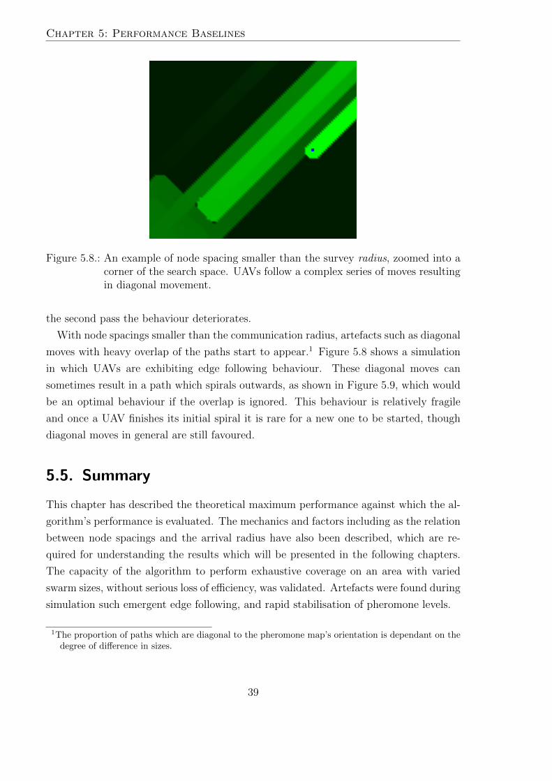
Chapter 5: Performance Baselines
Figure 5.8.: An example of node spacing smaller than the survey radius, zoomed into acorner of the search space. UAVs follow a complex series of moves resultingin diagonal movement.
the second pass the behaviour deteriorates.
With node spacings smaller than the communication radius, artefacts such as diagonal
moves with heavy overlap of the paths start to appear.1 Figure 5.8 shows a simulation
in which UAVs are exhibiting edge following behaviour. These diagonal moves can
sometimes result in a path which spirals outwards, as shown in Figure 5.9, which would
be an optimal behaviour if the overlap is ignored. This behaviour is relatively fragile
and once a UAV finishes its initial spiral it is rare for a new one to be started, though
diagonal moves in general are still favoured.
5.5. Summary
This chapter has described the theoretical maximum performance against which the al-
gorithm’s performance is evaluated. The mechanics and factors including as the relation
between node spacings and the arrival radius have also been described, which are re-
quired for understanding the results which will be presented in the following chapters.
The capacity of the algorithm to perform exhaustive coverage on an area with varied
swarm sizes, without serious loss of efficiency, was validated. Artefacts were found during
simulation such emergent edge following, and rapid stabilisation of pheromone levels.
1The proportion of paths which are diagonal to the pheromone map’s orientation is dependant on thedegree of difference in sizes.
39
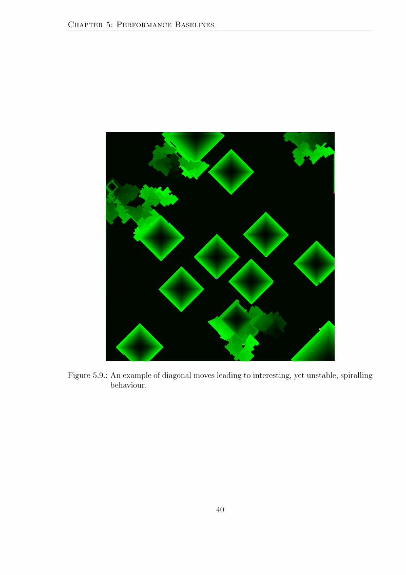
Chapter 5: Performance Baselines
Figure 5.9.: An example of diagonal moves leading to interesting, yet unstable, spirallingbehaviour.
40
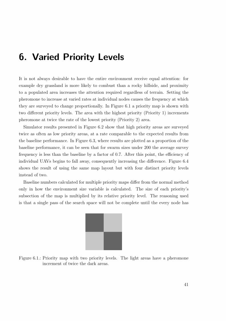
6. Varied Priority Levels
It is not always desirable to have the entire environment receive equal attention: for
example dry grassland is more likely to combust than a rocky hillside, and proximity
to a populated area increases the attention required regardless of terrain. Setting the
pheromone to increase at varied rates at individual nodes causes the frequency at which
they are surveyed to change proportionally. In Figure 6.1 a priority map is shown with
two different priority levels. The area with the highest priority (Priority 1) increments
pheromone at twice the rate of the lowest priority (Priority 2) area.
Simulator results presented in Figure 6.2 show that high priority areas are surveyed
twice as often as low priority areas, at a rate comparable to the expected results from
the baseline performance. In Figure 6.3, where results are plotted as a proportion of the
baseline performance, it can be seen that for swarm sizes under 200 the average survey
frequency is less than the baseline by a factor of 0.7. After this point, the efficiency of
individual UAVs begins to fall away, consequently increasing the difference. Figure 6.4
shows the result of using the same map layout but with four distinct priority levels
instead of two.
Baseline numbers calculated for multiple priority maps differ from the normal method
only in how the environment size variable is calculated. The size of each priority’s
subsection of the map is multiplied by its relative priority level. The reasoning used
is that a single pass of the search space will not be complete until the every node has
Figure 6.1.: Priority map with two priority levels. The light areas have a pheromoneincrement of twice the dark areas.
41
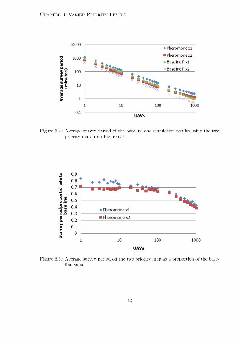
Chapter 6: Varied Priority Levels
Figure 6.2.: Average survey period of the baseline and simulation results using the twopriority map from Figure 6.1
Figure 6.3.: Average survey period on the two priority map as a proportion of the base-line value
42
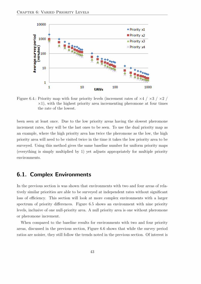
Chapter 6: Varied Priority Levels
Figure 6.4.: Priority map with four priority levels (increment rates of ×4 / ×3 / ×2 /×1), with the highest priority area incrementing pheromone at four timesthe rate of the lowest.
been seen at least once. Due to the low priority areas having the slowest pheromone
increment rates, they will be the last ones to be seen. To use the dual priority map as
an example, where the high priority area has twice the pheromone as the low, the high
priority area will need to be visited twice in the time it takes the low priority area to be
surveyed. Using this method gives the same baseline number for uniform priority maps
(everything is simply multiplied by 1) yet adjusts appropriately for multiple priority
environments.
6.1. Complex Environments
In the previous section is was shown that environments with two and four areas of rela-
tively similar priorities are able to be surveyed at independent rates without significant
loss of efficiency. This section will look at more complex environments with a larger
spectrum of priority differences. Figure 6.5 shows an environment with nine priority
levels, inclusive of one null-priority area. A null priority area is one without pheromone
or pheromone increment.
When compared to the baseline results for environments with two and four priority
areas, discussed in the previous section, Figure 6.6 shows that while the survey period
ratios are noisier, they still follow the trends noted in the previous section. Of interest is
43
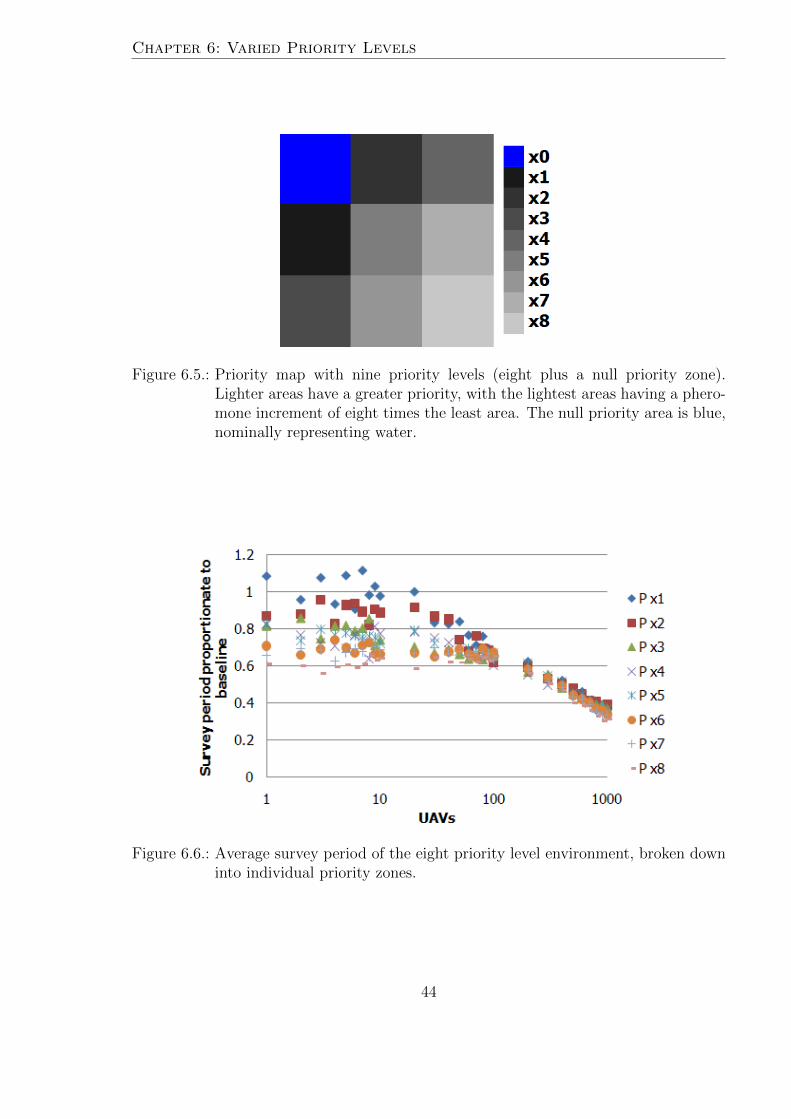
Chapter 6: Varied Priority Levels
Figure 6.5.: Priority map with nine priority levels (eight plus a null priority zone).Lighter areas have a greater priority, with the lightest areas having a phero-mone increment of eight times the least area. The null priority area is blue,nominally representing water.
Figure 6.6.: Average survey period of the eight priority level environment, broken downinto individual priority zones.
44
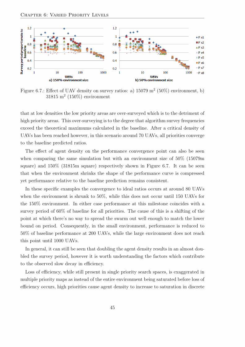
Chapter 6: Varied Priority Levels
Figure 6.7.: Effect of UAV density on survey ratios: a) 15079 m2 (50%) environment, b)31815 m2 (150%) environment
that at low densities the low priority areas are over-surveyed which is to the detriment of
high priority areas. This over-surveying is to the degree that algorithm survey frequencies
exceed the theoretical maximums calculated in the baseline. After a critical density of
UAVs has been reached however, in this scenario around 70 UAVs, all priorities converge
to the baseline predicted ratios.
The effect of agent density on the performance convergence point can also be seen
when comparing the same simulation but with an environment size of 50% (15079m
square) and 150% (31815m square) respectively shown in Figure 6.7. It can be seen
that when the environment shrinks the shape of the performance curve is compressed
yet performance relative to the baseline prediction remains consistent.
In these specific examples the convergence to ideal ratios occurs at around 80 UAVs
when the environment is shrunk to 50%, while this does not occur until 150 UAVs for
the 150% environment. In either case performance at this milestone coincides with a
survey period of 60% of baseline for all priorities. The cause of this is a shifting of the
point at which there’s no way to spread the swarm out well enough to match the lower
bound on period. Consequently, in the small environment, performance is reduced to
50% of baseline performance at 200 UAVs, while the large environment does not reach
this point until 1000 UAVs.
In general, it can still be seen that doubling the agent density results in an almost dou-
bled the survey period, however it is worth understanding the factors which contribute
to the observed slow decay in efficiency.
Loss of efficiency, while still present in single priority search spaces, is exaggerated in
multiple priority maps as instead of the entire environment being saturated before loss of
efficiency occurs, high priorities cause agent density to increase to saturation in discrete
45
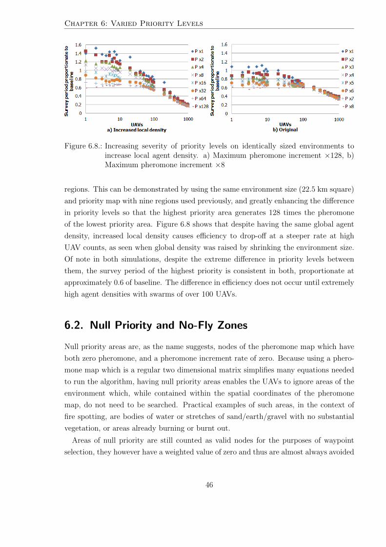
Chapter 6: Varied Priority Levels
Figure 6.8.: Increasing severity of priority levels on identically sized environments toincrease local agent density. a) Maximum pheromone increment ×128, b)Maximum pheromone increment ×8
regions. This can be demonstrated by using the same environment size (22.5 km square)
and priority map with nine regions used previously, and greatly enhancing the difference
in priority levels so that the highest priority area generates 128 times the pheromone
of the lowest priority area. Figure 6.8 shows that despite having the same global agent
density, increased local density causes efficiency to drop-off at a steeper rate at high
UAV counts, as seen when global density was raised by shrinking the environment size.
Of note in both simulations, despite the extreme difference in priority levels between
them, the survey period of the highest priority is consistent in both, proportionate at
approximately 0.6 of baseline. The difference in efficiency does not occur until extremely
high agent densities with swarms of over 100 UAVs.
6.2. Null Priority and No-Fly Zones
Null priority areas are, as the name suggests, nodes of the pheromone map which have
both zero pheromone, and a pheromone increment rate of zero. Because using a phero-
mone map which is a regular two dimensional matrix simplifies many equations needed
to run the algorithm, having null priority areas enables the UAVs to ignore areas of the
environment which, while contained within the spatial coordinates of the pheromone
map, do not need to be searched. Practical examples of such areas, in the context of
fire spotting, are bodies of water or stretches of sand/earth/gravel with no substantial
vegetation, or areas already burning or burnt out.
Areas of null priority are still counted as valid nodes for the purposes of waypoint
selection, they however have a weighted value of zero and thus are almost always avoided
46
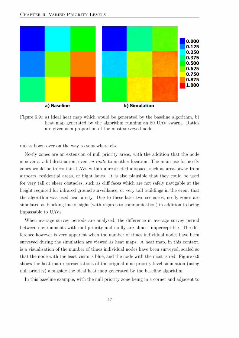
Chapter 6: Varied Priority Levels
Figure 6.9.: a) Ideal heat map which would be generated by the baseline algorithm, b)heat map generated by the algorithm running an 80 UAV swarm. Ratiosare given as a proportion of the most surveyed node.
unless flown over on the way to somewhere else.
No-fly zones are an extension of null priority areas, with the addition that the node
is never a valid destination, even en route to another location. The main use for no-fly
zones would be to contain UAVs within unrestricted airspace, such as areas away from
airports, residential areas, or flight lanes. It is also plausible that they could be used
for very tall or sheer obstacles, such as cliff faces which are not safely navigable at the
height required for infrared ground surveillance, or very tall buildings in the event that
the algorithm was used near a city. Due to these later two scenarios, no-fly zones are
simulated as blocking line of sight (with regards to communication) in addition to being
impassable to UAVs.
When average survey periods are analysed, the difference in average survey period
between environments with null priority and no-fly are almost imperceptible. The dif-
ference however is very apparent when the number of times individual nodes have been
surveyed during the simulation are viewed as heat maps. A heat map, in this context,
is a visualisation of the number of times individual nodes have been surveyed, scaled so
that the node with the least visits is blue, and the node with the most is red. Figure 6.9
shows the heat map representations of the original nine priority level simulation (using
null priority) alongside the ideal heat map generated by the baseline algorithm.
In this baseline example, with the null priority zone being in a corner and adjacent to
47
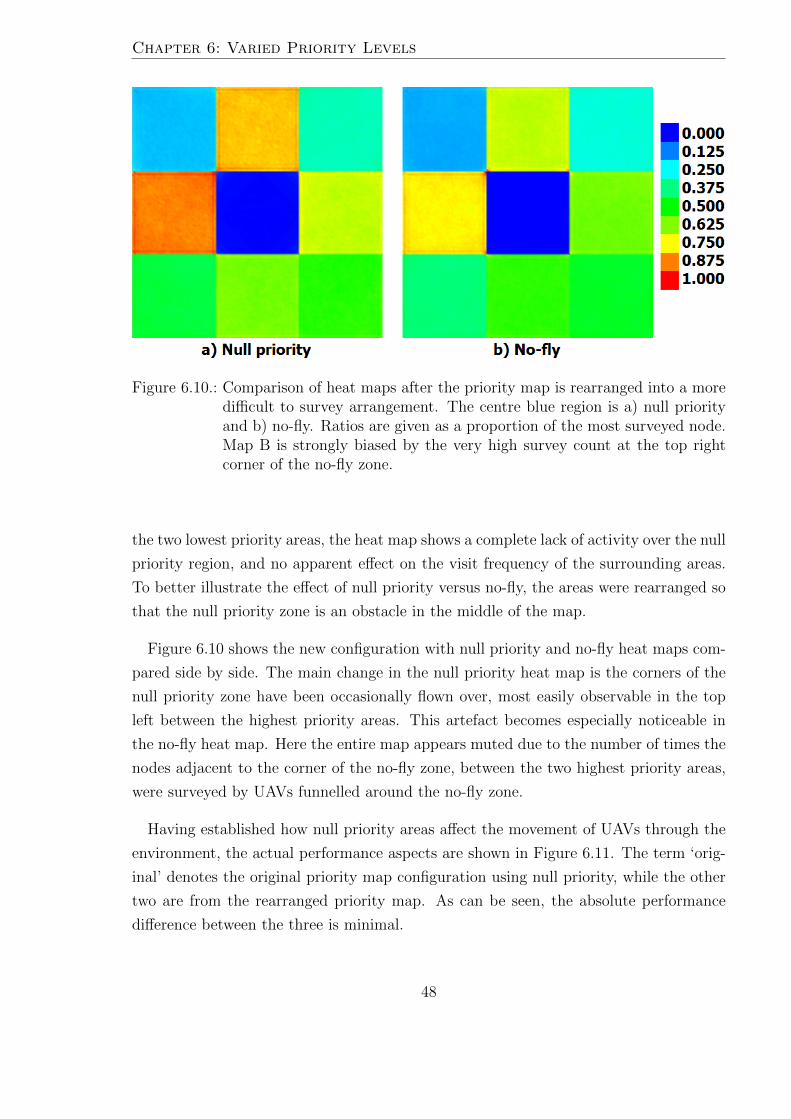
Chapter 6: Varied Priority Levels
Figure 6.10.: Comparison of heat maps after the priority map is rearranged into a moredifficult to survey arrangement. The centre blue region is a) null priorityand b) no-fly. Ratios are given as a proportion of the most surveyed node.Map B is strongly biased by the very high survey count at the top rightcorner of the no-fly zone.
the two lowest priority areas, the heat map shows a complete lack of activity over the null
priority region, and no apparent effect on the visit frequency of the surrounding areas.
To better illustrate the effect of null priority versus no-fly, the areas were rearranged so
that the null priority zone is an obstacle in the middle of the map.
Figure 6.10 shows the new configuration with null priority and no-fly heat maps com-
pared side by side. The main change in the null priority heat map is the corners of the
null priority zone have been occasionally flown over, most easily observable in the top
left between the highest priority areas. This artefact becomes especially noticeable in
the no-fly heat map. Here the entire map appears muted due to the number of times the
nodes adjacent to the corner of the no-fly zone, between the two highest priority areas,
were surveyed by UAVs funnelled around the no-fly zone.
Having established how null priority areas affect the movement of UAVs through the
environment, the actual performance aspects are shown in Figure 6.11. The term ‘orig-
inal’ denotes the original priority map configuration using null priority, while the other
two are from the rearranged priority map. As can be seen, the absolute performance
difference between the three is minimal.
48
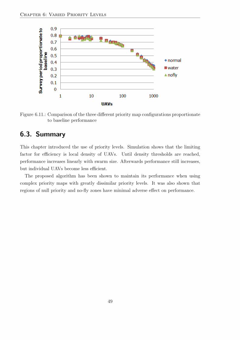
Chapter 6: Varied Priority Levels
Figure 6.11.: Comparison of the three different priority map configurations proportionateto baseline performance
6.3. Summary
This chapter introduced the use of priority levels. Simulation shows that the limiting
factor for efficiency is local density of UAVs. Until density thresholds are reached,
performance increases linearly with swarm size. Afterwards performance still increases,
but individual UAVs become less efficient.
The proposed algorithm has been shown to maintain its performance when using
complex priority maps with greatly dissimilar priority levels. It was also shown that
regions of null priority and no-fly zones have minimal adverse effect on performance.
49

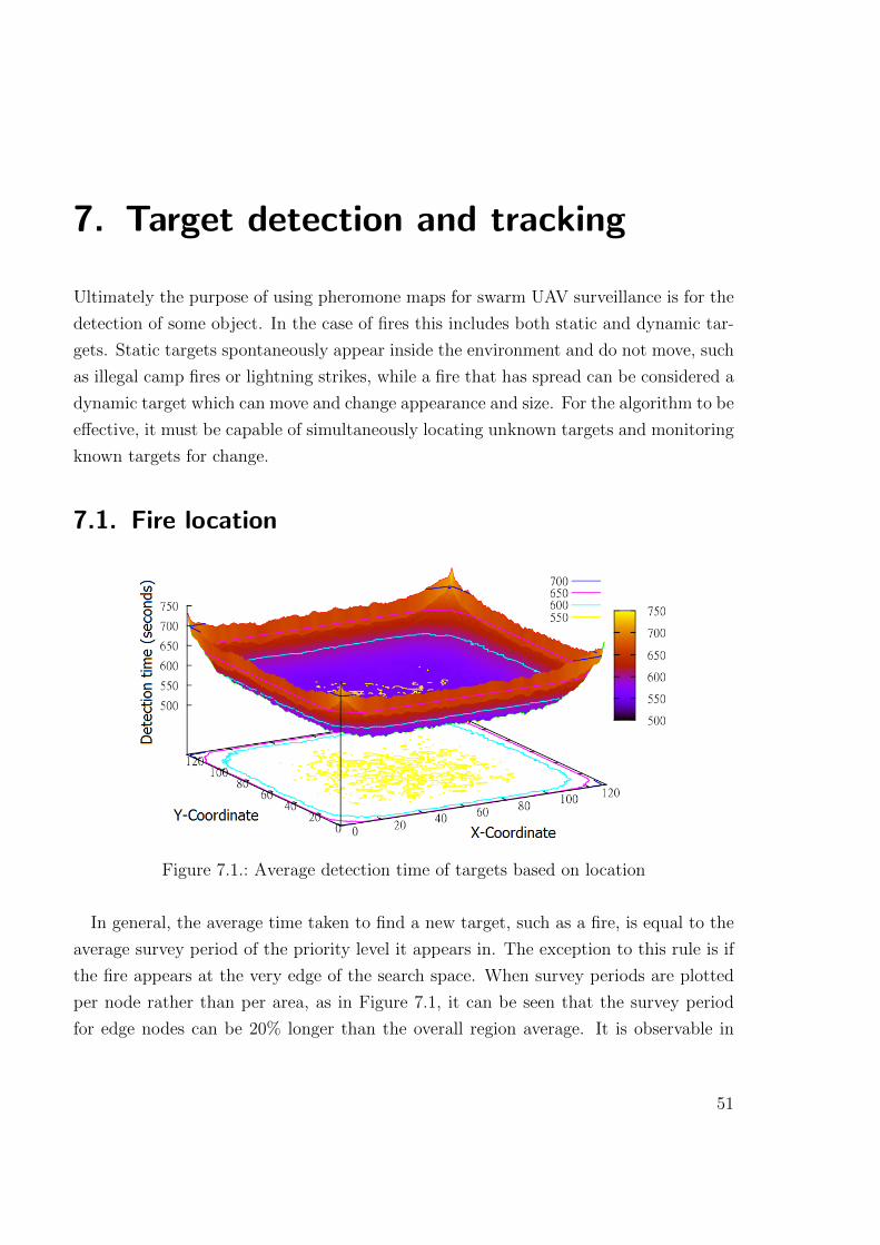
7. Target detection and tracking
Ultimately the purpose of using pheromone maps for swarm UAV surveillance is for the
detection of some object. In the case of fires this includes both static and dynamic tar-
gets. Static targets spontaneously appear inside the environment and do not move, such
as illegal camp fires or lightning strikes, while a fire that has spread can be considered a
dynamic target which can move and change appearance and size. For the algorithm to be
effective, it must be capable of simultaneously locating unknown targets and monitoring
known targets for change.
7.1. Fire location
Figure 7.1.: Average detection time of targets based on location
In general, the average time taken to find a new target, such as a fire, is equal to the
average survey period of the priority level it appears in. The exception to this rule is if
the fire appears at the very edge of the search space. When survey periods are plotted
per node rather than per area, as in Figure 7.1, it can be seen that the survey period
for edge nodes can be 20% longer than the overall region average. It is observable in
51
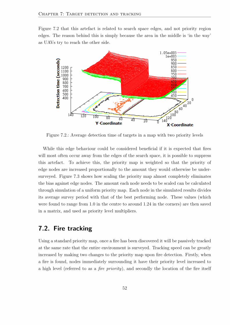
Chapter 7: Target detection and tracking
Figure 7.2 that this artefact is related to search space edges, and not priority region
edges. The reason behind this is simply because the area in the middle is ‘in the way’
as UAVs try to reach the other side.
Figure 7.2.: Average detection time of targets in a map with two priority levels
While this edge behaviour could be considered beneficial if it is expected that fires
will most often occur away from the edges of the search space, it is possible to suppress
this artefact. To achieve this, the priority map is weighted so that the priority of
edge nodes are increased proportionally to the amount they would otherwise be under-
surveyed. Figure 7.3 shows how scaling the priority map almost completely eliminates
the bias against edge nodes. The amount each node needs to be scaled can be calculated
through simulation of a uniform priority map. Each node in the simulated results divides
its average survey period with that of the best performing node. These values (which
were found to range from 1.0 in the centre to around 1.24 in the corners) are then saved
in a matrix, and used as priority level multipliers.
7.2. Fire tracking
Using a standard priority map, once a fire has been discovered it will be passively tracked
at the same rate that the entire environment is surveyed. Tracking speed can be greatly
increased by making two changes to the priority map upon fire detection. Firstly, when
a fire is found, nodes immediately surrounding it have their priority level increased to
a high level (referred to as a fire priority), and secondly the location of the fire itself
52
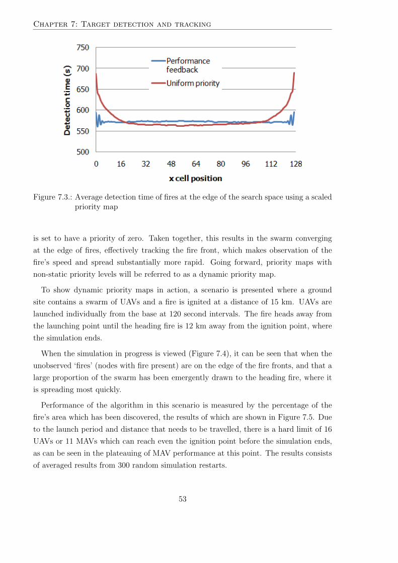
Chapter 7: Target detection and tracking
Figure 7.3.: Average detection time of fires at the edge of the search space using a scaledpriority map
is set to have a priority of zero. Taken together, this results in the swarm converging
at the edge of fires, effectively tracking the fire front, which makes observation of the
fire’s speed and spread substantially more rapid. Going forward, priority maps with
non-static priority levels will be referred to as a dynamic priority map.
To show dynamic priority maps in action, a scenario is presented where a ground
site contains a swarm of UAVs and a fire is ignited at a distance of 15 km. UAVs are
launched individually from the base at 120 second intervals. The fire heads away from
the launching point until the heading fire is 12 km away from the ignition point, where
the simulation ends.
When the simulation in progress is viewed (Figure 7.4), it can be seen that when the
unobserved ‘fires’ (nodes with fire present) are on the edge of the fire fronts, and that a
large proportion of the swarm has been emergently drawn to the heading fire, where it
is spreading most quickly.
Performance of the algorithm in this scenario is measured by the percentage of the
fire’s area which has been discovered, the results of which are shown in Figure 7.5. Due
to the launch period and distance that needs to be travelled, there is a hard limit of 16
UAVs or 11 MAVs which can reach even the ignition point before the simulation ends,
as can be seen in the plateauing of MAV performance at this point. The results consists
of averaged results from 300 random simulation restarts.
53
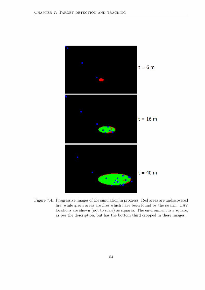
Chapter 7: Target detection and tracking
Figure 7.4.: Progressive images of the simulation in progress. Red areas are undiscoveredfire, while green areas are fires which have been found by the swarm. UAVlocations are shown (not to scale) as squares. The environment is a square,as per the description, but has the bottom third cropped in these images.
54
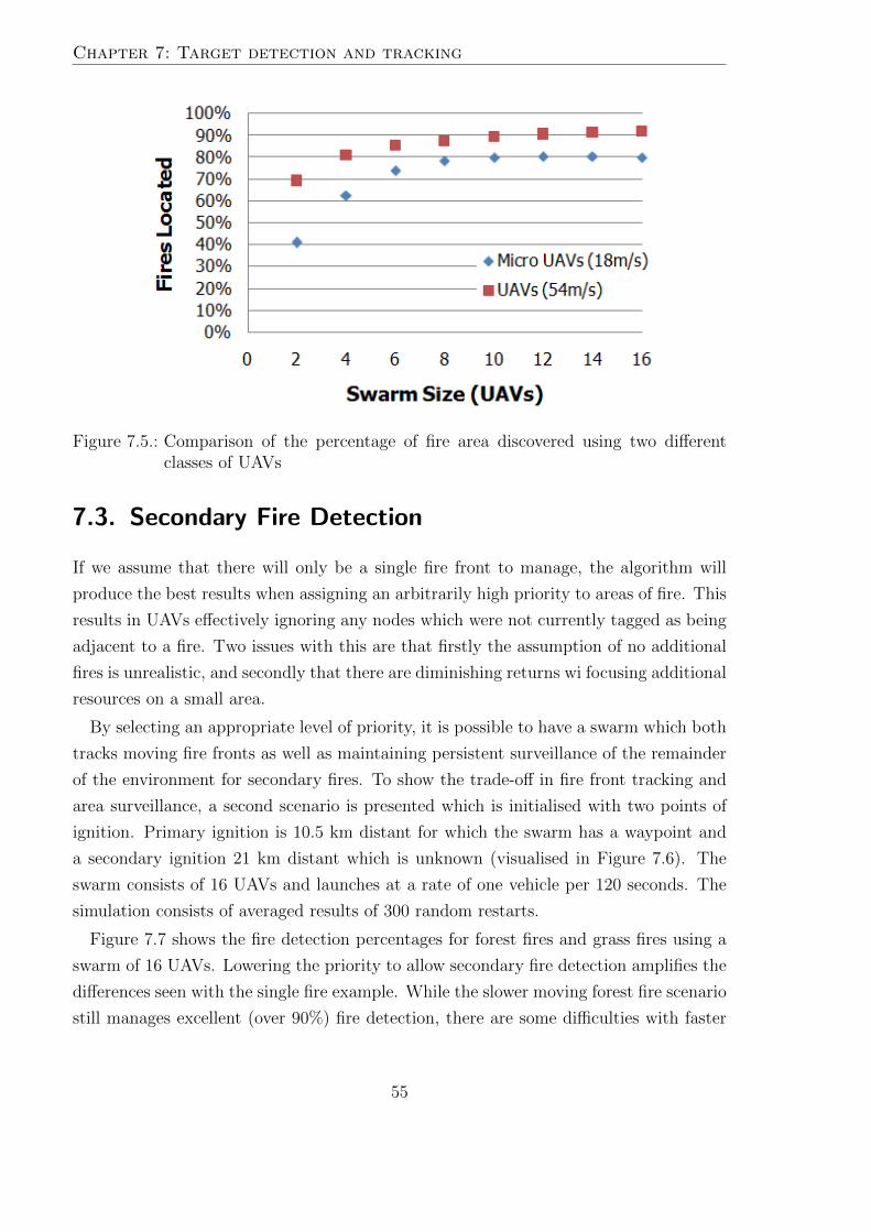
Chapter 7: Target detection and tracking
Figure 7.5.: Comparison of the percentage of fire area discovered using two differentclasses of UAVs
7.3. Secondary Fire Detection
If we assume that there will only be a single fire front to manage, the algorithm will
produce the best results when assigning an arbitrarily high priority to areas of fire. This
results in UAVs effectively ignoring any nodes which were not currently tagged as being
adjacent to a fire. Two issues with this are that firstly the assumption of no additional
fires is unrealistic, and secondly that there are diminishing returns wi focusing additional
resources on a small area.
By selecting an appropriate level of priority, it is possible to have a swarm which both
tracks moving fire fronts as well as maintaining persistent surveillance of the remainder
of the environment for secondary fires. To show the trade-off in fire front tracking and
area surveillance, a second scenario is presented which is initialised with two points of
ignition. Primary ignition is 10.5 km distant for which the swarm has a waypoint and
a secondary ignition 21 km distant which is unknown (visualised in Figure 7.6). The
swarm consists of 16 UAVs and launches at a rate of one vehicle per 120 seconds. The
simulation consists of averaged results of 300 random restarts.
Figure 7.7 shows the fire detection percentages for forest fires and grass fires using a
swarm of 16 UAVs. Lowering the priority to allow secondary fire detection amplifies the
differences seen with the single fire example. While the slower moving forest fire scenario
still manages excellent (over 90%) fire detection, there are some difficulties with faster
55
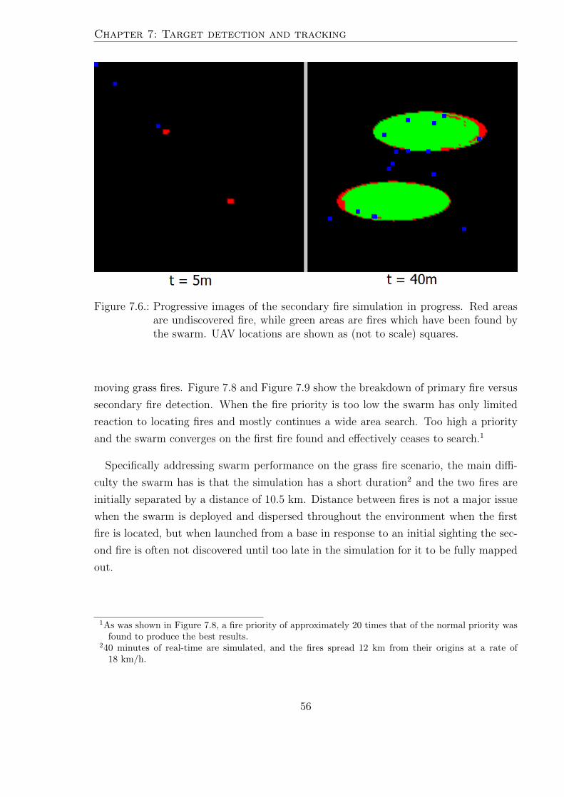
Chapter 7: Target detection and tracking
Figure 7.6.: Progressive images of the secondary fire simulation in progress. Red areasare undiscovered fire, while green areas are fires which have been found bythe swarm. UAV locations are shown as (not to scale) squares.
moving grass fires. Figure 7.8 and Figure 7.9 show the breakdown of primary fire versus
secondary fire detection. When the fire priority is too low the swarm has only limited
reaction to locating fires and mostly continues a wide area search. Too high a priority
and the swarm converges on the first fire found and effectively ceases to search.1
Specifically addressing swarm performance on the grass fire scenario, the main diffi-
culty the swarm has is that the simulation has a short duration2 and the two fires are
initially separated by a distance of 10.5 km. Distance between fires is not a major issue
when the swarm is deployed and dispersed throughout the environment when the first
fire is located, but when launched from a base in response to an initial sighting the sec-
ond fire is often not discovered until too late in the simulation for it to be fully mapped
out.
1As was shown in Figure 7.8, a fire priority of approximately 20 times that of the normal priority wasfound to produce the best results.
240 minutes of real-time are simulated, and the fires spread 12 km from their origins at a rate of18 km/h.
56
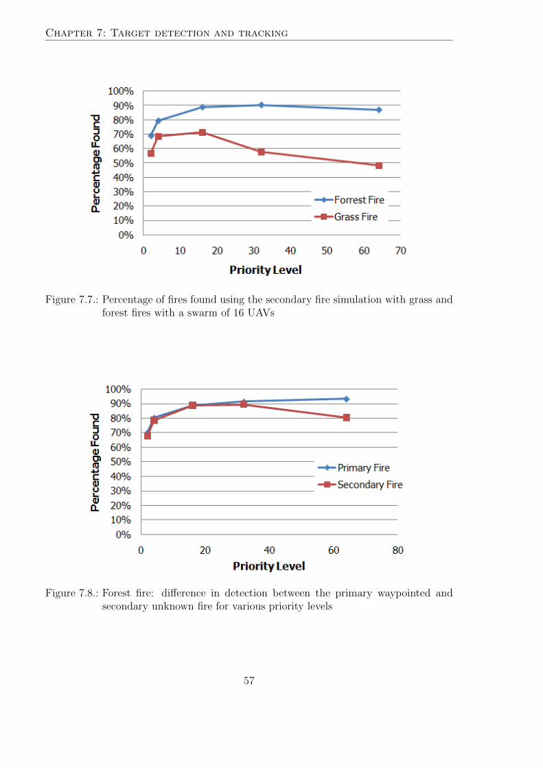
Chapter 7: Target detection and tracking
Figure 7.7.: Percentage of fires found using the secondary fire simulation with grass andforest fires with a swarm of 16 UAVs
Figure 7.8.: Forest fire: difference in detection between the primary waypointed andsecondary unknown fire for various priority levels
57
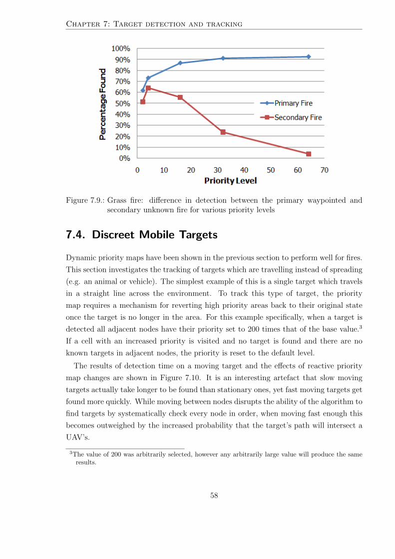
Chapter 7: Target detection and tracking
Figure 7.9.: Grass fire: difference in detection between the primary waypointed andsecondary unknown fire for various priority levels
7.4. Discreet Mobile Targets
Dynamic priority maps have been shown in the previous section to perform well for fires.
This section investigates the tracking of targets which are travelling instead of spreading
(e.g. an animal or vehicle). The simplest example of this is a single target which travels
in a straight line across the environment. To track this type of target, the priority
map requires a mechanism for reverting high priority areas back to their original state
once the target is no longer in the area. For this example specifically, when a target is
detected all adjacent nodes have their priority set to 200 times that of the base value.3
If a cell with an increased priority is visited and no target is found and there are no
known targets in adjacent nodes, the priority is reset to the default level.
The results of detection time on a moving target and the effects of reactive priority
map changes are shown in Figure 7.10. It is an interesting artefact that slow moving
targets actually take longer to be found than stationary ones, yet fast moving targets get
found more quickly. While moving between nodes disrupts the ability of the algorithm to
find targets by systematically check every node in order, when moving fast enough this
becomes outweighed by the increased probability that the target’s path will intersect a
UAV’s.
3The value of 200 was arbitrarily selected, however any arbitrarily large value will produce the sameresults.
58
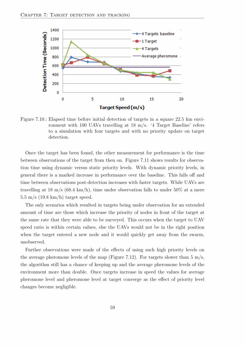
Chapter 7: Target detection and tracking
Figure 7.10.: Elapsed time before initial detection of targets in a square 22.5 km envi-ronment with 100 UAVs travelling at 18 m/s. ‘4 Target Baseline’ refersto a simulation with four targets and with no priority update on targetdetection.
Once the target has been found, the other measurement for performance is the time
between observations of the target from then on. Figure 7.11 shows results for observa-
tion time using dynamic versus static priority levels. With dynamic priority levels, in
general there is a marked increase in performance over the baseline. This falls off and
time between observations post-detection increases with faster targets. While UAVs are
travelling at 18 m/s (68.4 km/h), time under observation falls to under 50% at a mere
5.5 m/s (19.8 km/h) target speed.
The only scenarios which resulted in targets being under observation for an extended
amount of time are those which increase the priority of nodes in front of the target at
the same rate that they were able to be surveyed. This occurs when the target to UAV
speed ratio is within certain values, else the UAVs would not be in the right position
when the target entered a new node and it would quickly get away from the swarm,
unobserved.
Further observations were made of the effects of using such high priority levels on
the average pheromone levels of the map (Figure 7.12). For targets slower than 5 m/s,
the algorithm still has a chance of keeping up and the average pheromone levels of the
environment more than double. Once targets increase in speed the values for average
pheromone level and pheromone level at target converge as the effect of priority level
changes become negligible.
59
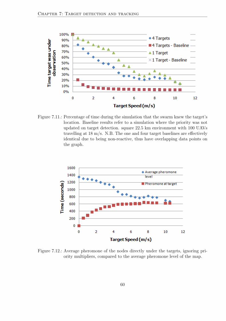
Chapter 7: Target detection and tracking
Figure 7.11.: Percentage of time during the simulation that the swarm knew the target’slocation. Baseline results refer to a simulation where the priority was notupdated on target detection. square 22.5 km environment with 100 UAVstravelling at 18 m/s. N.B. The one and four target baselines are effectivelyidentical due to being non-reactive, thus have overlapping data points onthe graph.
Figure 7.12.: Average pheromone of the nodes directly under the targets, ignoring pri-ority multipliers, compared to the average pheromone level of the map.
60
Chapter 7: Target detection and tracking
7.5. Summary
This chapter has described the use of dynamic priority updates for use in tracking fires
and other targets. This involved incorporating rules which automatically increase or
decrease the priority of an area under certain triggering conditions, such as targets
being found or a period of time passing.
The results presented indicate that effective wildfire tracking can be performed by a
decentralised UAV swarm. Using dynamic priority updates has been shown to enable
persistent surveillance for fire ignition, while at the same time closely tracking fire fronts
via exploitation of emergent behaviours.
Performance was not found to carry over to discrete moving targets such as vehicles.
Better target tracking might be possible by incorporating predictive target direction
algorithms, such as those used in radar systems.
61

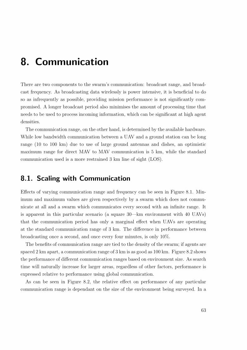
8. Communication
There are two components to the swarm’s communication: broadcast range, and broad-
cast frequency. As broadcasting data wirelessly is power intensive, it is beneficial to do
so as infrequently as possible, providing mission performance is not significantly com-
promised. A longer broadcast period also minimises the amount of processing time that
needs to be used to process incoming information, which can be significant at high agent
densities.
The communication range, on the other hand, is determined by the available hardware.
While low bandwidth communication between a UAV and a ground station can be long
range (10 to 100 km) due to use of large ground antennas and dishes, an optimistic
maximum range for direct MAV to MAV communication is 5 km, while the standard
communication used is a more restrained 3 km line of sight (LOS).
8.1. Scaling with Communication
Effects of varying communication range and frequency can be seen in Figure 8.1. Min-
imum and maximum values are given respectively by a swarm which does not commu-
nicate at all and a swarm which communicates every second with an infinite range. It
is apparent in this particular scenario (a square 30—km environment with 40 UAVs)
that the communication period has only a marginal effect when UAVs are operating
at the standard communication range of 3 km. The difference in performance between
broadcasting once a second, and once every four minutes, is only 10%.
The benefits of communication range are tied to the density of the swarm; if agents are
spaced 2 km apart, a communication range of 3 km is as good as 100 km. Figure 8.2 shows
the performance of different communication ranges based on environment size. As search
time will naturally increase for larger areas, regardless of other factors, performance is
expressed relative to performance using global communication.
As can be seen in Figure 8.2, the relative effect on performance of any particular
communication range is dependant on the size of the environment being surveyed. In a
63
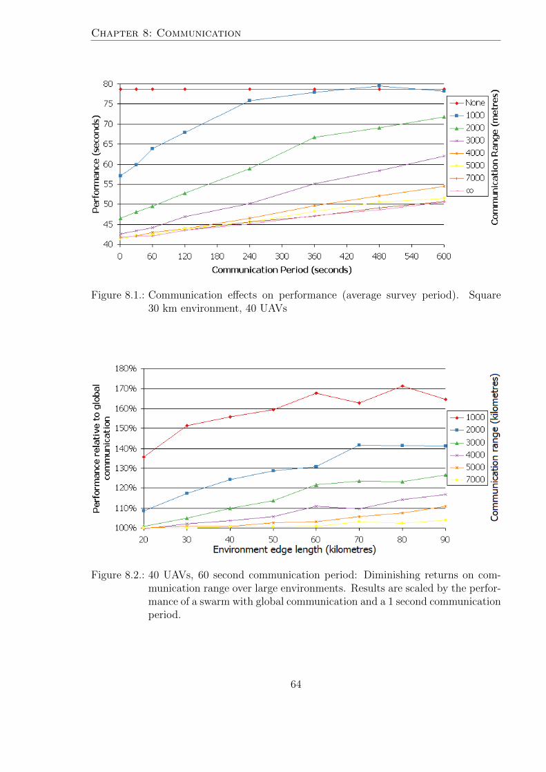
Chapter 8: Communication
Figure 8.1.: Communication effects on performance (average survey period). Square30 km environment, 40 UAVs
Figure 8.2.: 40 UAVs, 60 second communication period: Diminishing returns on com-munication range over large environments. Results are scaled by the perfor-mance of a swarm with global communication and a 1 second communicationperiod.
64
Chapter 8: Communication
square 60 km environment a 4 km range is needed to get the same performance as a 3 km
range in a 40 km environment. The difference in performance between a 5 km radius
and an unlimited/global range is only 10% even at 90 km. This relative performance
gap will shrink as the agent density increases with the addition of agents, or grow as
agents are removed.
In summary, communication parameters do not have a significant effect on swarm
performance as long as relatively frugal minimums are met (e.g. 2 km range, 120 s
interval). While this is sufficient for what is considered to be the algorithm’s normal
parameters, information flow within the swarm has interesting and noteworthy artefacts,
especially at extremely low or transitional values, which are examined in further detail
in Section 8.3.
8.2. Information Flow
In swarm systems using distributed pheromone maps, any new information in a trans-
mission overwrites old information while travelling through the swarm in a series of
‘hops’. This process can be modelled as a dynamic, ad hoc network which has nodes
and connections based on spatial coordinates and UAV proximity. The spread of new
information in the swarm can thus be analysed in the context of a shortest path problem
in a dynamic tree (Chabini 1998). In a swarm of n agents, assuming an infinite search
space and finite communication range, the maximum hop count is n− 1.
Information is not guaranteed to traverse the entire tree due to the possibility of data
becoming out of date before it reaches a given node, at which point it will progress no
further down that branch. In an optimised network, the maximum path length would be
minimised, and every node would be connected to every other node via a path with a hop
count of one, such as maximally connected through global peer-to-peer communication.
Issues with setting up such a network include agents being required to know the
location all other agents in the swarm. In practice this is difficult to achieve without
global communication. If this long range communication, in the quantities of bandwidth
required, is a viable option then an algorithm that optimises using centralised control
should be seriously considered.
Depending on the connectivity of the swarm, itself dependant on factors such as swarm
density, communication rage, and knowledge of other UAVs, the network will resemble
a scale free or small world network (Newman 2003). In practice, communication ranges
are limited and the network formed between UAVs has a small-world topology, where
65
Chapter 8: Communication
the majority of nodes are not neighbours, yet most nodes can be reached by a small
number of hops (Olsson et al. 2010).
If the swarm’s algorithms include a weak repulsion mechanism, a large or uncapped
pheromone map evaluation radius, or a weak distance penalty in the heuristic, UAVs
crowd into dense, discrete sub-swarms with individual networks. These sub-swarms
periodically combine and then split, sharing their accumulated knowledge as they do
so. This behaviour has a secondary dependence on environment variables such as size
versus UAV cruising speed.1
More effective area search is achieved when factors such as repulsion are strong enough
to achieve a uniform distribution. This enables rapid information flow as there exists
only a single network.
8.2.1. Data Synchronisation
An individual UAV’s knowledge of its general vicinity is up to date in most cases. The
chance of data being known by any particular individual is directly related to the age
of the data. Areas with high pheromone have the oldest information, and UAVs are
drawn to the highest pheromone areas. However as the agent density goes up the rate of
information flow becomes increasingly important in maintaining this state of local area
knowledge. When a UAV is not alone in surveying a locality, the UAV’s individually
observed information needs to be shared with greater frequency if performance is to be
maintained. Otherwise nodes go unvisited until their pheromone level is high enough to
attract a UAV (as normal) followed by multiple redundant searches in a small period of
time by multiple UAVs who have yet to receive knowledge of the first’s efforts.
The flow of information within a swarm can be measured by how synchronised the
data contained in pheromone maps of individuals in the swarm are. Synchronisation is
measured on a per-agent basis: a synchronised node of the pheromone map is one in
which the survey time known to the selected UAV is the most recent available in the
entire swarm. As an example, in a swarm of 20 non-communicating agents, each agent
will always have, on average, a minimum of 5% of its pheromone map ‘in sync’ simply due
to having been the most recent agent to directly observe that subset of nodes. Adding
communication broadcasts increases this percentage, relative to broadcast frequency, by
enabling the incorporation of survey timestamps from peer agents.
Of the information in the environment, the age of data has an inverse relationship
1If the UAVs are able to traverse the length of the environment very quickly then it is too small toshow visibly distinct sub-swarms.
66
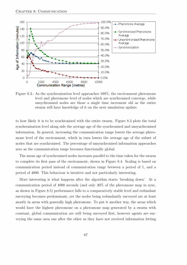
Chapter 8: Communication
Figure 8.3.: As the synchronisation level approaches 100%, the environment pheromonelevel and pheromone level of nodes which are synchronised converge, whileunsychronised nodes are those a single time increment old as the entireswarm will have knowledge of it on the next simulation update.
to how likely it is to be synchronised with the entire swarm. Figure 8.3 plots the total
synchronisation level along side the average age of the synchronised and unsynchronised
information. In general, increasing the communication range lowers the average phero-
mone level of the environment, which in turn lowers the average age of the subset of
nodes that are synchronised. The percentage of unsynchronised information approaches
zero as the communication range becomes functionally global.
The mean age of synchronised nodes increases parallel to the time taken for the swarm
to complete its first pass of the environment, shown in Figure 8.4. Scaling is based on
communication period instead of communication range between a period of 1, and a
period of 4000. This behaviour is intuitive and not particularly interesting.
More interesting is what happens after the algorithm starts ‘breaking down’. At a
communication period of 4000 seconds (and only 30% of the pheromone map in sync,
as shown in Figure 8.5) performance falls to a comparatively stable level and redundant
surveying becomes predominant, yet the nodes being redundantly surveyed are at least
mostly in areas with generally high pheromone. To put it another way, the areas which
would have the highest pheromone on a pheromone map generated by a swarm with
constant, global communication are still being surveyed first, however agents are sur-
veying the same area one after the other as they have not received information letting
67
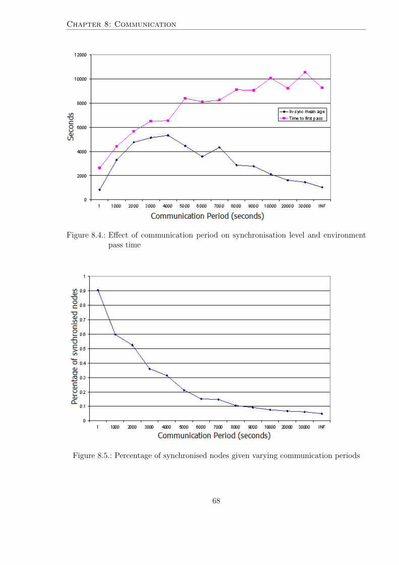
Chapter 8: Communication
Figure 8.4.: Effect of communication period on synchronisation level and environmentpass time
Figure 8.5.: Percentage of synchronised nodes given varying communication periods
68
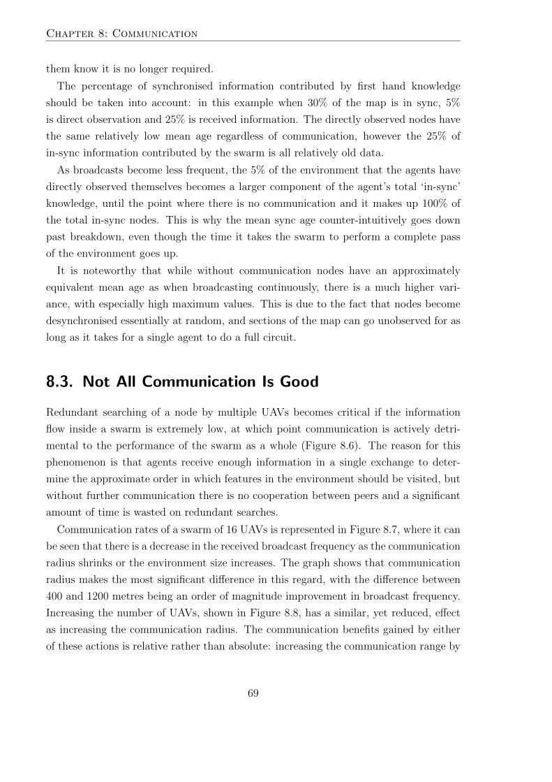
Chapter 8: Communication
them know it is no longer required.
The percentage of synchronised information contributed by first hand knowledge
should be taken into account: in this example when 30% of the map is in sync, 5%
is direct observation and 25% is received information. The directly observed nodes have
the same relatively low mean age regardless of communication, however the 25% of
in-sync information contributed by the swarm is all relatively old data.
As broadcasts become less frequent, the 5% of the environment that the agents have
directly observed themselves becomes a larger component of the agent’s total ‘in-sync’
knowledge, until the point where there is no communication and it makes up 100% of
the total in-sync nodes. This is why the mean sync age counter-intuitively goes down
past breakdown, even though the time it takes the swarm to perform a complete pass
of the environment goes up.
It is noteworthy that while without communication nodes have an approximately
equivalent mean age as when broadcasting continuously, there is a much higher vari-
ance, with especially high maximum values. This is due to the fact that nodes become
desynchronised essentially at random, and sections of the map can go unobserved for as
long as it takes for a single agent to do a full circuit.
8.3. Not All Communication Is Good
Redundant searching of a node by multiple UAVs becomes critical if the information
flow inside a swarm is extremely low, at which point communication is actively detri-
mental to the performance of the swarm as a whole (Figure 8.6). The reason for this
phenomenon is that agents receive enough information in a single exchange to deter-
mine the approximate order in which features in the environment should be visited, but
without further communication there is no cooperation between peers and a significant
amount of time is wasted on redundant searches.
Communication rates of a swarm of 16 UAVs is represented in Figure 8.7, where it can
be seen that there is a decrease in the received broadcast frequency as the communication
radius shrinks or the environment size increases. The graph shows that communication
radius makes the most significant difference in this regard, with the difference between
400 and 1200 metres being an order of magnitude improvement in broadcast frequency.
Increasing the number of UAVs, shown in Figure 8.8, has a similar, yet reduced, effect
as increasing the communication radius. The communication benefits gained by either
of these actions is relative rather than absolute: increasing the communication range by
69
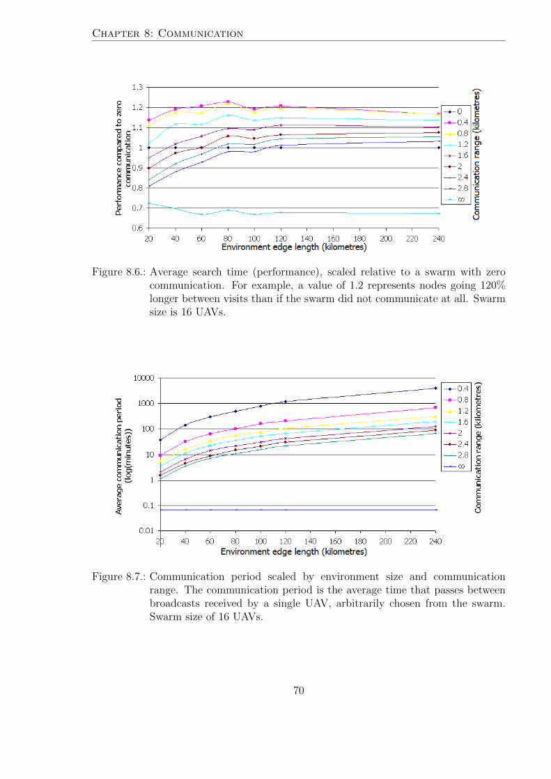
Chapter 8: Communication
Figure 8.6.: Average search time (performance), scaled relative to a swarm with zerocommunication. For example, a value of 1.2 represents nodes going 120%longer between visits than if the swarm did not communicate at all. Swarmsize is 16 UAVs.
Figure 8.7.: Communication period scaled by environment size and communicationrange. The communication period is the average time that passes betweenbroadcasts received by a single UAV, arbitrarily chosen from the swarm.Swarm size of 16 UAVs.
70
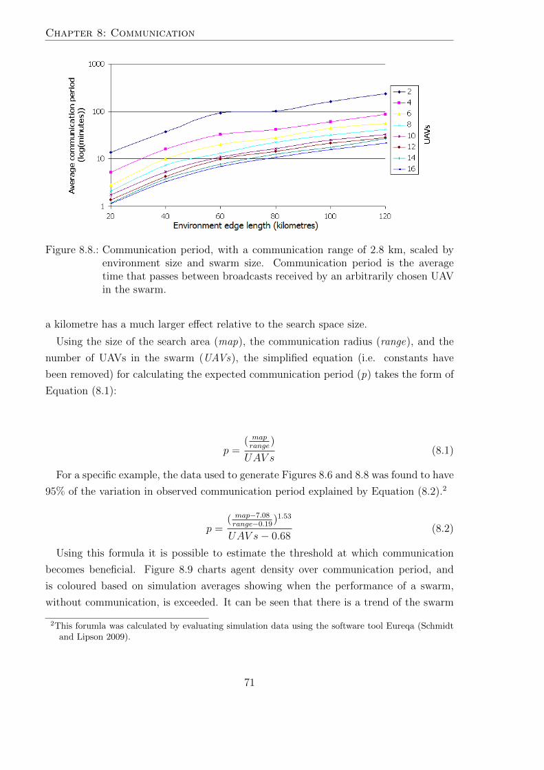
Chapter 8: Communication
Figure 8.8.: Communication period, with a communication range of 2.8 km, scaled byenvironment size and swarm size. Communication period is the averagetime that passes between broadcasts received by an arbitrarily chosen UAVin the swarm.
a kilometre has a much larger effect relative to the search space size.
Using the size of the search area (map), the communication radius (range), and the
number of UAVs in the swarm (UAVs), the simplified equation (i.e. constants have
been removed) for calculating the expected communication period (p) takes the form of
Equation (8.1):
p =( maprange
)
UAV s(8.1)
For a specific example, the data used to generate Figures 8.6 and 8.8 was found to have
95% of the variation in observed communication period explained by Equation (8.2).2
p =( map−7.08range−0.19)1.53
UAV s− 0.68(8.2)
Using this formula it is possible to estimate the threshold at which communication
becomes beneficial. Figure 8.9 charts agent density over communication period, and
is coloured based on simulation averages showing when the performance of a swarm,
without communication, is exceeded. It can be seen that there is a trend of the swarm
2This forumla was calculated by evaluating simulation data using the software tool Eureqa (Schmidtand Lipson 2009).
71
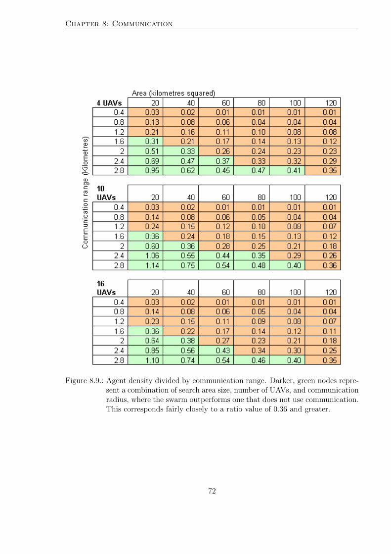
Chapter 8: Communication
Figure 8.9.: Agent density divided by communication range. Darker, green nodes repre-sent a combination of search area size, number of UAVs, and communicationradius, where the swarm outperforms one that does not use communication.This corresponds fairly closely to a ratio value of 0.36 and greater.
72
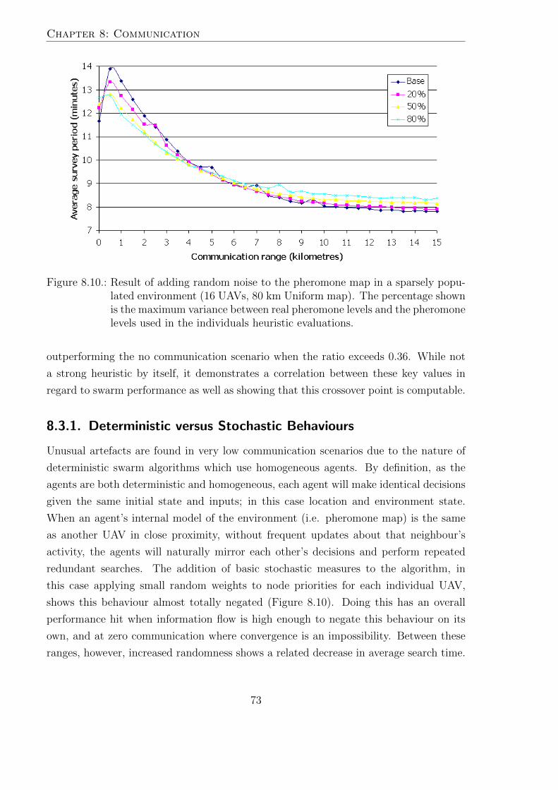
Chapter 8: Communication
Figure 8.10.: Result of adding random noise to the pheromone map in a sparsely popu-lated environment (16 UAVs, 80 km Uniform map). The percentage shownis the maximum variance between real pheromone levels and the pheromonelevels used in the individuals heuristic evaluations.
outperforming the no communication scenario when the ratio exceeds 0.36. While not
a strong heuristic by itself, it demonstrates a correlation between these key values in
regard to swarm performance as well as showing that this crossover point is computable.
8.3.1. Deterministic versus Stochastic Behaviours
Unusual artefacts are found in very low communication scenarios due to the nature of
deterministic swarm algorithms which use homogeneous agents. By definition, as the
agents are both deterministic and homogeneous, each agent will make identical decisions
given the same initial state and inputs; in this case location and environment state.
When an agent’s internal model of the environment (i.e. pheromone map) is the same
as another UAV in close proximity, without frequent updates about that neighbour’s
activity, the agents will naturally mirror each other’s decisions and perform repeated
redundant searches. The addition of basic stochastic measures to the algorithm, in
this case applying small random weights to node priorities for each individual UAV,
shows this behaviour almost totally negated (Figure 8.10). Doing this has an overall
performance hit when information flow is high enough to negate this behaviour on its
own, and at zero communication where convergence is an impossibility. Between these
ranges, however, increased randomness shows a related decrease in average search time.
73
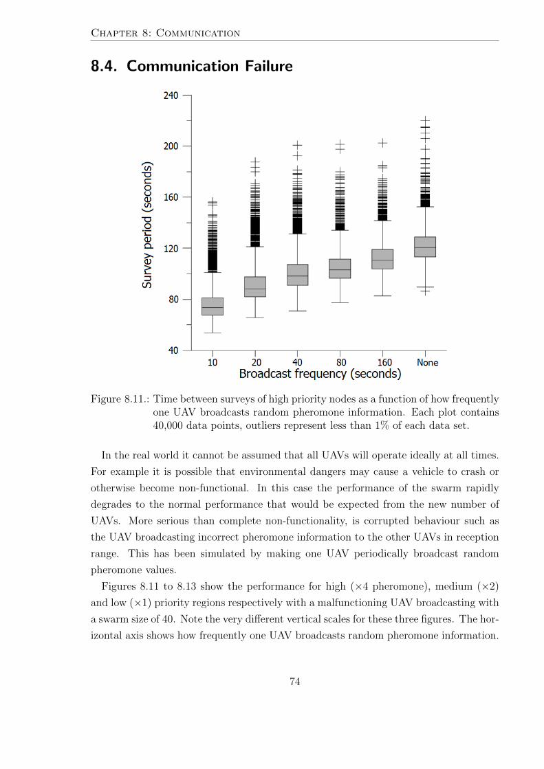
Chapter 8: Communication
8.4. Communication Failure
Figure 8.11.: Time between surveys of high priority nodes as a function of how frequentlyone UAV broadcasts random pheromone information. Each plot contains40,000 data points, outliers represent less than 1% of each data set.
In the real world it cannot be assumed that all UAVs will operate ideally at all times.
For example it is possible that environmental dangers may cause a vehicle to crash or
otherwise become non-functional. In this case the performance of the swarm rapidly
degrades to the normal performance that would be expected from the new number of
UAVs. More serious than complete non-functionality, is corrupted behaviour such as
the UAV broadcasting incorrect pheromone information to the other UAVs in reception
range. This has been simulated by making one UAV periodically broadcast random
pheromone values.
Figures 8.11 to 8.13 show the performance for high (×4 pheromone), medium (×2)
and low (×1) priority regions respectively with a malfunctioning UAV broadcasting with
a swarm size of 40. Note the very different vertical scales for these three figures. The hor-
izontal axis shows how frequently one UAV broadcasts random pheromone information.
74
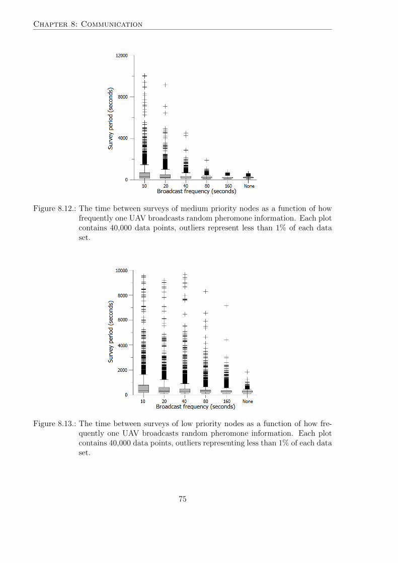
Chapter 8: Communication
Figure 8.12.: The time between surveys of medium priority nodes as a function of howfrequently one UAV broadcasts random pheromone information. Each plotcontains 40,000 data points, outliers represent less than 1% of each dataset.
Figure 8.13.: The time between surveys of low priority nodes as a function of how fre-quently one UAV broadcasts random pheromone information. Each plotcontains 40,000 data points, outliers representing less than 1% of each dataset.
75
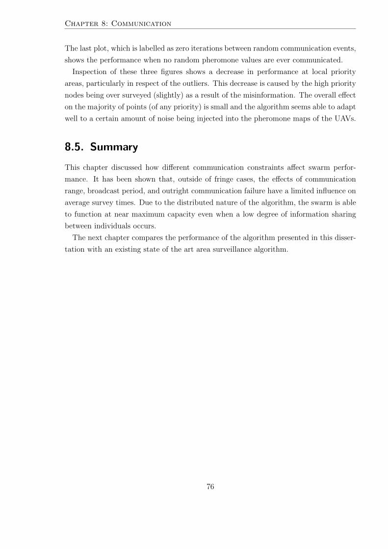
Chapter 8: Communication
The last plot, which is labelled as zero iterations between random communication events,
shows the performance when no random pheromone values are ever communicated.
Inspection of these three figures shows a decrease in performance at local priority
areas, particularly in respect of the outliers. This decrease is caused by the high priority
nodes being over surveyed (slightly) as a result of the misinformation. The overall effect
on the majority of points (of any priority) is small and the algorithm seems able to adapt
well to a certain amount of noise being injected into the pheromone maps of the UAVs.
8.5. Summary
This chapter discussed how different communication constraints affect swarm perfor-
mance. It has been shown that, outside of fringe cases, the effects of communication
range, broadcast period, and outright communication failure have a limited influence on
average survey times. Due to the distributed nature of the algorithm, the swarm is able
to function at near maximum capacity even when a low degree of information sharing
between individuals occurs.
The next chapter compares the performance of the algorithm presented in this disser-
tation with an existing state of the art area surveillance algorithm.
76
9. Comparative Results
Of the algorithms simulated to find a baseline for comparison, the best performing was
one by Erignac (2007). Erignac’s algorithm is designed to perform a single exhaustive
pass of an environment, and uses Euclidean distance to the closest unexplored node
as pheromone. Behaviour of the UAVs is determined by a finite state machine, which
defaults to performing gradient descent on the pheromone if no other conditions are met.
This chapter compares the performance of the proposed algorithm with Erignac’s.
9.1. Exhaustive Swarming Search Strategy
The finite state machine used to determine UAV behaviour in Erignac’s algorithm is
shown in Figure 9.1. Due to an interesting implementation of state-based behaviours,
the search pattern which emerges is highly efficient when communication is continuous.
The state-space that Erignac’s algorithm is designed for is one with a uniform level of
priority, where each cell starts in the ‘unexplored’ state, and needs to be visited at least
once to change it to ‘explored’. To be useful as a comparison to the proposed algorithm
in this work a variant is required.
Firstly, the Euclidean distance pheromone map is used side-by-side with a modified
priority pheromone map which indicates a cell as being in the explored state if its phero-
mone is lower than one. When enough time passes to raise pheromone above one, the
state changes to unexplored. Even when cells are showing as explored, visiting them
during a random move or a repulsion move would reset their pheromone to zero as with
a ‘normal’ pheromone map.
As absolute pheromone values are needed due to the binary nature of the node states,
the rate of pheromone increase needs to be optimised offline (pre-simulation). When
pheromone increases too slowly the swarm spends an inefficient amount of time moving
long distances towards newly triggered nodes. Alternatively, when pheromone increase is
too fast, the inability of UAVs to distinguish ‘old’ unexplored cells from ‘new’ unexplored
cells becomes pronounced.
77
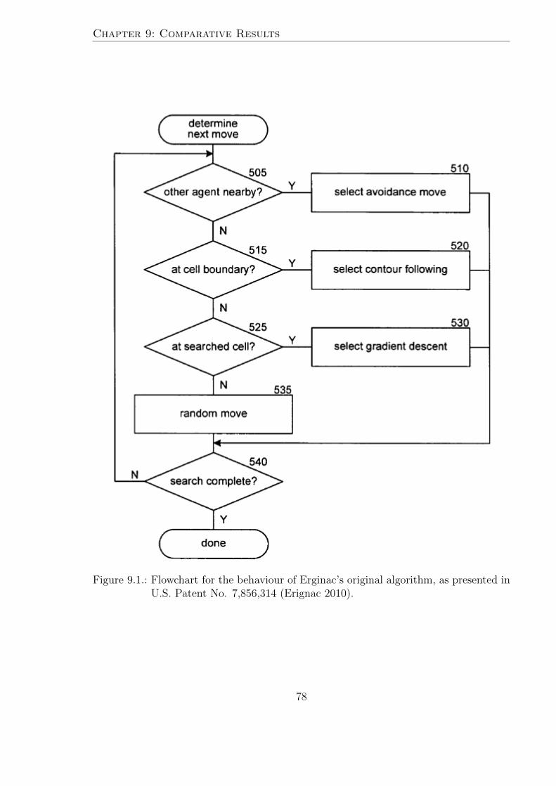
Chapter 9: Comparative Results
Figure 9.1.: Flowchart for the behaviour of Erginac’s original algorithm, as presented inU.S. Patent No. 7,856,314 (Erignac 2010).
78
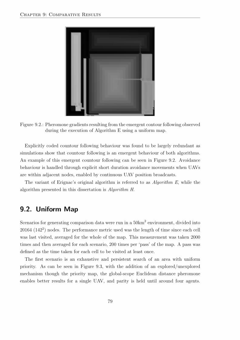
Chapter 9: Comparative Results
Figure 9.2.: Pheromone gradients resulting from the emergent contour following observedduring the execution of Algorithm E using a uniform map.
Explicitly coded countour following behaviour was found to be largely redundant as
simulations show that countour following is an emergent behaviour of both algorithms.
An example of this emergent countour following can be seen in Figure 9.2. Avoidance
behaviour is handled through explicit short duration avoidance movements when UAVs
are within adjacent nodes, enabled by continuous UAV position broadcasts.
The variant of Erignac’s original algorithm is referred to as Algorithm E, while the
algorithm presented in this dissertation is Algorithm H.
9.2. Uniform Map
Scenarios for generating comparison data were run in a 50km2 environment, divided into
20164 (1422) nodes. The performance metric used was the length of time since each cell
was last visited, averaged for the whole of the map. This measurement was taken 2000
times and then averaged for each scenario, 200 times per ‘pass’ of the map. A pass was
defined as the time taken for each cell to be visited at least once.
The first scenario is an exhaustive and persistent search of an area with uniform
priority. As can be seen in Figure 9.3, with the addition of an explored/unexplored
mechanism though the priority map, the global-scope Euclidean distance pheromone
enables better results for a single UAV, and parity is held until around four agents.
79
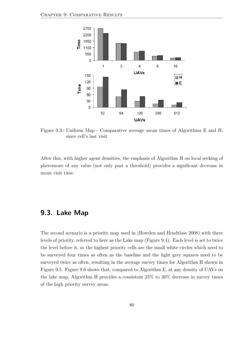
Chapter 9: Comparative Results
Figure 9.3.: Uniform Map - Comparative average mean times of Algorithms E and H,since cell’s last visit
After this, with higher agent densities, the emphasis of Algorithm H on local seeking of
pheromone of any value (not only past a threshold) provides a significant decrease in
mean visit time.
9.3. Lake Map
The second scenario is a priority map used in (Howden and Hendtlass 2008) with three
levels of priority, referred to here as the Lake map (Figure 9.4). Each level is set to twice
the level before it, so the highest priority cells are the small white circles which need to
be surveyed four times as often as the baseline and the light grey squares need to be
surveyed twice as often, resulting in the average survey times for Algorithm H shown in
Figure 9.5. Figure 9.6 shows that, compared to Algorithm E, at any density of UAVs on
the lake map, Algorithm H provides a consistent 25% to 30% decrease in survey times
of the high priority survey areas.
80
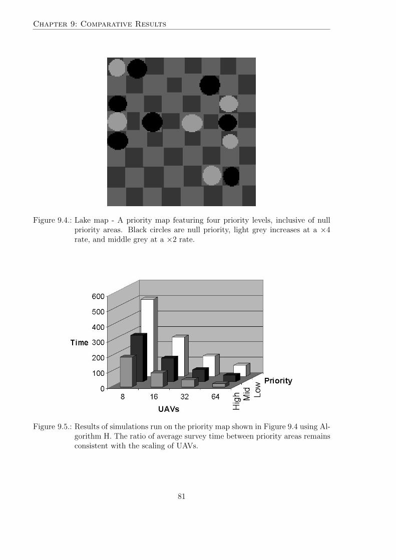
Chapter 9: Comparative Results
Figure 9.4.: Lake map - A priority map featuring four priority levels, inclusive of nullpriority areas. Black circles are null priority, light grey increases at a ×4rate, and middle grey at a ×2 rate.
Figure 9.5.: Results of simulations run on the priority map shown in Figure 9.4 using Al-gorithm H. The ratio of average survey time between priority areas remainsconsistent with the scaling of UAVs.
81
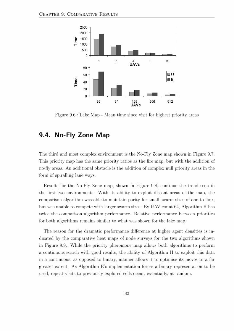
Chapter 9: Comparative Results
Figure 9.6.: Lake Map - Mean time since visit for highest priority areas
9.4. No-Fly Zone Map
The third and most complex environment is the No-Fly Zone map shown in Figure 9.7.
This priority map has the same priority ratios as the fire map, but with the addition of
no-fly areas. An additional obstacle is the addition of complex null priority areas in the
form of spiralling lane ways.
Results for the No-Fly Zone map, shown in Figure 9.8, continue the trend seen in
the first two environments. With its ability to exploit distant areas of the map, the
comparison algorithm was able to maintain parity for small swarm sizes of one to four,
but was unable to compete with larger swarm sizes. By UAV count 64, Algorithm H has
twice the comparison algorithm performance. Relative performance between priorities
for both algorithms remains similar to what was shown for the lake map.
The reason for the dramatic performance difference at higher agent densities is in-
dicated by the comparative heat maps of node surveys for the two algorithms shown
in Figure 9.9. While the priority pheromone map allows both algorithms to perform
a continuous search with good results, the ability of Algorithm H to exploit this data
in a continuous, as opposed to binary, manner allows it to optimise its moves to a far
greater extent. As Algorithm E’s implementation forces a binary representation to be
used, repeat visits to previously explored cells occur, essentially, at random.
82
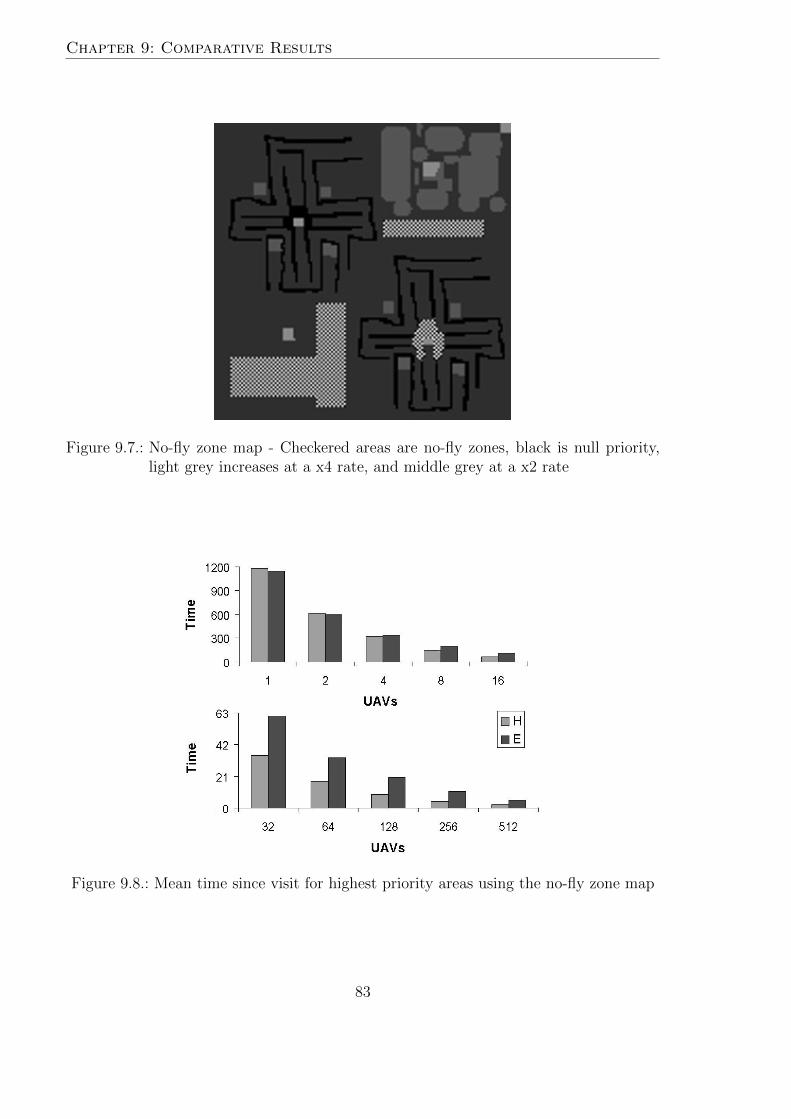
Chapter 9: Comparative Results
Figure 9.7.: No-fly zone map - Checkered areas are no-fly zones, black is null priority,light grey increases at a x4 rate, and middle grey at a x2 rate
Figure 9.8.: Mean time since visit for highest priority areas using the no-fly zone map
83
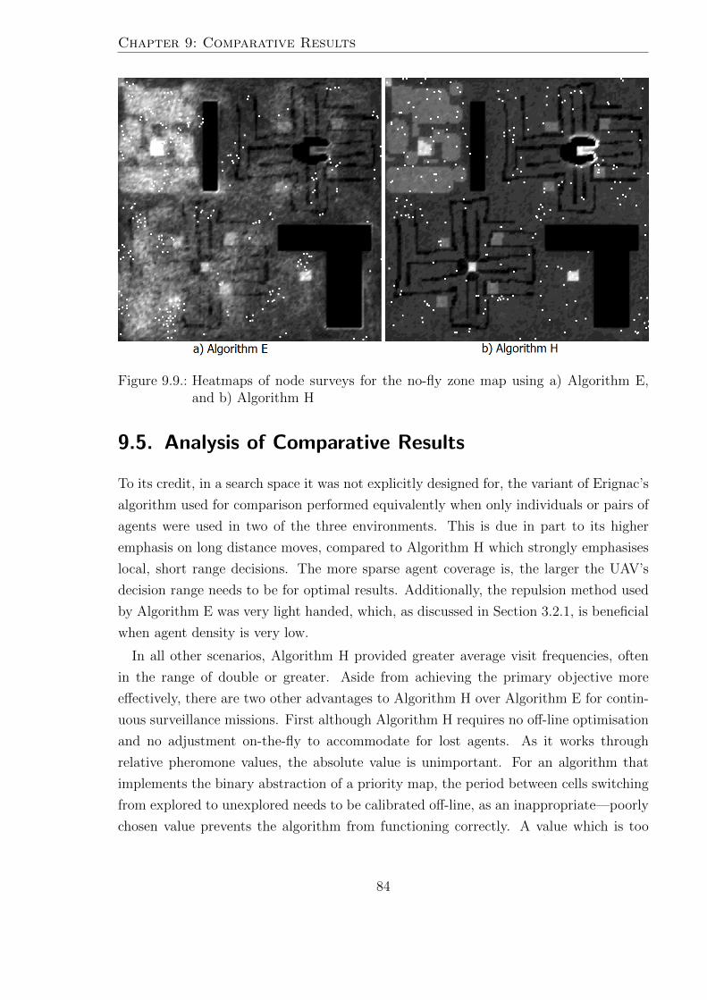
Chapter 9: Comparative Results
Figure 9.9.: Heatmaps of node surveys for the no-fly zone map using a) Algorithm E,and b) Algorithm H
9.5. Analysis of Comparative Results
To its credit, in a search space it was not explicitly designed for, the variant of Erignac’s
algorithm used for comparison performed equivalently when only individuals or pairs of
agents were used in two of the three environments. This is due in part to its higher
emphasis on long distance moves, compared to Algorithm H which strongly emphasises
local, short range decisions. The more sparse agent coverage is, the larger the UAV’s
decision range needs to be for optimal results. Additionally, the repulsion method used
by Algorithm E was very light handed, which, as discussed in Section 3.2.1, is beneficial
when agent density is very low.
In all other scenarios, Algorithm H provided greater average visit frequencies, often
in the range of double or greater. Aside from achieving the primary objective more
effectively, there are two other advantages to Algorithm H over Algorithm E for contin-
uous surveillance missions. First although Algorithm H requires no off-line optimisation
and no adjustment on-the-fly to accommodate for lost agents. As it works through
relative pheromone values, the absolute value is unimportant. For an algorithm that
implements the binary abstraction of a priority map, the period between cells switching
from explored to unexplored needs to be calibrated off-line, as an inappropriate—poorly
chosen value prevents the algorithm from functioning correctly. A value which is too
84
Chapter 9: Comparative Results
high (where agents always move to the closest adjacent cell) or too low (where agents
spend most of their time using the random move behaviour) leads to results no better
than a random search.
The second advantage of Algorithm H is computation time. Utilising a Euclidean
distance pheromone map requires that each cell be populated with the distance to the
closest unexplored cell. This consequently requires the use of a wave front propagation
algorithm every time the map is changed, either via an agent’s visit, or through com-
munication of an updated pheromone map through the swarm. This is computationally
expensive, and occurs every few seconds in large swarms. Using the priority map algo-
rithm from this dissertation, only the few nodes on the agent’s immediate path need to
be checked when new information is received, and only a small and constant sized area
of the map needs to be evaluated when a new decision is required. Due to the constant
size of the evaluation area, the heuristic’s computation time does not increase with map
size, as opposed to an exponential increase for searching the entire map.
An interesting observation is that while the performance is good, the ratios observed
are not the 4/2/1 relationship that was set. Both algorithms are able to maintain
an exact relationship if that is the desired result: for Algorithm H the heuristic is
changed to negate the distance penalty; for Algorithm E the period between explored
and unexplored is increased. The side effect of these changes is that every area performs
worse as the agents spend a disproportionate amount of time in transit chasing global
maxima. The larger a swarm is, the worse this approach becomes as it is rarer that any
individual will be the one to reach the target first. Even with the current experiment
configuration, the ratios approach their 4/2/1 ideal as the agent count increases, often
being almost exact by 512 UAVs.
9.6. Summary
In the majority of simulated scenarios, including all scenarios involving mid to large
swarm sizes, the proposed algorithm achieves significantly higher survey frequencies than
the comparison algorithm. In addition to increased mission performance, the proposed
algorithm provides two additional benefits. Firstly there is greatly reduced dependence
on pre-mission calibration of variables for optimal performance. Secondly less on-board
computational resources are required to execute the algorithm.
85

10. Conclusions and Final Remarks
10.1. Summary
Bushfires are a problem around the world, especially common in countries such as Aus-
tralia where summers can be long, hot, and dry. Effective bushfire management includes
the simultaneous goals of minimising risk to fire fighters on the ground, and limiting the
potential of the fire to spreading out of control. These goals are largely dependant on
surveillance and predictive modelling based on observational data, which is traditional
gained through personnel manually patrolling a fire’s perimeter.
With recent advances in the field of autonomous robotics, there has been interest in the
use of UAVs in fire surveillance roles. For a problem with inherent dangers and in which
swift response is critical, UAVs are uniquely suited for this role due to being rapidly
deployable and relatively expendable. Initial studies with single, non-autonomous drones
have been promising, however problems were found with maintaining adequate coverage.
While adding more drone-type UAVs is largely impractical due to the need to main-
tain enough trained staff to individually operate each vehicle, swarm intelligence provides
mechanisms for coordinating the actions of autonomous entities as a group. In addition,
swarm intelligence enables collaboration and cooperation between individuals without
the need for centralised control, an important consideration when operating in environ-
ments that typically do not have existing communication infrastructure. The advantages
of deploying robots as a swarm instead of a centrally controlled system include massive
scalability, reduced need for human supervision, and resilience against individual failure.
A promising branch of inquiry into swarm robotics has been biomimicry, specifically
the use of artificial pheromone. Using pheromone maps to represent the environment
a swarm occupies allows algorithms to combine the information sharing and collective
decision making elements of swarm behaviour into a single intuitive concept. The prob-
lem with pheromone as a concept, however, is that the analogy only holds so long as the
information is stored in the environment itself. With the problem of detecting and then
monitoring bushfires in an area without the infrastructure needed to provide long range
87
Chapter 10: Conclusions and Final Remarks
communication there is no immediately apparent medium to store this information.
The algorithm proposed in this dissertation implements a pheromone map to represent
environmental knowledge. A unique copy of this pheromone map is stored in each
UAV’s memory. Pheromone levels are a function of information age and priority level,
and a heuristic is used to generate waypoints based on this information. The use of
priority maps allows for pheromone maps to specify areas of the environment to avoid
or prioritise, and also allows this knowledge to be communicated in an intuitive manner.
As priority maps are most often arranged as a matrix, there is a level of redundancy
when searching this grid with a non-square camera. A formula for calculating the optimal
dimensions of the priority map matrix to ensure minimal redundancy while ensuring
exhaustive coverage was found which also incorporates the safeguard of an arrival radius.
An artefact of using optimal node spacings was found to be emergent edge following
behaviour.
UAVs controlled by priority maps have local autonomy, which means they are self
contained with regard to decision making. As a result of this communication constraints
are not pronounced. Outside of fringe cases, the effects of communication range, broad-
cast period, and outright communication failure have a limited influence on the ability of
UAVs to perform their mission. Due to the distributed nature of the swarm intelligence
algorithms, the swarm is able to function at near maximum capacity even with a low
degree of information sharing between individuals.
With priority maps, the algorithm presented in this dissertation achieved significantly
higher survey frequencies than a comparable field-leading algorithm. In addition to in-
creased mission performance, there was a greatly reduced dependence on pre-mission
calibration of variables for optimal performance. In addition, fewer computational re-
sources were required to execute the algorithm.
10.2. Research Contributions
This dissertation has made the following contributions to the field of swarm intelligence:
• An algorithm has been developed for performing exhaustive, continuous surveil-
lance of an area using a decentralised UAV swarm. The algorithm uses inter-
nal pheromone maps to both represent the environment and communicate with
the swarm. Simulation results demonstrating that the proposed priority map al-
gorithm shows significant improvements in average search times compared to a
similar field leading algorithm.
88
Chapter 10: Conclusions and Final Remarks
• A method for producing avoidance and prioritisation in UAVs using priority maps
has been established. By replacing dynamic pheromone quantities with static
timestamps and scaling the change in time by priority level, computational over-
heads are reduced and new behaviours are made possible.
• A lower bound for the positive effects of communication between swarm peers
has been presented. In very low communication scenarios, the decreased diversity
resulting from communication is more detrimental than the effect of cooperation
through shared information.
• Outside very low communication fringe cases, the effects of communication range,
broadcast period, and outright communication failure have a limited influence
on a swarm which prioritises local search. Due to the distributed nature of the
algorithm, the swarms are able to function at near maximum capacity even with
a low degree of information sharing between individuals.
• An explanation for the emergent edge following found in uniform environments
has been provided, which is applicable to all matrix based pheromone maps which
prioritise movements to adjacent nodes. Analysis of search patterns shows that
discrete decision spaces result in predictable movement patterns in the continuous
environment.
• Bounding factors for swarm efficiency have been identified. With decision logic
which is fully distributed, search efficiency of the swarm increases near-linearly
until such point as UAV density exceeds a calculable threshold. Agent density
thresholds are applicable on both global and local scales, with local agent density
limiting maximum practical relative priority levels.
• The relation between monitoring active bushfire events and maintaining surveil-
lance for new ignitions was described. By using dynamic priority updates, it is
possible to use priority maps to both closely track fire fronts and simultaneously
discover secondary fires.
10.3. Future Work
A primary extension for this work would be real world testing using inexpensive kit-built
MAVs. While simulations suggest that priority maps will be an effective technique for
89
Chapter 10: Conclusions and Final Remarks
swarm coordination, hardware constraints and environmental dynamics will necessitate
platform specific optimisations for real world performance to be realised.
Additionally, and closely related, is the issue of safety verification. For Unmanned
Aircraft Systems (UAS) to become a practical solution to civil applications such as fire
spotting, they will require access to non-segregated civil airspace. While autonomy offers
promises of improved capabilities at a reduced operational cost, there are concerns about
being able to verify such autonomous systems (Pecheur 2000).
The route to airframe certification has already been established with regard to tra-
ditional aircraft, however with regard to the decision making logic, which acts as the
aircraft’s pilot, the process is still unclear. In this area regulators themselves are still to
reach consensus about what will be required, a process being aided by projects such as
ASTRAEA, ASTRAEA II, SEAS DTC, and FAA UAPO. At a minimum, certification
will likely require verification and validation of unmanned aerial system models against
the rules of the air (Alexander et al. 2007, 2009; Sirigineedi et al. 2009). Any future
work in implementing the proposed algorithm in a UAS will require breakthroughs in
non-deterministic behaviour modelling and safety verification.
A further potential extension of this work would be in extending the priority map
into a third dimension and implementing a test bed of underwater vehicles. Underwater
vehicles share many similarities with aerial vehicles, without the herculean task of safety
certification (Heidemann et al. 2006). Their use would allow for real world results as
well as the potential for new applications such as micro-habitat monitoring, structural
monitoring, and wide-area environmental monitoring.
90
Bibliography
R. D. Alexander, M. Hall-may, and T. P. Kelly. Certification of autonomous systems
under uk military safety standards, 2007.
R. D. Alexander, T. Kelly, and N. Herbert. Deriving safety requirements for autonomous
systems. In Proceedings of the 4th SEAS DTC Technical Conference, 2009.
Y. Altshuler, V. Yanovsky, I. A. Wagner, and M. Alfred. The cooperative hunters -
efficient cooperative search for smart targets using UAV swarms. In Second Inter-
national Conference on Informatics in Control, Automation and Robotics (ICINCO),
the First International Workshop on Multi-Agent Robotic Systems (MARS), pages
165–170, 2005.
V. G. Ambrosia, S. S. Wegener, D. V. Sullivan, and et al. Demonstrating UAV-acquired
real-time thermal data over fires. In Photogrammetric Engineering & Remote Sensing,
volume 69, pages 391–402, April 2003.
E.M. Arkin, S.P. Fekete, and J.S.B. Mitchell. Approximation algorithms for lawn mowing
and milling. Computational Geometry, 17(1):25–50, 2000.
J. Bachrach, J. D. McLurkin, and A. Grue. Protoswarm: a language for program-
ming multi-robot systems using the amorphous medium abstraction. In Proceedings
of the 7th international joint conference on Autonomous agents and multiagent sys-
tems, volume 3, pages 1175–1178, Estoril, Portugal, 2008. International Foundation
for Autonomous Agents and Multiagent Systems.
D. B. Barber, J. D. Redding, T. W. Mclain, R. W. Beard, and C. N. Taylor. Vision-based
target geo-location using a fixed-wing miniature air vehicle. Journal of Intelligent and
Robotic Systems, 47:361–382, December 2006.
M. Batalin, M. Hattig, and G. S. Sukhatme. Mobile robot navigation using a sensor
network. In International Conference on Robotics and Automation, pages 636–642.
IEEE, 2003.
91
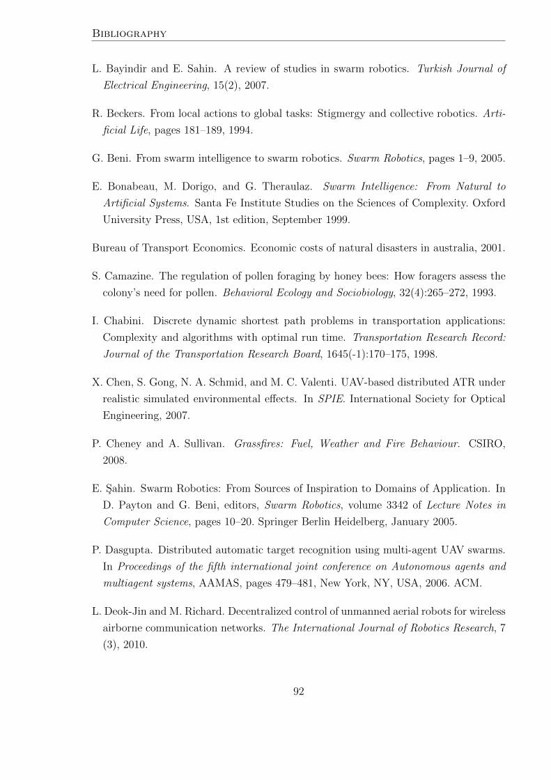
Bibliography
L. Bayindir and E. Sahin. A review of studies in swarm robotics. Turkish Journal of
Electrical Engineering, 15(2), 2007.
R. Beckers. From local actions to global tasks: Stigmergy and collective robotics. Arti-
ficial Life, pages 181–189, 1994.
G. Beni. From swarm intelligence to swarm robotics. Swarm Robotics, pages 1–9, 2005.
E. Bonabeau, M. Dorigo, and G. Theraulaz. Swarm Intelligence: From Natural to
Artificial Systems. Santa Fe Institute Studies on the Sciences of Complexity. Oxford
University Press, USA, 1st edition, September 1999.
Bureau of Transport Economics. Economic costs of natural disasters in australia, 2001.
S. Camazine. The regulation of pollen foraging by honey bees: How foragers assess the
colony’s need for pollen. Behavioral Ecology and Sociobiology, 32(4):265–272, 1993.
I. Chabini. Discrete dynamic shortest path problems in transportation applications:
Complexity and algorithms with optimal run time. Transportation Research Record:
Journal of the Transportation Research Board, 1645(-1):170–175, 1998.
X. Chen, S. Gong, N. A. Schmid, and M. C. Valenti. UAV-based distributed ATR under
realistic simulated environmental effects. In SPIE. International Society for Optical
Engineering, 2007.
P. Cheney and A. Sullivan. Grassfires: Fuel, Weather and Fire Behaviour. CSIRO,
2008.
E. Sahin. Swarm Robotics: From Sources of Inspiration to Domains of Application. In
D. Payton and G. Beni, editors, Swarm Robotics, volume 3342 of Lecture Notes in
Computer Science, pages 10–20. Springer Berlin Heidelberg, January 2005.
P. Dasgupta. Distributed automatic target recognition using multi-agent UAV swarms.
In Proceedings of the fifth international joint conference on Autonomous agents and
multiagent systems, AAMAS, pages 479–481, New York, NY, USA, 2006. ACM.
L. Deok-Jin and M. Richard. Decentralized control of unmanned aerial robots for wireless
airborne communication networks. The International Journal of Robotics Research, 7
(3), 2010.
92
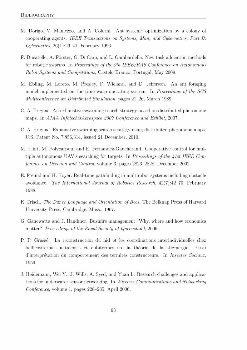
Bibliography
M. Dorigo, V. Maniezzo, and A. Colorni. Ant system: optimization by a colony of
cooperating agents. IEEE Transactions on Systems, Man, and Cybernetics, Part B:
Cybernetics, 26(1):29–41, February 1996.
F. Ducatelle, A. Forster, G. Di Caro, and L. Gambardella. New task allocation methods
for robotic swarms. In Proceedings of the 9th IEEE/RAS Conference on Autonomous
Robot Systems and Competitions, Castelo Branco, Portugal, May 2009.
M. Ebling, M. Loreto, M. Presley, F. Wieland, and D. Jefferson. An ant foraging
model implemented on the time warp operating system. In Proceedings of the SCS
Multiconference on Distributed Simulation, pages 21–26, March 1989.
C. A. Erignac. An exhaustive swarming search strategy based on distributed pheromone
maps. In AIAA Infotech@Aerospace 2007 Conference and Exhibit, 2007.
C. A. Erignac. Exhaustive swarming search strategy using distributed pheromone maps.
U.S. Patent No. 7,856,314, issued 21 December, 2010.
M. Flint, M. Polycarpou, and E. Fernandez-Gaucherand. Cooperative control for mul-
tiple autonomous UAV’s searching for targets. In Proceedings of the 41st IEEE Con-
ference on Decision and Control, volume 3, pages 2823–2828, December 2002.
E. Freund and H. Hoyer. Real-time pathfinding in multirobot systems including obstacle
avoidance. The International Journal of Robotics Research, 42(7):42–70, February
1988.
K. Frisch. The Dance Language and Orientation of Bees. The Belknap Press of Harvard
University Press, Cambridge, Mass., 1967.
G. Ganewatta and J. Handmer. Bushfire management: Why, where and how economics
matter? Proceedings of the Royal Society of Queensland, 2006.
P. P. Grasse. La reconstruction du nid et les coordinations interindividuelles chez
bellicositermes natalensis et cubitermes sp. la theorie de la stigmergie: Essai
d’interpretation du comportement des termites constructeurs. In Insectes Sociaux,
1959.
J. Heidemann, Wei Y., J. Wills, A. Syed, and Yuan L. Research challenges and applica-
tions for underwater sensor networking. In Wireless Communications and Networking
Conference, volume 1, pages 228–235, April 2006.
93
Bibliography
F. Heppner and U. Grenander. A stochastic nonlinear model for coordinated bird flocks.
In In The ubiquity of chaos, pages 233–238, 1990.
N. Hogan. Impedance control: an approach to manipulation. In Proceedings of American
Control Conference, San Diego, Caliornia, USA, 1984.
D. P. Horner. Use of artificial potential fields for uav guidance and optimization of
wlan communications. In Autonomous Underwater Vehicles, IEEE/OES, pages 88–
95, Monterey, CA, USA, June 2004.
D. Howden. Continuous swarm surveillance via distributed priority maps. In Proceedings
of the 4th Australian Conference on Artificial Life: Borrowing from Biology, ACAL,
pages 221–231, Berlin, Heidelberg, 2009. Springer-Verlag.
D. Howden and T. Hendtlass. Collective intelligence and bush fire spotting. In Proceed-
ings of the 10th annual conference on Genetic and evolutionary computation, GECCO,
pages 41–48, New York, NY, USA, 2008. ACM.
T. Hutchings, S. Jeffryes, and SJ Farmer. Architecting uav sense & avoid systems. In
Autonomous Systems, 2007 Institution of Engineering and Technology Conference on,
pages 1–8. IET, 2007.
C. Intanagonwiwat, R. Govindan, and D. Estrin. Directed diffusion: A scalable and
robust communication paradigm for sensor networks. In MOBICOM, pages 56–67.
ACM, 2000.
E. Izquierdo-Torres. Collective intelligence in multi-agent robotics: Stigmergy, self-
organization and evolution, 2004.
M. Jasiunas. Mobility of reconfigurable computing tasks with applications to swarms of
small UAVs. Master’s thesis, University of South Australia, 2009.
Y. Kant, V. K. Prasad, and Badarinath K. V. S. Algorithm for detection of active fire
zones using NOAA AVHRR data. Infrared Physics & Technology, 41(1):29–34, 2000.
D. Kearney and M. Jasiunas. Using simulated partial dynamic run-time reconfiguration
to share embedded FPGA compute and power resources across a swarm of unpiloted
airborne vehicles. EURASIP Journal on Embedded Systems, 2007:8–8, January 2007.
J. Kennedy. Swarm intelligence. In Albert Zomaya, editor, Handbook of Nature-Inspired
and Innovative Computing, pages 187–219. Springer US, 2006.
94
Bibliography
J. Kennedy and R. Eberhart. Particle swarm optimization. In Proceedings of the IEEE
International Conference on Neural Networks, volume 4, pages 1942–1948, November
1995.
O. Khatib. Real-time obstacle avoidance for manipulators and mobile robots. The
International Journal of Robotics Research, 5(1):90–98, Spring 1986.
B. H. Krogh. A generalized potential field approach to obstacle avoidance control. In
Proceedings of SME Conference on Robotics Research, August 1984.
Y. Kuwana, I. Shimoyama, Y. Sayama, and H. Miura. Synthesis of pheromone-oriented
emergent behavior of a silkworm moth. In Proceedings of the IEEE/RSJ International
Conference on Intelligent Robots and Systems, volume 3, pages 1722–1729, November
1996.
Y. Kuwana, S. Nagasawa, I. Shimoyama, and R. Kanzaki. Synthesis of the pheromone-
oriented behaviour of silkworm moths by a mobile robot with moth antennae as phero-
mone sensors. Biosensors and Bioelectronics, 14(2):195–202, 1999.
C. Martin and K. S. Barber. Multiple, simultaneous autonomy levels for agent-based sys-
tems. In Proceedings of the Fourth International Conference on Control, Automation,
Robotics, and Vision, pages 1318–1322, 1996.
J. D. McLurkin. Algorithms for distributed sensor networks. Master’s thesis, University
of California at Berkeley, 1999.
J. D. McLurkin. Stupid robot tricks : a behavior-based distributed algorithm library for
programming swarms of robots. Master’s thesis, Massachusetts Institute of Technol-
ogy. Dept. of Electrical Engineering and Computer Science., 2004.
J. D. McLurkin and E. D. Demaine. A distributed boundary detection algorithm for
multi-robot systems. In Intelligent Robots and Systems, 2009. IROS 2009. IEEE/RSJ
International Conference on, pages 4791–4798, October 2009.
J. D. McLurkin and J. Dwight. Analysis and implementation of distributed algorithms for
multi-robot systems. PhD thesis, Massachusetts Institute of Technology. Dept. of Elec-
trical Engineering and Computer Science., Cambridge, MA, USA, 2008. AAI0821012.
J. D. McLurkin and J. Smith. Distributed Algorithms for Dispersion in Indoor Envi-
ronments using a Swarm of Autonomous Mobile Robots. In Distributed Autonomous
Robotic Systems Conference, 2004.
95
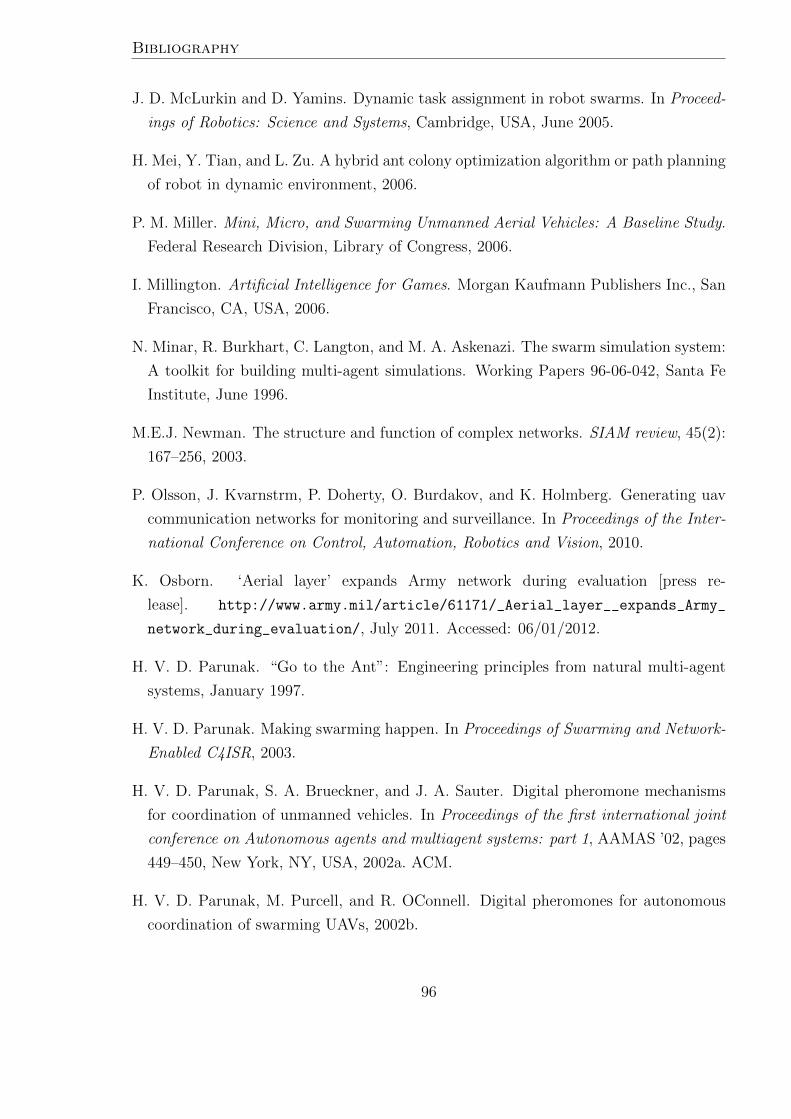
Bibliography
J. D. McLurkin and D. Yamins. Dynamic task assignment in robot swarms. In Proceed-
ings of Robotics: Science and Systems, Cambridge, USA, June 2005.
H. Mei, Y. Tian, and L. Zu. A hybrid ant colony optimization algorithm or path planning
of robot in dynamic environment, 2006.
P. M. Miller. Mini, Micro, and Swarming Unmanned Aerial Vehicles: A Baseline Study.
Federal Research Division, Library of Congress, 2006.
I. Millington. Artificial Intelligence for Games. Morgan Kaufmann Publishers Inc., San
Francisco, CA, USA, 2006.
N. Minar, R. Burkhart, C. Langton, and M. A. Askenazi. The swarm simulation system:
A toolkit for building multi-agent simulations. Working Papers 96-06-042, Santa Fe
Institute, June 1996.
M.E.J. Newman. The structure and function of complex networks. SIAM review, 45(2):
167–256, 2003.
P. Olsson, J. Kvarnstrm, P. Doherty, O. Burdakov, and K. Holmberg. Generating uav
communication networks for monitoring and surveillance. In Proceedings of the Inter-
national Conference on Control, Automation, Robotics and Vision, 2010.
K. Osborn. ‘Aerial layer’ expands Army network during evaluation [press re-
lease]. http://www.army.mil/article/61171/_Aerial_layer__expands_Army_
network_during_evaluation/, July 2011. Accessed: 06/01/2012.
H. V. D. Parunak. “Go to the Ant”: Engineering principles from natural multi-agent
systems, January 1997.
H. V. D. Parunak. Making swarming happen. In Proceedings of Swarming and Network-
Enabled C4ISR, 2003.
H. V. D. Parunak, S. A. Brueckner, and J. A. Sauter. Digital pheromone mechanisms
for coordination of unmanned vehicles. In Proceedings of the first international joint
conference on Autonomous agents and multiagent systems: part 1, AAMAS ’02, pages
449–450, New York, NY, USA, 2002a. ACM.
H. V. D. Parunak, M. Purcell, and R. OConnell. Digital pheromones for autonomous
coordination of swarming UAVs, 2002b.
96
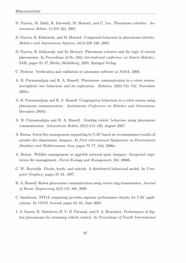
Bibliography
D. Payton, M. Daily, R. Estowski, M. Howard, and C. Lee. Pheromone robotics. Au-
tonomous Robots, 11:319–324, 2001.
D. Payton, R. Estkowski, and M. Howard. Compound behaviors in pheromone robotics.
Robotics and Autonomous Systems, 44(3):229–240, 2003.
D. Payton, R. Estkowski, and M. Howard. Pheromone robotics and the logic of virtual
pheromones. In Proceedings of the 2004 international conference on Swarm Robotics,
SAB, pages 45–57, Berlin, Heidelberg, 2005. Springer-Verlag.
C. Pecheur. Verification and validation of autonomy software at NASA, 2000.
A. H. Purnamadjaja and R. A. Russell. Pheromone communication in a robot swarm:
necrophoric bee behaviour and its replication. Robotica, 23(6):731–742, November
2005a.
A. H. Purnamadjaja and R. A. Russell. Congregation behaviour in a robot swarm using
pheromone communication. Australasian Conference on Robotics and Automation,
December 2005b.
A. H. Purnamadjaja and R. A. Russell. Guiding robots’ behaviors using pheromone
communication. Autonomous Robots, 23(2):113–130, August 2007.
A. Restas. Forest fire management supporting by UAV based air reconnaissance results of
szendro fire department, hungary. In First international Symposium on Environment
Identities and Mediterranean Area, pages 73–77, July 2006a.
A. Restas. Wildfire management at aggtelek national park, hungary: Integrated vege-
tation fire management. Forest Ecology and Management, 234, 2006b.
C. W. Reynolds. Flocks, herds, and schools: A distributed behavioral model. In Com-
puter Graphics, pages 25–34, 1987.
R. A. Russell. Robot pheromone communication using vortex ring transmission. Journal
of Bionic Engineering, 6(2):153–160, 2009.
C. Sanderson. FPGA computing provides superior performance density for UAV appli-
cations. In COTS Journal, pages 82–85, June 2003.
J. A. Sauter, R. Matthews, H. V. D. Parunak, and S. A. Brueckner. Performance of dig-
ital pheromones for swarming vehicle control. In Proceedings of Fourth International
97
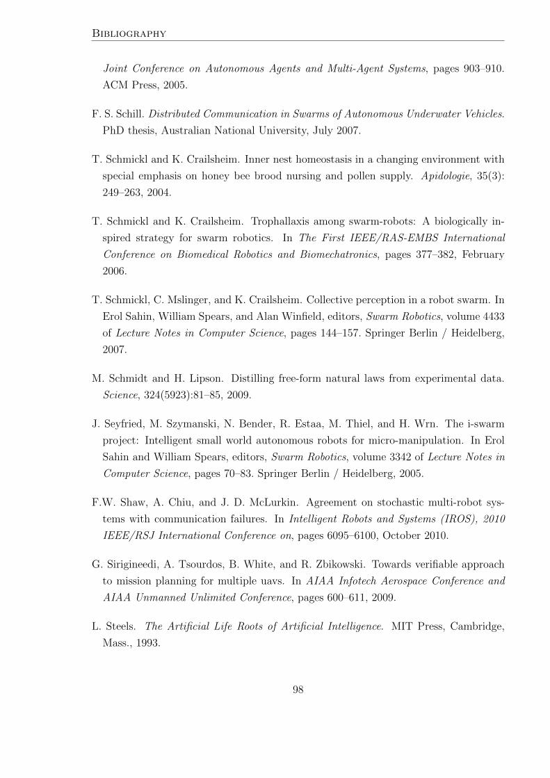
Bibliography
Joint Conference on Autonomous Agents and Multi-Agent Systems, pages 903–910.
ACM Press, 2005.
F. S. Schill. Distributed Communication in Swarms of Autonomous Underwater Vehicles.
PhD thesis, Australian National University, July 2007.
T. Schmickl and K. Crailsheim. Inner nest homeostasis in a changing environment with
special emphasis on honey bee brood nursing and pollen supply. Apidologie, 35(3):
249–263, 2004.
T. Schmickl and K. Crailsheim. Trophallaxis among swarm-robots: A biologically in-
spired strategy for swarm robotics. In The First IEEE/RAS-EMBS International
Conference on Biomedical Robotics and Biomechatronics, pages 377–382, February
2006.
T. Schmickl, C. Mslinger, and K. Crailsheim. Collective perception in a robot swarm. In
Erol Sahin, William Spears, and Alan Winfield, editors, Swarm Robotics, volume 4433
of Lecture Notes in Computer Science, pages 144–157. Springer Berlin / Heidelberg,
2007.
M. Schmidt and H. Lipson. Distilling free-form natural laws from experimental data.
Science, 324(5923):81–85, 2009.
J. Seyfried, M. Szymanski, N. Bender, R. Estaa, M. Thiel, and H. Wrn. The i-swarm
project: Intelligent small world autonomous robots for micro-manipulation. In Erol
Sahin and William Spears, editors, Swarm Robotics, volume 3342 of Lecture Notes in
Computer Science, pages 70–83. Springer Berlin / Heidelberg, 2005.
F.W. Shaw, A. Chiu, and J. D. McLurkin. Agreement on stochastic multi-robot sys-
tems with communication failures. In Intelligent Robots and Systems (IROS), 2010
IEEE/RSJ International Conference on, pages 6095–6100, October 2010.
G. Sirigineedi, A. Tsourdos, B. White, and R. Zbikowski. Towards verifiable approach
to mission planning for multiple uavs. In AIAA Infotech Aerospace Conference and
AIAA Unmanned Unlimited Conference, pages 600–611, 2009.
L. Steels. The Artificial Life Roots of Artificial Intelligence. MIT Press, Cambridge,
Mass., 1993.
98
Bibliography
T. Stirling, S. Wischmann, and D. Floreano. Energy-efficient indoor search by swarms of
simulated flying robots without global information. Swarm Intelligence, 4(2):117–143,
February 2010.
K. Sugawara, T. Kazama, and T. Watanabe. Foraging behavior of interacting robots
with virtual pheromone. In Proceedings of the IEEE/RSJ International Conference
on Intelligent Robots and Systems, volume 3, pages 3074–3079, September 2004.
United Kingdom Central Authority. Cap 722–unmanned aerial vehicle operations in uk
airspace: Guidance. The Stationery Office, 2004.
U.S. Government Accountability Office. Defense acquisitions: Restructured JTRS pro-
gram reduces risk, but significant challenges remain, 2005.
P. Valdastri, P. Corradi, A. Menciassi, T. Schmickl, K. Crailsheim, J. Seyfried, and
P. Dario. Micromanipulation, communication and swarm intelligence issues in a swarm
microrobotic platform. Robotics and Autonomous Systems, 54(10):789–804, 2006.
R. Varga. The UAV reloaded: Placing video intelligence on-board. In COTS Journal,
pages 72–76, June 2003.
C. E. V. Wagner. A simple fire-growth model. National Emergency Training Center,
1969.
B. Walter, A. Sannier, D. Reiners, and J. Oliver. UAV swarm control: Calculating
digital pheromone fields with the gpu. In Interservice/Industry Training, Simulation,
and Education Conference (I/ITSEC), 2005.
H. Woern, M. Szymanski, and J. Seyfried. The i-swarm project. In The 15th IEEE
International Symposium on Robot and Human Interactive Communication, pages
492–496, September 2006.
H. Yamada, T. Tominaga, and M. Ichikawa. An autonomous flying object navigated by
real-time optical flow and visual target detection. In Proceedings of International Con-
ference on Field-Programmable Technology (FPT), pages 222–227, December 2003.
H. Yamaguchi and T. Arai. Distributed and autonomous control method for generating
shape of multiple mobile robot group. In Proceedings of the IEEE/RSJ/GI Interna-
tional Conference on Intelligent Robots and Systems ’Advanced Robotic Systems and
the Real World’, volume 2 of IROS, pages 800–807, September 1994.
99

Appendices
101

A. Glossary
ACO : “Ant colony optimisation” is metaheuristic optimisation algo-
rithm inspired by foraging behaviour in ant colonies.
Dead reckoning : Dead reckoning is a process of navigation where current loca-
tion is calculated based on a previous determined position.
FPGA : A “field programmable gate array” is an integrated circuit de-
signed to be customisable post-manufacturing.
FSM : A “finite state machine” is a model of computation which re-
quires that the abstract machine be in one of a number of states.
GPS : The “global positioning system” is a publicly accessible satel-
lite network which provides time and location information to
anyone with a receiver.
INS : An “inertial navigation system” uses motion and rotation sen-
sors to calculate position, velocity and orientation based on
dead reckoning.
ISR : Acronym for “intelligence, surveillance and reconnaissance”,
military terminology for battlefield information gathering.
MAV : A “miniature aerial vehicle” is a subclass of UAVs informally
defined by having dimensions under 1m square.
PSO : “Particle swarm optimisation” is a metaheuristic optimisation
algorithm inspired by flocking behaviour in birds.
Stigmergy : Stigmergy is the indirect communication between members of
a colony through modification of a shared environment.
UAS : An “unmanned aircraft system” is a UAV with its attendant
support hardware, such as ground terminals and communica-
tion stations. While still relatively uncommon, this term is
becoming increasingly preferred in regulatory literature.
UAV : An “unmanned aerial vehicle” is any aircraft without a human
pilot on board.
103

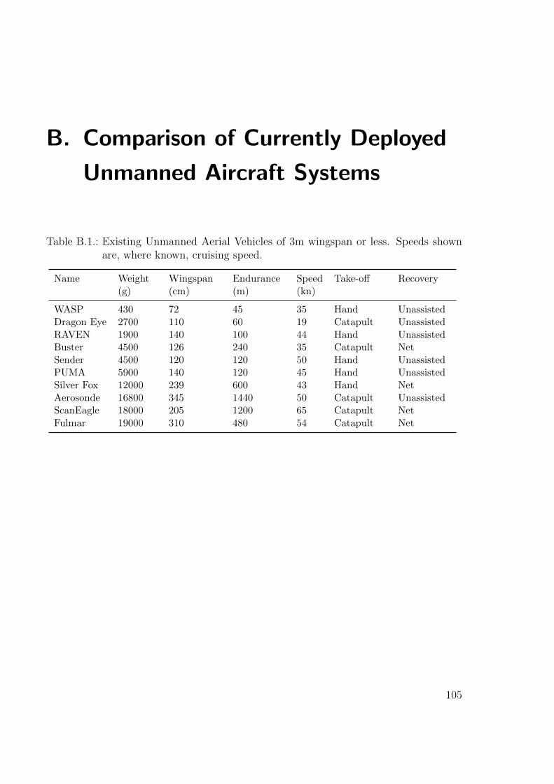
B. Comparison of Currently Deployed
Unmanned Aircraft Systems
Table B.1.: Existing Unmanned Aerial Vehicles of 3m wingspan or less. Speeds shownare, where known, cruising speed.
Name Weight(g)
Wingspan(cm)
Endurance(m)
Speed(kn)
Take-off Recovery
WASP 430 72 45 35 Hand UnassistedDragon Eye 2700 110 60 19 Catapult UnassistedRAVEN 1900 140 100 44 Hand UnassistedBuster 4500 126 240 35 Catapult NetSender 4500 120 120 50 Hand UnassistedPUMA 5900 140 120 45 Hand UnassistedSilver Fox 12000 239 600 43 Hand NetAerosonde 16800 345 1440 50 Catapult UnassistedScanEagle 18000 205 1200 65 Catapult NetFulmar 19000 310 480 54 Catapult Net
105

C. Publications Arising from this Study
Publications by the Candidate Relevant to the
Dissertation
D. J. Howden, T. Hendtlass. Collective intelligence and bush fire spotting. In Proceed-
ings of the 10th annual conference on Genetic and evolutionary computation, GECCO
’08, pages 41-48, New York, NY, USA, 2008. ACM.
D. J. Howden. Continuous swarm surveillance via distributed priority maps. In Pro-
ceedings of the 4th Australian Conference on Artificial Life: Borrowing from Biology,
ACAL ’09, pages 221-231, Berlin, Heidelberg, 2009. Springer-Verlag.
D. J. Howden. Fire Tracking with Collective Intelligence using Dynamic Priority Maps
(manuscript in preparation for journal publication)
Additional Publications by the Candidate Relevant to
the Dissertation but not Forming Part of it
K. Bogdanov, D. J. Howden, T. Dodd. Automated Model Inference for Autonomous
UAV Systems (manuscript in preparation for journal publication)
107


