co-c:

>-

=cc

.--=

~.-

.=""'C~

=""'C

E= ~

:=cc

en""'C

enc:::L

c:::z::;::)

=""'C

5:

c:

=cc

cc""'C

c:..::a=

~en.-

=:::-

.c:

=5

:a

:::

=-=~....=

The Future Populationof the World

What Can We Assume Today?

Revised 1996 Edition

Edited by

Wolfgang Lutz

International Institute for Applied Systems AnalysisLaxenburg, Austria

The Future Populationof the World

What Can We Assume Today?

DIIASAInternational Institutefor Applied Systems Analysis

~a~u!:l~~~1Il

Earthscan Publications Ltd, London

Earthscan Publications Ltd120 Pentonville Road, London Nl 9JNTel: 01712780433Fax: 01712781142Email: earthinfo@earthscan.co.uk

Copyright © International Institute for Applied Systems Analysis, 1996Copyright is not claimed on Chapter 9.

All rights reserved. First edition 1994Revised Edition 1996

A catalogue record for this book is available from the British Library

ISBN: 185383 349 5 paperback1 85383 344 4 hardback

Printed and bound in Great Britain by BiddIes Limited, Guildford andKing's Lynn

Earthscan Publications Ltd is an editorially independent subsidiary ofKogan Page Ltd and publishes in association with the InternationalInstitute for Environment and Development and the World Wide Fundfor Nature.

Contents

List of Illustrations viii

Foreword xu

Preface XIV

Introduction xvi

Contributors xxi

PART I: Why Another Set of Global PopulationProjections? 1

1 Long-range Global Population Projections:Lessons LearnedTomas Frejka 3

2 Alternative Approaches to Population ProjectionWolfgang Lutz, Joshua R Goldstein, Christopher Prinz 14

PART II: Future Fertility in Developing Countries 45

3 A Regional Review of Fertility Trends inDeveloping Countries: 1960 to 1995John Cleland 47

4 Reproductive Preferences and Future Fertility inDeveloping CountriesCharles F Westoff 73

5 Population Policies and Family-Planning inSoutheast AsiaMercedes B Concepcion 88

v

VI

6 Fertility in China: Past, Present, ProspectsGriffith Feeney 102

PART III: Future Mortality in Developing Countries 131

7 Mortality Trends in Developing Countries:A SurveyBirgitta Bucht 133

8 Mortality in Sub-Saharan Africa:Trends and ProspectsMichel Garenne 149

9 Global Trends in AIDS MortalityJohn Bongaarts 170

10 How Many People Can Be Fed on Earth?Gerhard K Heilig 196

PART IV: Future Fertility and Mortality inIndustrialized Countries 251

11 Future Reproductive Behavior inIndustrialized CountriesWolfgang Lutz 253

12 The Future of Mortality at Older Ages inDeveloped CountriesJames W Vaupel and Hans Lundstrom 278

PART V: The Future of Intercontinental Migration 297

13 Migration to and from Developing Regions:A Review of Past TrendsHania Zlotnik 299

14 Spatial and Economic Factors in FutureSouth-North MigrationSture Oberg 336

VIl

PART VI: Projections 359

15 World Population Scenarios for the 21st CenturyWolfgang Lutz, Warren Sanderson, Sergei Scherbov,Anne Goujon 361

16 Probabilistic Population Projections Based onExpert OpinionWolfgang Lutz, Warren Sanderson, Sergei Scherbov 391

11 Epilogue: Dilemmas in Population StabilizationWolfgang Lutz 429

Appendix Tables 431

References 463

Index 495

Illustrations

Figures

2.1 Components of uncertainty entering population projections. 214.1 The nuptiality-fertility model for 216 regions. 826.1 Fertility decline in China compared with fertility decline in

other areas in the developing world. 1046.2 Rate of fertility decline and log population size in Asia. 1086.3 Conventional total fertility rates in China. 1106.4 Mean age at first marriage in China. 1126.5 Approximate annual numbers of first marriages in China. 1136.6 Total fertility rates calculated from period parity progression

ratios in China. 1186.7 Period parity progression ratios in China. 1216.8 Observed and estimated total fertility rates in China. 1258.1 Crude death rates in Dakar and Saint-Louis (Senegal). 1518.2 Estimated mortality trends in Senegal. 1568.3 Estimated mortality trends in Zambia. 1618.4 Estimated mortality trends in Uganda. 1628.5 Estimated mortality trends in Central Mozambique. 1638.6 Estimated mortality trends in Kenya. 1658.7 Estimated adult mortality trends in Abidjan. 1658.8 Famine areas and locations of major wars in Africa. 1669.1 Estimated levels of HIY seroprevalence (percentage of adults

infected) for urban populations in Africa. 1749.2 Estimated trends in HIY prevalence among adults. 1779.3 Estimates and medium projections for incidence rates of HIY

infections, AIDS cases, and AIDS deaths among adults. 1809.4 Estimates and projections of annual number of HIY infections

and AIDS cases among adults, world total. 1839.5 Projection of deaths due to AIDS as a percentage of deaths

from all causes. 1879.6 Impq.ct of the AIDS epidemic on the death rate and popula-

tion growth rate in Rakai District, Uganda. 19210.1 Model for analyzing the earth's carrying capacity. 20011.1 Age-specific marriage rates for women in Sweden and USA. 25611.2 Total divorce rates in selected European countries. 258

Vlll

IX

11.3 Total fertility rates in five selected industrialized countries. 26111.4 Completed fertility rate for 1940-1963 birth cohorts. 26211.5 Total fertility rates, 1965-1995, and assumptions until

2030-2035 in North America and Western Europe. 27712.1 Force of mortality for females, ages 85, 90, and 95, Sweden. 28412.2 Force of mortality for males, ages 85, 90, and 95, Sweden. 28512.3 Force of mortality for females, ages 80-111, Sweden. 28912.4 Force of mortality for males, ages 80-111, Sweden. 28914.1 The world regions used in this book. 33814.2 Ethnic territories and national boundaries in Africa. 34314.3 Hard and soft push factors of migration. 34614.4 Potential emigration areas. 34814.5 The gap between demand for cheap labor in the North and

the South. 35015.1 Alternative projected paths of world population size. 37715.2 Alternative paths of population size in North America. 38115.3 World population in high-fertilityfhigh-mortality scenario. 38415.4 World population in low-fertilityflow-mortality scenario. 38515.5 Alternative projected trends in the proportion of population

above age 60 in China and CPA. 38615.6 Projected population size in sub-Saharan Africa. 39016.1 Future population size in the European FSU. 40816.2 Future population size in North America. 40916.3 Percentage of the population in the 0-14 age group in North

America and the European FSU. 41416.4 Percentage of the population in the 60+ age group in North

America and the European FSU. 41516.5 Probability distribution of population, regions dependent and

independent; fertility and mortality independent. 42016.6 Merged distribution of the population sizes of the world. 42216.7 Merged distribution of world population in 0-14 age group. 42316.8 Merged distribution of world population in 60+ age group. 42417.1 Unavoidable and avoidable world population growth to 2050. 432

Tables

1.1 Long-term global population projections. 52.1 Major characteristics of our projection approach. 423.1 Fertility trends in East and Southeast Asia. 503.2 Fertility trends in continental South Asia. 543.3 Fertility trends in Latin America. 583.4 Year of onset of decline and percentage decline in following

decade in Latin America. 593.5 Fertility trends in the Arab states. 62

x

3.6 Fertility levels in sub-Saharan Africa. 653.7 Fertility trends in island states. 684.1 Indices of reproductive preferences of married women. 754.2 Forecasts of reproductive preferences, contraceptive preva-

lence, and fertility. 784.3 Linear regression equations for variables related to number of

children desired by women aged 25-29. 846.1 Total fertility rates in China and in other major areas in the

developing world. 1056.2 Comparative data on fertility decline in Asia. 1066.3 Total fertility rates and mean age at marriage in China. 1116.4 Parity progression ratios for selected populations. 1166.5 Period progression ratios and total fertility rates in China. 1207.1 Estimated and projected life expectancy at birth. 1357.2 Model for mortality improvement, quinquennial gains in life

expectancy at birth by initial level of mortality. 1427.3 Maximum life expectancies in UN mortality decline models. 1427.4 Estimated and projected life expectancy at birth for less de-

veloped regions, both sexes, UN assessments. 1457.5 Estimated and projected life expectancy at birth for less de--

veloped regions, both sexes, World Bank assessments. 1458.1 Estimates of child mortality in sub-Saharan Africa prior to

1960, probability of dying before age 5. 1528.2 Estimates of child mortality in sub-Saharan Africa 1960-1990,

probability of dying before age 5. 1538.3 Values of socioeconomic indicators. 1588.4 Mean annual rates of change in socioeconomic indicators. 1598.5 Elasticities of q(5) with respect to various socioeconomic in-

dicators, in 36 countries of continental tropical Africa. 1609.1 Cumulative number of adults infected with HIV, cumulative

AIDS deaths, number of infected adults, and percentage ofadults- infected by region at the end of 1994. 173

9.2 High, medium, and low variants of cumulative HIV infections,AIDS cases, and AIDS deaths among adults in 2005. 184

9.3 Projected annual number of child deaths due to AIDS, per-centage of births ending in AIDS deaths, and deaths amongchildren as a percentage of all AIDS deaths. 185

9.4 Projected annual number of AIDS deaths, percentage of alldeaths due to AIDS, and AIDS death rate. 186

9.5 Birth, death, and growth rates with and without AIDS. 19010.1 Estimates of the earth's population carrying capacity during

the past 100 years. 19710.2 Cropland in percent of land without soil constraints. 20610.3 Lifestyle-related and nonfood agricultural production. 212

Xl

10.4 Freshwater resources and withdrawals for selected countries. 21411.1 Marital-status above age 15 in selected European countries. 25511.2 Evolution of nonmarital unions in Europe. 25711.3 Total fertility rates in 30 industrialized countries. 26011.4 Responses to question: "[In your country] today what do you

think is the ideal number of children for a family like yoursor the one you might have?" 263

11.5 Responses to questions on family size in Austria from womenmarried five to eight years. 264

12.1 Average annual rates of progress in reducing mortality rates. 28612.2 Age when remaining life expectancy is two or five years. 29113.1 Average annual number of immigrants originating in the dif-

ferent developing regions and average annual net migrationby country of destination and period. 306

13.2 Average annual number of asylum seekers in Europe. 31613.3 Average annual number of migrant workers from selected

countries of South Asia, East/Southeast Asia, and China. 32213.4 Distribution of migrant workers originating in countries of

East and Southeast Asia by destination. 32313.5 Annual migration to Saudi Arabia by region of citizenship. 32414.1 Countries of resettlement of refugees and asylum seekers. 35515.1 Alternative fertility assumptions used in projections. 36415.2 Alternative mortality assumptions to 2030-2035. 36715.3 Assumed high values of annual net migration flows. 37015.4 Projections of total population according to alternative fertil-

ity and mortality assumptions. 37615.5 Distribution of world population by continent, according to

three scenarios and under central migration. 38015.6 Projections of percentages of the population above age 60

according to alternative fertility and mortality assumptions. 38315.7 Proportion above age 60 and population size in China and

CPA and Pacific OECD under the population-aging/fertility-feedback scenarios. 393

15.8 Most likely projections produced by the United Nations, theUS Bureau of the Census, the World Bank, and IIASA. 395

16.1 Forecasts and 95 percent CI for US population around 2065. 40216.2 Population by regions, independent case. 40716.3 Percentage of the population in the 0-14 age group. 41216.4 Percentage of the population in the 60+ age group. 41316.5 Mean, median, and 95 percent CI for sub-Saharan Africa. 41816.6 Summary of world population projections with different as-

sumptions of the correlation between fertility and mortalityboth within and between regions. 418

Foreword

Forecasting is one of the oldest of demographic activities, and yet ithas never been fully integrated with the main body of demographictheory and data. The fact that the public regards it as our most im­portant task finds no reflection in our research agenda; the amountof it done is out of all proportion to the fraction of space devoted toit in professional journals. The best demographers do it, but nonewould stake their reputation on the agreement of their forecastswith the subsequent realization - in fact some of the most eminentdemographers have been the authors of the widest departures.

Demographers do not use the departures as data for learninghow to improve their skills; in fact they rarely even look back atforecasts made 10 or 20 years earlier to note what the errors havebeen. Anyone who expects that after a census is taken there will bea flurry of articles recalling previous forecasts and congratulating orcondemning will be disappointed. Writers merely go on to forecastthe next following census, usually without even a glance at theirpast errors.

The present volume is designed to correct this unsatisfactorycondition. Its writers include some of the best-known names in theprofession, as well as younger people who in due course will succeedthem as leaders. They systematically go through the components offuture population - births, deaths, migration - that for any individ­ual include all the possible ways of entering or leaving the world orany country in it. The chapters explore the possibilities of bringingthe best demographic methods to the improvement of our knowledgeof future population. Few show any defensiveness in regard to theirown earlier forecasts; the approach throughout is fresh and original.

xii

Xlll

By bringing to bear the best of demographic knowledge on anapplication whose importance has recently been accentuated by con­cern with environment, this book will provide a valuable contribu­tion in its own right, and at the same time be a stimulus to furtherneeded research.

Nathan KeyfitzInternational Institute forApplied Systems Analysis

Preface to the 1996 Edition

The 1990s are developing into a period of significant demographicchanges in many parts of the world. The unexpected politicaland economic transformations in Eastern Europe brought aboutdramatic demographic consequences such as precipitously decliningbirth rates and increasing death rates, especially for men. In Russiamale life expectancy has recently declined by an estimated sevenyears. However, at the global level, the rapid fertility declines inSouthern Asia and the fact that the fertility transition in Africa fi­nally seems to have gained momentum have had a greater influencethan the changes in Eastern Europe. Also, fertility in China hasfurther declined below replacement level. Available data indicatethat fertility declined in every world region between 1990 and 1995.At the same time, AIDS and other infectious diseases have recentlydepressed the prospects for mortality improvements in many devel­oping countries. The combination of decreasing fertility and higherthan expected mortality means declines in world population growth.Indeed, most world population projections now call for somewhatlower growth than the forecasts presented earlier in the decade.

The population projections included in the first edition of TheFuture Population of the World were based on 1990 data and didnot reflect these recent changes in the starting population. Hence,when the publisher asked us whether we wanted to include any re­visions in a new edition of the book we decided to make the effortof recalculating the projections with a 1995 starting year. We alsointroduced a number of technical improvements, such as additionalage groups at the high end (up to age 120) and adjustments in themortality schedules. Also the definition of geographic regions wasmodified slightly to conform with that used by other IIASA projects.Most of the substantive background chapters in the volume were re­vised and updated. The chapter on AIDS in Africa was replaced bya recent paper on global AIDS mortality by the same author.

xiv

xv

What is most important is that this volume reflects a furtherevolution of how to deal with uncertainty in population projections.We decided to go beyond the alternative scenario approach thatwas used in the first edition (and is still used in Chapter 15) and topresent a fully probabilistic set of projections with confidence inter­vals based on expert opinion on probability distributions of fertility,mortality, and migration in the 13 world regions (as discussed inChapters 2 and 16). To my knowledge this is the first published setof probabilistic world population projections.

Wolfgang LutzLeader, Population Project

Spring 1996

Introduction

Public interest in population research seems to follow a cyclical pat­tern of ups and downs that is not directly related to demographictrends. Whereas the 1960s and early 1970s was a period of interna­tional upsurge in public concern about population and demographicresearch, during the 1980s population hardly made it into the head­lines. Currently, we are experiencing a new wave of public interestin world population growth which is largely fueled by ecologicalconcerns. Population growth has been mentioned repeatedly in in­ternational fora and the media as one of the driving forces, if notthe single most important factor, in global environmental change.But this time it is natural scientists rather than demographers whopoint at the importance of the issue.

Demographers remain conspicuously silent in the face of the at­tention suddenly given to an issue they have carefully studied fordecades, while researchers in other disciplines attempt to occupythis territory. Demographers, who should have better knowledgeof population dynamics and the determinants of fertility, mortality,and migration, tend to be embarrassed over frequent oversimplifica­tions in the present debate, and also tend to be puzzled over howto approach the highly complex issue of population---environment in­teraction. Scientists from other disciplines are often less cautious inmaking statements about the role of population and do not alwaysapply the same rules of scientific scrutiny to population studies thatthey apply to their own discipline. It is also problematic when sci­entific paradigms from the natural sciences and animal ecology aredirectly applied to complex social systems.

Without a doubt this new interest in population issues presentsnew challenges and opportunities for demographers and social sci­entists in general. Instead of retreating from this territory of

xvi

XVll

increasingly interdisciplinary population analysis, the demographiccommunity could show flexibility and directly address some of thewell-justified questions asked by the outside world. These questionsare discussed in Chapter 2 of this volume. One central question inthis context regards possible future population trends in the face ofecological constraints and new threats to human life. An increas­ing number of people want to know more about possible alternativepopulation trends than the information provided in standard pop­ulation projections. Such people include scholars in energy analysiswho want long-range population scenarios as inputs to their mod­els; regional planners, politicians, and business leaders who want todevelop robust strategies that hold under different possible futurepopulation patterns; and an increasing number of individuals whoare simply interested in the topic. These nondemographers oftenwant to know more about the assumptions made, their justifica­tions, and the range of uncertainty than has been given to them upto now by demographers.

This volume has been produced because of the belief that thedemographic community can do more in terms of summarizing itsknowledge about future population trends than has been done inthe past. In this, the book attempts to serve a dual purpose: torespond to the challenge of increased outside interest in alternativefuture population trends and to advance within the demographiccommunity the discussion on the approaches and assumptions to bechosen for population projections. By summarizing essential resultsof demographic research and how they relate to a broad range ofrelevant issues, the volume may also serve as a textbook.

The volume's approach follows that of an earlier book, FutureDemographic Trends in Europe and North America: What Can WeAssume Today? (Lutz, ed., 1991, Academic Press, London, UK).The basic idea is to devote the bulk of space to substantive delib­erations of experts with partly differing views about possible futuretrends in the three components of population change (fertility, mor­tality, and migration), and then translate these opinions into alter­native projections. In this book the geographic focus is widenedto encompass all world regions, and the treatment of uncertainty ismore elaborate than in the above-mentioned book.

XVlll

Part I of the volume addresses the question, Why another setof global population projections? It starts with a comprehensivesurvey of past long-range global population projections in Chap­ter 1 written by Tomas Frejka, who in the early 1970s produced themost influential set of long-range projections following Notestein'swork of 1945 and introduced the concept of convergence towardreplacement-level fertility. In his contribution, Frejka emphasizesthe lessons learned from past projections and points at desirablefeatures of new world population projections. In Chapter 2, Wolf­gang Lutz, Joshua Goldstein, and Christopher Prinz discuss somebasic questions in population projections which are rarely addressedin an explicit way. The chapter, entitled "Alternative Approaches toPopulation Projection," deals with such issues as who is interestedin projections, what output parameters are desired, what time hori­zons are appropriate, and how to handle uncertainty. Chapter 2 alsopresents and justifies the specific approach chosen for this study.

Part II is dedicated to future fertility in today's developing coun­tries. It consists of fOUf chapters dealing with different aspects ofthis issue which will dominate the extent of future world populationgrowth. In Chapter 3, John Cleland gives a comprehensive surveyof regional fertility trends between 1960 and 1995 and the factorsbehind these changes. This chapter serves as an important basisfor the IIASA fertility assumptions. Chapter 4, by Charles Westoff,is more explicitly oriented toward the future; it summarizes the ex­tensive empirical evidence on reproductive preferences and discussestheir implications for the future course of fertility decline. From thisanalysis, powerful arguments can be derived for assuming fertilitydeclines, at least in the near future. In Chapter 5, Mercedes Concep­cion looks at another important factor in determining future fertilitylevels, namely, the role of population policies and family-planningprograms. Based on the experience from Southeast Asia, she showsthat such programs can make a big difference if certain precondi­tions are met. In Chapter 6, Griffith Feeney gives an account of theamazing fertility changes in China. Based on the analysis of parityprogression ratios, he also derives some alternative scenarios for fu­ture fertility in that country, which currently is home to one-fifth ofthe world's population.

XIX

Part III of the volume looks at future mortality in developingcountries. It also consists of four chapters. An introductory chapterby Birgitta Bucht (Chapter 7) provides a comprehensive analysis ofrecent mortality trends in the different developing regions. MichelGarenne in Chapter 8 focuses on mortality in sub-Saharan Africa,the world region with the greatest uncertainties. One of the un­certainties, the mortality impact of AIDS, is explicitly addressed inChapter 9 by John Bongaarts. Finally, Gerhard Heilig in Chap­ter 10 addresses a crucial question which is usually excluded frompopulation projections, namely, Will there be enough food to feedall the people projected or is famine-related mortality likely to in­crease at some point? His conclusion is that, at least for the nextdecades, global food supplies should be sufficient under favorablepolitical conditions.

Part IV considers fertility and mortality in today's industrial­ized countries. It has two chapters but, in the discussion, referenceis also made to the 14 chapters included in an earlier book on thattopic (Lutz, 1991). Lutz in Chapter 11 considers various argumentsthat would suggest further fertility declines in today's low-fertilitycountries as well as some arguments implying higher fertility. JamesVaupel and Hans Lundstrom in Chapter 12 focus on the contro­versial issue of future old-age mortality in developed societies. Formaking future mortality assumptions over many decades in countriesthat already have female life expectancies of around 80 years, thequestion of an upper limit to the human life span becomes decisive.

Part V of the volume considers migration between the worldregions. International migration is a weak point in most populationprojections because of missing data and the volatility of migrationtrends. Fot these reasons it has sometimes been omitted in popu­lation studies; this omission results in the assumption of zero net­migration. This volume makes an effort to deal with migration moreexplicitly than it has been dealt with in the past. In Chapter 13,Hania Zlotnik uses the best data available to present a systematicanalysis of past interregional migration flows. This is complementedby a very broad consideration of possible future migration patternsby Sture Oberg in Chapter 14. Taken together, these two chap­ters provide a basis for making alternative assumptions on future

xx

interregional migration flows that have a status that is equal to thefertility and mortality assumptions used in the scenario calculationspresented in the final section.

Part VI presents the actual population projections for 13 worldregions with assumptions based on the substantive considerationsgiven in all previous chapters. Lutz, Warren Sanderson, SergeiScherbov, and Anne Goujon present two very different sets of pop­ulation projections to 2100. The first set, described in Chapter 15,includes 27 scenarios giving all possible combinations of high, cen­tral, and low values in fertility, mortality, and migration in all worldregions. It also gives a number of special scenarios assuming in­teractions between the components and feedbacks from the results.Chapter 16 goes further and provides a fully probabilistic projectionof all world regions. To my knowledge this is the first such attempt;it is based entirely on expert assumptions about the uncertainty dis­tributions offuture fertility, mortality, and migration trends. Exten­sive Appendix Tables at the end of the book document the results.There is also a section comparing IIASA's projections with those ofother institutions.

An epilogue by Lutz puts the results of the projection exercisesback into the broader perspective of global change and internationalcontroversies surrounding population issues. It considers two neces­sary trade-offs which are not always recognized in the political de­bates - namely, that between curbing population growth and rapidpopulation aging and that between slower growth and lower mor­tality. The epilogue also distinguishes between future populationtrends that are inevitable and those that can be influenced some-

. what by human activities and changes in behavior. There still isa wide range of uncertainty and room for alternative choices thatmay have significant impact. This book attempts to summarize thedemographic knowledge on which these choices can be based.

Wolfgang Lutz

Contributors

John BongaartsThe Population CouncilNew York, New York, USA

Birgitta BuchtPopulation DivisionUnited NationsNew York, New York, USA

John ClelandCentre for Population StudiesLondon School of Hygiene and

Tropical MedicineLondon, UK

Mercedes B ConcepcionThe Population InstituteUniversity of PhilippinesDiliman, Quezon City, Philippines

Griffith FeeneyProgram on PopulationEast-West CenterHonolulu, Hawaii, USA

Tomas FrejkaUnited NationsEconomic Commission for EuropeGeneva, Switzerland

Michel GarenneCentre Franc;ais sur la Population

et Ie DeveloppementParis, France

Joshua R GoldsteinDepartment of DemographyUniversity of CaliforniaBerkeley, California, USA

Anne GoujonInternational Institute for

Applied Systems AnalysisLaxenburg, Austria

Gerhard K HeiligInternational Institute for

Applied Systems AnalysisLaxenburg, Austria

Hans LundstromStatistics SwedenStockholm, Sweden

Wolfgang LutzInternational Institute for

Applied Systems AnalysisLaxenburg, Austria

Sture ObergDepartment of Social and

Economic GeographyUniversity of Uppsala, Swedenand IIASA

Christopher PrinzEuropean Centre for Social

Welfare Policy and ResearchVienna, Austria

xxi

XXII

Warren SandersonState University of New YorkStony Brook, New York, USAand IIASA

Sergei ScherbovUniversity of GroningenGroningen, Netherlandsand IIASA

James W VaupelOdense University Medical SchoolOdense, Denmark

Charles F WestoffOffice of Population ResearchPrinceton UniversityPrinceton, New Jersey, USA

Hania ZlotnikPopulation DivisionUnited NationsNew York, New York, USA

Part I

Why Another Set ofGlobal Population

Projections?

The two contributions in Part I provide a framework for the sub­stantive presentations in Parts II through V and in particular forthe projections discussed in Part VI. The chapters show that thegeneration of new world population projections is useful providedthat the approach followed (a) uses the most recent demographicdata; (b) reflects the current scientific knowledge of the relevantdisciplines; (c) considers several possible future trends in all threedemographic components (fertility, mortality, and migration); (d)leaves room for substantive considerations of justifiable alternativefuture trends in the components; and (e) possibly improves the wayprojections deal with uncertainty or considers the interactions be­tween the demographic variables and their socioeconomic and nat­ural environments. The projections presented in this volume try tomeet these criteria.

Users of population projections generally demand two types ofinformation from population projections: (a) one most likely pro­jections that can be used as a guideline and (b) information aboutthe range of uncertainty for sensitivity analyses and for testing therobustness of certain strategies (or policies). Several users - espe­cially environmental modelers - demand projections until the endof the 21st century.

To meet these demands the alternative assumptions definedby the group of experts are extended to the end of 21st centuryin Chapters 15 and 16. They provide users with one most likelypath, a broad range of alternative scenarios, and a fully probabilis­tic projection.

Chapter 1

Long-range Global PopulationProjections: Lessons Learned

Tomas Frejk:a

Gregory King (1648-1712), the first known creator of long-rangeglobal population projections, wrote that "if the World should con­tinue to N' Mundi [anno mundi] 20,000 [A.D. 16,052] it might thenhave 6,500 million" (King, 1696). In reality, the world's populationwill reach the number projected by King early in the next century,most likely in about 10 years from the writing of this chapter. Inhindsight his projection left much to be desired. But did he pro­vide knowledge and insights that were interesting and valuable tohis contemporaries?

This chapter provides an overview of the leading long-term pop­ulation projections that have been developed to date: their basiccharacteristics and an examination of this experience to extract thelessons learned and to attempt to formulate some general princi­ples on what makes long-range projections interesting and usefuland what kinds of circumstances justify the creation of a new setof projections. As a rule, to 'which there will be some exceptions,this chapter deals only with long-range population projections - i.e.,those that span over a century or more.

Frejka (1981a) introd nces a classification of global populationprojections which distinguishes between extrapolations oftotalnum­bers and global fomponent projections. The latter are component

This chapter uses a significant part of the work done in Frejka (1981a).

~~

4 Tomas Frejka

projections in two senses: demographic components (fertility, mor­tality, and age structure) and country and region components thatare aggregated into global projections. Progress from the former tothe latter was historically the basic methodological innovation. Inthis chapter we briefly review other new ideas and methods as theyare being applied in the preparation of long-range global populationprojections.

1.1 Early Global Projections:Extrapolations

The few global population projections made up to the mid-20thcentury tended to be long range and were based on extrapolationsof total numbers (Table 1.1). The authors (King, 1696; Knibbs,1928; Pearl, 1924; Pearl and Gould, 1936) based these projectionson their respective observations of population growth rates and ofmechanisms of population growth that were believed to regulatehuman population change. The reason for concern about futurepopulation growth was anxiety with regard to the world's carryingcapacity. The method used by King and Knibbs was very simple.They applied the current estimated population growth rates to theestimated size of the population.

Pearl undertook extensive research which led him to believe thatthere is a law according to which growth of populations (not onlyhuman) takes place, that this law is in principle shaped by biolog­ical and environmental forces, and that the resulting trend can beexpressed mathematically in various forms of the stretched out S­shaped logistic curve. In 1924 Pearl calculated the curve for theworld population and subsequently, in 1936, together with Gouldhe revised the curve for the world population upward arguing thatthere is a "necessity for frequent revision of human population lo­gistics as new data become available."

1.2 Modern Global Component Projections

The evolution of population theory and methods, as well as thecontinuously greater availability of demographic data, has providedthe base for developing more sophisticated population projections.

Long-range Global Popula.tion Projections 5

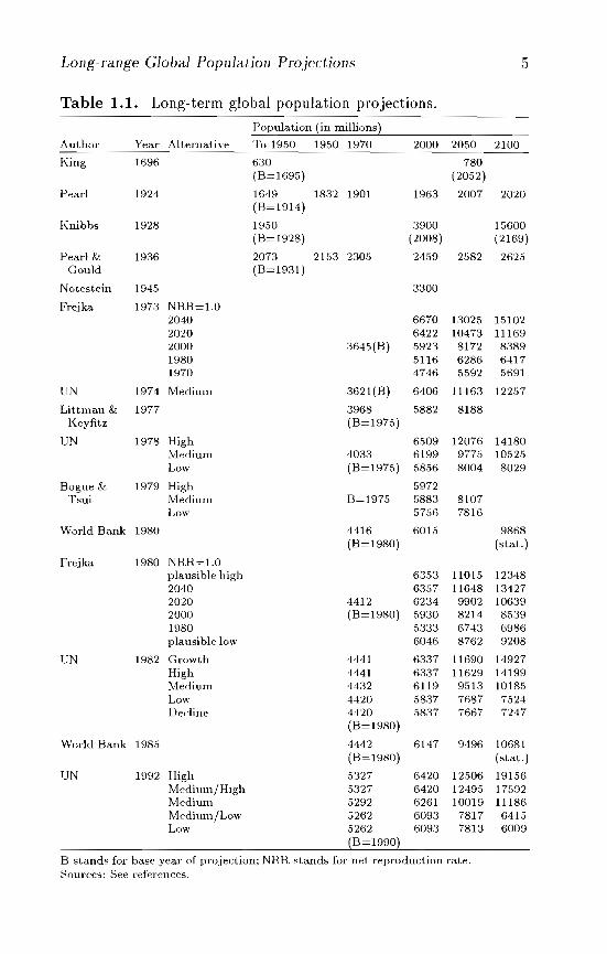
Table 1.1. Long-term global population projections.

Population (in millions)

Author Year Alternative To 1950 1950 1970 2000 2050 2100

King 1696 630 780(B=1695) (2052)

Pearl 1924 1649 1832 1901 1963 2007 2020(B=1914)

Knibbs 1928 1950 3900 15600(B=1928) (2008) (2169)

Pearl & 1936 2073 2153 2305 2459 2582 2625Gould (B=1931)

Notestein 1945 3300

Frejka 1973 NRR=l.O2040 6670 13025 151022020 6422 10473 111692000 3645(B) 5923 8172 83891980 5116 6286 64171970 4746 5592 5691

UN 1974 Medium 3621 (B) 6406 11163 12257

Littmau & 1977 3968 5882 8188Keyfitz (B=1975)

UN 1978 High 6509 12076 14180Medium 4033 6199 9775 10525Low (B=1975) 5856 8004 8029

Bogue & 1979 High 5972Tsui MedilUl1 B=1975 5883 8107

Low 5756 7816

World Bank 1980 4416 6015 9868(B=1980) (stat. )

Frejka 1980 NRH=1.0plausible high 6353 11015 123482040 6357 11648 134272020 4412 6234 9902 106392000 (B=1980) 5930 8214 85391980 5333 6743 6986plausible low 6046 8762 9208

UN 1982 Growth 4441 6337 11690 14927High 4441 6337 11629 14199Medium 4432 6119 9513 1018.5Low 4420 5837 7687 7524Decline 4420 .5837 7667 7247

(B=1980)

World Bank 1985 4442 6147 9496 10681(B=1980) (stat.)

UN 1992 High 5327 6420 12506 19156Medium/High 5327 6420 12495 17592Medium 5292 6261 10019 11186Medium/Low 5262 6093 7817 6415Low 5262 6093 7813 6009

(B=1990)

B stands for base year of projection; NRR stands for net reproduction rate.Sources: See references.

6 Tomas Frejka

The leading scholar who transformed the potentiality into realitywas Frank Notestein. The methodology of component populationprojections was first applied in a study of Europe and the SovietUnion commissioned by the League of Nations in the early 1940s(Notestein et al., 19H). This study was perceived as the first vol­ume of a series of studies on world population trends and problems.Soon thereafter, Notestein (1945) presented the first modern globalpopulation projections. He reviewed past population trends of coun­tries and continents; he discussed his understanding of the mecha­nisms of population change, distinguishing three main demographictypes of populations corresponding to different stages of the "demo­graphic evolution" ("incipient decline," "transitional growth," and"high growth potential"'); and finally, he discussed prospects forgrowth and provided projections separately by continent on the ba­sis of which he concluded that "summing the hypothetical figuresfor the year 2000, we have a world total of 3.3 billion people. On theassumption of general order and the spread of modern techniquesof production the figure is probably conservative." Even though itspanned only over a period of" half a century, Notestein's projec­tion of the world populat ion is discussed in this chapter because ofits pioneering nature and because the applied ideas, approach, andmethods provided the base for a generation of world, regional, andnational projections to follow.

Notestein's projections permit the formulation of general char­acteristics and procedures that constitute the basis of long-rangepopulation projections:

• An explicit or implicit theoretical framework of the mechanismsof population change. which guides the formulation of assump­tions about future changes in delllographic trends.

• A wealth of accumulated demographic data which serves as theempirical base for the framework, provides the input data for thebenchmark year/period of the projections, and makes possiblea disaggregated approach.

• A methodology which usually consists of (a) a separate assess­ment of an initial age structure and separate projection of thetwo motor forces of demographic dynamics in a closed popula­tion -- mortality and fertility (the combination of these elements

Long-range Glohal Population Projections I'

yields the so-called component projection of a population) - and(b) a separate assessment and projection of national and/or re­gional populations, which, when aggregated, yield global projec­tions or which provide a check on separately computed globalprojections.

• Advances in any of these characteristics and procedures dependon advances of demographic and social science research as wellas on advances in data collection.

Notestein 's contribution was not only important because he ap­plied and combined all of the above elements but also critical from asubstantive perspective. His theoretical framework is based on thedemographic transition theory labeled the "demographic evolution"in Notestein 's 1945 piece. It is the demographic transition theorywhich - for the most part implicitly - is the theoretical base forthe majority of the global long-range population projections thatfollowed.

The sets of the United Nations population projections of the19.50s and 1960s followed Notestein 's model, with refinements beingintroduced as methods of demographic analysis developed and newdata became available. The time span of these projections was from:30 to 45 years. A particularly innovative set was prepared in 1957(U N, 1958) which made considerable use of sophisticated methods inestimating demographic parameters and in the projection computa­tions. For these projections the UN (19.55) prepared a set of modellife tables, as well as models of fertility trends. This was the firstUN projection extended to the yeaT 2000, for which time a globalpopulation ranging between 4.9 and 6.9 billion was projected. As weapproach the year 2000 it now appears that the UN's 19.57 mediumprojection will come remarkably close to what the actual figure forthe year 2000 is likely to be, 6.:~ billion. The central objective of theUN sets was defined as "an attempt to project population changesinto the future as accurately as possible with available informationto provide basic data on population size and characteristics for fu­hue planning" (UN, 197:3). The focus of population projections upto this point in time was on providing the best possible, "as accurateas possible," projection. forecast. or even prediction.

R Tomas Frejka

1.3 Contemporary Long-range Projections

The first set of long-range projections to follow Notestein's workof 1945 was developed by Frejka (i97:3a) in the early 1970s (theideas and methods applied were originally developed in a study ofthe US population in Frejka, 19(8). These projections were meantto demonstrate t he strength of the population growth momentuminherent in current demographic characteristics - age structure andlevels as well as age-specific st mct mes of fertility and mortality ­and the strength of behavioral continuities. The principal innovationwas to prepare scenario pro,jections in contrast to projections thatwere aimed at projecting future demographic trends as accuratelyas possible. More specifically, these projections were designed:

• To map alternative scenarios of how the demographic transitioncould proceed toward an assumed low mortality-low fertilityequilibrium expressed by a net reproduction rate of unity beingreached at defined alternative future dates.

• To illustrate the long-range implications for population growthof specific demographic, mainly fertility, trends.

• To demonstrate the more likely alternatives of future popula­tion growth in the context of unrealistic/unlikely projectionsbased on implausibly rapid or implausibly slow assumed trendsof fertility decline.

The emphasis was on generating illustrative scenario projec­tions, not on generating projections that would aim at depictingfuture trends as accurately as possible. At the same time, however,there was a dear intention to supply a good idea of likely futuretrends by providing the possibility of comparing more realistic al­ternatives with what appeared to be clearly unrealistic options. Theprojections were computed for a period of almost 200 years ratherthan the customary period of between 30 and 50 years (for instance,the UN projections).

The assumption that a, low fertility-low mortality stationarypopulation could be achieved and possibly maintained in the longrun appeared quite plausible in light of the trends in the demograph­ically mature countries through the late 1960s. There seemed to bea reasonable (tacit) consensus at the time that post-demographic

Long-range Global Population Projections 9

transition societies would stabilize, with fertility and mortality be­ing such that the long- term net reproduction rate average would bearound unity. In hindsight, the experience of Western countries, par­ticularly since the early 1970s, has not confirmed this assumption.

These projections provided a vivid illustration of the long-termconsequences for population growth of demographic trends, mainlyof fertility, of the foreseeable fllture, say of the 1970s and 1980s,which presumably could be modified by public policies. While thecalculations of the global population for the year 20.50, for example,ranged between 5.6 and 1:3.0 billion (see Table 1.1), it was arguedthat the alternative results yielding figures below 8 billion couldbe dismissed as unrealistic because the calculations were based onassumptions of unrealistically rapid fertility decline. With consid­erably less certainty the numbers at the upper limits of the rangewere cast in doubt, as historical experience seemed to indicate thatfertility would be likely to decline faster than the defined assump­tions for the high projection. Consequently, it was argued that theglobal population in the middle of the next century would probablybe between 8 and 12 billion and tha.t whether the actual populationwould be closer to the upper or lower limit would depend on howvigorously major factors shaping fertility decline, including publicpolicies, would exert their impact.

During the 1970s and 1980s various institutions, in particu­lar the UN (197.5, 1981b, 1982b, 1992c) but also the World Bank(Zachariah and Vu, 1978, 1980: VlI, 198.5), the US Bureau of theCensus (1979), and individuals (Littman and Keyfitz, 1977; Bogueand Tsui, 1979) prepared long-range projections. To a large extent,these projections used a principle analogous to Frejka's projections,namely, that they were scenario projections aiming, sooner or later,for an eventual low mortality-low fertility equilibrium. Many did in­troduce additional ideas/arguments or methodological refinements.

In their projections of the early 1970s, the UN adjusted themodels for the future course of fertility in both the developedand developing countries, and introduced the reverse logistic curve(a stretched-out reverse S) with specified time points at whichreplacement-level fertility will be reached and, beyond it, sustained.

A notable departure from the principle of aiming at eventualreplacement-level fertility is contained in the UN 1992 projections

10 Tomas Frejka

where the experience of below replacement-level fertility in the West­ern countries is reflected. The idea of reaching and maintainingreplacement-level fertility is assumed only for the medium variantand for an instant replacement-level fertility projection. Two vari­ants assume reaching and maintaining below replacement-level fer­tility, two other projections assume a fertility decline that is abovereplacement-level fertility which when the defined level is reachedit is ma.intained, and a fifth projection assumes constant fertilityand mortality. Among the conclusions of these recent projections,the UN stresses that according to the medium projection the worldpopulation would be 11.2 billion in the year 2100 which is 1 bil­lion, or 10 percent, larger than the UN 1982 projections. Accordingto the UN, "upwardly revised estimated and projected average lifeexpectancies at birth probably play the key role." Also, there is amuch wider range between the lowest and highest results in the 1992compared with the 1982 projections for the year 2100, namely, 6.0­19.2 compared with 7.2-14.9 billion. The authors emphasize "thatthere is a wide range of uncertainty regarding the future size of theworld population."

Bogue and Tsui (1979) reached a \'ery different conclusion, al­beit over a decade earlier: "the magnitude and pace of the (1965­1975 fertility) decline is greater than many demographers had ex­pected" and therefore

this development makes it necessary for demographers to reviewand re-examine their projections for the future. We predict thatby the year 2025 the world will have nearly achieved zero pop­ulation growth. It is estimated that this equilibrium will beachieved with a world population of about 7.4 billion (8.1 in2050) ... primarily because of the worldwide dri ve by Third Worldcountries to introduce family planning as part of their nationalsocial-development services.

In the early 1970s studies associated with the Club of Romeintroduced ambitious methodological innovations. An attempt wasmade to link population projections more tightly to social, economic,environmental, resource consumption, and political trends. Mead­ows et al. (1972) and Mesarovic and Pestel (1974) defined global dy­namic systems analysis models that contained population as one ofseveral basic components. Projections of these systems were carried

Long-range Global Population Projections 11

into the 21st century to demonstrate possible disastrous or harmo­nious long-term consequences inherent in global societal trends. Ac­cording to these projections, the likely trends in population growthas well as in other societal trends will lead to a collapse of the worldsystem. This will include an increase in mortality and a consequentrapid population decline. The studies conclude that if such a col­lapse is to be avoided, a rapid fertility decline, significantly fasterthan that of the low UN projection of that era, would have to begenerated. These projections were indeed innovative in their com­prehensive approach. but numerous critics doubted the validity ofemployed assumptions and relationships (Ridker, 1973).

1.4 A Recent Critical Review ofLong-run Global Projections

A critical review of long-run population projections has recentlybeen undertaken by Lee (1991). He takes a substantive rather than ahistoric approach. Lee comprehensively analyzes important aspectsof population projections: demography's contribution to forecasting,theories underlying projections, the degree of uncertainty of long­run population projections, and recent long-run projections of theglobal population. Among the numerous insightful observations andfindings, many can be applied to fut me work.

One observation which appears to be a central concern to Leeand which deserves particnlar attention in the context of this chap­ter is that in a number of the above-discussed global projections asufficiently explicit and systematic theoretical framework is lacking.Two views expressed in Lee's paper warrant a brief discussion atthis point.

Lee eloquently challenges a central premise applied in the long­range global projections of the 1970s and the 1980s, namely, thatthe end point of most of these projections are stationary populationswith a net reproduction rate of unity. He claims that he could notfin d any explanation of this in Frejka's 1973 book (see Frejka, 1973a,which according to Lee provides the origin of this idea; actually theorigin of the idea is in Frejka. 19GR) and criticizes the justificationgiven in Frejka ( 1981b). Admittedly. the theoretical justification ofusing replacement-level fertilit~· as an end point might not have been

12 Tomas Frejka

thorough enough, however, it was clear that Frejka's work in thelate 1960s and early 1970s was conducted within the demographictransition theory framework as it was understood at that time. Ifnowhere else this was succinctly expressed in Frejka (1973b): "Theexperience of history suggests that the population of the world mayeventually reach a state close to non-growth, that is, all countrieswill be in the third stage of the demographic transition."

The second issue relates to the content and purpose of the con­cept of projections. A basic premise of Lee's, which he states with­out providing arguments or justification, is that "almost all demo­graphic projections are in fart forecasts, in that they present theauthor's best guess about the future." Therefore he uses forecaststhroughout his piece. As has been discussed at length above, thedistinction between Joncas!s - i.e., projections that attempt to de­pict future trends as accurately as possible at any given momentin time - and scelwrio projections - i.e., projections which intro­duce elements that aim to illustrate certain developments some ofwhich might actually be intentionally unrealistic in order to demon­strate a particula.r outcome - is justified. That does not excludethe purpose of also attempting to provide a reasonable perceptionof realistic future population trends through scenario projections.

1.5 Conclusions

Contemporary long-range global population projections of the past2.5 years are all constructed along the lines of the Notestein model.They are based on an explicit or implicit theoretical framework,using the best available data, and they are component projections.They aTe usually straightforward demographic projections where thepossi ble impacts of changes in behavioral, social, economic, or po­litical trends are introduced via the theoretical framework. A basicinnovation was added by devising and using scenario projections incontrast to projections aiming at prediction. However, even whenusing scenario-type projections the intention of more or less approx­imating likely future demographic trends is almost always present.

The various projections briefly discussed a.bove provide exam­ples of justifications for new projections. At the most general level,whenever a significant innovation can be introduced in anyone of

Long-ra.nge Global Pop ula tion Projections 1:3

the elements a new projection is justified. Thus, formulating a newor different theoretical framework, the application of new data, ort he development of a new or different methodology provides such ajustification.

Each of the subsequent (TN sets of projections used newlycollected or estimated base data. Some of these sets introducedmethodological advances, and in some the formulation of assump­tions about demographic trends was modified based on the devel­opments of actual trends. Bogue and Tsui (1979) based their pro­jections on their interpretation of fertility trends between 1965 and1975 and on their belief that policy measures in the form of strongfamily- planning programs could and would modify fertility trendsmore than experience to date indicated. Meadows et al. (1972) at­tempted to expand the theoretical framework by direct linkage tosocial, economic, environmental, resource consumption, and politi­cal trends and applied a large number of assumptions about trendsand linkages. In addition to using llew fertility and mortality data,the most recent United Nations long-range global projections (1992)assumed a variety of fertility trends: reaching and maintainingreplacement-level fertility, reaching and maintaining fertility levelsbelow and above replacement.

The purpose of long-range globa.! population projections can bemore than attempting to predict tota.! population numbers 50, 100,or 150 years into the future. In addition, their purpose can be:

• To demonstrate shorter- and long-run implications of alternativefertility and mortality trends of the foreseeable future.

• To demonstrate what type of trends need to occur to achievea population of a desirable size and with specific structuralcharacteristics.

• To demonstrate various structural implications of certain fertil­ity and mortality t rends for major regions and functional agegroups, for example.

• To demonstrate the consequences of intended policy interven­tions if they were to succeed.

Whatever the purpose of a single projection or a set of projec­tions may be, for them to be meaningful and to provide new insights,a significant and well-justified new or £nnovat£ve element has to beembedded in the projections.

Chapter 2

Alternative Approaches toPopulation Projection

Wolfgang Lutz, Joshua R. Goldstein, Christopher Prinz

Future demographic trends are inherently uncertain, and the furtherone goes into the future, the greater the uncertainty. On the otherhand, few social and economic trends are as stable as populationtrends. No social scientist would challenge the statement that thepercentage increase of the world population over the next five yearscan be more accurately projected than changes in unemploymentrates, trade balances, or stock markets. Because of the great iner­tia of population trends, long term and short term mean differentthings for demographic and economic forecasts, but in all forecastsuncertainty is assumed to increase with the time horizon because ofthe greater probability of structural changes.

Summarizing the limits of population forecasting, Nathan Key­fitz (1981:583) states: "The practical conclusion, then, is that rel­atively short-term forecasts, say up to ten or 20 years, do tell ussomething, but that beyond a quarter-century or so we simply donot know what the population will be." Such a statement still seemsto reflect the thinking of most demographers today, including manyof the experts invited to contribute to this book, who defined as­sumptions only up to the year 2030. But the question of what wecan know today about the future goes beyond the issue of the timehorizon, which is discussed later in this chapter.

First we need to ask, What kind of knowledge of the future dowe want to have? Do we want to have one single number, a certain

14

Alternative Approaches to Population Projection IS

range, or a probability distribution? Do we want total populationsize a.lone or age-structura.l information as well? Who is interestedin these numbers and for what reason? And what is the motivationof those who prepare population projections? These questions affectthe approach taken to project future population and the methodsand assumptions chosen.

This chapter gives a broad and nontechnica.l exposition of somefundamental questions involved in choosing an approach to projectfuture population. These kinds of questions are usually not ad­dressed in technical scientific papers or in the publication of pro­jection results because certain choices are taken for granted. Abroader perspective is necessary, however, to answer the questionwhich forms the title of Part [: Why another set of global popula­tion projections? Several fundamental issues in population projec­tion are addressed in the following eight sections in this chapter. Theapproach taken in this book is described and justified against thebackground of other possible approaches. The concluding sectiongives a concise summary of our choice.

2.1 Who Wants Population Projections?

\,yhat motivates demographers to prepare population projections.and for whom are they preparing them? Three major groups areinterested in population projections and are willing to pay demogra­phers to do this job: other scientists, governments and internationalagencies. and the general public, including private industry.

A large number of natural and social scientists are increasinglydemanding information about future population size and structure.The recent upsurge of environmental and global change research hasfurther heightened this demand. A major reason for this demandlies in the fact that many of the indicators used in such studies areon a per capita basis. By definition these require a population figureill the denominator. In particular, this is the case in studies on CO 2

emissions conducted by Bartiaux and vall Ypersele (199:3), Birdsall(1992), and Bongaarts (1992). These studies combine future popn­lation trends with assumed future per capita CO 2 emissions. Lutz( 1993) has also demonstrated that the level of regional aggregationsignificantly influences the results. The time horizon of these studies

16 Wolfgang Lutz, Joshua R. Goldstein, Christophel' Prinz

is typically long (at least to 2030-2050, often to 2100 and beyond)because global-warming is a long-term phenomenon.

Related to global-warming issues is the large group of energydemand models, which are probably the most numerous scientificconsumers of population projection data. A few forecasters (e.g ..Odell and Rosing, 1980) omit the explicit consideration of popu­lation, and instead project total energy demand. Most, however.combine scenarios of the evolution of energy demand with popula­tion forecasts (Gouse et at., 1992; Leontief and Sohn, 1984; WECCC,1983; IIASA and WEe, 1995). The time horizons of these studiesrange from 2020 to 2100.

Another field of studies which routinely includes populationprojections is the analysis of world food consumption. The Foodand Agriculture Organization (FAO, 1988) has produced forecastsof demand to 2010. The approach taken by Mellor and Paulino(1986), for example, is to produce two scenarios: the first is hased onpresent per capita calorie consumption and the second includes in­creased calorie consumption arising from assumed economic growth.Many more fields, such as economic forecasting, epidemiologicalstudies, and insurance mathematics, demand population projectionsas input.

In the past non-demographic scientific studies requiring popula­tion forecasts tended to consider only one variant of future popula­tion trends. Recently, however, the scenario approaches in many ofthese disciplines have become increasingly sophisticated and allowfor consideration of alternative population scenarios. There cleaTlyis a demand not only for one best guess of the future population butalso for information concerning the degree of uncertainty and moreextreme scenarios for sensitivity analysis. So far demographers havenot done much to satisfy this demand.

Politicians, including public administrators, need populationprojections largely for planning purposes. Especially in the health,education, and social-security sectors, medium- and long-term plan­ners regard demographic variables as crucial components. Typically,politicians and administrators would like to receive one likely vari­ant of future population size and structure that they can use illtheir models to determine, for example, where new hospitals amischools should be constructed and how the legal system of pension

Alternative A.pproaches to Population Projection 17

payments should be organized to accommodate changes in the agecomposition of the population.

Unlike the scientific community, public administrators and po­litical planners rarely ask for alternative variants and generally havelittle appreciation of the methods dealing with uncertainty in pop­ulation projections, despite the fact that policies should be robustand hold under varying conditions. They typically want one. mostlikely figure.

Despite the tradition of government planners to use only onecentral forecast, the design of policies that hold under uncertainfuture conditions should be a main concern of good politics. Forinstance. a restructuring of the pension scheme, as currently be­ing done in many European countries, should by no means consideronly one future mortality trend. Since national population projec­tions tend to assume very low future mortality improvements, evena continuation of past increases in life expectancy results in a muchfaster increase of the old-age dependency ratio, and might bringabout painful, if not disastrous, surprises in the new system. Inthis situation demographers have a responsibility for communicat­ing their knowledge about uncertainty.

The third group of users of population projections is by far thelargest and most heterogeneous. Many individuals, organizations,and enterprises in the general public are interested in specific pop­ulation projections. Aside from individual curiosity, this interest isused in the planning of future activities and in the estimation ofexpected returns from such activities; the activities range from anindividual's decision to buy real estate in an area with potential in­creases in population density to an enterprise's marketing strategyfor a commercial product, such as baby food or special products forthe elderly.

Generally the expectations of this group tmvard population pro­jections can be assumed to be similar to that of the group of politi­cians and administrators. The interest tends to focus on one mostlikely variant. Considerations of uncertainty may playa role in cor­porate planning, but generally the planning horizon of companies istoo short for alternative population trends to make a difference. Anexception may be energy-supply companies that tend to have longtime horizons.

18 Wolfgang Lutz, Joshua R. Goldstein, Christopher Prinz

In addition to these three major groups some specific groupsexplicitly use population projections for educational and illustrativepurposes. The most vocal of these are environmental and family­planning groups that want to draw attention to what would happenin the distant future if policies aiming at a reduction of popula­tion growth were not implemented. Such people are not as muchinterested in one medium population projection as they are in thecaleulation of extreme alternatives to demonstrate the long-termimpacts of today's choices.

Another special group are students in the social sciences whoshould understand the basic functioning of population dynamics.For this group, phenomena such as the momentum of populationgrowth could best be illustrated through comparisons of alternativelong- term population projections.

In summary the different groups interested in population pro­jections are demanding two different types of results from demogra­phers preparing such projections: one most likely variant that canbe used without further consideration of the problem of uncertaintyaud information about less likely but still possible trends that can bensed for sensitivity analysis. i.e., for understanding how the systemsstudied or any planned policy or individual action would performunder different possible demographic futures. Although most usersof projections are satisfied with a 30- to 40-year time horizon, someclearly want a longer time horizon.

2.2 Time Horizon

Technically, it is a simple matter to continue a population projec­tion one hundred, or even one million, years into the future. Butthe question is, how meaningful is such an exercise. The choice of aprojection horizon, therefore, represents a compromise between theadvantages of providing more information and the dangers of mak­ing inaccurate assumptions. Beyond a certain point in time, we aretoo unsure about the state of the family, health, and the world tospecify rates of fertility, mortality, and migration. In this section weexplore the possible reasons demographers have for regarding :30 to40 years as a threshold beyond which projections become less reli­able. We also address the question of whether uncertainty increases

Alternative Approaches to Population Projection 19

monotonically with time or whether there are thresholds and dis­continuities suggesting a certain cutoff point.

The time scale of population projections is of distinctly humandimensions. This is not only because the human life span and thegap between generations have important demographic consequences.but also because forecasters' judgments about the speed of socialchange depend on their personal experiences.

From a psychological perspective, there may be reasons for beingsuspicious of projections that forecast further than 40 or 50 yea,rsinto the future, a little less than two generations.[l] During ourlifetimes, most of us get to know our grandparents, but not ourgreat-grandparents. Consequently, we know first-hand the amountof social change that can occur over two generations. When wespecify demographic rates beyond this, not only must we forecastthe behavior of individuals whom we will probably never meet, butwe must deal with individuals who are more distant, in generationalterms, than anyone we have met in our own lives. In addition to thissubjective reason for setting a threshold of increased uncertainty. \vecan point to other. less personal, justifications for a particular timehorizon.

In developing countries the average age is roughly between 35and 40. As such, this average age marks the period of time beyondwhich a population will consist of a majority of people not yet born.The wholly individual psychological perspective just mentioned thusalso corresponds to the experience of the entire population, the tim­ing of which might mark a rupture in social change.

In addition to uncertainty in the inputs of population projection(the demographic rates that reflect individual behavior), we mustalso consider the size of the population at risk. The number ofbirths in the future is a function not only of birth rates but also ofthe number of potential parents in the population, itself a function ofpast demographic rates. This feedback property is well known in thecase of the echoes of a baby boom (or bust). The time it takes for aboom to echo is approximately the mean age of childbearing, whichranges between ages 2.5 and 30 in almost all populations. Beyondthis time horizon, therefore, we add to our uncertainty about birthrates the uncertainty of how many potential mothers will be in thepopulation.

20 Wolfgang Lutz, Joshua R. Goldstein, Christopher Prinz

The number of deaths in a population is also a function of thenumber of past births and deaths, but since in developed countriesthe mean age at death (in a stationary population, equal to lifeexpectancy) is roughly three-quarters of a century, the lagged mor­tality effect will be of relatively minor importance. In developingcountries where mortality is still high, however, a rapid improvementin infant mortality might increase the number of potential mothersin as little as 1.5 to 20 years.

While not subject to uncertainties about cohort size, migrationlevels are subject to perhaps a more arbitrary type of change - thechange in government policy. Annual migration trends are largelydetermined by government policy. If we were to ask, for instance,how many immigrants will Western Europe admit, most analystswould be reluctant to predict more than a few years into the future.And indeed we have seen tremendous ups and downs in migrationflows in recent years. \iVhen migration plays a major role in deter­mining the demography of a region, it would seem that 05 to 10 yearsmight mark the point beyond which any projection would becomequite speculative.

If we ask, on the other hand, why 10,000 years is too long toperform a projection, we discover a further constraint on forecasthorizons. In addition to the fact that we are in no position to specifydemographic rates for such a long period, the meaningfulness of theprojection models used applies only to certain time scales. Assumingthe case of an ageless population growing at a constant exponentialrate, the only possible average growth rate in the long term thatwould avoid extinction or inconceivable explosion is zero.

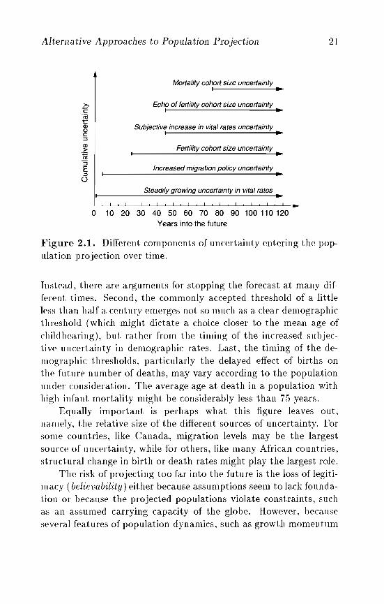
Figure 2.1 summarizes the possible thresholds of increasing un­certainty. The times shown are in an extremely stylized form and aremeant to summarize the arguments given earlier. The second waveof fertility cohort size uncertainty is added to indicate that the habyboom (hust) resulting from the cohort size uncertainty after about205 years will have echoes in the following generation also, a1thoughof less amplitude than in the past. Cohort size is also determinedby migration, so we might want to add additional uncertainty 205,SO, and 75 years after the migration uncertainty begins.

Despite its speculative nature, we can draw several lessons fromFiguT'E 2.1. First, no single clear threshold of uncertainty emerges.

Alternative Approaches to Population Projection

Mortality cohort size uncertaintyI ..

21

>-C"iiitQ)(..lC::JQ)

"~Cil:JE::J()

Echo of fertility cohort size uncertaintyI ..

Subjective increase in vital rates uncertaintyI ..

I Fertility cohort size uncertainty ..

Increased migration policy uncertaintyI •

I Steadily growing uncertainty in vital rates ..

o 10 20 30 40 50 60 70 80 90 100 11 0 120Years into the future

Figure 2.1. Different components of uncertainty entering the pop­ulation projection over time.

Instead, there are arguments for stopping the forecast at many dif­ferent times. Second, the commonly accepted threshold of a littleless than half a century emerges not so much as a clear demographicthreshold (which might dictate a choice closer to the mean age ofchildbearing), but rather from the timing of the increased subjec­tive uncertainty in demographic rates. Last, the timing of t.he de­mographic thresholds, particularly the delayed effect of births onthe future number of deat.hs, may vary according t.o the populationunder consideration. The average age at deat.h in a populat.ion withhigh infant mortalit.y might be considerably less t.han 75 years.

Equally important is perhaps what this figure leaves out,namely, the relat.ive size of the different. sources of uncert.ainty. Forsome count.ries, like Canada, migrat.ion levels may be the largestsource of uncertaint.y, while for ot.hers, like many African countries,structural change in birt.h or deat.h rates might play the largest role.

The risk of projecting too far into the future is the loss of legiti­macy ( believability) either because assumptions seem to lack founda­tion or because the projected populations violate constraint.s, suchas an assumed carrying capacity of the globe. However, becauseseveral features of population dynamics, such as growth momentum

22 Wolfgang Lutz, Joshua R. Goldstein, Christopher Prinz

and echoes, persist strongly for at least one or two generations pro­jections of less than 50 years probably do not reveal all the informa­tion already present in even today's age structure. This explanationsupports the argument for a minimum length of projection.

The reluctance of demographers to go beyond a certain timehorizon is in conflict with some of the expectations of potentialusers as described in Section 2.1. Some users clearly want popula­tion figures for the year 2100 and beyond. Should the demographerdisappoint such expectations and leave it to others with less exper­tise to produce them'? The answer given in this study is no, Butas discussed below, we make a clear distinction between what wecall projections up to 2030-2050 and everything beyond that time.which we term extensions for illustrative purposes.

2.3 Spatial Resolution and Heterogeneity

Because of the great heterogeneity of the world population it clearlydoes not make sense to treat the whole world as one region in apopulation projection. Users of projections want information to bearranged by countries or at least by major world regions that groupcountries by demographic, socioeconomic, and cultural characteris­tics. If the output parameters are to be regional, clearly the projec­tion needs to be done on a regional basis. But even if the user isonly interested in aggregate global results, meaningful assumptionson future fertility and mortality cannot be made for all the differentregions together for two reasons.[2]

First, different parts of the world are at very different stages ofdemographic transition; in most projections this factor is the basicunderlying paradigm on which assumptions about future fertility arebased. The aggregation of these different parts obscures the pictureand makes the reasoning behind assumptions more difficult.

Second, because population growth rates are much higher in theSouth than in the North, the weights of the two hemispheres willchange significantly in the future; by itself this factor leads to achange in aggregate rates even if the rates remain constant in eachhemisphere. Lutz and Prinz (1991) have quantitatively illustratedthis by using a simple calculation. In the purely hypothetical case,

Alternative Approaches to Population Projection 23

in which all vital rates are kept at their present levels, the projectioncarried out on the basis of six world regions yields a total populationthat by the end of the 21st century is 50 percent higher than theprojection treating the world as one region. This amazing differenceis simply due to the fact that the low-fertility regions make up alarger proportion of the world population today than they will inthe future. Africa, which has by far the highest fertility, increasesfrom 12 percent of the world population to roughly one-third underconstant fertility. With this change in weights, constant fertility inthe main world regions results in increasing fertility in the worldtotal and hence in a larger total population than in the case ofconstant global fertility.

While the above example clearly shows that heterogeneity ofthepopulation can have a strong effect, it is not clear how much OIlemust disaggregate to avoid this problem. Even within nations theremay be subpopulations with very different demographic regimes.In some Latin American countries, such as Bolivia, national fertil­ity rates have been stagnant at a rather high level; this may beexplained by the bifurcation of society into one group that is welladvanced in its demographic transition and another group, the In­dian population, that has not fully entered the fertility decline andis rapidly increasing. In addition to the observable heterogeneityin a population, Vaupel and Yashin (1983) have demonstrated thl?significance of unobserved heterogeneity for population dynamics.

For our global population projections a basic question was, Howfar should one go in disaggregating the world population? The­oretically, disaggregations need not follow territorial or nationalboundaries but should follow the most strongly discriminating vari­ables. In practice, however, data are most readily available by coun­tries and groups of countries. The United Nations and the WorldBank produce their population projections at the level of individ­ual countries. In this approach the 1.2 billion Chinese receive asmuch attention as the 72,000 inhabitants of the Seychelles. This isdue to the national constituencies of these organizations and conve­nience of data availability rather than to questions of demographicheterogeneity.

With more than 150 countries in the world today, however, si­multaneous projections become awkward especially with respect to

24 Wolfgang Lutz, Joshua R. Goldstein, Christopher Prinz

the migration matrix to be assumed for all these states. This per­haps explains why migration is not a major emphasis of the UN andWorld Bank projections. An alternative, which has been chosen forthe present study, is to limit the number of populations projectedsimultaneously to subcontinental regions. The 13 world regions havebeen defined according to geographic proximity and socioeconomiccriteria, as well as similar demographic and institutional aspectssuch as compatibility with other data sets. These 13 regions areprojected simultaneously by a multistate model assuming region­specific future paths of age-specific fertility and mortality rates andfull matrices of interregional migratory streams.

These regional assumptions must be considered aggregate fu­ture paths of fertility, mortality, and migration that reflect not onlychanging behavior within the subpopulations of the region but alsothe compositional effect of changing weights. This method seemsto be the most pragmatic way to deal with the bothersome issue ofpopulation heterogeneity.

2.4 Expected Output Parameters

The methodology used for population projection crucially dependson the choice of relevant population characteristics. If the user isinterested only in total population size, methods such as simpleexponential growth models may be used; these methods, however,are not sufficient if one is also interested in the future age and sexcomposition of the population. But many other population charac­teristics, such as urban/rural residence, marital-status composition.and educational or labor-force composition, may be of considerableinterest to the user of projections and require specific methodologies.

Questions about desired output parameters. together with theabove-discussed issues of time horizon and of the desirability of arange of projections, need to be discussed before the question ofappropriate methodologies. Introductions to population forecastingusually do not address these issues explicitly, but rather group pro­jection methods by the statistical models on which they are based(e.g., time-series models, structural equation models) as is done inthe introduction to a recent comprehensive volume on population

Alternative Approaches to Population Projection 25

forecasting (Ahlburg and Land, 1992). Because the evaluation of dif­ferent methods requires the systematic consideration of objectives,in this section we distinguish between projections of total populationsize, projections of the age and sex compositions of the population,and projections of characteristics other than age and sex.

2.4.1 Projections of total population size

For projections of total population size alone a basic choice is be­tween methods that consider the age structure of the population andthose that do not. 'When advocates of projections of population to­tals through various time-series models (e.g., Pflaumer, 1992) stressthat such models may be more reliable than cohort-component mod­els, which project the population by age groups, it is important tokeep in mind that this argument only concerns the aggregate totals- figures that, from a substantive point of view, have rather limitedvalue. Most economic and social issues, for which the populationvariable is considered important, heavily depend on the age pro­file of the population, ranging from social-security considerations tomarketing, from health expenditures to education, from the size ofthe labor force to internal migration. Even in the recent discussionon population-environment and carrying capacity, the populationcomposition seems to make a big difference because of varying age­specific impacts (see Lutz, 1994a).

For the time being, let us assume that the number of total pop­ulation size in a territory, at some point in the future, has meaningand value in itself. To derive such a figure we must choose be­tween simple and sophisticated guesses. The most simple would bea guess of the future population size without any formal model. Butthis would be difficult to defend. Probably the simplest meaning­ful model of population growth over time is an exponential growthmodel with a constant rate of growth. In practice, however, growthrates have never been fonstant over long periods. Through themillennia of early human history, birth and death rates fluctuatedwidely due to weather, war, food shortages, and diseases. Typ­ically birth rates were high when death rates were low and viceversa, resulting in even wider fluctuations in the growth rates of thepopulation. Although during the 20th fentury the curve of world

26 Wolfgang Lutz, JoslJUa R. Goldstein, Christopher Prinz

population growth has resembled the typical exponential growthcurve, growth rates have been far from constant even if the trend issmoothed. The growth rate of the world population was about 0.5percent during the first half of this century, increased to a peak of2.06 percent between 1965 and 1970, and slowly declined thereafter.The appealing feature of an exponential growth model, as opposedto more sophisticated ones, is that one has to make assumptionsonly for one parameter - the growth rate.

Several significant deficiencies of the exponential growth modelresult from the fact that it does not consider the age structure ofthe population. The most important is that it cannot capture themomentum of population growth. a phenomenon caused by the factthat only women aged 15--49 have children, and in the case of a veryyoung age distribution, more and more women enter this age groupand hence the population would grow significantly even with fertil­ity at replacement level. Another aspect of this deficiency relatesto countries with very irregular age pyramids, such as some Euro­pean countries where irregularities in births due to world wars, thebaby boom, and the baby bust have resulted in great fluctuationsin cohort size. Here some changes in the population growth rate arepreprogrammed by the population age structures that do not reflectany change in fertility, mortality, and migration. For instance, aphenomenon such as the echo of the baby boom - the large num­ber of babies born by the large baby- boom cohorts- could never becaptured by a model that considers only total population size.

For these reasons it is generally advisable to use projection mod­els such as the cohort-component method which explicitly considersage and sex, even if one is only interested in total population size.However, in these models one has to make assumptions on a largernumber of parameters, which raise the danger of losing sight of thebehavior of the total system while giving increased attention to spe­cific issues such as period-cohort translation in fertility. In thisrespect the suggestion made by Pflaumer (1992), that time-seriesmethods applied to population totals should be used as a baselineagainst which the results of more complex models should be as­sessed, is worth considering. Ideally the analyst could then identifythe sources of the difference between the two approaches.

.4lternative Approaches to Population Projection

2.4.2 Projecting the age and sex composition

27

As mentioned above, people are interested in population projectionsbecause they want to understand population changes that go beyondprojecting total population size. This knowledge is used in a varietyof ways, ranging from aging and social-security considerations tolabor-market questions, educational issues, and even marketing inprivate business. For all these considerations one needs to have esti­mates of the future population structure at least in broad age groups.Few users would demand projections in single-year age groups, es­pecially in a long time horizon. Projection of five-year age groupsin five-year steps of historical time has become popular, mostly forconvemence.

A projection of the population by age and sex requires first theage and sex composition of the population in the starting year. Nextone must assume age-specific fertility, mortality, and migration ratesfor each five-year period to be projected. For this age-groupwise pro­jection of the population, the so-called cohort-component methodhas become standard. This method was introduced by Whelptonin 1936 and formalized by Leslie (1945). Notestein (19c1.5) flrst ap­plied it to project the world population. The basic method has notchanged since then. In short, cohorts are groups of men and womenborn in the same time interval and representing a specific age groupat any later point in time. Their sizes can only change throughmortality and migration. The size of the youngest age group is de­termined by age-specific fertility levels applied to the correspondingfemale age groups. Hence the projected size and age structure of thepopulation at any point in the future depends exclusively on the sizeand age structure in the starting year and on assumed age-specificfertility, mortality, and migration over the projection period.

The cohort-component method tells us what to do with assump­tions on future fertility, mortality. and migration, but not how toderive them. And it is in this all-deciding question of the choice of as­sumptions and structuring of sets of alternative assumptions wherecontroversy exists and continuous improvement of population pro­jection methodologies is possible and indeed necessary. Alternativeapproaches to deriving assumptions on future fertility. mortality.and migration are discussed in the following sections of this chapter.

28 Wolfgang Lutz, Joshua R. Goldstein, Christophel' Prinz

In the context of the cohort-component method, one unresolvedqHestion is whether assumptions should be made in terms of pe­riod or cohort fertility. Technically, the Leslie matrix requires age­specific period rates. But these period rates could be either assumeddirectly or derived from assumptions on future cohort fertility be­havior. This decision essentially goes back to the rather philosophi­cal controversy of whether the cohort approach is more appropriatein fertility analysis. In practical terms the cohort-fertility approachrequires assumptions of both the level of cohort fertility and thetiming of births over the reproductive life Spall. If the age pattern isassumed to be constant and the level is assumed to approach a cer­tain constant value, there will be no difference between cohort andperiod fertility assumptions. Theoretically similar cohort-period ar­gnments could be made for mortality and migration, but they arerarely discussed.

2.4.3 Multistate models for additional characteristics

Usually populations are defined by the a territory in which theylive. But, as mentioned earlier, populations may also be definedas su bgroups of the population in a given territory, such as ethnicgroups. marital-status groups, or educational gronps. These groupscan be treated as independent populations that may interact witheach other, i.e., people leave one group and join another. The tradi­tional cohort-component method can only consider one populationand needs to be expanded to simultaneously project several pop­ulations that are interacting with one another. Such expansionsare called multistate models, and were developed by Rogers (1975)and others during the 1970s. The original applications of multistatemodels were in the field of multiregional demography and migration.

So far no global population projection has gone beyond project­ing the age and sex distribution by regions or countries.[:3] Highlyrelevant and promising from a global development perspective aremultistate projections of urban/rural place of residence and educa­tional composition. A recent set of multistate educational projec­tions for North African countries (Yousif dol., 199G) demonstratesthat because of strong educational fertility differentials the changingeducational composition of the population significantly effects totalfertility and therefore population growth. Assumptions on fertility.

Alternative Approaches to Population Projection 29

mortality. and transitions between the states must be state spe­cific in addition to age and sex specific. This lllultistate approachcan be applied to any other breakdown of the population (socioeco­nomic, ethnic, etc.) providing that the categories are clearly definedand sufficient empirical information on transition intensities is given.Population projections that also provide estimates of future distri­butions of socioeconomic variables other than age and sex may beuseful for many users, and may become increasingly popular as moremethodologies and computer programs become available.

At the global level, however. one difficulty in applying lllulti­state models that include not strictly demographic variables is theavailability of relevant empirical data. Hence, the projections pre­sented in this book are based on alternative projections of only theage and sex distribution for the 1:3 world regions specified.

2.5 Different Uses of Past Experience toDerive Assumptions for the Future

The real challenge in population projection is not the method itselfbut the generation of one set or several sets of assumptions on age­specific fertility and age- and sex-specific mortality and migration.In this context there are two basic questions. The first questionrelates to the way in which the past is used to derive future as­sumptions. The second concerns the strategy one takes to deal withnncertainty, whether to consider a range of possible assumptionsbased on some distribution or individual point scenarios. vVe candistinguish three ways to draw on past experience.

• The Future as (l Continuation of the Past Trend. This is thestrongest possible way in which the past ca.n enter into futureassumptions. A simple trend extra.polation can be performedwithout any additional input about likely future conditions. Itcan be blind and mechanical after one has chosen the indicatorto be extrapolated, the length of the period to be considered.and the information to be derived from the time series. It cantake the form of simple linear trend extrapolation, other func­tional forms of extrapolation, or. if periodicity is assumed. acombined trend with superimposed cycles.

:30 Wolfgang Lutz, Joshua R. Goldstein. Christopher Prinz

The blind continuation of past trends seems appropriateonly when absolutely no information is available about likelyfuture trends. In the context of fertility assumptions it wouldmean completely disregarding considerations derived from de­mographic transition theories, information about desired familysize, and surveys on family-planning demands. But even thissimple method does not save the forecaster from making choices.The indicator, the length of the past period. and the structureof the process must be defined.

• Only Variance from Histo'l'Y. If one is willing to incorporate intoone's assumptions external substantive information about likelyfuture trends, one possibility of combining this with informationfrom the past is to determine the average level from external ex­pert knowledge but still take the variance from past time series.The idea behind such a procedure is that the level cannot bederived by extrapolation but that the past can tell us somethingabout the variability of the process, i.e .. by how much fertilitytends to change (in any direction) over a five-year period. Alongthese lines Goldstein et al. (1994) have proposed a probabilisticmodel by which the upper and lower bounds of a random walkof fertility are externally assumed while the stepsize of changeis resampled from the past. Also the work by Keyfitz (1981)and Stoto (1983) falls into this category; they estimated futureerrors in population projections from past errors.

• S't'l'uclll'l'e and Unde'l'standing from History. Uneler this ap­proach it is not the past time series itself which is used to deriveassumptions on future evolution, but the substantive knowledgeabout the process and its structure. Taking mortality as an ex­ample. this approach goes beyond the analysis of past trends inintegrating knowledge from medicine and biology and address­ing questions such as that of a genetically determined limit tohuman life. Naturally this understanding is also informed by theanalysis of past trends but goes further, by integrating outsideknowledge derived from other sources. In this approach histor­ical information enters only indirectly into the formulation ofassumptions about the future. This third approach is the onechosen for our study. For this reason large parts of this volumeconsist of substantive papers about our understanding of the

Alternative Approaches to Population Projection :31

processes of fertility, mortality, and migration in the differentworld regions. Experts were asked to write about alternativefuture paths of fertility, mortality, and migration and to pro­duce assumptions of a most likely centraL vaLue as well as highand low extreme values for the various indicators by the year20:30, based on their substantive understanding of the processes.For the probabilistic world population projections presented inChapter 16, these three points were assumed to define a subjec­tive probability distribution with 90 percent of all cases betweent he high and low values. The approach chosen for this book isdescribed in more detail in Section 2.9.

The evolution of the future population of the world will almostsurely differ from the central scenario as described in this volume,This is unavoidable, for there is inherent uncertainty in the future.Wars will break out; some societies will modernize more quickly tha11we expect while others will develop more slowly; new diseases maybreak out, old ones may be cured; childbearing may become morefashionable in the developed world, or, quite the contrary, less so;the industrialized countries may close themselves to immigration, ormight even become more open. All these factors are crucial to thedemographic future, but they are also uncertain.

~What does a forecaster do in the face of such uncertainty'? 1\first approach is to freeze all demographic rates at their currentlevel. Rates will almost certainly not remain unchanged as the fu­ture unfolds, but this approach enables the forecaster to avoid mak­ing statements about the direction of demographic trends alld. atthe same time, makes absolutely clear the hypothetical nature oft he projection. This approach was followed by early demographicforecasters in the 1920s, 1930s, and 1940s.

A second approach is to create extreme case scenarios in addi­tion to a most likely scenario. This enables one to make statementsabout how far off future population projections could be from themost likely expected evolution. It is also 1Iseful for sensitivity anal­ysis. However, there is a danger that the range between the highand low scenarios might be so large that it is uninformative. On theother hand, when the alternative scenarios include conditions thatare more probable, one automatically begins to ask about the likeli­hood of a given scenario. Alternative scenarios or variants without

32 Wolfgang Lutz, Joshua R. Goldstein, Christopher Prinz

any information about their likelihood somehow remain unsatisfac­tory to the user.

The third approach, explicit quantification of uncertainty, istherefore designed to explicitly incorporate information about thedegree of uncertainty. It is evident that both forecasters and userswould like to know how much confidence to place in different projec­tions, but as yet no single technique is available to do this unambigu­ously. Sanderson (1995) shows that it is impossible to produce "ob­jective" confidence ranges for future population projections. Sub­jective confidence intervals are the best we can ever attain becauseassumptions are always involved. As a recent US Bureau of the Cen­sus (1989) forecast notes: "Many problems remain before a methodcan be developed for placing reliable confidence intervals aroundpopulation projections." This failure to solve the problem is not forwant of trying, but occurs because it is impossible to derive any "ob­jective" confidence interval. In the following two sections we discussin more detail the second approach (i.e., variants and scenarios) andthe third approach (i.e., probabilistic population projections).

2.6 Non-probabilistic Approaches:Single Projections, Variants, Scenarios

In practice, both national statistics departments and internationalagencies have taken non-probabilistic approaches to forecasting. Un­til recently, some agencies still offered only one set of rate trajecto­ries. Thus, it was possible to speak of the future population. Today,however, there is increasing concern about the uncertainties of fu­ture population growth, and it is rare to find a projection withoutat least one alternative set of assumptions.

Both "variants" and "scenarios" offer alternative sets of assump­tions. The difference between the two is, to some extent, only adifference in detail, but this difference is also reflected in the in­tended use. The variant approach usually offers three alternatives:high, medium, and low. The high and low scenarios are typicallydefined by the resulting population size, and not by their compo­nents. Therefore, the large population in the high alternative cancome from increased migration, low mortality, high fertility, or acombination of any of these.

Alternative Approa.ches to Popula.tion Projection 33

The World Population Prospects produced by the United Na­tions Population Division (UN, 1995), the most commonly used setof world projections, currently offers four projections to 20S0: high,medium, and low variants and a constant fertility projection whichis called scenario. Fertility is allowed to vary, but only one set ofmortality and migration assumptions are used throughout.

In their recently published long-range world population projec­tions, the UN (1992c) gives projections to 21S0 for nine world re­gions. Seven different fertility extensions are considered, but againmortality and migration assumptions remain invariant. The WorldBank (1992b) offers only one central set of projections. Birdsall(1992), however, offers a set of alternative projections resulting fromfaster than expected fertility decline in the developing world.

Sometimes the selection of inputs for high and low variants isdirectly influenced by the interests of the agency producing the fore­casts. For example, the US Social Security Administration, whoseprincipal interest lies in the age structure of the population, com­bines high fertility and high mortality for its high variant and lowfertility and low mortality for its low variant, giving the two mostextreme values for the old-age dependency ratio. The US Bureauof the Census, however, combines low fertility and high mortalityand vice versa to arrive at the most extreme values for the totalpopulation size.

Recently an increasing number of authors (Ahlburg and Vaupel,1990; Lutz, 1991; Cliquet, 1993) and agencies (EUROSTAT, UN)have chosen to speak of population scenarios instead of, or in ad­dition to, the traditional variants. Originally the word "scenario"comes from the theater. The Oxford English Dictionary (1982 sup­plement) defines it as, "A sketch, outline, or description of an imag­ined situation oj' sequence of events." During the 1970s and 1980sthe word "scenario" became popular in the social sciences, especiallyin the context of computer models (Lutz, 1995a). In the realm ofpopulation projections the notion is being used in two somewhatdifferent meanings: 1. in the sense of purely hypothetical assump­tions, e.g., a "constant fertility scenario"; and 2. in the sense of aconsistent story in which fertility, mortality, and migration assump­tions are embedded to provide a comprehensive picture of what thefuture might be. While the second usage is certainly closer to the

;34 Wolfgang Lutz, Joshua R. Goldstein, Christopher Prinz

original meaning in terms of a consistent picture, the first has gainedgreat popularity; it seems futile to try to change the common llsage,especially since there is no readily acceptable alternative word forthe first meaning. Hence, it remains with the authors of a projectionto define what they mean by a scenario.

The meaning the user chooses not only influences the conceptualdesign of the scenario, but also implies differences in the setting ofparameters. In the first case the three components of change (fertil­ity, mortality, and migration) may be assumed to be independent,whereas in the second case they should be dependent. Chapter ISof this book gives examples of both approaches. In the systematicpermutations of scenario assumptions the components are assumedto be independent in the first part of the chapter; in the speciallong-term scenarios, specific consistent stories are described suchas fertility responses to aging or mortality responses to excessivegrowth.

2.7 Different Probabilistic Approachesto Deal with Uncertainty

How can the fut ure population size differ from that which is pro­jected'? The compendium of possible mistakes is long (I\eilman,1990), but we can categorize the sources of error into three types:

1. Measurement and calculation errors. These can take the formof mistaken input data (for example, starting the projection\vith a population based on an incorrect census count), imprecisealgorithms, or a simple calculation mistake.

2. Incorrect specification of t'rends in vital rates and migration.One can predict that life expectancy will continue to rise atthe rate that it has over the past 20 years, but instead it mightwell increase at twice that rate. Fertility may reverse its declin­ing trend, or less spectacularly, the seemingly random "natural"variation (see Brillinger, 1986) might cause fertility, mortality.and migration rates to vary from year to year.

3. Unexpected events. The unexpected could cause large structuralchanges: the outbreak of war, a sudden cure for AIDS, an eco­nomic boom in Africa. Any number of ruptures with current

Alternative Approaches to Population Projection :35

trends is imaginable, any of which might render extrapolatedvisions of the future irrelevant.

We can call these, respectively, measurement error, parameterspecification error, and model specification error. To these modelspecification errors we could also add significant errors resultingfrom aggregation of heterogeneous groups. The sum of all formsof error is called total error.

At first glance, only the second source of error - the variation invital rates - seems a likely candidate for the application of proba­bilistic thinking, and most attempts to incorporate randomness intopopulation forecasting have used this as the focus. Before examiningthese techniques, however, one technique for quantifying the totalerror deserves mention. The empirical evaluation of the successesand failures of past forecasts, developed by Keyfitz and Stoto inthe early 1980s, consists simply of gathering a large number of pastforecasts and evaluating the average error. The most noteworthyconclusion of these studies, both of which focused only on error intotal population size, was that the traditional high and low variantsoffered by population projections corresponded to approximately atwo- thirds confidence interval. In other words, the population grewat rates outside those predicted by the high and low variants aboutone-third of the time (Keyfitz, 1981; Stoto, 1983).

This empirical method of estimating uncertainty clearly takesinto account all three types of error. [4] To apply it to current fore­casts, however, a strong assumption must be made: the errors infuture forecasts are assumed to be of the same magnitude as thosein the past. This assumption is of particular concern since the sam­ple of past forecasts tends to be biased toward the older ones forwhich the accuracy can be checked. This is problematic becausenot only do the methods of choosing high, low, and medium vari­ants change, but the potential variability of vital rates also changes.Unless both the variability of vital rates and the methodology ofprojection, together with the degree of care used in making the as­sumptions, stay the same, it is unclear how good an indicator pasterrors are of future uncertainty.

While an applicaiion of the results from Keyfitz and Stoto tofuture population projections is one way of determining uncertaintyestimates, the direct analysis of population trends themselves offers

36 Wolfgang Lutz, Joshua R. Goldstein, Christopher Prinz

a distinct alternative. It is here that time-series analysts have pliedtheir trade. Work on time-series analysis began with Lee (1974),which studied US fertility rates, and analyses continue today. Time­series methods aim to assign structure to the process of changingrates, for example, a random walk with drift or an Auto-RegressiveIntegrated Moving Average (ARIMA) model. Time-series methodsproduce not only a central forecast, but also the entire probabilitydistribution, showing where fertility and mortality rates are likely tobe at any future specified date contingent on a normal distributionof errors.

The principal drawback of time-series methods has been thedependence of the results all the choice of a model structure - par­ticularly for fertility, the demographic component that not only hasthe largest effect on the evolution of populations but also is the morevariable one (Lee, 1974; Ahlburg and Land, 1992) when migrationis left out, as is often done. Assuming a constant model structureis particularly problematic in the case of countries that are in themidst of the process of fertility transition and where we know thatthe model is likely to change toward the end of the transition pro­cess. Mortality appears to hold more promise in forecasting, atleast in the most developed countries. In particular, both the Lee­Carter (1992) and McNown-Rogers (1989) methods offer means ofproducing trends based on large matrices of age-specific mortalityrates. These techniques have large data requirements and have beencriticized for producing overly narrow confidence intervals. Never­theless, they are clear in their aim, which is to provide estimates ofparameter variation, providing minimum error ranges.

An alternative method for obtaining probability distributions isto simulate the evolution of demographic rates using Monte Carlosimulation methods. Random draws of past levels (for example, seeKeyfitz, 1985 and 1989) or of past variations (Goldstein et at., 1994)are made and applied to the evolving population. A large number,for instance 10,000, of sample populations are projected forward,and the resulting empirical distribution of population size and agestructure is used to estimate the theoretical probability range. Thesesimulations allow users to analyze the combined effect of uncertainty

Alternative Approaches to Population Projection 37

in mortality, fertility, and migration; the last component, mortality,has usually not been included in time-series models.

Both the history- based simulation and the time-series tech­niques are means to address only the second type of parameter un­certainty. They do not deal with the possibility of structural change.Questions, such as will there be another baby boom in Western Eu­rope, when will sub-Saharan Africa experience a fertility transition,what are the chances of a new deadly virus or of a war or revolution,cannot be addressed without probability models of the likelihood foreach unexpected event. The scenario approach, based on assump­tions of experts, offers the possibility of seeing the hypothesizedimpact of unpredictable events, and seems to be the best means foranalyzing structural change in addition to parameter uncertainty.With this approach experts can step back from recent experienceand consider possible alternative stories that might happen in thefuture. These stories may include unlikely and unexpected eventsthat can then be translated into specific parameter assumptions.

Based on such expert knowledge it is also possible to definespecific scenarios that describe not only one path out of countlesspossible paths but also a whole range of possible future paths. View­ing scenarios as just specific lines in the spectrum of possible futuretrends, one can also attempt to define the full predictive probabilitydistribution (see Lutz et ai., 199.5). Such an approach takes nei­ther the trend nor the variance directly from past time series. Thepredictive probability distribution is entirely based on the subjec­tive judgment of the expert who is equipped with an analysis ofpast trends, knows about fertility, mortality, and migration deter­minants, and is able to make informed guesses about possible futurechanges in those determinants. Such projections based on subjec­tive probability distributions are not unusual in other disciplines,but they have not received much attention in demographic researchalthough the approach was discussed by Muhsam (19.56) and Keyfitz(1977). In practice the expert can choose one statistical distribu­tion (e.g., normal or uniform) and then define only certain fractiles(e.g., median and upper and lower .5 percent). Combining the su b­jective probability distributions of a number of experts to form one

38 Wolfgang Lutz, Joshua R. Goldstein, Christopher Prinz

joint predictive probability distribution diminishes the danger of in­dividual bias. However, there can never be a population projectionwithout personal judgment. Even models largely based on past timeseries are subject to a serious judgmental issue of whether to assumestructural continuity or any alternative structure.

This approach to probabilistic projections based on the subjec­tive distributions of a number of experts is applied in Chapter 16of this volume. The chapter presents what we call "probabilisticworld population projections based on expert opinion." It signifi­cantly adds to the scenario projections in Chapter 15 by giving usersa better understanding of the likelihood of certain scenarios. It isimportant for users to know the probability of the scenario (or vari­ant) they are considering. For example, a high-fertility scenario (orvariant) with a 20 percent probability should be taken more seriousin policy considerations than one with only 2 percent probability.

The reason for choosing the probabilistic approach, which isbased on subjective distributions provided by a group of experts,rather than a time-series approach lies in our belief that in both thenear and distant future structural changes and unexpected eventsare likely to happen in many parts of the world which makes alter­native expert-based assumptions the only meaningful way to cap­ture future uncertainty. Time-series analysts could be among theexperts giving their subjective views, but at the global level theirmodels could never be applied simply because the necessary dataare not available.

As to the relationship between fertility, mortality, and migra­tion, these simulations can assume either independence or certaincorrelations. Examples for both are given in Chapter 16. Anotherimportant issue is, whether regional demographic trends should beconsidered independent or follow a uniform pattern (such as highfertility in all regions) as is traditionally assumed in uncertaintyvariants of population projection. There is, however, no particularsubstantive reason why, for example, unexpectedly high fertility inChina should coincide with unexpectedly high fertility in Africa. Ifregions are considered independent at the global level, much of thevariation will be canceled out. Chapter 16 considers both regionaldependence and regional independence.

Alternative Approa.ches to Popula.tion Projection

2.8 Interactions among Components andPossible Feedbacks from Results

39

It is essential to determine whether the assumptions made for fer­tility, mortality, and migration are unrelated or have some form ofinteraction. Yet this question is rarely discussed explicitly in thedescription of existing population projections. The problem lies inthe fact that, even when some dependency is suspected, it is verydifficult to quantitatively capture and specify the nature of suchinteractions. One can distinguish at least three different levels ofinteraction:

1. Correlation between trends of demographic components.2. Feedbacks from demographic variables resulting from projec­

tions, in particular population size or age structure.3. Feedbacks from non-demographic variables, such as economic

development, education, or environmental factors, which in turndepend on population factors.

Correlation between demographic components is incorporatedrelatively easily. For example, one can assume that in countries inthe process of demographic transition the declines in fertility andmortality are positively correlated.

Feedbacks from other demographic variables, such as popula­tion size or age structure, are more controversial and hence moredifficult to include. There is full consensus that the world popula­tion cannot grow indefinitely, but no agreement exists on the levelsat which some sort of collapse might happen. The land-carrying ca­pacity concept is accepted in the nat ural sciences, but less so amongsocial scientists. Collapses, if they happen at all, will probably oc­cur suddenly and with large regional differences. As to possiblereactions of fertility, mortality, or migration to negative effects ofpopulation aging, little agreement has been reached. Rapid agingwill certainly create problems, in particular when countries are notwell prepared, for example, with regard to social security. But, asis shown by the example of today's industrialized world, popula­tions can adapt to gradnal changes in the age structure. Becauseof the possible discrepancy between individual desired family sizes

40 lVoltg"ang Lutz, Joshua R. Goldstein, Christopher Prinz

and societal goals, it is unclear whether, for example, extreme aging\vill result in higher fertility. Examples of possible feedbacks of thiskind are given in Chapter 1.5.

Feedbacks from non-demographic variables work indirectly viasuch complex matters as levels of education, status of health care.economic development, or environmental pollution. Only a compre­hensive, multisector system would be able to track such feedbacks.However, the strength - and sometimes even the dire<tion - of suchmultifarious feedbacks is largely unknown, or at least highly un­certain. Conseq uently, multisector-systems models tend to createdependencies and future paths that are far different frollJ reality, aworld in itself driven by feedback loops based often on shaky empir­ical or theoretical grounds.

A well-known example of such a multisector system is the\Vorld;3 model - an economic. demographic. and ellvironmentalmodel of the world taken as a whole - developed by the Forrester­Meadows group during the 1970s (Forrester. 1971; Meadows (-t al..

1972. 1974, 1992b; Meadows and Meadows, 1973). The crude deathrate decreases with increasing food intake and improvements in thematerial standard of living, and increases with increasing pollutionand (to a much lesser extent) population crowding.

The Bariloche model (Bariloche Grollp, 1976; Herrera rt al..197G) is also noteworthy since it includes a relativel,v large nUlll­ber of feedbacks to the population submodel. For example, amongother things, the crude birth rate is influenced by school ellrollment.calorie intake, housing availability, and the life expectancy at birth(Herrera et aI., 1976:.51).

A different approach was recently developed for a study onpopulation-development-environment interactions in a specific set­ting (Lutz, 1994a).[.5] A main feature of this PDE model is that it isextraordinarily flexible. Since the nature and the strength of lllOStof the feedbacks included in previous models are subject to much de­bate among scientists, most of those feedbacks are not hard-wired inthe model. These feedbacks must be defined by the scenario makerusing the model software.

Conceptually such multisector models are desirable. but theyare usually not suited for the purpose of population projections.Inclusion of multiple feedbacks from non-demographic variables in

Alternative Approaches to Population Projection 41

such models increases the potential for introducing more errors thanone resolves.

2.9 Summary: The Approach We Chose

In this chapter we have addressed the following questions: Why an­other set of global population projections? YVho wants projectionsand for what reasons? What should the time horizon and spatialresolution be'? What output parameters are expected? Which al­ternative approaches address the issue of uncertainty in populationprojections? \Ve have contrasted our approach to that of ot hers.Issues have been identified in which progress is possible and de­sirable, and where alternative new strategies promise new insights.The left- hand side of Table 2.1 summarizes some of the key issuesin population projection, and the right-hand side specifies the ap­proachs we have chosen.

There is little disagreement on the projection methodology tobe used for (global) population projections. Our projections are car­ried out using a multiregional cohort-component model, with five­year age groups. In contrast to global projections produced by theUN and the World Bank, which are based on individual country esti­mates, we have disaggregated the globe into 1:3 major world regions.By doing so, much ofthe world's heterogeneity is taken into account.and we need not bother with national particularities. especially withrespect to migration.

The crucial difference with respect to existing global populationprojections lies in the specification, justification, and combination ofalternative scenario assumptions (Chapter 15) and in the definitionof the first probabilistic world population projections (Chapter 16).

The approach chosen involves a number of steps. First, selectedexperts with different backgrounds in the fields of fertility, mortal­ity, and migration analysis are asked to think about the future ofthe three demographic components. If necessary, different expertsare invited for different regions. The experts are asked to suggestpossible high and low assumptions for future fertility. mortality, andmigration levels up to the year :2030 and discuss them in a group spt­ting. The experts must argue their points substantively and justifytheir views. These elements are documented in Chapters ;3 to Ii.

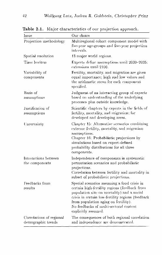
42 Wolfgang Lutz, Joshua R. Goldstein, Christopher Prinz

Table 2.1. Major characteristics of our projection approach.

Issue

Projection methodology

Spatial resolution

Time horizon

Variability ofcomponents

Basis ofassumptions

.J ustification ofassumptions

Uncertainty

Interactions betweenthe components

Feedbacks fromresults

Correlations of regionaldemographic trends

Our choice

Multiregional cohort-component model withfive-year age-groups and five-year projectionintervals.

13 major world regions.

Experts define assumptions until 2030-20:35;extensions until 2100.

Fertility, mortality, and migration are givenequal importance; bigb and low values andthe arithmetic mean for each componentspecified.

Judgment of an interacting group of expertsbased on understanding of the underlyingprocesses plus outside knowledge.

Scientific chapters by experts in the fields offertility, mortality, and migration; fordeveloped and developing areas.

Cbapter 15: Alternative scenarios combiningextreme fertility, mortality, and migrationassumptions.Chapter 16: Probabilistic projections bysimulations based on expert-definedprobability distributions for all t.hreecomponents.

Independence of components in systematicpermutation scenarios and probabilisticprojections.Correlation bet.ween fertility and mortality insubset of probabilistic projectiolls.

Specia.l scenarios assuming a food crisis incertain bigh-fertility regions (feedback frompopulat.ion size on mortality) and a socialcrisis in certain low-fertility regions (feedbackfrom population aging on fertility).No feedbacks of multi-sectora.l contextexplicitly assumed.

The consequences of botb regional correlationand independence are demonstrated.

Alternative ApproaclJes to Population Projection 43

Next, those alternative views expressed on future levels of fertility,mortality, and migration, which are sometimes only of a qualitativenature, are transformed into alternative quantitative assumptionson different future paths in each region considered. The high andlow assumptions are assumed to correspond roughly to a 90 percentconfidence interval of a subjective probability distribution. In otherwords, on each side only about 5 percent of all possible cases shouldlie outside the values considered. Assuming a normal distributionas representing the intuitive subjective probability distribution, theassumed central value is both the most likely case and the mean ofthe high and low values.

The specific process by which these subjective probability dis­tributions were defined and combined in practical terms is describedin detail in Lutz et ai. (199.)) and summarized in Chapters 15 and16 of this book.

Acknowledgments

We would like to thank Gustav Feichtinger and Warren Sandersonfor their valuable comments and discussions on this chapter.

Notes

[1] The word projection, of course, carries psychological connotations.Webster's defines the word as follows: "projection. 6b: the attri­bution of one's own ideas, feelings, or attitudes to other people or toobjects ... 8: an estimate of future possibilities based on a currenttrend" (Webster's NelL' Collegiate Dictionary, 1974). These two mean­ings are not wholly separable, for in imagining individual behavior inthe future, we cannot but include our own perspectives.

[2] Birg (1995) presents a large set of simulations to assess the impactof alternative fertility and mortality trends on world population size.However, these calculations consider the whole world one region.

[3] The UN Population Division regularly publishes urban/rural projec­tions for all countries by multiplying the projected population by as­sumed urban proportions.

[4] The possibility does exist. that mistaken counts of the achieved popu­lation would give false estimates of empirical error. These could resultin either overestimates or underestimates of error size.

44 Wolfgang Lutz, Joshua R. Goldstein, Christopher Prinz

[5] The past two decades produced a lively and rapidly growing literatureon the interrelationships between economic, demographic, and envi­ronmental variables, but the development of simulation models thatincluded these three factors almost came to a complete halt after theburst of activity in the early 1970s.

Part II

Future Fertility inDeveloping Countries

The material presented in Part II shows that fertility has started todecline in virtually all countries of the world. Even countries thatuntil recently showed very high fertility levels seem to have enteredthe fertility transition toward low average fertility. The majority ofdeveloping countries are in the middle of this transition process, butsome have nearly completed it. The China and Centrally PlannedAsia (CPA) region is the most advanced in the transition process,followed by the regions of Latin America and Southeast Asia. Africais least advanced in this process, but the most recent informationshows that fertility is declining in this region as well. Survey researchon preferred family sizes suggests further fertility declines in devel­oping regions, and in many countries government family-planningpolicies have already had some success in lowering fertility levels.

Fertility is assumed to decline further in the future in all regionsexcept in China and CPA, where fertility has already reached sucha Low level that one could even infer a slight increase if the one-childpolicy is relaxed in the future. In all other developing regions, differ­ences between high- and low-fertility scenarios mostly reflect differ­ent assumed speeds of decline. But the question of what the ultimatefertility level will be at the end of the demographic transition pro­cess remains unanswered. There seems to be little substantive justi­fication to assume that eventually fertility will stay at replacementlevel, which is defined as two surviving children per woman. Accord­ingly the low-fertility scenarios assume below-replacement fertilityby 2030-2035 in all regions, while the high-fertility scenarios assumea retardation of the fertility decline.

A more detailed justification of the numerical assumptions isgiven in Chapter 15.

Chapter 3

A Regional Review of FertilityTrends in DevelopingCountries: 1960 to 1995

John Cleland

This chapter contains a review of fertility trends in developing coun­tries over the period L960 to 199.5. The choice of the starting date issimple to justify. Before 1960, fertility decline was very rare in devel­oping countries. Indeed, there is evidence that levels of childbearingin many countries increased in the 15 years following World WarII. In this period, substantial improvements in life expectancy wereachieved and thus rates of growth of Third World populations accel­erated. Concerns about the effects of rapid population growth arose,and the 1960s saw the first examples of a unique and new form of so­cial engineering: state-sponsored family-planning programs. Theseprograms originated in Asia before spreading to other regions. Aswe shall see, any account of fertility trends has to address the cen­trally important issue of the contribution made to fertility declineby government in terventions.

A broad-ranging review such as that contained in this chapterhas to make explicit choices about the framework within which topresent the demographic elata. The goal is to choose a frameworkthat will clarify the underlying forces of change. In this instance, aregional grouping of data has been chosen, rather than one based ondevelopment indicators. There are several reasons for this choice.

L17

48 John Cleland

First, one clear lesson from the past 30 years is that simple mono­causal explanations of fertility decline totally fail to capture thecomplex interplay offactors that influence the onset and speed of fer­tility decline. Thus fertility trends cannot be illuminated adequatelyby a straightforward ordering of nations in terms of their stage ofsocioeconomic development. This is not to deny that development,particularly in the social sector, has an influence on childbearing.Rather it is to assert that this influence is strongly conditioned bycultural factors and government policies.

A second reason for choosing a regional framework is the exis­tence of a pronounced regional imprint on fertility transition. Theclearest example is the European fertility transition that was dis­tinct in its timing from that in other regions. As demonstrated inthis chapter, there is also an undeniable element of synchronicity inthe onset of fertility transition in other major regions, such as LatinAmerica and East Asia.

The importance of a region lies less in the implied geographicalcontiguity of constituent states than in the fact that it represents asurrogate for shared cultural values and features of social organiza­tion. A major advance in our understanding of fertility transitionhas been the realization that cultural factors, as denoted by reli­gious, ethnic, or linguistic markers, may have a decisive impact onfertility, independent of economic and other types of influence.

The statistical underpinning for this review is the fertility ratescollated and published by the United Nations Population Division.Specifically, the 199/~ revision of World Population Prospects is thesource of information on trends since the quinquennium 1960 to196.5 (UN, 199.5). For some countries, UN fertility estimates arelittle more than guesswork; in other cases, they are based on poordata and may be incorrect and for the most recent period are basedpartly on projections. Nevertheless they represent the most care­fully compiled and adjusted set of figures in existence and carry acorresponding authority. In the account that follows, major uncer­tainties about the rates for specific important countries are noted,but no attempt is made to amend VN estimates.

Throughout the chapter. levels of fertility are represented in theform of period total fertility rates (TFRs): the single most usefuland widely used indicator. As is well known, period fertility rates

Fertility Trends in Developing COllntries 49

are sensitive to variations in the tempo of childbearing as well as tothe numbers of births that any cohort will achieve. Thus a periodTFR can provide misleading impressions of the underlying level ofcohort fertility. vVith the main exception of China, however, there islittle evidence that TFRs in developing countries have been heavilyinftuenced by large, reversible changes in the speed of child bearing.Insofar as this assertion is correct, period TFRs provide a validindication of what age-specific fertility rates in a particular calendarperiod imply in terms of ultimate family size.

With these introductory remarks, the groundwork has been laidfor the main part of the chapter: an essentially descriptive reviewof the course of fertility in the main regions of the developing world.Following this, an attempt is made to distill the main lessons thathave been learned and what may lie ahead.

3.1 The Course of Fertility in MajorRegions

3.1.1 East and Southeast Asia

East and Southeast Asia, excluding .Japan, accounts for nearly one­third of the world's population, with China alone comprising aboutone-fifth of the total. Global population trends are thus largelydetermined by the course of events in this region. In contrast toSouth Asia, economic growth has been rapid: China, Indonesia,Thailand, Malaysia, Republic of I\:orea, Taiwan, Hong Kong, andSingapore have aU achieved annual rates of growth in GDP perhead between 1965 and 1988 of 4 percent or more. (The equivalentfigure for India is 2.5 percent.) As a consequence, an increasingnumber of states in the region are now classified as upper-middle orhigh income countries; they are included in this review only becauseincomes per head were low at the start of the 35-year period.

As shown in Table .1.1, several countries (China, South Korea,Hong Kong, and Singapore) now have period fertility that is belowreplacement level. In all cases, decline started in the late 1950s or1960s in response to rising age at marriage as well as increasinguse of birth control. Careful ana.lyses of South Korea (Park, 1992)and of Taiwan (Feeney, 1991) suggest that current period fertility

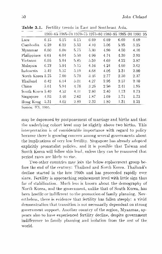
50 John Cleland

Table 3.l. Fertility trends in East and Southeast Asia.

H)60-65 1965-70 1970-75 1975-80 1980-85 1985-90 1990-95

Laos 6.15 G.15 6.15 6.69 6.69 6.69 6.69Cambodia 6.29 6.22 5.5:3 4.10 5.06 5.25 5.25Myanmar 6.00 6.00 5.75 5.30 4.90 4.50 4.16Philippines 6.61 6.04 5.50 4.96 4.74 4.30 3.93Vietnam 6.05 5.94 5.85 5.59 4.69 4.22 3.87Malaysia 6.72 5.94 5.15 4.16 4.24 4.00 3.62Indonesia 5.42 r:::: r::"" 5.10 4.68 4.06 3.31 2.90.).;) ,North Korea 5.75 7.00 5.70 :3.46 2.77 2.50 2.37Thailand 6.42 6.14 5.01 4.27 2.96 2.57 2.10China 5.61 5.94 4.76 :3.26 2.50 2.41 1.95South Korea 5.40 4.52 4.11 2.80 2.40 1.73 1.73Singapore 4.9:3 :3.46 L.62 1.87 1.69 1.71 1.73Hong Kong 5.31 4.02 L.89 2.32 1.80 1.31 1.21

Source: UN, 1995.

may be depressed by postponement of marriage and births and thatthe underlying cohort level may be slightly above two births. Thisinterpretation is of considerable importance with regard to policybecause there is growing concern among several governments aboutthe implications of very low fertility. Singapore has already adoptedexplicitly pronatalist policies. and it is possible that Taiwan andSouth Korea will follow this lead, unless they can be reassured thatperiod rates are likely to rise.

Two other countries may join the below-replacement group be­fore the end of the century: Thailand and North Korea. Thailand'sdecline started in the late 1960s and has proceeded rapidly eversince. Fertility is approaching replacement level with little sign thusfar of stabilization. 11,11 Hch less is known about the demography ofNorth Korea, and the government, unlike that of South Korea, hasbeen hostile or indifferent to the promotion of family planning. Nev­ertheless, there is evidence that fertility has fallen steeply: a vividdemonstration that transition is not necessarily dependent on stronggovernment support. Another country of the region, Myanmar, ap­pears also to haw experienced fertility decline, despite governmentindifference to family planning and isolation from the rest of theworld.

Fel'tilitj! Trends in Developing Countries 51

Fertility trends in urban China closely parallel those in the citystates of Hong Kong and Singapore. Decline started in the early1960s from a level of about 5.0 births. By 1980, fertility in allthree settings had fallen below or close to replacement level. Amajor mechanism was increased birth control within marriage; ageat marriage for women also rose sharply from about 20 years in 1960to about 25 years in the early L9kOs.

Of course. fertility in China as a whole is determined by ruraltrends. As in India, traditional fertility levels in China appear tohave been modest, within the range of five to six births. Also like In­dia, there is some evidence t hat natural fertility increased initiallyunder the impact of modernization. Marital fertility rates in themid-1950s appear to have been about 15 percent higher than ratesrecorded in the 1930s (Coale and Freedman, 1993). The first ma­jor destabilization of rural fertility was the disastrous Great LeapForward in the late 1950s. Mortality rose sharply and period fer­tility plummeted to a little above three births before rebounding toover seven in 19():3. There followed a period of vacillation in fertilityrates during the Cultural Revolution. The dramatic decline in ruralfertility started in about 1970, coinciding with the introduction ofa forceful family-planning program. Between 1970 and 1980, theTFR for the whole country fell from about 6.0 to 2.4 births. Thisdecline of nearly 60 percent in 10 years represents the single mostimportant contribution to the fall in global fertility over the past30 years. However, the emergence of pronounced regional variationsduring this period is often overlooked (Peng, 1981). By the endof the decade, TFRs in remote provinces of China, such as Tibet,Guizhou, and Ningxia. were still over 4.0.

In 1979, the Chinese govf'rnment announced the one-child pol­icy, and in the following year passed a marriage law that was widelyinterpreted as a relaxation of the previous strong discouragementof early marriage. Both measures had profound but partially off­setting effects on the course of fertility in the 1980s. The one-childpolicy was enforced with considerable success in urban areas. By1985-1987, urban fertility was well below 2.0 in all provinces ofChina. Indeed in most of the larger cities, second- and higher-orderbirths almost disappeared. In the rural areas, however, the policyencountered strong resistance. The majority was not prepared to

52 John Cleland

sign the one-child pledge, and period fertility in nearly all provincesremained well above 2.0.

For the whole country, the period TFR fluctuated throughoutthe 1980s around a level of 2.4 births per woman, with no clearevidence of a continuation of the decline of the 1970s. Many com­mentators assumed that the economic reforms of the 1980s madeit increasingly difficult for central and local officials to enforce anunpopular policy. However. in 1989 population policy was againstrengthened and responsihility for enforcement was transferred tolocal civilian authorities. Allalyses of results from a 1992 surveyconducted by the State Family Planning Commission suggest thatfertility fell sharply in the period 1989 to 1992 (Feeney and Yuan,1994).

Fertility transition in Indonesia shares several characteristicswith that in China. In both countries, levels of socioeconomic devel­opment were low at the onset of decline and, in both cases, coupleswere subjected to strong official pressure to adopt birth control. TheIndonesian government illitiaUy focused its attention on densely set­tled Java, which comprises just 6 percent of the country's land areabut over 60 percent of the population. Fertility started to declinethere (and in Bali) in the early 1970s. By 1976, fertility in Javawas actually lower among the least-educated rural population thanamong the urban, more-educated sectors: a highly unusual situationthat undoubtedly reflected the impact of the government program(Freedman et al., 1981).

Between the late 1960s and the early 1990s, fertility in the wholecountry fell from 5.7 to 2.9 hirths, a decline of over 40 percent. In.J ava, the current level is well below 3.0 births per woman but inSumatra, the second most populous island, fertility remains muchhigher.

The neighboring countries of the Philippines and Malaysia con­trast in numerous and fascinating ways with Indonesia. In the 1960s,economic and educational standards were higher than in Indonesiaand fertility began to decline earlier. But the pace of decline hasbeen much more gradual. Total fertility rates in Malaysia and thePhilippines - estimated by the UN to be 3.6 and 3.9 over the period1990-1995 - are now markedly higher than in Indonesia.

Fertility Trends in Developing Countries 53

The stalling of fertility decline in Malaysia dates from the late1970s and appears to originate with a resurgence in Islamic valuesand shifts in government policy. While fertility among the Chineseand Indian minorities continued to decline, and is now little abovereplacement level, that of the majority Malay population actuallyrose in the 1980s, in response to a decline in the use of contraception(Leete and Tan, 199:3). In 1984. the government announced a newpopulation policy which set a target of 70 million inhabitants bythe year 2100. It was widely perceived to be a pronatalist measure,and a national survey conducted shortly afterward indicated thata significant fraction of Malay women had revised their family-sizeexpectations upward in response (Arshat et al., 1988).

In the Philippines, there was no radical change in populationpolicy but official Sll pport for family planning has always been rela­tively weak because of the opposition of the Roman Catholic Church.Although President Marcos created, in 1969, a Commission on Pop­ulation to coordinate family-planning activities, it failed to secureconsensus support or widespread coverage of services. Support fur­ther weakened during the Aquino era. Between 1978 and 1993, thelevel of modern contraceptive practice among married women roseonly from 1/ to 25 percent.

In summary, the fertility transition in East and Southeast Asiais varied and complex. Variability is evident in the starting levelof fertility; the timing of the onset of decline and level of socioeco­nomic development at the time; the speed of decline; and the roleof government policy. Anyone who still believes that the level ofreproduction is a predictable outcome of education, urbanization,and living standards should pause to ponder the difference in fer­tility transition between Indonesia. and Thailand, on the one hand,and Malaysia and the Philippines. on the other.

3.1.2 South Asia

For present purposes, this region is defined as the Indian subcon­tinent, extending west to include Iran. It accounts for about 20percent of the world's population and represents the largest numer­ical concentration of poverty. Bangladesh and Nepal, with CDPsper head of US$liO-$180, are among the poorest countries of the

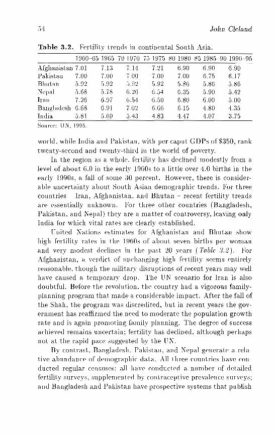
.54 John Cleland

Table 3.2. Fertility trends in continental South Asia.

1960-65 1965-70 1970-75 1975-S0 19S0~S5 19S5-90 1990-95

Afghanistan 7.01 7.13 7.14 7.21 6.90 6.90 6.90Pakistan 7.00 7.00 7.00 7.00 7.00 6.75 6.17Bhutan 5.92 G.92 G.92 G.92 5.8G 5.S6 5.SGNepal G.68 5.78 G.2() 6.54 6.35 5.90 5.42Iran 7.26 (Ull 6.5,1 6.50 6.S0 6.00 5.00Bangladesh 6.G8 ().~n 7.02 6.6G 6.15 4.S0 4.35India 5.81 ,1.69 5.4:3 4.S3 4.47 4.07 3.75

Source: UN, 1995.

world, while India and Pakistan, with per caput GDPs of $350, ranktwenty-second and twenty-third in the world of poverty.

In the region as a whole. fertility has declined modestly from alevel of about 6.0 in the early 19GOs to a little over 4.0 births in theearly 1990s, a fall of some :50 percent. However, there is consider­able uncertainty about South Asian demographic trends. For threecountries - Iran, Afghanistan. and Bhutan - recent fertility trendsare essentially unknown. For three other countries (Bangladesh,Pakistan, and Nepal) they are a matter of controversy, leaving onlyIndia for which vital rates are clearly established.

United Natiolls estimates for Afghanistan and Bhutan showhigh fertility rates in the 1960s of about seven births per womanand very modest declines in the past :20 years (Table ';.2). ForAfghanistan, a verdict of nnchanging high fertility seems entirelyreasonable, though the military disruptions of recent years may wellhave caused a temporar~' drop. The UN scenario for Iran is alsodoubtful. Before the revolution, the country had a vigorous family­planning program that made a considerable impact. After the fall ofthe Shah, the program was discredited, but in recent years the gov­ernment has reaffirmed the need to moderate the population growthrate and is again promoting family planning. The degree of successachieved remains uncertain; fertility has declined, although perhapsnot at the rapid pace suggested by the UN.

By contrast, Bangladesh. Pakistan, and Nepal generate a rela­tive abundallce of demographic data. All three countries have con­ducted regular censuses: all have conducted a number of detailedfertility surveys, supplemented by contraceptive prevalence surveys;and Bangladesh and Pakistan have prospective systems that pu blish

Fertility Trends in Developing COllntries 55

vital rates. Yet demographic trends remain in dispute. The reasonfor this uncertainty lies in thE' poor quality of the data. Surveys, inparticular, tend to suffer from the pernicious problem of backwarddisplacement of dates of recent births, leading to an underestima­tion of the current level of fertility. Claims of fertility decline areoften made but these are equally often shown to be false by the nextsurvey.

Accordingly. the results of the 1991 Demographic and HealthSurvey (DHS) in Pakistan, which indicates a big decline in fertil­ity to about !5.S births. should be regarded with great skepticism.Reliance on the prospective system, run by the Federal Bureau ofStatistics in Karachi, is more prudent. This system portrays a con­stant total fertility of about 7.0 births until 1988, when a drop to6.5 is recorded. The results for the early 1990s show levels of about6.2. Falls in lower-order birt h rates tend to be more pronouncedt han in higher-order births; thus it remains unclear whether maritalfertility decline (which normally affects higher-order births at theinitial stages) has really started. Certainly the level of contracep­tive practice reported in the 1991 DHS (12 percent) is too low tomake an appreciable impact on fertility. To conclude, the level offertility in Pakistan remained high and constant until the late 1980sbut has probably fallen slightly in the period 1988-1990. The UNestimates in Table 8.2 are essentially correct.

In Nepal, evidence of decline is more secure than in Pakistan.The 1991 Fertility. Family Planning, and Health Survey yielded anunadjusted TFR of 15.1. The level of contraceptive use rose fromS percent in 1976 to 2;3 percent in 1991, and age at marriage forwomen also increased over this period. Thus fertility transition inNepal has almost certainly started.

In Bangladesh the pace of change is more rapid and pronouncedthan in Pakistan and Nepal. It is increasingly apparent that fertil­ity decline started in the late 19705 and gathered pace in the 1980s.Between 1975 and 1990, the TFR fell from about 7.0 to about 4.5.Evidence for these assertions comes largely from 1989 and 1994 fer­tility surveys and from two contraceptive prevalence surveys in 1989and 1991, both of which collected truncated birth histories. Theconsistency of these data sets is striking, although the unadjustedestimate from the more recent survey is implausibly low. Detailed

.56 John Cleland

analysis of the 1989 fertility survey shows that the main change hastaken the form of a reduction in higher-order births; for instance,the percentage decline in age-order specific rates (cumulated to age40) between the period L97.f~1978 and 1984-1986 was 10 percentfor second births btl t :38 percent for fifth births. This evidence ofincreasing marital fertility control is confirmed by the rising level ofreported contraceptive use, from 7 percent in 197.5 to 4.5 percent in1994. Age at marriage for women has also increased but the anti­natal effect is modest and offset by a decline in widowhood and inthe length of the first- birth interval.

In broad terms, the remarkable transition in Bangladesh, thefifth poorest country in the world, has affected all socioeconomicstrata equally. Thus fertility decline is as pronounced among illiter­ate, landless laborers as among the slightly more affluent cultivators.The experience of Bangladesh proves beyond a doubt that extremepoverty and low literacy do not represent absolute barriers to fertil­ity decline.

Like Nepal, but in contrast to its Islamic neighbors, the tradi­tionallevel of fertility in India was low, fluctuating between five andsix births per woman between 1880 and 1960 (Bhat, 1989). Onepossible reason for the slow pace of fertility decline in India is thatmodernization acted to increase natural fertility through changesin lactational and sexual behavior. There is evidence that maritalfertility in the rural areas of many states actually increased duringthe 1960s, despite the existence of a family-planning program anda gradual rise in reported contraceptive practice (Srinivasan, 1989).The onset of decline in total fertility occurred in the late 1960s andcontinued for almost a decade; it then stalled before resuming itsdownward path in the micl-1980s. The most obvious explanationfor this sequence concerns the politics of population control. Inthe 1960s under Indira Ghandi, the family-planning program be­came increasingly coercive and, when she fell from power in 1977,its credibility also fell and recovered only gradually. Over the entireperiod from the early 19605 to the early 1990s, total fertility in Indiafell by 36 percent, from .5.8 to :3.7 births. Various decompositions(e.g., Chaudhry, 1989; Srikantan and Balasubramanian, 1989) in­dicate that one-fifth of this decline is attributable to rising age atmarriage and the rest to marital fertility.

Fertility Trends in Developing Countries 57

Some of the reasons for the slow pace of change in India - thepossible relaxation of traditional restraints on fertility and the check­ered history of the family-planning program - have already beenmentioned. However, no account of Indian transition can fail to notethe immense cultural and economic diversity of the country and itsrelevance to demographic trends. Transition is most advanced in thesouthern states, notably Kerala and Tamil Nadu with TFRs of 2.0and 2.5, respectively, according to the recent results of the 1993 Na­tional Family Health Survey. In most of the northern states such asRajasthan, Uttar Pradesh, and Bihar, fertility and childhood mor­tality remain high with TFRs ranging between 3.6 and 4.8. Many(e.g., Dyson and Moore, 198:3) attribute this north-south divide tofundamental cultural differences that affect the status of women. InKerala, for instance, 87 percent of women are literate, comparedwith 20-30 percent in the high- fertility, northern states.

3.1.3 Latin America

Latin America is defined here to include all states of continentalSouth America and Central America, except Guyana and Surinam.In contrast to other major developing regions, Latin America expe­rienced large-scale and permanent settlement of European popula­tions, and this legacy is evident in certain features of the economyand fertility transition. Two countries, Argentina and Uruguay,were once among the wealthiest in the world and are still rankedin the upper-middle income category. Both had completed theirfertility transition by 1950, with TFRs of 3.2 and 2.7, respectively,at that time. In the past 40 years, fertility in both countries haschanged Little, remaining well above replacement level (Table 3.3).This stabilization at levels ranging between 2.3 and 3.5 births perwoman appears to be characteristic of the region. In Chile, as inArgentina and Uruguay, the era of rapid decline is over but pe­riod fertility remains within this range. However, there is no goodreason for believing that Latin American culture possesses featuresthat will sustain moderate fertility indefinitely. The majorities ofthe populations of these three countries are of Spanish and Italianextraction. Fertility levels in the countries of origin, Spain and Italy,are now among the lowest in the world. If Latin America experi­ences the socioeconomic transformation - particularly with regard

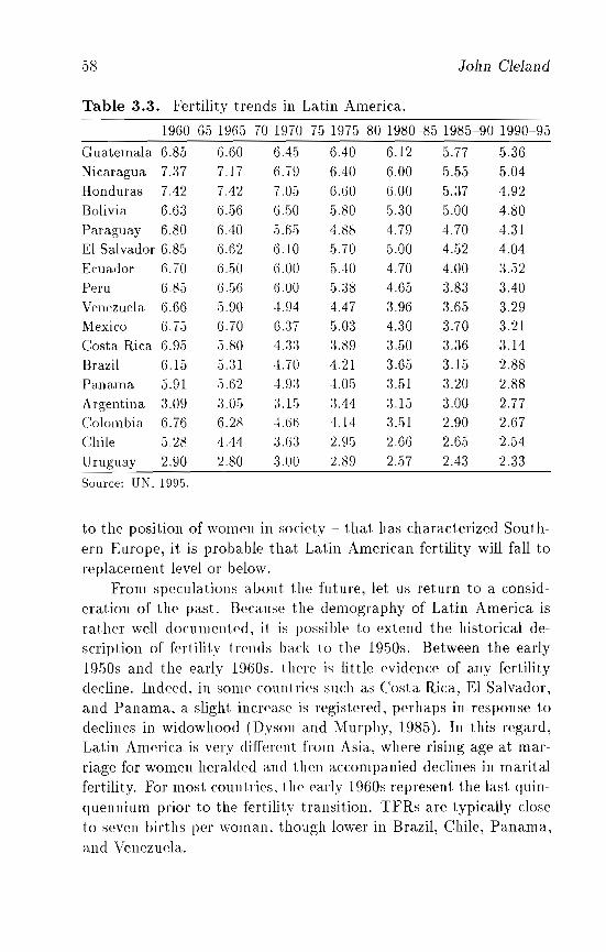
.58 John Cleland

Table 3.3. Fertility trends in Latin America.

1960-65 1965-70 1970-75 1975-80 1980-85 1985-90 1990-95

Guatemala 6.8.5 6.60 6.45 6.40 6.12 5.77 5.36Nicaragua 7.37 7.17 6.79 6.40 6.00 5.55 5.04Honduras 7.42 7.42 7.05 6.60 6.00 5.37 4.92

Bolivia 6.63 6.56 6.50 5.80 5.30 5.00 4.80

Paraguay 6.80 6.40 5.65 4.88 4.79 4.70 4.31El Salvador 6.85 6.G2 G.I0 5.70 5.00 4.52 4.04

Ecuador G.70 6.50 (UJO 5.'10 4.70 4.00 3.52

Peru 6.8.5 6.5G 6.00 5.:38 4.6.5 3.83 3.40

Venezuela 6.66 5.90 4.94 4.47 3.96 3.65 3.29

Mexico 6.75 6.70 (U7 5.03 4.30 3.70 3.21

Costa Rica 6.95 5.80 4.3:3 3.89 3.50 3.36 3.14

Brazil 6.15 5.31 4.70 4.21 3.65 3.15 2.88

Panama 5.91 5.62 4.9:3 4.05 :3.51 3.20 2.88

Argentina 3.09 3.05 :3.15 :3.,14 3.15 3.00 2.77

Colombia 6.76 G.28 A.66 4.14 3.51 2.90 2.67

Chile 5.28 4.44 ::Ui:3 2.95 2.G6 2.G5 2.54

Uruguay 2.90 2.80 :3.00 2.89 2.57 2.43 2.33

Source: UN, 1995.

to the position of women in society - that has characterized South­ern Europe, it is probable that Latin American fertility will fall toreplacement level or below.

From speculations about the future, let us return to a consid­eration of the past. Because the demography of Latin America israther well documented, it is possible to extend the historical de­scription of fertility trends back to the 19.50s. Between the early19.50s and the eaTly 1960s, there is little evidence of any fertilitydecline. Indeed, in some countries such as Costa Rica, El Salvador,and Panama, a slight increase is registered, perhaps in response todeclines in widowhood (Dyson and Murphy, 1985). In this regard,Latin America is very different from Asia, where rising age at mar­riage for women heralded and then accompanied declines in maritalfertility. For most countries. the early 1960s represent the last quin­quennium prior to the fertility transition. TFRs are typically closeto seven births per woman. though lower in Brazil, Chile, Pa.nama,and Venezuela.

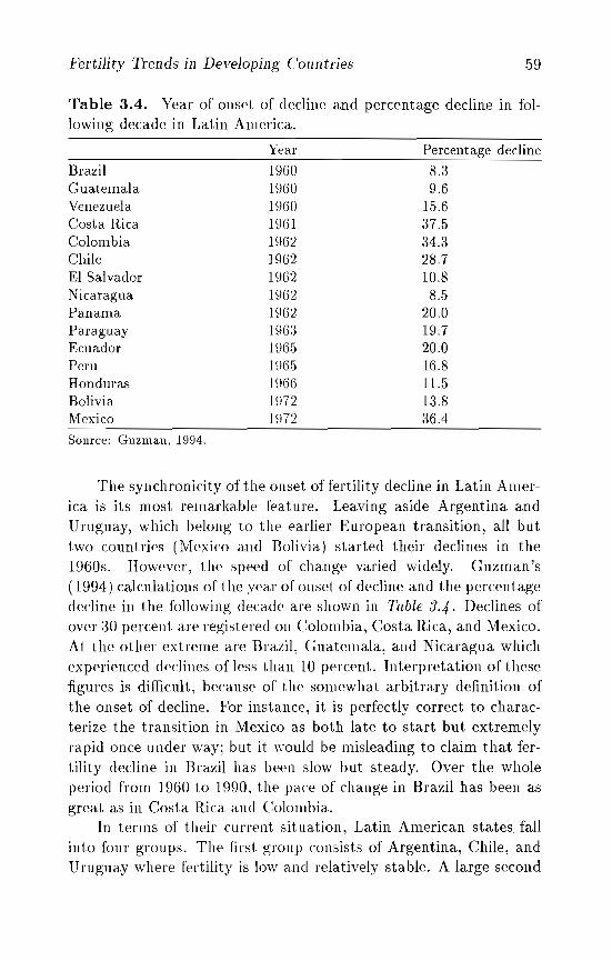
Fertility Trends in Developing COllntries 59

Table 3.4. Year of onset of decline and percentage decline in fol­lowing decade in Latin America.

BrazilGuatemalaVenezuelaCosta RicaColombiaChileEl SalvadorNicaraguaPanamaParaguayEcuadorPeruHondurasBoliviaMexico

Source: Guzmau, 1994.

Year

19601960196019611962H1621962196219621~)63

1~)651~)()5

1966H)72H) 72

Percentage decline

8.39.6

15.637.534.328.710.88.5

20.019.720.016.8U.513.836.4

The synchronicity of the onset of fertility decline in Latin Amer­ica is its most remarkable feature. Leaving aside Argentina andUruguay, which belong to the earlier European transition, all buttwo countries (Mexico and Bolivia) started their declines in the1960s. However, the speed of change varied widely. Guzman's(1994) calculations of the year of onset of decline and the percentagedecline in the following decade are shown in Table 3.4. Declines ofover 30 percent are registered on Colombia, Costa Rica, and Mexico.At the other extreme are Brazil, Guatemala, and Nicaragua whichexperienced declines of less than LO percent. Interpretation of thesefigures is difficult, because of the somewhat arbitrary definition ofthe onset of decline. For instance, it is perfectly correct to charac­terize the transition in Mexico as both late to start but extremelyrapid once under way; but it would be misleading to claim that fer­tility decline in Brazil has been slow but steady. Over the wholeperiod from 1960 to 1990, t.he pace of change in Brazil has been asgreat. as in Costa Rica and Colombia.

In terms of t.heir current sit.uation, Latin American states fallinto four groups. The first group consists of Argentina, Chile, andUruguay where fertility is low and relatively stable. A large second

60 John Cleland

group follows. In this group total fertility is now in the range of 2.7to 3.3 births, and this group shows some sign of incipient stabiliza­tion, particularly in Costa Rica. The three most populous countriesof the region - Brazil, },/Iexico, and Colombia - fall into this group.It should be noted that fertility in Colombia is now slightly lowerthan in Argentina. The third group comprises four countries whichare in the midst of transition with recent fertility rates of 3.5 to 4.5births per woman. Finally, there is a cluster of four high-fertilitycountries, three of which are in Central America.

While the simultaneity of the onset of decline is the most re­markable feature of Latin American transition, a further distin­guishing feature is the emergence of very pronounced but temporaryurban-rural, socioeconomic, and regional differentials during the pe­riod of decline. In most countries of the region, decline startedamong the better-educated and metropolitan sectors and spreadgradually to poorly educated, rural sectors. The typical processis well illustrated by Rodriguez and Hobcraft (1984) in an analy­sis of Colombian data. They were able to identify the beginningsof decline in the 1960s for women with complete primary or highereducation, in the late 1960s for women with incomplete primaryschooling, and in the late 1970s for those with no formal school­ing. Furthermore, they demonstrated that, within each educationalstratum, decline was initially restricted to a reduction in higher­order births and only subsequently affected earlier stages of familyformation.

This sequence suggests strongly that fertility decline in Colom­bia has taken the form of social diffusion of a new form of behav­ior, birth control. An analysis by Rodriguez and Aravena (1991)supports this view. They examined subgroup changes in fertilitybehavior, using World Fertility Survey (WFS) and DHS data for 15surveys including five from Latin America. Remarkable regularitieswere observed in the spacing and limitation components of maritalfertility. Specifically, the strata with the least evidence of fertilitycontrol at the start tended to experience the greatest proportionalchange. Within strata, transition followed a self-sustaining coursethat is consistent with a basic diffusion process. To the extent thatRodriguez's analysis and interpretation are correct, it is inevitablethat fertility in all strata will converge at a modest level. Thus the

Fertility Trends in Developing Countries 61

prospects for a continuation of fertility decline in the region as awhole appear good.

3.1.4 The Arab states

The Arab states constitute a linguistic and cultural rather than acompact geographical entity. Ivlost have small populations: Egypt,with over 50 million inhabitants. followed by Sudan, Morocco, andAlgeria, with about 2.5 million each, are the main exceptions. Thereis a very wide spread in living standards. At one extreme are theUnited Arab Emirates, Kuwait, and Saudi Arabia, classified as high­income countries. At the other end of the spectrum are Sudan,Mauritania, and Yemen with per caput GDPs of less than $500.

Information on the demography of the Arab world is patchy.For Libya, Lebanon, Syria, and some of the Gulf states, there islittle recent evidence concerning fertility levels. In other countriesof the region - for instance, Sudan and Mauritania - recent surveyinformation is available, but as in South Asia, data quality is poorand the estimation of trends is correspondingly difficult.

Nevertheless, several features of Arab fertility have clearly beenestablished. At the start of the period under discussion, the early1960s, levels of fertility were universally very high, with TFRs rang­ing between 6.5 and 8.0. This exceptionally high level is the resultof an unusual combination of early marriage ages, relatively shortperiods of breast-feeding, and limited practice of birth control. Itis clear from Table 3.5 that fertility remains high in this region.Only three countries, Lebanon. Kuwait, and Tunesia, record ratesdecisively below 4.0.

For the entire region, total fertility has fallen from about 7.0 inthe early 1960s to about 4.5 in the early 1990s, a drop of 35 percent.This average conceals very large differences in trends and currentlevels and an equally large divergence in government policies towardpopulation and family planning. Apart from Lebanon, whose ethnicand religious diversity sets it apart from the rest of the Arab world,the Egyptian and Tunisian governments were the first to providepublic sector family-planning services and associated publicity, andwere among the few Arab states to experience fertility decline inthe 1960s. Tunisian fertility dropped steadily, and this country nowrecords one of the lowest TFRs in the region with 3.2 births per

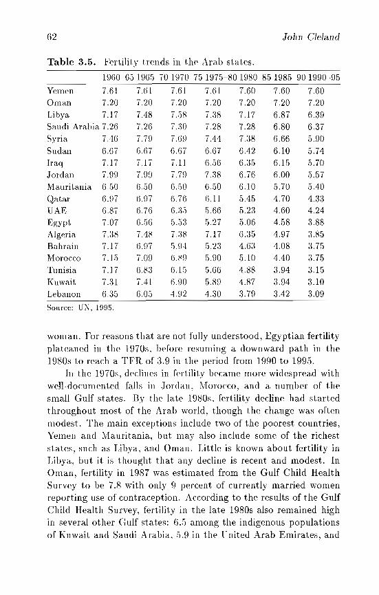
62 John Cleland

Table 3.5. Fertility trends in the Arab states.

1960-651965-701970-751975-801980-851985-901990-95

Yemen 7.61 7.61 7.61 7.61 7.60 7.60 7.60Oman 7.20 7.20 7.20 7.20 7.20 7.20 7.20Libya 7.17 7.48 7.58 7.38 7.17 6.87 6.39Saudi Arabia 7.26 7.26 7.:30 7.28 7.28 6.80 6.37Syria 7.46 7.79 7.69 7.44 7.38 6.66 5.90Sudan 6.67 6.G7 6.67 6.67 6.42 6.10 5.74Iraq 7.17 7.17 7.11 6..56 6.35 6.15 5.70Jordan 7.99 7.99 7.79 7.38 6.76 6.00 5.57Mauritania 6.50 6.50 6.50 6.50 6.10 5.70 5.40Qatar 6.97 6.97 6.76 6.11 5.45 4.70 4.33UAE 6.87 G.76 (j .:35 5.66 5.23 4.60 4.24Egypt 7.07 6.56 5.5:3 5.27 5.06 4.58 3.88Algeria 7.38 7.48 7.38 7.17 G.35 4.97 3.85Bahrain 7.17 6.97 5.94 5.23 4.63 4.08 3.75Morocco 7.15 7.09 6.89 5.90 5.10 4.40 3.75Tunisia 7.17 6.8:) 6.15 5.66 4.88 3.94 3.15Kuwait 7.31 7.41 6.90 5.89 4.87 3.94 3.10Lebanon 6.:35 6.05 ·Ul2 4.30 3.79 3.42 3.09

Source: UN, 199.5.

woman. For reasons that are not fully understood, Egyptian fertilityplateaued in the 1970s, before resuming a downward path in the1980s to reach a TFR of 3.9 in the period from 1990 to 1995.

In the 1970s, declines in fertility became more widespread withwell-documented falls in Jordan, Morocco, and a number of thesmall Gulf states. By the late 1980s, fertility decline had startedthroughout most of the Arab world, though the change was oftenmodest. The main exceptions include two of the poorest countries,Yemen and Mauritania, but may also include some of the richeststates, such as Libya, and Oman. Little is known about fertility inLibya, but it is thought that a.ny decline is recent and modest. InOman, fertility in 1987 was estimated from the Gulf Child HealthSurvey to be 7.8 with only 9 percent of currently married womenreporting use of contraception. According to the results of the GulfChild Health Survey, fertility in the late 1980s also remained highin several other Gulf states: 6.05 among the indigenous populationsof Kuwait and Saudi Arabia, 05.9 in the United Arab Emirates, and

Fertility Trends in Del'eloping COlin tries 63

.5.:3 in Iraq (Farid, 199:3). However, fertility had fallen more steeplyin Bahrain and Qatar.

Fertility transition in this region shares some features of boththe Asian and the Latin American transitions. As in Asia, risingage at marriage for women has made an important contribution tofertility decline, and as in Latin America, huge differences in fertilityhave arisen between urban and rural strata and between educationalstrata. This differentiation, in both Latin America and the Arabstates, may reflect the rat her weak nature or nonexistence of manygovernment family-planning services; under such circumstances, thepoor and less-educated have limited access to modern birth control.

In general, levels of Arab fertility remain much higher thanmight be expected from consideration of living standards and ur­banization. This resilience is sometimes attributed to low levels offemale autonomy and education. vVhile it is true that female labor­force participation remains low, educational standards for womenare rising rapidly in many Arab countries. But even among educatedwomen, fertility is remarkabl.Y high. For instance, the 1990 Jorda­nian Demographic and Health Survey records the following TFRsby educational status of women: no schooling, 6.92; primary, 6.00;secondary, .5.39; and postsecondary, 4.10. There are few highly ur­banized countries with reasonable access to family-planning serviceswhere fertility levels, even among educated couples, remain as buoy­ant as in Jordan. It seems reasonable to conclude that replacement­level fertility is a more distant prospect for the Arab world than forsome other regions.

3.1.5 Sub-Saharan Africa

S11 b-Saharan Africa comprises only 10 percent of the population ofthe Third World but accouuts for a disproportionately large numberof the least developed countries. The economic plight of the regiondeteriorated further in the 19;;;005, with declines in income per head inmany countries. Although it possesses more cultural diversity thanmost of the other regions considered in this chapter, sub-SaharanAfrica exhibits features of social organization and cultural valuesthat distinguish it from other major regions: traditions of postnatalabstinence. polygyny. and the importance of lineage are the bestk1l0w1l of these.

64 John Cleland

The first comprehensive account of Africa's demography hadlittle direct information on fertility at its disposal and had to relyheavily on stable population analysis (Brass et al., 1968). Since thisreport, data availability has improved steadily. Large sums were in­vested in censuses, and in the L970s an increasing number of coun­tries undertook more specialized demographic surveys. The WorldFertility Survey represented the next step forward with the partici­pation of 10 African countries. Under the successor to this program(the Demographic and Health Survey project) national surveys havebeen conducted in a further L:2 countries.

Despite this improvement, knowledge of fertility levels in Africaremains uneven. Out of :35 continental states with a population of 1million or more, direct information on fertility in the period 1985 to1990 is available for only 17. tvioreover, the reliability of estimatesis lower than in South Asia. Hence Table 3.6 is restricted to currentlevels and no attempt has been made to depict trends as has beendone for other regions.

However, the evidence strongly suggests that, prior to L980,fertility in Africa remained constant at a high level and increaseswere even recorded in some countries. Between the early 1960sand the 1980s, UN statistics show increases of 0..5 births or morefor Rwanda, Angola, Zaire, Central African Republic, Gabon, andGuinea-Bissau. III :-lOme cases, the most plausible explanation isa decline in pathological sterility. In other cases, it may be at­tributed to an attenuation of traditional birth-spacing mechanisms.Indeed it is probable that, prior to L960, fertility increase was morewidespread. Feeney's analysis of Kenyan census data, for instance,suggests that fertility rose substantially prior to 1960 (for detailssee Feeney, 1988b). Unfortunately few countries have a record ofcensus taking as good as Kenya's to allow a similar historical depthof analysis.

The persistence of high fertility in Africa gave rise to a prevailingview that this situation would continue for some time. It was arguedthat Africa possessed unique cultural and economic characteristicsthat would render reproductive behavior unusually impervious tothe forces of change (e.g .. Caldwell and Caldwell, 1990). The highdesired family sizes reported in surveys further strengthened thisprognosis.

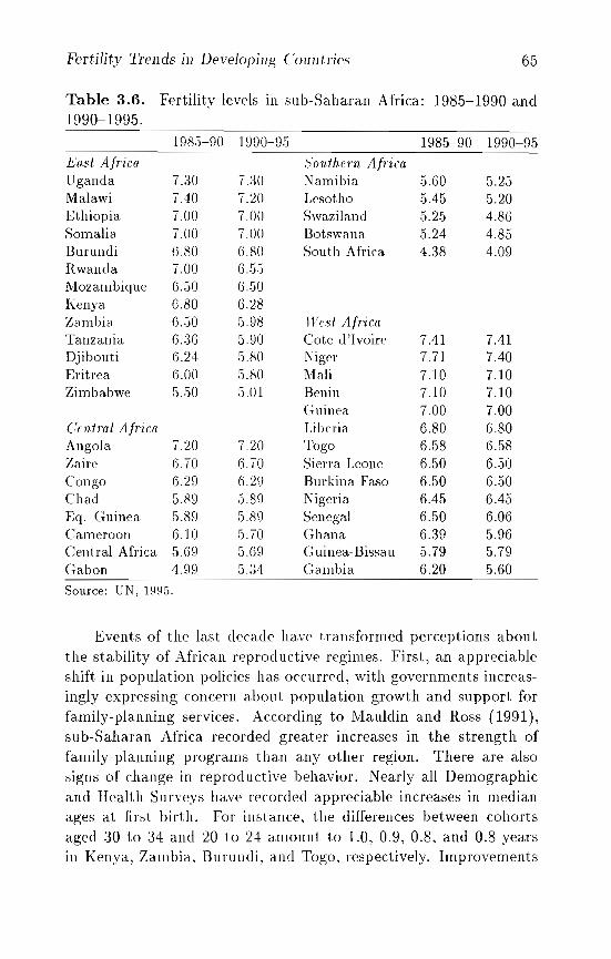
Fertility Trends ill Developing COllntries 65

Table 3.6. Fertility levels in sub-Saharan Africa: 1985-1990 and1990-1995.

1985-90 1990-95 1985-90 1990-95East Africa Southern AfricaUganda 7.30 7.:30 Namibia 5.60 5.25Malawi 7.40 7.20 Lesotho 5.45 5.20Ethiopia 7.00 7.00 Swaziland 5.25 4.86Somalia 7.00 7.00 Botswana 5.24 4.85Burundi 6.80 6.80 South Africa 4.38 4.09Rwanda 7.00 6.55Mozambique 6.50 6.50Kenya 6.80 6.28Zambia 6.50 5.98 West AfricaTanzania (U6 5.90 Cote d 'Ivoire 7.41 7.41Djibouti 6.24 5.80 Niger 7.71 7.40Eritrea 6.00 5.80 l'vlali 7.10 7.10Zimbabwe 5.50 5.01 Benin 7.10 7.10

Guinea 7.00 7.00Central Africa Liberia 6.80 6.80Angola 7.20 7.20 Togo 6.58 6.58Zaire 6.70 6.70 Sierra Leone 6.50 6.50Congo 6.2~) 6.2D Burkina Faso 6.50 6.50Chad 5.89 5.89 Nigeria 6.45 6.45Eq. Guinea 5.89 5.89 Senegal 6.50 6.06Cameroon G.10 5.70 Ghana 6.39 5.96Central Africa 5.69 5.69 Guinea-Bissau 5.79 5.79Gabon 4.99 5.34 Gambia 6.20 5.60

Source: UN, 1995.

Events of the last decade have transformed perceptions about

the stability of African reproductive regimes. First, an appreciable

shift in population policies has occurred, with governments increas­ingly expressing concern about population growth and support for

family-planning services. According to Mauldin and Ross (1991),sub-Saharan Africa recorded greater increases in the strength of

family-planning programs than any other region. There are alsosigns of change in reproductive behavior. Nearly all Demographic

and Health Surveys ha.ve recorded appreciable increases in medianages at first birth. For instance, the differences between cohorts

aged 30 to 34 and 20 to 24 amount to 1.0, 0.9, 0.8, and 0.8 yearsin Kenya, Zambia, Burundi, and Togo, respectively. Improvements

66 John Cleland

in the educational attainment of young African women may be onereason for t his change. It is also possible that economic stress hasacted to delay the formation of stable partnerships and the onset ofchild bearing.

Postponement of childbearing may be a temporary phe­nomenon. But there is evidence in an increasing number of Eastand Southern African states that fertility decline, fueled by contra­ceptive use, has started. Such a trend is much more likely to markthe onset of a sustained transition than to represent a transitoryresponse to economic hardship. At the forefront of this movementis the Republic of South Africa. By the late 1980s, the level of con­traceptive practice among the black population was estimated to beabout .50 percent and total fertility at about 4.5 births (Mostert,1991). Moderate levels of use among married women have also beenrecorded in Zimbabwe (4<~ percent). Botswana (33 percent), Kenya(33 percent), Namihia (2:3 percent). and Swaziland (21 percent). Inall these countries there is parallel evidence of declining fertility. InSouth Africa. Zimbabwe. and I\:enya the decline has amounted toabout 2..5 births. in Botswana to abou t 1..5 births, and in Namibiaand Swaziland to less than 1.0 birth per woman.

Successive surveys in l\enya show how rapidly the climate ofreproductive opinion and behavior can change. The Kenya FertilitySurvey of 1977~ 197:'\ portrayed a very pronatalist society. Totalfertility was about :'\.0; desired family size averaged 7.2 children;only 7 percent of couples reported contra.ceptive use; and only 16percent of women said that they wanted no more children. Therewas little ground for believing tl1at fertility transition was about tostart. Yet a mere decade later. desired family size had dropped to4.4 children, 49 percent of women expressed a wish to have no morechildren, contraceptive Use had risen to 27 percent, and fertility hadfallen to 6..5 births. In the early 1990s, fertility was well below sixbirths and the mean desired family size was 3.7 births. This radicalchange had affected women of all educational backgrounds and ages.

This impression of change in the subregion should be balancedby data from other countries. Recent Demographic and Health Sur­veys provide no convincing evidence of appreciable decline in Bu­rundi, Uganda, Zambia, or Tanzania. Nor is it reasonable to expect

Fertility Trends in De\'eloping COllntries 67

any decline in Angola or :tvIozambique because of prolonged civilunrest.

In West and Central Africa, fertility shows fewer signs of ac­tual or incipient decline. though it is probable that fertility declinehas started among young women in Senegal and in Southwest andSoutheast Nigeria (Cleland Ef al.. 1994). Elsewhere, however, thereis no strong evidence of fertility decline. This stability is particu­larly puzzling in a collntry snch as Ghana. Ghana has long had arather well-educated and urbanized population, where women pos­sess considerable autonomy aud iJl(leed dominate trading. Moreover,there has been some attempt. since the late 1960s, to promote fam­ily planning, albeit on a limited scale. Despite the severe economicrecession of the late 1970s and early 1980s which threatened livingstandards of the urban middle classes, fertility remained rather con­stant until the late 1980s (Onuoha and TimGeus, 1995). However, the1993 Ghana Demographic and Health Survey suggests that fertilitydecline has now started. The experience suggests that Ghanaiansociety and perhaps other \Vest African societies present obstaclesto fertility decline and mass adoption of contraception that are ab­sent in East and Southel'1l Africa. '''!hile the prospects are good forwidespread fertility decline in the East and South, the prognosis forvVest and Central Africa is uncertain.

3.1.6 Island states

To complete this geographic account of fertility trends, Table S.7provides data for the main islands and island groups. Their contri­bution to global population trends is minimal; yet the demographyof islands is of special interest. and several have been at the forefrontof fertility transition. In the 1960s, Fiji, Mauritius, and Sri Lankawere among the few developing countries to have started fertilitytransition. This evidence supported speculations that Malthusianconstraints on population growth may take a particularly visibleform in islands where territorial expansion is precluded.

Table S. 7 shows that such simple generalizations are unjustified.In the period 198,5 to 1990, fertility in island states ranged fromclose to replacement level in Mauritius to about to seven births perwoman in Comoros and the :tVIaldives.

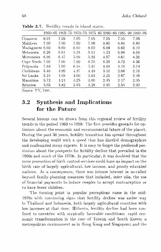
68

Table 3.7. Fertility trends in island states.

John Cleland

1960-65 1965-70 1970-75 1975-80 1980-85 1985-90 1990-95

Comoros 6.91 7.05 7.05 7.05 7.05 7.05 7.05Maldives 7.00 7.00 7.00 7.00 6.80 6.80 6.80Madagascar 6.60 6.60 6.60 6.60 6.60 6.60 6.10Melanesia 6.25 6.01 5.78 5.51 5.23 5.04 4.68Micronesia 6.98 6.47 5.90 5.:33 4.87 4.61 4.36Cape Verde 7.00 7.00 7.00 6.70 6.29 4.70 4.26Polynesia 7.64 7.09 6.1i' 5.31 4.69 4.19 3.74Caribbean 5.46 4.99 ,1.:37 3.49 :3.10 2.88 2.76Sri Lanka 5.16 4.68 4.00 3.83 3.25 2.67 2.48Mauritius 5.72 4.24 :3.25 3.06 2.45 2.17 2.35Reunion 5.65 4.82 :3.9:3 :3.28 2.90 2.54 2.32

Source: UN, 1995.

3.2 Synthesis and Implicationsfor the Future

Several lessons can be drawn from this regional review of fertilitytrends in the period 1960 to 1990. The first provides grounds for op­timism about the economic and environmental future of the planet.During the past 30 years, fertility transition has spread throughoutthe developing world with a speed that has dazzled demographersand confounded many experts. It is easy to forget the profound pes­simism about the prospects for fertility decline that prevailed in the1960s and much of the 1970s. In particular, it was doubted that themere promotion of birth-control services could have an impact on thebirth rate of largely agriculturaL low income, and poorly educatednations. As a consequence, there was intense interest in so-calledbeyond family-planning measures that included, inter alia, the useof financial payments to induce couples to accept contraception orto have fewer children.

The turning point in popular perceptions came in the mid­1970s with convincing signs that fertility decline was under wayin Thailand and Indonesia, both largely agricultural countries withlow incomes at that time. Hitherto, fertility decline had been con­fined to countries with atypically favorable conditions: rapid eco­nomic transformation in the case of Taiwan and South Korea; ametropolitan environment as in Hong Kong and Singapore; and the

Fertility Trends in Developing COlin tries 69

idiosyncrasies of an insular status such as Fiji, Mauritius, and partsof the Caribbean.

As we have seen, sustained fertility decline in the Third Worldis now the norm rather than the exception. In Asia, the main ex­ceptions are Pakistan, Afghanistan, and some of the small countriesof Indochina. In Central and South America, fertility decline is al­ready completed or under way in all countries. Among the Arabstates of North Africa and the I\iiddle East, most countries haveexperienced falls in fertility though decline is not yet ubiquitous.Finally in sub-Saharan Africa, fertility transition is clearly start­ing in East and Southern Africa, leaving Central and West Africaas the main areas where fertility remains largely unchanged. Suchwidespread transformations of reproductive behavior have come asa surprise and their existence is not yet fully appreciated outside thespecialist domain of demography. The rates of population growthill most developing countries remain high because of the continueddecline in mortality and because crude birth rates are buoyed byincreases in the relative and absolute numbers of couples in the re­productive ages. Thus. the impact of declining fertility is offset bythese other demographic forces and, in many countries, will not befelt until the next century.

A major generalization of demographic transition theory is thatonce fertility decline, fueled by birth control within marriage, is un­der way, the trend is irreversible and sustained until fertility reachesreplacement level or thereabouts. Like most simple generalizations,this one must be qualified. Reversals have occurred, most notablythe post-World War II baby boom in Western Europe and NorthAmerica. More commonly. fertility may plateau before resuming adownward path. as has been t he case in Egypt and Malaysia. More­over, the speed of decline has varied from the near-precipitous dropsin China and Mexico to a slow pace of change, as in the Philippinesor Jordan. A much more profound uncertainty exists about theproposition that fertility will continue to fall until the replacementlevel of a little over two births per woman is reached. In the aggre­gate, there is a logic in this ultimate destination for levels of humanreproduction because it implies long- term stability of populationsizes and, in the very long term, no animal population can continueto grow or decline indefinitely. But, at the level of families and

70 John Cleland

individuals, such a.g~regate considerations may hold little force. Ithas already been noted that family sizes appear to have stabilized insome Latin American countries at a level that is well above replace­ment. In other regions, most notably sub-Saharan Africa and theArab states, it is difficult to imagine the achievement of replacement­level fertility under existing socioeconomic and cultural conditions.Fertility aspirations, as recorded in surveys, remain much higher. InZimbabwe, for instance, which is at the forefront of fertility transi­tion in Africa. the 1988 Demographic and Health Survey indicatesa mean ideal family size of G.-+ children among currently marriedwomen; and nearly half of women who already have 4 or more livingchildren want additional children.

Of course, societal conditions do not remain stable. Indeed oneof the biggest mistakes of demographers has been to underestimatethe rapidity with which societies change. Nevertheless, the prospectsfor the attainment of replacement-level fertility within the next 40years remain doubtful in some parts of the developing world.

The second major lesson from this review concerns the need forhumility on the part of scientists. ])pspite a huge volume of new em­pirical evidence concerning fertility transition that has accumulatedin the past :30 years. our nnd('rstanding of the underlying causesremains rudimentary. Noris t h('re any sign of a growing consensusamong population scientists regarding fertility theories or the rela­tive importance of specific causes. The gulf remains wide betweenthe two dominant schools of thought - one emphasizing economicdeterminism and the other. culture and the diffusion of ideas.

At the start of this chapter. t he inadequacy of simple mono­causal explanations of fertility dpcline was noted. This point isvividly illustrated by recent reviews of the socioeconomic status ofAsian and Latin American countries at the onset of fertility de­cline (Casterline, 1994; Guzman, 1994). For every indicator (lifeexpectancy, infant mortality, urbanization, adult literacy, incomeper head, percentage engaged in agriculture), there was a verywide spread among countries. To take but two examples fromLatin America, infant mortality ranged from 62 per 1,000 birthsin Paraguay to 151 in Bolivia. and adult literacy from 84 percent inCosta Rica to 34 percent in Guatemala. This huge disparity in thestage of socioeconomic development reinforces similar conclusions

Fertility Trends in Developing ('olin tries 71

from studies of the European transition, where birth control spreadacross a region with little regard for socioeconomic differences be­tween counties, bringing lower fertility in its wake.

\Vith the steady increase in the number of countries where fertil­ity transition has already started, research priorities will shift fromthe study of the determinants of the onset of decline to the studyof factors that influence speed of decline and point of stabilization.Here again, though, it is unlikely that very strong links will be foundbetween speed of transition and socioeconomic indicators. The ear­lier comparison between Indonesia, Malaysia, and the Philippines isa pertinent example. Even more striking is the rapid fertility declinethat has taken place in Bangladesh, one of the poorest countries inthe world.

The reason for this complexity is that both culture and govern­ment policies exert strong independent influences on fertility. It isappropriate to end this chapter with a brief consideration of one ofthese factors (government policies) because of its practical relevance.To the extent that state-sponsored initiatives to promote birth con­trol and the acceptability of smaller families can be effective, thefuture course of human fertility depends, at least in part, on gov­ernment policies and the availability of funds to implement them.Conversely, if the influence of such interventions is minor, then fu­ture fertility trends will be determined by broader forces of culturaland socioeconomic change that are less amenable to governmentaland international decisions.

The effectiveness of family-planning programs has been high onthe demographic research agenda for the past 20 years. The mostinfluential body of work comprises statistical estimations of the rela­tionship between the strength of family-planning programs and thedemographic outcomes such as level of fertility, percentage decline infertili ty, and contraceptive use, using countries as units of analysis(e.g., Mauldin and Berelson. 1978; IvIauldin and Ross, 1991). Thegeneral finding is that strong programs do reduce fertility, thoughthis effect is conditioned by, and subordinate to, the effect of so­cioeconomic development. It is also clear from these analyses thatthe creation of family-planning programs cannot be divorced eas­ily from general development. Few of the least developed countrieshave birth-control services, education, and publicity that are rated

7:2 .John Cleland

as strong. Conversely. fe\v of the more developed countries haveprograms that are rated as nonexistent or weak. This correlationobviously complicates the task of isolating the effect of programsfrom effects of broader development.

A major limitation of this type of study is that program strengthis taken as an exogenous factor. The analytic design is vulnerableto the cri ticism that serious programs are most likely to arise in re­sponse to spontaneous expressions of need and prior fertility decline,and only grow in strength (i.e., political commitment and resourceallocation) when success is already visible. Programs can thus beseen as a consequence as well as a potential cause of demographicchange. This weakness severely limits the validity of results.

A more convincing approach to an assessment of program im­pact would be to compare fertility trends in countries that arebroadly similar in cultural characteristics and stage of developmentbut where population policies have diverged, perhaps because ofthe convictions of political leadership. Algeria and Tunisia, Pakistanand Bangladesh, Mexico and Colombia, North Korea and South Ko­rea, Zambia and Zimbabwe are possible candidates for such a study.In each pair, the first country was much slower than the secondcountry to adopt and implement policies and programs to reducefertility. And in each case. the timing of the start of fertility declineappears to reflect the policy divergence. Thus it is hard to resist theinference that Mexico's very late fertility transition is connected tothe government's hostility to provision of family-planning servicesuntil the dramatic change in 1972. Similarly, the persistence of highfertility in Algeria until the early 1980s is surely related to the lowpriority attached to birth control, which shifted only in the 1980s.

Such a comparative case study approach shows that governmentpolicies can have and have had appreciable demographic impacts bychanging reproductive attitlldes. by legitimizing birth control, andby enhancing access to family-planning services. To the extent thatthis verdict is valid, the future course of fertility in regions whereit is still high depends to some extent on political leadership. As aconsequence, demographic forecasting becomes more uncertain butthe politics of population and birth control become more importantand exciting.

Chapter 4

Reproductive Preferences andFuture Fertility in DevelopingCountries

Charles F. WestofJ

The classical paradigm of the demographic transition features a de­cline in the rate of reproduction from the conditions of natural fertil­ity at high levels to a regimen in which fertility is highly controlledand has declined to replacement or lower levels. In many of thedeveloping countries that have entered this transitional stage, in­creases in age at marriage have played an important role. But theprincipal mechanism driving this transition is birth control, mainlyin the form of contraception, though abortion has made significantimpacts at different times and in different places.

In Asia and in Latin America, the use of contraception has typ­ically been adopted at higher parities after couples have achievedthe number of children desired; its use at lower parities for the reg­ulation of spacing has appeared later in the fertility transition. Incontrast, in Africa, especially in sub-Saharan Africa, a demand forspacing evidently has emerged before a demand for limiting fertility.Currently, in the nine sub-Saharan African countries included in thefirst phase of the Demographic and Health Surveys (1986-1990), theaverage percentage of married women using contraception for spac­ing purposes was 10 percent compared with 8 percent for limitingfertility. In the 16 other developing countries (including those in

,:3

74 Charles F. Westoff

North Africa), the corresponding percentages were 12 and 36 per­cent, respectively, a dramatically different ratio (calculated fromdata presented in Westoff and Ochoa, 1991:7).

Whether contraception is employed for purposes of spacing orfor purposes of limiting fertility, it reduces the likelihood of preg­nancy and thus has an impact on the period rate of fertility. Thereis evidence that contraceptive failure rates are greater when meth­ods are used for spacing rather than for limiting births, but, evenwith such higher failure rates, fertility is reduced far below that im­plied in the natural fertility model (especially considering the higherfecundability at the younger ages, where spacing behavior is morecommon). In any event, a full appraisal of the subject of reproduc­tive preferences should ideally include both preferences to postponethe next birth and preferences to terminate fertility. Data on spacingpreferences are not as widely available, however, as data on prefer­ences to terminate fertility. The World Fertility Survey included nodirect questions on the subject. and the DHS-I questionnaire did notinclude the questions necessary to estimate preferred lengths of birthintervals for all women. Therefore. the emphasis in this chapter ison the number of children desired and the intention to terminate fer­tility. These measures are particularly relevant for Asian and LatinAmerican populations where the contraceptive prevalence level isdetermined largely by such limiting practice. As noted above, theuse of contraception for birth spacing dominates in the sub-SaharanAfrican countries and thus makes more of a contribution to the pre­diction of fertility in that part of the world.

4.1 Desired Number of Children

The most common measure of reproductive preferences is the num­ber of children desired. The basic question included in all DRSinterviews was "If you could go back to the time you did not haveany children and could choose exactly the number of children tohave in your whole life, how many would that be?"

The mean number of children desired is shown in the first col­umn of Table 4. J for currently married women in all of the countriesincluded in DRS-I. The range ofthese preferences varies widely, from

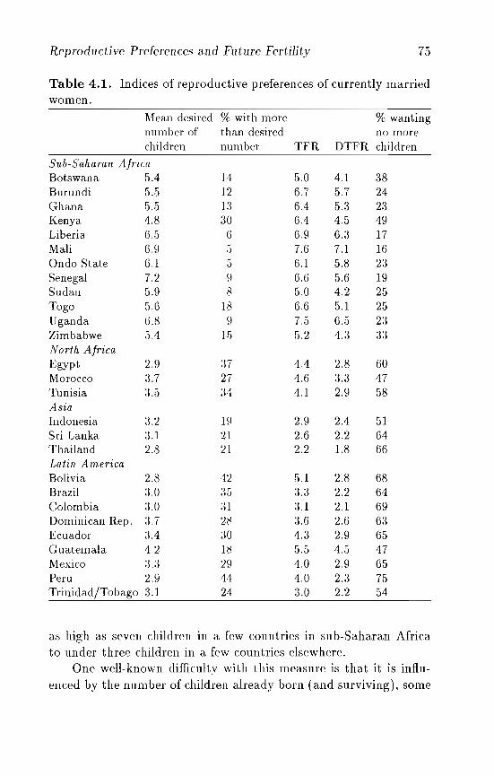
Reproductive Preferences and Future Fertility 75

Table 4.1. Indices of reproductive preferences of currently marriedwomen.

Mean desired % with more % wantingnumber of than desired no morechildren number TFR DTFR children

Sub-Saharan AfricaBotswana 5.4 14 5.0 4.1 38Burundi 5.5 12 6.7 5.7 24Ghana 5.5 13 6.4 5.3 23Kenya 4.8 30 6.4 4.5 49Liberia 6.5 6 6.9 6.3 17Mali 6.fl 5 7.6 7.1 16Ondo State 6.1 5 6.1 5.8 23Senegal 7.2 9 6.6 ,5.6 19Sudan 5.9 ~ 5.0 4.2 25Togo 5.6 1~ 6.6 ,5.1 25Uganda 6.8 9 7.5 6.5 23Zimbabwe 5.4 15 5.2 4.3 33North AfricaEgypt 2.9 :n 4.4 2.8 60Morocco 3.7 27 4.6 3.3 47Tunisia 3.5 34 4.1 2.9 ,58AsiaIndonesia 3.2 19 2.9 2.4 51Sri Lanka 3.1 21 2.6 2.2 64Thailand 2.8 21 2.2 1.8 66Latin AmericaBolivia 2.8 42 5.1 2.8 68Brazil 3.0 35 3.3 2.2 64Colombia 3.0 :31 3.1 2.1 69Dominican Rep. 3.7 28 3.6 2.6 63Ecuador 3.4 30 4.3 2.9 65Guatemala 4.2 18 5.5 4.5 47Mexico 3.:3 29 4.0 2.9 65Peru 2.9 44 4.0 2.3 75Trinidad/Tobago 3.1 24 3.0 2.2 54

as high as seven children in a few countries in sub-Saharan Africato under three children in a few countries elsewhere.

One welJ- known difficulty with this measure is that it is influ-

enced by the number of children already born (and surviving), some

76 Charles F. Westoff

of whom may not have been wanted at the time. The second col­umn of Table 4.1 shows, for each country, the percent of currentlymarried women whose number of living children exceeds their de­sired number. Even considering the likely tendency for women torationalize unwanted births as wanted, this statistic indicates sig­nificant proportions of women who prefer fewer children than theyhave. In sub-Saharan Africa, this measure shows the lowest levels ofexcess fertility. ranging between!) and 18 percent except in Kenya,where 30 percent of women are classified as preferring fewer childrenthan they have. The percentages with unwanted fertility are muchhigher elsewhere, involving roughly between one-fifth and two-fifthsof married women. It is clear, even from this simple measure, thatfertility is significantly higher in many countries of the Third Worldthan it would be if women's preferences prevailed.

What do these levels of unwanted births imply for the ratesof reproduction? In column :3 of Table 4.1, the total fertility rate(TFR) is shown for each country. These rates have been calculatedfrom the birth histories of all women based on person-months of ex­perience up to 2-1 months before the survey. A desired total fertilityrate (DTFR) has been derived by confining the numerator for eachage-specific category to those births classified as desired or, con­versely, by deleting those births in excess of the number preferred.The DTFR (in column .:l) is intended as an estimate of what theTFR would be if only wanted births prevailed.

In sub-Saharan Africa (including Sudan), the DTFR averagesabout 15 percent below the TFR. The greatest differences are inNorth Africa and in Latin America, where the DTFR averages 31percent and :32 percent. respectively, below their TFRs. The levelsof fertility implied by women's preferences are quite low. The lowestlevel is for Thailand, where the DTFR reaches 1.8, some 18 percentbelow the TFR of 2.2. The values of the DTFR in all of the LatinAmerican countries except Guatemala fall below three births perwoman.

In sum, the evidence implies a potential for further major de­clines in fertility in North Africa and in most of Latin America; formoderate further declines approaching replacement levels in Thai­land, Sri Lanka, and Indonesia: and for smaller declines in sub­Saharan Africa. Section -1.2 presents some short-term forecasts of

Reprodllctive Preferences and Future Fertility 77

the TFR and evaluates the extent to which the DTFRs are likely tobe approximated.

4.2 Fertility Forecasts

The TFR can be forecast (with considerable accuracy, judging fromeight DRS-II surveys recently completed) by taking advantage ofthestrong interrelationships among fertility, reproductive intentions,and contraceptive prevalence. We know (Westoff, 1990; Mauldinand Segal, 1988) that there is a very high correlation between theTFR and the percentage of married women currently practicing con­traception - an R 2 of 0.91, based on a large number (84) of nationalfertility surveys. 'We also now know that contraceptive prevalencehas a strong association with reprodnctive intentions, i.e., the per­centage of married women who want no more births. In a recentanalysis (Westoff, 1990) of data from these same countries, the R 2

between these two variables was estimated at 0.78. We also knowthat the same strong associations exist not only across countriesat a given time but also between successive surveys in the samecountries observed at five-year intervals. In developing forecastsbased on these associations, we relied upon the association betweenreproductive intentions and contraceptive prevalence measured inthose countries where surveys have been repeated. The procedurefirst estimated the future proportion of women who want no morebirths based on the regression equation connecting this variable attwo points in time. The predicted value for each country is thenincluded in a second equation to forecast the contraceptive preva­lence. To improve this fit, the regression is expanded to include theearlier contraceptive prevalence. Finally, the TFR'is forecast fromthe predicted prevalellce and, to improve the fit, from the earlierTFR. In short, the model relies upon estimates of the regressionsbetween t1 and t2 to predict the values at t3 , incorporating an ad­ditional predictor at each stage (Westoff, 1991b). The results areshown in Table "1-2.

Let us examine the end product first - the forecasts of the TFR- and then return to the foundation of reproductive intentions. Theforecasts of the TFR indicate an average decline over the next fiveyears or so of close to 10 percent in sub-Saharan African and range

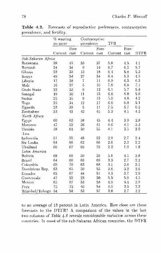
78 Charles F. Westoff

Table 4.2. Forecasts of reproductive preferences, contraceptiveprevalence, and fertility.

% wanting Contraceptiveno more prevalence TFR

Fore- Fore- Fore-Current cast Current cast Current cast DTFR

S'ub-S'aharan AfricaBotswana 38 45 33 37 5.0 4.5 4.1Burundi 24 34 9 14 6.7 6.1 .5.7Ghana 23 33 13 18 6.4 5.8 5.3Kenya 49 54 27 34 6.4 5.3 4.5Liberia 17 28 7 11 6.9 6.3 6.3Mali 16 27 5 10 7.6 6.8 7.1Gndo State 23 33 6 12 6.1 .5.7 5.8Senegal 19 30 11 15 6.6 6.0 .5.6Sudan 25 35 9 15 5.0 4.8 4.2Togo 25 34 12 17 6.6 6.0 5.1Uganda 23 33 5 11 7.5 6.7 6.5Zimbabwe 33 41 43 4.5 5.2 4.5 4.3North AfricaEgypt 60 63 38 45 4.4 3.9 2.8Morocco 47 52 36 41 4.6 4.1 :3.3Tunisia 58 61 50 55 4.1 3.5 2.9ASia

Indonesia 51 55 48 52 2.9 2.7 2.4Sri Lanka 64 66 62 66 2.6 2.3 2.2Thailand 66 67 66 70 2.2 1.9 1.8Latin AmericaBolivia 68 69 30 39 .5.1 4..5 2.8Brazil 64 66 66 69 3.3 2.7 2.2Colombia 69 70 63 68 3.1 2.6 2.1Dominican Rep. 63 65 50 .55 3.6 3.2 2.6Ecuador 65 67 44 51 4.3 3.7 2.9Guatemala 47 52 23 30 5.5 5.0 4.5Mexico 65 67 53 58 4.0 3.4 2.9Peru 75 75 46 .54 4.0 3.5 2.3Trinidad/Tobago 54 58 53 57 3.0 2.7 2.2

to an average of 13 percent in Latin America. How close are theseforecasts to the DTFR? A comparison of the values in the lasttwo columns of Table 4.2 reveals considerable variation across thesecountries. In most of the sub-Saharan African countries, the DTFR

Reproductive Preferences and Future Fertility 79

is modestly lower than the forecasts. Kenya and Togo show thelargest differences, indicating that women's reproductive preferencesare declining more rapidly than the likelihood of such preferencesbeing realized. In a few countries, there is hardly any difference ­Liberia, Ondo State in Nigeria, and (J ganda. Zimbabwe is also inthis category, with a forecast TFR of 4.5 and a DTFR, for example,of 4.:3.

The differences between \ lte:se rates are much greater in NorthAfrica, with the DTFR considerably lower than the expected TFR.In Egypt, the forecast shows a TFR of 3.9 with the DTFR at 2.8.The three Asian countries have already gone through most of thefertility transition; although the forecast TFRs show some contin­ued decline, they are very close to the DTFRs. In contrast, LatinAmerica is more like the three cOllntries in North Africa. Wide dif­ferences remain between the forecast values and the desired levels,especially in Bolivia ami Peru. where the DTFR is around one-thirdlower than the TFR forecast. In tlw other seven Latin Americancountries, the DTFR is an average of one-sixth below the averageforecast value.

One of the intrinsically unsatisfactory features of the forecast­ing procedure described here is its essential bootstrap nature, inparticular, the initial forecast of t he proportion of (married) womenwanting no more children from the regression equation connectingthis variable at two points in time. It is not unlike forecasting to­morrow's weather from today's weather in an area of the countrythat typically sends its weather systems in one direction. The un­derlying theory in this case is a knowledge of the prevailing winddirection and the pace of its movement. Our procedure is evenless theoretically grounded. It recognizes that a population's re­productive preferences at t 1 are highly correlated with those at t2

and that the sign of the regression coefficient indicates a decline.[l]It then uses this relationship to predict the proportion wanting nomore births at f3 . The next step, which relies upon the regressionof contraceptive prevalence on reproductive intentions, is less Ull­

satisfactory because it identifies a causal antecedent in substantiveterms,[2] whereas the forecast of reproductive intentions relies onlyon the association between these intentions over time.

80 Charles F. Westoff

The actual forecasts of reproductive intentions (columns 1 and2 of Table 4.2) appear reasonable enough. The forecast for thesub-Saharan African populations show a rise from an average of 27percent to an average of 36 percent of women who want no morechildren. The projected increases elsewhere in the percentage ofwomen who want no more are less dramatic: in North Africa from55 to 59 percent; in Asia from 60 to 63 percent; and in Latin Americafrom 63 to 65 percent.

4.3 Determinants of ReproductivePreferences

The main reason that the forecast of reproductive intentions relieson the same variable at an earlier time is simply that we have littleelse to use. In a broad sense, the determinants of reproductive in­tentions or preferences in developing countries cover the whole rangeof social changes included in the concept of modernization. Thesedeterminants are only partially represented in the WFS and DRS;e.g., economic status is inadequately measured. We do know thatthe desired number of children has been declining in many, proba­bly in most, developing countries. The mechanics of this process areless well known. The conventional explanations focus on the changesin the economic value of children; recent speculation minimizes theimportance of structural economic changes and emphasizes the roleof Western or modern ideas about the control of reproduction andsmall family norms (Cleland and Wilson, 1987). There is probablya time lag in the process of change in reproductive norms. The mostlikely process is one that first witnesses an increase in the propor­tion of women who want no more children without a commensuratedecline in ideal or desired family size. In turn, this leads to a de­mand for and the use of contraception and an ensuing decline infertility. Eventually the number of children desired begins its de­cline as smaller family norms develop. The urban and middle-classpopulations typically lead the transition.

In su b-Saharan Africa, the marital fertility transition may fol­Iowa different path. As noted earlier, the primary stage may be theadoption of fertility control to increase birth intervals, a motivationderived from health rather than from socioeconomic considerations.

Reproductive Preferences and Future Fertili(y 81

Kenya is a major exception to this generalization; over the decadefrom 1978 to 1988, the proportion of women wanting no more chil­dren increased from 17 to 49 percent.

Analysis of the determinants of reproductive preferences can beapproached at two levels: the macro-demographic level, in whichthe statistical units of observations are the provinces or regions ofcountries, and the micro or individual woman level.

4.4 Regional-level Analysis

Analysis of the determinants of reproductive preferences at theprovincial or regional level focuses on the question of what char­acteristics of these areas are associated with the mean number ofchildren desired or the proportion of married women who want nomore children. The areas assembled for this purpose are the 302provinces or regions of the :s L countries that participated in the'VFS or in the first stage of the DRS. Although this is a relativelylarge number of areas for analysis, it should be kept in mind that itis not a representative sample of the developing world; China andIndia, for example, are not included.

Since the object of interest is the number of children desiredrather than fertility and because there is some tendency to rational­ize as desired children that may have been unwanted at the time ofconception, we have tried to eliminate the life-cycle effects by sin­gling out a particular age group. ,,,romen aged 25-29 were selectedbecause most would be married by that age (removing the censoringby age at marriage) and the experience of unwanted fertility wouldbe still largely in the future. thus minimizing the factor of rational­ization. The mean number of children desired for this age groupacross the 302 regions is 4.6. with a range from 2.3 to 8.5. For theproportion of women who want no more children a similar logic wasfollowed by confining the analysis to married women with four orfive children. The mean percentage of women at this parity whowant no more children is 58.0, with a range from 0 to 98.1. Becausethere is a high correlation between these two measures (-0.92), thesame covariates are observed. Areas with women wanting no morechildren or desiring smaller families are those with high proportionsof their population classified as urban, high proportions of husbands

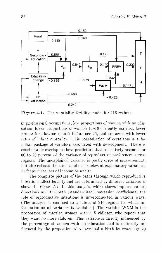
82

0.149

0.152

- 0.169

- 0.373

- 0.538

0.242

0.172

Charles F. Westoff

T

F

R-0.147

Figure 4.1. The nuptiality-fertility model for 216 regions.

in professional occupations, low proportions of women with no edu­cation, lower proportions of women 1.5-19 currently married, lowerproportions having a birth before age 20, and are areas with lowerrates of infant mortality. This constellation of correlates is a fa­miliar package of variables associated with development. There isconsiderable overlap in these predictors that collectively account for60 to 70 percent of the variance of reproductive preferences acrossregions. The unexplained variance is partly error of measurement,but also reflects the absence of other relevant explanatory variables,perhaps measures of income or wealth.

The complete picture of the paths through which reproductiveintentions affect fertility and are determined by different variables isshown in Figure 4.1. In this analysis, which shows imputed causaldirections and the path (standardized) regression coefficients, therole of reproductive intentions is interconnected in various ways.(The analysis is confined to a subset of 216 regions for which in­formation on all variables is available.) The variable WNM is theproportion of married women with 4-.5 children who report thatthey want no more children. This variable is directly influenced bythe percentage of women with no education and is indirectly in­fluenced by the proportion who have had a birth by exact age 20

Reproductive Preferences and Future Fertility 8:3

(B 20 ). In turn, the latter variable is determined by the proportionsfirst married by age 20 (M 20 ), which is seen to be a function ofresidence (the rural percentage), the proportion that attended sec­ondary school, and a measure of educational change that reflects thegenerational decline in the proportion of women with no education.The influence of reproductive intentions on the TFR, in turn, is seento operate indirectly through the prevalence of contraception anddirectly, presumably through unmeasured non-contraceptive pathssuch as abortion.

4.5 Individual-level Analysis

'rVe have also explored the determinants of reproductive preferencesat the level of individual women in several countries, partly to val­idate the aggregate analysis but also to exploit some economic andmedia exposure data that have not been collected by many of thesurveys included in the regional-level analysis. Several countrieswere selected from different areas that represent various stages inthe fertility transition: Colombia, Ghana, Kenya, Guatemala, Peru,Thailand, Tunisia, and Indonesia. The surveys in these countrieswere all part of the DHS-I project.

In none of these countries are we able to account for much of theindividual variance ofthe desired number of children. The regressionequations for each country are shown in Table 4.3; the R 2 s range invalue from only 0.065 to 0.314. We have confined the examination towomen 25-29 years of age as a life-cycle control, and our multivariateexploration has excluded measures of fertility that would add to theexplained variance. We have concentrated instead on social andeconomic measures and have added only age at marriage and/orage at first birth in order to parallel the aggregate analysis.

A similar set of determinants of reproductive norms operatesacross these countries. Several variables stand out prominently inall six countries. One is the importance of region of residence. In allof these countries, region exerts a strong influence on the number ofchildren desired. It is a surrogate for many other variables: regionfrequently reflects language, ethnic origin, or religion as well as thestage of economic development. In principle, region could be furtherdisaggregated to seek explanations at these compositional levels.

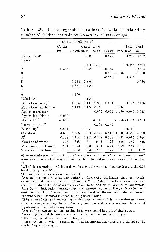
84 Charles F. Westoff

Table 4.3. Linear regression equations for variables related tonumber of children desirec!a by women 25-29 years of age.

Regression coefficients/>

Colom- Gna.te- Indo-bia Ghana mala nesia

Thai- Tuni­Kenya Peru land sia

:.\. J 76-1.224

-0.895 -0.431 -0.209 -0.531 -0.124 -0.175

-0.443 -0.476 -0.169 -0.266-(l.065 -0.052 -0.030 -0.045 -0.053

-0.050

-0.669 -0.340 -0.266 -0.154 -0.473

-0.234 -0.299-0.607 -0.733 -0.1994.835 6.655 8.016 6.247 5.317 4.000 3.495 4.9700.123 (1.:314 0.223 0.108 0.146 0.065 0.085 0.164

566 745 781 2448 1126 546 1252 8362.74 5.73 5.36 3.61 4.74 2.69 2.54 3.51

1.38 2.66 3.56 2.16 1.99 1.21 1.08 1.52

0.692 0.237 0.462Urban-ruralc

Region d

12

34

5

6

7

8EthnicityeEducation (wife)!Edncation (husband)!Age at marriage9

Age at first birth9

Watch TV h

Listen to radio"Electricity'ConstantR2

Number of women)Mean number desiredStandard deviation

-0.:.\65

0.586

-1.170 -1.100-0.989

-0.5:.\8 -0.890-0.651 -1.159

-0.4570.892 -0.240

-0.758

-0.246 -0.604-0.834-1.020

0.346-0.360

aNon-numeric responses of the type Has many as God sends" or "as many as corne'lwere nsually recoded in category 12+ or with t.he highest. numerical response if less t.han12.I> All of the regression coefficients shown in t.he table were significant at least at the 0.05level, mostly l' < 0.001.cUrban-rural residence scored as 0 and 1.dRegions were defined as dummy \'ariables. Those wit.h the highest significant. coeffi­cient.s recorded here are Pacifica in Colombia; Volt.a, Ashanti, and upper and nort.hernregions in Ghana; Guat.emala City, Central. Nort.e, and Norte Oriental in Guatemala;Java-Bali in Indonesia; cent.ral, coast. and eastern regions in Kenya; Selva in Peru;north and south in Thailand; and Tunis, nort.h-east, north-west., and Sallel in Tunisia.€Ethnicity in Guatemala is coded as Incligina or Ladino.! Education of wife and husband are coded here in terms of the categories: no educa­tion, primary, secondary, higher. Single years of schooling were not used because ofsignificant numbers of missing cases.9 Age at first marriage and age at first birt.h were coded in units of single years.h Wat.ching TV and listening t.o the radio coded as 0 for no and 1 for yes.'Electricit.y coded as 0 for no and I for yes.)These are the unweight.ed numbers. Missing informat.ion cases are assigned to t.hemodal frequency cat.egory.

Reproductive Preferences and Future Fertility 85

Where such requisite data are available, the variable still retains itspower, although sometimes it obliterates rural-urban differences aswell. Of course, the importance of region in the study of differencesin fertility has been underscored in many other studies, includingthe well-known 19th-century European fertility study (Coale andWatkins, 1986). Urban-rural residence also features in half of thecountries in the multivariate analysis.

One variable that holds up consistently is education of women,which is inversely related to preferences for fewer children, a patternthat persists in the presence of all other variables. In a few countries,the husband's education makes a similar and additive contribution(in Peru, it overshadows women's education). Education has beendemonstrated to be probably the most dependable and predictabledeterminant of fertility and fertility regulation behavior among allof the socioeconomic measures examined in hundreds of studies.

Several other determinants operate in some countries but notin others. Age at marriage or age at first birth is a factor in allof these countries except Ghana and Guatemala: the later the ageof the event, the fewer the number of children desired. How of­ten the woman reports listening to the radio or watching televisionhas an effect in all but these two countries as well. In all likelihood,the mass media transmit outside values and ideas. In other research,we have demonstrated a powerful association with reproductive atti­tudes and behavior of media messages on family planning, includingsoap operas that extol the advantages of smaller families ('Vestoffand RodrIguez, forthcoming).

One of the more surprising findings is a negative one, viz.. thatvarious measures of economic status either singly or in combina­tion fail to disclose any significant associations with the numberof children desired. Admittedly, the availability of economic datain these surveys is less than ideal. Nonetheless, there is a varietyof items including ownership of bicycles, cars, radios, televisions.refrigerators, kinds of toilet facilities, source of drinking water, elec­tricity, and different country-specific information on ownership ofhomes, land. livestock, and so on. In only a few countries do any ofthese measures seem to play any direct role in the determination ofreproductive preferences. Only in Colombia, Guatemala, and Thai­land does one of these economic variables hold up - the presence of

86 Charles F. Westoff

electricity in the household. The economic variables frequently showthe expected negative associations with reproductive preferences atthe zero-order level, but their influence is absorbed or dominated bythe regional and educational factors. It seems implausible that eco­nomic status would be totally irrelevant to the number of childrenwomen desire. However, there is simply no empirical support fromthe data for the hypothesis that smaller or larger families are viewedas inconsistent with economic resources, or more precisely, that an~'

such inconsistency persists in the presence of these other variables.One might of course reason that economic resources play an earlierrole in facilitating education, but this notion is not testable withthese data.

4.6 Conclusions

So what do we know about reproductive preferences and the dy­namics of fertility change in the developing world? A fair summarywould be as follows:

1. Whether measured by the average desired number of children orby the proportion of married women who want no more children.dramatic changes toward the small family norm are under wayin Latin America, much of Asia, and North Africa, but only ina few sub-Saharan African countries (where spacing rather thanlimiting preferences and behavior predominate).

2. Reproductive preferences are highly correlated (in the aggre­gate) with the fertility rate, operating mainly, though not ex­clusively, through contraceptive prevalence.

:3. At the regional or provincial level, the main determinants of re­productive preferences are those typically associated with mod­ernization: residence in cities or in rural areas, education ofwomen, occupational status of men, and age at marriage and atfirst birth.

cle. Our knowledge of determinants at the level of the individualwoman remains very limited: region, rural-urban residence. ed­ucation of women, age at marriage, and exposure to mass mediadominate the picture rather than individual economic variables.However, the amount of variation explained is very small.

Reproductive Preferences and Future Fertility

Notes

87

[1] Unlike the direction of the wind ill the weather analogy, the directionof reproductive preferences cannot remain pointed in the same wayindefinitely. At the end of the fertility transition, reproductive prefer­ences stabilize and may even change directions for periods of time, ashas been observed in some developed countries.

[2] Operationally, it is also corrupted by this bootstrapping quality in thatthe actual forecasting equation adds the earlier prevalence value. Theredeeming feature here is that at least it does not depend exclusively onthe forecast value of intentions that is based on its own earlier values.

Chapter 5

Population Policies andFamily-Planning in SoutheastAsia

1I1ercedes B. Concepcion

Impressive gains in the control of fertility and in the reductionof population growth rates have been observed in many countrieswithin the purview of the Economic and Social Commission forAsia and the Pacific (ESCAP). Family-planning (FP) and mater­nal and child health (M CR) programs have played an importantrole in reducing population growth, improving the quality of life,and developing human resources in the region. The success of FPand MCR programs is closely associated with the enhanced role andstatus of women, lower infant, child, and maternal mortality rates,better birth-spacing and breast-feeding practices, and the deliveryof services by trained personnel. Nevertheless, the population as awhole continues to grow by more than 50 million yearly. Moreover,progress in lessening population growth rates has been uneven andhas generally widened the gap between countries with continuedhigh growth rates and those which have succeeded in moderating orLowering their growth ra.tes.

In Southeast Asia, three of the region's 10 component countriesare expected to grow at rates of 1.8 percent or less per annum duringthe 1990-1995 quinquennium while the rest are expected to increaseannually by at least 2.1 percent. By the beginning of the 21st cen­tury, all but one of the countries in Southeast Asia are projected to

88

Population Policies in Southeast Asia 89

grow no faster than 1.7 percent yearly. Total fertility rates (TFRs)during the early 1990s are also expected to range from Singapore'sreported low 1.7 children to the estimated 6.4 children per woman inthe Lao People's Democratic Republic. These rates are foreseen bythe United Nations to drop to about 3 children or fewer at the startof the next century (UN, 1991b). The exceptions are Cambodia andthe Lao People's Democratic Republic.

Governments in .s of the 10 Southeast Asian countries perceivetheir current fertility levels as unsatisfactory and have ongoing pro­grams to lower such rates. Three others - Brunei Darussalam, LaoPeople's Democratic Republic, and Myanmar - are satisfied withtheir present fertility levels. Brunei Darussalam and Myanmar donot report any direct intervention, while the Lao People's Demo­cratic Republic is intervening to maintain current rates. Cambodiaand Singapore consider their fertility rates too low. The former re­stricts access to contraception. while the latter has been offering taxrebates to couples having a third or fourth child.

This chapter examines the population policies and FP pro­grams in selected Southeast Asian countries (Indonesia, Malaysia,the Philippines, Singapore, Thailand, and Vietnam) and attemptsto draw from their experience the critical preconditions for family­planning program success. Such experiences have been gleaned fromthe country statements provided by participants of the 4th Asianand Pacific Population Conference (APPC) held in Bali, Indonesia,on 19-27 August 1992.

5.1 Demographic Situation

During the 4th APpe, which was entitled Population and Sustain­able Development: Goals and Strategies into the 21st Century, thepresent population situation and future outlook were reviewed in thelight of the 1982 APPC Asia-Pacific Call for Action on Populationand Development. The participants noted that while substantialprogress had been achieved by the ESCAP region in responding tothe Asia-Pacific Call for Action, population issues continue to posea most critical challenge. The conference adopted the Bali Decla­ration on Population and Sustainable Development, which set goals

90 Mercedes B. Concepcion

and made recommendations for population and sustainable devel­opment into the next century.

One of the population goals included in the Bali Declarationenjoined countries and areas to adopt suitable strategies to attainreplacement-level fertility, equivalent to a TFR of around 2.2 chil­dren per woman, by the year 2010 or earlier. In addition, membercountries were also urged to reduce the level of infant mortality tono more than 40 infant deaths per 1,000 live births during the sameperiod. Countries and areas where maternal mortality remains highwere called upon to effect a 50 percent reduction by the year 2010.

The Bali Declaration recommended that priority be given tostrengthening policy development and related processes in thosecountries where the MCR and FP programs have not yet achieveddesired objectives. Furthermore, such countries were urged toexpand and streamline MCR and FP delivery systems withinthe primary health-care framework, adopt innovative managementand multi-sectoral approaches, and encourage wider communityand inter-sectoral participation in program implementation efforts.Countries which have already reduced their fertility to lawaI' ac­ceptable levels were prompted to devise program strategies aimedat achieving self-sustainability.

5.2 Family-planning Policies and Programs

The country statements circulated during the 4th APPC containeda section on the policy and objectives of national FP /family healthand welfare programs.

5.2.1 Indonesia

The state policy guidelines, issued by the 1973 People's ConsultativeAssembly, declared that the objective of the national FP programduring the second five-year development plan period (1974-1978)was to improve maternal and child health in order to create a small,happy, and prosperous family. The guidelines also stated that eco­nomic and social welfare development can be implemented rapidly,together with population growth control, through a properly admin­istered national FP program. The most recent guidelines, issued in

Population Policies ill Southeast Asia 91

1988, added that the Indonesian FP program should also be di­rected at reducing mortality rates. At the same time, the need forsuccessful implementation without endangering future generationswas emphasized. In addition, a policy to enhance support to FPacceptors through improvements in the quality of available contra­ceptives and services was outlined. As a general course of action,FP acceptors are encouraged to use more effective contraceptives,thus ensuring better protection against pregnancy and acceleratingfertility reduction.

The Indonesian FP program has three broad objectives: expan­sion of contraceptive coverage in accordance with government tar­gets; promotion of continued contraceptive use; and institutionaliza­tion of FP and small family norm concepts by shifting responsibilityfor FP decisions to the individual, the family, and the community.

Nine important program strategy elements have been taken intoaccount in the Indonesian FP program: integration of an arrayof governmental, nongovernmental, private, and community agen­cies; decentralization of responsibility and authority; commitmentto meet targets at every program level; provision of FP servicescombined with medical advice; National Family Planning Coordi­nating Board (BKKBN) cooperation with the Ministry of Health inhealth services beyond FP in order to improve FP outreach; devel­opment of a climate of community support for FP through the co­operation of community and religious leaders; support for activitieswhich raise women's social and economic status; emphasis on reach­ing the rapidly increasing numbers of youth; and encouragementof self-reliance, the newest strategy element involving the privatesector.

The Indonesian Country Report (1992) stated that the TFRwhich was .5.6 children between 1965 and 1969 fell to 3.0 by 1992.The corresponding decrease for the crude birth rate (CBR) was from42.6 to 25.2 births per 1,000. By 1990, the crude death rate (CDR)was estimated to be 9.7 deaths, down from 21 deaths per 1,000 overthe period 1961-1971. The CDR is projected to reach 8.5 deathsper 1,000 at the start of 199:3, declining to around 7 per 1,000 bythe year 2020. The infant mortality rate (IMR), currently estimatedat GS infant deaths per 1,000 live births, is expected to drop to 28by the year 2020. The life expectancy at birth, now reported to

92 Mercedes B. Concepcion

be around 60 years for both sexes, is forecast to lengthen by 10years during the next quarter of a century. Maternal mortality ispredicted to fall from a level of 450 deaths per 100,000 live births in1986 to 200 by 2020.

The Indonesians foresee a likely deceleration in the future rateof fertility decline. The reasons given in the Country Report werethat the desired family size of some couples is unlikely to decreasefurther; those who most want to avail themselves of family planningas well as those for whom the services are most accessible have al­ready been covered by the program; and the couples who still needto be brought into the program express larger family-size preferencesand are more difficult to reach. Among these are the urban poor,those living in outlying areas. those with low educational levels aswell as those who find it difficult to use contraceptives correctly.Therefore, further mortality and fertility reductions will entail con­siderably greater efforts. For example, the family-planning programwill have to reach unprecedented numbers of contraceptive acceptorsand motivate couples with high fertility preferences, people who areless likely to know about health and family-planning programs andare less disposed to seek services.

5.2.2 Malaysia

Given the rapid economic growth and the prospect of a further de­cline in fertility, the Malaysian government changed its official stancein 1984 and promulgated a national population policy. As expressedin the Malaysian Country Report (1992), a long-term target of 70million people by the year 2100 is to be achieved through deceler­ating the TFR decline. The plan is to reduce the TFR by 0.1 pointover five-year periods until a level of 2.05 children is reached in theyear 2070. The TFR in peninsular Malaysia had fallen from a high6.8 children in 1957 to about :l.3 children in 1990. At this pace. aTFR of 2.1 could be reached by 2010. The average age at marriagefor females had risen from 22.1 in 1970 to 24.6 years in 1990. TheIMR was recorded at n.:l infant deaths per 1,000 live births in 1990.The life expectancy at birth of rVIalaysian males was lengthened from55.8 years in 1957 to 69.1 years in 1990. The corresponding ratesfor females were 58.2 and i:L3 years, respectively. Given currenttrends, the most probable outlook during the next three decades is

Population Policies in Southeast Asia 93

for small nuclear families with the couples participating actively inthe labor force.

Since its inception in 1966, the Malaysian FP program has un­dergone several phases of development, each involving expansion interms of the approach used, the area covered, or the number of agen­cies involved in the provision of contraceptive services. The spreadof FP services to the rural areas as part of an integrated MCH/FPprogram was initiated in the early 1970s and led to FP services be­ing integrated in the MeH services provided by the Health Ministry.The blending of FP with health and other social programs not onlyaided in overcoming the resource constraints but also contributedto wider FP acceptance and a heightened contraceptive prevalencerate.

In line with the national objective of improving the quality oflife, a comprehensivE' family development program has been devel­oped and is now being implemented. It emphasizes the improvementof family health and welfare through family-life education, parent­ing courses, and marriage and family counseling. The stress is nowon improving infrastructure in underserved and remote areas, onenhancing coverage and quality of care in designated areas of lowcoverage, and on program consolidation. The implementation of therisk approach in MCH/FP care has for its ultimate objective theavailability and accessibility of a range of services, including FP, toall women and families for their better health and well- being.

5.2.3 The Philippines

Since 1970, the Philippine FP program as described in the Coun­try Report (1992) has been a social development initiative aimedat diminishing the country's fertility level for the benefit of familyand national welfare. Over the course of its history, the programhas adopted varying approaches and strategies to suit the changingneeds and conditions of the time. There have been modest increasesin contraceptive prevalence rate coupled with moderate declines intotal fertility. Program efforts have contributed substantially tothis decline. However, t he gains made did not approximate those ofneighboring countries owing to problems besetting policy and pro­gram implementation.

94 Mercedes B. Concepcion

In response to the difficulties experienced in relying on staticclinics, the Outreach Project was implemented in 1976 to expandthe availability and accessibility of services. The Outreach Projectviewed FP not only as a means to reduce fertility but, more impor­tantly, as advancing family welfare. Furthermore, a closer integra­tion of broader population concerns into the country's developmentplans, policies, and programs was sought. The Outreach Projectalso paved the way for strengthening and deepening local govern­ment involvement in, and support for, FP.

In 1987, a new population policy statement was formulated, tak­ing into account relevant provisions of the 1987 constitution. Thenew policy broadened program concern beyond that of fertility re­duction. Consequently. the 1989-199:3 five-year population programdirectional plan was drawn up focusing on two components, namely,responsible parenthood/FP and population and development. Theprogram's institutional arrangement was altered along with the pol­icy and the program. The Department of Health was designated asthe implementing agency for the FP program with jurisdiction overthe activities of aU FP service delivery agencies. The Commissionon Population, on the other hand, remained as the overall planning,policy-making, coordinating, and monitoring body of the entire pro­gram with specific responsibilit.v for coordinating the population anddevelopment integration thrust.

The new FP program uses a health-oriented, demand-driven ap­proach, anchored on safe motherhood and child survival. Its primaryobjective is to reduce the level of unmet needs for FP, particularlyamong poor families. The population and development thrust is oneof systematically incorporating population matters into the devel­opment efforts of concerned agencies.

Whether the program will be able to make a more significantcontribution toward development goals depends on its ability toalign policies and operational aspects to individual and societalneeds. Some considerations include expanding and intensifying theprovision of women's health and family-planning services; integrat­ing FP in other health programs, particularly MCH; strengthen­ing the capacity of agencies to manage the services; promoting col­laboration among the governments, nongovernmental organizations(NGOs), and other private organizations and local communities to

Population Policies in Southeast Asia 95

improve access to these services; and shortening the gestation pe­riod for an effective program implementation by local governmentunits, including appropriating local funds for the program.

As stated earlier, the slow pace of decline in Philippine pop­ulation growth is the consequence of a moderately decreasing fer­tility and a decelerating mortality decline. The CBR fell from alevel of 46 births per 1.000 in 1969 to about 30 in 1990. The CDRdropped from ;32 deaths pel' LOOO in 1940 to around 7.2 in 1990.Further pronounced decreases are not expected as the pace of de­cline has slackened significantly. The [MR has fluctuated around 61infant deaths per 1,000 live births since the 1960s. The estimate for1990 was .57. Communicable diseases still account for the majorityof morbidity and mortality cases. Since 1970, the TFR has beenslowly but steadily declining and was estimated to be around 4 chil­dren per woman in 1990. This gradual descent can be attributedto four causes: the continued expansion in the number of women ofreproductive age as an outcome of past high fertility; shrinkage in1, he prevalence and duration of bre<lst-feeding; low-level use of themore effective contraceptive methods; and the Roman Catholic hier­archy's open and active opposition to the government's FP program,thus affecting its political support.

5.2.4 Singapore

The country's FP and population program was initiated in 1966,soon after independence. Ambitious FP targets were set for eachfive-year plan (1966-1970, 1971-1975, and 1976-1980), and socialdisincentives were introduced. The government actively promotedthe two-child family norm. Contraceptives were made easily avail­able, and abortion and sterilization were legalized. With the attain­ment of replacement-level fertility in 1975, the government startedto emphasize child spacing as the main policy orientation. The pro­gram impact on population growth was significant. According tothe Country Report, Singapore's fertility fell by almost 70 percentwithin a span of two decades (Ministry of Health, 1992). The TFRdropped from 4.7 children in 196.5 to a historic low of 1.4 in 1986.

With the continued decline in fertility rates in the early 1980s,population projections indicated that if below-replacement fertility

96 Mercedes B. Concepcion

were to continue, the country would experience negative popula­tion growth within the next ;·W years. A new population policy waspromulgated in 1987 in response to the prospect of a decline in num­bers. The new policy thrust encourages marriage and childbearing.A new slogan, "Have three or more if you can afford it," was adoptedreflecting the new direction. Generous incentives are being providedsuch as income tax rebates, subsidies for child-care centers and fordelivery fees, and special leave schemes. In addition, two programs- Strengthening the Marriage Program and Family Life EducationProgram - have been implemented.

Since the adoption of the new policy, TFRs have inched up­ward. The rate rose to 1.9 in 19R8, but is now about 1.7 children.Since the tax incentives were announced, the number of third- andfourth-order births have gone up. However, marriage trends havenot manifested significant improvements. The critical issue on pop­ulation and development facing policy makers is one of ensuringreplacement-level fertility to achieve the optimum population sizeand a balanced age structure.

5.2.5 Thailand

In 1970, the government officially launched the National FamilyPlanning Program (NFPP) aimed at further reducing the popu­lation growth rate. According to targets set by successive five-yearplans in the last two decades, the program succeeded in decreasingthe growth rate through quantitative target-oriented strategies. Theprovision of an extensive contraceptive distribution system and theefforts to legitimize the preference for fewer children and to increaseawareness of the possibility of controlling family size through ef­fective and acceptable means contributed to the program's success.Past successes, however, do not imply that there are no longer anyunmet needs or new and more difficult challenges ahead. The sev­enth plan (1992-1996) has renewed the emphasis on human resourcedevelopment. thus posing new challenges to the health sector. Thestrategy for MCH /FP over the next fi ve years will be to maintainthe program momentum to raise contraceptive prevalence rates inthe face of a 10 percent rise in the nnmber of women of childbearingage; provide effective follow-up for conpIes who are already using

Population Policies in Southeast Asia 97

contraceptives; meet more effectively the special needs of adoles­cents and ethnic minorities; and improve the management, training,and information systems, particularly at the regional level. Sincehealth is a national responsibility. the strategy calls for providingMCH/FP services within a national and inter-sectoral framework.

Thailand's fairly well-developed and extensive health infrastruc­ture has brought about a significant improvement in the health sta­tns of mothers and children. The NFPP is well integrated in thetasks ofthe Ministry of Pnblic Health's Family Health Division. TheNFPP has effectively utilized the wide primary health-care networkto make contraceptive services available throughout the country.However, equal attention needs be given to both the quality of ser­vices and the achievement of the plan's targets. This action entailsstrong collaboration with other government agencies, with the pri­vate sector and with NGOs, all of whom have important roles toplay in supplementing government activities.

The population growth rate decreased from 3.0-3.3 percent inthe 196013 to about 1A percent in 1991, as stated in the ThailandCountry Statement (1992). The seventh plan has targeted the re­duction of the growth rate to 1.2 percent by the end of the planperiod. The TFR has dropped from about 6.1 during the period1968-1969 to less than V5 children per woman today. In 1990, theCDR was estimated at about 5 to 6 deaths per 1,000 population,with the IMR at approximately 34.5 infant deaths per 1,000 livebirths a year later. Currently. life expectancy is estimated to be 66years for males and 71 years for females. Recently, married coupleswhether rural- or urban-based, lesser or better educated, have over­whelmingly expressed a desire for a family size of some two children.

5.2.6 Vietnam

As recorded in the Country Report (1992), decision number 29 of theCouncil of Ministers of the Socialist Republic of Vietnam, issued on12 August 1981, contained the following objectives for the nationalpopulation and FP program: married women should be prompted tohave their first birth after age 22; each couple should be persuadedto have only one or two children; and a spacing of five years shouldbe encouraged between the first and second birth.

98 Mercedes B. Concepcion

According to the country's 1989 population census, there were64.4 million people in Vietnam. The intercensal growth rate forthe period 1979-1989 was 2.1 percent. The population in 1991 wasestimated at 67.7 million. The CBR recorded for the 12-monthperiod preceding the 1989 cenSllS was 31 births per 1,000, with urbanand rural areas reporting 2:3 and :34 births per 1,000, respectively.The CDR was SA deaths per 1.000, while the IMR was 49 infantdeaths per 1,000 live births. The average life expectancy at birthwas 63 years for men and 67..5 years for women.

On 18 October 1988, the Council of Ministers' Decree on Pop­ulation and Family Planning Policies was promulgated (Vietnam,1989). The stated goal is to reinforce and strengthen measuresto lower population growth and to ensure that adequate family­planning methods are readily available and utilized by the popula­tion. Norms were set for the minimum age at first birth (at least22 years for urban women, 19 for rural women), for the number ofchildren (no more than two for most families), and for birth spacing(three to five years after the first ).

A national health law passed by the National Assembly on 30June 1989 legalized some of the above-mentioned measures. In ad­dition, the law gives legal force to the individual's right to choose tolimit births and provides for recourse to the judicial system shouldthis right be violated (Allman cl at.. 1991).

The population of Vietnam is projected to reach 87 million bythe period 200.5~2010 with a growth rate of 1.4 percent, a CURof 22.2 births per 1,000 population, and a CD R of 7.9 deaths per1,000. In projecting the future population, the National Committeefor Population and Family Planning (NCPFP) took into account theover 17 million women currently of reproductive age who comprisenearly half of the country's total female population. Moreover, pasthigh fertility rates are obviollsly affecting the replacement capaci­ties of future generations. Starting in the year 2000, half a millionwomen, on the average, will be added yearly to the cohort of repro­ductive age. This poses additional constraints on the achievementof an annual decrease in the TFR of 0.11 in the 1990s and of 0.6 inthe first decade of the 21st century.

To achieve the immediate as well as long-term objectives setforth in the national population program, Vietnam will endeavor

Population Policies in Southeast Asia 99

to improve the quality and effectiveness of FP activities by utiliz­ing a network of intercommunal FP centers and communal healthclinics; make a wider choice of contraceptives available; integrateFP activities in other MeR, nutrition, rural development, incomegeneration, and women's status improvement programs; train FPstaff at the grass-roots level; and support studies on impacts of FPprograms and contraceptive methods as a basis for the formulationof a more effective and practical FP program.

5.3 Family-Planning Program Effectiveness

Family-planning programs have a long tradition in the Asian region,and are firmly established there. Various countries in the regionhave conceived novel approaches and have devised new strategiesto reduce fertility. In this section an attempt is made to extractthe most important factors contributing to family-planning programeffectiveness from the experiences of the countries considered in thischapter.

In common with other Asian countries, Indonesia, Malaysia, thePhilippines, Singapore, and Thailand boast of a relatively longer ex­perience with intervention schemes to modify reproductive behavior.All these countries directly support family-planning programs andprovide unlimited access to modern contraceptives. As a whole, themost common approaches in these countries consist of integratingfamily-planning services ill the health-care system at the communitylevel or in rural development schemes. Incentives and disincentiveshave been introduced to discourage large families.

Singapore, which achieved replacement fertility in 1975, intro­duced a comprehensive package of incentives and disincentives in1969 which was further intensified in 1972 to exert pressure on cou­ples to limit their family size. In addition, sterilization was promotedas the best contraceptive method for those who had completed theirfamilies. Abortion hecame available on demand for a small fee ingovernment facilities. There were graduated charges for delivery ingovernment hospitals. paid maternity leaves covering the first twochildren only, preferential treatment in choice of primary school forthe first three children in a family. and no priority for public hous­ing for large families. An additional policy which was made known

100 Mercedes B. Concepcion

to the public in 1976 was designed to encourage later marriage andwider birth spacing.

The high commitment of President Soeharto, reflected in theabove-mentioned state policy guidelines, represents one of the keysto the success of the Indonesian family-planning program. This com­mitment is not merely a personal one bnt is institutionalized in theexisting systems, both in the People's Consultative Assembly and inParliament and other executive systems. The program strengthenedits links with rural communities by recruiting acceptors by means ofa village- based delivery system. Acceptors in the program are main­tained through varions meaS1ll'es extending beyond family planning.To enhance family planning within the framework of institutionaliz­ing the small family-size norm, the BKKBN developed a system ofnonmonetary rewards for individual or group acceptors. A systemwas introduced in 1989 whereby a community with high contracep­tive prevalence rates receives a deep well. The reward can also bein the form of scholarships for children of low income families thathave been resorting to contraception for at least a decade. More­over, some private Indonesian finns give discount cards to certainacceptor groups in major cities for the purchase of selected items.

The success of Thailand's family- planning program, as statedin the preceding section, can be traced to both the provision ofan extensive system of contraceptive distribution and the efforts tolegitimize the preference for fewer children and increase awarenessof the possibility of controlling family size through effective andacceptable means.

The Philippines has tried a variety of schemes intended to in­duce couples to have fewer children. Among these are income taxdeductions limited to four dependents, abolition of paid maternityleaves after the fourth child, and payment of lower interest ratesfor rural bank loans by couples using contraceptives. However, thecoverage of these schemes was limited and therefore of little valuein motivating couples to limit their family size. Malaysia also intro­duced tax deductions and maternity benefits but limited them tothe first three children.

In Vietnam the rewards that had been implemented since 1982included monetary bonuses and exemption from the required monthper year of corvee labor for sterilization, IUD insertion, or agreeing

Population Policies in Southeast Asia 101

not to have another child (Banister, 1989). Violations of family­planning policy resulted in loss of bonuses, benefits, and family al­lowances. The Council of Ministers' Decree in October 1988 limitedcouples in cities, deltas. or lowlands to a maximum of two children.Those couples having more than the allowed number are requiredto pay extra for housing or land space, education, and health care.Such couples are prohibited from moving to urban areas and arerequired to perform more corvee work.

There is still considerable uncertainty concerning the processesand factors that motivate couples to limit the number of the childrenand account for the adoption of contraception in various societiesat different periods of time. There is general agreement that so­cioeconomic development and organized family-planning programsplay prominent roles in altering reproductive behavior. Accordingto Bongaarts et af. (1990), socioeconomic development and family­planning programs operate synergistically, with one reinforcing theother.

The family-planning program experience of the selected South­east Asian countries demonstrates that by making contraceptiveseasily available and by encouraging smaller families through a vari­ety of measures, public and private sector family-planning programshave heightened contraceptive use. In turn. fertility and populationgrowth rates have been reduced. The key to effective programs is toemphasize integrated high-quality outreach services and to take intoaccount the traditional social structure and norms where the deliv­ery system is to be introduced. Moreover, careful trial and phaseddevelopment of alternative approaches to service delivery systemsare critical to the success of a program. Finally, political supportfor family planning is often essential for the establishment of strongprogram effort.

Chapter 6

Fertility in China:Past, Present, Prospects

Griffith Feeney*

Future population growth in any population is determined by thecurrent age distribution and by future trends in fertility, mortal­ity, and migration. The influence of the current age distributionis governed by purely formal demographic considerations that arethe same for every population. The role of mortality depends cru­cially on its current level. 11 nder conditions of high mortality, rapiddeclines are possible, and the normal interaction of mortality andage structure may lead to rapid population increase even in theface of substantial fertility decline. Once mortality has declined tothe levels now observed in much of the world, however, mortality isrelatively stable, largely because the features relevant to future pop­ulation growth reflect biology more than social circumstance. Undercurrent world demographic conditions. then, appropriate consider­ation of mortality and age distribution may be given without closeattention to social structure or to policy issues that vary widely fromone country to another.

The assessment of future levels and trends in fertility and mi­gration is a different matter altogether. Circumstances influencingfertility, and even more so circumstances influencing migration, varywidely from one country to another, and all but the most superficialconsideration of possible future trends requires study of particular

*With the assist.ance of Jianhua \'nan.

102

Fertility in China: Past, Present, Prospects 103

circumstances. International migration may be an important in­fluence of future population growth for particular countries, largeas well as small. Immigration and emigration cancel out for theworld as a whole, however, whence a global perspective renders theassessment of migration trends relatively unimportant,

Fertility behavior is heavily conditioned by both biology and so­ciety. Social influences may be roughly classified into the direct andintended consequences of national government policy and all otherinfluences. The distinction is relevant to consideration of future fer­tility levels because it focuses attention in different directions: tobroad social and economic conditions thought to influence fertilityin the population at large, on the one hand, and to the minds of arelatively small number of policy makers, on the other. It shouldhardly be necessary to point out that the existence of policies tolimit fertility and/or population growth does not imply the effec­tiveness of such policies. This is an issue to be decided by empiricalanalysis in each case.

The argument for country-specific consideration of influences onfuture fertility is particularly compelling for China, which is uniqueboth in the nature and in the impacts of governmental popula­tion policies. This chapter aims to give a reasonably comprehen­sive treatment of China's fertility decline at the national level, withemphasis on those factors relevant to a consideration of the futuretrajectory of fertility. The qualifying clause is important, for thereis now such a quantity of demographic data available for China thatit is difficult to conceive, much less write in the space of one bookchapter, anything that might reasonably be called definitive.

6.1 China's Fertility Decline inInternational Perspective

That fertility declined rapidly in China is well known, but the speedof the decline can be appreciated only when China's experience issystematically compared with that of other countries. This sectioncompares Chinese experience with that of the rest of the developingworld. The analysis relies primarily on the historical estimates de­veloped by the United Nations (1991a). These estimates share the

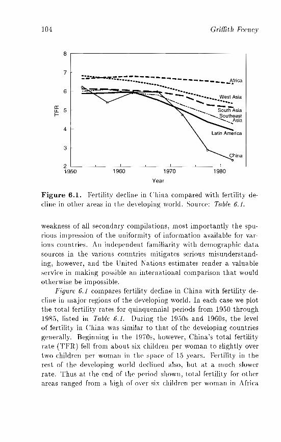
1980

Grjtli th Feeney

19701960

:.-,;.· _-::.-:::.7.7..: - .. - - _A.frica.......... ............~~--.......,,-~. ........... ~ ~: .._'t.......... West Asia

..".... . ................. ...... _-

................ South Asia......... Southeast

••............Asia

104

8

7

6

1E 5f-

4

3

21950

Year

Figure 6.1. Fertility decline in China compared with fertility de­cline in other areas in the developing world. Source: Table 6.1.

weakness of all secondary compilations, most importantly the spu­rious impression of the uniformity of information available for var­ious countries. An independent familiarity with demographic datasources in the various countries mitigates serious misunderstand­ing, however, and the United Nations estimates render a valuableservice in making possible an international comparison that wouldotherwise be impossible.

Figure 6.1 compares fertility decline in China with fertility de­cline in major regions of the developing world. In each case we plotthe total fertility rates for qninquennial periods from 19.50 through198.5, listed in Table 6.1. During the 19.50s and 1960s, the levelof fertility in China was similar to that of the developing countriesgenerally. Beginning in the 1970s, however, China's total fertilityrate (TFR) fell from about six children per woman to slightly overtwo children per woman in the space of 15 years. Fertility in therest of the developing world declined also, but at a much slowerrate. Thus at the end of the period shown, total fertility for otherareas ranged from a. high of over six children per woman in Africa

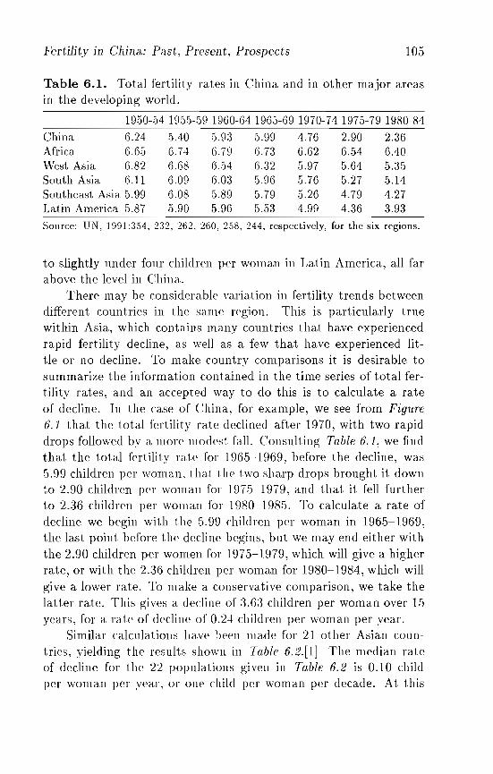
Fertility in China: Past, Present, Prospects 105

Table 6.1. Total fertility rates in China and in other major areasin the developing world.

1950-54 1955-59 1960-64 1965-69 1970-74 1975-79 1980-84China 6.24 5.40 0.93 5.99 4.76 2.90 2.36Africa 6.65 6.74 6.79 6.73 6.62 6.54 6.40West Asia 6.82 6.68 6.54 6.32 5.97 5.64 5.35South Asia 6.11 6.09 6.0:3 5.96 5.76 5.27 5.14Southeast Asia .5.99 6.08 5.89 5.79 5.26 4.79 4.27Latin America 5.87 .5.90 5.96 5.53 4.99 4.36 3.93Source: UN, 1991 :354, 232, 262, 260, 258, 244, respectively, for the six regions.

to slightly under four children per woman in Latin America, all farabove the level in China.

There may be considerable variation in fertility trends betweendifferent countries in the same region. This is particularly truewithin Asia, which contains many countries that have experiencedrapid fertility decline, as well as a few that have experienced lit­tle or no decline. To make country comparisons it is desirable tosummarize the information contained in the time series of total fer­tility rates, and an accepted way to do this is to calculate a rateof decline. In the case of China, for example, we see from Figure6.1 that the total fertility rate declined after 1970, with two rapiddrops followed by a more modest fall. Consulting Table 6.1, we findthat the total fertility rate for 1965-1969, before the decline, was5.99 children per woman, that tlte two sharp drops brought it downto 2.90 children per woman for 197.5-1979, and that it fell furtherto 2.36 children per woman for 1980-198.5. To calculate a rate ofdecline we begin with the .5.99 children per woman in 1965-1969,the last point before the decline begins, but we may end either withthe 2.90 children per women for 1975-1979, which will give a higherrate, or with the 2.36 children per woman for 1980-1984, which willgive a lower rate. To make a conservative comparison, we take thelatter rate. This gives a decline of 3.63 children per woman over 1.5years, for a rate of decline of 0.24 children per woman per year.

Similar calculations have heen made for 21 other Asian coun­tries, yielding the results shown in Table 6.2.[1] The median rateof decline for the 22 populations given in Table 6.2 is 0.10 childper woman per year, or one child per woman per decade. At this

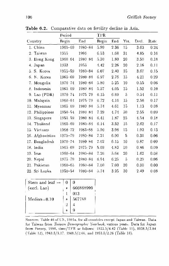
106 Griffith Feeney

Table 6.2. Comparative data on fertility decline in Asia.

Period TFR

Country Begin End Begin End Yrs. Decl. Rate

1. China 1965-69 1980-84 5.99 2.36 15 3.63 0.24

2. Taiwan 195.5 1986 6.53 1.68 31 4.85 0.16

3. Hong Kong 1960-64 1980-84 ,5.30 1.80 20 3.50 0.18

4. Japan 1933 1953 4.42 2.26 20 2.16 0.11

5. S. Korea 1955-59 1980-84 6.07 2.40 25 3.67 0.15

6. N. Korea 1965-69 1980-84 6.97 2.76 15 4.21 0.29

7. Mongolia 1970-74 1980-84 5.80 5.25 10 0.55 0.06

8. Indonesia 1965-69 1980-84 5.57 4.05 15 1.52 0.10

9. Lao (PDR) 1970-74 1975-79 6.15 6.69 5 -0.54 -0.11

10. Malaysia 1960-64 1975-79 6.72 4.16 15 2.56 0.17

11. Myanmar 1965-69 1980-84 5.74 4.61 15 1.13 008

12. Philippines 1950-54 1~)80-84 7.29 4.74 30 2.55 0.09

13. Singapore 1955-59 1980-84 6.41 1.87 25 4.54 0.18

14. Thailand 1965-69 1980-84 6.14 3.52 15 2.62 0.17

15. Vietnam 1968-72 1983-88 5.90 3.98 15 1.92 0.13

16. Afghanistan 1975-79 1980-84 7.21 6.90 5 0.31 0.06

17. Bangladesh 1970-74 1980-84 7.02 6.15 10 0.87 0.09

18. India 1965-69 1975-79 5.69 4.83 10 0.86 0.09

19. Iran 1960-64 1980-84 7.26 5.64 20 1.62 0.08

20. Nepal 1975-79 1980-84 6.54 6.2,5 5 0.29 0.06

21. Pakistan 1960-65 1980-84 7.00 7.00 20 0.00 0.00

22. Sri Lanka 1950-54 1980-84 5.74 3.25 30 2.49 0.08

Stem and leaf -+ 0 0(excl. Lao) * 666888999

1 013Median=0.10 * 567788

2 4

* 9

Sources: Table 46 of UN. 1991a. for all countries except Japan and Taiwan. Datafor Taiwan from TOlwon Demogmphlc Yearbook, various years. Data for Japanfrom Feeney, 1990, time/TFR as follows: 1933.5/4.42 (Table ll), 1938.5/3.84(Table 12), 1943.5/3.17. 1948.5/2.66, and 1953.5/2.26 (Table 13).

Fertility in China: Past, Present, Prospects 107

rate, decline from a roughly typical premodern fertility level of sixchildren per woman to an equally roughly typical modern level oftwo children per woman would take 40 years. China, with a rate ofdecline of 0.24 children per woman per year, experienced a declinenearly this large in only 15 years.

The range of values in TablE 6.2 illustrates the difficulties en­countered in international comparisons. Neither of the extreme val­ues, for example, -0.11 for Lao People's Democratic Republic and0.29 for Democratic People's Republic of Korea, should be givenmuch weight. The demographic data necessary for calculating totalfertility rates for Lao People's Democratic Republic over this pe­riod do not exist, and even casual scrutiny of the estimates givenin the United Nations source raises suspicion that the numbers arelittle more than rough guesses. Little is known of data sources forDemocratic People's Republic of Korea, for they are almost withoutexception not public, and here again scrutiny of the values shownin the source places their accuracy in doubt. For most of the othercountries, however, sources are plentiful and public, and while ac­curacy varies from one country to another, the estimates of rate ofdecline may be regarded as rea.sonably sound.

China's rapid fertility decline is more surprising and significantfor having occurred in the largest country in the world. It is moresurprising because, insofar as fertility decline reflects governmentpolicy initiatives, it is a reasonable hypothesis that larger countriespose greater challenges. It is more significant because an interest inworld population growth will weigh larger populations more heavilythan smaller ones. The rates of fertility decline shown in Table6.2 are therefore displayed together with population size in Figure6.2, which compares size and rate of fertility decline in China withthat for 20 other Asian populations. Because of the great range inpopulation sizes, from under 2 million for Mongolia to over 1 billionfor China, we use the logarithm of population size, rather than sizeas such, as the indicator. Thus the vertical axis shows the logarithmof population size, and the horizontal axis the rate of decline in thetotal fertility ra.te.

We see at once how far removed China is from the experience ofother countries. Only one other country in the world, DemocraticPeople's Republic of Korea, has a rate of fertility decline exceeding

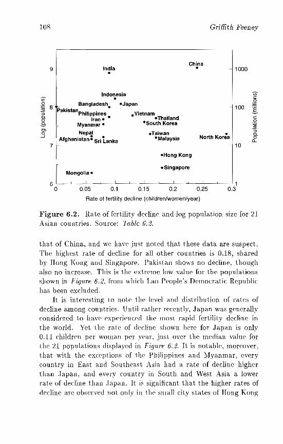
108

9 India•

China•

Griffith Feeney

-I 1000

Indonesia•c

o§ 8:::Ja.oSOJ

.37

Bangladesh.

PakistanphiliPPines •Iran·

Myanmar •

NepaJ •Afghanistan. Sri Lanka

.Japan

.Vietnam.Thailand

·South Korea

.Taiwan·Malaysia

-I 100

•North Korea

~10

Ulc~Ico~:5a.o

U.

.Hong Kong

• SingaporeMongolia.

6 I I I J 1o 0.05 0.1 0.15 0.2 0.25 0.3

Rate of fertility decline (children/women/year)

Figure 6.2. Rate of fertility decline and log population size for 21Asian countries. Source: Table 6.2.

that of China, and we have just noted that these data are suspect.The highest rate of decline for all other countries is 0.18, sharedby Hong Kong and Singapore. Pakistan shows no decline, thoughalso no increase. This is the extreme low value for the populationsshown in Figure 6.2, from which Lao People's Democratic Repu blichas been excluded.

It is interesting to note the level and distribution of rates ofdecline among countries. Until rather recently, Japan was generallyconsidered to have experienced the most rapid fertility decline inthe world. Yet the rate of decline shown here for Japan is only0.11 children per woman per year, just over the median value forthe 21 populations displayed in Figure 6.2. It is notable, moreover,that with the exceptiolls of the Philippines and Myanmar, everycountry in East and Southeast Asia had a rate of decline highertha,n Japan, and every country in South and West Asia a lowerrate of decline than Japan. It is significant that the higher rates ofdecline are observed not only in the small city-states of Hong Kong

Fertility in China: Past, Present., Prospects 109

and Singapore, but also in the large nations of Malaysia, Vietnam,and Thailand.

The inverted V pattern in the plot is particularly notable.Smaller countries tend to have either relatively high or relativelylow rates of fertility decline, with a convergence toward the medianas size increases. Perhaps this reflects the possibility that, in the dif­fusion of modernization, small countries may be bypassed altogetherfor a time, but may also modernize rapidly once the process begins,whereas larger countries cannot escape modernizing influences, buttend to react more slowly to them.

6.2 China's Fertility Decline:A Closer Look

Looking at total fertility rates for quinquennial periods obscures im­portant details of China's fertility decline. In this section we exam­ine several single-year time series to provide a more precise picture offertility decline, a picture that may then be compared with govern­ment population policy initiatives. Incidentally, we present evidenceof the accuracy of the data from which these fertility statistics arecalculated. While certainly not perfect, the Chinese data are supe­rior to those available for most countries in the world, developed aswell as developing.

Figure 6.3 shows conventional total fertility rates for China from1965 through mid-1987.[2] We are in fact looking at two differentseries here, shown in the first two columns in Table 6.3. The first,plotted wit h solid dots, is calculated from age-specific birth rates(ASBR) derived from the birth histories collected in the 1982 One­per-Thousand Fertility Survey conducted by the State Family Plan­ning Commission (see China Population Information Center, 1984;Coale, 1984; Coale and Chen, 1987). The values shown are thosegiven in Coale and Chen (1987), though these hardly differ fromthose reported in the first survey (China Population InformationCenter, 1984). These values are for calendar years.

The second series in Figun, 6.3, plotted with small circles, is cal­culated from age-specific birth rates derived from birth histories re­constructed from a 10 percent sample of the 1987 One-per-Hundred

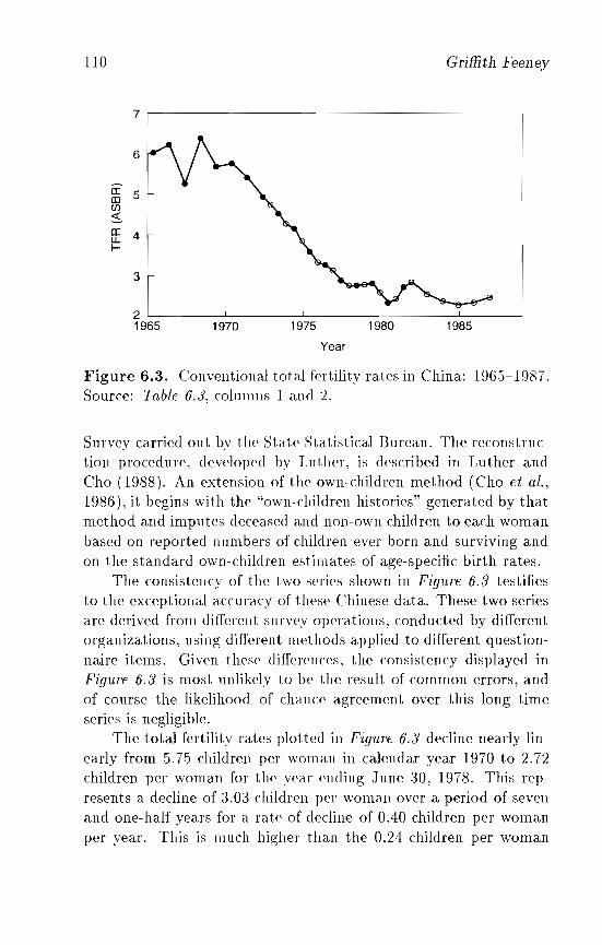
110

7

6

C? 5Inen~

fE 4~

3

21965 1970 1975

Year

1980

Griffith Feeney

1985

Figure 6.3. Conventional total fertility rates in China: 1965-1987.Source: Table 6.3, columns 1 and "2.

Survey carried out by tILe State Statistical Bureau. The reconstruc­tion procedure, developed by Lnther, is described in Luther andCho (1988). An extension of the own-children method (Cho et al.,

1986), it begins with the "own-children histories" generated by thatmethod and imputes deceased and non-own children to each womanbased on reported numbers of children ever born and surviving andon the standard own-children estimates of age-specific birth rates.

The consistency of the two series shown in Figure 6.3 testifiesto the exceptional accura.cy of these Chinese data. These two seriesare derived from different sLlrvey operations, conducted by differentorganizations, using different methods applied to different question­naire items. Given these differellces, the consistency displayed inFigure 6.:J is most unlikely to be the result of common errors, andof course the likelihood of chance agreement over this long timeseries is negligible.

The total fertility rates plotted in Figure 6.3 decline nearly lin­early from 5.7.5 children per woman in calendar year 1970 to 2.72children per woman for the year ending .Tune 30, 1978. This rep­resents a decline of 3.0:3 children per woman over a period of sevenand one-half years for a rate of decline of 0.40 children per womanper year. This is much higher than the 0.24 children per woman

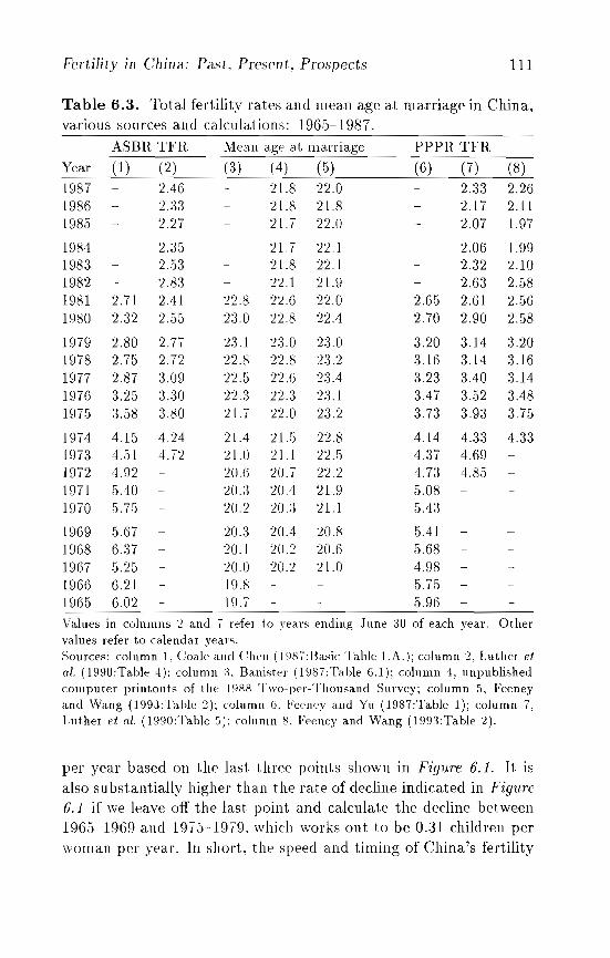
Fertility in China: Past, Present, Prospects III

Table 6.3. Total fertility rates and mean age at marriage in China,various sources and calculations: 1965-1987.

ASBR TFR Mea.n a.ge at ma.rriage PPPR TFR

Year (1) (2) (3) (4) (5) (6) (7) (8)

1987 2.46 21.8 220 2.33 2.261986 2.:~3 21.8 21.8 2.17 2.111985 2.27 21.7 22.0 2.07 1.97

1984 2.:35 21.7 22.1 2.06 1.991983 2.53 21.8 22.1 2.32 2.101982 2.83 22.1 21.9 2.63 2.581981 2.71 2.41 22.8 22.6 22.0 2.65 2.61 2.561980 2.32 2.55 2:3.0 22.8 22.4 2.70 2.90 2.58

1979 2.80 2.77 23.1 23.0 2:3. 0 3.20 3.14 :~.20

1978 2.75 2.72 22.8 22.8 23.2 3.16 3.14 3.161977 2.87 3.09 22.5 22.6 23.4 3.23 3.40 3.141976 3.25 :UO 22.3 22.:3 n.1 3.47 3.52 3.481975 3.58 3.80 21.7 22.0 2:3.2 3.73 3.93 3.75

1974 4.15 4.24 21.4 2Ui 22.8 4.14 4.33 4.331973 4.51 4.72 21.0 21.1 22.5 4.37 4.691972 4.92 20.6 20.7 22.2 4.73 4.851971 5.40 20.3 20.4 21.9 5.081970 h -" 20.2 20.:3 21.1 5.4:~;). (.)

1969 567 20.:3 20.4 20.8 .5.411968 6.:n 20.1 20.2 20.6 5.681967 .5.25 20.0 20.2 21.0 4.981966 6.21 19.8 5.751965 6.02 19.7 5.96

Values in colnmns 2 and I refer to ~'eaTS ending .J nne 30 of each year. Othervalues refer to calendar years.Sources: colnmn 1. Coale and Chen (19NI:Basic Table 1.A.); column 2. Luther etal. (1990:Table 4); column :l. Banister (1987:Table 6.1); column 4, unpublishedcomputer printouts of the 191'8 Two-per-Thousand Survey; column 5, Feeneyand Wa.ng (l993:Ta.ble 2); column G. Feeney and Yu (1987:Table 1); column 7,Luther et al. (1990:Table 5): column 8. Feeney and Wang (1993:Table 2).

per year based on the last tlm:~e points shown in Figure 6.1. It isalso substantially higher than t he rate of decline indicated in Figure6.1 if we leave off the last point and calculate the decline between196Ei-1969 and 1975-1979. which works out to be 0.31 children perwoman per year. In short, the speed and timing of China's fertility

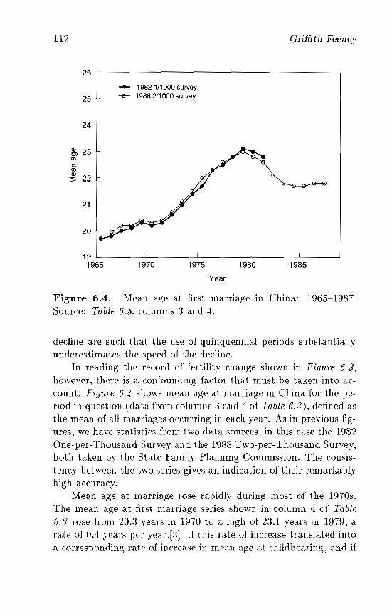
112 Griffith Peeney

26

...... 19821/1000 survey

25 1- -- 1988 2/1000 survey

24

~ 23CllcCllQ)

~ 22

21

20

198519801975197019 ! ! ! !

1965

Year

Figure 6.4. Mean age at first marriage in China: 196.5-1987.Source: Table 6.3, columns 3 and 4.

decline are such that the use of quinquennial periods substantiallyunderestimates the speed of the decline.

In reading the record of fertility change shown in Figure 6.3,however, there is a confounding factor that must be taken into ac­count. Figure 6.4 shows mean age at marriage in China for the pe­riod in question (data from columns :3 and 4 of Table 6.3), defined asthe mean of all marriages occurring in each year. As in previous fig­ures, we have statistics from two data sources, in this case the 1982One-per-Thousand Survey and the 1988 Two-per-Thousand Survey,both taken by the State Family Planning Commission. The consis­tency between the two series gives an indication of their remarkablyhigh accuracy.

Mean age at marriage rose rapidly during most of the 1970s.The mean age at first marriage series shown in column 4 of Table6.3 rose from 20.:3 years in 1970 to a high of 23.1 years in 1979, arate of 0.4 years per year.[:3] If this rate of increase translated intoa corresponding rate of increase in mean age at childbearing, and if

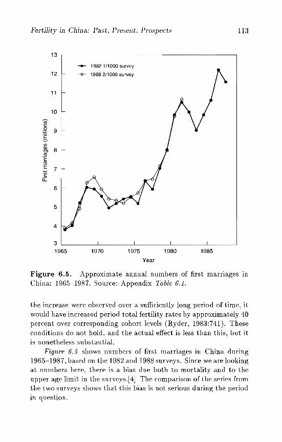
Fertility in China: Past, Present, Prospects 113

-- 1982 1/1000 survey

-e- 1988 2/1000 survey

13

12

11

10

(j)cg 9

IlJJ

~ 8ltl'CIt;E 7§u::

6

5

4

31965 1970 1975

Year

1980 1985

Figure 6.5. Approximate annual numbers of first marriages III

China: 196.5-1987. Source: Appendix Table 6.1.

the increase were observed over a sufficiently long period of time, itwould have increased period total fertility rates by approximately 40percent over corresponding cohort levels (Ryder, 1983:741). Theseconditions do not hold, and the actual effect is less than this, but itis nonetheless substantial.

Figure 6.5 shows numbers of first marriages in China during196.5-1987, based on the 1982 and 1988 surveys. Since we are lookingat numbers here, there is a bias due both to mortality and to theupper age limit in the surveys.[4] The comparison of the series fromthe two surveys shows that this bias is not serious during the periodin question.

114 Griffith Feeney

The striking feature of Figure 6.5 is the extraordinary rise innumbers of marriages between the late 1970s and the early 1980s.During the late 1960s and middle to late 1970s, we observe 5 to6 million first marriages per year. During the 1980s the numbersrange from slightly under 10 million in 1984 to over 12 million in1986, fully twice the level of the 1970s.

This jump in marriages exerts a powerful upward influence onbirth rates. Since virtually all Chinese women have a first birthwithin a few years of first marriage,[5] the increases in numbers offirst marriages translate almost directly into a slightly lagged in­crease in numbers of first births. Thus in Appendix Tables 6.1 and6.2 we see that annual numbers of first births rise from about 5million during the mid-1970s to about 10 million during the mid­1980s. This increase is due not to any change in the childbearingbehavior of Chinese women, but to the rapidly increasing numbersof recently married women. If we choose to interpret the total fer­tility rates shown in Figure 6.·] merely as indicators of numbersof births, these observations are irrelevant. If we wish to interpretthem as indicators of childbearing behavior, however, it is necessaryto recognize that they are distorted by the rapid changes in age atmarriage and numbers of marriages during the period in question.

6.3 Period Parity Progression Measuresof Fertility

The simplest approach to dealing with the effects of changing mar­riage patterns on the conventional fertility measures presented in thepreceding section is to use alternative measures that are less sensi­tive to changing marriage patterns. Period parity progression ratios(PPPRs) calculated from birth probabilities specific for parity andbirth interval provide an effective way to do this. In the calculationof probabilities of progression from marriage to first birth, for exam­ple, numbers of women marrying each year and the correspondingnumbers of married women remaining in parity zero appear in thedenominator of each birth probability, whence an increase in num­bers of marriages from one year to the next does not imply anyincrease in the proportion of women progressing to first birth.

Fertility in China: Past, Present, Prospects 115

The parity progression approach to fertility measurement askswhat proportions of women move from one childbearing event to thenext. Of all women born, wha t proportion have a first birth? Of allwomen who have a first birth, what proportion go on (progress) tohave a second, and so on'? The answers may be derived from parityprogression mtio8, and like other demographic measures, they maybe calculated on a period as well as on a cohort basis. (For a generaldiscussion of period parity progression ratio measures of fertility, seeFeeney and Lutz, 1991. For applications to China, see Feeney andWang, 1993; Feeney and Yu, 19:-(7: Feeney et al., 1989; Luther etal., 1990). For populations in which fertility is restricted to marriedcouples, as in China, it is useful to break down the proportion ofwomen ever having a first birth into two multiplicative components:the proportion of women who ever ma.rry and the proportion ofmarried women who ever have a first birth.

Total fertility rates may be calculated from period parity pro­gression ratios as well as from age-specific birth rates, and the logicof the calculation is para.Jlel. We ask what average number of chil­dren would be born to a hypothetical cohort of women that expe­rience the parity progression ratios observed during a given timeperiod. The formula is easily shown to be (see, for example, Feeneyand Yu, 1987)

TFR = Po +Polh + ]JO]Jl}J2 +...A convenient approximation for use with incomplete series of

parity progression ratio:-i is given by replacing the last term in theseries by it.self divided b.v 1-p", where p" is the last available ratio.[6]

Period parity progression ratios are unusual fertility measures,even within the field of demography, and it will be useful to pro­vide some examples of their values for different countries.[7] Table

6.4 assembles schedules of parity progression ratios for a variety ofhigh- and low-fertility countries. Progression to marriage and firstand second births is generally high for both high- and low-fertilitycountries. Among the high-fertility Hutterites, some 97 percent ofall married women have' at least one child. In China, virtually allwomen married and had a first birth, both before fertility began todecline (1965) and after it had declined nearly to replacement level(1982).[8] The lowest levels of progression from marriage to firstbirth occur in low-fertility countries, to be sure, but even here it is

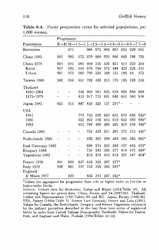
116 Griffith Feeney

Table 6.4. Parity progression ratios for selected populations, per1,000 women.

Progression

Canada 1985

Netherlands 1985

East Germany 1985­Hungary 1984Yugoslavia 1982

Population

Hutterites

China 1965

China 1979RuralUrban

Taiwan 1986

Thailand1960-19641975-1979

Japan 1982

USA194119601984

France 1976Italy 1978England

& Wales 1977

B--+M M--+ 1 0--+1 1--+2 2----+3 3--+4 4--+5 5--+6 6--+7 7--+8

971 - 988 972 968 967 953 929 905

990 982 972 979 964 929 886 845 786 720

994 991 985 959 700 539 431 414 322 309997 992 989 978 759 572 448 422 328 310981 979 960 799 259 168 131 185 44 373

992 959 951 782 428 212 170 185 198 216

948 966 951 925 918 890 859 800813 917 771 681 646 610 580 548

925 916 847 856 320 137 221 a -

779 745 628 639 651 670 666 635a

923 922 746 645 619 650 682 689 a

802 789 488 386 382 419 439 456a

793 423 301 287 370 412 430 a

835 382 298 363 483 555 562 a

688 274 300 366 427 443 422a

750 242 249 377 414 470 458a

815 318 416 518 567 547 464a

891 939 837 645 325 267 277a ­

926 861 797 739 345 280 287 a-

829 - 855 347 267 241 a -

aValues are aggregates for progression from i-th or higher order to (i+1)st orhigher-order births.Sources: Cohort data for Hutterites, Eaton and Mayer (1954:Table 10). Allremaining figures are period data. China, Feeney and Yu (1987:81). Thailand,Luther and Pejaranondam (1991:Tables Bl and B2). Japan, Feeney (1986:20).USA, Feeney (1988a:TabIe 1). Former East Germany, Feeney and Lutz (1991).Values for Canada, the Netherlands, Hungary, and former Yugoslavia estimatedby the indirect procedure described in the text from time series of registeredbirths by order from United Nations Demographic Yearbooks. Values for France,Italy, and England and Wales, Penhale (1984:Tables 12-14).

Fertility in China: Past, Present, Prospects 117

unusual for less than 80 percent of women who have a first birth togo on to have a second.

The difference between high- and low-fertility populations isgreatest in the higher-order parity progression ratios, and most im­portantly in the proportion of women progressing from second tothird birth. In a high-fertility population - the high-fertility Hut­terites, China in 1965, and Thailand in 1960-1964 - parity progres­sion ratios decline slowly with increasing parity, remaining in the70 to 90 percent range even for progression from seventh to eighthbirth. In a low-fertility population, however, progression from sec­ond to third birth is sharply lower than progression to first or fromfirst to second. The values shown in Table 6.4 range from a low of24 percent for Hungary to a high of 75 percent for the United Statesnear the height of the baby boom, but this last value is atypicallyhigh. The normal range for progression from second to third birthin low-fertility populations is 25 to 50 percent.

Higher-order parity progression ratios in low-fertility popula­tions are surprisingly high - the median value for progression fromseventh to ninth birth for the low-fertility countries in Table 6.4 is44 percent. There can be little doubt that this reflects a selectioneffect. In a low-fertility population, the only women who reach highparities are necessarily highly fecund, regularly exposed to the riskof conception, and either nonusers or inept users of contraception.These relatively high parity progression ratios have little effect onthe overall level of fertility, however, since only a small fraction ofwomen reach high parities.

6.4 Period Parity Progression Measures ofFertility in China

Total fertility rates calculated from period parity progression ratiosare plotted in Figure 6.6. Here as in Figure 6.3 we have valuesboth from the 1982 One-per-Thousand Fertility Survey conductedby the State Family Planning Commission and from the 1987 One­per-Hundred Survey conducted by the State Statistical Bureau, andthe consistency of the two series attests to their accuracy.

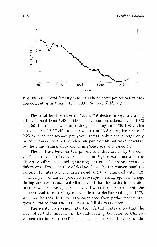
118

7

6

Ii' 5a...a...~a: 4u.I-

3

21965 1970 1975

Year

1980

Griffith Feeney

1985

Figure 6.6. Total fertility rates cakulated from period parity pro­gression ratios in China: L96.1-198'1. Source: Table 6.;]

The total fertility rates in Figure 6.6 decline irregularly alonga linear trend from .1.4:3 children per woman in calendar year 1970to 2.06 children per woman in the year ending June 30, 1984. Thisis a decline of :3.3'1 children per woman in 13.5 years, for a rate of0.25 children per woman per year - remarkably close, though onlyby coincidence, to the 0.24 children per woman per year indicatedby the quinquennial data shown in Figure 6.1 and Table 6.1.

The contrast between this picture and that shown by the con­ventional total fertility rates plotted in Figure 6.;] illustrates thedistorting effects of changing marriage patterns. There are two maindifferences. First. the rate of decline shown by the conventional to­tal fertility rates is much more rapid. 0.40 as compared with 0.25children per woman per year. because rapidly rising age at marriageduring the 1980s caused a decline beyond that due to declining child­bearing within marriage. Second. and what is more important, theconventional total fertility rates indicate a decline ending in 1978,whereas the total fertility rates calculated from period parity pro­gression ratios continue until 1984, a full six years later.

The parity progression ratio total fertility rates show that thelevel of fertility implicit in the childbearing behavior of Chinesewomen continued to decline until t he mid-1980s. Because of the

Fertility in China: Past, Present, Prospects 119

tremendous surge of marriages beginning in the late 1970s, thiscontinuing behavioral change is completely obscured by the con­ventional total fertility rates. The conventional total fertility ratessuggest that fertility clecline in China ended, at least temporarily,in 1979. This was precisely the year in which a major new policyinitiative, the one-child family program, was taken. The time se­ries of conventional total fertilit~, rates suggest that the new policywas unsuccessful. In fact, as we see below, it achieved considerablesuccess.

One advantage of total fertility rates calculated from period par­ity progression ratios is superior control over the distorting effectsof changing marriage patterns. A second advantage, and one partic­ularly important in the Chinese context, is the correspondence es­tablished with the period paTity progression ratios themselves. Thelevel of progression from first to second birth, in particular, reflectsthe demographic impact of the one-child family policy.

Table 6.5 and Figure 6.7 show period parity progression ra­tios and the corresponding total fertility rates for the years 1967­1987 calculated from the 1988 Two-per- Thousand Fertility Surveyconducted by the State Family Planning Commission (Feeney andWang, 1993; see also Lavely, 1991). Because progression to firstmarriage is virtually const ant at close to one throughout the periodshown, Figure 6.7 shows proportions of women progressing to firstbirth (B~l), the product of women progressing to first marriage(B~M) and women progressing from first marriage to first birth(M ----+ 1), rather than showing these two series separately.

Figw'e 6.7 shows that proportions of women ever having a firstbirth have been high, about 95 percent, throughout the period con­sidered. Fertility decline has resulted entirely from declines in pro­gression to higher-order births. Progression from first to secondbirth, in particular, shows the impact of the one-child family pro­gram. In 1979, the year the program was introduced, 95 percentof all women were progressing from first to second birth. By 1984,after the policy had been in effect for only five years, progression tosecond birth had been reduced to 6:1 percent. That year, however,marked a relaxation in the policy, and progression to second birthrose continuously through 1987, the last year of the series, at whichpoint it stood at 76 percent.

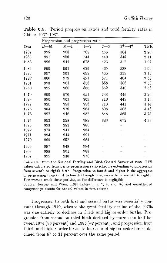
120 Griffith Feeney

Table 6.5. Period progression ratios and total fertility rates inChina: 1967-1987.

Progression and progression ratio

Year B--+M M--+1 1--+2 2--+3 3+ --+4+ TFR

1987 995 968 765 466 384 2.261986 997 950 734 440 345 2.111985 996 944 678 423 312 1.97

1984 999 961 626 465 338 1.991983 997 963 695 465 339 2.101982 1000 979 821 571 404 2.581981 998 963 858 558 388 2.561980 999 960 886 562 340 2.58

1979 999 970 951 743 446 3.201978 996 96:3 969 710 442 3.161977 996 958 958 713 441 3.141976 983 970 964 808 508 3.481975 992 946 982 848 565 3.75

1974 992 958 985 883 672 4.331973 993 952 9861972 973 941 9841971 994 944 9911970 999 952 984

1969 997 948 9841968 998 961 9881967 999 930 970

Calculated from the National Fertility and Birth Control Survey of 1988. TFRvalues calculated from parity progression ratio schedule extending to progressionfrom seventh to eighth birth. Progression to fourth and higher is the aggregateof progression from third to fourth through progression from seventh to eighth.Few women reach these parities, so the difference is negligible.Source: Feeney and Wang (1993:Tables 3, 5, 7, 9, and 16) and unpublishedcomputer printouts for annual values in first column.

Progression to both first and second births was essentially con­

stant through 1979, whence the great fertility decline of the 1970swas due entirely to declines in third- and higher-order births. Pro­

gression from second to third birth declined by more than half be­tween 1974 (88 percent) and 1985 (42 percent), and progression from

third- and higher-order births to fourth- and higher-order births de­clined from 67 to 31 percent over the same period.

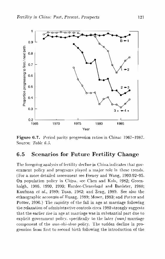
Fertility in China: Past, Present, Prospects 121

0.9£t:::cx 0.8Qlc

~ 0.7

.8Cl£ 0.6enen~Cl

e 0.5c..co

E 0.4c..oc::

0.3 3 + --4 +

19851980197519700.2 I ! I I I

1965

Year

Figure 6.7. Period parity progression ratios in China: 1967-1987.Source: Table 6.5.

6.5 Scenarios for Future Fertility Change

The foregoing analysis of fertility decline in China indicates that gov­ernment policy and programs played a major role in these trends.(For a more detailed assessment see Feeney and Wang, 1993:92-95.On population policy in China, see Chen and Kols, 1982; Green­halgh, 1986, 1990, 1993; Hardee-Cleaveland and Banister, 1988;Kaufman et al., 1989; Tuan, 1982; and Zeng, 1989. See also theethnographic accounts of Huang, 1989; Moser, 1983; and Potter andPotter, 1990.) The rapidity of the fall in age at marriage followingthe relaxation of administrative controls circa 1980 strongly suggeststhat the earlier rise in age at marriage was in substantial part due toexplicit government policy. specifically to the later (wan) marriagecomponent of the wan-8hi-shao policy. The sudden decline in pro­gression from first to second birth following the introduction of the

122 Griffith Feeney

one-child family program in 1979 and the subsequent rise followingthe relaxation of 1984 are even stronger evidence that this particularcomponent of fertility decline was due largely to government policy.

The structure of China's birth-planning efforts and the attentionand resources allocated to them make this remarkable effectivenessmore plausible than it might otherwise be. Government policy waseffective despite imperfect implementation. Substantial proportionsof men and women married beneath the prescribed ages in the 1970s,for example, but the encouragement to marry later did result in avery substantial increase in mean age at marriage. Even at the peakof its effectiveness, the one-child family program saw well over halfof all Chinese women having two or more children, but the programnonetheless had a substantial and continuing effect on fertility levels.

In considering future fertility trelLds, then, it makes sense to em­phasize the role of government policy. The centerpiece of China'scurrent birth-planning efforts is still the one-child family policy in­troduced in 1979, but this simple statement conceals a more com­plicated demographic rea1ity. One-child families llave been realizedamong most of the urban population, with progression from first tosecond birth in recent years between 10 and 20 percent (Feeney andWang, 199~~:Table G..5). The one-child family remains the officialpopulation policy in rural areas as well, but numerous adaptationsbelie the "one-child" labeL and progression from first to second birthin recent years has been around 85 percent. At the national level,progression from first to second birth in rural areas rose from a lowof G3 percent in 1984 to 7G percent in 1987 (Figure 6.7), with a.continued increase indicated.

This discussion of scenarios is limited to high and low extremesover the next two decades. A lligh trajectory is obtained by as­suming a continued relaxation of the one-child family policy, withprogression from first to second birth rising to about 95 percent,the level observed before the introduction of the policy in 1979; andwith progression from second to third birth rising modestly from47 to G2 percent, both plausible extrapolations of recent experience.This yields total fertility rates rising fro111 2.3 in 1987 to 2.5 in 1990,to 2.7 in 1995 and 2000. and finally to 2.8 in 2005.

A low trajectory is obtained by assuming implementation ofthe one-child policy in rural as well as urban areas, but assuming

Fertility in China: Past, Present, Prospects 123

both a somewhat higher level of progression from first to secondbirth than has been achieved in cities (30 percent as opposed toabout 15 percent recently) and a slower rate of decline (15 years forrural areas as compared with only four years for cities). Progressionfrom second to third birth is assumed to decline as well, though thevery low values of progression from first to second birth make thisrelatively unimportant. This ~'ields total fertility rates falling from2.3 in 1987 to 2.2 in L990, to 1. 7 in 1995, to 1.5 in 2000, and finallyto LA in 2005.

Between now and the beginning of the next century, we expectfertility in China not to exceed 2.7 children per woman or to fallbelow 1.5 children per woman.

6.6 The Scenarios Compared with RecentEvidence

The analysis and scenarios of the preceding sections are based onannual data on total fertility rates through 1987, the most recentavailable at the time the projections were made.[9] Detailed es­timates of fertility levels from the L990 population census becameavailable as the chapter went to press, too late to be incorporatedinto the scenario analysis. At this writing we have, in addition to thecensus results, fertility rates throngh 1991 calculated from a 1992fertility survey (Feeney and Yuan, 1994) and rates through L995indirectly estimated from published data on crude birth and deathrates through 199·) (Yuan. 1995). How well do the scenarios of thepreceding section stand up to recent evidence? Does the comparisonindicate that they should t hey be revised'?

The level of fertility rose over the period 1984-1987, and thoughthe magnitude of the increase was small, there were grounds, at thetime, for thinking that it might continue. In no large country (andalmost no small country) had fertility fallen as rapidly as it didin China during the L970s. This rapid decline was due in part tovigorous government policy measures. The one-child family policywas relaxed in the mid-1980s. partly as a result of peasant resistance,and it was conceivabl(· that the relaxation wonld continue. The highscenario for future fertility change anticipated this contingency andshowed fertility rising to 2.8 children per woman in 2005.

124 Griffith Feeney

Fertility estimates from the 1990 census show, however, that1988 was a turning point (Feeney et al., 1993).[10J The total fertil­ity rate declined between 1988 and 1990 as quickly as it had risenfrom 1985 to 1988. This reversal reconfirms the invalidity of simpleextrapolation and makes the low scenario for future fertility change,in which fertility falls to 1.4 children per woman in 2005, seem moreplausible.

The low-fertility scenario is both supported and confounded bythe results of a 1992 fertility survey taken by the State Family Plan­ning Commission. This survey shows a total fertility rate calculatedfrom age-specific birth rates of 1.65 children per woman for 1991.Few informed observers in or outside China believe that fertilitywas really this low. however, and initially the survey served mainlyto cast doubt not only on its O\\ln validity, but on that of previousefforts to measure fertility levels as well.

A detailed analysis of the 1992 data indicates that the surveyresults were not so poor as initially suspected (Feeney and Yuan,1994). Retrospecti \Ie estimates of total fertility rates for 1986-1989from the survey agree very well with the estimates from the 1990census and the 1990 total fertility rate is a plausible continuation ofthe trend. The very low value for 1991 was the result of a sharp dropfrom 1990, and it is likely that the 1991 figure is too low by about10 percent, but there is little statistical evidence of more seriousunderreporting.

The possibility of consistent errors is discussed in detail inFeeney and Yuan (1994:391<393). While it is possible that Chi­nese women have consistently unclerreported numbers of childrenin all the national-level data, we conclude that it is unlikely thatsuch consistent underreporting has biased observed fertility levelsby more than a few tenths of a child per woman.

Figu're 6.8 compares the 1988 TFR series given in Table 6.5and the high- ancllow-scenario TFR series (plotted with triangles)with corresponding estimates from the 1990 census (Feeney et al.,

1993) and age-specific total fertility rates from annual surveys con­ducted by the State Statistical Bureau (Yuan, 1995).[11J The lastmentioned series is not strictly comparable to the others, but dis­parities are likely to be small, and the extension of the observedseries through 1995 makes it worth including.[12J

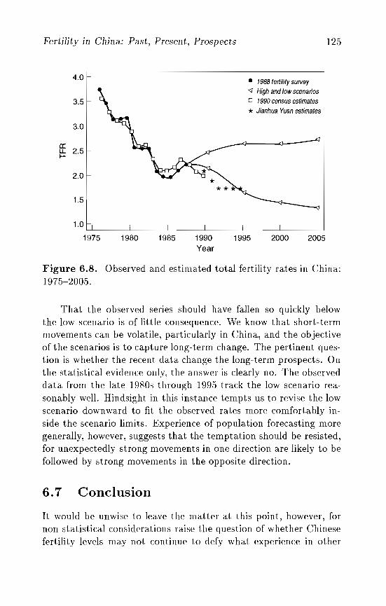
Fertility in China: Past, Present, Prospects 125

• 1988 fertility survey<1 High and low scenarioso 1990 census estimates

* Jianhua Yuan estimates

4.0

3.5

3.0

II:~ 2.5

2.0

1.5

1.0LL

1975 1980 1985 1990Year

1995 2000 2005

Figure 6.8. Observed and estimated total fertility rates in China:1975-2005.

That the observed series should have fallen so quickly belowthe low scenario is of little consequence. We know that short-termmovements can be volatile, particularly in China, and the objectiveof the scenarios is to capture long- term change. The pertinent ques­tion is whether the recent data change the long-term prospects. Onthe statistical evidence only, the answer is clearly no. The observeddata from the late 1980s through 1995 track the low scenario rea­sonably well. Hindsight in this instance tempts us to revise the lowscenario downward to fit the observed rates more comfortably in­side the scenario limits. Experience of population forecasting moregenerally, however, suggests that the temptation should be resisted,for unexpectedly strong movements in one direction are likely to befollowed by strong movements in the opposite direction.

6.7 Conclusion

It would be unwise to leave the matter at this point, however, fornon-statistical considerations raise the question of whether Chinesefertility levels may not continue to defy what experience in other

126 Griffith Feeney

countries teaches. Chinese population policy over the past 25 yearshas been tenaciously and effectively anti- natalist. The one-childfamily policy has been in place for over 15 years, and though it waseffectively loosened in the mid-1980s to allow a second child to manyrural families, there are no serious indications that it will be aban­doned. Further declines in fertility may not be in China's long-terminterest, but the negative consequences are speculative and appearmostly in the very long term. It is possible that the Chinese lead­ership will continue to push the one-child family policy. Perceptionof population pressure may override anticipation of future problemsand the sheer momentum of:25 years of incessant and determinedefforts to lower fertility may make it difficult to change course.

Over the past 15 years various social forces have kept the one­child policy from being fully implemented. It is possible that thiswill change in the future. Economic liberalization and opening tothe outside world have led to very rapid economic growth. This hasled to great opportunity for Chinese families able to exploit the newsituation, and to great uncertainty and anxiety for other familieswhose livelihoods are threatened. Both groups are likely to respondby having fewer children in the short run, and perhaps in the not soshort run.

Could this combination of influences result in long-term fertilitylevels substantially below the 1.4 children per woman anticipatedby the low scenario for future fertility change? My judgment isthat Chinese fertility is unlikely to fall below an average level of 1.4children per woman over the next two decades, though temporarydeclines below this level are possible.

There is very little basis for speculation about the extendedlong-term future of fertility. The only thing that can be said withany semblance of scientific support is that world demographic trendsto date suggest that a plausible range is between 1.5 and 3 childrenper woman. It is a reasonable supposition that levels and trendsof fertility over the past few decades contain information about thelikely trends over the next few decades, and that is the basis of theseconclusions about fertility in China through the early years of thenext century. Recent levels and trends cannot plausibly be expectedto contain any information about detailed levels 50 or 100 years intothe future, however. Assumptions about these more distant levels

Fertility in China: Past, Present, Prospects 127

must either be regarded as purely formal or be made on some basisother than a study of recent levels and trends.

Notes

[1] Since fertility decline occurs during different periods in different coun­tries, it makes little sense to compute rates of decline for the sameperiod for all countries. At tlIP same time, choosing a suitable timeperiod over which to compute a rate of decline involves an elementof judgment, if not of arbitrariness. The periods shown in Table 6.1have been selected by examining the plot of the TFR trend in eachcountry. Because we are interested in showing how different Chinais from other countries, we have chosen periods to give larger ratherthan smaller rates of declines for all other countries.

[2] "Conventionar total fertility rates means rates calculated from age­specific birth rates. These are to lw distinguished from total fertilityrates calculated from ]wriod parity progression ratios, discussed inSection 6.:3.

[3] Columns 3 and 4 of Table 6.3 show mean age at first marriage calcu­lated directly as the mean of all first marriages occurring during theindicated year. Column 5 shows mean age at first marriage calculatedfrom first marriage probabilities, i.e., for the period nuptiality table,for the given year. The former statistic is more readily computed andmore common. The latter has the advantage of being uninfluenced bychanging age distribution. All three series show a sharp rise in meanage at marriage. Comparing the plot of the nuptiality table values(not shown) with Figure 6.4 shows sharp divergences between the twotypes of means. See Feeney and Wang (1993:70-71) for discussion ofthese differences and their significance.

[4] The 1982 survey included women less than exact age 68 years; the1988 survey, women less than exact age 58 years.

[5] The evidence of this is given below in the form of period parity pro­gression ratios for progression from marriage to first birth. See Table6.5 and the corresponding text discussion.

[6] The approximation assumes that parity progression ratios beyond Pnare identically equal to Pn. Although not in the least realistic, theapproximation is very good as long as Pn is not too large, whichin practice means not much over one-half. The 1-Pn arises from ageometric series, as a little algebra readily shows.

[7] The reasons for this are beyond the scope of the present discussion:for more information seC' Feeney and Lutz (1991:186-187).

[8] The value shown for the proportion of married women having a firstbirth is probably too high, one of the relatively few imperfections in

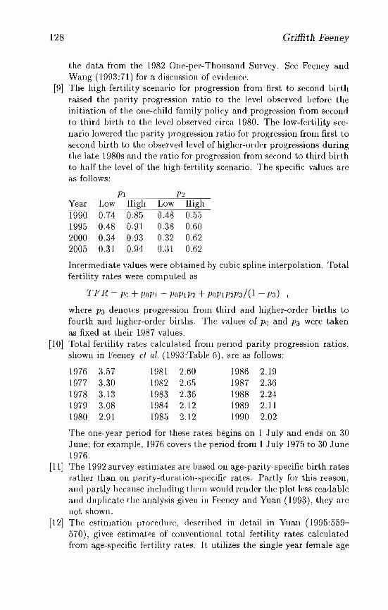
128 Griffith Feeney

the data from the 1982 One-per-Thousand Survey. See Feeney andWang (1993:71) for a discussion of evidence.

[9] The high-fertility scenario for progression from first to second birthraised the parity progression ratio to the level observed before theinitiation of the one-child family policy and progression from secondto third birth to the level observed circa 1980. The low-fertility sce­nario lowered the parity progression ratio for progression from first tosecond birth to the observed level of higher-order progressions duringthe late 1980s and the ratio for progression from second to third birthto half the level of the high-fertility scenario. The specific values areas follows:

171 172Year Low High Low High1990 0.74 0.85 0.48 0.551995 0.48 0.91 0.38 0.602000 0.34 0.93 0.32 0.622005 0.31 0.94 0.31 0.62

Intermediate values were obtained by cubic spline interpolation. Totalfertility rates were computed as

T F R = Po + 170171 + 170171])2 + 170171172173/(1 - 173) ,

where 173 denotes progression from third and higher-order births tofourth and higher-order births. The values of Po and 173 were takenas fixed at their 1987 values.

[10] Total fertility rates calculated from period parity progression ratios,shown in Feeney et at. (1993:Table 6), are as follows:

1976 3.57 1981 2.60 1986 2.191977 3.30 1982 2.65 1987 2.361978 3.13 1983 2.36 1988 2.241979 3.08 1984 2.12 1989 2.111980 2.91 1985 2.12 1990 2.02

The one-year period for these rates begins on 1 July and ends on 30June; for example, 1976 covers the period from 1 July 1975 to 30 June1976.

[11] The 1992 survey estimates are based on age-parity-specific birth ratesrather than on parity-duration-specific rates. Partly for this reason,and partly because including them would render the plot less readableand duplicate the analysis given in Feeney and Yuan (1993), they arenot shown.

[12] The estimation procedure, described in detail in Yuan (1995:559­570), gives estimates of conventional total fertility rates calculatedfrom age-specific fertility rates. It utilizes the single-year female age

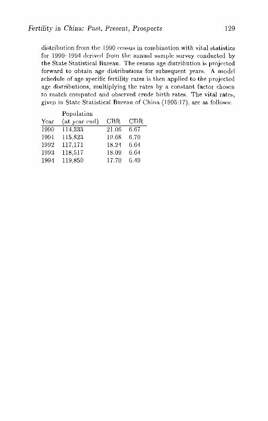
Fertility in China: Past, Present, Prospects 129

distribution from the 1990 census in combination with vital statisticsfor 1990-1994 derived from t.he annual sample survey conducted bythe State Statistical Bureau. The census age distribution is projectedforward to obtain age distributions for subsequent years. A modelschedule of age-specific fertility rates is then applied to the projectedage distributions, multiplying the rates by a constant factor chosento match comput.ed and observed crude birth rates. The vital rates,given in State Statistical Bureau of China (1995:17), are as follows:

PopulationYear (at year end) CBR CDR1990 114,333 21.06 6.671991 115,823 19.68 6.701992 117,171 18.24 6.641993 118,517 18.09 6.641994 119,850 17.70 6.49

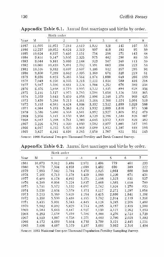
130 Griffith Feeney

Appendix Table 6.1. Annual first marriages and births by order.

Birth order

Yea.r M 1 2. :3 4 5 6 7 8

1987 11,605 11,951 7,28.3 2,619 1,022 321 145 107 551986 12,237 10,055 6,624 2,:319 897 418 193 95 591985 10,624 8,937 5,416 2,151 754 298 275 143 481984 9,851 9,147 5,056 2,.325 975 442 290 89 591983 9,044 9,161 5,060 2,148 923 547 348 113 591982 10,001 10,459 5,491 2,702 1,:391 663 398 223 531981 10,516 9.332 4,097 2.607 1.406 842 357 285 941980 9,850 7,289 4,662 2,:395 1.369 674 328 219 611979 8,036 6,92:3 5.365 :3,564 1,874 1,080 649 266 1831978 7,048 6,256 4,935 :3,218 2, III 1.014 580 416 2161977 ,5,947 5.,596 4.661 .3 .2'/6 1.904 1,252 676 389 2341976 6,376 5,948 4,719 :3,995 2,122 1,435 894 628 3341975 5,191 5,117 4,975 3,785 2,594 1.650 1,156 533 3651974 5,5,59 ,5.64.3 5.459 4.058 2,896 2,140 1,378 909 4251973 5,430 5,288 5,2],J ,t,161 .3,164 2,.366 1,524 1,004 5101972 5,193 4,985 4,824 4,046 3,332 2,512 1,699 1,029 5601971 4,964 5,193 5,38.3 4,151 3,832 2,609 1,616 971 5301970 5,586 5,680 4,568 3.841 3.882 2,527 1,809 852 4791969 5,956 5,141 4,1.50 4,384 3.129 2,186 1,548 826 4071968 6,047 5,298 4,761 5,109 3,645 2,512 1,459 829 3821967 5,226 3.781 4,020 4,030 2.592 2,077 1,001 547 1911966 4,047 4,225 5.425 3,869 2.689 1,912 1,107 448 1931965 3,827 4,241 4.836 3,285 2,650 1,707 821 351 143

Source: 1988 Nat.ional Two-per-Thousand Fertilit.y and Birt.h Cont.rol Survey.

Appendix Table 6.2. Annual first marriages and births by order.

Birth order

Yea.r M I 'J :j 4 5 6 7

1981 10,673 9,912 5,486 2,971 1,498 779 461 2331980 9,779 7,504 4.858 2,699 1,482 690 389 2221979 7,993 7,542 5,704 :3,470 2,025 1,061 688 3401978 7,166 6,713 ,5,178 3.459 1,980 1,220 671 4311977 6,489 6,178 4,892 :3,575 2,108 1,323 835 5271976 6,399 6,004 5,224 3,837 2,468 1,565 1,058 7091975 5,731 5,572 5,132 4.097 2,742 1,924 1,270 8351974 5,,530 5,8.34 5,579 -1,:J74 3,117 2,271 1,597 1,0561973 5,213 5,.389 5,628 ·1.'294 3,415 2,606 1,841 1,1861972 5,350 5,,500 5.488 '1.195 3,702 2,914 2,119 1,3561971 5,435 5,891 ,5,:343 4,449 4,126 3,245 2,208 1,4801970 5,942 6,092 5,029 4,,13 4,285 3,187 2,459 1,5801969 6,583 ,5,643 4,447 4,927 4,130 3,121 2,262 1,4931968 6,293 5,618 5.319 5,586 4,400 3,276 2,522 1,7291967 4,929 4,007 4,758 4,571 3,403 2,706 2,028 1,3021966 4,172 4,689 5,864 4,nO 3,798 3,121 2,445 1,5511965 3,896 4,687 5,579 4,197 3,601 3,062 2,316 1,494

Source: 1982 Nat.ional One-per-Thousand Populat.ion Fertility Sampling Survey.

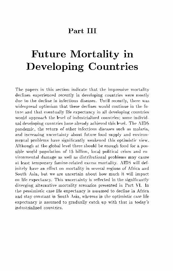
Part III

Future Mortality inDeveloping Countries

The papers in this section indicate that the impressive mortalitydeclines experienced recently in developing countries were mostlydue to the decline in infectious diseases. Until recently, there waswidespread optimism that these declines would continue in the fu­ture and that eventually life expectancy in all developing countrieswould approach the level of industrialized countries; some individ­ual developing countries have already achieved this level. The AIDSpandemic, the ret urn of other infectious diseases such as malaria,and increasing uncertainty about future food supply and environ­mental problems have significantly weakened this optimistic view.Althougb at the global level there should be enough food for a pos­sible world population of 15 billion, local political crises and en­vironmental damage as well as distributional problems may causeat least temporary famine-related excess mortality. AIDS will def­initely have an effect on mortality in several regions of Africa andSouth Asia, but we are uncertain about how much it will impacton life expectancy. This uncertainty is reflected in the significantlydiverging alternative mortality scenarios presented in Part VI. Inthe pessimistic case life expectancy is assumed to decline in Africaand stay constant in South Asia, whereas in the optimistic case lifeexpectancy is assumed to gradually catch up with that in today'sindustrialized countries.

Chapter 7

Mortality Trends inDeveloping Countries:A Survey

Bil>gitta Budd

In preparing population projections for low-mortality developedcountries with good statistics, mortality assumptions are consideredthe least problematic, at least for short-term projections, becausemortality rates tend to change slowly. In developing countries, as­sumptions about future mortality trends are much less certain, evenfor short-term projections, because of the inadequacy of reliable in­formation on past levels and trends.

This chapter reviews past levels and trends of mortality in de­veloping countries. makes assumptions about future trends made bythe United Nations, compares past assumptions with actual perfor­mance, and concludes with a review of recent and possible futurechanges in the pace of mortality decline. Mortality assumptionsmade recently by the World Bank are also reviewed.

The survey of past levels and trends is based on mortality es­timates prepared for the World Population Monitoring, 1993 (UN,1994b) as well as the latest United Nations population estimates andprojections, Wodd Population Pro.5pects: The 1994 Revision (UN,199.5).

The views and OpInIOns expressed in this paper a.re those of the author and donot necessarily reflect those of the United Nations.

133

134 Birgitta Bucht

7.1 Levels and '!rends of MortalitySince 1950

Considerable progress has been made in reducing mortality in lessdeveloped regions in recent decades. Over a period of 40 years, fromthe early 1950s to the early 1990s, the average expectation of lifeat birth in less developed region s is estimated to have increased 21years, from about 41 in 1950-19.55 to 62 in 1990-1995 accordingto the United Nations latest world population estimates and pro­jections (Table 7.1). The difference between the more and the lessdeveloped regions narrowed during this period, from 26 years in theearly 1950s to 12 years in 1990-1995. Life expectancy is projectedto further increase to 71 in 2020-2025. and the difference betweenthe more and the less developed regions is expected to decline toseven years. There is a considerable degree of heterogeneity, how­ever, at the regional and subregional levels, and differences amongcountries are even larger. Progress has been slowest in Africa, andlife expectancy is still estimated at only about 50 years in East,Central, and West Africa. Tviortality is somewhat lower in Northand Southern j-\frica where life expectancy is estimated at 62 and63 years, respectively. in 1990-1995. In Asia, estimates of life ex­pectancies at birth in 1985-1990 are generally higher than those inAfrica and range from 60 in Sour h-central Asia to 70 in East Asia.(It should be noted that the latter region includes Japan, which is adeveloped country.) There was less regional diversity in Asia in theearly 1950s, when life expectancy ranged from 39 in South-centralAsia to 45 in West Asia. The estimates for the Latin American re­gions are still higher, on the average, than those for Asia, and fallwithin a narrow range: 68 years in South America and 69 years inthe Caribbean and Central America. Among the developing regionsof Oceania, life expectancy ranges from 59 years in Melanesia to 68years in Micronesia and Pol,vnesia.

It should be noted that the estimates shown in Table 7.1 are amixture of estimates and projections and may be revised as new databecome available. The availability of data on mortality in develop­ing countries has improved considerably over the past two decades.Vital registration is gradually becoming more complete, particularly

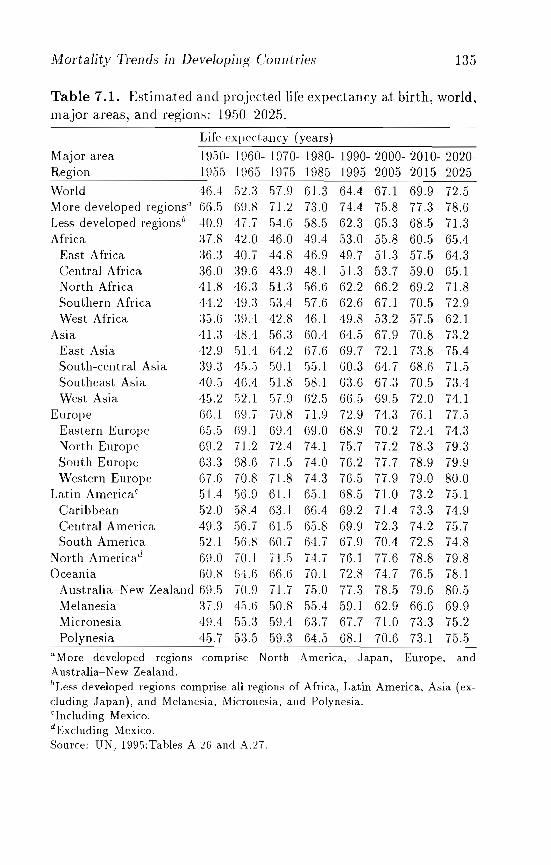
MortaJity Trends in Developing C'ountries 135

Table 7.1. Estimated and projected life expectancy at birth, world,major areas, and regions: 1950-2025.

Life expectancy (years)

Major area 1950- Hl60- HHO- 1980- 1990- 2000- 2010- 2020-Region 1955 1965 1975 1985 1995 2005 2015 2025

World 46.4 52.3 57.9 61.3 64.4 67.1 69.9 72.5More developed regions Q 66.5 69.8 71.2 73.0 74.4 75.8 77.3 78.6Less developed regionsb 40.9 47.7 54.6 58.5 62.3 65.3 68.5 71.3Africa :37.8 42.0 46.0 49.4 53.0 55.8 60.5 65.4

East Africa 36.;~ 40.7 44.8 46.9 49.7 51.3 57.5 64.3Central Africa :~6.0 :~9.6 43.9 48.1 51.3 53.7 59.0 65.1North Africa 41.8 4fU 51.3 56.6 62.2 66.2 69.2 71.8Southern Africa 44.2 49.:~ 53.4 .57.6 62.6 67.1 70.5 72.9West Africa 35.G :~9.4 42.8 46.1 49.8 53.2 57.5 G2.1

Asia 41.3 48.4 56.3 60.4 64.5 67.9 70.8 73.2East Asia 42.9 51.'1 G4.2 67.6 69.7 72.1 73.8 75.4South-central Asia :EJ.3 45.5 50.1 55.1 GO.3 64.7 68.6 71.5Southeast Asia fIO.S 46.4 51.8 58.1 63.6 67.3 70.5 73.4West Asia i1S.2 52.1 57.9 (52.5 66.5 69.5 72.0 74.1

Europe (5(U 69.7 70.8 71.9 72.9 74.3 76.1 77.5Eastern Europe G5.5 69.1 69.4 69.0 68.9 70.2 72.4 74.3North Europe 69.2 71.2 72.4 74.1 75.7 77.2 78.3 79.3South Europe 6:3.3 (j8.G 71.5 74.0 76.2 77.7 78.9 79.9Western Europe 67.6 70.8 71.8 74.3 76.5 77.9 79.0 80.0

Latin America" S1.4 56.9 61.1 65.1 68.5 71.0 73.2 75.1Caribbean 52.0 58.4 (j:3.1 66.4 69.2 71.4 73.3 74.9Central America 4~J .:3 56.7 61.5 G5.8 69.9 72.3 74.2 75.7South America 52.l !)6.8 60.7 64.7 67.9 70.4 72.8 74.8

North America d 6~).0 70.1 71.5 74.7 76.1 77.6 78.8 79.8Oceania 60.8 (i4.6 66.6 70.1 72.8 74.7 76.5 78.1

Australia-New Zealand 69.5 70.9 71.7 75.0 77.3 78.5 79.6 80.5Melanesia 37.~) 45.6 50.8 55.4 59.1 62.9 66.6 69.9Micronesia 49.4 55.3 59.4 6:3.7 67.7 71.0 73.3 75.2Polynesia 45.7 5:3.5 59.3 64.5 68.1 70.6 73.1 75.5

UMore developed regIOns comprise North America, Japan, Europe, andAustralia- New Zealand.bLess developed regions comprise all regions of Africa, Latin America, Asia (ex­cluding Japan), and Melanesia, Micronesia., and Polynesia.cIncluding Mexico.dExclnding Mexico.Source: UN, 1995:Tables A.~(j a.ncl A.n.

136 Birgitta Bucht

in Latin America and East Asia. Data that permit estimation of in­fant and child mortality have been widely collected in censuses andsurveys, in particular those conducted by the World Fertility Survey(WFS) program and more recently by the Demographic and HealthSurveys (DHSs). Despite these improvements, lack of reliable datacontinues to be a serious handicap in the analysis of mortality in de­veloping cOUlitries. Obviously. countries for which data on mortalityare available may not necessarily be representative of other countriessince mortality conditions are likely to be worse in countries lackingdata. For example, there are no recent surveys or registration datain countries affected by war or civil strife. The countries withoutany national-level data, however, form only a small part of the totalpopulation of less developed regions, so that even large errors in thecountry estimates will not greatly affect regional totals.

Although the data situation has improved in Africa, it is stillmore problematic to estimate levels and trends there than in otherless developed regions. The only countries in sub-Saharan Africawith reliable vital registration systems from which life tables canbe derived are three small island countries in the Indian Ocean:Mauritius, Reunion, and the Seychelles. All three have reachedlow levels of mortality with life expectancies now above 70 years.Most information for mainland sub-Saharan Africa refers to childmortality. Few countries have adequate data on adult mortality.

Mortality is high throughout most of sub-Saharan Africa, butthere is variation among countries in terms of both levels and trends.Child mortality has generally been most severe in West Africa, a factattributed both to the level of socioeconomic development and toenvironmental factors (Blacker, 1991). Although differences withthe other regions have narrowed, West Africa as a whole still hasthe highest child mortality on the continent. Sierra Leone, a WestAfrican country, exhibits the highest mortality ever measured ina contemporary country: a probability of dying by age 5 of 364per 1,000 in 1971, declining to 334 per 1,000 in 1981 according tothe 1974 and 1985 censuses. Gambia and Mali in West Africa andMalawi in East Africa, which had similarly high levels of child mor­tality in the 1970s, have experienced large improvements, but thelatest estimates of mortality under the age of 5 for these countries

Mortality Trends in Developing C'ountries 137

are still above 240 per LOOO. The lowest mortality in mainland sub­Saharan Africa has been achieved by Kenya and Zimbabwe in EastAfrica and Botswana in Southern Africa. The low child mortalityin Botswana (65 per 1,000.in 1984) may be explained, in additionto its impressive economic growth during the 1970s and 1980s, bythe high proportion of women receiving prenatal care and vacci­nated with tetanus toxoid, the high proportion of births deliveredby trained health personnel, and the high immunization coverage ofchildren (Lesetedi et al., 1989; World Bank, 1992a). Immunizationcoverage and the proportions of women receiving prenatal care arealso high in Kenya and Zimbabwe (Kenya, 1989; Zimbabwe, 1989).

The countries of North Africa have experienced more rapid mor­tality declines with an acceleration in the decline since the mid-1970sand late 1970s. In Algeria, the only country in the region with aseries of life tables derived from vital registration, life expectancyincreased slowly from 05:3 in 1970 to 057 in 1978 and then to 64 in1985, an annual increase of one year. Life tables after 1985 are notyet available, but recent data on infants show that mortality hascontinued to decline. In Egypt. infant and child mortality fell bymore than half between 1976 and 1986. In Tunisia, which currentlyhas the lowest infant and child mortality rates in North Africa, thedecline has been equally impressive, from an under-five mortality of204 per 1,000 in 1968-1969 to 605 per 1,000 in 1983-1987 accordingto a 1968-1969 demographic survey, the 19705 census, and the 1988DHS.

Asia presents the most varied picture among the developing re­gions, both in terms of levels and trends in mortality and in terms ofavailability and quality of elata, reflecting very diverse histories andlevels of development. East Asia has achieved the lowest mortalitylevels in the region. The main reason is obviously the remarkableprogress achieved by China. Life expectancy in China was estimatedat 41 in 1950-19.505 and reached 67 in 1980-1985, an annual increaseof almost one year. The other countries of the region with availabledata, Hong Kong and the Republic of Korea, have also successfullyreduced their mortality levels. According to its civil registrationdata, Hong Kong now has the lowest mortality among all develop­ing countries with a life expectancy in 1987-1989 of 77 years (80 for

138 Birgitta. Bucht

females and 74 for males) and all infant and under-five mortality of7 and 9 per 1,000, respectively.

Southeast Asia is characterized by a wide disparity of mortalitylevels and trends. Brunei Darussalam, peninsular Malaysia, and Sin­gapore have achieved mortality levels comparable with those of de­veloped countries with life-expectancy estimates above 70. Progresshas also been made in other countries in the region, particularly inThailand where expectation of life at birth reached 66 in 1985-1986and in the Philippines where it reached 64 in 1987-1989. However,the region also includes areas such as East Timor, Cambodia, andLao People's Democratic Republic where mortality is believed to behigh and life expectancy estimated to be below 50 years.

Sou th Asia exhibits the highest mortality levels and has experi­enced the slowest decline in Asia, although Sri Lanka has attainedrelatively low mortality: life expectancy was 69 in 1980-1981, and isnow estimated to exceed 70. Afghallistan has the highest mortalityin the region, which is not surprising given its social and politicalcircumstances. Although mortality is still high in the three largestcountries of the Indian subcontinent - Bangladesh, India, and Pak­istan - the levels have been declining. In Bangladesh, life expecta.ncyincreased from 48 in the late 1970s to 56 in 1987. In India, life ex­pectancy was estimated at 5:3 in 1981-198:3. More recent data fromthe Sample Registration System show that infant mortality has con­tinued to decline, from 107 per 1,000 in 1981-1983 to 94 per 1,000in 1988. The latest data for Pakistan give a life expectancy of 60 in1984-1988, an increase from 5:3 in 1972-1981.

In West Asia, several countries have experienced very rapid de­clines, not only the small oil-producing countries of the region, butalso countries such as Jordan, the Syrian Arab Republic, and Turkey.Cyprus and Israel have the lowest mortality in the region with lifeexpectancies above 75, followed by Kuwait where life expectancy wasestimated at 72 in 1984-1986. The only country with high mortalityin the region is Yemen, where infant and under-five mortality were162 and 237 per 1,000, respectively, according to the 1979 WFS.

As mentioned earlier. Latin America has achieved lower mor­tality levels than Africa and Asia. The mortality decline in theCaribbean is particularly impressive with levels of life expectancy

Mortality Trends in De\!eloping COllntries 139

reaching those of developed countries despite lower levels of eco­nomic development. Life expectancy at birth is estimated to beabove 70 years on all islands except the Dominican Republic andHaiti. In Cuba and Puerto Rico life expectancy was 75 in 1985­1986 and 1986-1988, respectively, the highest in Latin America. Togive an example of the mortality decline tha.t has occurred in someof those countries, life expectancy a.t birth in Barbados increasedfrom 57 in 19.50-19.55 to 72 in 1980. Infant mortality declined from1:32 per 1,000 in the early 19.50s to 13 per 1,000 in the late 1980s,over 90 percent. Decline has been slow in the Dominican Republicand Haiti. Under-five mortality in Haiti was still estimated at 193per 1,000 in 1983, higher than in many African countries.

Two countries in Central America - Costa Rica and Panama ­have also achieved very low levels of mortality with life expectan­cies above 70. In Mexico, the largest country in the region, lifeexpectancy at birth increased from 61 in 1970 to 66 in 1980 and isnow believed to be close to 70.

In South America, the lowest mortality levels are observed inArgentina, Chile, Uruguay, and Venezuela.. In Chile, life expectancyat birth increased from 62 to 71 during the 12-year period between1970 and 1982, and infant and child mortality declined by almost70 percent during the same period. Recent data show a continuingbut slower decline during the 1980s. Bolivia and Peru, however,have the highest mortality in the region but, like all South Ameri­can countries, have experienced substantial mortality reductions. InBolivia, for example, the probability of dying by age 5 declined byalmost half between 1972 and 1988, from 254 to 130 per 1,000. InBrazil, the largest country in the region, with half its population,the mortality decline has been moderate. Life expectancy at birthincreased from .58 in 1970 to 62 in 1976-1980 and may be above 65at present.

Mortality has also declined steadily in the developing countriesof Oceania, and some countries have achieved low levels of mortality.In Guam, life expectancy was estimated at 73 in 1979-1981 andinfant mortality at 11 per 1,000 in 1985-1987. The only areas wheremortality is still high is Kiribati, a small island in Micronesia, whereunder-five mortality was estimated at 123 in 1981 according to the

140 Birgitta Bucht

1985 census and Papua New Guinea, Melanesia, where under-fivemortality was estimated at 96 in 1976.

The United Nations has recently completed a review of childmortality since the 1960s in developing countries with an estimated1990 population of 1 million or more (UN, 1992b). Among the coun­tries with adequate estimates of the probability of dying by age 5 fortwo points in time between 1960 and 1985, altogether 79 observa­tions, child mortality declined by about 3 percent per annum. Asiaand Latin America both experienced rates slightly above this aver­age, whereas the rate of decline in Africa was only about 2 percentper annum. These figures may be somewhat different, however, ifdata for all countries were available. In sub-Saharan Africa, thereare a few countries where available data show that child-mortalitydeclines may have stalled, although the observed trend could be dueto poor data quality. Data are so defective in some countries, notonly in Africa, that it is not really possible to tell how mortality hasevolved. In many countries outside sub-Saharan Africa with suffi­cient data to indicate a change in trends, child-mortality declinesappear to have accelerated in the late 1970s and in the 1980s.

7.2 Assumptions about Future Trendsin Mortality

The United Nations has prepared global population projectionssince the 1950s. The details of the projections have expanded overtime with improvements in data and methods of analysis and withthe utilization of computer technology. Detailed mortality assump­tions by country were first made in 1968. The assumptions areformulated in terms of life expectancy at birth and age and sex pat­terns of probabilities of surviving, corresponding to different levelsof life expectancy at birth. The age-specific survival ratios neededfor the projections are derived from appropriate model life tables.For countries with reliable data on mortality by age and sex, thatinformation is used to complement the derivation of the requiredsurvival ratios. A national life table for a given date is used as abase for the projections, and as mortality is projected to decline,it is assumed that the mortality rates of the national life table willgradually approach those of a model life table. This procedure has

Morta.lity Trends ill Developing COllntries 141

been referred to as the "modified method" of mortality projection(UN, 1977a). For countries without reliable mortality data by ageand sex, the mortality rates are taken directly from the model lifetables selected for the projections. The Coale and Demeny regionalmodel life tables (Coale and Demeny, 1966, 1983) and, since the1988 assessment, the United Nations model life tables for develop­ing countries (UN, 1982a) are used in preparing the United Nationsprojections.

One of the roles of the United Nations projections is to pro­duce comparable global and interregional prospects of population.To maintain comparability in the assumptions of mortality betweenregions and among countries within regions, a uniform procedureis llsed for all countries. The assumptions about life expectancy atbirth are made to follow models of mortality improvement. Thesemodels have been developecl using data from countries with reliabledeath statistics and have been revised and modified as new data havebecome available, reflecting the most recent observations about mor­tality decline. It has generally been assumed that life expectancy atbirth would increase by half a year annually until life expectancy forfemales reaches SS, 62,S, or 65 years, followed by a slowdown in thegain thereafter. In countries where evidence suggests that the mor­tality decline has been faster or slower than the model implies, theassumptions have been adjusted. The most recent working model,which was developed for the 1988 assessment and is summarized inTable 7.2, introduces three variations in the speed of improvementand labels them fast, middle, and slow models.

In the model developed for the 1973 assessment, it was assumedthat the highest female life expectancy that could be attained wouldbe 77.5 years, the value given as maximum in the Coale-Demeny re­gional model life tables, and the highest male life expectancy wouldbe 72.6 years, the value given as maximum in the first United Na­tions model life tables (Table 7.3). In the 1978 assessment, themaximum life expectancies were raised to 80 for females and 73.5for males. In the 1982 assessment, the maxima were further raisedto 82.5 years for females and 7,5 for males. The Coale-Demeny re­gional model life tables were extrapolated to incorporate survivalratios corresponding to these higher levels of life expectancies. Themost recent model, developed for the 1988 assessment, represents a

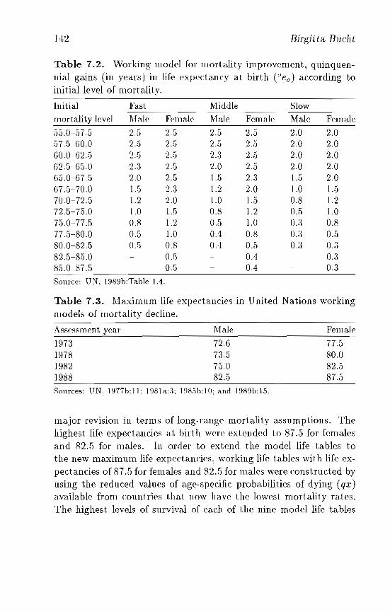
H2 Birgitta Bucht

Table 7.2. \Vorking model for mortality improvement, quinquen-nia.! gains (in years) in life expectancy at birth (Oe o ) according toinitial level of mortality.

Initial Fast Middle Slow--

mortality level Male Female Male Female Male Female

55.0-57.5 2.5 2.5 2.5 2.5 2.0 2.057.5-60.0 2.5 2.5 2.5 2.5 2.0 2.060.0-62.5 2.5 2.5 2.:3 2.5 2.0 2.062.5-65.0 2.:3 2.5 2.0 2.5 2.0 2.065.0-67.5 2.0 2.5 1.5 2.3 1.5 2.067.5-70.0 1.5 2:3 1.2 2.0 1.0 1.570.0-72.5 1.2 2.0 1.0 1.5 0.8 1.272.5-75.0 1.0 1.5 0.8 1.2 0.5 1.075.0-77.5 0.8 1.2 0.5 1.0 0.3 0.877.5-80.0 0.5 1.0 0.4 0.8 0.3 0.580.0-82.5 0.5 0.8 0.4 0.5 0.3 0.382.5-85.0 0.5 0.4 0.385.0-87.5 0.5 0.4 0.3Source: UN, 1989b:Table 1.4.

Table 7.3. Maximum life expectancies in United Nations workingmodels of mortality decline.

Assessment year

1973197819821988

Male72.673.575.082.5

Female77.580.082.587.5

Sources: UN, 1977b:ll; 1981a:3; 198.5b:l0; and 1989b:15.

major revision in terms of long-range mortality assumptions. Thehighest life expectancies at birth were extended to 87.5 for femalesand 82.5 for males. In order to extend the model life tables tothe new maximum life expectancies, working life tables with life ex­pectancies of 87.5 for females and 82.5 for males were constructed byusing the reduced values of age-specific probabilities of dying (qx)available from countries that now have the lowest mortality rates.The highest levels of survival of each of the nine model life tables

Mortality Trends in Developing Countries 143

(West, North, South, and East model of the Coale and Demeny re­gional model life tables and General, Latin American, Chilean, FarEastern, and South Asian model life tables of the United Nations)were linked individually with the age-specific survival ratios derivedfrom the working life table so that survival ratios of other interme­diate mortality levels could be obtained through interpolation (UN,1989b). These survival ratios have been used in the 1988-1994 re­visions of the population projections.

Several developing countries have now surpassed the maximumlife expectancy for females of 77.5 assumed in 1973. Only one coun­try, Hong Kong, is currently estimated to have a life expectancyabove 80 for females, the maximum assumed in 1978, although sev­eral other countries, mainly small island countries, have reached lifeexpectancies close to that level. Only one developed country, Japan,has reached the limit for females set in 1982, 82.5 years, but severalcountries have surpassed the limit assumed for males, 75 years.

The most recent United Nations projections have taken intoaccount the effects of the acquired immunodeficiency syndrome(AIDS) pandemic in 15 high prevalence countries in sub-SaharanAfrica and one country in Asia, Thailand (UN, 1995). The num­ber of deaths related to AIDS is estimated and projected using anepidemiological model developed by the World Health Organization(Chin and Lwanga, 1991b). In applying the model, it is assumedthat there are no new adult human immunodeficiency virus (HIV)infections after 2010; mother-to-child infections continue to occurafter this date and AIDS deaths follow for many years thereafterdue to the long latency period between HIV and AIDS. The as­sumption of no new adult infections after 2010 has little effect onprojected AIDS mortality until after 2025. The estimates of deathsfrom AIDS by age and sex, for each five-year period, are then in­tegrated into the existing (non-AIDS) model life tables, producinga set of life tables which incorporates the risk of dying from AIDSand which is used for the projections.

Recently, the World Bank has published mortality projections;the first results were published in World Development Report 1978

(World Bank, 1978). Detailed projections have been published only

144 Birgitta Bucht

since 1984 in World Population Projections (various years). Thebase-year mortality estimates used in the World Bank projectionswere mainly obtained from the United Nations, but methods usedto prepare assumptions about future trends are different. In the1984 to 1987-1988 assessments, life expectancy at birth was pro­jected with a model using past patterns of relationships betweenthe change in life expectancy, the level of life expectancy, and thefemale primary school enrollment ratio. Two different schedules ofannual increments in female life expectancy were developed: onefor countries with female primary school enrollment less than 70percent and another for those where the enrollment is 70 percentor more. For a given expectation of life at birth, survival ratiosfor males and females were derived from the Coale and Demeny re­gional model life tables. In recent projections, a different procedurehas been used to project mortality (Bulatao and Bos, 1989). Lifeexpectancy and infant mortality are projected separately using lo­gistic functions, taking into account past trends and socioeconomicfactors. The logistic function is determined so that life expectancyrises most rapidly from a level of .50 years and increasingly slowlyat higher levels. Rates of change are estimated from past rates ofchange and from the female secondary school enrollment ratio or,in a few cases where data on school enrollment are not available,from the percent urban. Maximum life expectancies were assumedto be 90 years for females and 83.3 for males. Life tables are se­lected from the Coale-Demeny regional model life tables combiningdifferent levels to give exactly the desired infant mortality rate andlife expectancy. Coale and Guo's (1989) extended model life tablesare used at low levels of mortality. The most recent World Bankprojections have also taken into account the effects of AIDS, apply­ing an epidemiological model developed by Bulatao (1991) and Boset al. (1992).

The World Bank assumptions show more variation among indi­vidual countries than do those assumed by the United Nations, andindicate, on average, slightly faster decline at lower levels of life ex­pectancy and slower decline at higher levels. Mortality assumptionsfor less developed regions according to different United Nations andWorld Bank assessments are shown in Tables 7.4 and 7.5.

Mortality Trends in Developing Countries 145

Table .7.4. Estimated and projected life expectancy at birth for lessdeveloped regions, both sexes, according to different United Nationsassessments.Year

estimated

1968197319781980198219841988199019921994

Projection period

1980-1985 1985-1990

58.0 60.6.56.7 58.757.1 59.257.0 58.956.6 58.257.3 59.157.6 .59.759,4 61.458.6 60.758.5 60.5

1990-1995

63.060.761.160.760.060.861.563.362,462.3

2020-2025

69.668.969.570,471.671.271.3

Sources: UN, 1973:Table A.2.1; 1977b:Table 41; 1979; 1981a:Table A-15;I985b:Table A-15; 1986:Table A-15; 1989b:Table 15; 1991a:Table 44; 1993a:Table A-15; and 1995:Tables A26 and A27.

Table 7.5. Estimated and projected life expectancy at birth forless developed regions, both sexes, according to different World Bankassessments.Year

estimated

198419851987-19881989-19901992-1993

Projection period

1980-1985 1985-1990

59.5 ()1.259,4 ()1.1

61.4():U()1.9

1990-1995

62.862.862.963.663.2

2020-2025

70.770.870.369.371.1

Sources: Vu, 1984, 1985; Zachariah and Vu, 1988; Bulatao et al., 1990; and Boset al., 1992.

7.3 Comparison of Past Assumptions withActual Performance

Since the United Nations has a long series of population estimatesand projections, assumptions made in past projections can be com­pared with more recent assumptions and with actual levels. Table7.4 shows estimated and projected life expectancies at birth for less

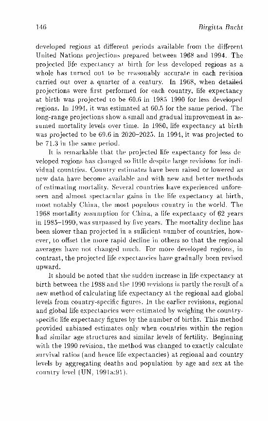
146 Birgitta Bucht

developed regions at different periods available from the differentUnited Nations projections prepared between 1968 and 1994. Theprojected life expectancy at birth for less developed regions as awhole has turned out to be reasonably accurate in each revisioncarried out over a quarter of a century. In 1968, when detailedprojections were first performed for each country, life expectancyat birth was projected to be 60.6 in 198.5-1990 for less developedregions. In 1994, it was estimated at 60..5 for the same period. Thelong-range projections show a small and gradual improvement in as­sumed mortality levels over time. In 1980, life expectancy at birthwas projected to be 69.6 in 2020-202.5. In 1994, it was projected tobe 71.3 in the same period.

It is remarkable that the projected life expectancy for less de­veloped regions has changed so little despite large revisions for indi­vidual countries. Country estimates have been raised or lowered asnew data have become available and with new and better methodsof estimating mortality. Several countries have experienced unfore­seen and almost spectacular gains in the life expectancy at birth,most notably China, the most populous country in the world. The1968 mortality assumption for China, a life expectancy of 62 yearsin 198.5-1990, was surpassed by five years. The mortality decline hasbeen slower than projected in a sufficient number of countries, how­ever, to offset the more rapid decline in others so that the regionalaverages have not changed much. For more developed regions, incontrast, the projected life expectancies have gradually been revisedupward.

It should be noted that the sudden increase in life expectancy atbirth between the 1988 and the 1990 revisions is partly the result of anew method of calculating life expectancy at the regional and globallevels from country-specific figures. In the earlier revisions, regionaland global life expectancies were estimated by weighing the country­specific life expectancy figures by the number of births. This methodprovided unbiased estimates only when countries within the regionhad similar age structures and similar levels of fertility. Beginningwith the 1990 revision, the method was changed to exactly calculatesurvival ratios (and hence life expectancies) at regional and countrylevels by aggregating deaths and population by age and sex at thecountry level (UN, 199130:91).

Mortalit.y Trends in Developing COllntries

7.4 Possible Changes in the Pace ofFuture Mortality Decline

147

There has been some concern that the deteriorating economic con­ditions since the mid-1970s in many developing countries would leadto a slowdown or stagnation in the mortality decline because of a re­duction in expenditures on social services implemented to cope withthe economic crisis. There is no evidence yet of such a change exceptpossibly in a few countries in sub-Saharan Africa where mortalitytrends are difficult to interpret. In countries with negative growth ofGDP per capita from 1965-1980 or 1980-1990 (World Bank, 1992a)and with sufficient data to estimate mortality trends - for exam­ple, Senegal in sub-Saharan Africa and several countries in LatinAmerica - mortality has continued to decline without change. How­ever, one cannot rule out the possibility that the deterioration ineconomic conditions and reduced spending on health could have adelayed effect on mortality in some countries.

An important measure that is likely to have a substantial effecton mortality trends in the near future is the child survival programsthat began in the 1980s b.v governments and international organiza­tions. These programs have consisted mainly in making a few simpleand low-cost technologies widely available. in particular immuniza­tion and oral rehydration therapy (ORT). When the World HealthOrganization launched its Expanded Programme on Immunizationin 1974, it was estimated that less than 5 percent of children in thedeveloping world were immunized (UNICEF, 1989). By 1985, thecoverage had increased to about 30 percent for measles and 40 per­cent for the other diseases. Since then, many countries have sharplyincreased their coverage, and it is estimated that by 1990 between 79and 90 percent of infants were vaccinated against certain diseases.Immunization of women against tetanus still lags behind, at about56 percent (UNICEF. 1992). Awareness and use of oral rehydrationtherapy have also increased substantially. These efforts should havean important impact on child mortality, and favorable results havealready been reported in a number of countries. However, since theprograms have only recently gained momentum in many countriesand since data for the late 1980s are still not available in many coun­tries, the full impact of these programs cannot yet be measured.

148 Birgitta Bucht

Other factors that will affect child survival in the future areincreasing education of women and declines in fertility, with a re­duction in high-risk births. Reduced fertility is also likely to haveindirect positive effects on a child's survival chances because a familywith fewer children can allocate more resources per child, includingparental care and attention, food, schooling, and access to healthservices. There is also a reduced risk of infection of children in smallhouseholds. Maternal mortality, which is high in many developingcountries, is also lowered with fertility declines.

In the near future, the outlook in general indicates a contin­uation of the mortality decline. In addition to those mentionedabove, other helpful factors include further improvements in educa­tion, medical research, training of health personnel, and the spreadof democracy which will enable people to put pressure on govern­ments to improve health services.

Several developing countries have reached mortality levels com­parable to those in developed countries, even in countries where thelevels of economic development are far behind those of developedcountries. There is no reason that the mortality declines will notcontinue and that other countries will not follow, barring of coursewars, famines, and other catastrophes.

This does not mean that it is going to be easy to achieve contin­ued impressive improvements. The progress in sub-Saharan Africa islikely to continue to lag behind that of the other developing regions.Apart from the droughts and famines that are plaguing substantialparts of Africa at the present time and the civil strife that existsnot only in Africa but also in Asia, there are two important con­cerns: the AIDS epidemic and the spread of chloroquine-resistantmalaria. Both are likely to have a particularly devastating effect insub-Saharan Africa. Environmental problems of various kinds ag­gravated by population growth, such as water scarcity and loss ofagricultural land, and cut backs in food production could also leadto increased risks to health.

Chapter 8

Mortality in Sub-SaharanAfrica: Trends and Prospects

Michel Garenne

Interest in the population growth of the Third World began afterWorld War II, owing mostly to the growing concern for populationpressure and its possible effects upon the economy, ecology, andpolitical balance of the world. The sources of the high rate of pop­ulation growth were the rapid decline of mortality and, to a lesserextent, the increase of natality. The primary concern was with Asia,in particular, China and the Indian subcontinent, and with LatinAmerica, in particular Central America. Somewhat later, the de­mography of sub-Saharan Africa became a subject for research.

The first systematic studies of African populations took placein the early 1960s. A team of researchers working at PrincetonUniversity published the first comprehensive account of African de­mography (Brass et aI., 1968). At about the same time, a group ofFrench demographers published a summary of their experiences andfindings on tropical Africa, with emphasis on the sample surveysconducted by the French National Statistical Office (INSEE) since1954 (GDA, 1967). Since this pioneer period, only a few synthe­ses on the population dynamics of the region have been published.Mandjale (1985) analyzed infant and child mortality. Van de Walleet al. (1988) reviewed the state of African demography. The col­lection of work edited by Feachem and Jamison (1991) focused onmorbidity and mortality.

149

150 Michel Garenne

Over the past 50 years, Africa experienced minimal fluctuationsin fertility, whereas its mortality rate underwent a major decline;this situation created a considerable potential for population growth.The decline in mortality has been documented only recently in asystematic way (Hill and Hill, 1988; Hill, 1991; Timc£us, 1991).However, there is a growing concern that the mortality decline willnot continue, and may even be reversed under new conditions suchas economic crises, political turmoils, and emerging diseases such asAIDS.

This paper reviews the available evidence of mortality decline,before and since independence, and discusses the future of mortality.It focuses on the countries of sub-Saharan Africa. The small islandsoff the African coast, such as Cape Verde, Sao Tome and Principe,Mauritius, and the Seychelles, have been ignored in this analysisbecause they have very different population dynamics. Three broadperiods are distinguished: prior to 1960 - that is, the colonial periodfor most countries; 1960-1990, the first three decades after the regionachieved independence; and recent trends (when available), 1985­1994.

8.1 The Colonial Period: 1920-1959

8.1.1 Mortality trends

Data from the end of the colonial period (1920-1959) are very scarce,and there is virtually no data on tropical Africa prior to 1915. Twolong- term series are available from Dakar and Saint- Louis, two citiesin Senegal, where an extensive vital registration system has beenmaintained. The vital registration data from Saint-Louis were re­cently analyzed in a Ph.D. dissertation (Diop, 1990) and the datafrom Dakar were discussed in a recent paper (Garenne et at., 199:3).

For Dakar, there is clear evidence that mortality has been declin­ing since at least 1920; the 191.5-1919 period was seriously disturbedby the 1918 influenza world epidemic as well as by a local plagueepidemic. For Saint- Louis, mortality has been declining steadilysince 1930, the earliest date for which data were analyzed (Figure8.1). In both cases. the crude death rates at the beginning of theseries were among the highest recorded, and were only slightly lower

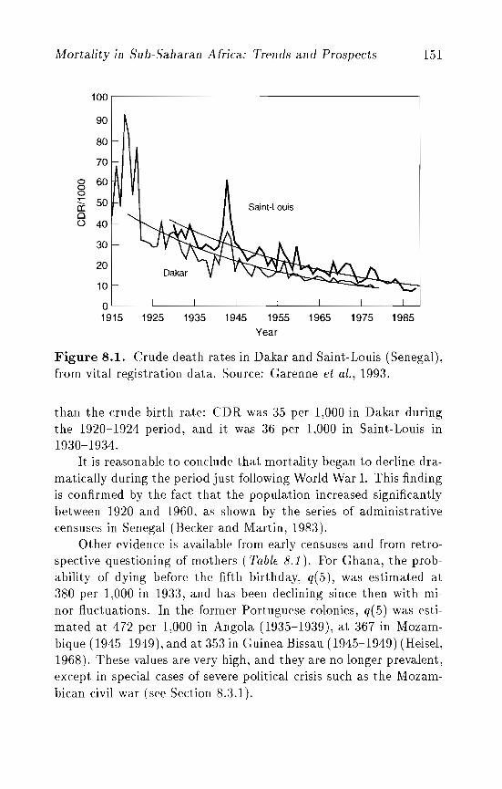
Mortality in Sub-Saharan Africa: Trends and Prospects 151

Saint-Louis

100

90

80

70

0 6000

~ 500() 40

30

20

10

01915 1925 1935 1945 1955 1965 1975 1985

Year

Figure 8.1. Crude death rates in Dakar and Saint-Louis (Senegal),from vital registration data. Source: Garenne et al., 1993.

than the crude birth rate: CDR was 35 per 1,000 in Dakar duringthe 1920-1924 period, and it was 36 per 1,000 in Saint-Louis in1930-1934.

It is reasonable to conclude that mortality began to decline dra­matically during the period just following World War 1. This findingis confirmed by the fact that the population increased significantlybetween 1920 and 1960, as shown by the series of administrativecensuses in Senegal (Becker and Martin, 1983).

Other evidence is available from early censuses and from retro­spective questioning of mothers (Table 8.1). For Ghana, the prob­ability of dying before the fifth birthday, q(5), was estimated at380 per 1,000 in 1933, and has been declining since then with mi­nor fluctuations. In the former Portuguese colonies, q( 5) was esti­mated at 472 per 1,000 in Angola (1935-1939), at 367 in Mozam­bique (1945-1949). and at 3,53 in Guinea Bissau (1945-1949) (Heisel,1968). These values are very high, and they are no longer prevalent,except in special cases of severe political crisis such as the Mozam­bican civil war (see Section 8.3.1).

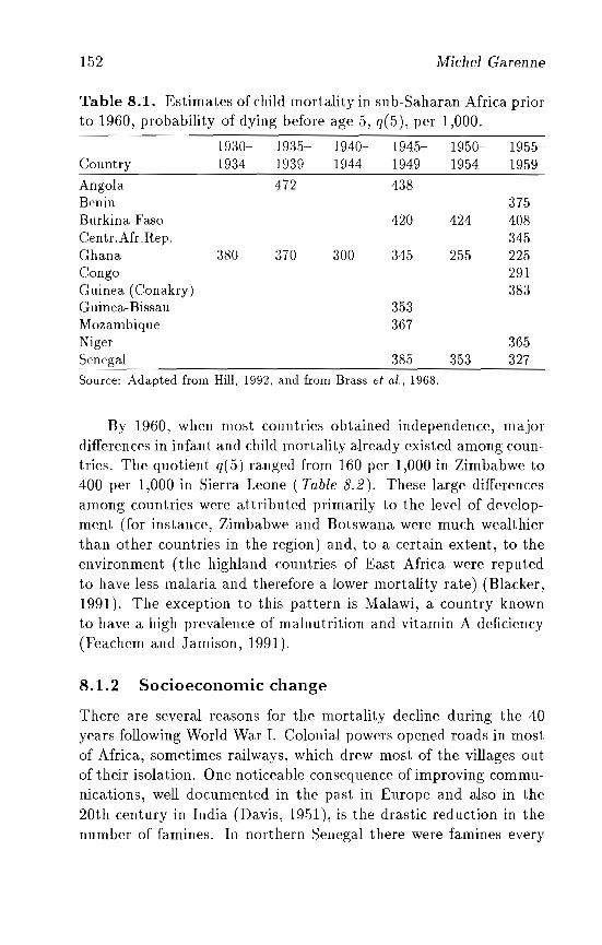
152 Michel Garenne

Table 8.1. Estimates of child mortality in sub-Saharan Africa priorto 1960, probability of dying before age .5, q(5), per 1,000.

Country1930- 1935- 1940- 1945- 1950- 1955-1934 1939 1944 1949 1954 1959

375424 408

345255 225

291383

365353 327

345

353367

420

300:370

472 438

:380

AngolaBeninBurkina FasoCentr.Afr.Rep.GhanaCongoGuinea (Conakry)Guinea- BissauMozambiqueNigerSenegal 385Source: Adapted from Hill, 1992, and from Brass et al., 1968.

By 1960, when most countries obtained independence, majordifferences in infant and child mortality already existed among coun­tries. The quotient q( 5) ranged from 160 per 1,000 in Zimbabwe to400 per 1,000 in Sierra Leone ( Table 8.2). These large differencesamong countries were attributed primarily to the level of develop­ment (for instance, Zimbabwe and Botswana were much wealthierthan other countries in the region) and, to a certain extent, to theenvironment (the highland countries of East Africa were reputedto have less malaria and therefore a lower mortality rate) (Blacker,1991). The exception to this pattern is Malawi, a country knownto have a high prevalence of malnutrition and vitamin A deficiency(Feachem and Jamison, 1991).

8.1.2 Socioeconomic change

There are several reasons for the mortality decline during the 40years following World War 1. Colonial powers opened roads in mostof Africa, sometimes railways, which drew most of the villages outof their isolation. One noticeable consequence of improving commu­nications, well documented in the past in Europe and also in the20th century in India (Davis, 19.51), is the drastic reduction in thenumber of famines. In northern Senegal there were famines every

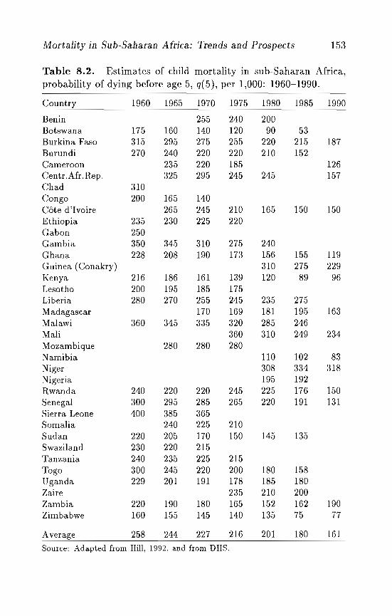
Mortality in Sub-Saharan Africa: Trends and Prospects 153

Table 8.2. Estimates of child mortality in sub-Saharan Africa,

probability of dying before age 5, q(5), per 1,000: 1960-1990.

Country 1960 1965 1970 1975 1980 1985 1990

Benin 255 240 200Botswana 175 160 140 120 90 53Burkina Faso 315 295 275 255 220 215 187Burundi 270 240 220 220 210 152Cameroon 235 220 185 126Centr.Afr.Rep. 325 295 245 245 157Chad 310Congo 200 165 140Cote d'Ivoire 265 245 210 165 150 150Ethiopia 235 230 225 220Gabon 250Gambia 350 345 310 275 240Ghana 228 208 190 173 156 155 119Guinea (Conakry) 310 275 229Kenya 216 186 161 139 120 89 96Lesotho 200 195 185 175Liberia 280 270 255 245 235 275Madagascar 170 169 181 195 163Malawi 360 345 335 320 285 246Mali 360 310 249 234Mozambique 280 280 280Namibia 110 102 83Niger 308 334 318Nigeria 195 192Rwanda 240 220 220 245 225 176 150Senegal 300 295 285 265 220 191 131Sierra Leone 400 385 365Somalia 240 225 210Sudan 220 205 170 150 145 135Swaziland 230 220 215Tanzania 240 235 225 215Togo 300 245 220 200 180 158Uganda 229 201 191 178 185 180Zaire 235 210 200Zambia 220 190 180 165 152 162 190Zimbabwe 160 155 145 140 135 75 77

Average 258 244 227 216 201 180 161Source: Adapted from Rill, 1992, and from DRS.

154 Michel GMenne

three to four years in the 19th century (Chastanet, 1982). Severefamines virtually disappeared after World War I, with a few ex­ceptions such as in 1942 in Senegal, and although food shortagescontinued to occur with the same frequency, they became far lessacute. Colonization also brought to Africa the monetary economy,in particular cash crops (peanuts, coffee, cocoa, rubber, and so on),which gave farmers the power to purchase what they needed.

Cities were rare and small in Africa prior to 1900. How­ever, they developed rapidly thereafter; these cities subsequentlyopened schools and provided a modern education to an elite groupof Africans. The level of modern education has been shown tobe closely associated with mortality decline throughout the world(Caldwell, 1986).

8.1.3 Public health

In addition to improving socioeconomic conditions, considerable ef­forts were made to improve public health. Health programs focusedon diseases affecting the expatriate community, especially adults,but were also directed to the whole population. Modern hospitalswere built at the turn of the century. Local dispensaries soon fol­lowed in secondary towns. Treatment of the water supply began incities during the same period (1928 in Dakar).

Newly developed vaccines against tuberculosis (BCG), yellowfever, smallpox, and plague became available and widely used, evenin the remotest villages. As a consequence of vaccination and vectorcontrol, the last three of these deadly diseases were under controlby 1960. Tuberculosis has been more difficult to control, mostlybecause BCG has a low efficacy but also because the disease has amore complex epidemiology. Major efforts were also made to con­trol syphilis and yaws, as well as trypanosomiasis. The control ofsyphilis and other infectious diseases reached a new dimension withthe marketing of antibiotics just after World War II. Synthetic anti­malarial drugs became available in 194.5 in most of tropical Africa.Malaria control programs also started after World War II, and al­though they failed to achieve their goals, they certainly contributedto mortality decline and perhaps to an increase in fertility.

Mortality in Sub-Saharan A1rica: Trends and Prospects 155

8.2 Evolution Since Independence:1960-1990

After 1960, a relatively large amount of data concerning mortal­ity became available: censuses with retrospective questions, sam­ple surveys (prospective or retrospective), maternity histories in theWorld Fertility Survey (WFS), and Demographic and Health Sur­veys (D HSs). These surveys provide levels and trends in child mor­tality at various points in time from which a history of mortalitydecline can be reconstructed (Hill, 1991). Results of this recon­struction are shown in Table 8.2.

Among the countries listed in Table 8.2, data are satisfactory inmore than half the cases and roughly indicate a 40 percent declinein q( 5) between 1960 and 1990, from an average of 258 in 1960 toan average of 161 ill 1990. This is a rapid decline in mortality.In England and vVales, it took about 80 years to achieve the samedecline. A typical example of a steady mortality decline can befound in the case of SenegaL where the estimates of q(5) followquite accurately the fitted trend up to the early 1990s, which is themost recent point (Figu.re 8.2).

The speed ofthe mortality decline varied widely from country tocountry. For instance, the evolution in Ghana differed greatly fromthat in Kenya. Mortality levels were virtually the same in 1960 (228and 216 per 1,000). Mortality decline was steady in Kenya from 1960to 1985, whereas in Ghana mortality decline was slower between1960 and 1975 and almost stopped in 1975 for about 10 years, sothat by 1985 mortality \vas 7-J. percent higher than in Kenya. How­ever, recent data show that Ghana had a rapid mortality declinebetween 1985 and 1993, while mortality was reversing in Kenya (seeSection 8.3.1). III 1993, mortality levels in the two countries wereagain quite close (1n and 122), with a small excess in Kenya.

During t his period, some countries failed to achieve the largemortality decline that most countries experienced. In Niger mortal­ity was above 300 per 1,000 in the 1980-1992 period. Burkina Faso,a neighboring country, experienced this level in the 1960s; today itslevel is below 200 per 1,000. Another striking case is Madagascar,which experienced little change ill 25 years (Table 8.2).

=o~~~_, _

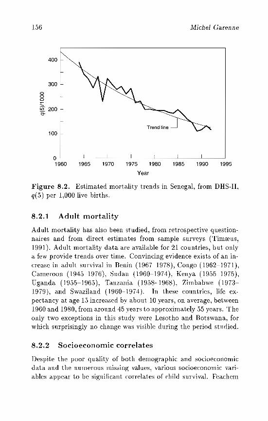
156 Michel Garenne

1980

400

300

ooo~

---Gl 2000:

100

o1960 1965 1970 1975

Year

1985 1990 1995

Figure 8.2. Estimated mortality trends in Senegal, from DRS-II,q(5) per 1,000 live births.

8.2.1 Adult mortality

Adult mortality has also been studied, from retrospective question­naires and from direct estimates from sample surveys (TimCEus,1991). Adult mortality data are available for 21 countries, but onlya few provide trends over time. Convincing evidence exists of an in­crease in adult survival in Benin (1967-1978), Congo (1962-1971),Cameroon (1945-1976), Sudan (1960-1974), Kenya (1955-1975),Uganda (1955-1965), Tanzania (1958-1968), Zimbabwe (1973­1979), and Swaziland (1960-1974). In these countries, life ex­pectancy at age 15 increased by about 10 years, on average, between1960 and 1980, from around 45 years to approximately 55 years. Theonly two exceptions in this study were Lesotho and Botswana, forwhich surprisingly no change was visible during the period studied.

8.2.2 Socioeconomic correlates

Despite the poor quality of both demographic and socioeconomicdata and the numerous missing values, various socioeconomic vari­ables appear to be significant correlates of child survival. Feachem

Mortality in Sub-Saharan Africa: Trends and Prospects 157

and Jamison (1991) found a significant correlation between the levelof infant and child mortality and income, measured by the GNP percapita in 1987, as well as by secondary school enrollment.

A systematic review of these correlations was undertaken byTrani (1992), using all the available evidence from socioeconomicdata published by the World Bank (Tables 8.3, 8.4, and 8.5). Inthe linear simple regressions, seven variables appear significant: twomeasures of income (index of CDP/ capita and GNP/capita), threemeasures of education (literacy and enrollment in primary and sec­ondary schools), one measure of public health (number of physi­cians) , and one measure of nutrition (caloric consumption). Owingto the poor quality of the data, no further analysis could be done.However, these correlations indicate that the mortality decline ispart of the whole development process, and that countries doingwell economically and socially are also showing improvements inmortality levels. There are, however, a number of outliers in theregression analysis. Countries such as Sierra Leone, Gambia, andMalawi have higher than expected mortality, and this was also thecase in 1960. Countries such as Kenya, Botswana, and Zimbabwehave lower than expected mortality; they were also among the coun­tries with the lowest mortality in 1960 (Table 8.2).

8.2.3 Public health and primary health care

Modern health infrastructures developed significantly after 1960,and the number of health personnel per capita also increased. Inparticular, the number of physicians per capita increased by about100 percent during the 1960-1985 period and the number of nursesper capita, by 373 percent. In Botswana, the number of physi­cians per capita has increased 6.2 times and the number of nurses,70 times. Botswana has 38 times more physicians per capita thanBurkina Faso. Hence, there is little wonder why Botswana has thelowest mortality levels.

Major health programs were also implemented in Africa after1960. The interest of the health authorities and of donor agenciesshifted from tropical diseases affecting adult mortality toward ma­ternal and child health care. Efforts were made to provide new vac­cines, in particular vaccines against measles and poliomyelitis. Af­ter 1978, selective primary health-care strategies were implemented

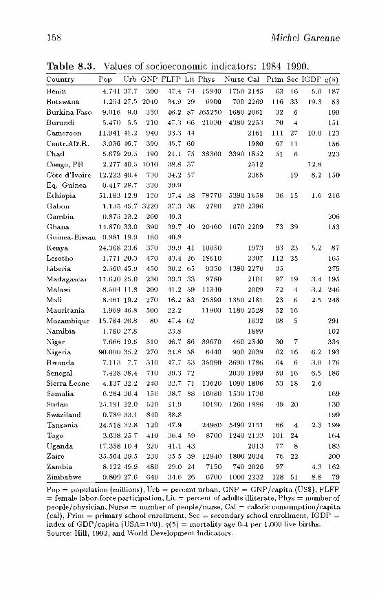
158 Michel Garenne

Table 8.3. Values of socioeconomic indicators: 1984-1990.Country Pop Urb GNP FLFP Lit Phys Nurse Cal Prim Sec IGDP q(.5)

Benin 4.741 37.7 390 47.4 74 1.5940 17.50 2145 63 16 5.0 187

Botswana 1.254 27.5 2040 34.9 29 6900 700 2269 116 33 19.3 53

Burkina Faso 9.016 9.0 330 ·16.2 87 265250 1680 2061 32 6 199

Burundi 5.470 5.5 210 47.3 66 21030 4380 2253 70 4 151

Cameroon 11.941 41.2 940 33.3 44 2161 111 27 10.0 123

Centr.Afr.R. 3.03646.7 390 4.5.7 60 1980 67 11 156

Chad 5.679 29.5 190 21.1 75 38360 3390 1852 51 6 223

Congo, PR 2.277 40.5 1010 38.8 37 2512 12.8

Cote d'Ivoire 12.223 40.4 730 34.2 57 2365 19 8.2 150

Eq. Guinea 0.417 28.7 330 39.9

Ethiopia 51.183 12.9 120 :37.4 38 78770 5390 1658 36 15 1.6 216

Gabon 1.13545.7 3220 37.3 38 2790 270 2396

Gambia 0.875 23.2 260 40.3 206

Ghana 14.870 33.0 390 39.7 40 20460 1670 2209 73 39 153

Guinea- Bissau 0.981 19.9 180 40.8

Kenya 24.368 23.6 370 39.9 41 100.50 1973 93 23 5.2 87

Lesotho 1.171 20.3 470 43.4 26 18610 2307 112 25 165

Liberia 2.560 45.9 4.50 30.2 65 9350 1380 2270 35 275

Madagascar 11.620 25.0 230 39.3 33 9780 2101 97 19 3.4 195

Malawi 8.50411.8 200 41.2 59 11340 2009 72 4 3.2 246

Mali 8.461 19.2 270 16.2 83 25390 1350 2181 23 6 2.5 248

Mauritania 1.969 46.8 500 22.2 11900 1180 2528 52 16

Mozambique 15.784 26.8 80 47.4 62 1632 68 5 291

Namibia 1.780 27.8 2:3.8 1889 102

Niger 7.666 19.5 310 46.7 86 39670 460 2340 30 7 334

Nigeria 90.000 35.2 270 34.8 58 6440 900 2039 62 16 6.2 193

Rwanda 7.113 7.7 310 47.7 53 35090 36901786 64 6 3.0 176

Senegal 7.428 38.4 710 39.3 72 2030 1989 59 16 6.5 186

Sierra Leone 4.137 32.2 240 32.7 71 13620 1090 1806 53 18 2.6

Somalia 6.284 36.4 150 38.7 88 16080 1530 1736 169

Sudan 25.191 22.0 .520 2UI 10190 1260 1996 49 20 130

Swaziland 0.78933.1 840 38.8 199

Tanzania 24.518 32.8 120 47.9 24980 5490 2151 66 4 2.3 199

Togo 3.638 25.7 410 36.4 59 8700 1240 2133 101 24 164

Uganda 17.358 10.4 220 41.1 43 2013 17 8 183

Zaire 3.5.564 39.5 230 35 ..5 39 12940 1800 2034 76 22 200

Zambia 8.122 49.9 480 29.0 24 7150 740 2026 97 4.3 162

Zimbabwe 9.80927.6 640 34.6 26 6700 1000 2232 128 51 8.8 79

Pop = population (millions), Urb = percent urban, GNP = GNP/capita (US$), FLFP= female labor-force participation, Lit = percent of adults illiterate, Phys = number ofpeople/physician, Nurse = number of people/nurse, Cal = caloric consumption/capita(cal), Prim = primary school enrollment, Sec = secondary school enrollment, IGDP =index of GDP/capita (USA=100). q(.5} = mortality age 0-4 per 1,000 live births.Source: Hill, 1992, and \Vorld Development Indicators.

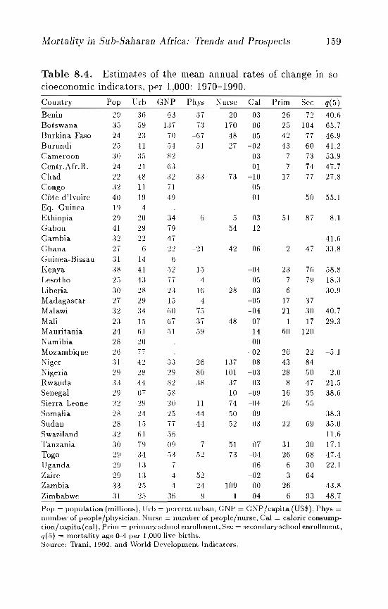
Mortality in Sub-Saharan Africa: Trends and Prospects 159

Table 8.4. Estimates of the mean annual rates of change III so-cioeconomic indicators, per 1,000: 1970-1990.

Country Pop Urb GNP Phys Nurse Cal Prim Sec q(5)Benin 29 36 63 37 20 03 26 72 40.6Botswana 35 59 1:37 73 170 06 25 104 65.7Burkina Faso 24 23 70 -67 48 05 42 77 46.9Burundi 25 41 54 5] 27 -02 43 60 41.2Cameroon :30 35 k'~ 03 7 73 53.9Centr.Afr.R. 24 21 63 -01 7 74 47.7Chad 22 48 32 33 73 -10 17 77 27.8Congo 32 11 7] 05Cote d'Ivoire 40 19 49 01 50 55.1Eq. Guinea 19 4Ethiopia 29 20 34 -6 5 -03 51 87 8.]Gabon 4] 29 79 54 12Gambia 32 2'2 47 41.6Ghana .)- (j :t2 -21 42 06 2 47 33.8_I

Guinea- Bissau 31 14 (j

I\enya 38 41 52 ]5 -04 23 76 58.8Lesotho ') r:: 13 II 4 05 7 79 18.3... ,)

Liberia 30 28 n ](j 28 03 -6 30.9Madagascar 27 29 15 4 -05 17 37MaIawi 32 34 60 75 -04 21 30 40.7Mali 23 ]5 fi7 37 48 07 -1 17 29.3Mauritania 24 (j] 51 59 14 60 120Namibia 28 20 00Mozambique 26 77 -02 26 22 -5.1Niger :31 42 :B 26 137 08 43 84Nigeria 29 28 29 80 101 -03 28 50 2.0Rwanda :33 44 1'\'1 38 37 03 8 47 21.5'- -Senega.! 29 0, 58 10 -09 16 35 38.6Sierra Leone 22 29 211 11 74 -04 26 55Somalia 28 24 2.5 44 50 09 :38.3Sudan 28 15 II 44 52 03 22 69 35.0Swaziland 32 61 56 11.6Tanzania 30 79 09 -7 -51 07 31 30 17.1Togo 29 34 53 52 73 -04 26 68 47.4Uganda 29 13 , -06 6 30 22.]Zaire 29 ]3 -4 5') -02 3 64Zambia 33 25 4 24 109 -00 26 43.8Zimbabwe 31 25 36 9 - 1 04 6 93 48.7

Pop = population (millions), Urb = percent urban, GNP = GNP /capita (US$), Phys =nunlher of people/physician. Nurse = nnmber of people/nurse, Cal = caloric consump-tion/capi ta (cal). Prim = primary school enrollment., Sec = secondary school enrollment,q(5) = mort.ality age 0-4 per 1.000 live births.Source: Trani, 1992, and 'Norld D"velopmenl. Indicators.

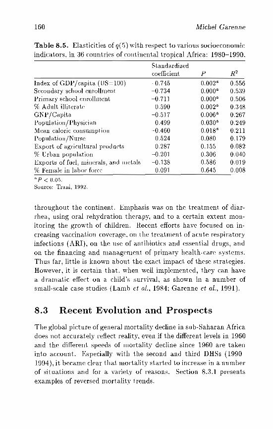
160 Michel Garenne

R2p

Table 8.5. Elasticities of q(S) with respect to various socioeconomicindicators, in 36 countries of continental tropical Africa: 1980-1990.

Standardizedcoefficient

Index of GDP/capita (US=100)Secondary school enrollmentPrimary school enrollment% Adult illiterateGNP/CapitaPopulation/ PhysicianMean caloric consumptionPopulation/NurseExport of agricultural products% Urban populationExports of fuel, minerals, and metals% Female in labor force

-0.745-0.734-0.711

0.590-0.5170.499

-0.4600.5240.287

-0.201-0.1380.091

0.002 a

O.oooaO.oooa0.002a

0.006 a

0.030a

0.018a

0.0800.1550.3060.5860.645

0.5560.5390.5060.3480.2670.2490.2110.1790.0820.0400.0190.008

a p < 0.05.SQurce: Trani, 1992.

throughout the continent. Emphasis was on the treatment of diar­rhea, using oral rehydration therapy, and to a certain extent mon­itoring the growth of children. Recent efforts have focused on in­creasing vaccination coverage. on the treatment of acute respiratoryinfections (ARI), on the use of antibiotics and essential drugs, andon the financing and management of primary health-care systems.Thus far, little is known about the exact impact of these strategies.However, it is certain that. when well implemented, they can havea dramatic effect on a child's survival, as shown in a number ofsmall-scale case studies (Lamb et 01., 1984; Garenne et 01., 1991).

8.3 Recent Evolution and Prospects

The global picture of general mortality decline in sub-Saharan Africadoes not accurately reflect reality. even if the different levels in 1960and the different speeds of mortality decline since 1960 are takeninto account. Especially with the second and third DHSs (1990­1994), it became clear that mortality started to increase in a numberof situations and for a variety of reasons. Section 8.3.1 presentsexamples of reversed mortality trends.

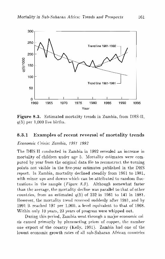
Mortality in Sub-Saharan Africa: Trends and Prospects 161

300

250

200000:;;.. 150L{)

0:

100

Trend line 1981-1992

l

Trend line 1961-1981 J50

1995199019851980197519701965

o LI__-'----__L-__---L__---l.-__L-_----.il _

1960

Year

Figure 8.3. Estimated mortality trends in Zambia, from DHS-II,q( 5) per 1,000 live births.

8.3.1 Examples of recent reversal of mortality trends

Economic Crisis: Zambia, 1981-1992

The DRS-II conducted in Zambia in 1992 revealed an lllcrease III

mortality of children under age 5. Mortality estimates were com­puted by year from the original data file to reconstruct the turningpoints not visible in the five-year estimates published in the DHSreport. In Zambia, mortality declined steadily from 1961 to 1981,with minor ups and downs which can be attributed to random fluc­tuations in the sample (Figure 8.3). Although somewhat fasterthan the average, the mortality decline was parallel to that of othercountries, from an estimated q(5) of 232 in 1961 to 141 in 1981.However, the mortality trend reversed suddenly after 1981, and by1991 it reached 197 per 1,000, a level equivalent to that of 1968.Within only 10 years, 23 years of progress were whipped out.

During this period, Zambia went through a major economic cri­sis caused primarily by plummeting prices of copper, the numberone export of the country (Kelly, 1991). Zambia had one of thelowest economic growth ra.tes of all sub-Saha.ran African countries

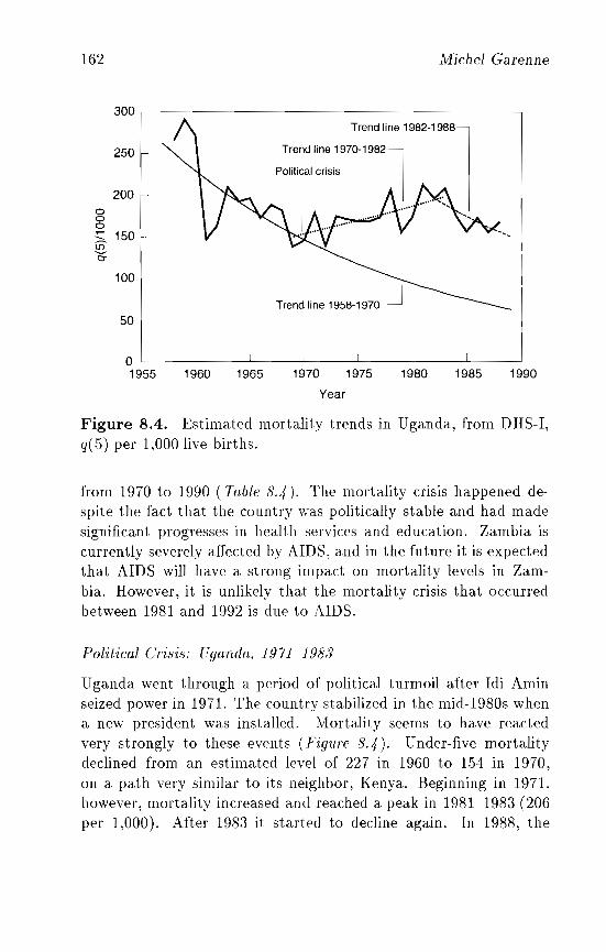
162 Michel Garenne

300, ~

250

200000::::: 150to0:

100

Trend line 1956-1970 J50

o1955 1960 1965 1970 1975 1980 1985 1990

Year

Figure 8.4. Estimated mortality trends in Uganda, from DHS-I,q(.5) per 1,000 live births.

from 1970 to 1990 (Table 8..{). The mortality crisis happened de­spite the fact that the country was politically stable and had madesignificant progresses in health services and education. Zambia iscurrently severely affected by AIDS, and in the future it is expectedthat AIDS will have a strong impact on mortality levels in Zam­bia. However, it is unlikely that the mortality crisis that occurredbetween 1981 and 1992 is due to AIDS.

Political Crisis: Uganda, 1971-1988

Uganda went through a period of political turmoil after Idi Aminseized power in 1971. The country stabilized in the mid-1980s whena new president was installed. Mortality seems to have reactedvery strongly to these events (Figure 8.4). Under-five mortalitydeclined from an estimated level of 227 in 1960 to 1.54 in 1970,on a path very similar to its neighbor, Kenya. Beginning in 1971,however, mortality increased and reached a peak in 1981-1983 (206per 1,000). After 198;3 it started to decline again. In 1988, the

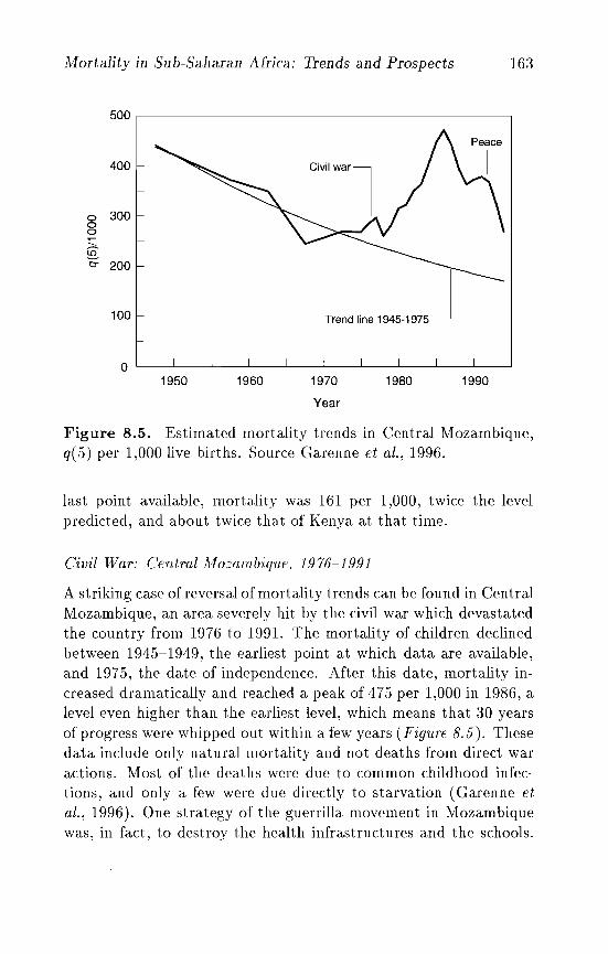
Mortality in Sub-Saharan Africa: Trends and Prospects 163

19901980

"eo' Ii" 1945-1975 I

19701960

500

400

0 30000~--it)0: 200

100

01950

Year

Figure 8.5. Estimated mortality trends in Central Mozambique,q(5) per 1,000 live births. Source Garenne et al., 1996.

last point available, mortality was 161 per 1,000, twice the levelpredicted, and about twice that of Kenya at that time.

Civil War: Central Mozambique, 1976-1991

A striking case of reversal of mortality trends can be found in CentralMozambique, an area severely hit by the civil war which devastatedthe country from 1976 to 1991. The mortality of children declinedbetween 1945-1949, the earliest point at which data are available,and 1975, the date of independence. After this date, mortality in­creased dramatically and reached a peak of 475 per 1,000 in 1986, alevel even higher than the earliest level, which means that 30 yearsof progress were whipped out within a few years (Figure 8.5). Thesedata include only natural mortality and not deaths from direct waractions. Most of the deaths were due to common childhood infec­tions, and only a few were due directly to starvation (Garenne etal., 1996). One strategy of the guerrilla movement in Mozambiquewas, in fact, to destroy the health infrastructures and the schools.

164 Michel Garenne

This study clearly shows that the destruction of the health systemcan have a devastating impact on child mortality.

Possible Impact of AIDS on Child Mortality: Kenya, 1989-1993

After a long history of steady mortality decline, Kenya recently ex­perienced a mortality increase. This increase is evident in the mostrecent DHS (Figure 8.6). The adjusted trend fits the mortality de­cline in Kenya from 1961 to 1989, when mortality reached its lowestvalue, 76 per 1,000. But from 1990 to 1993 mortality increased sig­nificantly above the value predicted from the previous trend. By1993 it reached 122 per 1,000, the mortality level of 1976. This verymarked mortality increase after :30 yea,rs of rapid improvements wassurprising. No obvious explanation comes to mind: Kenya had po­litical stability (despite significant domestic problems), steady eco­nomic growth, major improvements in health and education, and aremarkable decline in fertility. The recent mortality increase couldbe attributed to the onset ofthe AIDS epidemic raging in Kenya, butthis interpretation would require confirmation from cause of deathinformation.

Impact of A IDS on Adult Mortality: Abidjan, 1986-1992

AIDS is already having a strong impact on mortality of young adultsin sub-Saharan Africa. A recent study in Abidjan, the capital cityof Cote d'Ivoire, shows a doubling of mortality within the first sevenyears of the AIDS epidemics (1986-1992), after 13 years of small butregular improvements (1973-1985) (Figure 8.7). The demographicdata are from the city's vital registration statistics, which have ahigh degree of reliability. From scarce cause of death information,this changing pattern has been attributed almost entirely to AIDS(Garenne et al., 1995). A similar increase in adult mortality hasbeen found in the rural areas of southwestern Uganda.

8.3.2 Socio-political factors

The complete picture of the recent evolution of mortality in sub­Saharan Africa may be optimistically biased, since the demographicsituations of the most critical cases are not documented. For in­stance, recent reports state that famine is threatening one-third

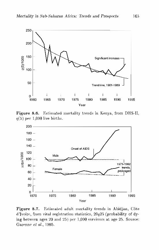
Mortality in Sub-Saharan Africa: Trends and Prospects 165

250 ,,--------------------------,

200

o 150oo~--§:0- 100

50

Significant increasel

Trend line, 1961-1989Ja I J J I I

1960 1965 1970 1975 1980 1985 1990 1995

Year

1995199019851980

Female

1975

.........................................,1973-1982

"'---........... ~ trends,_ ~......... ~ / prolonged............................~ ~

0 12000~ 100"'N0- 800N

60

40

20

01970

Figure 8.6. Estimated mortality trends in Kenya, from DRS-II,q(5) per 1,000 live births.

2001

",

180

160

140

Year

Figure 8.7. Estimated adult mortality trends in Abidjan, Coted'Ivoire, from vital registration statistics, 20q25 (probability of dy­ing between ages 20 and 25) per 1,000 survivors at age 25. Source:Garenne et ai., 1995.

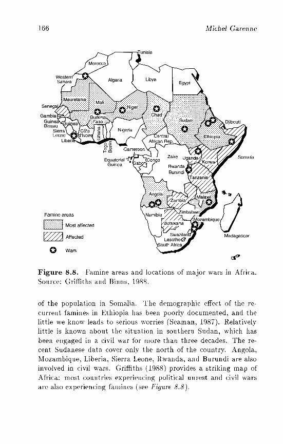
166

GambiaGuinea'Bissau

SierraLeoneLiberl~

Famine areas

k>«:1 Most affected

~ Affected

o Wars

Michel Garenne

rJ.C>

Figure 8.8. Famine areas and locations of major wars in Africa.Source: Griffiths and Binns, 1988.

of the population in Somalia. The demographic effect of the re­current famines in Ethiopia has been poorly documented, and thelittle we know leads to serious worries (Seaman, 1987). Relativelylittle is known about the situation in southern Sudan, which hasbeen engaged in a civil wa,r for more than three decades. The re­cent Sudanese data cover only the north of the country. Angola,Mozambique, Liberia, Sierra Leone, Rwanda, and Burundi are alsoinvolved in civil wars. Griffiths (1988) provides a striking map ofAfrica: most countries experiencing political unrest and civil warsare also experiencing famines (see Figure 8.8).

Mortality in Sub-Saharan Africa: Trends and Prospects 167

The future of African mortality may be divided into two cate­gories: countries continuing their rapid trend toward low-mortalitysituations, and countries so politically and economically disturbedthat any improvements in the mortality situation must be postponedto the unforeseeable future. International aid seems to reinforce thisdichotomy rather than to diminish it. For instance, USAID, themost active agency for child-survival programs, has a list of coun­tries for which it will not intervene. These countries are often thepoorest and the most desperate. Countries that are democratic anddeveloping rapidly receive more international support than thosethat are undemocratic and not developing or slowly developing.

8.3.3 Epidemiological factors

Tropical Africa is also experiencing a profound sociological and epi­demiological transition. The emergence of the modern economy de­stroyed most of the traditional agricultural and economic systemand perturbed the ecological balance between populations and re­sources. This change led to massive migration flows and to veryrapid urbanization. In Senegal, about half of the population nowlives in cities or large towns, whereas at the turn of the century99 percent of the population was rural and no city accounted formore than 5,000 inhabitants. In Mauritania, more than half of thepopulation became urban in less than one generation.

This pattern of migration has been favorable to the rapid spreadof communicable diseases, in particular sexually transmitted dis­eases - as happened with syphilis at the onset of economic de­velopment in Europe, and basically for the same reasons (Shorter,1990). The AIDS epidemic is the leading source of concern in thisrespect. The dynamics of the AIDS epidemic has been affected bythe existence of the network of international truck drivers (alongthe Tanzania-Kenya-Ugancla highway), by the emergence of largenumbers of urban commercial sex workers, and by the appearanceof large communities of single male migrants in cities, like Abidjanand Johannesburg. The spread of AIDS is probably the single mostimportant factor propelling the mortality increase in sub-SaharanAfrica. Projections made of the mortality of future generations arealarming: up to half of the population of some countries or regions

168 Michel Garenne

may have AIDS as a cause of death. The death rates may evenexceed the birth rates in extreme situations, reversing the patternof population growth (Anderson, 1991). The AIDS epidemic hasanother major consequence: the disruption of families, by the deathof one parent or both, exposing new orphans to risks of infection,malnutrition, and accidents. There are also increases in mortalityfrom tuberculosis, as already shown in developed countries (Murrayet at., 1990), and possibly of viral hepatitis B.

The massive implementation of modern medicine has also af­fected the ecology of certain diseases. This is the case for malaria,as more and more cases of strains resistant to chloroquine are doc­umented (Bradley, 1991). Malaria has always been a leading causeof death in Africa. Resistant malaria strains may lead toward anincrease in deaths attributed to this disease. There is now somelimited evidence suggesting increasing malaria mortality, such asthe case of Abidjan and Ouagadougou, two cities in West Africa(Garenne et at., 1995). Furthermore, the wide-scale use of anti­malarial drugs may have led to a decline in natural immunity. This,in turn, may make certain populations vulnerable to major out­breaks of malaria, such as what happened in Madagascar in 1988.

Cholera came back to Africa in 1971 after an 80-year absence.The index case was brought by plane to Conakry, Guinea, an exam­ple of a new way of spreading communicable diseases. Since then,cholera has become endemic in most of tropical Africa, and seemsalso to have become a leading cause of death, at least in rural areas.

The vaccination coverage against yellow fever has droppedmarkedly in many countries. Recent outbreaks have taken placein Nigeria and will occur again in the future unless vaccination cov­erage increases dramatically. Although rare, plague still exists inMadagascar and occurs occasionally on the east coast of Africa.

With changing lifestyles and growing urbanization, new diseaseswill also emerge or reappear as a result of increasing risk factors orchanging ecological conditions. Smoking has increased in Africa,with the help of massive commercial campaigns by tobacco compa­nies. Obesity, rare in villages, has become prevalent in cities andmay be linked with a probable increase in the prevalence of diabetes.Car accidents are also becoming a significant cause of death; Africanroads are among the most dangerous in the world. Political violence

Mortality in Sub-Saharan Africa: Trends and Prospects 169

has been taking a heavy toll in the recent years; for instance, thepopulation of Rwanda was devastated during the 1994-1995 civilwar.

8.4 Discussion

The past trends of mortality in Africa have been induced by trans­fers of technology from the 'Vest, which have affected virtually allcountries on the continent in a short period of time. Public health,nutrition, economic development, and modern education seem tohave been the key determinants ill mortality change. However, thefuture of mortality in Africa is hard to determine and even harderto quantify. There are reasons to believe that the major and quiteuniform mortality decline experienced over the first 25 years of inde­pendence (1960-1985) will not be followed by a com parable declinein the next 25 years in all the countries of sub-Saharan Africa. Mostlikely, the principal differences that already exist between countrieswill prevail and may even increase. Some nations will continue alongtheir successful routes to low mortality, and others will see theirhealth transition stop or even reverse for some period of time. Be­sides the socio-political conditions, a critical factor will be the spreadof the HIV virus, resistant malaria, tuberculosis, and other diseasesinfecting the general population.

The control that the countries have over the health of theirpopulation is also a function of their research capacity to identifynew problems and to choose the most appropriate solutions in time.Essential National Health Research has recently been seen as oneof the top priorities for developing countries (ENHR Report, 1990).Data information systems to identify and tackle new diseases andnew health problems may be an important component of the successof health policies in the future. The AIDS epidemics could have beensmaller in size if appropriate steps had been taken at its onset.

Acknowledgments

I would like to thank Jean Fran!;ois Trani for his contribution tothe statistical analysis and Meg Tyler for editorial comments on anearlier draft.

Chapter 9

Global Trends in AIDSMortality

John Bongaarts

The AIDS epidemic began spreading around 1980 in North Amer­ica, Western Europe, and sub-Saharan Africa; since then HIV, thevirus that causes AIDS, has quickly reached all corners of the globe(WHO, 1994).[1] Despite significant efforts to contain the epidemic,HIV is now spreading more rapidly than ever, resulting in an esti­mated 2.4 million new infections each year among adults (WHO,1995b). Expansion is most rapid in sub-Saharan Africa and Asia,with approximately 1 million new infections annually in each con­tinent. In addition, a growing number of infections occur through"vertical transmission" from mother to child during pregnancy, de­livery, or breastfeeding. In the early 1980s AIDS was thought tobe primarily a disease of homosexuals and injecting drug users, butheterosexual transmission was soon found to be common in Africaand elsewhere (Piot et al., 1988). Today the large majority of infec­tions worldwide are the result of sexual intercourse between men andwomen, even though this is a relatively inefficient mode of transmis­sion (the probability of infection per heterosexual contact betweenan uninfected individual and an asymptomatic carrier averages lessthan 1 percent if the uninfected person is healthy). Transmissionthrough transfusion with contaminated blood and blood products

Reprinted with the permission of the Population Council, from Population andDevelopment Review 22(1), March 1996.

170

Global Trends in AIDS Mortality 171

has been reduced to very low levels in countries with extensive test­ing, but where screening is incomplete transfusion can be a signifi­cant source of HIV infection.

The HIV/ AIDS epidemic has become a serious public healthproblem because no cure or vaccine exists and infection almostinvariably leads to death. Infection is followed by years of slowdestruction of the immune system, rendering carriers increasinglyvulnerable to fatal opportunistic infections such as pneumocysticpneumonia and cancers such as Kaposi's sarcoma. The median in­cubation period between initial infection and onset of AIDS is abouta decade (Chin and Lwanga, 1991a). Carriers are typically asymp­tomatic for most of the incubation period and they therefore canunwittingly infect others, thus contributing to the rapid dissemina­tion of HIV.

The World Health Organization (WHO) monitors the epidemicclosely and estimates that by mid-1995 a cumulative total of about18.5 million adults had been infected with HIV worldwide since the1970s (WHO, 1995a). Despite the many uncertainties and limi­tations regarding available statistics, this global estimate and thegeographic distribution of infections published by WHO are widelyaccepted.[2] However, the future course of the epidemic remainscontroversial.

During the remainder of the 1990s WHO expects 10-15 millionnew HIV infections among adults and 5-10 million among children(through vertical transmission), bringing the cumulative total bythe year 2000 to 30-40 million HIV infections (WHO, 1994). Oth­ers expect more severe epidemics. For example Mann et al. (1992)project that the cumulative total of infections by 2000 could exceed100 million. Model simulations of African epidemics by Andersonet at. (1991) and by Gregson et al. (1994) indicate that a majorityof adults could become infected, leading to massive AIDS mortalityand possibly even to declines in population size.

This article presents a set of projections of the epidemic from1995 to 2005 for major world regions and assesses the correspond­ing effects on death rates and population growth. Estimates of thefuture demographic impact of AIDS for world regions have not yetbeen made. The United Nations (UN, 1995) and the US Bureau

172 John Bongaarts

of the Census (Way and Stanecki, 1994) have prepared such assess­ments for a number of African countries especially affected by AIDS,but their findings differ substantially from each other.

9.1 Global Patterns

In the 1980s the number of AIDS cases reported to WHO wasthe most widely used statistic to monitor the epidemic's expansionworldwide. The exponential growth in AIDS cases then observed ­a doubling annually for much of the 1980s - reflected the exception­ally rapid spread of this new disease. Unfortunately, underreportingdue to limited access to health care, lack of diagnostic facilities, andreluctance of individuals, medical personnel, or governments to re­port the disease and/or the full extent of the epidemic has been aserious problem, especially in Africa. The cumulative number ofAIDS cases reported by the beginning of 1994 is estimated to beless than a quarter of the actual number (WHO, 1994). Moreover,the number of AIDS cases, even if accurately known, does not givea complete picture of the epidemic because there are several timesmore individuals infected with HIV than there are AIDS cases. As aconsequence, WHO now relies on the estimated cumulative numberof HIV infections in major world regions as the principal statisticwith which to monitor the global epidemic.

By the end of 1994 an estimated cumulative total of 17.2 mil­lion adults had been infected worldwide. Nearly 3 million of theseinfections have resulted in deaths from AIDS before 1995, leavingapproximately 14.3 million HIV-infected individuals alive at the endof 1994 (WHO, 1995b).[3] Sub-Saharan Africa accounts for overhalf of this total (see Table 9.1). Asia and Latin America havethe next largest numbers with, respectively, 3.4 and 1.7 million in­fected adults, and North America and Western Europe each haveless than 1 million. The estimated proportion of adults infectedaverages 0.4 percent worldwide, ranging from a high of 2.5 percentin sub-Saharan Africa to a low of 0.2 percent in Asia and WesternEurope.

These regional averages, in turn, conceal large differences in thesize of the epidemic between countries. This is the case in every con­tinent, but especially in Africa. Figure 9.1 presents the geographic

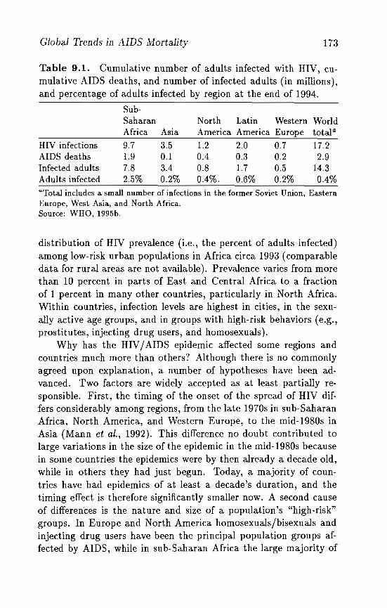
Global Trends in AIDS Mortality 173

Worldtotal a

North Latin WesternAmerica America Europe

Table 9.1. Cumulative number of adults infected with HIV, cu­mulative AIDS deaths, and number of infected adults (in millions),and percentage of adults infected by region at the end of 1994.

Sub-SaharanAfrica Asia

HIV infectionsAIDS deathsInfected adultsAdults infected

9.71.97.82.5%

3.50.13.40.2%

1.2 2.0 0.70.4 0.3 0.20.8 1.7 0.50.4%. 0.6% 0.2%

17.22.9

14.30.4%

aTotal includes a small number of infections in the former Soviet Union, EasternEurope, West Asia, and North Africa.Source: WHO, 1995b.

distribution of HIV prevalence (i.e., the percent of adults infected)among low-risk urban populations in Africa circa 1993 (comparabledata for rural areas are not available). Prevalence varies from morethan 10 percent in parts of East and Central Africa to a fractionof 1 percent in many other countries, particularly in North Africa.Within countries, infection levels are highest in cities, in the sexu­ally active age groups, and in groups with high-risk behaviors (e.g.,prostitutes, injecting drug users, and homosexuals).

Why has the HIV/ AIDS epidemic affected some regions andcountries much more than others? Although there is no commonlyagreed upon explanation, a number of hypotheses have been ad­vanced. Two factors are widely accepted as at least partially re­sponsible. First, the timing of the onset of the spread of HIV dif­fers considerably among regions, from the late 1970s in sub-SaharanAfrica, Nor.th America, and Western Europe, to the mid-1980s inAsia (Mann et ai., 1992). This difference no doubt contributed tolarge variations in the size of the epidemic in the mid-1980s becausein some countries the epidemics were by then already a decade old,while in others they had just begun. Today, a majority of coun­tries have had epidemics of at least a decade's duration, and thetiming effect is therefore significantly smaller now. A second causeof differen'ces is the nature and size of a population's "high-risk"groups. In Europe and North America homosexuals/bisexuals andinjecting drug users have been the principal population groups af­fected by AIDS, while in sub-Saharan Africa the large majority of

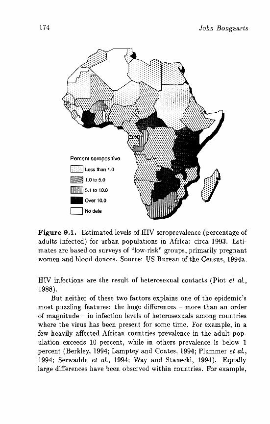
174

Percent seropositive

k /1 Less than 1.0

• 1.0 to 5.0

m:mmm 5.1 to 10.0

• Over 10.0

o No data

John Bongaarts

Figure 9.1. Estimated levels of HIV seroprevalence (percentage ofadults infected) for urban populations in Africa: circa 1993. Esti­mates are based on surveys of "low-risk" groups, primarily pregnantwomen and blood donors. Source: US Bureau of the Census, 1994a.

HIV infections are the result of heterosexual contacts (Piot et al.,1988).

But neither of these two factors explains one of the epidemic'smost puzzling features: the huge differences - more than an orderof magnitude - in infection levels of heterosexuals among countrieswhere the virus has been present for some time. For example, in afew heavily affected African countries prevalence in the adult pop­ulation exceeds 10 percent, while in others prevalence is below 1percent (Berkley, 1994; Lamptey and Coates, 1994; Plummer et al.,1994; Serwadda et al., 1994; Way and Stanecki, 1994). Equallylarge differences have been observed within countries. For example,

Global Trends in AIDS Mortality 175

according to a 1991 survey in Rwanda, prevalence was above 25 per­cent in urban areas, but only 2.2 percent in rural areas (Serwadda eta1., 1994). In one rural area of Zaire prevalence was low and stableat 0.8 percent for a decade (Nzilambi et aZ., 1988), while urban infec­tion levels were about 5 percent. Low infection levels (0.17 percent)are also found among childbearing women nationwide in the UnitedStates (Centers for Disease Control and Pr.evention, 1994). Thesefindings may be explained by variations in the following factors thatfacilitate or inhibit spread of the virus among heterosexuals:

• SexuaZ behavior. Frequent sexual contacts with individuals otherthan a permanent partner and frequent changes in partners arekey determinants of the speed of diffusion of HIV. There is littlecomparative evidence on sexual behavior, but differences amongcountries can be substantial. According to WHO-sponsored sur­veys in five sub-Saharan countries, the proportion of men report­ing sex with someone other than their regular partner in the pastyear ranged from 14 to 53 percent (Carael et a1., 1992). Cald­well et aZ. (1989), Piot and Carael (1988), and Larson (1989)discuss the social-institutional context that supports the highdegree of sexual networking in sub-Saharan Africa.

• Condom use. African men report infrequent reliance on con­doms when engaging in commercial sex (Carael et a1., 1992).Condoms are more widely used in developed countries, espe­cially in sexual contacts with one-time partners (UN, 1989a;Laumann et aZ., 1994).

• Sexually transmitted diseases (STDs). The infectiousness ofHIV carriers and the susceptibility of uninfected partners are ap­parently increased in the presence of STDs, particularly thosethat cause genital ulcers (e.g., chancroid, genital herpes, andsyphilis) (Piot et aZ., 1994; Cameron et aZ., 1989; Plummer etaZ., 1991, 1994). The prevalence of STDs is relatively high insome parts of sub-Saharan Africa (Caldwell and Caldwell, 1983).

• Absence of maZe circumcision. There is a highly significantcorrelation between the proportion of uncircumcised males inAfrican ethnic groups and countries and the prevalence of HIV(Bongaarts et a1., 1989; Moses et a1., 1990; Caldwell and Cald­well, 1993). Although this association may in part be due to

176 John Bongaarts

confounding factors (De Vincenzi and Mertens, 1994), it is con­sistent with clinic-based case-control studies in which circum­cised males were significantly less likely to be infected with HIVthan uncircumcised controls (Cameron et at., 1989; Seed et at.,1995). Several biological mechanisms, including enhanced sus­ceptibility to genital ulcer disease, may be responsible for theincreased risk of HIV infection among uncircumcised males (DeVincenzi and Mertens, 1994; Over and Piot, 1993; Caldwell andCaldwell, 1994).

Lack of reliable measures prevents a quantitative assessment ofthe relative roles played by these factors, but it is likely that theyare responsible for much of the differences in heterosexual epidemicsbetween countries, as well as for the equally large differences betweenregions and demographic groups within countries.

9.2 Past Trends

9.2.1 Prevalence

HIV prevalence trends from 1980 to 1995 for five major world re­gions are plotted in Figure 9.2. Epidemics in Africa, Asia, andLatin America, although differing widely in size, continued to ex­pand through the first half of the 1990s. Prevalence rates in NorthAmerica and Western Europe also grew rapidly during the 1980s,but they apparently have leveled off in the 1990s at less than one­half percent of the adult population. These trends represent aver­ages for regions; epidemics in countries within regions can deviatesignificantly from these averages not only in size but also in trend.For example, in Africa the epidemic is generally expanding rapidly,but in a few instances (e.g., in the capital cities of Bangui, Bujum­bura, Kampala, and Kinshasa) the epidemic appears to be levelingoff (US Bureau of the Census, 1993a, 1993b, 1994b).

The appearance of a plateau in HIV prevalence while a large pro­portion of a population remains uninfected is one of the epidemic'smost crucIal features. Although still rare in the developing world,this plateau is likely to be found eventually in all geographic ar­eas. A stable prevalence level implies that the virus is disseminated

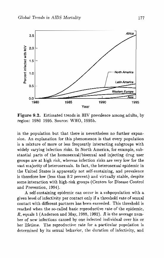
Global Trends in AIDS Mortality 177

2.5

~ 2.0£.3:-g 1.5"0Q)

:§C 1.0Q)

~Q)

a.0.5

0.01980 1985

Year1990

Africa

1995

Figure 9.2. Estimated trends in HIV prevalence among adults, byregion: 1980-1995. Source: WHO, 1995b.

in the population but that there is nevertheless no further expan­sion. An explanation for this phenomenon is that every populationis a mixture of more or less frequently interacting subgroups withwidely varying infection risks. In North America, for example, sub­stantial parts of the homosexual/bisexual and injecting drug usergroups are at high risk, whereas infection risks are very low for thevast majority of heterosexuals. In fact, the heterosexual epidemic inthe United States is apparently not self-sustaining, and prevalenceis therefore low (less than 0.2 percent) and virtually stable, despitesome interaction with high-risk groups (Centers for Disease Controland Prevention, 1994).

A self-sustaining epidemic can occur in a subpopulation with agiven level of infectivity per contact only if a threshold rate of sexualcontact with different partners has been exceeded. This threshold isreached when the so-called basic reproductive rate of the epidemic,R, equals 1 (Anderson and May, 1988, 1992). R is the average num­ber of new infections caused by one infected individual over his orher lifetime. The reproductive rate for a particular population isdetermined by its sexual behavior, the duration of infectivity, and

178 John Bongaarts

the infectivity per contact (which in turn is affected by the presenceof such cofactors as condom use, the prevalence of other sexuallytransmitted diseases, and the absence of male circumcision). In apopulation with homogeneous behavioral and biological character­istics, an epidemic will spread until nearly everyone is infected ifR exceeds 1. On the other hand, if in such a population R is lessthan 1, a self-sustaining epidemic cannot o.ccur. This is true evenif the virus is introduced repeatedly through contacts with infectedindividuals outside the group.

For the sake of simplicity, this explanation for the leveling offin prevalence rates has ignored some key aspects of the epidemic,such as changes in behavior over time, the movement of individualsbetween risk groups, and membership in more than one group, butthe main points remain valid. The virus first invades the subgroupswith the highest reproductive rates, and HIV prevalence rates inthese core groups rise rapidly to high levels. In contrast, the plateauin prevalence for the lowest-risk groups of heterosexuals can be ata fraction of 1 percent, as in North America and Western Europe,because the large majority of these populations do not engage inrisky behavior or engage in it so infrequently that their reproduc­tive rate is well below 1, and because their interaction with high-riskgroups is limited. In sub-Saharan Africa, on the other hand, the coregroup comprises prostitutes and their male partners; the virus canspread efficiently from these male partners to their wives and chil­dren, thus putting a large proportion of the general population atrisk. An epidemic reaches a plateau when the virus has achievedmaximum penetration in the vulnerable subpopulations. Becausethe size of the subgroups with high reproductive rates and their in­teractions with the general population vary widely among countries,the plateau levels of HIV prevalence also differ greatly, ranging fromno more than a few tenths of a percent in most developed countriesto more than 10 percent in a few countries in sub-Saharan Africa.

9.2.2 Incidence

The prevaience of infection at a point in time is the net result ofpast additions to the infected population through new infectionsand subtractions through deaths. Further insight into the dynam­ics of the epidemic can therefore be gained by examining trends in

Global Trends in AIDS AJortality 179

the annual incidence rates at which the key events - HIV infection,onset of AIDS, and death - occur. Figure 9.3 presents WHO esti­mates of these incidence rates for each region up to 1995. Becausethe epidemics in North America and Western Europe have evolvedfurthest, they give the most complete picture of the phases throughwhich other epidemics are likely to progress. In these two regions,a key turning point in the epidemic was reached in the mid-1980swhen the annual rate of new infections reached a maximum, esti­mated, respectively, at about 0.7 and 0.3 per thousand adults peryear.

The peaks in new HIV infections in sub-Saharan Africa andLatin America are estimated by WH0 to have occurred in the early1990s at, respectively, 3.6 and 0.9 infections per thousand adultsper year. The incidence of infections in Asia has not yet reachedits maximum, although one Asian country, Thailand, may alreadyhave passed it. In Thailand, HIV spread very rapidly in the late1980s, and prevalence in the adult population had reached 1.5 per­cent in urban areas at the end of 1993. Recent analyses suggestthat the incidence of HIV has been declining since 1991, in part dueto vigorous public health measures implemented by the government(Hanenberg et al., 1994; Tim Brown as cited in Cohen, 1994b).

Past trends in AIDS incidence are also plotted in Figure 9.3.Since the incubation period averages about a decade, there is asubstantial delay between the rise in new infections and the corre­sponding increase in new AIDS cases. In all regions, the estimatedAIDS incidence rose through 1994. However, in North America andWestern Europe the rate of increase in AIDS incidence has slowed inthe early 1990s, suggesting that a plateau is approaching. Patternsof incidence of AIDS deaths are very similar to those of AIDS; theonly difference is a delay of about one year.

A comparison of Figures 9.2 and 9.3 shows that the prevalenceof HIV can continue rising for a number of years after the incidencerate has begun its decline. This is possible because individuals whoare HIV-positive in a given year have become infected over a num­ber of years in the past. For example, in the hypothetical case inwhich an infected individual survives exactly 10 years before dying,the number of infected individuals at any given time would equalthe sum of all infections in the past 10 years regardless of whether

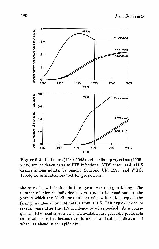
180 John Bongaarts

4 r'--------------,-------------,

Africaen'5"5l§...~.l!lS&i'5G>.0EE~c.:i: 1965 1990 1995

AIDS onset

AIDS death

2000 2005Year

20052000199519901965

0' !, I ,.............. I1960 I ~

I I.l!l 0.61 A ..;~.I"3"5l§. 0.6...~en~ 0.4&i'5Q;-g 0.2

E1U::lC

.:i:Year

Figure 9.3. Estimates (1980-1995) and medium projections (1995­2005) for incidence rates of HIV infections, AIDS cases, and AIDSdeaths amo.ng adults, by region. Sources: UN, 1995, and WHO,1995b, for estimates; see text for projections.

the rate of new infections in those years was rising or falling. Thenumber of infected individuals alive reaches its maximum in theyear in which the (declining) number of new infections equals the(rising) number of annual deaths from AIDS. This typically occursseveral years after the HIV incidence rate has peaked. As a conse­quence, HIV incidence rates, when available, are generally preferableto prevalence rates, because the former is a "leading indicator" ofwhat lies ahead in the epidemic.

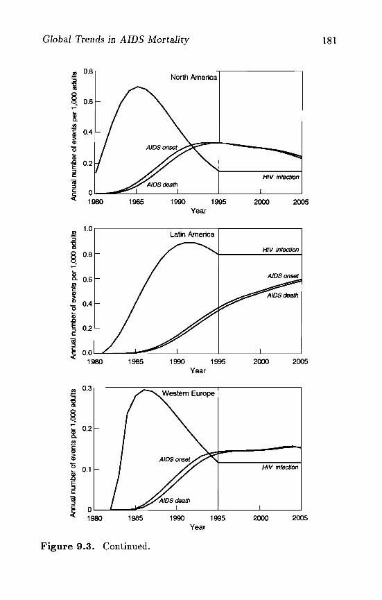
Global Trends in AIDS Mortality 181

HIV infection

2000 2005199519901985

0' ~ I I I I I

1980

.<g 0.81 North America I I:::3

a1§ 0.6...~.l!llii 0.4iD'0

~E:::3C

(ij:::3C

~

Year

200520001995

Latin America

19901985

0.4

0.0' "~ I I !

1980

rn 1.0"'5a1§ 0.8...~ 0.6

i'0

~§ 0.2c(ij:::3

~Year

HIV infection

2000 20051995199019850' «rr+-" I I I I

1980

~ 0.3,III I

§...~ 0.2

rn

55iD'0 01I .c

~

~Year

Figure 9.3. Continued.

----- -- --

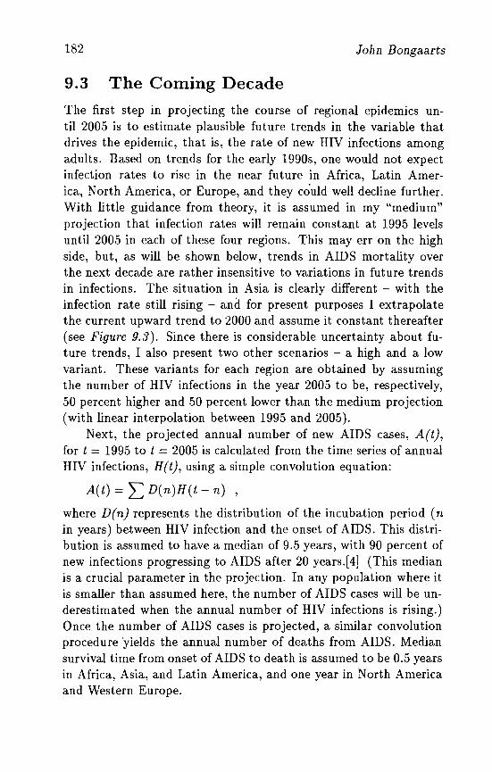
182 John Bongaarts

9.3 The Coming Decade

The first step in projecting the course of regional epidemics un­til 2005 is to estimate plausible future trends in the variable thatdrives the epidemic, that is, the rate of new HIV infections amongadults. Based on trends for the early 1990s, one would not expectinfection rates to rise in the near future in Africa, Latin Amer­ica, North America, or Europe, and they could well decline further.With little guidance from theory, it is assumed in my "medium"projection that infection rates will remain constant at 1995 levelsuntil 2005 in each of these four regions. This may err on the highside, but, as will be shown below, trends in AIDS mortality overthe next decade are rather insensitive to variations in future trendsin infections. The situation in Asia is clearly different - with theinfection rate still rising - and for present purposes I extrapolatethe current upward trend to 2000 and assume it constant thereafter(see Figure 9.3). Since there is considerable uncertainty about fu­ture trends, I also present two other scenarios - a high and a lowvariant. These variants for each region are obtained by assumingthe number of HIV infections in the year 2005 to be, respectively,50 percent higher and 50 percent lower than the medium projection(with linear interpolation between 1995 and 2005).

Next, the projected annual number of new AIDS cases, A(t),for t = 1995 to t = 2005 is calculated from the time series of annualHIV infections, H(t) , using a simple convolution equation:

A(t) =L D(n)H(t - n) ,

where D(n) represents the distribution of the incubation period (nin years) between HIV infection and the onset of AIDS. This distri­bution is assumed to have a median of 9.5 years, with 90 percent ofnew infections progressing to AIDS after 20 years.[4] (This medianis a crucial parameter in the projection. In any population where itis smaller than assumed here, the number of AIDS cases will be un­derestimated when the annual number of HIV infections is rising.)Once the number of AIDS cases is projected, a similar convolutionprocedure 'yields the annual number of deaths from AIDS. Mediansurvival time from onset of AIDS to death is assumed to be 0.5 yearsin Africa, Asia, and Latin America, and one year in North Americaand Western Europe.

------,.~-

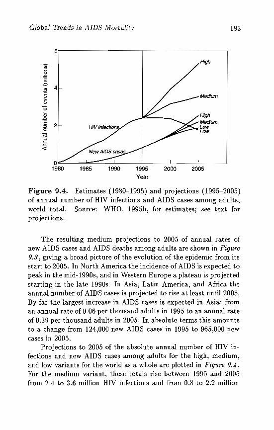
Global Trends in AIDS Mortality 183

6"------------,-------------------,

200520001995Year

199019850.......... ! ---- I I I ! I

1980

VI,High

c:,g"E2l 4c: I I / __ MediumQ)

>Q)

'0Q;

2~High.c

E Medium::J HIV infections Lowc: Low"iii::Jc:c:«

Figure 9.4. Estimates (1980-1995) and projections (1995-2005)of annual number of HIV infections and AIDS cases among adults,world total. Source: WHO, 1995b, for estimates; see text forprojections.

The resulting medium projections to 2005 of annual rates ofnew AIDS cases and AIDS deaths among adults are shown in Figure9.3, giving a broad picture of the evolution of the epidemic from itsstart to 2005. In North America the incidence of AIDS is expected topeak in the mid-1990s, and in Western Europe a plateau is projectedstarting in the late 1990s. In Asia, Latin America, and Africa theannual number of AIDS cases is projected to rise at least until 2005.By far the largest increase in AIDS cases is expected in Asia: froman annual rate of 0.06 per thousand adults in 1995 to an annual rateof 0.39 per thousand adults in 2005. In absolute terms this amountsto a change from 124,000 new AIDS cases in 1995 to 965,000 newcases in 2005.

Projections to 2005 of the absolute annual number of HIV in­fections and new AIDS cases among adults for the high, medium,and low variants for the world as a whole are plotted in Figure 9.4.For the medium variant, these totals rise between 1995 and 2005from 2.4 to 3.6 million HIV infections and from 0.8 to 2.2 million

184 John Bongaarts

Table 9.2. Projected high, medium, and low variants of cumula­tive HIV infections, AIDS cases, and AIDS deaths (millions) amongadults in 2005, by region.

Sub-SaharanAfrica Asia

North Latin Western WorldAmerica America Europe totala

Cumulative HIV infectionHigh variant 23.3Medium variant 20.7Low variant 18.1

23.019.115.3

1.61.51.4

5.24.64.0

1.00.90.9

54.747.440.1

Cumulative AIDS casesHigh variant 9.4 5.3 1.0 2.0 0.6 18.5Medium variant 9.1 4.9 1.0 1.9 0.6 17.8Low variant 8.9 4.6 1.0 1.9 0.6 17.2

Cumulative AIDS deathsHigh variant 8.9 4.8 1.0 1.9 0.5 17.2Medium variant 8.7 4.5 1.0 1.8 0.5 16.8Low variant 8.5 4.2 1.0 1.8 0.5 16.2GTotai includes a small number of infections in the former Soviet Union, EasternEurope, West Asia, and North Africa.

new AIDS cases per year. Interestingly, the difference between thehigh and low variants is larger for the projected number of new HIVinfections than for new AIDS cases. The same is true for the cu­mulative number of HIV infections and AIDS cases for each region(see Table 9.2). The reason for this is the long incubation period.Projected AIDS cases in 2005 are the result of HIV infections thatoccurred on average in the mid-1990s, when the uncertainty aboutthe number .of infections is much smaller. As a consequence, projec­tions of AIDS cases and AIDS mortality until 2005 are subject tosmaller errors than the corresponding projections of HIV incidence.Of course, future trends in AIDS mortality are highly sensitive toany errors in the WHO estimates of HIV incidence up to 1995, whichprovide the basis for these projections. Estimates of past levels andtrends in infections are perhaps most uncertain for Africa, and theprojections for this continent are therefore the least reliable.

The discussion to this point has dealt only with the epidemicamong adults. A complete assessment of AIDS mortality must alsoinclude the effects of vertical transmission from mother to child. The

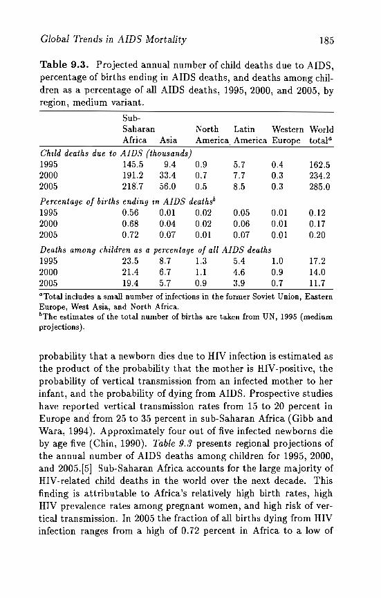
Global Trends in AIDS Mortality 185

Table 9.3. Projected annual number of child deaths due to AIDS,percentage of births ending in AIDS deaths, and deaths among chil­dren as a percentage of all AIDS deaths, 1995, 2000, and 2005, byregion, medium variant.

Sub-Saharan North Latin Western WorldAfrica Asia America America Europe totala

Child deaths due to AIDS (thousands)1995 145.5 9.4 0.92000 191.2 33.4 0.72005 218.7 56.0 0.5

Percentage of births ending in AIDS deathsb

1995 0.56 0.01 0.022000 0.68 0.04 0.022005 0.72 0.07 0.01

5.77.78.5

0.050.060.07

0.40.30.3

0.010.010.01

162.5234.2285.0

0.120.170.20

Deaths among children as a percentage of all AIDS deaths1995 23.5 8.7 1.3 5.4 1.0 17.22000 21.4 6.7 1.1 4.6 0.9 14.02005 19.4 5.7 0.9 3.9 0.7 11.7QTotal includes a small number of infections in the former Soviet Union, EasternEurope, West Asia, and North Africa.bThe estimates of the total number of births are ta.ken from UN, 1995 (mediumprojections) .

probability that a newborn dies due to HIV infection is estimated asthe product of the probability that the mother is HIV-positive, theprobability of vertical transmission from an infected mother to herinfant, and the probability of dying from AIDS. Prospective studieshave reported vertical transmission rates from 15 to 20 percent inEurope and from 25 to 35 percent in sub-Saharan Africa (Gibb andWara, 1994). Approximately four out of five infected newborns dieby age five (Chin, 1990). Table 9.3 presents regional projections ofthe annual number of AIDS deaths among children for 1995, 2000,and 2005.[5] Sub-Saharan Africa accounts for the large majority ofHIV-related child deaths in the world over the next decade. Thisfinding is attributable to Africa's relatively high birth rates, highHIV prevalence rates among pregnant women, and high risk of ver­tical transmission. In 2005 the fraction of all births dying from HIVinfection ranges from a high of 0.72 percent in Africa to a low of

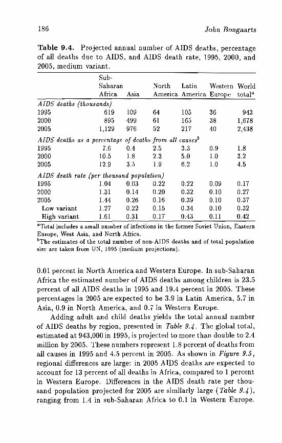
186 John Bongaarts

Table 9.4. Projected annual number of AIDS deaths, percentageof all deaths due to AIDS, and AIDS death rate, 1995, 2000, and2005, medium variant.

Sub­SaharanAfrica Asia

North Latin Western WorldAmerica America Europe totala

AIDS deaths (thousands)1995 619 109 64 1052000 895 499 61 1652005 1,129 976 52 217

AIDS deaths as a percentage of deaths from all causei1995 7.6 0.4 2.5 3.32000 10.5 1.8 2.3 5.02005 12.9 3.5 1.9 6.2

363840

0.91.01.0

9431,6782,438

1.83.24.5

AIDS death rate (per thousand population)1995 1.04 0.03 0.22 0.22 0.09 0.172000 1.31 0.14 0.20 0.32 0.10 0.272005 1.44 0.26 0.16 0.39 0.10 0.37

Low variant 1.27 0.22 0.15 0.34 0.10 0.32High variant 1.61 0.31 0.17 0.43 0.11 0.42

aTotal includes a small number of infections in the former Soviet Union, EasternEurope, West Asia, and North Africa.bThe estimates of the total number of non-AIDS deaths and of total populationsize are taken from UN, 1995 (medium projections).

0.01 percent in North America and Western Europe. In sub-SaharanAfrica the estimated number of AIDS deaths among children is 23.5percent of all AIDS deaths in 1995 and 19.4 percent in 2005. Thesepercentages in 2005 are expected to be 3.9 in Latin America, 5.7 inAsia, 0.9 in North America, and 0.7 in Western Europe.

Adding adult and child deaths yields the total annual numberof AIDS deaths by region, presented in Table 9.4. The global total,estimated at 943,000 in 1995, is projected to more than double to 2.4million by 2005. These numbers represent 1.8 percent of deaths fromall causes in 1995 and 4.5 percent in 2005. As shown in Figure 9.5,regional differences are large: in 2005 AIDS deaths are expected toaccount for 13 percent of all deaths in Africa, compared to 1 percentin Western Europe. Differences in the AIDS death rate per thou­sand population projected for 2005 are similarly large (Table 9.4),ranging from 1.4 in sub-Saharan Africa to 0.1 in Western Europe.

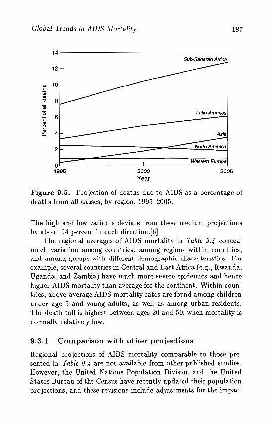
Global Trends in AIDS Mortality

14

12

UJ 10..ciiiQ)"0

"iii15'EQ)

~Q)a..

2000Year

187

Sub-Saharan Africa

Latin America

Asia

Western Europe

2005

Figure 9.5. Projection of deaths due to AIDS as a percentage ofdeaths from all causes, by region, 1995-2005.

The high and low variants deviate from these medium projectionsby about 14 percent in each direction.[6]

The regional averages of AIDS mortality in Table 9.4 concealmuch variation among countries, among regions within countries,and among groups with different demographic characteristics. Forexample, several countries in Central and East Africa (e.g., Rwanda,Uganda, and Zambia) have much more severe epidemics and hencehigher AIDS mortality than average for the continent. Within coun­tries, above~averageAIDS mortality rates are found among childrenunder age 5 and young adults, as well as among urban residents.The death toll is highest between ages 20 and 50, when mortality isnormally relatively low.

9.3.1 Comparison with other projections

Regional projections of AIDS mortality comparable to those pre­sented in Table 9.4 are not available from other published studies.However, the United Nations Population Division and the UnitedStates Bureau of the Census have recently updated their populationprojections, and these revisions include adjustments for the impact

188 John Bongaarts

United NationsUS Bureau of the CensusPresent study

of the AIDS epidemic in sub-Saharan African countries with HIVprevalence above 1 percent in 1990 (UN, 1995; Way and Stanecki,1994). These projections made no revisions for AIDS mortality inother African countries, even though it is recognized that these coun­tries are not entirely free of HIV infection (accounting for perhaps10 percent of Africa's total). Results from these studies, comparedwith those of the present study, are as follows:

Average annual AIDS deaths insub-Saharan Africa, 2000-20051.07 million2.16 million1.01 million

Even though these findings are not entirely comparable, it isclear that the mortality projection from the present study is similarto the UN's but much lower than that of the US Bureau of theCensus.[7] There are three potential causes for this discrepancy:differences in the HIV prevalence levels estimated at the startingpoint of the projections, different rates of growth in HIV infectionsover time, and differences in the key parameters (e.g., the durationof the incubation period and vertical transmission rates) used forcalculating the AIDS mortality associated with a given level of HIVinfection. Detailed further analyses will be required to quantify therole of each of these three factors in causing the differences in results.

Another comparison can be made for the global cumulativenumber of adult HIV infections by the year 2000. The low, medium,and high variants project, respectively, 28.1, 29.3, and 30.5 millioncumulative infections. Forecasts of this same variable by Mann etal. (1992) have a much wider range - from 38 to 109 million by 2000.To achieve an increase from 18.5 million in 1995 to 109 million in2000 requires more new infections each year between 1995 and 2000than have occurred in the entire history of the epidemic until 1995.This is implausible, and the high projection of Mann et al. (1992)must therefore be considered unrealistic.

9.3.2 Impact of the epidemic on population growth

Table 9.5 presents estimates of the effect of AIDS mortality on an­nual rates of population growth by world regions in 1995 and 2005.

Global Trends in AIDS Mortality 189

Birth, death, and growth rates are listed for both years with andwithout the epidemic. Estimates in the absence of AIDS are basedon UN medium population projections,[8] which assume negligibleregional migration so that the growth rate equals the difference be­tween the birth and death rates. The estimates with AIDS areobtained by adding the AIDS death rate (from Table 9.4) to thedeath rate from other causes and by making the simplifying as­sumption that the birth and the non-AIDS death rates as well asthe population age structure remain unaffected by the epidemic.

In sub-Saharan Africa the growth rate in 2005 is projected tobe 27.7 per thousand per year in the absence of the epidemic (Le.,38.9-11.2). AIDS mortality raises the death rate from 11.2 to 12.7per thousand, resulting in an equivalent decline in the growth ratefrom 27.7 to 26.3 per thousand. If maintained over 25 years, suchlevels of growth would yield increases in population size of 93.4percent with AIDS and 99.9 percent without. The epidemic has asignificant moderating effect on population growth in sub-SaharanAfrica, but even under the high variant AIDS projection the growthrate remains at a substantial 26.1 per thousand. In all other worldregions the epidemic's impact on population growth is substantiallysmaller. Due to AIDS mortality, the growth rate in 2005 is expectedto be 12.6 (per thousand population) instead of 12.9 in Asia, -0.5instead of -0.4 in Western Europe, 14.4 instead of 14.8 in LatinAmerica, and 5.1 instead of 5.2 in North America. Results for thehigh and low variant AIDS projections are remarkably similar.

These estimates of the effect of AIDS on population growth areapproximate. The assumption that migration at the regional levelis negligibl~ is reasonable for present purposes and is also made inthe standard population projections of the UN. However, the as­sumption that fertility and non-AIDS mortality remain invariant inthe presence of the epidemic is only a first approximation. Fertil­ity could be reduced if HIV-infected adults engage less frequentlyin sexual intercourse due to poor health, rely more on condoms orother contraception, or have a higher prevalence of other sexuallytransmitted diseases, in particular those that can cause infertility.Among uninfected adults fear of infection might also lead to lowerfrequency of intercourse and more condom use. Alternatively, in­creased fertility might result from a desire to replace dead children

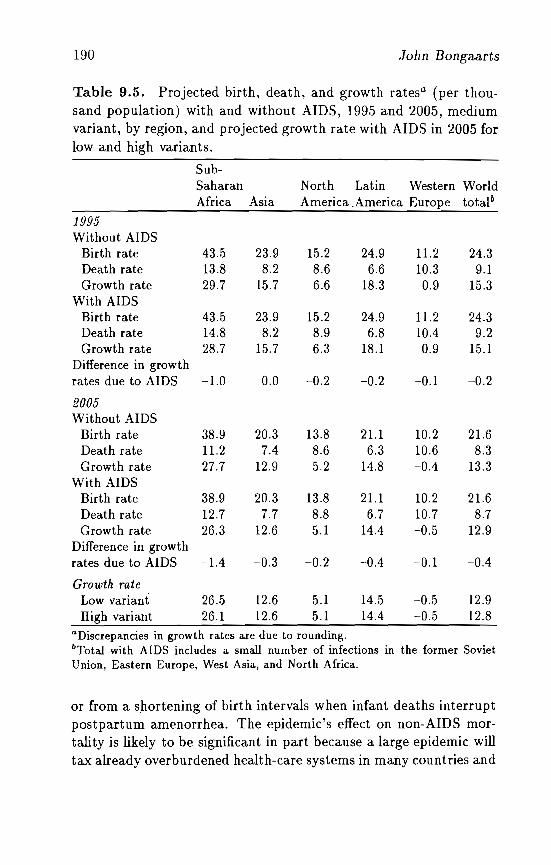
190 John Bongaarts

Table 9.5. Projected birth, death, and growth rates a (per thou-sand population) with and without AIDS, 1995 and 2005, mediumvariant, by region, and projected growth rate with AIDS in 2005 forlow and high variants.

Sub-Saharan North Latin Western WorldAfrica Asia America .America Europe total b

1995Without AIDS

Birth rate 43.5 23.9 15.2 24.9 11.2 24.3Death rate 13.8 8.2 8.6 6.6 10.3 9.1Growth rate 29.7 15.7 6.6 18.3 0.9 15.3

With AIDSBirth rate 43.5 23.9 15.2 24.9 11.2 24.3Death rate 14.8 8.2 8.9 6.8 10.4 9.2Growth rate 28.7 15.7 6.3 18.1 0.9 15.1

Difference in growthrates due to AIDS -1.0 0.0 -0.2 -0.2 -0.1 -0.2

2005Without AIDS

Birth rate 38.9 20.3 13.8 21.1 10.2 21.6Death rate 11.2 7.4 8.6 6.3 10.6 8.3Growth rate 27.7 12.9 5.2 14.8 -0.4 13.3

With AIDSBirth rate 38.9 20.3 13.8 21.1 10.2 21.6Death rate 12.7 7.7 8.8 6.7 10.7 8.7Growth rate 26.3 12.6 5.1 14.4 -0.5 12.9

Difference in growthrates due to AIDS -1.4 -0.3 -0.2 -0.4 -0.1 -0.4

Growth rateLow variant 26.5 12.6 5.1 14.5 -0.5 12.9High variant 26.1 12.6 5.1 14.4 -0.5 12.8

aDiscrepancies in growth rates are due to rounding.bTotal with AIDS includes a small number of infections in the former SovietUnion, Eastern Europe, West Asia, and North Africa.

or from a s.hortening of birth intervals when infant deaths interruptpostpartum amenorrhea. The epidemic's effect on non-AIDS mor­tality is likely to be significant in part because a large epidemic willtax already overburdened health-care systems in many countries and

Global Trends in AIDS Mortality 191

may draw resources from programs addressing other diseases. In ad­dition, other diseases (e.g., tuberculosis) can become more prevalentbecause HIV-infected individuals are more susceptible to them. Therise in the non-AIDS death rate from these effects is counteracted bya small change in the age composition of the population caused byelevated AIDS mortality.[9] The net effect of these secondary effectson fertility and mortality cannot be assessed, with available evidence,and the overall impact of an AIDS epidemic on population growthcould therefore be somewhat different from the estimates presentedin Table 9.5.

Further insight into these issues can be gained from a uniqueprospective study in the Rakai District of Uganda (Sewankambo etal., 1994). An initial 1990 survey of 1,945 households with 5,795adults and children collected demographic and socioeconomic infor­mation as well as blood samples. A follow-up survey of the samehouseholds in 1991 provided estimates of changes in households andof the number of births and deaths in the time between surveys.From this information, estimates were obtained of the demographicimpact of the AIDS epidemic in the district. In 1990 13 percentof adults were found to be seropositive, a very high level (morethan eight times the 1990 average for Africa) matched by very fewother largely rural districts in Africa. The proportion of deaths at­tributable to HIV infection was estimated to be 28 percent amongthe population as a whole, 52 percent among all adults, and 87percent among adults aged 20-39. Infant mortality among the off­spring of infected mothers was nearly double that oftheir uninfectedcounterparts (210 vs. 111 per thousand births).

Despite this very high AIDS mortality, population growth de­clined only 'modestly. The main reason is that the birth rate wasmuch higher than the death rate, and the rise in the death ratecaused by the epidemic only partly reduced this difference (see Fig­ure 9.6). Observed annual vital rates per thousand population wereas follows: birth rate, 45.7; death rate, 28.1; and growth rate (nat­ural), 17.6.

The authors estimated that in the absence of the epidemic thedeath rate would have been 20.4 per thousand. AIDS mortalitytherefore elevated the death rate by 7.7 per thousand. If one as­sumes that the birth rate remains unaltered by the epidemic, then

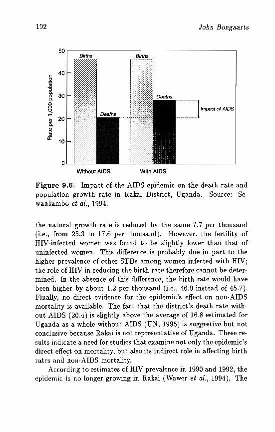
192

50

c: 40.2Cii"5a.0 30a.0

8~

Q; 20a.alCiia:

10

0

Births

........ ..............

.............................................................................

I

Births

Deaths

John Bongaarts

_-_-_-_-_-_-_-_-~]Impact of AIDS

Without AIDS With AIDS

Figure 9.6. Impact of the AIDS epidemic on the death rate andpopulation growth rate in Rakai District, Uganda. Source: Se­wankambo et al., 1994.

the natural growth rate is reduced by the same 7.7 per thousand(Le., from 25.3 to 17.6 per thousand). However, the fertility ofHIV-infected women was found to be slightly lower than that ofuninfected women. This difference is probably due in part to thehigher prevalence of other STDs among women infected with HIV;the role of HIV in reducing the birth rate therefore cannot be deter­mined. In the absence of this difference, the birth rate would havebeen higher by about 1.2 per thousand (i.e., 46.9 instead of 45.7).Finally, no direct evidence for the epidemic's effect on non-AIDSmortality is available. The fact that the district's death rate with­out AIDS (20.4) is slightly above the average of 16.8 estimated forUganda as a whole without AIDS (UN, 1995) is suggestive but notconclusive because Rakai is not representative of Uganda. These re­sults indicate a need for studies that examine not only the epidemic'sdirect effe~t on mortality, but also its indirect role in affecting birthrates and non-AIDS mortality.

According to estimates of HIV prevalence in 1990 and 1992, theepidemic is no longer growing in Rakai (Wawer et al., 1994). The

Global Trends in AIDS Mortality 193

epidemic has apparently reached an equilibrium at which HIV inci­dence has to remain high to offset AIDS deaths and to maintain theplateau level of prevalence in a growing population. These findingssuggest that population growth will remain substantially positivein Rakai. Since Rakai is one of the districts in sub-Saharan Africamost severely affected by AIDS, it is also unlikely that populationgrowth will drop precipitously elsewhere in ,the continent.[10]

9.4 Outlook

Regional trends in HIV infections over the coming decade are uncer­tain. The course of the epidemic depends chiefly on the behavioralresponses of the affected populations, on the wider application ofexisting public health approaches to reduce transmissions, and onthe successful development of new medical technology. A worst­case scenario would be sluggish spontaneous behavioral responses,the lack of new medical solutions for several more years, and a con­tinuation of current, mostly weak, and uneven public-health effortsto change high-risk behaviors. In that case, the epidemic will con­tinue largely along its natural course until all vulnerable groups (i.e.,those in which R exceeds 1) are heavily infected, and HIV prevalencein the developing world will reach levels much higher than today'sbefore eventually leveling off. This gloomiest of possible outcomescan be improved upon considerably by vigorous implementation ofsuch public health measures as control of sexually transmitted dis­eases and screening of donated blood as well as behavioral interven­tions such as information campaigns and the distribution of condoms(Berkley, 1994; Lamptey and Coates, 1994; Philipson and Posner,1995; Potts et ai., 1991). Such efforts have demonstrated their ef­fectiveness in the past, for example, in Thailand (Hanenberg et ai.,1994) and among homosexuals in the United States (Centers for Dis­ease Control and Prevention, 1991; Morris and Dean, 1994). Lack ofpolitical commitment and resources unfortunately hinders the widerapplication of these measures.

A larg'e effort is now under way to develop effective HIV ther­apies, microbicides, and vaccines, but obstacles are many and suc­cess is probably years away (Haynes, 1993; Cohen, 1994a; Elias and

194 John Bongaarts

Heise, 1994; Johnston and Hoth, 1993). If and when this effort suc­ceeds, it could end the epidemic. However, the cost of preventionor treatment may be so high as to be out of reach for the poorestsegments of the population in Asia, Latin America, and Africa. Theepidemic would then become even more a Third World disease thanit is now.

Regardless of the long-range trends in HIV infections, the overallcourse of AIDS mortality during the next decade is relatively clear.The toll in deaths will continue to rise in much of Asia, Africa, andLatin America, while population growth will remain high in someregions and positive in all.

Notes

[1] This article focuses on HIV-l, which is the cause of virtually all AIDSdeaths. HIV-2, primarily found in West Africa, is less pathogenic.

[2] Estimates by Mann et al. (1992) put the cumulative global total ofHIV-infected adults at 17.5 million at the beginning of 1995.

[3] WHO assumes that all deaths among HIV-infected individuals arecaused by AIDS.

[4] Following WHO practice, HIV-infected individuals are assumed to beat risk of dying from AIDS alone (see note 3). The distribution ofthe incubation period is taken from Chin and Lwanga (1991a). Theprojection results presented in this article are not very sensitive tothe precise shape of the distribution of the incubation period with agiven median duration.

[5] Projections assume perinatal transmission rates of 30 percent in devel­oping regions and 17.5 percent in the developed world. The distribu­tions of the incubation period and the survival interval after perinatalinfection are the same as those used by WHO (Chin, 1990).

[6] All variants of HIV/ AIDS projections rely on the medium projectionsof the UN (1995) for population estimates (including births and non­AIDS deaths).

[7] The similarity of the results of the UN and the present study is in partbecause both rely on past estimates of HIV incidence from WHO, andtheir projection methodologies are similar (US Bureau of the Censusestimate: Peter Way, personal communication).

[8] Medium projections are taken from UN (1995). The projections with­out AIDS are obtained by subtracting estimates of AIDS deaths de­tailed in the same publication.

Global Trends in AIDS lHortality 19.5

[9] Projections by the UN (1995) for African countries provide estimatesof the effect of a changing age structure. In the 15 sub-Saharan coun­tries with the most severe epidemics, the total number of deaths be­tween 2000 and 2005 in the presence and absence of the AIDS epi­demic is estimated at 19.504 and 15.169 million, respectively, giving adifference of 4.335 million. The actual number of AIDS deaths for thisfive-year period is projected to be 5.362 million. Non-AIDS deathstherefore decline from 15.169 to 14.142 million due to the epidemic'seffect on the age structure alone.

[10] The level of HIV prevalence at which population growth becomes zerois highest in countries with the highest birth rates. Once birth ratesdecline, lower prevalence levels suffice to stop population growth.

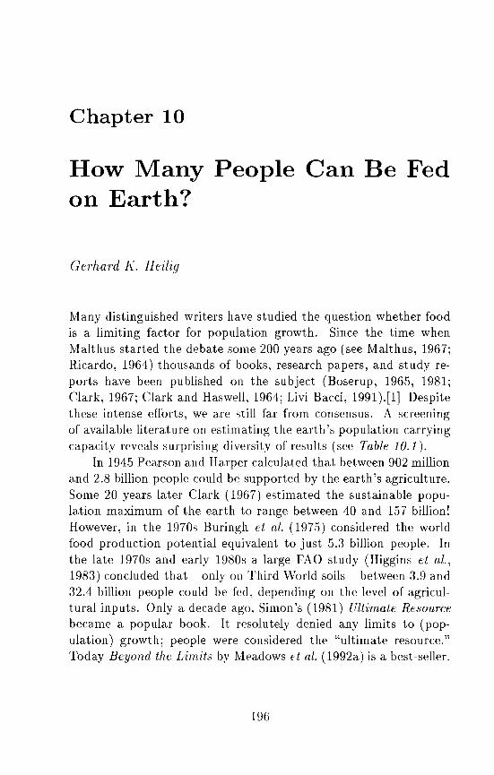
Chapter 10

How Many People Can Be Fedon Earth?

GeThard K Heilig

Many distinguished writers have studied the question whether foodis a limiting factor for population growth. Since the time whenMalthus started the debate some 200 years ago (see Malthus, 1967;Ricardo, 1964) thousands of books, research papers, and study re­ports have been published on the subject (Boserup, 1965, 1981;Clark, 1967; Clark and Haswell, 1964; Livi Bacci, 1991).[1] Despitethese intense efforts, we are still far from consensus. A screeningof available literature on estimating the earth's population carryingcapacity reveals surprising diversity of results (see Table 10.1).

In 1945 Pearson and Harper calculated that between 902 millionand 2.8 billion people could be supported by the earth's agriculture.Some 20 years later Clark (1967) estimated the sustainable popu­lation maximum of the earth to range between 40 and 157 billion!However, in the 1970s Buringh et al. (1975) considered the worldfood production potential equivalent to just 5.3 billion people. Inthe late 1970s and early 1980s a large FAO study (Higgins et al.,1983) concluded that - only on Third World soils - between 3.9 and32.4 billion people could be fed, depending on the level of agricul­tural inputs. Only a decade ago, Simon's (1981) Ultimate Resourcebecame a popular book. It resolutely denied any limits to (pop­ulation) growth; people were considered the "ultimate resource."Today Beyond the Limits by Meadows et al. (1992a) is a best-seller.

19G

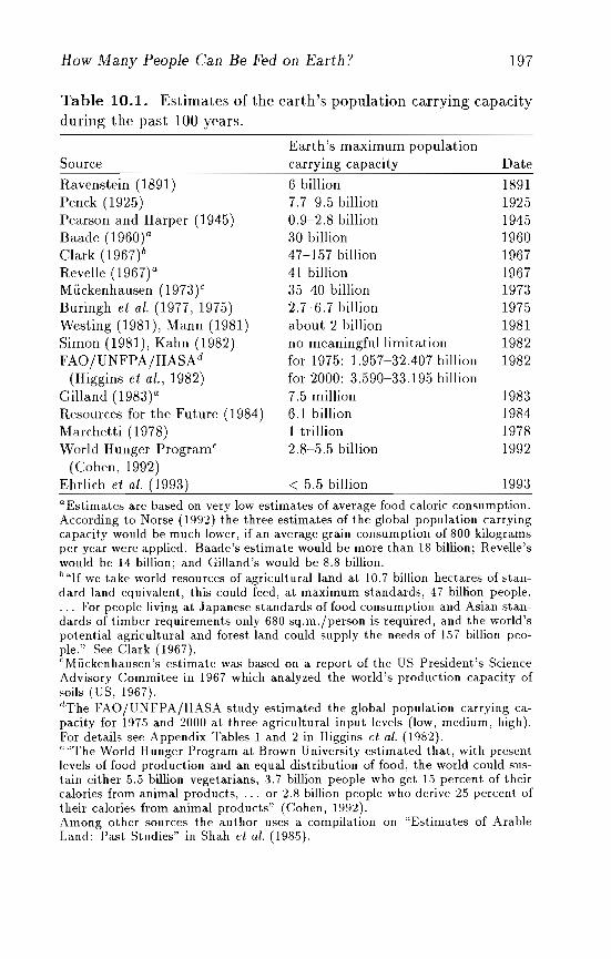
How Many People Can Be Fed on Earth? 197

Table 10.1. Estimates of the earth's population carrying capacityduring the past 100 years.

Source

Ravenstein (1S91)Penck (1925)Pearson and Harper (1945)Baade (1960)aClark (1967)bRevelle (1967)aMiickenhausen (1973)CBuringh et ai. (1977, 1975)Westing (19S]), Mann (19S1)Simon (19S1), Kahn (19S2)FAOjUNFPAjIIASA d

(Higgins et ai., 19S2)Gilland (19S3)aResources for the Future (19S4)Marchetti (1 97S)World Hunger Program e

(Cohen, 1992)Ehrlich et ai. (1993)

Earth's maximum populationcarrying capacity

6 billion7.7-9.5 billion0.9-2.S billion30 billion47-157 billion41 billion35-40 billion2.7-6.7 billionabout 2 billionno meaningful limitationfor 1975: 1.957-32.407 billionfor 2000: 3.590-33.195 billion7.5 million6.1 billion1 trillion2.S-5.5 billion

< 5.5 billion

Date

IS91192519451960196719671973197519S119S219S2

19S3198419781992

1993

a Estimates are based on very low estimates of average food caloric consumption.According to Norse (1992) the three estimates of the global population carryingcapacity would be much lower, if an average grain consumption of 800 kilogramsper year were applied. Baade's estimate would be more than 18 billion; Revelle'swould be 14 billion; and Gilland's would be 8.8 billion.b"]f we take world resources of agricultural land at 10.7 billion hectares of stan­dard land equivalent, this could feed, at maximum standards, 47 billion people .. .. For people living at Japanese standards of food consumption and Asian stan­dards of timber requirements only 680 sq.m.jperson is required, and the world'spotential agricultural and forest land could supply the needs of 157 billion peo­ple." See Clark (1967).eM iickenhausen 's estimate was based on a report of the US President's ScienceAdvisory Commitee in 1967 which analyzed the world's production capacity ofsoils (US, 1967).dThe FAO/UNFPA/liASA study estimated the global population carrying ca­pacity for 1975 and 2000 at three agricultural input levels (low, medium, high).for details see Appendix Tables 1 and 2 in Higgins et al. (1982).e ''The World Hunger Program at Brown University estimated that, with presentlevels of food production and an equal distribution of food, the world could sus­tain either 5.5 billion vegetarians, 3.7 billion people who get 15 percent of theircalories from animal products, ... or 2.8 billion people who derive 25 percent oftheir calories from animal products" (Cohen, 1992).Among other sources the author uses a compilation on "Estimates of ArableLand: Past Studies" in Shah et al. (1985).

198 Gerha.rd K. Heilig

They argue that we have already passed the limits of sustainabil­ity and are on the way to ecological disaster. In 1992 the WorldResources Institute published a wealth of data and analyses whichimply that we are already approaching ecological limits in manysectors of our economies, including agriculture.

Most recently Ehrlich fl al. (199:3) analyzed the subject. Ac­cording to their estimate it is "doubtful ... whether food securitycould be achieved indefinitely for a global population of 10 or 12billion people." They thought it "'rather likely that a sustainablepopulation, one comfortable below Earth's nutritional capacity, willnumber far fewer than today's 5..5 billion people." There are manyother studies, but probably the highest estimate of the globe's pop­ulation carrying capacity was published by Marchetti (1978), whoargued that a world population of 1 trillion people would not beimpossi ble.

Obviously, these numbers are not much help to the student offuture population trends. One reason for the large discrepancies ismethodological divergences of the various approaches. Some authorsdeal with global averages of carrying capacity; others study smallagro-ecological areas and only later aggregate the results. Some au­thors base their estimates on the most advanced agricultural tech­nology or assume future innovation; others define the carrying ca­pacity in terms of current. and in some regions rather low, levels ofagricultural output.

Biologists llsually explain carrying capacity as the balance be­tween natural resources and the number of people; social scientistsconsider human resources the critical factor and accentuate sociallimits to growth. More systematically, we can identify four reasonsfor the conceptual confusion: dissent about the reference area, dis­agreement about the means of sustenance, controversy on the modeof reaction to limitations, and confusion about the time frame. Wediscuss some of these problems in detail in later sections of this chap­ter. For now we can only conclude that there are more dimensionsto the problem than one would expect at first sight. It seems tobe necessary to combine the various aspects of the earth's carryingcapacity into a consistent theoretical framework.

Hor.v MallY People Call Be Fed all Earth? 199

10.1 Dimensions of the Earth'sCarrying Capacity

To visualize the major dimensions of the problem, imagine a pipethrough which the earth's food resources have to pass before theycan be used for feeding people (see Figure 10.1). The diameter ofthe pipe, however, is 1l0t constant. \i\Thile it is quite large on the"input" side, it is significantly smaller on the "output" end. Thepipe's stepwise decreasing diameter symbolizes different kinds of re­strictions to the earth's carrying capacity - technological, economic,ecological, and sociocultural.

10.1.1 The hypothetical maxirnum carrying capacity

On the input side of our conceptual pipe we have the theoreticalmaximum of the earth's food production capacity. This purely hy­pothetical measure is roughly equivalent to what biologists havetermed the net primary production (NPP) of the earth. The mea­sure is based on the assumption that the ultimate limitation of foodproduction is given by the energy conversion ratio of photosynthe­sis. This is the basic biochemical process by which green plantstransform solar radiation into biomass. Since we (roughly) knowthe total solar radiatioll illput of the earth, we can calculate theglobe's maximum biomass production, which quantifies the initialproduct of aU animal and human food chains.

The NPP is only restricted by physical constants, such as thetotal solar radiation energy input of earth, and by natural laws thatgovern the biochemical processes of plant growth.[2] In its mostextreme version the measure ignores not only economic, social, cul­tural, and political restrictions of food production, but also technicalconstraints and ecological feedback mechanisms. It assumes homo­geneous implementation of most advanced agricultural technologiesthroughout the world. Authors who have adopted this rather nar­row definition of carrying capacity estimate the maximum worldpopulation that can be sustained indefinitely into the future in therange of 16 to 147 billion people. depending on the specific methodapplied.[3] Marchetti's (197~) monstrous estimate of 1 trillion isbased on a similar approach.

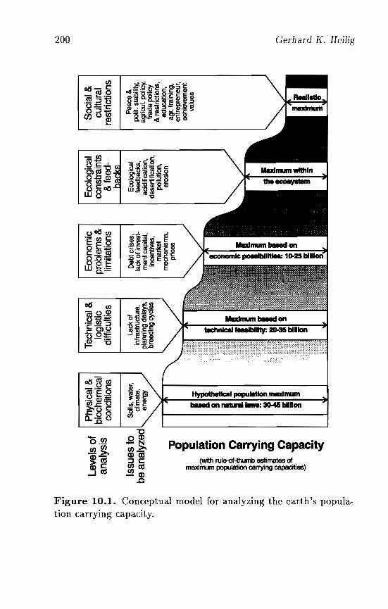
t\.:

)o o

Pea

ce&

polit

.st

abilit

y,ag

ricul

.po

licy,

trade

polic

y&

rest

rictio

ns,

educ

atio

n,ag

r.tra

inin

g,en

trepr

eneu

r,ac

hiev

emen

tva

lues

Soc

ial&

cultu

ral

rest

rictio

ns

Eco

logi

cal

feed

back

s,ac

idifi

catio

n,de

serti

ficat

ion,

pollu

tion,

eros

ion

Eco

logi

cal

cons

train

ts&

feed

-

Deb

tcris

es,

lack

ofin

vest

­m

entc

apita

l,in

cent

ives

,m

arke

tm

echa

nism

s,pr

ices

Eco

nom

icpr

oble

ms

&lim

itatio

ns

Tech

nica

l&lo

gist

icdi

fficu

lties

Lack

ofin

frast

ruct

ure,

plan

ning

dela

ys,

bree

ding

cycl

es

Phy

sica

l&bi

oche

mic

alco

nditi

ons

Leve

lsof

anal

ysis

Issu

esto

bean

alyz

ed

s o p..

(1) --

How Ma.ny People Ca.n Be Fed on Earth? 201

10.1.2 Technical and logistic restrictions and chances

The previous definition of ca.rryin~ capacity assumes homogeneousdistribution and instantaneous implementation of (advanced) foodproduction technology. But this is impossible in reality. Even withexisting agricultural technologies we would need years before wecould use them throughout the world. They have to be adapted tolocal conditions; they must be integrated with existing food distri­bution channels; and they often require previous implementation ofservice and support schemes. The production and distribution ofregionally adapted high-yield seeds, for instance, can take years ordecades. Also the breeding cycles in husbandry must be considered.

In addition to the usual delays in technology transfer, we mustrealize that advanced agricultural methods are primarily availablefor good-quality soils in temperate climates and for subtropical andtropical irrigation cultures (such as Asian paddy rice crops). Inthe arid and semiarid zones of Africa, however, we still have tra­ditional pastoral systems which survive quite well provided animaland human population density remains low. But since the popula­tion has doubled or tripled, the socioecological system is out of bal­ance. The situation obviously requires new technology to increaseproductivity of food production. However, we cannot be sure thathigh- tech alternatives of animal husbandry, which could potentiallyboost productivity by orders of magnitude, are adaptable to the hotand dry climate. Current experiments are not too promising. Itis not impossible that there simply is no high-tech alternative totraditional cattle ranging and primitive agriculture in certain partsof the world. We are just beginning to apply scientific methods tothe management of arid and tropical soils, and it will probably takeyears or decades before we have drought-resistant, high-yield cropsand livestock.

This indicates that the global carrying capacity is certainlydiminished by agro-technical and logistic restrictions and delays.Some studies have tried to take this into account by defining dif­ferent input levels for various agro-climatic regions. The FAO/UND P /IIASA (1982) study, for instance, assumed three levels ofagricultural input which largely correspond to levels of technology.

202 Gerhard K. Heilig

10.1.3 Economic barriers

Nothing in the world is free. Also the implementation of advancedagricultural technology and the expansion of agricultural areas intopreviously unused land is costly. One needs investment capital, func­tioning price mechanisms. adequate incentives for farmers, and awhole set of other economic conditions and mechanisms to boostfood production for a world population of several billion. Currentestimates of a global carrying capacity usually ignore these economicdimensions. However, in reality we find numerous economic diffi­culties and limitations which could further restrict global carryingcapacity. On the other hand, few spheres in human life are capableof generating more powerful incentives and driving forces than theeconomy. Recent histor,v has shown (for instance, in China) thatagriculture can modernize within a few years and double or tripleits productivity when the economic framework is right. Only fewstudies have developed agricultural models that take into accounteconomic mechanisms. such as prices and (international) trade. Un­fortunately these models are extremely complex and their method­ology and assumptions are highly debatable (Pa.rikh et ai., 1988).

It is an illusion to belie\'e that economic development is pre­dictable for more than a few years. The fundamental changes inglobal economic patterns, from the rise of the Asian Tigers (Tai­wan, South Korea, Singapore. Thailand, Malaysia) and the eco­nomic boom in China to the total breakdown of former Soviet andEast European economies, should have taught us a lesson. The eco­nomic framework of agriculture is man-made and can be changedfor the better or the worse.

The earth's carrying capacity in the 21st century will be a mat­ter of economic decisions at least to the same extent as it will bea matter of sufficient natural reSOl1rces. Three aspects are mostimportant: the conditions of international agricultural trade, thedissemination of agricultural technology, and the implementationof functioning incentive structures. \,ve can strengthen or weakenworldwide agricultural productivity. depending on what we do withtrade restrictions and food subsidies. We can speed up or slow downagricultural modernization. depending on what we do with the re­sults of agricultural research and development. We can block farm­ers' initiative or encourage their entrepreneurial spirit, depending on

How Many People Can Be Fed on Earth? 203

how we arrange property rights, taxation, price mechanisms, accessto modern agricultural inputs, and education. The earth's carryingcapacity not only depends on natural conditions and technology; itis also a function of specific economic arrangements.

10.1.4 Ecological constraints and feedbackmechanisnls

Since agriculture and livestock production - as everything else ­is embedded into a natura! environment, we also have to take intoaccount ecological constraints and feedback mechanisms, such asacidification, soil loss, groundwater pollution, or desertification.These consequences of intense agriculture and animal productioncan gradually diminish returns. Some ecologists have argued thatthe overutilization of arable land and forest areas in Europe andNorth America has already degraded the soils to such an extentthat artificial fertilization and soil management techniques cannotrepair the damage.

However, there is more to the ecological perspective than thenecessary modification of production systems in order to minimizeharmful impact on the environment. For instance, we need to re­serve space for the (still rema.ining) fauna and flora, if we want toavoid additional termination of whole strains of evolution. Keep­ing biodiversity at a high level is not (only) a matter of aestheticsand respect -- a large pool of plant and animal genes could be aprimary resource for future bio-sciences. We must also reserve nat­ural space for human recreation. The 10 billion world populationof the 21st century, cramped into multi-million urban agglomerates,will certainly need some of the potential crop area for leisure activ­ities, such as playing golf or riding a horse. Finally, a significantproportion of our environment cannot be utilized for agriculture orcattle ranging because it has vital functions in stabilizing the cli­mate. Cutting down tropical rain forests for agricultural expansionwould probably backfire. It would trigger or speed up climate changewhich could worsen agricultural conditions elsewhere and diminishoverall food prod uction. These examples show that the ecologicallysustainable population maximum is certainly below a level that isdetermined by physical laws, technological possibilities, or optimaleconomic structures.

204 Gerhard K. Heilig

10.1.5 Social, cultural, and political conditions

Some people believe that we just have to provide land, tractors,high-yield seeds, fertilizers and pesticides, agricultural training, andfree markets to make a farmer highly efficient. This technocratic ap­proach, however, ignores the social nature of man. We must realizethat probably the most serious restrictions for maximal utilization ofthe earth's population carrying capacity arise from social, political,and cultural conditions.

Social and cultural constraints which prevent optimal land uti­lization can be found not only among traditional food collectors,hunters, and cattle rangers of Africa and Asia. In many societies wehave political and social conditions which hinder farmers from fullyexploiting the carrying capacity of their land. In some cases these re­strictions are voluntary and based on ecological considerations. Forinstance, a growing number of European farmers and agriculturalpoliticians have realized that maximizing food production by meansof agrochemistry and mechanization cannot be the ultimate goal ofagriculture. They begin to exclude land from cultivation to make itavailable for natural reservations or recreational purposes. In Ger­many, for instance, 911.576 hectares (or 7.8 percent) of arable landwas taken out of production between 1988-1989 and 1990-1991. Ineastern Germany even 12.8 percent of the arable land was excludedfrom cultivation in 1990-1991. There are similar trends in all Eu­ropean countries, especially in Italy and France, where 357,922 and113,922 hectares of land were taken out of agricultural production(Bundesministerium fiir Raumordnung, Bauwesen und Stadtebau,1991:62-64).

However, this noble self-restriction of agriculture (which is fa­cilitated by substantial government subsidies) is rather untypical.Usually, there are other, more nnpleasant sociocultural and politicalconstraints. Many fanners throughout the world are working theirfields amid (civil) wars, suffer from lack of technology and moderninputs, or are restricted by ridiculously low producer prices or mar­ket regulations. They are forced into collectivization by fanaticalbureaucrats, and their children are deprived of adequate educationand training. These kinds of sociocultural and political constraintsprobably restrict the carrying capacity of the earth much more thananything else.

How Many People Call Be Fed on Earth? 205

To my knowledge there is no estimate of carrying capacity whichtakes into account all five kinds of restrictions. Scientists partic­ularly shy away from addressing sociocultural and political con­straints. Usually, the concept is defined in terms of natural resourcesavailable for food production at a given level of agricultural technol­ogy. This reflects widespread ignorance of key factors - economic,social, cultural, and political - that limit food production. In Sec­tion 10.2 we examine the multiple dimensions of the earth's carryingcapacity in greater detail.

10.2 Natural Resources

According to our pipe concept of carrying capacity, natural con­ditions (such as the globe's solar radiation input) and basic bio­chemical processes (such as photosynthesis) ultimately determinethe earth's food production potential. If we could transform thetotal solar energy input of the earth into biomass - and if we couldeat this biomass - we could probably feed 1 trillion people. But thisis just a theoretical exercise (which we discuss later). For all prac­tical purposes we must consider real agro-climatic conditions. Fournatural resources and conditions directly limit the globe's carryingcapacity: land, water, climate, and fossil energy.

10.2.1 Land

Since the beginning of the debate on the globe's carrying capacity,the land factor has usually been considered a limitation for increas­ing food production. The world's land area is, undoubtedly, limited,and only a small proportion is suitable for agriculture (Table 10.2).Many physical and chemical constraints restrict the arable area ­some land is too steep or too shallow, other areas have drainageor tillage problems. There are serious constraints of soil fertility,such as low nutrient retention capacity, aluminum toxicity, phos­phorus fixations hazards, low potassium reserves, or excess of saltsor sodium.

Both in its 1990-1991 and 1992-1993 reports on world resources,the World Resources Institute (WRI) published detailed estimatesof these physical and chemical soil constraints by climatic class formajor regions and on a country- by-country basis. The estimates in

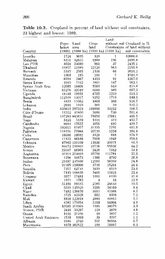
206 Gerhard K. Heilig

Table 10.2. Cropland in percent of land without soil constraints,23 highest and lowest: 1989.

Country

LesothoMalaysiaLao PDRThailandBurundiMauritiusRwandaSierra LeoneSyrian Arab Rep.VietnamUgandaBangladeshBeninLebanonIndiaCote d'IvoireBrazilTogoCambodiaNigeriaPakistanCubaCameroonEthiopiaMexicoKenyaArgentinaBotswanaSudanPeruSomaliaBoliviaUruguayKuwaitEgyptChadNigerNamibiaMaliLibyaSaudi ArabiaYemen, PDROmanUnited Arab EmiratesAlbaniaMauritania

LandPopu- Land Crop- without soil Cropland in %lation area land Constraints of land without(1000) (1000 hal (1000 hal (1000 hal soil constraints

1724 3035 320 1 32000.08451 32855 4880 196 2489.84024 23080 901 37 2435.1

54857 51089 22126 983 2250.95315 2565 1336 66 2024.21069 185 106 7 1514.36994 2467 1153 91 1267.04049 7162 1801 187 963.1

12085 18406 5503 643 855.865276 32549 6600 989 667.318118 19955 6705 1210 554.1

112548 13017 9292 1719 540.54493 11062 1860 360 516.72694 1023 301 59 510.2

835610 297319 168990 33232 508.511552 31800 3660 730 501.4

147283 845651 78650 17081 460.53424 5439 1444 319 452.78044 17652 3056 695 439.7

105015 91077 31335 7797 401.9118476 77088 20730 5250 394.9

10500 10982 3329 888 374.911453 46540 7008 1949 359.647942 110100 13930 30079 46.386672 190869 24710 55930 44.223187 56969 2428 7342 33.131914 273669 35750 111781 32.0

1256 56673 1380 4792 28.824487 237600 12510 50390 24.821105 128000 3730 15264 24.4

7257 62734 1039 4519 23.07115 108439 3460 15415 22.43077 17481 1304 6100 21.41971 1782 4 31 12.9

51186 99545 2585 24633 10.55539 125920 3205 34160 9.47492 126670 3605 41388 8.71725 82329 662 9308 7.18938 122019 2093 40865 5.14382 175954 2150 54004 4.0

13585 214969 1185 30579 3.92416 33297 119 3870 3.11446 21246 48 3897 1.21538 8360 39 3707 1.13186 2740 707 96958 0.71970 102522 199 58867 0.3

How Many People Can Be Fed on EartlJ? 207

this discussion are from the 1992-1993 WRI report and are basedon a complex methodology, which combines the Fertility Capabil­ity Classification (FCC) system developed at North Carolina StateUniversity (Sanches et 01., 1982), agro-climatic data from FAO'sAgro-Ecological Zones project (FAO, 1978a, 1978b, 1981a, 1981b),and the FAO /UNESCO soil map of the world.

The estimates are shocking. The most seriously handicappedregion is Southeast Asia: more than 93 percent of the soils havephysical or chemical constraints. The situation is not much betterin Southwest Asia: only 12 percent of the soils are free of inherentfertility constraints. In South America 80 percent and in Africa 82percent of the soils have constraints. Central America is a little bet­ter: "only" 73 percent of the soils are hampered by physical or chem­ical restrictions (\iVorld Resources Institute/United Nations En­vironment Programme/United Nations Development Programme,1990:286-287).[4] On a country-by-country basis the estimates areeven more dramatic. For India. the WRI reports just 33.2 mil­lion hectares of unconstrained soils; this is equivalent to just 0.04hectares (or 400 square meters) per person. Bangladesh's uncon­strained soil resources are even less: only 0.02 hectares per person.Pakistan, the Philippines, and Indonesia would have from 0.4 to 0.6hectares of soil without inherent physical or chemical constraints foreach person.

What do these statistics indicate? The WRI reports that "theextent of land with soil constraints is an important indicator ofagricultural costs, the potential and success of future expansion [em­phasis added], and the comparative advantage of a nation's agricul­tural production" (World Resources Institute/United Nations En­vironment Programme/United Nations Development Programme,1990:289).

The WRI further explains that "in the past 10 years, the FCCsystem has proven a meaningful tool for describing fertility limita­tions on crop yields" (ibid:2:oI,9). Do the estimates - in other words ­indicate that we are already short of fertile soils for future expansionof food production?

Not at all! First, one has to read the footnotes attached tothe WRI tables. Here we find a few hints that explain what ismeant by the various soil constraints. It turns out that most of

208 Gerhard K. Heilig

the so-called constraints are just specific natural conditions thatcan be somewhat easily overcome with modern agricultural technol­ogy. Consider the case of soils with "low potassium reserves" whichconstrain crops because of potassium deficiency. There is a simplesolution: throw potassium fertilizer on them! Other examples ofsoil constraints are "steep slopes" or "drainage problems": wouldone think that many of these soils can be found in the extremelyproductive paddy rice and wheat areas of Asia, where agriculturein some places has been practiced for more than 8000 years (as inChina)? "Aluminum toxicity" is also called a constraint, but itsimpact turns out to be less dramatic than its name: it limits thegrowth of common crops, "unless lime is applied" (World ResourcesInstitute/United Nations Environment Programme/United NationsDevelopment Programme, 1992:284) - a practice that should not becompletely impossible.

There are, of course, serious soil constraints that cannot be over­come by technology, but the WRI data do not distinguish betweenthese and simple problems of soil ma.nagement. For thousands ofyears farmers had to cope with soils that were less than perfect.They had to build terraces, add (natural) fertilizers, irrigate or drainthe soil. But this did not hinder them from supplying some of themost prominent empires of history, such as the dynasties of Chinaor the kingdoms of ancient Egypt.

There is a second reason why the WRI data on soil constraintsare worthless as indicators of the earth's carrying capacity: theydo not match with current trends in food production - to be moreprecise, in some cases the indicators are just absurd when comparedwith agricultural performance. For instance, according to the WRIthe continent-size nation of India has only 33.2 million hectares ofinternally unconstrained soils, but FAa reports that India's farmersare cultivating some 169 million hectares of cropland - which is fivetimes the area of "unconstrained soils" (cropland equals arable landplus land under permanent crops). In other words, according to theWRI most of India's farmers are producing on marginal land, whichshould limit crop yields. But just the opposite has happened duringthe past 30 years. Between 1961 and 1989 India's farmers increasedcereal production by a spectacular 129 percent (from 87,376,000 to199,816,000 metric tons). They also increased the cereal yields from

How Many People ('a,l1 Be Fed all Earth? 209

947 to 1,921 kg per hectare area harvested. In Thailand just 983,000hectares are free of soil constraints, according to WRI data. Is it notstrange that the country's farmers actually cultivated 22.1 millionhectares of cropland - nearly 23 times the area of the unconstrainedsoils? Only the rice area harvested was 10 times the size of the un­constrained soils area. Thailand's farmers also managed to increasecereal production by 1:31 percent between 1961 and 1989. Most ab­surd are the estimates of soil constraints for Malaysia. Accordingto WRI data only 0.6 percent (or 196,000 hectares) of the country'sland area is covered by unconstrained soils. Obviously this did nothave a great effect on the country's farmers, who cultivated 4.9 mil­lion hectares of cropland in 1989 - 25 times the area of unconstrainedsoils. It also did not affect their productivity, since they managedto increase cereal production by 62 percent between 1961 and 1989.These are only a few examples. We can find a large number ofcountries where the farmers expa,nded cultivation far into the areaof so-called constrained soils, while at the same time substantiallyincreasing crop yields.

There is a third reason why WRI's soil data have limited rele­vance: a high percentage of unconstrained soils in a country doesnot correlate with good agricultural performance. For example, ac­cording to the WRI, Chad has one of the largest areas of excellentsoils - 34.2 million hectares have no inherent physical or chemicalconstraints, an opulent 6.2 hectares per person. Is it not strangethat the farmers use less than 10 percent of this area for cultivationand that famines are notorious in a place with one of the largest percapita resources of first-rate soils? This is not just an isolated case.According to WRI data, nearly all typical famine countries of Africa(Ethiopia, Sudan, Somalia, Mali) have huge areas of top-rated soilswhich are many times the size of their actual cropland.

Given these examples it is obvious that factors other than soilquality by itself are responsible for agricultural performance. Thereis simply no correlation between food production and soil constraintsas reported by the WRI.

On the other hand, we have a large number of agricultural tech­niques available that could help to either expand the arable land andincrease yields on marginal soils or improve the overall efficiency ofcrop production.

210 Gerhard K. Heilig

First, we could expand the area of multiple harvests. In manyplaces farmers could use their land several times during a grow­ing season instead of only once or twice. Modern seeds, advancedagricultural technology, artificial fertilizers, and other agriculturalinputs have made these techniques of multi-cropping possible. It isa myth that we are already overutilizing the world's arable land.This is only true in some European and Asian regions. Large partsof Latin America and Africa have excellent soils which are still cul­tivated with most primitive agricultural technology. Crop yields areoften 60 to 90 percent below the average European level. Better in­puts and modern agricultural methods could substantially expandthe area of multiple harvests.

Second, we could expand cultivation to marginal land. There isstill plenty of dry land that could be irrigated, swamps that couldbe drained, steep hills which could be terraced. We could coverland with greenhouses in cold regions or use forests for multilay­ered cultivation. It is also possible to convert shallow seas intoagricultural land. The Netherlands have demonstrated that evenin an adverse dimate one can produce more than enough (tropical)fruits and vegetables on artificially climatized and drained land. Inmost countries it was not necessary to increase arable land dur­ing the past decades, but some agricultures have demonstrated thata spectacular expansion of culti vat ion is still possible. Libya, forinstance, has converted desert into cirdes of irrigated cropland; be­tween 1961 and 1989 its area of irrigated agriculture doubled from121,000 to 242,000 hectares (Allan, 1976). Burundi, which is al­ready densely populated, managed to increase its arable land from765,000 to 1,120,000 hectares and the area of irrigated agriculturefrom 3,000 to 72,000 hectares. Tanzania nearly doubled its arableland and increased the irrigated agriculture more than seven times.There are still spectacular land reserves in parts of Africa and LatinAmerica. Of course, some of these expansions are rather absurd interms of energy efficiency or economic costs; one might even con­sider the idea of growing wheat in the desert a form of hypocrisy.But these cases show what could be done in agriculture if moneyand technology were accessible and environmental concerns couldbe ignored.

How Many People ('an Be Fed on Earth? 211

Third, we can expand food production areas to the water bod­ies of our globe -lakes, rivers, and seas (Sindermann, 1982). Whilethere is certainly a danger of exploiting the natural fish populationof the sea, efforts are being made to begin exploring the potentialof fish farming. There is already some fish farming on the northerncoast of England, in Norwegian fjords, along the coast of Sweden,and in Chinese paddy rice fields. A significant proportion of Eu­rope's salmon supply is produced in fish farms near the ShetlandIslands. But these are still small production sites compared withthe huge coastal zones of our continents. It has been argued thatlarge-scale fish-farming schemes might disturb the natural balanceof the maritime ecosystem, which, in turn, could limit its produc­tion potential (Uthoff, 1978; UNO /FAO, 1976). However, recentresearch has found only a minimal risk of local sea pollution causedby a discharge of nutrients in intense fish farming (Ackefors andEnell, 1990).

Fourth, we can switch from nonfood to food crops. Currently, asignificant proportion of fertile land is used not for food productionin a narrow sense, but to grow lifestyle-related cash crops, such astobacco, tea, cocoa, or coffee. It is hard to estimate the areas wastedfor the illegal cultivation of drugs (marijuana, coca, etc.), but itmust be substantial Farmers also spend arable land for producingnatural fibers, such as jute, flax, or sisal - nonfood products forwhich synthetic substitutes are available. In some countries, suchas Brazil, there is substantial energy-cropping (sugar cane), andsome European governments encourage farmers to grow rape seedand produce bio-fuel. In some countries (Italy, Spain) large areas areused to grow wine. And - last hut not least - we spend considerableamounts of land to produce hops, which is mainly used for brewingbeer. According to FAO statistics, it is quite likely that some 20percent of all arable land worldwide is used to produce nonfood orlifestyle-related products, including drugs (see Table 10.3).

Previously it was thought that a given plot of land can onlyfeed a fixed number of people. Later, scientists realized that it isnot only the size and natural quality of the land, but mainly the levelof agricultural technology which determines the land's food produc­tion capacity. This basic understanding is still rare among today's

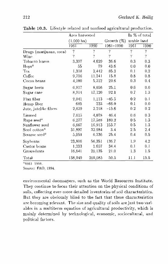
212 Gerhard K. Heilig

Table 10.3. Lifestyle-related and nonfood agricultural production.

Area harvested In % of total(1,000 ha) Growth (%) arable land1961 1990 1961-1990 1961 1990

Drugs (marijuana, coca) ? ? ? ? ?Wine ? ? ? ? ?Tobacco leaves 3,:397 4,629 36.6 0.3 0.3Hopsa 55 79 43.6 0.0 0.0Tea 1,318 2,442 85.3 0.1 0.2Coffee 9,706 11,241 15.8 0.8 0.8Cocoa beans 4,100 5,312 29.6 0.3 0.4

Sugar beets 6,917 8,656 25.1 0.6 0.6Sugar cane 8,914 17,120 92.1 0.7 1.3

Flax fiber 2,041 1,113 -45.5 0.2 0.1Hemp fiber 685 233 -66.0 0.1 0.0Jute, jutelike fibers 2,629 2,218 -15.6 0.2 0.2

Linseed 7,615 4,078 -46.4 0.6 0.3Rape seeda 6,277 17,588 180.2 0.5 1.3Sunflower seed 6,667 16,913 153.7 0.5 1.3Seed cottona 31,897 32,984 3.4 2.5 2.4Sesame seeda 5,051 6,336 25.4 0.4 0.5

Soybeans 23,806 56,351 136.7 1.9 4.2Castor beans 1,233 1,657 34.4 0.1 0.1Groundnuts 16,641 20,135 21.0 1.3 1.5

Total 138,949 209,085 50.5 11.1 15.5

a1961-1991.Source: FAO, 1994.

environmental doomsayers, such as the World Resources Institute.They continue to focus their attention on the physical conditions ofsoils, collecting ever-more detailed inventories of soil characteristics.But they are obviously blind to the fact that these characteristicsare becoming relevant. The size and quality of soils are just two vari­ables in a multiterm equation of agricultural productivity, which ismainly determined by technological, economic, sociocultural, andpolitical factors.

How Many People Can Be Fed on Earth?

10.2.2 Water

213

Some experts have argued that it is not land, but water which is thecritical resource for the global carrying capacity (Riviere, 1989). Themost prominent Cassandra of a world water crisis is Malin Falken­mark. She has argued that "water scarcity [is] now threateningtwo-thirds of the African population" (Falkenmark, 1989:118). Herpessimism, however, is not shared by prominent hydrologists whohave collected detailed water resource inventories for Africa. Al­most three dozen water experts, assisted by five major hydrologicalinstitutes, contributed to a UN publication which concluded:

There is almost nowhere in Africa where groundwater is not foundat one depth or another .... Mineral-water and thermo-mineralsprings abound in the African continent in the fracture zones.They constitute a major potential resource which has been ex­plored and exploited in only a few places. [UN, 1988:13-14]

Other water experts have raised the argument that we shouldnot confuse man-induced regional or local water shortages withclimate-related resource scarcity (Bandyopadhyay, 1989).

Globally about 70 percent of all water withdrawal is used inagriculture (Table 10.4). This explains why the water situationis, in fact, important to the food production capacity o'f the earth.There are also some reasons for concern. Available statistics confirmthat in some river basins, freshwater is being extracted for humanuse (including agriculture) at rates approaching those at which thesupply is renewed. In particular, Egypt is probably on the brink ofa water crisis. The country's renewable freshwater resources includesome 58.3 km3 , of which 56 ..5 km3 are from the Nile's annual flow and1.8 km3 from other internal renewable resources. Some 97 percent ofthese resources (or 56.4 km 3

) are already being withdrawn. Egypt'sagriculture needs 49.6 km3 of water. Only 2.8 km3 are used inindustry, and the withdrawal for domestic purposes is about 3.9 km3 .

Libya's agriculture might also be limited by extreme watershortages. According to recent estimates the country has a re­newable freshwater resource of some 0.7 km3 per year - mostlyfrom underground aquifers. Libya's annual withdrawal, however,

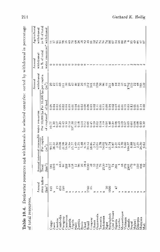
Tab

le1

0.4

.F

resh

wat

erre

sour

ces

and

wit

hd

raw

als

for

sele

cted

coun

trie

s:so

rted

by

wit

hd

raw

alin

per

cen

tag

eI'-.

:>>

-'

of

tota

lre

sour

ces.

,j;..

An

nu

alA

nn

ual

Ag

ricu

ltu

ral

An

nu

alA

nn

ual

inte

rnal

ren

ewab

lew

ater

reso

urc

esw

ith

dra

wal

wit

hd

raw

alw

ith

dra

wal

riv

erin

flow

To

tal

Per

cap

ita

Per

10

,00

0h

aP

er

10

,00

0h

ap

er

cap

ita

in%

of

tota

lin

%o

fto

tal

(km

e ')

(km

3)

(m3

)o

fcr

op

lan

db

of

lan

d(m

e')

wat

erre

sou

rces

aw

ith

dra

wal

Co

ng

o6

21

18

19

0.7

71

0.7

70.

005

20

011

Zai

rex

10

19

28.3

11

.30

0.0

422

01

7G

am

bia

19

33.

050

0.1

70

.03

33

091

Cam

bo

dia

41

08

8.1

10

.68

0.2

90.

005

69

094

Para

gu

ay

22

09

42

1.9

80

,42

0.0

211

10

78C

amer

oo

nx

20

818

.·50

0.3

00

.04

30

030

5U

gan

da

x6

63

.S8

0.1

00

.03

20

06

0A

ng

ola

"1·

5810

5.77

19

7..5

00

.01

43

07

6H

aiti

"11

1.6

90

.12

0.0

44

60

68

Zam

bia

"9

611

.305

0.1

80

.01

86

026

Ben

in"

26

S,4

80

.14

0.0

22

60

.58

Ch

ad

x3

8.4

6.7

60

.12

0.0

03S

08

2B

razi

l1

76

0S

19

03

4.S

20

.66

0.0

62

12

14

0U

rug

uay

65

S9

18

.86

0,4.

50

.03

24

11

91G

han

ax

S3

3.S

30

.19

0.0

23

S1

·52

Gu

ate

mala

x1

16

12

.61

0.6

20

.11

13

91

74T

anza

nia

"7

62

.78

0.1

40

.01

36

174

Ind

on

esia

"20

530

14

.02

1.1

90

.13

96

17

6N

iger

30

14

1.9

70

.04

0.0

04

41

74B

ang

lad

esh

10

00

13

57

11

.74

1.4

60

.94

211

19

6C

ote

d'I

vo

ire

x74

5.8

70

,20

0.0

26

81

67

CJN

iger

ia4

726

12

.31

0.0

80

.03

44

15

4~

Les

oth

ox

42

.25

0.1

30

.01

34

15

6..., :::r

-M

oza

mb

iqu

ex

58

3.7

00

.19

0.0

1S

31

66

'"V

ietn

am"

37

65

.60

0.5

70

.11

81

17

8..., a.

.C

an

ad

ax

29

01

10

9.3

70

.63

0.0

31

75

21

8~

Nep

alx

17

08

.88

0.6

40

.12

15

52

95M

alaw

ix

91

.07

0.0

40

.01

222

49

~E

thio

pia

x1

10

2.3

50

.08

0.0

14

82

86

~M

alay

sia

x4

S6

26

.30

0.9

30

.14

76

S2

47

~. .......

Mal

ix

62

6.6

20

.30

0.0

0lS

92

97

~.

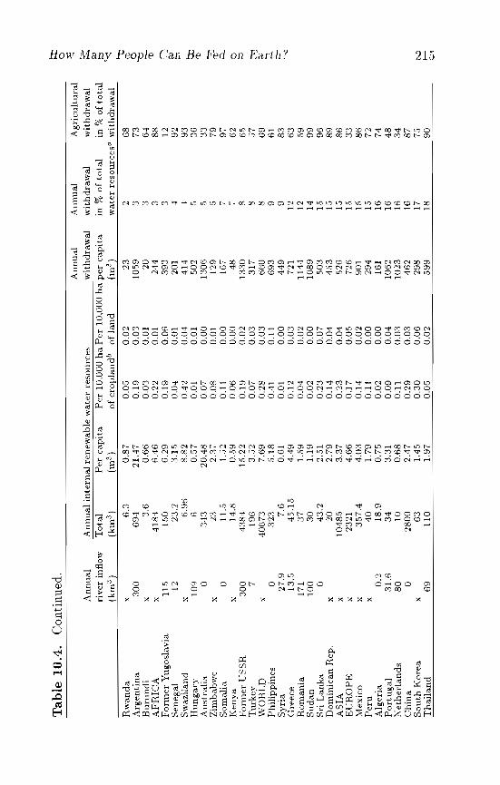
Ta

ble

10

.4.

Con

tinu

ed.

::r:: 0

An

nu

alA

nn

ual

Ag

ricu

ltu

ral

:EA

nn

ual

An

nu

al

inte

rnal

ren

ewab

lew

ate

rre

sou

rces

wit

hd

raw

alw

ith

dra

wal

wit

hd

raw

al~

rive

rin

flow

To

tal

Per

cap

ita

Per

10

,00

0h

aP

er

10

,00

0h

ap

er

cap

ita

in%

of

tota

lin

%o

fto

tal

~ ~

(krn

3)

(km

3)

(m3

)o

fcro

pla

nd

bo

fla

nd

(m3

)w

ate

rre

sou

rces

aw

ith

dra

wal

.~

Rw

an

da

x6

.30

.87

0.0

50

.02

23

26

8'"0 (]

)

Arg

en

tin

a3

00

69

42

1.4

70

.19

0.0

31

05

93

73

0 ""0B

uru

nd

ix

3.6

0.6

60.

0.'3

0.0

12

0:3

64

~A

FR

ICA

x4

18

46

.46

0.2

20

.01

24

43

88

Fo

rmer

Yu

go

slav

ia1

15

15

06

.29

0.1

90

.06

39

33

12'''""

'.6.

,-S

eneg

al12

23

.23

.15

0.0

40

.01

201

49

2::,

Sw

azil

and

x6

.96

8.8

20

.42

0.0

44

14

49

3H

un

gary

10

96

0.5

70

.01

0.0

15

02

.')3

6to (1

)

Au

stra

lia

a.'3

432

0.4

80

.07

0.0

01

30

6S

33

Zim

bab

we

x23

2.3

70

.08

0.0

11

29

S7

9~

So

mal

iaa

11

.51

.52

0.1

10

.00

167

79

7C

l..

Ken

ya

x1

4.8

0.5

90

.06

0.0

04

8,

62

gF

orm

er

US

SR

30

04

38

41

5.2

20

.19

0.0

21

33

08

65

Tu

rkey

71

96

3.5

20

.07

0.0

33

17

85

7t!

jW

OR

LD

x4

06

73

7.6

90

.28

0.0

36

60

86

9:l

l

Ph

ilip

pin

es

a3

23

5.1

80.

410.

116

93

961

... ,..:,.

Sy

ria

27

.97

.60.

610

.01

0.0

04

49

98

3~

Gre

ece

13

.54

5.1

54

.49

0.1

20

.03

721

126

3.~

Ro

man

ia17

13

71

.59

0.0

40

.02

11

44

1259

Su

dan

10

03

01

.19

0.0

20

.00

10

89

149

9S

riL

ank

aa

43

.22

.51

0.2

30

.07

50

31

59

6D

om

inic

an

Rep

.x

20

2.7

90

.14

0.0

44

53

15

89

AS

IAx

10

48

53

.37

0.2

30

.04

52

61

58

6E

UR

OP

Ex

2321

4.6

60

.17

0.0

57

26

153

3M

exic

ox

35

7.4

4.0

30

.14

0.0

29

01

158

6P

eru

x4

01

.79

0.11

0.0

02

94

157

2A

lger

ia0

.21

8.9

0.7

50

.02

0.0

016

11

67

4P

ort

ug

al

31

.63

43

.31

0.0

90

.04

10

62

16

48

Neth

erl

an

ds

80

10

0.6

80

.11

0.0

31

02

31

63

4C

hin

aa

28

00

2.4

70

.29

0.0

34

62

168

7S

ou

thK

ore

ax

63

1.4

50

.30

0.0

62

98

1775

~

Th

ail

an

d6

91

10

1.9

70

.05

0.0

25

99

189

0>

-'CJ

<

~

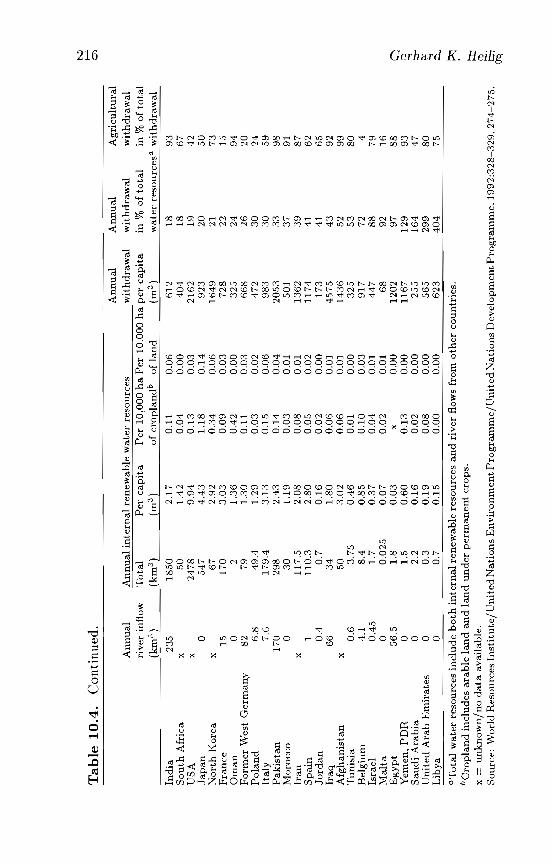
Tab

le1

0.4

.C

onti

nued

.>

-'0

)

An

nu

alA

nn

ual

Ag

ricu

ltu

ral

An

nu

al

An

nu

alin

tern

al

ren

ewab

lew

ate

rre

sou

rces

wit

hd

raw

alw

ith

dra

wal

wit

hd

raw

al

riv

erin

flo

wT

ota

lP

er

cap

ita

Per

10

,00

0h

aP

er

10

,00

0h

ap

er

cap

ita

in%

of

tota

lin

%o

fto

tal

(km

3)

(km

3)

(m3

)o

fcro

pla

nd

bo

fla

nd

(m3

)w

ate

rre

sou

rces

aw

ith

dra

wal

Ind

ia23

51

85

02

.17

0.1

10

.06

61

21

89

3S

ou

thA

fric

ax

50

1.4

20

.04

0.0

04

04

18

67

US

Ax

24

78

9.9

40

.13

0.0

32

16

21

942

Jap

an

a5

47

4.4

31

.18

0.1

49

23

205

0N

ort

hK

ore

ax

67

2.9

20

.34

0.0

61

64

921

73

Fra

nce

151

70

3.0

30

.09

0.0

37

28

221

5O

man

a2

1.3

60

.42

0.0

03

25

249

4F

orm

erW

est

Ger

man

y8

27

91

.30

0.1

10

.03

66

82

620

Po

lan

d6

.84

9.4

1.2

90

.03

0.0

24

72

30

24It

aly

7.6

17

9.4

3.1

30

.15

0.0

69

83

30

59

Pak

ista

n1

70

298

2.4

30

.14

0.0

42

05

33

39

8M

oro

cco

a3

01

.19

0.0

30

.01

501

37

91Ir

an

x1

17

.52

.08

0.0

80.

011

36

2:3

98

7S

pain

11

10

.32

.80

0.0

50

.02

11

74

4162

Jord

an

0.4

0.7

0.]

60

.02

0.0

017

:341

65

Iraq

66

34

1.8

00

.06

0.0

]4

57

54

39

2A

fgh

anis

tan

x5

03

.02

0.0

6om

14

36

529

9T

un

isia

0.6

3.7

50

.46

0.0

10

.00

32

553

80

Bel

giu

m4.

18

.40

.85

0.1

00

.03

91

772

4Is

rael

0.4.

51

.70

.37

0.0

40.

014

47

88

79

Malt

aa

0.0

25

0.0

70

.02

0.01

68

921

6E

gy

pt

56

.51

.80

.03

x0

.00

12

02

97

88

GY

emen

,P

DR

a1

.50

.60

0.]

30

.00

11

67

12

99

3(l

)

Sau

di

Ara

bia

a2.

20

.16

0.0

20

.00

25

51

64

47

~U

nit

edA

rab

Em

irate

sa

0.3

0.1

90

.08

0.0

05

65

29

98

0~ ...,

Lib

ya

a0

.70

.15

0.0

00

.00

62

34

04

75c..

aT

ota

lw

ater

reso

urc

esin

clu

de

bo

thin

tern

al

ren

ewab

lere

sou

rces

an

dri

ver

flow

sfr

om

oth

er

cou

ntr

ies.

~b

Cro

pla

nd

incl

ud

esara

ble

lan

dan

dla

nd

un

der

perm

an

en

tcr

op

s.~

x=

un

kn

ow

n/n

od

ata

avai

lab

le.

(l)

So

urc

e:W

orl

dR

eso

urc

esIn

stit

ute

/Un

ited

Nat

ion

sE

nv

iro

nm

en

tP

rog

ram

me/U

nit

ed

Nat

ion

sD

evel

op

men

tPro

gra

mm

e,

19

92

:32

8-3

29

,2

74

-27

5.

..... ..... ~.

How Many People Can Be Fed on Earth? 217

is estimated at 2.83 km3 - which is four times the rate of natu­ral replacement. Some 7.5 percent of this unsustainable withdrawalis used in agriculture. The country's spectacular increase of grainproduction is obviously borrowed from future generations.

Another interesting case is Saudi Arabia. Since 1961 the desertcountry has increased its wheat production by a spectacular 4,706percent, from merely 8.5,000 to 4,000,000 metric tons. Today, thecountry's farmers are not only able to provide more than 3.5 percentof the domestic food supply - which is a spectacular achievementin itself - but they actually produce more grain than the countryneeds. In 1991 Saudi Arabia's net export of wheat was 1,80.5,000metric tons, as compared with a net import of 67,600 metric tonsin 1974. Ecologists have argued that the bumper harvests weremainly achieved by exploiting fossil - that is, nonrenewable - waterresources below the desert. They estimate that in 1988 the countrywithdrew some 20..5 km 3 of water, 90 percent from nonrenewablefossil groundwater aquifers. They also estimate that Saudi Arabia'sagriculture needs 90 percent of the water available, with 3.5 percentof the agricultural water consumption being used in wheat produc­tion. According to the Middle East Economic Digest (Hopes dryup ... , 1989:1.5), which cites a confidential US government agencyreport, at the current rate of depletion Saudi Arabia's fossil ground­water would be exhausted by 2007.

Many authors have argued that Africa is a parched continent(Pearce, 1991). The most pessimistic position maintains that bythe year 2000, Tunisia, Kenya, Malawi, Burundi, and Rwanda willsuffer a permanent water crisis (Falkenmark, 1989:116).

There is also much concern about the arid regions of the northChina plain. According to recent calculations by the World Re­sources Institute, the 200 million population is already exploitingthe freshwater resources to a large extent. The WRI concludes that"if present trends continue, the region will have 6 percent less waterthan needed by the end of the century" (World Resources Insti­tute/United Nations Environment Programme/United Nations De­velopment Programme, 1992:16:3). These examples certainly seemto confirm the conclusion that water is a critical factor for limitingglobal carrying capacity, but there is also empirical evidence thatdoes not fit into the pessimistic outlook.

218 Gerhard K. Heilig

According to the most recent estimate the earth's total an­nual freshwater resource is some 40,673 km3 . The annual agricul­tural withdrawal is about 2,236 km3 , which is less than 6 percentof the globe's renewable water. Worldwide industrial and domes­tic water consumption together account for another 995 km3 , orjust 2.5 percent of the total water resource (\iVorld Resources Insti­tute/V nited Nations Environment Programme/Vnited Nations De­velopment Programme, 1992:328). It is hard to imagine that we areapproaching global limits of freshwater withdrawal when more than92 percent of the known reserves are still untouched.

If there is no scarcity at the global level, the uneven regionaldistribution of resources might be the problem. Africa is frequentlyconsidered an example of continentwide agricultural stagnation ­triggered, or at least intensified, by water scarcity (Falkenmark,1991). Available statistics, however, do not confirm this theory.Africa has 4,184 km3 of annual internal renewable water resources,which was nearly 6,500 m3 per person per year in 1990. This isalmost five times the per capita freshwater availability of westernGermany, which is only 1,:300 m3 . Moreover, Africa's freshwater isnot only located in the tropicaJ areas, as one might suspect. Thereare large reserves all over the continent: famine ridden Somalia hasmore than twice the per capita internal freshwater resource of theNetherlands (1,520 versus 680 m3 ).[5] The "arid" Chad has internalfreshwater sources of 6,760 m3 per person - more than three timesthe rainy VK's per capita water resource (which is only 2,110 m3 ).

In Angola there are 15,770 m3 of freshwater for each person - nearly28 times more than, for instance, ill Hungary, which has just 570m3 available.

There is also more than enough freshwater in South America.The total resource is estimated at 10,377 km3 which is equivalentto the combined renewable water resources of Europe, the formerSoviet Vnion, and Africa. On average, each inhabitant of SouthAmerica has potential access to 34,960 m3 of freshwater, which is7.5 times more than in Europe. All large South American nationshave abundant per capita freshwater resources, ranging from 18,860m3 in V ruguay to 43,370 m3 in Venezuela (which is many timesthe typical ratio for Europe, Asia. or the USA). Only Peru is some­what "shorter" in freshwater: 1,790 m3 per person are available -

How Many People Can Be Fed on Earth? 219

a still abundant amount, however, if compared with the 850 m3 ofBelgium's internal renewable water resource.

The situation in North America and Central America is mixed:very large resources ill Canada, more limited resources on theCaribbean Islands. HO\vever, there is no indication that freshwa­ter resources are running out in the region. Mexico, for instance,has larger internal freshwater resources than Italy: 4,030 comparedwith 3,130 m3 per person per year.

The freshwater resources of Asian countries are very different.At the national level, China has enough water - 2,470 m3 per personper year.[6] India, Pakistan, and Thailand have a little less (2,170,2,430, and 1,970 m3 per person per year, respectively), but are farfrom critical. There is abundant freshwater in Indonesia (14,020m3 ), Bangladesh (11,'140 m3

), and I\1alaysia (2,630 m3 ).

An interesting indicator of water stress is the proportion of an­nual withdrawals from available resources. In 51 countries the an­nual withdrawals are equal to or less than 1 percent of the renewablefreshwater resources - including populous nations such as Indonesia,Brazil, and Nigeria. China uses 16 percent of its annual freshwaterresource; India, 18 percent; Kenya, just 7 percent. In all of Africa,including the drought-affected Sahel, only three countries extractmore than 50 percent of their annual freshwater resource, namely,Egypt (90 percent), Libya (404 percent), and Tunisia (53 percent).Most African countries are extracting less than 3 percent of theirresources. In South America the highest extraction is reported fromPeru: a mere 15 percent. All other South American nations havenot even touched their renewable water reserves - they use typi­cally less than 2 percent. Even in Asia, where the situation is alittle tighter, extraction rates typically range between 1 and :30 per­cent. Only Afghanistan, Israel, and Cyprus have extraction rates ofmore than 50 percent. For these countries the situation is certainlyserious. Jordan, Algeria, and Tunisia are also critical. The real"dramatic" cases, however, are only a small number of states of theArabian peninsula: Qatar, Saudi Arabia, United Arab Emirates,and Yemen. They are all withdrawing water at much higher ratesthan those at which their resource is renewed.

These statistics indicate that at the national level only a verysmall number of countries are facing water resources shortages. On

220 Gerhard K. Heilig

the other hand, local or regional water shortages are well known, aswell as strong seasonal variation of availability. It is also obviousthat groundwater pollution is a major problem in some places, suchas in very intensely used agricultural or industrial areas. Can wesolve these water problems, or will they impose serious restrictionson the world's agricultural production? To answer these questionsthree aspects have to be taken into account.

First, with a 10 to 15 billion world population there is no al­ternative to the implementation of (advanced) water managementand exploitation technologies. It will also be necessary to find po­litical solutions to water conflicts. But this is nothing new. Water- as well as air -- has always been a natural resource that must bemanaged. Noone knew this better than the ancient civilizationsalong the Nile or in the desert. They developed highly sophisticatedmethods of water exploitation. storage, distribution, and conserva­tion. We tend to forget that large irrigation systems were built inthe Middle East some 4,000 to 5,000 years ago and that during theRoman Empire the capital city could flourish only because it wassupplied with water through aqueducts across hundreds of miles.We have to advance these methods (Meybeck et al., 1990). Mostlikely it will be necessary to pump freshwater to agricultural areasover long distances (such as from northern United States to south­ern California); we certainly will have to settle conflicts over limitedwater resources between neighboring countries (such as between Is­rael and Lebanon); some islands (such as Malta) and some denselypopulated agricultural regions (such as northern China) will requirethe implementation of advanced water conservation and recyclingschemes. These methods are not impossible, and they have provedto be successful in the past.

Second, we have to understand that water use is essentially arecycling process: frequently water is just moved through biologicaland technical systems for cleaning or as some kind of biological cat­alyst. Much of the freshwater withdrawal (especially in agriculture)is not consumed, but directly returned to a river or undergroundaquifer. From there it can be used several times before it finallyreaches the sea. ~!e usually do not consume water in the same waywe exploit fossil fuels or scarce minerals. These natural resources

How Ma.ny People Can Be Fed all Earth? 221

have a much lower recycling rate than water - they are actually de­stroyed or at least removed from natural cycles for a very long timethrough human consumption. Consumptive uses of water, such asthe evaporation from industrial cooling towers and irrigation sys­tems, make up only a, small proportion of water withdrawal. Thereal water problem is not its natural scarcity, but the pollution weadd to the returning flows and the carelessness with which we usefreshwater in households, industries, and agriculture.

Finally, both industries and private households have alreadycaused serious local or regional water contamination. Unfortunately,high-tech agriculture itself is a major polluter of groundwater andriver flows (Biswas, 1993). In some intensively cultivated agricul­tural areas of Europe the excessive use of fertilizers has raised thenitrate concentration in groundwater to dangerously high levels. Wecan also observe pesticide contamination of freshwater resources insome areas of North America and Europe (Hallberg, 1989; Leistraand Boesten, 1989). An increase in food production could easilylead to further deterioration of water resources. On the other hand,this trend is not inevitable. All experts agree that there is still ahuge potential for improving the efficiency of fertilizer use, irriga­tion, water treatment, and recycling (Biswas and Arar, 1988). Muchhas already been done to clean lakes and rivers in Europe. Twenty­five years ago the lakes in southern Germany frequently had to beclosed to swimmers because of pollution with coli bacteria; todayone could drink the water. European farmers have also realized thedanger of overfertilization. Contrary to popular belief they have notincreased nitrogen fertilizer application per hectare of arable landduring the past 10 years.

On the basis of these considerations we cannot see water as aserious limitation for the globe's carrying capacity. No doubt, thereare nations with rather limited resources. As well, local or regionalshortages will require expensive water infrastructures. However, theonly dramatic shortages can be found in a small number of desertstates of North Africa and West Asia. Most of these countries areenormously wealthy oil exporters that could artificially "produce"water for their unconventional high-tech agriculture - in fact, this iswhat they are doing with the highest density of desalination plants

222 Gerhard K. Heilig

in the world. But is the natural water scarcity of some oil billionairesreally worth the concern?

10.2.3 Climate

The globe's food production potential certainly depends on the cli­mate. The annual fluxes of precipitation and evapotranspirationwhich determine the potential water supply available for human ex­ploitation (runoff) vary greatly by region. They are much higher atthe equator than in the arid or semiarid regions around the latitudesof 40° north or 30° south (Baumgartner and Reichel, 197.5). Thevast deserts and arid lands of Asia and Africa that have emergedfrom these climatic conditions are certainly among the most hos­tile environments for agriculture on earth. The lowest precipitationand evapotranspiration, and consequently the lowest potential watersupply for human exploitation, can be found at the poles.

The spatial pattern of the global water cycle not only influ­ences the water supply for rainfed agriculture, but also determinesvariations in the flux of solar radiation energy, which is the fuel ofphotosynthesis - the basic process of plant growth. In the arid orsemiarid mid-latitudes of low precipitation, cloud cover is rare orabsent so that less solar radiation is absorbed or reflected. Conse­quently, insolation in these regions is some 20 percent higher thanat the equator, where one would expect the highest solar energy flux(Stanhill, 1983). Since there is also a low level of actual evapora­tion in these arid zones, the solar energy input mainly heats up theground and the air, which further increases the region's water deficitand worsens environmental conditions for agriculture.

It is not only the (absolute) shortage of water and the hightemperatures in arid and semiarid regions that make agriculturedifficult or impossible. There is also the interannual variation inprecipitation, which is typically three or four times greater in theseregions than in temperate regions. This high climatic variabilityexplains why the desert can widen and narrow in an unpredictabletemporal pattern. During the early 1970s we experienced a globalredistribution of rainfall which led to the 1970-1972 Sahel droughtand contributed to widespread famines in the Sahel and Ethiopia.The bioclimatic zones of the Sahel moved to the south and expandedthe area of high desertification risk.

How Many People Can Be Fed on Earth? 223

During the 1970s and 1980s many authors considered desertifi­cation ~ triggered by climate variation - a major cause of decliningfood production potential in large parts of Africa and Asia. Butthere is no general consensus. Other scientists reported evidencefor a major anthropogenic component in the desertification process(Garcia, 1981; Rubenson. 1991: Kiros, 1991). We also have to takeinto account that the transformation from arid and semiarid landsto desert during the Sahel drought was (at least partially) compen­sated by higher precipitation north of the Sahara (Stanhill, 1989).There is still a debate over whether the total desert area really ex­panded or just shifted southward into densely populated and moreintensely cultivated areas. causing serious famines.

There is also evidence that the climatic risk of desertification inthe arid and semiarid regions of Africa is amplified by unsustainablepractices of agriculture, deforestation, and cattle ranging in this re­gion. According to some authors, human mismanagement of landresources are major factors of desertification in the African Sahel(Stanhill, 1989). Finally, climate data show that the drought wasnot restricted to the famine areas of the Sahel. Much higher pre­cipitation anomalies were observed during the same period in Asiaand south of the equator. The absence of serious famines in theseregions indicates that factors other than climatic conditions musthave caused the great African famines (Lamb, 1982).

Climate conditions are certainly important factors restrictingthe area of profitable agriculture. but this does not mean that wea.re totally dependent on t hem. We can grow tropical fruits in coldclimates or wheat ill t he desert. "Ve can heat or cool, irrigate ordrain cultures. These are matters of technology, food prices, andinvestment capital. Of course, farmers are still restricted by naturalconditions, such as soils or climates, but they have also made greatsteps toward reducing t heir dependence. Between 1961 and 1990Finland, which certainly does not have the most favorable climatefor agriculture, increased its total production of cereals from 1.94to 4.30 million metric tons (by almost doubling average yields from1.88 to 3.54 metric tons per hectare).

Farmers in Sweden and Norway could also achieve spectacularincreases of cereal production. By comparison, climatically privi­leged Argentina only increased its cereal yields from 1.41 to 2.22

224 Gerhard K. Heilig

metric tons per hectare, and Brazil's farmers could only improveyields from 1.35 to 1.76 metric tons per hectare. Obviously, theremust be important conditions other than climate (and soils) whichdetermine agricultural output. As we discuss in Section 10.3, agri­cultural technology plays a major role in agricultural output.

10.2.4 Fossil energy input

Most experts agree that we could boost food production in many de­veloping regions if we modernize agriculture. Crop yields in Africaand Latin America are frequently 70 to 80 percent below the Eu­ropean average. Modern agricultural inputs, such as nitrogenousfertilizers, irrigation, pesticides, and agricultural machinery, couldeasily double or triple the output. There is no doubt that nitrogenfertilizer production must increase substantially to meet the fooddemand of the rapidly growing Third World population. Recentlyit was estimated that, until the year 2000, world nitrogen productionmust increase by 15 million metric tons, which is equivalent to theoutput of 10 large new plants each year (Constant and Sheldrick,1992:115). With modern technology after-harvest losses could alsobe reduced. These losses are substantial in many developing coun­tries. This modernization, however, is linked to one basic factor:commercial energy. Therefore, some authors have argued that (fos­sil) energy is the limiting factor for the global carrying capacity.[7]

However, available statistics and research on energy consump­tion in agriculture give no indication that fossil energy will be alimiting factor for agricultural modernization. Modern agriculturedoes not consume large amounts of commercial energy. On aver­age, just 3 percent of worldwide fossil energy consumption is usedin agriculture, and less than 1 percent is needed for the productionof (nitrogenous) fertilizers (Smil, 1987). Most likely it takes morefossil energy to fly the doomsayers of the global food problem totheir many international conferences than it would cost to produceadequate amounts of crop nutrients, pesticides, and fungicides forthe stagnating agricultures in Africa and Latin America.

Some critics have rejected agricultural modernization as an op­tion for increasing global food production on the basis of its suppos­edly high consumption of fossil energy. They obviously misunder­stand energy statistics which indicate that some 70 to 80 percent

How Many People Call Be Fed on Earth? 225

of all commercial energy is used in the food sector. While thesenumbers might certainly be correct, they only indicate the overallfossil energy consumption in human food chains. Most of this en­ergy, however, is not spent in agriculture, but used for packaging,cleaning, transport, conservation, bottling, canning, refrigeration,and preparation of food. vVe spend enormous amounts of fossil en­ergy for post-harvest processing of food and .or running a mostenergy-consuming international food distribution network (Heilig,1993). We have accepted the preposterous situation that, for in­stance, French or Austrian mineral water is bottled and shipped tothe USA or Australia - completely unaware of the fact that a hugeamount of fossil energy is needed to produce the bottles and shipthe water halfway around the globe. Most of the energy consump­tion in the food sector has nothing to do with agriculture, but withlifestyles, trade regulations, state subsidies, or marketing strategies.If we would discontinue only the most absurd practices in the foodprocessing and distri bution sector, we could save much more fossilenergy than is needed for modernization of agricultures in develop­ing countries.

10.2.5 Conclusion: Are the natural resources limited?

If we take into account the creative potential of man, there is noforeseeable limitation to the basic natural resources of food produc­tion, which are space, water, climate conditions, solar energy, andman-made inputs. All these resources are either unlimited or can beexpanded, better utilized, or redesigned to a very large extent. Thismight be the reason why several experts have denied any upper limitto population growth. The notion of "physical limits to growth" isa faulty concept. It makes it easy for agricultural technocrats todeny any basic problems in boosting the world food supply. Bet­ter arguments must be fonnd to convince people that global foodproduction may be limited.

10.3 Technical Limitations and Chances

Technology is certainly one of the most important determinants ofthe earth's carrying capacity. If the human race would have failed toinvent agriculture some 10,000 years ago, only a few million people

226 Gerhard K. Heilig

could have survived on this planet as hunters and gatherers. Cutand burn agriculture, which was the next step in the evolution ofhuman sustenance, lifted the carrying capacity to at least twice orthree times the level of primitive food collectors (Pimentel, 1984:4).The invention of soil cultivation and animal husbandry in stablesettlements, which was the first agricultural revolution, preparedthe way for the empires at the Nile, Euphrates, and Tigris andalong the great Asian rivers.

Since World War II, the second - chemo-technological - revolu­tion of agriculture has established a new level of sustenance. We arecertainly capable of producing enough food for a world populationof 5 to 6 billion; in fact we are facing severe problems of overproduc­tion. Now, the important question is \vhether technologies will beavailable that could further increase the earth's carrying capacity?And what are the restrictions on and risks for their implementation?

10.3.1 Chances

Despite nearly hysterical criticism by some scholars, only the appli­cation of modern technology to agriculture will provide the necessarytools for increasing the earth's carrying capacity. Of course, we arenot talking about simple-minded high-input agriculture which - forthe sake of short-term increase of yields - would degrade soils, pol­lute groundwater. or harm the environment in some other way. Weare talking about the numerous technical options that could improveyields, while at the same time reduce the environmental impact ofagriculture. In general these technical options would be targetedto improve energy and water efficiency, refertilize exhausted soils,or minimize pesticide application. They would optimize crop rota­tion, adapt cultivation methods to local soil conditions, or preventadverse effects of large-sca.le irrigation.

10.3.2 Fertilizer application

Many people are not aware t hat in some developing countries thereis a threat to the environment, not because of too much use of mod­ern technology, but because of too little. A case in point is fertilizerapplication. Especially in less developed Africa there is the prob­lem of excessive nutrient removal or "nutrient mining" from soils.

How Ma.llY People Call Be FecI Oll Earth '! 227

While farmers try to respond to the growing food demand by us­ing better crop seeds, reducing fallow periods, and so on, they havefrequently failed to prevent the constant nutrient removal whichis typical for modern crops. These require an essential supply ofplant nutrients (such as nitrogen, phosphorus, and potassium), be­cause with each harvest the farmer permanently removes some 100to 150 kg per hectare of these major plant nutrients from the field.Therefore it is imperative that (artificial) fertilizers are applied toensure sustained productivity of the soil. However, according to re­cent estimates, African farmers replace only some 50 percent of theharvest- related crop nutrien t loss in their soil by applying (artificial)fertilizers. They permanently degrade their soils because of a lessthan optimal in put of fertilizers (Constant and Sheldrick, 1992: 114).

10.3.3 Irrigation

One possibility for increasing the earth's food production capacityis the expansion of irrigation. However, since two-thirds of globalfreshwater withdrawal is already used in agriculture it would be es­sential to implement only those technologies that improve irrigationefficiency, reduce water loss, and prevent environmental damage inirrigation schemes. Fortunately. techniques are available that couldachieve these objectives. In a study on agricultural water efficiencyXie et at. (1983) conclude:

Technologically, there is great potential to improve water use effi­ciency in both the agriculture and urban sectors. Despite demon­strated success in water saving and favorable experience in manydeveloping countries, advanced technologies, such as sprinkler anddrip systems, are applied to less than 3 percent of the world's ir­rigated lands.

We cannot go into detail, but list a few options that are con­sidered rather promising by agricultural experts (most examples arefrom Stanhill, 1989).

An obvious technical option is the conservation of existing wa­ter resources (rather than the exploitation of new ones). In mostirrigation schemes efficiency is incredibly low - usually less than 25percent of the applied water is consumed by plants. In the USA itwas possible to double water-use efficiency by simple means, suchas laser land leveling and automatic pulsed water application.

228 Gerhard K. Heilig

Runoff control, cleaning, and recycling of agricultural waste­water could also contribute to the conservation of existing waterresources.

A modification of cropping practices could save water or increaseyields with available resources. For instance, farmers could switchto crops that can be grown during seasons of lower climatic waterdemand - which are the cooler and more humid seasons of the year.This simple measure could increase yields per unit of water by up to50 percent. Only by carefully timing planting dates are substantialyield increases possible.

Insufficient leaching is one of the most serious dangers in ir­rigation agriculture. [8] To avoid problems farmers tend to applymore water to their irrigated fields than would be necessary. Thisfrequently results in serious soil damage and has already destroyedlarge irrigation areas. Agricultural science and technology couldprevent this irrigation mismanagement. There are methods for cal­culating and applying the amount of water needed for leaching re­quirements, which take into account soil salinity and evaporation.

Desertification and soil loss is frequently triggered by removal ofsignificant areas of the vegetation cover - through overgrazing, cat­tle trampling, or deforestation. Intelligent land-use practices whichavoid phases of total vegetation removal could substantially increasethe local water availability. Afforestation on water catchment areaswould also help to conserve water resources.

Modern technology could reduce water evaporation losses. Thethree major sources of water evaporation in agriculture are waterstorage and conveyances, irrigation systems, and plant evapotran­spiration. All three can be reduced by technical means. There areseveral methods for reducing plant transpiration (Stanhill, 1986),but the gains are probably not very big and negative side effectsare likely. Much, however, could be done to reduce evaporationin irrigation, such as better timing of water application and trickleirrigation. The evaporation from lakes and conveyances could bereduced by removing water plants and by building deep, instead ofshallow, reservoirs. It was estimated that Lake Nasser, dammed bythe Aswan Dam, is losing more water by evaporation than it makesavailable for irrigation (Stanhill, 1989:268).

How Many People Can Be Fed all Earth? 229

Water harvesting is also a very attractive technical option forincreasing local water resources for agriculture (Reij et aZ., 1988).For example, special kinds of fences can be used at high altitude to"milk" water out of clouds, as is being done in some places in theAndes Mountains. A very cost-efficient method is cloud seeding.Certain chemicals are used to increase the number of condensationnuclei in the atmosphere which can trigger precipitation. Recentlydetailed studies were undertaken to assess the possibility of waterharvesting in Burkina Faso, Kenya, Niger, Somalia, Sudan, and Zim­babwe (Critchley et aZ., 1992). Rapid development of desalinationtechnologies has also been observed. Prices for the desalination ofwater are declining rapidly as larger plants with better technologyare set up (Wangnick, 1990).

Finally we can exploit previously neglected sources of water.Also several great rivers are practically unused for irrigation, suchas the Shari and Logone rivers in Chad (Melamed, 1989). Theircombined water flow is comparable to Egypt's withdrawal from theNile. Well-designed irrigation schemes could make the desert bloom.Many arid and semiarid countries in Africa have vast resources offertile soils. If these countries were able to apply proper irrigationtechnology to their lands (such as Israel did under similar climaticconditions), they could significa.ntly increase food production.

10.3.4 Breeding, bioengineering

Apart from irrigation there are many technological options to boostrainfed agriculture. We have just started to explore the potential ofbioengineering for increasing crop yields (Gasser and Fraley, 1989)and livestock efficiency (Pursel et az', 1989). In a few years ordecades the creation of new plants by techniques of bioengineer­ing could replace traditional breeding methods. This would speedup the process of adapting animal and plant species to marginalenvironments, such as arid regions or wetlands. The new techniquescould also lead to high-yield food and feed crops which bind nitro­gen from the air and thus require less fertilizer inputs. There is alsospeculation about bioengineering plants and animals that have anatural resistance against many kinds of diseases; this would reducethe consumption of pesticides and animal medicines. Most experts

230 Gerhard K. Heilig

agree that these techniques could possibly boost food production byorders of magnitude (Hollo, 1986).

Photosynthesis is the complex and still poorly understood bio­chemical process by which plants build up biomass. It is fueledby solar radiation energy, and needs - among other things - atmo­spheric carbon, plant nutrients, and water as inputs. Until todaynot much could be done to increase the overall efficiency of the pro­cess - other than creating artificially CO 2-enriched atmospheres ingreenhouses. However, there is a chance that recent advances inbiochemistry and plant genetics can somewhat improve the net ef­ficiency of photosynthesis by reducing the respiratory losses of CO 2

(Smil, 1987: 165-1(6). The gains will probably not be spectacularin food grain, but it is possible that animal food with very highphotosynthetic efficiency can be bioengineered.

10.3.5 Food processing

Much can be done to optimize post-harvest crop processing, drying,transport, and storage. In some parts of the Third World (such asIndia) enormous amounts of food and feed crops are lost to mice,rats, and fungi. Improper storage and transport frequently causesafter-harvest losses of up to between 40 and 50 percent.

Much can also be done to improve the processing, transport, andpreparation of food. Most people are not aware that some 90 percentof fossil energy use in the food chain is linked to nonagriculturalactivities - only 5 to 10 percent is consumed on the farm.

Also, if we were to reduce meat consumption in Europe andNorth America by a few percent we could save enormous amountsof grain. Finally, we could boost the productivity of agricultureby optimizing system integration of farms, such as linking energygeneration (biogas) and lives toek production.

10.3.6 "Frankenfood"

Finally, there is the option of synthetic food production. Those whoshiver from abhorrence about this possibility have coined the term"frankenfood"; but they should think twice about this option. Weare already using considerable amounts of artificial ingredients inour food. The yeast in our beer and bread is industrially produced

How Many People Can Be Fed all Earth? 231

in bioconverters, and citric acid and hundreds of food preservativesare manufactured by the biochemical industry.[9] The taste of fruityogurt is usually a synthetically redesigned and enforced "natural"flavor. The colors of meat sausages or fruit juices often come straightfrom the chemical laboratory. In the not-too-distant future it isvery possible that we will produce "synthetic" meat or vegetableprotein in cell cultures. If this perspective affects your appetite, itis just because you are not familiar with what is currently done inslaughterhouses or chicken farms all over the world. Actually, itmight be more humane to feed a 10 or 12 billion world populationon bioengineered protein than to breed and kill billions of animalsor convert the last natural ecosystems into paddy rice fields.

A big step toward synthetic food production was recently madein Japan, where 12 lettuce factories began production. They looklike high-tech electronic laboratories; the lettuce farmers wear whitegloves and breathing masks. The production sites are so-called cleanrooms - hermetically isolated and sterilized chambers which pre­vent introduction of fungi. insects, and crop diseases. There is nosoil, rainfall, or sun. The lettuce is grown on a synthetic fiber, theroots are automatically sprayed with fertilizer-enriched water, andradiation energy (for photosynt hesis) is applied by special electriclights. Lettuce output is 10 times that of natural cultivation andhighly profitable. The taste of this high-tech lettuce cannot be dis­tinguished from the naturally grown plant. Rash critics might jumpto the conclusion that this high-tech production is rather energy­inefficient as compared with conventional cultivation, but this ismost likely not the case. More fossil energy is used to control theproduction environment (heating, lighting, irrigation), but much lessis needed for production of pesticides, fungicides, weed killers, andinsecticides because of the sterile growing conditions.

Moreover, high-tech cultivation needs much less space and canbe located close to the consumers, such as in the middle of a city.Thus, enormous amounts of fossil energy for transportation, con­servation, and storage can be saved. (Usually, the fossil energyconsumption needed for the production of lettuce and other veg­etables is a small fraction of the energy that is spent in packaging,transportation, and storage of the product.) In some Japanese su­permarkets lettuce is a.lready produced directly on the spot and

232 Gerhard K. Heilig

harvested by the sales personuel according to demand. It is verylikely that the urban agglomerates of the 21st century will be sup­plied locally with vegetables and fruits. This is not science fiction.Large proportions of the tomatoes, cucumbers, zucchini, and egg­plants consumed in Europe are already produced in a similar wayin the high-tech greenhouses of the Netherlands.

10.3.7 Limitations

After reading the previous section one might have the impressionthat technology is the "golden key" to open the earth's unlimitedresources of food, but this is not t he case. Agro-science and agro­technology have limitations and dangers.

First, there are unintended side effects of agricultural technol­ogy. Especially the input-oriented large-scale technology of the197013 and early 198013 has caused many problems, such as soil degra­dation, over-fertilization, salination or water logging in irrigatedsoils, groundwater pollution, and toxification of agricultural work­ers. These problems are usually caused by lack of know-how, poormanagement techniques, faulty maintenance of irrigation systemsand agricultural machinery, or corruption and ignorance.

Second, we have consequences of agricultural modernization andexpansion that were well predicted but seem to be inevitable. Whenfarmers transform natural ecosystems into cropland or meadows,they inevitably disturb their biological balance. Anew, artificialbalance has to be re-established. This action requires careful plan­ning and proper long- term management of soils, water sources, andinfrastructure. One of the greatest threats to natural ecosystems ­such as the tropical rain forests - is the "unconfined cut-down, plant,and move" exploitation by poorly trained, inexperienced farmers (orignorant and cynical agribusinesses).

Third, there is the problem of education and sociocultural adap­tation. Not every culture and ethnic group is flexible enough tolearn new ways of food prod uctiOll. Chinese farmers, for instance,quickly adapted to using modern technology when the governmentabandoned many restrictions of the communist economy during the1970s. Within a few years China experienced one of the most spec­tacular increases in nitrogenous fertilizer consumption and tractoruse - and a tripling of cereal production. Compare this to Nigeria,

How Ma.ny People C'a.n Be Fhl on Ea.rth? 233

the oil-wealthy African nation. The country has all the resources(including capital, land, water, and fossil energy for fertilizers) tomake it the breadbasket of Africa, but agriculture has stagnated forthe last three decades.

Finally, there are enormous costs for implementing a more effi­cient agricultural technology. We are not only referring to farmerswho need investment capital. There is also the need for upgradingthe general infrastructure. Agricultural modernization requires asteady supply of inputs (fertilizers, water for irrigation, crop san­itation products) for which working transportation and distribu­tion systems have to be implemented. There are also significantsocial costs. Agricultural modernization inevitably increases thepressures on the rural labor force. Both farmers and landless agricul­tural workers have to adapt to new methods and conditions. Theymust accept retraining and technical education, and there are al­ways groups of the population that lack the necessary flexibilityfor change. It is also very likely that agricultural modernizationwill produce rural unemployment. even if labor-intensive produc­tion methods are applied.

lOA Ecological Limits

Ecological constraints and feedback mechanisms are frequently con­sidered limiting factors of growing food production (Chen, 1990).Currently scientists are discussing four types of problems. First,the expansion of agricultural areas and increases in the catch of fishcould destroy large ecological systems. This would lead to a reduc­tion of biodiversity in the fauna and flora and diminish the globalgene pool. Second, the increase of agricultural inputs, such as fertil­izers, pesticides, fungicides. weed killers, a.nd other chemicals, couldpollute groundwater bodies. lakes, and the sea. It could change thechemistry of the soils and speed up soil erosion. Third, genetica.llymodified pla.nts (and animals) could be a danger to the natural en­vironment. Finally, a significant increase in food production couldeven change the global climate; emissions of greenhouse gases, suchas methane, could dramatically increase clue to the expansion oflivestock and paddy rice production. What evidence do we havethat these ecological consequences are in fact unavoidable'?

234 Gerhard K. Heilig

10.4.1 Shrinking of natural ecological systems

There is little doubt that feeding an ever-growing number of peoplewill further diminish the living space of other species. For manykinds of wild animals we leave only small niches of natural ecosys­tems. This competitive race between man and other living creatures(including plants) is probably unavoidable. It seems to be an evolu­tionary constant. The best we can hope for is that we will be able topreserve key natural habitats in order to stop further extinction ofspecies. The only realistic protection of the planet's natural "genepools" and "green lungs," such as the Amazonas, is a combinationof strictly managed natural parks and careful economic utilizationwith a minimum of environmental damage. If we want to reserve thetropical rain forests exclusively for butterfly catchers, anthropolo­gists, and botanists in the face of millions of landless hungry farmers,we have to answer some tough questions on our moral standards.

Food production. however, is not the only activity that tends todiminish the natural ecosystem. The spread of human settlements,infrastructures, a.nd industries lllust be added to a possible expan­sion of agricultural land. Undoubtedly, the human race is changingthe surface of the earth with unprecedented speed.

10.4.2 Soil degradation (acidification, soil loss)and water pollution

Many agricultural practices can have a destructive impact on the en­vironment. Excessive use of fertilizers can contaminate the ground­water; crop monocultures and unsuitable tillage practices can ag­gravate soil erosion; the use of pesticides poses health risks on farmworkers; and the runoff of pesticides can pollute groundwater. Thereare concerns that "artificiar pest and weed control can trigger theemergence of resistant animal and plant species, which in turn wouldrequire the further increase of pesticides. In some parts of Europewe have industrial-size livestock production systems which produceenormous amounts of manure. If the manure is not properly pro­cessed and is only spread in large quantities on crop fields and mead­ows, it can run off into rivers and lakes, seep into the groundwater,or increase the already existing nitrogen overload of the soil. In

How Many People Can Be Fed on Earth? 235

Africa's pastoral societies over/!;razing and trampling by cattle is anenormous problem.

These environmental risks of agriculture are well known andcertainly diminish the actual carrying capacity of many regions. Arecent study conducted by the International Soil Reference and In­formation Centre in Wageningen has estimated that agricultural ac­tivities have caused moderate to extreme soil degradation of 1.2 bil­lion hectares worldwide - which is about the size of China and India(Oldemann et aL 1990). This does not mean that the soils are com­pletely unproductive, butt hat their natural fertility is diminished.The impact of agriculture on the water is also well documented:some 25 percent of the population in the European Union is alreadydrinking water with a nitrate level greater than the recommendedmaximum of 25 milligrams per liter (Gardner, 1990:5). Pesticidescan be found in the groundwater of ;~4 states in the USA.

These problems of intensive crop and livestock production areserious, but there is no reason why we should not be able to solvethem. With modern technology, agricultural know-how, and betteragricultural policy it would be possible to expand food production,while reducing its environmental impact. A good example is Eu­rope's agriculture. Contrary to widespread belief, the farmers didnot just proceed with their practices of overfertilization and mind­less use of pesticides (which they in fact had adopted during mostof the 1970s and 1980s).

If the FAa statistics are correct the consumption of nitrogenousfertilizers significantly declined during the past six or seven yearsin most European countries, while production increased. In all ofEurope the consumption of nitrogenous fertilizers fell from some1.5.1 in 1983-1984 to about LtG million metric tons in 1990-1991­a decline of more than 10 percent (FAa. 1992:56). In West Germanyfarmers consumed 1..52 million metric tons in 198.5; four years laterconsumption was down to 1.48 million metric tons (FAa, 1994).The fertilizer input in kilograms per hectare of cropland fell from464 to 404 between 1971-1979 and 1987-1989 (World ResourcesInstitute/United Nations Environment Programme/United NationsDevelopment Programme, 1992:27.5).

Modern methods of crop management have tried to optimize,rather than maximize. the input of crop nutrients and pesticides.

236 Gerhard K. Heilig

We also have to take into account that in large parts of the ThirdWorld, especially in Africa, fertilizer consumption is a small fractionof what is typical in Europe or some Asian countries. Even if thesefarmers doubled or tripled fertilizer consumption they would be farfrom the levels that are typical for high-input agriculture.

10.4.3 Risks of genetic engineering and advancedbreeding practices

Previously we mentioned that genetic engineering could be a greatopportunity for increasing food production, especially if we couldbreed drought- and pest-resistant crops, but it could also be a dan­gel'. There was much concern that genetically manipulated plantsand animals could escape and drive out other natural species fromtheir habitat. Also several other unintended side effects have beenunder discussion. However, governments in Europe and NorthAmerica have recently loosened restrictions for field experimentswith genetically modified plants. They obviously consider the risksrather low as compared with possible benefits.

10.4.4 Climate change

In theory, there are two links between climate change and global foodproduction. First, the expansion and intensification of agriculture,which is necessary for sustenance of the growing world population,could be a driving force for global warming. Emissions of methane(CH4 ), which is the third most important greenhouse gas, couldincrease when livestock and paddy rice areas are expanded. Live­stock and paddy rice areas are important sources of anthropogenicmethane emission to the atmosphere (Heilig, 1994b). Agriculturalmechanization could boost CO 2 emissions. The second link betweenclimate change and agriculture works the other way: global warm­ing could reduce (or increase) agricultural output. One of the mostdetailed approaches to the problem was IIASA's integrated climateimpact assessment which - for the first time - analyzed not onlyfirst-order consequences of global warming to agriculture, but alsosecond-order impacts (Parry et aL, 1988). This is not the place

How MallY People Can Be Fed all Earth? 237

to analyze this major scientific study, but it should be pointed outthat Parry and Carter (1988) are very cautious about the predictivevalidity of their research. In a summary of results they write:

The estimates reported in this volume are not predictions of fu­ture effects. Present-day uncertainties and inaccuracies in simu­lating the behavior of the world's climate and in evaluating theagricultural implications of climatic change do not permit real­istic predictions to be made. Furthermore, we cannot forecastwhat technological, economic and social developments in agricul­ture will occur over the next half century. The estimates shouldtherefore be considered as measures of the present-day sensitivityof agriculture to climate change. [Parry and Carter, 1988:69]

No doubt, there are links between climate and agriculture, butit is also obvious that these links are not just simple one-way cau­sations. They work through a complex system of intermediate vari­ables, which not only can modify their strengths, but also can turnthem around from positive to negative (and vice versa). The mostimportant intermediate variables are the availability of advancedtechnology, the existing economic arrangements, the political situ­ation, and the level of education and training among farmers. Iffarmers have no access to advanced technology, are hampered bypoor education and training, or are restricted by stupid economicarrangements, a worsening of climate conditions (such as the in­crease of drought or unstable precipitation) can seriously diminishagricultural output. However, the climate change could also havethe opposite effect: it could trigger the development of advancedagricultural methods, which in the end are even more productive.Israel's and Finland's farmers have demonstrated that high produc­tive agriculture is possible under harsh, and diverse, agro-climaticconditions.

Our knowledge is too limited to decide whether the projectedclimate change would reduce global carrying capacity. However, webelieve that a possible (but by no means certain) global warmingwould be a gradual process, which would give us enough time toadapt the socioeconomic framework of agriculture and implementnew technologies in order to counterbalance its negative effects.

238

10.5

Gerhard K. Heilig

Social, Economic, and PoliticalDimensions of Carrying Capacity

For decades the scientific discussion on the food-population nexushas avoided a key issue. While scientists spent their time elaborat­ing hypotheses with rather weak empirical evidence (such as the lawof diminishing returns) or engaged in intellectual self-gratificationby building all kinds of complex models of global carrying capacity,they mostly ignored the political. social, and economic dimensionof food production. The news media, however, reported the factson a day- by-day basis: in most cases it was colossal policy fail­ure which caused widespread undernutrition and famine during thepast four decades. Agricultural stagnation and food deficits wereusually unrelated to a shortage of soil, water, rainfall, fossil energy,or investment capital. They were also unrelated to high populationgrowth. Typically, food crises could be found where social, cultural,and economic conditions have prevented agricultural modernization,as in large parts of Africa.

There are so many sociocultural constraints to agricultural mod­ernization that we could dedicate an entire chapter to this problem.Due to space limitation we mention only a few of the most importantfactors.

Policy failu.re. The most serious famines in recent times had noth­ing to do with population pressure, crop failure, or natural disas­ters. They were directly and intentionally triggered by unscrupu­lous regimes as a means for executing their political strategies asthe Khmer Rouge did in Cambodia (Becker, 1986; Barnett et al.,1980), accepted as necessary side effects of coercive developmentmeasures as in China's Great Leap Forward during the Mao Tse­Tung era (Bernstein, 1984), or simply emerged from cynical igno­rance because the regimes were more interested in other politicaland military issues as in most civil wars of Africa from Ethiopia toSomalia (Griffith, 1988).

False economic policy and cornlption. The stagnation of agricul­tural production in some parts of the Third 'World - especially in

How Many People Can Be Fed on Earth? 239

sub-Saharan Africa and in parts of Latin America - was closely re­lated to the notorious inefficiency, massive corruption, unbelievableincompetence, and ideological blindness of political leaders and theiradministration. Many of these incompetent regimes in Africa sim­ply transplanted the Soviet model of a centrally planned commandeconomy to their preindustrial society. They eliminated traditionalmarket mechanisms by fixing food prices at ridiculously low levels toappease urban masses (Bale, 1981). They collectivized most of thefertile land (as in Ethiopia) and forced farmers to sell their produc­tion to state-owned trade agencies for prices that were close to pro­duction costs (as in Tanzania). The ideologically legitimized lack ofincentives discouraged farmers and prevented agricultural modern­ization (Bates, 1981). In Latin America military regimes stabilizedfeudalistic rural societies and prevented agricultural modernization.Very often these disasters of agricultural policy were joined by a gen­eral failure of development policy. The political and administrativeelites in many developing countries of Africa and Latin America didnot do much to modernize infrastructure; they neglected technicaleducation and training and blocked industrial modernization. Hugeamounts of development aid were wasted on expensive but uselessprestige projects or simply vanished into bank accounts of the smallruling class. Even rich countries, such as exporters of oil and othernatural resources (Nigeria). neglected the agricultural sector.

Social inequality. There is still chronic undernutrition and hungeramong certain groups of the population in food surplus countries, asin India or Indonesia. However, this kind of food problem can alsobe found in highly developed. affluent countries, such as the USA.It is a problem of income distribution and has nothing to do withthe availability of food. Lack of entitlements to acquire adequatefood in the lowest classes of society is the cause of the problem. Theclass and cast structure of some societies also prevents adequatedistribution of agricultural land.

Development of human resources (health, education). Much landin the Third World cannot be cultivated in the most efficient waybecause farmers are suffering from chronic diseases (malaria, river

240 Gerhard K. Heilig

blindness) or are hampered by a lack of education and agriculturalknow-how. Several studies, for instance, have shown the impactof malaria among rural populations on food production (Bradley,1991). A dramatic situation is evolving in parts of Africa and Asia(Thailand) because of AIDS. The spread of this disease among ruralpopulations in East Africa has already made a measurable impacton food production (Norse, 1991). Is it not rather absurd that wespend considerable efforts on the collection of soil inventories todetermine Africa's carrying capacity, while whole villages in Africaare wiped out by a virus infection?

Traditions. Many traditions help people improve their suste­nance. Agricultural societies have developed numerous rules, habits,taboos, and traditions to prevent food crises, maintain soil fertil­ity, or improve the environment for the next generation. Considerthe traditional rules of crop rotation or the tradition to plant atree on certain occasions. Unfortunately some cultural values alsoprevent agricultural modernization and full utilization of resources.For instance, in most of Africa agriculture is considered low- prestigewomen's work. It is part of their household duties - in addition tocooking and caring for children. Whenever a man can afford to avoidworking on a field, he will do so. This traditional disregard of foodproduction, deeply embedded in African men, can also be found indevelopment plans and investment decisions of African governments.

Culture and food are closely related. A society can only developsciences, technology, and arts when it has a highly productive sys­tem of food supply. As long as everyone is busy collecting or huntingfood, no real modern development is possible. We can study thislink between cultural development and food in early agricultural so­cieties that originated in the alluvial lowlands and river floodplainsof Africa and Asia. These ancient people developed complex socialand economic systems, which included bureaucratic hierarchies andspecialized professions. The social differentiation was necessary tosolve typical problems of agriculture, such as water management orstorage administration. The societies also institutionalized mecha­nisms of conflict resolution - for instance, to settle conflicts of waterdistribution and land ownership. They developed cognitive systemswhich helped them to understand and predict the natural cycles of

How Many People Can Be Fed on Earth? 241

floods and rainfalls. They also managed to establish a stable (if notalways peaceful) relationship with their neighbors. This social andcultural framework was essential for making their agriculture pros­per - and in turn, the highly productive agriculture also propelledsocial and cultural development. In his many books on Indonesia,Clifford Geertz (1963) has studied these dialectics of food and so­ciocultural development.

10.6 Discussion

From a system-analytic point of view, most studies on carrying ca­pacity are surprisingly unrealistic in their economic and social as­sumptions. They usually define carrying capacity in terms of directagricultural self-supply - as a population supporting capacity ofland, given a certain level of agricultural technology. This conceptmight be sufficient to describe traditional rural societies, which lacka clear division of labor, international trade, political organization,science, and industry. But this concept is inadequate for today'sfunctionally differentiated societies and economies. Here the divi­sion of labor expands from the household to the national economyand the international market. In the past, Arab nomads in thedeserts of Saudi Arabia could feed their families quite well fromthe scarce land by selling their oil resources on the world market ­for instance, to French farmers, who in turn produced a significantproportion of their meat supply.

Today, the supply of food, which once was a simple processof collecting, hunting, or self-sufficient local agriculture, has evolvedinto a complex international network of production activities, indus­trial processes, market and price mechanisms, trade arrangements,food policies, and distribution channels. At each stage of this widelyexpanding food chain we might find conditions that could limit thefood supply of a population. It might be a shortage of fertile soils orwater; it might be adverse climate conditions; or it could be a lackof fossil energy for fertilizer production. But the limitation mightalso arise from widespread analphabetism and a lack of agriculturalknow-how in a population; it could be caused by the persistence ofinefficient market structures and production regulations; or it mightbe the consequence of international trade restrictions.

242 Gerhard K. Heilig

The carrying capacity of the earth depends on its natural re­sources or the level of technology and on the quality of our world­wide economic, social, and political arrangements. Land, water,climate, and energy are just four parameters in a more complex setof equations for calculating a measure of carrying capacity. Theseequations must describe the world as a system of interdependencies- a system of exchange mechanisms (food trade) and complementaryproduction activities, which can counterbalance regional variationsin the density of natural and human resources. Today, carrying ca­pacity cannot be defined at a purely local or regional level. It cannotbe calculated from the availability of natural resources. We knowthat the natural supporting potential of land can only be realized ifthere are educated and trained people who can live in peace, whohave access to (world) markets, who can use modern agriculturaland industrial techniques and inputs, who are not punished andunmotivated by a centrally planned command economy.

10.7 ConclusionHow many people can be fed on earth if we take into account techni­cal, ecological, political, and social constraints? Most experts wouldprobably agree that we could sustainably supply the current 5.5 bil­lion world population. At t.he moment European governments arepressing their farmers to reduce food production; grain is cheap oninternational markets; and Asian countries are harvesting bumpercrops year after year. The scandal of famines in Africa is not aresult of agriculture approaching carrying capacity; it is mostly aconsequence of massive policy failures, corruption, ethnic conflicts,ignorance, and incompetence of ruling elites. There are differentand more complex reasons for widespread undernutrition in someparts of Asia. but they have nothing to do with natural limitations.Certain groups of the population lack the means to acquire food,which would be available in principle. Here we obviously have thesocioeconomic and cultural problems of uneven distribution of enti­tlements. Latin America has vast resources of land, freshwater, and- at least in some cases - oil money. The real problem is the feudal­istic distribution of land which prevents a more efficient agriculture.

But could we also feed 10 or 15 billion people? Most likely,if we can prevent (civil) wars with soldiers plundering harvests or

How Many People Can Be Fed on Earth? 243

devastating crop fields with land mines; if we can stop the stupid­ity of collectivization and central planning in agriculture; if we canagree on free (international) trade for agricultural products; if weredistribute agricultural land to those that actually use it for pro­duction; if we provide credits. training, and high-yield seeds to poorfarmers; if we can adapt the modern high-yield agriculture to theagro-climatic and sociocultural conditions of arid regions and use itcarefully to avoid environmental destruction; if we implement opti­mal water management and conservation practices. If we do all thisduring the next few decades, we would certainly be able to feed adoubled or tripled world population.

There are many "ifs" in our conclusion. Almost certainly, busi­ness as usual will not provide the conditions which are necessary forfeeding the world population of the 21st century. We need funda­mental political, social, and economic changes, especially in Africa,Latin America, and parts of Asia. Only a democratization in theseregions will open the gates for the development of human resources,for better education and training, for private economic initiatives,and for functioning markets.

There are positive and negative signs that this change will bepossible: the governments of China, India, and some other Asiancountries have removed economic controls which prevented agricul­tural productivity; they have provided a relatively stable politicalenvironment; and they have actively supported agricultural mod­ernization (the green revolution). Consequently, they doubled ortripled domestic food production within two or three decades. ManyAfrican governments, on the other hand, neglected the agriculturalsector. They introduced rigid methods of central planning, sup­pressed free markets, and collectivized or coercively resettled farm­ers. They did not stop the devastation of agricultural areas due tocivil wars, and they mostly failed in introducing modern techniquesof crop production and livestock management. It is no wonder thatper capita food production stagnated or declined in most parts ofAfrica during the past three decades.

Let us do a simple exercise: How many people can be fed inSudan? The FAG estimated that at a low input level the coun­try's arable land could sustain nea.rly 60 million people - 3.7 timesthe actual population of 197.5 (which was 16 million); a high-input

244 Gerhard K. Heilig

agriculture could feed 1.036 billion Sudanese, which would be twicethe actual population of Africa. All we hear from Sudan, how­ever, are reports of persistent famines and slow degeneration of theagricultural system. Theoretically, Sudan could be the breadbas­ket of Africa; in practical terms it is one of the continent's famineareas. On the other hand, the FAa has estimated that Algeria'sagro-climatic conditions could support only 7 million people at lowinputs and 24.6 million at medium inputs. Currently Algeria hasa population of 25 million and not much can be heard about foodshortages in this country. Given the substantial restraints and diffi­culties that can slow down or even prevent the theoretically almostunlimited increase of global food production, we have to lower ourexpectations. It is unlikely that the world food problem will besolved within the next decades, despite the fact that it would bepossible in theory. There are serious social, economic, and politicallimits to growth.

We should come back to the initial concept that visualizes theproblem of carrying capacity in a pipe with a declining diameter.Using this image, we can conclude that the key for balancing peopleand food is the speed with which the social, economic, cultural, andpolitical constraints are pushed bad; that hinder people to utilizethe full potential of the earth's food resources in a sustainable way.If we can open the pipe quickly enough, if we can stop some of ourcollective stupidities, we could produce more than enough food forthe people of the 21st century. The carrying capacity of the earthis not a natural constant - it is a dynamic equilibrium, essentiallydetermined by human action.

10.8 The Discussion Continues

Two major books have recently been published on the issue of thecarrying capacity of the earth. These books differ from each otherin intention, methodology, empirical data base, and analytical ap­proach, but both are important contributions to the ongoing de­bate on the world's carrying capacity. Do they provide any newarguments or data which would make it necessary to revise the con­clusions in this chapter? The authors of these books might see it

How Many People Can Be Fed on Earth? 245

differently, but I consider their analyses quite similar to my con­clusions. Of course, both books had access to new data, and theauthors have applied analytical techniques and models which arefar more advanced and rigorous than those I used. One can learna great deal from the authors' analytical insights and the wealth ofnew empirical evidence and agro-economical considerations. But, inthe end, both books answer the question, How many people can befed on earth?, in a way which confirms my arguments.

The first book is an updated edition of the well-known FAOstudy, World Agriculture: Towa'rds 2000 (Alexandratos, 1995). Itassesses world agricultural prospects to the year 2010; in some caseseven to 2025. An international team of highly acclaimed (mostlyagricultural and economic) experts selected, evaluated, and ana­lyzed empirical data, mostly from the FAO's statistical system, inorder to model the world's agricultural potential and project futuretrends in food supply. The book is packed with facts on (changing)biophysical conditions of agricultural production (such as land andwater resources, crop yields, livestock productivity). Fortunately, itis not restricted to this technical analysis of the world's agriculturalpotential. There are also detailed studies of agro-economical andsocia-political factors, such as "international trade issues and poli­cies" and "rural poverty." One of the most important sections of thebook, however, is the discussion of agricultural pressures on the en­vironment. One chapter explicitly deals with the trade-off betweennecessary agricultural development and environmental degradation.The book carefully investigates prospects and technological require­ments for putting worlel agriculture on a sustainable path.

It is risky to try to summarize the results of a 488-page book,but I consider the main messa.ge of this FAO study to be that wewill be - despite numerous pressures, constraints, and risks - ableto feed the growing world population in the foreseeable future. Wehave not reached, and will not reach during the next two or threedecades, insurmountable biophysical limits. The only sector whereglobal natural resource constraints are imminent is the sector offisheries (but even here we can anticipate alternatives, such as fishfarming). This optimistic outlook, however, is only possible undercertain conditions. We ca.n improve future food security only if webring modern agricultural technology and management techniques

246 Gerhard K. Heilig

to underdeveloped agricultures and if - and only if - we eliminatesocial and economic conditions (at both the national and interna­tional levels) that constrain farmers from fully utilizing their soilsand livestock. Food security also requires socioeconomic develop­ment to give the poor better access to available food supplies. Inconcluding remarks the FAG team writes:

There appear to be no insurmountable resource and technologyconstraints at the global level that would stand in the way ofincreasing world food supplies by as much as required by thegrowth of effective demand. And, on balance, there is scope forsuch growth in production to be achieved while taking measuresto shift agriculture on to a more sustainable production path.

The second book, How Many People Can the Earth Support, is alandmark study by Joel E. Cohen (1995). As a theoretical biologist,mathematician, and demographer (to list just a few of his talents),Cohen applies his analytical rigor to more dimensions of the problemthan most other authors. He first analyzes past long-term trendsin world population growth. This analysis is essential, because itreminds us to consider the uniqueness of the present demographicsituation and the exceptiona1 challenges we face. He then reviewsthe methods of projecting future population change - a soberingexercise that highlights fundamental uncertainties in demographicprojections and a few, rather irrelevant, facts we know for sure. Themain part of the book begins with a review of eight major studiesthat have attempted to estimate the human carrying capacity of theearth. It is followed by a survey that compiles estimates of carryingcapacity from 1679 to the early 1990s. Cohen reports a most strikingfinding:

There is no clear increasing or decreasing trend in the estimatedupper bounds [of carrying capacity]. '" [In fact,] the scatteramong the estimates seems to increase with the passage of time,as more and more extreme (both high and low) estimates areproposed, challenged and defended. [Cohen, 1995:214]

Cohen's interpretation of this growing diversity is carefully phrased:

The increasing scatter, or at least absence of convergence, is theopposite of the progressive refinement and convergence that wouldideally occur as time passes when a constant of nature like thespeed of light or Avogadro's number is measured.

How Many People Can Be Fed on Earth? 247

I arrive at a more drastic conclusion: This lack of scientificprogress indicates that we have probably used the wrong approachto deal with the earth's carrying capacity.

My last sentence in Section 10.7 of this chapter also points tothis problem: The carrying capacity of the earth is not a naturalconstant - it is a dynamic equilibrium, essentially determined byhuman action, The reason for highly diverse estimates of carryingcapacity is that human choices determine, to a great extent, howmany people can be fed on earth. The estimated number will varydepending on the type of food people will choose to eat and which(international) system of food distribution and trade they will imple­ment. There will be great differences in carrying capacity dependingon the technology and management farmers will apply; but carry­ing capacity will also vary with the level of environmental changeor degradation people will tolerate. Because of these future humanchoices we cannot base our estimates of carrying capacity on demo­graphic arithmetic and quantification of natural constraints alone.We must develop conditional models and projections that take intoaccount the element of human action. All we can say at this timeis that "if future choices are thus-and-so, then the human carryingcapacity is likely to be so-and-so" (Cohen, 1995).

Is this the end of the story? I don't think so. This is just theend of the agro-ecological approach to the problem of determiningcarrying capacity. Cohen's book is a brilliant dissection of all thefailed efforts to quantify the earth's carrying capacity by estimat­ing natural constraints. It is packed with critical (and sometimessarcastic) comments on all those gross abstractions, (unspoken) as­sumptions, and far-reaching ceter'is par'ibus clauses which are neces­sary to calculate carrying capacity but ignore important economic,social, cultural, and political factors of the problem. Conditionalmodels of carrying capacity are a last attempt to save the failingnatural science approach to solving an essentially social, economic,and political problem. These models just "download" the complex­ity of our socioeconomic world into long arrays of rather arbitraryconditions. In the end, we are as clever as before. We have to de­cide which future human choices (defined as model conditions) weconsider most likely. Cohen draws a similar conclusion. In his lastchapter, in which he is "looking beyond the next hill," he deals with

248 Gerhard K. Heilig

social and economic arrangements that would enable us to actuallyincrease the earth's real carrying capacity by improving our societiesand economies:

I aim in this book not to sell any particular approaches, but topromote a view of the Earth's human carrying capacity that ismore modest, more in touch with a complex reality and morelikely to enable you to think through your own choices of actionthan many of the simpler alternative views. [Cohen, 1995:380]

The carrying capacity of our earth is a problem of political plan­ning, education, social balance, economic restructuring, and insti­tutional efficiency. We are far from physical or biological limitsif - but only if - we use creativity, social responsibility, economicinitiative, and political vision to restructure still highly inefficientagricultural and international food trade systems. Where we do nothave enough fertile soils we can educate young people to design andproduce computer chips (as in Malaysia) which will provide themwith the means to buy food on international markets. Where wehave economic arrangements that discourage farmers (as in formercentrally planned command agriculture) we can introduce incentivesand more efficient, decentralized planning. Where we have environ­mental degradation from high-input agricultural practices we canintroduce legislation to ensure that pesticide or fertilizer use; wecan reduce the environmental impact of industrial-type pig farmingby limiting livestock per hectare of land. No natural law preventsus from changing absurd agricultural subsidies in Europe's Com­mon Agricultural Policy; no physical constant stands in the way ofsocial and economic reforms in India that would reduce poverty (amajor factor of food insecurity today and in the future). We canestablish or improve institutions, such as early warning systems andinternational emergency food reserves, to deal with sudden fooddeficits that are due to war, droughts, cyclones, and other unex­pected events. And, above all, we can plan and reduce the size offamilies in countries where rapid population growth prevents eco­nomic and social reforms.

How Many People Can Be Fed on Earth?

Notes

249

[1] Malthus was not the first scholar dealing with the problem, but prob­ably the most influential.

[2] Usually the total solar radiation input of earth is seen as a (near) con­stant. However, at the soil level, it can certainly vary considerably withspecific atmospheric conditions, such as water vapor and dust concen­tration in the higher atmosphere, as well as cloud cover conditions inthe lower atmosphere.

[3] Clark (1967) estimated that the earth could support between 47 billionpeople on an American-type diet and 147 billion on a cereal-subsistencediet.

[4] These data are from the 1992-1993 WRI report. The estimates ofsoil constraints in the 1990-1991 report were even higher for mostcountries.

[5] River flows from other countries are an unreliable source of water sup­ply, since they can be influenced by neighboring countries. Thereforewe compare only "annual internal renewable water resources," such asunderground aquifers.

[6] The situation within this continentlike country is, however, different.There is water scarcity in the northeastern agricultural areas.

[7] In 1974 The Futurist wrote that Lester Brown "refuses to own an au­tomobile and uses public transportation, so that more energy can gointo food production" (cited in Smil, 1987:100).

[8] In irrigation systems a certain proportion of the water applied is notintended for plants, but for washing out (leaching) soluble salts whichare concentrated in the topsoil by evapotranspiration. Especially inarid and semiarid areas this practice is absolutely essential. Otherwisesoil salinity would build up to toxic levels. Frequently farmers applytoo much water for leaching, which not only is a waste of the resource,but also results in serious soil damage.

[9] This industry is highly profitable; Austria's richest man made his for­tune by producing citric acid for the European food industry.

Part IV

Future Fertility andMortality in

Industrialized Countries

The nature of uncertainties in fertility and mortality in today's in­dustrialized countries is very different from that in developing re­gions. For mortality the relevant questions are: What will happento old-age mortality? Is life expectancy already approaching an up­per limit? These are highly controversial issues. Medical sciencedoes not provide a convincing reason to assume that a limit willsoon be reached. In our scenarios this optimistic view is translatedinto an assumed three-year increase in life expectancy per decade.The alternative view of stagnating improvements, due to a possibleincrease in adverse conditions (stress, toxification, risky behavior,etc.) is reflected in the low assumption of a general one-year im­provement per decade.

The future direction of fertility change is unclear in industrial­ized countries. On the one hand, fertility could further decline if cer­tain social trends such as increasing individualism and consumerismcontinue. On the other hand, fertility may increase to replacementlevel or above if certain counterforces, such as community orien­tation, become stronger than they are now and social services areimproved to make it easier for women to combine motherhood andwork. However, more factors seem to point toward lower fertilitythan toward higher fertility, but the issue remains unsettled. Thisuncertainty can be translated into possible low values of 1.3-1.4 chil­(lren and high values of 2.1-2.3 children per woman depending onthe specific region.

Chapter 11

Future Reproductive Behaviorin Industrialized Countries

Wolfgang Lutz

For countries that have fully passed through the fertility transitionfrom high fertility to modern family limitation, there is no convinc­ing theory on what should happen to fertility trends in the future.This is not for lack of trying. Approaching the issue from severaldifferent disciplines, scientists have made innumerable efforts to ana­lyze and understand past trends and to derive from these hypothesesabout the future.

Economists tend to look at fertility fluctuations, trying to dis­cover regularities in the sequence of ups and downs and associationswith economic cycles. Demographers have given much attention tothe comparison of period and cohort fertility rates. Sociologists andpsychologists have studied myriads of survey data and developedtheories of increasing individualization and changing gender roles.Family historians have pointed at the changing structure and func­tion of the family. And the medical profession has contributed to theissue by looking at sub-fecundity and effectiveness of contraceptives.In sum, there are many interesting ideas and hypotheses that tendto refer to specific aspects of reproductive behavior, but they are oflimited value for predicting the final outcome, namely, age-specificfertility rates in the years to come.

The remarks made in this chapter are based on the huge lit­erature available on the determinants of fertility in modern indus­trialized countries which cannot be exhaustively summarized here

253

254 Wolfgang Lutz

(see Kiernan, 1993, for a more detailed discussion). The chapteris guided by the goal of determining reasonable and defendable as­sumptions about alternative high and low paths of future fertilitytrends in modern industrialized countries. In doing this, we firstlook at unambiguous empirical evidence from past years, and thenlist possible arguments that could be used to support alternativeassumptions of either further declining fertility rates or increasingfertility levels. The final section focuses on how these alternativeforces could work in a heterogeneous society and result in specificassumed fertility levels.

11.1 Recent Trends in PartnershipFormation and Dissolution

Human procreation is intimately linked to the institution of mar­riage in virtually all historical and contemporary societies. In somepopulations this link has been stronger than in others, and recently,in highly industrialized countries, new forms of partnership havebeen spreading that directly compete with traditional marriage.With respect to fertility, this situation raises the obvious ques­tion whether such changes in living arrangements and partnershiphave affected and will affect the average number of children born towomen and men. For this reason we must first look at changes inthe marital-status composition of industrialized populations.

Over recent decades the proportion ofthe married adult popula­tion has declined markedly in many industrialized countries. Table11.1 gives these proportions for 1960 and 1985 in selected Euro­pean countries. This decline was most significant in Sweden, wherethe proportion of married adult women declined from more than 60percent in 1960 to only 48 percent in 1985. The decline for menwas of similar magnitude. The decline is mostly attributable to in­creases in the never-married and divorced proportions. A similarpattern can be found in the other Scandinavian countries and in theUK. In former West Germany (FRG) the decline in the proportionmarried was much steeper for men than for women, which is largelyexplained by a significant increase in the never-married male popu­lation. Of the countries listed, Italy shows a slight increase between1960 and 1985 which is due to the fact that the decline in marriage

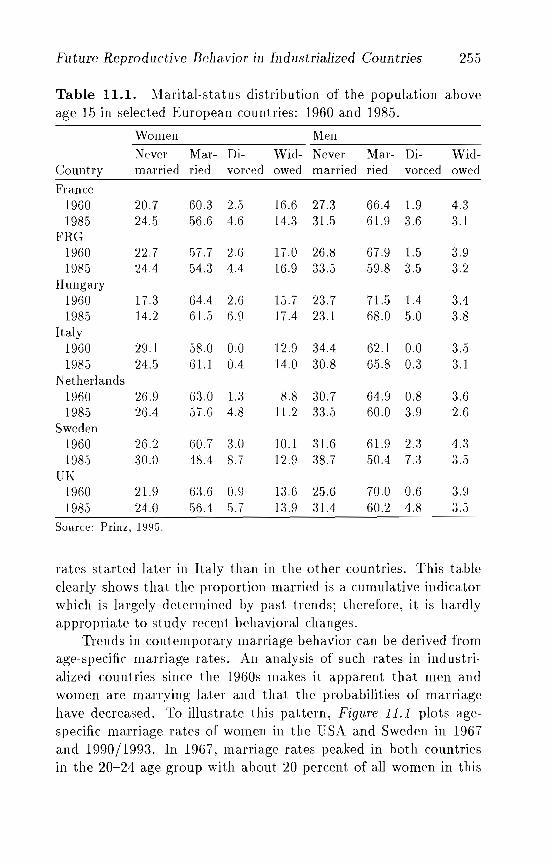
Future Reproductive Behavior ill Industrialized Countries 255

Table 11.1. Marital-status distribution of the population aboveage 15 in selected European countries: 1960 and 1985.

'Nomen Men

CountryNever Mar- Di- Wid- Never Mar- Di- Wid­married riecl von'ed owed married ried vorced owed

France1960 20.71985 24.5

F'RG1960 22.71985 24.4

Hungary1960 17.31985 14.2

Italy1960 29.11985 24.5

Netherlands1960 26.91985 26.4

Sweden1960 26.21985 :30.0

UK1960 2Ul1985 24.0

Source: Prinz, 1995.

60.3 2.556.6 4.6

57.7 2.654.:3 4.4

64.4 2.661.5 6.9

58.0 0.061.1 0.4

63.0 1.:351.G 4.8

60.7 3.048.4 8.7

6:Hj 0956.4 5.7

lG.G 27.314.3 31.5

17.0 26.816.9 33.5

15.7 23.717.4 23.1

12.9 34.414.0 30.8

8.8 30.711.2 33.5

10.1 31.612.9 38.7

13.6 2.5.613.9 :31.4

66.4 1.961.9 3.6

67.9 1..5.59.8 3..5

71.5 1.468.0 .5.0

62.1 0.06.5.8 0.3

64.9 0.860.0 3.9

61.9 2.3.50.4 7.3

70.0 0.660.2 4.8

4.33.1

3.93.2

3.43.8

3..53.1

3.62.6

4.33..5

3.93.5

rates started later in Italy than in the other countries. This tableclearly shows that the proportion married is a cumulative indicatorwhich is largely determined by past trends; therefore, it is hardlyappropriate to study recent behavioral changes.

Trends in contemporary marriage behavior can be derived fromage-specific marriage rates. An analysis of such rates in industri­alized countries since the 1960s makes it apparent that men andwomen are marrying later and that the probabilities of marriagehave decreased. To illustrate this pattern, Figu.re 11.1 plots age­specific marriage rates of women in the USA and Sweden in 1967and 1990/1993. In 1967, marriage rates peaked in both countriesin the 20-24 age group with about 20 percent of all women in this

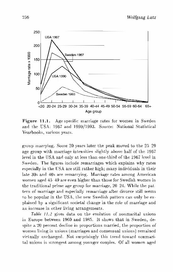
256 Wolfgang Lutz

250

USA 1967

150 I I i "_,, -----j

200 I I " I

o8x2~

~ 100 I I: L ~ '\. _ttl • ,,1>";;:

rn~

20-24 25-29 30-34 35-39 40-44 45-49 50-54 55-59 60-64 65+

Age group

Figure 11.1. Age-specific marriage rates for women in Swedenand the USA: 1967 and 1990/1993. Source: National StatisticalYearbooks, various years.

group marrying. Some 20 years later the peak moved to the 25-29age group with marriage intensities slightly above half of the 1967level in the USA and only at less than one-third of the 1967 level inSweden. The figures include remarriages which explains why ratesespecially in the USA are still rather high; many individuals in theirlate 30s and 40s are remarrying. Marriage rates among Americanwomen aged 45-49 are even higher than those for Swedish women inthe traditional prime age group for marriage, 20-24. While the pat­tern of marriage and especially remarriage after divorce still seemsto be popular in the USA, the new Swedish pattern can only be ex­plained by a significant societal change in the role of marriage andan increase in other living arrangements.

Table 11.2 gives data on the evolution of nonmarital unionsin Europe between 1960 and 1985. It shows that in Sweden, de­spite a 20 percent decline in proportions married, the proportion ofwomen living in unions (marriages and consensual unions) remainedvirtually unchanged. Not surprisingly this trend toward nonmari­tal unions is strongest among younger couples. Of all women aged

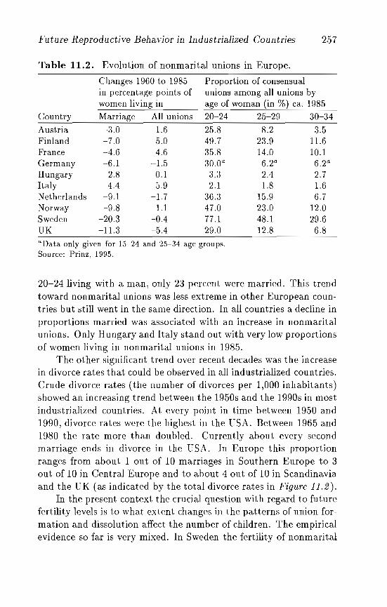
Future Reproductive Behavior in Industrialized Countries 257

Table 11.2.

Country

AustriaFinlandFranceGermanyHungaryItalyNetherlandsNorwaySwedenUK

Evolution of nonmarital unions in Europe.

Changes 1960 to 1985 Proportion of consensualin percentage points of unions among all unions bywomen living in age of woman (in %) ca. 1985

Marriage All unions 20-24 25-29 30-34

-3.0 1.6 25.8 8.2 3.5-7.0 5.0 49.7 23.9 11.6-4.6 4.6 35.8 14.0 10.1-6.1 -1.5 30.0 a 6.2a 6.2 a

-2.8 0.1 3.3 2.4 2.74.4 5.9 2.1 1.8 1.6

-9.1 -1.7 36.3 15.9 6.7-9.8 1.1 47.0 23.0 12.0

-20.3 -0.4 77.1 48.1 29.6-11.3 -5.4 29.0 12.8 6.8

aData only given for 15-24 and 25-34 age groups.Source: Prinz, 1995.

20-24 living with a man, only 23 percent were married. This trendtoward nonmarital unions was less extreme in other European coun­tries but still went in the same direction. In all countries a decline inproportions married was associated with an increase in nonmaritalunions. Only Hungary and Italy stand out with very low proportionsof women living in nonmarital unions in 1985.

The other significant trend over recent decades was the increasein divorce rates that could be observed in all industrialized countries.Crude divorce rates (the number of divorces per 1,000 inhabitants)showed an increasing trend between the 1950s and the 1990s in mostindustrialized countries. At every point in time between 1950 and1990, divorce rates were the highest in the USA. Between 1965 and1980 the rate more than doubled. Currently about every secondmarriage ends in divorce in the USA. In Europe this proportionranges from about lout of 10 marriages in Southern Europe to 3out of 10 in Central Europe and to about 4 out of 10 in Scandinaviaand the UK (as indicated by the total divorce rates in Figure 11.2).

In the present context the crucial question with regard to futurefertility levels is to what extent changes in the patterns of union for­mation and dissolution affect the number of children. The empiricalevidence so far is very mixed. In Sweden the fertility of nonmarital

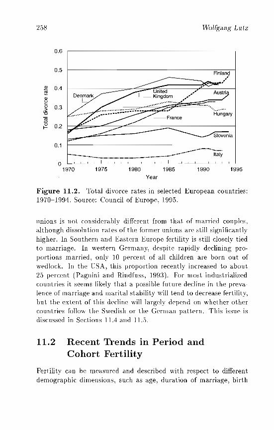
258

0.6

0.5

QJ 0.4~QJ

~0 0.3>'6"'iii(5

0.2f-

0.1

Wolfgang Lutz

""..................."","~ _s-~--.......

•.........Hungary

._._._._._._._._._._._._._._._._._._._._._._._._._._.-'It~y

o1970 1975 1980

Year

1985 1990 1995

Figure 11.2. Total divorce rates in selected European countries:1970-1994. Source: Council of Europe, 1995.

unions is not considerably different from that of married couples,although dissolution rates of the former unions are still significantlyhigher. In Southern and Eastern Europe fertility is still closely tiedto marriage. In western Germany, despite rapidly declining pro­portions married, only 10 percent of all children are born out ofwedlock. In the USA, this proportion recently increased to about25 percent (Pagnini and Rindfuss, 1993). For most industrializedcountries it seems likely that a possible future decline in the preva­lence of marriage and marital stability will tend to decrease fertility,but the extent of this decline will largely depend on whether othercountries follow the Swedish or the German pattern. This issue isdiscussed in Sections 11.4 and 11 ..5.

11.2 Recent Trends in Period andCohort Fertility

Fertility can be measured and described with respect to differentdemographic dimensions, such as age, duration of marriage, birth

Future Reproductive Behavior in Industrialized Countries 2,59

order, period between births, and calendar year. One principal con­ceptual distinction is whether to consider the reproductive experi­ence of birth cohorts of women over their life span (cohort approach)or to study the fertility of different age groups in a specific calendaryear (period approach). For the purpose of population projectionsthe number of children born in a particular year is needed as an in­put parameter, which is derived from the application of age-specificperiod fertility rates to the age structure of the female population.Hence, assumptions must be defined in terms of period fertility. Ifone believes, however, that cohort fertility - because it has greaterstability - is the more appropriate indicator for making assump­tions, assumed cohort fertility can be translated into period rates ifadditional assumptions about the timing of births over the courseof a life are made.

Table 11.3 gives period total fertility rates, i.e., the mean num­ber of children per woman implied by age-specific fertility rates of ayear, for 30 industrialized countries over the period 1950-199,5. Inall countries except Malta, Japan, and countries in Eastern Europe,fertility increased during the late 1950s. This indicates the start ofthe postwar baby boom, which peaked in the early 1960s in mostcountries. Of the 30 countries listed, in 1960-1965 only Estoniaand Hungary had fertility rates below two children per woman, butseveral countries had rates above :3.0. The 1970s were a period offertility decline in practically every industrialized country. By 1980­1985 only Iceland, Ireland, Poland, and Slovakia had a fertility levelabove 2.1. For all industrialized countries together- which com­prised 0.8 billion people in 1950 and 1.2 billion in 1995 (UN, 1995)- fertility declined from 2.77 in 1955-1960 to 1.91 in 1975-1980 andto 1. 70 in 1990-1995.

As to regional differences in fertility trends (see Figure 11.3 forfive selected countries), there seems to be a West European patternwith a moderate baby boom and a steep decline during the 1970s.Southern Europe follows the pattern with some delay. The UnitedStates clearly falls out of the general pattern: because of an excep­tionally pronounced baby boom, it reached fertility levels of 3.7 in195.5, which is above any level registered in Europe since early in thiscentury. Japan shows a completely different pattern with a steepfertility decline during the 1950s which brought down total period

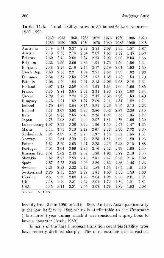
260 Wolfgang Lutz

Table 11.3. Total fertility rates in 30 industrialized countries:1950-1995.

1950- 1955- 1960- 1965- 1970- 1975- 1980- 1985- 1990­1955 1960 1965 1970 1975 1980 1985 1990 1995

Australia 3.18 3.41 3.27 2.87 2.53 2.09 1.93 1.87 1.87Austria 2.10 2.53 2.79 2.54 2.02 1.65 1.62 1.45 1.53Belarus 2.60 2.72 2.68 2.37 2.24 2.09 2.06 2.03 1.65Belgium 2.33 2.50 2.66 2.34 1.94 1.70 1.59 1.56 1.64Bulgaria 2.48 2.27 2.18 2.15 2.17 2.18 2.01 1.92 1.50Czech Rep. 2.69 2.35 2.21 1.94 2.21 2.32 1.99 1.92 1.83Denmark 2.54 2..54 2..59 2.25 1.97 1.68 1.43 1.54 1.70Estonia 2.06 1.99 1.94 2.01 2.15 2.06 2.08 2.18 1.61Finland 2.97 2.78 2.58 2.06 1.62 1.64 1.69 1.66 1.85France 2.73 2.71 2.85 2.61 2.31 1.86 1.87 1.80 1.74Greece 2.29 2.27 2.20 2.38 2.32 2.32 1.96 1.53 1.40Hungary 2.73 2.21 1.82 1.97 2.09 2.11 1.81 1.82 1.71Iceland 3.70 4.02 3.94 3.15 2.84 2.29 2.25 2.12 2.23Ireland 3.37 3.67 3.96 3.86 3.80 3.46 2.87 2.28 2.10Italy 2.32 2.35 2.55 2.49 2.28 1.92 1.55 1.35 1.27Japan 2.75 2.08 2.01 2.00 2.07 1.81 1.76 1.66 1.50Luxembourg 1.97 2.22 2.36 2.22 1.96 1.50 1.47 1.47 1.65Malta 4.14 3.73 :3.10 2.17 2.07 2.02 1.96 2.02 2.05Netherlands 3.06 3.09 3.12 2.73 1.97 1.58 1.51 1.56 1.61Norway 2.60 2.84 2.90 2.72 2.25 1.81 1.69 1.80 1.93Poland 3.62 3.29 2.65 2.27 2.25 2.26 2.33 2.15 1.88Portugal 3.05 3.04 3.09 2.86 2.76 2.42 1.99 1.60 1.55Russian Fed. 2.51 2.62 2.48 2.02 1.98 1.92 1.99 2.10 1.53Slovakia 3.52 3.27 2.89 2.49 2.51 2.47 2.28 2.15 1.92Spain 2.57 2.75 2.89 2.93 2.89 2.63 1.86 1.46 1.23Sweden 2.21 2.23 2.33 2.12 1.89 1.65 1.64 1.91 2.10Switzerland 2.28 2.33 2.50 2.27 1.81 1.53 1.53 1.53 1.60Ukraine 2.51 2.30 2.08 1.9.5 2.04 1.98 2.00 2.01 1.64UK 2.18 2.49 2.81 2.52 2.04 1.72 1.80 1.81 1.81USA 3.45 3.71 3.31 2.55 2.02 1.79 1.82 1.92 2.08

Source: UN, 1995.

fertility from 3.6 in 1950 to 2.0 in 1960. An East Asian particularityis the low fertility in 1966 which is attributable to the Hinoeuma("fire horse") year during which it was considered unpropitious tohave a daughter (Atoh, 1989).

In many of the East European transition countries fertility rateshave recently declined sharply. The most extreme case is eastern

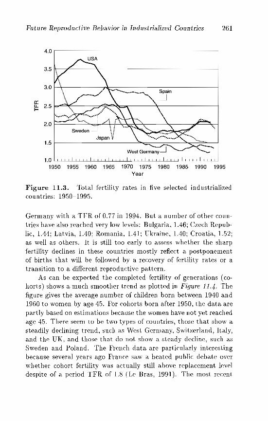
Future Reproductive Beha.vior in Industria.lized Countries 261

ISpain

---- 7.\::~....... .......... I3.01 , '~

a:l= 2.5

1.0 LLL I I I I I I I I I I I I I ! I ! I I I ! I I I I I J I I ( I I I I I I I I I I I I I I

1950 1955 1960 1965 1970 1975 1980 1985 1990 1995Year

4.0 I'-----------------

2.0 I-'" ....j•••,- \ -'. \ ... \. .... ", .,;' ~... I'.

1.5 I ...... ....-= '.......... I

Figure 11.3. Total fertility rates in five selected industrializedcountries: 1950-1995.

Germany with a TFR of 0.77 in 1994. But a number of other coun­tries have also reached very low levels: Bulgaria, 1.46; Czech Repub­lic, 1.44; Latvia, 1.40; Romania, 1.41; Ukraine, 1.40; Croatia, 1.52;as well as others. It is still too early to assess whether the sharpfertility declines in these countries mostly reflect a postponementof births that will be followed by a recovery of fertility rates or atransition to a different reproductive pattern.

As can be expected the completed fertility of generations (co­horts) shows a much smoother trend as plotted in Figure 11.4. Thefigure gives the average number of children born between 1940 and1960 to women by age 45. For cohorts born after 1950, the data arepartly based on estimations because the women have not yet reachedage 45. There seem to be two types of countries, those that show asteadily declining trend, such as West Germany, Switzerland, Italy,and the UK, and those that do not show a steady decline, such asSweden and Poland. The French data are particularly interestingbecause several years ago France saw a heated public debate overwhether cohort fertility was actually still above replacement leveldespite of a period TFR of 1.8 (Le Bras, 1991). The most recent

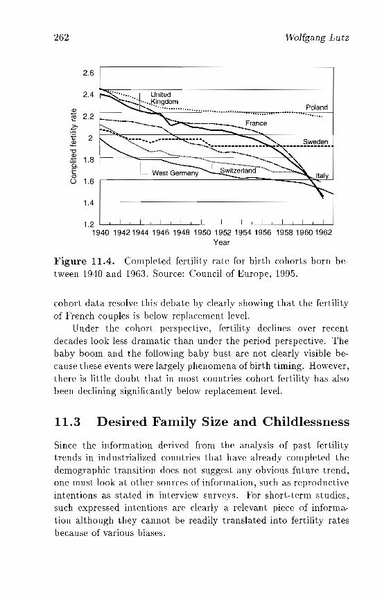
262

2.6

2.4

Q)

"§ 2.2

~1:' 22"0

.~ 1.80..E0() 1.6

1.4

Wolfga,ng Lutz

Poland.........

----___ France

---'......--.. ..---~.~---.. ~',. Sweden............~.~.~ :-.-.~~::..::.~:::.:.=.---~,------------

L ------........·C....=....·.. -.-.-.- ".West German~witzerl;;:n(j ..····· ::::::::-~

1.21940 19421944 1946 1948 1950 1952 1954 1956 195819601962

Year

Figure 11.4. Completed fertility rate for birth cohorts born be­tween 1940 and 1963. Source: Council of Europe, 1995.

cohort data resolve this debate by clearly showing that the fertilityof French couples is below replacement level.

Under the cohort perspective, fertility declines over recentdecades look less dramatic than under the period perspective. Thebaby boom and the following baby bust are not clearly visible be­cause these events were largely phenomena of birth timing. However,there is little doubt that in most countries cohort fertility has alsobeen declining significantly below replacement level.

11.3 Desired Family Size and Childlessness

Since the information derived from the analysis of past fertilitytrends in industrialized countries that have already completed thedemographic transition does not suggest any obvious future trend,one must look at other sources of information, such as reproductiveintentions as stated in interview surveys. For short-term studies,such expressed intentions are clearly a relevant piece of informa­tion although they cannot be readily translated into fertility ratesbecause of various biases.

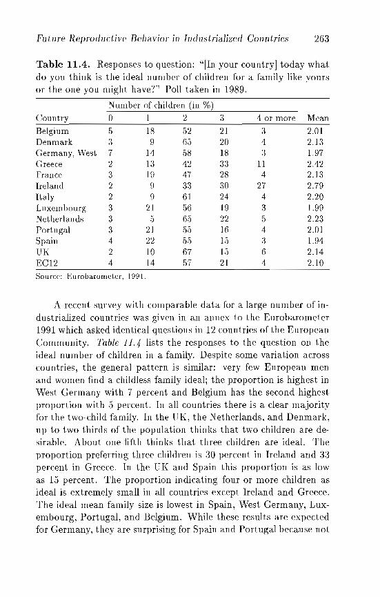
Fll t ure Reprod uctive Behavior in Ind llstrialized Countries 263

Table 11.4. Responses to question: "[In your country] today whatdo you think is the ideal number of children for a family like yoursor the one you might have?" Poll taken in 1989.

Number of children (in %)Country

BelgiumDenmarkGermany, WestGreeceFranceIrelandItalyLuxembourgNetherlandsPortugalSpainUKEC12

012

5 18 523 9 657 14 582 13 423 19 472 9 332 9 613 21 563 5 653 21 554 22 552 10 674 14 57

3

21201833283024192216151521

4 or more

343

114

274354364

Mean

2.012.131.972.422.132.792.201.992.232.011.942.142.10

Source: Eurobarometer, 1991.

A recent survey with comparable data for a large number of in­dustrialized countries was given in an annex to the Eurobarometer1991 which asked identical questions in 12 countries of the EuropeanCommunity. Table 11.4 lists the responses to the question on theideal number of children in a family. Despite some variation acrosscountries, the general pattern is similar: very few European menand women find a childless family ideal; the proportion is highest inWest Germany with 7 percent and Belgium has the second highestproportion with .s percent. In all countries there is a clear majorityfor the two-child family. In the UK, the Netherlands, and Denmark,up to two- thirds of the population thinks that two children are de­sirable. About one-fifth thinks that three children are ideal. Theproportion preferring three children is 30 percent in Ireland and 33percent in Greece. In the UK and Spain this proportion is as lowas 15 percent. The proportion indicating four or more children asideal is extremely small in all countries except Ireland and Greece.The ideal mean family size is lowest in Spain, West Germany, Lux­embourg, Portugal, and Belgium. While these results are expectedfor Germany, they are surprising for Spain and Portugal because not

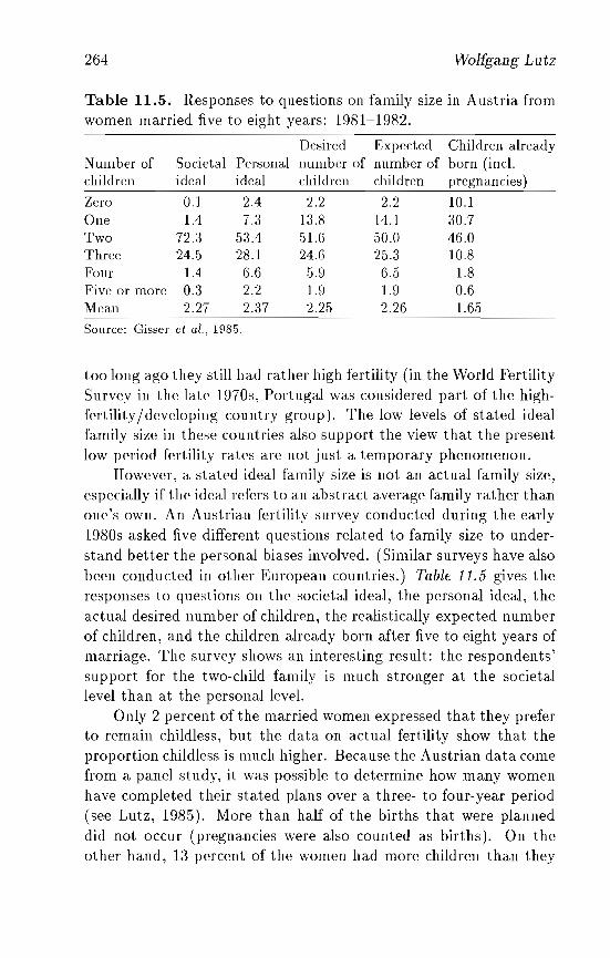
264 Wolfgang Lutz

Table 11.5. Responses to questions on family size in Austria fromwomen married five to eight years: 1981~1982.

Desired Expected Children alreadyNumber of Societal Personal number of number of born (incl.children ideal ideal children children pregnancies)Zero 0.1 2.4 2.2 2.2 10.1One 1.4 7.3 13.8 14.1 30.7Two 72.3 53.4 51.6 50.0 46.0Three 24.5 28.1 24.6 25.3 10.8Four 1.4 6.6 5.9 6.5 1.8Five or more 0.3 2.2 1.9 1.9 0.6Mean 2.27 2.37 2.25 2.26 1.65

Source: Gisser et al., 1985.

too long ago they still had rather high fertility (in the World FertilitySurvey in the late 197013, Portugal was considered part of the high­fertility/developing country group). The low levels of stated idealfamily size in these countries also support the view that the presentlow period fertility rates are not just a temporary phenomenon.

However, a stated ideal family size is not an actual family size,especially if the ideal refers to an abstract average family rather thanone's own. An Austrian fertility survey conducted during the early198013 asked five different questions related to family size to under­stand better the personal biases involved. (Similar surveys have alsobeen conducted in other European countries.) Table 11.5 gives theresponses to questions on the societal ideal, the personal ideal, theactual desired number of children, the realistically expected numberof children, and the children already born after five to eight years ofmarriage. The survey shows an interesting result: the respondents'support for the two-child family is much stronger at the societallevel than at the personal level.

Only 2 percent of the married women expressed that they preferto remain childless, but the data on actual fertility show that theproportion childless is much higher. Because the Austrian data comefrom a panel study, it was possible to determine how many womenhave completed their stated plans over a three- to four-year period(see Lutz, 198.5). More than half of the births that were planneddid not occur (pregnancies were also counted as births). On theother hand, 13 percent of the women had more children than they

Future Reproductive Behavior in Industrialized Countries 265

planned. This resulted in a significant net deficit. It also implies thatif unplanned pregnancies could be avoided by better contraception,the deficit may become even larger.

The most significant case of a personal deficit, that is, havingfewer children than originally intended, seems to be with the firstbirth. The actual number of childless women tends to be muchhigher than the number of women who say in their early adulthoodthat they prefer to remain childless. It is quite difficult to calculatethe proportion of women remaining without children (and completefamily-size distributions) as implied by period fertility rates becausebirth-order specific information is required. A recent survey articleby Feeney and Lutz (1991) describes alternative methods and showsestimates of childlessness among all women by age 45 as implied byperiod rates in the early 1980s: 27 percent of women remain childlessin the USA; 31 percent, in the Netherlands; and 28 percent, inAustria.

More accurate but less up-to-date information on childlessnessis available on cohorts of women. A study of Austria, East Germany,and West Germany shows that about 30 percent of cohorts aboveage 70 were childless in the late 1980s (see Buttner and Lutz, 1990b).Between 15 percent and 20 percent of cohorts aged 50-70 were child­less. This decline in childlessness is evidence of the disappearance ofthe traditional "European marriage pattern" under which high pro­portions of women remained unmarried. Childlessness had alwaysbeen somewhat lower in East Germany than in Austria, but afterthe 1940 cohort the trends of childlessness completely diverge, withdecreases in East Germany and increases in Austria. As discussedlater, the very low levels of childlessness in East Germany are partlyattributable to government policies. For West Germany the exist­ing data for marriage cohorts after 1956 show a clear increase ofchildlessness over time (after 11 to 15 years of marriage) to almost20 percent for those married in the period between 1971 and 1975.Taken together with the fact that the proportion of married womenhas been declining and that fertility outside marriage is very low,this implies very high levels of cohort childlessness in West Germany.

These family-size distributions, including childlessness, alsohave direct implications on distributional and equity issues, suchas the concentration of childbearing and the division of labor for

266 Wolfgang Lutz

society's reproduction among women of one generation. The rathereven distribution and low childlessness in East Germany in the late1980s implies that 3:3 percent of all women had half the childrenborn, whereas in Austria 23 percent of all women had half the chil­dren (Lutz and Vaupel, 1987). In West Germany 29 percent of allmarried women had half the children, but for all women together theproportion should be lower than in Austria, i.e., the concentrationhigher. The concentration of childbearing has many implicationswhich are discussed in Lutz (1989).

One relevant issue for future fertility levels is whether there willbe a trend toward some women specializing in childrearing whilethe rest have few or no children. Such a pattern could result inhigher total fertility, but is very unlikely. All empirical informationshows that very few women have expressed that they want to have alarge number of children and that the overwhelming majority haveexpressed the desire to have at least one child or two children. Thenormative trend toward the two-child family, at least as a goal, seemsto be very strong, which implies that in the future childrearing isunlikely to be concentrated in a certain group of women.

11.4 Arguments for Assuming HigherFertility

In several countries period fertility has been below so-calledrepla.cement-Ievel fertility (i.e., a net reproduction rate of 1.0) formore than two decades. Is this a stable and sustainable pattern ofreproduction in modern industrialized societies, or is it only a tran­sitory state that will be followed by higher fertility? One can thinkof several mechanisms that can potentially lead to higher averagefertility in these countries.

11.4.1 The homeostasis argument

The usual interpretation of the demographic transition theory is thatan initial equilibrium between high birth rates and high death ratesis disturbed by declining mortality which in turn triggers a fertilitydecline that brings birth and death rates back to an equilibrium atlow levels. However, history has shown that fertility declines with all

Future Reproductive Behavior in Industrialized Countries 267

their irregularities and national particularities generally do not stopat replacement level, but continue to decline further. The homeosta­sis argument would stress that this is simply an overshooting thatwill be reversed after some inevitable societal adjustments. Mostexplicitly this has recently been expressed by Vishnevsky (1991)who does not see fertility levels as the sum of individual behav­ior, but rather sees it as one aspect in the evolution of a systemthat determines behavior. He believes that the development of thedemographic system is directed by a proper, inherent goal. In theprocess of self-organization the system aims at self-maintenance andsurvival. For human beings at a certain stage of evolution, a new andhigher goal is assumed to appear that goes beyond pure populationsurvival - namely, that of maintaining homeostasis in the popula­tion's reproduction, even in the face of considerable fluctuations inexternal conditions (see Vishnevsky, 1991:265).

It is not yet possible to empirically test this hypothesis. Trendssuch as the recent fertility increase in Sweden, which has been aforerunner of many other social changes, may be taken as evidenceby supporters of this hypothesis. But the hypothesis is not specificenough to be tested (e.g., it does not state by how much fertilityshould increase over a period). Since studies have not addressed themechanisms and motivations that induce couples to have more chil­dren, it remains largely a philosophical argument. Nevertheless, thishypothesis seems worth considering at this general level, although itis highly controversial. For example, authors such as Westoff (1991a)criticize the assumption of a "magnetic force" toward replacement.

11.4.2 Assumption of fertility cycles

Several views summarized under this heading contend that thepresent low level of period fertility is just the end of a cycle and thatthe future will bring an upward trend. These views can be groupedinto arguments dealing with the timing of fertility within cohortsand those dealing with intergenerational fertility fluctuations. Thefirst argument is based on the observation that in many countriesthe recent declines in total fertility were accompanied by declinesin the fertility ra.tes of younger women. Hence, one could assumethat observed trends only reflect a. delay in childbearing (the timingof fertility) and do not indicate a decline in the number of children

268 Wolfgang Lutz

a woman has over her life span (the quantum of fertility). As de­scribed earlier it is evident in all countries that declines in cohortfertility have been slower than declines in period fertility. But inmost European countries, meanwhile, cohort fertility is also below2.0, and in several countries even below 1.6.

It is difficult to evaluate the argument that women will soonbegin having their delayed births, hence increasing period fertility.The slight recovery in total fertility around 1990 in several Europeancountries may be partly attributable to this phenomenon. Studiesfor Sweden have also shown that current high period fertility islargely due to this timing phenomenon and was likely to decline soon(Hoem, 1990). Indeed, the most recent data indicate such decline.The timing phenomenon could only have a sizable impact on futureperiod fertility levels if one assumes that cohort fertility tends tobe substantially higher than present period rates. This may be thecase in Southern Europe, where period fertility recently declinedextremely fast, but generally there is no clear substantive reasonto assume that a significant catch-up phenomenon will occur. Forlonger- term fertility trends (more than 10 years) such timing aspectsare irrelevant in any case.

The second argument focuses on longer-term cycles. It assumesthat the fertility level of the parents' generation is a determinant intheir children's reproductive behavior. Best known in this contextis Easterlin's relative income hypothesis (Easterlin, 1980). In short,it assumes that fertility is determined by income relative to aspira­tions, with cohort size determining income: generation one has lowrelative income and low fertility; generation two grows up with lowaspirations for wealth but finds advantages in labor-market condi­tions because of few competitors, hence it has high relative incomeand high fertility; generation three is large and has high aspirationsresulting in low relative income and low fertility. Empirically, thismodel fits nicely to the US baby boom in the 196013 and the subse­quent fertility decline. But this is not a complete cycle. So far a newbaby boom has failed to materialize. For other countries the his­torical long-term cycle argument is even less applicable. There arealso a number of conceptual problems such as the fact that withina generation fertility is unevenly distributed among families - somefamilies have many children, others only one (see discussion in Lutz,

Future Reproductive Behavior in Industrialized Countries 269

1989) - and that women have children at different ages which soonsmoothes out any cycles based on intergenerational dynamics. Buteven if this assumed mechanism is not a dominating factor for fer­tility trends, it may play some role.

11.4.3 Pronatalistic policies

Governments in countries with very low fertility have reason toworry about the long-term implications of subreplacement fertilitytogether with increasing life expectancy at higher ages on the pen­sion system and other social-security systems such as health care.Because the baby- boom generation is currently in its main produc­tive ages, the economic dependency burden is still quite favorable.But projections indicate that in Western Europe, the proportion ofthe population above age 60 will increase significantly over the nextfew decades. This situation poses an extremely serious threat topresent forms of pay-as-you-go pension schemes, where the activepeople pay for the pensioners. For this and other reasons, severalEuropean countries have tried to stimulate fertility through poli­cies that make it slightly more profitable to have children. It mustbe stressed, however, that most countries that provide extensivechild-care benefits do this for reasons of social policy rather thanpopulation policy (Holm, 1991). But still such policies might berelevant for individual reproductive decisions.

If couples react to reproductive incentives in the way that indi­viduals react to other incentives, then changes in the incentive struc­ture will have an impact on fertility. Monetary incentives for havingchildren are only one possible mechanism of government policies toincrease fertility. There is very little evidence that such monetarypolicies actually work. For instance, Germany and Austria pro­vide many direct and indirect child benefits while in the USA thebenefits are almost nonexistent; yet fertility is much lower in Ger­many and Austria than it is in the USA. Also over time it is hardto link changes in fertility rates to changes in government benefits(Chesnais, 1985; Klinger, 198.5). One exception is the marked fer­tility increase in East Germany between 1976 and 1977, which canclearly be attributed to the introduction of a package of social-policymeasures (Biittner and Lutz, 1990a; Vining, 1984). But conditionsin East Germany were very specific: there was a severe housing

270 Wolfgang Lutz

shortage, and the birth of a child was an easy way to get accessto an apartment and other benefits. Since these benefits providedfor basic needs that otherwise could hardly be met, the motivationfor childbearing became very strong. But this already goes beyondthe usual understanding of incentives, because it is associated withdeprivations that are hardly acceptable in democratic, free-marketsocieties.

Beyond material incentives, social pressure and changing atti­tudes as well as infrastructural arrangements for childrearing maybe very important. Because no monetary transfer can realisticallycompensate the cost of children, including the opportunity costsof women not working because of a child, nonmaterial motivationsfor parenthood remain extremely important. These motivations canalso be influenced by government policies that try to remove institu­tional and other obstacles so that women can combine motherhoodwith a profession. In Sweden, the universal and low-cost provisionof public child-care starting at very young ages and the many oppor­tunities for part-time work may be important factors in explainingthe high level of fertility.

11.4.4 National identity and ethnic rivalry

NationaJ identity may have an important influence on individualreproductive behavior. Fears related to the ethnic composition ofthe population and ingroup-outgroup feelings can be powerful emo­tional forces that may directly influence fertility. Examples of thismay be found in Israel, Northern Ireland, and the Baltic states; inthese areas there is clear rivalry between two groups of the popula­tion. This rivalry may be an important reason why fertility levelsare higher in these countries than in other countries under similarsocioeconomic conditions. One possible hypothesis is that throughinternational migration such rivalry may also affect other industrial­ized countries. But there are strong counterexamples, such as fran­cophone Canadians, non-Hispanic Californians, or Germans livingin cities with many Turks, where ethnic-linguistic rivalry is carriedout by means other than reproductive behavior.

Future Reproductive Behavior in Industrialized Countries 271

11.5 Arguments for Assuming LowerFertility

11.5.1 Trend toward individualism

According to the sociological theories of Durkheim (1902) andTonnies (1887) the process of "modernization" is characterizedby a transition from "community" (Gemeinschajt) to "society"( Gesellschaft). While "community" refers to a living arrangementthat is lasting and complete under a relatively stable structure, "so­ciety" means a mere proximity of persons who are independent ofone another living within relatively open structures. In this processof transition, an increasing number of needs that were once met bythe family are taken over by anonymous institutions. This meansan increase in equality and personal freedom, but also an increaseof individualism and a weakening of interpersonal bonds.

With respect to the future of the family, Hoffmann-Nowotny(1987) assumes that the trend of increa.sing differentiation as well asmultiple and partial integration will continue, especially for women.From a sociological point of view, he concludes that there is littlereason to believe that the family as we know it can and will surviveas the mainstream model for future living patterns. This view is nottoo different from the notion of a "second demographic transition"put forward by Lestaeghe (1983) and van de Kaa (1987) to char­acterize a new phase of demographic behavior that expresses itselfthrough lower marriage propensities, higher instability of unions,increase in extramarital fertility, and lower total fertility.

Another psychological aspect of this supposed trend toward in­dividualism is tha.t men and ,vomen are increasingly reluctant tomake decisions that have long-term consequences and clearly limitthe future freedom of choice. The decision to have a child prede­termines many choices for the following two decades, and makessecond thoughts impossible once the child is born. If the trend to­ward greater mobility in all aspects of life continues, this might wellmean fewer responsible men and women daring to become parents.

There is little empirical basis to evaluate the validity of thesehypotheses for the future, but they seem to be powerful arguments

272 Wolfgang Lutz

and plausible explanations of recent trends. In the future it mightwell happen that, if this trend develops to an extreme, counterforceswill be mobilized to compensate some of the negative aspects ofthis trend. But a return to traditional patterns of "community"with their restrictions on individual freedom is very unlikely. Mostof the following arguments are related to this general "continuedmodernization" argument.

11.5.2 Economic independence of women

One recent trend that has often been singled out as a dominatingfeature of societal change is the increasing economic independenceof women. Female labor-force participation has been steadily in­creasing in virtually all industrialized countries over recent decades.The increase has been strongest in Scandinavia, where labor-forceparticipation is almost universal among adult women below age 50,but female activity rates in North America are not much lower. InItaly, female labor-force participation increased by more than one­third in the 1980s. This fundamental change in economic activityof women is obviously connected to changing reproductive patterns.Increasing economic independence of women also tends to result in apostponement of marriage, which typically is associated with lowerfertility.

One must be cautious, however, in pointing out female economicactivity as a major determinant of declining fertility. It may alsobe that the lower desired number of children motivates women notto stay at home but rather to enter the labor force, or there maybe another driving force behind both trends. This last possibility issu pported by evidence from several countries that are experiencingimprovements in fertility rates, despite very high and still increas­ing female labor-force participation. The key question in this mul­tifaceted issue seems to be: How can women combine parenthoodwith participation in the labor market (see, e.g., Kiernan, 1991)?This may be a decisive question in determining future Europeanbirth rates. Nevertheless, even with flexible regulations and goodchild-care systems, working women, on average, will not have verylarge families.

Future Reproductive Behavior in Industrialized Countries 273

11.5.3 Instability of partnership

As described above, marital stability has been declining in all indus­trialized countries. Part of the reason for this phenomenon clearlylies in the increasing economic independence of women. Women areno longer economically forced to stay in an unsatisfactory union ifthey earn an independent income. Other reasons may lie in thegeneral increase in mobility in modern industrialized societies andin a decreasing threshold in the level of dissatisfaction necessary toattempt to change conditions. \Vhatever the social and psycholog­ical reasons may be, the chances of a young couple today stayingtogether for 20 years, the minimum time required to raise a child,are slimmer than they were in the past.

Increasing evidence from empirical studies (Kiernan, 1992)shows that the separation of parents actually does more harm tochildren than had been assumed in the past. Such harm is measuredby studying a child's social behavior, intellectual performance, andfeeling of happiness and security. Thus, responsible prospective par­ents may decide not to have children if they have doubts about thestability of their partnership. This may be a very important factorin the decisions of couples in consensual unions, which seem to havemuch lower stability than marital unions (Prinz, 1995).

One possible counterargument would be that remarriage (or for­mation of new nonmarital unions) may actually be an incentive tohave an additional child to strengthen the relationship with a newpartner. Empirical analysis on data cross-classified by marital sta­tus and number of children for Finland (see Lutz, 1993a) shows thata slight effect of this kind exists, but it does not have a significantimpact on total fert1lity.

11.5.4 Consumerism and use of time

Commentators often mention the increase in consumerism as a basicunderlying cause for the recent fertility decline. The argument isthat people would rather invest in pleasures for themselves than inchildren; they would rather buy a new car than have another child;they would rather spend their time watching TV than changingdiapers. Children are considered work and not fun. As pointedout by Keyfitz (1991), in earlier times couples had to work harder

274 Wolfgang Lutz

and more hours to earn a living and still found the time to havemany children. The extra leisure time couples have today is notbeing spent on having children. Having children is defined as workand therefore one talks about its opportunity cost. In the wordsof Keyfitz (1991:239): "No one complains about the opportunitycost of having sex. Thus to talk about opportunity cost of childrenindeed highlights the problem of non-childbearing." He suggeststhinking of a work-fun continuum and trying to move childbearingtoward the fun end of that continuum.

Whether childbearing and, especially, childrearing will becomefavored leisure-time activities of men and women will depend onthe trade-offs between fun and burdell. Some European cities al­ready have more dogs than children. Obviously in these areas thework-fun balance is more favorable for pets, which require less of acommitment and in the worst case can always be given away. Thisargument clearly suggests that unless the burden of having childrenis diminished or the rewards from children is enhanced, the balancewill continue to be negative for childbearing.

11.5.5 Improving contraception

The final argument in this series is less concerned with changing val­ues but is at a more mechanical level. It is an empirical fact that, inall industrialized societies, a significant number of pregnancies areunplanned. Demographers often distinguish between timing failure(early pregnancy) and quantum failure (unwanted pregnancy). Bothcould be reduced by more efficient contraceptive use: for the latterthis would clearly imply lower fertility; for the former this wouldtheoretically have no effect on fertility. In practice one can assumethat a certain number of the births categorized as timing failuresmay not be realized at a later point in time because of changingliving conditions, such as disruption of a union, a more demandingjob, or physiological reasons. With respect to unwanted pregnan­cies, Westoff et at. (1987) estimate that for a number of low-fertilitycountries, completely efficient contraception would bring down fer­tility rates by somewhat less than 10 percent, as well as significantlylower the number of abortions.

Currently, we are still far from a perfect contraceptive that re­quires no effort to use and has no negative side effects. An increasing

Future Reproductive Behavior in Industrialized Countries 275

number of women report being tired of using the pill, yet sterilizationis not acceptable to all men and women (especially in continentalEurope) because of its irreversibility. New empirical data suggestthat the number of risk-takers or couples practicing less reliable nat­ural methods may have increased because of higher awareness of theside effects of the pill. A hypothetical perfect contraceptive withoutany side effects, which is taken once and then requires some reverseaction for a woman to become pregnant, certainly would change thesituation; this hypothetica.l contraceptive would clearly inhibit un­planned pregnancies which currently are still quite numerous. It willmake quite a difference for future fertility levels whether one mustgo to the doctor to have a child or not to have a child; currently thelatter is the case.

11.6 Fertility Assumptions and PopulationHeterogeneity

All the arguments given in Sections 11.4 and 11.5 for a tendencytoward either lower or higher future fertility levels have some degreeof justification. Each argument is based 011 assumed developmentsthat impact on future reproductive behavior in industrialized coun­tries, but it is unclear what the possible balance, the synergism,of these partly contradictory developments will be. For this reasonwe cannot provide one estimate but can only suggest alternativescenario assumptions.

A probable situation is that the synergism of these varioustrends will not result in a uniform pattern of childbearing in allcountries and in all population groups within countries. Heterogene­ity of reproductive behavior has been increasing since the postwarbaby boom, and there is no indication that this heterogeneity islikely to diminish. Quite the contrary, the above-mentioned trendtoward a societal structure labeled "society" rather than "commu­nity" implies lower normative pressure toward uniform behavioralpatterns. There may be many subgroups and subcultures in societythat have quite different reproductive behavior. On the other hand,it is often argued that mass media exert a powerful force towardstandardization. But with respect to fertility the direction of thisstandardization is not clear. Among TV "protagonists" you find

276 Wolfgang Lutz

singles, childless couples, and traditional families. It seems to bethe case that the plurality of lifestyles is in itself one of the keymessages from the media.

Heterogeneity of the population has important impacts on de­mographic dynamics. In mortality, heterogeneity affects the over­all dynamics of the system through selection processes resulting inchanging weights ofthe subgroups. As to differential fertility- asidefrom individual biological differences - subgroups with higher fertil­ity grow more rapidly and hence have more weight in the populationstructure. Empirically this can be observed for certain high fertilityreligious groups but also with respect to foreigners who have notfully adapted to the host country's average fertility level. In Ger­many, for instance, the slightly positive balance of births and deathsaround 1990 was attributable to the large birth surplus of foreignersliving in Germany. While only 1 in 12 inhabitants of Germany isa foreigner, 1 in 8 children born has foreign citizenship. In otherwords, without non-Germans the German fertility rate would beeven lower than it actually is.

Such considerations of heterogeneity also entered the final nu­merical choice of fertility assumptions for the five industrialized re­gions considered in this study. At least in the long run, fertilitylevels should not be considered independent of migration Levels justas they should not be seen as being completely independent of mor­tality levels in developing countries. Some of these dependencies aremodeled in Chapters 1.5 and 16.

Figure 11.5 shows the fertility assumptions for Western Eu­rope and North America together with recent trends in total fertil­ity rates. The high, central, and low assumptions reflect differentcombinations of the trends described above. The often-assumedreplacement-level fertility was not used as a benchmark becausethere is little substantive reason for such a "magic" level. The un­certainty range is assumed to widen quickly over the next decade.By 2030-2035 the uncertainty range is assumed to increase evenfurther. The low value will reach 1.3 in Eastern Europe, WesternEurope, Pacific OECD, and the European part of the former SovietUnion and 1.4 in North America. The assumed high values are 2.1(which is somewhat above replacement under low-mortality condi­tions) in Western Europe, Pacific 0 ECD, and Eastern Europe and

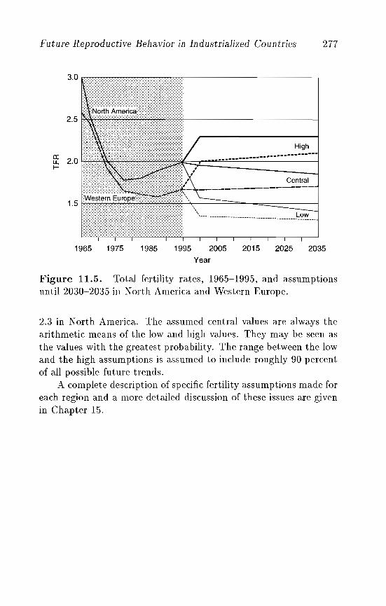
Future Reproductive Behavior in Industrialized Countries 277

Low

High

1965 1975 1985 1995 2005 2015 2025 2035

Year

Figure 11.5. Total fertility rates, 1965-1995, and assumptionsuntil 2030-203.5 in North America and Western Europe.

2.3 in North America. The assumed central values are always thearithmetic means of the low and high values. They may be seen asthe values with the greatest probability. The range between the lowand the high assumptions is assumed to include roughly 90 percentof all possible future trends.

A complete description of specific fertility assumptions made foreach region and a more detailed discussion of these issues are givenin Chapter 15.

Chapter 12

The Future of Mortality atOlder Ages in DevelopedCountries

James W. Vaupel and Hans Lundstrom

Death in developed countries usually strikes at older ages. In mostdeveloped countries the life table probability of survival to age 65 isover 75 percent for men and over 85 percent for women. Median lifetable life spans typically exceed 75 years for men and 80 years forwomen. Populations are aging, but even given current age distribu­tions, about one-third of male deaths and half of female deaths indeveloped countries occur after age 80.

Not only is mortality concentrated at advanced ages in devel­oped countries, but uncertainty about the future of mortality inthese countries largely stems from uncertainty about the future ofdeath rates among the elderly. There may be some surprises intrends at younger ages, analogous perhaps to the unanticipated epi­demic of AIDS, but it seems plausible that the death rates at mostages under 65 will continue to fall at rates of perhaps 1 or 2 percentper year. In some countries for some subpopulations and in someage categories ~ e.g., males in their 20s - death rates may rise some­what, at least in the short term. In the longer term, however, anysuch rise in mortality will produce public health responses that willprobably lead to mortality improvements.

278

Mortality at Older Ages in Developed Countries 279

Whether or not it will be possible to continue to reduce deathrates at older ages is, in contrast, an open and highly controver­sial question. Many gerontologists and demographers believe thatdeath rates at advanced ages cannot be substantially reduced andthat life expectancy will not increase beyond 85 years (Fries, 1980;Fries et ai., 1989; Olshansky et ai., 1990; Lohman et ai., 1992; Har­man, 1991; Hayflick, 1977; Bourgeois-Pichat, 1978; Keyfitz, 1978;Demeny, 1984). Most deaths after age 80 are taken to be natural,senescent deaths due to intrinsic, intractable aging process. Little,then, can be done about saving lives (i.e., substantially postpon­ing deaths) among the oldest-old. Opinions differ about whetherthis barrier to progress is due primarily to biological causes or topractical impediments, but the canonical view is that death ratesat advanced ages in developed countries are close to limits that canonly be relaxed by fundamental and currently unforeseeable break­throughs in slowing the process of aging itself. This assumptionunderlies the long-term mortality forecasts published by the WorldBank, the United Nations, and many national statistical offices.

Other researchers are skeptical about the existence of an upperlimit to life expectancy, at least at an age as early as 85. They fore­see continuing and perhaps even accelerating progress in reducingmortality rates at all ages, including the most advanced ages (Man­ton et ai., 1991). Some projections suggest that the life expectancyof the current generation of children in the United States might be100 years or more if progress in reducing mortality rates continuesover the next century (Vaupel and Gowan, 1986; Guralnik et ai.,1988).

If progress can be made, growth of the oldest-old population willquicken, with major economic and social consequences, including es­calation of the cost of public health care and retirement programs.Progress is most important at the ages when most deaths occur; it isthe weighted average of age-specific rates of mortality improvement,with weights corresponding to the product of death counts and re­maining life expectancy, that determines change in life expectancy.As a rule of thumb, an average rate of improvement of 1 percentwould yield an increase of one year in life expectancy per decade;an average progress rate of 2 percent would yield a two-year increaseper decade (Vaupel, 1986). At current mortality levels a newborn

280 James W. Vaupel and Hans Lundstrom

girl in most developed countries has a life expectancy of about 80years. If progress in reducing mortality rates could be maintainedat an average of 1 percent per year, then her life expectancy wouldbe about 90 years. Sustained 2 percent progress would imply thatthe typical newborn girl in developed countries will live to celebrateher 100th birthday (Vaupel and Owen, 1986; Vaupel and Gowan,1986).

Such an increase in female life expectancy and a correspondingincrease in male life expectancy would result in a radical increase inthe number of persons at advanced ages. For instance, according toone projection for the United States that assumes 2 percent annualprogress (Ahlburg and Vaupel, 1990), the population above age 85could increase from 3 million in 1990 to 72 million in 2080. Thisfigure may be contrasted with the estimate of 17 million persons inthe "middle projection" of the US Bureau of the Census (Spencer,1989), which assumes much lower rates of mortality improvement,especially after 2005.

The conjunction of these three considerations - most deaths indeveloped countries occur at older ages, future trends in death ratesat older ages are particularly uncertain, and alternative trends havevery different demographic implications - suggests that studies ofthe future of mortality in developed countries should pay particularattention to the future of death rates at older ages. In this chap­ter we therefore review the reasons for the uncertainty surroundingthe future of death rates at older ages and then present some newevidence based on Swedish data.

12.1 85 or 100+?

A major biomedical uncertainty lies at the core of the disagreementbetween those who foresee life expectancy leveling off at about 80 or85 years and those who predict more radical increases to a centuryor more. Does the force of mortality (i.e., the age-specific hazardof death) sharply and inexorably rise for the typical individual toextremely high levels around age 85 or increase after age 85 at aboutthe same rate or even at a slower rate than before age 85, with thelikelihood that the rate of progress being made in reducing the force

Mortality at Older Ages in Developed Countries 281

of mortality among the very old will be of the same magnitude asthe rate of progress being made among the younger old?

The first perspective implies that life spans are limited. Indi­viduals may differ somewhat in their maximum potential life spans,with some individuals having a potential of 100 years and others apotential of 75 years. On average, however, the typical individual'slongevity is unlikely to exceed the natural limit of 85 years or so thathas prevailed. Most of those who adhere to this perspective believethat continued progress in reducing mortality rates up to age 75 orso is likely to be made, so that death before age 75 will becomerare. Consequently, life expectancy will approach the length of thetypical maximum life span, i.e., about 85 years. Eventually, someextraordinary breakthroughs may be made that permit humans tolive beyond their natural life spans, but when such breakthroughswill occur, if ever, is uncertain.

This general point of view is often illustrated with diagramsshowing an increasing rectangularization of survivorship curves orshowing bell-shaped distributions, centered at age 85, of what Fries(1983) describes as "natural death (due to senescent frailty)." Suchsurvivorship curves and distributions of deaths imply that little orno progress can be made in reducing death rates after age 80.

The second perspective implies that the force of mortality risesfairly smoothly to very advanced ages exceeding 100 years or more;there is no sharp increase for the typical individual around age 85,and there may even be some gradual lessening of the rate of increaseafter age 90 (as implied by the power function or the logistic functionused instead of an exponential function in some models of mortality).Furthermore, there is no discontinuity around age 85 in the rate ofprogress that is likely to be made in reducing the force of mortality,so that substantial reductions in mortality rates will probably beachieved at all ages. Consequently, life expectancy will continueto gradually but steadily increase and may rise to 90, 95, or evenlonger by the year 2050. Major biomedical breakthroughs are likelyover the course of the next century, although the exact nature andsignificance of these breakthroughs cannot now be foreseen: thesebreakthroughs may result in some acceleration in the rate of progressmade in reducing the force of mortality, so that a life expectancy ofwell over 100 years less than 100 years from now cannot be ruled

282 James W. Vaupel and Hans Lundstrom

out. In contrast to the limited life-span paradigm, this might becalled the mortality-reduction paradigm.

Given current knowledge, no judicious researcher can claim toknow for certain which of these two paradigms is more correct ­or whether some combination of them or some entirely differentperspective will eventually prove to be true. Furthermore, eachparadigm has numerous variants that have not yet been conclusivelyshown to be inconsistent with reliable empirical evidence.

Broadly speaking, the limited life-span paradigm can be asso­ciated with the stream of research done by Pearson (1897), Pearl(1923), Clarke (1950), Bourgeois-Pichat (1952, 1978), Comfort(1964), Ryder (1975), Hayfiick (1977, 1980), Sacher (1977), Key­fitz (1978), Kohn (1982), and their colleagues. The most promi­nent advocate and popularizer of this general perspective is Fries(1980, 1983, 1984; Fries and Crapo, 1981; Fries et ai., 1989); use­ful reviews are also provided by Rosenfeld (1976) and Gavrilov andGavrilova (1991). These researchers generally assume that there arebiological barriers to longer life expectancy; in contrast, Olshanskyet al. (1990) stress practical barriers that may effectively limit lifeexpectancy to values less than 85. Whether the barriers are prac­tical or genetic is, however, rarely explicitly addressed: in much ofthe gerontological literature it is simply accepted as a stylized factthat natural or senescent death implies that mortality rates can­not be substantially reduced at advanced ages. Harman (1991) andLohman et ai. (1992) provide two recent examples of the strengthand persistence of this point of view.

The possibility that the mortality-reduction paradigm may bemore correct is implied by most of the process models of mortalitydeveloped from Gompertz (1825) onward. This viewpoint has beencogently argued by Manton (1982; Manton and Soldo; 1985; Man­ton and Woodbury, 1987; Myers and Manton, 1984; Manton et al.,1991), and is supported either explicitly or implicitly by Schatzkin(1980), Schneider and Brody (1983), Peto et al. (1986), Vaupel andOwen (1986), Vaupel and Gowan (1986), Schneider and Guralnik(1987), Poterba and Summers (1987), and Rowe and Kahn (1987).

The key reason that the controversy between the limited life­span and mortality-reduction paradigms has not been resolved isthat there is relatively little reliable data on mortality rates over

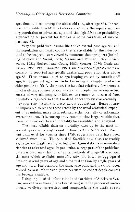
Mortality at Older Ages in Developed Countries 283

age, time, and sex among the oldest-old (i.e., after age 85). Indeed,it is remarkable how little is known considering the rapidly increas­ing population at advanced ages and the high life table probability,approaching 50 percent for females in some countries, of survivalpast age 85.

Very few published human life tables extend past age 85, andthe population and death counts that are available for the oldest-oldtend to be suspect. As reviewed by numerous demographers (includ­ing Shryock and Siegel, 1976; Mazess and Forman, 1979; Rosen­waike, 1981; Horiuchi and Coale, 1983; Spencer, 1986; Coale andKisker, 1986,1990; Kannisto, 1988), various kinds of gross errors arecommon in reported age-specific deaths and population sizes aboveage 85. These errors - such as age-heaping caused by rounding offages to the nearest age divisible by five or ten, the tendency of someolder people to falsify their age, the fact that relatively few errors inmisclassifying younger people as very old people can swamp actualcounts of very old people, or failures to remove the deceased frompopulation registers so that the dead appear to survive eternally ­may represent systematic biases across populations. Hence it maybe impossible to reduce these errors by the usual statistical expedi­ent of examining many data sets and either formally or informallyaveraging them. It is consequently essential that large, reliable databases on oldest-old human mortality be assembled and analyzed.

The most reliable data on mortality rates up to the most ad­vanced ages over a long period of time pertain to Sweden. Excel­lent data exist for Sweden since 1750; superlative data have beenarchived since 189.5. The published Swedish data that are readilyavailable are highly accurate, but even these data have some defi­ciencies at advanced ages. In particular, a large part ofthe publisheddata has been smoothed by actuarial methods after age 90 or so, andthe most widely available mortality rates are based on aggregateddata 011 several years of age and time rather than by single years ofage and time. Furthermore, the data, once published, have not beenrevised as new information (from censuses or cohort death counts)has become available.

Using unpublished information in the archives of Statistics Swe­den, one of the authors (Hans Lundstrom) is in the process of metic­ulously verifying, correcting, and computerizing the death counts

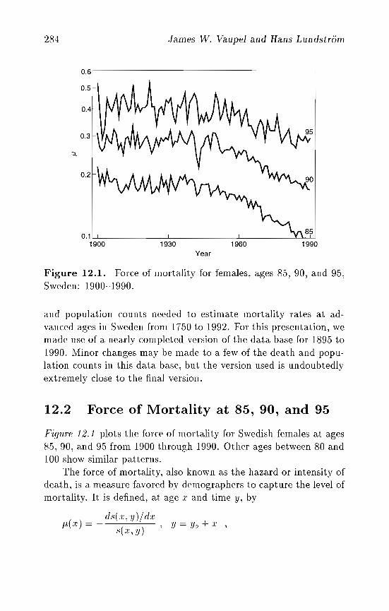
284 James W. Vaupel and Hans Lundstrom

0.6"----------------------~

199019601930

0.4

0.11 I ! \ I \

1900

0.5

0.3

::L

Year

Figure 12.1. Force of mortality for females, ages 85, 90, and 95,Sweden: 1900-1990.

and population counts needed to estimate mortality rates at ad­vanced ages in Sweden from 1750 to 1992. For this presentation, wemade use of a nearly completed version of the data base for 1895 to1990. Minor changes may be made to a few of the death and popu­lation counts in this data base, but the version used is undoubtedlyextremely close to the final version.

12.2 Force of Mortality at 85, 90, and 95

Figure 12.1 plots the force of mortality for Swedish females at ages8.5,90, and 95 from 1900 through 1990. Other ages between 80 and100 show similar patterns.

The force of mortality, also known as the hazard or intensity ofdeath, is a measure favored by demographers to capture the level ofmortality. It is defined, at age x and time y, by

j.1.(.T) = _ d8(:r, y)jd:r8(.T,y) ,y=yo+·l:,

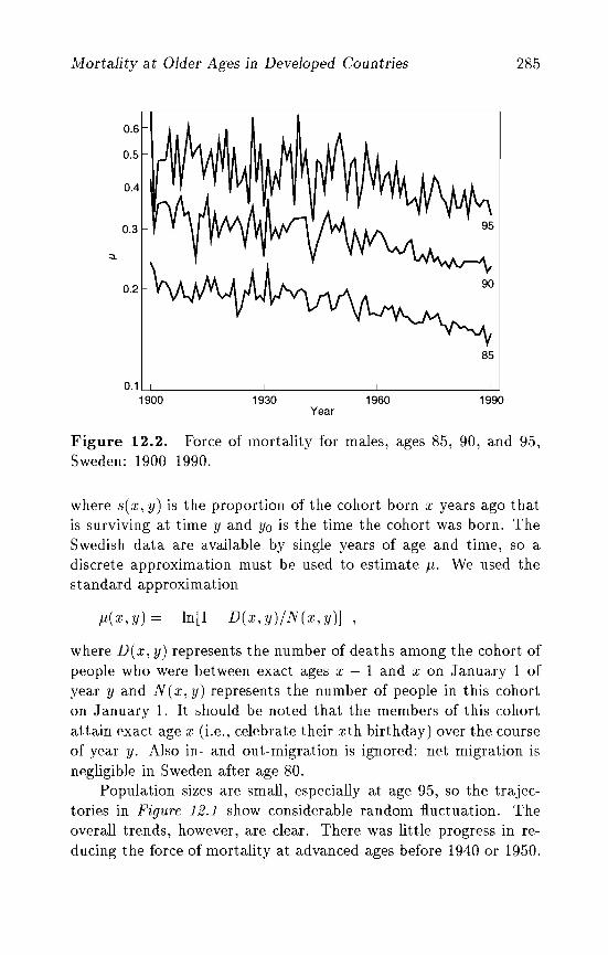
Mortality at Older Ages in Developed Countries 285

0.3

:J.

0.2

85

1990196019300.1, , , ,

1900Year

Figure 12.2. Force of mortality for males, ages 85, 90, and 95,Sweden: 1900-1990.

where s( x, y) is the proportion of the cohort born x years ago thatis surviving at time y and Yo is the time the cohort was born. TheSwedish data are available by single years of age and time, so adiscrete approximation must be used to estimate Jl. We used thestandard approximation

Jl(x,y) = -In[l- D(x,y)/N(x,y)] ,

where D(x, y) represents the number of deaths among the cohort ofpeople who were between exact ages x-I and x on January 1 ofyear y and N (x, y) represents the number of people in this cohorton January 1. It should be noted that the members of this cohortattain exact age x (i.e., celebrate their xth birthday) over the courseof year y. Also in- and out-migration is ignored: net migration isnegligible in Sweden after age 80.

Population sizes are small, especially at age 95, so the trajec­tories in Figure 12.1 show considerable random fluctuation. Theoverall trends, however, are clear. There was little progress in re­ducing the force of mortality at advanced ages before 1940 or 1950.

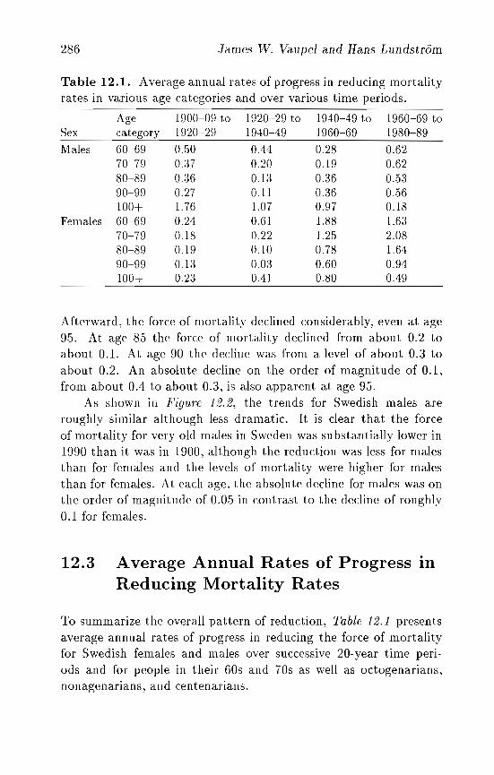
286 .Tames W. Vaupel and Hans Lundstrom

Table 12.1. Average annual rates of progress in reducing mortalityrates in various age categories and over various time periods.

Age 1900-09 to 1920-29 to 1940-49 to 1960-69 toSex category 1920-29 1940-49 1960-69 1980-89

Males 60-69 0.50 0.44 0.28 0.6270-79 0.37 0.20 0.19 0.6280-89 0.36 0.13 0.36 0.5390-99 0.27 0.11 0.36 0.56100+ 1.76 -1.07 0.97 0.18

Females 60-69 0.24 0.61 1.88 1.6370-79 0.18 0.22 1.25 2.0880-89 0.19 0.10 0.78 1.6490-99 0.13 0.03 0.60 0.94100+ 0.23 0.41 0.80 0.49

Afterward, the force of mortality declined considerably, even at age9.5. At age 85 the force of mortality declined from about 0.2 toabout 0.1. At age 90 the decline was from a level of about 0.3 toabout 0.2. An absolute decline on the order of magnitude of 0.1,from about 0.4 to about 0.3, is also apparent at age 95.

As shown in Figu're 12.2, the trends for Swedish males areroughly similar although less dramatic. It is clear that the forceof mortality for very old males in Sweden was substantially lower in1990 than it was in 1900, although the reduction was less for malesthan for females and the levels of mortality were higher for malesthan for females. At each age, the absolute decline for males was onthe order of magnitude of 0.0.5 in contrast to the decline of roughly0.1 for females.

12.3 A verage Annual Rates of Progress inReducing Mortality Rates

To summarize the overall pattern of reduction, Table 12.1 presentsaverage annual rates of progress in reducing the force of mortalityfor Swedish females and males over successive 20-year time peri­ods and for people in their 60s and 70s as well as octogenarians,nonagenarians, and centenarians.

Mortality at Older Ages in De\reloped Countries 287

For males and for females, the average level of the force of mor­tality over a decade of time and age was calculated as follows:

Yo+9 x o+9

L L N(x)p(.1:, y)Y-Yo x=xo

iL(x o, Yo) = Yo+ 9xo+9

L LN(x)Y=Yo :1'==X o

In this equation N is used to standardize the age compositionof the population. We calculated N from the population of Swedenin the 1980s:

1989

N(:r) = L N(:/:, y)y=1980

The values of J.1( x, y) were calculated as described above. If thedeath count equaled the population count, then the standard ap­proximation J.1 equals 2 was used. Occasionally, at ages greater than100, it was impossible to estimate p for some specific years becauseno one was alive at that age and year. In such cases, the J.1 termwas dropped from the numerator and a corresponding correctionwas made in the denominator. The average annual rate of progressin reducing the force of mortality was then calculated using

p( x 0' Yo) = _ { [P( x 0, Yo +20)] 0.0.5 _ I}p(:z:o,Yo)

Table 12.1 indicates that progress has been made in Sweden inreducing the force of mortality at all ages after 60 for both malesand females. Estimated rates of progress fluctuate erratically forcentenarian males, probably because there are so few observationsin this category, but even so the general trend is toward a reductionin mortality rates. For females and for younger age categories, thepicture is dear: mortality rates among the elderly are decliningin Sweden and at a faster pace in recent decades than in the firstdecades of the century.

For males in the most recent time period, the rate of progress isroughly the same - about half a percent per year - for men in their60s, 70s, 80s, and 90s. For females in the most recent time period,the rate of progress is about 2 percent for women in their 70s and

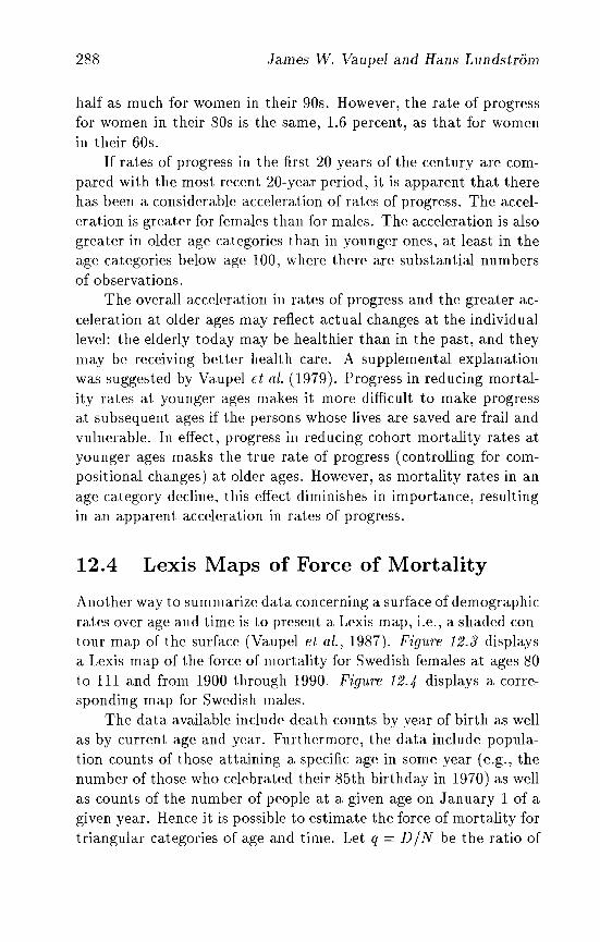
288 James W. Vaupel and Hans Lundstrom

half as much for women in their 90s. However, the rate of progressfor women in their 80s is the same, 1.6 percent, as that for womenin their 60s.

If rates of progress in the first 20 years of the century are com­pared with the most recent 20-year period, it is apparent that therehas been a considerable acceleration of rates of progress. The accel­eration is greater for females than for males. The acceleration is alsogreater in older age categories than in younger ones, at least in theage categories below age 100, where there are substantial numbersof observations.

The overall acceleration in rates of progress and the greater ac­celeration at older ages may reflect actual changes at the individuallevel: the elderly today may be healthier than in the past, and theymay be receiving better health care. A supplemental explanationwas suggested by Vaupel et at. (1979). Progress in reducing mortal­ity rates at younger ages makes it more difficult to make progressat subsequent ages if the persons whose lives are saved are frail andvulnerable. In effect, progress in reducing cohort mortality rates atyounger ages masks the true rate of progress (controlling for com­positional changes) at older ages. However, as mortality rates in anage category decline, this effect diminishes in importance, resultingin an apparent acceleration in rates of progress.

12.4 Lexis Maps of Force of Mortality

Another way to summarize data concerning a surface of demographicrates over age and time is to present a Lexis map, i.e., a shaded con­tour map of the surface (Vaupel et aL, 1987). Figure 12.3 displaysa Lexis map of the force of mortality for Swedish females at ages 80to 111 and from 1900 through 1990. Figure 12.4 displays a corre­sponding map for Swedish males.

The data available include death counts by year of birth as wellas by current age and year. Furthermore, the data include popula­tion counts of those attaining a specific age in some year (e.g., thenumber of those who celebrated their 85th birthday in 1970) as wellas counts of the number of people at a given age on January 1 of agiven year. Hence it is possible to estimate the force of mortality fortriangular categories of age and time. Let q = DIN be the ratio of

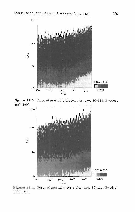
Mortality at Older Ages in Developed Countries 289

111

0.250

0.1250.500

198080 r ""'I" r '" .mm r I

1900 1920 1940 1960Year

90

100

l!lOl

<{

Figure 12.3. Force of mortality for females, ages 80-111. Sweden:1900-1990.

108

100

l!lOl

<{

90

0.2501980196019401920

80 'Wi'" I,.",,,, trlWf' '1 "'lff' !II , JILl---"...-.....__•

1900

Year

Figure 12.4. Force of mortality for males, ages 80-111, Sweden:1900-1990.

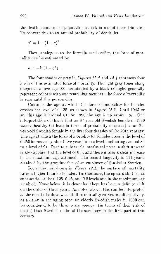
290 James W. Vaupel and Hans Lundstrom

the death count to the population at risk in one of these triangles.To convert this to an annual probability of death, let

q*=I-(I-q)2.

Then, analogous to the formula used earlier, the force of mor­tality can be estimated by

p = -In( 1 - q*) .

The four shades of gray in Figures 12.3 and 12.4 represent fourlevels of this estimated force of mortality. The light gray tones alongdiagonals above age 100, terminated by a black triangle, generallyrepresent cohorts with one remaining member: the force of mortalityis zero until this person dies.

Consider the age at which the force of mortality for femalescrosses the level of 0.125, as shown in Figure 12.3. Until 1945 orso, this age is around 81; by 1990 the age is up around 87. Oneinterpretation of this is that an 87-year-old Swedish female in 1990was as healthy (at least in terms of probability of death) as an 81­year-old Swedish female in the first four decades of the 20th century.The age at which the force of mortality for females crosses the level of0.2050 increases by about five years from a level fluctuating around 89to a level of 94. Despite substantial statistical noise, a shift upwardis also apparent at the level of 0.05, and there is also a clear increasein the maximum age attained. The record longevity is 111 years,attained by the grandmother of an employee of Statistics Sweden.

For males, as shown in Figure 12.4, the surface of mortalityrates is higher than for fenules. Furthermore, the upward shift is lesssubstantial at the 0.1205, 0.205, and 0.05 levels and in the maximum ageattained. Nonetheless, it is clear that there has been a definite shifton the order of three years. As noted above, this can be interpretedas the result of a downward shift in mortality curves or, alternatively,as a delay in the aging process: elderly Swedish males in 1990 canbe considered to be three years younger (in terms of their risk ofdeath) than Swedish males of the same age in the first part of thiscentury.

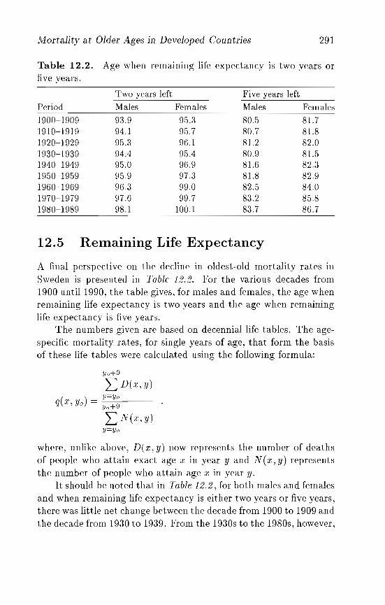
Mortality at Older Ages in Developed Countries 291

Table 12.2. Age when remaining life expectancy is two years orfive years.

Two years left Five years leftPeriod Males Females Males Females1900-1909 93.9 9.5.3 80.5 81.71910-1919 94.1 95.7 80.7 81.81920-1929 95.3 96.1 81.2 82.01930-1939 94.4 95.4 80.9 81.51940-1949 95.0 96.9 81.6 82.31950-1959 95.9 97.3 81.8 82.91960-1969 96.3 99.0 82.5 84.01970-1979 97.6 99.7 83.2 85.81980-1989 98.1 100.1 83.7 86.7

12.5 Remaining Life Expectancy

A final perspective on the decline in oldest-old mortality rates inSweden is presented in Table 12.2. For the various decades from1900 until 1990, the table gives, for males and females, the age whenremaining life expectancy is two years and the age when remaininglife expectancy is five years.

The numbers given are based on decennial life tables. The age­specific mortality rates, for single years of age, that form the basisof these life tables were calculated using the following formula:

Yo+9

L D(:r, y)y=Yo

q(x,yo) = yo+9

L N(x, y)y=Yo

where, unlike above, D(x, y) now represents the number of deathsof people who attain exact age :r in year y and N (x, y) representsthe number of people who attain age x in year y.

It should be noted that in Table 12.2, for both males and femalesand when remaining life expectancy is either two years or five years,there was little net change between the decade from 1900 to 1909 andthe decade from 1930 to 1939. From the 1930s to the 1980s, however,

292 Ja.mes ",T. Vaupel and Hans Lundstrom

the shifts were substantial. For males, the age when two years oflife expectancy are left increased by almost four years, from 94.4 to98.1. For females, the corresponding shift was close to five years,from 95.4 to 100.1. The age at which remaining life expectancy isfive years increased for males by almost three years, from 80.9 to83.7. For females, the increase was five years, from 81.5 to 86.7.

As suggested earlier, one interpretation of these shifts is thatthe process of aging has been slowed or delayed in Sweden such thatelderly Swedish men are effectively three or four years younger thanthey used to be, and elderly Swedish females are five years younger.Caution is required because these figures are based entirely on mor­tality statistics, with no information about morbidity or disability.Nonetheless, treated judiciously, this perspective suggests that cer­tainly mortality, and perhaps health more generally, is plastic evenat the most advanced ages. It has been possible, at least ill Sweden,to lower the force of mortality and to significantly postpone deatheven among the oldest-old.

12.6 Discussion

Swedish life expectancy has been among the very longest in theworld for many decades. If progress can be made ill Sweden in low­ering mortality rates at advanced ages, then the contention thatoldest-old mortality rates cannot be significantly reduced seemsquestionable. Using highly reliable data, we presented four perspec­tives on mortality changes in Sweden since 1900 among the elderly.As shown in Figures 12.1 and 12.2, the force of mortality at ages85,90, and 95 has substantially declined, especially since 1945, andmore for females than for males. As shown in Table 12.1, rates ofprogress in reducing mortality rates among the elderly have acceler­ated over the course of the century, and from the 1960s to the 1980sran at an average annual rate of 1 to 2 percent for females and halfa percent for males. As shown in Figures 12.3 and 12.4, the age atwhich the force of mortality attains the levels of 0.125,0.25, and 0.5has shifted upward substantially since 1945, by about five years forfemales and three years for males. Finally, as shown in Table 12.2,the age when remaining life expectancy reaches two years or fiveyears has also shifted upward, by about five years for females and

Mortality at Older Ages in Developed Countries 293

three or four years for males. These four perspectives are consis­tent with each other. They indicate that the theory that oldest-oldmortality rates cannot be significantly reduced is incorrect.

Other strands of evidence, reviewed by Manton et at. (1991),point in the same direction. Most of this evidence pertains to smallspecial populations followed for short periods of time or is based onthe results of sophisticated mathematical modeling. The evidencefrom Sweden is highly reliable, pertains to a sizable national popu­lation followed since 1900, and is so straightforward that it does nothave to be filtered through a statistical model.

The available evidence, taken together, suggests that if histori­cal rates of progress in reducing mortality rates continue to prevailin the future, today's newborns can expect to live about 90 years onaverage. If, as knowledge of health and biomedical research devel­ops, progress accelerates so that age-specific mortality rates comedown at an a.verage rate of about 2 percent per year, then the typi­cal newborn in developed countries will live to celebrate his or her100th birthday.

If our children survive to become centenarians, what will theirhealth be like during their extra life span? Will the added years beactive, healthy years or years of decrepitude, disability, and misery?The answer to this question is central to forecasting the impact ofpopulation aging on health and social needs and costs, on retirementdecisions and policies, and on other questions in the economics ofaging, but very little is currently known about what the answermight be.

12.7 Conclusion

Let us return now to the original question: What is the future ofmortality in developed countries? It has been argued that the an­swer to this question hinges on a narrower question: What is thefuture of mortality at older ages? This question in turn hinges onthe question: Is it possible to substantially reduce death rates afterage 80? The Swedish data, together with other data reviewed byManton et at. (1991), indica.te that it is possible. However, whetherprogress in reducing mortality rates will continue at historical levelsor even accelerate is, of course, an open question.

294 James W. Vaupel and Hans Lundstrom

Biomedical research may fail to continue to produce the ad­vances needed to reduce mortaIity rates. Social and economic con­ditions may become unfavorable to further improvements. Environ­mental conditions may substantially deteriorate. Nuclear war maykill millions or even billions. New diseases, like AIDS, may decimatepopulations.

On the other hand, the acceleration of mortality improvement atolder ages may continue, so that 1ll0rtaIity rates may fall not at 1 or 2percent per year but at :3 or 4 percent per year over the course of the21st century. Biological, medical, and gerontological breakthroughscould lead to considerable extensions of the human life span. Thelife sciences may be poised at roughly the point the physical scienceswere at a century ago, and biological innovations comparable toelectricity, automobiles, television, rockets, and computers may beforthcoming. Fundamental advances could occur over the next fewdecades in genetic engineering, in the prevention and treatment ofsuch diseases as arteriosclerosis, cancer, or diabetes, and perhapseven in understanding and controlling human aging itself.

The future is not just uncertain: it is surprisingly uncertain.As Ascher (1978), Keyfitz (1981), Stoto (1983), and others reviewedby Ahlburg and Land (1992) have demonstrated, the actual courseof demographic events often leads to outcomes beyond the mostextreme projections. Consequently, forecasts ought to include widebands of uncertainty that spread outward at an accelerating paceinto the more and more distant future.

Recent research by Lee (1992), Lee and Carter (1992), and Tul­japurkar (1992) provides a good starting point. Using time-seriesmethods, Lee and Carter project life expectancy in the UnitedStates, with confidence bands. Their forecast is that life expectancyat birth in the United States in 2065 will be around 86 years witha 9.5 percent confidence interval of plus or minus 4 or 5 years. Thisprojection, however, is based entirely on analysis of historical trendsof US data. The future of developed countries may not be like thepast of the United States: that is an important source of addi­tional uncertainty. The results presented above for Sweden plus theresearch summarized by Manton et aZ. (1991) suggest that futureimprovements in death rates at older ages may be more rapid thanin the past.

Mortality at Older A.ges ill Developed Countries 295

Taking those two considerations into account and using meth­ods of subjective probability assessment (as explained, e.g., in Behnand Vaupel, 1982), a more judicious guesstimate might be that lifeexpectancy in the typical developed country in 2065 is not 86 plusor minus 4 or 5 but perhaps the following. There is a 50/50 chancethat life expectancy will be above or below 92. There is a 50 per­cent chance that life expectancy will be between 85 and 100 and a50 percent chance it will be outside this range. There is a 5 percentchance that life expectancy will be below its current level of about75 and a 5 percent chance that it will exceed the current recordlongevity of 120. This is speculation, as are all predictions, but it isinformed speculation that takes into account our vast ignorance ofwhat breakthroughs or catastrophes the future might bring.

Part V

The Future ofIntercontinental

Migration

Chapter 13 gives the most complete account of intercontinental mi­gration that can be produced with existing data. Even withoutconsidering illegal migration, data on official or legal migration arefragmentary. In a discussion on the forces that will induce futuremigration, Chapter 14 shows that the traditional pull and push fac­tors of economic disparities are often submerged by the impact oflegal and logistical restrictions on international migration. Short­term political changes as well as refugee movements spurred by waror famine can significantly affect migration level. Given the expe­rience of the past, international migration can be assumed to showgreat volatility in the future.

How can one derive from this information assumptions aboutthe future? For our projections it seems reasonable to assume thatin the high-migration case the future annual level assumed over thewhole period will roughly equal the maximum that has been ob­served in the past. There is little basis for making any assumptionson possible future mass migration induced by global environmen­tal change. Past environmental disasters, however, show that suchmigration mostly occurs within regions.

At the low extreme a convenient assumption is that there willbe zero net-migration, namely, in-migrants will equal out-migrants.Such a scenario reflects the possibility of xenophobic policies. Thecentral scenario then gives the average of these two extreme scenar­ios; it is also considered the most likely case.

Chapter 13

Migration to and fromDeveloping Regions: AReview of Past Trends

Rania Zlotnik

At least since the "discovery" of the Americas in 1492, interconti­nental migration has been a key factor influencing the demographicevolution of the developing world. During the first decades of thiscentury, the major international flows originated in Europe and weredirected mostly to the "New World," that is, to the overseas coun­tries of permanent resettlement and certain Latin American coun­tries. Despite the dampening effects of the two world wars and theDepression, major intercontinental flows continued to be dominatedby Europeans until the early 1960s. Since then, migration from de­veloping to developed countries has been growing and importantinterregional flows within the developing world have also gainedprominence. This chapter provides a comprehensive view of themain migration flows either originating in or directed toward sevendeveloping regions, namely, sub-Saharan Africa, North Africa andWest Asia, South Asia, China, the rest of developing Asia (calledEast and Southeast Asia), Central America and the Caribbean, andSouth America.[1]

The task of quantifying migration to and from the regions isfar from straightforward. A variety of data sources must be used to

The views and opllllOns expressed in this paper are those of the author and donot necessarily reflect those of the United Nations.

299

300 Hania Zlotnik

piece together the facets of the phenomenon. The lack of compara­bility between data sources severely constrains the types of estimatesthat can be derived, so that in most cases only rough indications ofthe magnitude of flows can be presented. On the other hand, theuse of major regions as units of analysis precludes the need to con­sider every flow between developing countries. Most flows occurringbetween neighboring countries, which are often the main sources ofmigrants in specific countries, are excluded from the analysis.

Given the state of international migration statistics, more infor­mation is available on migration to and from developed regions thanon that between developing regions. Therefore, most of the quanti­tative analysis presented in this chapter focuses on statistics derivedfrom developed countries. Problems arising from lack of quantitativeinformation on a given flow are pointed out as appropriate. Beforeproceeding with the presentation of migration estimates from a com­parative perspective, an overview of the main data sources used andtheir limitations is provided.

13.1 The Statistics Used

13.1.1 The universe covered

There are basically two different sources of information on interna­tional migration: those producing data on the stock of migrants ata given time and those producing statistics on the flow of immi­grants or emigrants over a given period. Clearly, the latter are themost useful in tracking the evolution of migration through time andthus providing the basis to project it. However, whereas adequateestimates of migrant stocks can be obtained from censuses thatmay be carried out at relatively lengthy intervals, the availabilityof flow statistics depends on the existence of relatively sophisticateddata-collection systems that must function continuously. Only a fewcountries have those systems in place, and both their existence andadequacy are highly correlated with whether a country considers it­self to be a recipient of immigrants or a sender of emigrants. Indeed,most countries that gather information on migration on a continuousbasis do so for administrative purposes and, consequently, tend toidentify migrants on the basis of administrative or regulatory prin­ciples rather than on demographic ones (Zlotnik, 1987). The USA,

Migration to and from Developing Regions 301

for instance, gathers information on immigrants defined as aliensgranted the right of permanent residence. Since that right may begranted to aliens who are already present in the country under atemporary permit, the number of immigrants admitted annually bythe USA is not equivalent to the number of new arrivals of aliens. Incontrast, the statistics gathered on aliens granted only temporarypermission to stay in the USA refer to their entries into the country.Consequently, to the extent that some such persons enter the USAseveral times during a year, the statistics available overestimate thenumber of persons involved.

Aside from data on permanent immigration to the UnitedStates, this chapter makes use of those available for the other coun­tries of permanent resettlement, namely, Australia, Canada, andNew Zealand. Information on immigration to Israel is also used,together with those available for European countries having flowstatistics, namely, Belgium, Germany (the data refer only to theformer West Germany), the Netherlands, Sweden, and the UnitedKingdom. Selected data on immigration to France are also used.

The data for Canada resemble those available for the UnitedStates, because they reflect only the number of foreigners who aregranted the right of permanent residence. Australian and NewZealand statistics are gathered at the time of entry and conformbetter to demographic concepts. The Australian data in this chap­ter refer to the arrivals of persons admitted as permanent settlersand to their permanent departures. For New Zealand, the data alsoreflect the number of arrivals of permanent immigrants and their de­partures when they intend to stay away permanently. In all cases,the data are classified by place of birth. No emigration data areavailable for either Canada or the USA.

In the case of Israel, the data used represent the number of immi­grants and the so-called potential immigrants entering the countryand classified by place of birth. Although some statistics on depar­tures are gathered by the Israeli government, they are not tabulatedby place of birth, thus precluding the estimation of net migrationby region of origin.

In France, 1'Office National d'Immigration (0NI), which becamein 1988 l'Office des Migrations Internationales (OMI), has been incharge of gathering statistics on the number of migrant workers

302 Hania Zlotnik

and their families being "introdueed" into the country. However,since the data are gathered through control procedures from whichmany migrants are exempt by law, they have generally been in­complete. In particular, after Algeria became independent in 1962,Algerians have been subject to a special immigration regime thathas precluded a statistical accounting of their inflow (Tribalat andMunoz-Perez, 1989). Given that France is a major receiving coun­try of citizens from the Maghreb countries (Algeria, Morocco, andTunisia) and Turkey, statistics on both workers and family membersfrom those countries are used as indicative of migration from NorthAfrica and West Asia to France. The data regarding Algerians havebeen derived from estimates presented by Benamrane (1983) andTapinos (197.5). It must be noted that OMI statistics include bothnew arrivals and persons regularizing their status after being presentin France for a time.

Several European countries gathering information on migrationflows do so as part of the normal operation of their population regis­ters (Belgium, Germany, the Netherlands, and Sweden). Therefore,the definition of immigrant and emigrant is derived in each casefrom the rules establishing who can be added to or deleted from theregister. In the Netherlands a person is removed from the registerwhen he or she intends to stay abroad for at least a year. However,Dutch citizens who have been abroad are inscribed in the registerwhen they intend to sta.y in the Netherlands for at least one monthand aliens are inscribed if they intend to stay for at least six months(Verhoef, 1986). Statistics on immigrants and emigrants are appar­ently adjusted to take into account only persons who intend to stayin the country or out of it for a year or more (Schoorl and Voets,1990).

In Belgium, an emigrant is someone coming from abroad andintending to establish permanent residence in the country, whereasan emigrant is someone giving up permanent residence (UN, 1978).Similarly, in Germany, an immigrant is a person coming into thecountry to establish residence and an emigrant is a person departingand intending to give up residence in the country (UN, 1978). Inboth cases, "residence" is a legal concept that remains ill-definedsince it is not clear under what circumstances foreigners are allowedto establish residence.

Migra.tion to and hom Developing R.egions 303

In Sweden, incoming persons must register if they intend tostay in the country for at least a year and those leaving must de­register if they intend to stay abroad for a year or more. Differentdefinitions, however, are applied to immigrants and emigrants fromNordic countries in order to harmonize registration practices amongthem (Nilsson, 1990).

In the United Kingdom. information on immigration and emi­gration is gathered via the International Passenger Survey (IPS), asurvey of travelers entering or leaving the United Kingdom by theprincipal air and sea routes. The IPS has been operational since1964 and, although it gathers information on both British and for­eign travelers, persons moving between the United Kingdom andIreland are beyond its scope (Haskey et at., 1989). The IPS is basedon definitions of immigrant and emigrant consistent with UnitedNations standards, using an intended stay of over a year and anintended absence of over a year to identify each group, respectively.

It must be noted that both the systems based on population reg­isters and the British IPS gather information on both immigrationand emigration. Furthermore. similar coverage is extended to citi­zens and aliens. Consequently, there are major differences betweenthe data produced by such systems and those yielded by the admin­istrative records used by Ca.nada, France, or the USA. Aside fromthe fact that the latter records lack information on emigration, bothof nationals and foreigners. their statistics are only rough indicatorsof true population flows. Indeed. in the USA, a major problem of in­terpretation has arisen lately because normal immigration statisticshave been artificially swollen by t he regularization of undocumentedaliens carried out under the provisions of the Immigration Reformand Control Act (!RCA) of 1986.

According to the IRCA, two groups of undocumented alienscould legalize their status ( US Immigration and Naturalization Ser­vice, 1991). The first and larger group consisted of persons whocould prove that they had been present in the USA since before1 January 1982 and who began regularizing their status in 1989.The second group consisted of "special agricultural workers" whohad to prove that they had worked in agriculture at least 90 daysduring each of the three years preceding 1 May 1986 and who be­came eligible to start adjusting their status to permanent resident

304 Hania Zlotnik

on 1 December 1989. Therefore, although these two groups beganappearing in the immigration statistics only in 1989, the first entryof the former group must have taken place before 1982 and that ofthe latter group before 1984. Since other evidence suggests that il­legal immigration to the United States grew significantly during the1970s, the data presented here have been estimated assuming thatthose persons regularizing their status during 1989-1992 as part ofthe first group entered during 1972-1981. Their entries over that pe­riod were distributed according to a linearly increasing trend. Thatassumption is validated, to a certain extent, by the terms of the reg­ularization drive itself. With regard to special agricultural workers,however, assumptions about their entry and stay in the USA areless straightforward, particularly because many fraudulent applica­tions were reportedly filed. Thus the group of migrants regularizedunder the special agricultural worker program is likely to includean important number of undocumented migrants who arrived in theUSA after the 1 January 1982 cutoff date and even up to the time atwhich the IRCA was passed. It was decided, therefore, to distributetheir numbers uniformly over the 1982-1986 period.

13.1.2 Problerns of data classification

Regarding the criteria used to identify region of origin, data clas­sified by country of last or next residence would appear to be themost useful for projection purposes, since they allow straightfor­ward demographic accounting. However, aside from the misreport­ing problems arising from the different possible interpretations ofthe term "residence," data thus classified are often not available.Consequently, consideration of data classified by place of birth orcitizenship becomes mandatory, though their use involves the tacitassumption that persons born in a given country who leave anotherare intending to return to their country of birth or that citizens of acountry who leave another are intending to return to their countryof citizenship (and the equivalent in terms of arrivals).

The data used in this paper as indicative of migration flowsare classified by place of birth for Australia, Canada, Israel, NewZealand, and the USA; by citizenship for Belgium, France, and theNetherlands; and by country of last and next residence for Germany,

Migration to and from Developing Regions 30.5

Sweden, and the United Kingdom. However, citizenship being a cri­terion so intrinsically linked to the international migration process,it often colors the manner in which other criteria are used. Thus, thedata for Australia, Canada, Israel, and the USA include only foreign­ers. In addition, German data distinguish between foreigners andGerman citizens, thus permitting the consideration of only foreign­ers as originating in or leaving for developing regions. Similarly, theUnited Kingdom publishes data that are classified first by citizenship(Commonwealth citizens vs. other) and then by place of residence.Only the data thus classified distinguish between Commonwealthcitizens originating in Central American and Caribbean countriesand non-Commonwealth citizens originating mostly in South Amer­ica. British data classified only by place of last or next residencemake no distinction between the two regions of the Americas. Hence,the two series have been used, as appropriate, in presenting the databy regions (see Table 13.1).

Although the use of data classified by citizenship has been keptto a minimum, the series for the Netherlands is based on that cri­terion; consequently Dutch citizens from overseas Dutch territoriesmigrating to the Netherlands cannot be identified separately. In par­ticular, the relatively large flow of Dutch Surinamese who migratedto the Netherlands just before and after Surinam's independence in197.5 shows up as an increased inflow of Dutch citizens during the1970s. To take this group into account in interregional migration, anannual net gain of 4,000 persons during 1970-1974 and 6,000 during197.5-1979 has been added to the estimated number of migrants tothe Netherlands originating in South America (the net migrationgain of Dutch citizens during the 1970s was roughly of that mag­nitude, whereas during earlier or later periods net gains of Dutchcitizens were negative or virtually nil).

A further caveat relates to the actual classification by countryof origin used by the various receiving countries in publishing flowstatistics. The practice of listing separately only the countries oforigin of sizable numbers of migrants and grouping the rest into asingle figure often precludes an adequate calculation of regional indi­cators. Problems encountered fairly frequently include the practiceofreporting together all persons originating in the People's Republicof China and in Taiwan; the separate listing of only a few countries in

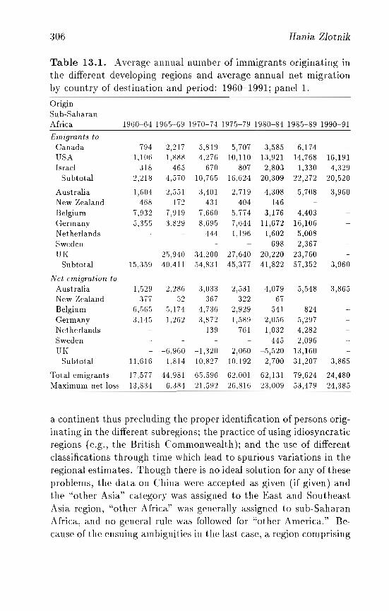
306 Hania Zlotnik

Table 13.l. Average annual number of immigrants originating inthe different developing regions and average annual net migrationby country of destination and period: 1960-1991; panell.

OriginSub-SaharanAfrica 1960-64 1965-69 1970-74 1975-79 1980-84 1985-89 1990-91

Emigmnts to

Canada 794 2,217 5,819 5,707 3,585 6,174USA 1,106 1,888 4,276 10,110 13,921 14,768 16,191Israel 318 465 670 807 2,803 1,330 4,329

Subtotal 2,218 4,570 10,765 16,624 20,309 22,272 20,520

Australia 1,604 2 1551 3,401 2,719 4,308 5,708 3,960New Zealand 468 I -'j 4:31 404 146,-Belgium 7,932 7,919 7.660 5,774 3,176 4,403Germany 5,:355 3,829 8.695 7,644 11 ,672 16,106Netherlands 444 1,196 1,602 5,008Sweden 698 2,367UK 2!5,940 :34.200 27,640 20,220 23,760

Subtotal 15,359 40.411 54,831 45,377 41,822 57,352 3,960

Net emigmtioll to

Australia 1,529 2,286 3,033 2,531 4,079 5,548 3,865New Zealand :377 r::.) 367 322 670_

Belgium 6,565 5,174 4,736 2,929 541 824Germany 3,145 1,262 3,872 1,589 2,056 5,297Netherlands 139 761 1,032 4,282Sweden 445 2,096UK - -6,960 -1,320 2,060 -5,520 13,160

Subtotal 11,616 1,814 10.827 10,192 2,700 31,207 3,865

Total emigrants 17.577 44,981 65.596 62,001 62,131 79,624 24,480Maximum net loss 13,834 6,384 21,592 26,816 23,009 53,479 24,385

a continent thus precluding the proper identification of persons orig­inating in the different subregions; the practice of using idiosyncraticregions (e.g., the British Commonwealth); and the use of differentclassifications through time which lead to spurious variations in theregional estimates. Though there is no ideal solution for any of theseproblems, the data 011 China were accepted as given (if given) andthe "other Asia" category was assigned to the East and SoutheastAsia region, "other Africa." wa.s generally assigned to sub-SaharanAfrica, and no general rule was followed for "other America." Be­cause of the ensuing ambiguities in the last case, a region comprising

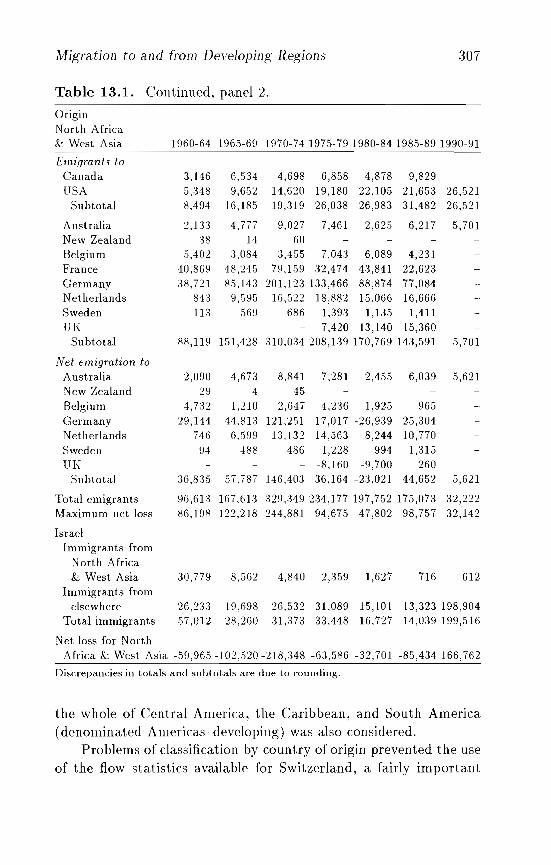
Migration to and from Developing Regions

Table 13.1. Continued, panel 2.

307

OriginNorth Africa& West Asia 1960-64 1965-69 1970-74 1975-79 1980-84 1985-89 1990-91

Emigrants toCanada 3,146 6,534 4,698 6,858 4,878 9,829USA 5,348 9,652 14,620 19,180 22,105 21,653 26,521

Subtotal 8,494 16,185 19,319 26,038 26,983 31,482 26,521

Australia 2,133 4,777 9,027 7,461 2,625 6,217 5,701New Zealand 38 J4 60Belgium 5,402 3,084 3,45.5 7,043 6,089 4,231France 40,869 48,24.5 79,1.59 32,474 43,841 22,623Germany 38,721 85.143 201,123133,466 88,874 77,084Netherlands 84:J 9,595 16,522 18,882 15,066 16,666Sweden 113 569 686 1,393 1,135 1,411UK 7,420 13,140 15,360

Subtotal 88,119 1.51,428 310,034208,139170,769 143,591 5,701

Net emigration toAustralia 2,090 4,673 8,841 7,281 2,455 6,039 5,621New Zealand 29 4 45Belgium 4,732 1,210 2,647 4,236 1,925 965Germany 29,144 44,813 121,2.51 17,017 -26,939 25,304Netherlands 746 6,599 13,132 14,563 8,244 10,770Sweden 94 488 486 1,228 994 1,315UK - -8,160 -9,700 260

Subtotal %,8:35 57,787 146,403 36,164 -23,021 44,652 5,621

Total emigrants 96,613 167,613 329,349234,177197,752 175,073 32,222Maximum net loss 86,198 122,218 244,881 94,675 47,802 98,757 32,142

Israellmmigrants from

North Africa& West Asia 30,779 8,562 4,840 2,359 1,627 716 612

Immigrants fromelsewhere 26,233 19,698 26.532 31,089 1.5,101 13,323 198,904

Total immigrants .57,012 28,260 31,373 33,448 16,727 14,039 199,516

Net loss for NorthAfrica & West Asia -59,965 -102,520 -218,348 -63,586 -32,701 -85,434 166,762

Discrepancies in totals and subtotals are due to rounding.

the whole of Central America, the Caribbean, and South America(denominated Americas-developing) was also considered.

Problems of classification by country of origin prevented the useof the flow statistics available for Switzerland, a fairly important

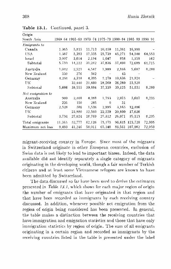
308 Rania Zlotnik

Table 13.1. Continued, panel 3.

OriginSouth Asia 1960-64 1965-69 1970-74 1975-79 1980-84 1985-89 1990-9]

Emigrants toCanada 1,365 5,815 11,713 10,450 11,361 16,990USA 1,387 5,393 17,335 25,739 45,271 54,540 64,553Israel 3,007 3,014 2,194 1,647 858 1,158 162

Subtotal 5,759 14,222 31,242 37,836 57,490 72,689 64,715

Australia 1,042 2,521 4,547 1,909 2,166 5,687 8,280New Zealand 330 276 342 43Germany 4,234 3,318 4,395 7,170 10,636 21,824UK - 32,440 21,600 28,260 26,280 23,520

Subtotal 5,606 38,555 30,884 37,339 39,125 51,031 8,280

Net emigration toAustralia 980 2,408 4,388 1,793 2,075 5,607 8,235New Zealand 226 150 285 0 31Germany 2,528 586 1,536 2,999 3,165 12,486UK - 23,880 12,560 22,520 20,800 17,020

Subtotal 3,734 27,024 18,769 27,312 26,071 35,113 8,235

Total emigrants 11,365 52,777 62,126 75,175 96,615 123,720 72,995Maximum net loss 9,493 41,246 50,011 65,148 83,561 107,802 72,950

migrant-receiving country in Europe. Since most of the migrantsin Switzerland originate in other European countries, exclusion ofSwiss data is not likely to lead to important biases. Indeed, the dataavailable did not identify separately a single category of migrantsoriginating in the developing world, though a fair number of Turkishcitizens and at least some Vietnamese refugees are known to havebeen admitted by Switzerland.

The data discussed so far have been used to derive the estimatespresented in Table 13.1, which shows for each major region of originthe number of emigrants that have originated in that region andthat have been recorded as immigrants by each receiving countrydiscussed. In addition, whenever possible net emigration from theregion of origin being considered has been presented. In general,the table makes a distinction between the receiving countries thathave immigration and emigration statistics and those that have onlyimmigration statistics by region of origin. The sum of all emigrantsoriginating in a certain region and recorded as immigrants by thereceiving countries listed in the table is presented under the label

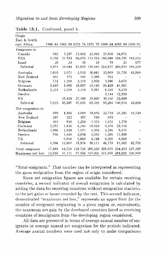
Migration to and from Developing Regions 309

Table 13.1. Continued, panel 4.

OriginEast & South-east Africa 1960-64 1965-69 1970-74 1975-79 1980-84 1985-89 1990-91

Emigmnts toCanada 692 7,237 15,602 21,064 27,850 34,871USA 9,156 21,783 66,070 114,762 186,948 168,707 183,552Israel 26 23 20 19 79 21 677

Subtotal 9,874 29,043 81,692 135,845 214,877 203,599 184,229

Australia 1,010 2,071 3,910 10,661 23,059 31,759 43,069New Zealand 391 472 496 1,080 925Belgium 752 1,298 2,219 2,932 3,206 3,675Germany 3,449 3,988 10,097 19,140 26,439 41,502Netherlands 2,213 2,258 3,214 5,981 6,329 8,679Sweden 3,144 12,559UK - 25,420 27,100 29,800 30,100 32,680

Subtotal 7,815 35,507 47,036 69,594 93,202 130,854 43,069

Net emigmtion toAustralia 888 1,880 3,689 10,450 22,710 31,285 42,739New Zealand 287 222 357 798 679Belgium 464 849 1,250 1,552 1,655 1,778Germany 2,257 1,836 6,243 10,932 9,378 22,776Netherlands 1,886 1,830 1,971 4,298 4,186 6,475Sweden -796 -1,409 -2,634 -2,059 1,365 11,808UK 6,860 5,000 4,140 6,200 6,960

Subtotal 4,986 12,068 15,876 30,111 46,173 81,082 42,739

Total emigrants 17,689 64.550 128,728 205,439 308,079 334,453 227,298Maximum net loss 14,860 41,111 97,568 165,956 261,050 284,681 226,968

"Total emigrants." That number can be interpreted as representingthe gross emigration from the region of origin considered.

Since net emigration figures are available for certain receivingcountries, a second indicator of overall emigration is calculated byadding the data for receiving countries without emigration statisticsto the net gains or losses recorded by the rest. This second indicator,denominated "maximum net loss," represents an upper limit for thenumber of emigrants originating in a given region or, equivalently,the maximum net gain by the developed countries listed as receivingcountries of immigrants from the developing region considered.

All data are presented in terms of average annual number of em­igrants or average annual net emigration for the periods indicated.Average annual numbers were used not only to make comparisons

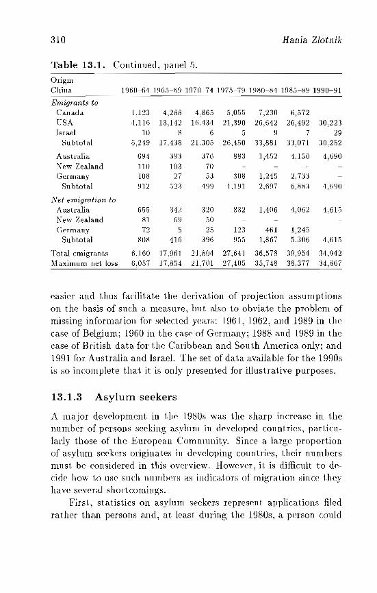
310 Hania Zlotnik

Table 13.1. Continued, panel 5.

OriginChina 1960-64 1965-69 1970-74 1975-79 1980-84 1985-89 1990-91

Emigmnts toCanada 1,123 4,288 4,865 5,055 7,230 6,572USA 4,116 13,142 16.434 21,390 26,642 26,492 30,223Israel 10 8 6 5 9 7 29

Subtotal 5,249 17,438 21,305 26,450 33,881 33,071 30,252

Australia 694 393 376 883 1,452 4,150 4,690New Zealand 110 103 70Germany 108 27 53 308 1,245 2,733

Subtotal 912 523 499 1,191 2,697 6,883 4,690

Net emigmtion toAustralia 65,) 342 320 832 1,406 4,062 4,615New Zealand 81 69 50Germany 72 5 25 123 461 1,245

Subtotal 808 416 396 955 1,867 5,306 4,615

Total emigrants 6,160 17,961 21,804 27,641 36,578 39,954 34,942Maximum net loss 6,057 17,854 21,701 27,405 35,748 38,377 34,867

easier and thus facilitate the derivation of projection assumptionson the basis of such a measure, but also to obviate the problem ofmissing information for selected years: 1961,1962, and 1989 in thecase of Belgium; 1960 in the case of Germany; 1988 and 1989 in thecase of British data for the Caribbean and South America only; and1991 for Australia and Israel. The set of data available for the 1990sis so incomplete that it is only presented for illustrative purposes.

13.1.3 Asylum seekers

A major development in the 1980s was the sharp increase in thenumber of persons seeking asylum in developed countries, particu­larly those of the European Community. Since a large proportionof asylum seekers originates in developing countries, their numbersmust be considered in this overview. However, it is difficult to de­cide how to use such numbers as indicators of migration since theyhave several shortcomings.

First, statistics on asylum seekers represent applications filedrather than persons and, at least during the 1980s, a person could

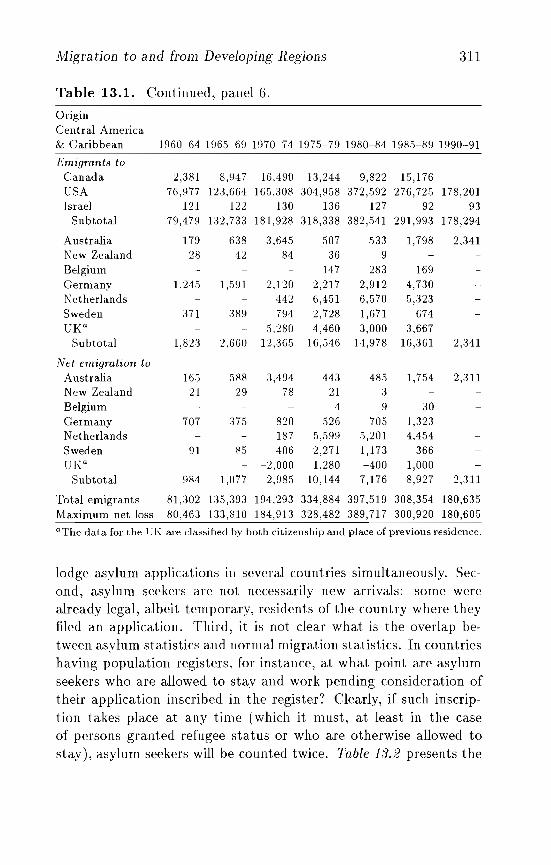
Migration to and from Developing Regions 311

Table 13.l. Continued, panel 6.

OriginCentral America& Caribbean 1960-64 1965-69 1970-74 1975-79 1980-84 1985-89 1990-91

Emigrants toCanada 2,381 8,947 16,490 13,244 9,822 15,176USA 76,977 123,664 165,308 304,958 372,592 276,725 178,201Israel 121 p') 130 136 127 92 93

Subtotal 79,479 132,733 181,928 318,338 382,541 291,993 178,294

Australia 179 638 3,645 507 533 1,798 2,341New Zealand 28 42 84 36 9Belgium 147 283 169Germany 1,245 1,591 2,120 2,217 2,912 4,730Netherlands 442 6,451 6,570 5,323Sweden 371 389 794 2,728 1,671 674UK u 5,280 4,460 3,000 3,667

Subtotal 1,823 2,660 12,365 16,546 14,978 16,361 2,341

Net emigration toAustralia 165 588 :3,494 443 485 1,754 2,311New Zealand 21 29 78 21 3Belgium 4 9 30Germany 707 .375 820 526 705 1,323Netherlands 187 5,599 5,201 4,454Sweden 91 85 406 2,271 1,173 366UK a -2,000 1,280 -400 1,000

Subtotal 984 1,077 2,985 10,144 7,176 8,927 2,311

Total emigrants 81,302 135,393 194,293 334,884 397,519 308,354 180,635Maximum net loss 80,463 133,810 184,913 328,482 389,717 300,920 180,605

aThe data for the UK are classified by both citizenship and place of previous residence.

lodge asylum applications in several countries simultaneously. Sec­ond, asylum seekers are not necessarily new arrivals: some werealready legal, albeit temporary, residents of the country where theyfiled an application. Third, it is not clear what is the overlap be­tween asylum statistics and normal migration statistics. In countrieshaving population registers, for instance, at what point are asylumseekers who are allowed to stay and work pending consideration oftheir application inscribed in the register? Clearly, if such inscrip­tion takes place at any time (which it must, at least in the caseof persons granted refugee status or who are otherwise allowed tostay), asylum seekers will be counted twice. Table 13.2 presents the

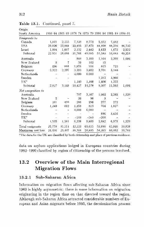
312 Hania Zlotnik

Table 13.1. Continued, panel 7.

OriginSout.h America 1960-64 1965-69 1970-74 1975-79 1980-84 1985-89 1990-91

Emigrants toCanada 1,031 2,555 7,139 8,773 5,452 7,492USA 20,026 23,844 22,495 37,870 44,498 44,316 46,732Israel 1,894 1,667 2,132 2,442 1,633 1,675 2,522

Subt.otal 22,951 28,066 31,766 49,085 51,583 53,483 49,254

Australia 809 3,300 1,164 2,399 1,604New Zealand 9 7 39 102 15Belgium 496 844 1,076 956 815 725Germany 2,322 2,297 3,393 3,052 3,701 3,140Net.herlands 4,000 6,000Sweden 1,212 3,966UK a 1,140 1,160 1,400 1,333

Subtotal 2,827 3,148 10,457 14,570 8,307 11,563 1,604

Net emigration toAust.ralia 797 3,167 1,002 2,265 1,529New Zealand 5 36 90 3Belgium 281 499 286 290 277 272Germany ] ,249 882 1,459 813 704 1,027Net.herlands 4,000 6,000Sweden 896 3,416UK a -240 -560 -200

Subt.otal l,.535 1,381 6,338 9,800 2,682 6,979 1,529

Tot.al emigrants 25,778 31,214 42,223 63,655 59,890 65,046 50,858Maximum net loss 24,486 29,447 38,104 58,885 54,265 60,462 50,783

aThe data for the UK are classified by both citizenship and place of previous residence.

data on asylum applications lodged in European countries during1983-1990 classified by region of citizenship of the persons involved.

13.2 Overview of the Main InterregionalMigration Flows

13.2.1 Sub-Saharan Africa

Information on migration flows affecting sub-Saharan Africa since1960 is highly asymmetric: there is more information on migrationoriginating in the region than on that directed toward the region.Although sub-Saharan Africa attracted considerable numbers of Eu­ropean and Asian migrants before 1960, the decolonization process

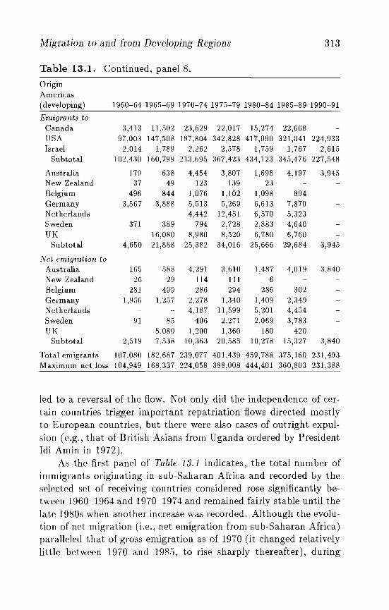
Migration to and from Developing Regions 313

Table 13.1. Continued, panel 8.

OriginAmericas(developing) 1960-64 1965-69 1970-74 1975-79 1980-84 1985-89 1990-91

Emigrants toCanada 3,413 11,502 23,629 22,017 15,274 22,668USA 97,003 147,508 187,804 342,828 417,090 321,041 224,933Israel 2,014 1,789 2,262 2,578 1,759 1,767 2,615

Subtotal 102,430 160,799 213,695 367,423 434,123 345,476 227,548

Australia 179 638 4,454 3,807 1,698 4,197 3,945New Zealand 37 49 123 139 23Belgium 496 844 1,076 1,102 1,098 894Germany 3,567 3,888 5,513 5,269 6,613 7,870Netherlands 4,442 12,451 6,570 5,323Sweden 371 389 794 2,728 2,883 4,640UK 16,080 8,980 8,520 6,780 6,760

Subtotal 4,650 21,888 25,382 34,016 25,666 29,684 3,945

Net emigration toAustralia 165 .588 4,291 3,610 1,487 4,019 3,840New Zealand 26 29 114 111 6Belgium 28] 499 286 294 286 302Germany 1,956 1,257 2,278 1,340 1,409 2,349Netherlands 4,187 11,599 5,201 4,454Sweden 91 85 406 2,271 2,069 3,783UK 5,080 -1,200 1,360 -180 420

Subtotal 2,519 7,538 10,363 20,585 10,278 15,327 3,840

Total emigrants 107,080 182,687 239,077 401,439 459,788 375,160 231,493Maximum net loss 104,949 168,337 224,058 388,008 444,401 360,803 231,388

led to a reversal of the flow. Not only did the independence of cer­tain countries trigger important repatriation flows directed mostlyto European countries, but there were also cases of outright expul­sion (e.g., that of British Asians from Uganda ordered by PresidentIdi Amin in 1972).

As the first panel of Table 13.1 indicates, the total number ofimmigrants originating in sub-Saharan Africa and recorded by theselected set of receiving countries considered rose significantly be­tween 1960-1964 and 1970-1974 and remained fairly stable until thelate 1980s when another increase was recorded. Although the evolu­tion of net migration (i.e., net emigration from sub-Saharan Africa)paralleled that of gross emigration as of 1970 (it changed relativelylittle between 1970 and 198.5, to rise sharply thereafter), during

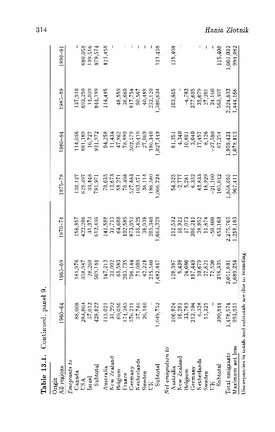
wT

ab

le1

3.l

.C

onti

nued

,pa

nel

9.f-'

,jO..

Ori

gin

All

regi

ons

19

60

-64

19

65

-69

19

70

-74

19

75

-79

19

80

-84

19

85

-89

1990

-91

Em

igra

nts

toC

anad

a88

.008

181,

976

158,

857

130,

127

114,

056

137,

910

US

A28

3,80

335

8,94

742

2,20

662

8,39

780

1,18

969

2,25

068

0,05

8Is

rael

57,0

1228

,260

31.3

7333

,448

16,7

2714

,039

199,

516

Su

bto

tal

428,

822

569.

184

612,

436

791,

971

931,

972

844,

199

879,

574

Au

stra

lia

115,

021

147,

213

141,

588

70,6

3594

,258

114,

485

121,

458

New

Zea

land

31,2

9231

,002

31,7

1313

,673

11,4

34B

elgi

um69

,056

65,5

8364

,688

58,2

7147

,862

48,5

59F

ranc

e17

4,28

520

3,73

519

2,58

570

,398

78,8

8936

,660

Ger

man

y57

6,21

170

6,14

487

3,0,

5152

7,48

350

2.17

981

7,75

4N

eth

erla

nd

s57

,746

71,0

0911

5,42

510

3,57

179

,419

90,.5

67S

wed

en26

,140

42,2

2138

,938

36,1

1427

,069

40,4

88U

r<21

5,54

020

5,34

018

6,58

018

6,34

023

2,12

0S

ub

tota

l1,

049,

752

1,48

2,44

71,

663,

329

1.06

6,72

41,

027,

449

1,38

0,63

412

1,45

8

Net

emig

rati

on

toA

ust

rali

a10

6,82

412

8,38

711

2,53

254

,525

81,3

5110

3,86

511

5,40

8N

ewZ

eala

nd16

,281

5,43

916

,921

-2,7

77

-4,3

40

Bel

gium

33,7

8524

,080

17,0

735,

281

-10

,80

1-4

,78

3G

erm

any

212,

104

197,

449

306,

211

6,35

23,

040

377,

695

Net

her

lan

ds

6,52

810

,679

38,9

5243

,833

17,4

5735

,079

Sw

eden

15,3

2127

,821

11,8

7418

,929

8,12

627

,291

::t1U

K77

,520

-50

,40

0-2

1,1

00

-27

,58

024

,160

~ ::l

Su

bto

tal

390,

844

316,

335

453,

163

105,

042

67,2

5456

3,30

711

5,40

8-. ~

To

tal

emig

ran

ts1,

478,

574

2,05

1,63

12,

275,

765

1,85

8,69

51,

959,

421

2,22

4,83

31,

001,

032

N "-

Max

imu

mn

etlo

ss99

3,95

11,

089,

254

1,25

8,18

396

7,41

11,

078,

115

1,44

4,16

699

4,98

20 """

Dis

crep

anci

esin

tota

lsan

dsu

bto

tals

are

du

eto

rou

nd

ing

.::

l -. >;0

Migration to and from Developing Regions 315

the 1960s the trend in net emigration was the opposite of that ingross emigration. The United Kingdom was mainly responsible forsuch contrasting trends during the 1960s because, even though it re­ceived nearly 26,000 immigrants annually from sub-Saharan Africabetween 1965 and 1969, it sent out an annual average of 33,000during the period. However, British data include both British citi­zens and foreigners, so that it is likely that a significant proportionof those individuals leaving for or coming from sub-Saharan Africawere British citizens.

The first panel of Table 13.1 also indicates that, since 1960,there has been a steady rise in the number of persons from sub­Saharan Africa admitted as immigrants by the main countries ofpermanent resettlement. For Israel, in particular, the admission ofEthiopian Jews led to the rise registered during the 1980s. Althoughgross immigration from sub-Saharan Africa to European countrieshas also, by and large, been growing, the changes registered duringthe 1980s are the most significant: net emigration from the region toEurope rose from 2,700 annually during 1980-1984 to over 31,000annually during 1985-1989, with Germany, the Netherlands, and,especially, the United Kingdom registering very substantial gains.Not surprisingly, the number of citizens from sub-Saharan Africancountries seeking asylum in Europe also rose dramatically: from16,000 annually during 1983-1984 (an average that would be con­siderably lower if the data for the full fi ve- year period were available)to 39,000 in 1985-1989 (see Table 13.2). Furthermore, preliminarydata for 1990 already indicate that the number of Africans fromsouth of the Sahara filing asylum applications in Europe rose tonearly 77,000.

In addition to the flows documented in Tables 13.1 and 1.1.2,between 500,000 and 800,000 inhabitants of the Portuguese coloniesof Angola, Cape Verde, Guinea-Bissau, and Mozambique returned toPortugal during the 1970s when those countries gained independence(Ferreira de Paiva, 1983). The majority of these returnees werePortuguese citizens. However, African nationals have also emigratedto Portugal. By 1990, over 45,000 citizens of African countries,mainly from Cape Verde (over 28,000), Angola (5,000), and Guinea­Bissau (3,500), were legal residents of that country (GECD, 1991,1992).

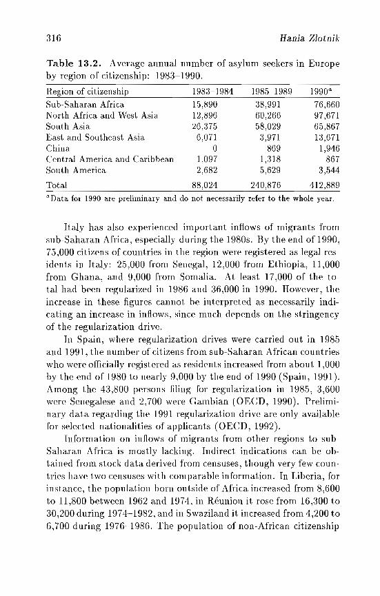
316 Rania Zlotnik

Table 13.2. Average annual number of asylum seekers in Europeby region of citizenship: 1983-1990.

Region of citizenship 1983-1984

Sub-Saharan Africa 15,890North Africa and West Asia 12,896South Asia 26,375East and Southeast Asia 6,071China 0Central America and Caribbean 1,097South America 2,682

Total 88,024

1985-1989

38,99160,26658,0293,971

8691,3185,629

240,876

1990a

76,66097,67165,86713,671

1,946867

3,544

412,889

UData for 1990 are preliminary and do not necessarily refer to the whole year.

Italy has also experienced important inflows of migrants fromsub-Saharan Africa, especially during the 1980s. By the end of 1990,75,000 citizens of countries in the region were registered as legal res­idents in Italy: 25,000 from Senegal, 12,000 from Ethiopia, 11,000from Ghana, and 9,000 from Somalia. At least 17,000 of the to­tal had been regularized in 1986 and 36,000 in 1990. However, theincrease in these figures cannot be interpreted as necessarily indi­cating an increase in inflows, since much depends on the stringencyof the regularization drive.

In Spain, where regularization drives were carried out in 1985and 1991, the number of citizens from sub-Saharan African countrieswho were officially registered as residents increased from about 1,000by the end of 1980 to nearly 9,000 by the end of 1990 (Spain, 1991).Among the 43,800 persons filing for regularization in 1985, 3,600were Senegalese and 2,700 were Gambian (OECD, 1990). Prelimi­nary data regarding the 1991 regularization drive are only availablefor selected nationalities of applicants (OECD, 1992).

Information on inflows of migrants from other regions to sub­Saharan Africa is mostly lacking. Indirect indications can be ob­tained from stock data derived from censuses, though very few coun­tries have two censuses with comparable information. In Liberia, forinstance, the population born outside of Africa increased from 8,600to 11,800 between 1962 and 1974, in Reunion it rose from 16,300 to30,200 during 1974-1982, and in Swaziland it increased from 4,200 to6,700 during 1976-1986. The population of non-African citizenship

Migration to and from Developing Regions 317

also rose from 5,500 in 1974 to 8,300 in 1984 in the Congo and from7,600 to 8,800 between 1963 and 1974 in Sierra Leone. A very roughestimation of net migration based on the figures spanning the 1975­1980 period would suggest that at least 2,500 persons immigratedannually to sub-Saharan Africa from other regions.

More recent data for the Republic of South Africa suggestthat this country alone may have recorded even higher net migra­tion gains. Thus, its foreign-born population rose from 426,000 to450,000 between 1980 and 1985. Making allowance for mortalityat the level of 8 per 1,000 (lower than the 11 per 1,000 estimatedby the United Nations for the total population of South Africa tomake some allowance for the selectivity of migration), the estimatednet inflow of migrants to South Africa during 1980-1985 would havebeen of the order of 41,000 - that is, about 8,200 per year. However,it is likely that at least some of those migrants have already beenaccounted for by the emigration data of the United Kingdom.

Given the paucity of the information available, only guesses arepossible regarding the possible net inflow to sub-Saharan Africa ofpersons originating in countries other than those listed in Table 13.1.

To conclude, it is worth noting that sub-Saharan Africa hoststhe second largest number of refugees in the world, amounting toabout 5.2 million in early 1991 (UN, 1994b). Most of the refugees,however, have found asylum in neighboring countries and have there­fore remained within the region as defined here. Their movements,therefore, need not be taken into account in projecting the totalsub-Saharan population.

13.2.2 North Africa and West Asia

The region comprising the northern part of Africa and the westernpart of Asia has been one of the most dynamic in terms of its par­ticipation in interregional migration flows, both as a region of originand as one of destination. There have also been important intrare­gional flows that need not be documented here. The main sources ofinterregional emigration have been the Maghreb countries (Algeria,Morocco, and Tunisia) and Turkey.

Because the region encompasses many of the oil-rich countries ofthe developing world, particularly those having a limited work force

318 Rania Zlotni](

both in general terms and, more importantly, in terms of neededskills, it has been a major destination of migrant workers, partic­ularly those originating in countries of South, East, and SoutheastAsia. The region also includes Israel, one of the few countries pur­suing an active policy of permanent resettlement. Lastly, as a resultof both internal and international conflict, the region has been thesource of important outflows of population both to neighboring re­gions (South Asia) and, to a lesser extent, to the rest of the world(via, for instance, the emigration of Lebanese).

Turkey

The second panel of Table 18.1 shows that the region has been thesource of very sizable migrant outflows directed mainly to Euro­pean countries, especially France and Germany. However, at leastin the case of Germany, gross inflows have been considerably largerthan net migration. The same may apply to France, although lackof information on emigra.tion from that country prevents an ade­quate assessment of net gains. Indirect evidence suggests that netmigration from the Maghreb countries to France was positive dur­ing the late 1970s but very low or possibly negative during at leastpart of the 1980s. Thus, the number of citizens of Algeria, Morocco,Tunisia, and Turkey enumerated by the censuses of France increasedfrom 1,161,000 in 1975 to 1,560,000 in 1982 and only to 1,614,000 in1990 (OECD, 1992). Whereas the number of Moroccans, Tunisians,and Turks in France grew bptween 1982 and 1990, that of Alge­rians declined sharply. passing from 805,000 in 1982 to 620,000 in1990. Although some of that change may have been due to natu­ralization or better reporting of citizenship by persons of Algeriandescent (many of whom have the right to French citizenship), returnmigration is also likely to have contributed to the change observed.

In 1990, Belgium, France, Germany, the Netherlands, and Swe­den were hosting a total of 2,196,000 Turks, 951,000 Moroccans,631,000 Algerians, and 242,000 Tunisians (OECD, 1992). SizableTurkish populations were also present in other European countries.Thus, between 1980 and 1990, the number of Turks in Norway andSwitzerland increased from 40,600 to 69,700, and the number ofTurkish workers in Austria rose from 28,300 to 50,500. At least

Migration to and from Developing Regions 319

part of the increase in the Turkish population in Europe was asso­ciated with the very sizable inflows of Turkish asylum seekers. AsTable 13.1 shows, the number of asylum seekers from North Africaand West Asia rose very markedly between the early and late 1980s,and Turks accounted for much of that increase (figures not shown).

Among the other nationalities, about 2,200 Moroccans were re­ported to be present in Norway in 1990 and they figured prominentlyin the regularization drives carried out by Italy and Spain since 1985.In Italy, for instance, 146,000 persons from North Africa and 12,000from West Asia were present in 1990, of which 78,000 were Moroc­can, 41,000 Tunisian, 20,000 Egyptian, and 6,000 each Lebanese andJordanian. Of the total 158,000 North Africans and West Asianspresent in 1990, 39,000 had regularized their status as a result ofthe 1990 drive and 18,400 during that held in 1986 (GECD, 1991).

In Spain, the register of foreigners indicates that the NorthAfrican and West Asian population declined slightly from 1975 to1980 (from 7,500 to 6,800), rose to 9,200 in 1985, and then increasedsharply to reach 21,100 by the end of 1990 (Spain, 1991). This risewas partly due to the 1985 regularization drive where at least 8,000Moroccans lodged applications for regularization (GECD, 1990).Preliminary results from the 1991 drive indicate that a further40,000 Moroccans may be regularized (GECD, 1992).

Lastly, it must be noted that the changes taking place in theformer East bloc countries have made Turkey a migrant-receivingcountry. Indeed, in 1989,314,000 Bulgarians of Turkish ethnic originmoved into the country. By September of 1991 there were 358,000Bulgarians in Turkey. Nearly two-thirds had settled permanentlyand virtually all had acquired Turkish citizenship (GECD, 1992).

Israel

Panel 2 of Table 13.1 indicates that gross immigration to Israel,most of which has originated outside the region in recent years, hascontributed significantly to red uce the net emigration balance of theregion (see the last line of the second panel). The high levels of im­migration recorded by Israel during the 1970s and again during the1990s are associated with the arrival of Soviet Jews whose emigra­tion during the 1970s was permitted as part of "detente" and during

320 Rania Zlotnik

the 1990s as a result of the liberalization of the Soviet and now theRussian regime. In 1990 alone, 185,200 Soviet Jews immigrated toIsrael, and the figure for 1991 is 147,800 (Sabatello, 1992). The 1989census of the USSR enumerated 1.45 million ethnic Jews. Takinginto account Jews registered under other "nationalities" and theirnon-Jewish relatives, an estimated 1.8 to 2 million persons mightstill be eligible for eventual admission to Israel (Sabatello, 1992).

Unfortunately, information on emigration from Israel by regionof origin or region of destination could not be obtained. Availableinformation on net migration indicates that during 1975-1979, itamounted to only 12,200 persons annually (UN, 1985a), a level farlower than the gross immigration figure of 33,400 shown in Table13.1. In addition, data on the number of Israeli residents who leftin a given year and had not yet returned by May 1990 indicate that,on average, 9,700 emigrated annually during 1976-1979, 12,100 didso during 1980-1984, and 22,700 during 1984-1988 (Israel, 1990). Ofcourse, the last figure is likely to overestimate permanent emigrationsomewhat because the time elapsed since departure is shorter. How­ever, such figures indicate the approximate levels of emigration thatIsrael has been experiencing, levels that would reduce considerablythe gross gains presented in Table 13.1.

Oil-rich Countries

It is well known that the oil-rich countries of North Africa and WestAsia have been major importers of foreign labor. Even before thedramatic rises in the price of oil during the early 1970s, severalcountries in the region had been resorting to foreign workers. Themost complete estimates on worker migration to the region indicatethat, between 1975 and 1980, the total number of foreign workersemployed in Bahrain, Iraq, Jordan, Kuwait, Libya, Oman, Qatar,Saudi Arabia, the United Arab Emirates, and Yemen increased from1.8 to 2.8 million (Birks and Sinclair, cited in UN, 1985a). Thelargest proportions (43 percent in 1975 and 36 percent in 1980)were employed in Saudi Arabia. Libya with 19 percent in 1980, theUnited Arab Emirates with 15, and Kuwait with 13 followed.

Until 1980, most foreign workers in the region also originatedin countries of North Africa and West Asia: 71 percent in 1975 and63 percent in 1980. The rest were mostly citizens of India, Iran,

Migration to and from Developing Regions 321

and Pakistan (2,5 percent in 191,5 and 27 percent in 1980). WhereasIndians and Pakistanis worked in almost every possible receivingcountry, Iranians were mostly concentrated in Iraq and Kuwait.

During the late 197013 a new trend took hold. The main labor­importing countries in the region turned to migrant workers fromEast and Southeast Asia. Table 13.3 shows the average annualnumber of persons granted permission to work abroad under tem­porary contractual agreements by various sending countries in bothSouth Asia and East and Southeast Asia. The data, though proba­bly fairly incomplete for earlier periods, indicate that by 1975-1979an annual average of 330,000 persons were being granted permissionto work abroad. During the 198013, the equivalent figure remainedabove 1 million. The distribution by region of origin has changedsubstantially since 1975. Whereas during 1975-1979,52 percent ofall workers securing permits to go abroad originated in South Asia,by 1980-1984 their share had dropped to 43 percent, and during1985-1989 it decreased further to 30 percent.

Care must be taken in interpreting the figures presented in Table13.3. They represent generally the number of exit permits grantedby government authorities to persons wishing to work abroad. Sincetemporary engagements are possible, multiple work permits may beissued to a single person during a given year. Furthermore, evenfrom year to year, figures cannot be interpreted as representing newworkers joining the expatriate labor force. The policy of workerrotation adopted by many receiving countries implies that foreignworkers usually remain abroad for relatively short periods (one ortwo years) and need to return home before having their contracts re­newed. Unfortunately, figures on !let flows are not available. On theother hand, since workers have been known to emigrate "illegally"without obtaining the necessary permits, the figures presented maybe subject to a counterbalancing negative bias. Lastly, althoughthe oil-rich countries of vVest Asia have been a major destination ofmigrants originating in most of the countries listed in Table 13.3,it is by no means certain that they are the only destination. Dataclassified crudely by region of destination indicate that, at least forIndonesia, the Philippines, the Republic of Korea, and Thailand,the proportion of workers intending to go to the Middle East hasvaried substantially since 1975 (see Table 13.4).

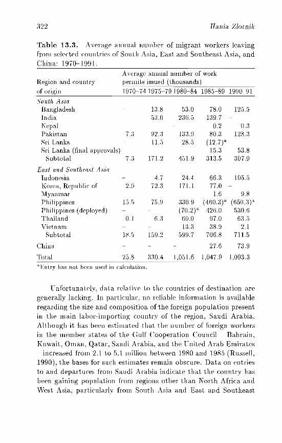
:322 Hania Zlotnik

Table 13.3. Average annual number of migrant workers leavingfrom selected countries of South Asia, East and Southeast Asia, andChina: 1970-1991.

Average annual number of workRegion and country permits issued (thousands)

of origin 1970-74 1975-791980-84 1985-89 1990-91

South AsiaBangladesh 13.8 53.0 78.0 125.5India 5;3,6 236.5 139.7 -

Nepal 0.2 0.3Pakistan 7.:3 92.3 133.9 80.3 128.3Sri Lanka 11.5 28.5 (12.7)a -Sri Lanka (final approvals) - 15.3 53.8

Subtotal 7.:3 171.2 451.9 313.5 307.9

East and Southeast AsiaIndonesia 4.7 24.4 66.3 10.5 ..5Korea, Republic of 2.9 72.3 171.1 77.0 -

Myanmar 1.6 9.8Philippines 15.5 75.9 330.9 (460.3)a (650.3)"Philippines (deployed) (70.2)" 426.0 530.6Thailand 0.1 6.3 60.0 97.0 63.5Vietnam 13.3 38.9 2.1

Subtotal 18.5 1.59.2 599.7 706.8 711.5

China 27.6 73.9

Total 25.8 330.4 1,0.51.6 1,047.9 1,093.3

aEntry has not been used in calculation.

Unfortunately, data relative to the countries of destination aregenerally lacking. In particular. no reliable information is availableregarding the size and composition of the foreign population presentin the main labor-importing country of the region, Saudi Arabia.Although it has been estimated that the number of foreign workersin the member states of the Gulf Cooperation Council - Bahrain,Kuwait, Oman, Qatar, Saudi Arabia, and the United Arab Emirates- increased from 2.1 to 5.1 million between 1980 and 1985 (Russell,1990), the bases for such estimates remain obscure. Data on entriesto and departures from Saudi Arabia indicate that the country hasbeen gaining population from regions other than North Africa andWest Asia, particularly from South Asia and East and Southeast

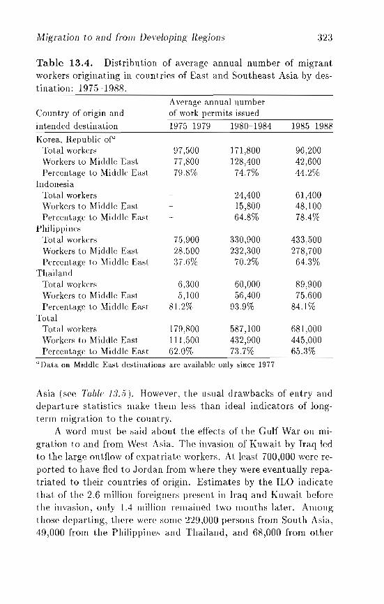
Migration to and hom Den'joping Regions 323

Table 13.4. Distribution of average annual number of migrantworkers originating in countries of East and Southeast Asia by des­tination: 1975-1988.

Average annual numberCountry of origin and of work permits issued

intended destination 1975-1979 1980-1984 1985-1988

Korea, Republic ofa

Total workers 97,500 171,800 96,200Workers to Middle East 77,800 128,400 42,600Percentage to Middle East 79.8% 74.7% 44.2%

IndonesiaTotal workers 24,400 61,400Workers to Middle East 15,800 48,100Percentage to Middle East 64.8% 78.4%

PhilippinesTotal workers 75.900 330,900 433,500Workers to Middle East 28,500 232,300 278,700Percentage to Middle East :37.()% 70.2% 64.3%

ThailandTotal workers 6,:300 60,000 89,900Workers to Middle East 5,100 56,400 75,600Percentage to Middle East 81.2% 93.9% 84.1%

TotalTotal workers 179,800 587,100 681,000Workers to Middle East 111,500 432,900 445,000Percentage to Middle East 62.0% 73.7% 65.3%

aData on Middle East destinations are available only since 1977.

Asia (see Table 13.5). However, the usual drawbacks of entry anddeparture statistics make t hem less than ideal indicators of long­term migration to the country.

A word must be said about the effects of the Gulf War on mi­gration to and from West Asia. The invasion of Kuwait by Iraq ledto the large outflow of expatriate workers. At least 700,000 were re­ported to have fled to Jordan from where they were eventually repa­triated to their countries of origin. Estimates by the ILO indicatethat of the 2.6 million foreigners present in Iraq and Kuwait beforethe invasion, only 1.4 million remained two months later. Amongthose departing, there were some 229,000 persons from South Asia,49,000 from the Philippines and Thailand, and 68,000 from other

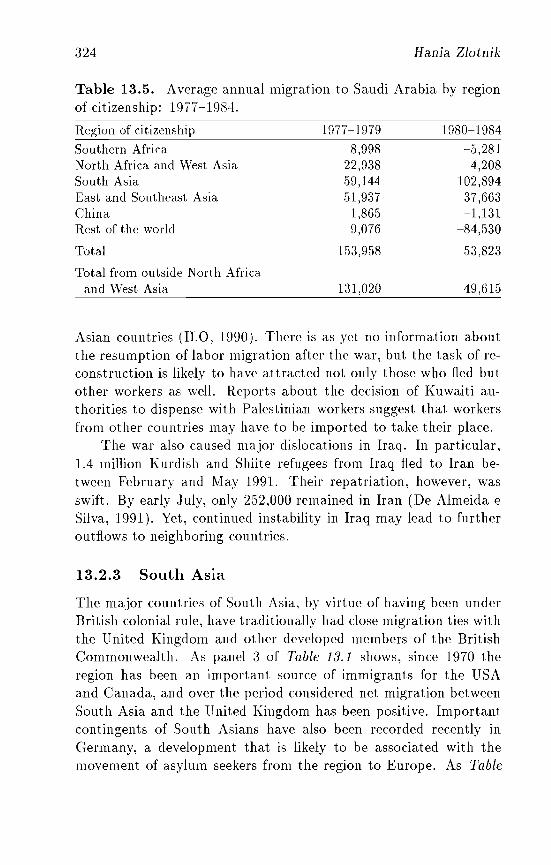
324 Hania Zlotnik

Table 13.5. Average annual migration to Saudi Arabia by regionof citizenship: 1977-1984.

Region of citizenship

Southern AfricaNorth Africa and West AsiaSouth AsiaEast and Southeast AsiaChinaRest of the world

Total

Total from outside North Africaand West Asia

1977-1979

8,99822,93859,14451,937

1,8659,076

153,958

131,020

1980-1984

-5,2814,208

102,89437,663-1,131

-84,530

53,823

49,615

Asian countries (1LO, 1990). There is as yet no information aboutthe resumption of labor migration after the war, but the task of re­construction is likely to have attracted not only those who fled butother workers as well. Reports about the decision of Kuwaiti au­thorities to dispense with Palestinian workers suggest that workersfrom other countries may have to be imported to take their place.

The war also caused major dislocations in Iraq. In particular,1.4 million Kurdish and Shiite refugees from Iraq fled to Iran be­tween February and May 1991. Their repatriation, however, wasswift. By early July, only 252,000 remained in Iran (De Almeida eSilva, 1991). Yet, continued instability in Iraq may lead to furtheroutflows to neighboring countries.

13.2.3 South Asia

The major countries of South Asia, by virtue of having been underBritish colonial rule, have traditionally had close migration ties withthe United Kingdom and other developed members of the BritishCommonwealth. As panel 3 of Table 13.1 shows, since 1970 theregion has been an important source of immigrants for the USAand Canada, and over the period considered net migration betweenSouth Asia and the United Kingdom has been positive. Importantcontingents of South Asians have also been recorded recently inGermany, a development that is likely to be associated with themovement of asylum seekers from the region to Europe. As Table

Migration to and [rom Developing Regions 32.5

13.2 shows, the number of asylum seekers from South Asia increasedfrom an annual average of 26,000 during 1983-1984 to .58,000 during198.5-1989. The main sources of asylum seekers in the region havebeen Iran and Sri Lanka.

As discussed in Section 13.2 ..5, South Asia has also been an im­portant source of labor migration for the oil-rich countries of WestAsia. Data on the outflow of workers from the main sending coun­tries in South Asia are presented in Table 13.3. It is worth notingthat, particularly for India and Sri Lanka, the number of work per­mits issued to those intending to work abroad is thought to under­estimate true outflows. Sri Lanka's worker migration has attractedattention because of the high proportion of women it involves. Mostof them work as maids in West Asian countries. Although there isno information on the country of destination of the South Asianworkers who have been granted exit permits, it is safe to assumethat most of them intend to work in West Asia.

Only lately have there been reports of an increasing number ofSouth Asian workers finding employment in other Asian countries,such as Japan or Taiwan. However, most of them work illegally.Japanese statistics show that during 198.5-1990, 11 ,600 citizens ofBangladesh, 10,700 of Pakistan, LOOO of Sri Lanka, 700 of each Iranand India, and 400 of Nepal were deported. For each nationality,the number of deportations rose rapidly over the period considered.

South Asian workers are also finding their way to Europe. To­ward the end of 1990, Italy recorded 34,100 citizens of Bangladesh,India, Pakistan, and Sri Lanka as legally residing in the country,13,400 of whom had legalized their status during the 1990 regular­ization drive and 12,100 during that held in 1986 (OEeD, 1990). InSpain, the number of Sonth Asian nationals legally present by theend of 1990 amounted to nearly 8,000, a substantial increase fromthe 2,600 registered in 1980 (Spain, 1991).

Some of the largest population outflows have occurred withinthe South Asian region itself. According to statistics on the foreign­born, India was the second largest migrant-receiving country in theworld in 1980. Most of the migrants thus identified had moved toIndia from Bangladesh or Pakistan, probably as a result of parti­tion. In addition, the region hosts the largest refugee populationoriginating from a single conntry. Afghanistan. As of early 1991 an

326 Hania Zlotnik

estimated 6.2 million Afghani refugees were present in Iran and Pak­istan (UN, 1994b). Furthermore, by mid-1991 Iran was still hosting252,000 Iraqi refugees.

13.2.4 East and Southeast Asia

The East and Southeast Asia region has been a major source ofmigrants for both the developed countries and the labor-importingcountries of West Asia. As Table 13.1 indicates, immigrants fromthe region have constituted the second largest contingent admittedby the USA since 1970-1974. The close strategic, military, or evencolonial ties that link several countries in the region with the USAhave fostered such migration. Thus, the Philippines, the Repub­lic of Korea, and Vietnam have been among the main sources ofimmigrants to the USA for over a decade. Migration from Viet­nam, Cambodia, and Laos has occurred mostly within the frame­work of refugee resettlement. It is estimated that between 1975and 1988 nearly 1.5 million Indo-Chinese refugees were resettledabroad, the vast majority (1.15 million) in developed countries, in­cluding 108,000 in France, 8,000 in Switzerland, and 6,000 each inNorway and .Japan (LTN. 1992a). The Vietnamese resettled in otherdeveloped countries are already reflected in the statistics presentedin Table 13.1. In addition, during the 1980s China admitted 284,000ethnic Chinese from Vietnam for resettlement.

Emigration from Vietnam has also occurred in the context oflabor migration. Newly available statistics from the former Ger­man Democratic Republic indicate that by the end of 1989 therewere over 60,000 Vietnamese in that country, a number that haddeclined to :3.5,000 by the eud of 1990 (GECD, 1992). In the formerCzech and Slovak Federal Republic :34,000 Vietnamese workers werepresent in 1990, but their number had declined to barely 10,000 by1991 (GECD, 1992). Vietnamese workers are also known to havemigrated to the former Soviet Union, but no information on theirnumbers is available. Table 1.1.3, however, indicates that during the1980s a growing number of Vietnamese received clearance to workabroad.

At least part of the growth of the number of East and SoutheastAsian immigrants recorded by the countries listed in panel 4 of Ta­

ble 18.1 is attributable to the intake of Indo-Chinese refugees after

Migration to and from Developing Regions 327

the fall of Saigon in 197.5. However, especially during the 1980s,the numbers of migrants originating in countries like the Philip­pines, Hong Kong, or Malaysia have also been growing. Indeed,the planned devolution of Hong Kong to the People's Republic ofChina has fueled emigration from the Crown Colony. Countries likeAustralia, Canada, and the United States have established specialimmigration categories aimed, at least in part, at attracting affluentHong Kong residents. AltllOugh emigration from Hong Kong hasbeen increasing, net migration to the Colony may still be positive.Estimates of net migration for earlier periods indicate that HongKong gained an annual average of 11,500 persons during 1961-1971,20,400 during 1971-1976, and 80,000 during 1976-1981 (Skeldon,1986). The sharp rise registered in the late 1970s was due to theincreased inflow of illegal migrants from China lured by the possi­bility of regularizing their status in Hong Kong if they managed toreach the urban areas of the Colony. The rise in illegal migrationprompted British authorities to remove that possibility in 1980. Theeffects of such a change aTe noticeable in the evolution of the HongKong population born in China. Whereas the 1976 census of HongKong showed that 1.66 million Hong Kong residents were born inChina and the 1981 census put that figure at 1.97 million, the 1986census showed that the population born in China increased only to2 million (Hong Kong, 1988). The figures imply that net Chinesemigration would have amounted to an annual average of 79,000 dur­ing 1976-1981 (assuming a mortality of 10 per 1,000) and of some25,000 during 1981-1986 under unchanging mortality conditions.

The growing variety of sources of emigration from East andSoutheast Asia has been paraUeled by an increasing diversificationof possible destinations. During the 1980s, not only did increas­ing numbers of East and Southeast Asian workers secure permits towork in West Asian countries, but the proportion obtaining permitsto work elsewhere rose in the Philippines, the Republic of Korea, andThailand (see Table 13.4). Although many of those workers foundemployment in other countries of the region, such as Brunei, HongKong, Malaysia, Singapore, or Taiwan, others went further afield.Rising numbers of Filipinos, in particular, have been recorded inJapan (49,000 were registered aliens in 1990 compared with only5,500 in 1980), Italy (;34,000 in 1990), and Spain (where 2,500

328 JIania Zlotnik

applied for regularization in 1991). In addition, during 1985-1990,;31 ,400 Filipinos were deported from Japan, 72 percent of whomwere women. The same proportion of women was found among the7,100 Thai migrants deported from Japan during 1985-1990. In con­trast, among the G,600 Malaysians deported during the same period,women accounted for only 12 percent (Japan, 1990).

In conclusion, the number of citizens from East and SoutheastAsia seeking asylum in Europe has remained relatively small (seeTable 1:J. 2). The generous resettlement opportunities granted toIndo-Chinese refugees during most of the 1980s are probably re­sponsible for these trends. However, as conflict in Indochina su b­sides and a growing number of would- be refugees are denied asylumin the region, they may start seeking it elsewhere.

13.2.5 China

The fact that in 1980 over 2G million Chinese or descendants of Chi­nese were estimated to be living in countries other than mainlandChina or Taiwan (Poston and Yu, 1990) proves that Chinese emi­gration has been significant in modern times. However, during thefirst three decades of the People's Republic of China (from the late1940s to the late 1970s), Chinese emigration from the mainland wasseverely restricted and only a small number of people left legallyduring the period. More recently, as Chinese authorities have in­creasingly opened the country to foreigners, emigration levels haverisen somewhat (see panel 5 of Table 1:J.1) but, in general, Chineseemigration remains highly restricted.

As panel 5 of Table 1:J.1 indicates, the main receivers of Chineseemigrants have been the USA and Canada. Only during the 1980sdid Chinese immigration to Australia or Germany surpass the 1,000mark. However, as already noted, Chinese emigration to neighbor­ing countries, particularly Hong Kong, has been considerably larger.In addition, the number of Chinese registered as resident aliens inJapan has been rising in recent years, passing from 49,000 in 1975to 75,000 in 1985 and reaching 150,000 in 1990 (Japan, 1990). It isnot clear, however, whether the data refer only to mainland Chineseor also to those of Hong Kong or Taiwanese origin.

As Table 1:J.2 indicates, the number of Chinese asylum seekersin Europe, though small, has been increasing. Chinese became more

Migration to and from Developing Regions 329

likely to obtain asylum after the events of Tiananmen Square in1989. The USA passed at the time a Deferred Enforced DepartureAct that allowed virtually every Chinese student in the country andhis or her dependents to stay. By August 1992, a bill that wouldgrant permanent residence to an estimated 80,000 Chinese studentsand dependents in the USA had been passed (FAIR, 1992).

Chinese are securing entry to developed countries not only viaasylum procedures but also as needed workers. In Italy 18,700 Chi­nese were resident aliens by the end of 1990, 4,500 of whom hadregularized their status in 1986 and a further 9,700 in 1990. A highproportion of them were registered as own-account workers. In ad­dition, Chinese authorities themselves are promoting the export oflabor. As Table 13.3 indicates, the number of Chinese workers ob­taining permits to work abroad increased markedly from an annualaverage of 27,600 during 198.5-1989 to nearly 74,000 during 1990­1991. Given the increasing misgivings that West Asian countriesare having about hiring ~Muslilll workers from other Asian countries(Economist Intelligence Unit, 1990). resorting to Chinese labor maybe a desirable option during the 1990s.

13.2.6 Central America and the Caribbean

According to the data presented in Table 13.1, the region identifiedhere as Central America and the Caribbean, which includes Mexico,has been the main source of emigrants during 1960-1984. Only forthe period 19805-1989 did the gross number of emigrants originat­ing in East and Southeast Asia surpass those coming from CentralAmerica and the Caribbean. However, the data in panel 6 of Table13.1 include the over 2 million legalizations from Central Americaand the Caribbean that were registered during 1989-1992 and thathave been redistributed over the period 1972-1986. As a result ofsuch redistribution, the average annual number of admissions of per­manent immigrants from Central America and the Caribbean by theUSA increased from 13;3,000 to 165,000 in 1970-1974, from 158,000to 305,000 in 197.5-1979, from 162,000 to 373,000 in 1980-1984, andfrom 198,000 to 277,000 in 198.5-1989. Since most of the legal­izations correspond to Mexican citizens, Mexico became the mainsource of migrants to the USA during the late 1970s.

330 Hania Zlotnik

In fact, any attempt at incorporating undocumented migrationinto overall migration estimates would make Mexico a major countryof emigration. Indeed, because the regularization established by theImmigration Reform and Control Act of 1986 imposed time limitson those who could have their status legalized, it did not eliminateentirely the undocumented population present in the USA. It hasbeen estimated that, even taking into account the regularization re­sults, by June 1988 nearly 1.9 million undocumented migrants werestill in the country, 1.1 million of whom were Mexican and anotherhalf a million were from the rest of North America (Woodrow andPassel, 1990). Furthermore, some 70,000 were estimated to haveentered the country during 1987-1988. However, that number ofentries was not statistically significant (Woodrow and Passel, 1990).

Not only do the figures on immigration to the USA presented inpanel 6 of Ta.ble 13.1 exclude estimates of undocumented migration,they also exclude the inflow of persons from Caribbean Islands whoseinhabitants are US citizens. Puerto Rico is probably the main sourceof such migrants. According to census figures, the number of netmigrants from Puerto Rico amounted to an average annual intakeby the United States of 1/,700 during 1955-1960, 19,200 during196.5-1970, and 20,000 during 1975-1980 (Ortiz, 1986).

It is noteworthy that relatively few migrants from the regionhave found their way to overseas countries. Although migrationfrom the English-speaking Caribbean to the United Kingdom wassignificant during the late 19.50s and early 1960s, as the data inTa.ble 13.1 show, the net migration of Commonwealth citizens fromthe Caribbean and Belize to the United Kingdom has been relativelysmall or even negative since 1970. However, several Caribbean coun­tries have been the source of emigrants to other regions. Cuba, forinstance, sent both troops and workers to Angola, and it was alsoa source of workers for certain East bloc countries. There were, forinstance, 8,000 Cubans in the former German Democratic Republicin 1989, only 3,000 of whom remained by 1990 (OECD, 1992). Inthe Czech and Slovak Federal Republic, 1,100 Cuban workers werepresent in 1990, but by 1991 only 100 remained.

Citizens from the Dominican Republic have also migrated insearch of work to both regional and overseas destinations. Thus,the 1980-1981 regularization drive of Venezuela recorded 4,300

Migration to and hom Developing Regions 331

Dominicans and 1,900 persons from other countries of Central Amer­ica and the Caribbean (Torrealba, 1985). In addition, by the end of1990,4,400 citizens from the Dominican Republic were registered aslegal resident aliens in Italy, and 5,000 more applied for regulariza­tion in Spain in 1991 (OECD, 1992). Interestingly, the foreign pop­ulation of Central American and Caribbean origin residing legallyin Spain changed relatively little, declining from 13,700 to 10,800between 1975 and 198.5 and then rising to 14,000 by 1990 (Spain,1991 ).

Although during the 1980s several countries of Central Americawere important sources of refugees, relatively few persons from theregion have applied for asylum in Europe (see Table 13.2). Again inthis instance, the USA and Canada have been the preferred desti­nations of asylum seekers from Central America and the Caribbean.During 1984-1990, US authorities adjudicated 102,000 applicationsfor asylum filed by citizens of just t.hree Central American coun­tries, namely, £1 Salvador, Guatemala, and Nicaragua. Those ap­plications constituted 64 percent of all the asylum cases adjudicatedin the USA during the period, and the vast majority (88,000) weredenied. Since most applicants remained in the USA even after theirasylum request was turned down, they became undocumented aliensand were probably adequately reflected by the statistics on undocu­mented alien stocks reported above. However, as a result of a lawsuitby human rights advocates, US authorities granted all Salvadoranspresent in the country as of 19 September 1990 and all Guatemalanspresent on 1 October 1990 the right to new hearings on their asylumclaims and the possibility of staying in the country and working un­til 30 June 1992 (UN, 1994b). Approximately 185,000 Salvadoranshave benefited from the temporary protected status thus granted(Weintraub and Diaz-Briquets, 1992).

13.2.7 South America

Until the late 19505, South America was a region of immigration,since countries like Argentina, Brazil, Chile, and Uruguay attractedan important number of immigrants from European countries afterthe end of \Vorld War II. The main sources of European migrationto the Americas were Italy, Spain, Portugal, and several East Eu­ropean countries. By the 1960s, however, the inflow of Europeans

332 Hania Zlotnik

had largely run its course. Only Venezuela was successful in at­tracting overseas migrants well into the 1970s. Entry and departurestatistics for Venezuela indicate that during 1974-1979 the countryregistered, on an annual basis, a net inflow of some 10,000 Europeanimmigrants and another 1,000 from other regions (Torrealba, 1982).During 1980-1981, however, the net flow became negative and islikely to have remained so during the rest of the decade.

Census data from two of the main receiving countries in theregion, Argentina and Brazil, suggest that during the 1970s netmigration became negative. In Argentina the population born inEurope declined from 1.47 million in 1970 to 1.08 million in 1980, areduction that cannot be a.ccounted for by mortality alone. In Brazilthe population of European nationality declined from 803,000 in1970 to 638,000 in 1980. Although such a change could be the resultof naturalization, return migration is likely to have also contributedto it.

As panel 7 of Ta.ble 13.1 shows, South America has been a rel­atively important source of immigrants to the USA. A fair numberof them remained in that country illegally because, although thenumbers legalizing under IRCA were small in comparison to thoseof undocumented aliens from Central America and the Caribbean,the trend since 1970 has been affected by the redistribution of thoselegalizing during 1989-1992. In particular, without the IRCA legal­izations, the average annual number of admissions of South Amer­icans by the USA would have amounted to only 31,000 instead of38,000 in 1975-1979, to 37,000 instead of 45,000 in 1980-1984, andto 42,000 instead of 44,000 in 198.5-1989.

Emigration from South America is likely to have grown signifi­cantly during the 1980s. Part of it, however, is difficult to measure,since it involves the emigration of second- and third-generation mi­grants (i.e., the children and grandchildren of the original immi­grants) who have been granted citizenship rights by the countries oforigin of their forebears. Thus, Italy and Spain have been receivingthe inflow of Italian or Spanish citizens born overseas who do notappear on statistics relative to foreigners. According to statisticson the foreign stock, there were 47,000 South American citizens inItaly at the end of 1990 (14,000 of whom were Brazilian and 13,000Argentine citizens). and the number of South American citizens in

Migration to and [rom De\·eloping Regions 333

Spain nearly doubled, passing from 24,000 in 1975 to 30,000 in 1985and then to 49,000 in 1990 (Spain, 1991). In addition, about 7,000nationals of Argentina and 5,000 of Peru lodged applications forregularization during the 1991 drive carried out in Spain.

Perhaps one of the most interesting cases of return migrationamong the descendants of former immigrants is the migration ofBrazilians and Peruvians of Japanese descent to Japan. Between1985 and 1990, the population of South American origin in Japanincreased dramatically, rising from 3,600 to 71,500. Underlying sucha change was the decision of Japanese authorities to permit theestablishment in Japan of persons of Japanese descent. Both Braziland Peru host relatively sizable Sllbpopulations of Japanese ethnicorigin that may decide to go back to their roots.

The number of South American asylum seekers in Europe hasremained modest. Until the 1990 change of government in Chile,citizens of that country were likely to obtain asylum in Europe,particularly in the Nordic countries. The new Chilean governmentis planning to facilitate the repatriation of those wishing to return.

13.3 Conclusion

This overview of migration trends to and from the main developingregions, though fairly comprehensive, is still a weak basis on whichto estimate current interregional migration or derive assumptionsregarding future trends. Although data on migration flows are notentirely lacking, those available are often incomplete (they do notrefer to all possible long-term movements), and they are not easilycomparable from one country to another. In addition, when themain countries of destination are located in the developing world,data on migration flows are often entirely lacking or cannot be read­ily obtained. The political sensitivity of the migration phenomenonis such that existing information is often treated as highly classi­fied material that must be protected. Countries are often guilty ofbenign neglect, preferring to ignore the magnitude of flows than tomeasure them adequately. Despite efforts to improve the quality andavailability of international migration statistics, little progress hasbeen made. In the meantime, migration continues to increase andits complexity rises. Part of that complexity stems from the barriers

334 Hania Zlotnik

that potential countries of destination are using to control or stopmigration. When legal migration is highly restricted or not desiredunder any circumstances, different varieties of illegal or undesirableflows will arise. Such a situation makes the job of the forecaster evenmore difficult, since policy aims are at odds with likely outcomes.

On the other hand, consideration of any time series on migrationis a sobering experience. As Table 13.1 indicates, relatively drasticchanges in trends can and have occurred over the course of the past30 years in many developing regions. Events like the Gulf War cantrigger large interregional flows over relatively short periods. Giventhe difficulties in forecasting such events and their likely effects onmigration, population projections are often based on relatively sim­plistic assumptions regarding future migration trends. Perhaps themost common assumption is that migration will, in the long run,have little effect on population dynamics, so that it can be assumedto be zero. Otherwise, migration assumptions are generally made interms of net numbers of migrants gained or lost during each of theprojection quinquennia (see, for instance, Arnold, 1989). When thelatter approach is taken, nonzero assumptions are typically made fora few projection periods (11Sually one to four, thus covering at most aspan of 20 years) and from then on migration is assumed to taper offto zero or to remain constant at the last assumed level. Although un­doubtedly simplistic, such practices have much to recommend them,particularly when one is dealing with large and complex regions suchas the ones considered in this paper. Given the relatively large pop­ulation bases of most regions, estimated net migration levels of themagnitude presented in Table 13.1 are likely to have relatively smalleffects on the overall evolution of the population.

At the level of individual countries or smaller regions, however,the situation may be different. Ivligration is also likely to be an im­portant component of population change when fertility has reachedvery low levels, especially if it remains below replacement for a cer­tain period (see, for instance, OEeD, 1991). Yet, even in countriesfacing such fertility prospects, projections continue to be made us­ing the type of migration assumptions described above: total netnumbers of migrants that vary minimally over time. Although theconstruction of more complex assumptions is technically possible,policy considerations usually dissuade technicians, who are mostly

Migra.tion to a.nd from Developing Regions 335

at the service of governments, from using more realistic scenarios,especially if these scenarios are likely to run counter to major policystances. Whether the use of such scenarios would help or hinder thedebate 011 migration, its desirability, or the degree to which it mustbe tolerated is a matter that needs to be considered carefully.

Note

[1] Definitions of developing regions used.Sub-Saharan Africa. East Africa: British Indian Ocean Territory,Burundi, Comoros, Djibouti, Ethiopia, Kenya, Madagascar, Malawi,Mauritius, Mozambique, Reunion, Rwanda, Seychelles, Somalia,Uganda, Tanzania, Zambia, Zimbabwe; Central Africa: Angola,Cameroon, Central African Republic, Chad, Congo, EquatorialGuinea, Gabon, Sao Tome & Principe, Zaire; Southern Africa:Bot.swana, Lesotho, Namibia. South Africa, Swaziland; West Africa:Benin, Burkina Faso, Cape Verde, Cote d'Ivoire, Gambia, Ghana,Guinea, Guinea-Bissau, Liberia, Mali, Mauritania, Niger, Nigeria,St.. Helena, Senegal, Sierra Leone, Togo.North Africa and ~lIfst ASia. North Africa: Algeria, Egypt, Libya,Morocco, Sudan, Tunisia, West Sahara; West Asia: Bahrain, Cyprus,Gaza Strip (Palestine), Iraq, Israel, Jordan, Kuwait, Lebanon, Oman,Qat.ar, Saudi Arabia, Syria, Turkey, United Arab Emirates, Yemen.South Asia. Afghanistan, Bangladesh, Bhutan, India, Iran, Maldives,Nepal, Pakistan, Sri Lanka.East and Southeast Asia. East Asia: Hong Kong, Korea (DemocraticPeople's Republic), Korea (Republic), Macau, Mongolia; SoutheastAsia: Brunei Darussa.lam, Cambodia, East Timor, Indonesia, Lao Peo­pie's Democratic Republic, Malaysia, Myanmar, Philippines, Singa­pore, Thailand, Vietnam.China.CcntT'al America and the Carib/lean, Central America: Belize, CostaRica, 81 Salvador, Guatemala, Honduras, Mexico, Nicaragua, Panama;Caribbean: Anguilla, Antigua & Barbuda, Aruba, Bahamas, Barba­dos, British Virgin Islands, Cayman Islands, Cuba, Dominica, Do­minican Republic, Grenada, Guadeloupe, Haiti, Jamaica, Martinique,rVlontserrat, Netherlands Antilles, Puerto Rico, St. Kitts & Nevis,St. Lucia, St, Vincent. & the Grenadines, Trinidad & Tobago, Turks &Caicos Islands, US Virgin Islands.South America. Argentina, Bolivia, Brazil, Chile, Colombia, Ecuador,Falkland Islands (Malvinas), French Guiana, Guyana, Paraguay, Peru,Surinam, Uruguay, Venezuela.

Chapter 14

Spatial and Economic Factorsin Future South-NorthMigration

Sture Oberg

The objective of this chapter is to estimate future migration flowsbetween less developed countries and more developed countries.This could be an easy task, where earlier flows are used as a ba­sis for trend projections, or an aim far too complex for the scope ofthis chapter.

The solution here is close to the first idea. The estimated figuresare based on three factors that determine the probabilities of futuremigration. The first is present trends as they are measured by theUN (see Chapter 13). The second is an estimate of public attitudestoward immigrants. The assumption is that these attitudes do notchange easily over time. Attitudes are also reflected in contempo­rary flows, so these two factors are interrelated. The third factorexamines the proximity of push and pull regions, present contactsbetween people living in rich and poor regions, and the welfare gapbetween regions. This last factor is, of course, also interrelated withthe other two.

There is no official prognosis on future international migration, afact which has to do with political politeness. For a sending countryit is not easy to accept in hard figures that it will not be able toorganize its labor market or food production in the near future viaemigration. For a receiving country, it is not easy to reveal, for

336

Factors in Future South-North Migration 337

example, that it will deny citizenship to refugees in the future orthat it will continue to accept mostly well-educated immigrants frompoor countries. Prognoses of this kind therefore have to be personalguesses made by individuals not working for UN agencies or anyother official authority.

Another reason for the lack of migration prognoses is the fairlylow interest in migration figures among demographers and othersworking with forecasts. Migration figures are small compared withother demographic changes. Every day there are 250,000 more in­habitants on the globe (UN, 1992a). Every day 25,000 childrenand adults die of starvation and diseases related to lack of nutrition(Durning, 1989). Compared with this, the number of net migrantsfrom the South to the North during one day is a small number, about5,000 each day. Per year, fewer than 1 inhabitant out of 2,000 indeveloping countries migrate North. This could partly explain thelack of prognoses on international migration.

The numbers are small, but the resulting political tension inboth sending and receiving countries is significant. Even smallstreams are visible and create positive and negative changes in theindustrialized world. In the long run, say after one generation,small numbers add up to large numbers and to more impressivedemographic-ethnic changes. But of course, at a very aggregatedlevel, the size of the numbers is still smaller than the numbers in­fluenced by future changes in fertility and mortality patterns.

Before the prognosis in this chapter is presented let us definesome concepts and then determine how theories from different sci­entific disciplines could be used to contribute to an understandingof historical and current flows which in turn would make it easierto speculate about future flows. This discussion is based on Obergand Wils (1992).

14.1 Definitions

The North is synonymous with the industrialized countries wherethe income, on average, is roughly six times higher than in the de­veloping countries, the South. The North consists of Europe, NorthAmerica, Japan, and Oceania.

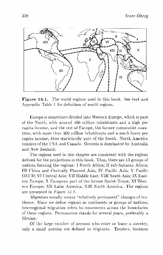
338 Sture Oberg

Figure 14.1. The world regions used in this book. See text andAppendix Table 1 for definition of world regions.

Europe is sometimes divided into Western Europe, which is partof the North, with around 400 million inhabitants and a high percapita income, and the rest of Europe, the former communist coun­tries, with more than 300 million inhabitants and a much lower percapita income, thus statistically part of the South. North Americaconsists ofthe USA and Canada. Oceania is dominated by Australiaand New Zealand.

The regions used in this chapter are consistent with the regionsdefined for the projections in this book. Thus, there are 13 groups ofnations forming the regions: I North Africa; II sub-Saharan Africa;III China and Centrally Planned Asia; IV Pacific Asia; V PacificOECD; VI Central Asia; VII Middle East; VIII South Asia; IX East­ern Europe; X Europea.n part of the former Soviet Union; XI West­ern Europe; XII Latin America; XIII North America. The regionsare presented in Figure 1>t.l.

NIigmtion usually means '"relatively permanent" changes of res­idence. Since we define regions as continents or groups of nations,interregional migration refers to movements across the boundariesof these regions. Permanence stands for several years, preferably alifetime.

Of the large number of persons who enter or leave a country,only a small portion are defined as migrants. Tourists, business

Factors in Future South-North Migration 339

executives, temporary workers, and asylum seekers trying to find anew home (Rogge, 1992) are usually not defined as migrants. Thisdefinition makes it easier to make a prognosis because the acceptedflows are statistically better known than the illegal and temporalones. Most of the discussion in this chapter uses a wider definitionof migrants, but the prognosis at the end of the chapter is onlyconcerned with migrants receiving permission to stay permanently,including those who later become citizens of the new country.

Citizenship is an individual's formal membership of a state.This is a purely legal definition that serves as the basis for a numberof rights and duties. The most important here is the legal right fora person to stay in the country where he or she is a citizen. Thereare also other aspects, like political and psychological ones, but theyare not considered here (see Reinans and Hammar, 1993).

14.2 Theories on International Migration

Today, migration is understood as a process of complexity and het­erogeneity. It can be analyzed from several perspectives and withindifferent conceptual frameworks or paradigms. Migration studiescan concentrate on individuals or structures, on micro or macro fac­tors. These studies consider a wide range of historical processes andcontemporary situations.

Migration concerns individuals, and thus it is a result of uniqueresponses to an actual, potential, or perceived understanding ofmany processes. It is partly a voluntary and partly a forced actioncontrolled not only by the migrant but also by others, including reg­ulating governments. With this complexity in mind, researchers stilltry to find regularities which could be used for theories or prognoses.Different scientific disciplines have specialized in different aspects onregularities or prevailing ideas behind migration processes.

The basic idea in the scientific literature on migration betweenless developed and more developed countries, South-North migra­tion, is that people should migrate North. This will equalize the cap­ital per worker ratio and thus increase efficiency and hence incomesand welfare. A majority of the population in the North will gainfrom migration (Simon, 1993). Industrialists are happy to employless-expensive labor. An increased snpply of labor would decrease

340 Sture Oberg

the wage level. Rich and well-educated people would also be bet­ter off if they could afford to employ housemaids and gardeners forLow wages. People in possession of real estate will earn money onincreased demand for housing.

Many people in the South would also gain. Migrants wouldbe better off in their new countries. They could help new migrantssettle in the North. They would probably send money home to theirrelatives in less developed countries. At present the remittances areabout $75 billion annually, substantially more than development aid.

The first ideas on international migration that were developedinto a theoretical framework are more than two centuries old. In astudy by Kryger (1764), a Swedish social scientist, causes of inter­national migration were discussed as well as how authorities couldinfluence the size of the flows. His idea was that migration cannotbe explained in simple words. Individual households could have sev­eral reasons for migrating, and the gross migration flows could haveseveral causes. At that time the academic disciplines were broaderand fewer than today, but Kryger's study could be labeled "appliedeconomics." As Sweden at that time was a poor country, he concen­trated his analysis on push factors, such as low wages in some sec­tors, unfair taxation, badly organized social-security systems, andlack of a well-functioning food distribution system. Several of thesefactors are still push factors in today's poor countries.

A little more than a century later, several researchers like Raven­stein (1885) in England and Rauchberg (1893) in Austria formu­lated theories on interregional migration that could be extendedto international migration. A French researcher (Lavasseur, 1885)discussed, as we often do today, "the increased facilities for commu­nication, and the multiplicity of the relations existing between thecountries of emigration and immigration" as two of the main factorsbehind migration.

An example of a summary of present knowledge on regularitiescan be found in Lee (1966). He deals with a prevailing set offactorsboth in the sending and in the potential receiving regions. Thesefactors could be positive, neutral, or negative. Added to them arepotential barriers to migration, "intervening obstacles," such as spa­tial and cultural distances between regions, costs of migration, or

Factors in Future South-North Migration 341

government restrictions. Bohning (1981) provides a more generaloverview. A recent survey of macro determinants of internationalmigration is given by Greenwood and McDowell (1992).

Today, economic theory is less applied than during Kryger'stime and thus further from actual socioeconomic processes. It isa scientific discipline with a hard and coherent theory, based on anumber of simplified assumptions about people and society. How­ever, several economists are struggling to develop theories that canbe applied to real world situations, like international migration (e.g.,Lucas, 1981; MacPhee and Hassan, 1990; Blanchard et ai., 1991).According to economic theory we could expect not only labor tomove North but also capital to move South. These activities wouldincrease the total production of goods and services. In a hypothet­ical future with only economic considerations, no restrictions oninternational migration, and no ethnic tension or social problems,the greatest economic efficiency would be attained by a very largeredistribution of the population.

In reality, economic theory cannot be used in this simplified way.Rather than calculating the flows necessary to achieve a theoreticallyefficient equilibrium, economic theory should be used to indicate thedirection of the flows - not only migrants but also capital and tradecommodities - and the marginal returns of these flows.

In geography, a more applied discipline, researchers on migra­tion have been concerned mainly with intranational migration, in­cluding urbanization. Strong theories, like the gravitation approachfrom the 1940s, could then be applied to make probable prognoseson migration flows. However, South-North migration is not onlydependent on factors such as distances, information flows, the sizeof populations, or the number of employment opportunities in dif­ferent regions. Legal restrictions in the rich countries prevent manyforeigners from entering. \Vith present trends, less than 1 percentof the population in the South will probably migrate to the Northbefore 2010.

The well-known mobility transition theory (Zelinsky, 1971),which sometimes is treated as a deterministic theory, tells us thatthere are historical phases, for exampIe, the demographic transi­tion, when movement is related to general processes of urbanization,

;342 Sture Oberg

industrialization, and modernization. It is, however, not self-evidenthow these ideas could be applied to South-North migration.

Political science can teach us about public institutions and pub­lic decision systems concerning, for example, the formation of im­migration policies (Kelley and Schmidt, 1979). Law can explain thebackground and practice of immigration rules. However, neitherdiscipline has a theory on international migration flows.

The geopolitical future of the world, studied by geographersand political scientists, is important, but there are no good theo­ries which could help us make forecasts. We know that the lackof congruence between ethnic settlements and political borders willcontinue to be a problem - it is a problem in several regions. Thepresent situation in Africa is shown in Figure 14.2. In Europe, astrong ethnic chauvinism not only created more than a dozen newnations in past years, but also caused "ethnic cleansing." Unwantedminorities have been either expelled from their settlements or killedin a systematic way. This type of geopolitics is currently takingplace in the former Yugoslavia.

Sociology can explain some of the flows. According to one the­ory (Hoffman-Nowotny, 1981), some flows have to do with the distri­bution of power and prestige in a social system. A typical migrantwould first live in a poor country with a specific status among friendsand neighbors, then migrate to a rich country where he or she wouldwork hard, accumulate savings, and finally move back to the poorcountry with the savings and with a higher status than before. Theattractive aspect of this theory is that it fits many movements be­tween South and North.

Demographers speculate less than other researchers. They wantclear assumptions and established methods. A typical study would,for instance, assume that 20,000 migrants with a specific ethnicbelonging and age and sex distribution settle permanently in Aus­tralia every year. The study would then make calculations on howthis flow would change the demographic structure of the Australianpopulation over time. Lutz and Prinz (1992), in their study on hy­pothetical migration flows from Eastern Europe to Western Europe,show that assimilation processes would soon reduce the number of"foreigners" in the West to very small numbers.

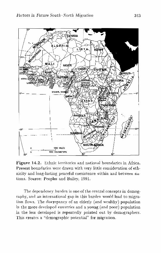
Factors in Future South-North Migration 343

0·-- _

2n •

,.y o·

o 1000 MILESI I

o 1000 KILOMETERS

20·--------\---------'"

Figure 14.2. Ethnic territories and national boundaries in Africa.Present boundaries were drawn with very little consideration of eth­nicity and long-lasting peaceful coexistence within and between na­tions. Source: Peoples and Bailey, 1991.

The dependency burden is one of the central concepts in demog­raphy, and an international gap in this burden would lead to migra­tion flows. The discrepancy of an elderly (and wealthy) populationin the more developed countries and a young (and poor) populationin the less developed is repeatedly pointed out by demographers.This creates a "demographic potential" for migration.

344 Sture Oberg

Demographers are also concerned with feedback and returnflows, as are scientists in other fields, such as geography and so­ciology. It is a well-known fact that small, pioneer flows of a newgroup of migrants into a region later generate larger flows. Firsta small group of new migrants is established in a new region. Ifthe members in this group are better off there than others are athome, they can receive friends or relatives and give them a base tostart from; these friends can in turn receive others, and so on. Afurther example of feedback effects is that a migration flow growsas agencies (formal and informal) are set up in the sending countryto help potential migrants by providing them with information andpractical assistance.

Another well- known fact is that migration flows in one directionwill later cause counterflows. An early reference with both ideas andempirical evidence on this statement regarding international migra­tion flows is Ravenstein (1885). For example, a large proportion ofthe immigrants, legal and illegal, to the USA from Mexico returnshome after a work season or a few years.

History is, of course, not only an academic discipline; it is alsothe empirical source of all applied social science. We understand theworld by observing it. By knowing more about past and present mi­gration flows it is hoped that we will be better prepared for expectedfuture flows. There have been many mass migration flows over longdistances. In the last century, Europeans migrated to North Amer­ica, South America, and Australia; Russians colonized parts of Asia;Chinese went South. The British, Ottoman, and, more recently, theRussian empires fell, resulting in large numbers of British, Turkish,and Russian settlers belonging to the ruling class migrating fromconquered territories. In recent decades, the Rio Grande and theMediterranean have become symbols of borders that are crossed bylarge numbers of migrants. Today, the need for foreign labor in theUSA, Europe, and the oil-producing countries is resulting in largeflows of labor migrants, staying for shorter or longer periods, someof them becoming citizens in their new countries.

Can these and other earlier movements tell us anything aboutthe future? Yes, they can teach us that a few thousand net migrantsper year add up to many millions over several decades. During the1970s and 1980s about 4 percent (net) of the Mexican population

Factors in Future South-North Migration 345

migrated to the USA. History also tell us that economic booms inthe North result in large labor flows in the future. Less comfortingis that history also tells us that several flows were not regarded asprobable before they became a fact. History, however, cannot tellus about future details; it can only provide probable patterns.

The main factors influencing historic and contemporary interna­tional migration are well known, and will continue to be important.There are many ways to label them. Economic factors include wagedifferences, different access to economic wealth, and material stan­dard of living. Social factors comprise proximity to relatives andfriends. Cultural factors, such as lifestyles and ethnicity, include so­cial organizations, religion, and values. Geopolitical factors concerntension or conflict, political instability, and threats to life. Environ­mental factors, such as the carrying capacity of land for inhabitantswith limited resources, cause large migration flows, especially whenthey are combined with geopolitical instability.

The causal links between these factors and the flows are gen­erally clear. For example, if everything else is equal, most peopleprefer higher wages, nearness to family, and religious freedom.

Migrants from the South usually go directly to the North, butsometimes they first migrate to another developing country beforecontinuing to an industrialized country. For example, ethnic Turksfrom the Balkan states often migrate to Turkey in a first move andthen to Western Europe. A study of such indirect internationalmigration to the United States was carried out by Greenwood andTrabka (1991).

14.3 Push Factors

The welfare gap between countries in the South and North, whichincludes factors such as a structural income gap or physical prox­imity, does not change easily over time. The income gap betweenEastern Europe and Western Europe or between North America andSouth America will not disappear before the year 2020 (Oberg andBoubnova, 1993). Also even with unrealistically large investmentsin the South (for example, 50 percent), it may still take a long timeto reduce this gap. If present policies continue, the gap could evenbe larger in the future than it is today. There are more dollars

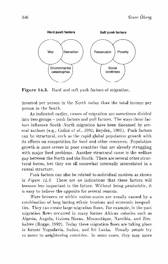
346

Hard push factors Soft push factors

Sture Oberg

Figure 14.3. Hard and soft push factors of migration.

invested per person in the North today than the total income perperson in the South.

As indicated earlier, causes of migration are sometimes dividedinto two groups - push factors and pull factors. The ways these fac­tors influence South-North migration have been discussed by sev­eral authors (e.g., Golini et al., 1991; Heyden, 1991). Push factorscan be structural, such as the rapid global population growth withits effects on competition for food and other resources. Populationgrowth is most severe in poor countries that are already strugglingwith major food problems. Another structural cause is the welfaregap between the North and the South. There are several other struc­tural forces, but they are aU somewhat internally interrelated in acausal structure.

Push factors can also be related to individual motives as shownin Figure 14.8. There are no indications that these factors willbecome less important in the future. Vlithout being pessimistic, itis easy to believe the opposite for several reasons.

Wars between or within nation-states are usually caused by acombination of long-lasting ethnic tensions and economic inequali­ties. They can create large migration flows. For example, in the pastmigration flows occurred in many former African colonies such asAlgeria, Angola, Guinea-Bissau, Mozambique, Namibia, and Zim­babwe (Rogge, 1992). Today these migration flows are taking placein former Yugoslavia, Sudan, and Sri Lanka. Usually people tryto move to neighboring countries. In some cases, they may move

Factors in Future South-North Migration 347

to distant places if relatives and friends are already located there.Indonesians migrated to the Netherlands, Armenians to the USA,and Croats to Sweden. War between nations usually occurs where ithas occurred before, where ethnic hate exists, and where the socialsystems are under too loose control (anarchy) or too strict control(dictatorship) .

In some parts of Africa, the Balkan area, and Southeast Asia,the risk of war in the coming decades is high. Countries like SouthAfrica and Israel have more tension in relations to their neighborsthan Switzerland or Canada, and thus the risk for future war ishigher in the former countries. However, higher risks do not forecastfuture outcome. Peace can come unexpectedly in some areas; andtension can rise fast in peaceful regions.

Persecution exists in many parts of the world, such as in Sudan,Myanmar, former Yugoslavia, and El Salvador. Ethnic tension leadsto murder in war times and persecution in peace times. It willcontinue to be a problem in most parts of the world in the comingdecade. Africa may see more of this problem than other parts of theworld in the near future.

Starvation with high mortality is already prevalent in manycountries (Dreze and Sen, 1989). In most African countries theconsumption of calories has decreased in the last decade: 35 out of47 countries were worse off in 1989 than in 1980, according to FAGstatistics. The worst decline was in sub-Saharan countries like An­gola, Botswana, Gabon, Mozambique, and Rwanda. Starvation inthe future is more probable in poor countries with a small domesticfood production or in nondemocratic nations, since "no democraticcountry with a relatively free press has ever experienced a majorfamine" (Sen, 1993). Starvation is also more probable in countrieswith ethnic/political tension since it is a weapon that can be usedto hurt enemies, for example, in the Ukraine in the 1930s, Biafrain the 1960s, and southern Sudan in the 1990s. Areas with currentlow income, high debts, and low food consumption are shown inFigure 14.4.

Poverty is probably the largest single factor behind current andfuture migration flows. According to one estimation from the UN(1993b), 100 million migrants have left their home countries be­cause of poverty. It is of course hard to define poverty gaps, but

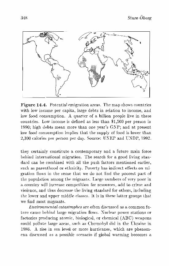
348 Sture Oberg

tJ

Figure 14.4. Potential emigration areas. The map shows countrieswith low income per capita, large debts in relation to income, andlow food consumption. A quarter of a billion people live in thesecountries. Low income is defined as less than $1,500 per person in1990; high debts mean more than one year's GNP; and at presentlow food consumption implies that the supply of food is lower than2,300 calories per person per day. Source: UNEP and UNDP, 1992.

they certainly constitute a contemporary and a future main forcebehind international migration. The search for a good living stan­dard can be combined with all the push factors mentioned earlier,such as parenthood or ethnicity. Poverty has indirect effects on mi­gration flows in the sense that we do not find the poorest part ofthe population among the migrants. Large numbers of very poor ina, country will increase competition for resources, add to crime andviolence, and thus decrease the living standard for others, includingthe lower and upper middle classes. It is in these latter groups thatwe find most migrants.

Environmental catastrophes are often discussed as a common fu­ture cause behind large migration flows. Nuclear power stations orfactories producing atomic, biological, or chemical (ABC) weaponscould pollute large areas, such as Chernobyl did in the Ukraine in1986. A rise in sea level or more hurricanes, which are phenom­ena discussed as a possible scenario if global warming becomes a

Factors in Future South-North Migration 349

reality, will create floods in lowlands in many countries. With lessozone protection in the atmosphere, large areas will be uninhabit­able. For the moment there are no good prognoses of where futureenvironmental catastrophes are likely to occur. Most environmentalcatastrophes have occurred in developing countries. Drought, floods,soil erosion, and desertification are widespread, recurrent problems.According to a 1992 report by the International Organization forMigration, environmental migration will be caused by the follow­ing disruptions: elemental, biological, slow-onset accidents; devel­opment factors; and finally, environmental warfare. Each categorycovers a spectrum of disruptions ranging from mild to catastrophic.For an excellent overview of the literature on links between environ­mental degradation and migration see Suhrke (1993).

Social loneliness is a problem of much less general importancethan others mentioned here. Furthermore, it will be a problem onlyfor a very small minority in the South, such as some parents withchildren in the North. However, this small group can be a sub­stantial proportion of the migrants going North, since they are usu­ally allowed to move to their close relatives (Jasso and Rosenzweig,1986).

Summarizing the short discussion of push factors is easy. Theyare overwhelming and will probably change the world in many ways.We may be facing an unrecognizable world in the year 2020 withmigration flows of the sa.me magnitude as during the last centurywhen Europeans flooded other parts of the world.

The North will be affected in a.n unforeseeable way, especiallyif the future flows are determined by the supply of emigrants in theSouth instead of, as today, by the demand for immigrants in theNorth. However, a large part of these international flows will con­tinue to be between neighboring countries in the South. A large partwill also be refugees who will not be allowed to stay permanentlyor temporary workers; neither group is defined as migrants in thischapter.

The basic assumption in this chapter is that changes are not veryspectacular. Restrictions placed by countries in the North will regu­late future immigration. Future changes in restrictions are assumedto be mainly influenced by present attitudes toward strangers, atti­tudes that will not change during one generation.

350

,.----f--- Demafor latin the

Dema

------ --- for latr---.--in the

Sture Oberg

ndorNorth

ndorSouth

t1 t2 t3 t4 ts t6

Figure 14.5. The gap between demand for cheap labor in theNorth and the South is so large that minor changes in the demandonly influence migration flows indirectly through policy formation.

14.4 Pull Factors

The distinction between push and pull factors is usually unclearfrom a scientific point of view. Wealth can be a pull factor in theNorth, attracting migrants from less wealthy countries, but this phe­nomenon could also be described as a push factor, lack of wealth,in the South. With this in mind. caution must be taken when pushand pull concepts are under study.

From a technical point of view, it is difficult to distinguish be­tween the importance of push and pull factors in relation to South­North migration. The gap between indicators such as salary, secu­rity, and demand for cheap labor is usually so large between theSou th and the North that changes in either the push or pull factoronly marginally affect it.

Also, theoretically a distinction is combined with severe prob­lems. A larger flow of migrants during a period of low demand inpoor countries could be dependent either on the low demand duringthe period, in which case it is a push factor, or on a delayed responseto an earlier situation with a high demand in the rich countries, inwhich case it is a pull factor (see Figure 14.5). Thus, not only

Factors in Future South-North Migration 3.51

can data be selected in different ways, but the same informationcan also be interpreted in many ways. Concerning, for example,the early migration flows between Sweden and the United States,Wilkinson (1967) states that they were mainly determined by labordemand in the USA, while Thomas (1941) reports that the economicconditions in Sweden were more important. Quigley (1972) showsthat conditions in both the sending country and the receiving coun­try were important. An overview of these and other empiricallybased studies on patterns and dynamics of push and pull factorscan be found in Greenwood and McDowell (1992). The most suc­cessful studies of international migration are theoretically weak butempirically strong.

Models of rnigration are specific to the relative importance ofpush or pull factors. Depending on which theory a researcher uses,he or she is restricted to specific mathematical tools. Each modelingtechnique emphasizes either push or pull factors. For example, aMarkov model "pushes" migrants between time steps in the futuredepending on earlier trends. An overview on how different methodsrely on push or pull ideas can be found in the geographic literature(Alonso, 1974).

In the literature, pull factors are expressed in terms of gaps.A high demand for labor with a corresponding high salary levelis related to the wage gap between countries. Pull factors of thiskind are difficult to trace in em pirical figures because the gap isso enormous that it is not theoretically sound to relate marginalchanges directly to migration flows.

It would be better to relate pull factors indirectly to migra­tion flows through the formation and implementation of immigra­tion policies in the North. According to this idea, there is alwaysa long-lasting, large structural welfare gap between the North andthe South. The average income on one side of a geographical bordercan be more than 2000 percent higher than on the other side - forexample, along the northern ~vIexican border or along the easternFinnish border. An increase in the wage level of a few percent­ages on either side of the border does not change the gap as such.However, in some situations, pull factors in the North, such as ashortage of labor, could make it easier for the people in the Northto accept immigrants. Policies could change and migration flows

352 Sture Oberg

could increase. This view makes the distinction between push andpull factors instrumental in studies of South-North migration.

Related to this idea is the concept of migration pressure. Thiscommonly used expression roughly means unrealized migration de­sires. The migration pressure from the South thus increases eitherif fewer people are allowed to migrate through a more restrictivepolicy or if a larger proportion of the population in the South wouldlike to move North.

Pull factors that could change migration policies are relatedto economic and humanitarian ideas. Economic considerations arestronger than humanitarian factors. If influential actors in the Northcould earn money on immigration, this would probably be the mostimportant pull factor. A few can always gain - farmers in Californiaor fishermen in Sicily - but they must be supported by other groups,usually more than half of the population in democracies.

Looking ahead, there are different opinions on the future de­mand of labor in the North. One extreme argument is that therewill not be a future need for more immigrants. The demand forlabor has changed structurally in recent decades. In the future fewlaborers will be employed in modern agriculture in the North, yetthis sector will produce more food than ever. Furthermore, therewill not be a future need for industrial workers in the North. Thisis not only because of the increasing competition from the newlyindustrializing countries but also because of new technologies in theproduction system. More investments in industry and its produc­tivity will only decrease demand for employees. Robots and com­puters will run machines in some rich countries. For example, in theNetherlands, only three workers out of ten in the labor market arein farming or in industry.

A further argument for why there is no need for immigration isthat even with a future demand for labor in a booming economy,many millions of homemakers in the North can enter the labor mar­ket. Today, the low labor-market participation in southern Europe,for example, functions as a reserve supply of labor.

The opposite argument is that the demand for labor in the Northwill increase as a function of income, not as a function of demand forlabor in agriculture and industry. Service employment must also beincluded in the analysis. For example, many rich old people in the

Factors in Future South-North Migration 353

North will need help in the future, but a shortage of people willingto care for them has been projected. The shortage is due partly to anew demographic situation, with a decrease in working-age groups,and partly to the fact that it is difficult to recruit people living inthe North for jobs with a low status.

The humanitarian rationale for accepting refugees as immi­grants has been quite strong, and will probably maintain its strengthin the future. A tendency to decrease its influence on migration isthe argument that more refugees could get help for the same amountof money if they did not have to migrate to the North. Temporaryrefugee camps in the South will probably be more common in thefuture. Another tendency is that attitudes toward immigration arechanging slowly. Right-wing political parties tend to try to promotepolicies that result in fewer migrants (Vandermotten and Vanlaer,1993; Fielding, 1993). It is hard to see how the humanitarian pullfactor can change policies so that more migrants will be accepted inthe future. Yet, if a change in attitudes occurs, it could influenceimmigration much more than changes in the labor market.

14.5 Policies

In this chapter, the most important factor for future permanent im­migration flows to the developed countries is assumed to be attitudestoward foreigners within the receiving countries. These attitudesdetermine regulation policies in the North. Ethnicity in a broadsense plays an important part in this context. Feelings of superior­ity among rich majority groups in the North or of hate or fear ofpotential immigrant groups belonging to other ethnic groups causedecreases in future flows. Native ethnic Estonians are afraid of largeflows from Russia. Ethnicity also plays an important role when in­ternal flows in the South are determined. Muslims in Pakistan arenot interested in large flows of Hindus from India.

Since there is no comparative study of this sensitive issue onfeelings on ethnicity and attitudes toward other ethnic groups, thecurrent international discussion among researchers is based on acombination of nonsystematic interviews with colleagues from dif­ferent countries, official policies, and statistics on actual permissionsfor foreigners to obtain citizenship. According to this soft approach,

354 Sture Oberg

Japan, the oil-rich Muslim countries, and Australia will be hesitantto accept immigrants from other cultures; North America will wel­come large streams; and Western Europe will hold a position inbetween these two.

Within Western Europe, current practice varies: Sweden ac­cepted one non-European asylum seeker for every 80 inhabitantsduring the 1980s; Finland accepted almost no non-European immi­grants. On average, there are large migration flows within Europebut very limited immigration from other parts of the world.

However, small labor flows from neighboring regions continue.For example, in Germany, Belgium, and the Netherlands, the Turk­ish population increased from 1.6 million to 1.8 million between 1985and 1988. During the same period, the number of Algerians, Mo­roccans, and Tunisians living in those countries rose from 330,000to 370,000 (UN, 1992a:179). The majority of the labor migrantsare legal. Most of the illega.! migrants are now in Italy. There areseveral estimates on the number of illegal migrants, but most giveestimates of about 1 million (Montanari and Cortese, 1993).

In the past the immigration policy in Western Europe variedfrom country to country, but a more coherent policy is now emerg­ing (Widgren, 1992). Five countries (Germany, France, the Nether­lands, Belgium, and Luxembourg) have signed an agreement to har­monize immigration. This group of countries, the Schengen group,will directly or indirectly influence other countries to adjust theirpolicies in the same direction. Europeans are very restrictive tonon-European immigrants. On average, around 1 percent of thepopulation are non-Europeans. France, the UK, Germany, Sweden,and Belgium have higher figures.

Within the former USSR, which comprises a European part (theBaltic states, Russia, Ukraine, Belarus, and Moldova) and an Asianpart (including Georgia, Armenia, Azerbaijan, and Kazakhstan),there are now flows from Asia to Europe. Ethnic Russians migrateto Europe from territories where they used to belong to a ruling mi­nority, or where they were working for high salaries as compensationfor poor working conditions. The same is true for ethnic Ukrainiansand Belarussians (Oberg and Boubnova, 1993).

The two countries in the North American region are of spe­cial interest in this chapter since they have traditionally accepted

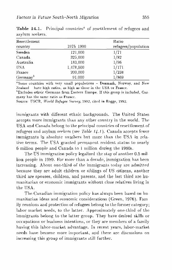
Factors in Future South-North Migration 355

Table 14.1. Principal countriesa of resettlement of refugees andasylum seekers.

ResettlementcountrySwedenCanadaAustraliaUSAFranceGermanyb

1975-1990

121,000325,000183,000

1,478,000200,00091,000

Ratiorefugees/population

1/711/821/961/1711/2381/869

aSome countries with very small populations - Denmark, Norway, and NewZealand - have high ratios, as high as those in the USA or France.bExcludes ethnic Germans from Eastern Europe. If this group is included, Ger­many has the same ratio as France.Source: USeR, World Refugee Survey, 1992, cited in Rogge, 1992.

immigrants with different ethnic backgrounds. The United Statesaccepts more immigrants than any other country in the world. The·USA and Canada belong to the principal countries of resettlement ofrefugees and asylum seekers (see Table 14.1). Canada accepts fewerimmigrants in absolute numbers but more than the USA in rela­tive terms. The USA granted permanent resident status to nearly6 million people and Canada to 1 million during the 1980s.

The US immigration policy legalized the stay of another 0.5 mil­lion people in 1989. For more than a decade, immigration has beenincreasing. About one-third of the immigrants today are admittedbecause they are adult children or siblings of US citizens, anotherthird are spouses, children, and parents, and the last third are hu­manitarian or economic immigrants without close relatives living inthe USA.

The Canadian immigration policy has always been based on hu­manitarian ideas and economic considerations (Green, 1976). Fam­ily reunions and protection of refugees belong to the former category;labor-market needs, to the latter. Approximately one-third of theimmigrants belong to the latter group. They have desired skills oroccupations or business intentions, or they are members of a familyhaving this labor-market advantage. In recent years, labor-marketneeds have become more important, and there are discussions onincreasing this group of immigrants still further.

356 Sture Oberg

The majority of the population in Oceania lives in Australia andNew Zealand. Australia admitted about 0.8 million immigrants fromcountries outside Oceania during the 1980s. New Zealand, a countrywith net emigration, admitted less than half in relative terms, whichis approximately one-tenth in absolute numbers. Roughly every fifthperson moving to Australia was skilled and defined as a "businessmigrant." Every tenth (between 1986 and 1989) was a refugee or aperson admitted under the Special Humanitarian Program.

Japan is a rich country with a demand for foreign labor. Itis by tradition a closed society. However, its strong and successfuleconomy has increased the demand for labor within the country toa degree where legal and illegal imports become a factor. The le­gal workers are mainly women entertaining Japanese men, 71,000 in1988 (UN, 1992a). The unregistered, illegal workers are increasingin numbers but are still less than 1 percent of the labor force (Shah,1992). Thus there are some foreigners working in Japan, but theyseldom get permission to settle in the country. A reasonable guess isthat present attitudes toward non-Japanese will not change withinone generation. The result could then be a large number of tempo­rary guests or guest workers employed in Japan but not allowed tobe citizens.

The rich oil-producing countries, especially in West Asia, willprobably use the same strategy; they will continue their policy toallow workers to stay in the country on temporary jobs but willnot allow foreigners to become citizens. Today, they accept largenumbers (perhaps 2 or 3 million) of foreign workers: people of Araborigin (e.g., Egyptians, Palestinians, and Jordanians), people fromcountries in South Asia (e.g., India, Pakistan, and Bangladesh),and people from Southeast Asia (e.g., the Philippines, Republic ofKorea, and Thailand). By 1985, it was estimated that 63 percent ofall workers in the six Gulf States (Bahrain, Kuwait, Oman, Qatar,Saudi Arabia, and the United Arab Emirates) were from South orSoutheast Asia (Shah, 1992). Since these workers are not allowed tobe citizens in West Asian countries, they are all temporary visitorsand are not treated as (permanent) immigrants in this chapter. Theassumption is that even in the coming decades, very few people willbe allowed to become permanent immigrants to this rich part of theworld.

Factors in Future South-North Migration 357

Hong Kong, which is a part of China in this book (and willformally be a part of China as of July 1997), has an unpredictablefuture. Many inhabitants have already moved to other countries.The UK says that it will no longer accept the inhabitants as privi­leged members of the Commonwealth, except for 50,000 people withtheir families. China will, according to a probable scenario, becomemore integrated with the economy of the rest of the world in thecoming decades. This event could result in larger migration flowsto North America where there is a positive attitude toward immi­grants from Asia. Also, Australia could be affected demographicallyby more intense economic cooperation with China.

The attitudes toward immigration in the rich countries are gen­erally in favor of strong regulations and limitations on the numbersallowed to enter. The attitudes vary from a more generous NorthAmerica to a restrictive Japan. Australia is similar to North Amer­ica, but has clear ethnic priorities. Europe is, on average, closer toJapan, but some individual countries are exceptions.

The discussion of attitudes is mainly based on knowledge fromhistoric and current situations. Attitudes toward future immigrantsare based 011 attitudes toward immigrants today. These attitudesare already known indirectly through the size of contemporary mi­gration flows. Previous migration flows between South and North,to a large extent, determine future flows. There are at least threereasons for this. First, an existing flow tells us that the receiving richcountry accepts immigrants. Second, earlier immigrants, now livingin the North, with social contacts to people in the South, make iteasier for potential migrants to realize their wishes and thus becomenew immigrants. Large proportions of present immigrants are re­lated to earlier immigrants. For example, more than one-third ofthe immigrant flow to the USA consists of close relatives of US citi­zens (spouses, children, and parents). Third, if many immigrants ofone ethnic background move to a country with a democratic society,they become a political force because they have many votes, haveeconomic power, and can organize lobbies. The Hispanic part of theUS population is a good example of an immigrant group reachingthe point of being able to exercise political power.

More detailed figures on assumed future migration streams be­tween the world regions are discussed in Chapters 15 and 16.

Part VI

Projections

This concluding section translates the substantive considerationsgiven in Parts II through V into alternative population projections.This exercise is done for 13 world regions over the 1995-2100 period.

The central scenario describes the most likely future populationpath under our assumptions. This scenario results in a world popu­lation of 7.88 billion in 2020, 9.87 billion in 2050, and 10.35 billionin 2100. These findings a,re remarkably close to the medium variantprojections of the United Nations.

The systematic combinations of the three values (low, central,and high) for all three demographic components (fertility, mortality,and migration) result in 27 scenarios. These scenarios provide abroad range of possible future population trends. However, threefindings hold across all scenarios:

• The world population will grow substantially.• The world population will become older.• The proportion ofthe population in today's developing countries

will continue to increase.

The fully probabilistic projections contribute additional infor­mation. For example, given our assumptions there is a 64 percentchance (i.e., roughly two-thirds) that the current world populationwill never again double in the future - that is, it will not reach the11.5 billion mark (which is twice the present level of 5.75 billion).

Chapter 15

"World Population Scenariosfor the 21st Century

Wolfgang Lutz) Warren Sanderson, Sergei Scherbov,Anne Coujon

The previous chapters provide expert views on fertility, mortality,and migration. This chapter presents a synthesis of the expert viewsand, based on this synthesis, two sets of alternative scenario projec­tions: one set in which the fertility, mortality, and migration compo­nents are assumed to be deterministic, independent of one another,and not subjected to any feedbacks; and another set in which cer­tain consistent "stories" are defined and the components interactand react to certain outcomes of the projections such as populationgrowth and aging. These two sets correspond to the two differentmeanings of "scenario" used in population projections (as discussedin Section 2.6). In Section 15.2 all possible combinations of the high,central, and low assumptions in fertility, mortality, and migrationare presented. Section 15.3 provides three examples of interactionscenanos.

15.1 Synthesis of Expert Views on FutureFertility, Mortality, and Migration

A complex process led to our specifications of low, central, and highvalues for the three components in each of the 13 regions definedin this book. A basic outline of the process is given in Chapter 2,and more details can be found in Lutz (1995a). One feature of

361

362 W. Lutz, W. Sanderson, S. Scherbov, A. Goujon

this exercise is that the experts only agreed to define alternativetrends up to the period 2030-203.5. For every world region and foreach component they assumed three values: high, central, and lowvalues. To limit the possible number of choices the central value wasdetermined to be the mean of the high and low extremes; roughly90 percent of all possible future cases were to be included in therange between these two extremes. Extensions of the assumptionsbeyond 2030-2035, as well as the specification of the exact pathbetween the current level and the level to be reached by 2030-2035,are defined in Section 15.2. In this section we present a synthesis ofthe reasoning that led to the low, central, and high values assumedfor 2030-2035 and listed in Tables 15.1 to 15.3.

15.1.1 Future fertility

Assumptions about the future course offertility may be derived fromseveral sources of information. First, past trends may be analyzedto assess the status of individual countries and regions in the processof demographic transition. Chapter 3 presents an assessment of thistype on today's developing countries. This assessment was a majorguideline in making specific assumptions for individual regions underthe basic premise that the fertility transition that has started almosteverywhere will essentially continue. While low values assume arapid pace in the continuation of the fertility transition, the highvalues assume a much slower pace, in some cases even a stagnation,of the declining trend. In parts of Asia this even implies increasingfertility.

For the near future the intentions expressed by women in repre­sentative surveys can be taken as an additional important piece ofevidence. Chapter 4 analyzes this information for a number of coun­tries. Sub-Saharan Africa has, by far, the highest fertility levels andthe lowest levels of contraceptive prevalence, but in all countries inthis region the desired fertility rates, which have been derived fromsurveys, are clearly lower than actual levels - for example, in Kenyaby almost two children. This fact, together with indications of in­creasing contraceptive prevalence, leads to the expectation of signifi­cant fertility declines in the next decade, even in sub-Saharan Africawhich until recently has shown constant high fertility. In North

World Population Scenarios for the 21st Century 363

Africa the fertility transition is already much further advanced, andmore than one-third of the female population uses contraceptives.Desired fertility rates in this region indicate that further significantfertility declines are to be expected unless dramatic events, such asa rise in pronatalist fundamentalism, change the pattern.

The three Asian countries considered in Chapter 4, Indonesia,Sri Lanka, and Thailand, already have total fertility levels below 3.0with further declines expected. Latin America has an intermediateposition comparable with that in North Africa. A noteworthy fea­ture of this region is that over recent decades fertility was ratherstagnant at this intermediate level, but the most recent evidenceindicates further decline.

In the long run, without doubt, the general socioeconomic andcultural changes will determine fertility levels. But these trends areby no means easier to forecast than the path offertility change itself.One more specific aspect in this context is the role of governmentpolicies and family-planning programs. As pointed out in Chap­ter 5, experience with such programs has shown that, over severaldecades, they can have an important effect if they are well integratedinto other government policies and particularly if the socioeconomicdevelopment of the population has reached a point at which limi­tation of family size is considered advantageous and a real optionby sizable segments of the population. Since many countries havebeen adopting such programs, they may well accelerate the fertilitydecline.

In terms of specific numerical assumptions, the high value in2030-2035 was assumed to be lower than the current fertility levelfor all developing regions except East and Central Asia. This is dueto the overwhelming evidence of a continuation of the demographictransition process in parts of the world that still have high fertil­ity. For this reason no constant fertility scenario was specified (asdone by the UN, 1994b). However, the high values do not assumea smooth fertility transition but rather an interruption or at leastretardation of the process. This could be due to setbacks in so­cioeconomic development, cultural or religious movements such as arise of fundamentalism, or strong heterogeneity with pre- and post­transitional populations living together in one region. The low val­ues indicate a very rapid fertility decline that does not stop at 2.1 but

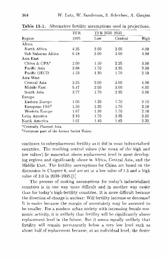
364 W. Lutz, W. Sanderson, S. Scherbov, A. Goujon

Table 15.!. Alternative fertility assumptions used in projections.

TFR TFR 2030-2035

Region 1995 Low Central HighAfrica

North Africa 4.35 2.00 3.00 4.00Sub-Saharan Africa 6.18 2.00 3.00 4.00

Asia-EastChina & CPAa 2.00 1.50 2.25 3.00Pacific Asia 2.88 1.70 2.35 3.00Pacific OECD 1.53 1.30 1.70 2.10

Asia-WestCentral Asia 3.35 2.00 3.00 4.00Middle East 5.47 2.00 3.00 4.00South Asia 3.77 1.70 2.35 3.00

EuropeEastern Europe U;6 1.30 1.70 2.10European FSUb 1.50 1.30 1.70 2.10Western Europe 1.67 1.30 1.70 2.10

Latin America 3.10 1.70 2.35 3.00North America 1.97 1.40 1.85 2.30

aCentrally Planned Asia.bEuropean part of the former Soviet Union.

continues to sub replacement fertility as it did in most industrializedcountries. The resulting central values (the mean of the high andlow values) lie somewhat above replacement level in most develop­ing regions and significantly above in Africa, Central Asia, and theMiddle East. The fertility assumptions for China are based on thediscussion in Chapter 6, and are set at a low value of 1.5 and a highvalue of 3.0 in 2030-2035.[1]

The process of making assumptions for today's industrializedcountries is in one way more difficult and in another way easierthan for today's high-fertility countries. It is more difficult becausethe direction of change is unclear: Will fertility increase or decrease?It is easier because the margin of uncertainty may be assumed tobe smaller. For a modern urban society with increasing female eco­nomic activity, it is unlikely that fertility will be significantly abovereplacement level in the future. But it seems equally unlikely thatfertility will remain permanently below a very low level such asabout half of replacement because, at an individual level, the desire

World Population Scenarios for the 21st Century 365

for children seems to be deeply rooted in women and men and, at asocietal level, very rapid population aging results in serious problems(see deliberations in Chapter 11).

Until a few years ago, the United Nations and other institu­tions preparing population forecasts assumed that fertility wouldincrease to replacement level and that subreplacement fertility wasonly a transitory phenomenon. This assumption is supported by theargument of homeostasis as discussed in Chapter 11. In this view,fertility levels are not seen as the sum of individual behavior, but asone aspect of the evolution of a system in which individual behavioris a function of the status of the system (see Vishnevsky, 1991). Un­der such a systems approach the assumption of replacement fertilityin the long run seems a defendable possibility. Therefore, we as­sumed a TFR between 2.1 and 2.3 in 2030-2035 as the high-fertilityassumption in the five industrialized regions.

It is difficult, however, to find many researchers who supportthis view. Too much evidence points toward low fertility. The returnto replacement fertility has been criticized as an assumed magneticforce without empirical support (Westoff, 1991). Many significantarguments support an assumption of further declining fertility lev­els. They range from the weakening of the family in terms of bothdeclining marriage rates and high divorce rates, to the increasing in­dependence and career orientation of women, and to a value changetoward materialism and consumerism.

These factors, together with increasing demands and personalexpectations for attention, time, and also money to be given tochildren, are likely to result in fewer couples having more than oneor two children and an increasing number of childless women. Also,the proportion of unplanned pregnancies is still high, and futureimprovements in contraceptive methods are possible.

In conclusion one can say that the bulk of evidence suggeststhat fertility will remain low or further decline in today's industri­alized societies. How far it will decline is not clear at this time. Theexpert group decided to settle for a TFR of 1.3 as the low value tobe reached by 2030-2035. This value is below the low-fertility as­sumptions in some other projections, but it is far from being impos­sible. Actually several populations have already experienced suchlevels for extended periods. Taking into account the different ethnic

366 VV. Lutz, W. Sanderson, S. Scherbov, A. Goujon

composition in North America, the fertility range in this region waschosen to be slightly higher (104 to 2.3) than in Europe and Japan.

15.1.2 Future mortality

Mortality conditions at one point in time can be conveniently sum­marized by period life expectancy at birth, an indicator that resultsfrom a life table based on all age-specific mortality rates observed atthat time. In this section, this indicator is used to define martali tyassumptions.[2]

The uncertainties about future improvements or possible de­clines in life expectancy in today's high-mortality countries differfrom those in low-mortality countries. With the exception of East­ern Europe, the latter countries have seen impressive increases inlife expectancy and segments of their populations are approachingages that were once considered a biological upper limit to the humanlife span. Hence assumptions about future improvements cruciallydepend on whether such a limit exists and will soon be reached (seeChapter 12; Manton, 1991). In regions that still have very low lifeexpectancy, this question is irrelevant, and future mortality condi­tions will be determined by the efficiency of local health services,the spread of traditional (e.g., malaria) and new (AIDS) diseases,and the general level of subsistence.

Currently, life expectancy at a national level is highest in Japan:82.5 years for women and 76.3 years for men. Only 30 years ago in1960-1964, female life expectancy was 71. 7 and male life expectancywas 66.6, implying an average increase of more than 3.5 years perdecade for women. Eastern Europe, on the other hand, had thesame life expectancy as Japan during the early 1960s but has hadalmost no improvement since then, bringing it to only 67.3 for menand 75 for women at present. During the 1980s the Soviet Unioneven experienced a decline in male life expectancy, and current esti­mates for Russia are as low as 59 years. Western Europe and NorthAmerica took an intermediate position; life expectancy increasedsteadily by about two to three years per decade. The recent trendclearly points toward further improvements, and the analysis of age­and cause-specific mortality trends does not give any indications ofimprovements leveling off (Valkonen, 1991). Also studies of occu­pational mortality differentials in the Nordic countries - which are

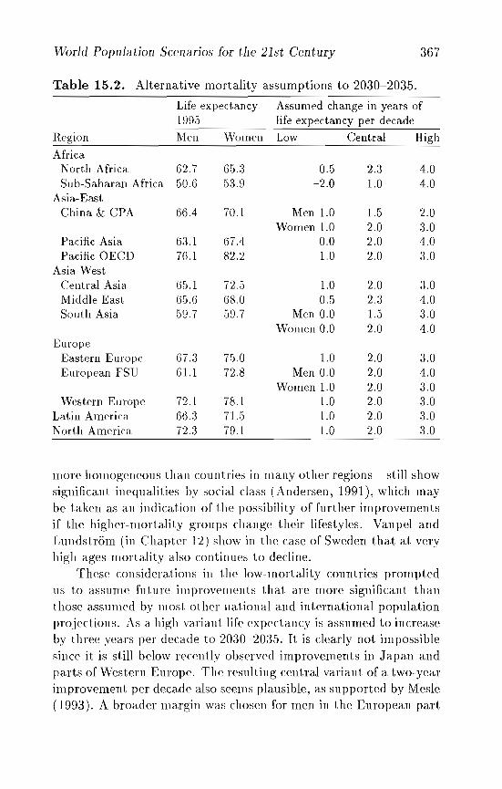
World Population Scenarios for tlle 21st Century 367

Table 15.2. Alternative mortality assumptions to 2030-203.5.

Life expectancy Assumed change in years of1995 life expectancy per decade

Region Men 'Women Low Cent.ral High

AfricaNort.h Africa 62.7 65.3 0.5 2.3 4.0Sub-Saharan Africa 50.6 53.9 -2.0 1.0 4.0

Asia-EastChina & CPA 66.4 70.1 Men 1.0 1.5 2.0

Women 1.0 2.0 3.0Pacific Asia 63.1 67.4 0.0 2.0 4.0Pacific OECD 76.1 82.2 1.0 2.0 3.0

Asia-West.Cent.ral Asia 65.1 72.5 1.0 2.0 3.0Middle East 65.6 68.0 0.5 2.3 4.0South Asia 59.7 59.7 Men 0.0 1.5 3.0

Women 0.0 2.0 4.0Europe

East.ern Europe 67.3 75.0 1.0 2.0 3.0European FSU 61.1 72.8 Men 0.0 2.0 4.0

Women 1.0 2.0 3.0West.ern Europe 72.1 78.1 1.0 2.0 3.0

Latin America 66.3 71.5 1.0 2.0 3.0North America 72.:3 79.1 1.0 2.0 3.0

more homogeneous than countries in many other regions - still showsignificant inequalities by social class (Andersen, 1991), which maybe taken as an indication of the possibility of further improvementsif the higher-mortality groups change their lifestyles. Vaupel andLundstrom (in Chapter 12) show in the case of Sweden that at veryhigh ages mortality also continues to decline.

These considerations in the low-mortality countries promptedus to assume future improvements that are more significant thanthose assumed by most other national and international populationprojections. As a high variant life expectancy is assumed to increaseby three years per decade to 2030-2035. It is clearly not impossiblesince it is still below recently observed improvements in Japan andparts of Western Europe. The resulting central variant of a two-yearimprovement per decade also seems plausible, as supported by Mesle(1993). A broader margin was chosen for men in the European part

368 W. LlItz, W. Sanderson, S. Scherbov, A. GOlljon

of the former USSR because of greater uncertainties: assuming acontinuation of bad conditions, the low value was set at zero years;the upper value was fixed at 4.0 because of the potential that lifeexpectancy will greatly improve if the lifestyles in the region becomesimilar to the Western patterns.

Health conditions in the developing regions have generally ex­perienced very impressive improvements since World War II. Lifeexpectancy in all developing countries has increased by more than 20years since 1950-19.55, when it was estimated to be about 40 yearsfor both men and women. Some regions, such as East and West Asia,have experienced especially rapid increases. Latin America, whichalready had higher life expectancies during the 1950s, has achievedlower mortality levels than Africa and Asia. In the Caribbean, themortality decline is particularly impressive.

These rapid improvements in mortality have led institutionsthat produce population projections to regularly change their as­sumptions. The UN raised the life expectancy limit for men from72.6 years, assumed in 1973, in steps to 82.5 years, assumed in 1988.Similar adjustments were made for women (see Chapter 7).

Africa has the greatest mortality uncertainties of all regions. InChapter 8, Garenne concludes his survey of African mortality bypointing out that past trends in Africa have been induced by tech­nology transfers from the West, which affected virtually all coun­tries in a short period of time. Public health, nutrition, economicdevelopment, and modern education were the key determinants ofmortality decline. There are reasons for assuming that this decliningtrend of the past 30 years will not continue in Africa, and that dif­ferences between countries will prevail or even increase: one reasonis that infectious diseases, especially the HIV virus, may spread fur­ther; another is that problems of basic subsistence and food supplymay continue (see Chapter 10). In Chapter 9, Bongaarts presents anew calculation of the possible impact of AIDS on mortality. Trans­lated into life expectancies and projected further into the future,his calculations result in a considerable range of uncertainties. Forsub-Saharan Africa, the values for the scenario assumptions includeuncertainties about AIDS as well as other uncertainties, such as pos­sible wars and food shortages. The most optimistic case assumes fur­ther increases of four years per decade during a catching-up process

World Population Scenarios for the 21st Century 369

with the rest of the world. The low scenario assumes declines in lifeexpectance of two years per decade. Consequently, the central valueshows only very modest improvements of one year per decade.

In the other developing regions, a general increase in life ex­pectancy of between one and three years per decade has been as­sumed. In South Asia and Pacific Asia, which are also seriouslyaffected by AIDS, the range was chosen to be greater assuming noimprovements in the low case and four years per decade in the highcase. In South Asia and China, where the sex differential in mor­tality is still unusually low because of differential treatment of girlsand boys, life expectancy is assumed to increase somewhat morerapidly for women over the coming decades. For the Islamic regionsof North Africa and the Middle East, a minimum increase of 0.5years and a maximum increase of 4 years was chosen reflecting thesomewhat greater potential for improvements in these regions.[3]

15.1.3 Future interregional migration

Of the three components of population change, international migra­tion is the most difficult to examine for two reasons: less reliable andrepresentative statistical information is available for assessing pastand present migration levels; and migration patterns tend to showmuch less continuity. Recent immigration trends in Western Eu­rope clearly demonstrate the volatility of migration trends. Duringthe early 1970s West Germany had an annual net migration gain ofmore than 300,000; five years later this number had declined to only6,000 and 3,000 during the early 1980s. During 1985-1989, however,the annual net gain increased sharply to 378,000, 100 times that ofthe previous period. Few other countries have these extreme fluc­tuations, but the traditional immigration countries - USA, Canada,and Australia - show remarkable ups and downs. Annual net mi­gration to Australia declined from 112,000 in the early 1970s to54,000 in the late 1970s. During the 1980s it increased again to over100,000. For the United States and Canada, only immigration fig­ures are available, which for the USA shows a steady increase fromaround 280,000 per year during the early 1960s to around 800,000during the early 1980s. In 1990-1991 the figures have declined tounder 700,000.

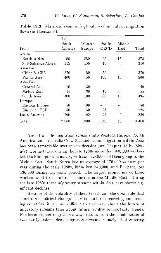
370 W. Lutz, W. Sanderson, S. Scherbov, A. Goujon

Table 15.3. Matrix of assumed high values of annual net migrationflows (in thousands).

ToNorth Western Pacific Middle

From America Europe OECD East TotalAfrica

North Africa 90 250 20 15 375Sub-Saharan Africa 115 150 40 5 310

Asia-EastChina & CPA 270 50 50 370Pacific Asia 400 50 100 10 560

Asia-WestCentral Asia 10 30 40Middle East 15 30 10 55South Asia :300 100 80 15 495

EuropeEastern Europe 50 100 150European FSU 50 150 25 225

Latin America 700 90 25 5 820

Total 2,000 1,000 350 50 3,400

Aside from the migration streams into Western Europe, NorthAmerica, and Australia/New Zealand, labor migration within Asiahas been remarkable over recent decades (see Chapter 13 by Zlot­nik). For instance, during the late 1980s more than 430,000 workersleft the Philippines annually, with some 280,000 of them going to theMiddle East. South Korea lost an average of 170,000 workers peryear during the early 1980s, India lost 240,000, and Pakistan lost130,000 during the same period. The largest proportion of theseworkers went to the oil-rich countries in the Middle East. Duringthe late 1980s these migratory streams within Asia have shown sig­nificant declines.

Because of the volatility of these trends and the great role thatshort- term political changes play in both the receiving and send­ing countries, it is more difficult to speculate about the future ofmigratory streams than about future fertility or mortality trends.Furthermore, net migration always results from the combination oftwo partly independent migration streams, namely, that entering

World Population Scenarios for t.he 21st Century 371

and that leaving a certain region for whatever reasons. These rea­sons are sometimes grouped into political (asylum seekers), eco­nomic (expected differentials in standard of living), and recentlyenvironmental factors. This last category remains rather vague be­cause worsening environmental conditions often result in worseningeconomic conditions. As pointed out in Chapter 14, for all categoriesthe potential for further increases in interregional migration is greatbecause of better communications between the regions, cheap masstransport facilities, and the persistent gap between the North, whichis not only richer but also rapidly aging and most likely in need ofyoung labor, and the South, which has many young people with onlylimited opportunities in their home countries.

The actual extent of future South-North migration streams de­pends not only on the pull and push factors, but also on the immi­gration policies in the receiving countries. If the European Union,for instance, decides to enforce a policy of virtually closed bordersto the outside because of popular demand within the EU, this maywell result in a situation of almost no net migration. Hence in theprojections, zero net migration was chosen for the low variant. Thisdoes not mean that borders are entirely closed to migrants; it onlyassumes that the number of in-migrants approximately equals thenumber of out-migrants.

For the high-migration scenarios, annual net migration gains of2 million in North America, 1 million in Western Europe, 350,000 inthe Pacific OECD region, and 50,000 in the Middle East have beenassumed. The distribution of migrants from the assumed sending re­gions to the recei ving regions and migration patterns among the lessdeveloped regions are based mostly on current migratory streams asdescribed in Chapter 13. Table J5.3 gives the migration matrixassumed in the high-migration case. In the low-migration case, allcells are zero; in the central scenario, values are half of those given inTable 15.3. The high scenario assumes an annual net migration lossof 375,000 in North Africa, 310,000 in sub-Saharan Africa, 370,000in China and other Centrally Planned Asia, 560,000 in Pacific Asia,495,000 in South Asia, 150,000 in Eastern Europe, and 225,000 inthe European part of the former Soviet Union. Model migrationschedules by Rogers and Castro (1981) were used to determine theage patterns of migrants.

372 W. Lutz. W. Sanderson, S. Scl1erbov, A. Goujon

It is almost certain that actual migration streams will not beconstant over time. But assuming that the short-term fluctuationsaverage around certain levels of constant annual net migration is themost practicable way to deal with this volatility.

15.2 Scenarios with Independent Fertility,Mortality, and Migration Trends

15.2.1 Specific model assumptions

In addition to the general assumptions described above, every pro­jection must make several specific choices concerning the age pat­terns of fertility, mortality, and migration as well as the specificpatterns of change over time and many other more technical details.The most important choices are summarized in this section.

The projections were generated using DIALOG, a software pro­gram developed by Sergei Scherbov; DIALOG is specifically de­signed for multistate population analysis and projection. The pro­jections were done in five-year intervals for five-year age groups.These projections differ from most other projection models becausewe define separate age groups up to age 120; extending the agecategories beyond the usual 80+ category helps to avoid serious bi­ases that occur when significant proportions of the population inlow-mortality regions come into the highest age group.

As described in previous chapters all countries were grouped intothirteen world regions that can be regrouped into six continents aswell as into two groups ofless developed and more developed regions.The population data for the starting year, 1995, were taken from thePopulation Reference Bureau (PRB) World Population Data Sheet1995, which gives the most recent estimates for total population sizeas well as fertility and mortality levels in aU countries. Since thissource does not provide the full age distribution of the population,age distributions were taken from the United Nations 1994 assess­ment by proportionally adjusting the age groups to match the PRBtotal population figures in the case of discrepancies between the twosources. Age patterns of fertility and mortality in the starting yearwere derived using the same procedure.

World Population Scenarios for the 21st Century 373

As to the assumptions offertility, mortality, and migration, the1995 values and the alternative values chosen for 2030-2035 havebeen described above. A more detailed table giving the specifictime path of the values and their extensions to 2100 is given inthe Appendix. The values for 1995-2000 and 2000-2005 reflect theassumption of a quick opening up of the uncertainty range over thefirst five years followed by linear interpolation ("sausage model").This particular decision was based on the observation that, understrictly linear interpolation, the range of uncertainty given for thefirst interval is far too small; therefore, between 1990 and 1995,many countries showed empirical trends that were outside the rangeassumed by the projections based on 1990 data.

Fertility assumptions for the second half of the 21st century areusually considered to be more art than science. Typically long-rangeprojections assume some kind of a convergence toward the so-calledreplacement level. This is done for two reasons: first, it is conve­nient; second, no plausible alternatives seem to exist. But thereis no good theory to explain how some magic hand should raisefertility to a level slightly above two children per woman after com­pletion of the demographic transition. Only a vague and unprovenhomeostasis hypothesis would suggest such a pattern.

In this analysis we suggest another rationale. Ultimate fertilityis assumed to be a function of region-specific population densitieswithin a predefined range of ultimate TFRs. After the completionof the demographic transition, low population densities are assumedto be associated with higher fertility, and vice versa. [4] Fertility isassumed to reach a level between 1.7 and 2.1 children per womandepending on density (for the central scenario) by the year 2080.The projected density for 2030 (central scenario) is taken as a cri­terion. The least densely populated region - South America with28 persons per km2 projected for 2030 - is given the highest TFR(2.1), while beyond 300 persons per km2 (only South Asia, with adensity of 478 persons per km2 by 2030) a TFR of 1.7 is assumed.For densities between 28 and 300, intermediate fertility levels areobtained through linear interpolation. The low-fertility (and high­fertility) assumptions are set at 0.5 children below (and above) thevalue obtained for the central scenario. Appendix Table 1 gives

374 W. Lutz, W. Sanderson, S. Scherbov, A. Goujon

assumed fertility and mortality levels for the period 2080-2085 foreach of the three scenarios. Beyond 2080-2085, levels are assumedto remain constant. Between the periods 2030-2035 and 2080-2085,levels are derived from linear interpolation.

Future age-specific fertility rates have been obtained by propor­tionally changing the age-specific rates of the starting year in accor­dance with the TFR level chosen. Extensive analysis of changingage profiles of fertility under different fertility levels has indicatedthat this is a reasonable approximation.

With respect to mortality, the United Nations (in the bi-annualassessments as well as in long-range projections) presents only onefixed path for each region without any uncertainty variants. Maxi­mum life expectancy at birth is assumed to be 87.5 years for womenand 82.5 years for men, and improvements in life expectancy endonce the maximum figure is reached (between 2075 and 2150, de­pending on the region). For countries that already have very lowmortality this implies very little prospects for further improvementsin the future. In sharp contrast, our mortality assumptions span avery broad range in the long term, reflecting the great uncertaintyabout possible maximum 1ll0rta1ity levels (see discussion in Section1.5.1.2). In the low-mortality case, mortality rates continue to de­cline with a speed that corresponds to the past experience of themore successful countries. The high-mortality case even assumessome worsening in certain regions (see Appendix Table 1). Life­expectancy increases after 2030-2035 are generally smaller than be­fore 2030, with constant mortality under the high-mortality assump­tion, a one-year increase per decade under the central-mortalityassumption, and a two-year increase per decade under the low­mortality assumption. In regions with small mortality differentialsby sex, future increase of the differentials has been assumed, as de­scribed in Appendix Table 1.

A Brass- type relationallogits model was used to produce a newset of age-specific mortality rates at a given level of mortality. Forsub-Saharan Africa and South Asia special life tables have been ap­plied; these tables include the specific age pattern of AIDS mortalitywhich has been used by Bongaarts (Chapter 9). For age-specific mi­gration, the model migration schedules by Rogers and Castro (1981)have been applied.

World Population Scenarios for the 21st Century 37.5

The following sections give a summary of the most importantresults. The Appendix Tables provide more information on eachregion. A complete set of results is available from the authors andaccessible on the internet (http://www.iiasa.ac.at); in this set theresults are arranged by five-year age groups (age 0-120) in five-yeartime intervals (1995-2100) for all 13 regions and all 27 scenariosthat result from the combination of the three fertility, mortality,and migration assumptions.

15.2.2 Population size by region

World Population

Table 15.4 lists the total population sizes for the six continentaldivisions, the two economic divisions, and the world total in 1995and population projections for 2020, 2050, and 2100. The table com­prises nine cells that present the results for all possible combinationsof assumptions of low, centraL and high fertility and mortality un­der central-migration assumptions. The Appendix provides detailedtables on the 13 regions, at additional points in time, and also un­der the low- and high-migration assumptions in the regions mostsignificantly affected by migration.

Table 15.4 is different from the usual presentation of popula­tion projection results in two important ways: first, the user canfreely choose any combination of the three fertility and mortalityassumptions; second, the user may combine different scenarios indifferent continents. Hence, the user can derive the total worldpopulation resulting from high fertility and low mortality in Africabut low fertility and low mortality in Europe. Traditionally, uncer­tainty variants, such as the low variant in UN projections or thelow-fertility flow-mortality scenario given in the 1994 edition of thisbook, present figures assuming lower than expected fertility in allparts of the world. This strong assumption of a perfect correlationbetween the regions results in the most extreme low figures for totalworld population. In the more likely case of no strict conformity oftrends in different parts of the world, results tend be close to thecentral scenario because, for example, higher than expected fertilityin Africa may be compensated by lower than expected fertility inEast Asia. The figures given for the world in Table 15.4 thus refer

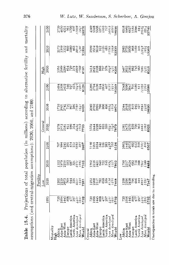
Ta

ble

15

.4.

Pro

ject

ions

ofto

tal

popu

lati

on(i

nm

illi

ons)

acco

rdin

gto

alte

rnat

ive

fert

ilit

yan

dm

orta

lity

assu

mpt

ions

(and

cent

ral-

mig

rati

onas

sum

ptio

ns):

2020

,20

50,

and

2100

.

Fer

tili

ty

1995

Low 20

2020

5021

00C

entr

al

2020

2050

2100

Hig

h

2020

2050

2100

Mo

rtal

ity

Hig

hA

fric

a72

012

0213

1270

712

7817

1014

8413

.55

2173

2739

Asi

a-E

ast

1956

2239

1979

994

2412

2601

2308

2589

3369

4650

Asi

a-W

est

1445

2073

2210

1241

2181

2741

2432

2290

3352

4321

Eu

rop

e80

876

959

329

181

171

6,5

4685

486

096

1L

ati

nA

mer

ica

477

644

687

4,54

686

867

927

729

1080

1700

No

rth

Am

eric

a29

733

.532

12,

5135

438

642

337

446

369

7L

ess

deve

lope

d4

45

160

1160

713

33

064

047

78

07

04

06

80

29

81

01.

9228

Afo

rede

velo

ped

12

51

12

50

10

32

60

71

31

912

411

08

11

38

81

48

6/8

41

Wo

rld

57

02

72

61

71

03

39

37

77

23

90

21

81

20

81

91

11

30

01

50

70

Cen

tral

Afr

ica

720

1252

1,56

211

4013

3220

4023

6614

1425

9943

49A

sia-

Eas

t19

5622

6821

1612

0524

4427

6027

0426

2135

,54

,534

8A

sia-

Wes

t14

4521

1724

2116

3422

2829

9531

3623

3836

59,5

508

Eu

rop

e80

878

264

034

282

576

662

486

891

210

7,5

Lati

nA

mer

ica

477

650

722

530

693

906

1056

737

1125

1910

No

rth

Am

eric

a29

733

934

028

335

940

646

737

848

375

7L

ess

deve

lope

d4

45

16

13

866

944

43

365

418

55

49

13

76

94

61

07

65

16

91

5M

ore

deve

lope

d1

25

11

27

011

07

700

13

40

13

19

12

16

14

10

15

68

20

33

Wo

rld

57

02

74

08

78

02

51

34

78

79

98

74

10

35

08

35

61

23

30

18

95

0

Low A

fric

a72

012

9817

9916

6213

8123

4433

4814

6729

8360

58A

sia-

Eas

t19

5622

9622

5714

4024

7329

1830

9026

5237

3359

60A

sia-

Wes

t14

4521

5826

2420

7322

7032

3538

4723

8339

3966

27E

uro

pe

808

796

692

402

83

981

970

588

296

811

85L

atin

Am

eric

a47

765

675

661

270

094

511

8074

311

6920

96N

ort

hA

mer

ica

297

344

360

318

363

427

511

383

505

812

Les

sde

velo

ped.

44

51

62

57

7301

5701

66

65

92

85

11

32

570

801

16

43

20

52 4

Mo

rede

velo

ped

12

51

12

91

11

88

80

61

36

01

40

21

35

514

311

65

42

21

4W

orl

d5

70

27

54

78

48

86

50

78

02

61

06

90

12

68

08

51

01

33

00

22

74

0

Dis

crep

anci

esin

tota

lsar

ed

ue

toro

un

din

g.

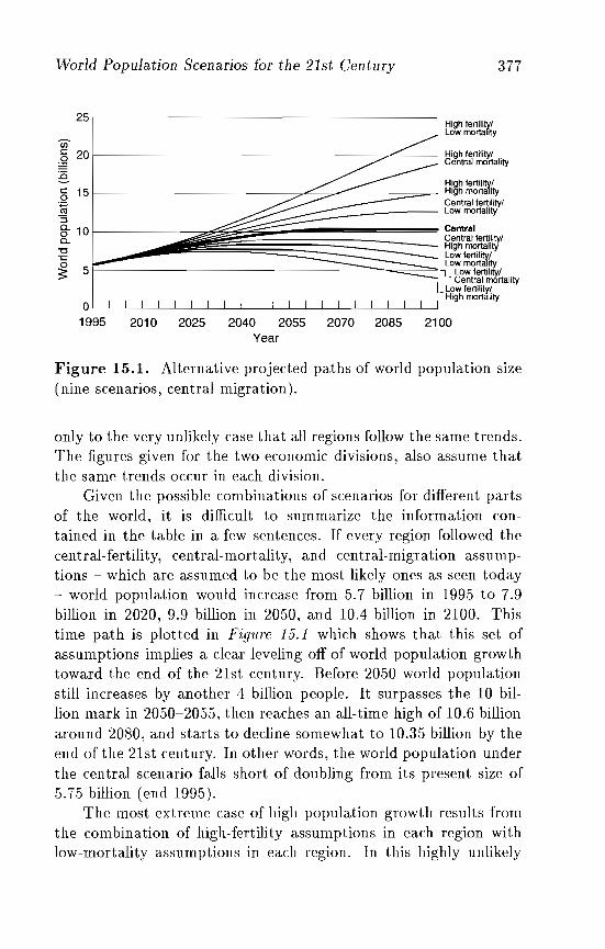
World Population Scenarios for the 21st Century 377

tb~~~tr,{y

High fertilitylCentral mortality

2010 2025 2040 2055 2070 2085 2100Year

o1995

25[High fertilitv/ity~ "'""~""~ 20 c.",., ""''>'g ,~_.,.B __ .

C 15 c•••,""11~ylo "'"_'"~ ""''''~I.~ ,~::::;,'" .o 1

0

L t~""., ~"",.o 'tylD.. LLow fertl I I'tyu """~""- , ," I I " ,3: I I I

I I I II I I I I

Figure 15.1. Alternative projected paths of world population size(nine scenarios, central migration).

only to the very unlikely case that all regions follow the same trends.The figures given for the two economic divisions, also assume thatthe same trends occur in each division.

Given the possible combinations of scenarios for different partsof the world, it is difficult to summarize the information con­tained in the table in a few sentences. If every region followed thecentral-fertility, central-mortality, and central-migration assump­tions - which are assumed to be the most likely ones as seen today- world population would increase from 5.7 billion in 1995 to 7.9billion in 2020, 9.9 billion in 2050, and 10.4 billion in 2100. Thistime path is plotted in Fig'ure 15.1 which shows that this set ofassumptions implies a clear leveling off of world population growthtoward the end of the 21st century. Before 2050 world populationstill increases by another 4 billion people. It surpasses the 10 bil­lion mark in 20,50-20,55, then reaches an all-time high of 10.6 billionaround 2080, and starts to decline somewhat to 10.35 billion by theend of the 21st century. In other words, the world population underthe central scenario falls short of doubling from its present size of5.7,5 billion (end 1995).

The most extreme case of high population growth results fromthe combination of high-fertility assumptions in each region withlow-mortality assumptions in each region. In this highly unlikely

378 VV Lutz, W. Sanderson, S. Scherbov, A. Goujon

case, the world population would double before the middle of thenext century and reach an incredible 22.7 billion by the year 2100.High fertility combined with high mortality - which is a more prob­able combination - would only result in 15.1 billion people. Hence,given a high-fertility case, alternative mortality assumptions canmake a difference in total population size that is larger than today'sworld population.

On the low-fertility side, the combination of low fertility withhigh mortality yields the lowest path of world population growth. Ifthese rather unlikely assumptions were strictly applied to all worldregions, world population would still increase by another 30 percentuntil 2030 and thereafter would enter a population decline that gainsmomentum during the second half of the century and might bringworld population down to a low 3.9 billion by 2100. This wouldbe significantly below today's total population size. It would equalthe population in 1973-1974. Because of the significant populationaging implied by this scenario, an inverse momentum of populationgrowth (shrinking momentum) suggests further population declineduring the 22nd century because smaller and smaller cohorts wouldenter the main reproductive ages. But aside from the incrediblepopulation aging implied by this, this scenario cannot be called de­sirable because it is associated with the highest mortality and thusa great deal of human suffering. In many parts of the world thisscenario assumes very little or no future progress in mortality re­duction; in sub-Saharan Africa it even assumes declining trends inlife expectancy. The most desirable, under the criteria of a highquality of life and low population growth, is the low-fertility /low­mortality scenario, which results in a further increase of populationsize to 8.5 billion by 2050 followed by a more moderate decline to6.5 billion by 2100.

Table 15.4, together with Figu.re 15.1, can be used to evaluatethe relative impacts of the difference in the assumed mortality andfertility alternatives. The nine cells in the table and the nine linesin the figure show a clear ranking of the demographic variables,with fertility being the dominating variable but mortality still beinghighly significant. The impact of alternative mortality assumptionson total population size is more significant in the low-fertility casethan in the high-fertility case. In the high-fertility case by 2100

World Population Scenarios for the 21st Century 379

the low-mortality assumptions yield a population size that is 50percent higher than that of the high-mortality assumption; in thelow-fertility case the differential is 6.5 percent. This differential isclearly big enough to justify the analysis of alternative mortalityassumptions in addition to alternative fertility assumptions.

As stated above, Figure j 5.1 only gives the scenarios in whichfertility and mortality trends in all regions follow the same pattern.Combining different assumptions in different regions results in sev­eral additional lines that all lie between the extremes given. Mostare close to the central scenario; the positions of the lines depend onthe degree to which trends in one region compensate for those in an­other. A more systematic analysis of these aspects is provided in thecontext of the probabilistic population projections in Chapter 16.

Regional Population Distribution

The global population growth described above results from a greatdiversity of different regional patterns. Under the assumptions ofcentral fertility, mortality, and migration the population on theAfrican continent grows the most rapidly. Its population almosttriples in size over the next five decades from 720 million in 1995 tomore than 2 billion in 20,50. Accordingly, the share of the world pop­ulation that lives in Africa increases from 13 percent to 21 percent(see Table 15.5). In the high-fertilityjlow-mortality case Africa'spopulation more than quadruples by 2050, whereas under the low­fertility jhigh-mortality scenario, it does not even double. By 2100the pessimistic mortality assumptions of this scenario lead to a pop­ulation size that is smaller than today's.

The population of East Asia, which is currently home to one­third of the world's population, increases by 41 percent under thecentral assumptions until the year 20.50. Because this growth lieswell below the world average of 7:3 percent, the proportion of theworld population living in this region declines by six percentagepoints to 28 percent. West Asia, on the other hand, gains five per­centage points and holds 30 percent of the world population; by 2050the population in this region more than doubles under the centralassumptions. The reason for this difference lies predominantly in thefact that the fertility transition is already much further advanced in

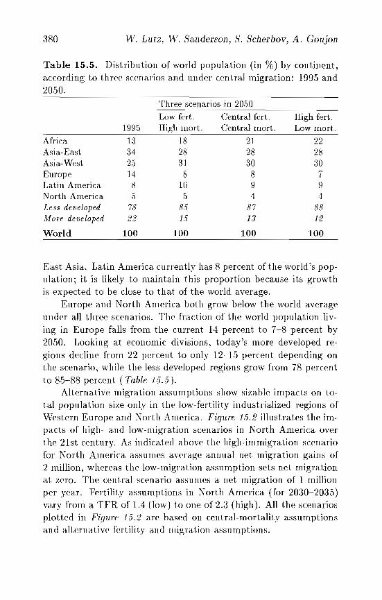
380 vV. Lutz, VV. Sanderson, S. Scherbov, A. Goujon

Table 15.5. Distribution of world population (in %) by continent,according to three scenarios and under central migration: 1995 and2050.

Three scenarios in 2050

Low fert.. Central fert. High fert.1995 High mort. Central mort. Low mort.

Africa 13 18 21 22Asia.-East 34 28 28 28Asia.- West 25 31 30 30Europe 14 8 8 7Latin America 8 10 9 9North America 5 5 4 4Le88 developed 78 85 87 88More developed ,~,~ 15 13 12,,~

World 100 100 100 100

East Asia. Latin America currently has 8 percent of the world's pop­ulation; it is likely to maintain this proportion because its growthis expected to be close to that of the world average.

Europe and North America both grow below the world averageunder all three scenarios. The fraction of the world population liv­ing in Europe falls from the current 14 percent to 7-8 percent by2050. Looking at economic divisions, today's more developed re­gions decline from 22 percent to only 12-15 percent depending onthe scenario, while the less developed regions grow from 78 percentto 85-88 percent (Table 15.5).

Alternative migration assumptions show sizable impacts on to­tal population size only in the low-fertility industrialized regions ofWestern Europe and North America. Figure 15.2 illustrates the im­pacts of high- and low-migration scenarios in North America overthe 21st century. As indicated above the high-immigration scenariofor North America assumes average annual net migration gains of2 million, whereas the low-migration assumption sets net migrationat zero. The central scenario assumes a net migration of 1 millionper year. Fertility assumptions in North America (for 2030-2035)vary from a TFR of 1.4 (low) to one of 2.3 (high). All the scenariosplotted in Figure 15.2 are based on central-mortality assumptionsand alternative fertility and migration assumptions.

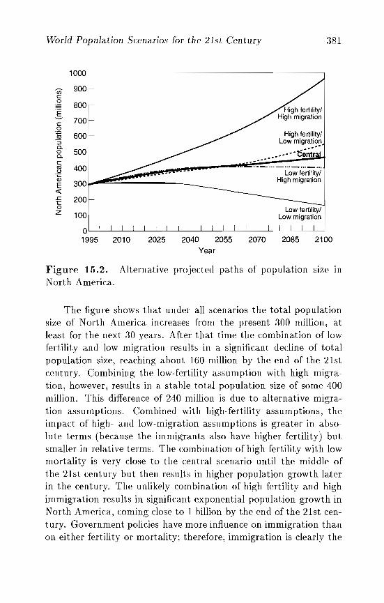
World Population Scenarios for the 21st Century 381

21002085

Low fertility!Low migration

Low fertility!High migration

High fertility!Low migration

._ ~';~;;a'

20702040 2055

Year

2025

1000

Cil 900c2 800"E

700c0

~ 600:JC.

5000c.Cell 400u-cQ)

300E«..c 200t:::0z 100

01995 2010

Figure 15.2. Alternative projected paths of population SIze In

North America.

The figure shows that under all scenarios the total populationsize of North America increases from the present 300 million, atleast for the next 30 years. After that time the combination of lowfertility and low migration results in a significant decline of totalpopulation size, reaching about 160 million by the end of the 21stcentury. Combining the low-fertility assumption with high migra­tion, however, results in a stable total population size of some 400million. This difference of 240 million is due to alternative migra­tion assumptions. Combined with high-fertility assumptions, theimpact of high- and low-migration assumptions is greater in abso­lute terms (because the immigrants also have higher fertility) butsmaller in relative terms. The combination of high fertility with lowmortality is very close to the central scenario until the middle ofthe 21st century but then results in higher population growth laterin the century. The unlikely combination of high fertility and highimmigration results in significant exponential population growth inNorth America, coming close to 1 billion by the end of the 21st cen­tury. Government policies have more influence on immigration thanon either fertility or mortality; therefore, immigration is clearly the

382 W. Lutz, W. Sanderson, S. Scherbov, /1. Goujon

key policy variable for influencing the extent of population growthin North America over the next century.

15.2.3 Population aging

Universal population aging (as measured by the mean age of thepopulation or the proportion of the population above age 60) is themost consistent and dominant population trend of the next century.In all regions, the scenario projections show an aging population.Population aging has long been recognized as a cause of concern inthe industrialized countries, but projections clearly show that overthe coming decades it is likely to hit less developed countries evenharder than it has industrialized countries because of more rapidfertility declines.

Table 15.6 has the same structure as Table 15.4 but gives theproportions above age 60 instead of total population. Currently only9..5 percent of the world population is above age 60. Since the early1950s this percentage has slowly increased from 8.1 percent in 1950to 8.4 percent in 1970 and 8.8 percent in 1985. Over the comingdecades this percentage is projected to increase much more rapidlyunder all possible scenarios. Under the three central assumptionsit increases to 1:3.2 percent in 2020, 19.6 percent in 2050, and 26.8percent in 2100. These projected increases are much higher thanany increases that have been experienced today in industrializedcountries. Currently, Western Europe, the region with the oldestpopulation, has 18.6 percent of the population above age 60.

Even under the extreme high-fertility and low-mortality sce­nario, which results in more than 22 billion people in 2100, thepercentage of elderly increases to above 17 percent. Under the low­fertility flow-mortality assumptions the aging figures become trulydaunting. By the end of the the 21st century, this scenario showsthat 42.5 percent of the population is above age 60. In industrial­ized countries half of the population is projected to be above age60 under these assumptions, which are often called most desirableby ecologists and the media because they result in the lowest totalpopulation size. If mortality is high, fewer people survive to an oldage, lowering the old-age dependency ratio. But even in this case ofundesirably high mortality one- third of the population will be aboveage 60 by the end of the 21st century.

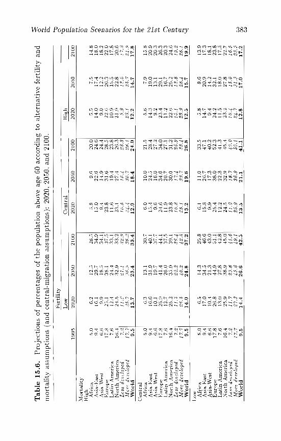
Tab

le1

5.6

.P

roje

ctio

nsof

perc

enta

ges

ofth

ep

op

ula

tio

nab

ove

age

60ac

cord

ing

toal

tern

ativ

efe

rtil

ity

and

mo

rtal

ity

assu

mpt

ions

(an

dce

ntra

l-m

igra

tion

a.ss

umpt

ions

):2

02

0,2

05

0,

and

2100

.

w 00 w:; ill

l-"';' ,......

lfJ '""V'J "ill ::l

III ... O· tJ'l ~~ ::!...

I:l.. '"tl

,g ~ (i;'" '"" gO C1 ill ::l '"" ~ .~

21

00

20

S0

20

20

Hig

h

21

00

20

S0

20

20

Cen

tral

21

00

20

S0

20

20

Fer

tili

ty

Low

19

95

-~.--

----

----

---

---

---

---

----

----

---

-

Mo

rtal

ity

Hig

hA

fric

aS.

O6

.21

2.5

28

..').1

.89

.62

0.0

·5.·5

7..1

14

.8A

sia-

Eas

t9

.41

6.1

29

.73

4.9

IS.0

22

.62

4.6

14

.01

7.4

18

.0A

sia-

Wes

t6

.69

.918

.S3

4.1

9.4

14

.92

4.4

9.0

12

.21

8.2

Eu

rop

e1

7.8

2S.1

38

.13

7.5

'2:3

.83

1.6

28

.52

2.6

26

.32

2.0

Lat

inA

mer

ica

7.6

12

.42

4.4

33

.11

1.6

19

.42

3.8

10

.91

5.S

17

.8N

ort

hA

mer

ica

16

.42

4.S

.32.

93

3.2

23.1

27

.42

6..3

21

.92

2.8

20

.6L

es8

deu

tlo

ped

7.2

11

.22

1.1

32

..41

0..

5JIL

l2

3.3

9.9

13

.01

7.3

Jlfo

red

o.d

op

ed

/7.7

;]·5

.73

6.9

36

.22

4·4

30

.72

8.1

23

./2.

5.7

21

.9W

orl

d9

.51

3.7

23

.43

3.4

12

.91

8.4

24

.01

2.2

14

.71

7.8

Cen

tral

Afr

ica

·5.0

6.:3

13

.13

0.7

6.0

10

.021

.SS

.67

.9lS

.8A

sia-

Eas

t9

.41

6.6

:31.

940

.11

5.4

24

.S2

8.4

14

.31

9.0

20

.9A

sia-

Wes

t6

.610

.11

9.7

37

.79

.61

6.0

27

.29

.21

3.1

20

.3E

uro

pe

17

.82

S.9

41

.44

4.1

24

.63

4.6

34

.02

3.4

29.1

26

.3L

atin

Am

eric

a7

.61

2.7

26

.03

7.S

11

.92

0.7

27.1

11

.21

6.7

20

.3N

ort

hA

mer

ica

16

.42

5.2

3-5.

93

9.1

23

.83

0.0

31

.22

2.6

2S

.22

4.6

Les

sde

lle/

oped

7.2

11..5

22

.23

6·4

10

.81

7.4

2.5.

91

0.1

13

.8/9

.2M

OTe

dev

elo

ped

17

.72

6..5

40

.24

2..5

2.5.

13

3.7

33

·42

3.9

28

·426

.1W

od

d9

.51

4.0

24

.83

7.2

13

.21

9.6

26

.81

2.5

15

.71

9.9

Low A

fric

a5

.06

.S1

4.3

3S

.86.

11

1.0

33

.55

.88

.61

3.9

Asi

a-E

ast

9.4

17

.03

4.S

46

.61

5.8

26

.747

.11

4.7

20

.91

7.3

Asi

a-W

est

6.6

10

.42

1.3

43

.09

.91

7.3

40

.29

.41

4.2

18

.1E

uro

pe

17

.82

6.8

44

.9·5

1.1

25

.43

8.0

S2

.32

4.2

32

.12

3.8

Lat

inA

mer

ica

7.6

13

.02

7.8

42

.81

2.2

22

.34

1.3

11

.S1

8.0

17

.5N

ort

hA

mer

ica

16

.42

S.9

38

.94.

5.0

24

.53

2.9

4S

.42

3.2

27

.82

2.7

Les

sd

evel

op

ed7

.211

.72

3.8

41

.61

1.0

18

.74

0.0

10

·41.

5.0

16

..5M

OTe

dev

elo

ped

17

.72

7.3

43

.64

9.1

2.5.

93

6.9

.50.

12

4·7

31

.32

3.9

Wo

rld

9.5

14

.42

6.6

42

.51

3.5

21

.14

1.1

12

.81

7.0

17

.2

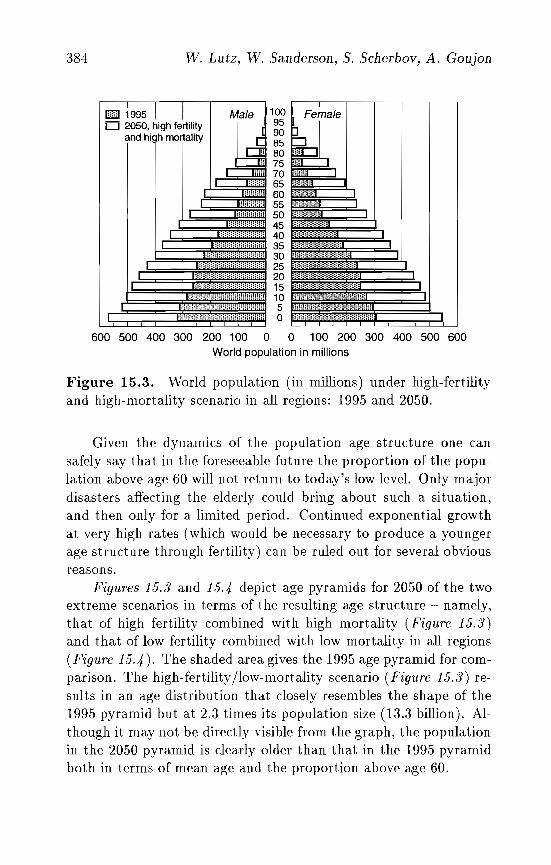
384 W. Lutz, W. Sanderson, S. Scherbov, A. Goujon

:: ;:;:;:iiiliiiiliii;;~;~:;i ~:;::

:;i;:;:;:;:;l;l;:;:;:;i;i;i;:;:;:;:;::

::1:;:;:;:;:;;;:;:;:;;:;;;;;::;::::::;:;:;:;:;:;:;:;:::;;;:,;;:;:;:;::

::;:;:::::r.;:;:;:;:;:;:1

-:;: ~:;: ~:;:~::

Male 1100 Female95

~" !g" 75

"", 70 ===­"""" 65

60555045 I;;;:;;:;;;~;:;;;

~~ ~"#'",#'"";;l""*,,,,*,,,,~,,,30 """"""""""""""25 """"""""""""""",20 ""*,*"""""""""",,,15 """"""""""""""""10 """""""""""""""""'"5 "",*,*,*","""",o """"""""""""""""""""

:~:;:;:m:rm;::

::::;:;:;:;:;:;:;:;:;::::::;::::;:::;:::;.:;::;;:

I:;;:;:;;:;::::::;:;:;:;:::;::;

:;:::;;:.E.;:;;l;;;;::;::;:i;!:::;::;::::::::;::::::;,;;;::::;;:;;;;;::::::=i;;=;;;;i;:

[[J ~995 I ILJ 2050, high fertility

and hiah mortality

600 500 400 300 200 100 0 0 100 200 300 400 500 600World population in millions

Figure 15.3. World population (in millions) under high-fertilityand high-mortality scenario in all regions: 1995 and 2050.

Given the dynamics of the population age structure one cansafely say that in the foreseeable future the proportion of the popu­lation above age 60 will not return to today's low level. Only majordisasters affecting the elderly could bring about such a situation,and then only for a limited period. Continued exponential growthat very high rates (which would be necessary to produce a youngerage structure through fertility) can be ruled out for several obviousreasons.

Figures 15.3 and 15.4 depict age pyramids for 2050 of the twoextreme scenarios in terms of the resulting age structure - namely,that of high fertility combined with high mortality (Figure 15.3)and that of low fertility combined with low mortality in all regions(Figure 15.4). The shaded area gives the 1995 age pyramid for com­parison. The high-fertility/low-mortality scenario (Figure 15.3) re­sults in an age distribution that closely resembles the shape of the1995 pyramid but at 2.3 times its population size (13.3 billion). Al­though it may not be directly visible from the graph, the populationin the 2050 pyramid is clearly older than that in the 1995 pyramidboth in terms of mean age and the proportion above age 60.

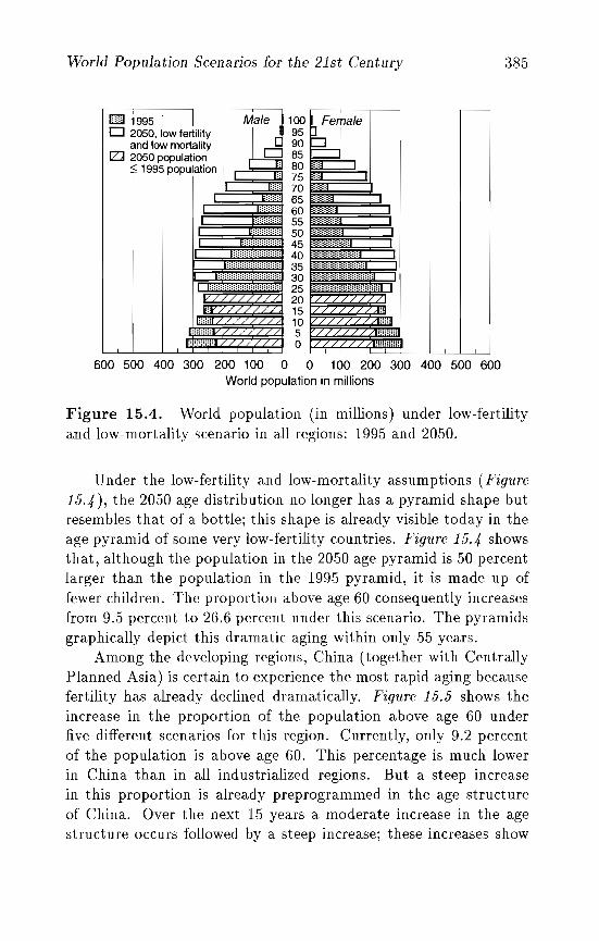
World Population Scenarios [or the 21st Century 385

::;:

:::;::::::;mmm

"/

'/

:::;;:::;::;:~:;:;:;::

1.':::;:;:=::::

r.:::::::::;:;=:=;:

"/

:l;:;;;i;:;:;:;:;:;:;::;:::;:;:::;:;l=::!:l::::

;;:;:;:;:;:;:;:;:;:;:;:;:::;:::m;m;;;;:;;;:;;;:;:;l;;;:;l:

,,,,,;1"//::;;:;:;l

:::::;::::::

E:J 1995 I I j"'J 100 Fema'eD 2050, low fertility 95and low mortality 90

lZJ 2050 population 85 0;:;;=1--.," 80

75~=::::!..."'"mill 70

"jffijj 6560555045

40 IIII135 """"""""""""30 """"""""""""""25 """"""""""""""*2015105o

600 500 400 300 200 100 0 0 100 200 300 400 500 600World population in millions

Figure 15.4. World population (in millions) under low-fertilityand low-mortality scenario in all regions: 1995 and 2050.

Under the low-fertility and low-mortality assumptions (Figure

15.4), the 2050 age distribution no longer has a pyramid shape butresembles that of a bottle; this shape is already visible today in theage pyramid of some very low-fertility countries. Figure 15.4 showsthat, although the population in the 2050 age pyramid is 50 percentlarger than the population in the 1995 pyramid, it is made up offewer children. The proportion above age 60 consequently increasesfrom 9.5 percent to 26.6 percent under this scenario. The pyramidsgraphically depict this dramatic aging within only 55 years.

Among the developing regions, China (together with CentrallyPlanned Asia) is certain to experience the most rapid aging becausefertility has already declined dramatically. Figure 15.5 shows theincrease in the proportion of the population above age 60 underfive different scenarios for this region. Currently, only 9.2 percentof the population is above age 60. This percentage is much lowerin China than in aU industrialized regions. But a steep increasein this proportion is already preprogrammed in the age structureof China. Over the next 15 years a moderate increase in the agestructure occurs followed by a steep increase; these increases show

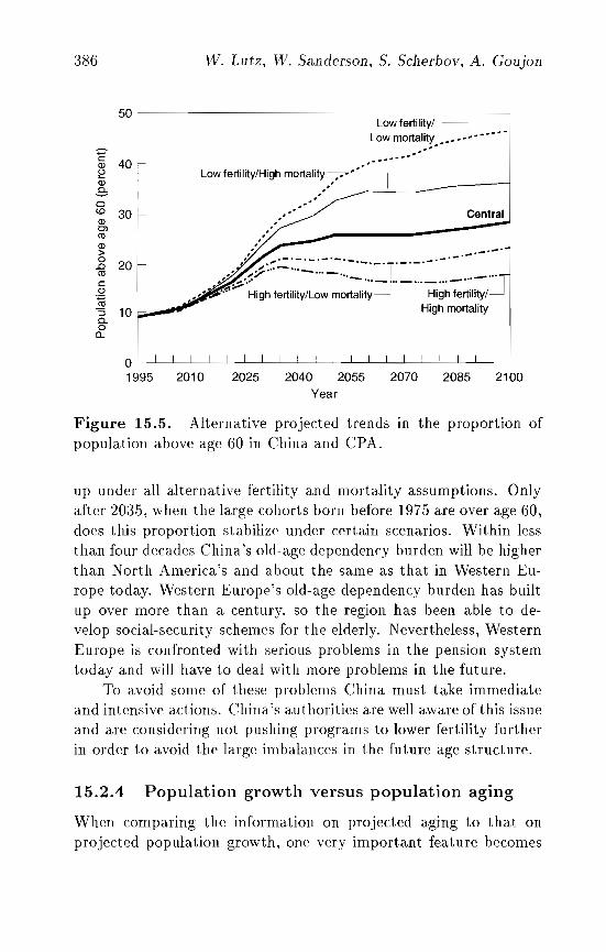
W. Lutz, W. Sanderson, S. Scherbov, A. Goujon

Central"

Low fertility/ ----,Low mortality ,'," L. ' - - • , -.. '

"

Low fertility/High mortality ., ••••• - - -' -,',,1' ~~______ I

..

~.......~;/ ..:7:::' :.-:::::.~:':.:.:~.~-'r=~.'~ ....~..~ ='.~ ~#. ~:,.;..- =.1

•• ' ~. High fertility/Low mortality High fertility/JHigh mortality

386

50

C40Q)

~Q)

-300to 30Q)enellQ)

>0

20.0ellC0

~"S 100-0a..

2100208520702040 2055Year

2025o I I

1995 2010

Figure 15.5. Alternative projected trends in the proportion ofpopulation above age 60 in China and CPA.

up under all alternative fertility and mortality assumptions. Onlyafter 203.5, when the large cohorts born before 197.5 are over age 60,does this proportion stabilize under certain scenarios. Within lessthan four decades China's old-age dependency burden will be higherthan North America's and about the same as that in Western Eu­rope today. Western Europe's old-age dependency burden has builtup over more than a century, so the region has been able to de­velop social-security schemes for the elderly. Nevertheless, WesternEurope is confronted with serious problems in the pension systemtoday and will have to deal with more problems in the future.

To avoid some of these problems China must take immediateand intensive actions. China's authorities are well aware of this issueand are considering not pushing programs to lower fertility furtherin order to avoid the large imbalances in the future age structure.

15.2.4 Population growth versus population aging

When comparing the information on projected aging to that onprojected population growth, one very important feature becomes

World Population Scenarios for the 21st Century 387

apparent. The scenarios that result in the highest population growthshow only moderate population aging, while those showing a levelingoff in population size imply very rapid population aging. Generally,very rapid population growth and very rapid aging are consideredundesirable, but the scenarios described above clearly show thatone cannot avoid both. An intermediate path, such as that givenby the central scenario, avoids extremes but still combines substan­tial population growth with substantial aging at the global level.Since the problems caused by rapid growth and rapid aging are feltmore at the regional level rather than at the global level, solutionsto the problems must work at the former level. This issue must bediscussed within a more regional context. The epilogue to this vol­ume takes up some of the policy issues related to the aging versuspopulation growth dilemma.

15.3 Special Interaction Scenarios forSelected Regions

So far in this chapter the fertility, mortality, and migration compo­nents have been considered independent determinants of populationsize and structure. When different scenario assumptions are com­bined to produce alternative scenarios, all combinations are givenequal weight. However, certain combinations of indicators, such asvery high fertility with very high mortality, are very unlikely andimplausible given the analysis of past trends.

Why, then, do we present such systematic permutations of sce­nario assumptions without explicitly specifying likely interactions?There are three reasons for first presenting the scenarios as if thethree components were independent:

1. In the short to medium term it is unclear whether any connec­tion between, for example, fertility and mortality or fertility andmigration exists. If such an interaction exists, it may be specificto certain regions.

2. There are an infinite number of possible types and intensities ofdependence in different parts of the world; no set of interactionscenarios can be exhaustive.

388 W. Lutz, W. Sa.nderson, S. Scherbov, A. Goujon

3. The scenarios presented in Section 15.2 provide details on theextreme cases. Any assumed interaction that keeps each com­ponent within the bounds defined by the high and low extremes- for example, a positive correlation between fertility and mor­tality - results in more moderate population trends than thosepresented in the extreme scenarios. In this sense users are on thesafe side when they look at the range of uncertainty as describedby the scenarios that assume the components are independentof one another.

But dearly not all of the possible interactions can be derivedfrom the scenario results provided above, especially if the objectiveis to focus on paths that change over time. To illustrate what typesof scenarios may be defined, the following three sections providea. small sample of possible future "stories" in selected parts of theworld.

15.3.1 Can migrants to Western Europe andNorth America stop the aging process?

This question is often directed to demographers when the issue of im­migration into industrialized countries is under discussion. Clearly,a one-time wave of young migrants can improve the old-age depen­dency ratio temporarily because the working-age population is in­creased while that above age 60 remains unchanged. But over timethese immigrants age, and ultimately increase the dependency ratiowhen they pass age 60. If retiring immigrants are replaced by thesame number of young immigrants there will be no additional deteri­oration in the dependency ratio but also no long- term improvement(assuming that the migrant population has the same fertility as thenative population). Only if the absolute number of immigrants con­tinuously increases, can the otherwise increasing dependency ratiobe kept down in a sustainable way.

To determine the growth rate of the immigrating population toWestern Europe and North America necessary to reduce the propor­tion of the population above age 60 - or more precisely, to have itincrease more slowly - we have defined a number of specific scenar­ios with different growth rates. The annual net migration under thecentral scenario was taken as the basis for comparison. This means

World Population Scena,rios for the 21st Century 389

a constant annual net inflow of 500,000 to Western Europe and 1million to North America. Each number was assumed to increase by0.5 percent, 1 percent, or 2 percent per year until 2080-2085 underthree additional scenarios.

In summary, the results show that, even with a 2 percent an­nual increase, immigration has a very low impact on the proportionelderly. Under constant net migration (central scenario) the propor­tion age 60+ in Western Europe increases from today's 18.6 percentto 35 percent in 2050. This percentage is only 1.9 percentage pointslower (33.1 percent) under the assumption of a 2 percent annualincrease. Until 2100 further improvements are even more moderate.But this scenario also results in a total population that is 7 percenthigher in 2050 and even 39 percent higher by 2100 than today's.The pattern for North America is not much different from WesternEurope's, although at somewhat lower levels of old-age dependency.By 2100 under a 2 percent annual increase the proportion above age60 is only 27 percent instead of 31 percent but the total populationis higher by 66 percent; in other words, the population of NorthAmerica is about 775 million with the migration factor instead of467 million as shown in the central scenario.

From this exercise we conclude that even immigration rates thatsignificantly increase the total population size have only a minusculeeffect in counteracting long-term increases in the proportion aboveage 60 if fertility remains low.

15.3.2 Overshooting carrying capacity insub-Saharan Africa

The popular literature, as well as parts of the scientific literaturein ecology, frequently mentions the scenario of overshooting carry­ing capacity - namely, the possibility of a collapse resulting from apopulation size so large that it hits the growth ceiling beyond whichadequate food supplies cannot be secured. Usually nothing spe­cific is said about the type of collapse. To illustrate a demographicscenario that reflects this situation, we simply assumed that thecollapse shows itself in the form of an increase in mortality. Butmortality can increase in many different ways and, in turn, can re­sult in very different demographic consequences. In the followingwe briefly look at alternative ways such a collapse might happen.

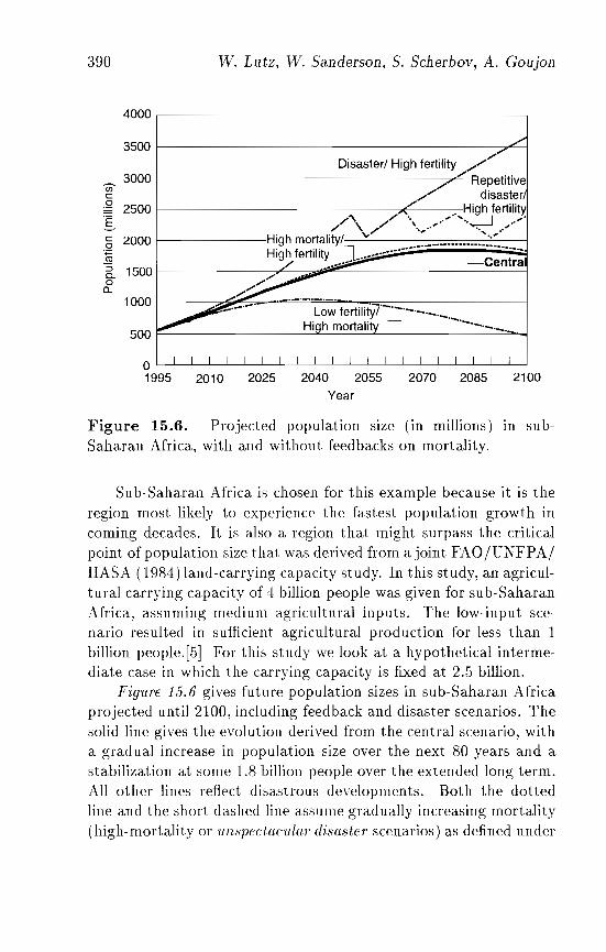
390 W. Lutz, W. Sanderson, S. Scherbov, A. Goujon

21002070 2085205520402025

'"Disaster/ High fertility //I 7/ Repetitive

/// disaster.. ;/ .' High fertili

/'\ /'. ..' ........-J .. './ \",// '.., .., ......., .. '

1------- High mortality/ ••••••••••••••••••.•••••••••••••Hig~fertilit~ ••~··· LCent'ii

4000

3500

3000VJc~ 2500I§ 2000~~ 15000a.

1000

500

01995 2010

Year

Figure 15.6. Projected population size (in millions) in sub-Saharan Africa, with and without feedbacks on mortality.

Sub-Saharan Africa is chosen for this example because it is theregion most likely to experience the fastest population growth incoming decades. It is also a region that might surpass the criticalpoint of population size that was derived from ajoint FAOjUNFPAjIIASA (1984) land-carrying capacity study. In this study, an agricul­tural carrying capacity of 4 billion people was given for sub-SaharanAfrica, assuming medium agricultural inputs. The low-input sce­nario resulted in sufficient agricultural production for less than 1billion people.[.5] For this study we look at a hypothetical interme­diate case in which the carrying capacity is fixed at 2..5 billion.

Figure 15.6 gives future population sizes in sub-Saharan Africaprojected until 2100, including feedback and disaster scenarios. Thesolid line gives the evolution derived from the central scenario, witha gradual increase in population size over the next 80 years and astabilization at some 1.8 billion people over the extended long term.All other lines reflect disastrous developments. Both the dottedline and the short dashed line assume gradually increasing mortality(high-mortality or 'Unspectacular disaster scenarios) as defined under

World Population Scenarios for tile 21st Century 391

the high-mortality assumptions for the region. Life expectancy de­creases by two years per decade until 2030-20305 and then remainsconst ant. This situation reflects the possibility of a slowly spreadingmortality crisis which could Iw due to AIDS, deteriorating healthsystems, local famines, and regional conflicts. Fertility rates in bothscenarios reflect the high- and low-fertility assumptions. Both caseshave undesirably high mortality. Combined with high fertility, thetrend is very close to the central scenario and almost reaches the 2billion mark. Combined with low fertility, population increases tosllghtly over I billion and then declines.

The remaining scenario projects initially more fortunate devel­opments in mortality: life expectancy increases four years per decadeuntil 2030-20305, when it reaches a level of 66 years for men and 69years for women, and continues to grow more slowly thereafter (low­mortality scenario). Fertility, on the other hand, does not decline asrapidly. The TFR declines as in the high-fertility scenario reachinga level of 4.0 in 2030-203.5 and 2.4 by 2080-20805. By 200505 this sce­nario passes the assumed critical level of 2.05 billion. At this point,something must happen along the lines of a Malthusian "positivecheck." LJ nder this assumed collapse, 20 percent of the population(more children than adults) die from war, starvation, disease, orsome other cause. Because fertility is not assumed to change, only10-105 years later, however, the magic 2.05 billion threshold is againexceeded (dashed line in Figure 15.6). Assuming that no furtherimprovements are made in agricultural production and fertility andmortality remain unchanged (except for years of collapse), catastro­phes occur in 10- to IS-year cycles.

The purpose of this highly speculative exercise of defining a col­lapse through an overshooting carrying capacity has been twofold:first, to show that the complaint of some ecologists that populationprojections simply do not consider the possibility of such feedbacksis not justified; second, to illustrate that the high-fertility jhigh­mortality scenario (labeled the unspectacular disaster scenario), un­der which the population size stays below the limits of carryingcapacity, is not really more desirable than the high-fertility jlow­mortality path checked by 20 percent collapses. In both cases thereare large numbers of premature deaths. The exercise also shows

392 W. Lutz, W. Sanderson, S. Scherbov, A. Goujon

that ecologists must provide more details about the kinds of col­lapse they have in mind if demographers should incorporate theminto their projections.

15.3.3 Fertility responses to rapid aging in China &CPA and the Pacific GECD regions

Unprecedented aging of populations might also cause reactions. Ifthe mean age of the population or the proportion of elderly ex­ceeds a certain threshold, a feedback to the migration or fertilitycomponents seems possible. Extremely high levels of aging couldbe disadvantageous for economic and/or social reasons. Economichandicaps might result in increased immigration, which would onlyhave minor long-term impacts on the proportions above age 60 asdemonstrated earlier. It is conceivable that reproductive behaviorin such societies changes through a combination of individual reori­entation and strong public incentives. In the following discussionit is assumed that such a response occurs. China (and CPA) andthe Pacific GECD region are used as examples because they areparticularly interesting as far as the speed of the fertility transition(China) and the level of life expectancy already reached (Japan)are concerned. The central scenario has been modified for thesecalculations.

The underlying assumption is simple: when a certain level ofaging is reached, the TFR is assumed to increase by 0.3. When theaging level exceeds a somewhat higher threshold, fertility is assumedto increase further by another 0.:3 - a total of 0.6 children per woman.The aging levels at which fertility responses are simulated are 20 and25 percent above age 60 in China and CPA (reached in 2025-2030and 2045-2050 under the central scenario) and 25 and 33 percent inthe Pacific GECD (reached in 2005-2010 and 2030-2035). Results ofsuch fertility feedbacks are given in Table 15.7, which contrasts totalpopulation sizes and proportions of elderly under three scenarios:the central scenario without responses, the central scenario withonly the one response, and the central scenario with two responses.

The effects of the first response become visible by 2050. By2100, the proportion of elderly in China and CPA is lowered by 4

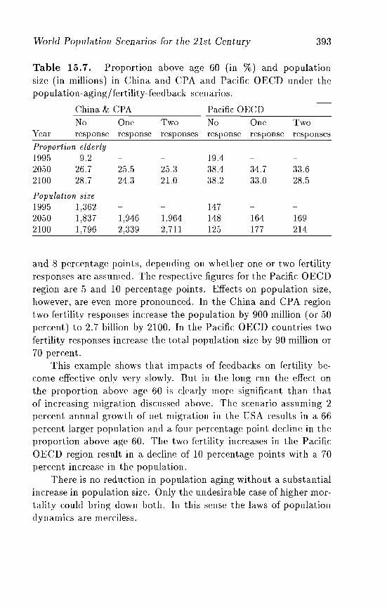
World Population Scena.rios for the 21st Century 393

Table 15.7. Proportion above age 60 (in %) and populationsize (in millions) in China and CPA and Pacific OECD under thepopulation-aging/fertility- feedback scenarios.

China & CPA Pacific OECD------------

No One Two No One TwoYear response

Proportion elderly1995 9.22050 26.72100 28.7

Population size1995 1,3622050 1,8372100 1,796

response

25.524.3

1,9462,339

responses

25.321.0

1,9642,711

response

19.438.438.2

147148125

response

34.733.0

164177

responses

33.628.5

169214

and 8 percentage points, depending on whether one or two fertilityresponses are assumed. The respective figures for the Pacific OECDregion are 5 and 10 percentage points. Effects on population size,however, are even more pronounced. In the China and CPA regiontwo fertility responses increase the population by 900 million (or 50percent) to 2.7 billion by 2100. In the Pacific OECD countries twofertility responses increase the total population size by 90 million or70 percent.

This example shows that impacts of feedbacks on fertility be­come effective only very slowly. But in the long run the effect onthe proportion above age 60 is clearly more significant than thatof increasing migration discussed above. The scenario assuming 2percent annual growth of net migration in the USA results in a 66percent larger population and a four percentage point decline in theproportion above age 60. The two fertility increases in the PacificOECD region result in a decline of 10 percentage points with a 70percent increase in the population.

There is no reduction in population aging without a substantialincrease in population size. Only the undesirable case of higher mor­tality could bring down both. In this sense the laws of populationdynamics are merciless.

394

15.4

W. Lutz, W. Sanderson, S. Scherbov, A. Goujon

Comparison with Other WorldPopulation Projections

In Chapter 2 we argue that there is a need for additional world pop­ulation projections that supplement those prepared by the UnitedNations, World Bank, and others. Because the differences in resultsoften lie in the approach taken by the organization - such as howto deal with uncertainty, whether to vary mortality assumptions inaddition to fertility assumptions, whether to consider dependenciesbetween the regions and between the components - it is difficultto directly compare our results with those of the other agencies.But an sets of projections have one common feature: they includeone projection that is presented as the most likely one, called themedium variant by the UN and the central scenario by us. Table15.8 summarizes the most likely projections of the UN, the WorldBank, the US Bureau of the Census, and IIASA.

However, even when a comparison is restricted to the most likelycase, it is impeded by the fact that different projections have differ­ent time horizons and different forms of spatial aggregation. For thisreason the information presented in Table 15.8 refers only to twopoints in time (2025 and 2100) and to the total world population.While the degree of increase between the two points in time givesa fair representation of the total path resulting from the assump­tions made by each agency, the global aggregation clearly hides someimportant regional differences. For example, the UN 1994 mediumvariant and the IIASA 1996 central scenario yield almost exactly thesame total world population size for 2025 but have different popula­tion figures for specific world regions and different proportions aboveage 60. One reason for this is that the UN assumes lower mortalityimprovements in industrialized countries and higher improvementin Africa than we do.

Naturally the differences between the projections are larger in2100 than in 202.5. The UN long-range projections produce thehighest population size and the lowest proportion above age 60.This is mostly due to higher fertility assumptions and, to a certainextent, to lower life-expectancy assumptions. But these projectionsalready date back to 1992 when most agencies were still assuminghigher fertility. In fact, the recent projections of population size

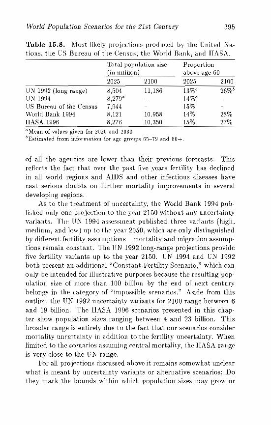
World Population Scenarios for the 21st Century 395

Table 15.8. Most likely projections produced by the United Na­tions, the US Bureau of the Census, the World Bank, and nASA.

Total population size(in million)

Proportionabove age 60

28%27%

UN 1992 (long range)UN 1994US Bureau of the CensusWorld Bank 1994IIASA 1996

2025

8,5048,2790

7,9448,1218,276

2100

11,186

10,95810,350

2025 2100

13%b 26W14%0

15%14%15%

a Mean of values given for 2020 and 2030.bEstimated from information for age groups 65-79 and 80+.

of all the agencies are lower than their previous forecasts. Thisreflects the fact that over the past five years fertility has declinedin all world regions and AIDS and other infectious diseases havecast serious doubts on further mortality improvements in severaldeveloping regions.

As to the treatment of uncertainty, the World Bank 1994 pub­lished only one projection to the year 2150 without any uncertaintyvariants. The UN 1994 assessment published three variants (high,medium, and low) up to the year 2050, which are only distinguishedby different fertility assumptions - mortality and migration assump­tions remain constant. The UN 1992 long-range projections providefive fertility variants up to the year 2150. UN 1994 and UN 1992both present an additional "Constant-Fertility Scenario," which canonly be intended for illustrative purposes because the resulting pop­ulation size of more than 100 billion by the end of next centurybelongs in the category of "impossible scenarios." Aside from thisoutlier, the UN 1992 uncertainty variants for 2100 range between 6and 19 billion. The nASA 1996 scenarios presented in this chap­ter show population sizes ranging between 4 and 23 billion. Thisbroader range is entirely due to the fact that our scenarios considermortality uncertainty in addition to the fertility uncertainty. Whenlimited to the scenarios assuming central mortality, the nASA rangeis very close to the UN range.

For all projections discussed above it remains somewhat unclearwhat is meant by uncertainty variants or alternative scenarios: Dothey mark the bounds within which population sizes may grow or

396 W. Lutz, W. Sanderson, S. Scherbov, A. Goujon

are they just randomly chosen sample paths? However, even in thelatter case, they may serve a useful purpose by providing extremesample paths to be used for sensitivity analysis. A more rigoroustreatment ofthe uncertainty issue in population projection, however,requires that specific probabilities of alternative paths be defined.These definitions are provided in Chapter 16.

Notes

[1] In all regions, 1990 age patterns of fertility were kept unchanged andscaled down (or up) according to the specification of the total fertilityrate.

[2] UN model life tables (UN, 1982) corresponding to the respective regionwere used as input for 1995 to obtain age-specific mortality rates fortoday's developing regions. For the remaining regions, observed mor­tality rates were used. For regions with assumed high AIDS mortalityspecial sets of age-specific mortality were used.

[3] Future age-specific mortality patterns were derived from model lifetables (UN, 1982; Coale and Guo, 1989). Coale-Guo "west tables" wereextended up to life expectancies of 100 to provide mortality schedulesfor very high life expectancies.

[4] Some very preliminary cross-sectional analyses suggest that such a re­lationship may indeed exist among societies that have fully passedthrough the demographic transition. It would also correspond to anecological approach which typically thinks in terms of "carrying capac­ity" and "crowdedness." But clearly much more research is needed onthis issue. Here the rationale is assumed simply to present an alterna­tive to the ubiquitous replacement-level assumption which also lackssound scientific foundations.

[5] This study has frequently been criticized for overestimating the agri­cultural potential of rain forests. Hence, without improvements in agri­cultural production and with no massive imports of food it is feasibleto assume a limit of 4 billion people for this region.

Chapter 16

Probabilistic PopulationProjections Based on ExpertOpinion

Wozfgang Lutz, WaTTen SandeTson, SeTgei ScheTbov

One thing that we know with certainty about the future populationsizes is that they are uncertain. The nature of this uncertainty andways to deal with it are highly controversial and still scientificallyunresolved issues. Can we speak meaningfully about a distributionof possible future population sizes? Can mean, median, and modalfuture population sizes be determined? Can confidence intervals forfuture population sizes be derived? The literature on projectionscontains three views, none of which we find completely satisfactory(se.e discussion in Chapter 2). In this chapter, we provide a fourthpel'Spective.

Most national and international agencies that produce popula­tion projections avoid addressing the issue of uncertainty explicitly.Typically they provide one main variant that is generally consid­ered the most likely case. Sometimes high, low, and other variantsare added, but these are virtually never given a probabilistic in­terpretation. If anything is said explicitly, it is that the high andlow variants should not be considered to define confidence intervals.Supplementing variants with presentations of extreme case scenar­ios can be useful for sensitivity analysis, but it does not help inquantifying the extent of uncertainty.

397

398 Woltg'ang Lut.z. Warren Sanderson, Sergei Scl1erbov

In contrast, many methods of producing fully probabilistic pop­ulation projections have been proposed and implemented, althoughso far only at the national level (see, for example, Alho, 1990; Carterand Lee, 1986; Lee and Tuljapurkar, 1994; McNown et al., 1995; andPflaumer, 1992). These approaches, which are almost exclusivelybased on time-series models, produce distributions of future popu­lation sizes and, thus, seem to be able to tell us, quite precisely, howmuch uncertainty there is in the results of population projections. Athird possibility of forecasting the uncertainty of future populationsizes is to make an assessment of the likely error in future projec­tions; this is done by evaluating the errors made in past projections.This tack has been suggested in Keyfitz (1981) and Stoto (1983).

In this chapter. we propose and implement a new method fordealing with the uncertainty of future population sizes. We call ourprojections "probabilistic population projections based on expertopinion." Our method is distinguished from other methods by itsuse of expert opinion both on the future courses of fertility, mortal­ity, and migration, and on the extent of their uncertainty. To ourknowledge, this is the first time that probabilistic population pro­jections have been made in this manner (aside from discussions inMuhsam, 1956, and Keyfitz. 1977), and the first time that a proba­bilistic model has been applied to all world regions. Therefore, ourresults should be treated with caution because these new ideas havenot yet been thoroughly tested. More systematic sensitivity analy­sis of the Delphi method in this context is needed. Nathan Keyfi tz(personal communication) points out that there is the danger ofa downward bias in the range of uncertainty assumed by experts.Nevertheless, we think that the use of expert opinion could havesignificant advantages over the use of time-series models or pastprojection performance.

In Section 16.1, we briefly discuss our motivation for developingthis approach to probabilistic population projections. Section 16.2provides a discussion of the interpretation of confidence intervals inthe present context. Section 16.3 contains a description of how wecombined the opinions of the experts presented in the first 14 chap­ters of this book to produce the assumptions for our probabilisticpopulation projections. In Section 16.4, we present the information

Probabilistic Population Projections 399

we have obtained on population size and age structure for the 13world regions. In Section 16 ..5, we present similar data for the worldas a whole. We conclude in Section 16.6 with a discussion of the im­plications of the expert- based probabilistic projections for the inter­pretation of the projections in Chapter 15, as well as for projectionsproduced by others.

16.1 The Motivation for New ProbabilisticPopulation Projections

The usefulness of a population projection is enhanced by knowing itsrange of uncertainty. Indeed, the uncertainty, as well as the mean ofa projection, could influence the actions of policy makers. Currently,there are two methods of quantitatively assessing the likely error of apopulation projection: time-series analysis and ex post error analy­sis. In time-series analysis, parameters are estimated from past dataon certain demographic variables. These parameters, along with es­timates of their uncertainty, are used to produce the informationneeded for population projections. In ex post error analysis, dataare collected on the errors in past projections. On the assumptionthat similar errors may occur again in future projections, we cantell policy makers and others the expected range of errors.

Time-series analysis is an approach, not a specific recipe. Differ­ent researchers using time-series analysis on the same data have pro­duced different projections along with different error estimates.[I]Most of the assumptions in the time-series approach are statisticalin nature. Thus, in the evaluation of a set of different time-series­based projections, we must consider concepts such as stationarity,linearity, transformations of variables, orders of autoregressive andmoving-average processes, autocorrelation, error-term correlations,as well as other elements that have no easy translation into the birthrates, death rates, and migration rates that we need to produce apopulation projection. It is easy to use statistical assumptions that,although individua.lly seem plausible, produce implications for fu­ture demographic changes that would be regarded as highly unlikelyby experts in the field. The problem may not be with any partic­ular assumption, but rather may be with a complex interaction of

400 Wolfgang Lutz, Warren Sanderson, Sergei Scherbov

assumptions that is difficult to diagnose. In addition, time-seriesanalysis typically derives only short- term information from a histor­ical data set. Demographic variables are often only related to theirown values over the previous few years. This application is appropri­ate for making relatively short-run projections. However, long-runprojections require a procedure that focuses on the determinants oflonger-term changes. Because of the indirect connection betweenassumptions and implications, it is difficult for policy makers andothers untrained in statistics to assess the error bounds producedby time-series analysis.

Ex post error analysis is more comprehensive than time-seriesanalysis, but it also has a problem when used in multiple projec­tions of the same population over the same period. Suppose oneprojection estimates the population at some future date at 10 mil­lion people and another estimates it at 20 million. If the mean errorof past projections were plus or minus 15 percent, we would tell pol­icy makers that the population would be 10 million plus or minus 15percent or 20 million plus or minus 15 percent. Thus it is possiblethat the average of past errors is small compared to the variationin the projections. In such cases, policy makers may ignore the av­erage past errors and use the range of population projections as anindicator of uncertainty. Also the application of ex post errors tofuture projections involves the important assumption that today'sforecasters make the same mistakes or neglect the same structuraldiscontinuities as did the forecasters of the past.

All population projections are based on judgment. In our judg­ment, the best way to produce projections is to base them explicitlyon the synthesized opinions of a group of experts.[2] We have al­ready discussed some of the advantages of using expert opinion as afoundation for making population projections in Chapters 2 and 105.In the case of probabilistic projections, we obtain information fromthe experts not only on fertility, mortality, and migration trends, butalso on the uncertainty of the trends. This information is providedin a clear and easy-to-assess form. By bringing together informa­tion from experts who are specialists in different fields, we believethat we can capture the best information currently available. Thisis reflected in the subtitle of this volume, "What can we assumetoday?"

Probabilistic Population Projections 401

16.2 The Concept of Confidence Intervalsfor Population Projections

In making a projection, we must focus on only a few elements froman extremely complex reality. There are an infinite number of waysof making these abstractions, and it is natural that different pro­jections would embody different assumptions. At any future date,differences in assumptions generally imply different distributions ofpopulation sizes, in particular, different mean populations and dif­ferent 95 percent confidence intervals.

Table 16.1 contains data on probabilistic projections of the pop­ulation of the United States around 2065; most of these projectionswere made in the early 1990s. The figures in the table are adaptedfrom Lee and Tuljapurkar (1994) and are ordered according to thelower bound of the 95 percent confidence interval. The first columnidentifies the forecaster. The second column lists the mean popu­lation size and the third and fourth columns show the lower andupper bounds, respectively, of the 95 percent confidence interval.In the table, the mean population of the USA around 2065 rangesfrom 296 million to 680 million. The lower bound of the 95 percentconfidence interval ranges from 207 million to 551 million people.The upper bound ranges between 349 million and 836 million.

The inconsistencies in this table are clear. Pflaumer (1992), us­ing a time-series approach with the logarithm of population as thevariable to be explained, is 95 percent confident that the US popula­tion around 2065 would lie between 551 and 836 million people. TheUS Bureau of the Census (1989) is 95 percent confident that the USpopulation at that time would lie between 207 and 456 million peo­ple. Clearly, both cannot be correct at the same time. For example,we cannot simultaneously believe that the probability of the popu­lation being 551 million or less is 2.5 percent and the probability ofthe population being 456 million or less is 97.5 percent.

The nine projections in Table 16.1 all produce different confi­dence intervals. How should we interpret this? First, it is vital to re­alize that there is no "correct" 95 percent confidence interval in thattable. Given that there are a large number of ways to forecast a fu­ture that will be clearly different from our current understanding ofthe world today, it is to be expected that different projections would

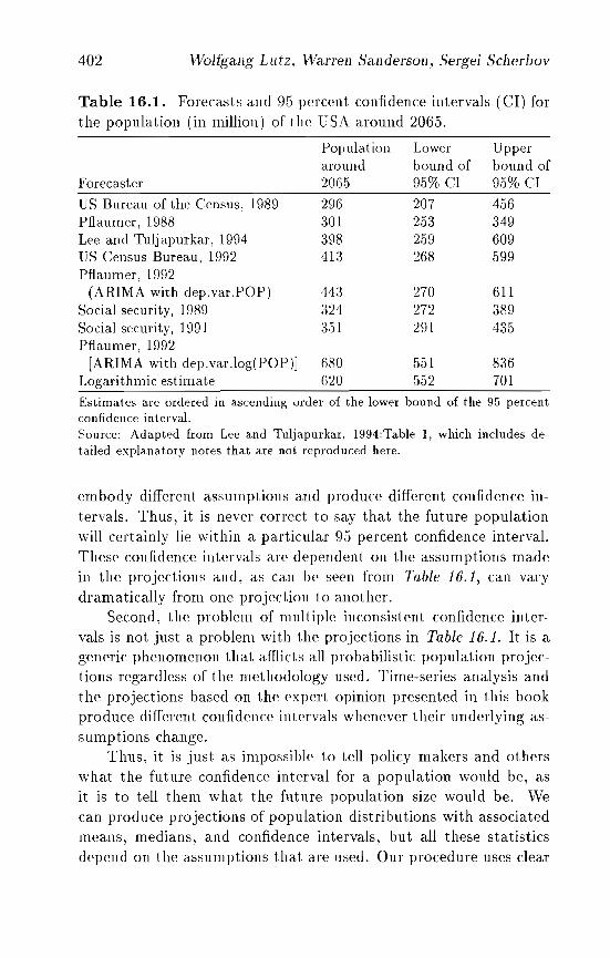
402 Woltg'ang Lutz, Warren Sanderson, Sergei Scherbov

Table 16.1. Forecasts and 95 percent confidence intervals (CI) forthe population (in million) of the USA around 2065.

611389435

Upperbound of95% CI

456349609599

270272291

207253259268

Lowerbound of95% CI

Populationaround2065

296301398413

443:324:351

Forecaster

us Bureau of the Census, 1989Ptlaumer, 1988Lee and Tuljapurkar, 1994US Census Bureau, 1992Ptlaumer, 1992

(ARIMA with dep.var.POP)Social security, 1989Social security, 1991Ptlaumer, 1992

[ARIMA with dep.var.log(POP)] 680 551 836Logarithmic estimate 620 552 701

Estimates are ordered in ascending order of the lower bound of the 95 percentconfidence interval.Source: Adapted from Lee and Tuljapurkar, 1994 :Table 1, which includes de­tailed explanatory notes that a.re not reproduced here.

embody different assumptions and produce different confidence in­tervals. Thus, it is never correct to say that the future populationwill certainly lie within a particular 95 percent confidence interval.These confidence intervals are dependent on the assumptions madein the projections and, as can be seen from Table 16.1, can varydramatically from one projection to another.

Second, the problem of multiple inconsistent confidence inter­vals is not just a problem with the projections in Table 16.1. It is ageneric phenomenon that afflicts all probabilistic population projec­tions regardless of the methodology used. Time-series analysis andthe projections based on the expert opinion presented in this bookproduce different confidence intervals whenever their underlying as­sumptions change.

Thus, it is just as impossible to tell policy makers and otherswhat the future confidence interval for a population would be, asit is to tell them what the future population size would be. vVecan produce projections of population distributions with associatedmeans, medians, and confidence intervals, but all these statisticsdepend on the assumptions that are used. Our procedure uses clear

Probabilistic Population Projections 403

assumptions, but no procedure can free us from our assumptions andprovide us with true future population distributions. We can providepolicy makers and others with possible mean future population sizesand confidence intervals, given the set of assumptions that we use.The assumptions we use are the best assessments that we can makeabout future trends and their uncertainties. Tomorrow, however,we may be able to make even better assessments, which, in turn,will result in more accurate projected mean population sizes andconfidence intervals.

16.3 The Methodology

In Chapter 1.5, we discuss how the opinions of the experts weretranslated into the high and low values that constituted 90 percentconfidence intervals for total fertility rate, life expectancy, and mi­gration level in the period 2030-203.5 and extended to 2100. Theseassumptions, however, are not sufficient to produce the probabilisticprojections. To complete them, we must first explore the additionalassumptions that are needed.

16.3.1 Fertility

Our fertility assumptions are based on the data in Table 15.1 andthe Appendix Tables. Table 15.1 gives four numbers for each region:the 199.5 total fertility rate (TFR) and low, central, and high valuesfor the interval 2030-203.5. The Appendix Tables define in moredetail the three paths from 199.5 to 2100. Clearly, there are manyways to use these data to generate random TFR paths into thefuture. We have chosen a simple procedure of random lines (orpiecewise linear paths).[3] Normal distributions are used to specifyrandom lines that conform to the 90 percent confidence intervals inthe Appendix Tables.

In the procedure, we use only one random draw from the normaldistribution to determine the full fertility path from 199.5 to 2100.We do not think that all paths of the total fertility rate will berandom lines. An alternative view would be that the TFRs wouldbehave like a random walk within predefined bounds. Each boundedrandom walk would produce a population total (see Goldstein et al.,1994, for a discussion of this sort of model) and in the aggregate a

404 Wolfgang Lutz, Warren Sanderson, Sergei Scherbov

population distribution would be generated for each projection pe­riod. These bounded random walks produce distributions of popu­lation sizes that are concentrated on a central value, and which aresimilar to those obtained using the assumptions described above.

The prime advantage of this combination of assuming normal­ity and linear trends over time (random lines instead of randomwalks) is that it provides a simple and reasonably robust way ofgenerating population distributions. Its main disadvantage is thatit is inappropriate for predicting short-term population dynamics.Those dynamics can be much more volatile than would be predictedusing the combination of the normality and linearity assumptions.

16.3.2 Mortality

The procedure selected to produce mortality paths is analogous tothat described for fertility. Because the mortality scenarios hadbeen defined in terms of improvements over 10-year periods, thelow, central, and high values must be converted into values of lifeexpectancy. This conversion provides us with three points of the2030-2035 life-expectancy distribution, which are the exact analogof the three points of the 2030-2035 TFR distribution given by theexperts. As in the case of fertility, random points are determinedfor life expectancies in 2030-2035 and 2080-2085.

Next, the time path of the life expectancy is linearly interpo­lated from the 1995 level to the randomly but jointly chosen 2030­2035 and 2080-2085 levels. After 2080-2085, all life expectanciesare assumed to remain constant. After the path of change in life ex­pectancy at birth is selected, age-specific mortality rates are derivedusing the model life tables as described in Chapter 15.

16.3.3 Migration

Expert opinion guided the production of a table of interregional mi­gration flows (see Table 15.3 for the annual levels of net migration).These flows are assumed to remain constant over time. The datain Table 15.3 represent the high values of those flows. The centralvalue is assumed to be half of the high value, and the low value isassumed to be zero.[4] Again a normal distribution is assumed with90 percent of all cases falling between the high and low values.[5]

Probabilistic Population Projections 405

We apply the same age-specific interregional migration rates thatwere used in Chapter 15. These rates are derived from age-specificschedules in Rogers and Castro (1981).

16.3.4 Interrelationships between the components

Population projections typically do not assume that the trends in thethree components of population change are related to one another.In this chapter, we consider migration to be independent of the othertwo components and of the age structure and size of the population,but we also consider the possibility of a correlation between fertilityand mortality. In Sections 16.4 and 16.5, we provide populationprojections of perfectly (positively) correlated fertility and mortalityand of uncorrelated fertility and mortality.

16.3.5 Interrelationships between regions

Most international population projections assume that all countriesand regions simultaneously have higher than expected fertility intheir high variants and lower than expected fertility in their lowvariant. However, fertility and mortality may not follow paralleltrends across regions. The interdependencies between the two de­mographic variables can be quite complex. For example, across theregions in which the majority of inhabitants are Muslim fertility maybe correlated, but the fertility level may be uncorrelated in Europeand Latin America.

In dealing with interrelations between regions, we considered thesituations in which fertility and mortality are either perfectly corre­lated across regions or uncorrelated. Fertility and mortality levelsmay be correlated across regions, but within regions, fertility andmortality may still be either correlated or uncorrelated with eachother. Similarly, fertility and mortality may be uncorrelated withfertility and mortality, respectively, across regions, but correlatedwith one another within each specific region.

In the case of both interrelationships between components andinterrelationships between regions, we are dealing with long-termdependencies. To address the relationships in both cases we useprocedures that link the entire time paths of fertility and mortalitytogether within regions and across regions.

406 Wolfgang Lutz, Warren Sanderson, Sergei Scherbov

16.4 Regional Results

16.4.1 Regional population sizes

Table 16.2 shows the populations of the 13 world regions in 1995.In addition, it gives the mean and median projected populations in2020, 2050, and 2100, as well as the upper and lower bounds of the95 percent confidence interval for each year. These numbers wereproduced on the assumption that there is no long-run correlationbetween fertility and mortality within regions. In Section 16.4.3,we provide an example of the impact that such a correlation couldhave.

The table contains two indicators of asymmetric population sizedistributions: the difference between the mean and median popu­lations, and the difference between the average of lower and upperbounds of the 95 percent confidence interval and the median. Whenthe mean is greater than the median and the difference betweenthe average and the bounds is positive, then the distribution of thepopulation size is asymmetric and points in the direction of higherpopulation sizes.

Consider first, the data for China and Centrally Planned Asia(CPA). In 1995, the region had a population of 1.36 billion people.Look at what happens to the lower bounds of the 95 percent con­fidence interval. By 2020 according to our population distribution,there is a 2.5 percent chance that the population will be below 1.53billion. Thirty years later. there is a 2..5 percent chance that thepopulation will be below L~5 billion, and by the end of the 21stcentury there is a 2.5 percent chance that the population will bebelow 0.71 billion. The table tells us that between 2050 and 2100,China's population may decline by almost half. At the high end ofthe spectrum, the table shows that in 2100 China has a 2.5 percentchance of having a population above 4.43 billion. The populationdistribution for China in 2100 is very skewed, with relatively highprobabilities of relatively high population sizes. The future popula­tion distributions of China behave in this way because we assumethat the lower end of its TFR range is below replacement level, whileits upper end is above replacement.

The time paths of the populations of North America and theEuropean part of the former Soviet Union (predominantly Russia)

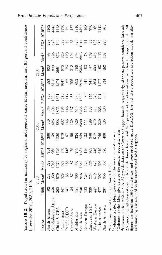
'i:l

,..,T

ab

le1

6.2

.P

op

ula

tio

n(i

nm

illi

ons)

byre

gio

ns,

ind

epen

den

tca

se.

Mea

n,

med

ian

,an

d95

per

cen

tco

nfi

den

cea 0

-~

inte

rval

s:2

02

0,2

05

0,2

10

0.

0-

~.

'-~.

2020

2100

'JJ

2050

~ ~.

1995

Mea

nb

Med

.c2.

5%d

97..5

%d

Mea

nb

Med

.c2.

5%d

97.5

%d

Mea

nb

nR

egio

nM

edC

2.5%

d97

.5%

d'i:

lN

orth

Afr

ica

162

277

277

254

300

440

439

:309

.583

630

.598

228

1202

.gS

ub-S

ahar

anA

fric

a55

810

5910

.58

965

1159

1625

1605

1085

2316

1909

1738

578

4345

I::'-~

Chi

na&

CP

A13

6216

7016

7015

2618

2618

8818

6513

512.

574

2051

1873

709

4428

~ ~. a

Pac

ific

Asi

a44

762

962

957

667

880

279

657

910

4787

682

932

216

96=::

l

Pac

ific

GE

eD14

715

515

.514

516

714

614

611

718

212

.512

059

221

'i:l ""

Cen

tral

Asi

a.54

8787

7610

013

91:3

788

206

212

194

6.547

7a <.....

.ro

Mid

dle

Eas

t15

130

0:3

0027

932

4.5

2051

538

069

278

673

832

015

16n ~ ~.

Sou

thA

sia

1240

1845

184.

517

3719

4923

8023

6818

3329

7023

6522

4610

1443

27g

Eas

tern

Eur

ope

122

124

124

116

133

III

110

8614

183

7831

168

'JJ

Eur

opea

nF

SU

a23

822

422

420

924

018

918

814

424

114

713

853

290

Wes

tern

Eur

ope

447

479

479

446

512

472

471

370

584

430

416

196

769

Lat

inA

mer

ica

477

697

696

646

746

930

925

707

1177

1163

1106

489

2142

Nor

thA

mer

ica

297

356

356

320

400

405

403

303

534

482

467

229

865

aEu

rop

ean

par

tof

the

form

erS

ovie

tU

nion

.bC

olum

nsla

bele

dM

ean

give

data

onth

em

ean

po

pu

lati

on

size

.cC

olum

nsla

bele

dM

ed.

give

dat

aon

the

med

ian

po

pu

lati

on

size

.dC

olum

nsla

bele

d2.

5%an

d97

.5%

prov

ide

dat

aon

the

low

eran

du

pp

erb

ou

nd

s,re

spec

tive

ly,

ofth

e95

per

cen

tco

nfid

ence

inte

rval

;2.

5p

erce

nt

ofal

lob

serv

atio

nslie

belo

wth

elo

wer

bo

un

dan

d97

.5p

erce

nt

ofal

lob

serv

atio

nsli

ebe

low

the

up

per

bo

un

d.

All

figu

res

are

bas

edon

1,00

0si

mul

atio

nsan

dw

ere

pro

du

ced

usin

gD

IAL

OG

,th

em

ult

ista

tep

op

ula

tio

np

roje

ctio

nm

odel

.F

erti

lity

and

mo

rtal

ity

are

assu

med

tob

eu

nco

rrel

ated

wit

hin

regi

ons.

~ 0 -1

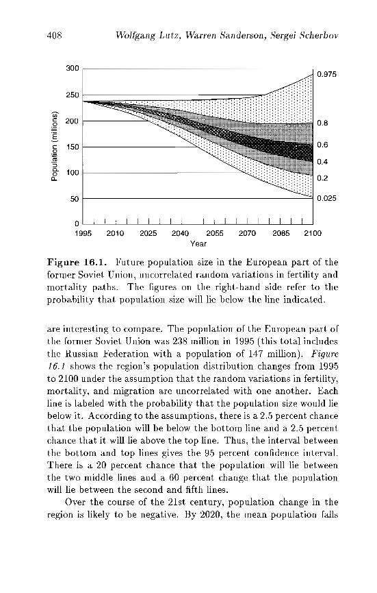
408

300

250

(j)c 200~'Ec 150.QIii::JCo 1000a..

50

Wolfgang Lutz, Warren Sanderson, Sergei Scherbov

0.975

I -:": ::::::::: ::.........~:::: .c:Q~<::::.:.:;~::::::::::::::::::::::::::::::::::

0.8

0.6

0.4

. :-:-: -: -: -:.:-: -:':1 0.2

I ='1 0.025

2085 21002025 2040 2055 2070Year

o I I ! I I I I I I I I I I

1995 2010

Figure 16.1. Future population size in the European part of theformer Soviet Union, uncorrelated random variations in fertility andmortality paths. The figures on the right-hand side refer to theprobability that population size will lie below the line indicated.

are interesting to compare. The population of the European part ofthe former Soviet Union was 238 million in 1995 (this total includesthe Russian Federation with a population of 147 million). Figure16.1 shows the region's population distribution changes from 1995to 2100 under the assumption that the random variations in fertility,mortality, and migration are uncorrelated with one another. Eachline is labeled with the probability that the population size would liebelow it. According to the assumptions, there is a 2.5 percent chancethat the population will be below the bottom line and a 2.5 percentchance that it will lie above the top line. Thus, the interval betweenthe bottom and top lines gives the 95 percent confidence interval.There is a 20 percent chance that the population will lie betweenthe two middle lines and a 60 percent change that the populationwill lie between the second and fifth lines.

Over the course of the 21st century, population change in theregion is likely to be negative. By 2020, the mean population falls

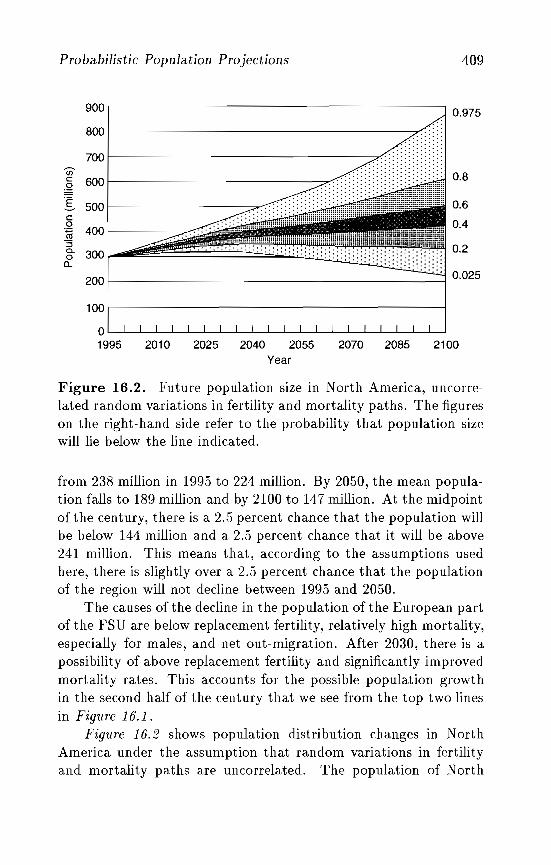
Probabilistic Population Projections 409

0.975

0.8

0.6

0.4

0.2

2070 2085 2100

f-- I 0.025

i <6d!':':':''':'H!,,,:,~,:,:m:;:;~;;;~;:T:T:;:Ti;~::;.:.:.:.:.:.:

900

800

700Vi'c 600~

I 500c0.~ 400"3g- 300a.

200

100

01995 2010 2025 2040 2055

Year

Figure 16.2. Future population size in North America, uncorre­lated random variations in fertility and mortality paths. The figureson the right-hand side refer to the probability that population sizewill lie below the line indicated.

from 238 million in 1995 to 224 million. By 2050, the mean popula­tion falls to 189 million and by 2100 to 147 million. At the midpointof the century, there is a 2.5 percent chance that the population willbe below 144 million and a 2.5 percent chance that it will be above241 million. This means that, according to the assumptions usedhere, there is slightly over a 2.5 percent chance that the populationof the region will not decline between 1995 and 2050.

The causes of the decline in the population of the European partof the FSU are below replacement fertility, relatively high mortality,especially for males, and net out-migration. After 2030, there is apossibility of above replacement fertility and significantly improvedmortality rates. This accounts for the possible population growthin the second half of the century that we see from the top two linesin Figure 16.1.

Figur'e 16.2 shows population distribution changes in NorthAmerica under the assumption that random variations in fertilityand mortality paths are uncorrelated. The population of North

410 Wolfgang Lutz, Warren Sanderson, Sergei Scherbov

America in 1995 was 297 million. The mean population distributionincreases to 356 million in 2020, 405 million in 2050, and 482 mil­lion in 2100. There is a possibility that the population of NorthAmerica will be smaller in 2100 than it was in 1995 but, given theassumptions used here, the chances of this are less than 20 per­cent. The continued growth of the US population is largely fueledby continuing migration. The population will shrink only if migra­tion is greatly restricted and the USA had a long period of belowreplacement fertility.

It is interesting to compare our 95 percent confidence intervalsfor North America in 2065 with those for the USA shown in Ta­ble 16.1. The lower bound of our 9.5 percent confidence intervalfor North America is around 280 million and our upper bound isaround 610 million (Figure 16.2). Taking into consideration thelarger population of North America (which includes Canada, Mex­ico, and the USA), our 9.5 percent confidence intervals are roughlysimilar to those in Lee and Tuljapurkar (1994) and the US Bureau ofthe Census (1992) and only slightly lower than the PHaumer (1992)time-series model with the population size as the dependent variable.

16.4.2 Regional age structures

Tables 16.3 and 16.4 are arranged like Table 16.2 except that theyrefer to the percentage of the population in the 0~14 age groupand the percentage in the 60 and above age group, respectively. Itis interesting to note that while the percentage of children 14 andunder will likely decrease during the 21st century in all regions, thepercentage 60 and above will grow. For example, in North Africa,38.8 percent of the population were age 14 and below in 1995. In2050, given the assumptions used here, the mean percentage falls to27.0 percent, with the 95 percent confidence interval lying between18.6 and 34.2 percent. By 2100, the mean is 18.7 percent and the 95percent confidence interval lies between 1L5 and 25.1 percent. Onthe other hand, the proportion of the North African population age60 and above was 5.9 percent in 1995. In 2100, the mean percentageis 24.0 percent, with the 95 percent confidence interval between 15.2and 37.4 percent. The phenomenon of population aging will occuron a worldwide scale during the 21st century. In our next examples,

Probabilistic Population Projections 411

we look again at the case of China and CPA and at the comparisonbetween the European part of the FSU and North America.

In China and CPA, 27.3 percent of the population in 1995 werebetween ages 0 and 14. By 2020, given the assumptions used here,the mean percentage falls to 21.2, with a 95 percent confidence in­terval stretching from 16.5 to 25.6 percent. This means that theprobability of a fall in the percentage of the 0-14 age group is over97.5 percent. The decrease in the percentage of this group contin­ues over the century, with the mean at 17.1 percent in 2100 and a95 percent confidence interval between 9.8 and 24.1 percent. It isinteresting to note that the skewness in the distribution of popula­tion sizes that emerges in the region between 2050 and 2100 is notmirrored in the distribution of the percentage of younger people,which remains quite symmetric. Indeed, the percentage distribu­tion of younger people in the population remains quite symmetricthroughout the 21st century for all regions in Table 16.3.

With this decrease in the percentage of the 0-14 age group in theChina and CPA region there is an increase in the percentage of thepopulation age 60 and above (Table 16.4). In 1995,9.2 percent ofthe population was 60 and above; by 2050 the mean is 25.3 percent,and by 2100 it increases to 28.3 percent. Most of the increase inthe older population takes place in the first half of the 21st century.We are quite confident of this, because the 95 percent confidenceinterval for 2050 lies between 17.8 and 34.1 percent. Even at thelower bound, the percentage of the population 60 and above almostdoubles between 1995 and 2050.

The comparison between the age structure changes in the Eu­ropean part of the former Soviet Union and those in North Americais especially interesting in view of the differences in their populationgrowth trends. Figures 16.3([ and 16.3b show the comparisons ofthe0-14 populations and Figures 16.4([ and 16.4b provide a compari­son of the 60 and above populations. In the European part of theFSU and in North America, the percentages of the 0-14 populationswere almost identical in 1995,21.6 and 22.0 percent, respectively. In2100, the mean percentages are even closer, 17.6 and 17.5 percent,respecti vely.

There is slightly more uncertainty about the percentage of thisage group in the European pa.rt of the FSU than in North America

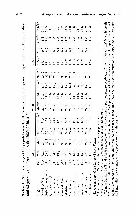
*""f-O t-.,;,

Ta

ble

16

.3.

Per

cen

tag

eo

fth

ep

op

ula

tio

nin

the

0-14

age

gro

up

,by

reg

ion

s,in

dep

end

ent

case

.M

ean

,m

edia

n,

and

95p

erce

nt

con

fid

ence

inte

rval

s:20

20,

2050

,21

00.

2020

2050

2100

Reg

ion

1995

Mea

nb

Med

.c2.

5%d

97.5

%d

Mea

nb

Med

.c2.

5%d

97.5

%d

Mea

nb

Med

.c2.

5%d

97.5

%d

Nor

thA

fric

a38

.833

.9:3

4.0

30.0

37.5

27.0

27.:3

18.6

34.2

18.7

19.0

11.5

25.1

~

Sub

-Sah

aran

Afr

ica

45.4

39.7

39.8

36.1

42.9

28.0

28.3

19.2

35.2

18.1

18.3

11.0

24.5

0'

~C

hin

a&

CP

A27

.321

.221

.316

.525

.619

.920

.012

.327

.317

.117

.29.

824

.1::

Pac

ific

Asi

a33

.226

.526

.622

.629

.921

.821

.915

.027

.816

.416

.59.

023

.1aq

Pac

ific

GE

eD17

.113

.913

.910

.816

.713

.013

.08.

117

.813

.113

.17.

019

.4t-< I:

:

Cen

tral

Asi

a:3

6.3

31.5

:31.

725

.037

.026

.526

.816

.834

.718

.718

.911

.425

.7""'" ~N

Mid

dle

Eas

t42

.837

.037

.033

.440

.327

.127

.:318

.834

.318

.218

.311

.224

.5~

Sou

thA

sia

36.6

30.1

30.1

27.4

32.7

22.5

22.6

16.4

28.1

15.3

15.4

8.7

21.8

Eas

tern

Eur

ope

21.3

16.5

16.6

13.3

19.6

14.1

14.1

8.9

19.4

15.0

17.3

7.8

15.6

:::; <1l

Eur

opea

nF

SU

a21

.616

.016

.012

.319

.214

.514

.58.

819

.817

.617

.79.

524

.7=: U

)W

este

rnE

urop

e19

.915

.815

.912

.818

.814

.214

.39.

319

.315

.215

.38.

721

.6Cl.

> bL

atin

Am

eric

a33

.727

.027

.123

.530

.422

.222

.316

.028

.218

.718

.711

.825

.2Q

...<1

lN

orth

Am

eric

a22

.017

.917

.914

.621

.116

.716

.711

.821

.317

.517

.611

.623

.3..., ti

l 0a

Eu

rop

ean

par

to

fth

efo

rmer

Sov

iet

Uni

on.

=:

bCol

umns

labe

led

Mea

ngi

ved

ata

onth

em

ean

po

pu

lati

on

size

.U

)<1

lcC

olu

mn

sla

bele

dM

ed.

give

dat

aon

the

med

ian

po

pu

lati

on

size

.oci

dC

olu

mn

sla

bele

d2.

5%an

d97

.5%

prov

ide

data

onth

elo

wer

and

up

per

bo

un

ds,

resp

ecti

vely

,o

fth

e95

per

cen

tco

nfid

ence

inte

rval

;~.

2.5

per

cen

tof

all

obse

rvat

ions

liebe

low

the

low

erb

ou

nd

and

97.5

per

cen

tof

all

ob

serv

atio

ns

liebe

low

the

up

per

bo

un

d.

All

U) "

figu

res

are

base

don

1,00

0si

mul

atio

nsan

dw

ere

pro

du

ced

usin

gD

IAL

OG

,th

em

ult

ista

tep

op

ula

tio

np

roje

ctio

nm

odel

.F

erti

lity

::l-

<1l

and

mo

rtal

ity

are

assu

med

tobe

un

corr

elat

edw

ithi

nre

gion

s...., 0

-0 -<:

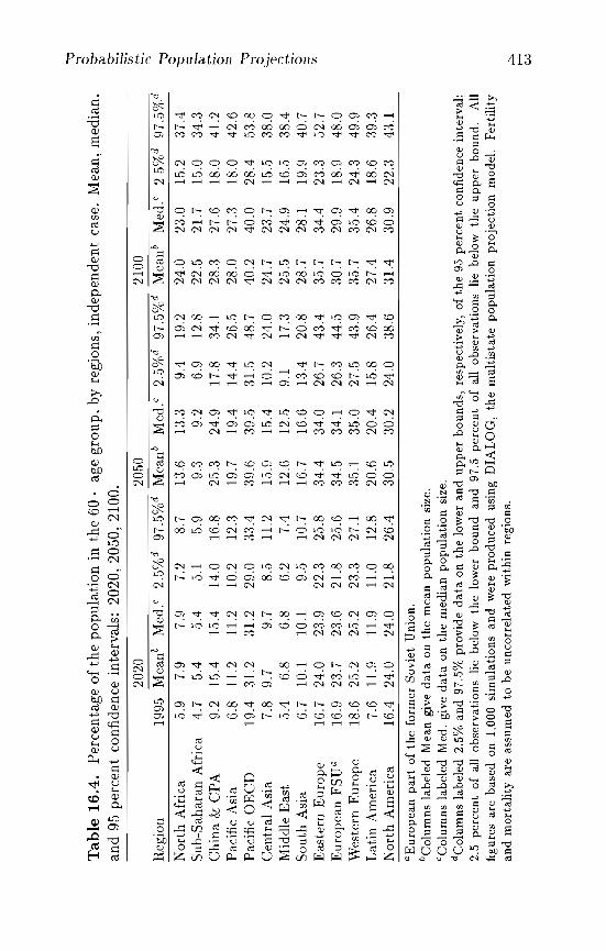
'"tl

...,T

ab

le1

6.4

.P

erce

nta

ge

of

the

po

pu

lati

on

inth

e6

0+

age

gro

up

,by

regi

ons,

ind

epen

den

tca

se.

Mea

n,

med

ian

.0 0

- '"an

d95

per

cen

tco

nfi

den

cein

terv

als:

2020

,20

50,

2100

.2: .....

.20

2020

5021

00tn· :':

'.

1995

Mea

nb

Med

.c2.

5%d

97.5

%d

Mea

nb

Med

.c2

..5%

d97

.5%

dM

ean

b<"

"l

Reg

ion

Med

.c2

..5%

d97

.5%

d'"t

lN

orth

Afr

ica

.5.9

7.9

7.9

7.2

8.7

13.6

13.3

9.4

19.:2

24.0

23.0

15.2

37.4

.gS

ub-S

ahar

anA

fric

a4.

75.

45.

4.5

.15.

99.

39.

26.

912

.822

.521

.715

.034

.3l::

: ...... '"

Ch

ina

&C

PA

9.2

1.5.

41.

5.4

14.0

16.8

25.3

24.9

17.8

34.1

28.3

27.6

18.0

41.2

"....

. 0'P

acif

icA

sia

6.8

11.2

11.2

10.2

12.3

19.7

19.4

14.4

26..5

28.0

27.3

18.0

42.6

::l

Pac

ific

GE

CD

19.4

31.2

31.2

29.0

33.4

39.6

39.5

31.5

48.7

40.2

40.0

28.4

.53.

8::0

Cen

tral

Asi

a7.

89.

79.

78

..511

.21.

5.9

1.5.

410

.224

.024

.723

.715

.538

.0a <.....

.(1

)

Mid

dle

Eas

t5.

46.

86.

86.

27.

412

.612

.59.

117

.325

.524

.916

..538

.4<"

"l".

....

Sou

thA

sia

6.7

10.1

10.1

9.5

10.7

16.1

16.6

13.4

20.8

28.7

28.1

19.9

40.7

2'E

aste

rnE

urop

e16

.724

.023

.922

.325

.8:3

4.4

:34.

026

.743

.435

.734

.423

.352

.7t;;

Eur

opea

nF

SU

"16

.923

.723

.621

.825

.634

.534

.126

.344

.530

.729

.918

.948

.0W

este

rnE

urop

e18

.62.

5.2

2.5.

223

.327

.135

.135

.027

.543

.935

.735

.424

.349

.9L

atin

Am

eric

a7.

611

.911

.911

.012

.820

.620

.415

.826

.427

.426

.818

.639

.3N

orth

Am

eric

a16

.424

.024

.021

.826

.430

.530

.224

.038

.631

.430

.922

.343

.1

aEu

rop

ean

par

tof

the

form

erS

ovie

tU

nion

.bC

olum

nsla

bele

dM

ean

give

data

onth

em

ean

po

pu

lati

on

size

.cC

olu

mn

sla

bele

dM

ed.

give

data

onth

em

edia

np

op

ula

tio

nsi

ze.

dCol

umns

labe

led

2.5%

and

97.5

%pr

ovid

ed

ata

onth

elo

wer

and

up

per

bo

un

ds,

resp

ecti

vely

,of

the

95p

erce

nt

conf

iden

cein

terv

al;

2.5

per

cen

tof

all

obse

rvat

ions

liebe

low

the

low

erb

ou

nd

and

97.5

per

cen

tof

all

obse

rvat

ions

liebe

low

the

up

per

boun

d.A

llfi

gure

sar

eb

ased

on1,

000

sim

ulat

ions

and

wer

ep

rod

uce

dus

ing

DIA

LO

G,

the

mu

ltis

tate

po

pu

lati

on

pro

ject

ion

mod

el.

Fer

tili

tyan

dm

ort

alit

yar

eas

sum

edto

be

un

corr

elat

edw

ithi

nre

gion

s...,. f-

-'W

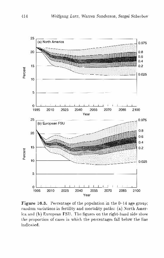
414 Woltg'ang Lutz, Warren Sanderson, Sergei Scherbov

25(a) North America

h-20

15C<I>~<I>[L

10

~0.975

0.80.60.4

0.2

:-:-:-:-:', :-:-:-:-: .':-."-'--'. ':':':':::::::::::::::::::::::':':':10.025

5 1-1-------------------------1

o I I! I! I I 1 I l ' I I I

1995 2010 2025 2040 2055 2070 2085 2100Year

25 , ,0.975

0.8

0.6

0.4

0.2

.. '-:-:-: ::.:<>::::::::::::>::,: :.: :-: 0.025

(b) European FSU

10 I Y,,-

15

201"- =~.

C<I>~<I>[L

5 I I

2085 21002025 2040 2055 2070Year

o I I I I I

1995 2010

Figure 16.3. Percentage of the population in the 0-14 age group;random variations in fertility and mortality paths: (a) North Amer­ica and (b) European FSU. The figures on the right-hand side showthe proportion of cases in which the percentages fall below the lineindicated.

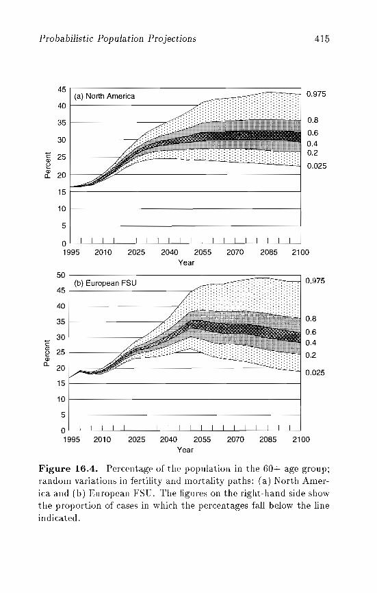
Probabilistic Population Projections 415

45I (a) North America ~ ~ 0.975

40 f-'-"- ?:::::-:-:

35~~08

~:I ,"~~!L8:. 20

15

10

5

o1995 2010 2025 2040 2055 2070 2085 2100

Year

50

451 (b) European FSU .:::::::::::::~ 0.975

40 /::::::::::::::::::::::::::::::::::::::::

~.........::::::::::::: :: .

i : h~.~:::~~:::::::: ~.~a...

20 V- fjiii!ffF~ ~ 0.025

15

10

5

o1995 2010 2025 2040 2055 2070 2085 2100

Year

Figure 16.4. Percentage of the population in the 60+ age group;random variations in fertility and mortality paths: (a) North Amer­ica and (b) European FSU. The figures on the right-hand side showthe proportion of cases in which the percentages fall below the lineindicated.

416 V\-Tolfgang Lutz, Warren Sanderson, Sergei Scherbov

in 2100. The 95 percent confidence interval for the European part ofthe FSU is between 9.5 and 24.7 percent, while for North Americait is between 11.6 percent and 23.3 percent. Most of the differencebetween the 95 percent confidence intervals is in the lower bounds.The large gap between the two bottom lines in Figure 16.3b for theEuropean part of the FSU indicates that the distribution is slightlyskewed in the direction of the smaller percentages. We can see thesame trend in Table 16.3 because the mean percentage of the 0­14 population is less than the median percentage. Indeed, in allregions it is generally the case that the mean percentage of the 0-14age group is less than the median.

The percentages of the 60 and above population were very closein the two regions in 1995. In the European part of the FSU it was16.9 percent and in North America it was 16.4 percent. Accordingto the assumptions, by 2050 the two mean percentages are 34.5 and30.5 percent, respectively. The four percentage point difference issmall compared with the 95 percent confidence intervals. In the caseof the European part of the FSU we are 95 percent confident thatthe percentage would lie somewhere between 26.3 and 44.5 percentin 2050. For North America, the 95 percent confidence interval isbounded by 24.0 and 38.6 percent in 2050. Clearly, we cannot besure in which region the percentage will rise more rapidly. In bothcases, the percentage for the 0-14 age group and the percentage forthe 60 and over age group, the differences between the two regionsare relatively minor. This is the case even though the trends inpopulation growth are very different.

16.4.3 An example of correlated fertility andmortality

The regional data presented above were computed on the assump­tion that there would be no future long-run relationship between therandom variations in the time paths of fertility and mortality. Tosee the effect of such a correlation, Table 16.5 compares two casesin sub-Saharan Africa in 2100: in one case the time paths of fertilityand mortality are independent (uncorrelated) over time and in theother they are perfectly correlated.[6] Sub-Saharan Africa currentlyhas a high fertility rate, but we assume that it will experience its

Probabilistic Population Projections 417

demographic transition during the period of our projection. Giventhe knowledge that we have on the experience of other countries thathave passed through fertility transitions, it is reasonable to assumethat the speeds of mortality and fertility decline will be positivelycorrelated over time. Correlated fertility and mortality means thatif, in the future, sub-Saharan Africa has a relatively fast decline inmortality, it would also have a relatively rapid decline in fertility,but if the decline in mortality were slow, the fall in fertility wouldalso be slow.[7]

Table 16.2 shows that sub-Saharan Africa is the region of theworld with the greatest uncertainty about future population size. In1995, the population in the region was 558 million people. By 2100,the mean population size is estimated at 1.909 billion; the medianis 1.738 billion; and the 95 percent confidence interval encompassesalmost 4 billion people, with a lower bound of 578 million and anupper bound of 4.345 billion. This gigantic confidence interval isthe result of unusually large uncertainty about both fertility andmortality in the region, and the assumption that the speeds of thedecline in fertility and mortality are unrelated to each other.

Table 16.5 shows that under correlated and uncorrelated as­sumptions, the median population size is about the same: 1.738billion when the paths of fertility and mortality are independentand 1.728 billion when they are perfectly correlated. However, thepopulation size distributions vary considerably. If fertility and mor­tality trends are considered unrelated, then the mean populationsize will be 1.909 billion in 2100; if the trends are assumed to becorrelated, the mean will be 1.663 billion. The greatest differenceis in the extent of uncertainty. In the case of uncorrelatedtrendsthe 95 percent confidence interval lies between 578 million and 4.345billion people; in the case of perfectly correlated trends the 95 per­cent confidence interval lies between 1.174 and 1.859 billion people.Thus, in the future the mean population size and especially the95 percent confidence intervals of Sub-Saharan Africa depend, to agreat extent, on whether or not future fertility and mortality trendsare assumed to be correlated.

Although uncertainty about population size shrinks dramati­cally when future trends in fertility and mortality are perfectly cor­related, uncertainty about age structure does not necessarily lessen.

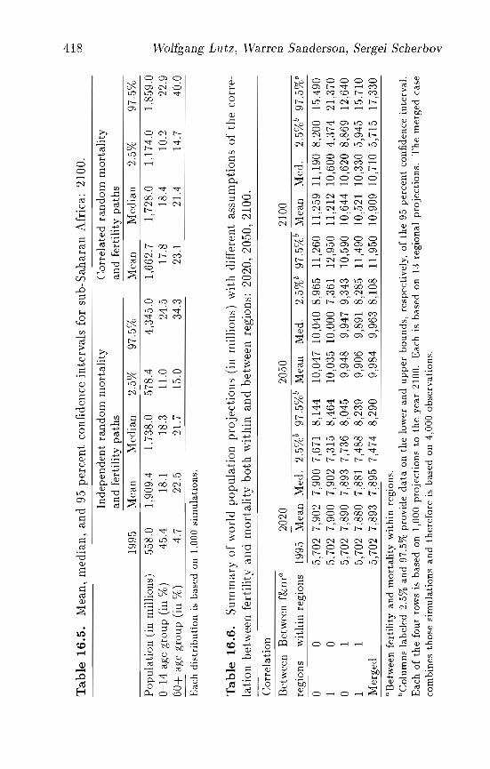
Ta

ble

16

.5.

Mea

n,m

edia

n,an

d95

perc

ent

conf

iden

cein

terv

als

for

sub

-Sah

aran

Afr

ica:

2100

.

97.5

%

Inde

pend

ent

ran

do

mm

ort

alit

yC

orre

late

dra

nd

om

mo

rtal

ity

and

fert

ilit

yp

ath

san

dfe

rtil

ity

pat

hs

-----"----''--------------

1995

Mea

nM

edia

n2.

5%97

.5%

Mea

nM

edia

n2

..5%

Ta

ble

16

.6.

Su

mm

ary

of

wor

ldpo

pula

tion

proj

ecti

ons

(in

mil

lion

s)w

ith

diff

eren

tas

sum

pti

on

sof

the

corr

e­la

tion

betw

een

fert

ilit

yan

dm

ort

alit

yb

oth

wit

hin

and

betw

een

regi

ons:

2020

,20

50,

2100

.

aB

etw

een

fert

ilit

yan

dm

ort

alit

yw

ith

inre

gion

s.b

Co

lum

ns

lab

eled

2.5%

and

97.5

%p

rov

ide

dat

ao

nth

elo

wer

and

up

per

bo

un

ds,

resp

ecti

vely

,o

fth

e95

per

cen

tco

nfid

ence

inte

rval

.E

ach

of

the

four

row

sis

bas

edon

1,00

0p

roje

ctio

ns

toth

ey

ear

2100

.E

ach

isb

ased

on

13re

gion

alp

roje

ctio

ns.

Th

em

erg

edca

seco

mb

ines

tho

sesi

mu

lati

on

san

dth

eref

ore

isb

ased

on4,

000

ob

serv

atio

ns.

Cor

rela

tion

Bet

wee

nB

etw

een

f&m

a20

2020

5021

00

regl

Ons

wit

hin

regi

ons

1995

Mea

nM

ed.

2.5%

b97

.5%

bM

ean

Med

.2.

5%b

97.5

%b

Mea

nM

ed.

2.5%

b97

.5%

b

00

5,70

27,

902

7,90

07,

671

8,14

410

,047

10,0

408,

965

11,2

6011

,259

11,1

908,

200

15,4

901

05,

702

7,90

07,

902

7,31

58,

464

10,0

3510

,000

7,36

112

,950

11,2

1210

,600

4,37

421

,370

01

5,70

27,

890

7,89

37,

736

8,04

59,

948

9,94

79,

343

10,5

9010

,644

10,6

208,

869

12,6

401

15,

702

7,88

07,

881

7,48

88,

239

9,90

69,

891

8,28

511

,490

10,5

2110

,330

5,94

515

,710

Mer

ged

5,70

27,

893

7,89

57,

474

8,29

09,

984

9,96

38,

108

11,9

5010

,909

10,7

105,

715

17,3

30

1,85

9.0

22.9

40.0

1,17

4.0

10.2

14.7

Pop

ulat

ion

(in

mil

lion

s)·5

58.0

1,90

9.4

1,73

8.0

578.

44,

345.

01,

662.

71,

728.

00-

14ag

egr

oup

(in

%)

45.4

18.1

18.3

11.0

24.5

17.8

18.4

60

+ag

egr

oup

(in

%)

4.7

22..5

21.7

15.0

34.3

23.1

21.4

Eac

hd

istr

ibu

tio

nis

bas

edon

1,00

0si

mu

lati

on

s.

Probabilistic Population Projections 419

The 95 percent confidence interval for the percentage of the popu­lation in the 0-14 age group is slightly smaller when we assume aperfect correlation, but the confidence interval for the percentage ofthe population age 60 and above is larger.

16.5 World Projections

In this section, we project world population sizes by combining theregional projections presented in Section 16.4. The process of ag­gregation adds one more complication, because we cannot simplyadd the regional figures together. We must also take into accountthe possibility that fertility and mortality paths could be correlatedacross regions.

Table 16.6 shows five world population projections. In the first,fertility and mortality paths are uncorrelated both across regionsand within regions. These data are derived by aggregating the re­gional data presented in Section 16.3. In Table 16.6, the mean pop­ulation size of the world at a future date can be derived by addingtogether the means for each region. The median and particularlythe bounds on the 95 percent confidence interval, however, are notderived from addition. They must be simulated. In the secondprojection, fertility and mortality paths are each correlated acrossregions, but not within regions (i.e., high fertility in one region goesalong with high fertility in all other regions). In theory, the meanpopulations in this projection are the same as those in the first case.In practice, they are slightly different from each other because therandom samples are different.

To illustrate the difference between these two assumptions, Fig­ures 16.50. and 16.5b show the resulting distributions of total popu­lation size for all world regions together in the case of perfect correla­tion between regions (Figure 16.50.) and in the case of independence(Figure 16. 5b). The X axis is given on a relative scale with 1.0 cor­responding to the mean. One thousand simulations were conductedfor each distribution. It is clearly visible that, in the case of indepen­dence, the distribution is more concentrated. This is because underthe independence assumption regions may compensate for one an­other; for example, an unusually low fertility level in one region maypartly be offset by high fertility in another region. In the case of

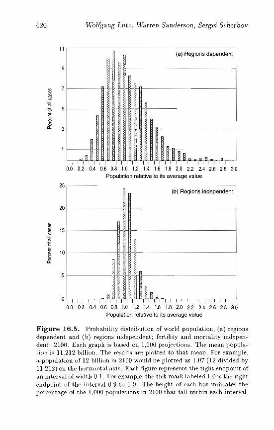
420

11

9

en 7Q)en

'"u(ij

'0 5cQ)

~Q)

0- 3

Wolfgang Lutz, Warren Sanderson, Sergei Scherbov

(a) Regions dependent

$;

{

m

'" III 1111., ",A nI I I I I I I I I I I I I I I I I I I

0.0 0.2 0.4 0.6 0.8 1.0 1.2 1.4 1.6 1.8 2.0 2.2 2.4 2.6 2.8 3.0

Population relative to its average value

(b) Regions independent

;

fIJ ~ mo I I I I I 1 I I I I I I I ) I I I I I I

0.0 0.2 0.4 0.6 0.8 1.0 1.2 1.4 1.6 1.8 2.0 2.2 2.4 2.6 2.8 3.0

Population relative to its average value

25

20

enQ)en 15'"u(ij

'0C

10Q)

~Q)

0-

5

Figure 16.5. Probability distribution of world population, (a) regionsdependent and (b) regions independent; fertility and mortality indepen­dent: 2100. Each graph is based on 1,000 projections. The mean popula­tion is 11.212 billion. The results are plotted to that mean. For example,a population of 12 billion in 2100 would be plotted as 1.07 (12 divided by11.212) on the horizontal axis. Each figure represents the right endpoint ofan interval of width 0.1. For example. the tick mark labeled 1.0 is the rightendpoint of the interval 0.9 to 1.0. The height of each bar indicates thepercentage of the 1,000 populations in 2100 that fall within each interval.

Probabilistic Population Projections 421

perfect correlation such compensations are not possible, thus manymore extreme cases result.

The third and fourth projections in Table 16.6 are based onthe assumption that fertility and mortality are perfectly correlatedwithin regions. This situation is most plausible in regions that arestill undergoing demographic transitions. The third projection as­sumes no correlation of fertility and mortality across regions, whilethe fourth assumes a perfect positive correlation across regions.Again, in theory the mean populations should be identical, but arenot because of random sampling.

We call the fifth projection the "merged" case because it is com­puted by merging the outcomes of the other four. Each of the firstfour projections is based on a sample size of 1,000 observations. Themerged projection is based on 4,000 observations. The experts werenot asked about correlations of fertility and mortality within andbetween regions; nevertheless, to produce world population projec­tions, information on these correlations is required. In particular,we must know both the correlations themselves and the uncertaintyassociated with each one. In the absence of expert opinion, we in­troduce uncertainties into the correlations by giving equal weightto, or merging, the four extreme case projections.[8]

The range of the 95 percent confidence intervals depends onwhich projection is chosen. On the one hand, if we were certain thatfuture time paths of fertility and mortality were uncorrelated withinand across regions, then according to the assumptions, the meanpopulation of the world in 2050 would be 10.0 billion people, withthe range of the 95 percent confidence interval between 9.0 and 11.3billion. On the other hand, if we were certain that future fertility andmortality trends were perfectly correlated across regions, but notwithin regions, the mean population of the world in 2050 would alsobe 10.0 billion, but the range of the 95 percent confidence intervalwould be wider, between 7.4 and 13.0 billion.

It is useless to try to determine which 95 percent confidenceinterval is the "correct" one. There is no "correct" 95 percent con­fidence interval. Each projection embodies different assumptionsabout the correlations and their uncertainties and, therefore, pro­duces different confidence intervals. We prefer the merged projectionbecause it is the only one of the five that incorporates uncertainty

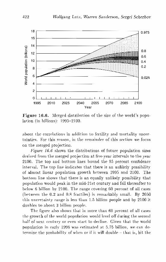
422 Wolfgang Lutz, Warren Sanderson, Sergei Scherbov

0.975

0.025

0.8

0.6

0.4

0.2

2085 21002040 2055 2070Year

~:::::::::::::;.:-:";.;.;.:...........:.-.:...:

f---------------------------------,""r.-;." " " " "

18

16

Vi 14c

~ 12e.c 100.~

:J 80..00..

6"0

~~ 4

2

0

1995 2010 2025

Figure 16.6. Merged distribution of the size of the world's popu­lation (in billions): 199.5-2100.

about the correlations in addition to fertility and mortality uncer­tainties. For this reason, in the remainder of this section we focuson the merged projection.

Figure 16.6 shows the distributions of future population sizesderived from the merged projection at five-year intervals to the year2100. The top and bottom lines bound the 9.5 percent confidenceinterval. The top line indicates that there is an unlikely possibilityof almost linear population growth between 199.5 and 2100. Thebottom line shows that there is an equally unlikely possibility thatpopulation would peak in the mid-21st century and fall thereafter tobelow 6 billion by 2100. The range covering 60 percent of all cases(between the 0.2 and 0.8 fractiles) is remarkably small. By 2050this uncertainty range is less than 1.5 billion people and by 2100 itdoubles to about 3 billion people.

The figure also shows that in more than 60 percent of all casesthe growth of the world population would level off during the secondhalf of next century or even start to decline. Given that the worldpopulation in early 1996 was estimated at 5.7.5 billion, we can de­termine the probability of when or if it will double - that is, hit the

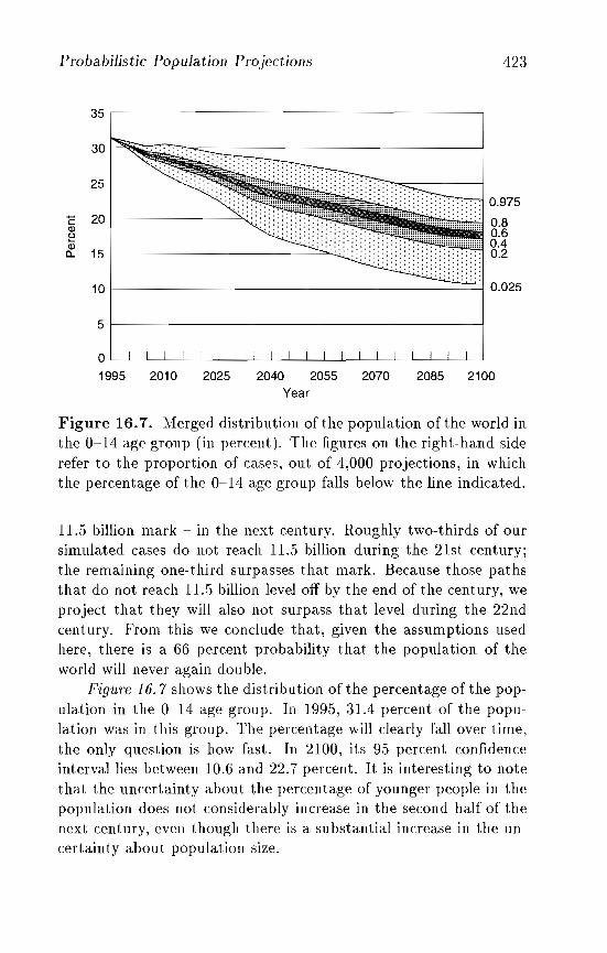
Proba.bilistic Popula.tion Projections 423

0.975

0.80.60.40.2

f- =---=l 0.025

f-------------------'=--....:::-."-..:"'-.:..;. .

35

30 I~~::.-:-:::..

25

"E 20Q)

~Q)

15c..

10

5 I----------------------l

2085 21002040 2055 2070Year

2025

o I I I

1995 2010

Figure 16.7. Merged distribution of the population of the world inthe 0-14 age group (in percent). The figures on the right-hand siderefer to the proportion of cases, out of 4,000 projections, in whichthe percentage of the 0-14 age group falls below the line indicated.

11.5 billion mark - in the next century. Roughly two-thirds of oursimulated cases do not reach 11.5 billion during the 21st century;the remaining one-third surpasses that mark. Because those pathsthat do not reach 1L5 billion level off by the end of the century, weproject that they will also not surpass that level during the 22ndcentury. From this we conclude that, given the assumptions usedhere, there is a 66 percent probability that the population of theworld will never again double.

Figure 16.7 shows the dist.ribution of the percentage of the pop­ulat.ion in the 0-14 age group. In 1995, 31.4 percent of the popu­lat.ion was in this group. The percentage will clearly fall over time,t.he only question is how fast. In 2100, its 95 percent confidenceinterval lies between 10.6 and 22.7 percent. It is interesting to notethat the uncertainty about the percentage of younger people in thepopulation does not. considerably increase in the second half of thenext. century, even though there is a substantial increase in the un­certainty about population size.

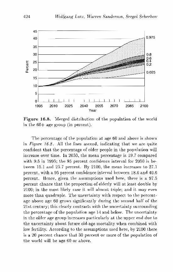
424 Wolfg'ang Lutz, Warren Sanderson, Sergei Scberbov

0.80.60.40.2

2085 2100II " I

,':':-:':-:':-:-:

.::::::::::.:;=

2040 2055 2070Year

--------;;T:::>_:~0.025

f--------------------------:;;::>....~-:.:.: .. -: -:.:.:.

f- --==-.-..-<1 0.975

1------------------::::>7<············· .

45

40

35

30

C 254l~4l 20c..

15

10

5

01995 2010 2025

Figure 16.8. Merged distribution of the population of the worldin the 60+ age group (in percent).

The percentage of the population at age 60 and above is shown111 Figure 16.8. All the lines ascend, indicating that we are quiteconfident that the percentage of older people in the population willincrease over time. In 2050, the mean percentage is 19.7 comparedwith 9.5 in 1995; the 95 percent confidence interval for 2050 is be­tween 15.1 and 25.7 percent. By 2100, the mean increases to 27.1percent, with a 95 percent confidence interval between 18.6 and 40.6percent. Hence, given the assumptions used here, there is a 97.5percent chance that the proportion of elderly will at least double by2100; in the most likely case it will almost triple; and it may evenmore than quadruple. The uncertainty with respect to the percent­age above age 60 grows significantly during the second half of the21st century; this clearly contrasts with the uncertainty surroundingthe percentage of the population age 14 and below. The uncertaintyin the older age group increases particularly at the upper end due tothe uncertainty about future old-age mortality when combined withlow fertility. According to the assumptions used here, by 2100 thereis a 20 percent chance that 30 percent or more of the population ofthe world will be age 60 or above.

Probabilistic Population Projections 425

16.6 Discussion

To generate population projections, we must make assumptionsabout an unknown future. There are many ways of making these as­sumptions and, in general, different assumptions will result in differ­ent future population sizes and different confidence intervals. Thereis no way around this problem. One tempting shortcut is to as­sume that the processes which generated fertility, mortality, andmigration in the past will continue unchanged in the future. Unfor­tunately, this assumption does not get us very far, because there area large number structures that could have generated the same pastdata (see Sanderson, 1995). We must first specify the equations forpast processes before we estimate their parameters. Therefore, inmaking projections, and in particular probabilistic ones, there is nosubstitute for judgment. The main question is, What is the bestway to incorporate judgment into projections?

In this chapter we have proposed a methodology for using judg­ment in making probabilistic projections. We suggest that expertsbe asked about: (1) the time paths of fertility, mortality, and mi­gration; (2) the perceived uncertainty of these time paths; (3) thecorrelations between the time paths both within and between re­gions; and (4) the assessment of the uncertainty ofthose correlations.We have also implemented the methodology by using informationobtained from experts on future fertility, mortality, and migrationpaths and on their uncertainty about those paths. In contrast to theconventional Delphi model we were concerned with the synthesizedjudgment of a group of experts on the extent of uncertainty in fer­tility and mortality rather than in deriving probability distributionsfrom what the experts thought to be the most likely occurrences.This is an important aspect for the choice of the normal distributionbecause in usual Delphi studies where experts give just one valuethe symmetry assumption is problematic because of the dependenceof experts. As to the shape of these intuitive (subjective) uncer­tainty distributions in the mind of the expert, the normal distribu­tion seems to be a natural choice. The calculations have also beenmade assuming a uniform distribution resulting in a somewhat wideruncertainty range of future populations. Since the uniform distri­bution is less appealing in that it gives equal weight to the centralvalue and to the high and low values and does not allow any cases

426 lVolfgang Lutz, Warren Sanderson, Sergei Scherbov

to be outside the range of the high and low values, the presentationin this chapter is based on the normal distribution. In our case, theexperts were not asked about correlations and so we assumed thatthere was a wide range of uncertainty.

Asking experts about future trends and uncertainties is one wayto obtain the information needed to make population projections.Another is to use statistical analyses of various sorts to determinethe parameters that are assumed to characterize the past. These pa­rameters and the estimated randomness of past time-series data canbe used to make projections of the future. We use expert opinionbecause it makes the inputs into the projections very clear. Sta­tistical assumptions, such as whether to use some transformationof the dependent variable or the untransformed variable, can haveimportant implications for the outcome of a projection, but theirexact meaning is often unclear. Since our proposal on how to useexpert opinion to make probabilistic projections is a new one in thefield of population projections, it will take time to assess whetherit has significant advantages over the alternative ways of makingprobabilistic projections.

The variation in the confidence intervals based on different as­sumptions about correlations is not just of theoretical interest. TheUnited Nations regularly publishes its population projections withlow, medium, and high variants for each country. Low, medium,and high variants for the world are derived by adding together therespective variants for each country. By doing so the UN implic­itly assumes that fertility trends in all countries of the world areperfectly correlated. In the more likely case that trends are diver­gent, the uncertainty range for the population of the world becomessmaller because diverging country trends partly compensate for oneanother.

Finally, it is important to stress, even at the risk of being repet­itive, that the confidence intervals that we produced are not trueconfidence intervals in the sense that we definitely know that thefuture population, at a specific future date, has a 95 percent prob­ability of being within some interval. Our probabilistic projectionsare our best estimates of expected future population sizes at futuredates combined with our best estimates of the associated confidenceintervals. The population sizes and confidence intervals are based

Probabilistic Population Projections 427

on expert opinion on both the components of population growthand the uncertainty about those components. Expert opinion canbe wrong and often is wrong. But there is no better alternative.Expert opinion - especially when derived from an interactive groupprocess - incorporates the relevant knowledge that has been accu­mulated over years of experience and study into a wide range ofdisciplines. It also accommodates human intuition and nonquan­titative judgment and is therefore more comprehensive than anyspecific formal model. It is far from perfect, but until we develop atrue model that generates future fertility, mortality, and migrationtrends, expert opinion is the best guide that we have.

Acknowledgments

We would like to thank Nathan Keyfitz and Gustav Feichtinger forvaluable comments on this chapter.

Notes

[1] This can be seen in Table 16.1 below. Sanderson (1995) also showsthis phenomenon using a simulation approach.

[2] The procedure that we used to elicit the expert opinion required thatthe experts reach a consensus and thus synthesize their opinions. Thosewho have studied a particular issue in detail can influence the opinionsof those who have not. We believe that synthesized opinions provide abetter measure of the extent of uncertainty than the individual opin­ions of the experts. (More details about the process from which theassumptions were derived can be found in Lutz, 1995.)

[3] Let Xi be the ith draw from a standard normal distribution. We use Xi

to choose three TFRs: one for 2000, one for the period 2030-2035, andthe third for the interval 2080-2085. We denote these TFRs by TFRi,j,where j = 1,2, or 3 depending on the date of the TFR. To completeour notation, we call the central value at time j, /-lj, and the differencebetween the high and low value at time j, fl j . We can express the ithrandom TFR at time j as

flTFRi,j = {lj + J:i . 3.~9

where 3.29 is the difference between the upper and lower bounds of the90 percent confidence interval for the standard normal distribution.The same ;Ei term appears in the expression for each TFR date. Thismeans that we are assuming persistence in fertility patterns. If fertility

428 VVoltg'ang Lutz, Wa,rren Sanderson, Sergei Scherbov

starts out lower than the average in 2000, it will be lower than averagein 2100. TFRs at other dates are computed from linear interpolationbetween two adjacent dates. TFRs after 2080-2085 are assumed toremain at their 2080-2085 values.

[4] Let Mi,",j be the migration flow in the ith random draw for cell r inTable 15.3, at time j. We can write:

D.,.M· '-1/ +X"-',",J - r" '3.29'

where J-Lr is the central migration level for region r, Xi is the valueof the ith random draw from a standard normal distribution, D.,. isthe difference between the high and low values for region r, and theconstant 3.29 is the difference between the upper and lower bounds ofthe 90 percent confidence interval of the standard normal distribution.The subscript j does not appear on the right-hand side of the equation,indicating that the migration flow is constant over time.

[5] If a random migration flow is less than zero, the migration flow in theprojection is assumed to be zero.

[6] A different scenario which can be derived from the data given in Chap­ter 15 would be to assume that increasing mortality caused by AIDS isassociated with a rapid fertility decline due to the increase of condomuse and a higher awareness of reproductive health.

[7] In the future, experts should address these correlations.[8] An alternative is to introduce the two correlations that are uniformly

distributed over a unit square. This procedure would have been con­sistent with our emphasis on distributions, but it would have beencomputationally more burdensome.

Chapter 17

Epilogue: Dilemmas inPopulation Stabilization

Wolfgang Lutz

There is no doubt that population growth will come to an end atsome point in the future. Infinite physical growth on a finite planetis impossible. Even if technological progress makes advances thatare unimaginable today, there is a limit to growth in the number ofpeople. Current understanding of our natural, social, and economicenvirons indicates that the sooner population growth stabilizes thebetter-off humankind will be. Hence population stabilization hasbecome a major goal of international politics. This goal was re­cently emphasized at the 1994 International Population Conferencein Cairo. In this epilogue I take a look at some of the trade-offs en­countered in efforts to stabilize population growth that result fromthe nature of population dynamics as described in this book.

17.1 Possible, Likely, and DesirablePopulation Trends

This book tries to give the best possible answer we can give todayto the question, What will be the size, regional distribution, andage and sex structure of the fut ure world population? It also triesto answer a related question, What is the range of uncertainty ofthis population projection? The book describes possibilities and

429

430 Wolfgang Lutz

likelihoods. But to ask which of the projected alternatives is desir­able is an altogether different question. This question intentionallywas not discussed before because the book does not take a normativeapproach. This latter issue is, however, addressed in this epiloguebecause discussions of future world population growth often mixtogether these different questions, and the end result tends to beconfusion.

One area where the combination of these questions tends to leadto confusion is in the disc ussion of the world's carrying capacity.Chapter 10 reviewed a large number of alternative estimates of howmany people can live and be fed on earth; these estimates rangefrom less than 1 billion to 1 trillion. In recent years a number ofestimates have been published that give figures which are below oronly slightly above the present world population (e.g., Ehrlich et at.,1993; Resources for the Future, 1984). These estimates are clearlywrong because evidently the earth can support a larger population(at least for the present and most likely also in the future). To inferfrom such estimates that the quality of life will deteriorate aftera certain threshold, transcends the original ecological meaning ofcarrying capacity (How many people can be alive?) and introducesliving standards that are clearly part of the second question, namely,What is the desirable quality oflife? This question is far beyond thescope of this book. In fact, it may never be possible to answer thisquestion. Great inequalities exist among people and are not likelyto disappear soon. Therefore, it is impossible to apply a universalstandard for quality of life, let alone define such a standard in theface of differing views on what is good.

In this context one must be cautious. Ecologists may demand,in the name of sustainable development, a drastic reduction in pop­ulation size that can only be reached through increased mortality.The projections described in Chapters 1.5 and 16 clearly show thateven with the most rapid fertility decline that can reasonably be as­sumed the world population will increase to more than 7 billion bythe middle of the 21st century. Lower growth means higher mortal­ity which is associated with immense human suffering. This mustbe taken into account when considering the benefits of a smallerpopulation size.

Epilogue: Dilemmas in Population Stabilization 431

17.2 The Low-Mortality /Rapid-Stabilization Dilemma

Future population growth cannot simply be switched off throughpopulation policies for two reasons: the reproductive behavior oflarge populations does not change radically overnight and due topast high fertility ever-increasing numbers of young women are en­tering the reproductive ages (i.e., the so-called momentum of pop­ulation growth). These two basic facts are slowly being recognizedoutside the demographic community. Of course, catastrophicallyhigh mortality levels or declines in birth rates to less than one-thirdof today's level could always stop population growth, but these sit­uations are extremely unlikely. In sub-Saharan Africa, for example,simulations show that fertility would have to decline to less than onechild per woman overnight to prevent further population growth;this is an absurd scenario. This book gives estimates of what is pos­sible in the real world based on our current understanding of humanbehavior.

Within the limits of what is possible, alternatives exist. Thesealternatives have been numerically demonstrated in Chapters 15 and16. One can interpret the minimum population growth resultingfrom the low-fertility scenarios as realistically unavoidable furtherpopulation growth, which is due to the combination of the age­structural momentum and the inertia of fertility rates. Figure 17.1gives this unavoidable population growth until 2050 as the shadedarea in the context of the five scenarios (disregarding migration)defined in Chapter 15. The figure shows that this realistically un­avoidable growth adds 2.4 to 3.8 billion people (depending on thechoice of mortality assumptions) to the world population.[l]

Figure 17.1 also shows that low fertility combined with highmortality would result in the lowest population growth (only 7.1billion by 2050). Although this scenario is possible, it is by no meansdesirable because the higher mortality would be associated withtremendous human suffering (for example, under this scenario malelife expectancy in sub-Saharan Africa declines from today's 52 yearsto only 44 years in 2030-203.5). Hence, it can be assumed that anypolicy intending to increase the quality of life by averting avoidable

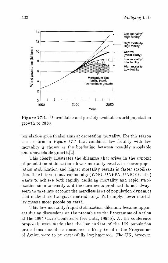
432

14

12

Ule 10gB-e 80

~:::J 6a.0a."0

15 43:

2

01950 2000

Momentum plusfertility inertia

(unavoidable growth)

2050Year

Wolfgang Lutz

Low mortality!High fertility

High mortality!High fertility

Central(most likely)Low mortality!Low fertility

High mortalityLow fertility

Figure 17.1. Unavoidable and possibly avoidable world populationgrowth to 2050.

population growth also aims at decreasing mortality. For this reasonthe scenario in Figur'e 17.1 that combines low fertility with lowmortality is chosen as the borderline between possibly avoidableand unavoidable growth.[2]

This clearly illustrates the dilemma that arises in the contextof population stabilization: lower mortality results in slower popu­lation stabilization and higher mortality results in faster stabiliza­tion. The international community (WHO, UNFPA, UNICEF, etc.)wants to achieve both rapidly declining mortality and rapid stabi­lization simultaneously and the documents produced do not alwaysseem to take into account the merciless laws of population dynamicsthat make these two goals contradictory. Put simply: lower mortal­ity means more people on earth.

This low-mortality Irapid-stabilization dilemma became appar­ent during discussions on the preamble to the Programme of Actionat the 1994 Cairo Conference (see Lutz, 1995b). At the conferenceproposals were made that the low variant of the UN populationprojections should be considered a likely trend if the Programmeof Action were to be successfully implemented. The UN, however,

Epilogue: Dilemmas in Population Stabilization 433

uses identical mortality assumptions for all three variants, whereasan important and widely praised aspect of the Cairo Programme ofAction was to embed family planning into reproductive health ef­forts, maternal mortality, child mortality, and health improvementsin general. Hence, successful implementation of the Programmewould result in not only lower fertility, but also lower mortality ­that is, more survivors - which contradicts the unchanged mortalityassumptions of the UN low variant. Therefore, when producing fu­ture population projections, variants that combine low fertility withlow mortality must be taken into account if the Cairo Programmeof Action is to be given serious consideration; this, however, willinevitably result in higher population growth.

17.3 The Population-Growth/Population-Aging Dilemma

Growth of total population size - which receives a great deal of at­tention in the discussion of future world population trends - is onlyone side of the coin. The other side is population aging. If pop­ulation growth follows the central scenario, the percentage of theworld population above age 60 increases from 9.5 percent currentlyto 13.2 percent in 2020, 19.6 percent in 2050, and 26.8 percent in2100. The low-fertilityflow-mortality scenario would bring the pro­portion above age 60 to an incredible 42.5 percent in 2100. Forcomparison, in the region with the oldest population today, West­ern Europe, less than 20 percent of the population is above age 60.And today's developing countries are hardly prepared to cope withthe social challenges of massive aging.

The figures on projected population aging under different sce­narios clearly show that when discussing possible and desired futurepopulation trends both sides of the coin - population growth andpopulation aging - must be taken into consideration. The issue ofpopulation aging is sometimes consciously disregarded with the ar­gument that, for an eventual stable situation of low fertility andlow mortality, the laws of population dynamics imply that at somepoint a certain high mean age of the population would be reached inany case whereas the ultimate population size would depend on thespeed of fertility decline. This is certainly true in the very long run;

434 Wolfgang Lutz

however, in the coming decades the speed of aging will have a bigimpact. A mean age of 36 years, which under a high-growth scenariowill only be reached in :2100, will already be reached around 2030under the low-growth scenario. Hence the low-growth scenario willcertainly put more stress on society to adapt to rapid and massiveaging and develop support networks for the aged that can no longercount on traditional family support.

Mentioning the aging associated with a rapid curbing of popu­lation growth is not to say that the problems associated with agingcancel the benefits of rapid stabilization. A science-based weightingof the socioeconomic and environmental consequences of both pop­ulation aging and rapid decrease in population growth is beyond thefocus of this book and requires very different considerations. With­out in-depth analyses I would guess that the benefits of rapidlydeclining fertility, such as a lower child dependency ratio, less stresson infrastructure and life support systems, better educational op­portunities for women, and a likely boost to productivity, wouldmore than compensate the problems of aging, if sufficient attentionis given to timely social policies.[:3]

17.4 Conclusion

This book attempts to assemble the most relevant knowledge aboutpast and future trends in fertility, mortality, and migration in dif­ferent parts of the world, translate this knowledge into alternativepopulation projections, and give a quantitative assessment aboutthe degree of uncertainty involved. In doing so it also tries to in­clude in the uncertainty assumptions the possible impacts of futureenvironmental, economic, political, and cultural changes as far asthey can be foreseen today as (even low-probability) possibilities ofthe future.

All of the chapters have made contributions to answer the ques­tion in the subtitle of this book: What can we assume today? Astrends evolve and more knowledge is acquired about the interact­ing processes that shape our future, tomorrow's assumptions willprobably look different from today's.

Epilogue: Dilemmas in Population Stabilization

Notes

435

[1] This decomposition into avoidable and unavoidable growth follows asomewhat different logic than the analysis by Bongaarts (1994) whichestimates that, of the likely 5.7 billion additional people in the develop­ing world by 2100 (based on the World Bank projections), 2.8 billionare due to population momentum, 1.0 billion to high desired familysize, and 1.9 billion to unwanted pregnancies. Aside from the issue ofwanted and unwanted pregnancies, which is part of the assumptions ofour scenarios but not a defining criterion, Bongaarts' decomposition isdifferent from ours in that it takes stable replacement-level fertility - aconvenient but problematic concept as discussed in previous chapters ­as the point of reference. All births below replacement fertility are con­sidered momentum, all births above that level are considered avoidablethrough reductions in unwanted pregnancies and reductions in demandfor large families. Alternative mortality trends are not considered inthese calculations.

[2] Alternatively the low-fertility/high-mortality scenario may be chosenas a reference if one prefers to consider high mortality as part of astrategy to avoid growth.

[3] This was found to be the case in a recent in-depth study on Mauritius(see Lutz, 1994).

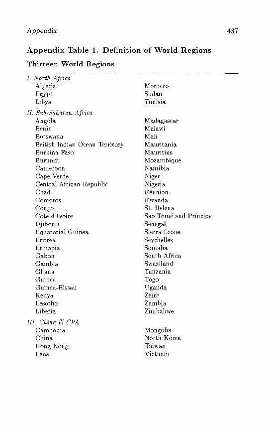
Appendix

Appendix Table 1. Definition of World Regions

Thirteen World Regions

437

I. North AfricaAlgeriaEgyptLibya

II. Sub-Saharan AfricaAngolaBeninBotswanaBritish Indian Ocean TerritoryBurkina FasoBurundiCameroonCape VerdeCentral African RepublicChadComorosCongoCote d'IvoireDjiboutiEquatorial GuineaEritreaEthiopiaGabonGambiaGhanaGuineaGuinea-BissauKenyaLesothoLiberia

III. China fj CPACambodiaChinaHong KongLaos

MoroccoSudanTunisia

MadagascarMalawiMaliMauritaniaMauritiusMozambiqueNamibiaNigerNigeriaReunionRwandaSt. HelenaSao Tome and PrincipeSenegalSierra LeoneSeychellesSomaliaSouth AfricaSwazilandTanzaniaTogoUgandaZaireZambiaZimbabwe

MongoliaNorth KoreaTaiwanVietnam

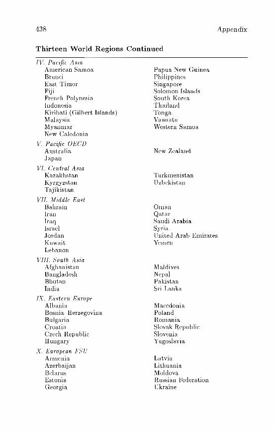
438

Thirteen World Regions Continued

Appendix

IV. Pacific AsiaAmerican SamoaBruneiEast TimorFijiFrench PolynesiaIndonesiaKiribati (Gilbert Islands)MalaysiaMyanmarNew Caledonia

V. Pacific 0 ECDAustraliaJapan

VI. Central ASia

KazakhstanKyrgyzstanTajikistan

Vll. :'vfiddle EastBahrainIranIraqIsraelJordanKuwaitLebanon

VIll. South AsiaAfghanistanBangladeshBhutanIndia

IX. Eastern EuropeAlbaniaBosnia-HerzegovinaBulgariaCroatiaCzech RepublicHungary

X. European FS UArmeniaAzerbaijanBelarusEstoniaGeorgia

Papua New GuineaPhilippinesSingaporeSolomon IslandsSouth KoreaThailandTongaVanuatuWestern Samoa

New Zealand

TurkmenistanUzbekistan

OmanQatarSaudi ArabiaSyriaUnited Arab EmiratesYemen

MaldivesNepalPakistanSri Lanka

MacedoniaPolandRomaniaSlovak RepublicSloveniaYugoslavia

LatviaLithuaniaMoldovaRussian FederationUkraine

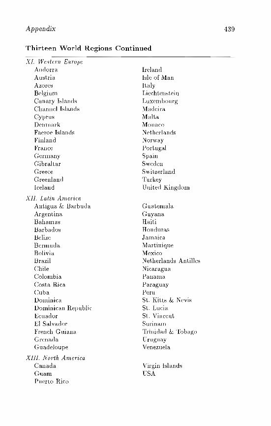
Appendix

Thirteen World Regions Continued

439

XI. Westem EuropeAndorraAustriaAzoresBelgiumCanary IslandsChannel IslandsCyprusDenmarkFaeroe IslandsFinlandFranceGermanyGibraltarGreeceGreenlandIceland

XII. Latin AmericaAntigua & BarbudaArgentinaBahamasBarbadosBelizeBermudaBoliviaBrazilChileColombiaCosta RicaCubaDominicaDominican RepublicEcuadorEI SalvadorFrench GuianaGrenadaGuadeloupe

XIII. North AmericaCanadaGuamPuerto Rico

IrelandIsle of ManItalyLiechtensteinLuxembourgMadeiraMaltaMonacoNetherlandsNorwayPortugalSpainSwedenSwitzerlandTurkeyUnited Kingdom

GuatemalaGuyanaHaitiHondurasJamaicaMartiniqueMexicoNetherlands AntillesNicaraguaPanamaParaguayPeruSt. Kitts & NevisSt. LuciaSt. VincentSurinamTrinidad & TobagoUruguayVenezuela

Virgin IslandsUSA

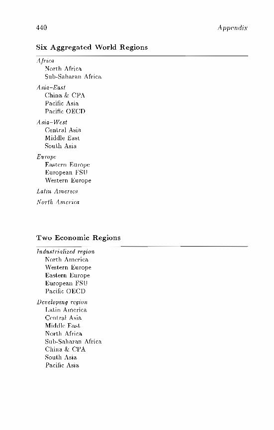
440

Six Aggregated World Regions

AfricaNorth AfricaSub-Saharan Africa

Asia-EastChina & CPAPacific AsiaPacific GECD

Asia-WestCentral AsiaMiddle EastSouth Asia

EuropeEastern EuropeEuropean FSUWestern Europe

Latin America

North America

Two Economic Regions

Industrialized regionNorth AmericaWestern EuropeEastern EuropeEuropean FSUPacific GECD

Developing regionLatin AmericaCentral AsiaMiddle EastNorth AfricaSub-Saharan AfricaChina & CPASouth AsiaPacific Asia

Appendix

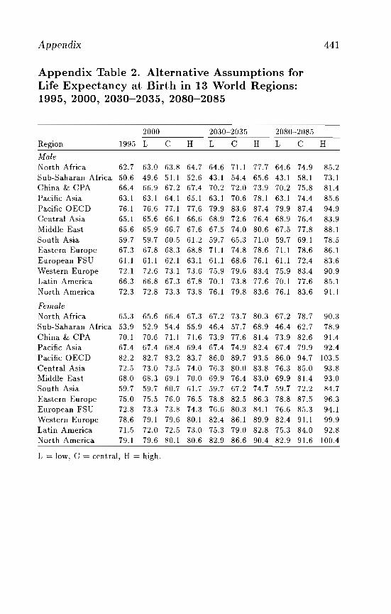
Appendix 441

Appendix Table 2. Alternative Assumptions forLife Expectancy at Birth in 13 World Regions:1995, 2000, 2030-2035, 2080-2085

:woo 2030-2035 2080-2085

Region 1995 L C H L C H L C H

MaleNorth Africa 62.7 63.0 63.8 64.7 64.6 71.1 77.7 64.6 74.9 85.2Sub-Saharan Africa 50.6 49.6 51.1 52.6 43.1 54.4 65.6 43.1 58.1 73.1China & CPA 66.4 66.9 67.2 67.4 70.2 72.0 73.9 70.2 75.8 81.4Pacific Asia 63.1 63.1 64.1 65.1 63.1 70.6 78.1 63.1 74.4 85.6Pacific GECD 76.1 76.6 77.1 77.6 79.9 83.6 87.4 79.9 87.4 94.9Central Asia 65.1 65.6 66.1 66.6 68.9 72.6 76.4 68.9 76.4 83.9Middle East 65.6 65.9 66.7 67.6 67.5 74.0 80.6 67.5 77.8 88.1South Asia 59.7 59.7 60.5 61.2 59.7 65.3 71.0 59.7 69.1 78.5Eastern Europe 67.3 67.8 68.3 68.8 71.1 74.8 78.6 71.1 78.6 86.1European FSU 61.1 61.1 62.1 63.1 61.1 68.6 76.1 61.1 72.4 83.6Western Europe 72.1 72.6 73.1 73.6 75.9 79.6 83.4 75.9 83.4 90.9Latin America 66.3 66.8 67.3 67.8 70.1 73.8 77.6 70.1 77.6 85.1North America 72.3 72.8 73.3 73.8 76.1 79.8 83.6 76.1 83.6 91.1

FemaleNorth Africa 65.3 65.6 66.4 67.3 67.2 73.7 80.3 67.2 78.7 90.3Sub-Saharan Africa 53.9 52.9 54.4 55.9 46.4 57.7 68.9 46.4 62.7 78.9China & CPA 70.1 70.6 71.1 71.6 73.9 77.6 81.4 73.9 82.6 91.4Pacific Asia 67.4 67.4 68.4 69.4 67.4 74.9 82.4 67.4 79.9 92.4Pacific GECD 82.2 82.7 83.2 83.7 86.0 89.7 93.5 86.0 94.7 103.5Central Asia 72.5 73.0 73.5 74.0 76.3 80.0 83.8 76.3 85.0 93.8Middle East 68.0 68.3 69.1 70.0 69.9 76.4 83.0 69.9 81.4 93.0South Asia 59.7 59.7 60.7 61.7 59.7 67.2 74.7 59.7 72.2 84.7East.ern Europe 75.0 7.1.5 76.0 76.5 78.8 82.5 86.3 78.8 87.5 96.3European FSU 72.8 73.3 73.8 74.3 76.6 80.3 84.1 76.6 85.3 94.1Western Europe 78.6 79.1 79.6 80.1 82.4 86.1 89.9 82.4 91.1 99.9Latin America 71.5 72.0 72.5 73.0 75.3 79.0 82.8 75.3 84.0 92.8North America 79.1 79.6 80.1 80.6 82.9 86.6 90.4 82.9 91.6 100.4

L = low, C = central, H = high.

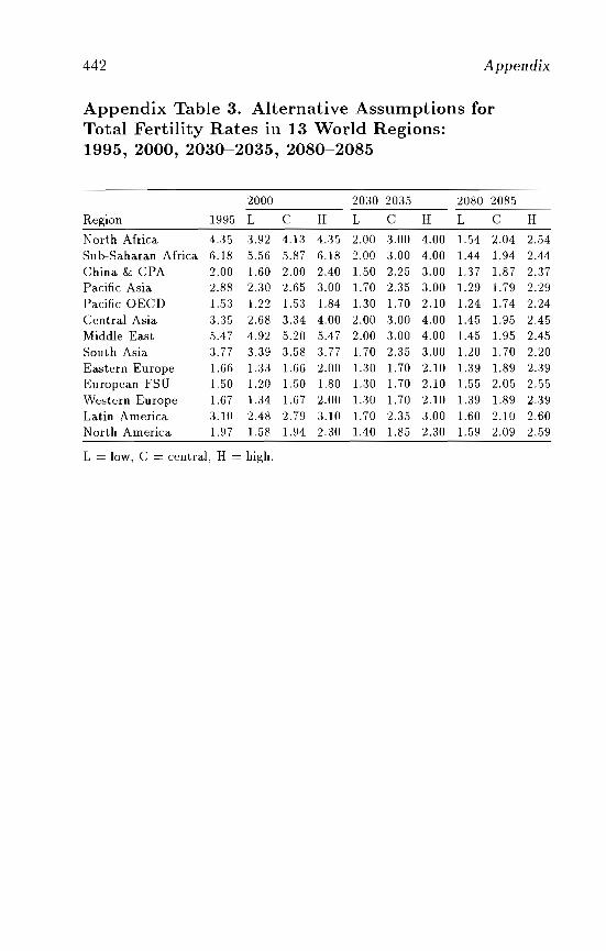
442 Appendix

Appendix Table 3. Alternative Assumptions forTotal Fertility Rates in 13 World Regions:1995, 2000, 2030-2035, 2080-2085

2000 2030-2035 2080-2085

Region 1995 L C H L C H L C H

North Africa 4.35 3.92 4.13 4.35 2.00 3.00 4.00 1.54 2.04 2..54Sub-Saharan Africa 6.18 5.56 5.87 6.18 2.00 3.00 4.00 1.44 1.94 2.44China & CPA 2.00 1.60 2.00 2.40 1.50 2.25 3.00 1.37 1.87 2.37Pacific Asia 2.88 2.30 2.65 3.00 1. 70 2.35 3.00 1.29 1.79 2.29Pacific OECD 1.53 1.22 1.53 1.84 1.30 1.70 2.10 1.24 1.74 2.24

Central Asia 3.35 2.68 3.34 4.00 2.00 3.00 4.00 1.45 1.95 2.45Middle East 5.47 4.92 5.20 5.47 2.00 3.00 4.00 1.45 1.95 2.45South Asia 3.77 3.39 3,58 3.77 1.70 2.35 3.00 1.20 1.70 2.20Eastern Europe 1.66 1.33 166 2.00 1.30 170 2.10 1.39 189 2.39European FSU 1.50 1.20 150 1.80 1.30 1.70 2.10 1.55 2.05 2.55Western Europe 1.67 1.34 1.67 2.00 1.30 1.70 2.10 1.39 1.89 2.39Latin America 3.10 2.48 2.79 3.10 1.70 2.35 3.00 1.60 2.10 2.60North America 1.97 1.58 1.94 2.30 1.40 1.85 2.30 1.59 2.09 2.59

L = low, C = ceutral, H = high.

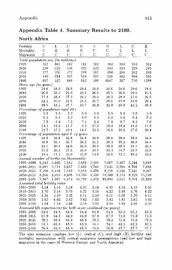
Appendix 443

Appendix Table 4. Summary Results to 2100.

North Africa

Fertility C L CMortality C H HMigration C C C

HHC

LCC

HCC

LLC

CLC

HLC

4.354.224.113.422.54

24.625.526.529.436.9

38.838.436.933.023.6

5.96.37.8

11.820.4

162235299593

1288

5,6887,6569,207

15,12021,880

]62229282468716

4.243.703.352.622.04

24.626.027.633.042.2

5.96.48.2

15.027.6

38.836.834.126.918.2

5,5446,7047,3218,9298,704

162223266362357

24.626.628.837.849.8

5.96.68.7

19.439.2

38.835.230.919.712.1

5,4075,7645,5304,5122,615

5.96.27.4

] 0.416.8

24.625.526.328.634.9

38.838.336.933.324.6

162233294558

1117

5,6877,6319,116

14,50019,890

5.96 ".U

16222226]337290

8.417.232.3

24.626.528.636.746.0

38.835.230.920.113.4

162232288519912

24.625.426.228.133.7

Total populatIOn size (in millions)1995 162 162 1622010 228 220 2262020 277 256 2722050 439 311 4072100 607 227 489Mean age (in years)1995 24.6 24.6 24.62010 26.0 26.5 25.92020 27.4 28.4 27.32050 32.1 35.9 31.52100 39.5 43.5 37.7Percentage of population aged 60+1995 5.9 5.9 5.9 5.92010 6.3 6.4 6.2 6.02020 7.9 8.0 7.5 7.12050 13.2 15.3 11.7 9.22100 22.7 27.2 19.1 14.1Percentage of population aged 0-14 yem's1995 38.8 38.8 38.8 38.82010 36.8 35.] 36.7 38.32020 34.1 30.9 34.0 36.92050 27.3 20.3 27.5 3:q2100 19.4 ]4.2 20.0 25.0Annual number of births (in thousands)1995-2000 5,543 5,405 5,542 5,686 5,4062010-2015 6,681 5,724 6,657 7.603 5,7452020-2025 7,250 5,416 7,169 9,014 5,4762050-2055 8,566 4,095 8,095 13,700 4,3302095-2100 7,907 1,997 6,674 16,790 2,372Assumed total fertility mtes1995-2000 4.24 4.]4 4.24 4.35 4.14 4.35 4.142010-2015 3.70 3.18 3.70 4.22 3.18 4.22 3.182020-2025 3.35 2.59 3.:35 4.11 2.59 4.11 2.592050-2055 2.62 1.82 2.62 3.42 1.82 3.42 1.822095-2100 2.04 1.54 2.04 2.54 1.54 2.54 1.54Assumed life expectancies fOl' both sexes combined (in years)]995-2000 64.8 64.4 64.4 64.4 64.8 64.8 65.2 65.2 65.22010-2015 67.9 64.9 64.9 64.9 67.9 67.9 71.0 71.0 71.02020-2025 70.2 65.4 65.4 65.4 70.2 70.2 75.0 75.0 75.02050-2055 74.] 65.9 65.9 65.9 74.1 74.] 82.5 82.5 82.52095-2100 76.8 65.9 65.9 65.9 76.8 76.8 87.7 87.7 87.7

The nine scenarios combine low (L), central (C), and high (H) fertility andmortality assumptions with central migration assumptions (and low and highmigration in the cases of Western Europe and North America).

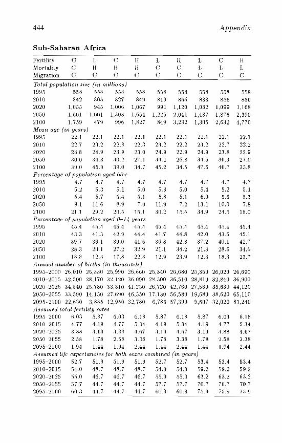
444 Appendix

Sub-Saharan Africa

Fert.ilit.y C L (-:; H L H L C HMort.alit.y C H H H C C L L LMigration C C C C C C C C C

Total population size (in millions)1995 558 558 558 558 558 558 558 558 5582010 842 805 827 849 819 865 833 856 8802020 1,055 945 1,006 1,067 991 1,120 1,032 1,099 1,1682050 1,601 1,001 1,303 1,654 1,225 2,041 1,437 1,876 2,3902100 1,759 479 996 1,827 849 3,232 1,305 2,632 4,770Mean age (in year's)1995 22.1 22,1 22,1 22.1 22,1 22.1 22.1 22,1 22,12010 22,7 23.2 22,8 22,3 23.2 22.2 23.2 22.7 22.22020 23,8 24.9 23.9 23.0 24.9 22.9 24.9 23.8 22.92050 30.0 :34.3 30.2 27.1 34.1 26.8 34.5 30.3 27.02100 39.0 45.0 39,0 34.7 45.2 34.5 47.6 40.7 35.8Pel'centage of population aged 60+1995 4.7 4.7 4.7 4,7 4.7 4.7 4.7 4.7 4.72010 5.2 5,3 5.1 5,0 5.3 5.0 5.4 5.2 5.12020 5.4 5.7 5.4 5.1 5.8 5.1 6.0 5,6 5.32050 9.1 11.6 8.9 7.0 11.9 7.2 13.1 10,0 7.82100 21.1 29.2 20.5 15.1 30.2 15.5 34,9 24.5 18.0Pel'centage of population aged 0-14 years1995 45.4 45.4 45.4 45.4 45.4 45.4 45.4 45.4 45.42010 43.3 41.3 42,9 44.4 41.7 44.8 42.0 43.6 45.12020 39,7 36.1 39,0 41.6 36.8 42.3 37.2 40.1 42.72050 28,3 20,1 27.2 32.9 21.1 34.2 21.3 28.6 34.62100 188 12.3 17.8 22,8 12,9 23.9 12,3 18.3 23.7Annual number of births (in thousands)1995-2000 26,010 25,330 25,990 26,660 25,340 26,680 25,350 26,020 26,6902010-2015 32,500 28,170 32,120 36,090 28,500 36,510 28,810 32,840 36,9002020-2025 34,540 25,780 33,310 41,230 26,720 42,760 27,560 35,630 44,1202050-2055 33,590 14,150 27,690 46,550 17,130 56,580 19,680 38,620 65,1102095-2100 22,630 3,885 12,950 32,780 6,786 57,390 9,607 32,020 81,240A ssumed total fertility mtes1995-2000 6.03 5,87 6.03 6.18 5.87 6.18 5.87 6.03 6.182010-2015 4.77 4.19 4.77 5.34 4.19 5.34 4.19 4.77 5,342020-2025 3.88 3.10 3.88 4.67 3.10 4.67 3.10 3.88 4.672050-2055 2,58 1.78 2.58 3.38 1.78 3.38 1.78 2.58 3.382095-2100 1.94 1.44 1.94 2.44 1.44 2.44 1.44 1.94 2.44Assumed life elpectancies for both sexes combined (in years)1995-2000 52.7 51.9 51.9 51.9 52.7 52.7 53.4 53.4 53.42010-2015 54.0 48.7 48.7 48.7 54,0 54.0 59.2 59.2 59.22020-2025 55.0 46.7 46.7 46.7 55.0 55.0 63.2 63.2 63.22050-2055 57.7 44.7 44.7 44.7 57,7 57.7 70.7 70.7 70.72095-2100 60.3 44,7 44.7 44,7 60.3 60.3 75.9 75,9 75.9

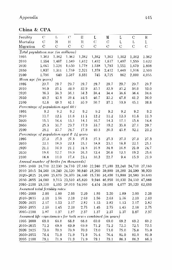
Appendix 445

China & CPA

Fertility C L C H L H L C HMortality C H H H C C L L LMigration C C C C C C C C C

Total population siZf (in millions)1995 1,362 1,362 1,362 1,362 1,362 ] ,362 ],362 1,362 1,3622010 1,554 1,487 1,549 1,612 1,492 1,617 1,497 1,559 1,6222020 1.665 1.524 1,650 1.778 1.538 1,793 1,551 1,679 1.8082050 1,837 1,311 1,759 2,321 1,378 2,412 1,449 1,916 2,5032100 1,796 640 1,587 3,331 745 3,715 862 2,000 4,055Mean age (in years)1995 29.7 29.7 29.7 29.7 29.7 29.7 29.7 29.7 29.72010 34.0 35.1 33.9 32.9 35.1 32.9 35.2 34.0 33.02020 ,16 ..3 .38 ..3 36.1 H ..3 38.4 .34.4 .38.6 .36.4 34.62050 40.2 45.8 39.4 :34.5 46.7 .35.2 47.8 41.2 .36.02100 42.8 48 ..3 41.1 35.9 50.7 .37.1 5.3.9 45.1 .38.8Per'centage of population aged 60+1995 9.2 9.2 9.2 9.2 9.2 9.2 9.2 9.2 9.22010 11.7 12.1 11.6 11.1 12.2 11.2 12..3 11.8 11..32020 15.5 16.4 15.1 14.1 16.7 14..3 17.1 15.8 14.62050 25 ..3 31.7 2.3.7 17.9 ,H.7 19.2 .35.8 27.1 20.72100 28.1 .35.7 24.7 17.9 40 ..3 20 ..3 45.8 .32.1 2.3.2Percentage of population aged 0-14 ye01'S1995 27.3 27.3 27.3 27 ..3 27 . .3 27 ..3 27.3 27 ..3 27 ..32010 22.1 18.9 22.1 25.1 18.8 25.1 18.8 22.1 25.12020 21.1 16.9 21.1 24.8 16.8 24.8 16.8 21.0 24.72050 19.6 12.7 1\1.9 26.3 12.4 26.0 12.1 19.2 25.62100 16.8 11.0 17.4 2.3.1 10.3 22.7 9.4 15.9 21.9Annual number' of births (in thousands)1995-2000 24,710 22,230 24,710 27,180 22,240 27,180 22,240 24,710 27,1802010-2015 24,560 18,240 24,520 30,840 18,260 30,880 18,280 24,590 30,9202020-2025 24,480 15,670 24,370 34,330 15,730 34,490 15,800 24,580 34,6402050-2055 24,080 9,71.3 23,510 45,820 9,946 46,950 10,130 24,550 47,8602095-2]00 19,550 4,105 18,010 54,980 4.454 59,680 4,677 20,520 62,680Assumed total fertility rates1995-2000 2.00 1.80 2.00 2.20 1.80 2.20 1.80 2,00 2.202010-2015 2.10 1.56 2.10 2.63 1.56 2.63 1.56 2.10 2.632020-2025 2.17 1.53 2.17 2.82 1.53 2.82 1.53 2.17 2.822050-2055 2.10 1.45 2.10 2.75 1.45 2.75 1.45 2.10 2.752095-2100 1.87 1.37 1.87 2.37 1.37 2..37 1.37 1.87 2.37Assumed life expectancies for both scres combined (in years)1995-2000 69.0 68.8 68.8 68.8 69.0 69.0 69.2 69.2 69.22010-2015 71.2 69.9 69.9 69.9 71.2 71.2 72.5 72.5 72.52020-2025 73.0 70.9 70.9 70.9 73.0 73.0 75.0 75.0 75.02050-2055 76.4 71.9 71.9 71.9 76.4 76.4 81.0 81.0 81.02095-2100 79.1 71.9 71.9 71.9 79.1 79,1 86.3 86.3 86.3

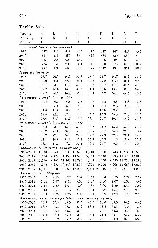
446 Appendix

Pacific Asia

Fertility C L C H L H L C HMortality C H H H C C L L LMigration C C c: c: c c c c C

Total population size (in milliolls)

199.5 447 447 447 447 447 447 447 447 4472010 554 530 550 ,569 535 574 539 559 5792020 623 568 609 650 581 665 594 636 6792050 776 550 703 884 611 970 673 845 10492100 783 289 609 1136 385 1433 492 951 1688Mean age (in years)1995 26.7 26.7 26.7 26.7 26.7 26.7 26.7 26.7 26.72010 30.0 30.8 29.9 29.1 30.9 29.2 31.0 30.1 29.32020 32. J 33.4 31.8 30.5 33.7 30.7 34.0 32.4 31.02050 37.2 40.5 36.0 32.5 41.9 33.5 43.7 38.9 34.92100 42.7 46.5 ,10.4 35.8 49.6 37.7 54.4 46.5 40.6Pn'centage of population aged 60+1995 6.8 6.8 6.8 6.8 6.8 6.8 6.8 6.8 6.82010 8.7 8.8 8.5 8 'J 9.0 8.4 9.2 8.9 8.62020 11.3 11.5 10.7 10.0 12.1 10.6 12.7 11.9 ILl

2050 19.8 22.2 17.:3 13.8 25.2 15.9 28.9 23.0 18.52100 27.6 31.7 22.7 J 7.0 :38.1 20.7 46.5 34.2 25.8Pel'centage of population aged 0-14 yeaTS1995 33.2 33.2 33.2 .13.2 33.2 33,2 33.2 33.2 33.22010 28.2 25.6 28.2 30.6 25.6 30.7 25.6 28.3 30.72020 26.2 22.7 26.2 29.:3 22.7 29.3 22.6 26.1 29.22050 21.5 16.0 21.9 27.1 15.6 26.8 14.9 20.8 26.12100 16.3 11.3 1- .) 22.4 10.4 21.7 9.0 14.9 20.41._

Annual numbel' of births (in thousands)1995-2000 10,930 10,240 10,930 11,620 10,240 11,620 10,240 10,930 11,6202010-2015 11,500 9,324 11,450 13,590 9,359 13,640 9,390 11,530 13,6902020-2025 11 ,590 8,402 11,460 14,780 8,499 14,950 8,580 11,710 15,1002050-2055 11 ,200 5.393 10,540 17.890 5.728 19,020 5,968 11,680 19,8302095-2100 8,214 1,906 6,853 18,200 2,294 21,810 2,521 9,010 23,910A ssumed total fatility rates1995-2000 2,77 2.59 2.77 2.94 2.59 2.94 2.59 2.77 2.942010-2015 2.54 2.(H 2.54 3.00 2.07 3.00 2.07 2.54 3.002020-2025 2.44 1.89 2.44 3.00 1.89 3.00 1.89 2.44 3.002050-2055 2.13 1.54 2.13 2.72 1.54 2.72 1.54 2.13 2.722095-2100 1.79 1.29 1. 79 2.29 1.29 2.29 1.29 1.79 2.29Assumed life eTpectancies for both sexes combined (in years)1995-2000 66.0 65.5 65.5 65.5 66.0 66.0 66.5 66.5 66.52010-2015 68.8 65.2 65.2 65.2 68.8 68.8 72.3 72.3 72.32020-2025 70.7 65.2 65.2 65.2 70.7 70.7 76.2 76.2 76.22050-2055 74.4 65.2 65.2 65.2 74.4 74.4 83.7 83.7 83.72095-2100 77.1 65.2 65.2 65.2 77.1 77.1 88.9 88.9 88.9

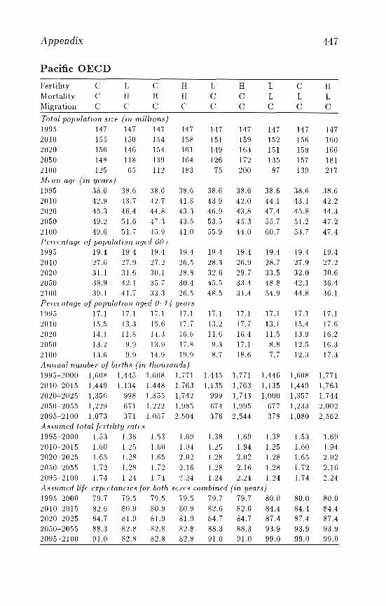
Appendix 447

Pacific OECD

Fertility C L C H L H L C HMortality C H H H C C L L LMigration C C C C C C C C C

Total population SiZE (in millions)

1995 ]47 ]47 147 147 147 ]47 147 147 1472010 155 150 154 158 151 159 ]52 156 1602020 156 146 154 16] 149 163 151 159 1662050 148 118 139 164 126 172 135 157 181'2100 125 65 112 183 75 200 87 139 217Mean agE (in years)

1995 38.6 38.6 :18.6 38.6 38.6 38.6 38.6 38.6 38.62010 42.9 43.7 42.7 41.8 43.9 42.0 44.1 43.1 42.22020 45.3 c16.4 44.8 43.:1 46.9 43.8 47.4 45.8 44.32050 49.2 51.6 47.:1 43.5 53.5 45.3 55.7 51.2 47.22100 49.6 51.T 45.9 41.0 55.9 44.0 60.7 53.7 47.4Pf.TccntagE of population aged 60+

199,5 19.4 19.4 19.4 19.4 19.4 19.4 19.4 19.4 19.42010 27.6 27.9 21.2 26.5 28.3 26.9 28.7 27.9 27.22020 31.1 31.6 3U.l 28.8 :32.6 29.7 33.5 32.0 30.62U50 38.9 42.1 3,5.7 30.4 45.5 33.4 48.8 42.] 36.42100 39.1 41.7 33.:3 26.5 48.,5 31.4 54.9 44.8 36.1Percentage of populatioll aged 0-14 years

1995 17. ] 17.1 17.1 17.1 17.] 17.1 17.1 17.1 17.12010 15.5 13.3 15.6 17.7 13.2 17.7 13.1 ]5.4 17.62020 14.1 11.8 14.3 16.6 11.6 16.4 !l.5 13.9 16.22U50 13.2 9.9 13.9 17.8 9.3 17.1 8.8 ]2.5 16.32100 13.6 9.9 14.9 19.9 8.7 18.6 7.7 12.3 17.3Annual Tlumber of birth8 (in tholJ8and.s)

1995-2000 1,608 1,445 1.608 1.T71 1,445 1,771 1,446 1,608 1,7712010-2015 l,449 1.134 1,448 1,763 1,135 1,763 1,135 1,449 1,7632020-2025 1,356 998 1,355 1,742 999 1,743 1,000 1,357 1,7442050-2055 1,229 671 I -I')') 1.985 674 1,995 677 1,233 2,002, .... _-2095-2]00 1,073 371 1.057 2,.504 376 2,544 378 1,080 2,562A s8umed total fel,tility mtf'8

]995-2000 1.53 1.38 1.53 1.69 U8 1.69 1.38 1.53 1.692010-2015 1.60 1.25 1.60 1.94 1.25 1.94 1.25 1.60 1.942020-202,5 1.65 1.28 1.65 2.02 1.28 2.02 1.28 1.65 2.0220.10-2055 1.72 1.28 1 -'I 2.16 1.28 2.16 1.28 1.72 2.16., -2095-2100 I. 74 l.24 1. 74 2.24 1.24 2.24 1.24 1,74 2.24AS8'umed life expectancies for both se.l'e.s combinEd (in years)

199.5-2000 79.7 79.5 79 ..1 79.,5 79.7 79.7 80.0 80.0 80.020]0-2015 82.6 80.9 8U.9 80.9 82.6 82.6 84.4 84.4 84.42020-2025 84.7 81.9 81.9 81.9 84.7 84.7 87.4 87.4 87.42050-2055 88.3 82.8 82.8 82.8 88.3 88.3 93.9 93.9 93.92095-2]00 91.0 82.8 82.8 82.8 91.0 91.0 99.0 99.0 99.0

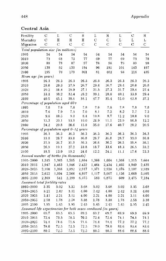
448 Appendix

Central Asia

Fertility C L C H L H L C HMortality C H H H C C L L LMigration C C C C C C C C C

Total population size (in millions)1995 54 54 54 ,54 54 54 54 54 542010 73 68 73 77 69 77 69 73 782020 88 78 87 97 78 98 79 89 982050 138 92 133 184 96 191 101 143 1972100 195 70 173 361 81 402 93 216 435Mean age (in years)1995 26.3 26.3 26.3 26.3 26.3 26.3 26.3 26.3 26.32010 28.0 29.3 27.9 26.7 29.4 26.7 29.4 28.0 26.82020 29.2 31.4 29.0 27.1 31.5 27.3 31.7 29.4 27.42050 33.1 38.2 32.4 28.2 39.1 28.8 40.1 33.9 29.42100 40.5 45.1 38.6 34.1 47.7 35.4 51.0 42.8 37.1Percentage of population aged 60+1995 7.8 7.8 7.8 7.8 7.8 7.8 7.8 7.8 7.82010 7.6 7.9 7.5 7.0 8.1 7.2 8.2 7.7 7.32020 9.6 10.5 9.3 8.4 10.8 8.7 11.2 10.0 9.02050 15.3 20.1 13.9 10.0 21.9 11.1 23.9 16.8 12.22100 24.2 29.8 20.6 15.0 35.0 17.6 40.7 28.2 20.5Percentage of population aged 0-14 years1995 36.3 36.3 36.3 36.3 36.3 36.3 36.3 36.3 36.32010 33.0 28.7 33.0 36.8 28.7 36.8 28.7 33.0 36.82020 31.9 26.7 31.9 36.3 26.6 36.2 26.5 31.8 36.12050 26.9 19.1 27.2 33.8 18.7 33.6 18.3 26.5 33.22100 18.5 13.0 19.2 24.6 12.2 24.1 11.1 17.6 23.3Annual numbel' of bil,ths (in thousands)1995-2000 1,51.5 1,365 1,515 1,664 1,366 1,664 1,366 1,515 1,6642010-2015 1,947 1,463 1,946 2,432 1,464 2,434 1,465 1,949 2,4352020-2025 2,100 1,366 2,092 2,917 1,371 2,928 1,376 2,107 2,9392050-2055 2,622 1,094 2,566 4,897 1,117 5,007 1,136 2,668 5,0952095-2100 2,369 541 2,199 6,375 583 6,875 609 2,475 7,184A ssumed total fertility rates1995-2000 3.35 3.02 3.35 3.68 3.02 3.68 3.02 3.35 3.682010-2015 3.21 2.42 3.21 4.00 2.42 4.00 2.42 3.21 4.002020-2025 3.11 2.21 3.11 4.00 2.21 4.00 2.21 3.11 4.002050-2055 2.58 1.78 2.58 3.38 1.78 3.38 1.78 2.58 3.382095-2100 1.95 1.45 1.95 2.45 1.45 2.45 1.45 1.95 2.45Assumed life expectancies for both sexes combined (in years)1995-2000 69.7 69.5 69.5 69.5 69.7 69.7 69.9 69.9 69.92010-2015 72.4 70.5 70.5 70.5 72.4 72.4 74.1 74.1 74.12020-2025 74.4 71.6 71.6 71.6 74.4 74.4 77.2 77.2 77.220.50-2055 78.0 72.5 72.5 72.5 78.0 78.0 83.6 83.6 83.62095-2100 80.5 72.5 72 ..5 72.5 80.5 80.5 88.6 88.6 88.6

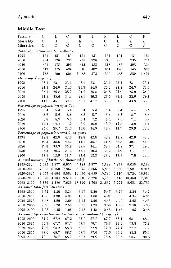
Appendix 449

Middle East

Fertility C L C H L H L C HMortality C H H H C C L L LMigration C C C C C C C C C

Total population size (in millions)1995 151 151 151 151 151 151 151 151 1512010 234 226 232 238 228 240 229 235 2412020 301 278 296 313 283 318 287 305 3232050 517 375 484 610 402 651 426 546 6852100 738 299 606 l,088 373 1,309 453 859 1,491Mean age (in yea/'s)1995 23.1 23.1 23.1 23.1 23.l 23.1 23.1 23.1 23.12010 24.3 24.8 24.3 23.8 24.8 23.8 24.8 24.3 23.82020 25.7 26.8 25.7 24.7 26.8 24.8 27.0 25.9 24.92050 31.8 35.6 31.4 28.1 36.2 28.5 37.1 32.6 29.12100 41.0 45.1 39.3 35.1 47.7 36.3 51.6 43.9 38.3Percentage oj population aged 60+1995 5.4 5.4 5.4 5.4 5.4 5.4 5.4 5.4 5.42010 5.6 5.6 5.5 5.3 5.7 5.4 5.8 5.7 5.52020 6.8 6.9 6.5 6.1 7.2 6.4 7.5 7.1 6.72050 12.4 14.4 11.2 8.9 16.0 9.9 17.8 13.9 11.12100 25.0 29.7 21.3 16.0 34.9 18.7 41.7 29.9 22.2Percentage oj population aged 0-14 years1995 42.8 42.8 42.8 42.8 42.8 42.8 42.8 42.8 42.82010 40.3 38.6 40.2 41.7 38.7 41.8 38.8 40.4 41.92020 37.0 33.9 36.9 39.5 34.1 39.7 34.2 37.1 39.82050 27.3 20.3 27.3 33.1 20.3 33.2 20.0 27.1 33.02100 18.1 12.9 18.5 23.4 12.3 23.2 11.1 l7.0 22.4Annual number oj births (in thousands)1995-2000 6,035 5,877 6,035 6,188 5,877 6,188 5,878 6,036 6,1892010-2015 7,885 6,850 7,867 8,875 6,866 8,895 6,880 7,901 8,9142020-2025 8,657 6,604 8,584 10,640 6,659 lO,730 6,710 8,724 10,8102050-2055 10,090 4,984 9,610 15,940 5,228 16,760 5,415 10,460 17,3802095-2100 8,886 2,386 7,639 18,740 2,768 21,850 3,002 9,651 23,750Assumed total jel,tility rates1995-2000 5.34 5.20 5.34 5.47 5.20 5.47 5.20 5.34 5.472010-2015 4.35 3.80 4.35 4.91 3.80 4.91 3.80 4.35 4.912020-2025 3.68 2.90 3.68 4.45 2.90 4.45 2.90 3.68 4.452050-2055 2.58 1.78 2.58 3.38 1.78 3.38 1.78 2.58 3.382095-2100 1.95 1.45 1.95 2.45 1.45 2.45 1.45 1.95 2.45Assumed lije expectancies jor both se:z:es combined (in years)1995-2000 67.7 67.2 67.2 67.2 67.7 67.7 68.1 68.1 68.12010-2015 70.7 67.7 67.7 67.7 70.7 70.7 73.8 73.8 73.82020-2025 72.9 68.2 68.2 68.2 72.9 72.9 77.7 77.7 77.72050-2055 77.0 68.7 68.7 68.7 77.0 77.0 85.3 85.3 85.32095-2100 79.6 68.7 68.7 68.7 79.6 79.6 90.5 90.5 90.5

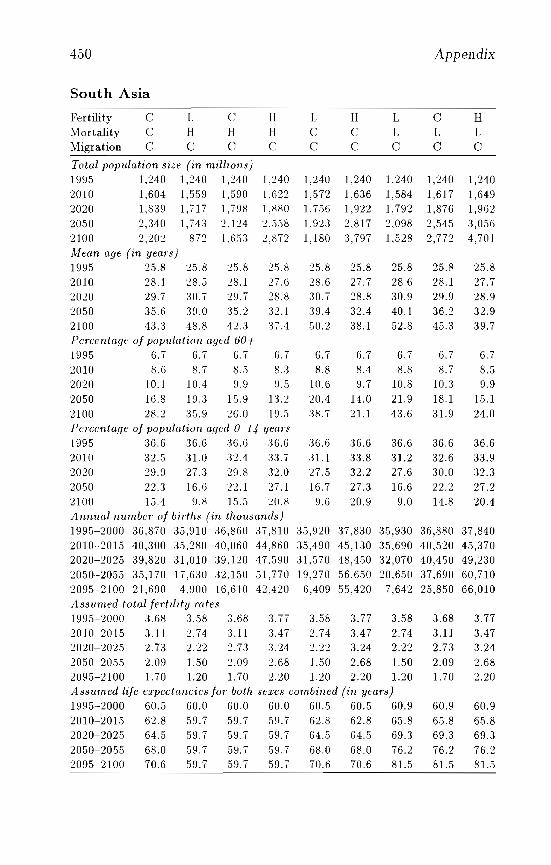
450 Appendix

South Asia

Fertility C L C H L H L C HMortality C H H H C C L L LMigration C C C C C C C C C

Total population size (in millions)1995 1,240 1,240 1,240 1,240 1,240 1,240 1,240 1,240 1,2402010 1,604 1,559 1,590 1,622 1,572 1,636 1,584 1,617 1,6492020 1,839 1,717 1,798 1,880 1,756 1,922 1,792 1,876 1,9622050 2,340 1,74:3 2.124 '2.558 1,9'23 2,817 2,098 2,545 3,0562100 2,20'2 872 1,65:3 '2,872 1,180 3,797 1,528 2,772 4,701Mean age (in yea1's)1995 25.8 25.8 25.8 25.8 25.8 25.8 25.8 25.8 25.82010 28.1 28.5 28.1 27.6 28.6 27.7 28.6 28.1 27.72020 29.7 30.7 29.7 28.8 30.7 28.8 30.9 29.9 28.92050 35.6 39.0 35.2 32.1 39.4 32.4 40.1 36.2 32.92100 43.3 48.8 42.3 37.4 50.2 38.1 52.8 45.3 39.7Percentage of population aged 60+1995 6.7 6.7 6.7 6.7 6.7 6.7 6.7 6.7 6.72010 8.6 8.7 8.5 8.3 8.8 8.4 8.8 8.7 8.52020 10.1 10.4 9.9 9.5 10.6 9.7 10.8 10.3 9.92050 16.8 19.3 15.9 13.2 20.4 14.0 21.9 18.1 15.12100 28.2 35.9 26.0 19.5 38.7 21.1 43.6 31.9 24.0Pel'centage of populatzon aged 0-14 years1995 36.6 36.6 36.6 :36.6 36.6 36.6 36.6 36.6 36.62010 32.5 31.0 32.4 33.7 31.1 :33.8 31.2 32.6 33.92020 29.9 27.3 29.8 32.0 27.5 32.2 27.6 30.0 32.32050 22.3 16.6 22.1 27.1 16.7 27.3 16.6 22.2 27.22100 15.4 9.8 15.5 20.8 9.6 20.9 9.0 14.8 20.4Annual number of birth.s (in thousands)1995-2000 36,870 35,910 36,860 37,810 35,920 37,830 35,930 36,880 37,8402010-2015 40,300 35,280 40,060 44,860 35.490 45,130 35,690 40,520 45,3702020-2025 ,39,820 31,010 39.120 47,590 31,570 48,450 32,070 40,450 49,2302050-2055 ,35,170 17,630 32,150 51,770 19,270 56,650 20,650 37,690 60,7102095-2100 21,690 4,900 16,610 42,420 6,409 55,420 7,642 25,850 66,010Assumed totalfel·tz/ity mtes1995-2000 ,3.68 3.58 3.68 3.77 3.58 3.77 3.58 ,3.68 3.772010-2015 ,3.11 274 3.11 3.47 2.74 3.47 2.74 ,3.ll 3.472020-2025 2.73 2.22 2.73 3.24 2.22 3.24 2.22 2.73 3.242050-2055 2.09 1.50 '2.09 2.68 1.50 2.68 1.50 2.09 2.682095-2100 1.70 1.20 1.70 2.20 1.20 2.20 1.20 1.70 2.20Assum.ed life expectancies f07' both seus com.bined (in years)1995-2000 60.5 60.0 60.0 60.0 60.5 60.5 60.9 60.9 60.92010-2015 62.8 59.7 59.7 59.7 62.8 62.8 65.8 65.8 65.82020-2025 64.5 59.7 59.7 59.7 64.5 64.5 69.,3 69.3 69.32050-2055 68.0 59.7 59.7 59.7 68.0 68.0 76.2 76.2 76.22095-2100 70.6 59.7 59.7 59.7 70.6 70.6 81.5 81.5 81.5

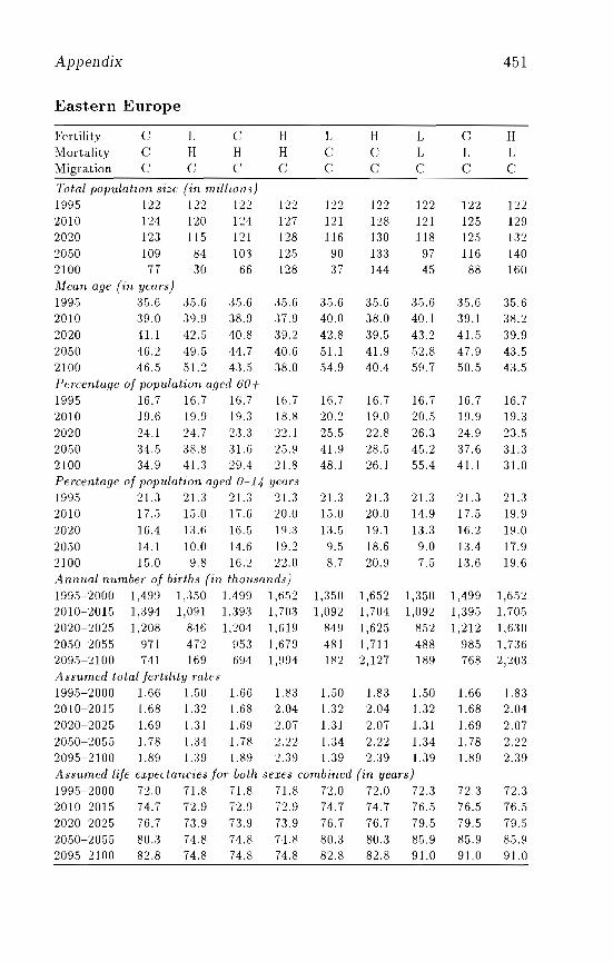
Appendix 451

Eastern Europe

Fertility C L C H L H L C HMortality C H H H C C L L LMigration C C C' C C C C C C

Total population sIze (in milliolls)1995 122 1')') p') 1')') l'n 122 122 122 1222010 1'24 120 124 127 121 128 121 125 1292020 123 115 121 128 116 130 118 125 1322050 109 84 10:3 12.5 90 133 97 116 1402100 77 30 66 128 37 144 45 88 160Mean age (in yeal's)1995 :35.6 35.G 3.5.6 :35.G 35.6 35.6 35.6 35.6 35.62010 39.0 39.9 38.9 :37.9 40.0 38.0 40.1 39.1 38.22020 41.1 42.5 40.8 39.2 42.8 39.5 43.2 41.5 39.92050 46.2 49.5 44.7 40.6 51.1 41.9 52.8 47.9 43.52100 46.5 .51.2 43.5 38.0 54.9 40.4 59.7 50.5 43.5Percentage of population aged 60+1995 16.7 16.7 16.7 16.7 16.7 16.7 16.7 16.7 16.72010 19.6 19.9 19.:3 18.8 20.2 19.0 20 ..5 19.9 19.32020 24.1 24.7 2:3.:3 22.1 25.5 22.8 26.3 24.9 23.52050 34.5 38.8 3Ui 25.9 41.9 28.5 45.2 37.6 31.32100 34.9 4l..3 29.4 21.8 48.] 26.] 55.4 41.1 31.0Percentage of popu.lation aged 0-14 yeCll's]995 21.3 21.3 21.:3 ::n.3 21.3 21.3 21.3 21.3 21.320]0 ]7.5 15.0 17.6 20.0 ]5.0 20.0 ]4.9 ] 7.5 19.92020 16.4 ]3.6 16.,5 19.3 ]3.5 ] 9.] 13.3 16.2 19.02050 ] 4.] ]0.0 14.6 ] 9.2 9.5 ]8.6 9.0 13.4 17.92]00 ]5.0 9.8 ]6.2 22.0 8.7 20.9 7.5 13.6 ]9.6A nllllal number of births (in thollwlUls)]995-2000 ] ,499 ] ,350 ],499 ],6.52 ],350 1,652 ],350 1,499 1,6,5220]0-2015 1,394 ] ,09] 1,393 1.703 1,092 J.704 1,092 1,395 1,7052020-2025 1,208 846 ],204 ] ,6] 9 849 1,625 852 ] ,212 ] ,6302050-2055 97] 4~') 953 1,679 48] 1,711 488 985 1,736,-2095-2100 74] 169 694 ],994 182 2,]27 189 768 2,203A ssumed total fel,tilitymtes1995-2000 1.66 1.50 1.66 1.83 1.50 1.83 1.50 1.66 1.8320]0-20]5 1.68 1.32 Ui8 2.04 1.32 2.04 1.32 1.68 2.042020-2025 1.69 1.31 1.G9 2.07 1.3] 2.07 1.3] 1.69 2.072050-2055 1.78 1.34 1.78 2.22 1.34 2.22 1.34 1.78 2.222095-2]00 1.89 1.39 1.89 2.39 1.39 2.39 1.39 1.89 2.39Assumed life expectancies for both sexes combined (in years)]995-2000 72.0 71.8 71.8 71.8 72.0 72.0 72.3 72.3 72.32010-2015 74.7 72.9 72.9 72.9 74.7 74.7 76.5 76.5 76.52020-2025 76.7 7:3.9 73.9 73.9 7G.7 76.7 79.5 79.5 79.52050-2055 80.3 74.8 74.8 74.8 80.3 80.3 85.9 85.9 85.92095-2]00 82.8 74.8 74.8 74.8 82.8 82.8 91.0 91.0 91.0

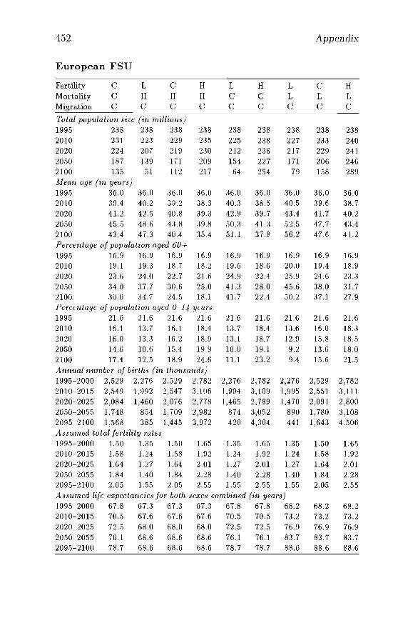
452 Appendix

European FSU

Fertility C L C H L H L C HMortality C H H H C C L L LMigration C C C C C C C C C

Total population size (in millions)1995 238 238 238 238 238 238 238 238 2382010 231 223 229 235 225 238 227 233 2402020 224 207 219 230 212 236 217 229 2412050 187 139 171 209 154 227 171 206 2462100 135 51 112 217 64 254 79 158 289Mean age (in years)1995 36.0 36.0 36.0 36.0 36.0 36.0 36.0 36.0 36.02010 39.4 40.2 39.2 38.3 40.3 38.5 40.5 39.6 38.72020 41.2 42.5 40.8 39.3 42.9 39.7 43.4 41.7 40.22050 45.5 48.6 43.8 39.8 50.3 41.3 52.5 47.7 43.42100 43.4 47.3 40.4 35.4 51.1 37.8 56.2 47.6 41.2Percentage of population aged 60+1995 16.9 16.9 16.9 16.9 16.9 16.9 16.9 16.9 16.92010 19.1 19.3 18.7 18.2 19.6 18.6 20.0 19.4 18.92020 23.6 24.0 22.7 21.6 24.9 22.4 25.9 24.6 23.32050 34.0 37.7 30.6 25.0 41.3 28.0 45.6 38.0 31.72100 30.0 34.7 24.5 18.1 41.7 22.4 50.2 37.1 27.9Percentage of population aged 0-14 years1995 21.6 21.6 21.6 21.6 21.6 21.6 21.6 21.6 21.62010 16.1 13.7 16.1 18.4 13.7 18.4 13.6 16.0 18.32020 16.0 13.3 16.2 18.9 13.1 18.7 12.9 15.8 18.52050 14.6 10.6 15.4 19.9 10.0 19.1 9.2 13.6 18.02100 17.4 12 ..5 18.9 24.6 11.1 23.2 9.4 15.6 21.5Annual number of births (in thousands)1995-2000 2,529 2,276 2,529 2,782 2,276 2,782 2,276 2,529 2,7822010-2015 2,549 1,992 2,547 3,106 1,994 3,109 1,995 2,551 3,1112020-2025 2,084 1,460 2,076 2,778 1,465 2,789 1,470 2,091 2,8002050-2055 1,748 854 1,709 2,982 874 3,052 890 1,780 3,1082095-2100 1,568 385 1,445 3,972 420 4,304 441 1,643 4,506Assumed total fe,·tility mtes1995-2000 1.50 1.35 1.50 1.65 1.35 1.65 1.35 1.50 1.652010-2015 1.58 1.24 1.58 1.92 1.24 1.92 1.24 1.58 1.922020-2025 1.64 1.27 1.64 2.01 1.27 2.01 1.27 1.64 2.012050-2055 1.84 1.40 1.84 2.28 1.40 2.28 1.40 1.84 2.282095-2100 2.05 1.55 2.05 2.55 1.55 2.55 1.55 2.05 2.55Assumed life expectancies for both sexes combined (in years)1995-2000 67.8 67.3 67.3 67.3 67.8 67.8 68.2 68.2 68.22010-2015 70.5 67.6 67.6 67.6 70.5 70.5 73.2 73.2 73.22020-2025 72.5 68.0 68.0 68.0 72.5 72.5 76.9 76.9 76.92050-2055 76.1 68.6 68.6 68.6 76.1 76.1 83.7 83.7 83.72095-2100 78.7 68.6 68.6 68.6 78.7 78.7 88.6 88.6 88.6

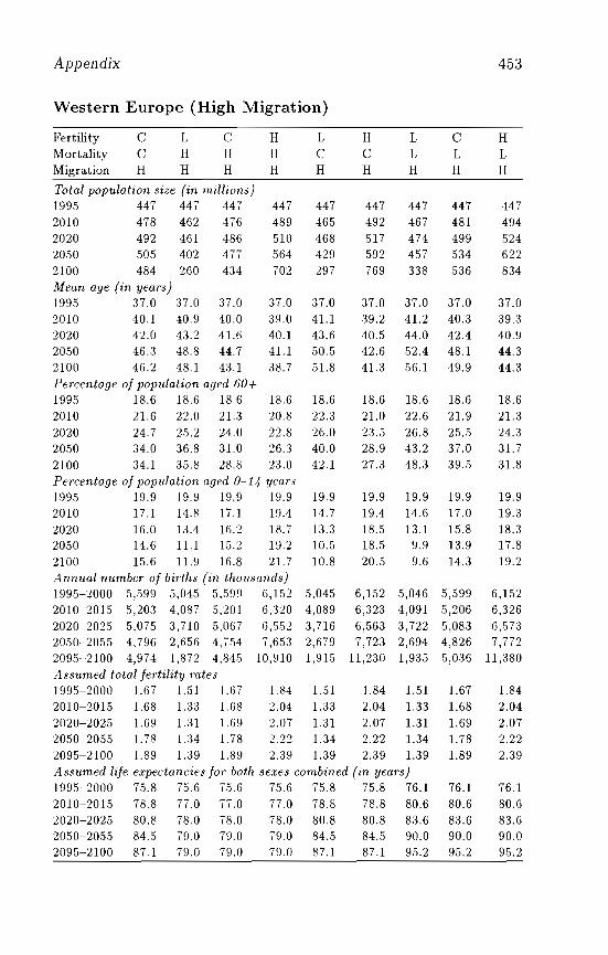
Appendix 453

Western Europe (High Migration)

Fertility C L C H L H L C HMortality C H H H C C L L LMigration H H H H H H H H H

Total population size (in millions)1995 447 447 447 447 447 447 447 447 4472010 478 462 476 489 465 492 467 481 4942020 492 461 486 510 468 517 474 499 5242050 505 402 4~~ 564 429 592 457 534 622, I

2100 484 260 434 702 297 769 338 536 834Mean age (in years)1995 37.0 37.0 37.0 37.0 37.0 37.0 37.0 37.0 37.02010 40.1 40.9 40.0 39.0 41.1 39.2 ·U.2 40.3 39.32020 42.0 43.2 41.6 40.1 43.6 40.5 44.0 42.4 40.92050 46.3 48.8 44.7 41.1 50.5 42.6 52.4 48.1 44.32100 46.2 48.1 43.1 38.7 51.8 41.3 56.1 49.9 44.3Pel'centage of population aged 60+1995 18.6 18.6 18.6 18.6 18.6 18.6 18.6 18.6 18.62010 21.6 22.0 21.3 20.8 22.3 21.0 22.6 21.9 21.32020 24.7 25.2 24.0 22.8 26.0 23.5 26.8 25.5 24.32050 34.0 36.8 31.0 26.3 40.0 28.9 43.2 37.0 31.72100 34.1 35.8 28.8 23.0 42.1 27.3 48.3 39.5 31.8Pel'centage of population aged 0-14 years1995 19.9 19.9 19.9 19.9 19.9 19.9 19.9 19.9 19.92010 17.1 14.8 17.1 19.4 14.7 19.4 14.6 17.0 19.32020 16.0 13.4 16.2 18.7 13.3 18.5 13.1 15.8 18.32050 14.6 11.1 15.2 19.2 10.5 18.5 9.9 13.9 17.82100 15.6 11.9 16.8 21.7 10.8 20.5 9.6 14.3 19.2Annual number of births (in thousands)1995-2000 5,599 5,045 5.599 6,152 5,045 6,152 5,046 5,599 6,1522010-2015 5,203 4,087 5,201 6,320 4,089 6,323 4,091 5,206 6,3262020-2025 5,075 3,710 5,067 6,552 3,716 6,563 3,722 5,083 6,5732050-2055 4,796 2,656 4,7.54 7,653 2,679 7,723 2,694 4,826 7,7722095-2100 4,974 1,872 4,845 10,910 1,915 11,230 1,935 5,036 11 ,380Assumed total fertility mtes1995-2000 1.67 1.51 I.G7 1.84 1.51 1.84 1.51 1.67 1.842010-2015 1.68 1.33 1.68 2.04 1.33 2.04 1.33 1.68 2.042020-2025 1.69 1.31 1.69 2.07 1.31 2.07 1.31 1.69 2.072050-2055 1.78 1.:34 1.78 2.22 1.34 2.22 1.34 1.78 2.222095-2100 1.89 1.39 1.89 2.:39 1.39 2.39 1.39 1.89 2.39Assumed life expectancies fOl' both se:res combined (in years)1995-2000 75.8 75.6 7.5.6 75.G 75.8 75.8 76.1 76.1 76.12010-2015 78.8 77.0 77.0 77.0 78.8 78.8 80.6 80.6 80.62020-2025 80.8 78.0 78.0 78.0 80.8 80.8 83.6 83.6 83.62050-2055 84.5 79.0 79.0 79.0 84.5 84.5 90.0 90.0 90.02095-2100 87.1 79.0 79.0 79.0 87.1 87.1 95.2 95.2 95.2

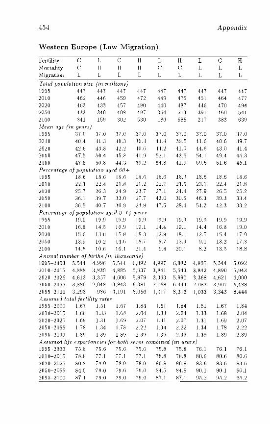
454 Appendix

Western Europe (Low Migration)

Fertility C L C H L H L C HMortality C H H H C C L L LMigration L L L L L L L L L

Total population size (in millions)1995 447 447 447 447 447 447 447 447 4472010 462 446 459 472 449 475 451 464 4772020 463 433 457 480 440 487 446 470 4942050 4:3:3 340 408 487 364 513 391 460 5412100 341 159 302 530 186 585 217 383 639Afean age (in years)199,5 :37.0 :l7.0 :37,0 :37.0 37.0 37.0 37.0 37.0 37,0

2010 40.4 41.:3 40,3 :EI.4 41.4 39 ..5 41.6 40,6 39.72020 42.6 43.8 42.2 ,10.6 44.2 41.0 44.6 43.0 41.42050 47.5 50.4 45.8 41.9 52.1 43.5 54.1 49.4 45.32100 47.6 50.8 44.3 39.2 54.8 41.9 59.6 51.6 45.1Pel'centage of population aged 60+1995 18.6 18.6 18.6 18.6 18.6 18.6 18.6 18.6 18.62010 22,1 22.4 21.8 21.2 22.7 21.5 23.1 22.4 21.82020 25.7 26.3 24.9 23.7 27.1 24.4 27.9 26.5 25.22050 36.1 39.7 33.0 27.7 43.0 30.5 46.3 39.3 33.42100 36.5 40.7 :311.9 23.9 ,11.5 28.4 54.2 42.3 33.2PfTcentage of population u!}ed 0-14 ye(/r.~

199,5 19.9 19.9 EUI 19.9 19.9 19.9 19.9 19.9 19.92010 16.8 14.5 16.9 19.1 14.4 19.1 14.4 16.8 19.02020 15.6 LUI 15.8 liU 12.9 18.1 12.7 15.4 17.92050 13.9 10.2 14.6 18.1 9.7 18.0 9.1 13.2 17.32100 14.8 10.6 16.1 2lA 9.4 20.1 8.2 13.5 18.8Annual number of births (m thousands)1995-2000 5.544 4.996 5.544 6.1J92 4,997 6,092 4,997 5,544 6,0922010-2015 4,888 3,839 4,885 5,937 3,841 5,940 3,842 4,890 5,9432020-2025 4,613 3,357 4.606 !i,979 3,363 5,990 3,368 4,621 6,0002050-2055 3,880 2.048 3,843 6,381 2,068 6,443 2,082 3,907 6,4882095-2100 3,293 986 :3,191 8.(J56 1,017 8,316 1,033 3,343 8,444A ssumed total fel·tility mte"1995-201J0 1.67 1.51 1.67 1.84 1.51 1.84 1.51 1.67 1.842010-2015 1.68 1.33 1.68 2.04 1.33 2.04 1.33 1.68 2.042020-202,5 1.6~) 1.:31 1.69 2.07 1.31 2.07 1.31 1.69 2.072050-2055 1. 18 1.34 1.78 2.·:t2 1.34 2.22 1.34 1.78 2.222095-2100 1.89 1.39 1.89 2.39 1.39 2.39 1.39 1.89 2.39Assumed life e.r:pectancies f01' both sen's combined (in yean)1995-2000 75.8 75.6 75.6 75.6 75.8 75.8 76.1 76.1 76.12010-2015 78.8 77.1 77.1 77.1 78.8 78.8 80.6 80.6 80.62020-2025 80.8 78.0 78.0 78.0 80.8 80.8 83.6 83.6 83.62050-2055 84.5 79.0 79.0 79.0 84.5 84.5 90.1 90.1 90.12095-2l00 87.1 79.0 79.0 79.0 87.1 87.1 95.2 95.2 95.2

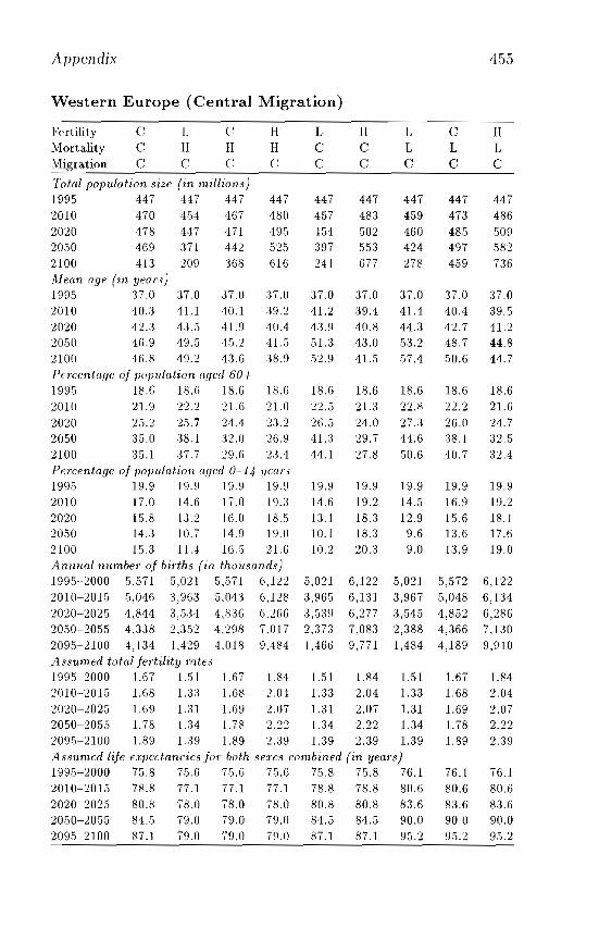
Appendix 455

Western Europe (Central Migration)

Fertility C L c: H L H L C HMortality C H H H C C L L LMigration C C C C C C C C C

Total population size (in millions)1995 447 447 441 447 447 44/ 447 447 4472010 410 454 461 480 457 483 459 473 4862020 478 HI 4/1 495 454 502 460 485 5092050 469 311 442 525 397 553 424 497 5822100 41.3 209 368 616 241 677 278 459 736Mean (lge (in years)1995 37.0 31.0 37.0 :no 37.0 37.0 31.0 37.0 37.02010 40.3 41.1 40.1 39.2 41.2 39.4 41.4 40.4 39.52020 42.3 43.5 41.9 40.4 43.9 40.8 44.3 42.7 41.22050 46.9 49.5 45.2 41.5 51.3 43.0 53.2 48.7 44.82100 46.8 49.2 43.6 38.9 52.9 41.5 57.4 50.6 44.1PeTcentage of population aged 60+1995 18.6 18.6 18.6 18.6 18.6 18.6 18.6 18.6 18.62010 21.9 22.2 21.6 21.0 22.5 21.3 22.8 22.2 21.62020 25.2 25.7 24.4 23.2 26.5 24.0 27.3 26.0 24.72050 35.0 38.1 32.0 26.9 41.3 29.7 44.6 38.1 32.52100 35.1 31.7 29.6 2:3.4 44.1 27.8 50.6 40.7 32.4Percentage of population aged 0-14 yeal'S1995 19.9 19.9 19.9 19.9 19.9 19.9 19.9 19.9 19.92010 17.0 14.6 11.0 19.3 14.6 19.2 14.5 16.9 19.22020 15.8 13.2 16.0 18.5 13.1 18.3 12.9 15.6 18.12050 14.3 ID.7 14.9 19.0 10.1 18.3 9.6 13.6 17.62100 15.3 11.4 16.5 21.6 10.2 20.3 9.0 13.9 19.0Annual 1111mber' of bir'ths (in thousands)1995-2000 5,571 5,021 5,571 6,122 5,021 6,122 5,021 5,572 6,1222010-2015 5,046 3.963 5.043 6,128 3,965 6,131 3,967 5,048 6,1342020-2025 4,844 3,534 4,836 6.266 3,539 6 .)~~ 3,545 4,852 6,286, ... ( (

2050-2055 4,338 2.352 4,298 7.017 2.373 7.083 2,388 4,366 7,1302095-2100 4,134 1,429 4,018 9,484 1,466 9,771 1,484 4,189 9,910Assumed total fer'tility mtes1995-2000 1.67 1.51 1.61 1.84 1.51 1.84 1.51 1.67 1.842010-2015 1.68 1.33 1.68 2.04 1.33 2.04 1.33 1.68 2.042020-2025 1.69 1.31 Ui9 2.07 1.31 2.07 1.31 1.69 2.072050-2055 1.78 1.34 1.78 2.22 1.34 2.22 1.34 1.78 2.222095-2100 1.89 1.:39 1.89 2.39 1.39 2.39 1.39 1.89 2.39Assumed life e:z;pectancies for both ,e:res combined (in years)1995-2000 75.8 75.6 15.6 75.6 75.8 75.8 76.1 76.1 76.12010-2015 78.8 77.1 77.1 17.1 78.8 78.8 80.6 80.6 80.62020-2025 80.8 18.0 78.0 78.0 80.8 80.8 83.6 83.6 83.62050-2055 84.5 79.0 79.0 79.0 84.5 84.5 90.0 90.0 90.02095-2100 87.1 79.0 79.0 79.0 87.1 87.1 952 95.2 9.5.2

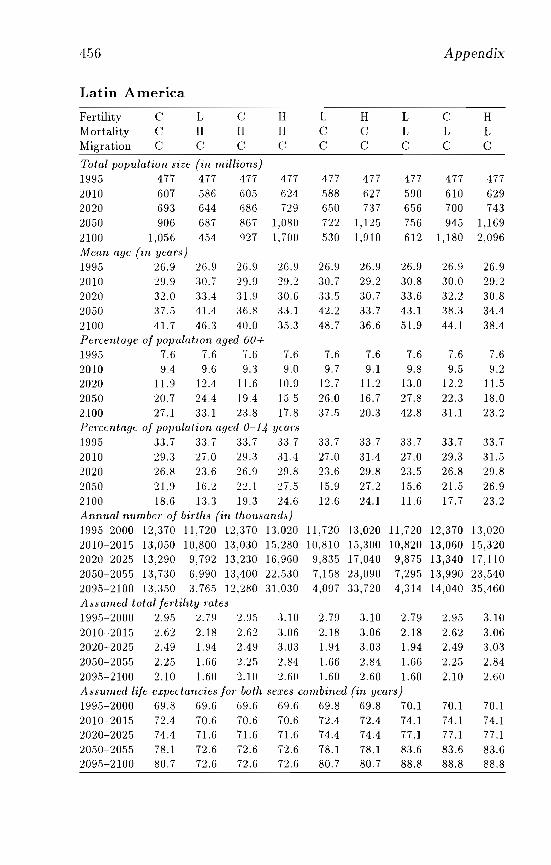
4.56 Appendix

Latin America

Fertility C L C II L II L C IIMortality C II II II C C L L LMigration (J C C C C C C C C

Total population size (in millions)1995 477 477 477 477 477 477 477 477 4772010 607 586 605 624 588 627 590 610 6292020 693 644 686 729 650 737 656 700 7432050 906 687 867 1,080 722 1,125 756 945 1,1692100 1,056 454 927 1,700 530 1,910 612 1,180 2,096Mean age (zn yea!'!!)1995 26.9 26.9 26.9 26.9 26.9 26.9 26.9 26.9 26.92010 29.9 :30.7 29.9 29.2 30.7 29.2 30.8 30.0 29.22020 32.0 :3:3.4 :31.9 30.6 :n.5 30.7 33.6 32.2 30.82050 37.5 41.4 36.8 :3:3.1 42.2 33.7 43.1 38.3 34.42100 41.7 46.3 40.0 35.3 48.7 36.6 51.9 44.1 38.4Pe"centage of populatIOn aged 60+1995 7.6 7.6 7.6 7.6 7.6 7.6 7.6 7.6 7.62010 9.4 9.6 9.3 9.0 9.7 9.1 9.8 9.5 9.22020 11.9 12.4 11.6 10.9 I·J - 11.2 13.0 12.2 11.5_.1

2050 20.7 24.4 19.4 15.5 26.0 16.7 27.8 22.3 18.02100 27.1 33.1 23.8 17.8 37.5 20.3 42.8 31.1 23.2Pe'rcentage of population aged 0-14 years1995 33.7 33.7 33.7 33.7 33.7 33.7 33.7 33.7 33.72010 29.3 27.0 29.3 31.4 27.0 31.4 27.0 29.3 31.52020 26.8 2:3.6 26.9 29.8 23.6 29.8 23.5 26.8 29.82050 21.9 16.2 22.1 27.5 15.9 27.2 15.6 21.5 26.92100 18.6 13.3 19.3 24.6 12.6 24.1 11.6 17.7 23.2Annual number of bi,·ths (in thousands)1995-2000 12,370 11,720 12,370 13,020 11,720 13,020 11,720 12,370 13,0202010-2015 13,050 10,800 13,030 15,280 10,810 15,300 10,820 13,060 15,3202020-2025 13,290 9,792 13,230 16,960 9,835 17,040 9,875 13,340 17,1102050-2055 13,730 6,990 13,400 22,530 7,158 23,090 7,295 13,990 23,5402095-2100 13,350 3,765 12,280 31,030 4,097 33,720 4,314 14,040 35,460Assumed total fertility mtes1995-2000 2.95 2.79 2.95 :3.10 2.79 3.10 2.79 2.95 3.1020 10~-20 15 2.62 2.18 2.62 3.06 2.18 3.06 2.18 2.62 3.062020-2025 2.49 1.94 2.49 3.03 1.94 3.03 1.94 2.49 3.032050-2055 2.25 1.66 2.25 2.84 1.66 2.84 1.66 2.25 2.842095-2100 2.10 1.60 2.10 2.60 1.60 2.60 1.60 2.10 2.60Assumed life expectancies for both SLrC8 combined (in yem's)1995-2000 69.8 69.6 69.6 69.6 69.8 69.8 70.1 70.1 70.12010-2015 72.4 70.6 70.6 70.6 72.4 72.4 74.1 74.1 74.12020-2025 74.4 71.6 71.6 71.6 74.4 74.4 77.1 77.1 77.12050-2055 78.1 72.6 72.6 72.6 78.1 78.1 83.6 83.6 83.62095-2100 80.7 72.6 72.6 72.6 80.7 80.7 88.8 88.8 88.8

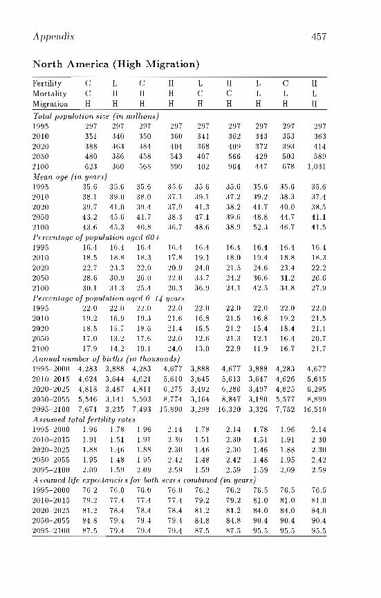
Appendix 457

North America (High Migration)

Fertility C L C H L H L C HMortality C H H H C C L L LMigration H H H H H H H H H

Total population size (in millions)1995 297 297 297 297 297 297 297 297 2972010 351 340 3.50 360 :341 362 343 353 3632020 388 363 384 404 368 409 372 393 4142050 480 386 4,58 543 407 566 429 503 5892100 623 360 568 890 402 964 447 678 1,031Mean age (in yean)1995 35.6 35.6 35.6 35.6 35.6 35.6 35.6 35.6 35.62010 38.1 39.0 38.0 37.1 39.1 37.2 39.2 38.3 37.42020 39.7 41.0 39.4 37.9 41.3 38.2 41.7 40.0 38.52050 43.2 45.6 41.7 38.3 47.1 39.6 48.8 44.7 41.12100 43.6 45.3 40.8 36.7 48.6 38.9 52.3 46.7 41.5Pel'centage of population aged 60+1995 16.4 16.4 16.4 16.4 16.4 16.4 16.4 16.4 16.42010 18.5 18.8 18.3 17.8 19.1 18.0 19.4 18.8 18.32020 22.7 23.3 21.0 20.9 24.0 21.5 24.6 23.4 22.22050 28.6 30.9 26.0 22.0 33.7 24.2 36.6 31.2 26.62100 30.1 31.3 25.4 20.3 36.9 24.] 42.5 34.8 27.9Percentage of popu.lation aged 0-14 years1995 22.0 22.0 22.0 22.0 22.0 22.0 22,0 22.0 22.02010 ]9.2 16.9 ]9.3 21.6 ]6.8 21.5 ]6.8 ]9.2 21.52020 18.5 1.5.7 ]8.6 21.4 ]5.5 21.2 ]5.4 ]8.4 21.12050 17.0 ]3.2 ] 7.6 :22.0 12.6 21.3 12.1 ]6.4 20.72100 17.9 ]4.2 19. ] 24.0 1:3.0 22.9 11.9 ]6.7 21.7Annu.al numbel' of births (in thousands)]995-2000 4,283 3,888 4,283 ·1,677 3,888 4,677 3,888 4,283 4,67720]0-20]5 4,624 3,644 4,621 5,610 3,645 5,6]3 3,647 4,626 5,6]52020-2025 4,8]8 3.487 4,811 6,275 3,492 6,286 3,497 4,825 6,2952050-2055 5,546 3, ]41 .5,503 8,774 3,164 8,847 3,180 5,577 8,8992095-2100 7,671 3,235 7,493 ]5,890 3,298 ]6,320 3,326 7,752 ]6,.5]0Assu.med total fel·tility mtes1Y95-2000 1.96 1.78 1.96 2.14 1.78 2.]4 1.78 1.96 2.]42010-2015 1.9] 1.51 1.9] 2.30 1.5] 2.30 1.5] 1.91 2.302020-2025 1.88 1.46 1.88 2.30 ] .46 2.30 1.46 1.88 2.302050-2055 1.95 ].48 UJ,5 2.42 1.48 2.42 ].48 1.95 2.422095-2100 2.09 1.59 2.09 2.59 1.59 2.59 1.59 2.09 2.59Assumed life expectancies fOI' both secus combined (in years)]995-2000 76.2 76.0 76.0 76.0 76.2 76.2 76.5 76.5 76.520]0-20]5 79.2 77.4 77.4 77.4 79.2 79.2 81.0 81.0 81.02020-2025 81.2 78.4 78.4 78.4 81.2 81.2 84.0 84.0 84.02050-2055 84.8 79.4 79.4 79.4 84.8 84.8 90.4 90.4 90.42095-2100 87.5 79.4 79.4 79.4 87.5 87.5 95.5 95.5 95.5

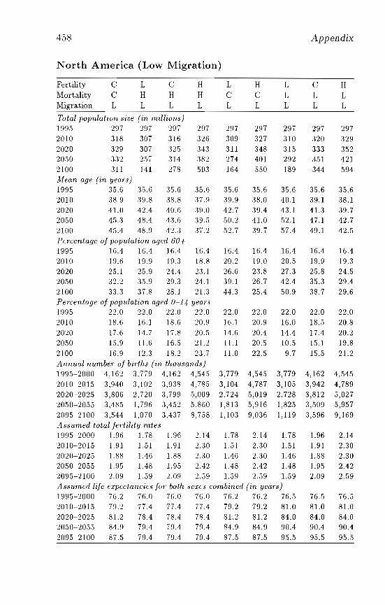
458 Appendix

North America (Low Migration)

Fertility C L C H L H L C HMortality C H H H C C L L LMigration L L L L L L L L L

Total population size (in millions)1995 297 297 297 297 297 297 297 297 2972010 318 307 316 326 309 327 310 320 3292020 329 307 325 343 311 348 315 333 3522050 332 25'1 314 :382 274 401 292 351 4212100 311 141 278 503 164 550 189 344 594Mean age (in yeal's)1995 35.6 3,5.6 35.6 35.6 35,6 35.6 35.6 35.6 35.62010 38,9 39.8 38.8 37.9 39.9 38.0 40.1 39.1 38.12020 41.0 42.4 40.6 39.0 42.7 39.4 43.1 41.3 39.72050 45.3 48.4 43.6 :39.5 50.2 41.0 52.1 47.1 42.72100 45.4 48.9 42.3 3~ ') 52.7 39.7 57.4 49.1 42.5,,_Percentage of population aged 60+1995 16.4 16.4 16.4 16.4 16.4 16.4 16.4 16.4 16.42010 19.6 19.9 19,3 18.8 20.2 19.0 20.5 19.9 19,3

2020 25.1 25.9 24.4 2:3.1 26.6 23.8 27.3 25.8 24.52050 32.2 35.9 29,3 24.1 39.1 26.7 42.4 35.3 29.42100 33.3 37.8 28.1 21.3 44.3 25.4 50.9 38.7 29.6Pel'centage of population aged 0-14 years1995 22.0 22.0 22.0 22.0 no 22.0 22.0 22.0 22.02010 18.6 16.1 18,6 20.9 16.1 20.9 16.0 18.5 20.82020 17.6 14.7 17.8 20.5 14,6 20.4 14.4 17.4 20.22050 1.5.9 11,6 16.5 n.2 11.1 20.5 10.5 15.1 19.82100 16.9 12.3 18.2 23,7 11.0 22.5 9.7 15.5 21.2Annual number of births (in thousands)1995-2000 4,162 3,779 4,162 4,545 3,779 4,545 3,779 4,162 4,5452010-2015 3,940 3,102 3,938 4,785 3,104 4,787 3,105 3,942 4,7892020-2025 3,806 2,720 3,799 5,009 2,724 5,019 2,728 3,812 5,0272050-2055 3,485 1,796 3,452 5.860 1,813 5,916 1,825 3,509 5,9572095-2100 3,544 1,070 3.437 8,758 1,103 9,036 1,119 3,596 9,169Assumed total fel·tility mtes1995-2000 1.96 1.78 1.96 2.14 1.78 2.14 1.78 1.96 2.142010-2015 1.91 1.51 1.91 2,30 1.51 2.30 1.51 1.91 2.302020-2025 1.88 1.46 1.88 2.30 1.46 2.30 1.46 1.88 2.302050-2055 1.95 1.48 1.95 2.42 1.48 2.42 1.48 1.95 2.422095-2100 2.09 1.59 2.09 2.,59 1.59 2.59 1.59 2.09 2.59Assumed life expectancies fOl' both sexes combined (in years)1995-2000 76.2 76.0 76.0 76,0 76.2 76.2 76.5 76.5 76.52010-2015 79,2 77.4 77.4 17.4 79.2 79.2 81.0 81.0 81.02020-2025 81.2 78.4 78.4 78.4 81.2 81.2 84.0 84.0 84.02050-2055 84.9 79.4 '19.4 79.4 84.9 84.9 90.4 90.4 90.42095-2100 87.5 '19.4 79.4 79.4 87.5 87.5 95.5 95.5 95.5

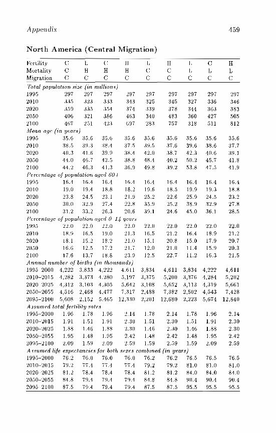
Appendix 459

North America (Central Migration)

Fertility C L C H L H L C HMortality C H H H C C L L LMigration C C C C C C C C C

Total population size (in millions)1995 297 297 297 297 297 297 297 297 2972010 335 323 333 343 325 345 327 336 3462020 359 33,'} 354 374 :l39 378 344 363 3832050 406 321 386 463 340 483 360 427 5052100 467 2,'}1 42:l 697 283 757 318 511 812Mean age (in yem"s)1995 3,'}.6 :l5.6 35.6 35.6 35.6 35.6 35.6 35.6 35.62010 38.5 39.3 :38.4 37.5 39.5 37.6 39.6 38.6 37.72020 40.3 41.6 39.9 38.4 42.0 38.7 42.3 40.6 39.12050 44.0 46.7 42.5 38.8 48.4 40.2 50.2 45.7 41.82100 44.2 46.3 41.3 36.9 49.8 39.2 53.8 47.5 41.9Pe/Tentage of population aged 60+1995 16.4 16.4 16.4 16.4 16.4 16.4 16.4 16.4 16.42010 19.0 19.4 18.8 18.2 19.6 18.5 19.9 19.3 18.82020 23.8 24.5 23.1 21.9 25.2 22.6 25.9 24.5 23.22050 30.0 32.9 27.4 22.8 35.9 25.2 38.9 32.9 27.82100 31.2 33.2 26.3 20.6 39.1 24.6 45.0 36.1 28.5Pel"Centage of population aged 0-14 years1995 22.0 22.0 22.0 no 22.0 22.0 22.0 22.0 22.02010 18.9 16.5 19.0 21.3 16.5 21.2 16.4 18.9 21.22020 18.1 1" '} 18.2 21.0 15.1 20.8 15.0 17.9 20.70._

2050 16.6 12.5 j- 'J 21.7 12.0 21.0 11.4 15.9 20.31._

2100 17.6 13.7 U3.8 23.9 12.5 22.7 11.2 16.3 21.5A nnual number of births (in thollsands)1995-2000 4 '''')'J 3,833 4,222 4,611 3,834 4,611 3,834 4,222 4,6111"'~'"

2010-2015 4,282 3,373 4,280 5,197 3,375 5,200 3,376 4,284 5,2022020-2025 4,312 3,103 4,305 5,642 3,108 5,652 3,113 4,319 5,6612050-2055 4,516 2,468 4,477 7,317 2,488 7,382 2,502 4,543 7,4282095-2100 5,608 2,152 5,465 12,330 2,201 12,680 2,223 5,674 12,840Assumed total /atility mtes199,'}-2000 1.96 1.78 1.96 2.14 1.78 2.14 1.78 1.96 2.142010-2015 Ull 1.51 1.91 2.30 LSI 2.30 1.51 1.91 2.302020-2025 1.88 1.46 1.88 2.30 1.46 2.30 1.46 1.88 2.302050-2055 1.95 1.48 1.95 2.42 1.48 2.42 1.48 1.95 2.422095-2100 2.09 1.59 2.09 2.59 1.59 2.59 1.59 2.09 2.59Assumed life expectancies /07" both sexes combined (in years)199.5-2000 76.2 76.0 76.0 76.0 76.2 76.2 76.5 76.5 76.52010-2015 79.2 77.4 77.4 77.4 79.2 79.2 81.0 81.0 81.02020-2025 81.2 78.4 78.4 78.4 81.2 81.2 84.0 84.0 84.02050-2055 84.8 79.4 79.4 79.4 84.8 84.8 90.4 90.4 90.42095-2100 87.5 79.4 79.4 79.4 87.5 87.5 95.5 95.5 95.5

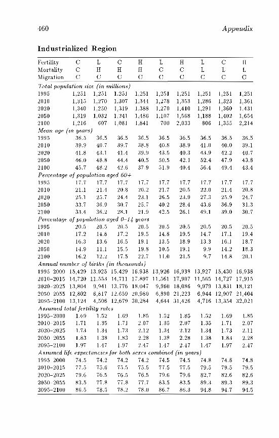
460 Appendix

Industrialized Region

Fertility C L C H L H L C HMortality C H H H C C L L LMigration C C C C C C C C C

Total population size (in mil/tOns)1995 1,251 1,:251 1,25] 1,251 1,25] 1,251 ],251 1,251 1,2512010 1,3]5 1,270 ],307 ],344 1,278 ] ,353 ] ,286 1,323 1,3612020 1,340 ],250 1,~n9 ] ,388 1,270 ],410 1,291 1,360 1,43]2050 1,3] 9 1,032 1,241 1,486 1,107 1,568 1,188 1,402 1,6542100 1,216 607 1,08] 1,84] 700 2,033 806 ],355 2,214Mean age (in years)1995 36.5 36.5 36.5 36.5 36.5 36.5 36.5 36.5 36.52010 39.9 40.7 39.7 38.8 40.8 38.9 41.0 40.0 39.12020 41.8 43.] 41.4 39.9 43.5 40.3 43.9 42.2 40.72050 46.0 48.8 44.4 40.5 50.5 42.1 52.4 47.9 43.82100 45.7 48.2 42.6 37.9 51.9 40.4 56.4 49.4 43.4Percentage of population aged 60+1995 17.7 17.7 17.7 17.7 17.7 17.7 17.7 17.7 17.72010 21.1 21.4 20.8 20.2 21.7 20.5 22.0 21.4 20.82020 25.1 25.7 24.4 23.1 26.5 23.9 27.3 25.9 24.72050 33.7 36.9 30.7 25.7 40.2 28.4 43.6 36.9 31.32100 33.4 36.2 28.1 21.9 42.5 26.1 49.1 39.0 30.7Pel'centage of population aged 0-14 years1995 20.5 20.5 20.5 20.5 20.5 20.5 20.5 20.5 20.52010 17.2 14.8 ] 7.2 ]9.5 14.8 19.5 14.7 17.1 19.42020 16.3 13.6 16.5 19. ] 13.5 18.9 13.3 16.] 18.72050 14.9 ] 1.1 15.5 19.8 10.5 19. ] 9.9 14.2 ]8.3

2100 16.2 12.2 17.5 22.7 11.0 21.5 9.7 14.8 20.]Annual number of bil·ths (in thousands)1995-2000 15,429 13.925 15.429 16.938 13,926 16,938 13,927 ]5,430 16,9382010-2015 14,720 11,553 14,711 17,897 11,561 17,907 11,565 14,727 17,9152020-2025 13,804 9,941 13,776 18,047 9,960 18,086 9,979 13,831 18,1212050-2055 12,802 6,817 12.659 20,980 6,890 21,223 6,944 12,907 21,4042095-2100 13,124 4,506 12,679 30,284 4,644 31,426 4,716 13,354. 32,02]Assumed total fel·tility mtes1995-2000 1.69 1.52 1.69 1.85 1.52 1.85 1.52 1.69 1.852010-2015 1.71 1.35 1. 7] 2.07 1.35 2.07 1.35 1.71 2.072020-2025 1.73 L14 1.73 2.12 1.34 2.12 1.34 1.73 2.112050-2055 1.83 138 1.83 2.28 1.38 2.28 1.38 1.83 2.282095-2100 1.97 1.47 1.97 2.47 1.47 2.47 1.47 1.97 2.47Assumed life expectancies for both sexes combined (in years)1995-2000 74.5 74.2 74..2 74.2 74.5 74.5 74.8 74.8 74..82010-2015 77.5 75.6 75.5 75.5 77.5 77.5 79.5 79.5 79.52020-2025 79.6 76.5 76.5 76.5 79.6 79.6 82.7 82.6 82.62050-2055 83.5 77.8 77.8 77.7 83.5 83.5 89.3 89.3 89.32095-2100 86.5 78.5 78.2 78.0 86.7 86.3 94.8 94.7 94.5

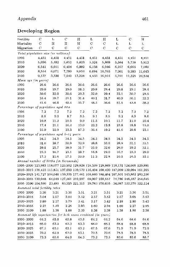
Appendix 461

Developing Region

Fertility C L CMortality C H HMigration C C C

HHC

LCC

HCC

LLC

CLC

HLC

Total population size (in mil/ions)

1995 4,451 4,451 4,451

2010 5,696 5,482 5,652

2020 6,541 6,011 6,404

2050 8,554 6,071 7,780

2100 9,137 3,330 7,040

Mean age (in years)

1995 26.6 26.6 26.6

2010 29.0 29.7 29.0

2020 30.6 32.0 30.6

2050 35.4 39.7 35.1

2100 41.6 46.8 40.4

Percentage of population aged 60+

1995 7.2 7.2 7.2

2010 8.8 9.0 8.7

2020 10.8 11.2 10.5

2050 17.4 21.1 16.4

2100 25.9 32.9 23.3

4,451

5,823

6,802

9,810

13,228

26.6

28.3

29.3

31.4

35.7

7.2

8.5

9.9

13.0

17.3

4,451

5,524

6,138

6,694

4,433

26.6

29.8

32.0

40.1

48.5

7.2

9.1

11.5

22.2

36.4

4,451

5,869

6,946

10,765

16,915

26.6

28.4

29.4

31.7

36.6

7.2

8.5

10.1

13.8

19.2

4,451

5,564

6,257

7,301

5,701

26.6

29.8

32.1

40.9

51.5

7.2

9.2

11.7

23.8

41.6

4,451

5,738

6,665

9,285

11,325

26.6

29.1

30.7

36.1

43.8

7.2

8.9

11.0

18.8

29.8

4,451

5,912

7,080

11,643

20,524

26.6

28.4

29.5

32.2

38.2

7.2

8.6

10.4

15.0

22.1

64.6

68.8

72.0

78.5

83.7

64.6

68.8

71.9

78.5

83.6

64.6

68.8

71.9

78.5

83.6

Percentage of population aged 0-14 years

1995 34.5 34.5 34.5 34.5 34.5 34.5 34.5 34.5 34.5

2010 31.0 28.7 30.9 32.9 28.8 33.0 28.9 31.1 33.1

2020 29.1 25.7 28.9 31.7 25.9 32.0 26.0 29.2 32.1

2050 23.3 16.7 23.1 28.7 16.8 29.0 16.7 23.3 29.0

2100 17.3 11.6 17.5 22.9 11.3 22.8 10.5 16.5 22.1

Annual number of birth.s (in thousands)

1995-2000 123,983 118,077 123,952 129,828118,109 129,869 118,131 124,005 129,891

2010-2015 138,423115,851 137,650 159,570 116,494 160,420 1l7,099 139,094 161,205

2020-2025141,727104,040139,335177.461105,860 180,464 107,501143,862 183,156

2050-2055 139,048 64,049 127,561 219,097 69,907 238,557 74,786 148,587 254,645

2095-2100 104,596 23,485 83,215 221,315 29,763 276,635 34,987 122,270 322,114

Assumed total fertility rates

1995-2000 3.36 3.21 3.36 3.51 3.21 3.51 3.21 3.36 3.51

2010-2015 3.04 2.57 3.04 3.52 2.57 3.52 2.57 3.05 3.53

2020-2025 2.80 2.17 2.79 3.41 2.17 3.42 2.18 2.80 3.42

2050-2055 2.27 1..59 2.26 2.93 1.60 2.94 1.60 2.27 2.95

2095-2100 1.88 1.38 1.88 2.39 1.38 2.38 1.38 1.88 2.38

Assumed life e:L'pectancies for both. sexes combined (in years)

1995-2000 64.2 63.8 63.8 63.8 64.2 64.2

2010-2015 66.0 63.2 63.3 63.3 66.0 66.1

2020-2025 67.5 63.1 63.1 63.2 67.5 67.6

2050-2055 70.5 62.9 63.0 63.1 70.5 70.6

2095-2100 73.3 63.6 64.0 64.3 73.2 73.5

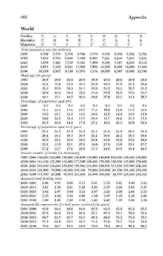
462 Appendix

World

Fertility C L C H L H L C HMortality C H H H C C L L LMigration C C C C C C C C C

Total popula.t;on size (in millions)

1995 5,702 5,702 .5,702 5,702 5,702 5,702 5,702 5,702 5,702

2010 7,012 6,752 6,960 7,168 6,802 7,221 6,850 7,061 7,272

2020 7,879 7,261 7,723 8,191 7,408 8,356 7,547 8,026 8,510

2050 9,874 7,103 9,021 11,300 7,802 12,330 8,488 10,690 13,300

2100 10,350 3,937 8,120 15,070 5,134 18,950 6,507 12,680 22,740

Mean age (in yea.7·s)

1995 28.8 28.8 28.8 28.8 28.8 28.8 28.8 28.8 28.8

2010 31.1 31.8 31.0 30.3 31.8 30.3 31.9 31.1 30.4

2020 32.5 33.9 32.4 31.1 34.0 31.2 34.1 32.7 31.3

2050 36.9 41.0 36.4 32.6 41.6 33.0 42.5 37.6 33.7

2100 42.1 47.1 40.7 36.0 49.0 37.0 52.1 44.4 38.7

Penentage of populo.tion aged 60+

1995 9.5 9.5 9.5 9.05 9.05 9.5 9.5 9.5 9.5

2010 11.1 11.3 11.0 10.7 11.5 10.8 11.6 11.2 10.9

2020 13.2 13.7 12.9 12.2 14.0 12.5 14.4 13.6 12.8

2050 19.6 23.4 18.4 14.7 24.8 15.7 26.6 21.1 17.0

2100 26.8 33.4 24.0 17.8 37.2 19.9 42.5 30.8 22.9

Pe7'centage of popu.la.tion o.ged 0-14 yea7'S

199.5 31.4 31.4 31.4 31.4 31.4 31.4 31.4 31.4 31.4

2010 28.4 26.1 28.3 30.4 26.2 30.5 26.3 28.5 30.6

2020 26.9 23.6 26.8 29.6 23.8 29.8 23.9 27.0 29.9

2050 22.2 15.9 22.1 27.6 16.0 27.8 15.8 22.1 27.7

2100 17.2 11.7 17.05 22.9 11.3 22.6 10.4 16.4 22.0

Annual numbe7' of bi7'ths (in thousa.nds)

1995-2000 139,400 132,000 139,400 146,800 132,000 146,800 132,000 139,400 146,800

2010-2015153,100127,400152,400177,500128,100 178,300128,700153,800179,100

2020-2025155,500 114,000 153,100 19.5,500 115,800 198,500 117,500 157,700 201,300

2050-2055 151,900 70,860 140,200 240,100 76,800 259,800 81,730161,500276,100

2095-2100117,700 27,990 95,910 251,600 34,410308,000 39,700 135,6003054,100

Assumed tota.1 fertility rates

1995-2000 2.96 2.81 2.96 3.12 2.81 3.12 2.81 2.96 3.12

2010-2015 2.81 2.36 2.81 3.26 2.36 3.27 2.36 2.82 3.27

2020-2025 2.65 2.07 2.64 3.22 2.07 3.23 2.08 2.66 3.23

2050-2055 2.23 1.58 2.22 2.86 1.58 2.87 1.59 2.23 2.88

2095-2100 1.90 1.40 1.90 2.40 1.40 2.40 1.39 1.89 2.39

Assumed life e2'pectancies for both se.res combined (in yea.7·s)

1995-2000 65.0 64.5 64.6 64.6 65.0 65.0 65.4 65.4 65.5

2010-2015 67.3 64.0 64.2 64.4 67.1 67.4 70.1 70.3 70.4

2020-2025 68.7 63.05 63.7 63.9 68.5 68.8 73.3 73.4 73.5

2050-20055 71.4 62.8 63.1 63.4 71.2 71.6 79.7 79.8 79.9

2095-2100 74.0 64.7 64.8 64.9 74.0 74.2 84.3 84.4 84.5

ReferencesAckefors, R., and Enell, M., 1990, Discharge of nutrients from Swedish fish

farming to adjacent sea areas, Ambio 19(1):28-35.Ahlburg, D.A., and Land, ICC., 1992, Population forecasting: Guest editors'

introduction, International Journal of Forecasting 8(3):289-299.Ahlburg, D.A., and Vaupel, J., 1990, Alternative projections of the US popula­

tion, Demography 27:639-652.Alexandratos, N., ed., 1995, World Agriculture: Towards 2010, FAO, Rome,

Italy.Alho, J.M., 1990, Stochastic methods in population forecasting, International

Journal of Forecasting 6:521-530.Allan, J.A., 1976, The Kufrah agricultural schemes, The Geographical Journal

142(1):48-56.Allman, J., Vu, Q.N., Nguyen, M.T., Pham, B.S., and Vu, D.M., 1991, Fertility

and family planning in Vietnam, Studies in Family Planning 22(5):308-317.Alonso, W., 1974, Policy-Oriented Interregional Demographic Accounting and

Generalization of Population Flow Models, Working Paper 247, Universityof California, Institute of Urban and Regional Development, Berkeley, CA,USA.

Andersen, 0., 1991, Occupational impacts on mortality declines in the Nordiccountries, in W. Lutz, ed., Future Demographic Trends in Europe and NorthAmerica: What Can We A.~sume Today? Academic Press, London, UK.

Anderson, R.M., 1991, AIDS and its demographic impact, in R. Feachem andD. Jamison, eds., Disease and Mortality in Sub-Saharan Africa, WorldBank/Oxford University Press, New York, NY, USA.

Anderson, R.M., and May, R.M., 1988, Epidemiological parameters of HIV trans­mission, Nature 333:514-522.

Anderson, R.M., and May, R.M., 1992, Infectious Diseases of Humans: Dynam­ics and Control, Oxford University Press, New York, NY, USA.

Anderson, R.M., May, R.M., Boily, M.C., Garnett, G.P., and Rowley, J.T., 1991,The spread of HIV-1 in Africa: Sexual contact patterns and the predicteddemographic impact of AIDS, Nature 352:581-589.

Arnold, F., 1989, Revised Estimates and Projections of International Migration1980-2000, Policy, Planning, and Research Working Papers, World Bank,Washington, DC, USA.

Arshat, H., Tan, B.A., Tey, N.P., and Subbiah, M., 1988, Marriage and Fam­ily Formation in Peninsular Malaysia: Analytic Report on the 1984/85Malaysian Population and Family Survey, National Population and FamilyDevelopment Board, Kuala Lumpur, Malaysia.

Ascher, W., 1978, Forecasting: An Appraisal for Policy Makers and Planners,Johns Hopkins University Press, Baltimore, MD, USA.

Atoh, M., 1989, Trends and differentials in fertility, Reprinted from CountryMonograph Series No. 11, Population of Japan, UN ESCAP, 1984, ReprintSeries No.9, Institute of Population Problems, Ministry of Health and Wel­fare, Tokyo, Japan.

Baade, F., 1960, Del' Wettlauf zum Jah,'e 2000, Oldenburg, Munich, Germany.

463

464 References

Bale, M.D., 1981, Price distortions in agriculture and their effects: An interna­tional comparison, A merican Journal of AgI'icultural Economics 63( 1):8-22.

Bandyopadhyay, J., 1989, Riskful confusion of drought and man-induced waterscarcity, Ambia 18(5):284-292.

Banister, J., 1987, China's Changing Population, Stanford University Press,Stanford, CA, USA.

Banister, J., 1989, Vietnam's evolving population policies, International Popu­lation Conference 1:155-168.

Bariloche Group, 1976, The Latin American world model, in G. Bruckmann, ed.,Proceedings of the Second IIASA Conference on Global Modeling, CP-76-8,International Institute for Applied Systems Analysis, Laxenburg, Austria.

Barnett, A., Kiernan, B., and Boua, C., 1980, The bureaucracy of death: Doc­uments from inside Pol Pot's torture machine, New Statesman, May 2.

Bartiaux, F., and van Ypersele, J.-F., 1993, The role of population growth inglobal warming, in IUSSP International Population Conference: Montreal,Vol. 4, International Union for the Scientific Study of Population, Liege,Belgium.

Bates, R.H., 1981, MW'kets and States in Tl'Opical Afl'ica: The Political Basis ofAgricultural Politics, University of California Press, Berkeley, CA, USA.

Baumgartner, A., and Reichel, E., 1975, The World Water Balance, ElsevierScientific Publishers, Amsterdam, Netherlands.

Becker, E., 1986, When the Wm' Was Over: The Voices of Cambodia's Revolu­tion and Its People, Simon & Schuster, New York, NY, USA.

Becker, C., and Collignon, R., 1989, Sante et Population en Senegambie desorigines d 1960, INED, Paris, France.

Becker, C., and Martin, V., 1983, Les premiers recensements au Senegal, etl'evolution demographique, ORSTOM, Dakar, Senegal.

Behn, R.D., and Vaupel, J.W., 1982, Quick Analysis for Busy Decision Makers,Basic Books, New York, NY, USA.

Benamrane, D., 1983, L 'Emigration Algel'ienne en France, Societe Nationaled'Edition et de Diffusion, Algiers, Algeria.

Berkley, S.F., 1994, Public health measures to prevent HIV spread in Africa, inM. Essex, S. Mboup, P.J. Kallki, and M.R. Kalengayi, eds., AIDS in Africa,Raven Press, New York, NY, USA.

Bernstein, T.P., 1984, Stalinism, famine, and the Chinese peasants: Grain pro­curements during the Great Leap Forward, Theory and Society 13:339-377.

Bhat, P.N.M., 1989, Mortality and fertility in India, 1881-1961: A reassessment,in T. Dyson, ed., India's Historical Demography, Curzon Press, London,UK.

Birdsall, N., 1992, Another Look at Population and Global Warming, PolicyResearch Working Paper WPS 1020, November, World Bank, Washington,DC, USA.

Birg, H., 1995, World Population Pl'Ojections fOl' the 21st Century: TheoreticalInterpretations alld Quantitative Simulations, Campus Verlag, Frankfurtand New York.

Biswas, A.K., 1993, Water for agricultural development: Opportunities and con­straints, Water Resources Development 9(1):3-12.

References 465

Biswas, A.K., and Arar, A., 1988, Treatment and Reuse of Wastewater, Butter­worths, London, UK.

Blacker, J .G.C., 1991, Infant and child mortality: Development, environment,and custom, in R.G. Feachem and D.T. Jamison, eds., Disease and Mortalityin Sub-Saharan Africa, World Bank/Oxford University Press, New York,NY, USA.

Blanchard, 0., Layard, R., Dornbusch, R., and Krugman, P., 1991, East-WestMigration: The Alternatives -. A Report of the Wider World EconomyGroup, \tVorking Paper No. 101, Centre for Economic Performance, London,UK.

Bogue, D.J., and Tsui, A.O., 1979, Zero world population growth? The PublicInterest 55(Spring):99-113.

Bohning, W.R., 1981, Elements of a theory of international migration to indus­trial nations, in M. Kritz, C. heely, and S. Tomasi, eds., Global Trends inMigration: The07'y and Research on Intemational Population Movements,Center for Migration Studies, Staten Island, NY, USA.

Bongaarts, J., 1992, Population gTOwth and global warming, Population andDevelopment Review 18(2):299-319.

Bongaarts, J., 1994, Population policy options in the developing world, Science263(February 11):771-776.

Bongaarts, J., Reining, P., Way, P., and Conant, F., 1989, The relationshipbetween male circumcision and HI V infection in African populations, AIDS3:373-377.

Bongaarts, J., Mauldin, W.P., and Phillips, J.E., 1990, The demographic impactof family planning programs, Studies in Family Planning 21(6):299-310.

Bos, E., Vu, M.T., Levin, A., and Bulatao, R.A., 1992, World Population Pm­jections 1992-1993 Edition: Estimates and Projections with Related Demo­gmphic Statistics, World Bank/Johns Hopkins University Press, Baltimore,MD, USA.

Boserup, E., 1965, The Conditions of Ag7'icultural Growth, Aldine, Chicago, IL,USA.

Boserup, E., 1981, Population and Technological Change. University of ChicagoPress, Chicago, IL, USA.

Bourgeois-Pichat, J., 1952, Essai sur la mortalite "biologique" de l'homme, Pop­ulation 7:381-394.

Bourgeois-Pichat, J., 1978, Future outlook for mortality declines in the World,Population Bulletin 0/ the United Nations, No. 11, United Nations, NewYork, NY, USA.

Bradley, D.J., 1991, Malaria, in R. Feachem and D. Jamison, eds., Diseaseand Mortality in Sub-Saha>'an A/I'iea, World Bank/Oxford University Press,New York, NY, USA.

Brass, W., Coale, A.J., Demeny. P., Heisel, D.F., Lorimer, F., Romaniuk, A., andvan de Walle, E., eds., 1968, The Demography 0/ Tropical A/rica, PrincetonUniversity Press, Princeton, NJ, USA.

Brillinger, D.R., 1986, The natural variability of vital rates and associated statis­tics, Biometrics 42(4) :693-734.

466 References

Bulatao, R.A., 1991, The Bulatao approach: Projecting the demographic impactof the HIV epidemic using standard parameters, in The AIDS Epidemic andIts Demographic Consequences, United Nations, New York, NY, USA.

Bulatao, R.A., and Bas, E. (with P.W. Stephens and M.T. Vu), 1989, Project­ing Mortality for All Conntries, Policy, Planning, and Population ResearchWorking Paper Series 337, World Bank, Washington, DC, USA.

Bulatao, R.A., Bos, E., Stephens, P.W., and Vu, M.T., 1990, World PopulationPmjections 1989-1990 Edition: Short- and Long- TeI'm Estimates, WorldBank/ Johns Hopkins University Press, Baltimore, MD, USA.

Bundesministerium fur Raumordnung, Bauwesen und Stiidtebau, eds., 1991,Raumordnungsbericht 1991, Bonll, Germany.

Buringh, P., and Van Heemst, H.D.J., 1977, An Estimation of World Food Pm­duction Based on Labour-oriented Agriculture, Centre for World Food Mar­ket Research, Agricultural Press, Wageningen, Netherlands.

Buringh, P., Van Heemst, H.D.J., and Staring, G.J., 1975, Computation of theAbsolute Maximum Food Pmduction of the World, Centre for World FoodMarket Research, Wageningen, Netherlands.

Buttner, T., and Lutz, W., 1990a, Estimating fertility responses to policy mea­sures in the German Democratic Republic, Population and DevelopmentReview 16(3):539-555.

Buttner, T., and Lutz, W., 1990b, Vergleichende Analyse der Fertilitiits­entwicklungen in der BRD, DDR und Osterreich, Acta Demographica 1:27­45, Physica-Verlag, Heidelberg, Germany.

Caldwell, J.G.C., 1986, Routes to low mortality in poor countries, Populationand Development Review 12(2):171-220.

Caldwell, J .C., and Caldwell, P., 1983, The demographic evidence for the inci­dence and cause of abnormally low fertility in tropical Africa, World HealthStatistics Quarterly 36:221.

Caldwell, J.C., and Caldwell, P., 1990, High fertility in sub-Saharan Africa,Scientific Amer'icfm May:1l8-125.

Caldwell, J.C., and Caldwell, P., 1993, The nature and limits of I. he sub-SaharanAfrican AIDS epidemic: Evidence from geographic and other patterns, Pop­ulation and Development Review 19:817-848.

Caldwell, J.C., and Caldwell, P., 1994, The neglect of an epidemiological expla­nation for the distribution of HIV / AIDS in sub-Saharan Africa: Exploringthe male circumcision hypothesis, in J. Cleland and P. Way, eds., AIDS Im­pact and Pr'evention in the Developing World: Demographic and Social Sci­ence Per'spectives, Supplement to Health Transition Review 4:23-46, HealthTransition Centre, Australian National University, Canberra, Australia.

Caldwell, J.C., Caldwell, P., and Quiggin, P., 1989, The social context of AIDSin sub-Saharan Africa, Population and Development Review 15:185-234.

Cameron, D.W., Simonsen, J.N., D'Costa, L.J., Ronald, A.R., Maitha, G.M.,Gakinya, M.N., Cheang, M., Ndiuya-Achola, J.O., Piot, P., Brunham, R.C.,et al., 1989, Female to male transmission of Human ImmunodeficiencyVirus Type 1: Risk factors for seroconversion in men, The Lancet (19August): 403-407.

References 467

Cantrelle, P., Diop, 1.1., Garenne, M., Gueye, M., and Sadio, A., 1986, Theprofile of mortality aud its det.erminants in Senegal, 1960-1980, in Detel'­minants of Mortality ChangE and Diffel'entials in Developing Countries:The Five-Country CaSE Study Project, Population Studies, No. 94, UnitedNations, New York, NY, USA.

Carael, M., Cleland, J., Deheneffe . .I.-C., and Adeokun, L., 1992, Research onsexual behaviour t.hat t.ransmits HIV: The GPA/WHO collaborat.ive sur­veys, Preliminary findings. in T. Dyson. ed., Sexual Behaviour and Net­working: A nthropological and Socio- Cultural Studies on the Transmissionof HIV, Deronaux-Ordina Editions, Liege, Belgium.

Carter, L.R., and Lee, R.D., 1986, .Ioint forecasts of US marital fertility, nuptial­ity, births and marriages using time series models, Journal of the AmericanStatistical Association 81(396):902-911.

Casterline, J., 1994, Fertility transition in Asia, in T. Locoh and V. Hertrich,eds., The Onset of Fertility Tmnsition in Sub-Saharan Africa, Ordina,Liege, Belgium.

Centers for Disease Control and Prevention, 1991, Patterns of behavior changeamong homosexual/bisexual men: Selected US sites, 1987-1990, Morbidityand Mortality Weekly Rep01't 40:792-794.

Centers for Disease Control and Prevention, 1994, National HIV SerosurveillanceSummary: Results through 1992, Vol. 3, US Department of Health andHuman Services. Atlanta, GA, USA.

Chastanet, M., 1982, Les crises de subsistances dans les villages Soninke ducercle de Bakel de 1858 it 1945, Problemes methodologiques et perspectivesde recherches, ORSTOM. Dakar, Senegal.

Chaudhry, M.D., 1989, Fertility behavior in India, 1961-1986: The stalled de­cline in the crude birth rate. in S.N. Singh, M.K. Premi, P.S. Bhatia, and A.Bose, eds., Population Tm.nsition in India, Vol. 2. B.R. Publishing Corp.,Delhi, India.

Chen, R.S .• 1990, Global agriculture, environment, and hunger: Past, present,and the future, EnvimnmEntal Impact Assessment Review 10:335-358.

Chen, P., and Kols, A., 1982. Popnlation and birth planning in the People'sRepublic of China. Population Reports, Series J, Number 25, Family Plan­ning Programs, Population Information Program, Johns Hopkins Univer­sity, Baltimore, MD, USA.

Chesnais, .I.-C., 1985, Les conditions d'efficacite d'une politique nataliste: ex­amen theoretique et exemples historiques (The conditions of efficiency ofa pronatalist policy: Theoretical considerations and some historical exam­ples), International Popu.lation Confel'ence, Florence 1985 3:413-425, In­ternational Union for t.he Scientific Study of Population, Liege, Belgium.

Chin, .I" 1990, Current and future dimensions of the HIV / AIDS pandemic inwomen and children, The Lancet 336:22]-224,

Chin, .I .• and Lwanga, S.K .. 1991a, Estimation and projection of adult AIDScases: A simple epidemiological model, Bulletin of the World Health Orga­nization 69: 399-406.

Chin . .I., and Lwanga, 5.1\:., 1991b, The World Health Organization approach:Projections of non-paediatric HIV infection and AIDS in pattern II areas,

468 References

in The AIDS Epidemic and Its Demographic Consequences, United Nations,New York, NY, USA.

China. Population Information Center, 1984, Analysis on China's National One­per- Thousand Population Fel,tility Sampling Sll1'vey, China Population In­formation Center, Beijing, China.

Cho, L.-J., Retherford, R.D., and Choe. M.I\., 1986, The Own-Children Methodof Fertility Estimation, East-West Center, University of Hawaii Press, Hon­olulu, HI, USA.

Clark, C., 1967, Population and food, in Population Growth and Land Use,Ma.cmillan, London, UK.

Clark, C" and Haswell, M., 1964, The Economics of Subsistence Agriculture,Macmillan, London, UK.

Clarke, R.D., 1950, A bio-actuarial approach to forecasting rates of mortality,Proceedings of the Centenary Assembly of the Institute of Actuaries, Uni­versity Press, Cambridge, UK.

Cleland, .1., and Wilson, C., 198i, Demand theories of the fertility transition:An iconoclastic view. Population Studies 41(1):5-30 (March).

Cleland, J., Onnoha, N., and Timaons, I.. 1994, Fertility change in sub-SaharanAfrica: A review of the evidence, in T. Locoh and V. Hertrich, eds., TheOnset of Fel·tility Tnlllsition in Sub-Saharan Africa, Ordina, Liege, Bel­gium.

Cliquet, R., ed., 1993, The Future of Ew'ope 's Population: A Scenario Approach,Conncil of Europe, Enropean Population Committee, Strasbourg, France.

Coale, A.J., 1984, Rapid Population Change in China, 1952-1982, Committeeon Popnlation and Demography, Report No. 27, National Academy Press,Washington, DC, USA.

Coale, A.J., and Chen, S.L., 1987, Basic Data on Fertility in the Provinces ofChina, 1940-1982,

CoaIe, A.J., and Demeny, P., 1966, Regional Model Life Tables and Stable Pop­ulations, Princeton University Press, Princeton, NJ, USA.

Coale, A.J., and Demeny, P. (with B. Vaughan), 1983, Regional Model LifeTables and Stable Populations, 2nd Edition, Academic Press, New York,NY, USA.

Coale, A.J., and Freedman, R., 1993, Similarities in the fertility transition inChina and three other East Asian populations, in R. Leete and I. Alam,eds., The Revolution in Asian Fertility. Oxford University Press, Oxford,UK.

Coale, A..1., and Guo, G., 1989, Revised regional model life tables at very lowlevels of mortality, Population Index 55(4):613-643.

Coale, A.J., and Watkins, S.C., eds., 1986, The Decline of Fel,tility in Europe,Princeton University Press, Princeton, NJ, USA.

Coale, J.A., and I<isker, E.E., 1986, Morality crossovers: Reality or bad data?Population Studies 40:389-401.

Coale, J.A., and Kisker, E.E., 1990, Asian and Pacific Population Forum 4(1):1­36. Papers of the East-West Popnlation Institute, Number 104, East-WestCenter, Honolulu, HI, USA.

Cohen, J., 1992, How many people can earth hold? Discover, November:1l4-1l9.

References 469

Cohen, .I., 1994a, Are researchers racing toward success, or crawling? Science265: 1373-1375.

Cohen, .I., [994 b, The epidemic in Thailand, Science 266: 1647.Cohen, .I.E., 1995, How Many Pwple Can the Earth Support? Norton, New

York, NY, USAComfort, A., 1964 [1979), The Biology of Senescence, 3rd Edition, Elsevier, New

York, NY, USA.Constant, K.M., and Sheldrick, W.F., 1992, World Nitrogen Survey, Technical

Paper No. 174, World Bank, Washington, DC, USA.Council of Europe, 1991, Recent Demographic Developments in Europe, Council

of Europe Press, Strasbonrg, France.Council of Europe, 1995, Recent Demographic Developments in Europe, Council

of Europe Press, Strasbonrg, France.Country Report, 1992, Population and Sustainable Development: The Chal­

lenges of Vietnam, Paper circulated during the 4th Asian and Pacific Pop­ulation Conference, Bali, Indonesia, 19- 27 August.

Country Report: Indonesia, 1992, Paper circulated during the 4th Asian andPacific Population Conference, Bali, Indonesia, 19-27 August.

Conntry Report: Malaysia, 1992, Paper circulated during the 4th Asian andPacific Population Conference, Bali, Indonesia, 19-27 August.

Country Report: Philippines, 1992, Paper circulated during the 4th Asian andPacific Population Conference, Bali, Indonesia, 19-27 August.

Country Statement: Thailand, 1992, Paper circulated during the 4th Asian andPacific Population Conference, Bali, Indonesia, 19-27 August.

Critchley, W., Reij, C., and Seznec, A., 1992, Water Harvesting for Plant Pro­duction, Volume 2: Case Studies and Conclusions for Sub-Saharan Africa,World Bank, Washington, DC, USA.

Davis, K., 1951, The Population of India and Pakistan, Princeton UniversityPress, Princeton, NJ, USA.

De Almeida e Silva, M., 1991, Persian Gulf exodus stretched resources, Refugees87(October):12-15 (Geneva).

Demeny, P., 1984, A perspective on long-term population growth, Populationand Development Review 10: 103-126.

De Vincenzi, 1., and Mertens, T., 1994, Male circumcision: A role in HIV pre­vention? AIDS 8:153-160.

Diop, 1.L., 1990, Etude de la mortalite it. Saint-Louis du Senegal it. partir desdonnees d'etat civil, These de doctorat de 3eme cycle, Universite de ParisI, Pantheon-Sorbonne, Paris, France.

Dreze, J., and Sen, A., 1989, Hunger and Public Action, Clarendon Press, Ox-ford, UK.

Dnrkheim, E., 1902, De 10 Division du Travail social, Felix Alcan, Paris, France.Durning, A., 1989, World Poverty, Worldwatch Institute, Washington, DC, USA.Dyson, T., and Moore, M., 1983, Kinship structure, female autonomy and de-

mographic behavior in India, Population and Development Review 9:35-60.Dyson, T., and Murphy, M., 1985, The onset of the fertility transition, Popula­

tion and Development Review 11 :399-440.

470 References

Easterlin, R.A., 1980, Bil'fh and F07·tune: The Impact oj Numbers on PersonalWelj(l1·e. Basic Books, New York, NY, USA.

Eaton, J.W., and Mayer, A.J., 1954, Man's Capacity to Reproduce: The Demog­mphy oj a Unique Population, The Free Press, New York, NY, USA.

Economist Intelligence Unit, 1990, Saudi Ambia: Country Report, No.2.Ehrlich, P., Ehrlich, A., and Daily, G.C .. 1993, Food security, population, and

environment, Population and Development Review 19(1):1-32.Elias, Ch.J., and Heise, L.L., 1994, Challenges for the development of female­

controlled vaginal microbicides, AIDS 8:19.ENHR Report, 1990, Volume 1, Health Research: Essential Link to Equity in

Development, Report from the Commission on Health Research for Devel­opment, Oxford University Press, New York, NY, USA.

ENHR Report, 1991, Volume 2, Essential National Health Research: A Strategyjor Action in Health and Human Development, Report from the Task Force011 Health Research for Development, UNDO, Geneva, Switzerland.

Eurobarometer, 1991, Desire for children, Eurobarometer 32.EUROSTAT, 1991, Two Long-Term Population Scenarios for the European

Community, Scenarios prepared for the Interuational Conference on HumanResources in Europe at the Dawn of the 21st Century, November 27-29,Luxembourg.

FAIR (Federation for American Immigration Reform), 1992, Chinese studentamnesty legislatioll passes, FAIR Immigmtion Report 12(8):3.

Falkenmark, M., 1989, The massive water scarcity now threatening Africa: Whyisn't it being addressed? Ambio 18(2):112-118.

Falkenmark, M., 1991, Water, energy, and development, Rapid populationgrowth and water scarcity: The predicament of tomorrow's Africa, in K.Davis and M.S. Bernstam, eds., Resources, Environment, and Population:P,'esent Knowledge, Future Options, A Supplement to Volume 16, 1990,Oxford University Press, New York, NY, USA.

Family Planning and Maternal and Child Health Project, 1987, Nepal Fertilityand Family Planning Survey Report 1986. Central Bureau of Statistics,Kathmandu, Nepal.

FAO, 1978a, Report on the Agm-Ecological Zones Project, Volume 1: Method­ology and Results fo" Aj,'ica, World Soil Resources Report 48/1, Food andAgriculture Organization, Rome, Italy.

FAO, 1978b, Report on the Agm-Ecological Zones Project, Volume 2: Results jorSouthwest Asia, World Soil Resources Report 48/2, Food and AgricultureOrganization, Rome, Italy.

FAO, 1981a, Report on the Agro-Ecological Zones Project, Volume .'1: Method­ology and Results j07' South and Central America, World Soil ResourcesReport 48/3, Food and Agriculture Organization, Rome, Italy.

FAO, 1981b, Rep07·t on the Agro-Ecological Zones Project, Volume 4: Results jorSoutheast Asia, World Soil Resources Report 48/4, Food and AgricultureOrganization, Rome, Italy.

FAO, 1988, World Agricultm'e: Toww'ds 2000: An FAO Study, New York Uni­versity Press, New York, NY, USA.

FAO, 1992, Fel·tilizel· Yearbook, Food and Agriculture Organization, Rome, Italy.

References 471

FAO, 1994, PC-AGROSTAT, Food and Agriculture Organization, Rome, Italy.FAO/UNDP/IIASA, 1982, Potential Population Supporting Capacities of Lands

in the Developing World, Technical Report of the Project, FPA/I NT/513,Food and Agriculture Organization, Rome, Italy.

FAO/UNFPA/IIASA, 198'!, Potential Population Canying Capacities in the De­veloping COlmtl'ies, Technical information to the project INT/75/PI3, Foodand Agriculture Organization, Rome, Italy.

Farid, S., 1993, Family Planning, Health and Family Well-Being in the ArabWorld, Paper presented at the Arab Population Conference, Ammon.

Feachem, R., and Jamison, D., eds., 1991, Disease and MOI,tality in Sub-SaharanAfrica, World Ba,nk/Oxford University Press, New York, NY, USA.

Feeney, G., 1986, Period Par'ity P7'Ogl'ession Ratios of Fel,tility in Japan, NUPRIResearch Paper Series No. 35 (December), Nihon University PopulationResearch Institute, Tokyo, Japan.

Feeney, G., 1988a, Comparative Structure of Low Fertility in Japan and theUnited States, Paper presented to the Conference on Future Changes inPopulation Age Structure, Sopron, Hungary, 18-21 October 1988, organizedby the International Iustitute for Applied Systems Analysis, Laxenburg,Austria.

Feeney, G., 1988b, The use of parity progression ratios in evaluating family plan­ning programs, in Pl'Oceedings of African Population Conference, Dakar,International Union for the Scientific Study of Population, Liege, Belgium.

Feeney, G., 1990, The Demography of Aging in Japan: 1950-2025, NUPRI Re­search Paper Series No. 55, Nihon University Population Research Institute,Tokyo, Japan.

Feeney, G., 1991, Fertility decline in Ta.iwan: A study using parity progressionratios, Demography 28:467-480.

Feeney, G., and Lutz, W., 1991, Distributional analysis of period fertility, in W.Lutz, ed., Future Demographic T/'ends in EU1'Ope and North America: WhatCan We Assume Today~ Academic Press, London, UK.

Feeney, G., and Wang. F., 1993, Parity progression and birth intervals in China:The influence of policy in hastening fertility decline, Population and Devel­opment Review 19(1):61-101.

Feeney, G., and Yu, J., 1987, Period parity progression measures of fertility inChina, Population Studies 41(1):77-102.

Feeney, G., and Yuan, .1., 1994, Below replacement fertility in China? A closelook at recent evidence, Population Studies 48:381-394.

Feeney, G., Wang, F., Zhou, M., a,nd Xiao, B., 1989, Recent fertility decline inChina: Results from the 1987 one percent population survey, Populationand Development Review 15(2):297-322.

Feeney, G., Luther, N.Y., Meng, Q.P., and Sun, Y., 1993, Recent fertility trendsin China: Results from the 1990 census, in China 1990 Population Census,State Statistical Bureau, Beijing, China.

Ferreira de Paiva, A., 1983, Portuguese migration: A critical survey of Por­tuguese studies on the economic aspects of the phenomenon since 1973,International Migration Review 17( 1):138-147.

472 References

Fielding, A., 1993, Migrations, institutions and politics: The evolution of Euro­pean migration policies, in R. King, ed., Mass Migration in Europe: TheLegacy and the Future, Belhaven Press, London, UK.

Forrester, J.W., 1971, Wodd Dynamics, Wright-Allen Press, Cambridge, MA,USA.

Freedman, R., Khoo, S., and Supraptilah, D., 1981, Modern Contraceptive Usein Indonesia: A Challenge to Conventional Wisdom, WFS Scientific ReportNo. 20, International Statistical Institute, Voorburg, Netherlands.

Frejka, T., 1968, Reflections on the demographic conditions needed to establisha US stationary population growth, Population Studies 22(3):379-397.

Frejka, T., 197330, The Futw'e of Population Growth: Alternative Paths to Equi­librium, John Wiley &. Sons, New York, NY, USA.

Frejka, T., 1973b, The prospects for a stationary world population, ScientificAmerican 228(3):15-23.

Frejka, T., 198130, World population projections: A concise history, in Interna­tional Population Confel'ence, Vol. 3, IUSSP, Manila, Philippines.

Frejka, T., 1981b, Long-term prospects for world population growth, Populationand Development Review 7(3):489-511.

Fries, J.F., 1980, Aging, natural death, and the compression of morbidity, NewEngland Journal of Medicine 303:130-135.

Fries, J.F., 1983, The compression of morbidity, Milbank Memorial Fund Quar­terly/Health and Society 61:397-419.

Fries, J.F., 1984, The compression of morbidity: Miscellaneous comments abouta theme, The Gemntologist 24:354-359.

Fries, J.F., and Crapo, I.M., 1981, Fitality and Aging, W.H. Freeman, San Fran­cisco, CA, USA.

Fries, J.F., Green, L.W., and Levine, S., 1989, Health promotion and the com­pression of morbidity, The Lancet 1:481-483.

Garcia, R., 1981, Drought and Man: The 1972 Case History, Volume 1: NaturePleads Not Guilty, Pergamon Press, New York, NY, USA.

Gardner, B., 1990, European Agricultnre's Environmental Problems, Paper pre­sented at the First Annual Conference of the Hudson Institute, Indianapolis,IN, USA.

Garenne, M., Cantrelle, P., and Diop, I.L., 1985, Senegal, in J. Vallin and A.Lopez, eds., Health Policy, Social Policy and Mortality Prospects, Ordina,Liege, Belgium.

Garenne, M., Leroy, 0., Bean, J.P., Sene, 1., Whittle, H., and Sow, A.R., 1991,Efficacy, Safety and Immunogenicity of Two High Titer Measles Vaccines:A Study in Niakhar, Final Report, ORSTOM, Dakar, Senegal.

Garenne, M., Cantrelle, P., Sarr, I., Diop, I.L., a.nd Becker, C., 1993, Estimationof Mortality Trends in Urban and Rural Senegal, Working Paper Series,Harvard Center for Population and Development Studies, Cambridge, MA,USA.

Garenne, M., Madison, M., Ta.rantola, D., et al., 1995, Consequences demogra­phiques du Sida en Abidjan: 1986-1992, Etudes du CEPED, Paris, France.

References 473

Garenne, M., Coninx, R., and Dupuy, C., 1996, Survie de [,enfant dans Ie districtde Afaringue au Mozambique et evaluotion d'une intervention, Dossiers duCEPED, No. 38, CEPED, Paris, France (forthcoming).

Gasser, C.S., and Fraley, R.T., 1989, Genetically engineering plants for cropimprovement, Science 244(16 June):1293-1299.

Gavrilov, L.A., and Gavrilova, N.S., 1991, The Biology of Life Span, HarwoodAcademic Publishers, Chur, Switzerland.

GDA, 1967, Manuel de demographie afl'icaine, Groupe de DemographieAfricaine, Paris, France.

Geertz, C., 1963, Agricultural Involution: The Process of Ecological Change inIndonesia, University of California Press, Berkeley, CA, USA.

Gibb, D., and Wara, D., 1994, Paediatric HIV infection, AIDS 8 (Suppl. 1)S275-S284.

Gilland, B., 1983, Considerations on world populat.ion and food supply, Popula­tion and Development Review 9(2 ):203-211.

Gisser, R., et al., 1985, Kinderwunsch und Kinderzahl, in R. Miinz, ed., Lebenmit Kindem: Wunsch und Wirklichkeit, Dellt.icke, Vienna, Aust.ria.

Goldstein, J.R., Lutz, W., Pflug, G., 1994, Const.ant. Variance Forecast.ing, un­published manuscript., Int.ernat.ional Inst.it.ut.e for Applied Syst.ems Analysis,Laxenburg, Austria.

Golini, A., Gerano, G., and Heins, F., 1991, Sout.h-Nort.h migrat.ion wit.h specialreference to Europe, in Vv.A. Dumon, ed., Ninth 10M Seminar on Mi­gration, South-North Migration, Int.ernat.ional Organization for Migration,Geneva, Switzerland.

Gompertz, B., 1825, On the nature of the function expressive of the law of hu­man mortality, and on a new mode of determining the value of life cont.in­gencies, Philosophical Tmnsactions of the Royal Society of London, SeriesA 115:513-585, Abst.ract in Abstmets of Philosophical Transactions of theRoyal Society of London 252-253.

Gonnot, J.-P., Keilman, N., and Prinz, C., eds., 1994, Social Security, Householdalld Family Dynamics ill Aging Societies, Swet.s & Zeitlinger, Amst.erdam,Netherlands.

Gouse, S.VV., Gray, D., Tomlinson, G.C., and Morrison, D.L., 1992, Poten­tial world development t.hrough 2100: The impacts on energy demand, re­sources, and t.he environment., Wodel Enel'9Y Council Journal December:18-32.

Green, A.G., 1976, Immigration and the Post- War Canadian Economy, Macrnil­lan, New York, NY, USA.

Greenhalgh, S., 1986, Shifts in China's population policy, 1984-1986: Viewsfrom the central, provincial, and local levels, Population and DevelopmentReview 12(3):491-515.

Greenhalgh, S., 1990, The Peasantization of Population Policy in Shaanxi: CadreMediat.ion of State-Society Conflict., Working Paper No. 21, The Populat.ionCouncil, New York, NY, USA.

Greenhalgh, S., 1993, The peasant.ization of t.he one-child policy in Shaanxi, inD. Davis and S. Harrell, eds., Chinese Family in the Post-Mao Era, HarvardUniversit.y Press, Cambridge, MA, USA.

474 References

Greenwood, M.J., and McDowell, J.M., 1992, The Macrodeterminants of Inter­national Migration, Paper presented at the Conference on Mass Migrationin Europe, 5-7 March, Laxenburg, Austria.

Greenwood, M.J., and Trabka, E., 1991, Temporal and spatial patterns of geo­graphically indirect. immigration to the United States, International Migra­tion Review 25( 1) (Spring).

Gregson, S., Garnett, G.P., and Anderson, R.M., 1994, Is HIV-1 likely to be­come a leading cause of adnlt mortality in sub-Saharan Africa? Journal ofAcquil'ed Immune Deficiency Syndmmes 7:839-852.

Griffiths, I.L., 1988, Famine and war in Africa, Geography 73(1):59-6l.Griffiths, 1.1., and Binns, J .A., 1988, Hunger, help and hypocrisy: Crisis and

response to crisis in Africa, Geogmphy 73( 1):48-54.Gnralnik, J.M., Yanagishita, M., and Schneider, E.L., 1988, Projecting the older

population of the United States: Lessons from the past and prospects forthe future, Milbank llJem01'ial Fund QUMterly 66:283-308.

Guzman, J.M., 1994, The onset offertility decline in Latin America, in T. Locohand V. Hertrich, eds., The Onset of Fel·tility Transition in Sub-SaharanAfrica, Ordina, Liege, Belgium.

Hallberg, G.R., 1989, Pesticides pollntion of groundwater in the humid UnitedStates, Agriculture, Ecosystems and Envimnment 26:299-367.

Hanenberg, R.S., Rojanapithayakorn, W., I\unasol, P., and Sokal, D.C., 1994,Impact of Thailand's HIV-control programme as indicated by the declineof sexually transmitted diseases, The Lancet 344:243-245.

Hardee-Cleaveland, E., and Banister, J., 1988, Fertility policy and implemen­tation in China, 1986--1988, Population and Development Review 14(2):245-286.

Harman, D., 1991, The aging process: Major risk factor for disease and death,Pmceedings of National Academy of Sciences USA 88:5360-5363.

Haskey, J., Shaw, C., Grebenik, E., Coleman, D., Balajaran, R., and Bulusu,L., 1989, Country Report: Great Britain, Paper prepared for the WorkingGronp on Immigrant Popnlations.

Hayflick, L., 1977, The cellnlar basis for biological aging, in C.E. Finch and L.Hayflick, eds., Handbook of the Biology of Aging, Van Nostrand Reinhold,New York, NY, USA.

Hayflick, L., 1980, The cell biology of human aging, Scientific American 242:58­65.

Haynes, B.F., 1993, Scientific and social issues of human immunodeficiency virusvaccine development, ScienCE 260: 1279-1286.

Heilig, G.K., 1993, Food, lifestyles, and energy, in D.G. van der Heij, ed., Foodand Nutrition Policy, Proceedings of the Second European Conference onFood and Nntrition Policy, The Hague, Netherlands, 21-24 April 1992,Pydoc, Wageningen, Netherlands.

Heilig, G.K., 1994a, Neglected dimensions of global land-use change: Reflectionsand data, Population and Development Review, September.

Heilig, G.K., 1994b, The greenhouse gas methane: Sources, sinks and possibleinterventions, Population and Environment 16(2):109-137.

References 475

Heisel, D.F., 1968, The demography of the Portuguese territories: Angola,Mozambique, and Portuguese Guinea, in W. Brass, A.J. Coale, P. Demeny,D.F. Heisel, F. Lorimer, A. Romanink, and E. van de Walle, eds., 1968, eds.,The Demography of Tmpical AFica. Princeton University Press, Princeton,NY, USA.

Herrera, A.D., Scolnik, H.D. et al., 19i6, Catast1'Ophe 01' New Society? A LatinAmerican Wodd Model, International Development Research Centre, Ot­tawa, Canada.

Heyden, H., 1991, South-North migration, in W.A. Dumon, ed., Ninth 10MSeminal- on Migration, South-NoI·th Migration, International Organizationfor Migratiou, Geneva, Switzerland.

Higgins, G.M., Kassam, A.H., Naiken, L., Fischer, G., and Shah, M.M., 1982,Potential Population Suppol-ting Capacities oj Lands in the DevelopingWorld, Technical Report FPA/INT/513 of Project Land Resources for Pop­Illation of the Fnture, Food and Agriculture Organization, Rome, Italy.

Hill, A., 1989, La mortalite des enfants: niveau actnel et evolution depuis 1945,in Mortalite et societe en A/rique: Cahier de l'INED, No. 124.

Hill, A., 1991, Infant and child mort.ality: Levels, trends and data deficiencies,in R. Feachem and D. Jamison, eds., Disease and Mortality in Sub-SahamnAjl-ica, World Bank/Oxford Universit.y Press, New York, NY, USA.

Hill, A .. 1992, Trends in Childhood Mort.ality in Sub-Saharan Africa in the 19iOsand 1980s, Draft paper, World Bank, Washington, DC, USA.

Hill, A., and Hill, K., 1988, Mort.ality in Africa: Levels, trends, different.ials andprospects, in E. van de Walle, P.O. Ohadike, and M.D. Sala-Diakanda, eds.,The State oj Ajr-ican Demogl-aphy, IUSSP-Derouaux, Liege, Belgium.

Hoem, J.M., 1990, Social policy and recent fert.ility change in Sweden, Populationand Development Review 16(4):i35-i48.

Hoffman-Nowotny, J., 1981, A sociological approach toward a general t.heory ofmigration, in M. Kritz, C. l~eely, and S. Tomasi, eds_, Global TI'ends inMigration: Theol'y and Research on International Population Movements,Cent.er for Migrat.ion St.ndies, Stat.en Island, NY, USA.

Hoffmann-Nowotny, H.-J., 198i, The fut.ure of t.he family, in Plenaries. Euro­pean Population Conjer-ellce 1987: Issues and Pl'Ospects, Central StatisticalOffice of Finland, Helsinki, Finnland.

Holm, Ch., 1991, Policies relevant. t.o fertilit.y, in W. Lutz, ed., Future Demo­gmphic Trends in Eumpe and North America: What Can We Assume To­day? Academic Press, London, UK.

Hollo, J., 1986, Foreseeable development.s in food production and processing,United Nat.ions, Economic Commission for Europe: Biotechnology and Eco­nomic Development., Economic Bulletin jor Europe 38(1).

Hong Kong, 1988, HOllg I\.ong 1986 By-Census: Main Report, Volume 1, Censusand Statistics Department., Government Printer, Hong Kong.

Hopes dry up for food security, 1989, Middle Eflst Economic Digest 33(40).Horiuchi, S., and Coale, A.J., 1983, Age Pat.terns of Mortality for Older Women:

Analysis Using t.he Age-Specific Rat.e of Mort.alit.y Change wit.h Age, Paperpresented at the 1983 Annual Meeting of the Population Society of America.

476 References

Huang, S., 1989, The Spiral Road: Change in a Chinese Village Through theEyes of a Communist Party Leade-r, Westview Press, Boulder, CO, USA.

IIASA (International Institute for Applied Systems Analysis) and WEC (WorldEnergy Council), 1995, Global Energy Perspectives to 2050 and Beyond,WEC, London, Ule

ILO, 1990, Informal Report on Migrant Workers Affected by the Gulf Crisis,International Labour Orgnization, Geneva, Switzerland.

Israel, 1990, JVfonthly Bulletin of Statistics, Central Bureau of Statistics,Jerusalem, Israel.

Japan, 1990, Statistics on Immigration Control, Tokyo, Japan.Jasso, G., and Rosenzweig, M.R., 1986, Family reunification and the immigra­

tion multiplier: US immigration law, origin, country conditions, and thereproduction of immigrants, Demography 23(3) (August).

Johnston, M.L, and Hoth, D.F., 1993, Present status and future prospects forHIV therapies, Science 260: 1286-1293.

Kahn, H., 1982, The Coming Boom, Silllou and Schuster, New York, NY, USA.Kannisto, V., 1988, On the survival of centenarians and the span of life, Popu­

lation Studies 42:389-406.Kaufman, J., Zhang, Z., Qiao, S., and Zhang, Y., 1989, Family planning pol­

icy and practice in China: A study of four rural counties, Population andDevelopment Review 15(4):707-729.

Keilman, N.W., 1990, Uncertainty in National Population Forecasting: Issues,Backgrounds, Analyses, Recommendations, Swets & Zeitlinger, Amsterdam,Netherlands.

Kelley, A.C., and Schmidt, R.M., 1979, Modeling the role of government policyin post-war Australian immigration, Economic Record 55(2).

Kelly, M.J., 1991, Education in a declining economy: The case of Zambia, 1975­1985, ED! Development Case Se"ies, Analytical Case Studies No.8, TheWorld Bank, Washington, DC, USA.

Kenya, 1989, Kenya Demogmphic and Health Survey, 1989, Ministry of HomeAffairs and National Heritage, Natioual Council for Population and Devel­opment, Nairobi, Kenya; and Institute for Resource Development/MacroSystems, Inc., Columbia, MD, USA.

Keyfitz, N., 1977, Applied Mathematical Demography, John Wiley & Sons, NewYork, NY, USA.

Keyfitz, N., 1978, Improving life expectancy: An uphill road ahead, AmericanJournal of Public Health 68:954-956.

Keyfitz, N., 1981, The limits of population forecasting, Population and Develop­ment Review 7(4):579-593.

Keyfitz, N., 1985, A probability representation of future population, ZeitschrijtfijI' Bevolkerungswissenschaft 11:179-191.

Keyfitz, N., 1989, Measuring in Advance the Accuracy of Population Forecasts,WP-89-72, International Institute for Applied Systems Analysis, Laxen­burg, Austria.

Keyfitz, N., 1991, Subreplacement fertility: The third level of explanation, inW. Lutz, ed., Future Demographic T,-ends in Europe and North America:What Can We Assume Today? Academic Press, London, UK.

References 477

Kiernan, K., 1991, The Respective Roles of Men and Women in TomolTow'sEumpe, Human Resources in Europe at the Dawn of the 21st Century,Eurostat, International Conference, 27-29 November, Luxembourg.

I":iernan, K., 1992, The impact of family disruption in childhood on transitionsmade in young adult life, Population Studies 46.

Kiernan, K., 1993, The future of partnership and fertility, in R. Cliquet, ed., TheFuture of Eumpe's Population, Population Studies 26, Council of EuropePress, Strasbourg, France.

King, G., 1696 [1973], 17th Century Manuscript Book of Gregory King, TheEarliest Classics: Graunt rmd Iling, Gregg [nternational, Germany.

Kiros, F.G., 1991, Economic conseqnences of drought, crop failure and faminein Ethiopia, 1973-1986, Ambio 20(5):183-188.

Klinger, A., 1985, Population policy measures: Effects on reproductive behaviorin Hungary, Population Bulletin of the United Nations 17:64-79.

Knibbs, G.H., 1928 [1976], The Slwdow of the World's FutUl-e, Reprint Edition,Arno Press, New York, NY, USA.

Kohn, R.R., 1982, Cause of death in very old people, Joumal of AmericanMedical Association 247:2793-2797.

I<ryger, J.F., 1764, Svar pa. den af Kong!. Vetenskaps Academien for sistleditar 1963, framstalde fragan: Hvad kan val'a orsaken, at sadan myckenhetSvensk folk a.rligen fiytter ur Landet? Och genom hvilka forfattningar kandet bast fore-kommas?

Lamb, H.H .. 1982, Climate, Histol-y and the Modem World, Methuen, London,DIC

Lamb, W.H., Foord, F.A., Lamb, C.M.B., and Whitehead, R.G., 1984, Changesin maternal and child mortality rates in three isolated Gambian villagesover ten years, The Lancet 8408 (October 20):912-913.

Lamptey, P.R., and Coates. T.J., 1994, Community-based AIDS interventionsin Africa, in M. Essex, S..Mboup, P.J. Kanki, and M.R. Kalengayi, eels.,AIDS in Africa, Raven Press, New York, NY, USA.

Larson, A., 1989, Social context of Human Immunodeficiency Virus transmissionin Africa: Historical and cultural bases of East and Central African sexualrelations, Reviews of Infectious Diseases 2:716-731.

Laumann, E.O., Gagnon, J.H., Michael, R.T., and Michaels, S., 1994, The SocialOl-ganization of Sexuality: Sexual Pmctices in the United States, Universityof Chicago Press, Chicago, IL, USA.

Lavasseur, E., 1885, Emigration in the nineteenth century, Journal of the Sta­tistical Society.

Lavely, W.R., 1991, China nnveils its monumental Two-per-Thousand FertilitySurvey, Asian and Pacific Population Forum 5(4):89-92, 116.

Le Bras, H., 1991, Marianne et les lapins: l'obsession demographique, OlivierOrban, Paris, France.

Lee, E., 1966, A theory of migration, Demography 3.Lee, R.D., 1974, Forecasting births in post-transitional populations: Stochastic

renewal with serially correlated fertility, Joumal of the American StatisticalAssociation 69(247):607-617.

478 References

Lee, R.D., 1991, Long-run global population forecasts: A critical appraisal, in K.Davis and M.S. Bernstam, eds., Resources, Environment, and Population:PI'esent Knowledge. Future Options, Oxford University Press, New York,NY. USA.

Lee, R.D., 1992, Stochastic demographic forecasting, International Journal ofForecasting 8:315-:328.

Lee, R.D., and Carter, L" 1992, Modeling and forecasting the time se­ries of US mortality, Journal of the American Statistical Association87{September) :659-675.

Lee, R.D., and Tuljapurkar, S.. 1994, Stochastic population forecasts for theUnited States: Beyond high, medium, and low, Journal of the Amel'icanStatistical Association 89(428):1175-1189.

Leete, R., and Tan Boon An. 1993, Contrasting fertility trends among ethnicgroups in Malaysia, in R. Leete and 1. Alam, eds., The Revolution in AsianFel'tility, Oxford University Press. Oxford, UI{.

Leistra, M., and Boesten, J., 1989, Pesticides contamination of groundwater inWestern Enrope, AgI'icultlll'e, Ecosystems and Environment 26:369-389.

Leontief, W., and Sohn, I., 1984, Population, food, and energy: The prospectsfor worldwide economic growth to the year 2030, in B.N. Kursunoglu et01., eds., Global Energy Assessment and Outlook: Proceedings of the Inter­national Scientific Forum on Changes in Energy, November 9-13, MexicoCity, Harwood, London, UE.

Lesetedi, L.T., Mompati, G.D., Khulumani, P., Lesetedi, G.N., and Rutenberg,N., 1989, Botswana FClmily Health Survey 11,1988, Ministry of Finance andDevelopment Planning, Gaborone, Botswana; and Institute for ResourceDevelopment/Macro Systems, Inc., Columbia, MD, USA.

Leslie, P.H., 1945, On the nse of matrices in certain population mathematics,Biometrika 33:183-212.

Lestaeghe, R., 1983, A century of demographic and cultural change in WesternEurope: An exploration of underlying dimensions, Population and Devel­opment Review 9(3):411-435.

Littman, G., and Keyfitz, N., 1977, The Next Hundred Years, Working PaperNo. 101, Harvard University Center for Population Studies, Cambridge,MA, USA.

Livi Bacci, M., 1991, Population and Nutrition: Essay on the Demographic His­tory of Europe, Cambridge University Press, Cambridge, UK.

Lohman, P.H.M., Sankaranarayanan, [\., and Ashby, J., 1992, Choosing thelimits to life, Natw'e 357:185-186.

Lucas, R.E.B., 1981, International migration: Economic causes, consequencesand evaluation, in M. I\ritz, C. Keely, and S. Tomasi, eds., Global Trends inMigration: Theory and Resem'ch on Intel'national Population Movements,Center for Migration Studies, Staten Island, NY, USA.

Luther, N.Y., and Cho, L.-J., 1988, Reconstruction of birth histories from censusand household survey data, Population Studies 42(3):451-472.

Luther, N.Y., and Pejaranondam, C., 1991, The parity structure of fertilitydecline in Thailand, 1953-1979, Genus 47(1-2):63-88.

References 479

Luther, N.Y., Feeney, G., and Zhang, W., 1990, One-child families of a baby­boom? Evidence from China's 1987 one-per-hundred survey, PopulationStudies 44(2) :341-357.

Lutz, W., 1985, Realisation und Verinderung von Kinderwiinschen: der dy­namische Aspect, in R. Miinz, ed., Leben mit Kindem: Wunsch und Wirk­lichkeit, Denticke, Vienna, Austria.

Lutz, W., 1989, Distl'ibutional Aspects of Human Fertility: A Global ComparativeStudy, Academic Press, London, UK.

Lutz, W., ed., 1991, Futw'e Demogmphic T7'ends in Em'ope and North America:What Can We Assume Today? Academic Press, London, UK.,

Lutz, W., 1993a, Effects of children on divorce probabilities and of divorce onfertility: The case of Finland 1984, Yearbook of Population Research inFinland 31:72-80.

Lutz, W., 1993b, Population and environment, what do we need more urgently:Better data, better models, or better questions? in J. Clarke and B. Zaba,eds., Environment and Population Change, Ordina, Liege, Belgium,

Lntz, W., ed., 1994a, Population-Development-Environment: Understanding In­temctions in Mauritius, Springer-Verlag, Berlin, Germany.

Lutz, W., ed., 1994b, The Future Population of the World: What Can We As­sume Today? 1st Edition, Earthscan Publications Ltd, London, UK.

Lntz, W., 1995a, Scenario Analysis in Population Projection, WP-95-57, Inter­national Institute for Applied Systems Analysis, Laxenburg, Austria (forth­coming in Journal of Official Statistics).

Lu tz, W., 1995b, Dilemmas of a demographic delegate, or the death of the wrong"Cairo Target," POPNET 26, International Institute for Applied SystemsAnalysis, Laxenburg, Austria.

Lutz, W., and Prinz, Ch., 1991, Scenarios for the World Population in the NextCentury: Excessive Growth or Extreme Aging, WP-91-22, InternationalInstitute for Applied Systems Analysis, Laxenburg, Austria.

Lntz, W., and Prinz, Ch., 1992, What Difference Do Alternative Immigrationand Integration Levels Make to vVestern Europe, WP-92-29, InternationalInstitute for Applied Systems Analysis, Laxenburg, Austria.

Lutz, W., and Prinz, Ch., 1993, Modeling future immigration and integration inWestern Europe, in R. King. ed., The New Geography of European Migra­tions, Belhaven Press, London, UK.

Lutz, W., and Scherbov, S., 1989, Modelirechnnngen zum EinfluB regional unter­schiedlicher Fertilititsniveaus auf die zukiinftige Bevolkerungsverteilung inder Sowjetunion, Zeitsc!II'ift fii,' Bevolke7'ungswissenschaft 15(3):271-292.

Lutz, W., and Vaupel, J., 1987, The division of labor for society's..reproduction:On the concentration of childbearing and rearing in Austria, Osten'eichischeZeitschrift fur Statistik und Inf01'matik 17:81-96.

Lutz, W., Scherbov, S., and Volkov, A., eds., 1994a, Demographic Trends andPatterns in the Soviet Union Befon: 1991, Routledge, London, UK.

Lutz, W., Prinz, Ch., and Langgassner, J., 1994b, The IIASA world populationscenarios to 2030, in W. Lutz, ed., The Future Population of the World:What Can We Assume Today? 1st Edition, Earthscan Publications Ltd,London, UK.

480 References

--------~-

Lutz, W., Goldstein, J.R., and Prinz, Ch., 1994c, Alternative approaches topopulation projection, in W. Lutz, ed., The Future Population of the World:What Can We Assume Today? 1st Edition, Earthscan Publications Ltd,London, UK.

Lutz, W., Sanderson, W., and Scherbov, S., 1995, Probabilistic Population Pro­jections Based on Expert Opinion, WP-95-123, International Institute forApplied Systems Analysis, Laxenburg, Austria.

MacPhee, C.R., and Hassan, M.K., 1990, Some economic determinants of ThirdWorld professional immigration to the United States: 1972-1987, WorldDevelopment 18(8) (Augnst).

Malthus, R., 1967 [1798], Essay on the p,'inciple of Population, 7t.h Edition,Dent, London, UK.

Mandjale, A.E., 1985, Mortalite infantile et juvenile en Afrique: niveaux et car­acterisitiques, causes et determinants, CIACO, Louvain la Neuve, Belgium.

Mann, D.W., 1981, Fewer people for a better world: A plea for negative popu­lation growth, Envimnmental Conservation 8(40):260-261.

Mann, J.M., Tarantola, D.J.M., and Netter, T.W., eds., 1992, AIDS in theWorld, Harvard University Press, Cambridge, MA, USA.

Manton, K.G., 1982, Changing concepts of mortality and morbidity in the elderlypopulation, Milbank Mem01'ial Fund Quarterly 60:183-244.

Manton, K.G., 1991, New biotechnologies and the limits to life expectancy, inW. Lutz, ed., Future Demogmphic Trends in Europe and North America:What Can We Assume Today? Academic Press, London, UK.

Manton, K.G., and Soldo, B.J., 1985, Dynamics of health changes in the oldestold: New perspectives and evidence, Milbank Memorial Fund Quarterly63:177-451.

Manton, K.G., and Woodbury, M.A .. 1987, Biological Models of Human Mor­tality and the Limits to Life Expectancy, Paper presented at the AnnualMeeting of the Population Association of America, 29 April-2 May, Chicago,IL. USA.

Manton, K.G., Stallard, E., and Tolley, H.D., 1991, Limits to human life ex­pectancy: Evidence, prospects, and implications, Population and Develop­ment Review 17(4):603-637.

Marchetti, C., 1978, On 1012: A Check on Earth Carrying Capacity for Man,

RR-78-7, International Institute for Applied Systems Analysis, Laxenburg,Austria.

Mauldin, W.P., and Berelson, B., 1978, Conditions of fertility decline in devel­oping countries, 1964-1975, Studies 111 Family Planning 9(5).

Mauldin, W. P., and Ross, ,}., 1991, Family planning programs: Efforts andresults, 1982-1989, Studies in Family Planning 22:350-367.

Mauldin, W.P., and Segal, S.,}., 1988, Prevalence of contraceptive use: Trendsand issues, Studies in Family Planning 19:335-353.

Mazess, R.B., and FOTman, S.H., 1979, Longevity and age exaggeration in Vil­cabamba, Ecuador, Joumalof Gemntology 34:94-98.

McNown, R., and Rogers, A., 1989, Forecasting mortality: A parameterized timeseries approach, Demogmphy 26:645-660.

References 481

McNown, R., Rogers, A., and Little, J., 1995, Simplicity and complexity in ex­trapolative population forecasting models, Mathematical Population Studies5(3).

Meadows, D.L., and Meadows, D.H., eds., 1973, Toward Global Equilibrium:Collected Papers, MIT Press, Cambridge, MA, USA.

Meadows, D.H., Meadows, D.L., Randel's, J., and Behrens III, W.W., 1972, TheLimits to GnHvth, Universe Books, New York, NY, USA.

Meadows, D.L., Behrens III, W.W., Meadows, D.H., Naill, R.F., Randel's, J.,and Zahn, E.K.O., 1974, Dynamics of Growth in a Finite World, MIT Press,Cambridge, MA, USA.

Meadows, D.H., Meadows, D.L., and Randel's, J., 1992a, Beyond the Limits:Global Collapse or a Sustainable Futw'e, Earthscan, London, UK.

Meadows, D.H., Meadows, D.L., and Randel's, J., 1992b, Beyond the Limits:Confronting Global Collapse, Envisioning a Sustainable Future, ChelseaGreen Publishing Company, Post Mills, VT, USA.

Melamed, A., 1989, Commentary on Gerald Stanhill's Paper, in S.F. Singer, ed.,Global Climate Change: Human and Natural Influences, Paragon House,New York, NY, USA.

Mellor, J.W., and Paulino, L., 1986, Food production needs in a consumptionperspective, in M.S. Swaminathan and S.K. Sinha, eds., Global Aspects ofFood Production, Tycooly International, Oxford, UK.

Mertens, T.E., et al., 1994, Global estimates and epidemiology of HIV infectionsand AIDS, AIDS 8 (Suppl. l)SJ61-S372.

Mesarovic, M., and Pestel, E., 1974, Afankind at the Tuming Point, E.P. Dutton,New York, NY, USA.

Mesle, F" 1993, The future of mortality, in R. Cliquet, ed., The Future of Eu­1'Ope's Population: A Sce7w7'io ApP7'oach, The Council of Europe, EuropeanPopulation Committee, Strasbourg, France.

Meybeck, M., Chapman, D., and Helmer, R., 1990, Global Environment Moni­t07'ing System: Global F'7-eshwrde7' Quality: A First Assessment, BlackwellReference for WHO/UNEP. Cambridge, MA, USA.

Ministry of Health, 1992, Popnlation and Development in Singapore, CountryReport circulated during the 4th Asian and Pacific Population Conference,Bali, Indonesia, 19-27 Angnst.

Montanari, A., and Cortese, A., 1993, Third World immigrants in Italy, in R.King, ed., Mass Migration in Ett7'Ope, the Legacy and the Future, BelhavenPress, London, UK.

Morris, M., and Dean, L., 1994, Effect of sexual behavior change on long-termhuman immunodeficiency virus prevalence among homosexual men, Ame7'­ican Joumal of Epidemiology 140:217-232.

Moser, S.W., 1983, Broken Earth: The Rural Chinese, The Free Press, NewYork, NY, USA.

Moses, S., Bradley, J.E., Nagelkerke, N.J.D., Ronald, A.R., Ndinya-Achola, J.O.,and Plummer, F.A., 1990, Geographical patterns of male circumcision prac­tices in Africa: Association with HIV prevalence, Intemational Joumal ofEpidemiology 19:693-697.

482 References

Mostert, W., 1991, Recent fertility trends in South Africa, in W. Mostert and J.Lotter, eds., South African Demogmphic Future, Human Science ResearchConncil. Pretoria, South Africa.

Miickenhausen, E., 1973, Die Produktionskapazitat der Boden der Erde,Vortrage N234, Rheinisch- Westfalische Akademie der Wissenschaften, Ger­many.

Muhsalll, H. V., 1956, The utilization of alternative population forecasts in plan­ning, Bulletin of the Reseal'ch Council of Ismel 5:133-146.

Murray, C.J.L., Styblo, K., and Rouillon, A., 1990, Tuberculosis in develop­ing conntries: Burden, intervention and cost, Bulletin of the InternationalUnion Against Tubel'culosis and Lung Disease 65(1 ):2-20.

Myers, G.C., and Manton, K.G., 1984, Compression of mortality: Myth or real­ity? The Gemntologist 24:346-353.

Nilsson, A., 1990, A Comparison ofthe Statistics on the Migration Flows betweenSweden and the Other Nordic Countries: 1945-1988, Paper presented at theConference of Enropean Statisticians. 9-11 April, Geneva, Switzerland,

Norse, D., 1991, Socioeconomic Impa.ct of AIDS on Food Production in EastAfrica, Paper prepared for the Seventh International Conference on AIDS,16-21 Jnne, Florence, ltaly.

Norse, D., 1992, A new strategy for feeding a crowded planet, Environment34(5):6-:39.

Notestein, F.W., 1945, Population: The long view, in T.W. Schultz, ed., Foodfor the Wodd, University of Chicago Press, Chicago, IL, USA.

Notestein, F.W., Taenber, LB., Kirk, D., Coale, A.J., and Kiser, L.K., 1944, TheFuture Population of Eumpt' and the Soviet Union: Population Pmjections1940-1970, League of Nations, Geneva, Switzerland.

Nzilambi, N., De Cock, E.M., Forthal, D.N., Francis, H., Ryder, R.W., Malebe,I., Getchell, J., Laga, M., Piot, P., and McCormick, J.B., 1988, The preva­lence of infection with hnman immunodeficiency virus over a 10-year periodin rural Zaire, New England Journal of Medicine 318:276-279.

Oberg, S., and Bonbllova, H., 1993, Pov('rty, ethnicity and migration potentialsin Eastern Europe, in R. King. ed., Mass Migmtion in Eumpe, the Legacyand the Futm'e, Belhaven Press, London, UK.

Oberg, S., and Wils, A.B., 1992, East-West migration in Europe, POPNET 22,International Institute for Applied Systems Analysis, Laxenburg, Austria.

Odell, P.R., and Rosing, K.E., 1980, The Future of Oil: A Simulation Study ofthe Inter-Relationship.s of Resow'ces, Reserves and U.se, 1980-2080, KoganPage, London, UK.

OECD, 1990, SOPEMI: Continuous RepOl'ting System on Migration 1989, Or­ganisation for Economic Co-operation and Development, Paris, France.

OECD, 1991, SOPEMI: Continuous Reporting System on Migration 1990, Or­ganisation for Economic Co-operation and Development, Paris, France.

OECD, 1992, SOPEMI: Tl'ends in International Migration. Organisation forEconomic Co-operation and Development, Paris, France.

Oldemann, L.R., Hakkeling, R.T.A., and Sombroek, W.G., 1990, World Map ofthe Status of Human Induced Soil Degradation: An Exploratory Note, Inter­national Soil Reference and Information Centre, Wageningen, Netherlands.

References 483

Olshansky, S.J., Ca.rnes, B.A., and Cassel, C., 1990, In search of Methuselah:Estimating the upper limits of human longevity, Science 250: 634-640.

Onuoha, N., and Tim<£us, 1., 1995. Has a fertility transition begun in WestAfrica? Journal oj Development Studies 7:93-116.

Ortiz, V., 1986, Changes in the characteristics of Puerto Rican migrants from1955 to 1980, International Migration Review 20(3):612-628.

Over, M., and Pial., P., 1993, HIV infection and sexually transmitted diseases,in D.T. Jamison, W.H. Mosley, A.R. Measham, and J.L. Bobadilla, DiseaseControl P,'iorities in Developing Count,'ies, Oxford University Press for theWorld Bank, New York, NY, USA.

Pagnini, D.L., and Rindfuss, R.R., 1993. The divorce of marriage and childbear­ing: Changing attitudes and behavior in the Uuited States, Population andDevelopment Review 19(2):331-348.

Parikh, K.S., Fischer, G., Frohberg, I~., and Gnlbrandsen, 0., 1988, TowaI'dsFree Trade in "4gl'iculture, Nijhoff, Dordrecht, Netherlands.

Park, C.B., 1992, Family buildiug in the Republic of Korea: Recent trends, inImpact oj Fertility Decline on Population Policies and P,'ogram Strategies,Korean Institute for Health and Social Affairs, Seoul, South Korea.

Parry, M.L., and Carter, T.R., 1988, The assessment of effects of climatic varia­tions on agricultnre: Aims, methods and summary of results, in M.L. Parry,T.R. Carter, and N.T. Konijn, eds., The Impact oj Climate Variations onAgriculture, Volume 1, Kluwer, Dordrecht, Netherlands.

Parry, M.L., Carter, T.R., and I~ouijn. N.T .. eds., 1988, The Impact oj ClimateVal'iations on Agncultm'e, Volumes 1 and 2, Eluwer, Dordrecht, Nether­lands.

Pearce, F., 1991, Africa at a watershed. New Scientist, March 23:34-40.Pearl. R., 1923, The Rate of Living. Alfred Enopf, New York, NY, USA.Pearl, R., 1924, Studies in Human Biology, Williams and Wilkins, Baltimore,

MD, USA.Pearl, R., and Gould, S., 1936, World population growth, Human Biology

8(3):399-419.Pearson, K., 1897 [1923], The Chances oj Death, and Other Studies in Evolution,

Arnold, London, UI~.

Pearson, F.A., and Harper, F.A., 1945. The World's Hunger, Cornell UniversityPress, New York, NY, USA.

Penck, A., 1925, Das Hauptproblem der physischen Anthropogeographie,Zeitschrijt jur Geopolitik 2.

Peng, X., 1981, Demographic TransitIOn in China. Oxford University Press,Oxford, UK.

Penhale, B., 1984, The Course of Fertility in France, Italy and England andWales since 1955, Msc. Thesis. Centre for Population Studies, LondonSchool of Hygiene and Tropical Medicine, London, UK.

Peoples, J., and Bailey, G., 1991, Humamty, West Publishing Company, St. Paul,MN, USA.

Peto, R., Parish, S.E., and Gray, R.G., 1986, There is no such thing as aging,and cancer is not related to it, in A. Likhachev et al., eds., Age-Related

484 References

Factors in Cal'cinogenesis, International Agency for Research on Cancer,Lyon, France.

Pflaumer, P., 1988, Confidence intervals for population projections based onMonte Carlo methods, International Journal of Forecasting 4:135-142.

Pflaumer, P., 1992, Forecasting US population totals with the Box-Jenkins ap­proach, International Journal of Forecasting 8(3):329-338.

Philipson, T., and Posner, R.A., 1995, The microeconomics ofthe AIDS epidemicin Africa, Population and Development Review 21:835-848.

Pimentel, D., 1984, Energy flow in the food system, in D. Pimentel and C.W.Hall, eds., Food and Energy Resoun.;es, Academic Press, Orlando, FL, USA.

Piot, P., and Carael, M., 1988, Epidemiological and sociological aspects of HIV­infection in developing countries, British Medical Bulletin 44:68-88.

Piot, P., Plummer, F., Mhalu, F., Lamboray, J., Chin, J., and Mann, J., 1988,AIDS: An international perspective, Science 239:573-579.

Piot, P., Goeman, J., and Laga, M., 1994, The epidemiology of HIV and AIDSin Africa, in M. Essex, S. Mboup, P.J. Kanki, and M.R. Kalengayi, eds.,AIDS in Africa, Raven Press, New York, NY, USA.

Plummer, F.A., Simonsen, .LN., Cameron, D.W., Ndinya-Achola, J.O., Kreiss,J.K., Galeinya., M.N., Waiyaki, P., Cheang, M., Piot, P., Ronald, A.R., andNgugi, E.N., 1991, Cofactors in male-female sexual transmission of HumanImmunodeficiency Virus Type 1, Journal of Infectious Diseases 163:233­239.

Plummer, F.A., Tyndall, M.W., Ndinya-Achola, J.O., and Moses, S., 1994, Sex­ual transmission of HIVs and the role of sexually transmitted diseases, inM. Essex, S. Mboup, P.J. Kanki, and M.R. Kalengayi, eds., AIDS in Afl'ica,Raven Press, New York, NY, USA.

Poston, D.L., and Yu, M.Y., 1990, The distribution of the overseas Chinese inthe contemporary world, International Migration Review 24(3):480-508.

Poterba, J .M., and Summers, L.H., 1987, Public policy implications of decliningold-age mortality, in G. Burtless, ed., WOl'k, Health, and Income among theElderly, Brookings, Washington, DC, USA.

Potter, S.H., and Potter, H.M., 1990, China's Peasants: The Anthropology of aRevolution, Cambridge University Press, Cambridge, UK.

Potts, M., Anderson, R., and Boily, M.-C., 1991, Slowing the spread of humanimmunodeficiency virus in developing countries, The Lancet 338:608-613.

Prinz, Ch., 1994, Patterns of marriage and cohabitation in Europe, with empha­sis on Sweden, POPNET 24, International Institute for Applied SystemsAnalysis, Laxenburg, Austria.

Prinz, Ch., 1995, Cohabiting, Man'ied, 01' Single: Portraying, Analyzing andModeling New Living A1Tangements in the Changing Societies of EU1'Ope,Avebury, Aldershot, UK.

Prinz, Ch., and Lutz, W., 1993, Alternative demographic scenarios for 20 largemember states of the Council of Europe 1990-2050, in R. Cliquet, ed.,The Future of Europe's Population: A Scenario Approach, The Council ofEurope, European Population Committee, Strasbourg, France.

References 485

Pursel, V.G., Pinkert, C.A., Miller, K.F., Bolt, D.J., Campbell, R.G., Palmiter,R.D., Brinster, R.L., and Jammer, R.E., 1989, Genetic engineering of live­stock, Science 244(16 June):1281-1288.

Quigley, J .M., 1972, An economic model of Swedish emigration, Quarterly Jour­nal of Economics (February).

Rauchberg, H., 1893, lnnere Wanderungen in Osterreich, Allgemeines Statistis­ches Archiv 3:183-208.

Ravenstein, E.G., 1885, The laws of migration, Journal of the Statistical Society48(2):167-227.

Ravenstein, G., 1891, Lands of the globe still available for European settlement,Proceedings of the Royal Geogmphic Society 13(27).

Reij, C., Mulder, P., and Begemann, L., 1988, Water Harvesting for Plant Pro­duction, Technical Pa.per No. 91, World Bank, Washington, DC, USA.

Reinans, S.A., and Hammar, T., 1993, New Citizens by Birth and Naturalization,CEIFO, Stockholm, Sweden.

Resources for the Future, 1984, Feeding a hungry world, Resources 76:1-20.Revelle, R., 1967, The resources available for agriculture, Scientific American

235(3):165-178.Ricardo, D., 1964, The Principles of Political Economy and Taxation, Dent,

London, UK.Ridker, R.G., 1973, To grow or not to grow: That is not the relevant question,

Science 128(December):1315-1318.Riviere, J .W.M., 1989, Threats to the world's water, Scientific A merican, Special

Issue: Managing Planet Earth 261(3):48-55.Rodriguez, G., and Aravena, R., 1991, Socia-economic factors and the transition

to low fertility in less developed countries: A comparative analysis, in Pro­ceedings of the Demographic and Health Sw"veys World Conference, Vol. 1,lRD/Marco International Inc., Washington, DC, USA.

Rodriguez, G., and Hobo'aft, J.N., 1984, Illustrative Analysis: Life Table Anal­ysis of Birth Intervals in Colombia, WFS Scientific Report No. 16, Interna­tional Statistical Institute, VOGl'burg, Netherlands.

Rogers, A., 1975, Introduction to Mvltiregional Mathematical Demography, JohnWiley & Sons, New York, NY, USA.

Rogers, A., and Castro, L., 1981, Model Migr-ation Schedules, RR-81-30, Inter­national Institute for Applied Systems Analysis, Laxenburg, Austria.

Rogge, J .R., 1992, Refugee Migration: Changing Characteristics and Prospects,Working Paper ESD/P/ICPD.1994/EG.Vl/19, United Nations, New York,NY, USA.

Rosenfeld, A., 1976 [1985], Prolongevity, 2nd Edition, Knopf, New York, NY,USA.

Rosenwaike, 1., 1981, A note on new estimates of the mortality of the extremelyaged, Demography 18:257-266.

Rowe, J.W., and Kahn, R.L., 1987, Human aging: Usual and successful, Science237:143-149.

Rubenson, S., 1991, Environmental stress and conflict in Ethiopian history:Looking for correlations, Ambio 20( 5): 179-182.

486 References

Russell, S.S., 1990, Policy Dimensions of Female Migration to the Arab Countriesof Western Asia, Paper presented at the Meeting on International MigrationPolicies and the Status of Female Migrants, 26-31 March, San Miniato,Italy.

Ryder, N.B., 1975, Notes on stationary populations, Population Index 41( 1):3-28.

Ryder, N.B., 1983, Cohort and period measures of changing fertility, in R.A.Bnletao and R.D. Lee, eds., Detenninants oj Fertility in Developing Coun­h-ies, Vol. 2, Academic Press, New York, NY, USA.

Sabatello, E., 1992, Migrants from the USSR to Israel in the 1990s: Socio­Demographic Background and First-year Occupational Trends, Paper pre­sented at the Conference 011 Mass Migration in Europe - Implications inEast and West, 5-7 March, Laxenburg, Austria.

Sacher, G.A., 1977, Life table modification and life prolongation, in C.E. Finchand L. Hayflick, eds., Handbook oj the Biology oj Aging, Van NostrandReinhold, New York, NY, USA.

Sanches, P.A., Couto, W., and Buol, S.\·V., 1982, The fertility capability soil clas­sification system: Interpretation, applicability and modification, Geoderma27:283-309.

Sanderson, W., 1995, Predictability, complexity, and catastrophe in a collapsiblemodel of population, development, and environmental interactions, Mathe­matical Population Studies 5(3):259-279.

Schatzkin, A., 1980, How long can we live? A lllore optimistic view of potentialgains in life expectancy, Amencan Jom-nal oj Public Health 70: 1199-1200.

Schneider, E.L., and Brody, J.A., 1983, Aging, natural death, and the com­pression of morbidity: Another view, New England Journal oj Medicine309:854-856.

Schneider, E.L., and Guralnik, J., 1987, The compression of morbidity: A dreamwhich comes true someday! Gemntologica Perspecta 1:8-13.

Schoorl, J.J., and Voets, S.Y., 1990, Country Report: The Netherlands, Paperprepared for the Working Gronp on Immigrant Populations.

Seaman, J., 1987, Famine mortality in Ethiopia and Sudan, in Proceedings oj theIUSSP Seminar' on (.'ompandive Mor-tality Changes, Younde, Cameroon,19-23 October, Oxford University Press, London, UK.

Seed, J., Allen, S., Mertens, T., Hudes, E., Serufilira, A., CaraeJ, M., Karita,E., Van De Pene, P., and Nsengumuremyi, F., 1995, Male circumcision,sexnally transmitted disease, and risk of HIV, Journal oj Acquired ImmuneDeficiency Syndmme's and Huma.n Retrovimlogy 8:83-90.

Sen, A., 1993, The economics of life and death, Scientific American (May).Serwadda, D.. Mhalu, F.S., I~arita, E., and Moses, S., 1994, HIVs and AIDS in

East AtTica, in M. Essex, S. Mboup, P.J. I\anki, and M.R. Kalengayi, eds.,AIDS in Ajr-ica. Raven Press, New York, NY, USA.

Sewankambo, N.K .. d al.. 1994, Demographic impact of HIV infection in ruralRakai District, Uganda: Results of a population-based cohort study, AIDS8: 1707-1713.

References 487

Shah, N.M., 1992, Migration Between Asian Countries and Its Likely Fn­ture, Working Paper ESD/P/ICPD.1994/EG, VI/114, United Nations, NewYork, NY, USA.

Shah, M.M., Fischer, G., Higgins, C.M., I"':assam, A.H., and Naiken, L., 1985,Estimates of arable land: Past studies, in People, Land, and Food Pro­duction, CP-85-11, International lnstitute for Applied Systems Analysis,Laxenburg, Anstria.

Shorter, E., 1990, What can two historical examples of sexually-transmitteddiseases teach us about AIDS? in Proceedings of the IUSSP Seminar onAnthropological Studies Relevant to the Sexual Tmnsmission of HIV, 19-22November, Sonderborg, Denmark.

Shryock, H.S., and Siegel, J .S., 1976, The Methods and Materials of Demography,Academic Press, New York, NY, USA.

Simon, J., 1981, The Ultimate ResourcE, Princeton University Press, Princeton,NJ, USA.

Simon, J., 1993, The economic effect of immigration, Eumpean Review I( 1).Sindermann, C.J., 1982, Aquatic animal protein food resources: Actual and po­

tential, in R. G. Woods, ed., Futw'e Dimensions of World Food and Popula­tion, A Wiurock International Study, Westview Press, Boulder, CO, USA.

Skeldon, R., 1986, Hong Kong and its hinterland: A case of international rural­to-urban migration? Asian Geogmpher 5(1):1-24.

Smil, V., 1987, Energy, Food, Environment: Realities, Myths, Options, Claren­don Press, Oxford, UK.

Spain, 1991, Anuario Estadistico, Instituto Nacional de Estadistica, Madrid,Spain.

Spencer, G., 1986, The First-Ever Examination of the Characteristics of Cente­narians in the 1980 Census, Paper presented at the 1986 Annual Meetingof the Population Association of America.

Spencer, G., 1989, Current Populatlon Reports, Series P-25, No. 1018, Projec­tions of the Popu.lation of the United States, by Age, Sex, and Race, USBureau of the Census, US Government Printing Office, Washington, DC,USA.

Srikantan, K.S., and Balasubramanian, K., 1989, Stalling of fertility decline inIndia. in S.N. Singh, M.K. Premi, P.S. Bhatia, and A. Bose, eds., PopulationTmnsition in India, Vol. 2, B.R. Publishing Corp., Delhi, India.

Srinivasan,1\., 1989, Natural fertility aud nuptiality patterns in India: Historicallevels and recent changes, in S.N. Singh, M.K. Premi, P.S. Bhatia, and A.Bose, eds., Population Tmnsition in India, Vol. 1, B.R. Publishing Corp.,Delhi, India.

Stanhill, G., 1983, The distribution of global solar radiation over the land sur­faces on earth, Solar Energy 31:95-104

Stanhill, G., 1986, Water use efficiency, Advances with Agromanagement 39:53­8,5.

Stanhill, G., 1989, World water problems: Desertification, in S.F. Singer, ed.,Global Climate Change: Human and Natural Influences, Paragon House,New York, NY, USA.

488 References

State Statistical Bureau of China, 1995, A Statistical Survey of China: 1995,China Statistical Press, Beijing, China.

Stoto, M., 1983, The accuracy of population projections, Journal of the AmericanStatistical Association 78( 381): 13-20.

Suhrke, A., 1993, Pressure Points: Environmental Degradation, Migration andConflict, Number 3 of the Occasional Paper Series of the Project on En­vironmental Change and Acute Conflict, University of Toronto and theAmerican Academy of Arts and Sciences (March), Washington, DC, USA.

Tapinos, G., 1975, L 'Immigmtion Etmngere en Fmnce: 1946-1973, Presses Uni­versitaires de France, Paris, France.

Thomas, D.S., 1941, Social and Economic Aspects of Swedish Population Move­ments, Macmillan, New York, NY, USA.

Tim<eus, I.M., 1991, Adult mortality: Levels, trends, and data sources, inR. Feachem and D. Jamison, eds., Disease and Mortality in Sub-SaharanA/7"ica, World Bank/Oxford University Press, New York, NY, USA.

Tonnies, F., 1887, Gemeinscha/t und Gesellschaft: Grundbegriffe der reinenSoziologie, Wissenschaftliche Buchgesellschaft, Darmstadt, Germany.

Torrealba, R., 1982, La migraci6n internacional hacia Venezuela en la decadade 1970: Caracteristicas socio-demognificas, Consejo Nacional de RecursosHumanos, Caracas, Venezuela.

Torrealba, R., 1985, El trabajador migrante en situaci6n irregular y su legal­izaci6n en Venezuela, International Migration for Employment Programme,International Labour Organization, Geneva, Switzerland.

Trani, J.F., 1992, Memoi7'e de DEA, Institut des Etudes Politiques de Paris,Paris, France.

Tribalat, M., and Munoz-Perez, F., 1989, Rapport Fran<;ais, Groupe de Travailsur les Migrations Internationales de I'Association Europeenne pour l'Etudede la Population, The Hague, Netherlands.

Tuan, Chi-hsien, 1982, China's population in perspective, in H. Brown, ed.,China Among the Nations of the Pacific, Westview Press, Boulder, CO,USA.

Tuljapurkar, S., 1992, Stochastic population forecasts and their uses, Interna­tional Journal of FOl'ecasting 8:38,5-392.

UN, 1955, Age and sex patterns of mortality: Model life tables for underdevel­oped countries, Population Studies 2.

UN, 1958, The future growth of world population, Population Studies 28.UN, 1973, World Population Prospects as Assessed in 1968, Population Studies,

No. 53, United Nations, New York, NY, USA.UN, 1975, Concise Report on the Wo7'ld Population Situation in 1970-1975 and

its Long-range Implications, Population Studies, No. 56, United Nations,NY, USA.

UN, 1977a, A Modified Method Estimating Age-Specific Survival Ratios,ESA/P/WP.61, United Nations, New York, NY, USA.

UN, 1977b, World Population Pmspects as Assessed in 1973, Population Studies,No. 60, United Nations, New York, NY, USA.

UN, 1978, Demographic Yearbook 1977, Statistical Office, United Nations, NewYork, NY, USA.

References 489

UN, 1979, Wodd Population T,'emls and Pmspects by Country, 1950-2000: Sum­mm'y Report oj the 1978 Assessment, ST/ESA/SER.R/33, United Nations,New York, NY, USA.

UN, 1981a, World Population Pmspects as Assessed in 1980, Population Studies,No. 78, United Nations, New York, NY, USA.

UN, 1981b, Long-range Global Population Projections, Based on Data As As­sessed in 1978, Population Division Working Paper, ESA/P / WP.75,United Nations, New York, NY, USA.

UN, 1982a, Model Lije Tables jor Developing Countries, Population Studies,No. 77, United Nations, New York, NY, USA.

UN, 1982b, Long-range global population projections, as assessed in 1980, Pop­ulation Bulletin oj the United Nations, 14.

UN, 1985a, Wodd Population T"ends. Population and Development Interrela­tions and Population Policies: 1983 Monitoring Report, Volume 1, UnitedNations, New York, NY, USA.

UN, 1985b, World Population Pmspects, Estimates and Projections as Assessedin 1982, Population Studies, No. 86, United Nations, New York, NY, USA.

UN, 1986, World Population Prospects, Estimates and Projections as Assessedin 1984, Population Studies, No. 98, United Nations, New York, NY, USA.

UN, 1988, Gmund Wate,' in No,·th and West Ajl'ica, Natural Resources/WaterSeries No. 18, Department of Technical Co-operation for Development andEconomic Commission for Africa, United Nations, New York, NY, USA.

UN, 1989a, Levels and Trends oj Contraceptive Use as Assessed in 1988, UnitedNations, New York, NY, USA.

UN, 1989b, World Population Pmspects 1988, Population Studies, No. 106,United Nations, New York, NY, USA,

UN, 1991a, World Population Pmspects: 1990, Population Studies, No. 120,Publication No. ST/ESA/SER.A/120, Department of International Eco­nomic and Social Affairs, United Nations, New York, NY, USA.

UN, 1991b, 1990 Assessment of the vVorld Population, United Nations, NewYork, NY, USA.

UN, 1992a, Wodd Population Monitoring, 1991, Population Studies, No. 126,United Nations, New York, NY, USA.

UN, 1992b, Child Mortality Since the 1960s.' A Database jor Developing Coun­tries, United Nations, New York, NY, USA.

UN, 1992c, Long-Range Wodd Population Projections: Two Centuries oj Pop­ulation Growth 1950-2150, ST/ESA/SER,A/125, United Nations, NewYork, NY, USA.

UN, 1993a, Wodd Population Pmspects: The 1992 Revision, Department forEconomic and Social Information and Policy Analysis, United Nations, NewYork, NY, USA.

UN, 1993b, Population Distribution and Migration: The Emerging Issues, UnitedNations, New York, NY, USA.

UN, 1994a, AIDS and the Demogmphy oj Aj,'ica, United Nations, New York,NY, USA.

UN, 1994b, Wodd Population Monitoring, 1993, ESA/P/WP.121, United Na­tions, New York, NY, USA.

490 References

UN, 1995, World Population Pl'Ospects: The 1994 Revision, United Nations,New York, NY, USA.

UNEP and UNDP, 1992, World Resounes, Oxford University Press, Oxford,UK.

UNICEF, 1989, The State of the World's Children 1989, United Nations Chil­dren's Fund/Oxford University Press, New York, NY, USA.

UNICEF, 1992, The State of the Wodd's Children 1992, United Nations Chil­dren's Fund/Oxford University Press, New York, NY, USA.

UNO /FAO, 1976, Report of the FA 0 Technical Conference on Aquaculture, Ky­oto 1976, FAO Fishery Report No. 188, Food and Agriculture Organization,Rome, Italy.

US, 1967, The Wodd Food Pl'Oblem, A Report of the President's Science ofAdvisory Committee, Volume 11. Washington, DC, USA.

US Bureau of the Census, 1979, Illnstrative projections of world populations tothe 21st century, CWTent Population Reports: Special Studies, Series P··23,No. 79, Washington, DC, USA.

US Bureau of the Census, 1989, Projections of the Population of the UnitedStates, by Age, Sex, and Race: 1988 to 2080, Current Population Reports,Series P-25, No. 1018, Washington, DC, USA.

US Bureau of the Census, 1992, Statistical Abstract of the United States 1992,Washington, DC, USA.

US Bureau of the Census, 1993a" Trends and patterns of HIV / AIDS infectionin selected developing countries: Country profiles, Research Note No. 10(J une), US Bureau of the Census, Center for International Research, Wash­ington, DC, USA.

US Bureau of the Census, 1993b, Trends and patterns of HIV / AIDS infectionin selected developing countries: Country profiles, Research Note No. 12(December), US Bureau of the Census, Center for International Research,Washington, DC, USA.

US Bureau of the Census, 1994a, Recent HIV seroprevalence levels by coun­try: December 1994, Research Note No. 15 (December), US Bureau of theCensus, Center for International Research, Washington, DC, USA.

US Bureau of the Census, 1994b, Trends and patterns of HIV/ AIDS infectionin selected developing countries: Country profiles, Research Note No. 14(June), US Bureau of the Census, Center for International Research, Wash­ington, DC, USA.

US Immigration and Naturalization Service, 1991, 1990 Statistical Yearbook ofthe Immigration and Naturalization Service, Government Printing Office,Washington, DC, USA.

Uthoff, D., 1978, Endogene und exogene Hemmnisse in der Nutzung desErnahrungspotentials der Meere, 41, Deutscher Geographentag Mainz 1977,Tagungsberichte und Wissenscha.ftliche Abhandlungen, pp. 347-361, Wies­baden, Germany.

Valkonen, T., 1991, Assumptions about mortality trends in industrialized coun­tries: A survey, in W. Lutz, ed., Future Demographic Trends in Europe andNOI,th America: l'1!hat Can We Assume Today? Academic Press, London,UK.

References 491

van de K aa, D., 1987, Europe's second demographic transition, Population Bul­letin 42(1), Population Reference Bureau.

Vandermotten, C., and Vanlaer, l., 199:3, Immigrants and the extreme-right votein Europe and in Belgium, in R. Kiug, ed., Mass Migration in Europe, theLegacy and the Future, Belhaven Press, London, UK.

van de Walle, E., Ohadike, P.O., and Sala-Diakanda, M.D., eds., 1988, The Stateof African Demography, IUSSP-Derouaux, Liege, Belgium.

Vaupel, J. W., 1986, How change in age-specific mortality affects life expectancy,Population Studies 40: 147-157.

Vaupel, l.W., and Gowan, A.E., 1986, Passage to Methuselah: Some demo­graphic consequences of continued progress against mortality, AmericanJournal of Public Health 76:4:30-422.

Vaupel, l.W., and Owen, J.M., 1986, Anna's life expectancy, Journal of PolicyAnalysis and Management 5::38:3-:389.

Vaupel, J.W., and Yashin, A.I., 198:3. The Deviant Dynamics of Death in Hetero­geneous Populations, RR-8:3-1, Iuternational Institute for Applied SystemsAnalysis, Laxenburg. Austria.

Vaupel, J.W., Manton, h.G., and Stallard, E., 1979, The impact of heterogeneityin individual frailty on the dynamics of mortality, Demography 16:4:39-454.

Vaupel, J.W., Gambill, B.A., and Yashin, A.I., 1987, Thousands of Data at aGlance: Shaded Contour Maps of Demographic Surfaces, RR-87-16, Inter­national Institute for Applied Systems Analysis, Laxenburg, Austria.

Verhoef, R., 1986, The Netherlands popnlation registers as a source of inter­national migration statistics, in National Data Sources and Programmesfor Implementing the United Nations Recommendations on Statistics of In­ternational Migration, Department of International Economic and SocialAffairs, United Nations, New York, NY, USA.

Vietnam, 1989, Vietnam's new fertility policy, Population and Development Re­view 15(1):169-172.

Vining, D.R., Jr., 1984, Family salaries and the East German birth rate: Acomment, Population and Development Review 10(4):69:3~696.

Vishnevsky, A., 1991, Demographic revolution and the future of fertility: A sys­tems approach, ill W. Lutz, ed., Futw'e Demographic Trends in Europe andNorth America: What Can We Assume Today? Academic Press, London,UK.

Vll, M.T., 1984, Wodd Population Projections 1984: Short- and Long-TermEstimates by Age and Sex with Related Demographic Statistics, World Bank,Washington. DC. USA.

Vu, M.T., 1985, Wodd Population Projections 1985: Short- and Long-TermEstimates by Age and Sex with Related Demographic Statistics, WorldBank! Johns Hopkins University Press, Baltimore, MD, USA.

Wangnick, K., 1990, IDA Worldwu!f Desalting Plants Inventory, Report No. 11,Prepared for the International Desalination Association (Wangnick Con­sulting), Gnarrenbllrg, Germany.

492 References

Wawer, M.J., Sewankambo, N.K., and Gray, R.H., 1994, Trends in crude preva­lence may not reflect incidence in communities with mature epidemics, Pa­per presented at the Tenth International Conference on AIDS - Interna­tional Conference on STD. 7-12 August, Yokohama, Japan.

Way, P.O., and Stanecki, ICA., 1994, The Impact of HIVjAIDS on World Pop­ulation, US Government Printing Office, Washington, DC, USA.

Webster's New Collegiate Dictionary, 1974, Merriam-Webster, Springfield, MA,USA.

WECCC (World Energy Conference Conservation Commission), 1983, Energy2000-2020: World Pmspeets and Regional Stresses, J.R. Frisch, ed., Gra­ham and Trotma.n, London, U1\,

Weintranb, S., and Diaz-Briqnets, S., 1992, The Use of Foreign Aid to Reduce In­centives to Emigrate from Central America, Working Paper, Work Employ­ment Programme Research, International Labour Organization, Geneva,Switzerland.

Westing, A.H., 1981, A world in balance, Environmental Consel'vation 8(3):177-183.

Westoff, Ch. F., 1990, Reprodnctive intentions and fertility rates, InternationalFamily Planning Pel'spectives 16(3):84-89 (September).

Westoff, Ch.F., 1991a, The return to replacement fertility: A magnetic force? inW. Lutz, ed., Futw'e Demogmphic Trends in Europe and North America:What Can We Assume Today? Academic Press, London, UK.

Westoff, ClI.F., 1991b, Reprodnctive preferences: A comparative view, Compar­ative Studies 3: 19-20, Iustitnte for Resources Development, Colnmbia, MD,USA.

Westoff, Ch.F., and Ochoa, L.H., 1991, Unmet Need and the Demand for FamilyPlanning, DHS Comparative Studies No.5, Institute for Resource Develop­ment, Columbia, MD, USA.

\tVestoff, Ch.F., and Rodriguez, G., forthcoming, Mass Media and ReproductiveBehavior in Kenya: An Illustrative Analysis.

Westoff, Ch,F., Hammerslough, R., and Paul, 1., 1987, The potentia.l impact ofimprovements in contraception on fertility and abortion in western coun­tries, Eumpean Journal of Population 3:7-32.

Whelpton, P.K., 1936, An empirical method of calculating future population,Journal of the American Statistical Association 31:457-473.

WHO, 1994, The HIV / AIDS pandemic: 1994 overview, DocumentWHO/GPA/TCO/SEF /94.4, World Health Organization, Geneva, Switzer­land.

WHO, 1995a, The cnrrent global sit nation of the HIV / AIDS pandemic, GlobalProgramme on AIDS memo, 3 July, World Health Organization, Geneva,Switzerland.

WHO, 1995b, Unpublished data compiled by the Global Programme on AIDS,World Health Organization, Geneva, Switzerland,

Widgren, J., 1992. Repod fo·,. the Inte,,.governmental Consultations on Asylum,Refugees, and Migration Policies in Europe, NOI,th America, and Australia,IC, Geneva, SwitzeTland.

References 493

Wilkinson, M., 196i, Evidence of long swings in the growth of Swedish pop­ulation and related economic variables, 1860-1965, Journal of EconomicHistory 27 (March).

Woodrow, K.A., and Passel, J.S., 1990, Post-IRCA undocumented immigrationto the United States: An assessment based 011 the June 1988 CPS, in F.D.Bean, B. Edmonston, and J.S. Passel, eds., Undocumented Migration tothe United States: IRCA and the Expel'ience of the 1980s, Urban InstitutePress, Washington, DC, USA.

World Bank, 19i8, Wodel Development Report 1978, Washington, DC, USA.World Bank, 1992a, Wodd Development Report 1992, World Bank/Oxford Uni­

versity Press, New York, NY, USA.World Bank, 1992b, Wodd Population Projections: 1992-1993 Edition, Johns

Hopkins University Press, Baltimore, MD, USA.World Resources Institute/Unit-ed Nations Environment Programme/ United

Nations Development Programme, 1990, Wodd Resources, 1990-1991, Ox­ford University Press, New York, NY, USA.

World Resources Institute/United Nations Environment Programme/ UnitedNations Development Programme, 1992, Wodd Resources, 1992-1993, Ox­ford University Press, New York, NY, USA.

Xie, M., Kiiffner, U., and LeMoigne, G., 1983, Using Water Efficiently: Tech­nological Options, Technical Paper No. 105, World Bank, Washington, DC,USA.

Yousif, H., Goujon, A., and Lutz, W., 1996, Future Population Trends and Edu­cation in the Countries of Northem Africa, Research Report, InternationalInstitute for Applied Systems Analysis, Laxenburg, Austria (forthcoming).

Yuan, J., 1995, Population Projections for China: Part 1, in J. Yu and E. Zhang,eds., Population ProjectIOns fOl' China, Monograph on the 1990 PopulationCensus of the People's Republic of China, China Statistical Press, Beijing,China.

Zachariah, K.C., a.nd Vu, M.T., 19i8, Population Projections: 1975-2000, WorldBank, Washington, DC, USA.

Zachariah, K.C., and Vu, M.T., 1980, Population Projections, 1980-2000 andLong- Term (Stotionory Population), World Bank, Washington, DC, USA.

Zachariah, ICC., and Vu, M.T., 1988, World Population Projections 1987-1988Edition: Short- and Long- Term Estimates, World Bank/ Johns HopkinsUniversity Press, Baltimore, MD, USA.

Zelinsky, W., 19i1, The hypothesis of the mobility transition, Geographical Re­view 61:219-249.

Zeng, Y., 1989, Is the Chinese family planning program "tightening up"? Pop­ulotion ond Development Review 15(2):333-337.

Zimbabwe, 1989, Zimbabwe Demographic ond Health Survey, 1988, Ministry ofFinance, Economic Planning, and Development, Central Statistical Office,Harare, Zimbabwe; and Institute for Resource Development/Macro Sys­tems, Inc., Columbia, MD, USA.

Zlotnik, H., 1987, The concept of international migration as reflected in datacollection systems, Internotional Migration Review 21 (4) :925-946,

Index

Africacarrying capacity 389-392fertility 69, 73-86

in sub-Saharan Africa 37,63-67, 416-419

impact of AIDS in 143, 144, 1,58,162, 170-195, 239, 240

HIY seroprevalence/AIDSmortality 164,174

past trends 176-182projection of mortality for the

continent 182-194snmmary of projection model

182-188trends in HIY infections/AIDS

worldwide 170-176migration flows

North Africa 317-319sub-Saharan Africa 312-317

mortality in sub-Saharan Africa149-169

colonial period (I920-59)150-154

prospects 160-169since independence 155-160

probabilistic projections 397-428summary results 441-444

aging, popiIlation 27, 28, 382-386,388, 389, 392-394

population growth versus agingsocial crisis/fertility increase 386,

387,433-434AIDS 143,144, 148, 162

epidemological factors 167, 168global trends in mortality 170-194

impact on population growth189-193

past trends 176-182projections 182-194

alternative approaches to populationprojections 14-43, 397-428

customers/clients for 15-18expected output parameters 24-29

age/sex composition 27, 28multistate models 28, 29

49.5

total population size 25-27interactions among components/

feedback from results 38-40non-probabilistic approaches

32-34past experience/assumptions for

the future 29-32future as continuation of past

trend 29structure/understanding from

history 30uncertainty 34-38variance from history 30

population aginggrowth versus aging 386, 387,

433-434population size by region 406-410probabilistic approaches 34-38,

397-428spatial resolution/heterogeneity

22-24time horizon 18-22

Arab States, fertility in 61-63Asia 88-101

4th Asian and Pacific PopulationConference (APPC) 89, 90

fertility inEast and Southeast Asia 49-53,

88-101South Asia 53-57

land-carrying capacity 204migration flows

East and Southeast Asia326-328

South Asia 324-326West Asia 317-319

mortality in 137-138population policies/

family-planning SoutheastAsia 99-113

demographic situation 89-90policies and programs 90-99program effectiveness 99-101

probabilistic projections 397-428

496

summary results 441, 442,445-448, 450

water resources 219asylum seekers 310-312

baby boom/echoes of 19, 21, 69, 269,386, 387

Bali Declaration 90Bangladesh, fertility rates in 53, 54,

55Bariloche Model 40Beyond the Limits (Meadows) 196bioengineering 229-230Bogue, D J 10, 13Bongaarts, J 170-195breeding programs, animal 224-230Bucht, B 133-148

Caribbeanmigration flows 329-331mortality rates in 134, 138, 139summary results 441, 442, 456water resources 219

Carter, T 237Central America

migration flows 329-331mortality rates in 139-144summary results 441, 442see also Latin America

Central Asia, summary results 441,442, 448

child survival programs 148childlessness 262-266China

fertility in 49-52, 102-130,385-387, 392, 393, 406-416

migration flows 328, 329population aging 392-394summary results 441, 442, 445

circumcision and susceptibility toHIV infection 175-176

Clark, C 197Cleland, J 47-72climate, effect of 222-224, 233-237Club of Rome 10, 11Cohen, J 197, 246-248cohort fertility 258-262Concepcion, M B 88-101confidence interval 400-428consumerism and fertility 273, 274contraceptives 274, 275correlated variables 399-428

Demographic and Health Survey(DHS) 55, 60, 65, 73, 74,80,81,83, 136, 155, 160-164

developing countries

Index

fertility in 45-130China 49-52, 102-130, 385-387,

392, 393, 406-416population policies/

family-planning SoutheastAsia 88-101

regional review 49-72future mortality in 131-249

impact of AIDS in Africa 143,144, 162, 164, 167, 169,170-195

population carrying capacity196-249

sub-Saharan Africa 149-169trends: a survey 133-148

summary results 461see also migration,

intercontinentalDIALOG 372

Eastern Europe, summary results441, 442, 451

ecological constraintsmechanisms 203

ecological limits 233-237Economic and Social Commission for

Asia and the Pacific (ESCAP)88, 89

economic barriers 202, 203education factor 40, 156-159Ehrlich, P 198energy demand models 16environmental factors 15-16, 203,

222-238catastrophes 348, 349

ethnic rivalry and fertility 270European part of former Soviet

Union, summary results 441,442, 452

EUROSTAT 233

Falkenmark, M 213family-planning policies/programs

18, 90-101demographic situation 89, 90effectiveness 99-101Indonesia 90-92Malaysia 92, 93the Philippines 93-95Singapore 95, 96Thailand 96, 97Vietnam 97-99

family size/childlessness 262-266feedbacks 38-40, 199, 387-393Feeney, G 102-130, 253-277, 362-366fertility, future 45-130, 253-277,

362-366

Index

in China 102-130decline: international

perspective on 103-109decline: single-year time series

109-114period parity progression

measures (PPPRs)114-121

scenarios for future change121-125

in developing countries 47-130fertility forecasts 77-80reproductive preferences 73-87trends: 1930-1995 47-72

IIASA scenario assumptions361-428

consumerism/use of time 273,274

desired family size/childlessuess 39, 262-266

economic independence ofwomen 272

fertility assumptions/population heterogeneity266-277

fertility cycles 267-269homeostatis 266, 267improving contraception 274,

275individualism, trend to 271, 272in industrialized countries

253-277methodology in scenarios 403,

404national identity/etlmic rivalry

270partnership formation/dissolution

254-258partnership instability 273period/cohort fertility 258-262pronatalistic policies 269, 270

population policies/family-planning SoutheastAsia 88-101

demographic situation 89, 90policies/programs 90-99program effectiveness 99-101

regional review 47-72the Arab States 61-63East and Southeast Asia 49-53Island states 67Latin America 57-61South Asia 53-57sub-Saharan Africa 63-67synthesis/implications for the

future 68-72fertilizer application 226, 227

497

Food and Agriculture Organization(FAO) forecasts 16

food processing 230-232Forrester-Meadows Group 40fossil energy 224, 225'Frankenfood' see synthetic food

productionFrejka, T 3-13

Garenne, M 149-169global warming 16, 203Goldstein, J R 14-43Goujon, A 361-396

Heilig, G H 196-249Herrera, A D et a/.heterogeneity, population 275-277,

339spatial resolution and 22-24

HIV / AIDS in Africa 143, 144, 162,164,167-195

global patterns 172-176past trends 176-182projections 182-195

homeostatis 266, 267

India, fertility rates in 56, 57individualism, trend to 271, 272Indonesia, family-planning

policies/programs 90-92industrialized countries

future fertility in 253-277future mortality in 278-295summary results 460

International Institute for AppliedSystems Analysis (IIASA)

special scenarios to 2100 361-428and other projections 401compared with UN/World Bank

projections 394-396confidence interval 400-428interaction scenarios for selected

regions 387-394motivation 399, 400probabilistic projections

397-428international migration theories

339-345International Passenger Survey 303irrigation 227-229Island states, fertility in 67Israel, migration flows 319, 320

l~eyfitz, N 14, 274

land-carrying capacity 196-212,234-236, 389-392

498

Latin America, fertility in 57-61summary results 441, 442, 456

Lexis map~ of mortality 288-290life expectancy 291, 292Lundstrom, H 278-295Lutz, W 14-43, 253-277, 361-396,

397-428, 429-435

Malaysia family-planningpolicies/programs 92, 93fertility rates 52

Middle Eas't, summary results 441,442, 449

migration, intercontinental 297-357,369-372

asylum seekers 310-312data classification 304-310future South-North migration

361, 362, 369-375definitions 337-339international migration theories

339-345policies 353-357pull factors 350-353push factors 345-344

IIASA scenario assumptions369-372

methodology in scenarios 404past trends: a review 299-335

Central America/Caribbean329-331

China 328, 329East and Southeast Asia

326-328Israel 319, 320North Africa/West Asia

317-319oil-rich countries 320-324Sou th America 331-33:3South Asia 324-326sub-Saharan Africa 312-317

statistics 300-312Monte Carlo simulation methods 36mortality 20, 37, 133-195, 278-295,

366-369IIASA scenario assumptions

366-369methodology in 404

impact of AIDS in Africa 170-195global patterns 172-176past trends 176-182projections 182-195

in developing countries 131-195comparison of projections 145,

146pace of decline 147, 148projections 140-145trends since 1950 134-140

Index

in industrialized countries 278-29585 or 100+ 280-284force of mortality: at 85, 90,

and 95 284-286force of mortality: Lexis maps

288-290reduction in mortality rates

286-288remaining life expectancy

291-293population carrying capacity

196-249, 382-392dimensions of 199-205ecological limits 233-237natural resources 205-225social, economic, and political

dimensions 238-241technical limitations/ ch ances

225-233sub-Saharan Africa 149-169

assumptions about futuretrends 140-144, 160-168

changes in pace of decline 147,148

past assumptions/actualperformance compared145, 146

since 1950 134-140trends 133-148

national identity and fertility 270Nepal, fertility rates in 53-55net primary production (NPP),

earth's 199, 200North Africa

migration flows 317-319summary results 441-443

North America, summary results441, 442, 457-459

Notestein, F 6, 7

Oberg, S 336-357oil-rich countries, migration flows

320-324old-age dependency ratio 17

see also industrialized countries,future mortality in

Pacific Asia, summary results 441,442,446

Pacific OECD, summary results 441,442, 447

Pakistan, fertility rates in 54, 55Parry, M L 237part~ership formation/ dissolu tion

trends 254-258partnership instability 273

Index

Pearl, R 4period fertility 258-262period parity progression measures

(PPPRs) 114-117in China 117-120

persecution, fertility and 347Philippines family-planning

policies/programs 93-95fertility rates 52, 53

population aging 382-386, 388, 389in China 392, 393vel'sus population growth 386,

387, 433, 434population carrying capacity, global

4, ] 96-249, 389-392dimensions of

ecological constraints/feedbackmechanisms 199-205

economic barriers 202, 203hypothetical maximum capacity

199social, culturaL and politica.l

conditions 204, 205technical/logistic restrictions

and chances 201ecological limits 233-2:37

climate change 236, 237genetic engineering/advanced

breeding practices 236shrinking systems 234soil degradation/water pollution

234natural resources 205-225

climate 222-224fossil energy input 224, 225land 205-212water 213-222

social, economic, and politica.ldimensions 238-241

technical limitations/chances225-233

breeding/bioengineering 229,230

fertilizer application 226, 227food processing 230irrigation 227-229limitations 232, 233synthetic food production 230,

231population heterogeneity 275-2/7population policies/family-planning

in developing countries 64, 65, 71,73-87

determinants of reproductivepreferences 80, 81

fertility forecasts 77-80indi vicl ual-Ievel analysis 83-86regional-level analysis 81-83

499

reprod uctive preferencesin industrialized countries 258-277

arguments assuming higherfertility 266-270

a.rguments assuming lowerfertility 271-275

desired fam"ily size/childlessness 262-266

fertility assumptions/population heterogeneity275-277

partnership formation/dissolution trends 254-258

period/cohort fertility trends258-262

in Southeast Asia 88-101demographic situation 89, 90family-planning

policies/programs 90-99program effectiveness 99-10]

population projections 3-13, 359-428alternative approaches 14-43

age-sex composition 27, 28spatial resolution 22-24time horizon 18-22

confidence interval 400-428lessons learned 3-13

contemporary long-rangeprojections 8-11

early global projections:extrapolations 4

modern global componentprojections 4-7

recent critical review 11, 12unavoidable versus avoidable

growth 432population projection scenarios

36]-396comparison with other projections

394-396scenarios with independent trends

372-387model assumptions 372-375population size 375-382population aging 382-384,

392-394population aging versus

population growth 386, 387special scenarios 357-394

migration and aging process385-389

carrying capacity insub-Saharan Africa389-392

population aging in China392-:394

synthesis of expert viewsfertility 361-366

500

migration 369-372mortality 366-369

world projection 419-427population stabilization 429-435

dilemmas 429-435trends 429-431versus low mortality 431-433

probabilistic populati~n projections397-428

confidence intervals 400-428methodology 403-406

fertility 403, 404interrelationships 405migration 404mortality 404

motivation 399, 400results

correlated fertility andmortality 4i6-419

regional population sizes406-410

regional age structure 410-416world projections 419-428

poverty 347Prinz, C 14-43pronatalistic policies 269, 270

regional definitions 437-440reproductive behavior/preferences

see population policies/familyplanning

Sanderson W 361-428Scherbov S 361-428Singapore, family-planning

policies/programs 95, 96, 99,100

social loneliness 349Sou th America

migration flows 331-333mortality rates in 140-144see also Latin America

Southeast Asia see AsiaSouth-North migration 336-357

definitions 337-339IIASA scenario assumptions

369-372international migration theories

339-345policies 353-357pull factors 350-353push factors 345-349

spatial resolution/heterogeneity22-24

starvation 347sub-Saharan Africa

carrying capacity 389-392

Index

fertility in 63-67migration flows 312-317mortality in 131-195

adults 156colonial period 150-154epidemiological factors 167-169public health/primary health

care 157-160recent evolution 160-164socioeconomic correlates

152-154, 156, 157sociopolitical factors 164-167

summary results 441, 442, 444synthetic food production 230-232

Thailand, family-planningpolicies/programs 96, 97, 100

Tsui, A 0 10

Ultimate Resource (Simon) 196United Nations projections 7, 9, 13,

23, 24, 33, 41, 133, 394-396Ground Water in North and West

Africa 213

Vaupel, J W 278-295Vietnam

family- planning policies/programs 97-99

water, global availability 213-222Western Europe, summary results

441, 442, 453-455Westoff, C F 73-87women, economic independence of

272World3 model 40World Bank projections 23, 41,

394-396Wodd Development Report (World

Bank) 143, 144World Fertility Survey (WFS) 60,

63,74,136, 138, 155World Population Monitoring (UN)

133World Population Projections

(World Bank) 143, 394-396Wodd Population Prospects (UN) 7,

9, 13, 24, 48, 394-396World Resources Institute (WRI)

205-213world summary results 462

Xie, N et al, 227

Zlotnik, H 299-335

Reviews of the first edition:'an excellent basis for thinking about the future of the world's population. Everycontributor to the population-environment debate needs to read the demographicsense the book contains and lecturers in population matters around the globe shouldrecommend it to their students' !\:;, , :: i~, 'J'.;:tjl I',

'the most authoritative assessment available of the extent to which populationis likely to grow' D,:I."!'::;'I1".," ,j~:: ,:~:!,. ,:: "

'Lutz and his colleagues at IIASA have done a masterful job of presenting andexplaining the dominant approach to forecasting the world's population and thepopulation of its 12 main regions' r'CI;lliI.l"IOllll::i [:':\.1'_ a:' 'lVll S'''.!!:'.''

'immensely readable,., highly recommended' Ul;'j~!i:\p: Iliilll !IHI Ci' .11·~W

The highly acclaimed The Future Population of the World contains the most authoritativeassessment available of the extent to which population is likely to grow over the next 50to 100 years. The book provides a thorough analysis of all the components of populationchange and translates these factors into a series of projections for the population of theworld's regions,

This revised and updated version incorporates completely new scenario projections basedon updated starting values and revised assumptions, plus several methodologicalimprovements. It also contains the best currently available information on global trends inAIDS mortality and the first ever fully probabilistic world population projections.The projections, given up to 2100, add important additional features to those of the UNand the World Bank: they show the impacts of alternative assumptions for all threecomponents (mortality and migration, as well as fertility); they explicitly take into accountpossible environmental limits to growth; and, for the first time, they define confidencelevels for global populations.

Combining methodological innovation with overviews of the most recent data andliterature, this updated edition of The Future Population of the World is sure to confirm itsreputation as the most comprehensive and essential publication in the field.

Wolfgang lutz is leader of the Population Project at IIASAand lecturer at the University of Vienna.

ISBN 1 85383 349 5

IIASAPublished in association with IIASA

rI!lIDDJII'ftti!l1ll£24.95 ISBN 1 85383 349 5