Callen-like method for the classical Heisenberg ferromagnet

Physica A 391 (2012) 1087–1096

Contents lists available at SciVerse ScienceDirect

Physica A

journal homepage: www.elsevier.com/locate/physa

Callen-like method for the classical Heisenberg ferromagnetL.S. Campana a, A. Cavallo b,∗, L. De Cesare b,c, U. Esposito a, A. Naddeo b,c

a Dipartimento di Scienze Fisiche, Università degli Studi di Napoli ‘‘Federico II’’, Piazzale Tecchio 80, I-80125 Napoli, Italyb Dipartimento di Fisica ‘‘E.R. Caianiello’’, Università degli Studi di Salerno, via Ponte don Melillo, I-84084 Fisciano (Salerno), Italyc CNISM, Unità di Salerno, I-84084 Fisciano (Salerno), Italy

a r t i c l e i n f o

Article history:Received 22 July 2011Received in revised form 14 September2011Available online 20 October 2011

Keywords:Classical statistical mechanicsMagnetismGreen functions

a b s t r a c t

A study of the d-dimensional classical Heisenberg ferromagnetic model in the presenceof a magnetic field is performed within the two-time Green function’s framework inclassical statistical physics. We extend the well known quantum Callen method to deriveanalytically a new formula for magnetization. Although this formula is valid for anydimensionality, we focus on one- and three- dimensional models and compare thepredictions with those arising from a different expression suggested many years ago inthe context of the classical spectral density method. Both frameworks give results in goodagreementwith the exact numerical transfer-matrix data for the one-dimensional case andwith the exact high-temperature-series results for the three-dimensional one. In particular,for the ferromagnetic chain, the zero-field susceptibility results are found to be consistentwith the exact analytical ones obtained by M.E. Fisher. However, the formula derived inthe present paper provides more accurate predictions in a wide range of temperatures ofexperimental and numerical interest.

© 2011 Elsevier B.V. All rights reserved.

1. Introduction

Classical spin models are widely studied in statistical mechanics and play an important role in condensedmatter physicsbut also in other disciplines, such as biology, neural networks, etc. Despite their intrinsic simplicity with respect to thequantum counterpart, classical spinmodels show highly nontrivial features as, for instance, a rich phase diagram and finite-temperature criticality.

Remarkably, in many relevant situations, the investigation of classical spin models allows to obtain several informationfor realistic magnetic materials. Indeed, they have turned out to be extremely versatile for describing a variety of relevantphenomena. This justifies the significant effort which has been devoted for optimized implementations of Monte Carlosimulations of spinmodels. Besides, there are several questions related to classical spinmodels whichmay further stimulatein developing new available computational resources, more efficient algorithms and powerful techniques for obtainingsatisfactory answers.

Along this direction, several methods have been employed to investigate different classical spin models such as Ising,Potts models and several variants of the basic Heisenberg model.

A very efficient tool of investigation, in strict analogy of the quantum many-body techniques, is constituted by the two-time Green functions (GF) framework in classical statistical physics, as suggested by Bogoliubov and Sadovnikov [1] somedecades ago and further developed and tested in Refs. [2–5].

∗ Corresponding author.E-mail address: [email protected] (A. Cavallo).

0378-4371/$ – see front matter© 2011 Elsevier B.V. All rights reserved.doi:10.1016/j.physa.2011.10.007

http://dx.doi.org/10.1016/j.physa.2011.10.007

http://www.elsevier.com/locate/physa

http://www.elsevier.com/locate/physa

mailto:[email protected]

http://dx.doi.org/10.1016/j.physa.2011.10.007

1088 L.S. Campana et al. / Physica A 391 (2012) 1087–1096

The central problem in applying this method to quantum [6] and classical [2–5,7] spin models is to find a suitableexpression for magnetization in terms of the basic two-time Green function for the specific spin Hamiltonian under study.

The same problem occurs in the related quantum [8] and classical [1–5] spectral density methods (QSDM and CSDM)whichhave been less frequently used in literature although they appear very effective to describe themacroscopic propertiesof a variety of many body systems [5].

For quantum spin-1/2 Heisenberg models, exact spin operator relations allow to solve the problem directly. The case ofspin-S was solved in an elegant way by Callen [9] (in the context of the two-time GF method) providing a general formulafor magnetization, successfully used in many theoretical studies.

Unfortunately, for classical Heisenbergmodels, a similar formula is lacking in the classical two-time GF framework [1–5].This difficulty is related to the absence of a kinematic sum rule for the z-component of the spin vector as it happens in aquantum counterpart.

Almost three decades ago [2], in the context of the CSDM [2–5], a suitable formula formagnetizationwas suggested for theclassical isotropic Heisenberg model. However, its analytical structure was conjectured on the ground of known asymptoticresults for near-polarized and paramagnetic states and not derived by means of general physical arguments. In spite of this,also in the intermediate regimes of temperature and magnetic field, this formula provided results in very good agreementwith the exact numerical transfer matrix (TM) [10,11] ones for a spin chain and with the exact high-temperature-series(HTS) data of Ref. [12], for the three-dimensional model.

Quite recently [7], a study on a class of spin models based on the classical Heisenberg Hamiltonian has provided clearevidence of the effectiveness of the old formula for magnetization suggested in Ref. [2] and of the CDSM itself to describemagnetic properties in a wide range of temperatures, in surprising agreement with high resolution simulation predictions.On this grounds, the authors were also able to explain some puzzling experimental features, confirming again that thisformula appears to work surprisingly well in different contexts.

In this paper we are primarily concerned with this relevant question by accounting for an extension of the quantumCallen method to derive, in the context of the classical two-time GF-framework, and, on the ground of general arguments,an expression formagnetization of the d-dimensional classical Heisenbergmodel, which is just the classical analogous of thefamous quantum Callen formula. Remarkably, the formula here derived reproduces the asymptotic results obtained withinthe CSDM [2] in the near-polarized and near-zero magnetization regimes.

To test the most reliability of our formula, here we limit ourselves to calculate relevant quantities, as the spontaneousmagnetization and critical temperature for d = 3 and other ones for d = 1, and to compare our predictions with thoseobtained in Ref. [2]. Noteworthy is that very small deviations are found in the intermediate regime corroborating theaccuracy of the formula for magnetization suggested many years ago [2] and, in turn, the robustness of that found here.

The paper is organized as follows. First, in Section 2, we introduce the classical spin model and the appropriateclassical Callen-like two-time Green function with the related equation of motion which are the main ingredients for nextdevelopments. Besides, we introduce, in a unified way, the Tyablikov- and Callen-like decouplings for higher order Greenfunctions. In Section 3 we extend the quantum Callen approach to derive the general formula for magnetization valid forarbitrary dimensionality, temperature and applied magnetic field. It is easily obtained overcoming the intrinsic difficultyrelated to the feature that the classical analogous of the quantum spin identities used by Callen [9] does not exist. InSection 4, self-consistent equations are obtained allowing to determine the magnetization and hence other thermodynamicquantities of experimental and numerical interest. Calculations for magnetization, transverse correlation length and criticaltemperature for d > 2 and different lattice structure are presented in Section 5. Finally, in Section 6, some conclusions aredrawn.

2. The model and Callen-like Green function

The classical Heisenberg ferromagnet is described by the Hamiltonian

H = −12

N−i,j=1

JijSi · Sj − hN−i=1

Szi

= −12

N−i,j=1

JijS+

i S−

j + Szi Szj

− h

N−i=1

Szi . (1)

Here N is the number of sites on a d-dimensional lattice with unitary spacing,Sj ≡

Sxj , S

yj , S

zj

; i = 1, 2, . . . ,N

are

classical spin vectors withSj = S, S±

j = Sxj ± iSyj , Jij = Jji, (Jii = 0) is the spin–spin coupling and h is the applied

magnetic field. Of course, the identity S2j =Szj2

+ S+

j S−

j = S2 is valid. For formal simplicity, in the next developments wewill assume S = 1. This assumption is perfectly legal in the classical context.

The model (1) can be appropriately described in terms of the 2N canonical variables φ ≡φjand Sz ≡

Szj, where φj

is the angle between the projection of the spin vector Sj in the x–y-plane and the x-axis.

L.S. Campana et al. / Physica A 391 (2012) 1087–1096 1089

The basic spin Poisson brackets are

Szi , S±

j = ∓iS±

i δij,

S+

i , S−

j = −2iSzi δij,

Sαi , Sβ

j = ϵαβγ Sγi δij, (α, β, γ = x, y, z),

(2)

where . . . , . . . denotes a Poisson bracket and ϵαβγ is the Levi–Civita tensor.In strict analogy with the quantum counterpart [9], we now introduce the classical two-time retarded GF [1,5]

Gij(t − t ′) = θ(t − t ′)⟨S+

i (t − t ′), eaSzj S−

j ⟩

= ⟨⟨S+

i (t − t ′); eaSzj S−

j ⟩⟩. (3)

Here θ(x) is the usual step function, a is the Callen-like parameter, ⟨· · ·⟩ = Z−1∏j

2π0 dφj

1−1 · · · dSzj e

−βHφj,

Szj

standsfor the usual statistical average, A, B denotes the Poisson bracket of the dynamical variables A(φ, Sz) and B(φ, Sz), andX(t) = eiLtX where L . . . = i H, . . . is the Liouville operator. Of course eiLt acts as a classical time-evolution operatorwhich transforms the dynamical variable X ≡ X(0) ≡ X(φ(0), Sz(0)) at the initial time t = 0 into the dynamical variableX(t) ≡ X(φ(t), Sz(t)) at the time t .

The equation of motion (EM) for the GF (3) is given by (with τ = t − t ′) [5]:

dGij(τ )

dτ= δ(τ )⟨S+

i , eaSzj S−

j ⟩ + ⟨⟨S+

i (τ ),H; eaSzj S−

j ⟩⟩, (4)

which, in the frequency-ω Fourier space, becomes:

ωGij(ω) = i⟨S+

i , eaSzj S−

j ⟩ + i⟨⟨S+

i (τ ),H; eaSzj S−

j ⟩⟩ω

(5)

with Gij(ω) = ⟨⟨S+

i (τ ); eaSzj S−

j ⟩⟩ωand ⟨⟨A(τ ); B⟩⟩ω =

+∞

−∞dτeiωτ ⟨⟨A(τ ); B⟩⟩.

Now, from basic Poisson brackets (2), employing a straightforward algebra yields:

i⟨S+

i , eaSzj S−

j ⟩ = ψ(a)δij, (6)

where

ψ(a) = i⟨S+

i , eaSzi S−

i ⟩ = −aΩ(a)+ 2Ω ′(a)+ aΩ ′′(a), (7)

and

Ω(a) = ⟨eaSzi ⟩. (8)

On the other hand, in Eq. (4), we easily have also:

S+

i ,H = i−h

JihSzi S

+

h − S+

i Szh− ihS+

i . (9)

Then Eq. (5) becomes

(ω − h)Gij(ω) = ψ(a)δij −−h

Jih⟨⟨Szi (τ )S

+

h (τ ); eaSzj S−

j ⟩⟩ω

− ⟨⟨S+

i (τ )Szh(τ ); e

aSzj S−

j ⟩⟩ω

. (10)

It is worth noting that, for magnetization per spin σ = ⟨Szi ⟩ we have:

σ =12ψ(0). (11)

Up to this stage, no approximations are involved.For our purposes, to close Eq. (10) we consider here the following decouplings for the higher order-GF’s:

⟨⟨Szh(τ )S+

k (τ ); eaSzj S−

j ⟩⟩ω

≈ σ

[Gkj(ω)− λ

⟨S−

h S+

k ⟩

2Ghj(ω)

], (12)

where λ = 0 (TD) and λ = 1 (CD) correspond to the Tyablikov- and Callen-like decouplings. At this level of approximation,Eq. (10) reduces to the closed equation:

(ω − h)Gij(ω) = ψ(a)δij − σ−h

JihGhj(ω)− Gij(ω)

+ λ

σ

2

−h

Jih⟨S−

i S+

h ⟩Gij(ω)− ⟨S−

h S+

i ⟩Ghj(ω). (13)


We now define [9], the k-wave vector Fourier transforms in the first Brillouin zone as:

Gij(ω) =1N

−k

eik·(ri−rj)Gk(ω),

Jij =1N

−k

eik·(ri−rj)J(k),

Cij(ω) = ⟨S+

i S−

i ⟩ =1N

−k

eik·(ri−rj)C(k).

(14)

By replacing (14) in (13), in the (k, ω)-Fourier space the resulting equation for Gk(ω) can be immediately solved andwe find:

Gk(ω) =ψ(a)ω − ωk

, (15)

where

ωk = h + σ(J(0)− J(k))+ λσ

21N

−k′

J(k′)− J(k − k′)

C(k′), (16)

defines the dispersion relation for the undamped classical oscillations in the systems in terms of the Fourier transform J(k)of the spin exchange coupling Jij.

At this stage, in order to determine Gk(ω), and hence the relevant magnetic properties of the classical HM as functionsof T and h at a = 0 (as for instance σ = ψ(0)/2), one must obtain an explicit expression of ψ(a) in terms of the basiccorrelation functions related to the original GF. A direct calculation of σ constitutes an intrinsic difficulty for classical spinmodels since the classical counterpart of the quantum kinematic rule for the z component of the spin does not exist.

Here, we extend to the classical HM the well known Callen method for calculation of ψ(a) and hence of magnetizationwhich is the key of the next thermodynamic analysis. This will be the main subject of the next section.

3. Callen-like approach for magnetization

We first note that, from Eq. (15) and the known relation for the spectral density Λk(ω), corresponding to the Greenfunction Gk(ω) [5],

Λk(ω) = i [Gk(ω + iϵ)− Gk(ω − iϵ)] , ϵ → 0+, (17)

we find

Λk(ω) = 2πψ(a)δ(ω − ωk). (18)

Then, it is easy to derive the spectral densityΛij(ω) for Gij(ω) by using the Fourier representation

Λij(ω) =1N

−k

eik·(ri−rj)Λk(ω)

= 2πψ(a)1N

−k

eik·(ri−rj)δ(ω − ωk). (19)

Now, we can calculate the correlation function ⟨eaSzj S−

j S+

i ⟩ associated to the initial GF Gij(ω) = ⟨⟨S+

i (τ ); eaSzj S−

j ⟩⟩ω[5].

From the classical spectral theorem [5]

⟨BA⟩ = T∫

+∞

−∞

dω2π

ΛAB(ω)

ω, (20)

we get

⟨eaSzj S−

j S+

i ⟩ = T∫

+∞

−∞

dω2π

Λij(ω)

ω

= Tψ(a)1N

−k

eik·(ri−rj)

ωk, (21)

which implies also that, in Eq. (16),

C(k) = ⟨S+

k S−

−k⟩ =Tψ(0)ωk

= T2σωk. (22)


In particular, for i = j, we have

⟨eaSzi S−

i S+

i ⟩ = Φψ(a), (23)

where the quantity

Φ =TN

−k

1ωk

N→∞= T

∫1BZ

ddk(2π)d

1ωk, (24)

does not depend on the Callen-like parameter a. On the other hand, by using the identity S+

i S−

i = S−

i S+

i = 1 − (Szi )2, the

correlation function on the left side of Eq. (23) can be independently expressed in terms of the functionΩ(a) = ⟨eaSzi ⟩ as

⟨eaSzi S−

i S+

i ⟩ = Ω(a)−Ω ′′(a). (25)

Then, with Eq. (7), we finally obtain forΩ(a) the equation

Ω ′′(a)+ 2

1Φ

+ a−1

Ω ′(a)−Ω(a) = 0, (26)

for which the initial conditionΩ(0) = 1 is valid by definition. This is, of course, insufficient to find the physical solution ofEq. (26) and one should add a supplementary condition to be searched properly. Unfortunately, there is no classical analogueof the operatorial identity Π S

p=−S (Sz− p) = 0 which is the key ingredient of the Callen approach for the spin-S quantum

HM [9]. In the following, we will show that, at our level of approximation, the additional condition

Ω(a) =

∫ 1

−1dSz f (Sz)eaS

z, (27)

which follows formally from the definition of the canonical ensemble average of the dynamical variable eaSz, combinedwith

Ω(0) = 1, allows to determine univocallyΩ(a).In view of the structure of the differential equation (26) forΩ(a), we assume

f (Sz) = g(Sz)eSz/Φ , (28)

so that, we can write

Ω(a) =

∫ 1

−1dSz g(Sz)e

1Φ +a

Sz. (29)

It is worth noting that, in terms of y = 1/Φ + a (Ω(a) ⇐⇒ Ω(y)), by introducing ρ(y) = yΩ(y) Eq. (26) reduces toρ ′′(y) − ρ(y) = 0 which can be simply solved by means of a combination of hyperbolic sine and cosine functions. So, oneeasily obtains the general solutionΩ(y) = A sinh(y)/y + B cosh(y)/y where the constants A and B have to be determinedby using the initial condition Ω(1/Φ) = 1 at a = 0 and the average-value nature of Ω(y), as expressed by the additionalcondition (27). Indeed, it is immediate to see that the odd solution cosh(y)/y is incompatible with this last requirement (itshould require a non-positive weighting function g(Sz) introduced in Eq. (29)), so that it must necessarily be B = 0. Besides,from Ω(1/Φ) = 1 one easily obtains A = (1/Φ)/ sinh(1/Φ) and hence, as a function of the Callen-like parameter, thephysical solution of the original Eq. (26) takes the form:

Ω(a) =1/Φ

1/Φ + asinh

1Φ

+ a

sinh 1Φ

. (30)

This is the central result of the paper which constitutes the classical analogue of the quantum Callen formula [9]. It providesfor the magnetization σ the expression (which is valid for any d, T and h)

σ =

[coth

1Φ

− Φ

], (31)

where L(x) = coth x −1x is the Langevin function. Here Φ is given by Eq. (24) in terms of the classical oscillation spectrum

ωk which depends on σ itself. Hence, Eq. (31) is a self-consistent equation for σ where T and h enter the problem throughΦ .

4. Self-consistent equations

For next developments, it is convenient to work in terms of the dimensionless quantities

γk =J (k)J (0)

, ωk =ωk

J (0), T =

TJ (0)

, h =h

J (0). (32)


Then, the basic equations to determine the spectrum of elementary excitations and the magnetization becomeωk =h + σ (1 − γk) R (k)

σ = L

1Φ

= coth

1Φ

− Φ,

(33)

with

R (k) = 1 + λσT ∫1BZ

ddk′

(2π)dγk′ − γk−k′

(1 − γk)ωk′

, (34)

and

Φ =T ∫1BZ

ddk

(2π)d1ωk. (35)

Although previous equations are true for generic center-symmetric exchange interactions, we focus here on short-rangeinteractions with J (k) = J

∑δ e

ik·δ and hence γk =1z

∑δ e

ik·δ where z is the coordination number and δ denotes thenearest-neighbor spin vectors.

In such a case, it is simple to show that [9]−k′

(γk′ − γk−k′) ϕk′

= (1 − γk)−k′

γk′ϕk′. (36)

Then, the basic equations becomeωk =h + σ (1 − γk) R

σ = L

1Φ

,

(37)

with

Φ =T ∫1BZ

ddk

(2π)d1h + σ (1 − γk) R

, (38)

where now R is independent of k and given by the equation

R = 1 + λσT ∫1BZ

ddk

(2π)dγkh + σ (1 − γk) R

. (39)

Of course, this quantity depends on the decoupling used to close the equation of motion for the original GF (λ = 0 for TDand λ = 1 for CD).

In the limith → 0+ with σ ≥ 0, Eqs. (37)–(38) reduce toωk = σ (1 − γk) R

σ = coth

σTQ T

−

TQ Tσ

,

(40)

with

Φ =

TQ Tσ

, (41)

QT =

Fd (−1)R

, (42)

and

R = 1 + λTRFd (−1) . (43)

Here

Fd (−1) =

∫1BZ

ddk

(2π)d1

(1 − γk), (44)

Fd (−1) =

∫1BZ

ddk

(2π)dγk

(1 − γk)= Fd (−1)− 1, (45)

from the conventional notation for the so-called ‘‘structure sums’’ Fd (n) =1N

∑k (1 − γk)

n depending only on the latticestructure of the spin model.


From Eq. (43) one immediately obtains the physical solution for R (≥ 1):

R =12

[1 +

1 + 4λTFd (−1)

]. (46)

With this expression, the basic equations for the zero-magnetic field problem assume the formωkT =

12σT [1 +

1 + 4λTFd (−1)

](1 − γk)

σT = coth

σTTQ T

−

TQ TσT

,

(47)

where

QT =

2Fd (−1)1 +

1 + 4λTFd (−1)

. (48)

Notice that for λ = 0 (TD) the quantity Q does not depend onT .Previous equations show that the zero-magnetic field problem reduces to solve the single self-consistent Eq. (40) for

σT for dimensionalities for which the integrals (44) and (45) converge and hence long-range order may occur.Now, we have all the ingredients to explore the relevant thermodynamic properties of our classical model for different

values of dimensionality. This will be the subject of the next section.It is worth emphasizing that previous equations differ from those obtained in Ref. [2] only for the expression of

magnetization. The use of this formula avoids making the assumptions which were not sufficiently justified and testedalmost thirty years ago in the context of the CSDM.

5. Magnetization calculations

By inspection of Eqs. (33)–(35) or (37)–(39), we see that at zero temperature it is Φ = 0 for any d and hence σ = 1 forany value ofh ≥ 0 (fully polarized ground state). On the other hand, for finite temperature andh = 0, since 1−γk ≃

1z k

2 ask → 0 (J (0)− J (k) ≃

1z J (0) k

2 as k → 0), the integrals (44) and (45) converge only for d > 2where long-range order (LRO)is expected, consistently with the classical version [13] of the Mermin–Wagner theorem [14]. For d ≤ 2 one has Φ = ∞

ath = 0 and no LRO may occur at finite temperature, i.e. σT ≡ 0, defining a paramagnetic phase. In this asymptotic

scenario, d = 2 assumes the role of lower critical dimension for the classical Heisenberg model.In the low-temperature regime, close to the polarized state, we have Φ ≪ 1 (Φ → 0 asT → 0) so that coth

1Φ

≃

1+ Oe−2/Φ

and Eq. (37) provides σ ≃ 1−Φ + O

e−2/Φ

. So, Eqs. (37)–(39) reduce exactly to those explored in detail in

Refs. [2–5] and here we do not consider again this regime.Besides, at high temperature we haveΦ ≫ 1, which implies σ ≪ 1, and the asymptotic results derived in Refs. [2,5] are

reproduced.Then, the properties for intermediate values ofΦ are ofmain interest for us since, in this crossover regime, the expression

for σ obtained in the present paper (see Eq. (33)) differs analytically from the corresponding one (in our notations) σ = 1−3σΦ1−σΦ

1/2suggested in Ref. [2] within the framework of the CSDM. This was successfully employed in the recent study [7]

about more complex classical Heisenberg models obtaining accurate results in surprising agreement with experiments.In the following part of this section, we limit ourselves to consider the cases d = 1 and d = 3 for which suitable results

exist [2,10] for a meaningful comparison with our predictions based on Eq. (33).

5.1. The classical ferromagnetic chain

As mentioned before, the one-dimensional model does not exhibit LRO (σT

≡ 0 in zero magnetic field) and thequantity of theoretical and experimental interest is the paramagnetic susceptibilityχ = limh→0

σh .In the asymptotic regimesT ≫ 1 andT ≪ 1 withΦ ≫ 1 we find, respectively,

χ ≃

1

3T1 +

1

3T +23

[1

3T]2

+ · · ·

, T ≫ 1,

83

[1

3T]2, T ≪ 1,

(49)

which coincide, as expected, with the corresponding ones derived in Ref. [2] in the same regime (Φ ≫ 1). Remarkably, theseresults differ from the exact ones [15] with 1

2 and 3 instead of 23 and 8

3 in Eq. (49).Similarly, in the regimeΦ ≪ 1, near the polarized state, we find the same results reported in Ref. [2].


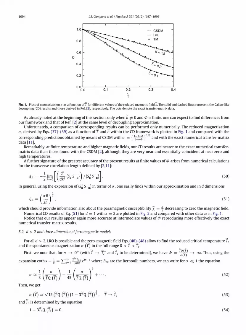
Fig. 1. Plots of magnetization σ as a function ofT for different values of the reduced magnetic fieldh. The solid and dashed lines represent the Callen-likedecoupling (CD) results and those derived in Ref. [2], respectively. The dots denote the exact transfer-matrix data.

As already noted at the beginning of this section, only whenh = 0 andΦ is finite, one can expect to find differences fromour framework and that of Ref. [2] at the same level of decoupling approximation.

Unfortunately, a comparison of corresponding results can be performed only numerically. The reduced magnetizationσ , derived by Eqs. (37)–(39) as a function ofT andh within the CD framework is plotted in Fig. 1 and compared with thecorresponding predictions obtained by means of CSDMwith σ =

1−3σΦ1−σΦ

1/2and with the exact numerical transfer-matrix

data [11].Remarkably, at finite temperature and higher magnetic fields, our CD results are nearer to the exact numerical transfer-

matrix data than those found with the CSDM [2], although they are very near and essentially coincident at near zero andhigh temperatures.

A further signature of the greatest accuracy of the present results at finite values ofΦ arises from numerical calculationsfor the transverse correlation length defined by [2,11]:

ξ⊥ = −12limk→0

[d2

dk2S+

k S−

−k/S+

k S−

−k]. (50)

In general, using the expression ofS+

k S−

−kin terms of σ , one easily finds within our approximation and in d dimensions

ξ⊥ =

σR

zh 1

2

, (51)

which should provide information also about the paramagnetic susceptibilityχ =σh decreasing to zero the magnetic field.

Numerical CD results of Eq. (51) for d = 1 with z = 2 are plotted in Fig. 2 and compared with other data as in Fig. 1.Notice that our results appear again more accurate at intermediate values of Φ reproducing more effectively the exact

numerical transfer-matrix results.

5.2. d > 2 and three-dimensional ferromagnetic models

For all d > 2, LRO is possible and the zero-magnetic field Eqs. (46)–(48) allow to find the reduced critical temperatureTcand the spontaneous magnetization σ

T in the full range 0 <T <Tc .First, we note that, for σ → 0+ (withT → T−

c andTc to be determined), we have Φ =TQ(T)σ(T) → ∞. Thus, using the

expansion coth x −1x =

∑∞

n=122nB2n(2n)! x2n−1 where B2n are the Bernoulli numbers, we can write for σ ≪ 1 the equation

σ ≃13

σTQ T

−

145

σTQ T

3

+ · · · . (52)

Then, we get

σT ≃

√15TQ T 1 − 3TQ T 1

2 , T →Tc (53)

andTc is determined by the equation

1 − 3TcQ Tc = 0. (54)


Fig. 2. Plot of the transverse correlation length ξ⊥ as a function of reduced temperatureT for different values of the reduced magnetic fieldh. The solidand dashed lines stand for the present CD-predictions and the CSDM ones of Ref. [2], respectively. The dots denote the exact transfer-matrix data.

Table 1Numerical values of the reduced critical temperatureTc of the three-dimensional classical Heisenbergmodelfor different lattice structures. HTS stands for the exact high-temperature-series results.Tc MFA CD TD CSDM HTS

sc (z = 6) 0.333 0.245 0.220 0.245 0.241bcc (z = 8) 0.333 0.262 0.239 0.262 0.257fcc (z = 12) 0.333 0.269 0.248 0.269 0.265

So, from Eq. (53), we have

σT ≃

53

1 +Tc Q ′

TcQTc

Tc −TTc1/2

, (55)

which defines the mean-field approximation (MFA) critical exponent β =12 .

The explicit expression ofTc for d > 2 can be immediately determined form Eqs. (48) and (54) providing

Tc =1

3Fd (−1)

1 +

λ

3

Fd (−1)Fd (−1)

. (56)

In particular, we get

T (TD)c =1

3Fd (−1), (57)

T (CD)c =T (TD)c

1 +

13

Fd (−1)Fd (−1)

>T (TD)c , (58)

similarly to the Callen result for the quantum Heisenberg model [9].The numerical values ofTc for the three-dimensional Heisenberg ferromagnet, as obtained bymeans of differentmethods,

are reported in Table 1 for simple cubic (sc) – body centered cubic (bcc) – and face centered cubic (fcc) spin lattices.Notice that our CD-results, as the identical CSDM ones, are very close to the exact HTS results of Ref. [12].As concerning the spontaneous magnetization σ

T as a solution of the self-consistent Eq. (47), one expects that the CDresults will differ from the CSDM [2] ones in a temperature range sufficiently far from the asymptotic regimes near zero(Φ ≫ 1) and critical (Φ ≪ 1) temperatures.

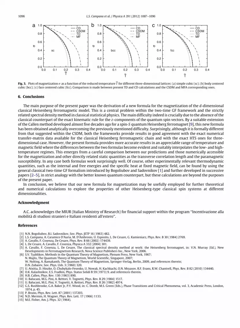
Eq. (47) can be solved only numerically for any temperature in the interval 0 <T <Tc . The data for σ T of the (d = 3)-classical Heisenberg ferromagnet for different lattice structures are plotted in Fig. 3 and compared with the CSDM and MFAresults.

It is worth emphasizing again that, as expected, differences between our results and the CSDM ones occur for finitetemperatures in the range 0.05 .T . 0.25.


Fig. 3. Plots ofmagnetization σ as a function of the reduced temperatureT for different three-dimensional lattices: (a) simple cubic (sc); (b) body centeredcubic (bcc); (c) face centered cubic (fcc). Comparison is made between present TD and CD calculations and the CSDM and MFA corresponding ones.

6. Conclusions

The main purpose of the present paper was the derivation of a new formula for the magnetization of the d-dimensionalclassical Heisenberg ferromagnetic model. This is a central problem within the two-time GF framework and the strictlyrelated spectral densitymethod in classical statistical physics. Themain difficulty indeed is crucially due to the absence of theclassical counterpart of the exact kinematic rule for the z-components of the quantum spin vectors. By a suitable extensionof the Callenmethod developed almost five decades ago for a spin-S quantumHeisenberg ferromagnet [9], this new formulahas been obtained analytically overcoming the previouslymentioned difficulty. Surprisingly, although it is formally differentfrom that suggested within the CSDM, both the frameworks provide results in good agreement with the exact numericaltransfer-matrix data available for the classical Heisenberg ferromagnetic chain and with the exact HTS ones for three-dimensional case. However, the present formula provides more accurate results in an appreciable range of temperature andmagnetic fieldwhere the differences between the two formulas become evident and suitably interpolates the low- and high-temperature regimes. This emerges from a careful comparison between our predictions and those numerically accessiblefor the magnetization and other directly related static quantities as the transverse correlation length and the paramagneticsusceptibility. In any case both formulas work surprisingly well. Of course, other experimentally relevant thermodynamicquantities, such as the internal and free energies and the specific heat at fixed magnetic field, can be found by using thegeneral classical two-time GF formalism introduced by Bogoliubov and Sadovnikov [1] and further developed in successivepapers [2–5], in strict analogy with the better known quantum counterpart, but these calculations are beyond the purposesof the present paper.

In conclusion, we believe that our new formula for magnetization may be usefully employed for further theoreticaland numerical calculations to explore the properties of other Heisenberg-type classical spin systems at differentdimensionalities.

Acknowledgment

A.C. acknowledges the MIUR (Italian Ministry of Research) for financial support within the program ‘‘Incentivazione allamobilità di studiosi stranieri e Italiani residenti all’estero’’.

References

[1] N.N. Bogoliubov, B.I. Sadovnikov, Sov. Phys. JETP 16 (1963) 482.[2] L.S. Campana, A. Caramico D’Auria, M. D’Ambrosio, U. Esposito, L. De Cesare, G. Kamieniarz, Phys. Rev. B 30 (1984) 2769.[3] A. Cavallo, F. Cosenza, De Cesare, Phys. Rev. B 66 (2002) 174439.[4] L. De Cesare, A. Cavallo, F. Cosenza, Physica A 332 (2004) 301.[5] A. Cavallo, F. Cosenza, L. De Cesare, The classical spectral density method at work: the Heisenberg ferromagnet, in: V.N. Murray (Ed.), New

Developments in Ferromagnetism Research, Nova Science Publishers Inc., New York, 2006.[6] S.V. Tyablikov, Methods in the Quantum Theory of Magnetism, Plenum Press, New York, 1967;

N. Majlis, The Quantum Theory of Magnetism, World Scientific, Singapore, 2007;W. Nolting, A. Ramakanth, The Quantum Theory of Magnetism, Springer-Verlag, Berlin, 2009, and references therein;D.N. Zubarev, Sov. Phys. Usb. 3 (1960) 320.

[7] U. Atxitia, D. Hinzke, O. Chubykalo-Fesenko, U. Nowak, H. Kachkachi, O.N. Mryasov, R.F. Evans, R.W. Chantrell, Phys. Rev. B 82 (2010) 134440.[8] O.K. Kalashnikov, E.S. Fradkin, Phys. Status Solidi B 59 (1973) 9. and references therein.[9] H.B. Callen, Phys. Rev. 130 (1963) 890.

[10] U. Balucani, M.G. Pini, A. Rettori, V. Tognetti, Phys. Rev. B 29 (1984) 1517.[11] U. Balucani, M.G. Pini, V. Tognetti, A. Rettori, Phys. Rev. B 26 (1982) 4974.[12] G.S. Rushbrooke, G.A. Baker Jr, P.Y. Wood, in: C. Domb, M.S. Green (Eds.), Phase Transitions and Critical Phenomena, vol. 3, Academic Press, London,

1974, p. 45.[13] P. Bruno, Phys. Rev. Lett. 87 (2001) 137203.[14] N.D. Mermin, H. Wagner, Phys. Rev. Lett. 17 (1966) 1133.[15] M.E. Fisher, Am. J. Phys. 32 (1964).

Documents

Callen-like method for the classical Heisenberg ferromagnet