Calorie Deprivation and Poverty Nutrition Trap in Rural India1

PRELIMINARY DRAFT: PLEASE DO NOT QUOTE OR CITE

Calorie Deprivation and Poverty Nutrition Trap in Rural India1

Raghbendra Jha, Raghav Gaiha, Anurag Sharma, Australian National University of Delhi Monash University University

April 2006

ABSTRACT

This paper tests for the existence of a Poverty Nutrition Trap (PNT) in the case of the nutrient most likely to have productivity impacts, i.e., calories, for three categories of wages – sowing, harvesting, and other – and for male and female workers separately. We use household level national data for rural India for the period January to June 1994. We use robust sample selection procedures due to Tobit methods and due to Heckman to arrive at consistent estimates. It is discovered that the PNT exists for women workers engaged in harvesting and sowing in the case of the Heckman methodology. In the case of the Tobit analysis a PNT exists in the case of female harvest, male other, and female other categories of wages.

All correspondence to:

Prof. Raghbendra Jha, ASARC, Division of Economics, Research School of Pacific and Asian Studies, Australian National University, Canberra ACT 0200, Australia Phone: + 61 2 6125 2683 Fax: +61 2 6125 0443 Email: [email protected]

ASARC Working Paper 2006/02

mailto:[email protected]


The effect of nutritional intake on labour productivity and wage rates has been an

important area for research for economists and nutritionists for some time. This

found initial expression in the form of the efficiency wage hypothesis developed by

Leibenstein (1957) and Mazumdar (1959) and formalized and extended by Mirrlees

(1975), Dasgupta and Ray (1986, 1987), and Dasgupta (1993), among others. Early

surveys include Bliss and Stern (1978a, 1978b) and Binswanger and Rosenzweig

(1984). The efficiency wage hypothesis postulated that in developing countries,

particularly at low levels of nutrition, workers are physically incapable of doing hard

manual labour. Hence their productivity is low which then implies that they get low

wages, have low purchasing power and, therefore, low levels of nutrition, completing

a vicious cycle of deprivation. These workers are unable to save very much so their

assets –both physical and human – are minimal. This reduces their chances of

escaping the poverty-nutrition trap (henceforth PNT).2 Barrett and Swallow (2006)

present a theoretical argument in support of the PNT emerging as the result of the

existence of multiple dynamic equilibria.3

There is a substantial literature on empirically testing for the existence of PNT.4

Strauss (1986) models the effect of nutrition on farm productivity. He tests and

quantifies the effects of nutritional status as measured by annual calorie intake on

annual farm production and, hence, labour productivity using farm household level

data from Sierra Leone. He finds significant and sizable effect of calorie intake on

farm output, even after accounting for endogeneity. These effects are stronger at

lower levels of calorie intake with this being determined through the presence of non-

linear terms. Thomas and Strauss (1997) investigate the impact of four indicators of

2


health (height, body mass index, per capita calorie intake and per capita protein

intake) on wages of urban workers in urban Brazil. They discover that even after

accounting for endogeneity issues and controlling for education and other dimensions

of health, these four indicators have significant positive effects on wages. The effect

of the nutritional variables - per capita calorie intake and per capita protein intake –

was higher at low levels of nutrition, again determined through non-linear terms. In

contrast Deolalikar (1988) finds in a (panel fixed effects) joint regression of the wage

equation and farm production in rural South India that calorie intake does not affect

either but a measure of weight-for-height does. He concludes that calorie intake does

not affect wages or productivity indicating that the human body can adapt to short-run

shortfalls in calorie intake. However, the fact that weight-for-height affects wages and

productivity indicates that chronic undernutrition is an important determinant of

productivity and wages. Barrett et al. (2006) provide empirical support for the

dynamic multiple equilibrium analysis of PNT (along the lines of Barrett and Swallow

2006) in the case of Kenya and Madagascar.

The contribution of the present paper is as follows. We test for the existence of a PNT

in the case of the nutrient most likely to have productivity impacts, i.e., calories,5 for

each category of wages – sowing, harvesting, and other – and for male and female

workers separately. We use robust sample selection procedures to arrive at consistent

estimates. It is discovered that the PNT exists in a number of cases.

The plan of this paper is as follows. We first motivate the analysis of PNT and then

discuss the data and present the estimation methodology. Finally we discuss the

results of the estimation and offer some concluding remarks.

3


Nutrition Poverty Traps

In Figure 1, a stylised version of the relationship between work capacity and nutrition

is given.6 The vertical axis represents a measure of work capacity and the horizontal

axis income. Note first that work capacity is a measure of the tasks that an individual

can perform during a period, say, the number of bushels of wheat that he can harvest

during a day. Income is used synonymously with nutrition in the sense that all income

is converted into nutrition. Nothing of importance changes if 70 or 80 per cent of

income share is spent on nutrition.

The shape of the capacity curve requires an explanation. It is assumed here

that much of the nutrition goes into maintaining the body’s resting metabolism. This

refers to the energy required to maintain body temperature, sustain heart and

respiratory action, and to support the ionic gradients across cell membranes. For the

“reference man” of the Food and Agriculture organisation (FAO)- a European male

weighing 65 kg-the requirement is 1700 calories per day. Of course the requirement

varies with the individual and the environment in which he lives. In the case of India

Gopalan et al. (1971) indicate that for men doing sedentary, moderate and heavy work

the calorie requirements per day are, respectively 2400, 2800 and 3900. A higher

body mass raises resting metabolism. Another significant component is energy

required to carry out physical labour. The FAO’s estimate, applied to their reference

man, prescribed lower calorific requirements. It is of course arguable that for the poor

in developing countries this may be an underestimate. Once resting metabolism is

taken care of, however, there is a marked increase in work capacity, as the bulk of the

energy input goes into work. This phase is followed by a phase of diminishing returns,

as the body’s frame restricts conversion of nutrition into work capacity.

4


Figure 1 here

Assume that working in a labour market generates income, and that piece rates

are paid. A piece rate, then, appears as a relationship between the number of tasks

performed and the total income of a person. Using these assumptions, a supply curve

of labour could be constructed that shows different quantities of labour supplied at

different piece rates. Aggregation across individuals yields an aggregate supply

curve, as shown in Figure 2.

Figure 2 here

At a piece rate of v3 there is a gap in labour supply and a discontinuous jump.

Introducing a downward sloping demand curve, an interesting case is that in which

the demand curve passes through the dotted supply curve. If the piece rate is larger

than v*, there is excess supply, which lowers this rate. On the other hand, if the piece

rate is lower than v*, there is excess demand, so that wages rise. Note, however, that a

piece rate of v* is an equilibrium wage, provided we allow for unemployment.

Figure 3 here

Having some people work and restricting labour market access to others could

fill the gap in labour supply. Those rationed out will be relatively undernourished.

This completes the vicious cycle of poverty. Lack of labour market opportunities

results in low wages and consequently low work capacity; a low work capacity feeds

back by lowering access to labour markets. It is easy to show that higher non-labour

assets (e.g. land) lead to higher wage incomes. Thus the poor without assets are

doubly disadvantaged: not only do they not enjoy non-labour income but also have

restricted access to labour market opportunities.

5


Note that nutritional status depends on both current consumption of nutrients

(e.g. calories) and the history of that consumption. In the analysis that follows, we

focus on the effects of differences in calorie intake.7

The essence of an empirical test for the PNT Hypothesis8 is the specification

of a wage equation conditional on energy intake and control variables as:

),,,,,( 4321 Xppppcaloriefw hh =

where wh and ‘calorie’ represents the wage and calorie intake of the hth individual.

pi is the probability of being occupied in the ith occupation with i =1 indicating

employment in agriculture, i=2 employment in non-agriculture, i=3 self employment

and i = 4 other employment. This set of variables controls for labour market

participation. ‘X’ represents control variables such as prices of various food products,

income of the household from the non-agricultural sector, some household

characteristics as well as some regional dummies. The probabilities are taken as the

control variables to incorporate the impact of labour market participation on wage

rate. It is thus argued that the wage rate of the worker depends on his nutrition proxied

by his energy intake, which in turn depends on his wages. Hence the wage rate and

nutritional intake are both endogenous in this model.

Data and Methodology

The data used in this paper comes from the National Council for Applied Economic

Research (NCAER). This data were collected through a multi-purpose household

survey spread over six months, from January to June 1994. The data were collected

using varied reference periods based on some conventional rules. The wage data used

are that for harvesting, sowing and other occupations for male and female workers

separately.

6


Any empirical strategy to estimate the PNT must deal with the mutual endogeneity of

wage and nutrition. In the literature two standard approaches to doing this have been

followed. The first predicts the probabilities of labour market participation from a

Maximum Likelihood Multinomial Logistic Regression (multi-logit) model

(discussed next) and then uses these in as determinants of the wage in an

appropriately specified Tobit model of the PNT. The second method uses the well-

known Heckman self selection procedure.

Tobit Methodology The predicted probabilities of participating in the labour market are calculated from a

regression equation that models labour market participation and used subsequently in

sample selection methods discussed next. In the Tobit analysis the number of hours

worked by an Agricultural labourer (AL) is a censored variable. The data is observed

only for the individuals who actually work and not for the individuals who are willing

to work but are unable to find employment.9 The efficiency wage hypothesis argues

that, starting from a low base, the higher the nutritional intake of an individual the

higher the probability that he/she would be employed, ceteris paribus. Given the low

nutritional attainment of individuals in the sample it is no surprise that there are many

households with unemployed individuals.

Hence there exist many zeroes in a random sample of wages of rural individuals. Our

motivation for the analysis is to investigate the linkages of nutrition and wage rate for

the whole sample rather than the sample comprising individuals who are employed.

The conventional regression methods fail to account for the qualitative difference

between limit (zero) observations and non-limit (continuous) observations.

7


Tobin (1958) suggested an estimation method suitable for the censored data. The

regression model is referred as the censored regression model or the Tobit model

discussed next.

The dependent variable is denoted by Y*, not Y. This is because the dependent

variable is latent, and not observed. In theory, we do not observe wages below zero.

Y* can be perceived as the desire to work. There is a threshold which one has to

reach before one can start working. What we observe is Y, which is the amount an

individual earned while working.

The Tobit model is generally represented in the following way. First, we postulate a

latent variable, Y*, which depends on some independent variables and a disturbance

term that is normally distributed with a mean of zero. But, we have a censoring at

point C, which in our case, is zero. Thus we have an observed Y that equals Y* if the

value of Y* is greater than 0, but equals 0 if the value of the unobserved Y* is less

than or equal to 0. The observed model, therefore, has a dependent variable Y, with

some independent variables and coefficients, and an error term. Because of the

censoring, however, the lower tail of the distribution of Yi, and of ui, is cut off and the

probabilities are piled up at the cut-off point. The implication is that the mean of Yi is

different from that of Yi*, and the mean of ui (the error term in the model with the

observed variable) is different from the mean of u*i (the error term in the model with

the latent variable; which is zero).

)1(*'* auXY iii += β

We have censoring at C =0:

8


)1(** bCYifYY iii >=

)1(* cCYifCY ii ≤=

So the observed model is

.,00' otherwiseYandYifuXY iiiii =>+= β

The procedure to estimate the above model has to take account of the censoring. We

note that the entire sample consists of two different sets of observations. The first set

contains the observations for which the value of Y is zero. For these observations we

know only the values of the X variables and the fact that Y* is less than or equal to 0.

The second set consists of all observations for which the values of both X and Y* are

known and the latter is positive. The likelihood function of the Tobit model consists

of each of these two parts.

[ ])2log(21 2

0πσ∑

>

−=iY

L - ))'((21

1

2

∑=

−n

i

ii XYσβ ∑

=⎥⎦

⎤⎢⎣

⎡⎟⎠⎞

⎜⎝⎛Φ−+

0

'1logiY

iXσ

β (2)

where the first two terms constitute the first part of the likelihood function and the

third is the second part.

9


The Tobit model has some notable limitations (Greene 2003, Smith and Brame 2003).

The first limitation is that in the Tobit model the same set of variables and coefficients

determine both the probability that an observation will be censored and the value of

the dependent variable. Second, the Tobit analysis is not based on a full theoretical

explanation of why the observations that are censored are censored. These limitations

can be remedied by replacing the Tobit model with a sample selection model.

Sample selection models address these shortcomings by modifying the likelihood

function. First, a different set of variables and coefficients determine the probability

of censoring and the value of the dependent variable given that it is observed. These

variables may overlap, to a point, or may be completely different. Second, sample

selection models allow for greater theoretical development because the observations

are said to be censored by some other variable, which we call Z. This allows us to

take account of the censoring process, as we will see, because selection and outcome

are not independent. A popular empirical strategy to pursue this is the Heckman

procedure which we now discuss.

The Heckman Procedure

The problem of sample selection arises when the data in the survey is incidentally

truncated or non-randomly selected. Our model determining wage nutrition

relationship contains following main regression equation:

)3(' iii XY εβ +=

where Yi is the wage rate and Xi is a vector comprising the nutrition and other

household characteristics. The model may imply a wage rate for all the individuals but

10


we observe it only for those who are actually employed. Hence the model is truncated

as the sample is selected on the basis of wages (in the agricultural sector).

Formally, the wages are observed only if:

iii uWZ += '* γ (4)

where Wi are independent variables that contribute to the employment probability of

an individual. Wi may or may not overlap with the Xi. In our case it does.

Equation (4) is called the selection equation. The sample rule thus becomes that Yi*

(the wage rate) is observed only when Zi*> 0 (or the person under consideration is

employed in agricultural sector). We now discuss the estimation issues related to the

observations in our sample (based on the above rule).

A simple OLS regression of the observed data produces inconsistent estimates

of β essentially because of omitted variables. Moreover, the disturbance term is

heteroscedastic so that the estimates will be inefficient.

Marginal Effects

The marginal effect of the regressors on Yi has two components: direct effect on mean

of Yi, which is β, and the indirect effect through the regressor which is present in Xi.

The problem of sample selection can lead the marginal effects to be overstated for the

observed category (for which Zi* > 0) and understated for the other category. For

example, suppose that nutrition affects both the probability of working in agricultural

sector and wage rate in either sectors (agricultural sector or non-agricultural sector). If

we assume that the wages of the agricultural labourers (AL) is higher than that of

otherwise identical non agricultural labourers (NAL), the marginal effects of nutrition

has two parts: one due to its influence in increasing the probability of the individuals

entering agricultural sector and the other due to its influence on wage rate within the

group. Hence the coefficient on nutrition in the regression overstates the marginal

11


effect of the nutrition of AL and understates it for the NAL. In the opposite case it

would understate the marginal effect.

Heckman suggested a two step procedure for estimating the above model. The model

is first reformulated to a probit form. It should be noted that although the variable Zi*

is not observed, one can infer its sign (for example whether an individual works in

agricultural sector or not) but not the magnitude. Thus the model can be reformulated

as follows:

Selection Mechanism and Regression Model:

.00*'* otherwiseandZifuWZ iiii >+= γ Whence we can write the regression model

as:

],,1,0,0[var~),(,1' ρσεεβ εnormaliatebiuZifonlyobservedXY iiiiii =+=

The parameters of the sample selection model can be estimated using Heckman’s two

step estimation procedure discussed next.

Heckman’s two step procedure

Heckman’s two step estimation procedure (Heckman 1976, 1979) involves the

following steps:

• Step 1: Estimate the probit equation by maximum likelihood to obtain estimates of γ.

For each model in selected sample compute the inverse Mills ratio

)(

)(

i

ii

w

w∧

∧∧

Φ=

γ

γφλ and )( iiii w∧∧∧∧

+= γλλδ

where Φandφ are, respectively, the probability density function and the cumulative

density function of a standard normal distribution.

12


• Step 2: Estimate β and ελ ρσβ =

by least squares regression of Yi on Xi and . ∧

λ

This methodology allows consistent estimates of the individual parameters. In this

paper we present Heckman estimates for the wages for which we have a PNT.

Results

We discover the existence of a Poverty Nutrition trap in two cases – female harvesting

and female sowing using the Heckman methodology. With the Tobit methodology we

found the PNT to hold in the case of Female Harvest, Male other, and Female other

categories of wages.

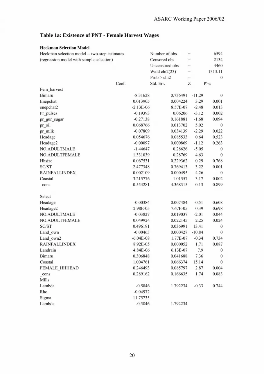
Results for the existence of PNT for the Heckman model10 are shown in Table 1.

Table 1 here.

In Table 2 we report on the nutritional requirement to break out of the PNT. From the

regression equation we compute the nutritional requirement to break the PNT. Thus if

we use the Heckman method for female harvest wage we discover that the minimum

daily calorie requirement is 3264.08. From the data the minimum annual per capita

expenditure that can attain this is Rs. 3011. This is much higher than the per capita

poverty line for that year which was Rs 2484 per year. As a percentage of the poverty

line this gap11 is over 21 percent.12

Table 2 here.

Conclusions

The possibility that when workers are acutely under-nourished they may not be able

to exert sufficient effort so that their wages remain low which then leads to further

13


poor nutritional outcomes has been known in the literature for almost fifty years now.

A number of authors have tried to empirically test for this existence of this trap but

none has been able to establish unambiguously that this holds for a subset of the

working population and not the whole. Further, the extant literature also has not been

able to establish the existence of PNT by occupation.

This paper has attempted to quantify and formally test for the presence of PNT in

rural India. It outlines a methodology that can identify the impact of energy

consumption, protein and micronutrients on wage rates, even in the presence of

mutual endogeneity.

This paper has an important policy implication in that it argues that if a minimum

wage has to be set in agriculture it must be adequate to ensure that workers are not

caught in the poverty-nutrition trap. The PNT is shown to exist for women using both

Tobit and Heckman procedures whereas it exists for men only in the case of Tobit

regression. These results then suggest a persistent gender bias in calorie

undernutrition against women workers in rural India’s labour markets. This is a matter

of urgent policy concern.

14


References

Barrett, C. and B. Swallow (2006) “Fractal Poverty Traps” World Development,

Vol. 34, no.1, pp. 1-15.

Barrett, C., Marenya, P. ,McPeak, J., Minten, B., Murithi, F., Oluoch-Kosura, W.,

Place, F., Randrianarisoa, J., Rasambainarivo, J. and J. Wangila (2006)

“Welfare Dynamics in Rural Kenya and Madagascar” Journal of Development

Studies, vol.42, no.2, pp.248-277.

Behrman J. and A. Deolalikar (1987) “Will Developing Country Nutrition

Improve with Income? A Case Study of Rural South India” Journal of

Political Economy, vol.95, no.1, pp.108-138.

Binswanger, J. and M. Rosenzweig (1984) “Contractual Arrangements,

Employment and Wages in Rural Labour Markets: A Critical review”

in Binswanger, J. and M. Rosenzweig (eds.) Contractual Arrangements,

employment and Wages in Rural Labour Markets in Asia, New Haven, Conn.:

Yale University Press.

Bliss, C. and N. Stern (1978a) “Productivity, Wages and Nutrition: Part I: The

Theory” Journal of Development Economics, vol.5, no.2, pp. 331-362.

Bliss, C. and N. Stern (1978b) “Productivity, Wages and Nutrition: Part II: Some

Observations” Journal of Development Economics, vol.5, no.2, pp. 363-398.

Dasgupta, P. and D. Ray (1986) “Inequality as a determinant of Malnutrition and

Unemployment: Theory” Economic Journal, vol.96, no.4, pp. 1011-1034.

Dasgupta, P. and D. Ray (1987) “Inequality as a determinant of Malnutrition and

Unemployment: Policy” Economic Journal, vol.97, no. 1, pp. 177-188.

Dasgupta, P. (1993) An Inquiry into well-being and Destitution, Oxford: Oxford

University Press.

Deolalikar, A. (1988) “Nutrition and Labour Productivity in Agriculture:

Estimates for rural South India” Review of Economics and Statistics, vol.70,

No.3, pp. 406-413.

Greene, W. (2003) Econometric Analysis, 5th Edition, Upper Saddle River, NJ:

Prentice Hall

Heckman, J. (1976) “The Common Structure of Statistical Models of Truncation,

Sample Selection, and Limited Dependent Variables and a Simple Estimator

for Such Models” Annals of Economic and Social Measurement, vol. 5,

no. 3, pp. 475-492.

Heckman, J. (1979) “Sample Selection Bias as a Specification Error” Econometrica,

Vol. 47, no.1, pp. 153-161.

15


Leibenstein, H. (1957) Economic Backwardness and Economic Growth: Studies

In the Theory of Economic Development, New York: Wiley and Sons.

Lipton, M. (2001) Successes in Anti-Poverty, ILO Geneva, Discussion Paper 8.

Lybbert, T., Barrett, C., Desta, S. and D. Coppock (2004) “ Stochastic Wealth

Dynamics and Risk Management among a Poor Population” Economic

Journal, vol.114, no.3, pp. 750-777.

Mazumdar, D. (1959) “The Marginal Productivity Theory of Wages and

Unemployment” Review of Economic Studies, vol.26, no.3, pp.190-197.

Mirrlees, J. (1975) “A Pure Theory of Underdeveloped Economies” in L. Reynolds

(ed.) Agriculture in Development Theory, New Haven: Yale University Press,

pp. 84-108.

Smith, D. and R. Brame (2003) “Tobit Models in Social Science Research: Some

Limitations and a More General Alternative” Sociological Methods and

Research, vol. 31, no.3, pp. 364-388.

Srinivasan, T. (1994) “Destitution: A Discourse” Journal of Economic Literature:

Vol. 32, no.4, pp. 1842-1855.

Strauss, J. and D. Thomas (1998) “Health, Nutrition and Economic Development”

Journal of Economic Literature, vol.36, no.3, pp.766-817.

Strauss, J. (1986) “Does Better Nutrition raise Farm Productivity?” Journal

Of Political Economy, vol. 94, no.2, pp.297-320.

Subramanian, S. and A. Deaton (1996) “The Demand for Food and Calories”

Journal of Political Economy, vol. 104, no.1, pp.133-162.

Thomas, D. and J. Strauss (1997) “Health and Wages: Evidence on men and

women in urban Brazil” Journal of Econometrics, vol. 77, no.1, pp.159-185.

Tobin, J. (1958) “Estimation of Relationships for Limited Dependent Variables”

Econometrica, vol. 26, no.1, pp. 24-36.

16


Figure 1: The Capacity Curve

Work Capacity

Income

17


Figure 2: Individual and Aggregate Labour Supply

Piece Rates Piece Rates

v1

v2

v3

v4 Individual Labour supply Aggregate Labour Supply

18


Figure 3: “Equilibrium” in the Labour Market Piece Rates Demand Supply v* Labour Supply and Demand Source: Ray (1998).

19


Table 1a: Existence of PNT - Female Harvest Wages

Heckman Selection Model Heckman selection model -- two-step estimates Number of obs = 6594(regression model with sample selection) Censored obs = 2134 Uncensored obs = 4460 Wald chi2(23) = 1313.11 Prob > chi2 = 0 Coef. Std. Err. Z P>z Fem_harvest Bimaru -8.31628 0.736491 -11.29 0Enepchat 0.013905 0.004224 3.29 0.001enepchat2 -2.13E-06 8.57E-07 -2.48 0.013Pr_pulses -0.19393 0.06206 -3.12 0.002pr_gur_sugar -0.27138 0.161881 -1.68 0.094pr_oil 0.068766 0.013702 5.02 0pr_milk -0.07809 0.034139 -2.29 0.022Headage 0.054676 0.085533 0.64 0.523Headage2 -0.00097 0.000869 -1.12 0.263NO.ADULTMALE -1.44647 0.28626 -5.05 0NO.ADULTFEMALE 1.331039 0.28769 4.63 0Hhsize 0.067531 0.229362 0.29 0.768SC/ST 2.477348 0.769413 3.22 0.001RAINFALLINDEX 0.002109 0.000495 4.26 0Coastal 3.215776 1.01557 3.17 0.002_cons 0.554281 4.368315 0.13 0.899 Select Headage -0.00384 0.007484 -0.51 0.608Headage2 2.98E-05 7.67E-05 0.39 0.698NO.ADULTMALE -0.03827 0.019037 -2.01 0.044NO.ADULTFEMALE 0.049924 0.022145 2.25 0.024SC/ST 0.496191 0.036991 13.41 0Land_own -0.00463 0.000427 -10.84 0Land_own2 -6.04E-08 1.77E-07 -0.34 0.734RAINFALLINDEX 8.92E-05 0.000052 1.71 0.087Landrain 4.84E-06 6.13E-07 7.9 0Bimaru 0.306848 0.041688 7.36 0Coastal 1.004761 0.066374 15.14 0FEMALE_HHHEAD 0.246493 0.085797 2.87 0.004_cons 0.289162 0.166635 1.74 0.083Mills Lambda -0.5846 1.792234 -0.33 0.744Rho -0.04972 Sigma 11.75735 Lambda -0.5846 1.792234

20


Table 1b: Existing of PNT - Female Sowing wages

Heckman selection model -- two-step estimates Number of obs = 6594 (regression model with sample selection) Censored obs = 2134 Uncensored obs = 4460 Wald chi2(23) = 1175.47 Prob > chi2 = 0 Coef. Std. Err. z P>z fem_sowing Bimaru -5.88153 0.627624 -9.37 0 Enepchat 0.017007 0.003599 4.73 0 enepchat2 -3.39E-06 7.30E-07 -4.65 0 pr_pulses -0.0691 0.05287 -1.31 0.191 pr_gur_sugar 0.103302 0.137909 0.75 0.454 pr_oil -0.08489 0.011671 -7.27 0 pr_milk -0.07162 0.029082 -2.46 0.014 Headage 0.180339 0.072909 2.47 0.013 headage2 -0.00209 0.000741 -2.82 0.005 NO.ADULTMALE -0.73618 0.243956 -3.02 0.003 NO.ADULTFEMALE 0.912363 0.245196 3.72 0 Hhsize -0.53584 0.195397 -2.74 0.006 SC/ST 4.987092 0.655711 7.61 0 RAINFALLINDEX -0.00227 0.000422 -5.38 0 Coastal 3.226689 0.8655 3.73 0 _cons -7.22458 3.722152 -1.94 0.052 Select Headage -0.00384 0.007484 -0.51 0.608 headage2 2.98E-05 7.67E-05 0.39 0.698 NO.ADULTMALE -0.03827 0.019037 -2.01 0.044 NO.ADULTFEMALE 0.049924 0.022145 2.25 0.024 SC/ST 0.496191 0.036991 13.41 0 Land_own -0.00463 0.000427 -10.84 0 Land_own2 -6.04E-08 1.77E-07 -0.34 0.734 RAINFALLINDEX 8.92E-05 0.000052 1.71 0.087 Landrain 4.84E-06 6.13E-07 7.9 0 Bimaru 0.306848 0.041688 7.36 0 Coastal 1.004761 0.066374 15.14 0 FEMALE_HHHEAD 0.246493 0.085797 2.87 0.004 _cons 0.289162 0.166635 1.74 0.083 Mills Lambda 0.867331 1.527327 0.57 0.57 Rho 0.08649 Sigma 10.02806 Lambda 0.867331 1.527327

21


Table 2: Nutritional Requirement to break Poverty Nutrition Trap

Nutritional Category Requirement to

Break PNT Minimum Equivalent Per Capita

Expenditure per year Calories (Calories/day)

HFH 3,264.08 3011

HFS 2,508.41 981.44

22


Appendix Table 1: Variables Used in the Analysis

Household Level Variables

Variable Name Variable Description headage Age of Household Head headage2 Square of Age of Household Head NO.ADULTMALE no. of adult males in HH NO.ADULTFEMALE no. of adult females in HH hhgrp HH Group Dummy Variable 1 if SC/ST HH and 0 Otherwise HINDU, MUSLIM, CHRISTIAN, SIKH, BUDDHIST, TRIBAL, JAIN, OTHERS

Religion dummies.

FEMALE_HHHEAD Whether head of household is female. HIGHESTFEMEDUPRIMARY Highest level of education for any adult female in household is primary HIGHESTFEMEDUMIDDLE Highest level of education for any adult female in household is middle HIGHESTFEMEDUMATRIC Highest level of education for any adult female in household is matric land_own Land Owned in Acres land_own2 Square of Land Owned

Other Variables RAINFALLINDEX Rainfall Index (actual - normal rain fall) for 76 agroclimatic zones in India.

bimaru Dummy for Bimaru states (Bihar, Madhya Pradesh, Rajasthan, Uttar Pradesh)

coastal Dummy for Coastal districts landrain Landowned*rainfall pr_pulses Price of Pulses pr_gur_sugar Price of Gur Sugar pr_oil Price of Oil pr_milk Price of Milk

Generated Variables Enepchat Predicted value of calorie consumption per capita Enepchat2 Predicted value of square of calorie consumption per capita

23


Endnotes 1 The UK Department for International Development (DFID) supports policies, programmes and

projects to promote international development. DFID provided funds for this study as part of that

objective but the views and opinions expressed are those of the authors alone. The authors would like

to thank DFID for supporting this research. Thanks are also due to participants of a workshop on

Poverty Nutrition Traps held in New Delhi in November 2005 and C.J. Bliss, J. Behrman, A.

Deolalikar, J. Ryan, P. Scandizzo, and P. Bardhan for helpful discussions.

2 In this paper we use the terms efficiency wage hypothesis and PNT interchangeably. 3 For an analysis of how idiosyncratic and covariate shocks can lead to entrapment in a PNT in a

dynamic framework see Lybbert et al. (2004).

4 For a comprehensive review see Strauss and Thomas (1998) and Lipton (2001).

5 Calorie deprivation is more likely to have an impact on nutrition than other forms of deprivation. An

aggregate of deprivation across various nutrients is essentially arbitrary and does not indicate which the

most pressing deprivation is.

6 The following exposition is based on Ray (1998).

7 For critiques of PNT hypothesis, see Srinivasan (1994), and Subramanian and Deaton (1996).

8 Since we have cross section data at our disposal we cannot pursue the analysis of PNT as dynamic

multiple equilibria as in Barrett and Swallow (2006).

9 Appendix Table 1 provides details of the variables used in the analysis.

10 Because of space considerations we only report results from the Heckman procedure. Results from

the estimated Tobit models are available from the corresponding author.

11 It should be noted that the calorie requirements in Table 2 could overstate the calorie requirements to

break out of the PNT because these workers would not be performing the demanding tasks of

harvesting or sowing throughout the year. However, since these workers are classified according to

their primary functions, the extent of such overestimation may be limited. Furthermore, this view

should be viewed with some scepticism since we do not have accurate estimates of the calorific

requirements of the household and related work that these workers perform.

12 The equivalent magnitudes of calories (per capita expenditure per year) for Tobit Female Harvest,

Tobit Male Other, Tobit Female Other categories of wages are, respectively 3,340.15 calories (Rs.

3142 per year), 3,037.86 (Rs. 2068 per year), and 3,212.47 (Rs. 1630.25).

24

Documents

Calorie Deprivation and Poverty Nutrition Trap in Rural India1