remote sensing

Article

Canopy Height Estimation from Single Multispectral2D Airborne Imagery Using Texture Analysis andMachine Learning in Structurally RichTemperate Forests

Christos Boutsoukis 1 , Ioannis Manakos 2,* , Marco Heurich 3 andAnastasios Delopoulos 1

1 Multimedia Understanding Group, Electrical and Computer Engineering Department, Aristotle Universityof Thessaloniki, 54124 Thessaloniki, Greece; chrimpou@ece.auth.gr (C.B.); adelo@eng.auth.gr (A.D.)

2 Information Technologies Institute, Centre for Research and Technology Hellas (CERTH), Charilaou-ThermiRd. 6th km, 57001 Thessaloniki, Greece

3 Department of Nature Protection and Research, Bavarian Forest National Park, Freyunger Str. 2,94481 Grafenau, Germany; marco.heurich@npv-bw.bayern.de

* Correspondence: imanakos@iti.gr; Tel.: +30-2311-257760

Received: 14 October 2019; Accepted: 28 November 2019; Published: 1 December 2019�����������������

Abstract: Canopy height is a fundamental biophysical and structural parameter, crucial forbiodiversity monitoring, forest inventory and management, and a number of ecological andenvironmental studies and applications. It is a determinant for linking the classification of land coverto habitat categories towards building one-to-one relationships. Light detection and ranging (LiDAR)or 3D Stereoscopy are the commonly used and most accurate remote sensing approaches to measurecanopy height. However, both require significant time and budget resources. This study proposes acost-effective methodology for canopy height approximation using texture analysis on a single 2Dimage. An object-oriented approach is followed using land cover (LC) map as segmentation vectorlayer to delineate landscape objects. Global texture feature descriptors are calculated for each landcover object and used as variables in a number of classifiers, including single and ensemble trees, andsupport vector machines. The aim of the analysis is the discrimination among classes in a wide rangeof height values used for habitat mapping (from less than 5 cm to 40 m). For that task, different spatialresolutions are tested, representing a range from airborne to spaceborne quality ones, as well as theircombinations, forming a multiresolution training set. Multiple dataset alternatives are formed basedon the missing data handling, outlier removal, and data normalization techniques. The approachwas applied using orthomosaics from DMC II airborne images, and evaluated against a referenceLiDAR-derived canopy height model (CHM). Results reached overall object-based accuracies of67% with the percentage of total area correctly classified exceeding 88%. Sentinel-2 simulation andmultiresolution analysis (MRA) experiments achieved even higher accuracies of up to 85% and91%, respectively, at reduced computational cost, showing potential in terms of transferability of theframework to large spatial scales.

Keywords: airborne image; Sentinel-2; texture features analysis; local binary patterns (LBP);multiresolution analysis (MRA); vegetation height

1. Introduction

In recent years, there has been an increasing interest in habitat mapping as a basis to monitorecosystem status and to assess the human impact on land cover. Canopy height is a basic

Remote Sens. 2019, 11, 2853; doi:10.3390/rs11232853 www.mdpi.com/journal/remotesensing

Remote Sens. 2019, 11, 2853 2 of 30

variable to characterize forests’ structure and is known to correlate with important biophysicalparameters, such as primary productivity [1] and forest health. It is important for a number ofapplications, such as biodiversity [2] and habitat monitoring and assessment, above-ground biomassestimation [3,4], environmental protection (flora-fauna), terrain characterization, fire or flood modeling,and disaster management.

Traditional methods applied for canopy height estimation rely on terrestrial measurementsthrough field campaigns for a high accuracy. Resource constraints and rapid changes in the lightof global changes, however, stress the need for satellite and airborne sensors as time-, cost-, andlabor-efficient alternative methods. Remote sensing advancements emerging at an unprecedented rateseem to be well-performing, while providing accurate information on vegetation structure. In thiscontext, numerous approaches have been proposed in the literature to estimate canopy height [5,6].

Light detection and ranging (LiDAR) data, as the most efficient alternative to groundmeasurements, are considered to provide the most accurate information on vegetation structure.LiDAR data, depending on the aerial platform, are broadly used to map canopy height of quitelarge areas, both as a single method [7–10] and in conjunction with data from other sensors (activeor passive) [11–13]. However, the cost per unit area may be relatively high. Today, airborneLiDAR systems are in operational use in many countries around the world for forest monitoringand management [14].

Synthetic aperture radar (SAR) data have proven to be effective in registering the vegetationstructure [15–17]; however, their use is still limited. As an active sensor alternative, interferometricsynthetic aperture radar (InSAR) data are used for the development of surface maps. Most studieswhich use SAR data focus on polarimetric interferometry or use the difference in wavelengthssensitivity [18]. In this context, Landsat images were combined with intensity and coherence imagesfrom ALOS PALSAR-1 to map canopy height in Chile, using ensembles of regression trees, with in situdata and airborne LiDAR as ground truth [18]. Root mean square errors of ≈ 2 m are achieved fortrees up to 30 m, whereas accuracy drops to ≈ 4 m if higher trees up to 40 m are present. In fact, theheight mapping for high trees is mainly supported by the optical Landsat imagery.

In digital photogrammetry, both nadir aerial and satellite-SAR stereo images [19,20] have beenextensively involved for years in the derivation of digital surface models (DSMs). In particular, densepixel-based image matching algorithms are applied to two or more passive images of the same areafor the generation of DSMs. When aerial or satellite stereo images are employed, canopy height iscalculated either by the subtraction of a LiDAR-derived digital terrain model (DTM) from the DSM [21]or by averaging the values of the highest DSM percentiles [22]. Similarly, SAR-based DSMs andexisting DTMs can be combined to predict canopy height (SRTM; [23]). These methods provide lessexpensive height estimations in comparison with the application of LiDAR data [24–26].

As an alternative to the aforementioned data, efforts are being undertaken by researchers to exploithigh spatial resolution remotely sensed earth observation data stemming from passive multispectralairborne or satellite sensors. These focus on the estimation of canopy height using regressionanalysis, which is based on (i) various statistical measures of reflectivity [27], (ii) spectral indices, e.g.,normalized difference vegetation index—NDVI, leaf area index—LAI [28,29], normalized differenceeater index—NDWI or optimized soil adjusted vegetation index—OSAVI [30], or (iii) simple texturefeatures including mean, standard deviation, variance, sill variance, and ratios of these metrics [31,32].

Utilization of texture features has proven particularly effective to derive information aboutthe physical structure and the edges of a canopy [33,34]. Some of the commonly utilized texturefeatures are (i) the texture statistics (Haralick features) [35] retrieved by the gray level co-occurrencematrix (GLCM) [36,37], (ii) the Markov random fields [38], and (iii) the wavelet transforms [39].In Kayitakire, et al. [40], GLCM texture features calculated from IKONOS-2 imagery have beenrelated to the height of oak, beech, and spruce trees with R2 values of up to 0.76. Moreover, globalmorphological texture descriptors (e.g., circular covariance histogram, rotation-invariant point triplets)have also been applied and evaluated for the segmentation of natural landscapes, forest mapping,

Remote Sens. 2019, 11, 2853 3 of 30

species discrimination, and content-based image retrieval [41], achieving better retrieval scores thanGabor filters, local binary patterns (LBPs), and local invariants.

Further approaches use multiscale geographic object-based image analysis (GEOBIA) models,in conjunction with texture analysis and reflectance values within a moving window, for theapproximation of canopy height and other forest structural parameters. As a characteristic example,spectral and texture features and shadow fraction were derived from a QuickBird image for each objectin Chen et al. [42]. The results verified that object-based models may achieve more accurate estimationsof forest height in most object scales. Furthermore, texture features based on local variance, entropy,and binary patterns, calculated from a WorldView-2 imagery, have already been tested for canopyheight estimation in the Netherlands with a variety of vegetation types, ranging from deciduous andconiferous trees to shrubs and heathlands [33]. They proved particularly effective in discriminatingamong different vegetation height categories in a wide range of height values (from less than 5 cmto 40 m), reaching very high object-based overall classification accuracies of over 90%. The coarsespatial level of analysis, due to the pixel size of the classified objects (i.e., from few to thousands pixels),suggests the use of texture features for habitat monitoring applications, where spatial accuracy is not astrong prerequisite.

This study introduces a cost-effective object-based approach for canopy height estimation innon-overlapping height classes, built around the texture analysis of a very high-resolution (VHR)passive airborne sensor image. This algorithm transforms the estimation problem into a multiclassprediction one. The main objective is the prediction of the canopy height class associated to eachlandscape object according to the habitat categorization scheme of general habitat categories (GHC) [43],providing valuable contribution to habitat monitoring applications. The problem is formulated as aclassification rather than a regression task, with the extracted height classes being able to discriminateobjects with similar spectral characteristics, which are assigned to different land cover categories in thereference map. The proposed framework is using [33] as a baseline, presenting substantial changesto improve the performance of the method. These are comprised initially of testing its applicationwith varying moving window dimensions to account for the effect of the differences in crown sizein an area with highly heterogeneous forests, e.g., the Bavarian Forest National Park (BFNP), andthe application of data imputation techniques, such as missing data handling, outlier removal, anddata normalization. Simulated (spatially aggregated) Sentinel-2 images are also put to test, since theabundance and accessibility of such data increases the applicability of the examined method. However,the most promising results are expected by the utilization of varying spatial resolutions and theirhierarchical combination through multiresolution approach.

The name multiresolution analysis has been broadly used for sub-band coding (signal processing),quadrature mirror filtering (speech processing), and pyramidal coding (image processing). Pyramidalcoding refers to multiscale image representation, in which an image is subject to repeated smoothingand subsampling. Images in general have locally varying statistics of pixel intensities resulting incombinations of edges, abrupt features, and homogeneous regions. Analysis of statistical propertiesof pixel neighborhoods of varying sizes may be useful. The fact that small objects are viewed athigh spatial resolutions, while large objects require only a coarse resolution, leads us to evaluatemultiresolution analysis (MRA) in conjunction with the proposed framework. Processing cost of bothfeature extraction and classification processes can be notably reduced, while very large areas of interestand ultra-high-resolution imagery can be assessed.

2. Materials

2.1. Study Area

The study area includes the entire Bavarian Forest National Park (BFNP) (243.69 km2) located atthe German–Czech border in the state of Bavaria (49◦3′19”N, 13◦12′49”E) (Figure 1). The southernpart of the current park was designated as the first national park of Germany in 1970 and was

Remote Sens. 2019, 11, 2853 4 of 30

extended to the northwest in 1997. Together with other neighboring forests, such as the Czech SumavaNational Park, they form the Bohemian Forest Ecosystem, one of Europe’s largest protected forestecosystems. The terrain is rough and uneven, while the forest area is characterized as mountainouswith an altitude ranging between 600 and 1453 meters a.s.l. The temperate climate with its seasonalfluctuations is characterized as cold and humid, with the average annual temperature ranging from 3to 6.5 ◦C and the annual rainfall estimated at 1200 to 1850 mm. Forest areas of the highest altitudeare covered with heavy and long-lasting snow for most of the year (7 to 8 months). The entire BFNPhas been managed under a no-intervention policy by maintaining natural ecological processes, whichhas resulted in heterogeneously structured and complex stands. The identified study areas mainlyencompass three major forest communities, including sub-alpine stands dominated by Norway spruce(Picea abies L. Karst) and occasionally mountain ash (Sorbus aucuparia L.), slopes covered by a mixtureof Norway spruce, silver fir (Abies alba Mill.), European beech (Fagus sylvatica L.), and sycamore maple(Acer pseudoplatanus L.), and valley bottoms dominated by Norway spruce, mountain ash, and birches(Betula pendula Roth and Betula pubescens Ehrh.) [44].

2.2. Height Classification Scheme

In particular, six (6) studied height classes are defined (see Table 1) as the core of the multiclassprediction problem, ranging from 0 to 40 m. They are based on GHC reference habitat mappingframework, as the main characteristic to discriminate among different tree and shrubs (TRS) species.

Table 1. Height classes characteristics as defined in the general habitat category (GHC) taxonomy.

Class Name Description Range (m) Class Label

Dwarf chamaephytes (DCH) Dwarf shrubs [0, 0.05) 1

Shrubby chamaephytes (SCH) Under shrubs [0.05, 0.3) 2

Low phanerophytes (LPH) Low shrubs buds [0.3, 0.6) 3

Mid phanerophytes (MPH) Mid shrubs buds [0.6, 2) 4

Tall phanerophytes (TPH) Tall shrubs buds [2, 5) 5

Forest phanerophytes (FPH) Trees [5, 40) 6

Based on the aforementioned height classification scheme, areas of interest were selected as themost suitable representatives of the BFNP, spanning across the whole range of canopy heights. In somestudy cases, four (4) height classes were used instead of six (6), i.e., the first three classes were mergedinto one, corresponding to a height class for land objects below 0.6 m, while the other three classesremained unchanged. This procedure was followed in order to reduce the effect of the terrain at areaswith very low vegetation that incorporate noise in the study of other classes and to cover for cases withvery few land objects that belong to the first three classes, resulting in very low representativeness.This way a more reliable low and sparse vegetation reference layer was obtained.

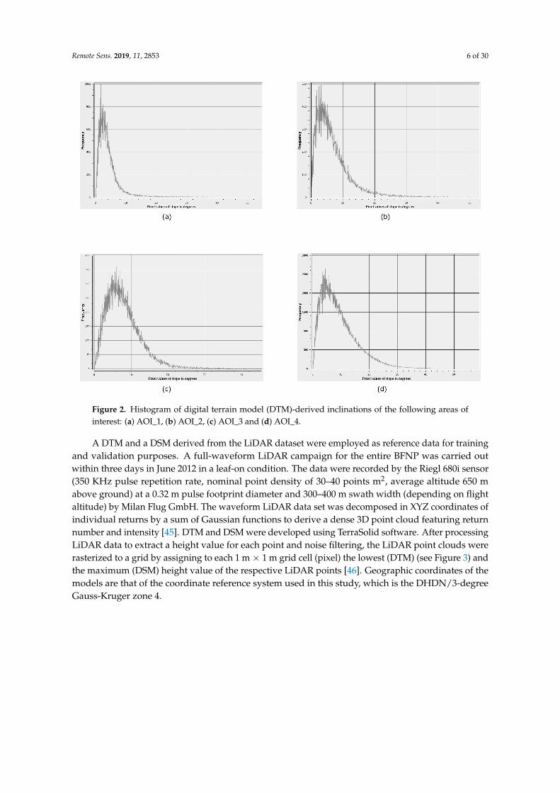
As far as the selection of the areas involved in the evaluation phases (see Appendix A) isconcerned, it is based on the following criteria: (i) existence of validation and segmentation layer,(ii) small degree of inclination to reduce topographical and shadow factor, as demonstrated inFigure 2, (iii) representativeness of height classes, and (iv) absence of land objects containing artificialconstructions, considered as out of the scope for this work.

Remote Sens. 2019, 11, 2853 5 of 30

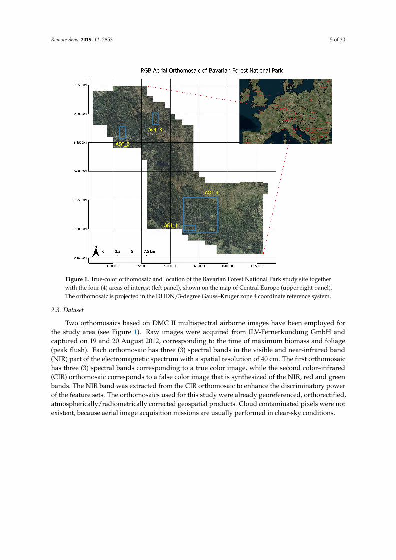
Figure 1. True-color orthomosaic and location of the Bavarian Forest National Park study site togetherwith the four (4) areas of interest (left panel), shown on the map of Central Europe (upper right panel).The orthomosaic is projected in the DHDN/3-degree Gauss–Kruger zone 4 coordinate reference system.

2.3. Dataset

Two orthomosaics based on DMC II multispectral airborne images have been employed forthe study area (see Figure 1). Raw images were acquired from ILV-Fernerkundung GmbH andcaptured on 19 and 20 August 2012, corresponding to the time of maximum biomass and foliage(peak flush). Each orthomosaic has three (3) spectral bands in the visible and near-infrared band(NIR) part of the electromagnetic spectrum with a spatial resolution of 40 cm. The first orthomosaichas three (3) spectral bands corresponding to a true color image, while the second color–infrared(CIR) orthomosaic corresponds to a false color image that is synthesized of the NIR, red and greenbands. The NIR band was extracted from the CIR orthomosaic to enhance the discriminatory powerof the feature sets. The orthomosaics used for this study were already georeferenced, orthorectified,atmospherically/radiometrically corrected geospatial products. Cloud contaminated pixels were notexistent, because aerial image acquisition missions are usually performed in clear-sky conditions.

Remote Sens. 2019, 11, 2853 6 of 30

Figure 2. Histogram of digital terrain model (DTM)-derived inclinations of the following areas ofinterest: (a) AOI_1, (b) AOI_2, (c) AOI_3 and (d) AOI_4.

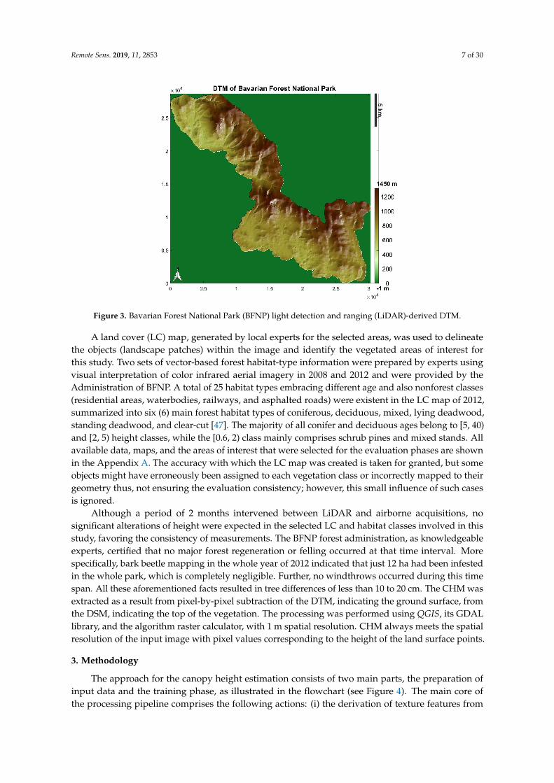
A DTM and a DSM derived from the LiDAR dataset were employed as reference data for trainingand validation purposes. A full-waveform LiDAR campaign for the entire BFNP was carried outwithin three days in June 2012 in a leaf-on condition. The data were recorded by the Riegl 680i sensor(350 KHz pulse repetition rate, nominal point density of 30–40 points m2, average altitude 650 mabove ground) at a 0.32 m pulse footprint diameter and 300–400 m swath width (depending on flightaltitude) by Milan Flug GmbH. The waveform LiDAR data set was decomposed in XYZ coordinates ofindividual returns by a sum of Gaussian functions to derive a dense 3D point cloud featuring returnnumber and intensity [45]. DTM and DSM were developed using TerraSolid software. After processingLiDAR data to extract a height value for each point and noise filtering, the LiDAR point clouds wererasterized to a grid by assigning to each 1 m × 1 m grid cell (pixel) the lowest (DTM) (see Figure 3) andthe maximum (DSM) height value of the respective LiDAR points [46]. Geographic coordinates of themodels are that of the coordinate reference system used in this study, which is the DHDN/3-degreeGauss-Kruger zone 4.

Remote Sens. 2019, 11, 2853 7 of 30

Figure 3. Bavarian Forest National Park (BFNP) light detection and ranging (LiDAR)-derived DTM.

A land cover (LC) map, generated by local experts for the selected areas, was used to delineatethe objects (landscape patches) within the image and identify the vegetated areas of interest forthis study. Two sets of vector-based forest habitat-type information were prepared by experts usingvisual interpretation of color infrared aerial imagery in 2008 and 2012 and were provided by theAdministration of BFNP. A total of 25 habitat types embracing different age and also nonforest classes(residential areas, waterbodies, railways, and asphalted roads) were existent in the LC map of 2012,summarized into six (6) main forest habitat types of coniferous, deciduous, mixed, lying deadwood,standing deadwood, and clear-cut [47]. The majority of all conifer and deciduous ages belong to [5, 40)and [2, 5) height classes, while the [0.6, 2) class mainly comprises schrub pines and mixed stands. Allavailable data, maps, and the areas of interest that were selected for the evaluation phases are shownin the Appendix A. The accuracy with which the LC map was created is taken for granted, but someobjects might have erroneously been assigned to each vegetation class or incorrectly mapped to theirgeometry thus, not ensuring the evaluation consistency; however, this small influence of such casesis ignored.

Although a period of 2 months intervened between LiDAR and airborne acquisitions, nosignificant alterations of height were expected in the selected LC and habitat classes involved in thisstudy, favoring the consistency of measurements. The BFNP forest administration, as knowledgeableexperts, certified that no major forest regeneration or felling occurred at that time interval. Morespecifically, bark beetle mapping in the whole year of 2012 indicated that just 12 ha had been infestedin the whole park, which is completely negligible. Further, no windthrows occurred during this timespan. All these aforementioned facts resulted in tree differences of less than 10 to 20 cm. The CHM wasextracted as a result from pixel-by-pixel subtraction of the DTM, indicating the ground surface, fromthe DSM, indicating the top of the vegetation. The processing was performed using QGIS, its GDALlibrary, and the algorithm raster calculator, with 1 m spatial resolution. CHM always meets the spatialresolution of the input image with pixel values corresponding to the height of the land surface points.

3. Methodology

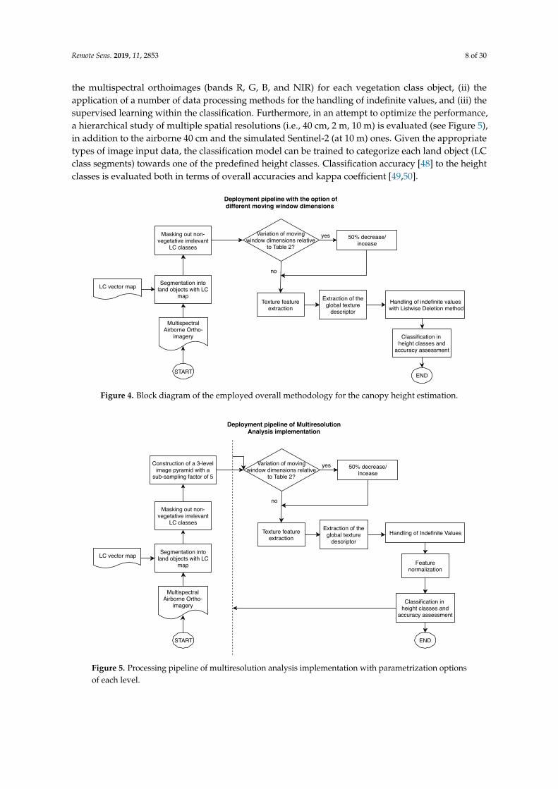
The approach for the canopy height estimation consists of two main parts, the preparation ofinput data and the training phase, as illustrated in the flowchart (see Figure 4). The main core ofthe processing pipeline comprises the following actions: (i) the derivation of texture features from

Remote Sens. 2019, 11, 2853 8 of 30

the multispectral orthoimages (bands R, G, B, and NIR) for each vegetation class object, (ii) theapplication of a number of data processing methods for the handling of indefinite values, and (iii) thesupervised learning within the classification. Furthermore, in an attempt to optimize the performance,a hierarchical study of multiple spatial resolutions (i.e., 40 cm, 2 m, 10 m) is evaluated (see Figure 5),in addition to the airborne 40 cm and the simulated Sentinel-2 (at 10 m) ones. Given the appropriatetypes of image input data, the classification model can be trained to categorize each land object (LCclass segments) towards one of the predefined height classes. Classification accuracy [48] to the heightclasses is evaluated both in terms of overall accuracies and kappa coefficient [49,50].

LC vector map

MultispectralAirborne Ortho-

imagery

Segmentation intoland objects with LC

map

Masking out non-vegetative irrelevant

LC classes

Texture featureextraction

Deployment pipeline with the option ofdifferent moving window dimensions 

Variation of movingwindow dimensions relative

to Table 2?50% decrease/

incease

no

yes

START

Extraction of theglobal texture

descriptor

Classification in height classes and

accuracy assessment

END

Handling of indefinite values with Listwise Deletion method

Figure 4. Block diagram of the employed overall methodology for the canopy height estimation.

Classification in height classes and

accuracy assessment

END

Construction of a 3-levelimage pyramid with a

sub-sampling factor of 5

Deployment pipeline of MultiresolutionAnalysis implementation

LC vector map

MultispectralAirborne Ortho-

imagery

Segmentation intoland objects with LC

map

Masking out non-vegetative irrelevant

LC classes

START

Texture featureextraction

Variation of movingwindow dimensions relative

to Table 2?50% decrease/

incease

no

yes

Extraction of theglobal texture

descriptorHandling of Indefinite Values

Featurenormalization

Figure 5. Processing pipeline of multiresolution analysis implementation with parametrization optionsof each level.

Remote Sens. 2019, 11, 2853 9 of 30

3.1. Texture Feature Extraction

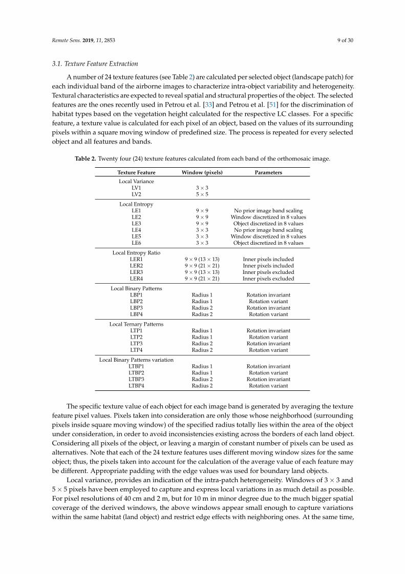
A number of 24 texture features (see Table 2) are calculated per selected object (landscape patch) foreach individual band of the airborne images to characterize intra-object variability and heterogeneity.Textural characteristics are expected to reveal spatial and structural properties of the object. The selectedfeatures are the ones recently used in Petrou et al. [33] and Petrou et al. [51] for the discrimination ofhabitat types based on the vegetation height calculated for the respective LC classes. For a specificfeature, a texture value is calculated for each pixel of an object, based on the values of its surroundingpixels within a square moving window of predefined size. The process is repeated for every selectedobject and all features and bands.

Table 2. Twenty four (24) texture features calculated from each band of the orthomosaic image.

Texture Feature Window (pixels) Parameters

Local VarianceLV1 3× 3LV2 5× 5

Local EntropyLE1 9× 9 No prior image band scalingLE2 9× 9 Window discretized in 8 valuesLE3 9× 9 Object discretized in 8 valuesLE4 3× 3 No prior image band scalingLE5 3× 3 Window discretized in 8 valuesLE6 3× 3 Object discretized in 8 values

Local Entropy RatioLER1 9× 9 (13× 13) Inner pixels includedLER2 9× 9 (21× 21) Inner pixels includedLER3 9× 9 (13× 13) Inner pixels excludedLER4 9× 9 (21× 21) Inner pixels excluded

Local Binary PatternsLBP1 Radius 1 Rotation invariantLBP2 Radius 1 Rotation variantLBP3 Radius 2 Rotation invariantLBP4 Radius 2 Rotation variant

Local Ternary PatternsLTP1 Radius 1 Rotation invariantLTP2 Radius 1 Rotation variantLTP3 Radius 2 Rotation invariantLTP4 Radius 2 Rotation variant

Local Binary Patterns variationLTBP1 Radius 1 Rotation invariantLTBP2 Radius 1 Rotation variantLTBP3 Radius 2 Rotation invariantLTBP4 Radius 2 Rotation variant

The specific texture value of each object for each image band is generated by averaging the texturefeature pixel values. Pixels taken into consideration are only those whose neighborhood (surroundingpixels inside square moving window) of the specified radius totally lies within the area of the objectunder consideration, in order to avoid inconsistencies existing across the borders of each land object.Considering all pixels of the object, or leaving a margin of constant number of pixels can be used asalternatives. Note that each of the 24 texture features uses different moving window sizes for the sameobject; thus, the pixels taken into account for the calculation of the average value of each feature maybe different. Appropriate padding with the edge values was used for boundary land objects.

Local variance, provides an indication of the intra-patch heterogeneity. Windows of 3× 3 and5× 5 pixels have been employed to capture and express local variations in as much detail as possible.For pixel resolutions of 40 cm and 2 m, but for 10 m in minor degree due to the much bigger spatialcoverage of the derived windows, the above windows appear small enough to capture variationswithin the same habitat (land object) and restrict edge effects with neighboring ones. At the same time,

Remote Sens. 2019, 11, 2853 10 of 30

they are large enough to avoid expressing variability within the same plant (e.g., conifer tree). As faras feature computational complexity is concerned, for each central pixel surrounded by a window ofn× n pixels, the only possible loop might involve the n2 operations required to calculate the differencebetween each pixel and the mean pixel value in the window. Thus, the complexity of O(n2) canbe considered.

Local entropy (LE) is a measure of variability, heterogeneity, and the overall information containedin an image. In particular, it offers an indication of texture randomness in the studied area. Similar tolocal variance, LE is calculated on a per pixel basis. For the calculation of the LE, initial pixel valuesranging in [0,255] were used. Due to potential sensor noise, insignificant value fluctuation would beconsidered as different values and could result in an unwanted entropy outcome. Two alternativequantization techniques, also introduced in Petrou et al. [33], are employed as a countermeasure. In awindow of n× n pixels, n2 pixels are serially searched to identify the distinct values. As the distinctvalues are less than or equal to n2, a maximum of n2 iterations are required for entropy calculation.Therefore, O(n2) can be considered as the complexity of the calculation of entropy for each movingwindow in an object.

For the characterization of relative variations within a small neighborhood compared with itssurrounding one, the ratio of the entropy values (LER) of two concentric windows is extracted inthe same way as in Petrou et al. [33]. Two versions of LER calculation are tested depending on theutilization of the pixels of the inner window. As a note, the smaller the ratio, the more homogeneousthe immediate neighborhood of the central pixel is, compared to its broader surroundings.

Local binary patterns (LBP) [52] are also tested in capturing local changes in texture, computed ona per pixel basis. For each pixel, its surrounding pixels in a circle of predefined radius are consideredfor the calculation. Starting from the pixel on the left of the central one, a scanning of the surroundingpixels in a clockwise order takes place. An LBP feature variation is also calculated, namely, therotation invariant, by considering every surrounding pixel in the circle as the starting point. Therespective binary and sequentially decimal numbers are calculated with the smallest assigned nowto the central pixel. To counterbalance the LBP drawback of ambiguity, two variations of the LBPalgorithm are tested, the local ternary patterns (LTP) and the local ter-binary pattern (LTBP), with theincorporation of a third value d in labeling neighboring pixels. Considering now a moving windowof n × n pixels (n = 2r + 1, where r is the defined circle radius), less than 4n pixels (the pixels ofthe square enclosing the circle around the central pixel) are compared with the central one, for theextraction of the binary or ternary numbers. Thus, the complexity of the calculation of LBP-basedfeatures can be considered O(n).

3.2. Handling of Indefinite Values, Outlier Removal, and Data Normalization

All pixels considered for the calculation of texture features, both central and those within thedefined surrounding windows, shall belong to the specific object under consideration. As a result,the texture features’ calculation is limited to the area of each individual object, avoiding influencesand biases from neighboring land objects. If this requirement is not fulfilled for a calculated feature,in cases such as with objects consisting of very few pixels, its value remains indefinite (NaN). Thisresults in objects with NaN values in certain texture features (e.g., LER), whose calculation requiressurrounding windows larger than the dimensions of the object, or all texture features, when one of thedimensions of the object is restricted to solely a few pixels. Prior to the classification to a height class,small objects with all their texture values NaN are excluded from the process, since no informationfor the classification is available. For objects with partially missing information, where only some oftheir texture values are indefinite (NaN), three (3) distinct processing approaches, followed by outlierremoval and appropriate normalization, all firstly introduced as a pipeline in [33], are employed:

- The first approach, coded as Feat with the derived dataset Feat. dataset, refers to the exclusionof one or more features from the classification process, which have missing data to at least oneobject. By reducing the number of final features used for each object, memory requirements

Remote Sens. 2019, 11, 2853 11 of 30

and classification processing cost are reduced; however, the resulting feature vector may havesignificantly less discriminatory power compared to the entire set;

- In the second approach, known as listwise deletion, case deletion, or complete-case analysis,objects with missing data to at least one texture feature are excluded, reducing the numberof finally classified objects and affecting the representativeness of the results. Listwisedeletion, coded as Obj with the derived dataset Obj. dataset, is supported by the fact thatthe assumption that missingness is not related to the observed and missing variables, i.e.,missing-completely-at-random (MCAR) assumption [53] is not valid for the missing data;

- In the third approach, coded as MI with the derived dataset MI. dataset, a multiple imputationtechnique of the missing data with approximated values is evaluated and employed. In particular,the Amelia II method [54] is used, based on the assumption that the values are drawn from amultivariate gaussian distribution, instead of drawing values from an unconditional distribution,where the missing data are filled in by randomly selected values among the observed ones. Five(5) complete datasets, including the values of all features from every image band, are created,averaged into one set to be used in the classification process. Five imputations have been selectedas a good trade-off between efficiency and processing time, according to the formula proposed byRubin [55].

Following the imputation of indefinite values, an efficient simple box plot approach, coded asOR, for multivariate data based on Mahalanobis distance has been employed as a check mechanismfor outliers’ detection, i.e., objects, which appear to be inconsistent with the remaining objects of thesite, based on their texture features values. Objects with extreme values in a large distance from themedian value, for each texture feature, are considered outliers and removed (OR. dataset).

Considering that each texture feature outcome value belongs to a different range, appropriatenormalization of the data may prove effective to prevent texture features with larger values fromhaving a higher impact than ones with smaller values during the classification process. The linearzero-mean feature normalization method, coded as Norm with the derived dataset (Norm. dataset),has been tested as providing comparable classifications results with the scaling to the range of [0, 1],and the nonlinear softmax scaling techniques [56] in Petrou et al. [33].

3.3. Classification

Classification is performed on an object basis, using a series of machine learning algorithms witheach object of the LC map characterized by a vector of texture feature values. Texture values constitutethe classification features. As far as the “ground truth” (i.e., the target for the classifiers’ optimization)is concerned, CHM is used as the reference layer. The average canopy height is calculated per objectout of its pixels in the CHM. The calculated height is mapped to one of the six height classes, and therespective label is assigned to the object. These are used for the training of the classifiers and for theevaluation of classification results. Objects having at least one texture feature assigned to them (i.e.,not all values are indefinite) are classified to one of the six or four GHC height categories reported inSection 2.2.

Ten (10) classifiers have been applied to test the discriminatory potential of the extracted features.Decision trees and support vector machines (SVMs) [57] classifiers were employed, since they areextensively used in various remote sensing applications [58–62], producing high accuracies. Two basicdecision tree implementations, namely, an implementation of the C4.5 algorithm introduced in Quinlan,1993 [63], J48, and a reduced-error pruning implementation [57], REPTree, were used as individualclassifiers. Aiming to reduce the generalization error and improve the classification performance ofthe individual classifiers, random forests [64], bagging [65], and AdaBoost.M1 [66] were employed asensemble methods, with J48 and REPTree used as base classifiers. Furthermore, three SVM classifierswith linear and rbf kernel, with and without fitting logistic models to the output [67,68], and usingsequential minimal optimization (SMO) have also been tested; for the classifiers’ implementations, aWEKA environment was used.

Remote Sens. 2019, 11, 2853 12 of 30

The REPTree algorithm with a fast reduced-error pruning approach has a computationalcomplexity of O(mn log n), where n is the number of land objects and m the number of features.However, J48 implementation uses more complex pruning (subtree raising); thus, its complexity isincreased to O(mn log n) + O(n(log n)2). The complexity of ensemble classifiers is calculated bymultiplying the complexity of the basis classifiers (J48 and REPTree) by the number of trees t produced.In the Bagging method, however, due to the increased number of constructed trees (100) producedin relation to that for the AdaBoost.M1 (20), the computation time is increased by 5 times. RandomForests is the fastest method among the ensemble decision tree techniques, with a complexity of classO(tn log n log m), since log(m) + 1 attributes are considered for the separation of each node, in contrastto m used in simple J48 and REPTree implementations. Regarding the complexity of SVM, mostly inthe case of nonlinear kernels, it is usually in the order of O(n2) to O(n3) since quadratic programming(QP) optimization is required.

Three (3) distinct experimental evaluation phases, with different versions each, have beenconducted in this study, depending on image pixel resolution, the selected areas of interest, thesize of moving window during texture feature extraction, the use of MRA analysis, and the numberof height classes. Experimental phase 1 evaluated the canopy height estimation utilizing the veryhigh resolution airborne dataset at 40 cm. Due to the relatively high computational cost of textureanalysis for each image band and consequently for each image, three areas of interest (AOI_1,2 and3) with a surface coverage of 6 km2 each were initially extracted from the BFNP. They contain themost representative samples belonging to the first three vegetation height categories. In order tofurther improve the classification accuracies, a 50% increase in moving windows’ dimensions (Phase 1’)was tested.

The scope of experimental phase 2 was to emulate Sentinel-2 images with 10 m spatial resolutionout of the airborne multispectral ortho imagery and to evaluate the ability to derive height informationfrom texture analysis. Sentinel-2 imagery is the largest source of spaceborne input data for landresources assessments today. Simulation was employed for direct comparison reasons, as Sentinelsatellites were not operational at the time of airborne data acquisition, which was 2012 for this study.For training and testing purposes, a larger area of interest (AOI_4) (see Figure A4 of Appendix A) wasselected, covering an area of 36 km2. Due to the fact that 10 m spatial resolution would lead to an Obj.dataset with a very small number of objects using the initial dimensions of moving windows, a 50%decrease of windows’ size was also examined (Phase 2’). Four height classes’ results were evaluated inorder to enhance the representativeness of observations. In this framework, only the Obj. dataset wasstudied as the one that outperformed other approaches in Phase 1.

3.4. Multiresolution Analysis

During evaluation phase 3, we examined the effectiveness and performance of the multiresolutionanalysis method in deriving the distinct GHC height categories. We proceeded with a 3-level analysisof the total area of interest 4 (AOI_4), using exclusively the Obj. dataset and the texture featuresdescribed in Table 2, keeping the computational cost low and offering a degree of freedom in theparameters’ configuration of each level. The third image input case uses an assessment of a combinedinput dataset, as follows.

Particularly, a 3-level image pyramid is constructed with a subsampling factor of 5 (see Figure A4of Appendix A). A collection of images at decreasing resolution levels is created, with top level 3having 10 m resolution, level 2 of 2 m resolution and bottom level 1 (initial image) of 40 cm. For imagedownsampling cases, the resize data tool of ENVI software is used, particularly the pixel aggregateresampling method. The main scope of this hierarchical structure of resolutions is to classify very largeobjects using low spatial resolution, whereas objects of smaller size using higher image resolution.Training and classification are carried out separately for each level. This method is described in Figure 5and by the following steps: Step 1. Start from the top of the pyramid and study one image level ata time. Step 2. Identify objects belonging to the Obj. dataset for this level. Step 3. Proceed to the

Remote Sens. 2019, 11, 2853 13 of 30

classification of the Obj. dataset to four height classes. Step 4. When on the bottom level, characterizeobjects not belonging to tje Obj. dataset (i.e., those with partially missing information in their texturefeature vector) as ‘not defined’ and calculate the total area-based classification accuracy of the system.If not, continue with Step. 5. Step 5. Proceed to the next lower level excluding the objects belongingto the Obj. dataset of the previous higher level. Continue with Step 2. For each level of analysis, allavailable classifiers are evaluated with the one achieving the highest accuracy participating in thecalculation of the total system area-based classification accuracy.

3.5. Validation

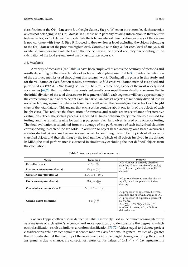
A variety of measures (see Table 3) have been employed to assess the accuracy of methods andresults depending on the characteristics of each evaluation phase used. Table 3 provides the definitionof the accuracy metrics used throughout this research work. During all the phases in this study andfor the validation of classification results, a stratified 10-fold cross-validation method is applied andperformed via WEKA 3 Data Mining Software. The stratified method, as one of the most widely usedapproaches [69,70] that provides more consistent results over repetitive evaluations, ensures that inthe initial division of the total dataset into 10 segments (folds), each segment will have approximatelythe correct sample ratio of each height class. In particular, dataset objects are randomly divided into 10non-overlapping segments, where each segment shall reflect the percentage of objects of each heightclass of the total dataset. This means that each section contains about one tenth of the objects of eachheight class. This reduces the fluctuation of estimates, and results are in accordance after iterativeevaluations. Then, the sorting process is repeated 10 times, wherein every time one-fold is used fortesting, and the remaining nine for training purposes. Each land object is used only once for testing.The final evaluation is calculated from the average of the performance of each individual classifiercorresponding to each of the ten folds. In addition to object-based accuracy, area-based accuraciesare also studied. Area-based accuracies are derived by summing the number of pixels of all correctlyclassified objects and then dividing by the total number of pixels of all objects involved in the dataset.In MRA, the total performance is extracted in similar way excluding the ‘not defined’ objects fromthe calculation.

Table 3. Accuracy evaluation measures.

Metric Definition Symbols

Overall accuracy OA ≡ NCN

NC: Number of correctly classifiedsamples; N: total number of samples;

Producer’s accuracy (for class A) PAA ≡ NCANOA

NCA: Correctly classified samples toclass A;

Omission error (for class A) EOA ≡ 1− PAA

User’s accuracy (for class A) UAA ≡ NCANPA

NOA: total observed samples of classA; NPA: total samples classified toclass A;

Commission error (for class A) ECA ≡ 1−UAA

Cohen’s kappa coefficient κ ≡ Po−Pc1−Pc

Po : proportion of agreement betweenclassified and observed samples ≡ OA;Pc: proportion of expected agreementby chance,Pc = ∑C

i=1(NOi/N)(NPi/N), C:number of classes, NOi, NPi, N asdefined above

Cohen’s kappa coefficient κ, as defined in Table 3, is widely used in the remote sensing literatureas a measure of a classifier’s accuracy, and more specifically to demonstrate the degree to whicheach classification result assimilates a random classification [71,72]. Values equal to 1 denote perfectclassifications, while values equal to 0 denote random classifications. In general, values of κ greaterthan 0.5 indicate that the majority of the assignments into the height classes, excluding the correctassignments due to chance, are correct. As reference, for values of 0.41 ≤ κ ≤ 0.6, agreement is

Remote Sens. 2019, 11, 2853 14 of 30

considered moderate, while for values 0.61 ≤ κ ≤ 0.8, agreement between observed and predictedvalues is considered substantial.

4. Results

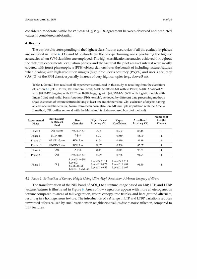
The best results corresponding to the highest classification accuracies of all the evaluation phasesare included in Table 4. Obj and MI datasets are the best-performing ones, producing the highestaccuracies when SVM classifiers are employed. The high classification accuracies achieved throughoutthe different experimental evaluation phases, and the fact that the pilot areas of interest were mostlycovered with forest phanerophyte (FPH) objects demonstrates the benefit of including texture featureswhen dealing with high-resolution images (high producer’s accuracy (PA)(%) and user’s accuracy(UA)(%) of the FPH class), especially in areas of very high canopies (e.g., above 5 m).

Table 4. Overall best results of all experiments conducted in this study as resulting from the classifiersof Section 3.3 (RT: REPTree; RF: Random Forest; A-RT: AdaBoost.M1 with REPTree; A-J48: AdaBoost.M1with J48; B-RT: bagging with REPTree; B-J48: bagging with J48; SVM-M: SVM with logistic models withlinear (.Lin) and radial basis function (.Rbf) kernels), achieved by different data processing methods(Feat: exclusion of texture features having at least one indefinite value; Obj: exclusion of objects havingat least one indefinite value; Norm: zero-mean normalization; MI: multiple imputation with the AmeliaII method; OR: outlier removal with the Mahalanobis distance-based box plot method).

ExperimentalPhase

Best Datasetor Dataset

Used

BestClassifier

Object-BasedAccuracy (%)

KappaCoefficient

Area-BasedAccuracy (%)

Number ofHeightClasses

Phase 1 Obj-Norm SVM.Lin-M 64.35 0.507 83.48 6

Phase 1 MI-Norm B-J48 67.77 0.550 88.99 4

Phase 1’ MI-OR-Norm SVM.Lin 64.58 0.490 82.49 6

Phase 1’ MI-OR-Norm SVM.Lin 69.67 0.560 83.67 4

Phase 2 Obj A-J48 91.11 0.811 96.31 4

Phase 2’ Obj SVM.Lin-M 85.29 0.738 91.94 4

Phase 3 Obj

Level 3: A-J48Level 2:SVM.Lin-MLevel 1: SVM.Lin

Level 3: 91.11Level 2: 80.73Level 1: 66.55

Level 3: 0.811Level 2: 0.684Level 1: 0.467

91.39 4

4.1. Phase 1: Estimation of Canopy Height Using Ultra-High Resolution Airborne Imagery of 40 cm

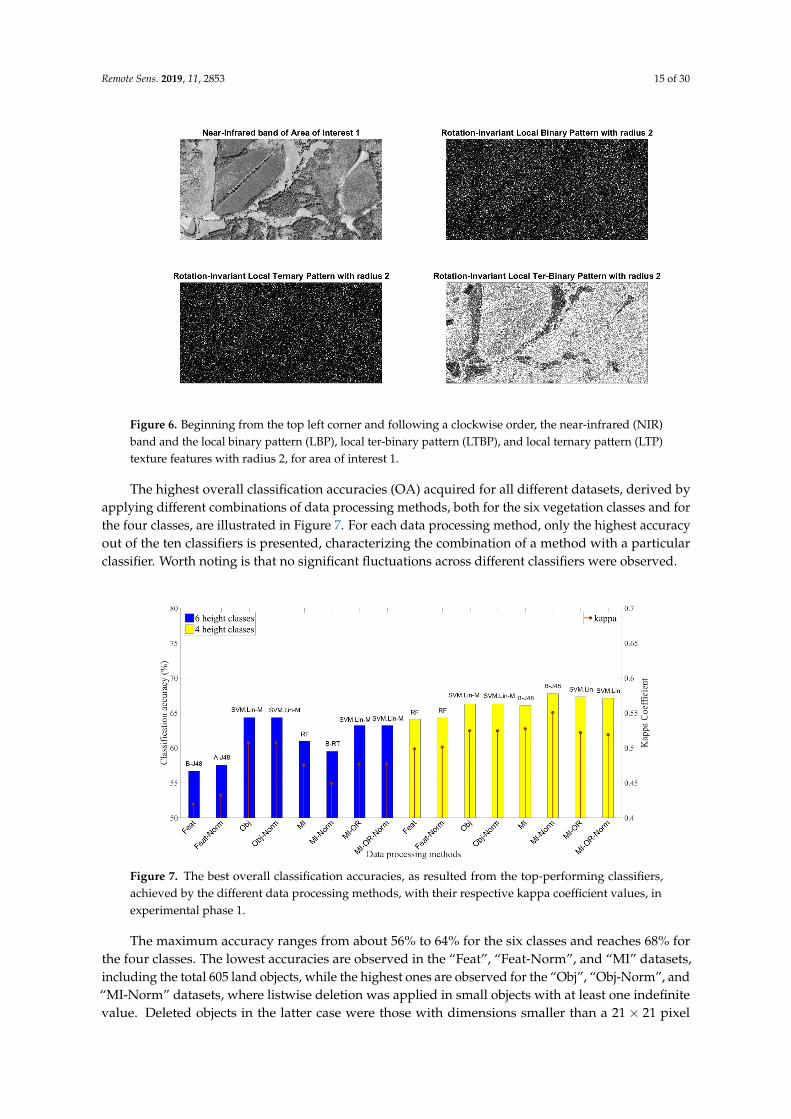
The transformation of the NIR band of AOI_1 to a texture image based on LBP, LTP, and LTBPtexture features is illustrated in Figure 6. Areas of low vegetation appear with more a heterogeneoustexture compared to areas of tall vegetation, where canopy, tree trunks, and bare ground alternate,resulting in a homogeneous texture. The introduction of a d range in LTP and LTBP variations reducesunwanted effects caused by small variations in neighboring values due to noise affliction, compared toLBP features.

Remote Sens. 2019, 11, 2853 15 of 30

Figure 6. Beginning from the top left corner and following a clockwise order, the near-infrared (NIR)band and the local binary pattern (LBP), local ter-binary pattern (LTBP), and local ternary pattern (LTP)texture features with radius 2, for area of interest 1.

The highest overall classification accuracies (OA) acquired for all different datasets, derived byapplying different combinations of data processing methods, both for the six vegetation classes and forthe four classes, are illustrated in Figure 7. For each data processing method, only the highest accuracyout of the ten classifiers is presented, characterizing the combination of a method with a particularclassifier. Worth noting is that no significant fluctuations across different classifiers were observed.

Figure 7. The best overall classification accuracies, as resulted from the top-performing classifiers,achieved by the different data processing methods, with their respective kappa coefficient values, inexperimental phase 1.

The maximum accuracy ranges from about 56% to 64% for the six classes and reaches 68% forthe four classes. The lowest accuracies are observed in the “Feat”, “Feat-Norm”, and “MI” datasets,including the total 605 land objects, while the highest ones are observed for the “Obj”, “Obj-Norm”, and“MI-Norm” datasets, where listwise deletion was applied in small objects with at least one indefinitevalue. Deleted objects in the latter case were those with dimensions smaller than a 21× 21 pixel

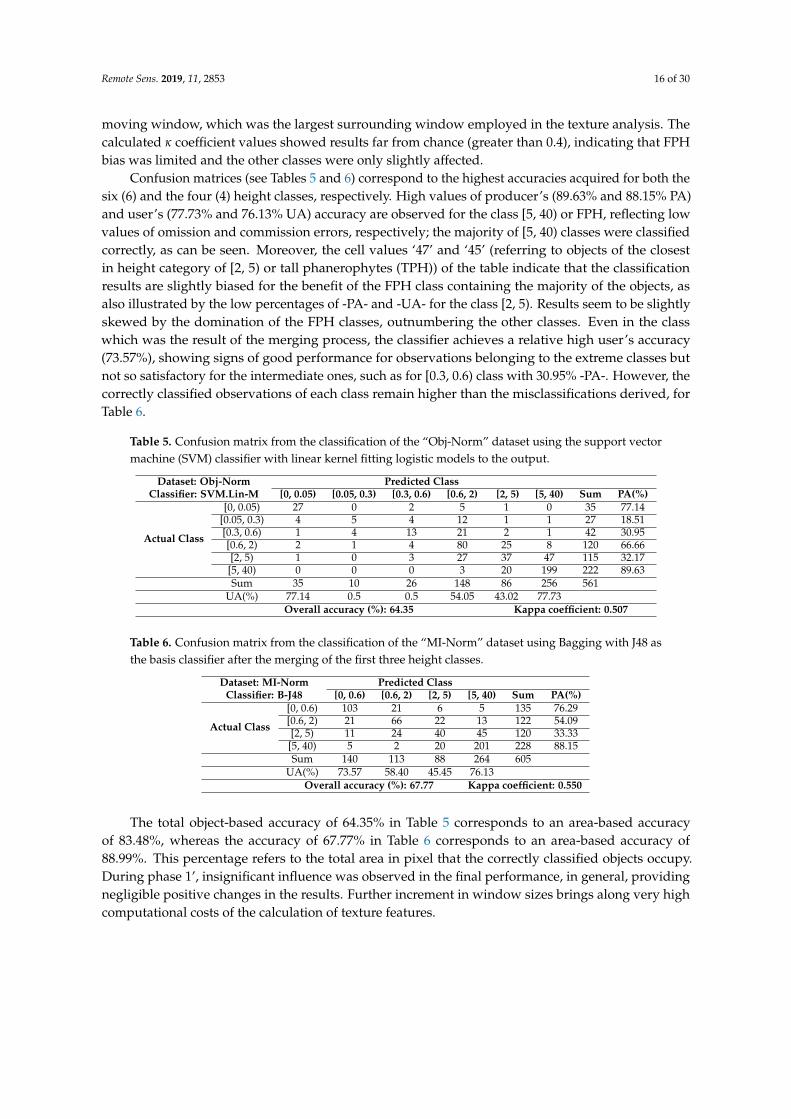
Remote Sens. 2019, 11, 2853 16 of 30

moving window, which was the largest surrounding window employed in the texture analysis. Thecalculated κ coefficient values showed results far from chance (greater than 0.4), indicating that FPHbias was limited and the other classes were only slightly affected.

Confusion matrices (see Tables 5 and 6) correspond to the highest accuracies acquired for both thesix (6) and the four (4) height classes, respectively. High values of producer’s (89.63% and 88.15% PA)and user’s (77.73% and 76.13% UA) accuracy are observed for the class [5, 40) or FPH, reflecting lowvalues of omission and commission errors, respectively; the majority of [5, 40) classes were classifiedcorrectly, as can be seen. Moreover, the cell values ‘47’ and ‘45’ (referring to objects of the closestin height category of [2, 5) or tall phanerophytes (TPH)) of the table indicate that the classificationresults are slightly biased for the benefit of the FPH class containing the majority of the objects, asalso illustrated by the low percentages of -PA- and -UA- for the class [2, 5). Results seem to be slightlyskewed by the domination of the FPH classes, outnumbering the other classes. Even in the classwhich was the result of the merging process, the classifier achieves a relative high user’s accuracy(73.57%), showing signs of good performance for observations belonging to the extreme classes butnot so satisfactory for the intermediate ones, such as for [0.3, 0.6) class with 30.95% -PA-. However, thecorrectly classified observations of each class remain higher than the misclassifications derived, forTable 6.

Table 5. Confusion matrix from the classification of the “Obj-Norm” dataset using the support vectormachine (SVM) classifier with linear kernel fitting logistic models to the output.

Dataset: Obj-Norm Predicted ClassClassifier: SVM.Lin-M [0, 0.05) [0.05, 0.3) [0.3, 0.6) [0.6, 2) [2, 5) [5, 40) Sum PA(%)

Actual Class

[0, 0.05) 27 0 2 5 1 0 35 77.14[0.05, 0.3) 4 5 4 12 1 1 27 18.51[0.3, 0.6) 1 4 13 21 2 1 42 30.95[0.6, 2) 2 1 4 80 25 8 120 66.66[2, 5) 1 0 3 27 37 47 115 32.17[5, 40) 0 0 0 3 20 199 222 89.63Sum 35 10 26 148 86 256 561

UA(%) 77.14 0.5 0.5 54.05 43.02 77.73Overall accuracy (%): 64.35 Kappa coefficient: 0.507

Table 6. Confusion matrix from the classification of the “MI-Norm” dataset using Bagging with J48 asthe basis classifier after the merging of the first three height classes.

Dataset: MI-Norm Predicted ClassClassifier: B-J48 [0, 0.6) [0.6, 2) [2, 5) [5, 40) Sum PA(%)

Actual Class

[0, 0.6) 103 21 6 5 135 76.29[0.6, 2) 21 66 22 13 122 54.09[2, 5) 11 24 40 45 120 33.33[5, 40) 5 2 20 201 228 88.15Sum 140 113 88 264 605

UA(%) 73.57 58.40 45.45 76.13Overall accuracy (%): 67.77 Kappa coefficient: 0.550

The total object-based accuracy of 64.35% in Table 5 corresponds to an area-based accuracyof 83.48%, whereas the accuracy of 67.77% in Table 6 corresponds to an area-based accuracy of88.99%. This percentage refers to the total area in pixel that the correctly classified objects occupy.During phase 1’, insignificant influence was observed in the final performance, in general, providingnegligible positive changes in the results. Further increment in window sizes brings along very highcomputational costs of the calculation of texture features.

Remote Sens. 2019, 11, 2853 17 of 30

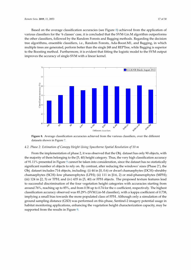
Based on the average classification accuracies (see Figure 8) achieved from the application ofvarious classifiers for the ‘6 classes’ case, it is concluded that the SVM-Lin.M algorithm outperformsthe other classifiers, followed by the Random Forests and Bagging methods. Regarding the decisiontree algorithms, ensemble classifiers, i.e., Random Forests, Ada-Boost.M1, and Bagging, in whichmultiple trees are generated, perform better than the single J48 and REPTree, while Bagging is superiorto the Boosting method. Furthermore, it is evident that fitting the logistic model to the SVM outputimproves the accuracy of single-SVM with a linear kernel.

Figure 8. Average classification accuracies achieved from the various classifiers, over the differentdatasets shown in Figure 7.

4.2. Phase 2: Estimation of Canopy Height Using Spaceborne Spatial Resolution of 10 m

From the implementation of phase 2, it was observed that the Obj. dataset has only 90 objects, withthe majority of them belonging to the [5, 40) height category. Thus, the very high classification accuracyof 91.11% presented in Figure 9 cannot be taken into consideration, since the dataset has no statisticallysignificant number of objects to rely on. By contrast, after reducing the windows’ sizes (Phase 2’), theObj. dataset includes 714 objects, including: (i) 44 in [0, 0.6) or dwarf chamaephytes (DCH)–shrubbychamaephytes (SCH)–low phanerophytes (LPH); (ii) 111 in [0.6, 2) or mid-phanerophytes (MPH);(iii) 124 in [2, 5) or TPH; and (iv) 435 in [5, 40) or FPH objects. The proposed texture features leadto successful discrimination of the four vegetation height categories with accuracies starting fromaround 76%, reaching up to 85%, and from 0.58 up to 0.74 for the κ coefficient, respectively. The highestclassification accuracy observed was 85.29% (SVM.Lin-M classifier), with a kappa coefficient of 0.738,implying a small bias towards the more populated class of FPH. Although only a simulation of theground sampling distance (GSD) was performed on this phase, Sentinel-2 imagery potential usage inhabitat monitoring applications, enhancing the vegetation height characterization capacity, may besupported from the results in Figure 9.

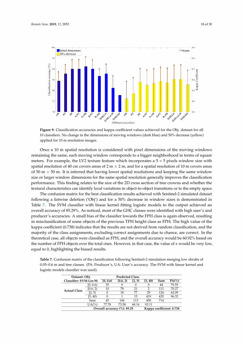
Remote Sens. 2019, 11, 2853 18 of 30

Figure 9. Classification accuracies and kappa coefficient values achieved for the Obj. dataset for all10 classifiers. No change in the dimensions of moving windows (dark blue) and 50% decrease (yellow)applied for 10 m resolution images.

Once a 10 m spatial resolution is considered with pixel dimensions of the moving windowsremaining the same, each moving window corresponds to a bigger neighborhood in terms of squaremeters. For example, the LV2 texture feature which incorporates a 5× 5 pixels window size withspatial resolution of 40 cm covers areas of 2 m × 2 m, and for a spatial resolution of 10 m covers areasof 50 m × 50 m. It is inferred that having lower spatial resolutions and keeping the same windowsize or larger window dimensions for the same spatial resolution generally improves the classificationperformance. This finding relates to the size of the 2D cross section of tree crowns and whether thetextural characteristics can identify local variations in object-to-object transitions or to the empty space.

The confusion matrix for the best classification results achieved with Sentinel-2 simulated datasetfollowing a listwise deletion (‘Obj’) and for a 50% decrease in window sizes is demonstrated inTable 7. The SVM classifier with linear kernel fitting logistic models to the output achieved anoverall accuracy of 85.29%. As noticed, most of the GHC classes were identified with high user’s andproducer’s accuracies. A small bias of the classifier towards the FPH class is again observed, resultingin misclassification of some objects of the previous TPH height class as FPH. The high value of thekappa coefficient (0.738) indicates that the results are not derived from random classification, and themajority of the class assignments, excluding correct assignments due to chance, are correct. In thetheoretical case, all objects were classified as FPH, and the overall accuracy would be 60.92% based onthe number of FPH objects over the total ones. However, in that case, the value of κ would be very low,equal to 0, highlighting the biased results.

Table 7. Confusion matrix of the classification following Sentinel-2 simulation merging low shrubs of0.05–0.6 m and tree classes. (PA: Producer’s, UA: User’s accuracy. The SVM with linear kernel andlogistic models classifier was used).

Dataset: Obj Predicted ClassClassifier: SVM.Lin-M [0, 0.6) [0.6, 2) [2, 5) [5, 40) Sum PA(%)

Actual Class

[0, 0.6) 35 9 0 0 44 79.55[0.6, 2) 10 78 21 2 111 70.27[2, 5) 0 18 77 29 124 62.09

[5, 40) 0 1 15 419 435 96.32Sum 45 106 113 450 714

UA(%) 77.78 73.58 68.14 93.11Overall accuracy (%): 85.29 Kappa coefficient: 0.738

Remote Sens. 2019, 11, 2853 19 of 30

4.3. Phase 3: Fusion of Spatial Resolutions in Hierarchical Mode—Multiresolution Analysis

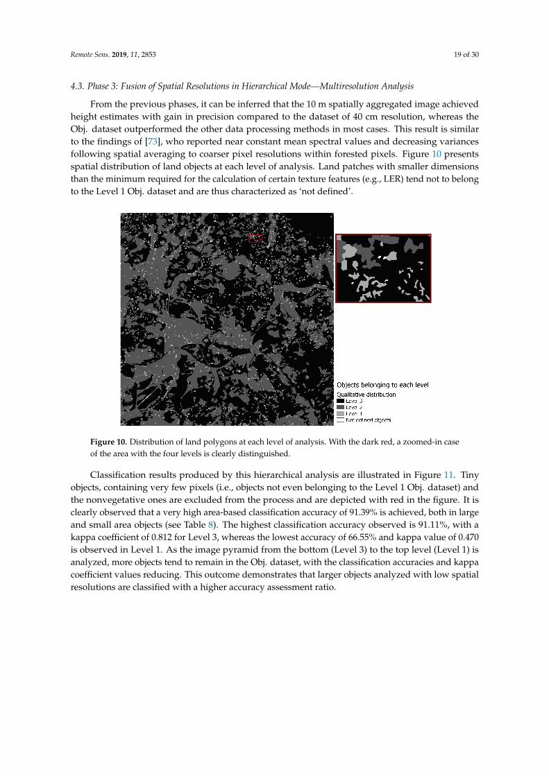
From the previous phases, it can be inferred that the 10 m spatially aggregated image achievedheight estimates with gain in precision compared to the dataset of 40 cm resolution, whereas theObj. dataset outperformed the other data processing methods in most cases. This result is similarto the findings of [73], who reported near constant mean spectral values and decreasing variancesfollowing spatial averaging to coarser pixel resolutions within forested pixels. Figure 10 presentsspatial distribution of land objects at each level of analysis. Land patches with smaller dimensionsthan the minimum required for the calculation of certain texture features (e.g., LER) tend not to belongto the Level 1 Obj. dataset and are thus characterized as ‘not defined’.

Figure 10. Distribution of land polygons at each level of analysis. With the dark red, a zoomed-in caseof the area with the four levels is clearly distinguished.

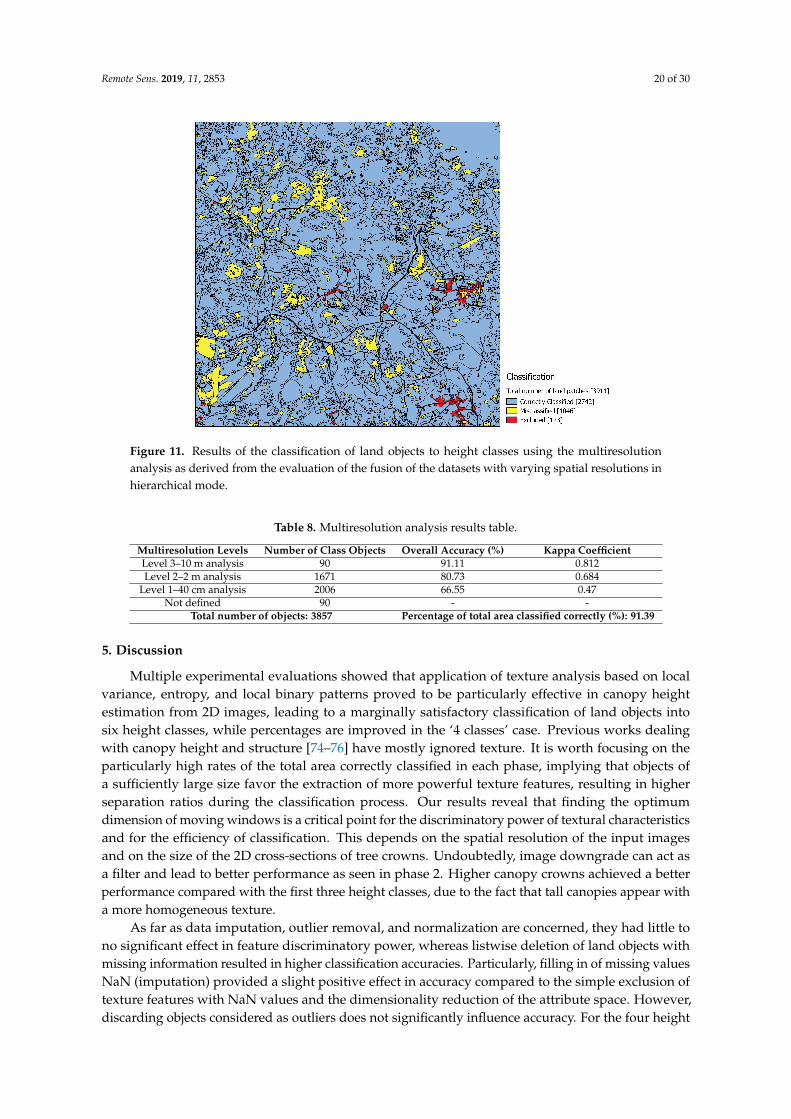
Classification results produced by this hierarchical analysis are illustrated in Figure 11. Tinyobjects, containing very few pixels (i.e., objects not even belonging to the Level 1 Obj. dataset) andthe nonvegetative ones are excluded from the process and are depicted with red in the figure. It isclearly observed that a very high area-based classification accuracy of 91.39% is achieved, both in largeand small area objects (see Table 8). The highest classification accuracy observed is 91.11%, with akappa coefficient of 0.812 for Level 3, whereas the lowest accuracy of 66.55% and kappa value of 0.470is observed in Level 1. As the image pyramid from the bottom (Level 3) to the top level (Level 1) isanalyzed, more objects tend to remain in the Obj. dataset, with the classification accuracies and kappacoefficient values reducing. This outcome demonstrates that larger objects analyzed with low spatialresolutions are classified with a higher accuracy assessment ratio.

Remote Sens. 2019, 11, 2853 20 of 30

Figure 11. Results of the classification of land objects to height classes using the multiresolutionanalysis as derived from the evaluation of the fusion of the datasets with varying spatial resolutions inhierarchical mode.

Table 8. Multiresolution analysis results table.

Multiresolution Levels Number of Class Objects Overall Accuracy (%) Kappa CoefficientLevel 3–10 m analysis 90 91.11 0.812Level 2–2 m analysis 1671 80.73 0.684

Level 1–40 cm analysis 2006 66.55 0.47Not defined 90 - -

Total number of objects: 3857 Percentage of total area classified correctly (%): 91.39

5. Discussion

Multiple experimental evaluations showed that application of texture analysis based on localvariance, entropy, and local binary patterns proved to be particularly effective in canopy heightestimation from 2D images, leading to a marginally satisfactory classification of land objects intosix height classes, while percentages are improved in the ‘4 classes’ case. Previous works dealingwith canopy height and structure [74–76] have mostly ignored texture. It is worth focusing on theparticularly high rates of the total area correctly classified in each phase, implying that objects ofa sufficiently large size favor the extraction of more powerful texture features, resulting in higherseparation ratios during the classification process. Our results reveal that finding the optimumdimension of moving windows is a critical point for the discriminatory power of textural characteristicsand for the efficiency of classification. This depends on the spatial resolution of the input imagesand on the size of the 2D cross-sections of tree crowns. Undoubtedly, image downgrade can act asa filter and lead to better performance as seen in phase 2. Higher canopy crowns achieved a betterperformance compared with the first three height classes, due to the fact that tall canopies appear witha more homogeneous texture.

As far as data imputation, outlier removal, and normalization are concerned, they had little tono significant effect in feature discriminatory power, whereas listwise deletion of land objects withmissing information resulted in higher classification accuracies. Particularly, filling in of missing valuesNaN (imputation) provided a slight positive effect in accuracy compared to the simple exclusion oftexture features with NaN values and the dimensionality reduction of the attribute space. However,discarding objects considered as outliers does not significantly influence accuracy. For the four height

Remote Sens. 2019, 11, 2853 21 of 30

classes case of phase 1, “Feat” and “Feat-Norm” datasets achieved accuracies almost similar to thoseof other datasets, while the feature space and the computational cost were reduced. Thus, it is inferredthat significantly localized variations of texture are proven crucial for canopy height characterization,instead of features that do study texture in larger neighborhoods. The observed advantage of featuresextracted with small moving windows, over features with large ones, supports the selection for perpixel calculation of values and their averaging over each object. High accuracies were achieved amongdifferent classifiers’ application, with ensemble decision trees Random Forest, Bagging with REPTree,and SVM with rbf kernel outperforming the single trees approaches. Decision tree ensemble classifiers,in particular bagging trees, have been consistently among the top-performing classifiers in both canopyheight estimation [33] and habitat classification applications [77] and can therefore be recommendedfor similar applications. Taking into account that the practical algorithmic complexity of SVM isbetween those of AdaBoost.M1 and Bagging (see Section 3.3), it is concluded that the Random Forestmethod is the best trade-off between classification accuracy and computational complexity.

To the extent of our knowledge, relatively few studies have so far assessed the estimationperformance of Sentinel-2 to map forest properties, including the growing stock volume forMediterranean forests, using regression tree ensembles [78], and canopy cover, as well as the LAI indexfor boreal and temperate forests, with generalized linear models [79] and multiple linear regressionmodels [80], respectively. Especially for canopy height estimation from Sentinel-2, only the attemptof [5] has been reported so far; a two-layer perceptron trained on a small number (<200) of fieldplots concluded that predictions from Sentinel-2 have slightly lower errors than those from Landsatfor a boreal forest. As such, the exploitation of spaceborne pixel resolution of 10 m, stemmingfrom the simulation of airborne imagery as Sentinel-2 derived, could lead to valuable insights ofSentinel-2 imagery potential for the estimation of canopy height through texture analysis. High overallclassification results of up to 85.29% object-based and 91.94% area-based demonstrate the efficacy ofthe proposed methodology, texture measures, and type of data. Hence, given a moderate amountof reference data, dense vegetation height maps with 10 m GSD can be derived at country-scale.However, further analysis should be done with real Sentinel-2 imagery in order to extract consistentand confident conclusions. Although in situ or LiDAR data provide much more accuracy in comparisonto our method, canopy height retrieval from high resolution optical satellite imagery could in somecases reduce the need for expensive LiDAR campaigns. In addition to the high spatial resolution,Sentinel-2 provides a new image up to a frequency of 5 days. In a similar context is the representativeexample of [6], where Sentinel-2 multispectral images were used to regress per-pixel vegetation heightfor Gabon and Switzerland using a deep CNN. Suitable spectral and textural features that wereapplied resulted in a mean absolute error (MAE) of 1.7 m in Switzerland and 4.3 m in Gabon, correctlyestimating heights up to 50 m.

Extensive research has demonstrated that classification based on multiresolution analysismethods resembling the human vision system shows effectiveness over traditional techniques that donot make strong use of region-based spatial information [81]. Hence, these methods are widelyused for the classification of textures and for many image analysis tasks. The most commonlyemployed multiresolution analysis techniques include the Gabor transformation [82] and the wavelettransformation [83], where the texture image is transformed to local spatial-frequency representationby wrapping the image with appropriate band-pass filters tuned to specific parameters. In this study,however, the spatial information for the MRA was derived over a range of resolutions, choosing thesubsampling simple aggregation method instead of scale-space transform or wavelet decomposition,achieving area-based classification accuracies of over 91% in total. MRA seems to provide significantinfluence in classification performance, in general, compared to other approaches studying different setof parameters and data processing methods. The 3-level fusion of spatial resolutions allows studyinglarge areas in hierarchical mode at reasonable processing times and a low computational cost, givingthe freedom to customize each level individually, e.g., spatial and spectral resolution, moving windowdimensions, and classifier selection.

Remote Sens. 2019, 11, 2853 22 of 30

Numerous actions can be taken towards a potential increase of the classification accuracies, eitherby the utilization of a wider region in the spectrum to enhance the feature analysis or the employmentof images from both the peak and decline of vegetative periods. However, the applied methodologyand the available dataset pose constraints for assessing the robustness of the method to differentspectral and vegetation conditions. Worth mentioning here is that a future merging of adjacent objectsbelonging to the same height class is not a good practice, since the target is to examine the classificationof land objects of different habitat categories. It is desirable also for the methodology to make decisionsfor small objects and moving windows, extracting the highest degree of height information from theimage. The detailed segmentation of the LC map, however, creates regions of small dimensions, whichend up being rejected from the process.

The reported classification accuracies pertain to areas of BFNP having a small degree of inclination(see Figure 2). The utility of the approach at higher inclined areas was not examined. Further researchsteps comprise: (a) the consideration of multiple areas whereupon investigation may reveal howinclination- and species-dependent features are, or how they are affected by the growing stage ofa single species; (b) the assessment of supervised (e.g., PCA, LPP, NPE, Isomap) and unsupervised(e.g., LDA) dimensionality reduction techniques or feature subset selection (e.g., correlation-basedfeature selector (CFS)) methods, aiming at reducing the processing cost of both feature extraction andclassification processes with insignificant loss in accuracy; (c) the use of multiple classifiers trainedon feature vectors of reduced size as a more natural alternative; thus, in regions where not all of thetexture features would have been calculated (but only some of them), only the trained classifier of thatspecific features would have been utilized; and (d) the use of very deep convolutional neural networks(CNNs) which are able to learn a tailored multilevel feature encoding for a given prediction task fromraw images, given a sufficient (large) amount of training data.

6. Conclusions

The majority of previous studies employing texture analysis focused on coniferous [32,84] andhardwood [32] forests, or oak, beech, and spruce trees [40] of several meters high. In the present work,a wide range of tree species were assessed, including coniferous, deciduous, dead woods lying andregenerated, ecotones, meadows, mixed stands, scrub pines, both with various height classes rangingfrom less than 5 cm to some tens of meters. In this context, there is a high likelihood that the approachcan be scaled up to global coverage.

Texture descriptors based on local variance, entropy, and local binary patterns, followed byobject-based classification, proved particularly effective in discriminating among different heightclasses related to habitat categories, useful for habitat monitoring and land use mapping applications.Resulting in classification accuracies of over 85% for the simulated Sentinel-2 image, or over 91% infusion of original 40 cm, and simulated 2 m and 10 m images (MRA), they indicate their high potentialfor canopy height estimation.

Being effective in such a complex area of BFNP supports the expectation that the methodologycan be applicable in other geographical areas, especially of similar climatic and topographic conditionsor with a similar vegetation and forest type; however, the degree of transferability is still to be furtherinvestigated. The suggested approach does not intend to replace data sources offering more accurateand dense canopy height information, such as the LiDAR-derived CHM used as reference layer, butrather to act as a cost-effective and higher-frequency-monitoring surrogate of more expensive andresource-demanding approaches.

Author Contributions: Conceptualization, A.D. and I.M.; Data Curation, M.H. and I.M.; Methodology, A.D.and I.M.; Software, C.B.; Investigation, C.B. with major contribution from I.M.; Results analysis was carried outby all authors; Writing—Original Draft Preparation, C.B.; Writing—Review and Editing, I.M., A.D., and M.H.;Supervision, A.D. and I.M.; Funding Acquisition, I.M. and M.H. All authors read, suggested improvements, andapproved the manuscript.

Remote Sens. 2019, 11, 2853 23 of 30

Funding: This research study leading to these results has been funded and supported by the EuropeanUnion’s Horizon 2020 research and innovation program under Grant Agreement No. 641762, ECOPOTENTIAL(http://www.ecopotential-project.eu/). Data has been provided by the Data Pool Initiative of the BohemianForest Ecosystem.

Acknowledgments: We gratefully acknowledge the support of Kalliroi Marini, for her initial literature reviewand involvement in draft preparation. Furthermore, authors greatly appreciate the useful explanations related tothe acquisition and creation process of LiDAR-derived digital models and true-color orthomosaics that have beengiven from Milan Flug GmbH and ILV-Fernerkundung GmbH companies, respectively. Part of the experimentshave been conducted during the internship of C.B. at AeroPhoto Co. Ltd. company; hence, credits for technicalsupport and access to computing resources shall be given.

Conflicts of Interest: The authors declare no conflict of interest. The funding sponsors had no role in the designof the study; in the collection, analyses, or interpretation of data; in the writing of the manuscript, and in thedecision to publish the results.

Abbreviations

The following abbreviations are used in this manuscript:

A-J48 AdaBoost.M1 with J48 as basis classifierA-RT AdaBoost.M1 with REPTree as basis classifierBFNP Bavarian Forest National ParkB-J48 Bagging with J48 as basis classifierB-RT Bagging with REPTree as basis classifierCHM Canopy Height ModelDCH Dwarf chamaephytes (TRS)DEM Digital Elevation ModelDSM Digital Surface ModelDTM Digital Terrain ModelFPH Forest phanerophytes (TRS)GHC General Habitat CategoriesGSD Ground Sampling DistanceJ48 J48 implementation of C4.5 tree classifierLC Land CoverLV Local VarianceLE Local EntropyLER Local Entropy RatioLPH Low phanerophytes (TRS)LTBP Local Binary Patterns with rangeLTP Local Ternary PatternsMRA Multiresolution AnalysisMPH Mid phanerophytes (TRS)OA Overall AccuracyPA Producer’s AccuracyRF Random ForestSCH Shrubby Chamaephytes (TRS)SVM Support Vector MachinesSVM-M SVM with fitting logistic models to the outputTPH Tall Phanerophytes (TRS)TRS Trees and ShrubsUA User’s AccuracyVHR Very High Resolution

Remote Sens. 2019, 11, 2853 24 of 30

Appendix A

Available Data and Maps of the Study Area.

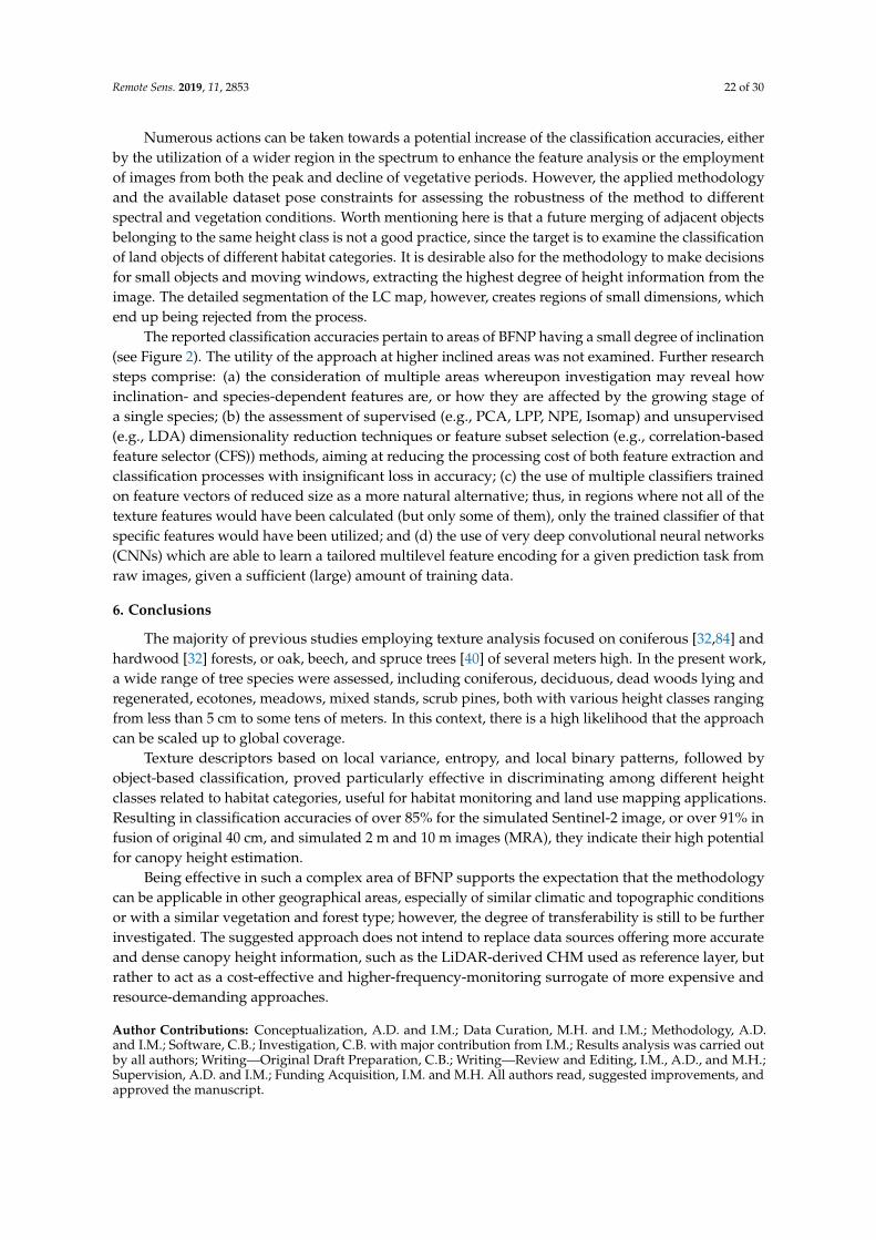
Figure A1. BFNP area of interest 1 (AOI_1) (a) RGB and (b) CIR image (c) with its CHM reference layerand (d) the segmentation vector mask.

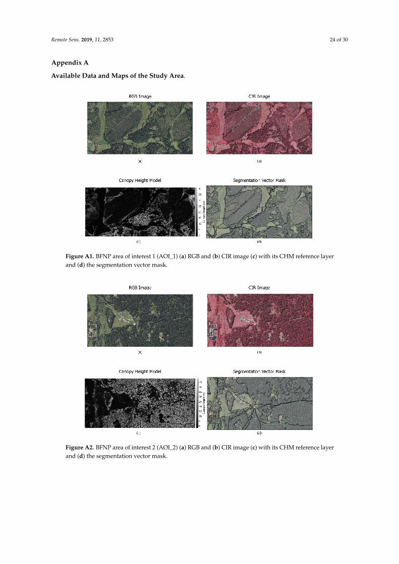
Figure A2. BFNP area of interest 2 (AOI_2) (a) RGB and (b) CIR image (c) with its CHM reference layerand (d) the segmentation vector mask.

Remote Sens. 2019, 11, 2853 25 of 30

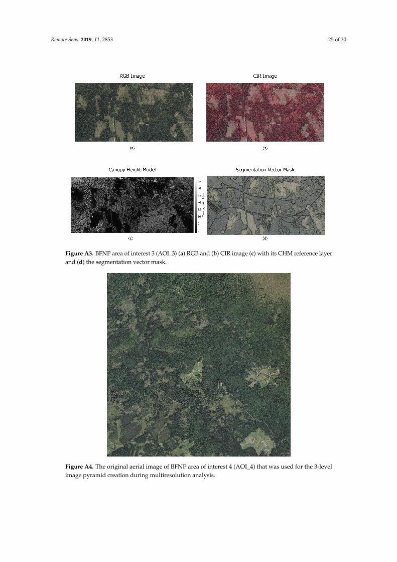
Figure A3. BFNP area of interest 3 (AOI_3) (a) RGB and (b) CIR image (c) with its CHM reference layerand (d) the segmentation vector mask.

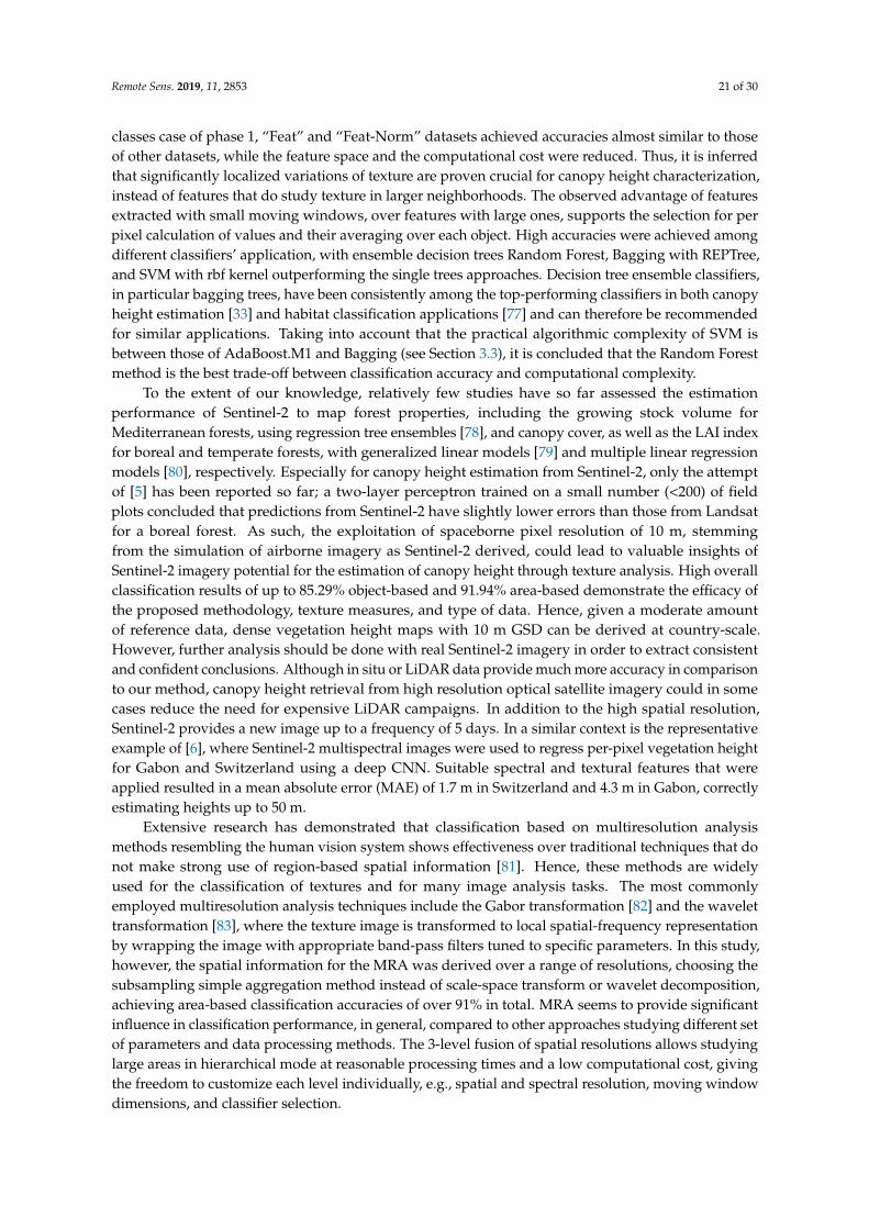
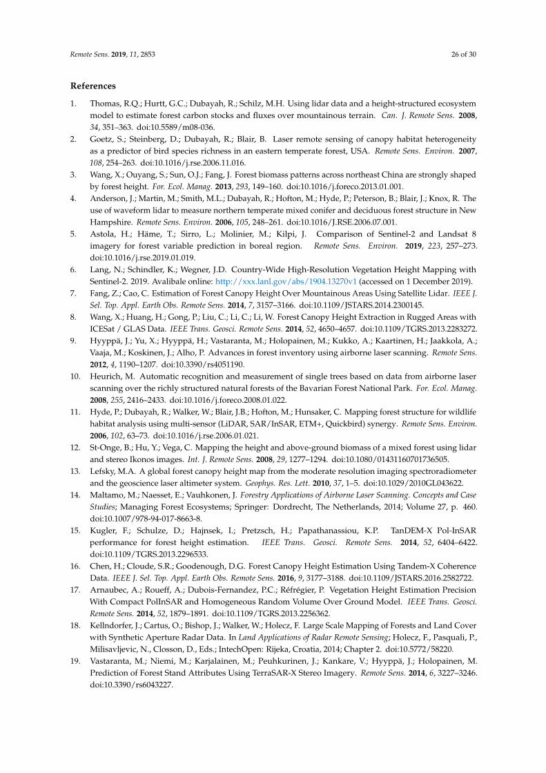
Figure A4. The original aerial image of BFNP area of interest 4 (AOI_4) that was used for the 3-levelimage pyramid creation during multiresolution analysis.

Remote Sens. 2019, 11, 2853 26 of 30

References

1. Thomas, R.Q.; Hurtt, G.C.; Dubayah, R.; Schilz, M.H. Using lidar data and a height-structured ecosystemmodel to estimate forest carbon stocks and fluxes over mountainous terrain. Can. J. Remote Sens. 2008,34, 351–363. doi:10.5589/m08-036.

2. Goetz, S.; Steinberg, D.; Dubayah, R.; Blair, B. Laser remote sensing of canopy habitat heterogeneityas a predictor of bird species richness in an eastern temperate forest, USA. Remote Sens. Environ. 2007,108, 254–263. doi:10.1016/j.rse.2006.11.016.

3. Wang, X.; Ouyang, S.; Sun, O.J.; Fang, J. Forest biomass patterns across northeast China are strongly shapedby forest height. For. Ecol. Manag. 2013, 293, 149–160. doi:10.1016/j.foreco.2013.01.001.

4. Anderson, J.; Martin, M.; Smith, M.L.; Dubayah, R.; Hofton, M.; Hyde, P.; Peterson, B.; Blair, J.; Knox, R. Theuse of waveform lidar to measure northern temperate mixed conifer and deciduous forest structure in NewHampshire. Remote Sens. Environ. 2006, 105, 248–261. doi:10.1016/J.RSE.2006.07.001.

5. Astola, H.; Häme, T.; Sirro, L.; Molinier, M.; Kilpi, J. Comparison of Sentinel-2 and Landsat 8imagery for forest variable prediction in boreal region. Remote Sens. Environ. 2019, 223, 257–273.doi:10.1016/j.rse.2019.01.019.

6. Lang, N.; Schindler, K.; Wegner, J.D. Country-Wide High-Resolution Vegetation Height Mapping withSentinel-2. 2019. Avalibale online: http://xxx.lanl.gov/abs/1904.13270v1 (accessed on 1 December 2019).

7. Fang, Z.; Cao, C. Estimation of Forest Canopy Height Over Mountainous Areas Using Satellite Lidar. IEEE J.Sel. Top. Appl. Earth Obs. Remote Sens. 2014, 7, 3157–3166. doi:10.1109/JSTARS.2014.2300145.

8. Wang, X.; Huang, H.; Gong, P.; Liu, C.; Li, C.; Li, W. Forest Canopy Height Extraction in Rugged Areas withICESat / GLAS Data. IEEE Trans. Geosci. Remote Sens. 2014, 52, 4650–4657. doi:10.1109/TGRS.2013.2283272.

9. Hyyppä, J.; Yu, X.; Hyyppä, H.; Vastaranta, M.; Holopainen, M.; Kukko, A.; Kaartinen, H.; Jaakkola, A.;Vaaja, M.; Koskinen, J.; Alho, P. Advances in forest inventory using airborne laser scanning. Remote Sens.2012, 4, 1190–1207. doi:10.3390/rs4051190.

10. Heurich, M. Automatic recognition and measurement of single trees based on data from airborne laserscanning over the richly structured natural forests of the Bavarian Forest National Park. For. Ecol. Manag.2008, 255, 2416–2433. doi:10.1016/j.foreco.2008.01.022.

11. Hyde, P.; Dubayah, R.; Walker, W.; Blair, J.B.; Hofton, M.; Hunsaker, C. Mapping forest structure for wildlifehabitat analysis using multi-sensor (LiDAR, SAR/InSAR, ETM+, Quickbird) synergy. Remote Sens. Environ.2006, 102, 63–73. doi:10.1016/j.rse.2006.01.021.

12. St-Onge, B.; Hu, Y.; Vega, C. Mapping the height and above-ground biomass of a mixed forest using lidarand stereo Ikonos images. Int. J. Remote Sens. 2008, 29, 1277–1294. doi:10.1080/01431160701736505.

13. Lefsky, M.A. A global forest canopy height map from the moderate resolution imaging spectroradiometerand the geoscience laser altimeter system. Geophys. Res. Lett. 2010, 37, 1–5. doi:10.1029/2010GL043622.

14. Maltamo, M.; Naesset, E.; Vauhkonen, J. Forestry Applications of Airborne Laser Scanning. Concepts and CaseStudies; Managing Forest Ecosystems; Springer: Dordrecht, The Netherlands, 2014; Volume 27, p. 460.doi:10.1007/978-94-017-8663-8.

15. Kugler, F.; Schulze, D.; Hajnsek, I.; Pretzsch, H.; Papathanassiou, K.P. TanDEM-X Pol-InSARperformance for forest height estimation. IEEE Trans. Geosci. Remote Sens. 2014, 52, 6404–6422.doi:10.1109/TGRS.2013.2296533.

16. Chen, H.; Cloude, S.R.; Goodenough, D.G. Forest Canopy Height Estimation Using Tandem-X CoherenceData. IEEE J. Sel. Top. Appl. Earth Obs. Remote Sens. 2016, 9, 3177–3188. doi:10.1109/JSTARS.2016.2582722.

17. Arnaubec, A.; Roueff, A.; Dubois-Fernandez, P.C.; Réfrégier, P. Vegetation Height Estimation PrecisionWith Compact PolInSAR and Homogeneous Random Volume Over Ground Model. IEEE Trans. Geosci.Remote Sens. 2014, 52, 1879–1891. doi:10.1109/TGRS.2013.2256362.

18. Kellndorfer, J.; Cartus, O.; Bishop, J.; Walker, W.; Holecz, F. Large Scale Mapping of Forests and Land Coverwith Synthetic Aperture Radar Data. In Land Applications of Radar Remote Sensing; Holecz, F., Pasquali, P.,Milisavljevic, N., Closson, D., Eds.; IntechOpen: Rijeka, Croatia, 2014; Chapter 2. doi:10.5772/58220.

19. Vastaranta, M.; Niemi, M.; Karjalainen, M.; Peuhkurinen, J.; Kankare, V.; Hyyppä, J.; Holopainen, M.Prediction of Forest Stand Attributes Using TerraSAR-X Stereo Imagery. Remote Sens. 2014, 6, 3227–3246.doi:10.3390/rs6043227.

Remote Sens. 2019, 11, 2853 27 of 30

20. Perko, R.; Raggam, H.; Gutjahr, K.; Schardt, M. The capabilities of TerraSAR-X imagery for retrieval of forestparameters. Int. Arch. Photogramm. Remote Sens. Spat. Inf. Sci. - ISPRS Arch. 2010, 38, 452–456.

21. St-Onge, B.; Vega, C.; Fournier, R.A.; Hu, Y. Mapping canopy height using a combination of digitalstereo-photogrammetry and lidar. Int. J. Remote Sens. 2008, 29, 3343–3364. doi:10.1080/01431160701469040.

22. Næsset, E. Determination of Mean Tree Height of Forest Stands by Digital Photogrammetry. Scand. J.For. Res. 2002, 17, 446–459. doi:10.1080/028275802320435469.

23. Kellndorfer, J.; Walker, W.; Pierce, L.; Dobson, C.; Fites, J.A.; Hunsaker, C.; Vona, J.; Clutter, M. Vegetationheight estimation from Shuttle Radar Topography Mission and National Elevation Datasets. Remote Sens.Environ. 2004, 93, 339–358. doi:10.1016/j.rse.2004.07.017.

24. Baltsavias, E.P. A comparison between photogrammetry and laser scanning. ISPRS J. Photogramm.Remote Sens. 1999, 54, 83–94. doi:10.1016/S0924-2716(99)00014-3.

25. Miller, D.R.; Quine, C.P.; Hadley, W. An investigation of the potential of digital photogrammetry toprovide measurements of forest characteristics and abiotic damage. For. Ecol. Manag. 2000, 135, 279–288.doi:10.1016/S0378-1127(00)00286-3.

26. Takaku, J.; Tadono, T. PRISM On-Orbit Geometric Calibration and DSM Performance. IEEE Trans. Geosci.Remote Sens. 2009, 47, 4060–4073. doi:10.1109/TGRS.2009.2021649.

27. Stojanova, D.; Panov, P.; Gjorgjioski, V.; Kobler, A.; Džeroski, S. Estimating vegetation height andcanopy cover from remotely sensed data with machine learning. Ecol. Inform. 2010, 5, 256–266.doi:10.1016/j.ecoinf.2010.03.004.

28. Dong, L.; Wu, B. A Comparison of Estimating Forest Canopy Height Integrating Multi-Sensor DataSynergy—A Case Study in Mountain Area of Three Gorges. In The International Archives of the Photogrammetry,Remote Sensing and Spatial Information Sciences; ISPRS: Beijing, China, 2008, Volume 37, pp. 379–384.

29. Jia, Y.; Niu, B.; Zhao, C.; Zhou, L. Estimate the height of vegetation using remote sensing in thegroundwater-fluctuating belt in the lower reaches of Heihe River, northwest China. In Proceedingsof the 2010 Second IITA International Conference on Geoscience and Remote Sensing, Qingdao, China,28–31 August 2010; Volume 2, pp. 507–510. doi:10.1109/IITA-GRS.2010.5602672.

30. Anderson, M.C.; Neale, C.M.U.; Li, F.; Norman, J.M.; Kustas, W.P.; Jayanthi, H.; Chavez, J. Upscaling groundobservations of vegetation water content, canopy height, and leaf area index during SMEX02 using aircraftand Landsat imagery. Remote Sens. Environ. 2004, 92, 447–464. doi:10.1016/j.rse.2004.03.019.

31. Puhr, C.B.; Donoghue, D.N.M. Remote sensing of upland conifer plantations using Landsat TMdata: A case study from Galloway, south-west Scotland. Int. J. Remote Sens. 2010, 21, 633–646.doi:10.1080/014311600210470.

32. Wolter, P.T.; Townsend, P.A.; Sturtevant, B.R. Estimation of forest structural parameters using 5 and 10 meterSPOT-5 satellite data. Remote Sens. Environ. 2009, 113, 2019–2036. doi:10.1016/j.rse.2009.05.009.

33. Petrou, Z.I.; Manakos, I.; Stathaki, T.; Mucher, C.A.; Adamo, M. Discrimination of Vegetation HeightCategories With Passive Satellite Sensor Imagery Using Texture Analysis. IEEE J. Sel. Top. Appl. Earth Obs.Remote Sens. 2015, 8, 1442–1455. doi:10.1109/JSTARS.2015.2409131.

34. Huang, X.; Zhang, L.; Wang, L. Evaluation of Morphological Texture Features for Mangrove Forest Mappingand Species Discrimination Using Multispectral IKONOS Imagery. IEEE Geosci. Remote Sens. Lett. 2009,6, 393–397. doi:10.1109/LGRS.2009.2014398.

35. Miyamoto, E.; Merryman, T., Jr. Fast Calculation of Haralick Texture Features; Human Computer InteractionInstitute Department of Electrical and Computer Engineering Carnegie Mellon University: Pittsburgh, PA,USA, 2011; Volume 15213, pp. 1–6.

36. Chowdhury, P.R.; Deshmukh, B.; Goswami, A.K.; Prasad, S.S. Neural network based dunal landformmapping from multispectral images using texture features. J. Sel. Top. Appl. 2011, 4, 171–184.doi:10.1109/JSTARS.2010.2062491.

37. Beguet, B.; Chehata, N.; Boukir, S.; Guyon, D. Retrieving forest structure variables from very high resolutionsatellite images using an automatic method. ISPRS Ann. Photogramm. Remote Sens. Spat. Inf. Sci. 2012,I-7, 1–6. doi:10.5194/isprsannals-I-7-1-2012.

38. Sarkar, A.; Biswas, M.K.; Kartikeyan, B.; Kumar, V.; Majumder, K.L.; Pal, D.K. A MRF model-basedsegmentation approach to classification for multispectral imagery. IEEE Trans. Geosci. Remote Sens. 2002,40, 1102–1113. doi:10.1109/TGRS.2002.1010897.

Remote Sens. 2019, 11, 2853 28 of 30

39. Planinsic, P.; Singh, J.; Gleich, D. SAR Image Categorization Using Parametric and NonparametricApproaches Within a Dual Tree CWT. IEEE Geosci. Remote Sens. 2014, 11, 1757–1761.doi:10.1109/LGRS.2014.2308328.

40. Kayitakire, F.; Hamel, C.; Defourny, P. Retrieving forest structure variables based on image texture analysisand IKONOS-2 imagery. Remote Sens. Environ. 2006, 102, 390–401. doi:10.1016/j.rse.2006.02.022.

41. Aptoula, E. Remote sensing image retrieval with global morphological texture descriptors. IEEE Trans.Geosci. Remote Sens. 2014, 52, 3023–3034. doi:10.1109/TGRS.2013.2268736.

42. Chen, G.; Hay, G.J.; Castilla, G.; St-Onge, B.; Powers, R. A multiscale geographic object-based image analysisto estimate lidar-measured forest canopy height using quickbird imagery. Int. J. Geogr. Inform. Sci. 2011,25, 877–893. doi:10.1080/13658816.2010.496729.

43. Bunce, R.G.H.; Metzger, M.J.; Jongman, R.H.G.; Brandt, J.; De Blust, G.; Elena-Rossello, R.; Groom, G.B.;Halada, L.; Hofer, G.; Howard, D.C.; et al. A standardized procedure for surveillance and monitoringEuropean habitats and provision of spatial data. Landsc. Ecol. 2008, 23, 11–25. doi:10.1007/s10980-007-9173-8.

44. Cailleret, M.; Heurich, M.; Bugmann, H. Reduction in browsing intensity may not compensate climatechange effects on tree species composition in the Bavarian Forest National Park. For. Ecol. Manag. 2014,328, 179–192. doi:10.1016/j.foreco.2014.05.030.

45. Yao, W.; Krzystek, P.; Heurich, M. Tree species classification and estimation of stem volume and DBH basedon single tree extraction by exploiting airborne full-waveform LiDAR data. Remote Sens. Environ. 2012,123, 368–380. doi:10.1016/j.rse.2012.03.027.

46. Latifi, H.; Fassnacht, F.E.; Müller, J.; Tharani, A.; Dech, S.; Heurich, M. Forest inventories by LiDAR data:A comparison of single tree segmentation and metric-based methods for inventories of a heterogeneoustemperate forest. Int. J. Appl. Earth Obs. Geoinf. 2015, 42, 162–174. doi:10.1016/j.jag.2015.06.008.

47. Silveyra Gonzalez, R.; Latifi, H.; Weinacker, H.; Dees, M.; Koch, B.; Heurich, M. Integrating LiDAR andhigh-resolution imagery for object-based mapping of forest habitats in a heterogeneous temperate forestlandscape. Int. J. Remote Sens. 2018, 39, 8859–8884. doi:10.1080/01431161.2018.1500071.

48. Smits, P.C.; Dellepiane, S.G.; Schowengerdt, R.A. Quality assessment of image classification algorithmsfor land-cover mapping: A review and a proposal for a cost-based approach. Int. J. Remote Sens. 1999,20, 1461–1486. doi:10.1080/014311699212560.

49. Congalton, R.G. A review of assessing the accuracy of classifications of remotely sensed data. Remote Sens.Environ. 1991, 37, 35–46. doi:10.1016/0034-4257(91)90048-B.

50. Kalkhan, M.A.; Reich, R.M.; Czaplewski, R.L. Variance Estimates and Confidence Intervals forthe Kappa Measure of Classification Accuracy. Can. J. Remote Sens. 1997, 23, 210–216.doi:10.1080/07038992.1997.10855203.

51. Petrou, Z.I.; Tarantino, C.; Adamo, M.; Blonda, P.; Petrou, M. Estimation of Vegetation Height ThroughSatellite Image Texture Analysis. Int. Arch. Photogramm. Remote Sens. Spat. Inf. Sci. 2012, 321–326.doi:10.5194/isprsarchives-xxxix-b8-321-2012.

52. Petrou, M.; García-Sevilla, P. Image Processing: Dealing with Texture; Wiley: Hoboken, NJ, USA, 2006; Chapter 2,pp. 297–606. doi:10.1002/047003534X.ch2.

53. Little, R.J.A.; Rubin, D.B. Statistical Analysis with Missing Data; John Wiley & Sons, Inc.: New York, NY,USA, 1986.

54. Honaker, J.; King, G.; Blackwell, M. AMELIA II: A Program for Missing Data. J. Stat. Softw. 2011, 45, 1–54.doi:10.18637/jss.v045.i07.

55. Rubin, D.B. Inference and missing data. Biometrika 1976, 63, 581–592. doi:10.2307/2335739.56. Theodoridis, S.; Koutroumbas, K. Feature Selection. In Pattern Recognition, 4th ed.; Academic Press: Boston,

MA, USA, 2009; Chapter 5, pp. 261–322. doi:10.1016/B978-1-59749-272-0.50007-4.57. Witten, I.H.; Frank, E.; Hall, M.A. Data Mining: Practical Machine Learning Tools and Techniques, 3rd ed.;

Morgan Kaufmann: San Mateo, CA, USA, 2011; p. 664. doi:10.1016/B978-0-12-374856-0.00018-3.58. Prasad, A.M.; Iverson, L.R.; Liaw, A. Newer Classification and Regression Tree Techniques: Bagging and

Random Forests for Ecological Prediction. Ecosystems 2006, 9, 181–199. doi:10.1007/s10021-005-0054-1.59. Gislason, P.O.; Benediktsson, J.A.; Sveinsson, J.R. Random Forests for land cover classification.

Pattern Recognit. Lett. 2006, 27, 294–300. doi:10.1016/J.PATREC.2005.08.011.60. Leitloff, J.; Hinz, S.; Stilla, U. Vehicle detection in very high resolution satellite images of city areas. IEEE Trans.

Geosci. Remote Sens. 2010, 48, 2795–2806. doi:10.1109/TGRS.2010.2043109.

Remote Sens. 2019, 11, 2853 29 of 30

61. Dalponte, M.; Bruzzone, L.; Gianelle, D. Fusion of Hyperspectral and LIDAR Remote Sensing Datafor Classification of Complex Forest Areas. IEEE Trans. Geosci. Remote Sens. 2008, 46, 1416–1427.doi:10.1109/TGRS.2008.916480.

62. Foody, G.M.; Mathur, A. A relative evaluation of multiclass image classification by support vector machines.IEEE Trans. Geosci. Remote Sens. 2004, 42, 1335–1343. doi:10.1109/TGRS.2004.827257.

63. Quinlan, R. C4.5: Programs for Machine Learning; Morgan Kaufmann Publishers: San Mateo, CA, USA, 1993.64. Breiman, L. Random forests. Mach. Learn. 2001, 45, 5–32. doi:10.1023/A:1010933404324.65. Breiman, L. Bagging Predictors. Mach. Learn. 1996, 24, 123–140. doi:10.1023/A:1018054314350.66. Freund, Y.; Schapire, R.E. Experiments with a new boosting algorithm. In Proceedings of the 13th International

Conference on Machine Learning; Morgan Kaufmann Publishers Inc.: San Mateo, CA, USA, 1996; pp. 148–156.67. Platt, J. Fast Training of Support Vector Machines Using Sequential Minimal Optimization. In Advances

in Kernel Methods—Support Vector Learning; Schölkopf, B., Burges, C.J.C., Smola, A.J., Eds.; MIT Press:Cambridge, MA, USA, 1998; Chapter 12, pp. 185–208.

68. Hastie, T.; Tibshirani, R. Classification by pairwise coupling. Ann. Stat. 1998, 26, 451–471.doi:10.1214/aos/1028144844.

69. Roelfsema, C.M.; Lyons, M.; Kovacs, E.M.; Maxwell, P.; Saunders, M.I.; Samper-Villarreal, J.; Phinn, S.R.Multi-temporal mapping of seagrass cover, species and biomass: A semi-automated object based imageanalysis approach. Remote Sens. Environ. 2014, 150, 172–187. doi:10.1016/j.rse.2014.05.001.

70. Xu, L.; Li, J.; Brenning, A. A comparative study of different classification techniques for marineoil spill identification using RADARSAT-1 imagery. Remote Sens. Environ. 2014, 141, 14–23.doi:10.1016/j.rse.2013.10.012.

71. Franke, J.; Navratil, P.; Keuck, V.; Peterson, K.; Siegert, F. Monitoring Fire and Selective Logging Activitiesin Tropical Peat Swamp Forests. IEEE J. Sel. Top. Appl. Earth Obs. Remote Sens. 2012, 5, 1811–1820.doi:10.1109/JSTARS.2012.2202638.

72. Delalieux, S.; Somers, B.; Haest, B.; Spanhove, T.; Vanden Borre, J.; Mücher, C.A. Heathland conservationstatus mapping through integration of hyperspectral mixture analysis and decision tree classifiers.Remote Sens. Environ. 2012, 126, 222–231. doi:10.1016/j.rse.2012.08.029.

73. Nelson, M.D.; McRoberts, R.E.; Holden, G.R.; Bauer, M.E. Effects of satellite image spatial aggregationand resolution on estimates of forest land area. Int. J. Remote Sens. 2009, 30, 1913–1940.doi:10.1080/01431160802545631.

74. Hansen, M.C.; Potapov, P.V.; Goetz, S.J.; Turubanova, S.; Tyukavina, A.; Krylov, A.; Kommareddy, A.;Egorov, A. Mapping tree height distributions in Sub-Saharan Africa using Landsat 7 and 8 data. RemoteSens. Environ. 2016, 185, 221–232. doi:10.1016/J.RSE.2016.02.023.

75. Tyukavina, A.; Baccini, A.; Hansen, M.C.; Potapov, P.V.; Stehman, S.V.; Houghton, R.A.; Krylov, A.M.;Turubanova, S.; Goetz, S.J. Aboveground carbon loss in natural and managed tropical forests from 2000 to2012. Environ. Res. Lett. 2015, 10. doi:10.1088/1748-9326/10/7/074002.

76. Ota, T.; Ahmed, O.S.; Franklin, S.E.; Wulder, M.A.; Kajisa, T.; Mizoue, N.; Yoshida, S.; Takao, G.; Hirata, Y.;Furuya, N.; et al. Estimation of Airborne Lidar-Derived Tropical Forest Canopy Height Using Landsat TimeSeries in Cambodia. Remote Sens. 2014, 6, 10750–10772. doi:10.3390/rs61110750.

77. Petrou, Z.; Stathaki, T.; Manakos, I.; Adamo, M.; Tarantino, C.; Blonda, P. Land cover to habitat mapconversion using remote sensing data: A supervised learning approach. In Proceedings of the IEEEInternational Geoscience and Remote Sensing Symposium (IGARSS), Quebec City, QC, Canada; 13–18 July2014; pp. 4683–4686. doi:10.1109/IGARSS.2014.6947538.

78. Chrysafis, I.; Mallinis, G.; Siachalou, S.; Patias, P. Assessing the relationships between growing stockvolume and sentinel-2 imagery in a mediterranean forest ecosystem. Remote Sens. Lett. 2017, 8, 508–517.doi:10.1080/2150704X.2017.1295479.

79. Korhonen, L.; Hadi; Packalen, P.; Rautiainen, M. Comparison of Sentinel-2 and Landsat 8 in theestimation of boreal forest canopy cover and leaf area index. Remote Sens. Environ. 2017, 195, 259–274.doi:10.1016/J.RSE.2017.03.021.

80. Meyer, L.H.; Heurich, M.; Beudert, B.; Premier, J.; Pflugmacher, D. Comparison of Landsat-8 andSentinel-2 data for estimation of leaf area index in temperate forests. Remote Sens. 2019, 11, 1160.doi:10.3390/rs11101160.

Remote Sens. 2019, 11, 2853 30 of 30

81. Aksoy, S.; Akçay, H.G. Multi-resolution segmentation and shape analysis for remote sensing imageclassification. In Proceedings of the 2nd International Conference on Recent Advances in Space Technologies,Istanbul, Turkey, 9–11 June 2005; pp. 599–604. doi:10.1109/RAST.2005.1512638.

82. Grigorescu, S.E.; Petkov, N.; Kruizinga, P. Comparison of Texture Features Based on Gabor Filters. IEEE Trans.Image Process. 2002, 11, 1160–1167. doi:10.1109/TIP.2002.804262.

83. Van De Wouwer, G.; Scheunders, P.; Van Dyck, D. Statistical texture characterization from discrete waveletrepresentations. IEEE Trans. Image Process. 1999, 8, 592–598. doi:10.1109/83.753747.

84. Franklin, J.; Logan, T.L.; Woodcock, C.E.; Strahler, A.H. Coniferous Forest Classification and InventoryUsing Landsat and Digital Terrain Data. IEEE Trans. Geosci. Remote Sens. 1986, GE-24, 139–149.doi:10.1109/TGRS.1986.289543.

c© 2019 by the authors. Licensee MDPI, Basel, Switzerland. This article is an open accessarticle distributed under the terms and conditions of the Creative Commons Attribution(CC BY) license (http://creativecommons.org/licenses/by/4.0/).