Cache me if you can: Capacitated Selfish Replication in Networks∗

Ragavendran GopalakrishnanCalifornia Institute of Technology

ragad3@caltech.edu

Dimitrios KanoulasNortheastern University

dkanou@ccs.neu.edu

Naga Naresh KaruturiGoogle Inc.

naganareshk@google.com

C. Pandu RanganIIT Madras, India

rangan@iitm.ernet.in

Rajmohan RajaramanNortheastern University

rraj@ccs.neu.edu

Ravi SundaramNortheastern University

koods@ccs.neu.edu

December 13, 2011

Abstract

Motivated by peer-to-peer (P2P) networks and content delivery applications, we study CapacitatedSelfish Replication (CSR) games, which involve nodes on a network making strategic choices regardingthe content to replicate in their caches. Selfish replication games were introduced in [6], who analyzedthe uncapacitated case leaving the capacitated version as an open direction.

In this work, we study pure Nash equilibria of CSR games with an emphasis on hierarchical net-works, which have been extensively used to model the communication costs of content delivery and P2Psystems. The best result from previous work on CSR games for hierarchical networks [21, 27] is the ex-istence of a Nash equilibrium for a (slight generalization of a) 1-level hierarchy when the utility functionis based on the sum of the costs of accessing the replicated objects in the network. Our main result is anexact polynomial-time algorithm for finding a Nash Equilibrium in any hierarchical network using a newtechnique which we term “fictional players”. We show that this technique extends to a general frame-work of natural preference orders, orders that are entirely arbitrary except for two natural constraints -“Nearer is better” and “Independence of irrelevant alternatives”. This axiomatic treatment captures a vastclass of utility functions and even allows for nodes to simultaneously have utility functions of completelydifferent functional forms.

Using our axiomatic framework, we next study CSR games on arbitrary networks and delineate theboundary between intractability and effective computability in terms of the network structure, objectpreferences, and the total number of objects. In addition to hierarchical networks, we show the existenceof equilibria for general undirected networks when either object preferences are binary or there are twoobjects. For general CSR games, however, we show that it is NP-hard to determine whether equilibriaexist. We also show that the existence of equilibria in strongly connected networks with two objectsand binary object preferences can be determined in polynomial time via a reduction to the well-studiedeven-cycle problem. Finally, we introduce a fractional version of CSR games (F-CSR) with applicationto content distribution using erasure codes. We show that while every F-CSR game instance possessesan equilibrium, finding an equilibrium in an F-CSR game is PPAD-complete.

∗Gopalakrishnan and Karuturi were partially supported by a generous gift from Northeastern University alumnus MadhavAnand. This work was also partially supported by NSF grants CCF-0635119 and CNS-0915985.

arX

iv:1

007.

2694

v3 [

cs.G

T]

10

Dec

201

1

1 Introduction

Consider a P2P movie sharing service where you need to decide which movies to store locally, given yourlimited disk space, and which to obtain from your friends. Note that your decisions affect those of yourfriends, who in turn take actions that affect you. A natural question arises: what is the prognosis for youand your network of friends in terms of the stability of your movie collections and the satisfaction you willderive from them? Similarly, in the brave new wireless world of 4G you will not only be a consumer ofdifferent apps, you (your personal communications and computing device) will also be a provider of apps toothers around you. And the question arises: could this lead to a situation of endless churn (in terms of whatapps to store) or could there be an equilibrium?

In this paper, we study Capacitated Selfish Replication (CSR) Games, which provide an abstraction ofthe above scenarios. These are games in which the strategic agents, or players, are nodes in a network. Thenodes have object preferences as well as bounded storage space – caches – in which they can store copiesof the content. Each node cooperates with other nodes by serving their requests to access objects stored inits cache. However, the set of objects that a node chooses to store in its cache is entirely based on its ownutility function and where objects of interest have been stored in the network.

Such a game-theoretic framework was first introduced by Chun et al [6], who analyzed pure Nash equi-libria in a setting with storage costs but no cache capacities, and left the capacitated version as an opendirection. Recent work on CSR games has focused on hierarchical networks, which have been extensivelyused to model the communication costs of content delivery and P2P systems. (For instance, see the seminalwork of [14] that uses the ultrametric model for content delivery networks and the work of of [22, 16, 17, 32]on cooperative caching in hierarchical networks.) The best result from previous work on CSR games forhierarchical networks [21, 27] is the existence of a Nash equilibrium for (a slight generalization of) a one-level hierarchical network using the sum utility function, i.e., when the utility of each node is based on aweighted sum of the cost of accessing the objects.

1.1 Our results

This paper studies the existence and computability of Nash equilibria for several variants of CSR games,with a particular focus on hierarchical networks. As with earlier studies [6, 21, 27, 1], we focus on the casewhere all pieces of content have the same size; note that otherwise even computing the best response of aplayer (node) is a generalization of the well-known knapsack problem and is NP-hard.

• Our main result is a polynomial-time algorithm for finding a Nash equilibrium for CSR games inany hierarchical network, thus resolving the question left open by [19, 20, 27]. Our algorithm, pre-sented in Section 3, is based on a new technique that we call the method of “fictional players1” wherewe introduce and eliminate fictional players iteratively in a controlled fashion, maintaining a Nashequilibrium at each step, until the end when we have the desired equilibrium for the entire network(without any fictional players).

The above result is presented specifically in the context of the sum utility function to elucidate thetechnique of fictional players. We then abstract the central requirements for our proof technique and developa general axiomatic framework which allows us to extend our results to a large class of utility functions.

• We present, in Section 4, a general framework for CSR games involving utility preference relationsand node preference orders. Rather than specifying a numerical utility assigned by each node to eachplacement of objects, we only require that the preference order each node has on object placements

1not to be confused with “fictitious play” [10] which involves learning

1

Object preferences and count Undirected networks Directed networksBinary, two objects Yes, in P (5.3) No, in P (6.2)Binary, three or more objects Yes, in PLS (5.2) No, NP-complete (6.1)General, two objects Yes, in P (5.3) No, NP-complete (6.1)General, three or more objects No, NP-complete (6.1) No, NP-complete (6.1)

Hierarchical: Yes, in P (5.1)

Table 1: Existence and computability of equilibria in CSR games. Each cell (other than in the first row or the firstcolumn) first indicates whether equilibria always exist in the particular sub-class of CSR games. If equilibria alwaysexist, then the cell next indicates the complexity of determining an equilibrium; otherwise, it indicates the complexityof determining whether equilibria exist for a given instance. The relevant subsection is given in parentheses.

satisfy two natural constraints of Monotonicity (or “Nearer is better”) and Consistency (or “Indepen-dence of irrelevant alternatives”). This axiomatic treatment captures a vast class of utility functionsand even allows for nodes to simultaneously have utility functions of completely different functionalforms.

• We extend our result for hierarchical networks to the broader class of utilities allowed by the axiomaticframework, and then study general CSR games obtained by considering different network structures(directed or undirected) and different forms of object preferences (binary or general). We delineatethe boundary between intractability and effective computability of equilibria in terms of the networkstructure, object preferences, and the total number of objects. These results are presented in Sections 5and 6 and summarized in Table 1. Notable results include: (1) the existence of equilibria for undirectednetworks with two objects that also utilizes the technique of fictional players, (2) the existence ofequilibria for undirected networks when object preferences are binary, and (3) the equivalence offinding equilibria in CSR games with two objects and binary object preferences to the well-studiedeven-cycle problem [29].

Our last set of results concerns fractional CSR (F-CSR) games, where each node is allowed to storefractions of objects. In our framework, a node can satisfy an object access request by retrieving any set offractions of the object as long as these fractions sum to at least one. As we discuss in Section 7, a naturalimplementation of this framework is via erasure codes (e.g., using the Digital Fountain approach [4, 31]).

• We show that F-CSR games always have equilibria, and the problem of finding an equilibrium is inPPAD. We also show, however, that finding equilibria is PPAD-hard even for a sum-of-distancesutility function.

1.2 Related work

In the last decade there has been a tremendous flowering of research at the intersection of game theoryand computer science [24]. In a seminal paper [26] Papadimitriou laid the groundwork for algorithmicgame theory by introducing syntactically defined subclasses of FNP with complete problems, PPAD beinga notable such subclass. Recently, in a major breakthrough 2-player Nash Equilibrium was shown to bePPAD-complete [7, 5]. The term PPAD-complete is coming to occupy a role in algorithmic game theoryanalogous to the term NP-complete in combinatorial optimization [11].

Selfish caching games were introduced in [6] who considered the uncapacitated case where nodes couldstore more pieces of content by paying for the additional storage. We believe that limits on cache-capacitymodel an important real-world restriction and hence our focus on the capacitated version which was left as

2

an open direction by [6]. Special cases of the integral version of CSR games have been studied. In [21],Nash equilibria were shown to exist for when nodes are equidistant from one another and a special serverholds all objects. [27] slightly extends [21] to the case where special servers for different objects are atdifferent distances. Our results generalize and completely subsume all these prior cases of CSR games. TheMarket sharing games defined by [12] also consider caches with capacity, but are of a very special kind;unlike CSR games, market sharing games are a special case of congestion games. In this work we focusprimarily on equilibria and our general axiomatic framework has the flavor of similar frameworks from thetheory of social choice [2]; in this sense, we deviate from prior work [9, 8] that is focused on the price ofanarchy [18].

There has been considerable research on capacitated caching, viewed as an optimization problem. Vari-ous centralized and distributed algorithms have been presented for different networks in [1, 3, 22, 16, 33].

2 A basic model for CSR games

We consider a network consisting of a set V of nodes labeled 1 through n = |V | sharing a collection O ofunit-size objects. For any i and j in V , let dij denote the cost incurred at i for accessing an object at j; werefer to d as the access cost function. We say that j is node i’s nearest node in a set S of nodes if j is inS and dij ≤ dik for all k in S. We say that the given network is undirected if d is symmetric; that is, ifdij = dji for all i, j in V . We call an undirected network hierarchical if the access cost function forms anultrametric; that is, if dik ≤ max{dij , djk} for all i, j, k ∈ V .

Each node i has a cache to store a certain number of objects. The placement at a node i is simply theset of objects stored at i. The strategy set of a given node is the set of all feasible placements at the node.A global placement is any tuple (Pi : i ∈ V ), where Pi ⊆ O represents a feasible placement at node i. Forconvenience, we use P−i to denote the collection (Pj : j ∈ V \ {i}), thus often using P = (Pi, P−i) torefer to a global placement. We also assume that V includes a (server) node that has the capacity to store allobjects. This ensures that at least one copy of every object is present in the system; this assumption can bemade without loss of generality since we can set the access cost of every node to this server to be arbitrarilylarge.

CSR Games. In our game-theoretic model, each node attaches a utility to each global placement. Weassume that each node i has a weight ri(α) for each object α representing the rate at which i accesses α.We define the sum utility function Us(i) as follows: Us(i)(P ) = −

∑α∈O ri(α) · diσi(P,α), where σi(P, α)

is i’s nearest node holding α in P .A CSR game is a tuple (V,O, d, {ri}). Our focus is on pure Nash equilibria (henceforth, simply equi-

libria) of the CSR games we define. An equilibrium for a CSR game instance is a global placement P suchthat for each i ∈ V there is no placement Qi such that Us(i)(P ) > Us(i)(Q).

Unit cache capacity. In this paper, we assume that all objects are of identical size. Under this assumption,we now argue that it is sufficient to consider the case where each node’s cache holds exactly one object.Consider a set V of nodes in which the cache of node i can store ci objects. Let V ′ denote a new set ofnodes which contains, for each node i in V , new nodes i1, i2, . . . , ici , i.e., one new node for each unit ofthe cache capacity of i. We extend the access cost function as follows: dj`ik = dji for all 1 ≤ ` ≤ cj ,1 ≤ k ≤ ci.

We consider an obvious onto mapping f from placements in V ′ to those in V . Given placement P ′ forV ′, we set f(P ′) = P where Pi = ∪1≤k≤ciP

′ik

. This mapping ensures that Us(i)(P ′) = Us(i)(P ), givingus the desired reduction. Thus, in the remainder of the paper, we assume that every node in the networkstores at most one object in its cache.

3

3 Hierarchical networks

In this section, we give a polynomial-time construction of equilibria for CSR games on hierarchical net-works. Any hierarchical network can be represented by a tree T whose set of leaves is the node set V andevery internal node v has a label `(v) such that (a) if v is an ancestor2 of w in T , then `(v) ≥ `(w), and (b)for any i, j in V , dij is given by `(lca(i, j)), where lca(i, j) denotes the least common ancestor of nodes iand j [14, 16].

Fictional players. In order to present our algorithm, we introduce the notion of a fictional player. For anobject α, a fictional α-player is a new node that stores α in any equilibrium; for any fictional α-player `,r`(α) is 1 and r`(β) is 0 for any β 6= α. Each fictional player is introduced as a leaf in the current hierarchy;the exact locations in the hierarchy are determined by our algorithm. The access cost function is naturallyextended to the fictional players using the hierarchy and the labels of the internal nodes. In the following,we use “node” to refer to both the elements of V and fictional players.

A preference relation. The hierarchical network and the weights that nodes have for different objectsinduce, for each node i, a natural preorder wi among elements of O × Ai, where Ai is the set of properancestors of i in T . Specifically, we define (α, v) Ai (β,w) whenever ri(α) · `(v) > ri(β) · `(w). Wecan now express the best response of any player directly in terms of these preference relations. We defineµi(P ) = (α, v) where Pi = {α} and v is lca(i, σi(P−i, α)), where σi(P−i, α) denotes i’s nearest node inthe set of nodes holding α in P−i.

Lemma 1. A best response Pi of a node i for a placement P−i of V \ {i} is {α} where α maximizes(γ, lca(i, σi(P−i, γ))), over all objects γ, according to wi.

Proof. For a given placement P with Pi = {α}, Us(i)(P ) equals−∑

γ 6=α ri(γ)`(lca(i, σi(P−i, γ))), whichcan be rewritten as −(

∑γ∈O ri(γ)`(lca(i, σi(P−i, γ)))) + ri(α) · `(lca(i, σi(P−i, α))). Thus, {α} is a best

response to P−i if and only if α maximizes ri(γ) · `(lca(i, σi(P−i, γ)) over all objects γ. The desired claimfollows from the definition of wi.

The algorithm. We introduce several fictional players at the start of the algorithm. We maintain the invariantthat the current global placement is an equilibrium in the current hierarchy. As the algorithm proceeds, theset of fictional players and their locations change as we remove existing fictional players or add new ones.On termination, there are no fictional players leaving us with a desired equilibrium. Let Wt and P t denotethe set of fictional players and equilibrium, respectively, at the start of step t of the algorithm.

Initialization. We add, for each object α and for each internal node v of T , a fictional α-player as a leafchild of v; this constitutes the set W0. The initial equilibrium P 0 is defined as follows: for each fictionalα-player i, we have P 0

i = {α}; each node i in V plays its best response. Clearly, each fictional player is inequilibrium, by definition. Furthermore, for every α, every i in V has a sibling fictional α-player. Thus, thebest response of every i in V is independent of the placement of nodes in V \ {i}, implying that P 0 is anequilibrium.

Step t of algorithm. Fix an equilibrium P t for the node set V ∪Wt. If Wt is empty, then we are done.Otherwise, select a node j in Wt. Let P tj = {α}, and let µj(P t) = (α, v). Let S denote the set of all nodesi ∈ V such that (α, v) Ai µi(P

t). We now describe how to compute a new set of fictional players Wt+1 anda new global placement P t+1 such that P t+1 is an equilibrium for V ∪Wt+1. We consider two cases.

• S is empty: Remove the fictional player j from Wt and the hierarchy, and leave the placement in theremaining nodes as before. Thus Wt+1 = Wt − {j} and P t+1 is the same as P t except that P t+1

j isno longer defined.

2We adopt the convention that each node is both descendant and ancestor of itself.

4

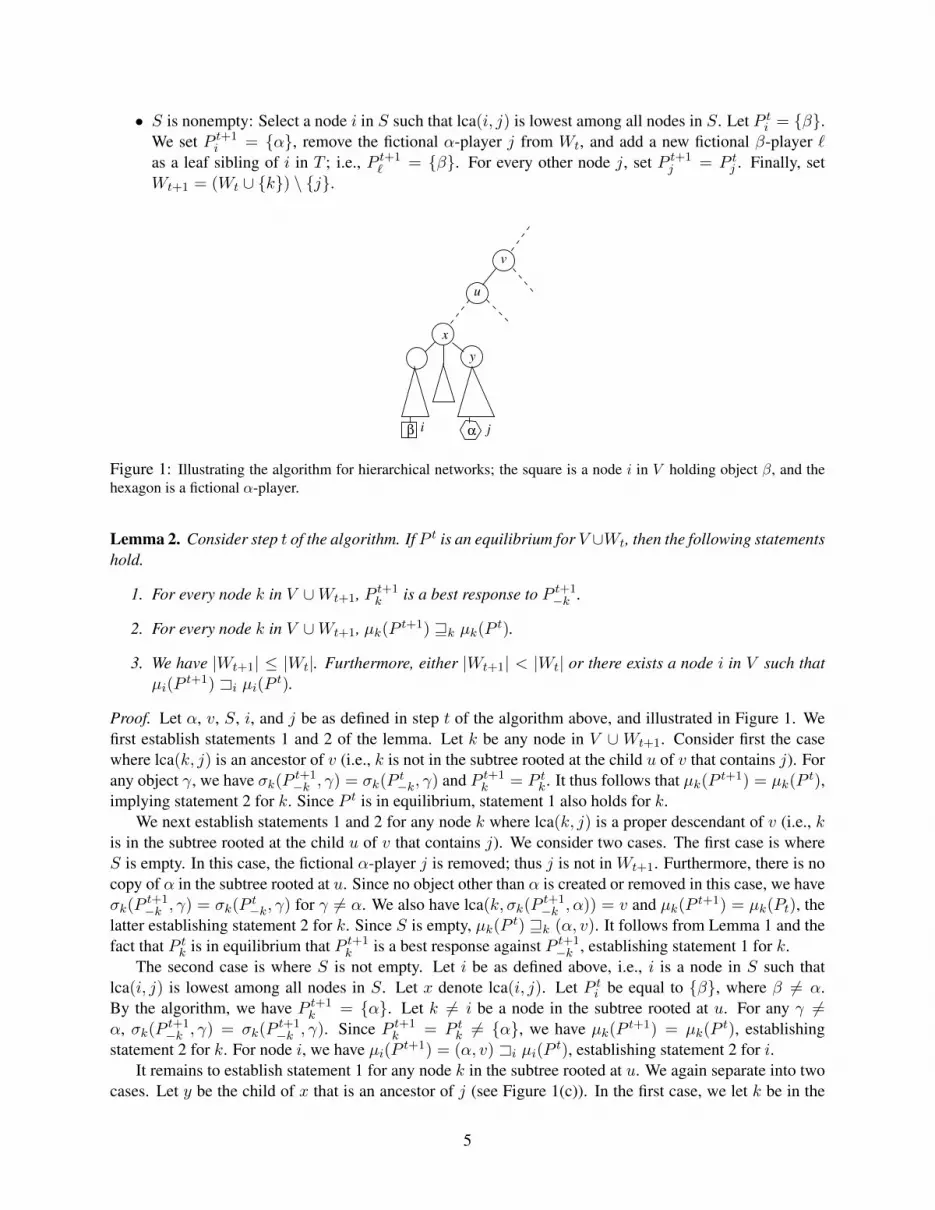
• S is nonempty: Select a node i in S such that lca(i, j) is lowest among all nodes in S. Let P ti = {β}.We set P t+1

i = {α}, remove the fictional α-player j from Wt, and add a new fictional β-player `as a leaf sibling of i in T ; i.e., P t+1

` = {β}. For every other node j, set P t+1j = P tj . Finally, set

Wt+1 = (Wt ∪ {k}) \ {j}.

v

u

y

x

iβ α j

Figure 1: Illustrating the algorithm for hierarchical networks; the square is a node i in V holding object β, and thehexagon is a fictional α-player.

Lemma 2. Consider step t of the algorithm. If P t is an equilibrium for V ∪Wt, then the following statementshold.

1. For every node k in V ∪Wt+1, P t+1k is a best response to P t+1

−k .

2. For every node k in V ∪Wt+1, µk(P t+1) wk µk(P t).

3. We have |Wt+1| ≤ |Wt|. Furthermore, either |Wt+1| < |Wt| or there exists a node i in V such thatµi(P

t+1) Ai µi(Pt).

Proof. Let α, v, S, i, and j be as defined in step t of the algorithm above, and illustrated in Figure 1. Wefirst establish statements 1 and 2 of the lemma. Let k be any node in V ∪Wt+1. Consider first the casewhere lca(k, j) is an ancestor of v (i.e., k is not in the subtree rooted at the child u of v that contains j). Forany object γ, we have σk(P t+1

−k , γ) = σk(Pt−k, γ) and P t+1

k = P tk. It thus follows that µk(P t+1) = µk(Pt),

implying statement 2 for k. Since P t is in equilibrium, statement 1 also holds for k.We next establish statements 1 and 2 for any node k where lca(k, j) is a proper descendant of v (i.e., k

is in the subtree rooted at the child u of v that contains j). We consider two cases. The first case is whereS is empty. In this case, the fictional α-player j is removed; thus j is not in Wt+1. Furthermore, there is nocopy of α in the subtree rooted at u. Since no object other than α is created or removed in this case, we haveσk(P

t+1−k , γ) = σk(P

t−k, γ) for γ 6= α. We also have lca(k, σk(P

t+1−k , α)) = v and µk(P t+1) = µk(Pt), the

latter establishing statement 2 for k. Since S is empty, µk(P t) wk (α, v). It follows from Lemma 1 and thefact that P tk is in equilibrium that P t+1

k is a best response against P t+1−k , establishing statement 1 for k.

The second case is where S is not empty. Let i be as defined above, i.e., i is a node in S such thatlca(i, j) is lowest among all nodes in S. Let x denote lca(i, j). Let P ti be equal to {β}, where β 6= α.By the algorithm, we have P t+1

k = {α}. Let k 6= i be a node in the subtree rooted at u. For any γ 6=α, σk(P t+1

−k , γ) = σk(Pt+1−k , γ). Since P t+1

k = P tk 6= {α}, we have µk(P t+1) = µk(Pt), establishing

statement 2 for k. For node i, we have µi(P t+1) = (α, v) Ai µi(Pt), establishing statement 2 for i.

It remains to establish statement 1 for any node k in the subtree rooted at u. We again separate into twocases. Let y be the child of x that is an ancestor of j (see Figure 1(c)). In the first case, we let k be in the

5

subtree rooted at y. Then, by our choice of i, we have

µk(Pt+1) wk (α, v) wk (α, x) = (α, σk(P

t+1−k , α)),

which, by Lemma 1, implies that statement 1 holds for k. In the second case, we let k be in the subtreerooted at u but not in the subtree rooted at y. Again, σk(P t+1

−k , γ) = σk(Pt−k, γ) for γ 6= α. And for α we

have(α, lca(k, σk(P

t+1−k , α))) = (α, lca(k, i)) wk (α, x) wk µk(P t) = µk(P

t+1),

establishing statement 1 for k using Lemma 1.We finally establish statement 3 of the lemma. The fact |Wt+1| ≤ |Wt| is immediate from the definition

of step t of the algorithm. When S is empty, |Wt+1| < |Wt| since a fictional player is deleted. When S isnonempty, we have shown above that µi(P t+1) Ai µi(P

t), thus completing the proof for statement 3 andfor the whole lemma.

Theorem 3. For hierarchical node preferences, an equilibrium can be found in polynomial time.

Proof. It is immediate from the definition of the algorithm and Lemma 2 that at termination, the algorithmreturns a valid equilibrium. It remains to show that our algorithm terminates in polynomial time. Considerthe potential given by the sum of |Wt| and the sum, over all i, of the position of µi(P t) in the preorder wi.The term |W0| is at most nm, where n is |V | (which is at least the number of internal nodes) and m is thenumber of objects. Furthermore, since |O× I| is at most nm, the initial potential is at most nm+ n2m. ByLemma 2, the potential decreases by at least one in each step of the algorithm. Thus, the number of steps ofthe algorithm is at most nm+ n2m.

We now show that each step of the algorithm can be implemented in polynomial time. The initializationconsists of adding the O(nm) fictional players and computing the best response for each node i in V ;the latter task involves, for each k in V , comparing at most m placements (one for each object). Eachsubsequent step of the algorithm involves the selection of a fictional player j, determination whether theset S is nonempty, and if so, computation of the node i, and then updating the placement. The only partsthat need explanation are the computation of S and i – S is simply the set of all nodes k that are not inequilibrium when fictional player j is deleted. We compute S as follows: for each node k in V , if replacingthe current object in their cache by α yields a more preferable placement (according to the utility) then add kto S. Thus, S can be computed in time polynomial in n. The node i is simply a node in S such that lca(i, j)is lowest among all nodes in S, and can be computed in time polynomial in n. This completes the proof ofthe theorem.

4 A general axiomatic framework for CSR games

We now present a new axiomatic framework which generalizes the result of Section 3 to a broad class ofutility functions, and also enables us to study the existence and complexity of equilibria in more generalsettings.

Node preference relations. We assume that each node i in V has a total preorder ≥i among all the nodesin V 3; ≥i further satisfies i ≥i j for all i, j ∈ V . We say that a node i prefers j over k if j ≥i k, and call anode j most i-preferred in a set S of nodes if j is in S and j ≥i k for all k in S. We also use the notationj =i k whenever j ≥i k and k ≥i j, and j >i k whenever it is not the case that k ≥i j. Note that >i is

3A total preorder is a binary relation that satisfies reflexivity, transitivity, and totality. Totality means that for any i, j, k, eitherj ≥i k or k ≥i j.

6

a strict weak order4, and for any i, j, and k, we have exactly one of these three relations holding: j >i k,k >i j, k =i j. We also extend the notation σi(P, α) and σi(P−i, α) denote a most i-preferred node holdingα in P and P−i, respectively, breaking ties arbitrarily.

The access cost function d introduced in Section 2 induces a natural node preference relation: j >i kif dij < dik, and j =i k if dij = dik. In fact, as we show in Lemma 4, undirected networks (i.e., whenthe access cost function is symmetric) are equivalent to acyclic node preference collections. Formally, thecollection {≥i: i ∈ V } is an acyclic node preference collection if there does not exist a sequence of nodesi0, i1, . . . , ik−1 for an integer k ≥ 3 such that i(j−1) mod k >ij i(j+1) mod k for all 0 ≤ j < k.

Lemma 4. Any undirected network yields an acyclic node preference collection. For any acyclic nodepreference collection, we can compute, in polynomial time, symmetric cost functions that are consistent withthe node preferences.

Proof. Let d denote a symmetric access cost function over the set V of nodes. For a given node i ∈ V ,we have j ≥i k iff dij ≤ dik. We now argue that the collection {≥i: i ∈ V } is acyclic. Suppose, for thesake of contradiction, that there exists a sequence of nodes i0, i1, . . . , ik−1 for an integer k ≥ 3 such thati(j−1) mod k >ij i(j+1) mod k for all 0 ≤ j < k. It then follows that:

diji(j−1) mod k< diji(j+1) mod k

for 0 ≤ j < k.

Since d is symmetric, we obtain

diji(j−1) mod k< di(j+1) mod kij for 0 ≤ j < k,

which is a contradiction.Given an acyclic collection of node preferences, we compute an associated access cost function d in

polynomial time as follows. We construct a directed graph G over the set U of all unordered pairs (i, j) :i, j ∈ V , i 6= j. There is a directed edge from node (i, j) to (i, k) if and only if k ≥i j. Since the collection{≥i: i ∈ V } is acyclic, G is a dag. We compute the topological ordering π : U → Z; thus, we haveπ((i, j)) < π((k, `)) whenever there is a directed path from (i, j) to (k, `). Setting dij to be π((i, j)) givesus the desired undirected network.

Utility preference relations. In our game-theoretic model, each node attaches a utility to each globalplacement. We present a general definition that allows us to consider a large class of utility functionssimultaneously. Rather than define a numerical utility function, we present the utility at each node i as atotal preorder �i among the set of all global placements. (The notation �i and =i over global placementsare defined analogously.) We require that �i, for each i ∈ V , satisfies the following two basic conditions.

• Monotonicity: For any two global placements P and Q, if, for each object α and each node q withα ∈ Qq, there exists a node p with α ∈ Pp and p ≥i q, then P �i Q.

• Consistency: Let (Pi, P−i) and (Qi, Q−i) denote two global placements such that for each objectα ∈ Pi ∪ Qi, if p (resp., q) is a most i-preferred node in V \ {i} holding α, i.e., α ∈ Pp (resp.,α ∈ Qq), then p =i q. If (Pi, P−i) �i (Qi, P−i), then (Pi, Q−i) �i (Qi, Q−i).

In words, the monotonicity condition says that for any node, if all the objects in a placement are placed atnodes that are at least as preferred as in another placement, then the node prefers the former placement atleast as much as the latter. The consistency condition says that the preference for a node to store one set of

4A strict weak order is a strict partial order > (a transitive relation that is irreflexive) in which the relation “neither a > b norb > a” is transitive. Strict weak orders and total preorders are widely used in microeconomics.

7

objects instead of another is entirely a function of the set of most preferred other nodes that together holdthese objects. For instance, if a node i with unit capacity prefers to store α over β in a scenario where themost i-preferred node (other than i) storing α (resp., β) is j (resp., k), then i prefers to store α at least asmuch as β in any other situation where the most i-preferred node (other than i) storing α (resp., β) is j(resp., k).

Generality of the conditions. We note that many standard utility functions defined for replica placementproblems [6, 20, 27], including the sum and max functions, satisfy the monotonicity and consistency con-ditions. Indeed, any utility function that is an Lp norm, for any p, over the costs for the individual objects,also satisfies the conditions. Furthermore, since the monotonicity and consistency conditions apply to theindividual utility functions, our model allows the different nodes to adopt different types of utilities, as longas each separately satisfies the two conditions.

Binary object preferences. One class of utility preference relations that we highlight is the ones based onbinary object preferences. Suppose that each node i has a set Si of objects in which it is equally interested,and it has no interest in the other objects. Let τi(P ) denote the |Si|-length sequence consisting of theσi(P, α), for α ∈ Si, in nonincreasing order according to the relation ≥i. Then, the consistency conditioncan be further strengthened to the following.

• Binary Consistency: For any placements P = (Pi, P−i) and Q = (Qi, Q−i) with P−i = Q−i, wehave P �i Q if and only if for 1 ≤ k ≤ |Si|, the kth component of τi(P ) is at least as i-preferred asthe kth component of τi(Q).

CSR Games. In the general framework, a CSR game is a tuple (V,O, {≥i}, {�i}). A (pure) Nash equilib-rium for an CSR game instance is a global placement P such that for each i ∈ V there is no placement Qisuch that (Qi, P−i) �i (Pi, P−i).

For our complexity results, we need to give the specification for a given game instance. The set Vis specified, together with node cache capacities, and O is an enumerated list of object names. The nodepreference relation ≥i is specified succinctly by a set of at most

(n2

)bits, for each i. The utility preference

relation �i, however, is over a potentially exponential number of placements (in terms of n, m, and cachesizes). For our complexity results, we assume that the utility preference relations are specified by an effi-cient algorithm – which we call the utility preference oracle – that takes as input a node i, and two globalplacements P and Q, and returns whether P �i Q. For the sum, max, and Lp-norm utilities, the utilitypreference oracle simply computes the relevant utility function. For binary object preferences, the binaryconsistency condition yields an oracle that is polynomial in number of nodes, objects, and cache sizes.

Unit cache capacity. We now argue that the unit cache capacity assumption of Section 2 continues to holdwithout loss of generality. Consider a set V of nodes in which the cache of node i can store ci objects. LetV ′ denote a new set of nodes which contains, for each node i in V , new nodes i1, i2, . . . , ici , i.e., one newnode for each unit of the cache capacity of i. We set the node preferences as follows: for all i, i′, j ∈ V ,1 ≤ f, ` ≤ cj , 1 ≤ k, k′ ≤ ci, we have ik ≥j` i′k′ whenever i ≥j i′, and jf =ik j`.

We consider an obvious onto mapping f from placements in V ′ to those in V . Given placement P ′

for V ′, we set f(P ′) = P where Pi = ∪1≤k≤ciP′ik

. This mapping naturally defines the utility preferencerelations for the node set V ′. In particular, for any i ∈ V and 1 ≤ k ≤ ci, P ′ �ik Q′ whenever f(P ′) �if(Q′). We also note that f is computable in time polynomial in the number of nodes and the sum of thecache capacities. It is easy to verify that the utility preference relation �ik for all ik ∈ V ′ satisfies themonotonicity and consistency conditions. Furthermore, P ′ is an equilibrium for V ′ if and only if f(P ′) isan equilibrium for V ; this together with the onto property of the mapping f gives us the desired reduction.

8

5 Existence of equilibria in the general framework

In this section, we establish the existence of equilibria for several CSR games under the axiomatic frame-work of Section 4. We first extend our result for the sum utility function on hierarchical networks to thegeneral framework (Section 5.1). We next show that CSR games for undirected networks and binary objectpreferences are potential games (Section 5.2). Finally, when there are only two objects in the system, weuse the technique of fictional players to give a polynomial-time construction of equilibria for CSR gamesfor undirected networks (Section 5.3).

5.1 Hierarchical networks

We now show that the polynomial time algorithm of Section 3 extends to the axiomatic framework we haveintroduced. In the general framework, a hierarchical network can be represented as a tree T whose set ofleaves is the node set V and the node preference relation ≥i given by: j ≥i k if lca(i, j) is a descendantof lca(i, k). Our algorithm of Section 3 and its analysis are completely determined by the structure of thehierarchical network and the pair-preference relations wi defined for each node i; the latter were definedfor the sum utility function. In order to extend our analysis to the general framework, it suffices to derive anew preference relation and establish the analogue of Lemma 1, which we now present for arbitrary utilitypreference relations satisfying the monotonicity and consistency properties.

Pair preference relations. Given any utility preference relation �i that satisfies the monotonicity andconsistency conditions, we define a strict weak order Ai on O×Ai, where Ai is the set of proper ancestorsof i in T .

1. For each object α, node i, and proper ancestors v and w of i, we have (α, v) Ai (α,w) whenever v isa proper ancestor of w.

2. Consider distinct objects α, β and nodes i, j, k with j, k 6= i. LetP denote the set of global placementsP such that j (resp., k) is a most i-preferred node in V \ {i} holding α (resp., β) in P−i. If there existglobal placements P = ({α}, P−i) and Q = ({β}, P−i) in P with P �i Q, then (α, lca(i, j)) Ai

(β, lca(i, k)).

In words, item 1 says that i’s preference for keeping α in its cache increases as the most i-preferrednode holding α becomes less preferred (or “moves farther away”). In item 2, (α, v) Ai (β,w) means thatif i needs to place either α or β in its cache, and the least common ancestor of i and the most i-preferrednode in V \ {i} holding α (resp., β) is v (resp., w), then i prefers to store α over β. The strict weak orderAi induces a total preorder wi as follows: (α, v) wi (β,w) if it is not the case that (β, v) Ai (α,w). Wesimilarly define =i: (α, v) =i (β,w) if (α, v) wi (β,w) and (β, v) =i (α,w).

Lemma 5. For each i, Ai as given above, is a well-defined strict weak order.

Proof. We need to ensure the well-definedness of part 2 of the definition of pair preference relations. Thatis, we need to show that for any placements P−i and Q−i such that a most i-preferred node in P−i hold-ing α (resp., β) is also a most i-preferred node in Q−i, it is impossible that ({α}, P−i) �i ({β}, P−i)and ({β}, Q−i) �i ({α}, Q−i) both hold. This directly follows from the consistency condition for utilitypreference relations.

The reflexivity and transitivity of wi are immediate from the definitions and the reflexivity and tran-sitivity of �i. Finally, to ensure the well-definedness of the strict preorder Ai, we also have to showthat there is no collection of pairs (αj , vj), 0 ≤ j < ` for some integer ` > 1, such that (αj , vj) Ai

(αj+1 mod `, vj+1 mod `) for 0 ≤ j < `. To see this, it is sufficient to note that if (α, v) Ai (α′, v′) then forall placements P and P ′ such that P−i = P ′−i and the least common ancestor of i and the most i-preferred

9

node in V \ {i} that holds α (resp., α′) is v (resp., v′) we have P �i P ′. So any cycle in the strict preorderAi implies a cycle in �i, yielding a contradiction.

Lemma 6. For any global placement P = ({α}, P−i), if j (resp., k) is a most i-preferred node holdingobject α (resp., β) in P−i, and ({β}, P−i) �i ({α}, P−i), i.e., for node i, storing β is a better response toP−i than storing α, then (β, lca(i, k)) Ai (α, lca(i, j)). Futhermore, for any global placement P , {α} is abest response to P−i, where α maximizes (γ, lca(i, σi(P−i, γ))), over all objects γ, according to wi.

Proof. The first statement of the lemma directly follows from item 2 of the definition of pair preferencerelations. We establish the second statement by contradiction. Suppose that for node i, {β} is a betterresponse to P−i than {α}. Then, we have ({β}, P−i) �i ({α}, P−i), which, by item 2 of the definition ofpair preference relations, implies that (β, lca(i, σi(P−i, β))) Ai (α, lca(i, σi(P−i, α))), a contradiction tothe choice of α.

The remainder of the analysis for hierarchical networks (Lemma 2 and Theorem 3) follows as before,invoking Lemma 6 instead of Lemma 1.

5.2 Undirected networks with binary object preferences

Let d be a symmetric cost function for an undirected network over the node set V . Recall that for binaryobject preferences, we are given, for each node i a set Si of objects in which i is equally interested. Ourproof of existence of equilibria is via a potential function argument. Given a placement P , let Φi(P ) = dij ,where j is the most i-preferred node in V −{i} holding the object in Pi. We introduce the potential functionΦ: Φ(P ) = (Φ0,Φi1(P ),Φi2(P ), . . . ,Φin(P )), where Φ0 is the number of nodes i such that Pi ⊆ Si, andΦij (P ) ≤ Φij+1(P ), ∀j, where V = {i1, i2, . . . , in}. We prove that Φ is an increasing potential function:after any better response step, Φ increases in lexicographical order.

Let P = (Pi, P−i) be an arbitrary global placement. Assume that Pi = {α} and j is the most i-preferred node in P−i holding α. Consider any better response step, from placement P to Q = (Qi, P−i),where Qi = {β}. Clearly β ∈ Si. We consider two cases. First, suppose α /∈ Si and β ∈ Si. Then, Φ0

increases, and so does the potential. The second case is where α, β ∈ Si. Let k be the most i-preferrednode in P−i holding β. In this case, Φ0 does not change. However, since this is a better response step ofi, j >i k, implying that dik > dij and hence Φi(Q) > Φi(P ). Consider any other node j. If j holds anyobject γ other than β, since no new copy of γ has been added, Φj(Q) ≥ Φj(P ). It remains to consider thecase where j holds β. If S is the set of nodes in V \ {j} holding β in P−j , then S ∪ {i} is the set of nodesin V \ {j} holding β. Thus, Φj(Q) = min{Φj(P ), dji} ≥ min{Φj(P ),Φi(Q)}. This also means thatΦj(P ) appears later in the sorted order than Φi(P ) and Φj(Q) appears no earlier in the sorted order thanΦi(Q). Hence, Φ(Q) is lexicographically greater than Φ(P ). This establishes that for undirected networkswith binary object preferences, the resulting CSR game is a potential game, and hence also in PLS [13].

5.3 Undirected networks with two objects

We give a polynomial-time algorithm for computing an equilibrium in any undirected network with twoobjects. Our algorithm uses the fictional player technique introduced in Section 5.1. It starts by introducingfictional players serving both the objects in the network at zero cost from each node. In each subsequentstep, we move the fictional players progressively “further” away, ensuring that each instant, we have anequilibrium. Finally, when the fictional players are at least preferred cost from all the nodes, they can beremoved yielding an equilibrium for the original network.

Suppose we are given a undirected network with access cost function d. Also letD be the set {0, `1, `2, . . . , `r}of all access costs between nodes in the system in increasing order; that is, `1 = mini,j dij and `r =maxi,j dij and `i < `i+1 for all 1 ≤ i < r.

10

Fictional player. For an object α, a fictional α-player is a new node that will store α in every equilibrium;an fictional α-player prefers storing α over any other object. We denote by srvα(`) the fictional α-playerwhich is at access cost ` from every node in V .The algorithm.Initialization. Assuming that there are two objects α and β in the system, we initially set up a fictionalα-player srvα(0) and β-player srvβ(0) at access cost 0 from each node in V . We let nodes replicate theirmost preferred object and access the other without any access cost from the corresponding fictional player.This placement is obviously an equilibrium.Step t of algorithm. Fix an equilibrium P for the node set V ∪ {srvα(`t)} ∪ {srvβ(`t)}. We describe onestep of the algorithm which computes a new set of fictional players srvα(`t+1) and srvβ(`t+1) and a newplacement P ′ such that P ′ is an equilibrium for the node set V ∪ {srvα(`t+1)} ∪ {srvβ(`t+1)}. We firstremove the α-player srvα(`t) from the system and instead we add srvα(`t+1). If there do not exist nodesthat want to deviate we are done. Otherwise, assume that there exists a node i that wants to deviate fromits strategy. Since the most i-preferred node holding β in V ∪ {srvα(`t)} ∪ {srvβ(`t)} remains the samein V ∪ srvα(`t+1) ∪ srvβ(`t), i is not holding object α. Thus the only nodes that may want to deviate arethose that are holding object β. We argue that if we let i to deviate from β ∈ Pi to α ∈ P ′i , there is no nodej ∈ V \ {i} that gets affected by i’s deviation. Consider the following two cases:

• If a node j has access cost at most `t from i, then β ∈ Pj . Otherwise, if α ∈ Pj , srvα(`t) would notbe the most i-preferred node holding α and thus i would not be affected by any change of α-players.Thus there does not exist any node j ∈ V \ {i} with access cost at most `t from i, such that α ∈ Pj ,and as we showed above α ∈ P ′j .

• If a node j has access cost at least `t+1 from i, then Pj = P ′j . Because of the α-player srvα(`t+1)and the β-player srvβ(`t), i would never be the j-most preferred node in P ′.

We then remove the β-player srvβ(`t) from the system and instead we add srvβ(`t+1). Using a similarargument as above, we obtain a new equilibrium at the end of this step.

Theorem 7. For undirected networks with two objects, an equilibrium can be found in polynomial time.

Proof. An initial placement P , where we have the set of fictional players srvα(0) and srvβ(0) in the system,is obviously an equilibrium. It is immediate from our argument above that at termination the algorithmreturns a valid equilibrium.

The size of the set D is at most(n2

)which is at most n2. In each step t at most n nodes may want to

deviate from their strategy, since we showed above that if a node deviates once in a step, it will not deviateagain during the same step . Thus, the total number of deviations in the algorithm is at most n3.

6 Non-Existence of equilibria in CSR games and the associated decisionproblem

In this section, we show that the classes of games studied in Section 5 are essentially the only games whereequilibria are guaranteed to exist. We identify the most basic CSR games where equilibria may not exist,and study the complexity of the associated decision problem.

6.1 NP-Completeness

The main result of this section is the following theorem, which establishes the NP-hardness of determiningwhether a given CSR game has an equilibrium even when the utility preference relations are based on the

11

sum utility function and either the number of objects is small or the object preferences are binary. The proofis by a polynomial-time reduction from 3SAT [11]. Each reduction is built on top of a gadget which has anequilibrium if and only if a specified node holds a certain object. Several copies of these gadgets are thenput together to capture the given 3SAT formula.

Theorem 8. The problem of determining whether a given CSR instance has an equilibrium is in NP. Itis NP-hard to determine whether an CSR intance has an equilibrium even if one of these three restrictionshold: (a) number of objects is two; (b) object preferences are binary and number of objects is three; (c)network is undirected and number of objects is three.

The membership in NP is immediate, since one can determine in polynomial time whether a given globalplacement is an equilibrium. The remainder of the proof focuses on the hardness reduction from 3SAT.

Given a 3SAT formula φ with n variables x1, x2, . . . , xn and k clauses c1, c2, . . . , ck, we construct anCSR instance as follows. For each variable xi in φ, we introduce two variable nodes: node Xi and Xi.We set dXiXi

and the symmetric dXiXito be 0.5, where d is the underlying access cost function. For each

clause cj , we introduce a clause node Cj . Assuming that `j,r, for r ∈ {1, 2, 3} are the three literals of clausecj in formula φ, we set dCjLj,r and dLj,rCj to be 1 for r ∈ {1, 2, 3}. Note that each Lj,s, for j ∈ [1, k], ands ∈ {1, 2, 3} is in fact some variable node Xh or Xh for some h ∈ [1, n]. We also introduce a gadget Gillustrated in Figure 3, consisting of nodes S, A, B, and C. We set the access cost dSCi and the symmetricdCiS , for all 1 ≤ i ≤ k between node S and all clause nodes to be 2. The general construction is illustratedin Figure 2.

1

1C Ck

A

0.5 0.50.5 0.5

1

22

S

B

C

1 2 3n

321X

X X X X

XXX

X X X

X

n−2n−1

n−1X

nX

0.5

4

4

X

Xn−2n−3

n−3

0.5 0.50.5

11

11

Figure 2: Instance of the construction for the undirectedcase proof of NP-Hardness, where φ = (x1 ∨ x3 ∨ x4) ∧. . . ∧ (xn−3 ∨ xn−1 ∨ xn)

1

S

A

BC

2

1

1

5

D

A

C

B

3 3

3.1

3.052

S

55

5

Figure 3: Gadget for the directed (left) and the undirected(right) case

Directed networks with two objects. We set dAS , dAB , dBC , dCA to be 1. The server node at access costdsrv = 10 from all nodes in V , stores a fixed copy of two objects α and β. We set the weights rxi(α),rxi(α), rxi(β), rxi(β) of each variable node on objects α and β, to be 1. For each clause node we set theweight rCi(α) on object α to be 1, and the weight rCi(β) on object β to be 0.7, for all 1 ≤ i ≤ k. We setthe weight rS(α) on object α to be 1, and the weight rS(β) on object β to be 0.7. We set the weight rA(α)of node A on object α to be 0.7 and the weight rA(β) of node A on object β to be 1. Finally, we set theweight of nodes B and C on both objects α, and β to be 1. We refer to this CSR instance as I1.Undirected networks with three objects. For the undirected case, we set dAS and dBS to be 3, dAB tobe 3.1, dBC to be 3.05, and dCA to be 2; while symmetry holds. The server node, which is at access cost

12

dsrv = 5 from all nodes in V , stores a fixed copy of three objects α, β, and γ. We set the weights rxi(α),rxi(α), rxi(β), rxi(β) of each variable node on objects α and β, to be 1. Also, for each clause node we setthe weight rCi(α) on object α to be 0.85, and the weight rCi(β) on object β to be 1, for all 1 ≤ i ≤ k.We set the weight rS(α) on object α to be 0.85, and the weight rS(β) on object β to be 1. Also we set theweight rA(α) = 1, rA(γ) = 2, rB(β) = 1, rB(γ) = 0.9837, rC(β) = 1, and rC(γ) = 1.6. We set all theremaining weights to be 0. We refer to this CSR instance as I2.

Lemma 9. A variable node Xi holds object α (resp., β) if and only if node Xi holds object β (resp., α).

Proof. The proof is immediate, since Xi (resp., Xi) is Xi’s (resp., Xi’s) nearest node, and both Xi and Xi

are interested equally in α and β.

Lemma 10. Clause node Ci holds object α if and only if its variable nodes Li,j , for j ∈ {1, 2, 3} holdobject β.

Proof. First, assume that Li,j , for j ∈ {1, 2, 3} hold β. These nodes are Ci’s nearest nodes holding β.By Lemma 9 we know that nodes Li,j , for j ∈ {1, 2, 3} hold α, and they are Ci’s nearest nodes holding α.Node’sCi cost for holding α and accessing β from Li,j , for j ∈ {1, 2, 3}, is rCi(β)dCiLi,j = 1·1 = 1; whilethe cost for holding β and accessing α from Li,j , for j ∈ {1, 2, 3}, is rS(α)dCiLij

= 0.85 · 1.5 = 1.275.Obviously, node Ci prefers to replicate α.

Now assume that at least one of the nodes Li,j , for j ∈ {1, 2, 3} holds α. These nodes are Ci’s nearestnodes holding α. Also, by Lemma 9, Ci’s nearest nodes holding β are all the remaining nodes from the setLi,j , Li,j , for j ∈ {1, 2, 3}, that don’t hold α. Node’s Ci cost for holding β and accessing α from Li,j , forj ∈ {1, 2, 3}, is rCi(α)dCiLi,j = 0.85 · 1 = 0.85; while the cost for holding α and accessing β from nodeLi,j (resp., Li,j), is rCi(β)dCi

¯Li,j= 1 · 1.5 = 1.5 (resp., rCi(β)dCiLi,j = 1 · 1 = 1). Obviously, in any case

node Ci prefers to replicate β.

Lemma 11. Node S holds object α if and only if all clause nodes C1, . . . , Ck hold object β.

Proof. First, assume that C1, . . . , Ck are holding β. These nodes are S’s nearest nodes holding β. Also byLemma 10, S’s nearest node holding α is at least one of Li,j nodes, where i ∈ [1, k], j ∈ {1, 2, 3}. Thecost for S holding α and accessing β from a node Ci, i ∈ [1, k], is rS(β)dSCi = 1 · 2 = 2; while the costfor holding β and accessing α from Li,j , where i ∈ [1, k], j ∈ {1, 2, 3}, is rS(α)dSLi,j = 0.85 · 3 = 2.55.Obviously, node S prefers to replicate α.

Now assume that at least one of C1, . . . , Ck holds α. These nodes are S’s nearest node holding α. AlsoS’s nearest node holding β, due to Lemma 10 is one of Li,j , where i ∈ [1, k], j ∈ {1, 2, 3}. The cost forholding β and accessing α from a node Ci, is rS(α)dSCi = 0.85 · 2 = 1.7; while the cost for holding α andaccessing β from a node Lij , where j ∈ {1, 2, 3}, is rS(β)dSLi,j = 1 · 3 = 3. Obviously, in any case nodeS prefers to replicate β.

Theorem 12. The CSR instance I1 has an equilibrium if and only if node S holds object α.

Proof. First, assume that S is holding α. By Lemma 11 nodes C1, . . . , Ck hold object β, and by Lemma 10at least one of nodes Li,j , for j ∈ {1, 2, 3} for each nodeCi, i ∈ [1, k], holds object α, and the correspondingLi,j is holding object β. We claim that the placement where A holds β, B holds β, and C holds α, is a pureNash equilibrium. We prove this by showing that none of these nodes wants to deviate from their strategy.

Node A does not want to deviate since its cost for holding object β and accessing α from A’s nearestnode S, is rA(α)dAS = 0.7 · 1 = 0.7; while the cost for holding object α and accessing β from A’s nearestnode B, is rA(α)dAB = 1 · 1 = 1. Node B does not want to deviate since its cost for holding object β andaccessing α from B’s nearest node C, is rB(α)dBC = 1 · 1 = 1; while the cost for holding object α andaccessing β from B’s nearest node A, is rB(β)dBA = 1 · 2 = 2. Node C does not want to deviate since

13

its cost for holding object α and accessing β from C’s nearest node A, is rC(β)dCA = 1 · 1 = 1; while thecost for holding object β and accessing α from C’s nearest node S, is rC(α)dCS = 1 · 2 = 2. Also note thatnone of S,C1, . . . , Ck, Lij , Lij for i ∈ [1, k], j ∈ {1, 2, 3} is getting affected of the objects been holded bythe gadget nodes.

Now assume that node S holds object β. We are going to prove that for every possible placement overnodes A, B, and C, at least one node wants to deviate from its strategy. Consider the following cases:

• Nodes A, B, and C hold object α: Node B (resp., C) wants to deviate, since the cost for holdingobject α and accessing β from B’s (resp., C’s) nearest node S, is rB(β)dBS = 1 · 3 = 3 (resp.,rC(β)dCS = 1 · 2 = 2); while the cost for holding object β and accessing α from B’s nearest nodeA, is rB(β)dBA = 1 · 2 = 2 (resp., rC(β)dCA = 1 · 1 = 1).

• Two nodes hold object α and the third holds β: In the case where A and B hold α, A wants to deviatesince the cost while holding α and accessing β from A’s nearest node S is rA(β)dAS = 1 · 1 = 1;while the cost for holding β and accessing α fromA’s nearest nodeB is rA(α)dAB = 0.7·1 = 0.7. Inthe case whereA andC hold α, thenC wants to deviate since the cost while holding α and accessing βfrom C’s nearest node B is rC(β)dCB = 1 ·2 = 2; while the cost for holding β and accessing α fromC’s nearest node A is rC(α)dCA = 1 · 1 = 1. In the case where B and C hold α, B wants to deviatesince the cost while holding α and accessing β from B’s nearest node A is rB(β)dBA = 1 · 2 = 2;while the cost for holding β and accessing α from B’s nearest node C is rB(α)dBC = 1 · 1 = 1.

• One node holds α: If A (resp., B, or C) holds α, B (resp., C, A) wants to deviate since the costwhile holding β and accessing α from B’s (resp., C’s, or A’s) nearest node A (resp., B, or C) isrB(α)dBA = 1 · 2 = 2 (resp., rC(α)dCB = 1 · 2 = 2, or rA(α)dAC = 0.7 · 2 = 1.4); while thecost for holding α and accessing β from B’s (resp., C’s, or A’s) nearest node C (resp., A, or B), isrB(β)dBC = 1 · 1 = 1 (resp., rC(β)dCA = 1 · 1 = 1, or rA(β)dAB = 1 · 1 = 1).

• Nodes A, B, and C hold β: All of them want to deviate. Node A wants to deviate since the cost whileholding β and accessing α from A’s nearest node Ci, for some i ∈ [1, k], is rA(β)dACi = 1 · 3 = 3;while the cost for holding β and accessing α from A’s nearest node S is rA(α)dAS = 0.7 · 1 = 0.7.Similar proof holds for nodes B and C.

Obviously the system does not have a pure Nash equilibrium, which completes the proof.

Theorem 13. The CSR instance I2 has an equilibrium if and only if node S holds object α.

Proof. First, assume that S is holding α. By Lemma 11 nodes C1, . . . , Ck hold object β, and by Lemma 10at least one of nodes Li,j , for j ∈ {1, 2, 3} for each nodeCi, i ∈ [1, k], holds object α, and the correspondingLi,j is holding object β. We claim that the placement where A holds γ, node B holds β, and C holds γis a pure Nash equilibrium. We prove this by showing that none of these nodes wants to deviate fromtheir strategy. Node A doesn’t want to deviate since the cost for holding object γ and accessing object αfrom node S is rA(α)dAS = 3; while the cost for holding α and accessing γ from node C increases torA(γ)dAC = 4. Node B doesn’t want to deviate since the cost for holding object β and accessing object γfrom node C is rB(γ)dBC = 0.9837 · 3.05 = 3.000285; while the cost for holding object β and accessing γfrom the server increases to rB(γ)dsrv = 5. NodeC doesn’t want to deviate since the cost for holding objectγ and accessing β from node B is rC(β)dCB = 3.05; while the cost for holding object β and accessing γfrom node A increases to rC(β)dCA = 3.2.

Now assume that node S holds object β. We are going to prove that for every possible placement overnodes A, B, and C, at least one node wants to deviate from its strategy. Consider the following cases:

14

• Node A holds α, node B holds γ, and node C holds β: Node A wants to deviate since the cost whileit is holding object α and accessing object γ from node B is (rA(γ)dAB = 6.2); while the cost forholding object γ and accessing α from the server decreases to rA(α)dsrv = 5.

• Node A holds γ, node B holds γ, and node C holds β: Node B wants to deviate since the cost whileit is holding object γ and accessing object β from node C is (rB(β)dBC = 3.05); while the cost forholding object β and accessing γ from node A decreases to rB(γ)dBA = 3.04947.

• Node A holds γ, node B holds β, and node C holds β: Node C wants to deviate since the cost whileit is holding object β and accessing object γ from node A is (rC(γ)dCA = 3.2); while the cost forholding object γ and accessing β from node B decreases to rC(β)dCB = 3.05.

• Node A holds γ, node B holds β, and node C holds γ: Node A wants to deviate since the cost whileit is holding object γ and accessing object α from the server is (rA(α)dsrv = 5); while the cost forholding object α and accessing γ from node C decreases to rA(γ)dAC = 4.

• Node A holds α, node B holds β, and node C holds γ: Node B wants to deviate since the cost whileit is holding object β and accessing object γ from node C is (rB(γ)dBC = 3.000285); while the costfor holding object γ and accessing β from node S decreases to rB(β)dBS = 3.

• Node A holds α, node B holds γ, and node C holds γ: Node C wants to deviate since the cost whileit is holding object γ and accessing object β from the server is (rC(β)dsrv = 5); while the cost forholding object β and accessing γ from B decreases to rC(γ)dBC = 4.88.

• Node A holds α, node B holds β, and node C holds β: Node C wants to deviate since the cost whileit is holding object β and accessing object γ from the server is (rC(γ)dsrv = 4.9185); while the costfor holding object γ and accessing β from node B decreases to rB(β)dCB = 3.05.

• Node A holds γ, node B holds γ, and node C holds γ: Node A wants to deviate since the cost whileit is holding object γ and accessing object α from the server is (rA(α)dsrv = 5); while the cost forholding object α and accessing γ from C decreases to rA(γ)dAC = 4.

The remaining placements where A holds α, B holds α, and C holds α, obviously are not stable since noneof the nodes are interested in these objects. Since there does not exist a stable placement, an equilibriumdoes not exist.

Binary object preferences over three objects.. For the binary object preferences, we introduce two extranodes K and L. We set dCiK , for i ∈ [1, k], between clause nodes and K to be 1.4, dSL to be 2.1, and dAS ,dAB , dBC , dCA to be 1. The server node, which is at access cost dsrv = 10 from all nodes in V , stores afixed copy of three objects α, β, and γ. Each node i has a set Si of objects in which it is equally interested.For nodes Xi, Xi, for i ∈ [1, n], we set SXi = {α, β} and SXi

= {α, β}. For nodes Ci, for i ∈ [1, k], weset SCi = {α, γ}. For node K we set SK = {γ}; while for node L we set SL = {β}. For node S we setSS = {α, β}. For nodes A, B, and C we set SA, SB , and SC correspondingly to be the set {α, γ}. As wementioned in the binary object preference definition for our utility function Us(i), equally interested meansweight 1 for all objects in Si, and 0 for the remaining. We refer to this instance as I3.

Lemma 9 holds as it is for the binary object preferences directed case.

Lemma 14. Clause node Ci holds object α if and only if its variable nodes Li,j , for j ∈ {1, 2, 3} holdobject β.

15

Proof. First, assume that Li,j , for j ∈ {1, 2, 3} hold β. By Lemma 9 we know that nodes Li,j , for j ∈{1, 2, 3} hold α, and they are Ci’s nearest nodes holding α; while Ci’s nearest node holding γ is node K.Node’s Ci cost for holding α and accessing γ from K is dCiK = 1.4; while the cost for holding γ andaccessing α from Li,j , for j ∈ {1, 2, 3}, is dCiLij

= 1.5. Obviously, node Ci prefers to replicate α.Now assume that at least one of the nodes Li,j , for j ∈ {1, 2, 3} holds α. These nodes are Ci’s nearest

nodes holding α; while again Ci’s nearest node holding γ is node K. Node’s Ci cost for holding γ andaccessing α from Li,j , for j ∈ {1, 2, 3}, is dCiLi,j = 1; while the cost for holding α and accessing γ fromnode K is dCiK = 1.4. Obviously, node Ci prefers to replicate γ.

Lemma 15. Node S holds object α if and only if all clause nodes C1, . . . , Ck hold object γ.

Proof. First, assume that C1, . . . , Ck are holding γ. By Lemma 14, S’s nearest node holding α is at leastone of Li,j nodes, where i ∈ [1, k], j ∈ {1, 2, 3}; while S’s nearest nodes holding β is node L. The cost forS holding α and accessing β from node L, is dSL = 2.1; while the cost for holding β and accessing α fromLi,j , where i ∈ [1, k], j ∈ {1, 2, 3}, is dSLi,j = 3. Obviously, node S prefers to replicate α.

Now assume that at least one of C1, . . . , Ck holds α. These nodes are S’s nearest node holding α; whileagain S’s nearest node holding β is L. The cost for holding β and accessing α from a node Ci, is dSCi = 2;while the cost for holding α and accessing β from a node L is dSL = 2.1. Obviously, node S prefers toreplicate β.

Theorem 16. There exists an equilibrium for the CSR instance I3 if and only if node S holds object α.

Proof. First, assume that S is holding α. By Lemma 15 nodes C1, . . . , Ck hold object γ, and by Lemma 14at least one of nodes Li,j , for j ∈ {1, 2, 3} for each nodeCi, i ∈ [1, k], holds object α, and the correspondingLi,j is holding object β. We claim that the placement where A holds γ, B holds γ, and C holds α, is a pureNash equilibrium. We prove this by showing that none of these nodes wants to deviate from their strategy.

Node A does not want to deviate since its cost for holding object γ and accessing α from A’s nearestnode S, is dAS = 1; while the cost for holding object α and accessing γ from A’s nearest node B, is stilldAB = 1. Node B does not want to deviate since its cost for holding object γ and accessing α from B’snearest node C, is dBC = 1; while the cost for holding object α and accessing γ from B’s nearest node A,is still dBA = 1. Node C does not want to deviate since its cost for holding object α and accessing γ fromC’s nearest node A, is dCA = 1; while the cost for holding object γ and accessing α from C’s nearest nodeS, is still dCS = 1. Also note that none of S,C1, . . . , Ck, Lij , Lij for i ∈ [1, k], j ∈ {1, 2, 3} is gettingaffected of the objects been holded by the gadget nodes.

Now assume that node S holds object β. We are going to prove that for every possible placement overnodes A, B, and C, at least one node wants to deviate from its strategy. Consider the following cases:

• Nodes A, B, and C hold object α: Node B (resp., C) wants to deviate, since the cost for holdingobject α and accessing γ from B’s (resp., C’s) nearest node Ci, for some i ∈ [1, k] or from node K,is dBCi = 5 or dBK = 6.4 (resp., dCCi = 4 or dCK = 5.4); while the cost for holding object γ andaccessing α from B’s nearest node A, is dBA = 2 (resp., dCA = 1).

• Two nodes hold object α and the third holds γ: In the case where A and B hold α, A wants to deviatesince the cost while holding α and accessing γ from A’s nearest node C is dAC = 2; while the costfor holding γ and accessing α from A’s nearest node B is dAB = 1. The other cases are symmetric.

• One node holds α: If A holds α, B wants to deviate since the cost while holding γ and accessing αfrom B’s nearest node A is dBA = 2; while the cost for holding α and accessing γ from B’s nearestnode C, is dBC = 1. The other cases are symmetric.

16

• Nodes A, B, and C hold γ: All of them want to deviate. Node A wants to deviate since the cost whileholding γ and accessing α from A’s nearest node Ci, for some i ∈ [1, k], is dACi = 3; while the costfor holding α and accessing γ from A’s nearest node B is dAB = 1. The other cases are symmetric.

Obviously the system does not have a pure Nash equilibrium, which completes the proof.

We now show that φ is satisfiable if and only if the above CSR games (both undirected and directedcases) (resp., for the binary object preferences, directed case) has a pure Nash equilibrium. Suppose that φis satisfiable and consider a satisfying assignment for φ. If the assignment of a variable xi is True, then wereplicate object α in cache of variable node Xi; otherwise, we replicate object β. By Lemma 9 we knowthat a variable node Xi holds object α (resp., β) if and only if node Xi holds object β (resp., α). In thisway we keep the consistency between truth assignment of a variable and its negation. By Lemma 10 (resp.,Lemma 14) we know that a clause node Ci, will replicate object β (resp., γ) if and only if at least one of itsvariable nodes, holds object α. From above, any clause node Ci will hold object β (resp., γ) only if at leastone of clause ci literals is True. By Lemma 11 (resp., Lemma 15), we know that node S, will replicate objectα if and only if all clause nodes C1, . . . , Ck are holding object β (resp., γ). Thus, node S replicates object αonly if all clauses c1, . . . , ck are True. By Theorems 12 and 13 (resp., 16), we know that there exists a pureNash Equilibrium if and only if object β is stored to node S; thus, there exists a pure Nash Equilibrium ifand only if all clauses are True. This gives our proof.

6.2 Binary preferences over two objects

Consider the problem 2BIN: does a given CSR instance with two objects and binary preferences possessan equilibrium? We prove that 2BIN is polynomial-time equivalent to the notorious EVEN-CYCLE prob-lem [34]: does a given digraph contain an even cycle? Despite intensive efforts, the complexity of theproblem EVEN-CYCLE was open until [23, 29] provided a tour de force polynomial-time algorithm. Ourresult thus also places 2BIN in P.

Theorem 17. EVEN-CYCLE is polynomial-time equivalent to 2BIN.

We prove the polynomial-time equivalence of 2BIN and EVEN-CYCLE by a series of reductions.We first show the equivalence between 2BIN and 2DIR-BIN, which is the sub-class of 2BIN instancesin which the node preferences are specified by an unweighted directed graph (henceforth digraph); in a2DIR-BIN instance, we are given a digraph, and the preference of a node for the other nodes increases withdecreasing distance in the graph.

Lemma 18. 2BIN is polynomial-time equivalent to 2DIR-BIN.

Proof. Given a 2BIN instance I with node set V , two objects, node preference relations {≥i: i ∈ V },and interest sets {Si : i ∈ V }, we construct a 2DIR-BIN instance I ′ with the same node set, objects, andinterest sets, but with the node preference relations specified by an unweighted digraph G. Our constructionwill ensure that any equilibrium in I is an equilibrium in I ′ and vice-versa. For distinct nodes i and j, wehave an edge from i to j if and only if j is a most i-preferred node in V \ {i}. We now argue that I hasan equilibrium if and only if I ′ has an equilibrium. A placement for I is an equilibrium if and only if thefollowing holds for each node i: (a) if |Si| = 1, then i holds the lone object in Si; (b) if |Si| = 2, then theobject not held by i is at an i-most preferred node. Similarly, any equilibrium placement for I ′ satisfies thefollowing condition for each i: (a) if |Si| = 1, then i holds the lone object in Si; (b) if |Si| = 2, then theobject not held by i is at a neighbor of i. By our construction of the instances, equilibria of I are equilibriaof I ′ and vice-versa.

17

We next define EXACT-2DIR-BIN, which is the subclass of 2DIR-BIN games where each node isinterested in both objects; thus, an EXACT-2DIR-BIN instance is completely specified by a digraph G.We say that a node i is stable in a given placement P if Pi is a best response to P−i. We say that anEXACT-2DIR-BIN instance G is stable (resp., 1-critical) if there exists a placement in which all nodes(resp., all nodes except at most one) are stable. Since each node has unit cache capacity, each placement is a2-coloring of the nodes: think of a node as colored by the object it holds in its cache. Given a placement, anarc is said to be bichromatic if its head and tail have different colors. Note that for any EXACT-2DIR-BINinstance, a node is stable in a placement iff it has a bichromatic outgoing arc.

Lemma 19. 2DIR-BIN and EXACT-2DIR-BIN are polynomial-time equivalent on general digraphs.

Proof. Since EXACT-2DIR-BIN games are a special subclass of 2DIR-BIN games, we only need to showthat 2DIR-BIN games reduce to EXACT-2DIR-BIN games. Given an instance of a 2DIR-BIN game,we need to handle the nodes that are interested in at most one object. First, note that we can remove theoutgoing arcs from all such nodes. Let V0 consist of the nodes with no objects of interest. For each nodeu in V0 we add a new node u0 to V0 along with arcs (u, u0) and (u0, u). Let red and blue denote the twoobjects. Let Vr and Vb denote the set of nodes interested in red and blue, respectively. Without loss ofgenerality, let |Vr| ≥ |Vb|. Add |Vr| − |Vb| additional nodes to the set Vb (so that |Vr| = |Vb|) and connectall the nodes in Vr

⋃Vb with a directed cycle that alternates strictly between Vr nodes and Vb nodes. The

rest of the network is kept the same and all the nodes are set to have interest in both objects. Now, if theoriginal instance is stable then we can stabilize the new instance by having each node in Vr (resp., Vb) cachethe red (resp., blue) object, the nodes in V0 cache any object (so long as an original node u and its associatednode u0 store complementary objects) and the other nodes cache the same object as in the placement thatmade the original instance stable. And in the other direction, if the transformed instance is stable then in anequilibrium placement, the nodes in Vr must each store an object of one color while each node in Vb storesthe object of the other color. By renaming the colors, if necessary, we get a stable coloring (placement) forthe original instance.

For completeness, we next present some standard graph-theoretic terminology that we will use in ourproof. A digraph is said to be weakly connected if it is possible to get from a node to any other by followingarcs without paying heed to the direction of the arcs. A digraph is said to be strongly connected if it ispossible to get from a node to any other by a directed path. We will use the following well-known structureresult about digraphs: a general digraph that is weakly connected is a directed acyclic graph on the uniqueset of maximal strongly connected (node-disjoint) components. We will also use the following strengtheningof the folklore ear-decomposition of strongly connected digraphs [30]:

Lemma 20. An ear-decomposition can be obtained starting with any cycle of a strongly connected digraph.

Proof. The proof is by contradiction. Suppose not, then consider a subgraph with a maximal ear-decompositionobtainable from the cycle in question. If it is not the entire digraph then consider any arc leaving the sub-graph. Note that the digraph is strongly connected and hence such an arc must exist. Further, note that everyarc in a digraph is contained in a cycle since there is a directed path from the head of the arc to the tail.Starting from the arc follow this cycle until it intersects the subgraph again, as it must because it ends at thetail which lies in the subgraph. This forms an ear that contradicts the maximality of the decomposition.

Lemma 21. EVEN-CYCLE on strongly connected digraphs and EVEN-CYCLE on general digraphsare polynomial-time equivalent.

Proof. Since strongly connected digraphs are a special subclass of general digraphs it suffices to show thatEVEN-CYCLE on general digraphs can be reduced to EVEN-CYCLE on strongly connected digraphs.

18

Remember that a general digraph has a unique set of maximal strongly connected components that are dis-joint and computable in polynomial-time. Further any cycle, including even cycles, must lie entirely withina strongly connected component. Thus a digraph possesses an even cycle iff one of its strongly connectedcomponents does. Hence it follows that EVEN-CYCLE on general digraphs reduces to EVEN-CYCLEon strongly connected digraphs.

Lemma 22. EVEN-CYCLE and EXACT-2DIR-BIN games are polynomial-time equivalent on stronglyconnected digraphs.

Proof. To show the polynomial-time equivalence, we show that a strongly connected digraph is stable iffit has an even cycle. One direction is easy. If the digraph is stable then consider the placement in whichevery node is stable. So every node has a bichromatic outgoing arc; by starting at any node and followingoutgoing bichromatic edges we will eventually loop back on ourselves. The loop so obtained is the requiredeven cycle; it is even because it is composed of bichromatic arcs. In the other direction, if there is aneven cycle then we take the ear-decomposition starting with that cycle (Lemma 20), stabilize that cycle(by making each arc bichromatic since it is of even cardinality) and then stabilize each node in each ear byworking backwards along the ear.

Lemma 23. Any EXACT-2DIR-BIN game on a strongly connected digraph is 1-critical.

Proof. Consider an ear-decomposition of the strongly connected digraph starting with a cycle. Observe thatall but at most one node of the cycle can be stabilized by arbitrarily assigning one color to a node, and thenassigning alternate colors to the nodes as we progress along the cycle. Every node in the cycle, other thanpossibly the initial node, is stable. The rest of the digraph can be stabilized ear by ear, stabilizing eachear by working backwards from the point of attachment. Hence, all but one node of the digraph can bestabilized.

Lemma 24. EXACT-2DIR-BIN on general digraphs is polynomial-time equivalent to EXACT-2DIR-BINon strongly connected digraphs.

Proof. Since strongly connected digraphs are a subclass of general digraphs we need only show that theproblem EXACT-2DIR-BIN on general digraphs reduces to EXACT-2DIR-BIN on strongly connecteddigraphs. A general digraph is stable iff all of its weakly connected components are. A weakly connectedcomponent is a directed acyclic graph (dag) on the strongly connected components. It is clear that a weaklyconnected component cannot be stabilized if any one of the strongly connected components that is a minimalelement of the directed acyclic graph cannot be stabilized. Interestingly, the converse is also true. If all ofthe strongly connected components that are minimal elements of the dag can be stabilized then the entireweakly connected component can be stabilized because each of the other strongly connected componentshas at least one outgoing arc which is used to stabilize its tail while the rest of the strongly connectedcomponent can be stabilized because strongly connected components are 1-critical by Lemma 23. We candetermine such a stable placement by processing the strongly connected components in topologically sortedorder (according to the dag) starting from the minimal elements. Thus a digraph is stable iff every stronglyconnected component that is a minimal element is stable. Hence, EXACT-2DIR-BIN on general digraphsis reducible in polynomial-time to strongly connected digraphs.

7 Fractional replication games

We introduce a new class of capacitated replication games where nodes can store fractions of objects, asopposed to whole objects, and satisfy an object access request by retrieving enough fractions that make up

19

the whole object. Rather than associate different identities with different fractions of a given object, we vieweach portion of an object as being fungible, thus allowing any set of fractions of an object, adding up to atleast one, to constitute the whole object. Such fractional replication scenarios naturally arise when objectsare encoded and distributed within a network to permit both efficient and reliable access.

Several implementations of fractional replication, in fact, already exist. For instance, fountain codes [4,31] and the information dispersal algorithm [28] present two ways of encoding an object as a number ofsmaller pieces – of size, say 1/m fraction of the full object size, where m is an integer – such that the fullobject may be reconstructed from any m of the pieces. A natural formalization is to view each object as apolynomial of high degree, and consider each piece of the object as the evaluation of the polynomial on arandom point in a suitable large field. Then, accessing an object is equivalent (with very high probability)to accessing a sufficient number of pieces of the object.

We now present fractional capacitated selfish replication (F-CSR) games, which are an adaptation of thegame-theoretic framework developed in Section 4 to fractional replication. We have a set V of nodes sharinga set O of objects. In an F-CSR game, the strategies are fractional placements; a fractional placement P isa |V |-tuple {Pi : i ∈ V } where Pi : O → < under the constraint that sum of Pi(α), over all α in O, is atmost the cache size of i.

We begin by presenting F-CSR games in the special case of sum utilities, where the generalization fromthe integral to the fractional setting is most natural. For sum utilities, recall that we are given a cost functiond and node-object weights ri(α), i ∈ V , α ∈ O. Given a fractional global placement P , we define the costincurred by i for accessing object α as the minimum value of xjdij under the constraints that

∑j xj = 1

and xj ≤ Pj(α) for all j. Then, the total cost incurred by i is the sum, over all objects α, of ri(α) times thecost incurred by i for accessing α. For a given fractional global placement P , the utility of i is the negativeof the total cost incurred by i under P .

We now consider F-CSR games under the more general setting of utility preference relations. Asbefore, each node i has a node preference relation ≥i and a preference relation �i among global (integral)placements. Recall that the node and placement preference relations of each node i induce a preorder wiamong the elements of O × (V \ {i}) (see Section 4). For F-CSR games, we require the existence of atotal preorder wi, for all i. We now specify the best response function for each player for a given fractionalglobal placement P . For each node i and object α, we determine the assignment µ

i,P ,α: V \ {i} →

< that is lexicographically minimal under the node preference relation ≥i subject to the condition thatµi,P ,α

≤ Pk(α) for each k and∑

k µi,P ,α(k) = 1. We next compute bi,P

: O × (V \ {i}) → < to bethe lexicographically maximal assignment under wi subject to the condition that b

i,P(α, k) ≤ µ

i,P ,α(k) for

all k and∑

α,k bi,P (α, k) is at most the size of i’s cache. The best response of a player i is then to store∑k bi,P (α, k) of α in their cache. This completes the definition of F-CSR games.Using standard fixed-point machinery, we show that every F-CSR game has an equilibrium. We also

show that finding equilibria in F-CSR games is PPAD-complete.

Theorem 25. Every F-CSR instance has a pure Nash equilibrium. Finding an equilibrium in an F-CSRgame is PPAD-complete.

We prove Theorem 25 by establishing separately the existence of equilibria, membership in PPAD, andthe PPAD-hardness of finding equilibria.

7.1 Existence of equilibria

Theorem 26. Every F-CSR instance has a pure Nash equilibrium.

Proof. By [25], a game has a pure Nash equilibrium if the strategy space of each player is a compact,non-empty, convex space, and the payoff function of each player is continuous on the strategy space of all

20

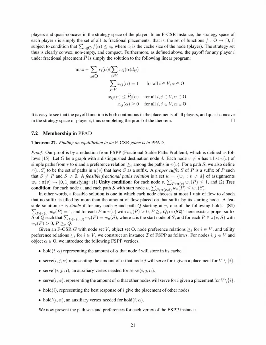
players and quasi-concave in the strategy space of the player. In an F-CSR instance, the strategy space ofeach player i is simply the set of all its fractional placements: that is, the set of functions f : O → [0, 1]subject to condition that

∑α∈O f(α) ≤ ci, where ci is the cache size of the node (player). The strategy set

thus is clearly convex, non-empty, and compact. Furthermore, as defined above, the payoff for any player iunder fractional placement P is simply the solution to the following linear program:

max−∑α∈O

ri(α)(∑j∈V

xij(α)dij)∑j∈V

xij(α) = 1 for all i ∈ V, α ∈ O

xij(α) ≤ Pj(α) for all i, j ∈ V, α ∈ O

xij(α) ≥ 0 for all i, j ∈ V, α ∈ O

It is easy to see that the payoff function is both continuous in the placements of all players, and quasi-concavein the strategy space of player i, thus completing the proof of the theorem.

7.2 Membership in PPAD

Theorem 27. Finding an equilibrium in an F-CSR game is in PPAD.

Proof. Our proof is by a reduction from FSPP (Fractional Stable Paths Problem), which is defined as fol-lows [15]. Let G be a graph with a distinguished destination node d. Each node v 6= d has a list π(v) ofsimple paths from v to d and a preference relation ≥v among the paths in π(v). For a path S, we also defineπ(v, S) to be the set of paths in π(v) that have S as a suffix. A proper suffix S of P is a suffix of P suchthat S 6= P and S 6= ∅. A feasible fractional paths solution is a set w = {wv : v 6= d} of assignmentswv : π(v) → [0, 1] satisfying: (1) Unity condition: for each node v,

∑P∈π(v)wv(P ) ≤ 1, and (2) Tree

condition: for each node v, and each path S with start node u,∑

P∈π(v,S)wv(P ) ≤ wu(S).In other words, a feasible solution is one in which each node chooses at most 1 unit of flow to d such

that no suffix is filled by more than the amount of flow placed on that suffix by its starting node. A fea-sible solution w is stable if for any node v and path Q starting at v, one of the following holds: (S1)∑

P∈π(v)wv(P ) = 1, and for each P in π(v) with wv(P ) > 0, P ≥v Q; or (S2) There exists a proper suffixS of Q such that

∑P∈π(v,S)wv(P ) = wu(S), where u is the start node of S, and for each P ∈ π(v, S) with

wv(P ) > 0, P ≥v Q.Given an F-CSR G with node set V , object set O, node preference relations ≥i for i ∈ V , and utility

preference relations �i for i ∈ V , we construct an instance I of FSPP as follows. For nodes i, j ∈ V andobject α ∈ O, we introduce the following FSPP vertices.

• hold(i, α) representing the amount of α that node i will store in its cache.

• serve(i, j, α) representing the amount of α that node j will serve for i given a placement for V \ {i}.

• serve’(i, j, α), an auxiliary vertex needed for serve(i, j, α).

• serve(i, α), representing the amount of α that other nodes will serve for i given a placement for V \{i}.

• hold(i), representing the best response of i give the placement of other nodes.

• hold’(i, α), an auxiliary vertex needed for hold(i, α).

We now present the path sets and preferences for each vertex of the FSPP instance.

21

• serve(i, α): the path set includes all paths of the form 〈serve(i, α), hold(j, α), d〉, and serve(i, α)prefers 〈serve(i, α), hold(j, α), d〉 over 〈serve(i, α), hold(k, α), d〉 if j ≥i k.

• serve’(i, j, α): the path set includes all paths of the form 〈serve’(i, j, α), serve(i, α), hold(j, α), d〉and the direct path 〈serve’(i, j, α), d〉. For the preference order, serve’(i, j, α) prefers all paths〈serve’(i, j, α), serve(i, α), hold(j, α), d〉 equally, and all of them over the direct path.

• serve(i, j, α): the path set includes the path 〈serve’(i, j, α), d〉 and the direct path 〈serve(i, j, α), d〉with a higher preference for the former path.

• hold(i): the path set includes paths of the form 〈hold(i), serve(i, j, α), d〉, and hold(i) prefers the path〈hold(i), serve(i, j, α), d〉 over 〈hold(i), serve(i, k, β), d〉 if (j, α) wi (k, β).

• hold’(i, α): the path set includes paths of the form 〈hold’(i, α), hold(i), serve(i, j, α), d〉 all of whichare preferred equally, and the direct path 〈hold’(i, α), d〉 which is preferred the least.

• hold(i, α): the path set includes two paths 〈hold’(i, α), d〉 and the direct path with a higher preferencefor the former path.

We now show that the F-CSR instance has an equilibrium if and only if the FSPP instance has anequilibrium. Our proof is by giving a mapping f from global fractional placements in the F-CSR instanceto feasible solutions in the FSPP instance such that (a) if P is an equilibrium for the F-CSR instance, thenf(P ) is an equilibrium for the FSPP instance, and (b) if w is an equilibrium for the FSPP instance, thenf−1(w) is an equilibrium for the F-CSR instance.

Let P denote any fractional placement of the F-CSR instance. We now define the solution f(P ) of theFSPP instance. In f(P ) vertex hold(i, α) plays Pi(α) on the direct path and 1− Pi(α) on the other path inits path set, for every i in V and α in O. The remaining vertices play their best responses, considered in thefollowing order. First, consider vertices of the form serve(i, α). In the best response, the amount played byserve(i, α) on the path 〈serve(i, α), hold(j, α), d〉, equals µ

i,P ,α(j); recall that µ

i,P ,α(j) is is the assignment

that is lexicographically minimal under the node preference relation≥i subject to the condition that µi,P ,α

≤Pk(α) for each k and

∑k µi,P ,α(k) = 1. We next consider the vertices of the form serve’(i, j, α). In its best

response, vertex serve’(i, j, α) plays µi,P ,α

(j) on the path 〈serve’(i, j, α), serve(i, α), hold(j, α), d〉. Next,in its best response, vertex serve(i, j, α) plays µ

i,P ,α(j) on its direct path and 1−µ

i,P ,α(j) on its remaining

path. We now consider the best response of vertex hold(i); it distributes its unit among paths of the form〈hold(i), serve(i, j, α), d〉 (for all j in V \ {i} and α in O) lexicographically maximally under the totalpreorder wi over node-object pairs. That is, hold(i) plays b

i,P(α, j) on the path 〈hold(i), serve(i, j, α), d〉.

We next consider the best response of the vertex hold’(i, α); it plays 1−∑

j bi,P (α, j) on its direct path andbi,P

(α, j) on the path 〈hold’(i, α), hold(i), serve(i, j, α), d〉. This completes the definition of the solution

f(P ).We now argue that if P is an equilibrium so is f(P ). By construction, every vertex other than of the

form hold(i, α) play their best responses in f(P ). We next show that i plays a best response in P if andonly if the vertices hold(i, α) play their best response in f(P ). The best response of hold(i, α) is to play1 −

∑j bi,P (α, j) on the path 〈hold(i, α), hold’(i, α), d〉 and the

∑j bi,P (α, j) on its direct path. The best

response of i in P is to set Pi(α) to∑

j bi,P (α, j). Thus if P is an equilibrium, then so is f(P ). Furthermore,

if w is an equilibrium, by definition of f , P = f−1(w) is well-defined. Since the best responses of i andthe vertices hold(i, α) are consistent, P is also an equilibrium. This completes the reduction from F-CSRto FSPP, placing F-CSR in PPAD.

22

7.3 PPAD-Hardness

This section is devoted to the proof of the following theorem.

Theorem 28. The problem of finding an equilibrium in F-CSR games is PPAD-hard even when the under-lying cost function d is a metric.

Our reduction is from preference games [15]. Given a preference game G with n players 1, 2, . . . , nand their preferences given by ≥i, we construct an F-CSR game G as follows. The game G has a setV of n2 + 3n players numbered 1 through n2 + 3n, and a set O of 2n objects α1, . . . , α2n. We set theutility function for each node to be the sum utility function, thus ensuring that the desired monotonicity andconsistency conditions are satisfied.

We next present the metric cost function d over the nodes. We group the players into four sets V1 ={i : 1 ≤ i ≤ n}, V2 = {i · n + j : 1 ≤ i ≤ n, 1 ≤ j ≤ n}, V3 = {n2 + n + i : 1 ≤ i ≤ n}, andV4 = {n2 + 2n + i : 1 ≤ i ≤ n}. For each node i in V1 and j in V3, we set dii = 2 and dij = 4. Weset dn2+n+i,n2+2n+i = 3. For each node i in V1 and k = i · n + j, we set dik as follows: if j >i i thendij equals 6 − `/n when j is the `th most preferred player for i; if i ≥i j, then dij equals 1. All the otherdistances are obtained by using metric properties.

We finally specify the object weights. For k ∈ V1, we set rk(αi) = 1 for all i 6= k such that i ≥k k; weset rk(αk) = 2.5 such that 4 < 2rk(αk) ≤ 5. For node k = i · n + j in V2, we set rk(αj) = 1. For nodek = n2 + n + i in V3, we set rk(αi) = rk(αi+n) = 1. Finally, for node k = n2 + 2n + i in V4, we setrk(αi+n) = 1.

Given a placement P for G, we define a solution ω(P ) = {wij} for the preference game G: wij =

Pi(αj). The following lemma immediately follows from the definition of G.

Lemma 29. The following statements hold for any placement P for G.

• For k = i · n+ j, 1 ≤ j ≤ n, Pk is a best response to P−k if and only if Pk(αj) = 1.

• For k = n2 + n+ i, 1 ≤ i ≤ n, Pk is a best response to P−k if and only if Pk(αn+i) = 1.

• For k = n2 + n+ i, Pk is a best response to P−k if and only if Pk(αi) = 1− Pi(αi) and Pk(αn+i =Pi(αi).

Lemma 30. Let P be a placement for G in which every node not in V1 plays their best response. Then, thebest response of a node i in V1 is the lexicographically maximum (Pi(αj1), Pi(αj2), . . . , Pi(αjn)), wherej1 ≥i j2 ≥i · · · ≥i jn, subject to the constraint that Pi(αj) ≤ Pj(αj) for j 6= i.

Proof. Fix a node i in V1. By Lemma 29, node i ·n+ j holds object j, for 1 ≤ j ≤ n; each of these nodes isat distance at least 5 and at most 6 away from i. By Lemma 29, for every node k = n2 + n+ j, 1 ≤ j ≤ n,Pk(αj) = 1− Pj(αj) and Pk(αn+j) = Pj(αj).

We now consider the best response of node i. We first note that for any j ∈ {1, . . . , n} \ {i} such thati ≥i j, Pi(αj) = 0 since the nearest full copy of αj is nearer than the nearest node holding any fractionof object αi. Let S denote the set of j such that j ≥i i. For any j in S \ {i}, Pi(αj) ≤ Pj(αj) sincenode n2 + n + j at distance 5 holds 1 − Pj(αj) fraction of αj , the nearest node holding any fraction ofαi is at distance 4, and 4ri(αi) > 5ri(αj). Furthermore, for any j, k in S if j >i k, then the farthestPj(αj) fraction of αj is farther than the farthest Pk(αk) fraction of αk, implying that in the best response, ifPi(αj) < Pj(αj) then Pi(αk) = 0. Thus, the best response of i is the unique lexicographically maximumsolution (Pi(αj1), Pi(αj2), . . . , Pi(αjn)), where j1 ≥i j2 ≥i · · · ≥i jn, subject to the constraint thatPi(αj) ≤ Pj(αj) for j 6= i.

23

Lemma 31. A placement P is an equilibrium for G if and only if ω(P ) is a equilibrium for G and everynode not in V1 plays their best response in P .

Proof. Consider an equilibrium placement P for G Clearly, every node plays their best response. We nowprove that ω(P ) is an equilibrium for G. Fix a node i in V1. By Lemma 30, the best response of i is theunique lexicographically maximum solution (Pi(αj1), Pi(αj2), . . . , Pi(αjn)), where j1 ≥i j2 ≥i · · · ≥i jn,subject to the constraint that Pi(αj) ≤ Pj(αj) for j 6= i. Since this applies to every node i, it is immediatefrom the definitions of ω(P ) and preference games that if P is an equilibrium for G then ω(P ) is anequilibrium for G.

We now consider the reverse direction. Suppose we have a placement P in which every player not inV1 plays their best response and ω(P ) is an equilibrium for the preference game G. By Lemma 30 and thedefinition of ω(P ), the best response of i in G matches that in the F-CSR game; hence every player in V1

also plays their best response in P , implying that P is an equilibrium for G.

The construction of G from G is clearly polynomial time. Furthermore, given any equilibrium for G,an equilibrium for G can be constructed in linear time. We thus have a reduction from a PPAD-completeproblem to F-CSR implying that the latter is PPAD-hard, thus completing the proof of Theorem 28.

8 Concluding remarks

In this paper we have defined integral and fractional selfish replication games (CSR and F-CSR) in net-works, where the cache capacity of each node is bounded and all objects are of uniform size. We haveshown that a pure Nash equilibrium can be computed for every hierarchical network, using a new notion offictional players. In general, we have almost completely characterized the complexity of CSR games: Forwhat classes of games do equilibria exist? Can we determine efficiently whether they exist? When theydo exist, can we efficiently find them? One complexity question that is still open is the case of undirectednetworks with binary preferences. We conjecture that finding equilbria in such games (which we proveare potential games) is PLS-hard. In general, we would like to study the convergence of the best responseprocess for the cases of games where equilibria exist.

We showed that F-CSR games always have equilibria, though they may be hard to find. It is not hard toargue that an equilibrium in the corresponding integral variant is an equilibrium in the fractional instance.So whenever an “integral” equilibrium can be determined efficiently, so can a “fractional” equilibrium. Aninteresting direction of research is to identify other special cases of fractional games where equilibria maybe efficiently determined. We also note that our proof of existence of equilibria in F-CSR games, currentlypresented for the case of unit-size objects, extends to arbitrary object sizes.

Finally, we note that our model assumes that the sets of nodes, objects, and preference relations are allstatic. We believe our results will be meaningful for environments where these sets change infrequently. De-veloping better models for addressing more dynamic scenarios is an important practical research direction.

References

[1] E. Angel, E. Bampis, G. G. Pollatos, and V. Zissimopoulos. Optimal data placement on networks withconstant number of clients. CoRR, abs/1004.4420, 2010.

[2] K. Arrow. Social Choice and Individual Values. Yale University Press, 1951.

[3] I. D. Baev, R. Rajaraman, and C. Swamy. Approximation algorithms for data placement problems.SIAM J. Comput., 38(4):1411–1429, 2008.

24

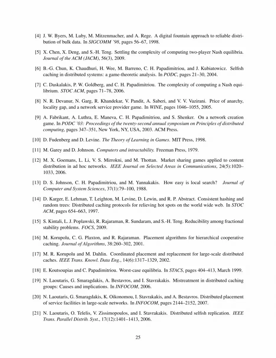
[4] J. W. Byers, M. Luby, M. Mitzenmacher, and A. Rege. A digital fountain approach to reliable distri-bution of bulk data. In SIGCOMM ’98, pages 56–67, 1998.

[5] X. Chen, X. Deng, and S.-H. Teng. Settling the complexity of computing two-player Nash equilibria.Journal of the ACM (JACM), 56(3), 2009.

[6] B.-G. Chun, K. Chaudhuri, H. Wee, M. Barreno, C. H. Papadimitriou, and J. Kubiatowicz. Selfishcaching in distributed systems: a game-theoretic analysis. In PODC, pages 21–30, 2004.

[7] C. Daskalakis, P. W. Goldberg, and C. H. Papadimitriou. The complexity of computing a Nash equi-librium. STOC ACM, pages 71–78, 2006.

[8] N. R. Devanur, N. Garg, R. Khandekar, V. Pandit, A. Saberi, and V. V. Vazirani. Price of anarchy,locality gap, and a network service provider game. In WINE, pages 1046–1055, 2005.

[9] A. Fabrikant, A. Luthra, E. Maneva, C. H. Papadimitriou, and S. Shenker. On a network creationgame. In PODC ’03: Proceedings of the twenty-second annual symposium on Principles of distributedcomputing, pages 347–351, New York, NY, USA, 2003. ACM Press.

[10] D. Fudenberg and D. Levine. The Theory of Learning in Games. MIT Press, 1998.

[11] M. Garey and D. Johnson. Computers and intractability. Freeman Press, 1979.

[12] M. X. Goemans, L. Li, V. S. Mirrokni, and M. Thottan. Market sharing games applied to contentdistribution in ad hoc networks. IEEE Journal on Selected Areas in Communications, 24(5):1020–1033, 2006.

[13] D. S. Johnson, C. H. Papadimitriou, and M. Yannakakis. How easy is local search? Journal ofComputer and System Sciences, 37(1):79–100, 1988.

[14] D. Karger, E. Lehman, T. Leighton, M. Levine, D. Lewin, and R. P. Abstract. Consistent hashing andrandom trees: Distributed caching protocols for relieving hot spots on the world wide web. In STOCACM, pages 654–663, 1997.

[15] S. Kintali, L. J. Poplawski, R. Rajaraman, R. Sundaram, and S.-H. Teng. Reducibility among fractionalstability problems. FOCS, 2009.

[16] M. Korupolu, C. G. Plaxton, and R. Rajaraman. Placement algorithms for hierarchical cooperativecaching. Journal of Algorithms, 38:260–302, 2001.

[17] M. R. Korupolu and M. Dahlin. Coordinated placement and replacement for large-scale distributedcaches. IEEE Trans. Knowl. Data Eng., 14(6):1317–1329, 2002.

[18] E. Koutsoupias and C. Papadimitriou. Worst-case equilibria. In STACS, pages 404–413, March 1999.

[19] N. Laoutaris, G. Smaragdakis, A. Bestavros, and I. Stavrakakis. Mistreatment in distributed cachinggroups: Causes and implications. In INFOCOM, 2006.

[20] N. Laoutaris, G. Smaragdakis, K. Oikonomou, I. Stavrakakis, and A. Bestavros. Distributed placementof service facilities in large-scale networks. In INFOCOM, pages 2144–2152, 2007.

[21] N. Laoutaris, O. Telelis, V. Zissimopoulos, and I. Stavrakakis. Distributed selfish replication. IEEETrans. Parallel Distrib. Syst., 17(12):1401–1413, 2006.

25

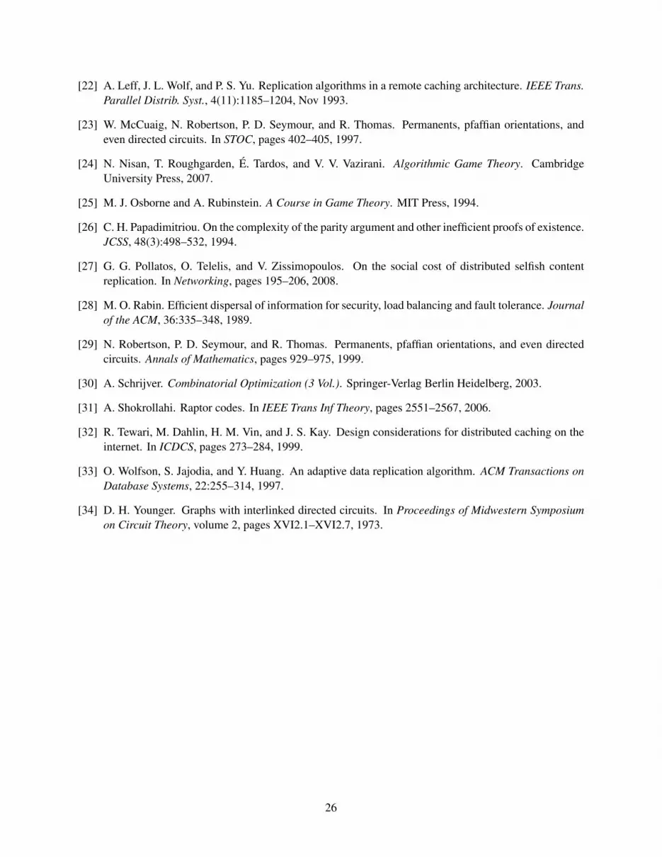
[22] A. Leff, J. L. Wolf, and P. S. Yu. Replication algorithms in a remote caching architecture. IEEE Trans.Parallel Distrib. Syst., 4(11):1185–1204, Nov 1993.

[23] W. McCuaig, N. Robertson, P. D. Seymour, and R. Thomas. Permanents, pfaffian orientations, andeven directed circuits. In STOC, pages 402–405, 1997.

[24] N. Nisan, T. Roughgarden, E. Tardos, and V. V. Vazirani. Algorithmic Game Theory. CambridgeUniversity Press, 2007.

[25] M. J. Osborne and A. Rubinstein. A Course in Game Theory. MIT Press, 1994.

[26] C. H. Papadimitriou. On the complexity of the parity argument and other inefficient proofs of existence.JCSS, 48(3):498–532, 1994.

[27] G. G. Pollatos, O. Telelis, and V. Zissimopoulos. On the social cost of distributed selfish contentreplication. In Networking, pages 195–206, 2008.

[28] M. O. Rabin. Efficient dispersal of information for security, load balancing and fault tolerance. Journalof the ACM, 36:335–348, 1989.

[29] N. Robertson, P. D. Seymour, and R. Thomas. Permanents, pfaffian orientations, and even directedcircuits. Annals of Mathematics, pages 929–975, 1999.

[30] A. Schrijver. Combinatorial Optimization (3 Vol.). Springer-Verlag Berlin Heidelberg, 2003.

[31] A. Shokrollahi. Raptor codes. In IEEE Trans Inf Theory, pages 2551–2567, 2006.

[32] R. Tewari, M. Dahlin, H. M. Vin, and J. S. Kay. Design considerations for distributed caching on theinternet. In ICDCS, pages 273–284, 1999.

[33] O. Wolfson, S. Jajodia, and Y. Huang. An adaptive data replication algorithm. ACM Transactions onDatabase Systems, 22:255–314, 1997.

[34] D. H. Younger. Graphs with interlinked directed circuits. In Proceedings of Midwestern Symposiumon Circuit Theory, volume 2, pages XVI2.1–XVI2.7, 1973.

26