Embed Size (px)
Citation preview
THE INTERACTION OF SOUND WITH TURBULENT FLOW
by
GEORGE PETER SUCCI
B.S., Massachusetts Institute of Technology(1973)
SUBMITTED IN PARTIAL FULFILLMENTOF THE REQUIREMENTS FOR THE
DEGREE OF
DOCTOR OF PHILOSOPHY
at the
MASSACHUSETTS INSTITUTE OF TECHNOLOGY
JUNE, 1977
Signature of Author . .Department of Physics, March 1977
Certified by./ Thesis Supervisor
I
Accepted by .Chairman, Dpa .rtmentof Physics Committee . . .hairman, Department of Physics Committee
Archives'Ss
JUN 20 1977
Rwo
THE INTERACTION OF SOUND WITH TURBULENT FLOW
by
GEORGE PETER SUCCI
Submitted to the Department of Physics on February 21,1977 in partial fulfillment of the requirements forthe Degree of Doctor of Philosophy.
ABSTRACT
Herein the generation of sound by subsonicturbulent air flow in cavities is studied. Two typesof cavity modes are considered; the axial modes ofa pipe open at both ends and the transverse modes ofa rectangular duct. Experiments were performed tomeasure the acoustic spectra of the flow generated noise.A linear theoretical analysis, based on an isotropicmodel of the turbulent fluctuations, is developed topredict this spectra. Certain non linear phenomena(screech), due to the alteration of the sourceflow by the emitted sound, are identified. Thenecessary conditions for such instabilitiesexamined.
Thesis Supervisor: K. U. Ingard
Title: Professor of Physics
2
ACKNOWLEDGEMENTS
I greatfully acknowledge the guidance of my
advisor, Dr. Uno Ingard. His clear explanation of the
physics of sound was essential to the task of completing
the thesis. I also thank the doctoral thesis committee
members, Dr. Bekefi and Dr. Dupree, for their interest and
suggestions.
On the non technical side, much appreciation is
due to my friend, Meg, who is the best of company when
I am buried in work.
The thesis is dedicated to my father, who
introduced me to experimental physics by granting me free
access to his tool box. His unfailing patience in
describing the inner Works of our household encouraged
me to think about the natural world.
3
TABLE OF CONTENTS
ABSTRACT 2
ACKNOWLEDGEMENTS 3
LIST OF FIGURES 8
NOMENCLATURE 13
INTRODUCTION 20
1. FREE SPACE JET NOISE 23
1.1 Introduction 23
1.2 Turbulence as a Source of Sound 27
1.2.1 Review of Classical Acoustics 27
1.2.2 Derivation of Lighthill's Equation 29
1.2.3 Ribner's Equation 31
1.3 A Comparison of Three Calculations 34
1.3.1 Monopole Source, Frequency-domain 34Green's Function
1.3.2 Monopole Source, Time-dome Green's 39Function
1.3.3 Quadrupole Source, Time-domain 43Green's Function
1.3.4 Velocity Intensity and Total Power 48
1.4 Comments on the Turbulent Correlation 49
1.4.1 Choice of the Correlation 49
1.4.2 The Eighth Power Law 53
1.4.3 The Kolmogorov Inertial Subrange 55
1.4.4 Gaussian Correlation and the Relation 56Between the Turbulent and AcousticSpectra
1.5 Summary 59
2. EXCITATION OF AXIAL PIPE MODES 62
2.1 Introduction 62
2.2 Experiment 64
2.2.1 Apparatus and Procedure 64
2.2.2 Variation With Pipe Length 66
4
TABLE OF CONTENTS (cont'd.)
Page
2.2.3 Variation With Flow Speed 67
2.2.4 Variation With Microphone Placement 69
2.2.5 Effect of Liner 71
2.3 Theory 72
2.3.1 On Distinguishing Mean Flow Effects 72from Turbulent Fluctuations
2.3.2 The Green's Function 75
2.3.3 Analysis of the Pressure Reflection 77Coefficient
2.3.4 Transmission Out of the Ends of the 81Pipe
2.3.5 Effect of the Convective Derivative 85on the Source Term
2.3.6 Acoustic Field of a Point Source 89
2.3.7 Acoustic Field of a Distributed Source 90
2.3.8 The Upstream Acoustic Field 92
2.3.9 Numerical Comparison of Theory to 95Experiment
3. EXCITATION OF TRANSVERSE DUCT MODES 99
3.1 Introduction 99
3.2 Experiments 101
3.2.1 Apparatus and Procedures 101
3.2.2 Basic Effect 104
3.2.3 Spectra Variation With Jet Velocity 105and Diameter
3.2.4 Reduction by Strouhl Number 107
3.2.5 Separating Linear From FeedbackEffects 110
3.2.6 Effect of Inlet Turbulence 112
3.2.7 Orifice Mounted on Axis 113
3.2.8 Upstream Versus Downstream Radiation 114
3.2.9 Effect of Microphone Placement 115
5
TABLE OF CONTENTS (cont'd.)
Page
3.3 Theory
3.3.1 Duct Acoustics With Mean Flow
3.3.2 The Green's Function
3.3.3 Random Source Representation in a Duct
3.3.4 The Radiated Pressure
3.3.5 Gaussian Correlation and a QualitativeAnalysis of the Low Frequency Spectra
3.3.6 Damping and the Smoothing of the HighFrequency Spectra
3.3.7 Radiation Impedance and the Similarityof the High Frequency Duct Spectra tothe Free Space Spectra
3.3.8 Velocity Power and Intensity
3.3.9 A Numeric Comparison of the Predictedto the Observed Low Frequency Spectra
4. SCREECH
4.1 Introduction
4.2 Orifice Screech
4.2.1 Orifice Screech: Apparatus andProcedure
4.2.2 Screech Dependence on the length toDiameter Ratio and Flow Speed
4.2.3 Similarity to Hole Tone
4.2.4 Perturbation of the Flow by Screens
4.2.5 A Kinematic Calculation of the Feed-back Frequency
4.2.6 Cavity Mode Excitation
4.3 Impingement Screech
4.3.1 Impingement Screech: Apparatus andProcedure
4.3.2 Free Jet Spectra From a Pipe andOrifice
4.3.3 Turbulent Sound Level Increase Due tothe Obstruction of the Flow by a FlatPlate
6
116
116
121
123
133
137
139
143
149
152
155
155
159
159
161
164
165
167
170
177
177
178
180
TABLE OF CONTENTS (cont'd.)
Page
4.3.4 Impingement Screech from a Tapered 181Orifice
4.3.5 Coupling of Impingement Screech to 184a Cavity Mode
4.3.6 Direct Comparison of Impingement 186Screech to Screech in Ducts
5. CONCLUSIONS AND RECOMMENDATIONS 188
APPENDIX: STABILITY ANALYSIS OF THE PERTURBED JET IN 196THE PRESENCE OF BOUNDARIES
A. 1 Introduction 196
A. 2 Problem Statement 197
A. 3 Integral Solution 199
A. 4 Comments on the Evaluation of the 204Integral
A. 5 Removing the Duct Wall 205
A. 6 Simplification to Two Dimensions 208
A. 7 Comments on the Application of the 212Theory to Screech
REFERENCES 217
FIGURES 225
BIOGRAPHICAL NOTE 292
LIST OF TABLES
TABLE
3.1 -- Table of Fourier Transforms 130
3.2 -- Table of Statistical Transform 131
4.1 -- Data for Screech Coupled to Cavity Modes 175
4.2 -- Normalized Data for Screech Coupled toCavity Modes 176
7
LIST OF FIGURES
FIGURE Page
1.1 -- Correlation contours for a free jet (Ref. 15). 225
1.2 -- Peak frequency of acoustic power spectra 226versus downstream distance (Ref.63).
1.3 -- Free space spectra fit by three independent 227isotropic correlation functions.
2.1 -- Acoustic spectra versus mean flow. 228
2.2 -- Apparatus used in axial mode study. 229
2.3 -- Frequency interval between axial modes 230versus pipe length.
2.4 -- Frequency interval between axial modes 231versus mean flow speed.
2.5 -- Comparison of inlet and exit pipe noise. 232
2.6 -- Inlet pressure reflection coefficient. 233
2.7 -- Exit pressure reflection coefficient. 234
2.8 -- Comparison of experimental and theoretical 235spectra at Mach .10.
2.9 -- Comparison of experimental and theoretical 236spectra at Mach .14.
2.10 -- Comparison of experimental and theoretical 237spectra at Mach .40.
2.11 -- Strouhl numbers used to compute the spectra. 238
2.12 -- Correlation time based on the Strouhl 239numbers.
2.13 -- Polar intensity plot for a 2" long pipe. 240
2.14 -- Polar intensity plot for a 4" long pipe. 241
2.15 -- Polar intensity plot for a 6" long pipe. 242
8
LIST OF FIGURES (cont'd.)
FIGURES Page
2.16 -- Polar intensity plot for an 8" long pipe. 243
2.17 -- Polar intensity plot for a 10" long pipe. 244
2.18 -- Polar intensity plot for a 12" long pipe. 245
2.19 -- Polar intensity plot for a 14" long pipe. 246
2.20 -- Polar intensity plot for a 16" long pipe. 247
2.21 -- Polar intensity plot for an 18" long pipe. 248
3.1 -- Photo of experimental apparatus used to 249study the turbulent excitation of trans-verse modes in ducts.
3.2 -- Hot wire velocity calibration. 250
3.3 -- Photo of microphone holder used to detect 251the mode shape of the radiated sound.
3.4 -- Photo of orifice plates used to form air jets. 252
3.5 -- Photo of 60" pipe used to form air jet. 253
3.6 -- Comparison of low and high frequency 254spectra in a rectangular duct.
3.7 -- Low frequency spectra using a 1/4" diameter 255orifice plate.
3.8 -- Low frequency spectra using a 1/2" diameter 256orifice plate.
3.9 -- Low frequency spectra using a 1" diameter 257orifice plate.
3.10 -- High frequency spectra using a 1/4" diameter 258orifice plate.
3.11 -- High frequency spectra using a 1/2" diameter 259orifice plate.
3.12 -- High frequency spectra using a 1" diameter 260orifice plate.
9
LIST OF FIGURES (cont'd.)
FIGURES Page
3.13 -- Reduction of low frequency spectra by 261Strouhl number. Here f =-2 ' 5.7 KC.
D3.14 -- Reduction of low frequency spectra by Strouhl 262
number. Here f =.2V = 2.5 KC.S D
3.15 -- Reduction of high frequency spectra by Strouhl 263number. Here f =_2V __ 1.9 KC.
S D
3.16 -- Sound level versus mean flow for a 1/2" 264diameter orifice plate. Levels at firstcutoff frequency (1.6 KC) are compared tothose at a frequency between the first andsecond cutoff.
3.17 -- Sound level versus mean flow for a 1/2" 265diameter orifice plate. Two frequencies atwhich screech occurs are shown.
3.18 -- Low frequency spectra from an initially 266turbulent jet.
3.19 -- High frequency spectra from an initially 267turbulent jet.
3.20 -- Low frequency spectra observed when jet and 268duct axis are parallel.
3.21 -- Comparison of upstream and downstream 269radiated acoustic spectra.
3.22 -- Transverse variation of radiated sound at 270frequencies selected to show the mode shape.
3.23 -- Influence of mode shape on the detected 271spectra.
3.24 -- Radiation resistance of a simple source. 272
3.25 -- Comparison of theoretical and experimental 273spectra at Mach .6 for a 1/2" diameter orificeplate.
10
LIST OF FIGURES (cont'd.)
FIGURES Page
4.1 -- Experimental apparatus used to generate 274screech.
4.2 -- Screech frequency versus flow speed for a 2751/4" long orifice plate.
4.3 -- Screech frequency versus flow speed for a 2761/2" long orifice plate.
4.4 -- Screech frequency versus flow speed for a 2771" long orifice plate.
4.5 -- Summary of tests made to determine the length 278to diameter ratio necessary for screech.
4.6 -- Summary of tests made to determine the length 279to diameter ratio necessary for the modifiedhole tone.
4.7 -- Screech frequencies versus flow speed for the 280modified hole tone with a 5/8" inside diameter.
4.8 -- Screech frequency versus flow speed for the 281modified hole tone with a 4-11/32" insidediameter.
4.9 -- The suppression of orifice screech by screens. 282
4.10 -- Typical orifice screech spectra. 283
4.11 -- Screech spectra for the modified hole tone at 284Mach .33.
4.12 -- Screech spectra for the modified hole tone at 285Mach .34. All but the first peak are shownto coincide with cavity modes which have theindicated number of nodal diameters.
4.13 -- Experimental apparatus used to generate 286impingement screech.
4.14 -- Free space spectra from a 1/2" diameter 287orifice plate.
4.15 -- Free space spectra from a 60" long pipe with 288a 1/2" inside diameter.
11
LIST OF FIGURES (cont'd.)
FIGURES Page
4.16 -- Increased sound level due to obstruction 289of the flow by a flat plate.
4.17 -- Impingement screech versus distance to plate. 290
4.18 -- Direct comparison of impingement screech to 291screech observed in a rectangular duct.
12
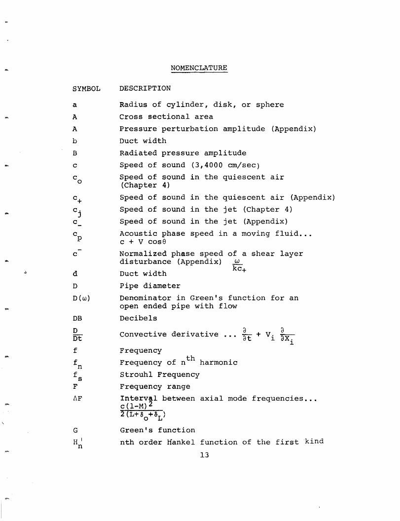
NOMENCLATURE
DESCRIPTION
Radius of cylinder, disk, or sphere
Cross sectional area
Pressure perturbation amplitude (Appendix)
Duct width
Radiated pressure amplitude
Speed of sound (3,4000 cm/sec)
Speed of sound in the quiescent air(Chapter 4)
Speed of sound in the quiescent air (Appendix)
Speed of sound in the jet (Chapter 4)
Speed of sound in the jet (Appendix)
Acoustic phase speed in a moving fluid...c + V cosO
Normalized phase speed of a shear layerdisturbance (Appendix) _
kc+Duct width
Pipe diameter
Denominator in Green's function for anopen ended pipe with flow
Decibels
Convective derivative ... a + Viat i x.Frequency
Frequency of n harmonic
Strouhl Frequency
Frequency range
Interval between axial mode frequencies...c(1-M)2
2(L+80 +&)
Green's function
nth order Hankel function of the first kind
13
SYMBOL
a
A
A
b
B
c
c o
c+
c.
c
cP
c
d
D
D (W)
DB
DDt
f
fnfsF
AF
G
H n
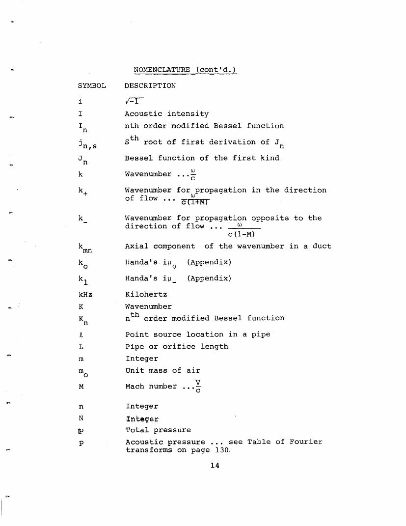
NOMENCLATURE (cont'd.)
DESCRIPTION
Acoustic intensity
nth order modified Bessel function
thS root of first derivation of J
Bessel function of the first kind
Wavenumber .cc
Wavenumber for propagation in the directionof flow ...
Wavenumber for propagation opposite to thedirection of flow ..
c (l-M)
Axial component of the wavenumber in a duct
Ilanda's ip 0
Handa's i_
(Appendix)
(Appendix)
Kilohertz
Wavenumber
nth order modified Bessel function
Point source location in a pipe
Pipe or orifice length
Integer
Unit mass of air
VMach number .. V
Integer
Integer
Total pressure
Acoustic pressure ... see Table of Fouriertransforms on page 130.
14
SYMBOL
i
I
In
n,s
Jn
k
k
kmn
k1
kHz
K
Kn
L
mm
o
M
n
N
p
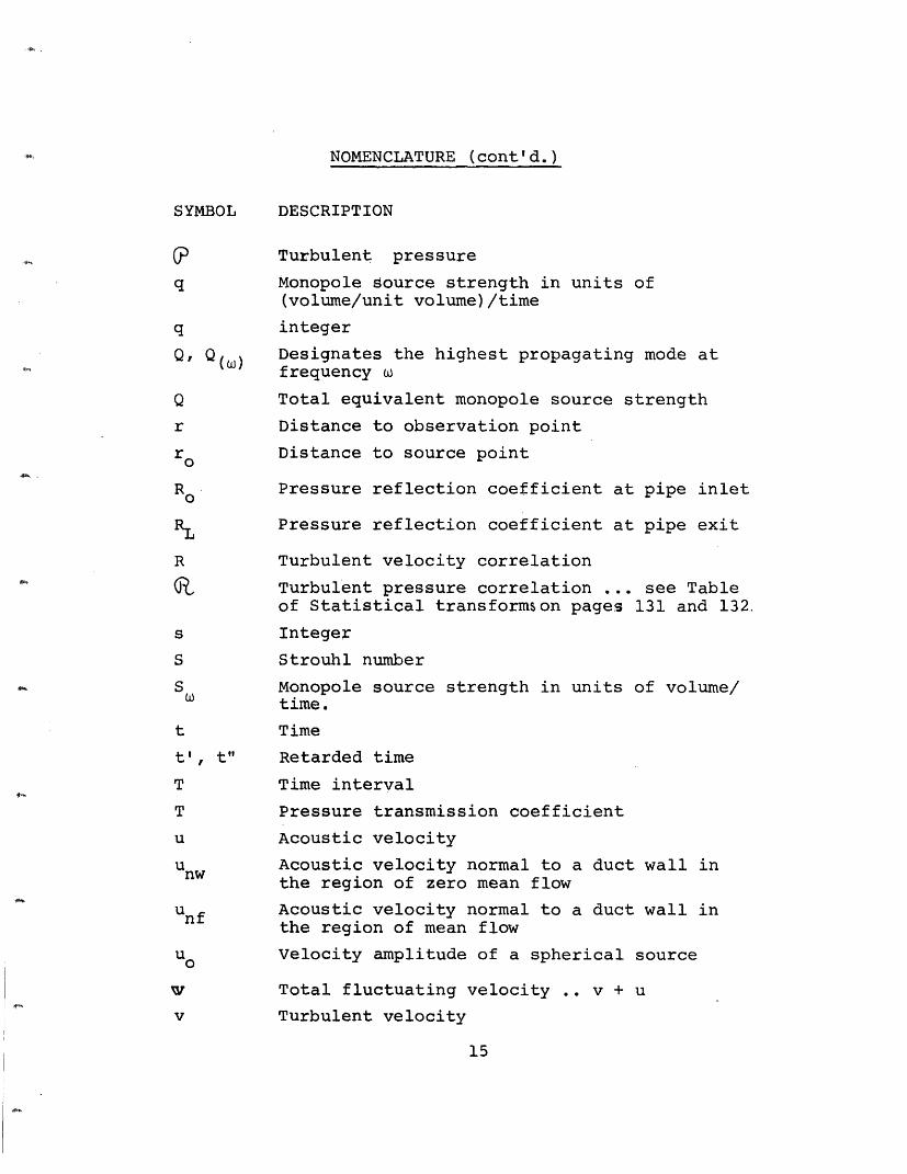
NOMENCLATURE (cont'd.)
SYMBOL DESCRIPTION
Turbulent pressure
q Monopole Source strength in units of(volume/unit volume)/time
q integer
Q, Q) Designates the highest propagating mode atfrequency w
Q Total equivalent monopole source strength
r Distance to observation point
ro Distance to source point
R° Pressure reflection coefficient at pipe inlet
RL Pressure reflection coefficient at pipe exit
R Turbulent velocity correlation
Turbulent pressure correlation ... see Tableof Statistical transformson pages 131 and 132.
s Integer
S Strouhl number
S Monopole source strength in units of volume/time.
t Time
t', t" Retarded time
T Time interval
T Pressure transmission coefficient
u Acoustic velocity
unw Acoustic velocity normal to a duct wall inthe region of zero mean flow
unf Acoustic velocity normal to a duct wall inthe region of mean flow
uo Velocity amplitude of a spherical source
Total fluctuating velocity .. v + u
v Turbulent velocity
15
.*.
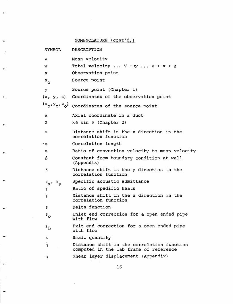
NOMENCLATURE (cont'd.)
SYMBOL DESCRIPTION
V Mean velocity
w Total velocity ... V + ... V + v + u
x Observation point
x ° Source point
y Source point (Chapter 1)
(x, y, z) Coordinates of the observation point
(XoYoZo) Coordinates of the source point
z Axial coordinate in a duct
Z ka sin (Chapter 2)
ca Distance shift in the x direction in thecorrelation function
a Correlation length
a Ratio of convection velocity to mean velocity
Constant from boundary condition at wall(Appendix)
Distance shift in the y direction in thecorrelation function
Ax' By Specific acoustic admittance
Y Ratio of spedific heats
y Distance shift in the z direction in thecorrelation function
8 Delta function
8 Inlet end correction for a open ended pipewith flow
8L Exit end correction for a open ended pipewith flow
£ Small quantity
Distance shift in the correlation functioncomputed in the lab frame of reference
Shear layer displacement (Appendix)
16
NOMENCLATURE (cont'd.)
DESCRIPTION
Mode wavenumber in a hard wall duct
Angle between flow and observer
Radiation resistance of a simple source in aduct.
Wave length of sound
Mean square amplitude of the cross duct mode
Coefficient of viscosity
(Q-KV) 2 + K2 (Appendix)
_( )2 + K2c+(Appendix)
Kinematic viscosity ... /P
Distance shift in the correlation function
computed in the jet frame of reference
Eddy volume
3.14159... ratio of circumference to diameterof a circle
Radiated acoustic power
Total density ... Po +P +P
Mean density
Turbulent density fluctuation
Acoustic density fluctuation
Density of acoustic modes in a rectangularduct at the wave number (kx,ky)
Mode wavenumber in a second absorbing duct
Mode wavenumber in a sound absorbing duct
Summation symbol
17
SYMBOLS
' mn
0a
X
Amn
1J
1-I
V
7
II
Po
p0P
P
P (kx, ky)
amrb
£
NOMENCLATURE (cont'd.)
DESCRIPTION
Time shift in the correlation function
Axial angle in cylindrical coordinates
Phase of Fourier coefficient
Characteristic function for a cross duct mode
Coefficient of heat conduction
Angular frequency ... 2f
Source volume
Angular frequency (Appendix)
Order of magnitude
Average of N measurements
Real part
Pipe inlet
Incident wave
Tensor component
Acoustic wave upstream of the source pointpropagating in the direction of flow
Acoustic wave upstream of the source pointpropagating opposite to the direction of flow
Pipe exitth
m, n transverse mode in a duct
n th order
n th harmonic
Source point
qth transverse mode in a duct
Reflected wave
Acoustic wave downstream of the source pointpropagating in the direction of flow
Acoustic wave downstream of the source pointpropagating opposite to the direction of flow
Strouhl frequency
Transmitted wave
Axial component
18
SYMBOL
T
X
Si
Re
SUB-SCRIPTS
0
i
i, j
9+
n
L
m,n
n
o
q
r
r+
st
z
NOMENCLATURE (cont'd.)
SUB-SCRIPT DESCRIPTION
+ Propagation in the flow direction
+ Points outside the jet (Appendix)... r>Rj
Propogation opposite to the direction of flow
Points inside the jet (Appendix) ... r<R.
SUPERSCRIPT
Vector
A Unit vector
Time average
19
INTRODUCTION
In the now classical theory of sound from turbulent
flow by Lighthill ' 2 boundaries were not considered.
Further, it was assumed that the turbulent flow field was
not altered by sound emission.
For closed systems, such as cavities and wave-
guides, discrete modes may be excited. It is possible
that the coupling between the flow field and acoustic
modes is strong enough to alter the primary flow field.
Under such conditions acoustically induced flow instabilities
such as whistles occur. The objective of this thesis is
to study the turbulent excitation of duct modes and the
conditions for possible instabilities.
Chapter One reviews the theory of turbulent
excitation of sound in free space. The induced acoustic
field is calculated in three ways. The sound field is
determined by time-domain Green's function technique for
both Lighthill's1' 2 quadrupole source model and
Ribner's3 , 4equivalent distribution of monopoles. The
omission of turbulent shear interactions in an isotropic
monopole model of the turbulence is demonstrated. The
sound field is also determined by a frequency-domain Green's
function technique for a monopole distribution. Time and
frequency domain calculations yield identical results for
the monopole source distribution. However, the frequency
domain technique allows the analysis to be extended to
20
systems with boundaries in simple fashion.
Chapter Two examines the excitation of axial
pipe modes by turbulent flow theoretically and experiment-
ally. The experiment is performed by drawing air through
a cylindrical pipe. The observations demonstrate that
mode excitation diminishes as the flow speed increases.
This is attributed to end losses which increase with flow
speed. A Green's function, based on the measured pressure
reflection coefficients, is used to predict the variation
in spectra with flow.
Chapter Three demonstrates the excitation of
transverse modes in pipes experimentally. Air is drawn
through a small orifice into a rectangular duct. Pro-
nounced asymmetric peaks are observed at the first few
cutoff frequencies. The asymmetric nature of the
peaks and relative spectral intensity are again explained
by Green's function techniques. For high frequencies,
where a large number of modes can propagate, the spectra
resembles the free-space jet spectra. In this frequency
range, the duct radiation impedance asymptotically
approaches the free space impedance, hence the similar
response to similar source distributions.
Chapter Four examines feedback instabilities,
cases where the emitted sound field alters the jet flow
itself. The chapter concentrates on screech tones of
21
circular orifices having length to diameter ratios
between one half and two. The frequency dependance of the
screech on Mach number and length is explained by a
kinematic analysis of the feedback loop. It is further
demonstrated that the frequency of the feedback instability
must be approximately equal to that of an acoustic made
for screech to occur. Similar observations are presented
with regard to air jets impinging on plates.
In conclusion two mechanisms exist whereby the
acoustic energy from a turbulent jet can be concentrated
at select frequencies. The first is the selective
response of a medium with boundaries to a random source.
The spectral line shape for such cases is accounted for
by Green's function techniques. The second mechanism is
the feedback instability which requires coupling of the
jet flow to the acoustic field. Here the modification
of the jet flow must be considered to determine the excita-
tion frequencies.
It is recommended that future work be done on
the screech instability. The influence of the acoustic
cavity mode on the feedback instability should be examined
in greater detail. In particular, the convection speed
of jet column disturbances with and without adjacent
resonators should be determined experimentally. Further-
more, the mechanism which limits the amplitude of the
screech should be determined.
22
1. FREE SPACE JET NOISE
1.1 Introduction
Aerodynamic noise may be defined as that noise
which is generated as a direct result of airflow without
any part due to the vibrations of solid bodies.5 The
basic theory of aerodynamic sound generation and its
application to noise radiated from turbulent jets was first
given in two papers by Lighthill.1' 2 He considers a
fluctuating hydrodynamic flow covering a limited region
surrounded by a large volume of fluid which is at rest,
apart from the infintessimal amplitude sound waves
radiated by the turbulent flow. The exact equations
governing the density perturbations in a turbulent, viscous,
heat conducting fluid are compared with the approximate
equations appropriate to an inviscid non heat conducting
media at rest. The difference between the two sets of
equations is treated as if it were an externally applied
source field which is known if the flow is known.
The forcing terms fall into three groups: a
Reynolds stress due to turbulent momentum convection,
a term due to heat conduction and one due to viscous
stresses. Not all terms contribute equally to the
acoustic field, only the Reynolds stresses need be
considered. It is a well established fact that in
turbulent flow6' 7 the ratio of inertial to viscous
23
stresses, the Reynolds number,3VD , is usually quite
large, at least in most aero-acoustic applications. We,
therefore, neglect viscosity. If we further assume that
the flow emanates from a region of uniform temperature
the effects of heat conduction ought to be the same order
of magnitude as the viscous effects. This is providing
the Prandtl number, S/,/ is of order one, in air
jA4//= .73. Our conclusion is that only the Reynolds
stress contributes to the acoustic field. Lighthill
further assumes that the turbulent flow is incompressible
in the source region. To calculate the acoustic field
one needs the statistical distribution of the Reynolds
stresses
Ribner simplified the source field by observing
that in low speed turbulence Lighthill's quadrapoles combine
to behave as simple sources proportional to D , where9ta
'CD' is the local pressure due to the turbulence. He
observed that the effective volume of the fluid element
in an unsteady flow fluctuates inversely as the local
pressure.. Part of this dilation is the sound source, the
other part propagates the sound. From incompressibility
it follows that the Reynolds stress is balanced by the
spatial derivatives of the turbulent pressure field.
The remaining unbalanced term is the second time deriva-
tive of the turbulent pressure. It is this term which
24
is the source of acoustic waves.
The simplification of source terms is essential
if one is to make any progress in theory. A weak point of
aeroacoustics is that it assumes the detailed structure
of the turbulent field is known. This is not the case,
either theoretically or experimentally.
Consider, for example, an experiment to determine
the statistical distribution of the Reynolds stresses.
To do this one measures the turbulent velocity fluctuations
vh vI at (x, t) and vi vj at (x+?, t+t) where and t are
the spatial and temporal separation of the measurement.
To evaluate the correlation one must carry out such
measurements at all separations and t , for all permu-
tations of the indicies.
Ribner's analysis provides a basis for
requiring only the properties of the scalar pressure
field. The problem reduces to the measurement of 6 (x, t)
ando (x+~, t+t) without additional permutation terms.
If Ribner's model is used, and the turbulent
fluctuations are assumed to be isotropic, the sound from
the interaction of turbulence with the mean shear is
neglected. Lighthill calls this interaction the aero-
dynamic sounding board, Lilley8 uses the phrase "shear
noise" to distinguish it from the "self noise" of turbu-
lence alone. In this thesis Ribner's model is used and
25
only the "self noise" is considered. To point out the
omission, the sound fields from the source dilation model
are here compared to that from the Reynolds stresses.10
In both instances the time domain Green's function is used.
The technique of manipulating the scalar source
terms with the frequency-domain Green's function is
introduced first. The results are identical to those
using time-domain techniques. The exercise is performed
to elicit the assumptions implicit in the frequency
domain calculation. One finds, for example, that the
spatial Fourier transform represent first order retarded
time effects. These points, are best demonstrated by
comparison to the time-domain calculations.
Frequency domain techniques let one extend
the theory to cases with boundaries. Such effects are
considered by Ffowcs-Williams and Hawkings9 and also by
Curle1 0 using time domain analysis. They use a free
space Green's function. The extra terms in the integral
expression due to not satisfying the boundary conditions
must be simplified and interpreted. If, however, one
works in the frequency-domain, the Green's function is
comparatively simple. Differences in spectra between
regions with and without boundaries are explained by
differences in Green's function. That is, the medium
responds differently to identical source functions
26
when boundaries are present.
With this in mind one simplifies a turbulent
jet by assuming homogeneity and isotropy of the fluid
fluctuations. One further specifies that the form of the
correlation for such fluctuations is Gaussian. The
predictions of such a distribution are compared to those
of dimensional analysis and to experimental results.
The same source correlation will be used to describe
fluctuations in enclosed regions. This underscores the
fact that a class of spectra variations can be attributed
to variations in the response of the medium as opposed
to changes in the turbulent sources.
1.2 Turbulence as a Source of Sound
1.2.1 Review of Classical Acoustics
Lighthill's1 2, 7 theory of turbulent noise
is developed by analogy to classical linear acoustics.
It is instructive, therefore, to review the solution
to the acoustic response of a media with distributed
volume sources g (7, t). The linearized equations of
mass and momentum conservation for an inviscid compres-
sible fluid are
aP +f. a ' Q - gjo 1.1a t a xi
1.2+ga p =ot 9 X 2
27
Here y, p, and ui are the acoustic density
pressure and velocity perturbations;o is the average
density. One further assumes adiabatic conditions
ip-C %2 1.3
Take the time derivative of Eq, 1.1 and subtract the
divergence of Eq. 1.2 to find the forced wave equation
c~~~2 72p 2 = SO1.4
Consider the associated equation for a point
source. Let (, t ) be the source coordinates and (, t)
be the field coordinates. One needs the Green's func-
tion G(2', tI"", t, t) such that
c2 v2 G _ .G =_ _(_ - - ) _ &(- X) 1.5
The solution is
G( t i, t')= , t'- .t I-?l) ~r 1.64 - C 2X~ - 1I C
The solution to the acoustic field of a distributed
source is then tt
· JJ.J ) /" t' 1.7
S .zc.2 /''
- RC2 ) -L yl a =(. Zt-IIwhere is a volume which contains the sources. c
28
1.2.2 Derivation of Lighthill's Equations
This section reviews the acoustic analogy
approach introduced by Lighthill.1' 2, 7 He considers
the sound radiated from a small region of fluctuating
flow embedded in a large volume of fluid which is at rest.
The equations governing the density perturbations in the
real fluid are compared to those appropriate to a uniform
media at rest, which coincide with the real fluid outside
the region of turbulence. The difference between the two
sets of equations will be considered as if it were the
effect of an external source field, known if the flow is
known, hence radiating sound according to the laws of
linear acoustics.
Consider the complete Navier Stokes equations
for fluid flow with no external sources. They are
Mass Conservation
-4B + a0goat d XL 1.8
Momentum Conservation
a eX .x x9J
Whereyj v and are the total density velocity and
pressure. In classical acoustics we assume particle
velocities are small so that squares of time dependent
terms are neglected.
29
In the analogy approach one compares the complete
equations of motion (Eq. 1.8 and 1.9) to the linearized
ones (Eq. 1.1 and 1.2) so as to group non linear terms
on the right hand side of the wave equation. To do this
rewrite the momentum equation as
P I C )f. + (tfg.f 1.10
Proceeding as in the linear case one has
2 2 T
9 of B c aX;Xj 1.11
where
T _ t.+( C _ - jft f&)+ - C 1.12
The procedure yields a wave equation in which
the non linear terms appear as source terms. An integral
form is obtained by replacing O in Eq. 1.7 with a
Tij. As the complete Navier-Stokes equations have not been
solved in differential form one will encounter similar
difficulties in the integral form. It is necessary to
simply Tij-
T.i is composed of three parts. The first,
f V.J , represents the convection of momentump at
velocity tV. At low flow speeds it is reasonable to
replacer by the average density o . One further
neglects the acoustic component of the fluctuating
30
velocities vi and vj, these velocities are assumed to be
due only to turbulence. The second term, (~j -A jD)
represents the viscous contribution to the stress tensor.
For high Reynolds numbers this term is negligible, compared
to pgvi v. The third term,j-)&,represents the effect
of heat conduction, i.e., the departure from the
adiabatic pressure density relation in Eq. 1.3. For
Prandtl numbers 1) this contribution is the same as
the viscous one, and therefore negligible. The solution
is r/
S~fc'rfd2 Gaitl)') 4 0 v[V 1.13
Where is the acoustic density fluctuation and vi vj the
turbulent velocity perturbations., An interesting approach was
used by Kraichn 11 and later by Mawardi.l2 They point out
that Lighthill's equation is an integral equation for
the unknown density (-p), assuming the medium is inviscid
and non heat conducting. If vi vj are assumed to be
independent of density Eq. 1.13 results as the first
approximation in an iterative solution.
1.2.3 Ribner's Equation
3Ribner reduces the source field to an equivalent
distribution of monopoles. He starts with Eq. 1.11,
ignores heat conduction and viscosity, and explores the
31
consequences of the approximate incompressibility of the
turbulence. The key to the analysis is to assume the
perturbation in the pressure consists of two parts; the
pseudosound '' generates the sound, the acoustic
pressure 'p' propogates the sound. He restates Eq. 1.11
as2 16+ P) 2 hi P) =4 2 p )_ 32 vf7
C t X 1.14
For an incompressible fluid
_ .. za2L,(i)= - V V) 1.15gxt a
That is, the pressure gradients balance the Reynolds
stress. Subtracting Eq. 1.15 from Eq. 1.14 gives
where he neglects I o . For lowwhere he neglects 9Ca to od D sedFjor.lospeed turbulence, e.g., jets up to moderate speeds, -p
within the turbulence and the neglected term is much
less than | Ud1A. Mawardi, in a separate analysis,lC2 t2 .
shows that this term is (M4) and therefore small com-
pared to , which is i(M2), for subsonic flow.
Ribner offers the following interpretation of
Eq. 1.16.
"For acoustic purposes we replace the turbulent
32
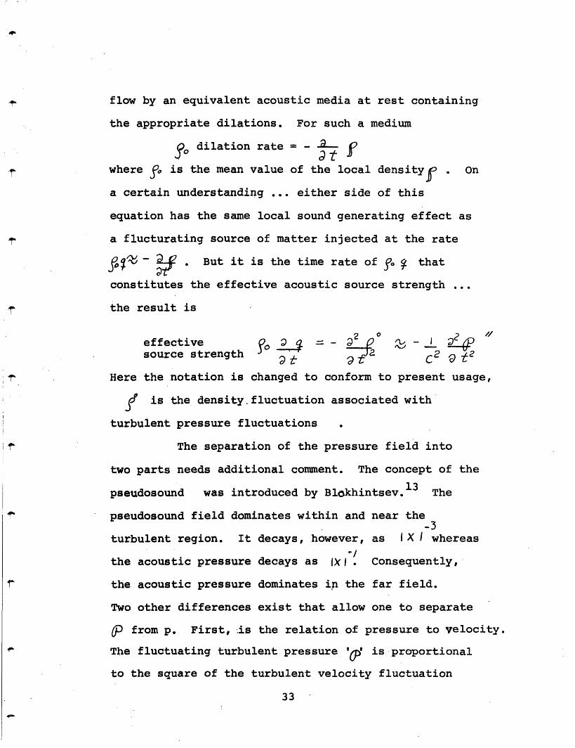
flow by an equivalent acoustic media at rest containing
the appropriate dilations. For such a medium
Yo dilation rate = - Jk fwhere is the mean value of the local densityf . On
a certain understanding ... either side of this
equation has the same local sound generating effect as
a flucturating source of matter injected at the rate
9~$S ~- M . But it is the time rate of o that
constitutes the effective acoustic source strength ...
the result is
effective P 4 I
source strength c ? -_ _
Here the notation is changed to conform to present usage,
I is the density fluctuation associated with
turbulent pressure fluctuations
The separation of the pressure field into
two parts needs additional comment. The concept of the
13pseudosound was introduced by Blokhintsev. The
pseudosound field dominates within and near the-3
turbulent region. It decays, however, as IX I whereas
the acoustic pressure decays as IXI. Consequently,
the acoustic pressure dominates in the far field.
Two other differences exist that allow one to separate
O from p. First, is the relation of pressure to velocity.
The fluctuating turbulent pressure '' is proportional
to the square of the turbulent velocity fluctuation
33
I I
(1y V 2~) whereas the acoustic pressure 'p' is directly
proportional to the acoustic velocity fluctuation
( = C). Turbulent pressure fluctuations are convected
only in the direction of the mean flow at approaximately
the average flow speeds. Acoustic waves travel in all
directions with speeds equal to c + rcos e, where e is
the angle between'the vector to the observation point and
the direction of mean flow. In summary, the pseudosound
field has the characteristics of a pressure field in an
incompressible flow, being dominated by inertial rather
than compressional effects.
1.3 A Comparison of Three Calculations
1.3.1 Monopole Source, Frequency-Domain Green'sFunction
The acoustic field of a turbulent jet is calculated
here using a frequency-domain Green's function. Morse
and Ingardl4 (Chapter 7.1) consider the sound radiated from
a random distribution of volume s6ur6es. The source term
they consider is proportional to a first time derivative.
Ribner's3 work indicates that the source term should be
proportional to a second time derivative; the extra deriva-
tive will give an additional factor of w2 in the intensity.
The results of Morse and Ingard are correct for a distri-
bution of volume sources, however, the monopole source
characteristics of turbulent jets are different from
this simple model, to see this compare Eq. 1.4 to Eq. 1.16.
34
The appropriate modifications are introduced in this
section.
The procedure is to first discuss the representa-
tion of random sources, then relate this representation
to the calculated acoustic field. The source field
can only be described in statistical fashion. On the
other hand, the instantaneous acoustic field depends on
the instantaneous distribution of the sources. The struc-
ture of the wave equation embodies this fact in requiring
an instantaneous description of the source field. The
theoretical task is to reduce all formulas to those
which only require statistical information.
Mathematically, one computes the instantaneous
acoustic pressure from a complete description of the
source. The statistical properties are extracted by
computing the magnitude of the Fourier pressure amplitude.
It is shown later that the amplitude of the Fourier spectra is
proportional to the Fourier transform of the source cor-
relation, the most often used description of random fields.
The technique has its analogue in laboratory
procedure. The microphone detects the instantaneous
value of the acoustic field. The signal is then Fourier
analyzed and averaged to provide a record of the statistical
behavior of the acoustic field. Hence, the parallel in
35
in deducing average properties from a instantaneous ones.
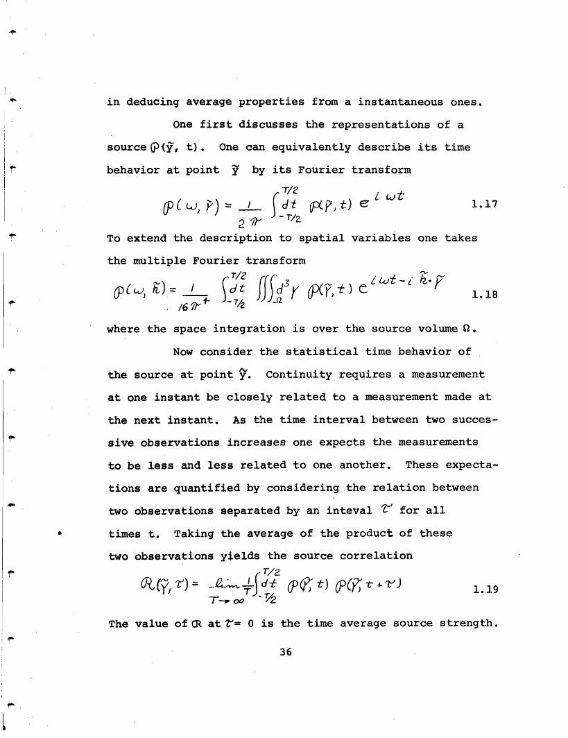
One first discusses the representations of a
source Gp{y, t). One can equivalently describe its time
behavior at point ~ by its Fourier transform
p(w, ) = at g)e w t 1.172 a' - T/z
To extend the description to spatial variables one takes
the multiple Fourier transform
ed)t ffP) 6/ y~ ~t a, )1.186 6 + -T/
where the space integration is over the source volume Q.
Now consider the statistical time behavior of
the source at point y. Continuity requires a measurement
at one instant be closely related to a measurement made at
the next instant. As the time interval between two succes-
sive observations increases one expects the measurements
to be less and less related to one another. These expecta-
tions are quantified by considering the relation between
two observations separated by an inteval V for all
times t. Taking the average of the product of these
two observations yields the source correlation
7T--)=t 1. 19
The value of R at Z= 0 is the time average source strength.
36
To extend this function to spatial coordinates
consider a similar set of measurements between two points
separated by a distance
T/2
~tcii; 1, A) Q Lv T i dt (,,~- t)I~ r, ( · i, tor t 1.20T -- - oo
If the source is homogeneous it is independent of uniform
translations of the coordinate system. One defines, for
homogeneous systems,
If there is mean flow the turbulent pattern will be
convected at some finite speed. With flow (t) will not
be peaked a = 0, this is because an eddy located at
y at t = 0 has moved a distance V t by the time
t =Z . One compensates for the convection by defining the
correlation in the system / = ~
( All- t) - , 0 P d , y r) 1.22Again, consider the point y. Since the descrip-
tions (t) and p (w) are derived from the same source
function Q (t) one expects the two to be related. Follow-
ing Morse and Ingard14 (Chapter 1.3) one computes the
Fourier transform of 6.
37
Id () e dr c dt tp(t/)
= Ifst ( Ju 6p(vP2 rT T/ e/
-2~1 t 1 (Q1. 1.23
The Fourier transform of the auto-correlation function
over time T is T times the spectra amplitude IF()lof
The extension to spatial coordinates yields
/ V2 2I+d ) JtL',() 1.24A shift to the system / in the frame of the jet flow,
gives
f2R T /6 / M- T/z
where M is the Mach number and the angle between the1.25
where M is the Mach number and e the angle between the
observer and mean flow.
One can now compute the pressure radiated
from a stochastic distribution of monopoles via frequency-
domain techniques. Start with the forced wave equation,
Eq. 1.16. Take the Fourier transform to find
( )e pG') t v fnpc,ti ) for te el) euat 1.,26
The Green's function for the Helmholtz equation is
38
Gcway = e r4Lr wr Ix"-
from which one finds
p (WC X) =id e i kiZ-? Ile
4 x e d -I( F4,r x.
1.28
where
e 2 2 ( )4 XIC
Now compute the magnitude of p(w, w) to find
Ip &q Z) I'/
However, {1cfw{,)is proportional to the multiple
1.29
Fourier
transform of the autocorrelation k of p, by Eq. 1.24we
have
Transforming to crdinates by Eq. 1.25 gives0
Transforming to %' coordinates by Eq. 1.25 gives
T Q I d 1 ( f c E Zc~ i ) 1 . 3141- "T 2~ d I& Q )c .1)J31Jt 14;L~- 7Z2
1.3.2 Monopole Source, Time Domain Green'sFunction
The radiated pressure is here calculated for
the same monopole source field, this time using a time-
39
= LC-C
1.27
44 / 2 r. id 1z) I P-ul
(W 4 -= /C') I 1 2IP ) (-E -i -W-x
domain Green's function. The radiated acoustic pressure
p, which is a solution to Eq. 1.16, is determined by the
Green's function Eq. 1.6, note that G is multiplied by
c2 since we are calculating the pressure and not the
density.
(adt )J G(d, z,) t of p/ 2C t 1.32
where t' = t - rX c, i2c
1 1Here the distance p FI is approximated by x, t is
the retarded time. Now compute the convariance of
P(% r F p, t) p -,, )P- to '
2 A
1.33
where t' 1 Izx'
-&'= ~-.. '1C
Here bars indicate time averages and primes indicate
source coordinates.
To proceed one uses the relations given in
Goldstein6 (Chapter 2)
Z2 -( ) _ 4 =~"' 2e P XPt t r- 1.34
9T,4
40
134 zrelats time = terit+e) 1. 35
Eq. 1.34 relates time derivatives to derivatives in the
correlation interval . Eq. 1.35 states that the
correlation of a stochastic function is independent
of uniform time translations. Substituting o = l
gives
where one approximates
-' I ~ 'l_ X x* (/: I) =C IX C
1.37
C
Here is the separation vector (yo-yo). One now intro-
duces the average position = '. The Jacobian
of the transform from (y , ") to (r, ) is unity. Hence
P ( X"r) = I- a I(*;4 A C
C 1.38
where, as before,
1.39
To find the spectral density compute the Fourier trans-
form of p(x, ) Tle
..L) ..L.. C' VI1 |P( V) = pa', rT - 2 11
It,/. (#,7 e) ' 1.40
41
O * Y·J3 -, , ) 1/r .1 O 4 P v; t~C ) tt 9 13P(X,- T- = I
(4v'X X> PI
4 . 13fd '
U L, ) = Pr . - ) Pe t - "' - -f'r
Where the following identities have been used
he wr9 O d-- case ZL8~~"' rt~ ~&,dz ,,r, 1.41
e + Y-.r r= zCir)dr 1.42
If the source is homogeneous the integral over r yields
the source volume i. Thus,
ap~w 4- 1 2 TQ ild r C,)ci 'gfl.43C ((u v) = T2 t/
Transferring to the; coordinate system
P8 cRJ(fX T2 dz 1,.44
Inspection shows Eqs. 1.30 and 1.31 are identical to
Eqs. 1.43 and 1.44, as was to be demonstrated.
Note that the spatial Fourier transform has
its origin in the first order retarded time effects, (see
Eq. 1.42). The question "what is the spectral density
of the source?" can now be assured without ambiguity.
The answer is to consider only the temporal variations at a
point.
The answer depends on whether the spectra is
computed in the/ or system. It has been shown that
the Fourier amplitude spectra of the source is propor-
tional to the Fourier transform of the source correla-
tion (Eq. 1.22). However, depends on the frame
42
in which it is measured. For moving eddies the turbulent
fluctuations seen by a fixed observer will appear much
more rapid because of the convection of the random spatial
pattern of the turbulence with the flow. The rapid con-
vection of the fluctuations cause the time variation seen
by an observer moving with the flow to be much slower than
those seen by a fixed observer. In a moving frame the
correlation at a point will decay much more slowly.
Figure 1.1 is taken from measurements of the
second order time delay correlation carried out by Davies,
Fisher, and Barratt.1 5 The spacing between lines
parallel to the t axis is a measure of the correlation
, the smaller the spacing, the shorter the interval
of correlation. The diagram indicates that measurements
made in the frame of the jet flow are correlated for
longer intervals than those made in a stationary frame.
Note that these considerations do not modify
the radiated pressure spectra. Variations in a1 from
the to systems are compensated for by the appear-
ance of the (1 -Mcos ) term in the exponential.
1.3.3 Quadrupole Source, Time Domain Green'sFunction
Now consider the radiated pressure from a
stochastic distribution of Reynolds stresses. Here
only the major steps in calculating the spectra are
43
outlined, the reader is referred to the literature1 ' 6, 16
for more detailed accounts. The point is Eq. 1.51 which
demonstrates that the radiated field has its origin in
two mechanisms, turbulence alone and turbulent shear
interactions. Eq. 1.13 is the starting point of this
analysis. As the observer is in the far-field, where the
laws of classical acoustics apply, can be replaced by
c~ to yieldc
pTT) }JY Ai al2 Ti t) 1.45
where
Here t is the retarded time, y the source point and x'
the observation point. Twice applying the divergence
1theorem together with a decay of Tij faster than
allows a change to differentiation in the observers
coordinates.
pit)= r ( 1.46jf x7,xxj 2I-1 I
Differentiating and neglecting terms h(X'ives
/pXXtThI =3 2, 7[j(¢, t') 1.47p(, t) - xi ' r r4 C X St 2
where we have approximated
E Xi. X lies I I I
Eq. 1.47 implies that if the source is stochastic so is
44
the radiated pressure field. Now compute the correla-
tion of p to find
P(tr)- p7)p (,t+ r)3 d3 '/ T.(,Jv) T I` -)= ji 2i X X j I" r /
24--)C X# f',y1.48where we have used the identity given in Eq. 1.34. Again,
noting the cross correlation of a stationary function is
independent of time translation (see Eq. 1.35) and
switching to the coordinates (%, i) (see paragraph fol-
lowing Eq. 1.37) gives
2Jdp(xg I Ai 3rc 'j ae T iJ (roCt t ,t+O C)('~~~~'~ -1K) ~C X1.49
The flow is now separated into a mean part V and a fluc-
tuating part v. Contracting over the indicies16' 17
and assuming homogeneous isotropic turbulnce gives
a(A' -- >2 CM T*fdi' w 3rd3?7 ai Lv 2 v2
2 ___ _ _ 1.50
where the prime and double prime indicate
y'= V( tt)
The first term in Eq. 1.50 is due to turbulence alone and
the second to turbulent shear interactions. To get
45
the spectral density one computes the Fourier transform
of p(x, t ) to find
w 2 ) ( iw) 2)' 7Transforming to moving coordinates f gives,,, (,, -e ,,
c (42x); +Y J / K 1.52r[R.,, ,( ~ ) + 2(ca<F.4e +c e) ,-,,Inspection reveals the similarity of Eqs. 1.51
and 1.52 to Eqs. 1.43 and 1.44 and also to Eqs. 1.30 and
1.31. The first terms are identical if the quadrupole
covariance R is replaced by the pressure covariance
rt. In effect, Sov2 is replaced with the pressure LP.This is physically consistent since Bernoulli's equation
requires that incompressible pressure fluctuations be
equal to v .
The second term is the "shear noise" that origin-
ated in the turbulent shear interactions. By assuming a
specific model for the correlations R111 and Rll
Ribner shows that the contribution to the time average
intensity is approximately equal. The shear noise
46
modifies the angular distribution by cos4 + cos2 0.
Ribner further points out that the self noise peak
is shifted to a frequency above the shear noise peak by
a factor of For example, if R ' e(o) one
expects R which gives the factor of /~.
This point is important in that the emphasis in the
thesis has been to collate the results with a single
correlation function. Such attempts consistently fail
to account for low and high frequency regimes simul-
taneously. If the low frequency results are in agree-
ment with the data, the high frequency spectra will
disagree and vice versa.
Experiments18, 19 reveal that there is an
additional angular dependence due to the refraction of
sound through the shear layer. All these calculations
assume that once the sound is generated it travels
through a medium at rest. This is not so, especially
for sources near the centerline of the jet. Sound
emitted from this region has to travel through the
velocity gradients that separate the center of the
jet from the ambient atmosphere. The complete solution
to refraction through axisymmetric shear layers in
three dimensions is, as yet, unsolved. Results are
available in two dimensions for refraction through one20
and two2 1 shear layers.
47
1.3.4 Velocity Intensity and Total Power
Three separate methods have been used to calculate
Ip(w, )2 . This quantity was chosen for discussion
as it is the one measured in the laboratory with the
microphone and spectrum analyzer. However, it is not
the only quantity of interest. Other acoustical quanti-
ties are often required, which are here derived from the
Fourier amplitude spectra.
The radial acoustic intensity at frequency
f =- - is
l((,W) X ) ,pd..P, )el u e )e )]"- p#~) ~ A&¼xY 1.53
= ) u ( ,) + p(x) (,) .x
In the far field the velocity is radial and equal to the
pressure divided by the free space impedance f.C . Hence,
:I (, )= I Ip(w, X ) 1.542 SoC
Integrating over a sphere of radius x gives
the power radiated at frequency a-..
1.55
The approximation becomes exact if the radiation is
isotropic.
One can also construct the time average
48
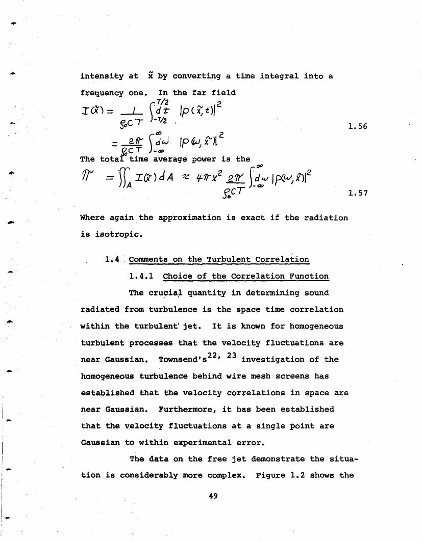
intensity at x by converting a time integral into a
frequency one. In the far field
IT, = _L dt jp( x,t)JfCT 1.56
= e ~id@ p(X")I
The total time average power is the
7' WA (z)JA * 4T2 =7&a) id 1 X)1poCT 1.57
Where again the approximation is exact if the radiation
is isotropic.
1.4 Comments on the Turbulent Correlation
1.4.1 Choice of the Correlation Function
The crucial quantity in determining sound
radiated from turbulence is the space time correlation
within the turbulent' jet. It is known for homogeneous
turbulent processes that the velocity fluctuations are
near Gaussian. Townsend's22' 23 investigation of the
homogeneous turbulence behind wire mesh screens has
established that the velocity correlations in space are
near Gaussian. Furthermore, it has been established
that the velocity fluctuations at a single point are
Gaussian to within experimental error.
The data on the free jet demonstrate the situa-
tion is considerably more complex. Figure 1.2 shows the
49
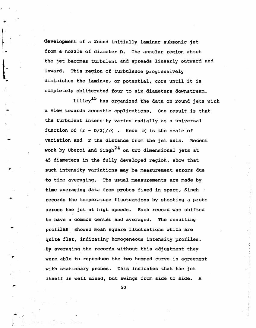
Development of a round initially laminar subsonic jet
from a nozzle of diameter D. The annular region about
the jet becomes turbulent and spreads linearly outward and
inward. This region of turbulence progressively
diminishes the laminar, or potential, core until it is
completely obliterated four to six diameters downstream.
Lilley 5 has organized the data on round jets with
a view towards acoustic applications. One result is that
the turbulent intensity varies radially as a universal
function of (r - D/2)/o( . Here o( is the scale of
variation and r the distance from the jet axis. Recent
work by Uberoi and Singh24 on two dimensional jets at
45 diameters in the fully developed region, show that
such intensity variations may be measurement errors due
to time averaging. The usual measurements are made by
time averaging data from probes fixed in space, Singh
records the temperature fluctuations by shooting a probe
across the jet at high speeds. Each record was shifted
to have a common center and averaged. The resulting
profiles showed mean square fluctuations which are
quite flat, indicating homogeneous intensity profiles.
By averaging the records without this adjustment they
were able to reproduce the two humped curve in agreement
with stationary probes. This indicates that the jet
itself is well mixed, but swings from side to side. A
50
stationary probe will randomly measure ambient and jet
conditions thereby recording an apparent fluctuation where
there are none.
Aside from intensity variations, there is also the
problem of scale variations along the length of the jet.
Lassiter25 has demonstrated that both the longitudinal
and radial scales were found to increase with the axial
distance. Goldstein and Rosenbaum1 7 have developed a
theory for the axisymmetric jet which can deal with such
variations. Roughly speaking, the jet is sliced perpen-
dicular to its axis into a series of disks, each of
which radiates independently.
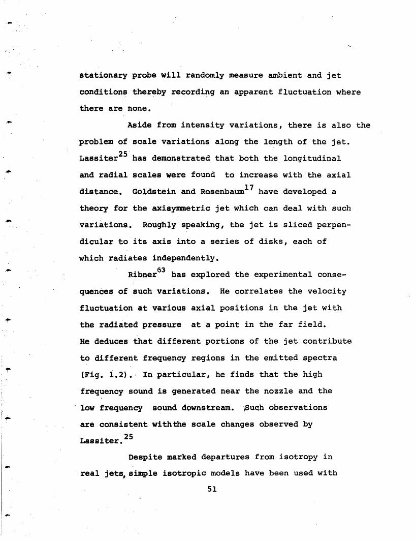
63Ribner has explored the experimental conse-
quences of such variations. He correlates the velocity
fluctuation at various axial positions in the jet with
the radiated pressure at a point in the far field.
He deduces that different portions of the jet contribute
to different frequency regions in the emitted spectra
(Fig. 1.2). In particular, he finds that the high
frequency sound is generated near the nozzle and the
low frequency sound downstream. Such observations
are consistent withthe scale changes observed by
25Lassiter.
Despite marked departures from isotropy in
real jets, simple isotropic models have been used with
51
some success in accounting for the observed behavior
of jets. Gaussian correlation, in particular, is used
in view of the fact that it accounts for the structure
of homogeneous turbulence. Recall that the measurements
of Davies15 et al have confirmed that the turbulent
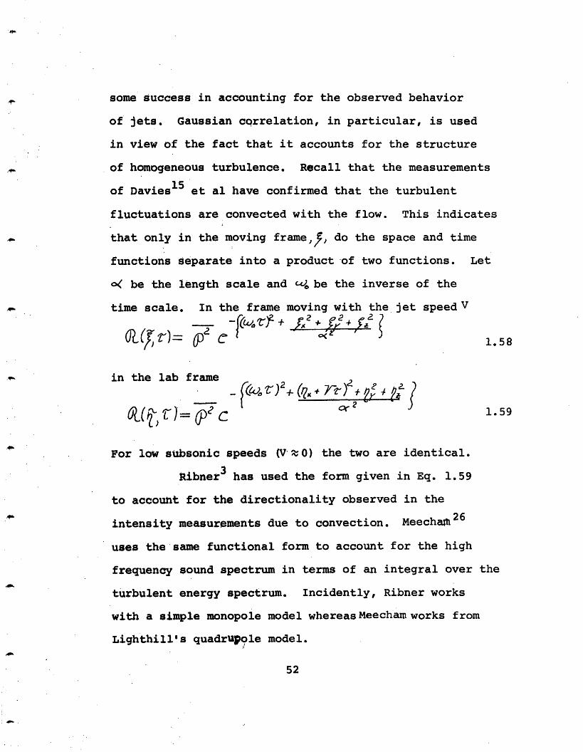
fluctuations are convected with the flow. This indicates
that only in the moving frame,F, do the space and time
functions separate into a product of two functions. Let
o( be the length scale and '4 be the inverse of the
time scale. In the frame moving with the jet speed V
t= IUD -(24f+t2 + 1.58
in the lab frame
On- or- 1.59
For low subsonic speeds (VtO) the two are identical.
Ribner3 has used the form given in Eq. 1.59
to account for the directionality observed in the
intensity measurements due to convection. Meechat 26
uses the same functional form to account for the high
frequency sound spectrum in terms of an integral over the
turbulent energy spectrum. Incidently, Ribner works
with a simple monopole model whereas Meecham works from
Lighthill's quadrupole model.
52
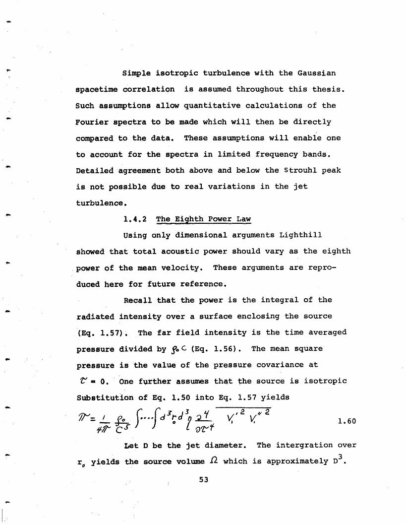
Simple isotropic turbulence with the Gaussian
spacetime correlation is assumed throughout this thesis.
Such assumptions allow quantitative calculations of the
Fourier spectra to be made which will then be directly
compared to the data. These assumptions will enable one
to account for the spectra in limited frequency bands.
Detailed agreement both above and below the Strouhl peak
is not possible due to real variations in the jet
turbulence.
1.4.2 The Eighth Power Law
Using only dimensional arguments Lighthill
showed that total acoustic power should vary as the eighth
power of the mean velocity. These arguments are repro-
duced here for future reference.
Recall that the power is the integral of the
radiated intensity over a surface enclosing the source
(Eq. 1.57). The far field intensity is the time averaged
pressure divided by fo C (Eq. 1.56). The mean square
pressure is the value of the pressure covariance at
m O0. One further assumes that the source is isotropic
Substitution of Eq. 1.50 into Eq. 1.57 yields
°'r, V. 1.60
Let D be the jet diameter. The intergration over
ro yields the source volume i2 which is approximately D3.
53
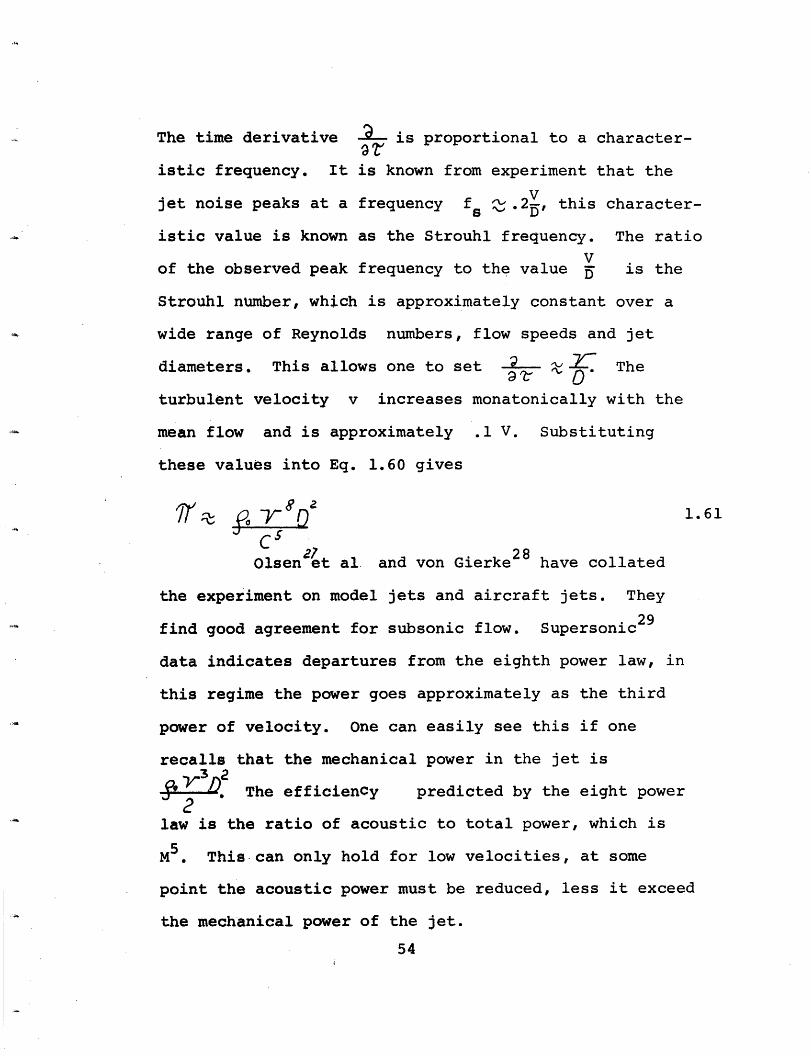
The time derivative ~ is proportional to a character-
istic frequency. It is known from experiment that the
jet noise peaks at a frequency fs .2 V, this character-
istic value is known as the Strouhl frequency. The ratio
of the observed peak frequency to the value D is the
Strouhl number, which is approximately constant over a
wide range of Reynolds numbers, flow speeds and jet
diameters. This allows one to set ; t-- The
turbulent velocity v increases monatonically with the
mean flow and is approximately .1 V. Substituting
these values into Eq. 1.60 gives
Yff 4.r~8,2 1.61v C
28Olsen et al and von Gierke have collated
the experiment on model jets and aircraft jets. They
find good agreement for subsonic flow. Supersonic29
data indicates departures from the eighth power law, in
this regime the power goes approximately as the third
power of velocity. One can easily see this if one
recalls that the mechanical power in the jet is
. The efficiency predicted by the eight power
law is the ratio of acoustic to total power, which is
M5 This can only hold for low velocities, at some
point the acoustic power must be reduced, less it exceed
the mechanical power of the jet.
54
1.4.3 The Kolmogorov Inertial Subrange
Now consider the spectral distribution of
acoustic energy from a dimensional standpoint. The jet
velocity and diameter are not sufficient scales, as
these combine to give only a single characteristic
frequency. To get frequency variations one must scale
the equations to the eddy size and the power per
unit mass 6.
In the turbulent region the particular form
of the driving mechanism that maintains the turbulence
must influence its structure, at least for those eddies
whose size is comparable to the driving mechanism. These
large eddies transmit their energy to the smaller eddies
via non linear coupling, eventually the energy is dis-
sipatdd as heat in the microscale eddies. Kolmogorov
postulates that there is a range of eddy sizes, termed
the inertial subrange, for which the statistical
properties are supposed to be independent of both the
diriving mechanism and the viscosity. The size of the
eddies in this range is smaller than the size D of
the large eddies and larger than the size d-t - of
the heat dissapating eddies.
Morse and Ingardl4 (Chapter 11.4) have calcu-
lated the acoustic spectra implied by such considerations.
They use a Lighthill model neglecting turbulent shear
55
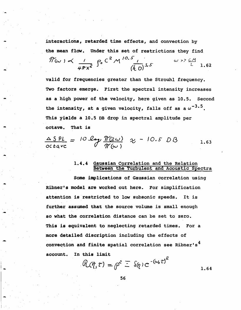
interactions, retarded time effects, and convection by
the mean flow. Under this set of restrictions they find
l~( ) ° / /o c 1 z. ' 7 _24 G · 2 /ot X (- oL 1.62
valid for frequencies greater than the Strouhl frequency.
Two factors emerge. First the spectral intensity increases
as a high power of the velocity, here given as 10.5. Second
the intensity, at a given velocity, falls off as a w-5.
This yields a 10.5 DB drop in spectral amplitude per
octave. That is
h S PL = /0 ' ) ~ - I0. DA 1.63oc t VC fC )
1.4.4 Gaussian Correlation and the RelationBetween the Turbulent and Acoustic Spectra
Some implications of Gaussian correlation using
Ribner's model are worked out here. For simplification
attention is restricted to low subsonic speeds. It is
further assumed that the source volume is small enough
so what the correlation distance can be set to zero.
This is equivalent to neglecting retarded times. For a
more detailed discription including the effects of
convection and finite spatial correlation see Ribner's4
account. In this limit
C-6Pe 1.64
56
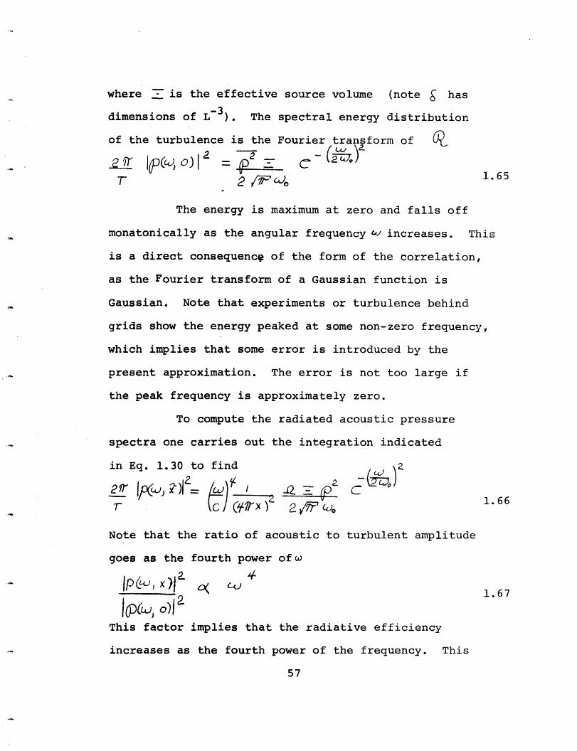
where - is the effective source volume (note has
dimensions of L 3). The spectral energy distribution
of the turbulence is the Fourier transform of
~ I?(~oW)l 2 - e2 caT2 heo 1.65
The energy is maximum at zero and falls off
monatonically as the angular frequency w increases. This
is a direct consequence of the form of the correlation,
as the Fourier transform of a Gaussian function is
Gaussian. Note that experiments or turbulence behind
grids show the energy peaked at some non-zero frequency,
which implies that some error is introduced by the
present approximation. The error is not too large if
the peak frequency is approximately zero.
To compute the radiated acoustic pressure
spectra one carries out the integration indicated
in Eq. 1.30 to find
2J 1if, At , ) a - c (C °) 1.66
Note that the ratio of acoustic to turbulent amplitude
goes as the fourth power ofw
his xa cor )I l 1.67
I(P(, o lThis factor implies that the radiative efficiency
increases as the fourth power of the frequency. This
57
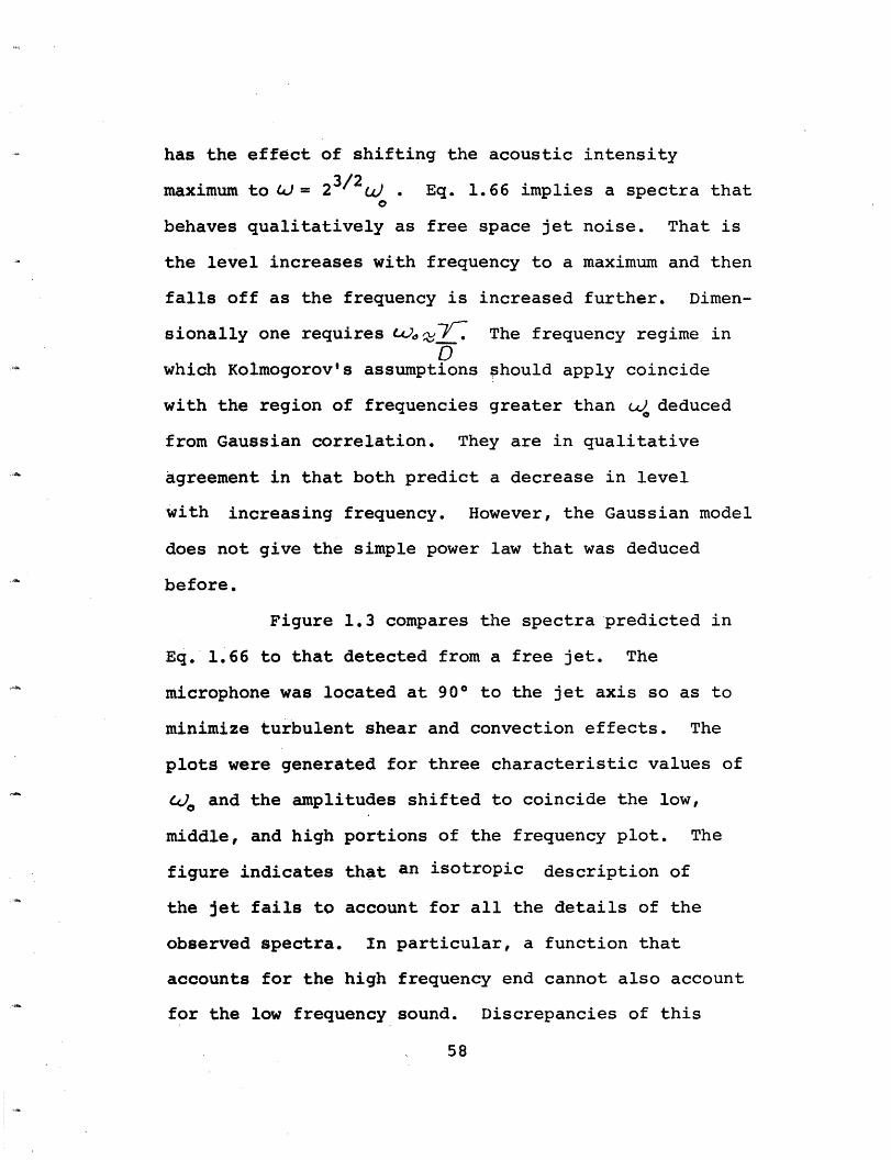
has the effect of shifting the acoustic intensity
maximum to W = 23/2 J . Eq. 1.66 implies a spectra that
behaves qualitatively as free space jet noise. That is
the level increases with frequency to a maximum and then
falls off as the frequency is increased further. Dimen-
sionally one requires wa7 The frequency regime inD
which Kolmogorov's assumptions should apply coincide
with the region of frequencies greater than WI deduced
from Gaussian correlation. They are in qualitative
agreement in that both predict a decrease in level
with increasing frequency. However, the Gaussian model
does not give the simple power law that was deduced
before.
Figure 1.3 compares the spectra predicted in
Eq. 1.66 to that detected from a free jet. The
microphone was located at 90° to the jet axis so as to
minimize turbulent shear and convection effects. The
plots were generated for three characteristic values of
c]o and the amplitudes shifted to coincide the low,
middle, and high portions of the frequency plot. The
figure indicates that an isotropic description of
the jet fails to account for all the details of the
observed spectra. In particular, a function that
accounts for the high frequency end cannot also account
for the low frequency sound. Discrepancies of this
58
form will occur in our evaluation of the spectra for systems
with boundaries. However, it will always be possible to
get close agreement for limited portions of the spectra.
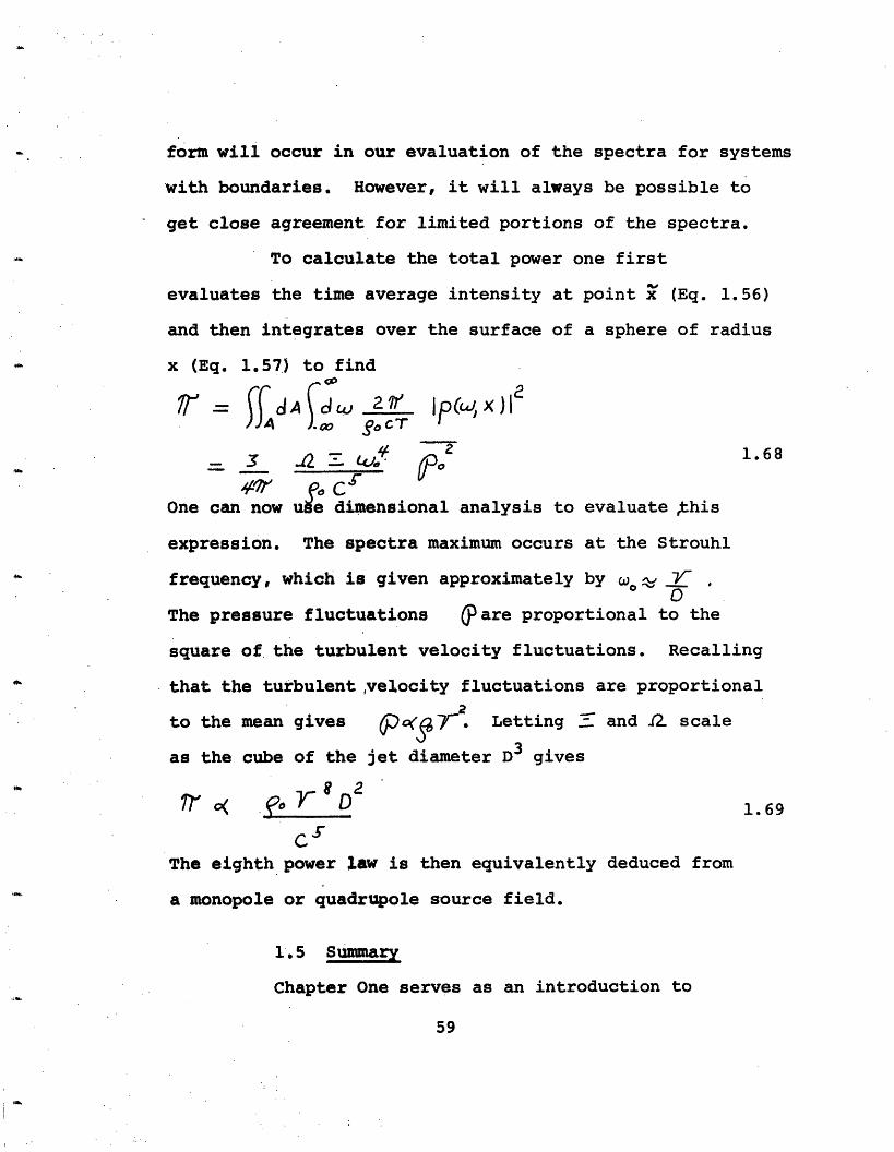
To calculate the total power one first
evaluates the time average intensity at point (Eq. 1.56)
and then integrates over the surface of a sphere of radius
x (Eq. 1.57) to find
=7J rfAdd r/ Ip( X)_c X / goCT3 4 2 1.68
wr e 6COne can now ue dimensional analysis to evaluate this
expression. The spectra maximum occurs at the Strouhl
frequency, which is given approximately by o e- 'O
The pressure fluctuations are proportional to the
square of the turbulent velocity fluctuations. Recalling
that the turbulent velocity fluctuations are proportional
to the mean gives apo(r. Letting - and 12 scale
as the cube of the jet diameter D3 gives
T2< OTD 1.69
C The eighth power law is then equivalently deduced from
a monopole or quadrupole source field.
1.5 Summary
Chapter One serves as an introduction to
59
Lighthill's acoustic analogy analysis of turbulent jet
noise. Ribner's reduction of the source field to an
equivalent monopole distribution is presented.
The statistical properties of the radiated
acoustic field were calculated in three separate
fashions. The first concerned the prediction of sound
from a monopole source distribution via frequency-
domain analysis. The results are identical to the
same analysis using time-domain techniques. The
parallel development clarifies certain details of the
calculation. The third calculation proceeded from the
quadrupole source field via time domain techniques. By
comparison one finds that the isotropic monopole
model neglects turbulent shear interactions. Aside
from this the predictions are identical.
To proceed one needs the source correlation, i.e.,
a statistical description of the turbulent fluctuations.
Observations on homogeneous turbulence have indicated
that an isotropic Gaussian distribution is appropriate.
The results-of such an assumption are compared to those
of dimentional analysis and found to be in qualitative
agreement. The drawback is that turbulent inhomogeneities
cannot be accounted for, this limits comparison of data
and theory to limited portions of the spectra. However,
such a model enables one to make numerical predictions
60
for systems with boundaries and will be used in
Chapters Two and Three.
61
2. EXCITATION OF AXIAL PIPE MODES
2.1 Introduction
Now consider the effect of boundary conditions
on the spectra of sound emitted by turbulence. Herein
the flow excitation of an axial pipe of uniform cross
section A and length L is examined. The problem is
reduced to one dimension, the boundary conditions are the
reflection coefficients at the ends.
In the most elementary treatment of the plane
wave eigenmodes of an open ended pipe it is assumed
that the ends are pressure nodes. Hence, the pipe
ncresonates at frequencies fn = n. With mean flow,
one must account for the difference in phase speed for
a wave travelling with the flow, c = c(l+M), andP
against the flow, c = c(1-M). With flow the pipeP 2
eigenmodes are fn c(- M. The acoustic response
of the pipe to an oscillating source will be greatest
when the source frequency equals an eigenfrequency.
The ends of the pipe, however, are not
perfect reflectors of the incident intensity. There
is always some portion of the incident wave that
radiates out the end. Ingard and Singhal30 have
demonstrated that the departure from perfect reflection
increases with flow. This implies that the eigenmodes
are damped by the ound radiated out of the ends of the
62
pipe. The response of a pipe at its eigenfrequencies
diminishes with increasing flow.
Herein the response of the pipe to the turbulence
in the air flow itself is investigated. A cylindrical
pipe was connected to a plenum chamber and then to a
pump (Fig. 2.2). The mean flow was varied from Mach
0.0 to Mach 0.5. A microphone, placed several diameters
in front. of the inlet, detected the resulting acoustic
field. The signal was then spectrum analyzed, an average
of 256 spectra was computed by a separate device, at each
flow speed, and then plotted.
One observes that at low flow speeds the pres-
sure spectra varies periodically with frequency, with peaks
at the eigenfrequencies. As the flow speed increases
the peaks at the eigenfrequencies are no longer there,
the pressure spectra resembles the smooth variation with
frequency seen in free space jet noise (Fig. 2.1). The
results are consistent with the observed behavior of
the reflection coefficients.
In the theoretical section, Ingard's31 con-
struction of a Green's function from the emperical
pressure reflection coeffieients is presented. The response
of a pipe to a turbulent field with Gaussian correlation
is predicted with this Green's function. This model
accounts for the observed changes in spectra with flow.
63
2.2 Experiment
2.2.1 Apparatus and Procedure
The experimental apparatus is shown schematically
in Fig. 2.2. A small cylindrical pipe was connected to
a pump through a plenum chamber. The pressure in the
plenum was lowered so as to draw air through the pipe
at flow speeds to to Mach .5. The mass flux was
monitored by a calibrated orifice downstream of the
plenum.
A microphone was placed several diameters
in front of the inlet at an angle to the pipe axis.
The signal was amplified and spectrum analyzed in the
zero to ten kilocycle range. A second microphone,
connected to a sound level meter, was used to evaluate the
C weighted intensity as a function of the angle.
Additional meansurements were made with the microphone
in the chamber. The discussion will concentrate,
however, on the upstream measurements.
Consider the placement of the microphone.
In the chamber, the acoustic wave from the pipe must
first pass through the exit jet, where it is refracted,
before it reaches the microphone. Apart from this,
the turbulent noise from the exit jet completely masks
the pipe noise, which makes detection of the pipe
modes impossible. If the microphone were mounted in
64
the pipe in addition to the acoustic wave it would
detect the turbulent pressure fluctuations in the mean
flow. The acoustic pressure also depends on the axial
position of the microphone. If it was located at a node
for a given mode the pressure amplitude at this frequency
is not detected. The problem is further complicated by
the fact that the node location depends on the flow speed since
the effective length depends on the mean flow. The final
option is to mount the microphone in front of the inlet.
This has its own problems, the pressure spectra is
multiplied by W due to the radiation impedance of free
space. In addition, there is some dependence on the
angle 6' due to the finite size of the inlet. However, the
transfer function for these effects is independant of
the Mach number, it is this condition that motivates
measurements in front of the inlet.
The upper limit on flow speed of Mach .5 is
due to the vena contracta. The flow entering the pipe
contracts to an area six-tenths the pipe cross section.
The mass flux is maximum when the flow speed at the
contraction is sonic. The mass flux in the pipe is
identical to that in the ena contraction, hence the
velocity in the pipe is about six-tenths that in the
contraction. This means the maximum flow speed in the
pipe is approximately half the speed of sound.
65
2.2.2 Variation with Pipe Length
Herein it is established that it is the axial
modes of the pipe which are excited. In the simplest
model of a pipe open at both ends the wavelength of the
fundamental is twice the pipe length. It follows that
the fundamental frequency is inversely proportional to the
pipe length, since f = c . Since overtones areL
harmonics the frequency interval between modes is equal
to the fundamental and should therefore show the same
dependence on length.
If one accounts for variations with flow speed
and phase changes at the ends the frequency of the nth
mode is given by
ij = n_ (__ _) 2.1
2 (L+ + 1L)
Where go and L are the end corrections which give the
phase shifts *= i+ - = hj. Ingard and Singhal find
So 6L .3D (1-M2). It follows that the interval
between peaks is given by
2.22L .
To check this prediction a 1" diameter pipe was
examined for lengths from 2" to 18" in 2" increments.
The flow speed in the pipe was held at a constant value of
Mach .14. With the exception of 2" pipe the data agrees
66
with the prediction in Eq. 2.2. The 2" case is an
example of orifice screech which is discussed in
Chapter Four. The length test demonstrates it is the
axial modes which are excited (Fig. 2.3).
2.2.3 Variation With Flow Speed
There is an additional way to check for axial
modes. That is to monitor the variation in frequency
with mean flow. The prediction is that the fundamental
frequency is reduced as the flow speed increases. This
result can be understood if one recalls that the sound
is convected with the mean flow. The time for a wave to
travel downstream is L and back upstream is LC+V c-V'
The frequency is iversly proportional to the period to
complete such a cycle and is given by fl = 2L (-M 2)
To check this variation, spectra were obtained
for a 1/2" inner diameter pipe 12" long with a 1/16"
wall. The microphone was 2" in front of the inlet. The
pressure drop across the pipe was set and the spectra
plotted from zero to ten kilohertz. The flow speed was
determined from the pressure drop and from a calibrated
orifice downstream. Figure 2.1 is an example of
spectra taken with this setup. Pronounced excitation
only occurs for flow speeds up to Mach .3, the funda-
mental varies approximately 10% in this range. As the
67
observed bandwidth is about 50% of the fundamental frequency
some comment on data reduction is advisable.
The experimenter has two options to determine
variations with flow. One is to study the location of
the fundamental, fl, and the other is to measure the
spacing between peaks,A f. In a frequency analysis the
minimum error is the channel width of the analyzer, in
1these experiments this is always 0- of the maximum
frequency. Graphically, this is approximately the line
width of the pen. Assume one chooses to locate the
fundamental. The frequency range is set to 1,000 Hz
and the instrument resolution is 5 Hz. However, the
resonant peak has a finite bandwidth which is approxim-
ately one half the separation between modes. The
resonant peak, or certer, is extremely difficult to de-
termine.
Now assume that the average spacing between
peaks is studied. The frequency range is set to 10,000 Hz
and the instrument resolution is 50 Hz. However, a
large number of modes are now in evidence and the average
spacing can be determined with great accuracy. If n modes
are excited in a range F the spacing is simply f n
So long as a large number of modes are evident the measure-
ment is quite accurate. If, however, the flow speed is
above Mach .3 the modes are overdamped and neither method
68

is adequate.
Figure 2.4 presents an analysis of Af versus
mean flow. The error bars are set to 50 Hz, i.e., the
resolution of the spectrum analyzer. At low flow speeds
it is clear that the accuracy is much better than this.
Only at high flow speeds, where the modes are heavily
damped, does the error approach the resolution
limit. The frequency shifts are clearly those predicted
in Eq. 2.2. Hence, the second test establishes the fact
that it' is the axial pipe modes which are excited.
Given the fact that the axial modes are excited
one now has at his disposal an independent means of
measuring the flow speed. This is to measure the in-
terval between modes and calculate what flow speed is
necessary to produce this interval. The flow speed
determined in this fashion agrees with that determined
by the pressure drop to ± Mach .05. The acoustic
calibration of flow speed is used in Figure 2.1. The
data in Figure 2.4 is based on flow speeds calculated
from the pressure drop across the inlet, and there is
no circular reasoning used in the evaluation of the
shifts with flow speed.
2.2.4 Variation with Microphone Placement
This section establishes the acoustic field
for different microphone locations. A cylindrical pipe
69
of 1" inner diameter and 1/16" walls was used. Pipe
lengths from 2" to 18" in 2" increments at flow speeds
of Mach .07, .11 and .14 were investigated. Acoustic
spectra were taken at 00, 450 and 900 to the pipe
axis 12" from the inlet.
With the exception of the 2" pipe, the excitation
of axial modes was evident for the entire range explored.
In addition to spectra, intensity measurements were
taken at 100 increments from 00 to 90°,(Figure 2.13 to
2.21). Again, excepting the 2" length the variation is
smooth and approximately independent of angle. There
is some decrease in level, approximately 2DB, as the
microphone travels from a maximum at 0° to a minimum at
90°. This may be suppression of the high frequencies
by interference effects due to the finite size of the
inlet.
In addition spectra measurements were made with
the microphone in the plenum chamber. No mode excitation
was observed. The spectra in the chamber is dominated
by the exit jet noise. Figure 2.5 plots the C weighted
SPL for a microphone in the chamber versus one on axis
in front of the inlet. Before comparing plots the
increase in level due to chamber reverberation must be
determined. The screech data from the 2" pipe provides
this calibration as the screech level far exceeds any
70
turbulent noise at the inlet or exit. At Mach .14 the
screech is greatest, the level in the chamber exceeds that
outside by 10DB. One concludes that, all other things
being equal, chamber measurements should exceed exterior
measurements by 10DB. However, the observed level changes
for 4" to 18" pipes are approximately 30DB. This can
only be accounted for by noting the sound from the exit
jet dominates the acoustic field in the chamber.
Of interest is the fact that the sound level,
for 4" to 18" pipes, is independent of length. If
boundary layer turbulence along the pipe walls was the
sound source, the level would increase with length. It
does not, therefore the spectra is determined by inlet
and exit conditions. This implies that in a study of
self noise of duct liners great care must be taken to
separate end effects from sound generated in pipes.
2.2.5 Effect of Liners
This experiment considers the effect of an
absorbent liner on the spectra. A 1-1/2" inner diameter
pipe was lined with a 1/4" thick blanket of Scott
acoustic foam. Lengths from 2" to 18" in 2" increments
were examined for velocities from Mach .07 to .20.
For lengths greater than 6" no evidence of mode excitation
occurred. For lengths below 6" only the first or
second mode was detected, and these were severely damped.
71
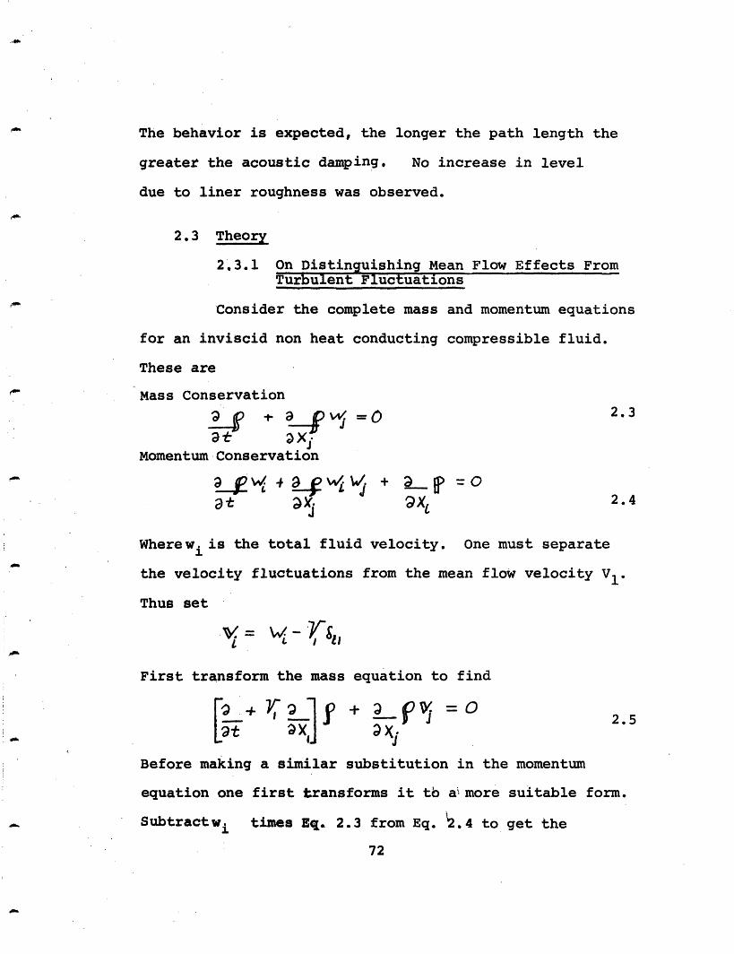
The behavior is expected, the longer the path length the
greater the acoustic damping. No increase in level
due to liner roughness was observed.
2.3 Theory
2.3.1 On Distinguishing Mean Flow Effects FromTurbulent Fluctuations
Consider the complete mass and momentum equations
for an inviscid non heat conducting compressible fluid.
These are
Mass Conservation
24 + 9 = 0 2.3at 3X-
Momentum Conservation
4avi4W + 0 =at ax XI 2.4
Wherew i is the total fluid velocity. One must separate
the velocity fluctuations from the mean flow velocity V1.
Thus set
First transform the mass equation to find
_ t S f-j _ 2.5
Before making a similar substitution in the momentum
equation one first transforms it tb a more suitable form.
Subtractw i times Eq. 2.3 from Eq. 2.4 to get the
72
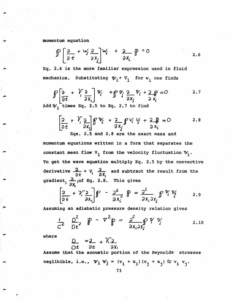
momentum equation
~-j1w + 02.6Eq. 2.6 is the more familiar expression used in fluid
mechanics. Substituting \Vi+ V1 for wi one finds
Y l sV +f O 'j A 4 = =0 2.7¥x, axj xi
Eq. 2.5 to Eq. 2.7 to findAdd
t V I1 f Vl + I f I V + =0 2.8p X ad9 Xj a xi
Eqs. 2.5 and 2.8 are the exact mass and
momentum equations written in a form that separates the
constant mean flow V1 from the velocity fluctuation Vi'
To get the wave equation multiply Eq. 2.5 by the convective
derivative - + V and subtract the result from the
gradient) d )of Eq. 2.8. This givesis. f- F I)D 2.9i adiatic pressu dengDvXDj
Assuming an adiabatic pressure density relation gives
-2 fP Vv 2.10c ot axI
whereD_ =2 +, 7t aat ax,
Assume that the acoustic portion of the Reynolds. stresses
neglibible, i.e., ~i ~j = (vi + ui) (vj + j) vi vj.
73
If the turbulent fluctuations are approximately incom-
pressible we have
2 _ 472 pJ (iZ d M~i ; 2.11
x: DXj
which we have used = p + . Using the same approxim-
ation as in Eq. 1.16 one finds
2 2 D2
2C~~c2 = 2.12
To reduce the problem to one dimension take
the average over the cross section. One finds
- - PA VG - PA VG - V 2.13o Ot sXa C t2
where PA G A || p Jyd
LPAV t~ f~d)'d~~E~ ~2.14
Taking the Fourier transform gives
Dx2 P(LJ, X)9X)oCax X ~2~~ ~ 12.15
where -
P(Q9)i~ X)vG t ~PAVG 212.16T~~~~~~~akigthForetrnfrgis
74
2.3.2 The Green's Function
The linear acoustic response of an open-ended
pipe is given by the Green's function. This will be
constructed here from the empirical pressure reflection
coefficients at the ends following Ingard's31 procedure.
A coordinate system is used such that the inlet is at
x = 0 and the exit at x = L. The boundary conditions are
the pressure reflection coefficients Ro and RL. It is
assumed that these are given for all values of the mean
flow.
Consider a harmonic source of unit strength lo-
cated at x = x. The pressure field induced by this
source is the Green's function Gxlx O) which solves
(1- ,A) 2G + 2 k M G + G= -g(x-Xo) 2.17
To develop the Green's function one specifies the acoustic
field to the right and left of the source point (subscript
r and A) as the sum of a wave propagating with (subscript
+) and against (subscript -) the mean flow.
GW = pe L X+p et i ox < Xo2.18
GG 3 to + P. x Xo<X<Lwhere
One needs four restrictions to determine
the coefficients Pt,-' Pr+" P ' ,and P+ uniquely.
75
Continuity of pressure at the point x gives
p- L k o, -+ ,xp L kp x + pr+e 2.19
To find the second restriction integrate Eq. 2.17 over a
small region e about the source point xo. The value of
the right hand side is -1. Let e go to zero and assume
continuity at x xo, only the first term on the left
hand side contributes. Dividing by 1-M2 gives the magni-
tude of the discontinuity in slope.
/?~. Xo- L (2) X+ L t 2.20i /. ptkc:-' x° cpC+L / *X
- M-The third and fourth restrictions come from the
pressure reflection coefficients Ro and RL. Care is
needed as to which wave is the incident one. At the
inlet it is the wave travelling against the flow; at the
exit, it is the wave travelling with the flow. Hence
Pe4 = rIo p. -
P - - RL C Z(/+, k. ) L p
2.21
2.22
Solving Eqs. 2.19 to 2.22 for the incident wave coeffi-
cients at the ends ives
Pe -2 I D -a) * L O - /? (t CS + k- LC -L k22.23
+ +k-xo+ PtoCPI-+= -26t Z A, 'xo[
P-} 2- 6D((.) I 2.24
76
where
D()- /- pZtet Q(et)L 2.25
Substituting Es. 2.21 and 2.22 into E. 2.18 gives
Gts k + rFo e X<,,Xo2.26
G ro PrL Ce-k x> x,Substituting Eqs. 2.23 and 2.24 into Eq. 2.26 gives
GW(x Xo)
=... + C -
k(X- XO) Re+ +i )L- x t 4 4 iE C)X 0- + /L JL 0 o.
-2 ih Ok C ) 227Which is identical to the expression published by Ingard
and Singhal.30 The problem was worked in detail so as
to identify the incident wave at either end. The
discrepancy between perfect and measured reflection
will be attributed to radiation losses out the ends. One
can then deduce the magnitude of the transmission coef-
ficients from the intensity difference between the
incident and reflected wave.
2.3.3 Analysis of the Pressure ReflectionCoefficients
Consider the pressure reflection coefficients
in a pipe with flow. To clarify their influence the
fundamental pipe mode will be constructed first through
77
simple arguments. We will then consider the effects of
mean flow.
In the most elementary treatment of the axial
modes of a straight pipe with no flow it is assumed that
the ends are pressure nodes, so that the wavelength of
the nth mode is 2L. The frequency of oscillation isn
then fn = c
If the ends are pressure nodes then one finds
Pi Pr 0which implies
Pr= ~ 2 ~~~~2.28
Piat the inlet. An identical expression is found at the
exit. Here the subscripts i and r indicate the incident
and reflected. wave respectively.
The condition is identical to the requirement
that the intensity of the incident wave equal that of the
reflected wave 2 2
IP'I _ -t[
which impli e pC C
mIB == IRl- 2.29
IPHIdentical results are obtained at the exit. At zero flow
the condition of a pressure node implies perfect intensity
reflection. -If one allows for phase shifts, the ends are
no longer pressure nodes. However, so long as the
78
magnitude of the pressure reflection coefficient is
unity the ends are perfect reflectors of the incident
intensity.
The condition that the incident intensity be
completely reflected will be used to derive pressure
reflection coefficients for a lossless pipe with flow.
The flow makes the medium anisotropic as the phase
speed depends on the direction of propagation. Moreover,
the intensity express
gation with the flow
against the flow I =- oC
the reflected intensity equal the incident one finds
at the inlet 2 2 2IP/ (I- , I Pd (I 4M)2
which impliesS C C
I1P= '1 - IolIPi N- - I i 2.30
Similar requirement at the exit gives
IPI= 't PA -Ir 2.31
The measurements of Ingard and Singhal30 show
that
i ] = (X8+IfI 1~ iRT/" ) 2.33In~1:· r R,--!~c
79
Figures 2.6 and 2.7 compare the measured coefficients
(Eqs. 2.32 and 2.33) to those of a lossless duct (Eqs. 2.30
and 2.31.). The measurements extend only up to Mach .5.
It is clear that the discrepancy between perfect and
measured reflection increases with the flow speed. That
is, as the flow increases so do the losses.
Their measurements show that the end corrections
o and Age are approximately equal to .3D(1-M2). That is,
the effective length of the pipe depends on flow. The
importance of these measurements is that they can be
substituted into the Green's function to give the actual
response of ducts. The measured reflection coefficients
will be used to account for the decreased mode excitation
with increasing flow.
It is of some interest to note that the
reflection coefficient at the upstream end can be
derived assuming the duct inlet is a one dimensional
nozzle in which the fluid is accelerated from rest to
the mean speed V. If one considers the limit as the
nozzle length is much less than the wavelength, the
nozzel can be described as a set of boundary conditions
32at the inlet. Marble has considered the acoustic
response of quasi-steady nozzles. The solution may be
found by matching stagnation temperature, mass flow, and
entropy across the nozzle. The application to pipe
80
flow was pointed out in Bohn and ZukQski's33 discussion
of the measured inlet pressure reflection coefficient.
They find, by the circuitous route of Marble's calculations,
the expression in Eq. 2.30.
Cummings34 has considered the reflection
coefficient at the exit. He also uses a quasi-steady
model. One point brought out is that the air leaving
the exit retains the form of a circular jet for some
diameters downstream and that this must be accounted for
in the analysis of the exit reflection. This is in marked
contrast to the inlet where one assumes the flow acceler-
ates from zero in a negligible distance.
2.3.4 Transmission Out of the Ends of the Pipe
Consider the sound transmitted out of the ends
of the pipe. The calculation is done in two steps. The
first quantity one needs is the pressure just outside
the ends of the pipe. This follows from an energy
balance assuming all losses are due to radiation. The
second step it to replace the fields just outside the
ends by an equivalent distribution of monopoles. From
this distribution one calculates the radiation into
free space.
In the first step one must account for the
asymmetry in flow conditions in the intensity expressions.
81
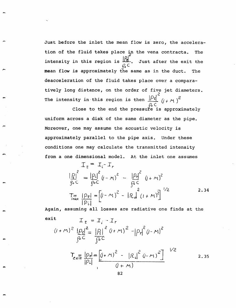
Just before the inlet the mean flow is zero, the accelera-
tion of the fluid takes place in the vena contracta. The
intensity in this region is . Just after the exit the?~c
mean flow is approximately the same as in the duct. The
deacceleration of the fluid takes place over a compara-
tively long distance, on the order of five jet diameters.
The intensity in-this region is then IPrl 0t M )2£oC
Close to the end the pressure is approximately
uniform across a disk of the same diameter as the pipe.
Moreover, one may assume the acoustic velocity is
approximately parallel to the pipe axis. Under these
conditions one may calculate the transmitted intensity
from a one dimensional model. At the inlet one assumes
Zt I,~- Il
C pOC S C
inlet
IPilAgain, assuming all losses are radiative one finds at the
exit t -r
IP | IPI p (I- )
5LC foC
ptl r: Ei2 + - [R, IQ 0-' ') 2.35
82

where T inlet and T exit are the magnitudes of the
inlet and exit pressure transmission coefficients.
Consider the second step in the calculation
which describes the propagation from the immediate
vicinity of the inlet into free space. Outside the in-
let the medium is uniform and at rest, hence the result-
ing pressure field is transmitted according to the laws
of classical acoustics. At the exit the field is
embedded in the center of a cylindrical jet with large
velocity gradients at the shear layer. One expects
refraction due to these shear layers, and possible
channeling of the sound in the aerodynamic duct formed
by the velocity gradients (ref. 14, Chapter 11).
Consider the inlet first. As a first approx-
imation one can model the end conditions as a distribu-
tion of volume sources. Let the average acoustic
velocity be Uo C and uniform in a direction
parallel to the tube axis. Then the strength of an
equivalent volume source is SU equal to A or So
equal to IPt1A . If one distributes the source over the
duct cross section A the source strength per unit area
O,,j is then IPl The model is by Morse35
to calculate the radiation from a piston in a plane wall.
One finds the free space acoustic pressure p ,) is
83
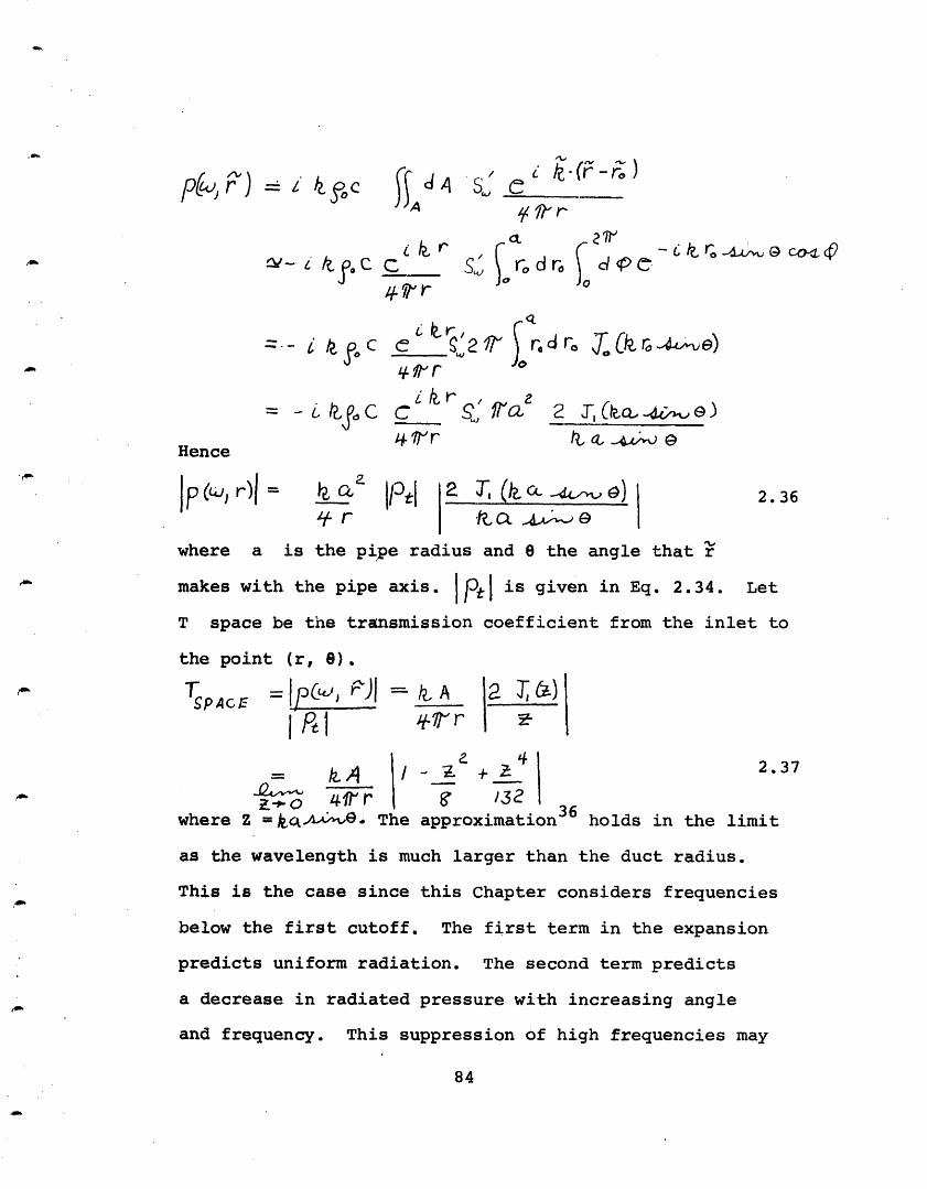
zvkj'.C Srodrode4 r
C e1 c 2 d y r (aO r -,- e)
- 6 .aC C i a ,
Hence
¥ r , fo..J.,,, H ewhere a is the pipe radius and the angle that r
makes with the pipe axis. ptI is given in Eq. 2.34. Let
T space be the transmission coefficient from the inlet to
the point (r, ).
Tpc, = ip., r)l = A ̂ T a)I P1I 1,"~ " IPtl r 2~c t-
4 ! ' Z + 4 2.37
l& o 4 r 132where Z =ko--. The approximation36 holds in the limit
as the wavelength is much larger than the duct radius.
This is the case since this Chapter considers frequencies
below the first cutoff. The first term in the expansion
predicts uniform radiation. The second term predicts
a decrease in radiated pressure with increasing angle
and frequency. This suppression of high frequencies may
84
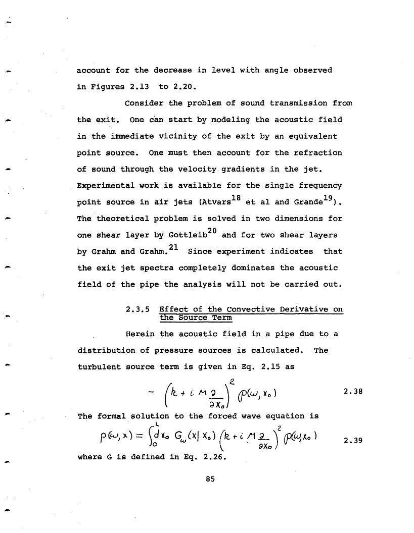
account for the decrease in level with angle observed
in Figures 2.13 to 2.20.
Consider the problem of sound transmission from
the exit. One can start by modeling the acoustic field
in the immediate vicinity of the exit by an equivalent
point source. One must then account for the refraction
of sound through the velocity gradients in the jet.
Experimental work is available for the single frequency
point source in air jets (Atvarsl8 et al and Grandel9).
The theoretical problem is solved in two dimensions for
one shear layer by Gottleib20 and for two shear layers
by Grahm and Grahm.21 Since experiment indicates that
the exit jet spectra completely dominates the acoustic
field of the pipe the analysis will not be carried out.
2.3.5 Effect of the Convective Derivative onthe Source Term
Herein the acoustic field in a pipe due to a
distribution of pressure sources is calculated. The
turbulent source term is given in Eq. 2.15 as
- (& 6 Q)p(,sX 0 ) 2,38
The formal solution to the forced wave equation is
where ) = ix G(defined in Eq. 2.26.
where G is defined in Eq. 2.26.
85
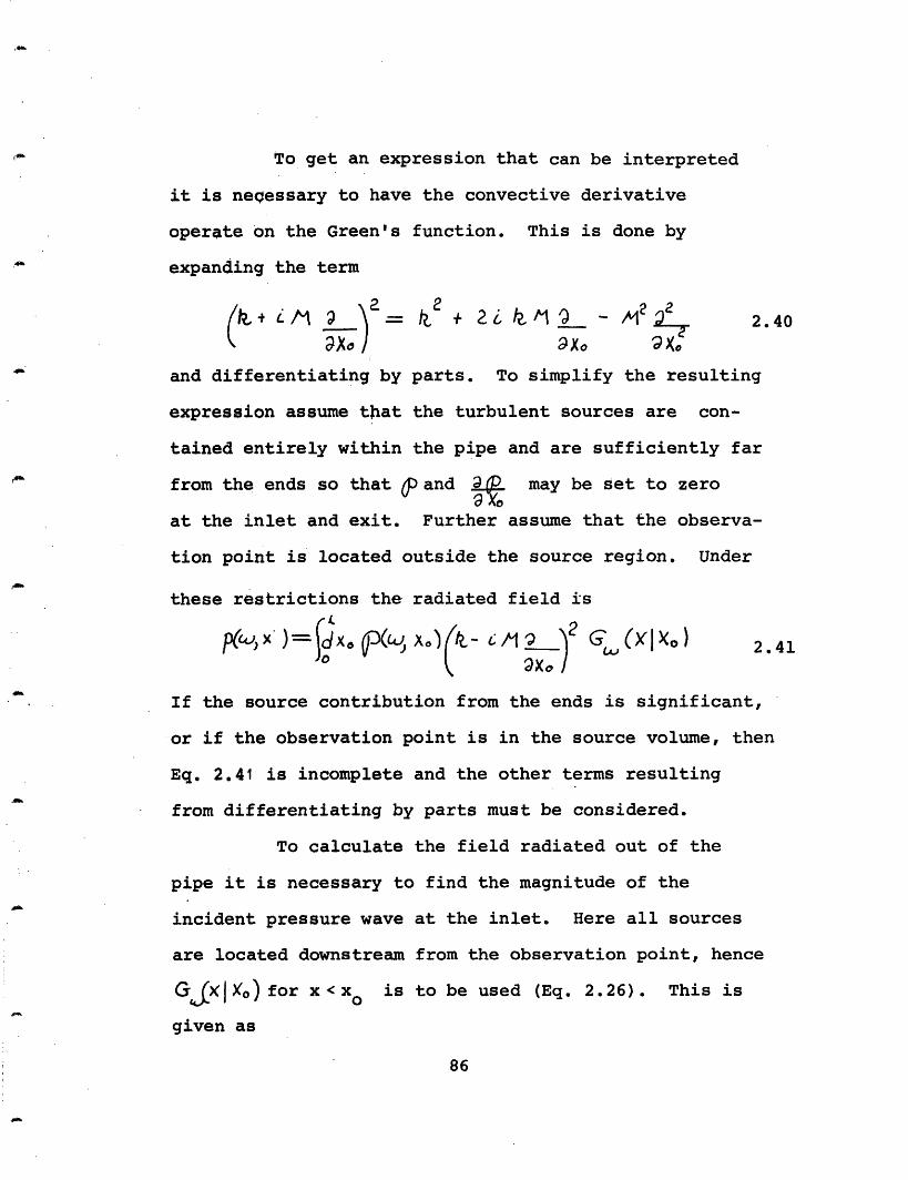
To get an expression that can be interpreted
it is necessary to have the convective derivative
operate on the Green's function. This is done by
expanding the term
a(f-= & 8_ + 2m lm O _ 1 2.40
and differentiating by parts. To simplify the resulting
expression assume that the turbulent sources are con-
tained entirely within the pipe and are sufficiently far
from the ends so that and .f may be set to zero
at the inlet and exit. Further assume that the observa-
tion point is located outside the source region. Under
these restrictions the radiated field is
'p(4 )=dx oQD xo)(&- L MO ) G(Xlx ) 2.41
If the source contribution from the ends is significant,
or if the observation point is in the source volume, then
Eq. 2.41 is incomplete and the other terms resulting
from differentiating by parts must be considered.
To calculate the field radiated out of the
pipe it is necessary to find the magnitude of the
incident pressure wave at the inlet. Here all sources
are located downstream from the observation point, hence
G (jXo) for x<x O is to be used (Eq. 2.26). This is
given as
86
sG, (x ~x o) = /:_D) X'- p "(,x0 ) f? 0 ekx
2.42
The Green's function is composed of two waves, one
travelling with the flow and the other against the
flow. The incident pressure wave at the origin travels
against the flow and is proportional to e -
Substituting G into Eq. 2.41 and selecting the incident
pressure wave, PL(x)j| gives
p,, , ) d Xo ( L xo) (- 2
AlX
- 5iXc7o/NWX 0)
-2 C-2L~~~X kS(W)Xo
L I X + e? (t kt) k XI+ f,~ CC2.43= ,, 6/, , : I_) JdXoc k.1JXo)
- Z 6 0( ) o L
t kle (k - I k- ) Xo P(O ¥0) C
To interpret this expression note that the spatial
Fourier expansion of &J' Xo)is given by
OWP L)-
2.44o0
87
J-
c\
MI-d(1 k XI X Is (L, )jk " )
e ~ -exV
~~ -i~~a f2
The limits of integration and changed by noting 6 iszero outside the pipe. The spatial transform is given
in the set of travelling waves C - since the Green's
function is expressed in this set. Had the Green's
function been expanded in the set of standing waves
sin nffx the standing wave expansion of would have to
be used. Expressing Eq. 2.44 in terms of oJ4$,E) gives
C ) -M) ( j)2.45The incident pressure field is composed of two
parts, which are interpreted as follows. The first is
proportional to (I)i k1 This is due to sound waves that
travel directly to the inlet from the source. Only that
portion of the turbulence that has a wave number kt=
LU contributes. That is, that portion of the
source distribution whose wavenumber satisfies the disper-
sion relation for propagation upstream contributes.
The second term is due to sound waves that initially
travel downstream but are reflected off the exit. If
there was no reflection at the exit, i.e., if RL equals
zero, this term would not exist. This interpretation
is supported by the fact that only the portion (p}; k4)
of the turbulence contributes. That is only disturbances
whose wavenumber satisfies the dispersion relation for
88
propagation downstream, += contribute to this
term.
2.3.6 Acoustic Field of a Point Source
Consider a source whose dimensions are much
less than the wavelength of sound generated. In this
limit it can be modeled as a single point source
X} yo)== BS) 0 s C-.Q) 2.46
where e' is the location of the equivalent source and D the
effective length of the source (note the function has
units of L 1). Taking the transform indicated in
Eq. 2.44 and substituting into Eq. 2.45 gives
pf>o °)-W kw _ D i C Q+ R ttL _L ek Q O(w) 1-) ( +M)
2.47
From which one finds the magnitude
6(a:)lt_ a2 2 + 1 Y
O,'12 l0_') te + h~)l~t ~- n ) 2.48
Ate Ct (is. . .The cosine term in the expression arises from interf er-
ence effects, which are possible only because the source
location . is specified. If one lets 4 vary over the
length of the pipe and computes the average value of Ip£(O)[
this term drops out whereas the others remain the same.
Computing this average one finds
89
<pl go +l
2 L 2<p I w, )IT 2'
DUCT 1 '12.50
Note that averaging overall source positions has removed
all dependence on 2. The magnitude of the generated
acoustic wave depends only on the Fourier amplitude of
the source field, which can be derived from a statistical
description of the time variations of the source strength.
The location of the source has its counterpart, in
distributed sources, in the phases of the Fourier
coefficients of the source. The neglect of such phases
is equivalent to the neglect of interference effects.
2.3.7 Acoustic Field of a Distributed Source
Consider the acoustic field of a distributed
source. Let the Fourier coefficient of the source be
given by
((Do _t )- = -Ad k)le h 2.51
where is the phase of the coefficient. Substituting
into Eq. 2.45 and computing the amplitude gives the
incident pressure amplitude
90
Ip, C )i- +2 , 2 ~.)l2a:
I lW2l ( - l) (o+ I t )
_S(@J>1IF(NIZ+I [LI 4()(2-101-0-001
2.SNote the similarity of Eq. 2.52 to Eq. 2.48.
The interference term due to localization of a point source
has been replaced by the phase term ( - 4 ). The
expression, as it stands, cannot predict the sound field
of a random source, because only amplitudes and not
phases can be deduced from the correlation function.
Consider the average of N measurements of the incident
pressure and assume the value of the phases to be random,
one finds
< IP(C °)I - , ,, I? )
= aI 2 2 2.53
I(c) l I (- A)T M )1The result is equivalent to taking the average over all
source locations.
To understand the effect of averaging consider
a point source that moves in a random fashion in the
duct. Let the time needed to compute a Fourier analysis
at the inlet be smaller than the time it takes for the
position 2 to change significantly. Any single anslysis
will contain interference effects due to the approximate
localization of the source. An average of N such
91
measurements would have the cosine term contribute
randomly and therefore tend toward zero.
Consider the Fourier analysis of the field
due to a distrubuted source. Any single analysis depends
on the precise distribution in time and space of the
sources, hence it will include interference effects.
If the average of N measurements is taken these inter-
fernece effects contribute randomly and therefore tend
toward zero.
One may ask which expression to use, i.e.,
Eq. 2.49 or 2.53. The answer depends on the extent of
information concerning the source. To use the model of
a distributed source requires statistical information
concerning the distribution in both time and space.
Information concerning turbulent fields in
short pipes is limited and the approximation of a random
point source is more appropriate. Eq. 2.49 only requires
that one specify the correlation in time and will there-
fore be used.
2.3.8 The Upstream Acoustic Field
The transfer coefficients Tare now used to
predict the acoustic spectra in front of the inlet. The
various calculations are tied together so as to derive
the acoustic spectra outside the pipe from the turbulent
92
source spectra inside the pipe. Only the correlation in
time will be assumed. In effect, one considers the
average field from a collection of random point sources.
From Eqs. 2.50, 2.37 and 2.34 one finds
dR(% ?!? T T T I(PC2 2.54S PAC: INLE7 DUCT 2.54
Assume that the source is described by a
Gaussian correlation in time
(- J== .e ~jA -(L t' 22.55
Taking the Fourier transform yields the source spectra
kF~w~ )l= iz p C )2.56
To concentrate on the spectral line shape,
separate the frequency dependent terms in Eq. 2.54 from
those which determine the average amplitude to get
2 2.57
6,-,o ID&)IIf the microphone is on the pipe axis 8 = 0
and the last line is exact. The exponential term comes
from the source distribution. A factor of cw comes from
the radiation impedance of free space and a second factor
of cu from this second time derivative in the source
term. The D(J) 12 in the denominator comes from the
93
response characteristic of the duct (Eq. 2.25), it
depends on the flow speed through the reflection coef-
ficients. It is this term that is responsible for the
periodic amplitude variations observed in Figure 2.1.
Explicitly
lD(LJ)(a / - 2R I1a1zc g2(ct'L+.I*0 i± t 1c I i2 2.58- I~ I~ 2.58
The duct response is maximum at frequencies where IDCJ )[
is minimum. This occurs at frequencies where the
cosine term is equal to one. That is when
$n "· = 2.59Ir 2L o + L)If the product JRol IRLI was equal to one, then D( w ) 12
equals zero at 3 . Hence the duct response is infinite.h
This occurs if the ends are perfect reflectors of the
incident intensity, i.e. if
However, the=- meaurement ofA Ingard and have2.60
However, the measurement of Ingard and Singhal30 have
shown that
I2 I 9II .45(1 PAl) Kc ~ 2.61
As the flow speed increases, the product IR [ IRLI
decreases, consequently ID( w )12 varies less and the acoustic
spectra smooths out. That is, the eigenmodes are damped.
94
2.3.9 Numerical Comparison of Theory toExperiment
Herein the observed spectra is fit by the
expression in Eq. 2.57. All mean intensity information
is lumped into a proportionality constant,
B, which is a function of the flow speed and the
distance of the microphone from the inlet. The data
is fit by adjusting B and w.
Figures 2.8 to 2.10 compare the theoretical
spectra to that observed in experiment. All of the
qualitative features are accounted for. First, it is
clear that the spectral lineshape agrees with that
observed. Second, the amplitude peaks at the
resonant frequencies are damped at the higher flow
speeds. Finally, the average rise and fall of the
amplitude with frequency is the same as is observed.
It should be noted that at high frequencies
the theoretical amplitudes match the observations. At
low frequencies the data exceeds the theoretical levels.
The same effect was observed in fitting the free space
spectra with an isotropic turbulent model. The inhomo-
geneities of the turbulence must be accounted for to fit
both the high and low frequency ends of the spectra.
Moreover, at low speeds, the theoretical reson-
ant peaks are greater than those observed. This
95
discrepancy is due to non-radiative damping such as
turbulent and visco thermal losses. At high flow speeds
the predicted and observed resonant peaks agree. At these
velocities, radiative damping is the dominant loss mechan-
ism and the model, based only on end losses, is more
accurate.
it is also possible that some modification of
the exit reflection coefficient may be necessary at low
flow speeds. The empirical coefficients given by Ingard
and Singhal30 are used throughout (Eqs. 2.'32 and 2.33).
At zero flow the two reflection coefficients should agree,
however, they give IROI = 1 whereas IRLI = .95. They
indicate that IRLI is an average for all frequency ranges
and flow speeds, at best, a good approximation. Such
discrepancies do indicate that a more detailed study
of the exit reflection coefficient is in order. In
particular, if one substitutes the value .95 for IRLI
at low flow speeds greater radiative damping would
occur. This would bring the theory in better agreement
with the observations.
In Figure 2.11 the Strouhl numbers that were
used to fit the data are plotted. This fit was done on
a computer using a least squares procedure. Here, one
assumes that the correlation frequency W, is related
to the Strouhl frequency f ass
96
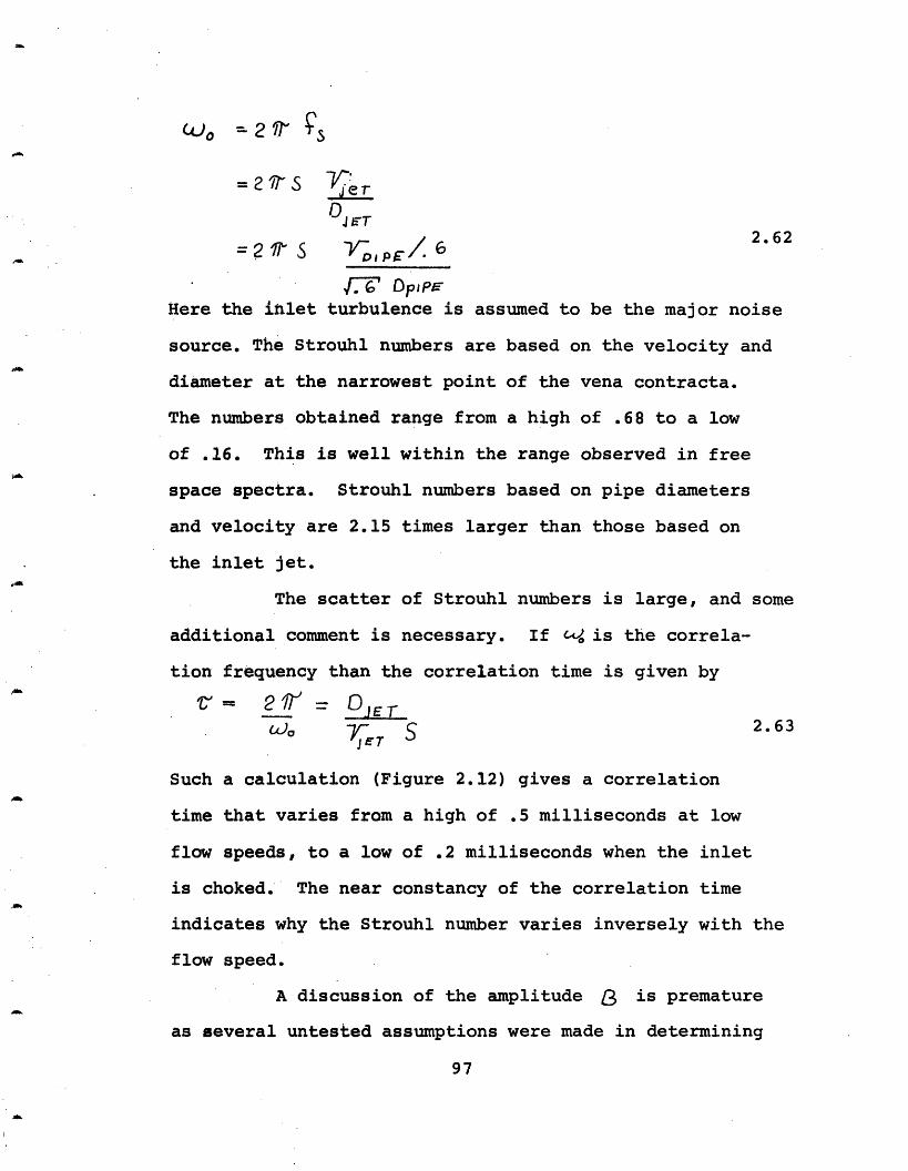
=2oS 2/je r
JET
=211 rppr 6 2.62
' - DpiPEHere the inlet turbulence is assumed to be the major noise
source. The Strouhl numbers are based on the velocity and
diameter at the narrowest point of the vena contracta.
The numbers obtained range from a high of .68 to a low
of .16. This is well within the range observed in free
space spectra. Strouhl numbers based on pipe diameters
and velocity are 2.15 times larger than those based on
the inlet jet.
The scatter of Strouhl numbers is large, and some
additional comment is necessary. If Wc is the correla-
tion frequency than the correlation time is given by
JE 2.63JET
Such a calculation (Figure 2.12) gives a correlation
time that varies from a high of .5 milliseconds at low
flow speeds, to a low of .2 milliseconds when the inlet
is choked. The near constancy of the correlation time
indicates why the Strouhl number varies inversely with the
flow speed.
A discussion of the amplitude 3 is premature
as several untested assumptions were made in determining
97
how sound is transmitted out of the ends. For example,
it has been assumed that the departure from perfect
intensity reflection is due solely to radiative damping.
Any non-radiative losses at the ends would alter the
transmission coefficients and obscure the interpretation
of 3. Suffice to say that the change in amplitude
serves only to move the pattern of spectal variation by
a constant factor and does not alter the relative line
shape.
98
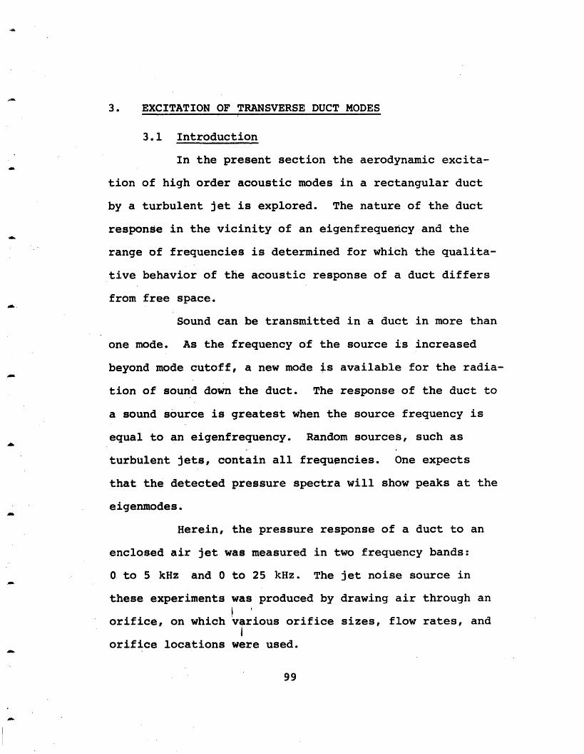
3. EXCITATION OF TRANSVERSE DUCT MODES
3.1 Introduction
In the present section the aerodynamic excita-
tion of high order acoustic modes in a rectangular duct
by a turbulent jet is explored. The nature of the duct
response in the vicinity of an eigenfrequency and the
range of frequencies is determined for which the qualita-
tive behavior of the acoustic response of a duct differs
from free space.
Sound can be transmitted in a duct in more than
one mode. As the frequency of the source is increased
beyond mode cutoff, a new mode is available for the radia-
tion of sound down the duct. The response of the duct to
a sound source is greatest when the source frequency is
equal to an eigenfrequency. Random sources, such as
turbulent jets, contain all frequencies. One expects
that the detected pressure spectra will show peaks at the
eigenmodes.
Herein, the pressure response of a duct to an
enclosed air jet was measured in two frequency bands:
0 to 5 kHz and 0 to 25 kHz. The jet noise source in
these experiments was produced by drawing air through an
orifice, on which various orifice sizes, flow rates, and
orifice locations were used.
99
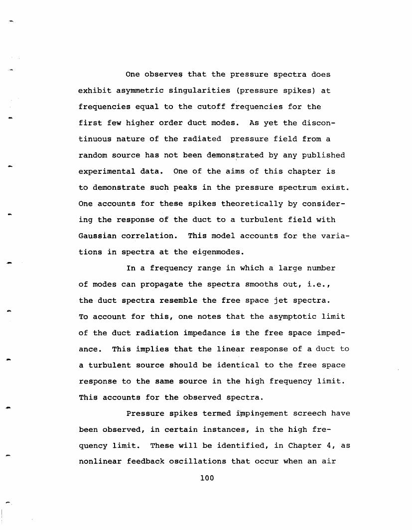
One observes that the pressure spectra does
exhibit asymmetric singularities (pressure spikes) at
frequencies equal to the cutoff frequencies for the
first few higher order duct modes. As yet the discon-
tinuous nature of the radiated pressure field from a
random source has not been demonstrated by any published
experimental data. One of the aims of this chapter is
to demonstrate such peaks in the pressure spectrum exist.
One accounts for these spikes theoretically by consider-
ing the response of the duct to a turbulent field with
Gaussian correlation. This model accounts for the varia-
tions in spectra at the eigenmodes.
In a frequency range in which a large number
of modes can propagate the spectra smooths out, i.e.,
the duct spectra resemble the free space jet spectra.
To account for this, one notes that the asymptotic limit
of the duct radiation impedance is the free space imped-
ance. This implies that the linear response of a duct to
a turbulent source should be identical to the free space
response to the same source in the high frequency limit.
This accounts for the observed spectra.
Pressure spikes termed ipingement screech have
been observed, in certain instances, in the high fre-
quency limit. These will be identified, in Chapter 4, as
nonlinear feedback oscillations that occur when an air
100
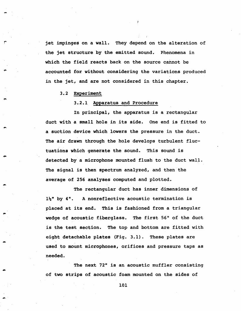
jet impinges on a wall. They depend on the alteration of
the jet structure by the emitted sound. Phenomena in
which the field reacts back on the source cannot be
accounted for without considering the variations produced
in the jet, and are not considered in this chapter.
3.2 Experiment
3.2.1 Apparatus and Procedure
In principal, the apparatus is a rectangular
duct with a small hole in its side. One end is fitted to
a suction device which lowers the pressure in the duct.
The air drawn through the hole develops turbulent fluc-
tuations which generate the sound. This sound is
detected by a microphone mounted flush to the duct wall.
The signal is then spectrum analyzed, and then the
average of 256 analyses computed and plotted.
The rectangular duct has inner dimensions of
1½" by 4". A nonreflective acoustic termination is
placed at its end. This is fashioned from a triangular
wedge of acoustic fiberglass. The first 56" of the duct
is the test section. The top and bottom are fitted with
eight detachable plates (Fig. 3.1). These plates are
used to mount microphones, orifices and pressure taps as
needed.
The next 72" is an acoustic muffler consisting
of two strips of acoustic foam mounted on the sides of
101
I
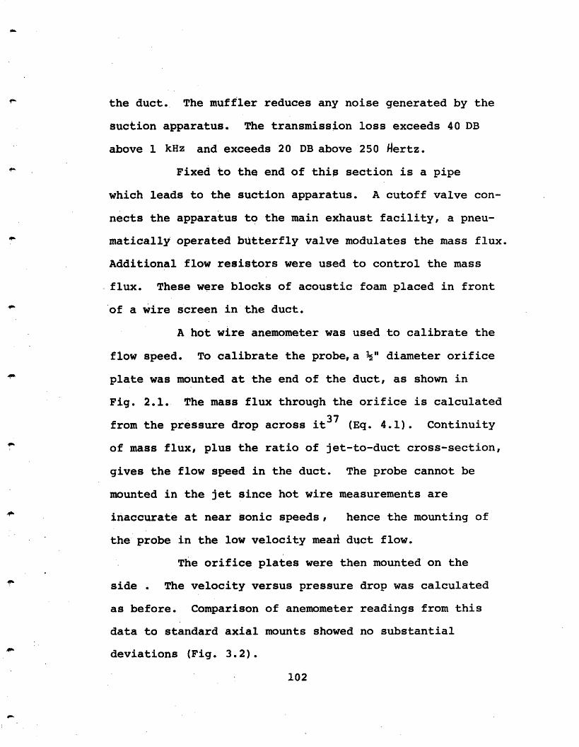
the duct. The muffler reduces any noise generated by the
suction apparatus. The transmission loss exceeds 40 DB
above 1 kHz and exceeds 20 DB above 250 ertz.
Fixed to the end of this section is a pipe
which leads to the suction apparatus. A cutoff valve con-
nects the apparatus to the main exhaust facility, a pneu-
matically operated butterfly valve modulates the mass flux.
Additional flow resistors were used to control the mass
flux. These were blocks of acoustic foam placed in front
of a wire screen in the duct.
A hot wire anemometer was used to calibrate the
flow speed. To calibrate the probe,a " diameter orifice
plate was mounted at the end of the duct, as shown in
Fig. 2.1. The mass flux through the orifice is calculated
from the pressure drop across it37 (Eq. 4.1). Continuity
of mass flux, plus the ratio of jet-to-duct cross-section,
gives the flow speed in the duct. The probe cannot be
mounted in the jet since hot wire measurements are
inaccurate at near sonic speeds, hence the mounting of
the probe in the low velocity mead duct flow.
The orifice plates were then mounted on the
side . The velocity versus pressure drop was calculated
as before. Comparison of anemometer readings from this
data to standard axial mounts showed no substantial
deviations (Fig. 3.2).
102
One quarter inch B + K microphones were used to
detect the acoustic field. The protective cover which
shields the microphone membrane was removed so as to pro-
vide a smooth surface to the flow. The microphone was
mounted in a test plate with the membrane flush to the
surface of the plate. Recall that transverse modes are
characterized by their variation in a plane normal to the
duct axis. To detect such modes, the microphone must be
at a pressure antinode. In rectangular ducts, the
corners are pressure antinodes for all modes. Two plates
with the microphone mounted at the corner were made. A
third plate was machined to allow transverse variation of
the microphone (Fig. 3.3). The plate has a double row of
¼" holes spaced by " from center to center. The second
row is staggered behind the first to provide " increments
in microphone location. The holes are stopped with alumi-
num plugs when the microphone is not in place.
Circular orifice plates of ", " and 1" dia-
meter were machined from '%" thick aluminum plate (Fig.
3.4). The orifices are tapered so as to present a sharp
edge to the in-coming flow. Tapering is necessary to
avoid orifice screech when the thickness to diameter is
between and 2. The plates were mounted on the side of
the duct so that the jet enters perpendicular to the duct
axis. A fourth plate, " diameter, was mounted to let
103
the air enter parallel to the duct axis. It was this
plate that was used for the velocity calibration (Fig.
3.1). Finally, a 60" pipe, " inner diameter, was
mounted on a plate (Fig. 3.5).
The electric apparatus consists of a micro-
phone power supply, a spectrum analyzer, a spectrum
averager, and an x-y plotter.
3.2.2 Basic Experiment
In the experiment an orifice plate is mounted
in the center of the test section. The pressure in the
duct is reduced and air drawn through the orifice. The
air jet impinges on the opposite wall. The turbulent
fluctuations in the air jet act as the sound source.
The acoustic signal is analyzed in two frequency ranges,
termed low ( to 5 kHz ) and high ( to 25 kHz ) (Fig.
3.6).
The low frequency range spans the first four
transverse duct modes. In this limit the frequency
separation between modes is greater than their bandwidth
when excited by a random source. Inspection of Fig. 3.6
shows that just beyond each mode cutoff the sound level
increases abruptly. Of particular interest is the
asymmetric shape of the curves which characterizes the
excitation of transverse modes. Recall that such modes
progagate only if the frequency is above a certain cutoff.
104
The duct pressure response to excitation of a given mode
is zero below its cutoff frequency w n infinite at the
cutoff frequency, and proportional to e1 aboveJ -e n
cutoff (see section 3.3.1). The infinite response is in
the ideal case of infinite source impedance and zero
damping. Real fluid effects limit the response to
approximately 10 DB. Nonetheless, the asymmetric shape
is still evident.
In the high frequency range the spectra
resembles the free space jet spectra (Fig. 3.6 ). Below
five kilohertz the level jumps at the cross modes are
still evident. Above five kilohertz the spectra smooths
out. One can show that the radiation impedance in the
high frequency limit asymptotically approaches the free
space impedance, hence the similarity. Two physical
effects are responsible for the smoothing of the curve.
First, the damping limits the level jump at cutoff.
Second, a new mode cuts on before the level shift from
the previous mode has subsided. The influence of the
neighboring modes overlap so as to make the contribution
of any given mode small, in this range.
3.2.3 Spectra Variation with Jet Velocityand Diameter
Herein the effects of flow speed and orifice
diameter are investigated. Since the flow rate in the
duct is much smaller than that of the jet, the duct
105
response should remain approximately independent of flow
speed. Aside from level shifts due to increased turbu-
lence, the spectralshould be similar. Three orifice
diameters, ¼", " and 1", were tested for jet flow
speeds up to Mach 1. Representative spectra are pre-
sented for each of these cases.
The low frequency spectra are presented in
Figs. 3.7, 3.8, and 3.9. Level jumps at the first three
cutoff frequencies are observed for all flow speeds.
Moreover, the characteristic asymmetric shape of the
peak is observed in all cases. The sound level rises
monatonically with velocity as expected. The intensity
at the high frequency end appears to increase at a faster
rate than the low frequency intensity in these plots.
Recall that, in free space, the spectra peaks at a
Strouhl frequency approximately equal to . As the
velocity increases, the intensity shifts toward the higher
frequencies. Hence the observed level increases at low
frequencies-should be smaller than those at high fre-
quencies.
The high frequency spectra are presented in
Figs. 3.10, 3.11, and 3.12. Here the average response
of the duct is most evident. Aside from screech tones,
the spectra increases with flow in a manner similar to
free space spectra. Dotted lines, indicating average
106
behavior, are drawn at low and high velocities in Figs.
3.10 and 3.11. As before, the sound level increases
monatonically with velocity. Moreover, the peak of the
average behavior increases with flow speed approximately
as the Strouhl frequency. These observations are con-
sistent with the low frequency behavior.
Certain spectral anomalies, termed screech
peaks are sometimes observed above Mach .6. These peaks
are nonlinear effects which are due to the coupling of
the jet flow to the acoustic waves produced. One indi-
cator of a separate mechanism is the line shape. Screech
peaks are symmetric about their maximum, the duct response
is asymmetric and peaked at a cutoff frequency.
3.2.4 Reduction by Strouhl Number
It is oftentimes useful to establish scaling
lows for data reduction. In aeroacoustics the Lighthill
eighth power law, and its extension by von Gierke38 to
spectral analysis (see section 4.3.2) has been found use-
ful. The basis for data reduction is the proposition
that the spectral intensity is maximum at a frequency
.2Vgiven by fs = *2D , where V and D are the jet velocity
and diameter. The point is that spectra should be simi-
lar for experiments with similar Strouhl numbers.
Such a comparison is made here. Figs. 3.13 and
3.14 present the spectra with the same Strouhl frequency
107
(5.7 kHz and 2.5 kHz ) for the low frequency regime.
Fig. 3.i5 compares two orifices of similar Strouhl fre-
quency (1.9 kHz ) in the high frequency regime. From
the figures it is clear that the spectral shape reduces
according to Strouhl number.
One exception is of note, the line shape below
the first cutoff. In each case (Figs. 3.13 and 3.14) the
orifice with the lower jet velocity exhibits a decay in
level as the frequency increases from zero to the first
cutoff. The orifice with the greater velocity exhibits
levels approximately independent of frequency. Such
behavior may indicate the dominance of sources other than
sound from the jet turbulence at low jet speeds. One
possibility is the wall turbulence in the duct.
One item of note is that the overall level
increases with increasing velocity. Let us assume that
the radiated power in the duct is proportional to 8D2 as
is the case for free jets. If the spectra shape is iden-
tical, the power per unit frequency should increase in
the same fashion. The level ratio between orifices of
different diameters but similar Strouhl numbers is given
by
108
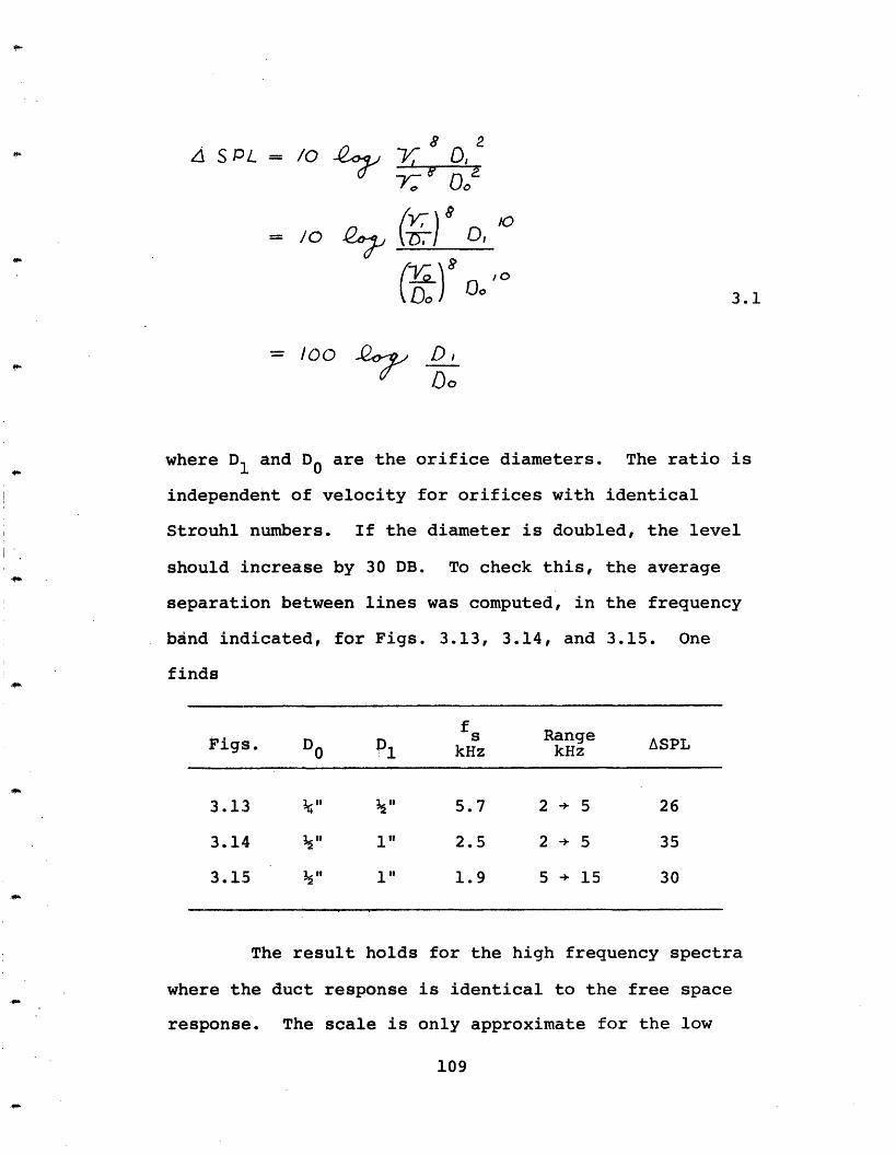
SP=/CQ o? (r)8 2
3.1
- 100 D,
where D1 and D are the orifice diameters. The ratio is
independent of velocity for orifices with identical
Strouhl numbers. If the diameter is doubled, the level
should increase by 30 DB. To check this, the average
separation between lines was computed, in the frequency
band indicated, for Figs. 3.13, 3.14, and 3.15. One
finds
fs Range SPLFigs. D P1 ASPLFigs. D kHz kHz
3.13 ¼" ½" 5.7 2 + 5 26
3.14 i" 1" 2.5 2 + 5 35
3.15 ½" 1" 1.9 5 + 15 30
The result holds for the high frequency spectra
where the duct response is identical to the free space
response. The scale is only approximate for the low
109
frequency spectra. In this range the turbulent sound
field is especially sensitive to variations in the jet
velocity and diameter. The error for a 10% deviation of
the Strouhl number gives an uncertainty of
10 log +3.4 DB, or a net error of 6.8 DB. The
observed deviations are 4 and 5 DB. This suggests that
the dimensional scaling laws do apply to the ducts, even
in the low frequency region.
3.2.5 Separating Linear from Feedback Effects
Certain peaks in the spectra were identified as
nonlinear effects. These were termed screech peaks.
They were distinguished from the linear duct response at
cutoff by their symmetric line shape. Herein the two
effects are separated by plotting amplitude variations
versus flow speeds.
In the linear response of the duct the sound
pressure level is proportional to the turbulent intensity.
Since the turbulent intensity increases monatonically
with flow speed, it follows that the level should also
increase monatonically.
A nonlinear effect depends on the interaction of
the jet flow with the acoustic wave it produces. Such
interactions depend strongly on the jet flow speed.
Screech instabilities only occur for certain flow speeds.
One finds that the sound level no longer increases
monatonically with flow speed.
110
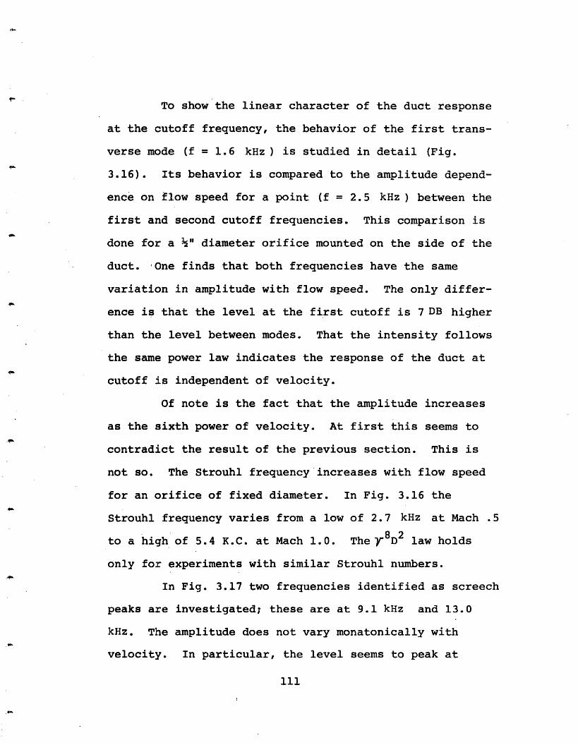
To show the linear character of the duct response
at the cutoff frequency, the behavior of the first trans-
verse mode (f = 1.6 kHz ) is studied in detail (Fig.
3.16). Its behavior is compared to the amplitude depend-
ence on flow speed for a point (f = 2.5 kHz ) between the
first and second cutoff frequencies. This comparison is
done for a " diameter orifice mounted on the side of the
duct. One finds that both frequencies have the same
variation in amplitude with flow speed. The only differ-
ence is that the level at the first cutoff is 7 DB higher
than the level between modes. That the intensity follows
the same power law indicates the response of the duct at
cutoff is independent of velocity.
Of note is the fact that the amplitude increases
as the sixth power of velocity. At first this seems to
contradict the result of the previous section. This is
not so. The Strouhl frequency increases with flow speed
for an orifice of fixed diameter. In Fig. 3.16 the
Strouhl frequency varies from a low of 2.7 kHz at Mach .5
to a high of 5.4 K.C. at Mach 1.0. The 8D2 law holds
only for experiments with similar Strouhl numbers.
In Fig. 3.17 two frequencies identified as screech
peaks are investigated; these are at 9.1 kHz and 13.0
kHz. The amplitude does not vary monatonically with
velocity. In particular, the level seems to peak at
111
Mach .7 and .8 and then fall off. Such variations with
flow speed identify the screech as a separate, nonlinear
effect.
3.2.6 Effect of Inlet Turbulence
Herein the effect of inlet turbulence on spectral
line shape is determined. The spectral line shape should
be independent of variations in inlet flow conditions
since it is dominated by the duct response. Contrast the
simple orifice to the flow from a long pipe. The flow
entering the duct from a sharp edged orifice is laminar;
it does not become turbulent until points further down-
stream. The flow from a long pipe, on the other hand,
is fully turbulent. For comparison to the orifice data
the flow was drawn into the duct from a 60" pipe of "
inner diameter (Fig. 3.5).
The low frequency spectral dependence on flow
speed is presented in Fig. 3.18. The line shape is
similar to that observed for orifices. In particular, the
asymmetric shape of the peak at cutoff is evident for all
flow speeds.
The high frequency spectral dependence on flow
speed is presented in Fig. 3.19. Again the line shape is
similar to that observed for orifices. In particular, the
spectra resembles the free space spectra in this range.
Absent from this figure is evidence of screech peaks. In
112
section 4.3.5 one screech peak is shown to occur at suf-
ficiently high flow velocities.
Of note is the periodic ripples superimposed on
the low frequency plot in Fig. 3.18. The spacing between
these ripples is 112.5 Hertz. This corresponds to a
Ccavity ength L = F = 60". The ripples represent the
excitation of the axial pipe modes. The response of the
pipe is superimposed on the duct response.
3.2.7 Orifice Mounted on Axis
Herein the orifice was placed so that the air jet
entered parallel to the duct axis. The acoustic foam
wedge was removed from the upstream end and a " orifice
plate was mounted in its place (Fig. 3.1).
Acoustic spectra versus velocity in the low fre-
quency range are presented in Fig. 3.20. Again, one
observes asymmetric peaks at cutoff frequencies for all
flow speeds. The effect, however, is not as pronounced
as it is for side-mounted orifices. This is due to mask-
ing of the acoustic wave by the convected turbulence.
The hard-walled orifice plate in the plane of the duct
cross-section also influences the spectra. To circumvent
these e:Efects, the orifice was mounted on the duct side.
The microphone could be mounted upstream in a region of
zero mean flow.
113
The change of location introduces impingement
screech. This screech occurs only if the air jet strikes
an opposing wall. No screech was observed for the ori-
fice mounted on axis.
3.2.8 Upstream versus Downstream Radiation
With the exception of the orifice mounted on axis
all spectra were taken with the microphone located up-
stream. In this region, apart from some recirculation,
there is negligible convected turbulence to mask the
acoustic wave. In ddition, the duct response is inde-
pendent of jet velocity as the mean flow is zero. Condi-
tions downstream of the orifice should be similar since
the flow speed in the duct is small.
Two microphones were used to check this, one up-
stream and the other downstream. The flow speed was set,
and both upstream and downstream spectra were plotted on
the same graph. The only error introduced by such pro-
cedure is the difference in microphone response, which
is approximately 0.8 DB.
The spectra at Mach .25 and 1.0 for a " orifice
are compared in Fig. 3.21. The response at the low flow
speed is approximately identical. At high flow speeds a
periodic variation of level with frequency is observed
downstream, but not upstream. Aside from these variations
the response is identical. The microphone was placed
114
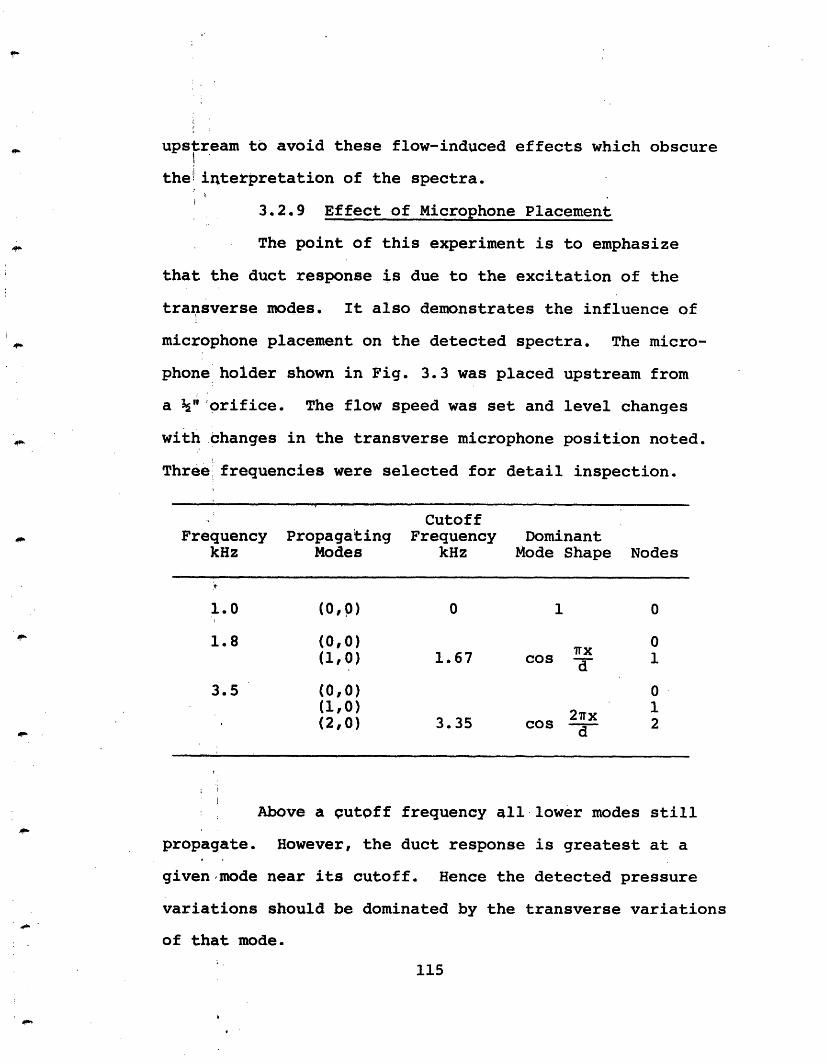
upstream to avoid these flow-induced effects which obscure
the interpretation of the spectra.
3.2.9 Effect of Microphone Placement
The point of this experiment is to emphasize
that the duct response is due to the excitation of the
transverse modes. It also demonstrates the influence of
microphone placement on the detected spectra. The micro-
phone holder shown in Fig. 3.3 was placed upstream from
a "'orifice. The flow speed was set and level changes
with changes in the transverse microphone position noted.
Three frequencies were selected for detail inspection.
CutoffFrequency Propagating Frequency Dominant
kHz Modes kHz Mode Shape Nodes
1.0 (0,0) 0 1 0
1.8 (0,0) 0(1,0) 1.67 cos 1
3.5 (0,0) 0(1,0) 1(2,0) 3.35 cos 2
d
Above a cutoff frequency all lower modes still
propagate. However, the duct response is greatest at a
given mode near its cutoff. Hence the detected pressure
variations should be dominated by the transverse variations
of that mode.
115
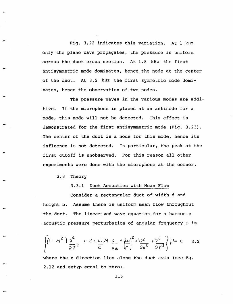
Fig. 3.22 indicates this variation. At 1 kHz
only the plane wave propagates, the pressure is uniform
across the duct cross section. At 1.8 kHz the first
antisymmetric mode dominates, hence the node at the center
of the duct. At 3.5 kHz the first symmetric mode domi-
nates, hence the observation of two nodes.
The pressure waves in the various modes are addi-
tive. If the microphone is placed at an antinode for a
mode, this mode will not be detected. This effect is
demonstrated for the first antisymmetric mode (Fig. 3.23).
The center of the duct is a node for this mode, hence its
influence is not detected. In particular, the peak at the
first cutoff is unobserved. For this reason all other
experiments were done with the microphone at the corner.
3.3 Theory
3.3.1 Duct Acoustics with Mean Flow
Consider a rectangular duct of width d and
height b. Assume there is uniform mean flow throughout
the duct. The linearized wave equation for a harmonic
acoustic pressure perturbation of angular frequency w is
+ )C 6/ +~2 ,- .. p=8 ?2 0 3.2
where the z direction lies along the duct axis (see Eq.
2.12 and setcp equal to zero).
116
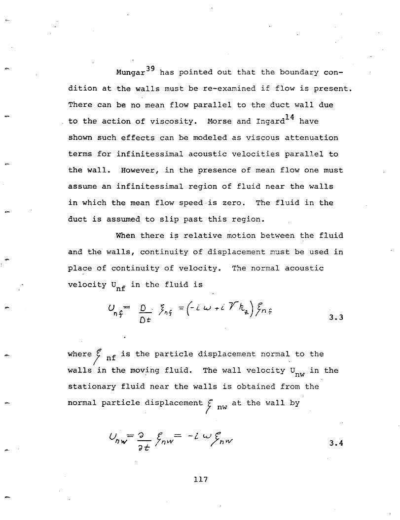
Mungar 39 has pointed out that the boundary con-
dition at the walls must be re-examined if flow is present.
There can be no mean flow parallel to the duct wall due
to the action of viscosity. Morse and Ingard1 4 have
shown such effects can be modeled as viscous attenuation
terms for infinitessimal acoustic velocities parallel to
the wall. However, in the presence of mean flow one must
assume an infinitessimal region of fluid near the walls
in which the mean flow speed is zero. The fluid in the
duct is assumed to slip past this region.
When there is relative motion between the fluid
and the walls, continuity of displacement must be used in
place of continuity of velocity. The normal acoustic
velocity Unf in the fluid is
wnh t
where / nf is the particle displacement normal to the
walls in the moving fluid. The wall velocity U in the
stationary fluid near the walls is obtained from the
normal particle displacement f nw at the wall by
/ v P..= -i W z 3.4
117
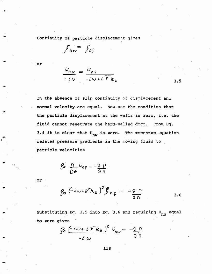
Continuity of particle displacement gi.-es
or
U _ Un W n;
- L4) -~L . 7-J*LY 3.5
In the absence of slip continuity of displacement anL
normal velocity are equal. Now use the condition that
the particle displacement at the wails is zero, i.e. the
fluid cannot penetrate the hard-walled duct. From Eq.
3.4 it is clear that U is zero. The momentum equation
relates pressure gradients in the moving fluid to
particle velocities
go .U, = -U P9 n
or
g (- Lcow y'7 )25 = 9 P 3.63.69 n
Substituting Eq. 3.5 into Eq. 3.6 and requiring Unw equal
to zero gives
fo ( - - )2 u - _
_c am, on
118
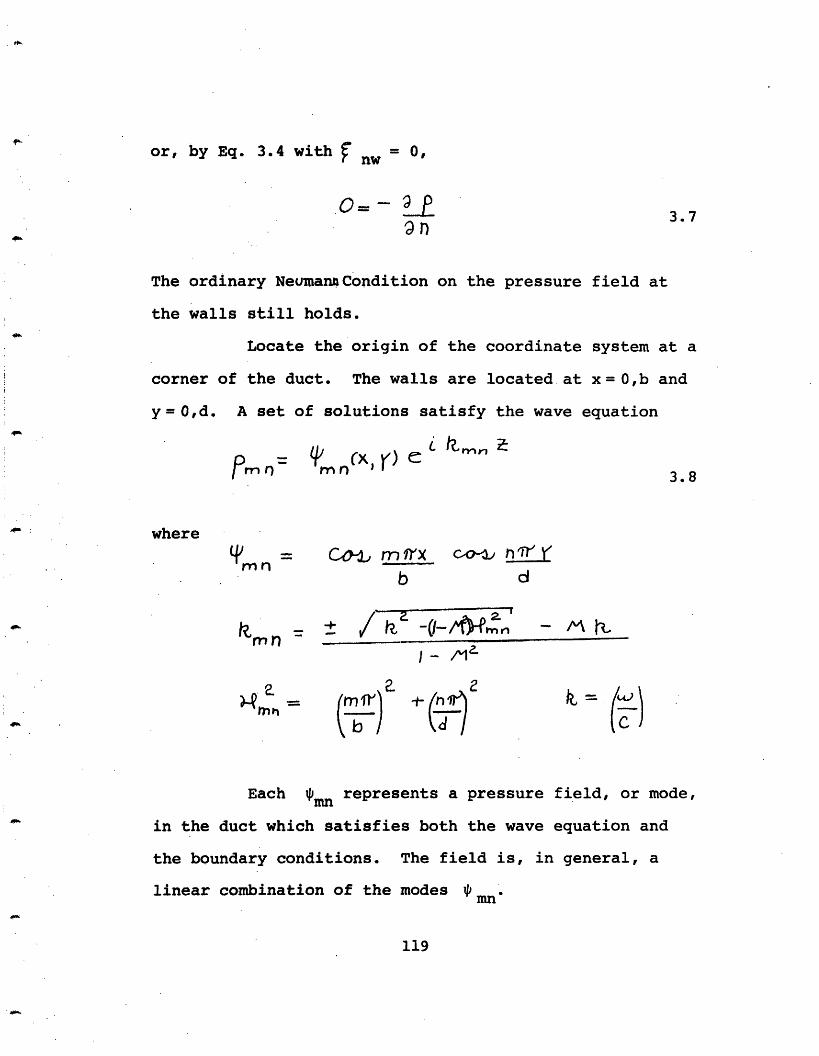
or, by Eq. 3.4 with nw = 0,
o=- ean
3.7
The ordinary NeumannCondition on the pressure field at
the walls still holds.
Locate the origin of the coordinate system at a
corner of the duct. The walls are located at x= O,b and
y = O,d. A set of solutions satisfy the wave equation
pqn a= rx, )e 3.8PMrn m n 3.8
where
Ymn= Cao nn Mf
b d
Mrnn ~ ~ rr- m4' a = (Mi)2-- / a2r l t 1
Each mn represents a pressure field, or mode,
in the duct which satisfies both the wave equation and
the boundary conditions. The field is, in general, a
linear combination of the modes mnmn
119
k i =
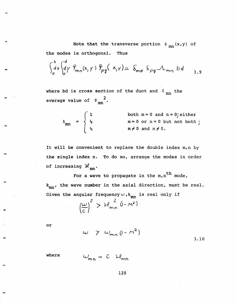
Note that the transverse portion i (x,y) ofmn
the modes is orthogonal. Thus
Fix idy Yr rx y ( xl)_ r,p Ya)t bdmy, "MPP p A rn r ,3.9
where bd is cross section of the duct and A themn2
average value of mn2mn
1 both m= 0 and n= O;either
Amn{ m= 0 or n= 0 but not both;
m 0 and n 0.
It will be convenient to replace the double index m,n by
the single index n. To do so, arrange the modes in order
of increasing -fmn.
For a wave to propagate in the m,nth mode,
kmn, the wave number in the axial direction, must be real.
Given the angular frequencyL ,kmn is real only if
or
7n Q3.10
where = C r"rn r) C ¥'P~mn
120
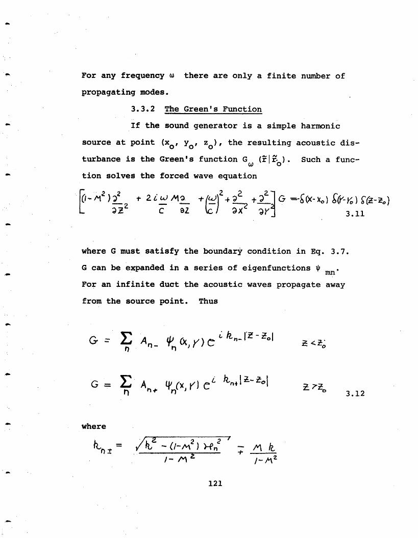
For any frequency w there are only a finite number of
propagating modes.
3.3.2 The Green's Function
If the sound generator is a simple harmonic
source at point (o, YO, zo), the resulting acoustic dis-
turbance is the Green's function G (rIrb). Such a func-
tion solves the forced wave equation
-A2)i 2 t 2 +2% G =-g(-x.) i(r- )(ty- 0 )·a3E; a c aX 3.11
where G must satisfy the boundary condition in Eq. 3.7.
G can be expanded in a series of eigenfunctions mnmn
For an infinite duct the acoustic waves propagate away
from the source point. Thus
G = - An
.r)
G=CA~G) _ Ad
r),C kn- [- Zl4, CX) I ) 11o~ue ·
3.12
where
&t /a _ ( 2) tf '
/_-
: / ,A
/- Mz
121
WnO(I K) C kni I;Z -;Lo
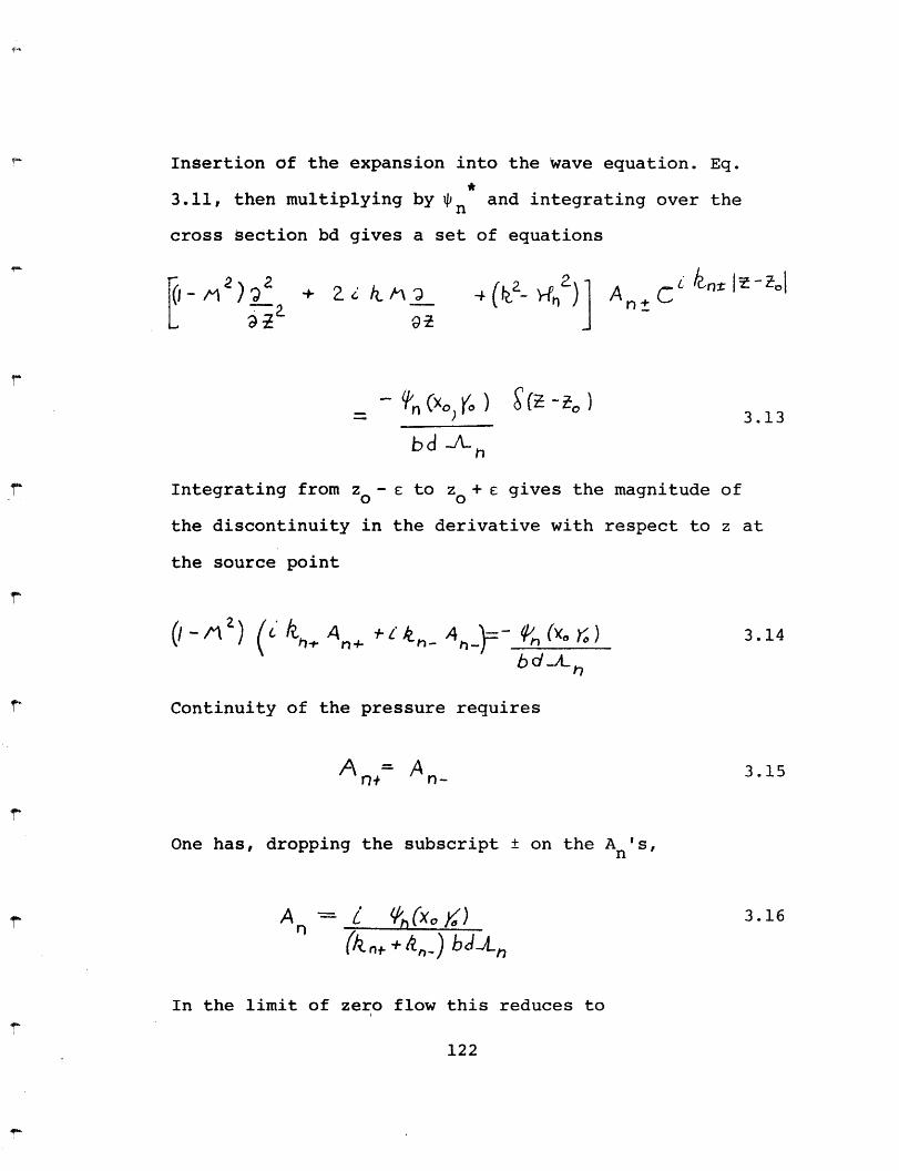
Insertion of the expansion into the wave equation. Eq.
3.11, then multiplying by n and integrating over the
cross section bd gives a set of equations
F(:,AI 2
L+ a' & h ' 4(62 te2- - A +C6 k4 1 Iz- I
3.13
bd -h
Integrating from zo - E to zo + gives the magnitude of
the discontinuity in the derivative with respect to z at
the source point
(-/A2 ) (6 k An * kh -At, (x0 t )b AL 7
3.14
3.15
Continuity of the pressure requires
A = A
One has, dropping the subscript on the A n's,
An - t J Clx0K)(nnte +li-) b d-n
In the limit of zero flow this reduces to
3.16
122
2 t, bd/L n
which can be found in Morse and Ingard1 4 (Chapter 9).
The Green's function is
=i (x c) kl(X Y° ) Cik | i ln '3.17
(kr) + kt.) bdY Ar
where the + sign holds for z> z and the - sign for
z < z on the term in the exponential.
3.3.3 Random Source Representation in a Duct
Consider the representation of a random source
in a duct. The issue is sufficiently complex to warrant
a separate discussion. The discription is done in steps.
First comes a review of the correlation in time, next
space correlation along the duct axis, then the space
correlation in the plane of the duct cross section.
Finally, the full space time correlation is presented as
the union of the above. A number of transforms are
introduced; to keep track of these the results are sum-
marized in tables3l and32. On the right hand side is a
note on dimensions which provides a useful check on the
formulas.
123
Consider a region of turbulent pressure fluc-
tuations p inside a rectangular duct (O< x< b, O< y< d)
with rigid walls. Let the fluctuations be confined to
a region - L/2 < z < L/2. To construct a measure of the
temporal variations of the source at point r, one pro-
ceeds as in free space.
R(p(", : -~t Ott) e 3.183.18
:,Pt)-d 5L 4J ' e v t 3.19
Similarly, the correlation is
~ro)° -t y t#) r f)r -r/2
3.20oo
T i
~T~~~~~ ~3.21
124
See Eq. 1.23 for a proof of Eq. 3.21. If the source is
homogeneous, one can drop the source point r in the
description of R.
Now consider a measure of the spatial variation
along the duct axis. Again, one proceeds as in free
space. The Fourier transform is
00
3.22
d ()e 3.23
Similarly, the correlation is
t(¥> T L t X t I _/2
-Lo
3.24
- l,,d p c (rt) e- "3.25L
125
Now consider a measure of the spatial variation
for points separated in the plane of cross section of the
duct. If one defines
o6?d,)= i idxr (Y,/) J( +o(, r )_ 3.26
as the pressure correlation for simultaneous measurements
separated by a and B, one must decide what values to use
forqe when x +a exceeds b or y+ exceeds d.
One possibility is that P is zero outside the
source region, as was the case for axial pipe modes (Eq.
2.44). In this case, however, computational difficulties
are encountered when the source correlation is related to
the radiated pressure. In particular, it is impossible
to expand the source in the duct eigenfunctions if the
source strength is assumed to be zero outside the walls.
Here is is more convenient to consider the walls as
reflectors and to considers outside the duct to be the
mirror image of the distribution inside. Following Morse
and Ingardl4 (Chapter 9), one expands the source in the
eigenfunctions of cross section and limits attention to
points inside the duct. The Fourier transform is
ax~,y))C mn 4 tnCn x' 3.27rn 11ru
126
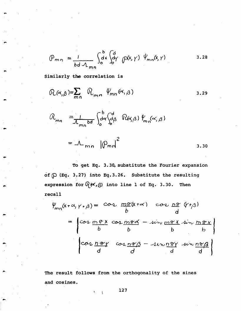
(Pm r =_ bd A mn
Similarly the correlation is
mn
n= I -
r bdmn o
To get Eq. 3.30, substitute the Fourier expansion
of (Eq. 3.27) into Eq.3.26. Substitute the resulting
expression for q(j(,3) into line 1 of Eq. 3.30. Then
recall
Y,n(X t ' " ) = b (X ,+)
- co r Xb
d
cao-v n t (c'jt13)d
CO-a r>)1)( -M -Ir -X f 7P XW
b b h
d- Y3- . 2v d d-4i n 13d d d
The result follows from the orthogonality of the sines
and cosines.
I 1 127
3.28
3.29
3.30
baCb) ,v
dx 6(.,K mooV
9r, 4mn6<,/3)
&,W /s (Cn j ,3
2= _J� r" n 103m
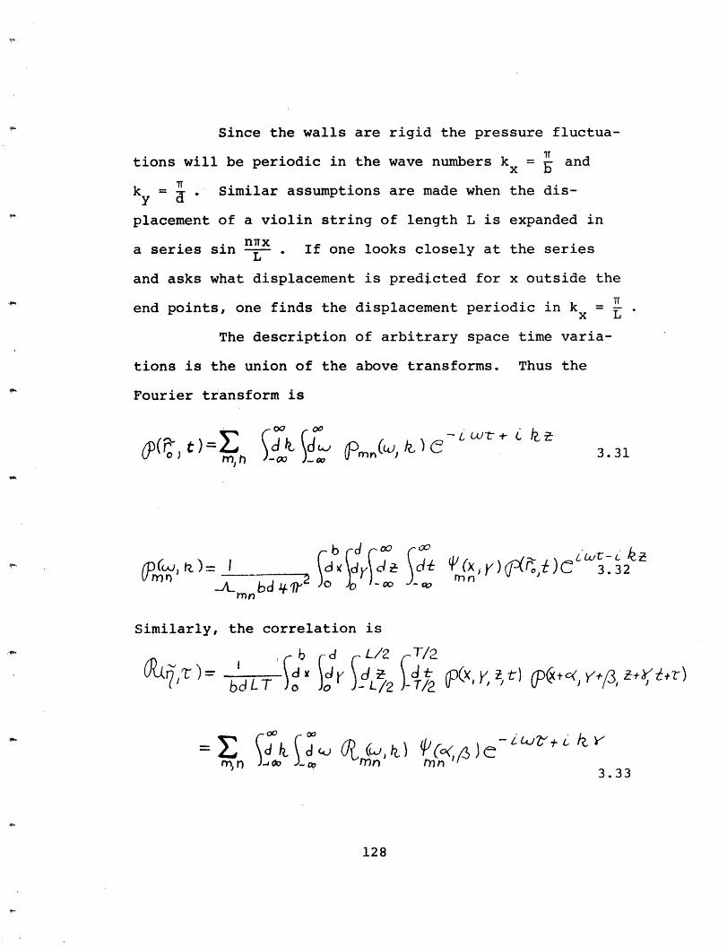
Since the walls are rigid the pressure fluctua-
tions will be periodic in the wave numbers kx = andb
ky = d Similar assumptions are made when the dis-
placement of a violin string of length L is expanded in
a series sin nx If one looks closely at the seriesL
and asks what displacement is predicted for x outside the
end points, one finds the displacement periodic in k =Lx L
The description of arbitrary space time varia-
tions is the union of the above transforms. Thus the
Fourier transform is
y(t, )t t)=,( I n ) 3.31
fL3Cu ~t =I C~(1~t)>C 3.32
ONr)n C, b 2 )= I o r n- X /~Pn ~): 332 /i~~ 7O JO0 'ooJ-
Mn
Similarly, the correlation is
b rd L/2 T/2
tP~t,-o qa )= =r A / tJ/ (X(~ i ti a~~ ) Bat ye t r)bd L T )- iL/2 T 2t
m, n " r n mn3.33
128
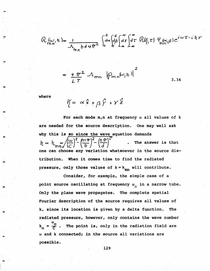
rnn
- fi mn I2o n rl(W)L T 3.34
where
A A
For each mode m,n at frequency w all values of k
are needed for the source description. One may well ask
why this is so since the wave equation demands
= i /(w)2 (y#)2 (n-l)- . The answer is that
one can choose any variation whatsoever in the source dis-
tribution. When it comes time to find the radiated
pressure, only those values of k= kmn will contribute.
Consider, for example, the simple case of a
point source oscillating at frequency O in a narrow tube.
Only the plane wave propagates. The complete spatial
Fourier description of the source requires all values of
k, since its location is given by a delta function. The
radiated pressure, however, only contains the wave number
k The point is, only in the radiation field are0o Cw and k connected; in the source all variations are
possible.
129
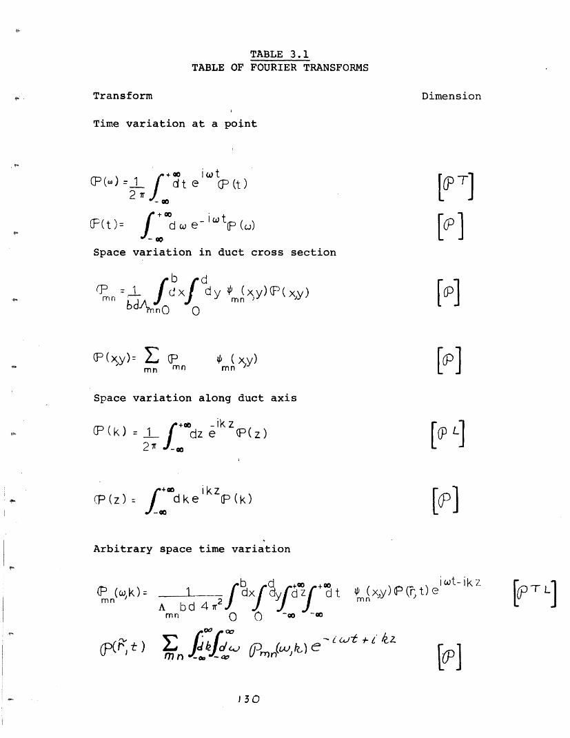
TABLE 3.1TABLE OF FOURIER TRANSFORMS
Transform Dimension
Time variation at a point
e
P t-F(t)= 0((t) = C
0- o
iwtOP(t)
iwe - tP (W)
Y J0 ( XY)F(PX XY
JI ( )Fxxyy
mn
Space variation in duct cross section
rb rdrn b Anno O
D(xy): Cmn mn
Space variation along duct axis
ikz(k) = 1 +dz e (P(z)
211 '- [CL]
r+0(CP(z)= = dke k (k)
Lf1
Arbitrary space time variation
b d +ao +co
1 dxr dyfdZ dtA bd 4r .1mn 00 - 0
c(jt) EM n
00 00
f f L /-J -k2, ODn(w ) e
- W-t~ * 1,
130
1Pm]
EcP)
(P (,k)=mn T L]
Lw]
iwt- ikzz.s( t
( () = d t
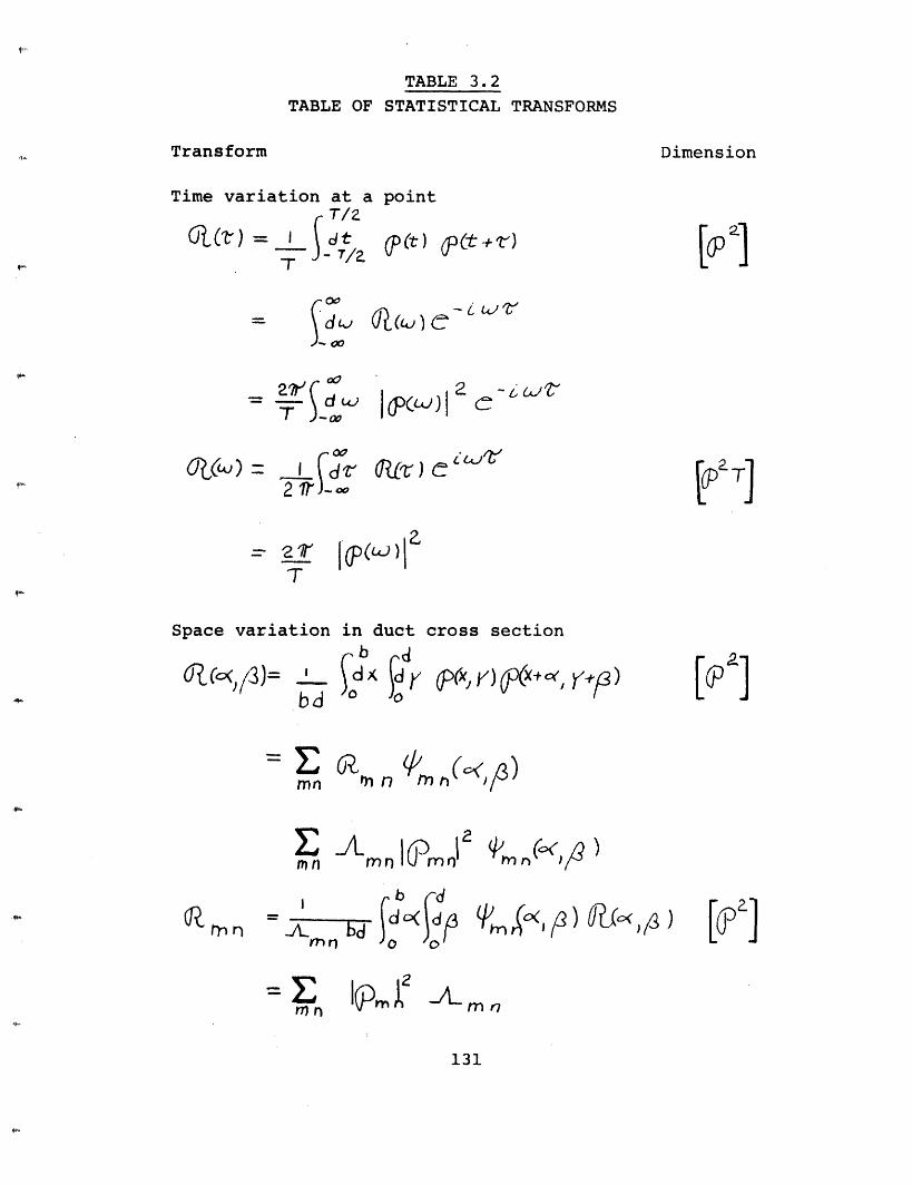
TABLE 3.2
TABLE OF STATISTICAL TRANSFORMS
Dimension
Time variation at a point
I
T
T/2dt- 7/2
r0o
2 \Nd
J'P(WiI
otfc) =
K) 2
oz(,))C -L~j
2 ,WV1C-1
Q&z) C
2TT
pT]
I6IA) I
Space variation in duct cross section
I
bd
M n h(c-<p)
Lmn 1mr) I(P , /2a
q/f o, r < , ) , )
Transform
mn)
L be 1 XJddn r) o o
[P]
m r7
131
6 (t ) op (t + TI
1= -~fd Lo,T Xo
rwo
I V
q �3) = P(X) ) O, C', Y,--ep
R r l
Fb dd/o
lpP
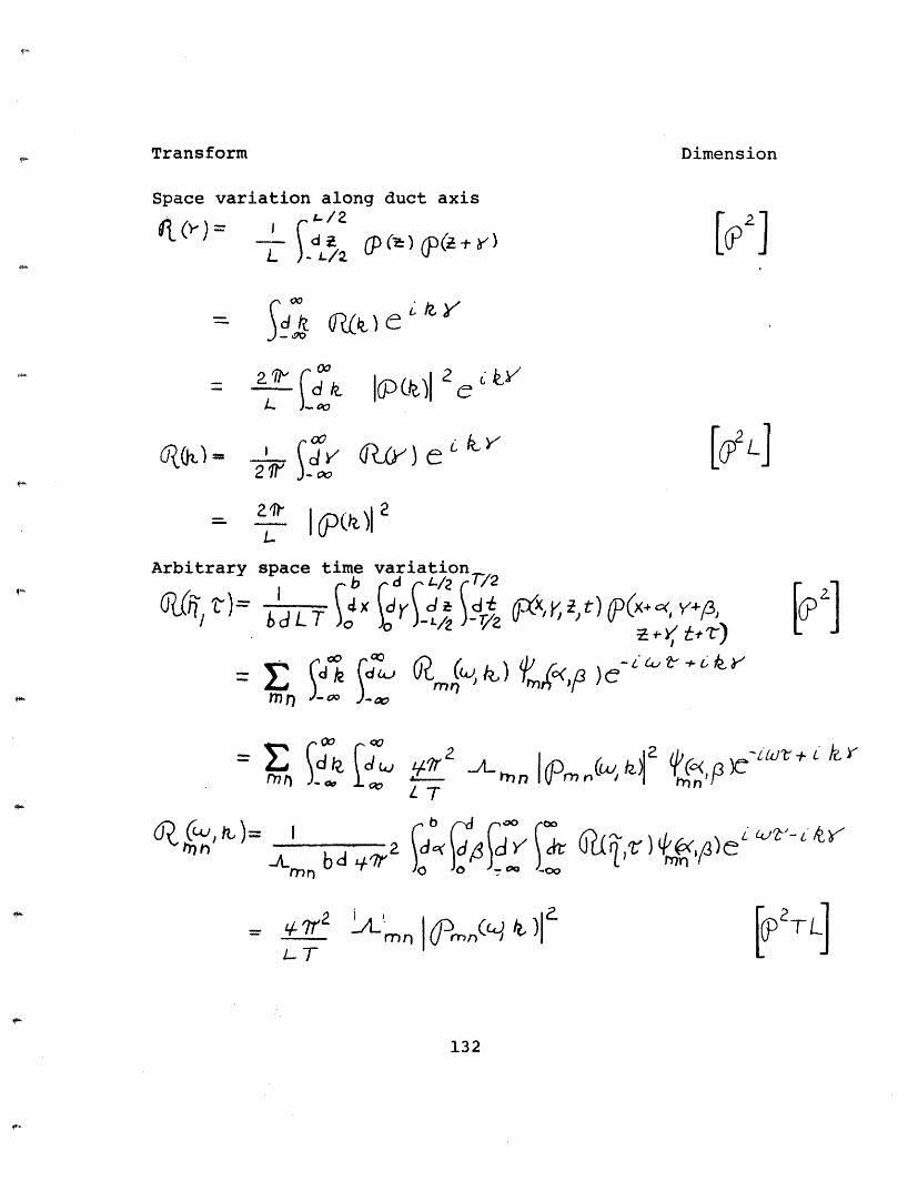
Dimension
Space variation along duct axis
- ai _ -Z ( t y= , t-d /2 1t, ed k
/_L _ J/o
_ , t o( 2L oihL
Arbitrary
OThi T4=
space time variationrb d /12 T7/2
bd L T -j/Z
2 (,)
X, , t) (X+,( Y+P,
1 < L, k-< *+z-J~rnk~p ) Lk Y
mnr I( k (r2Y
I
-n bd t1 2rmr)
=L T2
T
b S4- d
mI
132
[P2]
[y2L]
[c ]
Lo
L T
00-00
[2TL]
Transform
=1 2rn 1
PK-1WV
41D (w, tL ) �=\V rn h ) e'-
A-) (C,)) k
C3 co
= E k
nc;i�z
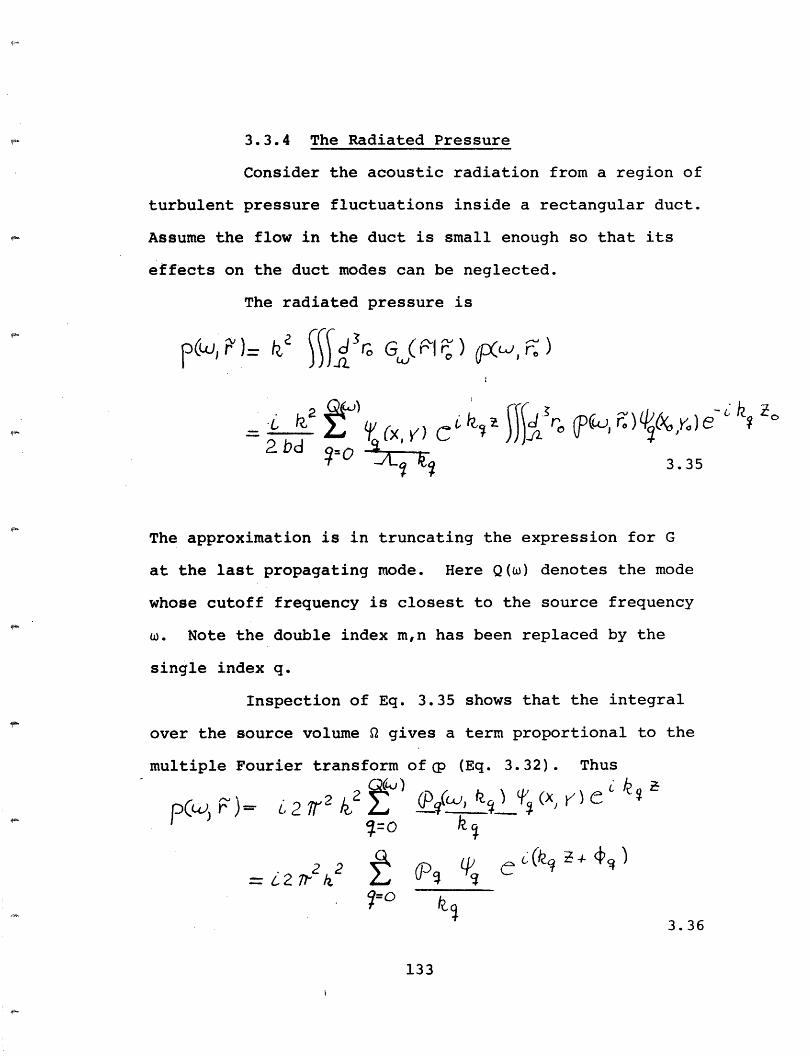
3.3.4 The Radiated Pressure
Consider the acoustic radiation from a region of
turbulent pressure fluctuations inside a rectangular duct.
Assume the flow in the duct is small enough so that its
effects on the duct modes can be neglected.
The radiated pressure is
( i) k i9|dj r G (w,r)
.i 2 B) It iJi (r)ls¢y)e~6 k2bd
2.bd ;·~ '4~ ~3.35
The approximation is in truncating the expression for G
at the last propagating mode. Here Q(w) denotes the mode
whose cutoff frequency is closest to the source frequency
w. Note the double index m,n has been replaced by the
single index q.
Inspection of Eq. 3.35 shows that the integral
over the source volume gives a term proportional to the
multiple Fourier transform of p (Eq. 3.32). Thus
$=o k~
2 i~s ei~q~~~9L,2 =2 +3.363.36
133
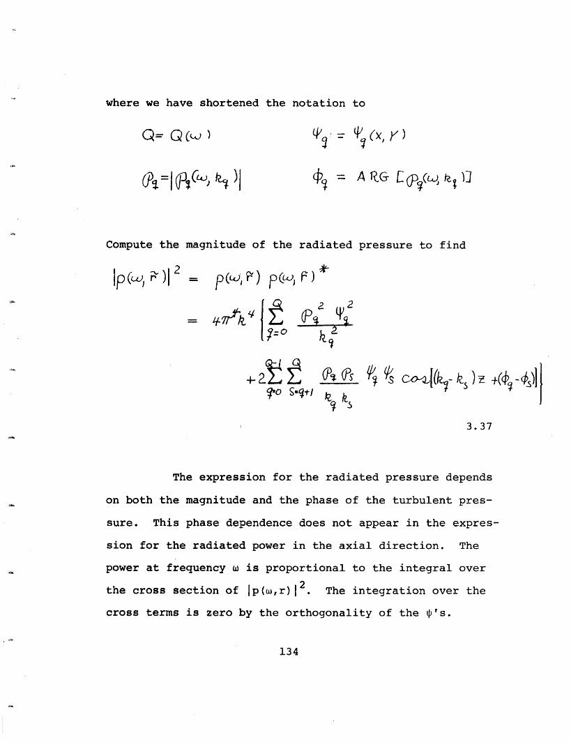
where we have shortened the notation to
0,(Xf's1f LI )= A R• C 0 (WLhi)
Compute the magnitude of the radiated pressure to find
Ip~ r )12_ p(w, r) pc~a A) u
?=o k
3.37
The expression for the radiated pressure depends
on both the magnitude and the phase of the turbulent pres-
sure. This phase dependence does not appear in the expres-
sion for the radiated power in the axial direction. The
power at frequency w is proportional to the integral over
the cross section of p(w,r) 12. The integration over the
cross terms is zero by the orthogonality of the p's.
134
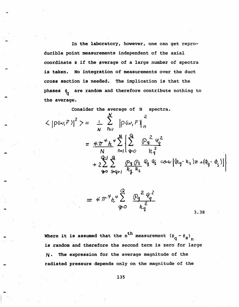
In the laboratory, however, one can get repro-
ducible point measurements independent of the axial
coordinate z if the verage of a large number of spectra
is taken. No integration of measurements over the duct
cross section is needed. The implication is that the
phased ~ are random and therefore contribute nothing to
the average.
Consider the average of N spectra.
M22
N tIrrm: ,A ~l ~h=l
2N nalo q tj
3.3.8
Where it is assumed that the nth measurement (~q - ~S)
is random and therefore the second term is zero for large
N. The expression for the average magnitude of the
radiated pressure depends only on the magnitude of the
135
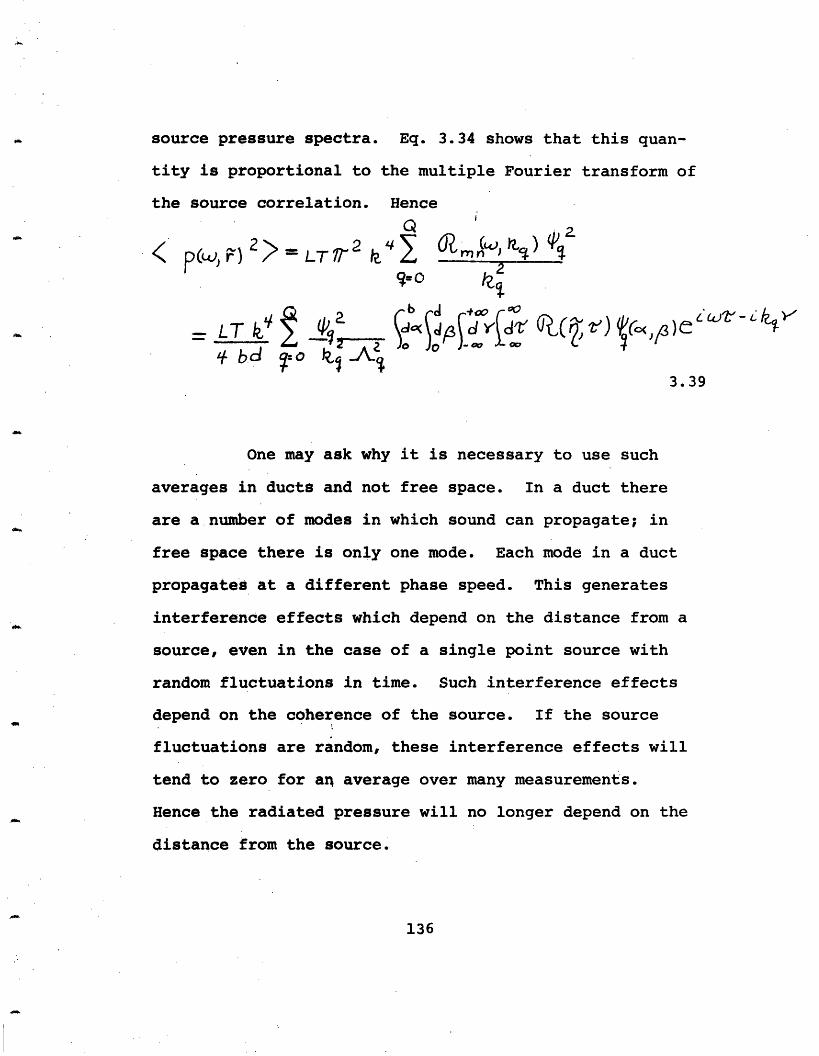
source pressure spectra. Eq. 3.34 shows that this quan-
tity is proportional to the multiple Fourier transform of
the source correlation. Hence
< p(L, 2> T2 s E 2
LT k dd jFe ) ed/ VY bd o kx Ax
3.39
One may ask why it is necessary to use such
averages in ducts and not free space. In a duct there
are a number of modes in which sound can propagate; in
free space there is only one mode. Each mode in a duct
propagates at a different phase speed. This generates
interference effects which depend on the distance from a
source, even in the case of a single point source with
random fluctuations in time. Such interference effects
depend on the coherence of the source. If the source
fluctuations are random, these interference effects will
tend to zero for an average over many measurements.
Hence the radiated pressure will no longer depend on the
distance from the source.
136
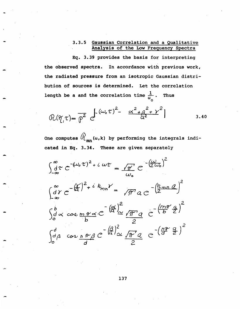
3.3.5 Gaussian Correlation and a QualitativeAnalysis of the Low Frequency Spectra
Eq. 3.39 provides the basis for interpreting
the observed spectra. In accordance with previous work,
the radiated pressure from an isotropic Gaussian distri-
bution of sources is determined. Let the correlation
length be a and the correlation time Thus0
"r)-' .. ,.,.,.,)"2 2 2
3.40
One computes mn (w,k) by performing the integrals indi-
cated in Eq. 3.34. These are given separately
6 WV
t_)o
2
' T m i
-~L M7 A O e )b 22
d - _ ) J2 d 2
C
e a- (
137
To
CdY
(b_ C<
zd
/3
00 -(Wo 2+ d It, Cc
::b- 0 --. rn-zn L
IF <2 C
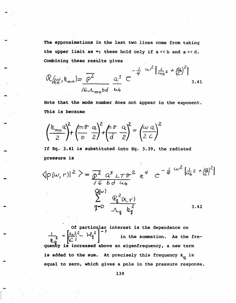
The approximations in the last two lines come from taking
the upper limit as ; these hold only if a<<b and a<< d.
Combining these results gives
e/ C. Z I + (t)2]/' ~
3.41(X(LJ) hA)= rPn bdo
/cGnn b d o
Note that the mode number does not appear in the exponent.
This is because
- 0-2 o- 2 a)(L2 +h 2 2b
If Eq. 3.41 is substituted into Eq. 3.
pressure is
<p(w, r)l > (p a3-)a LTa Tr 4./ b d C'
-p ' >I (XI )
1=0 k 2
39, the radiated
-/ Wc2 [ ]_ 2I-: (CI C
3.42
Of particular interest is the dependence on
}•~ J -- f _ >in the summation. As the fre-
queny is increased above an eigenfrequency, a new term
is added to the sum. At precisely this frequency k isq
equal to zero, which gives a pole in the pressure response.
138
!
As the frequency is increased above the eigenfrequency,
the contribution ofithis term diminishes and approaches
k- 2 assymtotically. These poles have their origin in the
Green's function, i.e., the duct response, and not on the
turbulent field. Further, note the asymmetric nature of
this contribution. For w < q the sum terminates before
this mode contributes. For > wq the mode propagates
and is included in the summation. Hence the asymmetry of
the peaks in the low frequency spectra (Figs. 3.7, 3.8,
3.9, 3.18 and 3.20).
Further note the dependcnce of iq on the observcr's
coordinates. If the microphone is at a node, q equals
zero, and the mode is not detected. This feature is
demonstrated experimentally in Fig. 3.23. With the micro-
phone in the center, the (1,0) mode is not detected. The
behavior is further demonstrated in Fig. 3.22 by altering
the transverse position of the microphone.
3.3.6 Damping and the Smoothing of the HighFrequency Spectra
Herein the theoretical infinite peaks at the
cutoff frequencies is corrected. To remedy the situation,
one postulates some damping of the modes. This can be
done in a formal manner by assuming a uniform specific
acoustic admittance at the walls. Thus the Neumannbound-
ary conditions for zero mean flow
139
12o =°9 X X b 0O.d
are replaced by
X b - 3.43
This change introduces a damping of the
acoustic waves; see Morse and Ingardl4 (Chapter 9). In
working such a problem, the difficulty arises in that the
eigenfunctions are no longer orthogonal to their complex
conjugates4 0. To expand the Green's function in such a
set becomes quite tedious. Recall, however, that the
2poles are due to k2 0 as the cutoff frequency is
q
approached. It will be assumed that the damping is so
small that the wave functions and eigenfrequencies are
given sufficiently accurately by the undamped values. The
only modification by damping is assumed to be in the wave
number kq. Such assumptions are common to the treatment
of similar problems in room acoustics.4 1 The argument is
that damping modifies the response only in the vicinity of
an eigenfrequency, i.e., at a pole.
Consider the modified boundary conditions given
in Eq. 3.43. The addition of damping gives
140
where, in the limit of small B
b b Ir n
d d rrn
Hence2
khr)
2
rn r
2N krnn
2 2 n- - ( ~ ~ ) 2 ~ ( T h t 7 < ~ ~ ( .` LI
The b' idl reduce-d to the mode wave numbers WP, plus a
Phr)
correction factor. One then has
/ m nl2
I
;
2.C
1rm n
4 s;+afI1
V' A ? fl
h #2 d )3.45
/h =0
m o
141
f > 0
fl7o
3.44
2 k t 6)
That is,, at the eigenfrequency the magnitude of the wave
number kmn is now nonzero. This implies that the singu-
larities at the cutoff frequencies have been removed from
the theory.
Numeric calculations based on visco-thermal
damping have been done. The results for the first mode
show that the predicted level changes exceed those
observed. Such work suggests that the radiative damping
may be the dominant loss mechanism.42
To determine the influence of damping on the
high frequency spectra, consider the radiated pressure at
frequencies just above and below the cutoff frequency wQ.
Consider the change in radiated pressure normalized to
the pressure at a frequency just below the cutoff.
P X p >-e)L J ip,*ei2 >KI- JD~- eI 11
_Aj i(JQtE )
= 1 ~1
(Q- 7) tz
(Q- 7)
Jr 7C
10-
I- | vite ) (o- (4 )
~ ~~2 ~~< Q 67<-
*1-!~~~~ 10.9( d s
i )Q(WJQ) < 3.46
142
-6)
The approximation is in substituting the
asymptotic limit of kq for the sum in the denominator.
This substitution is correct if Q is large. If k is
finite, it is clear that the pressure change approaches
zero as , where Q is the number of propagating modes.
Note that the limit is correct only if k is nonzero at
the cutoff, as is the case when there is damping.
The conclusion is the change in radiated pres-
sure when a new mode propagates is small compared to the
contribution from all other modes if there are a large
number of propagating modes. In this fashion, the
assumption of finite damping accounts for the smoothing
of the spectra in the high frequency limit. This collates
with the observed spectra under a variety of conditions
(Figs. 3.10, 3.11, 3.12 and 3.19).
3.3.7 Radiation Impedance and the Similarityof the High Frequency Duct Spectra toFree Space Spectrat
The damping argument (Eq. 3.46) states that the
spectra smooths out in the high frequency limit. It can
be shown that the spectra is identical to the free space
spectra in the high frequency limit. Morse and Ingard14
have shown this is true for a simple volume source.
143
tThe author is indebted to Dr. Rice of NASA Lewis for sug-gesting the use of averaging techniques in duct acoustics.
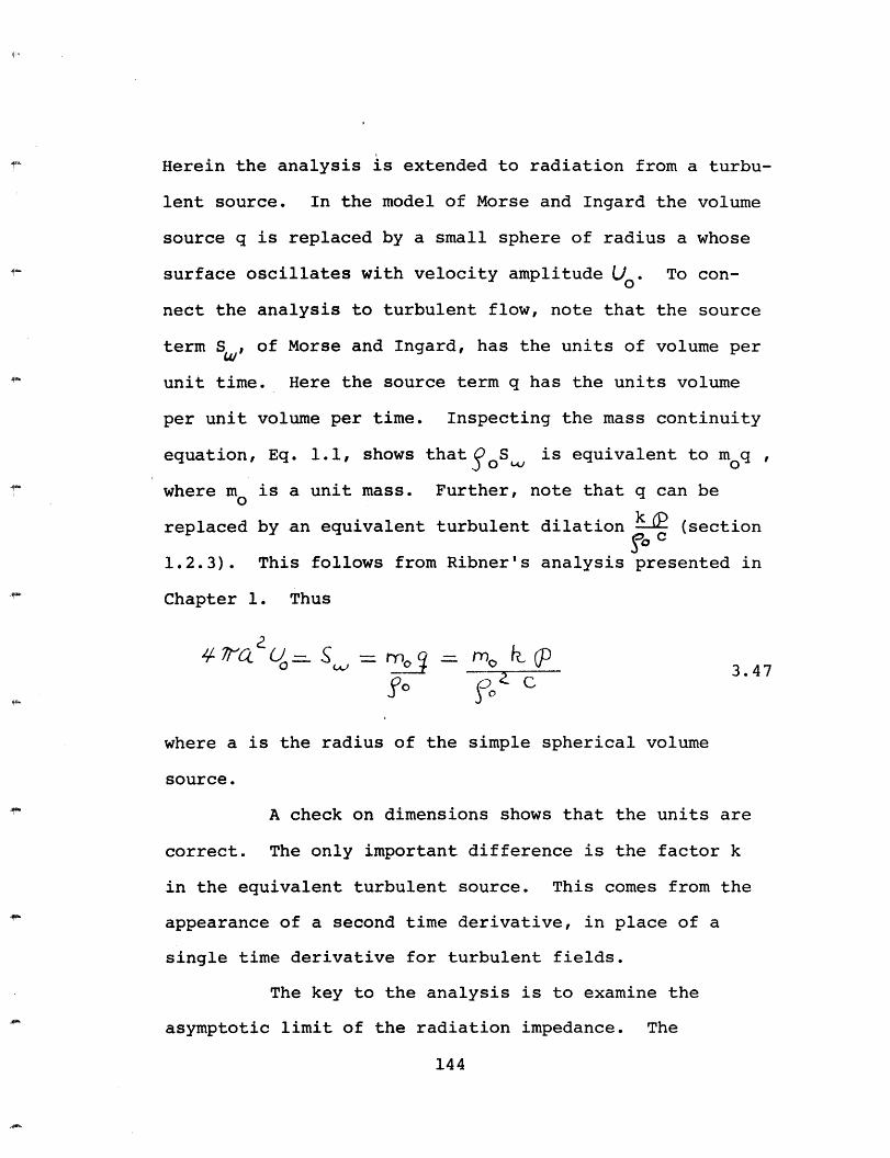
Herein the analysis is extended to radiation from a turbu-
lent source. In the model of Morse and Ingard the volume
source q is replaced by a small sphere of radius a whose
surface oscillates with velocity amplitude Uo . To con-
nect the analysis to turbulent flow, note that the source
term Sw, of Morse and Ingard, has the units of volume per
unit time. Here the source term q has the units volume
per unit volume per time. Inspecting the mass continuity
equation, Eq. 1.1, shows that oSS is equivalent to mq ,
where m is a unit mass. Further, note that q can be
replaced by an equivalent turbulent dilation kP (section
1.2.3). This follows from Ribner's analysis presented in
Chapter 1. Thus
4li7 UC_ S. . S 3 47-0 (w) - rY) 3.47
So For C
where a is the radius of the simple spherical volume
source.
A check on dimensions shows that the units are
correct. The only important difference is the factor k
in the equivalent turbulent source. This comes from the
appearance of a second time derivative, in place of a
single time derivative for turbulent fields.
The key to the analysis is to examine the
asymptotic limit of the radiation impedance. The
144
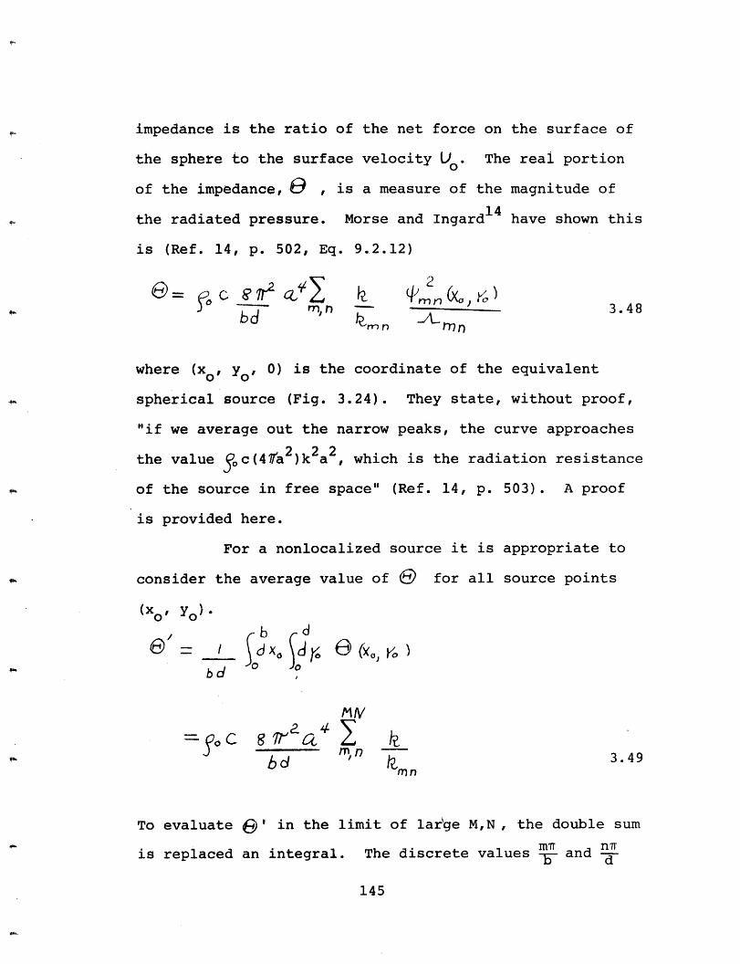
impedance is the ratio of the net force on the surface of
the sphere to the surface velocity o). The real portion
of the impedance, & , is a measure of the magnitude of
the radiated pressure. Morse and Ingardl4 have shown this
is (Ref. 14, p. 502, Eq. 9.2.12)
----- ---- 3.48bd = m,n n 3.48
where (xo, y, 0) is the coordinate of the equivalent
spherical source (Fig. 3.24). They state, without proof,
"if we average out the narrow peaks, the curve approaches
the value 5,c(4Fa2)k2a2 , which is the radiation resistance
of the source in free space" (Ref. 14, p. 503). A proof
is provided here.
For a nonlocalized source it is appropriate to
consider the average value of 6 for all source points
(xo ' Yo) .
bd
MM
bd
To evaluate e' in the limit of large M,N, the double sum
is replaced an integral. The discrete values and d
145
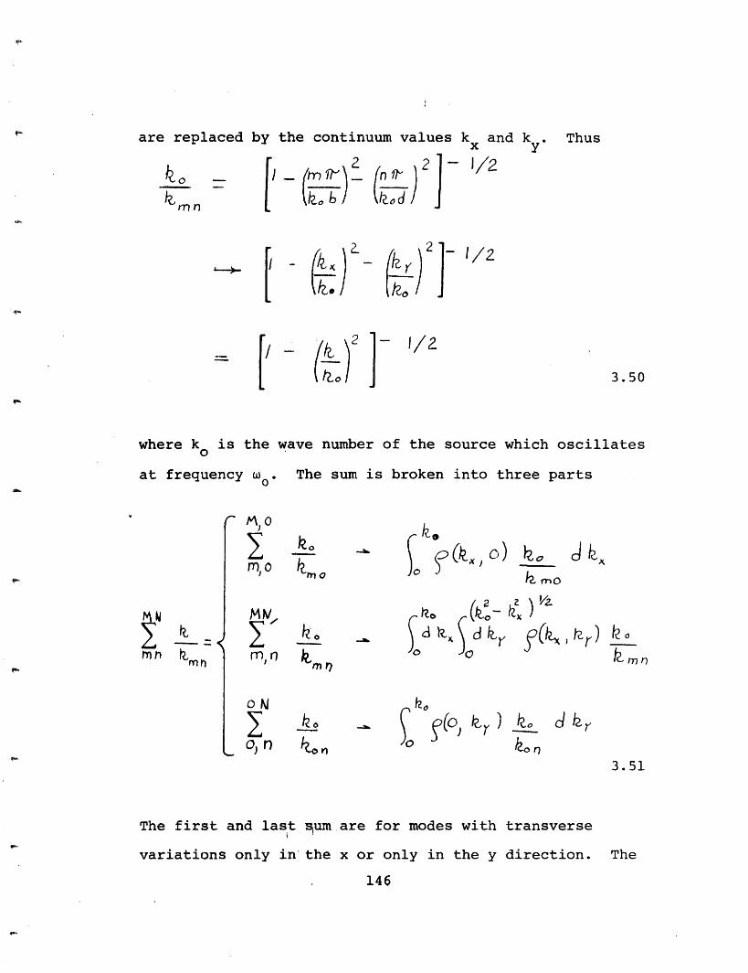
are replaced
ko -
kimn
by the continuum values kx and ky . Thus
( )[ \ (drx y[-mo - Iod
k) ( )J]to 2to
1/2
(i)2 j
cto J
I [I
where k is the wave number of the source which oscillatesO
at frequency 0.
Mnh km
The sum is broken into three parts
M; 0
M,O
,0
ke--a. . , (/) tmok no
MS
mr)
cik A
-o 5 xjd, r f(k&, tr) nkmn
o) n
The first and last mum are for modes with transverse
variations only in the x or only in the y direction. The
146
3.50
3.51
I-I
- Se(9"O
k, r
middle sum indicates modes that have both x and y varia-
tions. The density terms indicate the number of new modes
added per unit increase in wave number at the wave number
(kx, ky). For a rectangular geometry these densities are
constant. They are
S.(kx o)=I,
3.52
f (I kr ) dr)Integrating using the values given in Eq. 3.52 yields
t b2
aIto bi
2 t/
a0-
4,0
I,o
O,N
q.
mo
o
ko v
3.53
147
kx ) kr)=
Substituting back into Eq. 3.49 gives'"9 '" Z jk2bd / k,(b+d)lSo C 8 t tobd 2 2
~,b ie ko i 3.54
Which was to be proven. The procedure is identical to
that used to predict the high frequency behavior of rooms.
Close inspection of Eq. 3.54 shows that bd is the area of
the duct cross section and 2(b + d) is the circumference.
By analogy to room acoustics, one can generalize
O) __ioC o A + , L 3.55A 2 /
for ducts of arbitrary cross section. A is the cross
sectional area and L the length of the perimeter.
Since the radiation impedance of a duct is the
same as that of free space, in the high frequency limit,
the duct response should be similar to the free space
response. The same source distribution should yield
similar spectra. Hence the explanation for the high fre-
quency behavior observed in Figs. 3.10, 3.11, 3.12 and
3.19. The arguments concerning finite damping showed that
148
the spectra should smooth out in this limit. The averag-
ing procedure demonstrates that the duct response is
identical to the free space response.
3.3.8 Velocity, Power and Intensity
Now consider other acoustical quantities. The
situation in a duct is quite different from free space.
In free space, assuming source isotropy, the intensity
power and velocity could be deduced from a single pressure
measurement in the far field. The relations between'
acoustic quantities is much more complicated in a duct if
transverse modes are excited. A single point measurement
is not sufficient to determine the other parameters. If,
however, the pressure measurement is made at a common
antinode for all the excited modes, then a maximum value
can be established for the intensity and power.
Let the pressure field be given by Eq. 3.36
p(W, r )= 2r ( 3.56
It follows that the velocity in the z direction is
U )= c 22 eRi ku2NsY10·C 30O 3.57
149
apwhere U follows from the momentum equation p tUz =U -
The intensity in the z direction at frequency is
I (W, ?)-_ I[
) pQrP, r (t,( ) p r) I
Q
foC =-o-H
+2 e S c ) ( -(s )3.58
Using the random phase assumption to compute the average
of N measurements gives
< I'A r) > =3 Q
3.592 ? 2(Pe(Pq
The power radiated in the +z direction at fre-
quency w is obtained by integrating over the duct cross
section
1 7(w)b rd
Q
C0 C PC 3.60
150
(P, Ik'
Y(t(:: r)
To establish a relation between these exact
quantities and a single pressure measurement, first
recall Eq. 3.38
p ciG >i 3.61
c40 k k
It follows from the definitions of kq and A that
__- K , 4 1 t a3.62
If the microphone is placed at a corner, ~q is identically
1 for all q. The inequalities in Eq. 3.62 then show
< )|22>| a < (4 r)
and
3.63
In engineering problems the maximum values are
often the quantities that are needed. The inequalities
of Eq. 3.63 demonstrate that an upper limit on the radiated
power and intensity can be established from a single meas-
urement.
151
3.3.9 A Numeric Comparison of Predicted tothe Observed Law Frequency Spectra
Consider the spectra predicted in Eq. 3.42.
Examine the prediction for a " orifice mounted on the
side of a 1" by 4" rectangular duct. The duct height
and width is then equal to
b= D d= 3 3.64
where is the jet diameter. For numerical comparison,
let the inverse of the correlation time, wo, be given by
the Strouhi frequency
ago"""~:"i n i 2/- 2 3.65
Choose a velocity so that the contribution of space and
time correlation is approximately equal; that is
C Wo
3.66
Here the correlation length is assumed to be equal to the
jet diameter. Substituting these values into Eq. 3.42
gives
152
'I
X2
< p(c,@r)>= 3 e ,
3.67
where
XAll information concerning the absolute level is absorbed
All information concerning the absolute level is absorbed
into B.
In Fig. 3.25 a comparison of Eq. 3.67 is made
to the observed spectra for a " orifice with mean flow
speed Mach .61. The qualitative features of the curve
are in agreement with the prediction. First, the asym-
metric shape of the peaks is predicted quite accurately.
In fact, the spectra levels are accurate to ±2 DB for fre-
quencies above the first cutoff. This is quite good con-
sidering only dimensional arguments are used to fit the
data. It should be noted that the parameter B was choosen
so that predicted and observed spectra lie close to one
another. This does not affect the curve shape at the
peaks, which is the point of interest.
The most glaring disparity is for frequencies
below the first cutoff. As was the case for free space,
an isotropic model of the source fluctuations can only
153
account for limited portions of the spectra. A complete
analysis requires that the inhomogeneities of the turbu-
lent field be accounted for. This discrepancy does not
detract from the main point. The spectral line shape can
be explained through a linear analysis of the duct
response. The asymmetric peaks have their origin in the
selective response of the duct to a source near a cutoff
frequency. No alteration of the turbulent spectra needs
to be assumed.
154
4. SCREECH
4.1 Introduction
In these studies of flow-generated sound several
instances where the sound field departed from that pre-
dicted by linear models were observed. Until now it was
assumed that the aerodynamic sources in the fluid could be
given without reference to the acoustic field that they
produce. This assumption must be abandoned if one is to
account for the screech anomalies. In such cases the
acoustic pressure reacts back on the flow field so as to
produce a coupled, or feedback, oscillation.
Previously it was assumed that the jet fluctua-
tions which produce the sound are random and could be
statistically described by a Gaussian correlation. This
method is not adequate for screech. There exist collec-
tive modes of oscillation of the jet that are different
than the random turbulent fluctuations. It is these
modes which are important in feedback. In a feedback loop
a perturbation of the jet results in an amplifying fluc-
tuation of the flow. The fluctuation breaks into ring
vortices which are convected downstream. When these
vortices encounter some obstruction or discontinuity,
they produce an acoustic wave. This travels back to the
origin of the jet and perturbs it, thereby closing the
feedback loop.
155
The whistling teapot is a common example of just
such an effect43. In escaping from the teapot, the vapour
passes through two concentric circular orifices spaced a
short distance apart. The first orifice serves to form a
jet. This jet passes through the second orifice and, if
the flow speed is right, a discrete tone is generated. In
the absence of a second orifice one hears only the broad-
band hiss which typifies sound emission from model jets.
Two similar instabilities have occurred in these
studies. The first was observed in the excitation of
axial pipe modes. Intense pure tone oscillations occurred
for pipe lengths which were short compared to the pipe
diameter. This is shown here to occur for cylindrical
orifices having length-to-diameter ratios between one half
and two.
The second instability was observed in the tur-
bulent excitation of transverse modes in ducts. Intense
pure tone oscillations occurred if the flow speed was
right. These are here shown to be those due to a jet
impinging on a flat plate.
Anderson44 studied the orifice tone extensively.
He explores the conditions for the excitation of pure
tones by airflow through a sharp-edged cylindrical ori-
fice. Here separation of the flow from the upstream edge
allows for shear layer oscillations and thereby orifice
156
screech. His results are presented in nondimensional
form as Strouhl number versus Reynolds number. Heller45
also observed such tones occurred for length-to-diameter
ratios between one half and two.
This investigation of orifice screech presents
the results in plots of frequency versus flow speed to
facilitate the kinematic analysis of the problem. In
particular, one can account for the observed screech fre-
quencies by careful analysis of the feedback loop. One
assumes that disturbances of the jet at the inlet are
propagated downstream4 6. At the exit the sudden expan-
sion of orifice diameter generates an acoustic wave. This
propagates upstream and perturbs the jet at the inlet.
The fundamental screech frequency is inversely propor-
tional to the period required to transverse such a cycle.
Overtones are assumed to be integral multiples of the
fundamental.
It is further shown that screech occurs only if
the frequency is approximately that of an axial acoustic
mode. This is seen by noting the screech tones occur near
the intersection of a screech mode with the axial pipe
frequency. Suitable alterations of the geometry are then
explored to show coupling with the radial acoustic modes.
The second instability was observed in the
excitation of transverse modes in ducts. These were the
157
narrow band peaks which occurred at certain flow speeds.
Analysis of level versus jet velocity showed that these
were nonlinear effects.
Recall the screech occurred in configurations
where the air jet impinged on the opposite duct wall.
Pure tone oscillations have been observed when a subsonic
jet impinges on a wall. The impingement couples the air
jet to the acoustic field.
Powell and Unfried47'4 8 observed a similar
effect in the study of edge tones. In their work a jet
from a rectangular slot impinges on a triangular wedge
located downstream. In the classical edge tone experi-
ments the wedge angle is acute. However, these experi-
menters varied the angle to 1800, i.e., a flat plate.
They observed screech in this setup.
Wagner4 9, and later Neuwerth50, investigate the
free subsonic circular jet impinging on a flat plate.
Screech occurs at Mach numbers greater than .6 and nozzle-
to-plate separations less than 6 jet diameters. They
observe that periodic shedding of ring vortices at the
jet boundary can be induced by an acoustic wave either
inside or outside the jet. To minimize the influence of
acoustic modes, Neuwerth lined all surfaces with sound
proofing material. In this fashion he isolates the effect
of the wave travelling inside the jet column.
158
Herein such modes are shown to occur in the
presence of an acoustic mode. A free jet exists from an
orifice in a flat plate and impinges on a second plate.
The separation is the same as is the duct experiment.
The screech frequencies produced here are the same as
those observed in the duct. These frequencies are approxi-
mately those of thelacoustic mode between two flat plates.
In a separate experiment the change in frequency
by the presence of an acoustic resonator is demonstrated.
First, an air jet from a long pipe is set to impinge on a
flat pipe, and the screech tone is noted. Next, a cavity
is formed by fitting a plate snugly over the pipe exit.
The screech frequency is observed to shift to that of the
acoustic cavity.
4.2 Orifice Screech
4.2.1 Orifice Screech: Apparatus and Procedure
Herein the generation of pure tones caused by
drawing air through circular orifices of small length-to-
diameter (L/D) ratio is described. The phenomena is
characterized by intense pure tone oscillations termed
"orifice screech." The apparatus differs from that used
to determine the axial mode excitation of pipes in that
the L/D ratio is small. Roughly speaking, orifice screech
is observed for holes in plates, whereas the axial modes
are observed in long pipes. The critical parameter is the
159
length-to-diameter ratio and not whether the entrance is
a flat plate or a pipe (Fig. 4.1).
The apparatus is a flat plate fixed to a cylin-
drical plenum chamger, 15" in diameter by 30" long. The
plenum was damped by two flat boards of fiberglass sound
absorber. At the center of the plate a small circular
hole was drilled, typically " diameter. The plenum was
evacuated to a pressure below atmospheric and air drawn
through the orifice. The flow-generated sound was
detected with a microphone, and the signal was spectrum
analyzed. The microphone was mounted in the ambient air
outside the plenum.
44The apparatus differs from Anderson's in one
important feature. He uses a compressor system. The
plenum is raised to a pressure higher than atmospheric,
and air is forced through the orifice. He finds it
necessary to place a stainless steel screen " in front of
the orifice plate to "stabilize" the flow. All air is
passed through the screen before entering the orifice.
The precaution is necessary since upstream disturbances
generated in the compressor plumbing are forced through the
orifice. In the present setup, air enters from the quies-
cent atmosphere and such precautions are unnecessary.
As the flow velocity increases, the jet tones
appear quite suddenly. As the velocity of the flow
160
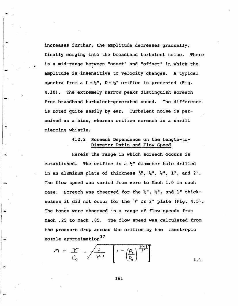
increases further, the amplitude decreases gradually,
finally merging into the broadband turbulent noise. There
is a mid-range between "onset" and "offset" in which the
amplitude is insensitive to velocity changes. A typical
spectra from a L= ", D= " orifice is presented (Fig.
4.10). The extremely narrow peaks distinguish screech
from broadband turbulent-generated sound. The difference
is noted quite easily by ear. Turbulent noise is per-
ceived as a hiss, whereas orifice screech is a shrill
piercing whistle.
4.2.2 Screech Dependence on the Length-to-
Diameter Ratio and Flow Speed
Herein the range in which screech occurs is
established. The orifice is a " diameter hole drilled
in an aluminum plate of thickness 18", ¼", ½", 1", and 2".
The flow speed was varied from zero to Mach 1.0 in each
case. Screech was observed for the ¼", ", and 1" thick-
nesses it did not occur for the 1I or 2" plate (Fig. 4.5).
The tones were observed in a range of flow speeds from
Mach .25 to Mach .85. The flow speed was calculated from
the pressure drop across the orifice by the isentropic
nozzle approximation37
Co 4.1
161
where
V velocity in the air jet
Co speed of sound in the quiescent air
y ratio of specific heats
PT pressure in the plenum
PA upstream atmospheric pressure
The results on the (L/D) necessary for screech confirm the
observations of Heller45 .
It is especially important that the inlet edge
of the orifice be sharp for maximum efficiency in the pro-
duction of tones. If one does so little as to place a
pencil point near the inlet, the tones are suppressed.
This is not true for the exit; here wide variations in the
geometry can be tolerated.
The importance of a sharp inlet motivates
several aspects of the study. The flow separates from the
walls of the orifice at the leading edge. It then con-
tracts to approximately .6 of the inlet area forming a jet
surrounded by an annulus of quiescent air between the jet
and the walls. Such a well-defined symmetric system can
support collective modes of oscillation which propagate
down the jet column. These begin as perturbations in the
jet diameter and develop into rihg vortices. Such
vortices have been observed in both orifice screech51 and
impingement screech.49 ,50
162
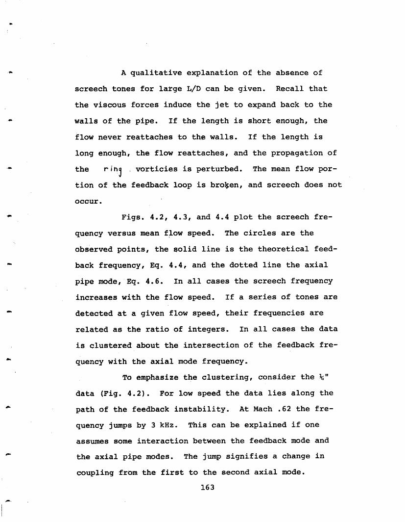
A qualitative explanation of the absence of
screech tones for large L/D can be given. Recall that
the viscous forces induce the jet to expand back to the
walls of the pipe. If the length is short enough, the
flow never reattaches to the walls. If the length is
long enough, the flow reattaches, and the propagation of
the ring vorticies is perturbed. The mean flow por-
tion of the feedback loop is broken, and screech does not
occur.
Figs. 4.2, 4.3, and 4.4 plot the screech fre-
quency versus mean flow speed. The circles are the
observed points, the solid line is the theoretical feed-
back frequency, Eq. 4.4, and the dotted line the axial
pipe mode, Eq. 4.6. In all cases the screech frequency
increases with the flow speed. If a series of tones are
detected at a given flow speed, their frequencies are
related as the ratio of integers. In all cases the data
is clustered about the intersection of the feedback fre-
quency with the axial mode frequency.
To emphasize the clustering, consider the ¼"
data (Fig. 4.2). For low speed the data lies along the
path of the feedback instability. At Mach .62 the fre-
quency jumps by 3 kHz. This can be explained if one
assumes some interaction between the feedback mode and
the axial pipe modes. The jump signifies a change in
coupling from the first to the second axial mode.
163
4.2.3 Similarity to Hole Tone
If orifice screech is similar to the hole tone,
one expects that the critical features are determined by
the diameter and separation between inlet and exit. To
check this feature, two thin orifice plates were con-
structed. These were separated by a short length of pipe
with an inner diameter larger than the orifice diameter.
The orifice plates were fashioned out of 1/16"
thick sheet of aluminum. In each plate a 450 tapered
hole was drilled to form a " diameter hole so as to
fashion a sharp edge. In the first test, the separation
between edges was set to ". Two pipe diameters were
studied, 56" and 4 z2 ".
Fig. 4.7 is a plot of the screech data observed
for the 5" inner diameter separator. Superimposed on the
graph is the trace of the feedback and axial frequencies
used for the " x " orifice (Fig. 4.3). The data from
this experiment follows the same trend as that observed
for the simple orifice of similar length and diameter.
Fig. 4.8 is a plot of the screech data observed
for the 4 /32' inner diameter separator. Superimposed on
the graph is the trace of the feedback frequency used for
the " x ½" orifice. Besides the axial modes, there are
now radial cavity modes whose frequencies are below 20 kHz.
Two pronounced cases of radial mode excitation are
164
indicated by triangles in place of circles for the data
points. There are too many radial modes below 20 kHz
to plot with any clarity on the graph. However, the
excitation of such modes, for the down pointing triangles,
is verified in section 4.2.6. Note that the data points
approximately follow the feedback frequency. The rela-
tions, however, are considerably more complex than that
of observed for the 8" inner diameter separator.
In the next experiment the L/D bounds on screech
are determined for the " inner diameter separator. The
geometry is identical to that presented in Fig. 4.7,
except for the separation between edges. The plate separa-
tion was set at 0", ¼", 1", 1" and 2". The ratio of
orifice diameter-to-plate separation in which screech was
observed is the same as that of a simple orifice. To see
this, compare Figs. 4.5 and 4.6.
4.2.4 Perturbation of the Flow by Screens
Herein it is shown that the unimpeded propaga-
tion of disturbances down the jet column play an essential
role in the production of screech tones. It was once
thought that the perturbation of the jet shear layer at
the inlet drives the axial acoustic mode. In such a
model, only the inlet flow conditions are critical. This
model is incorrect, as it is demonstrated here.
165
To settle the question, one needs to perturb
the jet downstream without any perturbation of the axial
mode. This is done with a wire screen placed in the
center of the orifice. A jet passing through the screen
becomes turbulent, whereas the axial mode is undisturbed.
Consider the first axial acoustic mode. The center of
the orifice is at a velocity node, a screen placed at
this point has negligible effect on the acoustic fluctua-
tions in the orifice. Hence only the jet is perturbed.
Two 8 " diameter holes were drilled in a "
plexiglass plate. The rear side of one hole was then
drilled to a slightly larger diameter so as to allow a
wire screen to be mounted in the center. The screen was
held in place by an annular plexiglass plug with a 38 "
inner diameter. The only difference between the two ori-
fices is the screen at the center. The screen was com-
posed of 5 mil wire with 30 strands per inch. This gives
approximately 70% open area.
Air was drawn through the unmodified orifice
and screech was observed. Next, air was drawn through
the screened orifice. No screech occurred for any flow
speed up to Mach 1.0. One concludes that the continuity
of the jet column is an essential part of orifice screech.
A screen flush to the inlet inhibits screech
for the same reason. The inlet flow is turbulent and
collective modes of oscillation on the jet are supressed.
166
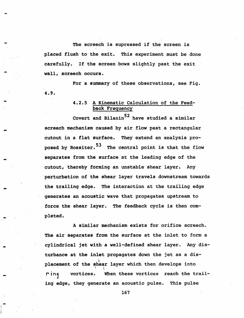
The screech is supressed if the screen is
placed flush to the exit. This experiment must be done
carefully. If the screen bows slightly past the exit
wall, screech occurs.
For a summary of these observations, see Fig.
4.9.
4.2.5 A Kinematic Calculation of the Feed-back Frequency
Covert and Bilanin52 have studied a similar
screech mechanism caused by air flow past a rectangular
cutout in a flat surface. They extend an analysis pro-
posed by Rossiter.5 3 The central point is that the flow
separates from the surface at the leading edge of the
cutout, thereby forming an unstable shear layer. Any
perturbation of the shear layer travels downstream towards
the trailing edge. The interaction at the trailing edge
generates an acoustic wave that propagates upstream to
force the shear layer. The feedback cycle is then com-
pleted.
A similar mechanism exists for orifice screech.
The air separates from the surface at the inlet to form a
cylindrical jet with a well-defined shear layer. Any dis-
turbance at the inlet propagates down the jet as a dis-
placement of the shear layer which then develops into
ring vortices. When these vortices reach the trail-
ing edge, they generate an acoustic pulse. This pulse
167
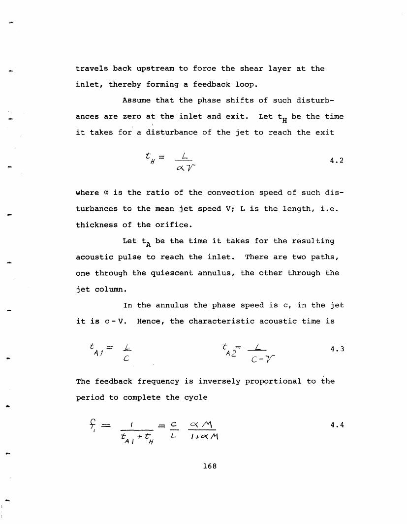
travels back upstream to force the shear layer at the
inlet, thereby forming a feedback loop.
Assume that the phase shifts of such disturb-
ances are zero at the inlet and exit. Let tH be the time
it takes for a disturbance of the jet to reach the exit
H 4.2
where a is the ratio of the convection speed of such dis-
turbances to the mean jet speed V; L is the length, i.e.
thickness of the orifice.
Let tA be the time it takes for the resulting
acoustic pulse to reach the inlet. There are two paths,
one through the quiescent annulus, the other through the
jet column.
In the annulus the phase speed is c, in the jet
it is c- V. Hence, the characteristic acoustic time is
t L t = L 4.3c-A2-
The feedback frequency is inversely proportional to the
period to complete the cycle-- -- / = C o /' 4.4
t -t L I+ o( AA/t /
168
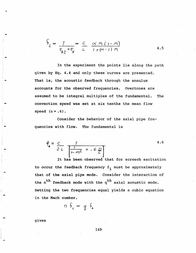
7 -- l C _ 4 A2 H
In the experiment the points lie along the path
given by Eq. 4.4 and only these curves are presented.
That is, the acoustic feedback through the annulus
accounts for the observed frequencies. Overtones are
assumed to be integral multiples of the fundamental. The
convection speed was set at six tenths the mean flow
speed (a= .6).
Consider the behavior of the axial pipe fre-
quencies with flow. The fundamental is
4=c 1 4.6A 2~ [L.1a + .I- ^11P L
It has been observed that for screech excitation
to occur the feedback frequency fl must be approximately
that of the axial pipe mode. Consider the interaction of
the nth feedback mode with the qth axial acoustic mode.
Setting the two frequencies equal yields a cubic equation
in the Mach number.
gives
169
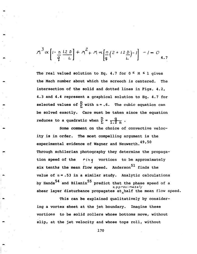
i- D + + 2 2D)- -= 0[ L ] 2 L J 4. 7
The real valued solution to Eq. 4.7 for 0 M 1 gives
the Mach number about which the screech is centered. The
intersection of the solid and dotted lines in Figs. 4.2,
4.3 and 4.4 represent a graphical solution to Eq. 4.7 for
Dselected values of D with a= .6. The cubic equation canL
be solved exactly. Care must be taken since the equation
reduces to a quadratic when =
Some comment on the choice of convective veloc-
ity is in order. The most compelling argument is the
experimental evidence of Wagner and Neuwerth.4 9'50
Through schilerian photography they determine the propaga-
tion speed of the rijg vortices to be approximately
six tenths the mean flow speed. Anderson51 finds the
value of a= .53 in a similar study. Analytic calculations
by Handa54 and Bilanin55 predict that the phase speed of aq p p rox i mat e l
shear layer disturbance propagates atAhalf the mean flow speed.
This can be explained qualitatively by consider-
ing a vortex sheet at the jet boundary. Imagine these
vortices to be solid rollers whose bottoms move, without
slip, at the jet velocity and whose tops roll, without
170
slip, on the quiescent air. The center of mass of these
rollers will then move a half the jet velocity.
4.2.6 Cavity Mode Excitation
The screech studies of thin orifice plates
separated by a 4 1l/" cylinder (Fig. 4.8) demonstrated the
excitation of additional tones. These are due to the
coupling of the feedback instability to the cylinder modes.
This is demonstrated by examining one velocity in great
detail.
The case under review is represented in Fig. 4.8
as triangles that point down, i.e., at Mach .34. The
excited modes have nodal lines that lie along the radii.
These divide the cylinder into a set of "pie slice"
regions. Only those modes with an odd number of nodes
are excited; these are called the antisymmetric modes.
First, one establishes that the phenomena is a
screech instability. In Fig. 4.10 the spectra for a simple
orifice is presented. In Fig. 4.11 the spectra of the hole
tone at Mach .33 is presented. The similarity in line
shape and the magnitude of the fundamental, in comparison
to the harmonics, shows that the screech mechanism is
similar. At Mach .34, only 5 mm Hg larger pressure drop,
the cavity modes are excited (Fig. 4.12). The feedback
frequency should increase about 3% in a shift of flow
speed from Mach .33 to Mach .34 (Eq. 4.4). This slight
171
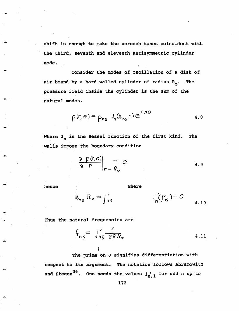
shift is enough to make the screech tones coincident with
the third, seventh and eleventh antisymmetric cylinder
mode.
Consider the modes of oscillation of a disk of
air bound by a hard walled cylinder of radius Ro. The
pressure field inside the cylinder is the sum of the
natural modes.
P (r 9) in= J n r)e 4.8
Where J is the Bessel function of the first kind. The
walls impose the boundary condition
4.9
hence where
.kn Ro jn'
Thus the natural frequencies are
_/ c
Ens Jnj 21
I
The prime on J
respect to its argument.
and Stegun36. One needs
4.10
4.11
signifies differentiation with
The notation follows Abramowitz
the values ' for odd n up tothea172ue n,
172
~~ p ~r, R
J-/ / =
0-`n
17. For values greater than n= 8 tables are not easily
found, and it proved necessary to calculate the roots
j ' by computer.n,l
Let the radius Ro = 5.54 cm, the speed of sound
C= 34,000 cm and the length L= 1.27 cm. To place thesec
predicted screech notes at the observed values, it is
necessary to assume a= .547. An equivalent change would
be to lower the Mach number to nine tenths its nominal
value of .34 and keep a= .6. Table 4.1 presents a
numerical comparison of the observed frequencies of excita-
tion to those given by Eq. 4.11.
Based on the ratio of observed-to-calculated
frequencies, it is clear that all but the first peak
coincide with the antisymmetric cavity modes. There is,
however, a numerical discrepancy that increases with
increasing frequency. At the last observed peak the dif-
ference is 250 Hz. The error in the frequency measurement
is approximately 100 Hertz, hence the difference cannot be
attributed to experimental error in the frequency measure-
ment.
One possibility is that the radial frequencies
are altered by the presence of the air jet in the center.
An accurate calculation should include this modification.
Another possibility is that the error lies in the value
Cof 2 .Ro The ratio of the observed-to-calculated
173
frequencies is correct to 2%. A 2% error in the radius
Ro, approximately 1 mm, would then account for the dis-
crepancy.
The data can be reduced in a manner independent
of 2-R ' This is to consider the ratio of the screech0o
tones to the screech tone of maximum amplitude, observed
at 4.2 kilocycles. If Eq. 4.11 is correct, this ratio
nlshould be given as Table 4.2 presents the datashould be given as if . Table 4.2 presents the data3 ,1
reduced in this fahsion. The numbers agree in absolute
value within an error of .05.
Only the first peak differs significantly.
Inspection of Table 4.1 shows the observed peaks are
separated, on the average, by 2.1 kilohertz. It is most
probable that the first peak is the difference tone due
to the interaction of the excited modes with their nearest
neighbors. All the other peaks are clearly due to the
excitation of the antisymmetric cavity modes.
It is instructive to recall that this entire
section is devoted to the screech behavior at a single
velocity. A complete analysis of the data given in Fig.
4.8 requires a similar study at each velocity. Such a
task is beyond the scope of this chapter. One point that
comes out is that the screech depends, in some fashion, on
the distance of the wall from the jet column. This effect
is incorporated into an analysis of the shear layer sta-
bility of a jet and is presented in the appendix.
174
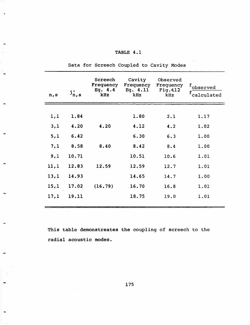
TABLE 4.1
Data for Screech Coupled to Cavity Modes
Screech Cavity ObservedFrequency Frequency Frequency fobservedEq. 4.4 Eq. 4.11 Fig.4,12 f
n,s Jn,s kHz kHz kHz calculated
1,1 1.84 1.80 2.1 1.17
3,1 4.20 4.20 4.12 4.2 1.02
5,1 6.42 6.30 6.3 1.00
7,1 8.58 8.40 8.42 8.4 1.00
9,1 10.71 10.51 10.6 1.01
11,1 12.83 12.59 12.59 12.7 1.01
13,1 14.93 14.65 14.7 1.00
15,1 17.02 (16.79) 16.70 16.8 1.01
17,1 19.11 18.75 19.0 1.01
This table demonstreates the coupling of screech to the
radial acoustic modes.
175
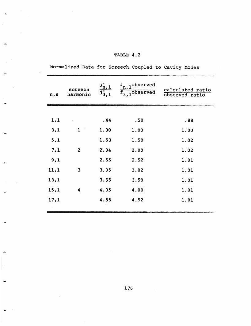
TABLE 4.2
Normalized Data for Screech Coupled to Cavity Modes
n' f ,lobservedscreech 1 n, 1 sred calculated ratio
n,s harmonic J3,1 3,1bserved observed ratio
1,1 .44 .50 .88
3,1 1 1.00 1.00 1.00
5,1 1.53 1.50 1.02
7,1 2 2.04 2.00 1.02
9,1 2.55 2.52 1.01
11,1 3 3.05 3.02 1.01
13,1 3.55 3.50 1.01
15,1 4 4.05 4.00 1.01
17,1 4.55 4.52 1.01
176
4.3 Impingement Screech
4.3.1 Impingement Screech, Apparatus andProcedure
A screech mode was also observed in the experi-
ments on the excitation of transverse modes in ducts. It
was shown that the initial peaks in the observed spectra
were due to the selective response of the duct at its
cutoff frequency. Further, it was proved that the spectra
should smooth out in the high frequency limit, i.e., when
a large number of modes can propagate. However, intense
pure tones were observed in this frequency regime at flow
velocities above Mach .6. These are here identified as a
feedback instability, termed impingement screech, due to
the obstruction of the air jet by the opposing wall of the
duct.
Wagner49 has shown that a jet incident on a flat
plate screeches. This occurs only if the plate is less
than 6 diameters from the jet nozzle, and if the Mach
number is greater than .6. He collated the acoustic fre-
quency with the shedding of ring vorticies on the jet
column. He concludes that the screech is due to "feedback
between the flow and the pressure field generated by it."
Neuwerth5 0 later extended the work to include screech at
supersonic velocities.
The nozzle they used is not quite the same as
the orifice plate or pipe used in the duct experiments
177
(Figs. 3.4 and 3.5). Their apparatus was a converging
nozzle followed by a short length of pipe (Fig. 4.13).
Herein it is shown that impingement screech occurs using
an orifice plate and a 60" pipe. That is, the slight
variations of inlet conditions in the duct experiments
from Wagner's nozzle do not suppress impingement screech.
The apparatus used here is a plenum chamber 60"
long and 12" wide. At the exit the chamber converges to
a diameter of 4". A " thick orifice plate with a hole
tapered to 450 to a " diameter was attached to this end.
In the second experiment a 60" pipe with a " inner
diameter was fixed to a plate that was, in turn, secured
to the chamber exit. A square flat plate, 4" on a side,
was placed in the air jet at various distances from the
exit. The plenum pressure is raised to force air out at
a constant rate.
Before investigating the screech, some data on
the turbulent-generated noise is taken. A qualitative
presentation is given so as to provide spectra for compari-
son to the turbulent excitation of cavities.
4.3.2 Free Jet Spectra from Pipes and Orifices
The variation in free space spectra with jet
flow speed is given here. This is done to demonstrate that
the qualitative spectra of free jets is the same for both
a long pipe and an orifice. For a more detailed analysis
178
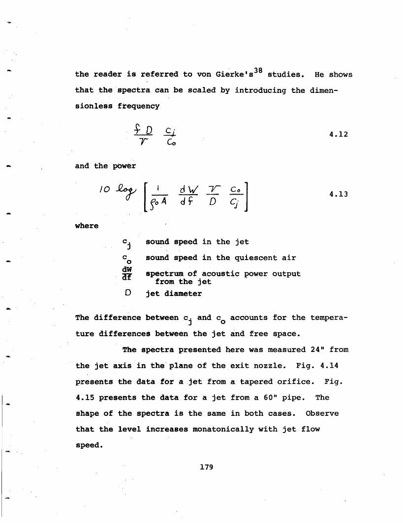
the reader is referred to von Gierke's38 studies. He shows
that the spectra can be scaled by introducing the dimen-
sionless frequency
4.12r cc
and the power
/ <I jdC1 4.13
Lyr ~4 Jf FD C-
where
c. sound speed in the jet
c sound speed in the quiescent air
dWspectrum of acoustic power output
from the jet
D jet diameter
The difference between c and c accounts for the tempera-
ture differences between the jet and free space.
The spectra presented here was measured 24" from
the jet axis in the plane of the exit nozzle. Fig. 4.14
presents the data for a jet from a tapered orifice. Fig.
4.15 presents the data for a jet from a 60" pipe. The
shape of the spectra is the same in both cases. Observe
that the level increases monatonically with jet flow
speed.
179
The point is that the qualitative features are
not altered by the initial level of turbulence. Air from
a tapered orifice is laminar at the exit. The turbulence
is caused by the mass entrainment at the jet boundary.
The air jet from a long pipe is turbulent at the exit. The
level, of course, is altered by mass entrainment at the
jet boundaries. The differences at the exit do not alter
the character of the emitted acoustic spectra. These
observations reinforce those made in the study of turbulent
sources in ducts. In the duct, the spectral line shape was
similar for both the orifice and pipe jets.
4.3.3 Turbulent Sound Level Increase due tothe Obstruction of the Flow by a FlatPlate
The increased broadband noise due to obstructing
. the flow is demonstrated. First, the sound generated by
an air jet from a tapered orifice is measured. Next a
flat plate is placed in the air jet and the sound is
measured again. Hre the distance of the plate from the
orifice is great enough, 9 jet diameters, so that screech
does not occur.
In Fig. 4.16 the spectral sound intensity for
this experiment is given. At the same flow speed, the jet
incident on the plate is much louder than the free jet.
Actual shifts range from 7 to 12 DB depending on the fre-
quency. The line shape of the spectra is unchanged. This
180
indicates that the mechanism for sound generation is
similar in both the free jet and the obstructed jet.
This is not the case if the plate is within 6
jet diameters of the orifice. In such cases screech
occurs at selected flow speeds. The resulting spectra
shows intense narrow band peaks at the screech frequen-
cies. These peaks have the same shape as those observed
in the high frequency duct spectra (Figs. 3.10, 3.11 and
3.12).
There are, of course, quantitative differences
in the generated sound when the flow is obstructed. These
differences are of secondary importance in establishing
the mechanism for sound generation. One must first
separate the linear effects from the feedback effects
before addressing the more quantitative aspects of the
study. It is with this intent that the arguments concern-
ing spectral line shape are presented. For a more detailed
study of the sound generated by air jets on flat plates,
we refer the reader to the work of Olsen, Miles and Dorsh.62
4.3.4 Impingement Screech from a Tapered Orifice
Here we reproduce impingement screech, observed
by Wagner49 and Neuwerth50 , using a jet from a tapered
orifice impinging on a flat plate. The apparatus is shown
in the middle diagram of Fig. 4.13. The pressure drop
across the plate was set at a ratio of .60 which gives a
181
flow speed of Mach .83 (Eq. 4.1). The separation between
orifice and plate was altered at constant flow speed.
The orifice is mounted with its flat side toward
the compressor. The direction of air flow through the
orifice is the same as in the duct experiment. The ori-
fice plate is " thick, and the hole tapers at 450 to the
nominal diameter of ", such orifices do not screech by
themselves. The separation "x" is measured from the inner
surface to the obstructing wall.
Screech was observed for separations from kj6"
to 21" , i.e., from .88 to 5 jet diameters. For separa-
tions greater than 5 jet diameters no screech is observed.
This result agrees with Wagner49 and Neuwerth's50 observa-
tion that the obstructing plate must be less than 6 dia-
meters from the nozzle.
In Fig. 4.17 the observed screech frequencies
are plotted against the inverse of the plate separation.
If the screech is associated with an axial acoustic mode
parallel to the jet, the frequency should scale as ; i.e.,
the data points should lie along straight lines. This
happens; however, the screech frequencies are only approxi-
mately equal to the cavity frequencies . In fact, two2x ' In fact, two
screech modes appear. All other frequencies can be inter-
preted as harmonics or difference tones based on these two
modes, which have been arbitrarily labeled FA and FB
182
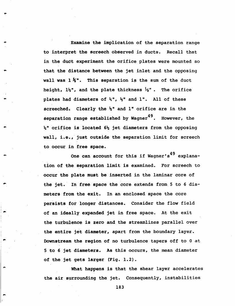
Examine the implication of the separation range
to interpret the screech observed in ducts. Recall that
in the duct experiment the orifice plates were mounted so
that the distance between the jet inlet and the opposing
wall was 1 ". This separation is the sum of the duct
height, 1", and the plate thickness 1" . The orifice
plates had diameters of ¼", ½" and 1". All of these
screeched, Clearly the " and 1" orifice are in the
separation range established by Wagner49. However, the
¼" orifice is located 6 jet diameters from the opposing
wall, i.e., just outside the separation limit for screech
to occur in free space.
One can account for this if Wagner's49 explana-
tion of the separation limit is examined. For screech to
occur the plate must be inserted in the laminar core of
the jet. In free space the core extends from 5 to 6 dia-
meters from the exit. In an enclosed space the core
persists for longer distances. Consider the flow field
of an ideally expanded jet in free space. At the exit
the turbulence is zero and the streamlines parallel over
the entire jet diameter, apart from the boundary layer.
Downstream the region of no turbulence tapers off to 0 at
5 to 6 jet diameters. As this occurs, the mean diameter
of the jet gets larger (Fig. 1.2).
What happens is that the shear layer accelerates
the air surrounding the jet. Consequently, instabilities
183
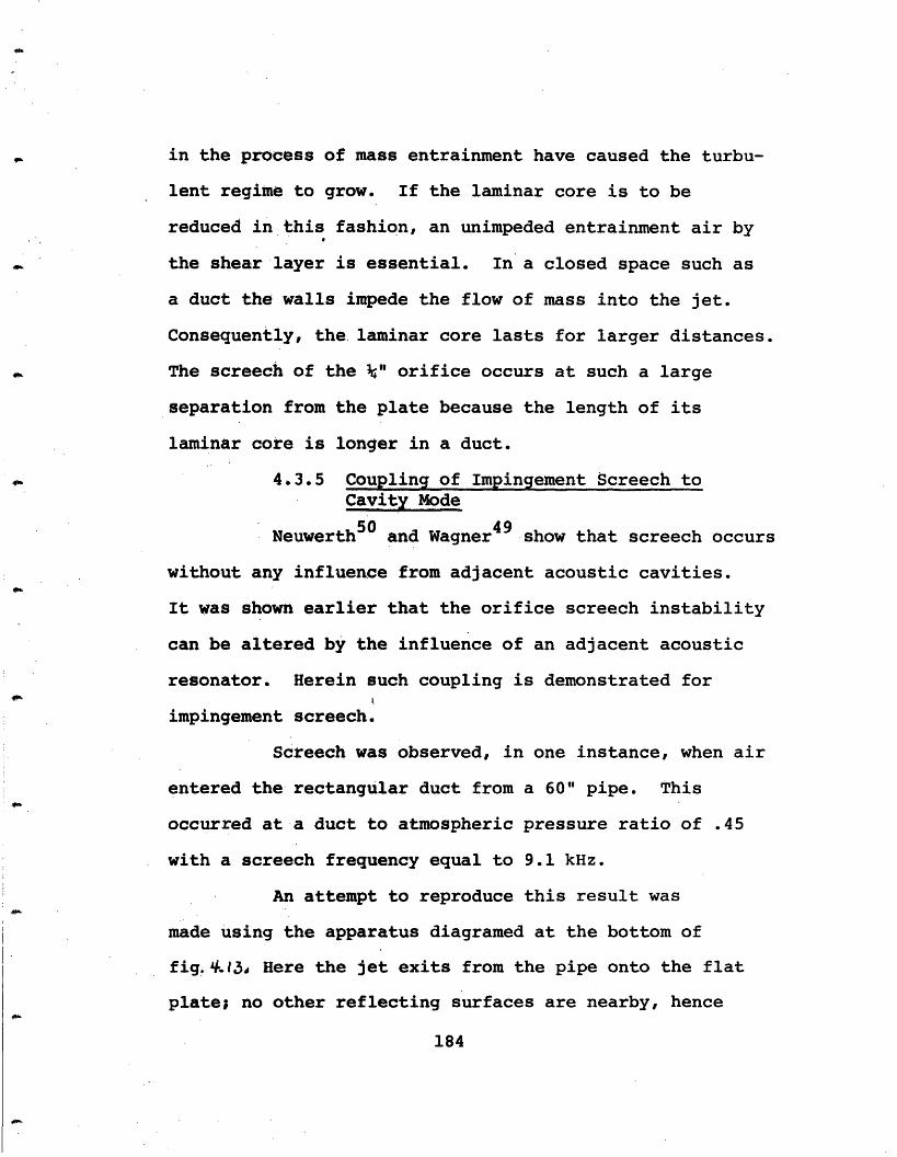
in the process of mass entrainment have caused the turbu-
lent regime to grow. If the laminar core is to be
reduced in this fashion, an unimpeded entrainment air by
the shear layer is essential. In a closed space such as
a duct the walls impede the flow of mass into the jet.
Consequently, the laminar core lasts for larger distances.
The screech of the " orifice occurs at such a large
separation from the plate because the length of its
laminar core is longer in a duct.
4.3.5 Coupling of Impingement Screech toCavity Mode
50 49Neuwerth50 and Wagner49 show that screech occurs
without any influence from adjacent acoustic cavities.
It was shown earlier that the orifice screech instability
can be altered by the influence of an adjacent acoustic
resonator. Herein such coupling is demonstrated for
impingement screech.
Screech was observed, in one instance, when air
entered the rectangular duct from a 60" pipe. This
occurred at a duct to atmospheric pressure ratio of .45
with a screech frequency equal to 9.1 kHz.
An attempt to reproduce this result was
made using the apparatus diagramed at the bottom of
fig. .I3, Here the jet exits from the pipe onto the flat
plate; no other reflecting surfaces are nearby, hence
184
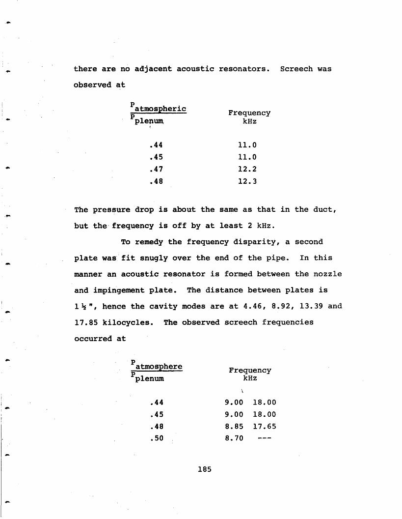
there are no adjacent acoustic resonators. Screech was
observed at
Patmosphericp Frequencyplenum kHz
.44 11.0
.45 11.0
.47 12.2
.48 12.3
The pressure drop is about the same as that in the duct,
but the frequency is off by at least 2 kHz.
To remedy the frequency disparity, a second
plate was fit snugly over the end of the pipe. In this
manner an acoustic resonator is formed between the nozzle
and impingement plate. The distance between plates is
1 ", hence the cavity modes are at 4.46, 8.92, 13.39 and
17.85 kilocycles. The observed screech frequencies
occurred at
PPatmosphere FrequencyPplenum kHz
.44 9.00 18.00
.45 9.00 18.00
.48 8.85 17.65
.50 8.70 ---
185
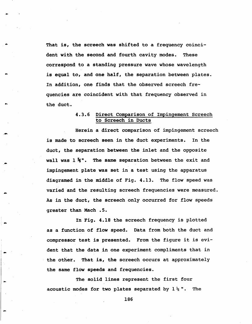
That is, the screech was shifted to a frequency coinci-
dent with the second and fourth cavity modes. These
correspond to a standing pressure wave whose wavelength
is equal to, and one half, the separation between plates.
In addition, one finds that the observed screech fre-
quencies are coincident with that frequency observed in
the duct.
4.3.6 Direct Comparison of Impingement Screechto Screech in Ducts
Herein a direct comparison of impingement screech
is made to screech seen in the duct experiments. In the
duct, the separation between the inlet and the opposite
wall was 1 ". The same separation between the exit and
impingement plate was set in a test using the apparatus
diagramed in the middle of Fig. 4.13. The flow speed was
varied and the resulting screech frequencies were measured.
As in the duct, the screech only occurred for flow speeds
greater than Mach .5.
In Fig. 4.18 the screech frequency is plotted
as a function of flow speed. Data from both the duct and
compressor test is presented. From the figure it is evi-
dent that the data in one experiment compliments that in
the other. That is, the screech occurs at approximately
the same flow speeds and frequencies.
The solid lines represent the first four
acoustic modes for two plates separated by 1 ". The
186
observed screech frequencies are clustered about these
lines. Such a comparison is only approximate, as the
data of the previous section has shown that the fre-
quency still depends somewhat on the flow speed.
187
5. CONCLUSIONS AND RECOMMENDATIONS
Herein the generation of sound by turbulent flow
in cavities is examined. Two types of cavities are con-
sidered: the axial modes of a pipe open at both ends,
and the transverse modes of a rectangular duct. Experi-
ments are performed to measure the acoustic spectra of the
flow-generated noise. A linear theoretical analysis,
based on an isotropic model of the turbulent fluctuations,
is developed to predict this spectra. Certain nonlinear
phenomena, due to the alteration of the source flow by
the emitted sound, are identified. The conditions neces-
sary for such instabilities are examined.
To introduce the linear procedure, calculations
are carried out for a turbulent source in free space.
Here some of the limitations of the model are discussed.
One assumes a finite volume of turbulent fluid. An iso-
tropic pattern of noise sources is created continuously
at one face of the volume and is convected at a finite
velocity to the downstream face where it disappears.
Implicit in this description is a neglect of turbulent
shear and refraction effects.
To make the comparison between alternate pro-
cedures explicit, detailed calculations were carried out.
The results derived from Lighthill's '2 quadrupole model
using time domain techniques are given in Eqs. 1.51 and
188
1.52. Similar results are derived from Ribner's equivalent
distribution of monopoles, again using time domain analysis
(Eqs. 1.43 and 1.44). Ribner's model is used again, this
time using frequency domain analysis to derive the spectra
of the radiated pressure (Eqs. 1.30 and 1.31). Frequency
and time domain techniques give precisely the same answer
for Ribner's source model. Aside from the turbulent shear
interaction, these are the same results as one gets from
Lighthill's model. This is providing Ribner's turbulent
pressure sources p are assumed identical to the local
turbulent kinetic energy fluctuations pov .
An interesting extension of this analogy would
be to assume a second distribution of monopoles whose
strength is proportional to poVv, where V is the mean
flow speed and v the fluctuating velocity. This would, in
some fashion, account for the turbulent shear effects.
However, care must be taken to introduce the angular
dependence 2(cos40 + cos20), where is the angle between
the observor and the direction of flow. It is recommended
that theoretical studies be continued to establish this
analogy.
Another problem that needs further work is the
inhomogeneities in the turbulent field. Ribner 63has
already used the variation in characteristic scales of
the turbulence to collate data on the free space spectra.
189
He observes that a single correlation function cannot
account for the entire spectra. Nonetheless, limited
portions of the spectra can be described assuming a single
correlation function. Here attention is placed on the
mid and high frequencies. It is recommended that the
minimum number of separate correlation functions needed
to account for the observed spectra be established.
In the second chapter an experimental study of
the turbulent excitation of axial pipe modes is given.
Such effects have been reported before 3 0 5 6 , but were not
conclusively identified. Identification is accomplished
by showing that the interval between modes depends on
flow speed and length precisely as an axial mode (Figs.
2.3 and 2.4). Previous observations concerning diminished
mode excitation at high flow speeds are confirmed here.
To account for these observations in detail, a
frequency domain analysis of sound generation by isotropic
turbulence in pipes is developed. To carry the analysis
to a point where only a statistical description of the
turbulence is required, it proves necessary to introduce
a random phase assumption. It is demonstrated that the
influence of the Fourier phase coefficient is identical
to localization of the source (Eqs. 2.48 and 2.52). Thus,
neglecting phase terms is equivalent to averaging overall
possible source positions. Sound generation from the ends
190
of the pipe can then be predicted from a statistical des-
cription of the source field (Eq. 2.54). Direct compari-
son to theexperimental results (Figs. 2.8, 2.9 and 2.10)
demonstrates that radiative damping accounts for the
diminished excitation at high flow speeds.
It was assumed that the losses at the ends are
purely radiative. From this assumption the transmission
coefficients out the pipe ends can be derived from the
measured pressure reflection coefficients. It may be
that some other loss mechanism acts at the ends. This
will alter the transmission coefficient. It is recom-
mended that an eperimental study of the transmission
coefficient be performed. It is further recommended that
the behavior of the exit pressure reflection coefficient
be examined in greater detail to account for some small
discrepancies.
In the third chapter an experimental study of
the turbulent excitation of the transverse modes in ducts
is presented. Two effects are established. The first is
that the level of radiated sound increases in discrete
jumps at the first few cutoff frequencies. For fre-
quencies slightly greater than the nearby cutoff, the
level decreases smoothly. The asymmetric shape of these
curves is predicted using frequency domain techniques
(Eq. 3.38). Again it proved necessary to introduce a
random phase assumption to carry the calculations to completion.
191
In the ideal case the level jumps should be
infinite at the cutoff frequencies. Damping requires
that these jumps be finite as is indicated in Eq. 3.45.
However, visco-thermal damping alone cannot predict the
magnitude of the observed jumps. It is recommended that
the mechanism that limits these level shifts be estab-
lished. n particular, the approximation that the
acoustic contribution to the Reynolds stress
is negligible is not valid when the predicted acoustic
velocities are infinite.
The second effect established by these experi-
ments is that the spectra smooths out at frequencies
where a large number of modes can propagate. In fact,
the spectra strongly resembles the spectra of sound
generated by turbulence in free space. To understand the
smoothing, recall that damping effects make the peak
height finite. At frequencies of large modal density a
new mode cuts on before the sound level has diminished
from the level jump at the previous cutoff frequency.
This overlap of peaks causes the curve to smooth out. A
quantitative analysis based on this idea is given in
Eq. 3.46.
The problem can also be approached by calculat-
ing the average radiative resistance of the duct. In
the high frequency limit the radiative resistance
192
approaches that in free space. Herein, this concept is
applied to the interpretation of acoustic spectra in
rectangular ducts. An extension of the limit to ducts of
arbitrary shape is given in Eq. 3.55. In short, the duct
spectra is similar to the free space spectra since the
duct and free space response are approximately the same
in this limit.
In the experimental phase two anomalies occurred
that are identified as nonlinear effects. Orifice screech
occurred in pipes having small length-to-diameter ratios.
Impingement screech occurred in ducts when the air jet
impinged on a nearby wall. Further experiments were per-
formed to establish the conditions necessary for such
instabilities. It is shown that the emitted acoustic
field reacts back on the jet so as to alter the primary
flow field. A kinematic analysis of orifice screech
proved adequate to predict the frequency dependenceon
length and flow speed (Eq. 4.4). Further it was demon-
strated experimentally that the feedback cycle is unstable
only if the feedback frequency is approximately that of an
adjacent axial acoustic mode. From this observation one
can predict the velocities and frequencies at which the
feedback cycle is most likely to be unstable and thereby
produce "screech" (Eq. 4.7).
193
It is further observed that variations in geo-
metry that produce additional acoustic modes can markedly
alter the screech frequencies. In the appendix the shear
layer instability of a circular jet subject to an acoustic
perturbation in the presence of boundaries is derived.
The dispersion relation for such a disturbance is deduced
(Eq. A28), and its limiting forms are presented (Eqs. A35,
A39, A42 and A43). Phase speed calculations of the shear
layer instability indicate that the coupling of feedback
to the resonator may be through the spatial gradients.
That is to say, if a resonator is present, all spatial
variations are dominated by the characteristic wavenumber
of the resonator. The influence of such coupling is to
alter the phase speed of the shear disturbance (Eqs. A48
and A49). Preliminary experimental observations are in
qualitative agreement with this result. It is recommended
that a quantiative experimental study be initiated to see
how the phase speed is changed when a resonator is present.
It is further recommended that one establish whether or
not the phase speed is adequately described by linear
analysis.
In summary, a study of flow-generated sound in
cavities has been performed. For linear effects, a
detailed prediction of spectral line shape of the radiated
sound is possible. For nonlinear effects, some important
194
aspects of how sound couples to the flow that generates
it are established.
195
APPENDIX: STABILITY ANALYSIS OF HEi PERTURBED JET IN THEPRESENCE OF BOUNDARIES
A.1 Introduction
The collective oscillations of the jet play an
essential role in screech instabilities. It is therefore
useful to calculate the motion of the jet subject to an
acoustic perturbation. Herein the linear analysis of a
forced jet surrounded by a quiescent annular region
bound, in turn, by a hard-walled duct is presented. The
theory is developed to the point where a rather complex
dispersion relation must be solved. Rather than solve
the equation numerically, several limiting cases are pre-
sented. These correspond to a free circular jet, a two-
dimensional -shear layer in the vicinity of a hard wall,
and a free two-dimensional shear layer. The solutions of
the linear equations in these limits have been given by
Tam57 , Sedel'nikov5 8, Handa54 , Covert and Bilanin52, and
Miles59
One should first establish what portion of the
acoustic pulse couples to the shear layer. Three possi-
bilities exist, the particle displacement, the particle
velocity, and the pressure perturbation. Chanaund and
Powell43 demonstrate that the pressure perturbation forces
the shear layer. They force a circular jet from an ori-
fice with an acoustic wave from a loudspeaker. This was
196
done in the study of the hole tone, where a second ori-
fice plate is mounted downstream. They find:
With the sound from the speaker (locatedon the jet axis) disturbing the jet, the flowpattern was observed to be symmetric and simi-lar to that found with the plate and no speaker.The speaker was then moved to a position per-pendicular to the jet axis, and again asymmetric pattern resulted! Since the acousti-cal wavelength was much greater than thenozzle diameter, the particle motion lateralto the jet must have been in phase across thejet diameter and so, if the jet were appreciablysensitive to the motion, sone asymmetry of thedisturbances, at least, should have occurred.Since they did not, it appears that the axi-symmetric jet is predominantly pressure sensi-tive.
In an acoustic wave the particle velocity and
displacement are parallel to the direction of propagation.
The acoustic pressure, being a scalar field, has no such
directionaltiy. With the loudspeaker downstream, the
propagation direction is parallel to the jet. With the
loudspeaker perpendicular to the axis, the propagation
direction is perpendicular to the jet. If the jet were
sensitive to either the acoustic displacement or velocity,
some changes should have occurred by changing the direc-
tion of the incident acoustic wave. Since no changes
were observed, one concludes that the acoustic pressure
forces the jet.
A.2 Problem Statement
Consider the perturbation of a compressible,
inviscid, cylindrical jet in the vicinity of a rigid
197
boundary. Let the jet and the boundary be coaxially
symmetric and have radii Rj and Ro. Assume the mean
velocity V = V z is uniform for all r < Rj and zero for
all r > Rj. Here the jet axis lies along the z axis, and
r is the radial distance from this axis. Let the shear
layer at Rj be driven by a localized pressure disturbance
at z = 0. Assuming isentropic conditions gives
V2 2 D2V p = D r< Rj AlC bt
P I - V 2v r > R A2
where the "'--" subscript refers to points in the jet and
the + to points outside the jet. Here
0 = . s ,Ot gt a
Let the shear layer displacement from the equi-
Alibrium position Rj be labelled (Rj,t)r. Momentum con-
servation requires that the radial particle accelration
be equal to the radial pressure gradient at the shear
layer. Thus
-P- - A3Dt
198
A4
Oehre
Ot 2 t a = r fni,
On the jet axis the pressure must be finite,
hence
A5r = o
The hard wall demands that the radial particle
velocity be zero at r= R. Equivalently
A6
Continuity of pressure at the shear interface
requires
i (n~p .t)r=
where A(z)e i (n- t) is the acoustic forcing term
inlet.
A.3 Integral Solution
A7
at the
To solve Eqs. Al to A7, introduce the Fourier
Laplace transform. This procedure is identical to Tam's
analysis of the free jet. Thus
p- p C - Z (K - 2 t) A8
199
5 . . 0
r- - ft0
__ -dt C-
whose inverse transforms are
-I d < '
V 7r -+L
ic (A peL'4(- i2t)
i d Ct)-,2
Transforming Eqs. Al and A2, assuming initial
conditions are zero, gives
vt P-=
Vt P+
IE- K 7- a + 2C21 2 C K / +
lj 2 + 1<2
p-2 p,
A12
P+, = + +
2 and 2where 2 and 2 are the quantities in curly brackets,
in A12 and A13 and
t
A13
{},
tr r r r f
200
A9
A10
All
k /1iC,P- - 1-2
Continuing the transforms of Eqs. A3 to A7 givesI p- , % A14
If S~r ._L-' ~ 2r A159 r
p ...'< o=
r+ZI - o 0 A17r -
p'p + A e.-- RO A18- L fA
incpTo solve A12 and A13, assume p(r)e which gives
I ~ b( r= pp(r) = gv 2e sr ar ' r r 2
or
ra~ r, p(r) |(g r) n p A19ar r
The solution to A19 is the nth modified Bessel
functions of the argument x= r+, where the + or - holds
for r>Rj or r<Rj. Eqs. A14 through A19 are the
boundary conditions the solution must satisfy. Explictly
one has
201
)_,(r)- A I n(._ r) + o Kn(L_ r)In K n - I~~~~~~~~~~~~~~~~,m
pa ~r)= B IP,3In(+ r) + K< (A, r)
n
r R A213
where A, B, a and are numerical constants to be deter-
mined by the boundary conditions. The factor has been
used to facilitate the expansions in the limiting cases.
36The notation of Abramowitz and Stegun is used for the
Bessel functions.
That the pressure be finite at the origin
(Eq. A16) requires a= 0. The hard wall (Eq. A16) requires
P / KN ( x) A22
X= + Ro
where the prime signifies differentiation with respect to
the argument x. Substituting A20 and A21 into A14 and
A15 gives
z n ix) |_( )¢ e r~J /( - _ (X) J- ?-" .
AA -J
JQ ,12
A23
S In(x) + K K/X) |
/3 x) '- + + ( ) 1 Lb-~/j.
202
r< e. A20j
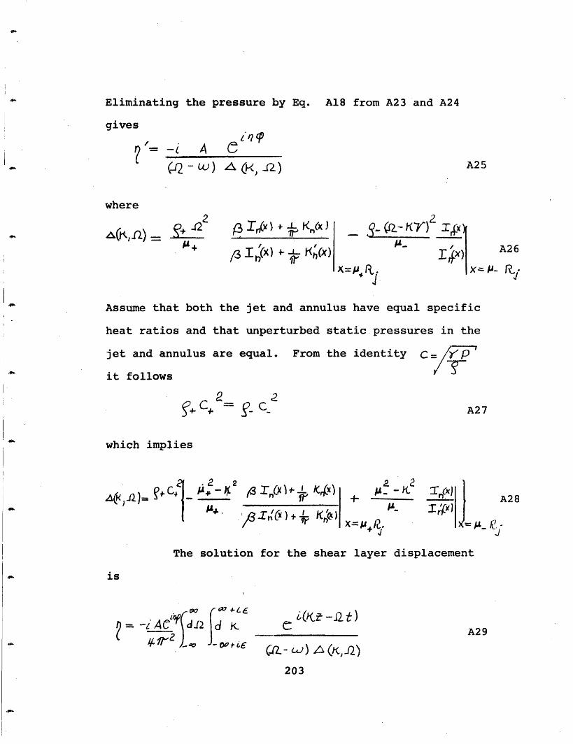
Eliminating the pressure by Eq. A18 from A23 and A24
gives
A C- (2 - U) A (k, a)
where
,&(KI) = nA48 ITXX) + IK(X)<3 In) +- I tK,(x)
- 9Žif- K rx)
X-6tAj I pJK = P" R.
*1
Assume that both the jet and annulus have equal specific
heat ratios and that unperturbed static pressures in the
jet and annulus are equal. From the identity C= P
it follows
2= wC A27
which implies
2 2 PT10)z aS..62J2)_ fC,]_i -i i 3 Icx + kn(X)9 A- t2
M s~n~x)+ t K>)| X~ +A & , X) " + n'X X ;, AIGX'C Tr +nj
fx) 1)Incx L|. A28
-= Jlejr~gc~ld,.
The solution for the shear layer displacement
is
? .fi"2 IV - 00 f. i6t .-iALn jr2 d 2fd
eC -.Q t)
- W) (Kc, 2)203
A25
A26
x=- %,'I-"- [~
A29
= - z
? .I -
. . 11
p· C+
The general form of the amplifying solution is
IL (t - t)o< C
where w is the frequency of the acoustic perturbation,
and k is the solution to the dispersion relation
A (k,w) =0.
A.4 Cmments on the Evaluation of the Integral
The integral given in A29 is, in general, quite
difficult to solve. The customary approach is via the
theorem of residues. It is essential, therefore, to
locate the roots of the dispersion relation A(k,w) =0.
A detailed analysis of the evaluation in the limit of a
two-dimensional free shear layer is provided by Miles.59
Bilanin and Covert52 have solved the dispersion relation
numerically for a two-dimensional shear layer located
near a hard wall. Similar numerical solutions for the
free vibrations of a supersonic cylindrical jet given by
Sedelhnikov58 and Handa54 . Tam57 has demonstrated that
so long as the radius of such a jet is large compared to
the wavelength of the disturbance, Miles59 solution can be used.
Handa provides a detailed analysis of the integration
procedure once the dispersion relation is solved.
Such detail in carrying out the integrations
is not warranted in this analysis. Experiments by
Wagner4 9 and Anderson51 demonstrate that the perturbations
204
of subsonic jets "roll up" to form ring vortices that
propagate down the jet column. It is these vortices that
are essential to screech. The process of formation of
these vortices is not contained in linear analyses such
as this one.
The argument is that such vortices can form
only if there is an amplifying disturbance of the shear
layer. The hydrodynamic analogue is the formation of
droplets by the amplifying oscillations of a water jet,
first described by Rayleigh61. The key is to identify
the amplifying roots of the dispersion relation. This is
done analytically by the asymptotic procedure used by
57Tam
A.5 Removing the Duct Wall
Handa54 and Sedel'nikov5 8 have analyzed the
free oscillations of a circular jet. Their analysis can
be recovered if one assumes the wall is infinitely far
from the jet. To evaluate this limit, the following
expansions are used
205
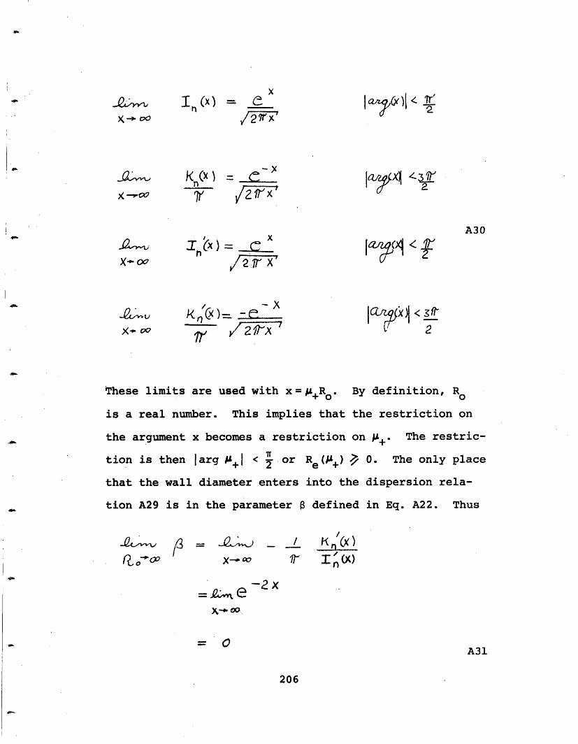
xIn(x) = e
,Tr' /r2rtx"
I;'x = ._.el//-2':/"X'/ I7 A30
P X(). - 7
/r / 2 t-'
These limits are used with x= I+Ro. By definition, RO
is a real number. This implies that the restriction on
the argument x becomes a restriction on A+. The restric-
tion is then larg A+1 < 2 or Re (+) 0. The only place
that the wall diameter enters into the dispersion rela-
tion A29 is in the parameter defined in Eq. A22. Thus
= .... ,.. _ _/Ado t~~~~~1-In(x)
-2 x
= OA31
206
X' -Ii oC:
_..ooX v 00
q 0-f-C
I a/ A 7r
ly" 'f
i~P
la/ " < 3t2
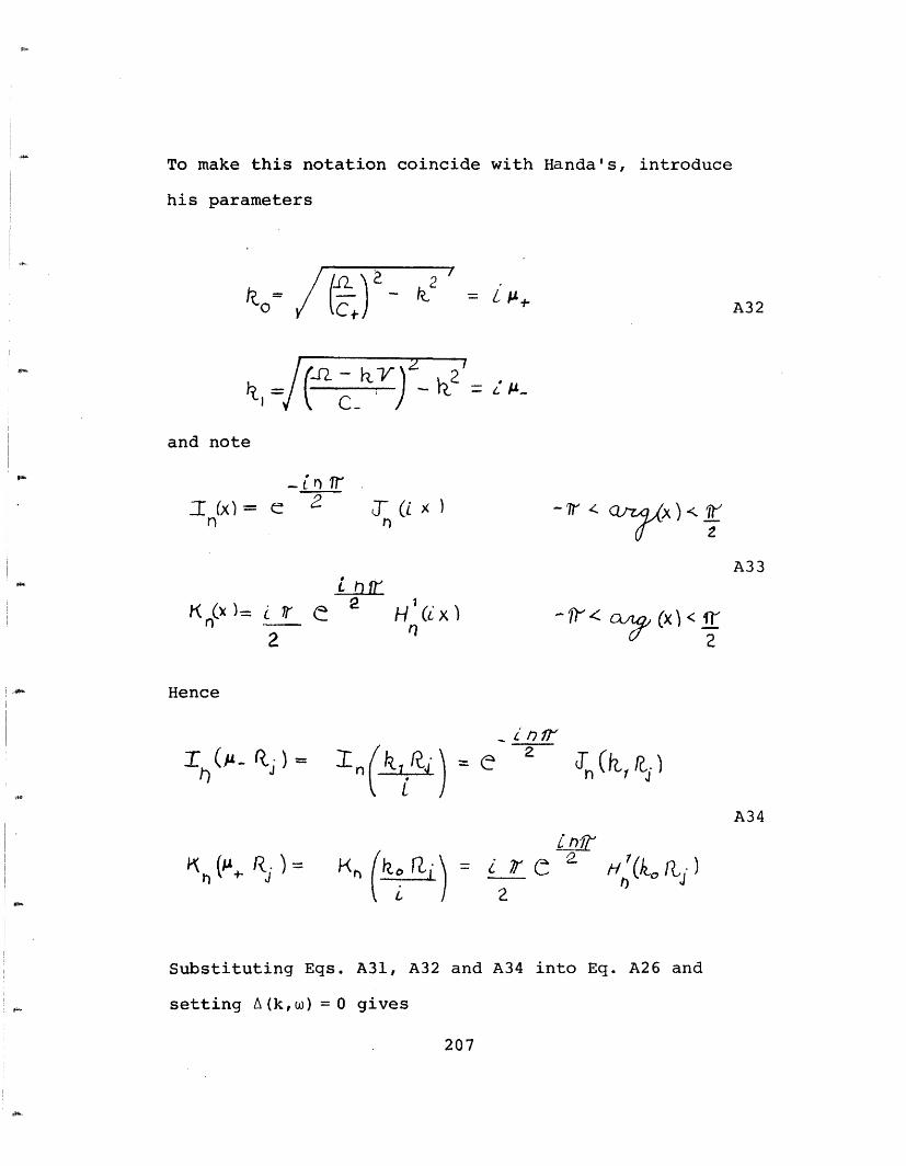
To make this notation coincide with Handa's, introduce
his parameters
z_ <)= _
(- A2 =and note
T ()= en
(X), e 2n~22
2 T( x)r)
H I(X)
, 11 -< J
2
Hence
I(,_ Qj)-
(A+ RJ )- Kr( (Z C, rI) = j y 2
2
Substituting Eqs. A31, A32 and A34 into Eq. A26 and
setting A(k,w) = 0 gives
207
A32
A33
- / r2
A34
HI (k- f n- 1)
in k Q4 J (k, y
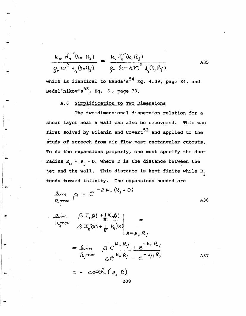
I O ! iIl(? -PI=-~~~ ~A35
H (o %) _ v (..-A JI ,
which is identical to Handa's54 Eq. 4.39, page 84, and
Sedel'nikov's58, Eq. 6 , page 73.
A.6 Simplification to Two Dimensions
The two-dimensional dispersion relation for a
shear layer near a wall can also be recovered. This was
first solved by Bilanin and Covert52 and applied to the
study of screech from air flow past rectangular cutouts.
To do the expansions properly, one must specify the duct
radius R = Rj + D, where D is the distance between the
jet and the wall. This distance is kept finite while R.
tends toward infinity. The expansions needed are
Q'A,=e -2 + (j+ D)F~ _0 A36
/3 LnM) -K )
208
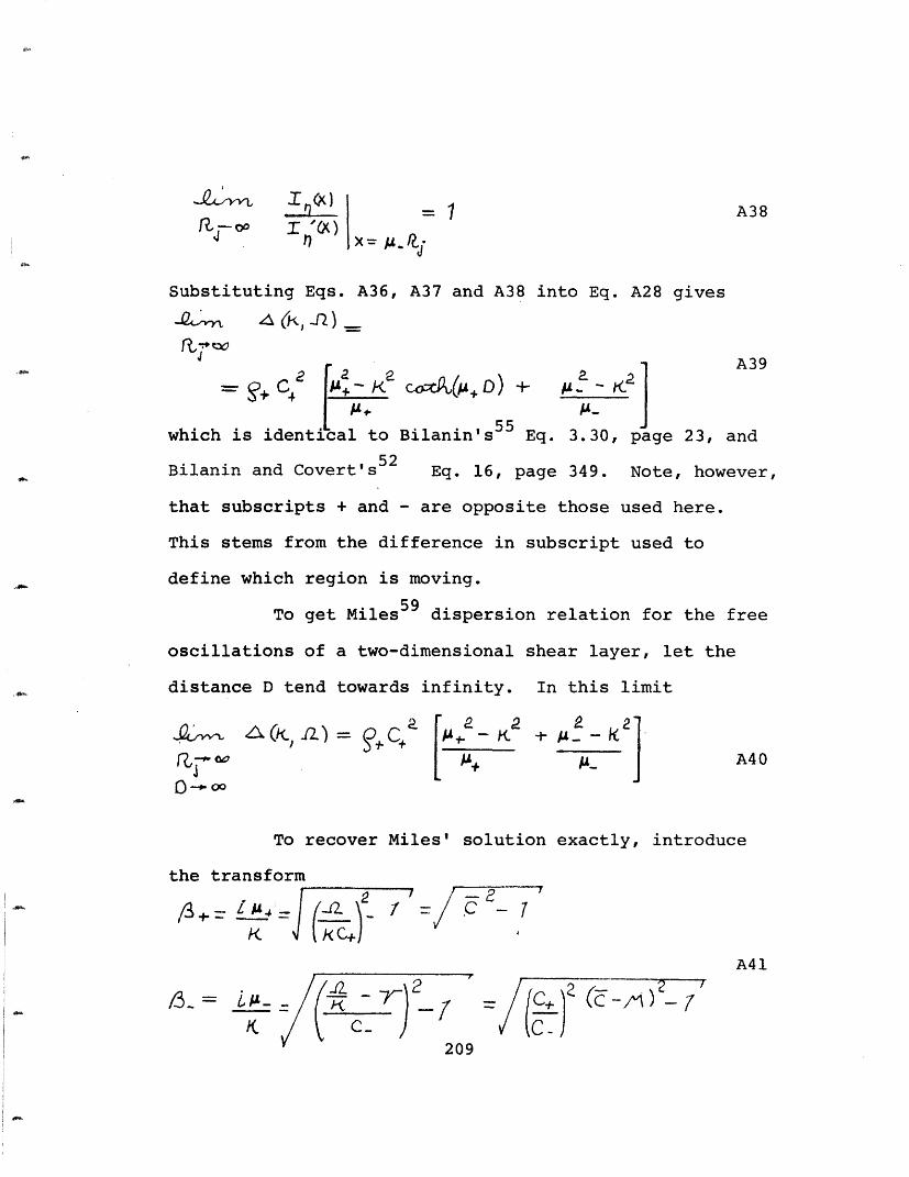
I, )I A38
RJ-°° I n ) IX- /1 I
Substituting Eqs. A36, A37 and A38 into Eq. A28 gives
A39
+ C i+ d tcalt(oD) + , A'a
52which is identical to Bilanin's5 Eq. 3.30, pBilanin and Covert's52 Eq. 16, page 349. Note, however,
that subscripts + and - are opposite those used here.
This stems from the difference in subscript used to
define which region is moving.
To get Miles5 9 dispersion relation for the free
oscillations of a two-dimensional shear layer, let the
distance D tend towards infinity. In this limit
r9 _7`~ n) J LA ~tC~. I+ ] A40
0 00
To recover Miles' solution exactly, introduce
the transform
A41
/3-= _&
2 I_- " C+ C
\c-4U7
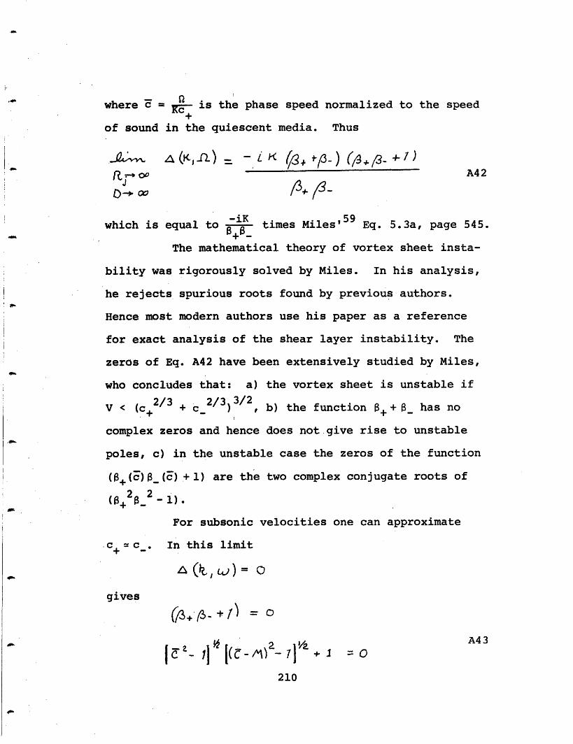
where e = K is the phase speed normalized to the speed
of sound in the quiescent media. Thus
a (Kl,) = - L+ 1)go fl - -A42
which is equal to -iK times Miles'5 9 Eq. 5.3a, page 545.
The mathematical theory of vortex sheet insta-
bility was rigorously solved by Miles. In his analysis,
he rejects spurious roots found by previous authors.
Hence most modern authors use his paper as a reference
for exact analysis of the shear layer instability. The
zeros of Eq. A42 have been extensively studied by Miles,
who concludes that: a) the vortex sheet is unstable if
V < (c 2/3 + c 2/3)3/2, b) the function ++ B_ has no
complex zeros and hence does not give rise to unstable
poles, c) in the unstable case the zeros of the function
(+(c)B_ ()+ +1) are the two complex conjugate roots of
( _2 -2 1).
For subsonic velocities one can approximate
c+ c_. In this limit
a (, w) ogives
A43
210
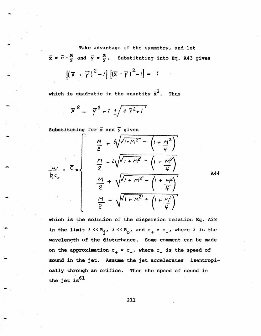
Take advantage of the symmetry, and let
= -M Mx -= c 2 and = . Substituting into Eq. A43 gives
whsuaihqat-2which is quadratic in the quantity x . Thus
--aX = 72+ _/y I
Substituting for and y gives
s -
*1 -+ 1 2'-I-
I1V * M+
)r( 1* 2)(IM2\(4
1
/l -I M-'\-
41
A44
which is the solution of the dispersion relation Eq. A28
in the limit << Rj, A<< Ro, and c+ = c_, where X is the
wavelength of the disturbance. Some comment can be made
on the approximation c+ = c_, where c is the speed of
sound in the jet. Assume the jet accelerates isentropi-
cally through an orifice. Then the speed of sound in
the jet is61
211
- W- U
2
2
- -
I
I
I
2 2C = C+
- I (a- 1) V22
when the orifice is choked c is minimum and equal to
.913 c+, where c+ is the sound speed in the surrounding
air (see Landau61 Eq. 80.18). Thus the approximation is
good for subsonic flow.
The dispersion relation yields complex roots
for all Mach numbers less than T 2.83. The imaginary
part of c is maximum at M = i3 = 1.73 and has a numerical
value of .5. The imaginary portion increases monatonically
from zero to the maximum as the flow speed increases from
Mach 0 to Mach 1.73, then it decreases monatonically to
zero as the flow speed increases to Mach 2.83.
A.7 Comments on the Application of the Theory toScreech
The most important point of the analysis is that
the shear layer is unstable at subsonic speeds. Some
ambiguity is inherent in further interpretation. This is
because only the ratio of w to k is specified in Eq. A44
and not the absolute values. To interpret the relation,
consider the limiting cases of w real and then k real.
Recall that the shear displacement P is given by
212
A45
For a3 real one has
C1 T i (k, - t ) eA46
For k real one has
(se- - car )- e -LC- e< (f t C L·CJ A47
Specify that the acoustic pressure perturbation
is harmonic in time at frequency w, where w is a real
number. From Eq. A46 it is clear that the wave grows
spatially in the downstream direction. This interpreta-
tion is used by Tam in his study of supersonic jets.
Given , it follows that
WC, Te ReI Il_ _
U.) F~~c cI
C( T I _
C.^ Of
C-
C* J_ +Mc- 1
- A48
,A1Lo
M1- O
where the second root of Eq. A44 was chosen so that
ki < 0, and the wave amplifies downstream.
213
C3
C~
2
JI~~
=
-
-)- -7
/%A1
2
YhQ se= - C,PI &Ihr
Assume, on the other hand, that the acoustic
perturbation grows in time, at a rate to be determined.
Let the spatial perturbations be dominated by the spa-
tial variation of the adjacent acoustic resonator. For
an orifice one would require the wave number k to be
real and equal to that of the axial acoustic mode.
Given k, it follows that
(4r - C+Rc cj= k c2
LC 2 2 A49
where the first root of Eq. A44 was chosen so that
m > 0 and the wave grows in time.
Concentrate on the phase speeds for each limit.
If the forcing acoustic perturbation does not grow in
time, the phase speed of the shear layer disturbances
is approximately V. If, however, the coupling is through
the spatial gradients, the phase speed of the shear layer
disturbances is . Recall that the orifice data was
fit with a phase speed equal to .6 V. This suggests
coupling through the wave number
214
Also recall the experiment on the coupling of
impingement screech to the axial acoustic modes (section
Y 3.5). There the screech frequency shifted down by about
2 kHz when the plate forming the acoustic cavity was
fitted to the end of the pipe. One interpretation of
this shift is that the phase speed of the disturbances
on the jet was lowered.
These observations suggest that the influence
of an acoustic resonator on shear layer instabilities is
to determine the spatial gradients and thereby alter the
phase speed of such instabilities. Before proceeding
with such studies, the theoretical phase speed must be
derived in greater detail. For orifice screech the
acoustic wavelength is approximately the same length as
the jet diameter and the two-dimensional approximation
<< Rj is no longer valid. It is therefore necessary to
solve Eq. A28 numerically.
The interpretation is only preliminary.
Physically, it is clear that the formation of ring vortices
play an essential role in screech. If these are formed
close to the inlet, the time of transit down the jet is
determined by the propagation speed of such vortices.
This speed may or may not be close to that given in Eqs.
A48 and A49. One cannot reach a conclusion based on the
linear analysis. If the vortex speed is independent of
215
the initial perturbation that forms such vortices, then
the only important point is that the shear layer is
unstable at low flow speeds.
216
REFERENCES
1. Lighthill, M. J.: "On Sound Generated Aerodynami-
cally: I. General Theory", Proc. Roy. Soc. (London)
Ser. A, Vol. 211, No. 1107 (March, 1952) pp. 564-
587.
2. Lighthill, M. J.: "On Sound Generated Aerodynami-
cally: II. Turbulence as a Source of Sound", Proc.
Roy. Soc. (London) Ser. A, Vol. 222, No. 1148
(February, 1954) pp. 1-32.
3. Ribner, H. S.: "New Theory of Jet-Noise Generation,
Directionality and Spectra", J. Acoust. Soc. Amer.,
Vol. 31, No. 2 (February, 1959) p. 245.
4. Ribner, H. S.: "The Generation of Sound by Turbulent
Jets" in Advances in Applied Mechanics, Vol. 8, New
York: Academic Press (1964), pp. 103-182.
5. Curle, S. N.: "General Theory of Aerodynamic Sound"
in Noise and Acoustic Fatigue in Aeronautics, edited
by E. J. Richards and D. J. Mead, New York: Wiley
Press (1968) pp. 111-134.
6. Goldstein, M. E.: Aerocoustics, NASA, SP-346 (1974).
7. Lighthill, M. J.: "On Sound Generated Aerodynami-Se r. A
cally", Proc. Roy. Soc. (London), Vol. 267, No.
11329 (May, 1962) pp. 147-181.
8. Lilley, G. M.: "On the Noise from Air Jets", ARC-20,
376; N40: FM-2724, British Aeronautical Research
Council (September, 1958).
217
9. Ffowcs Williams, J. E. and Hawkings, D. L.: "Sound
Generation by Turbulence and Surfaces in Arbitrary
Motion", Phil. Trans. Roy. Soc. (London), Ser. A,
Vol. 264 (May, 1969) pp. 321-342.
10. Curle, S. N.: "The Influence of Solid Boundaries
on Aerodynamical Sound", Proc. Roy. Soc. (London),
Ser. A., Vol. 231, No. 1187 (September, 1955) pp.
505-514.
11. Kraichnan, R. H.: "The Scattering of Sound in a
Turbulent Medium", J. Acoust. Soc. Amer., Vol. 25,
No. 6 (November, 1953) pp. 1096-1104.
12. Mawardi, O. K.: "On the Spectrum of Noise from
Turbulence", J. Acoust. Soc. Amer., Vol. 27, No. 3
(May, 1955) pp. 442-445.
13. Blokhintsev, D. I.: Acoustics of a Nonhomogeneous
Moving Medium, in Russian (1946), translated as
NACA T.M. 1399 (February, 1956).
14. Morse, P. M. and Ingard, K. U.: Theoretical Acous-
tics, New York: McGraw-Hill (1958).
15. Davies, P. O. A. L., Fisher, M. J. and Barratt,
M. J.: "The Characteristics of Turbulence in the
Mixing Region on a Round Jet", J. Fluid Mech. Vol.
15, Pt. 3 (March, 1963) pp. 337-367.
16. Ribner, H. S.: "Quadrupole Correlations Governing
the Pattern of Jet Noise", J. Fluid Mech., Vol. 38,
Pt. 1 (August, 1969) pp. 1-29.
218
17. Goldstein, M. E. and Rosenbaum, B.: "Effect of
Anisotropic Turbulence on Aerodynamic Noise", J.
Acoust. Soc. Amer., Vol. 54, No. 3 (September, 1973)
pp. 630-645.
18. Atvars, J., Schubert, T. K. and Ribner, H. S.:
"Refraction of Sound from a Point Source Placed in
an Air Jet", J. Acoust. Soc. Amer., Vol. 37, No. 1
(January, 1965) pp. 168-170.
19. Grande, E.: "Refraction of Sound by Jet Plow and
Jet Temperature", NASA CR-840 (August, 1967).
20. Gottlieb, P.: "Acoustics in Moving Media", Ph.D.
Thesis, Physics Dept., M.I.T. (June, 1959); also:
"Sound Source Near a Velocity Discontinuity", J.
Acoust. Soc. Amer., Vol. 82, No. 9 (September,
1960) pp. 1117-1122.
21. Grahm, E. W. and Grahm, B. B.: "The Acoustical
Source in a Two-Dimensional Jet", Boeing Scientific
Research Laboratories, DI-82-0909 (1969).
22. Townsend, A. A.: "The Measurement of Double and
Triple Correlation Derivatives in Isotropic Turbu-
lence", Proc. Camb. Phil. Soc., Vol. 43 (1947)
p. 560.
23. Batchelor, G. G.: The Theory of Homogeneous
Turbulence, Cambridge: Cambridge University Press
(1953).
219
24. Uberoi, M. S. and Singh, P. I.: "Turbulent Mixing
in a Two-Dimensional Jet" in The Physics of Fluids,
Vol. 18, No. 7 (July, 1975)pp. 764-7,6 9.
25. Lassiter, L. W.; "Turbulence in Small Air Jet at
Exit Velocities Up to 705 Feet Per Second", J. Appl.
Mech., Vol. 24, No. 3 (September, 1957) pp. 349-354.
26. Meecham, W. C.: "Acoustic Spectra from Turbulent
Jets" in Basic Aerodynamic Noise Research, edited
by I. R. Schwartz, NASA SP-207 (July, 1969) pp.
177-185.
27. Olsen, W. A., Guturry, O. A. and Dorsch, R. G.:
"The Effect of Nozzle Inlet Shape, Lip Thickness
and Exit Shape on Subsonic Jet Noise", NASA T.M.
X-68182 (1973).
28. von Gierke, H.: "Types of Pressure Fields of Inter-
est in Acoustical Fatigue Problems" in University of
Minnesota Conference on Acoustical Fatigue, edited
by W. J. Trapp and D. M. Forney, W.A.D.C. Tech. Rep.,
pp. 59-676.
29. Ffowcs Williams, J. E.: "The Noise from Turbulence
Convected at High Speed", Phil. Trans. Roy. Soc.
(London), Ser. A, Vol. 255, No. 1061 (April, 1963)
pp. 469-503.
30. Ingard, K. U. and Singhal, V. K.: "Effect of Flow
on the Acoustic Resonance of an Open-Ended Duct",
220
J. Acoust. Soc. Amer., Vol. 58, No. 4 (October,
1975) pp. 788-793.
31. Ingard, K. U.: lecture notes in "Noise Control
Engineering", M.I.T. course 16.56 (Fall semester,
1976).
32. Marble, F. E.: "Acoustic Disturbance from Gas Non-
uniformities Convected through a Nozzle" in Vol. II,
Proceedings, Interagency Symposium on University
Research in Transportation Noise, Stanford Univer-
sity (March 28-30, 1973) pp. 547-560.
33. Bohn, M. S. and Zukoski , E. E.: "Effect of Flow
on the Acoustic Reflection Coefficient at a Duct
Inlet", J. Acoust. Soc. Amer., Vol. 59, No. 6 (June,
1976) pp. 1497-1499.
34. Cummings, A.: "Sound Transmission at a Sudden Area
Expansions in Circular Ducts with Superimposed Mean
Flow", J. Sound and Vib., Vol. 38, No. 1 (January,
1975) pp. 149-155.
35. Morse, P. M.: Vibration and Sound, New York:
McGraw-Hill (1948).
36. Abramowitz, M. and Stegun, I.: Handbook of Mathe-
matical Functions with Formulas, Graphs and Mathe-
matical Tables, N.B.S. Applied Math, Ser. 55 (1964).
37. Lee, J. F. and Sears, F. W.: Thermodynamics, Read-
ing, Mass.: Addison-Wesley (1963) Chap. 8.
221
38. von Gierke, H. E., Parrach, H. O., Gannon, W. J.
and Hansen, R. G.: "The Noise Field of a Turbo-
Jet Engine", J. Acoust. Soc. Amer., Vol. 24, No. 1
(March, 1952) pp. 169-174.
39. Mungar, P. and Gladwell, G. M. L.: "Acoustic Wave
Propagation in a Sheared Fluid Contained in a Duct",
J. Sound and Vib., Vol. 9, No. 1 (January, 1969)
pp. 28-48.
40. Ingard, K. U.: lecture notes in "Noise Control
Engineering", M.I.T. course 16.56 (Fall semester,
1975).
41. Roe, G. M.: "Frequency Distribution of Normal
Modes", J. Acoust. Soc. Amer., Vol. 13, No. 1
(July, 1941) pp. 1-7.
42. Doak, P. E.: "Elements of Sound Propagation" in
Noise and Acoustic Fatigue in Aeronautics, edited
by E. J. Richards and D. J. Mead, New York: Wiley
Press (1968) pp. 43-72.
43. Chanaud, R. C. and Powell, A.: "Some Experiments
Concerning the Hole and Ring Tone", J. Acoust. Soc.
Amer., Vol. 37, No. 5 (May, 1965) pp. 902-911.
44. Anderson, A. B. C.: "A Jet Tone Orifice Study for
Orifices of Small Thickness - Diameter Ratio", J.
Acoust. Soc. Amer., Vol. 26, No. 1 (January, 1954)
pp. 21-25.
222
45. Heller, H. H.: "Tone Generation by Subsonic Flow
Through Sharp-Edged Circular Nozzles", '73 meeting
of Acoust. Soc. Amer. (April 21, 1967) paper
N/EF3 (abstract only) p. 1615.
46. Thomas, N.: "On the Production of Sound by Jets",
J. Acoust. Soc. Amer., Vol. 27, No. 3 (May, 1955)
pp. 446-448.
47. Powell, A. and Unfreid, H. H.: "An Experimental
Study of Edgetones", U.C.L.A. Rept. 64-49 (1964).
48. Powell, A.: "On the Edgetone", J. Acoust. Soc.
Amer., Vol. 33, No. 4 (April, 1961) pp. 395-409.
49. Wagner,-F. R.: "Zum Schall-und Strommungsfeld
,eines Axialsymmetrischen Freistralls beim Auftreffen
auf eine Wund", in German, English abstract,
Z. Flugwiss 19 (1971) Heft. 1, pp. 30-44.
50. Neuwerth, G.: "Acoustic Feedback Phenomena of the
Subsonic and Hypersonic Free Jet Impinging on a
Foreign Body", NASA TT-F-15719 (July, 1974).
51. Anderson, A. B..C.: "Vortex Ring Structures in a
Jet Emitting Discrete Acoustic Frequencies", J.
Acoust. Soc. Amer., Vol. 28, No. 5 (September, 1956)
pp. 914-921.
52. Bilanin, A. J. and Covert, E. E.: "Estimation of
Possible Excitation Frequencies for Shallow Rectan-
gular Cavities", AIAA Jour., Vol. 71, No. 3 (March,
1973) pp. 347-351.
223
53. Rossiter, J. E.: "Wind Tunnel Experiments in the
Flow over Rectangular Cavities at Subsonic and
Transonic Speeds", R and M 3438 (1966), Aeronauti-
cal Research Council, Brittain.
54. Handa, H.: "Jet Instabilities and Noise", Ph.D.
Thesis, Mechanical Engineering Dept., M.I.T.
(February, 1974).
55. Bilanin, A. J.: "Flow-Induced Oscillations in
Rectangular Cavities", M. S. Thesis, Aeronautics
Dept., M.I.T. (September, 1970).
56. Ingard, K. U., Cho, Y. C., Singhal, V. K., Succi,
G. P. and Patric, W. P.: "Studies of Sound Absorp-
tion Materials and Attenuation of Sound in Ducts",
Proc. 2nd Interagency Symp. on Research in Trans-
portation Noise, Vol. 2, N. Carolina State Univ.
(June, 1974) p. 816.
57. Tarn, C. K. W.: "Directional Acoustic Radiation
from a Supersonic Jet Generated by Shear Layer
Instabilities", J. F. Mech., Vol. 46, Pt. 4 (April,
1974) pp. 757-768.
58. Sedel'nikov, T. Kh.: "The Frequency Spectrum of
the Noise in a Supersonic Jet" in Physics of-Aero-
dynamic Noise, edited by Rimskey-Korsakov, trans-
lated in NASA TT-F-538 (November, 1969) pp. 71-75.
224
59. Miles, J. W.: "On the Disturbed Motion of a Plane
Vortex Sheet", J. Fluid Mech., Vol. 4, Pt. 5
(September, 1958) pp. 538-552.
60. Rayleigh, Theory of Sound, Dover Reprint (1945).
61. Landau, L. D. and Lifshitz, E. M.: Fluid Mechanics,
Reading, Mass.: Addison Wesley (1959).
62. Olsen, W. A., Miles, J. H. and Dorsch, R. G.:
"Noise Generated by the Impingement of a Jet on a
Jet on a Large Flat Plate", NASA TN D-7075 (December,
1972).
63. Lee, H. K., and Ribner, H. S.: "Direct Correlation
of Noise and Flow of a Jet", J. Acoust. Soc. Amer.,
Vol. 52, No. 5, Pt. 1 (1972), pp. 1280-1290.
22 4%
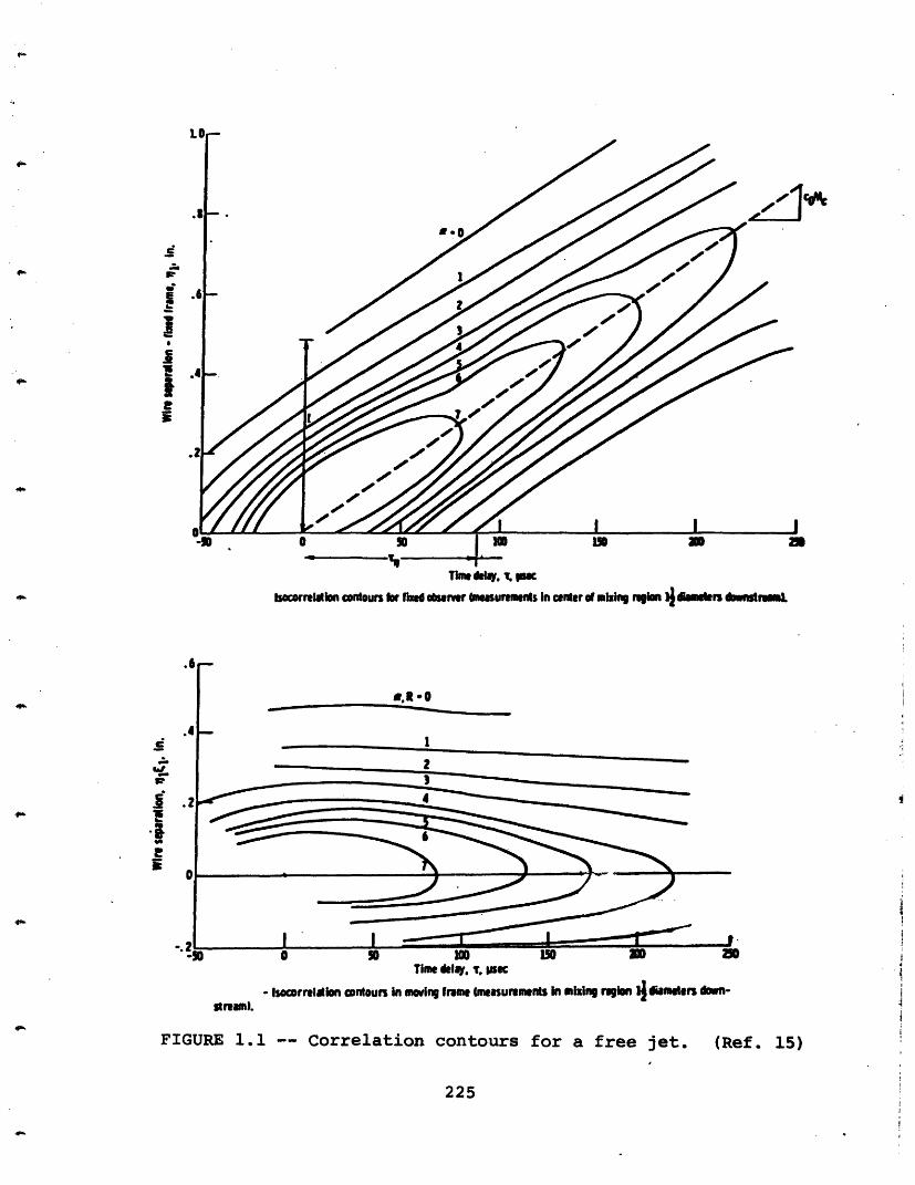
C
iA.w4;I
bocorrelalon contours r fied debsur Imremnts in center of miing region 4 diaurn s dn strmL
.1
.4
g.
'e
5
_ - 3 1
2
' -:So0 X 100 15 so -iTime delay, T, Ise
- Isocorrelfion contours in moving frame measuremmns n mixing region diameters down-
FIGURE 1.1 -- Correlation contours for a free jet. (Ref. 15)
225
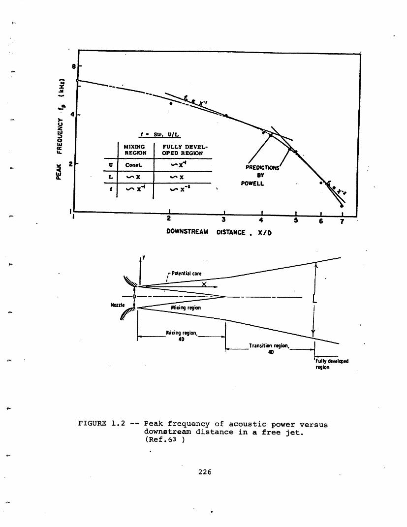
I0U.
DOWNSTREAM DISTANCE ,. X /D
Fullyiregion
FIGURE 1.2 -- Peak frequency of acoustic power versusdownstream distance in a free jet.(Ref.63 )
226
develped
I
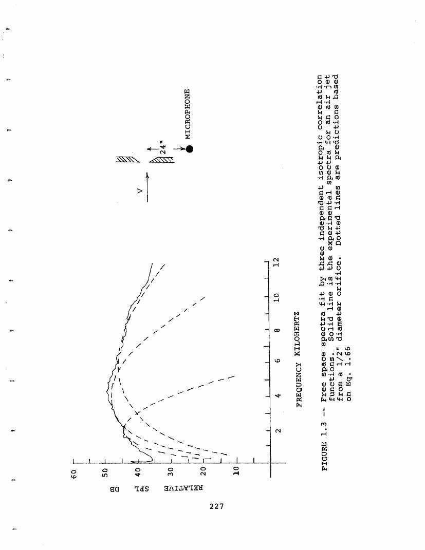
00
0e I,4 I : 0P4 $4
0 k --U 0U .H k4 U
t- v~~~LI CL~0 QI
_ O r k0 0
000U)4I->-H 0
On0 4Ja) · )
,1 E 444 -O
0 Cr 0oO Q U)
H _ VD
/lN i ·-- 4- - H
I
3Hr4
Ga ras aAIlVqaH
227
C
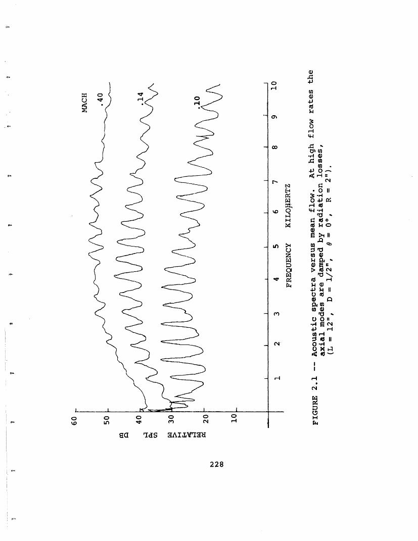
a)
4.
tQ
Wo
-Ir-4
cl U)
403N NE- 0 II
0-4
0)O>1
IQ>4 03
Z ( flu
0Q X
0 o
-rd64) H
to4N iH r
cm
228
ea ads a~I~Llvqaut
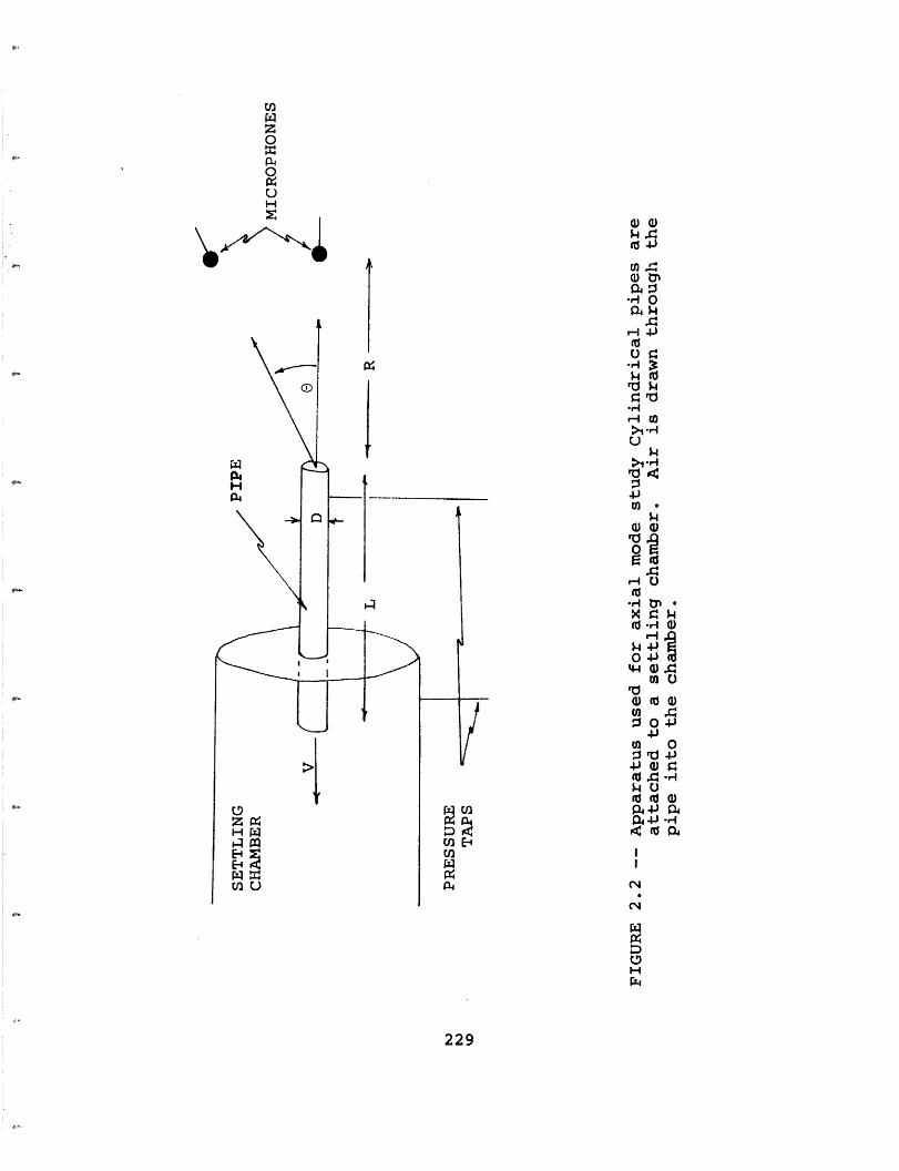
U)
z0m
UHCz
r-7
I
Z CH
E4
u u
T]
>v
.r 3.1i0 hrlg
.l
r-4
UtO
-,- t,
m - ,1
O. w O(
u 0/ ax O~~~~iI~~~r Og11 ".
( 4 -H
I
U) E-
U I
c4
229
Q 4J
.r 004 Q
p9I.
f v J I 5
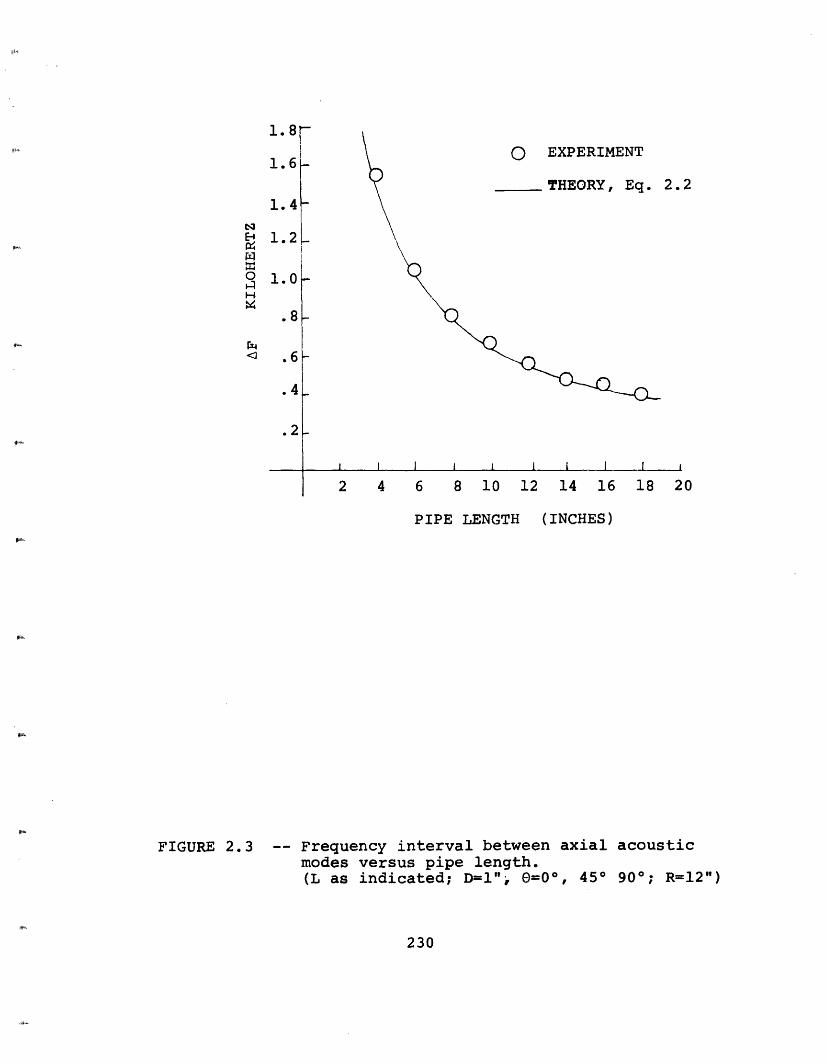
1.8
1.6
1.4
N
oH
a
1.2
1.0
.8
.6
.4
.2
2.2
I I I I
2 4 6 8 10 12 14 16 18 20
PIPE LENGTH (INCHES)
FIGURE 2.3 -- Frequency interval between axial acousticmodes versus pipe length.(L as indicated; D=1",; =00, 450 900; R=12")
230
--
-
L
-
_
_
_
I I I
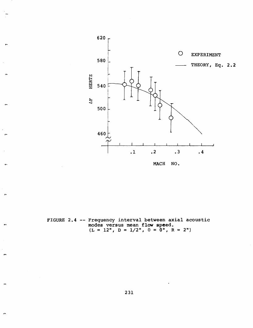
580
NE-1
540
500
460
0 :RIMENT
DRY, Eq. 2.2
I I I I I 1 I I
.1 .2 .3 .4
MACH NO.
FIGURE 2.4 -- Frequency interval between axial acousticmodes versus mean flow speed.(L = 12", D = 1/2", 0 = 0° , R = 2")
231
... �__
Aw)n
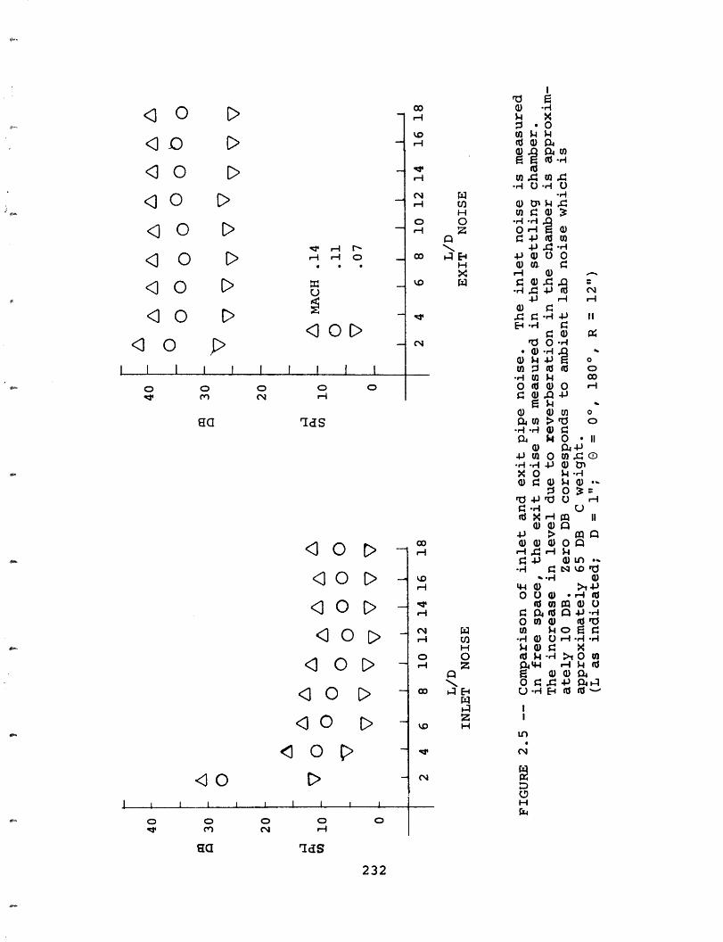
<O D
<O D
< O D
<10 >
0<1
<}
o DO >
< O
, r-H r-
I I I I I I I
0m
0C...
ai
0H-
0
aIdS
< O ><10 D
< 0 D< O D<JO><l0t
<10 >
<OI I I I
0 0mv
I I I
0, i I I I i 0 0
o a
rIdS
.- k X: .0
.- tn P
rlr~~-i 0 .,
H 0C 0 3 rH CZ 0)N C
t: ~: -0 0 )
X H r~a~O00 44 4. 0) 0 0
Qo r4 4
C14 o 0 -rq
%- 0,4 EU) 0)U4
04 kO.1-i 0 <-: -I 4 )4.)J >m di O d)
O a~3 tC
W4.) I
o .4 -4H 4-)
0 0
OU)0N t n ko--I rl -)0 UO
o 0 N -~ >
c c- Eq U 4 Er -
'.0 H
V 4
H
C!rl
0o
0
. 1
II
0)C)- *1.4 --rl
O 04-
232
i · I r
I
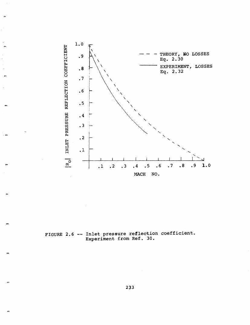
ElZHUH
U
zoHE-U
i--z
H~-A
Mn
MI
:Dcl)U)
1.0
.9
.8
.7
.6
.3
.2
.1
0__
- - - THEORY, NO LOSSESEq. 2.30
EXPERIMENT, LOSSESEq. 2.32
I I
.1 .2 .3 .4 .5 .6 .7 .8 .9 1.0
MACH NO.
FIGURE 2.6 -- Inlet pressure reflection coefficient.Experiment from Ref. 30.
233
- · · · · · · · Y
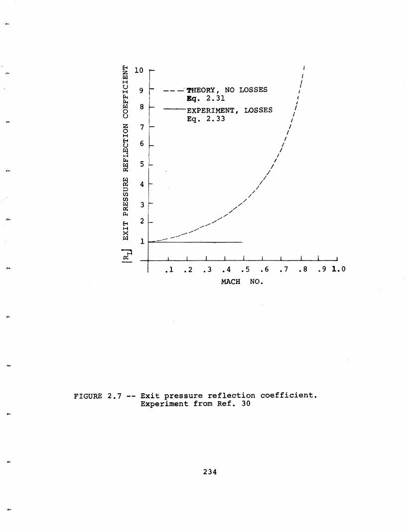
--- THEORY, NO LOSSESEq. 2.31
-- EXPERIMENT, LOSSESEq. 2.33
i
IIIII
/
I/
/
/
-- -
i I I I I i i I I
.1 .2 .3 .4 .5 .6 .7 .8 .9 1.0
MACH NO.
FIGURE 2.7 -- Exit pressure reflection coefficient.Experiment from Ref. 30
234
ZzHUH
30C4
z0HE-HU
U)O3
HX..En
10
9
8
7
6
5
4
3
2
1
· · · · · · · I
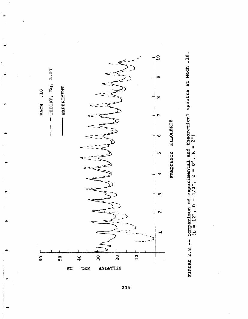
c,--~~~~~~,F- -Ln
cu~~~~~~-
o 1:= ZH~~
0 0.;.1U . . -
O x3:X
I =_
l '- ,,-- - _
-D -)
L_ __ LL I I"
I I _1 1___1 1 I Iz 0 o 0
UN 0(Y)
0(-4
0
o O
0 0
-J
(d
04
,-I
4J0)
D 0 0-
0U (U
r 1 H1(rU I
4I0
HU
C4
H340235
_ ___ _ __ .I
Ha id 2ILVIS'
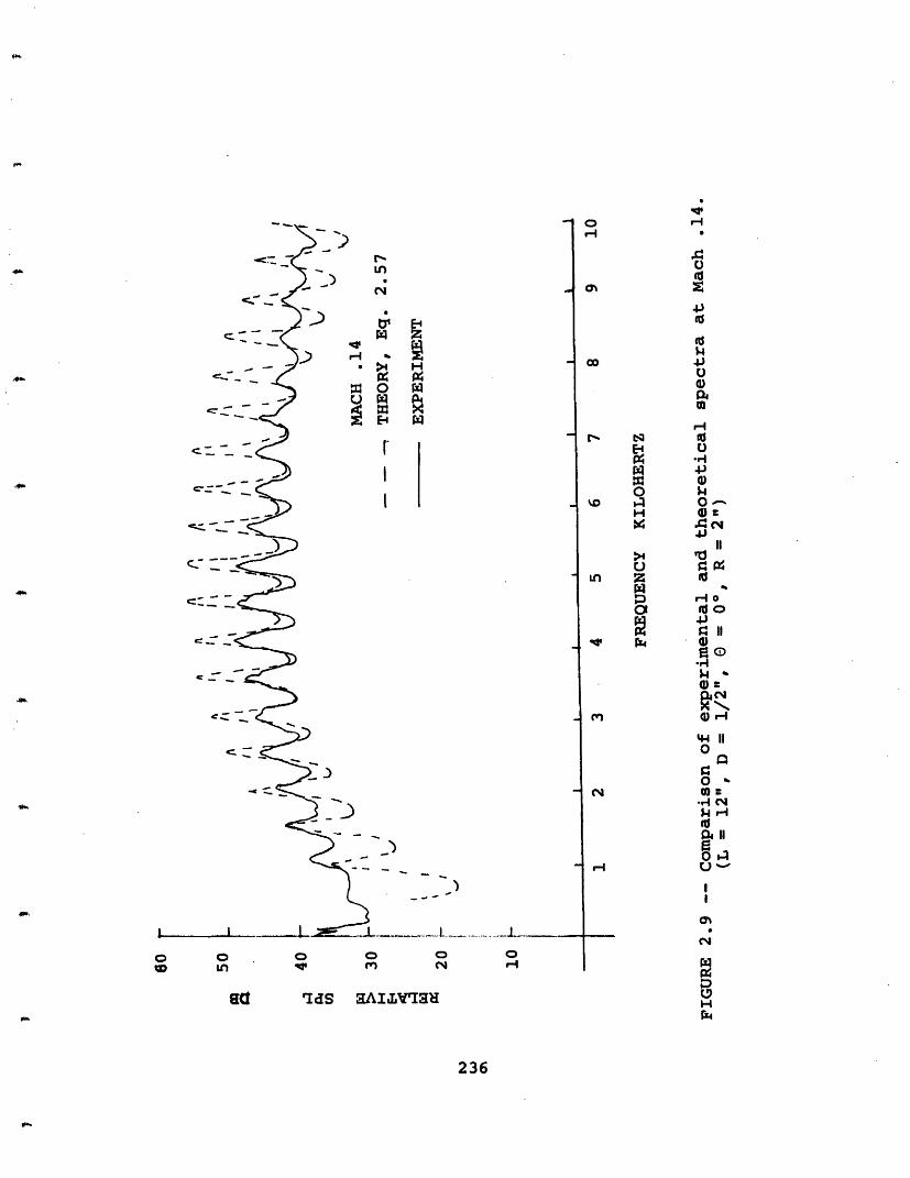
<2
CN
F)lrw
II.64
I.
E-4zH
W
W
C-
_)
_ 9
o 0m
oN4
o04H
E4
.)
U(d
)--0
IIO
0
,- 0-U a:
*ri C
IIIl
3u
raS aAI&VTqa
0 0Iv Un)
so
236
Hr4d
,,
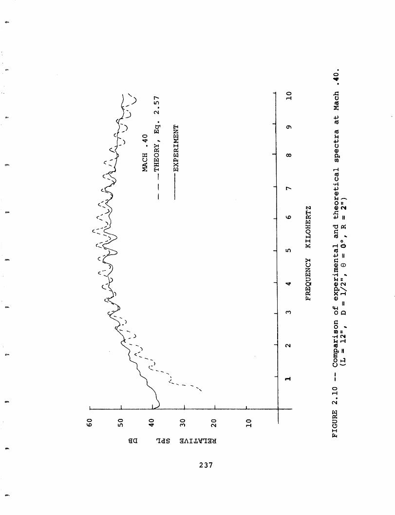
0C;.r
0
w O) )
E-
I
I
E
H;l
wI
13
r1 (N M
U
(J
i4
-)Urla)
0:
H o
P II
Z-I
O4O :-
0 t
HCl jIdO 1
o
_
r r
C4
HrZ4
gIdS aAILvqaI
237
C
c
)
_ )
cLI)w lw
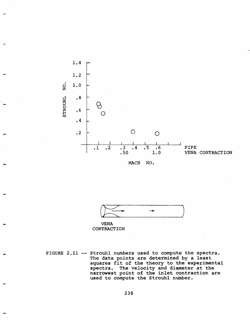
0
0I I
0i I I I
.1 .2 .3 .4 .5 .6.50 1.0
PIPEVENA CONTRACTION
MACH NO.
C ---
VENACONTRACTION
FIGURE 2.11 -- Strouhl numbers used to compute the spectra.The data points are determined by a leastsquares fit of the theory to the experimentalspectra. The velocity and diameter at thenarrowest point of the inlet contraction areused to compute the Strouhl number.
238
1.4
1.2
Z
0E-En
1.0
.8
.6
.4
.2
- ... ! w.
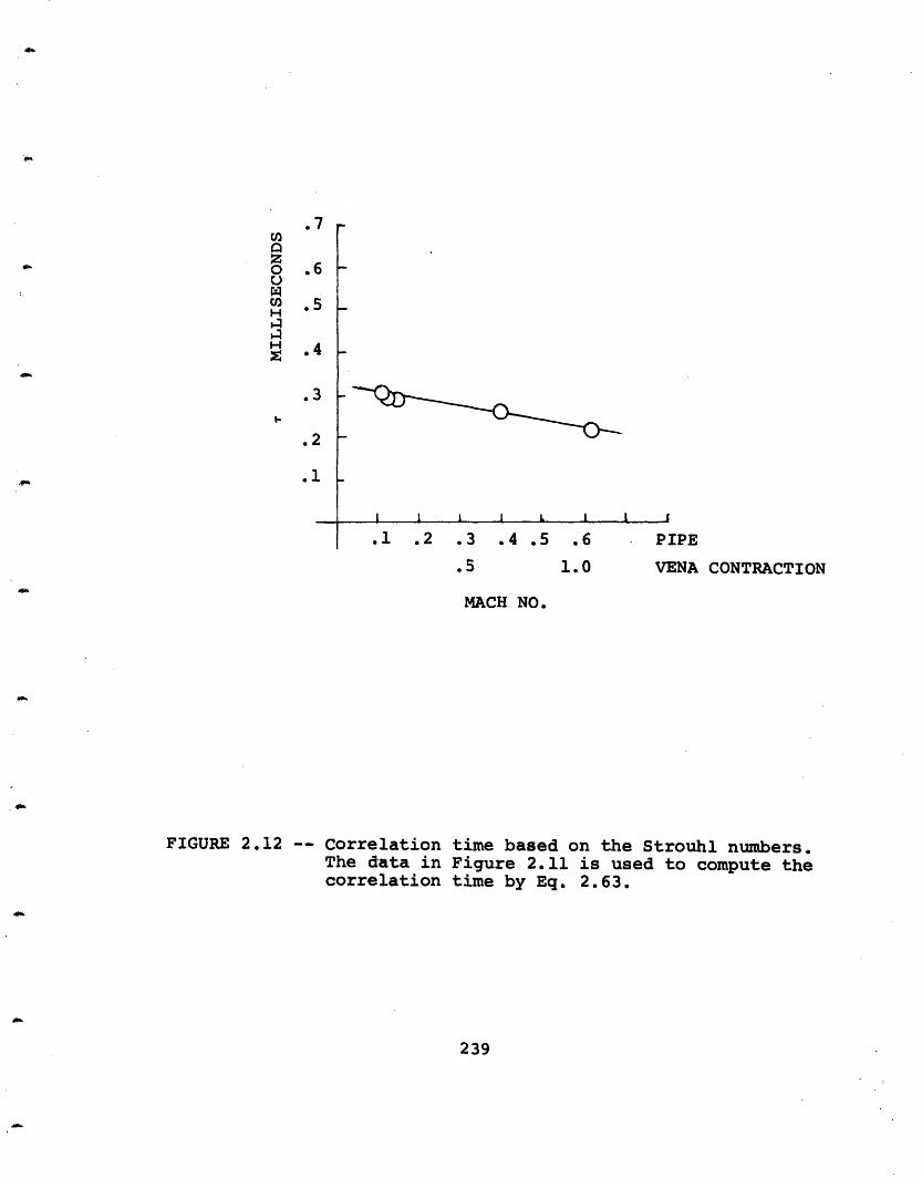
I I I I L I I I
.1 .2 .3 .4 .5 .6
.5 1.0
PIPE
VENA CONTRACTION
MACH NO.
FIGURE 2.12 -- Correlation time based on the Strouhl numbers.The data in Figure 2.11 is used to compute thecorrelation time by Eq. 2.63.
239
El
zouC)H
Hz
.7
.6
.5
.4
.3I-
.2
.1
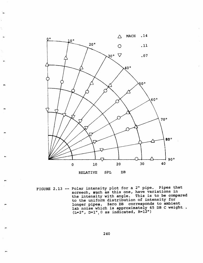
A MACH .14
90l
900 10 20 30 40
RELATIVE SPL DB
FIGURE 2.13 -- Polar intensity plot for a 2" pipe. Pipes thatscreech, such as this one, have variations in
the intensity with angle. This is to be comparedto the uniform distribution of intensity for
longer pipes. Zero DB corresponds to ambientlab noise which is approximately 65 DB C weight.(L=2", D=1" 0 as indicated, R=12")
240
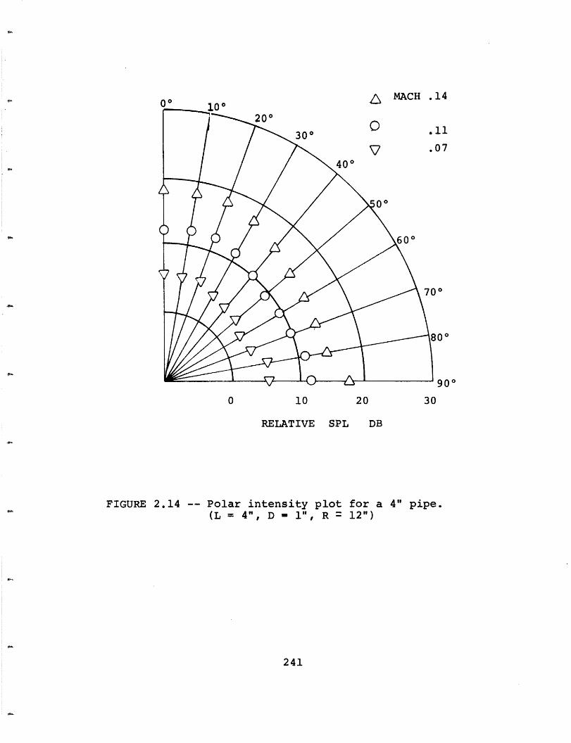
A MACH .14
20
RELATIVE SPL DB
FIGURE 2.14 -- Polar intensity plot for a 4" pipe.(L = 4", D - 1", R = 12")
241
11
07
o
:00
90 °
0 30
_-

/L MACH .14
L1
)7
0
00
90
0 10 20 30
RELATIVE SPL DB
FIGURE 2.15 -- Polar intensity plot for a 6" pipe.(L = 6", D = 1", R = 12")
242
AO
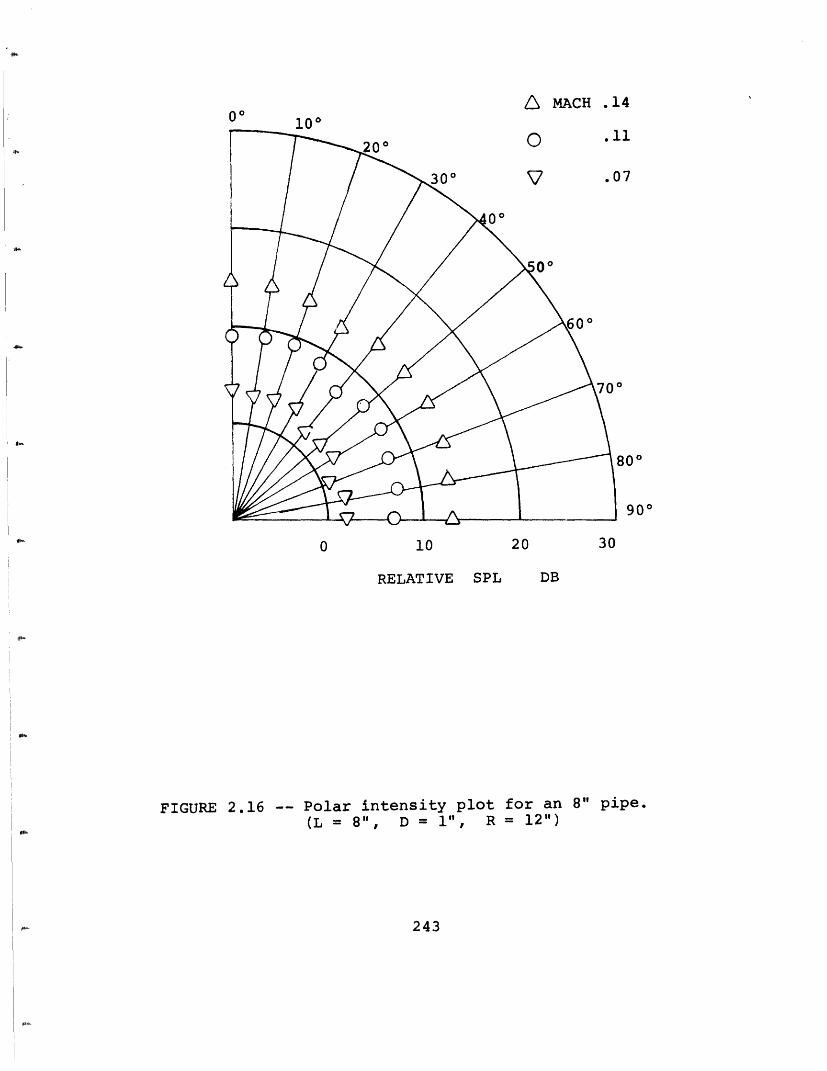
L MACH .140 10°
1
7
00
90
0 10 20 30
RELATIVE SPL DB
FIGURE 2.16 -- Polar intensity plot for an 8" pipe.(L = 8", D = 1", R = 12")
243
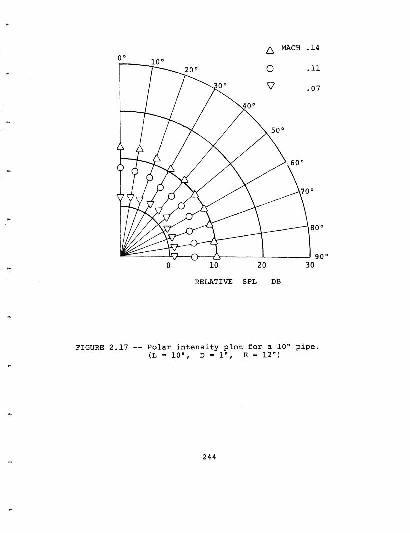
a MACH .14
0 10 20
RELATIVE SPL
30
DB
FIGURE 2.17 -- Polar intensity plot for a 10" pipe.(L = 10", D = 1", R = 12")
244
0
.1
17
0o
90
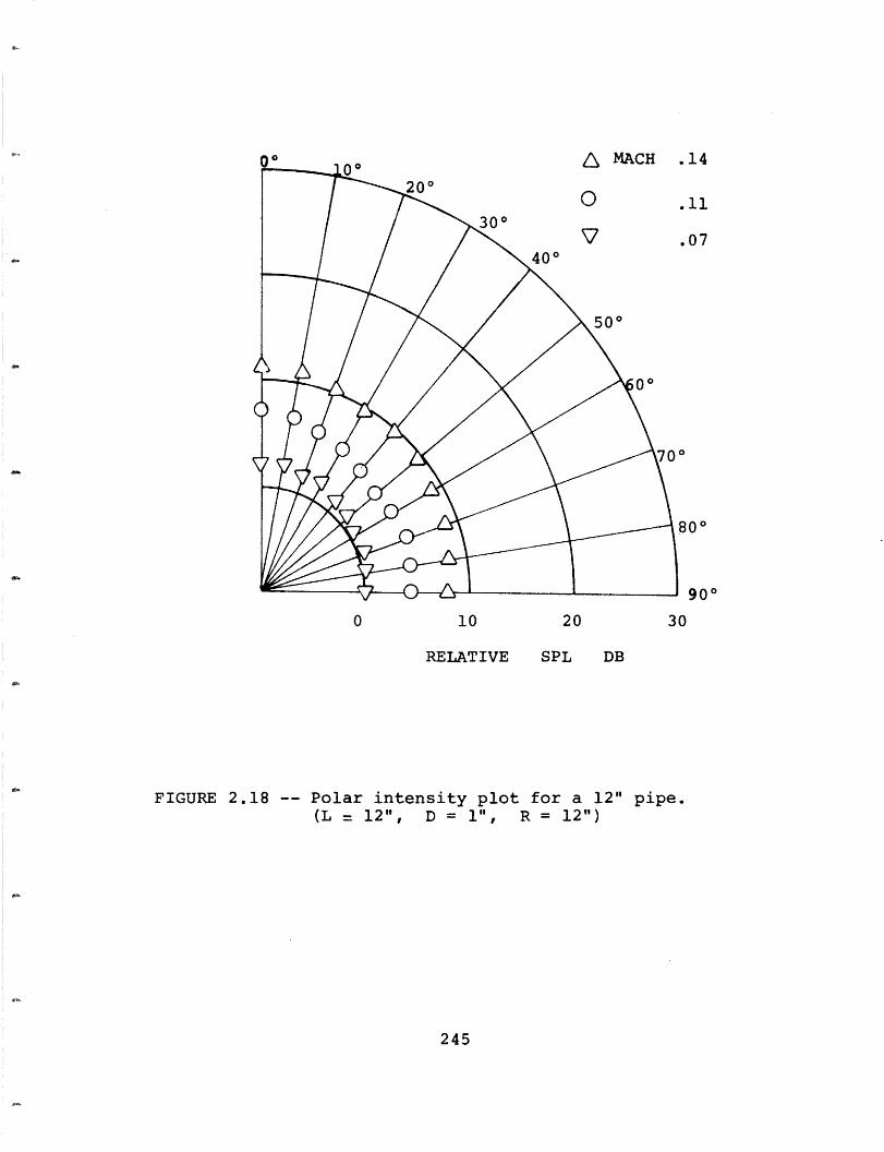
.14
.11
.07
80°
90
0 10 20 30
RELATIVE SPL DB
FIGURE 2.18 -- Polar intensity plot for a 12" pipe.(L = 12", D = 1", R = 12")
245
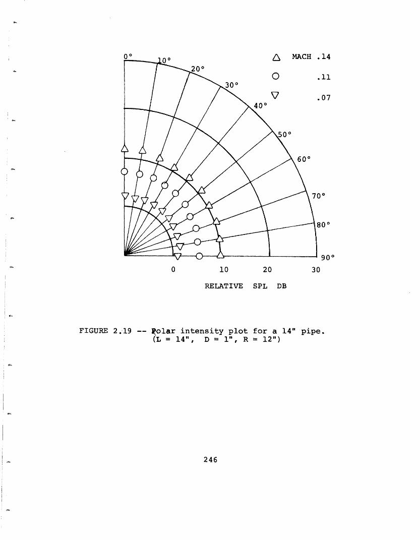
0 10 20 30
RELATIVE SPL DB
FIGURE 2.19 -- Rolar intensity plot for a 14" pipe.(L = 14", D = 1", R = 12")
246
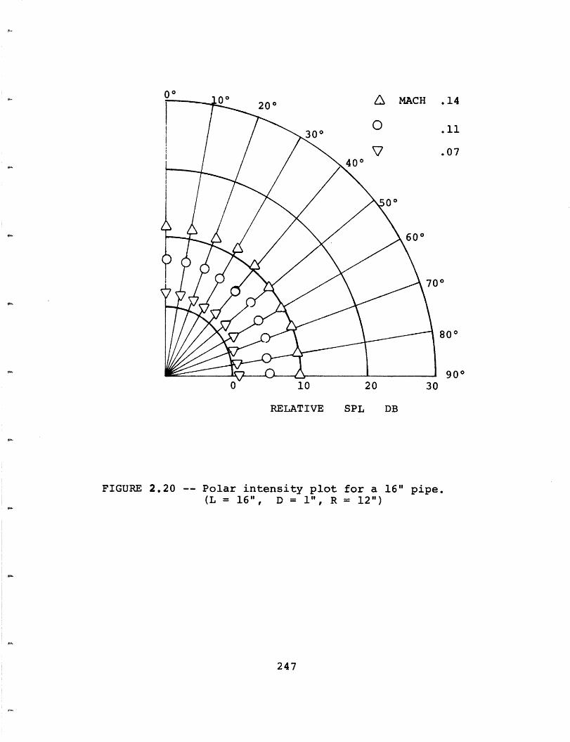
0 10 20
RELATIVE SPL DB
FIGURE 2.20 -- Polar intensity plot for a 16" pipe.(L = 16", D = 1", R = 12")
247
no.14
.11
.07
0
800
90
70
30
A
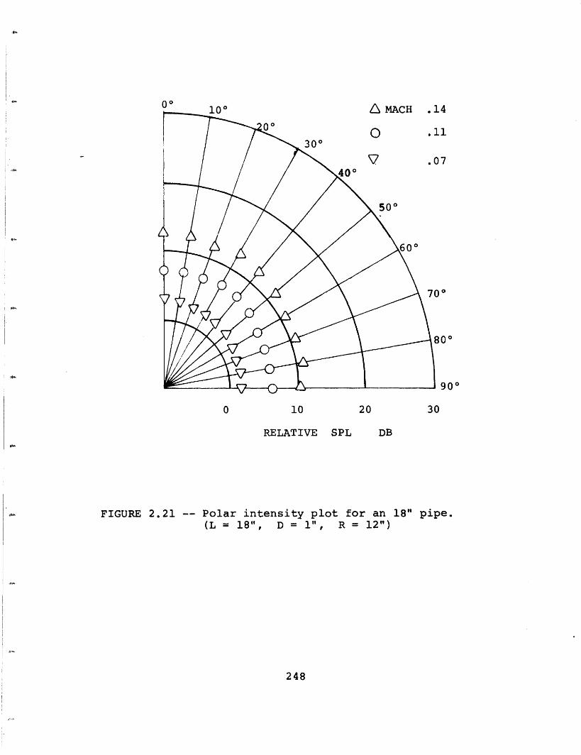
0 10 20
RELATIVE SPL DB
FIGURE 2.21 -- Polar intensity plot for an 18" pipe.(L = 18", D = 1", R = 12")
248
00 1 no A MAH I 14
80°
90
30
-1
) 7
) 0
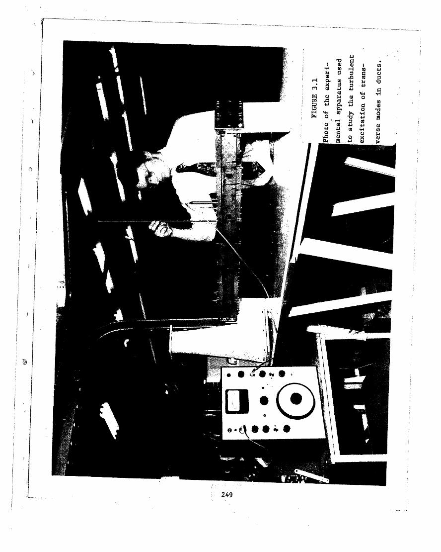
.. .…….. -- .. . .. .
· 249
I ii
i
Ii
I
II
�
i
i
r
i
i
i
ii
i .1
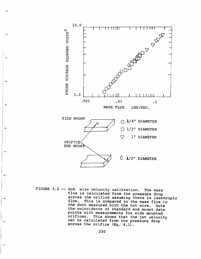
I I I I 1 1111
I ° 1 111_I I I I I ~I � � 0I I it ill I � I I nih f I
I I i I 1 1111
.01
MASS FLUX
o /4"
[i 1/2"
7
.1
LBS/SEC.
DIAMETER
DIAMETER
1" DIAMETER
0 /2" DIAMETER
FIGURE 3.2 -- Hot' wire velocity calibration. The massflux is calculated from the pressure dropacross the orifice assuming there is isentropicflow. This is compared to the mass flux inthe duct measured with the hot wire. Notethe coincidence of standard end mount datapoints with measurements for side mountedorifices. This shows that the jet velocitycan be calculated from the pressure dropacross the orifice (Eq. 4.1).
250
10.0cu
Ec
0
001m
P4 1.0
,&27
,7
.001
I
I
I
TnVF MTTMM
ORIFEND
____ _ _ _ _ _ · E E _ _ _ X Wia
I
Il
_ if-1
I I I I I
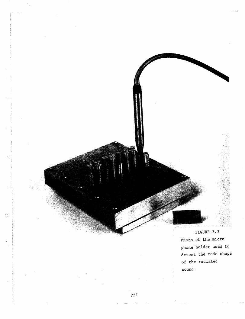
Photo of the micro-
phone holder used to
detect the mode shape
of the radiated
i sound.
251
PI,I- , "" ---i 7 , ~~~rM
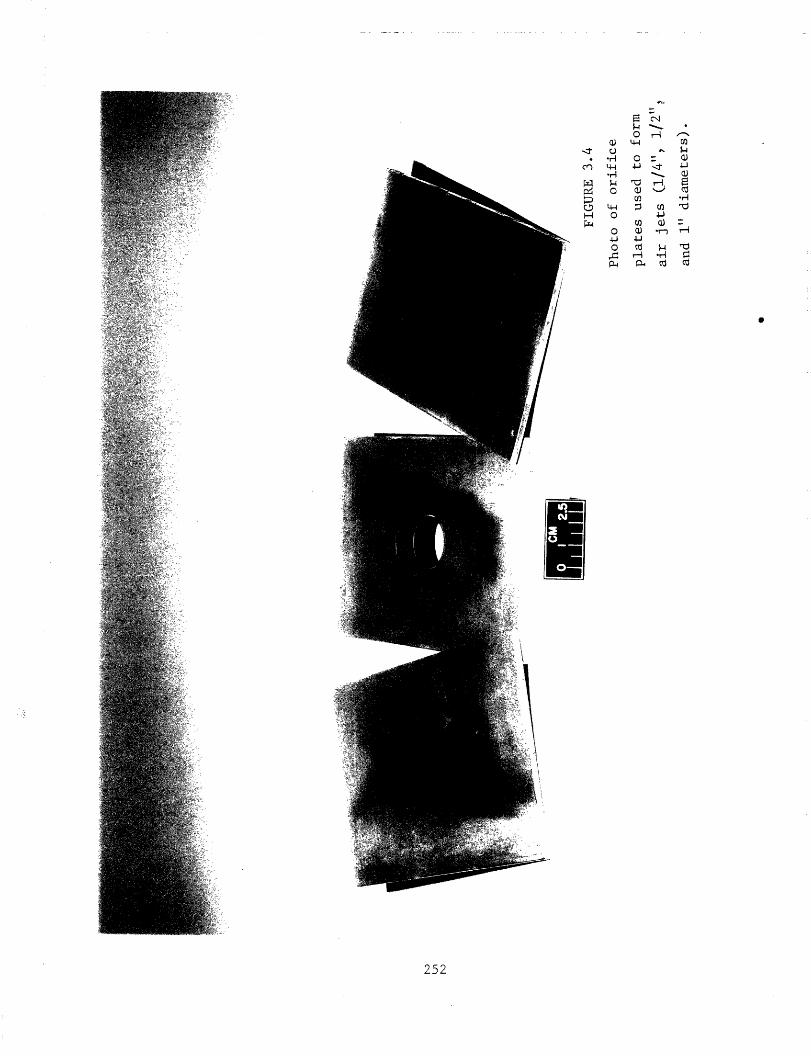
' - ·k -X. n - )
*H -- ();4 ~4 - 0
P= v Z: r
0 4 02Pr4 rn (1)
C) (3) rI r -
p , ;a d cd
252
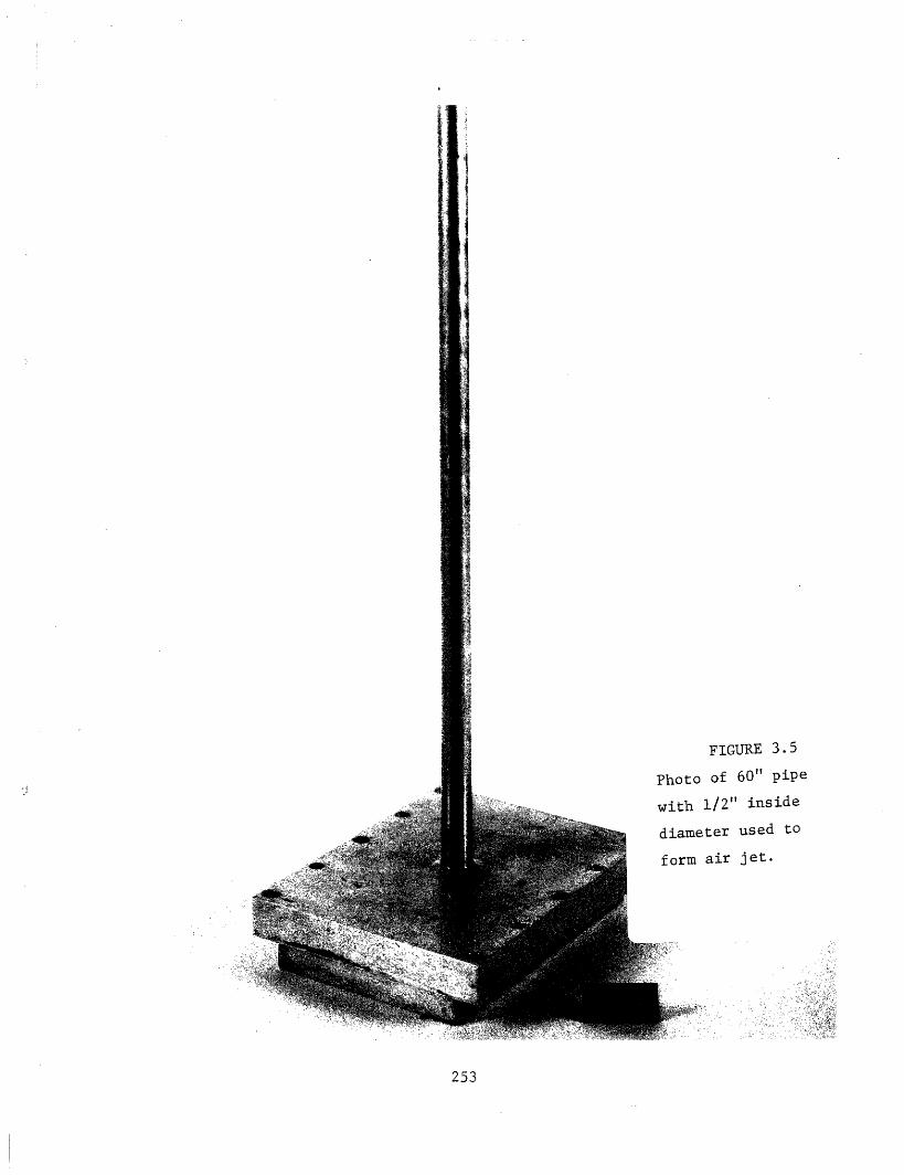
I
FIGURE 3.5
of 60" pipe
1/2" inside
.ter used to
air jet.
-,??
253
l
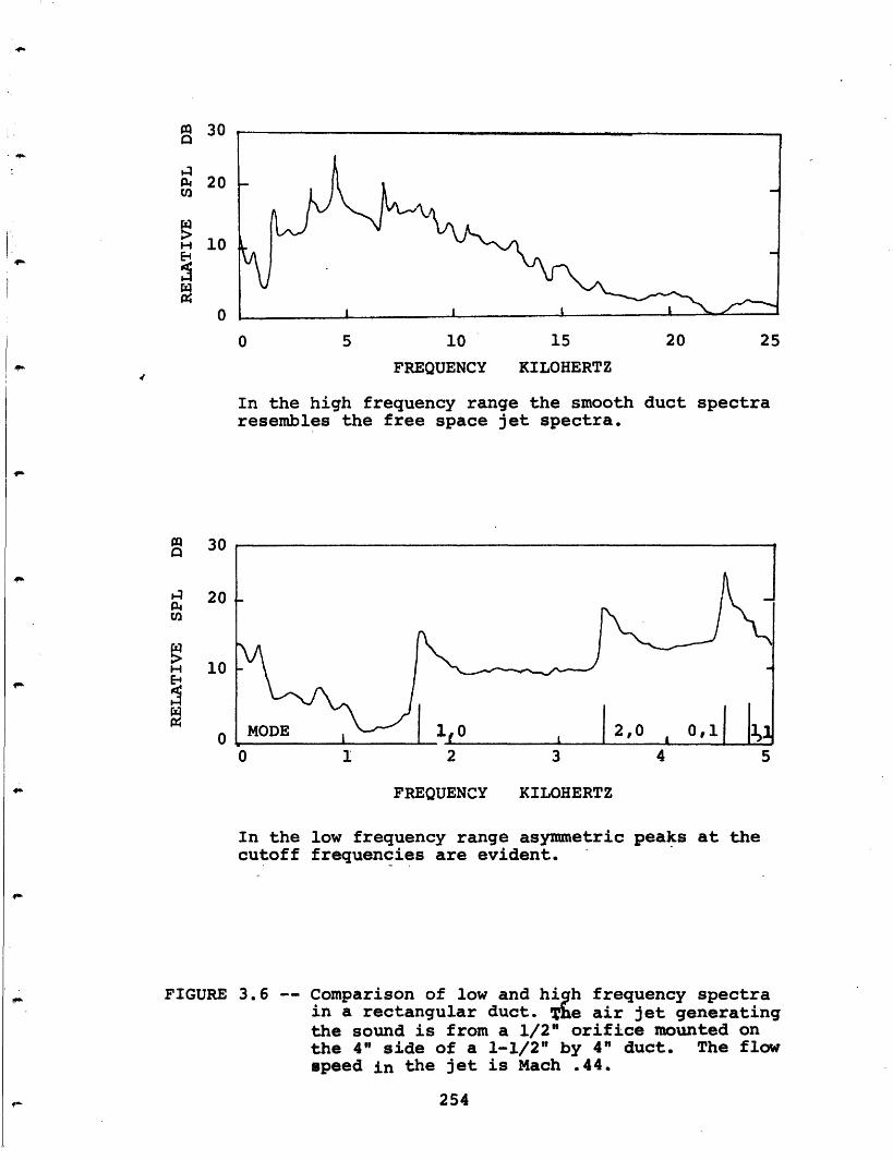
30
20
10ICA
0
0 5 10 15 20 25
FREQUENCY KILOHERTZ
In the high frequency range the smooth duct spectraresembles the free space jet spectra.
FREQUENCY KILOHERTZ
In the low frequency range asymmetriccutoff frequencies are evident.
, . .~~~~~
peaks at the
FIGURE 3.6 -- Comparison of low and high frequency spectrain a rectangular duct. The air jet generatingthe sound is from a 1/2" orifice mounted onthe 4" side of a 1-1/2" by 4" duct. The flowspeed in the jet is Mach .44.
254
30
U)1H4w
wH
a;4
20
10
0
I
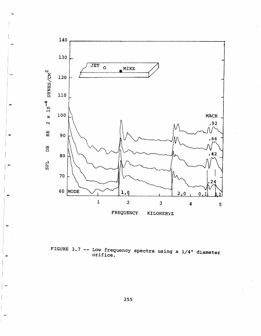
Nci-
z
to
To0
x
'I-
1 AnA
130
120
110
100
90
80
UtU)
70
60
1 2 3 4 5
FREQUENCY KILOHERTZ
FIGURE 3.7 -- Low frequency spectra using a 1/4" diameterorifice.
255
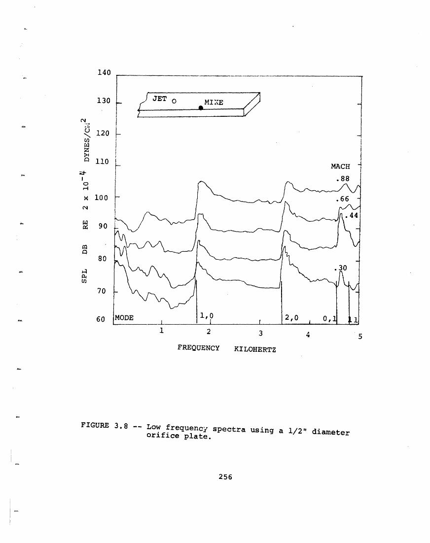
140
130
120
110
100
90
80
I)laLO
70
60
1 2 3 4 5
FREQUENCY KILOHERTZ
FIGURE 3.8 -- Low frequency spectra using a 1/2" diameterorifice plate.
256
N, 4
u
za
0Ix
xN
I.,
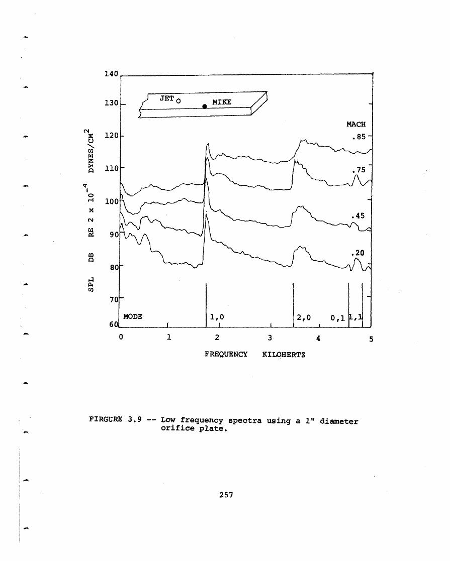
1
1
1
1
1
Un1:4En
0 1 2 3 4 5
FREQUENCY KILOHERTZ
FIRGURE 3.9 -- Low frequency spectra using a 1" diameterorifice plate.
257
C.)uzUrEWz>4
0Hq
r-To
x
cuN
_ __
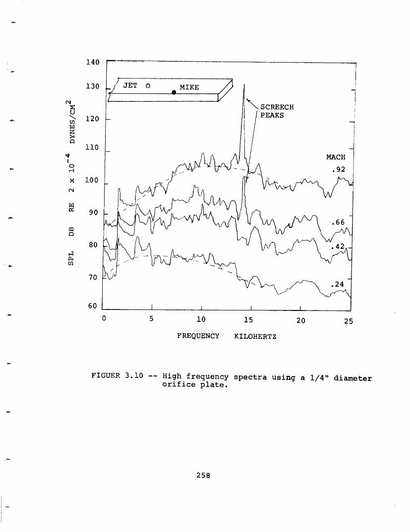
0 5 10 15 20 25
FREQUENCY KILOHERTZ
FIGUER 3.10 -- High frequency spectra using a 1/4" diameterorifice plate.
258
140
130
uzU
!za>-
0
xN~
120
110
100
90
80
70
60
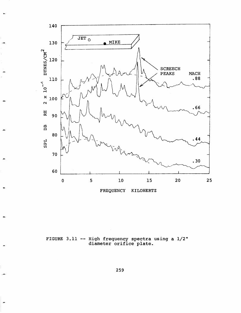
140
130
cU
za
or-l
xCN
120
110
100
M 90
80
70
60
0 5 10 15 20
FREQUENCY KILOHERTZ
FIGURE 3.11 -- High frequency spectra using a 1/2"diameter orifice plate.
259
25
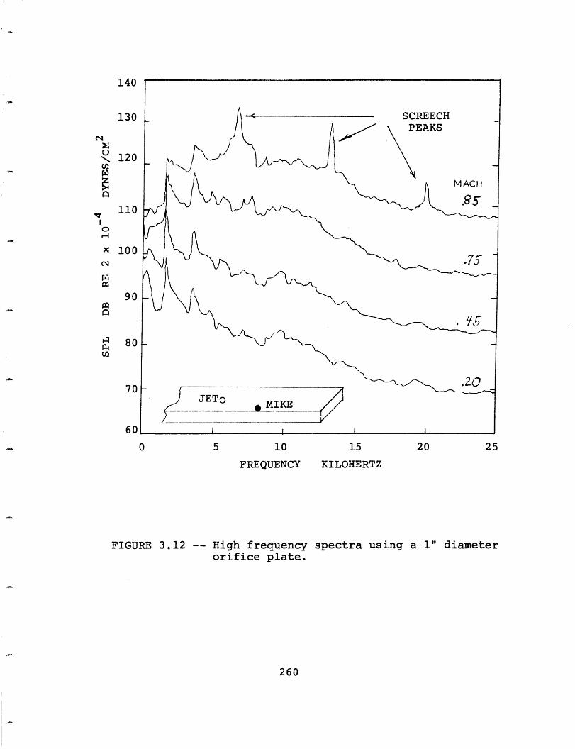
0 5 10 15 20 25
FREQUENCY KILOHERTZ
FIGURE 3.12 -- High frequency spectra using a 1" diameterorifice plate.
260
140
130
U
0v]
oX
C1
m
u)
120
110
100
90
80
70
60
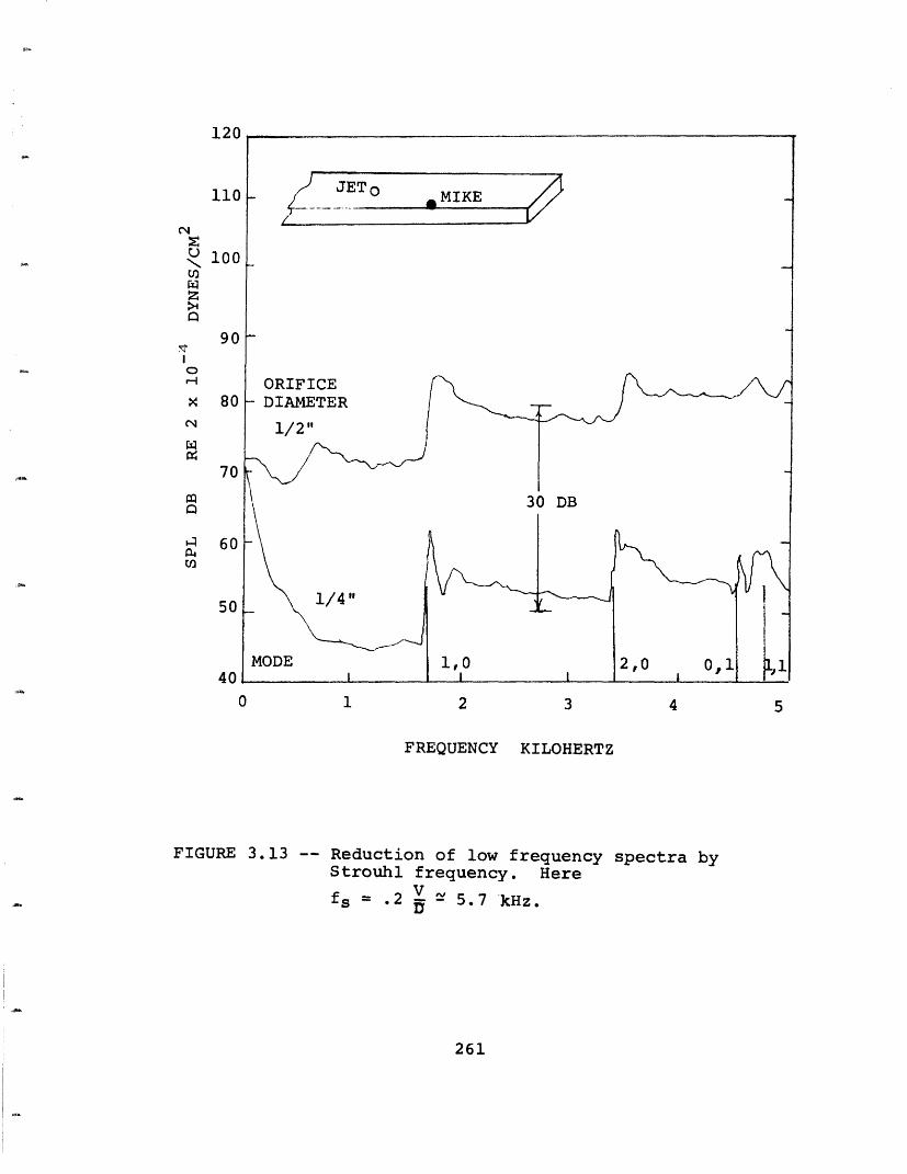
I n
110
CIu
za
>4
x
100
90
80
70
4 60
50
40
0 1 2 3 4
FREQUENCY KILOHERTZ
FIGURE 3.13 -- Reduction of low frequency spectra byStrouhl frequency. Here
fs = .2 V 5.7 kHz.·
261
5
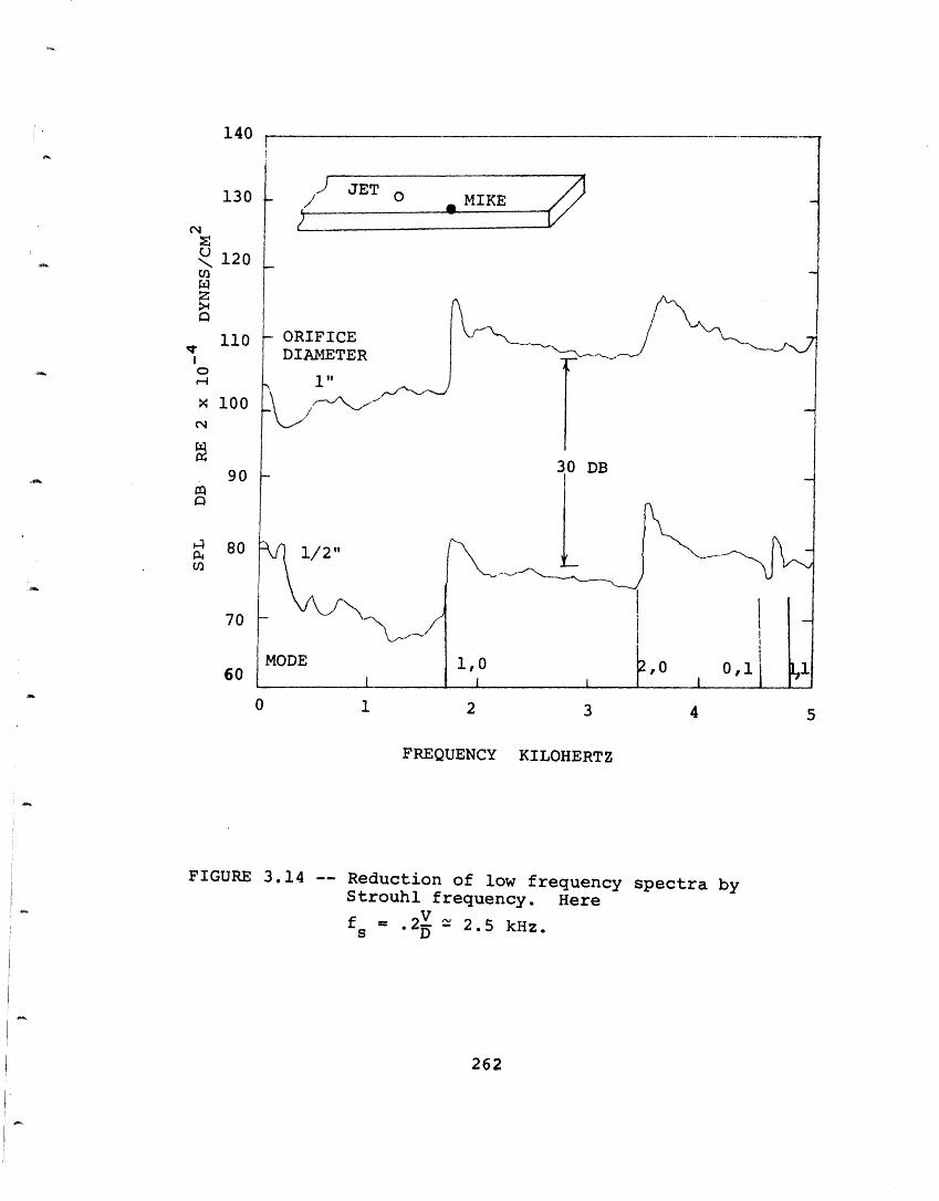
140
130
X 120
110Io
x 100N
90m
804 80U)
70
60
0 1 2 3 4
FREQUENCY KILOHERTZ
FIGURE 3.14 -- Reduction of low frequency spectra byStrouhl frequency. Here
f - .2 2.5 kHz.s
262
cI
5
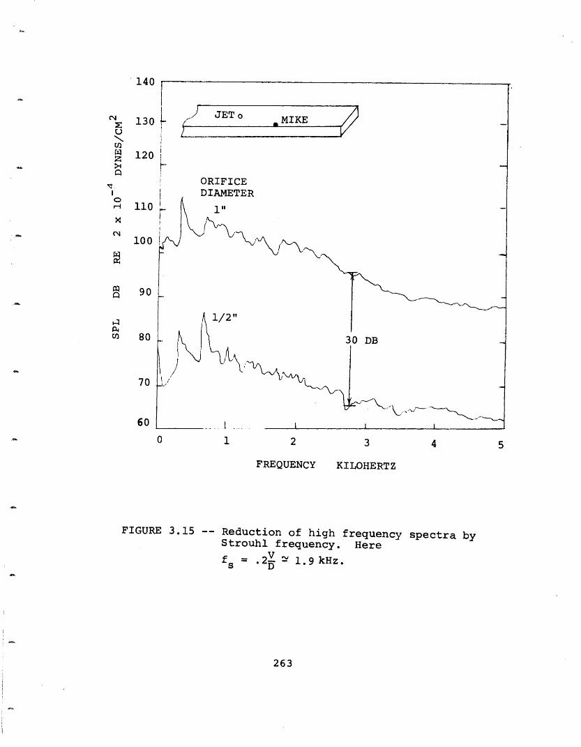
JET o , MIKE
ORIFICE
1"
1/2"
30 DB
0 1 2 3 4 5
FREQUENCY KILOHERTZ
FIGURE 3.15 -- Reduction of high frequency spectra byStrouhl frequency. Here
fs .2V 1.9 kHz.
263
140
C1
U
WZ
CH
x
CN
Q
130
120
110
100
90
80
70
60
__-~~ ~ ~ ~ ~ ~ ~~ _
i
---- I
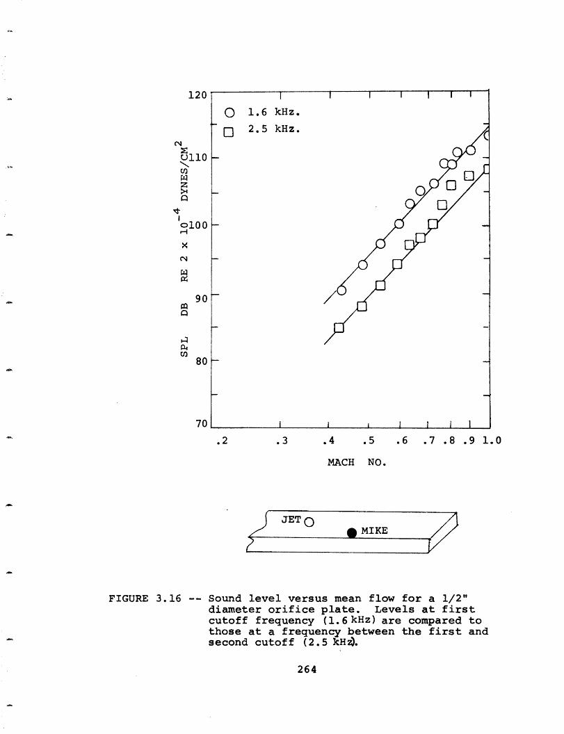
120
N
U110
z
Io100lO
N(
Q
P4m
90
80
70
.2 .3 .4 .5 .6 .7 .8 .9 1.0
MACH NO.
JET Ol MIKE
FIGURE 3.16 -- Sound level versus mean flow for a 1/2"diameter orifice plate. Levels at firstcutoff frequency (1.6 kHz) are compared tothose at a frequency between the first andsecond cutoff (2.5 kH.
264
---
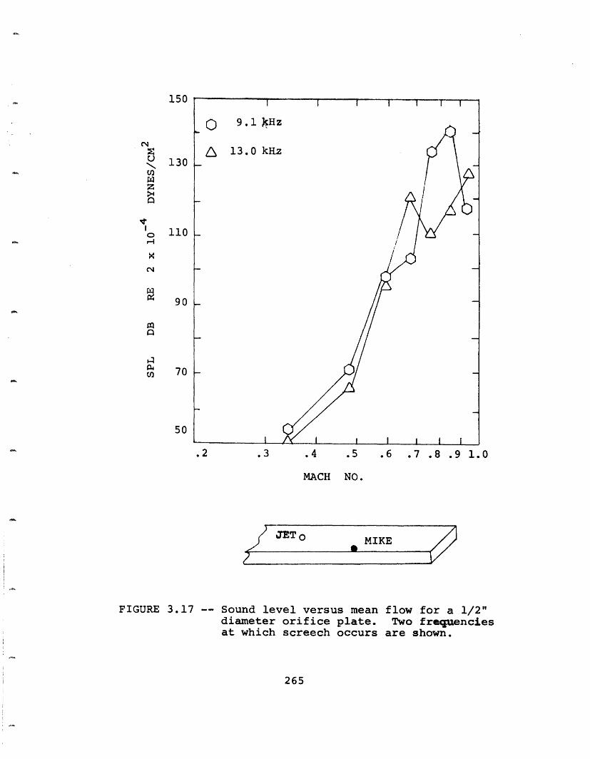
150
130
110
90
70
50
.2 .3 .4 .5 .6 .7 .8 .9 1.0
MACH NO.
JET O MIKE -2
FIGURE 3.17 -- Sound level versus mean flow for a 1/2"diameter orifice plate. Two frequenciesat which screech occurs are shown.
265
CzU
>4
oX
Al s
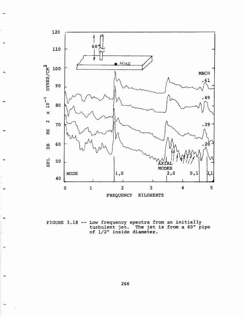
120
110
z 100UNN
z> 900
° 80
x
CN70
m 60
50
40
0 1 2 3 4
FREQUENCY KILOHERTZ
FIGURE 3.18 -- Low frequency spectra from an initiallyturbulent jet. The jet is from a 60" pipeof 1/2" inside diameter.
266
Cs
I
5
a
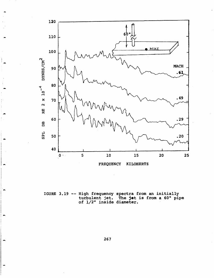
120
110
100
90
80
70
60
50
40
0 ' - 5 10 15 20
FREQUENCY KILOHERTZ
IGURE 3.19 -- High frequency spectra from an initiallyturbulent jet. The jet is from a 60" pipeof 1/2" inside diameter.
267
U
uz>4
,q.Io
-I
x
c4
,)r.D
25
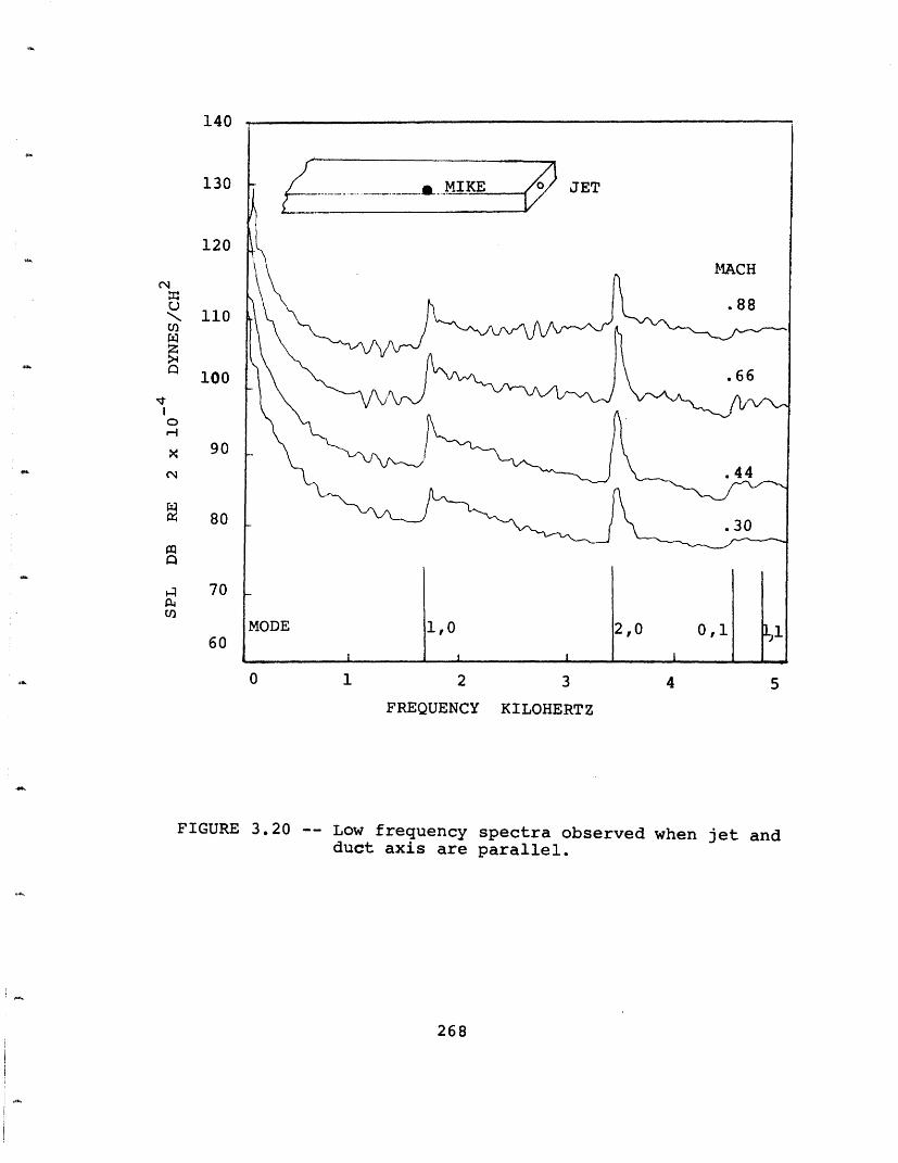
140
130
120
NW.U)
0
Hzl
>oQ11Ie
110
100
90
80
Q
70P4
60
0 1 2 3 4 5
FREQUENCY KILOHERTZ
FIGURE 3.20 -- Low frequency spectra observed when jet andduct axis are parallel.
268
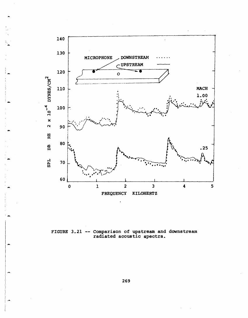
0 1 2 3 4 5
FREQUENCY
FIGURE 3.21 --
KILOHERTZ
Comparison of upstream and downstreamradiated acoustic spectra.
269
140
130
120cj
z
o
xN
110
100
90
80
70
60
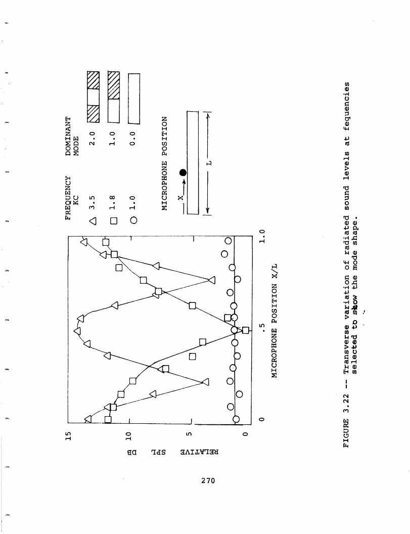
o o o04 .H 0
00 O
00
z0HEH0
z
o·0P;
U XH
I
0 LnH-4
Sa 8 lS aAIIIBa
H Wz 00
>4uzI-. u01
rX
I:
q I
oH;
U)
Q)
C44.4l
Uo0
rU)rl 0" (
~ TeU)
a
0
0
0 0U0
C1I(%4
rz4.~~~~~~a
Z0HHHEI
cn
.4
004
UHz
,t
LnH
oo
270
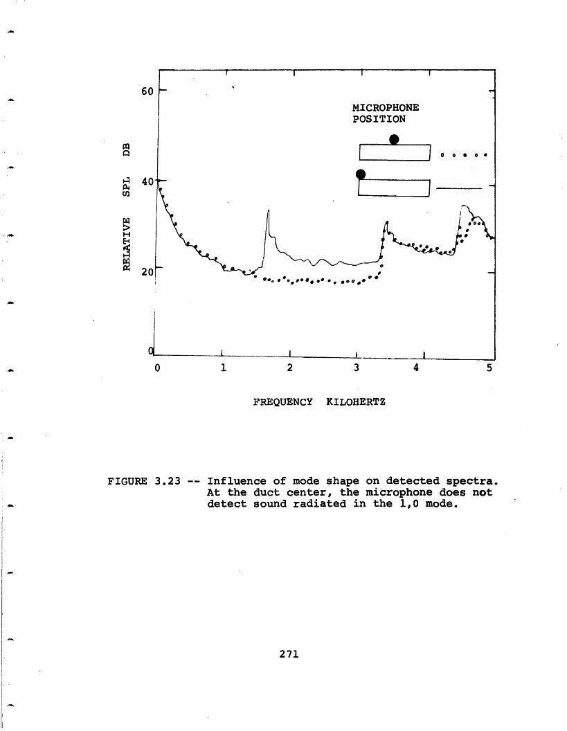
61
mpr
a 4U)
HH$cc0M
0 1 2 3 4 5
FREQUENCY KILOHERTZ
FIGURE 3.23 -- Influence of mode shape on detected spectra.At the duct center, the microphone does notdetect sound radiated in the 1,0 mode.
271
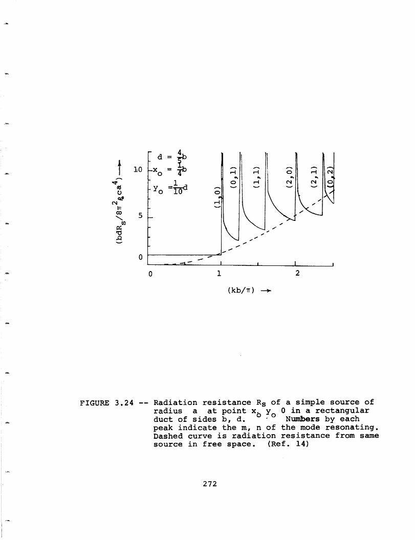
t
Cfcq
co
n
10
5
0
0 1 2
(kb/7) -o
FIGURE 3.24 -- Radiation resistance Rs of a simple source ofradius a at point x yo 0 in a rectangularduct of sides b, d. Numbers by eachpeak indicate the m, n of the mode resonating.Dashed curve is radiation resistance from samesource in free space. (Ref. 14)
272
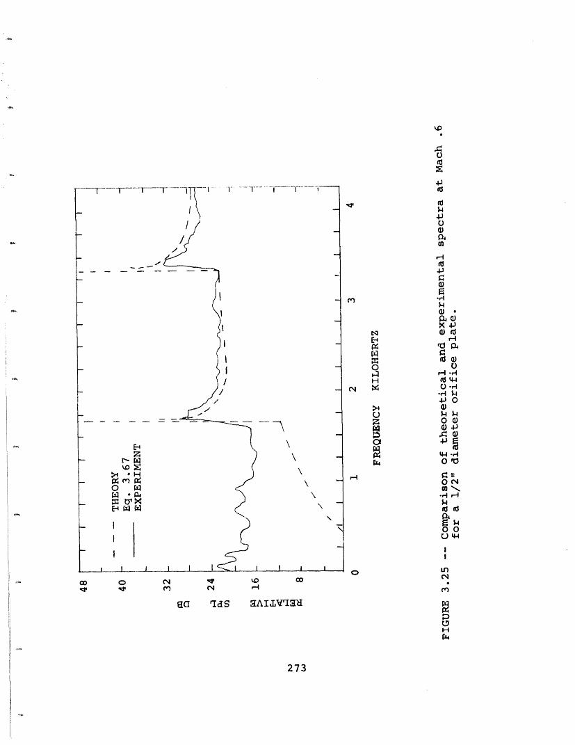
Co4
.sr UJ4~r
4J IC)
O 4a)E0 H(d 44
o 14
H r~4W
O
Z 0H
04j= 0o NN
W4
reQ4
_N
OD 0 (N -o c w -
er v n ~N H 10 IV m (14 r-i IH
9a 'dS aAIJIqRU0CDHrZ4
273
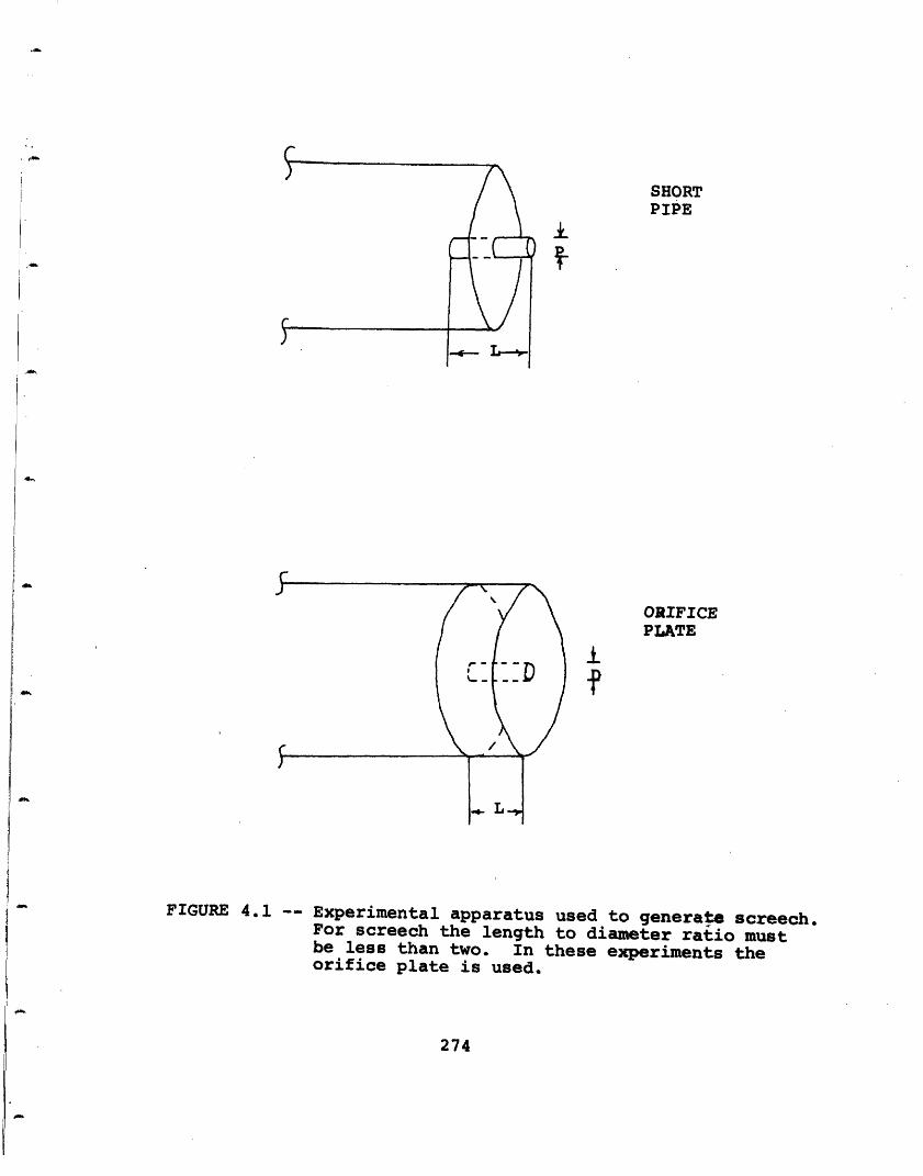
SHORTPIPE
i
ORIFICEPLATE
±
FIGURE 4.1 -- Experimental apparatus used to generate screech.For screech the length to diameter ratio mustbe less than two. In these experiments theorifice plate is used.
274
2
1
1
O4 1H:4
1UZDa1
I4
.1 .2 .3 .4 .5 .6 .7 .8 .9 1.0
MACH NO.
- - FEEDBACK MODEEq. 4.4AXIAL MODE
Al . 1/2" Eq. 4.6
1/4"
FIGURE 4.2 -- Screech frequency versus flow speed for a1/4" long orifice plate.
275
A
20
18E
1E
1d
11'
1(
OO
0
MACH NO.
V 1/2
_ _ FEEDBACK MODEEq. 4.4
AXIAL MODEEq. 4.5
1/2"
FIGURE 4.3 -- Screech frequency versus flow speed fora 1/2" long orifice plate.
276
N
oH
uz
o
I
_-
1
1
1
8
6
n. u . J . V
MACH NO.
V 1/2
FEEDBACK MODEEq. 4.4
AXIAL MODE2" Eq. 4.6
-- 1" --*
FIGURE 4.4 -- Screech frequency versus flow speed for a1" long orifice plate.
277
2
1
1
N
0H
>4Uz
r4rL
. L . . . J . - · J - ·
V
I 1/2
- L --
FIGURE 4.5 -- Summary of tests made to determine thelength to diameter ratio necessary forscreech.
278
SCREECHSCREECH NOT
LENGTH OBSERVED OBSERVED
1/8"
1/4" V
1/2" \
1" v
2" v/_~ ~ ~ ~ ~
�
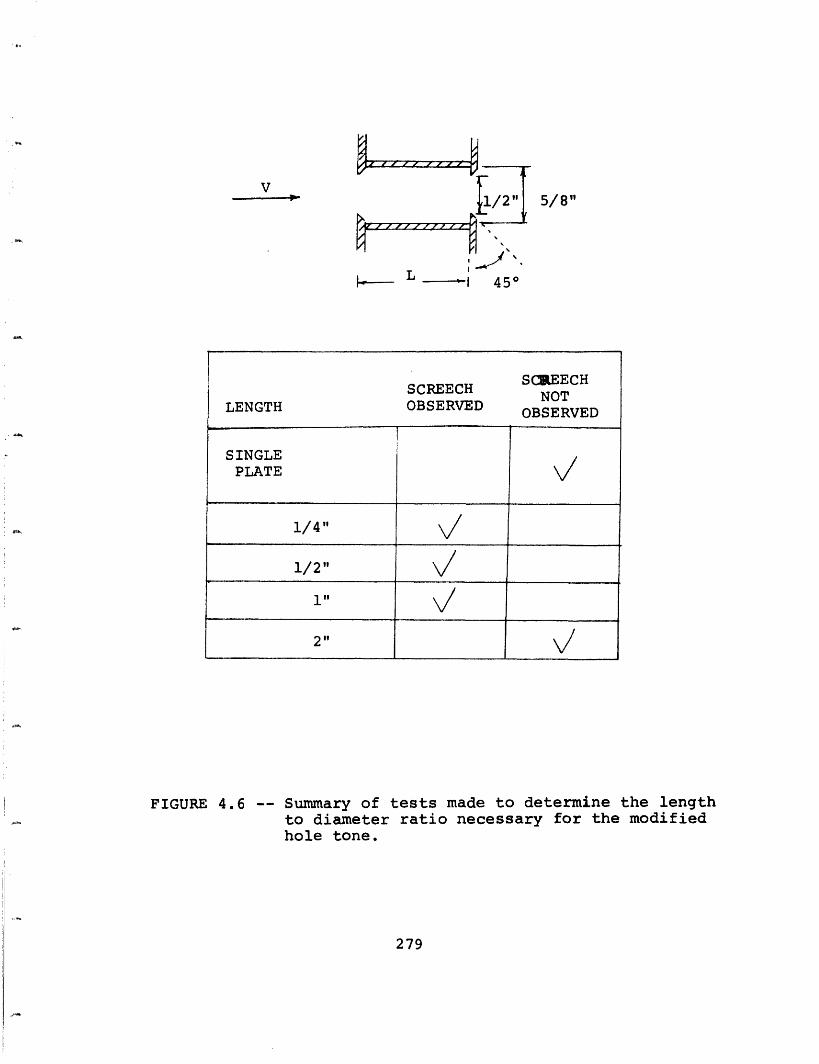
V5/8"
L 1450
~_ L- -_ 1 450
FIGURE 4.6 -- Summary of tests made to determine the lengthto diameter ratio necessary for the modifiedhole tone.
279
SCREECH SCREECHSCREECH NOT
LENGTH OBSERVED OBSERVED
SINGLEPLATE
1/4"
1/2" V
1"
2"
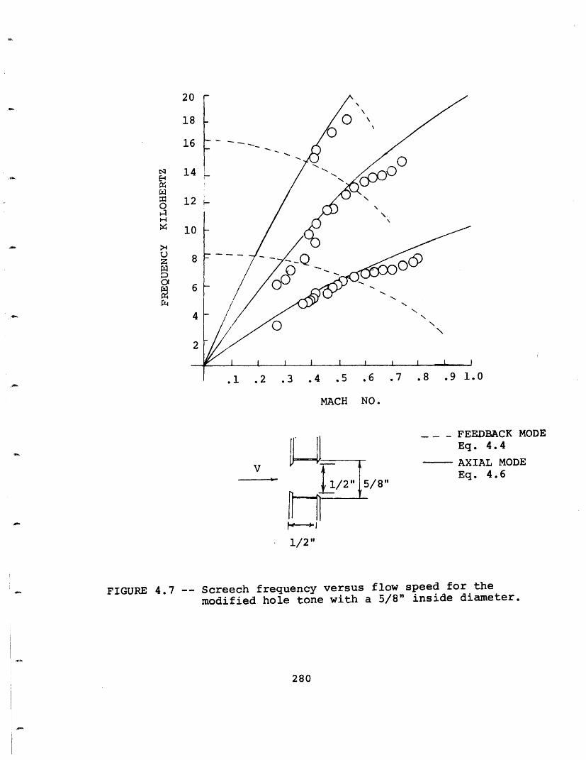
24
1
8
6
4
2
.0.· . . _ .
MACH NO.
V2I
-- FEEDBACK MODEEq. 4.4
AXIAL MODEEq. 4.6
1/2"
FIGURE 4.7 -- Screech frequency versus flow speed for themodified hole tone with a 5/8" inside diameter.
280
1
1
1
w
oH
1
>4U
W
r3
2A
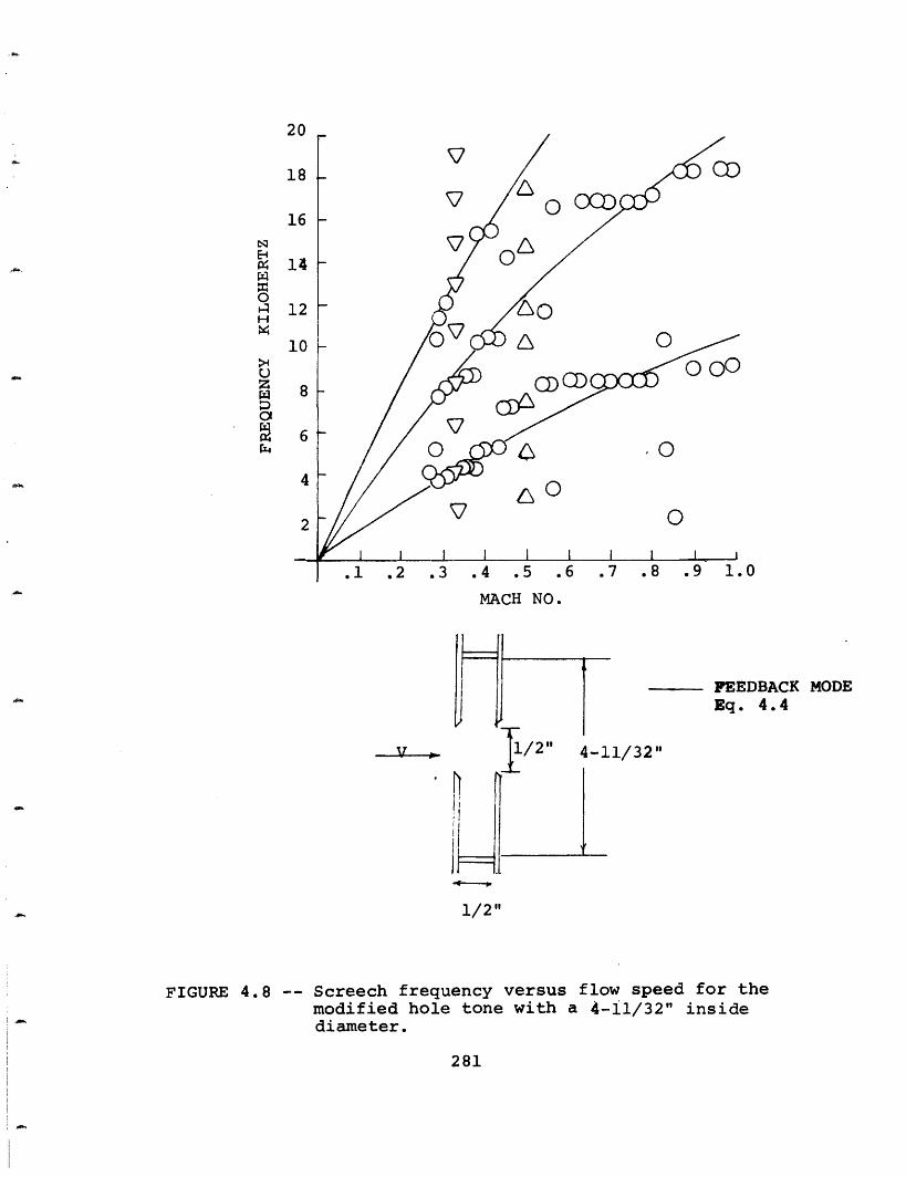
7
0
O
,0
0
.1 .2 .3 .0
MACH NO.
FEEDBACK MODEEq. 4.4
4-11/32"1/2"
I1'1
1/2"
FIGURE 4.8 -- Screech frequency versus flow speed for themodified hole tone with a 4-11/32" insidediameter.
281
1
1
1
1I
I
J
I
N
W
W0H
>4Uz
r14
- !
Il -
9n
)
)
4
2
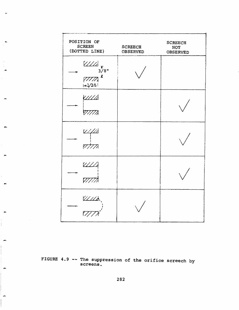
POSITION OF SCREECHSCREEN SCREECH NOT
(DOTTED LINE) OBSERVED OBSERVED
3/8"
P7717A
- I
r/
FIGURE 4.9 -- The suppression of the orifice screech byscreens.
282
aoH-
rD
co
C)0 loH
-d
>44
IL)- 0rz D O
0~a~ )
U
.-I4-HU
.1-r4
0
q-I
:H
H
283
NHl
/ /I/lilt
In or I
r
NIN
SC dS RI~H
C\Jm
(Y)1H-
-4 C~~~~~~
C)
4.
04.
U)u0
NE-4t
O
H O
U)U 4J
4 .J01~C)ul
U
a)E)U)
t
H
scia 'las AIN'IlI
284
I
0Lf
I
r,
r-4LO
H-
.-
C)
OZ
oJ
oo 0 (3
0rdOI
_I-I 0H q
ra
oN ~0 - q O I U
HH 0 OO
O1 0 4-.I. -.
0) 4-) 0)
-Ho O
la ridS aAI IrIH
285
CNH
CNN.
I
LOL~
0 O(Y
Or-
___ _· I -
I
1---
I J I I I I I I
WAGNER'S NOZZLE
1/2" ORIFICE PLACE
ICo4"
MICROPHONE 4 1
LONG PIPE
&%
FIGURE 4.13 -- Experimental apparatus used to generate
impingement screech.
286
fl
11
ld·
-. 9I5JZ7~
v
--- -
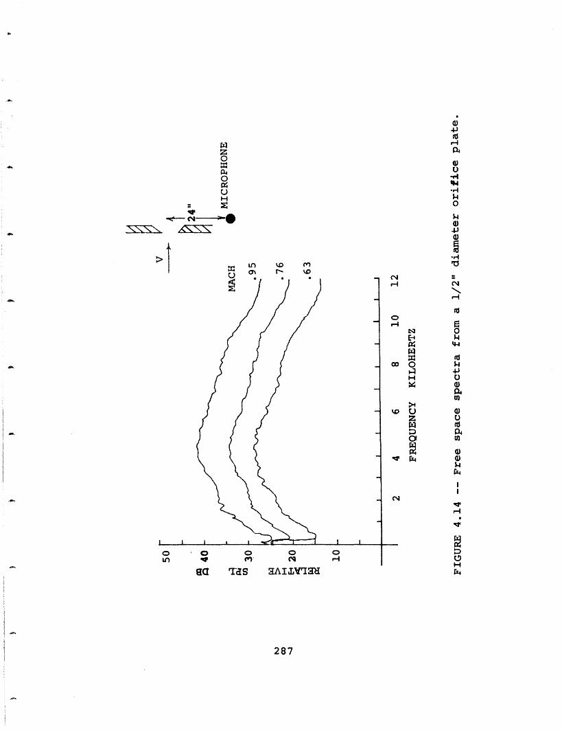
4-,to
,) k0
z 44= L ; O
,., ( !"
gSa TS aAI1 LVrIad
W toN 00 I.
4JH UW4; a)
a04
U Uz u
w rd
Is-I
H
I-4
287
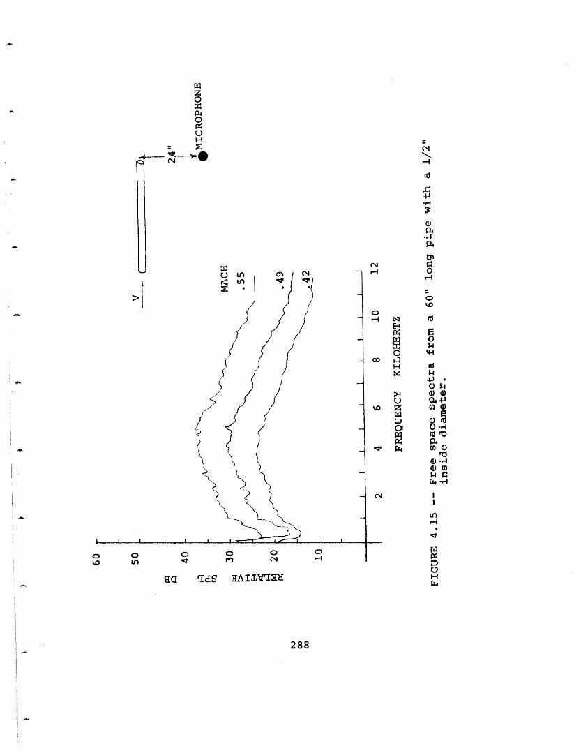
N4-I
r-IP.,,P4
NnCN 9~~E
0
O M
H (: wk
-IV k
-I
_.
iH
Hr4
288
P4
H
LnLn
¢ OCN
oCH
{
%w U _,
sa UdS aAIIdqHE
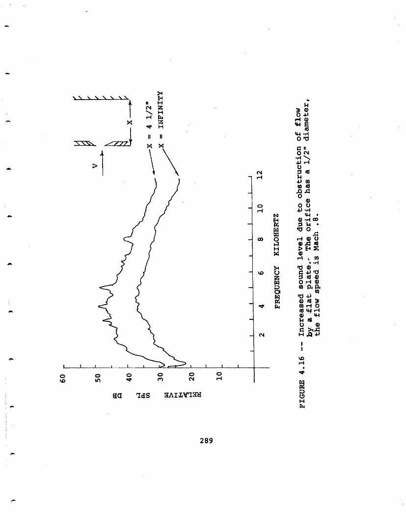
\\ & N \
4.X•ZZ
>1~
CI'
E>- H-
H.- I
H
II II11 11
O 0C ,
34)44 gr
O
- ,-O N.4 rU
C14 : g
0 0N HI
mo
O
0 *-zl OHC
0 ,-. w o
e U)
0 .i (m oa
rI rQ) u43 QL= ir
ii.
3I4
289
I I I
0MD
j ! i
sa uds HAIJ;LIqaUI
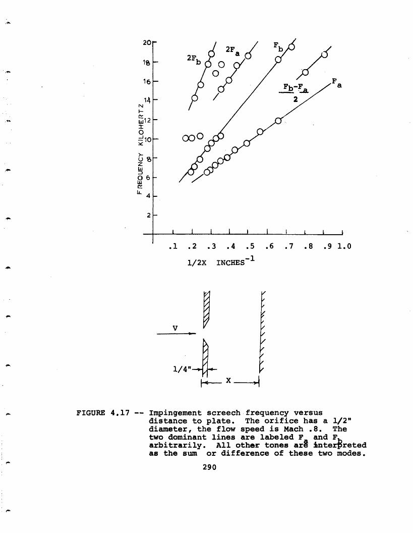
20
16
14NF-
w1 2IO
10
Z.t D06
4
2
t~FIGURE 4.17 -- I
ta
a: e~~~~~~~
Fa
1.0
1/2"TheF4retedmodes.
I I l I I I I L I
.1 .2 .3 .4 .5 .6 .7 .8 .9 1.0
1/2X INCHES 1
V
1/4" ·
mpingement screech frequency versusdistance to plate. The orifice has a 1/2"diameter, the flow speed is Mach .8. Thewo dominant lines are labeled F and Farbitrarily. All other tones ara nterretedas the sum or difference of these two modes.
290
I
. 1
V
1,
mpingiis tan,i ametiwo dorbitr,s the
.I
V
1,
.f FIGURE 4.17 -- Impingidistantdiametitwo doarbitr,as the
C:LL4
1.~~~~~~~~~~2
.f FIGURE 4.17 -- IIddtaa
.1 . .3 .4 .5 . .7 B8 .9 10
1/2X INCHES-
V
r ~~FIGURE 4.17 -- Impingement screech frequency versusdistance to plate. The orifice has a 1/211diameter, the flow speed is Mach .8. Thetwo dominant lines are labeled F and Farbitrarily. All other tones ara nte retedas the sum or difference of these two modes.
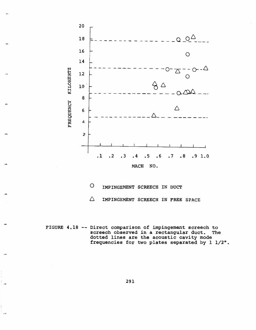
- _ __ _ Q OL
O
I - -- O E--- a a0
_ A
- - -IN
I I I I I I II _ I .I . I I I
.1 .2 .3 .4 .5 .6 .7 .8 .9 1.0
MACH NO.
IMPINGEMENT SCREECH IN DUCT
L IMPINGEMENT SCREECH IN FREE SPACE
FIGURE 4.18 -- Direct comparison of impingement screech toscreech observed in a rectangular duct. Thedotted lines are the acoustic cavity modefrequencies for two plates separated by 1 1/2".
291
20
18
16
14
N
w
0H
>4
Z'
12
10
8
6
4
2
0
t
BIOGRAPHICAL NOTE
George Succi was born in Stamford, Connecticut,
on May 8, 1951. He attended St. Mary's Grammar School and
Stamford Catholic High School in the same town.
From September, 1969, his studies were continued
at the Massachusetts Institute of Technology in the
Department of Physics, leading to a S.B. Degree in June,
1973. He attended M.I.T. under a grant from the Engineer-
ing Education Foundation. He was employed as a mathema-
tician at Data Control Systems, in 1969, and as a research
assistant at Trans-Sonics, in 1972. After finishing his
undergraduate studies he headed for the mountains and
eventually hiked 900 miles in the Southern Appalachian
Wilderness.
In September, 1973, he returned to M.I.T. for
his doctoral program in the Department of Physics under
the direction of Dr. Uno Ingard. During this time he
was employed as an acoustic consultant for Sonotech, in
1974, and in the aero-acoustics group at NASA Lewis
Research Center, in 1976.
292