Embed Size (px)
Citation preview

ORIGINAL RESEARCH ARTICLEpublished: 10 October 2012
doi: 10.3389/fneur.2012.00138
Characterization of interictal epileptiform discharges withtime-resolved cortical current maps using theHelmholtz–Hodge decompositionJeremy D. Slater 1*, Sheraz Khan2, Zhimin Li 3 and Eduardo Castillo4
1 Department of Neurology, University of Texas Health Science Center at Houston, Houston, TX, USA2 Department of Neurology, Massachusetts General Hospital, University of Texas Health Science Center at Houston, Houston, TX, USA3 Department of Pediatrics, University of Texas Health Science Center at Houston, Houston, TX, USA4 Pediatric Epilepsy Program, Florida Hospital in Orlando, Orlando, FL, USA
Edited by:Fernando Cendes, University ofCampinas, Brazil
Reviewed by:Luiz Eduardo Betting, University ofCampinas, BrazilMarino M. Bianchin, UniversidadeFederal do Rio Grande do Sul, Brazil
*Correspondence:Jeremy D. Slater , Department ofNeurology, University of Texas HealthScience Center at Houston, 6431Fannin Street, MSB 7.100, Houston,TX 77030, USA.e-mail: [email protected]
Source estimates performed using a single equivalent current dipole (ECD) model for inter-ictal epileptiform discharges (IEDs) which appear unifocal have proven highly accurate inneocortical epilepsies, falling within millimeters of that demonstrated by electrocorticogra-phy. Despite this success, the single ECD solution is limited, best describing sources whichare temporally stable. Adapted from the field of optics, optical flow analysis of distributedsource models of MEG or EEG data has been proposed as a means to estimate the currentmotion field of cortical activity, or “cortical flow.”The motion field so defined can be used toidentify dynamic features of interest such as patterns of directional flow, current sources,and sinks.The Helmholtz–Hodge Decomposition (HHD) is a technique frequently applied influid dynamics to separate a flow pattern into three components: (1) a non-rotational scalarpotential U describing sinks and sources, (2) a non-diverging scalar potential A accountingfor vortices, and (3) an harmonic vector field H. As IEDs seem likely to represent periodsof highly correlated directional flow of cortical currents, the U component of the HHDsuggests itself as a way to characterize spikes in terms of current sources and sinks. In aseries of patients with refractory epilepsy who were studied with magnetoencephalogra-phy as part of their evaluation for possible resective surgery, spike localization with ECDwas compared to HHD applied to an optical flow analysis of the same spike. Reasonableanatomic correlation between the two techniques was seen in the majority of patients,suggesting that this method may offer an additional means of characterization of epilepticdischarges.
Keywords: epilepsy, epileptic spike localization, magnetoencephalography, optical flow, dipole modeling
INTRODUCTIONSource localization of interictal epileptiform discharges (IEDs)recorded with electroencephalography has traditionally been per-formed via visual analysis. As Rose and Ebersole have written,visual analysis relies on three assumptions: (1) the electrode(s)demonstrating the highest amplitude abnormal potential directlyoverlie the generator, (2) a cortical generator always produces afocal potential, and (3) a widespread potential indicates a dif-fuse source or multiple sources (Rose and Ebersole, 2009). Allthree assumptions are frequently incorrect. To go beyond visualanalysis, a variety of mathematical techniques of source localiza-tion have been proposed and utilized including equivalent currentdipoles (ECD; Henderson et al., 1975), minimum norm estimates(MNE; Hauk, 2004; Silva et al., 2004), standardized low-resolutionbrain electromagnetic tomography (sLORETA; Pascual-Marqui,2002),and dynamic statistical parametric mapping (dSPM; Tanakaet al., 2009). Each of these techniques have advantages and dis-advantages, but particularly in combination with higher densityEEG arrays and magnetoencephalography, the single ECD modelhas proven value in helping to identify the ictal onset zone in
neocortical epilepsies (Huiskamp et al., 2010; Shiraishi, 2011). Asan example, source estimates performed using a single ECD modelfor IEDs which appear predominantly unifocal in their gener-ation such estimates have proven to be highly accurate, fallingwithin millimeters of those demonstrated by electrocorticogra-phy (Ishibashi et al., 2002). Despite this success, the single ECDsolution is limited, best describing non-moving sources. Sourcesthat move over time have been described by moving dipoles ormultiple dipole models (Ochi et al., 2000), or iterative applicationof the ECD model (Papanicolaou et al., 2006), but mathematicalsolutions that incorporate more details of the complexity of thegenerating cortical tissue have multiple solutions, become com-putationally intractable, or both (Yetik et al., 2005). Alternativemethods for IED source localization such as minimum norm esti-mation have been proposed, and may be theoretically better thanECD given the potential complexity of the generators involved, butthe vast majority of clinical validation has been performed withthe ECD model (Wheless et al., 1999; Pataraia et al., 2004). Giventhe fairly large area of cortex involved in spike generation (at leastthose identified on scalp EEG which serve as the basis for MEG
www.frontiersin.org October 2012 | Volume 3 | Article 138 | 1

Slater et al. Characterizing IEDS with HHD
FIGURE 1 | Original spike at time 122.8732 s.
FIGURE 2 | Same spike as Figure 1 after 30 Hz low-pass filtering.
Frontiers in Neurology | Epilepsy October 2012 | Volume 3 | Article 138 | 2

Slater et al. Characterizing IEDS with HHD
FIGURE 3 | MEG dipole map of spike from Figure 1.
ECD localization), the limitation of the ECD method in reducingcortical sources to dimensionless points renders it less than ideal.While appropriate pre-processing of the signal data and adjust-ments to the head model can produce significant improvementsin source localization results, all of these methods generally eval-uate a single point in time, so that a spike, for example, is reducedto the moment of peak negativity (unless you use the ECD itera-tively). An analysis method that evaluates signal change over timemight contribute useful information to the existing models.
In the field of optics, the goal of optical flow estimation is tocompute an approximation to the motion field from time-varyingimage intensity (Fleet and Weiss, 2005). Optical flow analysis ofdistributed source models of MEG or EEG data has recently beenproposed as a means to estimate the current motion field of cor-tical activity, or “cortical flow.” This technique can be used toestimate local kinetic energy of cortical surface currents, and hasbeen used to characterize correspondence between the speed anddirection of the surface current flow within the visual cortex andthe dynamical properties of the visual stimulus itself (Lefevre andBaillet, 2008, 2009). The motion field so defined can be used toidentify dynamic features of interest such as patterns of directionalflow, current sources, and sinks.
The Helmholtz–Hodge Decomposition (HHD) is a techniquefrequently applied in fluid dynamics to separate a flow patterninto three components: (1) a non-rotational scalar potential U
describing sinks and sources, (2) a non-diverging scalar poten-tial A accounting for vortices, and (3) an harmonic vector field H(Chorin and Marsden, 1993; Tong et al., 2003). A recently pub-lished abstract demonstrated the use of the HHD for mappingand characterizing current flow over primary somatosensory cor-tex during sensory-stimulation triggered evoked potentials (Khanet al., 2009). As IEDs seem likely to represent periods of highlycorrelated directional flow of cortical currents, the HHD U poten-tial lends itself to the characterization of spikes in terms of currentsources and sinks. The methodology is reviewed in greater detailin the addendum.
In this study, its relative efficacy compared to that of the stan-dard ECD model, was assessed with a series of six candidates forepilepsy surgery.
MATERIALS AND METHODSMEG RECORDINGAll patients underwent an MEG recording sessions. MEG record-ings were performed pre-operatively for localization of the sourcesof interictal epileptiform activity. Spontaneous MEG was recordedwith a whole-head neuromagnetometer containing 248 first-orderaxial gradiometer channels (Magnes WH3600, 4-D Neuroimaging,San Diego, CA, USA) in a magnetically shielded room. Simultane-ous EEG was recorded, with gold disk electrodes, using a bipolarmontage (Neurofax, Nihon-Kohden, Tokyo, Japan) from 21 scalp
www.frontiersin.org October 2012 | Volume 3 | Article 138 | 3

Slater et al. Characterizing IEDS with HHD
FIGURE 4 | Magnetic resonance imaging plot of ECD of spike from Figure 1.
locations, placed according to the International 10–20 system. TheMEG recordings were digitized at a sampling rate of 508.63 Hz.The online bandpass filter was set between 1 and 200 Hz.
As part of the analysis of the MEG-recorded interictal parox-ysmal activity, we calculated the ECD location, orientation, andmoment for each event. Concurrently recorded EEG was used toidentify interictal epileptiform event sand to rule out artifacts,such as those produced by body or eye movements, cardiac, andsleep-related activity. We used single epileptiform events for sourcelocalization in order to avoid introducing artificial time delays byaveraging variable spike populations. Calculation of the location,orientation, and strength of the dipolar sources that best fitted themeasured magnetic fields was performed using the single, mov-ing, ECD model that is part of the 4-D Neuroimaging software.The algorithm was applied to magnetic flux distributions thatshowed clear and stable dipolar morphology. For each calcula-tion, magnetic flux data from 37 magnetometer sensors were used,encompassing both extrema of the dipolar surface distribution.For each epileptiform event source solutions were examined every2 ms during a 200-ms window (100 ms before and 100 ms after thepeak of the interictal spike complex). The goal of this method wasto find the best combination of ECD location, strength, and ori-entation parameters. A dipole solution was considered acceptable
FIGURE 5 | Plot of the dynamic energy (DE) and global field power(GFP) over the time course of the spike from Figure 1. Arrows mark theDE maxima before and after the spike peak (which in this instancecorresponds to the GFP maximum).
Frontiers in Neurology | Epilepsy October 2012 | Volume 3 | Article 138 | 4

Slater et al. Characterizing IEDS with HHD
FIGURE 6 | Helmholtz–Hodge decomposition source field plot of the spike from Figure 1 (at time = 122.8653 s). The color bar corresponds to thenormalized amplitude of the component of current flow perpendicular to the cortical manifold, positive if directed inward (red= sink), negative if outward(blue= source).
FIGURE 7 | Helmholtz–Hodge decomposition sink field plot of the spike from Figure 1 (at time = 122.8929 s). The color bar corresponds to the normalizedamplitude of the component of current flow perpendicular to the cortical manifold, positive if directed inward (red= sink), negative if outward (blue= source).
www.frontiersin.org October 2012 | Volume 3 | Article 138 | 5
Slater et al. Characterizing IEDS with HHD
if it was associated with a correlation coefficient of 0.95 or greater,global field power (GFP; or root mean square of the magnetic fluxin the set of 37 magnetometer sensors entered in the analysis) of400 ft or greater, and an ECD product moment of 400 nAm or less.
The methodology is the same as that used in a prior report fromour group (Pataraia et al., 2004).
For the purpose of identifying the location of the estimatedsources in the brain, an magnetic resonance imaging (MRI) scan
FIGURE 8 | Continued
Frontiers in Neurology | Epilepsy October 2012 | Volume 3 | Article 138 | 6

Slater et al. Characterizing IEDS with HHD
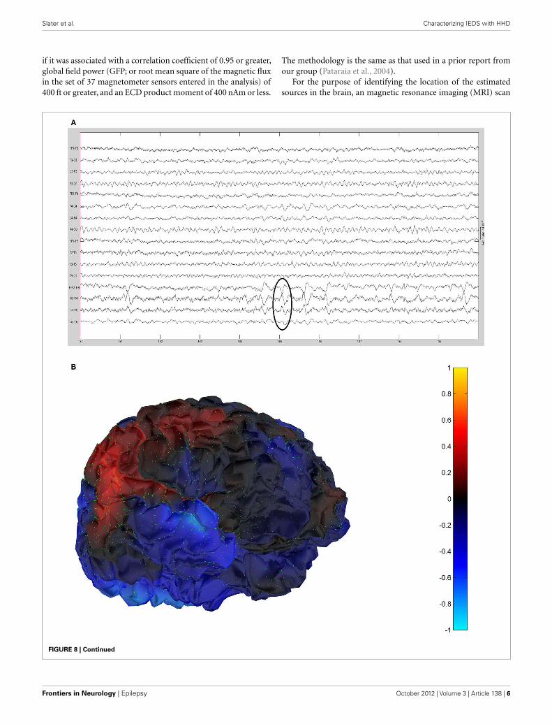
FIGURE 8 | (A) Sample sharp wave from patient 2243 (highlighted withblack oval). (B) HHD source field plot of the spike from patient 2243. (C)HHD sink field plot of the spike from patient 2243. (D) Plot of the dynamic
energy (DE) and global field power (GFP) over the time course of the spikefrom patient 2243. Arrows mark the DE maxima before and after the spikepeak.
www.frontiersin.org October 2012 | Volume 3 | Article 138 | 7

Slater et al. Characterizing IEDS with HHD
was performed. Before scanning, three skin markers were placedat fiducial points on the patient’s head (the nasion, the left, andthe right external meati). The location of the same fiducial pointswas also recorded, at the beginning of the MEG recording session,relative to the MEG sensor, thus establishing a common spatialreference for the transposition of 3-D coordinates between MEGand MRI data, as previously described.
CORTICAL SURFACE RECONSTRUCTIONCortical surface segmentation and tessellation from T1-weightedaxial MRI scans (1 mm× 1 mm× 1 mm3 voxel size) was obtainedusing BrainSuite software (Shattuck and Leahy, 2002)1. Data
1http://www.loni.ucla.edu/Software/BrainSuite
FIGURE 9 | Continued
Frontiers in Neurology | Epilepsy October 2012 | Volume 3 | Article 138 | 8
Slater et al. Characterizing IEDS with HHD
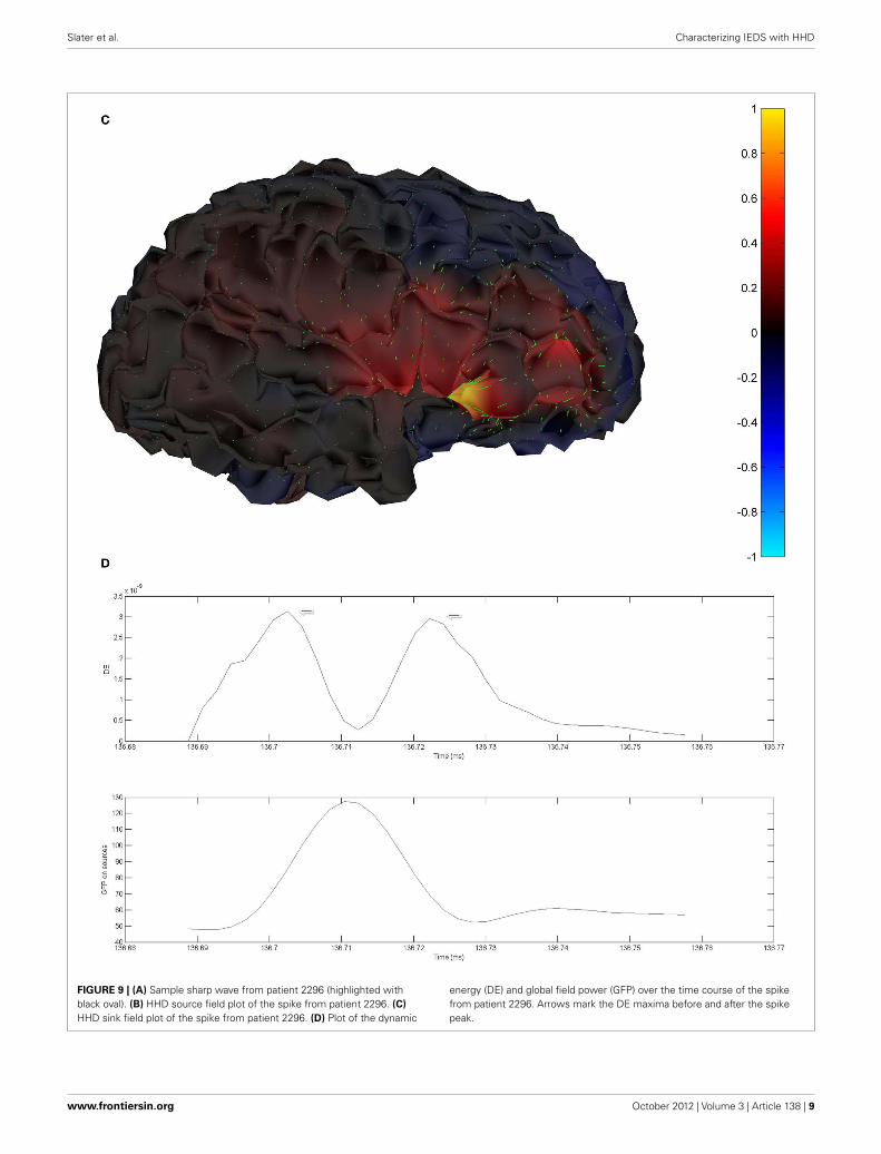
FIGURE 9 | (A) Sample sharp wave from patient 2296 (highlighted withblack oval). (B) HHD source field plot of the spike from patient 2296. (C)HHD sink field plot of the spike from patient 2296. (D) Plot of the dynamic
energy (DE) and global field power (GFP) over the time course of the spikefrom patient 2296. Arrows mark the DE maxima before and after the spikepeak.
www.frontiersin.org October 2012 | Volume 3 | Article 138 | 9

Slater et al. Characterizing IEDS with HHD
analysis was performed with Brainstorm (Tadel et al., 2011), whichis documented and freely available for download online under theGNU general public license2.
Three-dimensional reconstruction of the head and cortical sur-face was carried out for each patient individually. For forward
2http://neuroimage.usc.edu/brainstorm
modeling of MEG signals, an overlapping spheres head model wascomputed using the method of Huang et al. (1999). The com-puted head and cortex models were used in combination withthe MEG fields to compute an estimate of current-source densitydistribution over the cortex based on a Tikhonov-regularized min-imum norm estimate (Baillet et al., 2001). The default value forthe Tikhonov parameter is λ= 10% of maximum singular valueof the lead field.
FIGURE 10 | Continued
Frontiers in Neurology | Epilepsy October 2012 | Volume 3 | Article 138 | 10

Slater et al. Characterizing IEDS with HHD
FIGURE 10 | (A) Sample sharp wave from patient 2334 (highlighted withblack oval). (B) HHD source field plot of the spike from patient 2334. (C)HHD sink field plot of the spike from patient 2334. (D) Plot of the dynamic
energy (DE) and global field power (GFP) over the time course of the spikefrom patient 2334. Arrows mark the DE maxima before and after the spikepeak.
OPTICAL FLOW AND HHDOptical flow and HHD data analysis were also performed withBrainstorm (Tadel et al., 2011). Pre-processing of the MEG dataconsisted of applying a low-pass filter of 30 Hz to minimizedistortions produced by higher frequency jitter. The computedhead and cortex models were used in combination with the MEG
fields to compute an estimate of the current-source density dis-tribution over the cortex based on a minimum norm estimate.Optical flow velocity fields were computed from the cortical cur-rent distribution estimated over the individual cortical surface ofeach subject. For each spike identified, the MEG recording for atime period covering spike onset, peak, and offset (as identified on
www.frontiersin.org October 2012 | Volume 3 | Article 138 | 11

Slater et al. Characterizing IEDS with HHD
the corresponding scalp EEG) was subjected to optical flow analy-sis, and subsequent HHD. The GFP was compared to the globaldynamic energy (DE) measurement.
DE (t ) =
∫M
‖v‖2dµ
DE= displacement energyV= vector fieldM = surface manifold (in this case, the cortex)
The peak DE occurring prior to the peak GFP during a spikeidentified the time of the source. The peak DE occurring after thepeak GFP during the same spike identified the sink. The HHD Upotential was then calculated for the source time point and sinktime point and plotted over the cortical manifold.
As this method results in a broad area of simulated current flow,rather than a focal point, localization was based on the locationof the visible maximum in terms of lateralization and lobe. Thislocalization was then classified as either concordant or discordantwith the dipole calculated for the same spike.
FIGURE 11 | Continued
Frontiers in Neurology | Epilepsy October 2012 | Volume 3 | Article 138 | 12

Slater et al. Characterizing IEDS with HHD
FIGURE 11 | (A) Sample sharp wave from patient 2353 (highlighted withblack oval). (B) HHD source field plot of the spike from patient 2353. (C)HHD sink field plot of the spike from patient 2353. (D) Plot of the dynamic
energy (DE) and global field power (GFP) over the time course of the spikefrom patient 2353. Arrows mark the DE maxima before and after the spikepeak.
RESULTSThe sequential results for the first patient (2092) are presented indetail. The original spike prior to filtering is shown in Figure 1.The same spike after 30 Hz low-pass filtering is illustrated inFigure 2. The same discharge in the context of alpha back-ground rhythm demonstrating a right temporal preponderance
on MEG is shown in Figure 3. The MEG demonstrated onlya weak dipolar map over right temporal area. The plot of thecalculated ECD on the patient’s MRI, revealing a right mesialtemporal localization, is shown in Figure 4. The DE map,with the source and sink time points marked, is shown inFigure 5.
www.frontiersin.org October 2012 | Volume 3 | Article 138 | 13

Slater et al. Characterizing IEDS with HHD
Cortical surface localization of spike source and sink are shownon Figures 6 and 7 respectively, where blue shading of the cor-tical manifold indicates the outward current flow or source, andred shading indicates the inward current flow or sink. For thosefigures, the arrow size in each region gives an approximation ofrelative current magnitude.
The remaining five patients are summarized in Figures 8–12.The first Figure in each set (a) shows the original spike or
sharp wave as identified on scalp EEG. For each patient,the best example of a given spike population has been cho-sen for presentation. The second figure (b) is the HHDsource map. The third figure (c) is the HHD sink map.The fourth figure (d) is the combined plot of the DEand GFP.
Table 1 lists the six patients whose interictal activity was ana-lyzed, including: the dipole localization using ECD of most of IEDs
FIGURE 12 | Continued
Frontiers in Neurology | Epilepsy October 2012 | Volume 3 | Article 138 | 14

Slater et al. Characterizing IEDS with HHD
FIGURE 12 | (A) Sample sharp wave from patient 2406 (highlighted withblack oval). (B) HHD source field plot of the spike from patient 2406. (C)HHD sink field plot of the spike from patient 2406. (D) Plot of the dynamic
energy (DE) and global field power (GFP) over the time course of the spikefrom patient 2406. Arrows mark the DE maxima before and after the spikepeak.
recorded during the session, whether or not the HHD topographicplot was concordant with the ECD localization and the pathologicdiagnosis if known. For five out of six subjects, the HHD projec-tion was concordant with the ECD localization. With the sixth,
the ECD localization was in the left perisylvian region, concordantwith the pathology visible on MRI, but the HHD sink and source,while broad and low amplitude, were maximal over the lateralfrontal lobe.
www.frontiersin.org October 2012 | Volume 3 | Article 138 | 15

Slater et al. Characterizing IEDS with HHD
Table 1 | MEG dipole localization, concordance and diagnosis.
ID MEG dipole localization HHD/optical flow analysis concordant
with dipole analysis
Diagnosis (if known)
2092 Right temporal Yes Right mesial temporal sclerosis (surgical pathology)
2243 Right mesial temporal Yes Right mesial temporal sclerosis (surgical pathology)
2296 Right frontal Yes Right mesial temporal sclerosis (by MRI, no pathology available)
2234 Right temporal Yes Right mesial temporal sclerosis (surgical pathology)
2353 Right parietal Yes Right parietal low grade glioma (surgical pathology)
2406 Left temporal (perisylvian) No (left lateral frontal) Abnormal signal and architectural abnormality in the tail of the
left hippocampus on MRI
DISCUSSIONFor most cases, spikes and sharp waves recorded with simulta-neous EEG/MEG, the source and sink areas defined by HHD ofthe optical flow analysis of the MEG signals appear concordantwith the location identified by ECD. Where the two techniquesare in disagreement, the divergence may be due to a failure of theOF/HHD to make an accurate localization, or it may be due to anerror on the part of the ECD localization. An additional possibilityis that neither is in error, but rather the area of cortex identifiedby each model is different simply because the models representalternative aspects of the biomagnetic activity (a point dipole isnot a current flow). The OF analysis is based on the minimumnorm estimate source modeling of the magnetic activity, and so issubject to the limitations of that model. By its nature, OF/HHDdescribes a region, not a point, and given that the underlying corti-cal activation generating a discharge visible on a scalp recording isvirtually never a point, this may be a more intuitive representation.Compared to the minimum norm estimate, the OF/HHD analysismay have an advantage in the defined direction of current flow,which not only allows for tracking the region of involvement overtime, but the characterization of regions of cortex as source andsink for the discharges. At a minimum, this allows for differentia-tion of stationary versus “moving” sharp waves. Whether the areaof involvement reflects source depth or the extent of the epilepticzone remains speculative at this time. As might be expected, thepoint in time of the traditional spike “peak” frequently occurs at apoint of maximal GFP and minimal DE. This was less consistentwhen other high energy and or high frequency activity occurredconcurrent with the spike generation, and a more accurate depic-tion might result from limiting the analysis to a region of interest,rather than the entire cortical surface.
One limitation of the current study is the relatively small num-ber of patients included in the analysis. While any number offactors might prevent a subject from inclusion during the periodof data collection, the most common reason was that no interic-tal discharges were recorded during the MEG session. A second
limitation is the lack of medial cortical surface views, particu-larly critical for patients with mesial temporal discharges. In theinstance of subject 2406, where the HHD localization was discor-dant from that of the ECD, the absolute amplitude of the sourceand sink flow vectors are less than maximal. As the magnitude ofthe flow vectors are normalized for each HHD image, this impliesthat there sink and source regions of greater amplitude that are notvisible with the available set of views. The software used for thecurrent analysis lacks the capacity to present these views, but onemay anticipate that increased use in the community of the HHDanalysis component of the software will result in this functionalitybeing added.
Many other questions remain to be answered. Defining therelationship (if any) between the source/sink areas and the epilep-togenic zone is important, but of greater importance is discoveringif OF/HHD can be used in relationship to the eventual surgicalresection to predict outcome. Association of particular source/sinkpatterns with specific pathology should also be investigated, inaddition to the potential effects of drugs such as antiepilepticmedications.
This study represents the first use of OF/HHD techniques thatwe are aware of for the localization of epileptic activity. While thisapproach is novel, it is important to emphasize that despite theappearance of the graphics and the terms source and sink giv-ing the appearance of electrical currents over the cortex, it seemsexceedingly unlikely that the actual surface dynamics of the electri-cal activity of the cortex resemble that which is depicted. The MEGspike data suffers from the same limitations that all MEG record-ings do, namely that the MEG is relatively insensitive to superficialradial sources (Nunez and Srinivasan, 2006). While the argumenthas been made that use of the MNE is the optimal solution for theinverse problem of bioelectromagnetic source localization (Hauk,2004), the model remains limited by the data upon which it isbased. Thus the eventual value of the OF/HHD analysis of spikeswill be only determined by the degree to which it demonstratesclinically useful correlations with pathologic brain states.
REFERENCESBaillet, S., Mosher, J. C., and Leahy, R. M.
(2001). Electromagnetic brain map-ping. IEEE Signal Process. Mag. 18,14–30.
Chorin, A. J., and Marsden, J.E. (1993). A Mathematical
Introduction to Fluid Dynamics,3rd Edn. New York: Springer-Verlag.
Fleet, D. J., and Weiss, Y. (2005). “Opti-cal flow estimation,” in Mathemat-ical Models in Computer Vision:The Handbook, eds N. Paragios, Y.
Chen, and O. Faugeras (New York:Springer), 239–258.
Hauk, O. (2004). Keep it simple: acase for using classical minimumnorm estimation in the analysis ofEEG and MEG data. Neuroimage 21,1612–1621.
Henderson, C. J., Butler, S. R.,and Glass, A. (1975). The local-ization of equivalent dipoles ofEEG sources by the applicationof electrical field theory. Electroen-cephalogr. Clin. Neurophysiol. 39,117–130.
Frontiers in Neurology | Epilepsy October 2012 | Volume 3 | Article 138 | 16

Slater et al. Characterizing IEDS with HHD
Huang, M. X., Mosher, J. C., and Leahy,R. M. (1999). A sensor-weightedoverlapping-sphere head model andexhaustive head model compari-son for MEG. Phys. Med. Biol. 44,423–440.
Huiskamp, G., Agirre-Arrizubieta, Z.,and Leijten, F. (2010). Regional dif-ferences in the sensitivity of MEGfor interictal spikes in epilepsy. BrainTopogr. 23, 159–164.
Ishibashi, H., Simos, P. G., Wheless,J. W., Baumgartner, J. E., Kim, H.L., Castillo, E. M., et al. (2002).Localization of ictal and interic-tal bursting epileptogenic activity infocal cortical dysplasia: agreement ofmagnetoencephalography and elec-trocorticography. Neurol. Res. 24,525–530.
Khan, S., Lefevre, J., and Baillet, S.(2009). Feature extraction fromtime-resolved cortical current mapsusing the Helmholtz-Hodge decom-position. Neuroimage 47, S39–S41.
Lefevre, J., and Baillet, S. (2008).Optical flow and advection on2-Riemannian manifolds: a com-mon framework. IEEE Trans. PatternAnal. Mach. Intell. 30, 1081–1092.
Lefevre, J., and Baillet, S. (2009). Opti-cal flow approaches to the identifica-tion of brain dynamics. Hum. BrainMapp. 30, 1887–1897.
Nunez, P. L., and Srinivasan, R. (2006).“Fallacies in EEG,”in Electric Fields ofthe Brain: The Neurophysics of EEG,
eds P. L. Nunez and R. Srinivasan(New York, NY: Oxford UniversityPress), 56–98.
Ochi, A., Otsubo, H., Shirawawa, A.,Hunjan, A., Sharma, R., Bettings, M.,et al. (2000). Systematic approach todipole localization of interictal EEGspikes in children with extratempo-ral lobe epilepsies. Clin. Neurophys-iol. 111, 162–168.
Papanicolaou, A. C., Pazo-Alvarex, P.,Castillo, E. M., Billingsley-Marshall,R. L., Breier, J. I., Swank, P. R., etal. (2006). Functional neuroimag-ing with MEG: normative languageprofiles. Neuroimage 33, 326–342.
Pascual-Marqui, R. D. (2002). Stan-dardized low-resolution brainelectromagnetic tomography(sLRORETA): technical details.Methods Find. Exp. Clin. Pharmacol.24D, 5–12.
Pataraia, E., Simos, P. G., Castillo, E.M., Billingsley, R. L., Swank, P. R.,Breier, J. I., et al. (2004). Does mag-netoencephalography add to scalpvideo-EEG as a diagnostic toolin epilepsy surgery? Neurology 62,943–948.
Rose, S., and Ebersole, J. S. (2009).Advances in spike localization withEEG dipole modeling. Clin. EEGNeurosci. 40, 281–287.
Shattuck, D. W., and Leahy, R. M.(2002). BrainSuite: an automatedcortical surface identification tool.Med. Image Anal. 6, 129–142.
Shiraishi, H. (2011). Source localiza-tion in magnetoencephalography toidenitify epileptogenic foci. BrainDev. 33, 276–281.
Silva, C., Maltez, J. C., Trindade, E.,Arriaga, A., and Ducla-Soares, E.(2004). Evaluation of L1 and L2minimum norm performances onEEG localizations. Clin. Neurophys-iol. 115, 1657–1668.
Tadel, F., Baillet, S., Mosher, J. C.,Pantazis, D., and Leahy, R. M.(2011). Brainstorm: a user friendlyapplication for MEG/EEG analy-sis. Comput. Intell. Neurosci. 2011,1–13.
Tanaka, N., Cole, A. J., von Pechmann,D., Wakeman, D. G., Hämäläi-nen, M. S., Heshing, L., et al.(2009). Dynamic statistical para-metric mapping for analyzing ictalmagnetoencephalographic spikes inpatients with intractable frontallobe epilepsy. Epilepsy Res. 85,279–286.
Tong, Y., Lombeyda, S., Hirani, A.N., and Desbrun, M. (2003). Dis-crete multiscale vector field decom-position. ACM Trans. Graph. 22,445–452.
Wheless, J. W., Willmore, L. J., Breier,J. I., Kataki, M., Smith, J. R., King,D. W., et al. (1999). A comparisonof magnetoencephalography, MRI,and V-EEG in patients evaluatedfor epilepsy surgery. Epilepsia 40,931–941.
Yetik, I. S., Nehorai, A., Lewine, J. D.,and Muravchik, C. H. (2005). Dis-tinguishing between moving andstationary sources using EEG/MEGmeasurements with an applicationto epilepsy. IEEE Trans. Biomed. Eng.52, 471–479.
Conflict of Interest Statement: Theauthors declare that the research wasconducted in the absence of any com-mercial or financial relationships thatcould be construed as a potential con-flict of interest.
Received: 01 May 2012; accepted: 11 Sep-tember 2012; published online: 10 Octo-ber 2012.Citation: Slater JD, Khan S, Li Zand Castillo E (2012) Characteri-zation of interictal epileptiform dis-charges with time-resolved cortical cur-rent maps using the Helmholtz–Hodgedecomposition. Front. Neur. 3:138. doi:10.3389/fneur.2012.00138This article was submitted to Frontiersin Epilepsy, a specialty of Frontiers inNeurology.Copyright © 2012 Slater , Khan, Li andCastillo. This is an open-access article dis-tributed under the terms of the CreativeCommons Attribution License, whichpermits use, distribution and reproduc-tion in other forums, provided the originalauthors and source are credited and sub-ject to any copyright notices concerningany third-party graphics etc.
www.frontiersin.org October 2012 | Volume 3 | Article 138 | 17

Slater et al. Characterizing IEDS with HHD
APPENDIXOPTICAL FLOW AND HHD THEORY REVIEWThe critical assumption for use of optical flow to approximate cortical surface current flow is a conservation of intensity:
I (x , t ) = I (x + dx , t + dt ) = I (x , t )+∂I
∂x1dx1 +
∂I
∂x2dx2 +
∂I
∂tdt + . . .
While the concept that the overall energy level at the cortical surface remains constant over time is clearly incorrect, the assumptionas an approximation is reasonable for a small enough time interval compared to the time scale of the phenomenon being evaluated.
The first-order approximation:
∂I
∂x1
dx1
dt+
∂I
∂x2
dx2
dt+
∂I
∂t= 0
leading to the constraining equation for optical flow:
∂I
∂t+∇I · V = 0
For a two-dimensional Riemannian manifold:
∂t I + V · ∇MI = 0
The Helmholtz–Hodge decomposition (HHD) is a method to detect features in vector field. Borrowing from the ideas of fluiddynamics, identifiable features of current flow fields include sources, sinks, and vortices. For purposes of characterizing epileptic spikes,the identification of the portion of current flow that emerges perpendicular to the cortical surface (the source) and conversely theportion of current flow directed inward, again perpendicular to the surface (the sink) suggest themselves as potentially importantfeatures to extract from the overall flow pattern.
For a vector field V, there exist two potentials U and A and a vector field h such that
V = ∇U+∇ × A+H
where U is a scalar potential and A is a vector potential. To ensure the uniqueness of the decomposition, boundary conditions have tobe introduced: scalar potential U is demanded to be normal to the boundary while curl A has to be tangential to it.
V = ∇MU + CurlMA +H
With the following properties:
CurlM (∇MU ) = 0,
divM (CurlMA) = 0,
divMH = 0,
CurlMH = 0.
U and A minimize the two functionals:∫M‖V −∇MU‖2∫
M‖V − CurlMA‖2
where ||.|| is the norm associated with the Riemannian metric g (.,.). These two functionals are convex therefore they have uniqueminimum on L2(M) which satisfies:
∀φ ∈ L2 (M) ,
∫M
g (V ,∇Mφ) =
∫M
g (∇MU ,∇Mφ)
∀φ ∈ L2 (M) ,
∫M
g (V , CurlMφ) =
∫M
g (CurlMA,CurlMφ)
Frontiers in Neurology | Epilepsy October 2012 | Volume 3 | Article 138 | 18

Slater et al. Characterizing IEDS with HHD
FIGURE A1 | Construction of the manifold approximation from the composite nodes and triangles.
If we have basis functions (φ1, . . ., φn), then we can write U= (U 1, . . ., Un)T, A= (A1, . . ., An)T.[∫M
g(∇Mφi ,∇Mφj
)]i,j
U =
[∫M
g (V ,∇Mφi)
]i
[∫M
g(CurlMφi , CurlMφj
)]i,j
A =
[∫M
g (V , CurlMφi)
]i
with tessellationM approximating the manifold consisting of N nodes and T triangles (Figure A1).∑T�i,j
hi
‖hi‖2 ·
hj∥∥hj∥∥2 A (T )
U =
[∑T�i
A (T ) V ·hi
‖hi‖2
]
∑T�i,j
(hi
‖hi‖2 ∧ n
)·
(hj∥∥hj∥∥2 ∧ n
)A (T )
A =
[∑T�i
A (T ) V ·
(hi
‖hi‖2 ∧ n
)]
Where hi is the height taken from the i in the triangle T. ((T ) is the area of the triangle T. n is the normal to the triangle T.The result is that U is a curl-free potential and A is a divergence free potential (Figure A2).
www.frontiersin.org October 2012 | Volume 3 | Article 138 | 19

Slater et al. Characterizing IEDS with HHD
FIGURE A2 | Illustration of two motion fields, one purely demonstrating the curl-free activity and the second the divergence-free activity. The top twoillustrations are the original motion fields. The bottom two are the corresponding plots of the U and A fields.
Frontiers in Neurology | Epilepsy October 2012 | Volume 3 | Article 138 | 20


