Appears in Proceedings of the 23rd IEEE International Conference on Computer Communications (INFOCOM 2004).

Characterizing Selfishly Constructed OverlayRouting Networks

Byung-Gon Chun, Rodrigo Fonseca, Ion Stoica, and John KubiatowiczComputer Science Division

University of California, BerkeleyEmail:

�bgchun,rfonseca,istoica,kubitron � @cs.berkeley.edu

Abstract— We analyze the characteristics of overlay routingnetworks generated by selfish nodes playing competitive networkconstruction games. We explore several networking scenarios—some simplistic, others more realistic—and analyze the resultingNash equilibrium graphs with respect to topology, performance,and resilience. We find a fundamental tradeoff between per-formance and resilience, and show that limiting the degreeof nodes is of great importance in controlling this balance.Further, by varying the cost function, the game produces widelydifferent topologies; one parameter in particular—the relativecost between maintaining an overlay link and increasing the pathlength to other nodes—can generate topologies with node-degreedistributions whose tails vary from exponential to power-law.We conclude that competitive games can create overlay routingnetworks satisfying very diverse goals.

I. INTRODUCTION

Overlay routing networks [1], [2], [3], [4], [5], [6], [7] havebecome increasingly popular over the last few years. Theyform supporting technology for diverse application domainssuch as multicast, object location, and secure data dissemi-nation. Overlays are easy to deploy and flexible, and can beresilient to faults. To achieve desired properties, however, mostoverlay systems assume that nodes cooperate with one anotherby following well-defined protocols, regardless of the costsincurred.

In reality, however, nodes may behave selfishly—seekingto maximize their own benefit. For instance, when parties indifferent domains utilize their own resources (overlay nodes)to participate in an overlay network, they have clear incentivesto create links that maximize the benefit to their domain,possibly at the expense of globally optimum behavior. It isan open question whether these networks can have desirableglobal properties, in spite of the distinct local interests of theparticipating nodes.

Inspired by the game-theoretical model in [8], we studyselfishly constructed networks by modeling network formationas a non-cooperative game. In this game, each node chooses itsoverlay neighbors to maximize its benefit and to minimize itslinking cost. Consequently, nodes can have conflicting goals:on the one hand, they want to have low cost paths to othernodes in the network by establishing more links, and on theother hand, they may not want to establish many links, whichmay turn out to be costly. The outcome of the game is a

network topology, which is a Nash equilibrium1.In this paper, we simulate the network creation game in two

different physical domains. The first involves a fully-connectedphysical topology with unit distance between nodes; thisexposes the non-trivial effects of linking cost. The second in-volves more realistic topologies and physical limits—allowingan analysis of a practical overlay construction protocol. Ourcost model extends the one suggested in [8] in several ways:the cost to establish a link is a general function, distance canrepresent any metric such as latency, and the neighbors of anode can be constrained.

We characterize the Nash equilibria obtained with metricssuch as stretch, resilience to failures and attacks, and nodedegree distribution, and link these properties with variationsin the game. We show that variations in a single parameter—the relative cost between maintaining an overlay link andincreasing the path length to other nodes—can generate diversetopologies. We find a fundamental tradeoff between perfor-mance and resilience in the selfishly constructed networks.We show that varying parameters in the game model, suchas limiting the degree of nodes, is of great importance incontrolling this balance. A surprising fact, for example, is thatby restricting the maximum number of links any node canestablish, the game produces networks that are more resilientto attacks. Due to the selfish nature of the game, when degreeis unrestricted, a few nodes establish many links, and mostof the others free ride, by linking to the highly connectednodes. We conclude that, given the appropriate setting for thegame, desirable global properties may be obtained by selfishoptimization by local nodes.

The rest of the paper is organized as follows. In Section IIwe discuss related work. Section III discusses details of thenetwork creation game, while Section IV describes the domainof our investigation. In Section V we explore properties ofthe networks formed by the games. Then, Section VI probesthe resilience of these networks. We summarize the resultsand discuss directions for future work in Section VII. Finally,Section VIII concludes.

II. RELATED WORK

There has been considerable research on overlay routingnetworks such as RON [3], CAN [4], Chord [5], Pastry [6], and

1A Nash equilibrium is a set of strategies with the property that noplayer can benefit by changing its strategy, while the other players keep theirstrategies unchanged [9].

1

�

� �

�

(a)

�

� �

�

(b)

Fig. 1. Overlay routing networks. The ellipses are physical nodes and the rectangles are overlay nodes labeled A, B, C, and D. The firstoverlay network (a) has virtual links AB, BC, and CD. In (a), A’s messages are sent to D through B and C. The path length is 6 physicalhops. When A decides to add a link to D, the resulting network is the network (b). A incurs cost to establish this new link, but the distancereduces to 2 physical hops due to the virtual link AD. This example shows the importance of selections of links in individual nodes.

Tapestry [7]. These overlay protocols assume obedience to theprotocol and ignore participants’ incentives. Our work startsfrom the assumption that nodes are selfish and characterizesthe networks created by such local optimization procedures.Overlays such as Narada [1] and Gossamer [2] use a meshoptimization process, which can be modeled as a specializationof our game. The detailed description of these protocols ispresented in Section III-C.

The open problem of the characteristics of overlay networkscreated by selfish nodes, which is our focus of the study,is first mentioned by Feigenbaum and Shenker in [10]. Agame-theoretic approach to the network creation problem isintroduced in [8]. Their model is simplified for mathematicalanalysis. In their model, the cost of establishing an edge isthe same for all nodes and the distance between two nodesis the number of hops. They investigate the price of anarchy.This concept, introduced by Papadimitriou in [11] is the ratioof the social costs of the worst-case Nash equilibrium and thesocial optimum, i.e., the price the participants pay as a group,for being selfish. They prove upper and lower bounds for thisratio, and also present a conjecture that says that, if the relativecost of establishing links is high enough, all Nash equilibriaof the game are trees. Our work bridges this theoretical studyto a practical network creation protocol (e.g., Narada), thusimproving the understanding of selfishly constructed routingnetworks.

We analyze the failure and attack tolerance of the networkscreated by games. Albert, Jeong, and Barabasi first studied thefailure and attack tolerance of the scale-free networks [12].Park et al. also analyzed the Internet’s susceptibility to faultsand attacks with new metrics [13], one of which we use inour characterization.

The topological design of (physical) networks has beenwidely studied as a centralized optimal design problem [14].Since the network design is NP-hard, approximation algo-rithms and heuristics such as genetic algorithms are explored.Our network creation problem is different in that the optimiza-tion process is performed among distributed selfish nodes.

III. ROUTING NETWORK CREATION

A. Overlay Routing Network

The overlay routing problem is to find a path with certainproperties (e.g., shortest path) in overlay networks. To see howrouting is determined given the overlay topology, Figure 1shows two examples of overlay networks over the same phys-ical topology. Suppose A wants to communicate with D. Therouting path of messages from A to D is different in the twonetworks. A’s messages go through B, C, and D in the network(a) and the path length is 6 physical hops. A has an incentiveto set up a link to D, if the benefit (reduction in distance) ismore than the linking cost. Network (b) is the network afterA sets up the link to D. The path length is only 2 physicalhops. As one can see, the topology of the network significantlyaffects the routing performance. Understanding the formationof overlay networks is the domain of our study in this paper.Unless a centralized entity dictates how to set up links toeach overlay node, each node needs to determine neighborsto establish links. Our focus is specifically to understand theformation of the overlay routing networks when nodes selectlinks selfishly.

Since the routing is not the focus of our study, we assumethat overlay nodes run a routing protocol to route packets. Forexample, in a scenario we investigate, nodes run the link stateprotocol.

B. Routing Network Creation Game

We model the network creation game problem as a non-cooperative game with � nodes (i.e., players) whose strategiesare to select which nodes to connect to. In the game, eachplayer changes its pure strategy2 to minimize its cost. Ourfocus is to investigate resulting network topologies, which arethe Nash equilibria of the games.

The cost model is the most important part of the game. Wegeneralize the model of [8] in the following ways.

1) The cost to connect to a node

is not constant, but afunction of

. This allows us to represent, for instance,

congested links, in the sense that it may be moreexpensive to connect to popular or congested nodes.

2A pure strategy is one where players deterministically choose their moves.

2

2) The “distance” between two nodes may be representedby other functions than the number of hops (examplesinclude the monetary cost of the path or the latency).

3) The possible neighbors that a node can connect toare a subset of all the nodes, which can increase thetractability of the model.

The cost of a node is a function of the cost paid for links andthe distances from the node to the other nodes. The strategyof a node, at a given time, is the choice that the node canmake, i.e., the subset of the other nodes in the graph the nodechooses to connect to. Let the set of nodes be � , and let theset of feasible strategies of node � be ��� . ��� is constrainedto the neighbor candidate set ��� ��� �� where node � canestablish links (i.e., ������������� ). The total cost incurred bynode � , given a strategy ��� ������� ���"!#!$!#��� %& where � �(' � � forall � ' � is given by

�)� � *�,+.-/10 �)23�4 /)5 %763�-/983:<;>=@? ACB �D� E� (1)

where �GF�� �� ���)�C is the set of neighbors of node � , 4 / isthe cost incurred to connect to node

, and ;H=<? ACB �D� is the

distance from node � to node

in the graph IKJ �"L . The distancefrom node � to node

is M when node

is unreachable from

node � . This condition prevents the generated graphs frombeing disconnected. In this model, + can be thought of asthe relation between the cost of establishing a link and thechange in distance to other nodes caused by the link. Noticethat its magnitude depends on the units used in these costs,and also on the size of the network.

The total cost of the graph I is then defined as

� IN )� %76O�- � 83: � �9 �� 1� (2)

where �)� �� is the cost incurred by node � . This cost is usedto compare Nash equilibria with the social optimum, which isthe graph with smallest total cost.

C. Game Optimization Process

To study the equilibrium graphs created by overlay routingnetwork creation game, we use an iterative procedure in whichplayers make decisions based on their current view of thenetwork in order to select which actions to perform (changelinks). We start the game from a connected random graph,and in each round, each player changes its link configurationto minimize its cost as given by Equation 1. We employtwo variants of this model in our simulations. The first ischaracterized by an exhaustive search of the (exponential)strategy space, which can only feasibly be used in rather smalltopologies. For larger topologies we use a randomized localsearch strategy, in which we restrict the set of neighboringstrategies nodes can choose. These procedures are describedin detail below.

a) Exhaustive search: Regarding how nodes choose theirnext strategy given the current configuration, ideally all of thestrategy space should be examined, i.e., the node should verifyall possible configurations of the edges existing or not, to all

Algorithm 1 Link Addition for node �Randomly select node

not in the neighborhood of �

Compute �QP�� 4 %�RTS with

includedif �QP�� 4�U�V$WYX �QP�� 4 %�RTS[Z]\ then

Add the link

Algorithm 2 Link Dropping for node ��GP ;>^ _ Pa`cb�PDde� Xfg � �h�QP�� 4 �i�QP�� 4�U�V$Wfor all node

in the neighborhood of � do

Compute �QP�� 4 %�RTS without

ifg � �h�QP�� 4hX �QP�� 4 %�RTS Zj\ theng � �h�QP�� 4 �i�QP�� 4 %�RkS�GP ;l^m_ Pa`KbaPDde�

if �GP ;>^ _ Pa`cb�PDdonl� Xfthen

Drop the link between � and �GP ;l^ _ Pa`KbaPDd .

other neighbors. Thus, for each node, at each step, there are�7p %763��q different strategies. The time complexity of running thegame in this fashion is exponential in the number of nodes,and indeed the problem is NP-hard [8].

For small number of nodes, we use exhaustive search tofind Nash equilibria. One node at a time, each node examinesall possible configuration of links that it can drop or add,and chooses the one with the least cost, given the currentconfiguration of the network. At each step the nodes take turnsin adding and removing links, using a fixed ordering of actionestablished in the beginning.

b) Randomized local search: To allow us to run largersimulations, we replace the exponential-time strategy searchwith a local search, a practical overlay protocol, which wedescribe next.

We use a randomized local search that can be implementedin practice. It should be noted that this search may converge tonetwork configurations that do not meet the Nash condition.In the randomized local search, the game update procedureis as follows. We assume each node runs the link state (LS)protocol. Each node periodically performs the link drop andlink addition procedures. The link drop procedure computesthe minimum of the latency from the node to the othernodes when each link in the neighborhood is dropped. If thedifference between the minimum value and the old latencyvalue is less than a threshold ( + ), we drop the link thatgives the minimum value. Then, the link addition procedurerandomly selects a node that is not the previously dropped linkand is not in the neighborhood. It fetches the link state and thecost

4 / of the contacted node. If the latency improves by morethan + , the link is added in the neighborhood. In addition,each node has a maximum degree bound. If the chosen nodehas already reached the maximum degree bound, the linkcannot be established. The reason for which the proceduresfor adding and removing links are different is the informationthat is available to the node making the decision. For removinglinks, the node has information about all of its neighbors,and can select the best one. For adding links, information is

3

not available for all potential new neighbors, and this is whya random decision is made regarding which node to probe.Below we describe the algorithms more precisely.

Link Addition: We randomly choose one node that is notin the neighborhood of node � , and fetch its link state and cost4 / . We add the link if the cost of node � is reduced by linkingto node

. The algorithm is presented as Algorithm 1.

Now, we explain the meaning of the if condition in the algo-rithm. By replacing �QP�� 4 U�V$W X �QP�� 4 %�RTS with the equation 1,we get the following inequality when the maximum degreebound is met.

�QP�� 4 U�V$W X �QP�� 4 %�RkS Zj\���

%763�-/983: ; =������ �D� X ; =�� � �D� 9 )Zj+ 4 /where the �QP�� 4 U�V$W and ; = ����� �D� are the cost and the distancebefore the new link is added, respectively and �QP�� 4 %�RTS and

; = � � �D� are the cost and the distance after the new link isadded, respectively. The cost reduction means that the latencyreduction is greater than + 4 / .

Link Drop: The link drop procedure is presented in Algo-rithm 2. It computes the node’s cost of a new graph when aparticular link is dropped. It chooses the neighbor that leadsto the minimum cost value that is less than the old value. Notethat the new cost should be reduced if a player wants to movein the game.

Likewise, we explain the meaning of �QP�� 4 UkV#W X �QP�� 4 %�RTS .In this case, the cost reduction means that the latency willincrease by less than + 4 / when the node drops a link. Thefollowing relation can be derived.

�QP�� 4 U�V$W X �QP�� 4 %�RkS Zj\���

%763�-/983: ; = � � ��� X ; = ����� �D� 9 ��j+ 4 /This strategy selection represents a generalization of two

similar protocols for an overlay network creation which havebeen proposed in the literature, Narada[1] and Gossamer[2].In Narada, nodes self-organize into an overlay mesh usinga distributed protocol. The protocol optimizes the efficiencyof the overlay by the adaptation mechanisms of individualnodes. Each node adds a link or drops a link by evaluatingthe utility of each link periodically. There are thresholds toadd or drop a link. The threshold values are dependent on thenumber of nodes. The difference between our protocol andNarada is that our protocol also exchanges linking cost valuesin addition to routing information. Furthermore, Narada usesthe distance vector (DV) protocol. Since it’s not possible tocompute the increase of the latency when a link is dropped,the Narada relies on a heuristics to choose a link to drop. Ifthe LS protocol is used, we can compute the latency increaseswhen a link is dropped.

IV. CASE STUDIES

Given the large parameter space of the general game modelpresented in Section III-B, we divided our study in two

Scenario ������������� Explored StrategyParameters Selection

Simple Number � , Exhaustiveof Hops Linking Cost Search

Realistic Latency from � , Randomizedphysical topology Max Degree Local Search

TABLE I

SUMMARY OF THE SCENARIOS INVESTIGATED

Cost Model Linking Cost ( ��� )

Unit-Countout 1Exp-Countout � �Unit-Nodedegree �! #"%$ & '� ���

TABLE II

COST MODELS WE EXAMINE. � IS A NODE LINKED TO BY � . �� &"%$ # (� ��� IS

THE NUMBER OF EDGES OF � , AND � � IS THE COST TO CONNECT TO NODE

� , DRAWN FROM AN EXPONENTIAL DISTRIBUTION OF MEAN 1.

scenarios, which are summarized in Table I and describedin more detail in the following subsections. In Section VIIwe describe other variations of the model, which we leave asdirections for future work. The simulation results are presentedin Sections V and VI.

A. Simple Scenario

In the first scenario, which we refer to as the ‘simplescenario’, we assume a ‘simple’ underlying physical topologywhere all pairs of physical nodes are connected and thedistance between them is one. In other words, the underlyingtopology is a complete graph where all links have the samecost. The only reason not to establish a connection, in this case,is the cost incurred in maintaining many connections. We usethis scenario to investigate different linking cost functions (

4 / ),described below, and summarized in Table II.

Unit-Countout: In this cost function,4 / � f �*)

, and thenode that initiates the connection pays the total cost of theconnection. This is the linking cost studied in [8].

Exp-Countout: In this function, we explore the effect ofnode heterogeneity. Each node pays a different amount toestablish a connection depending on the node that is beingconnected to. The linking costs are generated from an expo-nential distribution of mean 1.0. Like the previous model, thenode that initiates connection pays the cost of the link.

Unit-Nodedegree: In this cost function, cost incurred by anode to create a link depends on the node degree of the node toconnect to. This can be thought of as relating to the congestionat a node: if there are many links already using a node, thenthere is a higher cost (that may represent a higher expecteddelay or loss rate), associated with connecting to this node.The linking cost dynamically changes as the graph changes.As the node degree of a node grows, it is less likely to acquiremore links. This has the effect of balancing node degrees inthe graph, which may be very desirable, as we show later.

B. Realistic Scenario

In the second scenario, which we call the ‘realistic scenario’,we use a more realistic underlying topology modeling theInternet. The strategy selection we use is the randomized localsearch described in Section III-B. The linking cost function we

4

use in this scenario (Equation 3) is a generalization of Unit-Countout, in that it allows for a restriction in the maximumdegree nodes can have in the graph. The linking cost

4 / whennode � requests to connect to node

, is defined as

4 / ��� � f ��� ;>^�� b ^ ^ �� g�� ` ^�� b ^ ^��� ��;>^�� b ^ ^ �T � g�� ` ^�� b ^�^M P 4�� ^ b��Y�k� ^ !

(3)

where the ;>^�� b ^ ^ is the degree of node

and MaxDegreeis the maximum degree bound of the node. As we shall seelater, limiting the degree has a positive effect in the resilienceof the network.

The underlying topology we use consists of 1000 nodetransit-stub physical network topologies generated using theGT-ITM library [15]. Given the physical topology, we ran-domly choose nodes in stub domains from the underlyingtopology in which to place overlay nodes, and compute theshortest path latency between all pairs of overlay nodes.We use these as the distances between nodes in the overlaynetwork creation game. The delays in the overlay topologythus obtained are approximately distributed according to anormal distribution, with mean delay around 328(ms). Thedistance ; = �D� in the model is the sum of the latencies inthe overlay path between node � and node

in this setting.

V. ANALYSIS OF NETWORK FORMATION

In this and in the next section we describe the results ofthe simulations for the two scenarios discussed in Section IV,exploring the parameter space. Here we look at topologicaland performance metrics of the equilibrium graphs, and inSection VI we examine the resilience of the created networksto failures and attacks.

For each set of parameters, we averaged simulation resultsover 50 different initial overlay configurations for the simplescenario and 100 different initial overlay configurations forthe realistic scenario. In the plots, the errorbars represent onestandard deviation in the value shown. We examine the graphsin this section through metrics described below.

Graph Cost: Defined in Equation 2, this metric is the totalcost of the graph, i.e., the sum over all nodes of � � . We useit to compare the graphs generated with the social optimumgraphs.

Node Degree Distribution: This metric is important for itsdirect impact on the link stress of the network [1], on the statemaintained by the node, and also, as we show in Section VI,on the resilience properties of the network.

Characteristic Path Length [16]: Defined as the averageshortest distance among all pairs of nodes, this metric isimportant as a performance metric because the latency growswith the distance to reach other nodes.

Stretch: Defined as the average ratio of the shortest pathlatency in the overlay network to the shortest path latencyin the physical network, this is also a performance metric. Itmeasures, given the underlying topology, the efficiency of theoverlay paths.

A. Simple Scenario

We analyze the equilibrium graphs in the simple scenariofor the three linking cost functions as we increase + . We ransimulations involving 20 nodes using the exhaustive strategysearch described in Section III, varying linking cost functions(4 / ) and + values. The characteristics for the smaller networks

followed similar trends. We leave the study of larger networksfor the realistic scenario. Figure 2 shows sample equilibriumgraphs we obtained, and the diverse topologies that can begenerated by the game. Figure 3 shows the histogram of thedegree distribution for sample graphs, for different parametervalues. We refer to these figures throughout the evaluation ofthe graph characteristics.

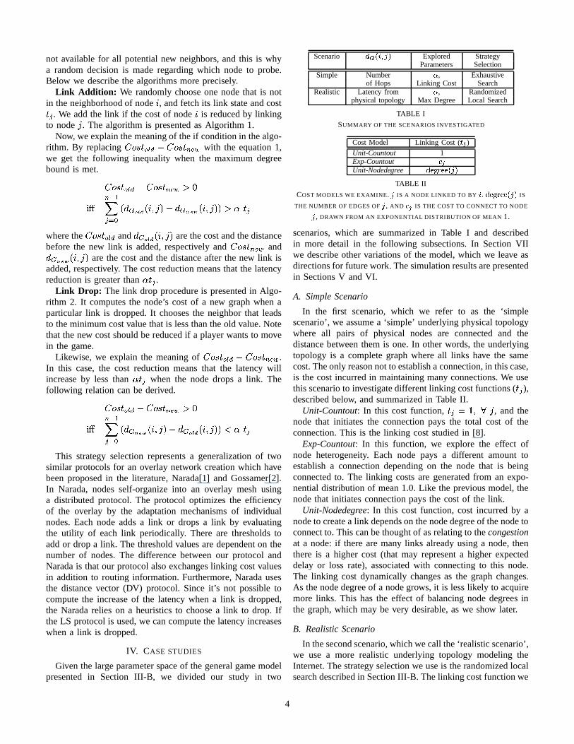
The total cost of the graphs is shown in Figure 4. As thenodes optimize for their own cost, one can examine how thetotal cost of the resulting networks compares to that of thesocial optimum. The curves labeled ‘Optimum’ in the figureare the results of the nodes optimizing for the total cost ofthe graph, rather than for their own, an approximation of thesocial optimum. The cost of the graphs produced by the Unit-Countout game does not seem to asymptotically differ fromthe cost found with the global optimization by more than aconstant. This is not true for the case of the Unit-Nodedegreemodel, and this fact is an indicative that it is importantto consider factors such as the dynamic and heterogeneouscharacteristics of networks when studying the price of anarchyin these systems. The cost of Exp-Countout grows with high + ,the reason being that with low + the links are always createdto the nodes with the least cost.

We now move to examining the topological properties of thegraphs. At a high level, the first two linking cost functions,Unit-Countout and Exp-Countout have the tendency to formstar-shaped graphs, in which one or a few nodes have (very)high connectivity, and the others have no incentive to formadditional links. This can be easily seen in Figure 2. Thegraphs in the Unit-Nodedegree cost model never form stars,and always have more balanced degree distributions. Thisdoes, however, come at the cost of longer path lengths. Also,for sufficiently high values of + , all equilibrium graphs for thethree cases are trees, albeit with different properties. Thesefindings are discussed in more detail below, for the threelinking cost functions.

Unit-Countout: We observe 4 main phases as + increases.Our results are in line with the theoretical results in [8], sincetheir model is equivalent to our simple scenario with thislinking cost function.

When + � f, all equilibrium graphs are complete graphs,

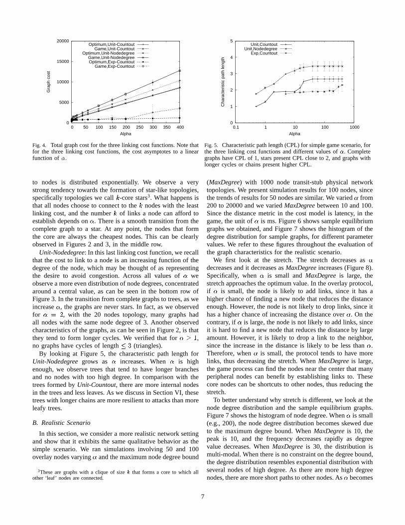
as adding an edge is always cheaper than having to traverseat least two hops to a non-neighbor node. This can be seenin Figure 5, which shows the characteristic path length of thegraphs. We can see that the characteristic path length is one forthis range of + in the Unit-Countout curve. We can also seethat all nodes, for Unit-Countout, with +o� \&!�� , have degreeof 19 (Figure 3(a)).

Whenf�� + �j� , all equilibrium graphs have path length of

at most 2 [8]. We obtained dense graphs, with characteristicpath lengths between 1 and 2 (Figure 5). An example such

5

+Linking Cost 1 5 10 60

Unit Countout0

1.00

11.00

21.00

31.00

41.00

61.00

71.00

81.00

131.00

141.00

151.00

161.00

181.00

51.00

91.00

101.00

111.00

121.00

191.00

171.00

01.00

171.00

11.00

21.00

31.00

41.00

51.00

61.00

71.00

81.00

91.00

101.00

111.00

121.00

131.00

141.00

151.00

161.00

181.00

191.00

01.00

171.00

11.00

21.00

31.00

41.00

51.00

61.00

71.00

81.00

91.00

101.00

111.00

121.00

131.00

141.00

151.00

161.00

181.00

191.00

01.00

161.00

11.00

191.00

21.00

151.00

31.00

171.00

41.00

181.00

51.00

61.00

71.00

81.00

91.00

141.00

101.00

111.00

121.00

131.00

Exp Countout

00.01

12.74

20.76

30.13

40.79

51.66

60.11

71.17

80.09

90.65

100.30

113.70

120.89

131.1414

1.19

150.55

160.97

172.00

180.90

190.70

02.25

50.01

70.07

11.46

20.14

32.04

40.25

60.96

80.52

91.36

100.48

110.27

121.83

130.84

140.55

152.49

160.45

172.76

180.21

191.17

02.25

50.01

11.46

20.14

32.04

40.25

60.96

70.07

80.52

91.36

100.48

110.27

121.83

130.84

140.55

152.49

160.45

172.76

180.21

191.17

Unit Nodedegree

01.00

51.00

151.00

161.00

171.00

11.00

101.00

131.00

141.00

191.00

21.00

71.00

111.00

31.00

61.00

121.00

41.00

181.00

81.00

91.00

01.00

171.00

11.00

31.00

51.00

81.00

91.00

181.00

21.00

41.00

71.00

61.00

111.00

121.00

131.00

101.00

141.00

151.00

161.00

191.00

01.00

161.00

171.00

11.00

191.00

21.00

151.00

31.00

141.00

41.00

181.00

51.00

61.00

71.00

81.00

91.00

101.00

111.00

121.00

131.00

01.00

161.00

171.00

11.00

191.00

21.00

151.00

31.00

141.00

41.00

181.00

51.00

61.00

71.00

81.00

91.00

101.00

111.00

121.00

131.00

Fig. 2. Sample equilibrium graphs for the simple scenario with 20 nodes, for the different cost models and values of � . With Exp-Countoutand ��� � , we could not find an Nash equilibrium in our experiments.

0

0.2

0.4

0.6

0.8

1

0 2 4 6 8 10 12 14 16 18 20

Rel

ativ

e F

requ

ency

Node degree

(a) Unit-Countout, ������

0

0.2

0.4

0.6

0.8

1

0 2 4 6 8 10 12 14 16 18 20

Rel

ativ

e F

requ

ency

Node degree

(b) ��� �

0

0.2

0.4

0.6

0.8

1

0 2 4 6 8 10 12 14 16 18 20

Rel

ativ

e F

requ

ency

Node degree

(c) �������

0

0.2

0.4

0.6

0.8

1

0 2 4 6 8 10 12 14 16 18 20

Rel

ativ

e F

requ

ency

Node degree

(d) �������

0

0.2

0.4

0.6

0.8

1

0 2 4 6 8 10 12 14 16 18 20

Rel

ativ

e F

requ

ency

Node degree

(e) Exp-Countout, ����

0

0.2

0.4

0.6

0.8

1

0 2 4 6 8 10 12 14 16 18 20

Rel

ativ

e F

requ

ency

Node degree

(f) �������

0

0.2

0.4

0.6

0.8

1

0 2 4 6 8 10 12 14 16 18 20

Rel

ativ

e F

requ

ency

Node degree

(g) �������

0

0.2

0.4

0.6

0.8

1

0 2 4 6 8 10 12 14 16 18 20

Rel

ativ

e F

requ

ency

Node degree

(h) Unit-Nodedegree, �����

0

0.2

0.4

0.6

0.8

1

0 2 4 6 8 10 12 14 16 18 20

Rel

ativ

e F

requ

ency

Node degree

(i) �������

0

0.2

0.4

0.6

0.8

1

0 2 4 6 8 10 12 14 16 18 20

Rel

ativ

e F

requ

ency

Node degree

(j) �������

Fig. 3. Histograms of the node degree distributions for the simple scenario. On the top, the phases of Unit-Countout: complete graph (a),dense graph (b), star (c), and ‘leafy’ tree (d). Exp-Countout (e-g) goes through � -core stars, and Unit-Nodedegree (h-k) produces much moredegree-balanced graphs.

graph can be seen in Figure 2, for Unit-Countout and + � f.

For +�� � , a sharp transition occurs, as the social optimumshifts from being the complete graph to the star [8]. FromFigure 5, we notice a flat region for + between 2 and 15,with characteristic path length of 2. Indeed, if we look atthe corresponding sample graphs in Figure 2, and at the nodedegree distributions in Figure 3, we see examples of stars.

Finally, for even larger + values, another shift happens,

when even the star becomes expensive to maintain, and treetopologies in which most of the nodes are leaves start toappear. These have longer characteristic path lengths, but thedistribution of degrees is still very skewed. We discuss theimplications of this topology, and of the star, for the resilienceof the network in Section VI.

Exp-Countout: In this cost function, as described in Sec-tion IV, nodes are not created equal: the cost of linking

6

0

5000

10000

15000

20000

0 50 100 150 200 250 300 350 400

Gra

ph c

ost

Alpha

Optimum,Unit-CountoutGame,Unit-Countout

Optimum,Unit-NodedegreeGame,Unit-NodedegreeOptimum,Exp-Countout

Game,Exp-Countout

0

1

2

3

4

5

0.1 1 10 100 1000

Cha

ract

eris

tic p

ath

leng

th

Alpha

Unit,CountoutUnit,Nodedegree

Exp,Countout

Fig. 4. Total graph cost for the three linking cost functions. Note thatfor the three linking cost functions, the cost asymptotes to a linearfunction of � .

Fig. 5. Characteristic path length (CPL) for simple game scenario, forthe three linking cost functions and different values of � . Completegraphs have CPL of 1, stars present CPL close to 2, and graphs withlonger cycles or chains present higher CPL.

to nodes is distributed exponentially. We observe a verystrong tendency towards the formation of star-like topologies,specifically topologies we call � -core stars3. What happens isthat all nodes choose to connect to the � nodes with the leastlinking cost, and the number � of links a node can afford toestablish depends on + . There is a smooth transition from thecomplete graph to a star. At any point, the nodes that formthe core are always the cheapest nodes. This can be clearlyobserved in Figures 2 and 3, in the middle row.

Unit-Nodedegree: In this last linking cost function, we recallthat the cost to link to a node is an increasing function of thedegree of the node, which may be thought of as representingthe desire to avoid congestion. Across all values of + weobserve a more even distribution of node degrees, concentratedaround a central value, as can be seen in the bottom row ofFigure 3. In the transition from complete graphs to trees, as weincrease + , the graphs are never stars. In fact, as we observedfor + � � , with the 20 nodes topology, many graphs hadall nodes with the same node degree of 3. Another observedcharacteristics of the graphs, as can be seen in Figure 2, is thatthey tend to form longer cycles. We verified that for + � f

,no graphs have cycles of length

���(triangles).

By looking at Figure 5, the characteristic path length forUnit-Nodedegree grows as + increases. When + is highenough, we observe trees that tend to have longer branchesand no nodes with too high degree. In comparison with thetrees formed by Unit-Countout, there are more internal nodesin the trees and less leaves. As we discuss in Section VI, thesetrees with longer chains are more resilient to attacks than moreleafy trees.

B. Realistic Scenario

In this section, we consider a more realistic network settingand show that it exhibits the same qualitative behavior as thesimple scenario. We ran simulations involving 50 and 100overlay nodes varying + and the maximum node degree bound

3These are graphs with a clique of size � that forms a core to which allother ‘leaf’ nodes are connected.

(MaxDegree) with 1000 node transit-stub physical networktopologies. We present simulation results for 100 nodes, sincethe trends of results for 50 nodes are similar. We varied + from200 to 20000 and we varied MaxDegree between 10 and 100.Since the distance metric in the cost model is latency, in thegame, the unit of + is ms. Figure 6 shows sample equilibriumgraphs we obtained, and Figure 7 shows the histogram of thedegree distribution for sample graphs, for different parametervalues. We refer to these figures throughout the evaluation ofthe graph characteristics for the realistic scenario.

We first look at the stretch. The stretch decreases as +decreases and it decreases as MaxDegree increases (Figure 8).Specifically, when + is small and MaxDegree is large, thestretch approaches the optimum value. In the overlay protocol,if + is small, the node is likely to add links, since it has ahigher chance of finding a new node that reduces the distanceenough. However, the node is not likely to drop links, since ithas a higher chance of increasing the distance over + . On thecontrary, if + is large, the node is not likely to add links, sinceit is hard to find a new node that reduces the distance by largeamount. However, it is likely to drop a link to the neighbor,since the increase in the distance is likely to be less than + .Therefore, when + is small, the protocol tends to have morelinks, thus decreasing the stretch. When MaxDegree is large,the game process can find the nodes near the center that manyperipheral nodes can benefit by establishing links to. Thesecore nodes can be shortcuts to other nodes, thus reducing thestretch.

To better understand why stretch is different, we look at thenode degree distribution and the sample equilibrium graphs.Figure 7 shows the histogram of node degree. When + is small(e.g., 200), the node degree distribution becomes skewed dueto the maximum degree bound. When MaxDegree is 10, thepeak is 10, and the frequency decreases rapidly as degreevalue decreases. When MaxDegree is 30, the distribution ismulti-modal. When there is no constraint on the degree bound,the degree distribution resembles exponential distribution withseveral nodes of high degree. As there are more high degreenodes, there are more short paths to other nodes. As + becomes

7

+Max Degree 800 2000 10000

10

01.00

41.00

171.00

341.00

441.00

601.00

651.00

751.00

821.00

851.00

981.00

11.00

21.00

61.00

71.00

271.00

481.00

561.00

861.00

31.00

191.00

531.00

701.00

711.00

841.00

871.00

91.00

111.00

151.00

331.00

401.00

451.00

741.00

831.00

881.00

951.00

801.00

991.00

51.00

181.00

301.00

501.00

551.00

581.00

81.00

361.00 63

1.00

641.00

901.00

121.00

661.00

921.00

261.00

321.00

571.00

591.00

931.00

391.00

521.00

691.00

101.00

431.00

781.00

291.00

621.00

811.00

911.00

971.00

131.00

511.00

681.00

891.00

211.00

671.00

141.00

161.00

461.00

961.00

941.00

241.00

351.00

281.00

721.00

411.00

201.00

221.00

371.00

611.00

731.00

231.00

471.00

251.00

761.00

791.00

311.00

541.00

771.00

421.00

381.00

491.00

01.00

21.00

71.00

101.00

111.00

201.00

331.00

371.00

801.00

11.00

251.00

481.00

621.00

931.00

961.00

991.00

161.00

591.00

811.00

31.00

301.00

441.00

701.00

41.00

321.00

51.00

341.00

61.00

361.00

381.00

501.00

611.00

631.00

641.00

821.00

841.00

901.00

211.00

651.00

861.00

81.00

171.00

281.00

431.00

511.00

661.00

721.00

791.00

921.00

91.00

521.00

561.00

691.00

771.00

541.00

891.00

551.00

581.00

681.00

761.00

981.00

121.00

261.00

571.00

741.00

131.00

941.00

141.00

151.00

271.00

291.00

411.00

461.00

471.00

731.00

181.00

191.00

241.00

231.00

351.00

851.00

221.00

451.00

751.00

831.00

601.00

911.00

311.00

881.00

951.00

671.00

871.00

711.00

421.00

781.00

391.00

401.00

531.00

971.00

491.00

01.00

121.00

441.00

11.00

101.00

21.00

491.00

801.00

841.00

31.00

291.00

391.00

421.00

581.00

621.00

701.00

771.00

41.00

51.00

341.00

61.00

71.0075

1.00

81.00

241.00

251.00

91.00

371.00

921.00

111.00

301.00

531.00

931.00

141.00

401.00

541.00

131.00

171.00

511.00

151.00

221.00

161.00

181.00

191.00

281.00

661.00

201.00

591.00

211.00

321.00

501.00

551.00

871.00

971.00

991.00

231.00

411.00

451.00

471.00

691.00

821.00

891.00

901.00

981.00

261.00

271.00

311.00

641.00

331.00

831.00

381.00

431.00

351.00

361.00

791.00

601.00

811.00

911.00

961.00

761.00

461.00

481.00

681.00

781.00

521.00

561.00

571.00

611.00

651.00

721.00

671.00

631.00

731.00

881.00

711.00

741.00

861.00

951.00

851.00

941.00

30 01.00

151.00

341.00

381.00

511.00

921.00

931.00

11.00

61.00

261.00

271.00

801.00

901.00

21.00

371.00

941.00

31.00

101.00

201.00

221.00

291.00

321.00

441.00

461.00

771.00

831.00

841.00

971.00

41.00

51.00

211.00

661.00

71.00

81.00

251.00

611.00

651.00

671.00

861.00

331.00

431.00

721.00

881.00

91.00

121.00

171.00

311.00

471.00

521.00

571.00

981.00

111.00

701.00

131.00

141.00

351.00

421.00

691.00

781.00

871.00

961.00

561.00

281.00

301.00

451.00

581.00

731.00

791.00

821.00

991.00

161.00

501.00

391.00

541.00

621.00

641.00

181.00

191.00

601.00

681.00

741.00

911.0095

1.00

231.00

241.00

811.00

401.00

591.00

361.00

531.00

711.00

761.00

411.00

481.00

891.00

491.00

631.00

551.00

751.00

851.00

01.00

291.00

931.00

11.00

51.00

621.00

941.00

21.00

601.00

801.00

31.00

441.00

881.00

991.00

41.00

191.00

571.00 6

1.00

341.00

751.00

71.00

761.00

81.00

121.00

481.00

91.00

171.00

101.00

111.0070

1.00

311.00

351.00

371.00

631.00

691.00

771.00

961.00

131.00

151.00

201.00

141.00

741.00

791.00

821.00 86

1.00

901.00

161.00

521.00

561.00

181.00

211.00

411.00

221.00

231.00

661.00

241.00

841.00

251.00

261.00

271.00

281.00

431.00

581.00

611.00

781.00

301.00

361.00

501.00

671.00

891.00

721.00

321.00

331.00

391.00

401.00

461.00

471.00

491.00

511.00

651.00

681.00

831.00

921.00

451.00

711.00

731.00

911.00

951.00

381.00

421.00

641.00

531.00

541.00

551.00

871.00

591.00

811.00

981.00

971.00

851.00

01.00

241.00

11.00

621.00

21.00

31.00

221.00

41.00

341.00

51.00

281.00

801.00

61.00

71.00

81.00

721.00

91.00

521.00

101.00

301.00

111.00

121.00

351.00

131.00

141.00

151.00

601.00

821.00

161.00

211.00

701.00

171.00

181.00

361.00

191.00

761.00

201.00

231.00

251.00

261.00

331.00

401.00

441.00

591.00

611.00

661.00

671.00

751.00

941.00

271.0088

1.00

291.00

311.00

641.00

321.00

851.00

461.00

371.00

381.00

921.00

391.00

411.00

511.00

421.00

781.00

431.00

451.00

471.00

481.00

491.00

501.00

931.00

561.00

631.00

741.00

911.00

531.00

541.00

551.00

571.00

581.00

711.00

731.00

651.00

681.00

691.00

971.00

811.00

831.00

961.00

981.00

991.00

771.00

791.00 84

1.00

861.00

871.00

891.00

951.00

901.00

1000

1.0051

1.00

661.00

801.00

11.00

101.00

341.00

621.00

21.00

211.00

701.00

31.00 4

1.00

51.00

281.00

61.00

871.00

991.00 7

1.00

81.00

91.00

171.00

521.00

111.00

381.00

851.00

121.00

351.00

561.00

571.00

641.00

691.00

981.00

131.00

141.00

391.00

771.0015

1.00

161.00

471.00

671.00

781.00

181.00

361.00

191.00

201.0037

1.00

651.00

681.00

221.00

231.00

241.00

251.00

261.00

271.00

881.00

291.00

301.00

311.00

811.00

321.00

331.00

931.00

421.00

431.00

541.00

551.00

601.00

611.00

721.00

741.00

751.00

761.00

791.00

821.00

861.00

921.00

411.00

451.00

491.00

531.00

631.00

711.00

911.00

951.00

961.00

401.00

441.00

461.00

591.00

481.00

891.00

501.00

731.00

901.00

971.00

581.00

831.00

941.00

841.00

01.00

621.00

11.00

101.00

931.00

21.00 3

1.00

661.00

41.00 34

1.00

51.00

281.00

61.00

251.00

471.00

611.00

71.00

81.00

591.00

91.00

121.00

141.00

521.00

111.00

701.00

161.00

351.00

391.00

511.00

571.00

131.00

171.00

151.00

801.00

561.00

181.00 36

1.00

191.00

291.00

201.00

211.00

371.00

681.00

911.00

951.00

221.00

231.00

241.00

261.00

271.00

651.00

671.00

301.00

311.00

321.00

331.00

431.00

461.00

641.00

751.00

761.00

781.00

821.00

881.00

901.00

921.00

981.00

991.00

411.00

491.00

531.00

601.00

711.00

381.00

401.00

421.00

441.00

451.00

481.00

501.00

691.00

731.00

741.00

811.00

871.00

961.00

541.00

551.00

941.00

581.00

631.00

831.00

851.00 86

1.00

721.00

891.00

971.00

771.00

791.00

841.00

01.00

321.00

11.00

381.00

851.00

21.00

621.00

31.00

341.00

41.00

51.00

61.00

171.00

331.00

401.00

471.00

561.00

661.00

881.00

981.00

71.00

591.00

81.00

441.00

611.00

91.00

941.00

101.00

111.00

801.00

121.00

371.00

751.00

131.00

291.00

141.00

151.00

741.00

161.00

241.00

181.00

361.00

191.00

871.00

201.00

211.00

681.00

221.00

781.00

231.00

531.00

711.00

791.00

891.00

251.00

261.00

271.00

281.00

391.00

501.00

641.00

761.00

901.00

991.00

301.00

701.00

311.00

571.00

861.00

421.00

431.00

451.00

461.00

511.00

521.00

551.00

631.00

731.00

771.00

811.00

821.00

831.00

841.00

961.00

971.00

351.00

491.00

921.00

411.00

481.00

541.00 58

1.00

651.00

721.00

601.00

671.00 69

1.00

911.00

951.00

931.00

Fig. 6. Sample equilibrium graphs created in the realistic scenario. The network has 100 nodes, and we vary the maximum degree bound,as well as the � parameter.

0

0.05

0.1

0.15

0.2

0.25

0.3

0.35

0.4

0.45

0.5

0 10 20 30 40 50 60 70 80

Rel

ativ

e F

requ

ency

Node degree

(a) � =200, MaxDegree=10

0

0.05

0.1

0.15

0.2

0.25

0.3

0.35

0.4

0.45

0.5

0 10 20 30 40 50 60 70 80

Rel

ativ

e F

requ

ency

Node degree

(b) � =200, MaxDegree=30

0

0.05

0.1

0.15

0.2

0.25

0.3

0.35

0.4

0.45

0.5

0 10 20 30 40 50 60 70 80R

elat

ive

Fre

quen

cy

Node degree

(c) � =200, MaxDegree=100

0

0.05

0.1

0.15

0.2

0.25

0.3

0.35

0.4

0.45

0.5

0 10 20 30 40 50 60 70 80

Rel

ativ

e F

requ

ency

Node degree

(d) � =2000, MaxDegree=10

0

0.05

0.1

0.15

0.2

0.25

0.3

0.35

0.4

0.45

0.5

0 10 20 30 40 50 60 70 80

Rel

ativ

e F

requ

ency

Node degree

(e) � =2000, MaxDegree=30

0

0.05

0.1

0.15

0.2

0.25

0.3

0.35

0.4

0.45

0.5

0 10 20 30 40 50 60 70 80

Rel

ativ

e F

requ

ency

Node degree

(f) � =2000, MaxDegree=100

Fig. 7. Histogram of node degree distributions for the realistic scenario, for different values of � and MaxDegree.

large (e.g, 2000), the degree distribution becomes very skewedwith the peak value of 3 or 4. Therefore, the stretch becomeslarger. In the case of MaxDegree of 100, there are still afew nodes of high degree, which reduces latency. For furtherunderstanding, we present the sample equilibrium graphs inFigure 6. When MaxDegree is 100, the graph has a few coresthat connect most of the nodes. However, when MaxDegree is10, each node has multiple links to other nodes and there areno central points unless + is very large. In this case, morenodes need to establish many links (e.g., more than 3) tomaintain fair stretch. The overall trends of the graph formsare similar to those of the Nash equilibria produced by theUnit-Countout linking cost in the simple scenario, althoughdegree bound is imposed. As + decreases, the graphs at Nash

equilibria transform from trees to almost � -regular graphs.4

To characterize the resulting graph topologies by comparingwith widely known topologies, we also examined the tail of thenode degree distribution. Figure 9 shows the tail distributionof the node degree when the game does not constrain degreebound, i.e., MaxDegree is 100. We plot three lines, for + of200, 800, and 2000. The graph is shown in a log-log scale, andthe curves indicate, for a given node degree ; , the fraction ofnodes with degree greater than ; . We also show, for reference,the curves for the tail of an exponential distribution, and ofa Pareto (power-law) distribution. For + =200, the distributionis not very skewed, and its tail decays in a similar fashion tothe exponential distribution. When + =2000, the decay in thedistribution is much more pronounced, and exhibits similar

4 � -regular graphs are ones in which all nodes have the same degree � ����� � .

8

0

0.5

1

1.5

2

2.5

3

3.5

100 1000 10000 100000

Str

etc

h

Alpha

MaxDegree=100MaxDegree=50MaxDegree=30MaxDegree=20MaxDegree=15MaxDegree=10 0.01

0.1

1

1 10 100

P(X

> x

) (1

-CD

F)

Node degree

α=200α=800α=2000Exponential Decay (λ=0.093)Pareto Decay (Shape=1.30)

Fig. 8. Stretch for the realistic scenario, for different values of � andMaxDegree. The stretch is lowest for high MaxDegree, and alwaysincreases with � .

Fig. 9. Tail of the distribution of node degree, for the realisticscenario, and unrestricted node degree. For a low value of � , thetail has exponential decay, while for a high value of � the decayapproximately follows a power-law.

behavior to that of the Pareto distribution. This is an importantfinding, since the game can be a way to create power-lawgraphs. These results are obtained when we create overlaynetworks on top of the GT-ITM topology. We are currentlyinvestigating the degree distributions for other underlyingtopologies. While we do not have enough evidence to provesuch behavior, we conjecture that these distributions are notan artifact of the particular network used here. We leave morecomplete investigations on this subject, including using realInternet measurements for latencies, for future work.

Lastly, we present control overhead to evaluate the statemaintenance overhead of the created networks compared tocomplete graphs. The control overhead is defined as thenumber of messages exchanged in the network created bythe game normalized by the number of messages exchangedin the complete graph. The overhead is proportional to thenumber of links in the network. In Figure 10, the overhead ismaximum 8 � and decreases to 1 � . The created networks havegood properties even though they use only a small percentageof links among the total number of possible links. Overall,networks under high MaxDegree have lower overhead thanthose under low MaxDegree, since fewer number of edges areestablished in the networks under high MaxDegree. When thelow degree bound is applied, the control overhead is saturatedas + becomes small. At this stage, the most of nodes in thenetwork have links of MaxDegree.

VI. ANALYSIS OF FAILURE AND ATTACK TOLERANCE

In this section, we analyze the failure and attack toleranceof the Nash equilibrium networks. To evaluate the tolerance,we use the � metric presented in [13]. � is the ratio of allconnected node-pairs in the network over the total number ofdistinct node-pairs in the network. This is used to characterizethe whole network connectivity under certain percentages ofnode failures or attacks. For failures, we remove a fraction ofrandomly selected nodes. For attacks, we remove a fraction ofnodes, starting from the node with the largest degree, followedby the next largest, and so on.

0

0.02

0.04

0.06

0.08

0.1

100 1000 10000 100000

Co

ntr

ol o

verh

ea

d

Alpha

MaxDegree=100MaxDegree=50MaxDegree=30MaxDegree=20MaxDegree=15MaxDegree=10

Fig. 10. Control overhead. In general, networks under higherMaxDegree have lower overhead. We also observe the overhead issaturated under small � and low MaxDegree.

A. Simple Scenario

In the simple scenario, we evaluate the effects that failuresand attacks of nodes have on the graphs produced by thedifferent linking cost functions, for different values of + .Looking again at Figure 2, we can gain intuition in theresilience properties to be expected. Let us look at the threegraphs for + � f \ , for example. Unit-Countout and Exp-Countout show star-like topologies, while Unit-Nodedegreeshows a graph with long chains. If nodes are taken downrandomly, the star topologies will most likely suffer the least,since a very small fraction of the nodes are really importantfor connectivity. However, if the most connected nodes areattacked, it is easy to see that the star topologies will collapse,while the Unit-Nodedegree generated topology will still havea good fraction of its nodes connected among themselves.

Figure 11(a) shows the value of � when 10% of the nodesare subject to failure. The results for other fractions of nodestaken down are very similar. The � -core star topologies createdby the Exp-Countout model are the most resilient to failures,as we just discussed. Similarly, the star and the ‘leafy’ tree

9

0

0.2

0.4

0.6

0.8

1

0.1 1 10 100 1000

K

Alpha

Unit,CountoutUnit,Nodedegree

Exp,Countout

(a) Failure

0

0.2

0.4

0.6

0.8

1

0.1 1 10 100 1000

K

Alpha

Unit,CountoutUnit,Nodedegree

Exp,Countout

(b) Attack

Fig. 11. Failure and attack tolerance (a) K when 10 � of nodes fail, (b) K when 10 � of nodes are attacked

0

0.2

0.4

0.6

0.8

1

100 1000 10000 100000

K

Alpha

MaxDegree=100MaxDegree=50MaxDegree=30MaxDegree=20MaxDegree=15MaxDegree=10

(a) Failure

0

0.2

0.4

0.6

0.8

1

100 1000 10000 100000

K

Alpha

MaxDegree=100MaxDegree=50MaxDegree=30MaxDegree=20MaxDegree=15MaxDegree=10

(b) Attack

Fig. 12. Failure and attack tolerance (a) K when 10 � of nodes fail, (b) K when 10 � of nodes are attacked

topologies created by Unit-Countout are resilient to failures,since most nodes are leaves.

More degree-balanced graphs produced by Unit-Nodedegreeare less resilient to failures, as more nodes are important forconnectivity. However, when it comes to resilience to attacks,the cost in longer paths and lower resilience to failure paysoff. Figure 11(b) shows the value of � when the 10% mostconnected nodes are attacked. The situation is reversed in thiscase, as the stars are very susceptible to attacks: some nodesare very important for connectivity and the network collapseswhen they are taken down. Comparing Figures 5 and 11(b),we see that exactly when the graphs are stars (and the pathlength is close to 2), � is equal to 0 (since removing thecenter node disconnects all others).

There is an interesting phenomenon in the resilience toattacks of the graphs created by the Unit-Nodedegree games.The graphs for +,� 2 are the most resilient to both failuresand attacks. By examining the topologies and the node degreedistributions, we see that when + � f

, the equilibrium graphshave long cycles, and some nodes have a tendency to havemore links than others (see Figure 3(h)). When + � � ,however, the distribution of node degrees becomes much morecentered around a single value. We observed graphs in whichall nodes had degree 3. In this case, the attack is equivalent

to failure, since all nodes have the same degree.

B. Realistic Scenario

The equilibrium networks achieve good performance (lowstretch) at the cost of lower resilience of the networks.Figure 12 shows K when 10 � of nodes fail and K when10 � of nodes are attacked in the realistic scenario. Thenetworks restricted by MaxDegree of 10 have the highestfailure tolerance (Figure 12(a)). When + is 5000, the differenceamong different MaxDegree’s in the failure tolerance is thelargest, but the difference diminishes as + gets smaller orlarger. As shown in Figure 7, if a node is randomly selected forremoval, the chance of removing the very high degree nodes issmall, thus the difference in the tolerance decreases. However,the attack tolerance shows striking results (Figure 12(b)).The networks with the lowest stretch have the worst attacktolerance. They lose their connectivity among nodes rapidlyas + increases. The attack tolerance graphs shift right aswe decrease MaxDegree. Imposing node degree bounds iskey to create networks with good attack tolerance property.The node degree distribution and sample graphs show theeffects of attack in a straightforward way. When + is 2000and MaxDegree is 100, by taking down a few high degreenodes, the network is completely disconnected, since mostof the nodes have low degree and they are connected to the

10

high degree nodes. On the contrary, when + is 2000 andMaxDegree is 10, each node is well connected to several othernodes. There is no vulnerable core that significantly affects theconnectivity of the network under attacks.

VII. DISCUSSION AND FUTURE WORK

We show that wide variety of linking cost functions createoverlay networks with diverse properties such as low stretch,balanced degree distribution, and high failure or attack re-silience. Some examples are k-regular graphs, k-core stars,trees, and graphs whose degree distributions have tails withdecay ranging from exponential to power-law.

Exp-Countout creates graphs with cores comprising nodeswith small linking cost values. Such nodes can be more power-ful nodes than others, and games can exploit the heterogeneity.On the contrary, Unit-Nodedegree can produce graphs withbalanced degrees without hot spots and nodes too vulnerableto attacks. Depending on the goals, one can use other vari-ations of linking cost (

4 / ) functions, which is an interestingresearch question. For example, the product of a heterogeneousconstant linking cost term and the node degree may get thebenefit of both Exp-Countout and Unit-Nodedegree, exploitingheterogeneities with balanced load distribution among nodes.We also observe interesting relationships between linking costfunctions. Unit-Nodedegree with small + creates � -regulargraphs that can be produced by MaxDegree bound. Indeed,one can use an increasing function of node degree as anapproximation for MaxDegree.

The exploration of Nash equilibria in the realistic scenariowas restricted due to the limits on computation. If the interac-tion among agents are constrained, the computation dependson the size of the neighborhood candidate set, even if the net-work size is large. We intend to study the effect of constrainedneighborhood candidate sets on the Nash equilibria.

We also found out that there is an important tradeoffbetween performance and resilience in the networks. Themore the node degrees are balanced, the more resilient thenetwork is to attacks. In the simple scenario, Unit-Nodedegreeproduces graphs with longer paths, more balanced degreedistributions, and higher resilience to attacks. In the realisticscenario, limiting the degree achieves higher resilience, forsimilar reasons, at the cost of higher stretch. An overlayrouting network among multiple parties can be created tomeet its target goals by exploiting this tradeoff. If the mostimportant requirement of the overlay routing network is lowstretch, one can choose high MaxDegree and low + . To beresilient to attacks and failures, the game should impose lowMaxDegree, forcing nodes to establish redundant links.

There are plenty of other interesting directions for futurework. We want to further study the relationship betweencharacteristics of the underlying topology and the producedoverlay topologies. The current game is run with a fixednumber of players. We want to examine the game in a dynamicnetwork where the total number of nodes changes over timedue to node joins and leaves. Another interesting area is totake traffic into consideration. If there is no traffic betweentwo nodes, there may be little incentive to set up a link. We

also intend to apply the model to other scenarios, e.g., overlaynetworks created by minimizing the path failure probabilities.Finally, we want to examine mechanism designs to providenodes no incentive to tell lies about linking cost values.

VIII. CONCLUSIONS

In this work we characterize selfishly constructed overlayrouting networks. We use a non-cooperative game modelto evaluate such networks and examine the effects of theunderlying topology and different linking cost functions in theresulting Nash equilibria of the game. We find that the gamescan produce widely different networks, from complete graphsto trees with different properties. For the realistic scenario,varying the + parameter in the cost model produces networkswith degree distribution with tails ranging from exponential topower-law distributions. We show that the networks obtainedcan present desirable properties, with respect to stretch andresilience, even though nodes are not interested in such globalproperties. We also find that there is a fundamental tradeoffbetween these two metrics, and that it can be controlled byrestricting the maximum node degree. This tradeoff can beexploited to construct overlay routing networks that satisfydiverse requirements.

REFERENCES

[1] Y.-H. Chu, S. G. Rao, and H. Zhang, “A case for end system multicast,”in Proceedings of ACM SIGMETRICS, Santa Clara, CA, June 2000.

[2] Y. Chawathe, “Scattercast: An architecture for Internet broadcastdistribution as an infrastructure service,” 2000.

[3] D. G. Andersen, H. Balakrishnan, M. F. Kaashoek, and R. Morris,“Resilient overlay networks,” in Proceedings of SOSP. ACM, 2001.

[4] S. Ratnasamy, P. Francis, M. Handley, R. Karp, and S. Shenker, “Ascalable content-addressable network,” in Proceedings of SIGCOMM.ACM, August 2001.

[5] I. Stoica, R. Morris, D. Karger, M. F. Kaashoek, and H. Balakrishnan,“Chord: A scalable peer-to-peer lookup service for Internet applica-tions,” in Proceedings of SIGCOMM. ACM, August 2001.

[6] A. Rowstron and P. Druschel, “Pastry: Scalable, decentralized objectlocation, and routing for large-scale peer-to-peer systems,” Lecture Notesin Computer Science, vol. 2218, 2001.

[7] B. Y. Zhao, L. Huang, J. Stribling, S. C. Rhea, A. D. Joseph, andJ. Kubiatowicz, “Tapestry: A resilient global-scale overlay for servicedeployment,” in Journal on Selected Areas in Communications. IEEE,January 2004.

[8] A. Fabrikant, A. Luthra, E. Maneva, C. Papadimitriou, and S. Shenker,“On a network creation game,” in Proceedings of ACM PODC, 2003.

[9] M. J. Osborne and A. Rubinstein, A Course in Game Theory, MITPress, 1994.

[10] J. Feigenbaum and S. Shenker, “Distributed algorithmic mechanismdesign: Recent results and future directions,” in Proceedings of the 6thInternational Workshop on Discrete Algorithms and Methods for MobileComputing and Communications, 2002.

[11] C. Papadimitriou, “Algorithms, games, and the Internet,” in Proceedingsof the 33rd Annual ACM Symposium on the Theory of Computing, 2001.

[12] R. Albert, H. Jeong, and A.-L. Barabasi, “Error and attack tolerance ofcomplex networks,” in Nature 406, July 2000.

[13] S.-T. Park, A. Khrabrov, D. M. Pennock, S. Lawrence, C. L. Giles, andL. H. Ungar, “Static and dynamic analysis of the Internet’s susceptibilityto faults and attacks,” in Proceedings of IEEE INFOCOM, 2003.

[14] F. K. Hwang, D. S. Richards, and P. Winter, The Steiner Tree Problem,Annals of Discrete Mathematics, 1992.

[15] E. W. Zegura, K. L. Calvert, and S. Bhattacharjee, “How to model aninternetwork,” in Proceedings of IEEE INFOCOM, 1996.

[16] D. J. Watts and S. H. Strogatz, “Collective dynamics of small-worldnetworks,” in Nature 393, June 1998.

11