Embed Size (px)
Citation preview
Copyright © Mandeep Dalal
CHAPTER 7 Chemical Dynamics – II Chain Reactions: Hydrogen-Bromine Reaction, Pyrolysis of Acetaldehyde,
Decomposition of EthaneA German chemist, Max Bodenstein, proposed the idea of chemical chain reactions in 1913. He
suggested that if two molecules react with each other, some unstable molecules may also be formed along- products that can further react with the reactant molecules with a much higher probability than the initial reactants. Another German chemist, Walther Nernst, explained the quantum yield phenomena in 1918 by suggesting that the photochemical reaction between hydrogen and chlorine is actually a chain reaction. He proposed that only one photon of light is actually accountable for the formation of 106 molecules of the final product. W. Nernst proposed that the incident photon breaks a chlorine molecule into two individual Cl atoms, each of which initiates a long series of stepwise reactions giving a large amount of hydrochloric acid.
A Danish scientist, Christian Christiansen; alongside a Dutch chemist, Hendrik Anthony Kramers; observed the polymer-synthesis in 1923 and conclude that a chain reaction doesn’t need a photon always but can also be started by the violent collision of two molecules. They also concluded that if two or more unstable molecules are produced during this reaction, the reaction chain could branch itself to grow enormously resulting in an explosion as well. These ideas were the very initial explanations for the mechanism responsible for the chemical explosions. A more sophisticated theory was proposed by Soviet physicist Nikolay Semyonov in 1934 to explain the quantitative aspects. N. Semyonov received the Nobel Prize in 1956 for his work (along with Sir Cyril Norman Hinshelwood for his independent developments).
Steps Involved in a Typical Chain Reaction: The primary steps involved in a typical chain reaction are discussed below.
i) Initiation: This step includes the formation of chain carriers or simply the active particles usually freeradicals in a photochemically or thermally induced chemical change.
ii) Propagation: This step may include many elementary reactions in a cycle in which chain carriers react toforms another chain carrier that continues the chain by entering the next elementary reaction. In other words, we can label these chain carriers as a catalyst for the overall propagation.
iii) Termination: This step includes the elementary chemical change in which the chain carriers lose theiractivity by combining with each other.
It is also worthy to note that the average number of times the propagation cycle is repeated is equal to the ratio of the overall reaction rate to the rate of initiation, and is called as “chain length”. Furthermore, some chain reactions follow very complex rate laws with mixed or fractional order kinetics. In this section, we will discuss nature and kinetics some of the most popular chain reactions such as ethane’s decomposition.
CHAPTER 7 Chemical Dynamics – II 345
Copyright © Mandeep Dalal
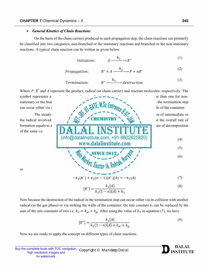
General Kinetics of Chain Reactions
On the basis of the chain carriers produced in each propagation step, the chain reactions can primarily be classified into two categories; non-branched or the stationary reactions and branched or the non-stationary reactions. A typical chain reaction can be written as given below.
𝐼𝑛𝑖𝑡𝑖𝑎𝑡𝑖𝑜𝑛: 𝐴
𝑘1 → 𝑅∗
(1)
𝑃𝑟𝑜𝑝𝑎𝑔𝑎𝑡𝑖𝑜𝑛: 𝑅∗ + 𝐴
𝑘2 → 𝑃 + 𝑛𝑅∗
(2)
𝑇𝑒𝑟𝑚𝑖𝑛𝑎𝑡𝑖𝑜𝑛: 𝑅∗
𝑘3 → 𝑑𝑒𝑠𝑡𝑟𝑢𝑐𝑡𝑖𝑜𝑛
(3)
Where P, R* and A represent the product, radical (or chain carrier) and reactant molecules, respectively. The symbol represents a number that equals unity for stationary chain reactions and greater than one for non-stationary or the branched-chain reactions. Furthermore, the destruction of the radical in the termination step can occur either via its collision with another radical (in gas phase) or by striking the walls of the container.
The steady-state approximation can be employed to determine the concentration of intermediate or the radical involved in the propagation step. The general procedure for which is to put the overall rate of formation equals to zero. In other words, the rate of formation of R* must be equal to the rate of decomposition of the same i.e.
𝑅𝑎𝑡𝑒 𝑜𝑓 𝑓𝑜𝑟𝑚𝑎𝑡𝑖𝑜𝑛 𝑜𝑓 𝑅∗ = 𝑅𝑎𝑡𝑒 𝑜𝑓 𝑑𝑖𝑠𝑎𝑝𝑝𝑒𝑎𝑟𝑎𝑛𝑐𝑒 𝑜𝑓 𝑅∗ (4)
𝑘1[𝐴] = 𝐾3[𝑅∗] − 𝑘2(𝑛 − 1)[𝑅
∗][𝐴] (5)
𝑘1[𝐴] − 𝑘3[𝑅
∗] + 𝑘2(𝑛 − 1)[𝑅∗][𝐴] = 0 =
𝑑[𝑅∗]
𝑑𝑡
(6)
or
−𝑘3[𝑅∗] + 𝑘2(𝑛 − 1)[𝑅
∗][𝐴] = −𝑘1[𝐴] (7)
[𝑅∗] =
𝑘1[𝐴]
𝑘2(1 − 𝑛)[𝐴] + 𝑘3
(8)
Now because the destruction of the radical in the termination step can occur either via its collision with another radical (in the gas phase) or via striking the walls of the container, the rate constant k3 can be replaced by the sum of the rate constants of two i.e. 𝑘3 = 𝑘𝑤 + 𝑘𝑔. After using the value of 𝑘3 in equation (7), we have
[𝑅∗] =
𝑘1[𝐴]
𝑘2(1 − 𝑛)[𝐴] + 𝑘𝑤 + 𝑘𝑔
(9)
Now we are ready to apply the concept on different types of chain reactions.
Buy the complete book with TOC navigation, high resolution images and
no watermark.
346 A Textbook of Physical Chemistry – Volume I
Copyright © Mandeep Dalal
Hydrogen-Bromine Reaction
The hydrogen-bromine or the H2-Br2 reaction is a typical case of stationary type chain reactions (n = 1) for which the overall reaction can be written as given below.
H2 + Br2⟶ 2HBr (10)
Furthermore, the elementary steps for the same can be proposed as
𝐼𝑛𝑖𝑡𝑖𝑎𝑡𝑖𝑜𝑛: Br2
𝑘1 → 2Br
(11)
𝑃𝑟𝑜𝑝𝑎𝑔𝑎𝑡𝑖𝑜𝑛: Br + H2
𝑘2 → HBr + H
(12)
H + Br2
𝑘3 → HBr + Br
(13)
𝐼𝑛ℎ𝑖𝑏𝑖𝑡𝑖𝑜𝑛: H + HBr
𝑘4 → H2 + Br
(14)
𝑇𝑒𝑟𝑚𝑖𝑛𝑎𝑡𝑖𝑜𝑛: Br + Br
𝑘5 → Br2
(15)
The net rate of formation of HBr must be equal to the sum of the rate of formation and the rate of disappearance of the same i.e.
𝑑[HBr]
dt= 𝑘2[𝐵𝑟][𝐻2] + 𝑘3[𝐻][𝐵𝑟2] − 𝑘4[𝐻][𝐻𝐵𝑟]
(16)
Now, in order to obtain the overall rate expression, we need to apply the steady-state approximation on the H and Br first i.e.
d[H]
dt= 0 = 𝑘2[𝐵𝑟][𝐻2] − 𝑘3[𝐻][𝐵𝑟2] − 𝑘4[𝐻][𝐻𝐵𝑟]
(17)
Similarly,
d[Br]
dt= 0 = 2𝑘1[𝐵𝑟2] − 𝑘2[𝐵𝑟][𝐻2] + 𝑘3[𝐻][𝐵𝑟2] + 𝑘4[𝐻][𝐻𝐵𝑟] − 2𝑘5[𝐵𝑟]
2 (18)
Taking negative both side of equation (17), we have
−𝑘2[𝐵𝑟][𝐻2] + 𝑘3[𝐻][𝐵𝑟2] + 𝑘4[𝐻][𝐻𝐵𝑟] = 0 (19)
Using the above result in equation (18), we get
2𝑘1[𝐵𝑟2] + 0 − 2𝑘5[𝐵𝑟]2 = 0 (20)
2𝑘5[𝐵𝑟]2 = 2𝑘1[𝐵𝑟2] (21)
Buy the complete book with TOC navigation, high resolution images and
no watermark.
CHAPTER 7 Chemical Dynamics – II 347
Copyright © Mandeep Dalal
[𝐵𝑟] = (
𝑘1𝑘5)1/2
[𝐵𝑟2]1/2
(22)
Similarly, rearranging equation (17) again
𝑘3[𝐻][𝐵𝑟2] + 𝑘4[𝐻][𝐻𝐵𝑟] = 𝑘2[𝐵𝑟][𝐻2] (23)
[𝐻] =
𝑘2[𝐵𝑟][𝐻2]
𝑘3[𝐵𝑟2] + 𝑘4[𝐻𝐵𝑟]
(24)
Now using the value of [Br] from equation (22), the above equation takes the form
[𝐻] =
𝑘2(𝑘1/𝑘5)1/2[𝐵𝑟2]
1/2[𝐻2]
𝑘3[Br2] + 𝑘4[HBr]
(25)
Now rearranging equation (17) again in different mode i.e.
𝑘2[𝐵𝑟][𝐻2] − 𝑘4[𝐻][𝐻𝐵𝑟] = 𝑘3[𝐻][𝐵𝑟2] (26)
Using the above result in equation (16), we have
𝑑[HBr]
dt= 𝑘3[𝐻][𝐵𝑟2] + 𝑘3[𝐻][𝐵𝑟2]
(27)
𝑑[HBr]
dt= 2𝑘3[𝐻][𝐵𝑟2]
(28)
After putting the value of [𝐻] from equation (24), the equation (28) takes the form
𝑑[HBr]
dt=2𝑘3𝑘2(𝑘1/𝑘5)
1/2[𝐵𝑟2]3/2[𝐻2]
𝑘3[Br2] + 𝑘4[HBr]
(29)
Taking 𝑘3[Br2] as common in the denominator and then canceling out the same form numerator, we get
𝑑[HBr]
dt=2𝑘2(𝑘1/𝑘5)
1/2[𝐵𝑟2]1/2[𝐻2]
1 + (𝑘4/𝑘3)[HBr]/[𝐵𝑟2]
(30)
Now consider two new constants as
𝑘′ = 2𝑘2(𝑘1/𝑘5)1/2 𝑎𝑛𝑑 𝑘′′ = 𝑘4/𝑘3 (31)
Using the above results in equation (30), we get
𝑑[HBr]
dt=
𝑘′[𝐵𝑟2]1/2[𝐻2]
1 + 𝑘′′[HBr]/[𝐵𝑟2]
(32)
The initial reaction rate expression can be obtained by neglecting [𝐻𝐵𝑟] i.e. 1 + 𝑘′′[HBr]/[𝐵𝑟2] ≈ 1 as
Buy the complete book with TOC navigation, high resolution images and
no watermark.
348 A Textbook of Physical Chemistry – Volume I
Copyright © Mandeep Dalal
[𝑑[HBr]
dt]0
= 𝑘′[𝐵𝑟2]1/2[𝐻2]0
(33)
Hence, the order of the hydrogen-bromine reaction in the initial stage will be 1.5 only i.e. first-order w.r.t. hydrogen and half w.r.t. bromine.
Pyrolysis of Acetaldehyde
The pyrolysis of acetaldehyde is another typical case of stationary type chain reactions (n = 1) for which the overall reaction can be written as given below.
CH3CHO⟶ CH4 + CO (34)
Furthermore, the elementary steps for the same can be proposed as
𝐼𝑛𝑖𝑡𝑖𝑎𝑡𝑖𝑜𝑛: CH3CHO
𝑘1 → ˙CH3 + ˙CHO
(35)
𝑃𝑟𝑜𝑝𝑎𝑔𝑎𝑡𝑖𝑜𝑛: ˙CH3 + CH3CHO
𝑘2 → CH4 + ˙CH2CHO
(36)
˙CH2CHO
𝑘3 → ˙CH3 + CO
(37)
𝑇𝑒𝑟𝑚𝑖𝑛𝑎𝑡𝑖𝑜𝑛: ˙CH3 + ˙CH3
𝑘4 → CH3CH3
(38)
The net rate of formation of CH4 must be equal to the sum of the rate of formation and the rate of disappearance of the same i.e.
𝑑[CH4]
dt= 𝑘2[˙CH3][CH3CHO]
(39)
Now, in order to obtain the overall rate expression, we need to apply the steady-state approximation on the [˙CH3] and [˙CH2CHO] first i.e.
d[˙CH3]
dt= 0 = 𝑘1[CH3CHO] − 𝑘2[˙CH3][CH3CHO] + 𝑘3[˙CH2CHO] − 2𝑘4[˙CH3]
2 (40)
Similarly,
d[˙CH2CHO]
dt= 0 = 𝑘2[˙CH3][CH3CHO] − 𝑘3[˙CH2CHO]
(41)
Taking negative both side of equation (41), we have
−𝑘2[˙CH3][CH3CHO] + 𝑘3[˙CH2CHO] = 0 (42)
Using the above result in equation (40), we get
Buy the complete book with TOC navigation, high resolution images and
no watermark.
CHAPTER 7 Chemical Dynamics – II 349
Copyright © Mandeep Dalal
𝑘1[CH3CHO] + 0 − 2𝑘4[˙CH3]2 = 0 (43)
[˙CH3] = (
𝑘12𝑘4
)1/2
[CH3CHO]1/2
(44)
After putting the value of [˙CH3] from equation (44) in equation (39), we have
𝑑[CH4]
dt= 𝑘2 (
𝑘12𝑘4
)1/2
[CH3CHO]1/2 [CH3CHO]
(45)
𝑑[CH4]
dt= 𝑘2 (
𝑘12𝑘4
)1/2
[CH3CHO]3/2
(46)
Now consider a new constant as
𝑘 = 𝑘2 (
𝑘12𝑘4
)1/2
(47)
Using in equation (46), we get
𝑑[CH4]
dt= 𝑘[CH3CHO]
3/2 (48)
The kinetic chain length for the same can be obtained by dividing the rate of formation of the product by rate of initiation step i.e.
𝐾𝑖𝑛𝑒𝑡𝑖𝑐 𝑐ℎ𝑎𝑖𝑛 𝑙𝑒𝑛𝑔𝑡ℎ =
𝑅𝑝
𝑅𝑖
(49)
Where 𝑅𝑝 and 𝑅𝑖 are the rate of propagation and rate of initiation respectively. Now since the rate of propagation is simply equal to the overall rate law i.e. equation (48), the rate of initiation can be given as
𝑅𝑖 = 𝑘1[CH3CHO] (50)
After using the values of 𝑅𝑝 and 𝑅𝑖 from equation (48, 50) in equation (49), we get the expression for kinetic chain length as
𝐾𝑖𝑛𝑒𝑡𝑖𝑐 𝑐ℎ𝑎𝑖𝑛 𝑙𝑒𝑛𝑔𝑡ℎ =
𝑘[CH3CHO]3/2
𝑘1[CH3CHO]
(51)
or
𝐾𝑖𝑛𝑒𝑡𝑖𝑐 𝑐ℎ𝑎𝑖𝑛 𝑙𝑒𝑛𝑔𝑡ℎ =
𝑘
𝑘1[CH3CHO]
1/2 (52)
Buy the complete book with TOC navigation, high resolution images and
no watermark.
350 A Textbook of Physical Chemistry – Volume I
Copyright © Mandeep Dalal
Decomposition of Ethane
The decomposition of ethane is another typical case of stationary type chain reactions (n = 1) for which the overall reaction can be written as given below.
CH3CH3⟶ CH2 = CH2 + H2 (53)
Furthermore, the elementary steps for the same can be proposed as
𝐼𝑛𝑖𝑡𝑖𝑎𝑡𝑖𝑜𝑛: CH3CH3
𝑘1 → ˙CH3 + ˙CH3
(54)
𝑃𝑟𝑜𝑝𝑎𝑔𝑎𝑡𝑖𝑜𝑛: ˙CH3 + CH3CH3
𝑘2 → CH4 + ˙CH2CH3
(55)
˙CH2CH3
𝑘3 → CH2 = CH2 + ˙H
(56)
CH3CH3 + ˙H
𝑘4 → ˙CH2CH3 + H2
(57)
𝑇𝑒𝑟𝑚𝑖𝑛𝑎𝑡𝑖𝑜𝑛: ˙CH2CH3 + ˙H
𝑘5 → CH3CH3
(58)
The net rate of decomposition of ethane must be equal to the rate of formation ethylene i.e.
−𝑑[C2H6]
dt=𝑑[C2H4]
dt= 𝑘3[˙CH2CH3]
(59)
Now, in order to obtain the overall rate expression, we need to apply the steady-state approximation on the [˙H], [˙CH3] and [˙CH2CH3] first i.e.
d[˙CH3]
dt= 0 = 2𝑘1[CH3CH3] − 𝑘2[˙CH3][CH3CH3]
(60)
Similarly,
d[˙CH2CH3]
dt= 0 = 𝑘2[˙CH3][CH3CH3] − 𝑘3[˙CH2CH3] + 𝑘4[˙H][CH3CH3] − 𝑘5[˙H][˙CH2CH3]
(61)
Similarly,
d[˙H]
dt= 0 = 𝑘3[˙CH2CH3] − 𝑘4[˙H][CH3CH3] − 𝑘5[˙H][˙CH2CH3]
(62)
Rearranging equation (60), we get
2𝑘1 − 𝑘2[˙CH3] = 0 (63)
[˙CH3] =
2𝑘1𝑘2
(64)
Buy the complete book with TOC navigation, high resolution images and
no watermark.
CHAPTER 7 Chemical Dynamics – II 351
Copyright © Mandeep Dalal
Rearranging equation (62), we get
𝑘4[˙H][CH3CH3] + 𝑘5[˙H][˙CH2CH3] = 𝑘3[˙CH2CH3] (65)
[˙H] =
𝑘3[˙CH2CH3]
𝑘4[CH3CH3] + 𝑘5[˙CH2CH3]
(66)
After putting the value of [˙CH3] and [˙H] from equation (64, 66) in equation (61), we have
𝑘2 (2𝑘1𝑘2) [CH3CH3] − 𝑘3[˙CH2CH3] + 𝑘4 (
𝑘3[˙CH2CH3]
𝑘4[CH3CH3] + 𝑘5[˙CH2CH3]) [CH3CH3]
− 𝑘5 (𝑘3[˙CH2CH3]
𝑘4[CH3CH3] + 𝑘5[˙CH2CH3]) [˙CH2CH3] = 0
(67)
or
𝑘3𝑘5[˙CH2CH3]2 − 𝑘1𝑘5[˙CH2CH3][CH3CH3] − 𝑘1𝑘4[CH3CH3]
2 = 0 (68)
The equation (68) is quadric in nature and can be solved to give
[˙CH2CH3] =
𝑘1𝑘5 + (𝑘12𝑘52 + 4𝑘1𝑘5𝑘3𝑘4)
1/2
2𝑘5𝑘3[CH3CH3]
(69)
Now putting the result in equation (59), we get
−𝑑[C2H6]
dt=𝑑[C2H4]
dt= 𝑘3
𝑘1𝑘5 + (𝑘12𝑘52 + 4𝑘1𝑘5𝑘3𝑘4)
1/2
2𝑘5𝑘3[CH3CH3]
(70)
−𝑑[C2H6]
dt=𝑘1𝑘5 + (𝑘1
2𝑘52 + 4𝑘1𝑘5𝑘3𝑘4)
1/2
2𝑘5[CH3CH3]
(71)
At this stage, defining a new constant as
𝑘 =
𝑘1𝑘5 + (𝑘12𝑘52 + 4𝑘1𝑘5𝑘3𝑘4)
1/2
2𝑘5
(72)
Now owing to the very small rate of initiation step, all the terms 𝑘1𝑘5 and 𝑘12𝑘52 can be neglected i.e.
𝑘 =
(4𝑘1𝑘5𝑘3𝑘4)1/2
2𝑘5= (𝑘1𝑘3𝑘4𝑘5
)1/2
(73)
the equation (71) takes the form
−𝑑[C2H6]
dt= 𝑘[CH3CH3]
(74)
Buy the complete book with TOC navigation, high resolution images and
no watermark.
352 A Textbook of Physical Chemistry – Volume I
Copyright © Mandeep Dalal
The kinetic chain length for the same can be obtained by dividing the rate of formation of the product by rate of initiation step i.e.
𝐾𝑖𝑛𝑒𝑡𝑖𝑐 𝑐ℎ𝑎𝑖𝑛 𝑙𝑒𝑛𝑔𝑡ℎ =𝑅𝑝𝑅𝑖
(75)
Where 𝑅𝑝 and 𝑅𝑖 are the rate of propagation and rate of initiation respectively. Now since the rate ofpropagation is simply equal to the overall rate law i.e. equation (74), the rate of initiation can be given as
𝑅𝑖 = 𝑘1[CH3CH3] (76)
After using the values of 𝑅𝑝 and 𝑅𝑖 from equation (74, 76) in equation (75), we get the expression for kineticchain length as
𝐾𝑖𝑛𝑒𝑡𝑖𝑐 𝑐ℎ𝑎𝑖𝑛 𝑙𝑒𝑛𝑔𝑡ℎ =𝑘[CH3CH3]
𝑘1[CH3CH3]
(77)
or
𝐾𝑖𝑛𝑒𝑡𝑖𝑐 𝑐ℎ𝑎𝑖𝑛 𝑙𝑒𝑛𝑔𝑡ℎ =𝑘
𝑘1=1
𝑘1(𝑘1𝑘3𝑘4𝑘5
)1/2
= (𝑘3𝑘4𝑘1𝑘5
)1/2 (78)
Photochemical Reactions (Hydrogen-Bromine & Hydrogen-ChlorineReactions)
There are many chemical reactions which occur also when the reactants are exposed to light. These reactions are called as photochemical reactions. Now before we discuss the nature and types of photochemical reactions, we need to discuss two laws first; the first is Grotthuss-Draper law while the second one is Stark-Einstein law.
The first law of photochemistry was given by Theodor Grotthuss and John W. Draper, and therefore, got its unique name.
The first law of photochemistry states that when the light is allowed to strike the reactions mixture, it can be partially transmitted, reflected and absorbed; and it is the absorbed portion of the incident light which is responsible to carry out any chemical change.
The second law of photochemistry was given by Johannes Stark and Albert Einstein, and therefore, is popularly known as Stark-Einstein law.
The second law of photochemistry states that one photon of light must be absorbed for one molecule to get activated in a photochemical reaction by a chemical system.
The quantum yield of a reaction is simply the ratio of number of molecules reacting in a given time to the number of photons absorbed in the same time i.e.
CHAPTER 7 Chemical Dynamics – II 353
Copyright © Mandeep Dalal
𝑄𝑢𝑎𝑛𝑡𝑢𝑚 𝑦𝑖𝑒𝑙𝑑(𝜙) =
𝑁𝑢𝑚𝑏𝑒𝑟 𝑜𝑓 𝑚𝑜𝑙𝑒𝑠 𝑜𝑓 𝑟𝑒𝑎𝑐𝑡𝑎𝑛𝑡 𝑟𝑒𝑎𝑐𝑡𝑖𝑛𝑔 𝑝𝑒𝑟 𝑠𝑒𝑐𝑜𝑛𝑑
𝑁𝑢𝑚𝑏𝑒𝑟 𝑜𝑓 𝑒𝑖𝑛𝑠𝑡𝑒𝑖𝑛𝑠 𝑎𝑏𝑠𝑜𝑟𝑏𝑒𝑑 𝑝𝑒𝑟 𝑠𝑒𝑐𝑜𝑛𝑑
(79)
Where one einstein represents one mole of photons (6.022×10²³). The quantum yield is of two types in photochemical reactions; one for the primary process and the second one for the secondary process. During the course of the primary process, light is absorbed by the reactant and the quantum yield of this part is always unity. Therefore, we can say that the number of radiation-absorbing molecules consumed per unit time in the primary process is equal to intensity of absorbed radiation i.e. Iab (number of photons striking the sample per unit time). For instance, consider the photo-decomposition
Br2 +ℎ𝜈
𝑘 → 2Br
(80)
Then, the quantum yield will be
𝜙 =
𝑁𝑢𝑚𝑏𝑒𝑟 𝑜𝑓 𝑚𝑜𝑙𝑒𝑠 𝑜𝑓 𝐵𝑟2 𝑑𝑒𝑐𝑜𝑚𝑝𝑜𝑠𝑒𝑑 𝑝𝑒𝑟 𝑢𝑛𝑖𝑡 𝑡𝑖𝑚𝑒
𝑁𝑢𝑚𝑏𝑒𝑟 𝑜𝑓 𝑒𝑖𝑛𝑠𝑡𝑒𝑖𝑛𝑠 𝑎𝑏𝑠𝑜𝑟𝑏𝑒𝑑 𝑝𝑒𝑟 𝑢𝑛𝑖𝑡 𝑡𝑖𝑚𝑒
(81)
or
𝜙 =
−𝑑[𝐵𝑟2]/𝑑𝑡
𝐼𝑎𝑏
(82)
Since 𝜙 = 1 for primary process, we have
1 =
−𝑑[𝐵𝑟2]/𝑑𝑡
𝐼𝑎𝑏
(83)
or
−𝑑[𝐵𝑟2]
𝑑𝑡= 𝐼𝑎𝑏
(84
−𝑑[𝐵𝑟2]
𝑑𝑡= 𝑘[𝐵𝑟2] = 𝐼𝑎𝑏
(85)
If rate of formation of Br is asked, then
−𝑑[𝐵𝑟2]
𝑑𝑡= +
1
2
𝑑[𝐵𝑟]
𝑑𝑡= 𝑘[𝐵𝑟2] = 𝐼𝑎𝑏
(86)
𝑑[𝐵𝑟]
𝑑𝑡= 2𝑘[𝐵𝑟2] = 2𝐼𝑎𝑏
(87)
Two of the most common examples of photochemical reactions are hydrogen-bromine and hydrogen-chlorine reactions whose kinetics and nature will be discussed in this section.
Buy the complete book with TOC navigation, high resolution images and
no watermark.
354 A Textbook of Physical Chemistry – Volume I
Copyright © Mandeep Dalal
Kinetics of Photochemical Reaction Between Hydrogen and Bromine
The hydrogen-bromine or the H2-Br2 reaction is a typical case of photochemical reactions for which the overall reaction can be written as given below.
H2 + Br2
ℎ𝜈 → 2HBr
(88)
Since it is a chain reaction, the elementary steps for the same can be proposed as
𝐼𝑛𝑖𝑡𝑖𝑎𝑡𝑖𝑜𝑛: Br2 + ℎ𝜈
𝑘1 → 2Br
(89)
𝑃𝑟𝑜𝑝𝑎𝑔𝑎𝑡𝑖𝑜𝑛: Br + H2
𝑘2 → HBr + H
(91)
H + Br2
𝑘3 → HBr + Br
(92)
𝐼𝑛ℎ𝑖𝑏𝑖𝑡𝑖𝑜𝑛: H + HBr
𝑘4 → H2 + Br
(93)
𝑇𝑒𝑟𝑚𝑖𝑛𝑎𝑡𝑖𝑜𝑛: Br + Br
𝑘5 → Br2
(94)
The net rate of formation of HBr must be equal to the sum of the rate of formation and the rate of disappearance of the same i.e.
𝑑[HBr]
dt= 𝑘2[𝐵𝑟][𝐻2] + 𝑘3[𝐻][𝐵𝑟2] − 𝑘4[𝐻][𝐻𝐵𝑟]
(95)
Now, in order to obtain the overall rate expression, we need to apply the steady-state approximation on the H and Br first i.e.
d[H]
dt= 𝑘2[𝐵𝑟][𝐻2] − 𝑘3[𝐻][𝐵𝑟2] − 𝑘4[𝐻][𝐻𝐵𝑟] = 0
(96)
Similarly,
d[Br]
dt= 2𝑘1[𝐵𝑟2] − 𝑘2[𝐵𝑟][𝐻2] + 𝑘3[𝐻][𝐵𝑟2] + 𝑘4[𝐻][𝐻𝐵𝑟] − 2𝑘5[𝐵𝑟]
2 = 0 (97)
Taking negative both side of equation (96), we have
−𝑘2[𝐵𝑟][𝐻2] + 𝑘3[𝐻][𝐵𝑟2] + 𝑘4[𝐻][𝐻𝐵𝑟] = 0 (98)
Using the above result in equation (97), we get
2𝑘1[𝐵𝑟2] + 0 − 2𝑘5[𝐵𝑟]2 = 0 (99)
2𝑘5[𝐵𝑟]2 = 2𝑘1[𝐵𝑟2] (100)
Buy the complete book with TOC navigation, high resolution images and
no watermark.
CHAPTER 7 Chemical Dynamics – II 355
Copyright © Mandeep Dalal
[𝐵𝑟] = (
𝑘1𝑘5)1/2
[𝐵𝑟2]1/2
(101)
Similarly, rearranging equation (96) again
𝑘3[𝐻][𝐵𝑟2] + 𝑘4[𝐻][𝐻𝐵𝑟] = 𝑘2[𝐵𝑟][𝐻2] (102)
[𝐻] =
𝑘2[𝐵𝑟][𝐻2]
𝑘3[𝐵𝑟2] + 𝑘4[𝐻𝐵𝑟]
(103)
Now using the value of [Br] from equation (101), the above equation takes the form
[𝐻] =
𝑘2(𝑘1/𝑘5)1/2[𝐵𝑟2]
1/2[𝐻2]
𝑘3[Br2] + 𝑘4[HBr]
(104)
Now rearranging equation (96) again in different mode i.e.
𝑘2[𝐵𝑟][𝐻2] − 𝑘4[𝐻][𝐻𝐵𝑟] = 𝑘3[𝐻][𝐵𝑟2] (105)
Using the above result in equation (95), we have
𝑑[HBr]
dt= 𝑘3[𝐻][𝐵𝑟2] + 𝑘3[𝐻][𝐵𝑟2]
(106)
𝑑[HBr]/dt = 2𝑘3[𝐻][𝐵𝑟2] (107)
After putting the value of [𝐻] from equation (104), the equation (107) takes the form
𝑑[HBr]
dt=2𝑘3𝑘2(𝑘1/𝑘5)
1/2[𝐵𝑟2]3/2[𝐻2]
𝑘3[Br2] + 𝑘4[HBr]
(108)
Taking 𝑘3[Br2] as common in the denominator and then canceling out the same form numerator, we get
𝑑[HBr]
dt=2𝑘2(𝑘1/𝑘5)
1/2[𝐵𝑟2]1/2[𝐻2]
1 + (𝑘4/𝑘3)[HBr]/[𝐵𝑟2]
(109)
Now since 2𝑘1[𝐵𝑟2] = 2𝐼𝑎𝑏, then
𝑘11/2[𝐵𝑟2]
1/2 = (𝐼𝑎𝑏)1/2 (110)
Using the above result in equation (109), we get
𝑑[HBr]
dt=
2𝑘2(𝐼𝑎𝑏/𝑘5)1/2[𝐻2]
1 + (𝑘4/𝑘3)[HBr]/[𝐵𝑟2]
(111)
Hence, the rate of hydrogen-bromine reaction is directly proportional to the square root of the intensity of absorbed radiation.
Buy the complete book with TOC navigation, high resolution images and
no watermark.
356 A Textbook of Physical Chemistry – Volume I
Copyright © Mandeep Dalal
Kinetics of Photochemical Reaction Between Hydrogen and Chlorine
The hydrogen-bromine or the H2-Cl2 reaction is a typical case of photochemical reactions for which the overall reaction can be written as given below.
H2 + Cl2
ℎ𝜈 → 2HCl
(112)
Since it is a chain reaction, the elementary steps for the same can be proposed as
𝐼𝑛𝑖𝑡𝑖𝑎𝑡𝑖𝑜𝑛: Cl2 + ℎ𝜈
𝑘1 → 2Cl
(113)
𝑃𝑟𝑜𝑝𝑎𝑔𝑎𝑡𝑖𝑜𝑛: Cl + H2
𝑘2 → HCl + H
(114)
H + Cl2
𝑘3 → HCl + Cl
(115)
𝑇𝑒𝑟𝑚𝑖𝑛𝑎𝑡𝑖𝑜𝑛: 2Cl(at the walls)
𝑘4 → Cl2
(116)
The net rate of formation of HCl must be equal to the sum of the rate of formation and the rate of disappearance of the same i.e.
𝑑[HCl]
dt= 𝑘2[𝐶𝑙][𝐻2] + 𝑘3[𝐻][𝐶𝑙2]
(117)
Now, in order to obtain the overall rate expression, we need to apply the steady-state approximation on the H and Cl first i.e.
d[H]
dt= 𝑘2[𝐶𝑙][𝐻2] − 𝑘3[𝐻][𝐶𝑙2] = 0
(118)
Similarly,
d[Cl]
dt= 2𝑘1[𝐶𝑙2] − 𝑘2[Cl][𝐻2] + 𝑘3[𝐻][𝐶𝑙2] − 2𝑘4[𝐶𝑙] = 0
(119)
Taking negative both side of equation (118), we have
−𝑘2[𝐶𝑙][𝐻2] + 𝑘3[𝐻][𝐶𝑙2] = 0 (120)
Using the above result in equation (119), we get
2𝑘1[𝐶𝑙2] + 0 − 2𝑘4[𝐶𝑙] = 0 (121)
or
2𝑘1[𝐶𝑙2] = 2𝑘4[𝐶𝑙] (122)
or
Buy the complete book with TOC navigation, high resolution images and
no watermark.
CHAPTER 7 Chemical Dynamics – II 357
Copyright © Mandeep Dalal
[𝐶𝑙] =
𝑘1𝑘4[𝐶𝑙2]
(123)
Similarly, rearranging equation (118) again
𝑘2[𝐶𝑙][𝐻2] − 𝑘3[𝐻][𝐶𝑙2] = 0 (124)
or
[𝐻] =
𝑘2[𝐶𝑙][𝐻2]
𝑘3[𝐶𝑙2]
(125)
Now using the value of [Cl] from equation (123), the above equation takes the form
[𝐻] =
𝑘2[𝐻2]
𝑘3[𝐶𝑙2]
𝑘1𝑘4[𝐶𝑙2] =
𝑘1𝑘2[𝐻2]
𝑘3𝑘4
(126)
Using values of [𝐶𝑙] and [𝐻] from equation (123, 126) in equation (117), we have
𝑑[HCl]
dt= 𝑘2
𝑘1𝑘4[𝐶𝑙2][𝐻2] + 𝑘3
𝑘1𝑘2[𝐻2]
𝑘3𝑘4[𝐶𝑙2]
(127)
or
𝑑[HCl]
dt=𝑘1𝑘2[𝐶𝑙2][𝐻2]
𝑘4+𝑘1𝑘2[𝐻2][𝐶𝑙2]
𝑘4
(128)
Now since 2𝑘1[𝐶𝑙2] = 2𝐼𝑎𝑏, then
𝑘1[𝐶𝑙2] = 𝐼𝑎𝑏 (129)
Using the above result in equation (129), we get
𝑑[HCl]
dt=𝑘2𝐼𝑎𝑏[𝐻2]
𝑘4+𝑘2𝐼𝑎𝑏[𝐻2]
𝑘4
(130)
or
𝑑[HCl]
dt=2𝑘2𝐼𝑎𝑏[𝐻2]
𝑘4
(131)
Hence, we can conclude that the rate of hydrogen-bromine reaction is directly proportional to the intensity of absorbed radiation. It is also worthy to note that the quantum yield of the hydrogen-chlorine reaction is much higher than that of hydrogen-bromine reaction which may simply be attributed to the exothermic nature of the second step in H2-Cl2 reaction which makes it spontaneous in nature.
Buy the complete book with TOC navigation, high resolution images and
no watermark.
358 A Textbook of Physical Chemistry – Volume I
Copyright © Mandeep Dalal
General Treatment of Chain Reactions (Ortho-Para Hydrogen Conversionand Hydrogen-Bromine Reactions)
In this section, we will discuss the general treatment of some common chain reactions like ortho-para hydrogen conversion and hydrogen-bromine reactions. To do so, we may also recall some concepts discussed earlier in this chapter.
Ortho-Para Hydrogen Conversion
The ortho-hydrogen can convert into para-hydrogen and can easily be measured in the temperature range of 700−800°C. The conversion is completely homogeneous in nature and the order of the conversion is 1.5 as total. The widely accepted mechanism is given below.
𝑝-H2 ⇌ 2H (132)
𝐻 + 𝑝-H2 𝑘2
→ H + 𝑜-H2(133)
The equilibrium constant for the above-mentioned molecular-atomic equilibria given by equation (132) can be written as
𝐾 =[𝐻]2
[𝑝-H2]
(134)
[𝐻]2 = 𝐾[𝑝-H2] (135)
[𝐻] = 𝐾1/2 [𝑝-H2]12 (136)
The net rate of conversion of p-H2 must be equal to the sum of the rate of formation and the rate of disappearance of the same i.e.
𝑑[𝑝-H2]
𝑑𝑡= 𝑘2[𝑝-H2][𝐻]
(137)
After using the value of [𝐻] from equation (136) in equation (137), we get
𝑑[𝑝-H2]
𝑑𝑡= 𝑘2[𝑝-H2]𝐾
1/2 [𝑝-H2]12
(137)
or
𝑑[𝑝-H2]
𝑑𝑡= 𝑘2𝐾
1/2 [𝑝-H2]3/2 (137)
The overall activation energy of the conversion is 𝐸 = 𝐸2 + 𝐷/2 where E2 is the activation energy of thesecond step while D is the dissociation energy of dihydrogen molecule.
CHAPTER 7 Chemical Dynamics – II 359
Copyright © Mandeep Dalal
Hydrogen-Bromine Reactions
The hydrogen-bromine or the H2-Br2 reaction is a typical case of stationary type chain reactions (n = 1) for which the overall reaction can be written as given below.
H2 + Br2⟶ 2HBr (138)
Furthermore, the elementary steps for the same can be proposed as
𝐼𝑛𝑖𝑡𝑖𝑎𝑡𝑖𝑜𝑛: Br2
𝑘1 → 2Br
(139)
𝑃𝑟𝑜𝑝𝑎𝑔𝑎𝑡𝑖𝑜𝑛: Br + H2
𝑘2 → HBr + H
(140)
H + Br2
𝑘3 → HBr + Br
(141)
𝐼𝑛ℎ𝑖𝑏𝑖𝑡𝑖𝑜𝑛: H + HBr
𝑘4 → H2 + Br
(142)
𝑇𝑒𝑟𝑚𝑖𝑛𝑎𝑡𝑖𝑜𝑛: Br + Br
𝑘5 → Br2
(143)
The net rate of formation of HBr must be equal to the sum of the rate of formation and the rate of disappearance of the same i.e.
𝑑[HBr]
dt= 𝑘2[𝐵𝑟][𝐻2] + 𝑘3[𝐻][𝐵𝑟2] − 𝑘4[𝐻][𝐻𝐵𝑟]
(144)
Now, in order to obtain the overall rate expression, we need to apply the steady-state approximation on the H and Br first i.e.
d[H]
dt= 0 = 𝑘2[𝐵𝑟][𝐻2] − 𝑘3[𝐻][𝐵𝑟2] − 𝑘4[𝐻][𝐻𝐵𝑟]
(145)
Similarly,
d[Br]
dt= 0 = 2𝑘1[𝐵𝑟2] − 𝑘2[𝐵𝑟][𝐻2] + 𝑘3[𝐻][𝐵𝑟2] + 𝑘4[𝐻][𝐻𝐵𝑟] − 2𝑘5[𝐵𝑟]
2 (146)
Taking negative both side of equation (145), we have
−𝑘2[𝐵𝑟][𝐻2] + 𝑘3[𝐻][𝐵𝑟2] + 𝑘4[𝐻][𝐻𝐵𝑟] = 0 (147)
Using the above result in equation (146), we get
2𝑘1[𝐵𝑟2] + 0 − 2𝑘5[𝐵𝑟]2 = 0 (148)
2𝑘5[𝐵𝑟]2 = 2𝑘1[𝐵𝑟2] (149)
Buy the complete book with TOC navigation, high resolution images and
no watermark.
360 A Textbook of Physical Chemistry – Volume I
Copyright © Mandeep Dalal
[𝐵𝑟] = (
𝑘1𝑘5)1/2
[𝐵𝑟2]1/2
(150)
Similarly, rearranging equation (145) again
𝑘3[𝐻][𝐵𝑟2] + 𝑘4[𝐻][𝐻𝐵𝑟] = 𝑘2[𝐵𝑟][𝐻2] (151)
[𝐻] =
𝑘2[𝐵𝑟][𝐻2]
𝑘3[𝐵𝑟2] + 𝑘4[𝐻𝐵𝑟]
(152)
Now using the value of [Br] from equation (150), the above equation takes the form
[𝐻] =
𝑘2(𝑘1/𝑘5)1/2[𝐵𝑟2]
1/2[𝐻2]
𝑘3[Br2] + 𝑘4[HBr]
(153)
Now rearranging equation (145) again in different mode i.e.
𝑘2[𝐵𝑟][𝐻2] − 𝑘4[𝐻][𝐻𝐵𝑟] = 𝑘3[𝐻][𝐵𝑟2] (154)
Using the above result in equation (144), we have
𝑑[HBr]
dt= 𝑘3[𝐻][𝐵𝑟2] + 𝑘3[𝐻][𝐵𝑟2]
(155)
𝑑[HBr]
dt= 2𝑘3[𝐻][𝐵𝑟2]
(156)
After putting the value of [𝐻] from equation (152), the equation (156) takes the form
𝑑[HBr]
dt=2𝑘3𝑘2(𝑘1/𝑘5)
1/2[𝐵𝑟2]3/2[𝐻2]
𝑘3[Br2] + 𝑘4[HBr]
(157)
Taking 𝑘3[Br2] as common in the denominator and then canceling out the same form numerator, we get
𝑑[HBr]
dt=2𝑘2(𝑘1/𝑘5)
1/2[𝐵𝑟2]1/2[𝐻2]
1 + (𝑘4/𝑘3)[HBr]/[𝐵𝑟2]
(158)
Now consider two new constants as
𝑘′ = 2𝑘2(𝑘1/𝑘5)1/2 𝑎𝑛𝑑 𝑘′′ = 𝑘4/𝑘3 (159)
Using in equation (158), we get
𝑑[HBr]
dt=
𝑘′[𝐵𝑟2]1/2[𝐻2]
1 + 𝑘′′[HBr]/[𝐵𝑟2]
(160)
The initial reaction rate expression can be obtained by neglecting [𝐻𝐵𝑟] i.e. 1 + 𝑘′′[HBr]/[𝐵𝑟2] ≈ 1 as
Buy the complete book with TOC navigation, high resolution images and
no watermark.
CHAPTER 7 Chemical Dynamics – II 361
Copyright © Mandeep Dalal
[𝑑[HBr]
dt]0
= 𝑘′[𝐵𝑟2]1/2[𝐻2]0
(161)
Hence, the order of the hydrogen-bromine reaction in the initial stage will be 1.5 only i.e. first-order w.r.t. hydrogen and half w.r.t. bromine.
However, if the initiation occurs by the photon of the incident light, the expression for the overall rate can slightly be modified. Recall the initiation step again via photochemical decomposition i.e.
Br2 +ℎ𝜈
𝑘 → 2Br
(162)
Then, the quantum yield for this primary change will be
𝜙 =
−𝑑[𝐵𝑟2]/𝑑𝑡
𝐼𝑎𝑏
(163)
Where 𝐼𝑎𝑏 is the intensity of absorbed radiation. Since 𝜙 = 1 for primary process, we have
1 =
−𝑑[𝐵𝑟2]/𝑑𝑡
𝐼𝑎𝑏
(164)
−𝑑[𝐵𝑟2]
𝑑𝑡= 𝐼𝑎𝑏
(165)
−𝑑[𝐵𝑟2]
𝑑𝑡= 𝑘[𝐵𝑟2] = 𝐼𝑎𝑏
(166)
For the rate of formation of Br, we have
−𝑑[𝐵𝑟2]
𝑑𝑡= +
1
2
𝑑[𝐵𝑟]
𝑑𝑡= 𝑘[𝐵𝑟2] = 𝐼𝑎𝑏
(167)
𝑑[𝐵𝑟]
𝑑𝑡= 2𝑘[𝐵𝑟2] = 2𝐼𝑎𝑏
(168)
Now since 2𝑘1[𝐵𝑟2] = 2𝐼𝑎𝑏, then
𝑘11/2[𝐵𝑟2]
1/2 = (𝐼𝑎𝑏)1/2 (169)
Using the above result in equation (158), we get
𝑑[HBr]
dt=
2𝑘2(𝐼𝑎𝑏/𝑘5)1/2[𝐻2]
1 + (𝑘4/𝑘3)[HBr]/[𝐵𝑟2]
(170)
Hence, the rate of hydrogen-bromine reaction is directly proportional to the square root of the intensity of absorbed radiation.
Buy the complete book with TOC navigation, high resolution images and
no watermark.
362 A Textbook of Physical Chemistry – Volume I
Copyright © Mandeep Dalal
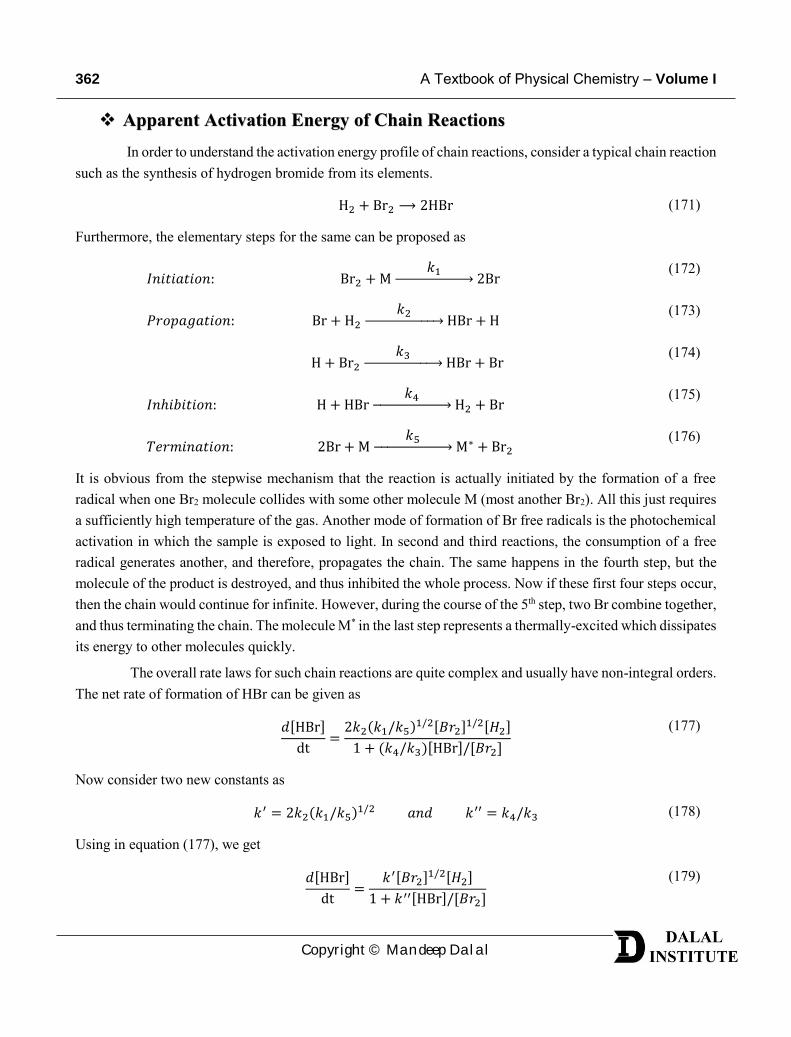
Apparent Activation Energy of Chain ReactionsIn order to understand the activation energy profile of chain reactions, consider a typical chain reaction
such as the synthesis of hydrogen bromide from its elements.
H2 + Br2⟶ 2HBr (171)
Furthermore, the elementary steps for the same can be proposed as
𝐼𝑛𝑖𝑡𝑖𝑎𝑡𝑖𝑜𝑛: Br2 +M 𝑘1
→ 2Br (172)
𝑃𝑟𝑜𝑝𝑎𝑔𝑎𝑡𝑖𝑜𝑛: Br + H2 𝑘2
→ HBr + H (173)
H + Br2 𝑘3
→ HBr + Br (174)
𝐼𝑛ℎ𝑖𝑏𝑖𝑡𝑖𝑜𝑛: H + HBr 𝑘4
→ H2 + Br(175)
𝑇𝑒𝑟𝑚𝑖𝑛𝑎𝑡𝑖𝑜𝑛: 2Br + M 𝑘5
→ M∗ + Br2(176)
It is obvious from the stepwise mechanism that the reaction is actually initiated by the formation of a free radical when one Br2 molecule collides with some other molecule M (most another Br2). All this just requires a sufficiently high temperature of the gas. Another mode of formation of Br free radicals is the photochemical activation in which the sample is exposed to light. In second and third reactions, the consumption of a free radical generates another, and therefore, propagates the chain. The same happens in the fourth step, but the molecule of the product is destroyed, and thus inhibited the whole process. Now if these first four steps occur, then the chain would continue for infinite. However, during the course of the 5th step, two Br combine together, and thus terminating the chain. The molecule M* in the last step represents a thermally-excited which dissipates its energy to other molecules quickly.
The overall rate laws for such chain reactions are quite complex and usually have non-integral orders. The net rate of formation of HBr can be given as
𝑑[HBr]
dt=2𝑘2(𝑘1/𝑘5)
1/2[𝐵𝑟2]1/2[𝐻2]
1 + (𝑘4/𝑘3)[HBr]/[𝐵𝑟2]
(177)
Now consider two new constants as
𝑘′ = 2𝑘2(𝑘1/𝑘5)1/2 𝑎𝑛𝑑 𝑘′′ = 𝑘4/𝑘3 (178)
Using in equation (177), we get
𝑑[HBr]
dt=
𝑘′[𝐵𝑟2]1/2[𝐻2]
1 + 𝑘′′[HBr]/[𝐵𝑟2]
(179)
CHAPTER 7 Chemical Dynamics – II 363
Copyright © Mandeep Dalal
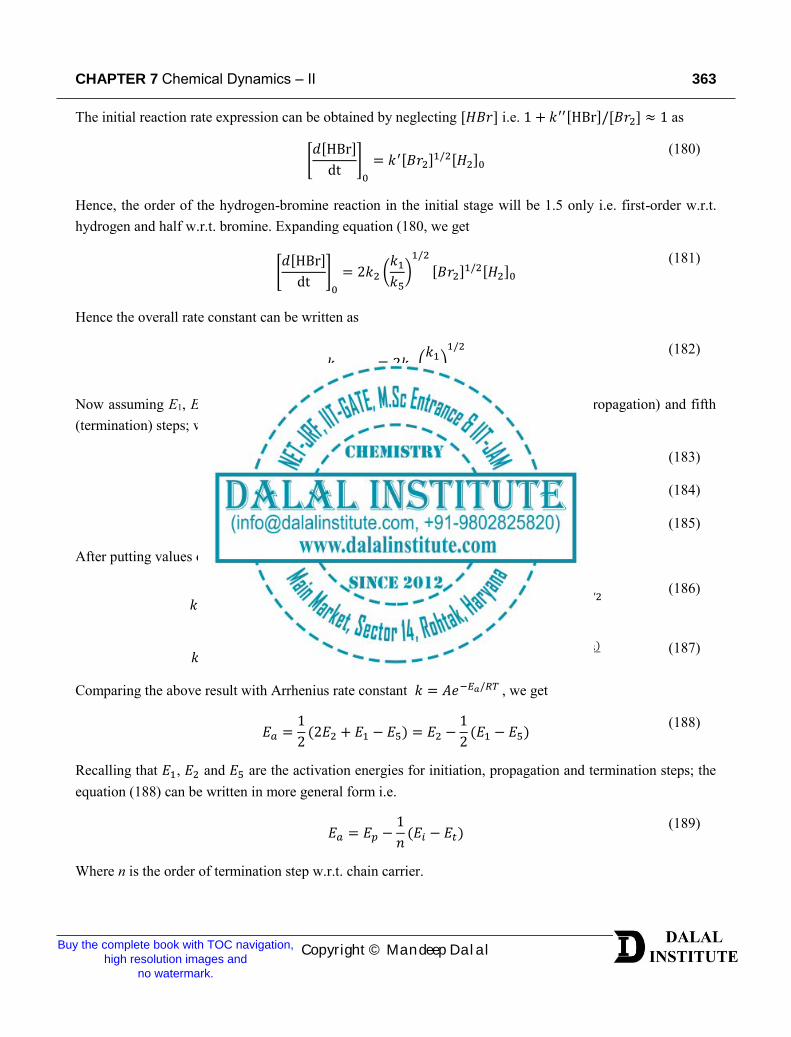
The initial reaction rate expression can be obtained by neglecting [𝐻𝐵𝑟] i.e. 1 + 𝑘′′[HBr]/[𝐵𝑟2] ≈ 1 as
[𝑑[HBr]
dt]0
= 𝑘′[𝐵𝑟2]1/2[𝐻2]0
(180)
Hence, the order of the hydrogen-bromine reaction in the initial stage will be 1.5 only i.e. first-order w.r.t. hydrogen and half w.r.t. bromine. Expanding equation (180, we get
[𝑑[HBr]
dt]0
= 2𝑘2 (𝑘1𝑘5)1/2
[𝐵𝑟2]1/2[𝐻2]0
(181)
Hence the overall rate constant can be written as
𝑘𝑜𝑣𝑒𝑟𝑎𝑙𝑙 = 2𝑘2 (
𝑘1𝑘5)1/2
(182)
Now assuming E1, E2 and E5 are the activation energies for first (initiation), second (propagation) and fifth (termination) steps; we can write general expressions for individual rate constants as
𝑘1 = 𝐴𝑒−𝐸1/𝑅𝑇 (183)
𝑘2 = 𝐴𝑒−𝐸2/𝑅𝑇 (184)
𝑘5 = 𝐴𝑒−𝐸5/𝑅𝑇 (185)
After putting values of 𝑘1, 𝑘2 and 𝑘5 from equation (183-185) in equation (182), we get
𝑘𝑜𝑣𝑒𝑟𝑎𝑙𝑙 = 2 𝐴𝑒
−𝐸2/𝑅𝑇 (𝐴𝑒−𝐸1/𝑅𝑇
𝐴𝑒−𝐸5/𝑅𝑇)
1/2
= 2 𝐴𝑒−𝐸2/𝑅𝑇(𝑒−𝐸1+𝐸5/𝑅𝑇)1/2
(186)
𝑘𝑜𝑣𝑒𝑟𝑎𝑙𝑙 = 2 𝐴𝑒
−𝐸2𝑅𝑇 𝑒
−𝐸1+𝐸52𝑅𝑇 = 2 𝐴𝑒
−2𝐸2−𝐸1+𝐸52𝑅𝑇 = 2 𝐴𝑒−
12 (2𝐸2+𝐸1−𝐸5)
𝑅𝑇 (187)
Comparing the above result with Arrhenius rate constant 𝑘 = 𝐴𝑒−𝐸𝑎/𝑅𝑇 , we get
𝐸𝑎 =
1
2(2𝐸2 + 𝐸1 − 𝐸5) = 𝐸2 −
1
2(𝐸1 − 𝐸5)
(188)
Recalling that 𝐸1, 𝐸2 and 𝐸5 are the activation energies for initiation, propagation and termination steps; the equation (188) can be written in more general form i.e.
𝐸𝑎 = 𝐸𝑝 −
1
𝑛(𝐸𝑖 − 𝐸𝑡)
(189)
Where n is the order of termination step w.r.t. chain carrier.
Buy the complete book with TOC navigation, high resolution images and
no watermark.
364 A Textbook of Physical Chemistry – Volume I
Copyright © Mandeep Dalal
Chain LengthThe chain length for any chemical chain reaction may simply be defined as the average number of
times that the closed cycle of chain propagation steps is repeated.
In other words, the chain length of any chain reaction is equal to the ration of the rate of the overall reaction to the rate of the initiation step in which the active particles are generated. Mathematically,
𝐾𝑖𝑛𝑒𝑡𝑖𝑐 𝑐ℎ𝑎𝑖𝑛 𝑙𝑒𝑛𝑔𝑡ℎ =𝑅𝑝𝑅𝑖
(190)
Where 𝑅𝑝 and 𝑅𝑖 are the rate of propagation and rate of initiation respectively. The concept can be wellunderstood by taking the example of thermal decomposition of acetaldehyde and ethane.
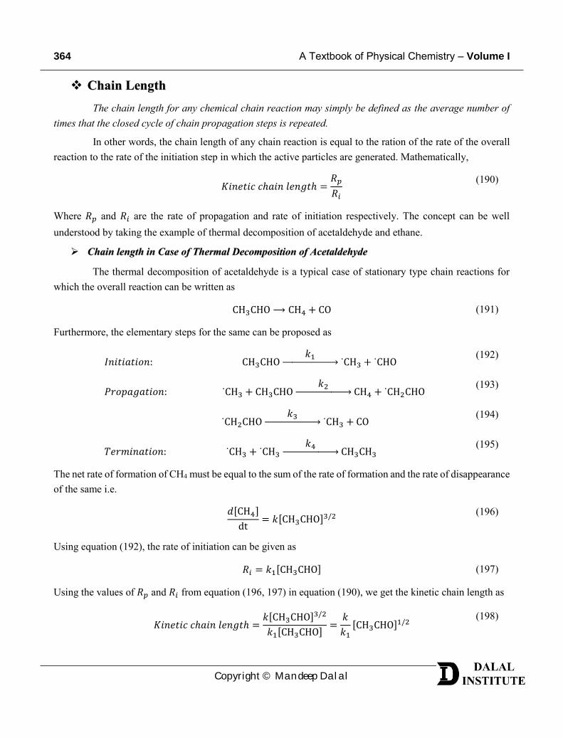
Chain length in Case of Thermal Decomposition of Acetaldehyde
The thermal decomposition of acetaldehyde is a typical case of stationary type chain reactions for which the overall reaction can be written as
CH3CHO⟶ CH4 + CO (191)
Furthermore, the elementary steps for the same can be proposed as
𝐼𝑛𝑖𝑡𝑖𝑎𝑡𝑖𝑜𝑛: CH3CHO 𝑘1
→ ˙CH3 + ˙CHO(192)
𝑃𝑟𝑜𝑝𝑎𝑔𝑎𝑡𝑖𝑜𝑛: ˙CH3 + CH3CHO 𝑘2
→ CH4 + ˙CH2CHO(193)
˙CH2CHO 𝑘3
→ ˙CH3 + CO(194)
𝑇𝑒𝑟𝑚𝑖𝑛𝑎𝑡𝑖𝑜𝑛: ˙CH3 + ˙CH3 𝑘4
→ CH3CH3(195)
The net rate of formation of CH4 must be equal to the sum of the rate of formation and the rate of disappearance of the same i.e.
𝑑[CH4]
dt= 𝑘[CH3CHO]
3/2 (196)
Using equation (192), the rate of initiation can be given as
𝑅𝑖 = 𝑘1[CH3CHO] (197)
Using the values of 𝑅𝑝 and 𝑅𝑖 from equation (196, 197) in equation (190), we get the kinetic chain length as
𝐾𝑖𝑛𝑒𝑡𝑖𝑐 𝑐ℎ𝑎𝑖𝑛 𝑙𝑒𝑛𝑔𝑡ℎ =𝑘[CH3CHO]
3/2
𝑘1[CH3CHO]=𝑘
𝑘1[CH3CHO]
1/2(198)
CHAPTER 7 Chemical Dynamics – II 365
Copyright © Mandeep Dalal
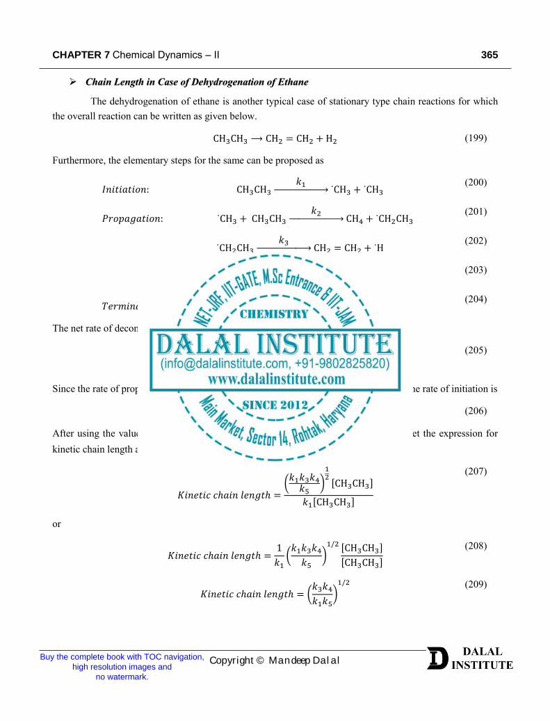
Chain Length in Case of Dehydrogenation of Ethane
The dehydrogenation of ethane is another typical case of stationary type chain reactions for which the overall reaction can be written as given below.
CH3CH3⟶ CH2 = CH2 + H2 (199)
Furthermore, the elementary steps for the same can be proposed as
𝐼𝑛𝑖𝑡𝑖𝑎𝑡𝑖𝑜𝑛: CH3CH3
𝑘1 → ˙CH3 + ˙CH3
(200)
𝑃𝑟𝑜𝑝𝑎𝑔𝑎𝑡𝑖𝑜𝑛: ˙CH3 + CH3CH3
𝑘2 → CH4 + ˙CH2CH3
(201)
˙CH2CH3
𝑘3 → CH2 = CH2 + ˙H
(202)
CH3CH3 + ˙H
𝑘4 → ˙CH2CH3 + H2
(203)
𝑇𝑒𝑟𝑚𝑖𝑛𝑎𝑡𝑖𝑜𝑛: ˙CH2CH3 + ˙H
𝑘5 → CH3CH3
(204)
The net rate of decomposition of ethane will be
−𝑑[C2H6]
dt= (𝑘1𝑘3𝑘4𝑘5
)1/2
[CH3CH3] (205)
Since the rate of propagation is simply equal to the overall rate law i.e. equation (205), the rate of initiation is
𝑅𝑖 = 𝑘1[CH3CH3] (206)
After using the values of 𝑅𝑝 and 𝑅𝑖 from equation (205, 206) in equation (190), we get the expression for kinetic chain length as
𝐾𝑖𝑛𝑒𝑡𝑖𝑐 𝑐ℎ𝑎𝑖𝑛 𝑙𝑒𝑛𝑔𝑡ℎ =(𝑘1𝑘3𝑘4𝑘5
)
12[CH3CH3]
𝑘1[CH3CH3]
(207)
or
𝐾𝑖𝑛𝑒𝑡𝑖𝑐 𝑐ℎ𝑎𝑖𝑛 𝑙𝑒𝑛𝑔𝑡ℎ =
1
𝑘1(𝑘1𝑘3𝑘4𝑘5
)1/2 [CH3CH3]
[CH3CH3]
(208)
𝐾𝑖𝑛𝑒𝑡𝑖𝑐 𝑐ℎ𝑎𝑖𝑛 𝑙𝑒𝑛𝑔𝑡ℎ = (
𝑘3𝑘4𝑘1𝑘5
)1/2
(209)
Buy the complete book with TOC navigation, high resolution images and
no watermark.
366 A Textbook of Physical Chemistry – Volume I
Copyright © Mandeep Dalal
Rice-Herzfeld Mechanism of Organic Molecules Decomposition(Acetaldehyde)
In 1934, Frank O. Rice and Karl F. Herzfeld performed an extensive study on the chain reactions and developed special mechanics to account the observed rate laws. In the honor of researchers, this mechanism is popularly known as Rice-Herzfeld mechanism. The conceptual foundation of this mechanism can easily be understood by taking the example of an organic compound, acetaldehyde.
The pyrolysis of acetaldehyde is a typical case of stationary type chain reactions (n = 1) for which the overall reaction can be written as given below.
CH3CHO⟶ CH4 + CO (210)
Furthermore, the elementary steps for the same can be proposed as
𝐼𝑛𝑖𝑡𝑖𝑎𝑡𝑖𝑜𝑛: CH3CHO 𝑘1
→ ˙CH3 + ˙CHO(211)
𝑃𝑟𝑜𝑝𝑎𝑔𝑎𝑡𝑖𝑜𝑛: ˙CH3 + CH3CHO 𝑘2
→ CH4 + ˙CH2CHO(212)
˙CH2CHO 𝑘3
→ ˙CH3 + CO(213)
𝑇𝑒𝑟𝑚𝑖𝑛𝑎𝑡𝑖𝑜𝑛: ˙CH3 + ˙CH3 𝑘4
→ CH3CH3(214)
The net rate of formation of CH4 must be equal to the sum of the rate of formation and the rate of disappearance of the same i.e.
𝑑[CH4]
dt= 𝑘2[˙CH3][CH3CHO]
(215)
Now, in order to obtain the overall rate expression, we need to apply the steady-state approximation on the [˙CH3] and [˙CH2CHO] first i.e.
d[˙CH3]
dt= 0 = 𝑘1[CH3CHO] − 𝑘2[˙CH3][CH3CHO] + 𝑘3[˙CH2CHO] − 2𝑘4[˙CH3]
2 (216)
Similarly,
d[˙CH2CHO]
dt= 0 = 𝑘2[˙CH3][CH3CHO] − 𝑘3[˙CH2CHO]
(217)
Taking negative both side of equation (217), we have
−𝑘2[˙CH3][CH3CHO] + 𝑘3[˙CH2CHO] = 0 (218)
Using the above result in equation (216), we get
CHAPTER 7 Chemical Dynamics – II 367
Copyright © Mandeep Dalal
𝑘1[CH3CHO] + 0 − 2𝑘4[˙CH3]2 = 0 (219)
[˙CH3] = (
𝑘12𝑘4
)1/2
[CH3CHO]1/2
(220)
After putting the value of [˙CH3] from equation (220) in equation (215), we have
𝑑[CH4]
dt= 𝑘2 (
𝑘12𝑘4
)1/2
[CH3CHO]1/2 [CH3CHO]
(221)
𝑑[CH4]
dt= 𝑘2 (
𝑘12𝑘4
)1/2
[CH3CHO]3/2
(222)
Now consider a new constant as
𝑘 = 𝑘2 (
𝑘12𝑘4
)1/2
(223)
Using in equation (222), we get
𝑑[CH4]
dt= 𝑘[CH3CHO]
3/2 (224)
The kinetic chain length for the same can be obtained by dividing the rate of formation of the product by rate of initiation step i.e.
𝐾𝑖𝑛𝑒𝑡𝑖𝑐 𝑐ℎ𝑎𝑖𝑛 𝑙𝑒𝑛𝑔𝑡ℎ =
𝑅𝑝
𝑅𝑖
(225)
Where 𝑅𝑝 and 𝑅𝑖 are the rate of propagation and rate of initiation respectively. Now since the rate of propagation is simply equal to the overall rate law i.e. equation (224), the rate of initiation can be given as
𝑅𝑖 = 𝑘1[CH3CHO] (226)
After using the values of 𝑅𝑝 and 𝑅𝑖 from equation (224, 226) in equation (225), we get the expression for kinetic chain length as
𝐾𝑖𝑛𝑒𝑡𝑖𝑐 𝑐ℎ𝑎𝑖𝑛 𝑙𝑒𝑛𝑔𝑡ℎ =
𝑘[CH3CHO]3/2
𝑘1[CH3CHO]
(227)
or
𝐾𝑖𝑛𝑒𝑡𝑖𝑐 𝑐ℎ𝑎𝑖𝑛 𝑙𝑒𝑛𝑔𝑡ℎ =
𝑘
𝑘1[CH3CHO]
1/2 (228)
Buy the complete book with TOC navigation, high resolution images and
no watermark.
368 A Textbook of Physical Chemistry – Volume I
Copyright © Mandeep Dalal
Branching Chain Reactions and Explosions (H2-O2 Reaction)On the basis of the chain carriers produced in each propagation step, the chain reactions can primarily
be classified into two categories; non-branched or the stationary reactions and branched or the non-stationary reactions. A typical chain reaction can be written as given below.
𝐼𝑛𝑖𝑡𝑖𝑎𝑡𝑖𝑜𝑛: 𝐴 𝑘1
→ 𝑅∗(229)
𝑃𝑟𝑜𝑝𝑎𝑔𝑎𝑡𝑖𝑜𝑛: 𝑅∗ + 𝐴 𝑘2
→ 𝑃 + 𝑛𝑅∗(230)
𝑇𝑒𝑟𝑚𝑖𝑛𝑎𝑡𝑖𝑜𝑛: 𝑅∗ 𝑘3
→ 𝑑𝑒𝑠𝑡𝑟𝑢𝑐𝑡𝑖𝑜𝑛 (231)
Where P, R* and A represent the product, radical (or chain carrier) and reactant molecules, respectively. The symbol represents a number that equals unity for stationary chain reactions and greater than one for non-stationary or the branched-chain reactions. Furthermore, the destruction of the radical in the termination step can occur either via its collision with another radical (in gas phase) or by striking the walls of the container.
The steady-state approximation can be employed to determine the concentration of intermediate or the radical involved in the propagation step. The general procedure for which is to put the overall rate of formation equals to zero. In other words, the rate of formation of R* must be equal to the rate of decomposition of the same i.e.
𝑅𝑎𝑡𝑒 𝑜𝑓 𝑓𝑜𝑟𝑚𝑎𝑡𝑖𝑜𝑛 𝑜𝑓 𝑅∗ = 𝑅𝑎𝑡𝑒 𝑜𝑓 𝑑𝑖𝑠𝑎𝑝𝑝𝑒𝑎𝑟𝑎𝑛𝑐𝑒 𝑜𝑓 𝑅∗ (232)
𝑘1[𝐴] = 𝑘3[𝑅∗] − 𝑘2(𝑛 − 1)[𝑅
∗][𝐴] (233)
𝑘1[𝐴] − 𝑘3[𝑅∗] + 𝑘2(𝑛 − 1)[𝑅
∗][𝐴] = 0 =𝑑[𝑅∗]
𝑑𝑡
(234)
or
−𝑘3[𝑅∗] + 𝑘2(𝑛 − 1)[𝑅
∗][𝐴] = −𝑘1[𝐴] (235)
[𝑅∗] =𝑘1[𝐴]
𝑘2(1 − 𝑛)[𝐴] + 𝑘3
(236)
Now because the destruction of the radical in the termination step can occur either via its collision with another radical (in gas phase) or via striking the walls of the container, the rate constant k3 can be replaced by the sum of the rate constants of two i.e. 𝑘3 = 𝑘𝑤 + 𝑘𝑔. After using the value of 𝑘3 in equation (236), we have
[𝑅∗] =𝑘1[𝐴]
𝑘2(1 − 𝑛)[𝐴] + 𝑘𝑤 + 𝑘𝑔
(237)
or
CHAPTER 7 Chemical Dynamics – II 369
Copyright © Mandeep Dalal
[𝑅∗] =
𝑘1[𝐴]
−𝑘2(𝑛 − 1)[𝐴] + 𝑘𝑤 + 𝑘𝑔
(238)
For non-stationary or branched chain reactions, more and more radicals are generated in each successive step (𝑛 > 1). In other words, for every radical consumed in a chain propagation step, more than one chain carriers or radicals are generated. Therefore, the possibility of explosion arises when
𝑘2(𝑛 − 1)[𝐴] = 𝑘𝑤 + 𝑘𝑔 (239)
The situation can be explained in terms of equation (238) because the abovementioned condition will make the denominator zero, and therefore, making radical concentration to approach infinite. Now because the rate is usually proportional to radical’s concentration, a very high rate may lead to an explosion.
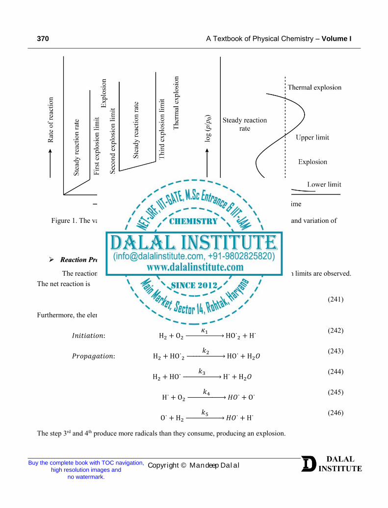
Conditions for Different Types of Explosion limits
However, it is also worthy to mention that the occurrence of explosion depends upon the experimental temperature and pressure. Typically, three explosion limits are observed as the pressure of the reacting system is raised. To understand the different explosion limits, the behavior of the denominator in equation (238) must be analysed with pressure.
1. The first explosion limit: When the pressure is very low, the movement of chain carriers towards the wall of the container is very fast resulting in a very large rate of radicals’ destruction at walls i.e. high 𝑘𝑤. Conversely, the probability of radicals colliding with each other at very low pressure resulting in a very low value of 𝑘𝑔. Therefore, we can conclude that the denominator in equation (238) has a sufficiently large positive value at low pressure giving smooth progression of the reaction without any explosion. However, with the rise in pressure, 𝑘𝑤 declines very rapidly than the increase in 𝑘𝑔. When a certain pressure value is achieved, the explosion condition is satisfied i.e.
𝑘2(𝑛 − 1)[𝐴] = 𝑘𝑤 + 𝑘𝑔 (240)
Which is the first explosion limit.
2. The second explosion limit: The first explosion limit exists over a wide range of pressure. However, if the pressure is raised continuously, the movement of chain carriers towards the wall of the container is more and more hindered resulting in a very small rate of radicals’ destruction at walls i.e. low 𝑘𝑤. Conversely, the probability of radicals colliding with each other further increases with pressure resulting in the very large value of 𝑘𝑔. Eventually, we can conclude that the denominator in equation (238) again becomes sufficiently positive giving a steady progression of the reaction. Which is the second explosion limit.
3. The third explosion limit: After the second explosion limit, the steady reaction-rate continues over a range of pressure. However, if the pressure is raised continuously, the heat produced in various propagating steps would not be able to leave the system at a rate equal to the rate at which it is produced. Therefore, this thermal effect will keep supporting the rate, eventually leading to a thermally-induced explosion. Which is the third explosion limit.
Buy the complete book with TOC navigation, high resolution images and
no watermark.
370 A Textbook of Physical Chemistry – Volume I
Copyright © Mandeep Dalal
Figure 1. The variation of reaction with pressure in branching chain reactions (left) and variation of relative pressure with time on a logarithmic scale (right).
Reaction Profile of H2-O2 Explosion
The reaction between H2 and O2 is a typical example in which all three explosion limits are observed. The net reaction is
2H2 + O2⟶ 2H2O (241)
Furthermore, the elementary steps for the same can be proposed as
𝐼𝑛𝑖𝑡𝑖𝑎𝑡𝑖𝑜𝑛: H2 + O2
𝑘1 → HO˙2 + H˙
(242)
𝑃𝑟𝑜𝑝𝑎𝑔𝑎𝑡𝑖𝑜𝑛: H2 + HO˙2
𝑘2 → HO˙ + H2𝑂
(243)
H2 + HO˙
𝑘3 → H˙ + H2𝑂
(244)
H˙ + O2
𝑘4 → 𝐻𝑂˙ + O˙
(245)
O˙ + H2
𝑘5 → 𝐻𝑂˙ + H˙
(246)
The step 3rd and 4th produce more radicals than they consume, producing an explosion.
Buy the complete book with TOC navigation, high resolution images and
no watermark.
CHAPTER 7 Chemical Dynamics – II 371
Copyright © Mandeep Dalal
Kinetics of (One Intermediate) Enzymatic Reaction: Michaelis-MentenTreatment
In 1901, a French Chemist, Victor Henri, proposed that enzyme reactions are actually initiated by a bond formed between the substrate and the enzyme. The concept was further developed by German researches Leonor Michaelis and Canadian scientist Maud Menten, who examined the kinetics of an enzymatic reaction mechanism of invertase. The final model of Michaelis and Menten's treatment was published in 1913 and gained immediate popularity among the scientific community.
𝐸 + 𝑆 𝑘1⇌𝑘−1
𝐸𝑆 𝑘2⟶ 𝑃
(247)
Where E is the enzyme that binds to a substrate S, and forms a complex ES. This enzyme-substrate complex then turns into product P. The overall rate of product formation should be
+𝑑[𝑃]
𝑑𝑡= 𝑟 = 𝑘2[𝐸𝑆]
(248)
Since [𝐸𝑆] is intermediate, the steady-state approximation can be applied i.e.
𝑅𝑎𝑡𝑒 𝑜𝑓 𝑓𝑜𝑟𝑚𝑎𝑡𝑖𝑜𝑛 𝑜𝑓 [𝐸𝑆] = 𝑅𝑎𝑡𝑒 𝑜𝑓 𝑑𝑒𝑐𝑜𝑚𝑝𝑜𝑠𝑖𝑡𝑖𝑜𝑛 𝑜𝑓 [𝐸𝑆] (249)
𝑘1[𝐸][𝑆] = 𝑘−1[𝐸𝑆] + 𝑘2[𝐸𝑆] (250)
𝑘1[𝐸][𝑆] = (𝑘−1 + 𝑘2)[𝐸𝑆] (251)
[𝐸𝑆] =𝑘1[𝐸][𝑆]
𝑘−1 + 𝑘2
(252)
Now, defining a new parameter named as Michaelis- Menten constant (𝐾𝑚) with the following expression,
𝐾𝑚 =𝑘−1 + 𝑘2𝑘1
(253)
equation (252) takes the form
[𝐸𝑆] =[𝐸][𝑆]
𝐾𝑚
(254)
Now, if we put the [𝐸𝑆] concentration given above into equation (248), we will get the rate of enzyme-catalyzed reaction in terms of substrate concentration and enzyme left unused i.e. [𝐸]. This is again a problem that can be solved if we obtain the rate expression in terms of total enzyme concentration i.e. [𝐸0]; whichwould make the calculation of catalytic efficiency much easier. In order to do so, recall the total enzyme concentration mathematically i.e.
372 A Textbook of Physical Chemistry – Volume I
Copyright © Mandeep Dalal
[𝐸0] = [𝐸] + [𝐸𝑆] (255)
Where [𝐸] is the enzyme concentration left unused whereas [𝐸𝑆] represents the enzyme concentration that is bound with the substrate. Rearranging equation (253), we get
[𝐸] = [𝐸0] − [𝐸𝑆] (256)
After using the value of [𝐸] from equation (256) in equation (254), we have
[𝐸𝑆] =
{[𝐸0] − [𝐸𝑆]}[𝑆]
𝐾𝑚
(257)
[𝐸𝑆] =
[𝐸0][𝑆] − [𝐸𝑆][𝑆]
𝐾𝑚
(258)
Rearranging for [𝐸𝑆] again
𝐾𝑚[𝐸𝑆] = [𝐸0][𝑆] − [𝐸𝑆][𝑆] (259)
𝐾𝑚[𝐸𝑆] + [𝐸𝑆][𝑆] = [𝐸0][𝑆] (260)
[𝐸𝑆] =
[𝐸0][𝑆]
𝐾𝑚 + [𝑆]
(261)
After putting the value of [𝐸𝑆] from above equation into equation (248), we get
𝑟 =
𝑘2[𝐸0][𝑆]
𝐾𝑚 + [𝑆]
(262)
If the rate of the enzyme-catalyzed reaction is recorded in the very initial stage, the substrate concentration can also be replaced by the initial substrate concentration i.e. [𝑆0]. Therefore, the initial enzyme-catalyzed rate (𝑟0) should be
𝑟0 =
𝑘2[𝐸0][𝑆0]
𝐾𝑚 + [𝑆0]
(263)
Which is the well-known Michaelis-Menten equation.
Although the equation (263) is the complete form of the Michaelis-Menten equation that has measurable quantities like[𝐸0] and [𝑆0], the more popular form of the same includes the maximum initial rate. At very large initial substrate concentration, the 𝐾𝑚 can simply be neglected in comparison to [𝑆0] in the denominator, which makes the equation (263) to take the form
𝑟𝑚𝑎𝑥 =
𝑘2[𝐸0][𝑆0]
[𝑆0]= 𝑘2[𝐸0]
(264)
Buy the complete book with TOC navigation, high resolution images and
no watermark.
CHAPTER 7 Chemical Dynamics – II 373
Copyright © Mandeep Dalal
After using the 𝑘2[𝐸0] = 𝑟𝑚𝑎𝑥 in equation (263), we have
𝑟0 =
𝑟𝑚𝑎𝑥[𝑆0]
𝐾𝑚 + [𝑆0]
(265)
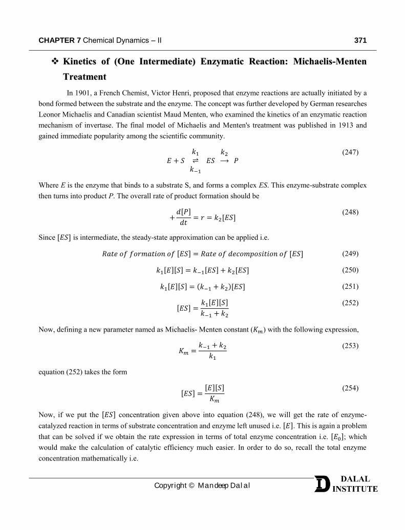
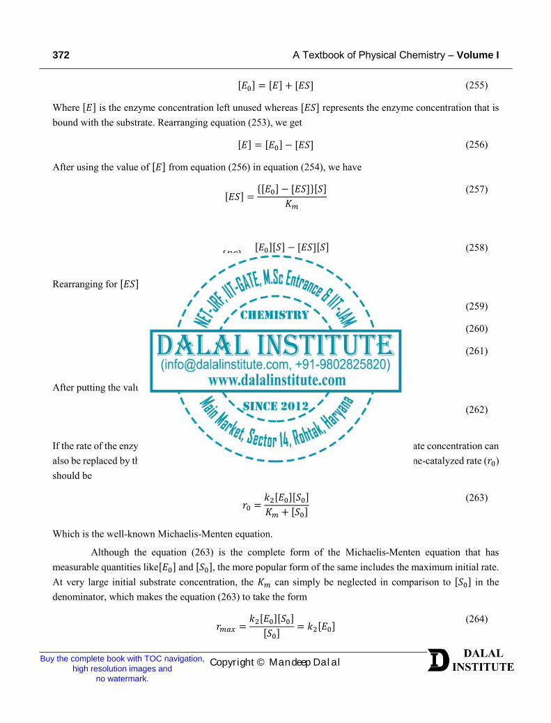
Which is the most popular form of the Michaelis-Menten equation. The plot of the initial reaction rate for the enzyme-catalyzed reaction is given below.
Figure 2. The variation of initial reaction rate as a function of substrate concentration for an enzyme-catalyzed reaction.
Order of Enzyme Catalysed Reactions
The reaction kinetics of the enzyme-catalyzed reactions can be well understood by looking at the general form of Michaelis-Menten equation.
i) At high [S0]: When initial substrate concentration is very high, Km can be neglected, and the equation (263) takes the form
𝑟0 =
𝑘2[𝐸0][𝑆0]
[𝑆0]= 𝑘2[𝐸0]
(266)
Hence, the reaction will be zero-order w.r.t. substrate concentration and first order w.r.t the total enzyme concertation.
Buy the complete book with TOC navigation, high resolution images and
no watermark.
374 A Textbook of Physical Chemistry – Volume I
Copyright © Mandeep Dalal
ii) At low [S0]: When initial substrate concentration is low, [S0] can be neglected, and the equation (263) takes the form
𝑟0 =
𝑘2𝐾𝑚[𝐸0][𝑆0]
(267)
Hence, the reaction will be the first-order w.r.t. substrate concentration and first order w.r.t the total enzyme concertation as well.
Calculation of Catalytic Efficiency
The catalytic efficiency of enzyme-catalyzed reactions is simply the maximum overall reaction rate per unit of enzyme concentration. When initial substrate concentration is very high, Km can be neglected, and the equation (263) takes the form
𝑟𝑚𝑎𝑥 =
𝑘2[𝐸0][𝑆0]
[𝑆0]= 𝑘2[𝐸0]
(268)
𝑘2 =𝑟𝑚𝑎𝑥[𝐸0]
(269)
Hence, k2 is simply equal to the catalytic efficiency of enzyme-catalyzed reactions.
Calculation of Michaelis-Menten Constant
The Michaelis-Menten constant of enzyme-catalyzed reactions can simply be calculated once the maximum initial reaction rate is known. When initial substrate concentration is very high, Km can be neglected, and the equation (263) takes the form
𝑟𝑚𝑎𝑥 =
𝑘2[𝐸0][𝑆0]
[𝑆0]= 𝑘2[𝐸0]
(270)
After using the 𝑘2[𝐸0] = 𝑟𝑚𝑎𝑥 in equation (263), we have
𝑟0 =
𝑟𝑚𝑎𝑥[𝑆0]
𝐾𝑚 + [𝑆0]
(271)
When the initial reaction rate is half of the maximum initial rate i.e. 𝑟0 = 𝑟𝑚𝑎𝑥/2, we have
𝑟𝑚𝑎𝑥2=𝑟𝑚𝑎𝑥[𝑆0]
𝐾𝑚 + [𝑆0]
(272)
𝐾𝑚 + [𝑆0] = 2[𝑆0] (273)
𝐾𝑚 = [𝑆0] (274)
Hence, the concentration at which the initial rate in half of the maximum initial rate, will be equal to 𝐾𝑚.
Buy the complete book with TOC navigation, high resolution images and
no watermark.
CHAPTER 7 Chemical Dynamics – II 375
Copyright © Mandeep Dalal
Evaluation of Michaelis's Constant for Enzyme-Substrate Binding byLineweaver-Burk Plot and Eadie-Hofstee Methods
The conventional approach to determine the Michaelis's constant (Km) involve the plot of initial reaction rate vs initial substrate concentration. Then the Michaelis-Menten constant of enzyme-catalyzed reactions can simply be calculated once the maximum initial reaction rate is known. The typical Michaelis-Menten is used to fit the data is given below.
𝑟0 =𝑟𝑚𝑎𝑥[𝑆0]
𝐾𝑚 + [𝑆0]
(275)
Where 𝑟𝑚𝑎𝑥 = 𝑘2[𝐸0] is the maximum initial rate at [𝐸0] enzyme concentration whereas [𝑆0] is the initialsubstrate concentration. Finally, the concentration at which the initial rate in half of the maximum initial rate, will be equal to 𝐾𝑚.
This conventional method, however, suffers from serious limitations like the need for lots of data points until the initial rate becomes constant. Therefore, two other methods are quite popular to find Michaelis's constant without getting the actual plateau in the initial reaction rate. In this section, we will discuss two such methods for the evaluation of Michaelis's constant for enzyme-substrate binding.
The Lineweaver-Burk Plot to Evaluate Michaelis's Constant
In order to understand the Lineweaver-Burk method for the determination of the maximum initial rate (𝑟𝑚𝑎𝑥) and Michaelis's constant, we need to rearrange the general Michaelis-Menten equation first i.e. thereciprocal of equation (275) as given below.
1
𝑟0=𝐾𝑚 + [𝑆0]
𝑟𝑚𝑎𝑥[𝑆0]
(276)
or
1
𝑟0=
𝐾𝑚𝑟𝑚𝑎𝑥[𝑆0]
+[𝑆0]
𝑟𝑚𝑎𝑥[𝑆0]
(277)
or
1
𝑟0=𝐾𝑚𝑟𝑚𝑎𝑥
1
[𝑆0]+
1
𝑟𝑚𝑎𝑥
(278)
Which is the equation of the straight line (𝑦 = 𝑚𝑥 + 𝑐). Therefore, if we plot the reciprocal of initial reaction rate vs the reciprocal of initial substrate concentration; the slope and intercepts will give 𝐾𝑚/𝑟𝑚𝑎𝑥 and 1/𝑟𝑚𝑎𝑥,respectively.
376 A Textbook of Physical Chemistry – Volume I
Copyright © Mandeep Dalal
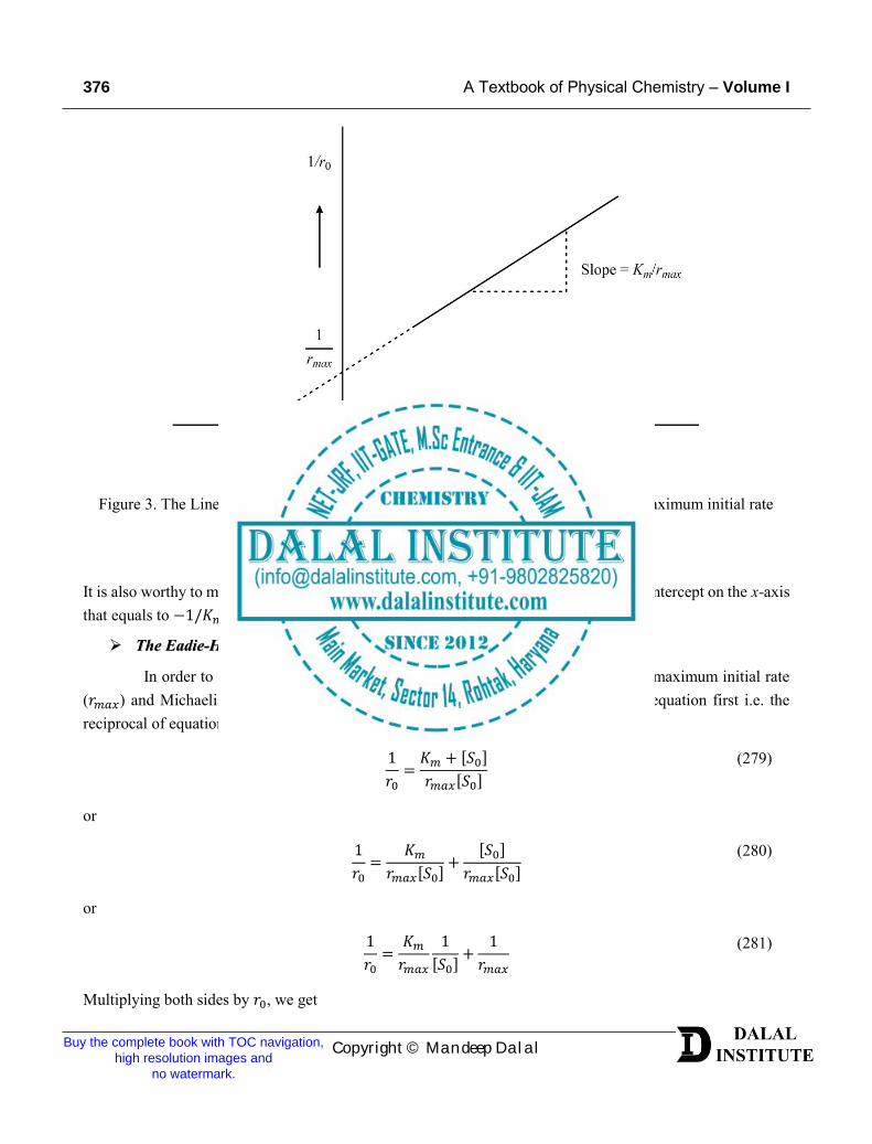
Figure 3. The Lineweaver-burk plot for enzyme-catalyzed reactions to evaluate the maximum initial rate (𝑟𝑚𝑎𝑥) and Michaelis's constant.
It is also worthy to mention that if the intercept is further extrapolated, it will lead to the intercept on the x-axis that equals to −1/𝐾𝑚.
The Eadie-Hofstee Plot to Evaluate Michaelis's Constant
In order to understand the Eadie-Hofstee method for the determination of the maximum initial rate (𝑟𝑚𝑎𝑥) and Michaelis's constant, we need to rearrange the general Michaelis-Menten equation first i.e. the reciprocal of equation (275) as given below.
1
𝑟0=𝐾𝑚 + [𝑆0]
𝑟𝑚𝑎𝑥[𝑆0]
(279)
or
1
𝑟0=
𝐾𝑚𝑟𝑚𝑎𝑥[𝑆0]
+[𝑆0]
𝑟𝑚𝑎𝑥[𝑆0]
(280)
or
1
𝑟0=𝐾𝑚𝑟𝑚𝑎𝑥
1
[𝑆0]+
1
𝑟𝑚𝑎𝑥 (281)
Multiplying both sides by 𝑟0, we get
Buy the complete book with TOC navigation, high resolution images and
no watermark.
CHAPTER 7 Chemical Dynamics – II 377
Copyright © Mandeep Dalal
𝑟0𝑟0=𝐾𝑚𝑟𝑚𝑎𝑥
𝑟0[𝑆0]
+𝑟0𝑟𝑚𝑎𝑥
(282)
Rearranging for 𝑟0/[𝑆0], we get
𝑟0𝑟0−𝑟0𝑟𝑚𝑎𝑥
=𝐾𝑚𝑟𝑚𝑎𝑥
𝑟0[𝑆0]
(283)
𝑟0[𝑆0]
=𝑟0𝑟0
𝑟𝑚𝑎𝑥𝐾𝑚
−𝑟0𝑟𝑚𝑎𝑥
𝑟𝑚𝑎𝑥𝐾𝑚
(284)
𝑟0[𝑆0]
=𝑟𝑚𝑎𝑥𝐾𝑚
−𝑟0𝐾𝑚
(285)
𝑟0[𝑆0]
= −1
𝐾𝑚𝑟0 +
𝑟𝑚𝑎𝑥𝐾𝑚
(286)
Which is the equation of the straight line (𝑦 = 𝑚𝑥 + 𝑐). Therefore, if we plot the ratio of initial reaction rate to initial substrate concentration vs the initial reaction rate; the slope and intercepts will give −1/𝐾𝑚 and 𝑟𝑚𝑎𝑥/𝐾𝑚, respectively.
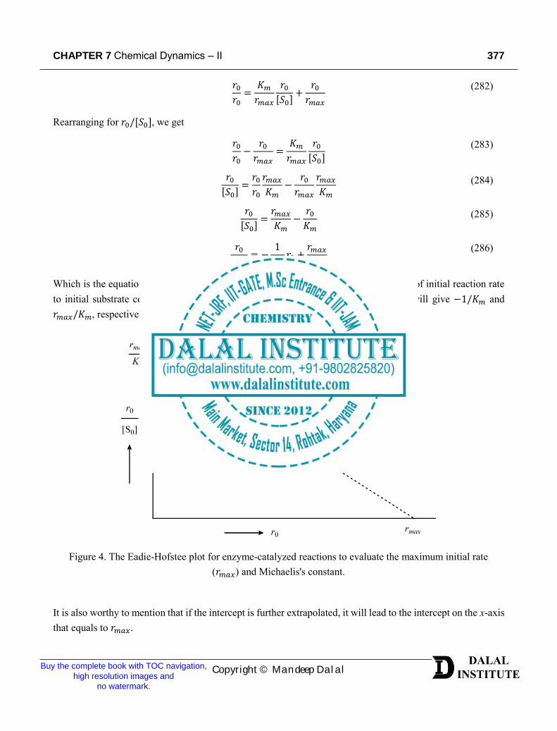
Figure 4. The Eadie-Hofstee plot for enzyme-catalyzed reactions to evaluate the maximum initial rate (𝑟𝑚𝑎𝑥) and Michaelis's constant.
It is also worthy to mention that if the intercept is further extrapolated, it will lead to the intercept on the x-axis that equals to 𝑟𝑚𝑎𝑥.
Buy the complete book with TOC navigation, high resolution images and
no watermark.
378 A Textbook of Physical Chemistry – Volume I
Copyright © Mandeep Dalal
Competitive and Non-Competitive InhibitionAn enzyme inhibitor is a compound that binds to an enzyme and decreases its overall activity, and
the phenomenon is typically known as “enzyme inhibition”. Two of the most common enzyme inhibition processes will be discussed in this section.
Competitive Inhibition
In the case of competitive enzyme inhibition, the binding of an inhibitor prevents the binding of the substrate and the enzyme. This type of behavior is actually achieved by blocking the binding site of the target molecule (the active site) by some means. The competitive enzyme inhibition can be classified into two types as discussed below.
1. Fully competitive inhibition: The fully competitive inhibition occurs when an enzyme (E) binds with thesubstrate (S) and inhibitor (I) separately, and it is only the enzyme-substrate complex (ES) that will convert into the product. This whole process can be described mathematically as
𝐸 + 𝑆 𝑘1⇌𝑘−1
𝐸𝑆 𝑘2⟶ 𝐸 + 𝑃
(287)
𝐸 + 𝐼 𝑘3⇌𝑘−3
𝐸𝐼 (288)
After applying the steady-state approximation on ES, we have
𝑑[𝐸𝑆]
𝑑𝑡= 𝑘1[𝐸][𝑆] − 𝑘−1[𝐸𝑆] − 𝑘2[𝐸𝑆] = 0
(289)
𝑘1[𝐸][𝑆] = 𝑘−1[𝐸𝑆] + 𝑘2[𝐸𝑆] (290)
[𝐸𝑆] =𝑘1[𝐸][𝑆]
𝑘−1 + 𝑘2
(291)
When [𝑆0] ≫ [𝐸0], we can assume [𝑆0] ≈ [𝑆], and also
[𝐸0] = [𝐸] + [𝐸𝑆] + [𝐸𝐼] (292)
[𝐸] = [𝐸0] − [𝐸𝑆] − [𝐸𝐼] (293)
Now recalling the equilibrium constant for inhibition equilibria i.e.
𝐾3 =𝑘3𝑘−3
=[𝐸𝐼]
[𝐸][𝐼]
(294)
𝐾I =1
𝐾3=[𝐸][𝐼]
[𝐸𝐼]
(295)
CHAPTER 7 Chemical Dynamics – II 379
Copyright © Mandeep Dalal
Hence, we can say
[𝐸𝐼] =
[𝐸][𝐼]
𝐾I
(296)
After using the value of [𝐸𝐼] from equation (296) into equation (293), we have
[𝐸] = [𝐸0] − [𝐸𝑆] −
[𝐸][𝐼]
𝐾I
(297)
[𝐸] =
𝐾I[𝐸0] − 𝐾I[𝐸𝑆] − [𝐸][𝐼]
𝐾I
(298)
𝐾I[𝐸] = 𝐾I[𝐸0] − 𝐾I[𝐸𝑆] − [𝐸][𝐼] (299)
𝐾I[𝐸] + [𝐸][𝐼] = 𝐾I[𝐸0] − 𝐾I[𝐸𝑆] (300)
[𝐸] =
𝐾I[𝐸0] − 𝐾I[𝐸𝑆]
𝐾I + [𝐼]
(301)
Using the above-derived result in equation (291), we have
[𝐸𝑆] =
𝑘1[𝑆]
𝑘−1 + 𝑘2 𝐾I[𝐸0] − 𝐾I[𝐸𝑆]
𝐾I + [𝐼]=[𝑆]
𝐾𝑚 𝐾I[𝐸0] − 𝐾I[𝐸𝑆]
𝐾I + [𝐼]
(302)
[𝐸𝑆] =
𝐾I[𝐸0][𝑆] − 𝐾I[𝐸𝑆][𝑆]
𝐾𝑚𝐾I + 𝐾𝑚[𝐼]
(303)
Now rearranging further for [𝐸𝑆], we get
𝐾𝑚𝐾I[𝐸𝑆] + 𝐾𝑚[𝐼][𝐸𝑆] = 𝐾I[𝐸0][𝑆] − 𝐾I[𝐸𝑆][𝑆] (304)
𝐾𝑚𝐾I[𝐸𝑆] + 𝐾𝑚[𝐼][𝐸𝑆] + 𝐾I[𝐸𝑆][𝑆] = 𝐾I[𝐸0][𝑆] (305)
[𝐸𝑆] =
𝐾I[𝐸0][𝑆]
𝐾𝑚𝐾I + 𝐾𝑚[𝐼] + 𝐾I[𝑆]
(306)
Since the rate of formation of product is
𝑟0 = 𝑘2[𝐸𝑆] (307)
Using the value of [𝐸𝑆] from equation (306) in equation (307), we get
𝑟0 =
𝑘2𝐾I[𝐸0][𝑆]
𝐾𝑚𝐾I + 𝐾𝑚[𝐼] + 𝐾I[𝑆]
(308)
Since 𝑘2[𝐸0] is 𝑟𝑚𝑎𝑥, the equation (308) takes the form
Buy the complete book with TOC navigation, high resolution images and
no watermark.
380 A Textbook of Physical Chemistry – Volume I
Copyright © Mandeep Dalal
𝑟0 =
𝑟𝑚𝑎𝑥 𝐾I[𝑆]
𝐾𝑚𝐾I + 𝐾𝑚[𝐼] + 𝐾I[𝑆]
(309)
Taking the reciprocal to get Lineweaver-Burk plot
1
𝑟0=𝐾𝑚𝐾I + 𝐾𝑚[𝐼] + 𝐾I[𝑆]
𝑟𝑚𝑎𝑥 𝐾I[𝑆]
(310)
1
𝑟0=
𝐾𝑚𝐾I𝑟𝑚𝑎𝑥 𝐾I[𝑆]
+𝐾𝑚[𝐼]
𝑟𝑚𝑎𝑥 𝐾I[𝑆]+
𝐾I[𝑆]
𝑟𝑚𝑎𝑥 𝐾I[𝑆]
(311)
1
𝑟0= (
𝐾𝑚𝑟𝑚𝑎𝑥
+𝐾𝑚[𝐼]
𝑟𝑚𝑎𝑥 𝐾I)1
[𝑆] +
1
𝑟𝑚𝑎𝑥
(312)
Rearranging further and using initial substrate concentration, we get
1
𝑟0=𝐾𝑚𝑟𝑚𝑎𝑥
(1 +[𝐼]
𝐾I)1
[𝑆0] +
1
𝑟𝑚𝑎𝑥
(313)
After comparing with equation without enzyme inhibition i.e.
1
𝑟0=𝐾𝑚𝑟𝑚𝑎𝑥
1
[𝑆0]+
1
𝑟𝑚𝑎𝑥 (314)
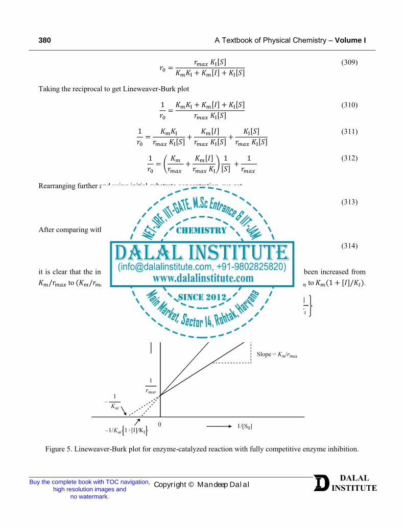
it is clear that the intercepts in both the equations are the same whereas the slope has been increased from 𝐾𝑚/𝑟𝑚𝑎𝑥 to (𝐾𝑚/𝑟𝑚𝑎𝑥)(1 + [𝐼]/𝐾𝐼). This implies that enzyme inhibition changed the 𝐾𝑚 to 𝐾𝑚(1 + [𝐼]/𝐾𝐼).
Figure 5. Lineweaver-Burk plot for enzyme-catalyzed reaction with fully competitive enzyme inhibition.
Buy the complete book with TOC navigation, high resolution images and
no watermark.
CHAPTER 7 Chemical Dynamics – II 381
Copyright © Mandeep Dalal
2. Partially competitive inhibition: The partially competitive inhibition occurs when the enzyme (E) binds with the substrate (S) and inhibitor (I) simultaneously, and complex ES and EI also combine with I and S to give EIS. Also, besides the enzyme-substrate complex (ES), the complex EIS will also convert into the product with the same rate of reaction. This whole process can be described mathematically as
𝐸 + 𝑆
𝐾1′
⇌ 𝐸𝑆 𝑘2⟶ 𝐸 + 𝑃
(315)
𝐸 + 𝐼
𝐾2′
⇌ 𝐸𝐼 (316)
𝐸𝐼 + 𝑆
𝐾3′
⇌ 𝐸𝐼𝑆 (317)
𝐸𝑆 + 𝐼
𝐾4′
⇌ 𝐸𝐼𝑆 (318)
𝐸𝐼𝑆
𝑘2⟶ 𝐸𝐼 + 𝑃
(319)
According to classical Michaelis-Menten equation 𝐾𝑚 = (𝑘2 + 𝑘−1)/𝑘1; however, if 𝑘2 ≪ 𝑘−1, we have 𝐾𝑚 = 𝑘−1/𝑘1 or 𝐾𝑚 = 1/𝐾1′. Now, set the following results
𝐾𝑚 =
1
𝐾1′ =
[𝐸][𝑆]
[𝐸𝑆]
(320)
𝐾2 =
1
𝐾2′ =
[𝐸][𝐼]
[𝐸𝐼]
(321)
𝐾3 =
1
𝐾3′ =
[𝐸𝐼][𝑆]
[𝐸𝐼𝑆]
(322)
𝐾4 =
1
𝐾4′ =
[𝐸𝑆][𝐼]
[𝐸𝐼𝑆]
(323)
Following enzyme conservation, we have
[𝐸0] = [𝐸] + [𝐸𝑆] + [𝐸𝐼] + [𝐸𝐼𝑆] (324)
Using values of [𝐸𝑆], [𝐸𝐼] and [𝐸𝐼𝑆] from equation (320-322) into equation (324), we get
[𝐸0] = [𝐸] +
[𝐸][𝑆]
𝐾𝑚+[𝐸][𝐼]
𝐾2+[𝐸][𝐼][𝑆]
𝐾2𝐾3
(325)
[𝐸] =
𝐾𝑚[𝐸0]
𝐾𝑚(1 + [𝐼]/𝐾2) + [𝑆](1 + 𝐾𝑚[𝐼]/𝐾2𝐾3)
(326)
The overall reaction rate of product formations should be
Buy the complete book with TOC navigation, high resolution images and
no watermark.
382 A Textbook of Physical Chemistry – Volume I
Copyright © Mandeep Dalal
𝑟0 = 𝑘2[𝐸𝑆] + 𝑘2[𝐸𝐼𝑆] (327)
After using values of [𝐸𝑆] and [𝐸𝐼𝑆] from equation (320, 322) into equation (327), we get
𝑟0 = 𝑘2
[𝐸][𝑆]
𝐾𝑚+ 𝑘2
[𝐸][𝐼][𝑆]
𝐾2𝐾3
(328)
Substituting the value of [𝐸] from equation (326) in (328), and rearranging at initial substrate concentration
𝑟0 =
𝑘2[𝐸0][𝑆0]
{𝐾𝑚(1 + [𝐼]/𝐾2)/(1 + 𝐾𝑚[𝐼]/𝐾2𝐾3)} + [𝑆0]
(329)
Since 𝑘2[𝐸0] is 𝑟𝑚𝑎𝑥, equation (329) takes the following form after the reciprocal to get Lineweaver-Burk plot
1
𝑟0={𝐾𝑚(1 + [𝐼]/𝐾2)/(1 + 𝐾𝑚[𝐼]/𝐾2𝐾3)}
𝑟𝑚𝑎𝑥
1
[𝑆0]+
1
𝑟𝑚𝑎𝑥
(330)
After comparing with equation without enzyme inhibition i.e.
1
𝑟0=𝐾𝑚𝑟𝑚𝑎𝑥
1
[𝑆0]+
1
𝑟𝑚𝑎𝑥 (331)
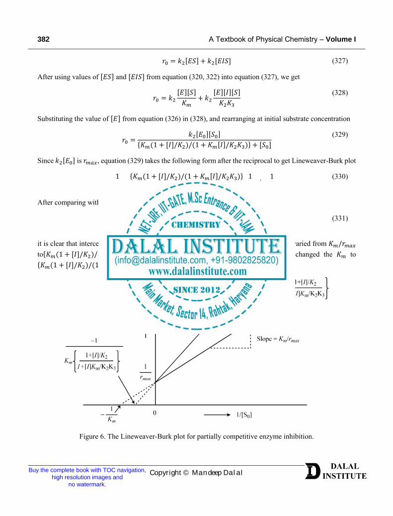
it is clear that intercepts in both the equations are the same whereas the slope has been varied from 𝐾𝑚/𝑟𝑚𝑎𝑥 to{𝐾𝑚(1 + [𝐼]/𝐾2)/(1 + 𝐾𝑚[𝐼]/𝐾2𝐾3)}/𝑟𝑚𝑎𝑥. This implies that enzyme inhibition changed the 𝐾𝑚 to {𝐾𝑚(1 + [𝐼]/𝐾2)/(1 + 𝐾𝑚[𝐼]/𝐾2𝐾3)}.
Figure 6. The Lineweaver-Burk plot for partially competitive enzyme inhibition.
Buy the complete book with TOC navigation, high resolution images and
no watermark.
CHAPTER 7 Chemical Dynamics – II 383
Copyright © Mandeep Dalal
Non-Competitive Inhibition
Non-competitive inhibition may simply be defined as the enzyme inhibition where the inhibitor decreases the activity of the enzyme catalysis and binds equally well to the enzyme whether or not it has already bound the substrate. The non-competitive enzyme inhibition can be classified into two types as discussed below.
1. Fully non-competitive inhibition: The fully non-competitive inhibition occurs when an enzyme (E) binds with inhibitor (I), and complex ES and EI also combine with I and S to give EIS. However, it is only the enzyme-substrate complex (ES) that converts into the product. This whole process can be described mathematically as
𝐸 + 𝑆
𝐾1′
⇌ 𝐸𝑆 𝑘2⟶ 𝐸 + 𝑃
(332)
𝐸 + 𝐼
𝐾2′
⇌ 𝐸𝐼 (333)
𝐸𝐼 + 𝑆
𝐾1′
⇌ 𝐸𝐼𝑆 (334)
𝐸𝑆 + 𝐼
𝐾2′
⇌ 𝐸𝐼𝑆 (335)
According to classical Michaelis-Menten equation 𝐾𝑚 = (𝑘2 + 𝑘−1)/𝑘1; however, if 𝑘2 ≪ 𝑘−1, we have 𝐾𝑚 = 𝑘−1/𝑘1 or 𝐾𝑚 = 1/𝐾1′. Now, set the following results
𝐾𝑚 =
1
𝐾1′ =
[𝐸][𝑆]
[𝐸𝑆]=[𝐸][𝑆]
[𝐸𝐼𝑆]
(336)
𝐾I =
1
𝐾2′ =
[𝐸][𝐼]
[𝐸𝐼]=[𝐸𝑆][𝐼]
[𝐸𝐼𝑆]
(337)
Following enzyme conservation, we have
[𝐸0] = [𝐸] + [𝐸𝑆] + [𝐸𝐼] + [𝐸𝐼𝑆] (338)
[𝐸] = [𝐸0] − [𝐸𝑆] − [𝐸𝐼] − [𝐸𝐼𝑆] (339)
Using values of [𝐸𝑆], [𝐸𝐼] and [𝐸𝐼𝑆] from equation (336-337) into equation (338), we get
[𝐸0] = [𝐸] +
[𝐸][𝑆]
𝐾𝑚+[𝐸][𝐼]
𝐾I+[𝐸][𝐼][𝑆]
𝐾𝑚𝐾I
(340)
[𝐸] =
[𝐸0]
(1 + [𝑆]/𝐾𝑚)(1 + [𝐼]/𝐾𝐼)
(341)
The overall reaction rate of product formations should be
Buy the complete book with TOC navigation, high resolution images and
no watermark.
384 A Textbook of Physical Chemistry – Volume I
Copyright © Mandeep Dalal
𝑟0 = 𝑘2[𝐸𝑆] (342)
After using values of [𝐸𝑆] from equation (336) into equation (342), we get
𝑟0 = 𝑘2
[𝐸][𝑆]
𝐾𝑚
(343)
Substituting the value of [𝐸] from equation (341) in (343), and rearranging at initial substrate concentration
𝑟0 =
𝑘2[𝐸0][𝑆0]
(𝐾𝑚 + [𝑆0])(1 + [𝐼]/𝐾𝐼)
(344)
Since 𝑘2[𝐸0] is 𝑟𝑚𝑎𝑥, the equation (344) takes the form
𝑟0 =
𝑟𝑚𝑎𝑥[𝑆0]
(𝐾𝑚 + [𝑆0])(1 + [𝐼]/𝐾𝐼)
(345)
Taking the reciprocal to get Lineweaver-Burk plot
1
𝑟0=𝐾𝑚𝑟𝑚𝑎𝑥
(1 +[𝐼]
𝐾I)1
[𝑆0]+
1
𝑟𝑚𝑎𝑥(1 +
[𝐼]
𝐾I)
(346)
After comparing with equation without enzyme inhibition i.e.
1
𝑟0=𝐾𝑚𝑟𝑚𝑎𝑥
1
[𝑆0]+
1
𝑟𝑚𝑎𝑥 (347)
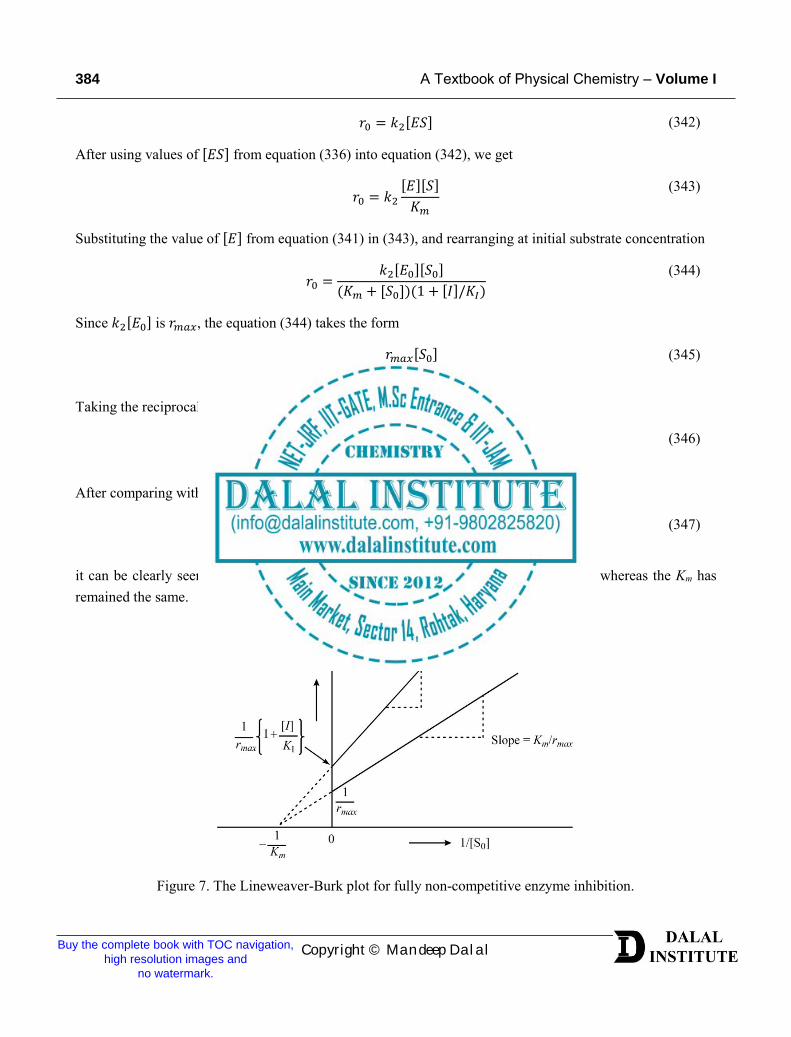
it can be clearly seen that intercept is increased from 1/𝑟𝑚𝑎𝑥 to (1/𝑟𝑚𝑎𝑥)(1 + [𝐼]/𝐾𝐼) whereas the Km has remained the same.
Figure 7. The Lineweaver-Burk plot for fully non-competitive enzyme inhibition.
Buy the complete book with TOC navigation, high resolution images and
no watermark.
CHAPTER 7 Chemical Dynamics – II 385
Copyright © Mandeep Dalal
2. Partially non-competitive inhibition: The partially non-competitive inhibition occurs when an enzyme (E) binds with inhibitor (I), and complex ES and EI also combine with I and S to give EIS. However, unlike fully non-competitive inhibition, besides the enzyme-substrate complex (ES), the complex will also convert into the product. This whole process can be described mathematically as
𝐸 + 𝑆
𝐾1′
⇌ 𝐸𝑆 𝑘2⟶ 𝐸 + 𝑃
(348)
and
𝐸 + 𝐼
𝐾2′
⇌ 𝐸𝐼 (349)
and
𝐸𝐼 + 𝑆
𝐾1′
⇌ 𝐸𝐼𝑆 (350)
and
𝐸𝑆 + 𝐼
𝐾2′
⇌ 𝐸𝐼𝑆 (351)
and
𝐸𝐼𝑆
𝑘′
⟶ 𝐸𝐼 + 𝑃 (352)
According to classical Michaelis-Menten equation 𝐾𝑚 = (𝑘2 + 𝑘−1)/𝑘1; however, if 𝑘2 ≪ 𝑘−1, we have 𝐾𝑚 = 𝑘−1/𝑘1 or 𝐾𝑚 = 1/𝐾1′. Now, set the following results
𝐾𝑚 =
1
𝐾1′ =
[𝐸][𝑆]
[𝐸𝑆]
(353)
and
𝐾𝐼 =
1
𝐾2′ =
[𝐸][𝐼]
[𝐸𝐼]
(354)
and
𝐾𝑚 =
1
𝐾1′ =
[𝐸𝐼][𝑆]
[𝐸𝐼𝑆]
(355)
and
𝐾𝐼 =
1
𝐾2′ =
[𝐸𝑆][𝐼]
[𝐸𝐼𝑆]
(356)
Buy the complete book with TOC navigation, high resolution images and
no watermark.
386 A Textbook of Physical Chemistry – Volume I
Copyright © Mandeep Dalal
Following enzyme conservation, we have
[𝐸0] = [𝐸] + [𝐸𝑆] + [𝐸𝐼] + [𝐸𝐼𝑆] (357)
Using values of [𝐸𝑆], [𝐸𝐼] and [𝐸𝐼𝑆] from equation (353-356) into equation (357), we get the following expression.
[𝐸0] = [𝐸] +
[𝐸][𝑆]
𝐾𝑚+[𝐸][𝐼]
𝐾𝐼+[𝐸][𝐼][𝑆]
𝐾𝑚𝐾𝐼
(358)
or
[𝐸] =
[𝐸0]
(1 + ([𝑆]/𝐾𝑚)(1 + [𝐼]/𝐾𝐼)
(359)
The overall reaction rate of product formations should be
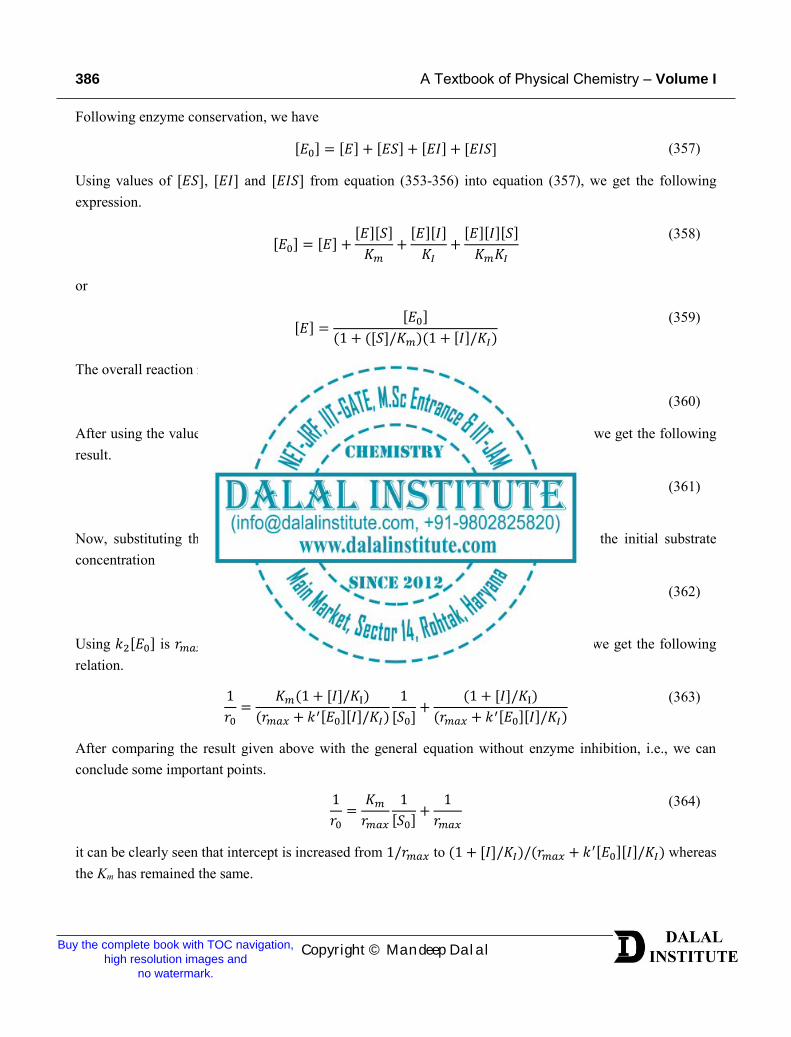
𝑟0 = 𝑘2[𝐸𝑆] + 𝑘′[𝐸𝐼𝑆] (360)
After using the values of [𝐸𝑆] and [𝐸𝐼𝑆] from equation (353-356) into equation (360), we get the following result.
𝑟0 = 𝑘2
[𝐸][𝑆]
𝐾𝑚+ 𝑘′
[𝐸][𝐼][𝑆]
𝐾𝑚𝐾𝐼
(361)
Now, substituting the value of [𝐸] from equation (359) in (361), and rearranging at the initial substrate concentration
𝑟0 =
(𝑘2[𝐸0][𝑆0] + 𝑘′[𝐸0][𝑆0][𝐼]/𝐾𝐼)/(1 + [𝐼]/𝐾𝐼 )
𝐾𝑚 + [𝑆0]
(362)
Using 𝑘2[𝐸0] is 𝑟𝑚𝑎𝑥 and then taking the reciprocal to get the Lineweaver-Burk plot, we get the following relation.
1
𝑟0=
𝐾𝑚(1 + [𝐼]/𝐾I)
(𝑟𝑚𝑎𝑥 + 𝑘′[𝐸0][𝐼]/𝐾𝐼)
1
[𝑆0]+
(1 + [𝐼]/𝐾I)
(𝑟𝑚𝑎𝑥 + 𝑘′[𝐸0][𝐼]/𝐾𝐼)
(363)
After comparing the result given above with the general equation without enzyme inhibition, i.e., we can conclude some important points.
1
𝑟0=𝐾𝑚𝑟𝑚𝑎𝑥
1
[𝑆0]+
1
𝑟𝑚𝑎𝑥 (364)
it can be clearly seen that intercept is increased from 1/𝑟𝑚𝑎𝑥 to (1 + [𝐼]/𝐾𝐼)/(𝑟𝑚𝑎𝑥 + 𝑘′[𝐸0][𝐼]/𝐾𝐼) whereas the Km has remained the same.
Buy the complete book with TOC navigation, high resolution images and
no watermark.
CHAPTER 7 Chemical Dynamics – II 387
Copyright © Mandeep Dalal
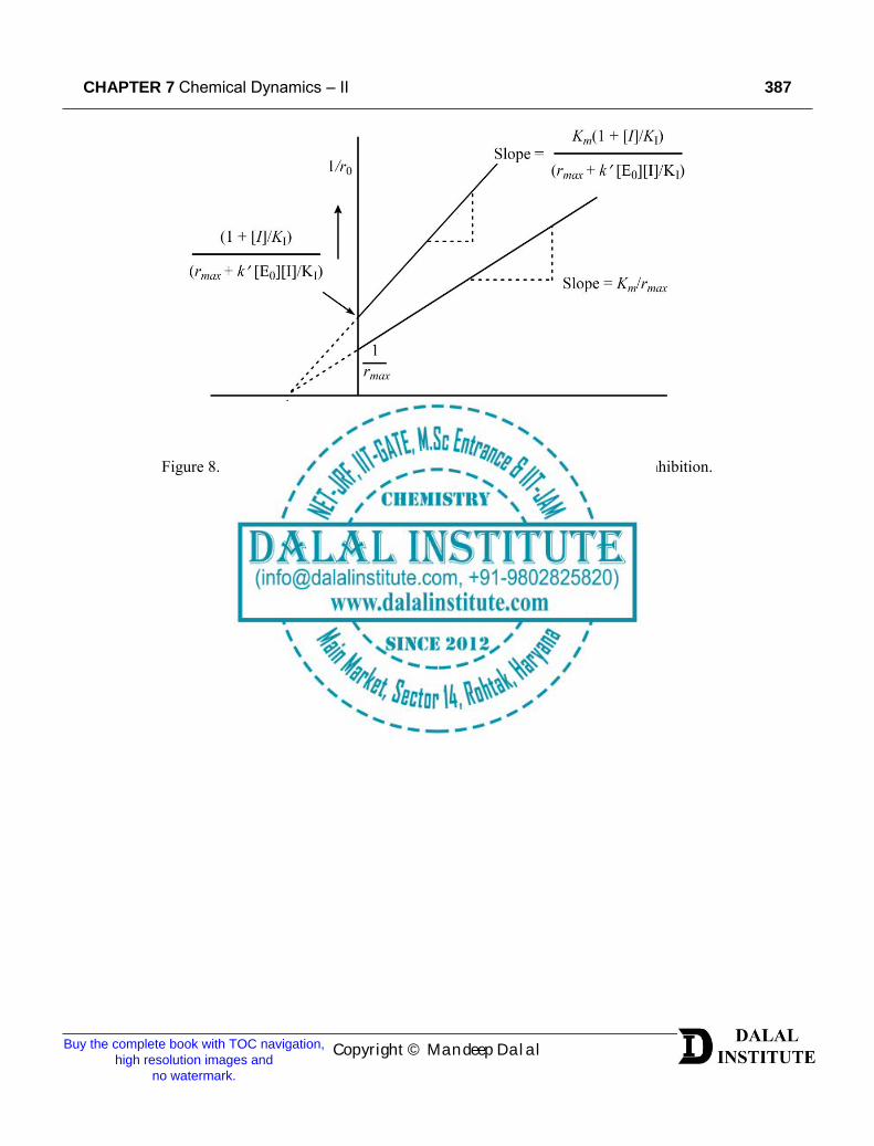
Figure 8. The Lineweaver-Burk plot for partially non-competitive enzyme inhibition.
Buy the complete book with TOC navigation, high resolution images and
no watermark.
388 A Textbook of Physical Chemistry – Volume I
Copyright © Mandeep Dalal
ProblemsQ 1. What are chemical chain reactions? Discuss their general kinetics.
Q 2. Derive and discuss the rate law for the decomposition of ethane.
Q 3. Define photochemical reactions. How they are different from thermochemical reactions?
Q 4. What is the photochemical quantum yield of a reaction? Derive and discuss the same for photochemical combination H2-Br2 case.
Q 5. Derive and discuss the Rice-Herzfeld mechanism of decomposition of Acetaldehyde.
Q 6. Define the chain length.
Q 7. Calculate the expression for the chain length for the dehydrogenation of ethane.
Q 8. What are the branching chain reactions? How they lead to the situation of the explosion?
Q 9. Derive and discuss the conventional Michaelis-Menten equation for enzyme-catalyzed reactions.
Q 10. How would you treat Michaelis-Menten equations to get Lineweaver-Burk plot?
Q 11. Discuss the Eadie-Hofstee method for the evaluation of Michaelis-Menten constant in enzyme-catalyzed reactions.
Q 12. What is enzyme inhibition? Discuss the fully competitive enzyme inhibition in detail.
CHAPTER 7 Chemical Dynamics – II 389
Copyright © Mandeep Dalal
Bibliography[1] B. R. Puri, L. R. Sharma, M. S. Pathania, Principles of Physical Chemistry, Vishal Publications, Jalandhar, India, 2008.
[2] P. Atkins, J. Paula, Physical Chemistry, Oxford University Press, Oxford, UK, 2010.
[3] E. Steiner, The Chemistry Maths Book, Oxford University Press, Oxford, UK, 2008.
[4] S. A. Arrhenius, Über die Dissociationswärme und den Einfluß der Temperatur auf den Dissociationsgrad der Elektrolyte. Z. Phys. Chem. 4 (1889) 96–116.
[5] S. A. Arrhenius, Über die Reaktionsgeschwindigkeit bei der Inversion von Rohrzucker durch Säuren Z. Phys. Chem. 4 (1889) 226–248.
[6] K. J. Laidler, Chemical Kinetics, Harper & Row, New York, USA, 1987.
[7] K. J. Laidler, The World of Physical Chemistry, Oxford University Press, Oxford, UK, 1993.
[8] H. Eyring, The Activated Complex in Chemical Reactions, J. Chem. Phys. 3 (1935) 107-115.
[9] K. L. Kapoor, A Textbook of Physical Chemistry Volume 5, Macmillan Publishers, New Delhi, India, 2011.
LEGAL NOTICEThis document is an excerpt from the book entitled “A
Textbook of Physical Chemistry – Volume 1 by Mandeep Dalal”, and is the intellectual property of the
Author/Publisher. The content of this document is protected by international copyright law and is valid
only for the personal preview of the user who has originally downloaded it from the publisher’s website
(www.dalalinstitute.com). Any act of copying (including plagiarizing its language) or sharing this document will
result in severe civil and criminal prosecution to the maximum extent possible under law.
This is a low resolution version only for preview purpose. If you want to read the full book, please consider buying.
Buy the complete book with TOC navigation, high resolution images and no watermark.

D DALAL INSTITUTE
Home Classes Books Videos Location Contact Us About Us °' Followus:OOOGO
CLASSES
NET-JRF, llT-GATE, M.Sc Entrance &
llT-JAM
Want to study chemistry for CSIR UGC - NET
JRF, llT-GATE, M.Sc Entrance, llT-JAM, UPSC,
ISRO, II Sc, TIFR, DRDO, BARC, JEST, GRE, Ph.D
Entrance or any other competitive
examination where chemistry is a paper?
READ MORE
Home
BOOKS
Publications
Are you interested in books (Print and Ebook)
published by Dalal Institute?
READ MORE
Share this article/info with your classmates and friends
VIDEOS
Video Lectures
Want video lectures in chemistry for CSIR UGC
- NET JRF. llT-GATE. M.Sc Entrance, llT-JAM,
UPSC, ISRO, II Sc, TIFR, DRDO, BARC, JEST, GRE,
Ph.D Entrance or any other competitive
examination where chemistry is a paper?
READ MORE
--------join the revolution by becoming a part of our community and get all of the member benefits like downloading any PDF document for your personal preview.
Sign Up
Copyright© 2019 Dalal Institute •
Home: https://www.dalalinstitute.com/Classes: https://www.dalalinstitute.com/classes/Books: https://www.dalalinstitute.com/books/
Videos: https://www.dalalinstitute.com/videos/Location: https://www.dalalinstitute.com/location/
Contact Us: https://www.dalalinstitute.com/contact-us/About Us: https://www.dalalinstitute.com/about-us/
Postgraduate Level Classes(NET-JRF & IIT-GATE)
AdmissionRegular Program Distance Learning
Test Series Result
Undergraduate Level Classes(M.Sc Entrance & IIT-JAM)
AdmissionRegular Program Distance Learning
Test Series Result
A Textbook of Physical Chemistry – Volume 1
“A Textbook of Physical Chemistry – Volume 1 by Mandeep Dalal” is now available globally; including India, America and most of the European continent. Please ask at your local bookshop or get it online here.
READ MORE
Join the revolution by becoming a part of our community and get all of the member benefits like downloading any PDF document for your personal preview.
Sign Up
Table of Contents CHAPTER 1 ................................................................................................................................................ 11
Quantum Mechanics – I ........................................................................................................................ 11
Postulates of Quantum Mechanics .................................................................................................. 11 Derivation of Schrodinger Wave Equation...................................................................................... 16 Max-Born Interpretation of Wave Functions .................................................................................. 21 The Heisenberg’s Uncertainty Principle .......................................................................................... 24 Quantum Mechanical Operators and Their Commutation Relations ............................................... 29 Hermitian Operators – Elementary Ideas, Quantum Mechanical Operator for Linear Momentum,
Angular Momentum and Energy as Hermitian Operator ................................................................. 52
The Average Value of the Square of Hermitian Operators ............................................................. 62 Commuting Operators and Uncertainty Principle (x & p; E & t) .................................................... 63 Schrodinger Wave Equation for a Particle in One Dimensional Box .............................................. 65 Evaluation of Average Position, Average Momentum and Determination of Uncertainty in Position
and Momentum and Hence Heisenberg’s Uncertainty Principle..................................................... 70
Pictorial Representation of the Wave Equation of a Particle in One Dimensional Box and ItsInfluence on the Kinetic Energy of the Particle in Each Successive Quantum Level ..................... 75
Lowest Energy of the Particle ......................................................................................................... 80 Problems .......................................................................................................................................... 82 Bibliography .................................................................................................................................... 83
CHAPTER 2 ................................................................................................................................................ 84
Thermodynamics – I .............................................................................................................................. 84
Brief Resume of First and Second Law of Thermodynamics .......................................................... 84 Entropy Changes in Reversible and Irreversible Processes ............................................................. 87 Variation of Entropy with Temperature, Pressure and Volume ...................................................... 92 Entropy Concept as a Measure of Unavailable Energy and Criteria for the Spontaneity of Reaction
...........................................................................................................................................................94 Free Energy, Enthalpy Functions and Their Significance, Criteria for Spontaneity of a Process ... 98 Partial Molar Quantities (Free Energy, Volume, Heat Concept) ................................................... 104 Gibb’s-Duhem Equation ................................................................................................................ 108 Problems ........................................................................................................................................ 111 Bibliography .................................................................................................................................. 112
CHAPTER 3 .............................................................................................................................................. 113
Chemical Dynamics – I ........................................................................................................................ 113
Effect of Temperature on Reaction Rates ...................................................................................... 113 Rate Law for Opposing Reactions of Ist Order and IInd Order..................................................... 119 Rate Law for Consecutive & Parallel Reactions of Ist Order Reactions ....................................... 127 Collision Theory of Reaction Rates and Its Limitations ............................................................... 135 Steric Factor ................................................................................................................................... 141 Activated Complex Theory ........................................................................................................... 143 Ionic Reactions: Single and Double Sphere Models ..................................................................... 147 Influence of Solvent and Ionic Strength ........................................................................................ 152 The Comparison of Collision and Activated Complex Theory ..................................................... 157 Problems ........................................................................................................................................ 158 Bibliography .................................................................................................................................. 159
CHAPTER 4 .............................................................................................................................................. 160
Electrochemistry – I: Ion-Ion Interactions ..................................................................................... 160
The Debye-Huckel Theory of Ion-Ion Interactions ....................................................................... 160 Potential and Excess Charge Density as a Function of Distance from the Central Ion ................. 168 Debye-Huckel Reciprocal Length ................................................................................................. 173 Ionic Cloud and Its Contribution to the Total Potential ................................................................ 176 Debye-Huckel Limiting Law of Activity Coefficients and Its Limitations ................................... 178 Ion-Size Effect on Potential ........................................................................................................... 185 Ion-Size Parameter and the Theoretical Mean - Activity Coefficient in the Case of Ionic Clouds with
Finite-Sized Ions ............................................................................................................................ 187
Debye-Huckel-Onsager Treatment for Aqueous Solutions and Its Limitations ............................ 190 Debye-Huckel-Onsager Theory for Non-Aqueous Solutions ........................................................ 195 The Solvent Effect on the Mobility at Infinite Dilution ................................................................ 196 Equivalent Conductivity (Λ) vs Concentration C1/2 as a Function of the Solvent ......................... 198 Effect of Ion Association Upon Conductivity (Debye-Huckel-Bjerrum Equation) ...................... 200 Problems ........................................................................................................................................ 209 Bibliography .................................................................................................................................. 210
CHAPTER 5 .............................................................................................................................................. 211
Quantum Mechanics – II .................................................................................................................... 211
Schrodinger Wave Equation for a Particle in a Three Dimensional Box ...................................... 211
The Concept of Degeneracy Among Energy Levels for a Particle in Three Dimensional Box .... 215 Schrodinger Wave Equation for a Linear Harmonic Oscillator & Its Solution by Polynomial Method
.........................................................................................................................................................217 Zero Point Energy of a Particle Possessing Harmonic Motion and Its Consequence ................... 229 Schrodinger Wave Equation for Three Dimensional Rigid Rotator .............................................. 231 Energy of Rigid Rotator ................................................................................................................ 241 Space Quantization ........................................................................................................................ 243 Schrodinger Wave Equation for Hydrogen Atom: Separation of Variable in Polar Spherical
Coordinates and Its Solution ......................................................................................................... 247
Principal, Azimuthal and Magnetic Quantum Numbers and the Magnitude of Their Values ....... 268 Probability Distribution Function .................................................................................................. 276 Radial Distribution Function ......................................................................................................... 278 Shape of Atomic Orbitals (s, p & d) .............................................................................................. 281 Problems ........................................................................................................................................ 287 Bibliography .................................................................................................................................. 288
CHAPTER 6 .............................................................................................................................................. 289
Thermodynamics – II ........................................................................................................................... 289
Clausius-Clapeyron Equation ........................................................................................................ 289 Law of Mass Action and Its Thermodynamic Derivation ............................................................. 293 Third Law of Thermodynamics (Nernst Heat Theorem, Determination of Absolute Entropy,
Unattainability of Absolute Zero) And Its Limitation ................................................................... 296
Phase Diagram for Two Completely Miscible Components Systems ........................................... 304 Eutectic Systems (Calculation of Eutectic Point) .......................................................................... 311 Systems Forming Solid Compounds AxBy with Congruent and Incongruent Melting Points ....... 321 Phase Diagram and Thermodynamic Treatment of Solid Solutions.............................................. 332 Problems ........................................................................................................................................ 342 Bibliography .................................................................................................................................. 343
CHAPTER 7 .............................................................................................................................................. 344
Chemical Dynamics – II ...................................................................................................................... 344
Chain Reactions: Hydrogen-Bromine Reaction, Pyrolysis of Acetaldehyde, Decomposition ofEthane ............................................................................................................................................ 344
Photochemical Reactions (Hydrogen-Bromine & Hydrogen-Chlorine Reactions) ....................... 352 General Treatment of Chain Reactions (Ortho-Para Hydrogen Conversion and Hydrogen-Bromine
Reactions) ....................................................................................................................................... 358
Apparent Activation Energy of Chain Reactions .......................................................................... 362 Chain Length ................................................................................................................................. 364 Rice-Herzfeld Mechanism of Organic Molecules Decomposition (Acetaldehyde) ...................... 366 Branching Chain Reactions and Explosions (H2-O2 Reaction) ..................................................... 368 Kinetics of (One Intermediate) Enzymatic Reaction: Michaelis-Menten Treatment .................... 371 Evaluation of Michaelis's Constant for Enzyme-Substrate Binding by Lineweaver-Burk Plot and
Eadie-Hofstee Methods ................................................................................................................. 375
Competitive and Non-Competitive Inhibition ............................................................................... 378 Problems ........................................................................................................................................ 388 Bibliography .................................................................................................................................. 389
CHAPTER 8 .............................................................................................................................................. 390
Electrochemistry – II: Ion Transport in Solutions ....................................................................... 390
Ionic Movement Under the Influence of an Electric Field ............................................................ 390 Mobility of Ions ............................................................................................................................. 393 Ionic Drift Velocity and Its Relation with Current Density .......................................................... 394 Einstein Relation Between the Absolute Mobility and Diffusion Coefficient .............................. 398 The Stokes-Einstein Relation ........................................................................................................ 401 The Nernst-Einstein Equation ....................................................................................................... 403 Walden’s Rule ............................................................................................................................... 404 The Rate-Process Approach to Ionic Migration ............................................................................ 406 The Rate-Process Equation for Equivalent Conductivity .............................................................. 410 Total Driving Force for Ionic Transport: Nernst-Planck Flux Equation ....................................... 412 Ionic Drift and Diffusion Potential ................................................................................................ 416 The Onsager Phenomenological Equations ................................................................................... 418 The Basic Equation for the Diffusion ............................................................................................ 419 Planck-Henderson Equation for the Diffusion Potential ............................................................... 422 Problems ........................................................................................................................................ 425 Bibliography .................................................................................................................................. 426
INDEX ......................................................................................................................................................... 427