Embed Size (px)
Citation preview
Kyoto-Protokoll: Untersuchung von Optionen für die Weiterentwicklung derVerpflichtungen für die 2. Verpflichtungsperiode, Teilvorhaben "Senken in der 2. Verpflichtungsperiode"
Climate Change
Climate
Change
0207
ISSN1862-4359
Climate Change UMWELTFORSCHUNGSPLAN DES BUNDESMINISTERIUMS FÜR UMWELT, NATURSCHUTZ UND REAKTORSICHERHEIT
Forschungsbericht 203 41 148/02 UBA-FB 000991
von
Prof. Dr. Ernst-Detlef Schulze Dr. Annette Freibauer
Max-Planck-Institut für Biogeochemie, Jena Dr. Felix Christian Matthes Anke Herold
Öko-Institut, Berlin Frank Wouters, Geschäftsführer Niklas Höhne
ECOFYS GmbH, Köln
Im Auftrag des Umweltbundesamtes
UMWELTBUNDESAMT
Climate Change
02 07
ISSN
1862-4359
Kyoto-Protokoll: Untersuchung von Optionen für die Weiterentwicklung der Verpflichtungen für die 2. Verpflichtungsperiode, Teilvorhaben „Senken in der 2. Verpflichtungsperiode“
Diese Publikation ist ausschließlich als Download unter http://www.umweltbundesamt.de verfügbar. Die in der Studie geäußerten Ansichten und Meinungen müssen nicht mit denen des Herausgebers übereinstimmen. Herausgeber: Umweltbundesamt Postfach 14 06 06813 Dessau Tel.: 0340/2103-0 Telefax: 0340/2103 2285 Internet: http://www.umweltbundesamt.de Redaktion: Fachgebiet I 4.1 Rosemarie Benndorf Kati Mattern Dessau, März 2007
Kyoto-Protokoll:
Untersuchung von Optionen für die Weiterentwicklung der Verpflichtungen
für die 2. Verpflichtungsperiode, Teilvorhaben
„Senken in der 2. Verpflichtungsperiode“
Endbericht zum UFO-Plan Vorhaben FKZ 203 41 148/02 des Umweltbundesamtes
Jena, Dezember 2006
Max-Planck-Institut für Biogeochemie ECOFYS GmbH
Büro Berlin Prof. Dr. Ernst-Detlef Schulze Dr. Felix Christian Matthes Frank Wouters, Geschäftsführer Dr. Annette Freibauer Anke Herold Niklas Höhne Postfach 100164 Novalisstraße 10 Eupener Straße 59 D-07701 Jena D-10115 Berlin D-50933 Köln
03641-5761-00 030-280 486-80 0221-510907-41 03641-5771-00 030-280 486-88 0221-510907-49
e-mail: [email protected]
e-mail: [email protected] e-mail: [email protected]
e-mail: [email protected] e-mail: [email protected] e-mail: [email protected] www.bgc-jena.mpg.de www.oeko.de www.ecofys.de
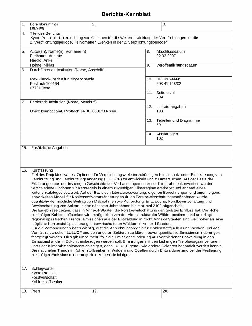
Berichts-Kennblatt
1. Berichtsnummer UBA-FB
2. 3.
4. Titel des Berichts Kyoto-Protokoll: Untersuchung von Optionen für die Weiterentwicklung der Verpflichtungen für die 2. Verpflichtungsperiode, Teilvorhaben „Senken in der 2. Verpflichtungsperiode“ 5. Autor(en), Name(n), Vorname(n) 8. Abschlussdatum Freibauer, Annette 02.03.2007 Herold, Anke Höhne, Niklas 9. Veröffentlichungsdatum 6. Durchführende Institution (Name, Anschrift) Max-Planck-Institut für Biogeochemie 10. UFOPLAN-Nr. Postfach 100164 203 41 148/02 07701 Jena 11. Seitenzahl 289 7. Fördernde Institution (Name, Anschrift) 12. Literaturangaben Umweltbundesamt, Postfach 14 06, 06813 Dessau 198 13. Tabellen und Diagramme 39 14. Abbildungen 102 15. Zusätzliche Angaben 16. Kurzfassung Ziel des Projektes war es, Optionen für Verpflichtungsziele im zukünftigen Klimaschutz unter Einbeziehung von Landnutzung und Landnutzungsänderung (LULUCF) zu entwickeln und zu untersuchen. Auf der Basis der Erfahrungen aus der bisherigen Geschichte der Verhandlungen unter der Klimarahmenkonvention wurden verschiedene Optionen für Kernregeln in einem zukünftigen Klimaregime erarbeitet und anhand eines Kriterienkataloges evaluiert. Auf der Basis von Literaturauswertung, eigenen Berechnungen und einem eigens entwickelten Modell für Kohlenstoffvorratsänderungen durch Forstbewirtschaftungsmaßnahmen wurde quantitativ der mögliche Beitrag von Maßnahmen wie Aufforstung, Entwaldung, Forstbewirtschaftung und Bewirtschaftung von Äckern in den nächsten Jahrzehnten bis maximal 2100 abgeschätzt. Die Ergebnisse zeigen, dass in Annex-I-Staaten die Forstbewirtschaftung den größten Einfluss hat. Die Höhe zukünftiger Kohlenstoffsenken wird maßgeblich von der Altersstruktur der Wälder bestimmt und unterliegt regional spezifischen Trends. Emissionen aus der Entwaldung in Nicht-Annex-I Staaten sind weit höher als eine mögliche Kohlenstoffspeicherung in bewirtschafteten Wäldern in Annex-I Staaten. Für die Verhandlungen ist es wichtig, erst die Anrechnungsregeln für Kohlenstoffquellen und -senken und das Verhältnis zwischen LULUCF und den anderen Sektoren zu klären, bevor quantitative Emissionsminderungen festgelegt werden. Dies gilt umso mehr, falls die Emissionsminderung aus vermiedener Entwaldung in den Emissionshandel in Zukunft einbezogen werden soll. Erfahrungen mit den bisherigen Treibhausgasinventaren unter der Klimarahmenkonvention zeigen, dass LULUCF genau wie andere Sektoren behandelt werden könnte. Die nationalen Trends in Kohlenstoffsenken in Wäldern und Quellen durch Entwaldung sind bei der Festlegung zukünftiger Emissionsminderungsziele zu berücksichtigen. 17. Schlagwörter Kyoto Protokoll Forstwirtschaft Kohlenstoffsenken 18. Preis 19. 20.
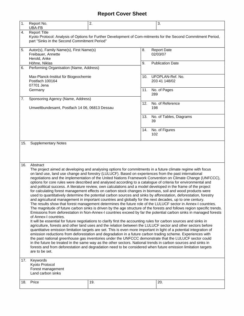
Report Cover Sheet
1. Report No. UBA-FB
2. 3.
4. Report Title Kyoto Protocol: Analysis of Options for Further Development of Com-mitments for the Second Commitment Period, part "Sinks in the Second Commitment Period" 5. Autor(s), Family Name(s), First Name(s) 8. Report Date Freibauer, Annette 02/03/07 Herold, Anke Höhne, Niklas 9. Publication Date 6. Performing Organisation (Name, Address) Max-Planck-Institut für Biogeochemie 10. UFOPLAN-Ref. No. Postfach 100164 203 41 148/02 07701 Jena Germany 11. No. of Pages 289 7. Sponsoring Agency (Name, Address) 12. No. of Reference Umweltbundesamt, Postfach 14 06, 06813 Dessau 198 13. No. of Tables, Diagrams 39 14. No. of Figures 102 15. Supplementary Notes 16. Abstract The project aimed at developing and analysing options for commitments in a future climate regime with focus on land use, land use change and forestry (LULUCF). Based on experiences from the past international negotiations and the implementation of the United Nations Framework Convention on Climate Change (UNFCCC), options for core rules were described and analysed according to a catalogue of criteria for environmental and and political success. A literature review, own calculations and a model developed in the frame of the project for calculating forest management effects on carbon stock changes in biomass, soil and wood products were used to quantitatively determine the potential carbon sources and sinks by afforestation, deforestation, forestry and agricultural management in important countries and globally for the next decades, up to one century. The results show that forest management determines the future role of the LULUCF sector in Annex-I countries. The magnitude of future carbon sinks is driven by the age structure of the forests and follows region specific trends. Emissions from deforestation in Non-Annex-I countries exceed by far the potential carbon sinks in managed forests of Annex-I countries. It will be essential for future negotiations to clarify first the accounting rules for carbon sources and sinks in agriculture, forests and other land uses and the relation between the LULUCF sector and other sectors before quantitative emission limitation targets are set. This is even more important in light of a potential integration of emission reductions from deforestation and degradation in a future carbon trading scheme. Experiences with the past national greenhouse gas inventories under the UNFCCC demonstrate that the LULUCF sector could in the future be treated in the same way as the other sectors. National trends in carbon sources and sinks in forests and from deforestation and degradation need to be considered when future emission limitation targets are to be set. 17. Keywords Kyoto Protocol Forest management Land carbon sinks 18. Price 19. 20.
MPI-BGC/Öko-Institut/ ECOFYS FKZ 203 41 148/02
3
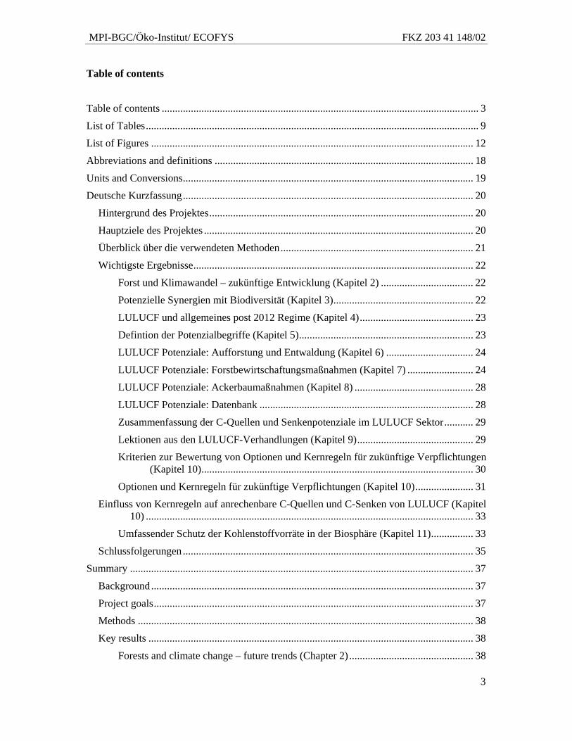
Table of contents
Table of contents ........................................................................................................................ 3
List of Tables.............................................................................................................................. 9
List of Figures .......................................................................................................................... 12
Abbreviations and definitions .................................................................................................. 18
Units and Conversions.............................................................................................................. 19
Deutsche Kurzfassung.............................................................................................................. 20
Hintergrund des Projektes.................................................................................................... 20
Hauptziele des Projektes ...................................................................................................... 20
Überblick über die verwendeten Methoden......................................................................... 21
Wichtigste Ergebnisse.......................................................................................................... 22
Forst und Klimawandel – zukünftige Entwicklung (Kapitel 2) ................................... 22
Potenzielle Synergien mit Biodiversität (Kapitel 3)..................................................... 22
LULUCF und allgemeines post 2012 Regime (Kapitel 4)........................................... 23
Defintion der Potenzialbegriffe (Kapitel 5).................................................................. 23
LULUCF Potenziale: Aufforstung und Entwaldung (Kapitel 6) ................................. 24
LULUCF Potenziale: Forstbewirtschaftungsmaßnahmen (Kapitel 7) ......................... 24
LULUCF Potenziale: Ackerbaumaßnahmen (Kapitel 8) ............................................. 28
LULUCF Potenziale: Datenbank ................................................................................. 28
Zusammenfassung der C-Quellen und Senkenpotenziale im LULUCF Sektor........... 29
Lektionen aus den LULUCF-Verhandlungen (Kapitel 9)............................................ 29
Kriterien zur Bewertung von Optionen und Kernregeln für zukünftige Verpflichtungen (Kapitel 10)....................................................................................................... 30
Optionen und Kernregeln für zukünftige Verpflichtungen (Kapitel 10)...................... 31
Einfluss von Kernregeln auf anrechenbare C-Quellen und C-Senken von LULUCF (Kapitel 10) ............................................................................................................................ 33
Umfassender Schutz der Kohlenstoffvorräte in der Biosphäre (Kapitel 11)................ 33
Schlussfolgerungen .............................................................................................................. 35
Summary .................................................................................................................................. 37
Background.......................................................................................................................... 37
Project goals......................................................................................................................... 37
Methods ............................................................................................................................... 38
Key results ........................................................................................................................... 38
Forests and climate change – future trends (Chapter 2) ............................................... 38
MPI-BGC/Öko-Institut/ ECOFYS FKZ 203 41 148/02
4
Synergies and conflicts between climate change mitigation and other ecosystem functions (Chapter 3)........................................................................................ 39
Emissions and removals from land use change and forestry in the context of necessary global emission reductions (Chapter 4)............................................................ 39
Definition of the term “potential” (Chapter 5) ............................................................. 39
LULUCF potentials: afforestation/reforestation and deforestation (Chapter 6) .......... 40
LULUCF potentials: Forest management (Chapter 7) ................................................. 40
LULUCF potentials: cropland management (Chapter 8) ............................................. 41
LULUCF potentials: data base (CD-Rom)................................................................... 41
Lessons from LULUCF negotiation history (Chapter 9) ............................................. 42
LULUCF and the general post 2012 regime (Chapter 9) ............................................. 42
Effect of key rules on accountable C sources and sinks in LULUCF (Chapter 10) ............ 42
Criteria for evaluation of options and key rules for future commitments (Chapter 10)43
Options and key rules for future commitments (Chapter 10)....................................... 43
Proposal for comprehensive protection of C stocks in the biosphere (Chapter 11) ..... 43
Conclusions.......................................................................................................................... 45
1 Introduction....................................................................................................................... 47
1.1 Background .............................................................................................................. 47
1.2 Project goals ............................................................................................................. 47
1.3 Overview of methods ............................................................................................... 48
2 Forests under global change – the future of the terrestrial carbon sink ............................ 49
2.1 Introduction .............................................................................................................. 49
2.2 Components of the carbon balance, stocks and fluxes of important forest regions . 50
2.3 Observed features of climate change........................................................................ 52
2.3.1 Gradual changes ............................................................................................... 52
2.3.2 Weather and climate variability ....................................................................... 52
2.4 Likely plant responses to climate change: experimental findings............................ 52
2.4.1 Carbon dioxide fertilization.............................................................................. 52
2.4.2 Temperature response and acclimation ............................................................ 53
2.5 Complex responses: coupled models including climate and terrestrial ecosystems 54
2.6 Vulnerability of the forest sink: response to extremes ............................................. 54
2.7 Indirect responses: the role of fires .......................................................................... 56
2.8 Conclusions .............................................................................................................. 57
3 Synergies and conflicts of LULUCF activities with other ecosystem functions .............. 59
3.1 Biodiversity .............................................................................................................. 59
MPI-BGC/Öko-Institut/ ECOFYS FKZ 203 41 148/02
5
3.1.1 Options at global level...................................................................................... 59
3.1.2 Options at project and national level ................................................................ 59
3.2 Nutrients and water .................................................................................................. 62
3.2.1 Cropland management...................................................................................... 62
3.2.2 Afforestation and reforetation .......................................................................... 62
3.3 Production function of ecosystems........................................................................... 62
4 Emissions and removals from land use change and forestry in the context of necessary global emission reductions................................................................................................ 63
4.1 Introduction .............................................................................................................. 63
4.2 Required emission reductions .................................................................................. 63
4.3 Political landscape.................................................................................................... 65
4.4 Magnitude of emissions from land use change and forestry in relation to other greenhouse gas emissions ........................................................................................ 67
4.5 Prominent proposals for a post 2012 climate regime and their implications on LULUCF.................................................................................................................. 71
4.5.1 LULUCF in a Multistage approach.................................................................. 72
4.5.2 LULUCF in Contraction & Convergence ........................................................ 74
4.5.3 Comparison ...................................................................................................... 76
4.5.4 LULUCF as incentive for developing countries to participate ........................ 77
4.6 Conclusions .............................................................................................................. 78
5 Biological, technical, economic and realistic potentials................................................... 80
6 Afforestation, reforestation and deforestation .................................................................. 82
6.1 Introduction .............................................................................................................. 82
6.2 Afforestation, reforestation and deforestation in past and present ........................... 82
6.3 Material and Methods............................................................................................... 85
6.3.1 FAO data projection until 2020........................................................................ 86
6.3.2 Global dynamic model approach until 2100 .................................................... 88
6.4 Afforestation, Reforestation and Deforestation: Projections until 2020 (FAO data projection) ................................................................................................................ 91
6.4.1 Forest area development................................................................................... 91
6.4.2 Emissions and removals ................................................................................... 92
6.5 Afforestation, Reforestation and Deforestation: Projections until 2100 .................. 94
6.5.1 Forest area development................................................................................... 94
6.5.2 Emissions and removals ................................................................................... 96
6.6 Comparison of approaches ....................................................................................... 97
6.7 Conclusions .............................................................................................................. 98
MPI-BGC/Öko-Institut/ ECOFYS FKZ 203 41 148/02
6
6.8 Acknowledgements .................................................................................................. 99
7 Forest management ......................................................................................................... 100
7.1 Introduction ............................................................................................................ 100
7.1.1 Definition of Forest Management .................................................................. 100
7.1.2 Forest management and its impact on the carbon cycle ................................. 101
7.2 Materials and methods............................................................................................ 103
7.2.1 Model description........................................................................................... 103
7.2.2 Model parameters ........................................................................................... 104
7.2.3 Description of datasets ................................................................................... 106
7.2.4 Model initialization and evaluation................................................................ 115
7.2.5 Uncertainty estimates ..................................................................................... 116
7.2.6 Scenario description ....................................................................................... 117
7.3 Forest management: full C balance ........................................................................ 121
7.4 Effects of management change............................................................................... 124
7.4.1 Scenario “Longer rotation” ............................................................................ 124
7.4.2 Scenario “Shorter rotation” ............................................................................ 125
7.4.3 Scenario “Product shift” ................................................................................. 125
7.5 Effects of past management ................................................................................... 129
7.6 Uncertainties and risks ........................................................................................... 132
7.7 Conclusions ............................................................................................................ 133
7.8 Acknowledgements ................................................................................................ 133
8 Cropland management .................................................................................................... 134
8.1 Introduction ............................................................................................................ 134
8.1.1 Definition of cropland management............................................................... 134
8.1.2 Impact of cropland management on the carbon cycle .................................... 134
8.2 Material and methods ............................................................................................. 134
8.2.1 Model.............................................................................................................. 134
8.2.2 Data and assumptions..................................................................................... 135
8.2.3 Uncertainty estimates ..................................................................................... 139
8.2.4 Scenarios ........................................................................................................ 139
8.3 Biological potential for C sinks in croplands ......................................................... 142
8.4 Scenarios of future C sources and sinks in agriculture .......................................... 143
8.4.1 Scenario “Mechanisation”.............................................................................. 145
8.4.2 Scenario “Intensification” .............................................................................. 145
8.4.3 Scenario “Conservation tillage” ..................................................................... 146
MPI-BGC/Öko-Institut/ ECOFYS FKZ 203 41 148/02
7
8.4.4 Scenario “No-till”........................................................................................... 146
8.4.5 Scenario “Manure on cropland” ..................................................................... 147
8.5 Uncertainties and risks ........................................................................................... 147
8.6 Effects of accounting rules ..................................................................................... 148
8.7 Discussion .............................................................................................................. 149
8.8 Conclusion.............................................................................................................. 150
9 The rules for land use, land use change and forestry under the Kyoto Protocol – Lessons learned for the future climate negotiations ..................................................................... 151
9.1 Introduction ............................................................................................................ 151
9.2 Provisions for land use, land-use change and forestry in the first commitment period of the Kyoto Protocol............................................................................................. 152
9.2.1 Principles ........................................................................................................ 152
9.2.2 Definition of categories of activities .............................................................. 153
9.2.3 Accounting rules and base year...................................................................... 153
9.2.4 Specific provisions for Article 3.3 activities .................................................. 156
9.2.5 Specific provisions for Article 3.4 activities .................................................. 157
9.2.6 Second sentence of Article 3.7 ....................................................................... 160
9.2.7 Reporting of LULUCF activities.................................................................... 160
9.2.8 Specific provisions for LULUCF in Joint Implementation (JI) ..................... 161
9.2.9 Rules for LULUCF in Non-Annex-I countries, Clean Development Mechanism (CDM) ............................................................................................................ 161
9.3 Outline of the negotiations leading to the LULUCF provisions ............................ 163
9.3.1 Timeline of events .......................................................................................... 163
9.3.2 History of the specific rules............................................................................ 168
9.4 Conclusions ............................................................................................................ 174
10 Options for future LULUCF rules .................................................................................. 176
10.1 Objectives for the analysis of options for a future climate regime ........................ 176
10.2 Criteria for the analysis of options for a future climate regime ............................. 176
10.2.1 Climate effectiveness ..................................................................................... 176
10.2.2 Creation of additional/general environmental benefits .................................. 176
10.2.3 Technical effectiveness: facilitation of monitoring, accounting and verification of compliance ................................................................................................. 176
10.2.4 Facilitation of negotiation process for post-2012 climate regime.................. 177
10.2.5 Acknowledgement of special characteristics of LULUCF activities ............. 177
10.2.6 Cost-efficiency ............................................................................................... 177
MPI-BGC/Öko-Institut/ ECOFYS FKZ 203 41 148/02
8
10.3 The key rules for LULUCF activities under the UNFCCC and the Kyoto Protocol and options for future rules .................................................................................... 177
10.3.1 Target type...................................................................................................... 178
10.3.2 Accounting of direct human-induced emissions and removals from sinks.... 189
10.3.3 Inclusion of defined LULUCF activities........................................................ 196
10.3.4 Accounting rules............................................................................................. 221
10.3.5 Flexible mechanisms including carbon removals .......................................... 225
10.3.6 Commitment period length............................................................................. 227
10.3.7 Forest definition ............................................................................................. 232
10.3.8 Elements of additional rules aiming at correcting effects of key rules .......... 233
10.3.9 Conclusions for the choice of key rules in future commitment period .......... 234
10.4 Conclusions: promising options for future LULUCF rules.................................... 237
11 Alternative framework for LULUCF rules ..................................................................... 239
11.1 Conclusions from previous chapters for an alternative framework ....................... 239
11.2 Concept of stabilizing regional biospheric C stocks .............................................. 240
11.3 Proposal for inclusion of biospheric C in a future climate policy regime.............. 240
11.3.1 Proposed key rules.......................................................................................... 241
11.3.2 Evaluation according to key principles and criteria ....................................... 245
11.4 Implications of the novel framework on individual Parties and regions................ 250
11.5 Conclusions ............................................................................................................ 252
References .............................................................................................................................. 253
Annex 1: Description of forest management model............................................................... 266
Annex 2: Country-specific results of quantitative analyses ................................................... 271
MPI-BGC/Öko-Institut/ ECOFYS FKZ 203 41 148/02
9
List of Tables
Table 1 Global economic potential for C sources and sinks in Pg CO2 per year.................. 44
Table 2 Distribution of area and carbon stocks over the three major forest biomes (WBGU, 1998)....................................................................................................................... 50
Table 3 Level and timing of required global emission reductions (Source: IPCC (2001b), table 6-1)................................................................................................................. 64
Table 4 Non-Annex-I countries showing significant increases in GHG per capita emissions when LULUCF is included .................................................................................... 70
Table 5 Cascade of potentials in agriculture and forestry in recent literature. N.E. Not estimated................................................................................................................. 81
Table 6 Forest area development over time in Mha of selected countries as reported by the FAO Forest Resource Assessment in 1990, 2000 and 2005 ((FAO et al.,2005)). The global numbers are taken from the FRA 2005 report and summarize the forest area of all countries considered by this report........................................................ 83
Table 7 Region specific average annual increment in aboveground biomass in natural regeneration and plantation increment factors in tonnes dry matter/ha/year for 17 regions according to Tables 3A.1.5 and 3A.1.6 of LULUCF GPG ((IPCC, 2003)). . .......................................................................................................................... 87
Table 8 Region specific aboveground biomass stock in naturally regenerated forests in tonnes dry matter/ha for 17 regions according to Table 3A.1.2 of LULUCF GPG (IPCC, 2003). ......................................................................................................... 88
Table 9 Large-scale biomass burning emission factors in gram species per kg dry matter burned((Andreae et al., 2001)................................................................................. 88
Table 10 The complete set of spatial datasets used to create a resultant database for modeling. ................................................................................................................ 89
Table 11 Net emissions and removals from land use change as projected with FAO data compared to values reported by the countries in the UNFCCC inventory in Pg CO2 per year. .................................................................................................................. 93
Table 12 Summary of projected C emissions and removals from afforestation/ reforestation and deforestation based on projected FAO area data and regional biomass estimates. Numbers are equivalent to the realistic potential of afforestation/reforestation and deforestation measures. The ranges in brackets reflect uncertainties in the biomass and forest growth estimates. .......................... 99
Table 13 Biomass carbon stocks in natural versus managed forests ((WBGU, 1998)). .... 101
Table 14 List of model parameters to be specified............................................................. 104
Table 15 Stratification of forestry data according to different types. Product of types does not result in the final number of srata because some combinations do not occur.105
Table 16 List of countries considered in forest management model runs and their forest extent as observed by remote sensing through the Global Land Cover dataset 2000 (GLC 2000; JRC, 2003) and reported and published by FAO (FAO et al., 1998). The right side of the table splits FAO forest area into exploited (managed in terms of timber extraction) and protected area. The discrimination was made according
MPI-BGC/Öko-Institut/ ECOFYS FKZ 203 41 148/02
10
to inventory information. Forest area that is not covered by the inventory is considered to be under protection. Area in 1000 ha. (1) countries belonging to the EU23 group (EU-25 without Cyprus and Malta). ................................................ 107
Table 17 Reported and observed values for forest area and area of protected forest.......... 108
Table 18 Factors determining the quality indicator I. ........................................................ 116
Table 19 Scenarios applied.................................................................................................. 117
Table 20 Mean residence time in years for both product pools and the initial distribution (business as usual) of harvested volume to the pools in %. In the product shift scenario the fraction moved to the long lifespan pool is 100. .............................. 120
Table 21 Overview of all countries considered in the analysis. Emissions and removals from forestry (biomass, soil, litter and products) for the years 2005, 2010, 2015 and 2020 in Tg CO2 per year................................................................................ 125
Table 22 Quality indicators for the five regarded regions................................................... 132
Table 23 Allocation rules for fractions of cropland under given land management intensity and tillage and input intensity regimes for the IPCC GPG Soil Tool .................. 138
Table 24 Quality indicators for selected countries (ranking: see Table 18)........................ 148
Table 25 Summary of C source (+) and sink (-) potentials in agriculture........................... 149
Table 26 Summary of the differences in the LULUCF activities ....................................... 153
Table 27 Limits for accounting net removals for forest management under Article 3.4 .... 159
Table 28 Characteristics of temporary certified emission reduction units (tCERs) and long-term certified emission reduction units (lCERs) .................................................. 162
Table 29 Value of the temporary unit compared to a permanent unit, assuming that the price for permanent units is the same today as in x years. ............................................ 163
Table 30 CO2 emissions and removals from afforestation/ reforestation (Land converted to forest land) and from deforestation (Forest land converted to other land-use categories) in 2003 for Annex-I Parties [Gg CO2] ............................................... 209
Table 31 Countries with highest forest reduction rates (Table comprises all countries for which annual change in forest area is above 50 kha per year in the 2000-2005 period.) and estimated CO2 emissions.................................................................. 210
Table 32 Countries with net increases in forest areas of more than 50,000 ha/year and estimated CO2 emissions ...................................................................................... 210
Table 33 Effects of changes in gross-net accounting rules for forest land (based on artificial commitment period) ............................................................................................. 224
Table 34 Percentage change to previous reporting year for net CO2 emissions or removals from LULUCF sector for Annex-I Parties ........................................................... 229
Table 35 Contribution of net emissions/removals from LULUCF to total national GHG inventories ............................................................................................................ 230
Table 36 Percentage change to previous reporting year for net CO2 emissions or removals from forest lands for Annex-I Parties................................................................... 231
MPI-BGC/Öko-Institut/ ECOFYS FKZ 203 41 148/02
11
Table 37 Average net emissions/removals from forest lands and standard deviations for a six five-year periods and a 10 year period based on current inventory data Numbers highlighted in yellow indicate higher standard deviation for 5-year period compared to the 10-year period............................................................................ 232
Table 38 Emissions and emission reductions in arbitrary units under the Greenhouse Gas Flux Target (GHGFT) and the Bio-Carbon Target (BCT) for two example countries in the base period and a commitment period ........................................ 242
Table 39 Country and regional GHG emissions in the year 2000, emission trends 1990 to 2000, estimated biospheric C stocks in forest biomass and rough estimates of C stock changes in biomass in the 1990s. GHGs (CO2, CH4 and N2O) from other sectors are calculated from UNFCCC submissions and, where not available, data from IEA, EDGAR and USEPA (Höhne et al., 2004). A positive sign means emission, a negative sign means sink. .................................................................. 251
MPI-BGC/Öko-Institut/ ECOFYS FKZ 203 41 148/02
12
List of Figures
Figure 1 Relation between Greenhouse Gas Flux Target and Bio-Carbon Target ............... 45
Figure 2 Terrestrial carbon cycling and storage ((Augustin et al., 1998))........................... 50
Figure 3 Possible future emissions, concentrations, temperature change and sea level rise (IPCC, 2001c)......................................................................................................... 64
Figure 4 Historic and future emission of Annex-I and Non-Annex-I countries under the IPCC SRES A1B scenario...................................................................................... 66
Figure 5 Sectoral split of emissions in different world regions in 2000............................... 67
Figure 6 LULUCF emissions as percentage of national total for all other sectors and gases (Source: UNFCCC submissions for the year 2002) ............................................... 68
Figure 7 CO2 emissions/removals from LULUCF by source category in Annex-I countries . .......................................................................................................................... 68
Figure 8 Magnitude of emissions from deforestation (land-use change) from Houghton (2003a) (left, total 2GtC) and EDGAR (Olivier JGJ et al., 1996)(right, total 0.5GtC) ................................................................................................................... 69
Figure 9 Per capita emission excluding LULUCF................................................................ 70
Figure 10 Per capita emission including LULUCF ................................................................ 71
Figure 11 Illustrative Multistage approach, participation in stages........................................ 73
Figure 12 Illustrative Multistage approach without LULUCF ............................................... 73
Figure 13 Illustrative Multistage approach with LULUCF .................................................... 73
Figure 14 Stringency of reductions, change in emission allowances from 1990 to 2020 under the illustrative multistage case including and excluding LULUCF ....................... 74
Figure 15 Contraction & Convergence without LULUCF .................................................... 75
Figure 16 Contraction & Convergence with LULUCF ......................................................... 75
Figure 17 Change in emission allowances from 1990 to 2020 under contraction and convergence including and excluding LULUCF.................................................... 76
Figure 18 Emission trajectories for selected countries under the illustrative multistage and contraction and convergence cases......................................................................... 77
Figure 19 Annual net forest area change between 1990 and 2000 and 2000 and 2005 for selected countries as reported by the FAO Forest Resource Assessment (FRA) in 1990, 2000 and 2005 (FAO FRA 2005)................................................................. 84
Figure 20 Comparison of different estimates of (net) emissions from tropical land use change of 1980 and 1990. (NB: EDGAR includes deforestation emissions only; IMAGE only biomass burning!)........................................................................................... 84
Figure 21 Integrated modeling approach (linked models – in red; input – in blue; output – in green)...................................................................................................................... 90
Figure 22 A2 Carbon price trajectory as projected by the MESSAGE model. ..................... 91
MPI-BGC/Öko-Institut/ ECOFYS FKZ 203 41 148/02
13
Figure 23 Global forest area change rate development until 2020. Period 2005-2020 as a projection of rates observed between 2000 and 2005 according to FRA 2005. Afforestation stands for afforestation/reforestation, “ann” means “annual”.......... 92
Figure 24 Projected global development of annual emissions (positive values) and removals (negative values) related to deforestation and afforestation/reforestation. Lines mark maximum and minimum values considered by LULUCF GPG. .................. 93
Figure 25 Proportion of area deforested, afforested (area has not been forest land after the start of the simulation in 2000) and reforested (area has been forest land after 2000) of total LUC area during 2000 – 2100. ........................................................ 95
Figure 26 Global forest area change rate development until 2100. ........................................ 95
Figure 27 Projected global net forest area change 2000 – 2100. ............................................ 96
Figure 28 Global net fluxes from land use change as projected by the model for the SRES A2 scenario and considering the mitigation effect of afforestation/reforestation. ....... 96
Figure 29 Comparison of area of deforestation (negative values) and afforestation/reforestation (positive values) as projected by both approaches...... 97
Figure 30 Comparison of net emissions from LUC as estimated by both approaches. .......... 98
Figure 31 Overview of main effects of forest management on carbon cycling in forest ecosystems. The chart shows pools (grey boxes), fluxes of carbon (arrows), direct (solid line boxes) and indirect (dashed line boxes) intervention types. + and – symbolize acceleration and decrease in speed respectively of flux as impact of intervention........................................................................................................... 100
Figure 32 Schematic carbon stock development of aboveground biomass and humus under different management scenarios (a-primary forest, b-primary forest under selective cutting management, c-secondary forest, d-plantation). Time scales are not identical and the curves represent hypothetical growth ((WBGU, 1998))........... 102
Figure 33 Simplified overview of FORMICA structure....................................................... 103
Figure 34 Map of considered countries and regions. Countries included in the analysis are filled grey. ............................................................................................................ 106
Figure 35 Age class distribution of 34 European countries.................................................. 109
Figure 36 Age class distribution of EU23 countries (EU25 without Cyprus and Malta). .... 110
Figure 37 Age class distribution of Canadian managed forest. ............................................ 111
Figure 38 Age class distribution of Russian forests of different management classes......... 112
Figure 39 Age class distribution of US forests. .................................................................... 113
Figure 40 Age class distribution of Chinese forests. ............................................................ 114
Figure 41 Comparison of volume removals by harvest of FAO reported values (average of FRA 2000 and 2005) and removals estimated by the FORMICA forestry model. The red bars show estimated losses by fire (derived from the RETRO dataset; courtesy of Dr. Martin Schultz, Max-Planck-Institute for Meteorology, Hamburg) that are not included in the model and need to be subtracted from the modeled removed volume. .................................................................................................. 115
MPI-BGC/Öko-Institut/ ECOFYS FKZ 203 41 148/02
14
Figure 42 Schematic view of management change (MC) effects: BaU – Business as Usual, the observed C flux under continued management; MC – management change, e.g. longer rotations. The upper graphs show absolute values, the graph at the bottom changes relative to Business as Usual. The area marked in grey is the difference between BaU and MC, i.e. the gain (or loss) of carbon compared to BaU. ......... 118
Figure 43 Schematic view of the different effects of past practice: BaU – Business as Usual, the observed C flux with current age class distribution, prescribed as a sink that is first decreasing and later increasing again; NF – Normal Forest scenario, age classes are equally distributed. The area under this curve marked in grey represents the management effect (ME), i.e. the mismatch between long-term C stocks and actual stocks under the applied management system. The difference between BaU and NF as shown in the graph at the bottom, is the age class effect (AE) that leads to a theoretically smaller sink/bigger source of C (if BaU>NF) or bigger sink/smaller source compared to ideal forest age class conditions. ..................... 121
Figure 44 Stock changes of different pools for all simulated countries(EU-23, Canada, USA, Russia and China) considering Business as Usual ............................................... 122
Figure 45 Emissions and removals from Forest Management for five regions considering continued business as usual. ................................................................................. 124
Figure 46 Comparison of the net effect of different options of forest management change in Canada. Positive values indicate additional CO2 released, negative values can be interpreted as enhanced sink. This graph does not indicate whether the CO2 flux is in reality a sink or a source but only shows the difference against the reference. 126
Figure 47 Comparison of the net effect of different options of forest management change in China. Positive values indicate additional CO2 released, negative values can be interpreted as enhanced sink. This graph does not indicate whether the CO2 flux is in reality a sink or a source but only shows the difference against the reference. 127
Figure 48 Comparison of the net effect of different options of forest management change in EU-23. Positive values indicate additional CO2 released, negative values can be interpreted as enhanced sink. This graph does not indicate whether the CO2 flux is in reality a sink or a source but only shows the difference against the reference. 127
Figure 49 Comparison of the net effect of different options of forest management change in Russia. Positive values indicate additional CO2 released, negative values can be interpreted as enhanced sink. This graph does not indicate whether the CO2 flux is in reality a sink or a source but only shows the difference against the reference. 128
Figure 50 Comparison of the net effect of different options of forest management change in USA. Positive values indicate additional CO2 released, negative values can be interpreted as enhanced sink. This graph does not indicate whether the CO2 flux is in reality a sink or a source but only shows the difference against the reference. 128
Figure 51 Comparison of the net effect of different options of forest management change in all considered regions (Canada, China, EU-23, Russia and USA). Positive values indicate additional CO2 released, negative values can be interpreted as enhanced sink. This graph does not indicate whether the CO2 flux is in reality a sink or a source but only shows the difference against the reference. ................................ 129
Figure 52 Comparison of different age class scenarios for Canada: Business as Usual (BaU) considers the actually observed distribution, Normal Forest (NF) is based on a
MPI-BGC/Öko-Institut/ ECOFYS FKZ 203 41 148/02
15
balanced age class structure, i.e. all age classes of a stratum have the same area. Fluxes under NF reflect management effects that refer to unbalanced carbon stocks at the beginning of the simulation. The Difference between BaU and NF reveals fluxes that can be explained by the actual age class distribution only. ................ 130
Figure 53 Comparison of different age class scenarios for EU-23: Business as Usual (BaU) considers the actually observed distribution, Normal Forest (NF) is based on a balanced age class structure, i.e. all age classes of a stratum have the same area. Fluxes under NF reflect management effects that refer to unbalanced carbon stocks at the beginning of the simulation. The Difference between BaU and NF reveals fluxes that can be explained by the actual age class distribution only. ................ 131
Figure 54 Comparison of different age class scenarios for China: Business as Usual (BaU) considers the actually observed distribution, Normal Forest (NF) is based on a balanced age class structure, i.e. all age classes of a stratum have the same area. Fluxes under NF reflect management effects that refer to unbalanced carbon stocks at the beginning of the simulation. The Difference between BaU and NF reveals fluxes that can be explained by the actual age class distribution only. ................ 131
Figure 55 Matrix of management changes in cropland scenarios. Letters indicate the column number of input input/tillage strata defined in Table 23. ..................................... 141
Figure 56 Historical soil C loss by cultivation in a) countries and b) world regions using the IPCC default factors for land use, and the low and high end of the error in the default factors. These losses indicate the theoretical biological cumulative potential for soil C sequestration in croplands. ................................................................... 143
Figure 57 Technical potential for C stock changes in cropland soils of Non-Annex-I countries over 20 years......................................................................................... 143
Figure 58 Technical potential for C stock changes in cropland soils of Annex-I countries over 20 years................................................................................................................. 144
Figure 59 Technical potential for C stock changes in cropland soils of world regions over 20 years...................................................................................................................... 144
Figure 60 Accounting for afforestation, reforestation and deforestation as well as forest management showing changes in carbon stocks (top) and, with different scale, carbon emissions (bottom) ................................................................................... 154
Figure 61 Accounted areas for afforestation (applies equally for reforestation and deforestation)........................................................................................................ 154
Figure 62 Accounted areas for forest management .............................................................. 155
Figure 63 Accounted areas for cropland management (applies equally for grazing land management and revegetation) (IPCC good practice guidance, box 4.2.8) ......... 155
Figure 64 Example case of one unit of land where debits from harvesting exceed the credits during the commitment period showing changes in carbon stocks (top) and, with different scale, carbon emissions (bottom)........................................................... 157
Figure 65 Diagram illustrating accounting for afforestation, reforestation, deforestation and forest management from emissions during the commitment period .................... 158
Figure 66 Diagram illustrating the accounting under Article 3.7(2) in the base year .......... 160
MPI-BGC/Öko-Institut/ ECOFYS FKZ 203 41 148/02
16
Figure 67 Flow of agreements on land-use, land-use change and forestry from COP3 to COP11 .................................................................................................................. 164
Figure 68 Overview of key rules and options for these key rules discussed in this chapter 178
Figure 69 Assessment matrix for tartget type and the objective “climate effectiveness"..... 181
Figure 70 Assessment matrix for tartget type and the objective “environmennntal effectiveness" ....................................................................................................... 183
Figure 71 Assessment matrix for tartget type and the objective “technical effectiveness".. 184
Figure 72 Assessment matrix for tartget type and the objective “facilitation of the negotiation process" ................................................................................................................ 186
Figure 73 Assessment matrix for tartget type and the objective “special characteristics of LULUCF sector" .................................................................................................. 188
Figure 74 Assessment matrix for definition of anthropogenic emissions/removals and the objective “climate effectiveness” ......................................................................... 191
Figure 75 Assessment matrix for definition of anthropogenic emissions/removals and the objective “environmental effectiveness”.............................................................. 192
Figure 76 Assessment matrix for definition of anthropogenic emissions/removals and the objective “technical effectiveness” ...................................................................... 193
Figure 77 Assessment matrix for definition of anthropogenic emissions/removals and the objective “facilitation of the negotiation process” ............................................... 194
Figure 78 Assessment matrix for definition of anthropogenic emissions/removals and the objective “special characteristics of LULUCF activities” ................................... 195
Figure 79 Assessment matrix for the inclusion of LULUCF activities and the objective “climate effectiveness”......................................................................................... 200
Figure 80 Assessment matrix for the inclusion of LULUCF activities and the objective “environmental effectiveness” ............................................................................. 201
Figure 81 Assessment matrix for the inclusion of LULUCF activities and the objective “technical effectiveness” ...................................................................................... 202
Figure 82 Assessment matrix for the inclusion of LULUCF activities and the objective “facilitation of the negotiation process”............................................................... 203
Figure 83 Average contribution of net emissions/removals from LULUCF to total GHG emissions per country. The range represents the maximum and minimum contribution over the 1990-2003 period (for EU Member States until 2004)...... 205
Figure 84 Net removals from forest land areas to the total GHG emissions (average contribution over 1990-2003)............................................................................... 206
Figure 85 Projected CO2 emissions and removals for forest management for selected Annex-I Parties................................................................................................................. 207
Figure 86 CO2 emissions and removals from afforestation/ reforestation (Land converted to forest land) and from deforestation (Forest land converted to other land-use categories) in 2003 for Annex-I Parties [Gg CO2] ............................................... 208
Figure 87 Projected CO2 emissions from deforestation for Brazil and Indonesia until 2020 based on FAO data ............................................................................................... 211
MPI-BGC/Öko-Institut/ ECOFYS FKZ 203 41 148/02
17
Figure 88 Projected CO2 emissions from deforestation for selected Non-Annex-I Parties until 2020 based on FAO data ...................................................................................... 213
Figure 89 Average net emissions/removals from cropland areas relative to total GHG emissions (average contribution over 1990-2003, until 2004 for EU Member States) ................................................................................................................... 214
Figure 90 Projected CO2 emissions and removals from cropland management................... 215
Figure 91 Average net emissions/removals from grasland areas relative to total GHG emissions (average contribution over 1990-2003, until 2004 for EU Member States) ................................................................................................................... 216
Figure 92 Average net emissions/removals from settlement areas relative to total GHG emissions (average contribution over 1990-2003, until 2004 for EU Member States) ................................................................................................................... 217
Figure 93 Net emissions/removals from individual land-use categories for EU-25 based on GHG inventory data ............................................................................................. 218
Figure 94 Net emissions/removals from individual land-use categories for EU-15 based on GHG inventory data ............................................................................................. 218
Figure 95 Net emissions/removals from individual land-use categories for Australia based on GHG inventory data ............................................................................................. 219
Figure 96 Net emissions/removals from individual land-use categories for Canada based on GHG inventory data ............................................................................................. 219
Figure 97 Net emissions/removals from individual land-use categories for Japan based on GHG inventory data ............................................................................................. 220
Figure 98 Net emissions/removals from individual land-use categories for Norway based on GHG inventory data ............................................................................................. 220
Figure 99 Net emissions/removals from individual land-use categories for USA based on GHG inventory data ............................................................................................. 221
Figure 100 Assessment matrix for the inclusion of LULUCF activities in flexible mechanisms and the objective “climate effectiveness"............................................................. 226
Figure 101 Trends in net CO2 emissions and removals from total LULUCF and subcategories for UK................................................................................................................... 230
Figure 102 Relation between Greenhouse Gas Flux Target and Bio-Carbon Target ............. 242
MPI-BGC/Öko-Institut/ ECOFYS FKZ 203 41 148/02
18
Abbreviations and definitions
A+D Afforestation and deforestation
AGBM Ad-hoc Group on the Berlin Mandate
ARD Afforestation, reforestation and deforestation
CDM Clean Development Mechanism
CER Certified Emission Reduction
CM Cropland management
CRF Common reporting format, for national reports under the UNFCCC and the Kyoto Protocol
FM Forest management
FRA Forest Resource Assessment of the FAO
FAO World Food and Agriculture Organisation
GHG Greenhouse gases
GM Grassland management
GPG Good Practice Guidance
HWP Harvested wood products
IPCC Intergovernmental Panel on Climate Change
JI Joint Implementation
KP Kyoto Protocol
KP Kyoto Protocol
Leakage Unaccounted GHG emissions induced by a mitigation measure, e.g. higher GHG emissions elsewhere induced by a mitigation project
LUC Land use change
LULUCF Land use, land use change and forestry
MA Marrakech Accords
NIR National Inventory Report
RMU Removal Unit
tCER temporary Certified Emission Reduction
UNFCCC United Nations Framework Convention on Climate Change
SRES IPCC Special Report on Emissions Scenarios
MPI-BGC/Öko-Institut/ ECOFYS FKZ 203 41 148/02
19
Units and Conversions
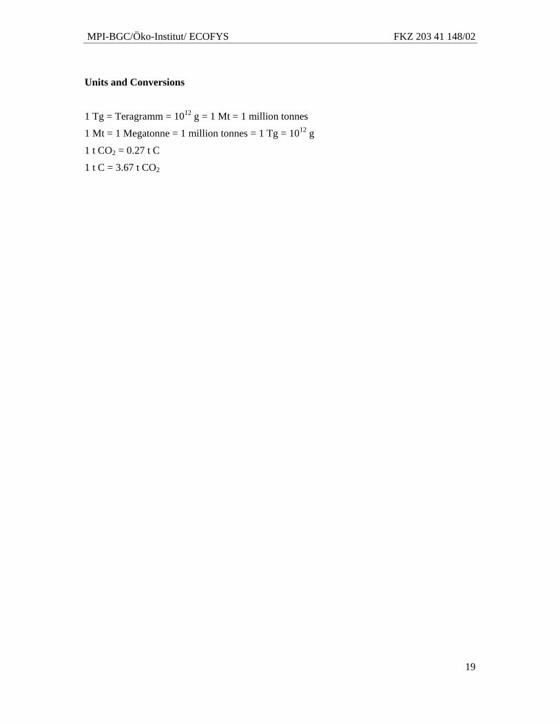
1 Tg = Teragramm = 1012 g = 1 Mt = 1 million tonnes
1 Mt = 1 Megatonne = 1 million tonnes = 1 Tg = 1012 g
1 t CO2 = 0.27 t C
1 t C = 3.67 t CO2
MPI-BGC/Öko-Institut/ ECOFYS FKZ 203 41 148/02
20
Deutsche Kurzfassung
Projekttitel Kyoto-Protokoll: Untersuchung von Optionen für die Weiterentwicklung der Verpflichtungen für die 2. Verpflichtungsperiode, Teilvorhaben „Senken in der 2. Verpflichtungsperiode“
Projektnehmer A. Freibauer, H. Böttcher; Max-Planck-Institut für Biogeochemie, Jena A. Herold; Öko-Institut, Berlin N. Höhne, S. Wartmann; ECOFYS, Köln
Laufzeit Juli 2003 - März 2006
Förderung Umweltbundesamt
Hintergrund des Projektes
Ursprünglich wurden 1997 im Kyoto-Protokoll Emissionsminderungsziele ohne Berücksichtigung des Landnutzungssektors ausgehandelt, aber bereits mit den Artikeln 3.3 und 3.4 eine Öffnung des KP hinsichtlich der Landnutzung vorgenommen. Erst 2001 wurden nach weiteren Verhandlungen Regeln zur Anrechnung von Kohlenstoffquellen und –senken im Landnutzungssektor in den Beschlüssen von Marrakesch festgelegt. Die getroffenen Vereinbarungen sind nur für die erste Verpflichtungsperiode von 2008 bis 2012 verbindlich. Da eine Aufweichung der ursprünglichen Ziele möglichst verhindert werden sollte, und sich der Landnutzungssektor wegen einiger Besonderheiten als unerwartet komplizierte Materie entpuppte, entstanden sehr komplexe, z.T. inkonsistente Modalitäten zur Anrechnung von Kohlenstoffquellen und –senken.
Die laufenden internationalen Verhandlungen zu zukünftigen Emissionsminderungs-verpflichtungen bieten neue Ansatzpunkte, um den Landnutzungssektor einfacher, umfassender und effizienter in ein neues Klimaschutzabkommen zu integrieren. Dabei sollten verstärkt andere Funktionen der Biosphäre, wie z.B. Biodiversität, Ernährungssicherheit und nachhaltige Nutzung berücksichtigt werden. Die Landnutzung kann einen wichtigen Beitrag leisten, um das Ziel der Klimarahmenkonvention zu erreichen und gefährlichen Klimawandel verhindern helfen.
Hauptziele des Projektes
Das Projekt will eine wissenschaftliche Grundlage für Verhandlungen im Rahmen der Klimarahmenkonvention zu zukünftigen Emissionsminderungspflichten im Bereich der Landnutzung leisten. Der vorliegende Bericht beinhaltet allgemeine Überlegungen zur Rolle der Landnutzung im Klimaschutz, schätzt das Potenzial für Klimaschutzmaßnahmen in der Land- und Forstwirtschaft ab und analysiert mögliche Optionen für zukünftige Regeln im Landnutzungssektor (LULUCF1). Der Bericht, insbesondere die Darstellung von Optionen und Vorschlägen für zukünftige Regelungen, spiegelt ausschließlich die Meinung der Autoren
1 Land Use, Land Use Change and Forestry
MPI-BGC/Öko-Institut/ ECOFYS FKZ 203 41 148/02
21
wieder und nimmt keinesfalls mögliche Positionen der in den Verhandlungen beteiligten Ministerien oder des Umweltbundesamtes vorweg.
Der Bericht enthält im Detail Folgendes:
1. Analyse der Unsicherheiten und Risiken der Kohlenstoffsenken in der Biosphäre im Hinblick auf mögliche Rückkopplungen mit dem Klimawandel (Kapitel 2).
2. Diskussion von möglichen Synergien und Konflikten zwischen Klimaschutz und anderen Ökosystemfunktionen (Kapitel 3).
3. Quantitative Abschätzung des möglichen Beitrags von LULUCF zum letztendlichen Ziel der Klimarahmenkonvention im Hinblick auf:
a. die zu erwartende Größenordnung von Quellen und Senken im LULUCF-Sektor im Vergleich zu anderen Sektoren (Kapitel 4),
b. die räumliche und zeitliche Verteilung von Quellen und Senken im LULUCF-Sektor im nächsten Jahrhundert (Kapitel 6, 7 und 8),
c. das Potenzial für Kohlenstoffspeicherung in der Biosphäre und mögliche Verluste durch menschlichen Einfluss in wichtigen Ländern und Regionen der Welt: Defintionen (Kapitel 5), Aufforstung, Wiederaufforstung und Entwaldung (Kapitel 6), Waldbewirtschaftung (Kapitel 7), landwirtschaftliche Maßnahmen (Kapitel 8).
4. Beschreibung der bestehenden LULUCF Regeln und ihrer Entstehungsgeschichte (Kapitel 9).
5. Untersuchung des Einflusses von verschiedenen Regeln auf die Menge der anrechenbaren Quellen und Senken im LULUCF-Sektor und Definition von Alternativen für Regeln im Bereich LULUCF und Analyse anhand von Kriterien zu Klimaschutz, Umweltschutz und politischer Akzeptanz, um vielversprechende Wege zu einem neuen Klimaschutzprotokoll zu identifizieren. Dabei wird systematisch unterschieden zwischen zentralen „Kernregeln“, die die Basis für zukünftige Verhandlungen bilden sollten, und „nachgeordneten Regeln“, die länderspezifische Besonderheiten oder politische Bedenken korrigieren sollen (Kapitel 10).
6. Vorschlag für ein neues Klimaregime, in dem die Kohlenstoffquellen und –senken im Landnutzungssektor vollständig integriert sind. Dazu müssten eine zweite Verpflichtung eingeführt und die Regeln im Kyoto-Protokoll erweitert werden (Kapitel 11).
Der Bericht berücksichtigt den Zeitraum von 1990 bis 2050 für die quantitativen Studien. Die politischen Optionen werden für den Zeitraum bis 2020 analysiert.
Überblick über die verwendeten Methoden
Die quantitativen Abschätzungen der zukünftigen Kohlenstoffquellen und –Senken beruhen auf den folgenden Daten und Modellen:
• Aufforstung, Wiederaufforstung und Entwaldung: Ein erster Ansatz schreibt die Aufforstungs- und Entwaldungsraten aus der Vergangenheit gemäß FAO-Daten bis 2020 fort. Dabei wird von konstanten Netto-Änderungsraten der Waldfläche ausgegangen. Ein zweiter Ansatz beruht auf dem von IIASA entwickelten DIMA-Modell (Rokityanskiy et al., eingereicht). Er berücksichtigt ökonomische Rahmenbedingungen und gibt globale Abschätzungen bis 2100.
MPI-BGC/Öko-Institut/ ECOFYS FKZ 203 41 148/02
22
• Waldbewirtschaftung: Für die Studie wurde von den Autoren ein eigenes Modell FORMICA entwickelt, das auf nationalen Forstinventaren beruht.
• Landwirtschaftliche Maßnahmen: Die IPCC-Richtlinien zur Berechnung von Änderungen in Bodenkohlenstoffvorräten wurde zusammen mit eigenen Abschätzungen von geeigneten Flächen verwendet.
• Anthropogene Treibhausgasemissionen aus anderen Sektoren wurden den SRES Szenarien und der EVOC-Datenbank des Projektpartners ECOFYS entnommen.
Wichtigste Ergebnisse
Forst und Klimawandel – zukünftige Entwicklung (Kapitel 2) In den 1990er Jahren wurden weltweit jährlich durch Landnutzungswandel, v.a. durch Entwaldung in den Tropen, 1.6 Pg C (5.9 Pg CO2) emittiert. Die Gesamtbilanz der Biosphäre war dagegen eine Nettosenke, da in der terrestrischen Biosphäre gleichzeitig etwa 2.4 Pg C (8.8 Pg CO2) aufgenommen wurden. Wälder in gemäßigten und borealen Klimaten sind derzeit die wichtigste terrestrische C-Senke. Doch auch in den Tropen werden C-Verluste durch Entwaldung weitgehend durch Zuwachs in den bestehenden Wäldern ausgeglichen.
Die Situation ist derzeit und wird auch zukünftig sehr stark von der Landnutzungsgeschichte, der Altersklassenverteilung von genutzten Wäldern und menschlichen Eingriffen geprägt sein. Indirekte Effekte wie Düngung durch CO2, Stickstoffdeposition und besseres Wachstum durch längere Vegetationsperioden scheinen dagegen von geringerer Bedeutung zu sein als ursprünglich angenommen. Menschliche Eingriffe werden auch in in den nächsten Jahrzehnten wichtiger als die Folgen des Klimawandels für die Entwicklung der Wälder sein.
Die vielfältigen, oft nicht linearen Wechselwirkungen zwischen Wäldern und Klima machen Vorhersagen über die zukünftige Waldentwicklung in der ferneren Zukunft sehr schwierig. Häufigere Wetterextremereignisse und Störungen wie Feuer und Insektenkalamitäten, wie sie in wichtigen Waldregionen der Erde vorhergesagt werden, machen v.a. die borealen und tropischen Wälder mit den global höchsten C-Vorräten pro Fläche anfällig für C-Verluste.
Potenzielle Synergien mit Biodiversität (Kapitel 3) Bisher wurden mögliche Synergien zwischen der Klimarahmenkonvention und der Biodiversitätskonvention nicht realisiert. Vielversprechende Möglichkeiten existieren auf verschiedenen Ebenen:
• Institutionen, z.B. gemeinsame Sekretariate und Konferenzen
• Mechanismen, z.B. Berichterstattung, wissenschaftliche Beratung, Training
• Aktivitäten im Bereich der Landnutzung, v.a. bei der Umsetzung von Projekten und nationalen Nachhaltigkeitsstrategien
Synergien könnten im Design eines zukünftigen Klimaabkommens gestärkt werden. Dafür ist eine breitere, möglichst vollständige Berücksichtigung aller Landnutzungsformen wesentlich, verbunden mit klaren Anreizen zu einer nachhaltigen Landnutzung. Der Erhalt der vorhandenen Kohlenstoffvorräte kann dabei nur ein wichtiger Indikator sein, der durch weitere biodiversitätsrelevante Indikatoren ergänzt werden muss. Synergien ergeben sich vor allem bei der nachhaltigen Forst- und Landwirtschaft sowie bei der Reduzierung der Entwaldung. Auf der Projektebene könnte eine gemeinsame Evaluierung nach Klima- und Biodiversitätsgesichtspunkten entwickelt werden, die nach Aktivitätstyp, z.B.
MPI-BGC/Öko-Institut/ ECOFYS FKZ 203 41 148/02
23
Landnutzungswandel, reduzierte Entwaldung, Managementänderung etc. differenziert sein sollte. Dabei wäre eine kombinierte Evaluierung möglicherweise sogar als Marktmechanismus, ähnlich wie die „Gold“-Prämierung von CDM-Projekten, geeignet.
Letztendlich ist die nachhaltige Landnutzung die entscheidende Brücke zwischen den Konventionen, die allerdings schwer fassbar ist.
LULUCF und allgemeines post 2012 Regime (Kapitel 4) Das 2°C Ziel für die Änderung der globalen Lufttemperatur, dessen Erreichung die Bundesregierung und der Europäischen Gemeinschaft für notwendig erachtet, um das letztendliche Ziel der Klimarahmenkonvention erfüllen zu können kann unterstützt werden, wenn auch die Emissionen aus dem LULUCF Sektor gemindert werden.
LULUCF Regeln können die Verpflichtungen zu Emissionsminderungen in anderen Sektoren beeinflussen, wenn alle Sektoren miteinander verknüpft sind. Die Regeln müssen daher vor der Festsetzung von quantitativen Verpflichtungen fest stehen. Es ist zu erwarten, dass im Laufe der Zeit immer mehr Länder einem Klimaregime beitreten werden.
Von der Ausgestaltung der LULUCF Regeln hängt ab, ob Länder strengere oder leichtere Verpflichtungen übernehmen. Länder sind eher geneigt, ambitionierte Verpflichtungen zu übernehmen, wenn diese nicht mit Sanktionen bei Nichteinhaltung verbunden sind. Andererseits verhindern weiche Verpflichtungen eine ernsthafte Kontrolle und Vorhersagbarkeit der Emissionsminderungen. In diesem Spagat bewegen sich die Verhandlungen. Wenn z.B. Pro-Kopf-Emissionen aus dem LULUCF Sektor zur Festsetzung von Verpflichtungen zugrunde gelegt werden, müssten die großen Entwaldungsnationen hohe Minderungsverpflichtungen übernehmen. Dies betrifft vor allem Nicht-Annex-I-Länder wie Brasilien und Indonesien, die unter dem Kyoto-Protokoll keine Verpflichtungen haben und die für ein zukünftiges Klimaregime erst gewonnen werden müssen. Diese Länder werden sich daher wahrscheinlich weigern, sofort strenge ambitionierte Verpflichtungen einzugehen. Wird dagegen ein System mit Vorteilen oder ohne Sanktionen geschaffen, könnte dies ein Anreiz sein, z.B. Entwaldung in Nicht-Annex-I Ländern einzudämmen, da eine größere Bereitschaft zum Mitmachen bei den betroffenen Ländern geweckt werden könnte. Wenn Anreize zu „weichen“ Emissionsminderungsverpflichtungen zusätzlich zu strengen und ambitionierten Emissionsminderungsverpflichtungen geschaffen werden, wird das Ziel der Klimarahmenkonvention nicht gefährdet.
Der LULUCF Sektor könnte auch separat von den Verpflichtungen in den anderen Sektoren behandelt werden, um Nicht-Annex-I Ländern einen ersten – evtl. nicht-quantitativen – Schritt in ein post 2012 Regime zu ermöglichen.
Defintion der Potenzialbegriffe (Kapitel 5)
Im Bericht werden verschiedene Potenzialbegriffe verwendet, die folgendermaßen definiert werden (geordnet in abfallender Größenordnung und zunehmend realistisch):
• Biologisches Potenzial: aus biologischer Sicht theoretisch mögliche Kapazität zur C-Speicherung in Ökosystemen. Dies bedeutet z.B. dass eine bestimmte Managementänderung auf allen Acker- oder Waldflächen sofort und überall umgesetzt würde.
• Technologisches Potenzial: ausgehend vom biologischen Potenzial werden zusätzliche Einschränkungen, wie z.B. die Eignung von Flächen für eine bestimmte Maßnahme, vorhandene Ressourcen, z.B. in Bezug auf organische Dünger in der Landwirtschaft,
MPI-BGC/Öko-Institut/ ECOFYS FKZ 203 41 148/02
24
berücksichtigt. Die Verfügbarkeit von Landflächen, sozioökonomische und politische Faktoren bleiben dagegen unberücksichtigt. Theoretisch werden hier auch mögliche Störungen und Kalamitäten berücksichtigt, was aber aufgrund der Datenlage häufig unmöglich ist.
• Ökonomisches Potenzial: Ausgehend vom technologischen Potenzial werden zusätzliche Barrieren bezüglich der Implementierung von Maßnahmen, wie Kosten, Flächenverfügbarkeit etc. berücksichtigt. Soziale und politische Barrieren bleiben unberücksichtigt, ebenso wird von ökonomischen Anreizen, typischerweise einem globalen CO2-Markt, zur Umsetzung von Maßnahmen ausgegangen.
• Realistisches Potenzial: Die tatsächliche kurzfristig umsetzbare Kapazität für bestimmte Maßnahmen, die alle Hindernisse politischer, sozialer und ökonomischer Natur berücksichtigt. Das realistische Potenzial beträgt oft nur wenige Prozent des biologischen und technologischen Potenzials.
LULUCF Potenziale: Aufforstung und Entwaldung (Kapitel 6)
Eine Fortschreibung der Nettoänderungsraten der Wald- und Plantagenflächen von 2000 bis 2020 nach FAO Forest Resource Assessment (FRA) 2005 lässt einen Rückgang der Netto-Entwaldung von 10 Millionen Hektar im Jahr 2000 auf 6 Millionen Hektar im Jahr 2020 erwarten. Im gleichen Zeitraum könnte die jährliche Netto-Aufforstung von Plantagen von 2,4 Millionen Hektar auf 13,8 Millionen Hektar steigen. Nach Einbeziehung von Wirtschaftlichkeitsbetrachtungen (IIASA) ist mit geringerer Entwaldung aber auch mit geringerer Aufforstung als mit FAO Daten vorhergesagt zu rechnen.
Beide Berechnungsansätze nach FAO FRA 2005 und IIASA ergeben, dass die Landnutzungsänderung in den nächsten Jahrzehnten eine Nettokohlenstoffquelle bleiben wird. Ab ca. 2020-2030 könnten aber die Emissionen aus der Entwaldung durch C-Speicherung in Aufforstungen kompensiert werden.
Es handelt sich bei diesen Schätzungen um ein ökonomisch realistisches Potenzial zur Emissionsminderung, da beide Berechnungsansätze (FAO und IIASA) von tatsächlich in den letzten Jahren aufgetretenen Aufforstungs- und Entwaldungsraten ausgehen.
Tabelle 1 zeigt beispielhaft die geschätzten CO2-Emissionen aus der Entwaldung und die CO2-Speicherung durch Aufforstung im Jahr 2020. Die größten CO2-Flüsse treten in Nicht-Annex-I Staaten auf. Emissionen aus der Entwaldung, v.a. in Brasilien und Indonesien, werden weitgehend von CO2-Speicherung durch Aufforstungen in China kompensiert. Diese Darstellung geht allerdings davon aus, dass China sein ambitioniertes Aufforstungsprogramm aus der Vergangenheit in Zukunft noch weiter stark ausbaut.
LULUCF Potenziale: Forstbewirtschaftungsmaßnahmen (Kapitel 7) Kohlenstoffvorratsänderungen durch Forstbewirtschaftungsmaßnahmen wurden für 37 Annex-I Länder (Europa, Russland, Kanada, USA) und China mit dem eigens entwickelten Modell FORMICA modelliert.
FORMICA ist ein generisches dynamisches Forstmodell, das Kohlenstoffvorräte und Vorratsänderungen in allen Speichern (Pools), die für die Klimarahmenkonvention und das Kyoto-Protokoll relevant sind, auf regionaler Basis berechnet. Die berücksichtigten Pools sind Biomasse, Totholz, Streu und Boden. Darüber hinaus besteht die Möglichkeit, Forstprodukte einzubeziehen. Die Umtriebszeiten von Wäldern, Biomassezuwächse und Mortalität wurden aus regionalen Daten berechnet. Für die Pools Totholz, Streu und Boden wurde das Modell YASSO in FORMICA integriert. YASSO berechnet Umsatzraten der toten organischen
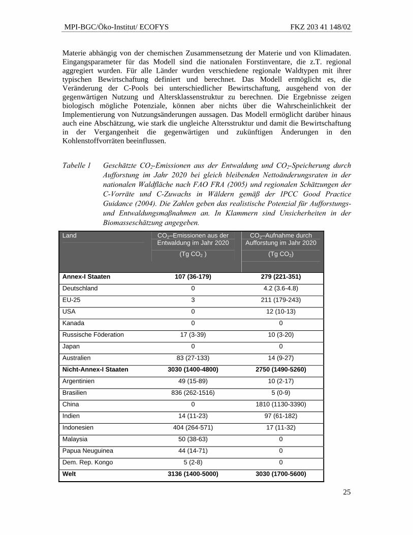
MPI-BGC/Öko-Institut/ ECOFYS FKZ 203 41 148/02
25
Materie abhängig von der chemischen Zusammensetzung der Materie und von Klimadaten. Eingangsparameter für das Modell sind die nationalen Forstinventare, die z.T. regional aggregiert wurden. Für alle Länder wurden verschiedene regionale Waldtypen mit ihrer typischen Bewirtschaftung definiert und berechnet. Das Modell ermöglicht es, die Veränderung der C-Pools bei unterschiedlicher Bewirtschaftung, ausgehend von der gegenwärtigen Nutzung und Altersklassenstruktur zu berechnen. Die Ergebnisse zeigen biologisch mögliche Potenziale, können aber nichts über die Wahrscheinlichkeit der Implementierung von Nutzungsänderungen aussagen. Das Modell ermöglicht darüber hinaus auch eine Abschätzung, wie stark die ungleiche Altersstruktur und damit die Bewirtschaftung in der Vergangenheit die gegenwärtigen und zukünftigen Änderungen in den Kohlenstoffvorräten beeinflussen.
Tabelle 1 Geschätzte CO2-Emissionen aus der Entwaldung und CO2-Speicherung durch Aufforstung im Jahr 2020 bei gleich bleibenden Nettoänderungsraten in der nationalen Waldfläche nach FAO FRA (2005) und regionalen Schätzungen der C-Vorräte und C-Zuwachs in Wäldern gemäß der IPCC Good Practice Guidance (2004). Die Zahlen geben das realistische Potenzial für Aufforstungs- und Entwaldungsmaßnahmen an. In Klammern sind Unsicherheiten in der Biomasseschätzung angegeben.
Land CO2–Emissionen aus der Entwaldung im Jahr 2020
(Tg CO2 )
CO2–Aufnahme durch Aufforstung im Jahr 2020
(Tg CO2)
Annex-I Staaten 107 (36-179) 279 (221-351)
Deutschland 0 4.2 (3.6-4.8)
EU-25 3 211 (179-243)
USA 0 12 (10-13)
Kanada 0 0
Russische Föderation 17 (3-39) 10 (3-20)
Japan 0 0
Australien 83 (27-133) 14 (9-27)
Nicht-Annex-I Staaten 3030 (1400-4800) 2750 (1490-5260)
Argentinien 49 (15-89) 10 (2-17)
Brasilien 836 (262-1516) 5 (0-9)
China 0 1810 (1130-3390)
Indien 14 (11-23) 97 (61-182)
Indonesien 404 (264-571) 17 (11-32)
Malaysia 50 (38-63) 0
Papua Neuguinea 44 (14-71) 0
Dem. Rep. Kongo 5 (2-8) 0
Welt 3136 (1400-5000) 3030 (1700-5600)
MPI-BGC/Öko-Institut/ ECOFYS FKZ 203 41 148/02
26
Eine unregelmäßige Nutzungsgeschichte und Störungen führen dazu, dass sich Wälder von ihrer theoretisch gleichmäßigen Altersklassenverteilung, die in allen Klassen die gleiche Nutzungsfläche vorsieht („Normalwald“), entfernen. Die ungleiche Altersklassenverteilung in den bewirtschafteten Wäldern führt zu Fluktuationen in den Kohlenstoffvorräten, so dass die Wälder über Zeiträume von Jahrzehnten zwischen C-Senke und C-Quelle fluktuieren. Das bedeutet, dass in einer Phase, in der junge und mittelalte, stark wüchsige Forststadien dominieren, die Wälder eine Nettosenke für C darstellen. Wenn dagegen hiebreife Stadien dominieren, wird durch den intensiven Einschlag und die Verjüngung der Bestände die Waldfläche zu einer Nettoquelle für C. Über sehr lange Zeiträume und Flächen hinaus gleichen sich diese temporären C-Senken und Quellen weitgehend aus. Aufgrund des Altersklasseneffektes wird sich die C-Senke in den Wäldern von 38 wichtigen Staaten (Kanada, Russische Föderation, USA, 34 europäische Staaten, China) bei gleich bleibendem Forstmanagement und gleich bleibender Forstfläche von gegenwärtig ca. 0.5 Pg CO2/Jahr bis 2050 auf ca. 1.3 Pg CO2/Jahr erhöhen.
Managementänderungen
Verlängerung der Rotationsperiode
Eine Verlängerung der Rotationsperiode speichert kurzfristig Kohlenstoff, indem der Erntezeitpunkt verschoben wird. Dieser Kohlenstoff wird zum Zeitpunkt einer späteren Nutzung wieder frei, so dass eine Verlängerung der Rotationsperiode eine sehr kurzfristig wirksame, reversible Klimaschutzmaßnahme darstellt. Zudem muss Holz bei gleicher Nachfrage aus Ernten in anderen Regionen/Ländern bereitgestellt werden.
In Europa und China herrschen derzeit relativ junge rasch wüchsige Altersstadien in den Wäldern vor, so dass die gegenwärtige Senke nahe dem Maximum innerhalb der C-Dynamik ist. In Europa und China wird die gegenwärtige C-Senke daher mittelfristig geringer werden und sich in einigen Jahrzehnten in eine Quelle umkehren. In Russland, USA und Kanada, wo eher alte Waldstadien dominieren, wird die gegenwärtige Senke größer werden bzw. die gegenwärtige geringe Quelle zur Senke werden, sobald die nächste Generation Wald heranwächst.
Forstbewirtschaftung kann sich nur im Zeitraum von Rotationsperioden (Jahrzehnte bis Jahrhunderte) ändern, wenn entsprechende Teilflächen im geeigneten Stadium für Maßnahmen sind. Der Effekt der Änderungen hält unterschiedlich lange an, je nach Rotationszeit der Wälder und Verweilzeit des Kohlenstoffs in den verschiedenen Pools. Wegen der vorherrschend jungen Forsten können Managementänderungen in Europa und China erst mit langer zeitlicher Verzögerung großflächig durchgeführt werden, nämlich wenn die jetzt heranwachsenden Wälder hiebreif sind.
Vermehrte C-Speicherung in langlebigen Holzprodukten
Eine vermehrte C-Speicherung in langlebigen Holzprodukten in 25 Annex-I Staaten hat ein kumulatives technisches Potenzial von 1.5 Pg CO2 (2000-2050). In der Realität dagegen ist dieses Potenzial deutlich geringer, da der Markt für kurzlebige Holzprodukte wesentlich größer und dynamischer ist als für langlebige Holzprodukte. Dies wird sich auch mittelfristig nicht ändern.
Veränderung in den Anrechnungsvorschriften
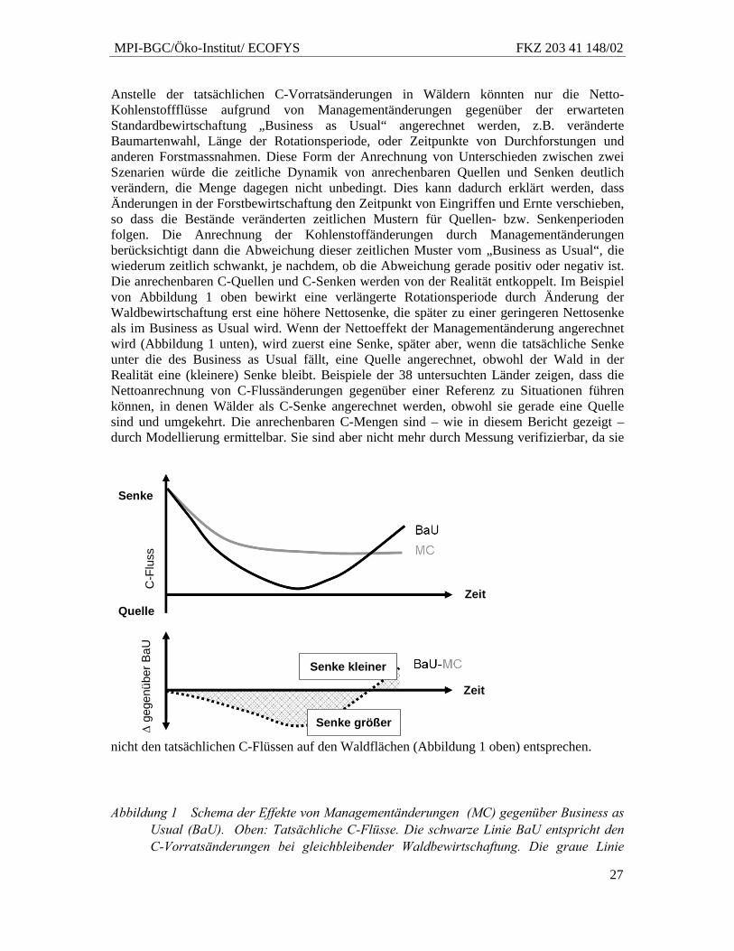
MPI-BGC/Öko-Institut/ ECOFYS FKZ 203 41 148/02
27
Anstelle der tatsächlichen C-Vorratsänderungen in Wäldern könnten nur die Netto-Kohlenstoffflüsse aufgrund von Managementänderungen gegenüber der erwarteten Standardbewirtschaftung „Business as Usual“ angerechnet werden, z.B. veränderte Baumartenwahl, Länge der Rotationsperiode, oder Zeitpunkte von Durchforstungen und anderen Forstmassnahmen. Diese Form der Anrechnung von Unterschieden zwischen zwei Szenarien würde die zeitliche Dynamik von anrechenbaren Quellen und Senken deutlich verändern, die Menge dagegen nicht unbedingt. Dies kann dadurch erklärt werden, dass Änderungen in der Forstbewirtschaftung den Zeitpunkt von Eingriffen und Ernte verschieben, so dass die Bestände veränderten zeitlichen Mustern für Quellen- bzw. Senkenperioden folgen. Die Anrechnung der Kohlenstoffänderungen durch Managementänderungen berücksichtigt dann die Abweichung dieser zeitlichen Muster vom „Business as Usual“, die wiederum zeitlich schwankt, je nachdem, ob die Abweichung gerade positiv oder negativ ist. Die anrechenbaren C-Quellen und C-Senken werden von der Realität entkoppelt. Im Beispiel von Abbildung 1 oben bewirkt eine verlängerte Rotationsperiode durch Änderung der Waldbewirtschaftung erst eine höhere Nettosenke, die später zu einer geringeren Nettosenke als im Business as Usual wird. Wenn der Nettoeffekt der Managementänderung angerechnet wird (Abbildung 1 unten), wird zuerst eine Senke, später aber, wenn die tatsächliche Senke unter die des Business as Usual fällt, eine Quelle angerechnet, obwohl der Wald in der Realität eine (kleinere) Senke bleibt. Beispiele der 38 untersuchten Länder zeigen, dass die Nettoanrechnung von C-Flussänderungen gegenüber einer Referenz zu Situationen führen können, in denen Wälder als C-Senke angerechnet werden, obwohl sie gerade eine Quelle sind und umgekehrt. Die anrechenbaren C-Mengen sind – wie in diesem Bericht gezeigt – durch Modellierung ermittelbar. Sie sind aber nicht mehr durch Messung verifizierbar, da sie
nicht den tatsächlichen C-Flüssen auf den Waldflächen (Abbildung 1 oben) entsprechen.
Abbildung 1 Schema der Effekte von Managementänderungen (MC) gegenüber Business as Usual (BaU). Oben: Tatsächliche C-Flüsse. Die schwarze Linie BaU entspricht den C-Vorratsänderungen bei gleichbleibender Waldbewirtschaftung. Die graue Linie
Zeit
Zeit
Senke
Quelle
C-F
luss
Δge
genü
ber B
aU
Senke kleiner
Senke größer
MPI-BGC/Öko-Institut/ ECOFYS FKZ 203 41 148/02
28
zeigt die C-Vorratsänderungen bei geänderter Waldbewirtschaftung MC, z.B. eine längere Rotationsperiode. Unten: Unterschied zwischen den beiden oberen Szenarien als Differenz zwischen BaU und MC.
Altersklasseneffekte
Der Einfluss von Forstmaßnahmen in der Vergangenheit drückt sich in der aktuellen Altersklassenverteilung aus. Der Einfluss einer ungleichen Altersklassenverteilung auf die Fluktuation von C-Vorräten in Wäldern lässt sich in ähnlicher Weise wie der Einfluss von Managementänderungen (Abbildung 1) berechnen. Man kann den Altersklasseneffekt herausrechnen, indem eine theoretische Gleichverteilung der Altersklassen angenommen wird, d.h., allen Altersklassen gleiche Flächenanteile zugewiesen werden („Normalwald“). Dies ist das theoretische Ziel von nachhaltiger Forstwirtschaft. Eine Anrechnung von C-Quellen und C-Senken, die diese theoretische Altersklassenverteilung als Vergleichsbasis zugrunde legt, kehrt in Extremfällen wie Kanada und China das Vorzeichen der anrechenbaren C-Mengen sowie die zeitlichen Trends (Ab- oder Zunahme von C-Speicherung) um. Die anrechenbaren C-Quellen und C-Senken werden von der Realität entkoppelt. Damit sind die anrechenbaren C-Mengen nicht mehr durch Messungen verifizierbar.
LULUCF Potenziale: Ackerbaumaßnahmen (Kapitel 8)
Das Potenzial für C-Sequestrierung durch Ackerbaumaßnahmen wurde mit dem IPCC Soil Tool für die oberen 30 cm in Ackerböden berechnet. Dadurch werden ca. 50% der C-Vorräte in Ackerböden erfasst. Die Kultivierung von Böden für den Ackerbau hat in den letzten Jahrhunderten global ca. 100 Pg CO2 freigesetzt. Dieser Wert stellt die theoretische Obergrenze für C-Sequestrierung dar. Die höchsten historischen C-Verluste traten in den USA, Russland, China und Indien sowie EU-25 auf. Dementsprechend liegen in diesen Regionen die größten C-Sequestrierungspotenziale in Ackerböden. Durch weitere Ackerbaumaßnahmen lassen sich technisch in den nächsten 20 Jahren ca. 0.5 Pg CO2 sequestrieren. In der Praxis werden vermutlich weniger als 10% davon realisiert.
Zukünftige C-Verluste könnten durch eine stärkere Mechanisierung in Entwicklungsländern auftreten. Ist die Mechanisierung mit einer Intensivierung gekoppelt, könnten sich die Boden-C-Vorräte dagegen leicht erhöhen.
Konservierende Bodenbearbeitung ist die wichtigste Ackerbaumaßnahme, um Kohlenstoff im Boden zu speichern, da sie universell einsetzbar ist. Auch pfluglose Bodenbearbeitung und Intensivierung weisen signifikante Potenziale auf, führen aber zu erhöhten N2O-Emissionen.
Die globalen technischen C-Senkenpotenziale der Ackerböden sind größer als ihre C-Quellenpotenziale. Ein Teil der C-sequestrierenden Ackerbaumaßnahmen wird derzeit bereits als Business as Usual umgesetzt.
LULUCF Potenziale: Datenbank
Im Projekt wurde eine Datenbank erstellt, die Projektionen und Szenarien der C-Quellen und Senken im LULUCF-Sektor für die wichtigsten Länder der Erde sowie Vergleichsdaten zu Emissionen aus anderen Sektoren enthält. Dabei wurden die C-Pools in der ober- und unterirdischen Biomasse, Totholz, Streu und Boden berücksichtigt, optional auch die in Forstprodukten.
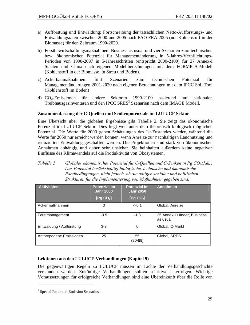
MPI-BGC/Öko-Institut/ ECOFYS FKZ 203 41 148/02
29
a) Aufforstung und Entwaldung: Fortschreibung der tatsächlichen Netto-Aufforstungs- und Entwaldungsraten zwischen 2000 und 2005 nach FAO FRA 2005 (nur Kohlenstoff in der Biomasse) für den Zeitraum 1990-2020.
b) Forstbewirtschaftungsmaßnahmen: Business as usual und vier Szenarien zum technischen bzw. ökonomischen Potenzial für Managementänderung in 5-Jahres-Verpflichtungs-Perioden von 1998-2097 in 5-Jahresschritten (entspricht 2000-2100) für 37 Annex-I Staaten und China nach eigenen Modellberechnungen mit dem FORMICA-Modell (Kohlenstoff in der Biomasse, in Streu und Boden).
c) Ackerbaumaßnahmen: fünf Szenarien zum technischen Potenzial für Managementänderungen 2001-2020 nach eigenen Berechnungen mit dem IPCC Soil Tool (Kohlenstoff im Boden)
d) CO2-Emissionen für andere Sektoren 1990-2100 basierend auf nationalen Treibhausgasinventaren und den IPCC SRES2 Szenarien nach dem IMAGE Modell.
Zusammenfassung der C-Quellen und Senkenpotenziale im LULUCF Sektor
Eine Übersicht über die globalen Ergebnisse gibt Tabelle 2. Sie zeigt das ökonomische Potenzial im LULUCF Sektor. Dies liegt weit unter dem theoretisch biologisch möglichen Potenzial. Die Werte für 2000 geben Schätzungen des Ist-Zustandes wieder, während die Werte für 2050 nur erreicht werden können, wenn Anreize zur nachhaltigen Landnutzung und reduzierten Entwaldung geschaffen werden. Die Projektionen sind stark von ökonomischen Annahmen abhängig und daher sehr unsicher. Sie beinhalten außerdem keine negativen Einflüsse des Klimawandels auf die Produktivität von Ökosystemen.
Tabelle 2 Globales ökonomisches Potenzial für C-Quellen und C-Senken in Pg CO2/Jahr. Das Potenzial berücksichtigt biologische, technische und ökonomische Randbedingungen, nicht jedoch, ob die nötigen sozialen und politischen Strukturen für die Implementierung von Maßnahmen gegeben sind.
Aktivitäten Potenzial im Jahr 2000
[Pg CO2]
Potenzial im Jahr 2050
[Pg CO2]
Annahmen
Ackermaßnahmen 0 <-0.1 Global, Anreize
Forstmanagement -0.5 -1.3 25 Annex-I Länder, Business as usual
Entwaldung / Aufforstung 3-8 0 Global, C-Markt
Anthropogene Emissionen 25 55 (30-88)
Global, SRES
Lektionen aus den LULUCF-Verhandlungen (Kapitel 9)
Die gegenwärtigen Regeln zu LULUCF müssen im Lichte der Verhandlungsgeschichte verstanden werden. Zukünftige Verhandlungen sollten schrittweise erfolgen. Wichtige Voraussetzungen für erfolgreiche Verhandlungen sind eine Übereinkunft über die Rolle von 2 Special Report on Emission Scenarios
MPI-BGC/Öko-Institut/ ECOFYS FKZ 203 41 148/02
30
LULUCF im Klimaregime und eine robuste Datenbasis, um die verschiedenen Verhandlungsoptionen zu analysieren. Die Ergebnisse des vorgestellten Projektes liefern eine erste Grundlage.
Die LULUCF Regeln sollten wissenschaftlich fundiert, vollständig und ausgewogen bezüglich C-Senken und Quellen sowie, einfach und umfassend sein, so dass alle C-Pools berücksichtigt werden. Sie sollten Anreize zur Reduzierung von Entwaldung und zu nachhaltiger Waldwirtschaft und damit zum Erhalt der bestehenden Kohlenstoffvorräte geben.
Quantitative Verpflichtungen sollten erst nach Festlegung der Regeln bestimmt werden.
Kriterien zur Bewertung von Optionen und Kernregeln für zukünftige Verpflichtungen (Kapitel 10)
Zukünftige LULUCF Regeln sollten die Ziele der Klimarahmenkonvention bestmöglich unterstützen. Dazu wurden sechs Kriterien und dazu gehörige Kernfragen formuliert:
1. Effizienter Klimaschutz
• Tragen die Regeln dazu bei, das Ziel der Klimarahmenkonvention zu erreichen und die globale Erwärmung auf 2°C zu begrenzen?
• Sind alle wichtigen anthropogenen Quellen berücksichtigt?
• Bieten die Regeln Anreize, um die Kohlenstoffvorräte in der terrestrischen Biosphäre zu schützen?
• Stimulieren die Regeln eine breite Beteiligung der wichtigsten Industrie-, Schwellen- und Entwicklungsländer?
2. Schaffung zusätzlicher Umweltvorteile
• Bieten die Regeln Anreize zu nachhaltiger Land- und Forstwirtschaft?
• Tragen die Regeln zum Schutz der Biodiversität bei?
• Erlauben es die Regeln, besonders gefährdete Gebiete zu schützen, die starke Wechselwirkungen mit dem Klimawandel aufweisen?
3. Technische Effizienz (einfaches Monitoring, einfache Anrechnung und Verifikation der Einhaltung der Verpflichtungen):
• Erlauben die Regeln eine einfache pragmatische technische Umsetzung?
• Werden konsistente Regeln für das Monitoring und die Berechnung von Quellen und Senken über den gesamten Zeitraum verwendet?
4. Unterstützung des Verhandlungsprozesses für ein Klimaregime nach 2012
• Berücksichtigen die Regeln die gemeinsame, aber differenzierte Verantwortung der Vertragsstaaten der Klimarahmenkonvention?
• Beruhen die Regeln auf vertrauenswürdigen Daten und guter wissenschaftlicher Praxis?
• Erlauben die Regeln den Vertragsstaaten genügend Flexibilität, um ihre Verpflichtungen einzuhalten?
• Erlauben die Regeln ausreichend Kontinuität mit der ersten Verpflichtungsperiode?
MPI-BGC/Öko-Institut/ ECOFYS FKZ 203 41 148/02
31
• Stimmen die Regeln mit Positionen der wichtigsten Verhandlungsführer überein, z.B., beinhalten sie keine bereits abgelehnten Vorschläge?
5. Berücksichtigung der besonderen Eigenschaften von LULUCF Aktivitäten
• Berücksichtigen die Regeln die Variabilität der terrestrischen Kohlenstoffflüsse innerhalb einer Verpflichtungsperiode?
• Berücksichtigen die Regeln die unterschiedlichen Zeitskalen für Kohlenstoffaufnahme bzw. –verlust in Ökosystemen?
• Berücksichtigen die Regeln die Dauerhaftigkeit der angerechneten Aktivitäten?
• Erlauben die Regeln zwischen direktem und indirektem menschlichen Einfluss auf die Treibhausgasflüsse in der Biosphäre zu unterscheiden?
• Berücksichtigen die Regeln die unterschiedlichen nationalen natürlichen, klimatischen und geographischen Umstände?
6. Kosteneffizienz
• Erlauben die Regeln den Vertragsstaaten, kostengünstige Emissionsminderungsstrategien zu wählen?
• Erlauben die Regeln genügend Flexibilität in der Umsetzung?
• Wie beeinflussen die Regeln die Transaktionskosten?
Optionen und Kernregeln für zukünftige Verpflichtungen (Kapitel 10)
Zukünftige Verpflichtungen lassen sich in einzelne Kernregeln zerlegen, die weitgehend unabhängig voneinander anhand der oben genannten Kriterien analysiert und z. T. auch verhandelt werden können. Im Verhandlungsprozess könnten durch zusätzliche Regeln nationale Besonderheiten berücksichtigt werden.
Die Kernregeln beschreiben
• das Verhältnis zwischen LULUCF Verpflichtungen und anderen Sektoren
• die Definition von „anthropogenen“ C-Senken und C-Quellen
• die berücksichtigten LULUCF Aktivitäten
• Anrechnungsregeln
• das Verhältnis zu den flexiblen Mechanismen.
Folgende Kernregeln und Optionen werden vorgeschlagen:
1. Auch in Zukunft wird das Prinzip der nach Ländern differenzierten Verpflichtungen beibehalten werden.
2. Eine einzige Verpflichtung, die alle Sektoren umfasst oder eine Verpflichtung nur für den Sektor LULUCF:
Option 1: eine einzige Verpflichtung wie bisher
Option 2: Separate quantitative Verpflichtungen für alle Sektoren außer LULUCF und für den LULUCF Sektor
MPI-BGC/Öko-Institut/ ECOFYS FKZ 203 41 148/02
32
Option 3: Neuer Verpflichtungstyp für den LULUCF Sektor, z.B. basierend auf C-Vorräten, Landnutzungsklassen mit typischen C-Vorräten oder Sonderverpflichtungen nur für den Erhalt von C-Vorräten in nicht genutzten Flächen
Option 4: Separates Protokoll für den Sektor LULUCF
3. Anrechnung des direkten menschlichen Einflusses auf Emissionen und Senken
Option 1: Wie bisher
Option 2: Anrechnung aller C-Emissionen und Senken auf den Landflächen
Option 3: Diskontierungsansatz, wie er teilweise zur Ableitung der anrechenbaren Maximalmengen von Kohlenstoff im Rahmen von Artikel 3.4. zu Waldbewirtschaftung im Kyoto-Protokoll angewandt wurde.
4. Einbeziehung von bestimmten LULUCF Aktivitäten
Option 1: Wie bisher werden Emissionen und Fixierung von CO2 durch Aufforstung, Wiederaufforstung und Entwaldung zwingend angerechnet, und solche durch Bewirtschaftung von Wald, Grünland und Ackerland und Wiederbegrünung auf freiwilliger Basis.
Option 2: Zusätzliche Aktivitäten, die nicht im Kyoto-Protokoll und den Marrakesch-Beschlüssen enthalten sind, z.B. Walddegradation, Vegetationsverluste, zwingende Anrechnung der C-Vorratsänderungen aller in Option 1 aufgeführten Aktivitäten, C-Vorratsänderungen in Holzprodukten, reduzierte Entwaldung und Schutz von Naturwäldern werden in das zukünftige Regime aufgenommen.
5. Länge der Verpflichtungsperiode:
Option 1: weiter mit 5-jährigen Verpflichtungsperioden
Option 2: längere Verpflichtungsperioden
Option 3: verschieden lange Verpflichtungsperioden für LULUCF einerseits und die anderen Sektoren andererseits
6. Walddefinition
Option 1: Beibehaltung der bisherigen Definition
Option 2: Walddefinition basierend auf Biomen
7. Anrechnungsregeln und Basisjahr
Option 1: Regeln des Kyoto-Protokolls bleiben weiter gültig, 1990 bleibt Bezugsjahr für LULUCF-Maßnahmen, die C-Änderungen ab 2012 in den folgenden Verpflichtungsperioden werden angerechnet
Option 2: „brutto-netto“-Anrechnung für alle LULUCF-Aktivitäten
Option 3: „seit 1990“ wird gestrichen, „netto-netto“-Anrechnung aller LULUCF-Aktivitäten
8. LULUCF in den flexiblen Mechanismen
Option 1: Regeln des Kyoto Protokolls bleiben weiter gültig
Option 2: Zeitlich befristete Anrechnung (tCERs) für alle LULUCF Aktivitäten
Option 3: Separate flexible Mechanismen für LULUCF
MPI-BGC/Öko-Institut/ ECOFYS FKZ 203 41 148/02
33
9. Zusätzliche Regeln für landesspezifische Besonderheiten
Diese können erst verhandelt werden, wenn die Kernregeln beschlossen sind und deren Auswirkungen auf die Anrechenbarkeit von verschiedenen Maßnahmen bekannt sind.
Die verschiedenen Optionen für die Kernregeln erfüllen nicht alle Kriterien gleichermaßen gut. Trotzdem lassen sich viel versprechende Ansätze identifizieren. Die zukünftigen Regeln sollten zwischen Kontinuität, Einfachheit, Symmetrie gegenüber Quellen und Senken und Vollständigkeit ausbalanciert sein.
Einfluss von Kernregeln auf anrechenbare C-Quellen und C-Senken von LULUCF (Kapitel 10)
Die nationalen Treibhausgasinventare für die UNFCCC Berichterstattung zeigen, dass Aufforstung und Entwaldung in den meisten Annex-I Staaten nur einen untergeordneten Beitrag zu den anthropogenen Emissionen und deren Variabilität liefern. Hingegen haben die CO2-Fixierung und Emissionen infolge von forstlichen und landwirtschaftlichen Bewirtschaftungsmaßnahmen in den Annex-I Staaten teilweise einen großen Beitrag an den CO2-Quellen und –Senken.
Für die Nicht-Annex-I Staaten liegen aus den Treibhausgasinventaren nicht genügend Daten vor. In Nicht-Annex-I Staaten tragen Emissionen aus Aufforstung und Entwaldung stärker zu den Gesamtemissionen bei. Vor allem Länder wie Indonesien, in denen das Auftreten von Waldbränden stark vom El Nino Phänomen geprägt ist, können sehr hohe Emissionen mit großer Variabilität auftreten, die auch in fünfjährigen Mittelwerten deutlich sichtbar sind. Allerdings ist diese Variabilität auch stark anthropogen geprägt, da die meisten Waldbrände von Menschen gelegt sind.
Die CO2-Emissionen aus der Entwaldung in den fünf größten Nicht-Annex-I Staaten sind zusammen höher als die Treibhausgasemissionen in der Europäischen Gemeinschaft (EU-25). Sollten Emissionsminderungen durch reduzierte Entwaldung in den Emissionshandel integriert werden, so kann die Art der Berechnung der reduzierten Emissionen und der Bestimmung der Basis-Emissionen die Höhe der aus der reduzierten Entwaldung anrechenbaren Gutschriften stark beeinflussen. Dies wiederum wird wesentlichen Einfluss auf die Preise in einem globalen CO2-Markt haben.
Die Variabilität der CO2-Quellen und Senken im LULUCF Sektor in den Annex-I Ländern ist meist anthropogen verursacht oder kommt durch Ergänzungen in den berichteten Kategorien sowie kleine Schwankungen in kleinen Quellen und Senken (z.B. Forstmanagement, neu berichtete Kategorien wie landwirtschaftliche Böden) zustande, die zu einem Gesamtwert für LULUCF in den Berichten aggregiert werden. Da die Gesamtmenge dieser Quellen und Senken klein ist, ist die relative Variabilität des Sektors z. T. bedeutend, aber nicht die absolute Menge der CO2-Quellen und Senken im LULUCF Sektor. Die durch Klimavariabilität bedingten interannuellen Schwankungen schlagen sich derzeit nicht in den Inventaren nieder, d.h. sie sind zum jetzigen Zeitpunkt vernachlässigbar. Einzige Ausnahme ist die indirekte Beeinflussung der Erhöhung des Auftretens von Waldbränden.
Umfassender Schutz der Kohlenstoffvorräte in der Biosphäre (Kapitel 11) Die Analysen (Tabelle 2) zeigen, dass gegenwärtig die anthropogenen C-Quellen die C-Senken übersteigen. Trotz weltweit abnehmender Trends der Entwaldung wird auch in den nächsten Jahrzehnten das Potenzial von C-Verlusten das Potenzial an C-Sequestrierung in der Biosphäre übersteigen. Kohlenstoff braucht Jahrzehnte, um in Ökosystemen zu akkumulieren, kann aber sehr rasch wieder freigesetzt werden. Ein umfassender Schutz der
MPI-BGC/Öko-Institut/ ECOFYS FKZ 203 41 148/02
34
Kohlenstoffvorräte in der Biosphäre sollte daher ein zentrales Element von zukünftigen LULUCF Verpflichtungen sein. Kohlenstoffverluste aus Entwaldung und Landnutzungsänderung, aber auch durch Degradation und nicht-nachhaltige Waldwirtschaft sollten erfasst werden. Die umfassende Berücksichtigung aller C-Quellen und C-Senken in der Biosphäre ist wesentlich für die Bestimmung der Reduktionsziele und zur Erreichung des 2°C Zieles der Europäischen Gemeinschaft. Viele Unsicherheiten zur Anrechenbarkeit und vor allem Effizienz entstehen im Moment aus dem Mosaik von Aktivitäten, wobei wesentliche Quellen aus der Entwaldung in Nicht-Annex-I Staaten, der globalen Walddegradation etc. nicht im Kyoto-Protokoll berücksichtigt sind. Wie in den Kriterien gefordert, muss effizienter Klimaschutz alle wesentlichen anthropogenen Emissionen einschließen.
Im Rahmen des Projektes wurde von den Autoren ein Vorschlag entwickelt, der auf zwei Verpflichtungen beruht: 1) Ein nationales Emissionsminderungsziel für Treibhausgase im LULUCF Sektor mit verallgemeinerten Regeln des Kyoto-Protokolls ohne Obergrenzen für heimische/nationale Aktivitäten und Projekte. 2) Ein nationales Ziel für Bio-Kohlenstoff, das für die nationalen CO2-Emissionen aus der terrestrischen Biosphäre gilt. Mit dem nationalen Ziel für Bio-Kohlenstoff verpflichten sich Länder zum langfristigen Erhalt der nationalen C-Vorräte in der Biosphäre auf einen zu verhandelnden Wert bzw. zu einer nationalen Obergrenze für CO2-Emissionen aus der Biosphäre, die langfristig Null wird. Diese neue Verpflichtung wirkt wie eine Leitplanke beim Klimaschutz: Minderung der anthropogenen Treibhausgasemissionen (Emissionsminderungsziel) bei gleichzeitigem Erhalt der C-Vorräte in der Biosphäre (Ziel für Bio-Kohlenstoff). Das nationale Ziel für Bio-Kohlenstoff könnte teilweise oder komplett von Verpflichtungen in anderen Sektoren entkoppelt sein oder mit anderen Sektoren verrechenbar sein. Sie könnte aber auch als Einstieg für Nicht-Annex-I Staaten in zukünftige Verpflichtungen dienen.
Abbildung 2 zeigt, wie die beiden Verpflichtungen miteinander gekoppelt sind. Wie gegenwärtig unter dem Kyoto-Protokoll kann das nationale Emissionsminderungsziel für Treibhausgase durch die Reduktion von nationalen anthropogenen Emissionen und durch die Reduktion von nationalen C-Quellen oder Vergrößerung von nationalen C-Senken, sowie durch flexible Mechanismen des Emissionshandels und von Projekten erreicht werden. Das nationale Ziel für Bio-Kohlenstoff kann durch die Reduktion von nationalen C-Quellen oder Vergrößerung von nationalen C-Senken sowie durch Bio-Projekte im eigenen Land erreicht werden.
Alle CO2-Quellen und Senken der gesamten (Nutzungs)Fläche des Landes werden in diesem Vorschlag verpflichtend angerechnet. Eine sehr weit gefasste Definition für die zu erfassende Biosphäre ist dabei Voraussetzung, um alle anthropogenen CO2-Quellen, insbesondere aus der Degradation von Ökosystemen, zu erfassen. Hier wird eine allgemeine Definition von „bewirtschafteter Landfläche“ vorgeschlagen, die alle Flächen umfasst, die direkt dem menschlichen Einfluss unterliegen. Damit sind bis auf wenige unbesiedelte Gebiete alle Landflächen und die sich in und auf ihnen befindlichen C-Speicher einbezogen. Das Emissionsminderungsziel für Treibhausgase umfasst Emissionen aus allen Sektoren eines Landes einschließlich LULUCF und kann – ähnlich wie im Kyoto-Protokoll – durch Maßnahmen in unbegrenztem Umfang bei flexiblen Mechanismen und Emissionshandel erreicht werden. Das nationale Ziel für Bio-Kohlenstoff bezieht sich auf die CO2-Quellen und Senken der gesamten (Nutzungs)Fläche des Landes und kann durch Maßnahmen des Landes, aber auch durch externe Investoren im Land, erfüllt werden.
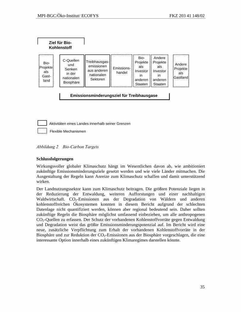
MPI-BGC/Öko-Institut/ ECOFYS FKZ 203 41 148/02
35
Abbildung 2 Bio-Carbon Targets
Schlussfolgerungen
Wirkungsvoller globaler Klimaschutz hängt im Wesentlichen davon ab, wie ambitioniert zukünftige Emissionsminderungsziele gesetzt werden und wie viele Länder mitmachen. Die Ausgestaltung der Regeln kann Anreize zum Klimaschutz schaffen und damit unterstützend wirken.
Der Landnutzungssektor kann zum Klimaschutz beitragen. Die größten Potenziale liegen in der Reduzierung der Entwaldung, weiteren Aufforstungen und einer nachhaltigen Waldwirtschaft. CO2-Emissionen aus der Degradation von Wäldern und anderen kohlenstoffreichen Ökosystemen konnten in diesem Bericht aufgrund der schlechten Datenlage nicht quantifiziert werden, können aber regional bedeutend sein. Daher sollten zukünftige Regeln die Biosphäre möglichst umfassend einbeziehen, um alle anthropogenen CO2-Quellen zu erfassen. Der Schutz der vorhandenen Kohlenstoffvorräte gegen Entwaldung und Degradation weist das größte Emissionsminderungspotenzial auf. Im Bericht wird eine neue, zusätzliche Verpflichtung zum Erhalt der vorhandenen Kohlenstoffvorräte in der Biosphäre und zur Reduktion der CO2-Emissionen aus der Biosphäre vorgeschlagen, die eine interessante Option innerhalb eines zukünftigen Klimaregimes darstellen könnte.
Bio-Projekte
als Gast-land
C-Quellen und
Senken in der
nationalen Biosphäre
Ziel für Bio-Kohlenstoff
Bio-Projekte
als Investor
in anderenStaaten
Emissionsminderungsziel für Treibhausgase
Emissions-handel
Treibhausgas-emissionenaus anderennationalenSektoren
AndereProjekte
alsInvestor
inanderenStaaten
AndereProjekte
alsGastland
Aktivitäten eines Landes innerhalb seiner Grenzen
Flexible Mechanismen

MPI-BGC/Öko-Institut/ ECOFYS FKZ 203 41 148/02
36
MPI-BGC/Öko-Institut/ ECOFYS FKZ 203 41 148/02
37
Summary
Project title Kyoto Protocol: Analysis of Options for Further Development of Com-mitments for the Second Commitment Period, part "Sinks in the Second Commitment Period"
Project partners A. Freibauer, H. Böttcher; Max-Planck-Institute for Biogeochemistry, Jena A. Herold; Öko-Institut, Berlin N. Höhne, ECOFYS, Köln
Running time July 2003 to March 2006
Funding Federal Environmental Agency
Background
Originally, the Kyoto Protocol was negotiated in 1997 without including the land use sector, but allowed an opening in later negotiations through articles 3.3 and 3.4. In consequence, sub-sequent negotiations until 2001 discovered unexpected complexity in the land use sector. This has resulted in complex, partly inconsistent rules and modalities for an accounting of carbon sources and sinks in the land use sector during the first commitment period 2008-2012.
The ongoing international negotiations about future emission reductions offer new opportuni-ties to integrate carbon sinks and sources in the land use sector in a future climate change agreement in a simpler and more comprehensive way. Land use can make and important con-tribution to achieve the goal of the United Nations Framework Convention on Climate Change (UNFCCC) to avoid dangerous climate change.
Project goals
The project gathered lessons learned from negotiation history, new scientific data and devel-oped potential options for future rules and modalities in order to provide scientific back-ground information for future negotiations. The options and proposals made purely reflect the view of the project participants and do by no means anticipate any positions by the German Federal Environment Agency and the German Ministries in charge of the negotiations.
The report covers in detail:
1. Uncertainties and risks associated with carbon sinks in the biosphere and potential feedbacks with climate change in the future (Chapter 2).
2. Potential synergies and conflicts between climate change mitigation and other ecosys-tem functions (Chapter 3).
3. A quantitative assessment of the potential of land use, land use change and forestry (LULUCF) to the ultimate goal of the UNFCCC regarding
a. the likely order of magnitude of carbon sources and sinks in the LULUCF sec-tor as compared to other sectors (Chapter 4)
b. the temporal and spatial patterns of carbon sources and sinks in the LULUCF sector in the next century (Chapters 6, 7, 8)
MPI-BGC/Öko-Institut/ ECOFYS FKZ 203 41 148/02
38
c. the potential of carbon sequestration in the biosphere and potential direct hu-man induced carbon losses in key countries and regions of the world: Defini-tions (Chapter 5), afforestation, reforestation and deforestation (Chapter 6), forest management (Chapter 7), and cropland management (Chapter 8).
4. The existing LULUCF rules and their negotiation history (Chapter 9).
5. The impact of the choice of rules and modalities on the accountable carbon sources and sinks in the LULUCF sector and the determination of alternatives for LULUCF rules and assessment according to criteria of climate change mitigation, environment and political acceptance. Rules are split into generally applicable key rules and secon-dary rules aimed at addressing national circumstances or political issues (Chapter 10).
6. A proposal by the authors for a future climate change regime that fully incorporates the carbon sources and sinks in the LULUCF sector by an additional commitment (Chapter 11).
The report addresses the time frame from 1990 to 2050 in the quantitative assessments. Politi-cal options are analysed until 2020.
Methods
The quantitative assessments of future carbon sinks and sources in the biosphere rely on the following data sources and models:
• Afforestation, reforestation, deforestation:
a. Projections of the past net afforestation/reforestation and deforestation rates ac-cording to FAO data until 2020 assuming constant net area change rates and forest biomass carbon stocks according to the IPCC Guidelines.
b. DIMA model developed by IIASA for a global estimate until 2100 of carbon stock changes in biomass and soils based on a dynamic forestry model driven by eco-nomic frame conditions and a global carbon market (Rokityanskiy et al. submit-ted).
• Forest management: The Max-Planck-Institute for Biogeochemistry developed an own forest inventory based dynamic carbon tracking model FORMICA for this study.
• Cropland management: Own estimates of potentially suitable areas for changes in cropland management, calculations by the Soil Tool of the IPCC Guidelines.
• Anthropogenic emissions from other sectors were taken from the SRES storylines of the IPCC and the EVOC database of the project partner ECOFYS.
Key results
Forests and climate change – future trends (Chapter 2) Forests of the temperate and boreal climate zones are currently acting as carbon sinks. In the tropics carbon losses by deforestation are roughly balanced by carbon uptake in forests.
MPI-BGC/Öko-Institut/ ECOFYS FKZ 203 41 148/02
39
The current and future situation is strongly influenced by land use history, age class distribu-tion and human interventions. Indirect human effects are of minor, regionally varying, impor-tance. Human activities will also be relevant in the future and will possibly remain dominant over the impacts of climate change on forest development.
The multiple – often non-linear – interactions between forests and climate render forecast dif-ficult. An increasing frequency of extreme weather events and disturbance as predicted for important forest regions of the world make forests of boreal and tropical zones particularly vulnerable to carbon losses. These regions coincide with the highest carbon stocks per area.
Synergies and conflicts between climate change mitigation and other ecosystem func-tions (Chapter 3)
If the land use activities included in a future climate change protocol are broadened there is significant potential for synergies with other environmental goals such as biodiversity protec-tion and sustainable land use. However, there is no automatism for synergies but rather a need for careful adjustment of activities to local circumstances. Only careful planning and use of natural resources can balance potential conflicts and stimulate synergies with other environ-mental goals. Streamlining of international conventions may open a promising avenue to-wards enhanced synergies.
Emissions and removals from land use change and forestry in the context of necessary global emission reductions (Chapter 4)
Substantial emission reductions in developed countries and slowed growth in emissions in developing countries are necessary to reach stabilization levels consistent with the EU’s goal to keep global average surface temperature increase below 2°C. This can only be achieved by targeting fossil fuel and industrial emissions as well as emissions from forestry.
The advantage or disadvantage for different countries of including LULUCF depends on the details of the rules. Rules on sinks will impact the stringency of the quantified emission reduc-tion commitments in other sectors. Therefore, rules for the sinks accounting have to be set before the emission levels of the other sectors are fixed. The rules on accounting sinks in the future will apply to an increasing number of countries, as it can be envisioned that more and more countries join the group of reducing countries.
Definition of the term “potential” (Chapter 5)
• Biological potential: Theoretical biologically achievable capacity, meaning some or all practical constraints have been ignored.
• Technological potential: capacity taking into account the biological potential plus constraints by suitability of land and available resources and technology, but some op-timistic assumptions are made about land availability, socio-economic and policy drivers.
• Economic potential: Conservative capacity taking into account the technical potential plus costs, with some optimistic assumptions about social barriers, incentives and speed of implementation of measures
• Realistic potential: Short-term capacity taking into account the economic potential plus social barriers, present policies and (lack of) incentives.
MPI-BGC/Öko-Institut/ ECOFYS FKZ 203 41 148/02
40
LULUCF potentials: afforestation/reforestation and deforestation (Chapter 6)
According to a projection of net changes in forest and plantation areas from 2000 to 2020 based on FAO FRA 2005, a reduction in net deforestation from 10 Mha in 2000 to 6 Mha in 2020 is expected. Net annual afforestation/reforestation rate of plantations is estimated to in-crease from 2.4 Mha to 13.8 Mha. In a second approach, the economic potential as calculated by IIASA results in lower deforestation as well as lower afforestation/reforestation rates.
Both projections by FAO and IIASA calculate a net carbon source from land use change dur-ing the next decades. From 2020 to 2030 onwards the emissions from deforestation could start to be compensated by C sequestration in afforestation/reforestation.
LULUCF potentials: Forest management (Chapter 7)
Carbon stock changes by forest management were modelled by the forest inventory based carbon tracking model FORMICA, which was specifically developed for this project. Forest management effects were calculated for 37 Annex-I countries (Europe, Russia, Canada, USA) and China. The uneven age class distribution of the forests results in fluctuations of the C stocks in forests at national level because the age distribution of the forests, and consequently, tree biomass, vary with time. As a result, forests oscillate between being C sinks when ac-tively growing forest stages dominate, and C sources when harvest increases and old and very young stands dominate. If forest management is continued as at present, the C sink in the for-ests of these 38 states will increase from currently around 0.5 Pg CO2 per year to 1.3 Pg CO2 per year in 2050.
An extension of the rotation period will sequester additional carbon for a short period which will be released again when the forest is used.
The technical potential of increased C storage in long-lived wood products in 25 Annex-I countries is 1.5 Pg CO2 (2000-2050).
In Europe and China the current C sink, driven by dominant actively growing forest stages will decline and revert into a source in a few decades. In Russia, USA and Canada, which develop into more actively growing forest stages in the near future, the current C sink will increase or, in the same direction, the current small C source will decline and turn into a C sink.
Forest management can change only very slowly over decades because only areas at certain forest age stages are suitable for management changes. The net effect of management changes on C stocks persists over various time spans, depending on the residence time of carbon in the C pools. Due to the dominant young managed forests in Europe and China management changes at large scale are only possible after long delay times when the existing forest will be harvested. Instead of taking the business as usual development of forest carbon sinks and sources, accounting could only take the net effect of management changes against buiness as usual, e.g. changes in tree species, rotation length or management regimes. In effect, the tem-poral dynamics of accountable carbon sinks and sources would drastically change, but less so the magnitude. This is because management changes alter the magnitude and timing of forest interventions and harvest, so that the forests follow a new temporal sink/source pattern. Ac-counting of the net effect of management change then only considers the discrepancy in this pattern from business as usual, which varies with time, depending on how much the forest phases differ. The accountable C sources and sinks would be decoupled from real C stock changes. At times when forests are C sinks the accounting could result in C sources and vice
MPI-BGC/Öko-Institut/ ECOFYS FKZ 203 41 148/02
41
versa, depending on whether the deviation from business as usual is positive or negative. The accountable C stock changes could not be verified by measurements.
The effect of past forest management is mainly reflected in the present age class distribution. This effect can be mathematically eliminated by assuming the theoretically optimal sustain-able age class distribution in which each age class has the same area extent. Account of C sources and sinks according to this theoretical age class distribution would reverse in the ex-treme cases of Canada and China with very strongly skewed age class distributions the sign (sink or source) as well as the trend (increase versus decrease of C stocks) of accountable C stock changes. The accountable C stock changes could not be verified by measurements.
LULUCF potentials: cropland management (Chapter 8)
The potential C sequestration by cropland management was calculated by the IPCC Soil Tool for the top 30 cm of cropland soils, representing about 50% of C stocks in cropland soils. The cultivation of soils during the last centuries has globally released about 100 Pg CO2. This value represents the theoretical upper limit of C sequestration. The largest historical soil C losses occurred in USA, Russia, China, India and EU-25. Accordingly, the highest C seques-tration potential in cropland soils is located in these regions. Changes in cropland manage-ment could sequester up to 0.5 Pg CO2 during the next 20 years. Less than 10% of this techni-cal potential is estimated to be realised.
Future C losses could occur through mechanisation in developing countries. In case the mechanisation goes along with intensification soil C stocks could also be slightly increased.
Conservation tillage represents the most important measure of cropland management for C sequestration because it is applicable under a wide range of climate, soil and cropping condi-tions. There are also significant technical potentials for no-till agriculture and intensification, which are, however, associated with increased N2O emissions and not suitable in all circum-stances.
Globally the technical potential for C sequestration exceeds the one for C losses from crop-land soils. Some of the C sequestration measures are already being implemented as business as usual.
LULUCF potentials: data base (CD-Rom)
A data base was developed during the project containing projections and scenarios of carbon sources and sinks in the LULUCF sector for the most important countries of the world as well as emission data from other sectors for comparison:
a) Afforestation/reforestation and deforestation: Projections for 1990-2020 according to FAO FRA 2005 net area changes and IPCC default values (biomass only).
b) Forest management: Business as usual and four scenarios of the technical and economic potential for changes in forest management 1998-2097 in 5-year steps (equivalent to 2000-2100) for 25 Annex-I countries according to own model calculations (biomass and lit-ter/soil).
c) Cropland management: Five scenarios of the technical potential for changes in cropland management 2001-2020 according to own calculations using the IPCC Soil Tool (soil).
MPI-BGC/Öko-Institut/ ECOFYS FKZ 203 41 148/02
42
d) Emissions from other sectors 1990-2100 based on national greenhouse gas inventories and IPCC SRES3 scenarios using the IMAGE model.
Lessons from LULUCF negotiation history (Chapter 9)
The present rules for LULUCF need to be understood in light of their negotiation history. Fu-ture negotiations should be performed in a stepwise manner.
The first precondition for negotiations is agreement about the future role of LULUCF in the climate regime.
The second precondition is a robust data base in order to analyse different options. The results of this project provide a preliminary basis for analysis.
LULUCF rules should be scientifically sound, complete and balanced with regard to carbon sources and sinks. They should be simple and comprehensive including all carbon pools. They should give incentives for reducing deforestation and enhancing sustainable forest manage-ment, thus preserving existing carbon stocks in the biosphere.
Quantitative targets should only be determined after the accounting rules have been fixed.
LULUCF and the general post 2012 regime (Chapter 9) The attainment of the 2°C target for global air temperature change, which the German gov-ernment and the European Community regard as a necessary target in order to fulfill the ulti-mate goal of the Climate Convention can be supported, if emissions and removals from the LULUCF sector are included in the greenhouse gas emission reduction efforts.
LULUCF rules can affect the commitments for emission reduction in other sectors, if rules and commitments are coupled. Accounting rules therefore need to be fixed prior to setting quantitative targets. It is expected that over time more and more countries will enter a future climate regime and will contribute to emission reductions including LULUCF.
The design of the LULUCF rules determines whether countries receive advantages or disad-vantages. If e.g. per capita emissions from the LULUCF sector are included in the definition of targets the large deforesting nations are seriously charged. A system of no regret targets without sanctions, however, could create incentives for e.g. reducing deforestation in Non-Annex-I countries.
The LULUCF sector could also be treated separately from other commitments in order to al-low Non-Annex-I countries a first – possibly non-quantitative – step into a post 2012 regime.
Effect of key rules on accountable C sources and sinks in LULUCF (Chapter 10)
The National Inventory Reports under the UNFCCC demonstrate that the LULUCF sector contributes to a minor extent to national greenhouse gas emissions and their interannual vari-ability in most Annex-I countries. Non-Annex-I countries do not have an adequate time series of National Inventory Reports to allow such kind of analysis.
Within the LULUCF sector forest management related C sources and sinks dominate in An-nex-I countries. CO2 emissions from deforestation in the five largest Non-Annex-I countries are higher than the total anthropogenic greenhouse gas emissions from EU-25. If emission reduction from avoided deforestation will enter the emission trading it is essential to fix un-
3 Special Report on Emission Scenarios
MPI-BGC/Öko-Institut/ ECOFYS FKZ 203 41 148/02
43
ambigously the national emission baselines for deforestation in the decision text for this issue prior to trading so that the magnitude of credits entering the market can be estimated.
The variability reported in the LULUCF sector is mainly due to anthropogenic reasons or due to the aggregation of slightly varying small sources and sinks within LULUCF (e.g. soil sources, forest sinks). Even though, in relative terms, the sector can greatly vary between years, the overall magnitude of variation as compared to sources in other sectors is small. The interannual variability induced by variation in regional climate is not reflected in the National Inventory Reports, except indirectly in fire emissions.
Criteria for evaluation of options and key rules for future commitments (Chapter 10) Future LULUCF rules should support the goal of the UN climate change convention as effec-tively as possible. In order to achieve this, criteria and core questions were formulated in the following domains:
a) Effectiveness for climate protection,
b) Effectiveness for other environmental goals,
c) Consideration of the specific characteristics of the LULUCF sector,
d) technical feasibility (monitoring, accounting and verification whether the com-mitments are achieved),
e) Support of the negotiation process for a post 2012 regime.
Options and key rules for future commitments (Chapter 10)
Future commitments can be disassembled into individual key rules, which can be analysed and partly negotiated independently from each other. Additional rules could then balance na-tional specifics at a later stage of the negotiation process. Key rules describe:
a) the relation between LULUCF commitments and other sectors: joint, partly or fully separated, same or different type of commitment?
b) the definition of “anthropogenic” carbon sources and sinks
c) the LULUCF activities included in the regime: as in the Kyoto Protocol, additional activities, comprehensive inclusion of the (managed) biosphere?
d) accounting rules: „net-net“, „gross-net“, mixes?
e) flexible mechanisms.
The key rules score in the various criteria listed above in a scattered way. Nevertheless prom-ising options can be identified. It will be crucial to balance between continuity, comprehen-siveness, simplicity, and symmetry between carbon sources and sinks.
Proposal for comprehensive protection of C stocks in the biosphere (Chapter 11)
The analyses (Table 1) demonstrate that at present, anthropogenic C sources exceed C sinks. Despite global trends to reduce deforestation rates the risk of C losses will continue to exceed the C sinks for the next decades. Carbon takes decades to accumulate in ecosystems, but can rapidly be lost. A comprehensive protection of existing C stocks in the biosphere should therefore become a central element of future LULUCF commitments. This would include C losses from deforestation, land use change, degradation and unsustainable forestry. The com-prehensive inclusion of C sources and sinks of the biosphere will help to plan how the 2°C
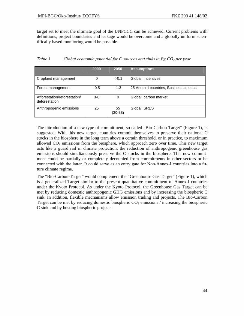
MPI-BGC/Öko-Institut/ ECOFYS FKZ 203 41 148/02
44
target set to meet the ultimate goal of the UNFCCC can be achieved. Current problems with definitions, project boundaries and leakage would be overcome and a globally uniform scien-tifically based monitoring would be possible.
Table 1 Global economic potential for C sources and sinks in Pg CO2 per year
2000 2050 Assumptions
Cropland management 0 <-0.1 Global, Incentives
Forest management -0.5 -1.3 25 Annex-I countries, Business as usual
Afforestation/reforestation/ deforestation
3-8 0 Global, carbon market
Anthropogenic emissions 25 55 (30-88)
Global, SRES
The introduction of a new type of commitment, so called „Bio-Carbon Target“ (Figure 1), is suggested. With this new target, countries commit themselves to preserve their national C stocks in the biosphere in the long term above a certain threshold, or in practice, to maximum allowed CO2 emissions from the biosphere, which approach zero over time. This new target acts like a guard rail in climate protection: the reduction of anthropogenic greenhouse gas emissions should simultaneously preserve the C stocks in the biosphere. This new commit-ment could be partially or completely decoupled from commitments in other sectors or be connected with the latter. It could serve as an entry gate for Non-Annex-I countries into a fu-ture climate regime.
The “Bio-Carbon-Target” would complement the “Greenhouse Gas Target” (Figure 1), which is a generalized Target similar to the present quantitative commitment of Annex-I countries under the Kyoto Protocol. As under the Kyoto Protocol, the Greenhouse Gas Target can be met by reducing domestic anthropogenic GHG emissions and by increasing the biospheric C sink. In addition, flexible mechanisms allow emission trading and projects. The Bio-Carbon Target can be met by reducing domestic biospheric CO2 emissions / increasing the biospheric C sink and by hosting biospheric projects.
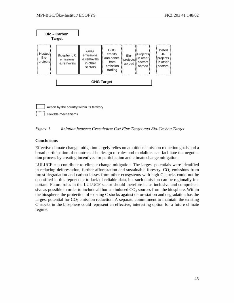
MPI-BGC/Öko-Institut/ ECOFYS FKZ 203 41 148/02
45
Figure 1 Relation between Greenhouse Gas Flux Target and Bio-Carbon Target
Conclusions
Effective climate change mitigation largely relies on ambitious emission reduction goals and a broad participation of countries. The design of rules and modalities can facilitate the negotia-tion process by creating incentives for participation and climate change mitigation.
LULUCF can contribute to climate change mitigation. The largest potentials were identified in reducing deforestation, further afforestation and sustainable forestry. CO2 emissions from forest degradation and carbon losses from other ecosystems with high C stocks could not be quantified in this report due to lack of reliable data, but such emission can be regionally im-portant. Future rules in the LULUCF sector should therefore be as inclusive and comprehen-sive as possible in order to include all human induced CO2 sources from the biosphere. Within the biosphere, the protection of existing C stocks against deforestation and degradation has the largest potential for CO2 emission reduction. A separate commitment to maintain the existing C stocks in the biosphere could represent an effective, interesting option for a future climate regime.
HostedBio-
projects
Biospheric C emissions& removals
Bio – Carbon Target
Bio-projectsabroad
GHG Target
GHG credits
and debitsfrom
emissiontrading
GHGemissions& removals
in othersectors
Projectsin othersectorsabroad
HostedJI-
projectsin othersectors
Action by the country within its territory
Flexible mechanisms

MPI-BGC/Öko-Institut/ ECOFYS FKZ 203 41 148/02
46
MPI-BGC/Öko-Institut/ ECOFYS FKZ 203 41 148/02
47
1 Introduction
1.1 Background
In 2001, in the Marrakech Accords (MA), the signatory Parties of the United Nations Frame-work Convention on Climate Change (UNFCCC) have agreed on detailed rules and modali-ties for implementing the Kyoto Protocol (KP). Detailed rules for accounting activities in the land use, land use change and forestry (LULUCF) sector, often called "sinks", were only de-termined for the first commitment period 2008-2012. These rules are very complex, partly because the emission limitation goals under the Kyoto Protocol had been set on the basis of real emission reduction without considering LULUCF. From the point of view of the Euro-pean Union, the late amendments for "sinks" in Kyoto 1997 have created "loopholes" that could reduce greenhouse gas mitigation efforts in the energy sector. Negotiations have tried to close such loopholes and constrained the accountable "sinks" to "direct human-induced" ef-fects, but resulted in turn in highly complex and incoherent rules and modalities for LULUCF activities. Partly the rules are complex because of the nature of LULUCF.
Negotiations about a future climate change agreement and mitigation efforts beyond 2012 have started in 2005. The fundamental conflicts and complications about the use of "sinks" to fulfil emission limitation commitments are likely to rise again. This may offer the opportunity to design new options to deal with LULUCF that are simpler, more transparent, efficient and balanced whilst meeting the requirements for sustainable land use, conservation of biodiver-sity and security of human nutrition and serve to the ultimate goal of the UNFCCC.
1.2 Project goals
The project aims to provide a scientific foundation for negotiations about future commitment periods and LULUCF rules under a future climate change agreement. This report addresses generic issues about the role of the biosphere in climate change mitigation, institutional as-pects for future negotiations, data and facts about LULUCF sources and sinks and analyses a suite of options for a future LULUCF regime. It
1. discusses uncertainties and risks associated with the future of carbon stocks in the bio-sphere and possible feedbacks with climate change (chapter 2).
2. discusses possible synergies and conflicts of LULUCF activities with other ecosystem functions (chapter 3).
3. quantifies globally
a. the likely magnitude of LULUCF sources and sinks in relation to other sectors (chapter 4).
b. the spatial and temporal patterns of LULUCF sources and sinks in the next century (chapters 6, 7, 8)
c. the potential for C sequestration and risk of C losses by nature (chapter 2) and human action (afforestation/reforestation and deforestation: chapter 6, forest management: chapter 7, agricultural management: chapter 8), at the level of world regions and countries.
MPI-BGC/Öko-Institut/ ECOFYS FKZ 203 41 148/02
48
4. describes status quo of the existing LULUCF rules and their negotiation history (chap-ter 9).
5. analyses (1) quantitatively the impact of choices of key rules on the magnitude of ac-countable LULUCF sources and sinks for the most important countries in the negotia-tions, and (2) alternative options for key rules according to climate, environmental and political criteria in order to identify promising ways forward that are consistent with the Kyoto Protocol (chapter 10).
6. systematically separates the existing LULUCF rules into fundamental "key rules", that may form the basis of future negotiations, and "secondary rules" that adjust the key rules to deal with country-specific or political concerns (chapter 10).
7. proposes an alternative framework of rules for LULUCF (chapter 11).
A time horizon from 1990 to 2050 is considered in the quantitative analysis, focussing on 1990 to 2020 in the discussion of political options, and taking retrospective analyses back to 1960 into account.
1.3 Overview of methods
The study analyses key steps of the past negotiation process on the basis of existing and own assessments and a new systematic approach to disaggregate rules and modalities regarding LULUCF. The carbon sinks and sources until 2050 are estimated by using the following data sources and models:
• Afforestation/reforestation and deforestation: Projections based on past afforesta-tion/reforestation and deforestation rates by FAO and IIASA-DIMA model, personal communication.
• Forest management: inventory based model FORMICA developed by the authors
• Cropland management: IPCC Soil Tool.
• Other anthropogenic emissions: SRES scenarios, EVOC data base of ECOFYS.
MPI-BGC/Öko-Institut/ ECOFYS FKZ 203 41 148/02
49
2 Forests under global change – the future of the terrestrial carbon sink
2.1 Introduction
Forest ecosystems of the world are considered as multifunctional, supplying timber, non-timber products, fresh water, local climate, water balance and supply and space for recreation or wildlife. Since the day scientists suggested that the terrestrial biosphere is currently gaining carbon (C) from the atmosphere C sequestration became an additional ecosystem service (e.g. Dixon, Brown et al. 1994; Ciais, Tans et al. 1995). In general it is obvious that a forest carbon sink, is limited due to the nutrient limited carrying capacity of forest stands. Therefore it is necessary that future anthropogenic CO2 emissions will get reduced by means of clean tech-nology. The expectation for the forest sink is to bridge the gap until the technology is avail-able and has been spread (Kirschbaum 2003).
According to the IPCC Special Report on Land Use, Land Use Change and Forestry (LULUCF, IPCC 2000) the net terrestrial carbon uptake was estimated to amount 0.2 Pg C (0.73 Pg CO2) per year during the 1980s and 0.7 (2.6 Pg CO2) from 1990 to 1998. Including emissions from land use change (about 1.7 Pg C in the 1980s and 1.6 Pg C in the 1990s) (about 6.2 Pg CO2 in the 1980s and 5.9 Pg CO2 in the 1990s) the gross terrestrial uptake was around 2.4 Pg C (8.8 Pg CO2). These estimates are highly uncertain. Uncertain is also the in-dividual share of processes contributing to the budget and directly or indirectly human in-duced changes of those.
Predicted changes in climate have raised concerns about potential impacts on the strength and permanence of the observed terrestrial C sink (see above). Due to their sensitivity to climate forest ecosystems are also supposed to respond to current changes that comprise a rise in global temperature, a rise in climate variability accompanied with an increase in global at-mospheric CO2 (IPCC 2001). As an effect of such a feedback the response could result in a considerably lower carbon sequestration rate or even a switch to a net source, both leading to a faster increase of CO2 in the atmosphere in the future. This report gives an overview of re-cent estimates concerning the sensitivity of the forest carbon sink-source behavior to climate change. It chooses a time frame of one century, because most projections concentrate on 10 decades or less due to the fact that projections become more uncertain the further they reach into the future. The following questions will be addressed in particular:
• What kind of forest ecosystems play a major role in the global carbon cycle and what kind of forest ecosystems are affected by climate change?
• Which climatic parameters constrain carbon fluxes in those forests and in which way limiting factors will change?
• Will ecosystems adapt to environmental changes caused by Climate Change?
• Will there be a limit to additional carbon storage in forest ecosystems or will the sys-tem even turn into a source?
• What additional biosphere climate feedbacks can be expected and what is their impact on the carbon balance?
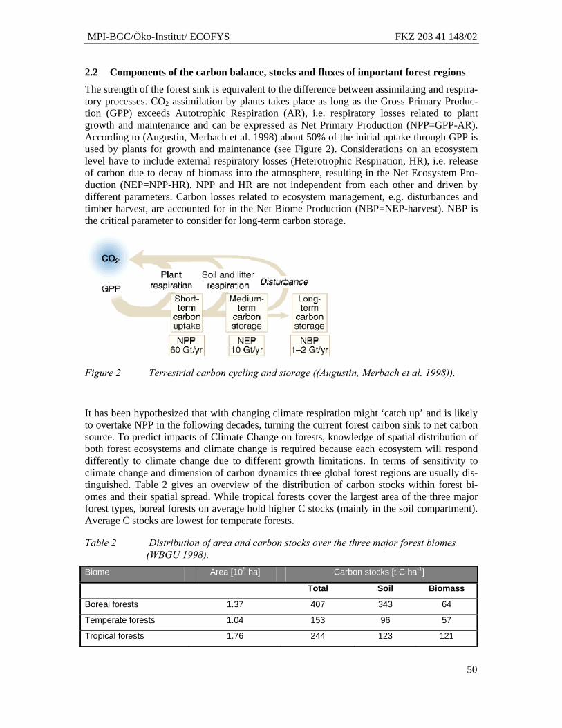
MPI-BGC/Öko-Institut/ ECOFYS FKZ 203 41 148/02
50
2.2 Components of the carbon balance, stocks and fluxes of important forest regions
The strength of the forest sink is equivalent to the difference between assimilating and respira-tory processes. CO2 assimilation by plants takes place as long as the Gross Primary Produc-tion (GPP) exceeds Autotrophic Respiration (AR), i.e. respiratory losses related to plant growth and maintenance and can be expressed as Net Primary Production (NPP=GPP-AR). According to (Augustin, Merbach et al. 1998) about 50% of the initial uptake through GPP is used by plants for growth and maintenance (see Figure 2). Considerations on an ecosystem level have to include external respiratory losses (Heterotrophic Respiration, HR), i.e. release of carbon due to decay of biomass into the atmosphere, resulting in the Net Ecosystem Pro-duction (NEP=NPP-HR). NPP and HR are not independent from each other and driven by different parameters. Carbon losses related to ecosystem management, e.g. disturbances and timber harvest, are accounted for in the Net Biome Production (NBP=NEP-harvest). NBP is the critical parameter to consider for long-term carbon storage.
Figure 2 Terrestrial carbon cycling and storage ((Augustin, Merbach et al. 1998)).
It has been hypothesized that with changing climate respiration might ‘catch up’ and is likely to overtake NPP in the following decades, turning the current forest carbon sink to net carbon source. To predict impacts of Climate Change on forests, knowledge of spatial distribution of both forest ecosystems and climate change is required because each ecosystem will respond differently to climate change due to different growth limitations. In terms of sensitivity to climate change and dimension of carbon dynamics three global forest regions are usually dis-tinguished. Table 2 gives an overview of the distribution of carbon stocks within forest bi-omes and their spatial spread. While tropical forests cover the largest area of the three major forest types, boreal forests on average hold higher C stocks (mainly in the soil compartment). Average C stocks are lowest for temperate forests.
Table 2 Distribution of area and carbon stocks over the three major forest biomes (WBGU 1998).
Biome Area [106 ha] Carbon stocks [t C ha-1]
Total Soil Biomass
Boreal forests 1.37 407 343 64
Temperate forests 1.04 153 96 57
Tropical forests 1.76 244 123 121
MPI-BGC/Öko-Institut/ ECOFYS FKZ 203 41 148/02
51
During the last 10.000 years boreal and northern temperate forest ecosystems have accumu-lated carbon, mainly in form of soil organic carbon. The mechanisms responsible for the pre-sent boreal forest net sink are believed to be continuing responses to past changes in the envi-ronment, notably recovery from the ice-age, changes in forest disturbance regimes, and in some regions, nutrient inputs from air pollution (Apps, Kurz et al. 1993). Nutrients and tem-perature are the limiting factors of carbon accumulation while temperature mainly controls decomposition of vegetation debris. Increased input of nutrients such as nitrogen (N) from the atmosphere in addition to higher temperatures and enlarged growing seasons, as predicted in IPCC scenarios, is very likely to enlarge plant growth (Peng and Apps 1999) and increase the potential of carbon sequestration in boreal forests in biomass and soil (e.g. Lelyakin, Kokorin et al. 1997; White, Cannell et al. 2000). However, there is still supposed to be an upper limit of the sink due to mechanical, biological, chemical and physiological constraints, especially for boreal conditions. Only a small part of the boreal biome is directly affected by forest man-agement and options for mitigating climate change impacts on C storage are therefore limited but the potential for accelerating the atmospheric C release are high (Apps, Kurz et al. 1993).
Temperate forests are considered to be a net carbon sink which is only partly due to fertilizing effects of N deposition and elevated atmospheric CO2 (e.g. Masera, Garza-Caligaris et al. 2003; Wirth, Schulze et al. 2003; Vetter, Fox et al. 2004). There is evidence that carbon se-questration in the mid-latitudes is obviously driven by forest management and forestry history (Caspersen, Pacala et al. 2000; Barford, Wofsy et al. 2001). Thus, in temperate forests age structure, species composition and health of forest ecosystems as management factors consid-erably control long-term carbon fluxes. Observations of natural temperate forests (e.g. (Knohl, Schulze et al. 2003) where management effects can be completely excluded are still too few for general conclusions. Since these forest areas are intensively managed they might have a high potential for climate change mitigation through forest management change.
Most scientists report that tropical forests can be regarded as a considerable gross sink (e.g. Phillips, Malhi et al. 1998) or to be in an equilibrium, i.e. gaining and losing carbon of the same amount (Clark 2002). Still tropical forests represent one of the largest biomass carbon pools in the world. Due to their huge extension, only slight annual increases could sequester enormous amounts of atmospheric CO2 (Körner 1998). There is model evidence that forest growth in the tropics is very sensitive to CO2 concentrations (Ciais, Janssens et al. 2005). A large unknown parameter is the behavior of tropical soils to climate change (Veldkamp, Becker et al. 2003). Increased atmospheric CO2 and changes in climate are likely to shift car-bon and nutrient allocation patterns and storage in tropical forest. Modeling and experimental studies e.g. suggest that even a small increase in temperature accompanied with a decline in rainfall might results in reduced growth and faster decomposition rates, which would have substantial effects on nutrient cycling (Bazzaz 1998). According to Bazzaz sensitivity of tropical forests to climate change is expected to be high also due to the high degree of spe-cialization of tropical organisms. However, because of land-use change, especially tropical deforestation and degradation, tropical forests are currently a strong net CO2 source (IPCC 2001). An approximation of the tropical forest contribution to the terrestrial C balance cannot be done without taking into account human interference.
MPI-BGC/Öko-Institut/ ECOFYS FKZ 203 41 148/02
52
2.3 Observed features of climate change
2.3.1 Gradual changes
According to the Third Assessment Report (TAR) of the IPCC (2001) the global atmospheric concentration of CO2 has increased from 280 ppm in 1750 to 367 ppm in 1999. Model estima-tions indicate that CO2 concentrations in the year 2100 might range between 500 to almost 1000 ppm, depending on scenario assumptions. In parallel the global average temperature has increased since the 1860 by 0.6° ± 0.2°C. The largest increases in temperature have occurred over the mid- and high latitudes of the continents in the Northern Hemisphere. The IPCC (2001) stresses that recent regional temperature patterns can be strongly influenced by re-gional variability in the climate system over some decades. Projections of future changes in temperature are derived from the expected response to a doubling of CO2 concentration in the atmosphere, i.e. climate sensitivity which is likely to be in the range of 1.5° to 4.5°C. This estimate of TAR is similar to earlier reports launched through the IPCC.
During the last decade precipitation has decreased over the sub-tropics and increased over tropical land and oceans. Increases were observed also over Northern Hemisphere mid- and high latitudes. Global mean water vapor, evaporation and precipitation are projected to in-crease. However, at a regional scale both, increases and decreases are expected (IPCC 2001).
2.3.2 Weather and climate variability
The IPCC reported in 2001 that higher maximum temperatures and more hot days over nearly all land areas are likely in the future as well as higher minimum temperatures, accompanied with fewer cold and frost days. Analyses show that in regions where total precipitation has increased, it is very likely that there have been even more pronounced increases in heavy and extreme precipitation events in the past decades. More intense precipitation events are consid-ered as very likely over many Northern Hemisphere mid- and high latitude land areas. In some regions, such as parts of Asia and Africa, the frequency and intensity of drought have been observed to increase in recent decades. The behavior of El Nino-Southern Oscillation (ENSO) has been unusual since the mid-1970s compared with the previous 100 years, with warm phase ENSO phenomena being relatively more frequent, persistent and intense than the opposite cool phase. Changes associated with ENSO produce large variations in weather and climate around the world leading to droughts, floods or heat waves with often severe impacts on humanity and ecosystems (IPCC 2001).
2.4 Likely plant responses to climate change: experimental findings
2.4.1 Carbon dioxide fertilization Each of the mechanisms involved in plant growth and decomposition is complex. Experimen-tal studies under controlled conditions can reveal trends how vegetation might respond to ele-vated CO2 concentration and rising ambient temperature.
From a large number of experiments with plants in greenhouses or growth chambers it was concluded that CO2 can be considered a limiting factor to plant growth (Curtis and Wang 1998; de Lucia, Hamilton et al. 1999; Hendrey, Ellsworth et al. 1999; Körner 2003; Lukac, Calfapietra et al. 2003; Sinsabaugh, Saiya-Cork et al. 2003; Gielen, Calfapietra et al. 2005). Young plants reacted with increased photosynthesis and dry mass when they were exposed to elevated CO2 concentrations (Curtis and Wang 1998) which can result in an increase of NPP
MPI-BGC/Öko-Institut/ ECOFYS FKZ 203 41 148/02
53
up to 25 % (DeLucia et al. 1999). FACE4-experiments allow the observation of effects on vegetation in situ (Hendrey, Ellsworth et al. 1999). Published evidence from those field-grown trees supports findings from greenhouse researchers that reported a stimulation of plant growth with increasing CO2 in the atmosphere (Sinsabaugh et al. 2003). At ecosystem level the overall evidence of CO2 enrichment experiments suggests that elevated CO2 stimulates carbon turnover but not necessarily carbon storage. The result of a review of studies of CO2 enrichment experiments suggests that higher CO2 levels enhance also microbial N demand and imply larger amounts of N immobilized by microbial biomass (van Groeningen et al. 2006). Hungate et al. (2003) demonstrate in a simple calculation that vegetation response to increasing atmospheric CO2 over the next century is exaggerated in global carbon models, which fail to consider the N limitation to plant growth. To take soil N dynamics into account is necessary to fully cover all aspects of environmental changes such as rising CO2 levels. This finding has recently been supported by field observations in grasslands (Nösberger et al., 2006).
Most studies investigated only short-term reactions to a dramatic step increase CO2 concentra-tions and even long-term experiments cover only a short fraction of a tree’s lifespan, therefore it is not yet clearly proven how long likely responses will continue. Still longer-term FACE experiments on larger treatment plots and experiments with tropical forests, which remain completely unrepresented in analyses so far, are needed to allow more accurate scaling of the physiological results to landscape levels (Nösberger et al., 2006).
2.4.2 Temperature response and acclimation An increase in temperature will most likely cause an exponential increase in plant and soil respiration as C decomposition is often controlled by temperature limitations to microbial activity, especially in the high-latitudes. Research on soil respiration indicates that heating may enhance CO2 efflux by 50% as reported for a Tundra site by Mertens et al. (2001). They detected a 39% increase in belowground respiration being the main component of the carbon budget. Similar changes can be expected in wooded ecosystems in the high latitudes. How-ever, these predictions have been challenged recently (Giardina and Ryan 2000), claiming that in mineral soils increased temperature alone will not stimulate the decomposition of carbon. In soil warming experiments, the initially increased carbon dioxide efflux returns to pre-warming rates within one to three years. The absence of a long-term temperature effect was contradicted to by (Knorr, Prentice et al. 2005) by explaining the results differently: a rapid depletion of labile carbon in the soil combined with the negligible response of non-labile car-bon in the short run. They claimed with the help of model simulation that in the long run the non-labile soil carbon fraction will respond even stronger to increased temperature.
Photosynthesis, on the other hand, is relatively unaffected by temperature. However, most findings indicate a future increase in plant growth mostly at sites where length of growing season is a limiting factor (Cao and Woodward 1998; Chen, Black et al. 1999; Menzel and Fabian 1999; Black, Chen et al. 2000; Drewitt, Black et al. 2002). Owing to growing imbal-ance between plant growth and autotrophic respiration with ecosystem development, older systems will be affected mostly by higher plant respiration (Ryan 1991), eventually turning from a carbon sink to a source of carbon to the atmosphere.
4 FACE: Free Air Carbon Dioxide Enrichment
MPI-BGC/Öko-Institut/ ECOFYS FKZ 203 41 148/02
54
2.5 Complex responses: coupled models including climate and terrestrial ecosystems
Carbon cycle feedbacks are a considerable source of uncertainty in large scale climate change response projections that are based on small scale experimental data. How complex responses of forest ecosystems may be show model results by Bachelet et al. (2001). Southern dry for-ests expanded under the more moderate scenarios but declined under more severe climate sce-narios with catastrophic fires potentially causing rapid vegetation conversions from forest to Savannah (Bachelet, Neilson et al. 2001). However, such a nonlinear behavior is typical for complex systems such as forest ecosystems. In addition the response of forests, e.g. to increas-ing CO2 and temperature, occurs over different time scales reaching from seconds to centu-ries. The latter can hardly be investigated through field experiments. Reliable projections can only be made through modeling. Ecosystem models provide practical tools and can serve as a translation of experimental results into projections of future ecosystem functioning.
Kirilenko and Solomon (1998) used a migration model to study potential changes in species composition and the impact on terrestrial carbon stocks as a response to climate change as-suming a doubling of atmospheric greenhouse gas concentration. The model results show that terrestrial vegetation and soil could lose carbon depending on the rate of migration relative to the rate of climate change (Kirilenko and Solomon 1998). A critical point is the invasion of well adapted plants that may be delayed (Solomon and Kirilenko 1997), e.g. due to slow seed dispersal and ecosystem fragmentation. In case of a delayed immigration, simulation results predicted lower forest carbon stocks by around 10 % in all three forest biomes compared to recent stocks (Solomon and Kirilenko 1997).
In general these models use static vegetation properties and CO2 concentrations from simple carbon-cycle models that do not include effects of climate change (“offline” studies). In a few advanced approaches terrestrial carbon cycle models representing dynamic ecosystems were coupled with General Circulation Models (GCM), i.e. models used to predict weather and climate variables (e.g. Cao and Woodward 1998; Cox et al. 2000). Results from such exten-sive “online” modeling experiments still contain a large amount of uncertainty. Besides at-mospheric phenomena like the Southern Ocean circulation a main source of the uncertainty is the vegetation and soil carbon response to global change (Friedlingstein, et al. 2003). Despite differences in the magnitude all coupled models show a positive feedback between climate change and the carbon cycle of terrestrial ecosystems, i.e. climate change is likely to cause additional CO2 emissions from these systems; an additional future source that has not been taken into account of emission scenarios so far. Accelerated by higher temperature and ele-vated CO2 forests will still stay a carbon sink under climate change but NEP is likely to de-cline rapidly when the CO2 fertilization effect becomes saturated as predicted by Cao and Woodward (1998). Recent simulations of a coupled GCM and dynamic vegetation models expect that the biosphere will turn into a source in the next decades (Cox, et al. 2000; Cox et al. 2004). An extreme scenario considered to be a ‘worst case’ scenario pointed at 2050 being the date when carbon release from forests will exceed sequestration. According to these simu-lations the Amazon region suffered from a 9 degree Celsius increase in temperature over the 21st century combined with a drop in rainfall by 64%. Together these changes lead to a 78% loss in vegetation carbon and a 72% loss in soil carbon in the Amazon region. As a conse-quence, CO2 concentrations reached about 980 ppm by 2100, which is about 280 ppm higher compared to scenarios ignoring these feedbacks (Cox et al. 2004).
2.6 Vulnerability of the forest sink: response to extremes
Climate change will also increase climate variability and most probable lead to more frequent and severe extreme weather conditions (IPCC 2001). Under global change, the severity of
MPI-BGC/Öko-Institut/ ECOFYS FKZ 203 41 148/02
55
climate and secondary stressors may increase, with consequences for future forest health, pro-ductivity, and carbon sequestration. The expected increase in intensity and frequency of ex-treme events may predispose forest ecosystems, i.e. ecosystems tend to become more unstable and vulnerable to secondary threats. Only slight changes may then trigger processes leading to environmental catastrophes.
The effect of rapid changes in humidity on ecosystems was observed by Goldstein et al. (2000). They compared photosynthesis of Mediterranean pine ecosystems in two different years, while one was wetter and cooler than average due to El Nino climate patterns and an-other hotter and drier than average. An extreme heat wave in the dry year caused decreased rates of C sequestration and evapotranspiration compared with the rest of the growing season (Goldstein, Hultman et al. 2000). Though, a cooler, wetter spring deferred the onset of photo-synthesis resulting in lower production as well (Goldstein, Hultman et al. 2000). According to the authors low soil moisture conditions jointly with extreme events are likely to change the carbon sink-source behaviour at Mediterranean sites.
Just recently a joint effort compiled measurements of ecosystem CO2 fluxes, remotely sensed radiation absorbed by plants, and country-level crop yields recorded during the European heatwave in 2003 and compared them to modelled data (Ciais, Reichstein et al. 2005). The study covered all terrestrial ecosystems, not only forest biomes. July temperatures in 2003 were up to 6 degrees C above long-term means, and annual precipitation deficits up to 300mm per year, 50% below the average. The group estimated a 30% reduction in GPP over Europe, which resulted in an anomalous net source to the atmosphere, i.e. compared to ‘normal’ condi-tions the sink capability of the European terrestrial biosphere was reduced significantly. The model suggested the effect amounts to 1.8 Pg CO2 per year (0.5 Pg C per year). Assuming a ‘normal’ net sink of C of 0.5 – 0.7 Pg CO2 per year (0.13 – 0.2 Pg C per year) under average climate conditions as reported by Janssens et al. (2003) this anomaly would turn the sink into a net source of carbon of around 1.2 Pg CO2 per year (0.3 Pg C per year) in the year 2003. The loss in carbon gain in 2003 thus reversed the effect of three years of net ecosystem carbon sequestration in Europe.
Due to drought stress, the future capacity of carbon sequestration of boreal forests may be less than expected. Data of far northern latitudes show that temperature-induced drought stress is an important factor limiting carbon uptake in boreal forests (Barberi and Lo Cascio 2001). Soil moisture is a crucial factor in all forest regions. An example of the Amazon region shows that in El Nino years, which bring hot, dry weather to the region, undisturbed ecosystems, comprising tropical evergreen forest and tropical savannas, act as a source of carbon to the atmosphere (Tian, Melillo et al. 1998). In non-El Nino years, these ecosystems act as a carbon sink.
An analysis of aspen tree-rings from a boreal site and forest health assessments revealed drought and defoliation by a forest insect to be responsible for reduced growth and predis-posed stands resulting in secondary damage by wood-boring insects and fungal pathogens (Black, Chen et al. 2000). Such dieback events have mostly multi-causal reasons while cli-matic extremes take the role of a trigger.
Since extreme events mostly affect relatively small areas, an increase in frequency is likely to lead to higher heterogeneity, variability and uncertainty in terrestrial carbon sequestra-tion/release patterns, with ecosystems shifting from sink to source and vice versa. Distur-bances accelerated under climate change may also trigger faster adaptation of long-lived for-est ecosystems to the changes. For example, changes in species composition are more quickly apparent after disturbance events, when better adapted species establish more easily. Thus, the
MPI-BGC/Öko-Institut/ ECOFYS FKZ 203 41 148/02
56
indirect effects of climate change may be of even greater importance because of their potential for altering the intensity, frequency, and nature of the disturbance regimes which drive forest dynamics.
2.7 Indirect responses: the role of fires
Besides natural breakdown (tree death) and harvest, C emissions tend to result from distur-bances (wind break, fire, pest outbreak). Unlike disturbances like insects and storm, forest fires have the potential to release large amounts of CO2 within a short period of time. In a fire, carbon accumulated over decades may be emitted within a few hours (Körner 2003). In many ecosystems of the world forest fires occur regularly representing a natural disturbance and strongly influencing biomass accumulation. In these regions, like the boreal forests of Siberia, climate change may affect ecosystem functions predominantly via changes in fire regimes (e.g. Wirth, Schulze et al. 1999).
Three major components need to be present to set a forest fire on: fuel, i.e. coarse woody de-bris and litter, favorable meteorological (i.e. dry) conditions and an ignition source. The fire regime has six components; fire frequency, size, intensity, seasonality, type and severity (Flannigan, Stocks et al. 2000). Most of them are relevant in terms of carbon cycling. Fire frequency affects species composition in an ecosystem through selection pressure. Fire size determines landscape patchiness and speed and type of regeneration. Fire type (e.g. crown, surface and ground fire) is to a large degree controlled by fire intensity, i.e. the energy re-leased during a fire. Fire severity is a measure of fuel consumption, and an important parame-ter for estimating ecosystem carbon losses. It is also another important controlling factor of post-fire regeneration. These components are highly dependent on weather and expected to respond rapidly to changes in climate (Flannigan, Bergeron et al. 1998; Wirth, Schulze et al. 1999; Flannigan, Stocks et al. 2000).
(Mouillot and Field 2005) estimate that an average of 608 Mha per year burned at the end of the 20th century. 86% of this occurred in tropical savannas. While fire area in temperate and boreal forests is currently decreasing, burned areas increased exponentially in tropical forests, reaching 54 Mha per year in the 1990s (Mouillot and Field 2005). According to the authors this increase reflects the use of fire in deforestation for expansion of agriculture.
However, model results of fire projection by (Harden, Trumbore et al. 2000) predict an in-crease in severe fire weather conditions for boreal regions in North America and Russia. The authors warn that emissions from boreal forest fires are obviously underestimated in recent global carbon cycle models. They assume that periods of drought and severe fire activity may result in net emissions of carbon from these systems although boreal forests act as net sinks today (Harden, Trumbore et al. 2000). Other investigations support the prediction of an in-crease in future area burned although there are large regional variations in fire activity (Flannigan, Logan et al. 2005). For Canada forest area burned is projected to increase by 74-118% by the end of this century, considering a scenario of tripled CO2 concentrations by 2100.
In the year 2001 Russian forests released 144-203 Tg CO2 (39.3-55.4 Tg C) as direct emis-sions from forest fires (Zhang, Wooster et al. 2003). According to (Flannigan, Logan et al. 2005) area burned in Canada is projected to increase by 74-118% by the end of this century in a 3 x CO2 scenario, only taking climate change into account and neglecting changes in vegeta-tion, ignitions, fire season length and human activity. Schulze et al. (1999) claim that fire ac-celerates the carbon cycle in boreal forests, but that fires also result in long-term carbon se-questration by charcoal formation (Schulze, Lloyd et al. 1999). However, the amount of car-bon remaining in such formations is quite small and recent findings doubt that charcoal from
MPI-BGC/Öko-Institut/ ECOFYS FKZ 203 41 148/02
57
forest fires increases the mean residence time of carbon in the ecosystem (Czimczik, Preston et al. 2003).
Severe fire events in tropical regions like in the Indonesian peat forests in late 1997 were caused by extreme drought conditions e.g. resulting from El Nino anomalies (Page, Siegert et al. 2002). However, forest fires primarily affected recently logged forests. Intensive forest use predisposed the remaining forest stands and made them more susceptible to fire. Primary for-ests or those logged long ago were less affected.
Human activity is one of the largest uncertainties also in the fire regime and yet not imple-mented in most fire models. It can both enhance and suppress the natural fire regime, through anthropogenic ignition, fire suppression and fire management by timber exploitation and de-bris abandonment (Ito 2005).
2.8 Conclusions
Excluding emissions from land use change forest ecosystems are currently a sink of CO2 to the atmosphere. The underlying processes are basically recovery from past natural and human induced disturbances and enhanced growth due to CO2 fertilization, nutrient deposition from air pollution and prolonged growing season by climate change, contributing differently in dif-ferent forest regions. In general it is obvious that a forest carbon sink, is limited due to the nutrient-limited carrying capacity of forest stands.
Forests are vulnerable to climate change. There is an overall agreement that climate change will have a feedback on both, single processes in plants and large scale forest dynamics. Inde-pendent from the question sink or source: climate change leads to an increased exchange of CO2 due to increased metabolic activity and higher turnovers. The rate of change in climate variables is important: damages and shifts in the C balance are especially caused when there is
1. a rapid change and
2. a large change exceeding tolerance boundaries.
Forest C stocks exposed to climate change bear potential CO2 efflux. It can be hypothesized that forest stand vulnerability by extreme events and expected effects of climate change (fire, drought) coincide with regions of highest carbon stocks, e.g. boreal and tropical forests.
An increase in extreme weather events will predispose forest stands. Forests are likely to lose carbon after or through extreme events. However, those systems will act as sinks while they recover from disturbances. There is a strong need to improve regional (climate) scenarios to account for heterogeneity and allow for predictions at regional scales.
Many recent studies depict a high potential for strong positive feedbacks between climate change and the terrestrial C balance that may accelerate the rate of anthropogenic global warming during the 21st century. This at least lowers the current sink’s strength or even turns it into a source. The forests’ contribution to stabilize GHG concentrations may all together last still for a few decades.
In general the most obvious uncertainties in any prediction of ecosystem behavior under cli-mate change are related to non-linearity and multi-causality of the involved processes. Future projections of the forest carbon sink also largely depend on other scenario parameters such as future human land use, ecosystem management, and nutrient deposition. The future develop-ment of natural disturbances and fires is also highly uncertain. A higher frequency and inten-sity of El Nino events puts tropical forests at a particular risk to burn.

MPI-BGC/Öko-Institut/ ECOFYS FKZ 203 41 148/02
58
There is overall consensus about the prevailing effect of human activities that may superim-pose all climate change effects on changes in the terrestrial C balance. Especially deforesta-tion in tropical regions leads to high losses of carbon while in temperate forests land use his-tory is supposed to be a major reason for a large proportion of the currently observed uptake there. Hardly any projection of the future state of the earth’s ecosystems can be made without taking into account past, present and future human land-use patterns.
MPI-BGC/Öko-Institut/ ECOFYS FKZ 203 41 148/02
59
3 Synergies and conflicts of LULUCF activities with other ecosystem functions
This chapter discusses possible synergies and conflicts of LULUCF activities with other eco-system functions such as biodiversity, sustainable land use with regard to nutrient and water management, and the production function for human needs.
3.1 Biodiversity
Land use related activities to mitigate climate change can have ambiguous effects on biodiver-sity which cannot generally predicted but depend to a large extent on the way in which meas-ures are implemented locally. Synergies could clearly be strengthened in the design of a future climate protocol because fields where synergies are most likely, such as agroforestry, recov-ery from degradation, protection of C-rich ecosystems like tropical forests and wetlands are covered by the Kyoto Protocol in a very sketchy way, if at all. Current negotations about avoiding deforestation and the likely trend to include land use and land management more comprehensively in climate protection efforts towards synergies without explicitly acknowl-edging potential synergies with other environmental conventions.
3.1.1 Options at global level
Several proposals are on the table or in development that propose new rules and mechanisms to broaden the scope of climate change mitigation activities in the land use sector. In order to be successful proposals have to fulfill the following criteria:
• Stimulate broad participation: New Signatories to a future climate protocol are at-tracted more easily if commitments are voluntary and there are no penalties for non-compliance. However, these criteria oppose the environmental effectiveness in the sense of clearly planned, and agreed, emission trajectories achieved by mandatory commitments.
• Economic incentives: is prefinancing possible? Can credits be traded on a volatile market? Are the underlying drivers of deforestation tackled so that measures are likely to be sustained and do not trigger emissions elsewhere?
• Technical implementation: A future climate protocol must find a compromise between simplicity and flexibility in measures. It must be compatible with the current rules so that the mechanisms and institutions established under the Kyoto Protocol can con-tinue to operate.
• Facilitation of negotiation process: Is the proposal in line with positions of key play-ers, or at least not in opposition to their strongest positions?
As the negotiations about a future climate protocol are slowly starting the positions of key players are yet vague and not necessarily in favour of collaboration between the climate and biodiversity conventions. Economic incentives are crucial for success. Recently strengthened interest to deal with avoided deforestation can be seen as test bed for new mechanisms in which the synergy with biodiversity can be established.
3.1.2 Options at project and national level
Several evaluation schemes for projects have been developed, some of which are already ap-plied in practice. We highlight three approaches, which allow to elaborate project criteria that strengthen synergy between climate change mitigation and biodiversity at the project level,
MPI-BGC/Öko-Institut/ ECOFYS FKZ 203 41 148/02
60
where it is most obvious and important. Synergies between the conventions at project level could be best evaluated by a new assessment scheme that combines the strengths of the exist-ing approaches into a joint climate/biodiversity evaluation. The assessment should follow a uniform scheme through all land use activities but still consider land use specific features. It should end with a quantitative ranking of the project according to decision sheets with scores and include recommendatins for research requirements to ensure the integrity of the project in face of the two conventions. A combined result in the form of e.g. “climate gold/silver – bio-diversity gold/silver” should highlight top level projects so that the mutual benefits for both conventions become marketable.
Unless stated otherwise, the information in this section is gathered from the (Secretariat of the Convention on Biological Diversity 2003). Definitions of the activities mentioned here can be found in the glossary at the end of this document.
3.1.2.1 Avoided deforestation Deforestation leads to immediate loss of biomass carbon stocks and may also result in forest fragmentation. This fragmentation adversely affects the ability of the forest to uptake carbon and can increase risks of fires. Deforestation therefore greatly influences biodiversity, species adaptation and seriously degrades ecosystems; a process further enhanced in the case of forest fragmentation. Therefore, slowing deforestation could have large biodiversity- as well as cli-mate change mitigation benefits. It should be said that although emissions from deforestation are to be accounted for in developed countries in the 1. CP, avoided carbon emissions from slowed or avoided deforestation in developing countries and developed countries are not ac-countable in the 1. CP. It is however a crucial mechanism for biodiversity conservation and climate change mitigation and should therefore be incorporated in a future synergetic agree-ment.
3.1.2.2 Afforestation and reforestation Establishing the degree to which afforestation and reforestation projects sequestrate carbon and influence biodiversity- and if these effects are positive, neutral or negative- is not an easy task. This depends on many factors such as the selected tree species and original land-use. Therefore, a number of different factors concerning afforestation and reforestation practices will be mentioned to illustrate the diversity of possible effects for the CBD and UNFCCC.
First of all, there is the choice for the type of tree used in the plantation, which is based upon the goal of the plantation. Short-lived, fast-growing trees sequestrate carbon quicker but have a shorter sequestration time as opposed to long-lived, slow-growing trees. The latter however support greater levels of biodiversity.
Second factor is the ecosystem being replaced by the plantation. If it concerns a degraded eco-system, practices are likely to be beneficial towards biodiversity since afforestation and refor-estation activities may help promote the return, survival, and expansion of native plant and animal populations. Also if the plantation provides a corridor-function for species migration (for instance under climate change pressure) and gene exchange, biodiversity will be posi-tively affected. On the other hand, plantations typically have lower biodiversity than natural forests making these practices unfavourable from a biodiversity prospective. These forests can however still benefit biodiversity if they reduce pressures on natural forests by serving as sources for forest products. Afforestation and reforestation activities that replace ecosystems like species-rich grasslands, heathland or shrublands can negatively influence biodiversity. The afforestation and reforestation of wetlands is damaging for both biodiversity and climate
MPI-BGC/Öko-Institut/ ECOFYS FKZ 203 41 148/02
61
change mitigation because this would mean enormous carbon emissions as well as the loss of rare species. All these factors lead to an almost continuous range of contributions of afforesta-tion and reforestation practices towards biodiversity and climate change issues; the case of plantations on degraded ecosystems being the most beneficial, and the ones on wetlands being the most damaging practises.
The last major important factor for biodiversity issues considering afforestation and reforesta-tion is the choice of species used in the plantation. This includes the choice for native or non-native species and the choice for a monoculture or mixed –species plantation (which in its case can consist of either a mix of native species, non-native species or a combination of both). Generally speaking, a plantation of non-native species is more likely to have negative effects on its environment (including biodiversity) than a plantation of (more) endemic spe-cies. Non-native or commercial species are less adapted to the regional climate and are more likely to cause water scarcity in ecosystems where water is limiting. These plantations are also more susceptible to reduced growth or dieback when climate becomes dryer or warmer. This makes them less favourable for both climate change mitigation as well as biodiversity.
3.1.2.3 Agroforestry The use of trees in agricultural landscapes has a high potential for carbon sequestration, due to the high amount of land used for agricultural purposes. Agroforestry can also be beneficial for biodiversity, especially in production agriculture since these mostly contain only monocul-tures. As with afforestation and reforestation, agroforestry is mostly beneficial for biodiversity when it replaces degraded or deforested sites and vice versa for (native) forests. Another commonality lies in the connectivity function agroforestry can fulfil to migrating species.
3.1.2.4 Revegetation Although revegetation practices rarely have the scope to increase carbon sequestration or to enhance biodiversity, both can certainly benefit from these projects. Once again, the degree of biodiversity benefits is dependant upon numerous factors. Positive influences can be achieved if (a) revegetation efforts create conditions whereby native plant species can increase over time, (b) if it prevents further degradation, (c) protects neighbouring ecosystems or (d) do not depend on direct seeding or planting. Negative influences can be found when exotic species invade native habitats beyond the area where they were originally used or if it impedes the colonisation of native species.
3.1.2.5 Land management The term land management covers the management of forests, croplands and grazing lands. These three practices have the potential to be beneficial for biodiversity and carbon sequestra-tion, but can also have adverse effects on both. The best synergetic options under forest man-agement are in forest regeneration and fire management in tropical rainforests. Other forest management practices such as forest fertilisation and improved regeneration can have either positive or negative effects on biodiversity.
Cropland management is important for carbon storage since the soil of croplands cover vast areas, however with low specific carbon stocks (8-10 percent of global carbon stocks). These activities should be done with great care in order to ensure biodiversity is not reduced when improving carbon sequestration, since all cropland management practices can be both benefi-cial and damaging to biodiversity. Grazing lands management to sequestrate carbon is mostly
MPI-BGC/Öko-Institut/ ECOFYS FKZ 203 41 148/02
62
beneficial for biodiversity and therefore holds excellent perspectives for synergies unless done by introduction of exotic species.
3.2 Nutrients and water
3.2.1 Cropland management
One of the measures often considered in theoretical studies is the application of all available manure on cropland. There are several caveats:
• There are still EU regions which do not comply with Nitrate Directive due to high loads of organic nitrogen from application of manure. In these regions, manure would need to be exported so these areas are not suitable for this measure.
• The measure requires effective redistribution of manure to areas where no manure has been applied so far. Preconditions are
o pretreatment of manure to become a commercial good that can be transported and traded, and better considered as N fertilizer
o avoidance of excess application of manure
• At present, there is no real incentive to redistribute manure over large distances in Europe, where the potential is greatest due to the large number of housed animals.
3.2.2 Afforestation and reforetation
• If intensive agricultural land is afforested/reforested this usually goes along with re-duced input of fertilizer and pesticides. The opposite, however, may be true if extensive grasslands are afforested with intensive plantations.
• Water use of plantations usually exceeds the one of cropland and grassland. Therefore, water constraints need to be carefully considered to avoid adverse effects on groundwa-ter recharge and water availability. Afforestation/reforestation relying on regular irriga-tion tends to have a relatively high energy cost and may not be sustainable.
3.3 Production function of ecosystems
It remains unclear which type of management will best serve for climate protection, and to what extent augmenting carbon stocks in ecosystems in the long run may conflict with the land holders´ interest of optimizing their financial returns. In view of meeting human needs there is obviously no unanonimous solution to competing land use interests. Instead, regional compromises need to be found. Carbon sequestration in ecosystems is a fast, effective option for climate change mitigation, but requires that harvest is abandoned to leave the accumulated carbon in the ecosystem, where it may be prone to decay or loss by disturbance. Bioenergy competes with other demands for renewable resources, such as pulp, or food production if large agricultural areas are turned to biomass production. These conflicts can only be solved by intensification of land use, which in turn will increase environmental pressures, or a more intensive recycling of products from the land, so that less area is needed to fulfill the demand.
MPI-BGC/Öko-Institut/ ECOFYS FKZ 203 41 148/02
63
4 Emissions and removals from land use change and forestry in the context of neces-sary global emission reductions
4.1 Introduction
The future rules for emissions of land use change and forestry in an international climate re-gime have to be discussed in relation to the general question of future commitments under the UNFCCC and the Kyoto Protocol. This chapter first provides an overview of the emission reductions that are required to stabilize the climate. It then describes the current status of dis-cussions on future commitments. After presenting the general magnitude of LULUCF emis-sion in section 4.4 it looks at prominent proposals for a post 2012 regime and makes the link to the requirements on specific rules on sinks. Finally, conclusions are presented in section 4.5.
4.2 Required emission reductions
The UNFCCC has the ultimate objective to stabilize greenhouse gas concentration at a level that would prevent dangerous anthropogenic interference with the climate system. Two as-pects are important: the stabilization of greenhouse gas concentrations and the prevention of dangerous interference.
The intergovernmental Panel on Climate Change (IPCC) in its Third Assessment Report and in its Special Report on Emissions Scenarios (IPCC 2001c) has laid out possible future emis-sions paths and their resulting effects on the climate assuming different global development paths but no additional measures specifically targeted to climate change. As shown in Figure 3, under all considered scenarios, global emissions rise at least until the middle of this cen-tury. Resulting concentrations of the major greenhouse gas carbon dioxide (CO2) do not stabi-lize within the next century. CO2 concentrations in 2100 are estimated to range from 500 to 900 ppmv. The resulting increase in the global average surface air temperature by the end of the next century is estimated to be between 1.4°C and 5.8°C, depending on the emission sce-nario and the climate model used.
The IPCC refrains from making judgements about what constitutes “dangerous” interference, since such advice could not be based exclusively on objective science. The IPCC, however, made a general statement about the timing of the stabilization of greenhouse gas concentra-tions: “Stabilization of atmospheric CO2 concentrations at 450, 650 or 1000 ppmv would re-quire global anthropogenic CO2 emissions to drop below 1990 levels within a few decades, about a century or about two centuries, respectively and continue to decrease steadily thereaf-ter.”
For any stabilization level, global emissions of CO2 have to be reduced below 1990 levels and ultimately drop to very low levels since the carbon is circulated between the air, biomass and oceans and not permanently removed. It is the cumulative emissions that ultimately determine the concentration level.
Table 3 provides some examples of stabilization paths from the IPCC Third Assessment Re-port.
Stabilization of greenhouse gas concentrations includes both, the stabilization of CO2 concen-tration and the stabilization of the concentration of other greenhouse gases. Historic emissions
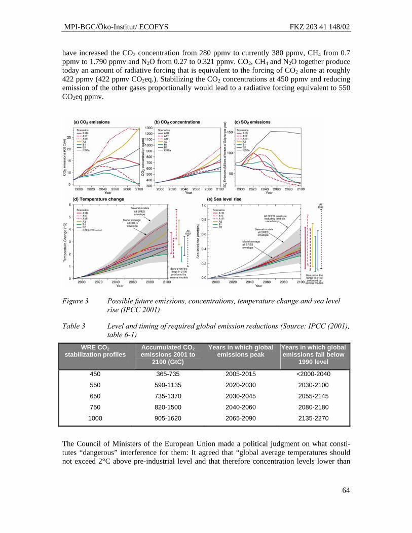
MPI-BGC/Öko-Institut/ ECOFYS FKZ 203 41 148/02
64
have increased the CO2 concentration from 280 ppmv to currently 380 ppmv, CH4 from 0.7 ppmv to 1.790 ppmv and N2O from 0.27 to 0.321 ppmv. CO2, CH4 and N2O together produce today an amount of radiative forcing that is equivalent to the forcing of CO2 alone at roughly 422 ppmv (422 ppmv CO2eq.). Stabilizing the CO2 concentrations at 450 ppmv and reducing emission of the other gases proportionally would lead to a radiative forcing equivalent to 550 CO2eq ppmv.
Figure 3 Possible future emissions, concentrations, temperature change and sea level rise (IPCC 2001)
Table 3 Level and timing of required global emission reductions (Source: IPCC (2001), table 6-1)
WRE CO2 stabilization profiles
Accumulated CO2 emissions 2001 to
2100 (GtC)
Years in which global emissions peak
Years in which global emissions fall below
1990 level
450
550
650
750
1000
365-735
590-1135
735-1370
820-1500
905-1620
2005-2015
2020-2030
2030-2045
2040-2060
2065-2090
<2000-2040
2030-2100
2055-2145
2080-2180
2135-2270
The Council of Ministers of the European Union made a political judgment on what consti-tutes “dangerous” interference for them: It agreed that “global average temperatures should not exceed 2°C above pre-industrial level and that therefore concentration levels lower than
MPI-BGC/Öko-Institut/ ECOFYS FKZ 203 41 148/02
65
550 ppmv CO2 should guide global limitation and reduction efforts”5 (European-Council 1996). Germany, the UK, Philippines and Micronesia have announced at COP9 in Milan in December 2003 the aim to keep global average temperatures increase below 2°C. The Nether-lands on behalf of the EU25, Bulgaria, Romania and Turkey reiterated the 2°C goal at COP 10 in Buenos Aires in December 2004.
Substantial emission reductions are necessary to reach this stabilization level: Emissions of Annex-I countries need to be 10% to 45% below 1990 levels in 2020 and 70% to 90% below 1990 levels in 2050 (den Elzen and de Moor 2002; Höhne and Blok 2005). In addition, emis-sions in some Non-Annex-I regions need to be below their today assumed reference scenarios as of 2020. Stopping emissions from deforestation, which make up around 1/3 to 1/6 of global CO2 emissions, would facilitate reaching these ambitious goals.
In addition to the absolute level of concentrations, also the rate of change is important. Many ecosystems can adapt to changes in climate. In the past, species always migrated or adapted to new circumstances. Such adaptation however, can only occur at a certain rate of change. The effect of rates of change on impacts is a matter of active research. Early results have suggested that rates of change exceeding the ability of ecosystems to migrate would be particularly dam-aging (IPCC 2001, chapters 5 and 19). Sequestration through carbon biogenic carbon sinks, although not permanent, could “buy time” and decrease the rate of warming.
4.3 Political landscape
The Kyoto Protocol defines binding emission limitations for Annex-I countries. These current commitments in the UNFCCC and the Kyoto Protocol will not be sufficient to reach ambi-tious long-term targets such as stabilization at 450 or 550 ppmv CO2 concentrations. The Kyoto Protocol is only a first step towards the ultimate objective of the Convention. Eventu-ally participation of all major countries will be required. The question is when and how.
The Kyoto Protocol entered into force 16 February 2005 after several years of uncertainty around its future. The USA and Australia are still rejecting with the argument that it would severely harm the US economy and that it excludes developing countries. The EU and its member states always supported the treaty and pledged to implement it, even if when it was not yet in force.
Industrialized countries are on the one hand responsible for most of the problem should take the first step in reducing emissions. On the other hand, their efforts can only be effective, if also developing countries’ emissions do not grow infinitely.
Developing countries object to restrictions to their economic growth, since the industrialized countries, which are mainly responsible for the problem, do not act, e.g. the Kyoto Protocol is not implemented. Developing countries are only to a relatively small part responsible for the problem. On the other hand, reaching the ultimate objective of the convention is only possible if developing countries ‘get it right the first place’, meaning that these countries do not first become large polluters and then reduce emissions.
Figure 4 shows the historic emissions from Annex-I and Non-Annex-I countries of the CO2, CH4, N2O and fluorinated greenhouse gases in CO2 equivalents as well as the expected future 5 Technical note: Climate models, which take into account greenhouse gases other than CO2 and use anaverage climate sensitivity, may predict a temperature increase higher than 2°C for a stabilization of CO2 concentrations at 550 ppmv.
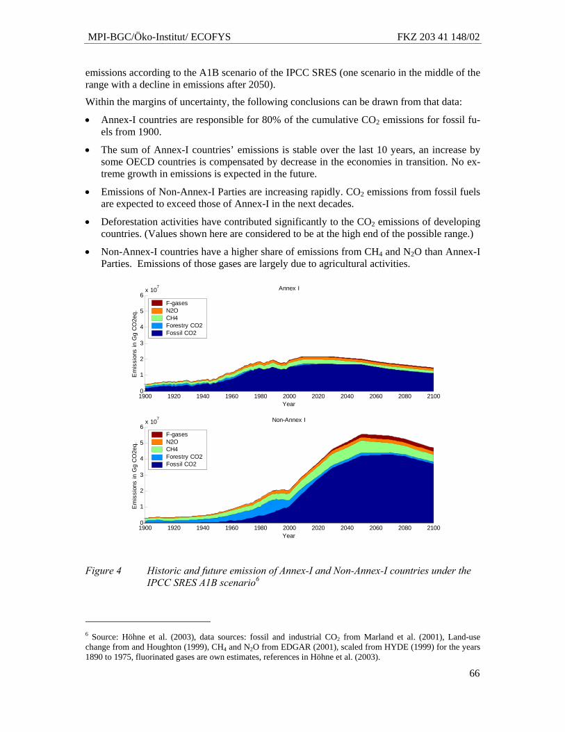
MPI-BGC/Öko-Institut/ ECOFYS FKZ 203 41 148/02
66
emissions according to the A1B scenario of the IPCC SRES (one scenario in the middle of the range with a decline in emissions after 2050).
Within the margins of uncertainty, the following conclusions can be drawn from that data:
• Annex-I countries are responsible for 80% of the cumulative CO2 emissions for fossil fu-els from 1900.
• The sum of Annex-I countries’ emissions is stable over the last 10 years, an increase by some OECD countries is compensated by decrease in the economies in transition. No ex-treme growth in emissions is expected in the future.
• Emissions of Non-Annex-I Parties are increasing rapidly. CO2 emissions from fossil fuels are expected to exceed those of Annex-I in the next decades.
• Deforestation activities have contributed significantly to the CO2 emissions of developing countries. (Values shown here are considered to be at the high end of the possible range.)
• Non-Annex-I countries have a higher share of emissions from CH4 and N2O than Annex-I Parties. Emissions of those gases are largely due to agricultural activities.
1900 1920 1940 1960 1980 2000 2020 2040 2060 2080 21000
1
2
3
4
5
6x 10⁷ Annex I
Em
issi
ons
in G
g C
O2e
q.
Year
F-gasesN2OCH4Forestry CO2Fossil CO2
1900 1920 1940 1960 1980 2000 2020 2040 2060 2080 21000
1
2
3
4
5
6x 10⁷ Non-Annex I
Em
issi
ons
in G
g C
O2e
q.
Year
F-gasesN2OCH4Forestry CO2Fossil CO2
Figure 4 Historic and future emission of Annex-I and Non-Annex-I countries under the IPCC SRES A1B scenario6
6 Source: Höhne et al. (2003), data sources: fossil and industrial CO2 from Marland et al. (2001), Land-use change from and Houghton (1999), CH4 and N2O from EDGAR (2001), scaled from HYDE (1999) for the years 1890 to 1975, fluorinated gases are own estimates, references in Höhne et al. (2003).
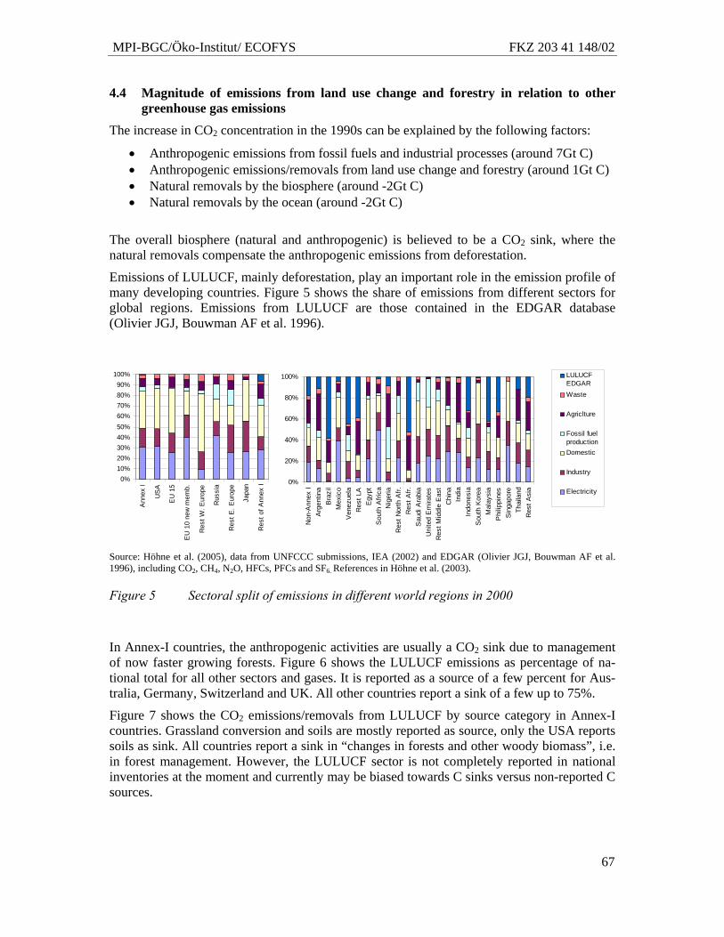
MPI-BGC/Öko-Institut/ ECOFYS FKZ 203 41 148/02
67
4.4 Magnitude of emissions from land use change and forestry in relation to other greenhouse gas emissions
The increase in CO2 concentration in the 1990s can be explained by the following factors:
• Anthropogenic emissions from fossil fuels and industrial processes (around 7Gt C) • Anthropogenic emissions/removals from land use change and forestry (around 1Gt C) • Natural removals by the biosphere (around -2Gt C) • Natural removals by the ocean (around -2Gt C)
The overall biosphere (natural and anthropogenic) is believed to be a CO2 sink, where the natural removals compensate the anthropogenic emissions from deforestation.
Emissions of LULUCF, mainly deforestation, play an important role in the emission profile of many developing countries. Figure 5 shows the share of emissions from different sectors for global regions. Emissions from LULUCF are those contained in the EDGAR database (Olivier JGJ, Bouwman AF et al. 1996).
0%10%20%30%40%50%60%70%80%90%
100%
Ann
ex I
US
A
EU
15
EU
10
new
mem
b.
Res
t W. E
urop
e
Rus
sia
Res
t E. E
urop
e
Japa
n
Res
t of A
nnex
I
0%
20%
40%
60%
80%
100%
Non
-Ann
ex I
Arg
entin
aB
razi
lM
exic
oV
enez
uela
Res
t LA
Egy
ptS
outh
Afri
caN
iger
iaR
est N
orth
Afr.
Res
t Afr.
Sau
di A
rabi
aU
nite
d E
mira
tes
Res
t Mid
dle
Eas
tC
hina
Indi
aIn
done
sia
Sou
th K
orea
Mal
aysi
aP
hilip
pine
sS
inga
pore
Thai
land
Res
t Asi
a
LULUCFEDGARWaste
Agriclture
Fossil fuelproductionDomestic
Industry
Electricity
Source: Höhne et al. (2005), data from UNFCCC submissions, IEA (2002) and EDGAR (Olivier JGJ, Bouwman AF et al. 1996), including CO2, CH4, N2O, HFCs, PFCs and SF6. References in Höhne et al. (2003).
Figure 5 Sectoral split of emissions in different world regions in 2000
In Annex-I countries, the anthropogenic activities are usually a CO2 sink due to management of now faster growing forests. Figure 6 shows the LULUCF emissions as percentage of na-tional total for all other sectors and gases. It is reported as a source of a few percent for Aus-tralia, Germany, Switzerland and UK. All other countries report a sink of a few up to 75%.
Figure 7 shows the CO2 emissions/removals from LULUCF by source category in Annex-I countries. Grassland conversion and soils are mostly reported as source, only the USA reports soils as sink. All countries report a sink in “changes in forests and other woody biomass”, i.e. in forest management. However, the LULUCF sector is not completely reported in national inventories at the moment and currently may be biased towards C sinks versus non-reported C sources.
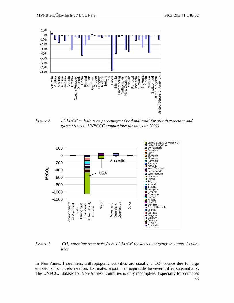
MPI-BGC/Öko-Institut/ ECOFYS FKZ 203 41 148/02
68
Figure 6 LULUCF emissions as percentage of national total for all other sectors and gases (Source: UNFCCC submissions for the year 2002)
-1200
-1000
-800
-600
-400
-200
0
200
Aba
ndon
men
tof
Man
aged
Land
sC
hang
es in
Fore
st a
ndO
ther
Woo
dyBi
omas
s
Soi
ls
Fore
st a
ndG
rass
land
Con
vers
ion
Oth
er
MtC
O2
United States of AmericaUnited KingdomSw itzerlandSw edenSpainSloveniaSlovakiaRomaniaPortugalNorw ayNew ZealandNetherlandsLuxembourgLithuaniaLatviaItalyIrelandIcelandHungaryGreeceGermanyFranceFinlandEstoniaDenmarkCzech RepublicCroatiaCanadaBulgariaBelgiumBelarusAustriaAustralia
USA
Australia
Figure 7 CO2 emissions/removals from LULUCF by source category in Annex-I coun-tries
In Non-Annex-I countries, anthropogenic activities are usually a CO2 source due to large emissions from deforestation. Estimates about the magnitude however differ substantially. The UNFCCC dataset for Non-Annex-I countries is only incomplete. Especially for countries
-80%-70%-60%-50%-40%-30%-20%-10%
0%10%
Aus
tralia
A
ustri
a B
elar
us
Bel
gium
B
ulga
ria
Can
ada
Cro
atia
C
zech
Rep
ublic
D
enm
ark
Est
onia
Fi
nlan
d Fr
ance
G
erm
any
Gre
ece
Hun
gary
Ic
elan
d Ire
land
Ita
ly
Latv
ia
Lith
uani
a Lu
xem
bour
g N
ethe
rland
s N
ew Z
eala
nd
Nor
way
P
ortu
gal
Rom
ania
S
lova
kia
Slo
veni
a S
pain
S
wed
en
Sw
itzer
land
U
nite
d K
ingd
om
Uni
ted
Sta
tes
of A
mer
ica
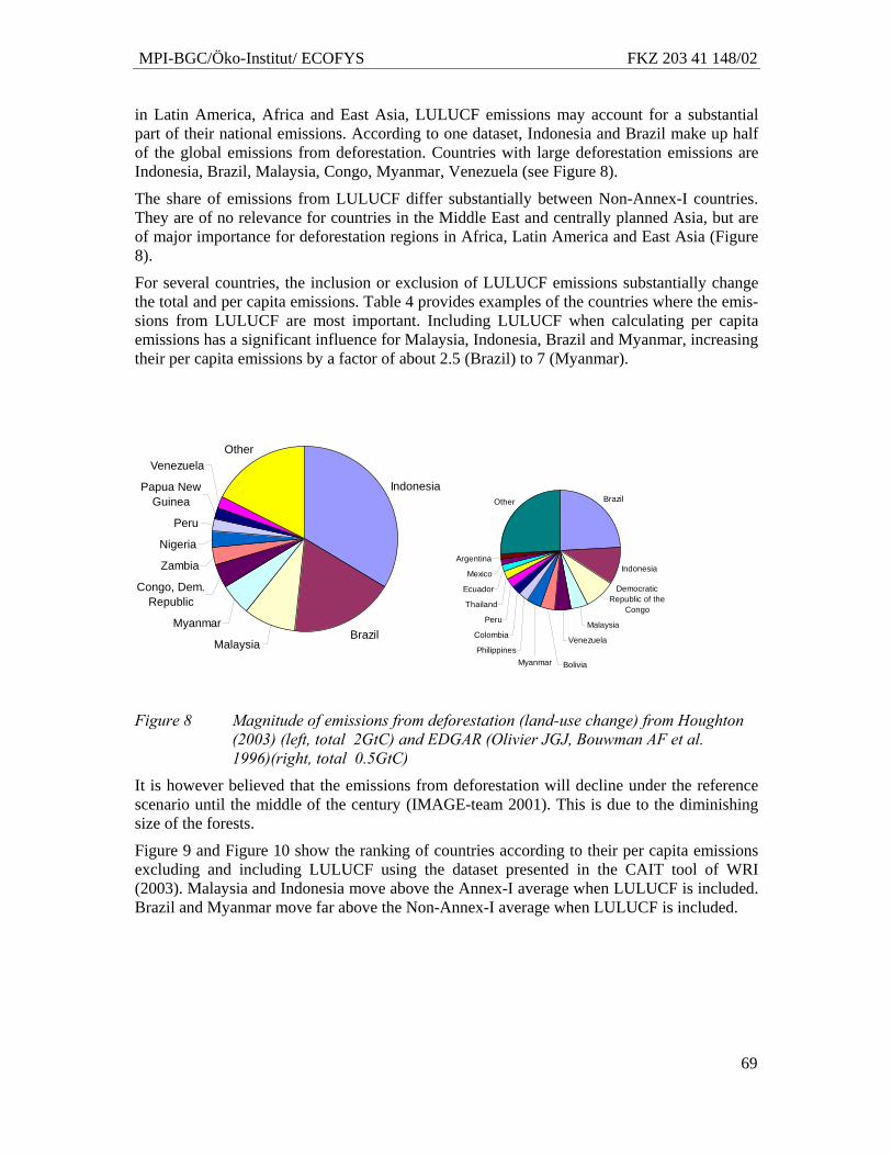
MPI-BGC/Öko-Institut/ ECOFYS FKZ 203 41 148/02
69
in Latin America, Africa and East Asia, LULUCF emissions may account for a substantial part of their national emissions. According to one dataset, Indonesia and Brazil make up half of the global emissions from deforestation. Countries with large deforestation emissions are Indonesia, Brazil, Malaysia, Congo, Myanmar, Venezuela (see Figure 8).
The share of emissions from LULUCF differ substantially between Non-Annex-I countries. They are of no relevance for countries in the Middle East and centrally planned Asia, but are of major importance for deforestation regions in Africa, Latin America and East Asia (Figure 8).
For several countries, the inclusion or exclusion of LULUCF emissions substantially change the total and per capita emissions. Table 4 provides examples of the countries where the emis-sions from LULUCF are most important. Including LULUCF when calculating per capita emissions has a significant influence for Malaysia, Indonesia, Brazil and Myanmar, increasing their per capita emissions by a factor of about 2.5 (Brazil) to 7 (Myanmar).
Indonesia
BrazilMalaysia
Myanmar
Congo, Dem. Republic
Zambia
Nigeria
Peru
Papua New Guinea
VenezuelaOther
Figure 8 Magnitude of emissions from deforestation (land-use change) from Houghton (2003) (left, total 2GtC) and EDGAR (Olivier JGJ, Bouwman AF et al. 1996)(right, total 0.5GtC)
It is however believed that the emissions from deforestation will decline under the reference scenario until the middle of the century (IMAGE-team 2001). This is due to the diminishing size of the forests.
Figure 9 and Figure 10 show the ranking of countries according to their per capita emissions excluding and including LULUCF using the dataset presented in the CAIT tool of WRI (2003). Malaysia and Indonesia move above the Annex-I average when LULUCF is included. Brazil and Myanmar move far above the Non-Annex-I average when LULUCF is included.
Brazil
Indonesia
Malaysia
VenezuelaPhilippines
Colombia
Peru
Thailand
Ecuador
Mexico
Argentina
Other
Democratic Republic of the
Congo
Myanmar Bolivia
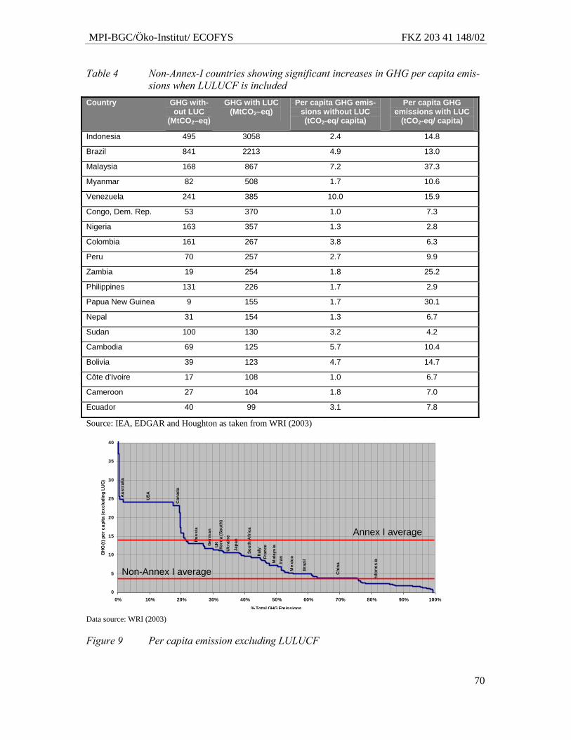
MPI-BGC/Öko-Institut/ ECOFYS FKZ 203 41 148/02
70
Table 4 Non-Annex-I countries showing significant increases in GHG per capita emis-sions when LULUCF is included
Country GHG with-out LUC
(MtCO2–eq)
GHG with LUC (MtCO2–eq)
Per capita GHG emis-sions without LUC (tCO2-eq/ capita)
Per capita GHG emissions with LUC
(tCO2-eq/ capita)
Indonesia 495 3058 2.4 14.8
Brazil 841 2213 4.9 13.0
Malaysia 168 867 7.2 37.3
Myanmar 82 508 1.7 10.6
Venezuela 241 385 10.0 15.9
Congo, Dem. Rep. 53 370 1.0 7.3
Nigeria 163 357 1.3 2.8
Colombia 161 267 3.8 6.3
Peru 70 257 2.7 9.9
Zambia 19 254 1.8 25.2
Philippines 131 226 1.7 2.9
Papua New Guinea 9 155 1.7 30.1
Nepal 31 154 1.3 6.7
Sudan 100 130 3.2 4.2
Cambodia 69 125 5.7 10.4
Bolivia 39 123 4.7 14.7
Côte d'Ivoire 17 108 1.0 6.7
Cameroon 27 104 1.8 7.0
Ecuador 40 99 3.1 7.8
Source: IEA, EDGAR and Houghton as taken from WRI (2003)
0
5
10
15
20
25
30
35
40
0% 10% 20% 30% 40% 50% 60% 70% 80% 90% 100%
%Total GHG Emissions
GHG
(t) p
er c
apita
(exc
ludi
ng L
UC)
USA
Can
ada
Braz
il
Indo
nesi
a
Chi
na
Russ
ia
Ger
man
Mal
aysi
a
Japa
n
Aus
tral
ia
Kore
a (S
outh
)UK
Sout
h A
fric
a
ItalyUk
rain
e
Fran
ce
Iran
Mex
ico
Annex I average
Non-Annex I average
Data source: WRI (2003)
Figure 9 Per capita emission excluding LULUCF
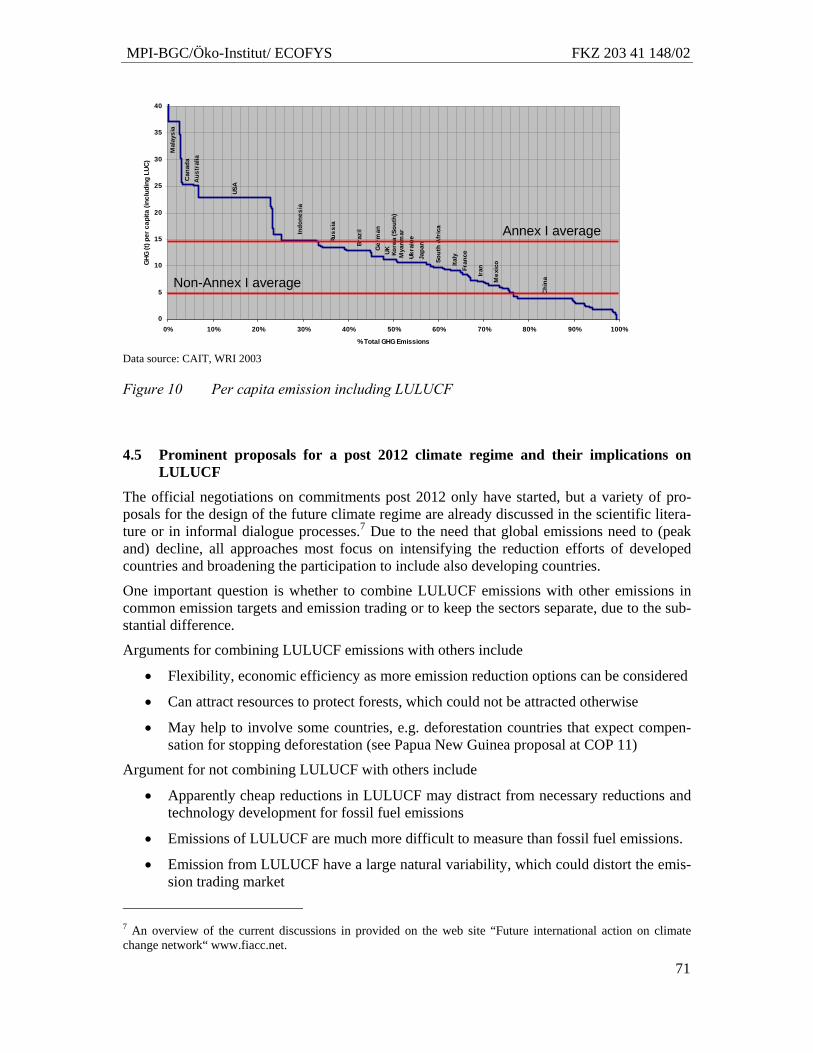
MPI-BGC/Öko-Institut/ ECOFYS FKZ 203 41 148/02
71
0
5
10
15
20
25
30
35
40
0% 10% 20% 30% 40% 50% 60% 70% 80% 90% 100%
% Total GHG Emissions
GHG
(t) p
er c
apita
(inc
ludi
ng L
UC)
USA
Can
ada
Braz
ilIndo
nesi
a
Chi
na
Russ
ia
Ger
man
Mal
aysi
a
Japa
n
Aus
tral
ia
Kore
a (S
outh
)UK
Sout
h A
fric
a
ItalyUk
rain
e
Fran
ce
Iran
Mex
ico
Mya
nmar Annex I average
Non-Annex I average
Data source: CAIT, WRI 2003
Figure 10 Per capita emission including LULUCF
4.5 Prominent proposals for a post 2012 climate regime and their implications on LULUCF
The official negotiations on commitments post 2012 only have started, but a variety of pro-posals for the design of the future climate regime are already discussed in the scientific litera-ture or in informal dialogue processes.7 Due to the need that global emissions need to (peak and) decline, all approaches most focus on intensifying the reduction efforts of developed countries and broadening the participation to include also developing countries.
One important question is whether to combine LULUCF emissions with other emissions in common emission targets and emission trading or to keep the sectors separate, due to the sub-stantial difference.
Arguments for combining LULUCF emissions with others include
• Flexibility, economic efficiency as more emission reduction options can be considered
• Can attract resources to protect forests, which could not be attracted otherwise
• May help to involve some countries, e.g. deforestation countries that expect compen-sation for stopping deforestation (see Papua New Guinea proposal at COP 11)
Argument for not combining LULUCF with others include
• Apparently cheap reductions in LULUCF may distract from necessary reductions and technology development for fossil fuel emissions
• Emissions of LULUCF are much more difficult to measure than fossil fuel emissions.
• Emission from LULUCF have a large natural variability, which could distort the emis-sion trading market
7 An overview of the current discussions in provided on the web site “Future international action on climate change network“ www.fiacc.net.
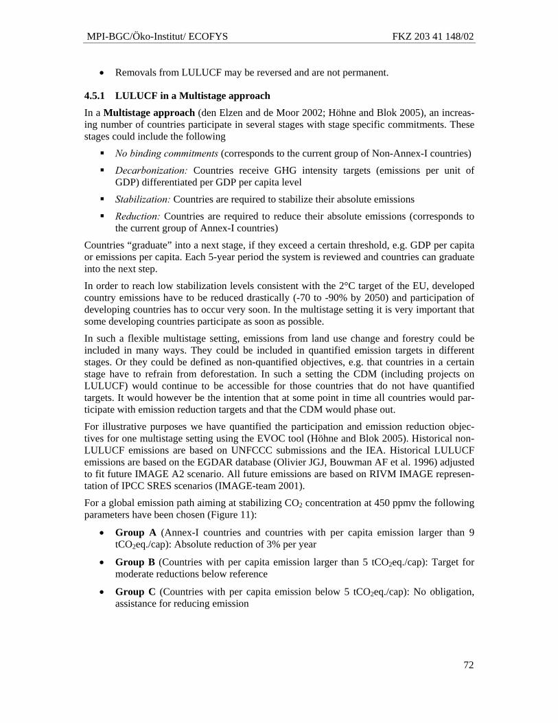
MPI-BGC/Öko-Institut/ ECOFYS FKZ 203 41 148/02
72
• Removals from LULUCF may be reversed and are not permanent.
4.5.1 LULUCF in a Multistage approach
In a Multistage approach (den Elzen and de Moor 2002; Höhne and Blok 2005), an increas-ing number of countries participate in several stages with stage specific commitments. These stages could include the following
No binding commitments (corresponds to the current group of Non-Annex-I countries)
Decarbonization: Countries receive GHG intensity targets (emissions per unit of GDP) differentiated per GDP per capita level
Stabilization: Countries are required to stabilize their absolute emissions
Reduction: Countries are required to reduce their absolute emissions (corresponds to the current group of Annex-I countries)
Countries “graduate” into a next stage, if they exceed a certain threshold, e.g. GDP per capita or emissions per capita. Each 5-year period the system is reviewed and countries can graduate into the next step.
In order to reach low stabilization levels consistent with the 2°C target of the EU, developed country emissions have to be reduced drastically (-70 to -90% by 2050) and participation of developing countries has to occur very soon. In the multistage setting it is very important that some developing countries participate as soon as possible.
In such a flexible multistage setting, emissions from land use change and forestry could be included in many ways. They could be included in quantified emission targets in different stages. Or they could be defined as non-quantified objectives, e.g. that countries in a certain stage have to refrain from deforestation. In such a setting the CDM (including projects on LULUCF) would continue to be accessible for those countries that do not have quantified targets. It would however be the intention that at some point in time all countries would par-ticipate with emission reduction targets and that the CDM would phase out.
For illustrative purposes we have quantified the participation and emission reduction objec-tives for one multistage setting using the EVOC tool (Höhne and Blok 2005). Historical non-LULUCF emissions are based on UNFCCC submissions and the IEA. Historical LULUCF emissions are based on the EGDAR database (Olivier JGJ, Bouwman AF et al. 1996) adjusted to fit future IMAGE A2 scenario. All future emissions are based on RIVM IMAGE represen-tation of IPCC SRES scenarios (IMAGE-team 2001).
For a global emission path aiming at stabilizing CO2 concentration at 450 ppmv the following parameters have been chosen (Figure 11):
• Group A (Annex-I countries and countries with per capita emission larger than 9 tCO2eq./cap): Absolute reduction of 3% per year
• Group B (Countries with per capita emission larger than 5 tCO2eq./cap): Target for moderate reductions below reference
• Group C (Countries with per capita emission below 5 tCO2eq./cap): No obligation, assistance for reducing emission
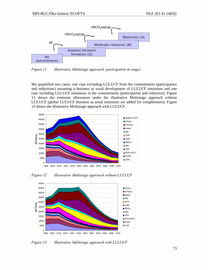
MPI-BGC/Öko-Institut/ ECOFYS FKZ 203 41 148/02
73
Reduction (A)
Moderate reduction (B)
Assisted emission limitation (C)
No commitments
all
>5tCO2eq/cap
>9tCO2eq/cap
Figure 11 Illustrative Multistage approach, participation in stages
We quantified two cases: one case excluding LULUCF from the commitments (participation and reductions) assuming a business as usual development of LULUCF emissions and one case including LULUCF emissions in the commitments (participation and reduction). Figure 13 shows the emission allowances under the illustrative Multistage approach without LULUCF (global LULUCF business as usual emissions are added for completeness). Figure 13 shows the illustrative Multistage approach with LULUCF.
Figure 12 Illustrative Multistage approach without LULUCF
Figure 13 Illustrative Multistage approach with LULUCF
0
5000
10000
15000
20000
25000
30000
35000
40000
45000
50000
1990 2000 2010 2020 2030 2040 2050 2060 2070 2080 2090 2100
Mt C
O2e
q.
EAsiaCPAsiaSasiaMEAFRLAMREEURAIJPNRUS+EEUEU25USA
0
5000
10000
15000
20000
25000
30000
35000
40000
45000
50000
1990 2000 2010 2020 2030 2040 2050 2060 2070 2080 2090 2100
Mt C
O2e
q.
Global LUCFEAsiaCPAsiaSasiaMEAFRLAMREEURAIJPNRUS+EEUEU25USA
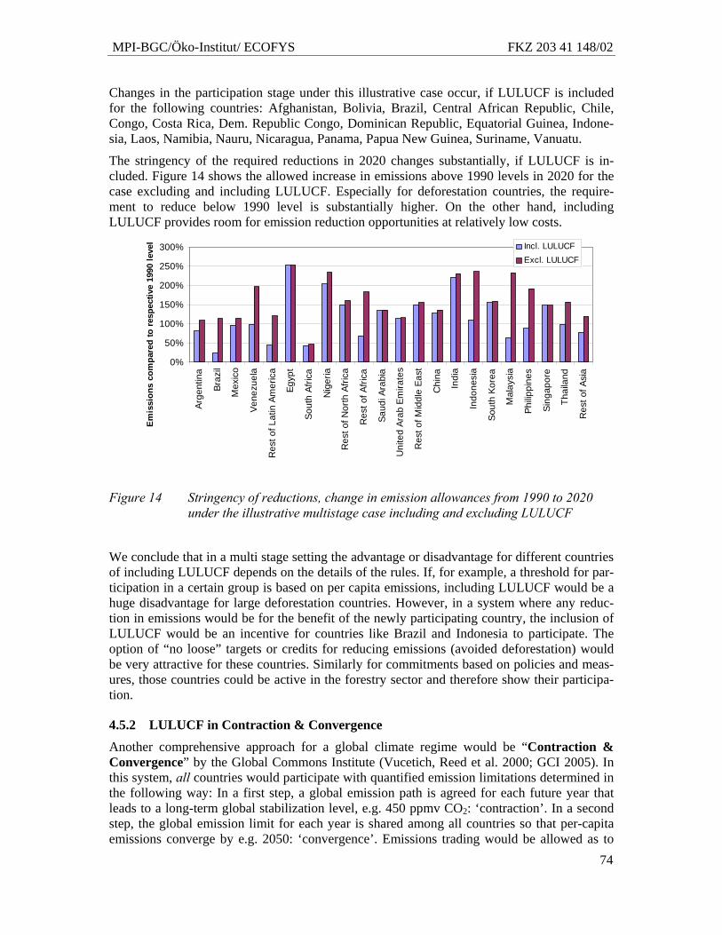
MPI-BGC/Öko-Institut/ ECOFYS FKZ 203 41 148/02
74
Changes in the participation stage under this illustrative case occur, if LULUCF is included for the following countries: Afghanistan, Bolivia, Brazil, Central African Republic, Chile, Congo, Costa Rica, Dem. Republic Congo, Dominican Republic, Equatorial Guinea, Indone-sia, Laos, Namibia, Nauru, Nicaragua, Panama, Papua New Guinea, Suriname, Vanuatu.
The stringency of the required reductions in 2020 changes substantially, if LULUCF is in-cluded. Figure 14 shows the allowed increase in emissions above 1990 levels in 2020 for the case excluding and including LULUCF. Especially for deforestation countries, the require-ment to reduce below 1990 level is substantially higher. On the other hand, including LULUCF provides room for emission reduction opportunities at relatively low costs.
0%
50%
100%
150%
200%
250%
300%
Arge
ntin
a
Braz
il
Mex
ico
Vene
zuel
a
Res
t of L
atin
Am
eric
a
Egyp
t
Sout
h Af
rica
Nig
eria
Res
t of N
orth
Afri
ca
Res
t of A
frica
Saud
i Ara
bia
Uni
ted
Arab
Em
irate
s
Res
t of M
iddl
e Ea
st
Chi
na
Indi
a
Indo
nesi
a
Sout
h Ko
rea
Mal
aysi
a
Philip
pine
s
Sing
apor
e
Thai
land
Res
t of A
sia
Emis
sion
s co
mpa
red
to re
spec
tive
1990
leve
l Incl. LULUCFExcl. LULUCF
Figure 14 Stringency of reductions, change in emission allowances from 1990 to 2020 under the illustrative multistage case including and excluding LULUCF
We conclude that in a multi stage setting the advantage or disadvantage for different countries of including LULUCF depends on the details of the rules. If, for example, a threshold for par-ticipation in a certain group is based on per capita emissions, including LULUCF would be a huge disadvantage for large deforestation countries. However, in a system where any reduc-tion in emissions would be for the benefit of the newly participating country, the inclusion of LULUCF would be an incentive for countries like Brazil and Indonesia to participate. The option of “no loose” targets or credits for reducing emissions (avoided deforestation) would be very attractive for these countries. Similarly for commitments based on policies and meas-ures, those countries could be active in the forestry sector and therefore show their participa-tion.
4.5.2 LULUCF in Contraction & Convergence Another comprehensive approach for a global climate regime would be “Contraction & Convergence” by the Global Commons Institute (Vucetich, Reed et al. 2000; GCI 2005). In this system, all countries would participate with quantified emission limitations determined in the following way: In a first step, a global emission path is agreed for each future year that leads to a long-term global stabilization level, e.g. 450 ppmv CO2: ‘contraction’. In a second step, the global emission limit for each year is shared among all countries so that per-capita emissions converge by e.g. 2050: ‘convergence’. Emissions trading would be allowed as to
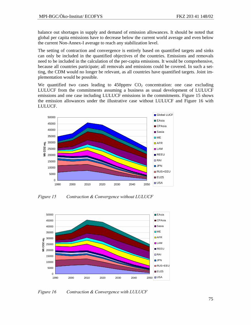
MPI-BGC/Öko-Institut/ ECOFYS FKZ 203 41 148/02
75
balance out shortages in supply and demand of emission allowances. It should be noted that global per capita emissions have to decrease below the current world average and even below the current Non-Annex-I average to reach any stabilization level.
The setting of contraction and convergence is entirely based on quantified targets and sinks can only be included in the quantified objectives of the countries. Emissions and removals need to be included in the calculation of the per-capita emissions. It would be comprehensive, because all countries participate; all removals and emissions could be covered. In such a set-ting, the CDM would no longer be relevant, as all countries have quantified targets. Joint im-plementation would be possible.
We quantified two cases leading to 450ppmv CO2 concentration: one case excluding LULUCF from the commitments assuming a business as usual development of LULUCF emissions and one case including LULUCF emissions in the commitments. Figure 15 shows the emission allowances under the illustrative case without LULUCF and Figure 16 with LULUCF.
Figure 15 Contraction & Convergence without LULUCF
Figure 16 Contraction & Convergence with LULUCF
0
5000
10000
15000
20000
25000
30000
35000
40000
45000
50000
1990 2000 2010 2020 2030 2040 2050
Mt C
O2
eq.
EAsia
CPAsia
Sasia
ME
AFR
LAM
REEU
RAI
JPN
RUS+EEU
EU25
USA
0
5000
10000
15000
20000
25000
30000
35000
40000
45000
50000
1990 2000 2010 2020 2030 2040 2050
Mt C
O2
eq.
Global LUCF
EAsia
CPAsia
Sasia
ME
AFR
LAM
REEU
RAI
JPN
RUS+EEU
EU25
USA
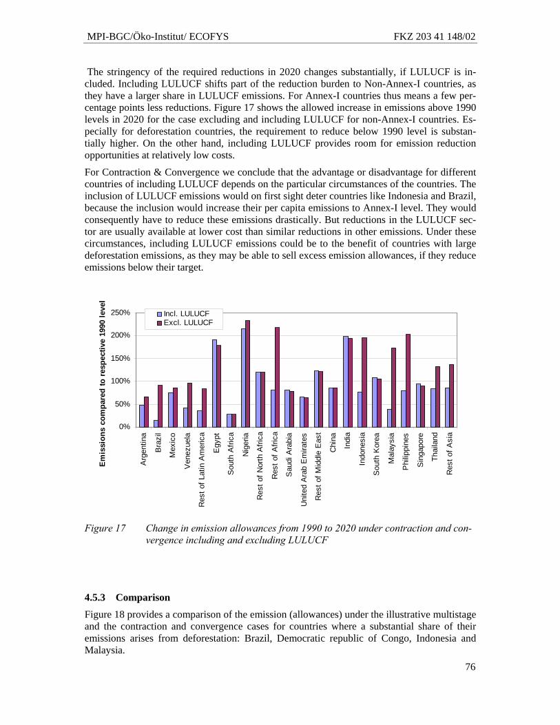
MPI-BGC/Öko-Institut/ ECOFYS FKZ 203 41 148/02
76
The stringency of the required reductions in 2020 changes substantially, if LULUCF is in-cluded. Including LULUCF shifts part of the reduction burden to Non-Annex-I countries, as they have a larger share in LULUCF emissions. For Annex-I countries thus means a few per-centage points less reductions. Figure 17 shows the allowed increase in emissions above 1990 levels in 2020 for the case excluding and including LULUCF for non-Annex-I countries. Es-pecially for deforestation countries, the requirement to reduce below 1990 level is substan-tially higher. On the other hand, including LULUCF provides room for emission reduction opportunities at relatively low costs.
For Contraction & Convergence we conclude that the advantage or disadvantage for different countries of including LULUCF depends on the particular circumstances of the countries. The inclusion of LULUCF emissions would on first sight deter countries like Indonesia and Brazil, because the inclusion would increase their per capita emissions to Annex-I level. They would consequently have to reduce these emissions drastically. But reductions in the LULUCF sec-tor are usually available at lower cost than similar reductions in other emissions. Under these circumstances, including LULUCF emissions could be to the benefit of countries with large deforestation emissions, as they may be able to sell excess emission allowances, if they reduce emissions below their target.
0%
50%
100%
150%
200%
250%
Arg
entin
a
Bra
zil
Mex
ico
Ven
ezue
la
Res
t of L
atin
Am
eric
a
Egy
pt
Sou
th A
frica
Nig
eria
Res
t of N
orth
Afri
ca
Res
t of A
frica
Sau
di A
rabi
a
Uni
ted
Ara
b E
mira
tes
Res
t of M
iddl
e E
ast
Chi
na
Indi
a
Indo
nesi
a
Sou
th K
orea
Mal
aysi
a
Phi
lippi
nes
Sin
gapo
re
Thai
land
Res
t of A
sia
Em
issi
ons
com
pare
d to
resp
ectiv
e 19
90 le
vel
Incl. LULUCFExcl. LULUCF
Figure 17 Change in emission allowances from 1990 to 2020 under contraction and con-vergence including and excluding LULUCF
4.5.3 Comparison
Figure 18 provides a comparison of the emission (allowances) under the illustrative multistage and the contraction and convergence cases for countries where a substantial share of their emissions arises from deforestation: Brazil, Democratic republic of Congo, Indonesia and Malaysia.
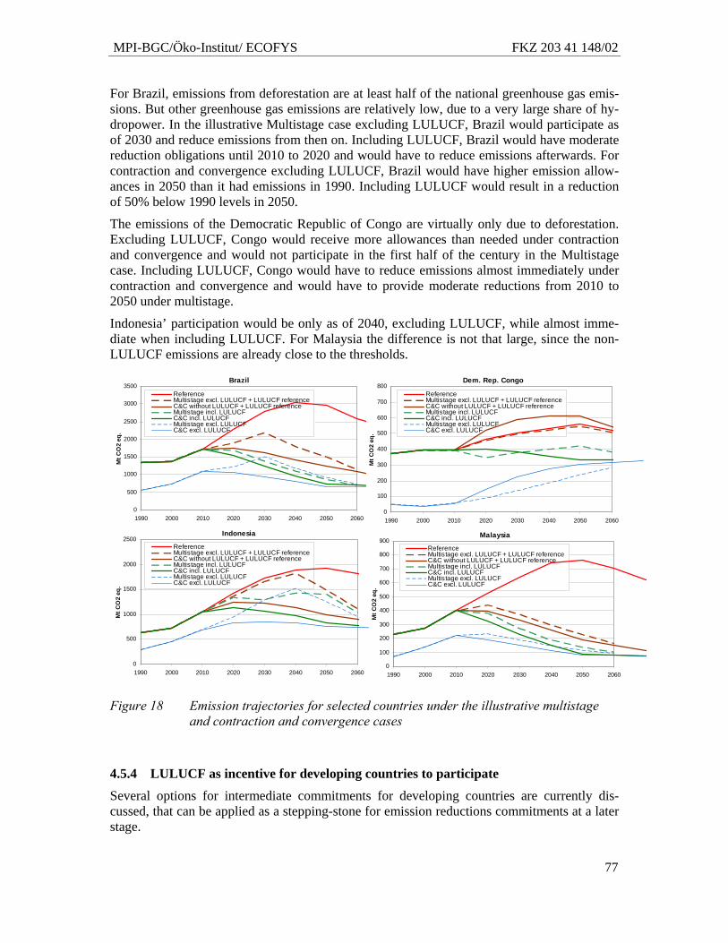
MPI-BGC/Öko-Institut/ ECOFYS FKZ 203 41 148/02
77
For Brazil, emissions from deforestation are at least half of the national greenhouse gas emis-sions. But other greenhouse gas emissions are relatively low, due to a very large share of hy-dropower. In the illustrative Multistage case excluding LULUCF, Brazil would participate as of 2030 and reduce emissions from then on. Including LULUCF, Brazil would have moderate reduction obligations until 2010 to 2020 and would have to reduce emissions afterwards. For contraction and convergence excluding LULUCF, Brazil would have higher emission allow-ances in 2050 than it had emissions in 1990. Including LULUCF would result in a reduction of 50% below 1990 levels in 2050.
The emissions of the Democratic Republic of Congo are virtually only due to deforestation. Excluding LULUCF, Congo would receive more allowances than needed under contraction and convergence and would not participate in the first half of the century in the Multistage case. Including LULUCF, Congo would have to reduce emissions almost immediately under contraction and convergence and would have to provide moderate reductions from 2010 to 2050 under multistage.
Indonesia’ participation would be only as of 2040, excluding LULUCF, while almost imme-diate when including LULUCF. For Malaysia the difference is not that large, since the non-LULUCF emissions are already close to the thresholds.
Brazil
0
500
1000
1500
2000
2500
3000
3500
1990 2000 2010 2020 2030 2040 2050 2060
Mt C
O2
eq.
ReferenceMultistage excl. LULUCF + LULUCF referenceC&C without LULUCF + LULUCF referenceMultistage incl. LULUCFC&C incl. LULUCFMultistage excl. LULUCFC&C excl. LULUCF
Indonesia
0
500
1000
1500
2000
2500
1990 2000 2010 2020 2030 2040 2050 2060
Mt C
O2
eq.
ReferenceMultistage excl. LULUCF + LULUCF referenceC&C without LULUCF + LULUCF referenceMultistage incl. LULUCFC&C incl. LULUCFMultistage excl. LULUCFC&C excl. LULUCF
Malaysia
0
100
200
300
400
500
600
700
800
900
1990 2000 2010 2020 2030 2040 2050 2060
Mt C
O2
eq.
ReferenceMultistage excl. LULUCF + LULUCF referenceC&C without LULUCF + LULUCF referenceMultistage incl. LULUCFC&C incl. LULUCFMultistage excl. LULUCFC&C excl. LULUCF
Dem. Rep. Congo
0
100
200
300
400
500
600
700
800
1990 2000 2010 2020 2030 2040 2050 2060
Mt C
O2
eq.
ReferenceMultistage excl. LULUCF + LULUCF referenceC&C without LULUCF + LULUCF referenceMultistage incl. LULUCFC&C incl. LULUCFMultistage excl. LULUCFC&C excl. LULUCF
Figure 18 Emission trajectories for selected countries under the illustrative multistage and contraction and convergence cases
4.5.4 LULUCF as incentive for developing countries to participate
Several options for intermediate commitments for developing countries are currently dis-cussed, that can be applied as a stepping-stone for emission reductions commitments at a later stage.
MPI-BGC/Öko-Institut/ ECOFYS FKZ 203 41 148/02
78
Some developing countries could for example participate in an enhanced CDM. CDM pro-jects could be initiated by the country that hosts the project (unilateral CDM) and encompass whole sectors and national policies. If emission reductions through such projects exceed a certain value domestically, the excess reductions can be sold on the market. In such an option, LULUCF in the CDM could make a high contribution.
A similar option are “positively binding” or “no lose” targets. A country with such an emis-sion targets can sell additional emission rights, if the target is overachieved, but does not have to buy additional emission rights, if no rights have been sold and the target is still not met.
Further, it has been proposed, that first developing countries participate with emission targets only for particular sectors. For those countries where electricity production plays a major role, only this sector would receive an emission target. For other countries, where LULUCF plays an important role, only this sector would receive an emission target.
Alternatively, some developing countries could subscribe to “sustainable development poli-cies and measures”. Here environmental objectives would be built into the development poli-cies. Requirements for such a sustainable pathway could be defined, e.g., that inefficient equipment is phased out and requirements and certain standards are met for any new equip-ment or a clear deviation from the current policies depending on the countries. The implemen-tation of such sustainable development pathway has to be monitored and verified. The addi-tional cost could be born by the country itself or by other countries. In such a “soft” option, a pledge for certain forest enhancing or preserving polices could be part of the strategy. Such action would count as “participation”, but would not entail an emission reduction targets and would therefore not allow emissions trading.
All of the above approaches are currently discussed under in the UNFCCC process under the agenda item “Reducing emissions from deforestation in developing countries” (UNFCCC 2006g).
4.6 Conclusions
Substantial emission reductions in developed countries and slowed growth in emissions in developing countries are necessary to reach stabilization levels consistent with the EU’s goal to keep global average surface temperature increase below 2°C. This can only be achieved by targeting fossil fuel and industrial emissions as well as emissions from forestry.
Rules on sinks will impact the stringency of the quantified emission reduction commitments in other sectors. Therefore, rules for the sinks accounting have to be set before the emission levels of the other sectors are fixed. The rules on accounting sinks in the future will apply to an increasing number of countries, as it can be envisioned that more and more countries join the group of reducing countries.
The advantage or disadvantage for different countries of including LULUCF depends on the details of the rules. If, for example, a threshold for participation in a certain group is based on per capita emissions, including LULUCF would be a huge disadvantage for large deforesta-tion countries. However, in a system where any reduction in emissions would be for the bene-fit of the newly participating country, the inclusion of LULUCF would be an incentive for countries like Brazil and Indonesia to participate. The option of “no loose” targets or credits for reducing emissions (avoided deforestation) would be very attractive for these countries.
In addition, sinks could also be handled independent of quantified commitments for countries that newly participate in the regime, possibly first with “soft” targets to implement certain

MPI-BGC/Öko-Institut/ ECOFYS FKZ 203 41 148/02
79
polices and measures. The accounting and inclusion of sinks could therefore be conducive to include Non-Annex-I countries in further commitments.
MPI-BGC/Öko-Institut/ ECOFYS FKZ 203 41 148/02
80
5 Biological, technical, economic and realistic potentials
The term “potential” is ambiguous. The magnitude of the carbon source and sink potential varies along with the types of constraints considered. In this study the following terms de-scribe the cascade of potentials from theoretical to realistic assumptions (IPCC 2001; Cannell 2003; Smith 2004):
• Biological potential: Theoretical biologically achievable capacity, meaning some or all practical constraints have been ignored.
• Technological potential: capacity taking into account the biological potential plus constraints by suitability of land and available resources and technology, but some op-timistic assumptions are made about land availability, socio-economic and policy drivers.
• Economic potential: Conservative capacity taking into account the technical potential plus costs, with some optimistic assumptions about social barriers, incentives and speed of implementation of measures
• Realistic potential: Short-term capacity taking into account the economic potential plus social barriers, present policies and (lack of) incentives.
In general managed ecosystems tend to have lower carbon stocks compared to unmanaged systems. This implies a huge theoretical potential for carbon storage through establishing close to nature forestry and refilling depleted soil carbon reservoirs (Table 5). Past degrada-tion and continued human need for resources from land, however, turns part, if not most of this biological potential unrealistic. Recent studies suggest that 10-20% of the biological po-tential are economically achievable within the next 10-50 years in case of strong incentives (Cannell 2003; Freibauer, Rounsevell et al. 2004; Smith 2004; Smith, Andren et al. 2005). Without changes in policy and significant efforts to overcome existing barriers to implementa-tion the realistic potential is likely to be negligible (Smith, Andren et al. 2005). The examples in Table 5 demonstrate that estimates of carbon sequestration potentials in forestry and agri-culture are highly sensitive to the region, time frame and assumptions included in the calcula-tions.
In this report, scenarios of carbon sequestration potentials in forest management and crop-land management mean technical potentials.
In contrast, afforestation/reforestation and deforestation scenarios were taken from eco-nomic models developed by IIASA or derived from past observed rates of change reported by FAO and give estimates of economic potentials.
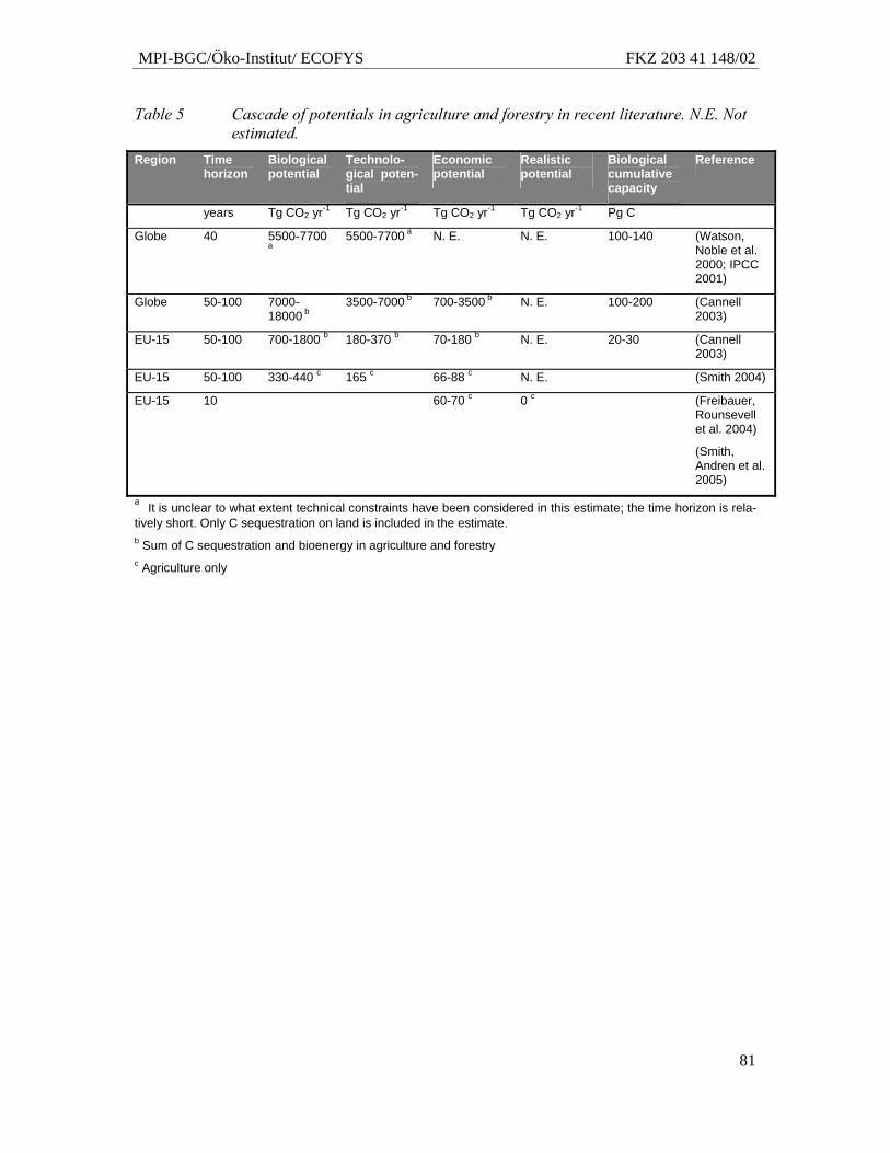
MPI-BGC/Öko-Institut/ ECOFYS FKZ 203 41 148/02
81
Table 5 Cascade of potentials in agriculture and forestry in recent literature. N.E. Not estimated.
Region Time horizon
Biological potential
Technolo-gical poten-tial
Economic potential
Realistic potential
Biological cumulative capacity
Reference
years Tg CO2 yr-1 Tg CO2 yr-1 Tg CO2 yr-1 Tg CO2 yr-1 Pg C
Globe 40 5500-7700 a
5500-7700 a N. E. N. E. 100-140 (Watson, Noble et al. 2000; IPCC 2001)
Globe 50-100 7000-18000 b
3500-7000 b 700-3500 b N. E. 100-200 (Cannell 2003)
EU-15 50-100 700-1800 b 180-370 b 70-180 b N. E. 20-30 (Cannell 2003)
EU-15 50-100 330-440 c 165 c 66-88 c N. E. (Smith 2004)
EU-15 10 60-70 c 0 c (Freibauer, Rounsevell et al. 2004)
(Smith, Andren et al. 2005)
a It is unclear to what extent technical constraints have been considered in this estimate; the time horizon is rela-tively short. Only C sequestration on land is included in the estimate. b Sum of C sequestration and bioenergy in agriculture and forestry c Agriculture only
MPI-BGC/Öko-Institut/ ECOFYS FKZ 203 41 148/02
82
6 Afforestation, reforestation and deforestation
6.1 Introduction
According to the Marrakech Accords Annex I.1 (FCCC/CP/2001/13/Add.1), the following definitions apply and are also used in this report (direct quotation in italics):
“Afforestation” is the direct human-induced conversion of land that has not been forested for a period of at least 50 years to forested land through planting, seed-ing and/or the human-induced promotion of natural seed sources;
“Reforestation” is the direct human-induced conversion of non-forested land to forested land through planting, seeding and/or the human-induced promotion of natural seed sources, on land that was forested but that has been converted to non-forested land. For the first commitment period, reforestation activities will be limited to reforestation occurring on those lands that did not contain forest on 31 December 1989;
“Deforestation” is the direct human-induced conversion of forested land to non-forested land.
The development of global deforestation rates is crucial information for projecting future GHG concentrations. The current annual rates of tropical deforestation from Brazil and Indo-nesia alone could result in an efflux of GHGs making up 80% of the emission reduction target of Annex-I countries during the first Commitment Period (Santilli, P. Moutinho et al. 2003). In addition partially degraded tropical forests by selective logging might become more sus-ceptible to severe draught and fire and cause emissions in the aftermath.
The notion of compensating for rising atmospheric CO2 concentrations through global scale afforestation/reforestation was first put forward in the late 1970's (Dyson 1977). Since the late 1980s, it has been suggested that sufficient lands are available to use the carbon sequestration approach to mitigate significant amounts of CO2 emissions (Marland 1988; Lashof and Tirpak 1989). Claims have been made that forestry-based carbon sequestration is a relatively inex-pensive means of addressing climate change (Marland, Fruit et al. 2001); (Dudek and Leblanc 1990)). The IPCC Third Assessment Report estimated that 12-15% of fossil-fuel emissions until 2050 could be offset by improved management of terrestrial ecosystems globally (Sathaye and Bouille 2001). In the following we will shortly discuss the results from different methods estimating emissions from afforestation/reforestation and deforestation in the past decades before presenting model results of sink/source projections.
6.2 Afforestation, reforestation and deforestation in past and present
The newest Forest Resource Assessment (FRA) by the United Nations Food and Agriculture Organization FAO (FAO, ISRIC et al. 1998) estimates the current rate of deforestation, mainly conversion of forests to agricultural land, to be around 13 Mha per year. At the same time, forest planting, landscape restoration and natural expansion of forests are significantly reducing the net loss of forest area. The net change in forest area in the period 2000-2005 is estimated to be a loss of 7.3 Mha per year. While forest area increased in most of the Annex-I countries, the largest losses of forest cover take place in the tropical region. Table 6 lists se-lected key countries contributing most to the global forest area balance. Further Figure 19
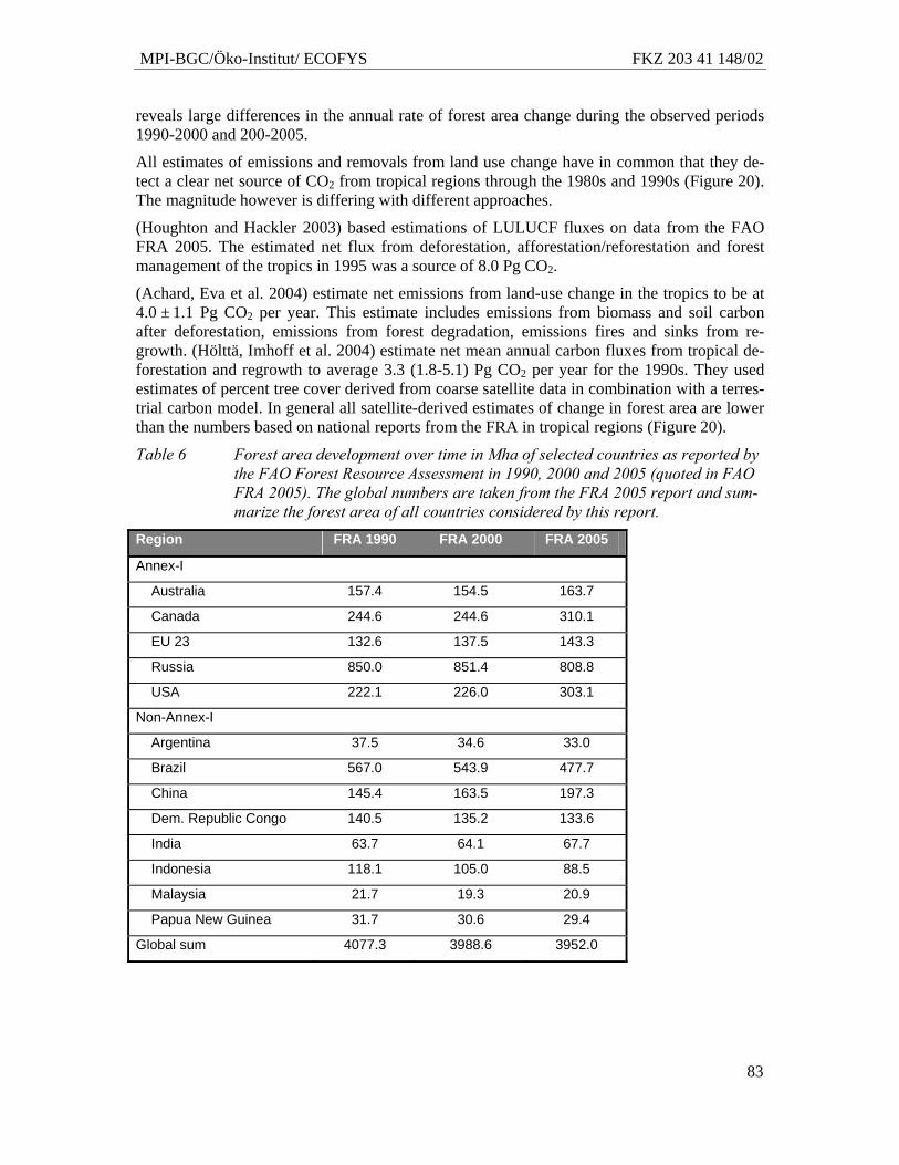
MPI-BGC/Öko-Institut/ ECOFYS FKZ 203 41 148/02
83
reveals large differences in the annual rate of forest area change during the observed periods 1990-2000 and 200-2005.
All estimates of emissions and removals from land use change have in common that they de-tect a clear net source of CO2 from tropical regions through the 1980s and 1990s (Figure 20). The magnitude however is differing with different approaches.
(Houghton and Hackler 2003) based estimations of LULUCF fluxes on data from the FAO FRA 2005. The estimated net flux from deforestation, afforestation/reforestation and forest management of the tropics in 1995 was a source of 8.0 Pg CO2.
(Achard, Eva et al. 2004) estimate net emissions from land-use change in the tropics to be at 4.0 ± 1.1 Pg CO2 per year. This estimate includes emissions from biomass and soil carbon after deforestation, emissions from forest degradation, emissions fires and sinks from re-growth. (Hölttä, Imhoff et al. 2004) estimate net mean annual carbon fluxes from tropical de-forestation and regrowth to average 3.3 (1.8-5.1) Pg CO2 per year for the 1990s. They used estimates of percent tree cover derived from coarse satellite data in combination with a terres-trial carbon model. In general all satellite-derived estimates of change in forest area are lower than the numbers based on national reports from the FRA in tropical regions (Figure 20).
Table 6 Forest area development over time in Mha of selected countries as reported by the FAO Forest Resource Assessment in 1990, 2000 and 2005 (quoted in FAO FRA 2005). The global numbers are taken from the FRA 2005 report and sum-marize the forest area of all countries considered by this report.
Region FRA 1990 FRA 2000 FRA 2005
Annex-I
Australia 157.4 154.5 163.7
Canada 244.6 244.6 310.1
EU 23 132.6 137.5 143.3
Russia 850.0 851.4 808.8
USA 222.1 226.0 303.1
Non-Annex-I
Argentina 37.5 34.6 33.0
Brazil 567.0 543.9 477.7
China 145.4 163.5 197.3
Dem. Republic Congo 140.5 135.2 133.6
India 63.7 64.1 67.7
Indonesia 118.1 105.0 88.5
Malaysia 21.7 19.3 20.9
Papua New Guinea 31.7 30.6 29.4
Global sum 4077.3 3988.6 3952.0
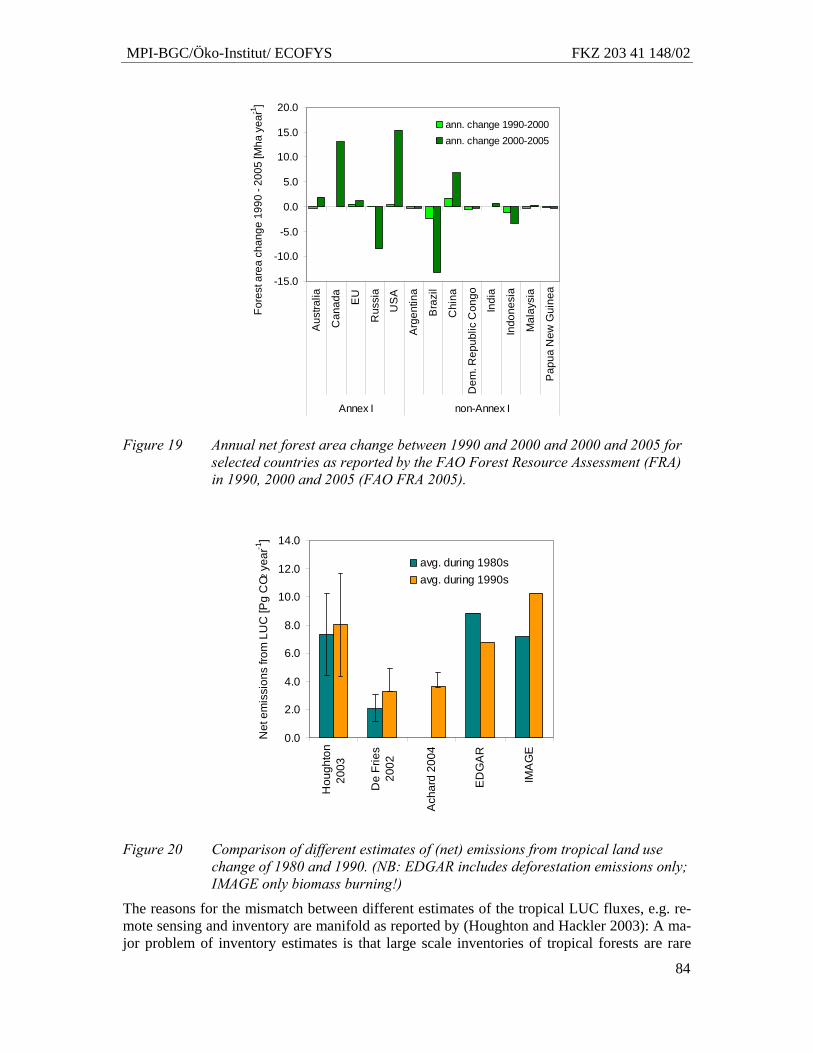
MPI-BGC/Öko-Institut/ ECOFYS FKZ 203 41 148/02
84
-15.0
-10.0
-5.0
0.0
5.0
10.0
15.0
20.0
Aus
tralia
Can
ada
EU
Rus
sia
US
A
Arg
entin
a
Bra
zil
Chi
na
Dem
. Rep
ublic
Con
go
Indi
a
Indo
nesi
a
Mal
aysi
a
Pap
ua N
ew G
uine
a
Annex I non-Annex I
Fore
st a
rea
chan
ge 1
990
- 200
5 [M
ha y
ear-1
]
ann. change 1990-2000ann. change 2000-2005
Figure 19 Annual net forest area change between 1990 and 2000 and 2000 and 2005 for selected countries as reported by the FAO Forest Resource Assessment (FRA) in 1990, 2000 and 2005 (FAO FRA 2005).
0.0
2.0
4.0
6.0
8.0
10.0
12.0
14.0
Hou
ghto
n20
03
De
Frie
s20
02
Ach
ard
2004
ED
GA
R
IMA
GE
Net
em
issi
ons
from
LU
C [P
g C
O2 y
ear-1
]
avg. during 1980savg. during 1990s
Figure 20 Comparison of different estimates of (net) emissions from tropical land use change of 1980 and 1990. (NB: EDGAR includes deforestation emissions only; IMAGE only biomass burning!)
The reasons for the mismatch between different estimates of the tropical LUC fluxes, e.g. re-mote sensing and inventory are manifold as reported by (Houghton and Hackler 2003): A ma-jor problem of inventory estimates is that large scale inventories of tropical forests are rare
MPI-BGC/Öko-Institut/ ECOFYS FKZ 203 41 148/02
85
and accompanied with higher errors. High uncertainties in the estimation of forest biomass lead to errors in both estimates, especially in those that use average biomass values for large regions.
Although satellites have observed tropical deforestation since three decades, many important activities influencing the regional carbon balance were still invisible for the sensors. Not until the recent development of high-resolution remote sensing analyses (Foley, DeFries et al. 2005) selective logging within and slowly progressing degradation of forest can be included in the tropical carbon budget. Processes of degradation may, according to (Houghton and Hackler 2003), have two effects (a and b) on the estimates: forest degradation and selective logging a) release carbon additional to carbon losses of extended deforestation observed and b) reduce of the biomass in existing forests, leading to lower emissions when those forest get deforested.
According to (Houghton and Hackler 2003) there are two major, mutually exclusive, explana-tions for the different appearances of the net terrestrial source of carbon from the tropics. One suggests that a large efflux of carbon from land-use change is partially offset by a large sink triggered by forest. The other explanation proposes that the source from deforestation is smaller (favoring remote sensing estimates) and that the net flux from intact forests is nearly zero. The first explanation implies that growth enhancement creates a large current sink in undisturbed forests. The second explanation claims that nearly the entire net flux of carbon is caused by changes in land use and would indicate the source from land-use change being smaller than estimated by (Houghton and Hackler 2003). So far there is no clear evidence for neither the first explanation (enhanced growth, e.g. by CO2 and nitrogen fertilization in the northern hemisphere and intact tropical forests) nor the second (lower emissions from land use change).
Inverse model calculations based on atmospheric CO2 as well as O2 measurements are used to evaluate the global carbon balance (Keeling, Chin et al. 1996), as e.g. in the third IPCC report (IPCC 2001). There are still quantitative mismatches between atmospheric inversion model estimates and inventory estimates. Some authors suggest that carbon fluxes to soils (often not accounted for in inventories), and into non-forest vegetation, may account for some of theses differences (e.g. (House, Prentice et al. 2003). Still, uncertainties associated with both bottom up (inventories) and top down (inverse modeling) approaches are large. The determination of more exact estimates of emissions and removals from land use change and a reduction of ma-jor uncertainties by more systematic and more spatially explicit analyses would constrain global carbon fluxes and help to determine other terms of the global carbon budget.
6.3 Material and Methods
The conversion of managed land to forest land by afforestation/reforestation and reforestation involves a change in land use. In the following calculations we will only consider directly human-induced regeneration and plantation of forests. According to IPCC GPG LULUCF (3.2.2) lands converted to forest land shall be followed in conversion status for 20 years. After 20 years the areas are accounted for under Forest land Remaining Forest land (IPCC 2003). However, the IPCC Guidelines allow an accounting for 100 years under Land converted to Forest land if necessary to monitor long term carbon dynamics in biomass, soil and litter pools. The computational separation of both categories (Forest land Remaining Forest land and Land converted to Forest land) over time facilitates the application of two modeling ap-proaches for each category. To project emissions and removals from Forest Management we
MPI-BGC/Öko-Institut/ ECOFYS FKZ 203 41 148/02
86
use an empirical forestry model that considers forest age class structure, aggregated forest management types and allows for additional forest management activities like thinning (cf. Chapter 10).
The projection of emissions and removals from land use change will be split into two time-frames: a FAO data projection covering the period of 2005-2020 and a model estimate for long-term developments until 2100. In the latter we will refer to projection 2020 and projec-tion 2100, respectively.
6.3.1 FAO data projection until 2020
FAO has been coordinating global forest resources assessments every five to ten years since 1946 (FAO website). Information from 229 countries and territories has been compiled for three points in time: 1990, 2000 and 2005. Among other variables the FAO database contains data on forest extent separated for the land use types natural forest and plantation.
We thus follow the FAO definition of natural forests (the latter referred to as forests) which compose of tree species known to be indigenous to the area and plantation forests (plantation) which are established artificially by afforestation on lands which previously did not carry for-est within living memory or involving the replacement of the indigenous species by a new and essentially different species or genetic variety.
We used the reported data on forest and plantation cover to derive annual net forest and plan-tation cover change rates by comparing the values of 2000 and 2005. The rates were extrapo-lated by country and land use type as fraction of existing forest or plantation cover until 2020. The algorithm leads to continuously increasing positive rates (as plantation cover in most countries) and continuously decreasing negative rates (e.g. forest cover in tropical countries).
To obtain data of emissions from deforested areas and removals from afforested/reforested land, the area was multiplied with IPCC LULUCF GPG default values. To estimate annual removals during a certain Commitment Period from afforestation/reforestation we used Equation 1, if plantation or forest area change was positive. We assumed an average global rotation time of plantations of 20 years. Assuming a linear constant growth rate and constant losses the average biomass of a plantation would accumulate over 10 years. Starting from 1990 we summed up the afforested area being younger than 10 years (AreaAffAccumu-lated10). AreaAffAccumulated10 in ha was multiplied with default values for annual average aboveground biomass increment in plantations (IPCC 2003); Table 3A.1.6) and a default fac-tor c of 1.833 to convert biomass into CO2.
Equation 1
Annual Removals during CP = AreaAffAccumulated10 * Increment * c
Increment values were chosen regionally and averaged over species. For extra-tropical region natural regeneration increment data was used (Table 3A.1.5, IPCC 2003). Forest area increase in these regions is mostly through natural regeneration or afforestation with indigenous spe-cies. A list of all region specific increment factors is given in Table 7.
Negative rates of forest and plantation area change were used to estimate emissions from de-forestation using Equation 2.
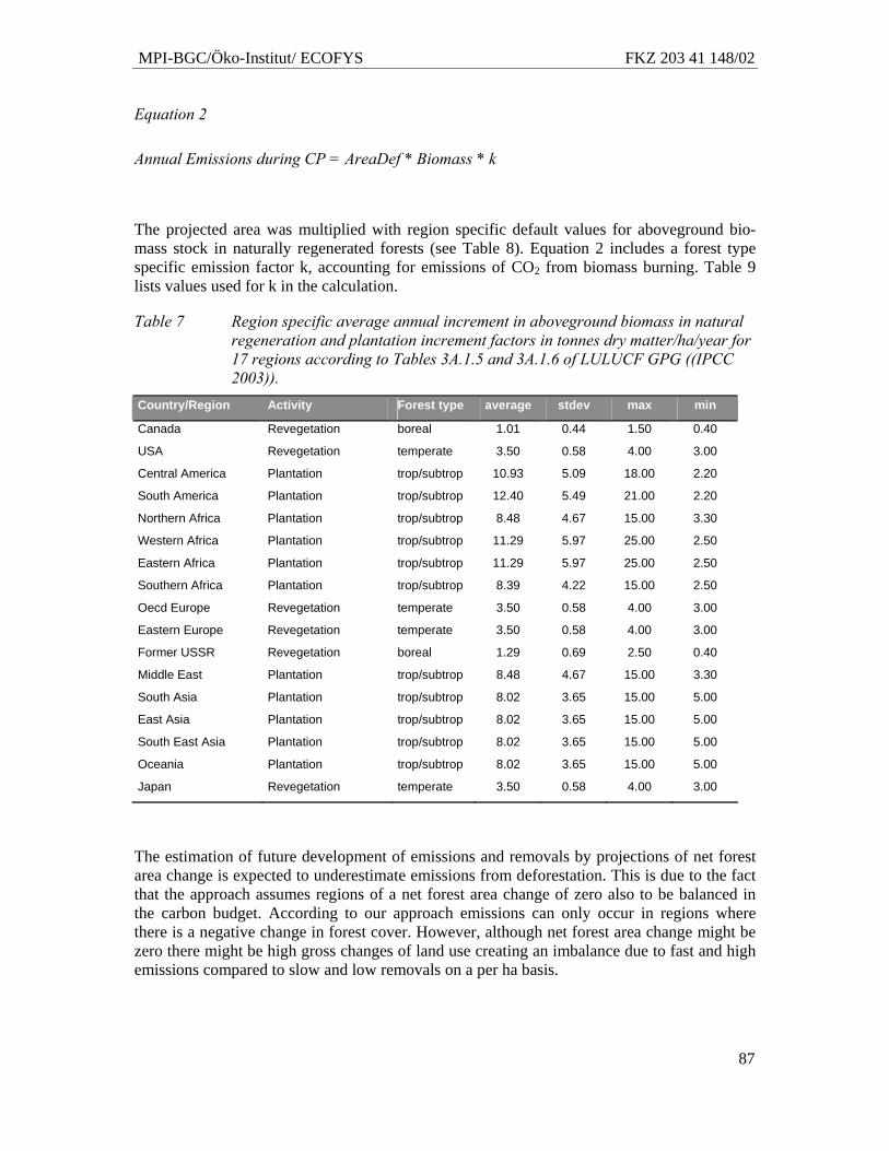
MPI-BGC/Öko-Institut/ ECOFYS FKZ 203 41 148/02
87
Equation 2
Annual Emissions during CP = AreaDef * Biomass * k
The projected area was multiplied with region specific default values for aboveground bio-mass stock in naturally regenerated forests (see Table 8). Equation 2 includes a forest type specific emission factor k, accounting for emissions of CO2 from biomass burning. Table 9 lists values used for k in the calculation.
Table 7 Region specific average annual increment in aboveground biomass in natural regeneration and plantation increment factors in tonnes dry matter/ha/year for 17 regions according to Tables 3A.1.5 and 3A.1.6 of LULUCF GPG ((IPCC 2003)).
Country/Region Activity Forest type average stdev max min
Canada Revegetation boreal 1.01 0.44 1.50 0.40
USA Revegetation temperate 3.50 0.58 4.00 3.00
Central America Plantation trop/subtrop 10.93 5.09 18.00 2.20
South America Plantation trop/subtrop 12.40 5.49 21.00 2.20
Northern Africa Plantation trop/subtrop 8.48 4.67 15.00 3.30
Western Africa Plantation trop/subtrop 11.29 5.97 25.00 2.50
Eastern Africa Plantation trop/subtrop 11.29 5.97 25.00 2.50
Southern Africa Plantation trop/subtrop 8.39 4.22 15.00 2.50
Oecd Europe Revegetation temperate 3.50 0.58 4.00 3.00
Eastern Europe Revegetation temperate 3.50 0.58 4.00 3.00
Former USSR Revegetation boreal 1.29 0.69 2.50 0.40
Middle East Plantation trop/subtrop 8.48 4.67 15.00 3.30
South Asia Plantation trop/subtrop 8.02 3.65 15.00 5.00
East Asia Plantation trop/subtrop 8.02 3.65 15.00 5.00
South East Asia Plantation trop/subtrop 8.02 3.65 15.00 5.00
Oceania Plantation trop/subtrop 8.02 3.65 15.00 5.00
Japan Revegetation temperate 3.50 0.58 4.00 3.00
The estimation of future development of emissions and removals by projections of net forest area change is expected to underestimate emissions from deforestation. This is due to the fact that the approach assumes regions of a net forest area change of zero also to be balanced in the carbon budget. According to our approach emissions can only occur in regions where there is a negative change in forest cover. However, although net forest area change might be zero there might be high gross changes of land use creating an imbalance due to fast and high emissions compared to slow and low removals on a per ha basis.
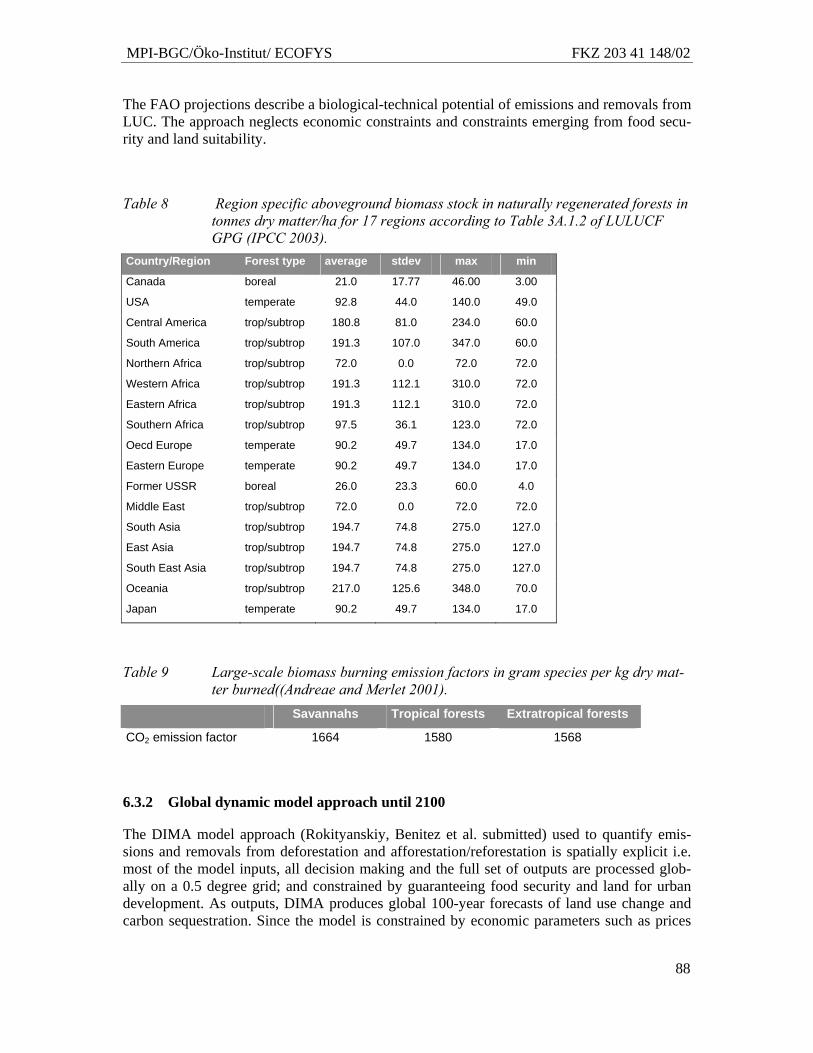
MPI-BGC/Öko-Institut/ ECOFYS FKZ 203 41 148/02
88
The FAO projections describe a biological-technical potential of emissions and removals from LUC. The approach neglects economic constraints and constraints emerging from food secu-rity and land suitability.
Table 8 Region specific aboveground biomass stock in naturally regenerated forests in tonnes dry matter/ha for 17 regions according to Table 3A.1.2 of LULUCF GPG (IPCC 2003).
Country/Region Forest type average stdev max min
Canada boreal 21.0 17.77 46.00 3.00
USA temperate 92.8 44.0 140.0 49.0
Central America trop/subtrop 180.8 81.0 234.0 60.0
South America trop/subtrop 191.3 107.0 347.0 60.0
Northern Africa trop/subtrop 72.0 0.0 72.0 72.0
Western Africa trop/subtrop 191.3 112.1 310.0 72.0
Eastern Africa trop/subtrop 191.3 112.1 310.0 72.0
Southern Africa trop/subtrop 97.5 36.1 123.0 72.0
Oecd Europe temperate 90.2 49.7 134.0 17.0
Eastern Europe temperate 90.2 49.7 134.0 17.0
Former USSR boreal 26.0 23.3 60.0 4.0
Middle East trop/subtrop 72.0 0.0 72.0 72.0
South Asia trop/subtrop 194.7 74.8 275.0 127.0
East Asia trop/subtrop 194.7 74.8 275.0 127.0
South East Asia trop/subtrop 194.7 74.8 275.0 127.0
Oceania trop/subtrop 217.0 125.6 348.0 70.0
Japan temperate 90.2 49.7 134.0 17.0
Table 9 Large-scale biomass burning emission factors in gram species per kg dry mat-ter burned((Andreae and Merlet 2001).
Savannahs Tropical forests Extratropical forests
CO2 emission factor 1664 1580 1568
6.3.2 Global dynamic model approach until 2100
The DIMA model approach (Rokityanskiy, Benitez et al. submitted) used to quantify emis-sions and removals from deforestation and afforestation/reforestation is spatially explicit i.e. most of the model inputs, all decision making and the full set of outputs are processed glob-ally on a 0.5 degree grid; and constrained by guaranteeing food security and land for urban development. As outputs, DIMA produces global 100-year forecasts of land use change and carbon sequestration. Since the model is constrained by economic parameters such as prices
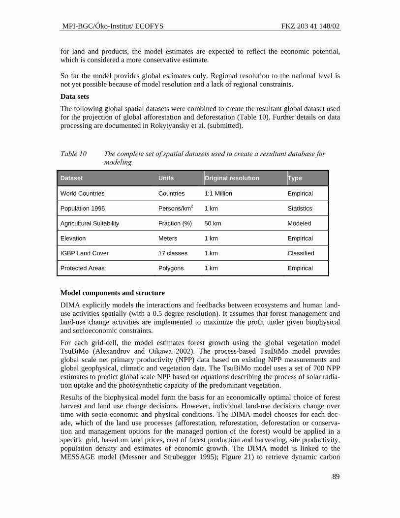
MPI-BGC/Öko-Institut/ ECOFYS FKZ 203 41 148/02
89
for land and products, the model estimates are expected to reflect the economic potential, which is considered a more conservative estimate.
So far the model provides global estimates only. Regional resolution to the national level is not yet possible because of model resolution and a lack of regional constraints.
Data sets
The following global spatial datasets were combined to create the resultant global dataset used for the projection of global afforestation and deforestation (Table 10). Further details on data processing are documented in Rokytyansky et al. (submitted).
Table 10 The complete set of spatial datasets used to create a resultant database for modeling.
Dataset Units Original resolution Type
World Countries Countries 1:1 Million Empirical
Population 1995 Persons/km2 1 km Statistics
Agricultural Suitability Fraction (%) 50 km Modeled
Elevation Meters 1 km Empirical
IGBP Land Cover 17 classes 1 km Classified
Protected Areas Polygons 1 km Empirical
Model components and structure
DIMA explicitly models the interactions and feedbacks between ecosystems and human land-use activities spatially (with a 0.5 degree resolution). It assumes that forest management and land-use change activities are implemented to maximize the profit under given biophysical and socioeconomic constraints.
For each grid-cell, the model estimates forest growth using the global vegetation model TsuBiMo (Alexandrov and Oikawa 2002). The process-based TsuBiMo model provides global scale net primary productivity (NPP) data based on existing NPP measurements and global geophysical, climatic and vegetation data. The TsuBiMo model uses a set of 700 NPP estimates to predict global scale NPP based on equations describing the process of solar radia-tion uptake and the photosynthetic capacity of the predominant vegetation.
Results of the biophysical model form the basis for an economically optimal choice of forest harvest and land use change decisions. However, individual land-use decisions change over time with socio-economic and physical conditions. The DIMA model chooses for each dec-ade, which of the land use processes (afforestation, reforestation, deforestation or conserva-tion and management options for the managed portion of the forest) would be applied in a specific grid, based on land prices, cost of forest production and harvesting, site productivity, population density and estimates of economic growth. The DIMA model is linked to the MESSAGE model (Messner and Strubegger 1995); Figure 21) to retrieve dynamic carbon
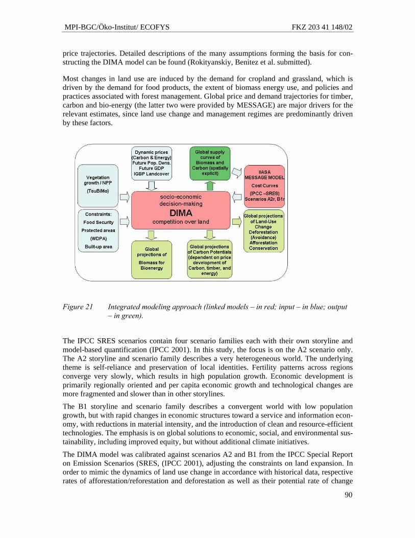
MPI-BGC/Öko-Institut/ ECOFYS FKZ 203 41 148/02
90
price trajectories. Detailed descriptions of the many assumptions forming the basis for con-structing the DIMA model can be found (Rokityanskiy, Benitez et al. submitted).
Most changes in land use are induced by the demand for cropland and grassland, which is driven by the demand for food products, the extent of biomass energy use, and policies and practices associated with forest management. Global price and demand trajectories for timber, carbon and bio-energy (the latter two were provided by MESSAGE) are major drivers for the relevant estimates, since land use change and management regimes are predominantly driven by these factors.
Figure 21 Integrated modeling approach (linked models – in red; input – in blue; output – in green).
The IPCC SRES scenarios contain four scenario families each with their own storyline and model-based quantification (IPCC 2001). In this study, the focus is on the A2 scenario only. The A2 storyline and scenario family describes a very heterogeneous world. The underlying theme is self-reliance and preservation of local identities. Fertility patterns across regions converge very slowly, which results in high population growth. Economic development is primarily regionally oriented and per capita economic growth and technological changes are more fragmented and slower than in other storylines.
The B1 storyline and scenario family describes a convergent world with low population growth, but with rapid changes in economic structures toward a service and information econ-omy, with reductions in material intensity, and the introduction of clean and resource-efficient technologies. The emphasis is on global solutions to economic, social, and environmental sus-tainability, including improved equity, but without additional climate initiatives.
The DIMA model was calibrated against scenarios A2 and B1 from the IPCC Special Report on Emission Scenarios (SRES, (IPCC 2001), adjusting the constraints on land expansion. In order to mimic the dynamics of land use change in accordance with historical data, respective rates of afforestation/reforestation and deforestation as well as their potential rate of change
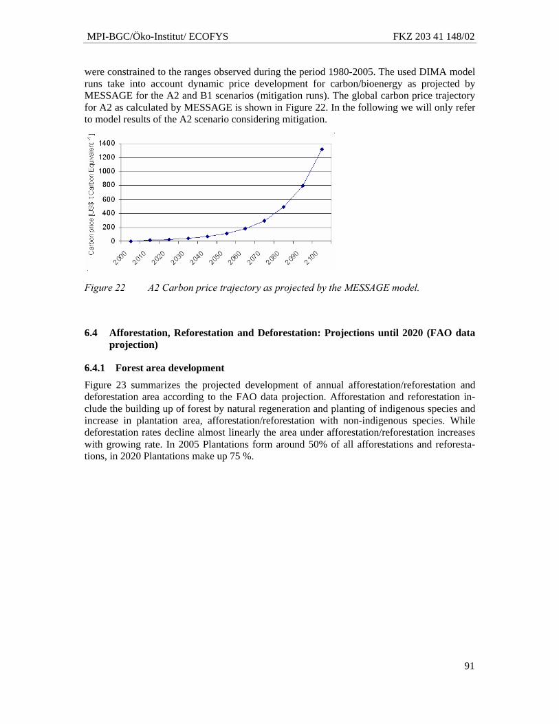
MPI-BGC/Öko-Institut/ ECOFYS FKZ 203 41 148/02
91
were constrained to the ranges observed during the period 1980-2005. The used DIMA model runs take into account dynamic price development for carbon/bioenergy as projected by MESSAGE for the A2 and B1 scenarios (mitigation runs). The global carbon price trajectory for A2 as calculated by MESSAGE is shown in Figure 22. In the following we will only refer to model results of the A2 scenario considering mitigation.
Figure 22 A2 Carbon price trajectory as projected by the MESSAGE model.
6.4 Afforestation, Reforestation and Deforestation: Projections until 2020 (FAO data projection)
6.4.1 Forest area development
Figure 23 summarizes the projected development of annual afforestation/reforestation and deforestation area according to the FAO data projection. Afforestation and reforestation in-clude the building up of forest by natural regeneration and planting of indigenous species and increase in plantation area, afforestation/reforestation with non-indigenous species. While deforestation rates decline almost linearly the area under afforestation/reforestation increases with growing rate. In 2005 Plantations form around 50% of all afforestations and reforesta-tions, in 2020 Plantations make up 75 %.
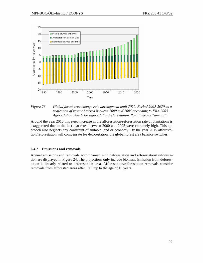
MPI-BGC/Öko-Institut/ ECOFYS FKZ 203 41 148/02
92
Figure 23 Global forest area change rate development until 2020. Period 2005-2020 as a projection of rates observed between 2000 and 2005 according to FRA 2005. Afforestation stands for afforestation/reforestation, “ann” means “annual”.
Around the year 2015 this steep increase in the afforestation/reforestation rate of plantations is exaggerated due to the fact that rates between 2000 and 2005 were extremely high. This ap-proach also neglects any constraint of suitable land or economy. By the year 2015 afforesta-tion/reforestation will compensate for deforestation, the global forest area balance switches.
6.4.2 Emissions and removals
Annual emissions and removals accompanied with deforestation and afforestation/ reforesta-tion are displayed in Figure 24. The projections only include biomass. Emission from defores-tation is linearly related to deforestation area. Afforestation/reforestation removals consider removals from afforested areas after 1990 up to the age of 10 years.
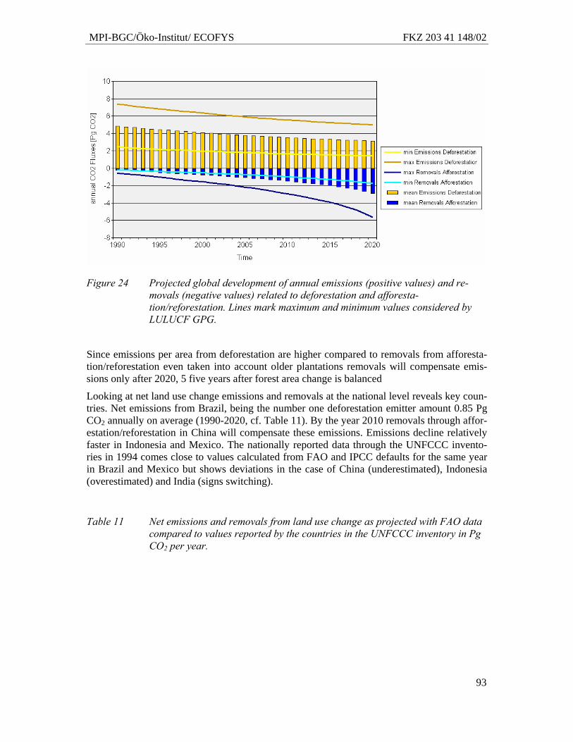
MPI-BGC/Öko-Institut/ ECOFYS FKZ 203 41 148/02
93
Figure 24 Projected global development of annual emissions (positive values) and re-movals (negative values) related to deforestation and afforesta-tion/reforestation. Lines mark maximum and minimum values considered by LULUCF GPG.
Since emissions per area from deforestation are higher compared to removals from afforesta-tion/reforestation even taken into account older plantations removals will compensate emis-sions only after 2020, 5 five years after forest area change is balanced
Looking at net land use change emissions and removals at the national level reveals key coun-tries. Net emissions from Brazil, being the number one deforestation emitter amount 0.85 Pg CO2 annually on average (1990-2020, cf. Table 11). By the year 2010 removals through affor-estation/reforestation in China will compensate these emissions. Emissions decline relatively faster in Indonesia and Mexico. The nationally reported data through the UNFCCC invento-ries in 1994 comes close to values calculated from FAO and IPCC defaults for the same year in Brazil and Mexico but shows deviations in the case of China (underestimated), Indonesia (overestimated) and India (signs switching).
Table 11 Net emissions and removals from land use change as projected with FAO data compared to values reported by the countries in the UNFCCC inventory in Pg CO2 per year.
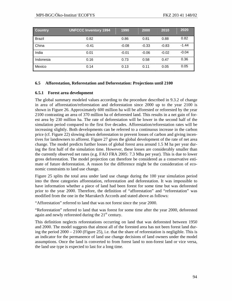
MPI-BGC/Öko-Institut/ ECOFYS FKZ 203 41 148/02
94
Country UNFCCC Inventory 1994 1990 2000 2010 2020
Brazil 0.82 0.86 0.81 0.88 0.82
China -0.41 -0.08 -0.33 -0.83 -1.44
India 0.01 -0.01 -0.06 -0.02 -0.04
Indonesia 0.16 0.73 0.58 0.47 0.36
Mexico 0.14 0.13 0.11 0.05 0.05
6.5 Afforestation, Reforestation and Deforestation: Projections until 2100
6.5.1 Forest area development
The global summary modeled values according to the procedure described in 9.3.2 of change in area of afforestation/reforestation and deforestation since 2000 up to the year 2100 is shown in Figure 26. Approximately 600 million ha will be afforested or reforested by the year 2100 contrasting an area of 370 million ha of deforested land. This results in a net gain of for-est area by 230 million ha. The rate of deforestation will be lower in the second half of the simulation period compared to the first five decades. Afforestation/reforestation rates will be increasing slightly. Both developments can be referred to a continuous increase in the carbon price (cf. Figure 22) slowing down deforestation to prevent losses of carbon and giving incen-tives for landowners to afforest. Figure 27 gives the global development of the rate of net area change. The model predicts further losses of global forest area around 1.5 M ha per year dur-ing the first half of the simulation time. However, these losses are considerably smaller than the currently observed net rates (e.g. FAO FRA 2005: 7.3 Mha per year). This is due to lower gross deforestation. The model projection can therefore be considered as a conservative esti-mate of future deforestation. A reason for the difference might be the consideration of eco-nomic constraints to land use change.
Figure 25 splits the total area under land use change during the 100 year simulation period into the three categories afforestation, reforestation and deforestation. It was impossible to have information whether a piece of land had been forest for some time but was deforested prior to the year 2000. Therefore, the definition of “afforestation” and “reforestation” was modified from the one in the Marrakech Accords and stated above as follows:
“Afforestation” referred to land that was not forest since the year 2000.
“Reforestation” referred to land that was forest for some time after the year 2000, deforested again and newly reforested during the 21st century.
This definition neglects reforestations occurring on land that was deforested between 1950 and 2000. The model suggests that almost all of the forested area has not been forest land dur-ing the period 2000 – 2100 (Figure 25), i.e. that the share of reforestation is negligible. This is an indicator for the permanence of land use change decisions of land owners under the model assumptions. Once the land is converted to from forest land to non-forest land or vice versa, the land use type is expected to last for a long time.
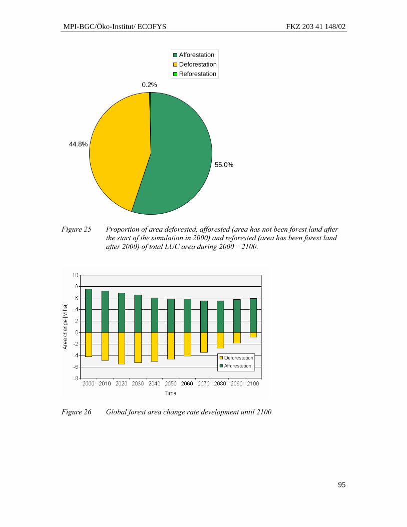
MPI-BGC/Öko-Institut/ ECOFYS FKZ 203 41 148/02
95
55.0%
44.8%
0.2%
AfforestationDeforestationReforestation
Figure 25 Proportion of area deforested, afforested (area has not been forest land after the start of the simulation in 2000) and reforested (area has been forest land after 2000) of total LUC area during 2000 – 2100.
Figure 26 Global forest area change rate development until 2100.
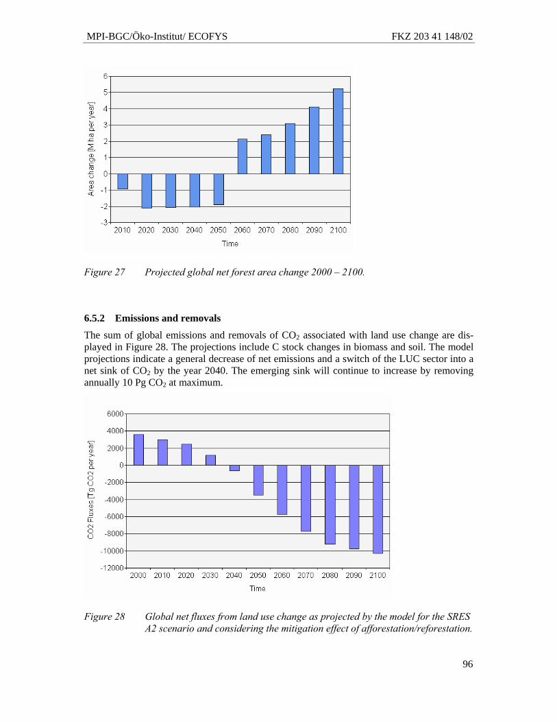
MPI-BGC/Öko-Institut/ ECOFYS FKZ 203 41 148/02
96
Figure 27 Projected global net forest area change 2000 – 2100.
6.5.2 Emissions and removals
The sum of global emissions and removals of CO2 associated with land use change are dis-played in Figure 28. The projections include C stock changes in biomass and soil. The model projections indicate a general decrease of net emissions and a switch of the LUC sector into a net sink of CO2 by the year 2040. The emerging sink will continue to increase by removing annually 10 Pg CO2 at maximum.
Figure 28 Global net fluxes from land use change as projected by the model for the SRES A2 scenario and considering the mitigation effect of afforestation/reforestation.
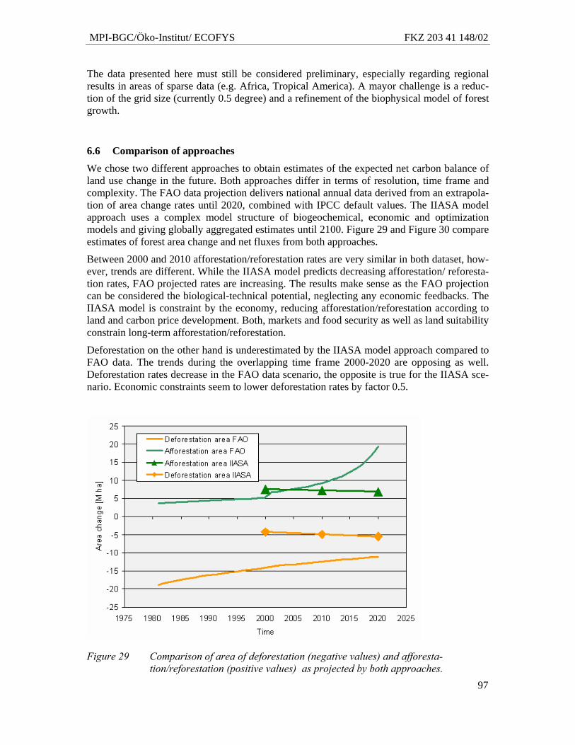
MPI-BGC/Öko-Institut/ ECOFYS FKZ 203 41 148/02
97
The data presented here must still be considered preliminary, especially regarding regional results in areas of sparse data (e.g. Africa, Tropical America). A mayor challenge is a reduc-tion of the grid size (currently 0.5 degree) and a refinement of the biophysical model of forest growth.
6.6 Comparison of approaches
We chose two different approaches to obtain estimates of the expected net carbon balance of land use change in the future. Both approaches differ in terms of resolution, time frame and complexity. The FAO data projection delivers national annual data derived from an extrapola-tion of area change rates until 2020, combined with IPCC default values. The IIASA model approach uses a complex model structure of biogeochemical, economic and optimization models and giving globally aggregated estimates until 2100. Figure 29 and Figure 30 compare estimates of forest area change and net fluxes from both approaches.
Between 2000 and 2010 afforestation/reforestation rates are very similar in both dataset, how-ever, trends are different. While the IIASA model predicts decreasing afforestation/ reforesta-tion rates, FAO projected rates are increasing. The results make sense as the FAO projection can be considered the biological-technical potential, neglecting any economic feedbacks. The IIASA model is constraint by the economy, reducing afforestation/reforestation according to land and carbon price development. Both, markets and food security as well as land suitability constrain long-term afforestation/reforestation.
Deforestation on the other hand is underestimated by the IIASA model approach compared to FAO data. The trends during the overlapping time frame 2000-2020 are opposing as well. Deforestation rates decrease in the FAO data scenario, the opposite is true for the IIASA sce-nario. Economic constraints seem to lower deforestation rates by factor 0.5.
Figure 29 Comparison of area of deforestation (negative values) and afforesta-tion/reforestation (positive values) as projected by both approaches.
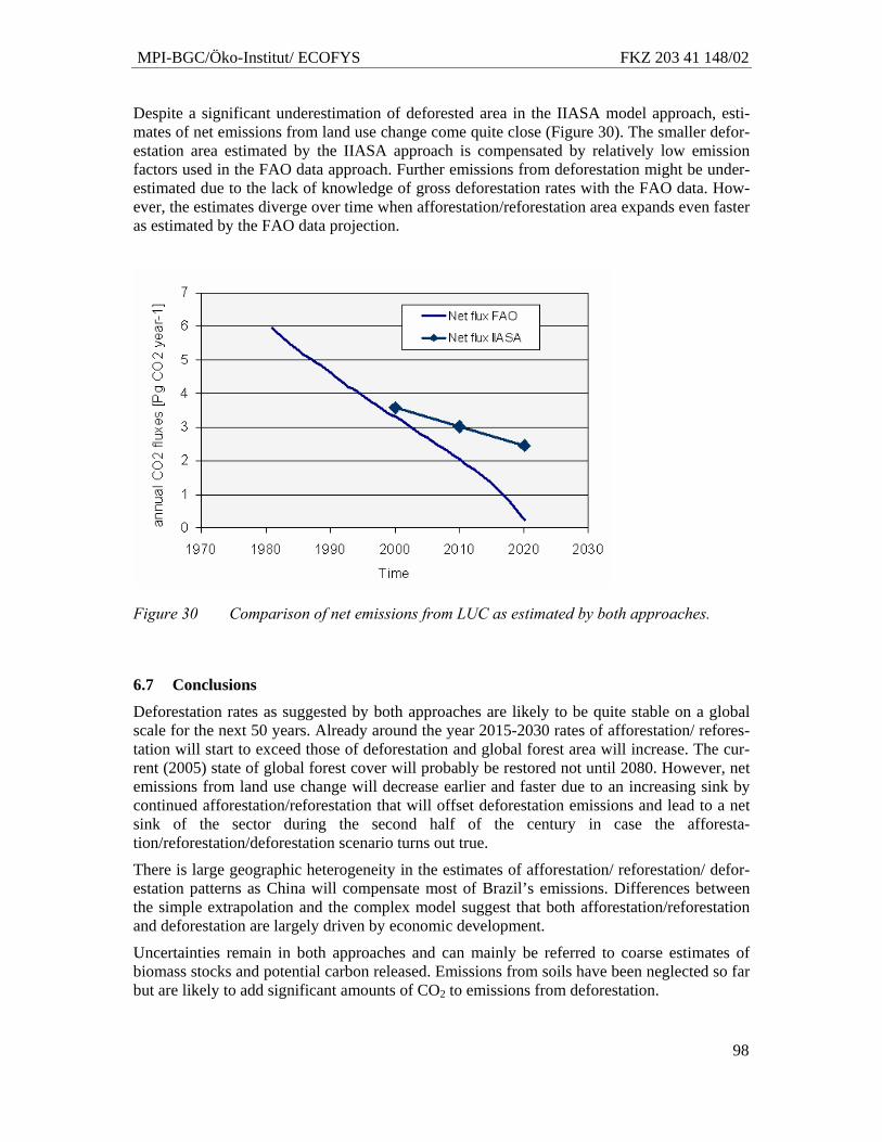
MPI-BGC/Öko-Institut/ ECOFYS FKZ 203 41 148/02
98
Despite a significant underestimation of deforested area in the IIASA model approach, esti-mates of net emissions from land use change come quite close (Figure 30). The smaller defor-estation area estimated by the IIASA approach is compensated by relatively low emission factors used in the FAO data approach. Further emissions from deforestation might be under-estimated due to the lack of knowledge of gross deforestation rates with the FAO data. How-ever, the estimates diverge over time when afforestation/reforestation area expands even faster as estimated by the FAO data projection.
Figure 30 Comparison of net emissions from LUC as estimated by both approaches.
6.7 Conclusions
Deforestation rates as suggested by both approaches are likely to be quite stable on a global scale for the next 50 years. Already around the year 2015-2030 rates of afforestation/ refores-tation will start to exceed those of deforestation and global forest area will increase. The cur-rent (2005) state of global forest cover will probably be restored not until 2080. However, net emissions from land use change will decrease earlier and faster due to an increasing sink by continued afforestation/reforestation that will offset deforestation emissions and lead to a net sink of the sector during the second half of the century in case the afforesta-tion/reforestation/deforestation scenario turns out true.
There is large geographic heterogeneity in the estimates of afforestation/ reforestation/ defor-estation patterns as China will compensate most of Brazil’s emissions. Differences between the simple extrapolation and the complex model suggest that both afforestation/reforestation and deforestation are largely driven by economic development.
Uncertainties remain in both approaches and can mainly be referred to coarse estimates of biomass stocks and potential carbon released. Emissions from soils have been neglected so far but are likely to add significant amounts of CO2 to emissions from deforestation.
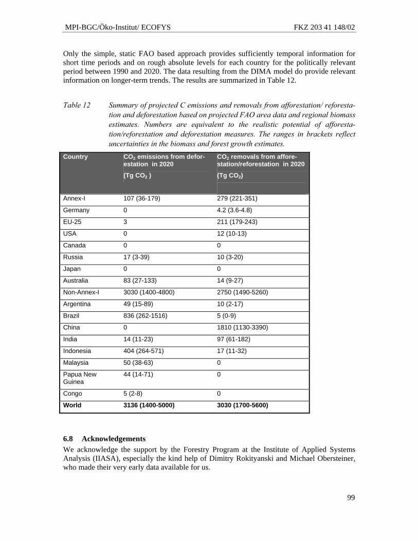
MPI-BGC/Öko-Institut/ ECOFYS FKZ 203 41 148/02
99
Only the simple, static FAO based approach provides sufficiently temporal information for short time periods and on rough absolute levels for each country for the politically relevant period between 1990 and 2020. The data resulting from the DIMA model do provide relevant information on longer-term trends. The results are summarized in Table 12.
Table 12 Summary of projected C emissions and removals from afforestation/ reforesta-tion and deforestation based on projected FAO area data and regional biomass estimates. Numbers are equivalent to the realistic potential of afforesta-tion/reforestation and deforestation measures. The ranges in brackets reflect uncertainties in the biomass and forest growth estimates.
Country CO2 emissions from defor-estation in 2020
(Tg CO2 )
CO2 removals from affore-station/reforestation in 2020
(Tg CO2)
Annex-I 107 (36-179) 279 (221-351)
Germany 0 4.2 (3.6-4.8)
EU-25 3 211 (179-243)
USA 0 12 (10-13)
Canada 0 0
Russia 17 (3-39) 10 (3-20)
Japan 0 0
Australia 83 (27-133) 14 (9-27)
Non-Annex-I 3030 (1400-4800) 2750 (1490-5260)
Argentina 49 (15-89) 10 (2-17)
Brazil 836 (262-1516) 5 (0-9)
China 0 1810 (1130-3390)
India 14 (11-23) 97 (61-182)
Indonesia 404 (264-571) 17 (11-32)
Malaysia 50 (38-63) 0
Papua New Guinea
44 (14-71) 0
Congo 5 (2-8) 0
World 3136 (1400-5000) 3030 (1700-5600)
6.8 Acknowledgements We acknowledge the support by the Forestry Program at the Institute of Applied Systems Analysis (IIASA), especially the kind help of Dimitry Rokityanski and Michael Obersteiner, who made their very early data available for us.
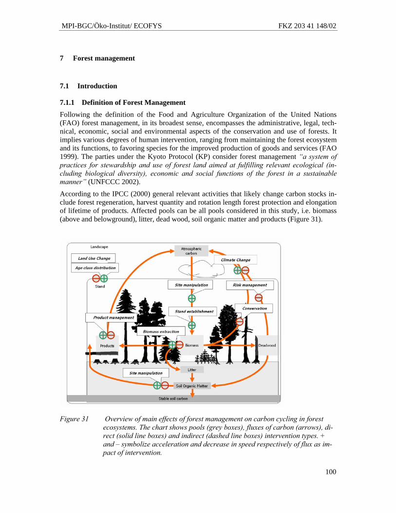
MPI-BGC/Öko-Institut/ ECOFYS FKZ 203 41 148/02
100
7 Forest management
7.1 Introduction
7.1.1 Definition of Forest Management
Following the definition of the Food and Agriculture Organization of the United Nations (FAO) forest management, in its broadest sense, encompasses the administrative, legal, tech-nical, economic, social and environmental aspects of the conservation and use of forests. It implies various degrees of human intervention, ranging from maintaining the forest ecosystem and its functions, to favoring species for the improved production of goods and services (FAO 1999). The parties under the Kyoto Protocol (KP) consider forest management “a system of practices for stewardship and use of forest land aimed at fulfilling relevant ecological (in-cluding biological diversity), economic and social functions of the forest in a sustainable manner” (UNFCCC 2002).
According to the IPCC (2000) general relevant activities that likely change carbon stocks in-clude forest regeneration, harvest quantity and rotation length forest protection and elongation of lifetime of products. Affected pools can be all pools considered in this study, i.e. biomass (above and belowground), litter, dead wood, soil organic matter and products (Figure 31).
Figure 31 Overview of main effects of forest management on carbon cycling in forest ecosystems. The chart shows pools (grey boxes), fluxes of carbon (arrows), di-rect (solid line boxes) and indirect (dashed line boxes) intervention types. + and – symbolize acceleration and decrease in speed respectively of flux as im-pact of intervention.
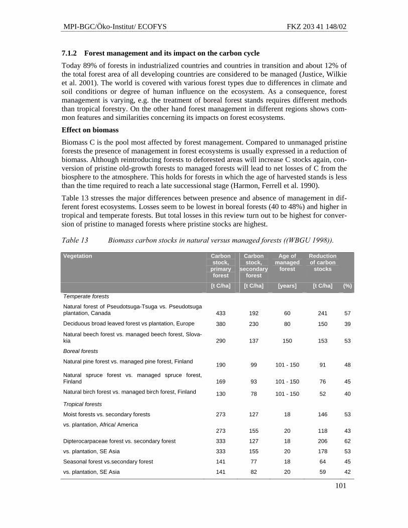
MPI-BGC/Öko-Institut/ ECOFYS FKZ 203 41 148/02
101
7.1.2 Forest management and its impact on the carbon cycle
Today 89% of forests in industrialized countries and countries in transition and about 12% of the total forest area of all developing countries are considered to be managed (Justice, Wilkie et al. 2001). The world is covered with various forest types due to differences in climate and soil conditions or degree of human influence on the ecosystem. As a consequence, forest management is varying, e.g. the treatment of boreal forest stands requires different methods than tropical forestry. On the other hand forest management in different regions shows com-mon features and similarities concerning its impacts on forest ecosystems.
Effect on biomass
Biomass C is the pool most affected by forest management. Compared to unmanaged pristine forests the presence of management in forest ecosystems is usually expressed in a reduction of biomass. Although reintroducing forests to deforested areas will increase C stocks again, con-version of pristine old-growth forests to managed forests will lead to net losses of C from the biosphere to the atmosphere. This holds for forests in which the age of harvested stands is less than the time required to reach a late successional stage (Harmon, Ferrell et al. 1990).
Table 13 stresses the major differences between presence and absence of management in dif-ferent forest ecosystems. Losses seem to be lowest in boreal forests (40 to 48%) and higher in tropical and temperate forests. But total losses in this review turn out to be highest for conver-sion of pristine to managed forests where pristine stocks are highest.
Table 13 Biomass carbon stocks in natural versus managed forests ((WBGU 1998)).
Vegetation Carbon stock,
primary forest
Carbon stock,
secondary forest
Age of managed
forest
Reduction of carbon
stocks
[t C/ha] [t C/ha] [years] [t C/ha] (%)
Temperate forests
Natural forest of Pseudotsuga-Tsuga vs. Pseudotsuga plantation, Canada 433 192 60 241 57
Deciduous broad leaved forest vs plantation, Europe 380 230 80 150 39
Natural beech forest vs. managed beech forest, Slova-kia 290 137 150 153 53
Boreal forests
Natural pine forest vs. managed pine forest, Finland 190 99 101 - 150 91 48
Natural spruce forest vs. managed spruce forest, Finland 169 93 101 - 150 76 45
Natural birch forest vs. managed birch forest, Finland 130 78 101 - 150 52 40
Tropical forests
Moist forests vs. secondary forests 273 127 18 146 53
vs. plantation, Africa/ America 273 155 20 118 43
Dipterocarpaceae forest vs. secondary forest 333 127 18 206 62
vs. plantation, SE Asia 333 155 20 178 53
Seasonal forest vs.secondary forest 141 77 18 64 45
vs. plantation, SE Asia 141 82 20 59 42
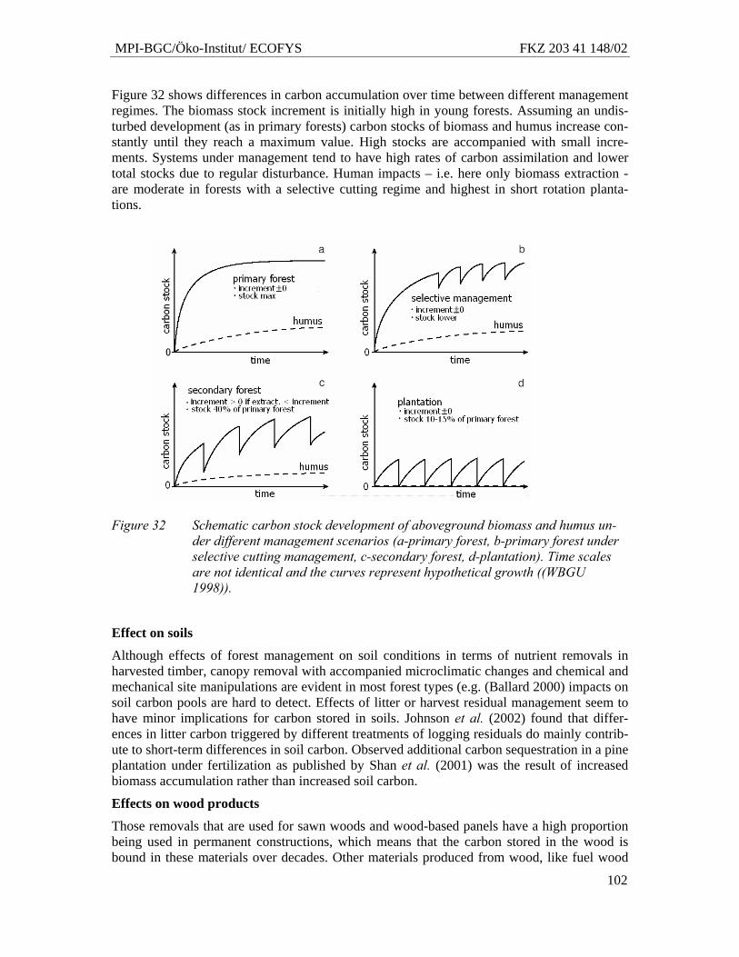
MPI-BGC/Öko-Institut/ ECOFYS FKZ 203 41 148/02
102
Figure 32 shows differences in carbon accumulation over time between different management regimes. The biomass stock increment is initially high in young forests. Assuming an undis-turbed development (as in primary forests) carbon stocks of biomass and humus increase con-stantly until they reach a maximum value. High stocks are accompanied with small incre-ments. Systems under management tend to have high rates of carbon assimilation and lower total stocks due to regular disturbance. Human impacts – i.e. here only biomass extraction - are moderate in forests with a selective cutting regime and highest in short rotation planta-tions.
Figure 32 Schematic carbon stock development of aboveground biomass and humus un-der different management scenarios (a-primary forest, b-primary forest under selective cutting management, c-secondary forest, d-plantation). Time scales are not identical and the curves represent hypothetical growth ((WBGU 1998)).
Effect on soils
Although effects of forest management on soil conditions in terms of nutrient removals in harvested timber, canopy removal with accompanied microclimatic changes and chemical and mechanical site manipulations are evident in most forest types (e.g. (Ballard 2000) impacts on soil carbon pools are hard to detect. Effects of litter or harvest residual management seem to have minor implications for carbon stored in soils. Johnson et al. (2002) found that differ-ences in litter carbon triggered by different treatments of logging residuals do mainly contrib-ute to short-term differences in soil carbon. Observed additional carbon sequestration in a pine plantation under fertilization as published by Shan et al. (2001) was the result of increased biomass accumulation rather than increased soil carbon.
Effects on wood products
Those removals that are used for sawn woods and wood-based panels have a high proportion being used in permanent constructions, which means that the carbon stored in the wood is bound in these materials over decades. Other materials produced from wood, like fuel wood
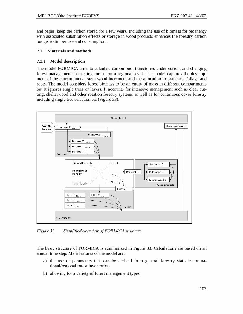
MPI-BGC/Öko-Institut/ ECOFYS FKZ 203 41 148/02
103
and paper, keep the carbon stored for a few years. Including the use of biomass for bioenergy with associated substitution effects or storage in wood products enhances the forestry carbon budget to timber use and consumption.
7.2 Materials and methods
7.2.1 Model description
The model FORMICA aims to calculate carbon pool trajectories under current and changing forest management in existing forests on a regional level. The model captures the develop-ment of the current annual stem wood increment and the allocation to branches, foliage and roots. The model considers forest biomass to be an entity of mass in different compartments but it ignores single trees or layers. It accounts for intensive management such as clear cut-ting, shelterwood and other rotation forestry systems as well as for continuous cover forestry including single tree selection etc (Figure 33).
Figure 33 Simplified overview of FORMICA structure.
The basic structure of FORMICA is summarized in Figure 33. Calculations are based on an annual time step. Main features of the model are:
a) the use of parameters that can be derived from general forestry statistics or na-tional/regional forest inventories,
b) allowing for a variety of forest management types,
MPI-BGC/Öko-Institut/ ECOFYS FKZ 203 41 148/02
104
c) the use of relative growth and allocation functions depending on accumulated stem biomass. This allows applications on a wide range of forest eco- and management sys-tems including uneven-aged, multilayered and natural forests. See Appendix 1 for a detailed model description.
7.2.2 Model parameters
The forestry model FORMICA (Böttcher, Freibauer et al. submitted) uses data from forest yield tables to parameterize forest growth (see Appendix 1). We used a collection of European yield tables (Federici, Quaratino et al. 2001) to parameterize forest growth of the forest types as provided by the forestry database (Schelhaas, Varis et al. 1999). For Canadian, US and Russian forests we derived growth curves from the forest inventories’ Net Annual Increment.
For allocation from stem volume to total biomass we applied a simple global relationship (Enquist and Niklas 2002) and converted total volume to total biomass by IPCC GPG LULUCF default values for wood densities (IPCC 2003).
Values for turnover of different biomass compartments, e.g. roots and leaves were taken from literature as well as parameters of litter quality that are required by the soil model applied (Liski, Palosuo et al. 2005). The soil model further requires average climate parameters as sum of precipitation in the growing season, average temperature during growing season and potential evapotranspiration. A complete list of parameters required to run the model is given in Table 14.
Table 14 List of model parameters to be specified.
Function Parameter
Pool initialization volume per age class
carbon in soil pool
carbon in product pool
Forest area per age class and forest type
Carbon content of wood and foliage
Wood density density of stem wood
Turnover rate of branches, foliage, roots and stem
Litter quality soluble
holocell
lignin-like
Allocation model parameters for branches, roots and foliage
Growth model forest growth modepl parameters a, b and c
max volume
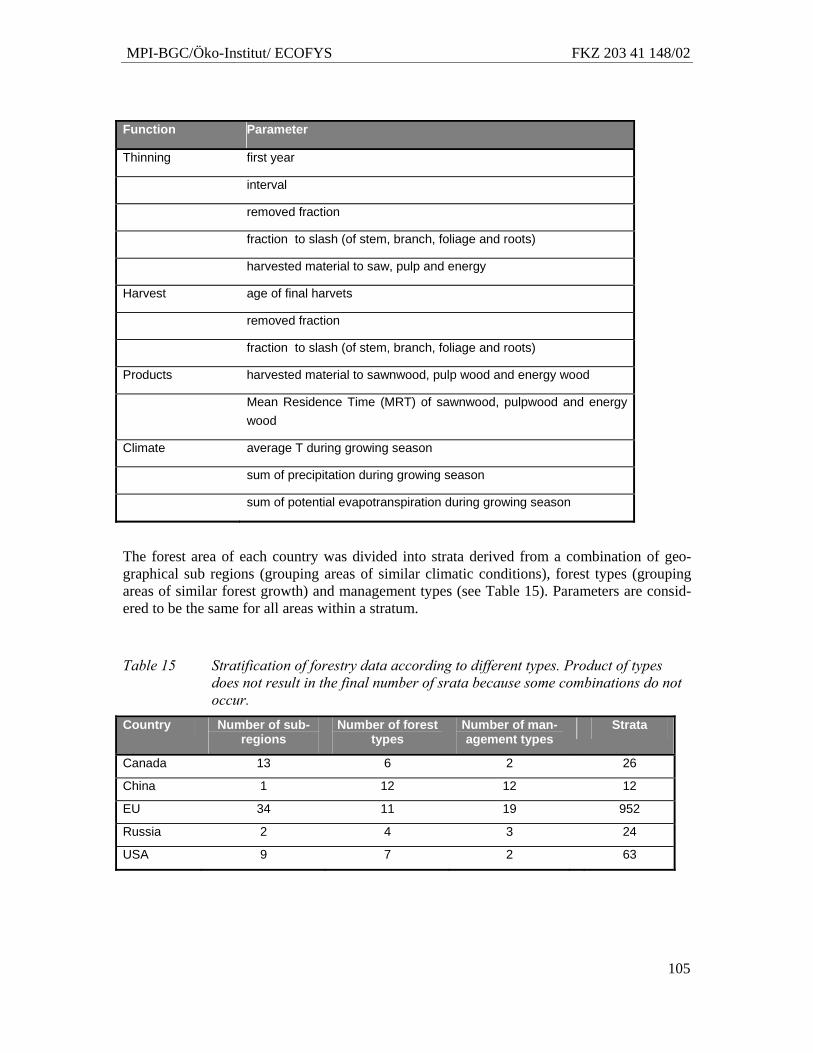
MPI-BGC/Öko-Institut/ ECOFYS FKZ 203 41 148/02
105
Function Parameter
Thinning first year
interval
removed fraction
fraction to slash (of stem, branch, foliage and roots)
harvested material to saw, pulp and energy
Harvest age of final harvets
removed fraction
fraction to slash (of stem, branch, foliage and roots)
Products harvested material to sawnwood, pulp wood and energy wood
Mean Residence Time (MRT) of sawnwood, pulpwood and energy wood
Climate average T during growing season
sum of precipitation during growing season
sum of potential evapotranspiration during growing season
The forest area of each country was divided into strata derived from a combination of geo-graphical sub regions (grouping areas of similar climatic conditions), forest types (grouping areas of similar forest growth) and management types (see Table 15). Parameters are consid-ered to be the same for all areas within a stratum.
Table 15 Stratification of forestry data according to different types. Product of types does not result in the final number of srata because some combinations do not occur.
Country Number of sub-regions
Number of forest types
Number of man-agement types
Strata
Canada 13 6 2 26
China 1 12 12 12
EU 34 11 19 952
Russia 2 4 3 24
USA 9 7 2 63
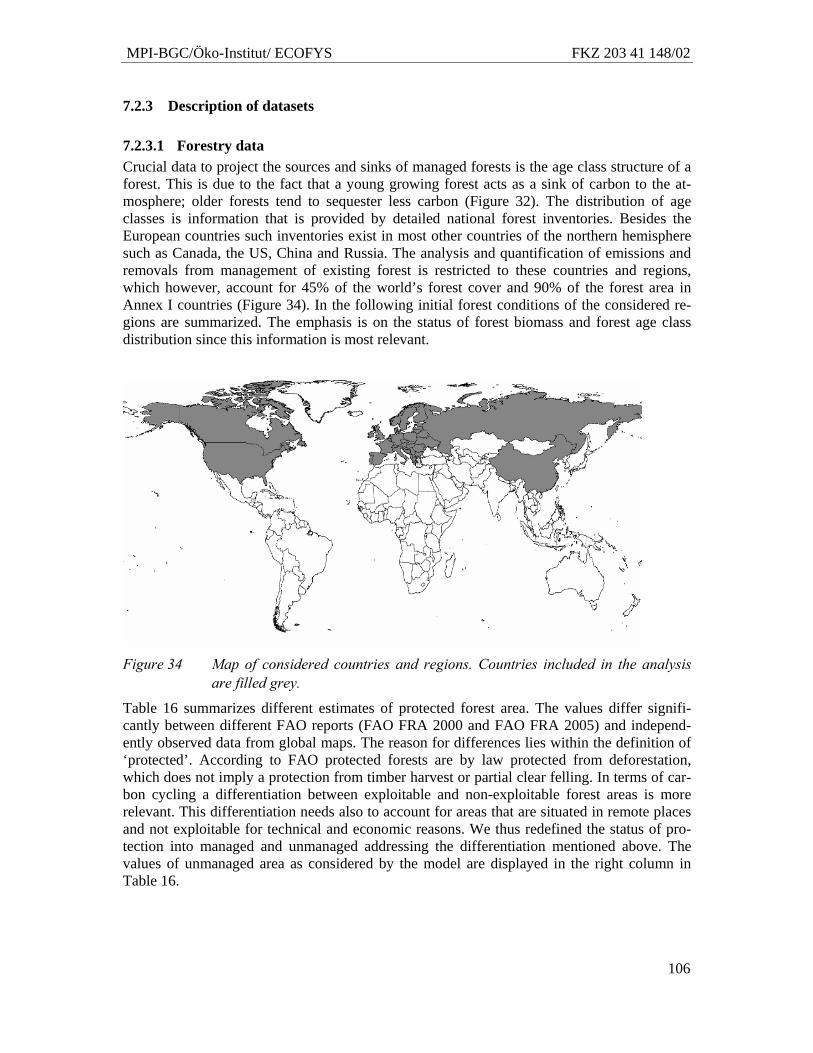
MPI-BGC/Öko-Institut/ ECOFYS FKZ 203 41 148/02
106
7.2.3 Description of datasets
7.2.3.1 Forestry data Crucial data to project the sources and sinks of managed forests is the age class structure of a forest. This is due to the fact that a young growing forest acts as a sink of carbon to the at-mosphere; older forests tend to sequester less carbon (Figure 32). The distribution of age classes is information that is provided by detailed national forest inventories. Besides the European countries such inventories exist in most other countries of the northern hemisphere such as Canada, the US, China and Russia. The analysis and quantification of emissions and removals from management of existing forest is restricted to these countries and regions, which however, account for 45% of the world’s forest cover and 90% of the forest area in Annex I countries (Figure 34). In the following initial forest conditions of the considered re-gions are summarized. The emphasis is on the status of forest biomass and forest age class distribution since this information is most relevant.
Figure 34 Map of considered countries and regions. Countries included in the analysis
are filled grey.
Table 16 summarizes different estimates of protected forest area. The values differ signifi-cantly between different FAO reports (FAO FRA 2000 and FAO FRA 2005) and independ-ently observed data from global maps. The reason for differences lies within the definition of ‘protected’. According to FAO protected forests are by law protected from deforestation, which does not imply a protection from timber harvest or partial clear felling. In terms of car-bon cycling a differentiation between exploitable and non-exploitable forest areas is more relevant. This differentiation needs also to account for areas that are situated in remote places and not exploitable for technical and economic reasons. We thus redefined the status of pro-tection into managed and unmanaged addressing the differentiation mentioned above. The values of unmanaged area as considered by the model are displayed in the right column in Table 16.
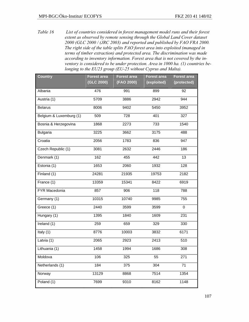
MPI-BGC/Öko-Institut/ ECOFYS FKZ 203 41 148/02
107
Table 16 List of countries considered in forest management model runs and their forest extent as observed by remote sensing through the Global Land Cover dataset 2000 (GLC 2000 / (JRC 2003) and reported and published by FAO FRA 2000. The right side of the table splits FAO forest area into exploited (managed in terms of timber extraction) and protected area. The discrimination was made according to inventory information. Forest area that is not covered by the in-ventory is considered to be under protection. Area in 1000 ha. (1) countries be-longing to the EU23 group (EU-25 without Cyprus and Malta).
Country Forest area (GLC 2000)
Forest area (FAO 2000)
Forest area (exploited)
Forest area (protected)
Albania 476 991 899 92
Austria (1) 5709 3886 2942 944
Belarus 8006 9402 5450 3952
Belgium & Luxemburg (1) 509 728 401 327
Bosnia & Herzegovina 1868 2273 733 1540
Bulgaria 3225 3662 3175 488
Croatia 2056 1783 836 947
Czech Republic (1) 3081 2632 2446 186
Denmark (1) 162 455 442 13
Estonia (1) 1653 2060 1932 128
Finland (1) 24281 21935 19753 2182
France (1) 13359 15341 8422 6919
FYR Macedonia 857 906 118 788
Germany (1) 10315 10740 9985 755
Greece (1) 2440 3599 3599 0
Hungary (1) 1395 1840 1609 231
Ireland (1) 259 659 329 330
Italy (1) 8776 10003 3832 6171
Latvia (1) 2065 2923 2413 510
Lithuania (1) 1458 1994 1686 308
Moldova 106 325 55 271
Netherlands (1) 184 375 304 71
Norway 13129 8868 7514 1354
Poland (1) 7699 9310 8162 1148
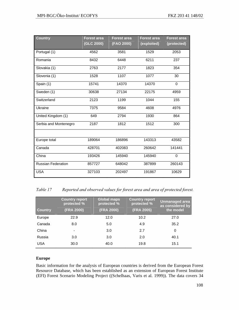
MPI-BGC/Öko-Institut/ ECOFYS FKZ 203 41 148/02
108
Country Forest area
(GLC 2000) Forest area (FAO 2000)
Forest area (exploited)
Forest area (protected)
Portugal (1) 4562 3581 1529 2053
Romania 8432 6448 6211 237
Slovakia (1) 2763 2177 1823 354
Slovenia (1) 1528 1107 1077 30
Spain (1) 15741 14370 14370 0
Sweden (1) 30638 27134 22175 4959
Switzerland 2123 1199 1044 155
Ukraine 7375 9584 4608 4976
United Kingdom (1) 649 2794 1930 864
Serbia and Montenegro 2187 1812 1512 300
Europe total 189064 186896 143313 43582
Canada 428701 402083 260642 141441
China 193426 145940 145940 0
Russian Federation 857727 648042 387899 260143
USA 327103 202497 191867 10629
Table 17 Reported and observed values for forest area and area of protected forest.
Country
Country report protected %
(FRA 2000)
Global maps protected %
(FRA 2000)
Country report protected %
(FRA 2005)
Unmanaged area as considered by
the model
Europe 22.9 12.0 10.2 27.0
Canada 8.0 5.0 4.9 35.2
China - 3.0 2.7 0
Russia 3.0 3.0 2.0 40.1
USA 30.0 40.0 19.8 15.1
Europe
Basic information for the analysis of European countries is derived from the European Forest Resource Database, which has been established as an extension of European Forest Institute (EFI) Forest Scenario Modeling Project ((Schelhaas, Varis et al. 1999)). The data covers 34
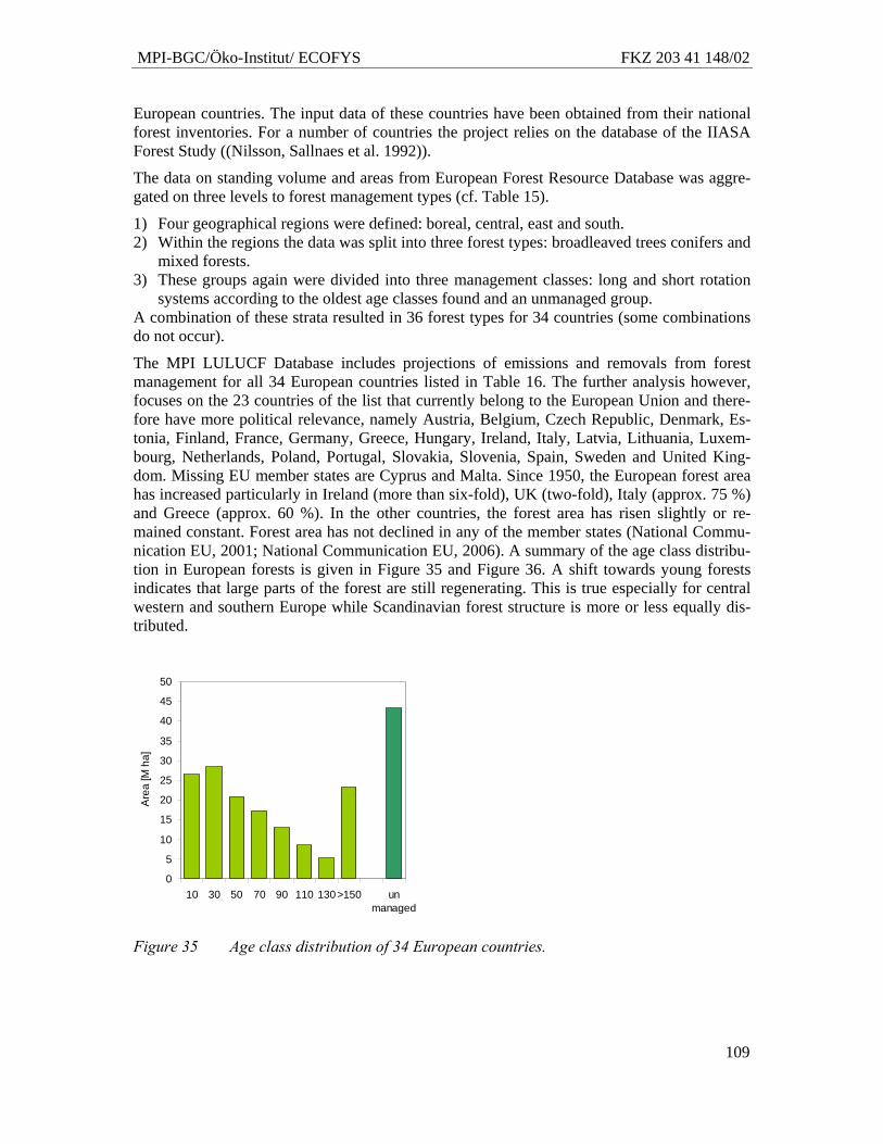
MPI-BGC/Öko-Institut/ ECOFYS FKZ 203 41 148/02
109
European countries. The input data of these countries have been obtained from their national forest inventories. For a number of countries the project relies on the database of the IIASA Forest Study ((Nilsson, Sallnaes et al. 1992)).
The data on standing volume and areas from European Forest Resource Database was aggre-gated on three levels to forest management types (cf. Table 15).
1) Four geographical regions were defined: boreal, central, east and south. 2) Within the regions the data was split into three forest types: broadleaved trees conifers and
mixed forests. 3) These groups again were divided into three management classes: long and short rotation
systems according to the oldest age classes found and an unmanaged group. A combination of these strata resulted in 36 forest types for 34 countries (some combinations do not occur).
The MPI LULUCF Database includes projections of emissions and removals from forest management for all 34 European countries listed in Table 16. The further analysis however, focuses on the 23 countries of the list that currently belong to the European Union and there-fore have more political relevance, namely Austria, Belgium, Czech Republic, Denmark, Es-tonia, Finland, France, Germany, Greece, Hungary, Ireland, Italy, Latvia, Lithuania, Luxem-bourg, Netherlands, Poland, Portugal, Slovakia, Slovenia, Spain, Sweden and United King-dom. Missing EU member states are Cyprus and Malta. Since 1950, the European forest area has increased particularly in Ireland (more than six-fold), UK (two-fold), Italy (approx. 75 %) and Greece (approx. 60 %). In the other countries, the forest area has risen slightly or re-mained constant. Forest area has not declined in any of the member states (National Commu-nication EU, 2001; National Communication EU, 2006). A summary of the age class distribu-tion in European forests is given in Figure 35 and Figure 36. A shift towards young forests indicates that large parts of the forest are still regenerating. This is true especially for central western and southern Europe while Scandinavian forest structure is more or less equally dis-tributed.
0
5
10
15
20
25
30
35
40
45
50
10 30 50 70 90 110 130>150 unmanaged
Are
a [M
ha]
Figure 35 Age class distribution of 34 European countries.
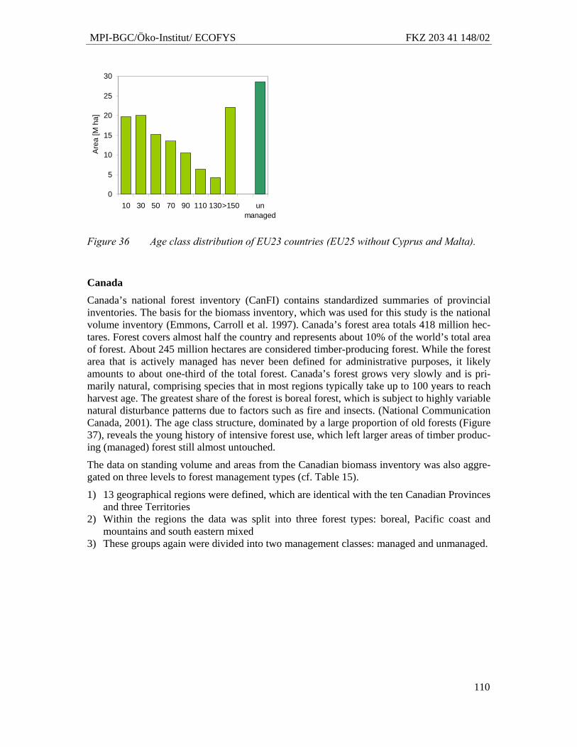
MPI-BGC/Öko-Institut/ ECOFYS FKZ 203 41 148/02
110
0
5
10
15
20
25
30
10 30 50 70 90 110 130>150 unmanaged
Are
a [M
ha]
Figure 36 Age class distribution of EU23 countries (EU25 without Cyprus and Malta).
Canada
Canada’s national forest inventory (CanFI) contains standardized summaries of provincial inventories. The basis for the biomass inventory, which was used for this study is the national volume inventory (Emmons, Carroll et al. 1997). Canada’s forest area totals 418 million hec-tares. Forest covers almost half the country and represents about 10% of the world’s total area of forest. About 245 million hectares are considered timber-producing forest. While the forest area that is actively managed has never been defined for administrative purposes, it likely amounts to about one-third of the total forest. Canada’s forest grows very slowly and is pri-marily natural, comprising species that in most regions typically take up to 100 years to reach harvest age. The greatest share of the forest is boreal forest, which is subject to highly variable natural disturbance patterns due to factors such as fire and insects. (National Communication Canada, 2001). The age class structure, dominated by a large proportion of old forests (Figure 37), reveals the young history of intensive forest use, which left larger areas of timber produc-ing (managed) forest still almost untouched.
The data on standing volume and areas from the Canadian biomass inventory was also aggre-gated on three levels to forest management types (cf. Table 15).
1) 13 geographical regions were defined, which are identical with the ten Canadian Provinces and three Territories
2) Within the regions the data was split into three forest types: boreal, Pacific coast and mountains and south eastern mixed
3) These groups again were divided into two management classes: managed and unmanaged.
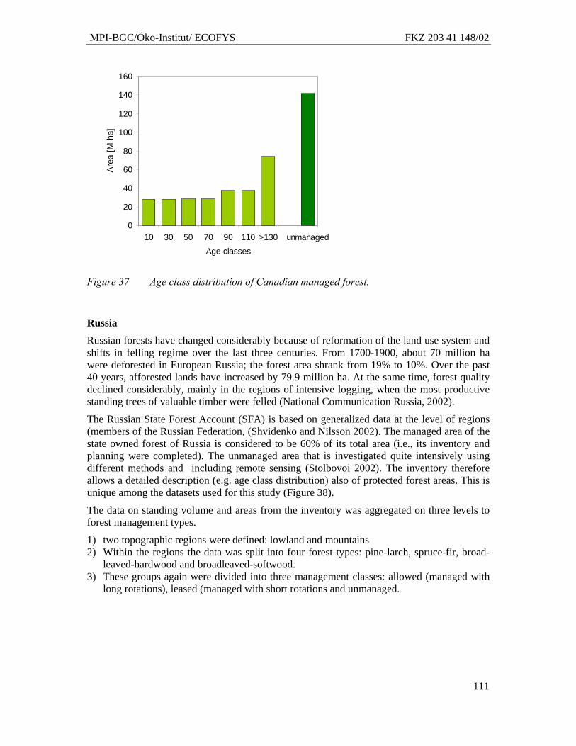
MPI-BGC/Öko-Institut/ ECOFYS FKZ 203 41 148/02
111
0
20
40
60
80
100
120
140
160
10 30 50 70 90 110 >130 unmanagedAge classes
Area
[M h
a]
Figure 37 Age class distribution of Canadian managed forest.
Russia
Russian forests have changed considerably because of reformation of the land use system and shifts in felling regime over the last three centuries. From 1700-1900, about 70 million ha were deforested in European Russia; the forest area shrank from 19% to 10%. Over the past 40 years, afforested lands have increased by 79.9 million ha. At the same time, forest quality declined considerably, mainly in the regions of intensive logging, when the most productive standing trees of valuable timber were felled (National Communication Russia, 2002).
The Russian State Forest Account (SFA) is based on generalized data at the level of regions (members of the Russian Federation, (Shvidenko and Nilsson 2002). The managed area of the state owned forest of Russia is considered to be 60% of its total area (i.e., its inventory and planning were completed). The unmanaged area that is investigated quite intensively using different methods and including remote sensing (Stolbovoi 2002). The inventory therefore allows a detailed description (e.g. age class distribution) also of protected forest areas. This is unique among the datasets used for this study (Figure 38).
The data on standing volume and areas from the inventory was aggregated on three levels to forest management types.
1) two topographic regions were defined: lowland and mountains 2) Within the regions the data was split into four forest types: pine-larch, spruce-fir, broad-
leaved-hardwood and broadleaved-softwood. 3) These groups again were divided into three management classes: allowed (managed with
long rotations), leased (managed with short rotations and unmanaged.
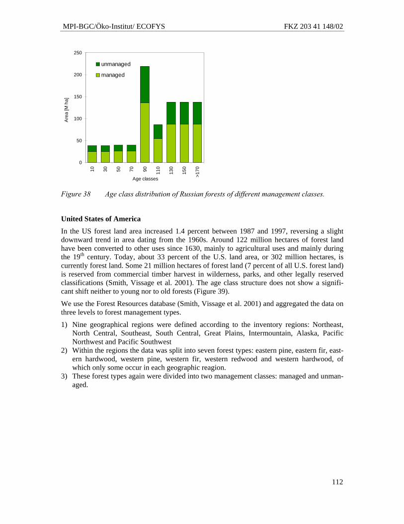
MPI-BGC/Öko-Institut/ ECOFYS FKZ 203 41 148/02
112
0
50
100
150
200
250
10 30 50 70 90 110
130
150
>170
Age classes
Are
a [M
ha]
unmanaged
managed
Figure 38 Age class distribution of Russian forests of different management classes.
United States of America
In the US forest land area increased 1.4 percent between 1987 and 1997, reversing a slight downward trend in area dating from the 1960s. Around 122 million hectares of forest land have been converted to other uses since 1630, mainly to agricultural uses and mainly during the 19th century. Today, about 33 percent of the U.S. land area, or 302 million hectares, is currently forest land. Some 21 million hectares of forest land (7 percent of all U.S. forest land) is reserved from commercial timber harvest in wilderness, parks, and other legally reserved classifications (Smith, Vissage et al. 2001). The age class structure does not show a signifi-cant shift neither to young nor to old forests (Figure 39).
We use the Forest Resources database (Smith, Vissage et al. 2001) and aggregated the data on three levels to forest management types.
1) Nine geographical regions were defined according to the inventory regions: Northeast, North Central, Southeast, South Central, Great Plains, Intermountain, Alaska, Pacific Northwest and Pacific Southwest
2) Within the regions the data was split into seven forest types: eastern pine, eastern fir, east-ern hardwood, western pine, western fir, western redwood and western hardwood, of which only some occur in each geographic reagion.
3) These forest types again were divided into two management classes: managed and unman-aged.
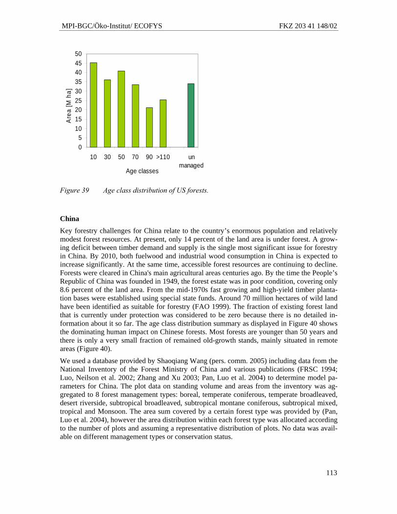
MPI-BGC/Öko-Institut/ ECOFYS FKZ 203 41 148/02
113
05
101520253035404550
10 30 50 70 90 >110 unmanaged
Age classes
Are
a [M
ha]
Figure 39 Age class distribution of US forests.
China
Key forestry challenges for China relate to the country’s enormous population and relatively modest forest resources. At present, only 14 percent of the land area is under forest. A grow-ing deficit between timber demand and supply is the single most significant issue for forestry in China. By 2010, both fuelwood and industrial wood consumption in China is expected to increase significantly. At the same time, accessible forest resources are continuing to decline. Forests were cleared in China's main agricultural areas centuries ago. By the time the People’s Republic of China was founded in 1949, the forest estate was in poor condition, covering only 8.6 percent of the land area. From the mid-1970s fast growing and high-yield timber planta-tion bases were established using special state funds. Around 70 million hectares of wild land have been identified as suitable for forestry (FAO 1999). The fraction of existing forest land that is currently under protection was considered to be zero because there is no detailed in-formation about it so far. The age class distribution summary as displayed in Figure 40 shows the dominating human impact on Chinese forests. Most forests are younger than 50 years and there is only a very small fraction of remained old-growth stands, mainly situated in remote areas (Figure 40).
We used a database provided by Shaoqiang Wang (pers. comm. 2005) including data from the National Inventory of the Forest Ministry of China and various publications (FRSC 1994; Luo, Neilson et al. 2002; Zhang and Xu 2003; Pan, Luo et al. 2004) to determine model pa-rameters for China. The plot data on standing volume and areas from the inventory was ag-gregated to 8 forest management types: boreal, temperate coniferous, temperate broadleaved, desert riverside, subtropical broadleaved, subtropical montane coniferous, subtropical mixed, tropical and Monsoon. The area sum covered by a certain forest type was provided by (Pan, Luo et al. 2004), however the area distribution within each forest type was allocated according to the number of plots and assuming a representative distribution of plots. No data was avail-able on different management types or conservation status.
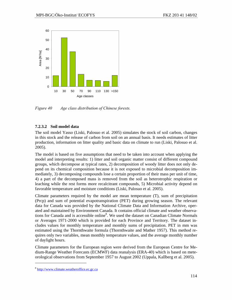
MPI-BGC/Öko-Institut/ ECOFYS FKZ 203 41 148/02
114
0
10
20
30
40
50
60
10 30 50 70 90 110 130 >150Age classes
Are
a [M
ha]
Figure 40 Age class distribution of Chinese forests.
7.2.3.2 Soil model data The soil model Yasso (Liski, Palosuo et al. 2005) simulates the stock of soil carbon, changes in this stock and the release of carbon from soil on an annual basis. It needs estimates of litter production, information on litter quality and basic data on climate to run (Liski, Palosuo et al. 2005).
The model is based on five assumptions that need to be taken into account when applying the model and interpreting results: 1) litter and soil organic matter consist of different compound groups, which decompose at typical rates, 2) decomposition of woody litter does not only de-pend on its chemical composition because it is not exposed to microbial decomposition im-mediately, 3) decomposing compounds lose a certain proportion of their mass per unit of time, 4) a part of the decomposed mass is removed from the soil as heterotrophic respiration or leaching while the rest forms more recalcitrant compounds, 5) Microbial activity depend on favorable temperature and moisture conditions (Liski, Palosuo et al. 2005).
Climate parameters required by the model are mean temperature (T), sum of precipitation (Prcp) and sum of potential evapotranspiration (PET) during growing season. The relevant data for Canada was provided by the National Climate Data and Information Archive, oper-ated and maintained by Environment Canada. It contains official climate and weather observa-tions for Canada and is accessible online8. We used the dataset on Canadian Climate Normals or Averages 1971-2000 which is provided for each Province and Territory. The dataset in-cludes values for monthly temperature and monthly sums of precipitation. PET in mm was estimated using the Thornthwaite formula (Thornthwaite and Mather 1957). This method re-quires only two variables, mean monthly temperature values, and the average monthly number of daylight hours.
Climate parameters for the European region were derived from the European Centre for Me-dium-Range Weather Forecasts (ECMWF) data reanalysis (ERA-40) which is based on mete-orological observations from September 1957 to August 2002 (Uppala, Kallberg et al. 2005). 8 http://www.climate.weatheroffice.ec.gc.ca
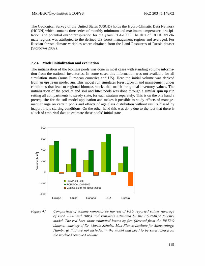
MPI-BGC/Öko-Institut/ ECOFYS FKZ 203 41 148/02
115
The Geological Survey of the United States (USGD) holds the Hydro-Climatic Data Network (HCDN) which contains time series of monthly minimum and maximum temperature, precipi-tation, and potential evapotranspiration for the years 1951-1990. The data of 18 HCDN cli-mate regions was attributed to the defined US forest management regions and averaged. For Russian forests climate variables where obtained from the Land Resources of Russia dataset (Stolbovoi 2002).
7.2.4 Model initialization and evaluation
The initialization of the biomass pools was done in most cases with standing volume informa-tion from the national inventories. In some cases this information was not available for all simulation strata (some European countries and US). Here the initial volume was derived from an upstream model run. This model run simulates forest growth and management under conditions that lead to regional biomass stocks that match the global inventory values. The initialization of the product and soil and litter pools was done through a similar spin up run setting all compartments to steady state, for each stratum separately. This is on the one hand a prerequisite for the soil model application and makes it possible to study effects of manage-ment change on certain pools and effects of age class distribution without results biased by inappropriate starting conditions. On the other hand this was done due to the fact that there is a lack of empirical data to estimate these pools’ initial state.
-400
-200
0
200
400
600
800
Europe China Canada USA Russia
Vol
ume
[M m
3 ]
FRA 2000-2005FORMICA 2000-2005Volume lost to fire (1990-2000)
Figure 41 Comparison of volume removals by harvest of FAO reported values (average of FRA 2000 and 2005) and removals estimated by the FORMICA forestry model. The red bars show estimated losses by fire (derived from the RETRO dataset; courtesy of Dr. Martin Schultz, Max-Planck-Institute for Meteorology, Hamburg) that are not included in the model and need to be subtracted from the modeled removed volume.
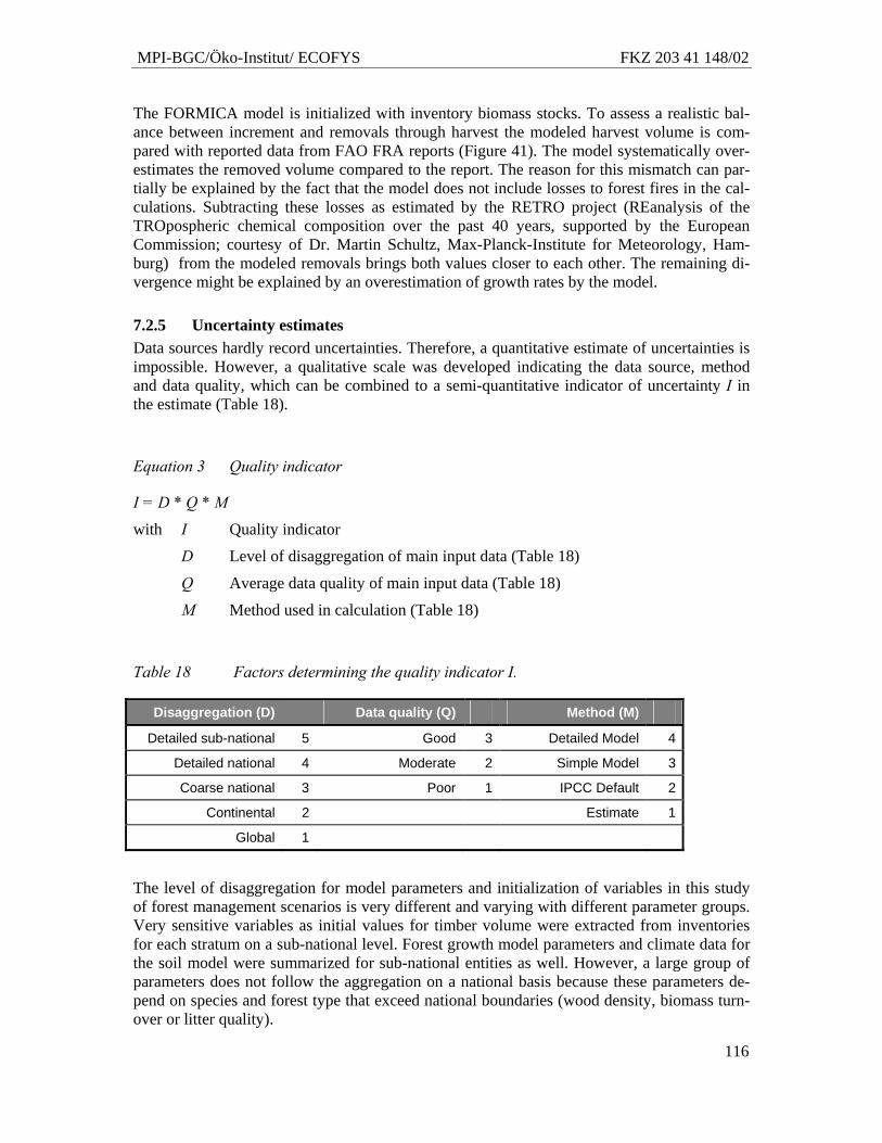
MPI-BGC/Öko-Institut/ ECOFYS FKZ 203 41 148/02
116
The FORMICA model is initialized with inventory biomass stocks. To assess a realistic bal-ance between increment and removals through harvest the modeled harvest volume is com-pared with reported data from FAO FRA reports (Figure 41). The model systematically over-estimates the removed volume compared to the report. The reason for this mismatch can par-tially be explained by the fact that the model does not include losses to forest fires in the cal-culations. Subtracting these losses as estimated by the RETRO project (REanalysis of the TROpospheric chemical composition over the past 40 years, supported by the European Commission; courtesy of Dr. Martin Schultz, Max-Planck-Institute for Meteorology, Ham-burg) from the modeled removals brings both values closer to each other. The remaining di-vergence might be explained by an overestimation of growth rates by the model.
7.2.5 Uncertainty estimates Data sources hardly record uncertainties. Therefore, a quantitative estimate of uncertainties is impossible. However, a qualitative scale was developed indicating the data source, method and data quality, which can be combined to a semi-quantitative indicator of uncertainty I in the estimate (Table 18).
Equation 3 Quality indicator
I = D * Q * M
with I Quality indicator
D Level of disaggregation of main input data (Table 18)
Q Average data quality of main input data (Table 18)
M Method used in calculation (Table 18)
Table 18 Factors determining the quality indicator I.
Disaggregation (D) Data quality (Q) Method (M)
Detailed sub-national 5 Good 3 Detailed Model 4
Detailed national 4 Moderate 2 Simple Model 3
Coarse national 3 Poor 1 IPCC Default 2
Continental 2 Estimate 1
Global 1
The level of disaggregation for model parameters and initialization of variables in this study of forest management scenarios is very different and varying with different parameter groups. Very sensitive variables as initial values for timber volume were extracted from inventories for each stratum on a sub-national level. Forest growth model parameters and climate data for the soil model were summarized for sub-national entities as well. However, a large group of parameters does not follow the aggregation on a national basis because these parameters de-pend on species and forest type that exceed national boundaries (wood density, biomass turn-over or litter quality).
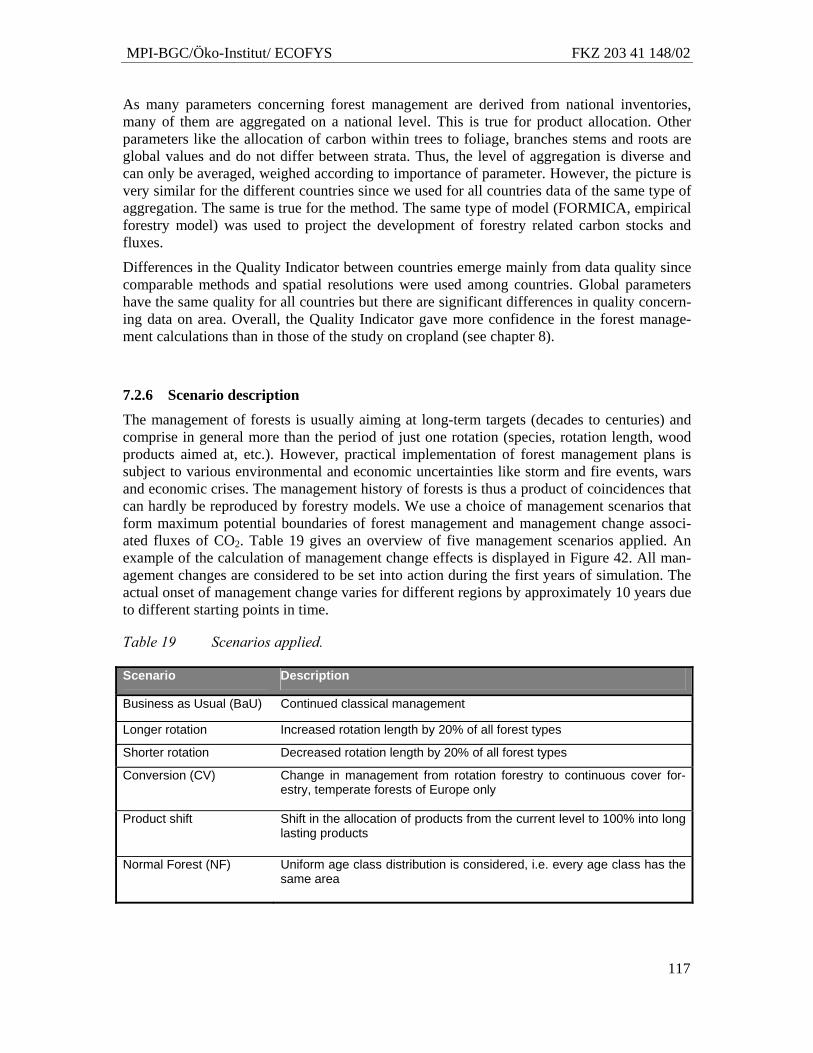
MPI-BGC/Öko-Institut/ ECOFYS FKZ 203 41 148/02
117
As many parameters concerning forest management are derived from national inventories, many of them are aggregated on a national level. This is true for product allocation. Other parameters like the allocation of carbon within trees to foliage, branches stems and roots are global values and do not differ between strata. Thus, the level of aggregation is diverse and can only be averaged, weighed according to importance of parameter. However, the picture is very similar for the different countries since we used for all countries data of the same type of aggregation. The same is true for the method. The same type of model (FORMICA, empirical forestry model) was used to project the development of forestry related carbon stocks and fluxes.
Differences in the Quality Indicator between countries emerge mainly from data quality since comparable methods and spatial resolutions were used among countries. Global parameters have the same quality for all countries but there are significant differences in quality concern-ing data on area. Overall, the Quality Indicator gave more confidence in the forest manage-ment calculations than in those of the study on cropland (see chapter 8).
7.2.6 Scenario description The management of forests is usually aiming at long-term targets (decades to centuries) and comprise in general more than the period of just one rotation (species, rotation length, wood products aimed at, etc.). However, practical implementation of forest management plans is subject to various environmental and economic uncertainties like storm and fire events, wars and economic crises. The management history of forests is thus a product of coincidences that can hardly be reproduced by forestry models. We use a choice of management scenarios that form maximum potential boundaries of forest management and management change associ-ated fluxes of CO2. Table 19 gives an overview of five management scenarios applied. An example of the calculation of management change effects is displayed in Figure 42. All man-agement changes are considered to be set into action during the first years of simulation. The actual onset of management change varies for different regions by approximately 10 years due to different starting points in time.
Table 19 Scenarios applied.
Scenario Description
Business as Usual (BaU) Continued classical management
Longer rotation Increased rotation length by 20% of all forest types
Shorter rotation Decreased rotation length by 20% of all forest types
Conversion (CV) Change in management from rotation forestry to continuous cover for-estry, temperate forests of Europe only
Product shift Shift in the allocation of products from the current level to 100% into long lasting products
Normal Forest (NF) Uniform age class distribution is considered, i.e. every age class has the same area
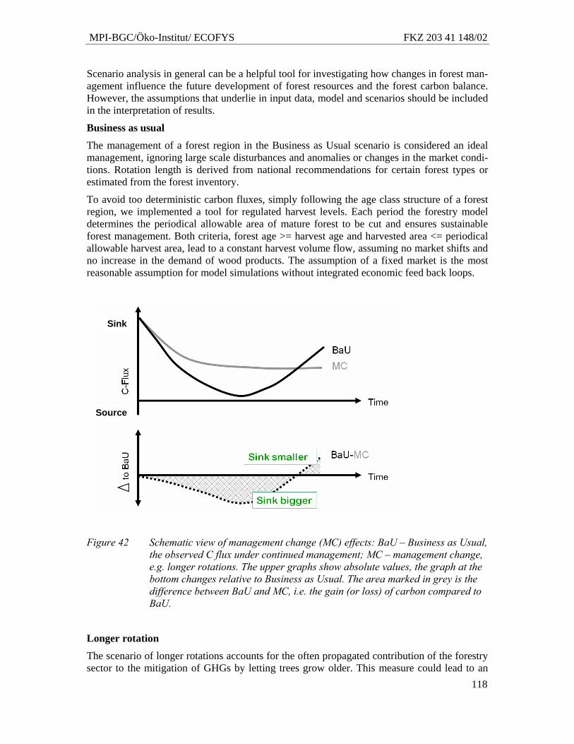
MPI-BGC/Öko-Institut/ ECOFYS FKZ 203 41 148/02
118
Scenario analysis in general can be a helpful tool for investigating how changes in forest man-agement influence the future development of forest resources and the forest carbon balance. However, the assumptions that underlie in input data, model and scenarios should be included in the interpretation of results.
Business as usual
The management of a forest region in the Business as Usual scenario is considered an ideal management, ignoring large scale disturbances and anomalies or changes in the market condi-tions. Rotation length is derived from national recommendations for certain forest types or estimated from the forest inventory.
To avoid too deterministic carbon fluxes, simply following the age class structure of a forest region, we implemented a tool for regulated harvest levels. Each period the forestry model determines the periodical allowable area of mature forest to be cut and ensures sustainable forest management. Both criteria, forest age >= harvest age and harvested area <= periodical allowable harvest area, lead to a constant harvest volume flow, assuming no market shifts and no increase in the demand of wood products. The assumption of a fixed market is the most reasonable assumption for model simulations without integrated economic feed back loops.
Figure 42 Schematic view of management change (MC) effects: BaU – Business as Usual, the observed C flux under continued management; MC – management change, e.g. longer rotations. The upper graphs show absolute values, the graph at the bottom changes relative to Business as Usual. The area marked in grey is the difference between BaU and MC, i.e. the gain (or loss) of carbon compared to BaU.
Longer rotation
The scenario of longer rotations accounts for the often propagated contribution of the forestry sector to the mitigation of GHGs by letting trees grow older. This measure could lead to an
Sink
Source
MPI-BGC/Öko-Institut/ ECOFYS FKZ 203 41 148/02
119
increase in forest biomass and remove CO2 from the atmosphere additionally compared to Business as Usual temporarily by delaying harvest and likely leading to higher average C stocks.
How effectively this measure will be implemented in the future is to a large degree dependent on economic incentives. In parts of Europe rotations are already prolonged for economic rea-sons. Private forest owners tend to keep high growing stocks because of low prices for sawn timber of large dimensions. To predict for which forest types and which regions rotation length enhancement could be a viable option is difficult. This study prescribes a general pro-longation of rotations by 20% for all regions and forest types. The effect on the carbon bal-ance following this scenario is more considered a technological-biological potential rather than a realistic management option.
Shorter rotation
The rotation time in managed forests is to a large degree determined by the potential product the forest owner wants to sell. The demand for a certain quality, quantity and type of product is changing over time and also linked to the technical development of wood processing. Euro-pean pulp and paper demand during the last decades increased more rapidly compared to the demand of sawn timber ((UNECE 2005)). Over the next 20 years it is expected that renewable energy policies encourage the establishment of short-rotation forest plantations for woodfuel production ((UNECE 2005)). In addition there is a trend towards compound products, result-ing in a higher demand for sawn timber of smaller diameters. It is likely that economic condi-tions will favour a reduction of rotation time in the future in some forest management regions. A scenario of 20% shorter rotations in all forest regions is estimating implications for the car-bon budget if the average forest age would be reduced.
Shift in wood products
Carbon enclosed in harvested wood is allocated to various product pools and affects the car-bon budget of the entire forestry sector through different mean residence times within the wood products. The model considers two pools of harvested wood products. Products made of sawn timber, plywood and veneer or particleboard used for construction and furnishing are summarized in a long lifespan pool with an average residence time of 25 years. A second pool comprises products made from wood or pulp like paper, boxes etc. has a mean residence time of 2 years.
An increased use of long lasting wood products results in lower emissions of carbon. The po-tential values are calculated in a product shift scenario that simulates a shift in the allocation towards long lasting products. The scenario assumes that wood removed in the final harvest (minus slash material) is distributed to 100% to long lifespan products (compare to Table 20). This scenario describes a technical potential and does not include any economic constraints or feed backs to the demand of certain products or processing capacities.
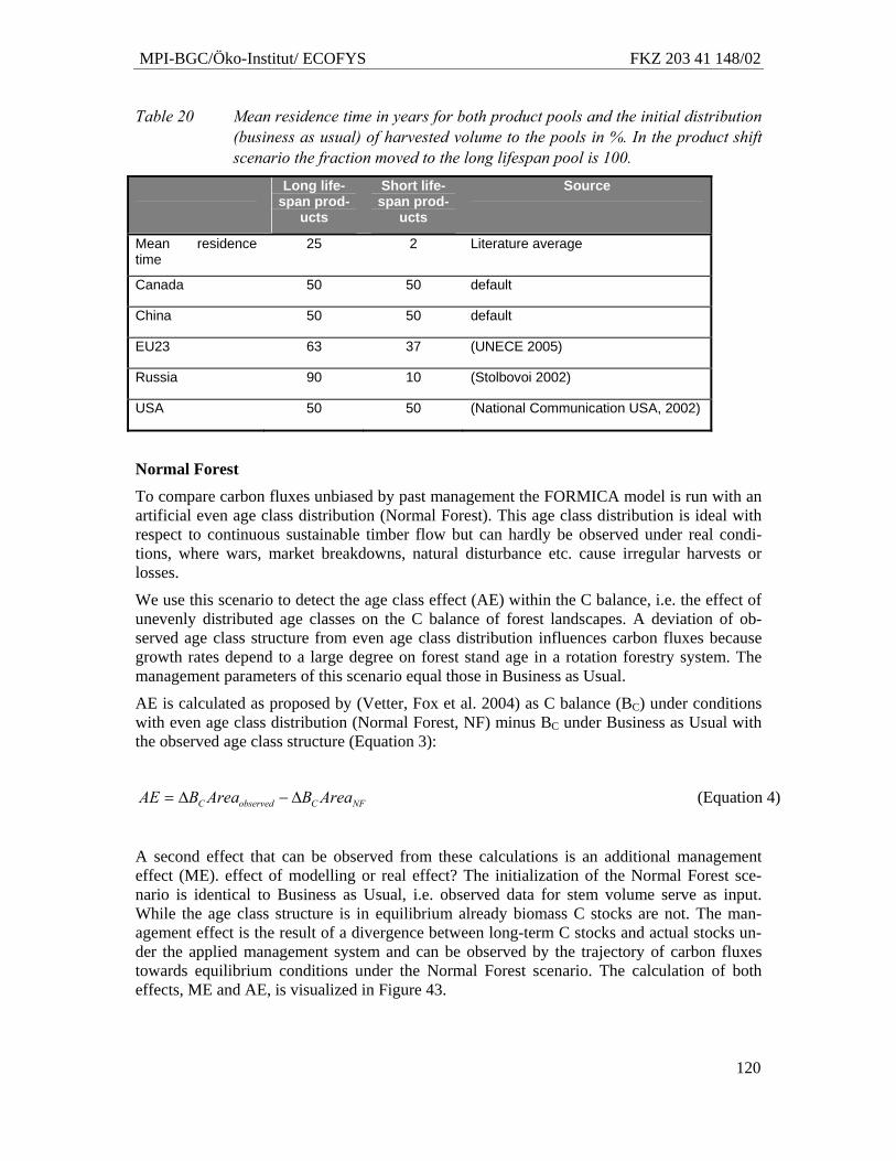
MPI-BGC/Öko-Institut/ ECOFYS FKZ 203 41 148/02
120
Table 20 Mean residence time in years for both product pools and the initial distribution (business as usual) of harvested volume to the pools in %. In the product shift scenario the fraction moved to the long lifespan pool is 100.
Long life-span prod-
ucts
Short life-span prod-
ucts
Source
Mean residence time
25 2 Literature average
Canada 50 50 default
China 50 50 default
EU23 63 37 (UNECE 2005)
Russia 90 10 (Stolbovoi 2002)
USA 50 50 (National Communication USA, 2002)
Normal Forest
To compare carbon fluxes unbiased by past management the FORMICA model is run with an artificial even age class distribution (Normal Forest). This age class distribution is ideal with respect to continuous sustainable timber flow but can hardly be observed under real condi-tions, where wars, market breakdowns, natural disturbance etc. cause irregular harvests or losses.
We use this scenario to detect the age class effect (AE) within the C balance, i.e. the effect of unevenly distributed age classes on the C balance of forest landscapes. A deviation of ob-served age class structure from even age class distribution influences carbon fluxes because growth rates depend to a large degree on forest stand age in a rotation forestry system. The management parameters of this scenario equal those in Business as Usual.
AE is calculated as proposed by (Vetter, Fox et al. 2004) as C balance (BC) under conditions with even age class distribution (Normal Forest, NF) minus BC under Business as Usual with the observed age class structure (Equation 3):
NFCobservedC AreaBAreaBAE Δ−Δ= (Equation 4)
A second effect that can be observed from these calculations is an additional management effect (ME). effect of modelling or real effect? The initialization of the Normal Forest sce-nario is identical to Business as Usual, i.e. observed data for stem volume serve as input. While the age class structure is in equilibrium already biomass C stocks are not. The man-agement effect is the result of a divergence between long-term C stocks and actual stocks un-der the applied management system and can be observed by the trajectory of carbon fluxes towards equilibrium conditions under the Normal Forest scenario. The calculation of both effects, ME and AE, is visualized in Figure 43.
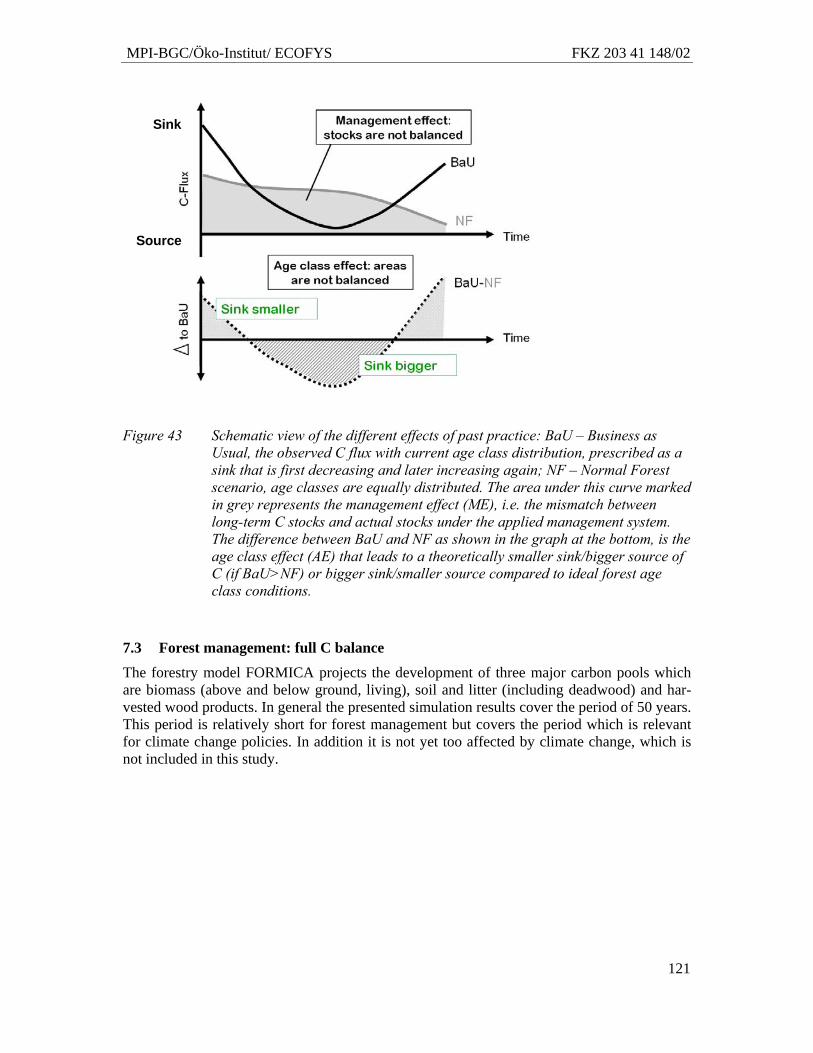
MPI-BGC/Öko-Institut/ ECOFYS FKZ 203 41 148/02
121
Figure 43 Schematic view of the different effects of past practice: BaU – Business as Usual, the observed C flux with current age class distribution, prescribed as a sink that is first decreasing and later increasing again; NF – Normal Forest scenario, age classes are equally distributed. The area under this curve marked in grey represents the management effect (ME), i.e. the mismatch between long-term C stocks and actual stocks under the applied management system. The difference between BaU and NF as shown in the graph at the bottom, is the age class effect (AE) that leads to a theoretically smaller sink/bigger source of C (if BaU>NF) or bigger sink/smaller source compared to ideal forest age class conditions.
7.3 Forest management: full C balance
The forestry model FORMICA projects the development of three major carbon pools which are biomass (above and below ground, living), soil and litter (including deadwood) and har-vested wood products. In general the presented simulation results cover the period of 50 years. This period is relatively short for forest management but covers the period which is relevant for climate change policies. In addition it is not yet too affected by climate change, which is not included in this study.
Sink
Source
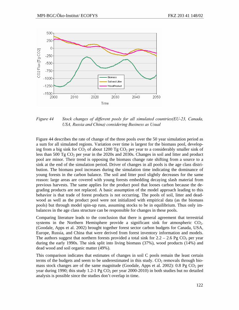
MPI-BGC/Öko-Institut/ ECOFYS FKZ 203 41 148/02
122
Figure 44 Stock changes of different pools for all simulated countries(EU-23, Canada, USA, Russia and China) considering Business as Usual
Figure 44 describes the rate of change of the three pools over the 50 year simulation period as a sum for all simulated regions. Variation over time is largest for the biomass pool, develop-ing from a big sink for CO2 of about 1200 Tg CO2 per year to a considerably smaller sink of less than 500 Tg CO2 per year in the 2020s and 2030s. Changes in soil and litter and product pool are minor. Their trend is opposing the biomass change rate shifting from a source to a sink at the end of the simulation period. Driver of changes in all pools is the age class distri-bution. The biomass pool increases during the simulation time indicating the dominance of young forests in the carbon balance. The soil and litter pool slightly decreases for the same reason: large areas are covered with young forests embedding decaying slash material from previous harvests. The same applies for the product pool that looses carbon because the de-grading products are not replaced. A basic assumption of the model approach leading to this behavior is that trade of forest products is not occurring. The pools of soil, litter and dead-wood as well as the product pool were not initialized with empirical data (as the biomass pools) but through model spin-up runs, assuming stocks to be in equilibrium. Thus only im-balances in the age class structure can be responsible for changes in these pools.
Comparing literature leads to the conclusion that there is general agreement that terrestrial systems in the Northern Hemisphere provide a significant sink for atmospheric CO2. (Goodale, Apps et al. 2002) brought together forest sector carbon budgets for Canada, USA, Europe, Russia, and China that were derived from forest inventory information and models. The authors suggest that northern forests provided a total sink for 2.2 – 2.6 Pg CO2 per year during the early 1990s. The sink split into living biomass (37%), wood products (14%) and dead wood and soil organic matter (49%).
This comparison indicates that estimates of changes in soil C pools remain the least certain terms of the budgets and seem to be underestimated in this study. CO2 removals through bio-mass stock changes are of the same magnitude (Goodale, Apps et al. 2002): 0.8 Pg CO2 per year during 1990; this study 1.2-1 Pg CO2 per year 2000-2010) in both studies but no detailed analysis is possible since the studies don’t overlap in time.
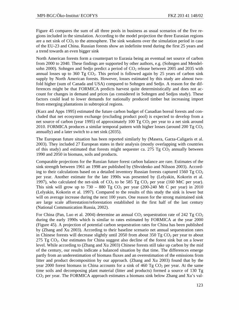
MPI-BGC/Öko-Institut/ ECOFYS FKZ 203 41 148/02
123
Figure 45 compares the sum of all three pools in business as usual scenarios of the five re-gions included in the simulation. According to the model projection the three Eurasian regions are a net sink of CO2 to the atmosphere. The sink weakens over the simulation period in case of the EU-23 and China. Russian forests show an indefinite trend during the first 25 years and a trend towards an even bigger sink
North American forests form a counterpart to Eurasia being an eventual net source of carbon from 2000 to 2040. These findings are supported by other authors, e.g. (Sohngen and Mendel-sohn 2000). Sohngen and Sedjo predict a period of CO2 release between 2005 and 2035 with annual losses up to 360 Tg CO2. This period is followed again by 25 years of carbon sink supply by North American forests. However, losses estimated by this study are almost two-fold higher (sum of Canada and USA) compared to Sohngen and Sedjo. A reason for the dif-ferences might be that FORMICA predicts harvest quite deterministically and does not ac-count for changes in demand and prices (as considered in Sohngen and Sedjos study). These factors could lead to lower demands for nationally produced timber but increasing import from emerging plantations in subtropical regions.
(Kurz and Apps 1995) estimated the future carbon budget of Canadian boreal forests and con-cluded that net ecosystem exchange (excluding product pool) is expected to develop from a net source of carbon (year 1995) of approximately 100 Tg CO2 per year to a net sink around 2010. FORMICA produces a similar temporal pattern with higher losses (around 200 Tg CO2 annually) and a later switch to a net sink (2035).
The European future situation has been reported similarly by (Masera, Garza-Caligaris et al. 2003). They included 27 European states in their analysis (mostly overlapping with countries of this study) and estimated that forests might sequester ca. 275 Tg CO2 annually between 1990 and 2050 in biomass, soils and products.
Comparable projections for the Russian future forest carbon balance are rare. Estimates of the sink strength between 1961 an 1998 are published by (Shvidenko and Nilsson 2003). Accord-ing to their calculations based on a detailed inventory Russian forests captured 1560 Tg CO2 per year. Another estimate for the late 1990s was presented by (Lelyakin, Kokorin et al. 1997), who calculated the net-sink of CO2 to be 585 Tg CO2 per year (160 MtC per year). This sink will grow up to 730 – 880 Tg CO2 per year (200-240 Mt C per year) in 2010 (Lelyakin, Kokorin et al. 1997). Compared to the results of this study the sink is lower but will on average increase during the next 100 years. One reason for the strong maintained sink are large scale afforestation/reforestation established in the first half of the last century (National Communication Russia, 2002).
For China (Pan, Luo et al. 2004) determine an annual CO2 sequestration rate of 242 Tg CO2 during the early 1990s which is similar to rates estimated by FORMICA at the year 2000 (Figure 45). A projection of potential carbon sequestration rates for China has been published by (Zhang and Xu 2003). According to their baseline scenario net annual sequestration rates in Chinese forests will decrease slightly until 2050 from about 350 Tg CO2 per year to about 275 Tg CO2. Our estimates for China suggest also decline of the forest sink but on a lower level. While according to (Zhang and Xu 2003) Chinese forests still take up carbon by the mid of the century, our results indicate a balanced situation by that time. The differences emerge partly from an underestimation of biomass fluxes and an overestimation of the emissions from litter and product decomposition by our approach. (Zhang and Xu 2003) found that by the year 2000 forest biomass in China accounts for a sink of 460 Tg CO2 per year. At the same time soils and decomposing plant material (litter and products) formed a source of 130 Tg CO2 per year. The FORMICA approach estimates a biomass sink below Zhang and Xu’s val-
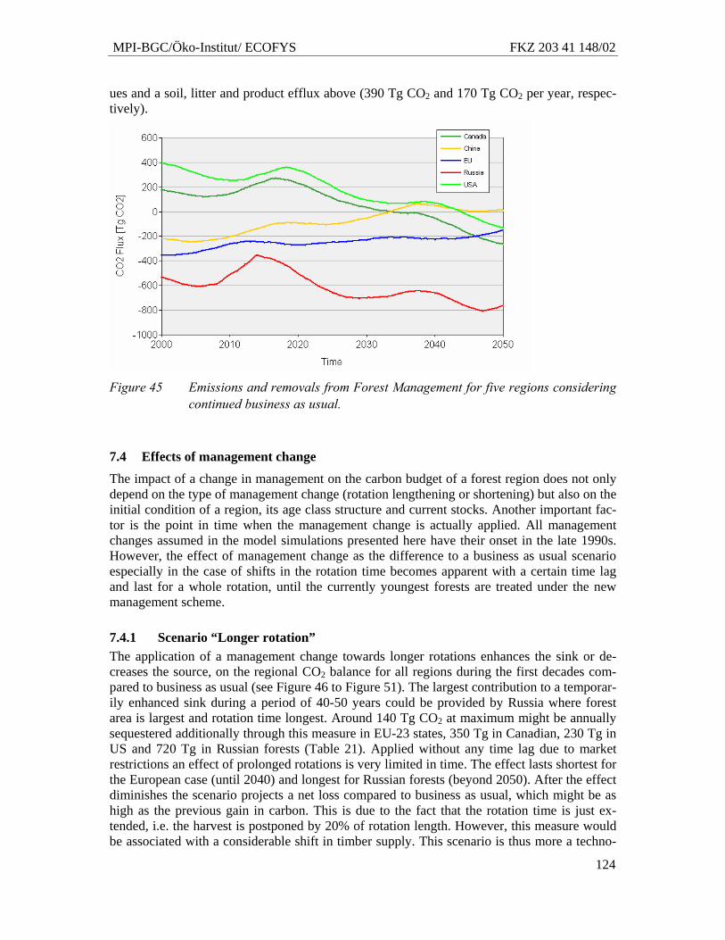
MPI-BGC/Öko-Institut/ ECOFYS FKZ 203 41 148/02
124
ues and a soil, litter and product efflux above (390 Tg CO2 and 170 Tg CO2 per year, respec-tively).
Figure 45 Emissions and removals from Forest Management for five regions considering
continued business as usual.
7.4 Effects of management change
The impact of a change in management on the carbon budget of a forest region does not only depend on the type of management change (rotation lengthening or shortening) but also on the initial condition of a region, its age class structure and current stocks. Another important fac-tor is the point in time when the management change is actually applied. All management changes assumed in the model simulations presented here have their onset in the late 1990s. However, the effect of management change as the difference to a business as usual scenario especially in the case of shifts in the rotation time becomes apparent with a certain time lag and last for a whole rotation, until the currently youngest forests are treated under the new management scheme.
7.4.1 Scenario “Longer rotation” The application of a management change towards longer rotations enhances the sink or de-creases the source, on the regional CO2 balance for all regions during the first decades com-pared to business as usual (see Figure 46 to Figure 51). The largest contribution to a temporar-ily enhanced sink during a period of 40-50 years could be provided by Russia where forest area is largest and rotation time longest. Around 140 Tg CO2 at maximum might be annually sequestered additionally through this measure in EU-23 states, 350 Tg in Canadian, 230 Tg in US and 720 Tg in Russian forests (Table 21). Applied without any time lag due to market restrictions an effect of prolonged rotations is very limited in time. The effect lasts shortest for the European case (until 2040) and longest for Russian forests (beyond 2050). After the effect diminishes the scenario projects a net loss compared to business as usual, which might be as high as the previous gain in carbon. This is due to the fact that the rotation time is just ex-tended, i.e. the harvest is postponed by 20% of rotation length. However, this measure would be associated with a considerable shift in timber supply. This scenario is thus more a techno-
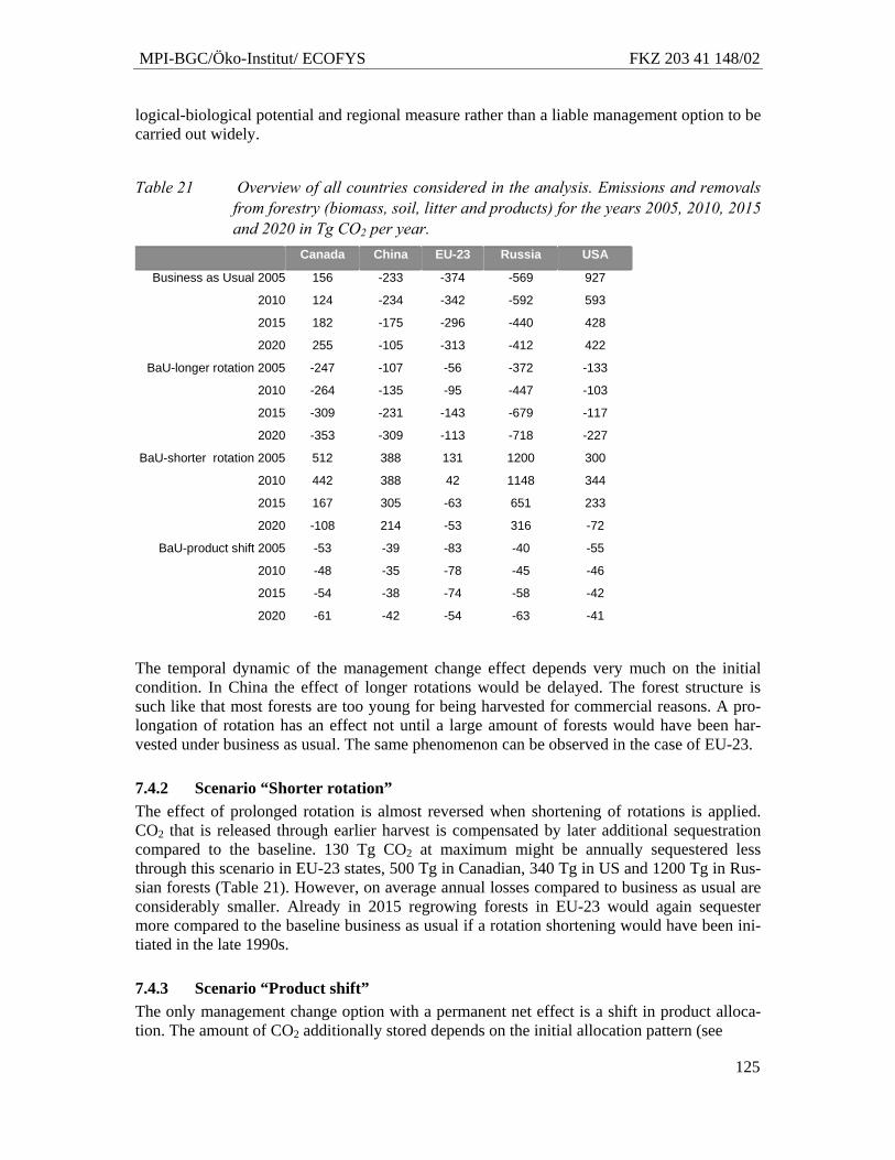
MPI-BGC/Öko-Institut/ ECOFYS FKZ 203 41 148/02
125
logical-biological potential and regional measure rather than a liable management option to be carried out widely.
Table 21 Overview of all countries considered in the analysis. Emissions and removals from forestry (biomass, soil, litter and products) for the years 2005, 2010, 2015 and 2020 in Tg CO2 per year.
Canada China EU-23 Russia USA
Business as Usual 2005 156 -233 -374 -569 927
2010 124 -234 -342 -592 593
2015 182 -175 -296 -440 428
2020 255 -105 -313 -412 422
BaU-longer rotation 2005 -247 -107 -56 -372 -133
2010 -264 -135 -95 -447 -103
2015 -309 -231 -143 -679 -117
2020 -353 -309 -113 -718 -227
BaU-shorter rotation 2005 512 388 131 1200 300
2010 442 388 42 1148 344
2015 167 305 -63 651 233
2020 -108 214 -53 316 -72
BaU-product shift 2005 -53 -39 -83 -40 -55
2010 -48 -35 -78 -45 -46
2015 -54 -38 -74 -58 -42
2020 -61 -42 -54 -63 -41
The temporal dynamic of the management change effect depends very much on the initial condition. In China the effect of longer rotations would be delayed. The forest structure is such like that most forests are too young for being harvested for commercial reasons. A pro-longation of rotation has an effect not until a large amount of forests would have been har-vested under business as usual. The same phenomenon can be observed in the case of EU-23.
7.4.2 Scenario “Shorter rotation” The effect of prolonged rotation is almost reversed when shortening of rotations is applied. CO2 that is released through earlier harvest is compensated by later additional sequestration compared to the baseline. 130 Tg CO2 at maximum might be annually sequestered less through this scenario in EU-23 states, 500 Tg in Canadian, 340 Tg in US and 1200 Tg in Rus-sian forests (Table 21). However, on average annual losses compared to business as usual are considerably smaller. Already in 2015 regrowing forests in EU-23 would again sequester more compared to the baseline business as usual if a rotation shortening would have been ini-tiated in the late 1990s.
7.4.3 Scenario “Product shift” The only management change option with a permanent net effect is a shift in product alloca-tion. The amount of CO2 additionally stored depends on the initial allocation pattern (see
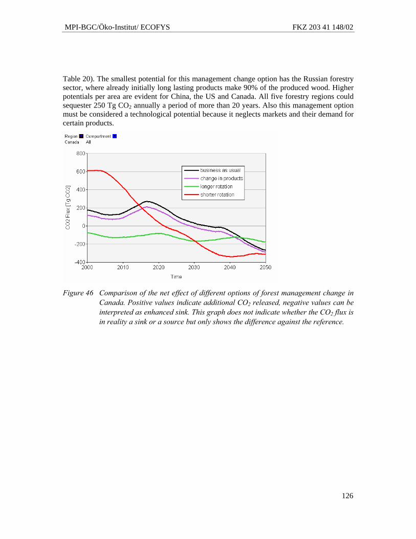
MPI-BGC/Öko-Institut/ ECOFYS FKZ 203 41 148/02
126
Table 20). The smallest potential for this management change option has the Russian forestry sector, where already initially long lasting products make 90% of the produced wood. Higher potentials per area are evident for China, the US and Canada. All five forestry regions could sequester 250 Tg CO2 annually a period of more than 20 years. Also this management option must be considered a technological potential because it neglects markets and their demand for certain products.
Figure 46 Comparison of the net effect of different options of forest management change in
Canada. Positive values indicate additional CO2 released, negative values can be interpreted as enhanced sink. This graph does not indicate whether the CO2 flux is in reality a sink or a source but only shows the difference against the reference.
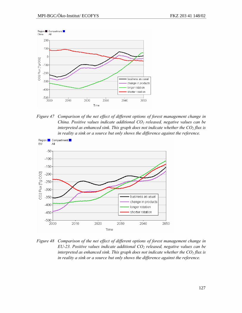
MPI-BGC/Öko-Institut/ ECOFYS FKZ 203 41 148/02
127
Figure 47 Comparison of the net effect of different options of forest management change in China. Positive values indicate additional CO2 released, negative values can be interpreted as enhanced sink. This graph does not indicate whether the CO2 flux is in reality a sink or a source but only shows the difference against the reference.
Figure 48 Comparison of the net effect of different options of forest management change in EU-23. Positive values indicate additional CO2 released, negative values can be interpreted as enhanced sink. This graph does not indicate whether the CO2 flux is in reality a sink or a source but only shows the difference against the reference.
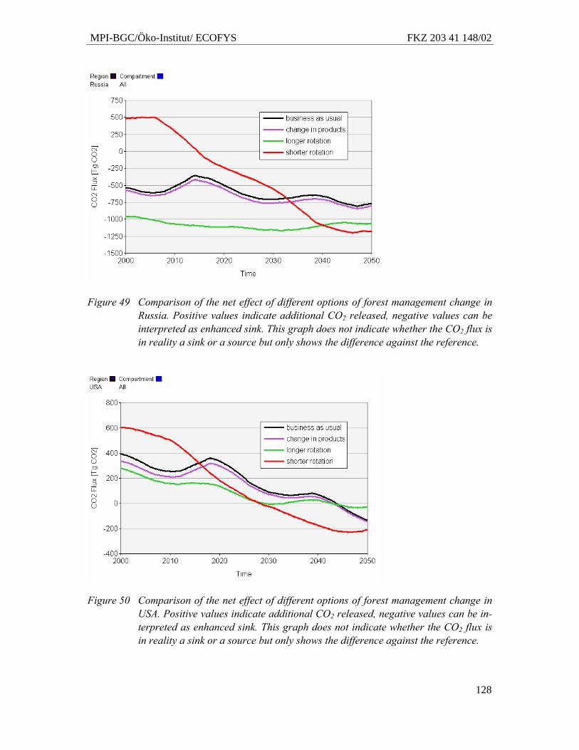
MPI-BGC/Öko-Institut/ ECOFYS FKZ 203 41 148/02
128
Figure 49 Comparison of the net effect of different options of forest management change in Russia. Positive values indicate additional CO2 released, negative values can be interpreted as enhanced sink. This graph does not indicate whether the CO2 flux is in reality a sink or a source but only shows the difference against the reference.
Figure 50 Comparison of the net effect of different options of forest management change in USA. Positive values indicate additional CO2 released, negative values can be in-terpreted as enhanced sink. This graph does not indicate whether the CO2 flux is in reality a sink or a source but only shows the difference against the reference.
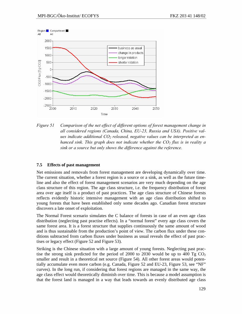
MPI-BGC/Öko-Institut/ ECOFYS FKZ 203 41 148/02
129
Figure 51 Comparison of the net effect of different options of forest management change in all considered regions (Canada, China, EU-23, Russia and USA). Positive val-ues indicate additional CO2 released, negative values can be interpreted as en-hanced sink. This graph does not indicate whether the CO2 flux is in reality a sink or a source but only shows the difference against the reference.
7.5 Effects of past management
Net emissions and removals from forest management are developing dynamically over time. The current situation, whether a forest region is a source or a sink, as well as the future time-line and also the effect of forest management scenarios are very much depending on the age class structure of this region. The age class structure, i.e. the frequency distribution of forest area over age itself is a product of past practices. The age class structure of Chinese forests reflects evidently historic intensive management with an age class distribution shifted to young forests that have been established only some decades ago. Canadian forest structure discovers a late onset of exploitation.
The Normal Forest scenario simulates the C balance of forests in case of an even age class distribution (neglecting past practise effects). In a “normal forest” every age class covers the same forest area. It is a forest structure that supplies continuously the same amount of wood and is thus sustainable from the production’s point of view. The carbon flux under these con-ditions subtracted from carbon fluxes under business as usual reveals the effect of past prac-tises or legacy effect (Figure 52 and Figure 53).
Striking is the Chinese situation with a large amount of young forests. Neglecting past prac-tise the strong sink predicted for the period of 2000 to 2030 would be up to 400 Tg CO2 smaller and result in a theoretical net source (Figure 54). All other forest areas would poten-tially accumulate even more carbon (e.g. Canada, Figure 52 and EU-23, Figure 53, see “NF” curves). In the long run, if considering that forest regions are managed in the same way, the age class effect would theoretically diminish over time. This is because a model assumption is that the forest land is managed in a way that leads towards an evenly distributed age class
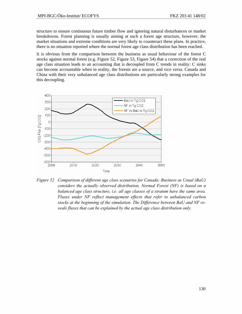
MPI-BGC/Öko-Institut/ ECOFYS FKZ 203 41 148/02
130
structure to ensure continuous future timber flow and ignoring natural disturbances or market breakdowns. Forest planning is usually aiming at such a forest age structure, however, the market situations and extreme conditions are very likely to counteract these plans. In practice, there is no situation reported where the normal forest age class distribution has been reached.
It is obvious from the comparison between the business as usual behaviour of the forest C stocks against normal forest (e.g. Figure 52, Figure 53, Figure 54) that a correction of the real age class situation leads to an accounting that is decoupled from C trends in reality: C sinks can become accountable when in reality, the forests are a source, and vice versa. Canada and China with their very unbalanced age class distributions are particularly strong examples for this decoupling.
Figure 52 Comparison of different age class scenarios for Canada: Business as Usual (BaU)
considers the actually observed distribution, Normal Forest (NF) is based on a balanced age class structure, i.e. all age classes of a stratum have the same area. Fluxes under NF reflect management effects that refer to unbalanced carbon stocks at the beginning of the simulation. The Difference between BaU and NF re-veals fluxes that can be explained by the actual age class distribution only.
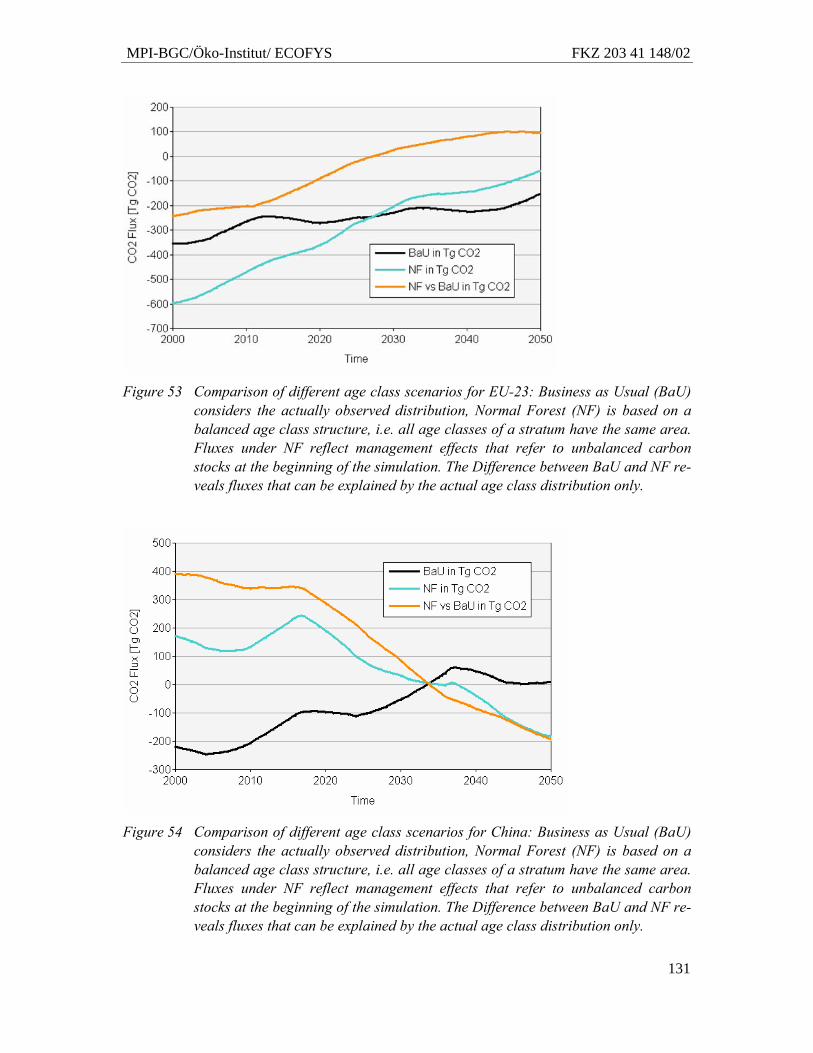
MPI-BGC/Öko-Institut/ ECOFYS FKZ 203 41 148/02
131
Figure 53 Comparison of different age class scenarios for EU-23: Business as Usual (BaU)
considers the actually observed distribution, Normal Forest (NF) is based on a balanced age class structure, i.e. all age classes of a stratum have the same area. Fluxes under NF reflect management effects that refer to unbalanced carbon stocks at the beginning of the simulation. The Difference between BaU and NF re-veals fluxes that can be explained by the actual age class distribution only.
Figure 54 Comparison of different age class scenarios for China: Business as Usual (BaU)
considers the actually observed distribution, Normal Forest (NF) is based on a balanced age class structure, i.e. all age classes of a stratum have the same area. Fluxes under NF reflect management effects that refer to unbalanced carbon stocks at the beginning of the simulation. The Difference between BaU and NF re-veals fluxes that can be explained by the actual age class distribution only.
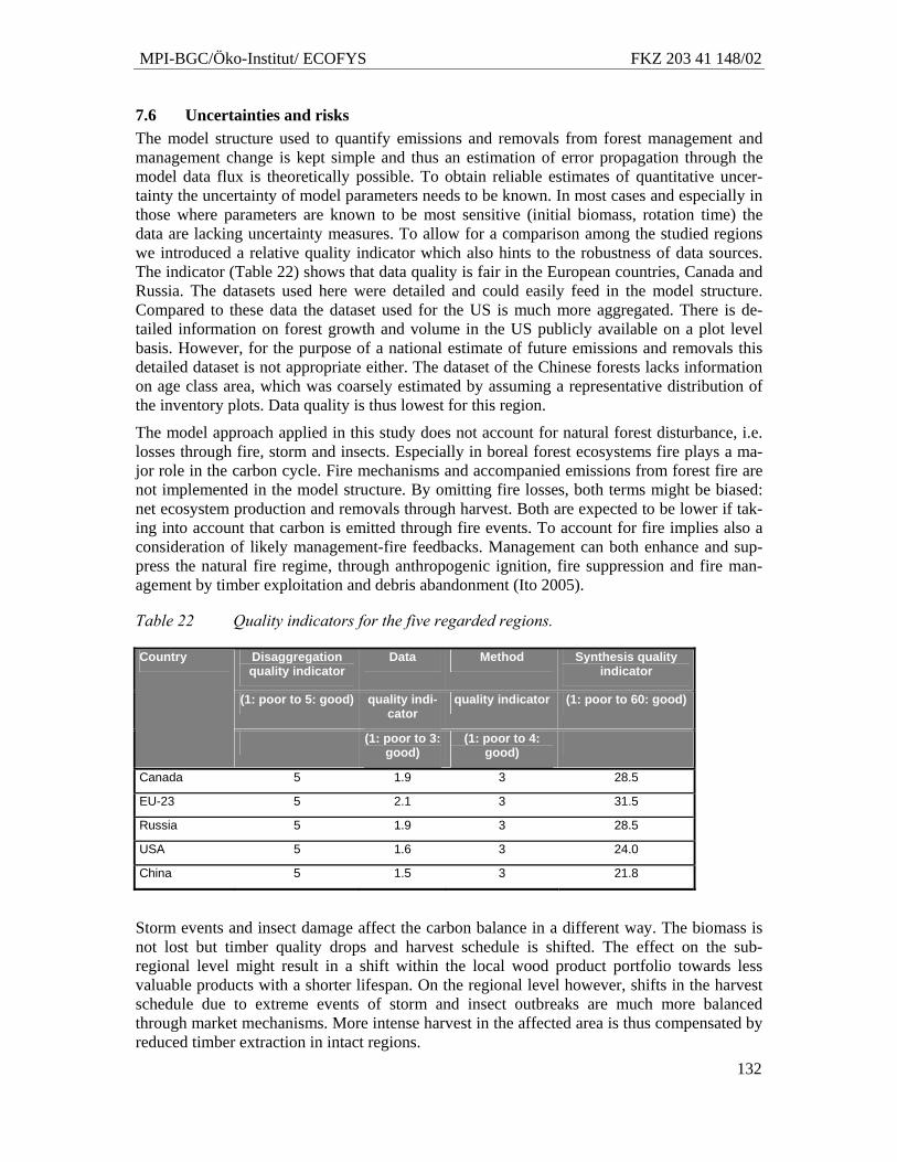
MPI-BGC/Öko-Institut/ ECOFYS FKZ 203 41 148/02
132
7.6 Uncertainties and risks The model structure used to quantify emissions and removals from forest management and management change is kept simple and thus an estimation of error propagation through the model data flux is theoretically possible. To obtain reliable estimates of quantitative uncer-tainty the uncertainty of model parameters needs to be known. In most cases and especially in those where parameters are known to be most sensitive (initial biomass, rotation time) the data are lacking uncertainty measures. To allow for a comparison among the studied regions we introduced a relative quality indicator which also hints to the robustness of data sources. The indicator (Table 22) shows that data quality is fair in the European countries, Canada and Russia. The datasets used here were detailed and could easily feed in the model structure. Compared to these data the dataset used for the US is much more aggregated. There is de-tailed information on forest growth and volume in the US publicly available on a plot level basis. However, for the purpose of a national estimate of future emissions and removals this detailed dataset is not appropriate either. The dataset of the Chinese forests lacks information on age class area, which was coarsely estimated by assuming a representative distribution of the inventory plots. Data quality is thus lowest for this region.
The model approach applied in this study does not account for natural forest disturbance, i.e. losses through fire, storm and insects. Especially in boreal forest ecosystems fire plays a ma-jor role in the carbon cycle. Fire mechanisms and accompanied emissions from forest fire are not implemented in the model structure. By omitting fire losses, both terms might be biased: net ecosystem production and removals through harvest. Both are expected to be lower if tak-ing into account that carbon is emitted through fire events. To account for fire implies also a consideration of likely management-fire feedbacks. Management can both enhance and sup-press the natural fire regime, through anthropogenic ignition, fire suppression and fire man-agement by timber exploitation and debris abandonment (Ito 2005).
Table 22 Quality indicators for the five regarded regions.
Disaggregation quality indicator
Data Method Synthesis quality indicator
(1: poor to 5: good) quality indi-cator
quality indicator (1: poor to 60: good)
Country
(1: poor to 3: good)
(1: poor to 4: good)
Canada 5 1.9 3 28.5
EU-23 5 2.1 3 31.5
Russia 5 1.9 3 28.5
USA 5 1.6 3 24.0
China 5 1.5 3 21.8
Storm events and insect damage affect the carbon balance in a different way. The biomass is not lost but timber quality drops and harvest schedule is shifted. The effect on the sub-regional level might result in a shift within the local wood product portfolio towards less valuable products with a shorter lifespan. On the regional level however, shifts in the harvest schedule due to extreme events of storm and insect outbreaks are much more balanced through market mechanisms. More intense harvest in the affected area is thus compensated by reduced timber extraction in intact regions.
MPI-BGC/Öko-Institut/ ECOFYS FKZ 203 41 148/02
133
7.7 Conclusions
Forests of the Northern Hemisphere currently form an annual sink of 1.2-1 Pg CO2. The re-sults point to a diminishing trend although the effect of disturbances was not included in the calculations. Management change can influence the development of sinks and sources both in the short and long run. The quantitative net effect of management change measures however, strongly depends on the observed time frame and is very dynamic with time. Prolongation of rotations first removes more CO2 from the atmosphere and later adds more CO2 to it, com-pared to a Business as Usual scenario.
Prolonging rotations could temporarily increase the forestry sink in the Northern Hemisphere by 25 Pg CO2 accumulated until 2020 which would account for 7% of fossil fuel emissions by these countries in the same period. However, the gain in comparison to business as usual is diminishing after 2020. Shifting wood product allocation to more long lasting products could result in a permanent storage of 5.3 Pg CO2 (2000 – 2020).
The results show that there is a huge dynamic in the development of sources and sinks from forest management over time. This dynamic is a result of age class structure and current man-agement applied. An impact of past practises is thus evident. However, accounting of such effects would make verification more complex.
The modelling results presented in this chapter (for results see Annex 2 and CD-Rom included in the report) do not provide sufficiently exact information for short time periods and on abso-lute levels for each country for the baseline in the politically relevant period between 1990 and 2020. However the modelling results do provide relevant information on trends, longer-term effects and potential contributions of forest management activities and allow distinguish-ing between the effects of past and present forest management.
7.8 Acknowledgements We would like to thank Youmin Chen (MPI BGC Jena) for help with the climate dataset for Europe, Shaoqiang Wang (CERN) for providing Chinese forestry and climate data, Gert-Jan Nabuurs (EFI) for providing the EFISCEN database.
MPI-BGC/Öko-Institut/ ECOFYS FKZ 203 41 148/02
134
8 Cropland management
8.1 Introduction
8.1.1 Definition of cropland management
According to MA Annex A.1.g, “Cropland management” is the system of practices that has taken place since 1 January 1990 on land on which agricultural crops are grown and on land that is set aside or temporarily not being used for crop production (FCCC/CP/2001/2/Add.3/Rev.1).
8.1.2 Impact of cropland management on the carbon cycle
Cropland is characterized by low biomass C stocks with high turnover rates except for trees in agroforestry systems. Cultivation of soils generally depletes soil organic carbon (SOC) stocks by disruption of soil aggregates, intensified aeration and low return of organic carbon in resi-dues. Cropland soils usually have the lowest SOC stocks of all possible land uses.
Carbon can be sequestered on cropland by
• increasing C input to soil by higher productivity through intensification and plant breeding, deep-rooting crops, crop residues, intercrops and organic amendments
• reducing mechanical soil disturbance by conservation tillage
• increasing woody biomass in agroforestry.
Carbon sequestration by agricultural activities is associated with higher uncertainty and risks than by forestry activities because management decisions in agriculture act over much shorter time scales. Agriculture is subject to high pressure by short-term changes in global markets, trades and tariffs and political frame conditions. Pressure on land is rising through a growing world population and higher living standards, driving the demand for food, feed, fibre as well as bioenergy. Due to this complexity the potential C sequestration and releases from agricul-tural areas can only be estimated in a relatively rough, simplified way.
Unlike in forests other GHGs than CO2 play an important role in croplands. The use of fertil-iser, organic amendments and nitrogen fixing crops stimulates emissions of N2O and NO. Flooding of rice paddies produces CH4. The effectiveness of climate change mitigation meas-ures on cropland can only be adequately assessed by a full greenhouse gas budget.
8.2 Material and methods
In this study, we consider changes between broad cropland management categories of differ-ent intensity and soil preparation. The analysis focuses on soils as the main C pool in agricul-tural systems. Data are taken from national statistics, FAO, IPCC, expert knowledge and syn-thesis of scientific literature, complemented by modelling where necessary. Scenarios of the technical potential for C sequestration (Chapter 5) in cropland soils are calculated.
8.2.1 Model The C sequestration and loss potential by cropland management is determined by the IPCC GPG Soil Tool (IPCC GPG, equation 3.3.3) as shown in Equation 5 and Equation 6. The C
MPI-BGC/Öko-Institut/ ECOFYS FKZ 203 41 148/02
135
stock changes refer to mineral soil to a depth of 30 cm. The types of land use and management factors supplied are very broadly defined and include: 1) a land use factor (FLU) that reflects C stock changes associated with type of land use, 2) a management factor (FMG) that for perma-nent cropland represents different types of tillage and 3) an input factor (FI) representing dif-ferent levels of C inputs to soil. For cropland, FLU describes base C stocks for long-term culti-vated soils, relative to native (uncultivated) soil C stocks. Annual rates of emissions (source) or removals (sink) are calculated as the difference in stocks (over time) divided by the default time period T of 20 years.
Equation 5 Soil C stocks in cropland dependent on climate, soil, management and tillage
SOC = SOCREF ● FLU ● FMG ● FI
with SOC = soil carbon stock, tonnes C ha-1 SOCREF = reference soil carbon stock, tonnes C ha-1 FLU = stock change factor for land use or land-use change type, dimensionless FMG = stock change factor for management regime, dimensionless FI = stock change factor for input of organic matter, dimensionless
Default values are given in IPCC GPG Table 3.3.3 and Table 3.3.4
Equation 6 Soil C stock changes in cropland after management change
ΔCCCMineral = [(SOC0 – SOC(0 –T) ● A] / T
with ΔCCCMineral = annual change in carbon stocks in mineral soils, tonnes C yr-1 SOC0 = soil organic carbon stock in the inventory year, tonnes C ha-1 SOC(0 –T) = soil organic carbon stock T years prior to the inventory, tonnes C ha-1 T = inventory time period, yr (here: 20 years) A = land area of each parcel, ha
8.2.2 Data and assumptions
Cropland area
Cropland area was derived from FAO statistical database on agriculture9 and defined as the land use area of arable land without the area under paddy rice10 for the year 2002.
Soil type and climate regime
The IPCC Soil Tool requires a coarse classification of soils according to their intrinsic carbon storage capacity and a coarse classification of climate zones. The database in the IPCC Soil Tool contains national areal fractions of the climate zones. We used a global cropland distri-bution map and the national fractional area of cropland derived from the FAO statistical data- 9 http://faostat.fao.org/faostat/form?collection=LandUse&Domain=Land&servlet=1&hasbulk=&version=ext&language=EN 10 http://faostat.fao.org/faostat/form?collection=Production.Crops.Primary&Domain=Production&servlet=1&hasbulk=&version=ext&language=EN
MPI-BGC/Öko-Institut/ ECOFYS FKZ 203 41 148/02
136
base was to determine for each country the dominant climate zones in areas with significant cropland. For most countries one climate zone was clearly dominant and used as the only cli-mate zone. Russia was split into two climate zones, China and USA into three, and India into four climate zones. The FAO World Soil Reference Base (FAO, ISRIC, ISSS 1998) was used to determine the dominant soil class for each country and climate zone (e.g. low-activity clay, high-activity clay, sand).
Management regime (input for factor FI)
The management regime distinguishes four classes: low input, medium input, high input without manure, and high input with manure. The fraction of cropland per country under a given management regime was calculated as follows:
Low and medium input: For developing countries, farm area was grouped by farm size. We assume that holdings <10 ha manage land with low input while larger farms manage with me-dium input. The 10 ha boundary relies on an expert estimate based on average farm size in private individual ownership (from FAO World Census of Agriculture26) and degree of mechanisation. It is assumed here that, unless other information was found, in developing countries, tillage by hand and draught animals occurs in low input small-holder farms, while tractor use goes along medium input in larger farms. The 10 ha boundary is subject to high uncertainty but corroborated by tillage information.
Farm size distribution was taken from FAO World Census of Agriculture11. For each country, the most recent available census data was used, reflecting the situation around the year 2000 or 1990. Farm size distribution for countries without census information was estimated by regional means (Northern, Western, Eastern, Southern Africa, Former USSR, Middle East, South Asia, East Asia; South East Asia; Japan, South America, Central America).
High input without manure was set as default land use intensity for developed countries.
High input with manure: It is assumed that manure is collected from housed cattle, horses, pigs and poultry in developed countries. Animal numbers are taken from FAOSTAT data-base12. The fractions of housed animals per animal category were set at 100% for horses, pigs and poultry by expert judgement. This assumption is valid for most types of intensive farming of these animal types, which also contribute to a minor extent to manure available for spread-ing. Conditions for cattle farmin are more variable. Therefore, country-specific literature was used for estimating the fraction of housed cattle. In Canada13 and European countries, national estimated fractions of manure spread on cropland (Freibauer and Kaltschmitt 2001) were available. Elsewhere it is assumed as reference that 50% of the manure is spread on cropland and 50% on grassland, which is equivalent to the European average (Smith and Powlson 2000). The IPCC GPG Soil Tool relies on a default proportional increase of soil C stocks when manure is applied on cropland. The input factor (FI) associated with manure in the IPCC GPG Soil Tool is relatively high (Freibauer, Rounsevell et al. 2004). This can only be realized by high input of animal manure per hectare, so we assume here that the maximum allowed amount of manure is spread per hectare. This is also justified by practical as well as economic considerations. Application rates are assumed to follow good agricultural practice and set at
11 http://www.fao.org/WAICENT/FAOINFO/ECONOMIC/ESS/census/wcares/default.asp 12 http://faostat.fao.org/faostat/form?collection=Production.Livestock.Stocks&Domain=Production&servlet=1& hasbulk =& version=ext&language=EN 13 Statistics Canada, Census of Agriculture, last modified: 2004-05-30. http://www40.statcan.ca/l01/cst01/agrc05a.htm
MPI-BGC/Öko-Institut/ ECOFYS FKZ 203 41 148/02
137
the maximum allowed amount in nitrate sensitive zones, which equals 2 livestock units in Europe. One livestock unit is equivalent to 1 cattle, 1 horse, 8.3 pigs, and 320 chicken. Con-sequently, the cropland area receiving manure can be calculated from the number of housed livestock units per country. In few countries with high animal numbers compared to cropland area, e.g. Netherlands, Switzerland and Iceland, the application rate of manure had to be in-creased in order to match the available cropland area.
Tillage (input for factor FMG)
No-till: Permanent no-till management is concentrated in the Americas, with Brazil, USA and Argentina accounting for 73% of the global no-till area. Reviews by Rolf Derpsch14 appear to be the only available global source of information, which is widely quoted and obviously well connected to regional no-till associations and the FAO. No-till is reported to be virtually ab-sent in Africa, Asia and little developed in Europe. National data sources were used for USA15 and European states16. Fraction of no-till cropland areas in Europe vary between 0 and 0.04 without any regional systematic feature. A default fraction of cropland under no-till of 0.0135 was assumed for European countries without data, being the average of European country reports. No information about Central America was found. Where national data were lacking in Asia, Africa, Central and South America the default fraction of no-till was set zero.
Reduced till: Unlike for no-till the data situation for reduced till is unclear. This is partly due to a variety of definitions and concepts about reduced till operations and incomplete knowl-edge about adoption of reduced till practices by farmers. We distinguish between two cases:
1. reduced till in all smallholder farms in developing countries, were resource limitation usually leads to infrequent or incomplete tillage: according to Derpsch, this is true for African smallholder farms below 2ha size. Here, we take the fraction of low input land that is not ploughed by animals.
2. reduced till as a soil conservation measure in all medium and high input cropland.
Data about farm size was taken from FAO World Census of Agriculture 2000 were available, or 1990 (see footnote 26). National data was used for European countries, USA and Canada as described for no-till.
Conventional till: It is assumed here that, unless other information was found, in developing countries, draught animals and tractors do conventional tillage, and the rest of the area is pre-pared by hand in reduced tillage. Conventional till occurs either
1. on low input croland by animals, or
2. on medium and high input by tractors.
14 Rolf Derpsch (1998), Historical Review on no-tillage cultivation of crops. Proceedings. The 1st JIRCAS Seminar on Soybean Research. No-tillage Cultivation and Future Research Needs. March 5-6, 1998, Iguassu Falls, Brazil, JIRCAS Working Report No. 13, p. 1-18; Rolf Derpsch (1999), Frontiers in Conservation Tillage and advances in Conservation Practice, Proceedings of hte 10th ISCO Conference, 24-28 May 1999, West La-fayette In.http://www.rolf-derpsch.com/ 15 Agricultural Resource Management Survey (ARMS), USDA, last updated November 2005. www.ers.usda/gov/arms/app/CropResponse.aspx 16 European Conservation Agriculture Federation (ECAF). http://www.ecaf.org/
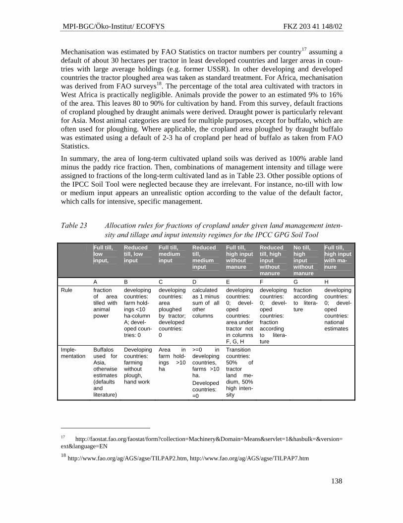
MPI-BGC/Öko-Institut/ ECOFYS FKZ 203 41 148/02
138
Mechanisation was estimated by FAO Statistics on tractor numbers per country17 assuming a default of about 30 hectares per tractor in least developed countries and larger areas in coun-tries with large average holdings (e.g. former USSR). In other developing and developed countries the tractor ploughed area was taken as standard treatment. For Africa, mechanisation was derived from FAO surveys18. The percentage of the total area cultivated with tractors in West Africa is practically negligible. Animals provide the power to an estimated 9% to 16% of the area. This leaves 80 to 90% for cultivation by hand. From this survey, default fractions of cropland ploughed by draught animals were derived. Draught power is particularly relevant for Asia. Most animal categories are used for multiple purposes, except for buffalo, which are often used for ploughing. Where applicable, the cropland area ploughed by draught buffalo was estimated using a default of 2-3 ha of cropland per head of buffalo as taken from FAO Statistics.
In summary, the area of long-term cultivated upland soils was derived as 100% arable land minus the paddy rice fraction. Then, combinations of management intensity and tillage were assigned to fractions of the long-term cultivated land as in Table 23. Other possible options of the IPCC Soil Tool were neglected because they are irrelevant. For instance, no-till with low or medium input appears an unrealistic option according to the value of the default factor, which calls for intensive, specific management.
Table 23 Allocation rules for fractions of cropland under given land management inten-sity and tillage and input intensity regimes for the IPCC GPG Soil Tool
Full till, low input,
Reduced till, low input
Full till, medium input
Reduced till, medium input
Full till, high input without manure
Reduced till, high input without manure
No till, high input without manure
Full till, high input with ma-nure
A B C D E F G H Rule fraction
of area tilled with animal power
developing countries: farm hold-ings <10 ha-column A; devel-oped coun-tries: 0
developing countries: area ploughed by tractor; developed countries: 0
calculated as 1 minus sum of all other columns
developing countries: 0; devel-oped countries: area under tractor not in columns F, G, H
developing countries: 0; devel-oped countries: fraction according to litera-ture
fraction according to litera-ture
developing countries: 0; devel-oped countries: national estimates
Imple-mentation
Buffalos used for Asia, otherwise estimates (defaults and literature)
Developing countries: farming without plough, hand work
Area in farm hold-ings >10 ha
>=0 in developing countries, farms >10 ha. Developed countries: =0
Transition countries: 50% of tractor land me-dium, 50% high inten-sity
17 http://faostat.fao.org/faostat/form?collection=Machinery&Domain=Means&servlet=1&hasbulk=&version= ext&language=EN 18 http://www.fao.org/ag/AGS/agse/TILPAP2.htm, http://www.fao.org/ag/AGS/agse/TILPAP7.htm
MPI-BGC/Öko-Institut/ ECOFYS FKZ 203 41 148/02
139
Set-aside land was disregarded due to inadequate information about areas and inconsistent use of the term “set-aside” as long-term or short-term fallow so that the areas could not be linked to the IPCC defaults.
8.2.3 Uncertainty estimates
Data sources hardly record uncertainties. Therefore, a quantitative estimate of uncertainties is impossible. However, a qualitative scale was developed indicating the data source, method and data quality, which can be combined to a semi-quantitative indicator of uncertainty I in the estimate as described in chapter 7.2.5 (Equation 3, Table 18). As in all cases, a coarse na-tional resolution and the same IPCC default method was used differences in the quality indi-cator only reflect the quality of the activity data to estimate prevailing cropland management. Industrial countries, countries in transition and croplands managed at medium to high input have fairly reliable activity data at national level. Activity data for most developing countries and Russia, however, are highly uncertain and rely on coarse regional aggregated information or expert judgement. Results for the latter countries have to be treated with caution as indica-tive numbers only.
The results in chapter 8.4 give mean estimated C stock changes and a range that neglect these uncertainties in activity data. The range indicates low and high estimates using the lower and upper values of the error in the stock change factors of Equation 5 reported in (IPCC 2004). These ranges have been derived from modelling where possible and can be considered rela-tively robust.
8.2.4 Scenarios It is assumed by default that croplands are in equilibrium under present management so that carbon stock changes on croplands are zero under business as usual. Five groups of scenarios were defined. Each group consists of (a) an extreme scenario equivalent to the technical po-tential assuming complete prompt implementation of the management change, and (b) a mod-erate, more realistic scenario of gradual adoption of the management change, which represents a moderate economic to realistic potential (Chapter 8). The scenarios are defined as follows (Figure 55):
Scenario “Mechanisation”: Mechanisation in developing countries
This scenario assumes an increase in full tillage by animal draught power or tractor without increased input of fertilizer or organic residues on land that is currently managed by hand. This scenario is likely to happen as business as usual in some regions of the world. The calcu-lation is performed by shifting the management stratum “Reduced till, low input” (Table 23 column B) to “Full till, low input” (Table 23 column A).
• Scenario “Mechanisation: tech. pot.”: extreme case: immediate shift on 100% of hand-tilled land
• Scenario “Mechanisation: econ. pot.”: moderate case: shift on 10% hand-tilled land every 20 years, equivalent with a linear increase of mechanisation on 0.5% of present hand-tilled land per year.
Scenario “Intensification”: Intensification in developing countries
MPI-BGC/Öko-Institut/ ECOFYS FKZ 203 41 148/02
140
This scenario assumes an increase in full tillage by tractor and simultaneous increase of fer-tilization and return of organic residues on current low-input cropland. This scenario is likely to happen as business as usual in some regions of the world. The calculation is performed by shifting the management strata “Low input” (Table 23 columns A + B) to “Full till, medium input” (Table 23 column C).
• Scenario “Intensification: tech. pot.”: extreme case: immediate shift on 100% of low-input land
• Scenario“Intensification: econ. pot.”: moderate case: shift on 10% low-input land every 20 years, equivalent with a linear increase of intensification on 0.5% of present low-input land per year.
This scenario includes intensification of fertilizer use and increased nitrogen input to soil, which will in turn lead to higher N2O emissions. Increased N2O emissions constitute a “leak-age” effect in this scenario that would be accounted for in the national GHG inventory. Here we disregard this effect due to lack of reliable information. The mitigation potential in this scenario has to be viewed as a high estimate.
Scenario “Conservation”: conservation tillage on most full-till cropland
This scenario assumes an expansion of conservation tillage without change in input on me-dium and high input cropland. This scenario is already happening as business as usual in some intensively managed regions of the world. The calculation is performed by shifting the man-agement strata “Full till, medium input” and “Full till, high input without manure” (Table 23 columns C and E) to “Reduced till, medium input” and “Reduced till, high input without ma-nure” (Table 23 columns D and F). The scenario is already partly being implemented as busi-ness as usual in developed countries but has also significant potential in less developed coun-tries.
• Scenario “Conservation: tech. pot.”: extreme case: immediate shift on 100% of full-till land with medium and high input
• Scenario “Conservation: econ. pot.”: moderate case: shift on 10% full-till land with medium and high input every 20 years, equivalent with a linear increase of conserva-tion tillage on 0.5% of present full-till land with medium and high input per year.
Scenario “No-till”: no-till on high-input cropland where possible
This scenario assumes an expansion of no-till cropping high input cropland without manure in all developed countries. This scenario is already happening as business as usual in some in-tensively managed regions of the world. Between 2003 and 2005, the area under no-till has increased globally by 25 million hectares and now amounts to 95 million hectares19. No-till management is very common in the Americas but elsewhere mainly applied in an intermittent mode to some crops during the crop rotation. The calculation is performed by shifting the management strata “Full till, high input without manure” and “Reduced till, high input with-out manure” where necessary (Table 23 columns E and F) to “No-till, high input without ma-nure” (Table 23 column G). There is evidence that no-till can lead to higher N2O emissions. These emissions are not yet incorporated in national GHG inventories but will lower the ef-fectiveness of no-till as mitigation measure ((Smith, Goulding et al. 2001)).
19 http://www.rolf-derpsch.com/
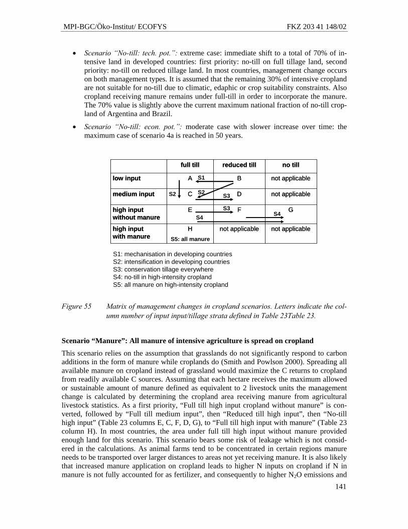
MPI-BGC/Öko-Institut/ ECOFYS FKZ 203 41 148/02
141
• Scenario “No-till: tech. pot.”: extreme case: immediate shift to a total of 70% of in-tensive land in developed countries: first priority: no-till on full tillage land, second priority: no-till on reduced tillage land. In most countries, management change occurs on both management types. It is assumed that the remaining 30% of intensive cropland are not suitable for no-till due to climatic, edaphic or crop suitability constraints. Also cropland receiving manure remains under full-till in order to incorporate the manure. The 70% value is slightly above the current maximum national fraction of no-till crop-land of Argentina and Brazil.
• Scenario “No-till: econ. pot.”: moderate case with slower increase over time: the maximum case of scenario 4a is reached in 50 years.
Figure 55 Matrix of management changes in cropland scenarios. Letters indicate the col-umn number of input input/tillage strata defined in Table 23Table 23.
Scenario “Manure”: All manure of intensive agriculture is spread on cropland
This scenario relies on the assumption that grasslands do not significantly respond to carbon additions in the form of manure while croplands do (Smith and Powlson 2000). Spreading all available manure on cropland instead of grassland would maximize the C returns to cropland from readily available C sources. Assuming that each hectare receives the maximum allowed or sustainable amount of manure defined as equivalent to 2 livestock units the management change is calculated by determining the cropland area receiving manure from agricultural livestock statistics. As a first priority, “Full till high input cropland without manure” is con-verted, followed by “Full till medium input”, then “Reduced till high input”, then “No-till high input” (Table 23 columns E, C, F, D, G), to “Full till high input with manure” (Table 23 column H). In most countries, the area under full till high input without manure provided enough land for this scenario. This scenario bears some risk of leakage which is not consid-ered in the calculations. As animal farms tend to be concentrated in certain regions manure needs to be transported over larger distances to areas not yet receiving manure. It is also likely that increased manure application on cropland leads to higher N inputs on cropland if N in manure is not fully accounted for as fertilizer, and consequently to higher N2O emissions and
not applicablenot applicableHhigh input with manure
GFEhigh inputwithout manure
not applicableDCmedium input
not applicableBAlow input
no tillreduced tillfull till
not applicablenot applicableHhigh input with manure
GFEhigh inputwithout manure
not applicableDCmedium input
not applicableBAlow input
no tillreduced tillfull till
S1: mechanisation in developing countriesS2: intensification in developing countriesS3: conservation tillage everywhereS4: no-till in high-intensity croplandS5: all manure on high-intensity cropland
S1
S2 S3
S3S4S4
S5: all manure
S2
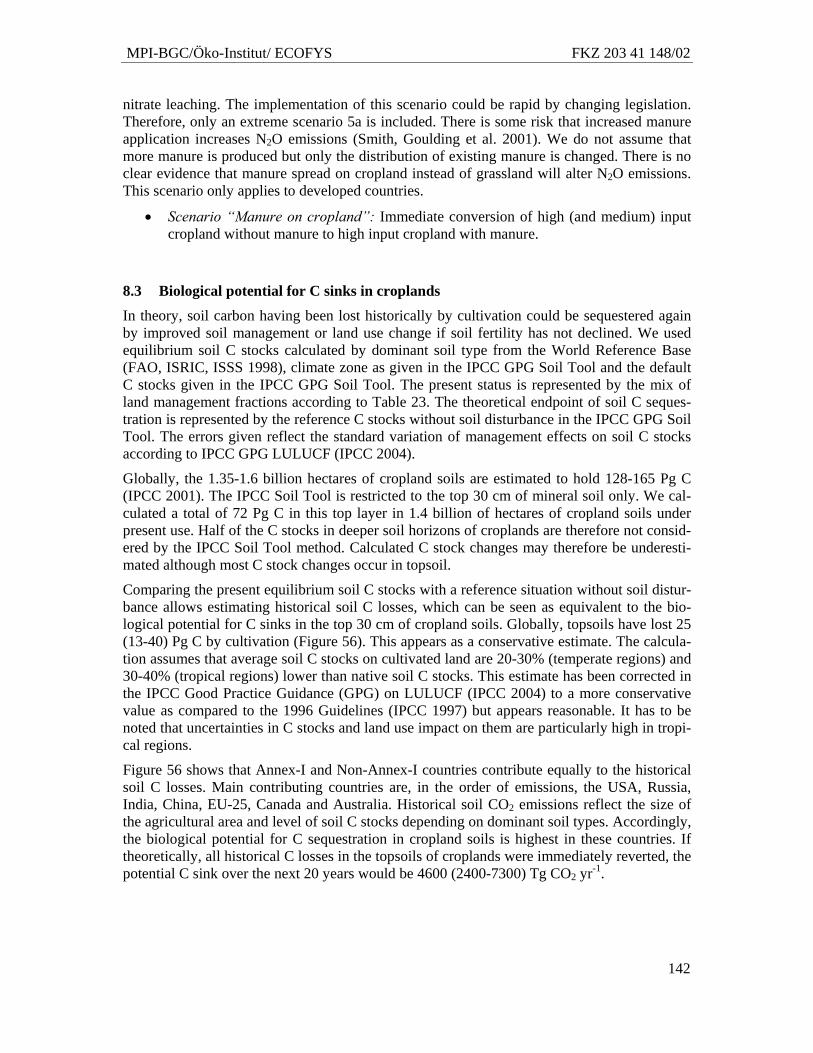
MPI-BGC/Öko-Institut/ ECOFYS FKZ 203 41 148/02
142
nitrate leaching. The implementation of this scenario could be rapid by changing legislation. Therefore, only an extreme scenario 5a is included. There is some risk that increased manure application increases N2O emissions (Smith, Goulding et al. 2001). We do not assume that more manure is produced but only the distribution of existing manure is changed. There is no clear evidence that manure spread on cropland instead of grassland will alter N2O emissions. This scenario only applies to developed countries.
• Scenario “Manure on cropland”: Immediate conversion of high (and medium) input cropland without manure to high input cropland with manure.
8.3 Biological potential for C sinks in croplands
In theory, soil carbon having been lost historically by cultivation could be sequestered again by improved soil management or land use change if soil fertility has not declined. We used equilibrium soil C stocks calculated by dominant soil type from the World Reference Base (FAO, ISRIC, ISSS 1998), climate zone as given in the IPCC GPG Soil Tool and the default C stocks given in the IPCC GPG Soil Tool. The present status is represented by the mix of land management fractions according to Table 23. The theoretical endpoint of soil C seques-tration is represented by the reference C stocks without soil disturbance in the IPCC GPG Soil Tool. The errors given reflect the standard variation of management effects on soil C stocks according to IPCC GPG LULUCF (IPCC 2004).
Globally, the 1.35-1.6 billion hectares of cropland soils are estimated to hold 128-165 Pg C (IPCC 2001). The IPCC Soil Tool is restricted to the top 30 cm of mineral soil only. We cal-culated a total of 72 Pg C in this top layer in 1.4 billion of hectares of cropland soils under present use. Half of the C stocks in deeper soil horizons of croplands are therefore not consid-ered by the IPCC Soil Tool method. Calculated C stock changes may therefore be underesti-mated although most C stock changes occur in topsoil.
Comparing the present equilibrium soil C stocks with a reference situation without soil distur-bance allows estimating historical soil C losses, which can be seen as equivalent to the bio-logical potential for C sinks in the top 30 cm of cropland soils. Globally, topsoils have lost 25 (13-40) Pg C by cultivation (Figure 56). This appears as a conservative estimate. The calcula-tion assumes that average soil C stocks on cultivated land are 20-30% (temperate regions) and 30-40% (tropical regions) lower than native soil C stocks. This estimate has been corrected in the IPCC Good Practice Guidance (GPG) on LULUCF (IPCC 2004) to a more conservative value as compared to the 1996 Guidelines (IPCC 1997) but appears reasonable. It has to be noted that uncertainties in C stocks and land use impact on them are particularly high in tropi-cal regions.
Figure 56 shows that Annex-I and Non-Annex-I countries contribute equally to the historical soil C losses. Main contributing countries are, in the order of emissions, the USA, Russia, India, China, EU-25, Canada and Australia. Historical soil CO2 emissions reflect the size of the agricultural area and level of soil C stocks depending on dominant soil types. Accordingly, the biological potential for C sequestration in cropland soils is highest in these countries. If theoretically, all historical C losses in the topsoils of croplands were immediately reverted, the potential C sink over the next 20 years would be 4600 (2400-7300) Tg CO2 yr-1.
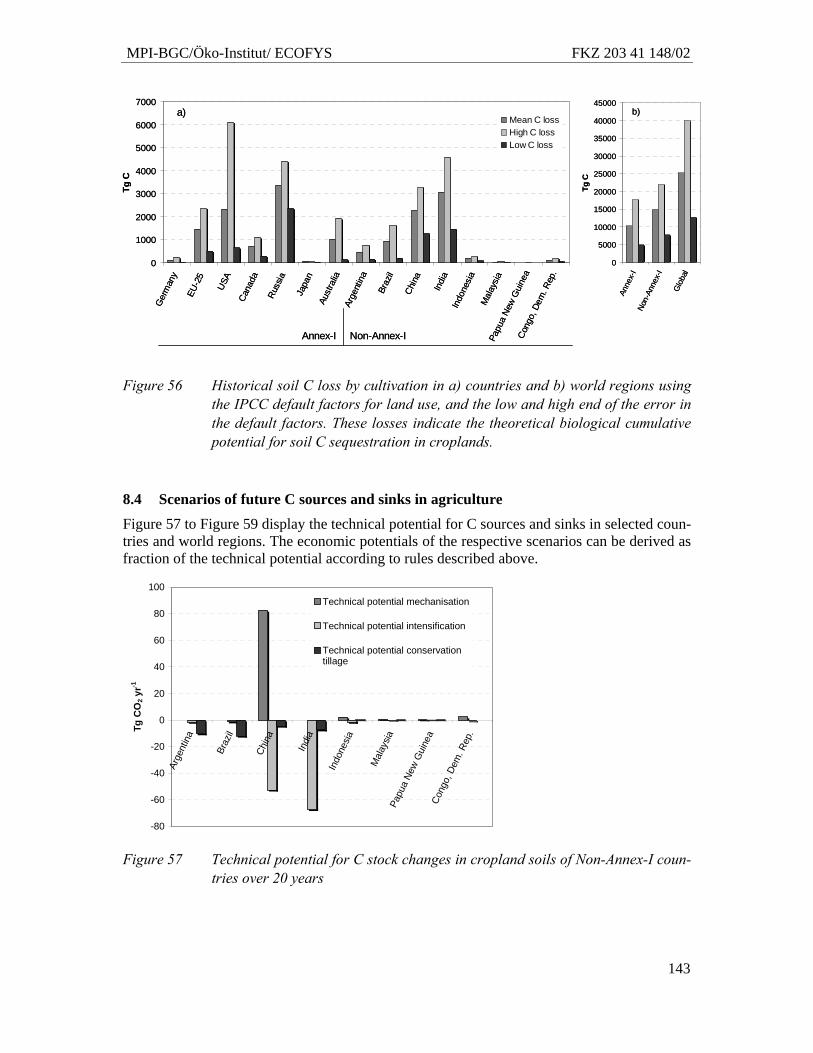
MPI-BGC/Öko-Institut/ ECOFYS FKZ 203 41 148/02
143
Figure 56 Historical soil C loss by cultivation in a) countries and b) world regions using the IPCC default factors for land use, and the low and high end of the error in the default factors. These losses indicate the theoretical biological cumulative potential for soil C sequestration in croplands.
8.4 Scenarios of future C sources and sinks in agriculture
Figure 57 to Figure 59 display the technical potential for C sources and sinks in selected coun-tries and world regions. The economic potentials of the respective scenarios can be derived as fraction of the technical potential according to rules described above.
Figure 57 Technical potential for C stock changes in cropland soils of Non-Annex-I coun-tries over 20 years
0
1000
2000
3000
4000
5000
6000
7000
Ger
man
y
EU-2
5
USA
Cana
da
Russ
ia
Japa
nAu
stra
liaAr
gent
ina
Braz
il
Chin
a
Indi
aIn
done
siaM
alay
siaPa
pua
New
Gui
nea
Cong
o, D
em. R
ep.
Tg C
Mean C lossHigh C lossLow C loss
Annex-I Non-Annex-I
a)
0
5000
10000
15000
20000
25000
30000
35000
40000
45000
Anne
x-I
Non-
Anne
x-I
Glo
bal
Tg C
b)
0
1000
2000
3000
4000
5000
6000
7000
Ger
man
y
EU-2
5
USA
Cana
da
Russ
ia
Japa
nAu
stra
liaAr
gent
ina
Braz
il
Chin
a
Indi
aIn
done
siaM
alay
siaPa
pua
New
Gui
nea
Cong
o, D
em. R
ep.
Tg C
Mean C lossHigh C lossLow C loss
Annex-I Non-Annex-I
a)
0
5000
10000
15000
20000
25000
30000
35000
40000
45000
Anne
x-I
Non-
Anne
x-I
Glo
bal
Tg C
b)
-80
-60
-40
-20
0
20
40
60
80
100
Arge
ntin
a
Braz
il
Chin
a
Indi
a
Indo
nesia
Mal
aysia
Papu
a Ne
w G
uine
aCo
ngo,
Dem
. Rep
.Tg C
O2 y
r-1
Technical potential mechanisation
Technical potential intensification
Technical potential conservationtillage
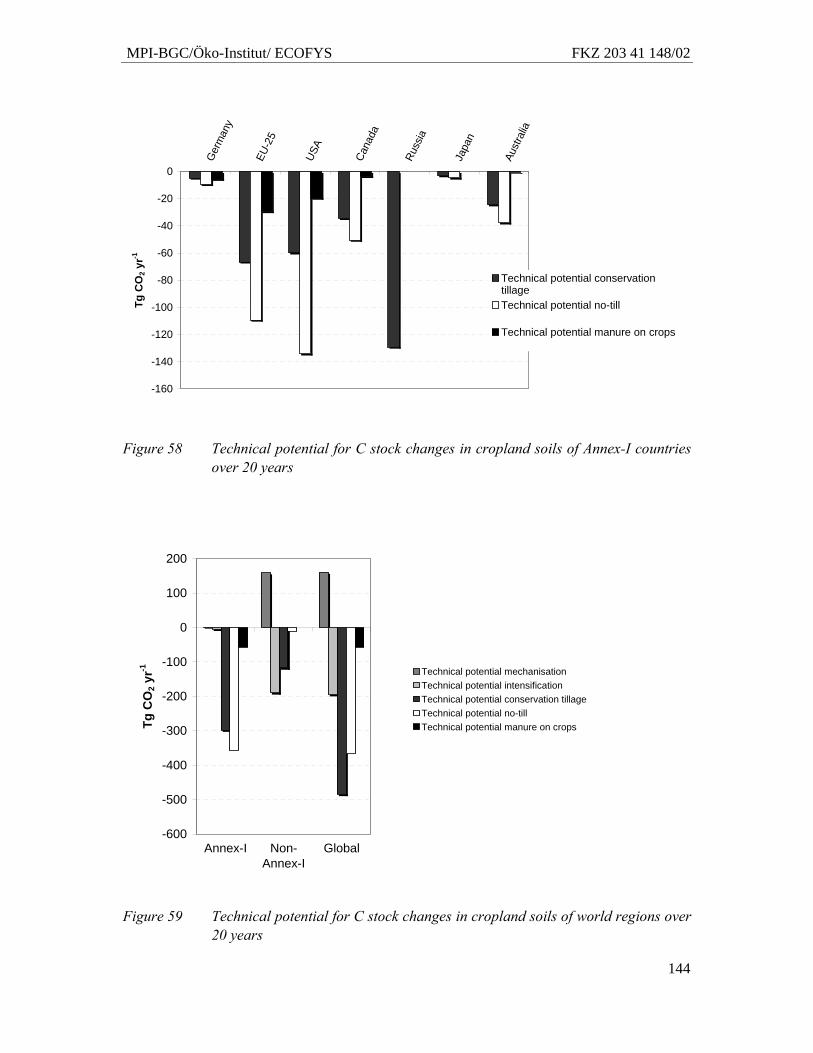
MPI-BGC/Öko-Institut/ ECOFYS FKZ 203 41 148/02
144
Figure 58 Technical potential for C stock changes in cropland soils of Annex-I countries over 20 years
Figure 59 Technical potential for C stock changes in cropland soils of world regions over 20 years
-600
-500
-400
-300
-200
-100
0
100
200
Annex-I Non-Annex-I
Global
Tg C
O2 y
r-1 Technical potential mechanisationTechnical potential intensification Technical potential conservation tillageTechnical potential no-till Technical potential manure on crops
-160
-140
-120
-100
-80
-60
-40
-20
0
Ger
man
y
EU-2
5
USA
Cana
da
Russ
ia
Japa
n
Aust
ralia
Tg C
O2 y
r-1
Technical potential conservationtillageTechnical potential no-till
Technical potential manure on crops
MPI-BGC/Öko-Institut/ ECOFYS FKZ 203 41 148/02
145
8.4.1 Scenario “Mechanisation”
The largest losses have happened in the past. Present C stocks in croplands already represent a C-depleted situation. Against those C losses in the past, any further expected losses are likely to be relatively small. The most likely driver of further C losses is an increased tillage in low input agriculture as long as it is not associated with an intensification of other means of pro-duction (use of organic residues, fertilizer), and will, in the worst case (technical potential), if all low-input land was immediately ploughed, lead to C losses of 160 (125-200) Tg CO2 yr-1 (43 (34-55) Tg C yr-1) over the next 20 years in the top 30 cm of soil.
The scenario exclusively applies to Non-Annex-I countries (Figure 57, Figure 59). By far the most important source risk is in China, followed by smaller contributions from Nigeria, Ethiopia, Mexico, Iran and Sudan (data not shown, see data on CD-Rom included in the re-port). It can, however, not be verified whether the low degree of mechanisation derived from FAO draught animal and tractor data is indeed reflecting the present situation in China which is facing a dramatic intensification. China is among the countries with the poorest data on cropland activities. FAO data suggest that croplands in India are already ploughed by animal power or tractor.
The mechanisation scenario represents the most uncertain one because
• subsistence agriculture consists of a wide range of practices affecting soil C stocks
• statistics are extremely poor
• assumptions about national activity data are particularly uncertain.
Despite these caveats the scenario indicates a potential for further soil C losses in developing countries. Taking the economic potential as roughly 10% of the technical potential could give an indication of a likely business-as-usual trend of mechanisation associated with projected soil C losses of up to 20 Tg CO2 yr-1 over the next decades.
8.4.2 Scenario “Intensification” Management changes in the scenario “Intensification” consist of mechanisation as in the sce-nario “mechanisation” plus higher input of resources, fertilizer and increased productivity, which will lead to higher C input by residues into soil. It is assumed that in net terms, intensi-ficiation of low-input agriculture sequesters carbon.
The global technical potential is estimated at 200 (150-240) Tg CO2 yr-1 (50 (40-70) Tg C yr-1) over the next 20 years in the top 30 cm of soil. The range given in brackets indicates the standard deviation of the effect of management change assuming that the original C stock was in equilibrium and well known.
The potential is almost entirely located in Non-Annex-I countries (Figure 57, Figure 59) where intensification is happening at large scale. India (67 Tg CO2 yr-1) and China (53 Tg CO2 yr-1) together contribute more than half to the global potential. Further important poten-tial is located in North Africa and the Near East.
As in the mechanisation scenario, lack of data about the national management practices and the simplification across a wide range of different management practices introduce large un-certainties into the intensification scenario, which could not be quantified and are not reflected in the error range given above. The scenario is further complicated by increased N2O emis-sions, which have been excluded from the analysis.
MPI-BGC/Öko-Institut/ ECOFYS FKZ 203 41 148/02
146
Despite these caveats the scenario indicates a potential for C sequestration in developing countries. Taking the economic potential as roughly 10% of the technical potential could give an indication of a likely business-as-usual trend of intensification associated with projected soil C sequestration of up to 20 Tg CO2 yr-1 over the next decades.
8.4.3 Scenario “Conservation tillage”
Conservation tillage comprises a range of soil preparation measures which avoid intensive soil disturbance and usually drill a fraction of the residues into a shallow soil layer. Conservation tillage is already wide spread as a means to combat erosion and conserve water and can be applied in a wide range of soil conditions and crops.
Due to the large suitable cropland area for conservation tillage the global technical potential over the next 20 years in the top 30 cm of soil is high: 480 (400-560) Tg CO2 yr-1 (130 (110-150) Tg C yr-1).
The technical potential for C sequestration by conservation tillage is about twice as high in Annex-I countries than in Non-Annex-I countries (Figure 59). The largest fraction of the technical potential is located in Russia. EU-25, USA, Canada, Australia, Argentina, Brazil, China and India also offer significant potential (Figure 57, Figure 58). In many world regions, in particular in the Americas, conservation tillage is already common agricultural practice. This explains why, in relation to cropland area, the C sequestration potential by conservation tillage is higher in Russia and Europe.
Uncertainty is introduced by lack of knowledge about the national degree at which conserva-tion tillage has already been implemented and whether it is applied continuously through the crop rotation. However, the general assumptions in this scenario are more robust than in the mechanisation and intensification scenarios.
The global economic potential for C sequestration by conservation tillage reaches up to 50 Tg CO2 yr-1. A significant fraction of this is likely to be implemented by business as usual.
8.4.4 Scenario “No-till” No-till cropping represents an intensive form of agriculture in which the residues are left on the ground and seeding is done by minimum soil disturbance. Weed control requires a higher application of herbicides than with tillage operations. Whilst no-till is rapidly spreading in intensive mono-cropping systems in the Americas the diverse crop rotations, which are more common in other world regions have hampered a continuous and wide-spread adoption of no-till practices. Calculations were limited to intensive agriculture.
The global technical potential is constrained by land and crop suitability. Over the next 20 years a C sequestration of 370 (300-410) Tg CO2 yr-1 (100 (80-110) Tg C yr-1) is theoretically achievable in the top 30 cm of soil.
Most of the potential is located in Annex-I countries, in particular in EU-25 USA, Canada and Australia (Figure 58, Figure 59). There is no reliable information for the situation in Russia where we assume that agriculture is not yet at the stage to pick up no-till management.
Important uncertainty is introduced by the risk of non-permanence of no-till practices when fields are returned into other tillage practices or are occasionally ploughed for reasons of pest control etc. No-till cropping was reported to increase N2O emissions from soil (Smith, Gould-ing et al. 2001) as compared to conventional tillage. This source is presently not explicitly included in the national GHG inventories. As N2O emissions from agricultural soils are calcu-
MPI-BGC/Öko-Institut/ ECOFYS FKZ 203 41 148/02
147
lated in the national inventories based on nitrogen input rather than on an area basis it cannot be verified whether changes in tillage practice are implicit in the present calculations or not.
Past experience demonstrates that innovation is picked up by intensively managing farmers more rapidly than in less intensive systems. Given that no-till is a purely intensive practice the economic potential is likely to be closer to the technical potential than in the scenarios above. We assume that the technical potential can be entirely realised within 50 years. This is equiva-lent to a global C sequestration of up to 145 Tg CO2 yr-1.
8.4.5 Scenario “Manure on cropland”
Applying all available manure on cropland instead of spreading part of it on grassland in-creases the C input to cropped soils, which tend to be C-limited. Labour and transportation costs suggest that relatively large amounts of manure are applied on a relatively small area of cropland. The amount of available manure and its geographic distribution is the limiting factor of this scenario. The scenario may go along with increased GHG emissions due to longer transportation of manure and a certain risk of increased N2O emissions (Smith, Goulding et al. 2001), in particular if the nitrogen contained in the manure is not entirely considered as fertil-izer by the farmers. Although this scenario has been proposed by scientists (Smith and Powl-son 2000) its applicability in practice is unclear.
The global technical potential for C sequestration by applying manure exclusively on cropland is 58 (48-65) Tg CO2 yr-1 (16 (13-18) Tg C yr-1) over the next 20 years in the top 30 cm of soil.
Most of the potential is located in Annex-I countries, in particular in EU-25 and the USA (Figure 58, Figure 59). There is no reliable information for the situation in Russia where we assume that animal husbandry and cropping are too segregated to make this scenario viable.
Uncertainties in this scenario stem from lack of data about the amount of manure that is cur-rently spread on grassland. It is further unclear whether the relatively high C sequestration factor also holds for the application of slurry which represents the most common form of managed animal waste in Europe.
We assume that this scenario can be rapidly implemented in case it is politically desirable. As major costs and a re-valuation of manure as fertilizer and marketable good are implied in the scenario it probably requires inforcement supported by law. In this case the economic poten-tial can be assumed to be close to the technical potential.
8.5 Uncertainties and risks
Common disaggregation of the calculations by country or large regions within the largest countries and a common method allow to assess the potentials on a common ground of simpli-fication and assumptions. The lack of information about cropland management per country and hence the allocation of cropland fractions to the strata given in Table 23 creates the major source of uncertainty. This uncertainty cannot be quantified. We therefore used a quality indi-cator that allows ranking countries and hints to the robustness of data sources. The indicator (Table 24) shows that data quality is fair in Annex-I countries except Russia and South American countries but poor in important agricultural countries such as Russia, China and India. The less developed countries generally have the poorest agricultural data.
Scenario specific sources of uncertainty are described above.
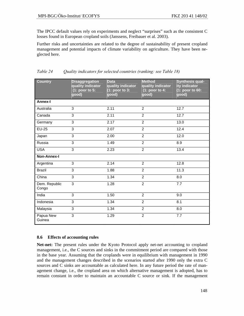
MPI-BGC/Öko-Institut/ ECOFYS FKZ 203 41 148/02
148
The IPCC default values rely on experiments and neglect “surprises” such as the consistent C losses found in European cropland soils (Janssens, Freibauer et al. 2003).
Further risks and uncertainties are related to the degree of sustainability of present cropland management and potential impacts of climate variability on agriculture. They have been ne-glected here.
Table 24 Quality indicators for selected countries (ranking: see Table 18)
Country Disaggregation quality indicator (1: poor to 5: good)
Data quality indicator (1: poor to 3: good)
Method quality indicator (1: poor to 4: good)
Synthesis qual-ity indicator (1: poor to 60: good)
Annex-I
Australia 3 2.11 2 12.7
Canada 3 2.11 2 12.7
Germany 3 2.17 2 13.0
EU-25 3 2.07 2 12.4
Japan 3 2.00 2 12.0
Russia 3 1.49 2 8.9
USA 3 2.23 2 13.4
Non-Annex-I
Argentina 3 2.14 2 12.8
Brazil 3 1.88 2 11.3
China 3 1.34 2 8.0
Dem. Republic Congo
3 1.28 2 7.7
India 3 1.50 2 9.0
Indonesia 3 1.34 2 8.1
Malaysia 3 1.34 2 8.0
Papua New Guinea
3 1.29 2 7.7
8.6 Effects of accounting rules
Net-net: The present rules under the Kyoto Protocol apply net-net accounting to cropland management, i.e., the C sources and sinks in the commitment period are compared with those in the base year. Assuming that the croplands were in equilibrium with management in 1990 and the management changes described in the scenarios started after 1990 only the extra C sources and C sinks are accountable as calculated here. In any future period the rate of man-agement change, i.e., the cropland area on which alternative management is adopted, has to remain constant in order to maintain an accountable C source or sink. If the management
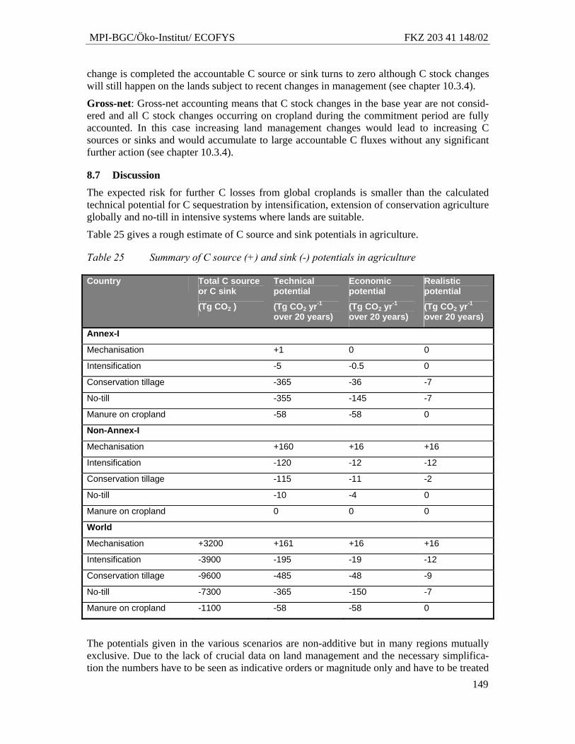
MPI-BGC/Öko-Institut/ ECOFYS FKZ 203 41 148/02
149
change is completed the accountable C source or sink turns to zero although C stock changes will still happen on the lands subject to recent changes in management (see chapter 10.3.4).
Gross-net: Gross-net accounting means that C stock changes in the base year are not consid-ered and all C stock changes occurring on cropland during the commitment period are fully accounted. In this case increasing land management changes would lead to increasing C sources or sinks and would accumulate to large accountable C fluxes without any significant further action (see chapter 10.3.4).
8.7 Discussion
The expected risk for further C losses from global croplands is smaller than the calculated technical potential for C sequestration by intensification, extension of conservation agriculture globally and no-till in intensive systems where lands are suitable.
Table 25 gives a rough estimate of C source and sink potentials in agriculture.
Table 25 Summary of C source (+) and sink (-) potentials in agriculture
Country Total C source or C sink
(Tg CO2 )
Technical potential
(Tg CO2 yr-1 over 20 years)
Economic potential
(Tg CO2 yr-1 over 20 years)
Realistic potential
(Tg CO2 yr-1 over 20 years)
Annex-I
Mechanisation +1 0 0
Intensification -5 -0.5 0
Conservation tillage -365 -36 -7
No-till -355 -145 -7
Manure on cropland -58 -58 0
Non-Annex-I
Mechanisation +160 +16 +16
Intensification -120 -12 -12
Conservation tillage -115 -11 -2
No-till -10 -4 0
Manure on cropland 0 0 0
World
Mechanisation +3200 +161 +16 +16
Intensification -3900 -195 -19 -12
Conservation tillage -9600 -485 -48 -9
No-till -7300 -365 -150 -7
Manure on cropland -1100 -58 -58 0
The potentials given in the various scenarios are non-additive but in many regions mutually exclusive. Due to the lack of crucial data on land management and the necessary simplifica-tion the numbers have to be seen as indicative orders or magnitude only and have to be treated
MPI-BGC/Öko-Institut/ ECOFYS FKZ 203 41 148/02
150
with caution. The potentials are conservative if compared with the literature but only refer to topsoil.
8.8 Conclusion
Technically there is significant potential to sequester carbon in cropland soils. However, it is unlikely that much of it will be implemented in short term and against raising land pressures. In total, the potential for C sequestration exceeds the potential for further C losses much of which have already occurred in the past. The technical potential for C sequestration by crop-land management is much lower than the one estimated for afforestation/reforestation (Chap-ter 6) and forest management (Chapter 7). Some of the sequestration activities will happen for other reasons like intensification and erosion control. As compared to the potential use of croplands to produce renewable materials and biomass for energy while reducing use of fossil fuel, the sequestration potential is almost negligible.
MPI-BGC/Öko-Institut/ ECOFYS FKZ 203 41 148/02
151
9 The rules for land use, land use change and forestry under the Kyoto Protocol – Lessons learned for the future climate negotiations
9.1 Introduction
With the Kyoto Protocol, industrialized countries (“Annex-I countries”) are to reduce their greenhouse gas emissions in the period 2008 to 2012 by roughly 5% compared to the 1990 level. The Kyoto Protocol set a target for the emissions of a basket of greenhouse gases (CO2, CH4, N2O, HFCs, PFCs, SF6) that can be met through efforts and activities in all sectors in-cluding energy, industrial processes, agriculture, waste. Activities from land use, land-use change and forestry (LULUCF) can also be used to a limited extent to reach the targets. The targets were set for the basket, not for individual gases, sectors or activities.
Separate rules for greenhouse gas emissions and removals from land use, land-use change and forestry activities have been designed under the Kyoto Protocol, since they have a signifi-cantly different character compared to greenhouse gas emissions from fossil fuels, for several reasons:
• LULUCF activities can also remove CO2 from the atmosphere. This removal can be reversed accidentally or intentionally and result in an emission of the equal amount of CO2, e.g. when the accumulated biomass is burnt or decays.
• Estimation of LULUCF emissions and removals is more uncertain than for fossil fuel emissions but within the range of uncertainty for non-CO2 greenhouse gases (IPCC 2000 page 58, para 8.a). While emissions from fossil fuels can be estimated relatively accurately from the quantity of fossil fuels used, the emissions and removals from land use and forestry activities depend on many mostly biological variables. Within the bands of uncertainty, the global CO2 emissions from forestry today may be 1/6 to 1/3 of fossil fuels emissions(Olivier JGJ, Bouwman AF et al. 1996; Houghton and Hackler 2003).
• The anthropogenic part of forestry emissions and removals is very small compared to the natural turnover of CO2 in the atmosphere, making it difficult in some cases to separate the human induced part from the natural part (IPCC 2001).
• The terrestrial biospheric uptake may be affected by climate change and can in some areas decline due to saturation effects (Cox, Betts et al. 2000). There is a risk that the biospheric sink in some areas is turning into a source in the course of this century.
• Forestry emissions and removals may still occur many years after the human interven-tion, while emissions from fossil fuels are immediate when the fuel is burnt. E.g. se-questration through afforestation/reforestation occurs many years after the trees are planted. An activity started in, e.g., 1993 may still be sequestering CO2 in 2010 and later.
As the emission reduction targets in the Kyoto Protocol were set before it was decided, whether and how LULUCF could be used to meet the targets, the subsequent controversial negotiation process led to a complicated accounting system for LULUCF (Fry 2002; Schulze, Valentini et al. 2002; Schlamadinger, Bird et al. 2006).
The objective of this chapter is three fold: First the chapter provides a detailed overview of the rules for accounting emissions of LULUCF for the first commitment period of the Kyoto Pro-tocol. These rules are relatively complicated, are contained in several different documents and have not been described in detail in one single document before. Second, it provides a detailed
MPI-BGC/Öko-Institut/ ECOFYS FKZ 203 41 148/02
152
overview of the history of negotiations that lead to these rules. It is instructive to follow the history to understand the rules and to avoid pitfalls in future negotiations. Finally, it provides conclusions on how the future negotiations could be shaped in the light of the current rules and the history of the negotiations.
9.2 Provisions for land use, land-use change and forestry in the first commitment pe-riod of the Kyoto Protocol
The provisions for land use, land use change and forestry in the first commitment period of the Kyoto Protocol are contained in several decisions of the Conference of the Parties to the UNFCCC (COP), the Conference of the Parties serving as the meeting of the Parties to the Kyoto Protocol (COP/MOP) and the Subsidiary Body for Scientific and Technological Ad-vice (SBSTA). The general rules are included in the decision on Land-use Change and For-estry, Decision 16/CMP.1, document FCCC/KP/CMP/2005/8/Add.3 (UNFCCC 2005). Some rules have been specified in the general accounting and reporting requirements, Decision 13/CMP.1 and 15/CMP.1, document FCCC/KP/CMP/2005/8/Add.2 (UNFCCC 2005; UNFCCC 2005). Details of the provisions for LULUF projects under the CDM are included in separate decisions, Decision 5/CMP.1, 6/CMP.1, document FCCC/KP/CMP/2005/8/Add.1 (UNFCCC 2005; UNFCCC 2005). The “Revised 1996 IPCC Guidelines for National Green-house Gas Inventories” (IPCC 1997) and the “Good Practice Guidance for Land Use, Land-Use Change and Forestry” (IPCC 2003) by the Intergovernmental Panel on Climate Change (IPCC) provide detailed estimation and reporting rules. This chapter explains these rules based on the documents above.
9.2.1 Principles The rules on LULUCF activities are governed by general principles, which have no binding character, but which shaped the detailed rules (Para 1 of UNFCCC (2005)20):
• That the treatment of these activities be based on sound science; • That consistent methodologies be used over time for the estimation and reporting of these
activities; • That the aim stated in Article 3, paragraph 1 of the Kyoto Protocol not be changed by ac-
counting for land use, land-use change and forestry activities; • That the mere presence of carbon stocks be excluded from accounting; • That the implementation of land use, land-use change and forestry activities contributes to
the conservation of biodiversity and sustainable use of natural resources; • That accounting for land use, land-use change and forestry does not imply a transfer of
commitments to a future commitment period; • That reversal of any removal due to land use, land-use change and forestry activities be
accounted for at the appropriate point in time; • That accounting excludes removals resulting from: (i) elevated carbon dioxide concentra-
tions above their pre-industrial level; (ii) indirect nitrogen deposition; and (iii) the dy-namic effects of age structure resulting from activities and practices before the reference year.
20 Unless otherwise indicated, paragraph numbers refer to paragraphs in the Annex to decision 16/CPM.1
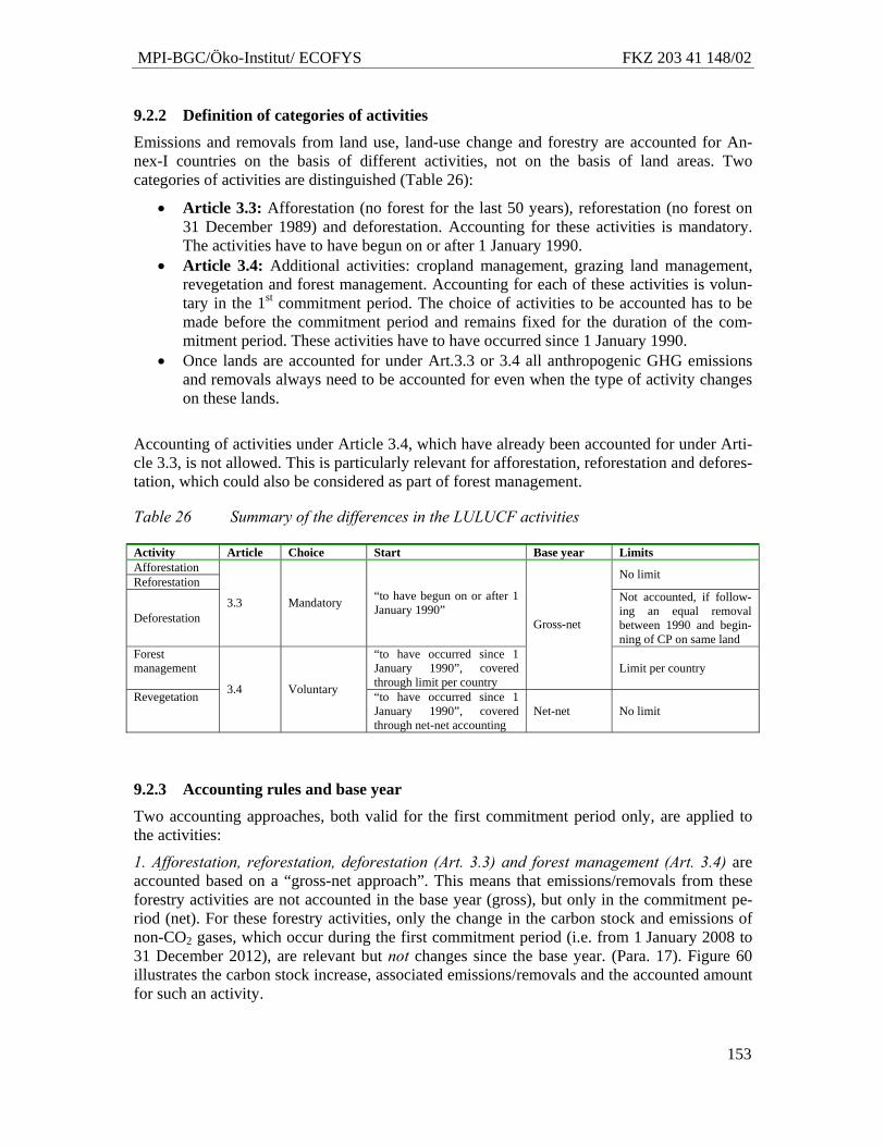
MPI-BGC/Öko-Institut/ ECOFYS FKZ 203 41 148/02
153
9.2.2 Definition of categories of activities
Emissions and removals from land use, land-use change and forestry are accounted for An-nex-I countries on the basis of different activities, not on the basis of land areas. Two categories of activities are distinguished (Table 26):
• Article 3.3: Afforestation (no forest for the last 50 years), reforestation (no forest on 31 December 1989) and deforestation. Accounting for these activities is mandatory. The activities have to have begun on or after 1 January 1990.
• Article 3.4: Additional activities: cropland management, grazing land management, revegetation and forest management. Accounting for each of these activities is volun-tary in the 1st commitment period. The choice of activities to be accounted has to be made before the commitment period and remains fixed for the duration of the com-mitment period. These activities have to have occurred since 1 January 1990.
• Once lands are accounted for under Art.3.3 or 3.4 all anthropogenic GHG emissions and removals always need to be accounted for even when the type of activity changes on these lands.
Accounting of activities under Article 3.4, which have already been accounted for under Arti-cle 3.3, is not allowed. This is particularly relevant for afforestation, reforestation and defores-tation, which could also be considered as part of forest management.
Table 26 Summary of the differences in the LULUCF activities
Activity Article Choice Start Base year Limits Afforestation Reforestation No limit
Deforestation 3.3 Mandatory “to have begun on or after 1
January 1990” Not accounted, if follow-ing an equal removal between 1990 and begin-ning of CP on same land
Forest management
“to have occurred since 1 January 1990”, covered through limit per country
Gross-net
Limit per country
Revegetation 3.4 Voluntary “to have occurred since 1 January 1990”, covered through net-net accounting
Net-net No limit
9.2.3 Accounting rules and base year
Two accounting approaches, both valid for the first commitment period only, are applied to the activities:
1. Afforestation, reforestation, deforestation (Art. 3.3) and forest management (Art. 3.4) are accounted based on a “gross-net approach”. This means that emissions/removals from these forestry activities are not accounted in the base year (gross), but only in the commitment pe-riod (net). For these forestry activities, only the change in the carbon stock and emissions of non-CO2 gases, which occur during the first commitment period (i.e. from 1 January 2008 to 31 December 2012), are relevant but not changes since the base year. (Para. 17). Figure 60 illustrates the carbon stock increase, associated emissions/removals and the accounted amount for such an activity.
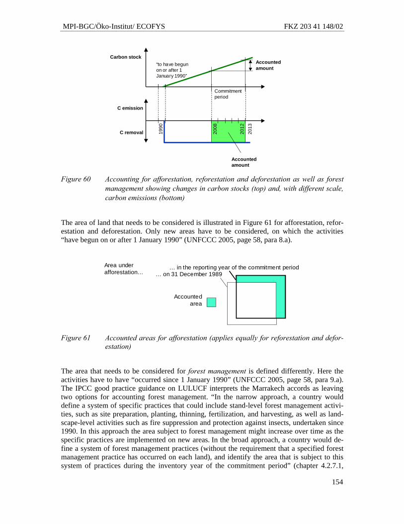
MPI-BGC/Öko-Institut/ ECOFYS FKZ 203 41 148/02
154
C emission
C removal
Accounted amount
Carbon stock
1990
2008
2012
2013
Accounted amount
Commitment period
“to have begun on or after 1 January 1990”
Figure 60 Accounting for afforestation, reforestation and deforestation as well as forest
management showing changes in carbon stocks (top) and, with different scale, carbon emissions (bottom)
The area of land that needs to be considered is illustrated in Figure 61 for afforestation, refor-estation and deforestation. Only new areas have to be considered, on which the activities “have begun on or after 1 January 1990” (UNFCCC 2005, page 58, para 8.a).
… on 31 December 1989… in the reporting year of the commitment period
Accounted area
Area under afforestation…
Figure 61 Accounted areas for afforestation (applies equally for reforestation and defor-estation)
The area that needs to be considered for forest management is defined differently. Here the activities have to have “occurred since 1 January 1990” (UNFCCC 2005, page 58, para 9.a). The IPCC good practice guidance on LULUCF interprets the Marrakech accords as leaving two options for accounting forest management. “In the narrow approach, a country would define a system of specific practices that could include stand-level forest management activi-ties, such as site preparation, planting, thinning, fertilization, and harvesting, as well as land-scape-level activities such as fire suppression and protection against insects, undertaken since 1990. In this approach the area subject to forest management might increase over time as the specific practices are implemented on new areas. In the broad approach, a country would de-fine a system of forest management practices (without the requirement that a specified forest management practice has occurred on each land), and identify the area that is subject to this system of practices during the inventory year of the commitment period” (chapter 4.2.7.1,
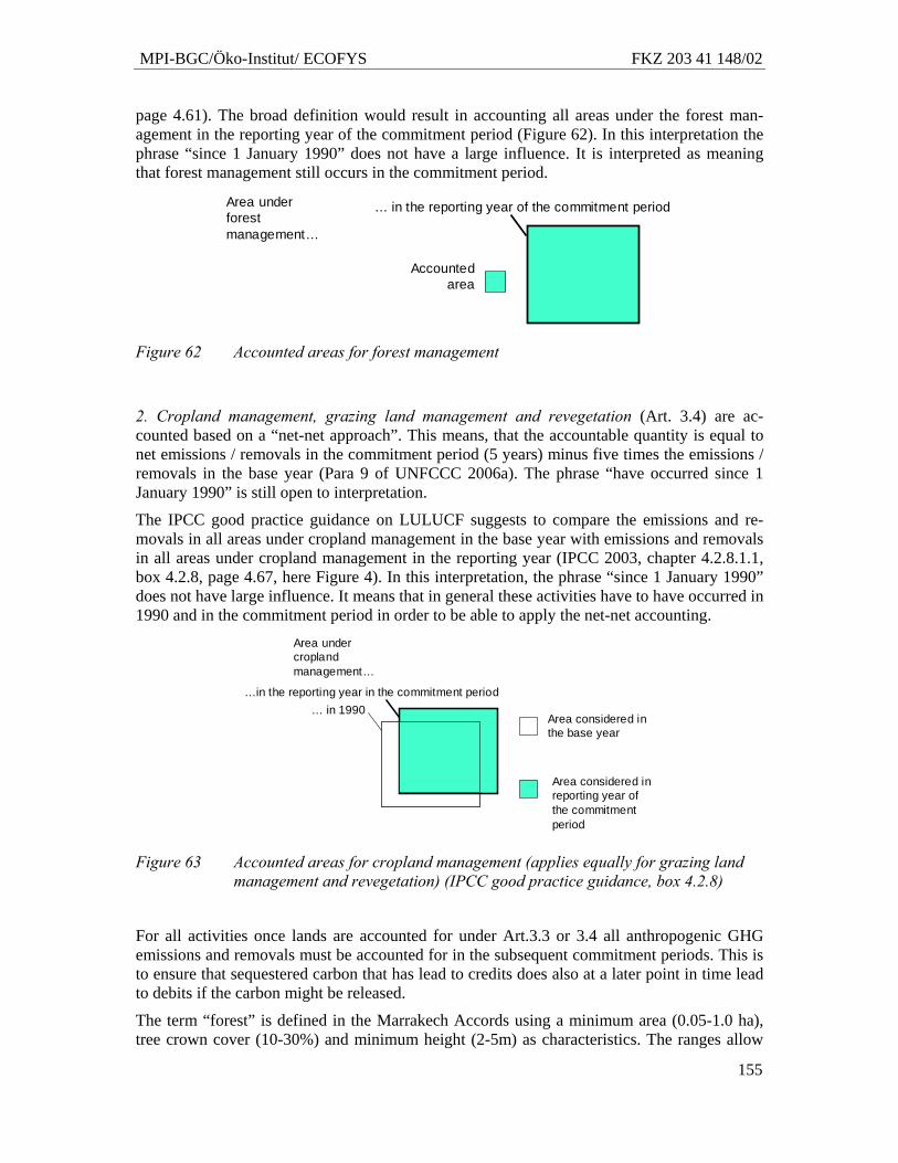
MPI-BGC/Öko-Institut/ ECOFYS FKZ 203 41 148/02
155
page 4.61). The broad definition would result in accounting all areas under the forest man-agement in the reporting year of the commitment period (Figure 62). In this interpretation the phrase “since 1 January 1990” does not have a large influence. It is interpreted as meaning that forest management still occurs in the commitment period.
… in the reporting year of the commitment period
Accounted area
Area under forest management…
Figure 62 Accounted areas for forest management
2. Cropland management, grazing land management and revegetation (Art. 3.4) are ac-counted based on a “net-net approach”. This means, that the accountable quantity is equal to net emissions / removals in the commitment period (5 years) minus five times the emissions / removals in the base year (Para 9 of UNFCCC 2006a). The phrase “have occurred since 1 January 1990” is still open to interpretation.
The IPCC good practice guidance on LULUCF suggests to compare the emissions and re-movals in all areas under cropland management in the base year with emissions and removals in all areas under cropland management in the reporting year (IPCC 2003, chapter 4.2.8.1.1, box 4.2.8, page 4.67, here Figure 4). In this interpretation, the phrase “since 1 January 1990” does not have large influence. It means that in general these activities have to have occurred in 1990 and in the commitment period in order to be able to apply the net-net accounting.
… in 1990…in the reporting year in the commitment period
Area considered in the base year
Area considered in reporting year of the commitment period
Area under cropland management…
Figure 63 Accounted areas for cropland management (applies equally for grazing land management and revegetation) (IPCC good practice guidance, box 4.2.8)
For all activities once lands are accounted for under Art.3.3 or 3.4 all anthropogenic GHG emissions and removals must be accounted for in the subsequent commitment periods. This is to ensure that sequestered carbon that has lead to credits does also at a later point in time lead to debits if the carbon might be released.
The term “forest” is defined in the Marrakech Accords using a minimum area (0.05-1.0 ha), tree crown cover (10-30%) and minimum height (2-5m) as characteristics. The ranges allow
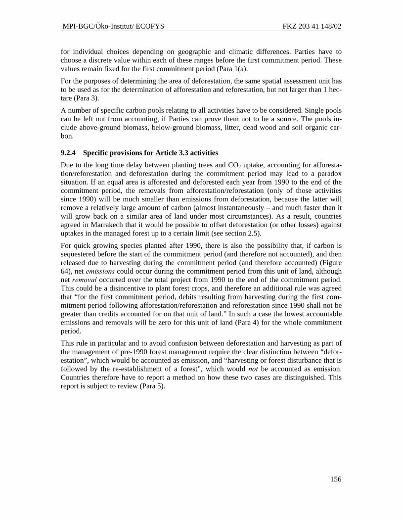
MPI-BGC/Öko-Institut/ ECOFYS FKZ 203 41 148/02
156
for individual choices depending on geographic and climatic differences. Parties have to choose a discrete value within each of these ranges before the first commitment period. These values remain fixed for the first commitment period (Para 1(a).
For the purposes of determining the area of deforestation, the same spatial assessment unit has to be used as for the determination of afforestation and reforestation, but not larger than 1 hec-tare (Para 3).
A number of specific carbon pools relating to all activities have to be considered. Single pools can be left out from accounting, if Parties can prove them not to be a source. The pools in-clude above-ground biomass, below-ground biomass, litter, dead wood and soil organic car-bon.
9.2.4 Specific provisions for Article 3.3 activities Due to the long time delay between planting trees and CO2 uptake, accounting for afforesta-tion/reforestation and deforestation during the commitment period may lead to a paradox situation. If an equal area is afforested and deforested each year from 1990 to the end of the commitment period, the removals from afforestation/reforestation (only of those activities since 1990) will be much smaller than emissions from deforestation, because the latter will remove a relatively large amount of carbon (almost instantaneously – and much faster than it will grow back on a similar area of land under most circumstances). As a result, countries agreed in Marrakech that it would be possible to offset deforestation (or other losses) against uptakes in the managed forest up to a certain limit (see section 2.5).
For quick growing species planted after 1990, there is also the possibility that, if carbon is sequestered before the start of the commitment period (and therefore not accounted), and then released due to harvesting during the commitment period (and therefore accounted) (Figure 64), net emissions could occur during the commitment period from this unit of land, although net removal occurred over the total project from 1990 to the end of the commitment period. This could be a disincentive to plant forest crops, and therefore an additional rule was agreed that “for the first commitment period, debits resulting from harvesting during the first com-mitment period following afforestation/reforestation and reforestation since 1990 shall not be greater than credits accounted for on that unit of land.” In such a case the lowest accountable emissions and removals will be zero for this unit of land (Para 4) for the whole commitment period.
This rule in particular and to avoid confusion between deforestation and harvesting as part of the management of pre-1990 forest management require the clear distinction between “defor-estation”, which would be accounted as emission, and “harvesting or forest disturbance that is followed by the re-establishment of a forest”, which would not be accounted as emission. Countries therefore have to report a method on how these two cases are distinguished. This report is subject to review (Para 5).
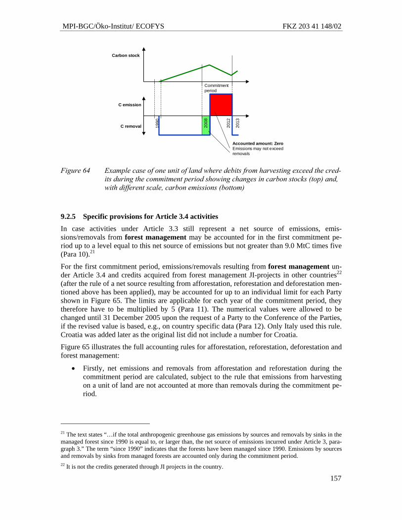
MPI-BGC/Öko-Institut/ ECOFYS FKZ 203 41 148/02
157
C emission
C removal
Carbon stock
1990
2008
2012
2013
Accounted amount: ZeroEmissions may not exceed removals
Commitment period
Figure 64 Example case of one unit of land where debits from harvesting exceed the cred-its during the commitment period showing changes in carbon stocks (top) and, with different scale, carbon emissions (bottom)
9.2.5 Specific provisions for Article 3.4 activities In case activities under Article 3.3 still represent a net source of emissions, emis-sions/removals from forest management may be accounted for in the first commitment pe-riod up to a level equal to this net source of emissions but not greater than 9.0 MtC times five (Para 10).21
For the first commitment period, emissions/removals resulting from forest management un-der Article 3.4 and credits acquired from forest management JI-projects in other countries22 (after the rule of a net source resulting from afforestation, reforestation and deforestation men-tioned above has been applied), may be accounted for up to an individual limit for each Party shown in Figure 65. The limits are applicable for each year of the commitment period, they therefore have to be multiplied by 5 (Para 11). The numerical values were allowed to be changed until 31 December 2005 upon the request of a Party to the Conference of the Parties, if the revised value is based, e.g., on country specific data (Para 12). Only Italy used this rule. Croatia was added later as the original list did not include a number for Croatia.
Figure 65 illustrates the full accounting rules for afforestation, reforestation, deforestation and forest management:
• Firstly, net emissions and removals from afforestation and reforestation during the commitment period are calculated, subject to the rule that emissions from harvesting on a unit of land are not accounted at more than removals during the commitment pe-riod.
21 The text states “…if the total anthropogenic greenhouse gas emissions by sources and removals by sinks in the managed forest since 1990 is equal to, or larger than, the net source of emissions incurred under Article 3, para-graph 3.” The term “since 1990” indicates that the forests have been managed since 1990. Emissions by sources and removals by sinks from managed forests are accounted only during the commitment period. 22 It is not the credits generated through JI projects in the country.
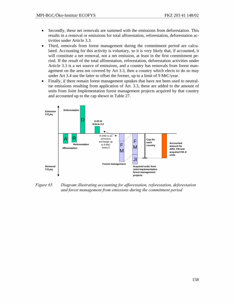
MPI-BGC/Öko-Institut/ ECOFYS FKZ 203 41 148/02
158
• Secondly, these net removals are summed with the emissions from deforestation. This results in a removal or emissions for total afforestation, reforestation, deforestation ac-tivities under Article 3.3.
• Third, removals from forest management during the commitment period are calcu-lated. Accounting for this activity is voluntary, so it is very likely that, if accounted, it will constitute a net removal, not a net emission, at least in the first commitment pe-riod. If the result of the total afforestation, reforestation, deforestation activities under Article 3.3 is a net source of emissions, and a country has removals from forest man-agement on the area not covered by Art 3.3, then a country which elects to do so may under Art 3.4 use the latter to offset the former, up to a limit of 9 MtC/year.
• Finally, if there remain forest management uptakes that have not been used to neutral-ise emissions resulting from application of Art. 3.3, these are added to the amount of units from Joint Implementation forest management projects acquired by that country and accounted up to the cap shown in Table 27.
A
EmissionCO2eq.
RemovalCO2eq.
Afforestation
RReforestation
D
Deforestation
A+R+DArticle 3.3
FM
Forest management
If ARD is an emission,
exchange up to 9 MtCtimes 5
FM
JIAcquired units from Joint Implementation forest management projects
Cap for each country
Accounted amount for ARD, FM and acquired FM JI units
Figure 65 Diagram illustrating accounting for afforestation, reforestation, deforestation and forest management from emissions during the commitment period
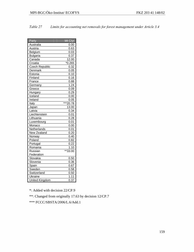
MPI-BGC/Öko-Institut/ ECOFYS FKZ 203 41 148/02
159
Table 27 Limits for accounting net removals for forest management under Article 3.4
Party Mt C/yr Australia 0.00 Austria 0.63 Belgium 0.03 Bulgaria 0.37 Canada 12.00 Croatia *0.265 Czech Republic 0.32 Denmark 0.05 Estonia 0.10 Finland 0.16 France 0.88 Germany 1.24 Greece 0.09 Hungary 0.29 Iceland 0.00 Ireland 0.05 Italy ***20.78 Japan 13.00 Latvia 0.34 Liechtenstein 0.01 Lithuania 0.28 Luxembourg 0.01 Monaco 0.00 Netherlands 0.01 New Zealand 0.20 Norway 0.40 Poland 0.82 Portugal 0.22 Romania 1.10 Russian Federation
**33.00
Slovakia 0.50 Slovenia 0.36 Spain 0.67 Sweden 0.58 Switzerland 0.50 Ukraine 1.11 United Kingdom 0.37
*: Added with decision 22/CP.9
**: Changed from originally 17.63 by decision 12/CP.7
*** FCCC/SBSTA/2006/L.6/Add.1
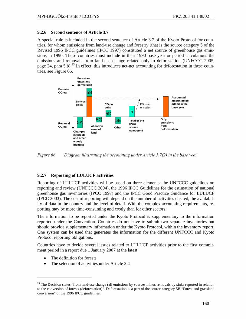
MPI-BGC/Öko-Institut/ ECOFYS FKZ 203 41 148/02
160
9.2.6 Second sentence of Article 3.7
A special rule is included in the second sentence of Article 3.7 of the Kyoto Protocol for coun-tries, for whom emissions from land-use change and forestry (that is the source category 5 of the Revised 1996 IPCC guidelines (IPCC 1997) constituted a net source of greenhouse gas emis-sions in 1990. These countries must include in their 1990 base year or period calculations the emissions and removals from land-use change related only to deforestation (UNFCCC 2005, page 24, para 5.b).23 In effect, this introduces net-net accounting for deforestation in these coun-tries, see Figure 66.
EmissionCO2eq.
RemovalCO2eq.
5A
5B
5C5D
5E
5
Changes in forests and other woody biomass
Forest and grassland conversion
Abandonment of land
CO2 in soils
Other
Total of the IPCC source category 5
If 5 is an emission
Only emissions from deforestation
Accounted amount to be added in the base year
Defores-tation
Figure 66 Diagram illustrating the accounting under Article 3.7(2) in the base year
9.2.7 Reporting of LULUCF activities Reporting of LULUCF activities will be based on three elements: the UNFCCC guidelines on reporting and review (UNFCCC 2004), the 1996 IPCC Guidelines for the estimation of national greenhouse gas inventories (IPCC 1997) and the IPCC Good Practice Guidance for LULUCF (IPCC 2003). The cost of reporting will depend on the number of activities elected, the availabil-ity of data in the country and the level of detail. With the complex accounting requirements, re-porting may be more time-consuming and costly than for other sectors.
The information to be reported under the Kyoto Protocol is supplementary to the information reported under the Convention. Countries do not have to submit two separate inventories but should provide supplementary information under the Kyoto Protocol, within the inventory report. One system can be used that generates the information for the different UNFCCC and Kyoto Protocol reporting obligations.
Countries have to decide several issues related to LULUCF activities prior to the first commit-ment period in a report due 1 January 2007 at the latest:
• The definition for forests • The selection of activities under Article 3.4
23 The Decision states “from land-use change (all emissions by sources minus removals by sinks reported in relation to the conversion of forests (deforestation)“. Deforestation is a part of the source category 5B “Forest and grassland conversion” of the 1996 IPCC guidelines.
MPI-BGC/Öko-Institut/ ECOFYS FKZ 203 41 148/02
161
• Whether activities under Article 3.4 will be accounted annually or for the entire commit-ment period
This report needs to contain the emission inventory for the base year, which will be reviewed and cannot be changed subsequently. Reporting on LULUCF activities under the Kyoto Protocol is, however, excluded from this procedure. The base year emissions/removals of these activities will not be fixed prior to the first commitment period.
Reporting of a most recent inventory in accordance with the guidelines is a condition to partici-pate in the Kyoto mechanisms (international emission trading, CDM and JI). This applies only to the inventory on, excluding land-use change and forestry, and the annual inventory on sinks (due under the Convention), but not to the reporting of supplementary information relevant to the ac-counting of LULUCF activities under the Kyoto Protocol. These activities are accounted via additional units in the commitment period, like the mechanisms, and not via the base year inven-tory. The inventories of the years of the commitment period are reviewed and additional units are only issued after the satisfactory completion of the review.
9.2.8 Specific provisions for LULUCF in Joint Implementation (JI) Under JI, projects aimed at enhancing anthropogenic removals by sinks are allowed. The cap on credits from forest management projects is to be applied as described above. The general rules for LULUCF for Annex-I countries apply also for JI projects.
9.2.9 Rules for LULUCF in Non-Annex-I countries, Clean Development Mechanism (CDM)
Under the clean development mechanism, only afforestation and reforestation activities are eli-gible (UNFCCC 2005, para 13). For the first commitment period, Annex-I countries can use credits/removals from these activities for up to a level of 1% of its base year emissions times five (UNFCCC 2005, para 14). CDM Etscheidung hier zitieren und erwähnen, dass wenn nicht anders geregelt, die allgem .CDM regeln gelten.
The crediting period of these projects is 20 years with the option to renew two times or 30 years with no option for renewal (UNFCCC 2005, para 23)24. This is to encourage long-term projects.
Potential reversal of sequestration of the CO2 in biomass (non-permanence) is addressed by the rule that emission credits from these projects are of a temporary nature, expire and have to be replaced after a specified period.
Project participants may select to use “temporary certified emission reduction units” (tCERs) or “long-term certified emission reduction units” (lCERs) (Para. 38) (Table 28).
Acquiring an lCER is equivalent to acquiring a string of regularly renewed tCERs. The liability to replace the credits upon reversal of the removal is always with the buyer of the credits and a check, whether the certified forest is still present, takes place in 5-year intervals. A very small difference is that, if the validation finds that the forest no longer exists, lCERs have to be re-placed within a month, the expiring tCERs only at the end of the commitment period. But ex-pired tCERs have to be replaced again by same number of tCERs, CERs, AAUs, RMUs or ERUs after 5 years, while lCERs only have to be replaced in case a reversal of the removal occurs and at the end of the crediting period.
TCERs and lCERs only postpone the obligation to reduce emissions, they do not fulfil the obli-gation to reduce emissions as credits from other CDM projects. This will be one factor lowering 24 If not stated otherwise, the following paragraph numbers refer to the Annex to decision 5/CP.9 in UNFCCC 2006e.
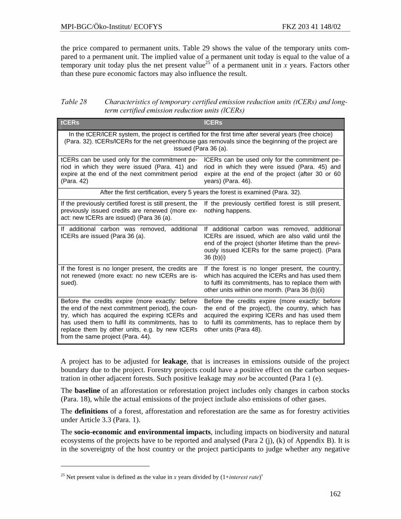
MPI-BGC/Öko-Institut/ ECOFYS FKZ 203 41 148/02
162
the price compared to permanent units. Table 29 shows the value of the temporary units com-pared to a permanent unit. The implied value of a permanent unit today is equal to the value of a temporary unit today plus the net present value25 of a permanent unit in x years. Factors other than these pure economic factors may also influence the result.
Table 28 Characteristics of temporary certified emission reduction units (tCERs) and long-term certified emission reduction units (lCERs)
tCERs lCERs
In the tCER/lCER system, the project is certified for the first time after several years (free choice) (Para. 32). tCERs/lCERs for the net greenhouse gas removals since the beginning of the project are
issued (Para 36 (a).
tCERs can be used only for the commitment pe-riod in which they were issued (Para. 41) and expire at the end of the next commitment period (Para. 42)
lCERs can be used only for the commitment pe-riod in which they were issued (Para. 45) and expire at the end of the project (after 30 or 60 years) (Para. 46).
After the first certification, every 5 years the forest is examined (Para. 32).
If the previously certified forest is still present, the previously issued credits are renewed (more ex-act: new tCERs are issued) (Para 36 (a).
If the previously certified forest is still present, nothing happens.
If additional carbon was removed, additional tCERs are issued (Para 36 (a).
If additional carbon was removed, additional lCERs are issued, which are also valid until the end of the project (shorter lifetime than the previ-ously issued lCERs for the same project). (Para 36 (b)(i)
If the forest is no longer present, the credits are not renewed (more exact: no new tCERs are is-sued).
If the forest is no longer present, the country, which has acquired the lCERs and has used them to fulfil its commitments, has to replace them with other units within one month. (Para 36 (b)(ii)
Before the credits expire (more exactly: before the end of the next commitment period), the coun-try, which has acquired the expiring tCERs and has used them to fulfil its commitments, has to replace them by other units, e.g. by new tCERs from the same project (Para. 44).
Before the credits expire (more exactly: before the end of the project), the country, which has acquired the expiring lCERs and has used them to fulfil its commitments, has to replace them by other units (Para 48).
A project has to be adjusted for leakage, that is increases in emissions outside of the project boundary due to the project. Forestry projects could have a positive effect on the carbon seques-tration in other adjacent forests. Such positive leakage may not be accounted (Para 1 (e).
The baseline of an afforestation or reforestation project includes only changes in carbon stocks (Para. 18), while the actual emissions of the project include also emissions of other gases.
The definitions of a forest, afforestation and reforestation are the same as for forestry activities under Article 3.3 (Para. 1).
The socio-economic and environmental impacts, including impacts on biodiversity and natural ecosystems of the projects have to be reported and analysed (Para 2 (j), (k) of Appendix B). It is in the sovereignty of the host country or the project participants to judge whether any negative
25 Net present value is defined as the value in x years divided by (1+interest rate)x
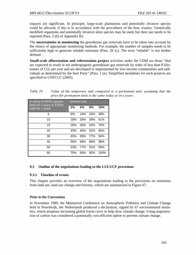
MPI-BGC/Öko-Institut/ ECOFYS FKZ 203 41 148/02
163
impacts are significant. In principle, large-scale plantations and potentially invasive species could be allowed, if this is in accordance with the procedures of the host country. Genetically modified organisms and potentially invasive alien species may be used, but their use needs to be reported (Para. 2 (b) of Appendix B).
The uncertainties in monitoring the greenhouse gas removals have to be taken into account by the choice of appropriate monitoring methods. For example, the number of samples needs to be sufficiently high to generate reliable estimates (Para. 26 (c). The term “reliable” is not further defined.
Small-scale afforestation and reforestation project activities under the CDM are those “that are expected to result in net anthropogenic greenhouse gas removals by sinks of less than 8 kilo-tonnes of CO2 per year and are developed or implemented by low-income communities and indi-viduals as determined by the host Party” (Para. 1 (e). Simplified modalities for such projects are specified in UNFCCC (2005).
Table 29 Value of the temporary unit compared to a permanent unit, assuming that the price for permanent units is the same today as in x years.
Interest rate A string of tCERs guaran-teed for x years or lCERs valid for x years 2% 3% 5% 10%
5 9% 14% 22% 38%
10 18% 26% 39% 61%
15 26% 36% 52% 76%
20 33% 45% 62% 85%
30 45% 59% 77% 94%
40 55% 69% 86% 98%
50 63% 77% 91% 99%
60 70% 83% 95% 100%
9.3 Outline of the negotiations leading to the LULUCF provisions
9.3.1 Timeline of events This chapter provides an overview of the negotiations leading to the provisions on emissions from land use, land use change and forestry, which are summarized in Figure 67.
Prior to the Convention
In November 1989, the Ministerial Conference on Atmospheric Pollution and Climate Change held in Noordwijk, the Netherlands produced a declaration, signed by 67 environmental minis-ters, which proposes increasing global forest cover to help slow climate change. Using sequestra-tion of carbon was considered a potentially cost efficient option to prevent climate change.
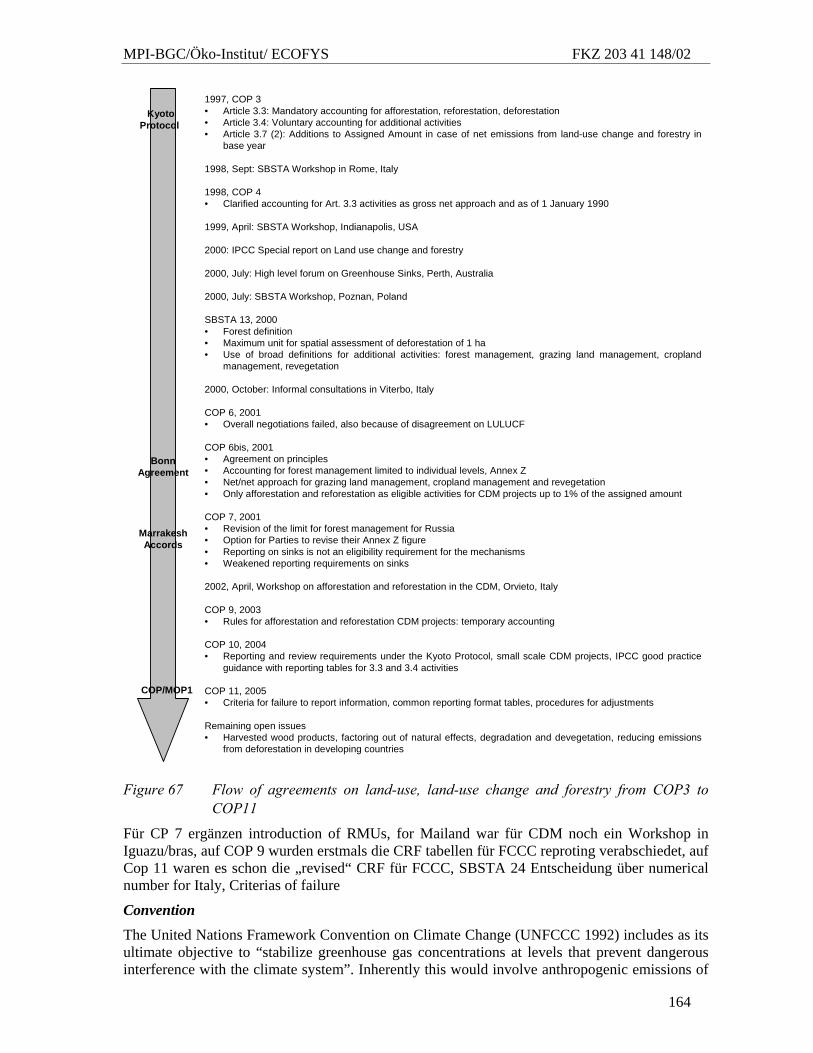
MPI-BGC/Öko-Institut/ ECOFYS FKZ 203 41 148/02
164
Kyoto Protocol
MarrakeshAccords
Bonn Agreement
1997, COP 3• Article 3.3: Mandatory accounting for afforestation, reforestation, deforestation• Article 3.4: Voluntary accounting for additional activities• Article 3.7 (2): Additions to Assigned Amount in case of net emissions from land-use change and forestry in
base year
1998, Sept: SBSTA Workshop in Rome, Italy
1998, COP 4• Clarified accounting for Art. 3.3 activities as gross net approach and as of 1 January 1990
1999, April: SBSTA Workshop, Indianapolis, USA
2000: IPCC Special report on Land use change and forestry
2000, July: High level forum on Greenhouse Sinks, Perth, Australia
2000, July: SBSTA Workshop, Poznan, Poland
SBSTA 13, 2000• Forest definition• Maximum unit for spatial assessment of deforestation of 1 ha• Use of broad definitions for additional activities: forest management, grazing land management, cropland
management, revegetation
2000, October: Informal consultations in Viterbo, Italy
COP 6, 2001• Overall negotiations failed, also because of disagreement on LULUCF
COP 6bis, 2001• Agreement on principles• Accounting for forest management limited to individual levels, Annex Z• Net/net approach for grazing land management, cropland management and revegetation• Only afforestation and reforestation as eligible activities for CDM projects up to 1% of the assigned amount
COP 7, 2001• Revision of the limit for forest management for Russia• Option for Parties to revise their Annex Z figure• Reporting on sinks is not an eligibility requirement for the mechanisms• Weakened reporting requirements on sinks
2002, April, Workshop on afforestation and reforestation in the CDM, Orvieto, Italy
COP 9, 2003• Rules for afforestation and reforestation CDM projects: temporary accounting
COP 10, 2004• Reporting and review requirements under the Kyoto Protocol, small scale CDM projects, IPCC good practice
guidance with reporting tables for 3.3 and 3.4 activities
COP 11, 2005• Criteria for failure to report information, common reporting format tables, procedures for adjustments
Remaining open issues• Harvested wood products, factoring out of natural effects, degradation and devegetation, reducing emissions
from deforestation in developing countries
COP/MOP1
Figure 67 Flow of agreements on land-use, land-use change and forestry from COP3 to
COP11
Für CP 7 ergänzen introduction of RMUs, for Mailand war für CDM noch ein Workshop in Iguazu/bras, auf COP 9 wurden erstmals die CRF tabellen für FCCC reproting verabschiedet, auf Cop 11 waren es schon die „revised“ CRF für FCCC, SBSTA 24 Entscheidung über numerical number for Italy, Criterias of failure
Convention
The United Nations Framework Convention on Climate Change (UNFCCC 1992) includes as its ultimate objective to “stabilize greenhouse gas concentrations at levels that prevent dangerous interference with the climate system”. Inherently this would involve anthropogenic emissions of
MPI-BGC/Öko-Institut/ ECOFYS FKZ 203 41 148/02
165
greenhouse gases but also anthropogenic removals by sinks. Article 4 of the Convention speaks of the commitment for all Parties to implement measures to mitigate climate change by address-ing emissions and removals by sinks. Annex-I Parties in particular should adopt policies by limit-ing its emissions and protecting and enhancing its greenhouse gas sinks and reservoirs (Article 4.2a). The aim for Annex-I Parties of returning to 1990 levels by the year 2000 also includes emissions and removals (Article 4.2b). The Convention itself, however, does not specify how exactly the removals should be incorporated, e.g. if emission by source and changes in carbon stocks should just be added to energy related emissions one to one or if a separate accounting systems should be used. The reporting requirements subsequently adopted under the Convention include specifications for removals from LUCF, but includes two different ways to add emis-sions, one including and one excluding emissions/removals from land-use change and forestry (e.g. the Common Reporting Format in UNFCCC 2004).
From Berlin to Kyoto - COP1 to COP3
To strengthen the commitments of the Convention, the Berlin Mandate was adopted at COP 1 in 1995, which refers to strengthening the commitments of Annex-I Parties by adopting a protocol or another legal instrument. As it refers to Article 4 of the Convention, it also refers to the use of removals (Fry 2002). The Ad-hoc Group on the Berlin Mandate (AGBM) established to negoti-ate the detailed rules of such an instrument continued until the negotiation of the Kyoto Protocol in 1997.
The choice of including sinks in all years (net-net), excluding sinks altogether (gross-gross) or including them only on the commitment period (gross-net) had significant influence on account-able credits.
Substantive discussion on sinks came up relatively late in the AGBM process. For a long period of time, the word “net” before “emissions” remained in square brackets indicating that this con-troversial issue needed to be revisited at a later date. The possibility to bring in sinks, particularly forest management, was seen by some Parties as an opportunity to obtain emission credits at very low price. Others noted that the estimation of sinks is uncertain and their magnitude may significantly water down the emission reduction efforts.
In their textual proposal for a protocol some countries included the term “net emissions” (Brazil, Iceland, Norway, Russian Federation, US) while others included “...and removals by sinks” (Australia, EU). On the other hand some countries explicitly excluded removals or did not men-tion these in their proposals (AOSIS, Czech Republic, Hungary et al., Japan, Switzerland). The EU later altered its position and suggested that sinks should be excluded in the first commitment period, but could be included in following commitment periods following additional research. New Zealand proposed that sinks should not be added to the base year emissions, but to the emission budget in the commitment period (Gross-net approach) (Depledge 2000, page 48).
After the last regular AGBM session and shortly before COP 3, the UNFCCC secretariat circu-lated a questionnaire on sink issues compiling the responses made by Parties. The most impor-tant issues were, which land-use change and forestry activities should be included and whether the allowed amount of sinks should be limited. The USA, Norway and Iceland were in favour of including all activities, Kenya and the Marshal Islands of including none. Moving again away from its original position, the EU now proposed to include removals, but to define the modalities at the first meeting of the Parties to the Protocol. Concerning the limitation of removals, the um-brella group (without Japan) voted against limitations, the Marshall Island proposed that a maximum of 6-7% of removals should be allowed to use to fulfil the emission reduction goal (UNFCCC 1997).
At the consultations on sinks shortly prior to an additional AGBM session just before COP3 all Parties present had agreed that sinks “were important and should be included in commitments,
MPI-BGC/Öko-Institut/ ECOFYS FKZ 203 41 148/02
166
subject to concerns about definitions, timing and scope” (UNFCCC 1997, page 3). At this ses-sion, environmental NGOs raised concerns about the gross-net approach claiming it would intro-duce a significant loophole into the accounting system.
At COP 3, the chairman of the consultation group of sinks proposed three LUCF categories: af-forestation, deforestation and reforestation, which later resulted in Article 3.3. These three were considered to be “no regret options” as their potential was relatively limited and well known at that time.
New Zealand detailed their proposal on the gross net accounting further, noting that to avoid a loophole while still having a full accounting of sinks in the commitment period, the gross targets of countries could be made more stringent by around 10%, the approximate aggregate figure for net removals from LUCF reported by Annex-I Parties in 1990. While this idea was not further pursued, another method to avoid the loophole, the "since 1990" activities approach previously proposed by Iceland (albeit unrelated to the gross-net loophole issue) was introduced again.
No agreement could be reached defining further categories, partly because many delegations had little or no information on the magnitude of emissions/removals from these categories. Article 3.4 first laid out that such further activities should be decided upon at COP/MOP 1. The phrase “Such a decision [on future additions to sink categories] shall apply in the second and subsequent commitment periods” was included in the contact group, with the effect that future decisions would not affect current commitments. At a very late stage at COP3, the level of commitments under discussion led to pressure for additional flexibility. Eventually Parties agreed to text giving flexibility for possible use of these additional, though at that time still unspecified, activities al-ready during the first commitment period, subject to the condition that these activities had taken place “since 1990”.
For the mechanisms, no explicit reference to LULUCF was made in Article 12 (CDM) to the Protocol, although they were referred to in Article 6 (JI). The reference in Article 12 had been included in earlier versions in a footnote and apparently was lost when all footnotes were re-moved (Depledge 2000, page 76). This ambiguity led to considerable debate subsequently about whether LULUCF activities were eligible for the CDM, or not.
To Buenos Aires – COP4
After COP-3 and for SBSTA 8 (June 1998), the secretariat issued a paper describing the issues on land use change and forestry in the Kyoto Protocol that need clarification (UNFCCC 1998). At that session, the IPCC was invited to prepare a Special Report on LULUCF, which should determine the present understanding of carbon sequestration as related to the Articles of the Kyoto Protocol from the scientific and technical side.
At COP 4 a first decision on sinks was made, clarifying the gross-net accounting for Article 3.3: “the adjustment to a Party’s assigned amount shall be equal to verifiable changes in carbon stocks during the period 2008 to 2012 resulting from direct human-induced activities of affore-station, reforestation and deforestation since 1 January 1990.” (UNFCCC 1998, decision 9/CP.4)
Further, the Buenos Aires Plan of Action was adopted, stating that the outstanding issues of the Kyoto Protocol, including sinks, should be solved by COP 6 in 2000.
From the Special Report to The Hague and Marrakech - COP6 to COP7
The IPCC issued its Special Report on LULUCF in early 2000 (IPCC 2000), which quantified a wide range of potential of 3.3. and 3.4 activities. SBSTA 12 (June 2000) invited Parties to report country specific data on sinks by August 2000 and the UNFCCC secretariat prepared a compara-tive overview of LULUCF activities in the national inventories for SBSTA 13 in September 2000. The overview showed gaps regarding uncertainty, transparency and verifiability as well as inconsistencies regarding the amounts of sinks reported by the Parties. The data submission was
MPI-BGC/Öko-Institut/ ECOFYS FKZ 203 41 148/02
167
nevertheless a major advance because it gave for the first time a quantitative indication of what key Parties might be seeking from the agreement, and could be combined with other data, nota-bly from the FAO, to provide a reasonably complete overview.
At SBSTA 13, in September 2000, further agreements were made on the forest definition, the maximum unit for spatial assessment of deforestation of 1 ha and the use of broad definitions for additional activities: forest management, grazing land management, cropland management, revegetation. At the same session, sinks in the CDM were discussed and the “Colombian pro-posal” of using temporary credits was made, though without reaching political agreement on actual inclusion.
At COP6, November 2000, the open questions on the limits to the use of sinks, especially forest management, were one of the major obstacles that led to the conference being adjourned at that stage without an agreement.
COP6 was resumed in June 2001 (referred to as COP6 bis). At that session Parties were able to reach the “Bonn Agreement”, including principles for the use of sinks, accounting for forest management limited to individual levels set out in the so-called Annex Z table and net/net ap-proach for grazing land management, cropland management and revegetation. Annex Z, subject to further negotiation on the Russian entry, became the table in the Appendix of the modalities for LULUCF. In addition, it was agreed that only afforestation and reforestation were eligible activities for CDM sink projects and that they were limited to 1% of the assigned amount.
At COP7 in November 2001, the detailed decisions on sinks were adopted, including a revision of the limit for forest management for Russia, the option for Parties to revise their Annex Z fig-ure, the exclusion of reporting on sinks as an eligibility requirement for the mechanisms and weakened reporting requirements on LULUCF. COP7 also defined supplementary data require-ments under Article 7.1 and 7.2, and reached agreement on language consistent with either com-plete enumeration of units of land subject to Article 3.3 and 3.4 activities, or with statistical iden-tification of land areas. The detailed modalities, rules and guidelines for sinks in the CDM were left for negotiation mutatis mutandis with the modalities, rules and guidelines that were agreed at COP7 for other CDM projects.
From Marrakech to Milan – COP7 to COP9
Although the basic rules for the accounting and reporting were fixed in Marrakech, guidance for the implementation had to be provided and rules leaving room for interpretation needed to be clarified.
The IPCC developed its Good Practice Guidance on LULUCF (IPCC 2003) for COP9 in De-cember 2003. At that session, the COP decided on the use by Annex-I Parties of the chapters of Guidance on LULUCF related to the UNFCCC for preparing their respected inventories. Con-sideration of the chapter on Kyoto Protocol was not completed at COP9 because of the need for detailed consideration to establish agreement on consistency with the Marrakech Accords.
At COP9 detailed rules on sinks in the CDM were adopted, including an agreement that credits from afforestation and reforestation projects in the CDM are of temporary nature.
From Buenos Aires to Montreal – COP10 to COP11
COP 10 in Buenos Aires agreed on further issues: It modified the reporting and review require-ments in order to incorporate decisions on LULUCF elaborated under the Kyoto Protocol and sinks under the CDM. It further agreed on modalities for small scale afforestation and reforesta-tion CDM projects. It finally accepted the IPCC Good Practice Guidance for the LULUCF ac-tivities under the Kyoto Protocol and agreed on reporting tables for Articles 3.3 and 3.4 under the Kyoto Protocol.
MPI-BGC/Öko-Institut/ ECOFYS FKZ 203 41 148/02
168
COP 11 in Montreal further agreed on common reporting format tables for reporting of emis-sions and removals from LULUCF under the UNFCCC, criteria for the failure of submitting in-formation under Articles 3.3 and 3.4 and agreed a document that incorporated LULUCF provi-sions in the guidelines on adjustments of GHG inventories by review teams under the UNFCCC. The discussion on the reporting and accounting of harvested wood products was forwarded to subsequent meetings without a detailed discussion. Upon request of Papua New Guinea, a new process was initiated to discuss ways to reduce emissions from deforestation in developing coun-tries.
Remaining open issues
With COP11, all issues related to LULUCF in the first commitment period have been agreed. Only at SBSTA 26 (2007) the LULUCF common reporting format tables for reporting under the KP are to be revised, but no major changes are expected.
Several issues are being considered by the SBSTA with relevance only for the second commit-ment period:
• Harvested wood products • Treatment of direct human-induced degradation and devegetation • Factoring out of past practices and indirect human-induced effects leading to changes in
carbon stocks • Reducing emissions from deforestation in developing countries.
9.3.2 History of the specific rules
Second sentence of 3.7
At a very late stage in the negotiations in Kyoto, Australia inserted the second sentence to Article 3.7: Annex-I Parties having net emissions in 1990 from land-use change and forestry are re-quired to add the emissions from land-use change to their base year emissions for the purpose of determining their assigned amount. As specifically Australia benefits from this sentence, it was later often referred to as the “Australian clause”.
Article 3.3
The text of Article 3.3 left open the definition of the term “forest” and when reforestation would occur. Canada and others suggested letting Parties use individual definitions, while others, e.g. France, argued for a definition based on percentages of tree canopy cover, a modified FAO-approach. AOSIS preferred a biome-based set of forest definitions. Concerns were expressed that both above and below the chosen threshold of canopy cover, significant amounts of carbon could be released into the atmosphere without triggering an act of “deforestation” and thus such emis-sions being accounted. In the end, ranges for minimum area of forest land, for canopy cover and for minimum tree height were agreed, within which Parties can choose their appropriate national values.
On reforestation it was agreed that the reforested land should not have contained forest on 31 December 1989. Any later date would have allowed that a piece of land could have been defor-ested in e.g. 2004 (emissions not accounted) and reforested in 2005 (removals accounted).
As Article 3.3 of the Protocol could be interpreted in different ways, especially “since 1990”, it was agreed at COP4 in Buenos Aires (November 1998) that for Article 3.3 activities the verifi-able changes in carbon stocks only in the period 2008 to 2012 would be accounted and only from activities since 1 January 1990 (UNFCCC 1998, decision 9/CP.4). The Marrakech agreement on sinks (UNFCCC 2005) extended that formulation to include also emissions from non-CO2 gases from those activities during the commitment period. Thus, e.g. emissions of CH4 and N2O that
MPI-BGC/Öko-Institut/ ECOFYS FKZ 203 41 148/02
169
occur after deforestation have to be accounted. This decision also includes the phrase “since 1 January 1990”. Only the reporting requirements for sink activities bring the final clarification that activities have to have “began on or after 1 January 1990” (UNFCCC 2005, page 58, para 8.a)
Article 3.4 mir ist hier die Struktur nicht klar, was ist der Unterschied zwischen den fett gedruckten und den schräg gestellten Begriffen
Activities: In the period following COP3 two issues were particularly important for Art 3.4 since they affect the magnitude of the emissions/removals substantially: Firstly, there was the defini-tion of these activities as “broad” or “narrow”, and secondly, the problem of separating the di-rect human induced effects on biomass growth from the indirect ones.
“The term ‘broad activity’ means an activity definition that is land- or area-based, where the net effect of all practices applied within the same area are included. […] This definitional approach would capture the net emission or removal effects of practices that deplete carbon stocks as well as those that increase removals by sinks. Broad activity definitions, particularly in cases where land-use change is involved, may make it difficult to separate human-induced changes from naturally-induced changes.” (IPCC 2000)
“The narrow definition of ‘activity’ is based on individual practices, such as reduced tillage or irrigation water management. The narrow definition may lend itself to activity based accounting, but land-based accounting is also possible. Under activity-based accounting, discrete definitions and associated rates of emissions or removals are needed for each individual practice. Narrow definitions raise the potential for multiple activities to occur on a single land area, raising ac-counting issues. Narrow activity definitions may facilitate the separation of human-induced changes from natural influences.” (IPCC 2000)
This issue was closely linked to concern about the magnitude of indirect effects, such as through elevated carbon dioxide concentrations above pre-industrial levels, indirect nitrogen deposition and dynamic effects of age structure resulting from activities prior to 1 January 1990.
The carbon cycle research showed that historical and current levels of emissions from fossil fuels and land-use change do not balance with the oceanic uptake and atmospheric accumulation. Hence the biosphere (without land-use change) would sequester around 2.3±1.3GtC in the 1990s compared to 6.3±0.6 GtC from fossil fuel combustion and cement production (IPCC 2000).
The interpretation of broad or narrow activities and the treatment of the indirect effects could have significant effect on the accountable carbon stocks. If no clear limiting rules were set, there was the possibility that LULUCF could outweigh the reduction efforts from industrial emissions. Limiting accounting to activities since 1990 was proposed as one way. Some Parties, notably the EU and the G77, called for limiting the amount of credits from these activities in addition.
Definitions: A SBSTA 13 (September 2000), Canada and USA were in favour of broad defini-tions for additional activities, Australia, Japan and others opted for narrow definitions. The EU originally opposed the inclusion of additional activities in the first commitment period, unless the issues of scale, uncertainty and risk related to the sinks are resolved (UNFCCC 2000). The IPCC special report on LULUCF leaned more towards broad definitions than to narrow defini-tions, which are in practical terms easier to establish. The broad definitions forest management, revegetation, crop land management and grazing land management were introduced in the text at SBSTA 13 and carried through to the final decision. Still the IPCC Good Practice Guidance provides several options for choosing a broad or narrow approach.
The agreed definitions tend towards activities that potentially sequester carbon, e.g. revegeta-tion, rather than activities that potentially lead to emissions such as devegetation and degrada-tion. The use of broad definitions helps counteract that fact. The COP6 bis agreement contained
MPI-BGC/Öko-Institut/ ECOFYS FKZ 203 41 148/02
170
a request for IPCC to develop definitions of forest degradation and devegetation of other vegeta-tion types.
Principles: At SBSTA 13 (September 2000), G-77/China suggested and introduced a set of prin-ciples on a very general level to help ensure that LULUCF would contribute positively to the objectives of the Convention and the Protocol. These principles were mainly aimed at forest management but were laid out as applying to all sinks. These principles were rephrased but car-ried through to the final agreement (cf. above).
Limits: At the SBSTA LULUCF workshop at Poznan in July 2000 the USA suggested a phase-in for carbon accounting for several activities, with net removals above a threshold to be included and a discount rate to be applied for the first commitment period. This was intended to enable the use of these activities, whilst accommodating the concerns of the EU and others that the estima-tion is uncertain and indirect effects needed to be factored out.
The country specific data provided at SBSTA 13 in September 2000 showed that the activities under Article 3.3 and 3.4 had large potential, in the magnitude of several percent of the industrial emissions. NGOs heavily protested.
At COP 6, EU, G77 and China and AOSIS intended to limit the use of sinks while essentially USA, Canada, Japan and Australia argued, that they signed the Protocol in confidence that sinks may be accounted and that the use of sinks would influence their ratification. The EU continued to argue for the exclusion of additional activities until uncertainties were resolved. On the other hand, USA, Canada and Japan proposed the use of sinks that would have been in the order of magnitude of the Annex-I reduction obligation of –5%.
At COP6, President Jan Pronk tried to find a compromise by presenting a set of solutions for all unresolved issues, the so called “Pronk paper” (UNFCCC 2000, annex to decision 1/CP.6). Con-cerning sink issues, he offered a list of additional sink categories and accounting discounts for the first commitment period. President Pronk proposed that the net carbon stock changes and net GHG emissions from forest management should be discounted by 85% and from additional crop-land and grazing land management activities by 30%. He also proposed that the total amount of credits from forest management, grazing land management and crop management should not exceed 3% of the assigned amount. He also proposed that debits under 3.3 (ARD) could be com-pensated by forest management to a certain extent. This rule, which propagated into the final agreement, was introduced to satisfy those Parties, whose national inventory showed that 3.3 could be result in a debit, while the total forest would be a sink.
The Pronk proposal provided about half the amount compared to the original USA, Canada, Ja-pan proposal but still resulted in substantial credits for Canada, Japan, Russia and USA for their business as usual activities under Article 3.3 and 3.4. NGOs were very critical, issued various press releases stating the amounts (Canada: 5.97MtC, Japan: 2.46MtC, Russia 33MtC, USA 57.7 MtC) and urged the EU not to modify its position.
When the negotiations moved to ministerial level, attempts were made to transform the percent-age limits into emission limits for individual countries, to take the circumstances of particular countries better into account. At the very late stage of COP6, USA and UK attempted to broker a deal, which needed the support from the whole EU and later the G77. But the apparent deal was not acceptable. Because of this disagreement on sinks and open questions on other issues, the conference of The Hague failed to reach agreement, but was scheduled to resume in June 2001.
In March 2001 the USA withdrew from the Kyoto Protocol, thus giving the remaining members of the Umbrella Group, especially Russia and Japan, more power, as their ratification was now indispensable for the coming into force of the Protocol. By offering to remove all limits on crop-land and grazing-land-management, President Pronk unsuccessfully tried to make the USA re-enter the negotiations. President Pronk then approached Japan, introducing a special sub-rule
MPI-BGC/Öko-Institut/ ECOFYS FKZ 203 41 148/02
171
only for Japan (countries with high population density), exempting them from the 85% discount on forest management.
At COP6(bis) the EU introduced an “Annex Z” with a list of limits for forest management based on the 85% discount / 3% base year emissions cap rule as well as net-net accounting of agricul-tural activities as a basis for negotiation. The initial Annex Z numbers were supplied by using FAO data where national estimates were not available via the data submission made for SBSTA13. Values for Canada and Japan were increased (above the values expected from the original “Pronk paper” of COP6) to take national circumstances into account. The Russian Fed-eration signalled its intention to return to negotiate the Annex Z number at a later date. Conse-quently, an additional rule was introduced, allowing the revision of the Annex Z figures within a certain period of time and under certain circumstances.
At COP 7 a new figure of 33 MtC per year for the Russian Federation was accepted (instead of 17.63 MtC per year as suggested in the COP6 bis version of Annex Z or 24.85MtC calculated at that time based on the formula and latest FAO data). In addition a general rule was accepted al-lowing the revision of Annex Z figures to all Parties.
Since 1990: In the negotiations at Kyoto, the introduction of the term “since 1990” for Article 3.4 was essential to reach an agreement at that time, as it was seen as a way to limit the use of these activities. In the now agreed rules, other ways were introduced to limit these activities, such as the values in Annex Z for forest management and the net-net accounting for the remain-ing activities. Hence, the phrase “since 1990” has no significant function in the final system for Article 3.4 activities.
Relation to international emission trading, CDM and JI
At COP 7, G77/China suggested the term “removal unit” (RMU) for credits generated from Arti-cle 3.3 and 3.4 activities to distinguish them from other assigned amount units and credits from JI and CDM. The EU supported the RMU concept, but the Umbrella Group objected to it, fear-ing the effects on inter-changeability with other certificates. As Umbrella Group’s suggestions for the use of RMU rules were accepted for the most part (RMUs as such may not be carried over to a second commitment period, but other units may be carried over instead; transfer of RMUs is unrestricted), an agreement on the term “RMU” could be reached.
Reporting
Details on reporting of emissions from LULUCF activities under the Kyoto Protocol were dis-cussed in Marrakech after a general agreement on the provisions on sinks was reached. The posi-tions of the supporters of the use of LULUCF activities were basically all carried through to the final agreement:
One issue was whether the emissions and removals from the LULUCF activities in the base year should be fixed prior to the commitment period, as is the case for all other emissions. However, the LULUCF activities are treated as “additions to and subtractions from the assigned amount”, which take place after the commitment period. Therefore, the base year emissions and removals from LULUCF are not fixed before the commitment period.
On the issue of factoring out natural effects from human induced effects, it only has to be re-ported “whether or not” these effects have been factored out. This is consistent with the intent of the COP6 bis agreement to use the system of caps based on discounts to deal pragmatically with this issue for the first commitment period, as reflected in the footnote in UNFCCC (2005, para 7).
Another issue was whether the quality of reporting of information on LULUCF activities of the most recent year in accordance with the guidelines should be a condition to participate in the Kyoto mechanisms, as is the case for all other emissions. This condition was dropped in Marra-
MPI-BGC/Öko-Institut/ ECOFYS FKZ 203 41 148/02
172
kech upon the request of Canada (UNFCCC 2005, para 2.e). It was decided instead that no RMUs should be issued if the data quality is insuffient.
LULUCF in the CDM
The IPCC Special Report on LULUCF had a section on project-based activities, although it was unclear at that time, whether LULUCF projects would in fact be agreed for inclusion in the CDM. Some developing countries saw large opportunities with avoided deforestation projects, while others expressed concerns that LULUCF in the CDM, especially emission avoidance pro-jects, could displace nearly all other CDM projects.
In the COP and SBSTA processes, the topic of sinks in the CDM was transferred between the working groups on mechanisms and the one on sinks, both of which had some interest in the issue but neither a complete overview. In lack of a solution at COP6 in the year 2000, President Pronk addressed it in his “Note by the President”, suggesting to include only afforestation and reforestation as eligible sink activities for the CDM and addressing concerns regarding non-permanence, social and environmental effects, leakage, additionality and uncertainty. Further-more, avoidance of deforestation should be an eligible activity for funding in a new Kyoto Pro-tocol Adaptation Fund. This text was relatively well received. As a limitation of scale, a 1% cap (relating to base year emissions of each party times five) for credits from sink activities under the CDM was introduced.
In two further years, the detailed rules for sinks in the CDM were developed and finally adopted at COP9 in Milan in the year 2003. Several issues were discussed:
Definitions for forest, afforestation and reforestation to be used for A/R CDM activities had to be agreed. The most obvious solution would have been the application of the definitions already agreed for use under Articles 3.3 and 3.4 However, some Parties (e.g. Bolivia, Canada, Colom-bia, Costa Rica and Japan) saw limitations of the current definition of reforestation to areas that did not contain forest after the 31 December 1989, and argued that data does not exist in some developing countries. After a side event(JRC) where data availability for 1989 was proved the final agreement was however to use the existing definitions.
The non-permanent nature of the carbon sequestration by afforestation or reforestation projects had to be considered. There are risks that the net carbon uptake from a CDM forestry project may be reduced at some point by re-release into the atmosphere, e.g. as a result of fire or pest attack. Several options were on the table:
“Permanent” emission credits, but with the greatest proportion of credits being generated towards the end of the crediting lifetime or secured by insurance
Credits that reflect the environmental benefit of temporary sequestration (i.e. by using ton-year accounting)
“Temporary” emission credits (e.g. as in the “Colombian proposal”). Temporary credits were first proposed at SBSTA 13 by Columbia and later further developed by the EU. This approach soon gained large support. In submissions (UNFCCC 2003), the concept of tCERs enjoyed very broad support as either as stand-alone option (EU, most Latin American countries, China, Norway, Switzerland) or as part of a menu of options (Bolivia, Canada, Japan, Senegal, New Zealand). Tuvalu opted for mandatory insurance as long as the carbon is stored (i.e. forever). Canada also proposed an insurance option that is closely linked to issue of credit-ing period (reversal of carbon loss has to be insured only 10 years after end of crediting period.)
At COP9, Canada first still supported the option of insurance, but later proposed the long-term CERs (lCER) scheme in exchange. As a compromise, the final agreement states that project par-ticipants can choose to use either the tCER scheme or the lCER scheme.
MPI-BGC/Öko-Institut/ ECOFYS FKZ 203 41 148/02
173
Regarding baseline definition and baseline methodology, it became clear during the negotiations that the understanding of the agreed text on baselines for general CDM projects varied consid-erably between Parties. Amongst the proposals was the EU’s to include a new criterion that the baseline shall be defined in a way that does not result in crediting avoided emissions from reduc-tion or cessation of previous land-use activities. The final text is now very similar to the text for other CDM projects. Only the option of choosing for the baseline of similar activities during the previous 5 years with similar circumstances whose performance is among top 20% was replaced by changes in carbon stocks from the most likely land use at the time the project starts. Framing it as “carbon stocks” excludes non-CO2 emissions from the baseline and therefore takes into ac-count the EU concern, at least in part.
In the issue of leakage, the EU opted for 100% leakage as a default and the exclusion of positive leakage. Similar approaches (default 100% leakage) were supported by China and Norway. A number of Parties supported the need to specify the elements to be included in a leakage estima-tion (Bolivia et al., China, EU, Mexico, New Zealand, Brazil). Leakage prevention by project design was included in the approaches expressed by China and Mexico. However, a considerable number of Parties also did not see the need for any further elaboration of specific rules for leak-age, such as Bolivia and a group of other Latin American countries, Canada, Chile, Costa Rica, Japan, Nicaragua, Malaysia and Senegal (Africa). (UNFCCC 2003).
The final text excludes positive leakage by defining leakage as the increase in greenhouse gas emissions by sources, which occurs outside the boundary of an afforestation or reforestation pro-ject activity under the CDM. It also includes a reference that the project should be designed to minimize leakage. The text does not include a reference to 100% leakage as a default.
On the issue of uncertainty and monitoring many countries (EU, Chile, Japan, Norway, Malay-sia, Senegal and Switzerland) requested that monitoring should be consistent with IPCC good practice guidance. Additional provisions related to sampling and measurements were proposed by EU, China, Malaysia, Mexico, Norway. The final text includes both provisions.
The issue if and how ecological and socio-economic impacts are addressed in additional provi-sions for afforestation and reforestation projects were highly controversial during the negotiation as it is seen as an issue of national sovereignty for developing countries. Bolivia and other Latin American countries, Brazil, Canada, Chile, Colombia, Costa Rica, as well as Japan, Malaysia were clearly opposing the approach to define provisions to address environmental and socio-economic impacts. Norway, Switzerland and Tuvalu and the EU were in favour of elaboration of additional text that sets standards for socio-economic and environmental impact assessments (UNFCCC 2003).
At the COP in Milan 2003, the last remaining issues on socio-economic impacts was whether to include or exclude large industrial plantations, potentially invasive alien species and genetically modified organisms.
The final text requires reporting and analysing the socio-economic and environmental impacts, including impacts on biodiversity and natural ecosystems of the projects. As for other CDM pro-jects, it remains the prerogative of the host country or the project participants to judge whether any negative impacts are significant. In principle, large-scale plantations, genetically modified plants and potentially invasive alien species could be allowed, but their use needs to be reported. Countries that might acquire these tCERs/lCERs have then to judge, whether they want to use these units. After the adoption of these rules, USA and Australia noted in the SBSTA, although they did not intervene, that they do not accept these rules.
MPI-BGC/Öko-Institut/ ECOFYS FKZ 203 41 148/02
174
9.4 Conclusions
The compromise reached in Kyoto in 1997 with the text of Article 3.3 and 3.4 on land use, land-use change and forestry left many issues open. This “constructive ambiguity” was essential to reach a final deal, but required considerable effort subsequently. The IPCC was charged to pro-vide unbiased scientific advice on land use, land-use change and forestry, in particular these Ar-ticles 3.3 and 3.4, and produced a 370-page special report providing options to implement them. In three years of negotiations, the SBSTA interpreted the Kyoto Articles and, in doing so there-fore effectively reinterpreted the emission reduction targets, resulting in six pages of agreement. Then IPCC was asked to provide guidance how to estimate and account emissions according to the agreed rules and provided 120 pages Good Practice Guidance on LULUCF in the Kyoto Pro-tocol. The SBSTA discussed whether both interpretations offered by the IPCC for identifying land areas are consistent with the Marrakech Accords and finally agreed.
In reaching an agreement on LULUCF, Parties had to overcome several obstacles:
• Solid figures on the potential amount of LULUCF activities to be included for several cate-gories (i.e. forests, grasslands, etc.) as well as a consideration of the long-term development of the carbon stocks was limited at COP3 and still incomplete at COP7.
• The need for flexibility, time constraints and lack of complete data at COP3 lead to the adop-tion of Articles 3.3 and 3.4, which left several issues open, e.g. definition of the activities that would be eligible for the first commitment period under Article 3.4.
• The different expectations on how much LULUCF activities would help countries meeting their commitments affected the subsequent negotiations. Emission reduction targets for other emissions had already been set before the rules on LULUCF were negotiated, which lead to the situation that the rules on LULUCF were used to effectively alter the individual reduction targets.
• Lastly, rules on sinks were used to keep the USA and after their withdrawal also Russia and Japan on board. The strong bargaining power of these countries lead to the specific design of these rules.
As a result of the negotiations and the political circumstances at that time, the rules are compli-cated and include exceptions. But they now fix the unintended das ist die frage ob das wirklich so unintended waroutcomes of the compromise language agreed in Kyoto.
Comparing the stringency of the overall Annex-I targets including the Marrakech Agreements for LULUCF, one finds that they are less ambitious than they would have been when excluding LULUCF and also weaker than the compromise that was within reach but failed in the last min-ute in The Hague (2000). The 5% reduction without LUCF would now be a 2% reduction with LULUCF under the assumption all sink activities would be used (den Elzen and de Moor 2002). This comparison is however hypothetical, because without theses LULUCF rules, the Kyoto Protocol would not have been acceptable in Kyoto and would not have been ratified by Russia and Japan. Only these rules made it possible that the Kyoto Protocol now enters into force.
The current rules only cover emissions and removals from LULUCF in developed countries and only a small proportion in developing countries through the CDM. The commitments for the first commitment period have been guided by the principle of “common but differentiated responsi-bilities and capabilities” and that the “developed countries should take the lead”. It was therefore the intention of including LULUCF as a way to help Annex-I countries to meet their targets effi-ciently. At that time it was not the intention to include all emissions from Non-Annex-I coun-tries. Considering that a large proportion of CO2 emissions in developing countries comes from deforestation and unsustainableFM, a future regime should aim to provide incentives to avoid these emissions.
MPI-BGC/Öko-Institut/ ECOFYS FKZ 203 41 148/02
175
From the experience of the past negotiations, we would identify the following important issues for the future negotiations:
• Develop agreement on the objectives of including LULUCF in the future climate regime, e.g. to contribute significantly to the ultimate objective of the Convention.
• Develop solid set of data that can assess the magnitude of possible options. Only if the impli-cations of proposals are clear, they can be adequately assessed.
• Allow for sufficient time to share information and to assess different options. Informal dia-logues are already ongoing to share information and ideas on new rules.
• Ensure that the rules are scientifically sound, complete and balanced as well as unambiguous before the quantitative targets are defined.
• Aim for simple rules. • Be inclusive to include all carbon pools, i.e. provide incentives to avoid deforestation and
unsustainable FM in all countries. Negotiating future rules on land use, land use change and forestry will be a challenging task. Creative thinking is needed to provide solutions that can be agreeable to all parties and at the same time help to avoid dangerous climate change.
MPI-BGC/Öko-Institut/ ECOFYS FKZ 203 41 148/02
176
10 Options for future LULUCF rules
10.1 Objectives for the analysis of options for a future climate regime
Before the presentation and discussion of the options for future treatment of LULUCF activities in a post-2012 regime, this section presents the objectives and a number of criteria that will be used in the following sections to evaluate the options presented.
At a general level future rules for the inclusion of LULUCF activities in a post-2012 climate regime should achieve the following objectives:
1. Climate effectiveness
2. Creation of additional/general environmental benefits
3. Technical effectiveness: facilitation of monitoring, accounting and verification of compliance
4. Facilitation of the negotiation process for a post-2012 climate regime
5. Acknowledgement of special characteristics of LULUCF activities
6. Cost-efficiency
For the evaluation of future rules to treat LULUCF activities it is necessary to further specify these general objectives into more specific and concrete criteria and questions.
10.2 Criteria for the analysis of options for a future climate regime
During the project the following criteria were elaborated for the assessment of the future options for LULUCF rules:
10.2.1 Climate effectiveness For the evaluation of climate effectiveness the following questions will be analysed:
• Do the proposed rules contribute to the ultimate objective of the UNFCCC (Article 2) and avoid a global warming exceeding more than 2°C since pre-industrial level?
• Are all relevant emissions from anthropogenic sources included in the proposed regime?
• Do the proposed rules provide an incentive to enhance or protect terrestrial carbon pools?
• Do the proposed rules stimulate a broad participation of countries and a participation of key countries in a future regime?
10.2.2 Creation of additional/general environmental benefits
• Do the proposed rules provide an incentive for sustainable forest and sustainable agricul-tural management?
• Do the proposed rules contribute to the conservation of biodiversity?
10.2.3 Technical effectiveness: facilitation of monitoring, accounting and verification of compliance
• Do the proposed rules allow a simple and straightforward technical implementation?
• Are consistent methodologies be used over time for the monitoring and the estimation of emissions and removals?
MPI-BGC/Öko-Institut/ ECOFYS FKZ 203 41 148/02
177
10.2.4 Facilitation of negotiation process for post-2012 climate regime
• Do the proposed rules take into account the common but differentiated responsibilities of the Parties under the UNFCCC?
• Are the proposed rules based on reliable data and on sound science?
• Are the proposed rules simple enough for the negotiation process?
• Do the proposed rules allow for sufficient flexibility for Parties to implement their com-mitments?
• Do the proposed rules ensure sufficient continuity with the first commitment period?
• Are the proposed rules in line with fundamental positions of key players, e.g. do they avoid to return to previous proposals that were already rejected during the past negotia-tion process?
10.2.5 Acknowledgement of special characteristics of LULUCF activities
• Do the proposed rules address the variability of terrestrial carbon fluxes in relation to timescales of commitment periods?
• Do the proposed rules address the different time scales for enhancement and loss of C stocks?
• Do the proposed rules address permanence of accounted activities?
• Do the proposed rules address the problem of factoring out direct human induced from indirect human induced GHG changes?
• Do the proposed rules take into account different national natural, climatic and geo-graphical circumstances?
10.2.6 Cost-efficiency
• Do the proposed rules allow countries to choose cost-efficient reduction or sink en-hancement strategies at national level?
• Do the proposed rules allow for sufficient flexibility in the implementation?
• What implications do the proposed rules have on transaction costs?
10.3 The key rules for LULUCF activities under the UNFCCC and the Kyoto Protocol and options for future rules
The present rules for the accounting of GHG changes in the terrestrial biosphere in the first commitment period under the Kyoto Protocol resulted from the need to resolve certain specific characteristics of processes in land-use, land-use change and forestry that release or sequester carbon, to take into account certain key positions of negotiating Parties as well as to modify quantitative effects of specific rules for individual Parties or to reduce efforts required from spe-cific countries.
Agreed accounting rules are therefore a mixture of key rules and principles and rules introduced to modify specific effects for some countries. Such effects can be different in the future com-pared to the first commitment period.
A key requirement is therefore to separate the rules under the Kyoto Protocol for the accounting of LULUCF activities into elements of key rules and elements of additional rules the latter of which mainly have a corrective function. On this basis a number of future options for key rules
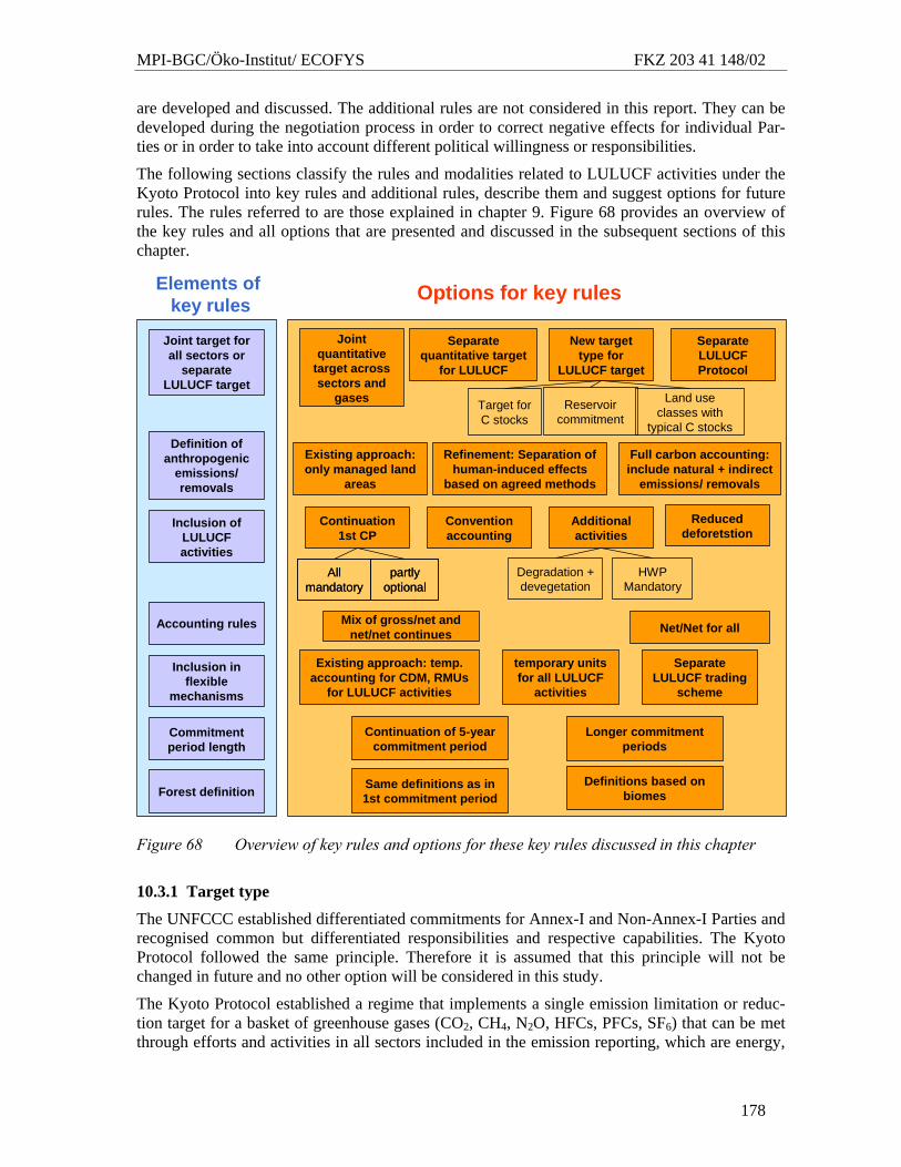
MPI-BGC/Öko-Institut/ ECOFYS FKZ 203 41 148/02
178
are developed and discussed. The additional rules are not considered in this report. They can be developed during the negotiation process in order to correct negative effects for individual Par-ties or in order to take into account different political willingness or responsibilities.
The following sections classify the rules and modalities related to LULUCF activities under the Kyoto Protocol into key rules and additional rules, describe them and suggest options for future rules. The rules referred to are those explained in chapter 9. Figure 68 provides an overview of the key rules and all options that are presented and discussed in the subsequent sections of this chapter.
Elements of key rules Options for key rules
Joint target for all sectors or
separate LULUCF target
Accounting rules
Inclusion of LULUCF activities
Definition of anthropogenic
emissions/removals
Inclusion in flexible
mechanisms
Joint quantitative
target across sectors and
gases
Separate quantitative target
for LULUCF
New target type for
LULUCF target
Separate LULUCF Protocol
Mix of gross/net and net/net continues Net/Net for all
Additional activities
Existing approach: only managed land
areas
Refinement: Separation of human-induced effects
based on agreed methods
Full carbon accounting: include natural + indirect
emissions/ removals
Continuation 1st CP
All mandatory
partly optional
All mandatory
partly optional
Degradation + devegetation
HWP Mandatory
Convention accounting
Target for C stocks
Reservoir commitment
Land use classes with
typical C stocks
Existing approach: temp. accounting for CDM, RMUs
for LULUCF activities
temporary units for all LULUCF
activities
Separate LULUCF trading
scheme
Commitment period length
Forest definition
Continuation of 5-year commitment period
Longer commitment periods
Same definitions as in 1st commitment period
Definitions based on biomes
Reduced deforetstion
Figure 68 Overview of key rules and options for these key rules discussed in this chapter
10.3.1 Target type
The UNFCCC established differentiated commitments for Annex-I and Non-Annex-I Parties and recognised common but differentiated responsibilities and respective capabilities. The Kyoto Protocol followed the same principle. Therefore it is assumed that this principle will not be changed in future and no other option will be considered in this study.
The Kyoto Protocol established a regime that implements a single emission limitation or reduc-tion target for a basket of greenhouse gases (CO2, CH4, N2O, HFCs, PFCs, SF6) that can be met through efforts and activities in all sectors included in the emission reporting, which are energy,
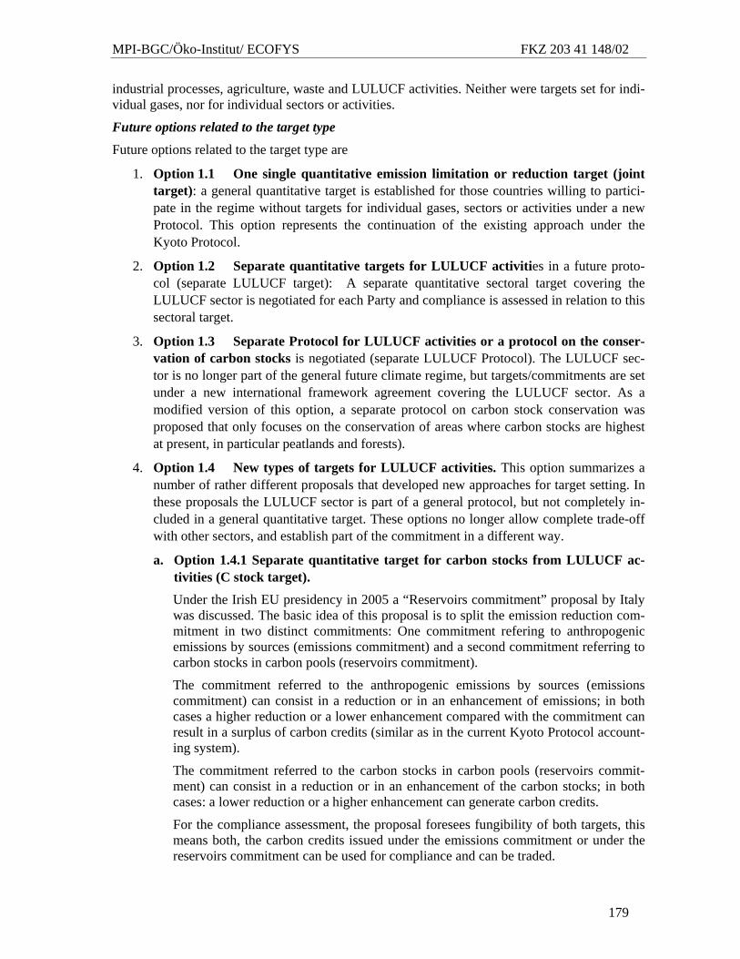
MPI-BGC/Öko-Institut/ ECOFYS FKZ 203 41 148/02
179
industrial processes, agriculture, waste and LULUCF activities. Neither were targets set for indi-vidual gases, nor for individual sectors or activities.
Future options related to the target type
Future options related to the target type are
1. Option 1.1 One single quantitative emission limitation or reduction target (joint target): a general quantitative target is established for those countries willing to partici-pate in the regime without targets for individual gases, sectors or activities under a new Protocol. This option represents the continuation of the existing approach under the Kyoto Protocol.
2. Option 1.2 Separate quantitative targets for LULUCF activities in a future proto-col (separate LULUCF target): A separate quantitative sectoral target covering the LULUCF sector is negotiated for each Party and compliance is assessed in relation to this sectoral target.
3. Option 1.3 Separate Protocol for LULUCF activities or a protocol on the conser-vation of carbon stocks is negotiated (separate LULUCF Protocol). The LULUCF sec-tor is no longer part of the general future climate regime, but targets/commitments are set under a new international framework agreement covering the LULUCF sector. As a modified version of this option, a separate protocol on carbon stock conservation was proposed that only focuses on the conservation of areas where carbon stocks are highest at present, in particular peatlands and forests).
4. Option 1.4 New types of targets for LULUCF activities. This option summarizes a number of rather different proposals that developed new approaches for target setting. In these proposals the LULUCF sector is part of a general protocol, but not completely in-cluded in a general quantitative target. These options no longer allow complete trade-off with other sectors, and establish part of the commitment in a different way.
a. Option 1.4.1 Separate quantitative target for carbon stocks from LULUCF ac-tivities (C stock target). Under the Irish EU presidency in 2005 a “Reservoirs commitment” proposal by Italy was discussed. The basic idea of this proposal is to split the emission reduction com-mitment in two distinct commitments: One commitment refering to anthropogenic emissions by sources (emissions commitment) and a second commitment referring to carbon stocks in carbon pools (reservoirs commitment).
The commitment referred to the anthropogenic emissions by sources (emissions commitment) can consist in a reduction or in an enhancement of emissions; in both cases a higher reduction or a lower enhancement compared with the commitment can result in a surplus of carbon credits (similar as in the current Kyoto Protocol account-ing system).
The commitment referred to the carbon stocks in carbon pools (reservoirs commit-ment) can consist in a reduction or in an enhancement of the carbon stocks; in both cases: a lower reduction or a higher enhancement can generate carbon credits.
For the compliance assessment, the proposal foresees fungibility of both targets, this means both, the carbon credits issued under the emissions commitment or under the reservoirs commitment can be used for compliance and can be traded.
MPI-BGC/Öko-Institut/ ECOFYS FKZ 203 41 148/02
180
JI actions could be implemented by Parties both under emissions commitment and reservoirs commitment. Both Parties need a commitment under the same option (emissions, reservoirs) in which they realize the actions. CDM actions could be im-plemented by Parties both under emissions commitment and reservoirs commitment. The donor Party needs a commitment under the option (emissions, reservoirs) in which it realizes the actions; the host Party would not have a commitment under this option.
b. Option 1.4.2 Targets for land-use classes with typical carbon stocks (land-use classes) Schlamadinger et al. (2006) presented a proposal in which separate targets for LULUCF are set in terms of land-use classes with typical carbon stocks. Temporary C changes within the same classes remain unaccounted whereas land units that move from one class to another are accounted over a transition period. This proposal re-quires the definition of land-use classes. For forest management for example, one class could be defined as “conventional forest management”, another class as “im-proved forest management”. The classes would need to be defined based on research and scientific evidence. The proposal in its draft form does neither address fungibility with emissions reductions commitments in other sectors nor the fact whether and how unmanaged forests would be considered in the approach.
c. Option 1.4.3 Emissions/removals commitment for LULUCF, reservoir commit-ment for new activity on unmanaged land (reservoir commitment)
Carbon losses from the biosphere are an order of magnitude faster than carbon up-take, so in the long term, the conservation of existing carbon stocks in the biosphere is a more sustainable strategy than the increase of present carbon stocks. This option proposes a new land management activity "Protection of high-C areas". A country can apply this to land in which the C stocks in all five C pools as defined in IPCC Good Practice Guidance for LULUCF or 2006 IPCC Guidelines pass a threshold, or in which the country chooses to maintain the present carbon stocks independent of a threshold. The option focuses on lands with high carbon stocks, mainly peatlands and virgin, unmanaged or old-growth forests where there is frequently a conflict between the use of wood or peat and the conservation of C reservoirs. The new category forms a voluntary or mandatory separate target for C stocks. This category is reserved for land for which the Party takes a long-term commitment of non-utilization (such as na-tional parks, nature conservation areas). Credits for the maintenance of existing stocks cannot directly be exchanged with other targets based on fluxes (see chapter 11).
The different options for target types as described above were assessed with the criteria de-scribed in section 10.2 (Figure 69). For this purpose an assessment matrix was used. The box in blue presents the key rule that is assessed. The orange boxes in the headline present the options for this key rule. The boxes in green on the left side present the criteria as introduced in section 10.2.
10.3.1.1 Climate effectiveness (Figure 69) Climate effectiveness of a future climate regime mainly depends on the stringency of future tar-gets, the inclusion of relevant countries as well as the inclusion of quantitatively relevant sources and sinks. The type of target however, may not be the major element for addressing climate ef-fectiveness.
Option 1.1 (joint target) and option 1.4.1 (C stock target) allow a trade-off between sectors and gases, in particular between the reduction of emissions and the enhancement of carbon sinks.
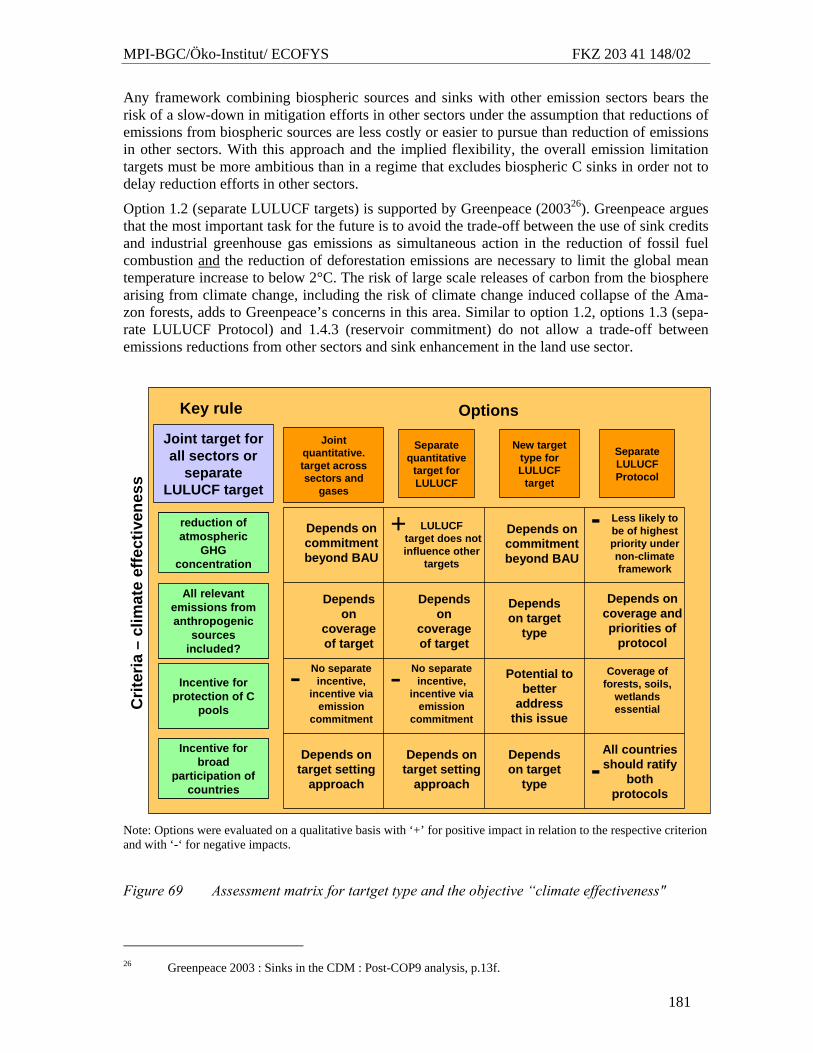
MPI-BGC/Öko-Institut/ ECOFYS FKZ 203 41 148/02
181
Any framework combining biospheric sources and sinks with other emission sectors bears the risk of a slow-down in mitigation efforts in other sectors under the assumption that reductions of emissions from biospheric sources are less costly or easier to pursue than reduction of emissions in other sectors. With this approach and the implied flexibility, the overall emission limitation targets must be more ambitious than in a regime that excludes biospheric C sinks in order not to delay reduction efforts in other sectors.
Option 1.2 (separate LULUCF targets) is supported by Greenpeace (200326). Greenpeace argues that the most important task for the future is to avoid the trade-off between the use of sink credits and industrial greenhouse gas emissions as simultaneous action in the reduction of fossil fuel combustion and the reduction of deforestation emissions are necessary to limit the global mean temperature increase to below 2°C. The risk of large scale releases of carbon from the biosphere arising from climate change, including the risk of climate change induced collapse of the Ama-zon forests, adds to Greenpeace’s concerns in this area. Similar to option 1.2, options 1.3 (sepa-rate LULUCF Protocol) and 1.4.3 (reservoir commitment) do not allow a trade-off between emissions reductions from other sectors and sink enhancement in the land use sector.
Crit
eria
–cl
imat
eef
fect
iven
ess
Joint quantitative. target across sectors and
gases
Separate quantitative
target for LULUCF
New target type for LULUCF
target
Separate LULUCF Protocol
Options
-
Joint target for all sectors or
separate LULUCF target
Key rule
Depends on commitmentbeyond BAU
Less likely to be of highestpriority undernon-climateframework
Depends on coverage and priorities of
protocol
Dependson target
type
+reduction of atmospheric
GHG concentration
All relevant emissions from anthropogenic
sources included?
Incentive for protection of C
pools
Incentive for broad
participation of countries
reduction of atmospheric
GHG concentration
All relevant emissions from anthropogenic
sources included?
Incentive for protection of C
pools
Incentive for broad
participation of countries
LULUCFtarget does not influence other
targets
Depends on commitmentbeyond BAU
No separate incentive,
incentive via emission
commitment
Potential to better
addressthis issue
Depends on target setting
approach
Dependson target
type
Coverage of forests, soils,
wetlandsessential
-All countriesshould ratify
bothprotocols
Depends on target setting
approach
Dependson
coverageof target
--
Dependson
coverageof target
No separate incentive,
incentive via emission
commitment
Note: Options were evaluated on a qualitative basis with ‘+’ for positive impact in relation to the respective criterion and with ‘-‘ for negative impacts.
Figure 69 Assessment matrix for tartget type and the objective “climate effectiveness"
26 Greenpeace 2003 : Sinks in the CDM : Post-COP9 analysis, p.13f.
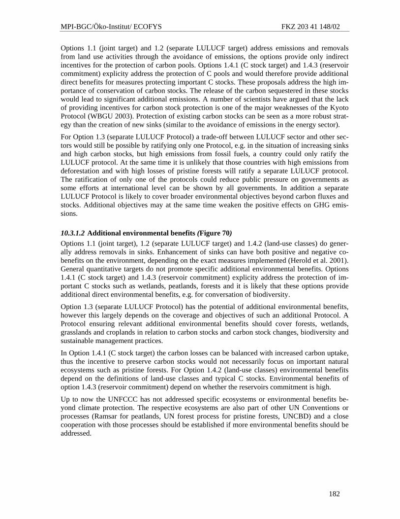
MPI-BGC/Öko-Institut/ ECOFYS FKZ 203 41 148/02
182
Options 1.1 (joint target) and 1.2 (separate LULUCF target) address emissions and removals from land use activities through the avoidance of emissions, the options provide only indirect incentives for the protection of carbon pools. Options 1.4.1 (C stock target) and 1.4.3 (reservoir commitment) explicity address the protection of C pools and would therefore provide additional direct benefits for measures protecting important C stocks. These proposals address the high im-portance of conservation of carbon stocks. The release of the carbon sequestered in these stocks would lead to significant additional emissions. A number of scientists have argued that the lack of providing incentives for carbon stock protection is one of the major weaknesses of the Kyoto Protocol (WBGU 2003). Protection of existing carbon stocks can be seen as a more robust strat-egy than the creation of new sinks (similar to the avoidance of emissions in the energy sector).
For Option 1.3 (separate LULUCF Protocol) a trade-off between LULUCF sector and other sec-tors would still be possible by ratifying only one Protocol, e.g. in the situation of increasing sinks and high carbon stocks, but high emissions from fossil fuels, a country could only ratify the LULUCF protocol. At the same time it is unlikely that those countries with high emissions from deforestation and with high losses of pristine forests will ratify a separate LULUCF protocol. The ratification of only one of the protocols could reduce public pressure on governments as some efforts at international level can be shown by all governments. In addition a separate LULUCF Protocol is likely to cover broader environmental objectives beyond carbon fluxes and stocks. Additional objectives may at the same time weaken the positive effects on GHG emis-sions.
10.3.1.2 Additional environmental benefits (Figure 70) Options 1.1 (joint target), 1.2 (separate LULUCF target) and 1.4.2 (land-use classes) do gener-ally address removals in sinks. Enhancement of sinks can have both positive and negative co-benefits on the environment, depending on the exact measures implemented (Herold et al. 2001). General quantitative targets do not promote specific additional environmental benefits. Options 1.4.1 (C stock target) and 1.4.3 (reservoir commitment) explicity address the protection of im-portant C stocks such as wetlands, peatlands, forests and it is likely that these options provide additional direct environmental benefits, e.g. for conversation of biodiversity.
Option 1.3 (separate LULUCF Protocol) has the potential of additional environmental benefits, however this largely depends on the coverage and objectives of such an additional Protocol. A Protocol ensuring relevant additional environmental benefits should cover forests, wetlands, grasslands and croplands in relation to carbon stocks and carbon stock changes, biodiversity and sustainable management practices.
In Option 1.4.1 (C stock target) the carbon losses can be balanced with increased carbon uptake, thus the incentive to preserve carbon stocks would not necessarily focus on important natural ecosystems such as pristine forests. For Option 1.4.2 (land-use classes) environmental benefits depend on the definitions of land-use classes and typical C stocks. Environmental benefits of option 1.4.3 (reservoir commitment) depend on whether the reservoirs commitment is high.
Up to now the UNFCCC has not addressed specific ecosystems or environmental benefits be-yond climate protection. The respective ecosystems are also part of other UN Conventions or processes (Ramsar for peatlands, UN forest process for pristine forests, UNCBD) and a close cooperation with those processes should be established if more environmental benefits should be addressed.
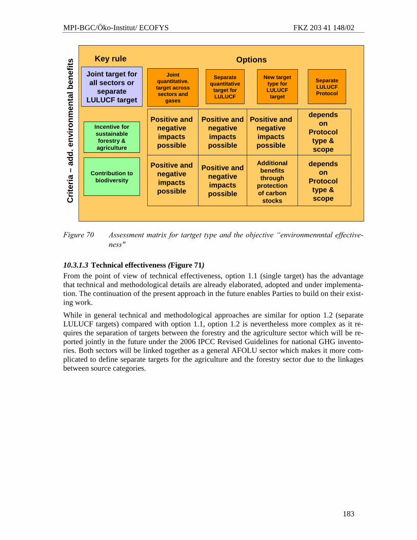
MPI-BGC/Öko-Institut/ ECOFYS FKZ 203 41 148/02
183
Joint quantitative. target across sectors and
gases
Separate quantitative
target for LULUCF
New target type for LULUCF
target
Separate LULUCF Protocol
Options
Joint target for all sectors or
separate LULUCF target
Key ruleC
riter
ia–
add.
env
ironm
enta
lben
efits
Additional benefitsthrough
protectionof carbon
stocks
Incentive for sustainable forestry & agriculture
Contribution to biodiversity
Incentive for sustainable forestry & agriculture
Contribution to biodiversity
dependson
Protocoltype & scope
Positive and negative impactspossible
Positive and negative impactspossible
Positive and negative impactspossible
Positive and negative impactspossible
dependson
Protocoltype & scope
Positive and negative impactspossible
Figure 70 Assessment matrix for tartget type and the objective “environmennntal effective-ness"
10.3.1.3 Technical effectiveness (Figure 71) From the point of view of technical effectiveness, option 1.1 (single target) has the advantage that technical and methodological details are already elaborated, adopted and under implementa-tion. The continuation of the present approach in the future enables Parties to build on their exist-ing work.
While in general technical and methodological approaches are similar for option 1.2 (separate LULUCF targets) compared with option 1.1, option 1.2 is nevertheless more complex as it re-quires the separation of targets between the forestry and the agriculture sector which will be re-ported jointly in the future under the 2006 IPCC Revised Guidelines for national GHG invento-ries. Both sectors will be linked together as a general AFOLU sector which makes it more com-plicated to define separate targets for the agriculture and the forestry sector due to the linkages between source categories.
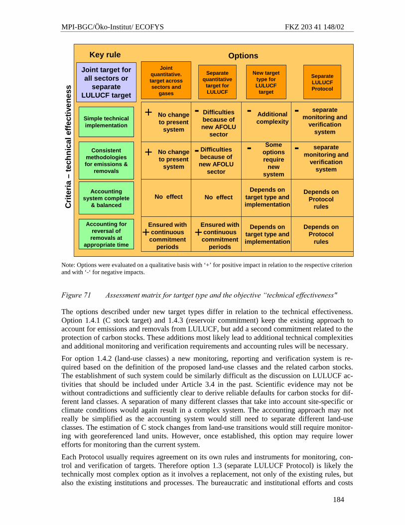
MPI-BGC/Öko-Institut/ ECOFYS FKZ 203 41 148/02
184
Joint quantitative. target across sectors and
gases
Separate quantitative
target for LULUCF
New target type for LULUCF
target
Separate LULUCF Protocol
Options
-
Joint target for all sectors or
separate LULUCF target
Key ruleC
riter
ia–
tech
nica
leffe
ctiv
enes
s
separate monitoring and
verificationsystem
Someoptionsrequire
newsystem
Simple technical implementation
Consistent methodologies for emissions &
removals
Accounting system complete
& balanced
Accounting for reversal of removals at
appropriate time
Simple technical implementation
Consistent methodologies for emissions &
removals
Accounting system complete
& balanced
Accounting for reversal of removals at
appropriate time
Additional complexity
No effect
Depends on Protocol
rules
+
+ - - separate monitoring and
verificationsystem
No effectDepends on
target type and implementation
Ensured withcontinuous
commitmentperiods
No changeto present
system
No changeto present
system
Ensured withcontinuous
commitmentperiods
Difficultiesbecause of new AFOLU
sector
Difficultiesbecause of new AFOLU
sector
Depends on Protocol
rules
Depends on target type and implementation
-
-
-
+ +
Note: Options were evaluated on a qualitative basis with ‘+’ for positive impact in relation to the respective criterion and with ‘-‘ for negative impacts.
Figure 71 Assessment matrix for tartget type and the objective “technical effectiveness"
The options described under new target types differ in relation to the technical effectiveness. Option 1.4.1 (C stock target) and 1.4.3 (reservoir commitment) keep the existing approach to account for emissions and removals from LULUCF, but add a second commitment related to the protection of carbon stocks. These additions most likely lead to additional technical complexities and additional monitoring and verification requirements and accounting rules will be necessary.
For option 1.4.2 (land-use classes) a new monitoring, reporting and verification system is re-quired based on the definition of the proposed land-use classes and the related carbon stocks. The establishment of such system could be similarly difficult as the discussion on LULUCF ac-tivities that should be included under Article 3.4 in the past. Scientific evidence may not be without contradictions and sufficiently clear to derive reliable defaults for carbon stocks for dif-ferent land classes. A separation of many different classes that take into account site-specific or climate conditions would again result in a complex system. The accounting approach may not really be simplified as the accounting system would still need to separate different land-use classes. The estimation of C stock changes from land-use transitions would still require monitor-ing with georeferenced land units. However, once established, this option may require lower efforts for monitoring than the current system.
Each Protocol usually requires agreement on its own rules and instruments for monitoring, con-trol and verification of targets. Therefore option 1.3 (separate LULUCF Protocol) is likely the technically most complex option as it involves a replacement, not only of the existing rules, but also the existing institutions and processes. The bureaucratic and institutional efforts and costs
MPI-BGC/Öko-Institut/ ECOFYS FKZ 203 41 148/02
185
necessary will be considerably higher than for the current basket approach. Negotiations would start from scratch without building on existing experiences. A shift from options 1.1 and 1.2 to the other options 1.3 and 1.4 concerns the entire regime and not only an improved and less com-plex accounting system for sinks.
10.3.1.4 Facilitation of the negotiation process (Figure 72) Option 1.1 (joint target) offers countries flexibility in the way how the general target will be achieved and in relation to the contributions of individual sectors and individual gases to the overall effort which can be decided nationally after the general agreement of the overall target. The efforts required in each sector remain a national decision on the basis of national circum-stances and priorities. The advantage is that such a type of target offers flexibility in the imple-mentation for those Parties willing to contribute with quantitative targets. For the negotiation process, such target types are straightforward to negotiate. From the experiences with the Kyoto Protocol, it would be beneficial if a future agreement will clearly specify all gases, sectors and sectoral activities included in a general cross-sectoral and cross-gas target and that such activities will not be negotiated in a second step after the setting of the general target as it occurred for Article 3.4 activities for the first commitment period. The coverage of the target should be clearly defined before the target is finally agreed. This approach builds on the inventory report-ing under the UNFCCC and the Kyoto Protocol, therefore it offers the favourable situation that emissions and removals at country level and long-term trends especially for Annex-I Parties since 1990 are well known and understood. A general quantitative target may not yet be applica-ble to Non-Annex I Parties, because the main emitters such as China, India and Brazil strongly oppose quantitative targets and targets comparable to Annex-I Parties.
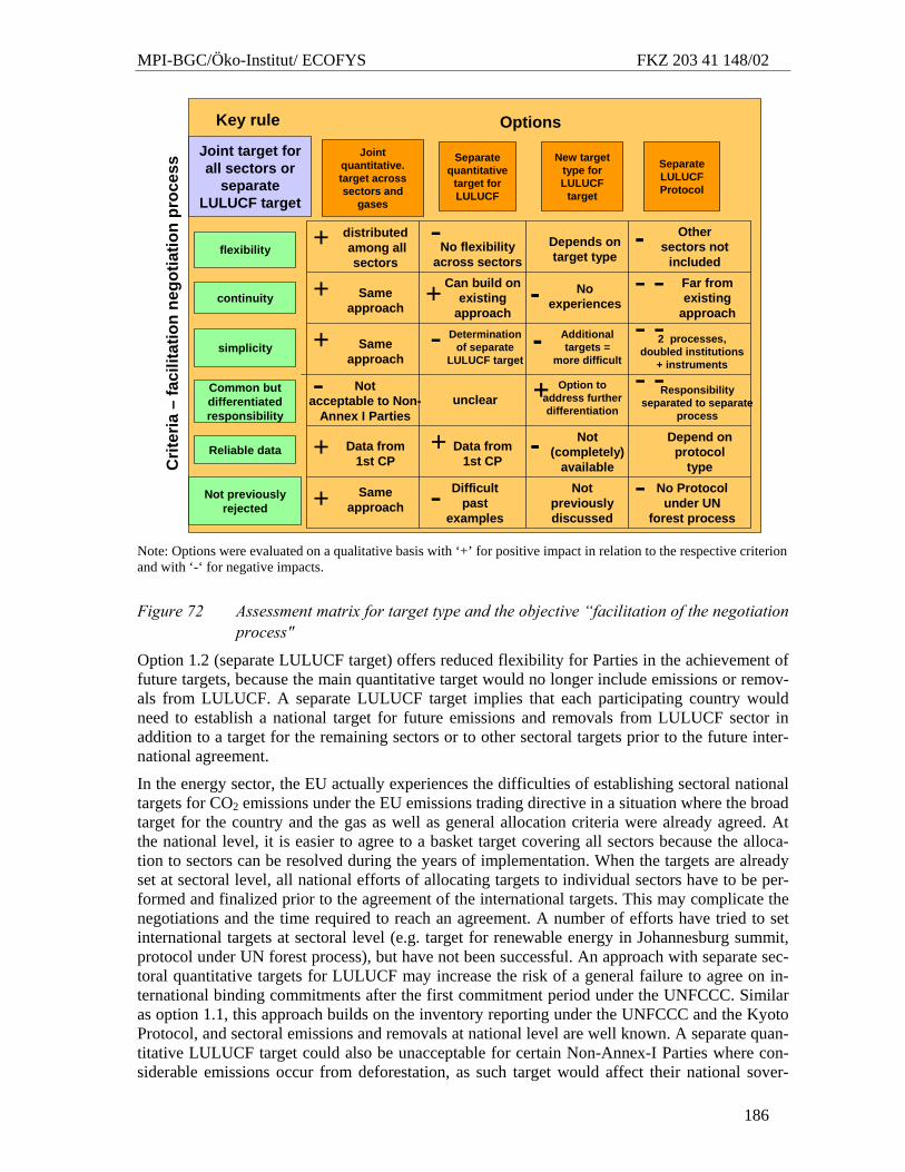
MPI-BGC/Öko-Institut/ ECOFYS FKZ 203 41 148/02
186
Joint quantitative. target across sectors and
gases
Separate quantitative
target for LULUCF
New target type for LULUCF
target
Separate LULUCF Protocol
flexibility
Common but differentiated responsibility
simplicity
Reliable data
Options
continuity
+
+
+
+
+
Not previously rejected
+
-
-- -- -- --
-
-
Joint target for all sectors or
separate LULUCF target
Key rule
Crit
eria
–fa
cilit
atio
nne
gotia
tion
proc
ess
distributedamong all sectors
No flexibilityacross sectors
Depends on target type
Othersectors not
included
Same approach
Determination of separate
LULUCF target
Data from1st CP
Not acceptable to Non-
Annex I Parties
2 processes, doubled institutions
+ instruments
Responsibilityseparated to separate
process
No Protocolunder UN
forest process
Data from1st CP
Option to address furtherdifferentiation+
Can build on existing
approach
Far fromexisting
approach
No experiences
Additional targets =
more difficult
unclear
Not (completely)
available
+
Difficultpast
examples
Depend on protocol
type
--
-
Same approach
Same approach
Not previouslydiscussed
-
Note: Options were evaluated on a qualitative basis with ‘+’ for positive impact in relation to the respective criterion and with ‘-‘ for negative impacts.
Figure 72 Assessment matrix for target type and the objective “facilitation of the negotiation process"
Option 1.2 (separate LULUCF target) offers reduced flexibility for Parties in the achievement of future targets, because the main quantitative target would no longer include emissions or remov-als from LULUCF. A separate LULUCF target implies that each participating country would need to establish a national target for future emissions and removals from LULUCF sector in addition to a target for the remaining sectors or to other sectoral targets prior to the future inter-national agreement.
In the energy sector, the EU actually experiences the difficulties of establishing sectoral national targets for CO2 emissions under the EU emissions trading directive in a situation where the broad target for the country and the gas as well as general allocation criteria were already agreed. At the national level, it is easier to agree to a basket target covering all sectors because the alloca-tion to sectors can be resolved during the years of implementation. When the targets are already set at sectoral level, all national efforts of allocating targets to individual sectors have to be per-formed and finalized prior to the agreement of the international targets. This may complicate the negotiations and the time required to reach an agreement. A number of efforts have tried to set international targets at sectoral level (e.g. target for renewable energy in Johannesburg summit, protocol under UN forest process), but have not been successful. An approach with separate sec-toral quantitative targets for LULUCF may increase the risk of a general failure to agree on in-ternational binding commitments after the first commitment period under the UNFCCC. Similar as option 1.1, this approach builds on the inventory reporting under the UNFCCC and the Kyoto Protocol, and sectoral emissions and removals at national level are well known. A separate quan-titative LULUCF target could also be unacceptable for certain Non-Annex-I Parties where con-siderable emissions occur from deforestation, as such target would affect their national sover-
MPI-BGC/Öko-Institut/ ECOFYS FKZ 203 41 148/02
187
eignty in taking land-use decisions. This could decrease the likelihood to integrate major emitters from Non-Annex-I Parties.
The option of new target types (option 1.4) can have considerable impacts on the accountable emissions in a future climate regime. When new target types are not based on the current report-ing system, but on a considerably changed system, it is likely that no reliable information for the assessment of the quantitative effects of such options exists for policy makers when future com-mitments are negotiated.
Option 1.4.1 (C stock target) keeps flexibility regarding the target types accepted by Parties and fungibility of credits from both targets. However, it requires the additional negotiation effort to establish targets for carbon stocks for each participating country prior to a general agreement. Option 1.4.3 (reservoir commitment) excludes the flexibility of a trade-off between the reservoir commitment and other targets. It requires the additional establishment of reservoir commitments for important C stocks. As a wide range of activities lead to carbon stock changes in reservoirs, it may be time-consuming to reach a general agreement at national level with all actors involved for such a commitment because this concerns infrastructure decisions, management decisions in agriculture, forestry and wetlands as well as strategies to conserve soil carbon. It may be difficult for Parties to develop their national targets in time prior to the end of the first commitment pe-riod under the Kyoto Protocol for options 1.4.1 and 1.4.3. Both options are not directly covered in the current reporting and verification system and data are not easily available for all countries. Commitments to protect important carbon stocks could be an option to involve Non-Annex I Parties with commitments in the process.
For option 1.4.2 (land-use classes), a number of issues such as fungibility with other commit-ments are not (yet) defined. Temporary C changes within the same classes would remain unac-counted whereas land units that move from one class to another would be accounted over a tran-sition period. Before a definition of such land-use classes is agreed, no country would be able to estimate the accountable effects. Once defined, national experts would have to analyse which land areas remain in the same classes and which land areas move to different classes and from that assessment they could calculate the accountable emissions and removals. If general targets are agreed before the detailed classes and typical C stocks are established, the same difficult ne-gotiation situation as under the Kyoto Protocol would arise: Parties would try to weaken the spe-cific rules and accounting system in order to facilitate compliance with general targets. It may be very time-consuming to negotiate all necessary details for the proposed land-use classes, as this may require further scientific work from bodies such as IPCC.
Option 1.3 (Separate LULUCF Protocol) will above all increase negotiation time and efforts, because a separate agreement needs to be negotiated covering rules, monitoring, reporting, veri-fication or compliance. However, a separate Protocol will not improve the likelihood to negotiate ambitious reduction or stabilisation targets. Each Protocol usually requires its own regular con-ferences, bodies and institutions, dispute settlement or non-compliance procedures. This option may create a system that is no longer related to the present LULUCF rules and commitments. Whether there are reliable data to judge the stringency of commitments depends on the specific type of commitments in such a Protocol.
10.3.1.5 Special characteristics of LULUCF sector (Figure 73) Some specific characteristics of the LULUCF sector have caused difficulties in the negotiations in the past, such as the variability of C fluxes from year to year, the non-permanent nature of carbon sequestration in terrestrial sinks, the factoring out of indirect effects or different national circumstances. Under the Kyoto Protocol these specific problems were resolved (see chapter 9 of this report) and those solutions could continue in the future (option 1.1).
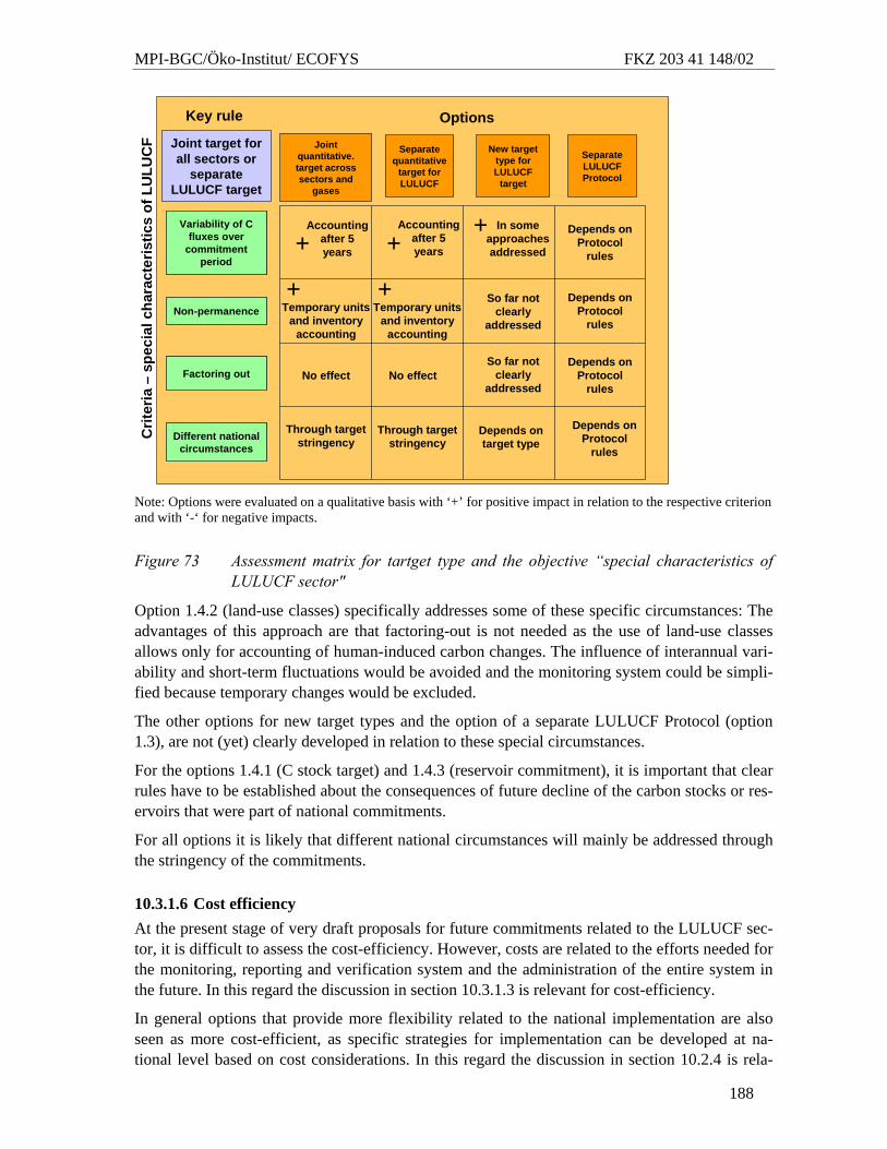
MPI-BGC/Öko-Institut/ ECOFYS FKZ 203 41 148/02
188
Joint quantitative. target across sectors and
gases
Separate quantitative
target for LULUCF
New target type for LULUCF
target
Separate LULUCF Protocol
Options
Variability of C fluxes over
commitment period
Different national circumstances
Factoring out
Non-permanence
Variability of C fluxes over
commitment period
Different national circumstances
Factoring out
Non-permanence
+
+
Joint target for all sectors or
separate LULUCF target
Key rule
Crit
eria
–sp
ecia
lcha
ract
eris
tics
of L
ULU
CF
Accountingafter 5 years
In someapproachesaddressed
No effect
Temporary unitsand inventory
accounting
So far not clearly
addressed
Accountingafter 5 years+
Temporary unitsand inventory
accounting
+
No effect
Through targetstringency
Through targetstringency
Depends on target type
+
Depends on Protocol
rules
Depends on Protocol
rules
So far not clearly
addressed
Depends on Protocol
rules
Depends on Protocol
rules
Note: Options were evaluated on a qualitative basis with ‘+’ for positive impact in relation to the respective criterion and with ‘-‘ for negative impacts.
Figure 73 Assessment matrix for tartget type and the objective “special characteristics of LULUCF sector"
Option 1.4.2 (land-use classes) specifically addresses some of these specific circumstances: The advantages of this approach are that factoring-out is not needed as the use of land-use classes allows only for accounting of human-induced carbon changes. The influence of interannual vari-ability and short-term fluctuations would be avoided and the monitoring system could be simpli-fied because temporary changes would be excluded.
The other options for new target types and the option of a separate LULUCF Protocol (option 1.3), are not (yet) clearly developed in relation to these special circumstances.
For the options 1.4.1 (C stock target) and 1.4.3 (reservoir commitment), it is important that clear rules have to be established about the consequences of future decline of the carbon stocks or res-ervoirs that were part of national commitments.
For all options it is likely that different national circumstances will mainly be addressed through the stringency of the commitments.
10.3.1.6 Cost efficiency At the present stage of very draft proposals for future commitments related to the LULUCF sec-tor, it is difficult to assess the cost-efficiency. However, costs are related to the efforts needed for the monitoring, reporting and verification system and the administration of the entire system in the future. In this regard the discussion in section 10.3.1.3 is relevant for cost-efficiency.
In general options that provide more flexibility related to the national implementation are also seen as more cost-efficient, as specific strategies for implementation can be developed at na-tional level based on cost considerations. In this regard the discussion in section 10.2.4 is rela-
MPI-BGC/Öko-Institut/ ECOFYS FKZ 203 41 148/02
189
vant.
One of the reasons for the development of options that include the conservation of existing car-bon stocks (option 1.4.1 C stock target and 1.4.3 reservoir commitment) is cost-efficiency be-cause it is regarded as more cost-efficient protecting existing high carbon stock areas and to avoid carbon losses, than enhancing carbon sequestration in terrestrial ecosystems.
10.3.2 Accounting of direct human-induced emissions and removals from sinks
The Kyoto Protocol specifies that accounting of LULUCF activities is restricted to land areas subject to “direct human-induced” (Art. 3.3) or “human-induced” (Art. 3.4) activities. This sepa-ration is based on the Convention where already Article 2 of the UNFCCC, addressing the objec-tive of the Convention, specifies that,
“The ultimate objective of this Convention and any related legal instruments that the Conference of the Parties may adopt is to achieve, in accordance with the relevant provisions of the Convention, stabilization of greenhouse gas concentrations in the atmosphere at a level that would prevent dangerous anthropogenic interference with the climate system.”
Article 4 (a) specifies that national greenhouse gas inventories are limited to “anthropogenic emissions by sources and removals by sinks of all greenhouse gases not controlled by the Mont-real Protocol”.
The philosophy behind the Convention and the Kyoto Protocol was to limit the accounting of GHG emissions to those parts influenced by human activities. Thus greenhouse gas inventories should above all reflect the effects of policies and measures undertaken to limit and reduce GHG emissions over the time period covered by the periodic inventories. The objective was also to limit commitments to those parts of emissions where human beings and countries are responsible for with their activities. The separation of human-induced from natural effects could be based on the cause (Indirectly human-induced: e.g. acid rain, N deposition, temperature increase; directly human induced, e.g. forest management etc.; natural, e.g. partly fire, storms) or on the land area (managed – unmanaged).
Future options related to the accounting of anthropogenic/direct human-induced emissions and removals:
Option 2.1: Continuation of existing approach (managed areas) The continuation of the existing approach implies that only directly human-induced effects are accounted for. Non-human-induced C sources and sinks are seen as limited to places and events remote from human activity. Management is considered as a token of human-inducement. Events in managed forests and on managed land areas are considered per se as human induced. Unman-aged land areas are not included in the commitments. Indirect human-induced influences on re-movals are deducted by coarse budgets/thresholds for those activities where such effects are relevant (e.g. currently for forest management).
Option 2.2: Refinement of Kyoto approach (Factoring out) In general there are three approaches to track only direct human-induced changes:
• Human-induced and natural effects are estimated on the basis of agreed models
• Control plots are established where “no treatment” regimes are monitored that represent
MPI-BGC/Öko-Institut/ ECOFYS FKZ 203 41 148/02
190
the natural, non-anthropogenic effects. These effects are subtracted from the measured ef-fects with different human-induced practices and management.
• Specification of agreed background corrections (caps or thresholds). One option is the es-tablishment of a business-as-usual scenario from which to estimate the net effects attrib-utable to human-induced activities. Model results and results from control plots could feed in such a scenario.
This option implies that Parties to a future climate regime adopt one or several of these ap-proaches and develop a scientific-technical method for the factoring-out of natural and indirect activities in order not to account for the non-human, indirect induced changes in carbon stocks.
Option 2.3: Full carbon accounting The term “full carbon accounting” is used for complete accounting of stock changes in all carbon pools for all landscape units in a given time period (IPCC 2000b, p. 78). Applying full carbon accounting to all lands in a country would, in principle, yield the net carbon exchange between terrestrial ecosystems and the atmosphere.
The complete accounting of all carbon pools is close to the agreed estimation of pools under the Kyoto Protocol that require the monitoring of all pools with significant changes. The complete accounting over all landscape units is not achieved by the Kyoto Protocol as Parties can elect defined Article 3.4 activities and because of the “since 1990” criterion which limits the land area covered by the Kyoto accounting systems and restricts activities to direct human-induced changes. The full carbon accounting approach also includes emissions and removals driven by natural processes and from natural ecosystems not experiencing any human interference.
The different options for accounting of direct human-induced emissions and removals from sinks as described above were assessed with the criteria described in section 10.2. The results are pre-sented in the following sections:
10.3.2.1 Climate effectiveness (Figure 74) WBGU criticised that the Kyoto Protocol does not acknowledge the carbon stocks in pristine forests or temperate, sustainably managed forests and that no incentives exist to prevent these stocks from being lost. Option 2.1 (managed areas) excludes carbon losses on unmanaged land areas and the emission or reduction commitments are not directly related to the signal in the at-mosphere. The amount of emissions excluded from a future regime due to the limitation to man-aged land areas will depend on the exact definition of managed land areas and on the fact whether the Parties covered by the regime have large land areas with relevant unmanaged areas. However, most countries that ratified the Kyoto Protocol do not have large unmanaged forest areas or other unmanaged areas. The countries with large areas of unmanaged forests under the Kyoto Protocol are Australia, Canada, and Russia. The existing caps for the accounting of forest management activities (see chapter 9) were agreed on a rather arbitrary basis and are not clearly linked to scientific research and true anthropogenic effects. Even if there are not yet general methodologies available, there may be possibilities to refine this approach and to provide closer linkages to scientific research in choosing budgets and thresholds for future commitments. If e.g. forest management continues to be capped, the basis for such a cap should be further discussed and agreed. However, additional research and concepts are necessary to enable a refined ap-proach in the future.
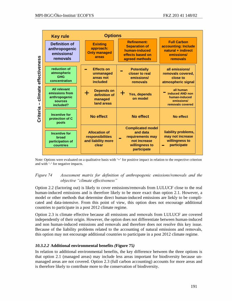
MPI-BGC/Öko-Institut/ ECOFYS FKZ 203 41 148/02
191
--
Existing approach:
Only managed areas
Refinement: Separation of
human-induced effects based on agreed methods
Full Carbon accounting: Include
natural + indirect emissions/ removals
Definition of anthropogenic
emissions/removals
Options
-
all emissions/ removals covered,
close to atmospheric signal
liability problems, may not increase
willingness to participate
all human induced AND non human-induced
emissions/ removals covered
Complicated modeland data
requirements maynot increase
willingness to participate
Key rule
No effect
-
- Effects on unmanagedareas not included
No effect
reduction of atmospheric
GHG concentration
All relevant emissions from anthropogenic
sources included?
Incentive for protection of C
pools
Incentive for broad
participation of countries
reduction of atmospheric
GHG concentration
All relevant emissions from anthropogenic
sources included?
Incentive for protection of C
pools
Incentive for broad
participation of countries
Crit
eria
–cl
imat
eef
fect
iven
ess
Allocation of responsibilities
and liability moreclear
No effect
Yes, dependson model
- Potentiallycloser to real emissions/ removals
+ -Depends on definition of managedland areas
+
Note: Options were evaluated on a qualitative basis with ‘+’ for positive impact in relation to the respective criterion and with ‘-‘ for negative impacts.
Figure 74 Assessment matrix for definition of anthropogenic emissions/removals and the objective “climate effectiveness”
Option 2.2 (factoring out) is likely to cover emissions/removals from LULUCF close to the real human-induced emissions and is therefore likely to be more exact than option 2.1. However, a model or other methods that determine direct human-induced emissions are liekly to be compli-cated and data-intensive. From this point of view, this option does not encourage additional countries to participate in a post 2012 climate regime.
Option 2.3 is climate effective because all emissions and removals from LULUCF are covered independently of their origin. However, the option does not differentiate between human-induced and non human-induced emissions and removals and therefore does not resolve this key issue. Because of the liability problems related to the accounting of natural emissions and removals, this option may not encourage additional countries to participate in a post 2012 climate regime.
10.3.2.2 Additional environmental benefits (Figure 75) In relation to additional environmental benefits, the key difference between the three options is that option 2.1 (managed areas) may include less areas important for biodiversity because un-managed areas are not covered. Option 2.3 (full carbon accounting) accounts for more areas and is therefore likely to contribute more to the conservation of biodiversity.
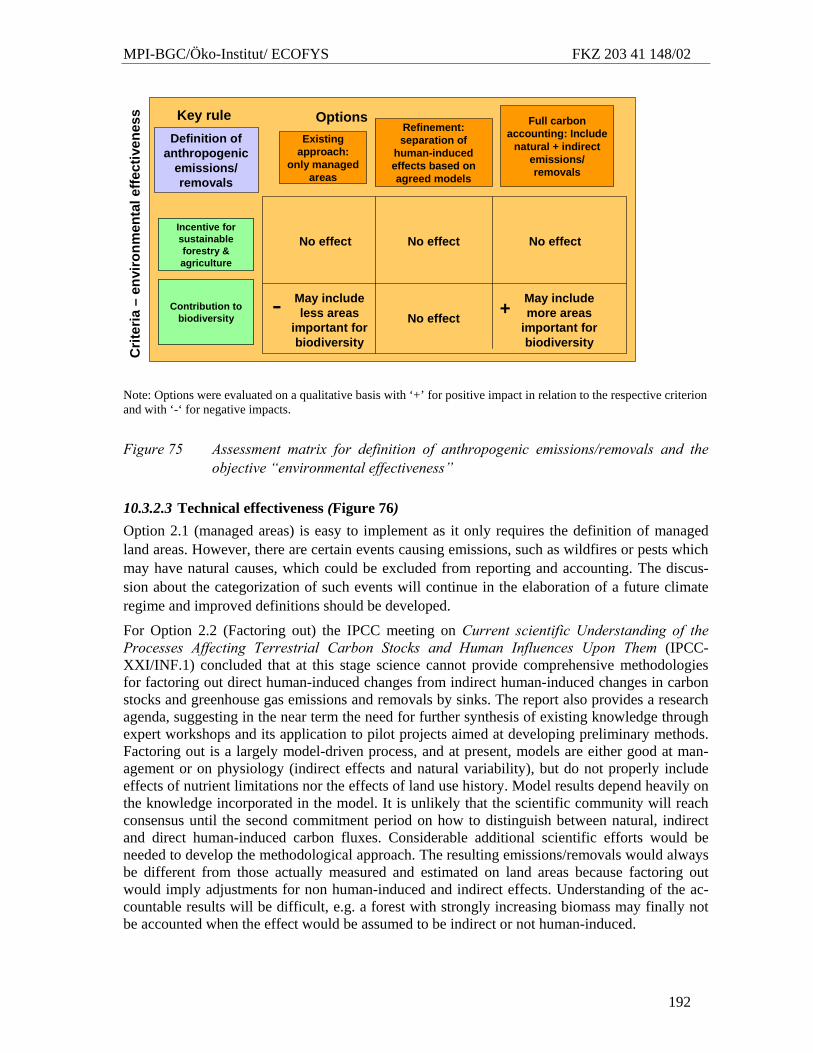
MPI-BGC/Öko-Institut/ ECOFYS FKZ 203 41 148/02
192
--
Existing approach:
only managed areas
Refinement: separation of
human-induced effects based on agreed models
Full carbon accounting: Include
natural + indirect emissions/ removals
Definition of anthropogenic
emissions/removals
Options
May includemore areas
important forbiodiversity
Key rule
No effect
Crit
eria
–en
viro
nmen
tale
ffect
iven
ess
Incentive for sustainable forestry & agriculture
Contribution to biodiversity
Incentive for sustainable forestry & agriculture
Contribution to biodiversity
- May includeless areas
important forbiodiversity
+
No effect No effect No effect
Note: Options were evaluated on a qualitative basis with ‘+’ for positive impact in relation to the respective criterion and with ‘-‘ for negative impacts.
Figure 75 Assessment matrix for definition of anthropogenic emissions/removals and the objective “environmental effectiveness”
10.3.2.3 Technical effectiveness (Figure 76) Option 2.1 (managed areas) is easy to implement as it only requires the definition of managed land areas. However, there are certain events causing emissions, such as wildfires or pests which may have natural causes, which could be excluded from reporting and accounting. The discus-sion about the categorization of such events will continue in the elaboration of a future climate regime and improved definitions should be developed.
For Option 2.2 (Factoring out) the IPCC meeting on Current scientific Understanding of the Processes Affecting Terrestrial Carbon Stocks and Human Influences Upon Them (IPCC-XXI/INF.1) concluded that at this stage science cannot provide comprehensive methodologies for factoring out direct human-induced changes from indirect human-induced changes in carbon stocks and greenhouse gas emissions and removals by sinks. The report also provides a research agenda, suggesting in the near term the need for further synthesis of existing knowledge through expert workshops and its application to pilot projects aimed at developing preliminary methods. Factoring out is a largely model-driven process, and at present, models are either good at man-agement or on physiology (indirect effects and natural variability), but do not properly include effects of nutrient limitations nor the effects of land use history. Model results depend heavily on the knowledge incorporated in the model. It is unlikely that the scientific community will reach consensus until the second commitment period on how to distinguish between natural, indirect and direct human-induced carbon fluxes. Considerable additional scientific efforts would be needed to develop the methodological approach. The resulting emissions/removals would always be different from those actually measured and estimated on land areas because factoring out would imply adjustments for non human-induced and indirect effects. Understanding of the ac-countable results will be difficult, e.g. a forest with strongly increasing biomass may finally not be accounted when the effect would be assumed to be indirect or not human-induced.
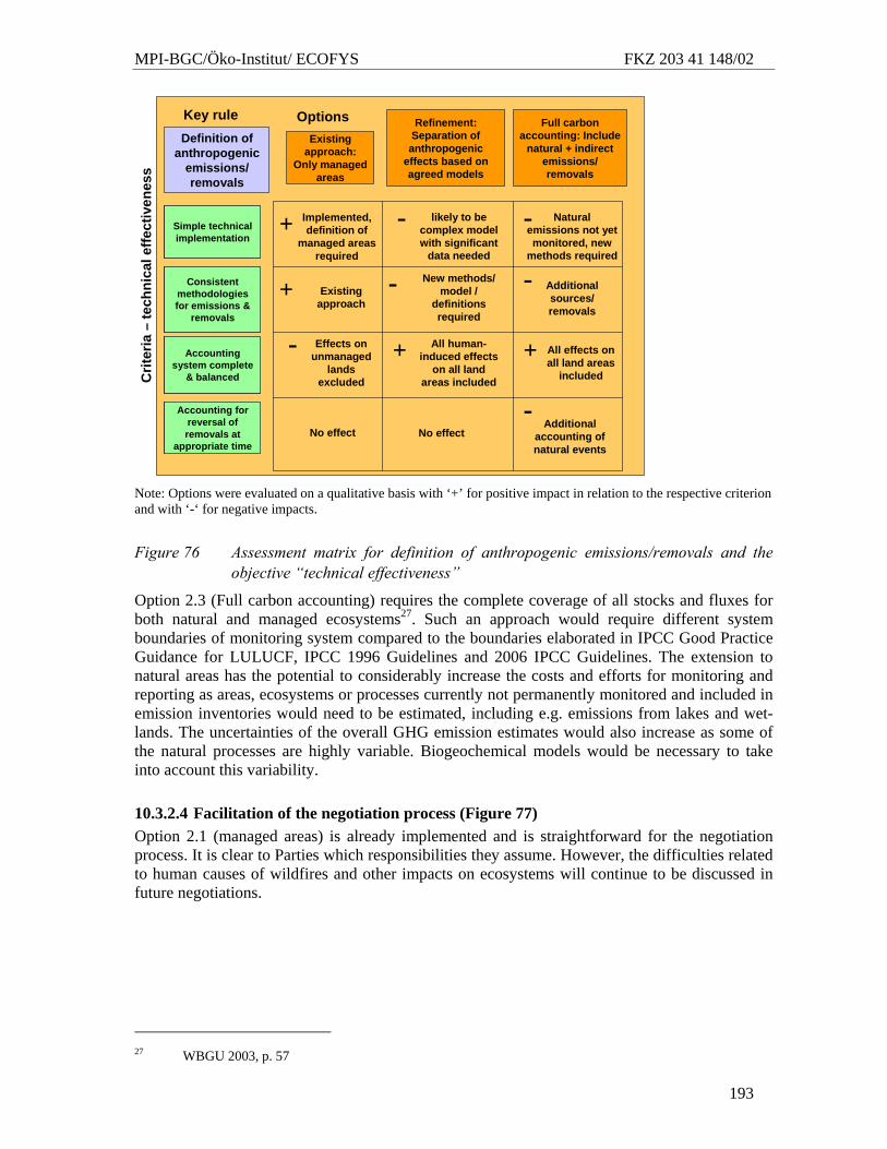
MPI-BGC/Öko-Institut/ ECOFYS FKZ 203 41 148/02
193
--
Existing approach:
Only managed areas
Refinement: Separation of anthropogenic
effects based on agreed models
Full carbon accounting: Include
natural + indirect emissions/ removals
Definition of anthropogenic
emissions/removals
Options
likely to becomplex modelwith significant
data needed
- Additional sources/ removals
Key rule
-
Effects on unmanaged
landsexcluded
No effect
New methods/ model /
definitionsrequired
Crit
eria
–te
chni
cale
ffect
iven
ess
Simple technical implementation
Consistent methodologies for emissions &
removals
Accounting system complete
& balanced
Accounting for reversal of removals at
appropriate time
Simple technical implementation
Consistent methodologies for emissions &
removals
Accounting system complete
& balanced
Accounting for reversal of removals at
appropriate time
+ -
+
- + +
No effectAdditional
accounting of natural events
Implemented, definition of
managed areasrequired
Naturalemissions not yetmonitored, new
methods required
-
Existingapproach
-
All human-induced effects
on all land areas included
All effects on all land areas
included
Note: Options were evaluated on a qualitative basis with ‘+’ for positive impact in relation to the respective criterion and with ‘-‘ for negative impacts.
Figure 76 Assessment matrix for definition of anthropogenic emissions/removals and the objective “technical effectiveness”
Option 2.3 (Full carbon accounting) requires the complete coverage of all stocks and fluxes for both natural and managed ecosystems27. Such an approach would require different system boundaries of monitoring system compared to the boundaries elaborated in IPCC Good Practice Guidance for LULUCF, IPCC 1996 Guidelines and 2006 IPCC Guidelines. The extension to natural areas has the potential to considerably increase the costs and efforts for monitoring and reporting as areas, ecosystems or processes currently not permanently monitored and included in emission inventories would need to be estimated, including e.g. emissions from lakes and wet-lands. The uncertainties of the overall GHG emission estimates would also increase as some of the natural processes are highly variable. Biogeochemical models would be necessary to take into account this variability.
10.3.2.4 Facilitation of the negotiation process (Figure 77) Option 2.1 (managed areas) is already implemented and is straightforward for the negotiation process. It is clear to Parties which responsibilities they assume. However, the difficulties related to human causes of wildfires and other impacts on ecosystems will continue to be discussed in future negotiations.
27 WBGU 2003, p. 57
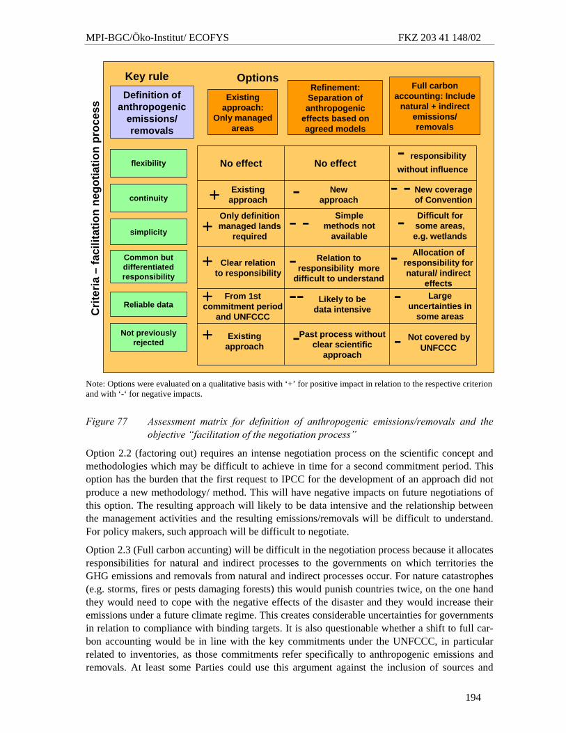
MPI-BGC/Öko-Institut/ ECOFYS FKZ 203 41 148/02
194
--
Existing approach:
Only managed areas
Refinement: Separation of anthropogenic
effects based on agreed models
Full carbon accounting: Include
natural + indirect emissions/ removals
flexibility
Common but differentiated responsibility
simplicity
Reliable data
Definition of anthropogenic
emissions/removals
Options
continuity
+
+
++
Not previously rejected
- - -
--
-
Clear relationto responsibility
No effect
- - -
No effect
Allocation of responsibility for natural/ indirect
effects
- responsibilitywithout influence
Not covered byUNFCCC
Simple methods not
available
Difficult for some areas, e.g. wetlands
Past process withoutclear scientific
approach
-+ - Relation to responsibility more
difficult to understand
Likely to bedata intensive
Key rule
- Large uncertainties in
some areas
-
Crit
eria
–fa
cilit
atio
nne
gotia
tion
proc
ess
Existingapproach
New approach
New coverageof Convention
Only definitionmanaged lands
required
From 1st commitment period
and UNFCCC
Existingapproach
Note: Options were evaluated on a qualitative basis with ‘+’ for positive impact in relation to the respective criterion and with ‘-‘ for negative impacts.
Figure 77 Assessment matrix for definition of anthropogenic emissions/removals and the objective “facilitation of the negotiation process”
Option 2.2 (factoring out) requires an intense negotiation process on the scientific concept and methodologies which may be difficult to achieve in time for a second commitment period. This option has the burden that the first request to IPCC for the development of an approach did not produce a new methodology/ method. This will have negative impacts on future negotiations of this option. The resulting approach will likely to be data intensive and the relationship between the management activities and the resulting emissions/removals will be difficult to understand. For policy makers, such approach will be difficult to negotiate.
Option 2.3 (Full carbon accunting) will be difficult in the negotiation process because it allocates responsibilities for natural and indirect processes to the governments on which territories the GHG emissions and removals from natural and indirect processes occur. For nature catastrophes (e.g. storms, fires or pests damaging forests) this would punish countries twice, on the one hand they would need to cope with the negative effects of the disaster and they would increase their emissions under a future climate regime. This creates considerable uncertainties for governments in relation to compliance with binding targets. It is also questionable whether a shift to full car-bon accounting would be in line with the key commitments under the UNFCCC, in particular related to inventories, as those commitments refer specifically to anthropogenic emissions and removals. At least some Parties could use this argument against the inclusion of sources and
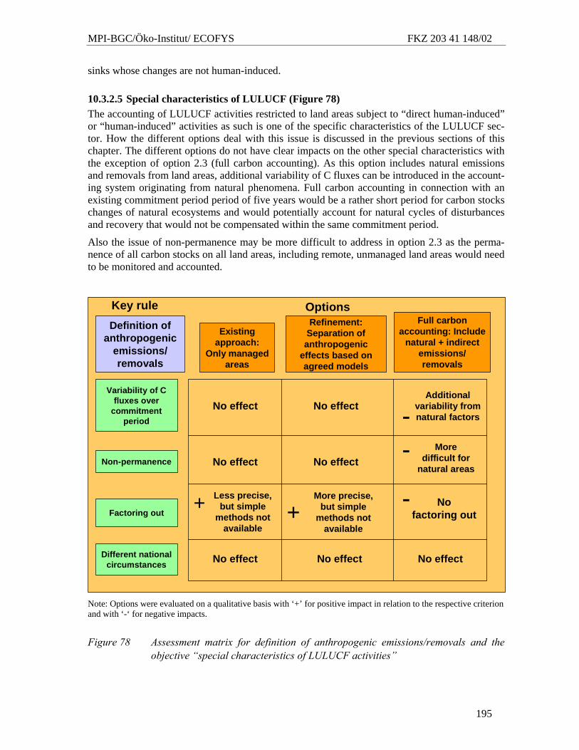
MPI-BGC/Öko-Institut/ ECOFYS FKZ 203 41 148/02
195
sinks whose changes are not human-induced.
10.3.2.5 Special characteristics of LULUCF (Figure 78) The accounting of LULUCF activities restricted to land areas subject to “direct human-induced” or “human-induced” activities as such is one of the specific characteristics of the LULUCF sec-tor. How the different options deal with this issue is discussed in the previous sections of this chapter. The different options do not have clear impacts on the other special characteristics with the exception of option 2.3 (full carbon accounting). As this option includes natural emissions and removals from land areas, additional variability of C fluxes can be introduced in the account-ing system originating from natural phenomena. Full carbon accounting in connection with an existing commitment period period of five years would be a rather short period for carbon stocks changes of natural ecosystems and would potentially account for natural cycles of disturbances and recovery that would not be compensated within the same commitment period.
Also the issue of non-permanence may be more difficult to address in option 2.3 as the perma-nence of all carbon stocks on all land areas, including remote, unmanaged land areas would need to be monitored and accounted.
--
Existing approach:
Only managed areas
Refinement: Separation of anthropogenic
effects based on agreed models
Full carbon accounting: Include
natural + indirect emissions/ removals
Definition of anthropogenic
emissions/removals
Options
No effect
+
-No effect
No factoring out
More precise, but simple
methods not available
Additional variability fromnatural factors
-+
Key rule
Variability of C fluxes over
commitment period
Different national circumstances
Factoring out
Non-permanence
Less precise, but simple
methods not available
No effect No effectMore
difficult fornatural areas
-
No effect No effect No effect
Note: Options were evaluated on a qualitative basis with ‘+’ for positive impact in relation to the respective criterion and with ‘-‘ for negative impacts.
Figure 78 Assessment matrix for definition of anthropogenic emissions/removals and the objective “special characteristics of LULUCF activities”
MPI-BGC/Öko-Institut/ ECOFYS FKZ 203 41 148/02
196
10.3.2.6 Cost efficiency Costs are related to the efforts needed for the monitoring, reporting and verification system and the administration of the entire system in the future. In this regard the potentially increased costs for monitoring and reporting of option 2.3 (full carbon accounting) as well as the responsibility allocated for natural phenomena in this option would imply higher costs of this option.
For option 2.2 (factoring out) additional costs arise for the scientific and technical development of the methodological approach and the data collection and implementation costs required for a future factoring-out model in each country.
Compared to these options, the currently implemented option 2.1 (managed areas) seems to be the most cost-efficient option. Even if further efforts would be developed to refine the existing definitions, criteria and thresholds, it is unlikely that higher costs would arise than for any of the other options.
10.3.3 Inclusion of defined LULUCF activities
As shown in chapter 9, the Kyoto Protocol established the situation that not all stock changes in all carbon pools on all land units from any LULUCF activities are estimated and accounted, but that individual LULUCF activities are selected for mandatory accounting (ARD in Article 3.3). The negotiations leading to the Marrakech Accords intensively debated the type of LULUCF activities (broad or narrow definition of activities) as well as the selection of possible additional LULUCF activities and their exact definition. Finally Marrakech Accords established that be-sides ARD, the activities cropland management (CM), grazing land management (GM), forest management (FM) and revegetation were agreed for voluntary accounting under the Kyoto Pro-tocol which implicitly includes a broad definition of LULUCF activities (as cropland or grazing land management does not refer to specific practices, but to general land use activities).
As broad definitions have been chosen already under the Kyoto Protocol28, it is highly likely that this approach continues in the future. First, advocates for narrowly defined activities have not been successful in negotiating for this approach, secondly the shift to a narrow approach would not be consistent with the reporting and accounting rules adopted for the first commitment pe-riod. Therefore only the option of broadly defined activities is further considered in this report.
Paragraph 19 of the Annex on definitions, modalities, rules and guidelines relating to LULUCF activities under the Kyoto Protocol (Decision 16/CMP.1) states: Once land is accounted for un-der Article 3.3 and 3.4 all anthropogenic GHG emissions by sources from and removals by sinks on this land must be accounted for throughout subsequent and contiguous commitment periods. This means negotiators already implied that the subset of activities accounted in future commit-ment periods will not be reduced compared to the accounted activities under the 1st commitment period.
Future options related to the inclusion of LULUCF activities
Option 3.1: Continuation of LULUCF activities included under the KP The continuation of the existing rules still provides different options regarding the mandatory character of the accounting:
28 e.g. Forest management includes selective cutting instead of clearance of large areas, longer rotation peri-ods, different species composition, forests enrichment or cropland management includes changing crop productivity, changing crop types cultivation of energy crops; tillage, herbizide use
MPI-BGC/Öko-Institut/ ECOFYS FKZ 203 41 148/02
197
Option 3.1.1: mix of mandatory and voluntary accounting
This option implies mandatory accounting of ARD activities, mandatory accounting of CM, GM, FM and revegetation for those countries that accounted for these activities in the first commit-ment period and voluntary accounting of CM, GM, FM and revegetation for those Parties that did not yet account for these activities.
Option 3.1.2: mandatory accounting of all KP activities
This option implies mandatory accounting of all activities defined under the Kyoto Protocol (ARD, CM, GM, FM and revegetation) for all Parties.
Option 3.2: Mandatory accounting of all emissions/removals from AFOLU sector This option includes mandatory accounting of all emissions and removals from carbon stock changes and non-CO2 gases on all managed land areas. It represents the accounting of all emis-sions and removals as reported in the GHG inventories under the Convention in the sectors agri-culture and LULUCF (in the future probably merged to AFOLU sector when IPCC 2006 Guiedlines will be implemented). This option is close to full carbon accounting, however with the key difference that effects on unmanaged lands would not be included in the accounting. It may require some further discussion how current methods of methodological prioritization as included in IPCC Good Practice Guidance for LULUCF and 2006 IPCC Guidelines (e.g. key category concept, default methods) will be implemented in the future in order to ensure that es-timation and reporting efforts can be efficiently allocated to the most important emission sources or sinks in the AFOLU sector. This option implies that no individual forestry or agricultural ac-tivities are defined any longer, but that the future accounting refers to the source/sink categories such as “Forest land remaining forest land“ and “Other lands converted to forest lands” as ac-counting categories for forestry activities.
Option 3.3: Addition of activities currently not covered by the Kyoto Protocol In general activities under Article 3.3 and 3.4 of the Kyoto Protocol already capture the dominant human-induced changes in carbon stocks. However there are some additional activities that could be included in the future.
A number of land areas and land uses are not included in accounting under the Kyoto Protocol, in particular urban land management, management of other land, erosion and restoration of de-graded lands, wetland restoration or wetlands/peatlands management. Dealing with those issues is at present sometimes constrained by the limited scientific and technical understanding. Most of these additional areas and land-uses are also not very important in relation to total C stock changes or connected with high uncertainties (e.g. erosion on forest land, cropland and grazing land is already covered and only erosion on non-forest, non-pasture and non-cropland areas would be concerned). These activities are not included as a separate option, as no proposals have been tabled so far with the aim to include these areas as separate additional activities.
Option 3.3.1: Forest degradation and devegetation
In the past two activities received particular attention regarding the inclusion under the Protocol or future regimes which are “direct human-induced degradation of forests and devegetation of other vegetation types”. Methodological issues for each option were discussed in the IPCC report “Definitions and Methodological Options to Inventory Emissions from Direct Human-induced Degradation of Forests and Devegetation of Other Vegetation Types. (IPCC 2003)” The report did not provide specific guidance on methodological options, however established clear recom-mendations in relation to the definition of those activities which is the basis for further methodo-logical work. For forest degradation, the recommended definition is:
MPI-BGC/Öko-Institut/ ECOFYS FKZ 203 41 148/02
198
“A direct human-induced long-term loss (persisting for X years or more) of at least Y% of forest carbon stocks since time [T] and not qualifying as deforestation or an elected activity under Article 3.4 of the Kyoto Protocol.”29
The proposed definition leaves it to Parties to specify the area thresholds, as well as time and carbon loss threshold. An additional activity “Forest degradation” would change the current ac-counting system in two ways: For managed forests, forest degradation is covered by forest man-agement, thus the activity “forest degradation” is only relevant when the accounting for forest management is not mandatory. As a mandatory activity it would require to account for some part of the emissions from forest management, even when this activity is not elected. And it would potentially include emissions from degradation of forests on unmanaged land areas when the definition above would be appplicable to all forest land areas (degradation of managed forests is already estimated with the methods used for forest management).
Similar to forest degradation the IPCC report recommends a definition for devegetation:
“A direct human-induced long-term loss (persisting for X years or more) of at least Y% of vegetation (characterized by cover/volume/carbon stocks) since time [T] on vegetation types other than forest and not subject to an elected activity under Article 3.4 of the Kyoto Protocol. Vegetation types consist of a minimum area of land of Z hectares with foliar cover of W%.”30
The proposed definition leaves for the Parties to specify the area thresholds, as well as time, re-duction/removal thresholds, referencing point and biomass cover threshold for other vegetation types. Examples for devegetation would be reduced carbon biomass stocks due to overgrazing or due to shrub suppression on grazing land areas.
If these activities are included, accounting for them would have to be mandatory, not optional. At least revegetation should be linked with the election of devegetation. Thus Parties that elect revegetation also have to account for devegetation in the same way as afforestation, reforestation and deforestation are linked under the Kyoto Protocol.
Option 3.3.2: Mandatory accounting of harvested wood products for all Parties The discussion on the inclusion of harvested wood products in commitments beyond the first commitment period is already quite advanced. Therefore it is likely that harvested wood products will be accounted for in a future commitment period, however the allocation method is still un-der discussion. The IPCC Good Practice Guidance for LULUCF and 2006 IPCC Guidelines sets out in detail calculation methods for the various stocks involved. The accounting rules for alloca-tion still have to be agreed and will be on the agenda of the twenty-sixth session of SBSTA.
Option 3.4: Avoided deforestation/ protection of forests:31
Avoided deforestation/ protection of forests is particularly important when the inclusion of Non-Annex-I Parties in a future climate regime is discussed. The following countries are seen as un-dergoing or at risk of large scale deforestation (Santilli et al. 2003)32: Brazil, Indonesia, Bolivia,
29 IPCC 2003, p. 16 30 IPCC 2003, p. 20 31 It is assumed that harvest – regeneration, replantation cycles take place in managed forests. Harvesting should not be counted as avoided deforestation. 32 Santilli, M., Moutino, P., Schwartzman, S., Nepstad, D., Curran, L., Nobre., C. (2003): Tropical deforesta-tion and the Kyoto Protocol: a new proposal. Paper presented and distributed during COP9, Milan 2003.
MPI-BGC/Öko-Institut/ ECOFYS FKZ 203 41 148/02
199
Peru, Columbia, Guiana and Suriname. For this report it is assumed that avoided deforestation/ protection of forests will only be discussed as an option for commitments for Non-Annex-I Par-ties, but that this option will not be eligible for Annex I-Parties where deforestation is already part of the existing accounting system.
In an accounting system this option always implies that a baseline or reference scenario is estab-lished against which a change in greenhouse gas emissions or removals is measured. The Kyoto Protocol opted for a simple baseline by taking the emissions of a base year as a reference. Such a simple approach however would not work for the accounting of forest conservation. There are many options for baselines, e.g.
• the stock change that results from projections of “business-as-usual” activities,
• the stock change resulting from the continuation of current activity levels,
• the stock changes resulting from past activities levels (e.g. average annual deforestation for the 1980’s as proposed by Santilli et al. (2003),
• performance benchmarks for forest conservation.
As the baseline without the activity is always a hypothetical scenario, and because the baseline level determines the quantitative effect towards targets, large uncertainties related to the justifi-cation of the accounted amounts are involved with this approach.
10.3.3.1 Climate effectiveness (Figure 79) Option 3.1 (continuation of 1st CP) continues with the current weaknesses of the system and ac-counts for only a subset of emissions and removals from LULUCF. Option 3.1.1 allows exclud-ing certain emissions from LULUCF activities from the accounting. In this respect this option is less effective.
Option 3.2 (Convention accounting) is considered as more climate effective because it includes all relevant emissions and removals from agricultural and forestry land uses and does not allow to elect certain favourable activities. In the negotiations for the commitment under the Kyoto Protocol this option was considered as reducing the global mitigation effort because removals can be accounted against emissions from other sectors and no data were available on the impact of removals from sinks in the different Parties. However, the data situation related to the report-ing under the Convention improved and better data is available now for an assessment of quanti-tative impacts (see section 10.3.3.7 of this report).
For option 3.3 (additional activities), the climate effectiveness depends on the quantitative ef-fects of additional activities, in particular whether they add considerable additional emissions that are currently excluded from the accounting. However, the quantitative effects of the activi-ties currently not included seem to be relatively low for Annex I Parties.
Option 3.4 (reduced deforestation) would include a very significant part of global emissions un-der a future climate regime. Tropical deforestation, in particular from Brazil and Indonesia, cur-rently contributes to a considerable part of global CO2 emissions (400 Tg C/year from Brazil and Indonesia, 800-2200 Tg C/year from total tropical deforestation according to Santilli et al. 2003). The climate effectiveness however will depend on the fact whether a robust accounting system is developed.
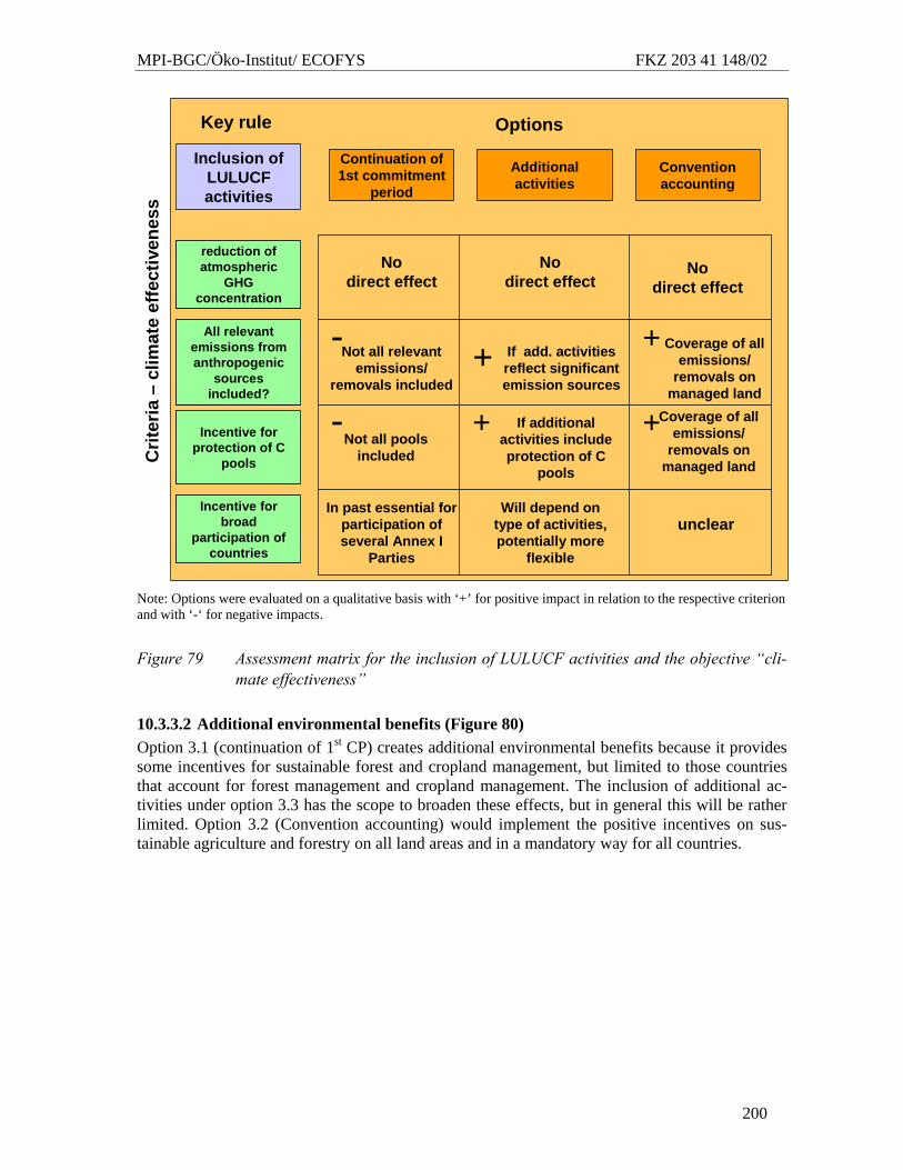
MPI-BGC/Öko-Institut/ ECOFYS FKZ 203 41 148/02
200
--
Continuation of 1st commitment
period
Additional activities
Convention accounting
Inclusion of LULUCF activities
Options
Coverage of all emissions/
removals on managed land
Will depend on type of activities, potentially more
flexible
If additional activities includeprotection of C
pools
Key rule
No direct effect
+
- + +
unclear
reduction of atmospheric
GHG concentration
All relevant emissions from anthropogenic
sources included?
Incentive for protection of C
pools
Incentive for broad
participation of countries
reduction of atmospheric
GHG concentration
All relevant emissions from anthropogenic
sources included?
Incentive for protection of C
pools
Incentive for broad
participation of countries
Crit
eria
–cl
imat
eef
fect
iven
ess
- + If add. activitiesreflect significantemission sources
In past essential forparticipation of several Annex I
Parties
Not all relevant emissions/
removals included
No direct effect
No direct effect
Not all poolsincluded
Coverage of all emissions/
removals on managed land
Note: Options were evaluated on a qualitative basis with ‘+’ for positive impact in relation to the respective criterion and with ‘-‘ for negative impacts.
Figure 79 Assessment matrix for the inclusion of LULUCF activities and the objective “cli-mate effectiveness”
10.3.3.2 Additional environmental benefits (Figure 80) Option 3.1 (continuation of 1st CP) creates additional environmental benefits because it provides some incentives for sustainable forest and cropland management, but limited to those countries that account for forest management and cropland management. The inclusion of additional ac-tivities under option 3.3 has the scope to broaden these effects, but in general this will be rather limited. Option 3.2 (Convention accounting) would implement the positive incentives on sus-tainable agriculture and forestry on all land areas and in a mandatory way for all countries.
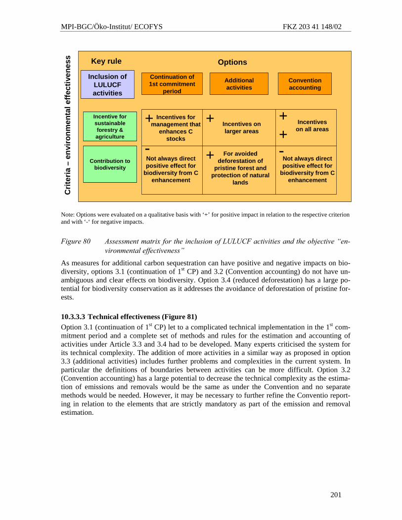
MPI-BGC/Öko-Institut/ ECOFYS FKZ 203 41 148/02
201
--
Continuation of 1st commitment
period
Additional activities
Convention accounting
Inclusion of LULUCF activities
Options
Not always directpositive effect for
biodiversity from C enhancement
Key rule
++
Incentives for management that
enhances C stocks
Crit
eria
–en
viro
nmen
tale
ffect
iven
ess
Incentive for sustainable forestry & agriculture
Contribution to biodiversity
Incentive for sustainable forestry & agriculture
Contribution to biodiversity
+
-
+ Incentives on larger areas
Incentiveson all areas
For avoideddeforestation of
pristine forest and protection of natural
lands
Not always directpositive effect for
biodiversity from C enhancement
-+
Note: Options were evaluated on a qualitative basis with ‘+’ for positive impact in relation to the respective criterion and with ‘-‘ for negative impacts.
Figure 80 Assessment matrix for the inclusion of LULUCF activities and the objective “en-vironmental effectiveness”
As measures for additional carbon sequestration can have positive and negative impacts on bio-diversity, options 3.1 (continuation of 1st CP) and 3.2 (Convention accounting) do not have un-ambiguous and clear effects on biodiversity. Option 3.4 (reduced deforestation) has a large po-tential for biodiversity conservation as it addresses the avoidance of deforestation of pristine for-ests.
10.3.3.3 Technical effectiveness (Figure 81) Option 3.1 (continuation of 1st CP) let to a complicated technical implementation in the 1st com-mitment period and a complete set of methods and rules for the estimation and accounting of activities under Article 3.3 and 3.4 had to be developed. Many experts criticised the system for its technical complexity. The addition of more activities in a similar way as proposed in option 3.3 (additional activities) includes further problems and complexities in the current system. In particular the definitions of boundaries between activities can be more difficult. Option 3.2 (Convention accounting) has a large potential to decrease the technical complexity as the estima-tion of emissions and removals would be the same as under the Convention and no separate methods would be needed. However, it may be necessary to further refine the Conventio report-ing in relation to the elements that are strictly mandatory as part of the emission and removal estimation.
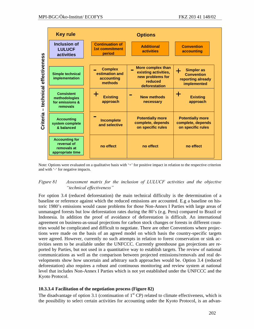
MPI-BGC/Öko-Institut/ ECOFYS FKZ 203 41 148/02
202
--
Continuation of 1st commitment
period
Additional activities
Convention accounting
Inclusion of LULUCF activities
Options
Simpler as Convention
reporting alreadyimplemented
no effect
Potentially morecomplete, depends
on specific rules
Key rule
More complex thanexisting activities, new problems for
reduceddeforestation
-
+-
Crit
eria
–te
chni
cale
ffect
iven
ess
Simple technical implementation
Consistent methodologies for emissions &
removals
Accounting system complete
& balanced
Accounting for reversal of removals at
appropriate time
Simple technical implementation
Consistent methodologies for emissions &
removals
Accounting system complete
& balanced
Accounting for reversal of removals at
appropriate time
-+
no effect no effect
Complexestimation and
accountingmethods
+Existingapproach
Existingapproach
New methodsnecessary
Incompleteand selective
Potentially morecomplete, depends
on specific rules
-
Note: Options were evaluated on a qualitative basis with ‘+’ for positive impact in relation to the respective criterion and with ‘-‘ for negative impacts.
Figure 81 Assessment matrix for the inclusion of LULUCF activities and the objective “technical effectiveness”
For option 3.4 (reduced deforestation) the main technical difficulty is the determination of a baseline or reference against which the reduced emissions are accounted. E.g a baseline on his-toric 1980’s emissions would cause problems for those Non-Annex I Parties with large areas of unmanaged forests but low deforestation rates during the 80’s (e.g. Peru) compared to Brazil or Indonesia. In addition the proof of avoidance of deforestation is difficult. An international agreement on business-as-usual projections for carbon stock changes or forests in different coun-tries would be complicated and difficult to negotiate. There are other Conventions where projec-tions were made on the basis of an agreed model on which basis the country-specific targets were agreed. However, currently no such attempts in relation to forest conservation or sink ac-tivities seem to be available under the UNFCCC. Currently greenhouse gas projections are re-ported by Parties, but not used in a quantitative way to establish targets. The review of national communications as well as the comparison between projected emissions/removals and real de-velopments show how uncertain and arbitrary such approaches would be. Option 3.4 (reduced deforestation) also requires a robust and continuous monitoring and review system at national level that includes Non-Annex I Parties which is not yet established under the UNFCCC and the Kyoto Protocol.
10.3.3.4 Facilitation of the negotiation process (Figure 82) The disadvantage of option 3.1 (continuation of 1st CP) related to climate effectiveness, which is the possibility to select certain activities for accounting under the Kyoto Protocol, is an advan-
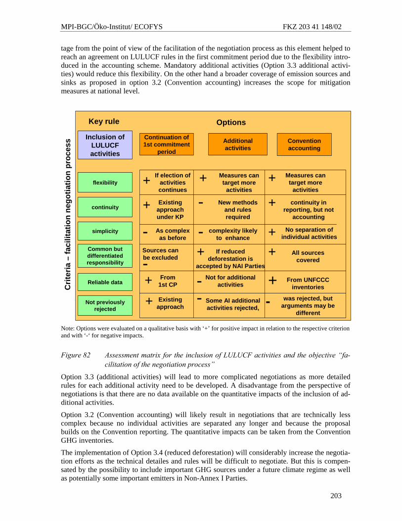
MPI-BGC/Öko-Institut/ ECOFYS FKZ 203 41 148/02
203
tage from the point of view of the facilitation of the negotiation process as this element helped to reach an agreement on LULUCF rules in the first commitment period due to the flexibility intro-duced in the accounting scheme. Mandatory additional activities (Option 3.3 additional activi-ties) would reduce this flexibility. On the other hand a broader coverage of emission sources and sinks as proposed in option 3.2 (Convention accounting) increases the scope for mitigation measures at national level.
--
Continuation of 1st commitment
period
Additional activities
Convention accounting
flexibility
Common but differentiated responsibility
simplicity
Reliable data
Inclusion of LULUCF activities
Options
continuity
++
+
Not previously rejected
--
Sources canbe excluded
-All sources
covered
No separation of individual activities
Some AI additional activities rejected,
If reduceddeforestation is
accepted by NAI Parties
Key rule
- As complexas before
complexity likelyto enhance
+
-+
From UNFCCC inventories
From1st CP
Not for additional activities
was rejected, butarguments may be
different
Measures cantarget more
activities+
+Crit
eria
–fa
cilit
atio
nne
gotia
tion
proc
ess
+
continuity in reporting, but not
accounting
-
If election of activitiescontinues
Measures cantarget more
activities+
Existingapproachunder KP
+
Existingapproach
New methodsand rulesrequired
- +
Note: Options were evaluated on a qualitative basis with ‘+’ for positive impact in relation to the respective criterion and with ‘-‘ for negative impacts.
Figure 82 Assessment matrix for the inclusion of LULUCF activities and the objective “fa-cilitation of the negotiation process”
Option 3.3 (additional activities) will lead to more complicated negotiations as more detailed rules for each additional activity need to be developed. A disadvantage from the perspective of negotiations is that there are no data available on the quantitative impacts of the inclusion of ad-ditional activities.
Option 3.2 (Convention accounting) will likely result in negotiations that are technically less complex because no individual activities are separated any longer and because the proposal builds on the Convention reporting. The quantitative impacts can be taken from the Convention GHG inventories.
The implementation of Option 3.4 (reduced deforestation) will considerably increase the negotia-tion efforts as the technical detailes and rules will be difficult to negotiate. But this is compen-sated by the possibility to include important GHG sources under a future climate regime as well as potentially some important emitters in Non-Annex I Parties.
MPI-BGC/Öko-Institut/ ECOFYS FKZ 203 41 148/02
204
10.3.3.5 Special characteristics of LULUCF The choice of LULUCF activities to be included in a future climate regime discussed in this sec-tion do mostly no have strong impacts on the criteria related to special characteristis of LULUCF activities.
For option 3.4 (reduced deforestation) issues such as non-permanence and factoring out (how will the regime deal with forest losses due to non-human interventions such as wildfires and pests?) need to be addressed and resolved.
10.3.3.6 Cost efficiency Costs are related to the efforts needed for the monitoring, reporting and verification system and the administration of the entire system in the future. In this regard, additional activities similar to the Kyoto activities (option 3.3) are likely to increase costs for monitoring and reporting.
Option 3.4 (reduced deforestation will bring new countries and activities in a climate regime which will also lead to higher transaction costs. However, mitigation costs at global level will be considerably reduced as an additional important GHG source would be covered by the regime.
Otion 3.2 (Convention accounting) is likely to reduce transaction cost, as a separate reporting scheme as under the Kyoto Protocol is avoided. However, for individual countries that did not elect any activities under Article 3.4 of the Kyoto Protocol and that have a rather weak data situation for the LULUCF sector under the Convention, additional costs for monitoring and re-porting in this sector may occur in the future.
10.3.3.7 Quantitative impacts of the inclusion of LULUCF source categories in future commitment periods
The data resulting from modelling approaches presented in previous chapters 6-8 provide rele-vant information on trends, long-term effects and relative contributions of LULUCF activities (afforestation, reforestation, forest management and cropland management) and allow to distin-guish between the effects of past and present forest management. However, the modelling results do not provide sufficiently exact information on emissions and removal trends for short time periods and on absolute levels for each individual country for the politically relevant period be-tween 1990 and 2020. Therefore additional data sources were considered for the discussion of the quantitative impacts of the options releated to the inclusion of LULUCF activities in this sec-tion.
The current LULUCF sector of national GHG inventories under the UNFCCC covers all land use, land-use change and forestry activities. Therefore the LULUCF inventory data under the UNFCCC give information on the quantitative scale of effects of a maximum coverage of LULUCF activities (when the inventory reporting is complete with regard to pools and source categories) and to individual land use categories (forest land, cropland, grassland, wetlands, set-tlements and other lands) with the limitation that this coverage is restricted to managed land ar-eas. The following sections only refer to CO2 emissions and removals, and exclude CH4 and N2O emissions as there are currently substantial gaps in the reporting of non-CO2 gases from LULUCF sector in many countries. Figure 83 shows the average contribution of net emis-sions/removals from the LULUCF sector to total GHG emissions and the range over the 1990-2003 period (until 2004 for EU countries). Looking at maximum source/removal years in this period as indicated by the range, in Latvia (a country with high removals), LULUCF activities have the largest share of inventory totals with 151%, however the most recent inventory review for Latvia pointed at significant problems in the estimation of removals in the LULUCF sector in this country and the current values reported may not be correct.
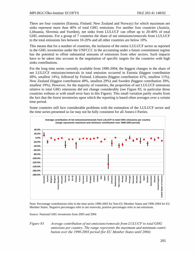
MPI-BGC/Öko-Institut/ ECOFYS FKZ 203 41 148/02
205
There are four countries (Estonia, Finland. New Zealand and Norway) for which maximum net sinks represent more than 40% of total GHG emissions. For another four countries (Austria, Lithuania, Slovenia and Sweden), net sinks from LULUCF can offset up to 20-40% of total GHG emissions. For a group of 7 countries the share of net emissions/removals from LULUCF to the total emissions lies between 10-20% and all other countries are below 10%.
This means that for a number of countries, the inclusion of the entire LULUCF sector as reported in the GHG inventories under the UNFCCC in the accounting under a future commitment regime has the potential to offset substantial amounts of emissions from other sectors. Such impacts have to be taken into account in the negotiation of specific targets for the countries with high sinks contributions.
For the long time series currently available from 1990-2004, the biggest changes in the share of net LULUCF emissions/removals in total emission occurred in Estonia (biggest contribution 49%, smallest 14%), followed by Finland, Lithuania (biggest contribution 41%, smallest 11%), New Zealand (biggest contribution 49%, smallest 29%) and Sweden (biggest contribution 39%, smallest 19%). However, for the majority of countries, the proportion of net LULUCF emissions relative to total GHG emissions did not change considerably (see Figure 83, in particular those countries without or with small error bars in this Figure). This small variation partly results from the fact that the forest inventories upon which the reporting is based often averages over a certain time period.
Some countries still face considerable problems with the estimation of the LULUCF sector and the time series presented so far may not be fully consistent for all Annex-I Parties.
Average contribution of net emissions/removals from LULUCF to total GHG emissions per country[range represents maximum and minimum contribution over 1990-2003 period]
-180.0%
-160.0%
-140.0%
-120.0%
-100.0%
-80.0%
-60.0%
-40.0%
-20.0%
0.0%
20.0%
40.0%
Aus
tral
ia
Aus
tria
Bel
gium
Bul
garia
Cze
ch R
epub
lic
Den
mar
k
Esto
nia
EU 1
5
EU 2
5
Finl
and
Fran
ce
Ger
man
y
Gre
ece
Hun
gary
Icel
and
Irela
nd
Italy
Japa
n
Latv
ia
Lith
uani
a
Net
herla
nds
New
Zea
land
Nor
way
Pola
nd
Port
ugal
Rom
ania
Slov
akia
Slov
enia
Spai
n
Swed
en
Switz
erla
nd
Ukr
aine
Uni
ted
Kin
gdom
Uni
ted
Stat
es o
f Am
eric
a
Note: Percentage contributions refer to the time series 1990-2003 for Non-EU Member States and 1990-2004 for EU Member States. Negative percentages refer to net removals, positive percentages refer to net emissions.
Source: National GHG inventories from 2005 and 2006
Figure 83 Average contribution of net emissions/removals from LULUCF to total GHG emissions per country. The range represents the maximum and minimum contri-bution over the 1990-2003 period (for EU Member States until 2004)
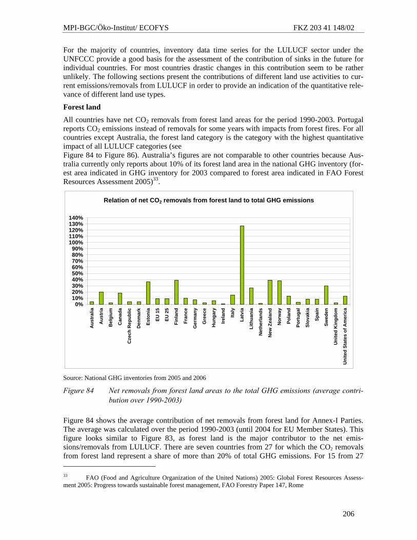
MPI-BGC/Öko-Institut/ ECOFYS FKZ 203 41 148/02
206
For the majority of countries, inventory data time series for the LULUCF sector under the UNFCCC provide a good basis for the assessment of the contribution of sinks in the future for individual countries. For most countries drastic changes in this contribution seem to be rather unlikely. The following sections present the contributions of different land use activities to cur-rent emissions/removals from LULUCF in order to provide an indication of the quantitative rele-vance of different land use types.
Forest land
All countries have net CO2 removals from forest land areas for the period 1990-2003. Portugal reports CO2 emissions instead of removals for some years with impacts from forest fires. For all countries except Australia, the forest land category is the category with the highest quantitative impact of all LULUCF categories (see Figure 84 to Figure 86). Australia’s figures are not comparable to other countries because Aus-tralia currently only reports about 10% of its forest land area in the national GHG inventory (for-est area indicated in GHG inventory for 2003 compared to forest area indicated in FAO Forest Resources Assessment 2005)33.
Relation of net CO2 removals from forest land to total GHG emissions
0%10%20%30%40%50%60%70%80%90%
100%110%120%130%140%
Aus
tral
ia
Aus
tria
Bel
gium
Can
ada
Cze
ch R
epub
lic
Den
mar
k
Esto
nia
EU 1
5
EU 2
5
Finl
and
Fran
ce
Ger
man
y
Gre
ece
Hun
gary
Irela
nd
Italy
Latv
ia
Lith
uani
a
Net
herla
nds
New
Zea
land
Nor
way
Pola
nd
Port
ugal
Slov
akia
Spai
n
Swed
en
Uni
ted
Kin
gdom
Uni
ted
Stat
es o
f Am
eric
a
Source: National GHG inventories from 2005 and 2006
Figure 84 Net removals from forest land areas to the total GHG emissions (average contri-bution over 1990-2003)
Figure 84 shows the average contribution of net removals from forest land for Annex-I Parties. The average was calculated over the period 1990-2003 (until 2004 for EU Member States). This figure looks similar to Figure 83, as forest land is the major contributor to the net emis-sions/removals from LULUCF. There are seven countries from 27 for which the CO2 removals from forest land represent a share of more than 20% of total GHG emissions. For 15 from 27 33 FAO (Food and Agriculture Organization of the United Nations) 2005: Global Forest Resources Assess-ment 2005: Progress towards sustainable forest management, FAO Forestry Paper 147, Rome
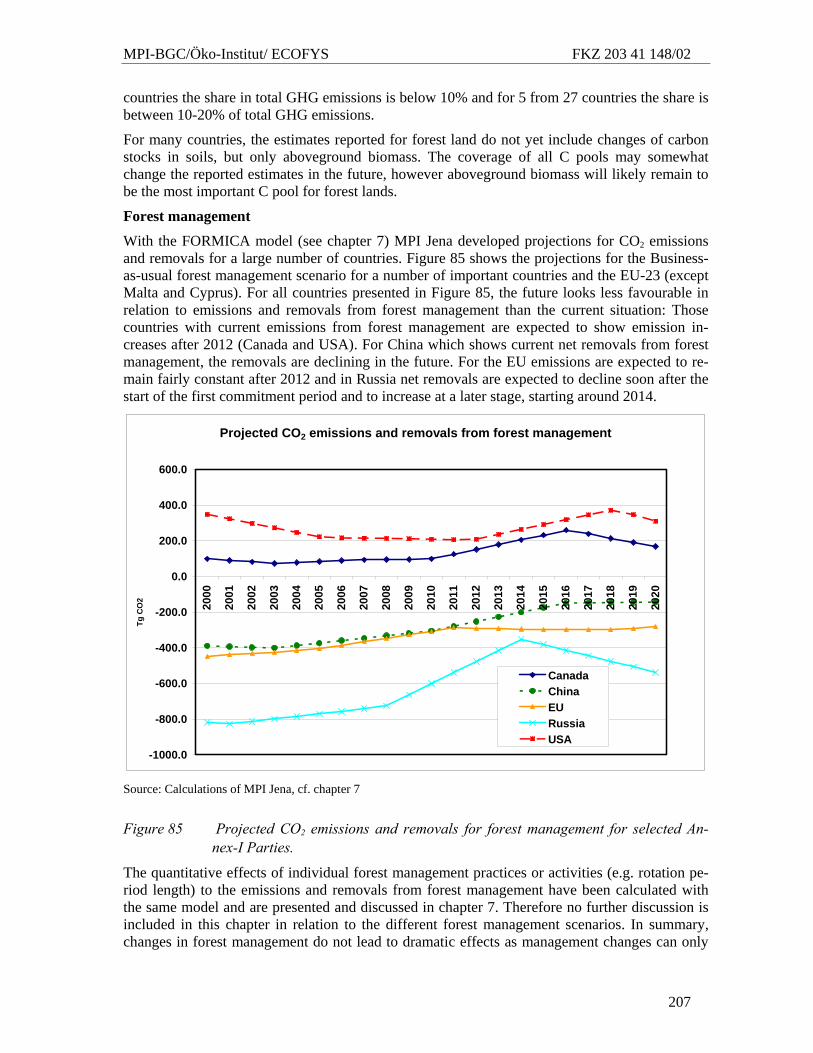
MPI-BGC/Öko-Institut/ ECOFYS FKZ 203 41 148/02
207
countries the share in total GHG emissions is below 10% and for 5 from 27 countries the share is between 10-20% of total GHG emissions.
For many countries, the estimates reported for forest land do not yet include changes of carbon stocks in soils, but only aboveground biomass. The coverage of all C pools may somewhat change the reported estimates in the future, however aboveground biomass will likely remain to be the most important C pool for forest lands.
Forest management
With the FORMICA model (see chapter 7) MPI Jena developed projections for CO2 emissions and removals for a large number of countries. Figure 85 shows the projections for the Business-as-usual forest management scenario for a number of important countries and the EU-23 (except Malta and Cyprus). For all countries presented in Figure 85, the future looks less favourable in relation to emissions and removals from forest management than the current situation: Those countries with current emissions from forest management are expected to show emission in-creases after 2012 (Canada and USA). For China which shows current net removals from forest management, the removals are declining in the future. For the EU emissions are expected to re-main fairly constant after 2012 and in Russia net removals are expected to decline soon after the start of the first commitment period and to increase at a later stage, starting around 2014.
Projected CO2 emissions and removals from forest management
-1000.0
-800.0
-600.0
-400.0
-200.0
0.0
200.0
400.0
600.0
2000
2001
2002
2003
2004
2005
2006
2007
2008
2009
2010
2011
2012
2013
2014
2015
2016
2017
2018
2019
2020
Tg C
O2
CanadaChinaEURussiaUSA
Source: Calculations of MPI Jena, cf. chapter 7
Figure 85 Projected CO2 emissions and removals for forest management for selected An-nex-I Parties.
The quantitative effects of individual forest management practices or activities (e.g. rotation pe-riod length) to the emissions and removals from forest management have been calculated with the same model and are presented and discussed in chapter 7. Therefore no further discussion is included in this chapter in relation to the different forest management scenarios. In summary, changes in forest management do not lead to dramatic effects as management changes can only
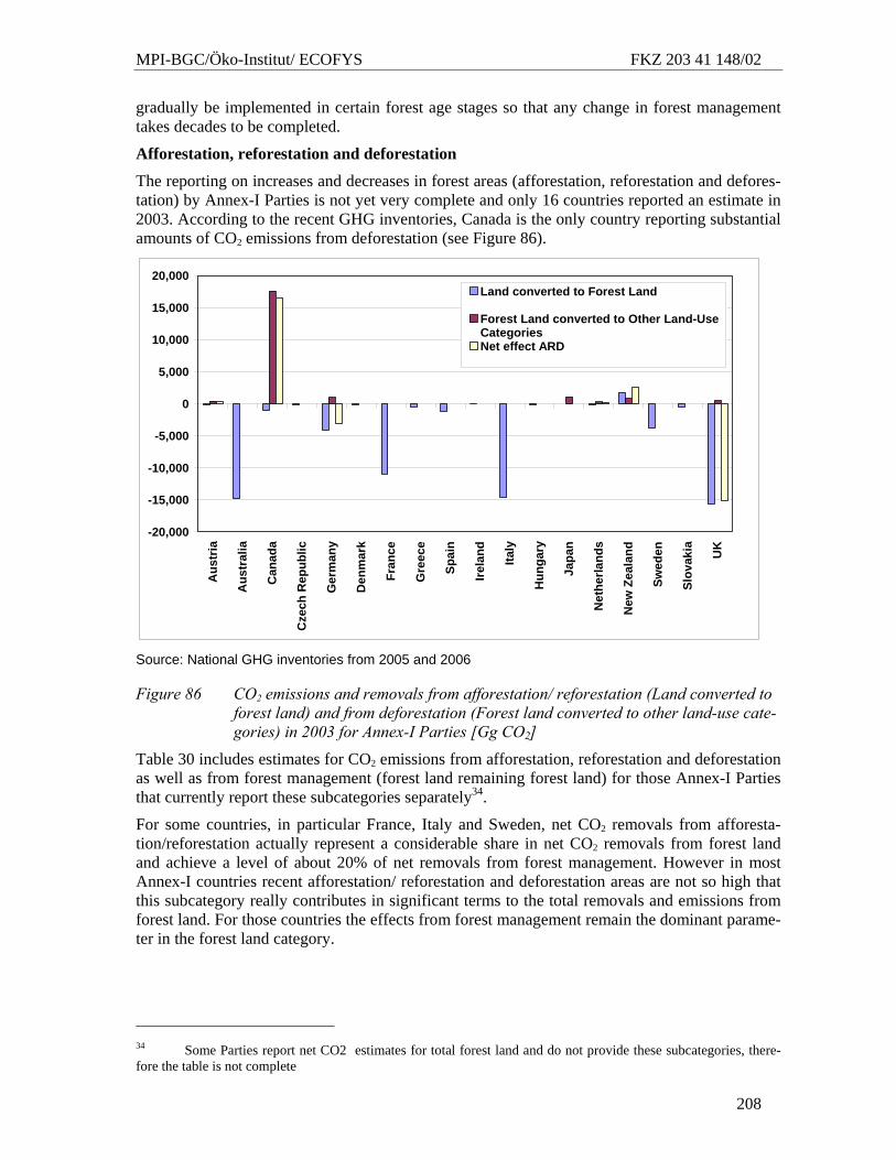
MPI-BGC/Öko-Institut/ ECOFYS FKZ 203 41 148/02
208
gradually be implemented in certain forest age stages so that any change in forest management takes decades to be completed.
Afforestation, reforestation and deforestation
The reporting on increases and decreases in forest areas (afforestation, reforestation and defores-tation) by Annex-I Parties is not yet very complete and only 16 countries reported an estimate in 2003. According to the recent GHG inventories, Canada is the only country reporting substantial amounts of CO2 emissions from deforestation (see Figure 86).
-20,000
-15,000
-10,000
-5,000
0
5,000
10,000
15,000
20,000
Aus
tria
Aus
tral
ia
Can
ada
Cze
ch R
epub
lic
Ger
man
y
Den
mar
k
Fran
ce
Gre
ece
Spai
n
Irela
nd
Italy
Hun
gary
Japa
n
Net
herla
nds
New
Zea
land
Swed
en
Slov
akia UK
Land converted to Forest Land
Forest Land converted to Other Land-UseCategoriesNet effect ARD
Source: National GHG inventories from 2005 and 2006
Figure 86 CO2 emissions and removals from afforestation/ reforestation (Land converted to forest land) and from deforestation (Forest land converted to other land-use cate-gories) in 2003 for Annex-I Parties [Gg CO2]
Table 30 includes estimates for CO2 emissions from afforestation, reforestation and deforestation as well as from forest management (forest land remaining forest land) for those Annex-I Parties that currently report these subcategories separately34.
For some countries, in particular France, Italy and Sweden, net CO2 removals from afforesta-tion/reforestation actually represent a considerable share in net CO2 removals from forest land and achieve a level of about 20% of net removals from forest management. However in most Annex-I countries recent afforestation/ reforestation and deforestation areas are not so high that this subcategory really contributes in significant terms to the total removals and emissions from forest land. For those countries the effects from forest management remain the dominant parame-ter in the forest land category.
34 Some Parties report net CO2 estimates for total forest land and do not provide these subcategories, there-fore the table is not complete
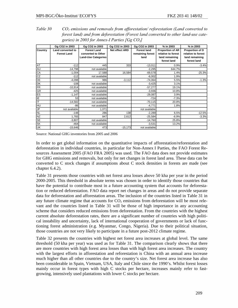
MPI-BGC/Öko-Institut/ ECOFYS FKZ 203 41 148/02
209
Table 30 CO2 emissions and removals from afforestation/ reforestation (Land converted to forest land) and from deforestation (Forest land converted to other land-use cate-gories) in 2003 for Annex-I Parties [Gg CO2]
Gg CO2 in 2003 Gg CO2 in 2003 Gg CO2 in 2003 Gg CO2 in 2003 % in 2003 % in 2003Country Land converted to
Forest LandForest Land
converted to Other Land-Use Categories
Net effect ARD Forest land remaining forest
land
Proportion of AR relative to forest land remaining
forest land
Proportion of D relative to forest land remaining
forest landAT -112 445 333 -13,011 0.9% -3.4%AU -14,798 not available -2,295 644.7%CA -1,004 17,588 16,584 -69,578 1.4% -25.3%CZ -112 not available -6,002 1.9%DE -4,098 986 -3,112 -74,064 5.5% -1.3%DK -108 not available -3,425 3.1%FR -10,914 not available -57,277 19.1%GR -425 not available -3,936 10.8%ES -1,147 not available -29,087 3.9%IE 53 not available -724 -7.3%IT -14,582 not available -70,115 20.8%HU -86 not available -4,771 1.8%JP not available 1,071 not availableNL -148 286 138 -2,289 6.5% -12.5%NZ 1,765 847 2,612 -25,584 -6.9% -3.3%SE -3,807 not available -14,760 25.8%SK -464 not available -3,531 13.2%UK -15,646 473 -15,173 not available Source: National GHG inventories from 2005 and 2006
In order to get global information on the quantitative impacts of afforestation/reforestation and deforestation in individual countries, in particular for Non-Annex I Parties, the FAO Forest Re-sources Assessment 2005 (FAO FRA 2005) was used. The FAO data does not provide estimates for GHG emissions and removals, but only for net changes in forest land area. These data can be converted to C stock changes if assumptions about C stock densities in forests are made (see chapter 6.4.2).
Table 31 presents those countries with net forest area losses above 50 kha per year in the period 2000-2005. This threshold in absolute terms was chosen in order to identify those countries that have the potential to contribute most in a future accounting system that accounts for deforesta-tion or reduced deforestation. FAO data report net changes in areas and do not provide separate data for deforestation and afforestation areas. The inclusion of the countries listed in Table 31 in any future climate regime that accounts for CO2 emissions from deforestation will be most rele-vant and the countries listed in Table 31 will be those of high importance in any accounting scheme that considers reduced emissions from deforestation. From the countries with the highest current absolute deforestation rates, there are a significant number of countries with high politi-cal instability and uncertainty, lack of international cooperation of governments or lack of func-tioning forest administration (e.g. Myanmar, Congo, Nigeria). Due to their political situation, those countries are not very likely to participate in a future post-2012 climate regime.
Table 32 presents the countries with highest net forest area increases at global level. The same threshold (50 kha per year) was used as for Table 31. The comparison clearly shows that there are more countries with high forest area losses than with high forest area increases. The country with the largest efforts in afforestation and reforestation is China with an annual area increase much higher than all other countries due to the country’s size. Net forest area increase has also been considerable in Spain, Vietnam, USA, Italy and Chile since the 1990’s. Whilst forest losses mainly occur in forest types with high C stocks per hectare, increases mainly refer to fast-growing, intensively used plantations with lower C stocks per hectare.
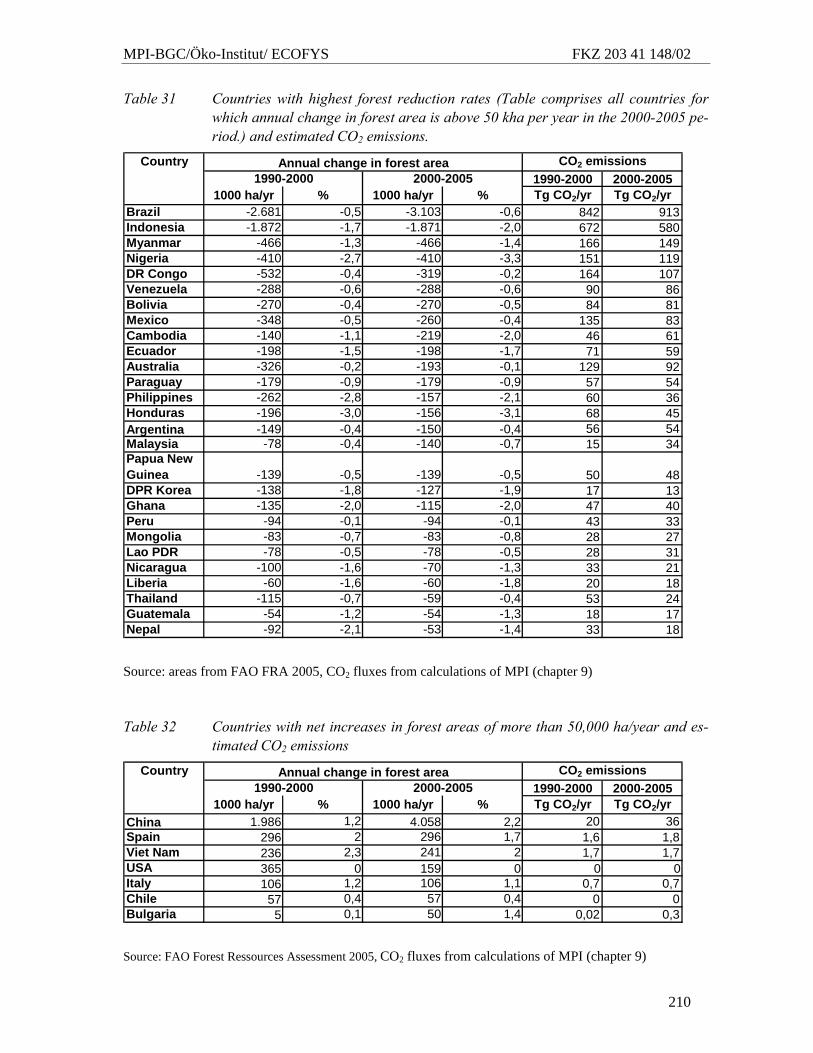
MPI-BGC/Öko-Institut/ ECOFYS FKZ 203 41 148/02
210
Table 31 Countries with highest forest reduction rates (Table comprises all countries for which annual change in forest area is above 50 kha per year in the 2000-2005 pe-riod.) and estimated CO2 emissions.
Source: areas from FAO FRA 2005, CO2 fluxes from calculations of MPI (chapter 9)
Table 32 Countries with net increases in forest areas of more than 50,000 ha/year and es-timated CO2 emissions
Source: FAO Forest Ressources Assessment 2005, CO2 fluxes from calculations of MPI (chapter 9)
1990-2000 2000-20051000 ha/yr % 1000 ha/yr % Tg CO2/yr Tg CO2/yr
Brazil -2.681 -0,5 -3.103 -0,6 842 913Indonesia -1.872 -1,7 -1.871 -2,0 672 580Myanmar -466 -1,3 -466 -1,4 166 149Nigeria -410 -2,7 -410 -3,3 151 119DR Congo -532 -0,4 -319 -0,2 164 107Venezuela -288 -0,6 -288 -0,6 90 86Bolivia -270 -0,4 -270 -0,5 84 81Mexico -348 -0,5 -260 -0,4 135 83Cambodia -140 -1,1 -219 -2,0 46 61Ecuador -198 -1,5 -198 -1,7 71 59Australia -326 -0,2 -193 -0,1 129 92Paraguay -179 -0,9 -179 -0,9 57 54Philippines -262 -2,8 -157 -2,1 60 36Honduras -196 -3,0 -156 -3,1 68 45Argentina -149 -0,4 -150 -0,4 56 54Malaysia -78 -0,4 -140 -0,7 15 34Papua New Guinea -139 -0,5 -139 -0,5 50 48DPR Korea -138 -1,8 -127 -1,9 17 13Ghana -135 -2,0 -115 -2,0 47 40Peru -94 -0,1 -94 -0,1 43 33Mongolia -83 -0,7 -83 -0,8 28 27Lao PDR -78 -0,5 -78 -0,5 28 31Nicaragua -100 -1,6 -70 -1,3 33 21Liberia -60 -1,6 -60 -1,8 20 18Thailand -115 -0,7 -59 -0,4 53 24Guatemala -54 -1,2 -54 -1,3 18 17Nepal -92 -2,1 -53 -1,4 33 18
CO2 emissionsCountry Annual change in forest area1990-2000 2000-2005
1990-2000 2000-20051000 ha/yr % 1000 ha/yr % Tg CO2/yr Tg CO2/yr
China 1.986 1,2 4.058 2,2 20 36Spain 296 2 296 1,7 1,6 1,8Viet Nam 236 2,3 241 2 1,7 1,7USA 365 0 159 0 0 0Italy 106 1,2 106 1,1 0,7 0,7Chile 57 0,4 57 0,4 0 0Bulgaria 5 0,1 50 1,4 0,02 0,3
CO2 emissionsAnnual change in forest area1990-2000 2000-2005
Country
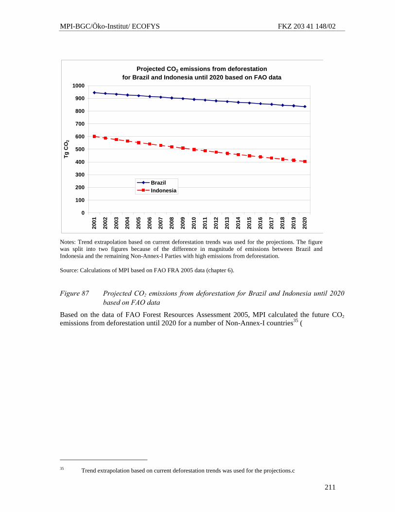
MPI-BGC/Öko-Institut/ ECOFYS FKZ 203 41 148/02
211
Projected CO2 emissions from deforestation for Brazil and Indonesia until 2020 based on FAO data
0
100
200
300
400
500
600
700
800
900
100020
01
2002
2003
2004
2005
2006
2007
2008
2009
2010
2011
2012
2013
2014
2015
2016
2017
2018
2019
2020
Tg C
O2
BrazilIndonesia
Notes: Trend extrapolation based on current deforestation trends was used for the projections. The figure was split into two figures because of the difference in magnitude of emissions between Brazil and Indonesia and the remaining Non-Annex-I Parties with high emissions from deforestation.
Source: Calculations of MPI based on FAO FRA 2005 data (chapter 6).
Figure 87 Projected CO2 emissions from deforestation for Brazil and Indonesia until 2020 based on FAO data
Based on the data of FAO Forest Resources Assessment 2005, MPI calculated the future CO2 emissions from deforestation until 2020 for a number of Non-Annex-I countries35 (
35 Trend extrapolation based on current deforestation trends was used for the projections.c
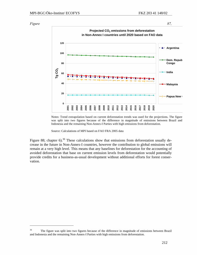
MPI-BGC/Öko-Institut/ ECOFYS FKZ 203 41 148/02
212
Figure 87,
Projected CO2 emissions from deforestation in Non-Annex I countries until 2020 based on FAO data
0
20
40
60
80
100
120
2001
2002
2003
2004
2005
2006
2007
2008
2009
2010
2011
2012
2013
2014
2015
2016
2017
2018
2019
2020
Tg C
O2
Argentina
Dem. RepubCongo
India
Malaysia
Papua New G
Notes: Trend extrapolation based on current deforestation trends was used for the projections. The figure was split into two figures because of the difference in magnitude of emissions between Brazil andIndonesia and the remaining Non-Annex-I Parties with high emissions from deforestation.
Source: Calculations of MPI based on FAO FRA 2005 data
Figure 88; chapter 6).36 These calculations show that emissions from deforestation usually de-crease in the future in Non-Annex-I countries, however the contribution to global emissions will remain at a very high level. This means that any baselines for deforestation for the accounting of avoided deforestation that base on current emission levels from deforestation would potentially provide credits for a business-as-usual development without additional efforts for forest conser-vation.
36 The figure was split into two figures because of the difference in magnitude of emissions between Brazil and Indonesia and the remaining Non-Annex-I Parties with high emissions from deforestation.
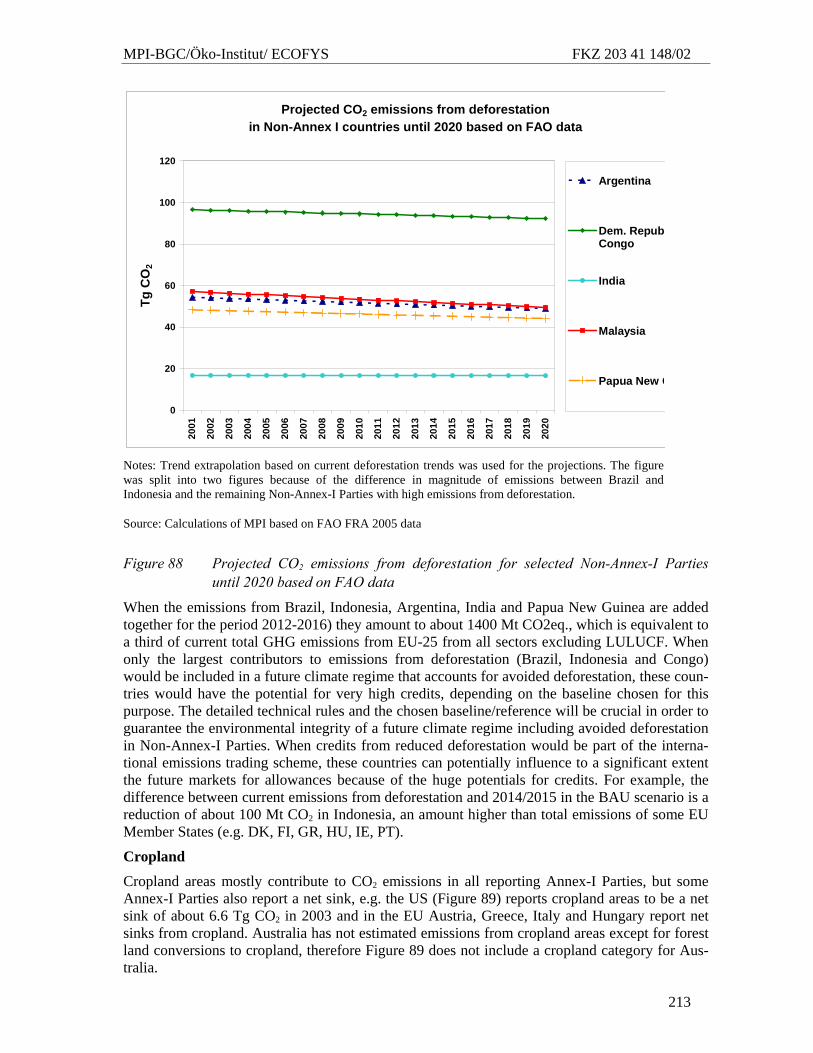
MPI-BGC/Öko-Institut/ ECOFYS FKZ 203 41 148/02
213
Projected CO2 emissions from deforestation in Non-Annex I countries until 2020 based on FAO data
0
20
40
60
80
100
120
2001
2002
2003
2004
2005
2006
2007
2008
2009
2010
2011
2012
2013
2014
2015
2016
2017
2018
2019
2020
Tg C
O2
Argentina
Dem. RepubCongo
India
Malaysia
Papua New G
Notes: Trend extrapolation based on current deforestation trends was used for the projections. The figure was split into two figures because of the difference in magnitude of emissions between Brazil andIndonesia and the remaining Non-Annex-I Parties with high emissions from deforestation.
Source: Calculations of MPI based on FAO FRA 2005 data
Figure 88 Projected CO2 emissions from deforestation for selected Non-Annex-I Parties until 2020 based on FAO data
When the emissions from Brazil, Indonesia, Argentina, India and Papua New Guinea are added together for the period 2012-2016) they amount to about 1400 Mt CO2eq., which is equivalent to a third of current total GHG emissions from EU-25 from all sectors excluding LULUCF. When only the largest contributors to emissions from deforestation (Brazil, Indonesia and Congo) would be included in a future climate regime that accounts for avoided deforestation, these coun-tries would have the potential for very high credits, depending on the baseline chosen for this purpose. The detailed technical rules and the chosen baseline/reference will be crucial in order to guarantee the environmental integrity of a future climate regime including avoided deforestation in Non-Annex-I Parties. When credits from reduced deforestation would be part of the interna-tional emissions trading scheme, these countries can potentially influence to a significant extent the future markets for allowances because of the huge potentials for credits. For example, the difference between current emissions from deforestation and 2014/2015 in the BAU scenario is a reduction of about 100 Mt CO2 in Indonesia, an amount higher than total emissions of some EU Member States (e.g. DK, FI, GR, HU, IE, PT).
Cropland
Cropland areas mostly contribute to CO2 emissions in all reporting Annex-I Parties, but some Annex-I Parties also report a net sink, e.g. the US (Figure 89) reports cropland areas to be a net sink of about 6.6 Tg CO2 in 2003 and in the EU Austria, Greece, Italy and Hungary report net sinks from cropland. Australia has not estimated emissions from cropland areas except for forest land conversions to cropland, therefore Figure 89 does not include a cropland category for Aus-tralia.
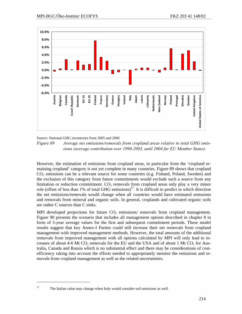
MPI-BGC/Öko-Institut/ ECOFYS FKZ 203 41 148/02
214
-6.0%
-4.0%
-2.0%
0.0%
2.0%
4.0%
6.0%
8.0%
10.0%
Aus
tria
Bel
gium
Can
ada
Cze
ch R
epub
lic
Den
mar
k
EU 1
5
EU 2
5
Finl
and
Fran
ce
Ger
man
y
Gre
ece
Hun
gary
Irela
nd
Italy
Japa
n
Latv
ia
Lith
uani
a
Net
herla
nds
New
Zea
land
Nor
way
Pola
nd
Port
ugal
Slov
akia
Swed
en
Uni
ted
Kin
gdom
Uni
ted
Stat
es o
f Am
eric
a
Source: National GHG inventories from 2005 and 2006 Figure 89 Average net emissions/removals from cropland areas relative to total GHG emis-
sions (average contribution over 1990-2003, until 2004 for EU Member States)
However, the estimation of emissions from cropland areas, in particular from the ‘cropland re-maining cropland’ category is not yet complete in many countries. Figure 89 shows that cropland CO2 emissions can be a relevant source for some countries (e.g. Finland, Poland, Sweden) and the exclusion of this category from future commitments would exclude such a source from any limitation or reduction commitment. CO2 removals from cropland areas only play a very minor role (offset of less than 1% of total GHG emissions)37. It is difficult to predict in which direction the net emissions/removals would change when all countries would have estimated emissions and removals from mineral and organic soils. In general, croplands and cultivated organic soils are rather C sources than C sinks.
MPI developed projections for future CO2 emissions/ removals from cropland management. Figure 90 presents the scenario that includes all management options described in chapter 8 in form of 5-year average values for the first and subsequent commitment periods. These model results suggest that key Annex-I Parties could still increase their net removals from cropland management with improved management methods. However, the total amounts of the additional removals from improved management with all options calculated by MPI will only lead to in-creases of about 4-6 Mt CO2 removals for the EU and the USA and of about 1 Mt CO2 for Aus-tralia, Canada and Russia which is no substantial effect and there may be considerations of cost-efficiency taking into account the efforts needed to appropriately monitor the emissions and re-movals from cropland management as well as the related uncertainties.
37 The Italian value may change when Italy would consider soil emissions as well.
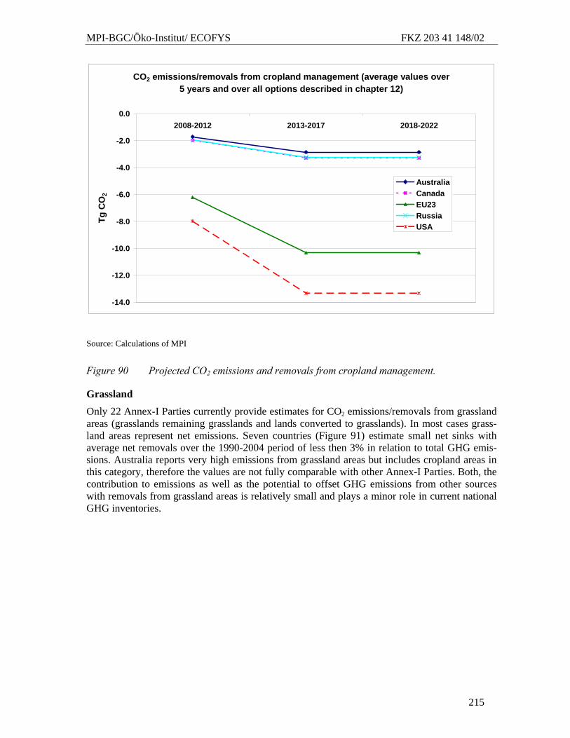
MPI-BGC/Öko-Institut/ ECOFYS FKZ 203 41 148/02
215
CO2 emissions/removals from cropland management (average values over 5 years and over all options described in chapter 12)
-14.0
-12.0
-10.0
-8.0
-6.0
-4.0
-2.0
0.02008-2012 2013-2017 2018-2022
Tg C
O2
AustraliaCanadaEU23RussiaUSA
Source: Calculations of MPI
Figure 90 Projected CO2 emissions and removals from cropland management.
Grassland
Only 22 Annex-I Parties currently provide estimates for CO2 emissions/removals from grassland areas (grasslands remaining grasslands and lands converted to grasslands). In most cases grass-land areas represent net emissions. Seven countries (Figure 91) estimate small net sinks with average net removals over the 1990-2004 period of less then 3% in relation to total GHG emis-sions. Australia reports very high emissions from grassland areas but includes cropland areas in this category, therefore the values are not fully comparable with other Annex-I Parties. Both, the contribution to emissions as well as the potential to offset GHG emissions from other sources with removals from grassland areas is relatively small and plays a minor role in current national GHG inventories.
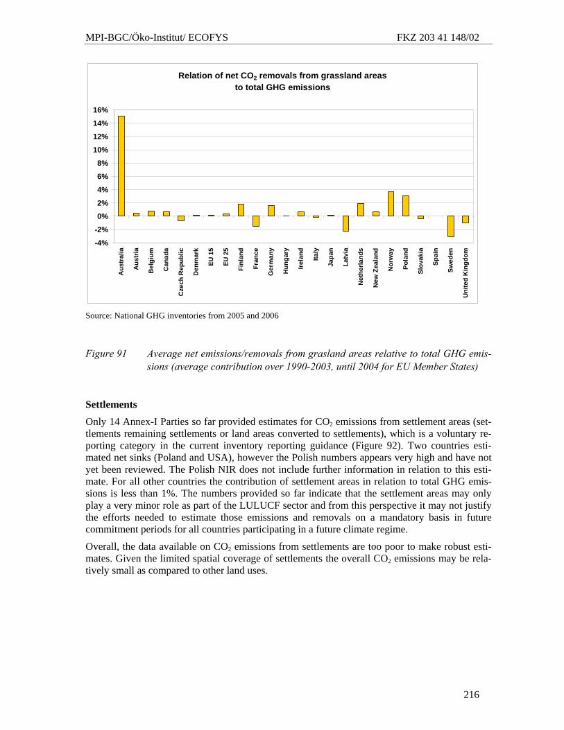
MPI-BGC/Öko-Institut/ ECOFYS FKZ 203 41 148/02
216
Relation of net CO2 removals from grassland areas to total GHG emissions
-4%
-2%
0%
2%
4%
6%
8%
10%
12%
14%
16%A
ustr
alia
Aus
tria
Bel
gium
Can
ada
Cze
ch R
epub
lic
Den
mar
k
EU 1
5
EU 2
5
Finl
and
Fran
ce
Ger
man
y
Hun
gary
Irela
nd
Italy
Japa
n
Latv
ia
Net
herla
nds
New
Zea
land
Nor
way
Pola
nd
Slov
akia
Spai
n
Swed
en
Uni
ted
Kin
gdom
Source: National GHG inventories from 2005 and 2006
Figure 91 Average net emissions/removals from grasland areas relative to total GHG emis-sions (average contribution over 1990-2003, until 2004 for EU Member States)
Settlements
Only 14 Annex-I Parties so far provided estimates for CO2 emissions from settlement areas (set-tlements remaining settlements or land areas converted to settlements), which is a voluntary re-porting category in the current inventory reporting guidance (Figure 92). Two countries esti-mated net sinks (Poland and USA), however the Polish numbers appears very high and have not yet been reviewed. The Polish NIR does not include further information in relation to this esti-mate. For all other countries the contribution of settlement areas in relation to total GHG emis-sions is less than 1%. The numbers provided so far indicate that the settlement areas may only play a very minor role as part of the LULUCF sector and from this perspective it may not justify the efforts needed to estimate those emissions and removals on a mandatory basis in future commitment periods for all countries participating in a future climate regime.
Overall, the data available on CO2 emissions from settlements are too poor to make robust esti-mates. Given the limited spatial coverage of settlements the overall CO2 emissions may be rela-tively small as compared to other land uses.
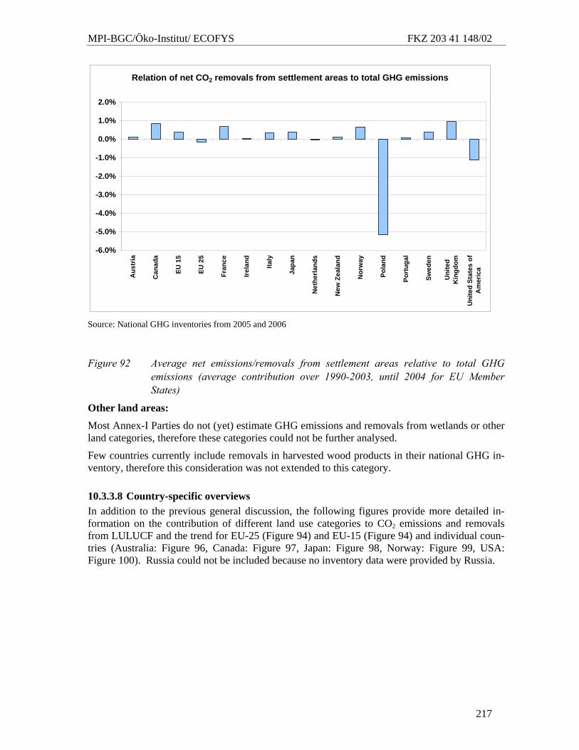
MPI-BGC/Öko-Institut/ ECOFYS FKZ 203 41 148/02
217
Relation of net CO2 removals from settlement areas to total GHG emissions
-6.0%
-5.0%
-4.0%
-3.0%
-2.0%
-1.0%
0.0%
1.0%
2.0%
Aus
tria
Can
ada
EU 1
5
EU 2
5
Fran
ce
Irela
nd
Italy
Japa
n
Net
herla
nds
New
Zea
land
Nor
way
Pola
nd
Port
ugal
Swed
en
Uni
ted
Kin
gdom
Uni
ted
Stat
es o
fA
mer
ica
Source: National GHG inventories from 2005 and 2006
Figure 92 Average net emissions/removals from settlement areas relative to total GHG emissions (average contribution over 1990-2003, until 2004 for EU Member States)
Other land areas:
Most Annex-I Parties do not (yet) estimate GHG emissions and removals from wetlands or other land categories, therefore these categories could not be further analysed.
Few countries currently include removals in harvested wood products in their national GHG in-ventory, therefore this consideration was not extended to this category.
10.3.3.8 Country-specific overviews In addition to the previous general discussion, the following figures provide more detailed in-formation on the contribution of different land use categories to CO2 emissions and removals from LULUCF and the trend for EU-25 (Figure 94) and EU-15 (Figure 94) and individual coun-tries (Australia: Figure 96, Canada: Figure 97, Japan: Figure 98, Norway: Figure 99, USA: Figure 100). Russia could not be included because no inventory data were provided by Russia.
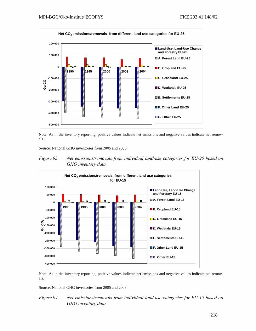
MPI-BGC/Öko-Institut/ ECOFYS FKZ 203 41 148/02
218
Net CO2 emissions/removals from different land use categories for EU-25
-500,000
-400,000
-300,000
-200,000
-100,000
0
100,000
200,000
1990 1995 2000 2003 2004
Gg
CO
2Land-Use, Land-Use Changeand Forestry EU-25
A. Forest Land EU-25
B. Cropland EU-25
C. Grassland EU-25
D. Wetlands EU-25
E. Settlements EU-25
F. Other Land EU-25
G. Other EU-25
Note: As in the inventory reporting, positive values indicate net emissions and negative values indicate net remov-als.
Source: National GHG inventories from 2005 and 2006
Figure 93 Net emissions/removals from individual land-use categories for EU-25 based on GHG inventory data
Net CO2 emissions/removals from different land use categories for EU-15
-400,000
-350,000
-300,000
-250,000
-200,000
-150,000
-100,000
-50,000
0
50,000
100,000
1990 1995 2000 2003 2004
Gg
CO
2
Land-Use, Land-Use Changeand Forestry EU-15
A. Forest Land EU-15
B. Cropland EU-15
C. Grassland EU-15
D. Wetlands EU-15
E. Settlements EU-15
F. Other Land EU-15
G. Other EU-15
Note: As in the inventory reporting, positive values indicate net emissions and negative values indicate net remov-als.
Source: National GHG inventories from 2005 and 2006
Figure 94 Net emissions/removals from individual land-use categories for EU-15 based on GHG inventory data
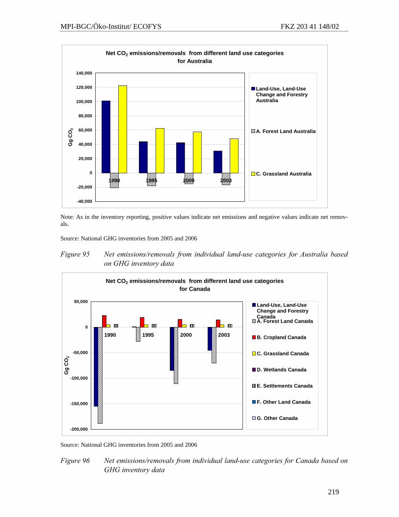
MPI-BGC/Öko-Institut/ ECOFYS FKZ 203 41 148/02
219
Net CO2 emissions/removals from different land use categories for Australia
-40,000
-20,000
0
20,000
40,000
60,000
80,000
100,000
120,000
140,000
1990 1995 2000 2003
Gg
CO
2
Land-Use, Land-UseChange and ForestryAustralia
A. Forest Land Australia
C. Grassland Australia
Note: As in the inventory reporting, positive values indicate net emissions and negative values indicate net remov-als.
Source: National GHG inventories from 2005 and 2006
Figure 95 Net emissions/removals from individual land-use categories for Australia based on GHG inventory data
Net CO2 emissions/removals from different land use categories for Canada
-200,000
-150,000
-100,000
-50,000
0
50,000
1990 1995 2000 2003
Gg
CO
2
Land-Use, Land-UseChange and ForestryCanadaA. Forest Land Canada
B. Cropland Canada
C. Grassland Canada
D. Wetlands Canada
E. Settlements Canada
F. Other Land Canada
G. Other Canada
Source: National GHG inventories from 2005 and 2006
Figure 96 Net emissions/removals from individual land-use categories for Canada based on GHG inventory data
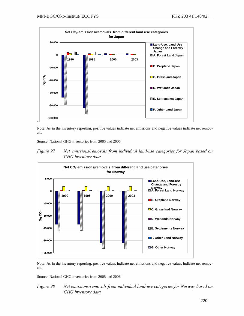
MPI-BGC/Öko-Institut/ ECOFYS FKZ 203 41 148/02
220
-
Net CO2 emissions/removals from different land use categories for Japan
-100,000
-80,000
-60,000
-40,000
-20,000
0
20,000
1990 1995 2000 2003
Gg
CO
2Land-Use, Land-UseChange and ForestryJapanA. Forest Land Japan
B. Cropland Japan
C. Grassland Japan
D. Wetlands Japan
E. Settlements Japan
F. Other Land Japan
Note: As in the inventory reporting, positive values indicate net emissions and negative values indicate net remov-als.
Source: National GHG inventories from 2005 and 2006
Figure 97 Net emissions/removals from individual land-use categories for Japan based on GHG inventory data
Net CO2 emissions/removals from different land use categories for Norway
-25,000
-20,000
-15,000
-10,000
-5,000
0
5,000
1990 1995 2000 2003
Gg
CO
2
Land-Use, Land-UseChange and ForestryNorwayA. Forest Land Norway
B. Cropland Norway
C. Grassland Norway
D. Wetlands Norway
E. Settlements Norway
F. Other Land Norway
G. Other Norway
Note: As in the inventory reporting, positive values indicate net emissions and negative values indicate net remov-als.
Source: National GHG inventories from 2005 and 2006
Figure 98 Net emissions/removals from individual land-use categories for Norway based on GHG inventory data
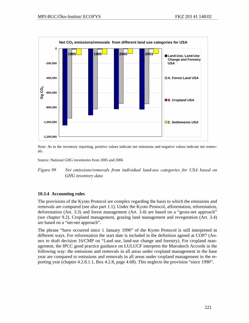
MPI-BGC/Öko-Institut/ ECOFYS FKZ 203 41 148/02
221
Net CO2 emissions/removals from different land use categories for USA
-1,200,000
-1,000,000
-800,000
-600,000
-400,000
-200,000
0
1990 1995 2000 2003
Gg
CO
2
Land-Use, Land-UseChange and ForestryUSA
A. Forest Land USA
B. Cropland USA
E. Settlements USA
Note: As in the inventory reporting, positive values indicate net emissions and negative values indicate net remov-als.
Source: National GHG inventories from 2005 and 2006
Figure 99 Net emissions/removals from individual land-use categories for USA based on GHG inventory data
10.3.4 Accounting rules
The provisions of the Kyoto Protocol are complex regarding the basis to which the emissions and removals are compared (see also part 1.1). Under the Kyoto Protocol, afforestation, reforestation, deforestation (Art. 3.3) and forest management (Art. 3.4) are based on a “gross-net approach” (see chapter 9.2). Cropland management, grazing land management and revegetation (Art. 3.4) are based on a “net-net approach”.
The phrase “have occurred since 1 January 1990” of the Kyoto Protocol is still interpreted in different ways. For reforestation the start date is included in the definition agreed at COP7 (An-nex to draft decision 16/CMP on “Land use, land-use change and forestry). For cropland man-agement, the IPCC good practice guidance on LULUCF interprets the Marrakech Accords in the following way: the emissions and removals in all areas under cropland management in the base year are compared to emissions and removals in all areas under cropland management in the re-porting year (chapter 4.2.8.1.1, Box 4.2.8, page 4.68). This neglects the provision “since 1990”.
MPI-BGC/Öko-Institut/ ECOFYS FKZ 203 41 148/02
222
Future options related to accounting rules
Option 4.1: Continuation of Kyoto Protocol accounting Net removals from afforestation, reforestation and deforestation as well as for forest manage-ment are accounted on a gross-net basis under the Kyoto Protocol. In the gross/net approach all net removals are accounted that relate to carbon stock changes and non CO2 emissions for a par-ticular year of the commitment period independent from the fact whether the total net removals are lower or higher than in previous years or a base period. During the commitment period the annual reported net removals for each year of the commitment period are converted into RMUs and issued into the national registries. The accountable emissions and removals still refer to ARD activities since 1990.
For CP, GM and revegetation the net-net accounting approach continues. A new base year for net-net accounting may be applicable depending on the general decisions taken on a base year for future commitments. A new base year or period would be necessary as changes between 1990 and 2008-2012 would have already been accounted for during the first commitment period.
Option 4.2: Net-net accounting for all activities with general base yearAs the gross-net account-ing approach chosen under the Kyoto Protocol is not consistent with the accounting of all other emissions. Therefore this option proposes a general net-net accounting system for all emissions and removals from LULUCF. A basis or reference has to be chosen and changes in relation to this base year are accounted for. As net emissions and removals resulting from changes between 1990 and 2008-2012 have already been issued as RMUs in the first commitment period, the new base year/ period should be the end of the first commitment period.
This option results in a change of accounting approach for emissions and removals from forest lands and the establishment of a base year or period for the accounting of emissions and remov-als from forestry. A net-net approach in a similar construction as for other GHG emissions com-pares the net removals resulting from carbon stock changes for a particular year to the net re-movals in the base year. When the net removals are higher than in the base year, the difference would enter the accounting scheme. When the net removals decrease below the chosen base year level, no removals would be accounted for. This means that decreasing net removals from the forest sector would no longer be accounted in this net-net system. In the situation where net re-movals in the commitment period are higher than in the base year period, the difference would enter the accounting scheme, but the net/net approach would considerably reduce the account-able removals compared to the gross/net approach (see Table 33). As a consequence, countries can claim C credits from removals until they reach maximum C uptake rates, and then zero, until the net removals turn into net emissions that would again be accounted in the same way as other GHG emissions. This would mean that countries with a declining C sink due to relatively old forests would no longer be able to get credits from their mature forests, despite the carbon stocks accumulated.
Option 4.3 Net-net accounting with basis related to forestry target
A different type of net-net approach for the forest sector would be to establish a separate forest target and this target could be expressed in terms of a level of net removals that the country has to achieve (e.g. is achieving in a business-as-usual scenario) in the commitment period. For each country this target could take into account its starting point in terms of forest age structure or status of sink depletion. Any net removals in the commitment period from the forest sector be-yond this target would then enter the accounting system. This approach would better take into account the national circumstances of individual countries. However, it requires the negotiation of separate targets for the forest sector for all participating countries. The targets would likely be based on future business-as-usual projections which are related to considerable uncertainties.
MPI-BGC/Öko-Institut/ ECOFYS FKZ 203 41 148/02
223
In theory another option exists which is the adoption of a gross-net accounting approach for cropland management, grassland management and revegetation. This option is not further con-sidered as it is rather unlikely. In general cropland management and grassland management are emission sources. Improved management methods can reduce emissions compared to a previous stage, however total cropland areas will not be converted to net sinks by management. A gross-net accounting approach would no longer account positive effects on reduced emissions due to management, but would account total cumulative CO2 emissions from cropland areas during a commitment period.
These accounting rules do not have many different implications on the criteria established and used in this assessment such as additional environmental benefits, technical effectiveness or spe-cial charecteristics of LULUCF. However, the options result in considerable differences in the accountable quantities and in the amounts of RMUs that can be issued. Therefore this section does not use the matrix approach as the previous sections but provides some quantitative assess-ment of the impacts of the options presented.
10.3.4.1 Quantitative impacts of gross-net and net-net accounting Table 33 compares the existing gross-net accounting approach (column gross/net) (Option 4.1) for forest land with different possibilities of a net-net accounting approach (two columns on the right) (Option 4.2) based on data from current national GHG inventories. In the example in Table 33 the assumed virtual commitment period covers four years from 2000-2003.38 The first net-net approach (second column from right) compares the net removals in the virtual commitment pe-riod 2000-2003 with the net removals in the year 1990. In the second net-net approach (right column), each country has the possibility to select a base year in the period 1990-1999, and the year with lowest net removals from this period was used in the calculations.
The total contributions of removals from forest land in the two net-net approaches always remain considerably below the accountable quantities of the gross-net approach. When the two options for the net-net approaches are compared, the approach where countries can choose the base year within a certain period is more favourable for most countries.
In the second column to the right the base year 1990 for a net-net approach is chosen. This ap-proach would not result in any accounting quantities for those countries for which 1990 had the largest removals over the time series (Australia, Canada, Finland, Latvia, Poland, USA). In this case, no further net removals could be accounted for during the commitment period.
This example also describes the effects for the accounting of the forest sector when a joint target is set across all sectors including LULUCF with a joint net-net accounting system.
38 The results for a base year period of several years were close to the base year variant with 1990 as base year and were therefore not included separately.
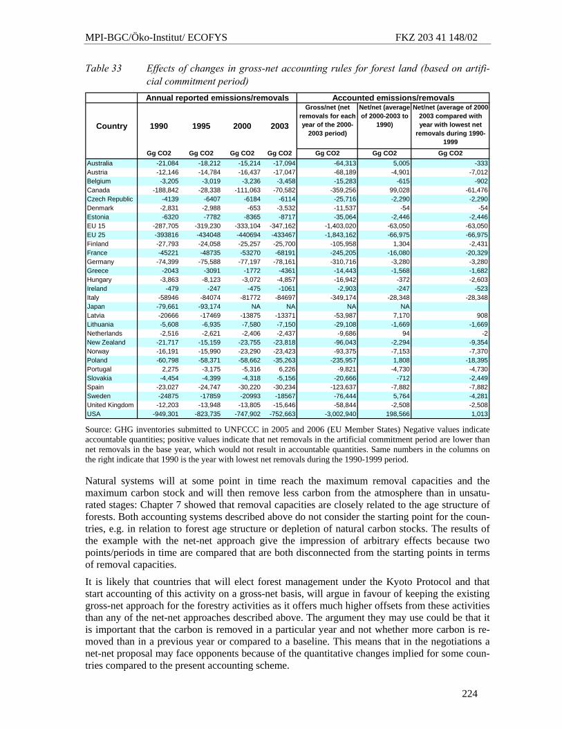
MPI-BGC/Öko-Institut/ ECOFYS FKZ 203 41 148/02
224
Table 33 Effects of changes in gross-net accounting rules for forest land (based on artifi-cial commitment period)
Country 1990 1995 2000 2003
Gross/net (net removals for each year of the 2000-
2003 period)
Net/net (average of 2000-2003 to
1990)
Net/net (average of 2000-2003 compared with year with lowest net
removals during 1990-1999
Gg CO2 Gg CO2 Gg CO2 Gg CO2 Gg CO2 Gg CO2 Gg CO2Australia -21,084 -18,212 -15,214 -17,094 -64,313 5,005 -333Austria -12,146 -14,784 -16,437 -17,047 -68,189 -4,901 -7,012Belgium -3,205 -3,019 -3,236 -3,458 -15,283 -615 -902Canada -188,842 -28,338 -111,063 -70,582 -359,256 99,028 -61,476Czech Republic -4139 -6407 -6184 -6114 -25,716 -2,290 -2,290Denmark -2,831 -2,988 -653 -3,532 -11,537 -54 -54Estonia -6320 -7782 -8365 -8717 -35,064 -2,446 -2,446EU 15 -287,705 -319,230 -333,104 -347,162 -1,403,020 -63,050 -63,050EU 25 -393816 -434048 -440694 -433467 -1,843,162 -66,975 -66,975Finland -27,793 -24,058 -25,257 -25,700 -105,958 1,304 -2,431France -45221 -48735 -53270 -68191 -245,205 -16,080 -20,329Germany -74,399 -75,588 -77,197 -78,161 -310,716 -3,280 -3,280Greece -2043 -3091 -1772 -4361 -14,443 -1,568 -1,682Hungary -3,863 -8,123 -3,072 -4,857 -16,942 -372 -2,603Ireland -479 -247 -475 -1061 -2,903 -247 -523Italy -58946 -84074 -81772 -84697 -349,174 -28,348 -28,348Japan -79,661 -93,174 NA NA NA NALatvia -20666 -17469 -13875 -13371 -53,987 7,170 908Lithuania -5,608 -6,935 -7,580 -7,150 -29,108 -1,669 -1,669Netherlands -2,516 -2,621 -2,406 -2,437 -9,686 94 -2New Zealand -21,717 -15,159 -23,755 -23,818 -96,043 -2,294 -9,354Norway -16,191 -15,990 -23,290 -23,423 -93,375 -7,153 -7,370Poland -60,798 -58,371 -58,662 -35,263 -235,957 1,808 -18,395Portugal 2,275 -3,175 -5,316 6,226 -9,821 -4,730 -4,730Slovakia -4,454 -4,399 -4,318 -5,156 -20,666 -712 -2,449Spain -23,027 -24,747 -30,220 -30,234 -123,637 -7,882 -7,882Sweden -24875 -17859 -20993 -18567 -76,444 5,764 -4,281United Kingdom -12,203 -13,948 -13,805 -15,646 -58,844 -2,508 -2,508USA -949,301 -823,735 -747,902 -752,663 -3,002,940 198,566 1,013
Annual reported emissions/removals Accounted emissions/removals
Source: GHG inventories submitted to UNFCCC in 2005 and 2006 (EU Member States) Negative values indicate accountable quantities; positive values indicate that net removals in the artificial commitment period are lower than net removals in the base year, which would not result in accountable quantities. Same numbers in the columns on the right indicate that 1990 is the year with lowest net removals during the 1990-1999 period.
Natural systems will at some point in time reach the maximum removal capacities and the maximum carbon stock and will then remove less carbon from the atmosphere than in unsatu-rated stages: Chapter 7 showed that removal capacities are closely related to the age structure of forests. Both accounting systems described above do not consider the starting point for the coun-tries, e.g. in relation to forest age structure or depletion of natural carbon stocks. The results of the example with the net-net approach give the impression of arbitrary effects because two points/periods in time are compared that are both disconnected from the starting points in terms of removal capacities.
It is likely that countries that will elect forest management under the Kyoto Protocol and that start accounting of this activity on a gross-net basis, will argue in favour of keeping the existing gross-net approach for the forestry activities as it offers much higher offsets from these activities than any of the net-net approaches described above. The argument they may use could be that it is important that the carbon is removed in a particular year and not whether more carbon is re-moved than in a previous year or compared to a baseline. This means that in the negotiations a net-net proposal may face opponents because of the quantitative changes implied for some coun-tries compared to the present accounting scheme.
MPI-BGC/Öko-Institut/ ECOFYS FKZ 203 41 148/02
225
10.3.5 Flexible mechanisms including carbon removals The Kyoto Protocol includes carbon removals in the flexible mechanisms in different ways. Dur-ing the 1st commitment period RMUs are issued for reported and reviewed greenhouse gas net removals. For CDM projects tCERs and lCERs are issued that take into account the potential problems of non-permanence of sink credits. The introduction of a carbon market is one of the major achievements under the Kyoto Protocol and it is assumed that a broad inclusion of all sec-tors in international emissions trading is a joint objective of most Parties, For the functioning of the emissions trading market in the first commitment period, it is important that commitments continue directly after 2012 and that there are early signals for the continuation of emissions trading, CDM and JI after the 1st commitment period.
Option 5.1: Continuation of existing situation (existing approach) The general accounting approach of RMUs for LULUCF activities and tCERs/lCERs (temporary credits) for forestry sink projects under the CDM continues in the future. The tCER/lCER con-cept is particularly necessary for LULUCF projects as they have a specified lifetime during which they are monitored and accounted.
The LULUCF activities accounted under the Kyoto Protocol remain in the future reporting and accounting system which recognizes positive as well as negative effects in future years. There-fore an additional approach to account for non-permanence is not necessary. If current Non-Annex-I Parties would join future commitments and if the three mechanisms continue to exist, CDM projects would be transformed in JI projects and ERUs converted from RMUs instead of tCERs/lCERs would be issued.
Option 5.2: tCERs for all LULUCF activities (all LULUCF units temporary) Option 5.2 proposes an additional discount of removals untits or a temporariliy limited account-ing for removal units in general. Some authors (e.g. presented by Schlamadinger et al., 2006) stress a general difference between emissions reduction in other sectors, e.g. from fossil fuel combustion, and carbon sequestration activities from LULUCF activities regarding permanence. If fossil fuels are substituted by non-CO2 emitting energy sources, the CO2 reduction will re-main, even if the substitution practice will discontinue in the future. However when sequestration activities were carried out to offset fossil fuel emissions and when they are reversed at a later stage, no net atmospheric CO2 effect occurs and emissions have only been postponed to a certain time in the future until the sinks are reversed. Several concepts have been suggested to address this non-permanence issue of removals in Annex-I Parties, such as the tCER/lCER concept or discounting approaches for removals.
Option 5.3: Separate flexible LULUCF instruments (separate LULUCF trading scheme) WBGU (2003) advocates for tradable non-utilization obligations of important carbon stocks. In this concept a system of tradable non-utilization commitment certificates would share the costs of foregoing the degrading use of carbon stocks among countries. Countries that no longer host sufficiently intact ecosystems would have to buy non-utilization commitments from other, re-source-rich countries.
10.3.5.1 Climate effectiveness (Figure 100) In Option 5.1 (existing approach) the accountable LULUCF activities – either in Annex I Parties or in Non-Annex I Parties – are fully integrated in the flexible mechanisms and the major prob-lems for climate effectiveness relating to the non-permanence nature of sinks were addressed in
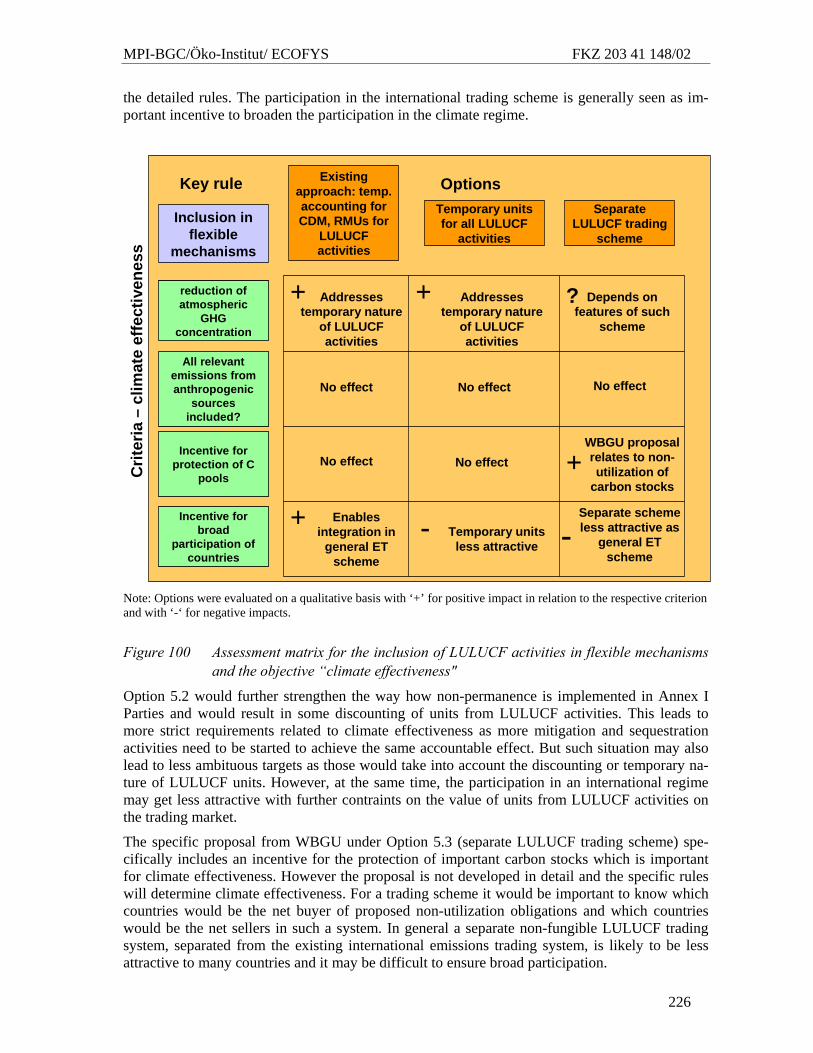
MPI-BGC/Öko-Institut/ ECOFYS FKZ 203 41 148/02
226
the detailed rules. The participation in the international trading scheme is generally seen as im-portant incentive to broaden the participation in the climate regime.
--
Existing approach: temp. accounting for CDM, RMUs for
LULUCF activities
Temporary units for all LULUCF
activities
Separate LULUCF trading
schemeInclusion in
flexible mechanisms
Options
+
+
Key rule
+ ?
No effectNo effectNo effect
WBGU proposalrelates to non-utilization of
carbon stocks
reduction of atmospheric
GHG concentration
All relevant emissions from anthropogenic
sources included?
Incentive for protection of C
pools
Incentive for broad
participation of countries
reduction of atmospheric
GHG concentration
All relevant emissions from anthropogenic
sources included?
Incentive for protection of C
pools
Incentive for broad
participation of countries
Crit
eria
–cl
imat
eef
fect
iven
ess
-Separate schemeless attractive as
general ET scheme
Addressestemporary nature
of LULUCF activities
Depends on features of such
scheme
- Temporary unitsless attractive
Enablesintegration in
general ET scheme
No effect
Addressestemporary nature
of LULUCF activities
No effect +
Note: Options were evaluated on a qualitative basis with ‘+’ for positive impact in relation to the respective criterion and with ‘-‘ for negative impacts.
Figure 100 Assessment matrix for the inclusion of LULUCF activities in flexible mechanisms and the objective “climate effectiveness"
Option 5.2 would further strengthen the way how non-permanence is implemented in Annex I Parties and would result in some discounting of units from LULUCF activities. This leads to more strict requirements related to climate effectiveness as more mitigation and sequestration activities need to be started to achieve the same accountable effect. But such situation may also lead to less ambituous targets as those would take into account the discounting or temporary na-ture of LULUCF units. However, at the same time, the participation in an international regime may get less attractive with further contraints on the value of units from LULUCF activities on the trading market.
The specific proposal from WBGU under Option 5.3 (separate LULUCF trading scheme) spe-cifically includes an incentive for the protection of important carbon stocks which is important for climate effectiveness. However the proposal is not developed in detail and the specific rules will determine climate effectiveness. For a trading scheme it would be important to know which countries would be the net buyer of proposed non-utilization obligations and which countries would be the net sellers in such a system. In general a separate non-fungible LULUCF trading system, separated from the existing international emissions trading system, is likely to be less attractive to many countries and it may be difficult to ensure broad participation.
MPI-BGC/Öko-Institut/ ECOFYS FKZ 203 41 148/02
227
10.3.5.2 Additional environmental benefits The impacts of the three options described above do not differ in relation to additional environ-mental benefits.
10.3.5.3 Technical effectiveness The existing approach described under option 5.1 is technically rather complex, but was success-fully agreed and is under implementation. Option 5.2 (all units temporary) does add complexity at technical level as RMUs would be treated in the trading system in a different way compared with AAUs. Option 5.3 (separate LULUCF Protocol) is very challenging at technical and meth-odological level as it requires the establishment of an additional, separate trading scheme where all technical issues have to be negotiated, agreed and implemented in addition to the current trad-ing system. Some additional complexities may be introduced compared to the existing system because non-utilization commitments for carbon stocks may need different and more complex liability rules.
10.3.5.4 Facilitation of the negotiation process The existing approach under option 5.1 is straightforward for the negotiation process. Option 5.2 (all units temporary) raises questions about the validity of RMUs used for compliance in the first commitment period. It may be difficult to argue for such modification while option 5.1 is already under implementation as the arguments for option 5.2 were already echoed when the rules for the first commitment period were negotiated. Option 5.3 reduces the incentives for carbon removals from LULUCF activities.
10.3.5.5 Special characteristics of LULUCF Options 5.1 (existing approach) and 5.2 (all units temporary) were developed to specifically ad-dress the special feature of non-permanence and the variability of carbon fluxes over time. For option 5.3 (separate LULUCF Protocol) a separate approach addressing these issue has to be developed.
10.3.5.6 Cost efficiency International emissions trading covering all sectors was introduced with the aim to increase cost efficiency and to provide a market instrument that contribute to select the most cost-efficient mitigation measures. Thus, the inclusion of LULUCF activities under options 5.1 and 5.2 in the flexible mechanisms increases cost efficiency of the regime. Option 5.3 is less cost efficient be-cause a separate trading scheme would not be fungible with the general trading scheme and cost efficient LULUCF sequestration activities could no longer replace more expensive mitigation measures in other sectors.
10.3.6 Commitment period length
The Kyoto Protocol established a commitment period of five years during which emissions and removals are considered for compliance with commitments. For changes of C stocks resulting from LULUCF activities, a 5-year-period is a rather short period as particular stock increases occur over long time periods.
Future options related to the commitment period length:
Option 6.1: Continuation of subsequent 5-year commitment periods This options assumes that 5-year commitment periods continue in the future.
MPI-BGC/Öko-Institut/ ECOFYS FKZ 203 41 148/02
228
Option 6.2: Longer commitment periods Under the Kyoto Protocol a five-year commitment period is used in order to avoid strong influ-ences of individual years with exceptional conditions. In relation to the accounting of the LULUCF sector, concerns have been raised whether this period is sufficiently long to level out the strong effects of natural incidents in single years and whether this period is sufficiently long to detect verifiable changes in carbon stocks in soils. Longer commitment periods are chosen for the accounting of LULUCF activities in this option, e.g. a period of 10 years. This option is linked to option 1.2 (separate LULUCF target) because a longer commitment period is not nec-essary for the other sectors.
A longer commitment period for LULUCF activities has advantages from the point of view of monitoring and estimation of emissions and removals. It also reduces the impacts of variability of C fluxes in individual years. Besides these advantages there are a number of disadvantages: 10 years are a long time period and it is difficult to project future emissions and removals and acitivities for such a long period, therefore it is difficult to establish specific commitments and targets over such a long period. Such long commitment periods fix a specific situations for a long time and do not allow to correct certain problems found during the implementation.
10.3.6.1 Quantitative impacts of the variability in carbon fluxes in relation to commitment period length Table 34 shows the annual variability of the CO2 emissions or removals of the LULUCF sector as reported in current national GHG inventories.
Changes from one year to another can be as high as 1450% (see UK in Table 34). However, such large annual changes are more pronounced when the absolute numbers in the inventory catego-ries are small. In this extreme case for UK, total net CO2 emissions from removals from LULUCF are close to zero for some years with the effect of high percentage changes which are not very relevant in absolute terms. When the trends for UK are considered individually, annual changes do not appear very dramatic (Figure 101).
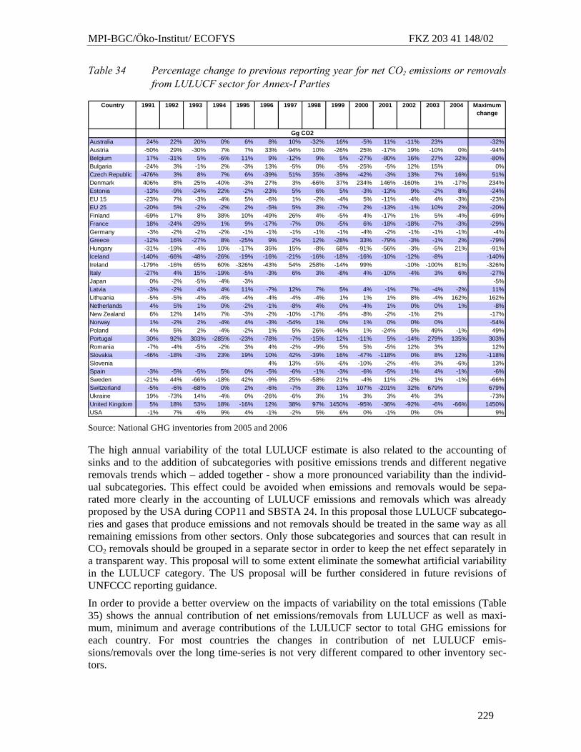
MPI-BGC/Öko-Institut/ ECOFYS FKZ 203 41 148/02
229
Table 34 Percentage change to previous reporting year for net CO2 emissions or removals from LULUCF sector for Annex-I Parties
Country 1991 1992 1993 1994 1995 1996 1997 1998 1999 2000 2001 2002 2003 2004 Maximum change
Australia 24% 22% 20% 0% 6% 8% 10% -32% 16% -5% 11% -11% 23% -32%Austria -50% 29% -30% 7% 7% 33% -94% 10% -26% 25% -17% 19% -10% 0% -94%Belgium 17% -31% 5% -6% 11% 9% -12% 9% 5% -27% -80% 16% 27% 32% -80%Bulgaria -24% 3% -1% 2% -3% 13% -5% 0% -5% -25% -5% 12% 15% 0%Czech Republic -476% 3% 8% 7% 6% -39% 51% 35% -39% -42% -3% 13% 7% 16% 51%Denmark 406% 8% 25% -40% -3% 27% 3% -66% 37% 234% 146% -160% 1% -17% 234%Estonia -13% -9% -24% 22% -2% -23% 5% 6% 5% -3% -13% 9% -2% 8% -24%EU 15 -23% 7% -3% -4% 5% -6% 1% -2% -4% 5% -11% -4% 4% -3% -23%EU 25 -20% 5% -2% -2% 2% -5% 5% 3% -7% 2% -13% -1% 10% 2% -20%Finland -69% 17% 8% 38% 10% -49% 26% 4% -5% 4% -17% 1% 5% -4% -69%France 18% -24% -29% 1% 9% -17% -7% 0% -5% 6% -18% -18% -7% -3% -29%Germany -3% -2% -2% -2% -1% -1% -1% -1% -1% -4% -2% -1% -1% -1% -4%Greece -12% 16% -27% 8% -25% 9% 2% 12% -28% 33% -79% -3% -1% 2% -79%Hungary -31% -19% -4% 10% -17% 35% 15% -8% 68% -91% -56% -3% -5% 21% -91%Iceland -140% -66% -48% -26% -19% -16% -21% -16% -18% -16% -10% -12% -8% -140%Ireland -179% -16% 65% 60% -326% -43% 54% 258% -14% 99% -10% -100% 81% -326%Italy -27% 4% 15% -19% -5% -3% 6% 3% -8% 4% -10% -4% 3% 6% -27%Japan 0% -2% -5% -4% -3% -5%Latvia -3% -2% 4% 4% 11% -7% 12% 7% 5% 4% -1% 7% -4% -2% 11%Lithuania -5% -5% -4% -4% -4% -4% -4% -4% 1% 1% 1% 8% -4% 162% 162%Netherlands 4% 5% 1% 0% -2% -1% -8% 4% 0% -4% 1% 0% 0% 1% -8%New Zealand 6% 12% 14% 7% -3% -2% -10% -17% -9% -8% -2% -1% 2% -17%Norway 1% -2% 2% -4% 4% -3% -54% 1% 0% 1% 0% 0% 0% -54%Poland 4% 5% 2% -4% -2% 1% 5% 26% -46% 1% -24% 5% 49% -1% 49%Portugal 30% 92% 303% -285% -23% -78% -7% -15% 12% -11% 5% -14% 279% 135% 303%Romania -7% -4% -5% -2% 3% 4% -2% -9% 5% 5% -5% 12% 3% 12%Slovakia -46% -18% -3% 23% 19% 10% 42% -39% 16% -47% -118% 0% 8% 12% -118%Slovenia 4% 13% -5% -6% -10% -2% -4% 3% -6% 13%Spain -3% -5% -5% 5% 0% -5% -6% -1% -3% -6% -5% 1% 4% -1% -6%Sweden -21% 44% -66% -18% 42% -9% 25% -58% 21% -4% 11% -2% 1% -1% -66%Switzerland -5% -6% -68% 0% 2% -6% -7% 3% 13% 107% -201% 32% 679% 679%Ukraine 19% -73% 14% -4% 0% -26% -6% 3% 1% 3% 3% 4% 3% -73%United Kingdom 5% 18% 53% 18% -16% 12% 38% 97% 1450% -95% -36% -92% -6% -66% 1450%USA -1% 7% -6% 9% 4% -1% -2% 5% 6% 0% -1% 0% 0% 9%
Gg CO2
Source: National GHG inventories from 2005 and 2006
The high annual variability of the total LULUCF estimate is also related to the accounting of sinks and to the addition of subcategories with positive emissions trends and different negative removals trends which – added together - show a more pronounced variability than the individ-ual subcategories. This effect could be avoided when emissions and removals would be sepa-rated more clearly in the accounting of LULUCF emissions and removals which was already proposed by the USA during COP11 and SBSTA 24. In this proposal those LULUCF subcatego-ries and gases that produce emissions and not removals should be treated in the same way as all remaining emissions from other sectors. Only those subcategories and sources that can result in CO2 removals should be grouped in a separate sector in order to keep the net effect separately in a transparent way. This proposal will to some extent eliminate the somewhat artificial variability in the LULUCF category. The US proposal will be further considered in future revisions of UNFCCC reporting guidance.
In order to provide a better overview on the impacts of variability on the total emissions (Table 35) shows the annual contribution of net emissions/removals from LULUCF as well as maxi-mum, minimum and average contributions of the LULUCF sector to total GHG emissions for each country. For most countries the changes in contribution of net LULUCF emis-sions/removals over the long time-series is not very different compared to other inventory sec-tors.
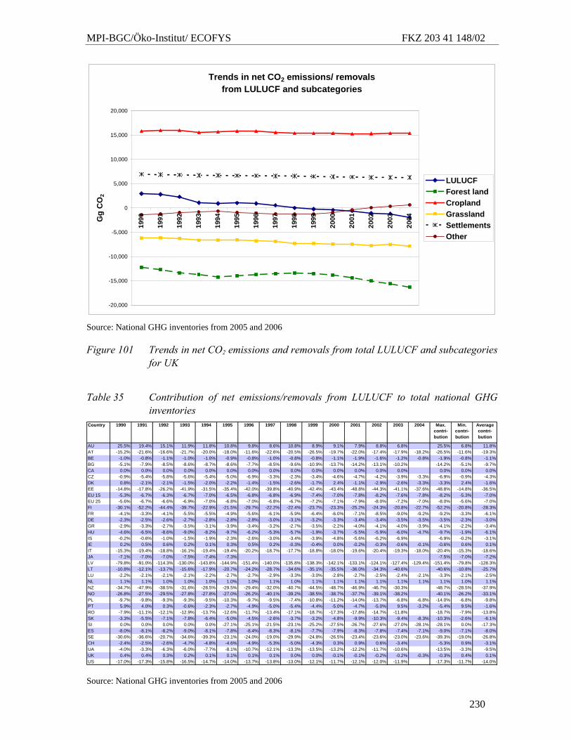
MPI-BGC/Öko-Institut/ ECOFYS FKZ 203 41 148/02
230
Trends in net CO2 emissions/ removals from LULUCF and subcategories
-20,000
-15,000
-10,000
-5,000
0
5,000
10,000
15,000
20,000
1990
1991
1992
1993
1994
1995
1996
1997
1998
1999
2000
2001
2002
2003
2004G
g C
O2
LULUCFForest landCroplandGrasslandSettlementsOther
Source: National GHG inventories from 2005 and 2006
Figure 101 Trends in net CO2 emissions and removals from total LULUCF and subcategories for UK
Table 35 Contribution of net emissions/removals from LULUCF to total national GHG inventories
Country 1990 1991 1992 1993 1994 1995 1996 1997 1998 1999 2000 2001 2002 2003 2004 Max. contri-bution
Min. contri-bution
Average contri-bution
AU 25.5% 19.4% 15.1% 11.9% 11.8% 10.8% 9.8% 8.6% 10.8% 8.9% 9.1% 7.9% 8.8% 6.8% 25.5% 6.8% 11.8%AT -15.2% -21.6% -16.6% -21.7% -20.0% -18.0% -11.6% -22.6% -20.5% -26.5% -19.7% -22.0% -17.4% -17.9% -18.2% -26.5% -11.6% -19.3%BE -1.0% -0.8% -1.1% -1.0% -1.0% -0.9% -0.8% -1.0% -0.8% -0.8% -1.1% -1.9% -1.6% -1.2% -0.8% -1.9% -0.8% -1.1%BG -5.1% -7.9% -8.5% -8.6% -8.7% -8.6% -7.7% -8.5% -9.6% -10.9% -13.7% -14.2% -13.1% -10.2% -14.2% -5.1% -9.7%CA 0.0% 0.0% 0.0% 0.0% 0.0% 0.0% 0.0% 0.0% 0.0% 0.0% 0.0% 0.0% 0.0% 0.0% 0.0% 0.0% 0.0%CZ -0.9% -5.4% -5.8% -5.6% -5.4% -5.0% -6.9% -3.3% -2.3% -3.4% -4.6% -4.7% -4.2% -3.9% -3.3% -6.9% -0.9% -4.3%DK 0.8% -2.1% -2.1% -1.5% -2.0% -2.2% -1.4% -1.5% -2.6% -1.7% 2.4% -1.1% -2.9% -2.6% -3.3% -3.3% 2.4% -1.6%EE -14.8% -17.8% -26.2% -41.9% -31.5% -35.4% -42.0% -39.8% -40.9% -42.4% -43.4% -48.8% -44.3% -41.1% -37.6% -48.8% -14.8% -36.5%EU 15 -5.3% -6.7% -6.3% -6.7% -7.0% -6.5% -6.8% -6.8% -6.9% -7.4% -7.0% -7.8% -8.2% -7.6% -7.8% -8.2% -5.3% -7.0%EU 25 -5.6% -6.7% -6.6% -6.9% -7.0% -6.8% -7.0% -6.8% -6.7% -7.2% -7.1% -7.9% -8.0% -7.2% -7.0% -8.0% -5.6% -7.0%FI -30.1% -52.2% -44.4% -39.7% -22.9% -21.5% -29.7% -22.2% -22.4% -23.7% -23.3% -25.2% -24.3% -20.8% -22.7% -52.2% -20.8% -28.3%FR -4.1% -3.3% -4.1% -5.5% -5.5% -4.9% -5.6% -6.1% -5.9% -6.4% -6.0% -7.1% -8.5% -9.0% -9.2% -9.2% -3.3% -6.1%DE -2.3% -2.5% -2.6% -2.7% -2.8% -2.8% -2.8% -3.0% -3.1% -3.2% -3.3% -3.4% -3.4% -3.5% -3.5% -3.5% -2.3% -3.0%GR -2.9% -3.3% -2.7% -3.5% -3.1% -3.9% -3.4% -3.2% -2.7% -3.5% -2.2% -4.0% -4.1% -4.0% -3.9% -4.1% -2.2% -3.4%HU -4.6% -6.5% -8.6% -9.0% -8.2% -9.7% -6.2% -5.3% -5.7% -1.9% -3.7% -5.5% -5.9% -6.0% -4.7% -9.7% -1.9% -6.1%IS -0.2% -0.6% -1.0% -1.5% -1.9% -2.3% -2.6% -3.0% -3.4% -3.9% -4.8% -5.6% -6.2% -6.9% -6.9% -0.2% -3.1%IE 0.2% 0.5% 0.6% 0.2% 0.1% 0.3% 0.5% 0.2% -0.3% -0.4% 0.0% -0.2% -0.3% -0.6% -0.1% -0.6% 0.6% 0.1%IT -15.3% -19.4% -18.8% -16.1% -19.4% -19.4% -20.2% -18.7% -17.7% -18.8% -18.0% -19.6% -20.4% -19.3% -18.0% -20.4% -15.3% -18.6%JA -7.1% -7.0% -7.0% -7.5% -7.4% -7.3% -7.5% -7.0% -7.2%LV -79.8% -91.0% -114.3% -130.0% -143.8% -144.9% -151.4% -140.0% -135.8% -138.3% -142.1% -133.1% -124.1% -127.4% -129.4% -151.4% -79.8% -128.3%LT -10.8% -12.1% -13.7% -15.6% -17.9% -20.7% -24.2% -28.7% -34.6% -35.1% -35.5% -36.0% -34.3% -40.6% -40.6% -10.8% -25.7%LU -2.2% -2.1% -2.1% -2.1% -2.2% -2.7% -2.7% -2.9% -3.3% -3.0% -2.8% -2.7% -2.5% -2.4% -2.1% -3.3% -2.1% -2.5%NL 1.1% 1.1% 1.0% 1.0% 1.0% 1.0% 1.0% 1.1% 1.0% 1.1% 1.1% 1.1% 1.1% 1.1% 1.1% 1.1% 1.0% 1.1%NZ -34.7% -47.9% -38.5% -31.6% -28.5% -29.5% -29.4% -32.0% -40.7% -44.5% -48.7% -46.9% -46.7% -30.3% -48.7% -28.5% -37.9%NO -26.8% -27.5% -29.5% -27.8% -27.8% -27.0% -26.2% -40.1% -39.2% -38.5% -38.7% -37.7% -39.1% -38.2% -40.1% -26.2% -33.1%PL -9.7% -9.8% -9.3% -9.3% -9.5% -10.3% -9.7% -9.5% -7.4% -10.8% -11.2% -14.0% -13.7% -6.8% -6.8% -14.0% -6.8% -9.8%PT 5.9% 4.0% 0.3% -0.6% -2.3% -2.7% -4.9% -5.0% -5.4% -4.4% -5.0% -4.7% -5.0% 9.5% -3.2% -5.4% 9.5% -1.6%RO -7.9% -11.1% -12.1% -12.9% -13.7% -12.6% -11.7% -13.4% -17.1% -18.7% -17.3% -17.8% -14.7% -11.8% -18.7% -7.9% -13.8%SK -3.3% -5.5% -7.1% -7.8% -6.4% -5.0% -4.5% -2.6% -3.7% -3.2% -4.8% -9.9% -10.3% -9.4% -8.3% -10.3% -2.6% -6.1%SI 0.0% 0.0% 0.0% 0.0% 0.0% -27.1% -25.1% -21.5% -23.1% -25.2% -27.5% -26.7% -27.6% -27.0% -28.1% -28.1% 0.0% -17.3%ES -8.0% -8.1% -8.2% -9.0% -8.1% -7.8% -8.4% -8.3% -8.1% -7.7% -7.9% -8.3% -7.8% -7.4% -7.1% -9.0% -7.1% -8.0%SE -30.6% -36.6% -20.7% -34.6% -39.3% -23.1% -24.0% -19.0% -29.9% -24.8% -26.5% -23.4% -23.6% -23.0% -23.6% -39.3% -19.0% -26.8%CH -2.4% -2.5% -2.6% -4.7% -4.8% -4.6% -4.9% -5.3% -5.0% -4.3% 0.3% 0.9% 0.6% -3.4% -5.3% 0.9% -3.1%UA -4.0% -3.3% -6.3% -6.0% -7.7% -8.1% -10.7% -12.1% -13.3% -13.5% -13.2% -12.2% -11.7% -10.6% -13.5% -3.3% -9.5%UK 0.4% 0.4% 0.3% 0.2% 0.1% 0.1% 0.1% 0.1% 0.0% 0.0% -0.1% -0.1% -0.2% -0.2% -0.3% -0.3% 0.4% 0.1%US -17.0% -17.3% -15.8% -16.5% -14.7% -14.0% -13.7% -13.8% -13.0% -12.1% -11.7% -12.1% -12.0% -11.9% -17.3% -11.7% -14.0%
Source: National GHG inventories from 2005 and 2006
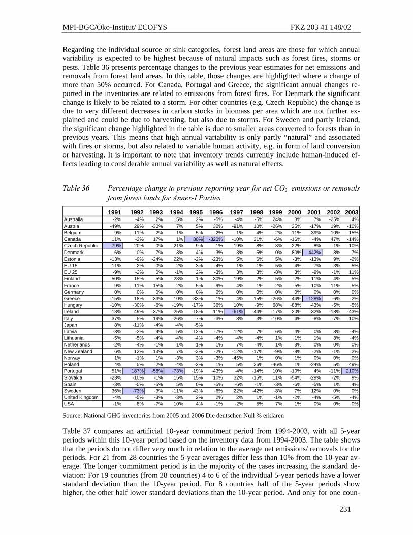
MPI-BGC/Öko-Institut/ ECOFYS FKZ 203 41 148/02
231
Regarding the individual source or sink categories, forest land areas are those for which annual variability is expected to be highest because of natural impacts such as forest fires, storms or pests. Table 36 presents percentage changes to the previous year estimates for net emissions and removals from forest land areas. In this table, those changes are highlighted where a change of more than 50% occurred. For Canada, Portugal and Greece, the significant annual changes re-ported in the inventories are related to emissions from forest fires. For Denmark the significant change is likely to be related to a storm. For other countries (e.g. Czech Republic) the change is due to very different decreases in carbon stocks in biomass per area which are not further ex-plained and could be due to harvesting, but also due to storms. For Sweden and partly Ireland, the significant change highlighted in the table is due to smaller areas converted to forests than in previous years. This means that high annual variability is only partly “natural” and associated with fires or storms, but also related to variable human activity, e.g. in form of land conversion or harvesting. It is important to note that inventory trends currently include human-induced ef-fects leading to considerable annual variability as well as natural effects.
Table 36 Percentage change to previous reporting year for net CO2 emissions or removals from forest lands for Annex-I Parties
1991 1992 1993 1994 1995 1996 1997 1998 1999 2000 2001 2002 2003Australia -2% -4% 2% 15% 2% -5% -4% -5% 24% 3% 7% -25% 4%Austria -49% 29% -30% 7% 5% 32% -91% 10% -26% 25% -17% 19% -10%Belgium 9% -11% 2% -1% 5% -2% -1% 4% 2% -11% -39% 10% 15%Canada 11% -2% 17% 1% 80% -320% -10% 31% -6% -16% -4% 47% -14%Czech Republic -79% -20% 0% 21% 9% 1% 19% 8% -8% -22% -8% -1% 10%Denmark -6% 0% -7% 3% 4% -3% -3% -5% 0% 80% -442% -8% 7%Estonia -13% -9% -24% 22% -2% -23% 5% 6% 5% -3% -13% 9% -2%EU 15 -11% -2% 0% -2% 3% -4% 1% -1% -5% 4% -7% -3% 5%EU 25 -9% -2% 0% -1% 2% -3% 3% 3% -8% 3% -9% -1% 11%Finland -50% 15% 5% 28% 1% -30% 19% 2% -5% 2% -11% 4% 5%France 9% -11% -15% 2% 5% -9% -4% 1% -2% 5% -10% -11% -5%Germany 0% 0% 0% 0% 0% 0% 0% 0% 0% 0% 0% 0% 0%Greece -15% 18% -33% 10% -33% 1% 4% 15% -26% 44% -128% -6% -2%Hungary -10% -30% -6% -19% -17% 36% 10% -9% 68% -88% -43% -5% -5%Ireland 18% 49% -37% 25% -18% 11% -61% -44% -17% 20% -32% -18% -43%Italy -37% 5% 19% -26% -7% -3% 8% 3% -10% 4% -8% -7% 10%Japan 8% -11% -4% -4% -5%Latvia -3% -2% 4% 5% 12% -7% 12% 7% 6% 4% 0% 8% -4%Lithuania -5% -5% -4% -4% -4% -4% -4% -4% 1% 1% 1% 8% -4%Netherlands -2% -4% -1% 1% 1% 1% 7% -4% 1% 3% 0% 0% 0%New Zealand 6% 12% 13% 7% -3% -2% -12% -17% -9% -8% -2% -1% 2%Norway 1% -1% 1% -3% 3% -3% -45% 1% 0% 1% 0% 0% 0%Poland 4% 5% 2% -4% -2% 1% 5% 26% -46% 1% -24% 5% 49%Portugal 51% 187% -58% -73% -19% -43% -4% -14% 10% -10% 4% -11% 210%Slovakia -23% -10% -1% 15% 15% 10% 32% -15% 11% -54% -29% -2% 9%Spain -3% -5% -5% 5% 0% -5% -6% -1% -3% -6% -5% 1% 4%Sweden 36% -73% -3% -11% 43% -6% 22% -42% -8% 7% 12% 0% 0%United Kingdom -4% -5% -3% -3% 2% 2% 2% 1% -1% -2% -4% -5% -4%USA -1% 8% -7% 10% 4% -1% -2% 5% 7% 1% 0% 0% 0% Source: National GHG inventories from 2005 and 2006 Die deutschen Null % erklären
Table 37 compares an artificial 10-year commitment period from 1994-2003, with all 5-year periods within this 10-year period based on the inventory data from 1994-2003. The table shows that the periods do not differ very much in relation to the average net emissions/ removals for the periods. For 21 from 28 countries the 5-year averages differ less than 10% from the 10-year av-erage. The longer commitment period is in the majority of the cases increasing the standard de-viation: For 19 countries (from 28 countries) 4 to 6 of the individual 5-year periods have a lower standard deviation than the 10-year period. For 8 countries half of the 5-year periods show higher, the other half lower standard deviations than the 10-year period. And only for one coun-
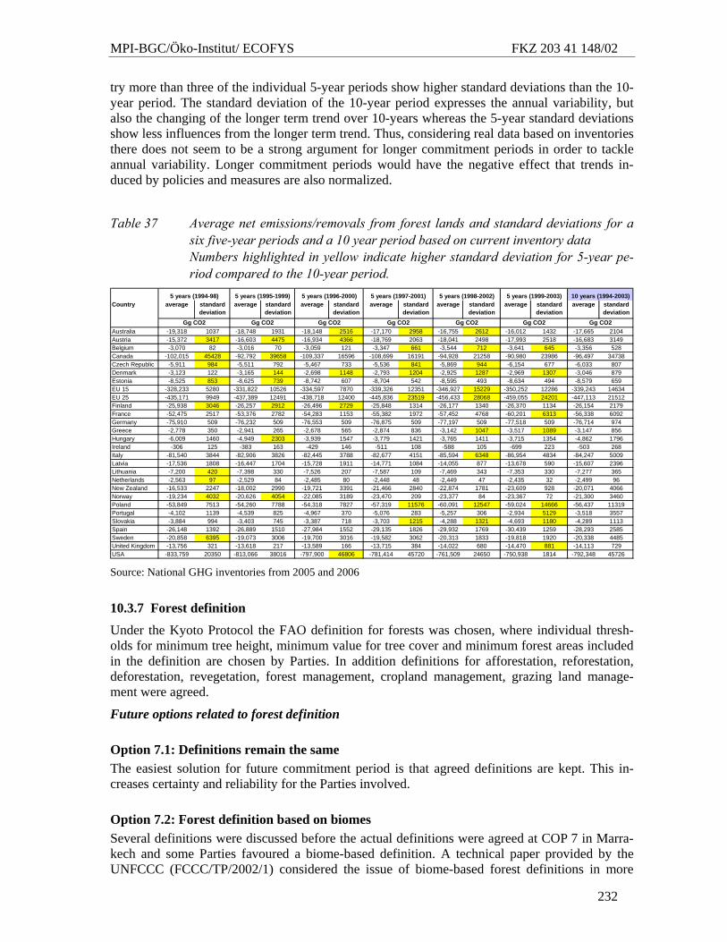
MPI-BGC/Öko-Institut/ ECOFYS FKZ 203 41 148/02
232
try more than three of the individual 5-year periods show higher standard deviations than the 10-year period. The standard deviation of the 10-year period expresses the annual variability, but also the changing of the longer term trend over 10-years whereas the 5-year standard deviations show less influences from the longer term trend. Thus, considering real data based on inventories there does not seem to be a strong argument for longer commitment periods in order to tackle annual variability. Longer commitment periods would have the negative effect that trends in-duced by policies and measures are also normalized.
Table 37 Average net emissions/removals from forest lands and standard deviations for a six five-year periods and a 10 year period based on current inventory data Numbers highlighted in yellow indicate higher standard deviation for 5-year pe-riod compared to the 10-year period.
Country average standard deviation
average standard deviation
average standard deviation
average standard deviation
average standard deviation
average standard deviation
average standard deviation
Australia -19,318 1037 -18,748 1931 -18,148 2516 -17,170 2958 -16,755 2612 -16,012 1432 -17,665 2104Austria -15,372 3417 -16,603 4475 -16,934 4366 -18,769 2063 -18,041 2498 -17,993 2518 -16,683 3149Belgium -3,070 82 -3,016 70 -3,059 121 -3,347 661 -3,544 712 -3,641 645 -3,356 528Canada -102,015 45428 -92,792 39658 -109,337 16596 -108,699 16191 -94,928 21258 -90,980 23986 -96,497 34738Czech Republic -5,911 984 -5,511 792 -5,467 733 -5,536 841 -5,869 944 -6,154 677 -6,033 807Denmark -3,123 122 -3,165 144 -2,698 1148 -2,793 1204 -2,925 1287 -2,969 1307 -3,046 879Estonia -8,525 853 -8,625 739 -8,742 607 -8,704 542 -8,595 493 -8,634 494 -8,579 659EU 15 -328,233 5280 -331,822 10526 -334,597 7870 -339,326 12351 -346,927 15229 -350,252 12286 -339,243 14634EU 25 -435,171 9949 -437,389 12491 -438,718 12400 -445,836 23519 -456,433 28068 -459,055 24201 -447,113 21512Finland -25,938 3046 -26,257 2912 -26,496 2729 -25,848 1314 -26,177 1340 -26,370 1134 -26,154 2179France -52,475 2517 -53,376 2782 -54,283 1153 -55,382 1972 -57,452 4768 -60,201 6313 -56,338 6092Germany -75,910 509 -76,232 509 -76,553 509 -76,875 509 -77,197 509 -77,518 509 -76,714 974Greece -2,778 350 -2,941 265 -2,678 565 -2,874 836 -3,142 1047 -3,517 1089 -3,147 856Hungary -6,009 1460 -4,949 2303 -3,939 1547 -3,779 1421 -3,765 1411 -3,715 1354 -4,862 1796Ireland -306 125 -383 163 -429 146 -511 108 -588 105 -699 223 -503 268Italy -81,540 3844 -82,906 3826 -82,445 3788 -82,677 4151 -85,594 6348 -86,954 4834 -84,247 5009Latvia -17,536 1808 -16,447 1704 -15,728 1911 -14,771 1084 -14,055 877 -13,678 590 -15,607 2396Lithuania -7,200 420 -7,398 330 -7,526 207 -7,587 109 -7,469 343 -7,353 330 -7,277 365Netherlands -2,563 97 -2,529 84 -2,485 80 -2,448 48 -2,449 47 -2,435 32 -2,499 96New Zealand -16,533 2247 -18,002 2990 -19,721 3391 -21,466 2840 -22,874 1781 -23,609 928 -20,071 4066Norway -19,234 4032 -20,626 4054 -22,085 3189 -23,470 209 -23,377 84 -23,367 72 -21,300 3460Poland -53,849 7513 -54,260 7788 -54,318 7827 -57,319 11576 -60,091 12547 -59,024 14666 -56,437 11319Portugal -4,102 1139 -4,539 825 -4,967 370 -5,076 283 -5,257 306 -2,934 5129 -3,518 3557Slovakia -3,884 994 -3,403 745 -3,387 718 -3,703 1215 -4,288 1321 -4,693 1180 -4,289 1113Spain -26,148 1392 -26,889 1510 -27,984 1552 -29,135 1826 -29,932 1769 -30,439 1259 -28,293 2585Sweden -20,858 6395 -19,073 3006 -19,700 3016 -19,582 3062 -20,313 1833 -19,818 1920 -20,338 4485United Kingdom -13,756 321 -13,618 217 -13,589 166 -13,715 384 -14,022 680 -14,470 881 -14,113 729USA -833,759 20350 -813,066 38016 -797,900 46806 -781,414 45720 -761,509 24650 -750,938 1814 -792,348 45726
5 years (1999-2003) 10 years (1994-2003)
Gg CO2 Gg CO2Gg CO2Gg CO2
5 years (1998-2002)
Gg CO2Gg CO2Gg CO2
5 years (1994-98) 5 years (1995-1999) 5 years (1996-2000) 5 years (1997-2001)
Source: National GHG inventories from 2005 and 2006
10.3.7 Forest definition
Under the Kyoto Protocol the FAO definition for forests was chosen, where individual thresh-olds for minimum tree height, minimum value for tree cover and minimum forest areas included in the definition are chosen by Parties. In addition definitions for afforestation, reforestation, deforestation, revegetation, forest management, cropland management, grazing land manage-ment were agreed.
Future options related to forest definition
Option 7.1: Definitions remain the same The easiest solution for future commitment period is that agreed definitions are kept. This in-creases certainty and reliability for the Parties involved.
Option 7.2: Forest definition based on biomes Several definitions were discussed before the actual definitions were agreed at COP 7 in Marra-kech and some Parties favoured a biome-based definition. A technical paper provided by the UNFCCC (FCCC/TP/2002/1) considered the issue of biome-based forest definitions in more
MPI-BGC/Öko-Institut/ ECOFYS FKZ 203 41 148/02
233
detail. The technical paper showed that the term “biome” can be interpreted in many different ways, each leading to a different classification system (page 8). The paper also concludes that
“There is no strong indication that a change in the way forests are defined in any ecological zone would lead to appreciable benefits either in terms of consistency of carbon estimates (agreement with the real values) or in terms of environmental bene-fits. The adoption of biome-specific forest definitions, if biome boundaries are not identical with national boundaries, is likely to make carbon accounting more difficult and/or less accurate, and is likely to lead to inconsistencies among forest carbon es-timates of different biomes within countries (since different definitions are likely to result in different error structures). The analysis of the implications of changing from one forest definition to another (be it biome-specific or otherwise) identified areas of concern. A change in forest definition between commitment periods will require dou-ble accounting (at least for the time of the changeover). In addition, it will inevitably create apparent changes in the amount of forest indicated, even if there is no actual change in the amount of woody vegetation. These apparent gains and/or losses of forest area will have to be differentiated from actual changes in woody vegetation. Separating accounted changes owing to real processes and those resulting from the definition change may pose considerable methodological problems. A change in for-est definition may also lead to paradoxical situations, may generate perverse incen-tives and may provide opportunities for abuses of the system.” (paragraphs 4 and 5 of FCCC/TP/2002/1)
From this analysis it is suggested that this report only keeps option 7.1 in its further discussion. The concerns expressed in this paper also show that a change of definitions will most likely lead to a much more complicated reporting and accounting system for LULUCF activities in the fu-ture.
10.3.8 Elements of additional rules aiming at correcting effects of key rules
There are a number of additional accounting rules under the Kyoto Protocol that are not seen as key part of the accounting system. The following provisions are included in this type of rules:
• Paragraph 4 of Annex to draft decision 16/CMP.1 on definitions, modalities, rules and guidelines relating to LULUCF activities under the Kyoto Protocol: Debits resulting from harvesting during the 1st commitment period following A/R since 1990 shall not be greater than credits accounted for on that unit of land. In case activities under Article 3.3 (paragraph 10) still represent a net source of emissions, emissions/removals from forest management may be accounted for in the first commitment period up to a level equal to this net source of emissions but not greater than 9.0 megatons of carbon times five
• Second sentence of Article 3.7 (Australian clause) : A special rule is included in the sec-ond sentence of Article 3.7 of the Kyoto Protocol for countries, for whom emissions from land-use change and forestry (that is the source category 5 of the Revised 1996 IPCC guidelines) constituted a net source of greenhouse gas emissions in 1990. These countries must include in their 1990 emissions base year or period the emissions and removals in 1990 from land-use change (that is a subset of category 5 related only to deforestation) (FCCC/CP/2001/13/Add.2 p.58).
• For the first commitment period, emissions/removals resulting from forest management under Article 3.4 and credits used from forest management JI-projects in other countries (after the rule of a net source resulting from afforestation, reforestation and deforestation
MPI-BGC/Öko-Institut/ ECOFYS FKZ 203 41 148/02
234
mentioned above has been applied), may be accounted for up to an individual limit for each Party shown in Table 27.
None of such rules are discussed here as they depend strongly on the rules accepted for a post 2012 regime.
10.3.9 Conclusions for the choice of key rules in future commitment period
10.3.9.1 Climate effectiveness The detailed assessment of options based on the detailed criteria shows that many options for key rules described in the previous section 10.3 have no or no clear influence on enhancement of climate effectiveness. Climate effectiveness is more related to stringency of targets and to the inclusion of relevant countries as well as to the inclusion of quantitatively relevant sources and sinks than to target types. Future rules should seek for:
• The inclusion of all significant C emissions and removals from all activities that lead to emissions/ removals. This excludes optional accounting that enables Parties not to ac-count for any significant emissions from LULUCF activities (e.g. from croplands, peat-lands or land-use conversions).
• The definition of „managed“ areas is important, when ‚anthropogenic‘ emis-sions/removals are based on the accounting on managed areas. When this definition is left to Parties, substantial forest land areas could be excluded from an accounting scheme.
• An appropriate way of dealing with non-permanence is important (temporary units where the accounting scheme does no automatically account for losses of sinks).
• Targets should cover key activities in the respective countries in order to have the most significant effects and options to broaden the coverage are more beneficial regarding cli-mate effectiveness.
• Data should exist for each country on which the stringency of the proposed commitments for all countries can be assessed.
10.3.9.2 Creation of additional/general environmental benefits In general there is mostly no clear effect between biodiversity/environmental benefits and C en-hancement in general, therefore additional rules at national local level are needed for biodiversity conservation, which go beyond UNFCCC or future Protocol.
• Some additional activities exist with clearly positive effects, in particular avoided defor-estation of pristine forest and protection of natural lands. When these activities can be enhanced appropriately under a future climate regime, there will be positive additional environmental effects
• There is no clear definition of sustainable forestry and agriculture, therefore it was very difficult to use these criteria in the assessment.
However, in general it would be more appropriate to ensure that climate change measures avoid negative impacts on other environmental objectives than to demand that there are additional en-vironmental benefits in other areas. Too many different targets in different areas may overburden the climate regime. It should also be acknowledged that it is unlikely that the climate negotia-tions can achieve efforts in relation to biodiversity or other areas that could not been achieved so far under the separate processes.
MPI-BGC/Öko-Institut/ ECOFYS FKZ 203 41 148/02
235
10.3.9.3 Technical effectiveness: facilitation of monitoring, accounting and verification of compliance
In relation to technical effectiveness, the following conclusions can be drawn:
• Joint or sectoral targets are technically easy to implement, new target types may be more difficult and costly in implementation, in particular when they do not longer base on the reporting system of emissions and removals under the UNFCCC.
• A net/net accounting system would considerably reduce some technical problems and complexities of the accounting system and would improve the understanding of the ac-counting system. However at the same time, the accountable quantities from forestry ac-tivities would be considerably reduced.
• The reference to managed areas regarding anthropogenic emissions and removals pre-sents a pragmatic technical approach to consider anthropogenic emissions and removals that avoids technical complexities. However the effects on climate effectiveness have to be assessed carefully and the definition of land management become a key issue for the negotiations. However, from a technical perspective this seems to be still easier to achieve improved defitions for land management than the elaboration of complex models that allow to differentiate natural and indirect from anthropogenic and direct effects.
• The present accounting system with temporary units is technically challenging and com-plex, at the same time it is a good solution to address non-permanence. As the technical more difficult part in developing the system with temporary units is already achieved, it seems straightforward to continue with the solution already agreed as the underlying problem will be the same in the future. However, the approach should not be extended when not absolutely necessary, e.g. the continuous inventory system with annual report-ing covers non-permanence without referring to temporary units.
• A broad approach for the inclusion of all LULUCF categories as reported under the Con-vention would facilitate the monitoring and reporting system, but may introduce some new problems for some Parties with the estimation of C pools and activities they did not elect in the first commitment period. From a technical perspective it would be beneficial when the reporting and accounting under a future climate regime would be closer to the reporting of emissions and removals from LULUCF under the Convention. This would avoid a complex separate reporting system as now established under the Kyoto Protocol. Chapter 10.3.3 provides a quantitative assessment of the significance of different land-use types.
• When additional single activities would be integrated in a monitoring system in addition to the activities under the Kyoto Protocol, additional technical complexities and problems will arise as the important activities are already covered and the remaining activities may be difficult to monitor and estimate.
• A separate Protocol would require a separate monitoring, verification and compliance scheme, as well as doubled institutions. This would considerably enhance transaction costs and does not seem to offer benefits from a technical and legal perspective.
10.3.9.4 Facilitation of negotiation process for post-2012 climate regime • For Annex-I Parties target types at national or sectoral level that would base on the exist-
ing reporting system and for which reported and reviewed data are available would largely facilitate the negotiation process because all negotiating Parties would have ac-cess to their own quantitative data as well as for other countries and a quantitative evalua-tion of different proposals would be straightforward. Due to the advances in reporting,
MPI-BGC/Öko-Institut/ ECOFYS FKZ 203 41 148/02
236
the existing database on emissions and removals from LULUCF activities has considera-bly improved and can be used as a basis for future negotiations. This improves the nego-tiation situation considerably as uncertainties about the quantitative impacts on the deci-sions taken could be considerably reduced which was a key problem when the Kyoto Protocol was negotiated. In the decision on different proposals for future targets, it is im-portant that the coverage of activities included in a future regime is clearly defined before final targets for countries are agreed.
• It is more difficult to integrate Non-Annex-I Parties in a future climate system as they don’t report on their emissions and removals from LULUCF or on afforestation and de-forestation. For deforestation international estimates show considerable differences and it is difficult to get reliable information for many countries. When discussions on avoided deforestation will enter into a more technical level, it would be essential to gather addi-tional reliable datasets for individual countries on existing and projected emissions from deforestation. Whereas the global estimates may be rather reliable, the results from mod-elling work for individual countries still show huge uncertainties and inconsistencies across different datasets.
• The protection of important global carbon stocks is an objective that is acknowledged in a positive way by all Parties. Whereas there is more or less unanimity regarding the ob-jective, the specific implementation of a regime that provides incentives and sets targets for the protection of carbon pools and stocks has a large potential for conflicts. Therefore it is essential to start soon with more specific proposals at the technical level for avoided deforestation in order to have sufficient negotiation time for the rather complicated de-tails in the technical implementation. Only such a process can avoid that targets are set before the rules and definitions are clarified.
• The definition of anthropogenic emissions/ removals as ‘managed areas’ facilitates the negotiation process, a change to different approaches for factoring out natural or indirect effects would require considerable methodological work with probably uncertain results and considerable negotiation efforts in order to implement new approaches.
• A separate Protocol would require separate monitoring and verification schemes, doubled institutions, a separate compliance scheme and a separate trading scheme which consid-erably enhances transaction costs and negotiation time and efforts and does not seem to be very promising from the perspective of negotiators.
10.3.9.5 Acknowledgement of special characteristics of LULUCF activities • The broader the coverage of LULUCF activities, the less importance will have single
events for individual land uses and their effects and may even equal out for the total sec-tor.
• Different national circumstances are difficult to address in an international regime. They can be addressed via the stringency of the target. Optional rules also address national cir-cumstances, but are counterproductive for climate effectiveness. The detailed technical implementation has to keep flexibility in order to fit to all circumstances.
10.3.9.6 Cost-efficiency At the level of the actual discussion of the role of sinks in future post-2012 commitments, it is premature to perform very detailed assessment of costs and cost-efficiency. But it is possible to provide some qualitative thoughts in relation to cost-efficiency:
MPI-BGC/Öko-Institut/ ECOFYS FKZ 203 41 148/02
237
• To ensure cost-efficiency for individual countries, it is important that they can concen-trate their efforts on those areas with high cost-efficiency of measures and on areas that are quantitatively relevant. Some degree of flexibility should be built into any future re-gime in order to avoid high transaction costs for rather unimportant areas.
• The protection of existing carbon stocks is clearly more cost-efficient than the increase of carbon stocks on other areas. However, the implementation of approaches to protect im-portant carbon stocks is related to transaction costs for the monitoring and verification.
• A separate protocol for LULUCF activities would imply very high transaction costs without clear gains in efficiency in other areas, and is likely to be the least cost-efficient approach.
10.4 Conclusions: promising options for future LULUCF rules
In relation to climate effectiveness the stringency of targets and the inclusion of relevant coun-tries are more relevant as the other key rules presented and discussed in the previous sections.
For improved climate effectiveness, it would be important to include all significant C emissions from LULUCF activities. Any optional accounting that enables Parties not to account for signifi-cant emissions from LULUCF activities (e.g. from croplands, peatlands or land-use conversions) should be avoided.
Regarding additional LULUCF activities, it is recommended to bring the reporting and account-ing under a future climate regime closer to the reporting of emissions and removals under the Convention. A definition of activities separate to the land-use categories included in the inven-tory lead to additional costs and complexities. The existing data from GHG inventories under the Convention provide a good basis for the assessment of quantitative impacts and of problems with the estimation of emissions and removals for some pools or land-uses that could be taken into account in the definition of the coverage of a post-2012 regime regarding the LULUCF sector. An accounting of partial areas for a specific land use activity should be avoided in the future.
For Annex I-Parties target types at national or sectoral level that would base on the existing re-porting system and for which reported and reviewed data are available would largely facilitate the negotiation process because all negotiating Parties would have access to their own quantita-tive data as well as for other countries and a quantitative evaluation of different proposals would be straightforward. Due to the advances in reporting, the existing database on emissions and re-movals from LULUCF activities has considerably improved and can be used as a basis for future negotiations. This improves the negotiation situation considerably as uncertainties about the quantitative impacts on the decisions taken could be considerably reduced which was a key prob-lem when the Kyoto Protocol was negotiated. In the decision on different proposals for future targets, it is important that the coverage of activities included in a future regime is clearly de-fined before final targets for countries are agreed.
For a future approach to consider all emissions and removals on managed areas as anthropogenic seems to be the most pragmatic and appropriate way to address the difficulties with factoring out of natural or indirect effects. However, within this approach the definition of „managed“ areas is important. When this definition is left to Parties, substantial forest land areas could be excluded from an accounting scheme. This is also relevant in relation to the discussions on avoided defor-estation. Therefore it is important to continue the elaboration of improved definitions of man-aged land that could be used in the future. This is difficult, but from a technical perspective this seems to be easier to achieve than individual monitoring and accounting approaches that allow separating natural from anthropogenic effects
The present accounting system with temporary units is technically challenging and complex, at the same time it is a good solution to address non-permanence. As the technical more difficult
MPI-BGC/Öko-Institut/ ECOFYS FKZ 203 41 148/02
238
part in developing the system with temporary units is already achieved, it seems good to con-tinue with the solution already agreed as the underlying problem will be the same in the future. However, the approach should not be extended when not absolutely necessary, e.g. the continu-ous inventory system with annual reporting covers non-permanence without referring to tempo-rary units.
The protection of important global carbon stocks is an objective that is acknowledged in a posi-tive way by all Parties. Whereas there is more or less unanimity regarding the objective, the spe-cific implementation of a regime that provides incentives and sets targets for the protection of carbon pools and stocks has a large potential for conflicts. Therefore it is essential to start soon with more specific proposals at the technical level, e.g. for avoided deforestation in order to have sufficient negotiation time for the rather complicated details in the technical implementation. Only such a process can avoid that targets are set before the rules and definitions are clarified.
International estimates for emissions from deforestation show considerable differences and it is difficult to get reliable information for many developing countries. When discussions on avoided deforestation will enter into a more technical level, it would be essential to have available addi-tional reliable datasets for individual countries on existing and projected emissions from defores-tation.
MPI-BGC/Öko-Institut/ ECOFYS FKZ 203 41 148/02
239
11 Alternative framework for LULUCF rules
Based on the findings and conclusions in the preceding chapters, this chapter proposes a novel, simple, yet comprehensive framework for addressing biospheric C sources and sinks. The framework could form one element of a future climate change agreement. The proposal resolves the present shortcomings in the Kyoto Protocol (KP), broadens the scope of action and creates a new incentive for conserving the existing biospheric C stocks.
11.1 Conclusions from previous chapters for an alternative framework Land use, land use change and forestry (LULUCF) represents the only sector
• in which not only anthropogenic emissions but also removals occur.
• emissions and removals are not solely driven by direct human action, but also by nature and indirect human effects. But even in remote areas, fires are often man-made such as 90% of the fires in Siberia (Mollicone et al., 2006). Gruber et al. (2004) expect that the major likely C stock changes in biomass and soils (excluding permafrost) over the next 20 to 50 years will be dominantly human-induced, in particular by land use change, degrada-tion and deforestation.
• rules for the first commitment period were determined after the targets were set, so that they became very complex (chapter 10).
At the same time, LULUCF is the sector
• bearing large uncertainties and methodological difficulty in quantifying emissions and removals and in projecting their future (chapter 2),
• dominating emissions from many Non-Annex-I countries but acting as a sink in many Annex-I countries (chapter 4)
• offering strong synergies with other environmental conventions (cf. chapter 4).
In conclusion and interpretation of the previous chapters in this report, in particular chapters 10.3 and 10.4, an alternative framework should best have the following characteristics:
1. The accounting for biospheric emissions and removals should remain completely under the UNFCCC and be more or less strongly linked to emission limitation targets in other sectors.
2. Although the stringency of targets and the inclusion of relevant countries in a future cli-mate change agreement remain political decisions, they can be facilitated by flexibility and incentives in an alternative framework.
3. New rules and modalities for including biospheric C in a future climate policy regime under the UNFCCC should overcome the shortcomings and constraints of the existing complex system for the first commitment period (2008-2012) without altering the UNFCCC and the general principles for LULUCF laid out in the KP and the Marrakech Accords (MA), which are valid beyond 2012.
4. New rules and modalities should at the same time not distract from efforts to reduce emissions in other sectors. This means that the linkage between biosheric C and emis-
MPI-BGC/Öko-Institut/ ECOFYS FKZ 203 41 148/02
240
sions from other sectors needs to be such that supply and demand for emission reduction credits in emission trading remain balanced.
5. The accounting for biospheric emissions and removals should include all significant C emissions from LULUCF activities in a mandatory form: land use change, deforestation, degradation, devegetation, and all management changes that reduce C stocks in ecosys-tems.
6. Full accounting of GHG emissions and removals on all managed land without distinction of activities in line with the reporting requirements under the UNFCCC is preferred for reasons of simplicity, consistency and balance.
7. Consequently, a broad, internationally accepted definition of „managed“ areas should be found in such a way that all anthropogenic sources are included.
8. The accounting for biospheric emissions and removals should be the same as in other sectors, i.e., net-net accounting.
9. The accounting system should include provisions to deal with non-permanence.
10. Protecting the existing C stocks in the biosphere against anthropogenic disturbance (de-forestation, degradation, devegetation) is more effective than the creation of new C pools in the biosphere.
11. The quantification, monitoring and verification of biospheric emissions and removals needs to be improved.
12. A stepwise, gradually more quantitative approach to include additional LULUCF activi-ties and more comprehensively the managed lands may facilitate acceptance and imple-mentation. It could be linked to the multi-stage approach to include further countries in future commitments.
11.2 Concept of stabilizing regional biospheric C stocks
The ultimate goal of the UNFCCC to stabilize atmospheric GHG levels implies the stabilization also of non-atmospheric C pools where feasible, i.e., reducing emissions, enhancing the mean residence time of C in labile pools and protecting labile C pools such as those in the biosphere (biomass, dead organic matter, soil, products) from being lost. This view sets the long-term goal of total ideally constant non-atmospheric C reservoirs (biospheric and fossil) from which the amount of biospheric C stock to be maintained at global, regional, and national level can be de-rived.
These biospheric C stocks goals can be easily related to other environmental goals such as biodi-versity, sustainable land use etc., where C stocks partly already serve as performance indicators. The C stock concept can be implemented in the existing accounting system as C stock changes and GHG fluxes. The time derivative of the C stock stabilization against present levels serves to define the short-, mid- and long-term goals of allowable C losses at global or national level.
11.3 Proposal for inclusion of biospheric C in a future climate policy regime
We propose below a novel architecture for a global climate policy regime beyond 2012. Without a comprehensive consideration of the large active C stocks and C fluxes in the terrestrial bio-sphere, climate change mitigation may fail to achieve an environmentally acceptable GHG emis-sion trajectory and stabilization goal (WBGU, 2003). We promote the inclusion of the entire terrestrial biosphere in future commitments, but are aware of the focus on "anthropogenic emis-
MPI-BGC/Öko-Institut/ ECOFYS FKZ 203 41 148/02
241
sions and removals" under the UNFCCC (Art. 4 UNFCCC). We hypothesize that future GHG emission reductions can best be achieved under quantitative national targets with flexibility through global emission trading buffered by a mechanism that protects/stabilizes the existing national biospheric C stocks. The proposed architecture introduces a separate commitment for the biosphere which is excluded from the emission trading. Whilst a legally binding instrument with stringent quantitative targets for all countries is presented below, political reality and the principles of differentiated responsibilities and broad participation are expected to approach this goal stepwise, e.g. in a multi-stage regime (Höhne et al., 2004), so that stringent quantitative targets will apply to an increasing number of Parties over time.
An international environmental agreement can only set the framework of goals and rules. Its im-plementation at national level, however, will ultimately need to tackle the underlying causes of GHG emissions and C losses from the biosphere and is not discussed here.
11.3.1 Proposed key rules
Rule 1. System of two interlinked GHG emission limitations
Two separate emission limitation targets are introduced.
a. Aimed at reducing GHG emissions, the "Greenhouse Gas Flux Target (GHGFT)" sets quantitative emission limitations for all anthropogenic GHG emissions including CO2 emissions and removals on all "managed land" (rules 2, 3) per country per commitment pe-riod which can be met by domestic action, performing projects elsewhere, and emission trading. The existing rules of the KP are maintained but accounting of emissions and re-movals on managed land is made mandatory. The extent at which flexible mechanisms (projects, emission trading) can be used to achieve the GHGFT is unlimited. The GHGFT can be defined against a base period as for the first commitment period under the KP or be derived from global or regional GHG emission caps for the commitment period. The GHGFT will become more ambitious over time.
b. The new "Bio-Carbon Target (BCT)" sets quantitative limitations for CO2 emissions from the biosphere on all "managed land" (rules 2, 3) per commitment period per country within the national territory, which can be met by domestic action by the country itself and by hosting biospheric projects. Credits under the BCT are not tradable. The BCT aims at maintaining/stabilizing the biospheric C stocks present in a country above a defined mini-mum threshold in the mid- to long-term. It can be nationally differentiated to adjust for the expected development of C stocks, risk of periodical disturbance or capacity to maintain or enhance C stocks, or reduce C losses as compared to a defined base period. A base period of e.g. five years is preferable to a single year in order to level out some of the interannual variability of CO2 fluxes. The BCT will approach zero (= stabilization of biospheric C stocks) over time.
The GHGFT and BCT create two independent but interlinked commitments (Figure 102). Both targets have to be met independently. There is no exchange of credits between the targets so that no double-counting of emissions and credits is possible. Double counting would only occur if credits from hosted projects entered the GHGFT. This is not allowed because credits under the BCT are not tradable.
Under the GHGFT, a donor country can trade credits from bio-projects abroad. In principle, the host could then buy back these credits for its own GHGFT, which would be accounted as GHG credits from emission trading and turn into a debit from emission trading in the seller country. There is hence flexibility, but no double counting in each of the targets. The BCT is not affected by trading under the GHGFT.
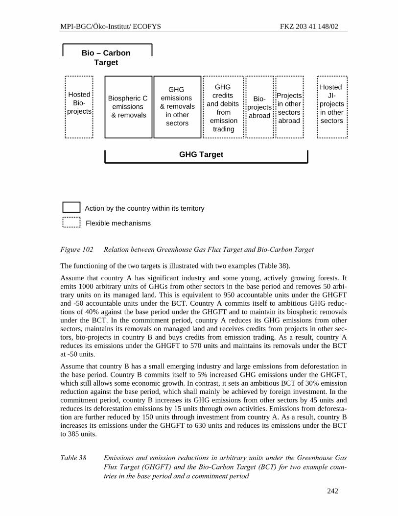
MPI-BGC/Öko-Institut/ ECOFYS FKZ 203 41 148/02
242
Figure 102 Relation between Greenhouse Gas Flux Target and Bio-Carbon Target
The functioning of the two targets is illustrated with two examples (Table 38).
Assume that country A has significant industry and some young, actively growing forests. It emits 1000 arbitrary units of GHGs from other sectors in the base period and removes 50 arbi-trary units on its managed land. This is equivalent to 950 accountable units under the GHGFT and -50 accountable units under the BCT. Country A commits itself to ambitious GHG reduc-tions of 40% against the base period under the GHGFT and to maintain its biospheric removals under the BCT. In the commitment period, country A reduces its GHG emissions from other sectors, maintains its removals on managed land and receives credits from projects in other sec-tors, bio-projects in country B and buys credits from emission trading. As a result, country A reduces its emissions under the GHGFT to 570 units and maintains its removals under the BCT at -50 units.
Assume that country B has a small emerging industry and large emissions from deforestation in the base period. Country B commits itself to 5% increased GHG emissions under the GHGFT, which still allows some economic growth. In contrast, it sets an ambitious BCT of 30% emission reduction against the base period, which shall mainly be achieved by foreign investment. In the commitment period, country B increases its GHG emissions from other sectors by 45 units and reduces its deforestation emissions by 15 units through own activities. Emissions from deforesta-tion are further reduced by 150 units through investment from country A. As a result, country B increases its emissions under the GHGFT to 630 units and reduces its emissions under the BCT to 385 units.
Table 38 Emissions and emission reductions in arbitrary units under the Greenhouse Gas Flux Target (GHGFT) and the Bio-Carbon Target (BCT) for two example coun-tries in the base period and a commitment period
HostedBio-
projects
Biospheric C emissions& removals
Bio – Carbon Target
Bio-projectsabroad
GHG Target
GHG credits
and debitsfrom
emissiontrading
GHGemissions& removals
in othersectors
Projectsin othersectorsabroad
HostedJI-
projectsin othersectors
Action by the country within its territory
Flexible mechanisms
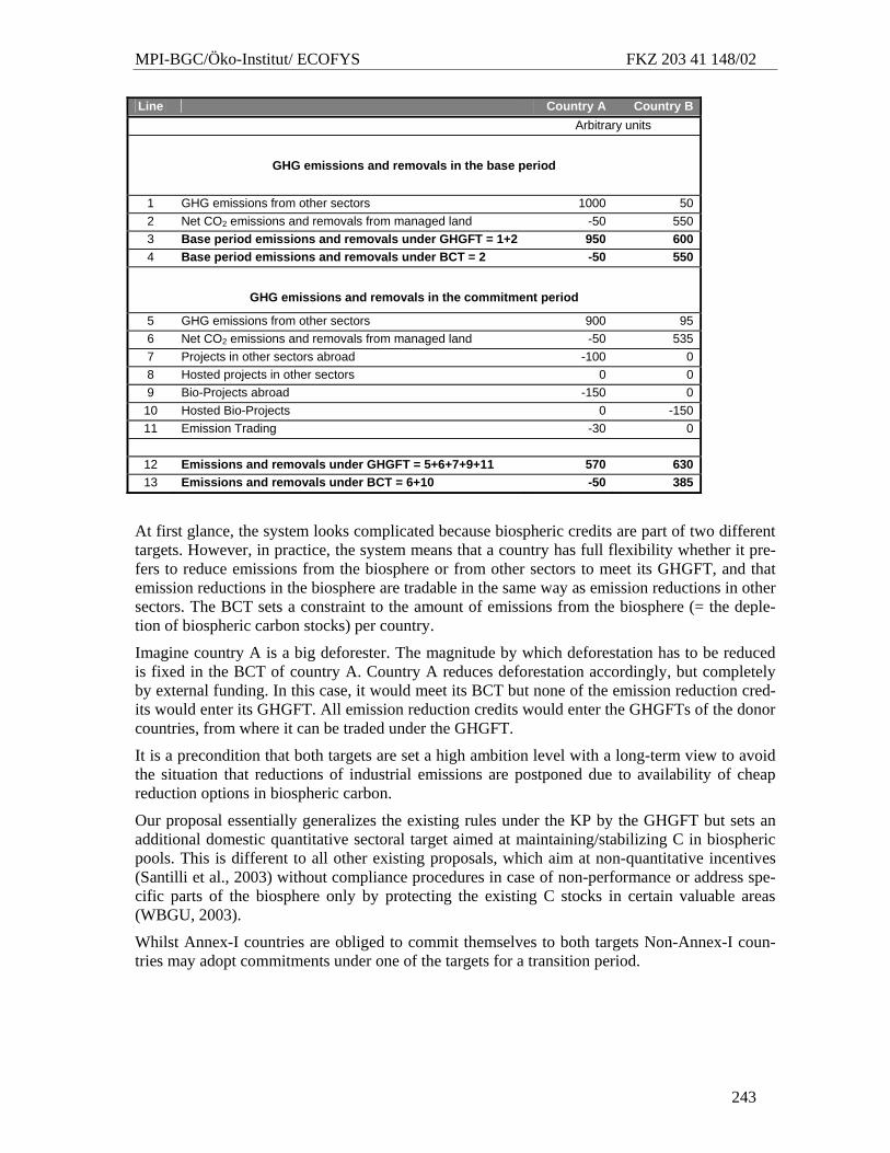
MPI-BGC/Öko-Institut/ ECOFYS FKZ 203 41 148/02
243
Line Country A Country B Arbitrary units
GHG emissions and removals in the base period
1 GHG emissions from other sectors 1000 50 2 Net CO2 emissions and removals from managed land -50 550 3 Base period emissions and removals under GHGFT = 1+2 950 600 4 Base period emissions and removals under BCT = 2 -50 550
GHG emissions and removals in the commitment period
5 GHG emissions from other sectors 900 95 6 Net CO2 emissions and removals from managed land -50 535 7 Projects in other sectors abroad -100 0 8 Hosted projects in other sectors 0 0 9 Bio-Projects abroad -150 0 10 Hosted Bio-Projects 0 -150 11 Emission Trading -30 0
12 Emissions and removals under GHGFT = 5+6+7+9+11 570 630 13 Emissions and removals under BCT = 6+10 -50 385
At first glance, the system looks complicated because biospheric credits are part of two different targets. However, in practice, the system means that a country has full flexibility whether it pre-fers to reduce emissions from the biosphere or from other sectors to meet its GHGFT, and that emission reductions in the biosphere are tradable in the same way as emission reductions in other sectors. The BCT sets a constraint to the amount of emissions from the biosphere (= the deple-tion of biospheric carbon stocks) per country.
Imagine country A is a big deforester. The magnitude by which deforestation has to be reduced is fixed in the BCT of country A. Country A reduces deforestation accordingly, but completely by external funding. In this case, it would meet its BCT but none of the emission reduction cred-its would enter its GHGFT. All emission reduction credits would enter the GHGFTs of the donor countries, from where it can be traded under the GHGFT.
It is a precondition that both targets are set a high ambition level with a long-term view to avoid the situation that reductions of industrial emissions are postponed due to availability of cheap reduction options in biospheric carbon.
Our proposal essentially generalizes the existing rules under the KP by the GHGFT but sets an additional domestic quantitative sectoral target aimed at maintaining/stabilizing C in biospheric pools. This is different to all other existing proposals, which aim at non-quantitative incentives (Santilli et al., 2003) without compliance procedures in case of non-performance or address spe-cific parts of the biosphere only by protecting the existing C stocks in certain valuable areas (WBGU, 2003).
Whilst Annex-I countries are obliged to commit themselves to both targets Non-Annex-I coun-tries may adopt commitments under one of the targets for a transition period.
MPI-BGC/Öko-Institut/ ECOFYS FKZ 203 41 148/02
244
Rule 2. Definition of "Managed Land"
Instead of using a set of LULUCF activities, all "managed land" is included by a broad defini-tion in line with the one adopted by the IPCC Good Practice Guidance for LULUCF (IPCC, 2004):
"Managed land is all land subject to human use, including production, social and eco-logical functions, even at very low frequency or intensity, or subject to any kind of di-rect human intervention".
This very comprehensive definition encompasses the entire biosphere except for, maybe, very remote and unpopulated regions. It refers to intensive and extensive types of land uses, fire man-agement, deliberate non-use and protection, areas prone to deforestation and logging, even in very long cycles, all land with semi-natural and secondary vegetation, land disturbed by present and past management such as peat drainage, logging, deforestation, land degradation, devegeta-tion (IPCC, 2004), lands on which management is abandoned in previous commitment periods or in the running one, and the effects of fires, pests and other disturbance on these areas. Conse-quently, difficulty with regard to thresholds and ambiguities in the definitions of land use types and activities becomes obsolete. The broad definition presented here avoids potential unbalanced accounting. The delineation of "managed land" could be scientifically based on remotely sensed and census information on land cover and land cover change, population density, and land man-agement, with ground-truthing in areas with high likelihood of human impact.
Rule 3. Scope of biospheric GHG emissions/removals
a. Mandatory full accounting of GHG emissions/removals on "managed land" as defined in rule 2 under the GHGFT and of C emissions/removals under the BCT. The scope is broadened from "activities" under the existing rules to all lands under direct human influ-ence.
b. Optional full GHG reporting and accounting of "unmanaged land", equivalent to full GHG accounting on all land, in order to fully match the atmospheric GHG signal.
All lands included in the first commitment period of the KP are included in this broader ap-proach. Countries hosting projects or accounting for activities under Articles 3.3 or 3.4 of the KP could continue to trace the GHG emissions and removals on these lands by their unit serial num-ber in the national registry in order to maintain consistency and transparency with their inventory in the first commitment period.
Rule 4. Flexible mechanisms
Flexible mechanisms are maintained as in the existing set of rules under the KP.
a. Emission trading under the GHGFT: Biospheric CO2 credits obtained by domestic action can be included in the emission trading in the same way as credits from other sectors. As in the existing system the unit serial number in the national registry allows to identify al-lowances from domestic and project-based Bio-CO2 sources and sinks in a country.
b. Biospheric projects: The existing rules for CDM projects are maintained for countries without a commitment under the BCT. Biospheric JI projects are restricted to countries with a BCT. JI project types are extended to any kind of project maintaining or enhancing biospheric C stocks or reducing biospheric C losses against a baseline. Project-based bio-spheric CO2 credits are accountable to fulfill the GHGFT in the investor country as under the existing rules. At the same time, the host country receives credits under its BCT (Figure 102). The host country is encouraged to set a legal framework for protecting its
MPI-BGC/Öko-Institut/ ECOFYS FKZ 203 41 148/02
245
national biospheric C stocks, which will help to increase the long-term success rate of in-vestments.
c. Further financial compensation mechanisms could be introduced for preserving high ex-isting C stocks in certain forests or peatlands.
Rule 5. Compliance procedures
The BCT has to be fulfilled within a country´s territory. However, a country may seek external assistance by hosting projects aimed at reducing biospheric CO2 emissions in order to meet its BCT (rule 4.b). In case a country fails to meet its BCT compliance procedures would need to secure that the BCT will be met in the following commitment period, and may consider an “in-terest rate” similar to the existing rules.
In contrast, in case the GHGFT is missed, the difference would need to be compensated by pur-chasing additional credits via the flexible mechanisms. This system avoids that emission reduc-tions be postponed in case of non-compliance. In case the GHGFT is exceeded, unused credits are tradable or bankable for meeting future commitments.
Rule 6. Incorporation of interannual variability of biospheric C fluxes
Interannual variability can significantly alter national GHG fluxes thus increasing the uncertainty of achieving fixed emission limitation targets. This challenge is already inherent to the existing rules of the Kyoto Protocol that treat the biosphere and other sectors under the same framework, but could be more relevant if countries subject to ENSO cycles participate. A detailed analysis of options to consider interannual variability goes beyond the scope of this paper but we mention some approaches a combination of which appears promising. A symmetric country-specific range of biospheric C fluxes in the order of e.g. the mean decadal detrended interannual variabil-ity could buffer fluctuations. Credits and debits for biospheric C fluxes would then only be ob-tained within this – periodically adjusted – range. Plenty of national and georeferenced data on forest fires is available globally to determine adequate country-specific buffer ranges (van der Werf et al., 2004). National liability reserves could be created by banking biospheric C credits from earlier periods or low-emission/high-removal years. Accounting could be allowed retro-spectively similar to the proposal by Santilli et al. (2003) so that uncertainty by fluctuations is eliminated. Current practice in inventory reports, however, demonstrates that interannual vari-ability driven by climate variation is ruled out by averaging in the national inventory reports.
11.3.2 Evaluation according to key principles and criteria
Chapter 10.2 has set up key principles that need to be met by a future political framework. The criteria set up in chapter 10.2 will be used to evaluate the proposed framework. The criteria are repeated from chapter 10.2 and directly answered. We demonstrate that the proposed framework meets these criteria under the condition that ambitious mitigation goals are achieved.
11.3.2.1 Climate effectiveness • Do the proposed rules contribute to the ultimate objective of the UNFCCC (Article 2)
and avoid a global warming exceeding more than 2 degrees since pre-industrial level? Any framework combining biospheric sources and sinks with other emission sectors bears the risk of a slow-down in mitigation efforts in other sectors under the assumption that reductions of emissions from biospheric sources are less costly or easier to pursue than reduction of emissions in other sectors. With this approach and the implied flexibil-ity, the overall emission limitation targets must be more ambitious than in a regime that
MPI-BGC/Öko-Institut/ ECOFYS FKZ 203 41 148/02
246
excludes biospheric C sinks in order not to delay reduction efforts in other sectors. Mechanisms dealing with the variability in biospheric GHG fluxes (rule 6) together with the great flexibility under the GHGFT (rules 1, 4) will facilitate the adoption of legally binding emission limitation targets.
• Are all relevant emissions from anthropogenic sources included in the proposed regime? The proposed framework includes all relevant anthropogenic GHG sources and sinks in-cluding those on managed land. The resulting global GHG estimates based on the na-tional inventories, together with knowledge about non-reported natural GHG sources and sinks, can ideally be verified by atmospheric GHG concentration measurements.
• Do the proposed rules provide an incentive to enhance or protect terrestrial carbon pools? By definition, the BCT aims to protect the C stocks in the biosphere. The stringency of BCT target setting will decide upon its success.
• Do the proposed rules stimulate a broad participation of countries and a participation of key countries in a future regime? A global GHG market (rules 1.a, 4.a) will facilitate the participation in GHG emission reduction activities and stimulate transfer of technology and knowledge to developing countries. The broader role of the biosphere in future commitments will help to increase investment in developing countries and in the land use sector where the greatest vulner-ability to climate change is assumed. Broad participation minimizes the risk of leakage by redistribution of GHG intensive activities to regions without commitments (Aldy et al., 2003).
11.3.2.2 Creation of additional/general environmental benefits • Do the proposed rules provide an incentive for sustainable forest and sustainable agri-
cultural management? Stabilizing national biospheric C stocks foresees continued land use and provision of non climate related goods and services, a certain intensification and land use change provided that existing C stocks are maintained at national level, as long as C losses in one area are compensated elsewhere in the nation. Carbon stocks are, of course, not the only indicator of sustainable land management, but an important one.
• Do the proposed rules contribute to the conservation of biodiversity? There is no automatism for synergy through conservation of biospheric C stocks as the only criterium because C rich ecosystems or regions are not automatically more diverse than C poor ones. However, C storage in ecosystems could be one out of a set of indica-tors supporting the mainstreaming of environmental UN Conventions and was also pro-posed as indicator for assessing progress under the CBD at a Royal Society (UK) work-shop in July 2004 (Balmford et al., 2005).
• Do the proposed rules allow to protect hot spot areas that have intensive feedbacks with regional and larger scale climate? Being country specific the BCT can be adjusted according to the vulnerability of regional LULUCF – climate interactions. This could help to protect hot spot areas but it will be the country´s responsibility to define those areas and create mechanisms for their protec-tion.
MPI-BGC/Öko-Institut/ ECOFYS FKZ 203 41 148/02
247
11.3.2.3 Technical effectiveness: facilitation of monitoring, accounting and verification of compliance
• Do the proposed rules allow a simple and straightforward technical implementation? The implementation of the proposed framework is easy because the reporting rules fol-low the requirements under the UNFCCC. As the reporting of biospheric emissions and removals under the UNFCCC is based on carbon stock changes, there is already knowl-edge about existing carbon stocks on managed lands. The monitoring requirements for the BCT are implicitly incorporated in those for the GHGFT. Full GHG monitoring of the biosphere is difficult today, but research and ob-servations are progressing. Australia has even demonstrated the operational feasibility of science based GHG monitoring of the biosphere at national to local level. We envisage in the medium term advanced operational monitoring systems based on models, linked to GIS and remote sensing, and validated against a network of ground based long-term eco-system monitoring sites. This will require initial investment, but once in place, the system will be transparent, verifiable, and can easily be upgraded upon emergence of new data or scientific findings. Regional monitoring networks could synergistically feed into and profit from global systematic observations (IGCO, 2004).
• Are consistent methodologies be used over time for the monitoring and the estimation of emissions and removals? The proposal allows to apply the IPCC Guidelines developped for reporting under the UNFCCC.
11.3.2.4 Facilitation of negotiation process for post-2012 climate regime • Do the proposed rules take into account the common but differentiated responsibilities of
the Parties under the UNFCCC? Both targets can be derived from global C conservation and emission reduction goals, ad-justed to country specific conditions, responsibilities and capacity – main concerns with regard to equity. The proposal maintains national sovereignty in land use decisions how to manage the biospheric C stocks and to implement an adequate institutional framework under both targets. The individual responsibilities of countries are best addressed by dif-ferentiated targets.
• Are the proposed rules based on reliable data and on sound science? The proposed framework incorporates the scientific criticism raised against the defini-tions, asymmetric accounting and impossibility of science based monitoring and verifica-tion of net GHG emission reductions under the existing rules. The reliability of land use data remains an issue in some regions of the world, but scientific progress towards better data is fast.
• Are the proposed rules simple enough for the negotiation process? The proposal applies a simple uniform rule for accounting for GHG emissions and sinks in all land use types and all sectors under both targets, thus overcoming the existing in-consistencies in accounting when land use changes. Full GHG accounting on all managed land (rules 2, 3) improves the transparency and eliminates the existing uncertainties in demarcation of land uses and activities, and in tracking of accountable areas.
• Do the proposed rules allow for sufficient flexibility for Parties to implement their com-mitments? National circumstances can be considered by adjusting the stringency and ambition of the commitments. Non-Annex-I countries can opt for one of the targets, thus facilitating the adoption of new commitments whilst still addressing a country´s major GHG emissions.
MPI-BGC/Öko-Institut/ ECOFYS FKZ 203 41 148/02
248
National specific variability and risks in the biospheric C balance can be considered (rule 6).
• Do the proposed rules ensure sufficient continuity with the first commitment period? Commitments under the two targets can be reported in the same land use based format as in the national inventories under the UNFCCC, following the IPCC Good Practice Guid-ance on LULUCF (IPCC, 2004). The GHGFT represents a generalisation of the rules for the first commitment period because the accounting of emissions and removals on all managed land is made mandatory and restrictions to the amount of emission reductions achieved by flexible mechanisms are abandoned. Although the BCT is conceptually based on C stocks the accounting rules are designed as the time derivative so that they are consistent with the approach of C stock changes in the existing rules.
• Are the proposed rules in line with fundamental positions of key players, e.g. do they avoid to return to previous proposals that were already rejected during the negotiation process? Any proposal in the climate negotiations can only be successful if accepted by all coun-tries or at least by the key players. Their attitude towards this proposal is difficult to judge and depends on all criteria mentioned here with different weightings and additional considerations. Simplifying the current set of rules, this proposal can satisfy the EU, if it leads to ambitious goals, and also large developing countries with tropical forests, as their contribution to avoiding deforestation can be acknowledged. The proposal also responds to the call of the USA for maximum flexibility across sectors and inclusion of the bio-sphere, but it remains to be seen whether additional governments can agree to legally binding emission reduction commitments. Net-net accounting of forest management was rejected earlier in the negotiations. On the other hand, we introduce it again in order to make mitigation activities in the biosphere comparable to those in other sectors.
11.3.2.5 Acknowledgement of special characteristics of LULUCF activities • Do the proposed rules address the variability of terrestrial carbon fluxes in relation to
timescales of commitment periods? Rule 6 highlights options to deal with the interannual variability of biospheric carbon fluxes.
• Do the proposed rules address the different time scales for enhancement and loss of C stocks? Important neglected activities for conserving and managing biospheric C stocks have been added to the existing portfolio of mitigation measures so that the focus of action is expected to move from creating new (small) C sinks to avoiding fast C losses.
• Do the proposed rules address permanence of accounted activities? With a continuous and contiguous inclusion of all managed lands in national accounting, eventual future C losses in areas of present C sinks will be implicitly considered in future commitment periods.
• Do the proposed rules address the problem of factoring out direct human induced from indirect human induced GHG changes? The multiple drivers of C sources and sinks can currently not be separated on a scientific basis (IPCC, 2003). A pragmatic area based approach (rules 2, 3) has been adopted that considers all GHG emissions and sinks on managed lands assuming that existing C stocks and GHG fluxes on these lands are dominated by human activities. Comparing GHG
MPI-BGC/Öko-Institut/ ECOFYS FKZ 203 41 148/02
249
fluxes in the commitment period against the respective fluxes in a base period, termed "net-net" accounting in earlier negotiations, removes from the accounting the background effects of climate change and past management to a large extent. Small indirect C sinks and sources cannot be excluded in some regions, but the magnitude of this bias by natural or indirect human induced processes is likely to be small and of transient nature as com-pared to direct land use effects, e.g. harvest intensity. Effects of past management and disturbances reflected in skewed age class distributions in forests result in oscillations of C sources and sinks around the theoretical mean C stock and will balance over time
• Do the proposed rules take into account different national natural, climatic and geo-graphical circumstances? National circumstances are best considered by the level of ambition in the BCT and pos-sible provisions to back up extreme events and unforeseen carbon losses.
11.3.2.6 Cost-efficiency • Do the proposed rules allow countries to choose cost-efficient reduction or sink en-
hancement strategies at national level? Do the proposed rules allow for sufficient flexi-bility in the implementation? The proposed framework improves flexibility and cost efficiency of emission reductions compared to the KP acknowledging the multiple functions of the biosphere in mitigation of and adaptation to climate change because
o GHG fluxes in the biosphere are fully tradable and exchangeable with other sec-tors and countries under the GHGFT (rule 1.a)
o it allows a more diverse role of the biosphere for meeting commitments and intro-duces new activities in Annex-I and developing countries to conserve existing C stocks
o monitoring is straightforward due to broad scope and wide definitions for the managed biosphere (rules 2, 3; cf. below)
o reporting commitments are very close to the national UNFCCC inventory.
• What implications do the proposed rules have on transaction costs? The combination of two targets has designed new win-win options for biospheric mitiga-tion measures. Even from a purely domestic perspective, land carbon management offers ancillary benefits for productivity, water management and sustainable development in general. If non marketed goods and services are included in cost considerations, sustain-able land use and conservation of extensively managed, relatively intact and even pristine ecosystems pays off (Balmford et al., 2002). Carbon credits are one possible mechanism for adequate valuation (Balmford et al., 2002), which would need to focus on the mainte-nance of existing C stocks at risk in order to meet the criteria of the UNFCCC.
Financing commitments and mechanisms represent crucial prerequisits for the success of any international environmental agreement, in particular if it shall enhance participation by devel-oping countries. (Aldy et al., 2003) regarded as economically favourable a system of 1) mod-erate short-term goals imbedded in much more stringent goals in the long-term, as implied in the proposal, 2) the increased developing country participation over time by e.g. incentives or graduation, compatible with the proposal, 3) provision of incentives for participation and com-pliance, contained in the proposal, and 4) the use of market based mechanisms, foreseen in the form of emission trading and projects.
MPI-BGC/Öko-Institut/ ECOFYS FKZ 203 41 148/02
250
11.4 Implications of the novel framework on individual Parties and regions
Official negotiations about the overall framework for a future climate change agreement are starting. A future climate policy regime is likely to encompass more options and different levels of stringency of commitments than the fixed targets under the 'cap and trade' system addressed here. Nevertheless we assume here that the same set of rules and indicators for setting targets applies to all countries. GHGFTs for individual countries can then be set on the basis of their total net GHG fluxes (Table 39, column C). So far, analyses and scenarios for future commit-ments include the CO2 or GHG emissions from other sectors only (Metz et al., 2002, Höhne et al., 2004). Estimates of LUC emissions (Table 39, column B) exceed by far the LULUCF C fluxes currently reported in the National Communications of Non-Annex-I countries (Table 39, column B'), which is partly related to different scope, assumptions and omissions. Including LUC emissions increases the per capita emissions of several Non-Annex-I countries to compara-ble levels as Annex-I countries. Including biospheric C fluxes in the target setting mainly affects Non-Annex-I and large countries in which biospheric C fluxes contribute significantly to net GHG fluxes and in which the trends of GHG emissions in other sectors differ from those in bio-spheric C fluxes.
The BCT is oriented at the existing C stocks in the biosphere at country level and their devel-opment in recent decades. An ambitious BCT does not necessarily relate to an ambitious GHGFT. Table 39 shows forest biomass C only, the most important vulnerable pool. Data are preliminary estimates only and have to be treated with caution. However, the forthcoming Global Forest Resources Assessment Update 2005 will provide significantly improved and harmonized data. Carbon stocks in the top metre of soils are several times higher than in biomass, but no globally consistent data sets are available so far that fully consider land use. In analogy to the procedures for GHG fluxes, national targets could be stepwise defined by first agreeing on a global trajectory of biospheric C stocks, e.g. a global goal to halve the present biospheric C losses by 2020 – a goal which still will create serious environmental damage in some world re-gions. Then priority areas of action could be identified according to vulnerability of C stocks at biome level, intensity of feedback mechanisms, capability and responsibility. National BCTs should be enforced in a way that countries with a biosphere that is neutral or is taking up C keep C stocks at least constant, while countries with a source reduce net biospheric C emissions. Lim-ited world regions face annual C losses far above the world´s average biomass loss of 1% per year while C accumulation in forests is a more widespread phenomenon (Table 39, columns, G, H).
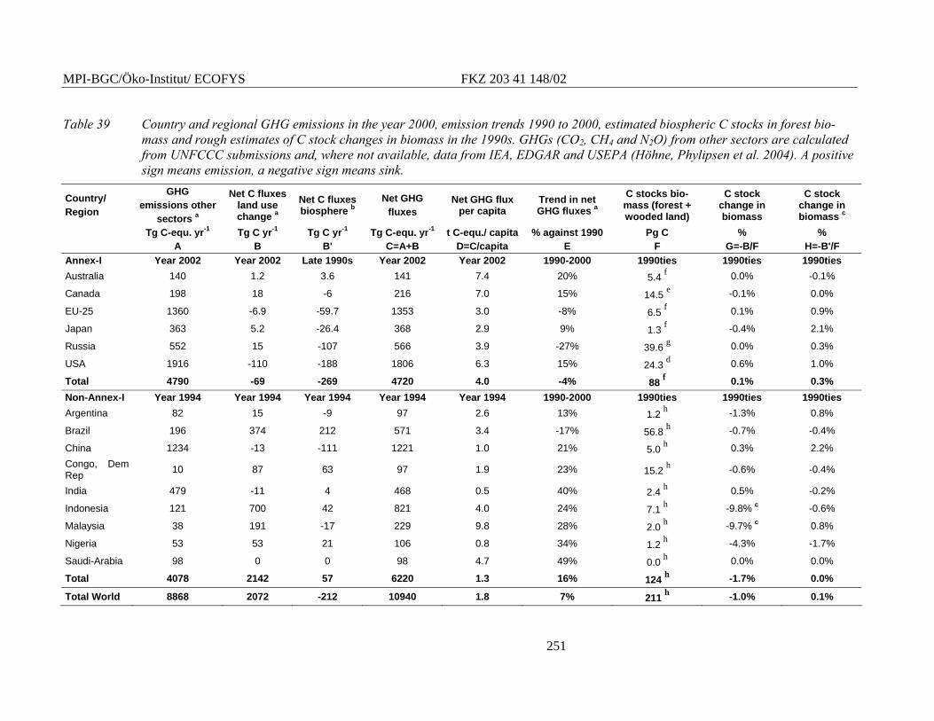
MPI-BGC/Öko-Institut/ ECOFYS FKZ 203 41 148/02
251
Table 39 Country and regional GHG emissions in the year 2000, emission trends 1990 to 2000, estimated biospheric C stocks in forest bio-mass and rough estimates of C stock changes in biomass in the 1990s. GHGs (CO2, CH4 and N2O) from other sectors are calculated from UNFCCC submissions and, where not available, data from IEA, EDGAR and USEPA (Höhne, Phylipsen et al. 2004). A positive sign means emission, a negative sign means sink.
Country/ Region
GHG emissions other
sectors a
Net C fluxes land use change a
Net C fluxes biosphere b
Net GHG fluxes
Net GHG flux per capita
Trend in net GHG fluxes a
C stocks bio-mass (forest + wooded land)
C stock change in biomass
C stock change in biomass c
Tg C-equ. yr-1 Tg C yr-1 Tg C yr-1 Tg C-equ. yr-1 t C-equ./ capita % against 1990 Pg C % % A B B' C=A+B D=C/capita E F G=-B/F H=-B'/F
Annex-I Year 2002 Year 2002 Late 1990s Year 2002 Year 2002 1990-2000 1990ties 1990ties 1990ties Australia 140 1.2 3.6 141 7.4 20% 5.4 f 0.0% -0.1%
Canada 198 18 -6 216 7.0 15% 14.5 e -0.1% 0.0%
EU-25 1360 -6.9 -59.7 1353 3.0 -8% 6.5 f 0.1% 0.9%
Japan 363 5.2 -26.4 368 2.9 9% 1.3 f -0.4% 2.1%
Russia 552 15 -107 566 3.9 -27% 39.6 g 0.0% 0.3%
USA 1916 -110 -188 1806 6.3 15% 24.3 d 0.6% 1.0%
Total 4790 -69 -269 4720 4.0 -4% 88 f 0.1% 0.3% Non-Annex-I Year 1994 Year 1994 Year 1994 Year 1994 Year 1994 1990-2000 1990ties 1990ties 1990ties Argentina 82 15 -9 97 2.6 13% 1.2 h -1.3% 0.8%
Brazil 196 374 212 571 3.4 -17% 56.8 h -0.7% -0.4%
China 1234 -13 -111 1221 1.0 21% 5.0 h 0.3% 2.2% Congo, Dem Rep 10 87 63 97 1.9 23% 15.2 h -0.6% -0.4%
India 479 -11 4 468 0.5 40% 2.4 h 0.5% -0.2%
Indonesia 121 700 42 821 4.0 24% 7.1 h -9.8% c -0.6%
Malaysia 38 191 -17 229 9.8 28% 2.0 h -9.7% c 0.8%
Nigeria 53 53 21 106 0.8 34% 1.2 h -4.3% -1.7%
Saudi-Arabia 98 0 0 98 4.7 49% 0.0 h 0.0% 0.0%
Total 4078 2142 57 6220 1.3 16% 124 h -1.7% 0.0%
Total World 8868 2072 -212 10940 1.8 7% 211 h -1.0% 0.1%
MPI-BGC/Öko-Institut/ ECOFYS FKZ 203 41 148/02
252
a Net C fluxes in the biosphere are taken from LUCF data (Houghton and Hackler 2003) as available in the WRI Cli-mate Analysis Indicator Tool CAIT (www.cait.org). b Data from National Communications. c We assume for simplifica-tion that all net C fluxes in the biosphere only occur in the forest biomass pool, which leads to overestimation of bio-mass losses in countries with significant losses of soil C and non-forest biomass such as Indonesia and Malaysia; d (Heath and Smith. 2004); e (Kurz and Apps 1999); f forest and other wooded land (TBFRA 2000); g (Shvidenko and Nilsson 2002); h forest (TBFRA 2000): total mass of woody biomass was converted to C by multiplication with 0.5.
11.5 Conclusions
The proposal presented here combines a Greenhouse Gas Flux Target achievable by domestic action and flexible mechanisms, with a Bio-Carbon Target that constrains CO2 emissions from the national territory. The proposal thus combines emission reductions in all sectors with the conservation of biospheric C stocks. Six simple rules allow the mitigation of all anthropogenic GHG hotspots in a transparent, yet flexible and cost-efficient manner and may hopefully stimu-late a fast significant reduction of global anthropogenic GHG emissions. The proposed frame-work can provide a scientific basis for further negotiations and could form one out of several elements in a future climate change agreement.
Yet it has been made clear that a framework by its own cannot guarantee sufficient GHG emis-sion reductions to reach the 2°C goal of Germany and the European Union. Success relies on a broad participation and ambitious commitments in emission reduction efforts.
MPI-BGC/Öko-Institut/ ECOFYS FKZ 203 41 148/02
253
References
Achard, F., Eva, H. D., Mayaux, P., Stibig, H. J. and Belward, A. (2004) Improved estimates of net carbon emissions from land cover change in the tropics for the 1990s - art. no. GB2008. Global Biogeochemical Cycles. 18, B2008.
Aldy JE, Barrett S, Stavins RN (2003) Thirteen plus one: a comparison of global climate policy architectures. Climate Policy, 3, 373-397, doi:310.1016/j.clipol.2003.1009.1004.
Alexandrov, G. and Oikawa, T. (2002) TsuBiMo: a biosphere model of the CO2 -fertilization effect. Climate Research. 19, 265-270.
Andreae MO, Merlet P (2001) Emission of trace gases and aerosols from biomass burning. Global Biogeochemical Cycles, 15, 955-966.
Apps, M. J., Kurz, W. A., Luxmoore, R. J., Nilsson, L. O., Sedjo, R. A., Schmidt, R., Simpson, L. G. and Vinson, T. S. (1993) Boreal forests and tundra. Water Air and Soil Pollution. 70, 39-53.
Augustin J, Merbach W, Steffens L, Snelinski B (1998) Nitrous oxide fluxes of disturbed min-erotrophic peatlands. Agribiological Research-Zeitschrift fur Agrarbiologie Agrikul-turchemie
Bachelet D, Neilson RP, Lenihan JM, Drapek RJ (2001) Climate change effects on vegetation distribution and carbon budget in the United States. Ecosystems, 4, 164-185.
Ballard TM (2000) Impacts of forest management on northern forest soils. Forest Ecology and Management, 133, 37-42.
Balmford A, Bennun L, Brink Bt, et al. (2005) ECOLOGY: The Convention on Biological Di-versity's 2010 Target. Science, 307, 212-213, DOI: 210.1126/science.1106281.
Balmford A, Bruner A, Cooper P, et al. (2002) Economic Reasons for Conserving Wild Na-ture. Science, 297, 950-953 [DOI: 910.1126/science.1073947].
Barber VA, Juday GP, Finney BP (2000) Reduced growth of Alaskan white spruce in the twenti-eth century from temperature-induced drought stress. Nature (London), 405, 668-673.
Barford CC, Wofsy SC, Goulden ML, et al. (2001) Factors Controlling Long- and Short-Term Sequestration of Atmospheric CO2 in a Mid-latitude Forest. Science, 294, 1688-1691.
Bazzaz FA (1998) Tropical forests in a future climate: Changes in biological diversity and im-pact on the global carbon cycle. Climatic Change, 39, 317-336.
Black, T. A., Chen, W. J., Barr, A. G., Arain, M. A., Chen, Z., Nesic, Z., Hogg, E. H., Neumann, H. H. and Yang, P. C. (2000) Increased carbon sequestration by a boreal deciduous forest in years with a warm spring. Geophysical Research Letters. 27, 1271-1274.
Böttcher H, Freibauer A, Obersteiner M, Schulze E-D (submitted) A generic model of the man-agement impact on forest biomass carbon dynamics: A landscape application. Ecological Modelling.
Canada (2001) Canada’s third national report on climate change: actions to meet commitments under the United Nations Framework Convention on Climate Change.
Cannell MGR (2003) Carbon sequestration and biomass energy offset: theoretical potential and achievable capacities globally, in Europe and the UK. Biomass & Bioenergy, 24, 97-116.
Cao MK, Woodward FI (1998a) Dynamic responses of terrestrial ecosystem carbon cycling to global climate change. Nature, 393, 249-252.
MPI-BGC/Öko-Institut/ ECOFYS FKZ 203 41 148/02
254
Cao MK, Woodward FI (1998b) Net primary and ecosystem production and carbon stocks of terrestrial ecosystems and their responses to climate change. Global Change Biology, 4, 185-198.
Caspersen JP, Pacala SW, Jenkins JC, Hurtt GC, Moorcroft PR, Birdsey RA (2000) Contribu-tions of land-use history to carbon accumulation in US forests. Science, 290, 1148-1151.
CBD (2003) In CBD Technical Series No.10(ed Diversity CoB), pp. 154p. SCBD, Montreal.
Chen WJ, Black TA, Yang PC, et al. (1999) Effects of climatic variability on the annual carbon sequestration by a boreal aspen forest. Global Change Biology, 5, 41-53.
Ciais P, Reichstein M, Viovy N, et al. (2005) Europe-wide reduction in primary productivity caused by the heat and drought in 2003. Nature, 437, 529-533.
Ciais P, Tans P, Trolier M, White JWC, Francey RJ (1995) A large Northern Hemisphere terres-trial CO2 sink indicated by the 13C/12C ratio of atmospheric CO2. Science, 269, 1098-1102.
Ciais, P., Tans, P. P., Trolier, M., White, J. W. C. and Francey, R. J. (1995) A Large Northern-Hemisphere Terrestrial Co2 Sink Indicated by the C-13/C-12 Ratio of Atmospheric Co2. Science. 269, 1098-1102.
Clark DA (2002) Are tropical forests an important carbon sink? Reanalysis of the long-term plot data. Ecological Applications, 12, 3-7.
Council of the European Union (2005) Climate Change: - Medium and longer term emission reduction strategies, including targets - = Council conclusions =. http://ue.eu.int/ueDocs/cms_Data/docs/pressData/en/envir/011a0006.htm, 7242/05.
Cox PM, Betts RA, Jones CD, Spall SA, Totterdell IJ (2000) Acceleration of global warming due to carbon cycle feedbacks in a coupled climate model. Nature, 408, 184-187.
Cox, P. M., Betts, R. A., Collins, M., Harris, P. P., Huntingford, C. and Jones, C. D. (2004) Amazonian forest dieback under climate-carbon cycle projections for the 21st century. Theoretical and Applied Climatology. 78, 137-156.
Curtis PA, Wang X (1998) A meta-analysis of elevated CO2 effects on woody plant mass, form, and physiology. Oecologia (Berlin), 113, 299-313.
Czimczik CI, Preston CM, Schmidt MWI, Schulze E-D (2003) How surface fire in Siberian Scots pine forests affects soil organic carbon in the forest floor: Stocks, molecular struc-ture, and conversion to black carbon (charcoal). Global Biogeochemical Cycles, 17, 10.1029/2002GB001956.
de Lucia EH, Hamilton JG, Naidu SL, et al. (1999) Net primary production of a forest ecosystem with experimental CO2 enrichment. Science, 284, 1177-1179.
DeFries RS, Houghton RA, Hansen MC, Field CB, Skole D, Townshend J (2002) Carbon emis-sions from tropical deforestation and regrowth based on satellite observations for the 1980s and 1990s. Proceedings of the National Academy of Sciences of the United States of America, 99, 14256-14261.
DeLucia EH, Hamilton JG, Naidu SL, et al. (1999) Net primary production of a forest ecosystem with experimental CO2 enrichment. Science, 284, 1177-1179.
den Elzen MGJ, Berk MM, Lucas P, Eickhout B, Vuuren DPv (2003a) Exploring climate re-gimes for differentiation of commitments to achieve the EU climate target. Report No. MNP-report 728001023, Netherlands Environmental Assessment Agency (MNP), Bilt-hoven, the Netherlands
MPI-BGC/Öko-Institut/ ECOFYS FKZ 203 41 148/02
255
den Elzen MGJ, Lucas P (2003b) FAIR 2.0: a decision-support model to assess the environ-mental and economic consequences of future climate regimes. Report No. MNP-report 550015001, www.mnp.nl/fair, Netherlands Environmental Assessment Agency (MNP), Bilthoven, the Netherlands
Depledge J (2000) Tracing the origins of the Kyoto Protocol: an article by article textual history, FCCC/TP/2000/2 (http://www.unfccc.int), UNFCCC, Bonn
Dixon RK, Brown S, Houghton RA, Solomon AM, Trexler MC, Wisniewski J (1994) Carbon pools and flux of global forest ecosystems. Science, 263, 185-190.
Dudek DJ, Leblanc A (1990) Offsetting New CO2 Emissions - a Rational First Greenhouse Pol-icy Step. Contemporary Policy Issues, 8, 29-42.
Dyson FJ (1977) Can we control the carbon dioxide in the atmosphere. Energy (UK), 2, 287-291.
Emmons LK, Carroll MA, Hauglustaine DA, et al. (1997) Climatologies of NOx and NOy – A comparison of data and models [Review]. Atmospheric Environment, 31, 1851-1904.
Enquist BJ, Niklas KJ (2002) Global Allocation Rules for Patterns of Biomass Partitioning in Seed Plants. Science, 295, 1517-1520.
European-Council (1996) Communication on Community Strategy on Climate Change, Council Conclusions, European Council, Brussels.
FAO FRA (1995) Forest Resources Assessment 1990 - Global Synthesis. FAO Forestry Paper, 124. Food and Agriculture Organization of the United Nations, Rome, Italy. http://www.fao.org/forestry/index.jsp.
FAO (1999) Beyond sustainable forest management: opportunities and challenges for improving forest management in the next millennium - summary report. FAO, Rome. http://www.fao.org/DOCREP/003/X4227E/X4227E00.htm#TopOfPage.
FAO FRA (2000) Global Forest Resources Assessment 2000 - Main Report. FAO Forestry Pa-per, 140. Food and Agriculture Organization of the United Nations, Rome, Italy. http://www.fao.org/forestry/index.jsp.
FAO FRA (2005) Global Forest Resources Assessment 2005. FAO Forestry Paper, 147. Food and Agriculture Organization of the United Nations, Rome, Italy. www.fao.org/forestry/site/fra2005/en.
Federici, S., Quaratino, R., Papale, D., Tulipano, S. and Valentini, R. (2001) Informatic system of Italy Yield Tables. DiSAFRi - University of Tuscia. http://gaia.agraria.unitus.it (Dec 2004).
Flannigan MD. Bergeron Y. Engelmark O. Wotton BM. (1998) Future wildfire in circumboreal forests in relation to global warming Journal of Vegetation Science. 9(4):469-476.
Flannigan MD, Logan KA, Amiro BD, Skinner WR, Stocks BJ (2005) Future area burned in Canada. Climatic Change, 72, 1-16.
Flannigan MD, Stocks BJ, Wotton BM (2000) Climate change and forest fires. Science of the Total Environment, 262, 221-229.
Foley JA, DeFries R, Asner GP, et al. (2005) Global Consequences of Land Use. Science, 309, 570-574.
Freibauer A, Rounsevell MDA, Smith P, Verhagen A (2004) Carbon Sequestration in the Agri-cultural Soils of Europe. Geoderma, 122, 1-23, doi:10.1016/j.geoderma.2004.1001.1021.
MPI-BGC/Öko-Institut/ ECOFYS FKZ 203 41 148/02
256
Freibauer, A. and M. Kaltschmitt (Eds., 2001) Biogenic Greenhouse Gas Emissions from Agri-culture in Europe. Universität Stuttgart, Institut für Energiewirtschaft und Rationelle En-ergieanwendung. Forschungsbericht 78
Friedlingstein P, Dufresne JL, Cox PM, Rayner P (2003) How positive is the feedback between climate change and the carbon cycle? Tellus Series B-Chemical & Physical Meteorology, 55, 692-700.
FRSC (1994) Forest Resource Statistics of China (1989-1993). Chinese Forestry Publishers, Bei-jing China.
Fry I (2002) Twists and Turns in the Jungle: Exploring the Evolution of Land use, Land-use Change and Forestry Decisions within the Kyoto Protocol. RECIEL, 11, 159-168.
GCI (2005) GCI Briefing: Contraction & Convergence. Global Commons Institute, London
Giardina CP, Ryan MG (2000) Evidence that decomposition rates of organic carbon in mineral soil do not vary with temperature. Nature, 404, 858-861.
Gielen B, Calfapietra C, Lukac M, et al. (2005) Net carbon storage in a poplar plantation (POPFACE) after three years of free-air CO2 enrichment. Tree Physiology, 25, 1399-1408.
GLC (2000) / JRC (2003) - The Land Cover of the World in the Year 2000, European Commis-sion Joint Research Centre.
Goldstein AH, Hultman NE, Fracheboud JM, et al. (2000) Effects of climate variability on the carbon dioxide, water, and sensible heat fluxes above a ponderosa pine plantation in the Sierra Nevada (CA). Agricultural and Forest Meteorology, 101, 113-129.
Goodale, C. L., Apps, M. J., Birdsey, R. A., Field, C. B., Heath, L. S., Houghton, R. A., Jenkins, J. C., Kohlmaier, G. H., Kurz, W., Liu, S. R., Nabuurs, G. J., Nilsson, S. and Shvidenko, A. Z. (2002) Forest carbon sinks in the Northern Hemisphere. Ecological Applications. 12, 891-899.
Griffis TJ, Black TA, Morgenstern K, et al. (2003) Ecophysiological controls on the carbon bal-ances of three southern boreal forests. Agricultural and Forest Meteorology, 117, 53-71.
Gruber N, Friedlingstein P, Field CB, et al. (2004) The vulnerability of the carbon cycle in the 21st century: An assessment of carbon-climate-human interactions. In The Global Carbon Cycle. Integrating Humans, Climate, and the Natural World (ed Raupach CBFaMR), pp. 45-76. Island Press, Washington - Covelo - London.
Harden JW, Trumbore SE, Stocks BJ, Hirsch A, Gower ST, O'neill KP, Kasischke ES (2000) The role of fire in the boreal carbon budget. Global Change Biology, 6, 174-184, doi:110.1046/j.1365-2486.2000.06019.x.
Harmon ME, Ferrell WK, Franklin JF (1990) Effects on Carbon Storage of Conversion of Old-Growth Forests to Young Forests. Science, 247, 699-702.
Heath LS, Smith. JE (2004) Criterion 5, Indicator 26: Total forest ecosystem biomass and carbon pool, and if appropriate, by forest type, age class and successional change. In Data report: A supplement to the national report on sustainable forests—2003. FS-766A (ed Darr DR), pp. 14 p. http://www.fs.fed.us/research/sustain/contents.htm, Washington, DC: U.S. Department of Agriculture.
Hendrey GR, Ellsworth DS, Lewin KF, Nagy J (1999) A free-air enrichment system for expos-ing tall forest vegetation to elevated atmospheric CO2. Global Change Biology, 5, 293-309.
MPI-BGC/Öko-Institut/ ECOFYS FKZ 203 41 148/02
257
Herold, A., Juelich, R. (1998) Monitoring and verification under the Kyoto Protocol. Study con-ducted for the Federal Environment Agency, Öko-Institut, Berlin.
Höhne N, Blok K (2005) Calculating Historical Contributions To Climate Change - Discuss-ing The 'Brazilian Proposal'. Climatic Change, 71, 141-173.
Höhne N, Galleguillos C, Blok K, Harnisch J, Phylipsen D (2003) In Environmental Research of the Federal Ministry of the Environment, Nature Conservation and Nuclear Safety(ed Federal Environmental Agency G). Berlin.
Höhne N, Phylipsen D, Ullrich S, Blok K (2004) Implementing Triptych 6.0 - Technical report, ECOFYS..
Höhne N, Phylipsen D, Ullrich S, Blok K (2005) Options for the second commitment period of the Kyoto Protocol, research report for the German Federal Environmental Agency. Re-port No. Climate Change 02/05, ISSN 1611-8855, available at www.umweltbundesamt.de, ECOFYS Gmbh, Berlin
Houghton RA (2003a) Emissions (and Sinks) of Carbon from Land-Use Change.” (Estimates of national sources and sinks of carbon resulting from changes in land use, 1950 to 2000). Report to the World Resources Institute from the Woods Hole Research Center. Avail-able at: http://cait.wri.org.
Houghton RA (2003b) Revised estimates of the annual net flux of carbon to the atmosphere from changes in land use and land management 1850-2000. Tellus Series B-Chemical & Physical Meteorology, 55, 378-390.
Houghton RA (2003c) Revised estimates of the annual net flux of carbon to the atmosphere from changes in land use and land management 1850–2000. Tellus, 55B, 378–390.
Houghton RA (2003d) Why are estimates of the terrestrial carbon balance so different? Global Change Biol, 9, 500-509.
House JI, Prentice IC, Ramankutty N, Houghton RA, Heimann M (2003) Reconciling apparent inconsistencies in estimates of terrestrial CO2 sources and sinks. Tellus Series B-Chemical & Physical Meteorology, 55, 345-363.
Hungate BA, Dukes JS, Shaw MR, Luo Y, Field CB (2003) ATMOSPHERIC SCIENCE: Nitro-gen and Climate Change. Science, 302, 1512-1513.
IEA (2002) CO2 Emissions from Fuel Combustion (2002 edition). Vol. International Energy Agency, Available online at: http://data.iea.org/ieastore/co2_main.asp., Paris, France
IGCO (2004) Integrated Global Carbon Observation. A Strategy to Realize a Coordinated Sys-tem of Integrated Global Carbon Cycle Observations. IGOS Carbon Theme Report www.ecmwf.int/research/EU_projects/GEMS/IGOS/igos_carbon_theme.pdf.
IMAGE-team (2001) The IMAGE 2.2 implementation of the SRES scenarios. A comprehensive analysis of emissions, climate change and impacts in the 21st century. Report No. CD-ROM publication 481508018, Bilthoven, the Netherlands
IPCC (1997) Revised 1996 IPCC Guidelines for National Greenhouse Gas Inventories, Vol. In-tergovernmental Panel on Climate Change, Bracknell, UK
IPCC (2000a) Good Practice Guidance and Uncertainty Management in National Greenhouse Gas Inventories, Vol. Intergovernmental Panel on Climate Change, Hayama, Japan
IPCC (2000b) Land Use, Land-Use Change, and Forestry, Special Report of the Intergovernmen-tal Panel on Climate Change, Vol. Cambridge University Press, Cambridge, UK
MPI-BGC/Öko-Institut/ ECOFYS FKZ 203 41 148/02
258
IPCC (2001a) Climate change 2001. Impacts, adaptation and vulnerability. Contribution of Working Group II to the Third Assessment Report of the Intergovernmental Panel on Climate Change, Vol. Cambridge University Press, Cambridge, UK
IPCC (2001b) Climate Change 2001: The Scientific Basis. Contribution of Working Group I to the Third Assessment Report of the Intergovernmental Panel on Climate Change. IPCC, 881.
IPCC (2001c) Special Report on Emission Scenarios. A Special Report of Working Group III of Intergovernmental Panel on Climate Change (IPCC). Cambridge, Cambridge University Press.
IPCC (2003a) Good Practice Guidance for Land Use, Land-Use Change and Forestry Vol. Inter-governmental Pannel on Climate Change, Hayama, Japan
IPCC (2003b) In Expert Meeting Report(ed Change IPoC). Geneva, Switzerland.
IPCC (2004) Good Practice Guidance for Land Use, Land Use Change and Forestry. Published for the IPCC by the Institute for Global Environmental Strategies (IGES), Japan.
Ito A (2005) Modelling of carbon cycle and fire regime in an east Siberian larch forest. Ecological Modelling 187(2-3): 121-139.
Janssens IA, Freibauer A, Ciais P, et al. (2003) Europe's Terrestrial Biosphere Absorbs 7 to 12% of European Anthropogenic CO2 Emissions. Science, 300, 1538-1542.
Johnson DW, Knoepp JD, Swank WT, Shan J, Morris LA, Van Lear DH, Kapeluck PR (2002) Effects of forest management on soil carbon: results of some long-term resampling stud-ies. Environmental Pollution, 116, 201-208.
Justice C, Wilkie D, Zhang QF, Brunner J, Donoghue C (2001) Central African forests, carbon and climate change. Climate Research, 17, 229-246.
Keeling CD, Chin JFS, Whorf TP (1996) Increased activity of northern vegetation inferred from atmospheric CO2 measurements. Nature, 382, 146-149.
Kirilenko AP, Solomon AM (1998) Modeling dynamic vegetation response to rapid climate change using bioclimatic classification. Climatic Change, 38, 15-49.
Kirschbaum MUF (2003) To sink or burn? A discussion of the potential contributions of forests to greenhouse gas balances through storing carbon or providing biofuels. Biomass & Bioenergy, 24, 297-310.
Kirschbaum, M. U. F. (2003) Can trees buy time? An assessment of the role of vegetation sinks as part of the global carbon cycle. Climatic Change. 58, 47-71.
Knohl A, Schulze E-D, Kolle O, Buchmann N (2003) Large carbon uptake by an unmanaged 250-year-old deciduous forest in Central Germany. Agricultural and Forest Meteorology, 118, 151-167.
Knorr W, Prentice IC, House JI, Holland EA (2005) Long-term sensitivity of soil carbon turn-over to warming. Nature, 433, 298-301.
Körner C (1998) Tropical forests in a CO2-rich world. Climatic Change, 39, 297-315.
Körner C (2003a) Ecological impacts of atmospheric CO2 enrichment on terrestrial ecosystems. Philosophical Transactions of the Royal Society of London Series a-Mathematical Physi-cal and Engineering Sciences, 361, 2023-2041.
Körner C (2003b) ATMOSPHERIC SCIENCE: Slow in, Rapid out--Carbon Flux Studies and Kyoto Targets. Science, 300, 1242-1243.
MPI-BGC/Öko-Institut/ ECOFYS FKZ 203 41 148/02
259
Kouba J (2002) Forest life and its temporal uncertainty. Forstwissenschaftliches Centralblatt, 121, 211-228.
Kurz WA, Apps MJ (1995) An analysis of future carbon budgets of Canadian boreal forests. Water Air and Soil Pollution, 82, 321-331.
Kurz WA, Apps MJ (1999) A 70-year retrospective analysis of carbon fluxes in the Canadian forest sector. Ecological Applications, 9, 526-547.
Lashof, D. and Tirpak, D. (1989) Policy Options for Stabilizing Global Climate. Report to Con-gress, Volume II. United States Environmental Protection Agency, Washington, D.C.
Lelyakin AL, Kokorin AO, Nazarov IM (1997) Vulnerability of Russian forests to climate changes. Model estimation of CO2 fluxes. Climatic Change, 36, 123-133.
Liski J, Palosuo T, Peltoniemi M, Sievanen R (2005) Carbon and decomposition model Yasso for forest soils. Ecological Modelling, 189, 168-182.
Lukac M, Calfapietra C, Godbold DL (2003) Production, turnover and mycorrhizal colonization of root systems of three Populus species grown under elevated CO2 (POPFACE). Global Change Biology, 9, 838-848.doi: 810.1046/j.1365-2486.2003.00582.x.
Luo, T. X., Neilson, R. P., Tian, H. Q., Vorosmarty, C. J., Zhu, H. Z. and Liu, S. R. (2002) A model for seasonality and distribution of leaf area index of forests and its application to China. Journal of Vegetation Science. 13, 817-830.
Marland G (1988). U.S. Department of Energy.
Marland G, Fruit K, Sedjo R (2001) Accounting for sequestered carbon: the question of perma-nence. Environmental Science and Policy, 4, 259 - 268.
Masera OR, Garza-Caligaris JF, Kanninen M, et al. (2003) Modeling carbon sequestration in afforestation, agroforestry and forest management projects: the CO2FIX V.2 approach. Ecological Modelling, 164, 177-199.
Menzel A, Fabian P (1999) Growing season extended in Europe. Nature, 397, 659-659.
Mertens S, Nijs I, Heuer M, Kockelbergh F, Beyens L, Van Kerckvoorde A, Impens I (2001) Influence of high temperature on end-of-season tundra CO2 exchange. Ecosystems, 4, 226-236.
Mollicone D, Eva HD, Achard F (2006) Ecology: Human role in Russian wild fires. Nature, 440, 436-437.
Mouillot F., Narasimha A., Balkanski Y., Lamarque JF., Field CB. (2005) Global carbon emis-sions from biomass burning in the 20th century - art. no. L01801. Geophysical Research Letters. 33(1):1801..
Nilsson S, Sallnaes O, Duinker P (1992) Future Forest Resources of Western and Eastern Europe. The Parthenon Publishing Group, Lancaster, UK.
Norby RJ, DeLucia EH, Gielen B, et al. (2005) Forest response to elevated CO2 is conserved across a broad range of productivity. Proceedings of the National Academy of Sciences of the United States of America, 102, 18052-18056.
Norby RJ, Wullschleger SD, Gunderson CA, Johnson DW, Ceulemans R (1999) Tree responses to rising CO2 in field experiments: implications for the future forest. Plant Cell and Envi-ronment, 22, 683-714.
MPI-BGC/Öko-Institut/ ECOFYS FKZ 203 41 148/02
260
Nösberger J, Long SP, Norby RJ, Stitt M, Hendrey GR, Blum H (Eds. 2006) Managed Ecosys-tems and CO2. Case Studies, Processes, and Perspectives. Series: Ecological Studies, Vol. 187, Springer, Berlin.
Olivier, J.G.J., Bouwman, A.F., Van der Maas, C.W.M., Berdowski, J.J.M., Veldt, C., Bloos, J.P.J., Visschedijk, A.J.H., Zandveld, P.Y.J. and Haverlag, J.L. (1996). Description of EDGAR Version 2.0: A set of global emission inventories of greenhouse gases and ozone-depleting substances for all anthropogenic and most natural sources on a per coun-try basis and on 1 x 1 ° grid. National Institute of Public Health and the Environment (RIVM) report no. 771060 002 / TNO-MEP report no. R96/119.
Olivier JGJ, Berdowski JJM (2001) Global emissions sources and sinks. In: Berdowski J, Guicherit R, Heij BJ (eds) The Climate System. A.A. Balkema Publishers/Swets & Zeitlinger Publishers, Lisse, The Netherlands. ISBN 90 5809 255 0, p 33-78
Page SE, Siegert F, Rieley JO, Boehm H-DV, Jaya A, Limin S (2002) The amount of carbon released from peat and forest fires in Indonesia during 1997. Nature, 420, 61 - 65.
Peng CH, Apps MJ (1999) Modelling the response of net primary productivity (NPP) of boreal forest ecosystems to changes in climate and fire disturbance regimes. Ecological Model-ling, 122, 175-193.
Pan, Y. D., Luo, T. X., Birdsey, R., Hom, J. and Melillo, J. (2004) New estimates of carbon stor-age and sequestration in China's forests: Effects of age-class and method on inventory-based carbon estimation. Climatic Change. 67, 211-236.
Phillips OL, Malhi Y, Higuchi N, et al. (1998) Changes in the carbon balance of tropical forests: Evidence from long-term plots. Science, 282, 439-442.
Rokityanskiy D, Benitez P, Kraxner F, McCallum I, Obersteiner M, Rametsteiner E, Yamagata Y (submitted) Geographically explicit global modeling of land-use change, carbon se-questration and biomass supply.
Ryan MG (1991) Effects of Climate Change on Plant Respiration. Ecological Applications, 1, 157-167.
Santilli M, P. Moutinho, Schwartzman S, Nobre C, Curran LM (2003) Florestas Tropicais e o Protocolo de Quioto: uma nova proposta. Clima em Revista: Informe sobre Mudanças Climáticas, 3, 1-2.
Santilli, M., Moutinho, P., Schwartzman, S., Nepstad, D., Curran, L. and Nobre, C. (2005) Tropical deforestation and the Kyoto Protocol. Climatic Change. 71, 267-276.
Sathaye J, Bouille D (2001) Barriers, Opportunities, and Market Potential of Technologies and Practices. In Climate change 2001: Mitigation. Contribution of Working group III to the Third assessment report of the Intergovernmental Panel on Climate Change (eds Metz B, O. D, Stewart R, J. P), pp. 345-398. Cambridge University Press, Cambridge.
Schelhaas, M. J., Varis, S., Schuck, A. and Nabuurs, G. J., 1999. EFISCEN's European Forest Resource Database. European Forest Institute, Joensuu, Finland. http://www.efi.fi/projects/eefr/
Schlamadinger B, Bird N, Brown S, et al. (2006) Options for including LULUCF activities in a post-2012 international climate agreement Part I - Synopsis of LULUCF under the Kyoto Protocol and Marrakech Accords and criteria for assessing a future agreement. Environ-mental Science and Policy, (forthcoming).
MPI-BGC/Öko-Institut/ ECOFYS FKZ 203 41 148/02
261
Schulze ED, Lloyd J, Kelliher FM, et al. (1999) Productivity of forests in the Eurosiberian boreal region and their potential to act as a carbon sink - a synthesis. Global Change Biology, 5, 703-722.
Schulze E-D, Valentini R, Sanz M-J (2002) The long way from Kyoto to Marrakesh: Implica-tions of the Kyoto Protocol negotiations for global ecology. Global Change Biology, 8, 505-518.
Shan JP, Morris LA, Hendrick RL (2001) The effects of management on soil and plant carbon sequestration in slash pine plantations. Journal of Applied Ecology, 38, 932-941.
Shan, J. P., Morris, L. A. and Hendrick, R. L. (2001) The effects of management on soil and plant carbon sequestration in slash pine plantations. Journal of Applied Ecology. 38, 932-941.
Shvidenko A, Nilsson S (2002a) Dynamics of Russian forests and the carbon budget in 1961-1998: An assessment based on long-term forest inventory data. Climatic Change, 55, 5-37.
Shvidenko A, Nilsson S (2002b) Dynamics of Russian Forests and the Carbon Budget in 1961–1998: An Assessment Based on Long-Term Forest Inventory Data. Climatic Change, 55, 5-37, doi:10.1023/A:1020243304744.
Shvidenko A, Nilsson S (2003) A synthesis of the impact of Russian forests on the global carbon budget for 1961-1998. Tellus Series B-Chemical and Physical Meteorology, 55, 391-415.
Smith P (2004) Carbon sequestration in croplands: the potential in Europe and the global con-text. European Journal of Agronomy, 20, 229-236.
Smith P, Andren O, Karlsson T, Perala P, Regina K, Rounsevell M, van Wesemael B (2005) Carbon sequestration potential in European croplands has been overestimated. Global Change Biology, 11, 2153-2163.
Smith P, Goulding KW, Smith KA, Powlson DS, Smith JU, Falloon P, Coleman K (2001a) En-hancing the carbon sink in European agricultural soils: including trace gas fluxes in esti-mates of carbon mitigation potential. Nutrient Cycling in Agroecosystems, 60, 237-252.
Smith P, Powlson DS (2000) Considering manure and carbon sequestration. Science, 287, 428-429.
Smith WB, Vissage JS, Darr DR, Sheffield RM (2001b). U.S. Dept. of Agriculture, Forest Ser-vice, North Central Research Station, St. Paul, MN.
Smith, W. B., Vissage, J. S., Darr, D. R. and Sheffield, R. M., 2001. Forest Resources of the United States (1997) U.S. Dept. of Agriculture, Forest Service, North Central Research Station, St. Paul, MN.
Sohngen B, Mendelsohn R (2000a) The cost of carbon sequestration in global forests under al-ternative policy mechanisms. JOURNAL OF AGRICULTURAL AND RESOURCE ECONOMICS, 25, 718-718.
Sohngen, B. and Sedjo, R. (2000b). Potential carbon flux from timber harvests and management in the context of a global timber market. Climatic Change. 44, 151-172.
Solomon AM, Kirilenko AP (1997) Climate change and terrestrial biomass: what if trees do not migrate! Global Ecology and Biogeography Letters, 6, 139-148.
Steffen, W., Noble, I., Canadell, J., Apps, M., Schulze, E. D., Jarvis, P. G., Baldocchi, D., Ciais, P., Cramer, W., Ehleringer, J., Farquhar, G., Field, C. B., Ghazi, A., Gifford, R., Heimann, M., Houghton, R., Kabat, P., Korner, C., Lambin, E., Linder, S., Mooney, H.
MPI-BGC/Öko-Institut/ ECOFYS FKZ 203 41 148/02
262
A., Murdiyarso, D., Post, W. M., Prentice, I. C., Raupach, M. R., Schimel, D. S., Shvi-denko, A. and Valentini, R. (1998) The terrestrial carbon cycle: Implications for the Kyoto Protocol. Science. 280, 1393-1394.
Stolbovoi VS (2002a) Carbon in Russian soils. Climatic Change, 55, 131-156.
Stolbovoi, V. and McCallum, I. (2002b) Land Resources of Russia. International Institute for Applied Systems Analysis and the Russian Academy of Science. Laxenburg, Austria. http://www.iiasa.ac.at/Research/FOR/ (Nov. 2005).
TBFRA (2000) United Nations, New York and Geneva.
Thornthwaite, C. W. and Mather, J. R. (1957) Instructions and tables for computing potential evapotranspiration and the water balance. Public. Climatol. 10, 183-311.
Tian HQ, Melillo JM, Kicklighter DW, McGuire AD, Helfrich JVK, Moore B, Vorosmarty CJ (1998) Effect of interannual climate variability on carbon storage in Amazonian ecosys-tems. Nature, 396, 664-667.
UNECE (2005), pp. 234. United Nations Economic Commission for Europe / Food and Agricul-ture Organization of the United Nations, Geneva, Switzerland.
UNFCCC (1992) United Nation Framework Convention on Climate Change. http://unfccc.int/resource/docs/convkp/conveng.pdf, 33.
UNFCCC (1998a) Methodological issues. Issues related to land-use change and forestry. Note by the secretariat, document FCCC/SBSTA/1998/INF.1
UNFCCC (1998b) Report of the fourth session of the Conference of the Parties, Buenos Aires 1998, Addendum, Action taken by the conference, document FCCC/CP/1998/16/Add.1
UNFCCC (2000a) Methodological issues: Land-use, land-use change and forestry. Submissions from Parties. Note by the secretariat, document FCCC/SBSTA/2000/Misc.6 (http://www.unfccc.int).
UNFCCC (2000a) Tracing the origins of the Kyoto Protocol: An article-by-article textual his-tory, document FCCC/TP/2000/2
UNFCCC (2000b) Methodological issues: Land-use, land-use change and forestry. Submissions from Parties. Note by the secretariat, document FCCC/SBSTA/2000/Misc.6
UNFCCC (2000b) Report of the Conference of the Parties on the first part of its sixth session, held at The Hague from 12 to 25 November 2000, Addendum, Part two: Action taken by the Conference of the Parties at the first part of its sixth session, FCCC/CP/2000/5/Add.2 (http://www.unfccc.int).
UNFCCC (2001a) Report of the conference of the parties on its seventh session, held at Marra-kech from 29 October to 10 November 2001, Addendum, Part two: Action taken by the conference of the parties, Decision 11/CP.7, Land use, land-use change and forestry, document FCCC/CP/2001/13/Add.1
UNFCCC (2001b) Report of the conference of the parties on its seventh session, held at Marra-kech from 29 October to 10 November 2001, Addendum, Part two: Action taken by the conference of the parties, Decision 22.CP/7, Guidance for the preparation of the informa-tion required under Article 7 of the Kyoto Protocol, FCCC/CP/2001/13/Add.3
UNFCCC (2002) Report of the Conference of the Parties on its senventh session, held ar Mar-rakesh from 29 October to 10 November 2001, FCCC/CP/2001/13/Add.1. FCCC/CP/2001/13/Add.1. Marrakesh.
MPI-BGC/Öko-Institut/ ECOFYS FKZ 203 41 148/02
263
UNFCCC (2003) Methodological issues. Land use, land-use change and forestry: definitions and modalities for including afforestation and reforestation activities under Article 12 of the Kyoto Protocol. Draft text for modalities. Submissions from Parties, document FCCC/SBSTA/2003/MISC.5
UNFCCC (2004) Guidelines for the preparation of national communications by Parties included in Annex-I to the Convention, Part I: UNFCCC reporting guidelines on annual invento-ries (following incorporation of the provisions of decision 13/CP.9), document FCCC/SBSTA/2004/8
UNFCCC (2005a) Report of the Conference of the Parties serving as the meeting of the Parties to the Kyoto Protocol on its first session, held at Montreal from 28 November to 10 De-cember 2005, Addendum, Part Two: Action taken by the Conference of the Parties serv-ing as the meeting of the Parties to the Kyoto Protocol at its first session, Decision 5/CMP.1 Modalities and procedures for afforestation and reforestation project activities under the clean development mechanism in the first commitment period of the Kyoto Protocol, FCCC/KP/CMP/2005/8/Add.1 (http://www.unfccc.int).
UNFCCC (2005b) Report of the Conference of the Parties serving as the meeting of the Parties to the Kyoto Protocol on its first session, held at Montreal from 28 November to 10 De-cember 2005, Addendum, Part Two: Action taken by the Conference of the Parties serv-ing as the meeting of the Parties to the Kyoto Protocol at its first session, Decision 6/CMP.1 Simplified modalities and procedures for small-scale afforestation and refores-tation project activities under the clean development mechanism in the first commitment period of the Kyoto Protocol and measures to facilitate their implementation, FCCC/KP/CMP/2005/8/Add.1 (http://www.unfccc.int).
UNFCCC (2005c) Report of the Conference of the Parties serving as the meeting of the Parties to the Kyoto Protocol on its first session, held at Montreal from 28 November to 10 De-cember 2005, Addendum, Part Two: Action taken by the Conference of the Parties serv-ing as the meeting of the Parties to the Kyoto Protocol at its first session, Decision 11/CMP.1 Modalities, rules and guidelines for emissions trading under Article 17 of the Kyoto Protocol, FCCC/KP/CMP/2005/8/Add.2 (http://www.unfccc.int).
UNFCCC (2005d) Report of the Conference of the Parties serving as the meeting of the Parties to the Kyoto Protocol on its first session, held at Montreal from 28 November to 10 De-cember 2005, Addendum, Part Two: Action taken by the Conference of the Parties serv-ing as the meeting of the Parties to the Kyoto Protocol at its first session, Decision 13/CMP.1 Modalities for the accounting of assigned amounts under Article 7, paragraph 4, of the Kyoto Protocol, FCCC/KP/CMP/2005/8/Add.2 (http://www.unfccc.int).
UNFCCC (2005e) Report of the Conference of the Parties serving as the meeting of the Parties to the Kyoto Protocol on its first session, held at Montreal from 28 November to 10 De-cember 2005, Addendum, Part Two: Action taken by the Conference of the Parties serv-ing as the meeting of the Parties to the Kyoto Protocol at its first session, Decision 15/CMP.1 Guidelines for the preparation of the information required under Article 7 of the Kyoto Protocol, FCCC/KP/CMP/2005/8/Add.2 (http://www.unfccc.int).
UNFCCC (2005f) Report of the Conference of the Parties serving as the meeting of the Parties to the Kyoto Protocol on its first session, held at Montreal from 28 November to 10 Decem-ber 2005, Addendum, Part Two: Action taken by the Conference of the Parties serving as the meeting of the Parties to the Kyoto Protocol at its first session, Decision 16/CMP.1 Land use, land-use change and forestry, FCCC/KP/CMP/2005/8/Add.3 (http://www.unfccc.int).
MPI-BGC/Öko-Institut/ ECOFYS FKZ 203 41 148/02
264
UNFCCC (2006a) Report of the conference of the parties serving as the meeting of the parties on its first session, held at Montreal from … Addendum, Part two: Action taken by the con-ference of the parties, Decision ../CMP.1 on land-use, land-use change and forestry
UNFCCC (2006b) Report of the conference of the parties serving as the meeting of the parties on its first session, held at Montreal from … Addendum, Part two: Action taken by the conference of the parties, Decision ../CMP.1 on land-use, land-use change and forestry (Russia)
UNFCCC (2006c) Report of the conference of the parties on its seventh session, held at Marra-kech from 29 October to 10 November 2001, Addendum, Part two: Action taken by the conference of the parties, Decision 19/CP.7 on modalities for the accounting of assigned amounts under Article 7, paragraph 4, of the Kyoto Protocol
UNFCCC (2006d) Report of the conference of the parties on its seventh session, held at Marra-kech from 29 October to 10 November 2001, Addendum, Part two: Action taken by the conference of the parties, Decision 22/CP.7 on guidance for the preparation of the infor-mation required under Article 7 of the Kyoto Protocol
UNFCCC (2006e) Report of the conference of the parties serving as the meeting of the parties on its first session, held at Montreal from … Addendum, Part two: Action taken by the con-ference of the parties, Decision ../CMP.1 on modalities and procedures for afforestation and reforestation project activities under the clean development mechanism in the first commitment period of the Kyoto Protocol
UNFCCC (2006f) Report of the conference of the parties serving as the meeting of the parties on its first session, held at Montreal from … Addendum, Part two: Action taken by the con-ference of the parties, Decision ../CMP.1 on Small scale LULUCF projects in CDM
UNFCCC (2006g) Issues relating to reducing emissions from deforestation in developing coun-tries and recommendations on any further process. Submissions from Parties, FCCC/SBSTA/2006/MISC.5 (http://www.unfccc.int).
Uppala, S. M., Kallberg, P. W., Simmons, A. J., Andrae, U., Bechtold, V. D., Fiorino, M., Gib-son, J. K., Haseler, J., Hernandez, A., Kelly, G. A., Li, X., Onogi, K., Saarinen, S., Sokka, N., Allan, R. P., Andersson, E., Arpe, K., Balmaseda, M. A., Beljaars, A. C. M., Van De Berg, L., Bidlot, J., Bormann, N., Caires, S., Chevallier, F., Dethof, A., Drago-savac, M., Fisher, M., Fuentes, M., Hagemann, S., Holm, E., Hoskins, B. J., Isaksen, L., Janssen, P., Jenne, R., McNally, A. P., Mahfouf, J. F., Morcrette, J. J., Rayner, N. A., Saunders, R. W., Simon, P., Sterl, A., Trenberth, K. E., Untch, A., Vasiljevic, D., Viterbo, P. and Woollen, J. (2005) The ERA-40 re-analysis. Quarterly Journal of the Royal Meteorological Society. 131, 2961-3012.
van der Werf GR, Randerson JT, Collatz GJ, et al. (2004) Continental-Scale Partitioning of Fire Emissions During the 1997 to 2001 El Nino/La Nina Period. Science, 303, 73-76.
van Groeningen, K.-J., de Graaf, M.-A., Six, J., Harris, D., Kuikman, P. and van Kessel, C., 2006. The impact of elevated atmospheric CO2 on soil C and N dynamics: a meta-analysis. In: Nösberger, J., Long, P., Norby, R. J., Stitt, M., Hendrey, G. R. and Blum, H., Mangaed Ecosystems and CO2 - Case studies, processes and perspectives, in press.Vanclay JK (1989) A growth model for north Queensland rainforests. Forest Ecol-ogy and Management, 27, 245-271.
Veldkamp E, Becker A, Schwendenmann L, Clark DA, Schulte-Bisping H (2003) Substantial labile carbon stocks and microbial activity in deeply weathered soils below a tropical wet forest. Global Change Biology, 9, 1171-1184.
MPI-BGC/Öko-Institut/ ECOFYS FKZ 203 41 148/02
265
Vetter M, Wirth C, Bottcher H, Churkina G, Schulze E-D, Wutzler T, Weber G (2005) Partition-ing direct and indirect human-induced effects on carbon sequestration of managed conif-erous forests using model simulations and forest inventories. Global Change Biology, 11, 810-827.
Vucetich JA, Reed DD, Breymeyer A, et al. (2000) Carbon pools and ecosystem properties along a latitudinal gradient in northern Scots pine (Pinus sylvestris) forests. Forest Ecology and Management, 136, 135-145.
WBGU (2003) Special Report 2003. Climate Protection Strategies for the 21st Century. Kyoto and Beyond. Berlin.
WBGU, 1998. The Accounting of Biological Sinks and Sources Under the Kyoto Protocol - A Step forwards or Backwards for Global Environmental Protection? WBGU, 75.
White A, Cannell MGR, Friend AD (2000) CO2 stabilization, climate change and the terrestrial carbon sink. Global Change Biology, 6(7), 817-833.
Wilkie, M. L., Abdel-Nour, H., Carneiro, C. M., Durst, P., Kneeland, D., Kone, P. D., Prins, C. F. L., Brown, C. and Frisk, T., 2003. Forest area covered by management plans: global status and trends. Unasylva. 54, 35-36.
Wirth C, Schulze ED, Schulze W, et al. (1999) Above-ground biomass and structure of pristine Siberian Scots pine forests as controlled by competition and fire. Oecologia, 121, 66-80.
Wirth, C., Schulze, E.-D., Schwalbe, G., Tomczyk, S., Weber, G. and Weller, E. (2003) Dynamik der Kohlenstoffvorräte in den Wäldern Thüringens. Abschlussbericht zur 1. Phase des BMBF-Projektes "Modelluntersuchung zur Umsetzung des Kyoto-Protokolls". Max Planck Institute for Biogeochemistry, Jena,
WRI (2003) Climate Indicator Analysis Tool. World Resource Institute, Washington
Zhang YH, Wooster MJ, Tutubalina O, Perry GLW (2003) Monthly burned area and forest fire carbon emission estimates for the Russian Federation from SPOT VGT. Remote Sensing of Environment, 87, 1-15.
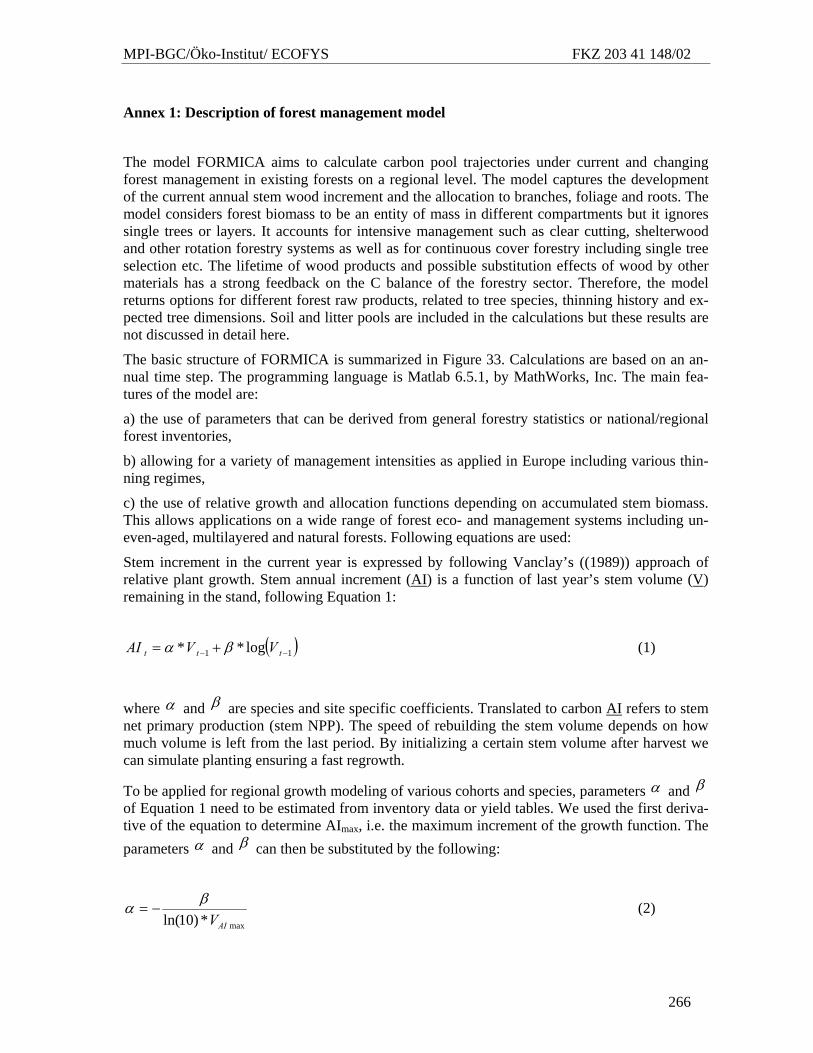
MPI-BGC/Öko-Institut/ ECOFYS FKZ 203 41 148/02
266
Annex 1: Description of forest management model
The model FORMICA aims to calculate carbon pool trajectories under current and changing forest management in existing forests on a regional level. The model captures the development of the current annual stem wood increment and the allocation to branches, foliage and roots. The model considers forest biomass to be an entity of mass in different compartments but it ignores single trees or layers. It accounts for intensive management such as clear cutting, shelterwood and other rotation forestry systems as well as for continuous cover forestry including single tree selection etc. The lifetime of wood products and possible substitution effects of wood by other materials has a strong feedback on the C balance of the forestry sector. Therefore, the model returns options for different forest raw products, related to tree species, thinning history and ex-pected tree dimensions. Soil and litter pools are included in the calculations but these results are not discussed in detail here.
The basic structure of FORMICA is summarized in Figure 33. Calculations are based on an an-nual time step. The programming language is Matlab 6.5.1, by MathWorks, Inc. The main fea-tures of the model are:
a) the use of parameters that can be derived from general forestry statistics or national/regional forest inventories,
b) allowing for a variety of management intensities as applied in Europe including various thin-ning regimes,
c) the use of relative growth and allocation functions depending on accumulated stem biomass. This allows applications on a wide range of forest eco- and management systems including un-even-aged, multilayered and natural forests. Following equations are used:
Stem increment in the current year is expressed by following Vanclay’s ((1989)) approach of relative plant growth. Stem annual increment (AI) is a function of last year’s stem volume (V) remaining in the stand, following Equation 1:
( )11 log** −− += ttt VVAI βα (1)
where α and β are species and site specific coefficients. Translated to carbon AI refers to stem net primary production (stem NPP). The speed of rebuilding the stem volume depends on how much volume is left from the last period. By initializing a certain stem volume after harvest we can simulate planting ensuring a fast regrowth.
To be applied for regional growth modeling of various cohorts and species, parameters α and β of Equation 1 need to be estimated from inventory data or yield tables. We used the first deriva-tive of the equation to determine AImax, i.e. the maximum increment of the growth function. The parameters α and β can then be substituted by the following:
max*)10ln( AIVβα −= (2)
MPI-BGC/Öko-Institut/ ECOFYS FKZ 203 41 148/02
267
)(10log*)10ln(1
1
maxmax
AIVAI
+−
=β (3)
where VAI max is the volume at AImax. The growth function (Equation 1) can by this means be parameterized more conveniently through determining the maximum increment during lifetime of a cohort and the volume at which this occurs, both site and species specific parameters.
To estimate growth of compartments other than stem (foliage, branches and roots) FORMICA uses generic biomass functions and expansion factors (Equations 4 – 8). We used equations by Wirth et al. ((2004)) for spruce (Picea abies) to calculate biomass B of each compartment i:
SV
i eEF *10
2* βββ −+= (4)
Sii BEFB *= (5)
where EF is the expansion factor of a compartment, 0β , 1β and 2β are compartment specific coefficients and BS stem biomass. For pine (Pinus sylvestris) we use the biomass functions of Lehtonen et al. ((1993)) based on biometric measurements from Swedish forests:
10 * ββ
Si VeB = (6)
0β and 1β are compartment specific coefficients and VS stem volume. Allocation of deciduous trees (here beech and oak) for foliage (index F) and roots (index R) is taken from a global analy-sis by Enquist and Niklas ((2002)):
( ) ( ) 10 *loglog ββ SF BB += (7)
( ) ( ) 10 /loglog ββ SR BB +−= (8)
where 0β and 1β are compartment specific coefficients.
Four different mortality components are included in the model. To estimate losses through natu-ral mortality due to aging (AM) of each plant compartment i we use a simple turnover rate, inde-pendent from forest age:
ii BAM *γ= (9)
where γ is a compartment and species specific turnover rate and B the accumulated biomass of a compartment i. The algorithm is applied to estimate branch, foliage and root mortality sepa-rately. Interpreted as the average mortality of a certain disturbance regime a ‘turnover’ factor of
MPI-BGC/Öko-Institut/ ECOFYS FKZ 203 41 148/02
268
tree individuals could be applied to stem volume as well to simulate losses through frequent regular fires, recurrent insect damage etc.
To account for losses due to increasing vegetation density we consider an approach including an ecosystem specific maximum biomass (BSmax). Density mortality (DM) is a fraction of stem in-crement (AIS) relative to how close the actual stem biomass (BS) of the system is to the maxi-mum value (Equation 10):
SSSS AIBBDM *)/( max= (10)
Density Mortality is suppressed if stem biomass has been already reduced through human activi-ties, e.g. thinning:
( )SSS
arThinningYe
arThinningYeSSS AIBB
TBB
DM *)/(* max
−= (11)
where TThinningYear is the volume removed during and BSThinningYear the amount of stem biomass before the last thinning. The fraction lost to density mortality of the remaining compartments is DMS/BS.
A third type of mortality is related to management (MM) and describes losses additional to har-vest. These include carbon losses by injured and dying trees after intensive logging are calcu-lated by the approach presented in Masera et al. ((2003)).
Forest stands face a risk to various hazards like storms, insects and fire. Kouba ((2002)) used the following form of the Weibull function to calculate a survival rate R dependent on stand age a:
( ) ( ) αλ aeaFaR *1 −=−= (12)
where α and λ are coefficients to be estimated. In the case study we accounted for risk mortal-ity through wind throw in spruce stands. We assume that wind throw mortality occurs in spruce stands above age 70 only where this type of disturbance is most likely and most pronounced. We used estimates for alpha α and λ from Kouba ((2002), α = 4.2002; λ = 3.5E-10) for spruce and introduced an asymptotic elimination rate c to avoid R to become zero:
( ) ( ) αλ aeccaR **1 −+−= (13)
Forest mortality due to wind (RM) is the compartment biomass in the year a multiplied by R. The litter fall of one year compartment i is the sum of every source contributing to the litter:
∑=
++++=n
iiiiii SRMDMAMMMLF
1 (14)
MPI-BGC/Öko-Institut/ ECOFYS FKZ 203 41 148/02
269
where MM, AM, DM and RM are litter inputs from management, natural, density and risk mor-tality and S (slash) is residual material from harvest and thinning. Litter is transferred to the soil model YASSO ((Kaipainen, Liski et al. 2004)) which requires these litter input data besides ba-sic information on climate and litter quality information. YASSO consists of five decomposition compartments and two litter compartments. The rates of decomposition and invasion of woody litter by microbes are controlled by temperature and summer drought. The model is applicable to different ecosystems and climate conditions ((Kaipainen, Liski et al. 2004)).
To estimate a regional C budget FORMICA calculates first the carbon pool trajectories on plot scale level. Those are computed for different strata, i.e. a combination matrix of age/biomass classes, management options, species and production levels. The total biomass of all compart-ments within a stratum k remaining after one period is then calculated as:
( )∑=
−−−−−−=n
iiiiiiiik RMDMAMMMHTAIB
1 (15)
where T and H are losses to thinning and harvest, respectively. In a second step the model aggre-gates plot scale calculations of fluxes and stocks to the regional C budget accounting for the ac-tual uneven distribution of species, age classes and management regimes through different strata. The total amount of biomass of a compartment of a region is estimated as:
∑=
=n
kkkgion AreaBB
1Re * (16)
where k represents one stratum and Area the area related to a certain stratum.

MPI-BGC/Öko-Institut/ ECOFYS FKZ 203 41 148/02
270

MPI-BGC/Öko-Institut/ ECOFYS FKZ 203 41 148/02
271
Annex 2: Country-specific results of quantitative analyses
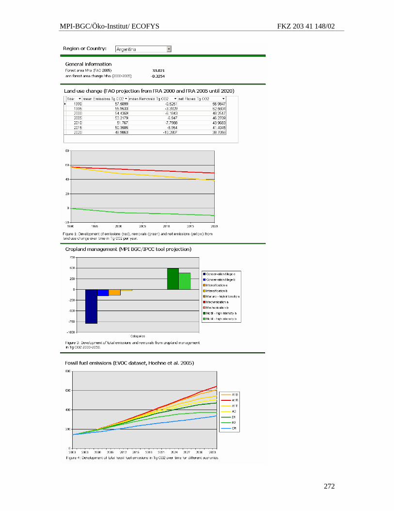
MPI-BGC/Öko-Institut/ ECOFYS FKZ 203 41 148/02
272
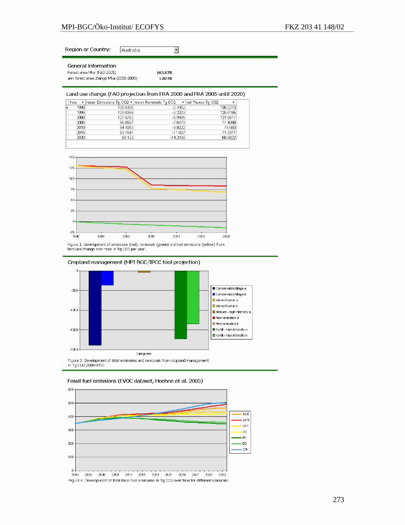
MPI-BGC/Öko-Institut/ ECOFYS FKZ 203 41 148/02
273
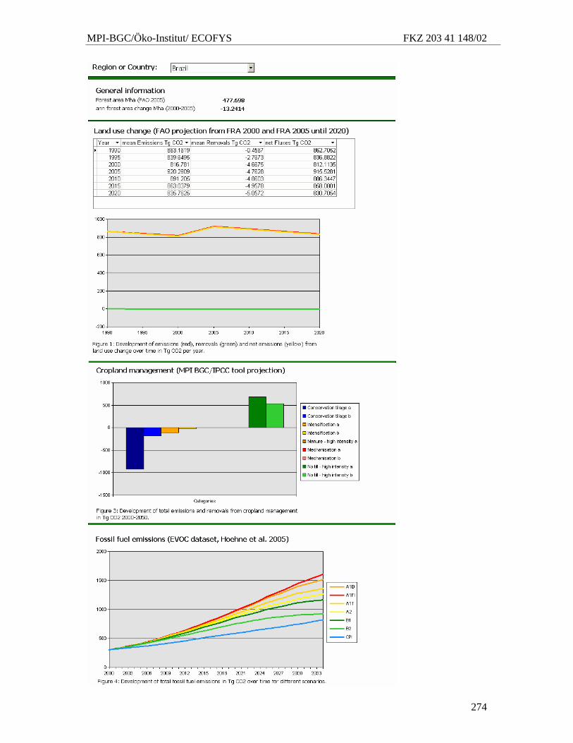
MPI-BGC/Öko-Institut/ ECOFYS FKZ 203 41 148/02
274
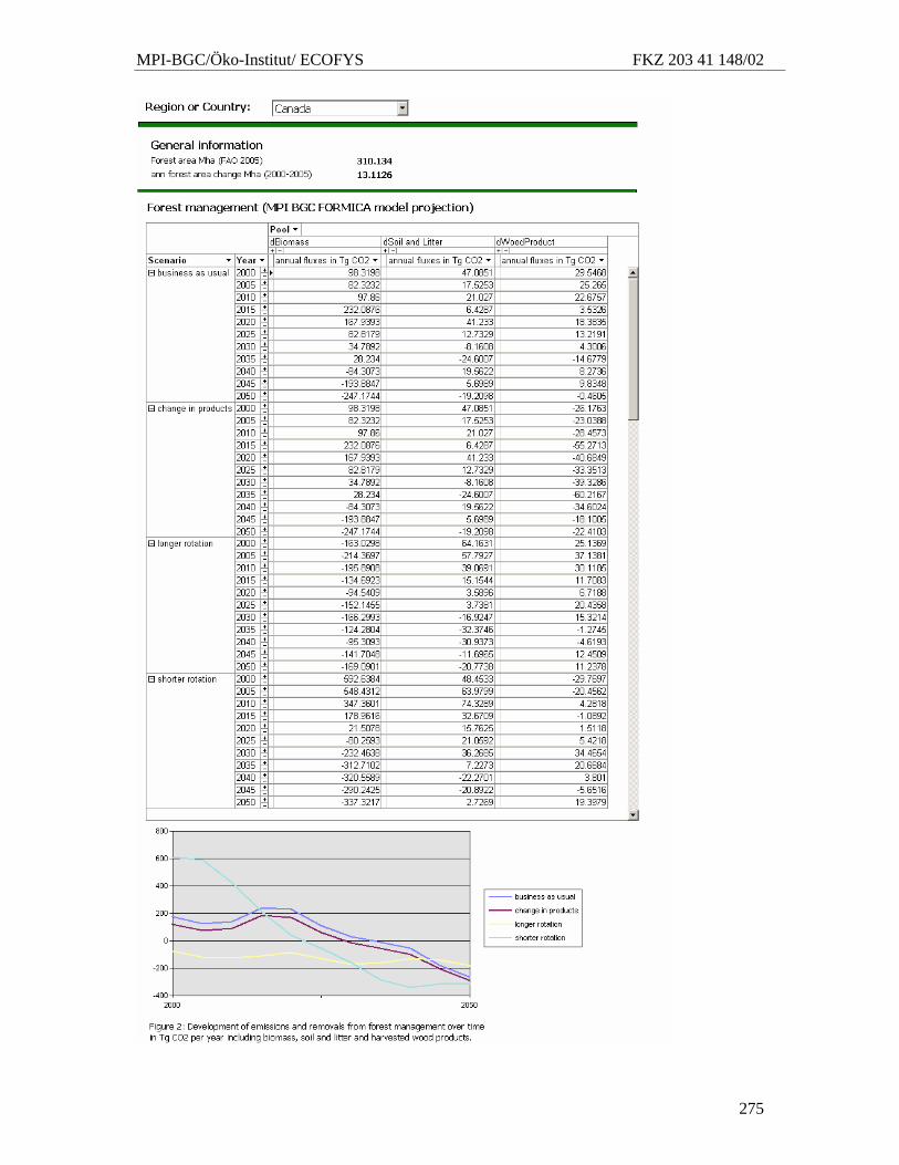
MPI-BGC/Öko-Institut/ ECOFYS FKZ 203 41 148/02
275
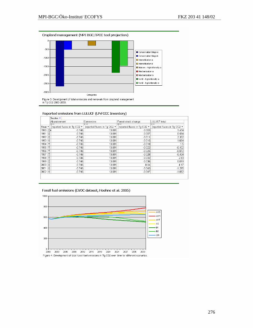
MPI-BGC/Öko-Institut/ ECOFYS FKZ 203 41 148/02
276
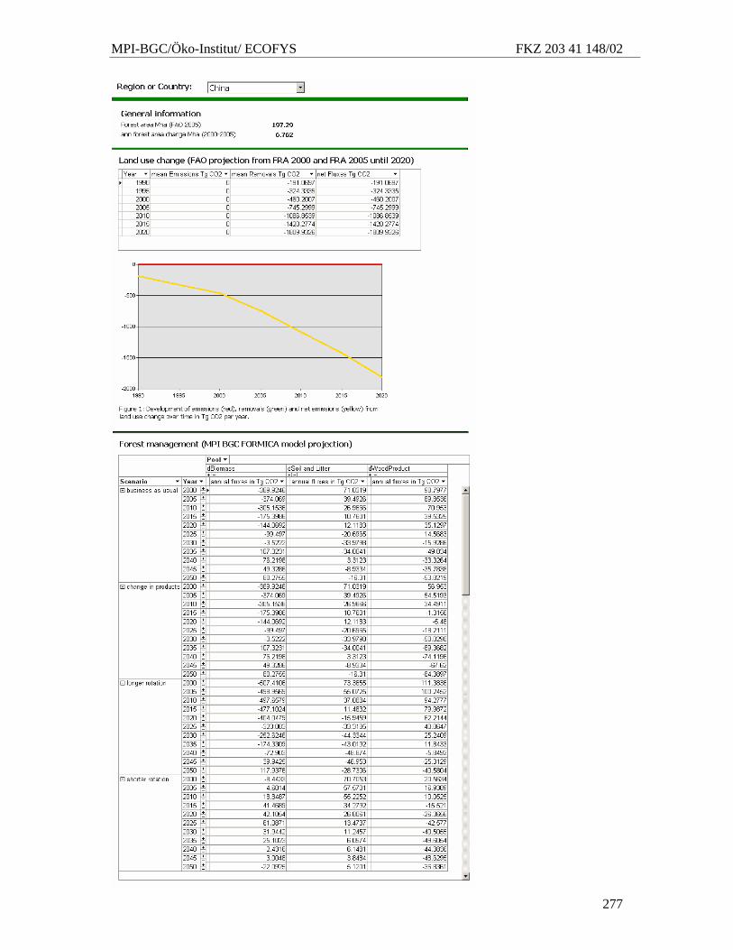
MPI-BGC/Öko-Institut/ ECOFYS FKZ 203 41 148/02
277
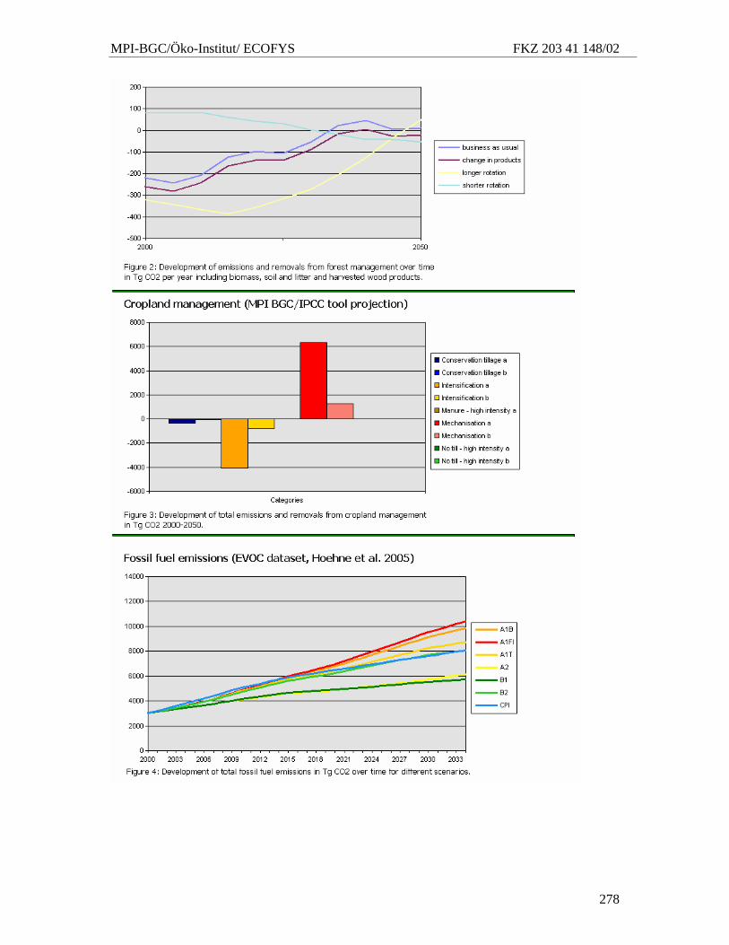
MPI-BGC/Öko-Institut/ ECOFYS FKZ 203 41 148/02
278
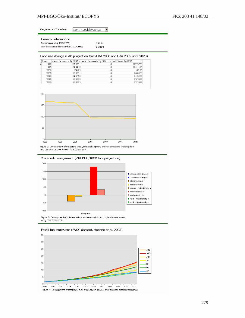
MPI-BGC/Öko-Institut/ ECOFYS FKZ 203 41 148/02
279
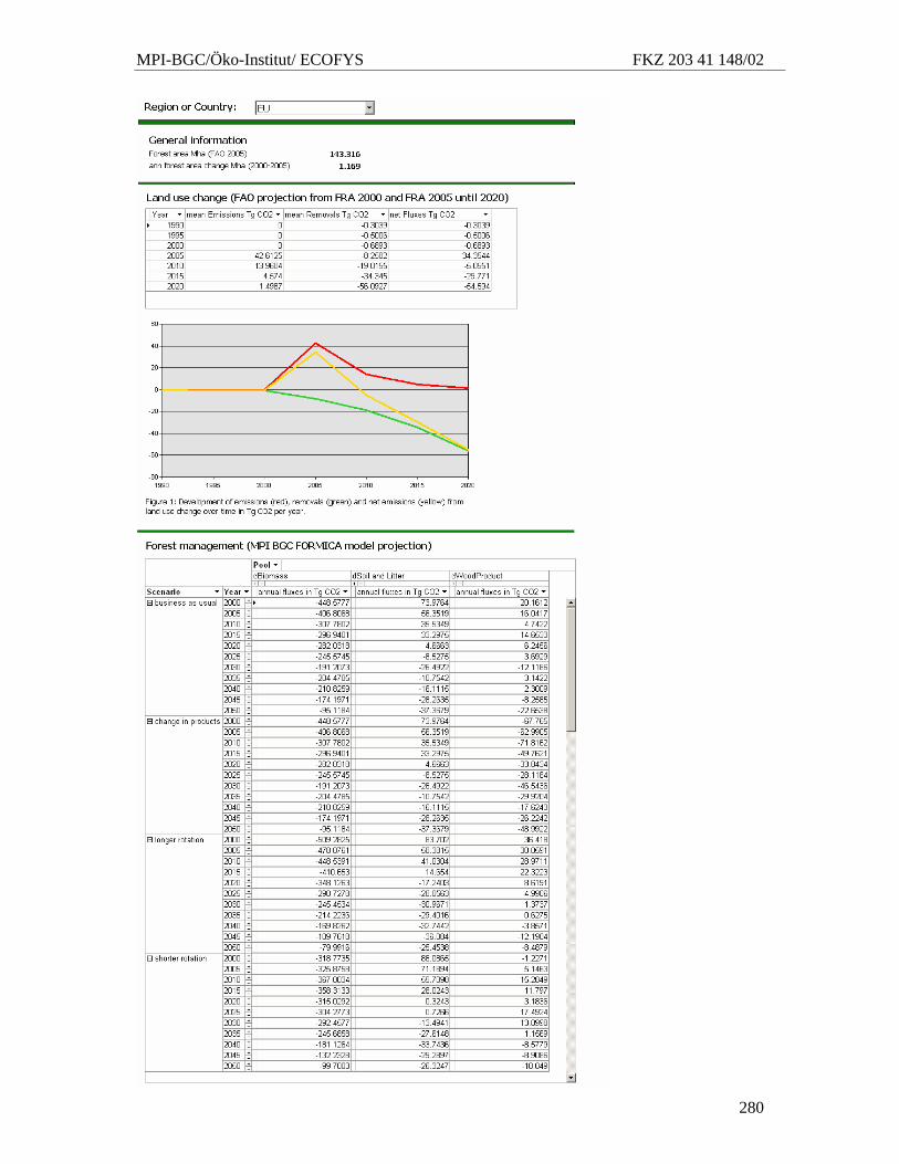
MPI-BGC/Öko-Institut/ ECOFYS FKZ 203 41 148/02
280
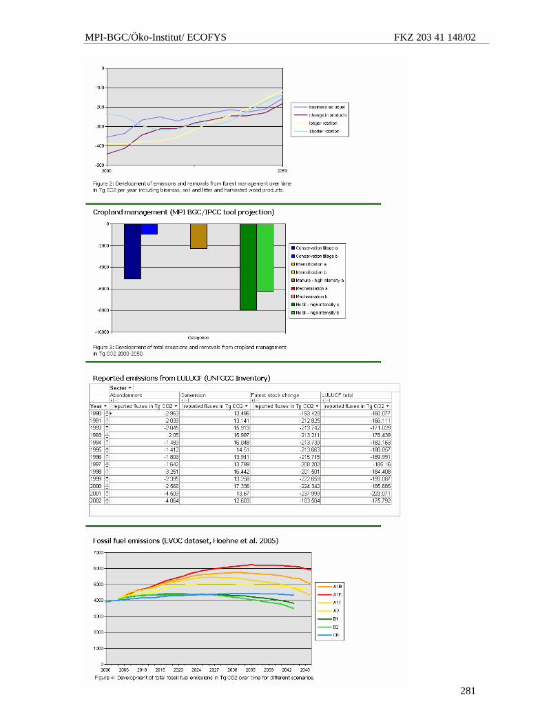
MPI-BGC/Öko-Institut/ ECOFYS FKZ 203 41 148/02
281
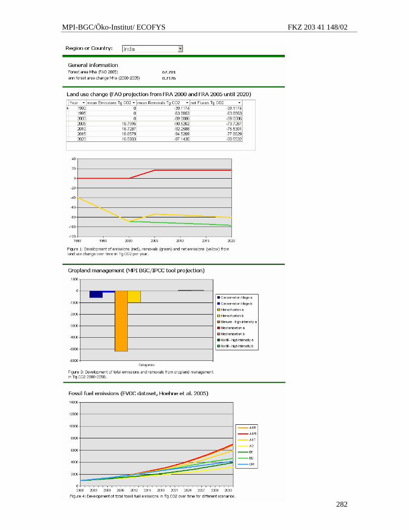
MPI-BGC/Öko-Institut/ ECOFYS FKZ 203 41 148/02
282
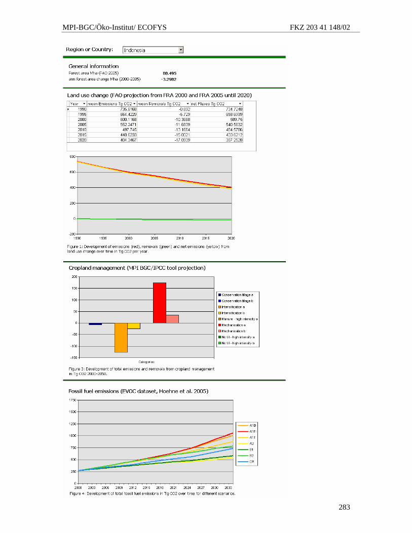
MPI-BGC/Öko-Institut/ ECOFYS FKZ 203 41 148/02
283
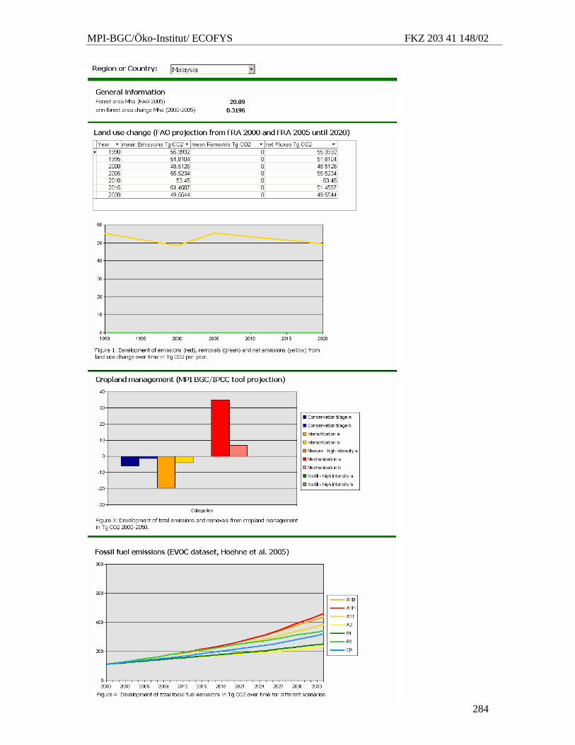
MPI-BGC/Öko-Institut/ ECOFYS FKZ 203 41 148/02
284
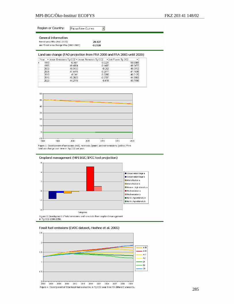
MPI-BGC/Öko-Institut/ ECOFYS FKZ 203 41 148/02
285
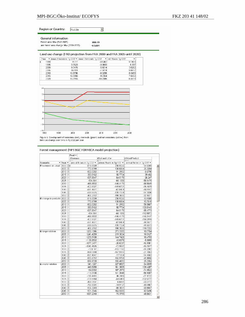
MPI-BGC/Öko-Institut/ ECOFYS FKZ 203 41 148/02
286
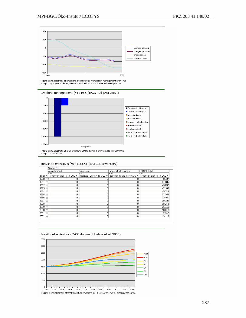
MPI-BGC/Öko-Institut/ ECOFYS FKZ 203 41 148/02
287
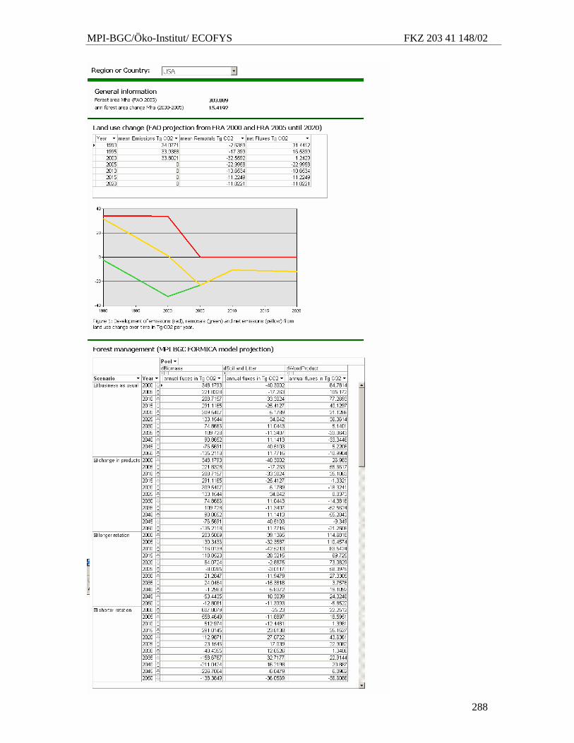
MPI-BGC/Öko-Institut/ ECOFYS FKZ 203 41 148/02
288
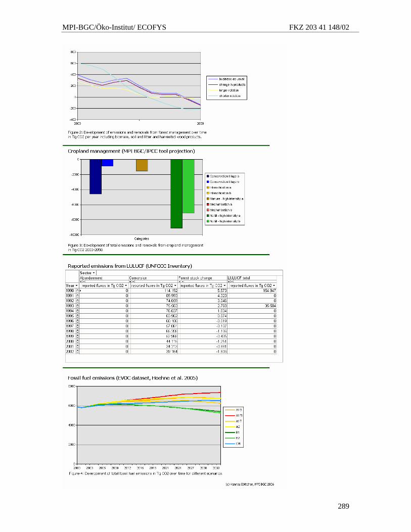
MPI-BGC/Öko-Institut/ ECOFYS FKZ 203 41 148/02
289


