Atmos. Chem. Phys., 11, 6311–6323, 2011www.atmos-chem-phys.net/11/6311/2011/doi:10.5194/acp-11-6311-2011© Author(s) 2011. CC Attribution 3.0 License.

AtmosphericChemistry

and Physics

Climatology and trends in the forcing of the stratosphericozone transport

E. Monier1 and B. C. Weare2

1Joint Program on the Science and Policy of Global Change, Massachusetts Institute of Technology, Cambridge,Massachusetts, USA2Atmospheric Science Program, Department of Land, Air and Water Resources, University of California, Davis, Davis,California, USA

Received: 29 November 2010 – Published in Atmos. Chem. Phys. Discuss.: 1 February 2011Revised: 1 June 2011 – Accepted: 20 June 2011 – Published: 4 July 2011

Abstract. A thorough analysis of the ozone transport wascarried out using the Transformed-Mean Eulerian (TEM)tracer continuity equation and the European Centre forMedium-Range Weather Forecasts (ECMWF) Re-Analysis(ERA-40). In this budget analysis, the chemical net produc-tion term, which is calculated as the residual of the otherterms, displays the correct features of a chemical sink andsource term, including location and seasonality, and showsgood agreement in magnitude compared to other methods ofcalculating ozone loss rates. This study provides further in-sight into the role of the eddy ozone transport and underlinesits fundamental role in the recovery of the ozone hole duringspring. The trend analysis reveals that the ozone hole intensi-fication over the 1980–2001 period is not solely related to thetrend in chemical losses, but more specifically to the balancebetween the trends in chemical losses and ozone transport.That is because, in the Southern Hemisphere from Octoberto December, the large increase in the chemical destructionof ozone is balanced by an equally large trend in the eddytransport, associated with a small increase in the mean trans-port. This study shows that the increase in the eddy transportis characterized by more poleward ozone eddy flux by tran-sient waves in the midlatitudes and by stationary waves in thepolar region. Overall, this study makes clearer the close in-teraction between the trends in ozone chemistry and ozonetransport. It reveals that the eddy ozone transport and itslong-term changes are an important natural mitigation mech-anism for the ozone hole. This work also underlines the needfor diagnostics of the eddy transport in chemical transportmodels used to investigate future ozone recovery.

Correspondence to:E. Monier(emonier@mit.edu)

1 Introduction

In the 1920s, chlorofluorocarbons (CFC) started replacingmore toxic compounds like ammonia, chloromethane or sul-fur dioxide as refrigerants as well as propellants in aerosolcans, fire extinguishers or cleaning solvents. In 1974, CFCswere identified as the major source of ozone-destroyingstratospheric chlorine (Molina and Rowland, 1974), a chem-ical element that was shown could engage in a catalytic cy-cle resulting in ozone destruction (Stolarski and Cicerone,1974). Since then, countless observational studies have re-ported that the total column ozone has decreased over manyregions of the globe since about 1980, with particularly se-vere ozone depletion over the Antarctica in the spring, lead-ing to what is now referred to as the ozone hole. Over Antarc-tica, extreme low temperatures during winter and early springfacilitate the formation of polar stratospheric clouds (PSCs),which support chemical reactions that produce active chlo-rine, which goes on to catalyze ozone destruction. The adop-tion of the Montreal Protocol 1987, banning the productionof CFCs and other ozone depleting chemicals, has made theozone hole a scientific success story and was called the mostsuccessful international environmental agreement.

However,Molina and Rowland(1974) andRowland andMolina (1975) pointed out that CFCs have very long atmo-spheric residence times and they would continue to depletethe stratospheric ozone well into the twenty-first century.While there has been clear evidence of a recovery since thelate 1990s, this fact was well illustrated by recent observa-tions of the 2006 ozone hole, the largest to date. As a result,the study of the ozone depletion is still drawing a large inter-est, especially since scientists are starting to acknowledge theimpact of climate change on the stratosphere. In the recentpast, many observational and modeling studies have focused

Published by Copernicus Publications on behalf of the European Geosciences Union.

6312 E. Monier and B. C. Weare: Trends in forcing of stratospheric ozone transport

on ozone variability and trend (Brunner et al., 2006; Gar-cia et al., 2007; Randel and Wu, 2007; Fischer et al., 2008;Jiang et al., 2008a,b). They all take advantage of the increas-ing high quality and diversity of models and observationaldatasets. The onset of comprehensive ozone and meteoro-logical re-analysis allowed for a better analysis of the dynam-ics of the ozone transport in the stratosphere. WhileSabutis(1997) restricted his analysis of the mean and eddy transportof ozone to the period 15 January 1979 to 10 February 1979,many subsequent studies of the dynamics of the stratosphericozone transport were extended to larger datasets (Corderoand Kawa, 2001; Gabriel and Schmitz, 2003; Miyazaki andIwasaki, 2005; Miyazaki et al., 2005). A large effort hasalso been devoted to the estimation of chemical ozone lossrates from observations using various techniques such as theMatch technique (Becker et al., 1998; Sasano et al., 2000),ozone-tracer correlations (Richard et al., 2001), Lagrangiantransport models (Manney et al., 2003) or chemical trans-port model passive substraction (Feng et al., 2005a,b; Sin-gleton et al., 2005, 2007). However, there is still a great dealof uncertainty in the accurate measurement of ozone chem-ical rate loss over large periods of time. Other areas of re-search include modeling studies to investigate the impact ofclimate change on ozone (Jiang et al., 2007). The recoveryof ozone during the 21st century (Oman et al., 2010; Eyringet al., 2010) points out the need to separate dynamical andchemical contributions to long-term ozone changes in orderto evaluate the influences of changing CFC amounts and theimpacts of climate change. Other more theoretical studiesinvolve examining the impact of the wave- and zonal mean-ozone feedback on the stratospheric dynamics, includingthe quasi-biennial oscillation (QBO) (Cordero et al., 1998;Cordero and Nathan, 2000) and the vertical propagation ofplanetary waves (Nathan and Cordero, 2007). Overall, thereseems to be a lack of thorough analysis of the impact ofwave-induced transport on the long-term changes in strato-spheric ozone based on meteorologically consistent three-dimensional ozone datasets.

Thus the aim of this study is to investigate the role of thevarious dynamical forcings on the transport of zonal-meanozone and its long-term changes, using a thorough budgetanalysis of the Transformed-Mean Eulerian (TEM) formu-lation of the tracer continuity equation with the EuropeanCentre for Medium-Range Weather Forecasts (ECMWF) Re-Analysis (ERA-40). The TEM formulation offers a useful di-agnostic to interpret the forcing of the ozone transport by ed-dies (Andrews et al., 1983). This work intends on providinga more comprehensive understanding of the contribution ofplanetary waves, their stationary and transient components,to the transport of ozone. Such analysis is vital as the im-pact of long-term changes in ozone and wave activity on thedynamics of the stratosphere is not yet fully understood.

2 Data and methodology

2.1 Data

In this study we use the six-hourly ERA-40 re-analysis (Up-pala et al., 2005) in order to calculate the various terms in-volved in the Transformed Eulerian-Mean formulation of theozone transport equation. These terms include flux quanti-ties like the eddy flux vector and the residual mean merid-ional circulation. The ERA-40 was chosen because it pro-vides a complete set of meteorological and ozone data, overthe whole globe on a 2.5◦×2.5◦grid and over a long timeperiod (1957–2001). The ERA-40 compares well with in-dependent ground-based Dobson observations, MicrowaveLimb Sounder (MLS) satellite and ozonesonde data, both intotal ozone and in ozone profiles (Dethof and H́olm, 2004).The ERA-40 ozone field has also been compared with Up-per Atmosphere Research Satellite (UARS) and Measure-ments of Ozone and Water Vapour by Airbus In-Service Air-craft (MOZAIC) measurements, showing broad agreement(Oikonomou and O’Neill, 2006). The ERA-40 shows sev-eral weaknesses, such as an enhanced Brewer-Dobson (B-D)circulation (van Noije et al., 2004; Uppala et al., 2005) and aweaker Antarctic ozone hole of less vertical extent than theindependent observations (Oikonomou and O’Neill, 2006).There is also the presence of vertically oscillating strato-spheric temperature biases over the Arctic since 1998 andover the Antarctic during the whole period (Randel et al.,2004). In addition, the pre-satellite ERA-40 data in theSouthern Hemisphere (SH) stratosphere are unrealistic (Ren-wick, 2004; Karpetchko et al., 2005). Nonetheless, the ERA-40 re-analysis provides a reasonable ozone and meteorolog-ical dataset in the lower stratosphere during the satellite era.For this reason, the climatological analysis of the wave forc-ing of the stratospheric ozone transport is performed over the1980 to 2001 period and for pressure levels up to 10 hPa.

2.2 Methodology

2.2.1 Transformed Eulerian-Mean formulation

This study uses the Transformed Eulerian-Mean (TEM) for-mulation of the zonal-mean tracer continuity equation inlog-pressure and spherical coordinates in order to accu-rately diagnose the eddy forcing of the zonal-mean trans-port of stratospheric ozone. In spherical geometry, the TEMzonal-mean ozone tracer continuity equation is (based onEq. 3.72 fromBrasseur and Solomon, 2005and onGarciaand Solomon, 1983):

Atmos. Chem. Phys., 11, 6311–6323, 2011 www.atmos-chem-phys.net/11/6311/2011/

E. Monier and B. C. Weare: Trends in forcing of stratospheric ozone transport 6313

∂χ

∂t︸︷︷︸Ozone tendency

= −v?

R

∂χ

∂φ−w? ∂χ

∂z︸ ︷︷ ︸Mean ozone transport

−1

ρ0∇ ·M︸ ︷︷ ︸

Eddy ozone transport

+ S︸︷︷︸Chemical term

(1)

In Eq. (1) and in the following equations,χ is the ozone vol-ume mixing ratio andv?, w? are, respectively, the horizontaland vertical components of the residual mean meridional cir-culation defined by (Eqs. 3.5.1a and 3.5.1b fromAndrewset al., 1987):

v?= v−

1

ρ0

∂

∂z

(ρ0

v′θ ′

θz

)(2)

w?= w+

1

acosφ

∂

∂φ

(cosφ

v′θ ′

θz

)(3)

where the overbars and primes indicate respectively the zonalmeans and departures from the zonal mean.θ is the potentialtemperature,v is the meridional wind andw is the verticalwind. ∇ ·M is the divergence of the eddy flux vector andrepresents the eddy transport of ozone. The components ofthe eddy flux vectorM are defined by (based onGarcia andSolomon, 1983):

M(φ)= ρ0

(v′χ ′ −

v′θ ′

θz

∂χ

∂z

)(4)

M(z)= ρ0

(w′χ ′ +

1

a

v′θ ′

θz

∂χ

∂φ

)(5)

Following that sign convention, the eddy flux vector repre-sents the mass flux of ozone eddies by the wave componentsof the wind velocities. Finally,S is the chemical net pro-duction term, which is calculated as the residual of the otherterms.

Dunkerton(1978) showed that the B-D circulation shouldbe interpreted as a Lagrangian mean circulation and could beapproximated by the residual mean meridional circulation ofthe TEM equations. Thus the various processes influencingthe evolution of the zonal-mean ozone that are investigated inthis study are separated into three categories: the advectionof ozone by the B-D circulation or mean ozone transport, thelarge-scale eddy transport, diagnosed by the divergence ofthe eddy flux vector, and the chemical net production term.The signs shown in Eq. (1) are included in the various dis-played terms. Each term is calculated using the six-hourlyERA-40 dataset. In addition, this formulation only allows forthe calculation of the resolved eddies (dominated by plane-tary waves) and we do not attempt to parameterize the eddy

flux divergence due to small-scale disturbances, such as grav-ity waves, using diffusion coefficients as described inGarciaand Solomon(1983) due to a lack of observations to evaluatesuch coefficients. Therefore, any contribution from the grav-ity waves to the eddy flux divergence would be included inthe residual term. For this reason, the residual term can onlybe an approximation of the net chemical production term. Fi-nally, all derivatives are computed using centered finite dif-ferences.

2.2.2 Stationary and transient components

Because both mean and eddy ozone transport are primarilydriven by planetary waves, whether directly or indirectly, itis useful to decompose the ozone transport forcing into con-tributions from stationary and transient waves. Stationaryplanetary waves are excited by the orography (Charney andEliassen, 1949), especially in the NH, as well as by land-sea heating contrasts, which vary on the seasonal time scale.Planetary transient waves, on the other hand, have smallertime scales ranging from a few days to a couple weeks anddominate synoptic weather patterns. The stationary com-ponents are computed by averaging temperature, wind andozone fields over a month and then calculating the variousterms of the TEM formulation. Once the stationary compo-nent is removed from the total term, which is calculated ev-ery six hours, only the contribution from the transient wavesis left (Madden and Labitzke, 1981).

3 Climatology of the stratospheric zonal-mean ozonetransport

3.1 Seasonal cycle of the ozone transport budget

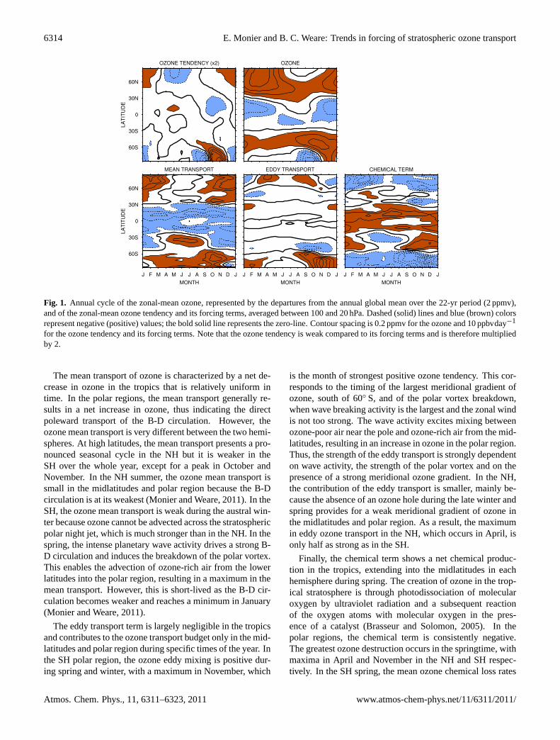
Using Eq. (1), we can separate the changes in ozone into con-tributions from the mean transport, the eddy transport andthe chemical net production. Figure1 shows the seasonalcycle of the zonal-mean ozone tendency, its forcing termsand the ozone mixing ratio averaged between 100 and 20 hPa(the layer where the largest concentrations of stratosphericozone are found). The zonal-mean ozone mixing ratio has itslargest values in the Northern Hemisphere high latitudes dur-ing spring with a minimum in late summer and early fall. Thelowest quantities of ozone are found in the Southern Hemi-sphere polar region during the austral late summer and earlyspring and are associated with the ozone hole. The ozonetendency shows that the largest changes in ozone occur in thepolar regions. In the Northern Hemisphere, there is a clearseasonal cycle in the ozone tendency with a distinct increasein ozone at high latitudes during the fall and winter and a de-crease in the spring and early summer. The ozone tendencyshows the complex development and decay of the SH ozonehole with a rapid decrease in July, August and September.This is followed by a strong increase in October and Novem-ber and a weaker decrease in December and January.

www.atmos-chem-phys.net/11/6311/2011/ Atmos. Chem. Phys., 11, 6311–6323, 2011

6314 E. Monier and B. C. Weare: Trends in forcing of stratospheric ozone transport

Fig. 1. Annual cycle of the zonal-mean ozone, represented by the departures from the annual global mean over the 22-yr period (2 ppmv),and of the zonal-mean ozone tendency and its forcing terms, averaged between 100 and 20 hPa. Dashed (solid) lines and blue (brown) colorsrepresent negative (positive) values; the bold solid line represents the zero-line. Contour spacing is 0.2 ppmv for the ozone and 10 ppbvday−1

for the ozone tendency and its forcing terms. Note that the ozone tendency is weak compared to its forcing terms and is therefore multipliedby 2.

The mean transport of ozone is characterized by a net de-crease in ozone in the tropics that is relatively uniform intime. In the polar regions, the mean transport generally re-sults in a net increase in ozone, thus indicating the directpoleward transport of the B-D circulation. However, theozone mean transport is very different between the two hemi-spheres. At high latitudes, the mean transport presents a pro-nounced seasonal cycle in the NH but it is weaker in theSH over the whole year, except for a peak in October andNovember. In the NH summer, the ozone mean transport issmall in the midlatitudes and polar region because the B-Dcirculation is at its weakest (Monier and Weare, 2011). In theSH, the ozone mean transport is weak during the austral win-ter because ozone cannot be advected across the stratosphericpolar night jet, which is much stronger than in the NH. In thespring, the intense planetary wave activity drives a strong B-D circulation and induces the breakdown of the polar vortex.This enables the advection of ozone-rich air from the lowerlatitudes into the polar region, resulting in a maximum in themean transport. However, this is short-lived as the B-D cir-culation becomes weaker and reaches a minimum in January(Monier and Weare, 2011).

The eddy transport term is largely negligible in the tropicsand contributes to the ozone transport budget only in the mid-latitudes and polar region during specific times of the year. Inthe SH polar region, the ozone eddy mixing is positive dur-ing spring and winter, with a maximum in November, which

is the month of strongest positive ozone tendency. This cor-responds to the timing of the largest meridional gradient ofozone, south of 60◦ S, and of the polar vortex breakdown,when wave breaking activity is the largest and the zonal windis not too strong. The wave activity excites mixing betweenozone-poor air near the pole and ozone-rich air from the mid-latitudes, resulting in an increase in ozone in the polar region.Thus, the strength of the eddy transport is strongly dependenton wave activity, the strength of the polar vortex and on thepresence of a strong meridional ozone gradient. In the NH,the contribution of the eddy transport is smaller, mainly be-cause the absence of an ozone hole during the late winter andspring provides for a weak meridional gradient of ozone inthe midlatitudes and polar region. As a result, the maximumin eddy ozone transport in the NH, which occurs in April, isonly half as strong as in the SH.

Finally, the chemical term shows a net chemical produc-tion in the tropics, extending into the midlatitudes in eachhemisphere during spring. The creation of ozone in the trop-ical stratosphere is through photodissociation of molecularoxygen by ultraviolet radiation and a subsequent reactionof the oxygen atoms with molecular oxygen in the pres-ence of a catalyst (Brasseur and Solomon, 2005). In thepolar regions, the chemical term is consistently negative.The greatest ozone destruction occurs in the springtime, withmaxima in April and November in the NH and SH respec-tively. In the SH spring, the mean ozone chemical loss rates

Atmos. Chem. Phys., 11, 6311–6323, 2011 www.atmos-chem-phys.net/11/6311/2011/

E. Monier and B. C. Weare: Trends in forcing of stratospheric ozone transport 6315

Fig. 2. Zonal-mean ozone tendency and its forcing terms averaged over DJF 1980–2001 in the SH. Dashed (solid) lines and blue (brown)colors represent negative (positive) values; the bold solid line represents the zero-line. Contour spacing is 10 ppbvday−1. Note that the ozonetendency is weak compared to its forcing terms and is therefore multiplied by 2.

of the 100–20 hPa layer can reach up to 60 ppbvday−1 (or∼2.5 DUday−1). This is about one and a half time more thanits counterpart in the NH spring. These results are consis-tent with previous studies. For example, chemical loss ratesof ozone lower-stratosphere partial column (350 to 660 Kor about 200 to 25 hPa) in the Antarctic polar region canrange from 1.5 to 2.5 DUday−1 in September 2000 and 2002(Feng et al., 2005b). In the NH polar region, these ratesrange between 0.5 and 1.2 DUday−1 for February and March2000, 2003 and 2004 (Feng et al., 2005a). Similarly, Sasanoet al. (2000) show chemical loss rates inside the Arctic po-lar vortex around 40 ppbvday−1 from 400 to 550 K (∼150to ∼50 hPa) in March 1997. This is consistent with thechemical loss rates inside the Arctic polar vortex of around40 ppbvday−1 at 450 K (∼100 hPa) in late February earlyMarch 2000 fromRichard et al.(2001).

Overall, Fig.1 shows that the ozone distribution resultsfrom a complex interaction between the ozone chemistry anddynamics. The ozone budget is largely driven by the bal-ance between two large terms, the mean ozone transport andthe chemical term, with the eddy transport playing mainly asecondary role except during specific times of the year. Thestrong poleward advection of ozone by the B-D circulation inthe NH fall and winter is responsible for the positive ozonetendency at high latitudes. On the other hand, the weak meanozone transport in the SH wintertime along with the chemicaldestruction of ozone in the polar region explains the negativeozone tendency in August and September that leads to theozone hole. In addition, Fig.1 shows that eddy transport islargely responsible for the positive ozone tendency in the SHpolar region in October and November and hence contributesto the recovery of the Antarctic ozone hole in the late spring.This is consistent with the findings ofMiyazaki et al.(2005)who estimate that the eddy transport represents more than80 % of the total ozone transport (advective + eddy) in theSouthern Hemisphere polar region in November. In addition,November is the month where the Eliassen-Palm (EP) fluxdivergence shows the largest values in the region, indicatingthe most intense planetary wave activity and the break-down

of the polar vortex (Monier and Weare, 2011). Therefore,there is a self-consistency between the seasonal variability ofthe EP flux divergence and the eddy flux divergence in theSH. Finally, the main characteristics of the seasonal variabil-ity of the chemical production and destruction of ozone arereproduced. Furthermore, the chemical loss rates in both theArctic and Antarctic polar regions are in reasonable agree-ment with previous studies. This gives confidence in thecalculation of the chemical term as a residual of the ozonetransport budget. It should be noted that single year analysiscan produce substantially different behavior than the 22-yrclimatology presented in this study.

3.2 Vertical structure of the ozone transport budget

An example of the vertical structure of the various ozoneforcings, for the months of December-January-February(DJF) in the SH, is shown in Fig.2. The ozone tendencyshows a distinct maximum decrease in the polar region cen-tered at 20 hPa. The vertical structure of each forcing re-veals that they are reasonably uniform with height, eventhough the mean transport exhibits some noise polewardof 80◦ S. All the forcing terms have the largest values be-tween the 50 and 10 hPa levels. They also tend to show adipole pattern with opposite effects between the polar re-gion and the midlatitudes. The mean and eddy transportsare both positive in the polar region and oppose the chem-ical destruction. In the subtropics, where the eddy trans-port and the ozone tendency are weak, the chemical netproduction offsets the mean transport of ozone by the B-Dcirculation. The chemical term shows destruction of polarozone, with maximum values of 70 ppbvday−1 centered at20 hPa and production in the tropics all the way to 50◦ S,with maximum values of 40 ppbvday−1 centered between30 and 20 hPa. The distribution of the chemical term isin good agreement with the chemical transport model usedin (Miyazaki and Iwasaki, 2005). Additionally, (Miyazakiand Iwasaki, 2005) find chemical loss rates for DJF of upto 7.5×1010cm−3day−1 (about 80 ppbvday−1) centered at

www.atmos-chem-phys.net/11/6311/2011/ Atmos. Chem. Phys., 11, 6311–6323, 2011

6316 E. Monier and B. C. Weare: Trends in forcing of stratospheric ozone transport

Fig. 3. Ozone density weighted Brewer-Dobson stream function av-eraged over (left) DJF and (right) JJA 1980–2001. Dashed (solid)lines and blue (brown) colors represent negative (positive) values;the bold solid line represents the zero-line. Contour spacing is103kgs−1.

30 hPa in the polar region and chemical production ratesup to 3×1010cm−3day−1 (about 30 ppbvday−1) at the sameheight in the tropics. Thus, there is further evidence that thedistribution and the magnitude of the chemical term comparewell with previous studies using chemical models, chemi-cal transport model passive substraction and other methodsbased on observations.

3.3 Mean transport

The contributions of the horizontal and vertical transport tothe mean ozone transport can be assessed from the anal-ysis of the ozone density weighted streamfunction associ-ated with the residual mean meridional circulation shownin Fig. 3. The ozone mass stream function shows that themean ozone transport follows the transport description pro-posed by Brewer and Dobson with upward motions in thetropics and extratropical downward motions, associated withpoleward motions. The ozone mass stream function presentsa distinct seasonal cycle with maximum poleward transportin each hemisphere during their respective winter. This isconsistent with the annual cycle of the mean ozone transportterm in Fig.1 and with other similar studies (Miyazaki andIwasaki, 2005). It should be pointed out that there exists con-siderable discrepancy in the representation of the B-D circu-lation among the various reanalyses currently available, es-pecially in low latitudes (Randel et al., 2008; Iwasaki et al.,2009). So while it is valid to use the ERA-40 for the demon-stration of the method, the results might be influenced bythe biases. This is why they should eventually be comparedto results from other datasets that include meteorologicallyconsistent three-dimensional ozone data. Nonetheless, theresidual term displays the correct spatial and seasonal distri-bution of a chemical ozone sink and source term, and showsgood agreement in magnitude compared to other methods ofcalculating ozone production and loss rates. This providesreasonable evidence of the validity of the ozone budget per-formed in this study.

3.4 Eddy transport

In order to better understand the origins of the eddy trans-port term, the horizontal and vertical eddy transport termsare evaluated along with the eddy flux vector, separated intostationary and transient components. A conspicuous featurerevealed by Fig.4 is that the eddy transport is controlledby its horizontal component as the vertical eddy transport isweak over the whole hemisphere. This can be explained bythe strong influence of the eddy ozone transport on the pres-ence of a steep meridional ozone gradient. This is consis-tent with the assumption that eddy transport is dominated bymeridional mixing processes, which has been adopted in sev-eral studies (Tung, 1986; Newman et al., 1988; Gabriel andSchmitz, 2003). In addition the eddy transport is providedabout equally by stationary and transient waves with the tran-sient eddy transport dominating only slightly in the midlati-tudes. This is consistent with the findings fromMonier andWeare(2011) who look at planetary wave activity in the SHdiagnosed by the Eliassen-Palm (EP) flux divergence. Thisanalysis provides further evidence of the influence of theeddy ozone transport by the meridional ozone gradient, wavebreaking activity and the strength of the polar vortex.

The components of the eddy flux vector represent the hor-izontal and vertical flux of ozone eddies by the wave compo-nents of the wind velocities. In comparison the eddy flux di-vergence corresponds to the net ozone transport in a specificregion due to the net ozone eddy flux entering this region. Inthe SH spring the vertical eddy ozone flux is upward in themidlatitues and near the pole and downward in the subpolarregion. Meanwhile, the horizontal eddy ozone flux is com-posed of poleward transport in the polar region and equator-ward transport in the midlatitudes and subtropics. The factthat the horizontal ozone eddy flux is three orders of mag-nitude greater than its vertical counterpart explains its majorrole in the eddy transport.

The eddy ozone transport is dominated by transient pro-cesses in the midlatitudes due to high transient wave activ-ity associated with storm tracks located near 50◦ S through-out the year (Trenberth, 1991). However, the stationary eddytransport is stronger than the transient eddy transport in thepolar region. This can be explained by the presence of theasymmetric Antarctic topography and ice-sea heating con-trasts driving the stationary wave activity in the polar re-gion, as it has been demonstrated in several studies (Parishet al., 1994; Lachlan-Cope et al., 2001). This suggests thatcalculating the various flux terms using monthly data (i.e.considering only stationary processes) does not provide thefull picture since the contribution from transient processesis considerable. Furthermore, the fact that the structure ofthe climatology of both transient and stationary terms can bereasonably explained (location of storm tracks and presenceof topography and sea-ice heating contrasts) provides furtherconfidence in the analysis.

Atmos. Chem. Phys., 11, 6311–6323, 2011 www.atmos-chem-phys.net/11/6311/2011/

E. Monier and B. C. Weare: Trends in forcing of stratospheric ozone transport 6317

Fig. 4. Same as Fig.2 but for the eddy ozone transport, its horizontal and vertical components, and the eddy flux vector, with the con-tributions of stationary and transient waves. Blue (brown) colors with dashed (solid) white lines represent negative (positive) values forM(φ). Dashed (solid) black lines represent negative (positive) values while the bold solid line represents the zero-line forM(z). Con-tour spacing is 5 ppbvday−1 for the eddy transport and its horizontal and vertical components, 2×105kgppbvm−2day−1 for M(φ) and2×102kgppbvm−2day−1 for M(z). Note that the vertical eddy transport is weak compared to the horizontal eddy transport and is thereforemultiplied by 5.

4 Trends in the wave forcing of the stratosphericzonal-mean ozone transport

4.1 Trends in the zonal-mean ozone

The long-term trends and interannual variability of the lowerand middle stratosphere (LMS) ozone are investigated inFig. 5. The variances and trends are calculated over the1980–2001 period based on monthly mean ozone averagedbetween 100 and 20 hPa. The ozone variance, represent-ing its interannual variability, is large in the polar regionin both hemispheres during their respective late winter andearly spring. A weaker variance maximum is also present inthe tropics, most likely related to the Quasi-Biennial Oscil-lation (QBO). In the SH, the year-to-year variability of theLMS zonal-mean ozone layer is associated with the ozonehole and located south of 60◦ S. The maximum ozone trends

associated with the Antarctic ozone hole occur in Septemberat a rate above 0.5 ppmv per decade, with a 99.9 % statis-tical significance level (calculated using a Student’s t-test).There is also a negative ozone trend in the NH polar regionduring spring that corresponds to a decrease of the ozonemaximum that occurs at that time. In March, the NH po-lar ozone has decreased between 1980 and 2001 at a rateof over 0.2 ppmv per decade, with a 93 % statistical signif-icance level. The long-term changes in the polar ozone workout to be a decrease of∼ −10 % over 22 yr in the NH inMarch and of∼ −40 % in the SH in September. This is con-sistent withBrunner et al.(2006), using the Candidoz As-similated Three-dimensional Ozone (CATO) multiple linearregression model. They find maximum negative trends northof 60◦ N in February and March at about−5 % per decade,and a maximum trend in the SH polar region in October,close to−20 % per decade, from 1979–2004. Moreover, the

www.atmos-chem-phys.net/11/6311/2011/ Atmos. Chem. Phys., 11, 6311–6323, 2011

6318 E. Monier and B. C. Weare: Trends in forcing of stratospheric ozone transport

Fig. 5. Annual cycle of the ozone sample variance and trend.The variances and trends are calculated over the 1980–2001 periodbased on monthly mean ozone averaged between 100 and 20 hPa.Dashed blue (solid brown) lines represent negative (positive) values;the bold solid line represents the zero-line. Light grey (dark grey)shading represents the 90 % (99 %) statistical significance level ofthe trends. Contour spacing is 0.05 ppmv2 for the ozone varianceand 0.1 ppmv per decade for the ozone trend.

seasonality of the trends is consistent with previous modelingand observational studies.Randel and Wu(2007) calculatedseasonal variations of the trends in the vertically integratedozone column derived from analysis of Stratospheric Aerosoland Gas Experiment (SAGE I and II) profile measurements,combined with polar ozonesonde data. They find a maximumtrend in the polar region over the 1979 to 2005 time period inthe NH April and SH October, weaker than in this study byabout 10-20 %. This can be explained by the extended periodthey consider and the recovery of their equivalent effectivestratospheric chlorine (EESC) proxy after 2000. Meanwhile,Garcia et al.(2007) provide a similar analysis based on theWhole-Atmosphere Community Climate Model (WACCM)column of ozone. They show maximum trends in the po-lar region from 1979 to 2003 in the NH February and SHOctober. Thus there is some uncertainty as to which monthdisplays the maximum trends, but an overall agreement con-cerning the seasonality of the trends in the stratospheric polarozone.

4.2 Trends in the wave forcing of ozone transport

Figure6 shows the annual cycle of the linear trends of theozone tendency and its forcing terms. The trends are calcu-lated over the 1980–2001 period based on the monthly meansof the various terms averaged between 100 and 20 hPa andbetween 60◦–85◦. A perhaps surprising result is that chemi-cal destruction can take place and exhibit trends all year long.This may be explained by the work ofLamago et al.(2003),who find that when taking into account large solar zenithangles, ozone concentrations are significantly affected fromJune to August south of 60◦ S because of photolysis ratesof Cl2O2. In the SH, the largest trends occur from Septem-ber to December and show that negative trends in the chemi-

cal losses are largely balanced by positive trends in the eddytransport, apparently following by a month. Meanwhile, thetrends in the ozone mean transport are weaker and not statis-tically significant (except for the month of December). Thetiming of the trends in the ozone chemical destruction corre-sponds to the ozone hole, when the polar region is the cold-est due to a lack of radiative heating by ozone. When theregion is very cold, PSCs can form thus inducing even morechemical destruction. Because the strength of the eddy trans-port is strongly dependent on not only wave breaking activitybut also on the presence of a strong meridional ozone gradi-ent, the destabilization of the ozone layer over the Antarc-tica leads to an increase in the spring eddy transport. As theozone hole grows stronger year after year, so does the merid-ional ozone gradient. This leads to more mixing, near theedge of the polar vortex, between rich and poor regions ofozone. This explains why the trends in the eddy transport lagby one month the trends in the chemical term. It is worthyto note that the dip in the eddy flux divergence in Novembercoincides with a weakening of the planetary wave activity,as is revealed from the trend analysis of the EP flux diver-gence inMonier and Weare(2011). Hence, the trends inthe eddy flux divergence might be controlled not only by thevariations in the meridional ozone gradient but also by thelong-term changes in wave activity. The weakening of theplanetary wave activity can also explain the similar dip in theozone mean transport trends during the month of November,since the long-term weakening of the planetary wave activityis accompanied by a weakening of the B-D circulation.

In August, the strength of the polar night jet is at its max-imum and it acts as an eddy mixing barrier (Haynes andShuckburgh, 2000; Miyazaki et al., 2005). Additionally, themeridional gradient of ozone is weak at the time. As a re-sult, the trend in the eddy ozone transport remains weak,much weaker than between September and December. Con-sequently, the negative trend in the chemical destruction ofozone in August, which is significantly weaker than fromSeptember to November, remains unbalanced by trends in theozone transport. This leads to a significantly negative trendin the ozone tendency in August, which in turn is respon-sible for the maximum ozone trend over Antarctica that oc-curs in September. Thus the ozone hole intensification over1980–2001 time period is not directly related to the trend inchemical losses, but more specifically to the balance betweenthe trends in chemical losses and depletion influenced ozonetransport.

The balance between the trends in the ozone forcing termsresults in month-to-month changes in the trend in the ozonetendency. Figure6 shows that the only statistically signifi-cant trends in the ozone tendency are negative in May, Julyand August (leading to the intensification of the ozone hole)and positive in October and December (leading to the inten-sification of the ozone hole recovery in late spring).

In the NH, the picture is more complicated, mainly dueto the absence of strong polar ozone depletion and the

Atmos. Chem. Phys., 11, 6311–6323, 2011 www.atmos-chem-phys.net/11/6311/2011/

E. Monier and B. C. Weare: Trends in forcing of stratospheric ozone transport 6319

Fig. 6. Annual cycle of the trends in the ozone tendency and its forcing terms, for the (left) NH and the (right) SH. The trends are calculatedover the 1980–2001 period based on monthly means of the various forcing terms averaged between 100 and 20 hPa and between 60◦–85◦.Trends that are statistically significant at the 95 % statistical significance level are indicated by a cross.

Fig. 7. OND trends in the ozone tendency and its forcing terms for the SH calculated over the 1980–2001 period. Dashed blue (solid brown)lines represent negative (positive) values; the bold solid line represents the zero-line. Light grey (dark grey) shading represents the 95 %(99 %) statistical signicance level of the trends. Contour spacing is 10 ppbvday−1 per decade. Note that the trends in the ozone tendency areweak compared to the forcings terms and are therefore multiplied by 4.

associated meridional gradient of ozone. Overall, the neg-ative trends in the chemical losses are balanced primarily bythe positive trends in the ozone mean transport, and not theeddy transport as in the SH, apparently at zero lag. How-ever, the trends are much weaker than in the SH. Two par-ticular months show distinct balances in the trends of theozone tendency forcings. In April, increases in the meanand eddy ozone transport balance a significant increase in theozone chemical destruction. This result is consistent withthe analysis of the trends of the stratospheric wave forcingin Monier and Weare(2011) who show a delay of the polarvortex break-down and an increase in the planetary wave ac-tivity in April in the NH, associated with an intensificationof the B-D circulation. The delay in the break-down of thepolar vortex can result in sustained cold temperature in April,thus extending the period of ozone chemical destruction andleading to an increase in the chemical term in April. In De-cember, a large positive significant trend in the mean ozonetransport is mirrored by a large negative significant trend inthe chemical term. However, an explanation for this behav-ior is not clear. In the polar region, the mean ozone transport

is controlled by its downward descent. Hence, the trend inthe mean transport can be influenced by long-term changesin both the vertical branch of the B-D circulation and the ver-tical gradient of ozone. It is therefore possible that changesin the vertical profile of ozone are responsible for the largepositive trend in the mean transport of ozone in December. Itis also possible that the trend in the chemical loss in Decem-ber in the NH polar region is an artifact, of either the datasetor the time period over which the trends are calculated.

Figure7 shows latitude-height cross-sections of the trendsin the ozone tendency and its forcing terms for the months ofOctober-November-December (OND) in the SH. It illustratesthe main balance between the trends in the chemical termand in the eddy transport, which applies only to this periodof the year. The ozone tendency shows a significant positivetrend in the polar region centered at 30 hPa, demonstratingthe strengthening of the recovering ozone hole in late spring.The trends in the ozone forcing terms are noisier, particu-larly for the mean ozone transport, but show distinct patterns.Both mean and eddy transport present positive trends in thepolar regions and negative trends at midlatitudes centered at

www.atmos-chem-phys.net/11/6311/2011/ Atmos. Chem. Phys., 11, 6311–6323, 2011

6320 E. Monier and B. C. Weare: Trends in forcing of stratospheric ozone transport

Fig. 8. Same as Fig.7 but for the eddy ozone transport and the horizontal component of the eddy flux vector, with the contributionsof stationary and transient waves. Contour spacing is 10 ppbvday−1 per decade for the eddy transport and 2×105kgppbvm−2day−1 perdecade forM(φ).

20 hPa, in opposition to that of the chemical term. Thesetrends reveal an intensification of the dipole pattern of ozoneforcing shown in Fig.2. The trends in the eddy transportare stronger than that in the mean transport, which is consis-tent with the results shown in Fig.6. In the SH springtime(OND), the trends in the eddy ozone transport reach a max-imum of 80 ppbvday−1 per decade at 20 hPa in the polar re-gion over the 1980–2001 period. As a comparison, the meaneddy ozone transport at the same location and over the sametime period is 100 ppbvday−1. This reveals a very large in-crease in the eddy transport from 1980 to 2001 in the strato-spheric polar region over Antarctica.

Figure 8 shows the SH latitude-height cross-sections ofthe OND trends in the eddy ozone transport and the hori-zontal component of the eddy flux vector with the contri-butions of stationary and transient waves. Figure8 revealsthat the trends in the eddy transport are present in both itsstationary and transient components. The trend in the eddyflux vector indicates stronger poleward eddy mixing above50 hPa in the polar region and midlatitudes, most likely dueto a stronger meridional ozone gradient caused by the ozonehole. The trend in the midlatitudes is dominated by transientwave activity, corresponding to the location of storm tracks;the contribution of stationary waves is limited to the polar re-gion, likely associated with the presence of the asymmetricAntarctic topography and ice-sea heating contrasts. The factthat the trends are similar between the stationary and tran-sient components of the eddy ozone transport and that theirmain differences (their latitudinal location) can be physicallyexplained gives credibility to these results.

5 Conclusions

A thorough analysis of the ozone transport was carried outusing the TEM tracer continuity equation with the ERA-40re-analysis. The resolved terms in the ozone transport equa-tion are the ozone tendency, the mean ozone transport bythe B-D circulation and the eddy ozone transport. In addi-tion, the residual term in the TEM ozone transport equationis shown to be representative of the chemical net productionterm. This is an approximation since it does also containozone transport due to unresolved waves, such as gravitywaves. However, the chemical term displays the correct fea-tures of a chemical sink and source term, including locationand seasonality, and shows good agreement in magnitudecompared to other methods of calculating ozone loss rates.This provides confidence in the ozone transport budget cal-culated in this study. Thus, we assume that the contributionfrom gravity waves is negligible compared to the chemicalterm, which should be especially true in the polar region andtropics where chemical rates of destruction and productionare large. Furthermore, the climatology of both the mean andeddy transports is consistent with previous studies (Miyazakiand Iwasaki, 2005; Miyazaki et al., 2005) using independentdatasets. Consequently, the ozone budget based on the TEMtracer continuity equation presented in this study provides areasonable method to investigate the dynamical and chemi-cal ozone forcing over the whole globe and over long timeperiods using re-analysis datasets.

In the wintertime, the transport of ozone from the trop-ics to the polar regions is primarily controlled by the trans-port of ozone by the B-D circulation, which is stronger inthe NH because the SH polar night jet is strong enough to

Atmos. Chem. Phys., 11, 6311–6323, 2011 www.atmos-chem-phys.net/11/6311/2011/

E. Monier and B. C. Weare: Trends in forcing of stratospheric ozone transport 6321

suppress the transport of ozone across the subpolar region(Miyazaki et al., 2005). The ozone advection reaches a max-imum in the late winter and early spring, when intense plan-etary wave activity drives a stronger B-D circulation and in-duces the breakdown of the polar vortex. In spring, the eddymixing effectively transports ozone into the polar region, es-pecially in the SH, where the eddy transport is so large that itbalances a large fraction of the chemical ozone destruction.Therefore, this study outlines the considerable contributionof eddy mixing to the overall transport of ozone in the SH.This is consistent with previous theoretical and observationalstudies (Muller et al., 2005; Manney et al., 2006). The chem-ical term shows a net production in the tropics, extending inthe midlatitudes in each hemisphere during spring. In the po-lar regions, the chemical term is consistently negative. Thegreatest ozone loss occurs in the springtime, with maxima inApril and November in the NH and SH respectively. Thisanalysis clarifies the role of eddy transport in the recoveryof the Antarctic ozone hole in the late spring. At the timethe meridional gradient of ozone is large and the polar vor-tex is breaking down leading to horizontal mixing across thesubpolar region between ozone-rich and ozone-poor regions.The contribution of the eddy ozone transport underlines theimportance of improving climate models and their represen-tation of wave propagation in the stratosphere, especially toinvestigate future ozone recovery.

The trend analysis reveals that the largest intensificationof the ozone chemical destruction coincides with the timingof the Antarctic ozone hole, from September to November.However, these trends are balanced by equally large posi-tive trends in the eddy transport, and a small increase in themean transport. On the other hand, a weaker intensificationof the ozone chemical destruction occurs in August and re-mains unchallenged by trends in the ozone transport. Con-sequently, the intensification of the ozone hole is the resultof a complex balance between the trends in the chemical de-struction and in the ozone transport. In August, the trendin the eddy ozone transport is weak because the strength ofthe polar night jet is at its maximum and it acts as an eddymixing barrier, and because the meridional gradient of ozoneremains weak. The increase in the spring eddy transport isinfluenced by an intensification of the meridional gradient ofozone associated with the enhancement of the ozone hole.The mixing between ozone-rich and ozone-poor regions nearthe edge of the polar vortex increases as a result. This iscorroborated by statistically significant trends showing a ten-dency for stronger horizontal eddy transport from the sub-tropics to the pole. Transient waves are responsible for mostof the trends in the midlatitudes while the contribution of sta-tionary waves is mainly limited to the polar region. The in-crease in the eddy transport presents a distinct dip in Novem-ber, corresponding to a decrease in planetary wave activityidentified inMonier and Weare(2011). This demonstratesthat the eddy transport is not only controlled by the merid-ional ozone gradient, but is also impacted by changes in the

planetary wave activity during the polar vortex breakdown.In October and December, the increase in the eddy trans-port overcomes the intensification of the chemical destruc-tion and provides the fundamental mechanism for the ozonerecovery in the late spring. This study underlines the closelink between the long-term changes in the ozone chemistryand transport: without an increase in the ozone chemical lossrates there would be no change in the ozone transport, andwithout an increase in the eddy ozone transport virtually allavailable ozone over Antarctica would be depleted, thus im-pacting the chemical loss rates. As such, the eddy ozonetransport and its long-term changes are an important naturalmitigation mechanism for the ozone hole.

This work suggests that care must be taken in modelingstudies of future ozone recovery. If the planetary eddies (andthus the eddy ozone transport) are not simulated realistically,models can produce cold biases in the polar regions (Austinet al., 2003), leading to false statements about ozone recov-ery. In particular, this study shows that trends in the dynami-cal transport of ozone have a significant impact on the long-term changes in polar ozone. Thus it appears obvious thatdiagnostics of the eddy transport should be systematicallycarried out in chemical transport models used to investigatestratospheric ozone. Furthermore, there is a great lack ofavailable stratospheric ozone loss rates datasets ranging overthe entire globe and over a large time period, other than com-puted by chemical models. This study also shows that the ap-plied methodology is a step toward filling that gap and that itshould be extended and compared to other re-analysis prod-ucts. Finally, a better understanding of the impact of climatechange on stratospheric planetary wave activity and its po-tential repercussions on future ozone changes is required inlight of the significant role of planetary waves on the evolu-tion of the ozone hole.

Acknowledgements.The authors want to thank Terrence R. Nathanfor his advice on this project and R. Alan Plumb for his comments,as well as the various anonymous reviewers for the helpfuldiscussions. ERA-40 data were provided by the European Centrefor Medium-Range Weather Forecasts from their website athttp://data-portal.ecmwf.int/data/d/era40daily/. This study waspartially supported by the National Science Foundation grantATM0733698.

Edited by: M. Dameris

References

Andrews, D., Holton, J., and Leovy, C.: Middle Atmosphere Dy-namics, Academic Press, 489 pp., 1987.

Andrews, D. G., Mahlman, J. D., and Sinclair, R. W.:Eliassen-Palm Diagnostics of Wave-Mean Flow In-teraction in the GFDL “SKYHI” General CirculationModel, J. Atmos. Sci., 40, 2768–2784,doi:10.1175/1520-0469(1983)040¡2768:ETWATM¿2.0.CO;2, 1983.

www.atmos-chem-phys.net/11/6311/2011/ Atmos. Chem. Phys., 11, 6311–6323, 2011

6322 E. Monier and B. C. Weare: Trends in forcing of stratospheric ozone transport

Austin, J., Shindell, D., Beagley, S., Bruhl, C., Dameris, M.,Manzini, E., Nagashima, T., Newman, P., Pawson, S., Pitari, G.,Rozanov, E., Schnadt, C., and Shepherd, T.: Uncertainties andassessments of chemistry-climate models of the stratosphere, At-mos. Chem. Phys., 3, 1–27,doi:10.5194/acp-3-1-2003, 2003.

Becker, G., M̈uller, R., McKenna, D., Rex, M., and Carslaw, K.:Ozone loss rates in the Arctic stratosphere in the winter 1991/92:Model calculations compared with Match results, Geophys. Res.Lett., 25, 4325–4328,doi:10.1029/1998GL900148, 1998.

Brasseur, G. and Solomon, S.: Aeronomy of the Middle Atmo-sphere: Chemistry and Physics of the Stratosphere and Meso-sphere, Springer, 644 pp., 2005.

Brunner, D., Staehelin, J., Maeder, J. A., Wohltmann, I., andBodeker, G. E.: Variability and trends in total and vertically re-solved stratospheric ozone based on the CATO ozone data set,Atmos. Chem. Phys., 6, 4985–5008,doi:10.5194/acp-6-4985-2006, 2006.

Charney, J. and Eliassen, A.: A numerical method for predicting theperturbations of the middle latitude westerlies, Tellus, 1, 38–54,doi:10.1111/j.2153-3490.1949.tb01258.x, 1949.

Cordero, E. and Kawa, S.: Ozone and tracer transport variationsin the summer Northern Hemisphere stratosphere, J. Geophys.Res., 106, 12227–12239,doi:10.1029/2001JD900004, 2001.

Cordero, E. and Nathan, T.: The Influence of Wave- andZonal Mean-Ozone Feedbacks on the Quasi-biennial Oscil-lation, J. Atmos. Sci., 57, 3426–3442,doi:10.1175/1520-0469(2000)057¡3426:TIOWAZ¿2.0.CO;2, 2000.

Cordero, E., Nathan, T., and Echols, R.: An Analytical Study ofOzone Feedbacks on Kelvin and Rossby–Gravity Waves: Effectson the QBO, J. Atmos. Sci., 55, 1051–1062,doi:10.1175/1520-0469(1998)055¡1051:AASOOF¿2.0.CO;2, 1998.

Dethof, A. and H́olm, E.: Ozone assimilation in the ERA-40 re-analysis project, Q. J. Roy. Meteorol. Soc., 130, 2851–2872,doi:10.1256/qj.03.196, 2004.

Dunkerton, T.: On the Mean Meridional Mass Motions of theStratosphere and Mesosphere, J. Atmos. Sci., 35, 2325–2333,doi:10.1175/1520-0469(1978)035¡2325:OTMMMM¿2.0.CO;2,1978.

Eyring, V., Cionni, I., Bodeker, G. E., Charlton-Perez, A. J., Kinni-son, D. E., Scinocca, J. F., Waugh, D. W., Akiyoshi, H., Bekki,S., Chipperfield, M. P., Dameris, M., Dhomse, S., Frith, S. M.,Garny, H., Gettelman, A., Kubin, A., Langematz, U., Mancini,E., Marchand, M., Nakamura, T., Oman, L. D., Pawson, S.,Pitari, G., Plummer, D. A., Rozanov, E., Shepherd, T. G., Shi-bata, K., Tian, W., Braesicke, P., Hardiman, S. C., Lamarque,J. F., Morgenstern, O., Pyle, J. A., Smale, D., and Yamashita, Y.:Multi-model assessment of stratospheric ozone return dates andozone recovery in CCMVal-2 models, Atmos. Chem. Phys., 10,9451–9472,doi:10.5194/acp-10-9451-2010, 2010.

Feng, W., Chipperfield, M., Davies, S., Sen, B., Toon, G., Blavier,J., Webster, C., Volk, C., Ulanovsky, A., Ravegnani, F., von derGathen, P., Jost, H., Richard, E. C., and Claude, H.: Three-dimensional model study of the Arctic ozone loss in 2002/2003and comparison with 1999/2000 and 2003/2004, Atmos. Chem.Phys., 5, 139–152,doi:10.5194/acp-5-139-2005, 2005a.

Feng, W., Chipperfield, M., Roscoe, H., Remedios, J., Water-fall, A., Stiller, G., Glatthor, N., Hoepfner, M., and Wang, D.:Three-Dimensional Model Study of the Antarctic Ozone Hole in2002 and Comparison with 2000, J. Atmos. Sci., 62, 822–837,

doi:10.1175/JAS-3335.1, 2005b.Fischer, A. M., Schraner, M., Rozanov, E., Kenzelmann, P., Schnadt

Poberaj, C., Brunner, D., Lustenberger, A., Luo, B. P., Bodeker,G. E., Egorova, T., Schmutz, W., Peter, T., and Brnnimann, S.:Interannual-to-decadal variability of the stratosphere during the20th century: ensemble simulations with a chemistry-climatemodel, Atmos. Chem. Phys., 8, 7755-7777,doi:10.5194/acp-8-7755-2008, 2008.

Gabriel, A. and Schmitz, G.: The Influence of Large-Scale Eddy Flux Variability on the Zonal Mean OzoneDistribution, J. Climate, 16, 2615–2627,doi:10.1175/1520-0442(2003)016¡2615:TIOLEF¿2.0.CO;2, 2003.

Garcia, R., Marsh, D., Kinnison, D., Boville, B., and Sassi, F.: Sim-ulation of secular trends in the middle atmosphere, 1950-2003, J.Geophys. Res., 112, D09301,doi:10.1029/2006JD007485, 2007.

Garcia, R. R. and Solomon, S.: A Numerical Model ofthe Zonally Averaged Dynamical and Chemical Structure ofthe Middle Atmosphere, J. Geophys. Res., 88, 1379–1400,doi:10.1029/JC088iC02p01379, 1983.

Haynes, P. and Shuckburgh, E.: Effective diffusivity as a diagnosticof atmospheric transport 1. Stratosphere, J. Geophys. Res., 105,22777–22794,doi:10.1029/2000JD900093, 2000.

Iwasaki, T., Hamada, H., and Miyazaki, K.: Comparisons ofBrewer-Dobson Circulations Diagnosed from Reanalyses, J. Me-teorol. Soc. Jpn., 87, 997–1006,doi:10.2151/jmsj.87.997, 2009.

Jiang, X., Eichelberger, S., Hartmann, D., Shia, R., and Yung,Y.: Influence of Doubled CO2 on Ozone via Changes in theBrewer–Dobson Circulation, J. Atmos. Sci., 64, 2751–2755,doi:10.1175/JAS3969.1, 2007.

Jiang, X., Pawson, S., Camp, C. D., Nielsen, J. E., Shia, R.-L., Liao,T., Limpasuvan, V., and Yung, Y. L.: Interannual variability andtrends of extratropical ozone. Part I: Northern Hemisphere, J. At-mos. Sci., 65, 3013–3029,doi:10.1175/2008JAS2793.1, 2008a.

Jiang, X., Pawson, S., Camp, C. D., Nielsen, J. E., Shia, R.-L.,Liao, T., Limpasuvan, V., and Yung, Y. L.: Interannual variabilityand trends of extratropical ozone. Part II: Southern Hemisphere,J. Atmos. Sci., 65, 3030–3041,doi:10.1175/2008JAS2793.1,2008b.

Karpetchko, A., Kyr̈o, E., and Knudsen, B.: Arctic and Antarcticpolar vortices 1957–2002 as seen from the ERA-40 reanalyses,J. Geophys. Res., 110, D21 109,doi:10.1029/2005JD006113,2005.

Lachlan-Cope, T., Connolley, W., and Turner, J.: The role of thenon-axisymmetric antarctic orography in forcing the observedpattern of variability of the Antarctic climate, Geophys. Res.Lett., 28, 4111–4114,doi:10.1029/2001GL013465, 2001.

Lamago, D., Dameris, M., Schnadt, C., Eyring, V., and Bruhl, C.:Impact of large solar zenith angles on lower stratospheric dy-namical and chemical processes in a coupled chemistry-climatemodel, Atmos. Chem. Phys., 3, 1981–1990,doi:10.5194/acp-3-1981-2003, 2003.

Madden, R. and Labitzke, K.: A Free Rossby Wave in the Tropo-sphere and Stratosphere During January 1979, J. Geophys. Res.,86, 1247–1254,doi:10.1029/JC086iC02p01247, 1981.

Manney, G., Froidevaux, L., Santee, M., Livesey, N., Sabutis,J., and Waters, J.: Variability of ozone loss during Arc-tic winter (1991-2000) estimated from UARS MicrowaveLimb Sounder measurements, J. Geophys. Res., 108, 4149,doi:10.1029/2002JD002634, 2003.

Atmos. Chem. Phys., 11, 6311–6323, 2011 www.atmos-chem-phys.net/11/6311/2011/

E. Monier and B. C. Weare: Trends in forcing of stratospheric ozone transport 6323

Manney, G., Santee, M., Froidevaux, L., Hoppel, K., Livesey,N., and Waters, J.: EOS MLS observations of ozone loss inthe 2004–2005 Arctic winter, Geophys. Res. Lett., 33, L04802,doi:10.1029/2005GL024494, 2006.

Miyazaki, K. and Iwasaki, T.: Diagnosis of meridional ozone trans-port based on mass-weighted isentropic zonal means, J. Atmos.Sci., 62, 1192–1208,doi:10.1175/JAS3394.1, 2005.

Miyazaki, K., Iwasaki, T., Shibata, K., and Deushi, M.: Roles oftransport in the seasonal variation of the total ozone amount, J.Geophys. Res., 110, D18309,doi:10.1029/2005JD005900, 2005.

Molina, M. and Rowland, F.: Stratospheric sink for chlorofluo-romethanes: chlorine atomc-atalysed destruction of ozone, Na-ture, 249, 810–812,doi:10.1038/249810a0, 1974.

Monier, E. and Weare, B.: Climatology and trends in the forcing ofthe stratospheric zonal-mean flow, Atmos. Chem. Phys. Discuss.,11, 11649–11690,doi:10.5194/acpd-11-11649-2011, 2011.

Muller, R., Tilmes, S., Konopka, P., Grooss, J., and Jost, H.:Impact of mixing and chemical change on ozone-tracer rela-tions in the polar vortex, Atmos. Chem. Phys., 5, 3139–3151,doi:10.5194/acp-5-3139-2005, 2005.

Nathan, T. and Cordero, E.: An ozone-modified refractive index forvertically propagating planetary waves, J. Geophys. Res., 112,D02105,doi:10.1029/2006JD007357, 2007.

Newman, P., Schoeberl, M., Plumb, R., and Rosenfield, J.: Mixingrates calculated from potential vorticity, J. Geophys. Res., 93,5221–5240,doi:10.1029/JD093iD05p05221, 1988.

Oikonomou, E. and O’Neill, A.: Evaluation of ozone andwater vapor fields from the ECMWF reanalysis ERA-40during 1991–1999 in comparison with UARS satellite andMOZAIC aircraft observations, J. Geophys. Res., 111, D14109,doi:10.1029/2004JD005341, 2006.

Oman, L. D., Waugh, D. W., Kawa, S. R., Stolarski, R. S., Douglass,A. R., and Newman, P. A.: Mechanisms and feedback causingchanges in upper stratospheric ozone in the 21st century, J. Geo-phys. Res., 115, D05303,doi:10.1029/2009JD012397, 2010.

Parish, T., Bromwich, D., and Tzeng, R.: On the role of the Antarc-tic continent in forcing large-scale circulations in the high south-ern latitudes, J. Atmos. Sci., 51, 3566–3579,doi:10.1175/1520-0469(1994)051¡3566:OTROTA¿2.0.CO;2, 1994.

Randel, W. and Wu, F.: A stratospheric ozone profile dataset for 1979–2005: Variability, trends, and comparisonswith column ozone data, J. Geophys. Res., 112, D06313,doi:10.1029/2006JD007339, 2007.

Randel, W. J., Udelhofen, P., Fleming, E., Geller, M., Gelman,M., Hamilton, K., D., K., Ortland, D., Pawson, S., Swin-bank, R., Wu, F., Baldwin, M. P., Chanin, M. L., Keck-hut, P., Labitzke, K., Remsberg, E., Simmons, A. J., andWu, D.: The SPARC Intercomparison of Middle-AtmosphereClimatologies, J. Climate, 17, 986–1003,doi:10.1175/1520-0442(2004)017¡0986:TSIOMC¿2.0.CO;2, 2004.

Randel, W. J., Garcia, R., and Wu, F.: Dynamical Balances andTropical Stratospheric Upwelling, J. Atmos. Sci., 65, 3584–3595,doi:10.1175/2008JAS2756.1, 2008.

Renwick, J.: Trends in the Southern Hemisphere polar vortexin NCEP and ECMWF reanalyses, Geophys. Res. Lett., 31,L07209,doi:10.1029/2003GL019302, 2004.

Richard, E., Gerbig, C., Wofsy, S., Romashkin, P., Hurst, D., Ray,E., Moore, F., Elkins, J., Deshler, T., and Toon, G.: Severechemical ozone loss inside the Arctic Polar Vortex during winter1999–2000 Inferred from in situ airborne measurements, Geo-phys. Res. Lett., 28, 2197–2200,doi:10.1029/2001GL012878,2001.

Rowland, F. and Molina, M.: Chlorofluoromethanes in the Environ-ment, Rev. Geophys., 13, 1–35,doi:10.1029/RG013i001p00001,1975.

Sabutis, J.: The Short-Term Transport of Zonal Mean OzoneUsing a Residual Mean Circulation Calculated from Obser-vations, J. Atmos. Sci., 54, 1094–1106,doi:10.1175/1520-0469(1997)054¡1094:TSTTOZ¿2.0.CO;2, 1997.

Sasano, Y., Terao, Y., Tanaka, H., Kanzawa, H., Nakajima, H.,Yokota, T., Nakane, H., Hayashida, S., and Saitoh, N.: ILASobservations of chemical ozone loss in the Arctic vortex dur-ing early spring 1997, Geophys. Res. Lett., 27, 213–216,doi:10.1029/1999GL010794, 2000.

Singleton, C., Randall, C., Chipperfield, M., Davies, S., Feng, W.,Bevilacqua, R., Hoppel, K., Fromm, M., Manney, G., and Har-vey, V.: 2002–2003 Arctic ozone loss deduced from POAMIII satellite observations and the SLIMCAT chemical transportmodel, Atmos. Chem. Phys., 5, 597–609,doi:10.5194/acp-5-597-2005, 2005.

Singleton, C., Randall, C., Harvey, V., Chipperfield, M., Feng, W.,Manney, G., Froidevaux, L., Boone, C., Bernath, P., Walker, K.,et al.: Quantifying Arctic ozone loss during the 2004–2005 win-ter using satellite observations and a chemical transport model, J.Geophys. Res., 112, D07304,doi:10.1029/2006JD007463, 2007.

Stolarski, R. and Cicerone, R.: Stratospheric chlorine: a possiblesink for ozone, Can. J. Chem., 52, 1610–1615,doi:10.1139/v74-233, 1974.

Trenberth, K.: Storm Tracks in the Southern Hemisphere,J. Atmos. Sci., 48, 2159–2178, doi:10.1175/1520-0469(1991)048¡2159:STITSH¿2.0.CO;2, 1991.

Tung, K.: Nongeostrophic Theory of Zonally Averaged Circu-lation. Part I: Formulation, J. Atmos. Sci., 43, 2600–2618,doi:10.1175/1520-0469(1986)043¡2600:NTOZAC¿2.0.CO;2,1986.

Uppala, S. M., K̊allberg, P., Simmons, A., Andrae, U., Bechtold,V., Fiorino, M., Gibson, J., Haseler, J., Hernandez, A., Kelly, G.,et al.: The ERA-40 re-analysis, Q. J. Roy. Meteorol. Soc., 131,2961–3012,doi:10.1256/qj.04.176, 2005.

van Noije, T., Eskes, H., van Weele, M., and van Velthoven, P.:Implications of the enhanced Brewer-Dobson circulation in Eu-ropean Centre for Medium-Range Weather Forecasts reanaly-sis ERA-40 for the stratosphere-troposphere exchange of ozonein global chemistry transport models, J. Geophys. Res., 109,D19308,doi:10.1029/2004JD004586, 2004.

www.atmos-chem-phys.net/11/6311/2011/ Atmos. Chem. Phys., 11, 6311–6323, 2011