arX

iv:h

ep-t

h/93

0707

7v1

10

Jul 1

993

Closed Strings with Low Harmonics and Kinks

R.W.Brown, M.E.Convery, S.A.Hotes, M.G.Knepley, and L.S.Petropoulos

Department of Physics, Case Western Reserve University,

Cleveland, Ohio 44106

Abstract

Low-harmonic formulas for closed relativistic strings are given. General

parametrizations are presented for the addition of second- and third-harmonic

waves to the fundamental wave. The method of determination of the parametriza-

tions is based upon a product representation found for the finite Fourier series

of string motion in which the constraints are automatically satisfied. The con-

struction of strings with kinks is discussed, including examples. A procedure

is laid out for the representation of kinks that arise from self-intersection, and

subsequent intercommutation, for harmonically parametrized cosmic strings.

1

I. Introduction

The relativistic string model has been at the heart of much of theoretical elementary

particle physics for the past decade, both as a model of elementary particles and as

a description of cosmic string defects postulated to have been produced in the early

universe. The cosmic string hypothesis [1] in particular continues to attract interest in

attempts to understand the large-scale structure observed in galaxy distributions. Re-

cently it has been argued that cosmic strings are consistent with the non-uniformities

observed in the background radiation [2]. In addition, the string model has proven

to be a well-spring of discoveries in connecting different mathematics to physics, and

as a vehicle for exploring new mathematics and new mathematical techniques.

In the study of closed cosmic strings, one subject of interest has been the har-

monic solutions to the relativistic string equations in flat space. Whenever there are

damping mechanisms at work, one expects that higher harmonics would get rela-

tively suppressed. One can then consider a finite Fourier series - a series of a finite

number of harmonics - and derive the Fourier coefficients required by the constraint

equations in a given gauge. Although an infinite number of harmonics is considered

at the outset in the study of a quantized string - in order to have a complete basis

for distributions and to preserve locality - certain fundamental string issues may be

conveniently studied with strings containing a finite number of harmonics.

There is a specific mechanism that regularly dumps power into the higher har-

monics of cosmic strings, in the midst of the damping. As a result of the intercommu-

tation of intersecting strings, infinite and closed, scars develop in the form of distinct

2

kinks [3, 4, 5]. The kinks present in generic cosmic loops at early stages of the uni-

verse do eventually decay away, not by radiation alone [6], but by back reaction to

that radiation [7].

In the course of cosmic string studies concerning radiation, self-intersection, and

black-hole formation, it has proven useful to construct loop solutions for a few low

harmonics [8, 9, 10, 11] . A systematic investigation of more and more general

parametrizations of the low-lying harmonics has been undertaken by our group over

the past few years [12, 13, 14]. This has led to a general solution for any closed string

with an arbitrarily large number N for the largest harmonic to be included [15, 16, 17].

The result corresponds to finding the most general Fourier series of a unit vector,

given an arbitrary but finite number of harmonics. Consistent with what we have

come to expect from string theory, we have a new mathematics tool useful for other

applications.

In this paper we put the new methodology to work. We construct general N ≤ 3

solutions for closed loops. A catalog of previous solutions is presented in terms of

the product representation parameters, and the inclusion of kinks is considered (see

Ref. [18, 19] for earlier discussions). A construction algorithm for string solutions

containing a single left or right moving kink is illustrated. We analyze the fact that

when kinks are created through intercommutation, the kink will split into right and

left traveling pieces. A general procedure is provided for analytically describing these

resulting equations of motion, and an example is given.

The flat-space string equations and their Fourier analysis comprise Sections II and

3

III, respectively. Section IV concentrates upon the exact solutions for the general

case of strings with first, second, and third harmonics using the special rotation

form described in Section III. Strings previously developed by others are rewritten

within the framework of the rotation form in Section V, and shown to be a subset of

this more general procedure. Figures are used to illustrate loop motion for various

parametrizations. We next introduce the concept of a kinked string. In section VI we

show how single kink strings may be introduced by fine-tuning the parametrization

of the right (or left) traveling wave as it traverses the Kibble-Turok sphere. Section

VII describes the process of intercommutation and an example, employing the results

of the previous section. Section VIII contains some concluding remarks.

II. Closed String Review

In an orthonormal gauge [20], the string position ~r(σ, t) satisfies the wave equation

~rtt − ~rσσ = 0 (ft ≡ ∂f/∂t, etc.), and the constraints are transverse motion ~rt · ~rσ = 0

and unit energy density r2t + r2

σ = 1. Within this Lorentz frame, the string parameter

σ has the same units as the time t, and we scale to the interval, 0 ≤ σ ≤ 2π. The

general “right-going” (u = σ − t) plus “left-going” (v = σ + t) wave solution is

~r =1

2[~a(u) +~b(v)], (1)

in what has become rather standard notation. The constraints imply

~a′ 2 = ~b′ 2 = 1; (2)

4

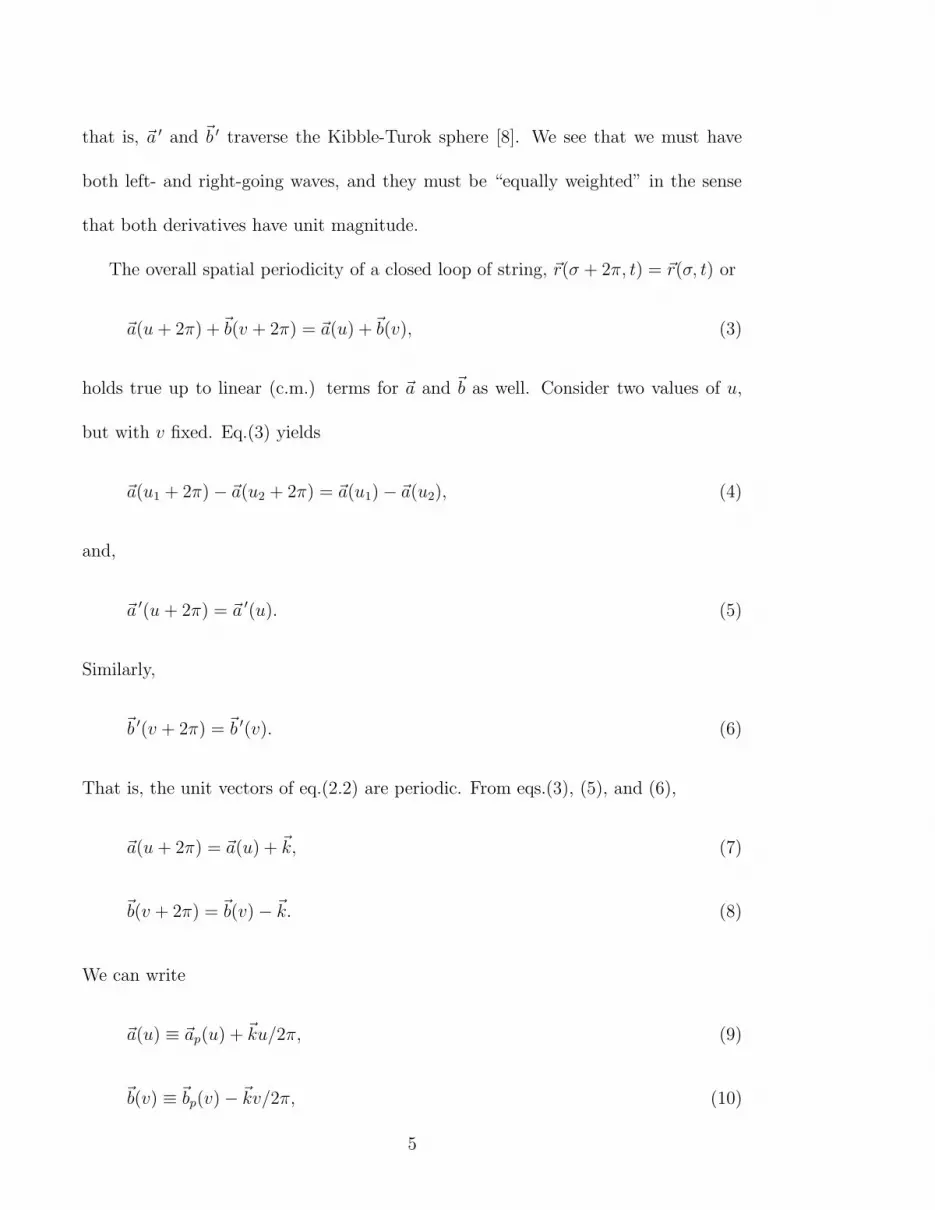
that is, ~a ′ and ~b ′ traverse the Kibble-Turok sphere [8]. We see that we must have

both left- and right-going waves, and they must be “equally weighted” in the sense

that both derivatives have unit magnitude.

The overall spatial periodicity of a closed loop of string, ~r(σ + 2π, t) = ~r(σ, t) or

~a(u+ 2π) +~b(v + 2π) = ~a(u) +~b(v), (3)

holds true up to linear (c.m.) terms for ~a and ~b as well. Consider two values of u,

but with v fixed. Eq.(3) yields

~a(u1 + 2π) − ~a(u2 + 2π) = ~a(u1) − ~a(u2), (4)

and,

~a ′(u+ 2π) = ~a ′(u). (5)

Similarly,

~b ′(v + 2π) = ~b ′(v). (6)

That is, the unit vectors of eq.(2.2) are periodic. From eqs.(3), (5), and (6),

~a(u+ 2π) = ~a(u) + ~k, (7)

~b(v + 2π) = ~b(v) − ~k. (8)

We can write

~a(u) ≡ ~ap(u) + ~ku/2π, (9)

~b(v) ≡ ~bp(v) − ~kv/2π, (10)

5

where ~ap and~bp are periodic functions of their arguments, with period 2π. In a Fourier

series, ~a ′p and ~b ′p have no zero harmonic terms. The derivatives,

~a ′ = ~a ′p + ~k/2π, (11)

~b ′ = ~b ′p − ~k/2π, (12)

are indeed periodic, and ±~k/2π are identified as the respective zero harmonics.

Finally, we have

~r(σ, t) = ~rp(σ, t) + ~Kt, (13)

with

~rp ≡1

2[~ap(u) +~bp(v)], (14)

~K ≡ −~k/π. (15)

Eq.(13) is the generic form for closed loops: periodic left-going and right-going su-

perimposed on uniform (c.m.) motion.

Now we address temporal periodicity. Modulo the c.m. motion, the string cer-

tainly repeats in 2π time intervals. From (4),

~rp(σ, t+ 2π) = ~rp(σ, t). (16)

But in fact the effective time period is half of this [8] because under σ → σ + π,

t→ t+ π, we have u→ u, v → v + 2π,

~rp(σ + π, t+ π) = ~rp(σ, t). (17)

6

The string “looks” exactly the same every time interval T ,

T = π. (18)

The first half of the string (0 < σ < 2π) switches places with the second half (π <

σ < 2π) every time T . The individual unit vectors eqs.(9) and (10), however, have

period 2π.

III. Fourier Analysis and Product Representation

We are thus led to consider the Fourier analysis of ~a ′ and ~b ′, the integration of which

will give us the string configuration. We restrict ourselves to a finite number of har-

monics according to the discussion in the introduction. The problem of finding the

harmonic coefficients in the finite Fourier series for a periodic vector whose magnitude

is fixed has just recently been solved. The product representation of Ref. [15] auto-

matically satisfies the magnitude constraint, exhibits the correct degrees of freedom,

and gives the general solution.

Consider a periodic unit vector uN(s) = uN(s + 2π) defined by the N -harmonic

real series,

uN(s) = ~Z +N∑

n=1

( ~An cos ns+ ~Bn sinns), (19)

with N arbitrary. The constraint (uN)2 = 1 requires a set of nonlinear relations

among the vector coefficients in eq.(19). In terms of the real basis, we have the

7

4N + 1 real equations

N∑

n=m−N

(~αn · ~αm−n − ~βn · ~βm−n) = 4δm0, m = 0, 1, . . . , 2N, (20)

N∑

n=m−N

(~αn · ~βm−n + ~βn · ~αm−n) = 0, m = 1, . . . , 2N. (21)

Here,

~αn = ~α−n = ~An, ~βn = −~β−n = ~Bn, n 6= 0, (22)

~α0 = 2~Z, ~β0 = 0. (23)

The product representation which solves eq.(19) can be written in terms of stan-

dard matrices such as Rξ(ψ), which refers to a rotation of a vector through the angle

ψ about the ξ-axis (or of the coordinate system through −ψ). Making a specific

choice of a constant unit vector which we rotate in succession, we have

uN(s) = rNRz(s)ρNRz(s)ρN−1 . . . Rz(s)ρ1z. (24)

Here,

ρi = Rz(−θi)Rx(φi)Rz(θi). (25)

We can let θ1 = π/2, or

ρ1 = Ry(−φ1). (26)

Also, there is the overall orientation freedom

rN =

Rz(α)Rx(β)Rz(γ), N ≥ 1,

Rz(α)Rx(β), N = 0.

(27)

8

where α, β, and γ are additional constants (angle parameters).

Let us consider how eq.(24) gives the desired properties. The rotations preserve

the vector magnitude, satisfying the original constraint, and the N factors of Rz(s)

generate N harmonics. In general, this is a complete and independent representation,

although one needs to look at the detailed proof [15, 16] to see this. The 2N + 2

independent degrees of freedom [(6N + 3)− (4N + 1)] are unrestricted angles, θi and

φi, whose ranges are independent of each other (0 ≤ θi ≤ π, 0 ≤ φi ≤ 2π). (In

examples, there may exist reflection symmetries, such as φi → −φi or π−φi for some

of the angles, reducing the overall range accordingly.) Because the signs can be a

source of confusion in the derivation of the results in the next section, we list the

matrix conventions for active rotations

Rx(θ) =

1 0 0

0 cθ −sθ

0 sθ cθ

, Ry(θ) =

cθ 0 sθ

0 1 0

−sθ 0 cθ

, Rz(θ) =

cθ −sθ 0

sθ cθ 0

0 0 1

,(28)

with sθ ≡ sin θ, cθ ≡ cos θ.

To complete the groundwork for a procedure for constructing closed strings for a

given N (zeroth plus first N harmonics), we note that the overall rotation rN can be

omitted in the product representation (3.6) of the unit vector ~a,

~a ′N(u, θi, φi) =

N∏

1

[Rz(u)ρi]z. (29)

Here, f(θi) ≡ f({θi}), etc. In place of rN , we consider the {x, y, z} basis as arbitrarily

oriented. To obtain final polynomial expressions in sin θi, cos θi, etc., it is convenient

9

to use the iterative property

~a ′N = Rz(u− θN)Rx(φN)Rz(θN )~a ′

N−1. (30)

Afterwards, it is necessary to separate out the zero harmonic piece in eq.(11), defined

to be ~αN ,

~a ′N(u, θi, φi) = ~a ′

p,N(u, θi, φi) + ~αN(θi, φi). (31)

We can immediately write down the other unit vector and its zero harmonic compo-

nent βN

~b ′N (v, θ′i, φ′i) = ~b ′p,N(v, θ′i, φ

′i) + ~βN(θ′i, φ

′i)

= ~a ′N (v, θ′i, φ

′i)|xyz→x′y′z′.

(32)

That is, u → v, and prime everything else. Finally, we must have the periodicity

condition (15),

~αN(θi, φi) = −βN (θ′i, φ′i) = −1

2~KN . (33)

This last condition can be met in two ways. The first we call the traveling string case

where all θ′i, φ′i, x

′, y′, z′ are found so that (33) is satisfied. The second we refer to

as the c.m. frame, where ~KN = 0. We find all θi, φi such that

~αN = 0, (34)

and θ′i, φ′i such that

~βN = 0. (35)

10

IV. General Parametrizations of N=0,1,2,3 Closed

Strings

We begin with a zeroth harmonic and then add in sequence a first, second, and finally

a third harmonic. In each case we describe two different solutions corresponding to

moving strings and c.m. strings, as described in the previous section.

A. N=0

The N=0 trivial zero-harmonic case for eq.(30) is included if only to highlight the

freedom to choose an overall z-axis direction. We have ~a ′ = −z, ~b ′ = z′, with the

periodicity of ~r in σ forcing z ′ = z [recall eq.(17)]. The result is a point moving at

the speed of light,

~r0 = zt. (36)

B. N=1

The general combination of zeroth plus first harmonic is the N=1 case in eq.(3.12).

In simpler notation (φ1 ≡ − θ,−θ′ for ~a ′,~b ′, respectively), matrix multiplication

leads to the intermediate answers

~a ′ = sin θ cos u x+ sin θ sin u y + cos θ z, (37)

~b ′ = sin θ′ cos v x ′ ± sin θ′ sin v y ′ + cos θ′ z ′. (38)

Besides the z freedom, we have chosen a particular handedness for the time rotation

of ~a ′ for a given θ. But then ~b ′ can have both right- and left-handed circulation.

11

i. Traveling string

For the “moving string” procedure of satisfying σ periodicity, z ′ = z and θ′ = θ + π.

Integration gives the traveling loop solution for both circulations,

~r± =1

2sin θ[(sin u− sin v)x+ (− cosu± cos v)y] − cos θzt. (39)

(In such deliberations, any rotation by an angle χ of x ′ − y ′ relative to x − y can

be absorbed into redefinitions (shifts) of σ and t: x ′ cos v + y ′ sin v = x cos (v + χ) +

y sin (v + χ) → x cos v+ y sin v, for σ → σ− χ/2, t→ t− χ/2.) Eq.(39) refers to two

simple planar strings with constant c.m. motion that is perpendicular to the planes.

Rewriting, we see these are, respectively, circles with oscillating radii,

~r+ = − sin θ sin tρ(σ) − cos θzt, (40)

and uniformly rotating sticks of fixed length,

~r− = − sin θ cosσφ(−t) − cos θzt. (41)

Here we have used the cylindrical unit vectors

ρ(A) = x cosA+ y sinA,

φ(A) = −x sinA+ y cosA. (42)

The speed of light is reached at the ends of the sticks or when the circles pass through

zero radius. The limits θ = 0, π give the trivial case presented in eq.(36).

12

ii. c.m. string

In the “c.m.” procedure, we eliminate the zero harmonics in eq.(37) and (38) sepa-

rately and hence the c.m. motion, by the requirement that θ = θ′ = π/2. Visualizing

the most general intersection of two great circles on the Kibble-Turok sphere, we let

y ′ = y and x ′ = x cosψ + z sinψ:

~r± =1

2[(sin u+ sin v cosψ)x− (cosu± cos v)y + sin v sinψz]. (43)

These strings look like rotating ellipses that oscillate in size, collapsing periodically to

sticks. They are natural interpolations between the circle and stick results in eq.(40),

(41), forms to which they reduce in the ψ = 0, π limits but without any overall

motion. See Fig. 1. for an illustration. It is interesting, however, that we cannot get

the general c.m. solution by simple limits on the traveling string solution.

C. N=2

The combination of the three harmonics - zeroth, first, second - illustrates an inter-

esting point. In the c.m. string limit where one eliminates the zeroth harmonic, it is

seen that no solution is possible for that particular “half” of the string (~a or ~b). A

first harmonic and a second harmonic cannot coexist. In fact, the only pair of nonzero

harmonics that can coexist must be in the ratio of three to one [13].

i. Traveling string

For a nonzero zero-harmonic contribution, all three harmonics coexist. In the “moving

string” procedure of dealing with the zero harmonics of ~a ′ and ~b ′, the σ terms cancel

13

when the angles are related as follows

φ′2 = ±φ2, φ

′1 = φ1 + π, θ′2 = θ2, (44)

where the unprimed and primed angles are parameters of ~a and ~b, respectively. This

gives four strings due to the two possible values of φ2 (represented by ±2) and to the

freedom for ~b to rotate in a right- or left-handed direction (represented by ±):

~r =

cos2 φ2

2sinφ1

0

0

1

4(sin 2u− sin 2v) +

0

cos2 φ2

2sinφ1

0

1

4(− cos 2u± cos 2v)

+

− sin φ2 cos φ1 sin θ2

− sinφ2 cosφ1 cos θ2

sinφ2 sinφ1 sin θ2

1

2(sin u− (±2) sin v)

+

sin φ2 cosφ1 cos θ2

− sinφ2 cosφ1 sin θ2

sinφ2 sinφ1 cos θ2

1

2(− cosu± (±2) cos v)

+

− sin2 φ2

2sin φ1 cos 2θ2

sin2 φ2

2sinφ1 sin 2θ2

− cosφ2 cosφ1

t . (45)

ii. c.m. string

There are two ways to set both the zero harmonics equal to zero.

φ′2 = φ2 =

π

2,3π

2, φ′

1 = φ1 = 0, π . (46)

14

This reduces the string to a two-parameter N = 1 string where θ1 = θ2, φ1 = π2,

θ′1 = θ′2, φ′1 = π

2.

The second set of angles

φ′2 = φ2 = 0, φ′

1 = φ1 =π

2,3π

2, (47)

give a string with only a second harmonic

~r = ±1

4

(sin 2u+ cosψ sin 2v)

− cos 2u∓ cos 2v

sinψ sin 2v

, (48)

which is simply a z-rotation of u on eq.(43).

Other solutions may be obtained by satisfing one of the above constraints on one

half of the string, and another set of constraints on the other half. For example,

setting φ2 = 0, φ1 = π2, φ′

2 = π2, φ′

1 = 0, we obtain the following string,

~r =1

4

−2(cos θ2 cosu+ sin θ2 sin u) + cosψ sin 2v

2(cosu sin θ2 − cos θ2 sin u) − cos 2v

sinψ sin 2v

. (49)

D. N=3

i. Traveling string

The general equations fixing the zero harmonics so that they cancel are highly non-

linear, and the solution set is very difficult to define, but the following four solutions

15

are fairly easy to see:

φ′3 = φ3, θ′3 = θ3, φ′

2 = φ2, θ′2 = θ2, φ′1 = φ1 + π,

φ′3 = φ3, θ′3 = θ3, φ′

2 = −φ2, θ′2 = θ2 + π, φ′1 = φ1 + π,

φ′3 = −φ3, θ′3 = θ3 + π, φ′

2 = φ2, θ′2 = θ2, φ′1 = φ1 + π,

φ′3 = −φ3, θ′3 = θ3 + π, φ′

2 = −φ2, θ′2 = θ2 + π, φ′1 = φ1 + π.

These all give the same two string equations (in the more concise form of φ, ρ

from (42)),

~r = − 1

3cos2

φ3

2cos2

φ2

2sin φ1 sin 3t ρ(3σ) +

1

2cos2

φ3

2sin φ2 cos φ1 sin 2t φ(2σ − θ2)

+1

4sinφ3 sinφ2 sin φ1 sin 2t ρ(2σ − θ3 + θ2) −

1

2sinφ3 cos2

φ2

2sinφ1 sin 2t sin (2σ + θ3)z

− cos2φ3

2sin2

φ2

2sinφ1 sin t ρ(σ − 2θ2) − sin2

φ3

2sin2

φ2

2sin φ1 sin t ρ(σ − 2θ3 + 2θ2)

+ sinφ3 cos φ2 cos φ1 sin t φ(σ − θ3) − sin2φ3

2cos2

φ2

2sin φ1 sin t ρ(−σ − 2θ3)

− cosφ3 sinφ2 sinφ1 sin t sin (σ + θ2)z + sinφ3 sinφ2 cosφ1 sin t cos (σ + θ3 − θ2)z

−1

2sinφ3 sinφ2 sinφ1 t ρ(−θ3 − θ2) − sin2

φ3

2sin φ2 cos φ1 t ρ(2θ3 − θ2)

− [cosφ3 cosφ2 cosφ1 + sin φ3 sin2φ2

2sinφ1 sin (θ3 − 2θ2)] t z , (50)

or

~r = −1

3cos2

φ3

2cos2

φ2

2sin φ1 cos 3σ φ(−3t) − 1

2cos2

φ3

2sin φ2 cosφ1 cos 2σ ρ(−2t− θ2)

+1

4sinφ3 sinφ2 sin φ1 cos 2σ φ(−2t− θ3 + θ2)

−1

2sinφ3 cos2

φ2

2sinφ1 cos 2σ cos (2t− θ3)z

16

− cos2φ3

2sin2

φ2

2sinφ1 cosσ φ(−t− 2θ2) − sin2

φ3

2sin2

φ2

2sin φ1 cos σ φ(−t− 2θ3 + 2θ2)

− sinφ3 cosφ2 cosφ1 cosσ ρ(−t− θ3) + sin2φ3

2cos2

φ2

2sin φ1 cosσ φ(t− 2θ3)

− cosφ3 sinφ2 sinφ1 cosσ cos (t− θ2)z + sinφ3 sinφ2 cosφ1 cosσ sin (t− θ3 + θ2)z

−1

2sinφ3 sinφ2 sinφ1 t ρ(−θ3 − θ2) − sin2

φ3

2sin φ2 cos φ1 t ρ(2θ3 − θ2)

− [cosφ3 cosφ2 cosφ1 + sin φ3 sin2φ2

2sinφ1 sin (θ3 − 2θ2)] t z. (51)

ii. c.m. string

There are many ways to set both zero harmonics equal to zero. Because any combi-

nation of these string halves is possible, we present only the equation for ~a.

There are three solutions which produce a string with first, second, and third

harmonics.

φ3 = 0, φ2 =π

2,3π

2, (52)

~a = [1

6sinφ1 sin 3u− (±2)

1

2cos φ1 cos (2u− θ2) +

1

2sinφ1 sin (u− 2θ2)] x

+[−1

6sinφ1 cos 3u− (±2)

1

2cosφ1 sin (2u− θ2) −

1

2sinφ1 cos (u− 2θ2)] y

+ [−(±2) sinφ1 cos (u+ θ2)] z , (53)

φ3 =π

2,3π

2, φ2 = 0, (54)

~a = [1

6sinφ1 sin 3u− (±3) cosφ1 cos (u− θ3) +

1

2sin φ1(sin (u+ 2θ3)] x

[−1

6sin φ1 cos 3u− (±3) cosφ1 sin (u− θ3) +

1

2sinφ1 cos (u+ 2θ3)] y

17

[−(±3)1

2sinφ1 cos (2u+ θ3)] z , (55)

φ2 = 0, φ1 =π

2,3π

2, (56)

~a = (±1)[1

3cos2

φ3

2sin 3u+ sin2

φ3

2sin (u+ 2θ3)] x

+(±1)[−1

3cos2

φ3

2cos 3u+ sin2

φ3

2cos (u+ 2θ3)] y

+ (±1)[−1

2sin φ3 cos (2u+ θ3)] z , (57)

The angles

φ3 = 0, φ1 =π

2,3π

2, (58)

give a string with only first and third harmonics

~a = (±1)[1

3cos2

φ2

2sin 3u+ sin2

φ2

2sin (u− 2θ2)] x

+(±1)[−1

3cos2

φ2

2cos 3u− sin2

φ2

2cos (u− 2θ2)] y

+ (±1)[− sin φ2 cos (u+ θ2)] z . (59)

The eight other solutions found reduce to strings with only a first harmonic. These

18

solutions are

φ3 = π, φ1 = π2, 3π

2,

φ3 = π2, 3π

2, φ2 = π, φ1 = 0, π,

φ3 = π2, 3π

2, φ2 = π, θ3 = 2θ2,

φ3 = π2, 3π

2, φ2 = π, θ3 = 2θ2 + π,

φ2 = π, φ1 = π2, 3π

2, θ3 = 2θ2,

φ2 = π, φ1 = π2, 3π

2, θ3 = 2θ2 + π,

φ2 = π, θ3 = 2θ2 + π2, φ3 = −φ1 + π

2,−φ1 + 3π

2,

φ2 = π, θ3 = 2θ2 + 3π2, φ3 = φ1 + π

2, φ1 + 3π

2.

(60)

An example of an N=3 string is given here,

~r =1

12sinφ1

cosα

sinα

0

sin 3u− 1

12sinφ1

− sinα cosβ

cosα cosβ

sin β

cos 3u

+1

4cosφ1

sinα cosβ

− cosα cosβ

− sin β

sin (2u− θ2) −1

4cos φ1

cosα

sinα

0

cos (2u− θ2)

+1

4sin φ1

cosα

sinα

0

sin (u− 2θ2) −1

4sin φ1

− sinα cos β

cosα sin β

sin β

cos (u− 2θ2)

−1

2sinφ1

sinα sin β

− cosα sin β

− cosβ

cos (u+ θ2) +1

12

sin φ′1

0

0

sin 3v

19

− 1

12

0

sin φ′1

0

cos 3v +1

4

0

− cosφ′1

0

sin (2v − θ′2)

−1

4

cosφ′1

0

0

cos (2v − θ′2) +1

4

sin φ′1

0

0

sin (v − θ′2)

− 1

4

0

sin φ′1

0

cos (v − 2θ′2) −1

2

0

0

sinφ′1

cos (v + θ′2). (61)

This string is displayed in Fig. 2 for a given choice of parameters.

V. Previous Strings

In this section we rewrite other existing parametrizations in terms of our rotation

angles. (These rewritten versions have also been referenced earlier in [15].) The

Turok string [9], shown in Fig. 3 for a particular choice of parameters, is a two-

parameter string which has a first and third harmonic in ~a, and a first in ~b. Defining

Turok’s parameter α to be α ≡ sin2 η

2, the string equation is

~rT =1

2

1

3sin2 η

2sin 3u+ cos2 η

2sin u

−1

3sin2 η

2cos 3u− cos2 η

2cosu

sin η cosu

20

+1

2

sin v

− cos φ cos v

− sinφ cos v

. (62)

The product of rotations which yields the 1-3 half of this string is

~a ′T = Rz(2u)Rx(π − η)Rz(u)x, (63)

which corresponds to our complete product representation for N = 3 with φ3 = 0,

φ2 = π − η, θ2 = 0, φ1 = π2, θ1 = −π

2, using the identity Rz(

π2)Rx(

π2)Rz(−π

2)z = x.

The second string half is given by

~b ′T = Rx(φ)Rz(v)x. (64)

The leftmost rotation is due to the fact that the Turok string is not in what we call

standard form. We see that this reduces to the Kibble-Turok [8] formula for φ = 0.

The Chen, DiCarlo, Hotes string [12], shown in Fig. 4 for a given choice of

paramterers, is a 1-3/1 string with an added parameter in ~a, which contains the

Turok string as a limit. We redefine the original CDH parameter ηCDH ≡ π2− η to be

consistent with our definition of α in the Turok string. The string equation becomes

~rCDH =1

6

C cos θ

S

−C sin θ

sin 3u− 1

6

−S cos θ

C

S sin θ

cos 3u

+1

4

2 − C cos θ

−S

C sin θ

sin u− 1

4

3S cos θ

cos θ + cos η

− sin η(1 − 3 cos2 θ)

cosu

21

+1

2

1

0

0

sin v − 1

2

0

cos φ

sinφ

cos v, (65)

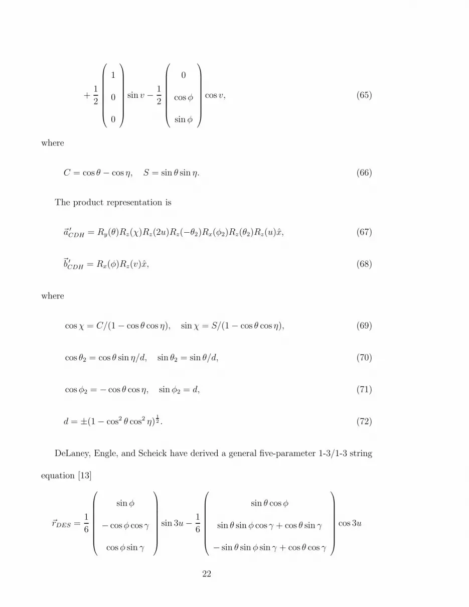
where

C = cos θ − cos η, S = sin θ sin η. (66)

The product representation is

~a ′CDH = Ry(θ)Rz(χ)Rz(2u)Rz(−θ2)Rx(φ2)Rz(θ2)Rz(u)x, (67)

~b ′CDH = Rx(φ)Rz(v)x, (68)

where

cosχ = C/(1 − cos θ cos η), sinχ = S/(1 − cos θ cos η), (69)

cos θ2 = cos θ sin η/d, sin θ2 = sin θ/d, (70)

cos φ2 = − cos θ cos η, sin φ2 = d, (71)

d = ±(1 − cos2 θ cos2 η)1

2 . (72)

DeLaney, Engle, and Scheick have derived a general five-parameter 1-3/1-3 string

equation [13]

~rDES =1

6

sinφ

− cosφ cos γ

cosφ sin γ

sin 3u− 1

6

sin θ cosφ

sin θ sin φ cos γ + cos θ sin γ

− sin θ sin φ sin γ + cos θ cos γ

cos 3u

22

+1

2

1 − c sinφ

c cosφ cos γ

−c cos φ sin γ

sin u− 1

2

x

y cos γ + z sin γ

−y sin γ + z cos γ

cosu

+1

6

sinφ′

− cos φ′

0

sin 3v − 1

6

sin θ′ cosφ′

sin θ′ sin φ′

cos θ′

cos 3v

+1

2

1 − c′ sinφ′

c′ cosφ′

0

sin v − 1

2

x′

y′

z′

cos v, (73)

with

x = −3c sin θ cos φ,

y = sin θ(1 − 3c sinφ),

z = cos θ sinφ− c sec θ(1 − 3 sin2 θ),

c = cos2 θ(1 + sinφ)/2, (74)

and with the same relationships between the primed variables.

In terms of the product representation,

~a ′DES = Rx(−γ)Rz(φ− π

2)Rx(

π

2− θ)Rz(2u)Rz(−θ2)Rx(φ2)Rz(θ2)Rz(u)x, (75)

~b ′DES = Rz(φ′ − π

2)Rx(

π

2− θ′)Rz(2v)Rz(−θ′2)Rx(φ

′2)Rz(θ

′2)Rz(v)x, (76)

23

with

cos θ2 = ± sin θ(1 + sin φ)/f, sin θ2 = ∓ cosφ/f, (77)

cos φ2 = cos2 θ sin φ− sin2 θ, sinφ2 = ±f cos θ, (78)

f = [cos2 φ+ sin2 θ(1 + sin φ)2]1

2 , (79)

and similarly for the primed angles. This string is displayed in Fig. 5 for a given

choice of parameters.

These early parametrizations contained only odd harmonics. For this reason, they

satisfy the symmetry relation ~r(σ + π, t) = −~r(σ, t). On the other hand, in Ref.[10]

Burden introduced a simple class of strings with m and n harmonics in the left and

right sectors, respectively,

~a ′(u) = cos(mu)x− sin(mu)z,

~b ′(v) = cos(nv)(cosΨx+ sinΨy) − sin(nv)z.

(80)

For m and n relatively prime, this symmetry no longer holds, and gravitational radi-

ation is no longer suppressed [10]. We can describe this class of strings as a subclass

of our general parametrization in the following way,

~a ′(u) = [Ry(u)]m x,

~b ′(v) = Rz(Ψ)[Ry(v)]n x.

(81)

Another string without the aforementioned symmetry is the Vachaspati-Vilenkin

string [11], an example of which is shown in Fig. 6. This has first, second, and third

24

harmonics in the left-going string half, and a first in the right-going half:

~rV V =1

2

−1

3α sin 3u+ (1 − α) sin u+ sin v

−1

3α cos 3u− (1 − α) cosu− cosφ cos v

√

α(1 − α) sin 2u− sinφ cos v

, (82)

where 0 ≤ α ≤ 1, and −π ≤ φ ≤ π. Defining φ3 by the relation α ≡ cos2 φ3

2, the

product representation gives

~a ′V V = −Rx(π)Rz(u)Rz(−

π

2)Rx(φ3)Rz(

π

2)Rz(2u)x, (83)

~b ′V V = Rx(φ)Rz(v)x. (84)

Kibble, Garfinkle and Vachaspati have derived a formula for cuspless loops [6],

shown in Fig. 7, again with arbitrary parameters:

~rGV =1

2

1

p2 + 2

1

2p2 + 1

p2

4sin 4u+ (p2 + 1)2 sin 2u

−2√

2

3p cos 3u− 2

√2p(p2 + 2) cosu

−p2

4cos 4u− ((p2 + 1)2 − 2) cos 2u

+1

2

1

p2 + 2

1

2p2 + 1

p2

4sin 4v + (p2 + 1)2 sin 2v

p2

4cos 4v + ((p2 + 1)2 − 2) cos 2v

2√

2

3p cos 3v + 2

√2p(p2 + 2) cos v

, (85)

where p is a constant. In terms of the product representation, this is

~a ′ = Rx(π

2)Rz(u)Rx(φ4)Rz(2u)Rx(φ2)Rz(u)x, (86)

~b ′ = −Ry(π)Rz(v)Rx(φ4)Rz(2v)Rx(φ2)Rz(v)x, (87)

25

where φ4 and φ2 are related to p by the definition

p ≡ −√

2 cotφ4

2≡ tan

φ2

2/√

2, (88)

so that

sin φ4 = −2√

2p/(p2 + 2), cos φ4 = (p2 − 2)/(p2 + 2), (89)

sin φ2 = 2√

2p/(2p2 + 1), cosφ2 = −(2p2 − 1)/(2p2 + 1). (90)

VI. Kink Parametrizations

While a cusp is a point on a string where ~rσ = 0, a kink is a discontinuity in ~rσ. A

discontinuity of this type may occur after intercommutation (e.g., if a loop crosses

itself, it splits and reconnects as two closed loops). The produced kink splits into

right and left traveling kinks residing in ~a and ~b, respectively. We should like to

define these as right kinks and left kinks, for short. Indeed, a picture of a loop with

both a left and right kink will show only one bend at the instant when the two pass

through each other.

A. Paired Kinks

Parametrization of loops with kinks has been investigated by Garfinkle and Vachas-

pati [6]. Using a greatest integer function, they were able to put symmetric sets of

kinks (i.e., two symmetric pairs of left and right kinks) in an extension of Burden

26

trajectories [10]. With four parameters, p, q, δ and Ψ, define

α = π(1 − p)[2(σ − t)/L],

β = π(1 − q)[2(σ + t)/L] + δ,

(91)

where [x] is the greatest integer less than or equal to x. The Garfinkle-Vachaspati

solution is given by

~a ′ = sin(2πp(σ − t)/L+ α)x+ cos(2πp(σ − t)/L+ α)z,

~b ′ = sin(2πq(σ + t)/L+ β)[cosΨx+ sinΨy] + cos(2πq(σ + t)/L+ β)z.

(92)

B. Symmetric Kinks

The paired kinks can be generalized to a symmetric set. Define

f(u) = p u+2π

n(1 − p)[u/

2π

n] (93)

where p ∈ (0, 1) is real and n > 1 is an integer. [x] is defined to be the greatest integer

less than or equal to x. Then a string with n symmetric kinks (n > 1) is given by

~a′ = (cos(f(u)), sin(f(u)), 0). (94)

Due to the symmetric placement of the kinks, the integral of ~a′ over u = 0 to 2π

clearly vanishes.

For an even number of symmetric kinks (n = even), this parametrization can be

generalized in the manner discussed in section III. For example, a large multiparam-

eter set of symmetric kinked strings is given by

~a′ =

(

∏

i

Rxi(2miu+ βi)

)

Rx3(f(u)) x1, (95)

where the xi, mi, and βi are, respectively, arbitrary axes, integers, and angles.

27

C. Single Kinks

Parametrizations having a single kink in either ~a or ~b, (left or right kink), or both,

instead of a pair of symmetric kinks such as shown above , are difficult to express in

closed form. To see this, consider the continuity constraint,

∫

2π

0

~rσ(σ)dσ = 0. (96)

For symmetric kinks, this constraint becomes trivial as the first half of the integral

cancels the second half for all components.

For the single kink string we can satisfy this continuity constraint in the following

way. As before, we split ~r into its left-going and right-going modes. Letting ~b be

smooth, we derive the discontinuity solely from ~a ′. We ask that ~a ′ lie in the x-y

plane and that the discontinuity occur at u = 2nπ where n is an integer. Letting

~a ′(0) =

cos α

sinα

0

; ~a ′(2π) =

cos α

−sin α

0

, (97)

will give us a kink with a discontinuity angle varying with time, and depending on ~b ′

and an arbitrary constant α. The problem now lies in finding a parametrization of

the path ~a ′ takes along the unit circle such that its integral vanishes.

We can set

~a ′(u) =

cos(α + π−απf(u))

sin(α + π−απf(u))

0

, (98)

28

asking that f(0) = 0 and f(2π) = 2π. To get the integral to vanish, one component

can be taken care of by symmetry condition on f . For the other component, we need

f to change slowly over a smaller part of the circle and then quickly over the rest. A

simple example is

f(u) = u− δsin u . (99)

δ is positive and constant. The integration constraint results in a nontrivial relation

between α and δ,

tanα =Jπ−α

π

(−δ π−απ

) − cosα Jπ−α

π

(δ π−απ

) − sinαEπ−α

π

(δ π−απ

)

Eπ−α

π

(−δ π−απ

) + sinα Jπ−α

π

(δ π−απ

) − cosαEπ−α

π

(δ π−απ

), (100)

where the Anger function and Weber function, J and E respectively, are given by

Jν(z) = 1

π

∫ π0 cos(νs− zsins)ds,

Eν(z) = 1

π

∫ π0cos(νs− zsins)ds.

(101)

This transcendental relation is well defined, and has as a sample numerical solu-

tion, δ = 0.736 for α = π4. This solution generalizes

easily to an infinite parameter set of string solutions, where f(u) is

f(u) = u+∞∑

n=0

δnsin(nu), (102)

subject to a single integral condition as a generalization of equation (97).

Other modulating functions can also be considered, such as polynomial functions

f(u) = u+∑

n=odd

αn

[

(u− π)

π

]n

, (103)

subject to two conditions. The first being the continuity condition, which is tran-

scendental in the arguments αn, and the condition that f(0) = 0, which means that

the sum of the coefficients αn vanishes.

29

VII. Kinks After Intercommutation

In the previous section we have discussed representations of strings with single kinks

traveling in one direction around the string loop, where only ~a ′ or ~b ′ but not both,

contains a discontinuity. We have also mentioned, however, that this description is

not adequate for describing a string kinked as a result of intercommutation. We will

first consider a generic case of intercommutation. This is followed by an explicit

analytic example.

A. A construction algorithm

At the point of intercommutation (say, σ = t = 0), locally the two legs of the newly

formed kink describe a plane in 3-space. The directions of these legs are given by ~rσ to

the left and right of the kink, and we define these vectors as ~rσ(−ǫ, 0) and ~rσ(+ǫ, 0),

respectively. Because the two legs of the kink were originally parts of string segments

crossing through each other, each leg moves transverse to itself and the plane, and

opposite, generally, to each other. That is, the initial conditions require that ~rt has

a non-zero component transverse to this plane that changes in sign when crossing

through the kink. We will show that this initial condition is contradictory to the

conditions of a string containing only a single left and right kink.

Consider the initial time-derivatives of ~r to the left and right of the kink, ~rt(−ǫ, 0)

and ~rt(+ǫ, 0), respectively. Suppose only ~a ′ is discontinuous, as in the examples in

30

the previous section. From eq.(1) we have,

~rσ(−ǫ, 0) = 1

2[~a ′(−ǫ) +~b ′(0)],

~rσ(+ǫ, 0) = 1

2[~a ′(+ǫ) +~b ′(0)],

~rt(−ǫ, 0) = 1

2[−~a ′(−ǫ) +~b ′(0)],

~rt(+ǫ, 0) = 1

2[−~a ′(+ǫ) +~b ′(0)].

(104)

Noticing that the right-hand-sides contain only 3 independent vectors, we can write

one in terms of the others,

~rt(+ǫ, 0) = ~rt(−ǫ, 0) + ~rσ(+ǫ, 0) − ~rσ(−ǫ, 0). (105)

And clearly since the last two vectors on the right-hand-side of eq.(105) lie in the

above-mentioned plane, the component of ~rt transverse to this plane must be equal

on both sides of the kink, in contradiction with the initial motion. We see therefore

that discontinuities must occur in both ~a ′ and ~b ′ to correctly describe a kink after

intercommutation.

Under these circumstances, the kink will split into left and right moving parts (left

and right kinks) after intercommutation. Given a string parametrization of a string

that self-intersects, we should like to show how one constructs the parametrization

for the daughter loops. Consider a low-harmonic string that at some point in time

crosses itself. Let this crossing occur at t = τ , for σ = σ0, σ1. To describe the

resulting motion, we concentrate on one of the daughter loops. Note that at the

point of intercommutation, this loop is described by its left and right moving parts:

~a(u), u ∈ [σ0 − τ, σ1 − τ ] and ~b(v), v ∈ [σ0 + τ, σ1 + τ ] , respectively. We can define a

new string with ~A, ~B , of invariant length ∆σ = σ1 − σ0, in terms of these functions

31

~a,~b. We ask that the left and right moving parts of this new string, ~A, ~B, take the

same values as ~a and ~b over the intervals given above, respectively, and demand that

their derivatives ~A ′, ~B ′ be periodic with period ∆σ.

~A, ~B will not generally be periodic, with the daughter usually acquiring some

center of mass velocity. To wit, let

~k = ~a(σ1 − τ) − ~a(σ0 − τ) = −(~b(σ1 + τ) −~b(σ0 + τ)). (106)

~k determines the resulting c.m. velocity of the piece. Define ~A, ~B in the following

way. For s ∈ [0,∆σ], set

~A(s) = ~a(σ0 − τ + s),

~B(s) = ~b(σ0 + τ + s).

(107)

For s = n∆σ + s′, s′ ∈ [0,∆σ], n ∈ Z we let

~A(s) = ~a(σ0 − τ + s) + n~k,

~B(s) = ~b(σ0 + τ + s) − n~k.

(108)

The functions ~A and ~B in eq.(108) describe a closed string of period ∆σ containing

a single kink at the time of intercommutation that subsequently splits into left and

right moving kinks. The closed-loop trajectory

~r(σ, t) =1

2( ~A(σ − t) + ~B(σ + t)) (109)

satisfies the gauge conditions discussed in Section II. The loop moves with c.m. ve-

locity −~k/∆σ, corresponding to the shift relation

~r(σ, t+ ∆σ) = ~r(σ, t) − ~k. (110)

32

We thus have a procedure for determining the equation of motion for a cosmic

string after intercommutation. Given the harmonic parameterization for a string, one

first needs to calculate the points of self-intersection (see Ref. [12, 13, 26] for typical

calculation). Then the above procedure can be used to find an analytical expression

for the resulting string motion.

B. Example

The construction of a loop with a single kink has been discussed in the previous sec-

tion. It was explained how a kink could be described in terms of a phase modification

of a low harmonic form. Here we wish to look at the more realistic situation where a

daughter loop is produced upon the self-intersection of a closed low-harmonic string.

In Reference [12], the range of parameters have been carefully determined for

which self-intersections occur in the Turok string of eq.(62). We shall follow the

evolution of one of these strings whose parameters lie in this range, before and after

self-intersection. The harmonic forms can be adapted according to the equations of

the above subsection in order to describe the daughter loops.

Using the techniques of Reference [12], we find, for our example, that a Turok-

string self-intersection occurs for α = 0.5, φ = 9π/20 at τ = 4.88707, σ0 = −.404027, σ1 =

.333862. One can add π to the σ values to describe the other self-intersection occur-

ring simultaneously (due to the symmetry of this class of loops). This example will

subsequently split into three subloops. Using the aforementioned procedure, we have

calculated the resulting disintegration of the string. Fig. 8 displays the parent string

33

at the point of self-intersection. Fig. 9 shows the split, and Fig. 10 is a close-up of

the point of intercommutation after the separation.

The evolution of the example is faithful to the gauge conditions chosen (and

described in Section II). All strings segments have the appropriate transverse motion

and unit energy density, in view of the fact that both ~A ′ and ~B ′ are unit vectors.

The two outside daughter loops have indeed acquired c.m. motion (with one kink in

each) but the middle daughter (with two symmetric kinks) having none. Of course,

the number of left and right kinks is twice the number of kinks. Correspondingly the

middle loop spins after the split, conserving angular momentum. The outer loops

are more circular and have smaller periods; they are observed to shrink rapidly down

to rather small size, as seen in Fig. 9. Finally, we note that as the kink separates

into the left and right kinks, the string segment between the two kinks is curved. In

general, there will not be a straight line between the left and right kinks.

VIII. Conclusions

The solutions to the classical relativistic string model for a fixed number of low

harmonics are useful in a number of different cosmic string applications. Starting with

the study of a simple first plus third harmonic string [8], the issue of self-intersections

has been addressed for increasingly more general parametrizations [9, 21, 12, 22, 23,

24, 25, 13, 26].

Harmonic parametrizations have been called upon in the calculation of string

angular momentum [9, 13], models of cosmic strings in an expanding universe [27, 28]

34

and also of the string gravitational radiation with and without kinks [29, 30, 31,

32, 33]. Gravitational particle production of cosmic strings has been studied using

harmonic forms [34]. It has been observed that string trajectories containing only

odd harmonics do not emit gravitational radiation [10, 35]. It is hoped that the

more general trajectories presented in this paper will aid in giving a more realistic

description of the gravitational radiation of cosmic strings. The electromagnetic self-

interaction of a string has been calculated using harmonic parametrizations [36, 37,

38]. The probability that harmonically parametrized string loops will collapse to black

holes has also been addressed [39] and the interaction between harmonic strings and

domain walls has been studied [40]. Solutions incorporating these parametrizations

have the advantage that analytic precision is not sacrificed for increasingly complex

structure.

Acknowledgements

We are grateful to Bruce Allen, Bob Scherrer and Alex Vilenkin for various dis-

cussions about various topics related to this paper. One of us (S.H.) would like to

thank Bob Hotes for the warm accommodations provided him while working on this

project. This research was supported in part by the National Science Foundation.

References

[1] T.W.B. Kibble, J. Phys. A9, 1387 (1976).

[2] See for example, D. Bennett, A. Stebbins, F. Bouchet, PRINT-92-0240, Jun

35

1992, 10pp. and L. Perivolaropoulos, Phys. Lett. B298, 305 (1993).

[3] E.P.S. Shellard, Nucl. Phys. B283, 624 (1987).

[4] R.A. Matzner, Comput. Phys. 2, 51 (1988).

[5] P. Laguna, and R.A. Matzner, Phys. Rev. Lett. 62, 1948 (1989).

[6] D. Garfinkle, and T. Vachaspati, Phys. Rev. D36, 2229 (1987).

[7] J.M. Quashnock, and D.N. Spergel, Phys. Rev. D42, 2505 (1990).

[8] T.W.B. Kibble and N. Turok, Phys. Lett. 116B, 141 (1982).

[9] N. Turok, Nucl. Phys. B242, 520 (1984).

[10] C.J. Burden, Phys. Lett. B164, 277 (1985).

[11] A. Vilenkin and T. Vachaspati, Phys. Rev. Lett. 58, 1041 (1987).

[12] A.L. Chen, D.A. DiCarlo, and S.A. Hotes, Phys. Rev. D37, 863 (1988).

[13] D.B. Delaney, K.A. Engle, and X. Scheick, Phys. Rev. D41, 1775 (1990).

[14] R.W. Brown, The Formation and Evolution of Cosmic Strings, edited by G.

Gibbons, S. Hawking, and T. Vachaspati (Cambridge U. P., Cambridge, 1990),

p. 127.

[15] R.W. Brown, and D.B. DeLaney, Phys. Rev. Lett. 63, 474 (1989).

[16] R.W. Brown, M.E. Convery, and D.B. DeLaney, J. Math. Phys. 32 (7), 1674

(1991).

36

[17] R.W. Brown, E.M. Rains, and C.C. Taylor, Class. and Quant. Grav. 8, 1245

(1991).

[18] R.J. Scherrer and W.H. Press, Phys. Rev. D39, 371 (1989).

[19] B. Allen and R.R. Caldwell, Phys. Rev. D43, 3173 (1991).

[20] P. Goddard, J. Goldstone, C. Rebbi, and C.B. Thorn, Nucl. Phys., B56, 109

(1973).

[21] E.J. Copeland, and N. Turok, Phys. Lett. B172 (2), 129 (1986).

[22] C. Thompson, Phys. Rev. D37, 283 (1988).

[23] A. Albrecht and T. York, Phys. Rev. D38, 2958 (1988).

[24] D. Hochberg, Nucl. Phys. B319, 709 (1989).

[25] T. York, Phys. Rev. D40, 277 (1989).

[26] F. Embacher, UWThPh-1992-14,15, March 26, 1992.

[27] N. Turok, Phys. Lett. B123, 387 (1983).

[28] N. Turok and P. Bhattacharjee, Phys. Rev. D29, 1557 (1984).

[29] A. Vilenkin , and T. Vachaspati, Phys. Rev. D31, 3052 (1985).

[30] T. Vachaspati, Phys. Rev. D39, 1768 (1989).

[31] R. Durrer, Phys. Rev. B328, 238 (1989) and PUPT-90-1165, (1990).

[32] A. Cresswell and R.L. Zimmerman, Phys. Rev. D42, 2527 (1990).

37

[33] B. Allen and E.P.S. Shellard, Phys. Rev. D45, 1898 (1992).

[34] J. Garriga, D. Harari, and E. Verdaguer, Nucl. Phys. B339, 560 (1990).

[35] R.J. Scherrer, J.M. Quashnock, D.N. Spergel and W.H. Press, Phys. Rev. D42,

1908 (1990).

[36] M. Aryal, A. Vilenkin, and T. Vachaspati, Phys. Lett. B194, 25 (1987).

[37] W. Press, R. Scherrer, and D. Spergel, Phys. Rev. D39, 379 (1989).

[38] P. Amsterdamski, Phys. Rev. D39, 1524 (1989).

[39] A. Polnarev and R. Zembowicz, Phys. Rev. Lett. 43, 1106 (1991).

[40] A. Vilenkin, Physics Reports 121, 263 (1985).

38

Figure Captions.

1. The N=1 C.M. string with φ = π2

at t = 0.

2. An N=3 C.M. string with α = 1.589, β = 1.712, θ = 1.23, θ ′ = 3.011,

φ = 0.785, and φ ′ = 2.901 at t = 2.

3. The Turok-PZ string with α = 0.8 and φ = π2

at t = 0.

4. The CDH string with θ = 4π10

, η = 1.60160, and φ = 2.64460 at t = 2.03.

5. The DES string with θ = 4π3

, θ ′ = 2.03, φ = 0.64460, φ ′ = 2.2345, and γ = 7π5

at t = 2.0.

6. The VV string with α = 0.6 and φ = 2.64460 at t = 0.

7. The GV cuspless, kinkless string with p = 0.2 at t = π2.

8. Self-intersection of a Turok string.

9. The Turok string shortly after intercommutation.

10. A close-up of the intercommutation region.

39