Embed Size (px)
Citation preview
11CO2 Emissions Targeting for
Petroleum Refinery Optimization
Mohmmad A. Al-Mayyahi1, Andrew F.A. Hoadley1 and Gade Pandu Rangaiah2
1Department of Chemical Engineering, Monash University, Australia2Department of Chemical and Biomolecular Engineering,
National University of Singapore, Singapore
11.1 Introduction
Petroleum refineries are under increasing pressure to minimize emissions of greenhousegases,mainlyCO2, to complywith the environmental regulations such as theKyoto protocolby the United Nations Framework Convention and Climate Change (UNFCC). Because ofthis trend, there is considerable interest from the petroleum-refining industry to targetand minimize CO2 emissions from different refinery processes. Many studies have beenpublished recently on the CO2 emissions produced in petroleum refining. These can becategorized as either academic or technical.In the academic studies, different methodologies are used to allocate / target and min-
imize CO2 emissions. The allocation of refinery CO2 emissions was investigated usingrefinery LP models and single-objective optimization [1–5]. These studies quantified andcompared CO2 emissions due to production of different finished products such as gasolineand diesel. However, the calculations were based on simple linear relations between productdemand/specifications and operating conditions. Moreover, the value of the results stronglydepends on the structure of the refinery concerned and the cost assigned for CO2 emissions.Szklo and Schaeffer [6] investigated the impact of the more restrictive environmental qual-ity of petroleum products on the energy consumption and consequential CO2 emissionsin the refinery. They also reviewed many energy-saving strategies in refineries such as
Multi-Objective Optimization in Chemical Engineering: Developments and Applications, First Edition.Edited by Gade Pandu Rangaiah and Adrian Bonilla-Petriciolet.© 2013 John Wiley & Sons, Ltd. Published 2013 by John Wiley & Sons, Ltd.
294 Multi-Objective Optimization in Chemical Engineering
improvement of heat integration and alternative treatment processes. Ba-Shammakh [7]developed a general mathematical model for an oil refinery. Single-objective optimizationis used to maximize the refinery profit subject to a certain CO2 reduction target using differ-ent mitigating strategies, namely, flow-rate balancing, fuel switching, and CO2 capturing.The refinery-planning model includes a CDU, different hydrotreaters, a reformer, FCC andHC. However, the CO2 emissions model was based only on the fuel-firing emissions anddid not account for process related emissions.On the technical side, Greek [8] studied the importance of gasification and pre-
combustion processes to reduce refinery CO2 emissions, and found that capturing pro-cesses are more expensive than other carbon management strategies such as improvingenergy efficiency and shifting to less carbon-intensive fuels to reduce refinery CO2 emis-sions. Different strategies for CO2 emissions reduction in the refinery were evaluated byMoore [9] including online optimization of fuel gas, hydrogen and utility systems. Ritteret al. [10] developed a systematic technique for estimating and reporting GHG emissions,especially CO2, in the oil and gas industry. Metrins et al. [11] illustrated an approach forpredicting CO2 emissions. They concluded that rigorous modeling of refinery processes,especially the fractionation columns, conversion reactors and heaters, and including directand indirect emissions, are required for accurate assessment of CO2 emissions. Spoor [12]discussed the major contributors to the refinery CO2 emissions and potential options foremissions reductions. The results of studies conducted at a European refinery are reviewedby Bruna et al. [13]. The results showed that significant reductions in CO2 emissions canbe achieved using an optimization approach based on operational improvements and a sys-tematic total site technique. Holmgren and Sternhufvud [14] evaluated different options forCO2 emissions reduction and the associated costs at petroleum refineries. They concludedthat the cost of emissions reduction is strongly dependent on fuel prices and efficienciesof emissions reduction strategies such as carbon capture and storage. Stockle et al. [15]used an LP model to identify the best combination of CO2 emissions reduction schemesto achieve a given reduction in CO2 emissions including the CO2 trading price as an oper-ating cost. The emissions reduction schemes considered are efficiency improvement, fuelshifting, carbon capture and sequestration, crude substitution, and hydrogen production.Three emissions sources were included in the LP model, namely; fuel for heat, steam andpower provision, hydrogen production, and FCC coke combustion. Ratan and Uffelen [16]claimed that 45% reduction in refinery CO2 emissions can be achieved by implementingappropriate improvements in the hydrogen plant. Different strategies for refinery emissionsreduction were also discussed by Mertens and Skelland [17] including utility optimiza-tion and cogeneration. Carter [18] emphasized the importance of energy management inimproving refinery margins and reducing CO2 emissions.Despite the contributions of these academic and technical studies to the optimization
of CO2 emissions in the petroleum refinery, the tradeoff between CO2 emissions andoperating and economic objectives was not properly addressed in these studies due to theuse of single-objective optimization. Furthermore, simple LP was often used to simulatethe refinery processes, which may omit important process features and may not adequatelyreflect the full picture of the refinery. More work, therefore, needs to be done on targetingCO2 emissions in the refinery using rigorous and comprehensive optimization approaches.The majority of CO2 emissions from refineries come from just a few main units such
as crude distillation, catalytic cracking and hydrotreating [12]. These units are also the
CO2 Emissions Targeting for Petroleum Refinery Optimization 295
major energy consumers due to the considerable amount of energy used including fuel,electric power and steam. Significant energy savings in such energy-intensive units can beobtained via improvements in waste heat recovery to minimize total energy consumption[17]. Energy integration technology has been proven to be successful in minimizing totalenergy requirement and reducing consequential emissions.In particular, pinch analysis has been proven to be an efficient tool in developing an
inherently energy-efficient design of integrated processes for both new plants and retrofits[19–25]. However, the degree of heat integration is often limited by many practical andoperational constraints. Furthermore, different levels of energy integration might lead tovery different economic and environmental effects. Therefore, the optimum level of energyintegration can only be determined by simultaneously considering different impacts onthe process. For such problems, multi-objective optimization (MOO) needs to be used,where a set of equally good solutions is produced. These solutions, referred to in theMOO community as the Pareto-optimal front, provide greater insight and enhance thedecision-making process.A new MOO framework to target CO2 emissions is presented in this chapter. Direct
and indirect sources of CO2 emissions, including emissions from fuel consumption andthe provision of heating and cooling utilities, are considered. Unlike some of the previousstudies, the two refinery units considered in this study, namely, the crude distillation unit(CDU) and the fluidized-bed catalytic cracker (FCC), are modeled rigorously. Differentobjectives are simultaneously optimized in two bi-objective problems to investigate thebest trade-off targets. The two refining units are presented in the next section, and this isfollowed by a brief overview of pinch analysis and MOO. Next, the MOO framework ispresented and then applied to two different case studies. More modeling details of the twoprocesses are provided in Appendix 11.A1.
11.1.1 Overview of the CDU
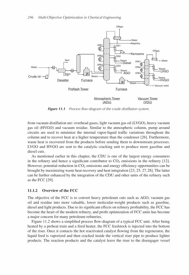
The CDU is the first major unit to process petroleum in any refinery. Its objective is toseparate crude oil into appropriate fractions, such as naphtha, kerosene, diesel, gas oil, andatmospheric residue, according to their boiling points, to be further treated in downstreamprocesses. Figure 11.1 shows the process flow-diagram of a CDU. Firstly, the crude oilfrom storage tanks is preheated by a series of heat exchangers. A Desalter is installed in theheat-exchanger train to reduce the salt content of the crude by an electric desalting process.Then, the desalted crude is further heated and sent to a preflash tower where vapors areseparated from the liquid feedstock to reduce the vapor pressure of the crude and decreasethe vapor load on the atmospheric column. A fired heater is used for further heating thepreheated crude before entering the atmospheric column where the fractionation occurs.Naphtha is produced as a vapor and condensed by the overhead condenser. Kerosene,
diesel, and atmospheric gas oil (AGO) are withdrawn as side streams and further refinedusing side columns, which are either reboiled or use stripping steam, to reduce the contentof the lighter components in each product. These products are sent for processing in otherdownstream units to increase the value of the final products whilst the atmospheric residueis further distilled under vacuum conditions to achieve the required separation between theheavy components at lower temperatures. A stripping steam is injected at the bottom of thevacuum tower to lower the bottom temperature and avoid degradation. The main products
296 Multi-Objective Optimization in Chemical Engineering
Offgas
Offgas
Water
SS1
SS2
SS3
Steam VPA1
SteamLVGO
Steam
Steam
Steam
Steam
Vent
Water
Water
Crude oilDesalter Furnace
Furnace
Atmospheric Tower(ADU)
Vacuum Tower(VDU)
Preflash TowerVacuum resid
HVGO
VPA2
VPA3
Diesel
AGO
Kerosene
APA1
APA2
APA3
Water
Naphtha
Figure 11.1 Process flow-diagram of the crude distillation system.
from vacuum distillation are: overhead gases, light vacuum gas oil (LVGO), heavy vacuumgas oil (HVGO) and vacuum residue. Similar to the atmospheric column, pump aroundcircuits are used to minimize the internal vapor-liquid traffic variations throughout thecolumn and to recover heat at a higher temperature than the condenser [26]. Furthermore,waste heat is recovered from the products before sending them to downstream processes.LVGO and HVGO are sent to the catalytic cracking unit to produce more gasoline anddiesel cuts.As mentioned earlier in this chapter, the CDU is one of the largest energy consumers
in the refinery and hence a significant contributor to CO2 emissions in the refinery [12].However, potential reduction in CO2 emissions and energy efficiency opportunities can bebrought by maximizing waste heat recovery and heat integration [23, 25, 27,28]. The lattercan be further enhanced by the integration of the CDU and other units of the refinery suchas the FCC [29].
11.1.2 Overview of the FCC
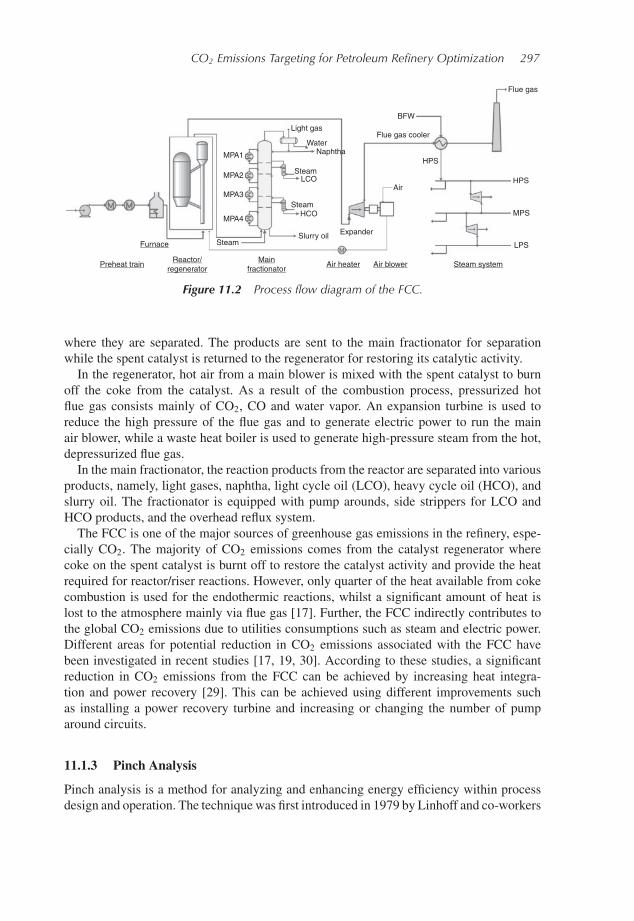
The objective of the FCC is to convert heavy petroleum cuts such as AGO, vacuum gasoil and residue into more valuable, lower molecular-weight products such as gasoline,diesel and light products. Due to its significant effects on refinery profitability, the FCC hasbecome the heart of the modern refinery, and profit optimization of FCC units has becomea major concern for many petroleum refineries.Figure 11.2 shows a simplified process flow-diagram of a typical FCC unit. After being
heated by a preheat train and a fired heater, the FCC feedstock is injected into the bottomof the riser. Once it contacts the hot reactivated catalyst flowing from the regenerator, theliquid feed is vaporized and then cracked inside the vertical riser pipe to produce lighterproducts. The reaction products and the catalyst leave the riser to the disengager vessel
CO2 Emissions Targeting for Petroleum Refinery Optimization 297
Flue gas
BFW
Flue gas cooler
HPS
HPS
MPS
LPS
Air
ExpanderSlurry oil
HCO
LCO
NaphthaWater
Light gas
MPA1
MPA2
MPA3
MPA4
Steam
SteamFurnace
Preheat trainReactor/
regeneratorMain
fractionatorAir heater Air blower Steam system
Steam
Figure 11.2 Process flow diagram of the FCC.
where they are separated. The products are sent to the main fractionator for separationwhile the spent catalyst is returned to the regenerator for restoring its catalytic activity.In the regenerator, hot air from a main blower is mixed with the spent catalyst to burn
off the coke from the catalyst. As a result of the combustion process, pressurized hotflue gas consists mainly of CO2, CO and water vapor. An expansion turbine is used toreduce the high pressure of the flue gas and to generate electric power to run the mainair blower, while a waste heat boiler is used to generate high-pressure steam from the hot,depressurized flue gas.In the main fractionator, the reaction products from the reactor are separated into various
products, namely, light gases, naphtha, light cycle oil (LCO), heavy cycle oil (HCO), andslurry oil. The fractionator is equipped with pump arounds, side strippers for LCO andHCO products, and the overhead reflux system.The FCC is one of the major sources of greenhouse gas emissions in the refinery, espe-
cially CO2. The majority of CO2 emissions comes from the catalyst regenerator wherecoke on the spent catalyst is burnt off to restore the catalyst activity and provide the heatrequired for reactor/riser reactions. However, only quarter of the heat available from cokecombustion is used for the endothermic reactions, whilst a significant amount of heat islost to the atmosphere mainly via flue gas [17]. Further, the FCC indirectly contributes tothe global CO2 emissions due to utilities consumptions such as steam and electric power.Different areas for potential reduction in CO2 emissions associated with the FCC havebeen investigated in recent studies [17, 19, 30]. According to these studies, a significantreduction in CO2 emissions from the FCC can be achieved by increasing heat integra-tion and power recovery [29]. This can be achieved using different improvements suchas installing a power recovery turbine and increasing or changing the number of pumparound circuits.
11.1.3 Pinch Analysis
Pinch analysis is a method for analyzing and enhancing energy efficiency within processdesign and operation. The technique was first introduced in 1979 by Linhoff and co-workers
298 Multi-Objective Optimization in Chemical Engineering
Hot compositecurve
Cold compositecurve
Enthalpy change (MW) Enthalpy change (MW)
(a) (b)
ΔTmin
QhminQhmin
Qcmin
Qcmin
Tem
pera
ture
(°C
)
Tem
pera
ture
(°C
)
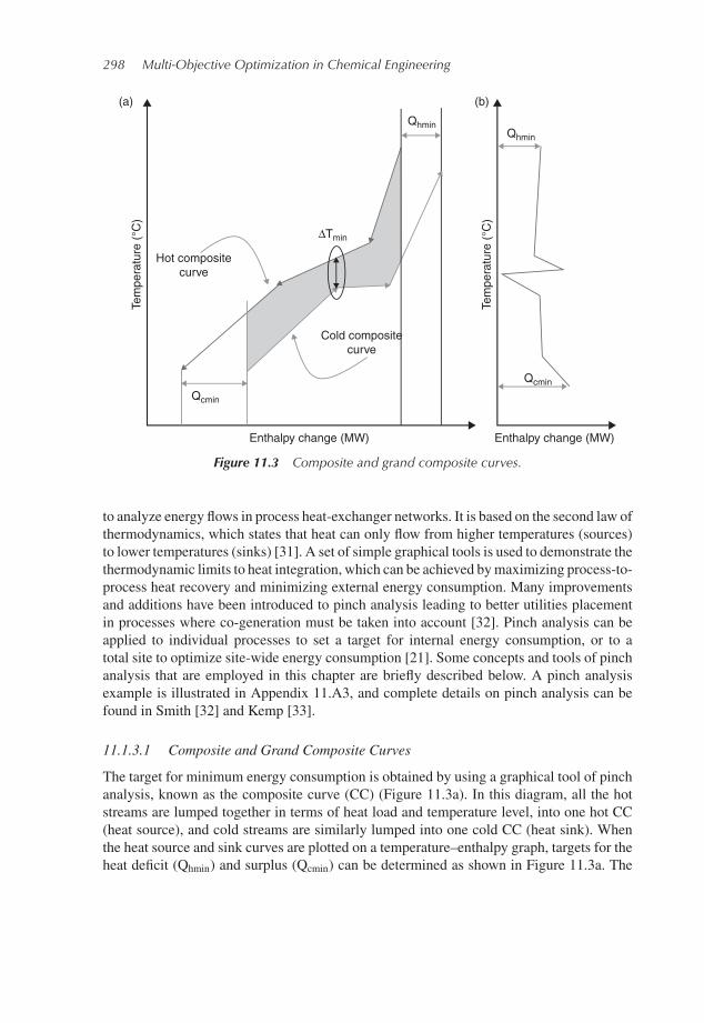
Figure 11.3 Composite and grand composite curves.
to analyze energy flows in process heat-exchanger networks. It is based on the second law ofthermodynamics, which states that heat can only flow from higher temperatures (sources)to lower temperatures (sinks) [31]. A set of simple graphical tools is used to demonstrate thethermodynamic limits to heat integration, which can be achieved bymaximizing process-to-process heat recovery and minimizing external energy consumption. Many improvementsand additions have been introduced to pinch analysis leading to better utilities placementin processes where co-generation must be taken into account [32]. Pinch analysis can beapplied to individual processes to set a target for internal energy consumption, or to atotal site to optimize site-wide energy consumption [21]. Some concepts and tools of pinchanalysis that are employed in this chapter are briefly described below. A pinch analysisexample is illustrated in Appendix 11.A3, and complete details on pinch analysis can befound in Smith [32] and Kemp [33].
11.1.3.1 Composite and Grand Composite Curves
The target for minimum energy consumption is obtained by using a graphical tool of pinchanalysis, known as the composite curve (CC) (Figure 11.3a). In this diagram, all the hotstreams are lumped together in terms of heat load and temperature level, into one hot CC(heat source), and cold streams are similarly lumped into one cold CC (heat sink). Whenthe heat source and sink curves are plotted on a temperature–enthalpy graph, targets for theheat deficit (Qhmin) and surplus (Qcmin) can be determined as shown in Figure 11.3a. The
CO2 Emissions Targeting for Petroleum Refinery Optimization 299
CC also shows the heat recovered within the process as the overlapping portion of the twocurves. The minimum temperature approach between the two CCs must be greater thanor equal to a specified temperature approach (�Tmin), see Figure 11.3a. As the �Tmin isincreased (the cold curve is moved to the right), the heat recovery region reduces and theutility requirements increase.�Tmin is usually set by the economics of a given process andshould be reviewed, when economic conditions change. The shaded area in Figure 11.3abetween the hot and cold CCs can be used to calculate the minimum heat transfer arearequired for maximum heat recovery.The grand composite curve (GCC) is another graphical pinch analysis tool and is con-
structed from enthalpy differences between the composite curves after vertically shiftingthe hot CC by (−1/2 �Tmin) and the cold CC by (+1/2 �Tmin). A typical GCC is shown inFigure 11.3b. Enthalpy in the x-axis of GCC refers to the enthalpy difference between CCsafter shifting. The horizontal arrows in Figure 11.3b show the minimum heating, Qhmin andcooling, Qcmin duty required.Often, several utilities are available at different temperature levels to fulfill the external
heating and cooling requirements of the system.Themost appropriate set of utilities requiredcan be best judged using GCC (Figure 11.3b) by matching available utilities against theprocess profile to meet the net heat requirements and minimize the consequential operatingcost. This is achieved by minimizing relatively expensive utilities such as high-pressuresteam and refrigeration, while maximizing the use of cheaper utilities such as low-pressuresteam and cooling water. Similarly, utilities consumption can be optimized using the GCCto target consequential CO2 emissions.The first step in matching utilities is to set�Tmin for the process-utility heat exchangers.
For a heating application, this parameter represents the minimum allowance between thehot utility and the cold process stream in the heater. Different values of �Tmin can be usedfor different utilities, and typically a higher value of �Tmin is used when heating withflue gas than with steam, due to flue gas being a low-pressure gas stream with poor heattransfer characteristics. Similarly, in a cooling application,�Tmin is theminimumallowancebetween the cold utility and the hot process stream, and again typically a higher value of�Tmin is used when cooling with re-circulated cooling water than with refrigeration, butthis time the reason is the high operating and capital costs of refrigeration.The available utility levels are then matched against the GCC in order to meet the total
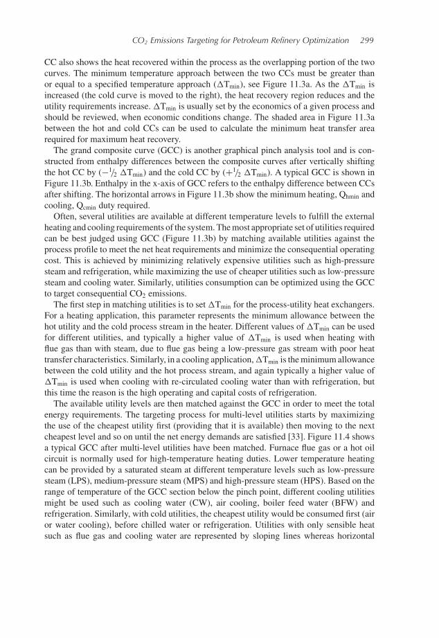
energy requirements. The targeting process for multi-level utilities starts by maximizingthe use of the cheapest utility first (providing that it is available) then moving to the nextcheapest level and so on until the net energy demands are satisfied [33]. Figure 11.4 showsa typical GCC after multi-level utilities have been matched. Furnace flue gas or a hot oilcircuit is normally used for high-temperature heating duties. Lower temperature heatingcan be provided by a saturated steam at different temperature levels such as low-pressuresteam (LPS), medium-pressure steam (MPS) and high-pressure steam (HPS). Based on therange of temperature of the GCC section below the pinch point, different cooling utilitiesmight be used such as cooling water (CW), air cooling, boiler feed water (BFW) andrefrigeration. Similarly, with cold utilities, the cheapest utility would be consumed first (airor water cooling), before chilled water or refrigeration. Utilities with only sensible heatsuch as flue gas and cooling water are represented by sloping lines whereas horizontal
300 Multi-Objective Optimization in Chemical Engineering
Process pinch
Heat load (MW)Heat load (MW)
MPSHPS
Flu
e ga
s
CW
0 20 40 60 80
Ref
Utilitypinches
(a) (b)
Qhmin
TTFT
Qcmin
Tem
pera
ture
(°C
)
Tem
pera
ture
(°C
)Figure 11.4 GCC with utility distribution: (a) before and (b) after matching multi-level utilities.
lines are used to represent single-component utilities that absorb or liberate their latent heatduring condensation or boiling such as saturated steam and pure refrigerants. The utilitypinch points, as shown in Figure 11.4, occur when the maximum heat duty is used at eachutility level. Once the different utilities have been matched against the GCC and the load ofeach utility has been determined, details of different utilities, including their marginal costsand consequential emissions, are used to estimate the operating cost and total emissions ofthe utility system.
11.1.3.2 Total Site Pinch Analysis
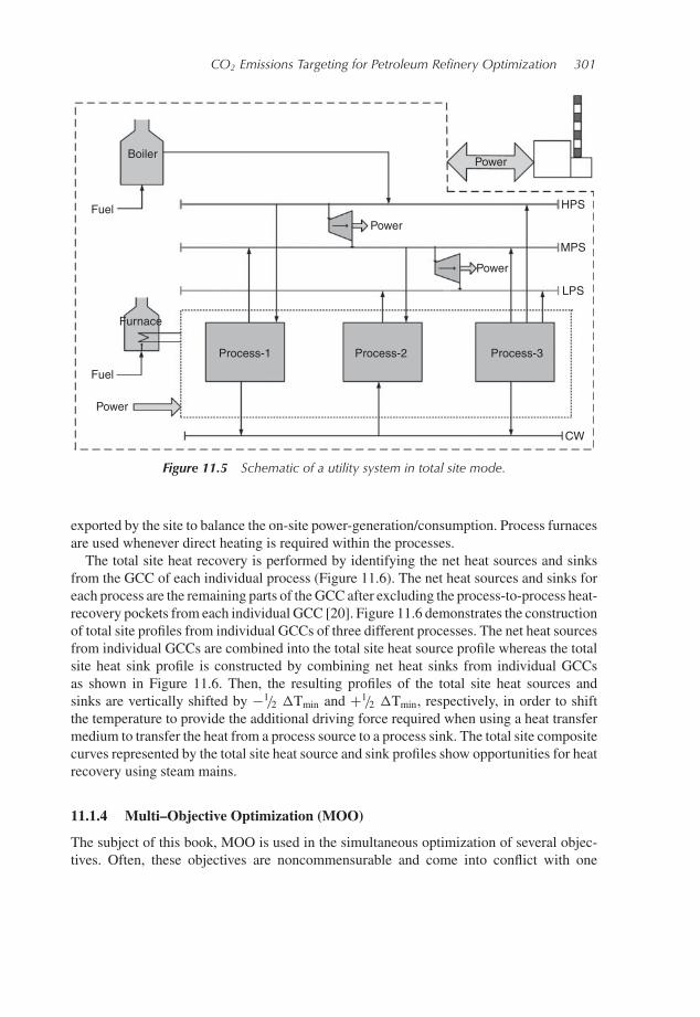
There are two modes of heat integration for a site with multiple processing units. First,there is direct integration where all hot and cold streams from different processes areassumed to be available. In this case, the minimum heating and cooling demands andthe best application for utilities can be determined using CC and GCC of the integratedprocesses, identical to a single processing unit. However, direct integration assumes thatdifferent processes will never be operated independently of each other so that heat is alwaysavailable to be transferred. Often this is not the case and the utility system is required tocompensate. Therefore, a more practical approach is indirect integration, or so-called totalsite heat recovery [34], where pinch analysis is applied to individual processes in orderto maximize heat recovery and these processes are then linked to the same utility system.Figure 11.5 shows a schematic of a multi-process site involving three different processes.Both consumption and generation of utilities such as steamand coolingwater fromprocessesare linked through a central utility system. A main steam boiler is used to supply the steamat different mains and co-generate power via expansion turbines. The power is imported or
CO2 Emissions Targeting for Petroleum Refinery Optimization 301
Boiler
FuelPower
Power
Power
Process-3Process-2Process-1
Furnace
Fuel
Power
HPS
MPS
LPS
CW
Figure 11.5 Schematic of a utility system in total site mode.
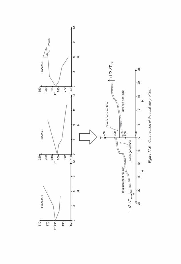
exported by the site to balance the on-site power-generation/consumption. Process furnacesare used whenever direct heating is required within the processes.The total site heat recovery is performed by identifying the net heat sources and sinks
from the GCC of each individual process (Figure 11.6). The net heat sources and sinks foreach process are the remaining parts of theGCC after excluding the process-to-process heat-recovery pockets from each individual GCC [20]. Figure 11.6 demonstrates the constructionof total site profiles from individual GCCs of three different processes. The net heat sourcesfrom individual GCCs are combined into the total site heat source profile whereas the totalsite heat sink profile is constructed by combining net heat sinks from individual GCCsas shown in Figure 11.6. Then, the resulting profiles of the total site heat sources andsinks are vertically shifted by −1/2 �Tmin and +1/2 �Tmin, respectively, in order to shiftthe temperature to provide the additional driving force required when using a heat transfermedium to transfer the heat from a process source to a process sink. The total site compositecurves represented by the total site heat source and sink profiles show opportunities for heatrecovery using steam mains.
11.1.4 Multi–Objective Optimization (MOO)
The subject of this book, MOO is used in the simultaneous optimization of several objec-tives. Often, these objectives are noncommensurable and come into conflict with one
Pro
cess
-131
0
270
230
T
T
T
190
150
03
6 H
9
T40
0
300
200
Tota
l site
hea
t sin
k
Ste
am c
onsu
mpt
ion
Ste
am g
ener
atio
n
HH
Tota
l site
hea
t sou
rce
2520
1510
50
510
1520
25
–1/2
ΔT
min
+1/
2 ΔT
min
100
12
Pro
cess
-232
0
240
280
200
160
120
03
6 H
912
Pro
cess
-3
Poc
ket
350
310
330
290
270
250
03
6 H
912
Figu
re11
.6C
onst
ruct
ion
ofth
eto
tals
itepr
ofile
s.
CO2 Emissions Targeting for Petroleum Refinery Optimization 303
another, and so there is no single optimum. Minimizing CO2 emissions, for example, mayaffect other objectives like profit and product yield, and so compromises must be made.Optimal solutions of MOO are a set of non-dominated solutions called Pareto-optimalsolutions. The non-dominated solutions mean that every solution is better than others in atleast one objective and worse than others in at least one other objective.Numerous studies have been reported in the MOO area since the early 1990s. These
include many different chemical engineering applications [35]. Multi-objective optimiza-tion has been applied successfully to a number of petroleum-refining operations. Differentobjectives have been optimized, such as product yields, capital cost and profit. Despiterecent studies, which applied MOO to different refinery processes [27, 30], heat integrationof multiple processes on a site and the resulting impacts on environmental targets are still tobe investigated. In this chapter, MOO is used in conjunction with both steady-state processsimulation and pinch analysis to investigate the tradeoffs associated with different levels ofCO2 emissions.
11.2 MOO-Pinch Analysis Framework to Target CO2 Emissions
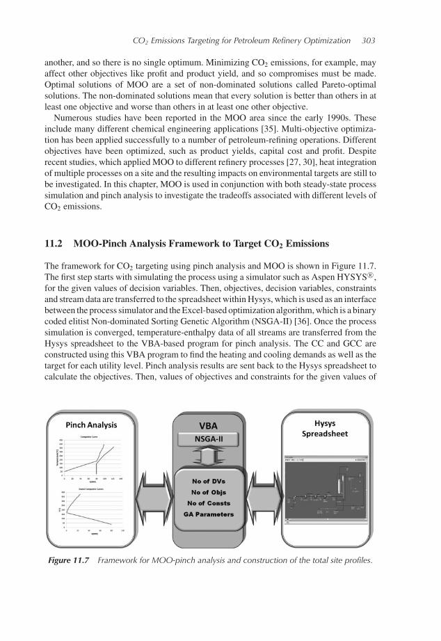
The framework for CO2 targeting using pinch analysis and MOO is shown in Figure 11.7.The first step starts with simulating the process using a simulator such as Aspen HYSYS R©,for the given values of decision variables. Then, objectives, decision variables, constraintsand stream data are transferred to the spreadsheet withinHysys, which is used as an interfacebetween the process simulator and theExcel-based optimization algorithm,which is a binarycoded elitist Non-dominated Sorting Genetic Algorithm (NSGA-II) [36]. Once the processsimulation is converged, temperature-enthalpy data of all streams are transferred from theHysys spreadsheet to the VBA-based program for pinch analysis. The CC and GCC areconstructed using this VBA program to find the heating and cooling demands as well as thetarget for each utility level. Pinch analysis results are sent back to the Hysys spreadsheet tocalculate the objectives. Then, values of objectives and constraints for the given values of
Figure 11.7 Framework for MOO-pinch analysis and construction of the total site profiles.
304 Multi-Objective Optimization in Chemical Engineering
decision variables are exported from Hysys spreadsheet to NSGA-II, to produce the nexttrial solution (i.e., values of decision variables) by the optimization algorithm. These stepscontinue until the maximum number of generations (Figure 11.7).
11.3 Case Studies
In this section, MOO-pinch analysis framework is demonstrated using two different casestudies of bi-objective optimization. The total yield of naphtha from both the CDU and FCC,Equation (11.1), is used as an economic objective to be maximized while minimizing thetotal CO2 emissions (the environmental objective), Equation (11.2). Total CO2 emissionsinclude emissions from furnaces, boilers, power importation and the FCC regenerator.These emission values are calculated by Equations 11.3 to 11.5. An Australian black coalis assumed to be used in the central power station with an emissions factor of 0.92 tonnesCO2/MWh [37]. In the first case study, direct heat integration of the CDU and FCC unitsis permitted, while the second study is on a total site integration, which only allows theexchange of heat between the CDU and FCC unit via the utility system.
Naphtha yield = (CDU Naphtha + FCC Naphtha)/Crude feed (11.1)
CO2emissions = (CO2(Furnaces) + CO2(Boilers) + CO2(power) + CO2(FCC)
)/Crude feed (11.2)
CO2(Furnaces) or CO2(Boilers) = QFuelEFact (11.3)
EFact = (RC/NHV) (C%/100) (11.4)
CO2(power) = [Power (MW)] [power emission factor (= 0.92)] (11.5)
In the above equations, QFuel = heat duty supplied by fuel (kJ/h), EFact = emission factorfor a specific fuel (kgCO2/kJ), RC = molar mass ratio of CO2 and C (=3.67), NHV = netheating value of the fuel (kJ/kg) and C% = carbon mass percent in fuel.During the optimization, 16 decision variables are allowed to vary, each within a realistic
range, to achieve optimum values for the objectives. These variables have been chosenfrom operating variables that have direct impact on both objectives. The decision variablesand their bounds are listed in Table 11.1. The objective functions are optimized, subject torelevant constraints to be kept within the defined bounds (Table 11.2). In order to maintainspecifications of products, the boiling point gaps between different products of the CDU arekept within acceptable ranges given in [38]. The remaining coke on the regenerated catalystand maximum regeneration temperature must be constrained to maintain activity and avoidthe decomposition of catalyst [39]. The concentration of CO in the regenerator flue gas mustbe as low as possible for full combustion mode regeneration to ensure complete combustioninside the regenerator and minimize pollution [39].Preliminary numerical experiments in order to select the appropriate NSGA-II param-
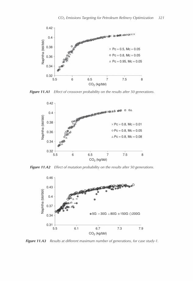
eters are shown in Appendix 11.A2. Values of computational parameters in the NSGA-IIalgorithm used are: random number seed = 0.857, crossover probability = 0.8, mutationprobability = 0.05 and population size = 50. Around 200 generations are required toprovide a smooth set of Pareto optimal solutions; see Figures 11.A1 to 11.A4.

CO2 Emissions Targeting for Petroleum Refinery Optimization 305
Table 11.1 Decision variables and their bounds.
Decision variable UnitsLowerbound
Upperbound Type
ADU feed temperature (AtmT) ◦C 350 380 ContinuousLight crude fraction 0.1 0.9 ContinuousKerosene reboiler duty (KerRQ) GJ/h 10 100 ContinuousVDU feed temperature (VacT) ◦C 360 400 ContinuousFCC feed temperature (FCCT) ◦C 380 400 ContinuousRiser temperature ◦C 480 520 ContinuousADU PA3 return temperature
(APA3T)
◦C 250 300 Continuous
ADU PA3 flow rate (APA3F) m3/h 150 300 ContinuousVDU PA3 return temperature
(VPA3T)
◦C 280 320 Continuous
VDU PA3 flow rate (VPA3F) m3/h 100 200 ContinuousMain fractionator PA3 flow
rate (MPA3F)m3/h 100 400 Continuous
Main fractionator PA3temperature drop (MPA3DT)
◦C 30 100 Continuous
Main fractionator PA3 drawstage (MPA3DS)
7 10 Discrete
Main fractionator PA4 flowrate (MPA4F)
m3/h 100 500 Continuous
Main fractionator PA4temperature drop (MPA4DT)
◦C 50 130 Continuous
Main fractionator PA4 drawstage (MPA4DS)
11 13 Discrete
11.3.1 Case Study 1: Direct Heat Integration
This case study involves the direct heat integration of all process streams within the CDUand FCC units. The Pareto optimal solutions obtained by simultaneously minimizing CO2emissions and maximizing naphtha product from the integrated model of the CDU and
Table 11.2 Constraints in the MOO problem.
Constraint Specification
Kerosene-Naphtha (5–95) Gap >16.7 ◦CDiesel-Kerosene (5–95) Gap >0 ◦CAGO-Diesel (5–95) Gap >–11 ◦CCoke on reg. catalyst <0.1 wt%Regeneration temperature <717 ◦CCO in the flue gas <0.2 wt%
306 Multi-Objective Optimization in Chemical Engineering
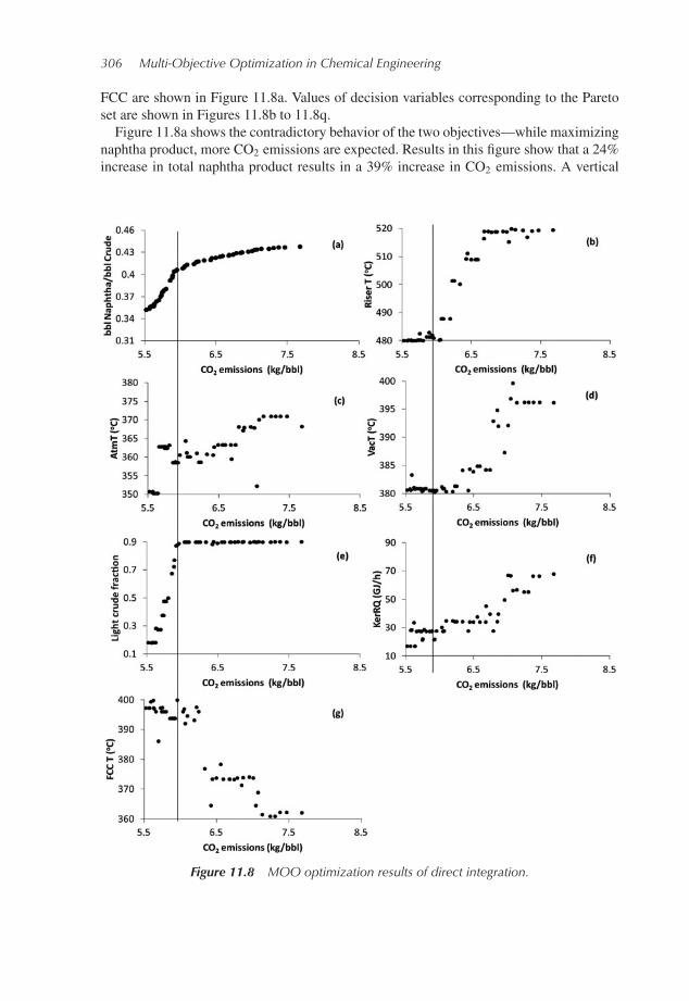
FCC are shown in Figure 11.8a. Values of decision variables corresponding to the Paretoset are shown in Figures 11.8b to 11.8q.Figure 11.8a shows the contradictory behavior of the two objectives—while maximizing
naphtha product, more CO2 emissions are expected. Results in this figure show that a 24%increase in total naphtha product results in a 39% increase in CO2 emissions. A vertical
Figure 11.8 MOO optimization results of direct integration.
CO2 Emissions Targeting for Petroleum Refinery Optimization 307
Figure 11.8 (Continued)
308 Multi-Objective Optimization in Chemical Engineering
2600 1200
1100
1000
900
800
700
600
CDU-Naphtha
FCC-Naphtha FC
C-N
apht
ha (
bbl/h
r)
CD
U-N
apht
ha (
bbl/h
r)2400
2200
20005.5 6.5
CO2 emissions (kg/bbl)
7.5 8.5
Figure 11.9 Optimum values of naphtha flow rate from the CDU and FCC.
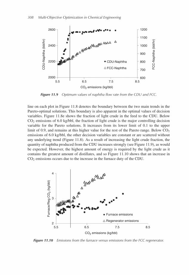
line on each plot in Figure 11.8 denotes the boundary between the two main trends in thePareto-optimal solutions. This boundary is also apparent in the optimal values of decisionvariables. Figure 11.8e shows the fraction of light crude in the feed to the CDU. BelowCO2 emissions of 6.0 kg/bbl, the fraction of light crude is the major controlling decisionvariable for the Pareto solutions. It increases from its lower limit of 0.1 to the upperlimit of 0.9, and remains at this higher value for the rest of the Pareto range. Below CO2emissions of 6.0 kg/bbl, the other decision variables are constant or are scattered withoutany underlying trend (Figure 11.8). As a result of increasing the light crude fraction, thequantity of naphtha produced from the CDU increases strongly (see Figure 11.9), as wouldbe expected. However, the highest amount of energy is required by the light crude as itcontains the greatest amount of distillates, and so Figure 11.10 shows that an increase inCO2 emissions occurs due to the increase in the furnace duty of the CDU.
Furnace emissions
Regenerator emissions
CO2 emissions (kg/bbl)
Fur
nace
/Reg
CO
2 (k
g/bb
l)
5.52
3
4
6.5 7.5 8.5
Figure 11.10 Emissions from the furnace versus emissions from the FCC regenerator.
CO2 Emissions Targeting for Petroleum Refinery Optimization 309
3500
3200
2900
2600
2300
CO2 emissions (kg/bbl)
FC
C fe
ed (
bbl/h
r)
5.5 6.5 7.5 8.5
Figure 11.11 Variation of flow rate of FCC feedstock with CO2 emissions.
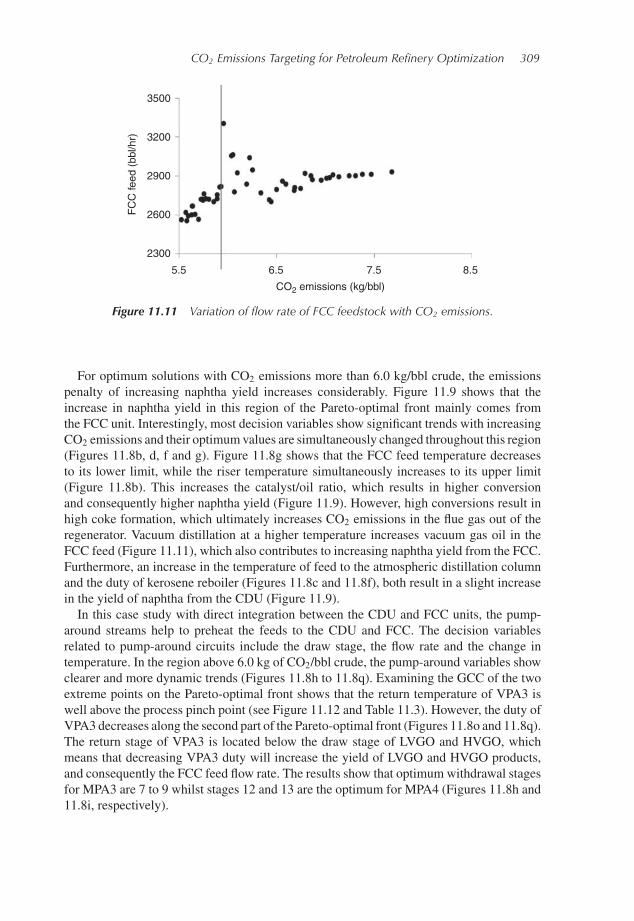
For optimum solutions with CO2 emissions more than 6.0 kg/bbl crude, the emissionspenalty of increasing naphtha yield increases considerably. Figure 11.9 shows that theincrease in naphtha yield in this region of the Pareto-optimal front mainly comes fromthe FCC unit. Interestingly, most decision variables show significant trends with increasingCO2 emissions and their optimumvalues are simultaneously changed throughout this region(Figures 11.8b, d, f and g). Figure 11.8g shows that the FCC feed temperature decreasesto its lower limit, while the riser temperature simultaneously increases to its upper limit(Figure 11.8b). This increases the catalyst/oil ratio, which results in higher conversionand consequently higher naphtha yield (Figure 11.9). However, high conversions result inhigh coke formation, which ultimately increases CO2 emissions in the flue gas out of theregenerator. Vacuum distillation at a higher temperature increases vacuum gas oil in theFCC feed (Figure 11.11), which also contributes to increasing naphtha yield from the FCC.Furthermore, an increase in the temperature of feed to the atmospheric distillation columnand the duty of kerosene reboiler (Figures 11.8c and 11.8f), both result in a slight increasein the yield of naphtha from the CDU (Figure 11.9).In this case study with direct integration between the CDU and FCC units, the pump-
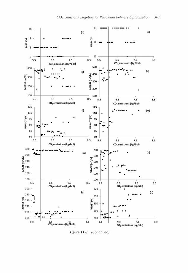
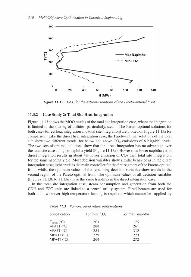
around streams help to preheat the feeds to the CDU and FCC. The decision variablesrelated to pump-around circuits include the draw stage, the flow rate and the change intemperature. In the region above 6.0 kg of CO2/bbl crude, the pump-around variables showclearer and more dynamic trends (Figures 11.8h to 11.8q). Examining the GCC of the twoextreme points on the Pareto-optimal front shows that the return temperature of VPA3 iswell above the process pinch point (see Figure 11.12 and Table 11.3). However, the duty ofVPA3 decreases along the second part of the Pareto-optimal front (Figures 11.8o and 11.8q).The return stage of VPA3 is located below the draw stage of LVGO and HVGO, whichmeans that decreasing VPA3 duty will increase the yield of LVGO and HVGO products,and consequently the FCC feed flow rate. The results show that optimumwithdrawal stagesfor MPA3 are 7 to 9 whilst stages 12 and 13 are the optimum for MPA4 (Figures 11.8h and11.8i, respectively).
310 Multi-Objective Optimization in Chemical Engineering
Figure 11.12 GCC for the extreme solutions of the Pareto-optimal front.
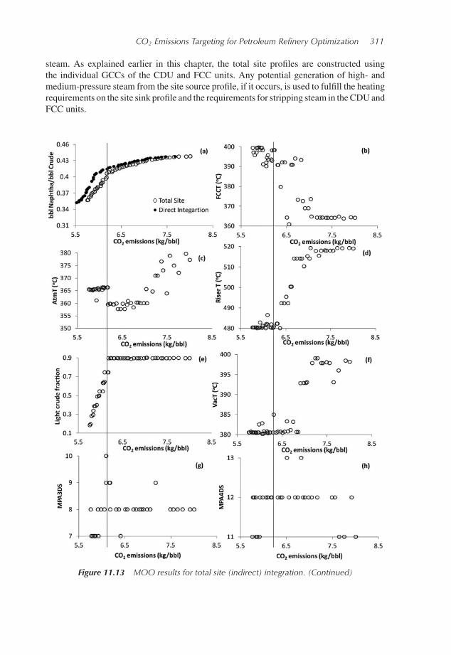
11.3.2 Case Study 2: Total Site Heat Integration
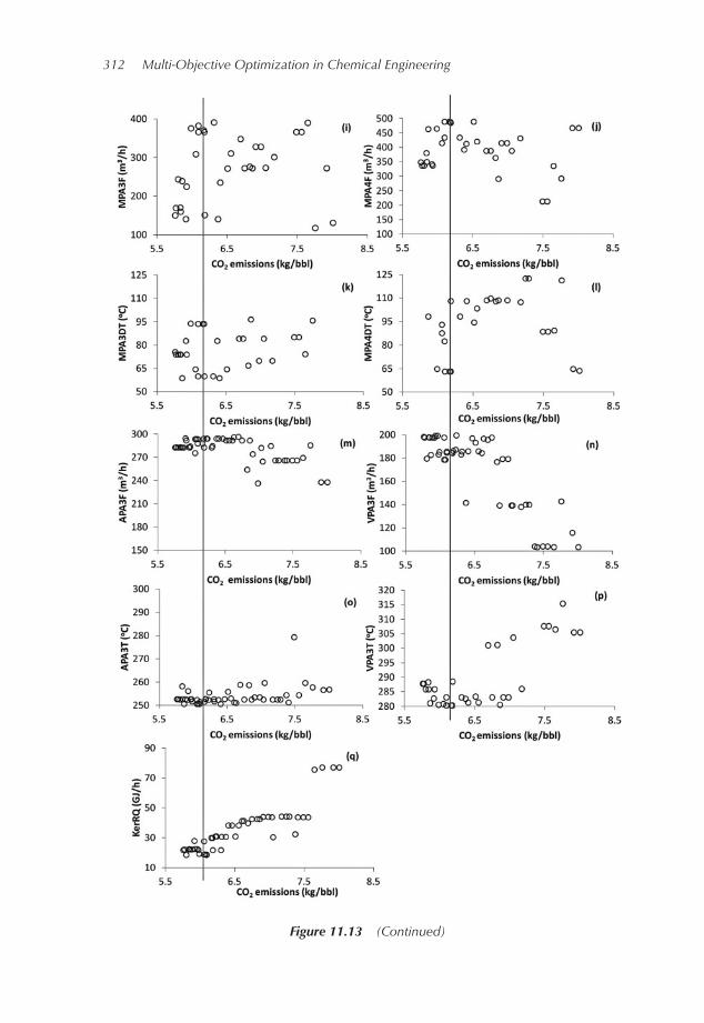
Figure 11.13 shows the MOO results of the total site integration case, where the integrationis limited to the sharing of utilities, particularly, steam. The Pareto-optimal solutions forboth cases (direct heat integration and total site integration) are plotted on Figure 11.13a forcomparison. Like the direct heat integration case, the Pareto-optimal solutions of the totalsite show two different trends, for below and above CO2 emissions of 6.2 kg/bbl crude.The two sets of optimal solutions show that the direct integration has no advantage overthe total site case at higher naphtha yield (Figure 11.13a). However, at lower naphtha yield,direct integration results in about 4% lower emission of CO2 than total site integration,for the same naphtha yield. Most decision variables show similar behavior as in the directintegration case; light crude is the main controller for the first segment of the Pareto-optimalfront, whilst the optimum values of the remaining decision variables show trends in thesecond region of the Pareto-optimal front. The optimum values of all decision variables(Figures 11.13b to 11.13q) have the same trends as in the direct integration case.In the total site integration case, steam consumption and generation from both the
CDU and FCC units are linked to a central utility system. Fired heaters are used forboth units wherever high-temperature heating is required, which cannot be supplied by
Table 11.3 Pump-around return temperatures.
Specification For min. CO2 For max. naphtha
Tpinch (◦C) 263 175APA3T (◦C) 288 261VPA3T (◦C) 284 312MPA3T (◦C) 229 223MPA4T (◦C) 264 272
CO2 Emissions Targeting for Petroleum Refinery Optimization 311
steam. As explained earlier in this chapter, the total site profiles are constructed usingthe individual GCCs of the CDU and FCC units. Any potential generation of high- andmedium-pressure steam from the site source profile, if it occurs, is used to fulfill the heatingrequirements on the site sink profile and the requirements for stripping steam in theCDUandFCC units.
Figure 11.13 MOO results for total site (indirect) integration. (Continued)
312 Multi-Objective Optimization in Chemical Engineering
Figure 11.13 (Continued)
CO2 Emissions Targeting for Petroleum Refinery Optimization 313
0
100
200
300
400
500
500
0
H (MW)
Pinch pointCDU
100 150
T(°
C)
0
100
200
300
400
500
0
100
200
300
400
500
50 50
H (MW) H (MW)
Site source profile
Fired heater
Site sink profile
HPS
Chilled water BFW
100 100150 150
T(°
C)
(Rea
l)
T(°
C)
(Rea
l)
0
100
200
300
400
500
50H (MW)
Pinch pointFCC
100 150
T(°
C)
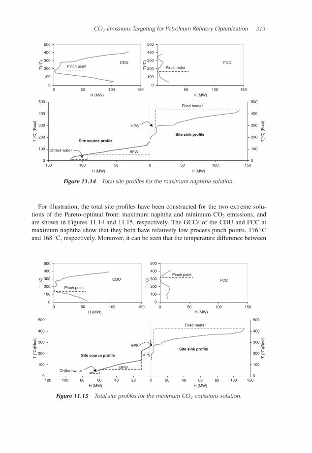
Figure 11.14 Total site profiles for the maximum naphtha solution.
For illustration, the total site profiles have been constructed for the two extreme solu-tions of the Pareto-optimal front: maximum naphtha and minimum CO2 emissions, andare shown in Figures 11.14 and 11.15, respectively. The GCCs of the CDU and FCC atmaximum naphtha show that they both have relatively low process pinch points, 176 ◦Cand 168 ◦C, respectively. Moreover, it can be seen that the temperature difference between
0
100
200
300
400
500
500 0
0
H (MW)
Pinch point
CDU
100 150
T (
°C)
0
100
200
300
400
500
0
100
200
300
400
500
80 8060 6040 4020 20H (MW) H (MW)
Site source profile
Fired heater
Site sink profileHPS
Chilled waterBFW
MPS
100 100120 150
T (
°C)(
Rea
l)
T (
°C)(
Rea
l)
0
100
200
300
400
500
50H (MW)
Pinch point
FCC
100 150
T (
°C)
Figure 11.15 Total site profiles for the minimum CO2 emissions solution.
314 Multi-Objective Optimization in Chemical Engineering
400
300
MPS
H (MW) H (MW)
MPS
HPS
LPS200
T (
°C)
100
050 5040 4030 3020 2010 100
400
300
200
T (
°C)
100
0
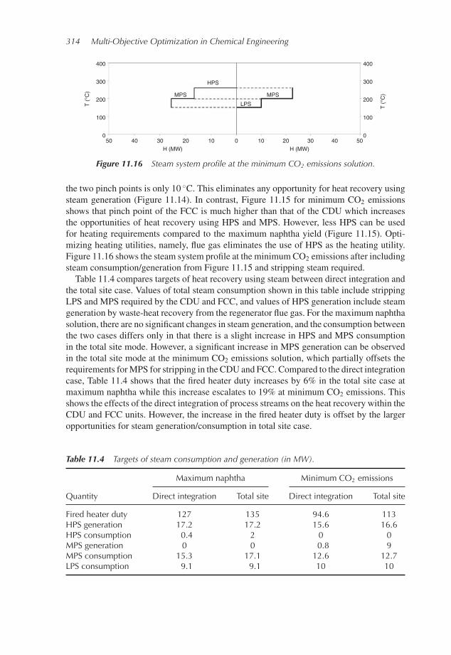
Figure 11.16 Steam system profile at the minimum CO2 emissions solution.
the two pinch points is only 10 ◦C. This eliminates any opportunity for heat recovery usingsteam generation (Figure 11.14). In contrast, Figure 11.15 for minimum CO2 emissionsshows that pinch point of the FCC is much higher than that of the CDU which increasesthe opportunities of heat recovery using HPS and MPS. However, less HPS can be usedfor heating requirements compared to the maximum naphtha yield (Figure 11.15). Opti-mizing heating utilities, namely, flue gas eliminates the use of HPS as the heating utility.Figure 11.16 shows the steam system profile at the minimumCO2 emissions after includingsteam consumption/generation from Figure 11.15 and stripping steam required.Table 11.4 compares targets of heat recovery using steam between direct integration and
the total site case. Values of total steam consumption shown in this table include strippingLPS and MPS required by the CDU and FCC, and values of HPS generation include steamgeneration by waste-heat recovery from the regenerator flue gas. For the maximum naphthasolution, there are no significant changes in steam generation, and the consumption betweenthe two cases differs only in that there is a slight increase in HPS and MPS consumptionin the total site mode. However, a significant increase in MPS generation can be observedin the total site mode at the minimum CO2 emissions solution, which partially offsets therequirements forMPS for stripping in the CDU and FCC. Compared to the direct integrationcase, Table 11.4 shows that the fired heater duty increases by 6% in the total site case atmaximum naphtha while this increase escalates to 19% at minimum CO2 emissions. Thisshows the effects of the direct integration of process streams on the heat recovery within theCDU and FCC units. However, the increase in the fired heater duty is offset by the largeropportunities for steam generation/consumption in total site case.
Table 11.4 Targets of steam consumption and generation (in MW).
Maximum naphtha Minimum CO2 emissions
Quantity Direct integration Total site Direct integration Total site
Fired heater duty 127 135 94.6 113HPS generation 17.2 17.2 15.6 16.6HPS consumption 0.4 2 0 0MPS generation 0 0 0.8 9MPS consumption 15.3 17.1 12.6 12.7LPS consumption 9.1 9.1 10 10
CO2 Emissions Targeting for Petroleum Refinery Optimization 315
11.4 Conclusions
In this chapter, a comprehensive MOO framework is introduced to find the Pareto-optimalsolutions that describe the tradeoff between economic objective(s) and CO2 emissionsassociated with energy use in chemical processes. The optimization framework enablesbetter targeting of CO2 emissions through linking pinch analysis with rigorous processmodels in process simulators and the MOO program. Two case studies of bi-objectiveoptimization, for the CDU and FCC units in petroleum refineries, have been used toillustrate the optimization framework. Direct heat integration is permitted in the first casestudy, whilst the total site mode (indirect integration) is used in the second case. The totalyield of naphtha is maximized while minimizing the total CO2 emissions.Despite difficulties in applying direct integration across a large site with many indepen-
dent process units, the analysis of this case is useful in order to set a target for maximumenergy recovery, and consequently minimum CO2 emissions, as in the CDU/FCC inte-grated model studied. However, except at the lower naphtha yields, the results show nosignificant improvement in the target of CO2 emissions between the direct integration caseand the total site case. This means the latter case is likely to be the preferred alternativeto direct integration, because of its reduced complexity of heat exchanger networks and itsgreater operational flexibility. However, the indirect approach does require greater capitalexpenditure for a larger fired heater and greater heat exchange area.The MOO-pinch analysis framework is a rigorous method of optimizing heat-integration
schemes and a powerful tool for optimizing process flow sheets for multiple economic andenvironmental objectives. This is the first demonstration of this technique using a total siteintegration approach, across two significant units in petroleum refineries.
Nomenclature
ADU atmospheric distillation unit.AGO atmospheric gas oil.APA atmospheric distillation pump around.APA3T ADU PA3 return temperature (◦C).APA3F ADU PA3 flow rate (m3/h).AtmT ADU feed temperature (◦C).BFW boiling feed water.C% carbon mass percent in fuel.CC composite curves.CCCold cold composite curve.CCHot hot composite curve.CDU crude distillation column.CP heat capacity (MW/◦C).CPc heat capacity of cold stream (MW/◦C).CPh heat capacity of hot stream (MW/◦C).CPcw heat capacity of cooling water (kJ/kg. ◦C).CW cooling water.EFact emission factor for a specific fuel (kgCO2/kJ).
316 Multi-Objective Optimization in Chemical Engineering
FCC fluidized-bed catalytic cracker.FCCT FCC feed temperature (◦C).GCC grand composite curve.H enthalpy (MW).HEN heat exchanger network.HPS high-pressure steam.KerRQ kerosene reboiler duty (GJ/h).LCO light cycle oil.LP linear programming.LPS low pressure steam.LVGO light vacuum gas oil.HCO heavy cycle oil.HVGO heavy vacuum gas oil.Mc mutation probability.MOO multi-objective optimization.MPA main fractionator pump around.MPA3DT main fractionator PA3 temperature drop (◦C).MPA4DT main fractionator PA4 temperature drop (◦C).MPA3DS main fractionator PA3 draw stage.MPA4DS main fractionator PA4 draw stage.MPA3F main fractionator PA3 flow rate (m3/h).MPA4F main fractionator PA4 flow rate (m3/h).MPS medium pressure steam.NHV net heating value of fuel (kJ/kg).PA pump around.PA3 third pump around.PA4 fourth pump around.Pc crossover probability.Qcmin minimum cooling duty (MW).Qhmin minimum heating duty (MW).QFuel heat duty supplied by fuel (kJ/h).RC molar masses ratio of CO2.Ref refrigeration.T temperature (◦C).Thot temperature of a hot stream (◦C).Tcold temperature of a cold stream (◦C).Tin inlet temperature (◦C).Tout outlet temperature (◦C).TTFT theoretical flame temperature (◦C).To ambient temperature (◦C).TPinch pinch temperature (◦C).Tstack stack temperature (◦C).VacT VDU feed temperature (◦C).VBA Visual Basic applications.VDU vacuum distillation unit.VPA vacuum distillation pump around.
CO2 Emissions Targeting for Petroleum Refinery Optimization 317
VPA3T VDU PA3 return temperature (◦C).VPA3F VDU PA3 flow rate (m3/h).�Tmin minimum temperature difference (◦C).�Hh enthalpy difference of hot stream (MW).�Hc enthalpy difference of cold stream (MW).ηF furnace efficiency.
Exercises
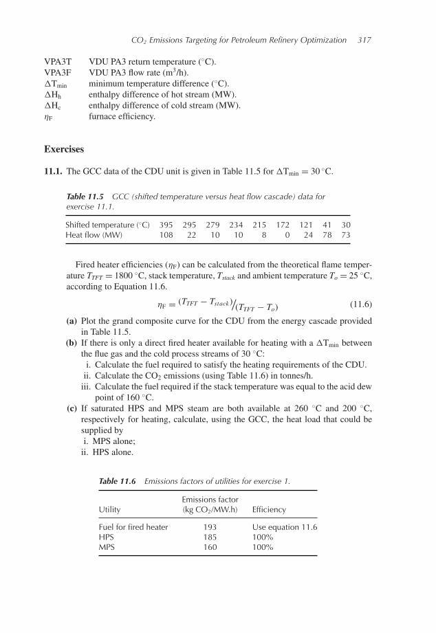
11.1. The GCC data of the CDU unit is given in Table 11.5 for �Tmin = 30 ◦C.
Table 11.5 GCC (shifted temperature versus heat flow cascade) data forexercise 11.1.
Shifted temperature (◦C) 395 295 279 234 215 172 121 41 30Heat flow (MW) 108 22 10 10 8 0 24 78 73
Fired heater efficiencies (ηF) can be calculated from the theoretical flame temper-ature TTFT = 1800 ◦C, stack temperature, Tstack and ambient temperature To = 25 ◦C,according to Equation 11.6.
ηF = (TTFT − Tstack)/(TTFT − To) (11.6)
(a) Plot the grand composite curve for the CDU from the energy cascade providedin Table 11.5.
(b) If there is only a direct fired heater available for heating with a �Tmin betweenthe flue gas and the cold process streams of 30 ◦C:i. Calculate the fuel required to satisfy the heating requirements of the CDU.ii. Calculate the CO2 emissions (using Table 11.6) in tonnes/h.iii. Calculate the fuel required if the stack temperature was equal to the acid dew
point of 160 ◦C.(c) If saturated HPS and MPS steam are both available at 260 ◦C and 200 ◦C,
respectively for heating, calculate, using the GCC, the heat load that could besupplied byi. MPS alone;ii. HPS alone.
Table 11.6 Emissions factors of utilities for exercise 1.
UtilityEmissions factor(kg CO2/MW.h) Efficiency
Fuel for fired heater 193 Use equation 11.6HPS 185 100%MPS 160 100%
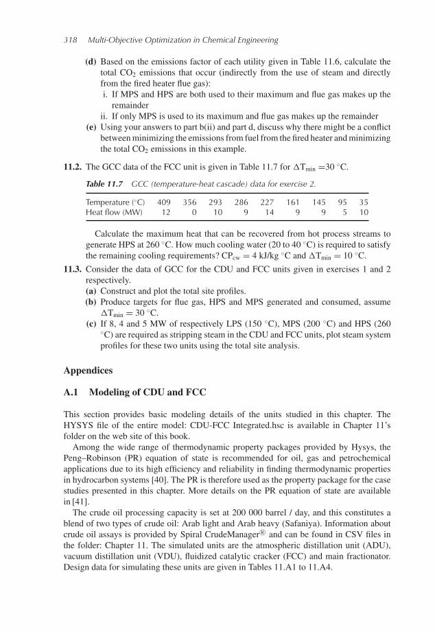
318 Multi-Objective Optimization in Chemical Engineering
(d) Based on the emissions factor of each utility given in Table 11.6, calculate thetotal CO2 emissions that occur (indirectly from the use of steam and directlyfrom the fired heater flue gas):i. If MPS and HPS are both used to their maximum and flue gas makes up theremainder
ii. If only MPS is used to its maximum and flue gas makes up the remainder(e) Using your answers to part b(ii) and part d, discuss why there might be a conflict
betweenminimizing the emissions from fuel from the fired heater andminimizingthe total CO2 emissions in this example.
11.2. The GCC data of the FCC unit is given in Table 11.7 for �Tmin =30 ◦C.
Table 11.7 GCC (temperature-heat cascade) data for exercise 2.
Temperature (◦C) 409 356 293 286 227 161 145 95 35Heat flow (MW) 12 0 10 9 14 9 9 5 10
Calculate the maximum heat that can be recovered from hot process streams togenerate HPS at 260 ◦C. How much cooling water (20 to 40 ◦C) is required to satisfythe remaining cooling requirements? CPcw = 4 kJ/kg ◦C and �Tmin = 10 ◦C.
11.3. Consider the data of GCC for the CDU and FCC units given in exercises 1 and 2respectively.(a) Construct and plot the total site profiles.(b) Produce targets for flue gas, HPS and MPS generated and consumed, assume
�Tmin = 30 ◦C.(c) If 8, 4 and 5 MW of respectively LPS (150 ◦C), MPS (200 ◦C) and HPS (260
◦C) are required as stripping steam in the CDU and FCC units, plot steam systemprofiles for these two units using the total site analysis.
Appendices
A.1 Modeling of CDU and FCC
This section provides basic modeling details of the units studied in this chapter. TheHYSYS file of the entire model: CDU-FCC Integrated.hsc is available in Chapter 11’sfolder on the web site of this book.Among the wide range of thermodynamic property packages provided by Hysys, the
Peng–Robinson (PR) equation of state is recommended for oil, gas and petrochemicalapplications due to its high efficiency and reliability in finding thermodynamic propertiesin hydrocarbon systems [40]. The PR is therefore used as the property package for the casestudies presented in this chapter. More details on the PR equation of state are availablein [41].The crude oil processing capacity is set at 200 000 barrel / day, and this constitutes a
blend of two types of crude oil: Arab light and Arab heavy (Safaniya). Information aboutcrude oil assays is provided by Spiral CrudeManager R© and can be found in CSV files inthe folder: Chapter 11. The simulated units are the atmospheric distillation unit (ADU),vacuum distillation unit (VDU), fluidized catalytic cracker (FCC) and main fractionator.Design data for simulating these units are given in Tables 11.A1 to 11.A4.
CO2 Emissions Targeting for Petroleum Refinery Optimization 319
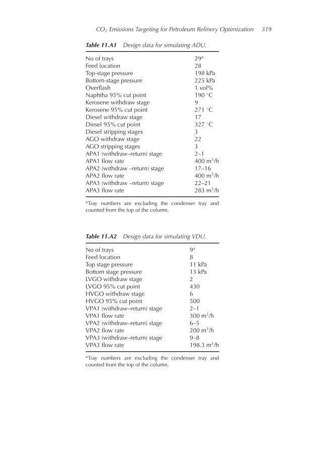
Table 11.A1 Design data for simulating ADU.
No of trays 29a
Feed location 28Top-stage pressure 198 kPaBottom-stage pressure 225 kPaOverflash 1 vol%Naphtha 95% cut point 190 ◦CKerosene withdraw stage 9Kerosene 95% cut point 271 ◦CDiesel withdraw stage 17Diesel 95% cut point 327 ◦CDiesel stripping stages 3AGO withdraw stage 22AGO stripping stages 3APA1 (withdraw–return) stage 2–1APA1 flow rate 400 m3/hAPA2 (withdraw –return) stage 17–16APA2 flow rate 400 m3/hAPA3 (withdraw –return) stage 22–21APA3 flow rate 283 m3/h
aTray numbers are excluding the condenser tray andcounted from the top of the column.
Table 11.A2 Design data for simulating VDU.
No of trays 9a
Feed location 8Top stage pressure 11 kPaBottom stage pressure 13 kPaLVGO withdraw stage 2LVGO 95% cut point 430HVGO withdraw stage 6HVGO 95% cut point 500VPA1 (withdraw–return) stage 2–1VPA1 flow rate 300 m3/hVPA2 (withdraw–return) stage 6–5VPA2 flow rate 200 m3/hVPA3 (withdraw–return) stage 9–8VPA3 flow rate 198.3 m3/h
aTray numbers are excluding the condenser tray andcounted from the top of the column.
320 Multi-Objective Optimization in Chemical Engineering
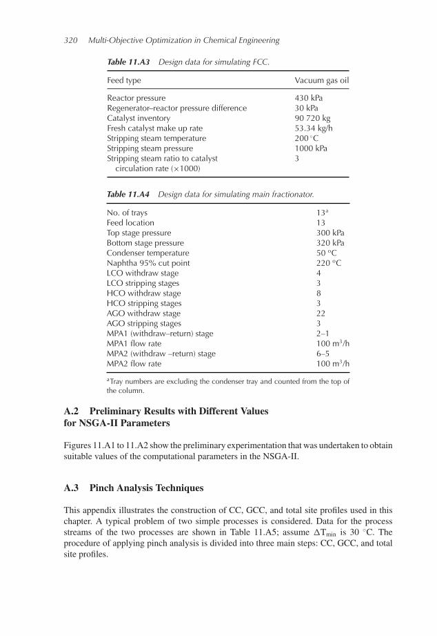
Table 11.A3 Design data for simulating FCC.
Feed type Vacuum gas oil
Reactor pressure 430 kPaRegenerator–reactor pressure difference 30 kPaCatalyst inventory 90 720 kgFresh catalyst make up rate 53.34 kg/hStripping steam temperature 200 ◦CStripping steam pressure 1000 kPaStripping steam ratio to catalyst
circulation rate (×1000)3
Table 11.A4 Design data for simulating main fractionator.
No. of trays 13a
Feed location 13Top stage pressure 300 kPaBottom stage pressure 320 kPaCondenser temperature 50 oCNaphtha 95% cut point 220 oCLCO withdraw stage 4LCO stripping stages 3HCO withdraw stage 8HCO stripping stages 3AGO withdraw stage 22AGO stripping stages 3MPA1 (withdraw–return) stage 2–1MPA1 flow rate 100 m3/hMPA2 (withdraw –return) stage 6–5MPA2 flow rate 100 m3/h
aTray numbers are excluding the condenser tray and counted from the top ofthe column.
A.2 Preliminary Results with Different Valuesfor NSGA-II Parameters
Figures 11.A1 to 11.A2 show the preliminary experimentation that was undertaken to obtainsuitable values of the computational parameters in the NSGA-II.
A.3 Pinch Analysis Techniques
This appendix illustrates the construction of CC, GCC, and total site profiles used in thischapter. A typical problem of two simple processes is considered. Data for the processstreams of the two processes are shown in Table 11.A5; assume �Tmin is 30 ◦C. Theprocedure of applying pinch analysis is divided into three main steps: CC, GCC, and totalsite profiles.
CO2 Emissions Targeting for Petroleum Refinery Optimization 321
Nap
htha
(bb
l/bbl
)
0.42
0.4
0.38
0.36
0.34
0.32
CO2 (kg/bbl)
Pc = 0.5, Mc = 0.05
Pc = 0.8, Mc = 0.05
Pc = 0.95, Mc = 0.05
5.5 6 6.5 7 7.5 8
Figure 11.A1 Effect of crossover probability on the results after 50 generations.
Nap
htha
(bb
l/bbl
)
0.42
0.4
0.38
0.36
0.34
0.32
CO2 (kg/bbl)
5.5 6 6.5 7 7.5 8
Pc = 0.8, Mc = 0.01
Pc = 0.8, Mc = 0.05
Pc = 0.8, Mc = 0.08
Figure 11.A2 Effect of mutation probability on the results after 50 generations.
Nap
htha
(bb
l/bbl
)
0.46
0.43
0.4
0.37
0.34
0.31
CO2 (kg/bbl)
5G 30G 80G 150G 200G
5.5 6.1 6.7 7.3 7.9
Figure 11.A3 Results at different maximum number of generations, for case study-1.
322 Multi-Objective Optimization in Chemical Engineering
Nap
htha
(bb
l/bbl
)
0.46
0.43
0.4
0.37
0.34
0.31
CO2 (kg/bbl)
5.5 6.1 6.7 7.3 7.9 8.5
5G 30G 80G 150G 200G
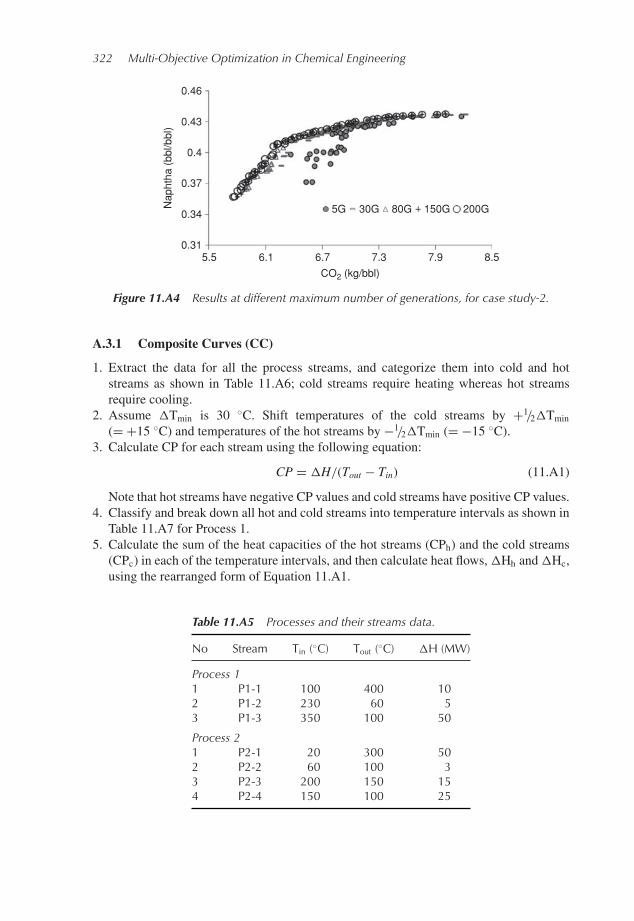
Figure 11.A4 Results at different maximum number of generations, for case study-2.
A.3.1 Composite Curves (CC)
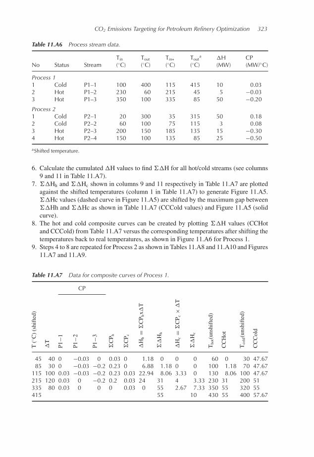
1. Extract the data for all the process streams, and categorize them into cold and hotstreams as shown in Table 11.A6; cold streams require heating whereas hot streamsrequire cooling.
2. Assume �Tmin is 30 ◦C. Shift temperatures of the cold streams by +1/2�Tmin(= +15 ◦C) and temperatures of the hot streams by −1/2�Tmin (= −15 ◦C).
3. Calculate CP for each stream using the following equation:
CP = �H/(Tout − Tin) (11.A1)
Note that hot streams have negative CP values and cold streams have positive CP values.4. Classify and break down all hot and cold streams into temperature intervals as shown inTable 11.A7 for Process 1.
5. Calculate the sum of the heat capacities of the hot streams (CPh) and the cold streams(CPc) in each of the temperature intervals, and then calculate heat flows,�Hh and�Hc,using the rearranged form of Equation 11.A1.
Table 11.A5 Processes and their streams data.
No Stream Tin (◦C) Tout (◦C) �H (MW)
Process 11 P1-1 100 400 102 P1-2 230 60 53 P1-3 350 100 50
Process 21 P2-1 20 300 502 P2-2 60 100 33 P2-3 200 150 154 P2-4 150 100 25
CO2 Emissions Targeting for Petroleum Refinery Optimization 323
Table 11.A6 Process stream data.
Tin Tout Tin∗ Touta �H CP
No Status Stream (◦C) (◦C) (◦C) (◦C) (MW) (MW/◦C)
Process 11 Cold P1–1 100 400 115 415 10 0.032 Hot P1–2 230 60 215 45 5 −0.033 Hot P1–3 350 100 335 85 50 −0.20
Process 21 Cold P2–1 20 300 35 315 50 0.182 Cold P2–2 60 100 75 115 3 0.083 Hot P2–3 200 150 185 135 15 −0.304 Hot P2–4 150 100 135 85 25 −0.50
aShifted temperature.
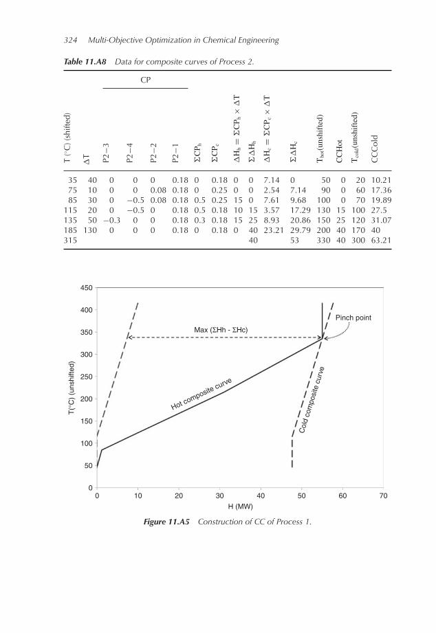
6. Calculate the cumulated �H values to find ��H for all hot/cold streams (see columns9 and 11 in Table 11.A7).
7. ��Hh and ��Hc shown in columns 9 and 11 respectively in Table 11.A7 are plottedagainst the shifted temperatures (column 1 in Table 11.A7) to generate Figure 11.A5.��Hc values (dashed curve in Figure 11.A5) are shifted by the maximum gap between��Hh and ��Hc as shown in Table 11.A7 (CCCold values) and Figure 11.A5 (solidcurve).
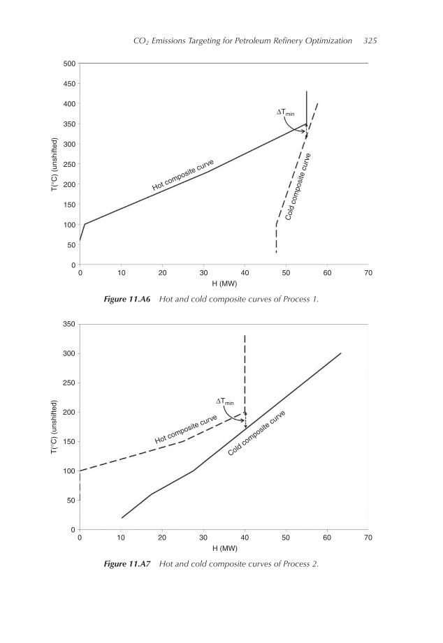
8. The hot and cold composite curves can be created by plotting ��H values (CCHotand CCCold) from Table 11.A7 versus the corresponding temperatures after shifting thetemperatures back to real temperatures, as shown in Figure 11.A6 for Process 1.
9. Steps 4 to 8 are repeated for Process 2 as shown in Tables 11.A8 and 11.A10 and Figures11.A7 and 11.A9.
Table 11.A7 Data for composite curves of Process 1.
CP
T(◦C)(shifted)
�T
P1−1
P1−2
P1−3
�CP h
�CP c
�Hh
=�CP hx�T
��Hh
�Hc=
�CP c
�T
��Hc
Thot(unshifted)
CCHot
Tcold(unshifted)
CCCold
45 40 0 −0.03 0 0.03 0 1.18 0 0 0 60 0 30 47.6785 30 0 −0.03 −0.2 0.23 0 6.88 1.18 0 0 100 1.18 70 47.67
115 100 0.03 −0.03 −0.2 0.23 0.03 22.94 8.06 3.33 0 130 8.06 100 47.67215 120 0.03 0 −0.2 0.2 0.03 24 31 4 3.33 230 31 200 51335 80 0.03 0 0 0 0.03 0 55 2.67 7.33 350 55 320 55415 55 10 430 55 400 57.67
324 Multi-Objective Optimization in Chemical Engineering
Table 11.A8 Data for composite curves of Process 2.
CP
T(◦ C
)(sh
ifted
)
�T P2−3
P2−4
P2−2
P2−1
�CP h
�CP c
�Hh
=�CP h
�T
��Hh
�Hc=
�CP c
�T
��Hc
Thot(unshifted)
CCHot
Tcold(unshifted)
CC
Col
d
35 40 0 0 0 0.18 0 0.18 0 0 7.14 0 50 0 20 10.2175 10 0 0 0.08 0.18 0 0.25 0 0 2.54 7.14 90 0 60 17.3685 30 0 −0.5 0.08 0.18 0.5 0.25 15 0 7.61 9.68 100 0 70 19.89
115 20 0 −0.5 0 0.18 0.5 0.18 10 15 3.57 17.29 130 15 100 27.5135 50 −0.3 0 0 0.18 0.3 0.18 15 25 8.93 20.86 150 25 120 31.07185 130 0 0 0 0.18 0 0.18 0 40 23.21 29.79 200 40 170 40315 40 53 330 40 300 63.21
0 10 20 30 40
H (MW)
Hot composite curve
Col
d co
mpo
site
cur
ve
50 60 70
T(°
C)
(uns
hifte
d)
0
50
100
150
200
250
300
350 Max (ΣHh - ΣHc)
Pinch point400
450
Figure 11.A5 Construction of CC of Process 1.
CO2 Emissions Targeting for Petroleum Refinery Optimization 325
T(°
C)
(uns
hifte
d)
0
50
100
150
200
250
300
350
400
500
450
0 10 20 30 40
H (MW)
50 60 70
Hot composite curve
Col
d co
mpo
site
cur
ve
ΔTmin
Figure 11.A6 Hot and cold composite curves of Process 1.
T(°
C)
(uns
hifte
d)
0
50
100
150
200
250
300
350
H (MW)
0 10 20 30 40 50 60 70
Hot composite curve
Cold composit
e curve
ΔTmin
Figure 11.A7 Hot and cold composite curves of Process 2.
326 Multi-Objective Optimization in Chemical Engineering
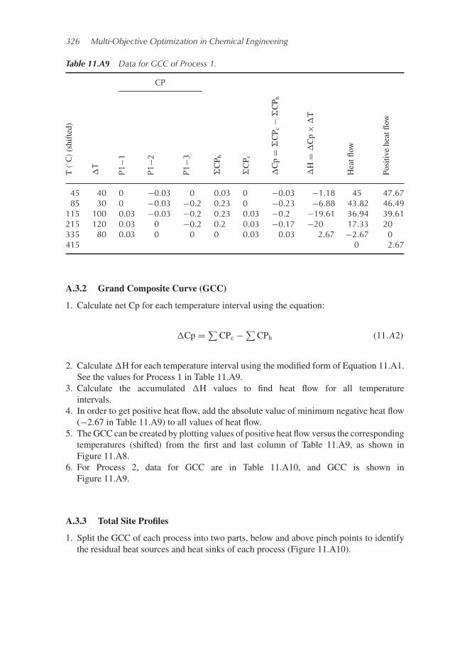
Table 11.A9 Data for GCC of Process 1.
CP
T(◦ C
)(shifted)
�T
P1−1
P1−2
P1−3
�CP h
�CP c
�Cp
=�CP c
−�CP h
�H
=�Cp
�T
Heatflow
Positiveheatflow
45 40 0 −0.03 0 0.03 0 −0.03 −1.18 45 47.6785 30 0 −0.03 −0.2 0.23 0 −0.23 −6.88 43.82 46.49
115 100 0.03 −0.03 −0.2 0.23 0.03 −0.2 −19.61 36.94 39.61215 120 0.03 0 −0.2 0.2 0.03 −0.17 −20 17.33 20335 80 0.03 0 0 0 0.03 0.03 2.67 −2.67 0415 0 2.67
A.3.2 Grand Composite Curve (GCC)
1. Calculate net Cp for each temperature interval using the equation:
�Cp = ∑CPc − ∑
CPh (11.A2)
2. Calculate�H for each temperature interval using the modified form of Equation 11.A1.See the values for Process 1 in Table 11.A9.
3. Calculate the accumulated �H values to find heat flow for all temperatureintervals.
4. In order to get positive heat flow, add the absolute value of minimum negative heat flow(−2.67 in Table 11.A9) to all values of heat flow.
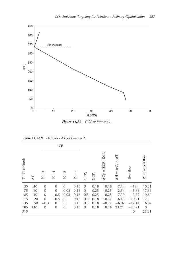
5. TheGCC can be created by plotting values of positive heat flow versus the correspondingtemperatures (shifted) from the first and last column of Table 11.A9, as shown inFigure 11.A8.
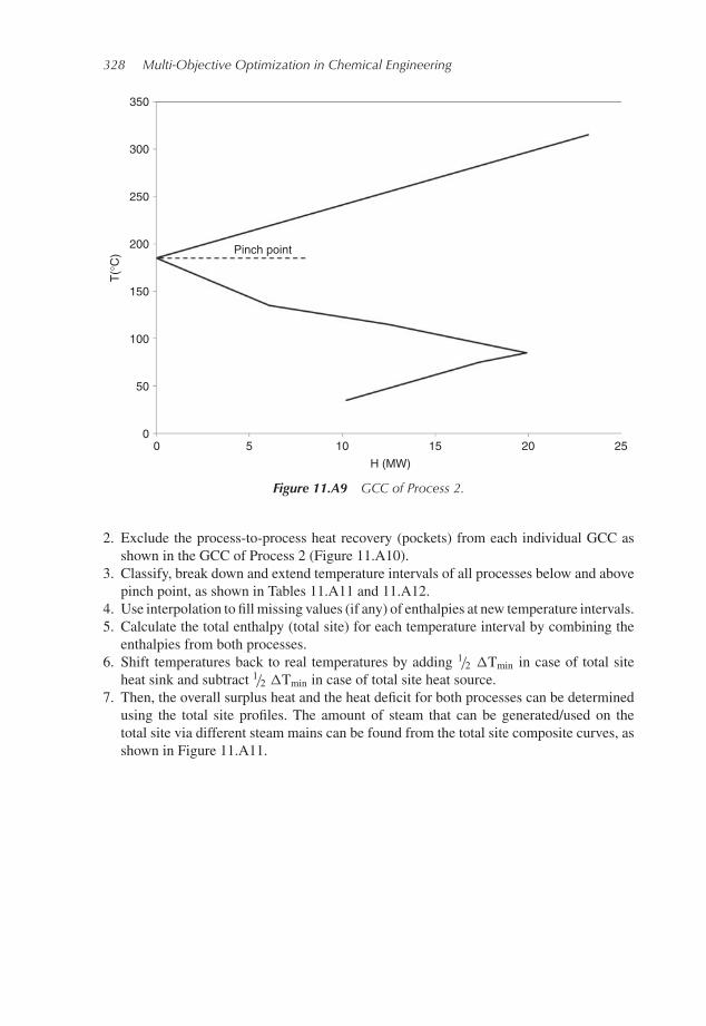
6. For Process 2, data for GCC are in Table 11.A10, and GCC is shown inFigure 11.A9.
A.3.3 Total Site Profiles
1. Split the GCC of each process into two parts, below and above pinch points to identifythe residual heat sources and heat sinks of each process (Figure 11.A10).
CO2 Emissions Targeting for Petroleum Refinery Optimization 327
T(°
C)
0
50
100
150
200
250
300
350
400
450
0 10 20 30 40
H (MW)
50 60
Pinch point
Figure 11.A8 GCC of Process 1.
Table 11.A10 Data for GCC of Process 2.
CP
T(◦ C
)(sh
ifted
)
�T P2−3
P2−4
P2−2
P2−1
�CP h
�CP c
�Cp
=�CP c
-�CP h
�H
=�Cp
�T
Heatflow
Positiveheatflow
35 40 0 0 0 0.18 0 0.18 0.18 7.14 −13 10.2175 10 0 0 0.08 0.18 0 0.25 0.25 2.54 −5.86 17.3685 30 0 −0.5 0.08 0.18 0.5 0.25 −0.25 −7.39 −3.32 19.89
115 20 0 −0.5 0 0.18 0.5 0.18 −0.32 −6.43 −10.71 12.5135 50 −0.3 0 0 0.18 0.3 0.18 −0.12 −6.07 −17.14 6.07185 130 0 0 0 0.18 0 0.18 0.18 23.21 −23.21 0315 0 23.21
328 Multi-Objective Optimization in Chemical Engineering
T(°
C)
0
50
100
150
200
250
300
350
H (MW)
0 5 10 15 20 25
Pinch point
Figure 11.A9 GCC of Process 2.
2. Exclude the process-to-process heat recovery (pockets) from each individual GCC asshown in the GCC of Process 2 (Figure 11.A10).
3. Classify, break down and extend temperature intervals of all processes below and abovepinch point, as shown in Tables 11.A11 and 11.A12.
4. Use interpolation to fill missing values (if any) of enthalpies at new temperature intervals.5. Calculate the total enthalpy (total site) for each temperature interval by combining theenthalpies from both processes.
6. Shift temperatures back to real temperatures by adding 1/2 �Tmin in case of total siteheat sink and subtract 1/2 �Tmin in case of total site heat source.
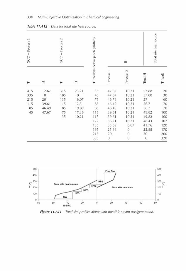
7. Then, the overall surplus heat and the heat deficit for both processes can be determinedusing the total site profiles. The amount of steam that can be generated/used on thetotal site via different steam mains can be found from the total site composite curves, asshown in Figure 11.A11.
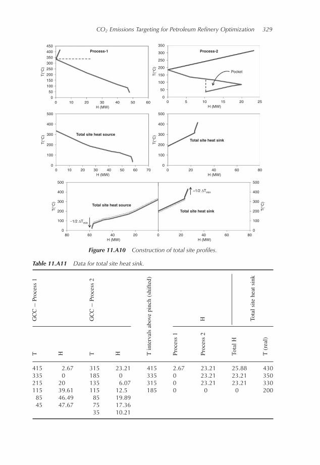
CO2 Emissions Targeting for Petroleum Refinery Optimization 329
450
400
350
300
250
200
150
100
50
0
H (MW)
Process-1
Total site heat source
Total site heat source
Total site heat sink
Total site heat sink
Process-2
0 10 20 30 40 50 60
H (MW) H (MW)0 20 40 60 800 10 20 30 40 50 60 70
H (MW) H (MW)
−1/2 ΔTmin
+1/2 ΔTmin
80 60 40 20 20 40 60 800
H (MW)
0 5 10 15 20 25
T(°
C)
500
400
300
200
100
0
T(°
C)
500
400
300
200
100
0
T(°
C)
500
400
300
200
100
0
T(°
C)
500
400
300
200
100
0
T(°
C)
350
300
250
200
150
100
50
0
T(°
C)
Figure 11.A10 Construction of total site profiles.
Table 11.A11 Data for total site heat sink.
GCC
−Process1
GCC
−Process2
H Totalsiteheatsink
T H T H Tintervalsabovepinch(shifted)
Process1
Process2
TotalH
T(real)
415 2.67 315 23.21 415 2.67 23.21 25.88 430335 0 185 0 335 0 23.21 23.21 350215 20 135 6.07 315 0 23.21 23.21 330115 39.61 115 12.5 185 0 0 0 200
85 46.49 85 19.8945 47.67 75 17.36
35 10.21
330 Multi-Objective Optimization in Chemical Engineering
Table 11.A12 Data for total site heat source.GCC
−Process1
GCC
−Process2
H Totalsiteheatsource
T H T H Tintervalsbelowpinch(shifted)
Process1
Process2
TotalH
T(real)
415 2.67 315 23.21 35 47.67 10.21 57.88 20335 0 185 0 45 47.67 10.21 57.88 30215 20 135 6.07 75 46.78 10.21 57 60115 39.61 115 12.5 85 46.49 10.21 56.7 70
85 46.49 85 19.89 85 46.49 10.21 56.7 7045 47.67 75 17.36 115 39.61 10.21 49.82 100
35 10.21 115 39.61 10.21 49.82 100122 38.21 10.21 48.43 107135 35.69 6.07 41.76 120185 25.88 0 25.88 170215 20 0 20 200335 0 0 0 320
500
400
300
200
100
0
T(°
C)
500
400
300
200
100
0
T(°
C)
Total site heat source
H (MW)80 60 40 20 0 20 40 60 80
Total site heat sink
CW
LPSMPS
HPS
HPS
Flue Gas
Figure 11.A11 Total site profiles along with possible steam use/generation.
CO2 Emissions Targeting for Petroleum Refinery Optimization 331
References
[1] D. Babusiaux,Allocation of theCO2 and pollutant emissions of a refinery to petroleumfinished product. Oil and Gas Science and Technology, 6, 685–692 (2003).
[2] D. Babusiaux, and A. Pierru, Modelling and allocation of CO2 emissions in amultiproduct industry: The case of oil refining. Applied Energy, 84, 828–841(2007).
[3] A. Pierru, Allocating the CO2 emissions of an oil refinery with Aumann–Shapleyprices. Energy Economics, 29, 563–577 (2007).
[4] A.N. Tehrani, Allocation of CO2 emissions in petroleum refineries to petroleum jointproducts: A linear programming model for practical application. Energy Economics,29, 974–997 (2007).
[5] A.N. Tehrani, Allocation of CO2 emissions in joint product industries via linearprogramming: A refinery example. Oil and Gas Science and Technology, 5, 653–662(2007).
[6] A. Szklo, and R. Schaeffer, Fuel specification, energy consumption and CO2 emissionin oil refineries. Energy, 32, 1075–1092 (2007).
[7] M.S. Ba-Shammakh, An optimization approach for integrating planning and CO2mitigation in the power and refinery sectors. Ph.D. thesis (2007), University ofWaterloo.
[8] T. Greek, Role of carbon capture in CO2 management. Petroleum TechnologyQuarterly. Spring, 63–69 (2004).
[9] I.Moore, Reducing CO2 emissions. PetroleumTechnologyQuarterly, Q2, 1–6 (2005).[10] K. Ritter, S. Nordrum, T. Shires and M. Levon, Ensuring consistent green-
house gas emissions estimates. Chemical Engineering Processes. September, 30–37(2005).
[11] J.N. Mertens, K. Minks and R.M. Spoor, Refinery CO2 challenges, Part III: Forthe prediction of CO2 emissions from a refinery, simple correlations are not alwayssufficient. A rigorous simulation tool that includes fractionation and reactor modelscan help to obtain a correct prediction of the total emissions. Petroleum TechnologyQuarterly, July, 113–121 (2006).
[12] V. Bruna, J. Hart and A. Rudman, Refinery CO2 challenges: part IV, Reducing CO2emissions with a strategic energy-improvement programmme. Petroleum TechnologyQuarterly, Q4 (2006).
[13] R.M. Spoor, Refinery CO2 challenges, Part I: measuring, reporting and reduction ofCO2 emissions, Petroleum Technology Quarterly, Q1, 1–5 (2006).
[14] K.Holmgren andC. Sternhufvud, CO2-emission reduction costs for petroleum refiner-ies in Sweden. Journal of Cleaner Production, 16, 385–394 (2008).
[15] M. Stockle, D. Carter and L. Jounes, Optimising refinery CO2 emissions. PetroleumTechnology Quarterly, Q1, 123–130 (2008).
[16] S. Ratan and R. Uffelen, Curtailing refinery CO2 through H2 plant. PetroleumTechnology Quarterly, Gas, 19–23 (2008).
[17] J. Mertens, and J. Skelland, Rising to the CO2 challenge, Part 3: CO2 emissionsreduction options in refineries, Hydrocarbon Engineering, March (2010).
[18] D. Carter, Improving refinery margins and reducing CO2, Green Forum, Dubrovnik17 June (2011).
332 Multi-Objective Optimization in Chemical Engineering
[19] B.A. Al-Riyami, J. Klemes, and S. Perry, Heat integration retrofit analysis of a heatexchanger network of a fluid catalytic cracking plant, Applied Thermal Engineering,21, 1449–1487 (2001).
[20] V.R. Dhole, and B. Linnhoff, Total site targets for fuel, co-generation, emissions, andcooling, Computational and Chemical Engineering, 17, S101–S109 (1993).
[21] B. Linnhoff andA.R. Eastwood, Overall site optimization by pinch technology, Chem-ical Engineering Research and Design, 65, S138–S144 (1987).
[22] M. Ebrahim and A. Kawari, Pinch technology: an efficient tool for chemical plantenergy and capital-cost saving, Applied Energy, 65, 45–49 (2000).
[23] M.M. Shanazari, F. Shahraki and M. Khorram, Retrofit of crude distillation unit usingprocess simulation and process integration, Proceedings of Chemeca, Melbourne,Australia (2007).
[24] J. Klemes, V.R. Dhole, K. Raissi, S.J. Perry and L. Puigjanerl, Targeting and designmethodology for reduction of fuel, power and CO, on total sites, Applied ThermalEngineering, 17, 993–1003 (1997).
[25] K. Liebmann, V.R. Dhole, M. Jobson, Integrated design of a conventional crude oildistillation tower using pinch analysis. Chemical Engineering Research and Design,76(3), 335–347 (1998).
[26] R.N.Watkins, PetroleumRefineryDistillation, 2nd edition,Gulf PublishingCompany,Houston, Texas (1979).
[27] M.A. Al-Mayyahi, A.F.A. Hoadley, N.E. Smith and G.P. Rangaiah, Investigating thetrade-off between operating revenue and CO2 emissions from crude oil distillationusing a blend of two crudes, Fuel, 90(12), 3577–3585 (2011).
[28] M. Gadalla, Z. Olujic, M. Jobson and R. Smith, Estimation and reduction of CO2emissions from crude oil distillation units, Energy, 31(13), 2398–2408 (2006).
[29] E.Worrell and C. Galitsky, Energy efficiency improvement and cost saving opportuni-ties for petroleum refineries, Environmental Energy Technologies Division, Berkeley,USA, February (2005).
[30] M.A. Al-Mayyahi, A.F.A. Hoadley, N.E. Smith and G.P. Rangaiah, Multi-objectiveoptimization of a fluidized bed catalytic cracker unit to minimize CO2 emissions,Proceedings of Chemeca, Sydney, Australia (2011).
[31] D. Boland, B. Linnhoff, The preliminary design of networks for heat exchange bysystematic methods, Chemical Engineering, 222, April (1979).
[32] R. Smith, (2005) Chemical Process Design and Integration, John Wiley & Sons, Ltd.[33] I.C. Kemp, (2006) Pinch Analysis and Process Integration: A User Guide on Process
Integration for the Efficient Use of Energy, 2nd edition, Butterworth-Heinemann.[34] B. Linnhoff and V.R. Dhole, Targeting for CO2 emissions for total sites, Chemical
Engineering Technology, 16, 256–259 (1993).[35] G.P. Rangaiah, (2009) Advances in Process Systems Engineering: Multi-Objective
Optimization, Techniques andApplications inChemical Engineering,World ScientificPublishing.
[36] S. Sharama,G.P.Rangaiah andK.S.Cheah,Multi-objective optimization usingMSEx-cel with an application to design of a falling-film evaporator system, Food and Bio-products Processing, 90, 123–134 (2012).
[37] K.A. Golonka and D.J. Brennan, Application of life cycle assesment to process selec-tion for pollutant treatment: A case study of sulfur dioxide emissions from Australia

CO2 Emissions Targeting for Petroleum Refinery Optimization 333
metallurgical smelters. Transactions of the Institution of Chemical Engineers, 74(B),May 105–119 (1996).
[38] M.J. Bagajewicz and S. Ji, Rigorous procedure for the design of conventional atmo-spheric crude fractionation units. Part I: Targeting, Industrial and Engineering Chem-istry Research 40(2), 617–626 (2011).
[39] D.Dave andN. Zhang,Multiobjective optimization of fluid catalytic cracker unit usinggenetic algorithms. Computer Aided Chemical Engineering, 14, 623–628(2003).
[40] Hyprotech Manuals, HYSYS 2.4 (Update), Appendix A—Property Methods andCalculations, AEA Technology, 2001 Hyprotech Ltd., pp. A1–69.
[41] D.Y. Peng and D.B. Robinson, A new two constant equation of state, Industrial andEngineering Chemistry Fundamentals, 15, 59–64 (1976).


