arX

iv:p

hysi

cs/0

7010

31v1

[ph

ysic

s.co

mp-

ph]

2 J

an 2

007

Coarse-grained analysis of a lattice Boltzmann model for planar streamer fronts

Wim Vanroose,∗ Giovanni Samaey, and Pieter Van LeemputDepartment of Computer Science, Katholieke Universiteit Leuven, Celestijnenlaan 200A, B-3001 Heverlee, Belgium

We study the traveling wave solutions of a lattice Boltzmann model for the planar streamer frontsthat appear in the transport of electrons through a gas in a strong electrical field. To mimic thephysical properties of the impact ionization reaction, we introduce a reaction matrix containingreaction rates that depend on the electron velocities. Via a Chapman–Enskog expansion, one is ableto find only a rough approximation for a macroscopic evolution law that describes the traveling wavesolution. We propose to compute these solutions with the help of a coarse-grained time-stepper,which is an effective evolution law for the macroscopic fields that only uses appropriately initializedsimulations of the lattice Boltzmann model over short time intervals. The traveling wave solution isfound as a fixed point of the sequential application of the coarse-grained time-stepper and a shift-back operator. The fixed point is then computed with a Newton-Krylov Solver. We compare theresulting solutions with those of the approximate PDE model, and propose a method to find theminimal physical wave speed.

I. INTRODUCTION

When a gas of neutral atoms or molecules is exposedto a strong electrical field, a small initial seed of electronscan lead to an ionization avalanche. Indeed, the seed elec-trons are accelerated by the field and gain enough energyto ionize the neutral atoms when they collide. The twoslow electrons that emerge from this reaction, i.e. theimpact and the ionized electron, are again accelerated bythe field and cause, on their turn, an ionization reaction.Simultaneously the electrical field is locally modified be-cause of the charge creation. This interplay between thedynamics of the electrons and the electrical field can leadto a multitude of phenomena studied in plasma physicssuch as arcs, glows, sparks and streamers.

In this article we will focus on the initial field drivenionization that can lead to traveling waves known asstreamer fronts. These waves have previously been stud-ied by Ebert et al. [1] who introduced and analyzed theminimal streamer model, a one-dimensional model forthe propagation of planar streamer fronts. This modelconsists of two coupled non-linear PDEs: a reaction-convection-diffusion equation for the evolution of theelectron density and a Poisson-like evolution equationfor the electrical field. The reaction term is based onthe Townsend approximation that expresses the growthof the number of electrons as a function of the local elec-trical field.

During the last two decades, however, a lot of progresshas been made in the microscopic understanding of im-pact ionization reactions in atomic and molecular sys-tems. In this reaction an impact electron ionizes the tar-get and kicks out an additional electron. There are sev-eral successful theories that can predict the exact prob-ability distribution of the escaping electron [7, 8, 9, 10].In the next decade, we expect that the theoretical tools

∗Present address: Departement Wiskunde-Informatica, Univer-

siteit Antwerpen, Middelheimlaan 1, 2020 Antwerpen, Belgium

will be able to accurately predict the microscopic physicsof electron impact on molecular targets such as N2 andO2, the most important molecules in the composition ofair. This progress in the understanding of the impactionization reaction, however, has not been incorporatedin the description of the macroscopic behavior such as theminimal streamer front of Ebert et al. Instead, such mod-els still make use of a phenomenological approximationto the reactions, such as the Townsend approximation.This article extends the minimal streamer model and in-corporates more microscopic information. We model thesystem by a Boltzmann equation, which is constructedsuch that the cross sections in the collision integral re-semble the true microscopic cross sections.

To find the traveling wave solutions of this more micro-scopic model, we exploit a separation of time scales be-tween the relaxation of the electron distribution functionto a local equilibrium and the evolution of the macro-scopic fields (electron density and electrical field). It isknown from kinetic theory that the first process is fast:once initialized, it takes a molecular gas not more thana few collisions to relax to its equilibrium state.

In kinetic theory, the fast times scales are often elimi-nated from the problem by assuming a local equilibriumdistribution function which leads to a reaction-diffusionmodel with transport coefficients that depend on the lo-cal electrical field. This reduction method, however, isonly successful in the absence of steep gradients in theelectron density [18], an assumption not valid for theplanar streamer fronts that have, typically, very steepincreases in the electron density.

In this article, we take an alternative route and findthe traveling wave solution through a so-called coarse-

grained time-stepper (CGTS) that exploits the separationof time scales to extract the effective macroscopic behav-ior. This method was proposed by Kevrekidis et al. [5]and the numerical aspects of its application to find trav-eling wave solutions of lattice Boltzmann models haverecently been studied [3]. The time-stepper uses a se-quence of computational steps to evolve the macroscopicstate. This sequence involves: (1) a lifting step, which

2

creates an appropriate electron distribution function fora given electron density, (2) a simulation step, wherethe lattice Boltzmann model is evolved over a coarse-grained time step ∆T , and (3) a restriction step, wherethe macroscopic state is extracted from the electron dis-tribution function. This method does not derive effec-tive equations explicitly, and therefore allows steep gra-dients to be present. We compare our results with thoseobtained by deriving an approximate macroscopic PDEmodel through the more traditional Chapman-Enskog ex-pansion. The paper therefore illustrates the applicabilityof the coarse-grained time-stepper on a non-trivial prob-lem where the exact macroscopic equations are hard toderive.

The outline of the paper is as follows. In section II, weshortly review the physics of the impact ionization reac-tion and the streamer fronts, and recapitulate the Boltz-mann equations. In section III, we derive from the Boltz-mann equation a lattice Boltzmann model with multiplevelocities and discuss how the ionization reaction, exter-nal field and electron diffusion are incorporated in themodel. Section IV derives a macroscopic PDE from themodel using the Chapman-Enskog expansion and dis-cusses the minimal velocity of the traveling waves. Sec-tion V formulates the coarse-grained time-stepper andVI how the traveling wave solutions are found. Finallyin section VII, we have some numerical results.

II. MODEL

A. The physics of the impact ionization reaction

The impact ionization reaction is a microscopic reac-tion where electrons with, typically, an energy around50eV collide with an atom or a molecule and ionize thistarget. The reaction rates of this process depend sensi-tively on a number of parameters. Let us consider thesimplest system: an electron hits a hydrogen atom witha bound electron in its ground state. When the incomingelectron has an energy larger than the binding energy ofthe electron in the atom, it can kick out, with a certainprobability, the bound electron that will escape, togetherwith the impact electron, from the atom. The total en-ergy of the two electrons after the collision is equal tothe energy of the incoming electron minus the originalbinding energy of the bound electron.

The reaction rates of this process are expressed by crosssections; these are probabilities that a certain event willtake place. One such cross section is the triple differ-ential cross section, which is the probability to find af-ter the collision one electron escaping in the direction(θ1, φ1) with an energy E1 and a second electron escap-ing in the direction (θ2, φ2) with an energy E2, wherethe angles are measured with respect to the axis definedby the momentum of the incoming electron. Since thetwo electrons repel each other, it is more likely that theyescape in opposite directions [13].

0

cros

ssec

tion

(arb

units

)

0 20 40 60

Energy (eV)

R

0

cros

ssec

tion

(arb

units

)

0 5 10 15 20 25

Energy (eV)

Figure 1: A sketch of the typical shape of the impact ion-ization cross section ( see the experimental results in [6]).On top, we show the total cross section as a function of theimpact energy where below a threshold energy of 25eV noreactions take place. In the proposed model we distinguishbetween slow particles with an energy below this thresholdthat do not react and fast particles with their energy abovethis threshold. The fast reacting particles experience a crosssection of R, as indicated by the dashed line. In the bottomfigure, we show the energy differential cross section for theescaping electron, where the total energy of the escaping elec-trons is 25eV. Since the two electrons are indistinguishablethere is a symmetry. In our five speed model, we make theapproximation that the two electrons can only escape withequal energy sharing.

When this cross section is integrated over all angles(θ1, φ1) and (θ2, φ2) of the escaping electrons and all pos-sible ratios of E1/E2 of the electron energies, we get thetotal cross section. This is the total probability that theincoming electron will cause an ionization event. Thistotal cross section depends on the energy of the incom-ing electron and is zero when the energy of the incomingelectron is below the binding energy of the bound elec-tron. Just above this binding energy, there is a steeprise in the cross section that is known as a threshold.Just above this threshold the cross section is the largestand as we further increase the energy the cross section

3

diminishes. This is illustrated in figure 1 (top).When the cross section is integrated of the angles only,

but not over the relative energies, we get the so called en-

ergy differential cross section, which is the probability ofcausing an ionization event with a given relative energyof the two electrons. In contrast with the electron direc-tions, there is no pronounced preference for the energysharing between the two electrons, see figure 1 (bottom).It is only slightly more likely that two electrons will comeout with unequal energy.

Recently, several theoretical methods have successfullypredicted the directions of the escaping electrons, the to-tal cross section and the energy differential cross sectionin the hydrogen atom. We name exterior complex scal-

ing [7], time dependent close coupling [8], HRW-SOW [9]and convergent close coupling [10].

When the electron hits a molecular system instead ofan atom, the physics is complicated by the extra degreesof freedom. The cross sections now depend on both theorientation and internuclear coordinates of the moleculeat the moment of electron impact, as is seen in processeswhere two electrons are ejected from molecules after it ishit by a photon [11, 12]. Therefore, there will be somerandom terms in the reaction cross section, which willneed to be included in a realistic microscopic model. Inthis paper, we will model the microscopic interactionsusing a Boltzmann equation, which is still deterministic;extensions that accurately account for random effects willbe treated in future work. However, we note that thecoarse-grained time-stepper approach that is used in thiswork has already been applied successfully to study sys-tems with stochastic effects [20].

B. Review of the physics of streamer fronts.

Ebert et al. [1] introduced the minimal streamer model.It consists of two coupled non-linear PDEs: a reaction-convection-diffusion equation for the evolution of theelectron density and an equation that relates the changein the electrical field to the charge flux. The electron den-sity evolves because of the drift due to the electrical field,the electron diffusion and the ionization reaction, whichis formulated in the Townsend approximation. The re-action rate is then given by an exponential that dependson the strength of the local electrical field. The evolu-tion of the electrical field is determined by Poisson’s lawof electrostatics where the field changes because of thecharge creation by the ionization reaction. This minimalstreamer model exhibits both negatively and positivelycharged fronts. The first moves in the direction of theelectrical field, while the positively charged moves in theopposite direction and can only propagate because of theelectron diffusion and the ionization reactions. Each ofthese fronts appears as a one-parameter family of uni-formly translating solutions (since any translate of thewave is also a solution).

In our extension of the Ebert model, we replace the

reaction-diffusion equation for the evolution of the elec-tron density with a Boltzmann equation for the one-electron distribution function f(x,v, t), that counts thenumber of electrons in the phase-space volume elementbounded by position x and x + dx and by speed v andv + dv. The Boltzmann equation is

∂f(x,v, t)

∂t+v·

∂f(x,v, t)

∂x+E(x, t)·

∂f(x,v, t)

∂v= Ω(x, t),

(1)where E(x, t) is the external electrical field and Ω(x, t)is the collision operator, an integral operator that inte-grates the cross sections of the ionization reaction overthe velocity space. This Boltzmann equation is coupledto an evolution equation for the electrical field. Becauseadditional electrons are created, the local charge densitychanges the electrical field through the Poisson law

∇ · E(x, t) = q(x, t),

where q(x, t) = (n+ − ne)e/q0 is the charge distribution.Here, n+ represents the number of ions, ne is the numberof electrons and q0 a unit of charge.

We now connect the change in electrical field with thechange in the charge distribution. We have

∂q(x, t)

∂t+ ∇ · j(x, t) = 0

in which j(x, t) is the charge flux. This leads to an equa-tion for the evolution of the electrical field,

∂E(x, t)

∂t+ j(x, t) = 0. (2)

Since we assume that the ions are immobile, the fluxj(x, t) is solely determined by the one-particle distribu-tion function f(x,v, t) of the electrons.

Our extension of the minimal streamer model is nowthe coupled evolution of eq. (1) and (2). Note that theset of coupled equations is very similar to the Wigner-Poisson problem [15] used to model electron transportthrough diodes.

III. LATTICE BOLTZMANN DISCRETIZATION

Together with the impact ionization cross sections, thecoupled equations (1) and (2) are a non-linear integro-differential equation coupled to a scalar partial differen-tial equation for the electrical field. This equation in itsfull dimension is hard to solve, both analytically and nu-merically. As a first step, we look at the one-dimensionalstreamer fronts of the Boltzmann equation in the latticeBoltzmann discretization.

4

A. Discretization of the Boltzmann equation

In this section, we discretize the one-dimensionalBoltzmann equation (1). The distribution functionsf(x, v, t) are discretized on a lattice in space, velocityand time. The grid spacing is ∆x in space and ∆t intime. The velocity grid of vi is chosen such that the dis-tance traveled in a single time step, vi∆t, is a multipleof the grid distance ∆x, or in short

vi = i∆x

∆t, with i ∈ S.

Typically, only a small set of discrete velocities is used.A discretization with three grid points on the velocitygrid has a set S = −1, 0, 1 and is called a D1Q3model. A discretization with five grid points has S =−2,−1, 0, 1, 2 and is a D1Q5 model. The size of the setS is denoted by m. We will also denote ci = vi∆t/∆xfor the dimensionless velocity.

Note that, for ease of notation, we will also use the setS to index matrices. For example, the result of a linearoperator A working on a vector vj∈S will be denoted as∑

i∈SAijvj , where both the indices i and j are in S.

The means that the A−2,−2 matrix element with S =−2,−1, 0, 1, 2 is the matrix element in the upper leftcorner of the matrix.

We start from the continuous equation for the distribu-tion function in the discrete point (x+ vi∆t, vi) in phasespace at time t. In the absence of external forces, theBoltzmann equation in this point reads

∂f(x+ vi∆t, vi, t)

∂t+ vi

∂f(x+ vi∆t, vi, t)

∂x= Ω(x+ vi∆t, vi, t) (3)

A discrete lattice Boltzmann equation is now obtainedby replacing the time derivative with an explicit forwarddifference, the introduction of an upwind discretizationof the convection term and a downwind discretization ofthe collision term Ω(x + vi∆t, vi, t) and replace it withΩ(x, vi, t) [14],

f(x+ vi∆t, vi, t+ ∆t) − f(x+ vi∆t, vi, t)

∆t

+vif(x+ vi∆t, vi, t) − f(x, vi, t)

vi∆t= Ω(x, vi, t). (4)

Note that this discretization of the spatial derivativebecomes less accurate for the largest speeds in the setS. Indeed, in the five speed model, for example, thelargest speed is v±2 = ±2∆x/∆t, and the convec-tion term will be calculated from the difference betweenf(x+v±2∆t, v±2, t) and f(x, v±2, t), which is 2∆x apart.The discretization error is then proportional to 2∆x.

Equation (4) reduces to

fi(x + vi∆t, t+ ∆t) − fi(x, t) = ∆tΩi(x, t), (5)

where we have introduced the shorthand fi(x, t) forf(x, vi, t) and Ωi(x, t) for Ω(x, vi, t) with i ∈ S.

B. The collision term

The collision term consists out of two parts

∆tΩi = Ωdiffi + Ωreaction

i (6)

where the first term will model the electron diffusion, thesecond term the ionization reactions and the third termthe influence of the external force. Note that we alsoincorporated ∆t in the notation. We will now discussthe two terms individually.

The first term models the electron diffusion as a BGKrelaxation process [21]. In this approximation, it as-sumed that the distribution is attracted to a local equi-librium distribution function feqi ,

Ωdiffi = −

1

τ(fi − feqi ) , (7)

with feqi (x, t) the equilibrium distribution for electrondiffusion. In the five speed model, we choose

feqi = weqi ρ with weqi = 0, 1/4, 2/4, 1/4, 0 (8)

and ρ(x, t) the electron density. This choice of equi-librium weights conserves the number of electrons, butdoes not conserve momentum as a traditional fluid woulddo. Indeed, the electrons diffuse because they randomlychange their direction during the elastic collisions withthe much heavier neutral molecular particles. We fur-ther chose the weights such that there are no fast parti-cles under diffusive equilibrium. The relaxation time τ isrelated to the electron diffusion coefficient

τ =1

2+

D∑

i∈Sc2iw

eqi

∆t

∆x2. (9)

Note that, in the literature, the relaxation time τ is oftencharacterized by its inverse ω = 1/τ .

The second term in (6) is the reaction term Ωreactioni

that is modelled with a m×m matrix R

Ωreactioni = ∆t

∑

j∈S

Rijfj , (10)

which represents the velocity dependent reaction ratesand allows us to select between slow and fast particles.

For the five speed model, we choose a reaction matrix

R =

−R 0 0 0 0R 0 0 0 R0 0 0 0 0R 0 0 0 R0 0 0 0 −R

(11)

that describes how the reaction cross sections depend on

5

the velocities of the particles. Each time step ∆t, a frac-tion R of the particles with speed v±2 will collide andcause a ionization reaction. The reaction rate R is cho-sen to match the height of the cross section, see figure1. Since the colliding fast particles transfer their energyto the bound electron, they will loose energy. There-fore, the number of particles with speed v±2 diminisheswith a rate −R∆t and we have R−2,−2 = R+2,+2 = −R.At the same time, the number of slow electrons increasesbecause both the impact electron and the ionization elec-tron emerge as slow particles with speed v±1. Because ofthe Coulomb repulsion, the two slow electrons are morelikely to emerge in opposite directions and we choose therates such that one electron emerges with speed of v−1

and the other with v+1.

This choice of model parameters ensures that the en-ergy balance during the ionization reaction is not vio-lated. As discussed in section II A, the energy of theincoming electron is larger that the sum of the energiesof the escaping electrons because some of the impact en-ergy covers the binding energy of the bound electron. Inthe above model, a single ionization reaction transformsone electron with speed v+2 into two electrons with, re-spectively, speed v+1 and speed v−1. The energy of theimpact electron is mv2

+2/2 = 2m∆x/∆t, while the sumof the escaping electrons is merely 2mv2

1/2 = m∆x/∆t,where m is the mass of the electron. So a portionm∆x/∆t of the impact energy covers the binding energy.For our model, this is half of the initial impact energy;for more general problems other values are possible.

C. External Force

We now derive a discretization of the E ∂fi

∂vterm that

models the external force in the Boltzmann equation. Westart by expanding

∂f

∂v= a0v0 + a1v1 + . . .+ am−1vm−1,

where V = v0,v1, . . . ,vm−1 forms a linear indepen-dent set of vectors in R

m. We find the coefficientsa0, a1, . . . , am−1 by enforcing the Galerkin condition.

(

∂f

∂v−m−1∑

i=0

aivi

)

⊥ V

In the current paper, we choose a particular set of vec-tors in V , namely the polynomials 1, v, v2, . . . , vm−1discretized in the points vi. For the five speed examplethe vectors are, besides their powers of ∆x/∆t,

V =

11111

,

−2−1012

,

41014

,

−8−1018

,

1610116

The Galerkin condition leads to the linear system

m 0 α 0 β0 α 0 β 0α 0 β 0 γ0 β 0 γ 0β 0 γ 0 δ

a0

a1

a2

a3

a4

=

vt0 ·∂f∂v

vt1 ·∂f∂v

vt2 ·∂f∂v

vt3 ·∂f∂v

vt4 ·∂f∂v

(12)

where α =∑

i∈Sv2i ,β =

∑

i∈Sv4i , γ =

∑

i∈Sv6i and δ =

∑

i∈Sv8i .

To calculate the right-hand side of (12) we make adetour around the continuous representation. We notethat

vtl ·∂f

∂v=

∫ +∞

−∞

vl∂f(x, v, t)

∂vdv, (13)

where l ∈ 0, 1, . . . ,m − 1. Because of our particularchoice of basis vectors and the fact that there are noparticles with infinite velocities, we have that

∫ +∞

−∞

vl∂f(x, v, t)

∂vdv +

∫ +∞

−∞

f(x, v, t)∂vl

∂vdv

= vlf(x, v, t)|+∞−∞ = 0 (14)

or, in other words,

vtl ·∂f

∂v= −i

∫ +∞

−∞

f(x, v, t)vl−1dv

= −l∑

j∈S

vl−1j fj (15)

With the help of

N =

0 0 0 0 0−1 −1 −1 −1 −1

−2v−2 −2v−1 −2v0 −2v1 −2v2−3v−2

2 −3v−12 −3v0

2 −3v21 −3v2

2

−4v−23 −4v−1

3 −4v03 −4v3

1 −4v23

, (16)

we can now define

V=

1 v−2 v−22 v−2

3 v−24

1 v−1 v−12 v−1

3 v−14

1 v0 v02 v0

3 v04

1 v1 v12 v1

3 v14

1 v2 v22 v2

3 v24

m 0 α 0 β0 α 0 β 0α 0 β 0 γ0 β 0 γ 0β 0 γ 0 δ

−1

N,

(17)and calculate the external force term as

E(x, t)∂fi(x, t)

∂v= E(x, t)

∑

j∈S

Vijfj(x, t), (18)

where the elements of S denote matrix elements.

From eq. (18), it is clear that we can include the exter-nal force as an additional collision term in the right-handside of the lattice Boltzmann equation.

6

D. Flux

The evolution of the electrical field E(x, t) is deter-mined by the net flux j(x, t) of electrons as expressed in(2). We discretize (2) on a staggered grid with grid pointshalfway between the grid points of the lattice Boltzmannmodel. The flux is defined as the number of particlesthat move between grid points (pass through an inter-face) within a single time step. For the five speed model,we have

j(x+ ∆x/2, t) = f1(x+ ∆x, t) − f−1(x, t)

+f2(x+ ∆x, t) − f−2(x, t) (19)

+f2(x+ 2∆x, t) − f−2(x− ∆x, t)

E. Coupled equations

The coupled equations (1) and (2) for the evolution ofthe electron distribution functions and the electrical fieldis now, after discretization,

fi(x+ vi∆t, t+ ∆t) − fi(x, t) =

−1

τ

(

fi(x, t) − feqi (x, t))

+∑

j∈S

∆tRijfj(x, t)

−(E(x− ∆x/2, t) + E(x+ ∆x/2, t))

2

∑

j∈S

∆tVijfj(x, t)

(20)

E(x+∆x

2, t+∆t) = E(x+

∆x

2, t)−∆tj(x+

∆x

2, t), (21)

where j(x + ∆x/2, t) is calculated from (19). The equa-tions are coupled because the electrical field appears as anexternal force in the first equation, while the flux drivesthe evolution of the electrical field in the second equa-tion. This coupling makes the evolution of the systemnon-linear.

IV. A PDE MODEL THROUGH

CHAPMAN-ENSKOG EXPANSION

The model (20)–(21) evolves the electrical field E(x, t)and the distribution functions fi∈S(x, t) from t to t +∆t simultaneously. Alternatively, the evolution of thedistribution functions can be rewritten in terms of thecorresponding (dimensionless) velocity moments definedas

l(x, t) =∑

i∈S

clifi(x, t), (22)

where l ∈ 0, 1, . . . ,m−1. The zeroth moment l=0(x, t)corresponds to the electron density ρ(x, t), i.e. the macro-

scopic variable of interest. The transformation betweendistribution functions fi and moments l can be writtenas a matrix transformation M . In the five speed model,this matrix is

M =

1 1 1 1 1−2 −1 0 1 2

4 1 0 1 4−8 −1 0 1 816 1 0 1 16

(23)

such that l =∑

i∈SMlifi and fi =

∑m−1l=0

(

M−1)

ill.

An evolution law for l(x, t) is now easily constructedby the following sequence: first transform l into fi(x, t)using M−1, then use the lattice Boltzmann equation (20)to evolve fi(x, t) to fi(x, t+∆t) and, then, transform backto the moments l(x, t+ ∆t).

It has been observed phenomenological that the ion-ization wave can approximately be described by a PDEin the density. This suggests that, in practice, the evo-lution of these moments is rapidly attracted to a lowdimensional manifold described by the lowest moment0(x, t), which is the density. The higher order momentshave then become functional of this density and the dy-namics of the system can effectively be described by theevolution of this macroscopic moment.

In general, however, it is very hard to find analytic ex-pressions for this low dimensional description in the formof a PDE without making crude approximations. For theproblem at hand, we illustrate these difficulties in thissection where we apply the Chapman-Enskog expansionand derive a macroscopic PDE in terms of electron den-sity. Only after dropping several coupling terms, a closedPDE is derived.

The model discussed in the previous sections can besummarized by the lattice Boltzmann equation

fi(x+ ci∆x, t+ ∆t) − fi(x, t) =

−1

τ(fi(x, t) − feqi (x, t)) +

∑

j∈S

Aijfj(x, t) , (24)

for ∀i ∈ S. Here, Aij can be the reaction term Rij , aforce term Vij , or a combination of both.

A second order Taylor expansion of the term fi(x +ci∆x, t+ ∆t) in (24) around fi(x, t) leads to

ci∆x∂fi∂x

+ ∆t∂fi∂t

+c2i∆x

2

2

∂fi∂x2

+ci∆x∆t∂2fi∂x∂t

+∆t2

2

∂2fi∂t2

= −1

τ(fi − feqi ) +

∑

j∈S

Aijfj , ∀i ∈ S.(25)

We then expand fi in terms of increasingly higher ordercontributions as follows

fi = f(0)i + ǫf

(1)i + ǫ2f

(2)i + . . . (26)

7

with ǫ a small tracer parameter. In fluid dynamics, ǫtypically refers to the Knudsen number. The spatial andtime derivatives are scaled respectively as

∂

∂t=

∂

∂t0+ ǫ

∂

∂t1+ ǫ2

∂

∂t2and

∂

∂x= ǫ

∂

∂x1, (27)

where we explicitly presume that a zeroth order timescale t0 is present in the system. As we will show lateron, this scale corresponds to the observed exponentialgrowth of the electron density.

Because of the multiple time scales t0, t1 and t2, all theterms in the expansion will couple to all the time scales,which complicates the derivation of an effective equation.

In our search for a reduced second order PDE model,we only keep the terms up to second order in ǫ2. For thesame reason, we also drop the second derivative w.r.t.time from (25). Substitution of (26) and (27) into (25)leads to

ǫci∆x∂f

(0)i

∂x+ ǫ2ci∆x

∂f(1)i

∂x+ ǫ2

c2i∆x2

2

∂2f(0)i

∂x2

+∆t∂f

(0)i

∂t0+ ǫ∆t

∂f(1)i

∂t0+ ǫ2∆t

∂f(2)i

∂t0

+ǫ∆t∂f

(0)i

∂t1+ ǫ2∆t

∂f(1)i

∂t1+ ǫ2∆t

∂f(0)i

∂t2

+ǫci∆x∆t∂2f

(0)i

∂x∂t0+ ǫ2ci∆x∆t

∂2f(1)i

∂x∂t0

+ǫ2ci∆x∆t∂2f

(0)i

∂x∂t1

= −1

τ

(

f(0)i + ǫf

(1)i + ǫ2f

(2)i − feqi

)

+∑

j∈S

Aij

(

f(0)j + ǫf

(1)j + ǫ2f

(2)j

)

(28)

We will now group the terms order by order and derive

expressions for f(0)i , f

(1)i and f

(2)i and the corresponding

evolution equations for ρ at the different time scales.

We will use the fact that if ∆t and ∆x2 are of the sameorder of magnitude — which is the case for our examples— the terms that have factors as ∆t∆x are effectively oforder ∆x3 and can be neglected compared to terms with∆t or ∆x2.

1. Zeroth order contribution

From expansion (28), we collect the zeroth order terms

∆t∂f

(0)i

∂t0= −

1

τ

(

f(0)i − feqi

)

+∑

j∈S

Aijf(0)j . (29)

We choose f(0)i such that the right-hand side of (24) is

zero; these distributions will not evolve on time scale t0

and are found as the the solution of the linear system

∑

j∈S

(1 − τAij) f(0)j = feqi . (30)

Since feqi = wiρ (8) only depend on the density, we find

f(0)i = w

(0)i ρ with the weights w

(0)i defined by

w(0)i =

∑

j∈S

(

(1 − τA)−1)

ijweqj . (31)

Since the matrix A can include the ionization reac-tion that does not conserve the particle number, the

sum of the weights∑

i∈Sw

(0)i is not necessarily equal

to one. This means that∑

i∈Sf

(0)i 6= ρ. We choose

to rescale the weights w(0)i with a normalization factor

N =∑

i∈Sw

(0)i =

∑

i,j∈S

(

(1 − τA)−1)

ijweqj such that

∑

i∈Sf

(0)i = ρ. With this rescaling we find the zeroth

order term of the Chapman-Enskog expansion

f(0)i = w

(0)i ρ =

1

N

∑

j∈S

(

(1 − τA)−1)

ijweqj ρ (32)

The rescaling, however, forces us to reconsider equa-

tion (30) because f(0)i , as defined above, fails to be a

solution. Still, we keep our f(0)i of (32) as our zeroth-

order term and find for the evolution of the system attime scale t0

∆t∂f

(0)i

∂t0= −

1

τ

∑

j∈S

(1 − τAij) f(0)j +

1

τfeqi

= −1

τ

∑

j∈S

(1 − τAij)∑

k∈S

1

N

(

(1 − τA)−1)

jkfeqk +

1

τfeqi

=1

τ

(

1 −1

N

)

feqi

= αfeqi ∆t, (33)

where the growth factor is

α = (1 − 1/N )/(τ∆t). (34)

Summation of (33) over the set S leads to the zerothorder PDE for the evolution of ρ

∂ρ

∂t0= αρ. (35)

This is a growth equation if α is positive, which is thecase for the ionization reaction.

8

2. First order contribution

To derive the first order equation, we collect the termsthat are first order in ǫ from (28)

ci∆x∂f

(0)i

∂x+ ∆t

∂f(1)i

∂t0

+∆t∂f

(0)i

∂t1+ ci∆t∆x

∂2f(0)i

∂x∂t0

= −1

τ

∑

j∈S

(1 − τAij) f(1)j . (36)

We drop the term ci∆t∆x∂2f

(0)i /(∂x∂t0) because it is of

order ∆t∆x, which is smaller than the other terms thatare first order in ∆t or ∆x. The second term we neglect

is ∆t∂f(1)i /∂t0 because we will show below, a postiori,

that it is also of order ∆t∆x.

We now have

ci∆x∂f

(0)i

∂x+ ∆t

∂f(0)i

∂t1=∑

j∈S

(

−1

τ+Aij

)

f(1)j

what leads to a first order term

f(1)i =

∑

j∈S

(

(−1/τ +A)−1)

ij

(

cj∆x∂f

(0)j

∂x+ ∆t

∂f(0)j

∂t1

)

.

(37)We now see that it is justified to neglect the term

∆t∂f(1)i /∂t0 in (36) because it is of order ∆t∆x. Using

(32) and∑

i∈Sf

(1)i = 0 (the latter because

∑

i∈Sfi =

∑

i∈S

(

f(0)i + ǫf

(1)i + ǫ2f

(2)i

)

= ρ and∑

i∈Sf

(0)i = ρ),

we find the following PDE at time scale t1 for the evolu-tion of the system

∂ρ

∂t1+ C

∂ρ

∂x= 0, (38)

where the advection coefficient c equals

C =

∑

i,j∈S

(

(−1/τ +A)−1)

ijcjw

(0)j

∑

i,j∈S

(

(−1/τ +A)−1)

ijw

(0)j

∆x

∆t. (39)

With the help of (38), the first order contribution (37)can be written alternatively as

f(1)i =

∑

j∈S

(

(−1/τ +A)−1)

ijw(0)(cj∆x− C∆t)

∂ρ

∂x.

(40)

3. Second order contribution

Finally, we derive the second order evolution. We col-lect from (28) the second order terms and find

ci∆x∂f

(1)i

∂x+c2i∆x

2

2

∂2f(0)i

∂x2+ ∆t

∂f(2)i

∂t0

+∆t∂f

(1)i

∂t1+ ∆t

∂f(0)i

∂t2+ ci∆t∆x

∂2f(1)i

∂x∂t0

+ci∆t∆x∂2f

(0)i

∂x∂t1= −

1

τ

∑

j∈S

(1 − τAij) f(2)j (41)

The terms ∂2f(1)i / (∂x∂t0), ∂2f

(0)i / (∂x∂t1), and

∂f(1)i /∂t1 (when replacing f

(1)i by (37)) are of order

∆t∆x, which is smaller than ∆x2 for our parameter

settings. We also neglect ∆t∂f(2)i /∂t0 because it can be

shown, again a postiori, that it is of order ∆t∆x.

The second order expansion term then becomes

ci∆x∂f

(1)i

∂x+c2i∆x

2

2

∂2f(0)i

∂x2

+∆t∂f

(0)i

∂t2= −

1

τ

∑

j∈S

(1 − τAij) f(2)j , (42)

When replacing f(1)i and f

(0)i by (40) and (32), we get

ci∆x∑

j∈S

(

(−1/τ +A)−1)

ijw

(0)j (cj∆x− C∆t)

∂2ρ

∂x2

+c2i∆x

2w(0)i

2

∂2ρ

∂x2+ ∆tw

(0)i

∂ρ

∂t2

= −1

τ

∑

j∈S

(1 − τAij) f(2)j (43)

and the expression for the second order term becomes

f(2)i =

∑

j∈S

Bijcj∑

j∈S

Bjk (ck∆x− C∆t)∆xw(0)k

∂2ρ

∂x2

+∑

j∈S

Bijc2jw

(0)j

∆x2

2

∂2ρ

∂x2

+∑

j∈S

Bijw(0)j ∆t

∂ρ

∂t2, (44)

where we use Bij =(

(−1/τ +A)−1)

ij. If we define

D =

∑

i,j,k∈S

BijcjBjk (ck∆x− C∆t)∆xw(0)k (45)

+∑

k,i∈S

Bijc2jw

(0)j ∆x2/2

/

−∑

i,j∈S

Bijw(0)j ∆t

,

9

we obtain the evolution at time scale t2 (because∑

f(2)k = 0)

∂ρ

∂t2= D

∂2ρ

∂2x, (46)

where D acts as a diffusion coefficient.

We are now in the position to combine the evolution atthe different timescales t0, t1 and t2 into a single PDE.Because the matrix A of the model equation (24) con-tains both the reaction term and the external force, thetransport coefficients α, C and D will depend on the localelectrical field E(x, t). For our example the dependenceof the transport coefficients is shown in figure 2, we findthat D hardly depends on the strength of the field andcan be set equal to the electron diffusion D used in (9)to define the relaxation of the lattice Boltzmann model.In a similar way, we find that c, the transport coefficientof the advection term, is approximately equal to the −E,the local electrical field that causes the drift. Only thegrowth factor α, defined in (34), depends on the strengthof the local electrical field. With the help of these obser-vations we get the coupled PDE

∂ρ

∂t= α(E(x, t))ρ + E(x, t)

∂ρ

∂x+D

∂2ρ

∂x2

∂E

∂t= −E(x, t)ρ−D

∂ρ

∂t(47)

for the evolution of E(x, t) and ρ(x, t). The second equa-tion expresses the flux with the help of the transportcoefficients.

These coupled equations are similar to minimalstreamer model of Ebert, Van Saarloos and Caroli [1],except that the growth rate is now defined by (34) in-stead of the Townsend approximation. In figure 2, weillustrate how the growth coefficient depends on the lo-cal electrical field and compare with a Townsend ap-proximation. We find that a Townsend reaction term0.111 · |E| exp(−1/|E|) approximately describes a similargrowth term as the PDE model derived from the latticeBoltzmann model.

4. Traveling wave solutions

The system (47) is non-linear and it is well-knownthat it has a one-parameter family of front solutions thattranslate uniformly with a speed c [2]. There is a minimalspeed c∗ that is usually found by looking at the asymp-totic region → +∞. In this limit, the electrical fieldbecomes constant and is denoted by E+ — the samenotation as in [1] — and the equation for the electrondensity becomes

∂ρ

∂t= α(E+)ρ+ E+ ∂ρ

∂x+D

∂2ρ

∂x2, (48)

0

0.01

0.02

0.03

0.04

0.05

grow

thfa

ctor

0 0.2 0.4 0.6 0.8 1

Electric field |E|

−1

−0.75

−0.5

−0.25

0

advecti

on

coeffi

cie

nt

0 0.2 0.4 0.6 0.8 1

Electric field |E|

1

1.001

1.002

1.003

1.004

diff

usi

on

coeffi

cie

nt

0 0.2 0.4 0.6 0.8 1

Electric field |E|

Figure 2: Top: The growth factor α(E) (solid) of thePDE model derived from the lattice Boltzmann model. Thegrowth depends on the strength of the local electrical fieldand is similar to the Townsend approximation with 0.111 ·|E| exp(−1/|E|)(dashed). We have a reaction rate R = 100and model parameters given in section VII. Middle: The ad-vection coefficient C is equal to the external field −E. Bottom:The diffusion coefficient D only changes with the external fieldin the fourth significant figure.

where the transport coefficients have become constants.In a co-moving coordinate frame that travels with thesame speed c along the x-axis, we define ξ = x − ct.The PDE (48) becomes stationary and the solution inthe asymptotic region fits

0 = α(E+)ρ(ξ) + (c+ E+)∂ρ(ξ)

∂ξ+D

∂2ρ(ξ)

∂ξ2. (49)

10

The latter is a second order ODE that can be transformedinto two coupled first order ODEs by denoting ∂ρ/∂ξ asv and ρ as u . The system of coupled equations is

(

uξvξ

)

=

(

0 1

−α(E+)D

− c+E+

D

)(

uv

)

(50)

where uξ and vξ denote derivatives of, respectively, u andv to ξ. The matrix has two eigenvalues

λ± =−(c+ E+) ±

√

(c+ E+)2 − 4Dα(E+)

2D.

There are two cases, if (c + E+)2 < 4Dα(E+) the twoeigenvalues are complex, otherwise, they are real.

The electron density in the asymptotic region is now alinear combination of two exponentials

limx→+∞

ρ(x) = Aeλ+x +Beλ−x. (51)

When the two eigenvalues are complex, the asymptoticdensity is oscillating and can becomes negative. This isunphysical because we cannot have a negative number ofparticles and it is concluded that the speed c has to beabove a minimal speed

c > c∗ = c(E+) + 2√

Dα(E+), (52)

to keep both eigenvalues real. Note that both eigenvaluesλ+ and λ− coalesce at the critical speed c = c∗.

V. THE COARSE-GRAINED TIME-STEPPER

In this section, we describe an alternative way to per-form the analysis of the macroscopic behavior of the sys-tem. It is based on the work of Kevrekidis et al. [5] whodeveloped a coarse-grained time stepper (CGTS), whichis an effective evolution law for the density. This evolu-tion law F is not an analytic expression such as a PDE,but the following sequence of computational steps: 1)lifting, 2) simulation and 3) restriction, denoted by theoperators µ, LBM and M respectively (figure 3). Notethat the simulation time ∆T is in general a multiple of∆t, the lattice Boltzmann time step. Formally, this iswritten as

U(x, t+ ∆T ) = F(U(x, t),∆T )

= M(LBM(µ(U(x, t)),∆T )), (53)

where we have introduced U(x, t) = (ρ(x, t), E(x, t)) asa shorthand notation. The time-stepper F evolves themacroscopic density ρ(x, t) =

∑

i∈Sfi(x, t) and the elec-

trical field E(x, t) from time t to t+ ∆T .

Algorithm 1 Constrained runs scheme for LBM

initialize f[0]i = weqi ρ(x, t) ∀i ∈ S

repeat

f [k+1] = LBM(f [k]) a single LBM step[k+1] = Mf [k+1] map into momentsρ[k+1] = ρ(x, t) reset the densityf [k+1] = M−1[k+1] map into distributions

until convergence heuristic

Table I: Lifting. The constrained runs algorithm computesthe distribution functions fi(x, t) corresponding to a givendensity ρ(x, t). The superscript k indicates the iteration num-ber.

A. Lifting

Since the electrical field E(x, t) is the same in both thelattice Boltzmann and the macroscopic model, we canignore it for the discussion of the lifting and restrictionoperators. In the lifting step, the particle distributionfunctions are initialized starting from the initial density

µ : Rn 7→ R

n×m : ρ(xj , t) 7→ fi(xj , t)

with i ∈ S, m the number of speeds in S, and j ∈1, 2, . . . , n denoting the discrete spatial grid points. Be-cause lifting is a one-to-many mapping problem, it is themost critical step in the coarse-grained time-stepper. Weuse the constrained runs scheme, an algorithm proposedin [17] in the context of singularly perturbed systems.Here, it is wrapped around a single time step ∆t of thelattice Boltzmann model [4].

The procedure is given in table I. Starting from an ini-tial guess ρ(x, t) for the density, we obtain initial guessesfor the distribution functions using the BGK equilibriumweights (8). This choice determines the initial guess forthe higher order moments through the transformationmatrix M , see equation (23). (In principle, the initialguesses for the higher order moments can be chosen ar-bitrarily; the scheme is designed precisely to converge tothe correct value of these moments for the given density.)

We then perform the following iteration. First, we use

the lattice Boltzmann model to evolve f[k]i∈S

from t tot+ ∆t. The result is transformed back into the momentrepresentation by a matrix multiplication with M , whichgives us [k+1]. Next, the zeroth moment of the vector[k+1] is reset to the initial value ρ(x, t). Transformingthis modified moment vector [k+1] back into distribu-

tion functions gives us the next f[k+1]i∈S

. We repeat thisiteration until the higher order moments have converged.

The convergence behavior of the constrained runs algo-rithm from table I is analyzed in [4] for one-dimensionalreaction-diffusion lattice Boltzmann models with S =−1, 0, 1 (D1Q3 stencil) and a density dependent re-action term. For such systems, the algorithm is uncondi-tionally stable and converges up to the first order terms inthe Chapman-Enskog expansion of the distribution func-

11

↓LB

M↓

↑ LIFT ↑ ↓ RESTRICT ↓

↑SH

IFT

-BA

CK

↑

Figure 3: A summary of the different steps involved in finding the traveling wave solutions as fixed points of the coarse-grainedtime-stepper. We start with an initial guess for the density in the left bottom (panel a). This density is mapped to thecorresponding components of the one-particle distribution function using the constrained runs lifting operator. The initialconditions (panel b) are then evolved with the full lattice Boltzmann model over a time ∆T . Each component travels over adistance c∆T and arrives at panel c. In the next step, the density at time t + ∆T is extracted using the restriction operator(panel d). The resulting density is shifted back over a distance c∆T to arrive at the original position. The traveling wavesolution should be invariant under this sequence of operations and is formulated as a fixed point.

tions. The convergence rate is |1 − 1/τ |, i.e. the samerate at which the lattice Boltzmann simulation relaxestowards the diffusive BGK equilibrium.

Below, we extend the results from [4] to the currentfive speed model with the velocity dependent reactionterm (11). In the absence of an electrical force field, thedistributions f±2 for the fast particles evolve as (20), i.e.

f±2(xj ± 2∆x, t+ ∆t) = (1 −1

τ− ∆tR)f±2(xj , t)

+1

τweq±2ρ(xj , t), (54)

where the second term is “frozen” because in each iter-ation of the constrained runs algorithm, the density isreset to its original value. Because the LBM propaga-tion of distributions is a conservative operation [16], thisiteration is linearly stable if

|1 −1

τ− ∆tR| < 1. (55)

The distributions f±1 evolve as

f±1(xj ± ∆x, t+ ∆t) = (1 −1

τ)f±1(xj , t)

+1

τweq±1ρ(xj , t) + ∆tR

(

f+2(xj , t) + f−2(xj , t))

,(56)

where the number of slow particles is increased pro-portional to the number of fast particles because of

the ionization reaction. Again, the density value inthe BGK equilibrium in (56) is “frozen” to the initialvalue. Because the convergence rate for the f±2 compo-nents is given by (55), equation (56) converges at a rate|1− 1/τ −∆tR| if this value dominates over |1− 1/τ |, orat a rate |1 − 1/τ | if the latter is dominant over (55).

So far, we have no formal proof for the convergencewhen an electrical field is present, but we can illustratethe convergence of the algorithm for the full system (20)–(21) numerically for the parameter settings from sec-tion VII. The figure is produced as follows. We first ex-tract the velocity moments (22) from a full lattice Boltz-mann simulation that has evolved from an initial statefor several thousand time steps. Subsequently, we usethe obtained density ρ as the initial condition for an-other lattice Boltzmann simulation and use algorithm Ifor its initialization; the distribution functions of the orig-inal simulation are considered to be the “exact” solution.Figure 4 (top) plots the norm of the error between theconstrained runs state and the state of the first latticeBoltzmann simulation that it tries to reconstruct. Wealso observe that after initialization, when evolving thefull lattice Boltzmann system both from the “exact” andthe re-initialized distributions, the error between the firstand second system further decreases (figure 4, bottom).The same observation was made in [3]. Note that we haveno analytical expression for the initial state returned bythe constrained runs scheme in this setting, but we be-lieve that the results on the accuracy from [4] generalizeand that the obtained initial state is a first order approx-

12

10−5

10−4

10−3

10−2

10−1

100er

ror

0 10 20 30 40

iteration [k]

10−9

10−8

10−7

10−6

10−5

err

or

0 0.025 0.05 0.075 0.1 0.125 0.15

time t

Figure 4: Convergence of the constrained runs algorithm forthe five speed ionization model both during lifting and simula-tion step. Top: Error (2-norm) in the lifted distribution func-tions (circles) and the flux (squares) as a function of the num-ber constrained runs iterations. After an initial convergencewith rate |1 − 1/τ − ∆tR|, the error stagnates after approx-imately 25 iterations. Bottom: Difference (2-norm) betweenthe distribution functions (circles) and the flux (squares) ofthe lattice Boltzmann simulation that started from the stag-nation point of the top figure and the original simulation.Again the error decreases for approximately 25 lattice Boltz-mann steps. Note however that after stagnation there is aslow evolution because the macroscopic fields also evolve.

imation of the Chapman-Enskog relations.

B. Simulation

In the simulation step, the initial distributions ob-tained from the lifting step, are evolved for a coarse-grained macroscopic time step ∆T using the latticeBoltzmann model discussed in the previous sections.This step is denoted as

fi(xj , t+ ∆T ) = LBM(fi(xj , t),∆T ),

where the number of time steps depends on the ratioof ∆T/∆t. When the ratio is not an integer, a linearinterpolation is used between subsequent steps.

C. Restriction

In the last step, the restriction step, we extract themacroscopic variables from the result of the simulation.The macroscopic density at time t+ ∆T is then

M : Rn×m 7→ R

n : fi(xj , t+ ∆T ) 7→

ρ(xj , t+ ∆T ) =∑

i∈S

fi(xj , t+ ∆T ). (57)

VI. THE TRAVELING WAVES AS A FIXED

POINT PROBLEM

In this section we describe the methodology outlinedin [3] to find the traveling wave solutions of the coarse-grained time-stepper F(U(x, t)) defined in section V. Ifa traveling wave solution with a speed c of F(U(x, t)) isevolved over a time ∆T , the solution has shifted over adistance c∆T . We define a shift-back operator σψ thatshifts the solution back over a distance ψ.

σψ : U(x, t) 7→ σψ(U(x, t)) = U(x, t) + ψ∂xU(x, t),

where we implement the shift-back by using the charac-teristic solution of ∂tU(x, t) + ψ∂xU(x, t) in the forwardEuler time discretization.

This shift-back operator is combined with the coarse-grained time-stepper to write a non-linear system for thetraveling wave in the co-moving coordinate system withξ = x− ct

U(ξ) − σc∆T (F(U(ξ),∆T )) = 0. (58)

This equation expresses the sequence of computationalsteps as illustrated in figure 3. This system, however, issingular because any translate of a solution will also bea solution of (58) [3].

To get a regular system we add phase (pinning) con-dition p(U) and a regularization parameter α as an ad-ditional unknown, as discussed in [3]. The resulting non-linear system is

G(U,α) =

U − σc∆T (F(U,∆T )) = 0p(U) = 0

, (59)

where the phase condition p(U) is defined as

p(U) =

∫ ξN−1

ξ0

U(ξ)dξUref (ξ)dξ.

This condition minimizes phase shifts with respect to thereference solution Uref(ξ).

13

A. Preconditioned Newton-GMRES

We solve the non-linear system (59) using a Newton-Raphson method,

U [k+1] = U [k] + dU [k]

α[k+1] = α[k] + dα[k] ,

where the corrections dU [k] and dα[k] are calculated bysolving, in each Newton iteration, a linear system of theform

(

I − J(U [k], α[k]) dξU[k]

dUp(U[k]) 0

)(

dU [k]

dα[k]

)

= −G(U [k], α[k]). (60)

This system is the linearization of G(U,α) around thepoint (U [k], α[k]) and J(U [k], α[k]) denotes the Jacobianof σc∆T (F(U [k], α[k])). Since F is defined as a sequenceof computational steps, it is impossible to construct theJacobian J explicitly. We therefore use a Krylov method(GMRES) that only requires its application to a vectorv, which can be estimated as

(I − J(U,∆T ))v ≈

v −σc∆T (F(U + ǫv,∆T )) − σc∆T (F(U,∆T ))

ǫ. (61)

Since the convergence rate of GMRES depends sen-sitively on the spectral properties of the system matrix(60), we propose to precondition the linear system (60)with a rough macroscopic model based on a PDE to speedup the convergence [3]. In section IV, we derived anapproximate PDE model using a Chapman-Enskog ex-pansion. We define a time-stepper for this approximatemodel as F (U(x, t),∆T ), we can again write a non-linearsystem

G(U,α) =

U − σc∆T (F (U,∆T )) = 0p(U) = 0

, (62)

in which we have replaced the coarse-grained time-stepper by a time-stepper for the approximate PDEmodel. The solution of this system will look very similarto the solution of the full model, but will differ in placeswhere the approximations made during the derivation ofthe PDE model fail. The linearization of this problemleads to a matrix problem for the Newton correctionsdU [k] and dα[k] as in (60) with very similar spectral prop-erties. The Jacobian however, is now known analyticallyand can be inverted easily. The idea is to use this matrixas a preconditioner of the linear system that is solvedeach Newton iteration. The preconditioned system reads

(

M(U [k], α[k]))−1

A(U [k], α[k])

(

dU [k]

dα[k]

)

= −(

M(U [k], α[k]))−1

G(U [k], α[k]), (63)

−1

−0.75

−0.5

−0.25

0

E(x,t

)

0 100 200 300 400

x

0

0.01

0.02

0.03

ρ(x,t

)

0 100 200 300 400

x

Figure 5: The traveling wave solution for c = 1.3 and R = 100.It is a fixed point of sequential application of the evolutionwith the coarse-grained time-stepper over a time ∆T and theshift-back over a distance c∆T .

where(

M(U [k], α[k]))−1

is the inverse of the matrix of

the linearization of (62) and A(U [k], α[k]) denotes thelinear system of (60). Because the spectral proper-ties of A(U [k], α[k]) and M(U [k], α[k]) are so similar that(

M(U [k], α[k]))−1

A(U [k], α[k]) has spectral properties fa-vorable for the convergence of GMRES. Detailed numer-ical experiments, showing the spectral properties of thelinear systems and the GMRES convergence, are reportedin [3].

14

B. The minimal speed and the coarse-grained

time-stepper

In section IV, we derived the minimal speed c∗ (52)of the uniformly translating front solution of the PDEmodel in terms of the asymptotic transport coefficients.Solutions with a speed below this critical value have adensity that oscillates in the asymptotic region, whichleads to unphysical negative densities.

For the coarse-grained time-stepper, the asymptotictransport coefficients are not available and no analyticexpression for the minimal speed can be found. We pro-pose to use the time-stepper and its fixed point solutionsto determine the minimal speed. We vary the imposedspeed of the shift-back operator σc∆T and monitor thesolutions of the fixed point problem in the asymptoticregion. As the imposed speed c falls below the minimalspeed c∗ the solutions will become oscillatory becausethe solution in the asymptotic region is a combination oftwo exponentials (51), whose exponents λ± coalesce andbecome complex at the critical speed.

We can extract the two exponents from the solution inthe asymptotic region, if we assume that it fits a secondorder ODE of the form

∂2ρ

∂x2= a1ρ+ a2

∂ρ

∂x.

The coefficients a1 and a2 are found by taking the fixedpoint solution in two grid points, where we estimate thespatial derivatives using finite differences. This allows usto formulate a 2-by-2 system for a1 and a2.

The eigenvalues of the 2-by-2 matrix

(

0 1a1 a2

)

(64)

are then λ+ and λ−, which coalesce at the critical speed.For a speed c far above the critical speed c∗, this

method estimates only one of the two exponents withconfidence. Indeed, above the critical speed the solutionin the asymptotic region is a combination of two decay-ing exponentials with different exponents. However, oneof them is slowly decaying, while the other decays fast.Far away from the critical speed, the method will onlydetect the slowly decaying exponential and a fit with afirst order ODE would be sufficient. Near the criticalspeed, however, the solution is a combination of both ex-ponentials that decay with comparable rates and botheigenvalues can be reliably extracted from the solution.

VII. NUMERICAL RESULTS

As an illustration, we look at a one-dimensional latticeBoltzmann model on a grid with N = 1600, grid dis-tance ∆x = 0.4 and a time step ∆t = 0.008. We look ata model with five velocities with (S = −2,−1, 0,−1, 2),weights weqi = 0, 1/4, 2/4, 1/4, 0 and an electron diffu-

sion coefficient of D = 1.0. This leads to a relaxationparameter of τ = 0.8 or ω = 1.25. Note that with thischoice of equilibrium weights only slow particles exist inthe absence of external fields.

We enforce boundary conditions at the level of the lat-tice Boltzmann model where we use homogeneous Dirich-let boundaries at the right and no-flux boundaries at theleft. The electrical field is kept constant at E+ = −1.0at the right and at the left we require that ∂2E/∂x2 = 0.

We first compute the traveling wave with speed c =1.30 for a reaction rate R = 100, which is shown in figure5. As an initial guess for the Newton procedure, we take

ρ(x, t) = 0.025/(1 + exp(0.15(x− L 2/3)))E(x, t) = −1/(1 + exp(0.05(x− L 5/9)))

(65)

To assess the overall performance of the method, we com-pute the total number of required lattice Boltzmann timesteps. We observe that about 5 Newton steps are needed.Each Newton step, in turn, requires the solution of alinear system with the help of a preconditioned Krylovsubspace. On average about 40 GMRES iterations arerequired to solve the linear system with a tolerance of1 · 10−12. Each GMRES iteration requires an evaluationof the CGTS, which costs about 50 lattice Boltzmanniterations — 25 for the lifting and 25 for the simulation.This leads to a total of 10 000 evolutions with the latticeBoltzmann system to find a single fixed point. Detailedfigures about convergence are given in [3].

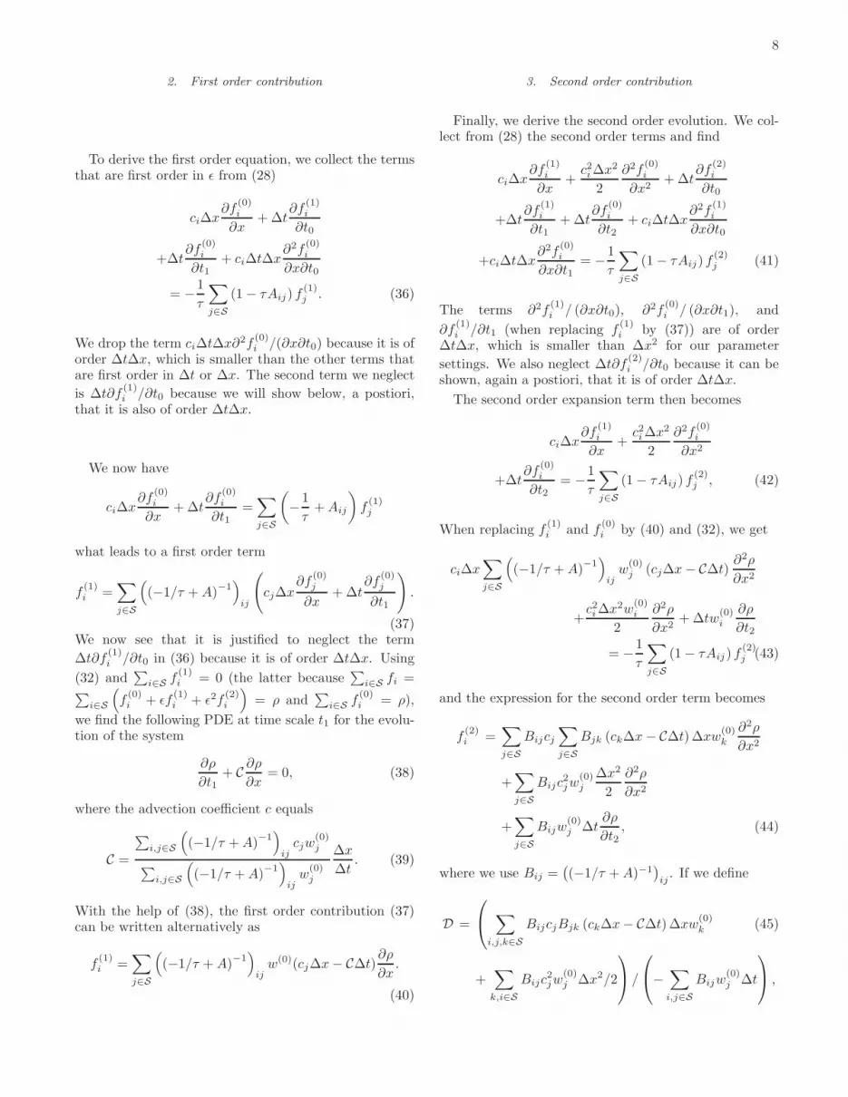
Next, we vary the cross section R, which is related tothe number of times an ionization reaction appears, andstudy the effect on the critical velocity of the travelingwave solution. We increase R from 60 to 100, which cor-responds at the level of the PDE to an increase of thegrowth transport coefficient from α(E+) = 0.02015 toα(E+) = 0.03707, with E+ = −1.0. For this range of re-action rates with the chosen value of ∆t, the constrainedruns algorithm always converges because all the eigenval-ues of the Jacobian are smaller than |1−1/τ−∆tR| < 1,as discussed in section VA.

We now turn to the numerical computation of the criti-cal velocity with the method proposed in section VI B. Intable II, we show the critical speed determined for a se-ries of ionization strengths between R = 60 and R = 100.As outlined in section VI B, the critical velocity for eachvalue of R is found by performing a numerical contin-uation with the wave speed c as a free parameter andmonitoring the eigenvalues of the 2-by-2 matrix (64).For comparison, we also show the minimal speed as ob-tained using the approximate analytical expressions forthe transport coefficients, which we found through theChapman-Enskog expansion. We observe a small differ-ence between the two results. The critical speed thatresults from the Chapman-Enskog expansion is higherthan the critical speed that is computed using the CGTS.Note that both methods make approximations and it isnot clear which method is more exact.

A short discussion about the accuracy of the shift-

15

R c∗ with c∗ withChapman-Enskog CGTS

60 1.3351 1.3177

70 1.3496 1.3318

80 1.3609 1.3433

90 1.3696 1.3517

100 1.3755 1.3566

Table II: The critical speed for different values of the ioniza-tion rate R.

back operator is necessary. Since we have implementedthe shift-back operator using a forward Euler approx-imation of the characteristic solutions of the equationut+cux = 0, the error in the critical speed grows linearlywith the time step ∆T . Therefore, we should take ∆Tas small as possible, i.e. the minimal possible numberof lattice Boltzmann steps in the simulation step. (Notethat accuracy and efficiency go together here.) However,we cannot take less than 25 LBM steps because thesesteps are necessary to reduce the error in the lifting (seefigure 4).

VIII. DISCUSSION AND CONCLUSIONS

In one dimension, an initial seed of electrons in a strongelectrical field will evolve into a streamer front that trav-els with a constant speed c. Before the front, the densityis zero and the electrical field is constant; behind thefront the electrical field is shielded and there is a sur-plus of electrons. In this article we extended the min-imal streamer model of Ebert et al. [1] to add somedetails about the microscopic physics. To this end, wereplaced the reaction-diffusion PDE with a lattice Boltz-mann model that has a velocity dependent reaction term.The reaction rates are a chosen to model the ionizationreaction, where fast particles have a given probability toundergo an ionization reaction and create two slow par-ticles. The electrical field changes simultaneously as aresult of the charge creation.

This macroscopic behavior of the model was analyzedwith two methods. The first is the more traditional anal-ysis based on a Chapman-Enskog expansion that derivesan approximate PDE model and the corresponding trans-port coefficients. The resulting PDE model is very simi-lar to the minimal streamer model of Ebert, Van Saarloosand Caroli, where the ionization rate depends on the lo-cal electrical field. Based on the transport coefficients, wefound the dependence of the critical speed (below whichthe traveling waves are unphysical) and its dependenceon the strength of the ionization cross section.

Our second method is a computational method basedon the coarse-grained time-stepper, which defines theeffective evolution law as a sequence of computationalsteps. The traveling wave solutions were formulated asfixed points of this coarse-grained time-stepper combined

with a shift-back operator. By varying the applied shift-back, we again found the critical speed, and we demon-strated how to calculate its dependence on the cross sec-tion strength numerically.

We showed that the coarse-grained time-stepper pro-vides a viable alternative to the traditional Chapman-Enskog analysis. However, in this paper, we did notmake any statements about which of the two methodsprovides the most accurate information. Both methodsmake approximations to obtain the critical velocity ofthe proposed lattice Boltzmann model. In contrast tothe theoretical approximations in the Chapman-Enskoganalysis, these approximations are due to numerical ac-curacy for the coarse-grained time-stepper.

Further progress in the accuracy can be made in severalways. First, the lifting can be done more accurately if ahigher order constrained runs algorithm is used. Such amethod would take multiple steps with the lattice Boltz-mann model and uses these multiple points to provide uswith an approximate initial state [17]. We expect thatthese higher order lifting procedures will reproduce morethan two terms in the Chapman-Enskog series and there-fore provide a better initial state for the simulation step.This will allow limiting the number of simulation steps,which will immediately improve the accuracy of the com-puted solutions and the critical speed.

Although the model problem in this paper is non-trivial, and the Chapman-Enskog expansion is tedious,we emphasize that our method is mainly developed withapplications in sight where the traditional Chapman-Enskog analysis is completely intractable. The modelproblem in this paper both allows us to analyze the pro-posed methods and provide directions for further devel-opment. In a forthcoming article, we will do a completeanalysis of the traveling wave solutions in the proposedmodel and illustrate more extensively how the macro-scopic behavior depends on the parameters of the micro-scopic model. In our calculations, we have also observedthe positively charged fronts that move in the oppositedirection of the electrical field. These solutions have beendiscussed by Ebert et al in [1] and our methods are alsoable to locate these states.

We expect that most of the results presented in thispaper will remain valid when the number of velocities inthe discretization of the Boltzmann model is increased.With additional velocities, it is possible to model thecross sections of colliding particles with more detail andstudy other reactions than the ionization reaction. Itwould also be interesting to study models with multiplespecies where the collision rates between the particlesare velocity dependent. This would allow us to includephoto-ionization effects into the minimal streamer model,an important effect that is neglected in the current model[22].

16

Acknowledgments

GS is a postdoctoral researcher of the Fund for Sci-entific Research — Flanders, who also supports PVLthrough projects G.0130.03 and G.0365.06. The paper

presents research results of the Belgian Programme onInteruniversity Attraction Poles, initiated by the BelgianFederal Science Policy Office, which also funded WV witha DWTC return grant. We also thank Christophe Van-dekerckhove for fruitful discussions.

[1] U. Ebert, W. Van Saarloos, and C. Caroli, Phys. Rev. E,55 p1530 (1997).

[2] W. Van Saarloos, Phys. Rep. 386 p29-222 (2003).[3] G. Samaey, W. Vanroose, D. Roose and I.G. Kevrekidis,

Coarse-grained computation of traveling waves of lattice

Boltzmann models with Newton-Krylov methods, submit-ted to Journal of Computational Physics, (2006). Arxivpreprint physics/0604147.

[4] P. Van Leemput, W. Vanroose and D. Roose, Initializa-

tion of a lattice Boltzmann model with constrained runs,submitted. Technical Report TW 444, Dept. of ComputerScience, K.U.Leuven (2005).

[5] I. G. Kevrekidis et al, Comm. Math. Sci. 1 p715 (2003).[6] W. Hu, D. Fang, Y. Wang and F. Yang, Phys. Rev. A,

bf 49 p 989 (2006)[7] T. N. Rescigno, M. Baertchy, W. A. Isaacs and C. W.

McCurdy, Science 5449 p2474 (1999).[8] M. S. Pindzola and D. R. Schultz. Phys. Rev. A 53 p1525

(1996).[9] L. Malegat, P. Selles, and A. K. Kazansky, Phys. Rev.

Lett 85 p4450 (2000).[10] I. Bray and A. T. Stelbovics, Phys. Rev. A 46 p6995

(1992).[11] W. Vanroose, F. Martin, T. N. Rescigno and C. W. Mc-

Curdy, Science, 310 p5755 (2005).[12] T. Weber et. al., Nature 7007 p437-439 (2004).

[13] G. H. Wannier, Phys. Rev. 90 817 (1953).[14] N. Cao, S. Chen, Shi Jin and D. Martinez, Phys. Rev E,

55, R21 (1997).[15] A. Arnold and C. Ringhofer, SIAM Journal of Numerical

Analysis, 33 p1622 (1996).[16] S. Succi, The lattice Boltzmann equation for fluid dy-

namics and beyond, Oxford University Press (2001).[17] C. W. Gear, T. J. Kaper, I. G. Kevrekidis, and A. Za-

garis. Projecting to a slow manifold: Singularly perturbed

systems and legacy codes. SIAM Journal on Applied Dy-namical Systems, 4 p711, (2005).

[18] G. E. Uhlenbeck and G. W. Ford, Lectures in Statistical

Mechanics, American Mathematical Society, Providence,Rhode Island, (1963).

[19] Y.H. Qian, D. d’Humieres, and P. Lallemand, Lattice

BGK models for the Navier-Stokes equation. EurophysicsLetters, 17 p479 (1992).

[20] L. Qiao, R Erban, C.T. Kelley, I. G. Kevrekidis, Spa-

tially distributed Stochastic Systems: Equation-free and

equation-assisted bifurcation analysis submitted to Phys.Rev. E, arxiv preprint q-bio/0606006.

[21] P. L. Bhatnagar, E. P. Gross and M. Krook, Phys. Rev.94, p511 (1954).

[22] A. A. Kulikovsky, Phys. Rev. Lett. 89 p229401 (2002)