Embed Size (px)
Citation preview
NORTHWESTERN UNIVERSITY
Coarsening of Dendrites in Solid-Liquid Mixtures: The Low Volume Fraction Limit
A DISSERTATION
SUBMITTED TO THE GRADUATE SCHOOL
IN PARTIAL FULFILLMENT OF THE REQUIREMENTS
for the degree
DOCTOR OF PHILOSOPHY
Field of Materials Science and Engineering
By
Thomas Cool
EVANSTON, ILLINOIS
July 2016

2
© Copyright by Thomas Cool 2016
All Rights Reserved
ABSTRACT 3
ABSTRACT
Coarsening of Dendrites in Solid-Liquid Mixtures: The Low Volume Fraction Limit
Thomas Cool
The morphological and topological evolution of dendritic structures during coarsening remains poorly un-
derstood. In particular, predicting the fissioning of secondary arms from the main dendrite stem and coa-
lescence and retraction events remains controversial. We perform experiments on the International Space
Station (ISS) since arms that fission from the stem do not sediment and thus can be detected. In addition,
it is also possible to follow the morphological evolution of the structure in the absence of convection. 30%
Pb-Sn samples were coarsened for different lengths of time from 10 minutes to 48 hours. The morphology
of the structure and the number of fissioned arms were determined using three-dimensional reconstructions.
The evolution of the microstructure, the change in length scale, the number of independent bodies, the evo-
lution of the anisotropy of the structure and the interfacial shape distributions as a function of time during
coarsening were studied. Key findings are that 1) the inverse of surface area per unit volume S−1V increases
with time as t1/3 that is almost identical to a sample coarsened on earth; 2) independent bodies were found
in all samples; 3) the number of independent bodies per unit volume multiplied by S−3V is independent of
coarsening time. Thus it is possible to predict the number of fragments during coarsening by a measurement
of SV ; 4) the genus scaled by S−3V is independent of coarsening time. A 3D reconstruction of a PbSn sample,
30% solid, that was coarsened aboard the ISS was used as an initial condition in a phase-field model to
study pinching (fisioning), retraction and coalescence (fusioning) of secondary dendrite arms. The overall
simulation box was 472x496x248 voxels; the phase field model was coded in OpenCL to run on a D700
FirePro GPU. In spite of the high speed of the simulations, evolving the PbSn structure from 10 mins to
ABSTRACT 4
1.6 hours still required 23 days. Two variants of the model that differ along the length of the secondary
arms and their spacing were run. The observed linear relations of S−1V and t1/3 for both simulated structures
confirmed the excellent fit of the model. The simulations show the dynamics of fragmentation and retraction
and also two mechanisms of coalescence: one where space is filling from the root up, and the other where
adjacent arms are forming handles and merging. The phase field analyses showed that the neck radius during
both the fusioning of secondary dendrite arms and the pinching of arms was evolving linearly in t1/3. The
simulations were also used to test whether fragmentation, retraction or coalescence events can be predicted.
Results indicate that in addition to secondary arm spacing and length, the angle of the dendrite arms, their
uneven spacing and length, and their uneven shapes and coarsening rates need to be included to improve
the accuracy of the predictions.
Acknowledgments 5
Acknowledgments
First and foremost, I would like to acknowledge my Ph.D advisor, Professor Peter Voorhees. His support,
great insight, guidance, patience and encouragements have been incredible during the last six (6!) years. I
have learned a great deal from Peter, including how to conduct research, checking my conclusions properly,
and really, how to properly analyze data. I have very much enjoyed working with Peter and am very grateful
to have gotten the opportunity.
Additionally, I’d like to thank Professors David Seidman, Katherine Faber and Steven Davis for taking
the time to serve on my committee.
I would also like to thank Begum Gulsoy, ePhD (which, by the way, I am convinced stands for evil PhD
- formerly known as Evil Postdoc) for her help in visualization. Her Fingerspitzengefuhl in this domain
is incredible. The moral support provided through the days and years has been immensely helpful. The
discussions on a very wide range of topics from politics to sports to colors, in particular my black t-shirts,
have always provided a lot of needed levity. I would also like to thank her and John Thompson for the help
provided during the long sectioning nights, in actually sectioning, providing moral support during arising
mechanical issues and brainstorming fixes.
A big thanks also to the rest of the group, in particular John Gibbs, Kevin, Ashwin but also Anthony,
Eddie, Eli, Kyoundoc, Matt, Megna, Olivier, Orianne, Rohit, Stefan, Thomas and Yue for the great times.
Finally, I would be remiss if I did not acknowledge my family for the incredible support given throughout
the years; my parents, Anne-Marie and Karel, and my sister Josephine, for the last 30 years, and more recently
the panicked phone calls. I consider myself extremely lucky to have you in my life. In addition, I would also
love to thank my grandparents, aunts, uncles and cousins for the great times and support. Thanks also to
Alexandre for his 30 year long friendship.
I would like to dedicate this thesis to my cousin Pieter Ombregt, who was taken from us too early.
TABLE OF CONTENTS 6
Table of Contents
ABSTRACT 3
Acknowledgments 5
List of Figures 10
List of Tables 20
Chapter 1. Introduction 21
Chapter 2. Background 25
2.1. Coarsening of Spherical Particles and Dendritic Microstructures 25
2.2. Interfacial Curvature 34
2.3. Interface Shape Distribution 35
2.4. Interface Normal Distribution 38
2.5. Topology of Dendritic Structures 40
2.6. Phase Field Simulation 43
2.7. Columnar to Equiaxed Transition (CET) 49
Chapter 3. Experimental Methods 52
3.1. The Lead-Tin System 52
3.2. Gravity in the Coarsening Process and the ISS 53
3.3. Sample 55
3.4. Room Temperature Coarsening Analysis 57
3.5. Final Sample Selection 58
3.6. Space Flight Experiment 58
TABLE OF CONTENTS 7
3.6.1. Sample preparation 58
3.6.2. Experiment and recovery 60
3.7. Automated Serial Sectioning 62
Chapter 4. Collection of Data, Smoothing and Analysis 66
4.1. Collecting Data 66
4.2. Segmentation 67
4.2.1. EM/MPM Method 67
4.2.2. EM/MPM Application 70
4.3. Generation of the 3D structures 71
4.4. Smoothing Analysis 72
4.4.1. No smoothing 72
4.4.2. Curvature Considerations 72
4.4.3. Smoothing 74
4.4.4. Mesh smoothing effects 74
4.4.5. Effect on the Interfacial Shape Distribution 76
4.4.6. Effects on S−1V 77
4.5. Summary 78
Chapter 5. Results 79
5.1. Initial Analysis 79
5.1.1. 2D Section analysis 79
5.1.2. Determination of the sample of focus for this research 84
5.1.3. Processing issues 84
5.1.4. SEM (Scanning Electron Microscope) Analysis 86
5.2. Generating Multiple Data Sets from a Single Specimen 88
5.3. Mushy zone analysis 88
5.3.1. Reconstructions 88
5.3.2. Evolution of S−1V 91
TABLE OF CONTENTS 8
5.3.3. Morphology - ISD 95
5.3.4. Morphology - IND 97
5.4. Independent Bodies 98
5.4.1. Identification method 98
5.4.2. Results 99
5.4.3. Errors in the search for Dendrite Fragments 104
5.4.4. Change in the fragment structure 108
5.5. Topological Analysis of the Genus and Handles 109
5.5.1. Method for determining the number of handles 111
5.5.2. Evolution of the number of handles 112
5.6. Free Growth Region 114
5.6.1. Morphological Evolution 115
5.6.2. Evolution of the ISDs 118
5.7. Conclusion 119
Chapter 6. Evolution of the Microstructure using Phase-Field Simulation 121
6.1. Model 121
6.2. Implementation 125
6.2.1. Testing - Confirming the implementation 126
6.3. Small Scale Simulations 131
6.4. Larger Evolutions 134
6.5. Fusion and Fission Events in Non-Ideal Structures 140
6.5.1. Fusion events in the Original structure 140
6.5.2. Fission events in the eroded structure 141
6.5.3. Comparison to theoretical predictions of pinching and retracting 144
6.6. Conclusion 147
Chapter 7. Conclusions 149

TABLE OF CONTENTS 9
References 153
Appendix A. Simulation Code 159
LIST OF FIGURES 10
List of Figures
2.1 3D Reconstruction of the 15% solid volume fraction PbSn sample coarsened for 48 h. The
volume reconstructed was approximately 7 mm 5 mm 1:8 mm containing a total of 773 particles.
The particles are colored by their relative size, red being much larger than the average particle
size and purple much smaller. 26
2.2 Shown is a three-dimensional reconstruction of a free-growing aluminum dendrite in an
aluminum-copper eutectic liquid. The interface of the dendrite is colored according to its mean
curvature, H. From Mendoza et al [1] 27
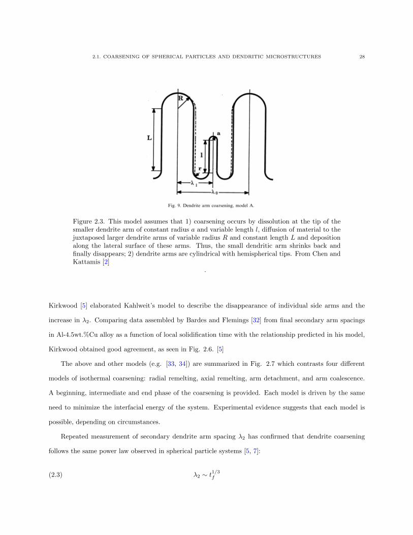
2.3 This model assumes that 1) coarsening occurs by dissolution at the tip of the smaller dendrite
arm of constant radius a and variable length l, diffusion of material to the juxtaposed larger
dendrite arms of variable radius R and constant length L and deposition along the lateral
surface of these arms. Thus, the small dendritic arm shrinks back and finally disappears; 2)
dendrite arms are cylindrical with hemispherical tips. From Chen and Kattamis [2] 28
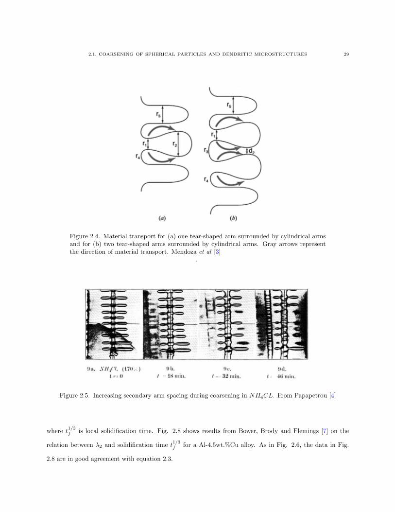
2.4 Material transport for (a) one tear-shaped arm surrounded by cylindrical arms and for (b)
two tear-shaped arms surrounded by cylindrical arms. Gray arrows represent the direction of
material transport. Mendoza et al [3] 29
2.5 Increasing secondary arm spacing during coarsening in NH4CL. From Papapetrou [4] 29
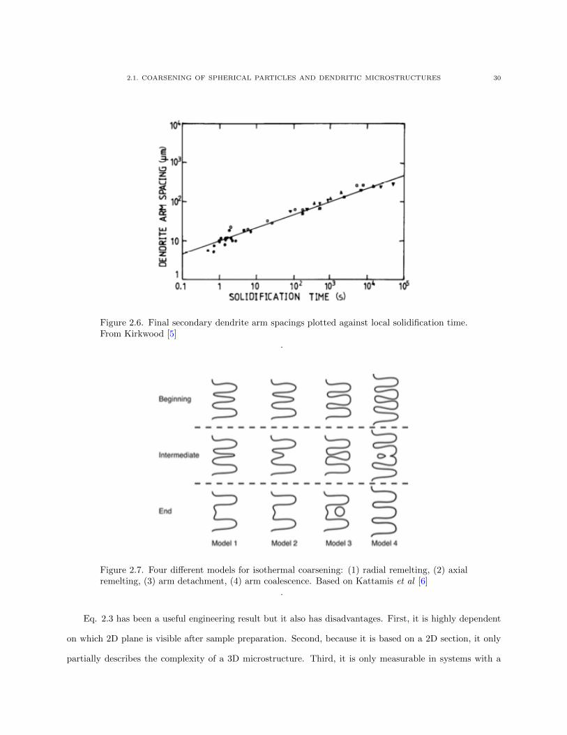
2.6 Final secondary dendrite arm spacings plotted against local solidification time. From Kirkwood
[5] 30
2.7 Four different models for isothermal coarsening: (1) radial remelting, (2) axial remelting, (3)
arm detachment, (4) arm coalescence. Based on Kattamis et al [6] 30
LIST OF FIGURES 11
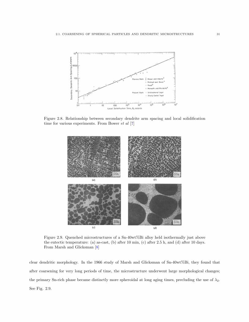
2.8 Relationship between secondary dendrite arm spacing and local solidification time for various
experiments. From Bower et al [7] 31
2.9 Quenched microstructures of a Sn-40wt%Bi alloy held isothermally just above the eutectic
temperature: (a) as-cast, (b) after 10 min, (c) after 2.5 h, and (d) after 10 days. From Marsh
and Glicksman [8] 31
2.10 Experimental values of the specific surface area, Sv, and average interfacial mean curvature,
H, measured from the micrographs in Fig. 2.9 and from additional samples not shown. Four
of the data points in Fig. 2.10 correspond to the micrographs in Fig. 2.9. The abscissa shows
time increasing nonlinearly from right to left, so the origin of this plot represents the long-time
asymptotic equilibrium state of the bulk phases. Sv and H decay linearly as t1/3. From Marsh
and Glicksman [8] 32
2.11 The relation between coarsening time and S−1V for directionally solidified Al-15wt%Cu samples.
From Mendoza et al [1]. 33
2.12 The relation between coarsening time and S−1V for directionally solidified Pb-80wt%Sn samples.
From Kammer and Voorhees [9]. 33
2.13 The relation between coarsening time and S−1V for directionally equiaxially Al-20wt%Cu
samples. From Fife and Voorhees [10]. 33
2.14 Local geometric parameters associated with a Monge patch. From [3, 8]. p is the center of the
patch; R1 and R2 are the two principal radii of curvature; n is a unit vector that is perpendicular
to the patch at p. 34
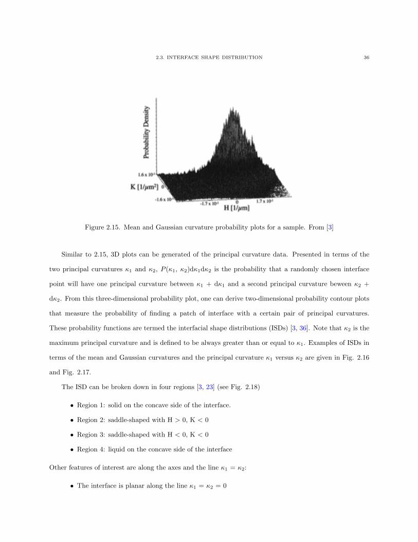
2.15 Mean and Gaussian curvature probability plots for a sample. From [3] 36
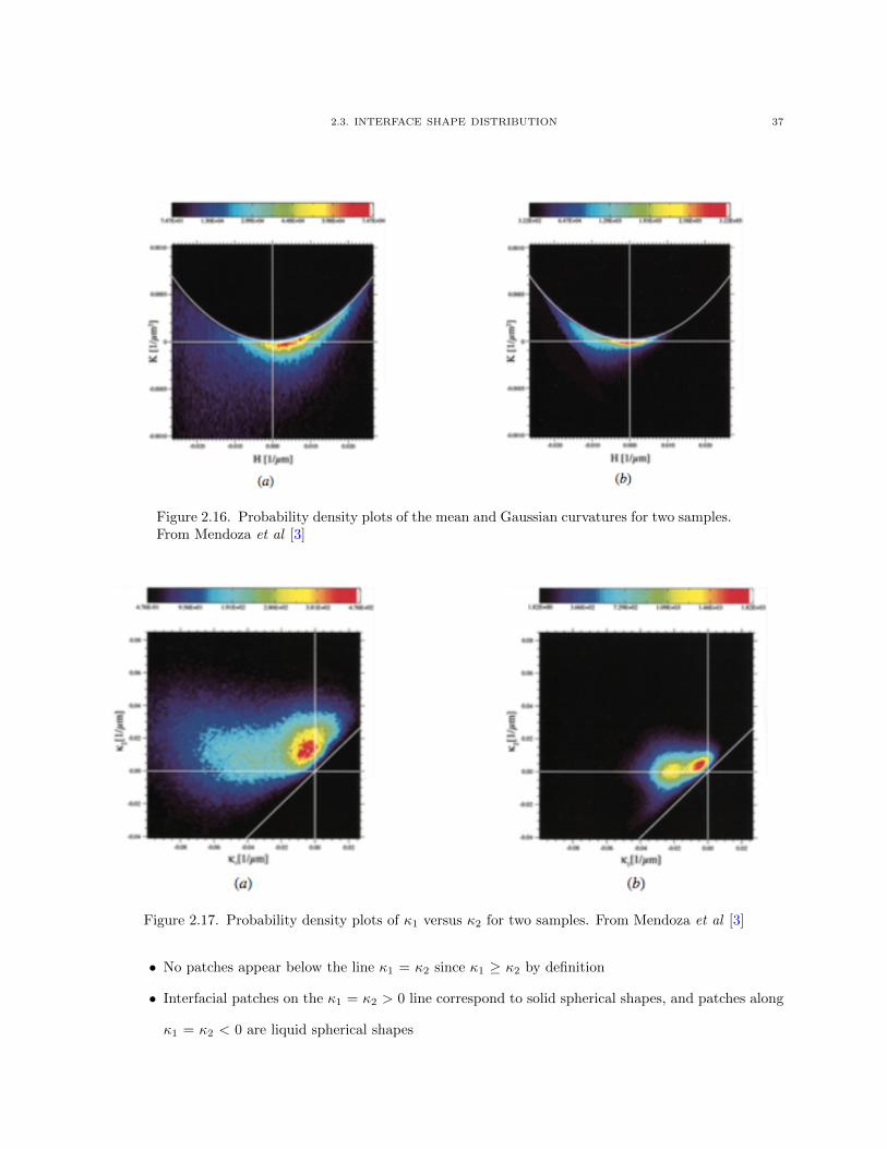
2.16 Probability density plots of the mean and Gaussian curvatures for two samples. From Mendoza
et al [3] 37
2.17 Probability density plots of κ1 versus κ2 for two samples. From Mendoza et al [3] 37
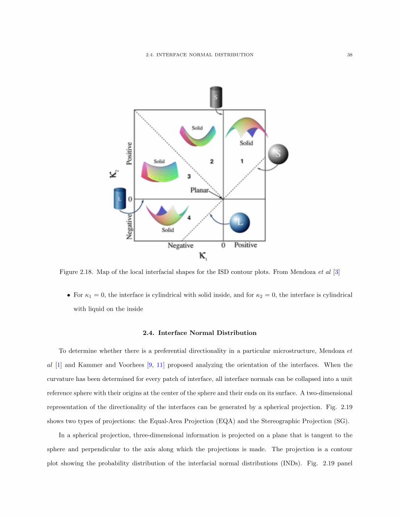
2.18 Map of the local interfacial shapes for the ISD contour plots. From Mendoza et al [3] 38
LIST OF FIGURES 12
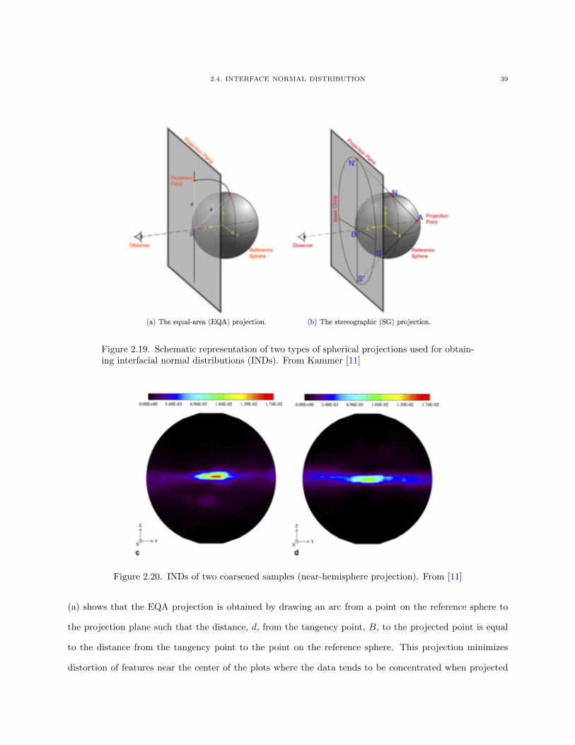
2.19 Schematic representation of two types of spherical projections used for obtaining interfacial
normal distributions (INDs). From Kammer [11] 39
2.20 INDs of two coarsened samples (near-hemisphere projection). From [11] 39
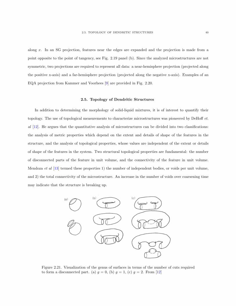
2.21 Visualization of the genus of surfaces in terms of the number of cuts required to form a
disconnected part. (a) g = 0, (b) g = 1, (c) g = 2. From [12] 40
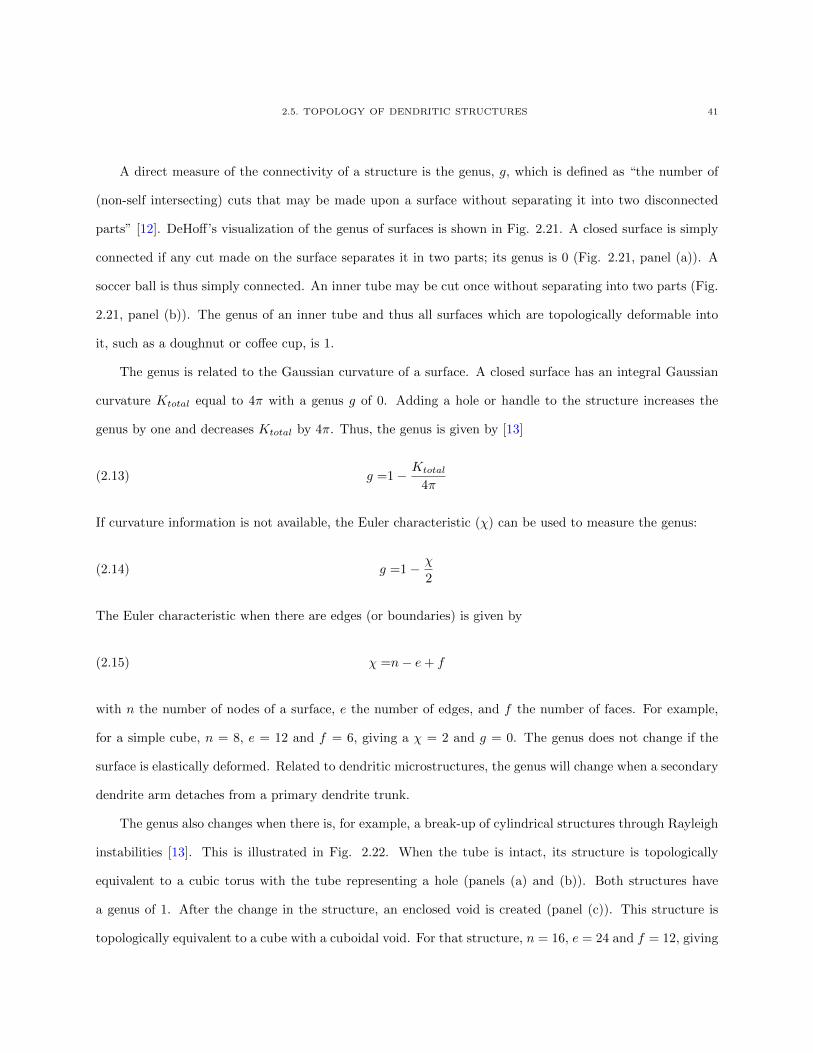
2.22 (a) A cubic torus is topologically equivalent to (b) a cube with a cylindrical tube. The cube can
undergo Rayleigh instability leading to the formation of a void (c) and change the genus from 1
to -1. (c) and (d) are topologically equivalent. From Mendoza et al [13] 42
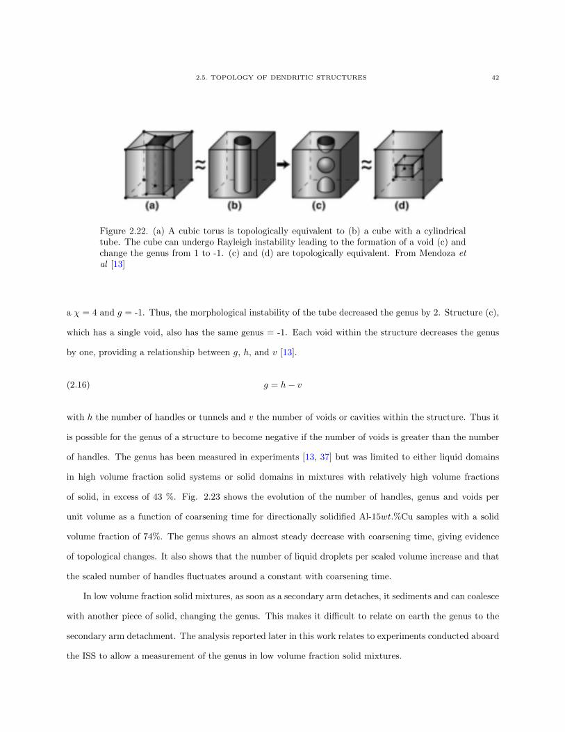
2.23 The scaled number of handles, genus, and voids per unit volume as a function of coarsening
time. From Mendoza et al [13] 43
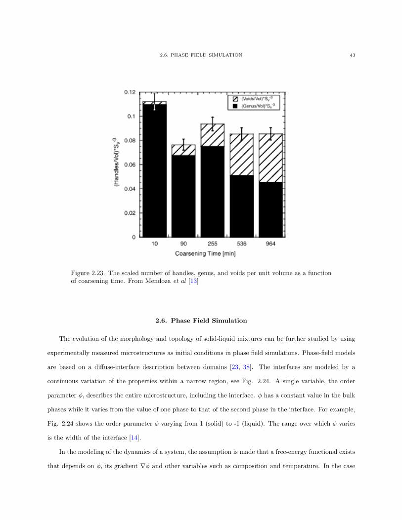
2.24 Order parameter as a function of distance for the (a) sharp interface and (b) diffuse interface
models. From [14] 44
2.25 A portion of the experimental interfacial morphology of the 964-min Al-15wt.%Cu sample
is colored by the interfacial velocity calculated from the phase-field simulations. Positive
interfacial velocity points into the liquid and is represented by warm colors. Liquid intersecting
the edges of the reconstruction box is capped with zero interfacial velocity. From [13] 47
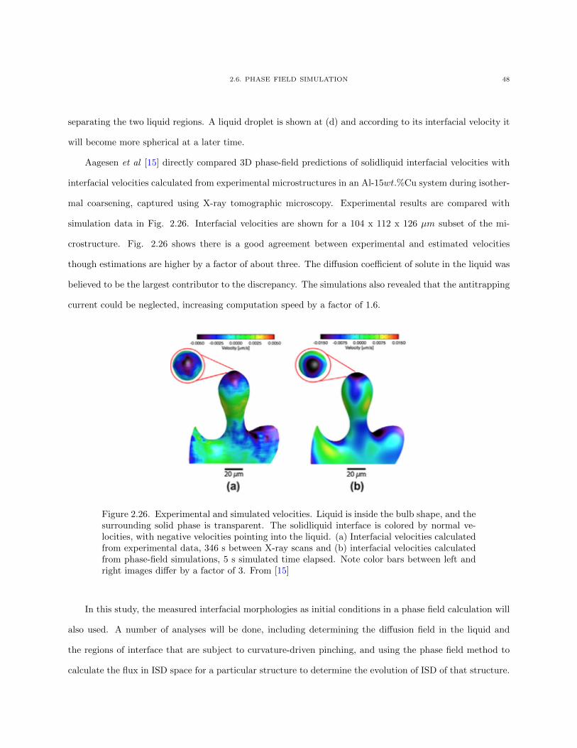
2.26 Experimental and simulated velocities. Liquid is inside the bulb shape, and the surrounding
solid phase is transparent. The solidliquid interface is colored by normal velocities, with negative
velocities pointing into the liquid. (a) Interfacial velocities calculated from experimental data,
346 s between X-ray scans and (b) interfacial velocities calculated from phase-field simulations,
5 s simulated time elapsed. Note color bars between left and right images differ by a factor of
3. From [15] 48
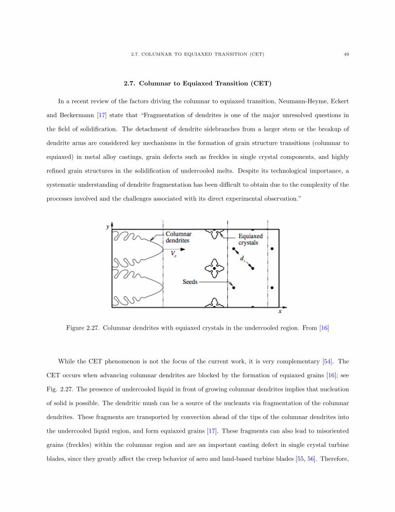
2.27 Columnar dendrites with equiaxed crystals in the undercooled region. From [16] 49
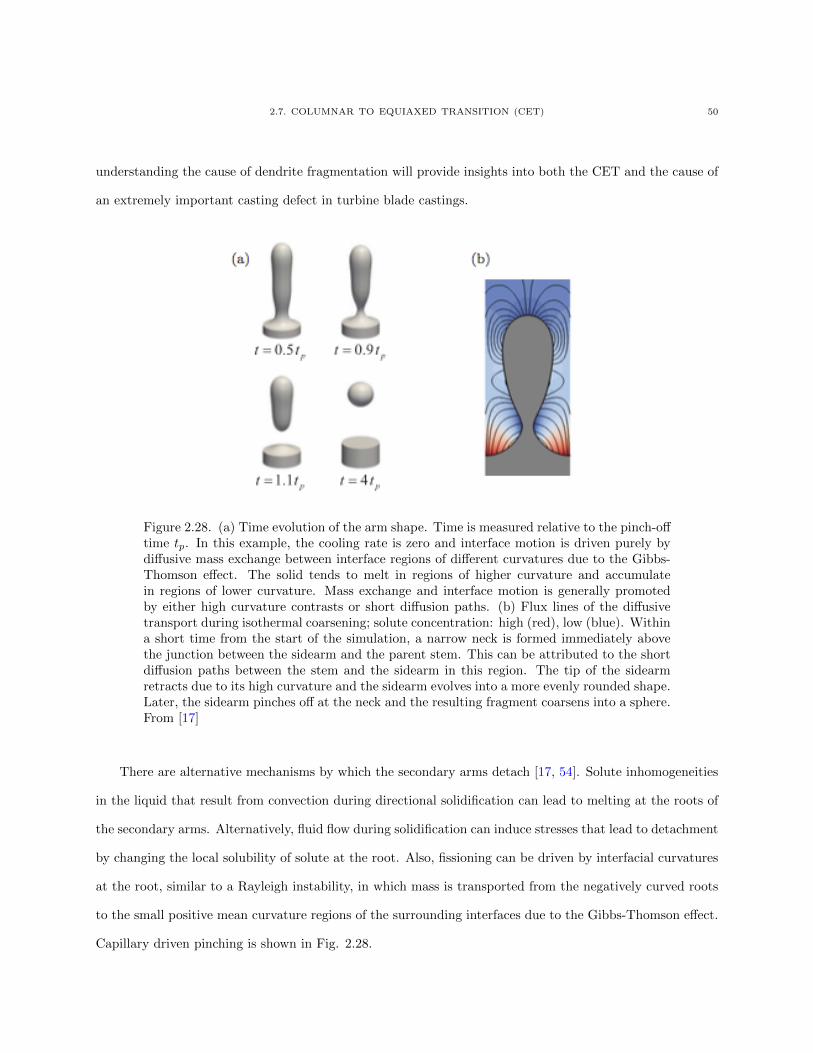
2.28 (a) Time evolution of the arm shape. Time is measured relative to the pinch-off time tp. In
this example, the cooling rate is zero and interface motion is driven purely by diffusive mass
exchange between interface regions of different curvatures due to the Gibbs-Thomson effect.
LIST OF FIGURES 13
The solid tends to melt in regions of higher curvature and accumulate in regions of lower
curvature. Mass exchange and interface motion is generally promoted by either high curvature
contrasts or short diffusion paths. (b) Flux lines of the diffusive transport during isothermal
coarsening; solute concentration: high (red), low (blue). Within a short time from the start of
the simulation, a narrow neck is formed immediately above the junction between the sidearm
and the parent stem. This can be attributed to the short diffusion paths between the stem and
the sidearm in this region. The tip of the sidearm retracts due to its high curvature and the
sidearm evolves into a more evenly rounded shape. Later, the sidearm pinches off at the neck
and the resulting fragment coarsens into a sphere. From [17] 50
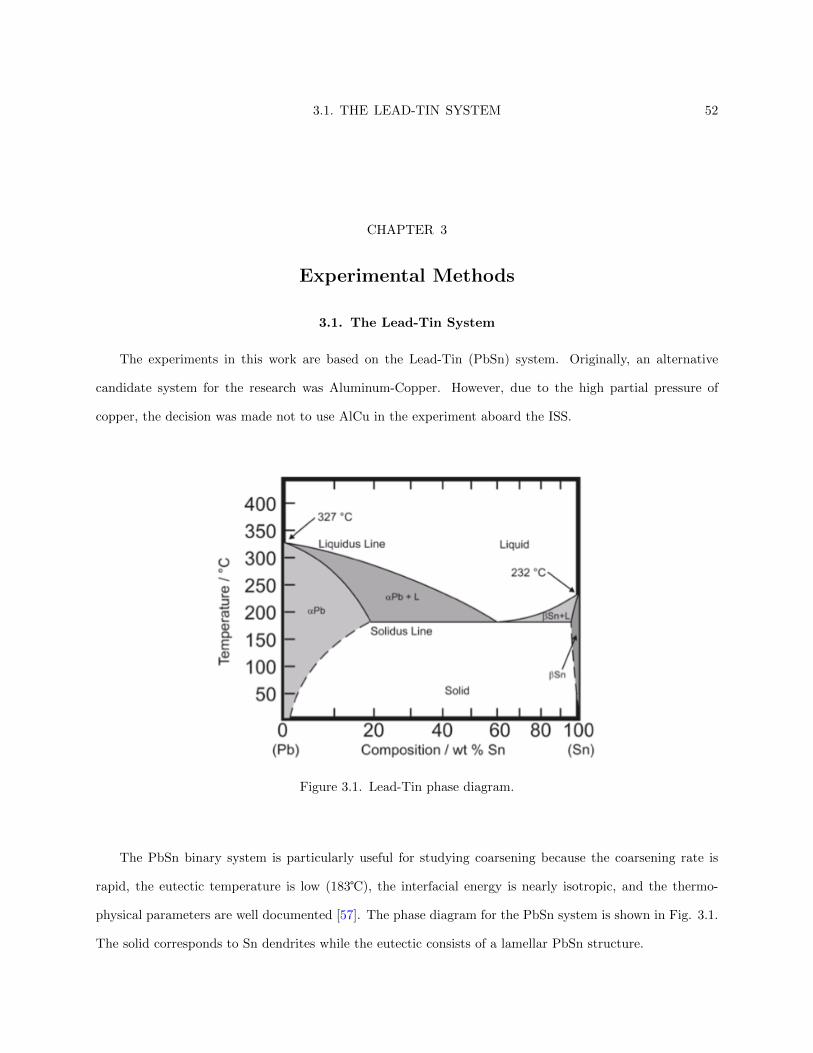
3.1 Lead-Tin phase diagram. 52
3.2 Cross sections of a 1.2 cm diameter Pb-Sn sample with a volume fraction of solid of 22% that
has been coarsened on the ground for 28 min.(left) and 2 days (right). From [18] The samples
were taken from a directionally solidified ingot. 53
3.3 Graphite beaker containing the lead and tin inside the furnace. 55
3.5 Evolution of the microstructure as a function of coarsening time under optical microscope. All
scales are the same with the length of the scale bar being 100µm 57
3.6 Micrographs of each of the PbSn samples as cast 59
3.7 Sample Processing Unit (SPU) in which the samples are loaded [19] 60
3.8 Parts of the Sample Processing Unit (SPU) [19] 60
3.9 SPU sample holder [19] 61
3.10 Microgravity Science Glovebox (MSG) showing the Sample Processing Unit(left) and the
Electronics Control Unit (right) 61
3.11 Schematic drawing of the serial sectioning procedure. The sample translates from the miller
to the microscope in the y-direction. The sections are taken in the z-direction. The two lines
of four short arrows indicate the simultaneous movement of the miller and microscope in the
z-direction between the individual cuts. [20] 63
LIST OF FIGURES 14
3.12 The Alkemper-Voorhees serial sectioning machine. The picture shows the current set-up,
including the modified Leica Polycut E and Z16APO optical microscope. 64
4.1 Registration of images using LVDT data and cross correlation. The two images are cross
sections of 3D data sets parallel to the sectioning axis. That is, if the section images are in the
XY-plane and the direction of sectioning is the Z-direction, these are images of the XZ-plane
cross sections. The top is the raw unaligned data. Application of the LVDT data takes care of
most of the registration, though there are still some misalignment issues. 67
4.2 Change in the image with median filtering in the Z direction. In the images (a,b), a large
reduction in the noise can be seen but it is especially when looking at the magnified images
that the difference can be noticed. In image (c), the eutectic is extremely coarse but even more
importantly, in the structure on the bottom left, there is a large white speckle that can easily
confuse a segmentation algorithm. This goes away with the filtering, as seen in (d). 68
4.3 Overview of the Expectation Maximization/Maximization of Posterior Marginals (EM/MPM)
segmentation method. From [21]. 69
4.4 Schematic of the MPM segmentation algorithm. The observed image is used as input to change
the pixels in the Label Map. The number of time a particular pixel has been classified as a
particular class is tabulated in the Histogram Map. The segmentation is then made by choosing
pixel by pixel the class with the most frequent classification in the Histogram Map. From [22] 70
4.5 Result of the segmentation comparing the basic thresholding (b) method and EM/MPM (c).
Due to the complexity of the structure and the eutectic sometimes blending into the structures,
thresholding is a very bad solution for this problem. 71
4.6 ISD and overlay of reconstruction on raw data of 1.6 Hour coarsened sample without smoothing 73
4.7 Schematic showing how the curvature is actually calculated for each point. The entire structure
is shown in (A). In (B), a small subsection is looked at (the blue triangle) along with its next
next nearest neighbors. A 2D parabola is then fit to these points (C). (Figure provided by A.
Shahani) 73
LIST OF FIGURES 15
4.8 Evolution of the ISD as a function of surface smoothing 75
4.9 Zoom of selected smoothing iterations from the 10, 20 and 60 iteration images in Fig. 4.8. 76
4.10 Evolution of the ISD as a function of surface smoothing 77
4.11 Evolution of S−1V as a function of smoothing iterations 78
5.1 Cross sections of PbSn samples with a volume fraction of solid of 10% that had coarsened on
the ground (upper left) and aboard the ISS for 10 min (upper right), 1.6 hrs (lower left) and 5.5
hrs (lower right). The samples were taken from a directionally solidified ingot. 80
5.2 Cross sections of PbSn samples with a volume fraction of solid of 20% as cast (upper left) and
coarsened aboard the ISS for 10 min (upper right), 1.6 hrs (lower left) and 5.5 hrs (lower right).
The samples were taken from a directionally solidified ingot. 81
5.3 Cross sections of PbSn samples with a volume fraction of solid of 20% that had coarsened
aboard the ISS for 13.5 hrs (left) and 27 hrs (right). The samples were taken from a directionally
solidified ingot. 82
5.4 Cross sections of PbSn samples with a volume fraction of solid of 30% as cast (upper left) and
coarsened aboard the ISS for 10 min (upper middle), 1.6 hrs (upper right), 5.5 hrs (lower left)
and 13.5 hrs (lower right). The samples were taken from a directionally solidified ingot. 83
5.5 Cross sections of PbSn samples with a volume fraction of solid of 30% that has been coarsened
for 13.5 hrs and 27 hrs. The samples were taken from a directionally solidified ingot. 84
5.6 Solidification of new, very small dendrites at the tips of 5.5 hrs coarsened sample due to lack of
quench (a. and b.) along with an inside image showing the lack of new dendrites there 85
5.7 Example of segmentation and the effects of slower cooling on it. 86
5.8 SEM micrographs of the samples coarsened for 10 min and 5.5 hrs showing the differences in
eutectic structures beyond the growth of new dendrites. The eutectic seen in the 5.5 hrs images
(Fig, b,c) have a much coarser eutectic. 87
LIST OF FIGURES 16
5.9 Image showing the two main types of selected regions for analysis. In the top right (green
region), there is a free growth regime and in the bottom right, there is a constrained regime
(red region) more akin to a mush 89
5.10 Unscaled reconstructions of selected data sets from the 10 min and 48 hrs samples with the
same dimensions in X,Y and Z along with same colorbars. The colorbars represent the mean
curvature H in units of (µm−1). They are, in this case, constrained to the same range. 90
5.11 Evolution of S−1V as a function of coarsening time for the mushy region in the 30% volume
fraction sample showing the linearity of the relationship between t1/3 and S−1V . 91
5.12 Evolution of S−1V as a function of t1/3 comparing the results from the present microgravity
experiment (red) and a previous 1g experiment (blue) of 43% solid PbSn samples from Kammer
[11]. In both cases the fits are very linear and closely match each other. In this image, the
volume used for S−1V calculation is the total volume of the bounding box. 92
5.13 Reconstructions of selected data sets from the 10 min and 1.6 hrs samples with axes scaled by
S−1V (colorbar is also scaled by S−1
V ) 93
5.14 Reconstructions of selected data sets from the 13.5 hrs and 48 hrs samples with axes scaled by
S−1V (colorbar is also scaled by S−1
V ) 94
5.15 ISDs of the reconstructions of the 30% sample for the different coarsening times. The axes
represent principal curvatures and are scaled by SV . The color axis is cropped to the same
range across all samples. 96
5.16 INDs of selected times showing the evolution of the overall symmetry of the structure.
Projections along [0 -1 0] 97
5.17 Schematic illustrating the method used in this study to identify independent bodies. (a) shows
the fragments in the actual structure. (b) displays the independent bodies separated from the
surrounding elements. Finally, (c) shows the surrounding, “discarded” dendrites that touch the
edge of the bounding box. 99
5.18 Independent bodies found in the reconstructed volumes (10m and 1.6h) 100
LIST OF FIGURES 17
5.19 Independent bodies found in the reconstructed volumes 101
5.20 Number of Dendrite Fragments scaled by the bounding box volume as a function of coarsening
time (fit is Nv = At−2.63) 103
5.21 Number of dendrite fragments scaled by S−3V as a function of time 103
5.22 Schematic depicting the search for the distribution of the independent bodies. The red box
represents a volume equivalent to the number of S−3V reconstructed for the 13.5 hrs sample. 104
5.23 Independent bodies found within a subset of the 10 min sample using different box sizes
(corresponding to the 13.5 hrs and 48 hrs samples), and a different number of iterations (10000
in (a) and (c) and 20000 in (b) and (d)). 106
5.24 Number of dendrite fragments scaled by S−3V and an estimate of the range of dendrite fragments
per sample as a function of time. The range is one standard deviation above and below the
observed number of fragments in each sample. The standard deviation was calculated from the
simulation of the 13.5 hrs bounding box in the 10 min scaled volume. 107
5.25 Number of dendrite fragments scaled by S−3V as a function of time with simulated independent
body errors overlaid. The observed number of fragments are in blue, the mean value of the
simulated number of fragments in red, and the range is one standard deviation above and below
the simulated mean number of fragments in each sample. 109
5.26 ISD’s of the independent bodies in the reconstructions of the 10 min, 1.6 hrs, 5.5 hrs, 13.5 hrs,
27 hrs, and 48 hrs samples. 110
5.27 The number of handles scaled by S−3V . 113
5.28 Evolution as S−1V as a function of t1/3 for the free growth region of the sample 114
5.29 Reconstructions of selected data sets from the 10 min and 1.6 hrs samples scaled by S−1V (the
colorbar is scaled by S−1V ) 116
5.30 Reconstructions of selected data sets from the 13.5 hrs and 48 hrs samples scaled by S−1V (the
colorbar is scaled by S−1V ) 117
5.31 ISD for the dendrites in the free growth region. 118
LIST OF FIGURES 18
6.1 Initial condition of the decay of a sinusoidal perturbation (done using AlCu material parameters
for ease of comparison with Aagesen [23]) 127
6.2 Profile of φ, U and c after relatively short evolution time with different precisions: (a) 32bit, (b)
64bit. Of particular note is the change in U going from 10−6 to unity when going from double
to single and the effect it has on both U and c 129
6.3 Comparison of the decay of the sinusoidal perturbation shown in Fig 6.1 using Al-Cu material
parameters executed on the new GPU code (a), and from Aagesen [23] with the theoretical
prediction overlaid (b) 130
6.4 Simulation with size: 128*172*248 µm 131
6.5 Early evolution of the structure showing coarsening of the spherical particles and retraction of
a small arm (can be seen in mirror) 132
6.6 Later evolution of the structure showing the creation and subsequent coarsening of a handle 133
6.7 Reconstruction of simulated volume after very low amount of coarsening (colored by curvature).
This is based on a PbSn sample with a 30% dendrite volume fraction coarsened for 10m aboard
the ISS. 134
6.8 Reconstruction of the Eroded structure after very low amount of coarsening (colored by
curvature). This is in contrast to the Original structure shown in Fig. 6.7. 135
6.9 Evolution of S−1V as a function of t1/3 showing similar slopes between the Eroded and Original
structures. (a) also has the S−1V fit of the experimental data superimposed on it. 136
6.10 Evolution of the Original structure as a function of coarsening time (the simulation starts at
t=600s). (a) early time. (b) handle formation. (c) handles coarsening out. (d) 1.6 hrs snapshot.
(e)&(f) long times. Colored by curvature H in units of µm−1 137
6.11 Evolution of the Eroded structure as a function of coarsening time (the simulation starts
at t=600s). (a) early time. (b) & (c) Pinching in the structure (d),(e),(f) Evolution of the
structure viewed from the top showing back arms. Colored by curvature H in units of µm−1 138
LIST OF FIGURES 19
6.12 Comparison of the evolution of the structure after 1.6 hours of simulations and coarsening
aboard the ISS. (a) The simulated ROI from the original structure; (b) The simulated ROI
from the eroded structure; (c) One dendrite from the coarsened sample; (d) An ROI extracted
from the arm in (c) comparable in size to the ROI in (a) and (b). Colored by scaled curvature
HS−1V (no units) 139
6.13 Two different coalescence events: Retraction + coalescence between the first and second
dendrite; Fusioning between the second and third dendrite. In both Figs (a) and (b) the base
grey structure is 2s before fusioning between arms 2 and 3. The red overlay in (a) is 35s after
the grey and the blue overlay is 62s thereafter (97s after fusion event) 140
6.14 Evolution of the neck radius as a function of time for two dendrites fusing together. Images
show the local region near the neck at different times (same times as figure 6.13). tf is the
initial time of fusion. 141
6.15 Comparison of the shape evolution of the dendrite bulb vs the neck at different discrete times 142
6.16 Evolution of the neck radius during pinching as a function of time 143
6.17 Early time reconstruction of Eroded structure (front view) 145
6.18 Early time reconstruction of Eroded structure (top view) 146
LIST OF TABLES 20
List of Tables
3.1 Overview of created and processed samples 58
4.1 Summary of the steps involved in the processing of the data for each data set (pre-reconstruction) 72
5.1 Evolution of the number of independent bodies as a function of time 102
5.2 Evolution of the number of independent bodies as a function of time, scaling the volumes by
S−3V 102
5.3 Evolution per sample of the observed number of independent bodies, the simulated mean
number of bodies and the simulated standard deviation from the mean, all scaled by S−3V . 108
5.4 The evolution of the handles as a function of time. 113
6.1 Physical properties of the PbSn System 124
6.2 Prediction and Evolution of dendrite pinching (P) and retraction (R) for the front dendrite
arms of the Eroded structure 144
6.3 Prediction and Evolution of dendrite pinching (P) and retraction (R) for the rear dendrite arms
146
1. INTRODUCTION 21
CHAPTER 1
Introduction
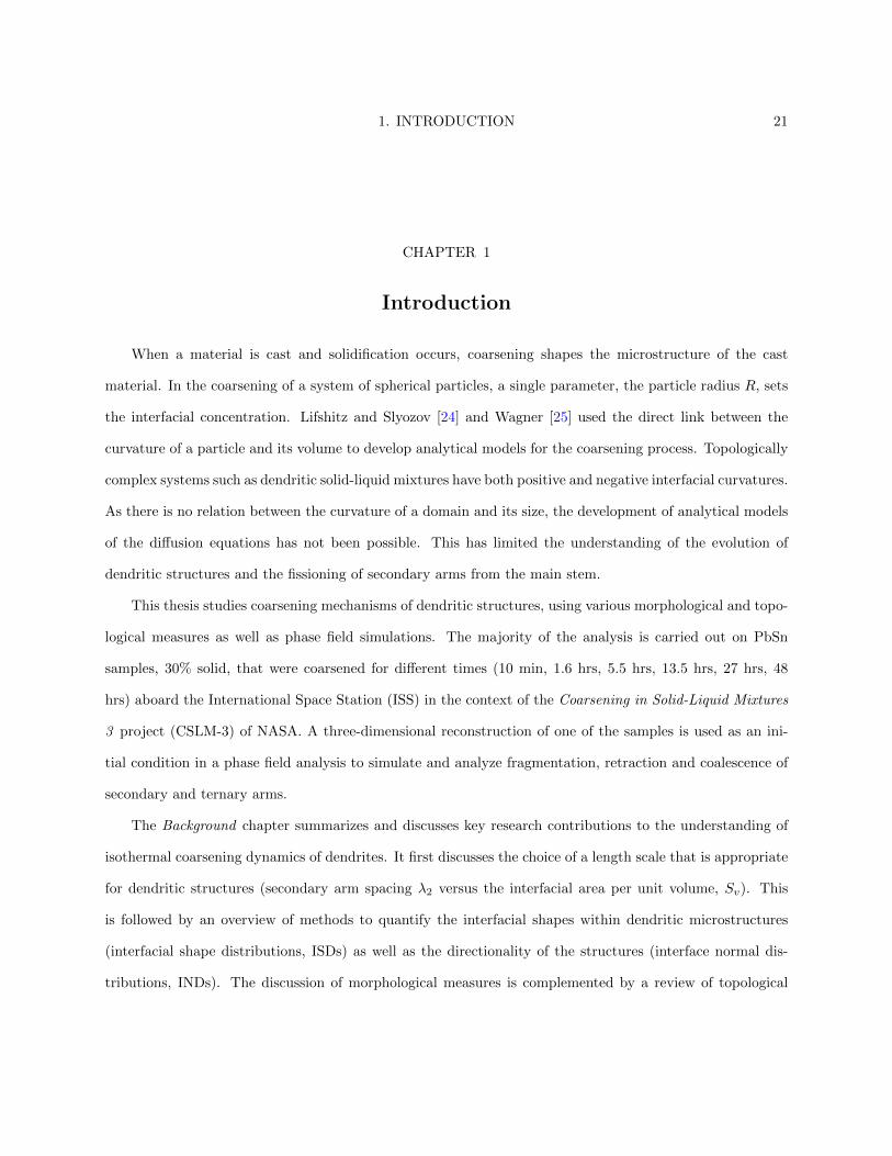
When a material is cast and solidification occurs, coarsening shapes the microstructure of the cast
material. In the coarsening of a system of spherical particles, a single parameter, the particle radius R, sets
the interfacial concentration. Lifshitz and Slyozov [24] and Wagner [25] used the direct link between the
curvature of a particle and its volume to develop analytical models for the coarsening process. Topologically
complex systems such as dendritic solid-liquid mixtures have both positive and negative interfacial curvatures.
As there is no relation between the curvature of a domain and its size, the development of analytical models
of the diffusion equations has not been possible. This has limited the understanding of the evolution of
dendritic structures and the fissioning of secondary arms from the main stem.
This thesis studies coarsening mechanisms of dendritic structures, using various morphological and topo-
logical measures as well as phase field simulations. The majority of the analysis is carried out on PbSn
samples, 30% solid, that were coarsened for different times (10 min, 1.6 hrs, 5.5 hrs, 13.5 hrs, 27 hrs, 48
hrs) aboard the International Space Station (ISS) in the context of the Coarsening in Solid-Liquid Mixtures
3 project (CSLM-3) of NASA. A three-dimensional reconstruction of one of the samples is used as an ini-
tial condition in a phase field analysis to simulate and analyze fragmentation, retraction and coalescence of
secondary and ternary arms.
The Background chapter summarizes and discusses key research contributions to the understanding of
isothermal coarsening dynamics of dendrites. It first discusses the choice of a length scale that is appropriate
for dendritic structures (secondary arm spacing λ2 versus the interfacial area per unit volume, Sv). This
is followed by an overview of methods to quantify the interfacial shapes within dendritic microstructures
(interfacial shape distributions, ISDs) as well as the directionality of the structures (interface normal dis-
tributions, INDs). The discussion of morphological measures is complemented by a review of topological
1. INTRODUCTION 22
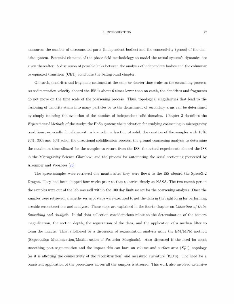
measures: the number of disconnected parts (independent bodies) and the connectivity (genus) of the den-
drite system. Essential elements of the phase field methodology to model the actual system’s dynamics are
given thereafter. A discussion of possible links between the analysis of independent bodies and the columnar
to equiaxed transition (CET) concludes the background chapter.
On earth, dendrites and fragments sediment at the same or shorter time scales as the coarsening process.
As sedimentation velocity aboard the ISS is about 6 times lower than on earth, the dendrites and fragments
do not move on the time scale of the coarsening process. Thus, topological singularities that lead to the
fissioning of dendrite stems into many particles or to the detachment of secondary arms can be determined
by simply counting the evolution of the number of independent solid domains. Chapter 3 describes the
Experimental Methods of the study: the PbSn system; the motivation for studying coarsening in microgravity
conditions, especially for alloys with a low volume fraction of solid; the creation of the samples with 10%,
20%, 30% and 40% solid; the directional solidification process; the ground coarsening analysis to determine
the maximum time allowed for the samples to return from the ISS; the actual experiments aboard the ISS
in the Microgravity Science Glovebox; and the process for automating the serial sectioning pioneered by
Alkemper and Voorhees [26].
The space samples were retrieved one month after they were flown to the ISS aboard the SpaceX-2
Dragon. They had been shipped four weeks prior to that to arrive timely at NASA. The two month period
the samples were out of the lab was well within the 100 day limit we set for the coarsening analysis. Once the
samples were retrieved, a lengthy series of steps were executed to get the data in the right form for performing
useable reconstructions and analyses. These steps are explained in the fourth chapter on Collection of Data,
Smoothing and Analysis. Initial data collection considerations relate to the determination of the camera
magnification, the section depth, the registration of the data, and the application of a median filter to
clean the images. This is followed by a discussion of segmentation analysis using the EM/MPM method
(Expectation Maximization/Maximization of Posterior Marginals). Also discussed is the need for mesh
smoothing post segmentation and the impact this can have on volume and surface area (S−1V ), topology
(as it is affecting the connectivity of the reconstruction) and measured curvature (ISD’s). The need for a
consistent application of the procedures across all the samples is stressed. This work also involved extensive
1. INTRODUCTION 23
writing of several codes to automate the sectioning and segmentation processes, significantly improving the
speed and accuracy of the analysis.
The Results chapter combines a large number of analyses on the morphology and topology of the samples
coarsened aboard the ISS. The 2D section analysis of all the samples showed that the experiments had been
successful and that the 30% sample was the most interesting for the purposes of this research: it had large
dendritic structures, making them easier to segment, and still had a volume fraction for which coarsening
could not be as well studied on earth as in space. The samples opened up several research avenues as
they had regions with a different morphology. There was in each the “mushy zone” (inside region) where
growth was constrained, the region of free growth (outside region) where dendrites could grow without
constraint, and a zone of plain eutectic. This chapter focuses for the most part on the dynamics in the
mushy zone; the final chapter zooms in on dynamics in the free growth region. The analysis of the mushy
zone includes the verification of the observed relationship between S−1V and t1/3; the comparative analysis of
the reconstructed samples on the basis of the images, the ISD’s and the IND’s; the discussion of the method
to identify independent bodies and the application to the samples; the analysis of the (scaled) number of
fragments as a function of coarsening time (t1/3) as well as estimates of the error in the determination of
the (scaled) number of independent bodies; the discussion of the method to measure the genus and handles
in the dendritic structures; and the relation between the (scaled) number of handles and coarsening time.
The final chapter on The evolution of microstructure using phase-field simulations studies coarsening
mechanisms based on the model of Echebarria et al [27] simplified for an isothermal and isotropic system.
A 3D reconstruction of the free growth region of the PbSn sample, 30% solid, that had been coarsened for
10 min aboard the ISS was used as an initial condition in a phase-field model to study pinching (fisioning),
retraction and coalescence (fusioning) of secondary dendrite arms. Two variants of the model that differ
along the length of the secondary arms and their spacing were run for 50 days and 30 days respectively.
This allowed a study of the importance of initial conditions for coarsening dynamics. Results are discussed
regarding the observation of alternative coalescence dynamics, fragmentation and retracting. The simulations
also allow a test of the theoretical predictions of the pinch-off dynamics as derived by Aageson et al by [15, 28]
and of the pinch-off/retraction model of [17] (which is based on an axisymmetric dendrite with symmetric

1. INTRODUCTION 24
dendrites defined by zero-flux boundary conditions, rather than the real dendritic structure used in this
work).
2.1. COARSENING OF SPHERICAL PARTICLES AND DENDRITIC MICROSTRUCTURES 25
CHAPTER 2
Background
2.1. Coarsening of Spherical Particles and Dendritic Microstructures
When a metallic alloy is cast, a thin layer of solid metal forms on the inner wall of the mold. As
solidification continues, dendrites form in the remaining liquid, creating a “mushy zone” in which solid
and liquid coexist. The dendritic structure evolves through a coarsening or Ostwald ripening process until
complete solidification has been achieved. This coarsening determines the microstructure of the cast material.
Variation in the solid-liquid interfacial curvature, H, is the driving force in coarsening. There is an
excess free energy associated with the presence of the interface and the system wants to minimize its free
energy. It does this by reducing its interfacial area through a mass diffusion process. The influence of the
variation in the interfacial mean curvature in this mass transfer process is expressed in the Gibbs-Thomson
equation for a binary alloy (2.1):
CL = C0 + ΓH(2.1)
where CL is the composition in the liquid at the interface, C0 is the equilibrium liquid composition at a flat
solid-liquid interface, and Γ is the capillary length. Since the mean curvature varies along the solid-liquid
interface of a dendrite, the composition in the liquid changes as well. This gives rise to diffusive transport
of solute and evolution of the structure.
In the coarsening of a system of spherical particles, a single parameter, the particle radius, R, sets the
interfacial concentration: H = 1/R. As the concentration along the interface is a constant, only the particle
radius is needed to determine interfacial concentration and curvature. Another important characteristic of
such a system is its self-similarity: the size distributions for spherical particles for different coarsening times
are identical when scaled by the time dependent length scale, R, the average radius. A 3D reconstruction of
2.1. COARSENING OF SPHERICAL PARTICLES AND DENDRITIC MICROSTRUCTURES 26
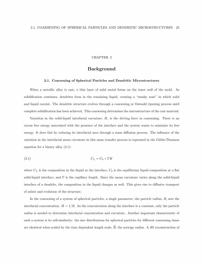
a 15% solid volume fraction PbSn sample with spherical particles is shown in Fig. 2.1, from Thompson et al
[21].
Figure 2.1. 3D Reconstruction of the 15% solid volume fraction PbSn sample coarsened for48 h. The volume reconstructed was approximately 7 mm 5 mm 1:8 mm containing a totalof 773 particles. The particles are colored by their relative size, red being much larger thanthe average particle size and purple much smaller.
For a system of infinitely separated solid, spherical particles in a liquid matrix, Lifshitz and Slyozov [24]
and Wagner [25] derived that the average particle radius R will evolve with time as:
R3(t)−R3
(0) = KLSW t(2.2)
where R(t) is the average particle radius at time t, R(0) is the average particle radius at the beginning of
the coarsening and KLSW is the coarsening constant that depends on the thermophysical parameters of the
system. A 2015 test of self-similar coarsening with tin rich lead-tin (PbSn) samples that were coarsened
aboard the ISS concluded that interfacial energy driven coarsening is well described by theory [21].
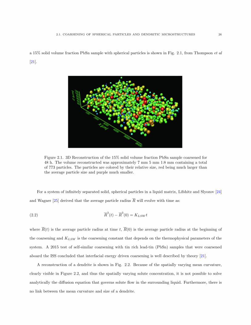
A reconstruction of a dendrite is shown in Fig. 2.2. Because of the spatially varying mean curvature,
clearly visible in Figure 2.2, and thus the spatially varying solute concentration, it is not possible to solve
analytically the diffusion equation that governs solute flow in the surrounding liquid. Furthermore, there is
no link between the mean curvature and size of a dendrite.
2.1. COARSENING OF SPHERICAL PARTICLES AND DENDRITIC MICROSTRUCTURES 27
Figure 2.2. Shown is a three-dimensional reconstruction of a free-growing aluminum dendritein an aluminum-copper eutectic liquid. The interface of the dendrite is colored according toits mean curvature, H. From Mendoza et al [1]
.
The search for a characteristic length scale other than R led to the measurement of the secondary arm
spacing λ2. Similar to R, λ2 was found to increase as coarsening progresses. Using an iron-nickel alloy,
Katamis and Flemings [29] found that as the structure coarsened with time, λ2 decreased with increasing
undercooling and decreasing distance from a chilled surface. Similar experiments were repeated on aluminum-
copper alloys and magnesium-zinc alloys [6, 30].
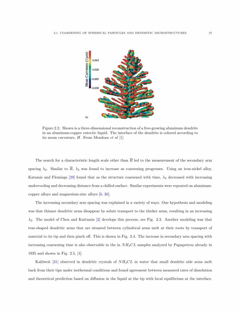
The increasing secondary arm spacing was explained in a variety of ways. One hypothesis and modeling
was that thinner dendritic arms disappear by solute transport to the thicker arms, resulting in an increasing
λ2. The model of Chen and Kattamis [2] develops this process, see Fig. 2.3. Another modeling was that
tear-shaped dendritic arms that are situated between cylindrical arms melt at their roots by transport of
material to its tip and then pinch off. This is shown in Fig. 2.4. The increase in secondary arm spacing with
increasing coarsening time is also observable in the in NH4CL samples analyzed by Papapetrou already in
1935 and shown in Fig. 2.5, [4].
Kahlweit [31] observed in dendritic crystals of NH4CL in water that small dendrite side arms melt
back from their tips under isothermal conditions and found agreement between measured rates of dissolution
and theoretical prediction based on diffusion in the liquid at the tip with local equilibrium at the interface.
2.1. COARSENING OF SPHERICAL PARTICLES AND DENDRITIC MICROSTRUCTURES 28
Figure 2.3. This model assumes that 1) coarsening occurs by dissolution at the tip of thesmaller dendrite arm of constant radius a and variable length l, diffusion of material to thejuxtaposed larger dendrite arms of variable radius R and constant length L and depositionalong the lateral surface of these arms. Thus, the small dendritic arm shrinks back andfinally disappears; 2) dendrite arms are cylindrical with hemispherical tips. From Chen andKattamis [2]
.
Kirkwood [5] elaborated Kahlweit’s model to describe the disappearance of individual side arms and the
increase in λ2. Comparing data assembled by Bardes and Flemings [32] from final secondary arm spacings
in Al-4.5wt.%Cu alloy as a function of local solidification time with the relationship predicted in his model,
Kirkwood obtained good agreement, as seen in Fig. 2.6. [5]
The above and other models (e.g. [33, 34]) are summarized in Fig. 2.7 which contrasts four different
models of isothermal coarsening: radial remelting, axial remelting, arm detachment, and arm coalescence.
A beginning, intermediate and end phase of the coarsening is provided. Each model is driven by the same
need to minimize the interfacial energy of the system. Experimental evidence suggests that each model is
possible, depending on circumstances.
Repeated measurement of secondary dendrite arm spacing λ2 has confirmed that dendrite coarsening
follows the same power law observed in spherical particle systems [5, 7]:
λ2 ∼ t1/3f(2.3)
2.1. COARSENING OF SPHERICAL PARTICLES AND DENDRITIC MICROSTRUCTURES 29
Figure 2.4. Material transport for (a) one tear-shaped arm surrounded by cylindrical armsand for (b) two tear-shaped arms surrounded by cylindrical arms. Gray arrows representthe direction of material transport. Mendoza et al [3]
.
Figure 2.5. Increasing secondary arm spacing during coarsening in NH4CL. From Papapetrou [4]
where t1/3f is local solidification time. Fig. 2.8 shows results from Bower, Brody and Flemings [7] on the
relation between λ2 and solidification time t1/3f for a Al-4.5wt.%Cu alloy. As in Fig. 2.6, the data in Fig.
2.8 are in good agreement with equation 2.3.
2.1. COARSENING OF SPHERICAL PARTICLES AND DENDRITIC MICROSTRUCTURES 30
Figure 2.6. Final secondary dendrite arm spacings plotted against local solidification time.From Kirkwood [5]
.
Figure 2.7. Four different models for isothermal coarsening: (1) radial remelting, (2) axialremelting, (3) arm detachment, (4) arm coalescence. Based on Kattamis et al [6]
.
Eq. 2.3 has been a useful engineering result but it also has disadvantages. First, it is highly dependent
on which 2D plane is visible after sample preparation. Second, because it is based on a 2D section, it only
partially describes the complexity of a 3D microstructure. Third, it is only measurable in systems with a
2.1. COARSENING OF SPHERICAL PARTICLES AND DENDRITIC MICROSTRUCTURES 31
Figure 2.8. Relationship between secondary dendrite arm spacing and local solidificationtime for various experiments. From Bower et al [7]
Figure 2.9. Quenched microstructures of a Sn-40wt%Bi alloy held isothermally just abovethe eutectic temperature: (a) as-cast, (b) after 10 min, (c) after 2.5 h, and (d) after 10 days.From Marsh and Glicksman [8]
clear dendritic morphology. In the 1966 study of Marsh and Glicksman of Sn-40wt%Bi, they found that
after coarsening for very long periods of time, the microstructure underwent large morphological changes;
the primary Sn-rich phase became distinctly more spheroidal at long aging times, precluding the use of λ2.
See Fig. 2.9.
2.1. COARSENING OF SPHERICAL PARTICLES AND DENDRITIC MICROSTRUCTURES 32
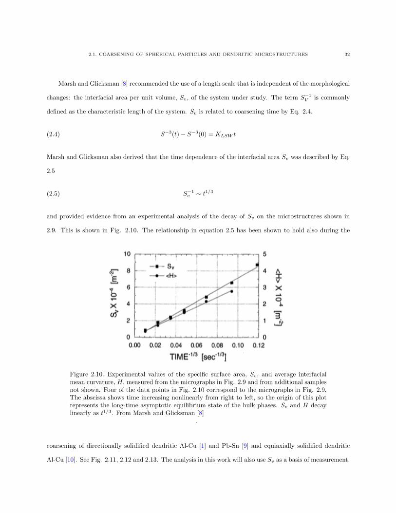
Marsh and Glicksman [8] recommended the use of a length scale that is independent of the morphological
changes: the interfacial area per unit volume, Sv, of the system under study. The term S−1V is commonly
defined as the characteristic length of the system. Sv is related to coarsening time by Eq. 2.4.
S−3(t)− S−3(0) = KLSW t(2.4)
Marsh and Glicksman also derived that the time dependence of the interfacial area Sv was described by Eq.
2.5
S−1v ∼ t1/3(2.5)
and provided evidence from an experimental analysis of the decay of Sv on the microstructures shown in
2.9. This is shown in Fig. 2.10. The relationship in equation 2.5 has been shown to hold also during the
Figure 2.10. Experimental values of the specific surface area, Sv, and average interfacialmean curvature, H, measured from the micrographs in Fig. 2.9 and from additional samplesnot shown. Four of the data points in Fig. 2.10 correspond to the micrographs in Fig. 2.9.The abscissa shows time increasing nonlinearly from right to left, so the origin of this plotrepresents the long-time asymptotic equilibrium state of the bulk phases. Sv and H decaylinearly as t1/3. From Marsh and Glicksman [8]
.
coarsening of directionally solidified dendritic Al-Cu [1] and Pb-Sn [9] and equiaxially solidified dendritic
Al-Cu [10]. See Fig. 2.11, 2.12 and 2.13. The analysis in this work will also use Sv as a basis of measurement.
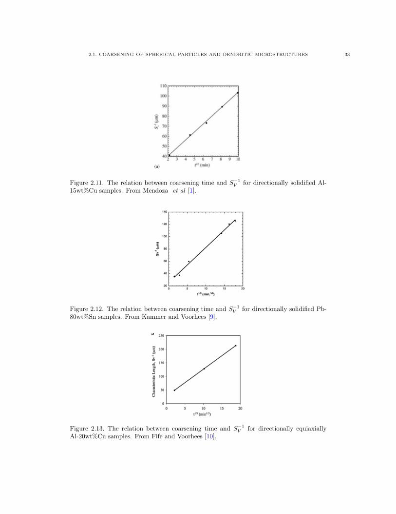
2.1. COARSENING OF SPHERICAL PARTICLES AND DENDRITIC MICROSTRUCTURES 33
Figure 2.11. The relation between coarsening time and S−1V for directionally solidified Al-
15wt%Cu samples. From Mendoza et al [1].
Figure 2.12. The relation between coarsening time and S−1V for directionally solidified Pb-
80wt%Sn samples. From Kammer and Voorhees [9].
Figure 2.13. The relation between coarsening time and S−1V for directionally equiaxially
Al-20wt%Cu samples. From Fife and Voorhees [10].
2.2. INTERFACIAL CURVATURE 34
2.2. Interfacial Curvature
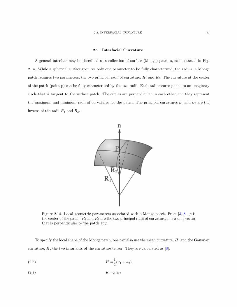
A general interface may be described as a collection of surface (Monge) patches, as illustrated in Fig.
2.14. While a spherical surface requires only one parameter to be fully characterized, the radius, a Monge
patch requires two parameters, the two principal radii of curvature, R1 and R2. The curvature at the center
of the patch (point p) can be fully characterized by the two radii. Each radius corresponds to an imaginary
circle that is tangent to the surface patch. The circles are perpendicular to each other and they represent
the maximum and minimum radii of curvatures for the patch. The principal curvatures κ1 and κ2 are the
inverse of the radii R1 and R2.
Figure 2.14. Local geometric parameters associated with a Monge patch. From [3, 8]. p isthe center of the patch; R1 and R2 are the two principal radii of curvature; n is a unit vectorthat is perpendicular to the patch at p.
To specify the local shape of the Monge patch, one can also use the mean curvature, H, and the Gaussian
curvature, K, the two invariants of the curvature tensor. They are calculated as [8]:
H =1
2(κ1 + κ2)(2.6)
K =κ1κ2(2.7)
2.3. INTERFACE SHAPE DISTRIBUTION 35
The Gaussian curvature provides an essential measure of the morphology since it distinguishes between a
saddle-shaped surface and a concave or convex surface. Marsh and Glicksman [8] and Alkemper and Voorhees
[26] demonstrate the interconnection between the two curvatures.
H and K can be calculated from either a surface-mesh based description of the interface or from a diffuse
interface representation. For the latter, the mean curvature H can be calculated using:
H =1
2(∇.n)(2.8)
where n is the normal vector to the interface calculated from gradients of the order parameter
n =∇φ|∇φ|
(2.9)
The Gaussian curvature can be obtained from:
K =n.adj(He(φ))n(2.10)
where He(φ) is the 3 × 3 Hessian matrix of the second partial derivatives of the order parameter and
adj(He(φ)) is the adjoint to the Hessian matrix [35].
2.3. Interface Shape Distribution
When the local mean and Gaussian curvatures are obtained for each interfacial patch, one can represent
the curvature information of the microstructure three-dimensionally [3]. This is shown in Fig. 2.15. P (H,K)
is a probability density function such that P (H,K)dHdK is the probability that a randomly chosen interface
point will have a mean curvature between H and H+dH and a Gaussian curvature between K and K+dK.
An alternate way of presenting curvature information is by constructing probability density plots of κ1 versus
κ2. These can be obtained from:
κ1 =H −√H2 −K(2.11)
κ2 =H +√H2 −K(2.12)
2.3. INTERFACE SHAPE DISTRIBUTION 36
Figure 2.15. Mean and Gaussian curvature probability plots for a sample. From [3]
Similar to 2.15, 3D plots can be generated of the principal curvature data. Presented in terms of the
two principal curvatures κ1 and κ2, P (κ1, κ2)dκ1dκ2 is the probability that a randomly chosen interface
point will have one principal curvature between κ1 + dκ1 and a second principal curvature beween κ2 +
dκ2. From this three-dimensional probability plot, one can derive two-dimensional probability contour plots
that measure the probability of finding a patch of interface with a certain pair of principal curvatures.
These probability functions are termed the interfacial shape distributions (ISDs) [3, 36]. Note that κ2 is the
maximum principal curvature and is defined to be always greater than or equal to κ1. Examples of ISDs in
terms of the mean and Gaussian curvatures and the principal curvature κ1 versus κ2 are given in Fig. 2.16
and Fig. 2.17.
The ISD can be broken down in four regions [3, 23] (see Fig. 2.18)
• Region 1: solid on the concave side of the interface.
• Region 2: saddle-shaped with H > 0, K < 0
• Region 3: saddle-shaped with H < 0, K < 0
• Region 4: liquid on the concave side of the interface
Other features of interest are along the axes and the line κ1 = κ2:
• The interface is planar along the line κ1 = κ2 = 0
2.3. INTERFACE SHAPE DISTRIBUTION 37
Figure 2.16. Probability density plots of the mean and Gaussian curvatures for two samples.From Mendoza et al [3]
Figure 2.17. Probability density plots of κ1 versus κ2 for two samples. From Mendoza et al [3]
• No patches appear below the line κ1 = κ2 since κ1 ≥ κ2 by definition
• Interfacial patches on the κ1 = κ2 > 0 line correspond to solid spherical shapes, and patches along
κ1 = κ2 < 0 are liquid spherical shapes
2.4. INTERFACE NORMAL DISTRIBUTION 38
Figure 2.18. Map of the local interfacial shapes for the ISD contour plots. From Mendoza et al [3]
• For κ1 = 0, the interface is cylindrical with solid inside, and for κ2 = 0, the interface is cylindrical
with liquid on the inside
2.4. Interface Normal Distribution
To determine whether there is a preferential directionality in a particular microstructure, Mendoza et
al [1] and Kammer and Voorhees [9, 11] proposed analyzing the orientation of the interfaces. When the
curvature has been determined for every patch of interface, all interface normals can be collapsed into a unit
reference sphere with their origins at the center of the sphere and their ends on its surface. A two-dimensional
representation of the directionality of the interfaces can be generated by a spherical projection. Fig. 2.19
shows two types of projections: the Equal-Area Projection (EQA) and the Stereographic Projection (SG).
In a spherical projection, three-dimensional information is projected on a plane that is tangent to the
sphere and perpendicular to the axis along which the projections is made. The projection is a contour
plot showing the probability distribution of the interfacial normal distributions (INDs). Fig. 2.19 panel
2.4. INTERFACE NORMAL DISTRIBUTION 39
Figure 2.19. Schematic representation of two types of spherical projections used for obtain-ing interfacial normal distributions (INDs). From Kammer [11]
Figure 2.20. INDs of two coarsened samples (near-hemisphere projection). From [11]
(a) shows that the EQA projection is obtained by drawing an arc from a point on the reference sphere to
the projection plane such that the distance, d, from the tangency point, B, to the projected point is equal
to the distance from the tangency point to the point on the reference sphere. This projection minimizes
distortion of features near the center of the plots where the data tends to be concentrated when projected
2.5. TOPOLOGY OF DENDRITIC STRUCTURES 40
along x. In an SG projection, features near the edges are expanded and the projection is made from a
point opposite to the point of tangency, see Fig. 2.19 panel (b). Since the analyzed microstructures are not
symmetric, two projections are required to represent all data: a near-hemisphere projection (projected along
the positive x-axis) and a far-hemisphere projection (projected along the negative x-axis). Examples of an
EQA projection from Kammer and Voorhees [9] are provided in Fig. 2.20.
2.5. Topology of Dendritic Structures
In addition to determining the morphology of solid-liquid mixtures, it is of interest to quantify their
topology. The use of topological measurements to characterize microstructures was pioneered by DeHoff et.
al [12]. He argues that the quantitative analysis of microstructures can be divided into two classifications:
the analysis of metric properties which depend on the extent and details of shape of the features in the
structure, and the analysis of topological properties, whose values are independent of the extent or details
of shape of the features in the system. Two structural topological properties are fundamental: the number
of disconnected parts of the feature in unit volume, and the connectivity of the feature in unit volume.
Mendoza et al [13] termed these properties 1) the number of independent bodies, or voids per unit volume,
and 2) the total connectivity of the microstructure. An increase in the number of voids over coarsening time
may indicate that the structure is breaking up.
Figure 2.21. Visualization of the genus of surfaces in terms of the number of cuts requiredto form a disconnected part. (a) g = 0, (b) g = 1, (c) g = 2. From [12]
2.5. TOPOLOGY OF DENDRITIC STRUCTURES 41
A direct measure of the connectivity of a structure is the genus, g, which is defined as “the number of
(non-self intersecting) cuts that may be made upon a surface without separating it into two disconnected
parts” [12]. DeHoff’s visualization of the genus of surfaces is shown in Fig. 2.21. A closed surface is simply
connected if any cut made on the surface separates it in two parts; its genus is 0 (Fig. 2.21, panel (a)). A
soccer ball is thus simply connected. An inner tube may be cut once without separating into two parts (Fig.
2.21, panel (b)). The genus of an inner tube and thus all surfaces which are topologically deformable into
it, such as a doughnut or coffee cup, is 1.
The genus is related to the Gaussian curvature of a surface. A closed surface has an integral Gaussian
curvature Ktotal equal to 4π with a genus g of 0. Adding a hole or handle to the structure increases the
genus by one and decreases Ktotal by 4π. Thus, the genus is given by [13]
g =1− Ktotal
4π(2.13)
If curvature information is not available, the Euler characteristic (χ) can be used to measure the genus:
g =1− χ
2(2.14)
The Euler characteristic when there are edges (or boundaries) is given by
χ =n− e+ f(2.15)
with n the number of nodes of a surface, e the number of edges, and f the number of faces. For example,
for a simple cube, n = 8, e = 12 and f = 6, giving a χ = 2 and g = 0. The genus does not change if the
surface is elastically deformed. Related to dendritic microstructures, the genus will change when a secondary
dendrite arm detaches from a primary dendrite trunk.
The genus also changes when there is, for example, a break-up of cylindrical structures through Rayleigh
instabilities [13]. This is illustrated in Fig. 2.22. When the tube is intact, its structure is topologically
equivalent to a cubic torus with the tube representing a hole (panels (a) and (b)). Both structures have
a genus of 1. After the change in the structure, an enclosed void is created (panel (c)). This structure is
topologically equivalent to a cube with a cuboidal void. For that structure, n = 16, e = 24 and f = 12, giving
2.5. TOPOLOGY OF DENDRITIC STRUCTURES 42
Figure 2.22. (a) A cubic torus is topologically equivalent to (b) a cube with a cylindricaltube. The cube can undergo Rayleigh instability leading to the formation of a void (c) andchange the genus from 1 to -1. (c) and (d) are topologically equivalent. From Mendoza etal [13]
a χ = 4 and g = -1. Thus, the morphological instability of the tube decreased the genus by 2. Structure (c),
which has a single void, also has the same genus = -1. Each void within the structure decreases the genus
by one, providing a relationship between g, h, and v [13].
g = h− v(2.16)
with h the number of handles or tunnels and v the number of voids or cavities within the structure. Thus it
is possible for the genus of a structure to become negative if the number of voids is greater than the number
of handles. The genus has been measured in experiments [13, 37] but was limited to either liquid domains
in high volume fraction solid systems or solid domains in mixtures with relatively high volume fractions
of solid, in excess of 43 %. Fig. 2.23 shows the evolution of the number of handles, genus and voids per
unit volume as a function of coarsening time for directionally solidified Al-15wt.%Cu samples with a solid
volume fraction of 74%. The genus shows an almost steady decrease with coarsening time, giving evidence
of topological changes. It also shows that the number of liquid droplets per scaled volume increase and that
the scaled number of handles fluctuates around a constant with coarsening time.
In low volume fraction solid mixtures, as soon as a secondary arm detaches, it sediments and can coalesce
with another piece of solid, changing the genus. This makes it difficult to relate on earth the genus to the
secondary arm detachment. The analysis reported later in this work relates to experiments conducted aboard
the ISS to allow a measurement of the genus in low volume fraction solid mixtures.
2.6. PHASE FIELD SIMULATION 43
Figure 2.23. The scaled number of handles, genus, and voids per unit volume as a functionof coarsening time. From Mendoza et al [13]
2.6. Phase Field Simulation
The evolution of the morphology and topology of solid-liquid mixtures can be further studied by using
experimentally measured microstructures as initial conditions in phase field simulations. Phase-field models
are based on a diffuse-interface description between domains [23, 38]. The interfaces are modeled by a
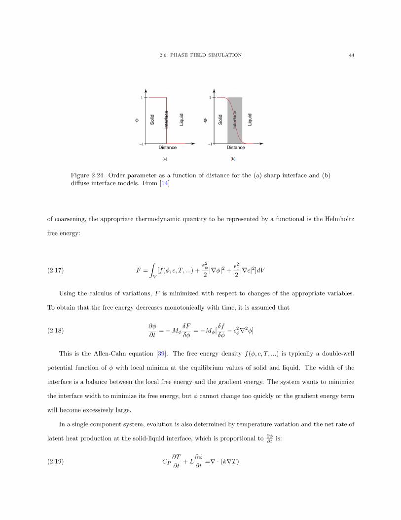
continuous variation of the properties within a narrow region, see Fig. 2.24. A single variable, the order
parameter φ, describes the entire microstructure, including the interface. φ has a constant value in the bulk
phases while it varies from the value of one phase to that of the second phase in the interface. For example,
Fig. 2.24 shows the order parameter φ varying from 1 (solid) to -1 (liquid). The range over which φ varies
is the width of the interface [14].
In the modeling of the dynamics of a system, the assumption is made that a free-energy functional exists
that depends on φ, its gradient ∇φ and other variables such as composition and temperature. In the case
2.6. PHASE FIELD SIMULATION 44
Figure 2.24. Order parameter as a function of distance for the (a) sharp interface and (b)diffuse interface models. From [14]
of coarsening, the appropriate thermodynamic quantity to be represented by a functional is the Helmholtz
free energy:
F =
∫V
[f(φ, c, T, ...) +ε2φ2|∇φ|2 +
ε2c2|∇c|2]dV(2.17)
Using the calculus of variations, F is minimized with respect to changes of the appropriate variables.
To obtain that the free energy decreases monotonically with time, it is assumed that
∂φ
∂t=−Mφ
δF
δφ= −Mφ[
δf
δφ− ε2φ∇2φ](2.18)
This is the Allen-Cahn equation [39]. The free energy density f(φ, c, T, ...) is typically a double-well
potential function of φ with local minima at the equilibrium values of solid and liquid. The width of the
interface is a balance between the local free energy and the gradient energy. The system wants to minimize
the interface width to minimize its free energy, but φ cannot change too quickly or the gradient energy term
will become excessively large.
In a single component system, evolution is also determined by temperature variation and the net rate of
latent heat production at the solid-liquid interface, which is proportional to ∂φ∂t is:
CP∂T
∂t+ L
∂φ
∂t=∇ · (k∇T )(2.19)
2.6. PHASE FIELD SIMULATION 45
T is the local temperature, CP is the constant pressure heat capacity, L is the latent heat of solidification,
and k is the thermal conductivity.
The model can be extended to a binary alloy (with components A and B) by adjusting f . For a regular
solution model
f(φ, c, T ) =(1− c)fA(φ, T ) + cfB(φ, T ) +RT [clnc+ (1− c)ln(1− c)] + c(1− c)[ΩS(1− p(φ)) + ΩLp(φ)]
(2.20)
with fA and fB the (double-well) free energy density functions for component A and B alone, c the mole
fraction of component B, ΩS and ΩL the regular solution parameters of the solid and the liquid, and p(φ)
an interpolating function with values p(0) = 0, p(1) = 1. For multicomponent systems, it is usually assumed
that heat diffusion takes place faster than solute diffusion so that the system may be taken to be isothermal.
If so, the evolution of the system is guided by the Allen-Cahn and the Cahn-Hilliard equations [40]:
∂c
∂t=∇ · [Mcc(1− c)∇(
δF
δc)] = ∇ · [Mcc(1− c)∇(
∂f
∂c− ε2c∇2c)](2.21)
More generally, an entropy functional S may be formulated [41, 42]
S =
∫V
[s(e, c, φ)− ε2e2|∇e|2 − ε2c
2|∇c|2 −
ε2φ2|∇φ|2]dV(2.22)
where s and e are respectively the entropy density and the internal energy density. Using this functional,
the system is evolved such that entropy is monotonically increasing as a function of time. An asymptotic or
thin-interface analysis is often made to demonstrate that the models are consistent with physical laws.
Dendritic growth in an undercooled liquid for pure materials has frequently been based on phase field
modeling [43, 44, 45, 46, 47, 48, 49, 50, 51, 52]. To model dendrite growth, some form of anisotropy in the
gradient energy coefficient εφ or in the kinetic coefficient Mφ is required. The concentration of the liquid
is set to be supersaturated for the given temperature, and a seed of solid or thermal noise is introduced to
provide a nucleation site.
McFadden et. al. [45] validated some of the original models of 2D dendritic growth in a pure material
[43, 44]. Karma and Rappel [47] introduced a new method for performing a sharp-interface analysis which
2.6. PHASE FIELD SIMULATION 46
allowed the use of much wider interface thicknesses. They also used a phase field model with intentionally
introduced thermal noise to allow the system to generate secondary arms [49].
Phase-field models of solidification can be extended to binary alloys by modifying the free energy density
to included corrections for alloy composition. To avoid the additional computation necessary to solve for
coupled heat and solute diffusion, it is usually assumed that heat diffuses much more quickly than solute, so
the system is either isothermal or held at a fixed temperature gradient by external constraints.
Karma [53] extended phase-field work of binary allows in a major way by introducing an anti-trapping
current in the Cahn-Hilliard equation. Karma concluded that three important non-equilibrium effects at the
solid-liquid interface would result from unequal diffusivities in the solid and liquid phases: 1) a chemical jump
across the interface leading to solute trapping, 2) an interface stretching correction to solute conservation,
and 3) a surface diffusion correction to solute conservation. Thus, solute trapping would appear at a much
lower interface velocity than would be expected physically in models with relatively large values of interface
thickness. He then modeled an antitrapping current into the Cahn-Hilliard equation to eliminate the effect
of solute trapping:
∂c
∂t=∇ · [Mc∇
δF
δc−~jat](2.23)
The three non-equilibrium effects were eliminated by a selection of parameters obtained in an asymptotic
analysis. This analysis also showed that it reproduces the sharp-interface equations correctly, and thus
should allow the evolution of the system to be modeled accurately.
Specifically related to the evolution of the microstructure of solid-liquid mixtures, Mendoza et al [13]
performed phase field calculations using reconstructions of the coarsened Al-15wt.%Cu as initial condition
for determining interfacial velocity and simulating the evolution of the microstructure. The normal velocity
of the interface for a given microstructure was computed by determining the diffusion field, U , in three
dimensions within the steady-state approximation. To obtain the diffusion field that is consistent with an
experimentally obtained microstructure, they evolved phase-field equations within the constraint of constant
2.6. PHASE FIELD SIMULATION 47
phase fractions:
∂φ
∂t= ∇2φ+ (1− φ2)(φ− λU(1− φ2))(2.24)
∂U
∂t− 1
2
∂φ
∂t= D∇2U(2.25)
until the time derivatives of φ and U were nearly zero. λ was set so that the GibbsThomson boundary
condition in the sharp interface limit was obtained; D is the diffusion coefficient. The diffusion coefficients
were assumed equal in both phases, and thus U was considered to be the dimensionless temperature or
concentration.
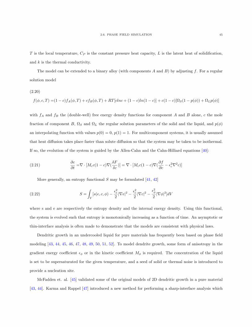
Figure 2.25. A portion of the experimental interfacial morphology of the 964-min Al-15wt.%Cu sample is colored by the interfacial velocity calculated from the phase-field simu-lations. Positive interfacial velocity points into the liquid and is represented by warm colors.Liquid intersecting the edges of the reconstruction box is capped with zero interfacial veloc-ity. From [13]
The calculations provided insights into the dynamics of the pinching or fissioning. Fig. 2.25 shows the
interfacial velocities [13]. Positive interfacial velocities point into the liquid and are represented by warm
colors. The velocities at region (a) imply that the solid-liquid interfaces will touch causing the tube to pinch.
If this also happens either above or below (a), a liquid droplet will be formed. The interfacial velocities
indicate that this is also possible at (b). A topological singularity will occur on the liquid channel (c)
2.6. PHASE FIELD SIMULATION 48
separating the two liquid regions. A liquid droplet is shown at (d) and according to its interfacial velocity it
will become more spherical at a later time.
Aagesen et al [15] directly compared 3D phase-field predictions of solidliquid interfacial velocities with
interfacial velocities calculated from experimental microstructures in an Al-15wt.%Cu system during isother-
mal coarsening, captured using X-ray tomographic microscopy. Experimental results are compared with
simulation data in Fig. 2.26. Interfacial velocities are shown for a 104 x 112 x 126 µm subset of the mi-
crostructure. Fig. 2.26 shows there is a good agreement between experimental and estimated velocities
though estimations are higher by a factor of about three. The diffusion coefficient of solute in the liquid was
believed to be the largest contributor to the discrepancy. The simulations also revealed that the antitrapping
current could be neglected, increasing computation speed by a factor of 1.6.
Figure 2.26. Experimental and simulated velocities. Liquid is inside the bulb shape, and thesurrounding solid phase is transparent. The solidliquid interface is colored by normal ve-locities, with negative velocities pointing into the liquid. (a) Interfacial velocities calculatedfrom experimental data, 346 s between X-ray scans and (b) interfacial velocities calculatedfrom phase-field simulations, 5 s simulated time elapsed. Note color bars between left andright images differ by a factor of 3. From [15]
In this study, the measured interfacial morphologies as initial conditions in a phase field calculation will
also used. A number of analyses will be done, including determining the diffusion field in the liquid and
the regions of interface that are subject to curvature-driven pinching, and using the phase field method to
calculate the flux in ISD space for a particular structure to determine the evolution of ISD of that structure.
2.7. COLUMNAR TO EQUIAXED TRANSITION (CET) 49
2.7. Columnar to Equiaxed Transition (CET)
In a recent review of the factors driving the columnar to equiaxed transition, Neumann-Heyme, Eckert
and Beckermann [17] state that “Fragmentation of dendrites is one of the major unresolved questions in
the field of solidification. The detachment of dendrite sidebranches from a larger stem or the breakup of
dendrite arms are considered key mechanisms in the formation of grain structure transitions (columnar to
equiaxed) in metal alloy castings, grain defects such as freckles in single crystal components, and highly
refined grain structures in the solidification of undercooled melts. Despite its technological importance, a
systematic understanding of dendrite fragmentation has been difficult to obtain due to the complexity of the
processes involved and the challenges associated with its direct experimental observation.”
Figure 2.27. Columnar dendrites with equiaxed crystals in the undercooled region. From [16]
While the CET phenomenon is not the focus of the current work, it is very complementary [54]. The
CET occurs when advancing columnar dendrites are blocked by the formation of equiaxed grains [16]; see
Fig. 2.27. The presence of undercooled liquid in front of growing columnar dendrites implies that nucleation
of solid is possible. The dendritic mush can be a source of the nucleants via fragmentation of the columnar
dendrites. These fragments are transported by convection ahead of the tips of the columnar dendrites into
the undercooled liquid region, and form equiaxed grains [17]. These fragments can also lead to misoriented
grains (freckles) within the columnar region and are an important casting defect in single crystal turbine
blades, since they greatly affect the creep behavior of aero and land-based turbine blades [55, 56]. Therefore,
2.7. COLUMNAR TO EQUIAXED TRANSITION (CET) 50
understanding the cause of dendrite fragmentation will provide insights into both the CET and the cause of
an extremely important casting defect in turbine blade castings.
Figure 2.28. (a) Time evolution of the arm shape. Time is measured relative to the pinch-offtime tp. In this example, the cooling rate is zero and interface motion is driven purely bydiffusive mass exchange between interface regions of different curvatures due to the Gibbs-Thomson effect. The solid tends to melt in regions of higher curvature and accumulatein regions of lower curvature. Mass exchange and interface motion is generally promotedby either high curvature contrasts or short diffusion paths. (b) Flux lines of the diffusivetransport during isothermal coarsening; solute concentration: high (red), low (blue). Withina short time from the start of the simulation, a narrow neck is formed immediately abovethe junction between the sidearm and the parent stem. This can be attributed to the shortdiffusion paths between the stem and the sidearm in this region. The tip of the sidearmretracts due to its high curvature and the sidearm evolves into a more evenly rounded shape.Later, the sidearm pinches off at the neck and the resulting fragment coarsens into a sphere.From [17]
There are alternative mechanisms by which the secondary arms detach [17, 54]. Solute inhomogeneities
in the liquid that result from convection during directional solidification can lead to melting at the roots of
the secondary arms. Alternatively, fluid flow during solidification can induce stresses that lead to detachment
by changing the local solubility of solute at the root. Also, fissioning can be driven by interfacial curvatures
at the root, similar to a Rayleigh instability, in which mass is transported from the negatively curved roots
to the small positive mean curvature regions of the surrounding interfaces due to the Gibbs-Thomson effect.
Capillary driven pinching is shown in Fig. 2.28.

2.7. COLUMNAR TO EQUIAXED TRANSITION (CET) 51
As explained in the previous sections, the experiments of the current work conducted in the microgravity
environment of the ISS will allow us to determine to what extent secondary and ternary branches detach
from the main trunk. This will be established by the reconstruction of the mushy region of the PbSn samples
and the identification of the dendrite fragments. The pinching and coalescence will be measured by tracking
the genus during the solidification, which changes as the topology of the solid-liquid mixture changes.
3.1. THE LEAD-TIN SYSTEM 52
CHAPTER 3
Experimental Methods
3.1. The Lead-Tin System
The experiments in this work are based on the Lead-Tin (PbSn) system. Originally, an alternative
candidate system for the research was Aluminum-Copper. However, due to the high partial pressure of
copper, the decision was made not to use AlCu in the experiment aboard the ISS.
Figure 3.1. Lead-Tin phase diagram.
The PbSn binary system is particularly useful for studying coarsening because the coarsening rate is
rapid, the eutectic temperature is low (183), the interfacial energy is nearly isotropic, and the thermo-
physical parameters are well documented [57]. The phase diagram for the PbSn system is shown in Fig. 3.1.
The solid corresponds to Sn dendrites while the eutectic consists of a lamellar PbSn structure.
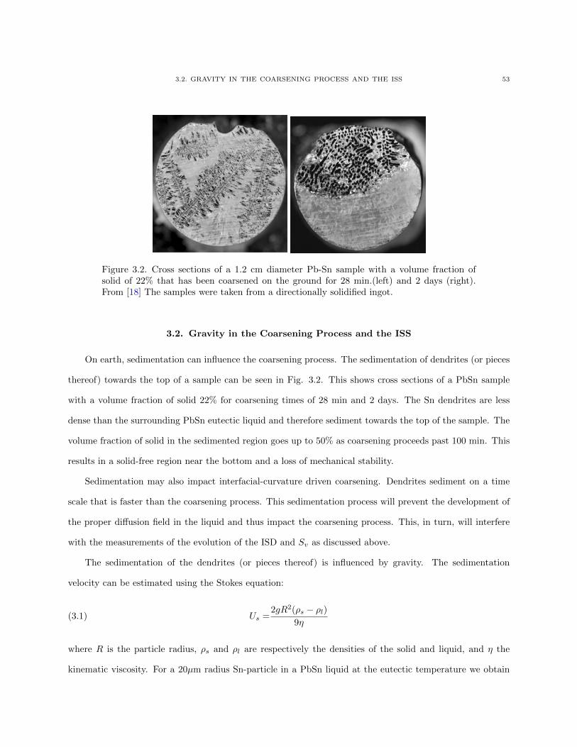
3.2. GRAVITY IN THE COARSENING PROCESS AND THE ISS 53
Figure 3.2. Cross sections of a 1.2 cm diameter Pb-Sn sample with a volume fraction ofsolid of 22% that has been coarsened on the ground for 28 min.(left) and 2 days (right).From [18] The samples were taken from a directionally solidified ingot.
3.2. Gravity in the Coarsening Process and the ISS
On earth, sedimentation can influence the coarsening process. The sedimentation of dendrites (or pieces
thereof) towards the top of a sample can be seen in Fig. 3.2. This shows cross sections of a PbSn sample
with a volume fraction of solid 22% for coarsening times of 28 min and 2 days. The Sn dendrites are less
dense than the surrounding PbSn eutectic liquid and therefore sediment towards the top of the sample. The
volume fraction of solid in the sedimented region goes up to 50% as coarsening proceeds past 100 min. This
results in a solid-free region near the bottom and a loss of mechanical stability.
Sedimentation may also impact interfacial-curvature driven coarsening. Dendrites sediment on a time
scale that is faster than the coarsening process. This sedimentation process will prevent the development of
the proper diffusion field in the liquid and thus impact the coarsening process. This, in turn, will interfere
with the measurements of the evolution of the ISD and Sv as discussed above.
The sedimentation of the dendrites (or pieces thereof) is influenced by gravity. The sedimentation
velocity can be estimated using the Stokes equation:
Us =2gR2(ρs − ρl)
9η(3.1)
where R is the particle radius, ρs and ρl are respectively the densities of the solid and liquid, and η the
kinematic viscosity. For a 20µm radius Sn-particle in a PbSn liquid at the eutectic temperature we obtain
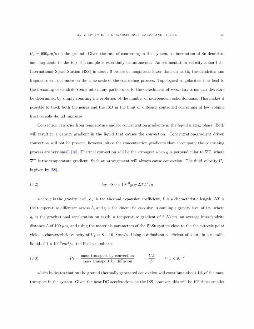
3.2. GRAVITY IN THE COARSENING PROCESS AND THE ISS 54
Us = 900µm/s on the ground. Given the rate of coarsening in this system, sedimentation of Sn dendrites
and fragments to the top of a sample is essentially instantaneous. As sedimentation velocity aboard the
International Space Station (ISS) is about 6 orders of magnitude lower than on earth, the dendrites and
fragments will not move on the time scale of the coarsening process. Topological singularities that lead to
the fissioning of dendrite stems into many particles or to the detachment of secondary arms can therefore
be determined by simply counting the evolution of the number of independent solid domains. This makes it
possible to track both the genus and the ISD in the limit of diffusion controlled coarsening of low volume
fraction solid-liquid mixtures.
Convection can arise from temperature and/or concentration gradients in the liquid matrix phase. Both
will result in a density gradient in the liquid that causes the convection. Concentration-gradient driven
convection will not be present, however, since the concentration gradients that accompany the coarsening
process are very small [18]. Thermal convection will be the strongest when g is perpendicular to ∇T, where
∇T is the temperature gradient. Such an arrangement will always cause convection. The fluid velocity UT
is given by [58],
UT =8.0× 10⁻³gαT∆TL2/η(3.2)
where g is the gravity level, αT is the thermal expansion coefficient, L is a characteristic length, ∆T is
the temperature difference across L, and η is the kinematic viscosity. Assuming a gravity level of 1ge, where
ge is the gravitational acceleration on earth, a temperature gradient of 2 K/cm, an average interdendrite
distance L of 100 µm, and using the materials parameters of the PbSn system close to the the eutectic point
yields a characteristic velocity of UT ≈ 8× 10⁻²µm/s. Using a diffusision coefficient of solute in a metallic
liquid of 1× 10⁻⁵cm2/s, the Peclet number is
Pe =mass transport by convection
mass transport by diffusion=UL
D≈ 1× 10⁻²(3.3)
which indicates that on the ground thermally generated convection will contribute about 1% of the mass
transport in the system. Given the near DC accelerations on the ISS, however, this will be 106 times smaller
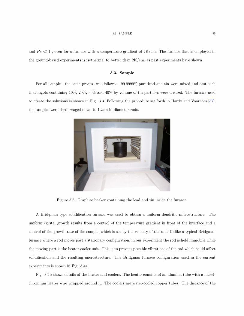
3.3. SAMPLE 55
and Pe 1 , even for a furnace with a temperature gradient of 2K/cm. The furnace that is employed in
the ground-based experiments is isothermal to better than 2K/cm, as past experiments have shown.
3.3. Sample
For all samples, the same process was followed. 99.9999% pure lead and tin were mixed and cast such
that ingots containing 10%, 20%, 30% and 40% by volume of tin particles were created. The furnace used
to create the solutions is shown in Fig. 3.3. Following the procedure set forth in Hardy and Voorhees [57],
the samples were then swaged down to 1.2cm in diameter rods.
Figure 3.3. Graphite beaker containing the lead and tin inside the furnace.
A Bridgman type solidification furnace was used to obtain a uniform dendritic microstructure. The
uniform crystal growth results from a control of the temperature gradient in front of the interface and a
control of the growth rate of the sample, which is set by the velocity of the rod. Unlike a typical Bridgman
furnace where a rod moves past a stationary configuration, in our experiment the rod is held immobile while
the moving part is the heater-cooler unit. This is to prevent possible vibrations of the rod which could affect
solidification and the resulting microstructure. The Bridgman furnace configuration used in the current
experiments is shown in Fig. 3.4a.
Fig. 3.4b shows details of the heater and coolers. The heater consists of an alumina tube with a nickel-
chromium heater wire wrapped around it. The coolers are water-cooled copper tubes. The distance of the
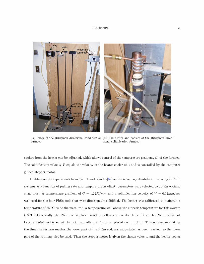
3.3. SAMPLE 56
(a) Image of the Bridgman directional solidificationfurnace
(b) The heater and coolers of the Bridgman direc-tional solidification furnace
coolers from the heater can be adjusted, which allows control of the temperature gradient, G, of the furnace.
The solidification velocity V equals the velocity of the heater-cooler unit and is controlled by the computer
guided stepper motor.
Building on the experiments from Cadirli and Gunduz[59] on the secondary dendrite arm spacing in PbSn
systems as a function of pulling rate and temperature gradient, parameters were selected to obtain optimal
structures. A temperature gradient of G = 1.22K/mm and a solidification velocity of V = 0.02mm/sec
was used for the four PbSn rods that were directionally solidified. The heater was calibrated to maintain a
temperature of 250inside the metal rod, a temperature well above the eutectic temperature for this system
(183). Practically, the PbSn rod is placed inside a hollow carbon fiber tube. Since the PbSn rod is not
long, a Ti-6-4 rod is set at the bottom, with the PbSn rod placed on top of it. This is done so that by
the time the furnace reaches the lower part of the PbSn rod, a steady-state has been reached, so the lower
part of the rod may also be used. Then the stepper motor is given the chosen velocity and the heater-cooler
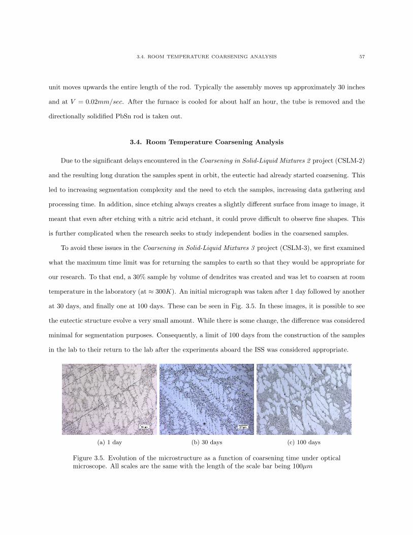
3.4. ROOM TEMPERATURE COARSENING ANALYSIS 57
unit moves upwards the entire length of the rod. Typically the assembly moves up approximately 30 inches
and at V = 0.02mm/sec. After the furnace is cooled for about half an hour, the tube is removed and the
directionally solidified PbSn rod is taken out.
3.4. Room Temperature Coarsening Analysis
Due to the significant delays encountered in the Coarsening in Solid-Liquid Mixtures 2 project (CSLM-2)
and the resulting long duration the samples spent in orbit, the eutectic had already started coarsening. This
led to increasing segmentation complexity and the need to etch the samples, increasing data gathering and
processing time. In addition, since etching always creates a slightly different surface from image to image, it
meant that even after etching with a nitric acid etchant, it could prove difficult to observe fine shapes. This
is further complicated when the research seeks to study independent bodies in the coarsened samples.
To avoid these issues in the Coarsening in Solid-Liquid Mixtures 3 project (CSLM-3), we first examined
what the maximum time limit was for returning the samples to earth so that they would be appropriate for
our research. To that end, a 30% sample by volume of dendrites was created and was let to coarsen at room
temperature in the laboratory (at ≈ 300K). An initial micrograph was taken after 1 day followed by another
at 30 days, and finally one at 100 days. These can be seen in Fig. 3.5. In these images, it is possible to see
the eutectic structure evolve a very small amount. While there is some change, the difference was considered
minimal for segmentation purposes. Consequently, a limit of 100 days from the construction of the samples
in the lab to their return to the lab after the experiments aboard the ISS was considered appropriate.
(a) 1 day (b) 30 days (c) 100 days
Figure 3.5. Evolution of the microstructure as a function of coarsening time under opticalmicroscope. All scales are the same with the length of the scale bar being 100µm
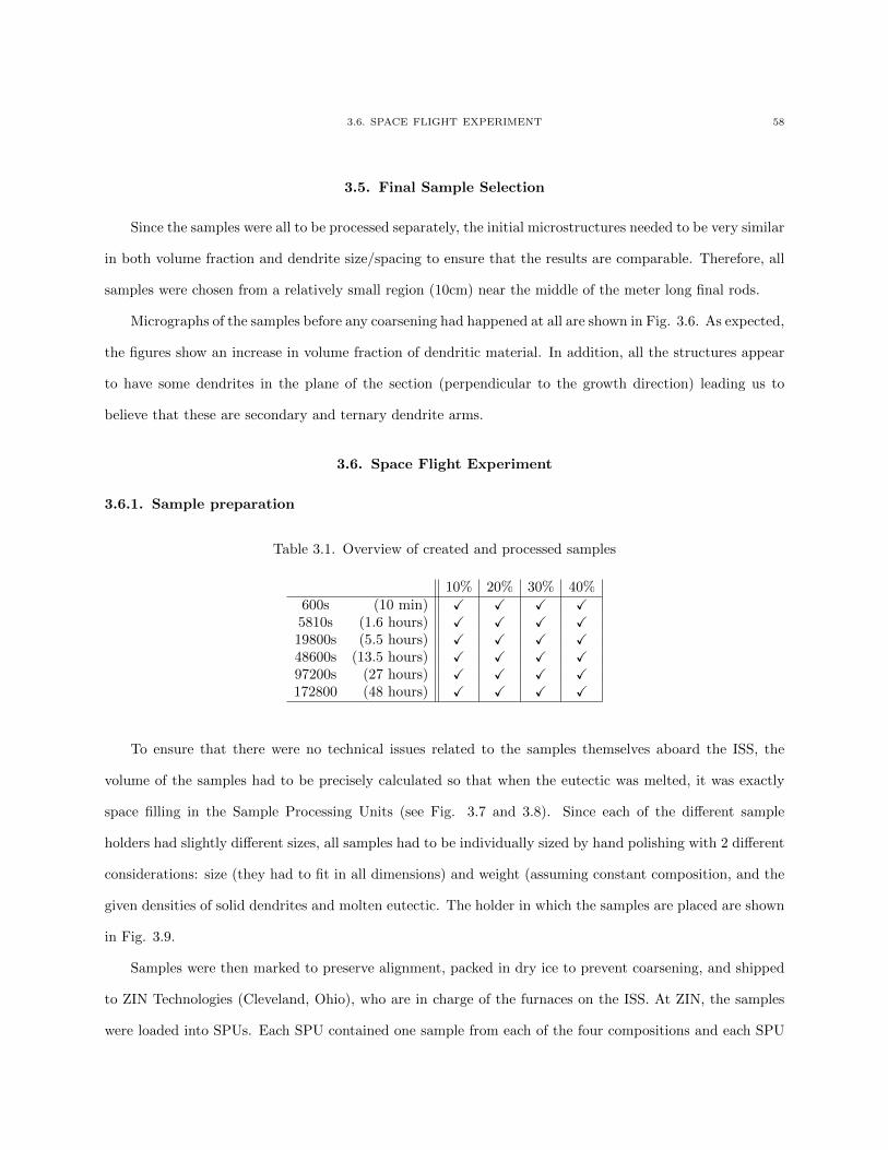
3.6. SPACE FLIGHT EXPERIMENT 58
3.5. Final Sample Selection
Since the samples were all to be processed separately, the initial microstructures needed to be very similar
in both volume fraction and dendrite size/spacing to ensure that the results are comparable. Therefore, all
samples were chosen from a relatively small region (10cm) near the middle of the meter long final rods.
Micrographs of the samples before any coarsening had happened at all are shown in Fig. 3.6. As expected,
the figures show an increase in volume fraction of dendritic material. In addition, all the structures appear
to have some dendrites in the plane of the section (perpendicular to the growth direction) leading us to
believe that these are secondary and ternary dendrite arms.
3.6. Space Flight Experiment
3.6.1. Sample preparation
Table 3.1. Overview of created and processed samples
10% 20% 30% 40%600s (10 min) X X X X5810s (1.6 hours) X X X X19800s (5.5 hours) X X X X48600s (13.5 hours) X X X X97200s (27 hours) X X X X172800 (48 hours) X X X X
To ensure that there were no technical issues related to the samples themselves aboard the ISS, the
volume of the samples had to be precisely calculated so that when the eutectic was melted, it was exactly
space filling in the Sample Processing Units (see Fig. 3.7 and 3.8). Since each of the different sample
holders had slightly different sizes, all samples had to be individually sized by hand polishing with 2 different
considerations: size (they had to fit in all dimensions) and weight (assuming constant composition, and the
given densities of solid dendrites and molten eutectic. The holder in which the samples are placed are shown
in Fig. 3.9.
Samples were then marked to preserve alignment, packed in dry ice to prevent coarsening, and shipped
to ZIN Technologies (Cleveland, Ohio), who are in charge of the furnaces on the ISS. At ZIN, the samples
were loaded into SPUs. Each SPU contained one sample from each of the four compositions and each SPU
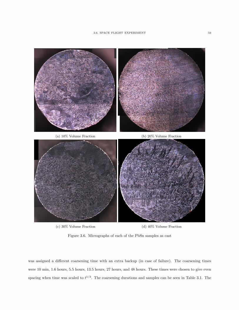
3.6. SPACE FLIGHT EXPERIMENT 59
(a) 10% Volume Fraction (b) 20% Volume Fraction
(c) 30% Volume Fraction (d) 40% Volume Fraction
Figure 3.6. Micrographs of each of the PbSn samples as cast
was assigned a different coarsening time with an extra backup (in case of failure). The coarsening times
were 10 min, 1.6 hours, 5.5 hours, 13.5 hours, 27 hours, and 48 hours. These times were chosen to give even
spacing when time was scaled to t1/3. The coarsening durations and samples can be seen in Table 3.1. The
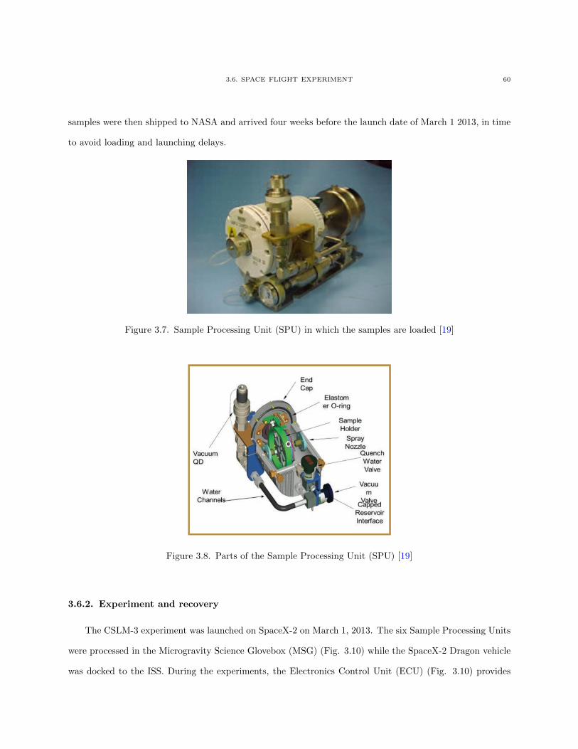
3.6. SPACE FLIGHT EXPERIMENT 60
samples were then shipped to NASA and arrived four weeks before the launch date of March 1 2013, in time
to avoid loading and launching delays.
Figure 3.7. Sample Processing Unit (SPU) in which the samples are loaded [19]
Figure 3.8. Parts of the Sample Processing Unit (SPU) [19]
3.6.2. Experiment and recovery
The CSLM-3 experiment was launched on SpaceX-2 on March 1, 2013. The six Sample Processing Units
were processed in the Microgravity Science Glovebox (MSG) (Fig. 3.10) while the SpaceX-2 Dragon vehicle
was docked to the ISS. During the experiments, the Electronics Control Unit (ECU) (Fig. 3.10) provides
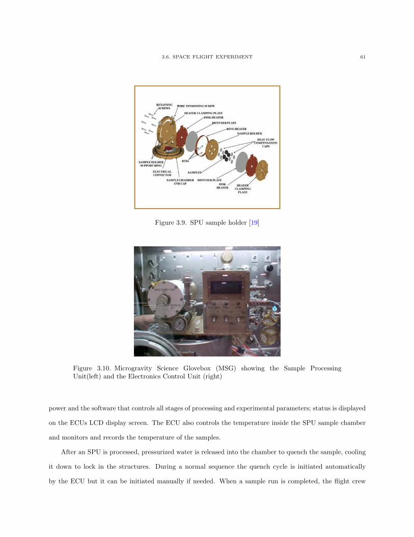
3.6. SPACE FLIGHT EXPERIMENT 61
Figure 3.9. SPU sample holder [19]
Figure 3.10. Microgravity Science Glovebox (MSG) showing the Sample ProcessingUnit(left) and the Electronics Control Unit (right)
power and the software that controls all stages of processing and experimental parameters; status is displayed
on the ECUs LCD display screen. The ECU also controls the temperature inside the SPU sample chamber
and monitors and records the temperature of the samples.
After an SPU is processed, pressurized water is released into the chamber to quench the sample, cooling
it down to lock in the structures. During a normal sequence the quench cycle is initiated automatically
by the ECU but it can be initiated manually if needed. When a sample run is completed, the flight crew
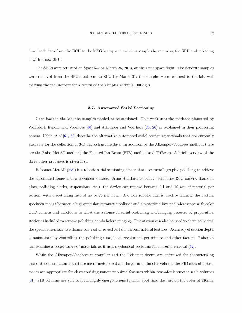
3.7. AUTOMATED SERIAL SECTIONING 62
downloads data from the ECU to the MSG laptop and switches samples by removing the SPU and replacing
it with a new SPU.
The SPUs were returned on SpaceX-2 on March 26, 2013, on the same space flight. The dendrite samples
were removed from the SPUs and sent to ZIN. By March 31, the samples were returned to the lab, well
meeting the requirement for a return of the samples within a 100 days.
3.7. Automated Serial Sectioning
Once back in the lab, the samples needed to be sectioned. This work uses the methods pioneered by
Wolfsdorf, Bender and Voorhees [60] and Alkemper and Voorhees [20, 26] as explained in their pioneering
papers. Uchic et al [61, 62] describe the alternative automated serial sectioning methods that are currently
available for the collection of 3-D microstructure data. In addition to the Alkemper-Voorhees method, there
are the Robo-Met.3D method, the Focused-Ion Beam (FIB) method and TriBeam. A brief overview of the
three other processes is given first.
Robomet-Met.3D ([63]) is a robotic serial sectioning device that uses metallographic polishing to achieve
the automated removal of a specimen surface. Using standard polishing techniques (SiC papers, diamond
films, polishing cloths, suspensions, etc.) the device can remove between 0.1 and 10 µm of material per
section, with a sectioning rate of up to 20 per hour. A 6-axis robotic arm is used to transfer the custom
specimen mount between a high-precision automatic polisher and a motorized inverted microscope with color
CCD camera and autofocus to effect the automated serial sectioning and imaging process. A preparation
station is included to remove polishing debris before imaging. This station can also be used to chemically etch
the specimen surface to enhance contrast or reveal certain microstructural features. Accuracy of section depth
is maintained by controlling the polishing time, load, revolutions per minute and other factors. Robomet
can examine a broad range of materials as it uses mechanical polishing for material removal [62].
While the Alkemper-Voorhees micromiller and the Robomet device are optimized for characterizing
micro-structural features that are micro-meter sized and larger in millimeter volume, the FIB class of instru-
ments are appropriate for characterizing nanometer-sized features within tens-of-micrometer scale volumes
[61]. FIB columns are able to focus highly energetic ions to small spot sizes that are on the order of 520nm.
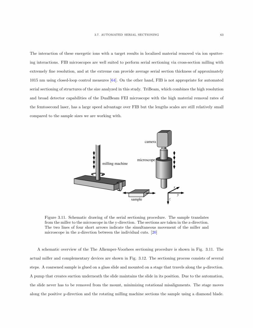
3.7. AUTOMATED SERIAL SECTIONING 63
The interaction of these energetic ions with a target results in localized material removed via ion sputter-
ing interactions. FIB microscopes are well suited to perform serial sectioning via cross-section milling with
extremely fine resolution, and at the extreme can provide average serial section thickness of approximately
1015 nm using closed-loop control measures [64]. On the other hand, FIB is not appropriate for automated
serial sectioning of structures of the size analyzed in this study. TriBeam, which combines the high resolution
and broad detector capabilities of the DualBeam FEI microscope with the high material removal rates of
the femtosecond laser, has a large speed advantage over FIB but the lengths scales are still relatively small
compared to the sample sizes we are working with.
Figure 3.11. Schematic drawing of the serial sectioning procedure. The sample translatesfrom the miller to the microscope in the y-direction. The sections are taken in the z-direction.The two lines of four short arrows indicate the simultaneous movement of the miller andmicroscope in the z-direction between the individual cuts. [20]
A schematic overview of the The Alkemper-Voorhees sectioning procedure is shown in Fig. 3.11. The
actual miller and complementary devices are shown in Fig. 3.12. The sectioning process consists of several
steps. A coarsened sample is glued on a glass slide and mounted on a stage that travels along the y-direction.
A pump that creates suction underneath the slide maintains the slide in its position. Due to the automation,
the slide never has to be removed from the mount, minimizing rotational misalignments. The stage moves
along the positive y-direction and the rotating milling machine sections the sample using a diamond blade.
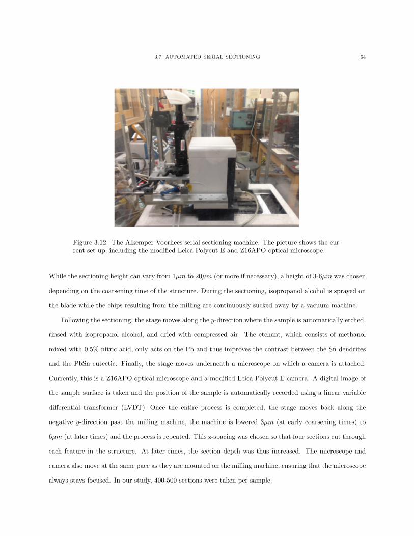
3.7. AUTOMATED SERIAL SECTIONING 64
Figure 3.12. The Alkemper-Voorhees serial sectioning machine. The picture shows the cur-rent set-up, including the modified Leica Polycut E and Z16APO optical microscope.
While the sectioning height can vary from 1µm to 20µm (or more if necessary), a height of 3-6µm was chosen
depending on the coarsening time of the structure. During the sectioning, isopropanol alcohol is sprayed on
the blade while the chips resulting from the milling are continuously sucked away by a vacuum machine.
Following the sectioning, the stage moves along the y-direction where the sample is automatically etched,
rinsed with isopropanol alcohol, and dried with compressed air. The etchant, which consists of methanol
mixed with 0.5% nitric acid, only acts on the Pb and thus improves the contrast between the Sn dendrites
and the PbSn eutectic. Finally, the stage moves underneath a microscope on which a camera is attached.
Currently, this is a Z16APO optical microscope and a modified Leica Polycut E camera. A digital image of
the sample surface is taken and the position of the sample is automatically recorded using a linear variable
differential transformer (LVDT). Once the entire process is completed, the stage moves back along the
negative y-direction past the milling machine, the machine is lowered 3µm (at early coarsening times) to
6µm (at later times) and the process is repeated. This z-spacing was chosen so that four sections cut through
each feature in the structure. At later times, the section depth was thus increased. The microscope and
camera also move at the same pace as they are mounted on the milling machine, ensuring that the microscope
always stays focused. In our study, 400-500 sections were taken per sample.
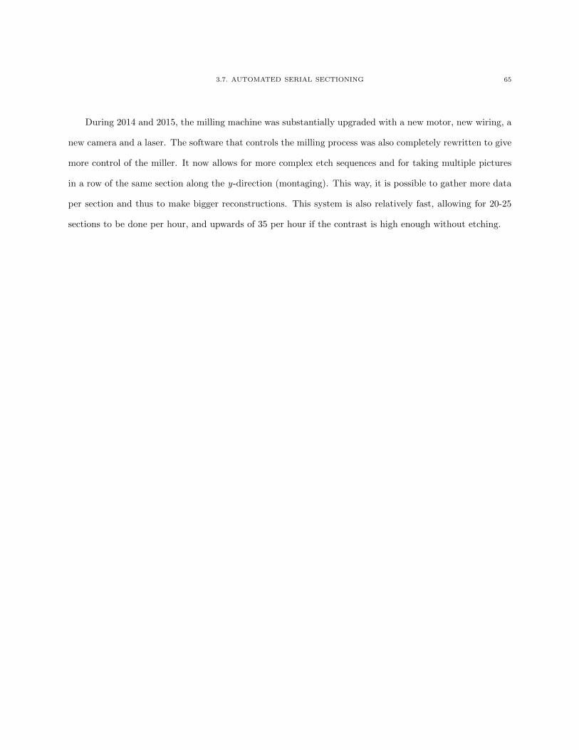
3.7. AUTOMATED SERIAL SECTIONING 65
During 2014 and 2015, the milling machine was substantially upgraded with a new motor, new wiring, a
new camera and a laser. The software that controls the milling process was also completely rewritten to give
more control of the miller. It now allows for more complex etch sequences and for taking multiple pictures
in a row of the same section along the y-direction (montaging). This way, it is possible to gather more data
per section and thus to make bigger reconstructions. This system is also relatively fast, allowing for 20-25
sections to be done per hour, and upwards of 35 per hour if the contrast is high enough without etching.
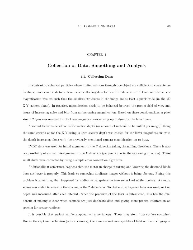
4.1. COLLECTING DATA 66
CHAPTER 4
Collection of Data, Smoothing and Analysis
4.1. Collecting Data
In contrast to spherical particles where limited sections through one object are sufficient to characterize
its shape, more care needs to be taken when collecting data for dendritic structures. To that end, the camera
magnification was set such that the smallest structures in the image are at least 5 pixels wide (in the 2D
X-Y camera plane). In practice, magnification needs to be balanced between the proper field of view and
issues of increasing noise and blur from an increasing magnification. Based on these considerations, a pixel
size of 2.6µm was selected for the lower magnifications moving up to 6µm for the later times.
A second factor to decide on is the section depth (or amount of material to be milled per image). Using
the same criteria as for the X-Y sizing, a 4µm section depth was chosen for the lower magnifications with
the depth increasing along with the previously mentioned camera magnification up to 6µm.
LVDT data was used for initial alignment in the Y direction (along the milling direction). There is also
is a possibility of a small misalignment in the X direction (perpendicular to the sectioning direction). These
small shifts were corrected by using a simple cross correlation algorithm.
Additionally, it sometimes happens that the motor in charge of raising and lowering the diamond blade
does not lower it properly. This leads to somewhat duplicate images without it being obvious. Fixing this
problem is something that happened by adding extra springs to take some load of the motors. An extra
sensor was added to measure the spacing in the Z dimension. To that end, a Keyence laser was used; section
depth was measured after each interval. Since the precision of the laser is sub-micron, this has the dual
benefit of making it clear when sections are just duplicate data and giving more precise information on
spacing for reconstructions.
It is possible that surface artifacts appear on some images. These may stem from surface scratches.
Due to the capture mechanism (optical camera), there were sometimes speckles of light on the micrographs.
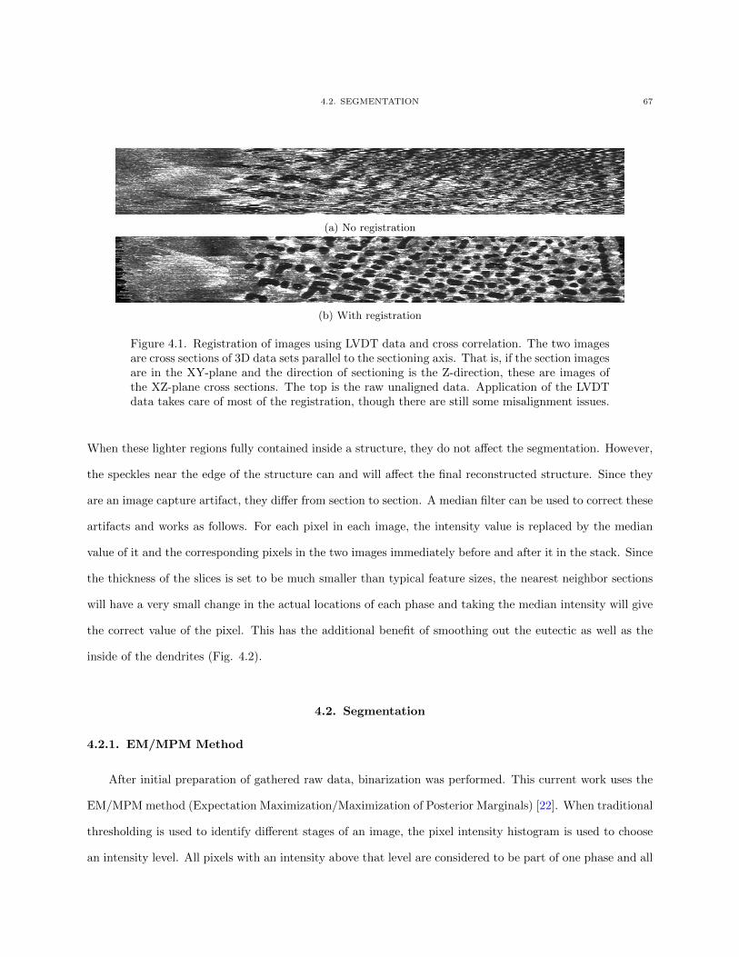
4.2. SEGMENTATION 67
(a) No registration
(b) With registration
Figure 4.1. Registration of images using LVDT data and cross correlation. The two imagesare cross sections of 3D data sets parallel to the sectioning axis. That is, if the section imagesare in the XY-plane and the direction of sectioning is the Z-direction, these are images ofthe XZ-plane cross sections. The top is the raw unaligned data. Application of the LVDTdata takes care of most of the registration, though there are still some misalignment issues.
When these lighter regions fully contained inside a structure, they do not affect the segmentation. However,
the speckles near the edge of the structure can and will affect the final reconstructed structure. Since they
are an image capture artifact, they differ from section to section. A median filter can be used to correct these
artifacts and works as follows. For each pixel in each image, the intensity value is replaced by the median
value of it and the corresponding pixels in the two images immediately before and after it in the stack. Since
the thickness of the slices is set to be much smaller than typical feature sizes, the nearest neighbor sections
will have a very small change in the actual locations of each phase and taking the median intensity will give
the correct value of the pixel. This has the additional benefit of smoothing out the eutectic as well as the
inside of the dendrites (Fig. 4.2).
4.2. Segmentation
4.2.1. EM/MPM Method
After initial preparation of gathered raw data, binarization was performed. This current work uses the
EM/MPM method (Expectation Maximization/Maximization of Posterior Marginals) [22]. When traditional
thresholding is used to identify different stages of an image, the pixel intensity histogram is used to choose
an intensity level. All pixels with an intensity above that level are considered to be part of one phase and all
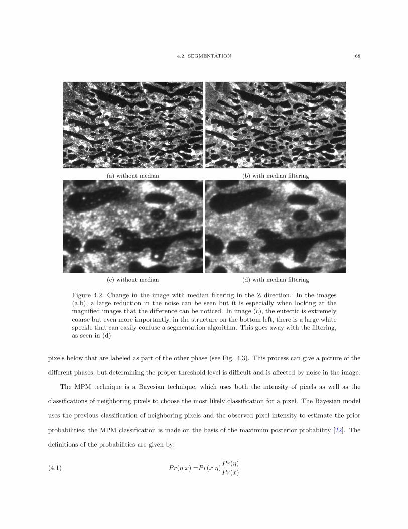
4.2. SEGMENTATION 68
(a) without median (b) with median filtering
(c) without median (d) with median filtering
Figure 4.2. Change in the image with median filtering in the Z direction. In the images(a,b), a large reduction in the noise can be seen but it is especially when looking at themagnified images that the difference can be noticed. In image (c), the eutectic is extremelycoarse but even more importantly, in the structure on the bottom left, there is a large whitespeckle that can easily confuse a segmentation algorithm. This goes away with the filtering,as seen in (d).
pixels below that are labeled as part of the other phase (see Fig. 4.3). This process can give a picture of the
different phases, but determining the proper threshold level is difficult and is affected by noise in the image.
The MPM technique is a Bayesian technique, which uses both the intensity of pixels as well as the
classifications of neighboring pixels to choose the most likely classification for a pixel. The Bayesian model
uses the previous classification of neighboring pixels and the observed pixel intensity to estimate the prior
probabilities; the MPM classification is made on the basis of the maximum posterior probability [22]. The
definitions of the probabilities are given by:
Pr(η|x) =Pr(x|η)Pr(η)
Pr(x)(4.1)
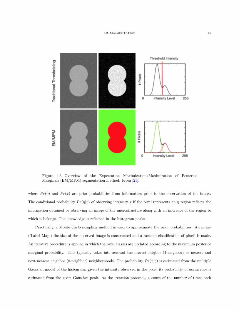
4.2. SEGMENTATION 69
Figure 4.3. Overview of the Expectation Maximization/Maximization of PosteriorMarginals (EM/MPM) segmentation method. From [21].
where Pr(η) and Pr(x) are prior probabilities from information prior to the observation of the image.
The conditional probability Pr(η|x) of observing intensity x if the pixel represents an η region reflects the
information obtained by observing an image of the microstructure along with an inference of the region to
which it belongs. This knowledge is reflected in the histogram peaks.
Practically, a Monte Carlo sampling method is used to approximate the prior probabilities. An image
(’Label Map’) the size of the observed image is constructed and a random classification of pixels is made.
An iterative procedure is applied in which the pixel classes are updated according to the maximum posterior
marginal probability. This typically takes into account the nearest neigbor (4-neighbor) or nearest and
next nearest neighbor (8-neighbor) neighborhoods. The probability Pr(x|η) is estimated from the multiple
Gaussian model of the histogram: given the intensity observed in the pixel, its probability of occurrence is
estimated from the given Gaussian peak. As the iteration proceeds, a count of the number of times each
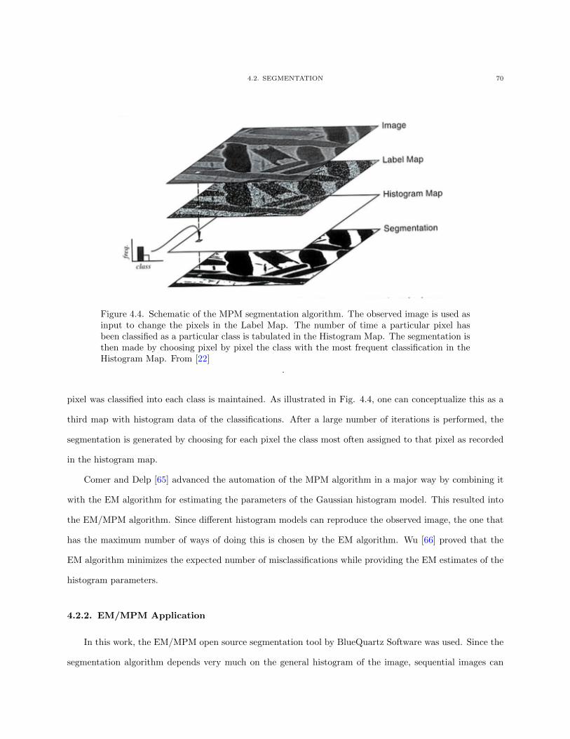
4.2. SEGMENTATION 70
Figure 4.4. Schematic of the MPM segmentation algorithm. The observed image is used asinput to change the pixels in the Label Map. The number of time a particular pixel hasbeen classified as a particular class is tabulated in the Histogram Map. The segmentation isthen made by choosing pixel by pixel the class with the most frequent classification in theHistogram Map. From [22]
.
pixel was classified into each class is maintained. As illustrated in Fig. 4.4, one can conceptualize this as a
third map with histogram data of the classifications. After a large number of iterations is performed, the
segmentation is generated by choosing for each pixel the class most often assigned to that pixel as recorded
in the histogram map.
Comer and Delp [65] advanced the automation of the MPM algorithm in a major way by combining it
with the EM algorithm for estimating the parameters of the Gaussian histogram model. This resulted into
the EM/MPM algorithm. Since different histogram models can reproduce the observed image, the one that
has the maximum number of ways of doing this is chosen by the EM algorithm. Wu [66] proved that the
EM algorithm minimizes the expected number of misclassifications while providing the EM estimates of the
histogram parameters.
4.2.2. EM/MPM Application
In this work, the EM/MPM open source segmentation tool by BlueQuartz Software was used. Since the
segmentation algorithm depends very much on the general histogram of the image, sequential images can
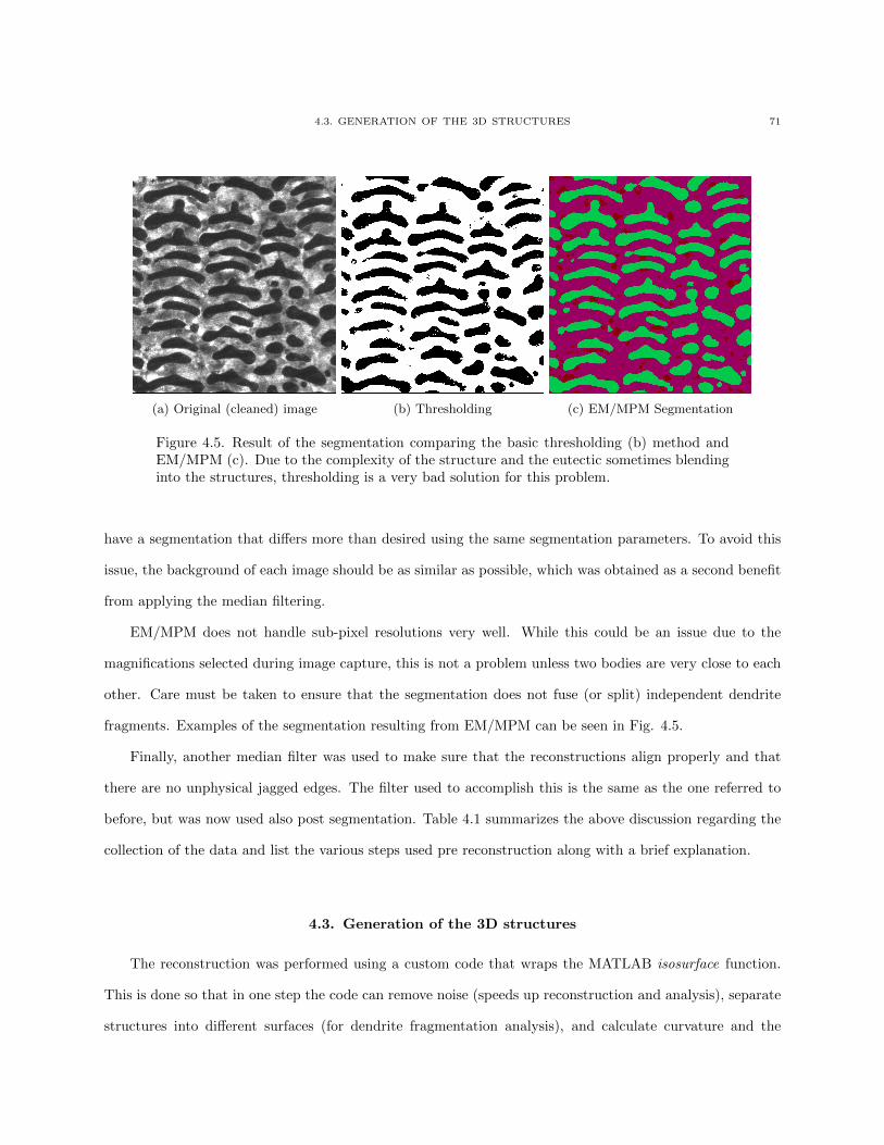
4.3. GENERATION OF THE 3D STRUCTURES 71
(a) Original (cleaned) image (b) Thresholding (c) EM/MPM Segmentation
Figure 4.5. Result of the segmentation comparing the basic thresholding (b) method andEM/MPM (c). Due to the complexity of the structure and the eutectic sometimes blendinginto the structures, thresholding is a very bad solution for this problem.
have a segmentation that differs more than desired using the same segmentation parameters. To avoid this
issue, the background of each image should be as similar as possible, which was obtained as a second benefit
from applying the median filtering.
EM/MPM does not handle sub-pixel resolutions very well. While this could be an issue due to the
magnifications selected during image capture, this is not a problem unless two bodies are very close to each
other. Care must be taken to ensure that the segmentation does not fuse (or split) independent dendrite
fragments. Examples of the segmentation resulting from EM/MPM can be seen in Fig. 4.5.
Finally, another median filter was used to make sure that the reconstructions align properly and that
there are no unphysical jagged edges. The filter used to accomplish this is the same as the one referred to
before, but was now used also post segmentation. Table 4.1 summarizes the above discussion regarding the
collection of the data and list the various steps used pre reconstruction along with a brief explanation.
4.3. Generation of the 3D structures
The reconstruction was performed using a custom code that wraps the MATLAB isosurface function.
This is done so that in one step the code can remove noise (speeds up reconstruction and analysis), separate
structures into different surfaces (for dendrite fragmentation analysis), and calculate curvature and the
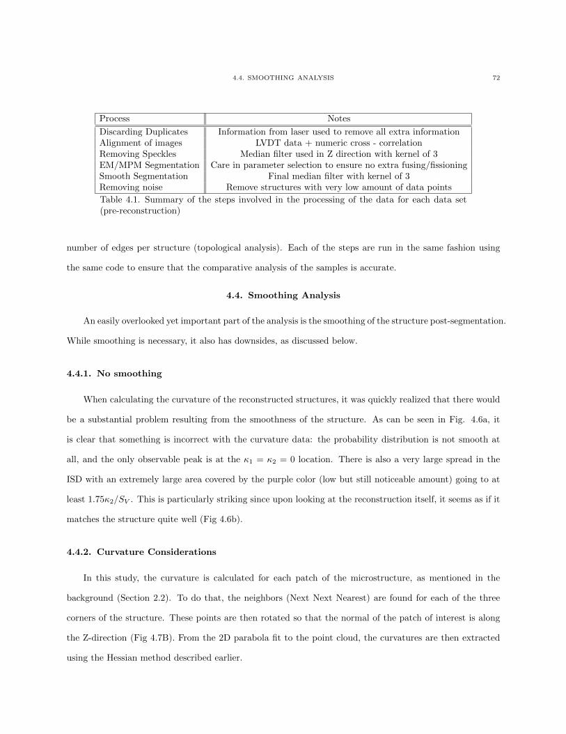
4.4. SMOOTHING ANALYSIS 72
Process Notes
Discarding Duplicates Information from laser used to remove all extra informationAlignment of images LVDT data + numeric cross - correlationRemoving Speckles Median filter used in Z direction with kernel of 3EM/MPM Segmentation Care in parameter selection to ensure no extra fusing/fissioningSmooth Segmentation Final median filter with kernel of 3Removing noise Remove structures with very low amount of data points
Table 4.1. Summary of the steps involved in the processing of the data for each data set(pre-reconstruction)
number of edges per structure (topological analysis). Each of the steps are run in the same fashion using
the same code to ensure that the comparative analysis of the samples is accurate.
4.4. Smoothing Analysis
An easily overlooked yet important part of the analysis is the smoothing of the structure post-segmentation.
While smoothing is necessary, it also has downsides, as discussed below.
4.4.1. No smoothing
When calculating the curvature of the reconstructed structures, it was quickly realized that there would
be a substantial problem resulting from the smoothness of the structure. As can be seen in Fig. 4.6a, it
is clear that something is incorrect with the curvature data: the probability distribution is not smooth at
all, and the only observable peak is at the κ1 = κ2 = 0 location. There is also a very large spread in the
ISD with an extremely large area covered by the purple color (low but still noticeable amount) going to at
least 1.75κ2/SV . This is particularly striking since upon looking at the reconstruction itself, it seems as if it
matches the structure quite well (Fig 4.6b).
4.4.2. Curvature Considerations
In this study, the curvature is calculated for each patch of the microstructure, as mentioned in the
background (Section 2.2). To do that, the neighbors (Next Next Nearest) are found for each of the three
corners of the structure. These points are then rotated so that the normal of the patch of interest is along
the Z-direction (Fig 4.7B). From the 2D parabola fit to the point cloud, the curvatures are then extracted
using the Hessian method described earlier.
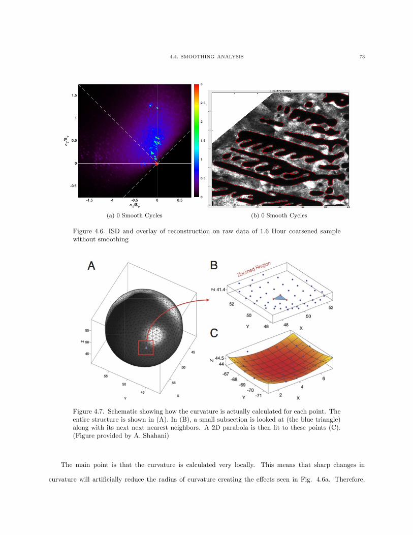
4.4. SMOOTHING ANALYSIS 73
(a) 0 Smooth Cycles (b) 0 Smooth Cycles
Figure 4.6. ISD and overlay of reconstruction on raw data of 1.6 Hour coarsened samplewithout smoothing
Figure 4.7. Schematic showing how the curvature is actually calculated for each point. Theentire structure is shown in (A). In (B), a small subsection is looked at (the blue triangle)along with its next next nearest neighbors. A 2D parabola is then fit to these points (C).(Figure provided by A. Shahani)
The main point is that the curvature is calculated very locally. This means that sharp changes in
curvature will artificially reduce the radius of curvature creating the effects seen in Fig. 4.6a. Therefore,
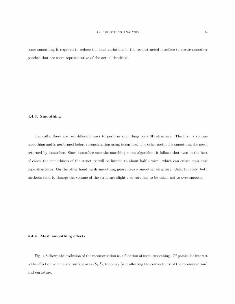
4.4. SMOOTHING ANALYSIS 74
some smoothing is required to reduce the local variations in the reconstructed interface to create smoother
patches that are more representative of the actual dendrites.
4.4.3. Smoothing
Typically, there are two different ways to perform smoothing on a 3D structure. The first is volume
smoothing and is performed before reconstruction using isosurface. The other method is smoothing the mesh
returned by isosurface. Since isosurface uses the marching cubes algorithm, it follows that even in the best
of cases, the smoothness of the structure will be limited to about half a voxel, which can create stair case
type structures. On the other hand mesh smoothing guarantees a smoother structure. Unfortunately, both
methods tend to change the volume of the structure slightly so care has to be taken not to over-smooth.
4.4.4. Mesh smoothing effects
Fig. 4.8 shows the evolution of the reconstruction as a function of mesh smoothing. Of particular interest
is the effect on volume and surface area (S−1V ), topology (is it affecting the connectivity of the reconstruction)
and curvature.
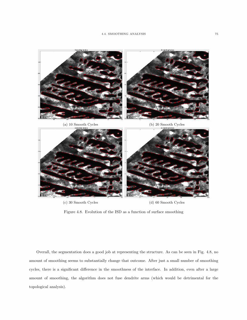
4.4. SMOOTHING ANALYSIS 75
(a) 10 Smooth Cycles (b) 20 Smooth Cycles
(c) 30 Smooth Cycles (d) 60 Smooth Cycles
Figure 4.8. Evolution of the ISD as a function of surface smoothing
Overall, the segmentation does a good job at representing the structure. As can be seen in Fig. 4.8, no
amount of smoothing seems to substantially change that outcome. After just a small number of smoothing
cycles, there is a significant difference in the smoothness of the interface. In addition, even after a large
amount of smoothing, the algorithm does not fuse dendrite arms (which would be detrimental for the
topological analysis).
4.4. SMOOTHING ANALYSIS 76
(a) 0 Smooth Cycles (b) 20 Smooth Cycles
(c) 60 Smooth Cycles
Figure 4.9. Zoom of selected smoothing iterations from the 10, 20 and 60 iteration imagesin Fig. 4.8.
Unfortunately, there are some overall changes in morphology as can be seen in Fig. 4.9. The hole
through the structure in the top center of the images does get smaller as the number of smoothing steps is
increased (“1” on the images). “2” shows that what would be a small dendrite fragment, is disappearing
at 60 iterations. At point “3”, it can be seen that at 0 and 20 iterations, the dendrite arm is accurately
represented, but that it shrinks at 60 iterations. From a curvature perspective, at point “4”, the notch in
the structure (segmentation error) is completely removed after even 20 iterations. These cases show that a
balance has to be struck between under- and over-smoothing.
4.4.5. Effect on the Interfacial Shape Distribution
When looking at the evolution of the Interfacial Shape Distribution (ISD) as a function of smoothing
iterations, the change becomes even more obvious (Fig. 4.10). Since this structure is at relatively low
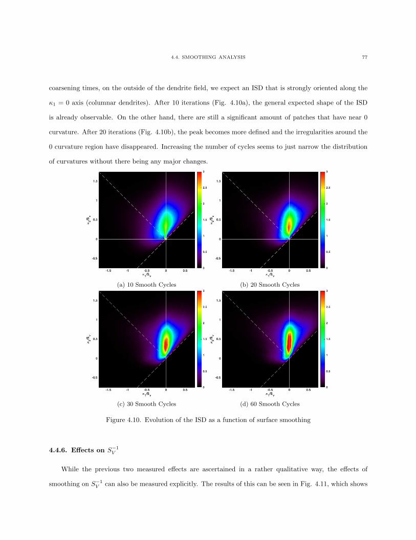
4.4. SMOOTHING ANALYSIS 77
coarsening times, on the outside of the dendrite field, we expect an ISD that is strongly oriented along the
κ1 = 0 axis (columnar dendrites). After 10 iterations (Fig. 4.10a), the general expected shape of the ISD
is already observable. On the other hand, there are still a significant amount of patches that have near 0
curvature. After 20 iterations (Fig. 4.10b), the peak becomes more defined and the irregularities around the
0 curvature region have disappeared. Increasing the number of cycles seems to just narrow the distribution
of curvatures without there being any major changes.
(a) 10 Smooth Cycles (b) 20 Smooth Cycles
(c) 30 Smooth Cycles (d) 60 Smooth Cycles
Figure 4.10. Evolution of the ISD as a function of surface smoothing
4.4.6. Effects on S−1V
While the previous two measured effects are ascertained in a rather qualitative way, the effects of
smoothing on S−1V can also be measured explicitly. The results of this can be seen in Fig. 4.11, which shows
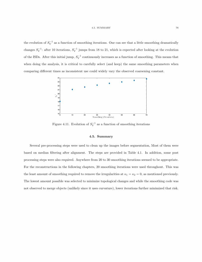
4.5. SUMMARY 78
the evolution of S−1V as a function of smoothing iterations. One can see that a little smoothing dramatically
changes S−1V : after 10 iterations, S−1
V jumps from 18 to 21, which is expected after looking at the evolution
of the ISDs. After this initial jump, S−1V continuously increases as a function of smoothing. This means that
when doing the analysis, it is critical to carefully select (and keep) the same smoothing parameters when
comparing different times as inconsistent use could widely vary the observed coarsening constant.
Figure 4.11. Evolution of S−1V as a function of smoothing iterations
4.5. Summary
Several pre-processing steps were used to clean up the images before segmentation, Most of them were
based on median filtering after alignment. The steps are provided in Table 4.1. In addition, some post
processing steps were also required. Anywhere from 20 to 30 smoothing iterations seemed to be appropriate.
For the reconstructions in the following chapters, 20 smoothing iterations were used throughout. This was
the least amount of smoothing required to remove the irregularities at κ1 = κ2 = 0, as mentioned previously.
The lowest amount possible was selected to minimize topological changes and while the smoothing code was
not observed to merge objects (unlikely since it uses curvature), lower iterations further minimized that risk.
5.1. INITIAL ANALYSIS 79
CHAPTER 5
Results
5.1. Initial Analysis
A number of 2D sections were gathered from the 10%, 20% and 30% samples to determine how the
structure evolved and to find out if the experiments aboard the ISS had been successful. There were two
samples that encountered problems. The 1.6 hour run had the data downlink fail but once contact was
re-established, it was showing that it processed properly. The 5.5 hour sample on the other hand did not
quench and was thus slow cooled. This could have resulted in a much coarser eutectic. The effects can be
observed in some samples but it is especially prevalent in the 30% sample.
5.1.1. 2D Section analysis
5.1.1.1. 10% samples. Figure 5.1 shows a section of the 10% sample as it coarsened on the ground (upper
left), and sections of the samples in space for coarsening times of 10 min (upper right), 1.6 hrs (lower left)
and 5.5 hrs (lower right). After 10 min, some of the very fine structures had already coarsened out but the
structure was still very similar to the sample that coarsened on the ground. On the other hand, after 1.6
hrs most of the dendritic structure had disappeared and only spherical (or cylindrical) particles remained.
It does appear as if the particles were still where they would have split off from the dendrite itself. This
suggests that no sedimentation happened during coarsening. After 5.5 hrs it seems that even more of the
structure had been lost and that no real dendritic shape could be observed anymore. Reconstructing the
samples in 3D allows us to determine if the Sn rich particles coarsened to spherical or columnar shapes.
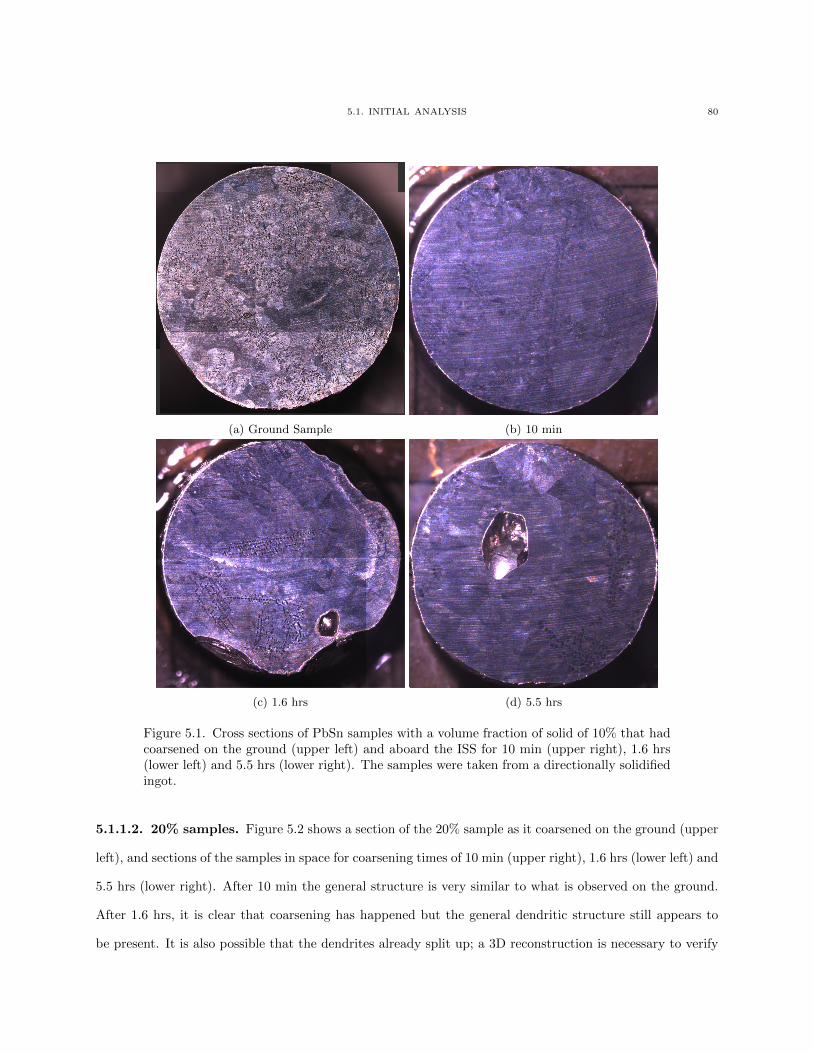
5.1. INITIAL ANALYSIS 80
(a) Ground Sample (b) 10 min
(c) 1.6 hrs (d) 5.5 hrs
Figure 5.1. Cross sections of PbSn samples with a volume fraction of solid of 10% that hadcoarsened on the ground (upper left) and aboard the ISS for 10 min (upper right), 1.6 hrs(lower left) and 5.5 hrs (lower right). The samples were taken from a directionally solidifiedingot.
5.1.1.2. 20% samples. Figure 5.2 shows a section of the 20% sample as it coarsened on the ground (upper
left), and sections of the samples in space for coarsening times of 10 min (upper right), 1.6 hrs (lower left) and
5.5 hrs (lower right). After 10 min the general structure is very similar to what is observed on the ground.
After 1.6 hrs, it is clear that coarsening has happened but the general dendritic structure still appears to
be present. It is also possible that the dendrites already split up; a 3D reconstruction is necessary to verify
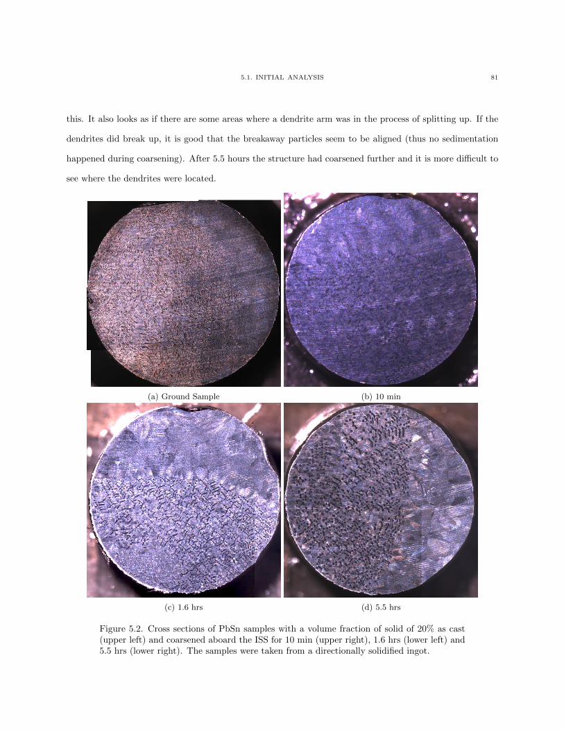
5.1. INITIAL ANALYSIS 81
this. It also looks as if there are some areas where a dendrite arm was in the process of splitting up. If the
dendrites did break up, it is good that the breakaway particles seem to be aligned (thus no sedimentation
happened during coarsening). After 5.5 hours the structure had coarsened further and it is more difficult to
see where the dendrites were located.
(a) Ground Sample (b) 10 min
(c) 1.6 hrs (d) 5.5 hrs
Figure 5.2. Cross sections of PbSn samples with a volume fraction of solid of 20% as cast(upper left) and coarsened aboard the ISS for 10 min (upper right), 1.6 hrs (lower left) and5.5 hrs (lower right). The samples were taken from a directionally solidified ingot.
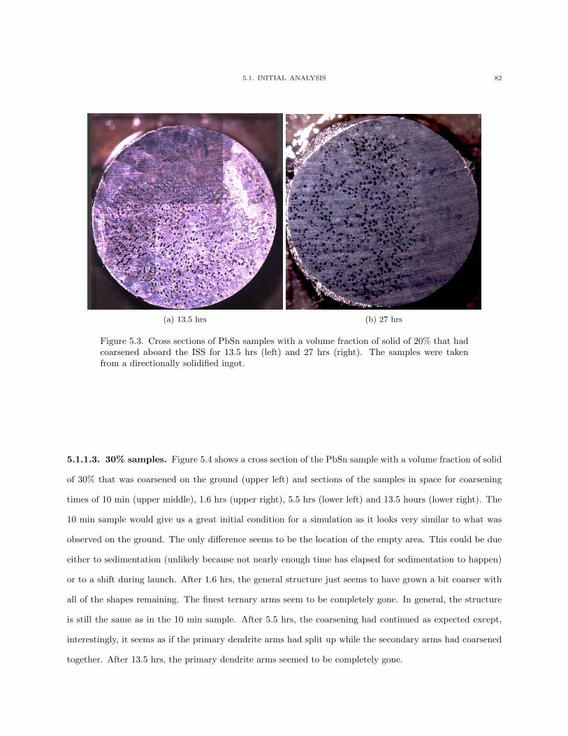
5.1. INITIAL ANALYSIS 82
(a) 13.5 hrs (b) 27 hrs
Figure 5.3. Cross sections of PbSn samples with a volume fraction of solid of 20% that hadcoarsened aboard the ISS for 13.5 hrs (left) and 27 hrs (right). The samples were takenfrom a directionally solidified ingot.
5.1.1.3. 30% samples. Figure 5.4 shows a cross section of the PbSn sample with a volume fraction of solid
of 30% that was coarsened on the ground (upper left) and sections of the samples in space for coarsening
times of 10 min (upper middle), 1.6 hrs (upper right), 5.5 hrs (lower left) and 13.5 hours (lower right). The
10 min sample would give us a great initial condition for a simulation as it looks very similar to what was
observed on the ground. The only difference seems to be the location of the empty area. This could be due
either to sedimentation (unlikely because not nearly enough time has elapsed for sedimentation to happen)
or to a shift during launch. After 1.6 hrs, the general structure just seems to have grown a bit coarser with
all of the shapes remaining. The finest ternary arms seem to be completely gone. In general, the structure
is still the same as in the 10 min sample. After 5.5 hrs, the coarsening had continued as expected except,
interestingly, it seems as if the primary dendrite arms had split up while the secondary arms had coarsened
together. After 13.5 hrs, the primary dendrite arms seemed to be completely gone.
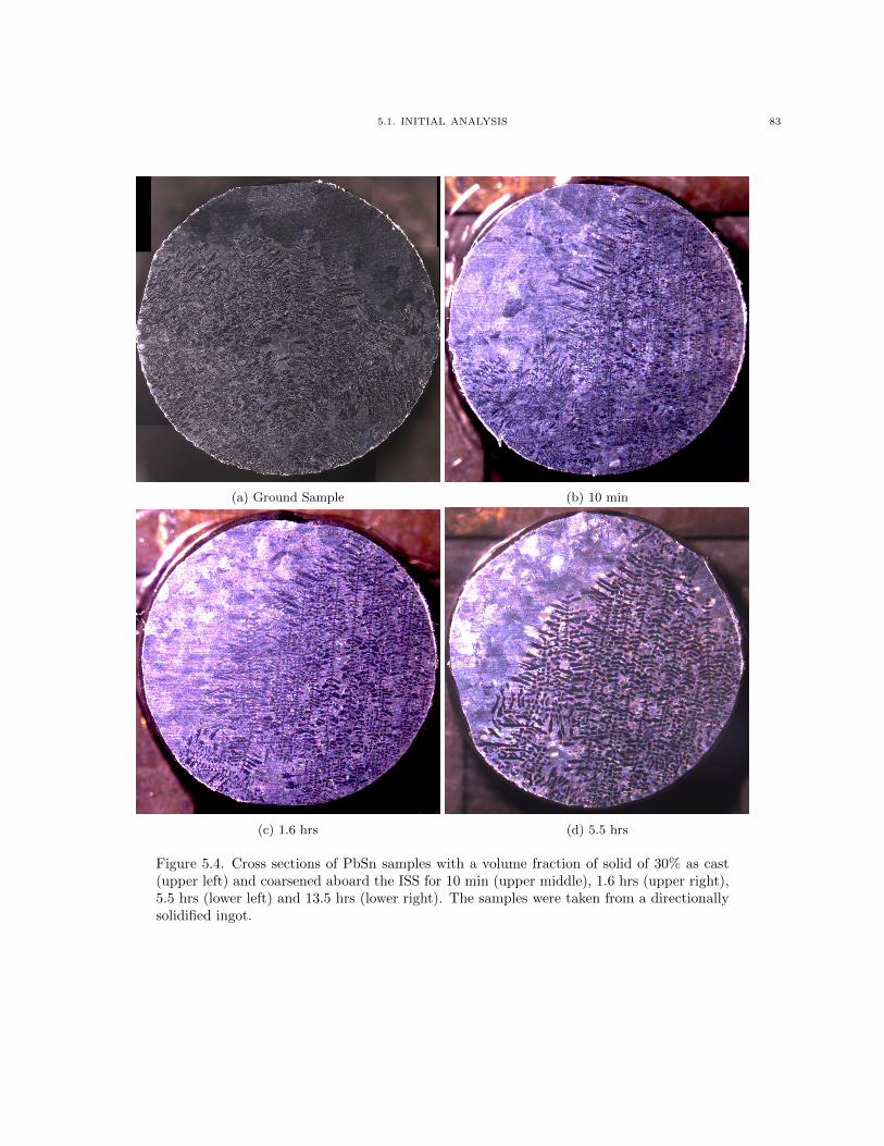
5.1. INITIAL ANALYSIS 83
(a) Ground Sample (b) 10 min
(c) 1.6 hrs (d) 5.5 hrs
Figure 5.4. Cross sections of PbSn samples with a volume fraction of solid of 30% as cast(upper left) and coarsened aboard the ISS for 10 min (upper middle), 1.6 hrs (upper right),5.5 hrs (lower left) and 13.5 hrs (lower right). The samples were taken from a directionallysolidified ingot.
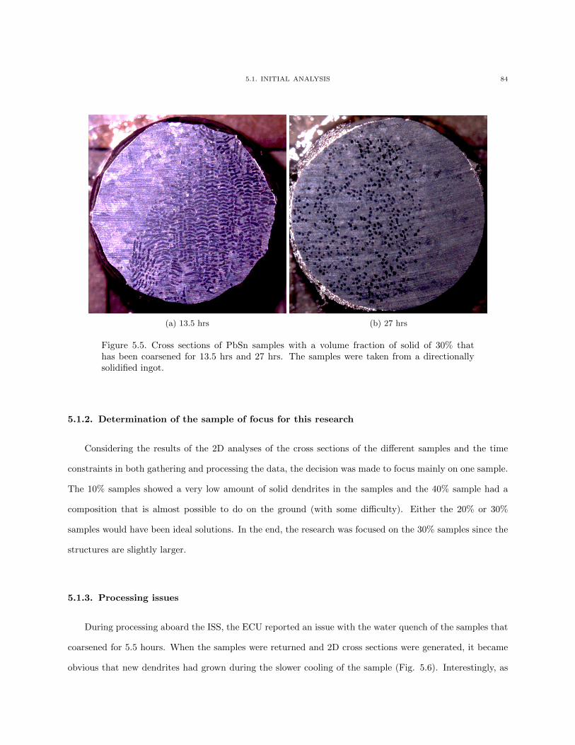
5.1. INITIAL ANALYSIS 84
(a) 13.5 hrs (b) 27 hrs
Figure 5.5. Cross sections of PbSn samples with a volume fraction of solid of 30% thathas been coarsened for 13.5 hrs and 27 hrs. The samples were taken from a directionallysolidified ingot.
5.1.2. Determination of the sample of focus for this research
Considering the results of the 2D analyses of the cross sections of the different samples and the time
constraints in both gathering and processing the data, the decision was made to focus mainly on one sample.
The 10% samples showed a very low amount of solid dendrites in the samples and the 40% sample had a
composition that is almost possible to do on the ground (with some difficulty). Either the 20% or 30%
samples would have been ideal solutions. In the end, the research was focused on the 30% samples since the
structures are slightly larger.
5.1.3. Processing issues
During processing aboard the ISS, the ECU reported an issue with the water quench of the samples that
coarsened for 5.5 hours. When the samples were returned and 2D cross sections were generated, it became
obvious that new dendrites had grown during the slower cooling of the sample (Fig. 5.6). Interestingly, as
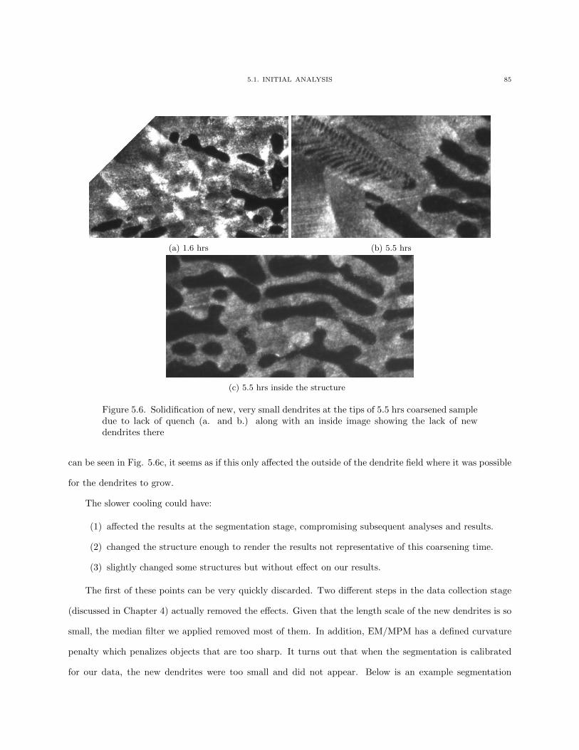
5.1. INITIAL ANALYSIS 85
(a) 1.6 hrs (b) 5.5 hrs
(c) 5.5 hrs inside the structure
Figure 5.6. Solidification of new, very small dendrites at the tips of 5.5 hrs coarsened sampledue to lack of quench (a. and b.) along with an inside image showing the lack of newdendrites there
can be seen in Fig. 5.6c, it seems as if this only affected the outside of the dendrite field where it was possible
for the dendrites to grow.
The slower cooling could have:
(1) affected the results at the segmentation stage, compromising subsequent analyses and results.
(2) changed the structure enough to render the results not representative of this coarsening time.
(3) slightly changed some structures but without effect on our results.
The first of these points can be very quickly discarded. Two different steps in the data collection stage
(discussed in Chapter 4) actually removed the effects. Given that the length scale of the new dendrites is so
small, the median filter we applied removed most of them. In addition, EM/MPM has a defined curvature
penalty which penalizes objects that are too sharp. It turns out that when the segmentation is calibrated
for our data, the new dendrites were too small and did not appear. Below is an example segmentation
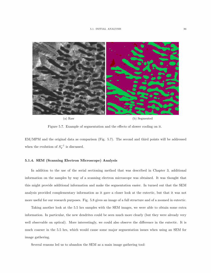
5.1. INITIAL ANALYSIS 86
(a) Raw (b) Segmented
Figure 5.7. Example of segmentation and the effects of slower cooling on it.
EM/MPM and the original data as comparison (Fig. 5.7). The second and third points will be addressed
when the evolution of S−1V is discussed.
5.1.4. SEM (Scanning Electron Microscope) Analysis
In addition to the use of the serial sectioning method that was described in Chapter 3, additional
information on the samples by way of a scanning electron microscope was obtained. It was thought that
this might provide additional information and make the segmentation easier. In turned out that the SEM
analysis provided complementary information as it gave a closer look at the eutectic, but that it was not
more useful for our research purposes. Fig. 5.8 gives an image of a full structure and of a zoomed in eutectic.
Taking another look at the 5.5 hrs samples with the SEM images, we were able to obtain some extra
information. In particular, the new dendrites could be seen much more clearly (but they were already very
well observable on optical). More interestingly, we could also observe the difference in the eutectic. It is
much coarser in the 5.5 hrs, which would cause some major segmentation issues when using an SEM for
image gathering.
Several reasons led us to abandon the SEM as a main image gathering tool:
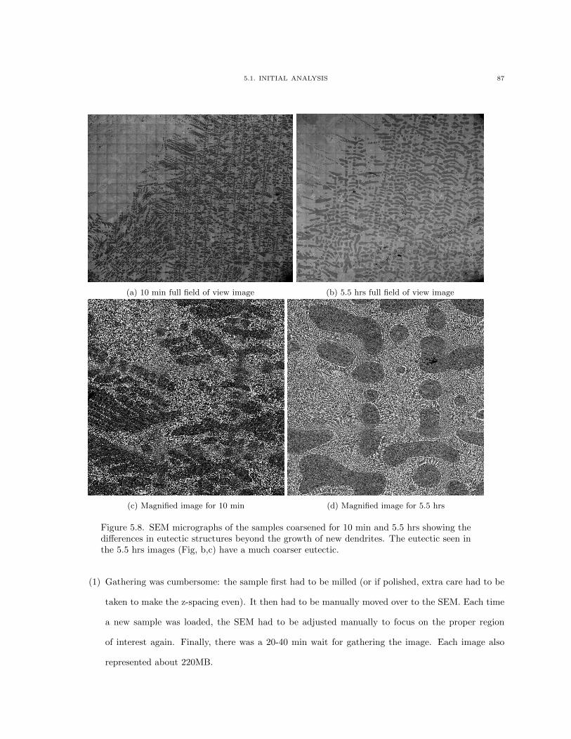
5.1. INITIAL ANALYSIS 87
(a) 10 min full field of view image (b) 5.5 hrs full field of view image
(c) Magnified image for 10 min (d) Magnified image for 5.5 hrs
Figure 5.8. SEM micrographs of the samples coarsened for 10 min and 5.5 hrs showing thedifferences in eutectic structures beyond the growth of new dendrites. The eutectic seen inthe 5.5 hrs images (Fig, b,c) have a much coarser eutectic.
(1) Gathering was cumbersome: the sample first had to be milled (or if polished, extra care had to be
taken to make the z-spacing even). It then had to be manually moved over to the SEM. Each time
a new sample was loaded, the SEM had to be adjusted manually to focus on the proper region
of interest again. Finally, there was a 20-40 min wait for gathering the image. Each image also
represented about 220MB.
5.3. MUSHY ZONE ANALYSIS 88
(2) Analysis was difficult: Even if the same region of interest (ROI) was obtained, rotation in plane
had to be accounted for (extra manipulation).
(3) Segmentation was more difficult: The extra detail provided about the eutectic caused the segmen-
tation algorithms to mark part of the eutectic as dendrite.
(4) Generally, the SEM analysis just provided too much detail for the research in this work.
Most of the issues that are listed are due to the extra human interaction needed in the gathering of the
data. This offsets the possible gain from the resolution increase, which in our case is not needed due to the
size scale of the dendrites, which makes them easily observable in optical microscope.
5.2. Generating Multiple Data Sets from a Single Specimen
Within one specimen (an actual physical sample), three different regions could very quickly be noticed.
They are visualized in Fig. 5.9. First is a region with hardly any dendrites, just plain eutectic. Next to it
is a “transition region” in which the dendrites could grow freely into the eutectic (green region in Fig. 5.9).
This will be called the “free growth region” or outside region. Finally there is a region that is completely
screened where dendrites were constrained in their growth (red region in Fig. 5.9). This will be called the
“mushy zone” or the inside region.
Due to the major morphological differences in the latter two regions, it was decided to analyze each
region separately. It was difficult to consistently define and identify the transition region in the samples
because the region in each sample is ill defined since this transition zone does not have the same shape and
depth across samples. Scaling is also difficult in this region. Generally any type of scaling is more meaningful
when there is a constant structure type over the measured volumes.
5.3. Mushy zone analysis
5.3.1. Reconstructions
As previously mentioned, the major focus of the in-depth analysis was the 30% samples. Reconstructions
of the samples coarsened for 10 min and 48 hrs are displayed in Fig. 5.10. The images are of the same
volume in both cases (2500x2000x800µm3) and they are colored based on the same scale bar (in µm−1).
The substantial differences in length scales make it it very difficult to compare the two structures. Despite
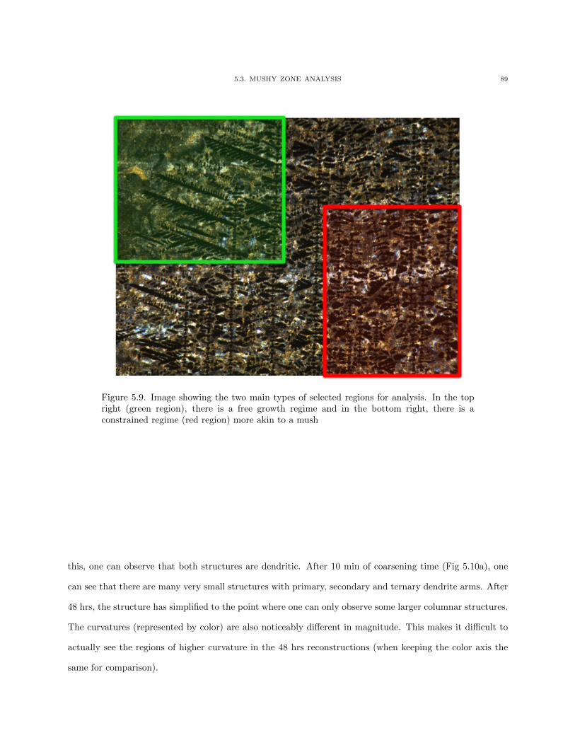
5.3. MUSHY ZONE ANALYSIS 89
Figure 5.9. Image showing the two main types of selected regions for analysis. In the topright (green region), there is a free growth regime and in the bottom right, there is aconstrained regime (red region) more akin to a mush
this, one can observe that both structures are dendritic. After 10 min of coarsening time (Fig 5.10a), one
can see that there are many very small structures with primary, secondary and ternary dendrite arms. After
48 hrs, the structure has simplified to the point where one can only observe some larger columnar structures.
The curvatures (represented by color) are also noticeably different in magnitude. This makes it difficult to
actually see the regions of higher curvature in the 48 hrs reconstructions (when keeping the color axis the
same for comparison).
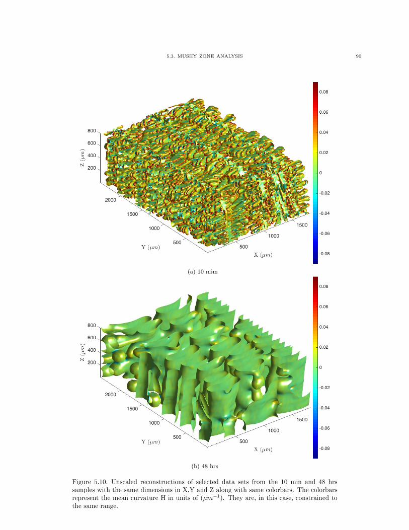
5.3. MUSHY ZONE ANALYSIS 90
(a) 10 mim
(b) 48 hrs
Figure 5.10. Unscaled reconstructions of selected data sets from the 10 min and 48 hrssamples with the same dimensions in X,Y and Z along with same colorbars. The colorbarsrepresent the mean curvature H in units of (µm−1). They are, in this case, constrained tothe same range.
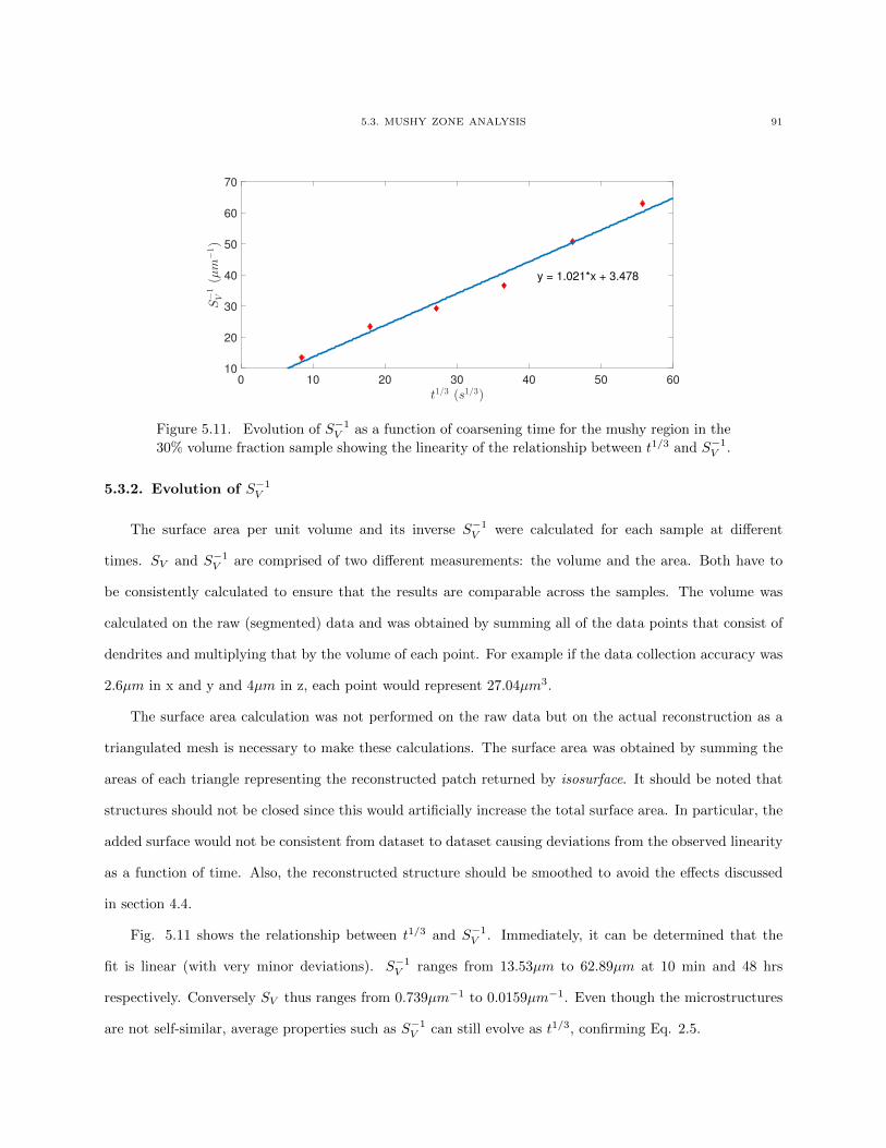
5.3. MUSHY ZONE ANALYSIS 91
0 10 20 30 40 50 60
t1/3 (s1/3)
10
20
30
40
50
60
70
S−1
V(µm
−1)
y = 1.021*x + 3.478
Figure 5.11. Evolution of S−1V as a function of coarsening time for the mushy region in the
30% volume fraction sample showing the linearity of the relationship between t1/3 and S−1V .
5.3.2. Evolution of S−1V
The surface area per unit volume and its inverse S−1V were calculated for each sample at different
times. SV and S−1V are comprised of two different measurements: the volume and the area. Both have to
be consistently calculated to ensure that the results are comparable across the samples. The volume was
calculated on the raw (segmented) data and was obtained by summing all of the data points that consist of
dendrites and multiplying that by the volume of each point. For example if the data collection accuracy was
2.6µm in x and y and 4µm in z, each point would represent 27.04µm3.
The surface area calculation was not performed on the raw data but on the actual reconstruction as a
triangulated mesh is necessary to make these calculations. The surface area was obtained by summing the
areas of each triangle representing the reconstructed patch returned by isosurface. It should be noted that
structures should not be closed since this would artificially increase the total surface area. In particular, the
added surface would not be consistent from dataset to dataset causing deviations from the observed linearity
as a function of time. Also, the reconstructed structure should be smoothed to avoid the effects discussed
in section 4.4.
Fig. 5.11 shows the relationship between t1/3 and S−1V . Immediately, it can be determined that the
fit is linear (with very minor deviations). S−1V ranges from 13.53µm to 62.89µm at 10 min and 48 hrs
respectively. Conversely SV thus ranges from 0.739µm−1 to 0.0159µm−1. Even though the microstructures
are not self-similar, average properties such as S−1V can still evolve as t1/3, confirming Eq. 2.5.
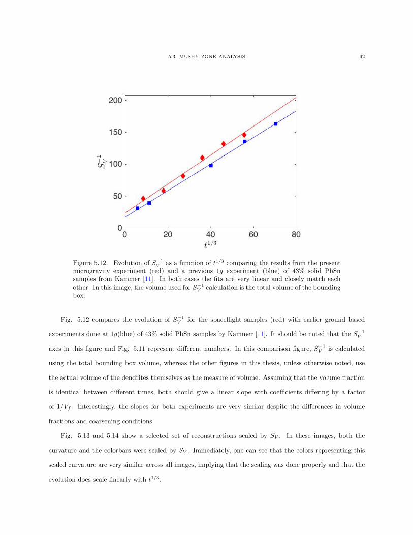
5.3. MUSHY ZONE ANALYSIS 92
Figure 5.12. Evolution of S−1V as a function of t1/3 comparing the results from the present
microgravity experiment (red) and a previous 1g experiment (blue) of 43% solid PbSnsamples from Kammer [11]. In both cases the fits are very linear and closely match eachother. In this image, the volume used for S−1
V calculation is the total volume of the boundingbox.
Fig. 5.12 compares the evolution of S−1V for the spaceflight samples (red) with earlier ground based
experiments done at 1g(blue) of 43% solid PbSn samples by Kammer [11]. It should be noted that the S−1V
axes in this figure and Fig. 5.11 represent different numbers. In this comparison figure, S−1V is calculated
using the total bounding box volume, whereas the other figures in this thesis, unless otherwise noted, use
the actual volume of the dendrites themselves as the measure of volume. Assuming that the volume fraction
is identical between different times, both should give a linear slope with coefficients differing by a factor
of 1/Vf . Interestingly, the slopes for both experiments are very similar despite the differences in volume
fractions and coarsening conditions.
Fig. 5.13 and 5.14 show a selected set of reconstructions scaled by SV . In these images, both the
curvature and the colorbars were scaled by SV . Immediately, one can see that the colors representing this
scaled curvature are very similar across all images, implying that the scaling was done properly and that the
evolution does scale linearly with t1/3.
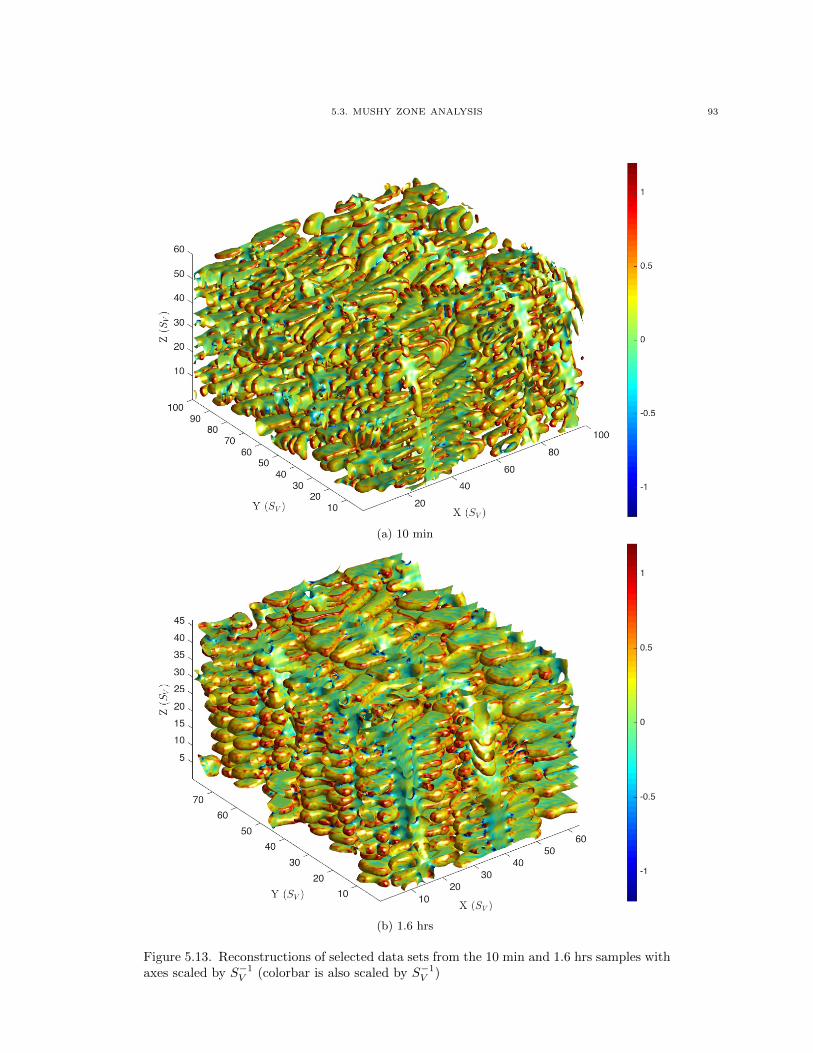
5.3. MUSHY ZONE ANALYSIS 93
(a) 10 min
(b) 1.6 hrs
Figure 5.13. Reconstructions of selected data sets from the 10 min and 1.6 hrs samples withaxes scaled by S−1
V (colorbar is also scaled by S−1V )
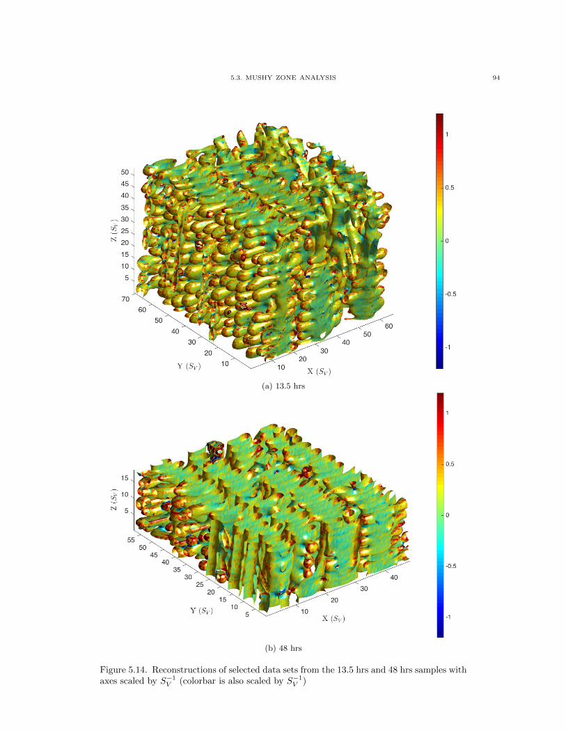
5.3. MUSHY ZONE ANALYSIS 94
(a) 13.5 hrs
(b) 48 hrs
Figure 5.14. Reconstructions of selected data sets from the 13.5 hrs and 48 hrs samples withaxes scaled by S−1
V (colorbar is also scaled by S−1V )
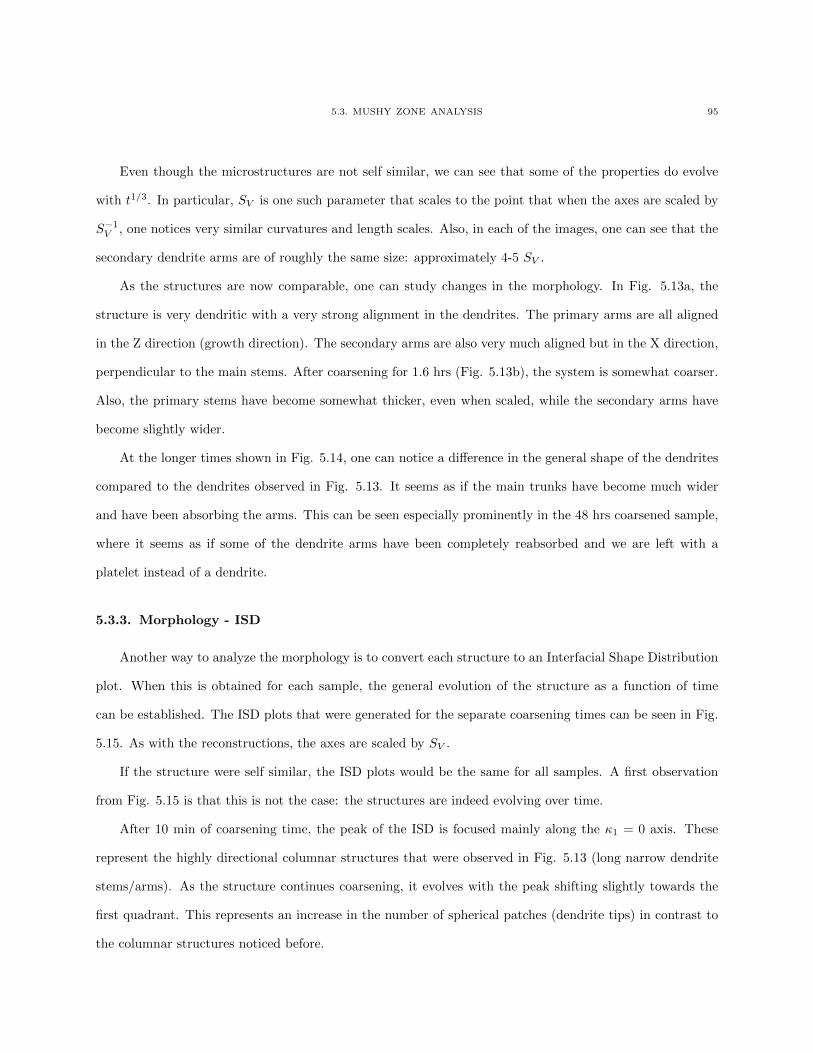
5.3. MUSHY ZONE ANALYSIS 95
Even though the microstructures are not self similar, we can see that some of the properties do evolve
with t1/3. In particular, SV is one such parameter that scales to the point that when the axes are scaled by
S−1V , one notices very similar curvatures and length scales. Also, in each of the images, one can see that the
secondary dendrite arms are of roughly the same size: approximately 4-5 SV .
As the structures are now comparable, one can study changes in the morphology. In Fig. 5.13a, the
structure is very dendritic with a very strong alignment in the dendrites. The primary arms are all aligned
in the Z direction (growth direction). The secondary arms are also very much aligned but in the X direction,
perpendicular to the main stems. After coarsening for 1.6 hrs (Fig. 5.13b), the system is somewhat coarser.
Also, the primary stems have become somewhat thicker, even when scaled, while the secondary arms have
become slightly wider.
At the longer times shown in Fig. 5.14, one can notice a difference in the general shape of the dendrites
compared to the dendrites observed in Fig. 5.13. It seems as if the main trunks have become much wider
and have been absorbing the arms. This can be seen especially prominently in the 48 hrs coarsened sample,
where it seems as if some of the dendrite arms have been completely reabsorbed and we are left with a
platelet instead of a dendrite.
5.3.3. Morphology - ISD
Another way to analyze the morphology is to convert each structure to an Interfacial Shape Distribution
plot. When this is obtained for each sample, the general evolution of the structure as a function of time
can be established. The ISD plots that were generated for the separate coarsening times can be seen in Fig.
5.15. As with the reconstructions, the axes are scaled by SV .
If the structure were self similar, the ISD plots would be the same for all samples. A first observation
from Fig. 5.15 is that this is not the case: the structures are indeed evolving over time.
After 10 min of coarsening time, the peak of the ISD is focused mainly along the κ1 = 0 axis. These
represent the highly directional columnar structures that were observed in Fig. 5.13 (long narrow dendrite
stems/arms). As the structure continues coarsening, it evolves with the peak shifting slightly towards the
first quadrant. This represents an increase in the number of spherical patches (dendrite tips) in contrast to
the columnar structures noticed before.
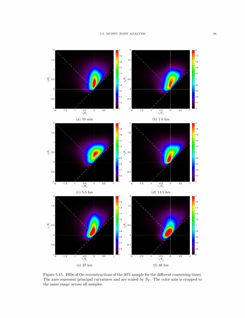
5.3. MUSHY ZONE ANALYSIS 96
(a) 10 min (b) 1.6 hrs
(c) 5.5 hrs (d) 13.5 hrs
(e) 27 hrs (f) 48 hrs
Figure 5.15. ISDs of the reconstructions of the 30% sample for the different coarsening times.The axes represent principal curvatures and are scaled by SV . The color axis is cropped tothe same range across all samples.
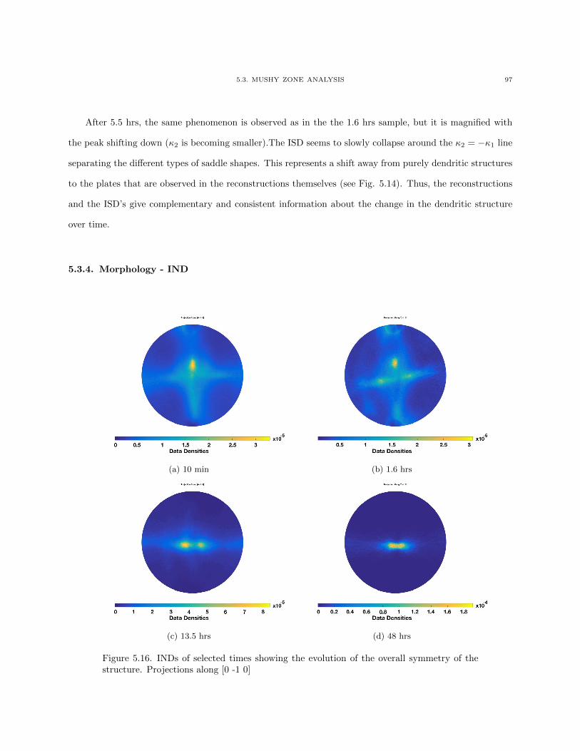
5.3. MUSHY ZONE ANALYSIS 97
After 5.5 hrs, the same phenomenon is observed as in the the 1.6 hrs sample, but it is magnified with
the peak shifting down (κ2 is becoming smaller).The ISD seems to slowly collapse around the κ2 = −κ1 line
separating the different types of saddle shapes. This represents a shift away from purely dendritic structures
to the plates that are observed in the reconstructions themselves (see Fig. 5.14). Thus, the reconstructions
and the ISD’s give complementary and consistent information about the change in the dendritic structure
over time.
5.3.4. Morphology - IND
(a) 10 min (b) 1.6 hrs
(c) 13.5 hrs (d) 48 hrs
Figure 5.16. INDs of selected times showing the evolution of the overall symmetry of thestructure. Projections along [0 -1 0]
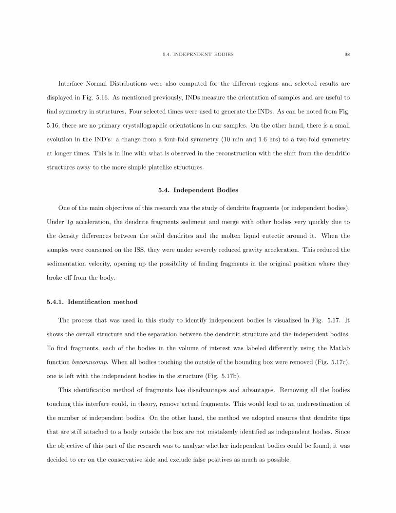
5.4. INDEPENDENT BODIES 98
Interface Normal Distributions were also computed for the different regions and selected results are
displayed in Fig. 5.16. As mentioned previously, INDs measure the orientation of samples and are useful to
find symmetry in structures. Four selected times were used to generate the INDs. As can be noted from Fig.
5.16, there are no primary crystallographic orientations in our samples. On the other hand, there is a small
evolution in the IND’s: a change from a four-fold symmetry (10 min and 1.6 hrs) to a two-fold symmetry
at longer times. This is in line with what is observed in the reconstruction with the shift from the dendritic
structures away to the more simple platelike structures.
5.4. Independent Bodies
One of the main objectives of this research was the study of dendrite fragments (or independent bodies).
Under 1g acceleration, the dendrite fragments sediment and merge with other bodies very quickly due to
the density differences between the solid dendrites and the molten liquid eutectic around it. When the
samples were coarsened on the ISS, they were under severely reduced gravity acceleration. This reduced the
sedimentation velocity, opening up the possibility of finding fragments in the original position where they
broke off from the body.
5.4.1. Identification method
The process that was used in this study to identify independent bodies is visualized in Fig. 5.17. It
shows the overall structure and the separation between the dendritic structure and the independent bodies.
To find fragments, each of the bodies in the volume of interest was labeled differently using the Matlab
function bwconncomp. When all bodies touching the outside of the bounding box were removed (Fig. 5.17c),
one is left with the independent bodies in the structure (Fig. 5.17b).
This identification method of fragments has disadvantages and advantages. Removing all the bodies
touching this interface could, in theory, remove actual fragments. This would lead to an underestimation of
the number of independent bodies. On the other hand, the method we adopted ensures that dendrite tips
that are still attached to a body outside the box are not mistakenly identified as independent bodies. Since
the objective of this part of the research was to analyze whether independent bodies could be found, it was
decided to err on the conservative side and exclude false positives as much as possible.
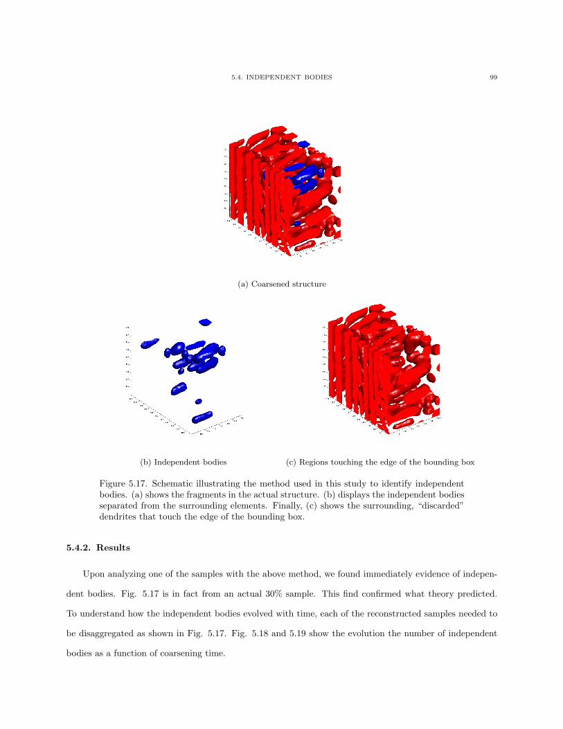
5.4. INDEPENDENT BODIES 99
(a) Coarsened structure
(b) Independent bodies (c) Regions touching the edge of the bounding box
Figure 5.17. Schematic illustrating the method used in this study to identify independentbodies. (a) shows the fragments in the actual structure. (b) displays the independent bodiesseparated from the surrounding elements. Finally, (c) shows the surrounding, “discarded”dendrites that touch the edge of the bounding box.
5.4.2. Results
Upon analyzing one of the samples with the above method, we found immediately evidence of indepen-
dent bodies. Fig. 5.17 is in fact from an actual 30% sample. This find confirmed what theory predicted.
To understand how the independent bodies evolved with time, each of the reconstructed samples needed to
be disaggregated as shown in Fig. 5.17. Fig. 5.18 and 5.19 show the evolution the number of independent
bodies as a function of coarsening time.
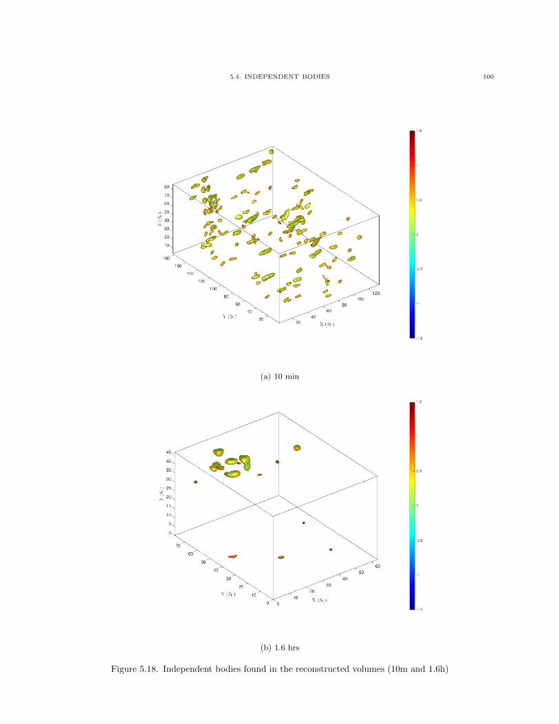
5.4. INDEPENDENT BODIES 100
(a) 10 min
(b) 1.6 hrs
Figure 5.18. Independent bodies found in the reconstructed volumes (10m and 1.6h)
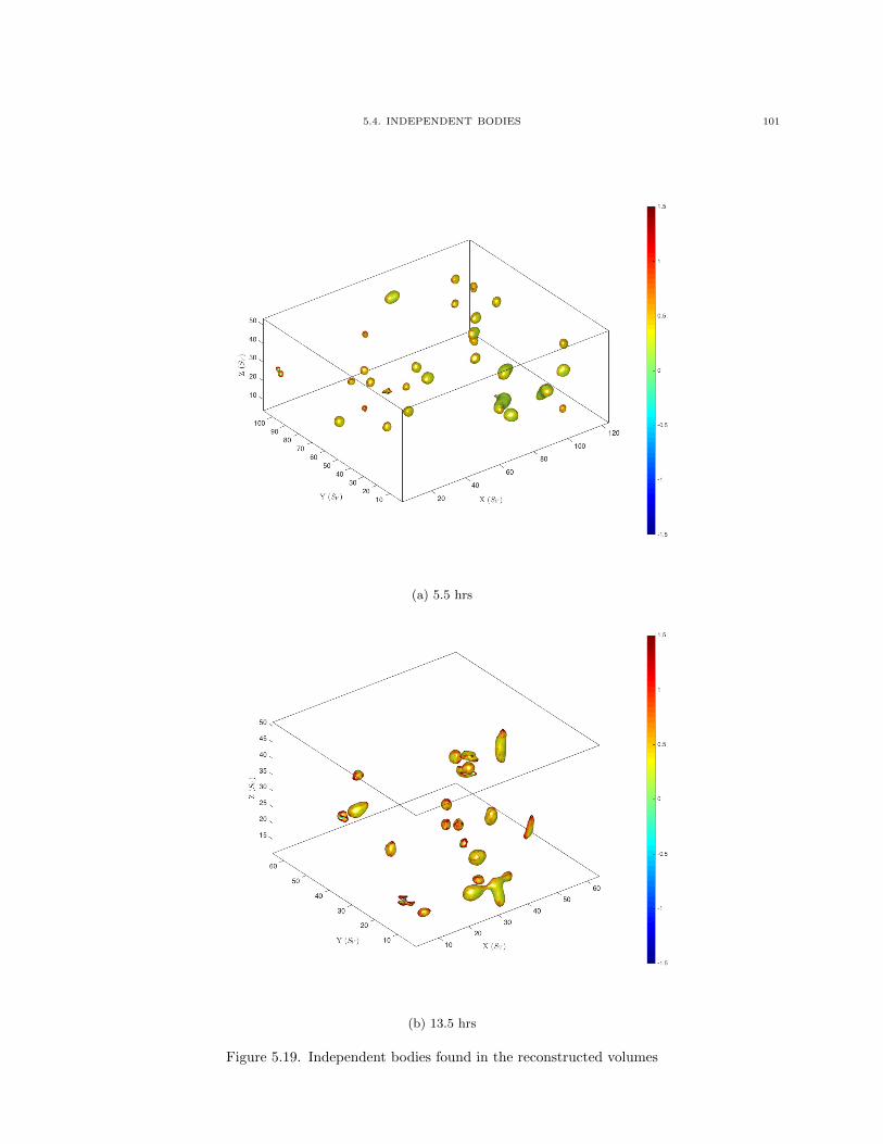
5.4. INDEPENDENT BODIES 101
(a) 5.5 hrs
(b) 13.5 hrs
Figure 5.19. Independent bodies found in the reconstructed volumes
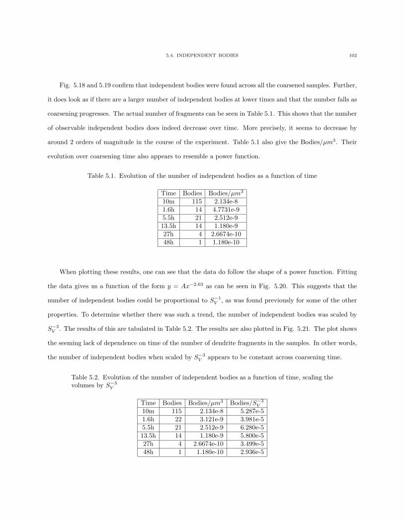
5.4. INDEPENDENT BODIES 102
Fig. 5.18 and 5.19 confirm that independent bodies were found across all the coarsened samples. Further,
it does look as if there are a larger number of independent bodies at lower times and that the number falls as
coarsening progresses. The actual number of fragments can be seen in Table 5.1. This shows that the number
of observable independent bodies does indeed decrease over time. More precisely, it seems to decrease by
around 2 orders of magnitude in the course of the experiment. Table 5.1 also give the Bodies/µm3. Their
evolution over coarsening time also appears to resemble a power function.
Table 5.1. Evolution of the number of independent bodies as a function of time
Time Bodies Bodies/µm3
10m 115 2.134e-81.6h 14 4.7731e-95.5h 21 2.512e-913.5h 14 1.180e-927h 4 2.6674e-1048h 1 1.180e-10
When plotting these results, one can see that the data do follow the shape of a power function. Fitting
the data gives us a function of the form y = Ax−2.63 as can be seen in Fig. 5.20. This suggests that the
number of independent bodies could be proportional to S−1V , as was found previously for some of the other
properties. To determine whether there was such a trend, the number of independent bodies was scaled by
S−3V . The results of this are tabulated in Table 5.2. The results are also plotted in Fig. 5.21. The plot shows
the seeming lack of dependence on time of the number of dendrite fragments in the samples. In other words,
the number of independent bodies when scaled by S−3V appears to be constant across coarsening time.
Table 5.2. Evolution of the number of independent bodies as a function of time, scaling thevolumes by S−3
V
Time Bodies Bodies/µm3 Bodies/S−3V
10m 115 2.134e-8 5.287e-51.6h 22 3.121e-9 3.981e-55.5h 21 2.512e-9 6.280e-513.5h 14 1.180e-9 5.800e-527h 4 2.6674e-10 3.499e-548h 1 1.180e-10 2.936e-5
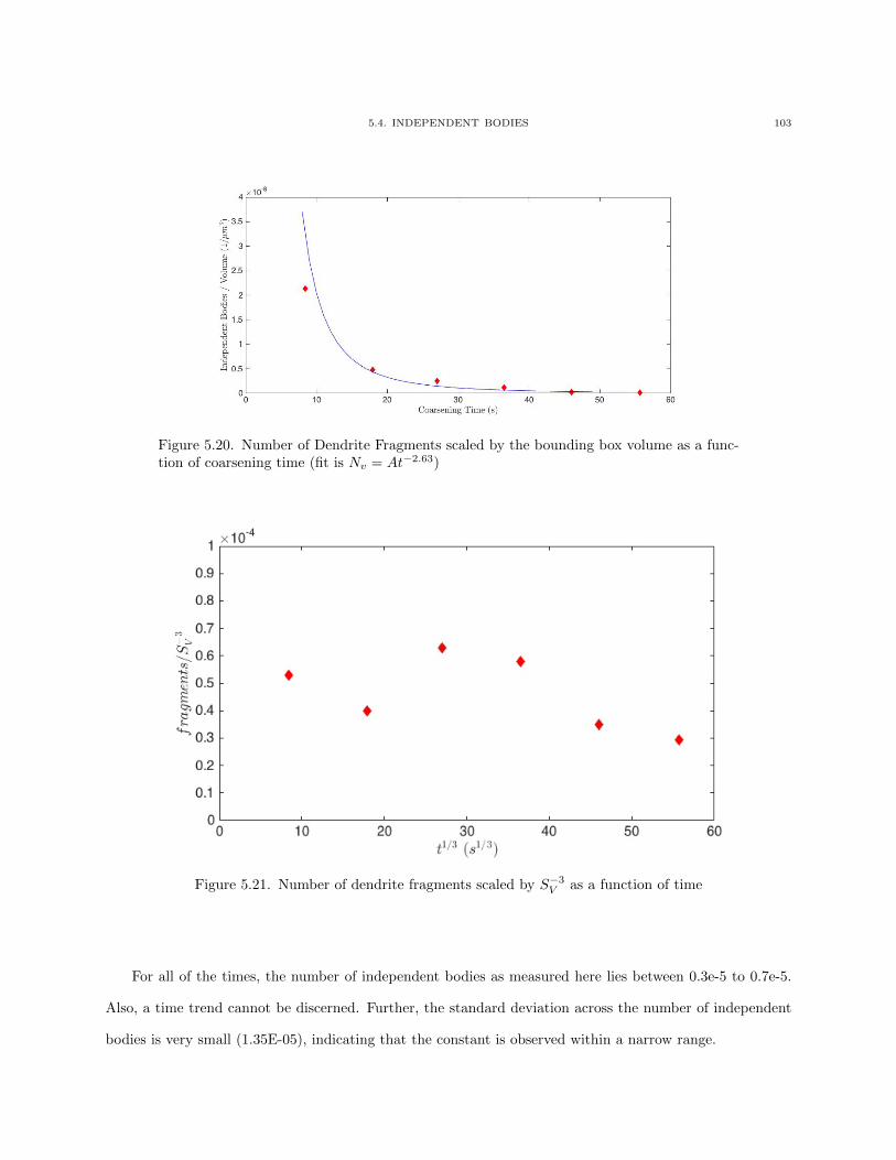
5.4. INDEPENDENT BODIES 103
Figure 5.20. Number of Dendrite Fragments scaled by the bounding box volume as a func-tion of coarsening time (fit is Nv = At−2.63)
Figure 5.21. Number of dendrite fragments scaled by S−3V as a function of time
For all of the times, the number of independent bodies as measured here lies between 0.3e-5 to 0.7e-5.
Also, a time trend cannot be discerned. Further, the standard deviation across the number of independent
bodies is very small (1.35E-05), indicating that the constant is observed within a narrow range.
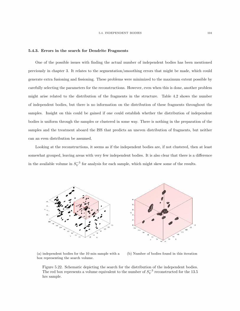
5.4. INDEPENDENT BODIES 104
5.4.3. Errors in the search for Dendrite Fragments
One of the possible issues with finding the actual number of independent bodies has been mentioned
previously in chapter 3. It relates to the segmentation/smoothing errors that might be made, which could
generate extra fusioning and fissioning. These problems were minimized to the maximum extent possible by
carefully selecting the parameters for the reconstructions. However, even when this is done, another problem
might arise related to the distribution of the fragments in the structure. Table 4.2 shows the number
of independent bodies, but there is no information on the distribution of these fragments throughout the
samples. Insight on this could be gained if one could establish whether the distribution of independent
bodies is uniform through the samples or clustered in some way. There is nothing in the preparation of the
samples and the treatment aboard the ISS that predicts an uneven distribution of fragments, but neither
can an even distribution be assumed.
Looking at the reconstructions, it seems as if the independent bodies are, if not clustered, then at least
somewhat grouped, leaving areas with very few independent bodies. It is also clear that there is a difference
in the available volume in S−3V for analysis for each sample, which might skew some of the results.
(a) independent bodies for the 10 min sample with abox representing the search volume.
(b) Number of bodies found in this iteration
Figure 5.22. Schematic depicting the search for the distribution of the independent bodies.The red box represents a volume equivalent to the number of S−3
V reconstructed for the 13.5hrs sample.
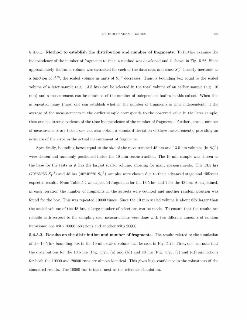
5.4. INDEPENDENT BODIES 105
5.4.3.1. Method to establish the distribution and number of fragments. To further examine the
independence of the number of fragments to time, a method was developed and is shown in Fig. 5.22. Since
approximately the same volume was extracted for each of the data sets, and since S−1V linearly increases as
a function of t1/3, the scaled volume in units of S−3V decreases. Thus, a bounding box equal to the scaled
volume of a later sample (e.g. 13.5 hrs) can be selected in the total volume of an earlier sample (e.g. 10
min) and a measurement can be obtained of the number of independent bodies in this subset. When this
is repeated many times, one can establish whether the number of fragments is time independent: if the
average of the measurements in the earlier sample corresponds to the observed value in the later sample,
then one has strong evidence of the time independence of the number of fragments. Further, since a number
of measurements are taken, one can also obtain a standard deviation of these measurements, providing an
estimate of the error in the actual measurement of fragments.
Specifically, bounding boxes equal to the size of the reconstructed 48 hrs and 13.5 hrs volumes (in S−3V )
were chosen and randomly positioned inside the 10 min reconstruction. The 10 min sample was chosen as
the base for the tests as it has the largest scaled volume, allowing for many measurements. The 13.5 hrs
(70*65*55 S−3V ) and 48 hrs (40*40*20 S−3
V ) samples were chosen due to their advanced stage and different
expected results. From Table 5.2 we expect 14 fragments for the 13.5 hrs and 1 for the 48 hrs. As explained,
in each iteration the number of fragments in the subsets were counted and another random position was
found for the box. This was repeated 10000 times. Since the 10 min scaled volume is about 65x larger than
the scaled volume of the 48 hrs, a large number of selections can be made. To ensure that the results are
reliable with respect to the sampling size, measurements were done with two different amounts of random
iterations: one with 10000 iterations and another with 20000.
5.4.3.2. Results on the distribution and number of fragments. The results related to the simulation
of the 13.5 hrs bounding box in the 10 min scaled volume can be seen in Fig. 5.23. First, one can note that
the distributions for the 13.5 hrs (Fig. 5.23, (a) and (b)) and 48 hrs (Fig. 5.23, (c) and (d)) simulations
for both the 10000 and 20000 runs are almost identical. This gives high confidence in the robustness of the
simulated results. The 10000 run is taken next as the reference simulation.
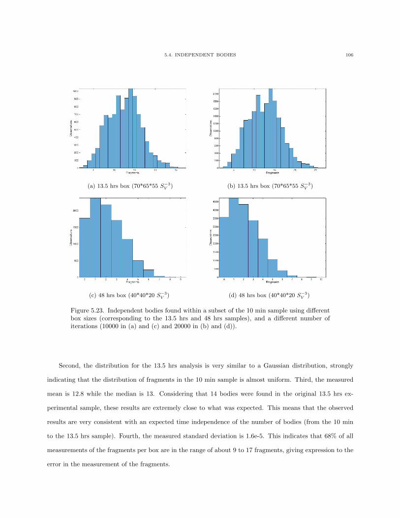
5.4. INDEPENDENT BODIES 106
(a) 13.5 hrs box (70*65*55 S−3V ) (b) 13.5 hrs box (70*65*55 S−3
V )
(c) 48 hrs box (40*40*20 S−3V ) (d) 48 hrs box (40*40*20 S−3
V )
Figure 5.23. Independent bodies found within a subset of the 10 min sample using differentbox sizes (corresponding to the 13.5 hrs and 48 hrs samples), and a different number ofiterations (10000 in (a) and (c) and 20000 in (b) and (d)).
Second, the distribution for the 13.5 hrs analysis is very similar to a Gaussian distribution, strongly
indicating that the distribution of fragments in the 10 min sample is almost uniform. Third, the measured
mean is 12.8 while the median is 13. Considering that 14 bodies were found in the original 13.5 hrs ex-
perimental sample, these results are extremely close to what was expected. This means that the observed
results are very consistent with an expected time independence of the number of bodies (from the 10 min
to the 13.5 hrs sample). Fourth, the measured standard deviation is 1.6e-5. This indicates that 68% of all
measurements of the fragments per box are in the range of about 9 to 17 fragments, giving expression to the
error in the measurement of the fragments.
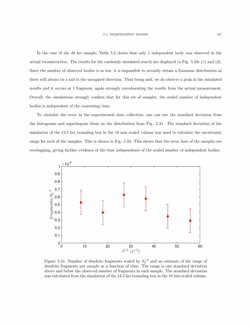
5.4. INDEPENDENT BODIES 107
In the case of the 48 hrs sample, Table 5.2 shows that only 1 independent body was observed in the
actual reconstruction. The results for the randomly simulated search are displayed in Fig. 5.23c (c) and (d).
Since the number of observed bodies is so low, it is impossible to actually obtain a Gaussian distribution as
there will always be a tail in the uncapped direction. That being said, we do observe a peak in the simulated
results and it occurs at 1 fragment, again strongly corroborating the results from the actual measurement.
Overall, the simulations strongly confirm that for this set of samples, the scaled number of independent
bodies is independent of the coarsening time.
To visualize the error in the experimental data collection, one can use the standard deviation from
the histograms and superimpose them on the distribution from Fig. 5.21. The standard deviation of the
simulation of the 13.5 hrs bounding box in the 10 min scaled volume was used to calculate the uncertainly
range for each of the samples. This is shown in Fig. 5.24. This shows that the error bars of the samples are
overlapping, giving further evidence of the time independence of the scaled number of independent bodies.
Figure 5.24. Number of dendrite fragments scaled by S−3V and an estimate of the range of
dendrite fragments per sample as a function of time. The range is one standard deviationabove and below the observed number of fragments in each sample. The standard deviationwas calculated from the simulation of the 13.5 hrs bounding box in the 10 min scaled volume.
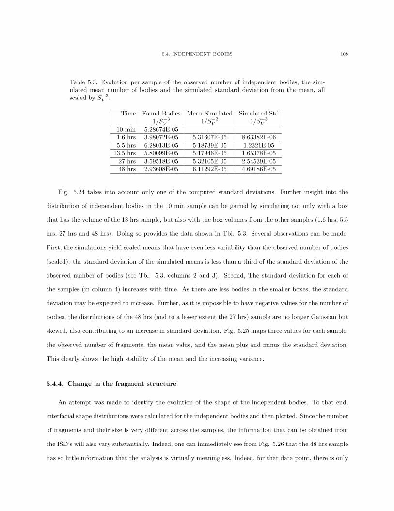
5.4. INDEPENDENT BODIES 108
Table 5.3. Evolution per sample of the observed number of independent bodies, the sim-ulated mean number of bodies and the simulated standard deviation from the mean, allscaled by S−3
V .
Time Found Bodies Mean Simulated Simulated Std1/S−3
V 1/S−3V 1/S−3
V
10 min 5.28674E-05 - -1.6 hrs 3.98072E-05 5.31607E-05 8.63382E-065.5 hrs 6.28013E-05 5.18739E-05 1.2321E-05
13.5 hrs 5.80099E-05 5.17946E-05 1.65378E-0527 hrs 3.59518E-05 5.32105E-05 2.54539E-0548 hrs 2.93608E-05 6.11292E-05 4.69186E-05
Fig. 5.24 takes into account only one of the computed standard deviations. Further insight into the
distribution of independent bodies in the 10 min sample can be gained by simulating not only with a box
that has the volume of the 13 hrs sample, but also with the box volumes from the other samples (1.6 hrs, 5.5
hrs, 27 hrs and 48 hrs). Doing so provides the data shown in Tbl. 5.3. Several observations can be made.
First, the simulations yield scaled means that have even less variability than the observed number of bodies
(scaled): the standard deviation of the simulated means is less than a third of the standard deviation of the
observed number of bodies (see Tbl. 5.3, columns 2 and 3). Second, The standard deviation for each of
the samples (in column 4) increases with time. As there are less bodies in the smaller boxes, the standard
deviation may be expected to increase. Further, as it is impossible to have negative values for the number of
bodies, the distributions of the 48 hrs (and to a lesser extent the 27 hrs) sample are no longer Gaussian but
skewed, also contributing to an increase in standard deviation. Fig. 5.25 maps three values for each sample:
the observed number of fragments, the mean value, and the mean plus and minus the standard deviation.
This clearly shows the high stability of the mean and the increasing variance.
5.4.4. Change in the fragment structure
An attempt was made to identify the evolution of the shape of the independent bodies. To that end,
interfacial shape distributions were calculated for the independent bodies and then plotted. Since the number
of fragments and their size is very different across the samples, the information that can be obtained from
the ISD’s will also vary substantially. Indeed, one can immediately see from Fig. 5.26 that the 48 hrs sample
has so little information that the analysis is virtually meaningless. Indeed, for that data point, there is only
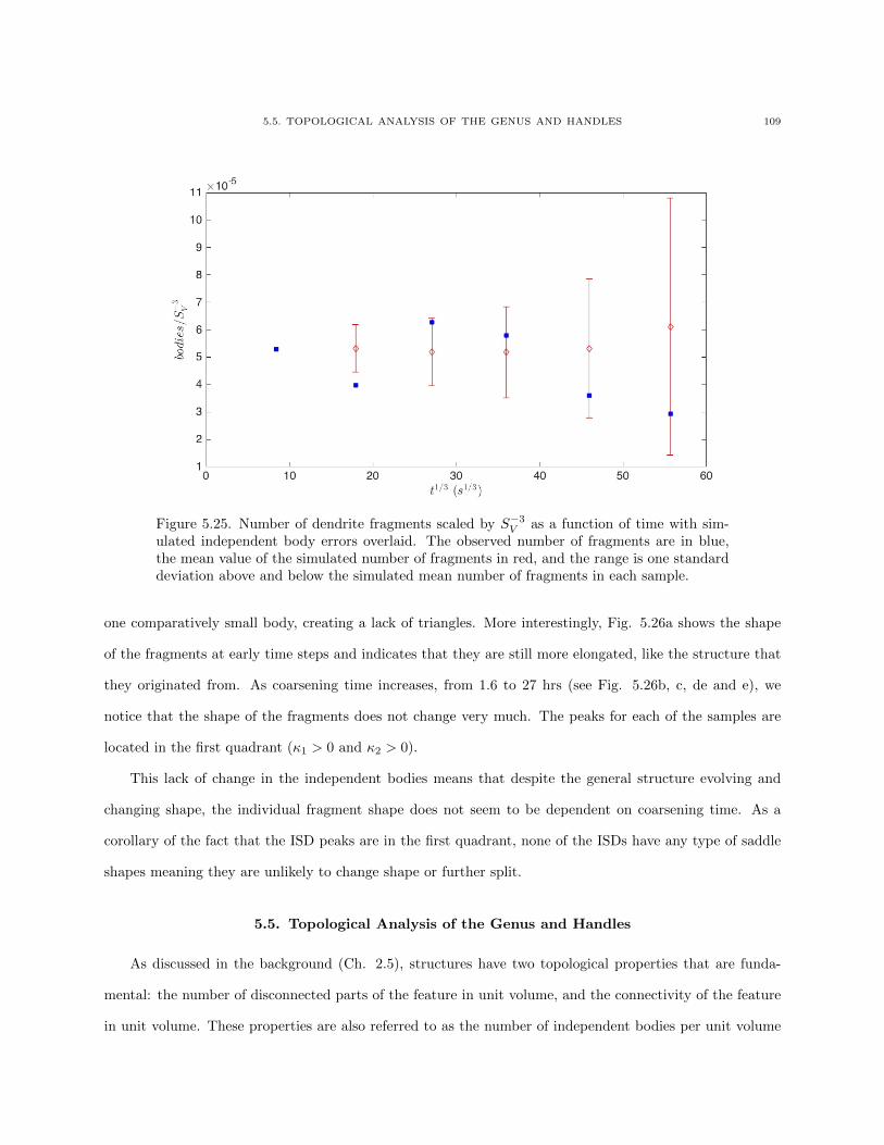
5.5. TOPOLOGICAL ANALYSIS OF THE GENUS AND HANDLES 109
Figure 5.25. Number of dendrite fragments scaled by S−3V as a function of time with sim-
ulated independent body errors overlaid. The observed number of fragments are in blue,the mean value of the simulated number of fragments in red, and the range is one standarddeviation above and below the simulated mean number of fragments in each sample.
one comparatively small body, creating a lack of triangles. More interestingly, Fig. 5.26a shows the shape
of the fragments at early time steps and indicates that they are still more elongated, like the structure that
they originated from. As coarsening time increases, from 1.6 to 27 hrs (see Fig. 5.26b, c, de and e), we
notice that the shape of the fragments does not change very much. The peaks for each of the samples are
located in the first quadrant (κ1 > 0 and κ2 > 0).
This lack of change in the independent bodies means that despite the general structure evolving and
changing shape, the individual fragment shape does not seem to be dependent on coarsening time. As a
corollary of the fact that the ISD peaks are in the first quadrant, none of the ISDs have any type of saddle
shapes meaning they are unlikely to change shape or further split.
5.5. Topological Analysis of the Genus and Handles
As discussed in the background (Ch. 2.5), structures have two topological properties that are funda-
mental: the number of disconnected parts of the feature in unit volume, and the connectivity of the feature
in unit volume. These properties are also referred to as the number of independent bodies per unit volume
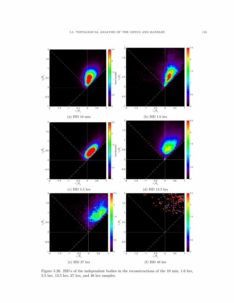
5.5. TOPOLOGICAL ANALYSIS OF THE GENUS AND HANDLES 110
(a) ISD 10 min (b) ISD 1.6 hrs
(c) ISD 5.5 hrs (d) ISD 13.5 hrs
(e) ISD 27 hrs (f) ISD 48 hrs
Figure 5.26. ISD’s of the independent bodies in the reconstructions of the 10 min, 1.6 hrs,5.5 hrs, 13.5 hrs, 27 hrs, and 48 hrs samples.
5.5. TOPOLOGICAL ANALYSIS OF THE GENUS AND HANDLES 111
and the total connectivity of the microstructure. Results on the number and distribution of independent
bodies or disconnected parts were reported in the previous section. Analysis and results on the connectivity
are reported in this section.
5.5.1. Method for determining the number of handles
The point of departure for the determination of the number of handles was the reconstructions that were
shown before, but a number of considerations led us to follow a different process. To prevent edge effects
(changes in the obtained results due to the artificial edges of the reconstruction due to the bounding box)
from affecting the actual results, the reconstructions had to be closed. This means that the structure before
reconstruction was padded with a plane of “eutectic” around it so that the isosurface function created a
surface on the outside edges of the bodies. This in turn had a couple of different effects on the reconstructed
structure. First, it increased the total surface area of the reconstruction (changing S−1V ). Second, it also
would affect the ISD by creating a totally flat area (large area with κ1 = κ2 = 0). Finally, those bodies
would now be considered independent bodies as they are now not touching the interface. All these factors
prevented us from using the same reconstructions as the ones used for the independent body calculations.
To obtain the genus of our reconstructions, we proceeded as follows. The total number of vertices and
faces from the isosurface output were obtained. This gives two of the three variables needed to calculate
the Euler Characteristic χ. To get the last needed value, the edges for each of the faces were calculated.
Since each edge is shared by two different triangles, duplicates were searched for and then removed. Once
the three values were obtained, the Euler characteristic was calculated using Eq. 2.15. The genus was then
calculated using Eq. 2.14.
In their study of the topology of AlCu samples, Mendoza et al [13] used Eq. 2.16 to calculate the genus.
This is necessary due to the fact that the number of voids in the structure has an effect on the measurement
of the genus. We similarly searched our reconstructions to determine the number of voids. However, none
were found in any of the samples. We suspect that this is due to the low volume fraction of the samples.
Connectivity calculations are more susceptible to changes in the reconstruction than the determination
of the number of independent bodies since we are looking at very localized structures. Slight variations due
to an erroneous segmentation can close a handle or break it. Since the segmentation algorithm tended to
5.5. TOPOLOGICAL ANALYSIS OF THE GENUS AND HANDLES 112
favor closing the loops, the decision was made to err on the side of slight under-segmentation. Also, no
smoothing was performed on the reconstructions that were used to calculate the handles and genus. Again,
this was done to avoid affecting the handles. Since these reconstructions were used exclusively to obtain the
handles and genus, this presented no problem for the other analyses.
While our reconstructions do not have voids, they have independent bodies. This requires us to slightly
adjust the conversion from genus to handles. Without voids, the genus equals the number of handles.
However, since each closed structure adds “2” to the Euler characteristic, one needs to adjust for each body
beyond the first one. This is done in equation 5.1, which adds the number of independent bodies to the
genus (substracting one for the original body) to obtain the number of handles.
handles = g +Nind − 1(5.1)
Note that what is called an independent body in the topological analysis is different from what is called
an independent body in the previous section. In this section, the term “fragment” or “independent body”
refers to all bodies, even those previously discarded for touching the edges of the bounding box. In the
previous section we were looking for fragments splitting off from the structure; here we are looking for
handles and to do so, we needed to define independent bodies in a different way. In the handle analysis,
an independent body is simply a reconstructed element not touching another one. This includes the ones
touching the edges of the bounding box.
5.5.2. Evolution of the number of handles
The number of handles was computed for each of the different coarsening times and the results can be
observed in Table. 5.4. First, similar to the evolution of the number of dendrite fragments reported in the
previous section, column 2 shows that the number of handles per µm3 is decreasing as a function of time
(barring the exception at 27h).
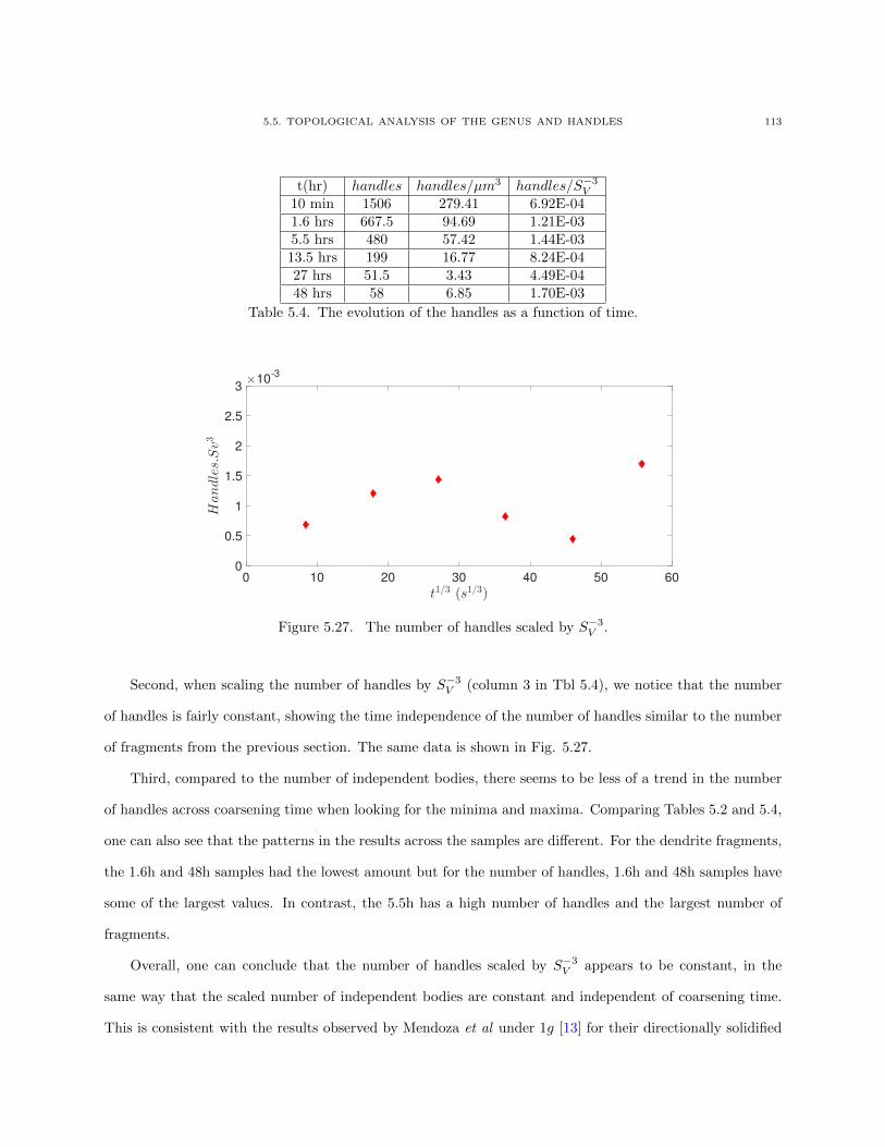
5.5. TOPOLOGICAL ANALYSIS OF THE GENUS AND HANDLES 113
t(hr) handles handles/µm3 handles/S−3V
10 min 1506 279.41 6.92E-041.6 hrs 667.5 94.69 1.21E-035.5 hrs 480 57.42 1.44E-0313.5 hrs 199 16.77 8.24E-0427 hrs 51.5 3.43 4.49E-0448 hrs 58 6.85 1.70E-03
Table 5.4. The evolution of the handles as a function of time.
0 10 20 30 40 50 60
t1/3 (s1/3)
0
0.5
1
1.5
2
2.5
3
Handles.Sv3
×10-3
Figure 5.27. The number of handles scaled by S−3V .
Second, when scaling the number of handles by S−3V (column 3 in Tbl 5.4), we notice that the number
of handles is fairly constant, showing the time independence of the number of handles similar to the number
of fragments from the previous section. The same data is shown in Fig. 5.27.
Third, compared to the number of independent bodies, there seems to be less of a trend in the number
of handles across coarsening time when looking for the minima and maxima. Comparing Tables 5.2 and 5.4,
one can also see that the patterns in the results across the samples are different. For the dendrite fragments,
the 1.6h and 48h samples had the lowest amount but for the number of handles, 1.6h and 48h samples have
some of the largest values. In contrast, the 5.5h has a high number of handles and the largest number of
fragments.
Overall, one can conclude that the number of handles scaled by S−3V appears to be constant, in the
same way that the scaled number of independent bodies are constant and independent of coarsening time.
This is consistent with the results observed by Mendoza et al under 1g [13] for their directionally solidified
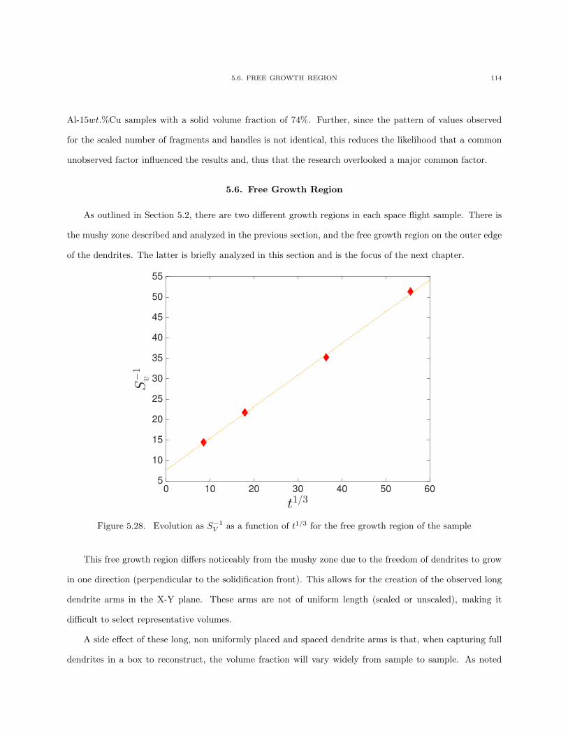
5.6. FREE GROWTH REGION 114
Al-15wt.%Cu samples with a solid volume fraction of 74%. Further, since the pattern of values observed
for the scaled number of fragments and handles is not identical, this reduces the likelihood that a common
unobserved factor influenced the results and, thus that the research overlooked a major common factor.
5.6. Free Growth Region
As outlined in Section 5.2, there are two different growth regions in each space flight sample. There is
the mushy zone described and analyzed in the previous section, and the free growth region on the outer edge
of the dendrites. The latter is briefly analyzed in this section and is the focus of the next chapter.
0 10 20 30 40 50 60
t1/3
5
10
15
20
25
30
35
40
45
50
55
S−1
v
Figure 5.28. Evolution as S−1V as a function of t1/3 for the free growth region of the sample
This free growth region differs noticeably from the mushy zone due to the freedom of dendrites to grow
in one direction (perpendicular to the solidification front). This allows for the creation of the observed long
dendrite arms in the X-Y plane. These arms are not of uniform length (scaled or unscaled), making it
difficult to select representative volumes.
A side effect of these long, non uniformly placed and spaced dendrite arms is that, when capturing full
dendrites in a box to reconstruct, the volume fraction will vary widely from sample to sample. As noted
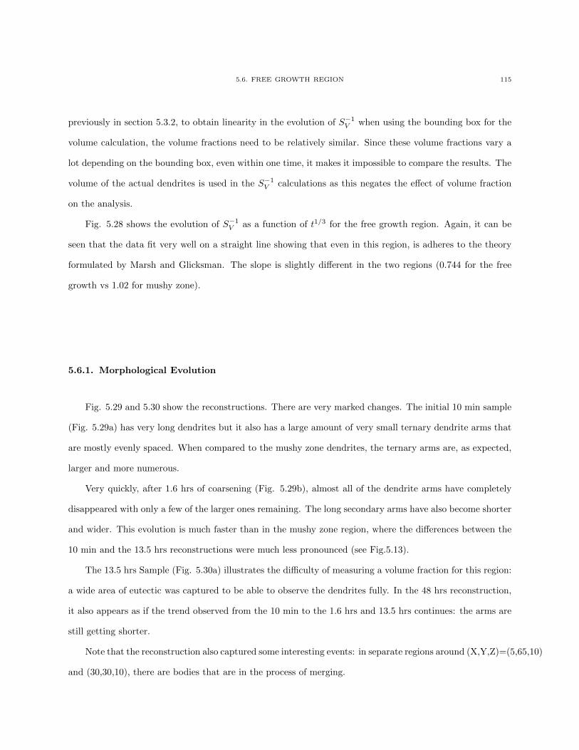
5.6. FREE GROWTH REGION 115
previously in section 5.3.2, to obtain linearity in the evolution of S−1V when using the bounding box for the
volume calculation, the volume fractions need to be relatively similar. Since these volume fractions vary a
lot depending on the bounding box, even within one time, it makes it impossible to compare the results. The
volume of the actual dendrites is used in the S−1V calculations as this negates the effect of volume fraction
on the analysis.
Fig. 5.28 shows the evolution of S−1V as a function of t1/3 for the free growth region. Again, it can be
seen that the data fit very well on a straight line showing that even in this region, is adheres to the theory
formulated by Marsh and Glicksman. The slope is slightly different in the two regions (0.744 for the free
growth vs 1.02 for mushy zone).
5.6.1. Morphological Evolution
Fig. 5.29 and 5.30 show the reconstructions. There are very marked changes. The initial 10 min sample
(Fig. 5.29a) has very long dendrites but it also has a large amount of very small ternary dendrite arms that
are mostly evenly spaced. When compared to the mushy zone dendrites, the ternary arms are, as expected,
larger and more numerous.
Very quickly, after 1.6 hrs of coarsening (Fig. 5.29b), almost all of the dendrite arms have completely
disappeared with only a few of the larger ones remaining. The long secondary arms have also become shorter
and wider. This evolution is much faster than in the mushy zone region, where the differences between the
10 min and the 13.5 hrs reconstructions were much less pronounced (see Fig.5.13).
The 13.5 hrs Sample (Fig. 5.30a) illustrates the difficulty of measuring a volume fraction for this region:
a wide area of eutectic was captured to be able to observe the dendrites fully. In the 48 hrs reconstruction,
it also appears as if the trend observed from the 10 min to the 1.6 hrs and 13.5 hrs continues: the arms are
still getting shorter.
Note that the reconstruction also captured some interesting events: in separate regions around (X,Y,Z)=(5,65,10)
and (30,30,10), there are bodies that are in the process of merging.
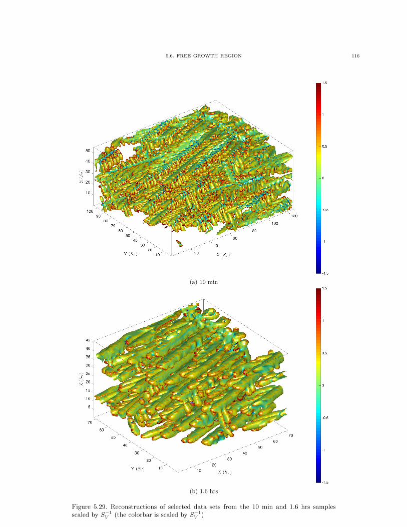
5.6. FREE GROWTH REGION 116
(a) 10 min
(b) 1.6 hrs
Figure 5.29. Reconstructions of selected data sets from the 10 min and 1.6 hrs samplesscaled by S−1
V (the colorbar is scaled by S−1V )
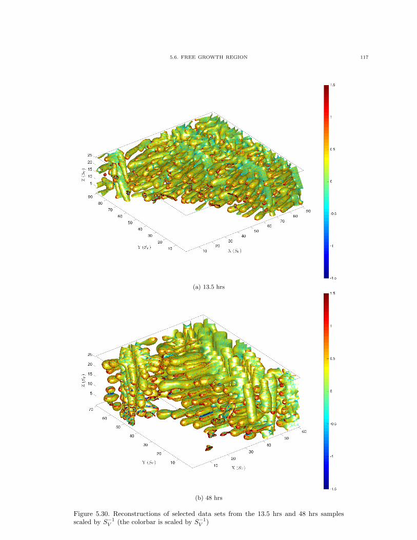
5.6. FREE GROWTH REGION 117
(a) 13.5 hrs
(b) 48 hrs
Figure 5.30. Reconstructions of selected data sets from the 13.5 hrs and 48 hrs samplesscaled by S−1
V (the colorbar is scaled by S−1V )
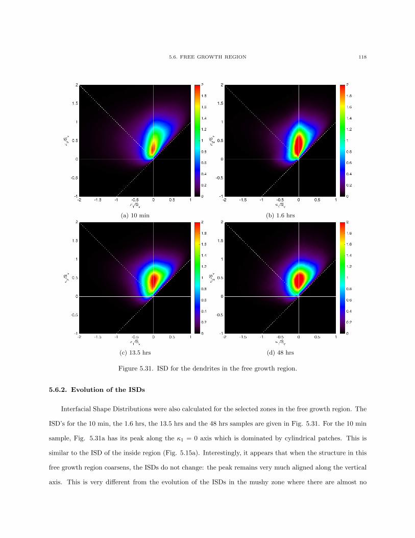
5.6. FREE GROWTH REGION 118
(a) 10 min (b) 1.6 hrs
(c) 13.5 hrs (d) 48 hrs
Figure 5.31. ISD for the dendrites in the free growth region.
5.6.2. Evolution of the ISDs
Interfacial Shape Distributions were also calculated for the selected zones in the free growth region. The
ISD’s for the 10 min, the 1.6 hrs, the 13.5 hrs and the 48 hrs samples are given in Fig. 5.31. For the 10 min
sample, Fig. 5.31a has its peak along the κ1 = 0 axis which is dominated by cylindrical patches. This is
similar to the ISD of the inside region (Fig. 5.15a). Interestingly, it appears that when the structure in this
free growth region coarsens, the ISDs do not change: the peak remains very much aligned along the vertical
axis. This is very different from the evolution of the ISDs in the mushy zone where there are almost no
5.7. CONCLUSION 119
observed patches with negative κ1 and κ2. Neither does the peak settle down near the κ1 = κ2 = 0 region,
but instead stays near κ2/SV = 0.5. This is because in this region there are none of the wide, slightly curved
structures with one side having a positive curvature and the other a negative curvature. This confirms the
evolutions seen in the reconstructions themselves: the higher curvature regions and ternary dendrite arms
disappear quickly but the overall shape remains the same due to a lack of constraints.
5.7. Conclusion
The experiments that were conducted aboard the International Space Station on the PbSn samples with
a volume fraction of solid of 30% volume lead to a number of significant conclusions regarding the dendritic
evolution in the mushy zone. First, independent bodies (fragments) that results from the breaking up of
the dendritic structure could be found in each of the reconstructed samples, providing direct evidence of
the fissioning of secondary (and ternary) arms. Second, when scaled by S−3V , we find that the number of
independent bodies is nearly invariant with respect to coarsening time. This finding is confirmed when more
extensive simulations are conducted on the number of independent bodies of the various dendritic structures.
This finding is surprising in view of the significant change in the dendritic structure across coarsening time
that is observed in Fig. 5.13 and Fig. 5.14. Third, the ISD analysis of the shape of the independent bodies
finds that their shape remains largely unchanged across coarsening time, in spite of a substantial change in
the overall dendritic structure. Fourth, the connectivity of the structures as measured by the number of
handles is also found to be largely time invariant when scaled by S−3V . These findings confirm that while the
morphology of structures may change substantially during coarsening, the structure may remain topologically
invariant. Fifth, the research also confirms the linear relation between surface area per unit volume S−1V and
coarsening time t1/3. Comparing the relation to a 43% solid volume fraction PbSn sample coarsened under
1g condition, we found that the relation is very similar, highlighting the absence of the effects of convection
on the ground based experiments.
Concerning the free growth region, we find, first, that the dendrites are longer than in the mushy zone
and also have longer secondary and ternary arms. Second, we observe that the shape changes and evolution
occur much faster than in the inside region. Third, in contrast to the mushy zone where the change in
the ISD’s across coarsening times showed a substantial change in the overall structure, the ISD’s in the

5.7. CONCLUSION 120
free growth region do not measure such change, implying that the structure is much more similar across
coarsening time. Fourth, the reconstructions capture some merging events. The phase field analysis in the
next chapter will examine in more detail the evolution of the dendritic microstructure in this outside region
and study coarsening mechanisms such as the merging observed here.
6.1. MODEL 121
CHAPTER 6
Evolution of the Microstructure using Phase-Field Simulation
The analysis in the Chapter 5 was based on “snapshots” of the samples that had coarsened for different
times aboard the ISS. Since there is little information on what happened during the time intervals between
these snapshots, the dynamics of the system have to be inferred. The phase field analysis discussed in this
chapter allows a direct analysis of the dynamics of the system and gives an opportunity to study in detail
the mechanisms of coalescence, fragmentation and retraction. A 3D reconstruction of the PbSn sample, 30%
solid, that had coarsened for 10 min under microgravity conditions is used as initial condition.
6.1. Model
The phase field analysis used to simulate coarsening is based on a model for a dilute binary alloy by
Echebarria et al. [27], similar to the work by Aagesen [23] whose notation and development is followed below.
The model assumes that the system is isothermal though it is possible to add a temperature gradient as in
the Echebarria model. The free-energy functional is
F =
∫V
[f(φ, Tm) + fAB(φ, c, T ) +
σ2φ
2|∇φ|2
]dV(6.1)
where f(φ, Tm) is the double well potential for the order parameter φ, and |∇φ|2 its gradient (A and B
are the two components of the alloy; c and Tm stand for the mole fraction of component B and the melting
point), and
f(φ, Tm) = H(−φ2/2 + φ4/4)(6.2)
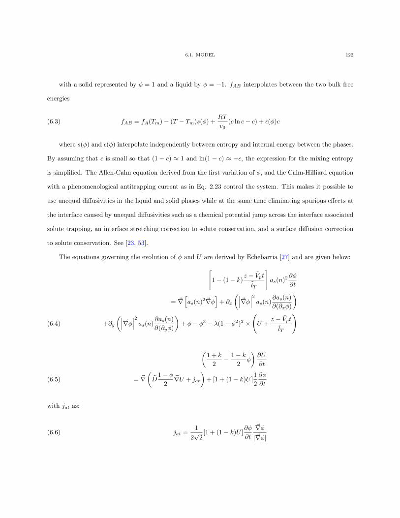
6.1. MODEL 122
with a solid represented by φ = 1 and a liquid by φ = −1. fAB interpolates between the two bulk free
energies
fAB = fA(Tm)− (T − Tm)s(φ) +RT
v0(c ln c− c) + ε(φ)c(6.3)
where s(φ) and ε(φ) interpolate independently between entropy and internal energy between the phases.
By assuming that c is small so that (1 − c) ≈ 1 and ln(1 − c) ≈ −c, the expression for the mixing entropy
is simplified. The Allen-Cahn equation derived from the first variation of φ, and the Cahn-Hilliard equation
with a phenomenological antitrapping current as in Eq. 2.23 control the system. This makes it possible to
use unequal diffusivities in the liquid and solid phases while at the same time eliminating spurious effects at
the interface caused by unequal diffusivities such as a chemical potential jump across the interface associated
solute trapping, an interface stretching correction to solute conservation, and a surface diffusion correction
to solute conservation. See [23, 53].
The equations governing the evolution of φ and U are derived by Echebarria [27] and are given below:[1− (1− k)
z − VptlT
]as(n)2 ∂φ
∂t
= ~∇[as(n)2~∇φ
]+ ∂x
(∣∣∣~∇φ∣∣∣2 as(n)∂as(n)
∂(∂xφ)
)
+∂y
(∣∣∣~∇φ∣∣∣2 as(n)∂as(n)
∂(∂yφ)
)+ φ− φ3 − λ(1− φ2)2 ×
(U +
z − VptlT
)(6.4)
(1 + k
2− 1− k
2φ
)∂U
∂t
= ~∇(D
1− φ2
~∇U + jat
)+ [1 + (1− k)U ]
1
2
∂φ
∂t(6.5)
with jat as:
jat =1
2√
2[1 + (1− k)U ]
∂φ
∂t
~∇φ|~∇φ|
(6.6)
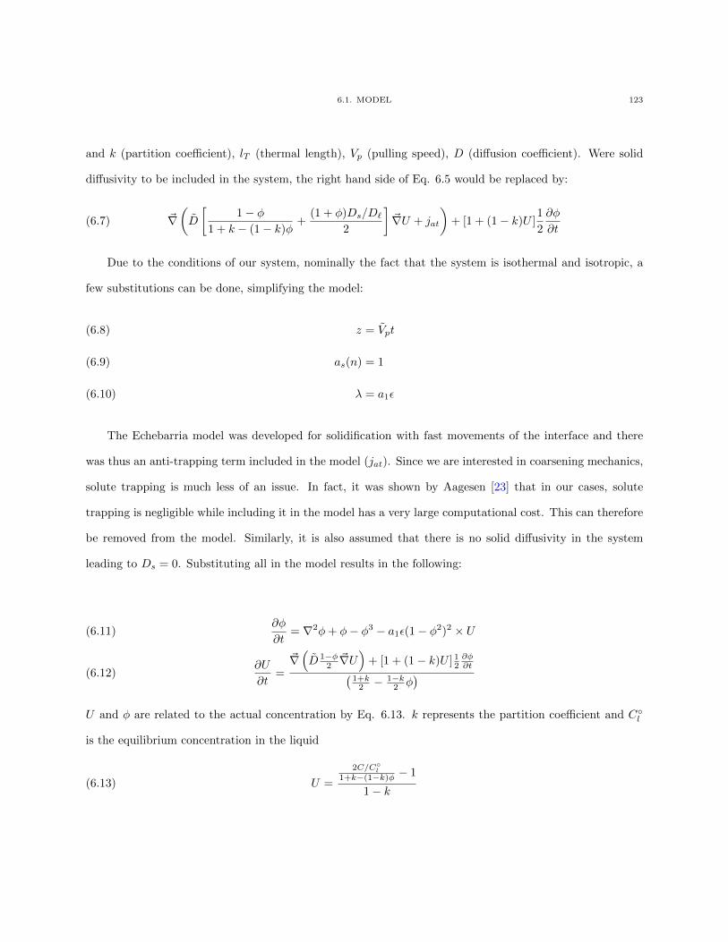
6.1. MODEL 123
and k (partition coefficient), lT (thermal length), Vp (pulling speed), D (diffusion coefficient). Were solid
diffusivity to be included in the system, the right hand side of Eq. 6.5 would be replaced by:
~∇(D
[1− φ
1 + k − (1− k)φ+
(1 + φ)Ds/D`
2
]~∇U + jat
)+ [1 + (1− k)U ]
1
2
∂φ
∂t(6.7)
Due to the conditions of our system, nominally the fact that the system is isothermal and isotropic, a
few substitutions can be done, simplifying the model:
z = Vpt(6.8)
as(n) = 1(6.9)
λ = a1ε(6.10)
The Echebarria model was developed for solidification with fast movements of the interface and there
was thus an anti-trapping term included in the model (jat). Since we are interested in coarsening mechanics,
solute trapping is much less of an issue. In fact, it was shown by Aagesen [23] that in our cases, solute
trapping is negligible while including it in the model has a very large computational cost. This can therefore
be removed from the model. Similarly, it is also assumed that there is no solid diffusivity in the system
leading to Ds = 0. Substituting all in the model results in the following:
∂φ
∂t= ∇2φ+ φ− φ3 − a1ε(1− φ2)2 × U(6.11)
∂U
∂t=
~∇(D 1−φ
2~∇U)
+ [1 + (1− k)U ] 12∂φ∂t(
1+k2 −
1−k2 φ
)(6.12)
U and φ are related to the actual concentration by Eq. 6.13. k represents the partition coefficient and Cl
is the equilibrium concentration in the liquid
U =
2C/Cl
1+k−(1−k)φ − 1
1− k(6.13)
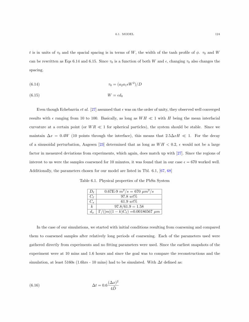
6.1. MODEL 124
t is in units of τ0 and the spacial spacing is in terms of W , the width of the tanh profile of φ. τ0 and W
can be rewritten as Eqs 6.14 and 6.15. Since τ0 is a function of both W and ε, changing τ0 also changes the
spacing.
τ0 = (a2a1εW2)/D(6.14)
W = εd0(6.15)
Even though Echebarria et al. [27] assumed that ε was on the order of unity, they observed well converged
results with ε ranging from 10 to 100. Basically, as long as WH 1 with H being the mean interfacial
curvature at a certain point (or WR 1 for spherical particles), the system should be stable. Since we
maintain ∆x = 0.4W (10 points through the interface), this means that 2.5∆xH 1. For the decay
of a sinusoidal perturbation, Aagesen [23] determined that as long as WH < 0.2, ε would not be a large
factor in measured deviations from experiments, which again, does match up with [27]. Since the regions of
interest to us were the samples coarsened for 10 minutes, it was found that in our case ε = 670 worked well.
Additionally, the parameters chosen for our model are listed in Tbl. 6.1, [67, 68]
Table 6.1. Physical properties of the PbSn System
D` 0.67E-9 m2/s = 670 µm2/sC` 97.8 wt%Cs 61.9 wt%k 97.8/61.9 = 1.58do Γ/(|m|(1− k)C`) =0.00186567 µm
In the case of our simulations, we started with initial conditions resulting from coarsening and compared
them to coarsened samples after relatively long periods of coarsening. Each of the parameters used were
gathered directly from experiments and no fitting parameters were used. Since the earliest snapshots of the
experiment were at 10 mins and 1.6 hours and since the goal was to compare the reconstructions and the
simulation, at least 5160s (1.6hrs - 10 mins) had to be simulated. With ∆t defined as:
∆t = 0.6(∆x)2
4D(6.16)
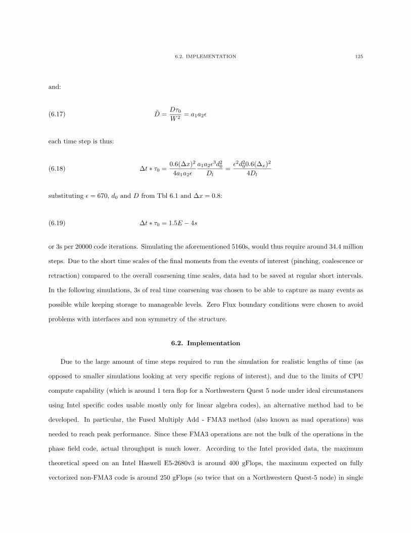
6.2. IMPLEMENTATION 125
and:
D =Dτ0W 2
= a1a2ε(6.17)
each time step is thus:
∆t ∗ τ0 =0.6(∆x)2
4a1a2ε
a1a2ε3d2
0
Dl=ε2d2
00.6(∆x)2
4Dl(6.18)
substituting ε = 670, d0 and D from Tbl 6.1 and ∆x = 0.8:
∆t ∗ τ0 = 1.5E − 4s(6.19)
or 3s per 20000 code iterations. Simulating the aforementioned 5160s, would thus require around 34.4 million
steps. Due to the short time scales of the final moments from the events of interest (pinching, coalescence or
retraction) compared to the overall coarsening time scales, data had to be saved at regular short intervals.
In the following simulations, 3s of real time coarsening was chosen to be able to capture as many events as
possible while keeping storage to manageable levels. Zero Flux boundary conditions were chosen to avoid
problems with interfaces and non symmetry of the structure.
6.2. Implementation
Due to the large amount of time steps required to run the simulation for realistic lengths of time (as
opposed to smaller simulations looking at very specific regions of interest), and due to the limits of CPU
compute capability (which is around 1 tera flop for a Northwestern Quest 5 node under ideal circumstances
using Intel specific codes usable mostly only for linear algebra codes), an alternative method had to be
developed. In particular, the Fused Multiply Add - FMA3 method (also known as mad operations) was
needed to reach peak performance. Since these FMA3 operations are not the bulk of the operations in the
phase field code, actual throughput is much lower. According to the Intel provided data, the maximum
theoretical speed on an Intel Haswell E5-2680v3 is around 400 gFlops, the maximum expected on fully
vectorized non-FMA3 code is around 250 gFlops (so twice that on a Northwestern Quest-5 node) in single
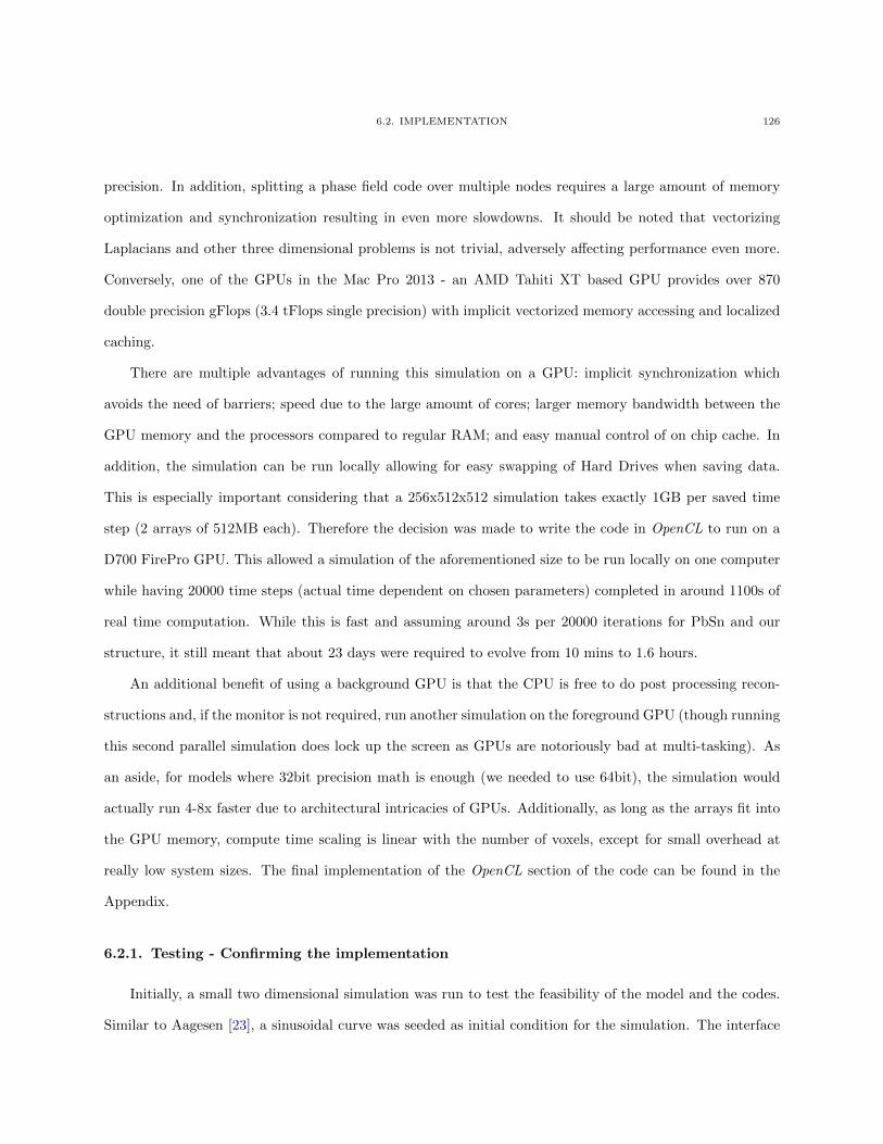
6.2. IMPLEMENTATION 126
precision. In addition, splitting a phase field code over multiple nodes requires a large amount of memory
optimization and synchronization resulting in even more slowdowns. It should be noted that vectorizing
Laplacians and other three dimensional problems is not trivial, adversely affecting performance even more.
Conversely, one of the GPUs in the Mac Pro 2013 - an AMD Tahiti XT based GPU provides over 870
double precision gFlops (3.4 tFlops single precision) with implicit vectorized memory accessing and localized
caching.
There are multiple advantages of running this simulation on a GPU: implicit synchronization which
avoids the need of barriers; speed due to the large amount of cores; larger memory bandwidth between the
GPU memory and the processors compared to regular RAM; and easy manual control of on chip cache. In
addition, the simulation can be run locally allowing for easy swapping of Hard Drives when saving data.
This is especially important considering that a 256x512x512 simulation takes exactly 1GB per saved time
step (2 arrays of 512MB each). Therefore the decision was made to write the code in OpenCL to run on a
D700 FirePro GPU. This allowed a simulation of the aforementioned size to be run locally on one computer
while having 20000 time steps (actual time dependent on chosen parameters) completed in around 1100s of
real time computation. While this is fast and assuming around 3s per 20000 iterations for PbSn and our
structure, it still meant that about 23 days were required to evolve from 10 mins to 1.6 hours.
An additional benefit of using a background GPU is that the CPU is free to do post processing recon-
structions and, if the monitor is not required, run another simulation on the foreground GPU (though running
this second parallel simulation does lock up the screen as GPUs are notoriously bad at multi-tasking). As
an aside, for models where 32bit precision math is enough (we needed to use 64bit), the simulation would
actually run 4-8x faster due to architectural intricacies of GPUs. Additionally, as long as the arrays fit into
the GPU memory, compute time scaling is linear with the number of voxels, except for small overhead at
really low system sizes. The final implementation of the OpenCL section of the code can be found in the
Appendix.
6.2.1. Testing - Confirming the implementation
Initially, a small two dimensional simulation was run to test the feasibility of the model and the codes.
Similar to Aagesen [23], a sinusoidal curve was seeded as initial condition for the simulation. The interface
6.2. IMPLEMENTATION 127
Figure 6.1. Initial condition of the decay of a sinusoidal perturbation (done using AlCumaterial parameters for ease of comparison with Aagesen [23])
was a hyperbolic tangent curve, similar to what would be used in a full scale simulation. The initial condition
seeded in the system is shown below in Fig 6.1. For the sake of simplicity, instead of converting the 3D code
to 2D, the third dimension (Z) was set to have the smallest thickness possible expected by the code and all
the points were the same in this direction to avoid any gradients, effectively making it a 2D system.
The phase-field model simulated the decay of a sinusoidal perturbation at a solid-liquid interface and
was compared to the predictions of a linear stability analysis. The diffusion equation in the solid and the
liquid, the Gibbs-Thomson condition for equilibrium composition of the solid and liquid at a fixed interface,
the far-field condition, and the flux condition for conservation of solute at the interface define the problem:
(C0l − C0
s )V = Dl∇Cl · ~n+Ds∇Cs · ~n(6.20)
with V the interfacial velocity V in the +z direction. The composition is assumed to decay exponentially to
its equilibrium value from the value at the interface (determined by the Gibbs-Thomson condition). Also,
it is assumed that in time amplitude A of the sinusoidal perturbation decays away with a decay constant σ.
Aagesen [23] showed that for λp A W (with W the width of the interface; Dl and Ds the equilibrium
liquid and solid diffusivities; l and s the capillary lengths in liquid and solid; λp the wavelength of the
perturbation;|m| is the absolute value of the liquidus slope; and k = 2π/λp.)
6.2. IMPLEMENTATION 128
(C0l − C0
s )σ
|m|= −DlΓlk
2
√σ +Dlk2
Dl−DsΓlk
2
√σ +Dsk2
Ds(6.21)
Eq. 6.21 can be solved for σ. It was immediately apparent that the system became unstable relatively
quickly leading to an asymmetry developing perpendicular to the interface. Initially, it was thought that
this was due to errors with the boundary conditions, especially since when reproducing the same code in
MATLAB on the CPU, this did not result in the same error. It turned out that the issue was one of precision.
The original code was written using 32 bit floating point operations to take maximum advantage of the GPU
capabilities. The magnitude difference between the supersaturation U (≈ 10−6) and φ (between 1 and -1)
caused rounding errors when using single precision math. The effects of these rounding errors (for a 1D
simulation) can be seen in Fig 6.2. After rewriting the code to use 64bit precision, the decay we observed
(6.3a) became extremely similar to what Aagesen found (6.3b).
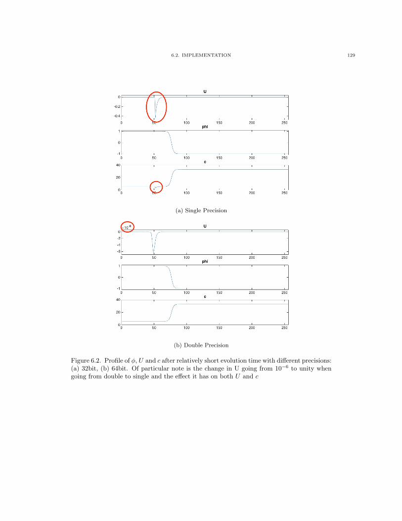
6.2. IMPLEMENTATION 129
(a) Single Precision
(b) Double Precision
Figure 6.2. Profile of φ, U and c after relatively short evolution time with different precisions:(a) 32bit, (b) 64bit. Of particular note is the change in U going from 10−6 to unity whengoing from double to single and the effect it has on both U and c
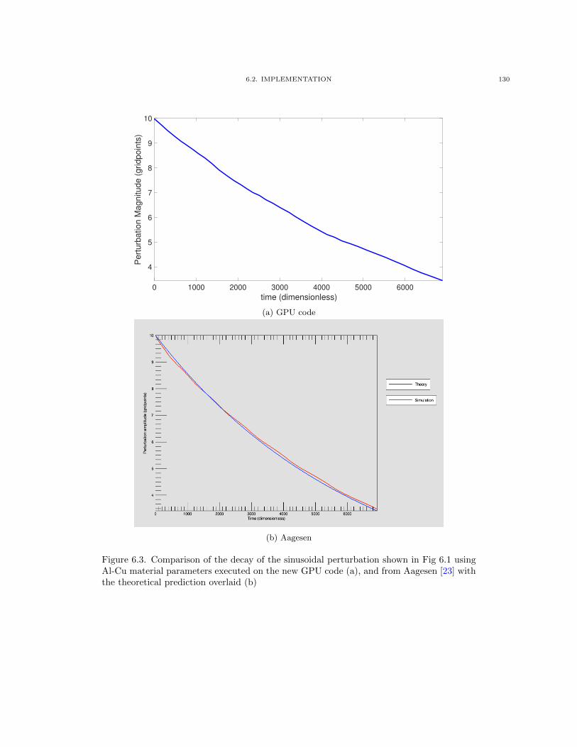
6.2. IMPLEMENTATION 130
0 1000 2000 3000 4000 5000 6000
time (dimensionless)
4
5
6
7
8
9
10
Pe
rtu
rba
tio
n M
ag
nitu
de
(g
rid
po
ints
)
(a) GPU code
(b) Aagesen
Figure 6.3. Comparison of the decay of the sinusoidal perturbation shown in Fig 6.1 usingAl-Cu material parameters executed on the new GPU code (a), and from Aagesen [23] withthe theoretical prediction overlaid (b)
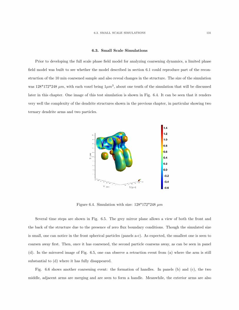
6.3. SMALL SCALE SIMULATIONS 131
6.3. Small Scale Simulations
Prior to developing the full scale phase field model for analyzing coarsening dynamics, a limited phase
field model was built to see whether the model described in section 6.1 could reproduce part of the recon-
struction of the 10 min coarsened sample and also reveal changes in the structure. The size of the simulation
was 128*172*248 µm, with each voxel being 1µm3, about one tenth of the simulation that will be discussed
later in this chapter. One image of this test simulation is shown in Fig. 6.4. It can be seen that it renders
very well the complexity of the dendrite structures shown in the previous chapter, in particular showing two
ternary dendrite arms and two particles.
Figure 6.4. Simulation with size: 128*172*248 µm
Several time steps are shown in Fig. 6.5. The grey mirror plane allows a view of both the front and
the back of the structure due to the presence of zero flux boundary conditions. Though the simulated size
is small, one can notice in the front spherical particles (panels a-c). As expected, the smallest one is seen to
coarsen away first. Then, once it has coarsened, the second particle coarsens away, as can be seen in panel
(d). In the mirrored image of Fig. 6.5, one can observe a retraction event from (a) where the arm is still
substantial to (d) where it has fully disappeared.
Fig. 6.6 shows another coarsening event: the formation of handles. In panels (b) and (c), the two
middle, adjacent arms are merging and are seen to form a handle. Meanwhile, the exterior arms are also
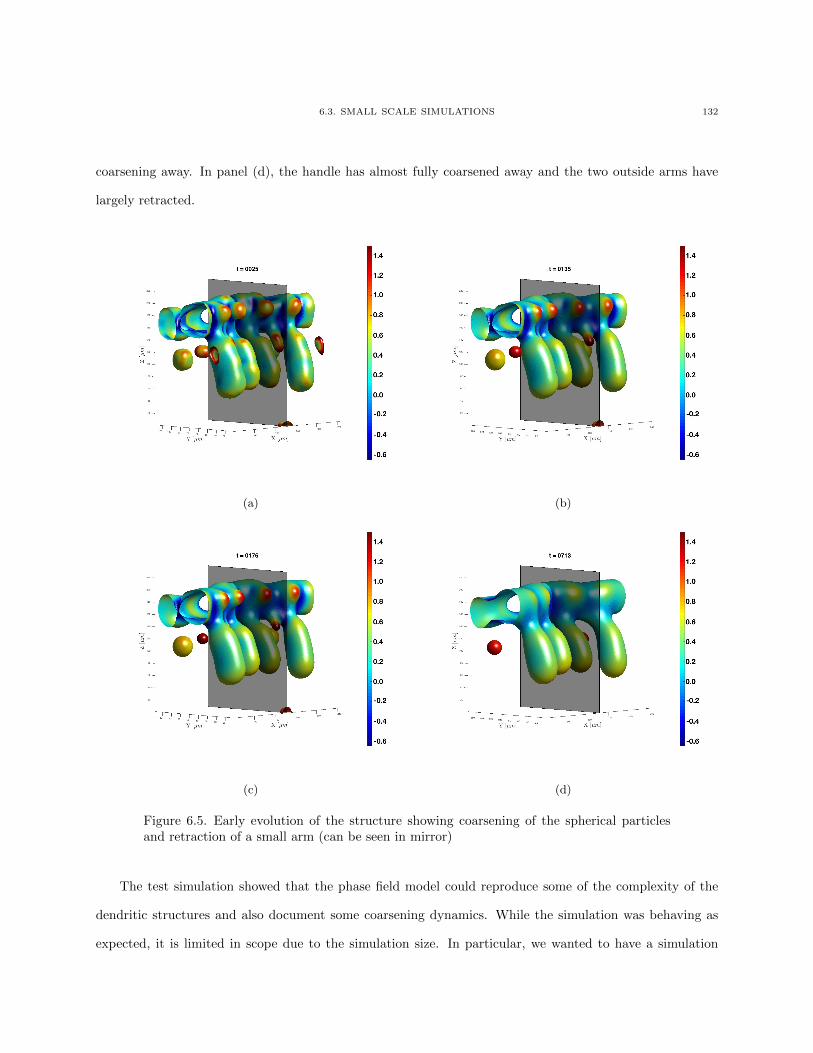
6.3. SMALL SCALE SIMULATIONS 132
coarsening away. In panel (d), the handle has almost fully coarsened away and the two outside arms have
largely retracted.
(a) (b)
(c) (d)
Figure 6.5. Early evolution of the structure showing coarsening of the spherical particlesand retraction of a small arm (can be seen in mirror)
The test simulation showed that the phase field model could reproduce some of the complexity of the
dendritic structures and also document some coarsening dynamics. While the simulation was behaving as
expected, it is limited in scope due to the simulation size. In particular, we wanted to have a simulation
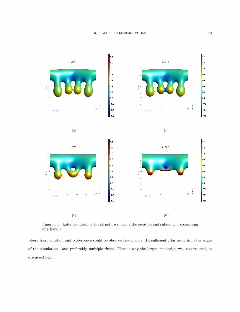
6.3. SMALL SCALE SIMULATIONS 133
(a) (b)
(c) (d)
Figure 6.6. Later evolution of the structure showing the creation and subsequent coarseningof a handle
where fragmentation and coalescence could be observed independently, sufficiently far away from the edges
of the simulations, and preferably multiple times. That is why the larger simulation was constructed, as
discussed next.
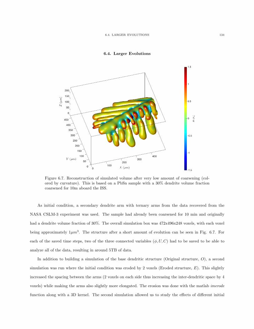
6.4. LARGER EVOLUTIONS 134
6.4. Larger Evolutions
Figure 6.7. Reconstruction of simulated volume after very low amount of coarsening (col-ored by curvature). This is based on a PbSn sample with a 30% dendrite volume fractioncoarsened for 10m aboard the ISS.
As initial condition, a secondary dendrite arm with ternary arms from the data recovered from the
NASA CSLM-3 experiment was used. The sample had already been coarsened for 10 min and originally
had a dendrite volume fraction of 30%. The overall simulation box was 472x496x248 voxels, with each voxel
being approximately 1µm3. The structure after a short amount of evolution can be seen in Fig. 6.7. For
each of the saved time steps, two of the three connected variables (φ,U,C) had to be saved to be able to
analyze all of the data, resulting in around 5TB of data.
In addition to building a simulation of the base dendritic structure (Original structure, O), a second
simulation was run where the initial condition was eroded by 2 voxels (Eroded structure, E). This slightly
increased the spacing between the arms (2 voxels on each side thus increasing the inter-dendritic space by 4
voxels) while making the arms also slightly more elongated. The erosion was done with the matlab imerode
function along with a 3D kernel. The second simulation allowed us to study the effects of different initial
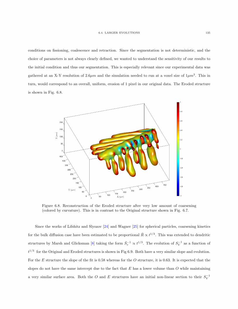
6.4. LARGER EVOLUTIONS 135
conditions on fissioning, coalescence and retraction. Since the segmentation is not deterministic, and the
choice of parameters is not always clearly defined, we wanted to understand the sensitivity of our results to
the initial condition and thus our segmentation. This is especially relevant since our experimental data was
gathered at an X-Y resolution of 2.6µm and the simulation needed to run at a voxel size of 1µm3. This in
turn, would correspond to an overall, uniform, erosion of 1 pixel in our original data. The Eroded structure
is shown in Fig. 6.8.
Figure 6.8. Reconstruction of the Eroded structure after very low amount of coarsening(colored by curvature). This is in contrast to the Original structure shown in Fig. 6.7.
Since the works of Lifshitz and Slyozov [24] and Wagner [25] for spherical particles, coarsening kinetics
for the bulk diffusion case have been estimated to be proportional R ∝ t1/3. This was extended to dendritic
structures by Marsh and Glicksman [8] taking the form S−1v ∝ t1/3. The evolution of S−1
V as a function of
t1/3 for the Original and Eroded structures is shown in Fig 6.9. Both have a very similar slope and evolution.
For the E structure the slope of the fit is 0.58 whereas for the O structure, it is 0.63. It is expected that the
slopes do not have the same intercept due to the fact that E has a lower volume than O while maintaining
a very similar surface area. Both the O and E structures have an initial non-linear section to their S−1V
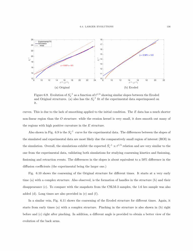
6.4. LARGER EVOLUTIONS 136
8 10 12 14 16 18 20 22 24
t1/3 (s1/3)
12
14
16
18
20
22
24
26
S−1
v
y = 0.63*x + 8.5
Experimental FitSimulation linear
(a) Original
8 10 12 14 16 18 20 22
t1/3 (s1/3)
10
11
12
13
14
15
16
17
18
S−1
v
y = 0.58*x + 5.9
(b) Eroded
Figure 6.9. Evolution of S−1V as a function of t1/3 showing similar slopes between the Eroded
and Original structures. (a) also has the S−1V fit of the experimental data superimposed on
it.
curves. This is due to the lack of smoothing applied to the initial condition. The E data has a much shorter
non-linear region than the O structure: while the erosion kernel is very small, it does smooth out many of
the regions with high positive curvature in the E structure.
Also shown in Fig. 6.9 is the S−1V curve for the experimental data. The differences between the slopes of
the simulated and experimental data are most likely due the comparatively small region of interest (ROI) in
the simulation. Overall, the simulations exhibit the expected S−1v ∝ t1/3 relation and are very similar to the
one from the experimental data, validating both simulations for studying coarsening kinetics and fusioning,
fissioning and retraction events. The differences in the slopes is about equivalent to a 50% difference in the
diffusion coefficients (the experimental being the larger one.)
Fig. 6.10 shows the coarsening of the Original structure for different times. It starts at a very early
time (a) with a complex structure. Also observed, is the formation of handles in the structure (b) and their
disappearance (c). To compare with the snapshots from the CSLM-3 samples, the 1.6 hrs sample was also
added (d). Long times are also provided in (e) and (f).
In a similar vein, Fig. 6.11 shows the coarsening of the Eroded structure for different times. Again, it
starts from early times (a) with a complex structure. Pinching in the structure is also shown in (b) right
before and (c) right after pinching. In addition, a different angle is provided to obtain a better view of the
evolution of the back arms.
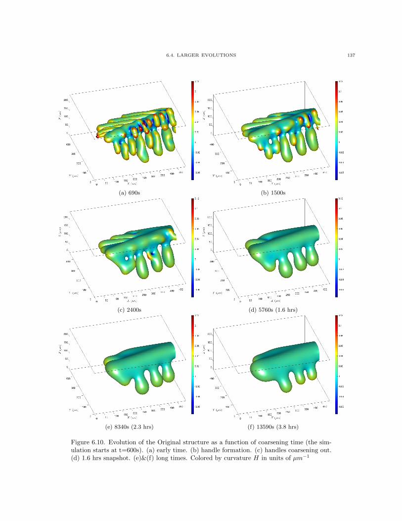
6.4. LARGER EVOLUTIONS 137
(a) 690s (b) 1500s
(c) 2400s (d) 5760s (1.6 hrs)
(e) 8340s (2.3 hrs) (f) 13590s (3.8 hrs)
Figure 6.10. Evolution of the Original structure as a function of coarsening time (the sim-ulation starts at t=600s). (a) early time. (b) handle formation. (c) handles coarsening out.(d) 1.6 hrs snapshot. (e)&(f) long times. Colored by curvature H in units of µm−1
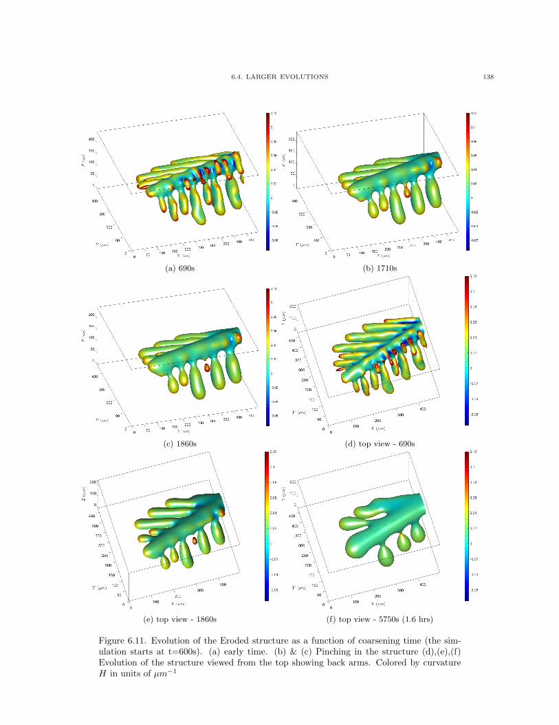
6.4. LARGER EVOLUTIONS 138
(a) 690s (b) 1710s
(c) 1860s (d) top view - 690s
(e) top view - 1860s (f) top view - 5750s (1.6 hrs)
Figure 6.11. Evolution of the Eroded structure as a function of coarsening time (the sim-ulation starts at t=600s). (a) early time. (b) & (c) Pinching in the structure (d),(e),(f)Evolution of the structure viewed from the top showing back arms. Colored by curvatureH in units of µm−1
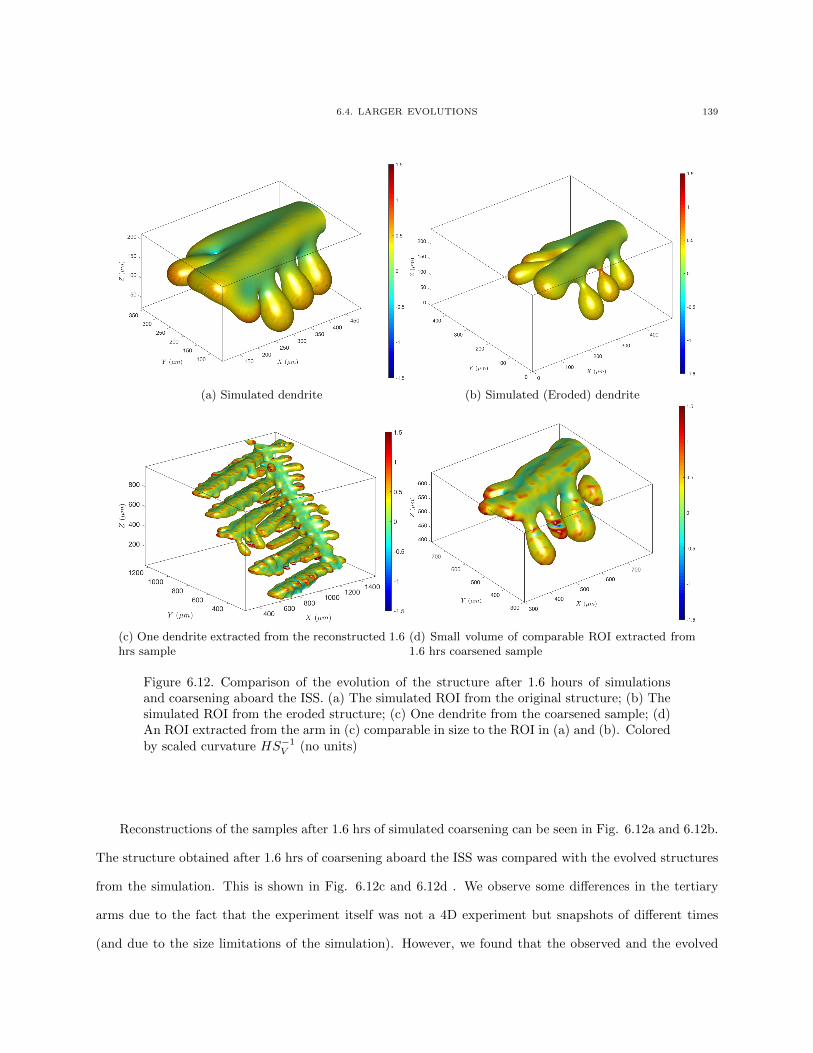
6.4. LARGER EVOLUTIONS 139
(a) Simulated dendrite (b) Simulated (Eroded) dendrite
(c) One dendrite extracted from the reconstructed 1.6hrs sample
(d) Small volume of comparable ROI extracted from1.6 hrs coarsened sample
Figure 6.12. Comparison of the evolution of the structure after 1.6 hours of simulationsand coarsening aboard the ISS. (a) The simulated ROI from the original structure; (b) Thesimulated ROI from the eroded structure; (c) One dendrite from the coarsened sample; (d)An ROI extracted from the arm in (c) comparable in size to the ROI in (a) and (b). Coloredby scaled curvature HS−1
V (no units)
Reconstructions of the samples after 1.6 hrs of simulated coarsening can be seen in Fig. 6.12a and 6.12b.
The structure obtained after 1.6 hrs of coarsening aboard the ISS was compared with the evolved structures
from the simulation. This is shown in Fig. 6.12c and 6.12d . We observe some differences in the tertiary
arms due to the fact that the experiment itself was not a 4D experiment but snapshots of different times
(and due to the size limitations of the simulation). However, we found that the observed and the evolved
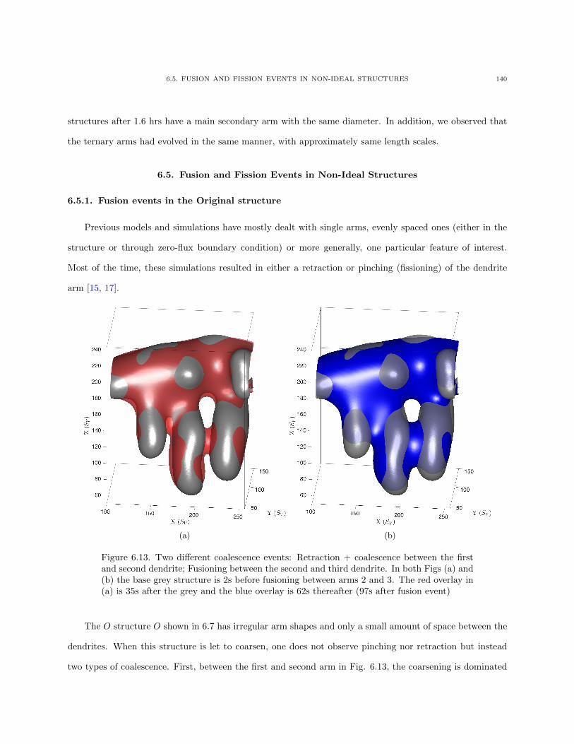
6.5. FUSION AND FISSION EVENTS IN NON-IDEAL STRUCTURES 140
structures after 1.6 hrs have a main secondary arm with the same diameter. In addition, we observed that
the ternary arms had evolved in the same manner, with approximately same length scales.
6.5. Fusion and Fission Events in Non-Ideal Structures
6.5.1. Fusion events in the Original structure
Previous models and simulations have mostly dealt with single arms, evenly spaced ones (either in the
structure or through zero-flux boundary condition) or more generally, one particular feature of interest.
Most of the time, these simulations resulted in either a retraction or pinching (fissioning) of the dendrite
arm [15, 17].
(a) (b)
Figure 6.13. Two different coalescence events: Retraction + coalescence between the firstand second dendrite; Fusioning between the second and third dendrite. In both Figs (a) and(b) the base grey structure is 2s before fusioning between arms 2 and 3. The red overlay in(a) is 35s after the grey and the blue overlay is 62s thereafter (97s after fusion event)
The O structure O shown in 6.7 has irregular arm shapes and only a small amount of space between the
dendrites. When this structure is let to coarsen, one does not observe pinching nor retraction but instead
two types of coalescence. First, between the first and second arm in Fig. 6.13, the coarsening is dominated
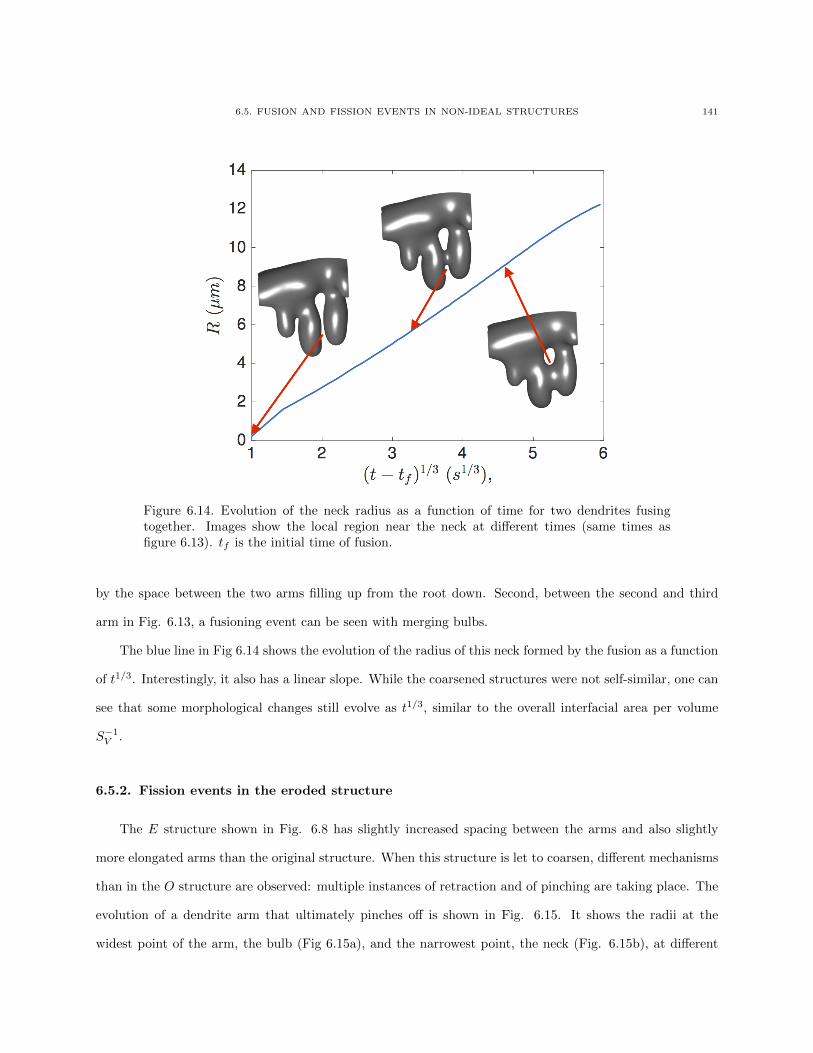
6.5. FUSION AND FISSION EVENTS IN NON-IDEAL STRUCTURES 141
Figure 6.14. Evolution of the neck radius as a function of time for two dendrites fusingtogether. Images show the local region near the neck at different times (same times asfigure 6.13). tf is the initial time of fusion.
by the space between the two arms filling up from the root down. Second, between the second and third
arm in Fig. 6.13, a fusioning event can be seen with merging bulbs.
The blue line in Fig 6.14 shows the evolution of the radius of this neck formed by the fusion as a function
of t1/3. Interestingly, it also has a linear slope. While the coarsened structures were not self-similar, one can
see that some morphological changes still evolve as t1/3, similar to the overall interfacial area per volume
S−1V .
6.5.2. Fission events in the eroded structure
The E structure shown in Fig. 6.8 has slightly increased spacing between the arms and also slightly
more elongated arms than the original structure. When this structure is let to coarsen, different mechanisms
than in the O structure are observed: multiple instances of retraction and of pinching are taking place. The
evolution of a dendrite arm that ultimately pinches off is shown in Fig. 6.15. It shows the radii at the
widest point of the arm, the bulb (Fig 6.15a), and the narrowest point, the neck (Fig. 6.15b), at different
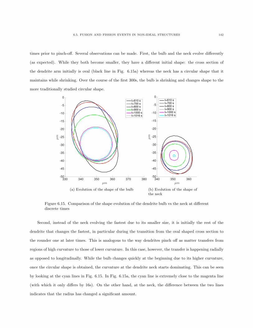
6.5. FUSION AND FISSION EVENTS IN NON-IDEAL STRUCTURES 142
times prior to pinch-off. Several observations can be made. First, the bulb and the neck evolve differently
(as expected). While they both become smaller, they have a different initial shape: the cross section of
the dendrite arm initially is oval (black line in Fig. 6.15a) whereas the neck has a circular shape that it
maintains while shrinking. Over the course of the first 300s, the bulb is shrinking and changes shape to the
more traditionally studied circular shape.
330 340 350 360 370 380
µm
-50
-45
-40
-35
-30
-25
-20
-15
-10
-5
0
µm
t=610 s
t=700 s
t=800 s
t=900 s
t=1000 s
t=1016 s
(a) Evolution of the shape of the bulb
340 350 360
µm
-50
-45
-40
-35
-30
-25
-20
-15
-10
-5
0
µm
t=610 s
t=700 s
t=800 s
t=900 s
t=1000 s
t=1016 s
(b) Evolution of the shape ofthe neck
Figure 6.15. Comparison of the shape evolution of the dendrite bulb vs the neck at differentdiscrete times
Second, instead of the neck evolving the fastest due to its smaller size, it is initially the rest of the
dendrite that changes the fastest, in particular during the transition from the oval shaped cross section to
the rounder one at later times. This is analogous to the way dendrites pinch off as matter transfers from
regions of high curvature to those of lower curvature. In this case, however, the transfer is happening radially
as opposed to longitudinally. While the bulb changes quickly at the beginning due to its higher curvature,
once the circular shape is obtained, the curvature at the dendrite neck starts dominating. This can be seen
by looking at the cyan lines in Fig. 6.15. In Fig. 6.15a, the cyan line is extremely close to the magenta line
(with which it only differs by 16s). On the other hand, at the neck, the difference between the two lines
indicates that the radius has changed a significant amount.
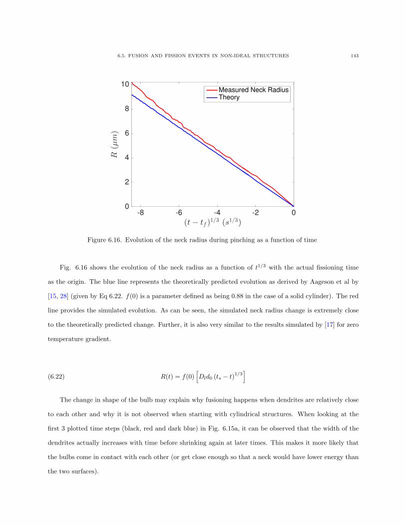
6.5. FUSION AND FISSION EVENTS IN NON-IDEAL STRUCTURES 143
-8 -6 -4 -2 0
(t− tf )1/3 (s1/3)
0
2
4
6
8
10
R(µm)
Measured Neck RadiusTheory
Figure 6.16. Evolution of the neck radius during pinching as a function of time
Fig. 6.16 shows the evolution of the neck radius as a function of t1/3 with the actual fissioning time
as the origin. The blue line represents the theoretically predicted evolution as derived by Aageson et al by
[15, 28] (given by Eq 6.22. f(0) is a parameter defined as being 0.88 in the case of a solid cylinder). The red
line provides the simulated evolution. As can be seen, the simulated neck radius change is extremely close
to the theoretically predicted change. Further, it is also very similar to the results simulated by [17] for zero
temperature gradient.
R(t) = f(0)[Dld0 (ts − t)1/3
](6.22)
The change in shape of the bulb may explain why fusioning happens when dendrites are relatively close
to each other and why it is not observed when starting with cylindrical structures. When looking at the
first 3 plotted time steps (black, red and dark blue) in Fig. 6.15a, it can be observed that the width of the
dendrites actually increases with time before shrinking again at later times. This makes it more likely that
the bulbs come in contact with each other (or get close enough so that a neck would have lower energy than
the two surfaces).
6.5. FUSION AND FISSION EVENTS IN NON-IDEAL STRUCTURES 144
6.5.3. Comparison to theoretical predictions of pinching and retracting
The competition between retraction and pinching was recently modeled and simulated in [17]. The
model was based on a number of simplifying assumptions: axisymmetric dendrites with the neighboring
dendrites defined by zero-flux boundary symmetry, and secondary dendrite arms that are assumed to be
perpendicular to the primary stem. Critical arm length above which pinching (as opposed to retraction)
occurs is expressed as a function of secondary dendrite arm spacing. The model showed that critical length
increases monotonically with increasing sidearm spacing to an upper limit where side arm spacing no longer
influences the boundary between pinching and retracting. The region separating pinching from retraction
was fit as equation 6.23:
lr−p (Λ2) = 6.67− 1.3e−0.25Λ2(6.23)
The Eroded structure where we observe pinching and retraction shown in Fig. 6.11 obviously does not
have axisymmetric dendrite arms. Neither are the arms of the same length and sidearm spacing varies.
Nonetheless, the model of [17] is an interesting test to see how a model based on idealized conditions can
predict pinching and retraction in a real dendritic structure. Note that in the Original structure, coarsening
resulted almost exclusively in coalescence events as opposed to pinching and retraction. As [17] did not
model coalescence events, it is impossible to compare the simulation results for O to the theoretical results.
Table 6.2. Prediction and Evolution of dendrite pinching (P) and retraction (R) for thefront dendrite arms of the Eroded structure
1 2 3 4 5 6Λ2/R 1.5 1.95 1.7 1.29 2.61 3l/R 5.2 8.5 6.6 6.94 9.2 8.7
Theory R P P P P PObserved R R P P P P
Fig. 6.17 zooms in on the front of the Eroded structure. Six instances of pitching and retraction were
observed during the 5700s simulated seconds. The actual pinching and retraction from the simulation and
the prediction for each arm according to [17] can be seen in Table 6.2. Λ2 and l are parameters defined in
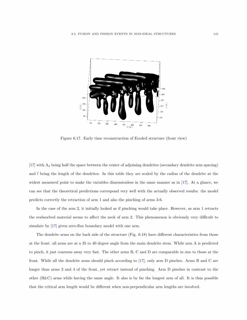
6.5. FUSION AND FISSION EVENTS IN NON-IDEAL STRUCTURES 145
Figure 6.17. Early time reconstruction of Eroded structure (front view)
[17] with Λ2 being half the space between the center of adjoining dendrites (secondary dendrite arm spacing)
and l being the length of the dendrites. In this table they are scaled by the radius of the dendrite at the
widest measured point to make the variables dimensionless in the same manner as in [17]. At a glance, we
can see that the theoretical predictions correspond very well with the actually observed results: the model
predicts correctly the retraction of arm 1 and also the pinching of arms 3-6.
In the case of the arm 2, it initially looked as if pinching would take place. However, as arm 1 retracts
the reabsorbed material seems to affect the neck of arm 2. This phenomenon is obviously very difficult to
simulate by [17] given zero-flux boundary model with one arm.
The dendrite arms on the back side of the structure (Fig. 6.18) have different characteristics from those
at the front: all arms are at a 35 to 40 degree angle from the main dendrite stem. While arm A is predicted
to pinch, it just coarsens away very fast. The other arms B, C and D are comparable in size to those at the
front. While all the dendrite arms should pinch according to [17], only arm D pinches. Arms B and C are
longer than arms 3 and 4 of the front, yet retract instead of pinching. Arm D pinches in contrast to the
other (B&C) arms while having the same angle. It also is by far the longest arm of all. It is thus possible
that the critical arm length would be different when non-perpendicular arm lengths are involved.
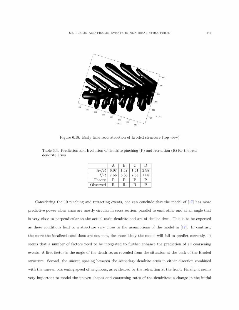
6.5. FUSION AND FISSION EVENTS IN NON-IDEAL STRUCTURES 146
Figure 6.18. Early time reconstruction of Eroded structure (top view)
Table 6.3. Prediction and Evolution of dendrite pinching (P) and retraction (R) for the reardendrite arms
A B C DΛ2/R 6.07 1.47 1.51 2.98l/R 7.56 6.65 7.53 11.8
Theory P P P PObserved R R R P
Considering the 10 pinching and retracting events, one can conclude that the model of [17] has more
predictive power when arms are mostly circular in cross section, parallel to each other and at an angle that
is very close to perpendicular to the actual main dendrite and are of similar sizes. This is to be expected
as these conditions lead to a structure very close to the assumptions of the model in [17]. In contrast,
the more the idealized conditions are not met, the more likely the model will fail to predict correctly. It
seems that a number of factors need to be integrated to further enhance the prediction of all coarsening
events. A first factor is the angle of the dendrite, as revealed from the situation at the back of the Eroded
structure. Second, the uneven spacing between the secondary dendrite arms in either direction combined
with the uneven coarsening speed of neighbors, as evidenced by the retraction at the front. Finally, it seems
very important to model the uneven shapes and coarsening rates of the dendrites: a change in the initial
6.6. CONCLUSION 147
condition that affected the size of the dendrites changed coarsening from pinching and retracting to fusioning
evolutions.
6.6. Conclusion
This chapter used the phase field method to gain insight into the dynamics of coarsening in general,
and the mechanisms of pinching, fusioning and retracting of secondary dendrites in specific. Rather than
assuming an idealized dendrite structure, the phase field used as initial condition a 3D reconstruction of
the PbSn sample, 30% solid, that had coarsened for 10 min under microgravity conditions. The model was
based on Echebarria et al [27], simplified for isothermal and isotropic conditions.
The overall simulation box was 472x496x248 voxels; the phase field model was coded in OpenCL to run
on a D700 FirePro GPU. In spite of the high speed of the simulations, evolving the PbSn structure from 10
min to 1.6 hrs still required 23 days. Two versions of the phase field model, the “Original” and “Eroded”
model were developed to examine coarsening kinetics and dynamics. The difference between the two models
stems from a variation in segmentation, motivated both by the fact that segmentation is not deterministic,
and by the quest to explore the effect of differences in initial conditions on coarsening mechanisms and effects.
The analyses in this chapter lead to a number of conclusions. First, the phase field model succeeds in
replicating the kinetics of the coarsening process. Similar to the kinetics of the actual samples that were
coarsened in space, we find that S−1v ∝ t1/3. This allowed us to use the phase field models to explore specific
research issues. We note that the very good kinetics of the phase field models were obtained without using
any fitting factors.
Second, our phase field models show the three coarsening mechanisms: coalescence, pinching and retrac-
tion. In fact, we were able to see two different types of coalescence: one dominated by the space between two
arms filling up from the root down, the other being the merging of two arms. Furthermore, when measuring
the fusioning of these arms, we could establish that the neck radius was reducing linearly in t1/3. While such
a relation has been found for pinching, this has not yet been shown for fusioning.
Third, the sight erosion of the Original structure gave rise to a slightly wider arm spacing and slightly
longer secondary arms. This very small change in initial condition of the phase field were sufficient to show
different coarsening mechanisms: pinching and retracting (and no fusioning anymore). The observation of
6.6. CONCLUSION 148
these events allowed us to verify another prediction: the kinetics of pinching as derived by Aagesen et al
[15]. We could find a similar relation between the radius of the neck during pinching and t1/3, giving another
validation of the kinetics of the phase field model.
Fourth, when studying the pinching in more detail, we observed a different dynamic at the neck than at
the bulb of the arm. While the shape of both the bulb and the neck were oval at pinch-off, the dendrite bulb
started with an oval shape while the neck had a circular shape that it maintained. Further, it was the dendrite
bulb that changed the fastest, in particular during the transition from the oval shaped cross section to the
rounder one. Once the circular shape was obtained, the curvature at the dendrite neck started dominating.
We were also able to observe that the bulb first became wider before becoming thinner, providing a possible
explanation for one of the types of coalesce seen before (merging).
Fifth, as the model replicates very well coarsening dynamics, we could test the predictive power of
a model of pinching and retracting that was based on a small number of idealized assumptions regarding
secondary dendrite length and spacing. The results of the test revealed that to the extent that real structures
resemble the idealized structures, predictions come out. However, when there were deviations, which may be
expected with complex dendritic structures, the model failed to predict correctly. It seems that an additional
number of factors need to be considered: the angle of the dendrite arms, their uneven spacing and length,
and their uneven shapes and coarsening rates.
7. CONCLUSIONS 149
CHAPTER 7
Conclusions
This thesis studied coarsening mechanisms of dendritic structures using various morphological and topo-
logical measures as well as phase field simulations. The majority of the analyses was carried out on PbSn
samples, 30% solid, that were coarsened for different times (10 min, 1.6 hrs, 5.5 hrs, 13.5 hrs, 27 hrs, 48h
hrs) aboard the ISS in the context of the CSLM-3 project of NASA. The microgravity environment of the
ISS was an essential part of the study as it allowed a detailed study of dendrite fragmentation, structure
connectivity and coarsening dynamics.
We found that each of the samples that had been coarsened in space had two different regions: an inside
region called the mushy zone where growth of the dendrites was constrained, and the outside region called
the region of free growth where dendrites had been able to advance freely into the eutectic. Due to the major
morphological differences in the two regions, each was analyzed separately. Chapter 5 deals primarily with
coarsening in the mushy zone while chapter 6 focuses on dynamics in the free growth region.
Concerning coarsening in the mushy zone, a number of key findings were obtained. First, the recon-
structions of the samples and the analysis of the Interfacial Shape Distribution (ISD) plots showed that the
structures of the earlier coarsening times were very different from the structures at later coarsening times.
In spite of the structures not being self similar, we found that the scaled (by S−1V ) number of fragments
was time invariant. This was established in a number of ways. A direct count and comparison of the scaled
number of fragments did not show a time trend. A more detailed analysis of the distribution of fragments in
some of the reconstructed samples confirmed the time independence. The estimation of the standard errors
of the number of independent bodies in these samples provided further evidence of the stability of the scaled
number of fragments across coarsening time. This set of complementary analysis provides substantial evi-
dence about the time invariance of the scaled number of independent bodies in the PbSn system we analyzed.
7. CONCLUSIONS 150
As a corollary, this finding also implies that the actual number of fragments is very high in the samples that
had little coarsening and declines precipitously (at a power of -6) as coarsening times get longer.
Second, the topology or connectivity analysis of the structures comparing the genus and handles across
the samples showed a similar pattern as for the number of fragments: while the actual number of handles
declines very fast from the 10min coarsened sample to the later samples, we could establish that the scaled
(by S−1V ) number of handles is time invariant. Again, in view of the substantial differences among the
structures, this finding is surprising.
Third, a similar S−1V ∝ t1/3 relationship for the PbSb system under microgravity and 1g conditions is
found. The PbSn system has been studied extensively before, but the study by Kammer [11] is of particular
interest as his samples had been coarsened on earth and had a volume fraction that is close to our 30%
space coarsened samples. In spite the very different coarsening conditions, we observed that both analyses
had a very similar S−1V ∝ t1/3 relationship. Both confirm the validity of this relationship (and also provide
evidence of the absence of the effects of convection on the ground based experiments of [11]).
The 3D reconstructions were essential to visualize the structures and to analyze the morphological and
topological effects of coarsening. However, this analysis remained limited to a comparison of a small number
of snapshots and made it difficult to draw conclusions regarding the exact mechanisms that generate the
changes in the dendritic structure during coarsening. The subsequent phase field analyses were a very
important complement and extension of the morphological and topological analysis of the samples. As
we were able to use an actual 3D reconstruction of one of our space samples as an initial condition, we
could deepen the understanding of coarsening dynamics, in particular the mechanisms of fragmentation (and
retraction) that contribute to the generation of independent bodies, and the mechanisms of coalescence that
influence the connectivity of the system.
Drawing on this part of the work, a fourth major finding of this study is the very high sensitivity of
coarsening evolution on initial conditions. It was observed that a very small change in the structure in terms
of dendrite length and spacing leads to a substantially different coarsening: a slightly wider spacing between
the secondary dendrite arms combined with slightly longer arms lead to fragmentation and retraction (and
7. CONCLUSIONS 151
no fusioning) during the analyzed coarsening time, as opposed to the coalescence that was seen when a more
dense structure was the initial condition of the phase field.
Fifth, in addition to finding confirming evidence of the evolution of the neck radius during fissioning as
a linear function of t1/3, our phase field analysis found a similar linear dynamic of the neck radius during
fusioning. To the best of our knowledge, this is the first time this has been found. As an aside, this finding
highlights the seemingly ubiquitous nature of the t1/3 dynamics of coarsening kinetics.
Sixth, the phase field analysis allowed us to demonstrate a mechanism of coalescence and the formation
of handles during coarsening. While previous research has focused extensively on the evolution of the neck
radius during the pinching process, our analysis showed the importance of the evolution of the bulb radius
during the coarsening process. An ongoing pinching process may be halted as a consequence of the evolution
of the radius of the bulb: we observed that the oval shaped bulb first became wider before becoming narrower
and circular, possibly leading to a coalescence with an adjacent arm rather than a pinching.
Seventh, our analyses identified key factors in the prediction of fragmentation events. The coarsening
mechanisms of fragmentation, retraction and coalescence have been identified for quite a while, but predicting
which one will take place in a particular coarsening process has been particularly difficult. This was stressed
recently by Beckermann et al [17]. The analysis of the coarsening dynamics in the Original and Eroded
structures showed how small changes in initial conditions can lead to a very different coarsening. It is
appealing to use simplifying assumptions to model complex dendritic structures and to predict fragmentation
on the basis of such a model. Our phase field analyses gave us an opportunity to test a recent, elegant
but idealized model of fragmentation dynamics. The analysis confirmed the importance of secondary arm
length and spacing to predict fragmentation, but equally demonstrated the importance of incorporating the
complexity of dendritic structures, specifically the angle of the dendrite arms, their uneven spacing and
length, and their uneven shapes and coarsening rates.
This thesis also hopes to have made a number of methodological contributions. First, 3D reconstructions
involve a complex sequence of processes. Chapter 3 has discussed in quite a bit of detail the many factors
that need to be considered to make useful reconstructions. The consistent S−1V ∝ t1/3 relationship of the
experimental and modeled structures is a validation of both the phase field model and the 3D reconstruction
7. CONCLUSIONS 152
process and output. Second, we hope that the methods for identifying the number of independent bodies and
for establishing their distribution and error in identification may help others in researching this important
matter. Third, our implementation of the Echebarria et al model[27] (without any fitting factors) provides
a means for testing specific predictions and uncovering important dynamics of the coarsening process. For
example, our model can be further used to determine the key factors for a prediction model of coarsening
events. Finally, we hope to have shown the computational benefits of studying the complex dynamics of
coarsening in large systems on GPU’s. While our simulations took about 50 days to run, it would have taken
a multiple with code running on CPU’s. The code provided in the Appendix will hopefully be of help to
other researchers.
References 153
References
[1] R Mendoza, J Alkemper, and P W Voorhees. Three-dimensional morphological characterization of
coarsened microstructures. Zeitschrift fur Metallkunde, 96:155–160, 2005.
[2] M. Chen and T.Z. Kattamis. Dendrite coarsening during directional solidification of AlCuMn alloys.
Materials Science and Engineering: A, 247(1-2):239–247, 1998.
[3] R Mendoza, J. Alkemper, and P.W. Voorhees. The morphological evolution of dendritic microstructures
during coarsening. Metallurgical And Materials Transactions A-Physical Metallurgy And Materials
Science, 34(3):481–489, 2003.
[4] AN Papapetrou. Untersuchungen uber dendritisches Wachstum von Kristallen. Zeitschrift fur Kristal-
lographie, (A92):89–130, 1935.
[5] D Kirkwood. A simple model for dendrite arm coarsening during solidification in multicomponent alloys.
Materials Science and Engineering, 73:L1–L4, 1985.
[6] T.Z. Kattamis, J.C. Coughlin, and M.C. Flemings. Influence of coarsening on dendrite arm spacing of
aluminum-copper alloys. Transactions of the Metallurgical Society of AIME, 239:1504–1511, 1967.
[7] T.F. Bower, H.D. Brody, and M.C. Flemings. Measurments of Solute Redistribution in Dendritic
Solidfication. Transaction of the Metallurgical Society of AIME, 236(May):624–634, 1966.
[8] S P Marsh and M E Glicksman. Overview of geometric effects on coarsening of mushy zones. Metallur-
gical And Materials Transactions A-Physical Metallurgy And Materials Science, 27(3):557–567, 1996.
[9] D. Kammer and P. W. Voorhees. The morphological evolution of dendritic microstructures during
coarsening. Acta Materialia, 54(6):1549–1558, 2006.
[10] J. L. Fife and P. W. Voorhees. The morphological evolution of equiaxed dendritic microstructures during
coarsening. Acta Materialia, 57(8):2418–2428, 2009.
References 154
[11] Dimitris Kammer. Three-Dimensional Analysis and Morphological Characterization of Coarsened Den-
dritic Microstructures. Thesis, (June), 2006.
[12] R.T. DeHoff, E.T. Aigeltinger, and K.R. Craig. Experimental determination of the topological properties
of three-dimensional microstructures. Journal of microscopy, 95(February):69–91, 1972.
[13] R. Mendoza, K. Thornton, I. Savin, and P. W. Voorhees. The evolution of interfacial topology during
coarsening. Acta Materialia, 54(3):743–750, 2006.
[14] Roberto Mendoza. Morphological and Topological Characterization of Coarsened Dendritic Microstruc-
tures. Thesis, (June), 2004.
[15] L. K. Aagesen, J. L. Fife, E. M. Lauridsen, and P. W. Voorhees. The evolution of interfacial mor-
phology during coarsening: A comparison between 4D experiments and phase-field simulations. Scripta
Materialia, 64(5):394–397, 2011.
[16] Arnoldo Badillo and Christoph Beckermann. Phase-field simulation of the columnar-to-equiaxed tran-
sition in alloy solidification. Acta Materialia, 54(8):2015–2026, 2006.
[17] H Neumann-Heyme, K Eckert, and C Beckermann. Dendrite fragmentation in alloy solidification due
to sidearm pinch-off. Nature Physics, 060401:1–5, 2015.
[18] P.W. Voorhees. Coarsening of Dendritic Solid-Liquid Mixtures: The Low Volume Fraction Limit. 2010.
[19] James Patton Downey. Microgravity Materials Research. Technical report, NASA, 2015.
[20] J. Alkemper and P. W. Voorhees. Quantitative serial sectioning analysis. Journal of microscopy, 201(Pt
3):388–394, 2001.
[21] John D Thompson, E Begum Gulsoy, and Peter W Voorhees. Self-similar coarsening : A test of theory.
Acta Materialia, 100:282–289, 2015.
[22] J P Simmons, P Chuang, M Comer, J E Spowart, M D Uchic, and M De Graef. Application and further
development of advanced image processing algorithms for automated analysis of serial section image
data. Modelling and Simulation in Materials Science and Engineering, 17(2), 2009.
[23] Larry Aagesen. Phase-Field Simulation of Solidification and Coarsening in Dendritic Microstructures.
Thesis, (March), 2010.
References 155
[24] I.M. Lifshitz and V.V. Slyozov. The kinetics of precipitation from supersaturated solid solutions. Journal
of Physics and Chemistry of Solids, 19(1):35–50, 1961.
[25] C Wagner. Theorie der Alterung von Niederschliigen durch Umlosen (Ostwald-Reifung. Ber. der Bunsen-
Ges. phys. Chem., (7):581–591, 1961.
[26] J Alkemper and P.W Voorhees. Three-dimensional characterization of dendritic microstructures. Acta
Materialia, 49(5):897–902, 2001.
[27] Blas Echebarria, Roger Folch, Alain Karma, and Mathis Plapp. Quantitative Phase Field Model of
Alloy Solidification. Review E - Statistical, Nonlinear, and Soft Matter Physics, pages 1–51, 2004.
[28] Larry K Aagesen, Anthony E Johnson, Julie L Fife, Peter W Voorhees, Michael J Miksis, Stefan O
Poulsen, Erik M Lauridsen, Federica Marone, and Marco Stampanoni. Universality and self-similarity
in pinch-off of rods by bulk diffusion. Nature Physics, 6(October):2–6, 2010.
[29] T.Z. Kattamis and M.C. Flemings. Dendrite structure and grain size of undercooled melts. Transactions
of the Metallurgical Society of AIME, 236(November):1523–1532, 1966.
[30] T.Z . Kattamis, U.T. Holmberg, and M.C. Flemings. Influence of coarsening on dendrite arm spacing
and grain size of magnesium-zinc alloys. Journal of the Institute of Metals, 195:343–347, 1967.
[31] Manfred Kahlweit. On the aging of dendrites. Scripta Metallurgica, 2(2):251–254, 1968.
[32] BP Bardes and Flemings MC. Dendrite Arm Spacing and Solidification Time in a Cast Aluminim-
Copper Alloy. AFS Transactions, pages 406–412, 1966.
[33] S.-C. Huang and M.E. Glicksman. Overview 12: Fundamentals of dendritic solidificationI. Steady-state
tip growth. Acta Metallurgica, 29(5):701–715, 1981.
[34] S.-C. Huang and M.E. Glicksman. Overview 12: Fundamentals of dendritic solidificationII development
of sidebranch structure. Acta Metallurgica, 29(5):717–734, 1981.
[35] J.A. Sethian. Level Set Methods and Fast Marching Methods: Evolving Interfaces in Computational
Geometry, Fluid Mechanics, Computer Vision, and Materials Science. Cambridge, U.K., 2nd edition,
1999.
[36] J. Alkemper, R. Mendoza, and P. W. Voorhees. Morphological evolution of dendritic microstructures.
Advanced Engineering Materials, 4(9):694–697, 2002.
References 156
[37] J.L. Fife and P.W. Voorhees. Self-similar microstructural evolution of dendritic solidliquid mixtures
during coarsening. Scripta Materialia, 60(10):839–842, 2009.
[38] Nele Moelans, Bart Blanpain, and Patrick Wollants. An introduction to phase-field modeling of mi-
crostructure evolution. Calphad, 32(2):268–294, 2008.
[39] S.M. Allen and J.W. Cahn. Microscopic theory for antiphase boundary motion and its application to
antiphase domain coarsening. Acta Metallurgica, 27(6):1085–1095, 1979.
[40] J.W. Cahn and J.E. Hilliard. ree energy of a nonuniform system. 1. interfacial free energy. Journal of
Chemical Physics, 28(2):258–267, 1958.
[41] O. Penrose and P.C. Fife. Thermodynamically consistent models of phase-field type for the kinetics of
phase-transitions. Physica D, 43(1):44–62, 1990.
[42] Z.Q. Bi and R.F. Sekerka. Phase-field model of solidification of a binary alloy. Physica A-Statistical
Mechanics and Its Applications, 261(1-2):95–106, 1998.
[43] R. Kobayashi. Modeling and numerical simulations of dendritic crystal-growth. Physica D, 63(3-4):410–
423, 1993.
[44] A.A. Wheeler, W.J. Boettinger, and G.B McFadden. Phase-field model of solute trapping during
solidification. Physical Review E, 47(3):1893–1909, 1993.
[45] G.B. McFadden, A.A. Wheeler, R.J. Braun, S.R. Coriell, and R.F. Sekerka. Phase-field models for
anisotropic interfaces. Physical Review E, 48(3):2016–2024, 1993.
[46] A. Karma and W.J. Rappel. Numerical Simulation of Three-Dimensional Dendritic Growth. Physical
Review Letters, 77(19):4050–4053, 1996.
[47] A. Karma and W.J. Rappel. Phase-field method for computationally effi. Physical Review E,
53(4):R3017–R3020, 1996.
[48] A. Karma and W.J. Rappel. Numerical simulation of three-dimensional dendritic growth. Physical
Review E, 77(19):4050–4053, 1996.
[49] A. Karma and W.J. Rappel. Phase-field model of dendritic sidebranching with thermal noise. Physical
Review E, 60(4):3614–3625, 1999.
References 157
[50] M Plapp and A. Karma. Multiscale random-walk algorithm for simulating inter- facial pattern formation.
Physical Review Letters, 84(8):1740–1743, 2000.
[51] A. Karma, Y.H. Lee, and M Plapp. Three-dimensional dendrite-tip morphology at low undercooling.
Physical Review E, 61(4):3996–4006, 2000.
[52] J. Bragard, A. Karma, Y.H. Lee, and M Plapp. Linking phase-field and atomistic simulations to model
dendritic solidification in highly undercooled melts. Interface Science, 10(2-3):121–136, 2002.
[53] A. Karma. Phase-field formulation for quantitative modeling of alloy solidification. Physical Review
Letters, 87(11):115701, 2001.
[54] E.B. Gulsoy and P. W. Voorhees. The Columnar to Equiaxed Transition and Dendrite Fragmentation,
2015.
[55] C. Beckermann, J. P. Gu, and W. J. Boettinger. Development of a freckle predictor via rayleigh number
method for single-crystal nickel-base superalloy castings. Metallurgical and Materials Transactions A,
31(10):2545–2557, 2000.
[56] M. C. Schneider, J. P. Gu, C. Beckermann, W. J. Boettinger, and U. R. Kattner. Modeling of micro- and
macrosegregation and freckle formation in single-crystal nickel-base superalloy directional solidification.
Metallurgical and Materials Transactions A, 28(7):1517–1531, 1997.
[57] S.C. Hardy and P.W. Voorhees. Ostwald ripening in a system with a high volume fraction of coarsening
phase. Metall. Trans. A, 19(A):2713–2721, 1988.
[58] S.R. Coriell and R.L. Parker. Stability of shape of a solid cylinder growing in a diffusion field. Journal
of Applied Physics, 36(2):632, 1965.
[59] E Cadirli and M Gunduz. The dependence of lamellar spacing on growth rate and temperature gradient
in the lead tin eutectic alloy. Journal of Materials Processing Technology, 97:74–81, 2000.
[60] T. Wolfsdorf, W. Bender, and P.W. Voorhees. The morphology of high volume fraction solid-liquid
mixtures: An application of microstructural tomography. Acta Materialia, 45(6):2279–2295, 1997.
[61] M D Uchic, M A Groeber, and A D Rollett. Automated serial sectioning methods for rapid collection
of 3-D microstructure data. JOM, 63(3):25–29, 2011.
References 158
[62] M. Uchic. Serial Sectioning Methods for Generating 3D Characterization Data of Grain- and Precipitate-
Scale Microstructures. In S Ghosh and K Dimiduk, editors, Computational Methods for Microstructure-
Property Relationships. New York, springer edition, 2011.
[63] Jonathan E. Spowart. Automated serial sectioning for 3-D analysis of microstructures. Scripta Materi-
alia, 55(1 SPEC. ISS.):5–10, 2006.
[64] M Uchic. Serial Sectioning Methods for Generating 3D Characterization Data of Grain- and Precipitate-
Scale Microstructures. In S Ghosh and D Dimiduk, editors, Computational Methods for Microstructure-
Property Relationships, pages 31–52. Springer, New York, 2011.
[65] Mary L Comer and Edward J Delp. The EM/MPM Algorithm for Segmentation of Textured Images:
Analysis and Further Experimental Results. IEEE TRANSACTIONS ON IMAGE PROCESSING,
9(10), 2000.
[66] C.F. Wu. On the convergence properties of the EM algorithm. The Annals of Statistics, 11:95–103,
1983.
[67] SC Hardy, GB Mcfadden, SR Coriell, PW Voorhees, and RF Sekerka. Measurement and Analysis of
Grain-Boundary Grooving by Volume Diffusion. J. of Crystal Growth, (114):467–480, 1991.
[68] M Gunduz and J. Hunt. The measurement of solidliquid surface energies in the AlCu, AlSi and PbSn
systems. Acta Metall, 33(9):1651–1672, 1985.
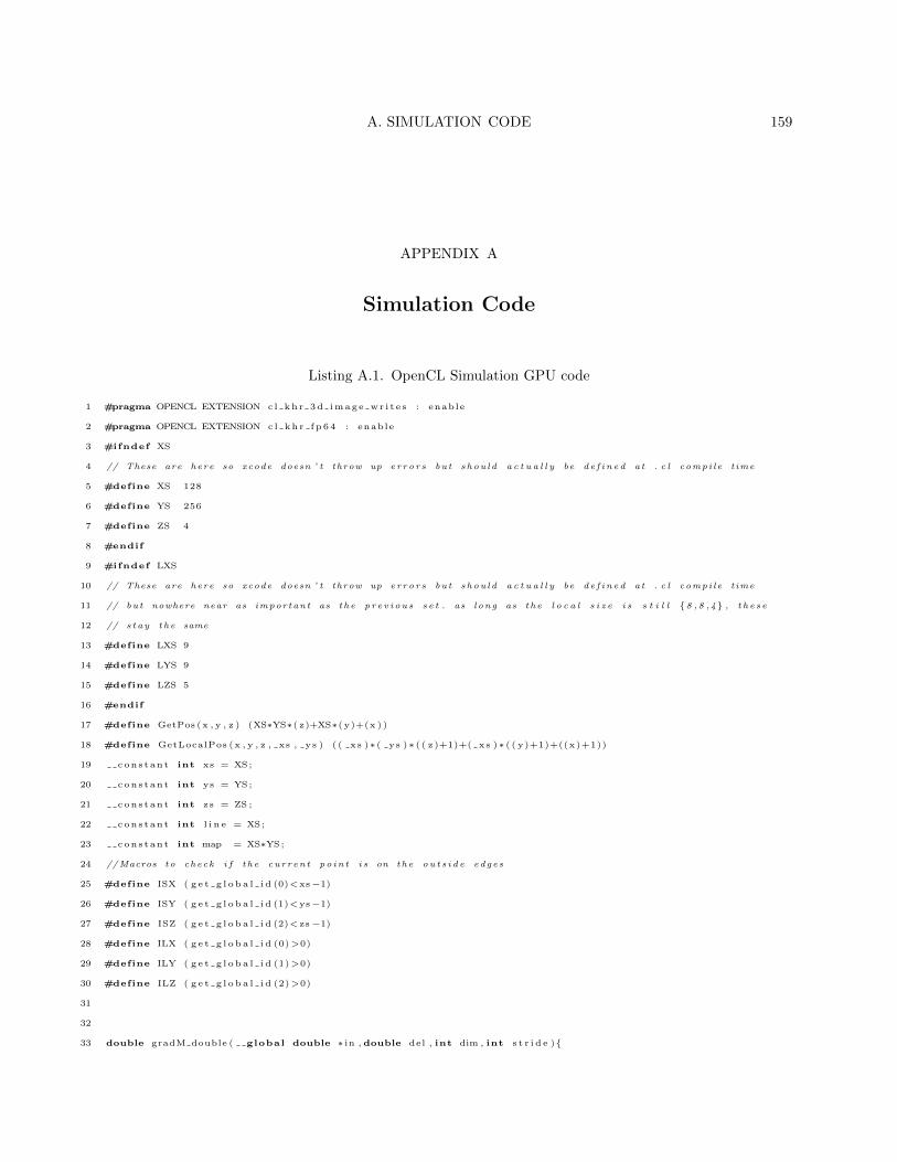
A. SIMULATION CODE 159
APPENDIX A
Simulation Code
Listing A.1. OpenCL Simulation GPU code
1 #pragma OPENCL EXTENSION c l kh r 3d image wr i t e s : enable
2 #pragma OPENCL EXTENSION c l kh r f p 6 4 : enable
3 #ifndef XS
4 // These are here so xcode doesn ’ t throw up e r r o r s bu t s hou l d a c t u a l l y be d e f i n e d a t . c l compi l e t ime
5 #define XS 128
6 #define YS 256
7 #define ZS 4
8 #endif
9 #ifndef LXS
10 // These are here so xcode doesn ’ t throw up e r r o r s bu t s hou l d a c t u a l l y be d e f i n e d a t . c l compi l e t ime
11 // bu t nowhere near as impor tan t as t h e p r e v i o u s s e t . as l ong as t h e l o c a l s i z e i s s t i l l 8 ,8 ,4 , t h e s e
12 // s t a y t h e same
13 #define LXS 9
14 #define LYS 9
15 #define LZS 5
16 #endif
17 #define GetPos (x , y , z ) (XS∗YS∗( z)+XS∗( y)+(x ) )
18 #define GetLocalPos (x , y , z , xs , y s ) ( ( xs )∗ ( ys )∗ ( ( z )+1)+( xs )∗ ( ( y)+1)+((x)+1))
19 con s t an t int xs = XS;
20 con s t an t int ys = YS;
21 con s t an t int zs = ZS ;
22 con s t an t int l i n e = XS;
23 con s t an t int map = XS∗YS;
24 //Macros to check i f t h e cu r r en t po i n t i s on the o u t s i d e edge s
25 #define ISX ( g e t g l o b a l i d (0)<xs−1)
26 #define ISY ( g e t g l o b a l i d (1)<ys−1)
27 #define ISZ ( g e t g l o b a l i d (2)< zs−1)
28 #define ILX ( g e t g l o b a l i d (0)>0)
29 #define ILY ( g e t g l o b a l i d (1)>0)
30 #define ILZ ( g e t g l o b a l i d (2)>0)
31
32
33 double gradM double ( global double ∗ in , double del , int dim , int s t r i d e )
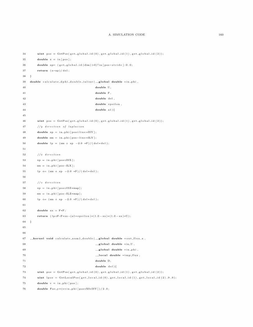
A. SIMULATION CODE 160
34 uint pos = GetPos ( g e t g l o b a l i d (0 ) , g e t g l o b a l i d (1 ) , g e t g l o b a l i d ( 2 ) ) ;
35 double x = in [ pos ] ;
36 double xp= ( g e t g l o b a l i d (dim)>0)? in [ pos−s t r i d e ] : 0 . 0 ;
37 return (x−xp )/ de l ;
38
39 double c a l c u l a t e d ph i d o ub l e i n l i n e ( global double ∗ in ph i ,
40 double U,
41 double F,
42 double del ,
43 double eps i l on ,
44 double a1 )
45
46 uint pos = GetPos ( g e t g l o b a l i d (0 ) , g e t g l o b a l i d (1 ) , g e t g l o b a l i d ( 2 ) ) ;
47 //y d i r e c t i o n o f l a p l a c i a n
48 double xp = in ph i [ pos+l i n e ∗ISY ] ;
49 double xm = in ph i [ pos−l i n e ∗ILY ] ;
50 double lp = (xm + xp −2.0 ∗F)/( de l ∗ de l ) ;
51
52 // x d i r e c t i o n
53 xp = in ph i [ pos+ISX ] ;
54 xm = in ph i [ pos−ILX ] ;
55 lp += (xm + xp −2.0 ∗F)/( de l ∗ de l ) ;
56
57 // z d i r e c t i o n
58 xp = in ph i [ pos+ISZ∗map ] ;
59 xm = in ph i [ pos−ILZ∗map ] ;
60 lp += (xm + xp −2.0 ∗F)/( de l ∗ de l ) ;
61
62 double xx = F∗F;
63 return ( lp+F−F∗xx−(a1∗ ep s i l o n )∗(1.0−xx )∗(1.0−xx )∗U) ;
64
65
66
67 kernel void ca lcu late num1 double ( global double ∗ out f l ux x ,
68 global double ∗ in U ,
69 global double ∗ in ph i ,
70 l oca l double ∗ tmp flux ,
71 double D,
72 double de l )
73 uint pos = GetPos ( g e t g l o b a l i d (0 ) , g e t g l o b a l i d (1 ) , g e t g l o b a l i d ( 2 ) ) ;
74 uint l po s = GetLocalPos ( g e t l o c a l i d (0 ) , g e t l o c a l i d (1 ) , g e t l o c a l i d ( 2 ) , 9 , 9 ) ;
75 double v = in ph i [ pos ] ;
76 double Fav y=(v+in ph i [ pos+XS∗ISY ] ) / 2 . 0 ;
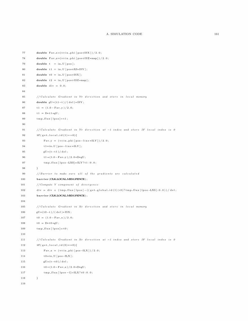
A. SIMULATION CODE 161
77 double Fav x=(v+in ph i [ pos+ISX ] ) / 2 . 0 ;
78 double Fav z=(v+in ph i [ pos+ISZ∗map ] ) / 2 . 0 ;
79 double t = in U [ pos ] ;
80 double t1 = in U [ pos+XS∗ISY ] ;
81 double t0 = in U [ pos+ISX ] ;
82 double t2 = in U [ pos+ISZ∗map ] ;
83 double div = 0 . 0 ;
84
85 // Ca l c u l a t e Gradient in Y+ d i r e c t i o n and s t o r e in l o c a l memory
86 double gU=(t1−t )/ ( de l )∗ ISY ;
87 t1 = (1.0−Fav y ) / 2 . 0 ;
88 t1 = D∗ t1 ∗gU ;
89 tmp flux [ lpo s ]= t1 ;
90
91 // Ca l c u l a t e Gradient in Y+ d i r e c t i o n a t −1 index and s t o r e IF l o c a l index i s 0
92 i f ( g e t l o c a l i d (1)==0)
93 Fav y = (v+in ph i [ pos−l i n e ∗ILY ] ) / 2 . 0 ;
94 t1=in U [ pos−l i n e ∗ILY ] ;
95 gU=(t−t1 )/ de l ;
96 t1=(1.0−Fav y )/2 .0∗D∗gU ;
97 tmp flux [ lpos−LXS]=ILY? t1 : 0 . 0 ;
98
99 // Barr i e r to make sure a l l o f t h e g r a d i e n t s are c a l c u l a t e d
100 barrier (CLKLOCALMEMFENCE) ;
101 //Compute Y component o f d i v e r g en c e
102 div = div + ( tmp flux [ lpo s ]−(( g e t g l o b a l i d (1)>0)? tmp flux [ lpos−LXS ] : 0 . 0 ) ) / de l ;
103 barrier (CLKLOCALMEMFENCE) ;
104
105 // Ca l c u l a t e Gradient in X+ d i r e c t i o n and s t o r e in l o c a l memory
106 gU=(t0−t )/ ( de l )∗ ISX ;
107 t0 = (1.0−Fav x ) / 2 . 0 ;
108 t0 = D∗ t0 ∗gU ;
109 tmp flux [ lpo s ]= t0 ;
110
111 // Ca l c u l a t e Gradient in X+ d i r e c t i o n a t −1 index and s t o r e IF l o c a l index i s 0
112 i f ( g e t l o c a l i d (0)==0)
113 Fav x = (v+in ph i [ pos−ILX ] ) / 2 . 0 ;
114 t0=in U [ pos−ILX ] ;
115 gU=(t−t0 )/ de l ;
116 t0=(1.0−Fav x )/2 .0∗D∗gU ;
117 tmp flux [ lpos−1]=ILX? t0 : 0 . 0 ;
118
119
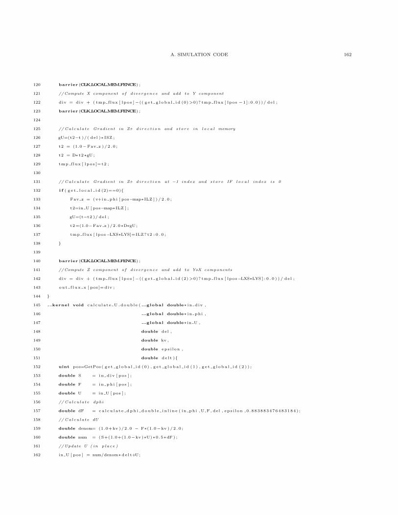
A. SIMULATION CODE 162
120 barrier (CLKLOCALMEMFENCE) ;
121 //Compute X component o f d i v e r g en c e and add to Y component
122 div = div + ( tmp flux [ lpo s ]−(( g e t g l o b a l i d (0)>0)? tmp flux [ lpos −1 ] : 0 . 0 ) ) / de l ;
123 barrier (CLKLOCALMEMFENCE) ;
124
125 // Ca l c u l a t e Gradient in Z+ d i r e c t i o n and s t o r e in l o c a l memory
126 gU=(t2−t )/ ( de l )∗ ISZ ;
127 t2 = (1.0−Fav z ) / 2 . 0 ;
128 t2 = D∗ t2 ∗gU ;
129 tmp flux [ lpo s ]= t2 ;
130
131 // Ca l c u l a t e Gradient in Z+ d i r e c t i o n a t −1 index and s t o r e IF l o c a l index i s 0
132 i f ( g e t l o c a l i d (2)==0)
133 Fav z = (v+in ph i [ pos−map∗ILZ ] ) / 2 . 0 ;
134 t2=in U [ pos−map∗ILZ ] ;
135 gU=(t−t2 )/ de l ;
136 t2=(1.0−Fav z )/2 .0∗D∗gU ;
137 tmp flux [ lpos−LXS∗LYS]=ILZ? t2 : 0 . 0 ;
138
139
140 barrier (CLKLOCALMEMFENCE) ;
141 //Compute Z component o f d i v e r g en c e and add to Y+X components
142 div = div + ( tmp flux [ lpo s ]−(( g e t g l o b a l i d (2)>0)? tmp flux [ lpos−LXS∗LYS ] : 0 . 0 ) ) / de l ;
143 ou t f l u x x [ pos ]=div ;
144
145 kernel void ca l cu l a t e U doub l e ( global double∗ i n d iv ,
146 global double∗ in ph i ,
147 global double∗ in U ,
148 double del ,
149 double kv ,
150 double eps i l on ,
151 double de l t )
152 uint pos=GetPos ( g e t g l o b a l i d (0 ) , g e t g l o b a l i d (1 ) , g e t g l o b a l i d ( 2 ) ) ;
153 double S = in d i v [ pos ] ;
154 double F = in ph i [ pos ] ;
155 double U = in U [ pos ] ;
156 // Ca l c u l a t e dph i
157 double dF = ca l c u l a t e d ph i d o ub l e i n l i n e ( in ph i ,U,F , del , eps i l on ,0 . 883883476483184) ;
158 // Ca l c u l a t e dU
159 double denom= (1.0+kv )/2 . 0 − F∗(1.0−kv ) / 2 . 0 ;
160 double num = (S+(1.0+(1.0−kv )∗U)∗0 .5∗dF ) ;
161 //Update U ( in p l a c e )
162 in U [ pos ] = num/denom∗ de l t+U;

A. SIMULATION CODE 163
163 //Update Phi bu t w r i t e to a t h e o l d d i v e r g en c e array because ph i i s needed in o t h e r k e r n e l s
164 // in t he c a l c u l a t e d p h i f u n c t i o n
165 i n d i v [ pos ]=F+de l t ∗dF ;
166


