Coexistence in the chemostat as a result of metabolic by-products

J. Math. Biol. (2006) 53:556–584DOI 10.1007/s00285-006-0012-3 Mathematical Biology

Coexistence in the chemostat as a result of metabolicby-products

Julia Heßeler · Julia K. Schmidt · Udo Reichl ·Dietrich Flockerzi

Received: 25 August 2005 / Revised: 28 April 2006 /Published online: 4 July 2006© Springer-Verlag 2006

Abstract Classical chemostat models assume that competition is purelyexploitative and mediated via a common, limiting and single resource. How-ever, in laboratory experiments with pathogens related to the genetic diseaseCystic Fibrosis, species specific properties of production, inhibition and con-sumption of a metabolic by-product, acetate, were found. These assumptionswere implemented into a mathematical chemostat model which consists of fournonlinear ordinary differential equations describing two species competing forone limiting nutrient in an open system. We derive classical chemostat resultsand find that our basic model supports the competitive exclusion principle, thebistability of the system as well as stable coexistence. The analytical results areillustrated by numerical simulations performed with experimentally measuredparameter values. As a variant of our basic model, mimicking testing of anti-biotics for therapeutic treatments in mixed cultures instead of pure ones, weconsider the introduction of a lethal inhibitor, which cannot be eliminated by

Julia Heßeler and Julia K. Schmidt contributed equally to this work.

J. Heßeler (B)Department of Mathematics and Physics, Albert-Ludwigs-University, Hermann-Herder-Str. 3,79104 Freiburg, Germanye-mail: [email protected]

J. K. Schmidt · U. ReichlDepartment of Bioprocess Engineering, Otto-von-Guericke-University, Universitätsplatz 2,39106 Magdeburg, Germanye-mail: [email protected]

U. Reichl · D. FlockerziMax Planck Institute for Dynamics of Complex Technical Systems, Sandtorstr. 1,39106 Magdeburg, Germany

Coexistence in the chemostat as a result of metabolic by-products 557

one of the species and is selective for the stronger competitor. We discuss ourtheoretical results in relation to our experimental model system and find thatsimulations coincide with the qualitative behavior of the experimental result inthe case where the metabolic by-product serves as a second carbon source forone of the species, but not the producer.

Keywords Competition · Chemostat · Coexistence · Metabolite · InterspecificCompetition · Inhibitor · Quantitative T-RFLP

1 Introduction

Experimental chemostats and mathematical chemostat models are oftenconsidered in mathematical biology, ecology and particularly in microbiologyor biotechnology to investigate competitive systems. Experimental chemostatsplay a central role in some fermentation processes and thus are a part of stan-dard laboratory equipment. They are perhaps the best laboratory idealizationof nature for population studies [18].

For microbial species competing for one limiting resource in a chemostat,mathematical models lead to the competitive exclusion principle (CEP) predict-ing survival of only one species in any case [1,15,18]. The competitive exclusionprinciple was also set into broader context including general environmentalinteraction variables not necessarily representing limiting resources [7].

However, this observation does not correspond to the biodiversity of organ-isms found in nature [26]. To bridge the gap between mathematical theory andobserved phenomena, a variety of mathematical models has been developedover the last decades. In all these models the idealized chemostat assumptionshave been modified. Either to confirm the competitive exclusion principle formore general settings (e.g. [4,17,28,41]) or to allow for coexistence of competingspecies. A detailed mathematical description of competition in the chemostat isdiscussed in the book of Smith and Waltman [39]. One of the later approaches,the incorporation of species’ interactions and inhibitors, is strongly motivatedby microbiology (e.g. cell-to-cell-communication [2,8,35]) as well as by appli-cations in biotechnology. The latter have been studied theoretically in differentscenarios (e.g. [3,5,19–23,25,27,29] and the references therein).

The first qualitative agreement of a theoretical and an experimental approachtowards single-nutrient microbial competition was worked out by Hansen andHubbell in 1980 [14]. Experiments incorporating more than two competing bac-terial species are rare, but they are claimed to be “one of the more importantchallenges for future ecological research” for substantiating the mathematicaltheory [33]. Taking this challenge, we here present a modeling approach thatis motivated by and based on quantitative data from our experimental modelsystem [38]. For this, experimental chemostat studies of a mixed culture consist-ing of three bacterial species Pseudomonas aeruginosa, Burkholderia cepaciaand Staphylococcus aureus were performed. These species occur among othersas secondary infections in lungs of patients suffering from the genetic disease

558 J. Heßeler et al.

cystic fibrosis (CF). They are assumed to exist in form of a natural microbialcommunity and pose severe problems to medical therapy, mainly by antibiot-ics. To establish these three species as a reproducible laboratory mixed modelculture for studies under defined and controllable conditions, a continuousstirred tank reactor (CSTR) in chemostat mode was set up, for which a digitalprocess control system allowed control of culture conditions. The aim was toquantitatively characterize mixed culture growth with at least three speciesfocusing on possible interspecies interactions. This could be done e.g. by gener-ating a stable three-species coexistence and then performing pulse disturbanceson it for the study of the system response. It was not our primary goal to estab-lish an experimental model system for direct transfer of results to medicalimplications. For this, additional aspects like biofilm mode of growth or host-pathogen interactions would have to be taken into account. The combinationof mathematical model analysis with pure and mixed culture studies was cho-sen for obtaining insight into physiological and growth-behavioral propertiesof the model community. To ensure good control and monitoring possibilitiesof the experiments, a homogeneous suspension culture mode and a chemicallycompletely defined medium with no complex (undefined) additives were used.

In our studies we found experimental evidence for a specific metabolic prop-erty of one of the species: S. aureus produced a by-product (acetate). In mixedculture growth this can have an activating effect (acetate can serve as a sec-ondary substrate) as well as an inhibiting effect (acetate is an organic acid andreduces pH value) on the competitors. So far, production and consumption inform of an internal metabolic product as an interspecific interaction have notyet been considered in the literature. Some authors [37] assumed that one spe-cies is auxotrophic for a metabolite produced by the other species which wecould not observe for our system. Furthermore in literature [9,34,40] it was notassumed that the metabolite has an inhibiting effect as it necessarily has in ourcase.

According to our model equations and their mathematical analysis, the bio-logical system property of acetate production is not sufficient to generate anon-trivial three-species coexistence. However, the production of acetate issuch a decisive system property that we characterize its impact on the dynamicbehavior. To investigate the possible effects of an acetate food-chain on the out-come of competition, chemostat experiments as well as mathematical analysiswere focused on the producer (S. aureus) and only one of the consumer strains(B. cepacia).

Our basic model (1) considers these two species and poses the followingassumptions for the acetate production, all of which are based on experimen-tal results from pure culture experiments: The species compete for the abioticresource glucose, and acetate

1. is produced growth-dependently without any costs,2. has an inhibiting effect on both species,3. is not exploited by the producing species and4. activates the other species by acting as a secondary resource.


The purposes of the theoretical analysis of the basic model are to determinethe overall dynamics and to identify possible coexistence states. In respect to theinterplay between the theoretical analysis and the experimental system we wantto test the model for its verification by biological system’s data and the purespecies parameters. We will discuss the possibilities for generating coexistencebased on the mathematically resulting parameter set and their realizability inour real experimental setup.

As mentioned above the species under consideration occur as secondaryinfections of CF patients. The treatment includes antibiotics that are dosedover a certain period of time [12]. Dosage and type of antibiotic composure arechosen according to the individual patient’s state. Typically, an antibiotic canbe either very strain specific or very general. Moreover, it will not be taken upby the bacteria of concern.

The standard tests for sensitivity to antibiotics are carried out on pure cul-tures [12]. As bacteria in CF patients exist as communities it seems more rea-sonable to apply such sensitivity tests to mixed cultures, as this would accountfor some differences in physiological behavior between pure and mixed cul-tures. A mixed culture chemostat provides an experimental system for testingits response to antibiotics. As a basic approach for mimicking the above con-cept within a chemostat, we introduce, as a variant of our basic model, a lethalinhibitor at constant dosage (in contrast to Hsu et al. [19]). We assume that itis selectively lethal for the stronger competitor and it cannot be degraded byeither species.

Within natural communities, it is clear that there are other possible inter-actions [32,33], which cannot be determined directly and quantified exper-imentally. As a substitute for possible interactions, we include interspecificcompetition as a general mechanism and comment on the resulting changesof the dynamic properties of the mathematical model. Such biologically rea-sonable interspecies interactions were already introduced into basic chemostatmodels [11,29,36,42], but in a different context.

The organization of the paper is as follows. In Sect. 2 we present our experi-mental system in detail, the protocol for performing chemostat experiments aswell as sample analysis. The results from pure culture experiments, serving asthe basis for our mathematical model assumptions, are given and elucidated.Additionally, a short description of parameter estimation from the above exper-iments is given.

In Sect. 3 we introduce and analyze our basic model equations under theabove assumptions. We give preliminary results such as positivity and bound-edness of solutions and the existence and local asymptotic stability of boundaryrest points. The global stability of the boundary rest points corresponds tothe washout of at least one competitor (extinction results). In Subsect. 3.3 weanalyze the model equation focusing on the existence of interior rest pointsand state our main result concerning the mathematical model. Thus, we giveconditions under which stable coexistence can occur. We present numericalsimulations (Subsect. 3.4) performed with XPPAUT [10] and using the exper-imentally estimated parameters from Sect. 2. These simulations illustrate the


analytical results for the system properties like the CEP, bistability or stablecoexistence.

In Sect. 4 we consider variants of our basic model. We analyze the modelincorporating lethal inhibition and find that the analytic results of the basicmodel are transferable. We comment on the resulting dynamics if negativeinteractions between the species are assumed. We discuss the interplay betweenthe experimental results and the basic model with its variants in Sect. 5 andelaborate on the implications of the mathematical analysis for the experimentalsystem and future research.

Most of the proofs are deferred to the Appendix.

2 Experimental system

For the presented work chemostat experiments with three species (P. aerugin-osa, S. aureus and B. cepacia) were performed in a stirred tank reactor witha working volume of 1 l (Biostat B2, B. Braun, Germany) and with the twospecies in focus (B. cepacia and S. aureus) in stirred tank reactors with 0.2 lworking volume (fedbatch pro, dasgip, Germany). The dilution rates appliedto the experimental chemostat studies were D = 0.05 h−1 or D = 0.2 h−1. Pro-cess parameter values were controlled by digital process control systems (PCS7,Siemens, Germany; fedbatch-pro, dasgip, Germany). The liquid culture mediumwas completely chemically defined, it contained no complex components, andsupported good growth of all three species with glucose as main carbon andenergy source as was shown in preliminary experiments. Precultures for chemo-stat experiments were grown overnight as single species culture in shaking flasksin the main culture medium. Equal volumes of equal biomass concentration ofthese single species suspensions were mixed prior to their use for inoculation.After complete consumption of the carbon source in the batch phase of theprocess, indicated by an increase of the online signal of oxygen partial pressure,process control was switched to continuous mode and feed and harvest pumpsstarted at the adequate speeds (chemostat mode). During chemostat processmode samples of the culture were taken and analyzed off-line for values ofinterest. Especially important for the presented work were species specific cellnumbers as needed for comparison of simulation results and experimental data.Species specific and absolute cell numbers were determined with a quantitativeterminal-restriction fragment length analysis (T-RFLP) method [38]. Glucoseconcentrations were measured with an automated enzymatic assay and acetateconcentrations with a chromatography system (HPLC).

Three-species chemostat experiments resulted in coexistence of at least twospecies B. cepacia and P. aeruginosa for more than 180 h for both dilution rates0.05 and 0.2 h−1, i.e. about 9 and 30 work volume exchanges, respectively. Cellnumbers of S. aureus were below the limit of quantification of quantitative T-RFLP method after approximately 50 h. Pure culture studies revealed acetateformation and secretion into the culture broth by S. aureus during its growthphase. Acetate accumulated and was not taken up by its producer even after


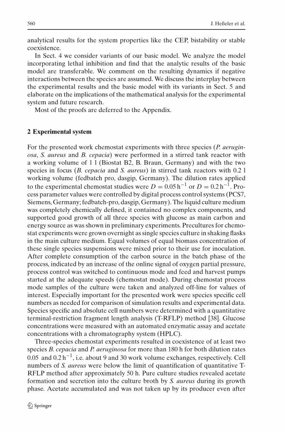
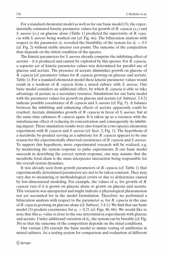
complete consumption of glucose. Astonishingly, no acetate was found in off-line analysis of samples from three species mixed cultures. Consumption of themetabolic by-product acetate by B. cepacia as well as P. aeruginosa was shownby adding acetate to the medium in pure culture experiments. The shaking flaskcultures showed significantly increased cell numbers and off-line compositionanalysis of samples indicated clear decrease of acetate concentration correlatedto increase of cell numbers (HPLC analysis). To investigate possible metabolicinteraction via acetate and its effect on mixed culture dynamics in further detail,chemostat experiments with only the producer and one of the consuming spe-cies were performed. Two-species chemostat experiments with B. cepacia andS. aureus for about 168 h indicated that none of the two species was washed outat that time (dilution rate D = 0.05 h−1, Fig. 1).

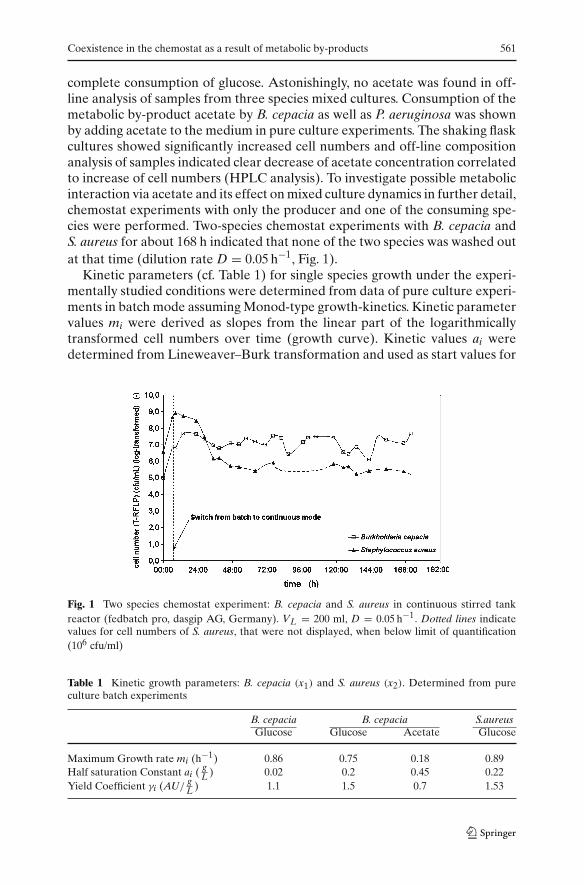
Kinetic parameters (cf. Table 1) for single species growth under the experi-mentally studied conditions were determined from data of pure culture experi-ments in batch mode assuming Monod-type growth-kinetics. Kinetic parametervalues mi were derived as slopes from the linear part of the logarithmicallytransformed cell numbers over time (growth curve). Kinetic values ai weredetermined from Lineweaver–Burk transformation and used as start values for

Fig. 1 Two species chemostat experiment: B. cepacia and S. aureus in continuous stirred tankreactor (fedbatch pro, dasgip AG, Germany). VL = 200 ml, D = 0.05 h−1. Dotted lines indicatevalues for cell numbers of S. aureus, that were not displayed, when below limit of quantification(106 cfu/ml)

Table 1 Kinetic growth parameters: B. cepacia (x1) and S. aureus (x2). Determined from pureculture batch experiments

B. cepacia B. cepacia S.aureusGlucose Glucose Acetate Glucose

Maximum Growth rate mi (h−1) 0.86 0.75 0.18 0.89Half saturation Constant ai ( g

L ) 0.02 0.2 0.45 0.22Yield Coefficient γi (AU/ g

L ) 1.1 1.5 0.7 1.53


nonlinear optimization (MatLab) of ai by fitting of experimental data. Yieldcoefficients γi were determined from experimental data as an overall quotientof cell number concentration at the point of time of complete glucose consump-tion.

Kinetic parameter values k1, l1 and β1 for consumption of acetate weredetermined by fitting of parameters to the experimental data (MatLab).

3 Model formulation and analysis

3.1 The basic model

At time t, let S(t) denote the nutrient concentration (glucose) and xi(t) (i = 1, 2)the biomass concentrations of the competitors B. cepacia and S. aureus, respec-tively. Let R(t) denote the concentration of the internally produced metabolite(acetate). The following model equations are obtained

S = D(S0 − S)− 1γ1

f1(S)x1 − 1γ2

f2(S)x2

x1 = x1(f1(S)+ g1(R)− d1R − D)

x2 = x2(f2(S)− d2R − D) (1)

R = αf2(S)x2 − 1β1

g1(R)x1 − DR

S(0) = 0 ≥ 0, xi(0) > 0, R(0) ≥ 0,

where the constants S0 and D denote the nutrient input concentration and thedilution rate. We assume that the dilution rate is large compared to the spe-cies specific death rates. The fi(S), g1(R) represent the uptake functions forthe nutrient and the metabolite, respectively, and are taken of Monod-type, i.e.fi(S) = miS

ai+S and g1(R) = k1Rl1+R , where mi, k1 are the maximum growth rate and

ai, l1 are the Monod constants. The yield coefficients for S and R are γi andβ1, respectively. The inhibition by the metabolite is modelled by a mass-action-term. The metabolite decreases the pH value (cf. Sect. 2) what negatively affectsgrowth rate and cell viability. The mathematical formulation for this inhibitoryeffect can be realized both ways [25]. We chose the description of the inhibitoryeffect to be death-rate enhancing and therefore denote the inhibition coeffi-cients of the metabolite by di. The metabolite is produced growth-dependentlyaccording to Luedeking–Piret with α as the proportion factor. All parametervalues are supposed to be positive with α ∈ (0, 1).

System (1) can be scaled to non-dimensional form by using the substitutions

S = SS0 , xi = xi

γiS0 , ai = ai

γiS0 , l1 = l1αγ2S0 , R = R

αγ2S0 and di = αγ2S0di


and introducing the additional parameter

b = γ1

αβ1γ2>

γ1

γ2β1> 0. (2)

After substituting the variables and dropping the hats, the scaled system isnon-dimensional and of the form

S = D(1 − S)− f1(S)x1 − f2(S)x2x1 = x1(f1(S)− D1(R))x2 = x2(f2(S)− D2(R))R = f2(S)x2 − bg1(R)x1 − DR

(3)

where

D1(R) := D + d1R − g1(R), and D2(R) := D + d2R (4)

represent the species specific dilution rates, which directly depend on the met-abolic by-product R.

It is easy to show that the system given by (3) is well-posed, i.e. the solutionsstarting with positive initial values remain nonnegative and are bounded as timegoes to infinity. Furthermore all solutions eventually lie in a bounded, globallyattracting set M defined by

M := {(S, x1, x2, R) : S, x1, x2, R ≥ 0, (2 + b)S + bx1 + bx2 + 2R ≤ 2 + b} ⊆ R4+.

3.2 The boundary rest point set

We study the equilibria on the boundary of R4+ of system (3). These equilibria

represent the washout of at least one species. The coordinates of the rest pointshave to be nonnegative in order to be relevant. Thus when we say ‘exists’ weintend ‘exists and is meaningful’. There are three rest points on the boundary,which we label as

E0 = (1, 0, 0, 0), E1 = (λ10, 1 − λ10, 0, 0), E2 = (S+, 0, x+2 , R+).

The equilibrium E0 always exists. In addition, the equilibria E1 and E2 existwhenever λ10 < 1 and λ20 < 1, respectively, where λi0 is defined as

λi0 := aiDmi − D

, i = 1, 2 (5)

and is of relevance for mi > D. It equals the standard break-even concentration[39] and is the solution of fi(S)− D = 0.


The coordinates of E2 are the following:

S+ = a2D2(R+)m2 − D2(R+)

and x+2 = DR+

D2(R+), (6)

and R+ being the unique positive solution of

R + a2D2(R)m2 − D2(R)

= 1. (7)

The boundary rest points E0, E1 and E2 lie in the invariant subspaces x1 =x2 = 0, x2 = 0 and x1 = 0, respectively. By evaluating the Jacobian of (3) ateach rest point, conditions for the local asymptotic stability of the boundaryrest points with respect to the full system are obtained.

Proposition 1 (Local stability)

(i) The equilibrium E0 is locally asymptotically stable if λi0 > 1 for i = 1, 2. Itis unstable, if either inequality is reversed.

(ii) The equilibrium E1 is locally asymptotically stable if λ10 < λ20. It is unsta-ble, if the inequality is reversed.

(iii) The equilibrium E2 is locally asymptotically stable if f1(S+) < D1(R+). Itis unstable, if the inequality is reversed.

The global asymptotic stability of a boundary rest point corresponds to anextinction result. The survival of at least one species is predicted in the case ofE1 and E2.

The quantities of interest are “break-even concentrations” λi(R) (i = 1, 2).The solution of fi(S) = Di(R) for (R, S) ∈ [0, ∞)× R is

S = λi(R) = aiDi(R)mi − Di(R)

with λi(0) = aiDmi − D

= λi0. (8)

The following proposition gives inequality conditions for the global stabilityof the boundary rest points if there are not any interior rest points.

Proposition 2 (Extinction)

(i) If λ20 > 1, then limt→∞ x2(t) = 0. Moreover, if λ10 < 1, then E1 is globallyasymptotically stable.

(ii) If minR≥0 λ1(R) > 1, then limt→∞ x1(t) = 0. Moreover, if λ20 < 1, then E2is globally asymptotically stable.

(iii) If λ20 > 1 and minR≥0 λ1(R) > 1, then E0 is globally asymptotically stable.

It is worth mentioning that the extinction of x1 is sensitive to the dilutionrate D1(R) and the corresponding function λ1(R), which will be discussed in thefollowing. If, e.g., minR≥0 λ1(R) ≤ 1 (cf. Case II b) in Subsect. 3.3.1), then theprevious Proposition 2 precludes the extinction of x1.


The following proposition provides necessary conditions for the survival ofthe species. If these condiditions are violated then the species are inadequatecompetitors and will be washed out of the chemostat (even in the absence ofcompetition).

Proposition 3 (Washout)

(i) If m2 ≤ D then limt→∞ x2(t) = 0.(ii) If m1 ≤ mint≥0 D1(R(t)) then limt→∞ x1(t) = 0.

3.3 The interior rest point set

The goals for our basic model (3) are on the one hand to reveal conditions underwhich non-trivial coexistence could be found and therefore the washout of atleast one species is prevented. On the other hand we are interested whetherthe basic model assumptions are already sufficient for describing the dynamicsof our biological system, or whether additional assumptions need to be posedin order to account for the parameter differences in mixed and pure culturegrowth.

We search for at least one steady state of the system (3) with positive xicomponents. We illustrate our theoretical results achieved in Subsects. 3.3.1and 3.3.2 for our basic model by numerical simulations (cf. Sect. 3.4) usingexperimentally measured parameter values.

3.3.1 Existence of interior rest points

The instability of all boundary rest points indicates the existence of interior restpoints of a system which hints at its potential for stable coexistence, either in theform of a globally stable rest point or some other attractor. In order to analyzethe existence of at least one coexistence state E = (S, x1, x2, R), the equationson the right hand side of (3) have to be set equal to zero. From the equationsxi = 0 (with xi �= 0, i = 1, 2) the solution components S and R are determinedby

S = λi(R), i = 1, 2. (9)

We will discuss the solution set of λ1(R) = λ2(R) at the end of this sub-section. The λi(R) from (8) depend on the qualitative behavior of the speciesspecific dilution rates Di(R) (i = 1, 2): If Di(R) is monotone increasing, thenthere exists a (unique) solution R∗

i for the equation mi − Di(R) = 0. It followsthat λi(R) → ∞ for R → R∗

i .If Di(R) is not monotone, then there exist one (R∗

i1) or two solutions (R∗ij, j = 2, 3)

for the equation mi − Di(R) = 0. Define R∗i = minj R∗

ij. Again it follows thatλi(R) → ∞ for R → R∗

i .


The S-coordinate is biologically meaningful, if

0 ≤ R < mini

R∗i (10)

such that the domain of interest becomes (R, S) ∈ [0, mini R∗i )× R.

The qualitative behavior of Di(R) can be transferred to the functions λi(R)because

Di(R) = 0 ⇔ λi(R) = 0,

D′i(R) = 0 ⇔ λ′

i(R) = 0,

(D′i(R) = 0 ∧ D′′

i (R) = 0) ⇒ λ′′i (R) = 0. (11)

Since D2(R) is monotone increasing and linear in R, the qualitative behavior ofD1(R) determines the (non-)existence of interior rest points.With the assumed Monod kinetic for g1(R) it follows that

D1(R) = D + d1R − k1Rl1 + R

= D +(

d1 − k1

l1 + R

)R. (12)

Case I: If k1 ≤ l1d1, then (i) D1(R) ≥ D > 0, (ii) D′1(R) > 0, i.e. D1(R) is

monotone increasing and (iii) D′′1(R) > 0, i.e. D1(R) is convex for R ≥ 0.

Case II: If k1 > l1d1, then D1(R) is not monotone, but first decreasing and then

increasing. The positive extreme value R0 = −l1(

1 −√

k1l1d1

)of D1(R) denotes

its minimum and it follows that

D1(R0) = D − l1d1

(1 −

√k1

d1l1

)2

. (13)

(a) If D > l1d1

(√k1

d1l1− 1

)2, then (i) D1(R0) > 0, (ii) D1(R) > 0 for all

R ≥ 0, (iii) D′1(R) ≤ 0 (D′

1(R) > 0) for R ∈ [0, R0] (for R > R0) and (iv)D′′

1(R) > 0.

(b) If D < l1d1

(√k1

d1l1− 1

)2, then (i) D1(R0) < 0, (ii) D1(R) < 0 (D1(R) > 0)

for R ∈ [a, b] (for R ∈ [0, a) ∪ (b, ∞)), (iii) D′1(R) ≤ 0 (D′

1(R) > 0) forR ∈ [0, R0] (for R > R0) and (iv) D′′

1(R) > 0.

From the S = 0 and R = 0 equations of (3) we determine the coordinatesx1 and x2 in dependence of R and S, which we suppose to be positive, i.e.S = λi(R) > 0. It follows for x1 and x2 that

x1 = D(1 − λ2(R)− R)

D1(R)+ bg1(R), x2 = D(bg1(R)(1 − λ2(R))+ D1(R)R)

D2(R)(D1(R)+ bg1(R)). (14)


Since g1(R) > 0 and D1(R) has to be positive (which will become apparentsubsequently), the denominator of x1 is positive. Therefore x1 > 0 if

1 > λi(R)+ R = S + R. (15)

The inequality (15) also ensures the positivity of x2. If this condition is violatedthe resulting steady state does not belong to the four-dimensional nonnegativecone.

The previous results depend on R being a solution of a cubic polynomialresulting from the equation

λ1(R) = λ2(R) ⇔ a1D1(R)m1 − D1(R)

= a2D2(R)m2 − D2(R)

.

The end result is a polynomial such that a root in the unit interval is acandidate for the R−coordinate of the interior rest point. This candidate addi-tionally has to fulfill inequality (15) for the positivity of the correspondingcoordinates given by (9) and (14).We study the equations fi(S) = Di(R) (i = 1, 2) in the (R, S)-plane. From (10)and (15) the domain of interest becomes

� := {(R, S) ∈ [0, min

RR∗

i )× [0, 1) : R + S < 1}. (16)

Again we distinguish the different behaviors for D1(R). It is easy to verify(cf. (11)) that we can transfer the qualitative behavior of D1(R), which we havealready mentioned in Case I and II, to the function λ1(R) defined in (8).The above argumentations directly lead to our main result about the existenceof interior rest points:

Proposition 4 (Existence of interior rest points) Consider (R, S) ∈ � where �is defined in (16).

(a) Let λ1(R) be monotone increasing and convex.(i) If λi0 < λj0 ∧ R∗

j < R∗i there is an even number of interior rest points.

(ii) If λi0 < λj0 ∧ R∗i < R∗

j there is an odd number of interior rest points.(b) Let λ1(R) be not monotone but convex.

(i) If (λ10 < λ20 ∧ R∗2 < R∗

1) or (λ20 < λ10 ∧ R∗1 < R∗

2) there is an evennumber of interior rest points.

(ii) If (λ10 < λ20 ∧ R∗1 < R∗

2) or (λ20 < λ10 ∧ R∗2 < R∗

1) there is an oddnumber of interior rest points.

In Case II (b) we have an interval [a, b] with λ1(R) ≤ 0. Since λ2(R) > 0 forall R ≥ 0, there is no point of intersection of λ1(R) and λ2(R) in (a, b) such thatthis interval is not feasible.


3.3.2 Stability of interior rest points

Up to now we have given conditions for the existence of interior rest pointsE. Subsequently we will discuss the stability of these points. The Jacobian,calculated at E = (S, x1, x2, R), takes the form:

JE =

⎛⎜⎜⎝

m11 m12 m13 0m21 0 0 m24m31 0 0 m34m41 m42 m43 m44

⎞⎟⎟⎠

with

m11 = −D − m1a1x1

(a1 + S)2− m2a2x2

(a2 + S)2, m12 = −f1(S), m13 = −f2(S),

m21 = m1a1x1

(a1 + S)2, m24 = k1l1x1

(l1 + R)2− d1x1, m31 = m2a2x2

(a2 + S)2,

m34 = −d2x2, m41 = m2a2x2

(a2 + S)2, m42 = −bg1(R),

m43 = f2(S), m44 = −D − bk1l1x1

(l1 + R)2.

Obviously m11, m12, m13, m34, m42, m44 are negative, m21, m31, m41, m43 arepositive and m24 can either be negative or positive.

Suppose that m24 is positive, i.e. g′1(R) > d1. It follows that

k1l1 > d1(l1 + R)2 > d1l21 (17)

and thus k1 > d1l1, i.e. D1(R) is not monotone.The characteristic polynomial χ(ψ) of JE takes the form:

χ(ψ) = ψ4 + A1ψ3 + A2ψ

2 + A3ψ + A4 (18)

with

A1 = −m11 − m44,

A2 = m11m44 − m34m43 − m42m24 − m12m21 − m13m31,

A3 = m11(m34m43 + m42m24)+ m44(m21m12 + m31m13)

−m41(m12m24 + m13m34),

A4 = m21m12m34m43 + m31m42m13m24

−m21m42m13m34 − m31m12m24m43.

Restating the Routh–Hurwitz criterion (cf. Appendix in [6]) we obtain forthe asymptotic stability of E = (S, x1, x2, R) the following


Proposition 5 If m24 ≥ 0, i.e. if (17) is satisfied, then the interior rest pointE = (S, x1, x2, R) is locally asymptotically stable if and only if

A3(A1A2 − A3) > A21A4. (19)

Obviously inequality (19) is a very involved algebraic expression in the orig-inal system parameters, but for a fixed set of parameters, it can be checkedeasily.

3.4 Simulations for the basic model

We illustrate the analytical results from above by numerical simulationsperformed with XPPAUT [10], where we use parameter values from our modelsystem described in Sect. 2.

The process parameters are D = 0.05 and S0 = 1. The kinetic determinedparameter values for x2 are m2 = 0.89, a2 = 0.22 and γ2 = 1.53. For growth ofx1 on acetate we determined the maximum growth rate k1 = 0.18, the Michae-lis–Menten constant l1 = 0.45 and the yield β1 = 0.7 reflecting that growth onacetate is not as good as on glucose.For the parameter values not yet determined experimentally the following val-ues d2 = 0.3 and α = 0.7 were fixed throughout the simulations.In the following we consider two different sets of parameter values for thex1-equation.

3.4.1 Simulations with kinetic parameter values for growth of x1 solelyon glucose

Experiments for growth of x1 solely on glucose resulted in the kinetic param-eter values: m1 = 0.86, a1 = 0.02 and γ1 = 1.1 (cf. Table 1). We perform abifurcation analysis with respect to the parameters d1 and a1, on the one handto illustrate the variety of outcomes of the basic model and on the other hand toinclude the possibility of uncertainties in these parameters. The kinetic param-eter a1 was determined in several single-species experiments and the resultingvalues varied over a significant range. So we take positive a1’s up to 0.25 andinvestigate the mathematical model within this parameter range. We also varythe parameter d1 modeling different inhibitory strengths of the metabolite onthe species (d1 ∈ [0, 1]).

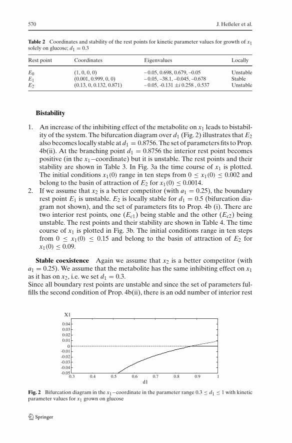
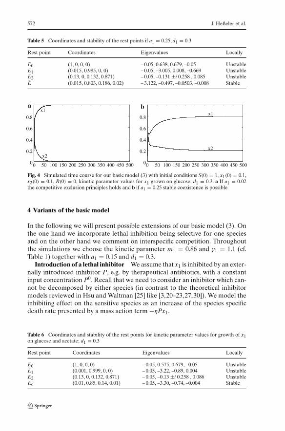
Competitive exclusion principle First we assume that the metabolite hasthe same inhibiting effect on x1 as it has on x2, i.e. d1 = 0.3. The set of param-eters fulfills the first conditions of Prop. 4b (i). The boundary rest points andtheir stability are shown in Table 2, the time course is plotted in Fig. 4a. Withthese parameter values the weaker competitor x2 cannot survive and is washedout, i.e. the CEP holds.


Table 2 Coordinates and stability of the rest points for kinetic parameter values for growth of x1solely on glucose; d1 = 0.3

Rest point Coordinates Eigenvalues Locally

E0 (1, 0, 0, 0) – 0.05, 0.698, 0.679, –0.05 UnstableE1 (0.001, 0.999, 0, 0) – 0.05, –38.1, –0.045, –0.678 StableE2 (0.13, 0, 0.132, 0.871) – 0.05, -0.131 ±i 0.258 , 0.537 Unstable

Bistability

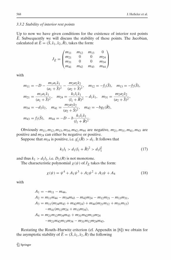
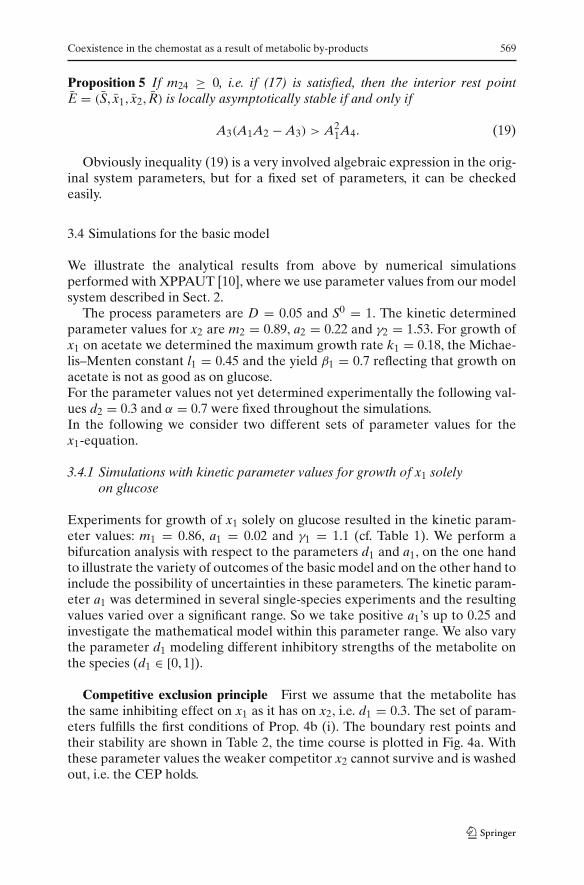
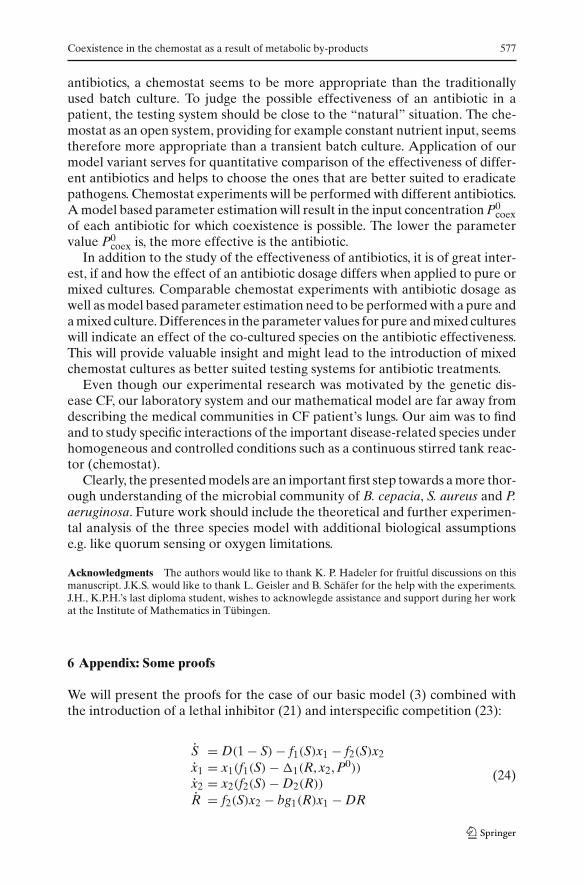
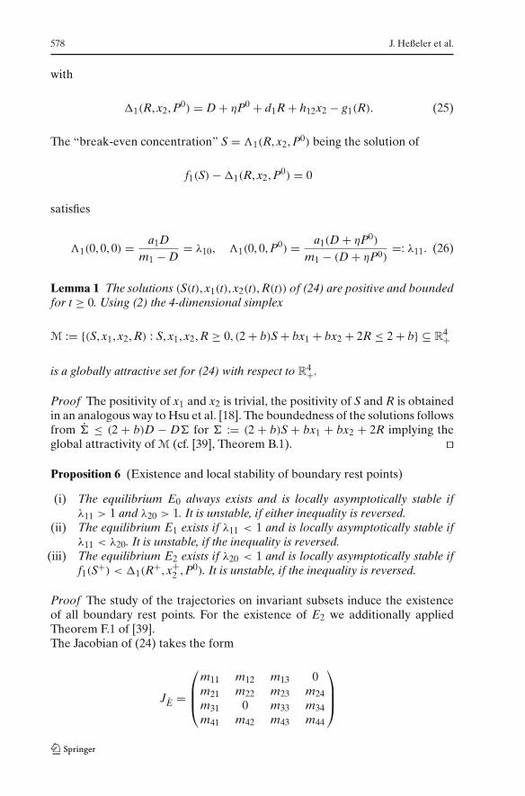
1. An increase of the inhibiting effect of the metabolite on x1 leads to bistabil-ity of the system. The bifurcation diagram over d1 (Fig. 2) illustrates that E2also becomes locally stable at d1 = 0.8756. The set of parameters fits to Prop.4b(ii). At the branching point d1 = 0.8756 the interior rest point becomespositive (in the x1−coordinate) but it is unstable. The rest points and theirstability are shown in Table 3. In Fig. 3a the time course of x1 is plotted.The initial conditions x1(0) range in ten steps from 0 ≤ x1(0) ≤ 0.002 andbelong to the basin of attraction of E2 for x1(0) ≤ 0.0014.

2. If we assume that x2 is a better competitor (with a1 = 0.25), the boundaryrest point E1 is unstable. E2 is locally stable for d1 = 0.5 (bifurcation dia-gram not shown), and the set of parameters fits to Prop. 4b (i). There aretwo interior rest points, one (Ec1) being stable and the other (Ec2) beingunstable. The rest points and their stability are shown in Table 4. The timecourse of x1 is plotted in Fig. 3b. The initial conditions range in ten stepsfrom 0 ≤ x1(0) ≤ 0.15 and belong to the basin of attraction of E2 forx1(0) ≤ 0.09.

Stable coexistence Again we assume that x2 is a better competitor (witha1 = 0.25). We assume that the metabolite has the same inhibiting effect on x1as it has on x2, i.e. we set d1 = 0.3.Since all boundary rest points are unstable and since the set of parameters ful-fills the second condition of Prop. 4b(ii), there is an odd number of interior rest

-0.05-0.04-0.03-0.02-0.01

00.010.020.030.04

X1

0.3 0.4 0.5 0.6 0.7 0.8 0.9 1d1

Fig. 2 Bifurcation diagram in the x1−coordinate in the parameter range 0.3 ≤ d1 ≤ 1 with kineticparameter values for x1 grown on glucose


Table 3 Coordinates and stability of the rest points for kinetic parameter values for growth of x1solely on glucose; d1 = 0.9


E0 (1, 0, 0, 0) –0.05, 0.698, 0.679, –0.05 UnstableE1 (0.001, 0.999, 0, 0) –0.05, –38.1, –0.045, –0.678 StableE2 (0.13, 0, 0.132, 0.871) –0.05, –0.131±i 0.258, –0.02 StableEc (0.124, 0.002, 0.13, 0.84) -0.136±i 0.26, -0.066, 0.017 Unstable

0

0.005

0.01

0.015

0.02

0 50 100 150 200

a b

x1(0)=0.0016

x1(0)=0.00140

0.050.1

0.150.2

0.250.3

0.350.4

0.450.5

0 20 40 60 80 100 120 140

x1(0)=0.09

x1(0)=0.105

Fig. 3 Simulated time course for varying initial conditions x1(0). a Set a1 = 0.02 and d1 = 0.9. Ifx1(0) > 0.014, then E1 (instead of E2) is attracting. b Set a1 = 0.25 and d1 = 0.5. If x1(0) > 0.09,then Ec1 (instead of E2) is attracting

Table 4 Coordinates and stability of the rest points if a1 = 0.25; d1 = 0.5


E0 (1, 0, 0, 0) – 0.05, 0.638, 0.679, –0.05 UnstableE1 (0.015, 0.985, 0, 0) – 0.05, –0.669, 0.008, –3.004 UnstableE2 (0.13, 0, 0.132, 0.871) – 0.05, –0.131±i 0.258, –0.101 StableEc1 (0.018, 0.487, 0.282, 0.062) – 2.400, –0.296, –0.05, –0.006 StableEc2 (0.032, 0.215, 0.246, 0.193) – 1.275, –0.196, 0.014, –0.05 Unstable

points (here just one) that attract the solutions of the system. The rest pointsand their stability are shown in Table 5, the time course is plotted in Fig. 4b.

3.4.2 Simulation with kinetic parameter values for growth of x1 on glucoseand acetate

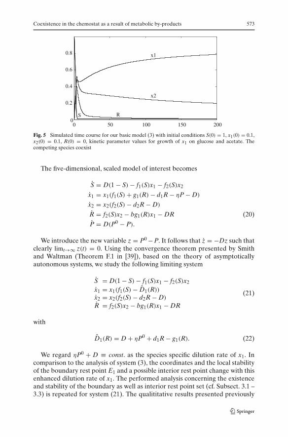
The second set of kinetic parameter values was determined from experimentsfor parallel use of glucose and acetate for which we obtained m1 = 0.75, a1 = 0.2and γ1 = 1.5. Assuming that the metabolite has the same inhibiting effect onx1 as it has on x2, i.e. setting d1 = 0.3, the set of parameters fulfills the secondcondition of Prop. 4b(ii) with one interior rest point. The coordinates and thestability of the rest points are shown in Table 6, the time course demostratesthe stable coexistence of the competing species (cf. Fig. 5) .


Table 5 Coordinates and stability of the rest points if a1 = 0.25; d1 = 0.3


E0 (1, 0, 0, 0) – 0.05, 0.638, 0.679, –0.05 UnstableE1 (0.015, 0.985, 0, 0) – 0.05, –3.005, 0.008, –0.669 UnstableE2 (0.13, 0, 0.132, 0.871) – 0.05, –0.131 ±i 0.258 , 0.085 UnstableE (0.015, 0.803, 0.186, 0.02) – 3.122, –0.497, –0.0503, –0.008 Stable

0

0.2

0.4

0.6

0.8

0 50 100 150 200 250 300 350 400 450 500

ax1

x20

0.2

0.4

0.6

0.8

0 50 100 150 200 250 300 350 400 450 500

x1

x2

b

Fig. 4 Simulated time course for our basic model (3) with initial conditions S(0) = 1, x1(0) = 0.1,x2(0) = 0.1, R(0) = 0, kinetic parameter values for x1 grown on glucose; d1 = 0.3. a If a1 = 0.02the competitive exclusion principles holds and b if a1 = 0.25 stable coexistence is possible

4 Variants of the basic model

In the following we will present possible extensions of our basic model (3). Onthe one hand we incorporate lethal inhibition being selective for one speciesand on the other hand we comment on interspecific competition. Throughoutthe simulations we choose the kinetic parameter m1 = 0.86 and γ1 = 1.1 (cf.Table 1) together with a1 = 0.15 and d1 = 0.3.

Introduction of a lethal inhibitor We assume that x1 is inhibited by an exter-nally introduced inhibitor P, e.g. by therapeutical antibiotics, with a constantinput concentration P0. Recall that we need to consider an inhibitor which can-not be decomposed by either species (in contrast to the theoretical inhibitormodels reviewed in Hsu and Waltman [25] like [3,20–23,27,30]). We model theinhibiting effect on the sensitive species as an increase of the species specificdeath rate presented by a mass action term −ηPx1.

Table 6 Coordinates and stability of the rest points for kinetic parameter values for growth of x1on glucose and acetate; d1 = 0.3


E0 (1, 0, 0, 0) – 0.05, 0.575, 0.679, –0.05 UnstableE1 (0.001, 0.999, 0, 0) – 0.05, –3.22, –0.89, 0.004 UnstableE2 (0.13, 0, 0.132, 0.871) – 0.05, –0.13 ±i 0.258 , 0.086 UnstableEc (0.01, 0.85, 0.14, 0.01) – 0.05, –3.30, –0.74, –0.004 Stable


0

0.2

0.4

0.6

0.8

0 50 100 150 200

x1

x2

RS

Fig. 5 Simulated time course for our basic model (3) with initial conditions S(0) = 1, x1(0) = 0.1,x2(0) = 0.1, R(0) = 0, kinetic parameter values for growth of x1 on glucose and acetate. Thecompeting species coexist

The five-dimensional, scaled model of interest becomes

S = D(1 − S)− f1(S)x1 − f2(S)x2

x1 = x1(f1(S)+ g1(R)− d1R − ηP − D)

x2 = x2(f2(S)− d2R − D)

R = f2(S)x2 − bg1(R)x1 − DR (20)

P = D(P0 − P).

We introduce the new variable z = P0 −P. It follows that z = −Dz such thatclearly limt→∞ z(t) = 0. Using the convergence theorem presented by Smithand Waltman (Theorem F.1 in [39]), based on the theory of asymptoticallyautonomous systems, we study the following limiting system

S = D(1 − S)− f1(S)x1 − f2(S)x2

x1 = x1(f1(S)− D1(R))x2 = x2(f2(S)− d2R − D)R = f2(S)x2 − bg1(R)x1 − DR

(21)

with

D1(R) = D + ηP0 + d1R − g1(R). (22)

We regard ηP0 + D ≡ const. as the species specific dilution rate of x1. Incomparison to the analysis of system (3), the coordinates and the local stabilityof the boundary rest point E1 and a possible interior rest point change with thisenhanced dilution rate of x1. The performed analysis concerning the existenceand stability of the boundary as well as interior rest point set (cf. Subsect. 3.1 –3.3) is repeated for system (21). The qualititative results presented previously


remain the same for the extended system (21) except that D1(R) is replaced byD1(R).

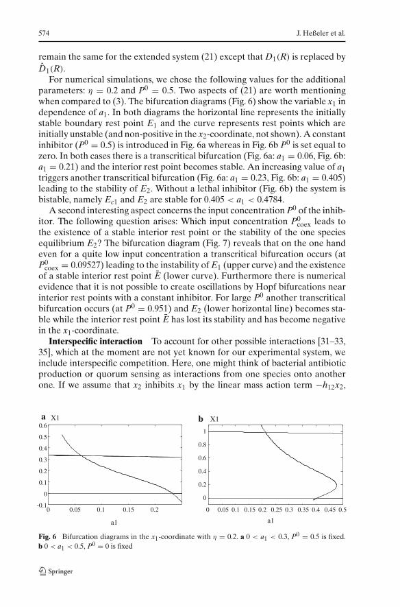
For numerical simulations, we chose the following values for the additionalparameters: η = 0.2 and P0 = 0.5. Two aspects of (21) are worth mentioningwhen compared to (3). The bifurcation diagrams (Fig. 6) show the variable x1 independence of a1. In both diagrams the horizontal line represents the initiallystable boundary rest point E1 and the curve represents rest points which areinitially unstable (and non-positive in the x2-coordinate, not shown). A constantinhibitor (P0 = 0.5) is introduced in Fig. 6a whereas in Fig. 6b P0 is set equal tozero. In both cases there is a transcritical bifurcation (Fig. 6a: a1 = 0.06, Fig. 6b:a1 = 0.21) and the interior rest point becomes stable. An increasing value of a1triggers another transcritical bifurcation (Fig. 6a: a1 = 0.23, Fig. 6b: a1 = 0.405)leading to the stability of E2. Without a lethal inhibitor (Fig. 6b) the system isbistable, namely Ec1 and E2 are stable for 0.405 < a1 < 0.4784.

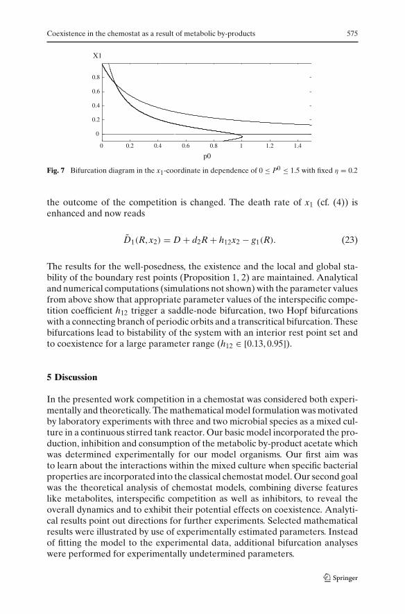
A second interesting aspect concerns the input concentration P0 of the inhib-itor. The following question arises: Which input concentration P0

coex leads tothe existence of a stable interior rest point or the stability of the one speciesequilibrium E2? The bifurcation diagram (Fig. 7) reveals that on the one handeven for a quite low input concentration a transcritical bifurcation occurs (atP0

coex = 0.09527) leading to the instability of E1 (upper curve) and the existenceof a stable interior rest point E (lower curve). Furthermore there is numericalevidence that it is not possible to create oscillations by Hopf bifurcations nearinterior rest points with a constant inhibitor. For large P0 another transcriticalbifurcation occurs (at P0 = 0.951) and E2 (lower horizontal line) becomes sta-ble while the interior rest point E has lost its stability and has become negativein the x1-coordinate.

Interspecific interaction To account for other possible interactions [31–33,35], which at the moment are not yet known for our experimental system, weinclude interspecific competition. Here, one might think of bacterial antibioticproduction or quorum sensing as interactions from one species onto anotherone. If we assume that x2 inhibits x1 by the linear mass action term −h12x2,

-0.1

0

0.1

0.2

0.3

0.4

0.5

0.6X1

0 0.05 0.1 0.15 0.2

a1

0

0.2

0.4

0.6

0.8

1

X1ba

0 0.05 0.1 0.15 0.2 0.25 0.3 0.35 0.4 0.45 0.5

a1

Fig. 6 Bifurcation diagrams in the x1-coordinate with η = 0.2. a 0 < a1 < 0.3, P0 = 0.5 is fixed.b 0 < a1 < 0.5, P0 = 0 is fixed


0

0.2

0.4

0.6

0.8

X1

0 0.2 0.4 0.6 0.8 1 1.2 1.4

p0

Fig. 7 Bifurcation diagram in the x1-coordinate in dependence of 0 ≤ P0 ≤ 1.5 with fixed η = 0.2

the outcome of the competition is changed. The death rate of x1 (cf. (4)) isenhanced and now reads

D1(R, x2) = D + d2R + h12x2 − g1(R). (23)

The results for the well-posedness, the existence and the local and global sta-bility of the boundary rest points (Proposition 1, 2) are maintained. Analyticaland numerical computations (simulations not shown) with the parameter valuesfrom above show that appropriate parameter values of the interspecific compe-tition coefficient h12 trigger a saddle-node bifurcation, two Hopf bifurcationswith a connecting branch of periodic orbits and a transcritical bifurcation. Thesebifurcations lead to bistability of the system with an interior rest point set andto coexistence for a large parameter range (h12 ∈ [0.13, 0.95]).

5 Discussion

In the presented work competition in a chemostat was considered both experi-mentally and theoretically. The mathematical model formulation was motivatedby laboratory experiments with three and two microbial species as a mixed cul-ture in a continuous stirred tank reactor. Our basic model incorporated the pro-duction, inhibition and consumption of the metabolic by-product acetate whichwas determined experimentally for our model organisms. Our first aim wasto learn about the interactions within the mixed culture when specific bacterialproperties are incorporated into the classical chemostat model. Our second goalwas the theoretical analysis of chemostat models, combining diverse featureslike metabolites, interspecific competition as well as inhibitors, to reveal theoverall dynamics and to exhibit their potential effects on coexistence. Analyti-cal results point out directions for further experiments. Selected mathematicalresults were illustrated by use of experimentally estimated parameters. Insteadof fitting the model to the experimental data, additional bifurcation analyseswere performed for experimentally undetermined parameters.


For a standard chemostat model as well as for our basic model (3), the exper-imentally estimated kinetic parameter values for growth of B. cepacia (x1) andS. aureus (x2) on glucose alone (Table 1) predicted the superiority of B. cepa-cia with S. aureus being washed out (cf. Fig. 4a). The bifurcation analysis withrespect to the parameter d1 revealed the bistability of the system for d1 > 0.5(cf. Fig. 2) without stable interior rest points. The outcome of the competitionthus depends on the initial condition of the species.

The kinetic parameters for S. aureus already comprise the inhibiting effect ofacetate – it is produced and cannot be exploited by this species. For B. cepacia,a separate set of kinetic parameter values was determined for parallel use ofglucose and acetate. The presence of acetate diminishes growth on glucose ofB. cepacia (cf. parameter values for B. cepacia growing on glucose and acetate,Table 1). For a standard chemostat model these kinetic parameter values wouldresult in a washout of B. cepacia from a mixed culture with S. aureus. Ourbasic model considers an additional effect, by which B. cepacia is able to takeadvantage of acetate as a secondary resource. Simulations for our basic modelwith the parameter values for growth on glucose and acetate (cf. Subsect. 3.4.2)indicate possible coexistence of B. cepacia and S. aureus (cf. Fig. 5). A balancebetween the inhibiting and enhancing effects of acetate apparently could bereached. Acetate diminishes growth of B. cepacia in favor of S. aureus, but atthe same time enhances B. cepacia again. It is taken up as a resource with thesimultaneous effect of reducing its concentration and consequently its inhibit-ing impact. These simulation results were also found in a two species chemostatexperiment with B. cepacia and S. aureus (cf. Sect. 2, Fig. 1). The hypothesis ofa metabolic by-product serving as a substrate for B. cepacia appears to be onereason for the experimentally observed coexistence of B. cepacia and S. aureus.To support this hypothesis, more experimental research will be realized, e.g.by monitoring the system response to pulse experiments. If our basic modelsucceeds in describing the correct system response, one may assume that themetabolic food chain is the main interpecies interaction being responsible forthe overall system dynamics.

It was already seen from growth parameters of B. cepacia (cf. Table 1) thatexperimentally determined parameters are not to be taken constant. They mayvary due to measuring or methodological errors or due to deficiencies causedby low-dimensional modeling. For example, the values of a1 for growth of B.cepacia vary if it is grown on glucose alone or grown on glucose and acetate.This variation was unexpected and might indicate a physiological phenomenonnot yet accounted for in the model formulation. Therefore we performed abifurcation analysis with respect to the parameter a1 for B. cepacia in the caseof B. cepacia growing on glucose alone (cf. Subsect. 3.4.1). We find that our basicmodel (3) predicts coexistence for a1 > 0.21 (cf. Figs. 4b, 6b). We would like tonote that this a1-value is close to the one determind in experiments with glucoseand acetate. Under additional variation of d1, the system can be bistable (cf. Fig.3b) so that the outcome of the competition depends on the intial conditions.

Our variant (20) extends the basic model to mimic testing of antibiotics inmixed cultures. As a testing system for comparison and evaluation of different


antibiotics, a chemostat seems to be more appropriate than the traditionallyused batch culture. To judge the possible effectiveness of an antibiotic in apatient, the testing system should be close to the “natural” situation. The che-mostat as an open system, providing for example constant nutrient input, seemstherefore more appropriate than a transient batch culture. Application of ourmodel variant serves for quantitative comparison of the effectiveness of differ-ent antibiotics and helps to choose the ones that are better suited to eradicatepathogens. Chemostat experiments will be performed with different antibiotics.A model based parameter estimation will result in the input concentration P0

coexof each antibiotic for which coexistence is possible. The lower the parametervalue P0

coex is, the more effective is the antibiotic.In addition to the study of the effectiveness of antibiotics, it is of great inter-

est, if and how the effect of an antibiotic dosage differs when applied to pure ormixed cultures. Comparable chemostat experiments with antibiotic dosage aswell as model based parameter estimation need to be performed with a pure anda mixed culture. Differences in the parameter values for pure and mixed cultureswill indicate an effect of the co-cultured species on the antibiotic effectiveness.This will provide valuable insight and might lead to the introduction of mixedchemostat cultures as better suited testing systems for antibiotic treatments.

Even though our experimental research was motivated by the genetic dis-ease CF, our laboratory system and our mathematical model are far away fromdescribing the medical communities in CF patient’s lungs. Our aim was to findand to study specific interactions of the important disease-related species underhomogeneous and controlled conditions such as a continuous stirred tank reac-tor (chemostat).

Clearly, the presented models are an important first step towards a more thor-ough understanding of the microbial community of B. cepacia, S. aureus and P.aeruginosa. Future work should include the theoretical and further experimen-tal analysis of the three species model with additional biological assumptionse.g. like quorum sensing or oxygen limitations.

Acknowledgments The authors would like to thank K. P. Hadeler for fruitful discussions on thismanuscript. J.K.S. would like to thank L. Geisler and B. Schäfer for the help with the experiments.J.H., K.P.H.’s last diploma student, wishes to acknowlegde assistance and support during her workat the Institute of Mathematics in Tübingen.

6 Appendix: Some proofs

We will present the proofs for the case of our basic model (3) combined withthe introduction of a lethal inhibitor (21) and interspecific competition (23):

S = D(1 − S)− f1(S)x1 − f2(S)x2x1 = x1(f1(S)−1(R, x2, P0))

x2 = x2(f2(S)− D2(R))R = f2(S)x2 − bg1(R)x1 − DR

(24)


with

1(R, x2, P0) = D + ηP0 + d1R + h12x2 − g1(R). (25)

The “break-even concentration” S = �1(R, x2, P0) being the solution of

f1(S)−1(R, x2, P0) = 0

satisfies

�1(0, 0, 0) = a1Dm1 − D

= λ10, �1(0, 0, P0) = a1(D + ηP0)

m1 − (D + ηP0)=: λ11. (26)

Lemma 1 The solutions (S(t), x1(t), x2(t), R(t)) of (24) are positive and boundedfor t ≥ 0. Using (2) the 4-dimensional simplex

M := {(S, x1, x2, R) : S, x1, x2, R ≥ 0, (2 + b)S + bx1 + bx2 + 2R ≤ 2 + b} ⊆ R4+

is a globally attractive set for (24) with respect to R4+.

Proof The positivity of x1 and x2 is trivial, the positivity of S and R is obtainedin an analogous way to Hsu et al. [18]. The boundedness of the solutions followsfrom � ≤ (2 + b)D − D� for � := (2 + b)S + bx1 + bx2 + 2R implying theglobal attractivity of M (cf. [39], Theorem B.1). ��

Proposition 6 (Existence and local stability of boundary rest points)

(i) The equilibrium E0 always exists and is locally asymptotically stable ifλ11 > 1 and λ20 > 1. It is unstable, if either inequality is reversed.

(ii) The equilibrium E1 exists if λ11 < 1 and is locally asymptotically stable ifλ11 < λ20. It is unstable, if the inequality is reversed.

(iii) The equilibrium E2 exists if λ20 < 1 and is locally asymptotically stable iff1(S+) < 1(R+, x+

2 , P0). It is unstable, if the inequality is reversed.

Proof The study of the trajectories on invariant subsets induce the existenceof all boundary rest points. For the existence of E2 we additionally appliedTheorem F.1 of [39].The Jacobian of (24) takes the form

JE =

⎛⎜⎜⎝

m11 m12 m13 0m21 m22 m23 m24m31 0 m33 m34m41 m42 m43 m44

⎞⎟⎟⎠


with

m11 = −D − f ′1(S)x1 − f ′

2(S)x2, m12 = −f1(S), m13 = −f2(S),

m21 = f ′1(S)x1, m22 = f1(S)−1(R, x2, P0),

m23 = −h12x1, m24 = g′1(R)x1 − d1x1,

m31 = f ′2(S)x2, m33 = f2(S)− D2(R), m34 = −d2x2,

m41 = f ′2(S)x2, m42 = −bg1(R), m43 = f2(S), m44 = −D − bg′

1(R)x1

and f ′i (S) = miai

(ai+S)2(resp. g′

1(R) = k1l1(l1+R)2

).The Jacobian at E0, E1 and E2 are

JE0 =

⎛⎜⎜⎝

−D −f1(1) −f2(1) 00 f1(1)− D − ηP0 0 00 0 f2(1)− D 00 0 f2(1) −D

⎞⎟⎟⎠ ,

JE1 =

⎛⎜⎜⎝

−D − f ′(λ11)(1 − λ11) −D −f2(λ11) 0f ′(λ11)(1 − λ11) 0 −h12(1 − λ11) −d1(1 − λ11)

0 0 f2(λ11)− D 00 0 f2(λ11) −D − bg′

1(0)(1 − λ11)

⎞⎟⎟⎠

and

JE2 =

⎛⎜⎜⎝

−D − f ′2(S

+)x+2 0 −f2(S+) −f1(S+)

f ′2(S

+)x+2 −D f2(S+) −bg1(R+)

f ′2(S

+)x+2 −d2x+

2 0 00 0 0 ψ4

⎞⎟⎟⎠ =

(A ∗0 ψ4

)

with ψ4 = f1(S+)−1(R+, x+2 , P0). We changed the order of the equations for

JE2 in order to have E2 = (S+, R+, x+2 , 0). The corresponding eigenvalues are

−D, f1(1)− D − ηP0, f2(1)− D and − D

for JE0 and

−D, −f ′(λ11)(1 − λ11), f2(λ11)− D and − D − bk1

l1(1 − λ11)

for JE1 . Thus if f1(1) − D − ηP0 < 0 and f2(1) − D < 0, then E0 is asymp-totically stable. If λ11 < λ20, it follows that f2(λ11) − D < 0, i.e. E1 is localasymptotically stable. The eigenvalues of JE2 are the eigenvalues of A and ψ4.The characteristic polynomial of A is

χ(ψ) = ψ3 + (2D + f ′2(S

+)x+2 )ψ

2 + (D(D + f ′2(S

+)x+2 )

+f2(S+)x+2 (d3 + f ′

2(S+))ψ + Df2(S+)x+

2 (d2 + f ′2(S

+)).


Now χ(−D) = 0, so that the remaining eigenvalues of A have to satisfy

ψ2 + A1ψ + A2 = 0,

with A1 = (D + f ′2(S

+)x+2 ) > 0 and A2 = f2(S+)x+

2 (d2 + f ′2(S

+)) > 0. It fol-lows that the eigenvalues of A are negative (or have negative real part). Ifadditionally ψ4 < 0, the local stability of E2 follows. ��Proposition 7 (Global stability of boundary rest points)

(i) If λ20 > 1, then limt→∞ x2(t) = 0. Moreover, if λ11 < 1, then E1 is globallyasymptotically stable.

(ii) If minR≥0�1(R, 0, P0) > 1, then limt→∞ x1(t) = 0. Moreover, if λ20 < 1,then E2 is globally asymptotically stable.

(iii) If λ20 > 1 and minR≥0�1(R, 0, P0) > 1, then E0 is globally asymptoticallystable.

Proof (ii) Because of the globally attracting set M we have lim supt→∞ S(t) ≤ 1.First we prove (by contradiction) that limt→∞ x1(t) exists. Suppose that lim inf x1and lim sup x1 are different and

0 ≤ lim inft→∞ x1(t) < lim sup

t→∞x1(t) = δ.

Since x1: R+ → R

+ is differentiable it follows from the Fluctuation Lemma (cf.[16]) that there is a sequence tk ↗ ∞ such that x1(tk) = 0, for all k, and

limk→∞

x1(tk) = lim supt→∞

x1(t) = δ > 0.

Because of x1(tk) = 0 we have limk→∞ x1(tk) = 0 and therefore

0 = limk→∞

x1(tk) = limk→∞

(x1(tk)

(m1S(tk)

a1 + S(tk)−1(R(tk), x2(tk), P0)

)).

This implies

limk→∞

(m1S(tk)

a1 + S(tk)−1(R(tk), x2(tk), P0)

)= 0. (27)

Because of the monotonicity of f1(S(t)) = m1S(t)a1+S(t) and lim supt→∞ S(t) ≤ 1 we

deduce

limk→∞

(S(tk)−�1(R(tk), x2(tk), P0)

)= 0 (28)

and thus

lim supk→∞

S(tk) = lim supk→∞

�1(R(tk), x2(tk), P0) ≥ minR≥0

�1(R, 0, P0) > 1


in contradiction to lim supt→∞ S(t) ≤ 1. So limt→∞ x1(t) exists.Suppose now that limt→∞ x1(t) > 0. Because of the Barbalat Lemma (cf. [13])we have

0 = limt→∞ x1(t) = lim

t→∞ x1(t)(

m1S(t)a1 + S(t)

−1(R(t), x2(t), P0)

).

The above argumentation leads to a contradiction to lim supt→∞ S(t) ≤ 1.Therefore we have limt→∞ x1(t) = 0.

Consider the invariant subspace x1 = 0. The system of interest becomes

S = D(1 − S)− f2(S)x2x2 = x2(f2(S)− d2R − D)R = f2(S)x2 − DR.

(29)

The dissipativeness is inherited by (24). With z = R + S − 1 and z = −Dzwe apply Theorem F.1 of [39] to the resulting (z, x2, R)-system and obtain thelimiting system

x2 = x2(f2(1 − R)− d2R − D) =: v1(x2, R)

R = f2(1 − R)x2 − DR =: v2(x2, R) (30)

confined to the region � := {(x2, R) : x2 ≥ 0, 0 ≤ R ≤ 1}.The region� is positively invariant because the flow on the boundary is inwards.Since the system (29) is dissipative, there is a global attractor inside {z = 0}where solutions satisfy (30).

The local stability of the positive interior rest point (x+2 , R+) of (30) is deter-

mined by the eigenvalues of the Jacobian, which has the form

J =(

0 −f ′2(1 − R+)x+

2 − d2x+2

d2R+ + D −f ′2(1 − R+)x+

2 − D

)

with f ′2(1 − R+) = m2a2

(a2+1−R+)2 > 0. If the positive interior rest point exists, it islocally asymptotically stable since tr(J) < 0 and det(J) > 0.By the Dulac criterion we can exclude the existence of periodic orbits for system(30) in the interior of �. For μ(x2, R) = 1/(x2R) (which is well-defined sincex2 �= 0 �= R) we have

∂

∂x2[μv1] + ∂

∂R[μv2] = ∂

∂x2

[f2(1 − R)− d2R − D

R

]+ ∂

∂R

[f2(1 − R)

R− D

x2

]

= f ′2(1 − R)R − f2(1 − R)

R2 = −m2(a2 + (1 − R)2)((a2 + 1 − R)R)2

< 0.


From an application of the Poincaré–Bendixson Theorem the global asymptot-ically stablity of the interior rest point is obtained, i.e.

limt→∞(x2(t), R(t)) = (x+

2 , R+).

Theorem F.1 in [39] allows the same conclusions for the three-dimensionalsystem (29) for f2(1) < D (or λ20 < 1):

limt→∞(S(t), x2(t), R(t)) = (λ2(R+), x+

2 , R+).

(i), (iii) Similar arguments as in the proof of (ii) establish (i) and (iii) (cf. e.g.[24]). We omit the details. ��The following proposition holds for (24) with h12 = 0.

Proposition 8 (Washout)

(i) If m2 ≤ D then limt→∞ x2(t) = 0.(ii) If m1 ≤ mint≥01(R(t), 0, P0) then limt→∞ x1(t) = 0.

Proof (ii) Suppose that 1(R(t), 0, P0) > 0 for all t ≥ 0. The solution x1(t) canbe rewritten as

x1(t) = x1(0) exp

⎛⎝

t∫0

(m1 −1(R(ξ), 0, P0))S(ξ)− a11(R(ξ), 0, P0)

a1 + S(ξ)dξ

⎞⎠ .

If 0 < m1 ≤ mint≥01(R(t), 0, P0) we obtain (because of the boundedness oflim supt→∞ S(t)) S(t) ≤ Smax with Smax > 1 for all t ≥ 0, such that

x1(t) ≤ x1(0) exp

⎛⎝

t∫0

−a11(R(ξ), 0, P0)

a1 + S(ξ)dξ

⎞⎠ ≤ x1(0) exp

⎛⎝

t∫0

−a1m1

a1 + Smaxtdξ

⎞⎠ .

We have limt→∞ x1(t) = 0.(i) Same arguments as in (ii). ��

References

1. Armstrong, R.A., McGehee, R.: Competitive exclusion. Am. Nat. 115(2), 151–170 (1980)2. Bassler, B.L.: How bacteria talk to each other: regulation of gene expression by quorum sensing.

Curr. Opin. Microbiol. 2, 582 (1999)3. Braselton, J.P., Waltman, P.: A competition model with dynamically allocated inhibitor produc-

tion. Math. Biosci. 173, 55–84 (2001)4. Butler, G.J., Wolkowicz, G.S.K.: A mathematical model of the chemostat with a general class

of functions describing nutrient uptake. SIAM J. Appl. Math. 45, 138–151 (1985)5. Chao, L., Levin, B.R.: Structured habitats and the evolution of anticompetitor toxins in bacteria.

Proc. Nat. Acad. Sci. USA 78, 6324–6328 (1981)


6. Coppel, W.A.: Stability and Asymptotic Behavior of Differential Equations. D.C. Heath andCo., Boston (1965)

7. Diekmann, O., Gyllenberg, M., Metz, J.A.J.: Steady-state analysis of structured populationmodels. Theor. Popul. Biol. 63, 309–338 (2003)

8. Dockery, J.D., Keener, J.P.: A mathematical model for quorum sensing in Pseudomonas aeru-ginosa. Bull. Math. Biol. 00, 1–22 (2000)

9. Doebeli, M.: A model for the evolutionary dynamics of cross-feeding polymorphisms in micro-organisms. Popul. Ecol. 44, 59–70 (2002)

10. Ermentrout, B.: Simulating, Analyzing, and Animating Dynamical Systems: A Guide to XP-PAUT for Researchers and Students. Society for Industrial and Applied Mathematics, (2002)

11. Freedman, H.I. Xu. Y.: Models of competition in the chemostat with instantaneous and delayednutrient recycling. J. Math. Biol. 31, 513–527 (1993)

12. Ghani, M., Soothill, J.S.: Ceftazidime, gentamicin, and rifampicin, in combination, kill biofilmof mucoid Pseudomonas aeruginosa. Can. J. Microbiol. 43, 999–1004 (1997)

13. Gopalsamy, K.: Stability and Oscillations in Delay Differential Equations of PopulationDynamics. Kluwer, Dordrecht (1992)

14. S.R. Hansen, S.R., Hubbell, S.P.: Single-nutrient microbial competition: Qualitative agree-ment between experimental and theoretically forecast outcomes. Science 207(4438), 1491–1493(1980)

15. Hardin, G.: The competitive exclusion principle. Science 131, 1292–1298 (1960)16. Hirsch, M.W., Hanisch, H., Gabriel, J.-P.: Differential equation models of some parasitic infec-

tions: methods for the study of asymptotic behavior. Comm. Pure Appl. Math. 38, 733–753(1985)

17. Hsu, S.B.: Limiting behavior for competing species. SIAM J. Appl. Math. 34, 760–763 (1978)18. Hsu, S.B., Hubbell, S.P., Waltman, P.: A mathematical theory for single-nutrient competition in

continuous cultures of micro-organisms. SIAM J. Appl. Math. 32(2), 366–383 (1977)19. Hsu, S.B., Li, Y.-S., Waltman, P.: Competition in the presence of a lethal external inhibitor.

Math. Biosci. 167(2), 177–199 (2000)20. Hsu, S.B., Luo, T.-K., Waltman, P.: Competition between plasmid-bearing and plasmid-free

organisms in a chemostat with an inhibitor. J. Math. Biol. 34, 225–238 (1995)21. Hsu, S.B., Waltman, P.: Analysis of a model of two competitors in a chemostat with an external

inhibitor. SIAM J. Appl. Math. 52(2), 528–541 (1991)22. Hsu, S.B., Waltman, P.: Competition between plasmid-bearing and plasmid-free organisms in

selective media. Chem. Eng. Sci. 52(1), 23–35 (1997)23. Hsu, S.B. Waltman, P.: Competition in the chemostat when one competitor produces a toxin.

Jpn J. Indust. Appl. Math. 15, 471–490 (1998)24. Hsu. S.B., Waltman, P.: A model of the effect of anti-competitor toxins on plasmid-bearing,

plasmid-free competition. Taiwanese J. Mathematics 6, 135–155 (2002)25. S.B. Hsu, S.B., Waltman, P.: A survey of mathematical models of competition with an inhibitor.

Math. Biosci. 187, 53–91 (2004)26. Hutchinson, G.E.: The paradox of the plankton. Am. Nat. 95, 137–145 (1961)27. Lenski, R.E., Hattingh, S.E.: Coexistence of two competitors on one resource and one inhibitor:

A chemostat model based on bacteria and antibiotics. J. Theor. Biol. 122, 83–96 (1986)28. Li, B.: Global asymptotic behavior of the chemostat: General response functions and different

removal rate. SIAM J. Appl. Math. 59(2), 411–422 (1998)29. Lu, Z., Hadeler, K.P.: Model of plasmid-bearing, plasmid-free competition in the chemostat

with nutrient recycling and an inhibitor. Math. Biosci. 148, 147–159 (1998)30. Luo, T.K., Hsu, S.B.: Global analysis of a model of plasmid-bearing, plasmid-free competition

in a chemostat with inhibitons. J. Math. Biol. 34, 41–76 (1995)31. Madigan, M.T. Martinko, J.M., Parker, J.: Brock Biology of Microorganisms. Prentice Hall

Englewood Cliffs, (2003)32. Marsh, P.D., Bowden, G.H.W.: Microbial community interactions in biofilms. In: Allison, D.G.,

Gilbert, P., Lappin-Scott, H.M., Wilson, M.: (eds.) Community Structure and Co-operation inBiofilms, pp. 167–198. Press Syndicate of the University of Cambridge, Cambridge (2000)

33. Passarge, J., Huisman, J.: Competition in well-mixed habitats: From competitive exclusion tocompetitive chaos. In Sommer, U., Worm, B. ed, Competition and Coexistence. EcologicalStudies., vol. 161, pp. 7–42. Springer, Berlin Heidelberg New York, (2002)


34. Reeves, G.T., Narang, A., Pilyugin, S.S.: Growth of mixed cultures on mixtures of substitutablesubstrates: the operating diagram for a structured model. J. Theor. Biol. 226, 143–157 (2004)

35. Riedel, K., et al.: N-acylhomoserine-lactone-mediated communication between Pseudomonasaeruginosa and Burkholderia cepacia in mixed biofilms. Microbiology 147, 3249–3262 (2001)

36. Ruan, S., He, X.-Z.: Global stability in chemostat-type competition models with nutrientrecycling. SIAM J. Appl. Math. 58(1), 170–198 (1998) A correction can be found online athttp://www.math.miami.edu/∼ruan/publications.html

37. Sardonini, C.A., DiBiasio, D.: A model for growth of Saccharomyces cerevisiae containing arecombinant plasmid in selective media. Biotechnol. Bioeng. 29, 469–475 (1987)

38. Schmidt, J.K., König, B., Reichl, U.: Characterization of a three bacteria mixed culture in achemostat: Evaluation and application of a quantitative Terminal-Restriction Fragment Poly-morphism (T-RFLP) analysis for absolute and species specific cell enumeration. Biotechnol.Bioeng. (2006) (submitted)

39. Smith, H.L., Waltman, P.: The Theory of the Chemostat. Cambridge University Press, Cam-bridge (1995)

40. Turner, P.E., Souza, V., Lenski, R.E.: Test of ecological mechanisms promoting the stablecoexistence of two bacterial genotypes. Ecology 77(7), 2119–2129 (1996)

41. Wolkowicz, G.S.K., Lu, Z.: Global dynamics of a mathematical model of competition in thechemostat: General response functions and differential death rates. SIAM J. Appl. Math. 52(1),222–233 (1992)

42. Wolkowicz, G.S.K., Zhiqi, L.: Direct interference on competition in a chemostat. J. Biomath.13(3), 282–291 (1998)

Documents

Coexistence in the chemostat as a result of metabolic by-products