PHYSICAL REVIEW E 91, 052815 (2015)

Collective relaxation dynamics of small-world networks

Carsten Grabow,1,2 Stefan Grosskinsky,3 Jurgen Kurths,1,4,5 and Marc Timme2,6,7

1Research Domain on Transdisciplinary Concepts and Methods, Potsdam Institute for Climate Impact Research,P.O. Box 60 12 03, 14412 Potsdam, Germany

2Network Dynamics, Max Planck Institute for Dynamics and Self-Organization (MPIDS), 37077 Gottingen, Germany3Mathematics Institute and Centre for Complexity Science, University of Warwick, Coventry CV4 7AL, United Kingdom

4Department of Physics, Humboldt University of Berlin, Newtonstr. 15, 12489 Berlin, Germany5Institute for Complex Systems and Mathematical Biology, University of Aberdeen, Aberdeen AB24 3UE, United Kingdom

6Institute for Nonlinear Dynamics, Faculty for Physics, Georg August University Gottingen, 37077 Gottingen, Germany7Bernstein Center for Computational Neuroscience Gottingen, 37077 Gottingen, Germany

(Received 29 March 2015; published 27 May 2015)

Complex networks exhibit a wide range of collective dynamic phenomena, including synchronization,diffusion, relaxation, and coordination processes. Their asymptotic dynamics is generically characterized by thelocal Jacobian, graph Laplacian, or a similar linear operator. The structure of networks with regular, small-world,and random connectivities are reasonably well understood, but their collective dynamical properties remainlargely unknown. Here we present a two-stage mean-field theory to derive analytic expressions for networkspectra. A single formula covers the spectrum from regular via small-world to strongly randomized topologiesin Watts-Strogatz networks, explaining the simultaneous dependencies on network size N , average degree k,and topological randomness q. We present simplified analytic predictions for the second-largest and smallesteigenvalue, and numerical checks confirm our theoretical predictions for zero, small, and moderate topologicalrandomness q, including the entire small-world regime. For large q of the order of one, we apply standard randommatrix theory, thereby overarching the full range from regular to randomized network topologies. These resultsmay contribute to our analytic and mechanistic understanding of collective relaxation phenomena of networkdynamical systems.

DOI: 10.1103/PhysRevE.91.052815 PACS number(s): 89.75.Hc, 05.45.Xt, 87.19.lm

I. INTRODUCTION

The structural features of complex networks underlietheir collective dynamics such as synchronization, diffusion,relaxation, and coordination processes [1,2]. Such processesoccur in various fields, ranging from opinion formation insocial networks [3] and consensus dynamics of agents [4] tosynchronization in biological circuits [5,6] and oscillationsin gene regulatory networks and neural circuits [7–9]. Theasymptotic collective dynamics of all such processes ischaracterized by the local Jacobian, the graph Laplacian,or similar linear operators. In general, such linear operatorsdirectly connect the structure of an underlying network toits dynamics and thus its function (see, e.g., Refs. [10,11]).Therefore, a broad area of research is related to the study ofproperties of such operators, in particular to the study of theirspectra [12–19].

Small-world models based on rewiring have receivedwidespread attention both theoretically and in applications, asdemonstrated, for instance, by the huge number of referencespointing to the original theoretical work [20]. But for most oftheir features analytical predictions are not known to date ([21];a mean field solution of its average path length constitutesa notable exception [22]). In particular, the spectrum ofsmall-world Laplacians has been studied for several specificcases and numerically [23–27], yet a general derivation ofreliable analytic predictions was missing.

Here we present a mean field theory [28] toward closingthis gap. The article is organized as follows. In Sec. II wefirst review the relations between relaxation dynamics andthe spectrum of the graph Laplacian. In Sec. III we present

rewiring “on average”, a new mean-field rewiring recentlyproposed in a brief report [28]. Based on this rewiring, wederive a single formula that approximates well the entirespectrum from regular to strongly randomized topologies. Wethen investigate the ordering of the mean-field eigenspectrumin Sec. IV. In Sec. V we quantify the accuracy of ourpredictions via systematic numerical checks for the extremeeigenvalues. For the topological randomness q of the order ofunity, standard random matrix theory is applied in Sec. VI. Weclose in Sec. VII with a summary and a discussion of furtherwork.

II. NETWORK RELAXATION DYNAMICS

The relaxation dynamics toward equilibrium and relatedcollective phenomena close to invariant sets or stationary dis-tributions emerge across a wide variety of systems ubiquitousin natural and artificial systems [1,29].

A. Generic linear relaxation

Mathematically, the relaxation of network dynamics to afixed point, a periodic orbit, or a similar stationary regime isgenerically characterized by equations of the form

dxi

dt=

N∑j=1

Jij (xj − xi) for i ∈ {1, . . . ,N}, (1)

where xi(t) quantifies the deviation at time t from an invariantstate, N ∈ N is the size of the network, and Jij ∈ R quantifies

1539-3755/2015/91(5)/052815(11) 052815-1 ©2015 American Physical Society

GRABOW, GROSSKINSKY, KURTHS, AND TIMME PHYSICAL REVIEW E 91, 052815 (2015)

the influence of unit j onto unit i. In general, xi(t) ∈ Rd , wehere take d = 1 for simplicity of presentation.

The equivalent mathematical description,

dxi

dt=

N∑j=1

�ijxj , (2)

for i ∈ {1, . . . ,N}, with the Laplacian

�ij ={

Jij for i �= j

−∑Nj=1 Jij for i = j,

(3)

follows directly from the original dynamics Eq. (1).The eigenvalues λn ∈ C and corresponding eigenvectors vn

of such a Laplacian, satisfying

�vn = λnvn, (4)

for n ∈ {1, . . . ,N}, fully characterize the asymptotic (linearor linearized) dynamics. For instance, for stable dynamics,where all xi(t) → 0 for t → ∞, the largest nonzero (principal)eigenvalue λ∗ dominates the long-term dynamics: if wehave xj (0) = ∑N

n=1 anvn, the vector x(t) = [x1(t), . . . ,xN (t)]T

evolves as

x(t) = exp(�t)x(0)

= exp(�t)∑

n

anvn

=N∑

n=1

an exp(λnt)vn. (5)

Due to stability we have an = 0 whenever λn = 0, and for longtimes this is dominated by

x(t) ∼ a∗ exp(λ∗t)v∗, (6)

where λ∗ is the principal eigenvalue.Note that Eq. (5) also reveals how exactly all eigenvalues

contribute to relaxation (and how much relative to each other).Additional individual eigenvalues of interest are given by theone with smallest real part λ−, because it bounds the real partsof the spectrum below and thereby determines the support ofthe spectrum, and also because it is involved in determiningsynchronizability conditions in coupled chaotic systems viathe ratio λ∗/λ−, see Ref. [30].

B. Different example systems

We briefly consider two very different paradigmatic exam-ple classes of systems and comment on a few others whoserelaxation properties are characterized by equations of thesame type as Eq. (2).

1. Stochastic processes

First, consider random walks on a graph, or equivalently,Markov chains defined by a weighted nonnegative graphwhose nodes represent the N states [31]. For such processes,the dynamics of the probability pi(t) to reside in state

i ∈ {1, . . . ,N} at time t is given by

dpi

dt=

N∑j=1

[Tijpj − Tjipi] for i ∈ {1, . . . ,N}, (7)

where Tij defines the transition rate (probability per unit time)of the system-switching state from j to i given it resides ini. We assume the process to be ergodic. Identifying p∗ tobe the unique stationary distribution �ij = Tij for i �= j and�ii = −∑

j Tji and setting xi(t) ≡ pi(t) − p∗i exactly maps

this process onto the generic form of Eq. (2) with xi(t) → 0as t → ∞ for all i ∈ {1, . . . ,N}.

2. Coupled deterministic oscillators

Second, consider the relaxation dynamics of weakly cou-pled limit cycle oscillators, generically modeled as phase-coupled oscillators

dθi

dt= ωi +

∑j

hij (θj − θi) for i ∈ {1, . . . ,N}, (8)

where θi(t) is the phase of unit i at time t , ωi is thelocal intrinsic frequency of oscillator i, and hij (.) definesa smooth coupling function from unit j to i [9,32,33].Phase-locking, where θj (t) − θi(t) = �ji is constant in time,constitutes a generic collective state of such systems, see, e.g.,Refs. [34–36]. A paradigmatic model is given by networks ofKuramoto oscillators coupled by simple sinusoidal functions,i.e., hij (θ ) = sin(θ ) [32,33,37].

In the most general setting, a matrix J is defined by elementsJij = ∂hij (θ )/∂θ |θ=�ji

that encode the network structure closeto the phase-locked state. Under certain conditions on the ωi

and the hij , the system’s dynamics exhibits a short transientdominated by nonlinear effects and thereafter exponentiallyrelaxes to the phase-locked state. Linearizing close to such astate yields phase perturbations defined as

δi(t) := θi(t) − θ (t), (9)

which evolve according to

dδi

dt=∑

j

�ij δj (t) for i ∈ {1, . . . ,N}, (10)

with the graph Laplacian given by Eq. (3).In a simple setting, we have Jij = 1 for an existing edge

and Jij = 0 for no edge such that the local linear operatorin Eq. (10) coincides with the graph Laplacian defined by itselements,

�ij = Jij (1 − δij ) − kiδij , (11)

for i,j ∈ {1, . . . ,N}, where now Jij are the elements of theadjacency matrix, ki is the degree of node i (replaced by thein-degree for directed networks), and δij is the Kronecker-δ.The asymptotic relaxation dynamics on such networks isthus characterized by this graph Laplacian �. Similarly,any dynamics near genuine fixed points, for instance ingene regulatory networks [38,39], is equally characterized bylinearized dynamics stemming from local Jacobians.

052815-2

COLLECTIVE RELAXATION DYNAMICS OF SMALL-WORLD . . . PHYSICAL REVIEW E 91, 052815 (2015)

3. Power grids, social networks, neural circuits,...

Several other systems exhibit qualitatively the same dynam-ical relaxation. In fact, power grids are often characterized bysecond-order oscillatory systems [40] that principally relax toperiodic phase-locked solutions (stationary operating statesof the grid) very similarly to the phase oscillator systemsdiscussed above [41]. In models of several social phenomena,e.g., of opinion formation of agents, the dynamics of consensusformation is equally akin to such locking dynamics, where thelocked state would now be a homogeneous, fully synchronousone [42]. Last but not least, perturbations of the spatiotemporalcollective dynamics of pulse-coupled systems such as neuralcircuits [43,44] also relax according to Eq. (2).

III. MEAN FIELD REWIRING AND SPECTRUM

Diving into explaining the small-world model, we analyzeand derive its approximate Laplacian based on a two-stagemean-field rewiring. We follow Ref. [28] and where appropri-ate take parts of the description presented there.

We consider an initial ring graph of N nodes. Each nodereceives k (being even) links from its k/2 nearest neighborson both sides. Then we introduce randomness in the networktopology by rewiring.

To define Watts-Strogatz randomized networks, singleinstances of an ensemble of stochastically rewired networksare generated (Fig. 1, left panel). Following Ref. [20] forundirected networks, we first cut each edge with probabilityq. Afterwards the cut edges are rewired to nodes chosen

FIG. 1. (Color online) Rewiring—stochastic and mean field.Cartoon for N = 10 and k = 4. Instead of taking out (step 1) andputting back (step 2) edges randomly (left column), the correspondingweight is subtracted (step 1) uniformly and added (step 2) in twofractions (right column).

uniformly at random from the whole network. Similarly, fordirected [45] networks, we first cut all outgoing edges withprobability q and rewire their tips afterwards. In both cases weavoid double edges and self-loops.

To analytically determine the Laplacian mean-field spec-trum in dependence of the network size N , the average degreek and the topological randomness q, we introduce a two-stagemean-field rewiring that effectively generates, at given q,the average network from the ensemble of all stochasticallyrewired networks. This is depicted in Fig. 1 (right panel) incomparison to both other rewiring procedures for undirectedand directed networks. First, we define a circulant mean-fieldLaplacian

�mf =

⎛⎜⎜⎜⎜⎜⎜⎜⎜⎜⎝

c0 c1 c2 · · · cN−1

cN−1 c0 c1 c2...

cN−1 c0 c1. . .

.... . .

. . .. . . c2

c1

c1 · · · cN−1 c0

⎞⎟⎟⎟⎟⎟⎟⎟⎟⎟⎠

. (12)

Its matrix elements for the initial configuration (Fig. 1, q = 0,top) are given by

ci =⎧⎨⎩

−k if i = 01 if i ∈ {1, . . . , k

2 ,N − k2 , . . . ,N − 1} = S1

0 if i ∈ { k2 + 1, . . . ,N − k

2 − 1} = S2,

(13)

where S1 represents the set of edges being present in the ringand S2 those absent ones outside that ring.

Instead of rewiring single edges randomly (Fig. 1, leftpanel), we now distribute the corresponding weight of rewirededges uniformly among the whole network (Fig. 1, rightpanel). Thus, for a given rewiring probability q we generatea mean-field version of the randomized network ensemble inthe following two steps:

First, we subtract the average total weight qkN/2 of alledges to be rewired (S1), i.e., ci = 1 − q if i ∈ S1.

Second, the rewired weight is distributed uniformly amongthe total “available” weight in the whole network given by

f = N (N − 1) − (1 − q)kN

2. (14)

With the weights

f1 = qkN

2(15)

being available in S1 and

f2 = N (N − 1) − kN

2(16)

in S2, we assign the fraction f1/f to elements representingedges in S1 and f2/f to those representing S2. Therefore, anindividual edge in S1 gets the additional weight

w1 = f1

f

qkN

2kN2

= q2k

N − 1 − (1 − q)k, (17)

052815-3

GRABOW, GROSSKINSKY, KURTHS, AND TIMME PHYSICAL REVIEW E 91, 052815 (2015)

FIG. 2. (Color online) The banded structure of the mean-fieldgraph Laplacian �mf given in Eqs. (12) and (19). It has the weightsw1 = 1 − q + w1 for ci |i ∈ S1 and w2 for ci |i ∈ S2 [see Eq. (13) forthe definition of Si]. For q = 0, and hence w1 = 1 and w2 = 0, werecover the exact ring Laplacian.

and an edge in S2 gets the new weight

w2 = f2

f

qkN

2N(N−1)−kN

2

= qk

N − 1 − (1 − q)k. (18)

Thus, as depicted in Fig. 2, in our mean-field theory theelements of the Laplacian �mf Eq. (12) of a network on N

nodes with degree k after rewiring with probability q are givenby

ci =⎧⎨⎩

−k if i = 01 − q + w1 if i ∈ S1

w2 if i ∈ S2.

(19)

The mean-field Laplacian defined by Eqs. (12) and (19) byconstruction is a circulant matrix with eigenvalues [46–48]

λmfl =

N−1∑j=0

cj exp

[−2πi(l − 1)j

N

]. (20)

Observing the structure in Fig. 2 we immediately obtain thetrivial eigenvalue for l = 1:

λmf1 =

N−1∑j=0

cj = −k + k(1 − q + w1) + (N − k − 1)w2 = 0,

(21)

which is common to all networks (for all q, N , and anyk � N − 1) and reflects the invariance of Laplacian dynamicsagainst uniform shifts, as seen from the associated eigenvectorv1 = (1, . . . ,1)T.

To obtain the remaining eigenvalues for l ∈ {2, . . . ,N}, wefirst define

xl := exp

[−2πi(l − 1)

N

], (22)

c′ := 1 − q

k+ qc′′, (23)

and

c′′ := q

N − 1 − (1 − q)k. (24)

This leads to

λmfl = −k + kc′

k2∑

j=1

xj

l + kc′′N−1− k

2∑j= k

2 +1

xj

l + kc′N−1∑

j=N− k2

xj

l

(25)

= −k + kc′k2∑

j=1

xj

l + kc′k2∑

j=1

xN−j

l

+ kc′′

⎛⎝ N−k

2 −1∑j=1

xN2 +j

l +N−k

2 −1∑j=1

xN2 −j

l + xN2

l

⎞⎠ , (26)

where we have exploited the additional transposition sym-metry �mf = (�mf)T, which implies cj = cN−j . Applyingthe Euler formula exp (iα) = cos(α) + i sin(α), the complexsummands cancel and we get

λmfl = −k + 2kc′

k2∑

j=1

cos

[2π (l − 1)j

N

]

+ xN2

l kc′′

⎧⎨⎩2

N−k2 −1∑j=1

cos

[2π (l − 1)j

N

]+ 1

⎫⎬⎭ . (27)

Using the identityn∑

j=0

cos(jα) = cos

(n + 1

2α

)sin

(nα

2

) 1

sin(

α2

) + 1

= 1

2

{1 + sin

[(n + 1

2

)α]

sin(

α2

)}

, (28)

we obtain

λmfl = −k + kc′

{sin

[ (k+1)(l−1)πN

]sin

[ (l−1)πN

] − 1

}

+ xN2

l kc′′ sin[ (N−k−1)(l−1)π

N

]sin

[ (l−1)πN

] . (29)

Taking advantage of additional identities, only valid forl ∈ Z (Fig. 3),

xN/2l = (−1)l−1, (30)

(−1)l−1 sin(α) = sin[α + (l − 1)π ], (31)

and the symmetry sin(−α) = − sin(α), the expression simpli-fies to

λmfl = −k + kc′

{sin

[ (k+1)(l−1)πN

]sin

[ (l−1)πN

] − 1

}

+ (−1)l−1kc′′ sin{ [−(k+1)+N](l−1)π

N

}sin

[ (l−1)πN

]052815-4

COLLECTIVE RELAXATION DYNAMICS OF SMALL-WORLD . . . PHYSICAL REVIEW E 91, 052815 (2015)

(29)(33)

FIG. 3. (Color online) Interpolating the eigenvalues. Equa-tions (29) (blue) and (33) (red) both contain the eigenspectrum λmf

l

for l ∈ {2, . . . ,N} correctly (green circles). While λmfl in Eq. (29)

includes λmf1 as liml→1 λmf

l = λmf1 = 0 as well, λmf

l for l ∈ {2, . . . ,N}in Eq. (33) does not: To further simplify expressions, we have usedEqs. (30) and (31) only valid for integer l, but apparently not forl = 0.

= −k + kc′{

sin[ (k+1)(l−1)π

N

]sin

[ (l−1)πN

] − 1

}

+ kc′′ sin{ [−(k+1)(l−1)+2N(l−1)]π

N

}sin

[ (l−1)πN

]= −k + kc′

{sin

[ (k+1)(l−1)πN

]sin

[ (l−1)πN

] − 1

}

− kc′′ sin[ (k+1)(l−1)π

N

]sin

[ (l−1)πN

] , (32)

which finally leads to

λmfl = −k − kc′ + k(c′ − c′′)

sin[ (k+1)(l−1)π

N

]sin

[ (l−1)πN

] , (33)

for l ∈ {2, . . . ,N}.

IV. THE ORDERING OF THE MEAN-FIELD SPECTRUM

The spectrum obeys the symmetry

λmfl = λmf

N−l+2, (34)

but is unordered otherwise; i.e., the index l does neither denoteeigenvalues with decreasing real part nor eigenvalues withdecreasing absolute value.

As we argue below the expression λmf2 [which equals

λmfN due to Eq. (34)] always constitutes the second-largest

(principal) eigenvalue λmf∗ . The only term depending on l in

Eq. (33) is the ratio

sin[ (k+1)(l−1)π

N

]sin

[ (l−1)πN

] . (35)

We therefore study the function

f (x) = sin[(k + 1)x]

sin x, (36)

FIG. 4. (Color online) λmf2 always constitutes the second largest

eigenvalue. Functions f (x) [Eq. (36)], the oscillating functionsin[(k + 1)x], and the envelope function 1/ sin(x) are plotted vs. x =(l−1)π

N∈ (0,π ) for k = 10. Obviously, a larger k leads to more roots

of f (x), but otherwise the functions show the same characteristicsfor all k � N − 1: f (x) has a local maximum at x = 0 and decreasesstrictly monotonically up to the following minimum. For larger x

the envelope function guarantees that all values up to x = π/2 aresmaller than f (xl=2 = π

N).

with

x = (l − 1)π

N(37)

and x ∈ (0,π/2). Due to the symmetry, Eq. (34), the interval(0,π/2) covers the entire spectrum, Eq. (33).

The function f (x) on x ∈ (0,π/2) is the product of theoscillating function sin[(k + 1)x] and a strictly monotonicallydecreasing function 1/ sin(x). Therefore, it is a dampedoscillation with period of 2π/(k + 1) and with the amplitudedecreasing as 1/ sin(x) (Fig. 4).

At x = 0 we apply the Theorem of l’Hospital to calculatethe following limits. There is a removable singularity,

limx→0

f (x) = k + 1, (38)

with

limx→0

f ′(x) = 0 and limx→0

f ′′(x) = − 13k(k2 + 3k + 2) < 0,

(39)

i.e., a local maximum.In order to show that the index l = 2 is always associated

with the second-largest eigenvalue, we first determine its x

value. It is given by

xl=2 = π

N. (40)

Since the roots of the function f (x) are located at

xroot,r = rπ

k + 1, (41)

for r ∈ Z. Thus, xl=2 is always smaller than the first root xroot,1,Eq. (41), of the function f (x) (Fig. 5).

The boundary points of function f (x) and the envelopefunction 1/ sin(x) are given by

xb,r = 4πr + π

2(k + 1), (42)

for r ∈ Z.

052815-5

GRABOW, GROSSKINSKY, KURTHS, AND TIMME PHYSICAL REVIEW E 91, 052815 (2015)

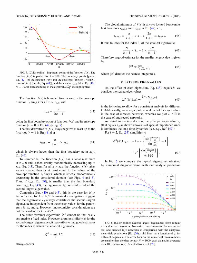
FIG. 5. (Color online) Important points of the function f (x). Thefunction f (x) is plotted for k = 100. The boundary points [green,Eq. (42)] of the function f (x) and the envelope function 1/ sin(x),roots of f (x) [purple, Eq. (41)], and the x value xl=2 [blue, Eq. (40),N = 1000] corresponding to the eigenvalue λmf

2 are highlighted.

The function f (x) is bounded from above by the envelopefunction 1/ sin(x) for all x > xb,0, with

xb,0 = π

2(k + 1)(43)

being the first boundary point of function f (x) and its envelopefunction [r = 0 in Eq. (42)] (Fig. 5).

The first derivative of f (x) stays negative at least up to thefirst root [r = 1 in Eq. (41)] at

xroot,1 = π

k + 1> xb,0, (44)

which is always larger than the first boundary point xb,0,Eq. (43).

To summarize, the function f (x) has a local maximumat x = 0 and is then strictly monotonically decreasing up toxb,0, Eq. (43). Then, for all x > xb,0 the function f (x) takesvalues smaller than or at most equal to the values of theenvelope function 1/ sin(x), which is strictly monotonicallydecreasing in the considered domain (see Figs. 4 and 5).Thus, if xl=2, Eq. (40), is smaller than the first boundarypoint xb,0, Eq. (43), the eigenvalue λ2 constitutes indeed thesecond-largest eigenvalue.

Comparing Eqs. (40) and (43), this is the case for N �2(k + 1), i.e., for k < N/2. Numerical investigations suggestthat the eigenvalue λ2 always constitutes the second-largesteigenvalue independent from the chosen values for the param-eters N , k, and q. However, monotonicity considerations arenot that evident for k > N/2.

The other extremal eigenvalue λmf- cannot be that easily

assigned to a fixed index. However, arguing similarly as for thesecond-largest eigenvalues, it is possible to find good estimatesfor the index at which the smallest eigenvalue,

λmf- = min

lλmf

l , (45)

always occurs.

The global minimum of f (x) is always located between itsfirst two roots xroot,1 and xroot,2 in Eq. (42); i.e.,

xroot,1 = π

k + 1< x− <

2π

k + 1= xroot,2. (46)

It thus follows for the index l− of the smallest eigenvalue:

N

k + 1< l− − 1 <

2N

k + 1. (47)

Therefore, a good estimate for the smallest eigenvalue is givenby

λmf− ≈ λmf

� 3N2(k+1) +1�, (48)

where �x� denotes the nearest integer to x.

V. EXTREME EIGENVALUES

As the offset of each eigenvalue, Eq. (33), equals k, weconsider the scaled eigenvalues

λmfl (N,k,q) = λmf

l (N,k,q)

k(49)

in the following to allow for a consistent analysis for differentk. Additionally, we always plot the real part of the eigenvaluesin the case of directed networks, whereas we plot λl ∈ R inthe case of undirected networks.

As stated in the introduction, the principal eigenvalue λ∗(that equals λ2 as shown above) is of special importance sinceit dominates the long time dynamics (see, e.g., Ref. [49]).

For l = 2, Eq. (33) simplifies to

λmf2 (N,k,q) = −1 + c′

{sin

[ (k+1)πN

]sin

(πN

) − 1

}

+ c′′{

sin[ (k+1)π

N

]sin

(πN

)}

. (50)

In Fig. 6 we compare the typical eigenvalues obtainedby numerical diagonalization with our analytic prediction

FIG. 6. (Color online) Second-largest eigenvalues from regularto randomized networks. Numerical measurements for undirected(×) and directed (©) networks in comparison with the analyticalmean-field predictions [Eq. (50), solid lines] as a function of q, fordifferent degrees k. The error bars on the numerical measurementsare smaller than the data points (N = 1000, each data point averagedover 100 realizations). Adapted from Ref. [28].

052815-6

COLLECTIVE RELAXATION DYNAMICS OF SMALL-WORLD . . . PHYSICAL REVIEW E 91, 052815 (2015)

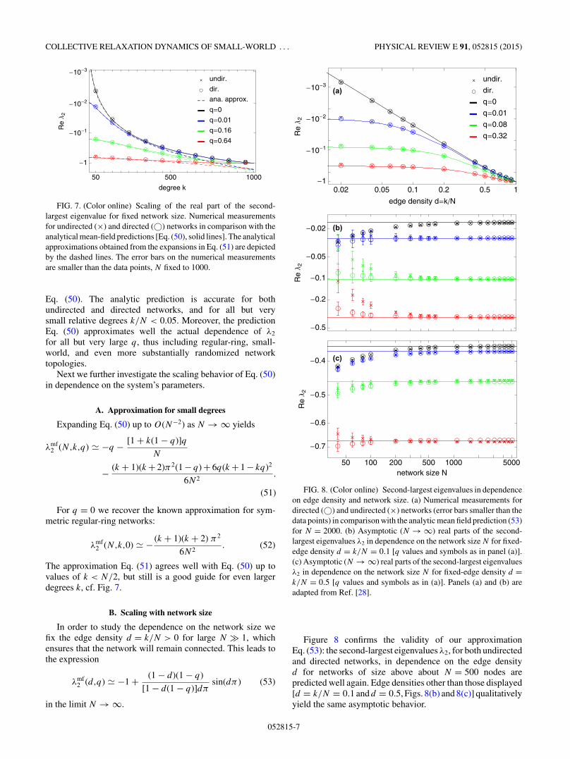
FIG. 7. (Color online) Scaling of the real part of the second-largest eigenvalue for fixed network size. Numerical measurementsfor undirected (×) and directed (©) networks in comparison with theanalytical mean-field predictions [Eq. (50), solid lines]. The analyticalapproximations obtained from the expansions in Eq. (51) are depictedby the dashed lines. The error bars on the numerical measurementsare smaller than the data points, N fixed to 1000.

Eq. (50). The analytic prediction is accurate for bothundirected and directed networks, and for all but verysmall relative degrees k/N < 0.05. Moreover, the predictionEq. (50) approximates well the actual dependence of λ2

for all but very large q, thus including regular-ring, small-world, and even more substantially randomized networktopologies.

Next we further investigate the scaling behavior of Eq. (50)in dependence on the system’s parameters.

A. Approximation for small degrees

Expanding Eq. (50) up to O(N−2) as N → ∞ yields

λmf2 (N,k,q) � −q − [1 + k(1 − q)]q

N

− (k + 1)(k + 2)π2(1 − q) + 6q(k + 1 − kq)2

6N2.

(51)

For q = 0 we recover the known approximation for sym-metric regular-ring networks:

λmf2 (N,k,0) � − (k + 1)(k + 2) π2

6N2. (52)

The approximation Eq. (51) agrees well with Eq. (50) up tovalues of k < N/2, but still is a good guide for even largerdegrees k, cf. Fig. 7.

B. Scaling with network size

In order to study the dependence on the network size wefix the edge density d = k/N > 0 for large N � 1, whichensures that the network will remain connected. This leads tothe expression

λmf2 (d,q) � −1 + (1 − d)(1 − q)

[1 − d(1 − q)]dπsin(dπ ) (53)

in the limit N → ∞.

FIG. 8. (Color online) Second-largest eigenvalues in dependenceon edge density and network size. (a) Numerical measurements fordirected (©) and undirected (×) networks (error bars smaller than thedata points) in comparison with the analytic mean field prediction (53)for N = 2000. (b) Asymptotic (N → ∞) real parts of the second-largest eigenvalues λ2 in dependence on the network size N for fixed-edge density d = k/N = 0.1 [q values and symbols as in panel (a)].(c) Asymptotic (N → ∞) real parts of the second-largest eigenvaluesλ2 in dependence on the network size N for fixed-edge density d =k/N = 0.5 [q values and symbols as in (a)]. Panels (a) and (b) areadapted from Ref. [28].

Figure 8 confirms the validity of our approximationEq. (53): the second-largest eigenvalues λ2, for both undirectedand directed networks, in dependence on the edge densityd for networks of size above about N = 500 nodes arepredicted well again. Edge densities other than those displayed[d = k/N = 0.1 and d = 0.5, Figs. 8(b) and 8(c)] qualitativelyyield the same asymptotic behavior.

052815-7

GRABOW, GROSSKINSKY, KURTHS, AND TIMME PHYSICAL REVIEW E 91, 052815 (2015)

FIG. 9. (Color online) Smallest eigenvalues from regular to ran-domized networks. Numerical measurements for undirected (×) anddirected (©) networks in comparison with the analytical mean-fieldpredictions [Eq. (45), solid lines] as a function of q, for differentdegrees k. Dashed lines show the analytic estimations of the smallesteigenvalues [Eq. (48)]. The error bars on the numerical measurementsare smaller than the data points (N = 1000, each data point averagedover 100 realizations).

C. The smallest eigenvalue

The smallest eigenvalue λ− defined in Eq. (45) isalso an important indicator for synchronization proper-ties, in particular—in combination with the second-largesteigenvalue—for the synchronizability (see, e.g., Ref. [25]).For directed networks this refers to the eigenvalue with thesmallest real part.

Here, the analytic prediction Eq. (33) again fits well withthe actual eigenvalues obtained by numerical diagonalization,cf. Fig. 9. Note also that our estimation Eq. (48) for the smallesteigenvalue agrees well with the actual analytic predictionEq. (45). It turns out that the analytic prediction is accuratefor both undirected and directed networks. The predictionEq. (50) approximates well the actual dependence of λ− forsmall q, thus including regular rings and small worlds. Theprediction is still a good guide for the general dependence ofthe second-largest eigenvalue on q, but shows some deviationfrom the numerical results for larger q, i.e., for substantiallyrandomized network topologies.

VI. ANALYTICAL PREDICTIONS FOR RANDOMTOPOLOGIES ANALYTICAL PREDICTIONS VIA

RANDOM MATRIX THEORY

To analytically predict the second largest eigenvalues for thegraph Laplacians of undirected and directed networks closeto q = 1 [see the shaded area (bottom, right) in Fig. 6] weconsult random matrix theory [50] (cf. also Refs. [51–54]).For a review of synchronization in networks with randominteractions, see, e.g., Ref. [55].

First, we consider undirected networks associated withsymmetric matrices. Here, every connection between a pairof nodes i and j �= i is present with a given probability P .

Second, we consider directed networks associated withasymmetric matrices. Here, all nodes have the same in-degreekini = kin. Each of the kin nodes that is connected to node i

is independently drawn from the set of all other nodes in thenetwork with uniform probability.

Given a sufficiently large network size N and a sufficientlylarge k (respectively, a sufficiently large kin), we numericallyfind that the set of nontrivial eigenvalues resemble disks ofradii r ′ for undirected networks and r for directed networks(cf. also Refs. [43,44]).

For directed networks where the in-degree kini = k for all

nodes i stays fixed during the whole rewiring procedure, i.e., alldiagonal elements are constant, the graph Laplacian is obtainedby shifting all eigenvalues of the adjacency matrix by −k. Forundirected networks there are small deviations from node tonode but the average degree equals k. However, numericalsimulations confirm that shifting here again the eigenvalues ofthe symmetric adjacency matrix by the negative average degree−k is feasible. Thus, we consider the adjacency matrices inthe following, Asym for undirected and Aasym for directednetworks, and later shift them by −k.

A. Ensembles of symmetric and asymmetric random matrices

First, consider N × N symmetric matrices A = AT withreal elements Aij . We constrain the diagonal entries to vanishAii = 0 and denote its N eigenvalues by λk . The elementsAij (i < j ) are independent, identically distributed randomvariables according to a probability distribution ρ(Aij ). Ac-cording to Refs. [56–58], there is only one known ensemblewith independent identically distributed matrix elements thatdiffers from the Gaussian one. Thus, there are exactly twouniversality classes, i.e., classes that do not depend on theprobability distribution ρ(Aij ) but are determined by matrixsymmetry only. Every ensemble of matrices within one ofthese universality classes exhibits the same distribution ofeigenvalues in the limit of large matrices, N → ∞, but theeigenvalue distributions are in general different for the twoclasses.

The arithmetic mean of the eigenvalues is zero,

[λi]i := 1

N

N∑i=1

λi = 1

N

N∑i=1

Aii = 0, (54)

and the ensemble variance of the matrix elements scales like

σ 2 = ⟨A2

ij

⟩ = r2

N, (55)

for N � 1 and r > 0 being the radii of disks that enclose theset of nontrivial eigenvalues for directed networks [43,44].

For the Gaussian symmetric ensemble, it is known [50,52]that the distribution of eigenvalues ρ

symGauss(λ) in the limit N →

∞ is given by Wigner’s semicircle law:

ρsymGauss(λ) =

{1

2πr2

√4r2 − λ2 if |λ| � 2r

0 otherwise.(56)

The ensemble of sparse matrices [56,57,59–62] exhibits adifferent eigenvalue distribution ρ

symsparse(λ) that depends on the

finite number k of nonzero entries per row and approaches thedistribution ρ

symGauss(λ) in the limit of large k, such that

limk→∞

ρsymsparse(λ) = ρ

symGauss(λ). (57)

052815-8

COLLECTIVE RELAXATION DYNAMICS OF SMALL-WORLD . . . PHYSICAL REVIEW E 91, 052815 (2015)

It is important to note that in the limit of large N theeigenvalue distributions ρ

symsparse and ρ

symGauss depend only on the

one parameter r , which is derived from the variance of thematrix elements Eq. (55).

For real, asymmetric matrices (independent Aij and Aji),there are no analytical results for the case of sparse matricesbut only for the case of Gaussian random matrices. TheGaussian asymmetric ensemble yields the distribution ofcomplex eigenvalues in a disk in the complex plane [63,64]

ρasymGauss(λ) =

{ 1πr2 if |λ| � r

0 otherwise,(58)

where r from Eq. (55) is the radius of the disk that is centeredaround the origin. Like in the case of symmetric matrices, thisdistribution also depends only on one parameter r , which isderived from the variance of the matrix elements.

B. Undirected random networks

The real symmetric adjacency matrix Asym is an N × N

matrix that satisfies Asymij = A

symji and A

symii = 0.

Furthermore, the matrix elements of Asym are independentup to the symmetry constraint A

symij = A

symji . They are equal to

1 with probability

P = 〈ki〉N − 1

≈ k

N, (59)

and equal to 0 with probability 1 − P .Thus, the variance σ 2 is given by

σ 2 = P (1 − P ) = k

N

(1 − k

N

). (60)

Therefore, the eigenvalues are located in a disk of radius

r ′ = 2r, (61)

with

r = σ√

N =√

k − k2

N(62)

centered around the origin.

C. Directed random networks

The real asymmetric adjacency matrix Aasym has exactly k

elements equal to one per row. Therefore, its elements have aspatial average

[A

asymij

]:= 1

N

N∑j=1

Aasymij = k

N(63)

and a second moment

[(Aasym

ij )2] = 1

N

N∑j=1

(Aasymij )

2 = k

N. (64)

Thus, the variance

σ 2 = [(Aasym

ij )2]− [

Aasymij

]2 = k

N− k2

N2. (65)

If we assume that the eigenvalue distribution for directednetworks with fixed in-degree is similar to those for random

matrices [43,44], we obtain a prediction from Eq. (55), whichyields

r = σ√

N =√

k − k2

N(66)

for the radius of the disk of eigenvalues centered around theorigin.

D. Predictions for the scaled graph Laplacians

To obtain predictions for the eigenvalues of the appropriategraph Laplacian, we have to consider the shift by −k

(discussed in the beginning of this section) and the scalingfactor 1/k introduced in Eq. (49).

Together with Eq. (62), the second-largest eigenvalues forundirected networks close to q = 1 [Fig. 10, (a)] are wellpredicted by Wigner’s semicircle law (wsc):

λwsc2 (N,k,1) = 1

k

(2

√k − k2

N− k

)

= 2

√1

k− 1

N− 1. (67)

The real parts of the eigenvalues for directed networks closeto q = 1 [Fig. 10(b)] with Eq. (66) are with the theory of

FIG. 10. (Color online) Analytic prediction of the second-largesteigenvalues close to q = 1. (a) Numerical measurements for undi-rected (×) networks in comparison with the analytical predictionsλwsc

2 via Wigner’s semicircle law [Eq. (67), solid lines], for differentdegrees k. (b) Numerical measurements for directed (©) networksin comparison with the analytical predictions λrmt

2 from the theoryof asymmetric random matrices [Eq. (68), solid lines]. The errorbars on the numerical measurements are smaller than the data points(N = 1000, each data point averaged over 100 realizations). Dashedlines are only a guide to the eye. Taken from Ref. [28].

052815-9

GRABOW, GROSSKINSKY, KURTHS, AND TIMME PHYSICAL REVIEW E 91, 052815 (2015)

asymmetric random matrices (rmt),

λrmt2 (N,k,1) = 1

k

(√k − k2

N− k

)

=√

1

k− 1

N− 1. (68)

Note that λwsc2 (N,k,1) in Eq. (67) acquires a positive value

for too small k values and a sufficiently large network sizeN (cf. [65]). However, for the k values we investigated[Figs. 10(a) and 10(b)], the second-largest eigenvalues arewell predicted by both Eqs. (67) and (68).

VII. SUMMARY AND DISCUSSION

In this article we have presented and explicated derivationsand extended a simple mean-field rewiring scheme suggestedrecently [28] to derive analytical predictions for the spectra ofgraph Laplacians. The key is replacing a stochastic realizationof a rewired network at given topological randomness by itsensemble-averaged network. We achieve this averaging via atwo-stage approach that distinguishes the original outer-ringstructure and the originally “empty” inner part of a networkand rewiring probabilities separately. For all q, the resultingaverage network in particular shares exactly the same (average)fraction of links in the original regular part of the network aswell as in its originally “empty” part. We derive expressionsfor the largest nontrivial and the smallest eigenvalues, the fullspectrum, as well as several scaling behaviors.

We remark that on theoretical grounds, the eigenvaluespectrum of the resulting average network in general isnot equal to the average of the spectra of the individualstochastic network realizations. Yet, systematic numericalchecks confirm that the mean-field approximation introducedis accurate as long as q is sufficiently below one. In the limitq → 1, we derive the eigenvalue spectra based on randommatrix theory, which become exact in the limit of infinitelylarge networks, N → ∞.

Although the mean-field rewiring is undirected, eigenvaluesfor directed networks are approximated more accurately andin a wider range of q values, which is in particular related tothe fact that the predictions for the undirected second-largesteigenvalues at q = 1 are larger in real part than the directedones, while all the mean-field eigenvalues converge to −1at q = 1. For “small” k values the mean-field approximationbecomes less accurate, which may be due to the fact thatthe ring structure is destroyed more easily while rewiring.Additionally, the bulk spectra spread much more drasticallywith q than for larger k values.

Furthermore, note that the analysis of the mean-fieldspectrum presented here can principally not be extendedto the Laplacian eigenvectors as these are independent ofthe mean-field Laplacian’s elements ci [19], just because ofthe circulant structure of the mean-field graph Laplacian.Consequently, the eigenvectors are the same and alwaysnonlocalized, independent of the system’s parameters N , k,and q. Studying distributed patterns of relaxation processesand potential localization phenomena thus requires access toeigenvectors beyond the mean-field approximation. Studiesof the Laplacian eigenvectors are rare, although there arefascinating results as well. For instance, the discrete analogsof solutions of the Schrodinger equation on manifolds can beinvestigated on graphs (cf., e.g., Ref. [11]).

The simple mean-field approach presented above stillsubstantially reduces computational efforts when studyingrandomized (regular or small-world) network models.

Generalizing our mean-field approach to higher dimensionsand/or to other rewiring approaches, as for instance, relevantfor neural network modeling [66], it will serve as a powerfultool to gain new insights into the relations between structuraland dynamical properties of complex networks.

ACKNOWLEDGMENTS

This work was supported by the BMBF, Grants No.03SF0472A (C.G., J.K.) and No. 03SF0472E (M.T.), by agrant of the Max Planck Society (M.T.), and by the Engineeringand Physical Sciences Research Council (EPSRC) Grant No.EP/E501311/1 (S.G.).

[1] A. Pikovsky, M. Rosenblum, and J. Kurths, Synchronization,A Universal Concept in Nonlinear Sciences, Vol. 12 of Cam-bridge Nonlinear Science Series (Cambridge University Press,Cambridge, UK, 2001).

[2] S. Strogatz, Nature 410, 268 (2001).[3] A. Pluchino, V. Latora, and A. Rapisarda, Int. J. Mod. Phys. C

16, 515 (2005).[4] R. Olfati-Saber, Proc. Am. Control Conf. 4, 2371 (2005).[5] M. Buchanan, G. Caldarelli, and P. De Los Rios, Networks in

Cell Biology (Cambridge University Press, Cambridge, 2010).[6] S. C. Manrubia, A. S. Mikhailov, and D. H. Zannette, Emergence

of Dynamical Order (World Scientific, Singapore, 2004).[7] D. McMillen, N. Kopell, J. Hasty, and J. Collins, Proc. Natl.

Acad. Sci. U.S.A. 99, 679 (2002).

[8] T. S. Gardner, D. di Bernardo, D. Lorenz, and J. J. Collins,Science 301, 102 (2003).

[9] F. C. Hoppensteadt and E. M. Izhikevich, Weakly ConnectedNeural Networks, Applied Mathematical Sciences (Springer,New York, 1997).

[10] B. Bollobas, Modern Graph Theory (Springer, New York,1998).

[11] T. Biyikoglu, J. Leydold, and P. F. Stadler, Laplacian Eigenvec-tors of Graphs (Springer, New York, 2007).

[12] A. E. Motter, C. Zhou, and J. Kurths, Phys. Rev. E 71, 016116(2005).

[13] F. Chung, Ann. Comb. 9, 1 (2005).[14] A. Motter, C. Zhou, and J. Kurths, Europhys. Lett. 69, 334

(2005).

052815-10

COLLECTIVE RELAXATION DYNAMICS OF SMALL-WORLD . . . PHYSICAL REVIEW E 91, 052815 (2015)

[15] R. Agaev and P. Chebotarev, Linear Algebra Appl. 399, 157(2005).

[16] L. Donetti, F. Neri, and M. A. Munoz, J. Stat. Mech.-Theory E.(2006) P08007.

[17] A. N. Samukhin, S. N. Dorogovtsev, and J. F. F. Mendes, Phys.Rev. E 77, 036115 (2008).

[18] A. Banerjee and J. Jost, Linear Algebra Appl. 428, 3015(2008).

[19] P. N. McGraw and M. Menzinger, Phys. Rev. E 77, 031102(2008).

[20] D. Watts and S. Strogatz, Nature 393, 440 (1998).[21] A. Barrat and M. Weigt, Eur. Phys. J. B 13, 547 (2000).[22] M. E. J. Newman, C. Moore, and D. J. Watts, Phys. Rev. Lett.

84, 3201 (2000).[23] R. Monasson, Eur. Phys. J. B 12, 555 (1999).[24] J. Jost and M. P. Joy, Phys. Rev. E 65, 016201 (2001).[25] M. Barahona and L. M. Pecora, Phys. Rev. Lett. 89, 054101

(2002).[26] F. Mori and T. Odagaki, J. Phys. Soc. Jpn. 73, 3294 (2004).[27] R. Kuhn and J. van Mourik, J. Phys. A 44, 165205 (2011).[28] C. Grabow, S. Grosskinsky, and M. Timme, Phys. Rev. Lett.

108, 218701 (2012).[29] A. Arenas, A. Diaz-Guilera, J. Kurths, Y. Moreno, and C. Zhou,

Phys. Rep. 469, 93 (2008).[30] L. M. Pecora and T. L. Carroll, Phys. Rev. Lett. 80, 2109

(1998).[31] B. Kriener, L. Anand, and M. Timme, New J. Phys. 14, 093002

(2012).[32] Y. Kuramoto, Chemical Oscillations, Waves and Turbulence

(Springer, Berlin, 1984).[33] J. Acebron, L. Bonilla, C. Vicente, F. Ritort, and R. Spigler, Rev.

Mod. Phys. 77, 137 (2005).[34] S. Kaka, M. R. Pufall, W. H. Rippard, T. J. Silva, S. E. Russek,

and J. A. Katine, Nature 437, 389 (2005).[35] M. Timme, Phys. Rev. Lett. 98, 224101 (2007).[36] C. Grabow, S. M. Hill, S. Grosskinsky, and M. Timme,

Europhys. Lett. 90, 48002 (2010).[37] D. Witthaut and M. Timme, Phys. Rev. E 90, 032917 (2014).[38] J. Tegner, M. K. S. Yeung, J. Hasty, and J. J. Collins, Proc. Natl.

Acad. Sci. USA 100, 5944 (2003).[39] M. Timme and J. Casadiego, J. Phys. A: Math. Theor. 47, 343001

(2014).

[40] M. Rohden, A. Sorge, M. Timme, and D. Witthaut, Phys. Rev.Lett. 109, 064101 (2012).

[41] D. Manik, D. Witthaut, B. Schafer, M. Matthiae, A. Sorge, M.Rohden, E. Katifori, and M. Timme, Eur. Phys. J.: Special Topics223, 2527 (2014).

[42] R. Olfati-Saber, J. A. Fax, and R. M. Murray, Proc. IEEE 95,215 (2007).

[43] M. Timme, F. Wolf, and T. Geisel, Phys. Rev. Lett. 92, 074101(2004).

[44] M. Timme, T. Geisel, and F. Wolf, Chaos 16, 015108 (2006).[45] G. Fagiolo, Phys. Rev. E 76, 026107 (2007).[46] G. Golub and C. Van Loan, Matrix Computations (Johns

Hopkins Studies in Mathematical Sciences) (Johns HopkinsUniversity Press, Baltimore, 1996).

[47] P. Lancaster and M. Tismenetsky, The Theory of Matrices, 2nded. (Academic Press, Orlando, 1985).

[48] R. M. Gray, Commun. Inf. Theory 2, 155 (2005).[49] C. Grabow, S. Grosskinsky, and M. Timme, Eur. Phys. J. B 84,

613 (2011).[50] E. P. Wigner, Proc. Cambridge Philos. Soc. 47, 790 (1951).[51] C. Porter, ed., Statistical Theory of Spectra: Fluctuations

(Academic Press, New York, 1965).[52] M. Mehta, Random Matrices (Academic Press, New York,

1991).[53] T. Tao and V. Vu, Bull. Amer. Math. Soc. 46, 377 (2009).[54] A. Edelman and N. R. Rao, Acta Numerica 14, 233 (2005).[55] J. Feng, V. Jirsa, and M. Ding, Chaos 16, 015109 (2006).[56] A. Mirlin and Y. Fyodorov, J. Phys. A 24, 2273 (1991).[57] Y. V. Fyodorov and A. D. Mirlin, Phys. Rev. Lett. 67, 2049

(1991).[58] G. Semerjian and L. F. Cugliandolo, J. Phys. A 35, 4837 (2002).[59] A. J. Bray and G. J. Rodgers, Phys. Rev. B 38, 11461 (1988).[60] G. J. Rodgers and A. J. Bray, Phys. Rev. B 37, 3557 (1988).[61] G. J. Rodgers, K. Austin, B. Kahng, and D. Kim, J. Phys. A 38,

9431 (2005).[62] F. Gotze and A. Tikhomirov, Ann. Probab. 38, 1444 (2010).[63] V. Girko, Theory Probab. Appl. 29, 694 (1985).[64] H. J. Sommers, A. Crisanti, H. Sompolinsky, and Y. Stein, Phys.

Rev. Lett. 60, 1895 (1988).[65] I. J. Farkas, I. Derenyi, A.-L. Barabasi, and T. Vicsek, Phys. Rev.

E 64, 026704 (2001).[66] O. Sporns and E. Bullmore, Nat. Rev. Neurosci. 10, 186 (2009).

052815-11