Comparative analysis of algorithms for identifying amplificationsand deletions in array CGH data

Weil R. Lai1, Mark D. Johnson2, Raju Kucherlapati1, and Peter J. Park1,3,*1Harvard-Partners Center for Genetics and Genomics, 77 Avenue Louis Pasteur, Boston, MA,021152Department of Neurological Surgery, Brigham and Women's Hospital and Harvard Medical School,75 Francis St, Boston, MA, 021153Children's Hospital Informatics Program, 300 Longwood Ave, Boston, MA, 02115

AbstractMotivation: Array Comparative Genomic Hybridization (CGH) can reveal chromosomalaberrations in the genomic DNA. These amplifications and deletions at the DNA level are importantin the pathogenesis of cancer and other diseases. While a large number of approaches have beenproposed for analyzing the large array CGH data sets, the relative merits of these methods in practiceare not clear.

Results: We compare eleven different algorithms for analyzing array CGH data. These includeboth segment detection methods and smoothing methods, based on such diverse techniques asmixture models, Hidden Markov Models, maximum likelihood, regression, wavelets, geneticalgorithms, and others. We compute the Receiver Operating Characteristic (ROC) curves usingsimulated data to quantify sensitivity and specificity for various levels of signal-to-noise ratio anddifferent sizes of abnormalities. We also characterize their performance on chromosomal regions ofinterest in a real data set obtained from patients with Glioblastoma Multiforme. While comparisonsof this type are difficult due to possibly sub-optimal choice of parameters in the methods, theynevertheless reveal general characteristics that are helpful to the biological investigator.

INTRODUCTIONLocating chromosomal aberrations in genomic DNA samples is an important step inunderstanding the pathogenesis of many diseases. This is especially true in cancer, and anenormous amount of effort and resources has been dedicated to the detailed characterizationof the chromosomal abnormalities in the development and progression of various cancers.Amplification or deletion of chromosomal segments can lead to abnormal mRNA transcriptlevels and results in the malfunctioning of cellular processes.

Array Comparative Genomic Hybridization (CGH) is a technique for measuring such changes(Solinas-Toldo et al., 1997; Pinkel et al., 1998). See Pinkel and Albertson (2005) for a review.The main difference between array CGH and mRNA expression profiling is that genomic DNArather than mRNA transcripts are hybridized in array CGH. As the resolution of the arrays hasimproved over the years, array CGH has become a powerful tool. As a high-throughputtechnique, it offers many advantages over other cytogenetic techniques such as Fluorescence

© Oxford University Press 2005.*to whom correspondence should be addressed.Contact: peter_park@harvard.edu

NIH Public AccessAuthor ManuscriptBioinformatics. Author manuscript; available in PMC 2010 February 10.

Published in final edited form as:Bioinformatics. 2005 October 1; 21(19): 3763. doi:10.1093/bioinformatics/bti611.

NIH

-PA Author Manuscript

NIH

-PA Author Manuscript

NIH

-PA Author Manuscript

in Situ Hybridization (FISH). Whereas early experimental techniques were only able to detectchromosomal changes at the whole chromosomal or whole arm level, the CGH arrays usingBAC (Bacterial Artificial Chromosome) clones have been widely used subsequently, with theresolution on the order of 1Mb (Pinkel et al., 1998). These arrays generally contain manyregions with known oncogenes and tumor suppressor genes, and can be iteratively designed ina locus-specific manner to identify candidate genes in a small region. More recently, cDNAand oligonucleotide arrays have become popular for CGH (Pollack et al., 1999; Brennan etal., 2004). The shorter probes on these new arrays may not be as robust as BACs for largesegments, but they offer much higher resolution (on the order of 50 – 100 Kb). In particular,oligonucleotide arrays allow design flexibility and greater coverage, and they appear to providesufficient sensitivity (Brennan et al., 2004). Tiling or custom arrays are also available now foreven finer resolution of specific regions and allow the detection of micro-amplifications anddeletions (Lucito et al., 2003; Ishkanian et al., 2004).

The resultant high-throughput array CGH data have prompted the development of variousalgorithms for data analysis, as briefly reviewed in the next section. However, while there havebeen numerous publications introducing new methods, the relative strengths and weaknessesof these methods are difficult to discern, due to the complexity of the algorithms and the lackof software with visualization tools. This problem is exacerbated by nondescript titles andabstracts of the articles and their lack of extensive performance comparisons to existingmethods. This is especially true from the perspective of the biologist who must choose analgorithm for the data set of interest. The purpose of this paper is to compare the algorithmsthat have been published so that the user can quickly gain an overview of the array CGHalgorithms and their performance. Both simulated data and real data obtained fromglioblastoma samples are used for evaluating the algorithms.

METHODSBasic Issues & Algorithms

Array CGH data consist of the log-ratios of normalized intensities from disease vs controlsamples, indexed by the physical location of the probes on the genome. The goal is to identifyregions of concentrated high or low log-ratios. In general, these regions of interest can be verysmall; some microdeletions may only contain a single probe. Because attempting to identifysuch small regions can result in too many false positives, information from consecutive probesare used to identify larger regions with more confidence.

The first analytical methods were simple yet intuitive and often effective, involving smoothingof the ratio profiles and applying a reasonable threshold to determine if the average ratio overa potential region signified an amplification or a deletion. For instance, a moving average wasused to process the ratios, and a ‘normal vs normal’ hybridization was used to compute athreshold level (Pollack et al., 2002). In another study, a simple maximum likelihood methodwas used to fit a mixture of three Gaussian distributions corresponding to gain, loss, and normalregions (Hodgson et al., 2001).

Broadly, there are two estimation problems. One is to infer the number and statisticalsignificance of the alterations; the other is to locate their boundaries accurately. The manyavailable methods differ in the ways in which each part is modeled and the two are combined.In general, the formulation of a model-based method presumes a sequence of piecewiseconstant segments, as a function of various parameters such as the number of breakpoints, theirlocations, and the mean/variance of the distributions for each segment. Then the maximizationof a function, typically a log-likelihood, is used to estimate the model parameters from the data.In the likelihood, a penalty term for the number of segments is often included to avoid too fine

Lai et al. Page 2

Bioinformatics. Author manuscript; available in PMC 2010 February 10.

NIH

-PA Author Manuscript

NIH

-PA Author Manuscript

NIH

-PA Author Manuscript

a partition which tends to increase the likelihood. Models differ in their distributionalassumptions and the incorporation of penalty terms.

Subsequently, more complicated methods for denoising and estimating the spatial dependencewere derived. Genomic amplifications and deletions are assumed to cover multiple probes ingeneral, and an effective incorporation of this spatial structure is a key component in anyalgorithm. For instance, a quantile smoothing method based on the minimization of errors inL1 norms (sum of absolute errors) rather than L2 norm (sum of squared errors) is shown to givesharper boundaries between segments (Eilers and de Menezes, 2005). Another promisingsmoothing algorithm is a denoising by wavelets (Hsu et al., 2005), a nonparametric techniquethat appears to handle abrupt changes in the profiles well. A simple and more common approachis based on robust locally weighted regression and smoothing scatterplots (lowess), introducedin Cleveland (1979). This has been used previously in other works such as in Beheshti et al.(2003).

In Olshen and Venkatraman (2002); Olshen et al. (2004), the binary segmentation method(Sen and Srivastava, 1975) is modified to allow splits into either two or three segments. In thisalgorithm, termed Circular Binary Segmentation (CBS), the maximum of a likelihood ratiostatistic is used recursively to detect narrower segments of aberration. In Jong et al. (2003,2004), a genetic search algorithm is used to maximize a likelihood with a penalty termcontaining the number of breakpoints. In Hupe et al. (2004), a more complex likelihoodfunction with weights determined adaptively is used to solve the estimation problem locallybased on data smoothed by the Adaptive Weights Smoothing procedure (Polzehl and Spokoiny,2000). A likelihood method with a different penalty function is used in Picard et al. (2005) forthe number of segments to avoid underestimation on the number of segments. It is pointed outthat a distribution assumption can have an importance consequence in a model: a homogeneousvariance assumption among different regions, for example, tends to lead to a more segmentedprofile in order to satisfy the variance assumption. In Daruwala et al. (2004), a Poissondistribution is used to model the number of segments and this is incorporated as an additionalcomponent in the likelihood. (This last method was not available publicly.)

In a more local approach (Myers et al., 2004), an edge filter is used to detect the approximatelocation of edges, and an EM algorithm is used to place them more precisely. In Lingjaerde etal. (2005), a simple smoothing is done using signs of neighbors, and significance is determinedby comparing both the width and height of the observed segments to their joint null distribution.A dynamic programming approach is used in Autio et al. (2003), but this was not part of ourstudy because the associated MATLAB package was difficult to port to our platform.

A different kind of modeling approach involves the Hidden Markov models (HMMs), in whichthe underlying copy numbers are the hidden states with certain transition probabilities (Snijderset al., 2003; Sebat et al., 2004; Fridlyand et al., 2004). In Wang et al. (2005), a simple buteffective method based on hierarchical clustering along the chromosomes is used to identifyregions of interest and the False Discovery Rate (FDR) is used as a selection criterion.

Evaluation MethodEvaluating the relative performance of these methods is complicated by several problems. Onedifficulty is that the goals of different algorithms are not the same. For example, those with anemphasis on the smoothing part may simply return the log-ratios without determining whichones are significant. More comprehensive methods may return the coordinates of only thestatistically significant segments with or without the estimated average log-ratio per segment.One may require a ‘normal vs normal’ sample as a control while another may not. Whennecessary, we simulated the control samples by Gaussian noise with zero mean and a varianceestimated from the tested data using the median absolute deviation.

Lai et al. Page 3

Bioinformatics. Author manuscript; available in PMC 2010 February 10.

NIH

-PA Author Manuscript

NIH

-PA Author Manuscript

NIH

-PA Author Manuscript

In terms of implementation, the primary issue was that not every algorithm was implementedin publicly available software. All our calculations were carried out in the statistical languageR (R Development Core Team, 2004), since this was the dominant platform for the softwarepackages. But other algorithms were implemented in MATLAB, a JAVA application, or anexecutable file. When the code could be ported easily from MATLAB to R, such as thealgorithm in Picard et al. (2005), this was carried out. When a program allowed a relativelysimple interface, as was the case with the algorithms in Jong et al. (2004), Myers et al.(2004), and Lingjaerde et al. (2005), it was used for computations.

The most appropriate way to compare these algorithms on simulated data was to calculate theReceiver Operating Characteristic (ROC) curves. Because different algorithms were tuned atdifferent sensitivity levels, it was important to examine the trade-off between sensitivity andspecificity in each case. This approach adjusts for the differences arising from identifyingdifferent numbers of segments in each algorithm. We have used the default parameters for eachalgorithm, as most users will be doing. If no default parameters were available, we used thesteps suggested in the program documentation or the papers describing the method to selectthe parameter values. We have not attempted to adjust the parameters to improve theperformance, due to the large number of algorithms and the large number of scenarios underwhich they were tested. This issue is further discussed in Discussion. The general propertiesare nonetheless apparent, even if the parameters were suboptimal.

RESULTSFirst, we tested the algorithms on simulated data of various abnormality widths and noise levels.To generate ROC curves corresponding to a particular aberration width and noise level, wecalculated the true positive rates (TPR) and the false positive rates (FPR) as we varied thethreshold for determining an aberration. We also tested the algorithms on cDNA microarraydata containing measurements from 26 different primary Glioblastoma Multiforme (GBM)tumors (Bredel et al., 2005).

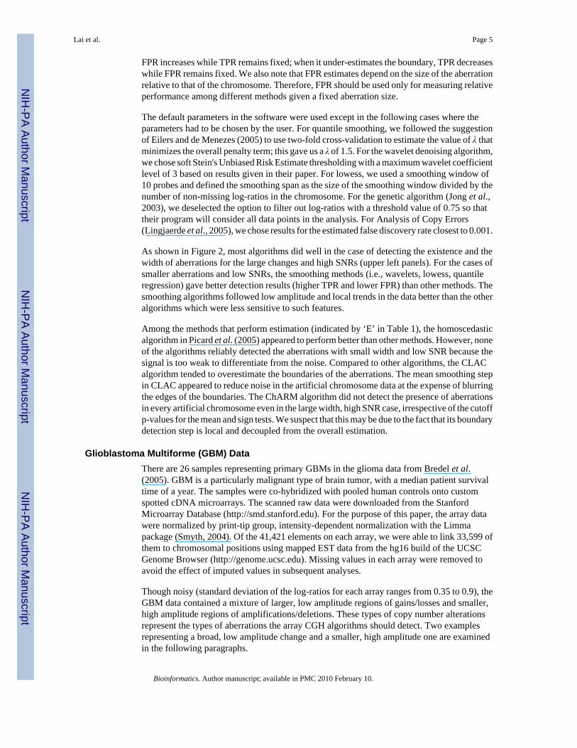
Simulated DataWe calculated the ROC profiles of each algorithm for aberration widths of 5, 10, 20, and 40probes and signal-to-noise ratios (SNR) of 1, 2, 3, and 4. SNR was defined as the meanmagnitude of the aberration (i.e., signal) divided by the standard deviation of the superimposedGaussian noise. Figure 1 illustrates the kind of profiles examined in this simulation. For eachaberration width and SNR, we generated 100 artificial chromosomes, each consisting of 100probes and with the square-wave signal profile added to the center of the chromosome. Theperformance of the algorithms for the aberrations at the boundaries was not examined here.

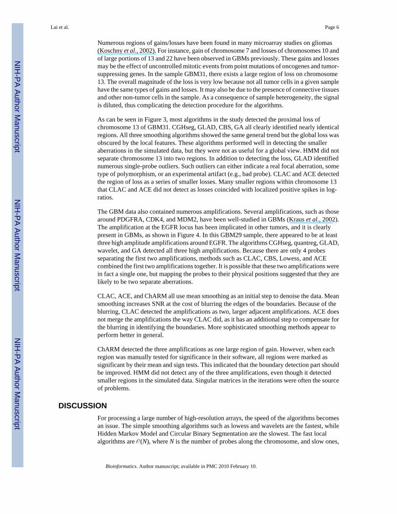
TPR was defined as the number of probes inside the aberration whose fitted values are abovethe threshold level divided by the number of probes in the aberration. FPR was defined as thenumber of probes outside the aberration whose fitted values are above the threshold leveldivided by the total number of probes outside the aberration. In order to compute the ROCcurve, we varied the threshold value for aberration from the minimum log-ratio value to themaximum. (This is equivalent to moving the x-axis cutoff value in a mixture distribution.) Eachthreshold value results in a TPR and a FPR, represented by a point on the ROC curve. A setof TPRs and FPRs were then plotted to reveal the algorithm's ROC profile for the particularaberration width and SNR (see Figure 2). We also computed confidence intervals around eachROC curve (not shown) but there did not appear to be significant differences among themethods.

We note that TPR and FPR are informative in understanding how an algorithm performs inestimating the boundary of the altered region. When the algorithm over-estimates the boundary,

Lai et al. Page 4

Bioinformatics. Author manuscript; available in PMC 2010 February 10.

NIH

-PA Author Manuscript

NIH

-PA Author Manuscript

NIH

-PA Author Manuscript

FPR increases while TPR remains fixed; when it under-estimates the boundary, TPR decreaseswhile FPR remains fixed. We also note that FPR estimates depend on the size of the aberrationrelative to that of the chromosome. Therefore, FPR should be used only for measuring relativeperformance among different methods given a fixed aberration size.

The default parameters in the software were used except in the following cases where theparameters had to be chosen by the user. For quantile smoothing, we followed the suggestionof Eilers and de Menezes (2005) to use two-fold cross-validation to estimate the value of λ thatminimizes the overall penalty term; this gave us a λ of 1.5. For the wavelet denoising algorithm,we chose soft Stein's Unbiased Risk Estimate thresholding with a maximum wavelet coefficientlevel of 3 based on results given in their paper. For lowess, we used a smoothing window of10 probes and defined the smoothing span as the size of the smoothing window divided by thenumber of non-missing log-ratios in the chromosome. For the genetic algorithm (Jong et al.,2003), we deselected the option to filter out log-ratios with a threshold value of 0.75 so thattheir program will consider all data points in the analysis. For Analysis of Copy Errors(Lingjaerde et al., 2005), we chose results for the estimated false discovery rate closest to 0.001.

As shown in Figure 2, most algorithms did well in the case of detecting the existence and thewidth of aberrations for the large changes and high SNRs (upper left panels). For the cases ofsmaller aberrations and low SNRs, the smoothing methods (i.e., wavelets, lowess, quantileregression) gave better detection results (higher TPR and lower FPR) than other methods. Thesmoothing algorithms followed low amplitude and local trends in the data better than the otheralgorithms which were less sensitive to such features.

Among the methods that perform estimation (indicated by ‘E’ in Table 1), the homoscedasticalgorithm in Picard et al. (2005) appeared to perform better than other methods. However, noneof the algorithms reliably detected the aberrations with small width and low SNR because thesignal is too weak to differentiate from the noise. Compared to other algorithms, the CLACalgorithm tended to overestimate the boundaries of the aberrations. The mean smoothing stepin CLAC appeared to reduce noise in the artificial chromosome data at the expense of blurringthe edges of the boundaries. The ChARM algorithm did not detect the presence of aberrationsin every artificial chromosome even in the large width, high SNR case, irrespective of the cutoffp-values for the mean and sign tests. We suspect that this may be due to the fact that its boundarydetection step is local and decoupled from the overall estimation.

Glioblastoma Multiforme (GBM) DataThere are 26 samples representing primary GBMs in the glioma data from Bredel et al.(2005). GBM is a particularly malignant type of brain tumor, with a median patient survivaltime of a year. The samples were co-hybridized with pooled human controls onto customspotted cDNA microarrays. The scanned raw data were downloaded from the StanfordMicroarray Database (http://smd.stanford.edu). For the purpose of this paper, the array datawere normalized by print-tip group, intensity-dependent normalization with the Limmapackage (Smyth, 2004). Of the 41,421 elements on each array, we were able to link 33,599 ofthem to chromosomal positions using mapped EST data from the hg16 build of the UCSCGenome Browser (http://genome.ucsc.edu). Missing values in each array were removed toavoid the effect of imputed values in subsequent analyses.

Though noisy (standard deviation of the log-ratios for each array ranges from 0.35 to 0.9), theGBM data contained a mixture of larger, low amplitude regions of gains/losses and smaller,high amplitude regions of amplifications/deletions. These types of copy number alterationsrepresent the types of aberrations the array CGH algorithms should detect. Two examplesrepresenting a broad, low amplitude change and a smaller, high amplitude one are examinedin the following paragraphs.

Lai et al. Page 5

Bioinformatics. Author manuscript; available in PMC 2010 February 10.

NIH

-PA Author Manuscript

NIH

-PA Author Manuscript

NIH

-PA Author Manuscript

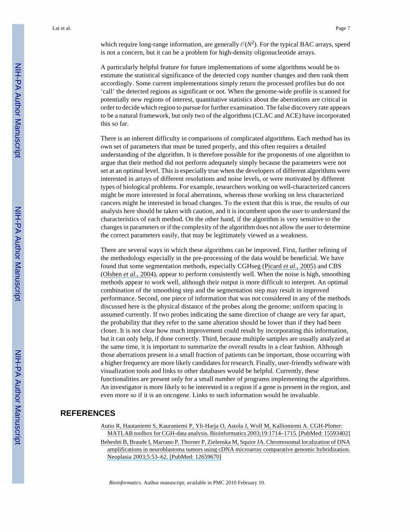
Numerous regions of gains/losses have been found in many microarray studies on gliomas(Koschny et al., 2002). For instance, gain of chromosome 7 and losses of chromosomes 10 andof large portions of 13 and 22 have been observed in GBMs previously. These gains and lossesmay be the effect of uncontrolled mitotic events from point mutations of oncogenes and tumor-suppressing genes. In the sample GBM31, there exists a large region of loss on chromosome13. The overall magnitude of the loss is very low because not all tumor cells in a given samplehave the same types of gains and losses. It may also be due to the presence of connective tissuesand other non-tumor cells in the sample. As a consequence of sample heterogeneity, the signalis diluted, thus complicating the detection procedure for the algorithms.

As can be seen in Figure 3, most algorithms in the study detected the proximal loss ofchromosome 13 of GBM31. CGHseg, GLAD, CBS, GA all clearly identified nearly identicalregions. All three smoothing algorithms showed the same general trend but the global loss wasobscured by the local features. These algorithms performed well in detecting the smalleraberrations in the simulated data, but they were not as useful for a global view. HMM did notseparate chromosome 13 into two regions. In addition to detecting the loss, GLAD identifiednumerous single-probe outliers. Such outliers can either indicate a real focal aberration, sometype of polymorphism, or an experimental artifact (e.g., bad probe). CLAC and ACE detectedthe region of loss as a series of smaller losses. Many smaller regions within chromosome 13that CLAC and ACE did not detect as losses coincided with localized positive spikes in log-ratios.

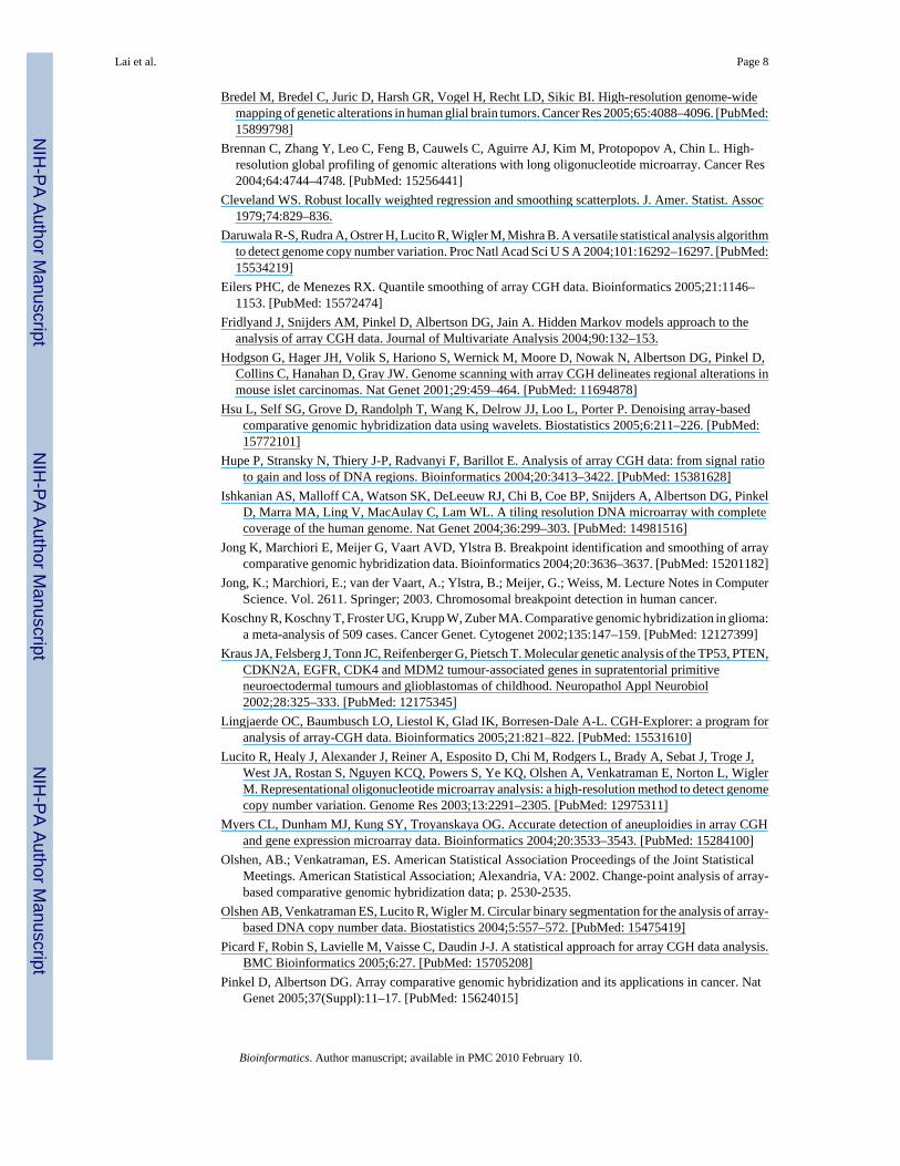
The GBM data also contained numerous amplifications. Several amplifications, such as thosearound PDGFRA, CDK4, and MDM2, have been well-studied in GBMs (Kraus et al., 2002).The amplification at the EGFR locus has been implicated in other tumors, and it is clearlypresent in GBMs, as shown in Figure 4. In this GBM29 sample, there appeared to be at leastthree high amplitude amplifications around EGFR. The algorithms CGHseg, quantreg, GLAD,wavelet, and GA detected all three high amplifications. Because there are only 4 probesseparating the first two amplifications, methods such as CLAC, CBS, Lowess, and ACEcombined the first two amplifications together. It is possible that these two amplifications werein fact a single one, but mapping the probes to their physical positions suggested that they arelikely to be two separate aberrations.

CLAC, ACE, and ChARM all use mean smoothing as an initial step to denoise the data. Meansmoothing increases SNR at the cost of blurring the edges of the boundaries. Because of theblurring, CLAC detected the amplifications as two, larger adjacent amplifications. ACE doesnot merge the amplifications the way CLAC did, as it has an additional step to compensate forthe blurring in identifying the boundaries. More sophisticated smoothing methods appear toperform better in general.

ChARM detected the three amplifications as one large region of gain. However, when eachregion was manually tested for significance in their software, all regions were marked assignificant by their mean and sign tests. This indicated that the boundary detection part shouldbe improved. HMM did not detect any of the three amplifications, even though it detectedsmaller regions in the simulated data. Singular matrices in the iterations were often the sourceof problems.

DISCUSSIONFor processing a large number of high-resolution arrays, the speed of the algorithms becomesan issue. The simple smoothing algorithms such as lowess and wavelets are the fastest, whileHidden Markov Model and Circular Binary Segmentation are the slowest. The fast localalgorithms are (N), where N is the number of probes along the chromosome, and slow ones,

Lai et al. Page 6

Bioinformatics. Author manuscript; available in PMC 2010 February 10.

NIH

-PA Author Manuscript

NIH

-PA Author Manuscript

NIH

-PA Author Manuscript

which require long-range information, are generally (N2). For the typical BAC arrays, speedis not a concern, but it can be a problem for high-density oligonucleotide arrays.

A particularly helpful feature for future implementations of some algorithms would be toestimate the statistical significance of the detected copy number changes and then rank themaccordingly. Some current implementations simply return the processed profiles but do not‘call’ the detected regions as significant or not. When the genome-wide profile is scanned forpotentially new regions of interest, quantitative statistics about the aberrations are critical inorder to decide which region to pursue for further examination. The false discovery rate appearsto be a natural framework, but only two of the algorithms (CLAC and ACE) have incorporatedthis so far.

There is an inherent difficulty in comparisons of complicated algorithms. Each method has itsown set of parameters that must be tuned properly, and this often requires a detailedunderstanding of the algorithm. It is therefore possible for the proponents of one algorithm toargue that their method did not perform adequately simply because the parameters were notset at an optimal level. This is especially true when the developers of different algorithms wereinterested in arrays of different resolutions and noise levels, or were motivated by differenttypes of biological problems. For example, researchers working on well-characterized cancersmight be more interested in focal aberrations, whereas those working on less characterizedcancers might be interested in broad changes. To the extent that this is true, the results of ouranalysis here should be taken with caution, and it is incumbent upon the user to understand thecharacteristics of each method. On the other hand, if the algorithm is very sensitive to thechanges in parameters or if the complexity of the algorithm does not allow the user to determinethe correct parameters easily, that may be legitimately viewed as a weakness.

There are several ways in which these algorithms can be improved. First, further refining ofthe methodology especially in the pre-processing of the data would be beneficial. We havefound that some segmentation methods, especially CGHseg (Picard et al., 2005) and CBS(Olshen et al., 2004), appear to perform consistently well. When the noise is high, smoothingmethods appear to work well, although their output is more difficult to interpret. An optimalcombination of the smoothing step and the segmentation step may result in improvedperformance. Second, one piece of information that was not considered in any of the methodsdiscussed here is the physical distance of the probes along the genome; uniform spacing isassumed currently. If two probes indicating the same direction of change are very far apart,the probability that they refer to the same alteration should be lower than if they had beencloser. It is not clear how much improvement could result by incorporating this information,but it can only help, if done correctly. Third, because multiple samples are usually analyzed atthe same time, it is important to summarize the overall results in a clear fashion. Althoughthose aberrations present in a small fraction of patients can be important, those occurring witha higher frequency are more likely candidates for research. Finally, user-friendly software withvisualization tools and links to other databases would be helpful. Currently, thesefunctionalities are present only for a small number of programs implementing the algorithms.An investigator is more likely to be interested in a region if a gene is present in the region, andeven more so if it is an oncogene. Links to such information would be invaluable.

REFERENCESAutio R, Hautaniemi S, Kauraniemi P, Yli-Harja O, Astola J, Wolf M, Kallioniemi A. CGH-Plotter:

MATLAB toolbox for CGH-data analysis. Bioinformatics 2003;19:1714–1715. [PubMed: 15593402]Beheshti B, Braude I, Marrano P, Thorner P, Zielenska M, Squire JA. Chromosomal localization of DNA

amplifications in neuroblastoma tumors using cDNA microarray comparative genomic hybridization.Neoplasia 2003;5:53–62. [PubMed: 12659670]

Lai et al. Page 7

Bioinformatics. Author manuscript; available in PMC 2010 February 10.

NIH

-PA Author Manuscript

NIH

-PA Author Manuscript

NIH

-PA Author Manuscript

Bredel M, Bredel C, Juric D, Harsh GR, Vogel H, Recht LD, Sikic BI. High-resolution genome-widemapping of genetic alterations in human glial brain tumors. Cancer Res 2005;65:4088–4096. [PubMed:15899798]

Brennan C, Zhang Y, Leo C, Feng B, Cauwels C, Aguirre AJ, Kim M, Protopopov A, Chin L. High-resolution global profiling of genomic alterations with long oligonucleotide microarray. Cancer Res2004;64:4744–4748. [PubMed: 15256441]

Cleveland WS. Robust locally weighted regression and smoothing scatterplots. J. Amer. Statist. Assoc1979;74:829–836.

Daruwala R-S, Rudra A, Ostrer H, Lucito R, Wigler M, Mishra B. A versatile statistical analysis algorithmto detect genome copy number variation. Proc Natl Acad Sci U S A 2004;101:16292–16297. [PubMed:15534219]

Eilers PHC, de Menezes RX. Quantile smoothing of array CGH data. Bioinformatics 2005;21:1146–1153. [PubMed: 15572474]

Fridlyand J, Snijders AM, Pinkel D, Albertson DG, Jain A. Hidden Markov models approach to theanalysis of array CGH data. Journal of Multivariate Analysis 2004;90:132–153.

Hodgson G, Hager JH, Volik S, Hariono S, Wernick M, Moore D, Nowak N, Albertson DG, Pinkel D,Collins C, Hanahan D, Gray JW. Genome scanning with array CGH delineates regional alterations inmouse islet carcinomas. Nat Genet 2001;29:459–464. [PubMed: 11694878]

Hsu L, Self SG, Grove D, Randolph T, Wang K, Delrow JJ, Loo L, Porter P. Denoising array-basedcomparative genomic hybridization data using wavelets. Biostatistics 2005;6:211–226. [PubMed:15772101]

Hupe P, Stransky N, Thiery J-P, Radvanyi F, Barillot E. Analysis of array CGH data: from signal ratioto gain and loss of DNA regions. Bioinformatics 2004;20:3413–3422. [PubMed: 15381628]

Ishkanian AS, Malloff CA, Watson SK, DeLeeuw RJ, Chi B, Coe BP, Snijders A, Albertson DG, PinkelD, Marra MA, Ling V, MacAulay C, Lam WL. A tiling resolution DNA microarray with completecoverage of the human genome. Nat Genet 2004;36:299–303. [PubMed: 14981516]

Jong K, Marchiori E, Meijer G, Vaart AVD, Ylstra B. Breakpoint identification and smoothing of arraycomparative genomic hybridization data. Bioinformatics 2004;20:3636–3637. [PubMed: 15201182]

Jong, K.; Marchiori, E.; van der Vaart, A.; Ylstra, B.; Meijer, G.; Weiss, M. Lecture Notes in ComputerScience. Vol. 2611. Springer; 2003. Chromosomal breakpoint detection in human cancer.

Koschny R, Koschny T, Froster UG, Krupp W, Zuber MA. Comparative genomic hybridization in glioma:a meta-analysis of 509 cases. Cancer Genet. Cytogenet 2002;135:147–159. [PubMed: 12127399]

Kraus JA, Felsberg J, Tonn JC, Reifenberger G, Pietsch T. Molecular genetic analysis of the TP53, PTEN,CDKN2A, EGFR, CDK4 and MDM2 tumour-associated genes in supratentorial primitiveneuroectodermal tumours and glioblastomas of childhood. Neuropathol Appl Neurobiol2002;28:325–333. [PubMed: 12175345]

Lingjaerde OC, Baumbusch LO, Liestol K, Glad IK, Borresen-Dale A-L. CGH-Explorer: a program foranalysis of array-CGH data. Bioinformatics 2005;21:821–822. [PubMed: 15531610]

Lucito R, Healy J, Alexander J, Reiner A, Esposito D, Chi M, Rodgers L, Brady A, Sebat J, Troge J,West JA, Rostan S, Nguyen KCQ, Powers S, Ye KQ, Olshen A, Venkatraman E, Norton L, WiglerM. Representational oligonucleotide microarray analysis: a high-resolution method to detect genomecopy number variation. Genome Res 2003;13:2291–2305. [PubMed: 12975311]

Myers CL, Dunham MJ, Kung SY, Troyanskaya OG. Accurate detection of aneuploidies in array CGHand gene expression microarray data. Bioinformatics 2004;20:3533–3543. [PubMed: 15284100]

Olshen, AB.; Venkatraman, ES. American Statistical Association Proceedings of the Joint StatisticalMeetings. American Statistical Association; Alexandria, VA: 2002. Change-point analysis of array-based comparative genomic hybridization data; p. 2530-2535.

Olshen AB, Venkatraman ES, Lucito R, Wigler M. Circular binary segmentation for the analysis of array-based DNA copy number data. Biostatistics 2004;5:557–572. [PubMed: 15475419]

Picard F, Robin S, Lavielle M, Vaisse C, Daudin J-J. A statistical approach for array CGH data analysis.BMC Bioinformatics 2005;6:27. [PubMed: 15705208]

Pinkel D, Albertson DG. Array comparative genomic hybridization and its applications in cancer. NatGenet 2005;37(Suppl):11–17. [PubMed: 15624015]

Lai et al. Page 8

Bioinformatics. Author manuscript; available in PMC 2010 February 10.

NIH

-PA Author Manuscript

NIH

-PA Author Manuscript

NIH

-PA Author Manuscript

Pinkel D, Segraves R, Sudar D, Clark S, Poole I, Kowbel D, Collins C, Kuo WL, Chen C, Zhai Y, DairkeeSH, Ljung BM, Gray JW, Albertson DG. High resolution analysis of DNA copy number variationusing comparative genomic hybridization to microarrays. Nat Genet 1998;20:207–211. [PubMed:9771718]

Pollack JR, Perou CM, Alizadeh AA, Eisen MB, Pergamenschikov A, Williams CF, Jeffrey SS, BotsteinD, Brown PO. Genome-wide analysis of DNA copy-number changes using cDNA microarrays. NatGenet 1999;23:41–46. [PubMed: 10471496]

Pollack JR, Sorlie T, Perou CM, Rees CA, Jeffrey SS, Lonning PE, Tibshirani R, Botstein D, Borresen-Dale A-L, Brown PO. Microarray analysis reveals a major direct role of DNA copy number alterationin the transcriptional program of human breast tumors. Proc Natl Acad Sci U S A 2002;99:12963–12968. [PubMed: 12297621]

Polzehl J, Spokoiny V. Adaptive weights smoothing with applications to image restoration. J. R. Statist.Soc. B 2000;62(Part 2):335–354.

R Development Core Team. R: A language and environment for statistical computing. R Foundation forStatistical Computing; Vienna, Austria: 2004. URL http://www.R-project.org

Sebat J, Lakshmi B, Troge J, Alexander J, Young J, Lundin P, Maner S, Massa H, Walker M, Chi M,Navin N, Lucito R, Healy J, Hicks J, Ye K, Reiner A, Gilliam TC, Trask B, Patterson N, ZetterbergA, Wigler M. Large-scale copy number polymorphism in the human genome. Science 2004;305:525–528. [PubMed: 15273396]

Sen A, Srivastava M. On tests for detecting a change in mean. Annals of Statistics 1975;3:98–108.Smyth GK. Linear models and empirical bayes methods for assessing differential expression in

microarray experiments. Statistical Applications in Genetics and Molecular Biology 2004;3 Article3.

Snijders AM, Fridlyand J, Mans DA, Segraves R, Jain AN, Pinkel D, Albertson DG. Shaping of tumorand drug-resistant genomes by instability and selection. Oncogene 2003;22:4370–4379. [PubMed:12853973]

Solinas-Toldo S, Lampel S, Stilgenbauer S, Nickolenko J, Benner A, Dohner H, Cremer T, Lichter P.Matrix-based comparative genomic hybridization: biochips to screen for genomic imbalances. GenesChromosomes Cancer 1997;20:399–407. [PubMed: 9408757]

Wang P, Kim Y, Pollack J, Narasimhan B, Tibshirani R. A method for calling gains and losses in arrayCGH data. Biostatistics 2005;6:45–58. [PubMed: 15618527]

Lai et al. Page 9

Bioinformatics. Author manuscript; available in PMC 2010 February 10.

NIH

-PA Author Manuscript

NIH

-PA Author Manuscript

NIH

-PA Author Manuscript

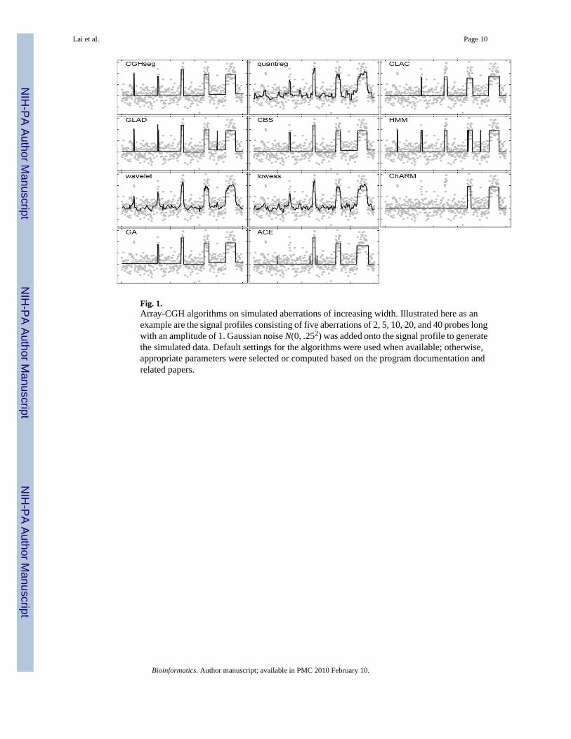
Fig. 1.Array-CGH algorithms on simulated aberrations of increasing width. Illustrated here as anexample are the signal profiles consisting of five aberrations of 2, 5, 10, 20, and 40 probes longwith an amplitude of 1. Gaussian noise N(0, .252) was added onto the signal profile to generatethe simulated data. Default settings for the algorithms were used when available; otherwise,appropriate parameters were selected or computed based on the program documentation andrelated papers.

Lai et al. Page 10

Bioinformatics. Author manuscript; available in PMC 2010 February 10.

NIH

-PA Author Manuscript

NIH

-PA Author Manuscript

NIH

-PA Author Manuscript

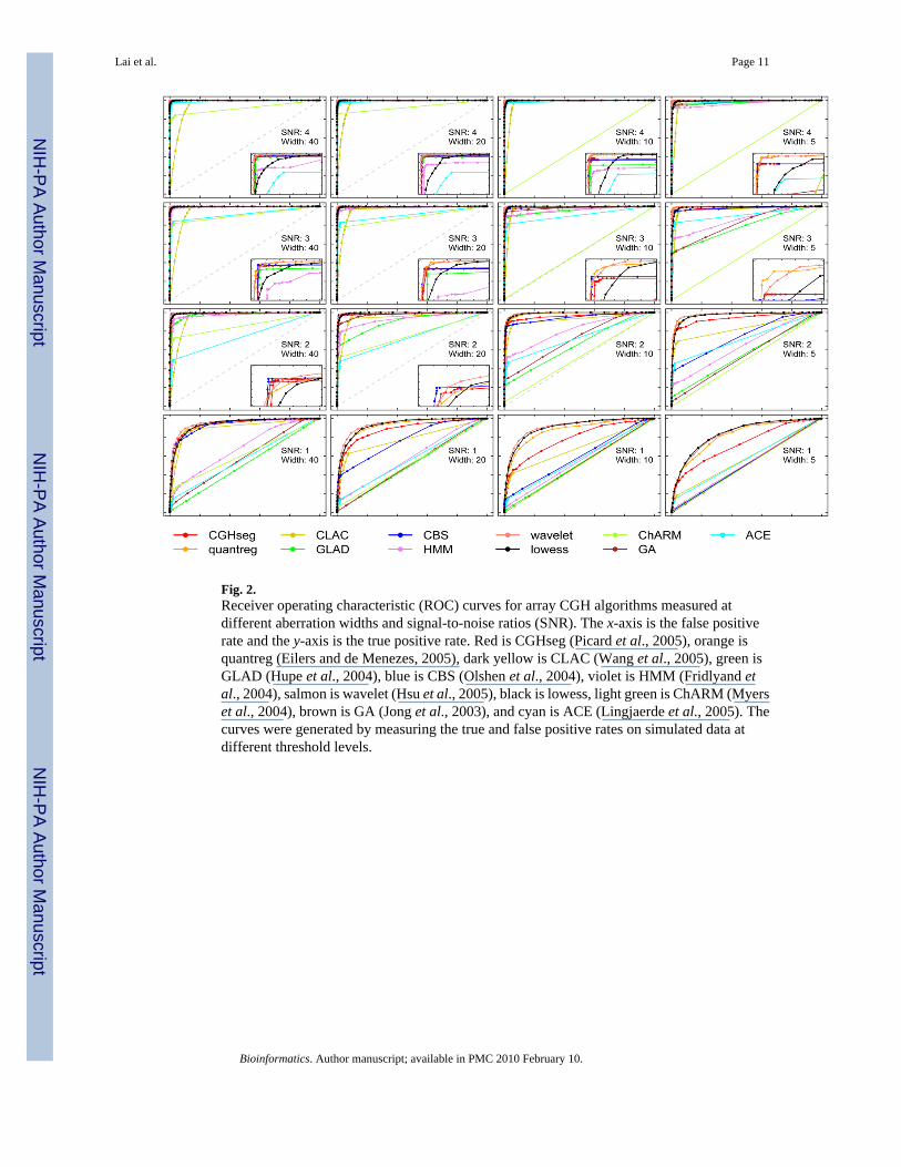
Fig. 2.Receiver operating characteristic (ROC) curves for array CGH algorithms measured atdifferent aberration widths and signal-to-noise ratios (SNR). The x-axis is the false positiverate and the y-axis is the true positive rate. Red is CGHseg (Picard et al., 2005), orange isquantreg (Eilers and de Menezes, 2005), dark yellow is CLAC (Wang et al., 2005), green isGLAD (Hupe et al., 2004), blue is CBS (Olshen et al., 2004), violet is HMM (Fridlyand etal., 2004), salmon is wavelet (Hsu et al., 2005), black is lowess, light green is ChARM (Myerset al., 2004), brown is GA (Jong et al., 2003), and cyan is ACE (Lingjaerde et al., 2005). Thecurves were generated by measuring the true and false positive rates on simulated data atdifferent threshold levels.

Lai et al. Page 11

Bioinformatics. Author manuscript; available in PMC 2010 February 10.

NIH

-PA Author Manuscript

NIH

-PA Author Manuscript

NIH

-PA Author Manuscript

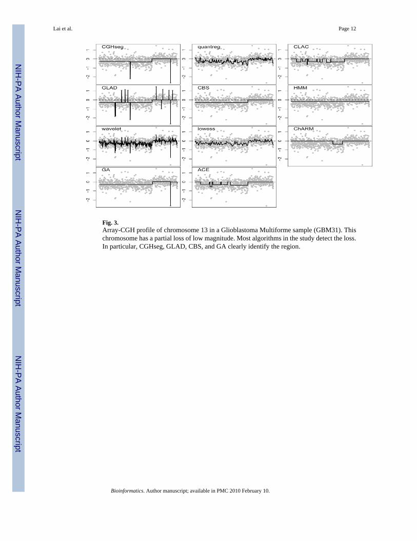
Fig. 3.Array-CGH profile of chromosome 13 in a Glioblastoma Multiforme sample (GBM31). Thischromosome has a partial loss of low magnitude. Most algorithms in the study detect the loss.In particular, CGHseg, GLAD, CBS, and GA clearly identify the region.

Lai et al. Page 12

Bioinformatics. Author manuscript; available in PMC 2010 February 10.

NIH

-PA Author Manuscript

NIH

-PA Author Manuscript

NIH

-PA Author Manuscript

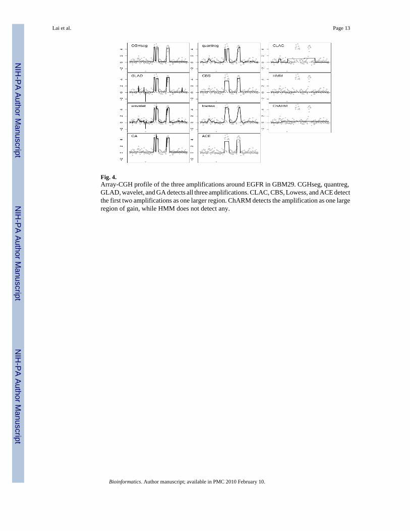
Fig. 4.Array-CGH profile of the three amplifications around EGFR in GBM29. CGHseg, quantreg,GLAD, wavelet, and GA detects all three amplifications. CLAC, CBS, Lowess, and ACE detectthe first two amplifications as one larger region. ChARM detects the amplification as one largeregion of gain, while HMM does not detect any.

Lai et al. Page 13

Bioinformatics. Author manuscript; available in PMC 2010 February 10.

NIH

-PA Author Manuscript

NIH

-PA Author Manuscript

NIH

-PA Author Manuscript

NIH

-PA Author Manuscript

NIH

-PA Author Manuscript

NIH

-PA Author Manuscript

Lai et al. Page 14

Table 1

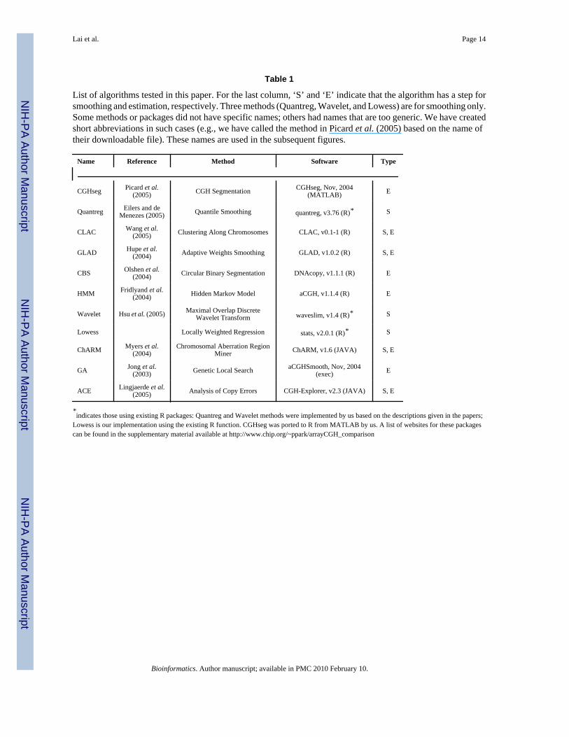
List of algorithms tested in this paper. For the last column, ‘S’ and ‘E’ indicate that the algorithm has a step forsmoothing and estimation, respectively. Three methods (Quantreg, Wavelet, and Lowess) are for smoothing only.Some methods or packages did not have specific names; others had names that are too generic. We have createdshort abbreviations in such cases (e.g., we have called the method in Picard et al. (2005) based on the name oftheir downloadable file). These names are used in the subsequent figures.

Name Reference Method Software Type

CGHseg Picard et al.(2005) CGH Segmentation CGHseg, Nov, 2004

(MATLAB) E

Quantreg Eilers and deMenezes (2005) Quantile Smoothing quantreg, v3.76 (R)* S

CLAC Wang et al.(2005) Clustering Along Chromosomes CLAC, v0.1-1 (R) S, E

GLAD Hupe et al.(2004) Adaptive Weights Smoothing GLAD, v1.0.2 (R) S, E

CBS Olshen et al.(2004) Circular Binary Segmentation DNAcopy, v1.1.1 (R) E

HMM Fridlyand et al.(2004) Hidden Markov Model aCGH, v1.1.4 (R) E

Wavelet Hsu et al. (2005) Maximal Overlap DiscreteWavelet Transform waveslim, v1.4 (R)* S

Lowess Locally Weighted Regression stats, v2.0.1 (R)* S

ChARM Myers et al.(2004)

Chromosomal Aberration RegionMiner ChARM, v1.6 (JAVA) S, E

GA Jong et al.(2003) Genetic Local Search aCGHSmooth, Nov, 2004

(exec) E

ACE Lingjaerde et al.(2005) Analysis of Copy Errors CGH-Explorer, v2.3 (JAVA) S, E

*indicates those using existing R packages: Quantreg and Wavelet methods were implemented by us based on the descriptions given in the papers;

Lowess is our implementation using the existing R function. CGHseg was ported to R from MATLAB by us. A list of websites for these packagescan be found in the supplementary material available at http://www.chip.org/~ppark/arrayCGH_comparison

Bioinformatics. Author manuscript; available in PMC 2010 February 10.