Comparing and Expanding SDA and INA TechniquesApplied to Physical Flows in the Economy

by Rutger Hoekstra and Jeroen van den Bergh1

Department of Spatial EconomicsFaculty of Economics and Econometrics

Free UniversityDe Boelelaan 1105

1081 HV AmsterdamThe Netherlands

rhoekstra@econ.vu.nl, jbergh@econ.vu.nl

ABSTRACTStructural decomposition analysis (SDA) and index number analysis (INA) aremethods that decompose (economic) relationships into determinant sources. Theeffects of technological, demand and structural changes on physical flows cantherefore be analyzed. A large number of environmental problems are related tomaterial flows generated by economy. The first aim of the paper is to compare theSDA and INA methods. The fundamental difference is that SDA is based on input-output data while INA uses only the aggregate sector data. SDA and INA havedeveloped fairly autonomously and different application practices are used. INA, forexample, has developed a more sophisticated set of decomposition indices. Thesecond aim of this paper is to transfer these INA insights to the SDA setting. Themethods are subsequently evaluated using a numerical example.

1 The authors would like to thank Erik Dietzenbacher and Marcel Boumans for their comments onearlier versions of the paper.

2

ABSTRACT..................................................................................................................1

1. INTRODUCTION....................................................................................................3

2. SDA AND INA COMPARED .................................................................................4FUNDAMENTAL DIFFERENCES......................................................................................4DIFFERENCES IN THE APPLICATIONS ............................................................................4

3. OVERVIEW OF INA INDICES ............................................................................6INDICATOR AND DECOMPOSITION TYPES .....................................................................6DECOMPOSITION INDICES.............................................................................................7

4. DERIVATION OF SDA INDICES ........................................................................7MULTIPLICATIVE DECOMPOSITION OF AN INTENSITY INDICATOR..................................8

Parametric Method 1 ..............................................................................................9Non-Parametric Method 1 ......................................................................................9Parametric Method 2 ............................................................................................10Parametric Methods 1 and 2 Combined ...............................................................10

ADDITIVE DECOMPOSITION OF AN ABSOLUTE INDICATOR...........................................11Parametric Method 1 ............................................................................................12Non-Parametric Method 1 ....................................................................................12Parametric Method 2 ............................................................................................12Parametric Methods 1 and 2 Combined ...............................................................13

ADDITIVE DECOMPOSITION OF AN ELASTICITY INDICATOR .........................................13Laspeyres, Marshall-Edgeworth and Paasche......................................................13

5. NUMERICAL EXAMPLE ...................................................................................14

6. APPROACH SELECTION...................................................................................16

7. CONCLUSIONS ....................................................................................................19

APPENDIX 1. VARIABLES.....................................................................................20

APPENDIX 2. INA DECOMPOSITION FORMULAS.........................................21

REFERENCES...........................................................................................................24

3

1. INTRODUCTION

To analyze and understand historical changes in economic or environmental indicatorsit is useful to assess the driving forces or determinants that underlie these changes.Two techniques for decomposing variable changes into their determinant effects arestructural decomposition analysis (SDA) and index number analysis (INA) methods.2Both methods allow researchers to assess the influence of economic growth, sectoralshifts and technical change on the indicator changes. SDA has been used to studyissues such as energy consumption, environmental emissions, economic output, valueadded, and employment. INA has been applied mainly to energy and energy relatedemissions.

The methods differ with regard to the model and data used and therefore alsoleads to different determinants being distinguished. SDA is based on the input-outputmodel of the economy, which includes data on the intersector deliveries. INA, on theother hand, only uses aggregate sector information. Apart from this fundamentaldifference some application distinctions also exist. The INA literature have used awider range of indicators types and decomposition indices. The aims of this paper aretwofold: To give an overview of the differences and similarities in the 2 streams ofdecomposition and to introduce the mathematical intricacies of the INA indices to theSDA context. A hypothetical numerical example is set up to further examinedifferences between the various INA and SDA methods. The example is an extensionof Ang (1999).

The two methods will focus on “physical flows” driven by sectors and theeconomy as a whole. Physical flows is a catch-all phrase to capture all the materialinputs (such as energy, metals, plastics) or outputs (such as CO2 emissions, acidifyingemissions). Many physical flows have a direct relation to environmental problems.The decomposition techniques discussed in this paper are, however, not exclusive tophysical flow analysis. The decomposed equations use an intensity vector of thematerial intensity per sector, i.e. material throughput per unit output. Similar vectorscould be used for analyses such as labor supply or value added development.

The structure of the paper is as follows. Section 2 gives a general comparisonof the SDA and INA fields. Section 3 discusses decomposition indicators, methodsand indices that are used in the INA literature. In section 4 these INA decompositiontechniques are translated to the SDA setting. Section 5 is devoted to the analysis of anumerical example in which all the decomposition methods are calculated. In section6 the characteristics of the indices are discussed to facilitate index choice. Section 6concludes.

2 This paper uses the terms adopted by Rose and Casler (1996). SDA is sometimes also referred to asinput-output structural decomposition analysis while INA is sometimes simply called decompositionanalysis or energy decomposition analysis.

4

2. SDA AND INA COMPARED

Fundamental DifferencesIn their review of SDA, Rose and Casler (1996) briefly compare SDA and INAmethods. It is noted that if input-output information was added to INA it “mightactually generalize to IO SDA”. A comprehensive comparison of the two methods ishowever lacking in the literature.

The primary difference is the economic data and model that are used (see table1 for the data and appendix 1 for the variables explanations). SDA uses input-outputdata in the form of technical coefficients (Aij=Zij/xj) and the final demand (yj) persector (Miller and Blair, 1985). INA on the other hand uses the output per sector (xi)for the economic decomposition. The material intensity (ri=mi/xi), a measure of thesector’s material use (mi) per unit output, is used as a determinant in both methods asthe link to the physical flows.

Table 1. Data used in INA and SDAMonetary Accounts Physical Accounts

Sector 1 Sector 2 Final Demand Output Material UseSector 1 Z11 Z11 y1 x1 m1Sector 2 Z11 Z11 y2 x2 m2

An advantage of the INA method is therefore the lower data requirement. However,the extra data used in SDA give more detailed decompositions of the economicstructure than INA. The input-output model also includes indirect demand effects ofdirect demand. Direct demand for the products of goods from one sector also leads toincreases in demand for other sectors because they supply inputs to that sector. This isknown as indirect demand. The INA model does not use the input-output model and istherefore only capable of assessing the impact of the direct effects.

A second advantage of the input-output model is that the columns of thetechnical coefficient matrix may be regarded as a production function. Thisdescription of the technology of the economy makes decomposition of substitutionand efficiency effects possible. Such effects can not be distinguished in the INAframework.

Differences in the ApplicationsSome of the differences of SDA and INA cannot be ascribed to the fundamentaldifferences mentioned above. One of these differences is the range of policy issuesthat have been analyzed. INA has almost exclusively been used for the analysis ofenergy use and energy related emissions. SDA has been applied to a wider range ofissues including energy use, CO2-emissions, labor requirements, value added andeconomic output. Another contrast is the shorter time-steps in INA applications(annual decomposition are common). SDA applications usually use 5-10 year time-steps. The reason for this difference is probably that input-output data is that manycountries do not produce input-output tables on an annual basis.

The largest difference in the applications is that INA has developed a greaterdegree of methodological sophistication. The decomposition studies have developed agreater amount of indicator types and decomposition indices than the SDA literature.

5

Figure 2 depicts the different decomposition approaches that have been applied in theINA literature. It is mainly based on the summary paper by Ang (1999).

Figure 1. Decomposition methods applied in the INA literature

Figure 1 shows that there are 3 indicator types3 (absolute, intensity and elasticity) thathave been decomposed. The energy consumption or material use would be an exampleof absolute indicators, while the intensity measure records the amount of material usedper unit output (or value added). The third indicator is the output elasticity of energythat measures the relative change of in energy use compared to the monetary output.The SDA literature is almost exclusively focussed on the absolute indicator type (theonly exception known to the authors is Dietzenbacher, Hoen and Los (2000)).

The intensity and absolute indicators may be decomposed by the multiplicativeand additive decomposition types. There seems to be no reason to prefer either ofthese methods and the INA literature uses both types. SDA applications generally usethe additive decomposition (exceptions being Dietzenbacher, Hoen and Los (2000,Han and Lakshmanan (1994)).

The INA literature has yielded 2 decomposition methods that may be appliedto either the multiplicative or additive decompositions. This distinction is based on thegrowth rate (method 1) or difference (method 2) decomposition of the determinants.4

Parametric forms of these methods were introduced in Liu, Ang and Ong (1992)Finally there are a number of decomposition indices: conventional Divisia and

refined Divisia (method 1); Laspeyres, Paasche and Marshall-Edgeworth (method 2);and the adaptive weighting Divisia index (combination of method 1 and 2).

Figure 1 shows 26 possible decomposition results that can be obtained fromthe same dataset. A researcher first needs to decide which indicator they would like toinvestigate. Thereafter an index should be chosen by selecting the decomposition type,method and index.

3 In Ang (1999) uses the terms “energy intensity approach”, “energy consumption approach” and“energy elasticity apporach”. Since the aim of the paper is to give an overview of SDA and INA in awider context, these energy related names have been replaced by more general terms.4 The terms “method 1 and 2” are based on Liu, Ang and Ong (1992) which proposed the“parametric Divisia index method 1 and 2”. Since these terms would not enable classification of therefined Divisia index, the classification has been broadened by excluding “parametric Divisia”.

CD - Conventional DivisiaRD - Refined DivisiaL - LaspeyresP- PaascheM-E - Marshall-EdgeworthAWD - Adaptive Weigthing Divisia

INDICATOR TYPE - Bold CapitalsDecomposition Type - BoldDecomposition Method - Bold ItalicDecomposition Indices - Normal Font

INTENSITY ABSOLUTE

CD RD

Method 1 AWD

L P M-E

Method 2

Multiplicative

CD RD

Method 1 AWD

L P M-E

Method 2

Additive

L M-E

Additive

ELASTICITY

6

In the SDA literature the indices that are used are more limited.Decomposition of intensity indicator is rare and multiplicative decompositions arealso rarely done. The standard SDA application uses the additive decomposition of anabsolute indicator. Laspeyres and Marshal-Edgeworth indices are used while theDivisia indices have not, as far as we know, been used.

The SDA literature has, however, yielded one approach that is not used in INAapplications. Dietzenbacher and Los (1998) note that a variable with n determinantscan be decomposed in n! ways, assuming that the decomposition has no residual andthat each determinant can either use base or terminal year weights. In other words themagnitude of the effect of a determinant d1 could be calculated by ∆d1·d2

t·d3t-1·d4

t-1·d5t

or ∆d1·d2t-1·d3

t·d4t-1·d5

t or any other combination of the determinants and weights. Asyou can see the assumption of consistent weights for all determinants (as in INA) isdiscarded. The average of all the possible combinations is then taken as the actualdeterminant effect.

3. OVERVIEW OF INA INDICES

Indicator and Decomposition TypesThe indicator types (absolute, intensity and elasticity) combined with thedecomposition types (multiplicative or additive decomposition) result in 5combinations.5

To illustrate the different indicator and decomposition types assume afunctional relationship m=f(d1,…dc) where m is an absolute indicator of material useby an economy and d1,…,dc are its determinants. Similarly the material intensity(r=m/x) (where x is the output) may be dependent on determinants g1,…,gc in thefunction r=f(g1,…,gc). The following equations illustrate the 5 combinations.

Table 2. Decomposition indicators and typesIndicator Type EquationIntensity Multiplicative ( ) ( ) ( )c211 geffect ...geffect geffect ×××=−t

t

rr (1)

Intensity Additive ( ) ( ) ( )c211 geffect ...geffect geffect +++=− −tt rr (2)

Absolute Additive ( ) ( ) ( )c211 deffect ...deffect deffect +++=− −tt mm (3)

Absolute Multiplicative ( ) ( ) ( )c211 deffect ...deffect deffect ×××=−t

t

mm (4)

Elasticity Additive ( ) ( ) ( )

xx

m

xx

m

xx

m

xx

mm

∆++

∆+

∆=

∆

∆ c21 deffect

...

deffect deffect

(5)

These 3 indicator types and 2 decomposition methods are the starting point for thedecompositions. As has been noted the INA literature uses all 5 of these

5 Remember that elasticity is only decomposed additively in the INA literature.

7

combinations. SDA focuses almost exclusively on the absolute-additivedecomposition.

Decomposition IndicesFigure 1 displayed the wide variety of indices that have been applied in INA. Indextheory has a long history that is mainly focussed on the development of price andquantity indices in economics. Fisher (1922) in “The Making of Index Numbers”,provided the most influential contribution to the development of index number theoryby comparing and discussing hundreds of different indices. Despite Fisher’s initialclaim to an “ideal” index6, the index number literature has concluded that there is nosingle index that is satisfies all beneficial properties.

Vogt (1978) introduced the idea that each index describes a path between twodiscrete time points. The index therefore acts as an approximation of the actualcontinual time path. There are an infinite number of integral paths and therefore aninfinite range of possible indices.

One method for selecting index numbers is based on the axiomatic approach.This approach analyses the properties of the indices by testing their properties (for anoverview see Vogt and Barta, 1997). The “commensurability test”, for example, findswhether the index is invariant to the units used. Clearly if the results change simplybecause you convert your data from kilograms to tonnes the index is of minor use.Another test is the “time reversal test” which checks if an index for which the time 0and 1 are reversed, gives the reciprocal value. Some of the indices that are often usedin SDA and INA, such as the Laspeyres and Paasche, fail this test.7

4. DERIVATION OF SDA INDICES

In this section, indices for the multiplicative decomposition of intensity and theadditive decomposition of absolute and elasticity indicators are derived for the SDAsetting. The intensity (additive) and absolute (multiplicative) are not derived becausetheir derivation is very similar. The equivalent INA equation can be found in appendix2 and the symbols used are given in appendix 1. The following indices are derived:Multiplicative decomposition of an intensity indicator

1. Method 1 (Conventional Divisia, Refined Divisia8)2. Method 2 (Laspeyres, Marshall-Edgeworth, Paasche)3. Method 1 and 2 combined (Adaptive Weighting Divisia index)

Additive decomposition of an absolute indicator4. Parametric Divisia Index Method 1 (Conventional Divisia, Refined Divisia)

6 Fisher was so convinced that his index was perfect that when he found that his index did not satisfythe so-called “circular test”, he concluded that it was the test which was flawed (see Vogt and Barta(1997)).7 For example if a quantity changes from 80 to 100 the Laspeyres index indicates that this is a 25%increase, while if the variable changes from 100 to 80 it gives a 20% decrease. The Laspeyres indextherefore fails the time reversal test.8 This is a special case of method 1 in which the equation is also expressed in growth terms but insteadof the arithmetic mean (which is used for the Conventional Divisia index) the logarithmic meanbetween two time periods is used.

8

5. Parametric Divisia Index Method 2 (Laspeyres, Marshall-Edgeworth, Paasche)6. Method 1 and 2 combined (Adaptive Weighting Divisia index)

Additive decomposition of an elasticity indicator7. Laspeyres, Marshall-Edgeworth, Paasche

Multiplicative decomposition of an intensity indicatorIn the following section the derivation of the multiplicative decomposition of thematerial intensity is given. In an economy with n sectors the material intensity r of theeconomy is given by the following equation:

x

ryL

xmr i j

ijij∑∑ ⋅⋅== (6)

Where i and j range from sectors 1 to n. The variables that do not have subscripts areeconomy-wide values. The national material intensity r is therefore equal to the ratioof the total material use and the total output of the country in question. The product ofthe Leontief inverse Lij and the final demand yj is the input-output model specificationfor sector level output (xi). Differentiating with respect to time and dividing both sidesby the r leaves:

⋅

−

⋅⋅

+

⋅⋅

+

⋅⋅

= ∑∑∑∑∑∑ dt

dxxm

yLdtdr

mrL

dtdy

mry

dtdL

ri j

jiji

i j

iijj

i j

ijij 1ˆ (7)

Where relative growth rates are indicated by a hat, e.g. rdtdrr =ˆ .

The equation could however also be rewritten entirely in relative growth terms:

xwrwywLri j

ijii j

ijji j

ijij ˆˆˆˆˆ −⋅+⋅+⋅= ∑∑∑∑∑∑ (8)

Where wij=mij/m is a weight function and mij (=Lij·yj·ri) is the material throughputgenerated in sector i due to the final demand of sector j. Equations 7 and 8 can both beused as a basis for the decomposition. If equation 7 is adopted it is referred to as amethod 2 decomposition because the determinants are expressed in terms ofdifferences, while equation 8 (method 1) expresses the determinant change in terms ofgrowth rates. Upon integration of the left and right hand side over discrete period t-1to t, both methods result in the same general decomposition form:

rsdmI

pdnmImI

fdmI

ltfmIt

t

mI DDDDDrrD )()(

int)()()(1)( ⋅⋅⋅⋅== −

(9)

The D variables are the decomposition effects for which the superscripts indicate thedeterminant.9 The subscript will be used to indicate the indictor and type of

9 ltf - technology (Leontief matrix) effect, fd – final demand effect, int – material intensity effect andpdn – the production effect. The rsd superscript stands for the residual effect.

9

decomposition that is used. In this case it is the multiplicative decomposition ofintenisty (I(m)). The total change in the indicator (no superscript) is given on the lefthand side of the equation. All decomposition subscripts and superscripts may befound in appendix 1.

The above decomposition results in 4 determinant effects and a residual.Further decomposition of the (n*n) elements of the Leontief matrix10 and the nelements of the final demand and material intensity vectors is however possible.

Parametric Method 1By integrating both sides of equation 8 the following Liu, Ang and Ong (1992) foundthe following parametric specification.11

[ ]

∆⋅+⋅

= ∑∑ −

i jij

ltfijijt

ij

tijltf

mI wwLL

D α1-t11)( lnexp

[ ]

∆⋅+⋅

= ∑∑ −

i jij

fdijijt

j

tjfd

mI wwyy

D α1-t11)( lnexp

[ ]

∆⋅+⋅

= ∑∑ −

i jijijijt

i

ti

mI wwrrD int1-t

1int

1)( lnexp α

−= −11)( lnexp t

tpdn

mI xxD

(10)

A special case of the parametric Divisia index method 1 is the conventional Divisiaindex where αij

ltf =αjfd =αi

int=0.5.

Non-Parametric Method 1The refined Divisia index is a non-parametric case of method 1 where instead of thearithmetic mean (as in the conventional Divisia index) the normalized logarithmicmean is taken of the weights. It is also classified under as “method 1” because itexpresses the determinants in growth rates as a basis for its decomposition12.

10 One could look at more specific technology effects by grouping technical coefficients (see Roseand Casler (1996) for details).11 Although mathematical details are not given in Liu, Ang and Ong (1992) it is assumed that theparametric specifications is based on the integral form of the mean value theorem. Assuming Lij(t) andwij(t) are continuous on [t-1,t] and Lij > 0 on (t-1,t). Then there is some point c between t-1 and t suchthat

∑∑ ∫∑∑ ∫−−

⋅=⋅i j

t

tijij

i j

t

tijij dLcwdwL

11

)()()()( τττττ

The point c also be written in the following parametric from:

ijltfijij wwcw ∆⋅+= α1-t

ij)(12 Although never applied in the INA literature, the “refined” methodology could, it seems, be appliedto method 2.

10

( ) ( )

∆∆⋅

= ∑∑ ∑∑ −−−

i j i jtij

tij

ijtij

tij

ijtij

tijltf

RmI www

www

LL

D 111)( lnlnlnexp

( ) ( )

∆∆⋅

= ∑∑ ∑∑ −−−

i j i jtij

tij

ijtij

tij

ijtj

tjfd

RmI www

www

yy

D 111)( lnlnlnexp

( ) ( )

∆∆⋅

= ∑∑ ∑∑ −−−

i j i jtij

tij

ijtij

tij

ijt

i

ti

RmI www

www

rr

D 111int

)( lnlnlnexp

−= −1)( lnexp t

tpdn

RmI xxD

(11)

Parametric Method 2The difference between method 1 and method 2 is the specification into growth ordifference terms respectively. Method 2 decomposition is based on integration of bothsides of equation 7.

⋅∆⋅+

⋅⋅∆= ∑∑ −

−−

i j

ijltfijt

ti

tj

ijltf

mI mry

mry

LD α1

11

2)( exp

⋅∆⋅+

⋅⋅∆= ∑∑ −

−−

i j

iijfdijt

ti

tij

jfd

mI mrL

mrL

yD α1

11

2)( exp

⋅∆⋅+

⋅⋅∆= ∑∑ −

−−

i j

jijijt

tj

tij

imI myL

myL

rD int1

11int

2)( exp α

∆⋅+

⋅∆−= − xx

xD pdnt

pdnmI

11exp 12)( α

(12)

Three special cases of parametric Divisia method 2 are Laspeyres (αijltf =αij

fd

=αijint=αpdn=0), Paasche (αij

ltf =αijfd =αij

int=αpdn=1) and Marshall-Edgeworth (αijltf

=αijfd =αij

int=αpdn=0.5).

Parametric Methods 1 and 2 CombinedThe adaptive weighting Divsia index provides a way of finding the α-terms in a non-arbitrary way by assuming that the decomposition results are the same for method 1and 2. The assumptions of the adaptive weighting Divisia index are as follows:

lftmi

lftmI DD 2)(1)( =

fdmI

fdmI DD 2)(1)( =

int2)(

int1)( mImI DD =

pdnmI

pdnmI DD 2)(1)( =

2) (method1) (method lftij

lftij αα =

2) (method1) (method fdij

fdij αα =

2) (method1) (method intintijij αα =

(13)

11

The equation equality lead to the following unique values for the parameters.

ijij

tij

tij

ij

tijt

ij

tij

t

ti

tj

ij

lftij

Lm

ryLL

w

wLL

mry

L

∆⋅

⋅∆−

⋅∆

⋅

−

⋅⋅∆

=

−

−−−

−−

1

111

11

ln

ln

α

jiij

tj

tj

ij

tijt

j

tj

t

ti

tij

j

fdij

ym

rLyy

w

wyy

mrL

y

∆⋅

⋅∆−

⋅∆

⋅

−

⋅⋅∆

=

−

−−−

−−

1

111

11

ln

ln

α

ijij

ti

ti

ij

tijt

i

ti

t

tj

tij

i

ij

rm

yLrrw

wrr

myL

r

∆⋅

⋅∆−

⋅∆

⋅

−

⋅⋅∆

=

−

−−−

−−

1

111

11

int

ln

ln

α

∆⋅∆

∆−

=−

−

xx

xx

xx

tt

t

pdn

1

ln 1

1

α

(14)

These values can be used an inputs to the method 1 or 2 decomposition equations toobtain the associated decomposition results.

Additive decomposition of an absolute indicatorIn this section an absolute indicator of material use will be decomposed by means ofadditive decomposition. To avoid repetition the derivation will be less detailed thanthose of the previous section. The base equation of material use in SDA is:

∑∑ ⋅⋅=i j

ijij ryLm (15)

Differentiating with respect to time gives:

( ) ( ) ( )∑∑∑∑∑∑ ⋅⋅

+⋅⋅

+⋅⋅

=

i jjij

i

i jiij

j

i jij

ij yLdtdr

rLdt

dyry

dtdL

dtdm

(16)

Which can also be rewritten in terms of relative growth rates:

∑∑∑∑∑∑ ⋅+⋅+⋅=

i jiji

i jijj

i jijij mrmymL

dtdm ˆˆˆ (17)

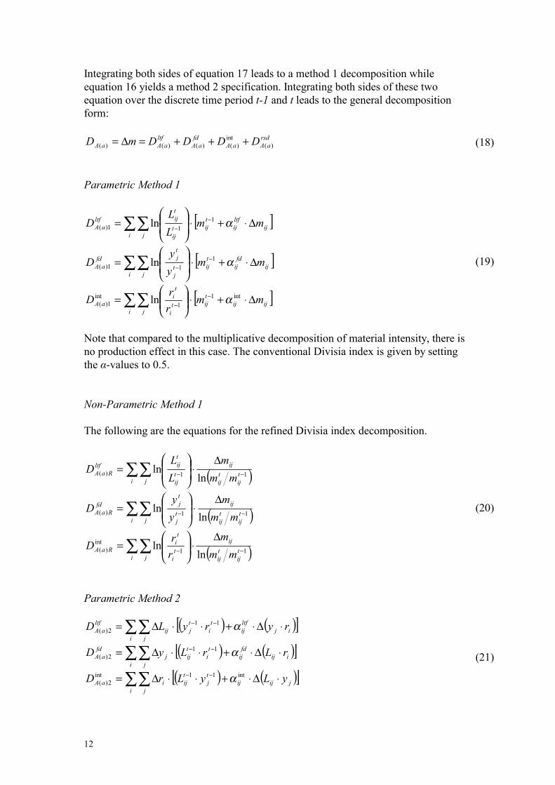
12

Integrating both sides of equation 17 leads to a method 1 decomposition whileequation 16 yields a method 2 specification. Integrating both sides of these twoequation over the discrete time period t-1 and t leads to the general decompositionform:

rsdaAaA

fdaA

ltfaAaA DDDDmD )(

int)()()()( +++=∆= (18)

Parametric Method 1

[ ]∑∑ ∆⋅+⋅

= −

−i j

ijltfij

tijt

ij

tijltf

aA mmLL

D α111)( ln

[ ]∑∑ ∆⋅+⋅

= −

−i j

ijfd

ijtijt

j

tjfd

aA mmyy

D α111)( ln

[ ]∑∑ ∆⋅+⋅

= −

−i j

ijijtijt

i

ti

aA mmrr

D int11

int1)( ln α

(19)

Note that compared to the multiplicative decomposition of material intensity, there isno production effect in this case. The conventional Divisia index is given by settingthe α-values to 0.5.

Non-Parametric Method 1

The following are the equations for the refined Divisia index decomposition.

( )∑∑ −−

∆⋅

=

i jtij

tij

ijtij

tijltf

RaA mmm

LL

D 11)( lnln

( )∑∑ −−

∆⋅

=

i jtij

tij

ijtj

tjfd

RaA mmm

yy

D 11)( lnln

( )∑∑ −−

∆⋅

=

i jtij

tij

ijt

i

ti

RaA mmm

rrD 11

int)( ln

ln

(20)

Parametric Method 2

( ) ( )[ ]∑∑ ⋅∆⋅+⋅⋅∆= −−

i jij

ltfij

ti

tjij

ltfaA ryryLD α11

2)(

( ) ( )[ ]∑∑ ⋅∆⋅+⋅⋅∆= −−

i jiij

fdij

ti

tijj

fdaA rLrLyD α11

2)(

( ) ( )[ ]∑∑ ⋅∆⋅+⋅⋅∆= −−

i jjijij

tj

tijiaA yLyLrD int11int

2)( α

(21)

13

The Laspeyres, Marshall-Edgeworth and Paasche and are produced if the α-parametersare set to 0, 0.5 and 1 respectively.

Parametric Methods 1 and 2 Combined

The adaptive weighting Divisia index result from the same assumptions (equation 13)as the intensity case except for those that are specifically focussed on the productioneffect.

( )

( ) ijijtij

tij

ij

tijt

ij

tijt

itjij

ltfij

LryLL

m

mLL

ryL

∆⋅⋅∆−

⋅∆

⋅

−⋅⋅∆

=

−

−−

−−

1

11

11

ln

ln

α

( )

( ) jiijtj

tj

ij

tijt

j

tjt

itijj

fdij

yrLyy

m

myy

rLy

∆⋅⋅∆−

⋅∆

⋅

−⋅⋅∆

=

−

−−

−−

1

11

11

ln

ln

α

( )

( ) ijijti

ti

ij

tijt

i

tit

jtiji

ij

ryLrrm

mrryLr

∆⋅⋅∆−

⋅∆

⋅

−⋅⋅∆

=

−

−−

−−

1

11

11

int

ln

lnα

(22)

Additive decomposition of an elasticity indicatorThe output elasticity13 of materials use can be found by replacing the results of theadditive decomposition of material use into the equation for the output elasticity:

∆+

∆+

∆+

∆=∆∆=xx

mD

xx

mD

xx

mD

xx

mD

xx

mmD

rsdaAaA

fdaA

ltfaA

aE)(

int)()()(

)( (23)

Laspeyres, Marshall-Edgeworth and PaascheIn Ang and Lee (1996) the Laspeyres and Marshall-Edgeworth version of thisdecomposition are given.

∆⋅+∆

∆⋅+= −− xx

xmm

DD ltftltft

ltfltfaAltf

aE ααα

112)(

)(

)((24)

13 Ang and Lee (1996) also refer to it as the “energy coefficient” in their study of energy issues.

14

∆⋅+∆

∆⋅+= −− xx

xmm

DD fdtfdt

fdfdaAfd

aE ααα

112)(

)(

)(

∆⋅+∆

∆⋅+= −− xx

xmm

DD tt

aAaE int1int1

intint2)(int

)(

)(αα

α

To obtain Laspeyres and Marshall-Edgeworth indices the α-parameters are set to 0 and0.5 respectively. Paasche, although not implemented in Ang and Lee (1996) could beobtained by setting the α-parameters to 1. The equation shows that the decompositionresults that come from the additive decomposition of material use are also dependenton the parameter values. I.e. If you are calculating the Laspeyres weighted determinanteffect on elasticity then the additive Laspeyres decomposition results should be usedas input.

5. NUMERICAL EXAMPLEIn this section a hypothetical numerical example used in Ang (1999) is expanded tostudy the differences in SDA and INA (Table 2). The bold information is from Ang(1999) while the input-output information (normal font) has been added for the SDAdecomposition. All information is in monetary units, except for the material use (inbrackets) which is in physical units. The results of all the decomposition approachesare given in table 4.

Table 3. Example in year t-1 and year tYear t-1 Sector 1 Sector 2 y x (m) Year t Sector 1 Sector 2 y x (m)Sector 1 3 2 5 10 (30) Sector 1 8 2 10 20 (40)Sector 2 5 20 15 40 (20) Sector 2 10 30 20 60 (24)W 2 18 W 2 28Total 10 40 Total 20 60

15

Table 4. Results for the SDA and INA decomposition approachMULTIPLICATIVE DECOMPOSITION OF AN INTENSITY INDICATOR

Determinant effectsMethod/Index SDA/INA Total Production Structure Leontief Final

DemandIntensity Residual

Method 1INA 0.8 1.118 0.716 1.000

Conventional Divisia SDA 0.8 0.625 1.050 1.701 0.716 1.002INA 0.8 1.118 0.716 1.000

Refined Divisia SDA 0.8 0.625 1.051 1.702 0.716 1.000Method 2

INA 0.8 1.133 0.756 0.934Laspeyres SDA 0.8 0.549 1.042 1.998 0.756 0.926

INA 0.8 1.119 0.710 1.008Marshall-Edgeworth SDA 0.8 0.614 1.051 1.740 0.710 1.004

INA 0.8 1.105 0.666 1.087Paasche SDA 0.8 0.687 1.059 1.515 0.666 1.089Method 1 & 2combined

INA 0.8 1.118 0.716 0.999Adaptive WeightingDivisia Index SDA 0.8 0.625 1.052 1.700 0.721 0.993

ADDITIVE DECOMPOSITION OF AN ABSOLUTE INDICATORDeterminant effects

Method/Index SDA/INA Total Production Structure Leontief FinalDemand

Intensity Residual

Method 1INA 14 26.8 6.4 -19.1 -0.1

Conventional Divisia SDA 14 2.9 30.4 -19.1 -0.3INA 14 26.7 6.3 -19.0 0.0

Refined Divisia SDA 14 2.9 30.0 -18.9 0.0Method 2

INA 14 30.0 6.3 -14.0 -8.3Laspeyres SDA 14 2.1 34.6 -14.0 -8.7

INA 14 27.0 6.3 -20.0 0.7Marshall-Edgeworth SDA 14 2.9 30.6 -20.0 0.5

INA 14 24.0 6.4 -26.0 9.6Paasche SDA 14 3.7 26.6 -26.0 9.7Method 1 & 2combined

INA 14 26.9 6.3 -18.5 -0.8Adaptive WeightingDivisia Index SDA 14 2.8 30.4 -18.5 -0.7

ADDITIVE DECOMPOSITION OF AN ABSOLUTE INDICATORDeterminant effects

Method/Index SDA/INA Total Production Structure Leontief FinalDemand

Intensity Residual

INA 0.47 1.00 0.21 -0.47 -0.28Laspeyres SDA 0.47 0.07 1.15 -0.47 -0.29

INA 0.53 1.03 0.24 -0.76 0.03Marshall-Edgeworth SDA 0.53 0.11 1.16 -0.76 0.02

INA 0.58 1.00 0.27 -1.08 0.40Paasche SDA 0.58 0.15 1.11 -1.08 0.41

16

In the multiplicative decomposition of material intensity INA leads to 2 separatedeterminant effects while SDA distinguishes 4 effects. In the additive decompositionof material use and elasticity both methods distinguish 3 effects. These are the top tiereffects but each of these, except the production effect, are composed of sub-effects.The Leontief (n2 sub-effects)14 and the structure, final demand and intensity effects (alln effects) can therefore be further decomposed. The multiplicative decomposition ofINA therefore has 2n sub-effects as opposed to n2+2n+1 in SDA. In the additivedecompositions of material use and elasticity the difference is 2n+1 versus n2+2n. It isnot surprising that SDA distinguishes more sub-effects since it also uses more data.

This paper has thusfar not discussed the interpretations of the determinanteffects. The production effect measures the effect of the changes in the overall outputlevel of the economy on the indicator in question. As table 4 shows if total outputgrows it has a diminishing effect on the intensity indicator because it is taken up in thedenominator of this SDA effect. In the case of an additive INA decomposition ofabsolute indicators, rising output obviously has a positive effect on the total materialuse. The structure effect indicates the effect of a shift in the relative shares of outputon the indicator. The Leontief effect indicates the effect of the changes in the Leontiefcoefficients. Since this matrix is actually derived from the technical coefficientsmatrix it is actually a measure of the change in technology of the economy. Anothertechnological effect is the intensity effect which assesses the effect of change in thematerial intensity values in each sector. Lastly, the final demand effect estimates thechange in the indicator that can be ascribed to the shift in the final demand forproducts from each sector.

Table 4 shows that each of the decomposition indices produces differentresults. An important component of each approach is the residual effects. The tableshows that Laspeyres and Paasche generally have substantial residuals that are largecomponents of the total decomposition. The Marshall-Edgeworth, conventionalDivisia, and adaptive weighting Divisia indices have lower residual effects. Therefined Divisia index, however, has no residual.

The range of results for each determinant effect can be quite large. Invariablythe Laspeyres and Paasche indices provide the two extremes of the range with theother indices somewhere close to the center of this range.

6. APPROACH SELECTION

INA or SDA?This paper has shown that research into historical data can provide valuableinformation about the importance of specific determinants. The question of thepreferred method has however not been addressed.

SDA has the main advantage of including indirect effects of demand changesand therefore giving a feel for the interactions that exist in an economy. The indirecteffects are often substantial and in environmental analyses these effects may be veryimportant. Although a sector may be very energy-extensive it could require a lot ofinputs that required large amounts of energy. In the input-output model this indirectenergy is included in the analysis. The drawback of the Leontief model is itsassumption of constant technical coefficients. No scale effects or substitution is

14 Remember that n is the number of sectors

17

therefore present in the standard input-output model. Nevertheless the input-outputmodel is widely used and the inclusion of the indirect effect is a major advantage ofSDA over INA.

Overall SDA decompositions provide more detailed information about theeffects of the determinants. Clearly this is related to the fact that more data is used inthe input-output setup. The decomposition of material intensity yields 4 effects whilethe INA distinguishes 2 effects. If these effects are further decomposed into theircomponent parts then INA (2n) has far fewer sub-effects than SDA (n2+2n+1). In theabsolute decomposition the difference in the number of sub-effects is 2n+1 versusn2+2n.15 The technical coefficient matrix (represented in the Leontief inverse) with itsn2 elements in fact holds information about the technological input requirements of allsectors. SDA therefore has the opportunity for further decomposition of thistechnology effect.It may be concluded that if input-output data is available then SDA should bepreferred over INA. It provides more details about the way economic changes affectmaterials use, intensity or elasticity. In cases where the data availability is low andshort time-step analysis is of interest, INA is more likely to be feasible. However itshould be noted that short time steps do have a disadvantage (whether for SDA orINA) in that the changes that are found may be short-term effects that do notnecessarily imply an irreversible shift in the economic structure. Long-termdecompositions therefore give a more accurate depiction of the determinant changes.

Intensity, Absolute or Elasticity?Clearly the choice of decomposition indicator depends on the issue underinvestigation. Changes in the output elasticity will be of interest to people who areresearching how material use reacts to output increases. Ang and Lee (1996) alsointroduced a method of using the elasticity indicator to project energy use towards thefuture.

The absolute indicator is best when it is important to investigate the actualquantity of material use. The intensity indicator looks at the use of material relative tothe output and is therefore better suited to questions of material productivity. Ang(1999) argues that the choice between absolute and intensity measures is a matter ofease of presentation and interpretation. Intensity indicators are more easily graphedbecause they are often indices that are close to one. Absolute decompositions arehowever easier to interpret by non-specialists.

An added selection criteria (in the INA case) is that if the time period is longor the output growth has been large, the production effect may dominate in theabsolute indicator decomposition. If the researcher is interested in investigations ofstructural change, the intensity approach is therefore preferred.

Multiplicative or additive?There seems to be no reason to prefer either of these decomposition types except forperhaps the ease of presentation and interpretation argument.

15 INA and SDA both have the same material intensity effect. It is only in the economic portion of thedecomposition that they differ.

18

Method 1 or Method 2?Again there is very little reason to prefer expressing the determinant in terms ofrelative growth rates (method 1) or differences terms (method 2). Perhaps a minorargument is that the method 1 formulas are easier to present because they all haveequal weights.

Which Index?The larger issue that has not been addressed in this paper is the issue of indexselection. All indices have certain properties and should therefore be chosen accordingto the demands set. Table 5 summarizes the properties of the indices discussed in thispaper (this summary of properties is largely based on Ang (1999).

Table 5. Properties of the indices in this paperParametric Residual Zero value problem

Laspeyres yes large noMarshall-Edgeworth yes moderate noPaasche yes large noConventional Divisia yes moderate yesRefined Divisia no none no (see explanation)Adaptive Weighting Divisia no moderate yes

The first issue is whether the index is a special case of a parametric form. As section 4showed, the Laspeyres, Marshall-Edgeworth and Paasche indices are special case ofparametric Divisia method 2. The conventional Divisia index is a special case ofparametric Divisia method 1. This means that the author has to choose the parametervalues. The non-parametric indices do not require an extra parameter assumption andthe result is therefore purely data driven. This does not, however, make the non-parametric theoretically superior since the assumptions that have to be made about theindex so that it leads to a unique value are just as arbitrary as choosing a parametervalue.

The value of the residual is very important because when you are interested inthe importance of determinant effects then large residuals defeat the purpose.Laspeyres and Paasche score worst on this criterion. Marshall-Edgeworth,conventional Divisia and the adaptive weighting Divisia index score better but Ang(1999) notes that if changes in the data are drastic the residuals may deteriorate. Therefined Divisia index leads to perfect decompositions of the indicator change.

The third criterion in table 5 is the issue of zero values in the data set. This is aparticularly important issue for SDA because detailed input-output data nearly alwayshave zero values in the table because many sectors do not have intersectoraldeliveries. Certain material types may also not be used in the base or terminal yearleading to zero value in the decomposition. The decomposition methods based onmethod 2 approaches are based on difference terms and therefore have no problem.The conventional refined Divisia do however have a problem if the terminal year iszero (natural logarithm of zero is minus infinity) or the base year (division by zerogives plus infinity). It is common practice to replace the zero value by a small value δto solve this problem. Ang and Choi (1997) show that the refined Divisia index showsconverging decomposition results as δ approaches zero but that this is not the case forthe conventional Divisia index.

19

Ang (1999) adds some observations about the interpretability of some of theindices. The Laspeyres index is deemed to be easy to understand because weighting bythe base year is often done. Weighting using parameter values of 0.5 has theadvantage of treating time symmetrically. The Paasche index both decomposition andforecasting can be done with reference to the same year.

Overall it can be said that the Laspeyres and Marshall-Edgeworth indices thatare commonplace in SDA do not measure up well against some of the indices thatcome from the INA literature. Particularly the refined Divisia index has some veryappealing properties. In particular it is the only index that does not generate a residual.

7. CONCLUSIONSA number of conclusions may be drawn from this paper.1. SDA and INA are closely related decomposition methods. Fundamentally the only

difference is the use of input-output data in SDA.2. The sophisticated decomposition methods developed in the INA literature are

transferable to the SDA framework (section 4).3. Many of the indices in use in INA have superior properties over the Laspeyres and

Marshall-Edgeworth indices that are common in SDA.4. INA and SDA researchers should be more aware of the literature in both fields to

fully benefit from the methodological advances in decomposition techniques.

Further research would include comparing the index system developed inDietzenbacher and Los (1998) and applying it to INA. The results for the additivedecomposition of intensity and the multiplicative decomposition of absolute indicatorsshould also be discussed.

20

APPENDIX 1. VARIABLESThe superscript t always defines the time at which the variable is taken.

Country-leveltm – Total material use (tons)

tx – Total output (>)tr – Material intensity of the economy (tons/>) (=m/x)

n – Number of sector in the economy

Sector-leveltijZ – The intersectoral deliveries of goods or services of sector i to sector j (>)tijA – Technical coefficient matrix. The amount of input from sector i required per unit

output of sector j.tijL – Leontief inverse.The direct and indirect effect on the output of sector i per unit

change of final demand of sector j (= 1)( −− tijAI ).

tijm – Material use by sector i due to demand for products from sector j (tonnes).tim – Material use by sector i (tonnes).tijw – Material use weights. Material use in sector i due to demand for products from

sector j as a proportion of the total material use (tonnes) (=mij/m).tiw – Material use weights. Material use in sector i as a proportion of the total material

use (tonnes) (=mi/m).tix – Output of sector i (>)tjy – Final demand of sector j (>)

tir – Material intensity of sector i (tons/>) (=mi/xi)tis – Output share. Sector i output as a proportion of total output (=xi/x)

Subscripts and Superscripts of parameters αijSuperscripts:

str – Structural effectint – Intensity effectpdn – production effectltf – Leontief effectfd – final demand effect

Subscripts and Superscripts of decomposition variable D(If it does not have a superscript it is equal to the total change of the indicator)Superscripts:

str – Structural effectint – Intensity effectpdn – production effectltf – Leontief effectfd – final demand effectrsd – residual effect

21

1st Subscript (Indicator type)I – IntensityA – AbsoluteE – Elasticity

2nd Subscript (Decomposition type)(a) – Additive(m) – Multiplicative

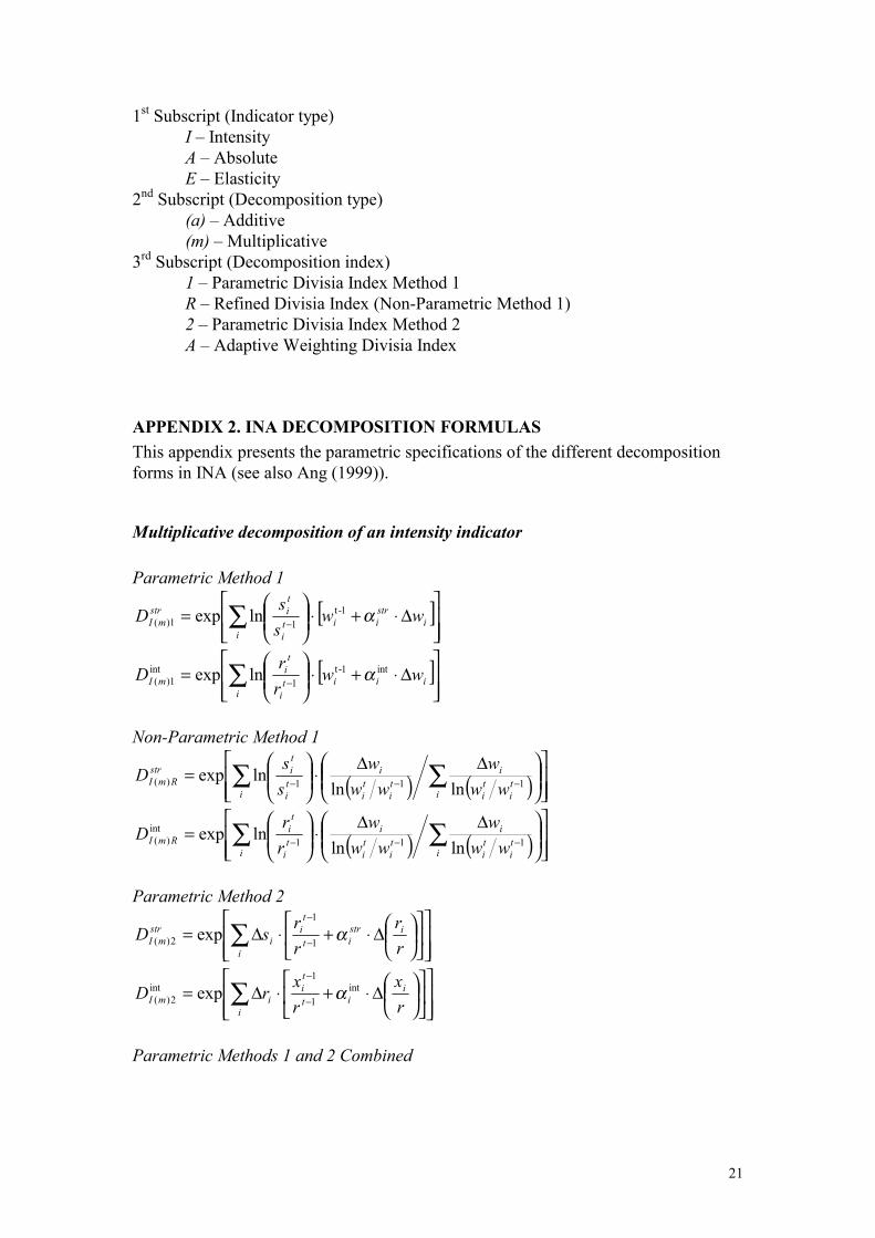
3rd Subscript (Decomposition index)1 – Parametric Divisia Index Method 1R – Refined Divisia Index (Non-Parametric Method 1)2 – Parametric Divisia Index Method 2A – Adaptive Weighting Divisia Index

APPENDIX 2. INA DECOMPOSITION FORMULASThis appendix presents the parametric specifications of the different decompositionforms in INA (see also Ang (1999)).

Multiplicative decomposition of an intensity indicator

Parametric Method 1

[ ]

∆⋅+⋅

= ∑ −

ii

striit

i

tistr

mI wwssD α1-t

11)( lnexp

[ ]

∆⋅+⋅

= ∑ −

iiiit

i

ti

mI wwrrD int1-t

1int

1)( lnexp α

Non-Parametric Method 1

( ) ( )

∆∆⋅

= ∑ ∑ −−−

i iti

ti

iti

ti

iti

tistr

RmI www

www

ssD 111)( lnln

lnexp

( ) ( )

∆∆⋅

= ∑ ∑ −−−

i iti

ti

iti

ti

it

i

ti

RmI www

www

rrD 111

int)( lnln

lnexp

Parametric Method 2

∆⋅+⋅∆= ∑ −

−

i

istrit

ti

istr

mI rr

rrsD α1

1

2)( exp

∆⋅+⋅∆= ∑ −

−

i

iit

ti

imI rx

rxrD int

1

1int

2)( exp α

Parametric Methods 1 and 2 Combined

22

ii

ti

ti

i

tit

i

ti

t

ti

istri

srr

ssw

wss

rr

s

∆⋅

∆−

⋅∆

⋅

−

⋅∆

=

−

−−−

−

1

111

1

ln

lnα

ii

ti

ti

i

tit

i

ti

t

ti

i

i

rrx

rrw

wrr

rx

r

∆⋅

∆−

⋅∆

⋅

−

⋅∆

=

−

−−−

−

1

111

1

int

ln

lnα

Additive decomposition of an absolute indicator

Parametric Method 1

[ ]∑ ∆⋅+⋅

= −

−i

istri

tit

i

tistr

aA mmss

D α111)( ln

[ ]∑ ∆⋅+⋅

= −

−i

iitit

i

ti

aA mmrr

D int11

int1)( ln α

[ ]∑ ∆⋅+⋅

= −

−i

ipdn

itit

tpdn

aA mmxxD α1

11)( ln

Non-Parametric Method 1

( )∑

∆⋅

= −−

iti

ti

iti

tistr

RaA mmm

ssD 11)( ln

ln

( )∑

∆⋅

= −−

iti

ti

it

i

ti

RaA mmm

rrD 11

int)( ln

ln

( )∑

∆⋅

= −−

iti

ti

it

tpdn

RaA mmm

xxD 11)( ln

ln

Parametric Method 2( )[ ]∑ ⋅∆⋅+⋅⋅∆= −−

ii

stri

ttii

straA xrxrsD α11

2)(

( )[ ]∑ ⋅∆⋅+⋅⋅∆= −−

iii

ttiiaA xsxsrD int11int

2)( α

( )[ ]∑ ⋅∆⋅+⋅⋅∆= −−

iii

pdni

ti

ti

pdnaA rsrsxD α11

2)(

Parametric Methods 1 and 2 Combined

23

( )

( ) iiti

ti

i

tit

i

titt

iistri

sxrssm

mssxrs

∆⋅⋅∆−

⋅∆

⋅

−⋅⋅∆

=

−

−−

−−

1

11

11

ln

lnα

( )

( ) iiti

ti

i

tit

i

titt

ii

i

rxsrrm

mrr

xsr

∆⋅⋅∆−

⋅∆

⋅

−⋅⋅∆

=

−

−−

−−

1

11

11

int

ln

lnα

( )

( ) xsrxxm

mxxsrx

iit

t

i

tit

tti

ti

pdni

∆⋅⋅∆−

⋅∆

⋅

−⋅⋅∆

=

−

−−

−−

1

11

11

ln

lnα

Additive decomposition of an elasticity indicator

∆⋅+∆

∆⋅+= −− xx

xmm

DD strtstrt

strstraAstr

aE ααα

112)(

)(

)(

∆⋅+∆

∆⋅+= −− xx

xmm

DD tt

aAaE int1int1

intint2)(int

)(

)(αα

α

∆⋅+∆

∆⋅+= −− xx

xmm

DD pdntpdnt

pdnpdnaApdn

aE ααα

112)(

)(

)(

If the α-values are set to 0, 0.5 and 1, the Laspeyres, Marshall-Edgeworth and Paascheindices are produced respectively.

24

REFERENCES

-Ang, B.W., 1999. Decomposition Methodology in Energy Demand andEnvironmental Analysis. In: Handbook of Environmental and Resource Economics.(ed.) J.C.J.M van den Bergh. Edward Elgar, Cheltenham.-Ang, B.W. and K.H. Choi, 1997. Decomposition of Aggregate Energy and GasEmissions Intenisties for Industry: A Refined Divisia ndex Method. The EnergyJournal 18(3) pp. 59-73-Ang, B.W. and P.W. Lee, 1996. Decomposition of Industrial Energy Consumption:The Energy Coefficient Approach. Energy Economics 18 pp. 129-143-Dietzenbacher, E., A. Hoen and B. Los, 2000. Labor Productivity in Western Europe1975-1985: An Intercountry, Interindustry analysis. Journal of Regional Science(forthcoming) pp.-Dietzenbacher, E. and B. Los, 1998. Structural Decomposition Techniques: Senseand Sensitivity. Economic Systems Research 10(4) pp. 307-323-Fisher, I., 1922. The Making of Index Numbers: A Study of their Varieties. Tests andReliability. Augutus M. Kelly, New York.-Han, X. and T.K. Lakshmanan, 1994. Structural Changes and Energy Consumptionin the Japanese Economy 1975-85: An Input-Output Analysis. The Energy Journal15(3) pp. 165-188-Liu, X.Q., B.W. Ang and H.L. Ong, 1992. The Application of the Divisia Index tothe Decomposition of Changes in Industrial Energy Consumption. The EnergyJournal 13(4) pp. 161-177-Miller, R.E. and P.D. Blair, 1985. Input-Output Analysis: Foundations andExtensions. Prentice-Hall, Englewood-Cliffs, New Jersey.-Rose, A. and S. Casler, 1996. Input-Output Structural Decomposition Analysis: ACritical Appraisal. Economic Systems Research 8(1) pp. 33-62-Vogt, A., 1978. Divisia Indices on Different Paths. In: Theory and applications ofeconomic indices. (eds.) W. Eichhorn, R. Henn, O.Opitz and R.W. Shepard. Physica-Verlag, Wurzburg.-Vogt, A. and J. Barta, 1997. The Making of Tests of Index Numbers: MathematicalMethods of Descriptive Statistics. Springer-Verlag, Heidelberg.