Compatible diameter and height incrementmodels for lodgepole pine, trembling aspen, andwhite spruce

Thompson K. Nunifu

Abstract: In this study, compatible height and diameter increment models were fitted for lodgepole pine (Pinus contortaDougl. ex Loud. var. latifolia Engelm.), trembling aspen (Populus tremuloides Michx.), and white spruce (Picea glauca(Moench) Voss), using the relationship between diameter and height growth. It was assumed that tree diameter increment isdirectly proportional to height increment, and the proportionality constant is a function of competition and site productivity.The results showed that the fit statistics are comparable with results of other studies, with adjusted R2 ranging from 30% to50%. A validation test of the models, using independent permanent sample plots data, showed that the short-term predictionsof the models for both pure and mixedwood stands are fairly unbiased. The models also gave reasonable average heightgrowth and diameter growth trajectories for pure stands of the three species and also projected long-term mixedwood (aspen –white spruce mixture) volume growth dynamics reasonably well. The models also projected reasonably well (i) the effect ofincreasing initial stem density on average diameter and height, and (ii) the stand volume compared with an older version theMixedwood Growth Model (ver. 2000A). It was concluded that explicitly linking tree height and diameter increment modelsdoes not only have a solid ecological basis, but it also results in a compatible prediction of tree growth and stand dynamics.

Resume : Dans cette etude, des modeles compatibles d’accroissement en hauteur et en diametre ont ete ajustes pour le pintordu (Pinus contorta Dougl. ex Loud. var. latifolia Engelm.), le peuplier faux-tremble (Populus tremuloides Michx.) etl’epinette blanche (Picea glauca (Moench) Voss) en utilisant la relation entre leur croissance en diametre et leur croissanceen hauteur. L’auteur a assume que l’accroissement en diametre des arbres est directement proportionnel a l’accroissementen hauteur et que la constante de proportionnalite est une fonction de la competition et de la productivite de la station. Lesresultats montrent que les statistiques d’ajustement sont comparables a celles provenant d’autres etudes avec des valeurs deR2 ajuste variant de 30 % a 50 %. Un test de validation des modeles avec des donnees independantes de placettes echantil-lons permanentes montre que les previsions a court terme des modeles ne sont pas biaisees pour les peuplements purs et lespeuplements mixtes. Les modeles ont produit des trajectoires raisonnables de croissance moyenne en hauteur et en diametrepour les peuplements purs des trois especes et ont aussi produit des projections a long terme raisonnables de la dynamiquede croissance en volume des peuplements mixtes (melange de peuplier et d’epinette blanche). Les projections de l’effetd’une augmentation de la densite initiale des tiges sur la moyenne du diametre, de la hauteur et du volume a l’hectare secomparaient raisonnablement bien a celles d’une version anterieure du Mixedwood Growth Model (version 2000A). En con-clusion, la creation d’un lien explicite entre les modeles d’accroissement en hauteur et en diametre, en plus d’avoir de sol-ides bases ecologiques, permet de predire la croissance des arbres et la dynamique des peuplements de facon compatible.

[Traduit par la Redaction]

1. IntroductionGrowth and yield models are usually made up of various

components, which function together hierarchically for mak-ing growth and yield projections. In typical empirical indi-vidual tree growth models, there are three majorcomponents: tree diameter and height growth models, whichare used to predict tree size increments at fixed time steps(usually one year), and mortality or survival probabilitymodels, which are used to determine the number of surviv-ing trees whose yields must be aggregated to obtain thestand level yield.

The significance of recognizing this hierarchy and esti-mating the parameters of the component models such thatthey are compatible with each other and maintain this hier-archical structure has been the basis of several studies in theforest growth and yield literature (e.g., Furnival and Wilson1971; Huang and Titus 1999). In most of these studies, ithas been argued that compatibility among the componentsof a growth and yield model is important in minimizingbias in yield prediction at the forest stand level, which inmost cases forms the basis for important management deci-sions. Various techniques have therefore been employed inforestry growth and yield research with the overall goal ofminimizing model prediction bias at the stand level. Theseefforts can be summarized in three broad categories: (i) esti-mating model parameters as a system of simultaneous equa-tions (e.g., Burkhart and Sprinz 1984; Huang and Titus1999), (ii) constraining individual tree level models withstand level models (e.g., Zhang et al. 1997; Yang 2002),and (iii) fitting a stand level model and then disaggregating

Received 3 June 2008. Accepted 27 October 2008. Published onthe NRC Research Press Web site at cjfr.nrc.ca on 21 January2009.

T.K. Nunifu. Forest Management Branch, Alberta SustainableResource Development, 8th Floor, 9920 – 108 Street, Edmonton,AB T5K 2M4, Canada (e-mail: Thompson.nunifu@gov.ab.ca).

180

Can. J. For. Res. 39: 180–192 (2009) doi:10.1139/X08-168 Published by NRC Research Press

the unbiased stand level model output by using empiricallyfit models to obtain individual tree level variables (Ritchieand Hann 1997; Qin and Cao 2006). This latter approach isto ensure that individual tree level information needed forpurposes such as testing silvicultural treatment effects on in-dividual tree development, which is the basis for why indi-vidual tree models are promoted over stand level models, isreadily obtained from the stand level model. An aspect ofcompatibility often ignored in these studies is the compati-bility in the height–diameter relationships of the individualtrees in relation to the stand structure and density. The in-compatible prediction of individual tree diameter and heightgrowth may result in tree height–diameter ratios that are notconsistent with the stem density and the level of competitionin the stand. This may ultimately result in an unreasonablevolume prediction at the stand level.

The ecological significance of tree height–diameter rela-tionship has been well documented in forestry literature(e.g., Opio et al. 2000; Meng et al. 2006). Often presented asthe ratio of tree height (measured in metres) to tree diameterat breast height (DBH, measured in centimetres), this rela-tionship, which is affected by various factors, including com-petition effects from neighbors, is constantly changing inresponse to the dynamics of the ecosystem and is the resultof factors that influence the relative allocation of growth byindividual trees to diameter and height, respectively (Schmidtet al. 1976; Seidel 1984). Under crowded conditions forinstance, trees may allocate stem growth biomass preferen-tially to height growth over diameter growth to minimizeover-topping by neighbors to maximize exposure to light(Rich et al. 1986), thereby becoming relatively slimmer,with higher height–diameter ratios (Assmann 1970). Reducedwind sway in dense stands has been shown to increase theheight–diameter ratios of trees (Meng et al. 2006). A directlinkage between competition and the relative allocation oftree growth to either height or diameter exists, which cannotbe ignored when predicting individual tree growth.

In this paper, the relationship between tree diametergrowth and tree height growth is utilized to develop systemsof individual tree diameter and height growth models forlodgepole pine (Pinus contorta Dougl. ex Loud. var. latifoliaEngelm.), trembling aspen (Populus tremuloides Michx.),and white spruce (Picea glauca (Moench) Voss). The spe-cific objectives of the study are (i) to develop compatibleindividual tree height and diameter growth models forlodgepole pine, trembling aspen, and white spruce; and(ii) to validate the fitted models and demonstrate that thepredictions from the new models are ecologically more real-istic than when the models are fitted independently.

2. Materials and methods

2.1. The dataThe data used in this study came from two sources: Weld-

wood Canada Ltd. (now called Hinton Wood Products) andthe Public Lands and Forests Division of Alberta Sustain-able Resource Development (ASRD). The ASRD data werecollected over the past four decades from about 1755 perma-nent sample plots (PSPs) located throughout the inventoryarea of the province of Alberta, Canada, to provide unbiasedinformation on forest growth and yield (ALFS 2000). The

Weldwood Canada Ltd. permanent growth database is per-haps the largest database in the province of Alberta and cov-ers just over 3000 PSPs. Most of these plots are found inlodgepole pine stands, throughout their forest managementagreement area located in west–central Alberta. The com-bined dataset covered various stand densities, site condi-tions, stand ages, and ecological (natural) regions.

The study area (PSPs) is between 49816’37@N and58838’31@N and 114819’52@W and 119819’34@W. Plot sizesvaried from 200 to 2000 m2, depending on stand densities.Within each plot, all trees with DBH >9.1 cm were meas-ured for DBH and a subset was measured for height, withall other tree heights predicted using a height–diametermodel. The DBHs of smaller trees (0 < DBH £ 9.0) weremeasured in a subplot, 1/16 of the full plot size.

A subset of the combined datasets from the Weldwood andASRD databases was selected for this study. Selection wasbased on the availability of information on site index treemeasurement, which was considered relevant to this study. Atotal of about 200 PSPs were used for this study, with remea-surements varying from three to seven measurements at inter-vals ranging from 5 to 15 years. Measurement intervals arechosen to correspond to varying rates of growth at the differ-ent stages of stand development. Shorter intervals are chosenfor the younger fast-growing stands to not miss any importantdynamics, whereas relatively longer intervals are used for theslowly growing older stands. In this study, periodic averageannual diameter and height increments were used. Thesewere computed for each tree as ðM2 �M1Þ=L, where M1 andM2 are any two consecutive measurements of individual treediameter or height, such that M2 > M1, and L is the intervallength between the two measurements.

Data from the selected plots were summarized to provideinformation on individual tree and stand characteristics,which were used as covariates in the model estimation.Since the data were intended to be used for simultaneousequation fits, it was necessary to choose only trees withboth diameter and height increments. Trees with predictedheights were excluded from the modeling data. However,all trees were included in the calculation of stand level vari-ables used as covariates in the model fitting. Summaries ofthese variables are provided in Table 1.

2.2. Model development

2.2.1. Height growth modelIn developing the height growth model the potential–

modifier approach was used (Golser and Hasenauer 1997;Hasenauer and Kindermann 2002). Each individual tree (i)in the stand was given a height growth adjustment Ai, whichis related to the potential height increment (PHI) and theachieved height growth (HIi) attained by tree (i) by

½1� HIi ¼ AiPHIþ ei

where ei is a random error term. A potential height growthmodel, developed based on site index data and presented inNunifu (2003), was used:

½2� PHI ¼ a1expða2SIþ a3CRÞHta4 expð�a5Ht2Þ

where PHI is the potential height increment, defined as the

Nunifu 181

Published by NRC Research Press

growth of a site index tree with a height equal to the currentheight of the subject tree of the same species and site index(Nunifu 2003); a1–a5 are parameters; Ht is the current siteindex tree height; SI is the site index of the species deter-mined at breast height age 50; and CR is an index for measur-ing crowding in the stand based on Czarnowski (1961) standdynamics theory, determined as CR ¼ ðHtp � SDÞ=10 000(Cieszewski and Bella 1993). Site index trees are selectedduring plot establishment following a set of criteria in theAlberta permanent sample plot manual (ALFS 2000).Among other things, the criteria include healthy trees withgood form that are free from competition. The variable Htp isthe species top or average dominant or co-dominant treeheight and SD is the number of stems per hectare (stemdensity). CR is used to account for the effects of densityon dominant height growth in lodgepole pine (Mitchelland Goudie 1980; Cieszewski and Bella 1993). The coeffi-cients of eq. 7 for the three species, as presented in Nunifu(2003), are given in Table 2. The potential height growthof each subject tree was calculated by replacing Htp ineq. 7 with the subject tree height H.

A suitable function for Ai was then defined, which al-lowed trees to grow in height close to their potential untilcompetition is relatively intense, forcing a substantial reduc-tion in height growth rate (e.g., see Mitchell 1975; Hann andRitchie 1988). Several tree and stand level variables andtheir transformations were included in the height growth ad-justment models for the three species. Equations 3, 4, and 5were selected for modeling the Ai for lodgepole pine (PL),trembling aspen (AW), and white spruce (SW), respectively,after preliminary analysis and dropping variables that werenot statistically significant.

½3� AiPL ¼ q0 þ q1SPHT0:5 þ exp � q2GGR2� �� �

þq5lnðQMDRÞ þ q6lnðCRÞ

½4� AiAW ¼ exp � q1SPHT2 þ q2GGR2 þ q3GGRC

��þq5QMDRþ q6CRÞ�

½5� AiSW ¼ exp � q3GGRC þ q4GGRD þ q6CR� �� �

where QMDR is the ratio of species quadratic mean DBH tothe stand quadratic mean DBH and measures the relativedominance of the species; SPHT is the average height of alltrees of the species in the stand; and CR is as defined be-fore. As usual, q1–q6 are parameters to be estimated sepa-rately for each species. Note that the parameters q1–q6 arenot necessarily comparable across equations; some of theassociated variables enter the models in quite differentforms and transformations. The variables GGRC and GGRDare the coniferous and deciduous basal areas in trees largerthan the subject tree, respectively, calculated as follows:

½6� GGRðkÞ ¼X

DBHj>DBHi

l� P� BAj

where l is an expansion factor for converting the tree basalarea (BAj) to square metres per hectare, DBHi is diameter atbreast height of the subject tree, and DBHj is diameter atbreast height of any tree bigger than the subject tree. Thesubscript k is the species type designation (C for coniferousand D for deciduous) and P is a dummy variable such that ifk = C then P = 1 for every coniferous tree and 0 for everydeciduous tree, if k = D then P = 0 for all coniferous treesand 1 for every deciduous tree bigger than the subject tree.

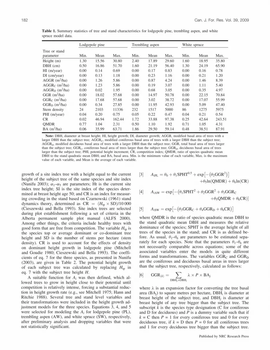
Table 1. Summary statistics of tree and stand characteristics for lodgepole pine, trembling aspen, and whitespruce model data.

Lodgepole pine Trembling aspen White spruce

Tree or standparameter Min. Mean Max. Min. Mean Max. Min. Mean Max.Height (m) 1.30 15.56 30.80 2.40 17.89 29.60 1.60 18.95 35.80DBH (cm) 0.50 16.86 51.70 1.60 21.19 56.40 1.30 24.19 65.90HI (m/year) 0.00 0.14 0.69 0.00 0.17 0.83 0.00 0.16 0.78DI (cm/year) 0.00 0.13 1.18 0.00 0.23 1.16 0.00 0.21 1.20AGGR (m2/ha) 0.00 1.26 5.86 0.00 0.87 4.24 0.00 1.46 8.39AGGRC (m2/ha) 0.00 1.23 5.86 0.00 0.19 3.07 0.00 1.11 5.40AGGRD (m2/ha) 0.00 0.02 1.95 0.00 0.68 3.05 0.00 0.35 4.97GGR (m2/ha) 0.00 18.02 57.68 0.00 14.97 50.78 0.00 22.15 70.84GGRC (m2/ha) 0.00 17.68 57.68 0.00 3.02 38.72 0.00 17.07 55.99GGRD (m2/ha) 0.00 0.34 27.85 0.00 11.95 42.93 0.00 5.09 47.40Stem density 24 2103 11336 232 1517 5000 86 1275 5975PHI (m/year) 0.04 0.20 0.75 0.05 0.22 0.47 0.04 0.21 0.54CR 0.02 46.94 162.44 1.72 33.88 97.38 0.25 42.64 243.51QMDR 0.77 1.04 2.31 0.50 1.10 1.92 0.71 1.05 4.31BA (m2/ha) 0.06 35.99 63.71 1.86 29.50 59.14 0.48 38.51 87.91

Note: DBH, diameter at breast height; HI, height growth; DI, diameter growth; AGGR, modified basal area of trees with alarger DBH than the subject tree; AGGRC, modified coniferous basal area of trees with a larger DBH than the subject tree;AGGRD, modified deciduous basal area of trees with a larger DBH than the subject tree; GGR, total basal area of trees largerthan the subject tree; GGRC, coniferous basal area of trees larger than the subject tree; GGRD, deciduous basal area of treeslarger than the subject tree; PHI, potential height increment; CR, competition index; QMDR, ratio of species quadratic meanDBH to the stand quadratic mean DBH; and BA, basal area. Min. is the minimum value of each variable, Max. is the maximumvalue of each variable, and Mean is the average of each variable.

182 Can. J. For. Res. Vol. 39, 2009

Published by NRC Research Press

GGR is the total basal area of trees larger than the subjecttree (i.e., GGR = GGRC + GGRD).

Variable selection for the height growth adjustment modelwas based on three premises: (i) size hierarchies are more ofthe result of one-sided competition for light where largertrees tend to overtop smaller ones (Weiner 1990; Nilsson1994); (ii) in mixed stands, the relative size of the speciesmay determine the amount of interspecific competition af-fecting trees of that species; and (iii) the number, size, andspecies type of the trees larger than the subject trees are im-portant in determining the amount of side shading and, to avery large extent, the amount of leaf area a tree can carry(Oliver and Larson 1996).

2.2.2. Diameter growth modelThe diameter growth model is formulated using a simple

linear relationship of height growth (HI) and diametergrowth (DI) (Sievanen 1993):

½7� DI ¼ hHIþ 3

where h is a coefficient to be estimated and 3 is a randomerror term.

The coefficient h is a function of competition and ishigher for dominant and (or) open-grown trees than for sup-pressed trees and (or) trees in high density stands. As thesize rank of a tree in the stand approaches that of an open-grown tree, h is assumed to approach an unknown constantvalue, Q, typical for each species and site index.

Sievanen (1993) used the ratio of height to crown base tototal tree height as a measure of an individual tree’s abilityto put on diameter growth, with reasonable results. In thisstudy, the modified basal area in trees with a larger DBHthan that of the subject tree (AGGR) was used as an indexof the tree’s ability to put on diameter growth. The choiceof this competition index made intuitive sense, as it can besafely assumed that the ratio of height to crown base to totalheight is highly correlated with stand density and the socialrank of the tree. This index may be expressed as GGR/SF,where SF is the plot spacing factor, defined as the averageinter-tree spacing expressed as a percentage of average dom-inant or codominant tree height in the plot. To account forspecies type differences, this variable was also split intoAGGRC and AGGRD for coniferous and deciduous species,respectively, where AGGRC = GGRC/SF and AGGRD =GGRD/SF.

Other variables typically used in empirical tree growthmodels, were considered. However, only total stand basalarea (BA) and individual tree DBH were selected after apreliminary regression fit. Site index was linked to diametergrowth through height growth formulated above. Equations8 to 10 present the final models selected for h for lodgepolepine, trembling aspen, and white spruce, respectively,

½8� hPL ¼ b0 þ b1 ln 1þ DBH� �

þ b2 ln 1þ AGGR� �

þb4 ln 1þ AGGRD

� �þ b5 ln 1þ BA

� �½9� hAW ¼ b0exp � b3AGGRC þ b4AGGRD

� �� �½10� hSW ¼ b0exp � b1DBHþ b2AGGR

��þ b4AGGRD þ b5BAÞ�

where b0–b5 are parameters to be estimated for each equa-tion. Again, note that b0–b5 are not necessarily comparableacross equations; some of the associated variables enter themodels in quite different forms and transformations.

2.3. Parameter estimationFor each species, the diameter and height growth models

were considered as a system rather than as individual equa-tions for two reasons:

(1) The dependent variable h in eqs. 8–10 is a ratio of dia-meter growth to height growth, which is also part of thedependent variable Ai in eqs. 3–5, and so, there is someevidence of cross-equation dependency.

(2) The random errors for the diameter and height growthmodels can be correlated. A major reason to expect across-equation correlation of the error terms in this studyis the fact that each h� Ai pair comes from the sametree.

Applying nonlinear ordinary least squares to estimate theparameters of simultaneous equations will result in a simul-taneous equation bias (Judge et al. 1988). However, becausethe ratio of diameter growth to height growth was used asthe dependent variable with no HI appearing on the right-hand side of the diameter growth model, seemingly unre-lated regression (SUR) was used to account for cross-equa-tion correlation (Zellner 1962). The SUR method requiresan estimate of the cross-equation error covariance matrix,S, with dimension (m � m), where m is the number of indi-vidual models in the system (Zellner 1962). The usual ap-

Table 2. Parameter estimates for eq. 7 (the potential height growth models) for lodgepole pine, trem-bling aspen, and white spruce.

Lodgepole pine Trembling aspen White spruce

Variable Parameter Estimate SE Estimate SE Estimate SEConstant a1 0.07365 0.00113 0.05048 0.00209 0.09666 0.00336SI a2 0.08932 0.00055 0.08261 0.00064 0.07565 0.00147CR a3 –0.00039 0.00012 — — — —Ht a4 0.06095 0.00846 0.31332 0.01710 0.02294 0.01140Ht2 a5 0.00240 0.00004 0.00281 0.00003 0.00145 0.00004RMSE 0.01430 0.00313 0.01390Sample n 850 415 320 .

Note: SI is species site index, CR is a competition index, Ht is individual tree height, RMSE is the root meansquare error, n is the number of observations (sample size) used for model fitting; SE, standard error.

Nunifu 183

Published by NRC Research Press

proach is to first fit the equations using OLS to compute anestimate bS from the OLS residuals as

½11� bS ¼ 1

nE0E

where E is an (n � m) matrix of model residuals, with eachcolumn representing a vector of residuals from an individualmodel, and n is the sample size. Based on bS, the SUR esti-mation is performed by minimizing the following equation:

½12� ZðqÞ ¼ 1

n½y � f ðqÞ� 0 bS�1 � I

� �½y � f ðqÞ�

where y is the vector of observed responses, I is a unit ma-trix (m � m), and : denotes the Kronecker product. Theassumption here is that bS is a symmetric positive definitematrix (m � m).

The MODEL procedure of the SAS/ETS software (SASInstitute Inc. 1988) was used to fit the system as nonlinearSUR equations. Several different transformations of treeDBH and height were used iteratively as weights for the hand Ai models, respectively. For Ai, the inverse of treeheight (1/H) was applied as weight, whereas for h, the in-verse of DBH (DBH–0.2) was applied as weight after somepreliminary analysis.

The first order autoregressive (AR(1)) process was usedinstead of the continuous-time autoregressive (CAR) processeven though the measurement intervals were unequal. TheCAR process accounts for the effect of differences in tempo-ral spacing (interval) between measurements on the autocor-relation structure, while AR(1) process assumes equalcorrelation between adjacent measurements. However, thedependent variables are ratios, which are calculated fromaverage annual increments. By calculating the differenceand averaging the difference between diameter and heightobservations to obtain the dependent variables, the impactof varying the measurement interval on the autocorrelationstructure is expected to be significantly reduced. Theoreti-cally, error variances are also expected to be inversely re-lated to the measurement interval, as shorter intervals areexpected to result in a higher error to increment ratio (Leary1979). However, the design of the permanent sample plotssystems used for this study indirectly corrects for this prob-lem by varying measurement lengths based on the differentstages of stand development.

The coefficients of first-order autocorrelation for h and Aimodels in the system represented by rh and rAi, respec-tively, were first estimated and incorporated into the gener-alized variance–covariance matrix, and the modelparameters were re-estimated. The process was repeated un-til convergence was achieved. The procedure is summarizedbelow from Huang (1997a).

1. Estimate model parameters q by nonlinear least squaresand estimate the predicted growth gi = f(Xi, q) and theresidual ri = Gi – f(Xi, q); where Gi is the observed dia-meter or height growth rate;

2. Estimate the coefficient of autocorrelation r by fitting ri =rri–1 + di;

3. Re-estimate q by fitting the equation: Gi – rG(i–1) = f(Xi,q) – rf(X(i–1), q) + di and estimate new ri and Gi values,as in step 1; where G(i–1) and X(i–1) are the tree diameter

or height growth and the set of explanatory variables forthe previous growth period;

4. Repeat steps 2 and 3 until the parameters converge.The potential height growth was implemented using eq. 7

and the parameters presented in Table 2.

2.4. Model validation and testingModel validation was carried out both at single-tree and

stand levels, using the coefficients of the models fitted withfirst-order autocorrelation adjustment (Table 3). In the ab-sence of independent tree growth data, the single tree levelvalidation was conducted using 100 simple random samplesof 20% of the model-fitting data for each species. For eachsample, k, the average prediction error (bias), the samplevariance (s2), and the root mean square error (RMSE) werecalculated for diameter and height growth of each species asfollows:

½13� bBk ¼Xðy� byÞmk

½14� sk ¼Xðy� byÞ2

mk � 1

!

½15� RMSEk ¼ffiffiffiffiffiffiffiffiffiffiffiffiffiffiffiffiffiffiffiffiðbBk þ skÞ

qwhere y and by are the observed and predicted diameter in-crements or height increments, respectively, bBk is the esti-mated prediction bias for the kth random sample and mk isthe number of individual tree observations in the kth randomsample. The estimated statistics were then pooled togetherto estimate the overall statistics for each model and eachspecies.

The single tree level validation test was also conductedusing the regression-based equivalence test proposed byRobinson et al. (2005). This test, which compared predictedtree growth with observed tree growth using linear regres-sion technique, was implemented using 10 000 bootstrapsimulation replicates. The equivalence intervals I0 and I1 forthe intercept parameter (bb0) and the slope parameter (bb1),respectively, were constructed as follows:

½16� I0 ¼ by � l%

½17� I1 ¼ 1:0� l%

where by is the average predicted tree diameter or heightgrowth (by), l% is the percentage interval of the equivalenceof intercept parameter (bb0) to by and the slope parameter(bb1) to 1.0. For this study, l was set at 25 and 30. A relaxedinterval was used because of the high variability encoun-tered in the tree growth data used for this study. Thisequivalence test technique estimates bb0 and bb1 by regres-sing the observed tree growth (y) on a transformed variable(by 0), created by subtracting the mean predicted growth byfrom predicted growth by. This transformation by 0 of by isadopted to ensure that the estimates, bb0 and bb1, are indepen-dent so that both parameters can be tested jointly by beingtested independently (Robinson et al. 2005). The number of

184 Can. J. For. Res. Vol. 39, 2009

Published by NRC Research Press

times bb0 is included in I0 and the number of times bb1 is in-cluded in I1 are then used to estimate the equivalence cover-age probabilities of I0 and I1, respectively. To test the nullhypothesis of nonequivalence, the joint two one-sided confi-dence intervals for bb0 and bb1 were used. This is given by

½18� CIa ¼ 100�ffiffiffiffiffiffiffiffiffiffiffiffiffiffiffið1� aÞ

pwhere CIa is the one-sided confidence interval constructedfor the probability level = a. For a = 0.05 probability usedin this study, CIa = 97.468%, which corresponds to the joint95% interval, was used. The null hypotheses of nonequiva-lence were tested in each case by comparing the proportionof times that the bootstrap estimates of bb0 and bb1 were eachwithin their respective equivalence intervals with 1– (2 �0.02532) = 0.949. The null hypothesis of nonequivalence isrejected if the proportion of times is greater than 0.949 (Ro-binson et al. 2005).

The new diameter and height growth models (Table 3)were coded into the Mixedwood Growth Model (MGM ver-sion 2002A) framework together with the mortality modelsreported in Yang (2002) and were tested with an independ-ent set of PSP data at the stand level. Predicted stand levelvariables were compared with the observed data for possiblebias. The stand level averages compared were mean heightand DBH, average stand basal area per hectare, and totalstand volume per hectare. PSP data used for model valida-tion were classified by the three major species considered inthis study based on the species relative basal area. A PSPwas assigned to a pure stand of a particular species if the

species constituted 75% or more by basal area of that PSP.Plots in which no particular species dominated were furtherclassified as coniferous or deciduous if the plot was madeup of 75% or more of coniferous or deciduous species, re-spectively, by basal area. Predicted stand level yields werecompared with real observed yields to assess prediction bias.

In addition, simulated stands of both pure and mixed spe-cies were established and projected until stand break-up totest if the projected trends were consistent with expectedtrends of stand dynamics. A large database of initial condi-tions (called MGM stands) was generated as part of theMGM development process for comprehensive validationand verification of the model (e.g., Yang 2002; Nunifu2003). These stands were generated using a module that uti-lizes the mean and standard deviation of juvenile tree diam-eters and heights as well as stem density to generate tree-lists (stands) consisting of tree diameter, height, age, andspecies by assuming a joint reverse J-type distribution of di-ameter and height. Several stand types were generated cov-ering a wide range of conditions from pure single-speciesstands to mixed-species stands of varying proportions. Someof these MGM stands were adopted for the simulation exer-cise of this study.

Although several pure and mixed-species or mixedwoodprojections were made, the results (graphs) for pure standsof the three species with site index 18 m at breast heightage 50, with initial densities varying from 600 to12 000 stems/ha, and for a aspen – white spruce mixed stand(spruce site index 16 m and an aspen site index 18 m) werechosen for illustrations. In the aspen–spruce stands, the ini-

Table 3. Parameter estimates of equations adjusted for autocorrelation.

Lodgepole pine (eq. 3) Trembling aspen (eq. 4) White spruce (eq. 5)

Variable Parameter Estimate SE Estimate SE Estimate SEConstant q0 0.14210 0.05290 — — — —SPHT q1 –0.06888 0.01910 –0.00252 0.00020 — —GGR q2 0.00010 0.00001 0.00026 0.00009 — —GGRC q3 — — 0.00069 0.00041 0.00024 0.00002GGRD q4 — — — — 0.00057 0.00007QMDR q5 0.63790 0.08270 0.26891 0.10760 — —CR q6 –0.04521 0.01200 0.00730 0.00189 0.00043 0.00036AR(1) rAi 0.34946 0.00953 0.20259 0.02820 0.15570 0.01710R-Square R2 0.39010 0.40310 0.36730 .

Lodgepole pine (eq. 8) Trembling aspen (eq. 9) White spruce (eq. 10)

Estimate SE Estimate SE Estimate SE

Constant b0 1.30688 0.17440 2.29574 0.16410 1.82501 0.11220DBH b1 0.11841 0.04880 — — –0.00339 0.00196AGGR b2 –0.55453 0.07450 — — 0.09179 0.03060AGGRC b3 — — 0.11563 0.05200 — —AGGRD b4 1.13139 0.25220 0.25835 0.08790 –0.21322 0.04300BA b5 –0.11369 0.06630 — — 0.01086 0.00205AR(1) rh 0.06632 0.00943 0.22117 0.02940 0.05761 0.01640R-Square R2 0.44860 0.25080 0.46680 .

Note: SPHT, average height of all trees of the species in the stand; GGR, total basal area of trees larger than the subjecttree; GGRC, coniferous basal area of trees larger than the subject tree; GGRD, deciduous basal area of trees larger than thesubject tree; QMDR, ratio of species quadratic mean DBH to the stand quadratic mean DBH; CR, competition index;AR(1), first-order autoregression; DBH, diameter at breast height; AGGR, modified basal area of trees with a larger DBHthan the subject tree; AGGRC, modified coniferous basal area of trees with a larger DBH than the subject tree; AGGRD,modified deciduous basal area of trees with a larger DBH than the subject tree; and BA, basal area; rh and rAi, the first-order autocorrelation coefficients for h and Ai, respectively.

Nunifu 185

Published by NRC Research Press

tial density for spruce was fixed at 2000 stems/ha, while thatof aspen varied from 600 to 40 000 stems/ha to simulate anincreasing aspen competition on white spruce. The initialdensity of 2000 stems/ha for spruce seems to be a higher-end density for the species in naturally regenerated stands,and the site index 16 m represents a good productivity sitefor white spruce in Alberta. The density – site index combi-nation represents a fairly high productivity site. All yield es-timates were based on stand totals and did not incorporateany merchantability standards or adjustment for unevenstocking or gaps in the stands, since the overall objectivewas to illustrate how well the new model can mimic long-term stand dynamics. Site index and taper equations arethose of the upper foothills natural subregion (Huang1997a, 1997b).

3. Results

The parameter estimates and asymptotic standard errorshow that the variables included in the models are reason-able predictors of growth (Tables 3 and 4) with a coefficientof determination (R2) between 30% and 50%. In lodgepolepine and white spruce diameter growth models, the competi-tion index AGGR reduces the relative allocation of growthto diameter, while the hardwood component (AGGRD)

seems to favour growth allocation to diameter, judging bythe signs of the coefficients. In addition, the impact of theconifer component (AGGRC) seems to be confounded byAGGR in both species, thus making AGGRC insignificant.The variable AGGRC was therefore dropped from the finalmodels for lodgepole pine and white spruce. For tremblingaspen, the split of AGGR into AGGRC and AGGRD to dif-ferentiate between hardwood competition and conifer com-petition seems to render AGGR redundant and insignificant.Therefore AGGR was dropped from the final diameter in-crement model for aspen.

For the height growth adjustment models, splitting GGRinto CGGR and DGGR appears to benefit trembling aspenand white spruce height growth prediction but not lodgepolepine. For aspen, the impact of the deciduous component(DGGR) appears to be confounded by GGR, thus makingDGGR insignificant. However, it seems that identifying theconifer component (CGGR) improves the fit of the aspenheight growth model. For lodgepole pine, only GGR wassignificant in predicting height growth in addition to SPHTand QMDR; both CGGR and DGGR were not. Interspecificcompetition seems to be accounted for in lodgepole pineheight growth prediction through the QMDR, which meas-ures the relative dominance of the species in the stand. Thesign of the coefficient of QMDR in lodgepole pine height

Table 4. Parameter estimates of equations fitted with no autocorrelation adjustment.

Lodgepole pine (eq. 3) Trembling aspen (eq. 4) White spruce (eq. 5)

Variable Parameter Estimate SE Estimate SE Estimate SEConstant q0 0.09403 0.03840 — — — —SPHT q1 –0.07149 0.01410 –0.00271 0.00017 — —GGR q2 0.00010 0.00001 0.00015 0.00007 — —GGRC q3 — — 0.00120 0.00045 0.00027 0.00002GGRD q4 — — — — 0.00059 0.00059QMDR q5 0.74225 0.06300 0.38744 0.09390 — —CR q6 –0.03011 0.00915 0.00699 0.00163 0.00009 0.00038

Lodgepole pine (eq. 8) Trembling aspen (eq. 9) White spruce (eq. 10)

Estimate SE Estimate SE Estimate SE

Constant b0 1.26279 0.16060 2.33005 0.14350 1.82463 0.10540DBH b1 0.15789 0.07200 — — –0.00803 0.00187AGGR b2 –0.52984 0.06960 — — 0.09179 0.02940AGGRC b3 — — 0.02552 0.00860 — —AGGRD b4 1.08919 0.23200 0.29488 0.07980 –0.23908 0.04040BA b5 –0.11369 0.06630 — — 0.01086 0.00205

Note: SE is the asymptotic standard error of each parameter estimate. SPHT, average height of all trees of the speciesin the stand; GGR, total basal area of trees larger than the subject tree; GGRC, coniferous basal area of trees larger thanthe subject tree; GGRD, deciduous basal area of trees larger than the subject tree; QMDR, ratio of species quadratic meanDBH to the stand quadratic mean DBH; CR, competition index; DBH, diameter at breast height; AGGR, modified basalarea of trees with a larger DBH than the subject tree; AGGRC, modified coniferous basal area of trees with a larger DBHthan the subject tree; AGGRD, modified deciduous basal area of trees with a larger DBH than the subject tree; and BA,basal area.

Table 5. Diameter and height model prediction bias, residual variance, and root mean squareerror (RMSE) for lodgepole pine, aspen, and white spruce.

Diameter growth model Height growth model

Species Bias Variance RMSE Bias Variance RMSELodgepole pine –0.00377 0.00970 0.01041 0.00182 0.00927 0.00945Trembling aspen –0.00344 0.00388 0.03900 –0.00666 0.02066 0.02171White spruce 0.00588 0.00211 0.02195 0.00518 0.00688 0.00861

186 Can. J. For. Res. Vol. 39, 2009

Published by NRC Research Press

model suggests a positive relationship between pine domi-nance and pine height growth in mixed-species stands. Onthe contrary, the sign of the coefficient of the same variablefor aspen suggests a negative relationship between heightgrowth and species dominance. The signs of the coefficientsof the variables GGR, CGGR, and DGGR all indicate thatheight growth decreases with increasing competition, an ob-servation that is ecologically logical.

Validation results at the individual tree level are given inTables 5 and 6. The estimated prediction bias for both diam-eter and height growth models are fairly minimal for allthree species. This may be indicative of a satisfactory fit.However, the results of the regression-based equivalencetest in Table 6 do indicate that at 25% equivalence interval,the null hypothesis of nonequivalence will be accepted forthe diameter and height growth models for all three species.Expanding this to 30% resulted in the rejection of the nullhypothesis for the height growth models but not the diame-ter growth models. Thus, the diameter growth models werecomparatively the worse fit.

Figure 1 presents the graphs of predicted stand levelyields plotted against the observed yields for pure stands(75% or greater by BA) of the three species. The relativescatter of the individual points (plots) about the diagonalline in each graph depicts fairly minimal bias in average di-

ameter and height predictions. The average bias and stand-ard deviation for each yield component are illustrated inTable 7. In terms of bias, the worse fit was observed for to-tal volume and basal area in the white spruce stand type.This is also evident in Fig. 1.

Table 6. The summary of regression-based equiva-lence tests for diameter and height growth models byspecies.

Speciesbb0 � I0(l = 25)

bb1 � I1(l = 25)

bb1 � I1(l = 30)

Height growth modelLodgepole pine 1.0000 0.9328 0.9989Trembling aspen 1.0000 0.8659 0.9868White spruce 1.0000 0.8589 0.9768

Diameter growth modelLodgepole pine 1.0000 0.6227 0.8950Trembling aspen 1.0000 0.7733 0.8863White spruce 1.0000 0.7465 0.9123

Note: bb0 � I0 and bb1 � I1 represent the proportion of

times bootstrap sample parameter estimates bb0 and bb1 fallinto their respective intervals of equivalence. l is the per-centage interval of equivalence.

Fig. 1. Short-term yield predictions against observed yields for pure trembling aspen, lodgepole pine, and white spruce stand types. Goodness-of-fit in each graph is assessed by how well the diagonal line fits the scatter-plots.

Nunifu 187

Published by NRC Research Press

The simulation results of the pure species stands are pre-sented in Fig. 2. Stand average DBH and height decreasedwith increasing initial density, with the average DBH af-

fected more by increased initial stem density. When thepure lodgepole pine results were contrasted with those of anolder version of MGM (version 2000A) coded with diameter

Table 7. Mean prediction error and standard deviations (SD) of stand level characteristics by stand type.

Volume (m3/ha) BA (m2/ha) DBH (cm) Height (m)

Stand type Plot count Mean bias SD Mean bias SD Mean bias SD Mean bias SDTrembling aspen 19 8.43 30.49 0.54 3.07 0.73 1.08 0.14 0.54Deciduous mixedwood 20 5.70 28.89 0.36 2.83 0.71 0.98 0.29 0.62Conifer mixedwood 20 7.66 39.69 0.77 4.25 0.60 0.67 0.14 0.54Lodgepole pine 20 6.71 23.27 0.99 2.60 0.36 0.64 –0.14 0.66White spruce 20 –28.68 60.99 –3.27 6.28 0.27 1.09 0.10 0.88

Note: BA is total basal area in square metres per hectare, DBH is the quadratic mean diameter at breast height. The prediction interval variedfrom 10 to 40 years, depending on the number of times a plot was measured and the measurement interval, which ranged from 5 to 15 years.

Fig. 2. Projection results of average diameter and height for pure species stands of trembling aspen, lodgepole pine, and white spruce ofvarious initial stand densities for site index 18 m and breast height age 50.

188 Can. J. For. Res. Vol. 39, 2009

Published by NRC Research Press

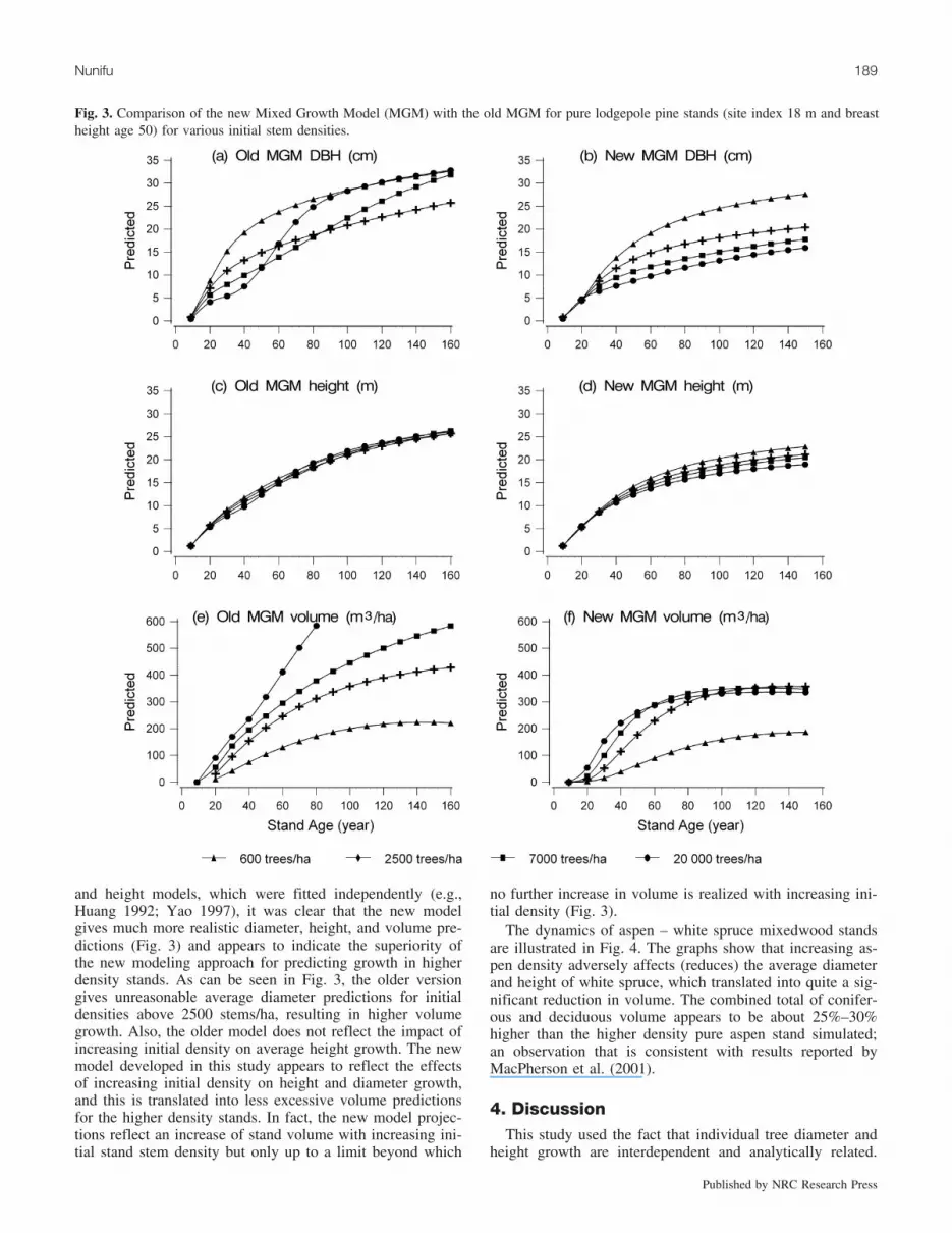
and height models, which were fitted independently (e.g.,Huang 1992; Yao 1997), it was clear that the new modelgives much more realistic diameter, height, and volume pre-dictions (Fig. 3) and appears to indicate the superiority ofthe new modeling approach for predicting growth in higherdensity stands. As can be seen in Fig. 3, the older versiongives unreasonable average diameter predictions for initialdensities above 2500 stems/ha, resulting in higher volumegrowth. Also, the older model does not reflect the impact ofincreasing initial density on average height growth. The newmodel developed in this study appears to reflect the effectsof increasing initial density on height and diameter growth,and this is translated into less excessive volume predictionsfor the higher density stands. In fact, the new model projec-tions reflect an increase of stand volume with increasing ini-tial stand stem density but only up to a limit beyond which

no further increase in volume is realized with increasing ini-tial density (Fig. 3).

The dynamics of aspen – white spruce mixedwood standsare illustrated in Fig. 4. The graphs show that increasing as-pen density adversely affects (reduces) the average diameterand height of white spruce, which translated into quite a sig-nificant reduction in volume. The combined total of conifer-ous and deciduous volume appears to be about 25%–30%higher than the higher density pure aspen stand simulated;an observation that is consistent with results reported byMacPherson et al. (2001).

4. DiscussionThis study used the fact that individual tree diameter and

height growth are interdependent and analytically related.

Fig. 3. Comparison of the new Mixed Growth Model (MGM) with the old MGM for pure lodgepole pine stands (site index 18 m and breastheight age 50) for various initial stem densities.

Nunifu 189

Published by NRC Research Press

This observation is supported by ecophysiology literature(e.g., Sjolte-Jørgensen 1967; Seidal 1984), which suggestthat relative allocation of growth to both diameter and heightare dependent on competition and wind-induced mechani-cal perturbation. The coefficients of the variables includedin the models are statistically significant at 5% probability,and the signs are ecologically interpretable except the pa-rameter for AGGRD in the pine and white spruce diametermodel and for QMDR in the aspen height growth model.

In lodgepole pine and white spruce diameter models, anincrease in AGGRD seems to favour diameter growth, an ob-servation that may seem ecologically illogical. It is specu-lated that competition from deciduous trees is relatively lessdetrimental to the diameter growth of trees of the two coni-

fer species than competition from other conifer trees. Thus,an increased proportion of deciduous trees appeared to mod-erate the effects of competition on the subject trees of theseconifer species. For white spruce, this observation seemsconsistent with the general belief that aspen serves as anurse crop to spruce by contributing, among other things, toaccelerated nutrient cycling (Man and Lieffers 1999). Thereduced competitive effects of the deciduous component ondiameter growth of lodgepole pine seems to be due to thegenerally low average of deciduous competition observed inthe lodgepole pine data used for model fitting (See Table 1).It is suspected that this will not cause a serious predictionproblem, as the coefficient affects only the relative alloca-tion of growth to diameter; the overall determinant of diam-

Fig. 4. Simulation results for varying aspen competition on white spruce in mixed stands. White spruce density is fixed at 2000 stems/ha atsite index 18 m and breast height age 50 and aspen competition is varied from 600 to 40 000 stems/ha with site index 18 m and breastheight age 50.

190 Can. J. For. Res. Vol. 39, 2009

Published by NRC Research Press

eter growth is height growth, which is affected by the totalamount of competition in the stand, including aspen compe-tition.

The sign of the coefficient of QMDR seems to suggestthat an increased aspen dominance in the stand negativelyaffects aspen tree height growth. It is speculated that eitherthe data used in the study do not portray significant interspe-cific competition in aspen stands or intraspecific competitionaffects aspen height growth more than interspecific competi-tion. Either way, simulation results, part of which are givenin Figs. 2 and 4, and the validation results, in Fig. 1 and Ta-ble 5, all indicate that the model predictions are satisfactoryfor all stand types. The simulation results presented inFigs. 2 and 4 may also be indicative of the fact that the ap-parent lack-of-fit results reflected in the equivalence tests(Table 6) are of little consequence at the stand level predic-tion both for the short and long terms.

The unusual bias observed for stand volume and BA inthe white spruce stand types (Fig. 1) perhaps can be ex-plained by the type of mortality predicted in these stands.The mortality models used in the version of MGM tested inthis study have a density–average size limit set for each spe-cies above which individual tree mortality is increased toforce the density–average size combination of the stand tofall below the maximum (Yang 2002). In addition, a set ofconstraining factors were set up in the model to reflect theaccelerated mortality associated with ecological standbreak-up at an older age. If the validation data are fromstands that do not break up at the age the model predicts,the predicted increased mortality rates of bigger trees mayresult in a lower mean DBH, stand BA, and ultimately,lower stand volume predictions than the actual observed val-ues. It is suspected that this is the case for the few whitespruce stands with biased volume and BA predictions, but Idid not investigate this further. Nevertheless, the model pre-dictions appear to be reasonable for the short term. The re-sults shown in Figs. 2 and 3 are also indicators that linkingdiameter and height growth can lead to more robust long-term predictions even if the model is applied to stands withdensities higher than the range of densities used in the fit-ting data (see Table 1). The results also demonstrate thecompatibility between diameter and height predictions andthat competition affects diameter growth more than heightgrowth, with the result that higher density stands havehigher height–diameter ratios than lower density stands.These model predictions seem to agree with well-docu-mented ecological research, which shows that tree diametergrowth, the result of lateral cambial growth, is limited moreby exhaustion of soil moisture, growth substances or neededassimilates (competition), and the accumulation of inhibitorsthan by cell preformation as in height growth (Zimmermannand Brown 1971; Fritts 1976).

The graphs in Fig. 4 show that increasing aspen densityreduces the final average DBH and height of spruce onlyslightly. However, it does appear from Fig. 4 that increasingaspen density results in an initial substantial decline inspruce volume trajectories. However, the individual volumetrajectories of spruce show relatively fast increasing trendsbetween 60 and 80 years even for stands with much heavieraspen competition. Available literature on mixedwood standdynamics suggests that aspen yield will peak at about age

80 years and begin to decline thereafter because of standbreak up, allowing growing space for the understory spruceor a new cohort of aspen. Figure 4 illustrates these dynamicsquite clearly and suggests a good performance of the newmodel for mixedwood stands. But these results reflect onlyan aspect of aspen–spruce dynamics where both species areestablished at the same time. Other scenarios in which thespruce component is established a few years after aspen canalso be implemented with reasonable results.

These results show that the models developed in thisstudy are ecologically logical and robust and can be appliedto both pure and mixed-species stands and for both short-term and long-term projections, with fairly unbiased results.These results demonstrate the utility of the model for short-term projections, such as inventory updates, and long-termprojection applications, such as yield curve development.Although there is still some room for improvement, particu-larly in the variable selection, the model predictions are ad-equate for most practical applications, such as yield curvedevelopment. The addition of crown-based variables maylikely improve model fit and prediction.

AcknowledgementsThis project was supported by the Weldwood Canada Ltd.,

Hinton division (now Hinton Wood Products Ltd.), throughthe Forest Resource Improvement Association of Alberta.Special thanks to Thomas Braun and Sharon Meredith whoboth served as contacts at Weldwood during the study. Iwould also like to acknowledge the contribution of theAlberta Sustainable Resource Development and D.J. Morganfor granting permission to use the provincial PSP data. Iwould like to acknowledge the assistance of Stephen J. Titus,Ellen Macdonald, Vic Lieffers, and Shongming Huang in re-viewing the earliest version of this manuscript included inmy Ph.D. thesis at the University of Alberta.

ReferencesALFS. 2000. Permanent sample plot field procedures manual. Al-

berta Lands and Forest Service, Forest Management Division,Resource Analysis Center, Edmonton, Alta.

Assmann, E. 1970. The principles of forest yield study studies. Per-gamon Press, Oxford.

Burkhart, H.E., and Sprinz, P.T. 1984. Compatible cubic volumeand basal area projection equations for thinned old-field loblollypine plantations. For. Sci. 30: 86–93.

Cieszewski, C.J., and Bella, I.E. 1993. Modeling density-relatedlodgepole pine height growth, using Czarnowski’s stand dynamicstheory. Can. J. For. Res. 23: 2499–2506. doi:10.1139/x93-311.

Czarnowski, M.S. 1961. Dynamics of even-aged forest stands.Louisiana State University, Baton Rouge. Biol. Ser.

Fritts, H.C. 1976. Tree rings and climate. Academic Press, NewYork, USA.

Furnival, G.M., and Wilson, R.W. 1971. Systems of equations forpredicting forest growth and yield. In Statistical ecology. Vol. 3.Edited by G.P. Patil, E.C. Pielou, and W.E. Walters. Pennsylva-nia State University Press, University Park, Pa. pp. 43–57.

Golser, M., and Hasenauer, H. 1997. Predicting juvenile tree heightgrowth in un-even-aged mixed species stands in Austria. For. Ecol.Manage. 97: 133–146. doi:10.1016/S0378-1127(97)00094-7.

Hann, D.W., and Ritchie, M.W. 1988. Height growth rate ofDouglas-fir: a comparison of model forms. For. Sci. 34: 165–175.

Nunifu 191

Published by NRC Research Press

Hasenauer, H., and Kindermann, G. 2002. Methods for assessingregeneration establishment and height growth in uneven-agedmixed species stands. Forestry, 75: 385–394. doi:10.1093/forestry/75.4.385.

Huang, S. 1992. Diameter and height growth models. Ph.D. thesis,Department of Renewable Resources, University of Alberta, Ed-monton, Alta.

Huang, S. 1997a. Subregion-based compatible height and site indexmodels for young and mature stands in Alberta: revisions andsummaries (Part I). For. Manage. Res. Note. No. 9, Alberta En-vironmental Protection, For. Manage. Div., Edmonton, Alta.

Huang, S. 1997b. Subregion-based compatible height and site indexmodels for young and mature stands in Alberta: revisions andsummaries (Part II). For. Manage. Res. Note. No. 9, AlbertaEnvironmental Protection, For. Manage. Div., Edmonton, Alta.

Huang, S., and Titus, S.J. 1999. Estimating a system of nonlinearsimultaneous individual tree models for white spruce in borealmixed-species stands. Can. J. For. Res. 29: 1805–1811. doi:10.1139/cjfr-29-11-1805.

Judge, G.G., Hill, R.C., Griffiths, W.E., Ltkepohl, H., and Lee,T.C. 1988. Introduction to the theory and practice of econo-metrics. 2nd ed. John Wiley and Sons, New York.

Leary, R.A. 1979. Design. In A generalized forest growth projec-tion system applied to the lake states region. USDA For. Serv.Gen. Tech. Rep. NC-49. pp. 5–15.

MacPherson, D.M., Lieffers, V.J., and Blenis, P.V. 2001. Produc-tivity of aspen stands with and without a spruce understory inAlberta’s boreal mixedwood forests. For. Chron. 77: 351–356.

Man, R., and Lieffers, V.J. 1999. Are mixtures of aspen and whitespruce more productive than single species stands? For. Chron.75: 505–513.

Meng, S.X., Lieffers, V.J., Reid, D.E.B., Rudnicki, M., Silins, U.,and Jin, M. 2006. Reducing stem bending increases heightgrowth of tall pines. J. Exp. Bot. 57: 3175–3182. doi:10.1093/jxb/erl079. PMID:16882643.

Mitchell, K.J. 1975. Dynamics and simulated yield of Douglas fir.For. Sci. Monogr. 17.

Mitchell, K.J., and Goudie, J.W. 1980. Stagnant lodgepole pine.Progress Report on EP 850.02, BC Ministry of Forests, Victoria.

Nilsson, U. 1994. Development of growth and stand structure Piceaabies stands planted at different initial densities. Scand. J. For.Res. 9: 135–142.

Nunifu, T.K. 2003. Calibrating the Mixedwood Growth Model(MGM) for lodgepole pine and associated species in Alberta.Ph.D. thesis, Department of Renewable Resources, Universityof Alberta, Edmonton, Alta.

Oliver, C.D., and Larson, B.C. 1996. Forest stand dynamics. Up-date edition. John Wiley and Sons, New York.

Opio, C., Jacob, N., and Coopersmith, D. 2000. Height to diameterratio as a competition index for young conifer plantations innorthern British Columbia. For. Ecol. Manage. 137: 245–252.doi:10.1016/S0378-1127(99)00312-6.

Qin, J., and Cao, Q.V. 2006. Using disaggregation to link indivi-dual-tree and whole-stand growth models. Can. J. For. Res. 36:953–960. doi:10.1139/X05-284.

Rich, P.M., Helenurm, K., Kearns, D., Morse, S.R., Palmer, M.W.,and Short, L. 1986. Height and stem diameter relationships fordicotyledonous trees and arborescent palms of Costa Rican tro-pical wet forest. Bull. Torrey Bot. Club, 113: 241–246. doi:10.2307/2996362.

Ritchie, M.W., and Hann, D.W. 1997. Implications of disaggrega-tion in forest growth and yield modeling. For. Sci. 43: 223–233.

Robinson, A.P., Duursma, R.A., and Marshall, J.D. 2005. A regres-sion-based equivalence test for model validation: shifting theburden of proof. Tree Physiol. 25: 903–913. PMID:15870057.

Schmidt, W.C., Shearer, R.C., and Roe, A.L. 1976. Ecology andsilviculture of western larch forests. USDA Tech. Bull. 1520.

Seidel, K.W. 1984. A western larch – Engelmann spruce spacingstudy in eastern Oregon: results after 10 years. USDA For.Serv. Res. Note PNW-409.

Sievanen, R. 1993. A process based model for the dimensionalgrowth of eve-aged stands. Scand. J. For. Res. 8: 28–48.

Sjolte-Jørgensen, J. 1967. The influence of spacing in the growthand development of coniferous plantations. Int. Rev. For. Res.2: 43–94.

Weiner, J. 1990. Asymmetric competition in plants. Trends Ecol.Evol. 5: 360–364. doi:10.1016/0169-5347(90)90095-U.

Yang, Y. 2002. Mortality modeling of major boreal species inAlberta. Ph.D. thesis, Department of Renewable Resources, Uni-versity of Alberta, Edmonton, Alta.

Yao, X. 1997. Modeling juvenile growth and mortality in mixed-wood stands of Alberta. Ph.D. thesis, University of Alberta,Edmonton, Alta.

Zellner, A. 1962. An efficient method of estimating seemingly un-related regressions and tests for aggregation bias. J. Am. Stat.Assoc. 57: 348–368. doi:10.2307/2281644.

Zhang, S., Amateis, R.L., and Burkhart, H.E. 1997. Constrainingindividual tree diameter increment and survival models for lo-blolly pine plantations. For. Sci. 43: 414–423.

Zimmermann, M.H., and Brown, C.L. 1971. Trees, structure andfunction. Springer-Verlag, New York, USA.

192 Can. J. For. Res. Vol. 39, 2009

Published by NRC Research Press