1

7th

International Conference on

Computer and IT Applications in the Maritime Industries

COMPIT’08

Liège, 21-23 April 2008

Edited by Volker Bertram, Philippe Rigo

This work relates to Department of the Navy Grant N00014-08-1-1007 issued by Office of

Naval Research Global. The United States Government has a royalty-free license throughout

the world in all copyrightable material contained herein.

ISBN-10 2-9600785-0-0

ISBN-13 978-2-9600785-0-3

2

Sponsored by

www.onrglobal.navy.mil

www.GL-group.com

www.aveva.com

www.sener.com

www.bureau-

veritas.com

http://dn-t.be

www.exmar.be

www.numeca.be

www.grc-ltd.co.uk

Platform for European Research Projects

ADOPT http://adopt.rtdproject.net

CAS http://www.shiphullmonitoring.eu

IMPROVE http://www.anast-eu.ulg.ac.be

3

Index

François-Xavier Dumez, Cedric Cheylan, Sébastien Boiteau, Cyrille Kammerer, 6

Emmanuel Mogicato, Thierry Dupau, Volker Bertram

A Tool for Rapid Ship Hull Modelling and Mesh Generation

Jan Tellkamp, Heinz Günther, Apostolos Papanikolaou, Stefan Krüger, Karl-Christian Ehrke, 19

John Koch Nielsen

ADOPT - Advanced Decision Support System for Ship Design, Operation and Training - An Overview

Steven J. Deere, Edwin R. Galea, Peter J. Lawrence 33

Assessing the Suitability of Ship Design for Human Factors Issues Associated with Evacuation and

Normal Operations

Jean-David Caprace, Frederic Bair, Nicolas Losseau, Renaud Warnotte, Philippe Rigo 48

OptiView − A Powerful and Flexible Decision Tool Optimising Space Allocation in Shipyard Workshops

Vidar Vindøy 60

A Functionally Oriented Vessel Data Model Used as Basis for Classification

Heinz Günther, Ina Tränkmann, Florian Kluwe 70

ADOPT DSS - Ocean Environment Modelling for Use in Decision Making Support

Rowan Van Schaeren, Wout Dullaert, Birger Raa 81

Enriching the Berth Allocation Problem

Philippe Rigo, Djani Dundara, Jean-Louis Guillaume-Combecave, Andrzej Karczewicz, Alan Klanac, 92

Frank Roland, Osman Turan, Vedran Zanic, Amirouche Amrane, Adrian Constantinescu

IMPROVE - Design of Improved and Competitive Products using an Integrated Decision Support

System for Ship Production and Operation

Catalin Toderan, J-L Guillaume-Combecave, Michel Boukaert, André Hage, Olivier Cartier, 107

Jean-David Caprace, Amirouche Amrane, Adrian Constantinescu, Eugen Pircalabu, Philippe Rigo

Structural Optimization of a 220 000 m³ LNG Carrier

Fernando Alonso, Carlos González, Antonio Pinto, Fernando Zurdo 121

Integrated Management of Ship Compartments

Antti Metsä, Pekka Ruponen, Christopher Ridgewell, Pasi Mustonen 135

Flooding Simulation as a Practical Design Tool

Charles Forrest 148

Development of an Innovative Surface Design Tool

Sandra Schrödter, Thomas Gosch 163

SESIS – Ship Design and Simulation System

Wilfried Abels, Lars Greitsch 174

Using a Bridge Simulator during the Early Design-Stage to Evaluate Manoeuvrability

Thomas Glotzbach, Matthias Schneider, Peter Otto 185

Multi System Mission Control for Teams of Unmanned Marine Vehicles – Software Structure for

Online Replanning of Mission Plans

Marcus Bentin, Folgert Smidt, Steffen Parth 200

Process Modeling and Simulation using CAD Data and PDM in Early Stage of Shipbuilding Project

4

Robert Hekkenberg 214

Development of a Rapid Conceptual Design Method for Inland Ships

Christian Cabos, David Jaramillo, Gundula Stadie-Frohbös, Philippe Renard, Manuel Ventura, 222

Bertrand Dumas

Condition Assessment Scheme for Ship Hull Maintenance

Thomas Brathaug, Jon Olav Holan, Stein Ove Erikstad 244

Representing Design Knowledge in Configuration-Based Conceptual Ship Design

Stefan Krüger, Florian Kluwe, Hendrik Vorhölter 260

Decision Support for Large Amplitude Roll Motions based on Nonlinear Time Domain Simulations

Andi Asmara, Ubald Nienhuis 271

Optimum Routing of Piping in Real Ships under Real Constraints

Matthias Grau, Carsten Zerbst, Markus Sachers 282

Building the Business Process View into Shipbuilding Data Exchange

Tomi Holmberg 291

Comprehensive Structural Design Package for Bulk Carriers

Carlos Vinícius Malheiros Santos 302

Production Simulation Applied to Military Shipbuilding

Rachel F. Nicholls-Lee, Stephen R. Turnock, Stephen W. Boyd 314

Simulation Based Optimisation of Marine Current Turbine Blades

Takakazu Nakamori, Mitsuru Kitamura, Kunihiro Hamada 329

Optimization of Arrangement of Longitudinal Stiffeners on Shell Plate at Fore and Aft Parts

of Ships

Dirk Wittkuhn, Karl-Christian Ehrke, John Koch Nielsen 338

ADOPT: Man-Machine Interface and Training

Björn Weidemann, Ralf Bohnenberg, Martin-Christoph Wanner 350

Shipyard Investment Planning by Use of Modern Process-Simulation and Layout-Planning Tools

Rafael Doig, Patrick Kaeding 364

Multi-Body Simulation of a Loading Operation

Karl Gunnar Aarsæther, Torgeir Moan 372

Autonomous Traffic Model for Ship Maneuvering Simulations Based on Historical Data

Andrea Caiti, Giuseppe Casalino, Alessio Turetta, Riccardo Viviani 384

Distributed Dynamic Programming for Adaptive On-line Planning of AUVs Team Missions with

Communication Constraints

Patrick Queutey, Michel Visonneau, Ganbo Deng, Alban Leroyer, Emmanuel Guilmineau, 392

Aji Purwanto

Computations for a US Navy Frigate Advancing in Head Waves in Fixed and Free Conditions

David Andrews, Lorenzo Casarosa, Richard Pawling 407

Interactive Computer Graphics and Simulation in Preliminary Ship Design

Hao Cui, Aykut Ölcer, Osman Turan 422

An Improved Particle Swarm Optimisation (PSO) Approach in a Multi Criteria Decision Making

Environment

5

Djani Dundara, Dario Bocchetti, Obrad Kuzmanovic, Vedran Zanic, Jerolim Andric, Pero Prebeg 435

Development of a New Innovative Concept of Ropax Ship

Darko Frank, Alan Klanac, Svemir Bralic 450

A Concept for Concurrent Group Design of Ships

Yves Le Thérisien, Chantal Maïs 460

Virtual Reality – Tool of Assistance to the Design of the Warship’s Complex Systems

Thomas Haberkorn, Monique Chyba, Ryan Smith, Song. K. Choi, Giacomo Marani, Chris McLeod 467

Efficient Control of an Autonomous Underwater Vehicle while Accounting for Thruster Failure

Cassiano M. de Souza, Rafael Tostes 481

Shipbuilding Interim Product Identification and Classification System Based on Intelligent Analysis

Tools

Jeroen F.J. Pruyn, Ubald Nienhuis, Eddy van de Voorde, Hilde Meersman 495

Towards a Consistent and Dynamic Simulation of Company Behaviour in the Maritime Sector

Adam Sobey, James Blake, Ajit Shenoi 502

Optimization of Composite Boat Hull Structures

Marc Wilken, Christian Cabos, Wiegand Grafe 516

Using CAD Data for Computation and Assessment of Global Ship Structures

Audun Grimstad, Arnulf Hagen 524

Customised Ship Design = Customised Ship Design Environments

Alan Klanac, Jasmin Jelovica, Matias Niemeläinen, Stanislaw Domagallo, Heikki Remes, 537

Structural Omni-Optimization of a Tanker

Hamid Hefazi, Adeline Schmitz, Igor Mizine, Geoffrey Boals 551

Multi-Disciplinary Synthesis Design and Optimization for Multi-Hull Ships

Dimitris Spanos, Apostolos Papanikolaou, George Papatzanakis, Jan Tellkamp 566

On Board Assessment of Seakeeping for Risk-Based Decision Support to the Master

Shimpei Watanabe, Kazuhiko Hasegawa, Philippe Rigo 578

Inland Waterway Traffic Simulator

Liming W. Salvino, Thomas F. Brady 589

Hull Monitoring System Development using a Hierarchical Framework for Data and Information

Management

Yvonne R. Masakowski 603

Cognition-Centric Systems Design: A Paradigm Shift in System Design

Index of authors 608

Call for Papers COMPIT’09

6

A Tool for Rapid Ship Hull Modelling and Mesh Generation

François-Xavier Dumez, GRANITX, Brest/France, dumez@granitx.com Cedric Cheylan, Sébastien Boiteau, Cyrille Kammerer, DCNS, Lorient/France

Emmanuel Mogicato, Thierry Dupau, BEC, Val de Reuil/France Volker Bertram, ENSIETA, Brest/France

Abstract

The paper describes SILEX, a tool for the rapid and associative generation of numerical hull models linked to different simulation tools. The underlying concepts are described. Industry applications illustrate the capabilities and efficiency of the approach.

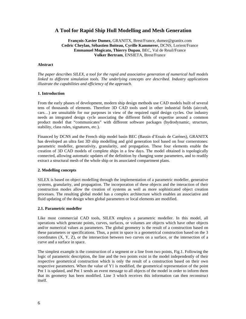
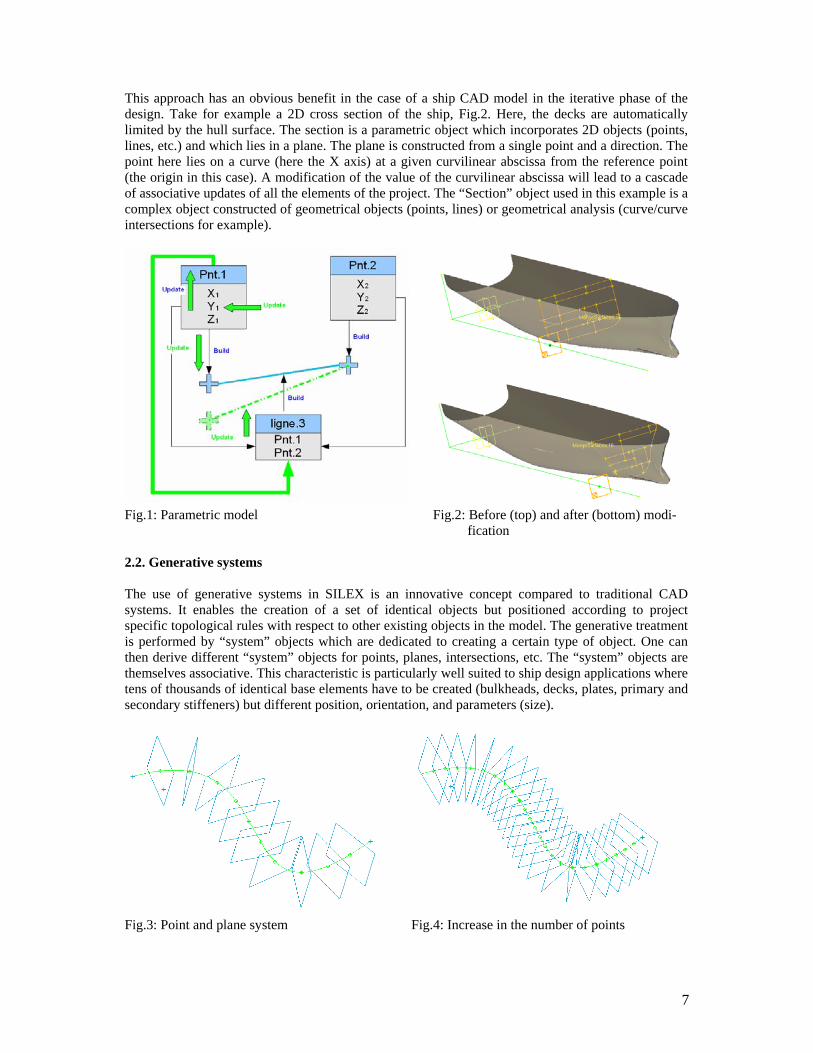
1. Introduction From the early phases of development, modern ship design methods use CAD models built of several tens of thousands of elements. Therefore 3D CAD tools used in other industrial fields (aircraft, cars…) are unsuitable for our purposes in view of the required rapid design cycles. Our industry needs an integrated design cycle associating the different fields of expertise around a common product model that “communicates” with different software packages (hydrodynamic, structure, stability, class rules, signatures, etc.). Financed by DCNS and the French ship model basin BEC (Bassin d’Essais de Carènes), GRANITX has developed an ultra fast 3D ship modelling and grid generation tool based on four cornerstones: parametric modeller, generativity, granularity, and propagation. These four elements enable the creation of 3D CAD models of complete ships in a few days. The model obtained is topologically connected, allowing automatic updates of the definition by changing some parameters, and to readily extract a structural mesh of the whole ship or its associated compartment plans. 2. Modelling concepts SILEX is based on object modelling through the implementation of a parametric modeller, generative systems, granularity, and propagation. The incorporation of these objects and the interaction of their construction modes allow the creation of systems as well as more sophisticated object creation processes. The resulting global model has a complex architecture which enables an associative and fluid updating of the design when global parameters or local elements are modified. 2.1. Parametric modeller Like most commercial CAD tools, SILEX employs a parametric modeller. In this model, all operations which generate points, curves, surfaces, or volumes are objects which have other objects and/or numerical values as parameters. The global geometry is the result of a construction based on these parameters or specifications. Thus, a point in space is a geometrical construction based on the 3 coordinates (X, Y, Z), or the intersection between two curves on a surface, or the intersection of a curve and a surface in space. The simplest example is the construction of a segment or a line from two points, Fig.1. Following the logic of parametric description, the line and the two points exist in the model independently of their respective geometrical construction which is only the result of a construction based on their own respective parameters. When the value of Y1 is modified, the geometrical representation of the point Pnt 1 is updated, and Pnt 1 sends an event message to all objects of the model in order to inform them that its geometry has been modified. Line 3 which receives this information can then reconstruct itself.

7

This approach has an obvious benefit in the case of a ship CAD model in the iterative phase of the design. Take for example a 2D cross section of the ship, Fig.2. Here, the decks are automatically limited by the hull surface. The section is a parametric object which incorporates 2D objects (points, lines, etc.) and which lies in a plane. The plane is constructed from a single point and a direction. The point here lies on a curve (here the X axis) at a given curvilinear abscissa from the reference point (the origin in this case). A modification of the value of the curvilinear abscissa will lead to a cascade of associative updates of all the elements of the project. The “Section” object used in this example is a complex object constructed of geometrical objects (points, lines) or geometrical analysis (curve/curve intersections for example).

Fig.1: Parametric model Fig.2: Before (top) and after (bottom) modi-

fication 2.2. Generative systems The use of generative systems in SILEX is an innovative concept compared to traditional CAD systems. It enables the creation of a set of identical objects but positioned according to project specific topological rules with respect to other existing objects in the model. The generative treatment is performed by “system” objects which are dedicated to creating a certain type of object. One can then derive different “system” objects for points, planes, intersections, etc. The “system” objects are themselves associative. This characteristic is particularly well suited to ship design applications where tens of thousands of identical base elements have to be created (bulkheads, decks, plates, primary and secondary stiffeners) but different position, orientation, and parameters (size).

Fig.3: Point and plane system Fig.4: Increase in the number of points

8

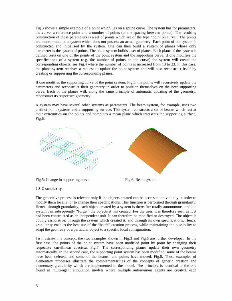
Fig.3 shows a simple example of a point which lies on a spline curve. The system has for parameters, the curve, a reference point and a number of points (or the spacing between points). The resulting construction of these parameters is a set of points which are of the type “point on curve”. The points are incorporated in a system which does not possess an actual geometry. Each point of the system is constructed and initialised by the system. One can then build a system of planes whose only parameter is the system of points. The plane system builds a set of planes. Each plane of the system is defined rests on one of the points of the point system and the supporting curve. If one modifies the specifications of a system (e.g. the number of points on the curve) the system will create the corresponding objects, see Fig.4 where the number of points is increased from 10 to 23. In this case, the plane system receives a request to update the point system and will also reconstruct itself by creating or suppressing the corresponding planes. If one modifies the supporting curve of the point system, Fig.5, the points will recursively update the parameters and reconstruct their geometry in order to position themselves on the new supporting curve. Each of the planes will, along the same principle of automatic updating of the geometry, reconstruct its respective geometry. A system may have several other systems as parameters. The beam system, for example, uses two distinct point systems and a supporting surface. This system constructs a set of beams which rest at their extremities on the points and computes a mean plane which intersects the supporting surface, Fig.6.

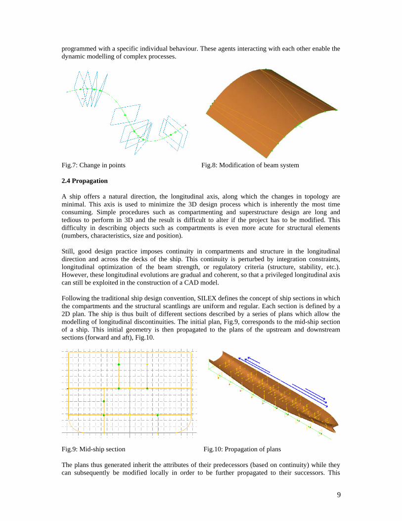
Fig.5: Change in supporting curve Fig.6: Beam system 2.3 Granularity The generative process is relevant only if the objects created can be accessed individually in order to modify them locally, or to change their specifications. This function is performed through granularity. Hence, through granularity, each object created by a system is thereafter totally autonomous, and the system can subsequently “forget” the objects it has created. For the user, it is therefore seen as if it had been constructed as an independent unit. It can therefore be modified or destroyed. The object is doubly associative: through the system which created it, and through its own specifications. Hence, granularity enables the best use of the “batch” creation process, while maintaining the possibility to adapt the geometry of a particular object to a specific local configuration. To illustrate this concept, the two examples shown in Fig.3 and Fig.6 are further developed. In the first case, the points of the point system have been modified point by point by changing their respective curvilinear abscissa, Fig.7. The corresponding planes update their own geometry automatically. In the second case, the supporting point system has been modified, some of the beams have been deleted, and some of the beams’ end points have moved, Fig.8. These examples of elementary processes illustrate the complementarities of the concepts of generic creation and elementary granularity which are implemented in the model. The principle is identical to the one found in multi-agent simulation models where multiple autonomous agents are created, each

9

programmed with a specific individual behaviour. These agents interacting with each other enable the dynamic modelling of complex processes.

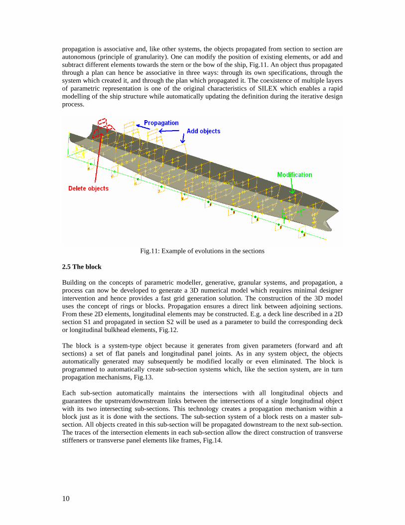
Fig.7: Change in points Fig.8: Modification of beam system 2.4 Propagation A ship offers a natural direction, the longitudinal axis, along which the changes in topology are minimal. This axis is used to minimize the 3D design process which is inherently the most time consuming. Simple procedures such as compartmenting and superstructure design are long and tedious to perform in 3D and the result is difficult to alter if the project has to be modified. This difficulty in describing objects such as compartments is even more acute for structural elements (numbers, characteristics, size and position). Still, good design practice imposes continuity in compartments and structure in the longitudinal direction and across the decks of the ship. This continuity is perturbed by integration constraints, longitudinal optimization of the beam strength, or regulatory criteria (structure, stability, etc.). However, these longitudinal evolutions are gradual and coherent, so that a privileged longitudinal axis can still be exploited in the construction of a CAD model. Following the traditional ship design convention, SILEX defines the concept of ship sections in which the compartments and the structural scantlings are uniform and regular. Each section is defined by a 2D plan. The ship is thus built of different sections described by a series of plans which allow the modelling of longitudinal discontinuities. The initial plan, Fig.9, corresponds to the mid-ship section of a ship. This initial geometry is then propagated to the plans of the upstream and downstream sections (forward and aft), Fig.10.

Fig.9: Mid-ship section Fig.10: Propagation of plans The plans thus generated inherit the attributes of their predecessors (based on continuity) while they can subsequently be modified locally in order to be further propagated to their successors. This

10

propagation is associative and, like other systems, the objects propagated from section to section are autonomous (principle of granularity). One can modify the position of existing elements, or add and subtract different elements towards the stern or the bow of the ship, Fig.11. An object thus propagated through a plan can hence be associative in three ways: through its own specifications, through the system which created it, and through the plan which propagated it. The coexistence of multiple layers of parametric representation is one of the original characteristics of SILEX which enables a rapid modelling of the ship structure while automatically updating the definition during the iterative design process.

Fig.11: Example of evolutions in the sections

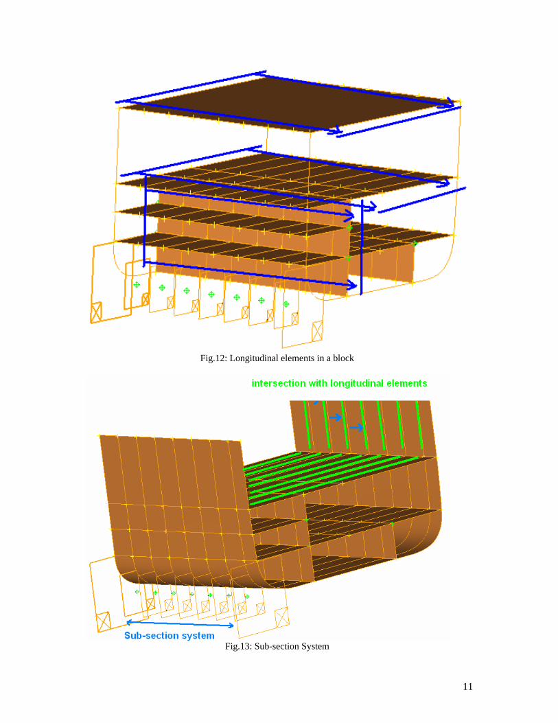
2.5 The block Building on the concepts of parametric modeller, generative, granular systems, and propagation, a process can now be developed to generate a 3D numerical model which requires minimal designer intervention and hence provides a fast grid generation solution. The construction of the 3D model uses the concept of rings or blocks. Propagation ensures a direct link between adjoining sections. From these 2D elements, longitudinal elements may be constructed. E.g. a deck line described in a 2D section S1 and propagated in section S2 will be used as a parameter to build the corresponding deck or longitudinal bulkhead elements, Fig.12. The block is a system-type object because it generates from given parameters (forward and aft sections) a set of flat panels and longitudinal panel joints. As in any system object, the objects automatically generated may subsequently be modified locally or even eliminated. The block is programmed to automatically create sub-section systems which, like the section system, are in turn propagation mechanisms, Fig.13. Each sub-section automatically maintains the intersections with all longitudinal objects and guarantees the upstream/downstream links between the intersections of a single longitudinal object with its two intersecting sub-sections. This technology creates a propagation mechanism within a block just as it is done with the sections. The sub-section system of a block rests on a master sub-section. All objects created in this sub-section will be propagated downstream to the next sub-section. The traces of the intersection elements in each sub-section allow the direct construction of transverse stiffeners or transverse panel elements like frames, Fig.14.

11

Fig.12: Longitudinal elements in a block

Fig.13: Sub-section System

12

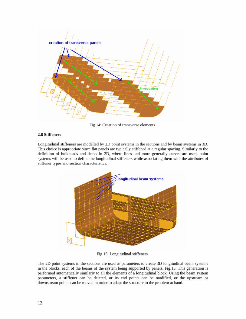
Fig.14: Creation of transverse elements

2.6 Stiffeners Longitudinal stiffeners are modelled by 2D point systems in the sections and by beam systems in 3D. This choice is appropriate since flat panels are typically stiffened at a regular spacing. Similarly to the definition of bulkheads and decks in 2D, where lines and more generally curves are used, point systems will be used to define the longitudinal stiffeners while associating them with the attributes of stiffener types and section characteristics.

Fig.15: Longitudinal stiffeners

The 2D point systems in the sections are used as parameters to create 3D longitudinal beam systems in the blocks, each of the beams of the system being supported by panels, Fig.15. This generation is performed automatically similarly to all the elements of a longitudinal block. Using the beam system parameters, a stiffener can be deleted, or its end points can be modified, or the upstream or downstream points can be moved in order to adapt the structure to the problem at hand.

13

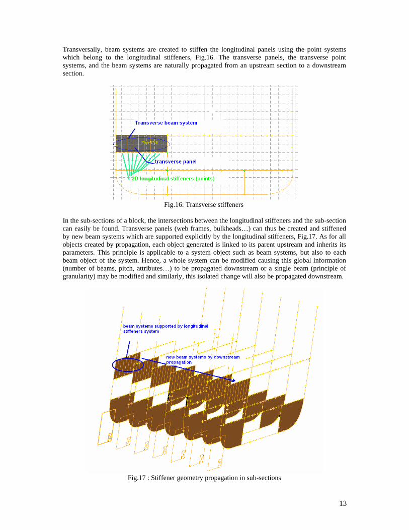
Transversally, beam systems are created to stiffen the longitudinal panels using the point systems which belong to the longitudinal stiffeners, Fig.16. The transverse panels, the transverse point systems, and the beam systems are naturally propagated from an upstream section to a downstream section.

Fig.16: Transverse stiffeners

In the sub-sections of a block, the intersections between the longitudinal stiffeners and the sub-section can easily be found. Transverse panels (web frames, bulkheads…) can thus be created and stiffened by new beam systems which are supported explicitly by the longitudinal stiffeners, Fig.17. As for all objects created by propagation, each object generated is linked to its parent upstream and inherits its parameters. This principle is applicable to a system object such as beam systems, but also to each beam object of the system. Hence, a whole system can be modified causing this global information (number of beams, pitch, attributes…) to be propagated downstream or a single beam (principle of granularity) may be modified and similarly, this isolated change will also be propagated downstream.

Fig.17 : Stiffener geometry propagation in sub-sections

14

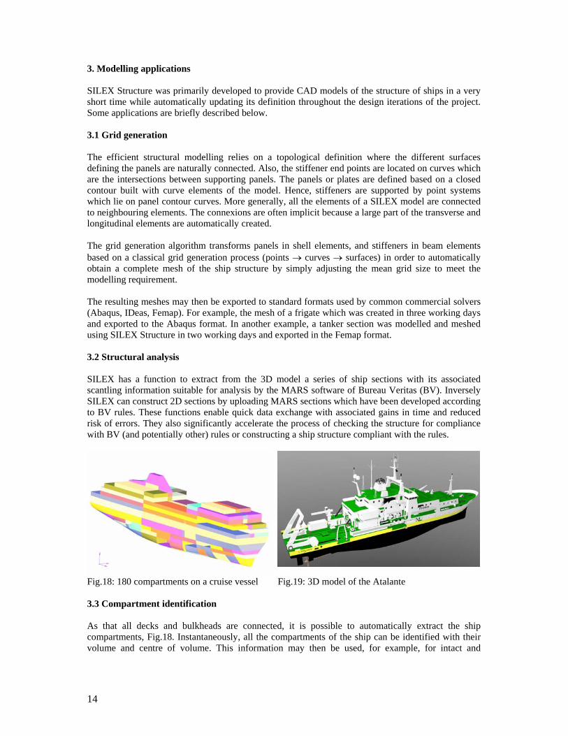
3. Modelling applications SILEX Structure was primarily developed to provide CAD models of the structure of ships in a very short time while automatically updating its definition throughout the design iterations of the project. Some applications are briefly described below. 3.1 Grid generation The efficient structural modelling relies on a topological definition where the different surfaces defining the panels are naturally connected. Also, the stiffener end points are located on curves which are the intersections between supporting panels. The panels or plates are defined based on a closed contour built with curve elements of the model. Hence, stiffeners are supported by point systems which lie on panel contour curves. More generally, all the elements of a SILEX model are connected to neighbouring elements. The connexions are often implicit because a large part of the transverse and longitudinal elements are automatically created. The grid generation algorithm transforms panels in shell elements, and stiffeners in beam elements based on a classical grid generation process (points → curves → surfaces) in order to automatically obtain a complete mesh of the ship structure by simply adjusting the mean grid size to meet the modelling requirement. The resulting meshes may then be exported to standard formats used by common commercial solvers (Abaqus, IDeas, Femap). For example, the mesh of a frigate which was created in three working days and exported to the Abaqus format. In another example, a tanker section was modelled and meshed using SILEX Structure in two working days and exported in the Femap format. 3.2 Structural analysis SILEX has a function to extract from the 3D model a series of ship sections with its associated scantling information suitable for analysis by the MARS software of Bureau Veritas (BV). Inversely SILEX can construct 2D sections by uploading MARS sections which have been developed according to BV rules. These functions enable quick data exchange with associated gains in time and reduced risk of errors. They also significantly accelerate the process of checking the structure for compliance with BV (and potentially other) rules or constructing a ship structure compliant with the rules.

Fig.18: 180 compartments on a cruise vessel Fig.19: 3D model of the Atalante 3.3 Compartment identification As that all decks and bulkheads are connected, it is possible to automatically extract the ship compartments, Fig.18. Instantaneously, all the compartments of the ship can be identified with their volume and centre of volume. This information may then be used, for example, for intact and

15

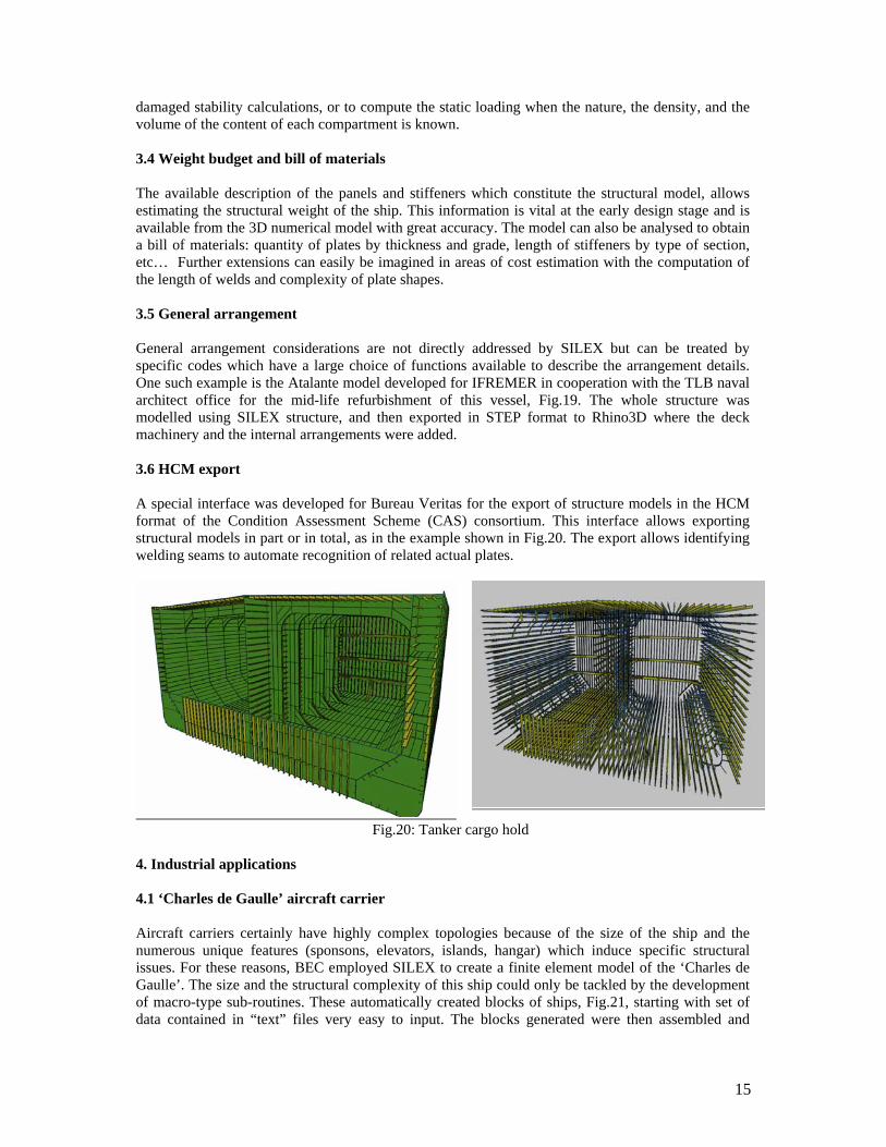
damaged stability calculations, or to compute the static loading when the nature, the density, and the volume of the content of each compartment is known. 3.4 Weight budget and bill of materials The available description of the panels and stiffeners which constitute the structural model, allows estimating the structural weight of the ship. This information is vital at the early design stage and is available from the 3D numerical model with great accuracy. The model can also be analysed to obtain a bill of materials: quantity of plates by thickness and grade, length of stiffeners by type of section, etc… Further extensions can easily be imagined in areas of cost estimation with the computation of the length of welds and complexity of plate shapes. 3.5 General arrangement General arrangement considerations are not directly addressed by SILEX but can be treated by specific codes which have a large choice of functions available to describe the arrangement details. One such example is the Atalante model developed for IFREMER in cooperation with the TLB naval architect office for the mid-life refurbishment of this vessel, Fig.19. The whole structure was modelled using SILEX structure, and then exported in STEP format to Rhino3D where the deck machinery and the internal arrangements were added. 3.6 HCM export A special interface was developed for Bureau Veritas for the export of structure models in the HCM format of the Condition Assessment Scheme (CAS) consortium. This interface allows exporting structural models in part or in total, as in the example shown in Fig.20. The export allows identifying welding seams to automate recognition of related actual plates.

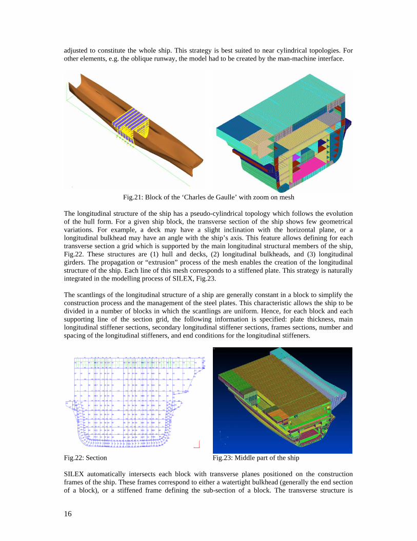
Fig.20: Tanker cargo hold 4. Industrial applications 4.1 ‘Charles de Gaulle’ aircraft carrier Aircraft carriers certainly have highly complex topologies because of the size of the ship and the numerous unique features (sponsons, elevators, islands, hangar) which induce specific structural issues. For these reasons, BEC employed SILEX to create a finite element model of the ‘Charles de Gaulle’. The size and the structural complexity of this ship could only be tackled by the development of macro-type sub-routines. These automatically created blocks of ships, Fig.21, starting with set of data contained in “text” files very easy to input. The blocks generated were then assembled and

16

adjusted to constitute the whole ship. This strategy is best suited to near cylindrical topologies. For other elements, e.g. the oblique runway, the model had to be created by the man-machine interface.

Fig.21: Block of the ‘Charles de Gaulle’ with zoom on mesh

The longitudinal structure of the ship has a pseudo-cylindrical topology which follows the evolution of the hull form. For a given ship block, the transverse section of the ship shows few geometrical variations. For example, a deck may have a slight inclination with the horizontal plane, or a longitudinal bulkhead may have an angle with the ship’s axis. This feature allows defining for each transverse section a grid which is supported by the main longitudinal structural members of the ship, Fig.22. These structures are (1) hull and decks, (2) longitudinal bulkheads, and (3) longitudinal girders. The propagation or “extrusion” process of the mesh enables the creation of the longitudinal structure of the ship. Each line of this mesh corresponds to a stiffened plate. This strategy is naturally integrated in the modelling process of SILEX, Fig.23. The scantlings of the longitudinal structure of a ship are generally constant in a block to simplify the construction process and the management of the steel plates. This characteristic allows the ship to be divided in a number of blocks in which the scantlings are uniform. Hence, for each block and each supporting line of the section grid, the following information is specified: plate thickness, main longitudinal stiffener sections, secondary longitudinal stiffener sections, frames sections, number and spacing of the longitudinal stiffeners, and end conditions for the longitudinal stiffeners.

Fig.22: Section Fig.23: Middle part of the ship SILEX automatically intersects each block with transverse planes positioned on the construction frames of the ship. These frames correspond to either a watertight bulkhead (generally the end section of a block), or a stiffened frame defining the sub-section of a block. The transverse structure is

17

consistent with the previous section grid, Fig.22, and more specifically it lies on a series of lines which form a closed contour which corresponds either to a stiffened transverse frame (beam), or a stiffened transverse plate (the plate is the surface within this contour). The data input concerns on one hand the main section at the beginning of the block and on the other all the sub-sections of the block. The transverse scantlings of each sub-section of a block are considered uniform between two adjacent sub-sections while possibly being different from the transverse scantlings of the main section of the block. For example, the main longitudinal stiffeners intersect all the sub-sections of a block (the construction frames of the ship). For each closed contour, one prescribes number of sides of the contour, transverse plate thickness, section of main vertical stiffeners, section of secondary vertical stiffeners, section of horizontal stiffeners, end conditions for the vertical and horizontal stiffeners. This data is input for the section at the beginning of the block and for the sub-sections of the block. The topological and scantling data contained in the structural drawings of the ship are input in Excel files. In this particular case, the model represents 70 m of the ship and is made of 17 blocks. The grid is composed of 580 supporting lines which delimit 252 closed contours. Only 30% of the lines and contours have been attributed some information; the others only serve as continuity in the programming algorithms. The man-machine interface for SILEX to input the data is replaced by a script of macro-commands which makes use of all the strategies and functions developed in SILEX. The different steps of the script were as follows: - Reading the topological and scantling data - Creation of the axis system, of points, planes, and sections which enable the positioning of the

main frame on the axis of the ship, - Creation of the supporting points for the plates of each section, - Creation of the plates from the points and of the longitudinal stiffeners in each section, - Creation of the transverse plates and stiffeners, - Creation of blocks by joining two adjacent sections, - Creation of the transverse stiffeners of the section, - Creation of the transverse plates and stiffeners of the sub-section, - Mesh generation for the blocks and sections. The different blocks and parts of ships generated are assembled and adjusted using Femap or IDeas to build the complete ship. If two adjacent parts of ships have significant topological differences (e.g. a deck or a longitudinal bulkhead disappearing) manual adjustments of either adjacent block at their interface are required to achieve an accurate description of the structure. The intensive use of macro-commands reduced the workload related to data input drastically. Although this vessel does not fulfil the fundamental assumption of longitudinal continuity, SILEX allowed creating the complete mesh of the ship within 4 man-months. A frigate or a commercial vessel with regular topology would take typically one man-month. 4.2 DCNS Frigate The first designs at DCNS modelled with SILEX were frigates described using entirely the man-machine interface. The description process was coherent with the way ship structures are usually designed: The hull form was imported and the bulkheads were allocated. The mid-ship section was described as a 2D plan with lines representing the main plates (decks, hull, longitudinal bulkheads, and girders) and with the properties of the longitudinal stiffeners attached to the panels. Then the transverse elements in the 2D sketch of the mid-ship section were described: transverse bulkheads, frames, and main vertical stiffeners. The mid-ship section was propagated to the other sections of the ship, and geometry and scantlings adapted at each section. Then the blocks between adjacent sections were generated, longitudinal stiffeners locally adapted, and transverse elements (frames, web frames,

18

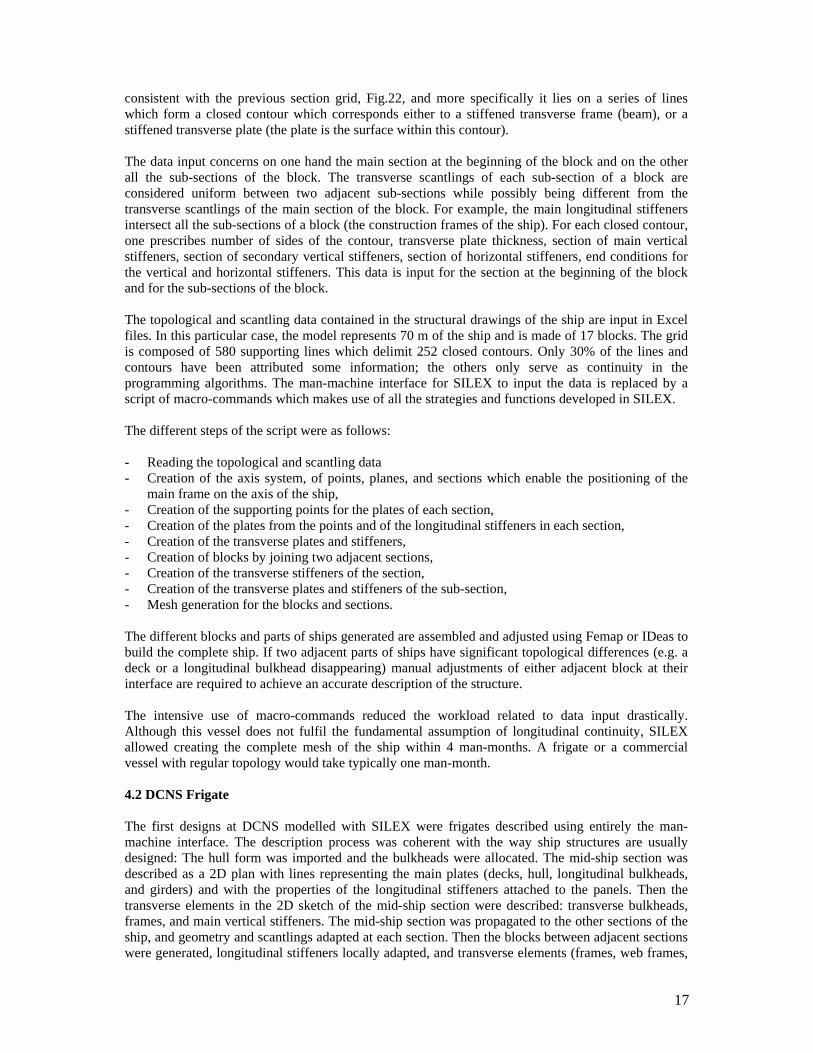
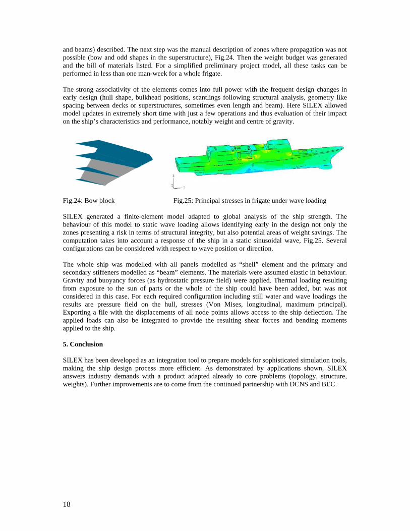
and beams) described. The next step was the manual description of zones where propagation was not possible (bow and odd shapes in the superstructure), Fig.24. Then the weight budget was generated and the bill of materials listed. For a simplified preliminary project model, all these tasks can be performed in less than one man-week for a whole frigate. The strong associativity of the elements comes into full power with the frequent design changes in early design (hull shape, bulkhead positions, scantlings following structural analysis, geometry like spacing between decks or superstructures, sometimes even length and beam). Here SILEX allowed model updates in extremely short time with just a few operations and thus evaluation of their impact on the ship’s characteristics and performance, notably weight and centre of gravity.

Fig.24: Bow block Fig.25: Principal stresses in frigate under wave loading SILEX generated a finite-element model adapted to global analysis of the ship strength. The behaviour of this model to static wave loading allows identifying early in the design not only the zones presenting a risk in terms of structural integrity, but also potential areas of weight savings. The computation takes into account a response of the ship in a static sinusoidal wave, Fig.25. Several configurations can be considered with respect to wave position or direction. The whole ship was modelled with all panels modelled as “shell” element and the primary and secondary stiffeners modelled as “beam” elements. The materials were assumed elastic in behaviour. Gravity and buoyancy forces (as hydrostatic pressure field) were applied. Thermal loading resulting from exposure to the sun of parts or the whole of the ship could have been added, but was not considered in this case. For each required configuration including still water and wave loadings the results are pressure field on the hull, stresses (Von Mises, longitudinal, maximum principal). Exporting a file with the displacements of all node points allows access to the ship deflection. The applied loads can also be integrated to provide the resulting shear forces and bending moments applied to the ship. 5. Conclusion SILEX has been developed as an integration tool to prepare models for sophisticated simulation tools, making the ship design process more efficient. As demonstrated by applications shown, SILEX answers industry demands with a product adapted already to core problems (topology, structure, weights). Further improvements are to come from the continued partnership with DCNS and BEC.

ADOPT – Advanced Decision Support System for Ship Design, Operationand Training – An Overview

Jan Tellkamp, FSG, Flensburg/Germany, jt@fsg-ship.deHeinz Gunther, GKSS, Geesthacht/Germany, heinz.guenther@gkss.deApostolos Papanikolaou, NTUA, Athens/Greece, papa@deslab.ntua.gr

Stefan Kruger, TUHH-SDIT, Hamburg/Germany, krueger@tu-harburg.deKarl-Christian Ehrke, SAM, Hamburg/Germany, Karl-Christian.Ehrke@sam-electronics.de

John Koch Nielsen, FORCE, Lyngby/Denmark, jnn@force.dk

Abstract

ADOPT aims at developing a concept for a risk-based, ship specific, real-time Decision Support Sys-tem (DSS) covering three distinct modes of use: Design, Training, Operation. The number one priorityof the ADOPT-DSS is to assist the master to identify and avoid potentially dangerous situations. TheADOPT-DSS will be customized for a specific ship and aims at utilizing state-of-the-art know-how andtechnology not available widely today. Therefore, the three modes are building upon each other. The ba-sis is the design (or office) mode. Information generated in the design mode is passed on to the trainingmode. Training can be provided directly using the information generated in design mode. In addition, themaster can be trained for using the operation mode implementation of the ADOPT-DSS. The challengein developing such a system is to interface and connect various data sources, hardware, and softwaresystems, that might run on various IT platforms.

1 Background

Ship accidents or near misses due to heavy seas are reported frequently, e.g. Kernchen (2008), McDaniel(2008). Apart from these safety related accidents, damages non-critical from a safety perspective occureven more frequently. These damages are of high economic concern, as their impact span from on-boardrepair to taking vessels out of service for docking. In the latter case, economic consequences are in theorder of magnitude of 100,000 Euro. IMO MSC/Circ. 707, IMO (1995), gives guidance to masters in theform of simple rules for identification of potentially harmful situations. There are also computer systemsthat aim at improving the situation.

All support on the bridge is subject to the ‘Warning Dilemma’. The warning dilemma as presented inTable I depicts a high-level requirement for any system aiming to warn in critical situations. In a nutshell,safety critical systems shall issue warnings only if action is required, but always if action is required.Warnings issued if no action is required might increase the risk. Warnings not issued if action is requiredmight have two reasons – either the system cannot assess a situation, or it malfunctions. If this occursduring operation the user confidence in the system decreases.

Table I: Warning dilemma (Courtesy of Arne Braathens, DNV)

Action Actionrequired not required

Warning issued OK not OKWarning not issued not OK OK

On the other hand, during the design phase of a ship a massive amount of numeric simulations are carriedout using direct calculation tools. Basis for these calculations are the ship in its current design stage, theoperational envelope of the intended service, and environmental data. As one result of these investiga-tions, limits of the operational envelope are determined, or the design is altered. Limits determined canbe displayed in polar diagrams, giving limiting significant wave heights as a function of encounter angleand ship speed. The parameters of the polar diagrams are the wave length, the loading condition, and theexceedance of a certain threshold value (e.g. particular roll angle, accelerations at a certain position ofthe vessel, stresses in the structure).

19

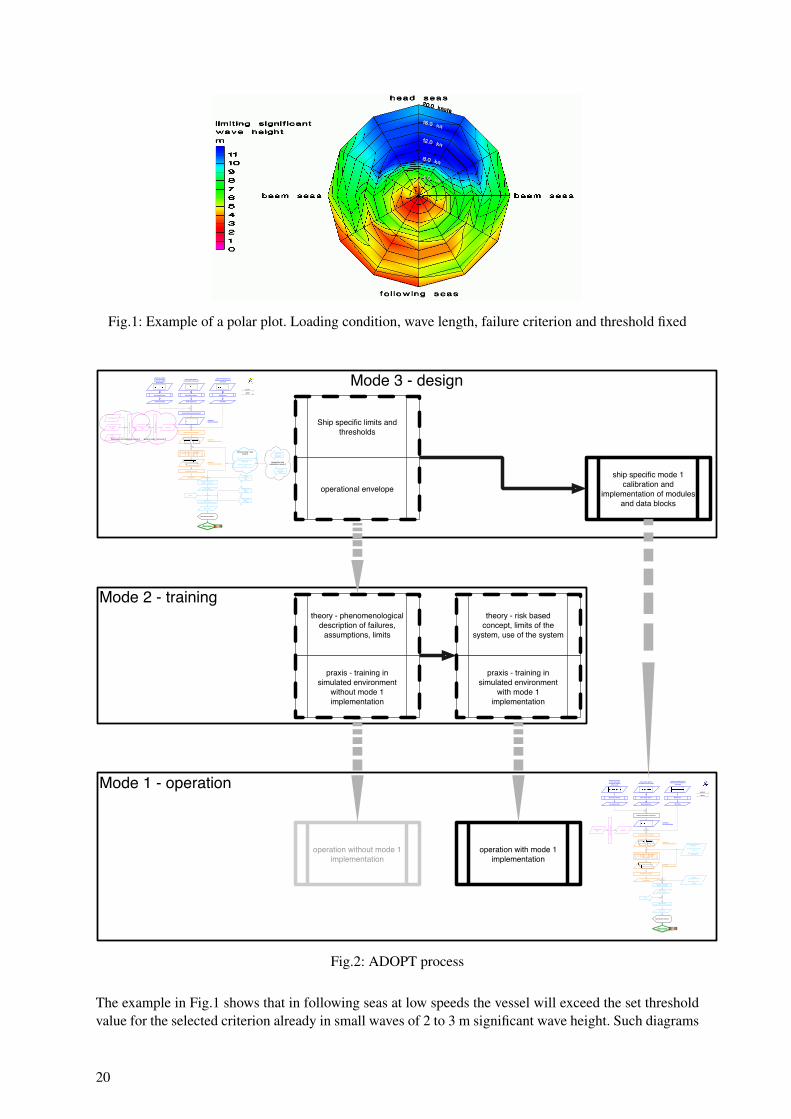
Fig.1: Example of a polar plot. Loading condition, wave length, failure criterion and threshold fixed

Decision Uncertainty

actual sea surface

in time and space

around the location

of the vessel

numerical Sea Surface Generator

Sea Surface Sensor

Sea Surface Data

numerical

Sea Surface Data

numerical Submode Load Analyzor

(excitation, velocity, acceleration

linear loads)

numerical Motion Analyzor

numerical

System Response Data

Input/

Output

numerical

Submode Analysis Data

Probability Calculator

Probabilities

Risk Level Generator

Safety / Economic

Risk Level

Safety / Economic

Risk Analyzor(internally rerunning to evaluate RCOs)

RCOs

Risk Picture

Man-Machine Interface

Safety

Consequence Data

Risk Aversion Data -

Safety

INPUT

OUTPUT

Wind Sensor

Wind Data

Water Depth Sensor

Water Depth Data

actual water depth at

the location of the vessel

actual wind velocity and

direction at the location of

the vessel

Ship data data

baseShip data

Sh

ip D

ata

Se

lec

tor

Sub Mode failure mode

thresholds

Economic Consequence

Data

Risk Aversion Data -

Economic

Decision Uncertainty

actual sea surface

in time and space

around the location

of the vessel

numerical Sea Surface Generator

Sea Surface Sensor

Sea Surface Data

numerical

Sea Surface Data

numerical Submode Load Analyzor

(excitation, velocity, acceleration

linear loads)

numerical Motion Analyzor

Sub Mode

failure mode

threshold

numerical

System Response Data

Input/

Output

numerical

Submode Analysis Data

Probability Calculator

Probabilities

Ship varying

data

Ship fixed data

Ship

operational

data

Risk Level Generator

Safety / Economic

Risk Level

Safety / Economic

Economic

Consequence

Data

Risk Analyzor(internally rerunning to evaluate RCOs)

RCOs

Risk Aversion

Data -

Safety

Risk Picture

Man-Machine Interface

Safety

Consequence

Data

Preparation and

calibration in mode 3

INPUT

OUTPUT

Wind Sensor

Wind Data

Water Depth Sensor

Water Depth Data

actual water depth at

the location of the vessel

actual wind velocity and

direction at the location of

the vessel

Risk Aversion

Data -

Economic

Sh

ip D

ata

Pre

pa

rato

r

Ship data data

baseShip data

Sh

ip D

ata

Se

lec

tor

Using in mode 1 and mode 2Preparation and calibration in mode 3

Sub Mode failure mode

thresholds

Economic Consequence

Data

Using in mode 1 and

mode 2

Mode 1 - operation

Mode 2 - training

Mode 3 - design

ship specific mode 1 calibration and

implementation of modules and data blocks

Ship specific limits and thresholds

operational envelope

theory - phenomenological description of failures,

assumptions, limits

praxis - training in simulated environment

without mode 1 implementation

operation with mode 1 implementation

operation without mode 1 implementation

praxis - training in simulated environment

with mode 1 implementation

theory - risk based concept, limits of the

system, use of the system

Fig.2: ADOPT process

The example in Fig.1 shows that in following seas at low speeds the vessel will exceed the set thresholdvalue for the selected criterion already in small waves of 2 to 3 m significant wave height. Such diagrams

20

are generated during ship design and compiled into operational manual booklets. These booklets aremade available to the crew in printed form. The challenge is to make this information available to thecrew by making best use of modern information, knowledge, and IT tools. The objective then is to

Assist the master to identify and avoid potentially dangerous situations.

Obviously, one usesz state-of-the-art tools and techniques to achieve this objective, namely those found inthe fields of risk–based decision making, sensing and modeling the environment, numerical simulations,handling of ship data, and Human-Machine-Interface (HMI). The ADOPT project is structured in thesefields:

WP1: Definition of the criteriaWP2: EnvironmentWP3: Numerical simulationWP4: Ship dataWP5: Man-machine interfaceWP6: IntegrationWP7: Validation

The result of ADOPT is not only hardware and software than can be installed on the bridge of a ship. Inorder to satisfy the requirements as listed in the Appendix, a process has been developed that covers shipdesign, training, and operation, Fig.2.

2 Approach

ADOPT has identified a number of high-level requirements for a decision support system (DSS), seeAppendix. The requirements were derived from a Hazard Identification Session, and by a number ofinterviews with captains. Additionally, requirements resulted from state-of-the-art studies in the fields ofenvironment, numerics, ship data, and HMI.

For assembling a system like the ADOPT system, expertise and subsystems are required from the fieldsof sensing of the environment, ship data handling, uncertainty modeling, motion simulation, probabilitycalculation, and HMI. These subsystems are either mature, or available as systems under development.On the other hand, these systems come from different manufacturers. Consequently, a modular approachwas chosen identifying all relevant systems and data sets with interfaces and functionalities. With theseinterfaces and functionalities, cross-platform implementation and exchange of components (e.g. due in-crease in knowledge) are possible. In addition, the modularity of the system provides an implementationindependent system definition.

Typical decision support systems provide decision support based on probabilities. This support has acore deficiency: If undesired events are assessed concurrently, it is not possible to decide what action totake. It is not obvious, whether a probability – or better frequency – of large roll angles of 10−7 per yearis worse than a slamming frequency of 10−5. Risk as a decision making concept is established in IMO(2007). It is reasonable to use the same principles for decision support on a ship, as they are used fordevelopments at IMO level. For these reasons, ADOPT uses risk as its decision metric. The other keyissue in ADOPT is the process view, that links design to operation via training.

3 Result

ADOPT provides a process with the three major process elements:mode 3 – designmode 2 – trainingmode 1 – operation

21

Decision support for mode 1 starts in mode 3. Mode 2 is required to convey the information generatedin mode 3 to mode 1. Operation of a ship in mode 1 will be improved by mode 2 even without a specificcomputerized mode 1 DSS. A computerized mode 1 DSS will further improve the operation in mode1 by given real time support, that might capture scenarios beyond the experience or capabilities of thecrew.

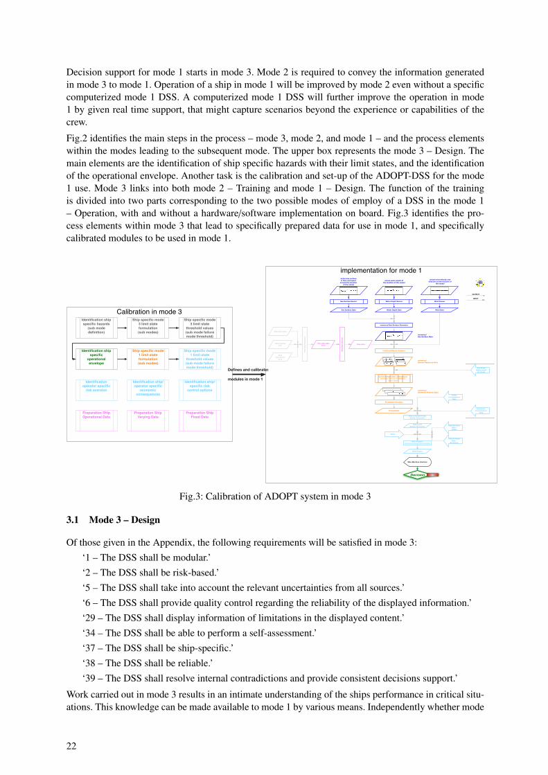
Fig.2 identifies the main steps in the process – mode 3, mode 2, and mode 1 – and the process elementswithin the modes leading to the subsequent mode. The upper box represents the mode 3 – Design. Themain elements are the identification of ship specific hazards with their limit states, and the identificationof the operational envelope. Another task is the calibration and set-up of the ADOPT-DSS for the mode1 use. Mode 3 links into both mode 2 – Training and mode 1 – Design. The function of the trainingis divided into two parts corresponding to the two possible modes of employ of a DSS in the mode 1– Operation, with and without a hardware/software implementation on board. Fig.3 identifies the pro-cess elements within mode 3 that lead to specifically prepared data for use in mode 1, and specificallycalibrated modules to be used in mode 1.

implementation for mode 1

Defines and calibrates

modules in mode 1

Calibration in mode 3

Preparation Ship Varying Data

Preparation Ship Fixed Data

Identification ship specific hazards

(sub mode definition)

Ship specific mode 3 limit state

threshold values(sub mode failure mode threshold)

Identification ship/operator specific

economic consequences

Identification operator specific

risk aversion

Identification ship/specific risk

control options

Ship specific mode 3 limit state formulation(sub modes)

Identification ship specific

operational envelope

Ship specific mode 1 limit state

threshold values(sub mode failure mode threshold)

Ship specific mode 1 limit state formulation(sub modes)

Preparation Ship Operational Data

Decision Uncertainty

actual sea surface

in time and space

around the location

of the vessel

numerical Sea Surface Generator

Sea Surface Sensor

Sea Surface Data

numerical

Sea Surface Data

numerical Submode Load Analyzor

(excitation, velocity, acceleration

linear loads)

numerical Motion Analyzor

Sub Mode

failure mode

threshold

numerical

System Response Data

Input/

Output

numerical

Submode Analysis Data

Probability Calculator

Probabilities

Ship varying

data

Ship fixed data

Ship

operational

data

Risk Level Generator

Safety / Economic

Risk Level

Safety / Economic

Economic

Consequence

Data

Risk Analyzor(internally rerunning to evaluate RCOs)

RCOs

Risk Aversion

Data -

Safety

Risk Picture

Man-Machine Interface

Safety

Consequence

Data

INPUT

OUTPUT

Wind Sensor

Wind Data

Water Depth Sensor

Water Depth Data

actual water depth at

the location of the vessel

actual wind velocity and

direction at the location of

the vessel

Risk Aversion

Data -

Economic

Sh

ip D

ata

Pre

pa

rato

r

Ship data data

baseShip data

Sh

ip D

ata

Se

lec

tor

Fig.3: Calibration of ADOPT system in mode 3

3.1 Mode 3 – Design

Of those given in the Appendix, the following requirements will be satisfied in mode 3:‘1 – The DSS shall be modular.’‘2 – The DSS shall be risk-based.’‘5 – The DSS shall take into account the relevant uncertainties from all sources.’‘6 – The DSS shall provide quality control regarding the reliability of the displayed information.’‘29 – The DSS shall display information of limitations in the displayed content.’‘34 – The DSS shall be able to perform a self-assessment.’‘37 – The DSS shall be ship-specific.’‘38 – The DSS shall be reliable.’‘39 – The DSS shall resolve internal contradictions and provide consistent decisions support.’

Work carried out in mode 3 results in an intimate understanding of the ships performance in critical situ-ations. This knowledge can be made available to mode 1 by various means. Independently whether mode

22

1 is supported by a hardware/software implementation, a ship performance manual can be compiled. Thismanual describes the ship and the effect of selected Risk Control Options for the most critical scenarios.In addition, if a hardware/software implementation of the DSS is available to mode 1, the underlyingdata should be generated in mode 3. This ensures data consistency and process reliability.

3.1.1 Identification of operational envelope

The actual sea surface is represented by sea state data describing (as well as possible) the operationalarea of the vessel. Preferably, hindcast data is used, as this gives consistent wind and wave data coveringa wide range of conditions. Based on the given environment and ship specific conditions, the added resis-tance in waves is calculated to determine the maximum speed possible in a seaway. During an optimiza-tion process (where the risk or frequency of a selected hazard is calculated) the operational envelope maybe restricted due to economic considerations, e.g. advising the master to avoid significant wave heightover a certain level or recommend speed and heading combination in heavy sea. The processing of theserecommendations by the master requires proper training (mode 2).

3.1.2 Identification of ship specific hazards

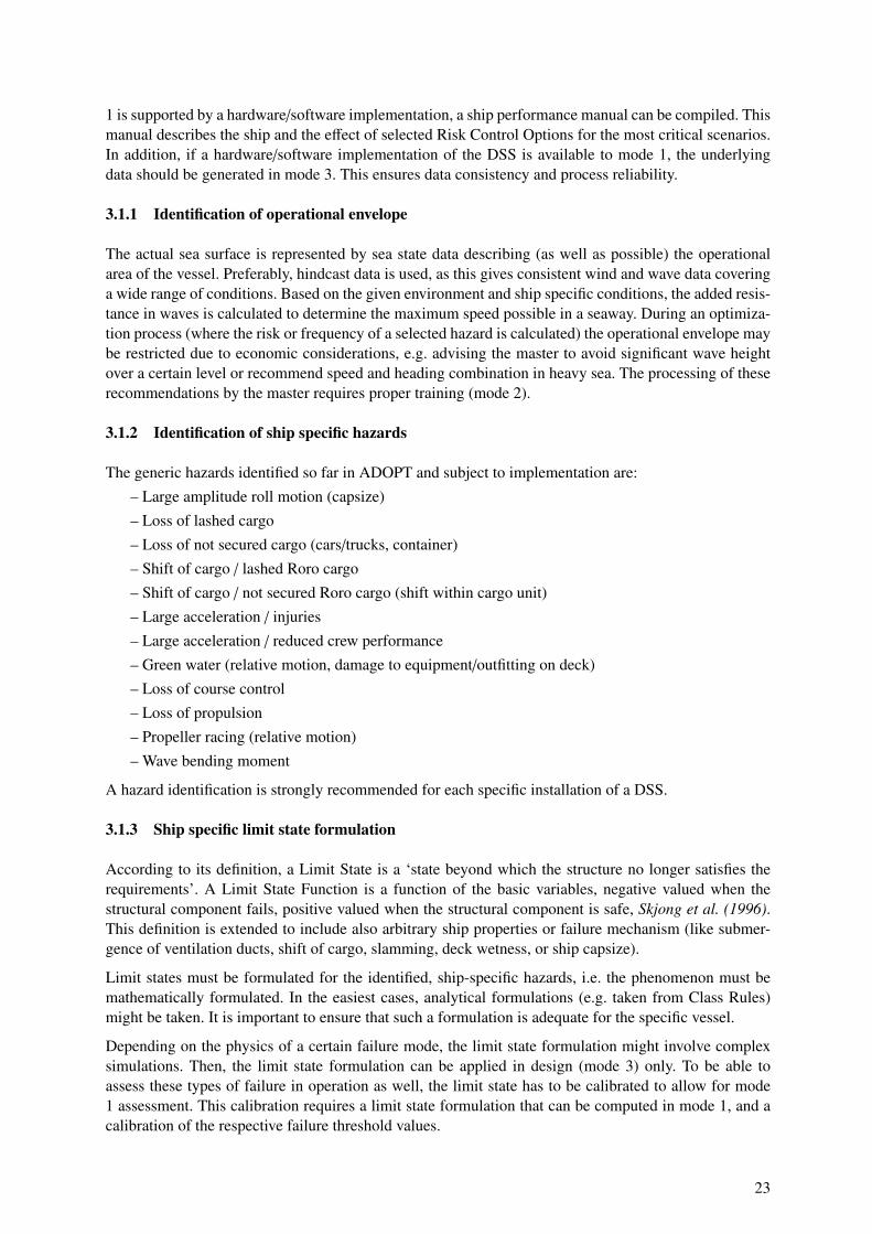
The generic hazards identified so far in ADOPT and subject to implementation are:– Large amplitude roll motion (capsize)– Loss of lashed cargo– Loss of not secured cargo (cars/trucks, container)– Shift of cargo / lashed Roro cargo– Shift of cargo / not secured Roro cargo (shift within cargo unit)– Large acceleration / injuries– Large acceleration / reduced crew performance– Green water (relative motion, damage to equipment/outfitting on deck)– Loss of course control– Loss of propulsion– Propeller racing (relative motion)– Wave bending moment

A hazard identification is strongly recommended for each specific installation of a DSS.

3.1.3 Ship specific limit state formulation

According to its definition, a Limit State is a ‘state beyond which the structure no longer satisfies therequirements’. A Limit State Function is a function of the basic variables, negative valued when thestructural component fails, positive valued when the structural component is safe, Skjong et al. (1996).This definition is extended to include also arbitrary ship properties or failure mechanism (like submer-gence of ventilation ducts, shift of cargo, slamming, deck wetness, or ship capsize).

Limit states must be formulated for the identified, ship-specific hazards, i.e. the phenomenon must bemathematically formulated. In the easiest cases, analytical formulations (e.g. taken from Class Rules)might be taken. It is important to ensure that such a formulation is adequate for the specific vessel.

Depending on the physics of a certain failure mode, the limit state formulation might involve complexsimulations. Then, the limit state formulation can be applied in design (mode 3) only. To be able toassess these types of failure in operation as well, the limit state has to be calibrated to allow for mode1 assessment. This calibration requires a limit state formulation that can be computed in mode 1, and acalibration of the respective failure threshold values.

23

An example is the combination of nonlinear simulations of ship motions, viscous CFD (computationalfluid dynamics), and nonlinear FEM to calculate loads induced by slamming and the respective systemresponse, namely the stresses within the steel structure. In mode 3, coupled fluid-structure interactionwill be used to assess certain scenarios. These results are used to calibrate a mode 1 implementation, i.e.using relative motions and/or relative accelerations of ship and water.

3.1.4 Ship specific limit state threshold values

For the identified limit states, threshold values have to be determined. Using the above example of slam-ming, the deflections the steel structure can bear without failure is a ship specific threshold value. De-pendent on the calculation procedure this corresponds to a hydrodynamic pressure on the ship’s wettedsurface which in turn is correlated to a relative velocity between water and hull at selected locations.

In the design process, the equivalence between a structural based threshold value and ship motion basedthreshold as in the previous example may be developed for two purposes – optimization of the vesselwith regard to the analyzed hazard and/or calibration for the mode 1 and 2. An optimization of a vesselwith regard to a hazard implies a calculation of the risk or frequency of the ship specific hazard. Duringthis step, the different thresholds are correlated. This equivalence can only be developed in mode 3, asmode 3 enables time for running necessary calculations and expertise for generation of math models andjudging results of calculations.

The following example demonstrates the necessity of different limit state formulations and thresholdclasses for the same hazard dependent on the specific vessel. For the hazard ‘Propeller Racing’, thethreshold value depends on the automation of the propulsion train and the main engine. If the automationenters shut-down mode if the revolutions increase and the moment decreases, propeller emergence andduration of the emergence jointly establish the threshold value. If the automation does not shut downthe main engine, but continuously adjusts engine revolutions and delivered power, the frequency of thisprocess is the threshold value. This is ship specific: If the automation is clever enough, the generic hazard‘propeller racing’ might not be that important for some implementations, except for perhaps very extremeoperational conditions.

It is suggested to have escalating threshold values for each limit state. I.e. the same hazard in its respectivelimit state formulation will have different consequences if different threshold values are exceeded. Forexample, if the hazard is ‘vertical accelerations leading to personnel injuries’, one threshold value ispertinent to ship crew, another – most likely smaller – threshold value is pertinent to passengers.

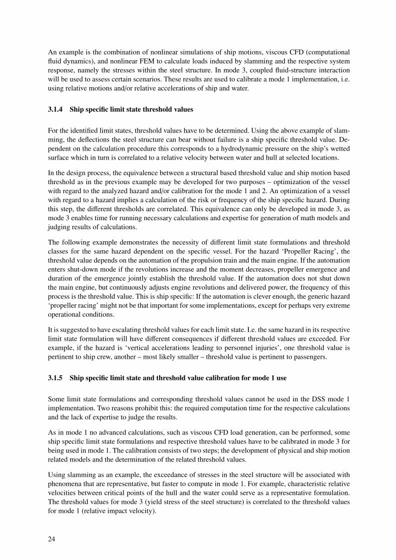
3.1.5 Ship specific limit state and threshold value calibration for mode 1 use

Some limit state formulations and corresponding threshold values cannot be used in the DSS mode 1implementation. Two reasons prohibit this: the required computation time for the respective calculationsand the lack of expertise to judge the results.

As in mode 1 no advanced calculations, such as viscous CFD load generation, can be performed, someship specific limit state formulations and respective threshold values have to be calibrated in mode 3 forbeing used in mode 1. The calibration consists of two steps; the development of physical and ship motionrelated models and the determination of the related threshold values.

Using slamming as an example, the exceedance of stresses in the steel structure will be associated withphenomena that are representative, but faster to compute in mode 1. For example, characteristic relativevelocities between critical points of the hull and the water could serve as a representative formulation.The threshold values for mode 3 (yield stress of the steel structure) is correlated to the threshold valuesfor mode 1 (relative impact velocity).

24

3.1.6 Identification of operator specific economic consequence data

The list of generic hazards given in section 3.1.3 has to be made concrete and to be made both ship andoperator specific. Afterwards it is necessary to assign a monetary consequence to the respective hazard.This gives the basis for the risk analysis that is carried out within the framework of an ADOPT-DSS.

For example, the hazard ‘Shift of cargo / not secured Roro cargo (shift within cargo unit)’ is made specificwith the formulation ‘The contents of trailers on the leg Gothenburg – Immingham are shifted due to shipmotions’ as a first step.

The next step is to assign a monetary consequence to this event. A guideline for defining consequence isnot to have the worst case scenario in mind, but to consider the ‘worst credible consequence’.

In this example, a worst case might be damaging the content of a trailer containing time critical expensivegoods (e.g. pharmaceuticals) that are sent once in a couple of years. The worst credible consequencecould be having the high-value goods in mind that are sent with the ship on a regular basis.

This process element (identification of operator specific economic consequence data) yields a list withthe relevant hazards in their specific formulation, associated with the respective costs. Note that generichazards and/or generic consequence data might lead to wrong decision support.

3.1.7 Identification of operator specific economic risk aversion

Risk aversion is expressed using measures for consequences drawn versus measures for likelihoods. Boththe quality and the quantity should be in a format that reflects the operators’ way of thinking. The scaleboth of frequency and consequences depends on the specific business. For example, an operator mightthink in terms of the duration of a roundtrip, the time period for internal accounting, up to the envisagedtime horizon of the operation. For consequences, a similar approach should be chosen. Most importanceis that monetary consequences are relevant and understandable to the operator.

Having the relevant scales for likelihoods and consequences (and their respective subdivision into bands),the next step is to identify those areas in the frequencies/consequences risk matrix, that are acceptable orintolerable for the operator. Acceptable is any combination of likelihood and consequences that does notmatter to the operator. Intolerable is any combination that the operator cannot live with. The remainingpart in between is the ALARP (As low as reasonably practicable) area, where hazards lying in that areawill be subject to a cost-benefit analysis (CBA). Only if the benefit exceeds the costs, hazard allocated inthat area will be subject to risk reduction.

3.1.8 Identification of ship specific risk control options

Risk Control Options generally available to a sailing vessel are change of course, change of speed, changeof status of motion stabilizing devices, change of ballast, or combinations of the above. During design,further RCO are available, like hull form design, specific layout of motion stabilizing devices, selectionand layout of equipment, etc.

Besides the selection and application of RCO pertinent to design, a particular task within mode 3 is theanalysis of the applicability and efficiency of the RCO available in mode 1. This task is closely linked towhat is described in section 3.1.9.

3.1.9 Preparation and calibration of ship data database for mode 1 and mode 2

Typical design work is the preparation of the stability documents for intact stability, the stability book-let. This document is based on contract loading conditions. Additional loading conditions covering theoperation are carefully prepared and used in the subsequent process elements.

The process element of preparing representative operational loading conditions covers the definition ofship varying data (particularly masses of payload) characterizing a particular loading condition. This

25

step includes correct modeling of masses (including their position in longitudinal, lateral and verticaldimension) and free surfaces.

When the loading conditions are defined, the seakeeping model (i.e. the mass model with mathematicalrepresentation of the corresponding wetted hull surface) is set up. As these models will be used by non-experts in an automated mode, this process element is critical.

In this part of the process, all three data groups (ship operational data, ship varying data, ship fixeddata) are first generated for those conditions that are relevant for mode 1. This creates three dataset withknown uncertainties. These data sets are then compiled into one database, which is accessible in mode1. By this method the unknown uncertainties in the loading data from the loading computer in operationare overcome and replaced by quantifiable uncertainties.

3.2 Mode 2 – Training

The general approach in the training mode of ADOPT is not only the familiarisation with the systemitself but also to give advise on the background of phenomena (like parametric rolling), as the purpose ofthe DSS only can be captured when the theoretical foundation is available. By this approach, the trainingdoes not only customise the user on the system but also contributes to an improved situational awarenessof the risks in specific sea states.

The training concept consists of two modules with two sessions each, starting with general ship theory.Since the ADOPT-DSS is ship specific, the theory will afterwards be consolidated by exercises in thesimulator demonstrating the vulnerability of the specific ship in particular seas. In the next session, thecrew will be familiarized with using the DSS. This again starts with the theoretical description howthe DSS works, which are its limitations, which are its modules, and in which situations it can help.Afterwards, in the final module, the user will be customised in a simulator environment to get experiencein using the system and improve his behaviour in critical situations.

3.2.1 Familiarization with the ship, theory

This module starts by providing the theoretical background on ship behaviour in general. It explains whatdetermines ship motions and how ships will move under specific conditions. It gives an introduction into‘new’ phenomena (like parametric roll) and how these phenomena are determined. It makes proposalshow (without any technological help) the master can identify the risk of his current situations and how hegenerally could avoid high risks. As the DSS is ship-specific, this module has a second part in which thetheoretical background is applied to the specific ship. This part employs the experience gained during thedesign of the ship and presents critical conditions for that specific ship (in aspects of loading, sea state,etc.) and how they could be avoided. It gives detailed insight into that ship and presents recommendationshow this ship should be operated in different situations.

3.2.2 Familiarization with the ship, practice

In this module, the experience gained in the first module is illustrated in practical exercises in a simulatorenvironment. The main learning objective is the consolidation of the theoretical knowledge. Therefore,selected dangerous situations are demonstrated to illustrate how the specific ship will behave under thoseconditions. Afterwards strategies will be trained how to avoid these situations and how to operate theship in them.

3.2.3 Familiarization with a mode 1 DSS, theory

After having laid the fundamentals in the previous modules, the student needs to be trained on how tothe DSS. The DSS covers only some risks and has a specific approach. Thus the user needs to grasp thephilosophy of the DSS in order to understand when and how the DSS can help him. Therefore a clearintroduction into the system is given, addressing its risk based approach, which hazards are covered and

26

what limitations the system has. This is complemented by an introduction into the application of thesystem and how the HMI needs to be used.

3.2.4 Familiarization with a mode 1 DSS, practice

The final module is again a practical exercise in a simulator environment, this time with the focus ontraining to sail the ship in difficult conditions with the assistance of a DSS. Several scenarios are devel-oped in which the student can prove that he knows how to deploy the DSS to achieve a status with lowerrisk. It is tested whether the user is able to assess situations right and derive the right conclusions. Healso has to prove that he knows the limitations of the DSS and can identify the situations in which theDSS cannot assist him.

3.3 Mode 1 – Operation

Of those given in the Appendix, the following requirements will be satisfied in mode 1:‘1 – The DSS shall be modular.’‘3 – The DSS shall support real-time decision making.’‘4 – Supported by a DSS, the master shall improve his decision making under uncertainty.’‘7 – Decision support shall have a time range of about one watch.’‘8 – The DSS shall operate on a ship while sailing.’‘9 – The DSS shall be operated and used by a ship’s crew.’‘19 – The DSS shall take into account extreme environmental conditions.’‘20 – The DSS shall take into account multiple wave systems.’‘24 – The DSS shall avoid misinterpretation of displayed information.’‘25 – The DSS shall avoid display of wrong information.’‘26 – The DSS shall be robust.’‘29 – The DSS shall display information of limitations in the displayed content.’‘32 – The DSS shall warn the user if risks arising from the identified hazards are beyond negligible.’‘34 – The DSS shall be able to perform a self-assessment.’‘37 – The DSS shall be ship-specific.’‘39 – The DSS shall resolve internal contradictions and provide consistent decisions support.’

3.3.1 Mode 1 DSS without hardware and software support

Without support by a hardware/software implementation, mode 1 depends both on mode 2 – familiar-ization with the ship in theory and practice – and the availability of guidance from mode 3 – operatorsguidance. The requirements No. 3, 4, and 24 are relevant only in that sense, that access to supportinginformation (e.g. operator’s manual) must be prepared to allow easy access.

Requirement ‘4 – Supported by a DSS, the master shall improve his decision making under uncertainty.’is ensured by training in mode 2. This training provides the master with the expertise necessary to im-prove his decision making. Requirements No. 9, 24, 25, and 37 remain as relevant for operating a shipwithout a hardware/software implementation. These requirements have to be directly addressed in thepreparation of a ship performance manual, and the set-up of training courses. Requirement No. 25 issubject to Quality Assurance in mode 3.

3.3.2 Mode 1 DSS with hardware and software support

Main components of the onboard installation are a wave sensor, a ship data database, fast and accuratemotion prediction tools, and a Man Machine Interface (MMI). Within ADOPT, a wave radar is used forsensing the environment. The reason is that only by using a radar it is possible to satisfy requirementNo. 19. The numerical motion simulation tools are linear frequency domain ship responses for economic

27

risks, and time domain ship responses with nonlinear roll motion for safety related risks. The MMI isembedded in the Conning Display.

To fulfil the requirement No. 3 and particularly ‘7 – Decision support shall have a time range of aboutone watch’, all time-consuming calculations are transferred to the mode 3, while all other calculationsare performed during training or on board.

The inclusion of all uncertainties – uncertainties in the input data and numerical model etc. – requirescomputational time in the range of months to a year with todays computer performance. Additionallymany specifications of uncertainties are in itself highly uncertain. The probability of a hazard is calcu-lated including only the variability of the seaway, neglecting uncertainties from wind, water depth, shipfixed data, ship varying data, ship operational data, the failure mode threshold and model uncertaintiesin the sea surface generator, numerical motion analyser and submode load analyser. The importance ofthe uncertainties is analyzed in mode 3. The calculations to establish a correlation between ship motionsand hazards are also time consuming. The calibration of the DSS for mode 1 by mode 3 consists partlyin linking the considered hazards to ship motions.

Another part of the calibration of the DSS for mode 1 is due to the requirement ‘9 – The DSS shall beoperated and used by a ship’s crew’. Calculations that require personnel that is experienced/educated inship theory are conveyed to mode 3. This concerns the setup and input of the Numerical Sea-surfaceGenerator and Numerical Motion Analyser.

One step of the calibration of the mode 1 is the set up of the seakeeping model where for all relevantloading condition the mass model and a mathematical representation of the wetted hull surface is gener-ated. The ship varying data, loading condition and sea water density are combined into one set of shipdata in the ship data database characterized by measures such as KG, draught fore and aft and heelingangle, which are easily checked by the crew. According to these measures appropriate preassembled shipdata are selected. The preassembled ship data are only applicable in a narrow, clearly defined range ofcharacteristics parameters (KG, draught and heel). This approach presumes that the weight distributiondoes not vary significantly for a specific vessel with the same KG and floating condition and therebyneglecting these uncertainties related to loading conditions.

Preassembled ship data including the setup of the seakeeping model have the advantage that the hydro-static and partly the hydrodynamic model are checked by an experienced person. This eliminates thepossibility of faults in the automatic or user defined generation of the seakeeping mode set-up in mode 1– Operation. Frequently observed use of correction weights in the load master on board, which introducesunacceptable faults in the mass model, is avoided.

If no appropriate ship data are available the DSS does not proceed the calculations. If this occurs fre-quently additional ship data must be generated onshore to cover the missing loading conditions.

The consequence of the combined requirements No. 34 and ‘25 – The DSS shall avoid display of wronginformation’, and ‘29 – The DSS shall display information of limitations in the displayed content’, is thateach module, data block, and interface shall have the possibility to stop the system or to inform the user.This makes the ADOPT-DSS an ‘Andon’ system, as it was introduced in manufacturing processes byToyota. The Toyota principle ‘Jidoka’, where Andon is a part of, aims at avoiding defects by immediatelyidentifying potential defects and then solving them, in order to achieve improved quality.

Risk control options are heading, speed, status of active/passive motion damping devices, and contentof ballast tanks. The hardware/software package of the ADOPT-DSS will compute speed and headingcombinations around the present combination to deliver a more complete guidance to the master. Theextent of this automatically calculated risk picture for the heading/speed combinations depends on theconcrete implementation.

The master can select sets of heading and speed as user input. The master decides his actions based onthe displayed information and the knowledge gained during mode 2 – Training.

28

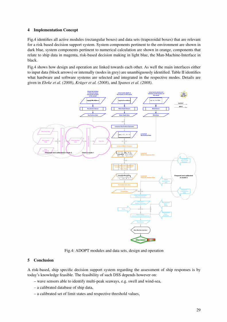
4 Implementation Concept

Fig.4 identifies all active modules (rectangular boxes) and data sets (trapezoidal boxes) that are relevantfor a risk based decision support system. System components pertinent to the environment are shown indark blue, system components pertinent to numerical calculation are shown in orange, components thatrelate to ship data in magenta, risk-based decision making in light blue, the Man-Machine-Interface inblack.

Fig.4 shows how design and operation are linked towards each other. As well the main interfaces eitherto input data (block arrows) or internally (nodes in grey) are unambiguously identified. Table II identifieswhat hardware and software systems are selected and integrated in the respective modes. Details aregiven in Ehrke et al. (2008), Kruger et al. (2008), and Spanos et al. (2008).

Decision Uncertainty

actual sea surfacein time and space

around the locationof the vessel

numerical Sea Surface Generator

Sea Surface Sensor

Sea Surface Data

numericalSea Surface Data

numerical Submode Load Analyzor(excitation, velocity, acceleration

linear loads)

numerical Motion Analyzor

Sub Modefailure mode

threshold

numericalSystem Response Data

Input/Output

numericalSubmode Analysis Data

Probability Calculator

Probabilities

Ship varying data

Ship fixed data

Ship operational

data

Risk Level GeneratorSafety / Economic

Risk LevelSafety / Economic

EconomicConsequence

Data

Risk Analyzor(internally rerunning to evaluate RCOs)

RCOs

Risk Aversion Data -Safety

Risk Picture

Man-Machine Interface

SafetyConsequence

Data

INPUT

OUTPUT

Wind Sensor

Wind Data

Water Depth Sensor

Water Depth Data

actual water depth atthe location of the vessel

actual wind velocity anddirection at the location of

the vessel

Risk Aversion Data -

Economic

Shi

p D

ata

Pre

par

ato

r

Ship data data base

Ship data

Shi

p D

ata

Sel

ecto

r

Used in mode 1Prepared and calibrated in mode 3

Prepared and calibrated in mode 3

Fig.4: ADOPT modules and data sets, design and operation

5 Conclusion

A risk-based, ship specific decision support system regarding the assessment of ship responses is bytoday’s knowledge feasible. The feasibility of such DSS depends however on:

– wave sensors able to identify multi-peak seaways, e.g. swell and wind-sea,– a calibrated database of ship data,– a calibrated set of limit states and respective threshold values,

29

– advanced state-of-the-art motion modeling tools onboard, and– a HMI embedded in typical bridge equipment as the conning display and designed from experts for

users, not from experts for experts.

Independently, the DSS needs to be embedded within a rational procedure that– makes the implementation ship specific,– ensures correctness of numerical models,– limits uncertainties or at least quantifies them,– strictly distinguishes between safety risks and economic risks,– accounts for the identified requirements, and– unambiguously identifies the limits of the support that can be expected.

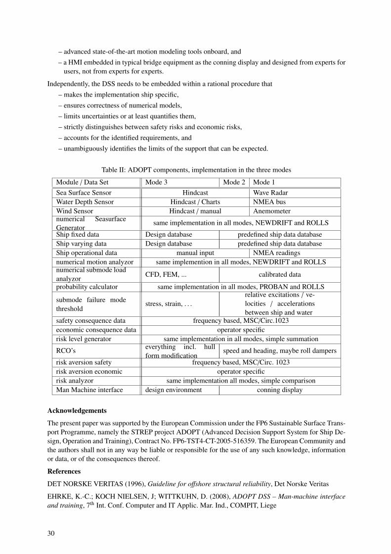
Table II: ADOPT components, implementation in the three modes

Module / Data Set Mode 3 Mode 2 Mode 1Sea Surface Sensor Hindcast Wave RadarWater Depth Sensor Hindcast / Charts NMEA busWind Sensor Hindcast / manual Anemometernumerical SeasurfaceGenerator

same implementation in all modes, NEWDRIFT and ROLLS

Ship fixed data Design database predefined ship data databaseShip varying data Design database predefined ship data databaseShip operational data manual input NMEA readingsnumerical motion analyzor same implemention in all modes, NEWDRIFT and ROLLSnumerical submode loadanalyzor CFD, FEM, ... calibrated data

probability calculator same implementation in all modes, PROBAN and ROLLS

submode failure modethreshold

stress, strain, . . .relative excitations / ve-locities / accelerationsbetween ship and water

safety consequence data frequency based, MSC/Circ.1023economic consequence data operator specificrisk level generator same implementation in all modes, simple summation

RCO’s everything incl. hullform modification

speed and heading, maybe roll dampers

risk aversion safety frequency based, MSC/Circ. 1023risk aversion economic operator specificrisk analyzor same implementation all modes, simple comparisonMan Machine interface design environment conning display

Acknowledgements

The present paper was supported by the European Commission under the FP6 Sustainable Surface Trans-port Programme, namely the STREP project ADOPT (Advanced Decision Support System for Ship De-sign, Operation and Training), Contract No. FP6-TST4-CT-2005-516359. The European Community andthe authors shall not in any way be liable or responsible for the use of any such knowledge, informationor data, or of the consequences thereof.

References

DET NORSKE VERITAS (1996), Guideline for offshore structural reliability, Det Norske Veritas

EHRKE, K.-C.; KOCH NIELSEN, J; WITTKUHN, D. (2008), ADOPT DSS – Man-machine interfaceand training, 7th Int. Conf. Computer and IT Applic. Mar. Ind., COMPIT, Liege

30

GUNTHER, H; TRANKMANN, I; KLUWE, F. (2008), ADOPT DSS – Ocean environment modellingfor use in decision making support, 7th Int. Conf. Computer and IT Applic. Mar. Ind., COMPIT, Liege

IMO (1995), Guidance to the master for avoiding dangerous situations in following and quartering seas,Int. Maritime Org., Maritime Safety Committee, MSC/Circ. 707

IMO (2002), Guidelines for formal safety assessment (FSA) for use in the IMO rule-making process, Int.Maritime Org., Maritime Safety Committee MSC/Circ. 1023

IMO (2007), Consolidated text of the guidelines for formal safety assessment (FSA) for use in the IMOrule-making process, Int. Maritime Org., Maritime Safety Committee MSC 83/INF.2

KERNCHEN, W. (2008), Seenotfalle – Archiv, http://www.janmaat.de/seenot archiv.htm

KRUGER, S.; KLUWE, F.; VORHOLTER, H. (2008), ADOPT DSS - Decision support for large ampli-tude roll motions based on nonlinear time domain simulations, 7th Int. Conf. Computer and IT Applic.Mar. Ind., COMPIT, Liege

McDANIEL, (2008), Singles only – Transport disasters, The Countrymanhttp://www.cargolaw.com/2000nightmare_singles.only.html

SPANOS, D.; PAPANIKOLAOU, A.; PANATZANAKIS, G.; TELLKAMP, J., (2008), ADOPT DSS –Onboard assessment of seakeeping for risk-based decision support to the master, 7th Int. Conf. Computerand IT Applic. Mar. Ind., COMPIT, Liege

SKJONG, R. et al. (1996), General, in DET NORSKE VERITAS (1996)

31

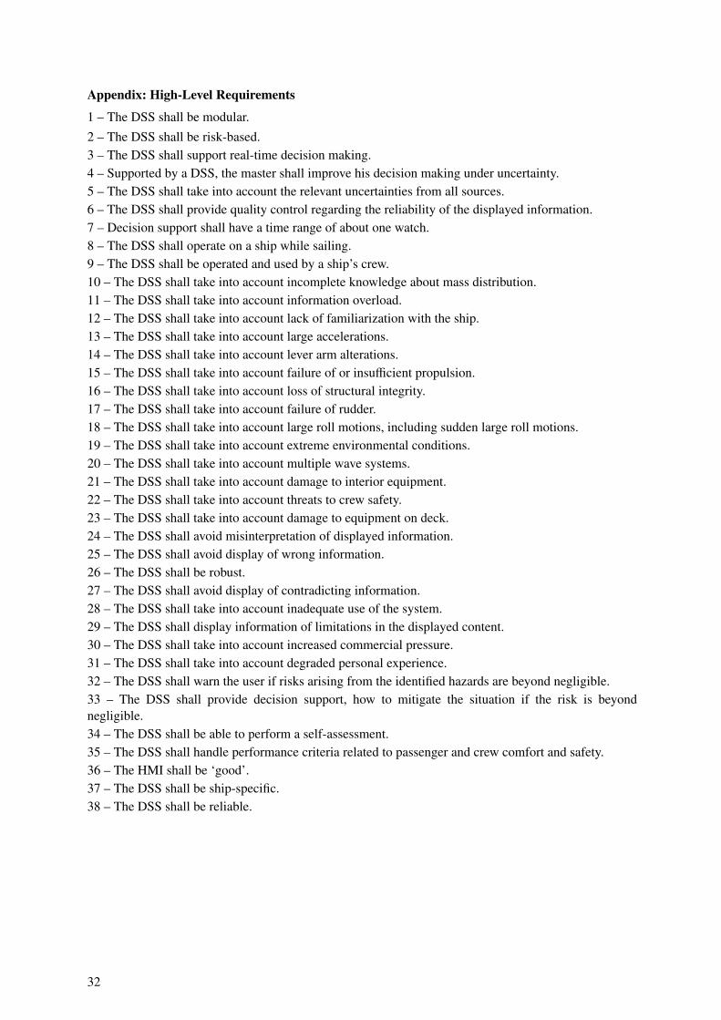
Appendix: High-Level Requirements

1 – The DSS shall be modular.2 – The DSS shall be risk-based.3 – The DSS shall support real-time decision making.4 – Supported by a DSS, the master shall improve his decision making under uncertainty.5 – The DSS shall take into account the relevant uncertainties from all sources.6 – The DSS shall provide quality control regarding the reliability of the displayed information.7 – Decision support shall have a time range of about one watch.8 – The DSS shall operate on a ship while sailing.9 – The DSS shall be operated and used by a ship’s crew.10 – The DSS shall take into account incomplete knowledge about mass distribution.11 – The DSS shall take into account information overload.12 – The DSS shall take into account lack of familiarization with the ship.13 – The DSS shall take into account large accelerations.14 – The DSS shall take into account lever arm alterations.15 – The DSS shall take into account failure of or insufficient propulsion.16 – The DSS shall take into account loss of structural integrity.17 – The DSS shall take into account failure of rudder.18 – The DSS shall take into account large roll motions, including sudden large roll motions.19 – The DSS shall take into account extreme environmental conditions.20 – The DSS shall take into account multiple wave systems.21 – The DSS shall take into account damage to interior equipment.22 – The DSS shall take into account threats to crew safety.23 – The DSS shall take into account damage to equipment on deck.24 – The DSS shall avoid misinterpretation of displayed information.25 – The DSS shall avoid display of wrong information.26 – The DSS shall be robust.27 – The DSS shall avoid display of contradicting information.28 – The DSS shall take into account inadequate use of the system.29 – The DSS shall display information of limitations in the displayed content.30 – The DSS shall take into account increased commercial pressure.31 – The DSS shall take into account degraded personal experience.32 – The DSS shall warn the user if risks arising from the identified hazards are beyond negligible.33 – The DSS shall provide decision support, how to mitigate the situation if the risk is beyondnegligible.34 – The DSS shall be able to perform a self-assessment.35 – The DSS shall handle performance criteria related to passenger and crew comfort and safety.36 – The HMI shall be ‘good’.37 – The DSS shall be ship-specific.38 – The DSS shall be reliable.

32

33

Assessing the Suitability of Ship Design for Human Factors Issues Associated with Evacuation and Normal Operations

Steven J. Deere, FSEG – University of Greenwich, UK, S.Deere@gre.ac.uk

Edwin R. Galea, FSEG – University of Greenwich, UK, E.R.Galea@gre.ac.uk Peter J. Lawrence, FSEG – University of Greenwich, UK, P.Lawrence@gre.ac.uk

Abstract Evaluating ship layout for human factors (HF) issues using simulation software such as maritimeEXODUS can be a long and complex process. The analysis requires the identification of relevant evaluation scenarios; encompassing evacuation and normal operations; the development of appropriate measures which can be used to gauge the performance of crew and vessel and finally; the interpretation of considerable simulation data. In this paper we present a systematic and transparent methodology for assessing the HF performance of ship design which is both discriminating and diagnostic. The methodology is demonstrated using two variants of a hypothetical naval ship. 1 Introduction Modifications to ship configuration such as hull form, length, beam, size and location of internal compartments have a direct impact on ship performance in terms of stability, powering, seakeeping and strength. These traditional design parameters are well understood and can be determined in a relatively straight forward manner. Equally, when modifying the internal configuration of a ship, it is also important to determine what, if any, human factors (HF) benefits or disbenefits may result. How these aspects can be assessed is less well defined. In this paper we present a novel mathematical procedure, based on computer simulation of evacuation and normal operations (NOP), for assessing the overall HF performance of ship design. Making modifications to the internal layout of a ship or its operating procedures will have HF implications for crew and passengers, which in turn will have an impact on overall levels of safety under emergency conditions and efficiency of operation in normal conditions. The procedures employed to undertake a specific task such as evacuation may be modified to improve the efficiency in undertaking these tasks. Equally, changing the location of cabins, public facilities, corridor systems, stairs, assembly locations etc will have a direct impact on the ability of crew and passengers to safely and efficiently evacuate the vessel under emergency conditions. Furthermore, for passenger vessels, size, location and configuration of public spaces such as restaurants, cinemas, bars, etc will influence the ease with which they can be accessed, filled and emptied under NOP. This will in turn impact the operational characteristics of the vessel. For naval vessels, the location and distribution of compartments may have an impact on the time required by crew to go from one state to another, it may also have an impact on the minimum number of crew required to safely and efficiently operate the vessel under a variety of different conditions. These factors will have an impact on the vessels overall operating efficiency, ability to fulfil the assigned mission and lifetime costs associated with crewing requirements. Changes to configuration that lead to improvements in one aspect of human performance e.g. assembly time, may have a negative impact on other aspects of human performance e.g. ease of access of public spaces. Advanced ship evacuation models such as maritimeEXODUS can be used to determine the performance of personnel under emergency conditions for both passenger ships, Deere et al. (2006), Galea et al. (2004), and naval vessels, Boxall et al. (2005), as well as the normal circulation of personnel for both passenger and naval vessels, Boxall et al. (2005), Caldeira-Saraiva et al. (2004). These models produce a wide variety of simulation outputs, such as time to assemble and the levels of congestion experienced. As the number of different scenarios investigated increases, so does the

34

volume of output data. It therefore becomes increasingly difficult to consistently assess changes in HF performance associated with changes in vessel configuration across a wide range of scenarios and performance requirements. The challenge therefore is to develop a procedure that allows accurate and rapid assessment of the large scale model outputs produced by HF simulation models and to determine if specified modifications to vessel layout or operating procedures generate improvements in human performance across a range of potentially competing requirements. In this paper we explore a methodology to assess changes in HF performance resulting from changes to vessel configuration and/or crew procedures. Furthermore, the methodology is intended to determine whether or not a net benefit results from imposed changes to the configuration/procedures and identify specific areas where performance may be improved. The approach is therefore intended to be both diagnostic and discriminating. The identified methodology is being developed as part of a collaborative project between the authors and the Design Research Centre (DRC) of University College London, funded by the UK EPSRC with support from MoD. While the proposed methodology is generic in nature, the development focuses on naval vessels to demonstrate proof of concept on a demanding set of ship operations. The methodology is similar in some respects to weighted point schemes used to rank fire safety provision in buildings, where points are awarded for the presence or absences of certain fire safety measures and the relative importance of the particular measure is represented by the assigned weight, Chow (2002). These types of schemes are common in quantitative fire risk assessment and are sometimes called “Indexing Schemes”, Watts (2002). A key difference between these schemes and the proposed methodology is that the performance measures are determined directly from detailed computer simulation of selected scenarios and not from experience of past performance or from expert judgement. 2 Methodology for assessing human factors performance In order to gauge the HF performance of the vessel it is essential to define a range of relevant Evaluation Scenarios (ES) against which the vessel will be tested. These scenarios are intended to define the scope of the challenges the vessel will be subjected to. In order to gauge vessel performance across a range of criteria, the ES are made up of both evacuation and NOP scenarios. Relevant evacuation scenarios may include those required by MSC Circular 1238, IMO (2007), and include the IMO night and day scenarios or their naval equivalent, NATO (2006). The NOP scenarios are dependent on the nature and class of vessel. For example, a cruise ship application may require the time to empty the cinema is minimised while a naval vessel may require watch changes to be completed within set period of time. In addition to defining the ES, a range of Performance Measures (PM) must be defined that measure various aspects of personnel performance in undertaking the tasks associated with the ES. PM for passenger ship evacuation scenarios may include the time required to complete the assembly process while for a naval vessel NOP scenario, the total number of water tight doors (WTD) opened and closed may be relevant. The suitability of the vessel layout will be evaluated for fitness of purpose through some combination of the PM resulting from the execution of the ES. Collectively the particular combination of ES and PM that results in a meaningful measure of the performance of the crew and vessel are described as the Human Performance Metric (HPM). Clearly, the HPM will be specific to the type and class of vessel being investigated thus; an aircraft carrier will have a different HPM to a submarine. However, the underlying concept of the HPM will be common to all types of vessels and some components that make up the HPM may be similar across different vessel types. The HPM works by systematically evaluating one layout design against another, whether this is two variants of the same design or two completely different designs.

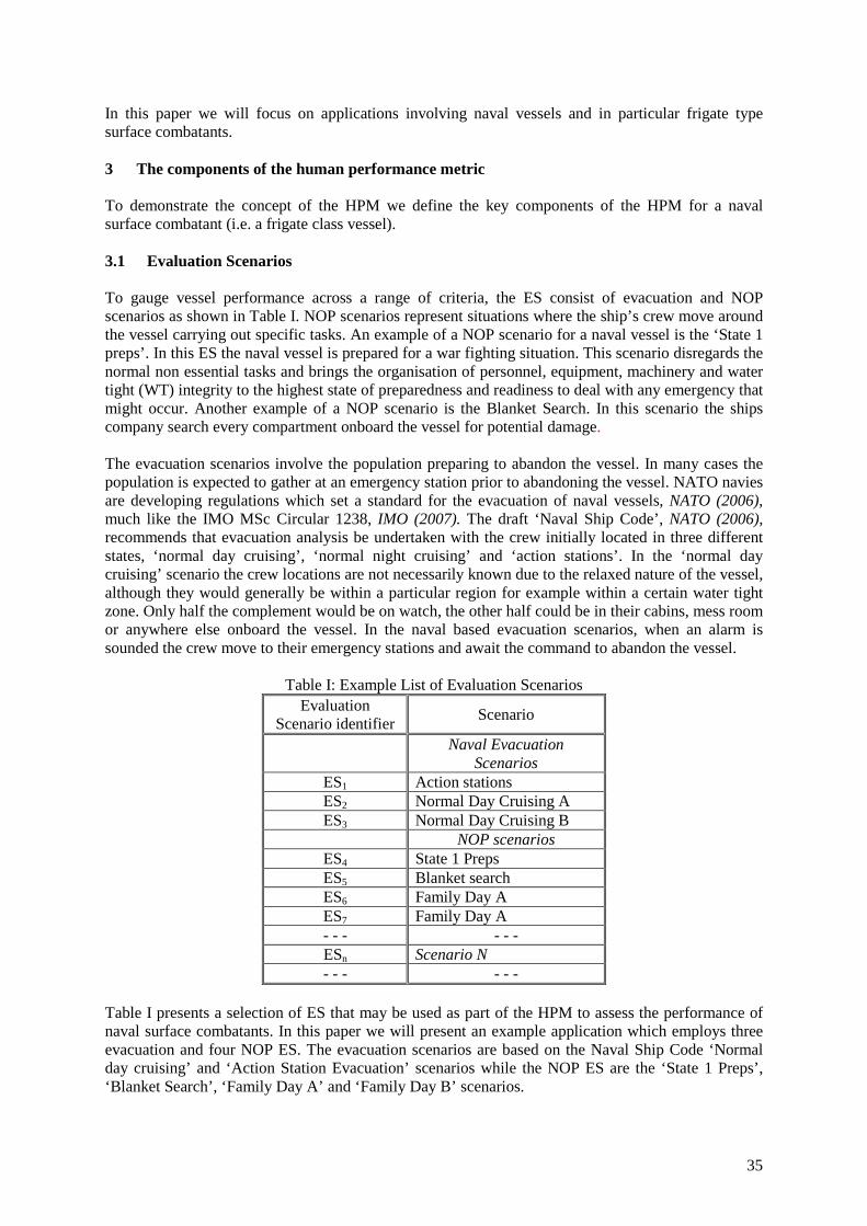
35

In this paper we will focus on applications involving naval vessels and in particular frigate type surface combatants. 3 The components of the human performance metric To demonstrate the concept of the HPM we define the key components of the HPM for a naval surface combatant (i.e. a frigate class vessel). 3.1 Evaluation Scenarios To gauge vessel performance across a range of criteria, the ES consist of evacuation and NOP scenarios as shown in Table I. NOP scenarios represent situations where the ship’s crew move around the vessel carrying out specific tasks. An example of a NOP scenario for a naval vessel is the ‘State 1 preps’. In this ES the naval vessel is prepared for a war fighting situation. This scenario disregards the normal non essential tasks and brings the organisation of personnel, equipment, machinery and water tight (WT) integrity to the highest state of preparedness and readiness to deal with any emergency that might occur. Another example of a NOP scenario is the Blanket Search. In this scenario the ships company search every compartment onboard the vessel for potential damage. The evacuation scenarios involve the population preparing to abandon the vessel. In many cases the population is expected to gather at an emergency station prior to abandoning the vessel. NATO navies are developing regulations which set a standard for the evacuation of naval vessels, NATO (2006), much like the IMO MSc Circular 1238, IMO (2007). The draft ‘Naval Ship Code’, NATO (2006), recommends that evacuation analysis be undertaken with the crew initially located in three different states, ‘normal day cruising’, ‘normal night cruising’ and ‘action stations’. In the ‘normal day cruising’ scenario the crew locations are not necessarily known due to the relaxed nature of the vessel, although they would generally be within a particular region for example within a certain water tight zone. Only half the complement would be on watch, the other half could be in their cabins, mess room or anywhere else onboard the vessel. In the naval based evacuation scenarios, when an alarm is sounded the crew move to their emergency stations and await the command to abandon the vessel.

Table I: Example List of Evaluation Scenarios Evaluation

Scenario identifier Scenario

Naval Evacuation

Scenarios ES1 Action stations ES2 Normal Day Cruising A ES3 Normal Day Cruising B

NOP scenarios ES4 State 1 Preps ES5 Blanket search ES6 Family Day A ES7 Family Day A - - - - - - ESn Scenario N - - - - - -

Table I presents a selection of ES that may be used as part of the HPM to assess the performance of naval surface combatants. In this paper we will present an example application which employs three evacuation and four NOP ES. The evacuation scenarios are based on the Naval Ship Code ‘Normal day cruising’ and ‘Action Station Evacuation’ scenarios while the NOP ES are the ‘State 1 Preps’, ‘Blanket Search’, ‘Family Day A’ and ‘Family Day B’ scenarios.

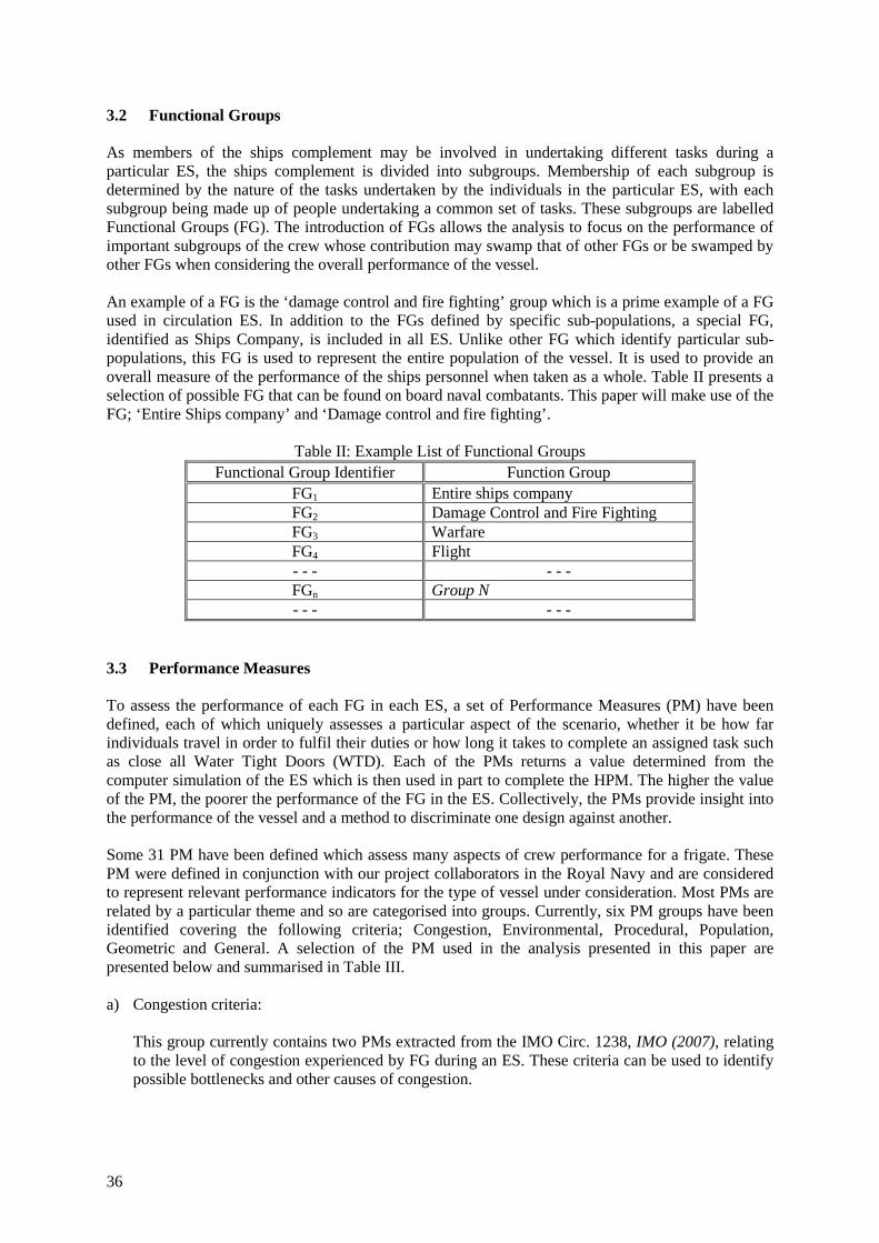
36

3.2 Functional Groups As members of the ships complement may be involved in undertaking different tasks during a particular ES, the ships complement is divided into subgroups. Membership of each subgroup is determined by the nature of the tasks undertaken by the individuals in the particular ES, with each subgroup being made up of people undertaking a common set of tasks. These subgroups are labelled Functional Groups (FG). The introduction of FGs allows the analysis to focus on the performance of important subgroups of the crew whose contribution may swamp that of other FGs or be swamped by other FGs when considering the overall performance of the vessel. An example of a FG is the ‘damage control and fire fighting’ group which is a prime example of a FG used in circulation ES. In addition to the FGs defined by specific sub-populations, a special FG, identified as Ships Company, is included in all ES. Unlike other FG which identify particular sub-populations, this FG is used to represent the entire population of the vessel. It is used to provide an overall measure of the performance of the ships personnel when taken as a whole. Table II presents a selection of possible FG that can be found on board naval combatants. This paper will make use of the FG; ‘Entire Ships company’ and ‘Damage control and fire fighting’.

Table II: Example List of Functional Groups Functional Group Identifier Function Group

FG1 Entire ships company FG2 Damage Control and Fire Fighting FG3 Warfare FG4 Flight - - - - - - FGn Group N - - - - - -

3.3 Performance Measures To assess the performance of each FG in each ES, a set of Performance Measures (PM) have been defined, each of which uniquely assesses a particular aspect of the scenario, whether it be how far individuals travel in order to fulfil their duties or how long it takes to complete an assigned task such as close all Water Tight Doors (WTD). Each of the PMs returns a value determined from the computer simulation of the ES which is then used in part to complete the HPM. The higher the value of the PM, the poorer the performance of the FG in the ES. Collectively, the PMs provide insight into the performance of the vessel and a method to discriminate one design against another. Some 31 PM have been defined which assess many aspects of crew performance for a frigate. These PM were defined in conjunction with our project collaborators in the Royal Navy and are considered to represent relevant performance indicators for the type of vessel under consideration. Most PMs are related by a particular theme and so are categorised into groups. Currently, six PM groups have been identified covering the following criteria; Congestion, Environmental, Procedural, Population, Geometric and General. A selection of the PM used in the analysis presented in this paper are presented below and summarised in Table III. a) Congestion criteria:

This group currently contains two PMs extracted from the IMO Circ. 1238, IMO (2007), relating to the level of congestion experienced by FG during an ES. These criteria can be used to identify possible bottlenecks and other causes of congestion.

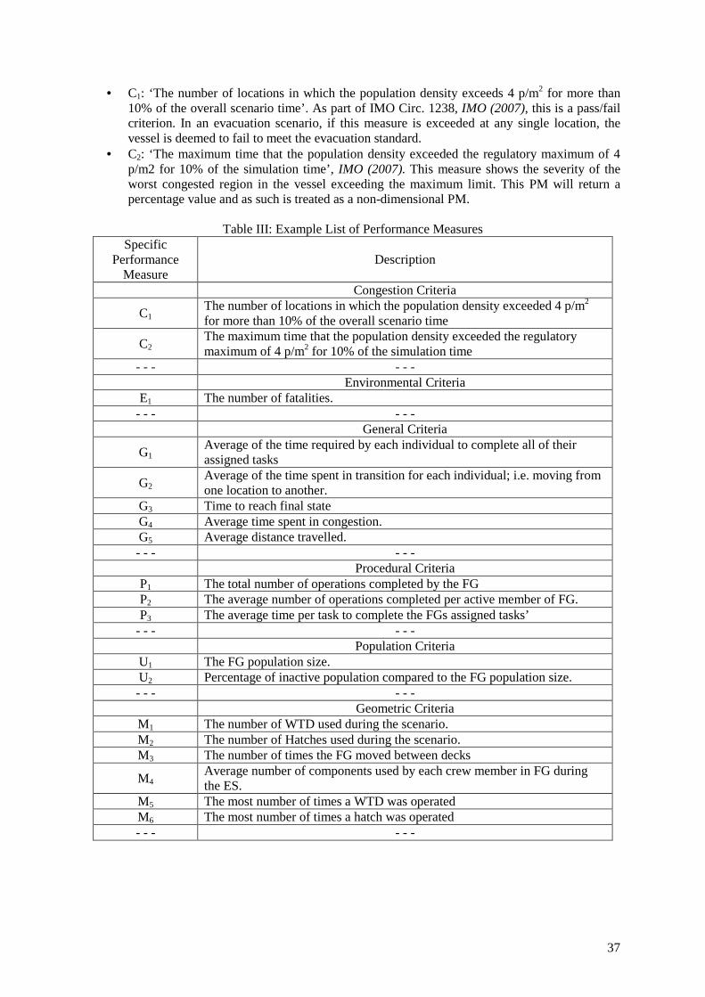
37

• C1: ‘The number of locations in which the population density exceeds 4 p/m2 for more than 10% of the overall scenario time’. As part of IMO Circ. 1238, IMO (2007), this is a pass/fail criterion. In an evacuation scenario, if this measure is exceeded at any single location, the vessel is deemed to fail to meet the evacuation standard.

• C2: ‘The maximum time that the population density exceeded the regulatory maximum of 4 p/m2 for 10% of the simulation time’, IMO (2007). This measure shows the severity of the worst congested region in the vessel exceeding the maximum limit. This PM will return a percentage value and as such is treated as a non-dimensional PM.

Table III: Example List of Performance Measures

Specific Performance

Measure Description

Congestion Criteria

C1 The number of locations in which the population density exceeded 4 p/m2 for more than 10% of the overall scenario time

C2 The maximum time that the population density exceeded the regulatory maximum of 4 p/m2 for 10% of the simulation time

- - - - - - Environmental Criteria

E1 The number of fatalities. - - - - - -

General Criteria

G1 Average of the time required by each individual to complete all of their assigned tasks

G2 Average of the time spent in transition for each individual; i.e. moving from one location to another.

G3 Time to reach final state G4 Average time spent in congestion. G5 Average distance travelled. - - - - - -

Procedural Criteria P1 The total number of operations completed by the FG P2 The average number of operations completed per active member of FG. P3 The average time per task to complete the FGs assigned tasks’

- - - - - - Population Criteria

U1 The FG population size. U2 Percentage of inactive population compared to the FG population size. - - - - - -

Geometric Criteria M1 The number of WTD used during the scenario. M2 The number of Hatches used during the scenario. M3 The number of times the FG moved between decks

M4 Average number of components used by each crew member in FG during the ES.

M5 The most number of times a WTD was operated M6 The most number of times a hatch was operated - - - - - -

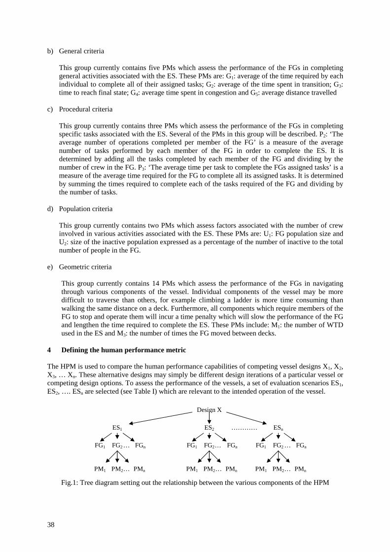
38

b) General criteria

This group currently contains five PMs which assess the performance of the FGs in completing general activities associated with the ES. These PMs are: G1: average of the time required by each individual to complete all of their assigned tasks; G2: average of the time spent in transition; G3: time to reach final state; G4: average time spent in congestion and G5: average distance travelled

c) Procedural criteria

This group currently contains three PMs which assess the performance of the FGs in completing specific tasks associated with the ES. Several of the PMs in this group will be described. P2: ‘The average number of operations completed per member of the FG’ is a measure of the average number of tasks performed by each member of the FG in order to complete the ES. It is determined by adding all the tasks completed by each member of the FG and dividing by the number of crew in the FG. P3: ‘The average time per task to complete the FGs assigned tasks’ is a measure of the average time required for the FG to complete all its assigned tasks. It is determined by summing the times required to complete each of the tasks required of the FG and dividing by the number of tasks.

d) Population criteria

This group currently contains two PMs which assess factors associated with the number of crew involved in various activities associated with the ES. These PMs are: U1: FG population size and U2: size of the inactive population expressed as a percentage of the number of inactive to the total number of people in the FG.

e) Geometric criteria

This group currently contains 14 PMs which assess the performance of the FGs in navigating through various components of the vessel. Individual components of the vessel may be more difficult to traverse than others, for example climbing a ladder is more time consuming than walking the same distance on a deck. Furthermore, all components which require members of the FG to stop and operate them will incur a time penalty which will slow the performance of the FG and lengthen the time required to complete the ES. These PMs include: M1: the number of WTD used in the ES and M3: the number of times the FG moved between decks.

4 Defining the human performance metric The HPM is used to compare the human performance capabilities of competing vessel designs X1, X2, X3, … Xn. These alternative designs may simply be different design iterations of a particular vessel or competing design options. To assess the performance of the vessels, a set of evaluation scenarios ES1, ES2, …. ESn are selected (see Table I) which are relevant to the intended operation of the vessel.

Fig.1: Tree diagram setting out the relationship between the various components of the HPM

Design X

ES1 ES2 ESn

FG2 FGn FG1 FG2 FGn FG1 FG2 FGn FG1

PM1 PM2 PMn PM1 PM2 PMn PM1 PM2 PMn

…………

… … …

… … …

39

The design alternatives are then crewed with the required number of personnel and the crew assigned to their functional groups FG1, FG2….FGn (see Table II). The number and type of FG may differ between design alternatives for each ES. Finally, each functional group FGi, has a set of performance measures PM1, PM2….PMn defining the performance of the FG (See Table III). The relationship between the various components of the HPM is illustrated in Fig.1. 5 Constructing the HPM To complete the HPM, performance scores, ai,j(PMk), associated with each PM must be determined. The PM score is simply its value derived from the execution of the simulation software for each FG within each ES. Thus,

ai,j(PMk) = Performance score derived from the simulation software for evaluation scenario ESi, functional group FGj and performance measure PMk.

Each page in the HPM is made up of a collection of these raw scores. In their present state the performance scores ai,j(PMk), represent a mix of dimensional and non-dimensional numbers. It is thus not possible to make a meaningful comparison between scores. To allow a meaningful comparison between performance scores, each score, with the exception of the PM G3 (‘time to reach final state’) in evacuation ES, is normalised using the largest performance score from the competing design variants as shown in Eq.(1). āi,j(PMk). = ai,j(PMk) / maxi,j(PMk) (1) where maxi,j(PMk) is the maximum value of ai,j(PMk) across the designs variants X1, X2, X3, … Xn. Using this approach, all the HPM entries will be less than or equal to 1.0. The larger the performance score, the worse the performance of the FG in that particular PM. Normalised performance scores equal to 1.0 indicate that the vessel achieved the worst performance of all the variants in this particular PM. Normalised performance scores close to or equal to 1.0 indicate an area of concern in the design. In evacuation Evaluation Scenarios (ESs), the Performance Measure (PM) G3 is normalised using the regulatory defined maximum value which is a function of the number of WT zones, IMO (2007). Thus a value of 1.0 indicates that the vessel’s performance equals the regulatory maximum, a value less than one indicates that the vessel is outperforming the regulatory requirement and a value greater than one indicates the vessel has failed the regulatory requirement. An overall score can be determined for each FG representing the performance of the particular FG in the particular ES. This is calculated by taking a weighted sum of the normalised PM scores achieved by the FG across all the PMs. As not all PMs are considered of equal importance, a weighting is introduced to differentiate between various PMs. For example, the PM ‘Number of fatalities’ is considerably more important than the PM ‘average distance travelled’. However, weighting of the PM is somewhat arbitrary and may depend on the nature of the ES and the FG being considered and the priorities of the assessor. Ideally, the weights should be set in consultation with the client so that their priorities are appropriately represented within the analysis. Alternatively, appropriate weights could be determined through canvassing expert opinion using the Delphi method, Harmathy (1982). Thus each normalised score āi,j(PMk) will have a weight associated with it Ai,j,k, where subscript i refers to evaluation scenario ESi, the j subscript refers to the functional group FGj and the k subscript refers to the performance measure PMk. Thus the functional group score άi,j is given by Eq.(2). άi,j = (Ai,j,1 x āi,j(PM1)) + (Ai,j,2 x āi,j(PM2)) + - - - + (Ai,j,n x āi,j(PMn)) + - - - (2)

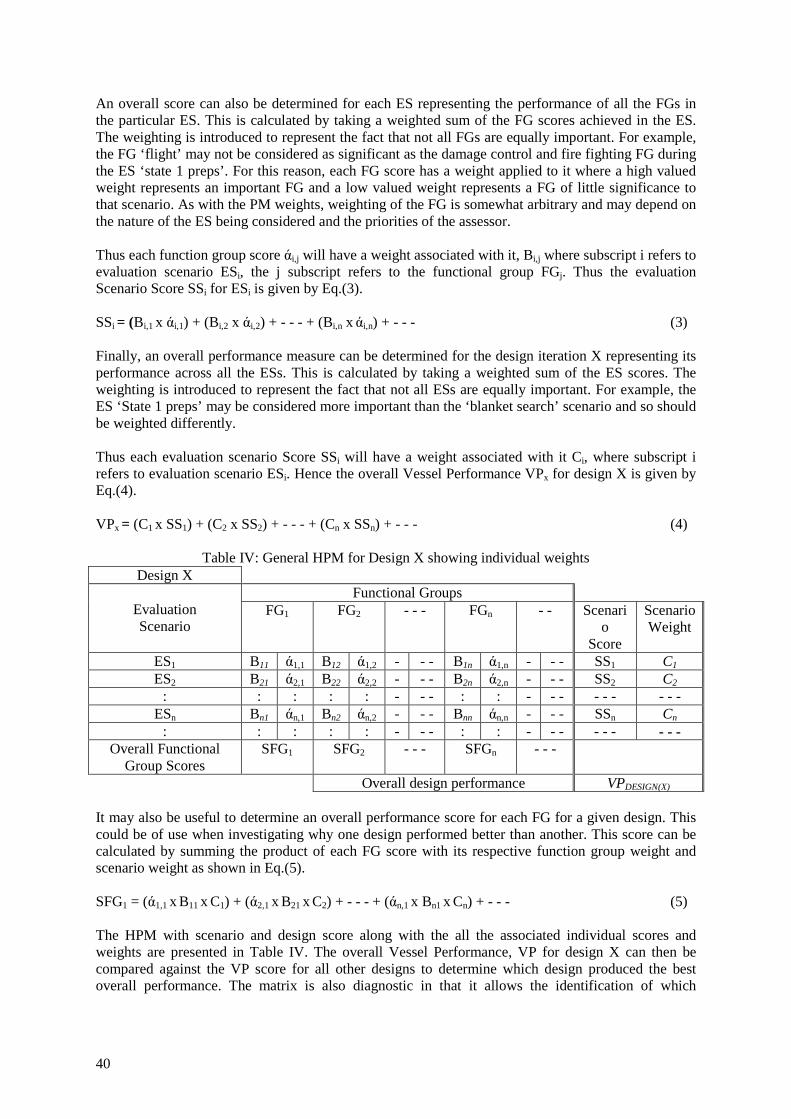
40

An overall score can also be determined for each ES representing the performance of all the FGs in the particular ES. This is calculated by taking a weighted sum of the FG scores achieved in the ES. The weighting is introduced to represent the fact that not all FGs are equally important. For example, the FG ‘flight’ may not be considered as significant as the damage control and fire fighting FG during the ES ‘state 1 preps’. For this reason, each FG score has a weight applied to it where a high valued weight represents an important FG and a low valued weight represents a FG of little significance to that scenario. As with the PM weights, weighting of the FG is somewhat arbitrary and may depend on the nature of the ES being considered and the priorities of the assessor. Thus each function group score άi,j will have a weight associated with it, Bi,j where subscript i refers to evaluation scenario ESi, the j subscript refers to the functional group FGj. Thus the evaluation Scenario Score SSi for ESi is given by Eq.(3). SSi = (Bi,1 x άi,1) + (Bi,2 x άi,2) + - - - + (Bi,n x άi,n) + - - - (3) Finally, an overall performance measure can be determined for the design iteration X representing its performance across all the ESs. This is calculated by taking a weighted sum of the ES scores. The weighting is introduced to represent the fact that not all ESs are equally important. For example, the ES ‘State 1 preps’ may be considered more important than the ‘blanket search’ scenario and so should be weighted differently. Thus each evaluation scenario Score SSi will have a weight associated with it Ci, where subscript i refers to evaluation scenario ESi. Hence the overall Vessel Performance VPx for design X is given by Eq.(4). VPx = (C1 x SS1) + (C2 x SS2) + - - - + (Cn x SSn) + - - - (4)

Table IV: General HPM for Design X showing individual weights

It may also be useful to determine an overall performance score for each FG for a given design. This could be of use when investigating why one design performed better than another. This score can be calculated by summing the product of each FG score with its respective function group weight and scenario weight as shown in Eq.(5). SFG1 = (ά1,1 x B11 x C1) + (ά2,1 x B21 x C2) + - - - + (άn,1 x Bn1 x Cn) + - - - (5) The HPM with scenario and design score along with the all the associated individual scores and weights are presented in Table IV. The overall Vessel Performance, VP for design X can then be compared against the VP score for all other designs to determine which design produced the best overall performance. The matrix is also diagnostic in that it allows the identification of which

Design X Functional Groups

Evaluation Scenario

FG1 FG2 - - - FGn - - Scenario

Score

Scenario Weight

ES1 B11 ά1,1 B12 ά1,2 - - - B1n ά1,n - - - SS1 C1 ES2 B21 ά2,1 B22 ά2,2 - - - B2n ά2,n - - - SS2 C2

: : : : : - - - : : - - - - - - - - - ESn Bn1 άn,1 Bn2 άn,2 - - - Bnn άn,n - - - SSn Cn

: : : : : - - - : : - - - - - - - - - Overall Functional

Group Scores SFG1 SFG2 - - - SFGn - - -

Overall design performance VPDESIGN(X)

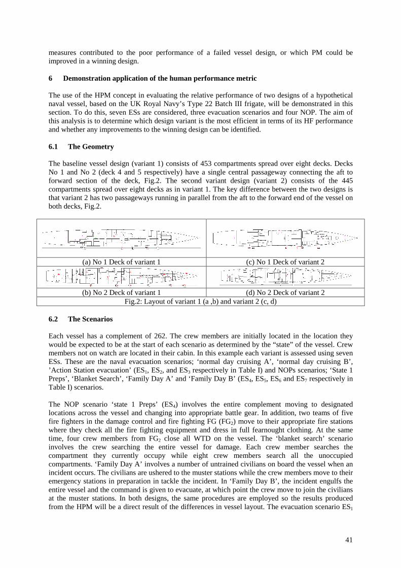
41

measures contributed to the poor performance of a failed vessel design, or which PM could be improved in a winning design. 6 Demonstration application of the human performance metric The use of the HPM concept in evaluating the relative performance of two designs of a hypothetical naval vessel, based on the UK Royal Navy’s Type 22 Batch III frigate, will be demonstrated in this section. To do this, seven ESs are considered, three evacuation scenarios and four NOP. The aim of this analysis is to determine which design variant is the most efficient in terms of its HF performance and whether any improvements to the winning design can be identified. 6.1 The Geometry The baseline vessel design (variant 1) consists of 453 compartments spread over eight decks. Decks No 1 and No 2 (deck 4 and 5 respectively) have a single central passageway connecting the aft to forward section of the deck, Fig.2. The second variant design (variant 2) consists of the 445 compartments spread over eight decks as in variant 1. The key difference between the two designs is that variant 2 has two passageways running in parallel from the aft to the forward end of the vessel on both decks, Fig.2.

(a) No 1 Deck of variant 1 (c) No 1 Deck of variant 2

(b) No 2 Deck of variant 1 (d) No 2 Deck of variant 2

Fig.2: Layout of variant 1 (a ,b) and variant 2 (c, d) 6.2 The Scenarios Each vessel has a complement of 262. The crew members are initially located in the location they would be expected to be at the start of each scenario as determined by the “state” of the vessel. Crew members not on watch are located in their cabin. In this example each variant is assessed using seven ESs. These are the naval evacuation scenarios; ‘normal day cruising A’, ‘normal day cruising B’, ’Action Station evacuation’ (ES1, ES2, and ES3 respectively in Table I) and NOPs scenarios; ‘State 1 Preps’, ‘Blanket Search’, ‘Family Day A’ and ‘Family Day B’ (ES4, ES5, ES6 and ES7 respectively in Table I) scenarios. The NOP scenario ‘state 1 Preps’ (ES4) involves the entire complement moving to designated locations across the vessel and changing into appropriate battle gear. In addition, two teams of five fire fighters in the damage control and fire fighting FG (FG2) move to their appropriate fire stations where they check all the fire fighting equipment and dress in full fearnought clothing. At the same time, four crew members from FG2 close all WTD on the vessel. The ‘blanket search’ scenario involves the crew searching the entire vessel for damage. Each crew member searches the compartment they currently occupy while eight crew members search all the unoccupied compartments. ‘Family Day A’ involves a number of untrained civilians on board the vessel when an incident occurs. The civilians are ushered to the muster stations while the crew members move to their emergency stations in preparation in tackle the incident. In ‘Family Day B’, the incident engulfs the entire vessel and the command is given to evacuate, at which point the crew move to join the civilians at the muster stations. In both designs, the same procedures are employed so the results produced from the HPM will be a direct result of the differences in vessel layout. The evacuation scenario ES1

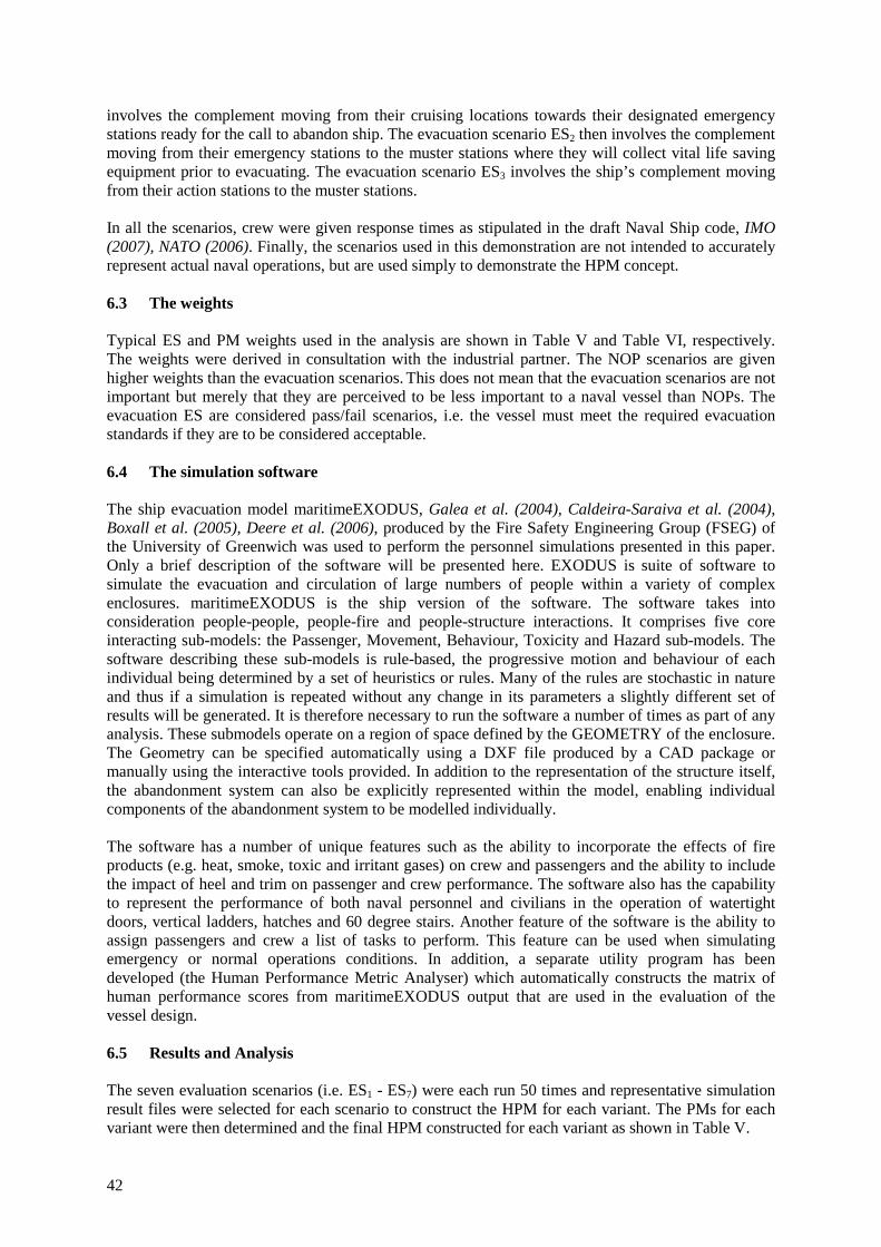
42

involves the complement moving from their cruising locations towards their designated emergency stations ready for the call to abandon ship. The evacuation scenario ES2 then involves the complement moving from their emergency stations to the muster stations where they will collect vital life saving equipment prior to evacuating. The evacuation scenario ES3 involves the ship’s complement moving from their action stations to the muster stations. In all the scenarios, crew were given response times as stipulated in the draft Naval Ship code, IMO (2007), NATO (2006). Finally, the scenarios used in this demonstration are not intended to accurately represent actual naval operations, but are used simply to demonstrate the HPM concept. 6.3 The weights Typical ES and PM weights used in the analysis are shown in Table V and Table VI, respectively. The weights were derived in consultation with the industrial partner. The NOP scenarios are given higher weights than the evacuation scenarios. This does not mean that the evacuation scenarios are not important but merely that they are perceived to be less important to a naval vessel than NOPs. The evacuation ES are considered pass/fail scenarios, i.e. the vessel must meet the required evacuation standards if they are to be considered acceptable. 6.4 The simulation software The ship evacuation model maritimeEXODUS, Galea et al. (2004), Caldeira-Saraiva et al. (2004), Boxall et al. (2005), Deere et al. (2006), produced by the Fire Safety Engineering Group (FSEG) of the University of Greenwich was used to perform the personnel simulations presented in this paper. Only a brief description of the software will be presented here. EXODUS is suite of software to simulate the evacuation and circulation of large numbers of people within a variety of complex enclosures. maritimeEXODUS is the ship version of the software. The software takes into consideration people-people, people-fire and people-structure interactions. It comprises five core interacting sub-models: the Passenger, Movement, Behaviour, Toxicity and Hazard sub-models. The software describing these sub-models is rule-based, the progressive motion and behaviour of each individual being determined by a set of heuristics or rules. Many of the rules are stochastic in nature and thus if a simulation is repeated without any change in its parameters a slightly different set of results will be generated. It is therefore necessary to run the software a number of times as part of any analysis. These submodels operate on a region of space defined by the GEOMETRY of the enclosure. The Geometry can be specified automatically using a DXF file produced by a CAD package or manually using the interactive tools provided. In addition to the representation of the structure itself, the abandonment system can also be explicitly represented within the model, enabling individual components of the abandonment system to be modelled individually. The software has a number of unique features such as the ability to incorporate the effects of fire products (e.g. heat, smoke, toxic and irritant gases) on crew and passengers and the ability to include the impact of heel and trim on passenger and crew performance. The software also has the capability to represent the performance of both naval personnel and civilians in the operation of watertight doors, vertical ladders, hatches and 60 degree stairs. Another feature of the software is the ability to assign passengers and crew a list of tasks to perform. This feature can be used when simulating emergency or normal operations conditions. In addition, a separate utility program has been developed (the Human Performance Metric Analyser) which automatically constructs the matrix of human performance scores from maritimeEXODUS output that are used in the evaluation of the vessel design. 6.5 Results and Analysis The seven evaluation scenarios (i.e. ES1 - ES7) were each run 50 times and representative simulation result files were selected for each scenario to construct the HPM for each variant. The PMs for each variant were then determined and the final HPM constructed for each variant as shown in Table V.

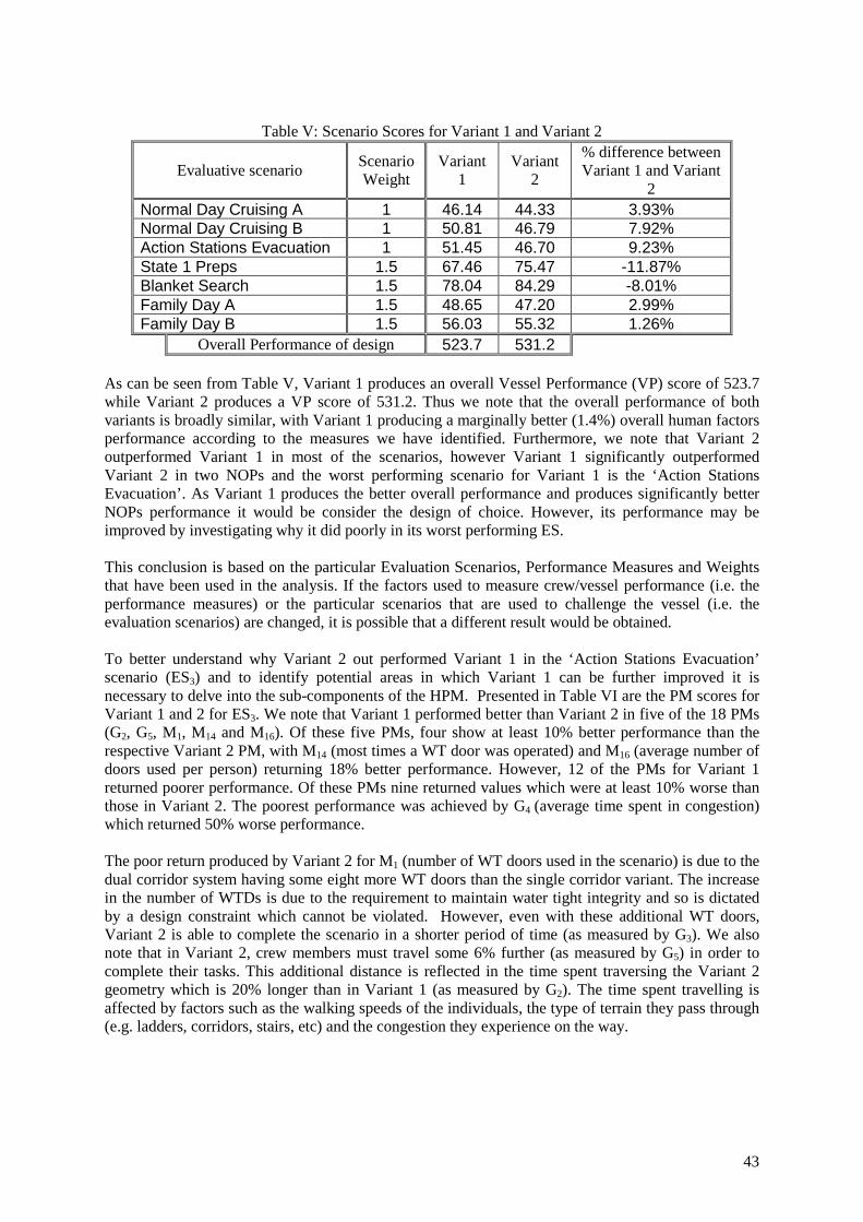
43

Table V: Scenario Scores for Variant 1 and Variant 2

Evaluative scenario Scenario Weight

Variant 1

Variant 2

% difference between Variant 1 and Variant

2 Normal Day Cruising A 1 46.14 44.33 3.93% Normal Day Cruising B 1 50.81 46.79 7.92% Action Stations Evacuation 1 51.45 46.70 9.23% State 1 Preps 1.5 67.46 75.47 -11.87% Blanket Search 1.5 78.04 84.29 -8.01% Family Day A 1.5 48.65 47.20 2.99% Family Day B 1.5 56.03 55.32 1.26%

Overall Performance of design 523.7 531.2 As can be seen from Table V, Variant 1 produces an overall Vessel Performance (VP) score of 523.7 while Variant 2 produces a VP score of 531.2. Thus we note that the overall performance of both variants is broadly similar, with Variant 1 producing a marginally better (1.4%) overall human factors performance according to the measures we have identified. Furthermore, we note that Variant 2 outperformed Variant 1 in most of the scenarios, however Variant 1 significantly outperformed Variant 2 in two NOPs and the worst performing scenario for Variant 1 is the ‘Action Stations Evacuation’. As Variant 1 produces the better overall performance and produces significantly better NOPs performance it would be consider the design of choice. However, its performance may be improved by investigating why it did poorly in its worst performing ES. This conclusion is based on the particular Evaluation Scenarios, Performance Measures and Weights that have been used in the analysis. If the factors used to measure crew/vessel performance (i.e. the performance measures) or the particular scenarios that are used to challenge the vessel (i.e. the evaluation scenarios) are changed, it is possible that a different result would be obtained. To better understand why Variant 2 out performed Variant 1 in the ‘Action Stations Evacuation’ scenario (ES3) and to identify potential areas in which Variant 1 can be further improved it is necessary to delve into the sub-components of the HPM. Presented in Table VI are the PM scores for Variant 1 and 2 for ES3. We note that Variant 1 performed better than Variant 2 in five of the 18 PMs (G2, G5, M1, M14 and M16). Of these five PMs, four show at least 10% better performance than the respective Variant 2 PM, with M14 (most times a WT door was operated) and M16 (average number of doors used per person) returning 18% better performance. However, 12 of the PMs for Variant 1 returned poorer performance. Of these PMs nine returned values which were at least 10% worse than those in Variant 2. The poorest performance was achieved by G4 (average time spent in congestion) which returned 50% worse performance. The poor return produced by Variant 2 for M1 (number of WT doors used in the scenario) is due to the dual corridor system having some eight more WT doors than the single corridor variant. The increase in the number of WTDs is due to the requirement to maintain water tight integrity and so is dictated by a design constraint which cannot be violated. However, even with these additional WT doors, Variant 2 is able to complete the scenario in a shorter period of time (as measured by G3). We also note that in Variant 2, crew members must travel some 6% further (as measured by G5) in order to complete their tasks. This additional distance is reflected in the time spent traversing the Variant 2 geometry which is 20% longer than in Variant 1 (as measured by G2). The time spent travelling is affected by factors such as the walking speeds of the individuals, the type of terrain they pass through (e.g. ladders, corridors, stairs, etc) and the congestion they experience on the way.

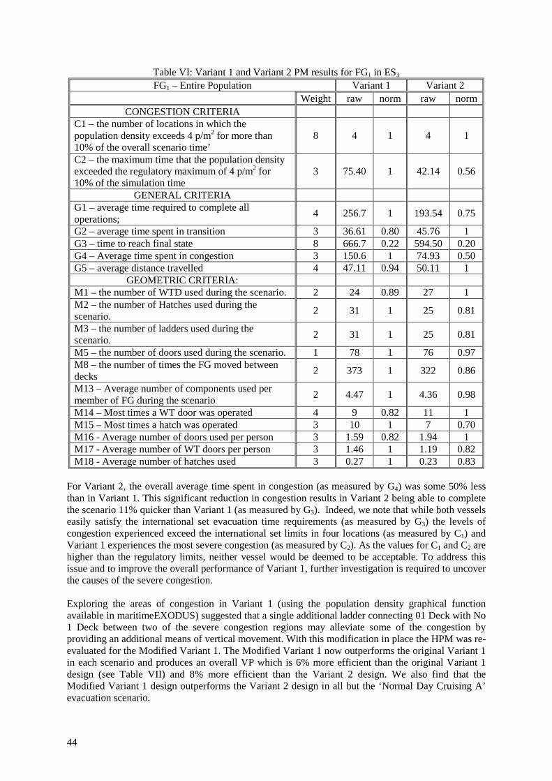
44

Table VI: Variant 1 and Variant 2 PM results for FG1 in ES3 FG1 – Entire Population Variant 1 Variant 2

Weight raw norm raw norm CONGESTION CRITERIA

C1 – the number of locations in which the population density exceeds 4 p/m2 for more than 10% of the overall scenario time’

8 4 1 4 1

C2 – the maximum time that the population density exceeded the regulatory maximum of 4 p/m2 for 10% of the simulation time

3 75.40 1 42.14 0.56

GENERAL CRITERIA G1 – average time required to complete all operations;

4 256.7 1 193.54 0.75

G2 – average time spent in transition 3 36.61 0.80 45.76 1 G3 – time to reach final state 8 666.7 0.22 594.50 0.20 G4 – Average time spent in congestion 3 150.6 1 74.93 0.50 G5 – average distance travelled 4 47.11 0.94 50.11 1

GEOMETRIC CRITERIA: M1 – the number of WTD used during the scenario. 2 24 0.89 27 1 M2 – the number of Hatches used during the scenario.

2 31 1 25 0.81

M3 – the number of ladders used during the scenario.

2 31 1 25 0.81

M5 – the number of doors used during the scenario. 1 78 1 76 0.97 M8 – the number of times the FG moved between decks

2 373 1 322 0.86

M13 – Average number of components used per member of FG during the scenario

2 4.47 1 4.36 0.98

M14 – Most times a WT door was operated 4 9 0.82 11 1 M15 – Most times a hatch was operated 3 10 1 7 0.70 M16 - Average number of doors used per person 3 1.59 0.82 1.94 1 M17 - Average number of WT doors per person 3 1.46 1 1.19 0.82 M18 - Average number of hatches used 3 0.27 1 0.23 0.83

For Variant 2, the overall average time spent in congestion (as measured by G4) was some 50% less than in Variant 1. This significant reduction in congestion results in Variant 2 being able to complete the scenario 11% quicker than Variant 1 (as measured by G3). Indeed, we note that while both vessels easily satisfy the international set evacuation time requirements (as measured by G3) the levels of congestion experienced exceed the international set limits in four locations (as measured by C1) and Variant 1 experiences the most severe congestion (as measured by C2). As the values for C1 and C2 are higher than the regulatory limits, neither vessel would be deemed to be acceptable. To address this issue and to improve the overall performance of Variant 1, further investigation is required to uncover the causes of the severe congestion. Exploring the areas of congestion in Variant 1 (using the population density graphical function available in maritimeEXODUS) suggested that a single additional ladder connecting 01 Deck with No 1 Deck between two of the severe congestion regions may alleviate some of the congestion by providing an additional means of vertical movement. With this modification in place the HPM was re-evaluated for the Modified Variant 1. The Modified Variant 1 now outperforms the original Variant 1 in each scenario and produces an overall VP which is 6% more efficient than the original Variant 1 design (see Table VII) and 8% more efficient than the Variant 2 design. We also find that the Modified Variant 1 design outperforms the Variant 2 design in all but the ‘Normal Day Cruising A’ evacuation scenario.

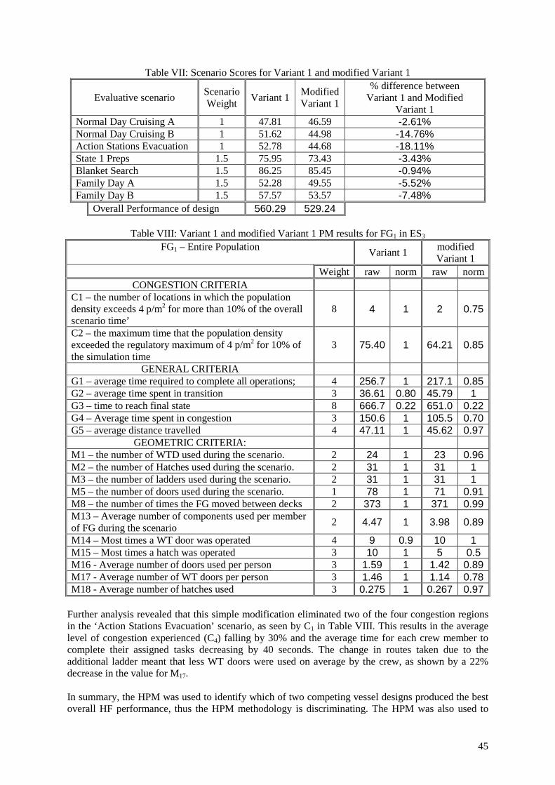
45

Table VII: Scenario Scores for Variant 1 and modified Variant 1

Evaluative scenario Scenario Weight

Variant 1 Modified Variant 1

% difference between Variant 1 and Modified

Variant 1 Normal Day Cruising A 1 47.81 46.59 -2.61% Normal Day Cruising B 1 51.62 44.98 -14.76% Action Stations Evacuation 1 52.78 44.68 -18.11% State 1 Preps 1.5 75.95 73.43 -3.43% Blanket Search 1.5 86.25 85.45 -0.94% Family Day A 1.5 52.28 49.55 -5.52% Family Day B 1.5 57.57 53.57 -7.48%

Overall Performance of design 560.29 529.24

Table VIII: Variant 1 and modified Variant 1 PM results for FG1 in ES3 FG1 – Entire Population

Variant 1 modified Variant 1

Weight raw norm raw norm CONGESTION CRITERIA

C1 – the number of locations in which the population density exceeds 4 p/m2 for more than 10% of the overall scenario time’

8 4 1 2 0.75

C2 – the maximum time that the population density exceeded the regulatory maximum of 4 p/m2 for 10% of the simulation time

3 75.40 1 64.21 0.85

GENERAL CRITERIA G1 – average time required to complete all operations; 4 256.7 1 217.1 0.85 G2 – average time spent in transition 3 36.61 0.80 45.79 1 G3 – time to reach final state 8 666.7 0.22 651.0 0.22 G4 – Average time spent in congestion 3 150.6 1 105.5 0.70 G5 – average distance travelled 4 47.11 1 45.62 0.97

GEOMETRIC CRITERIA: M1 – the number of WTD used during the scenario. 2 24 1 23 0.96 M2 – the number of Hatches used during the scenario. 2 31 1 31 1 M3 – the number of ladders used during the scenario. 2 31 1 31 1 M5 – the number of doors used during the scenario. 1 78 1 71 0.91 M8 – the number of times the FG moved between decks 2 373 1 371 0.99 M13 – Average number of components used per member of FG during the scenario

2 4.47 1 3.98 0.89

M14 – Most times a WT door was operated 4 9 0.9 10 1 M15 – Most times a hatch was operated 3 10 1 5 0.5 M16 - Average number of doors used per person 3 1.59 1 1.42 0.89 M17 - Average number of WT doors per person 3 1.46 1 1.14 0.78 M18 - Average number of hatches used 3 0.275 1 0.267 0.97

Further analysis revealed that this simple modification eliminated two of the four congestion regions in the ‘Action Stations Evacuation’ scenario, as seen by C1 in Table VIII. This results in the average level of congestion experienced (C4) falling by 30% and the average time for each crew member to complete their assigned tasks decreasing by 40 seconds. The change in routes taken due to the additional ladder meant that less WT doors were used on average by the crew, as shown by a 22% decrease in the value for M17. In summary, the HPM was used to identify which of two competing vessel designs produced the best overall HF performance, thus the HPM methodology is discriminating. The HPM was also used to

46

identify areas in which the HF performance of the winning design variant could be improved, thus the HPM methodology is diagnostic. Furthermore the HPM can routinely be applied to any given design and so is systematic, the logic process by which the decisions are made are transparent and another engineer using the methodology would arrive at the same conclusions and so the methodology is repeatable. 7 Concluding comments This paper has described and demonstrated a general methodology, the Human Performance Metric (HPM), for evaluating HF performance of competing ship designs. The use of the methodology was demonstrated using two hypothetical variants of a surface naval combatant, one variant involving a single longitudinal passageway and a competing variant involving two longitudinal passageways. Using the methodology the single passageway variant was identified as the superior design on the basis of seven evaluation scenarios, three evacuation scenarios and four NOP scenarios. The approach also identified why the winning design was superior and was used to suggest how the performance of the vessel could be improved even further. While the approach has been demonstrated for a naval surface combatant, it can be applied to any class of vessel, civilian or naval. The approach is both systematic and transparent allowing user priorities to be clearly stated as part of the methodology. The user priorities can be identified through the selection of appropriate evaluation scenarios and the weights assigned to the various components of the HPM. The methodology is intended to be used as a comparative tool, where the performance of one variant is compared with the performance of an alternative variant. The alternative variant may have its structural layout altered or the personnel procedures employed in the various scenarios may be altered. For a given class of vessel, it is possible to define a set of standards representing the desired or minimum acceptable performance of candidate vessels across a range of ES and PMs. By defining this standard it is possible to evaluate a one-off design, not against another contender vessel, but against the specified standard. This is a useful concept as it allows fleet owners to define the precise performance levels they expect from candidate vessels and also provide a means of measuring the performance of potential candidates. The standards can simply be defined on the basis of the existing best performer in class. Finally, the HPM methodology has application not just to ship design, but also to the optimal design of buildings, allowing competing evacuation and pedestrian dynamics requirements to be assessed in a systemic, transparent and repeatable manner. Acknowledgements: The authors gratefully acknowledge the support of the UK EPSRC under grant GR/T22100/01 and the UK Ministry of Defence through Directorate of Sea Systems, Defence Equipment and Support (DES-SESea) and our project partners UCL DRC. References: DEERE, S.; GALEA, E.R.; LAWRENCE, P.; GWYNNE, S. (2006), The Impact of the passenger response time distribution on ship evacuation performance, RINA Transactions Vol 148, Part A1 (Journal of Maritime Engineering), ISSN 1479-8751, pp.35-44 GALEA, E.R.; LAWRENCE, P.; GWYNNE, S.; SHARP, G.; HURST, N.; WANG, Z.; EWER., J. (2004), Integrated fire and evacuation in maritime environments, 2nd Int Maritime Safety Conference on Design for Safety, Sakai Japan, Publisher Ship and Ocean Foundation, pp.161-170

47

BOXALL, P.; GWYNNE, S.; FILIPPIDIS, L.; GALEA, E.R.; COONEY. D. (2005), Advanced evacuation simulation software and its use in warships, Human Factors in Ship Design, Safety and Operation, London UK, RINA, pp.49-56 CALDEIRA-SARAIVA, F.; GYNGELL, J.; WHEELER, R.; GALEA, E.R.; CARRAN, A.; SKJONG, R.; VANEM, E.; JOHANSSON, K.; RUTHERFORD, B.; SIMOES, A.J. (2004), Simulation of ship evacuation and passenger circulation, 2nd Int. Maritime Safety Conference on Design for Safety, Sakai Japan, Publisher Ship and Ocean Foundation, pp.197-205 CHOW, W.K. (2002), Proposed fire safety ranking system EB-FSRS for existing high-rise nonresidential buildings in Hong Kong, J. Architectural Engineering, pp.116-124 WATTS, J.M. (2002), Fire Risk Indexing, The SFPE, Handbook of Fire Protection Engineering (3rd Edition), National Fire Protection Association, Quincy, Ma, pp.(5-125)-(5-142) IMO (2007), Guidelines for Evacuation Analyses for New and Existing Passenger Ships, International Maritime Organisation MSC.1/Circ. 1238. NATO (2006), Chapter VII Escape Evacuation and Rescue, ALLIED NAVAL ENGINEERING PUBLICATION ANEP - 77, NAVAL SHIP CODE, Naval Armaments Group, Maritime Capability Group 6 HARMATHY, T.Z. (1982), The Delphi method – A complement to research, Fire and Materials, Vol. 6, No. 2, pp.76-79

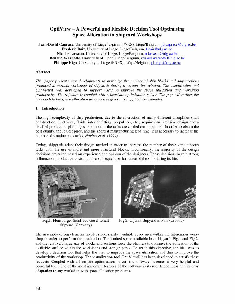
48

OptiView − A Powerful and Flexible Decision Tool Optimising Space Allocation in Shipyard Workshops

Jean-David Caprace, University of Liege (aspirant FNRS), Liège/Belgium, jd.caprace@ulg.ac.be

Frederic Bair, University of Liege, Liège/Belgium, f.bair@ulg.ac.be

Nicolas Losseau, University of Liege, Liège/Belgium, n.losseau@ulg.ac.be

Renaud Warnotte, University of Liege, Liège/Belgium, renaud.warnotte@ulg.ac.be

Philippe Rigo, University of Liege (FNRS), Liège/Belgium, ph.rigo@ulg.ac.be

Abstract

This paper presents new developments to maximize the number of ship blocks and ship sections

produced in various workshops of shipyards during a certain time window. The visualization tool

OptiView® was developed to support users to improve the space utilization and workshop

productivity. The software is coupled with a heuristic optimisation solver. The paper describes the

approach to the space allocation problem and gives three application examples.

1 Introduction

The high complexity of ship production, due to the interaction of many different disciplines (hull

construction, electricity, fluids, interior fitting, propulsion, etc.) requires an intensive design and a

detailed production planning where most of the tasks are carried out in parallel. In order to obtain the

best quality, the lowest price, and the shortest manufacturing lead time, it is necessary to increase the

number of simultaneous tasks, Hughes et al. (1994).

Today, shipyards adapt their design method in order to increase the number of these simultaneous

tasks with the use of more and more structural blocks. Traditionally, the majority of the design

decisions are taken based on experience and opinion of the designers. These decisions have a strong

influence on production costs, but also subsequent performance of the ship during its life.

Fig.1: Flensburger Schiffbau Gesellschaft

shipyard (Germany)

Fig.2: Uljanik shipyard in Pula (Croatia)

The assembly of big elements involves necessarily available space area within the fabrication work-

shop in order to perform the production. The limited space available in a shipyard, Fig.1 and Fig.2,

and the relatively large size of blocks and sections force the planners to optimise the utilization of the

available surface within the workshops and storage parks. To reach this objective, the idea was to

develop a decision tool that helps the user to improve the space utilization and thus to improve the

productivity of the workshop. The visualization tool OptiView® has been developed to satisfy these

requests. Coupled with a heuristic optimisation solver, the software becomes a very helpful and

powerful tool. One of the most important features of the software is its user friendliness and its easy

adaptation to any workshop with space allocation problems.

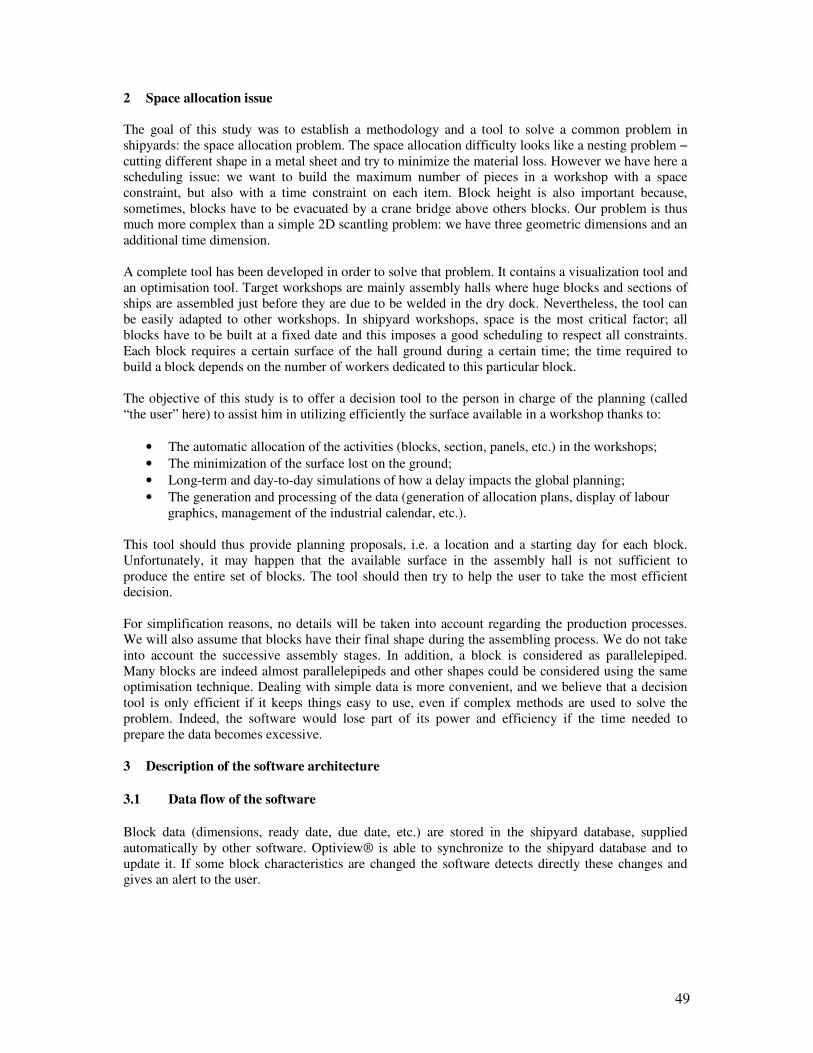
49

2 Space allocation issue

The goal of this study was to establish a methodology and a tool to solve a common problem in

shipyards: the space allocation problem. The space allocation difficulty looks like a nesting problem −

cutting different shape in a metal sheet and try to minimize the material loss. However we have here a

scheduling issue: we want to build the maximum number of pieces in a workshop with a space

constraint, but also with a time constraint on each item. Block height is also important because,

sometimes, blocks have to be evacuated by a crane bridge above others blocks. Our problem is thus

much more complex than a simple 2D scantling problem: we have three geometric dimensions and an

additional time dimension.

A complete tool has been developed in order to solve that problem. It contains a visualization tool and

an optimisation tool. Target workshops are mainly assembly halls where huge blocks and sections of

ships are assembled just before they are due to be welded in the dry dock. Nevertheless, the tool can

be easily adapted to other workshops. In shipyard workshops, space is the most critical factor; all

blocks have to be built at a fixed date and this imposes a good scheduling to respect all constraints.

Each block requires a certain surface of the hall ground during a certain time; the time required to

build a block depends on the number of workers dedicated to this particular block.

The objective of this study is to offer a decision tool to the person in charge of the planning (called

“the user” here) to assist him in utilizing efficiently the surface available in a workshop thanks to:

• The automatic allocation of the activities (blocks, section, panels, etc.) in the workshops;

• The minimization of the surface lost on the ground;

• Long-term and day-to-day simulations of how a delay impacts the global planning;

• The generation and processing of the data (generation of allocation plans, display of labour

graphics, management of the industrial calendar, etc.).

This tool should thus provide planning proposals, i.e. a location and a starting day for each block.

Unfortunately, it may happen that the available surface in the assembly hall is not sufficient to

produce the entire set of blocks. The tool should then try to help the user to take the most efficient

decision.

For simplification reasons, no details will be taken into account regarding the production processes.

We will also assume that blocks have their final shape during the assembling process. We do not take

into account the successive assembly stages. In addition, a block is considered as parallelepiped.

Many blocks are indeed almost parallelepipeds and other shapes could be considered using the same

optimisation technique. Dealing with simple data is more convenient, and we believe that a decision

tool is only efficient if it keeps things easy to use, even if complex methods are used to solve the

problem. Indeed, the software would lose part of its power and efficiency if the time needed to

prepare the data becomes excessive.

3 Description of the software architecture

3.1 Data flow of the software

Block data (dimensions, ready date, due date, etc.) are stored in the shipyard database, supplied

automatically by other software. Optiview® is able to synchronize to the shipyard database and to

update it. If some block characteristics are changed the software detects directly these changes and

gives an alert to the user.

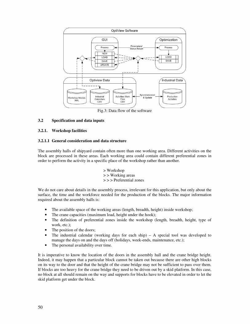
50

Fig.3: Data flow of the software

3.2 Specification and data inputs

3.2.1. Workshop facilities

3.2.1.1 General consideration and data structure

The assembly halls of shipyard contain often more than one working area. Different activities on the

block are processed in these areas. Each working area could contain different preferential zones in

order to perform the activity in a specific place of the workshop rather than another.

> Workshop

> > Working areas

> > > Preferential zones

We do not care about details in the assembly process, irrelevant for this application, but only about the

surface, the time and the workforce needed for the production of the blocks. The major information

required about the assembly halls is:

• The available space of the working areas (length, breadth, height) inside workshop;

• The crane capacities (maximum load, height under the hook);

• The definition of preferential zones inside the workshop (length, breadth, height, type of

work, etc.);

• The position of the doors;

• The industrial calendar (working days for each ship) – A special tool was developed to

manage the days on and the days off (holidays, week-ends, maintenance, etc.);

• The personal availability over time.

It is imperative to know the location of the doors in the assembly hall and the crane bridge height.

Indeed, it may happen that a particular block cannot be taken out because there are other high blocks

on its way to the door and that the height of the crane bridge may not be sufficient to pass over them.

If blocks are too heavy for the crane bridge they need to be driven out by a skid platform. In this case,

no block at all should remain on the way and supports for blocks have to be elevated in order to let the

skid platform get under the block.

51

3.2.1.2 Constraints and assumptions

The basic assumptions that we have seen are the following ones:

• Once a block is placed into the workshop, it cannot be moved until all processes on the block

are finished.

• The blocks cannot overlap each other.

• All blocks will have their final shape during the whole assembling process.

3.2.1.3 File format

All data related to the workshop facilities are stored in XML file format in order to improve the

flexibility of the software. The reading by the XML interpreter of OptiView® file will automatically

build the model in memory and allows using it directly in the program.

Space allocation problems in shipyards are not limited to assembly halls. We therefore created a

Graphic User Interface (GUI) able to read the parameters of any workshop.

3.2.2. Production activities (blocks, sections, etc.)

3.2.2.1 General consideration and data structure

Basically, the input data of the software may be summarized as a list of “activities”. Each activity

represents a certain work to be done on a particular block. Hence, the following information is

required:

• Description of the block (block identification, ship identification, comments, etc.).

• Prismatic dimensions of each block (length, breadth, height, and related spaces allocated to

movements around the blocks). Blocks are considered as parallelepipeds. The major reason

for this assumption is that this data is very easily available; it is easier to deal with basic

shapes and their representations on a surface are more easily interpretable. This idea does not

affect drastically the results since many blocks have indeed a (almost) parallelepiped shape.

For accessibility and security reasons, a certain distance may be required between nearby

blocks in the assembly hall. Therefore, a margin can be added to the length and to the width.

These parameters may also be used to correct manually the dimensions of a block,

particularly if the shape of the block is not a parallelepiped.

• Processing time evaluation dealing with two aspects: The total amount of workforce needed

for each block and the duration of work. At this stage of the planning, a precise processing

time cannot be furnished; therefore the processing time has to be estimated. An estimation of

the total amount of man-time needed is available, thus the processing time is computed by

dividing this man-time by the available number of workers. The user may need to adjust this

time manually (because he is able to change the number of workers during a certain period, or

because he knows that the estimates are too high). The workload assessments become more

precise over time. In addition to the processing time of an activity, some time may be required

to prepare the appropriate surface and build up supports for blocks or to dismantle them. This

work has no effect on the start and the end date. Therefore it has to be taken into account

separately.

• Dates of production start of each block. In this case, we use the earliest start date (earliest date

at which the production can start) and the latest end date (the date at which the activity has to

be finished), Fig.4;

• Target date – this option allows the user to give a preferential start date for the optimisation

module. If this date cannot be reached by the optimiser. The trend will be to approach it as

best as possible.

• Group of blocks − several blocks can be grouped so that the optimiser will position them as if

they were welded together. The advantage is that we can simulate the impact of the

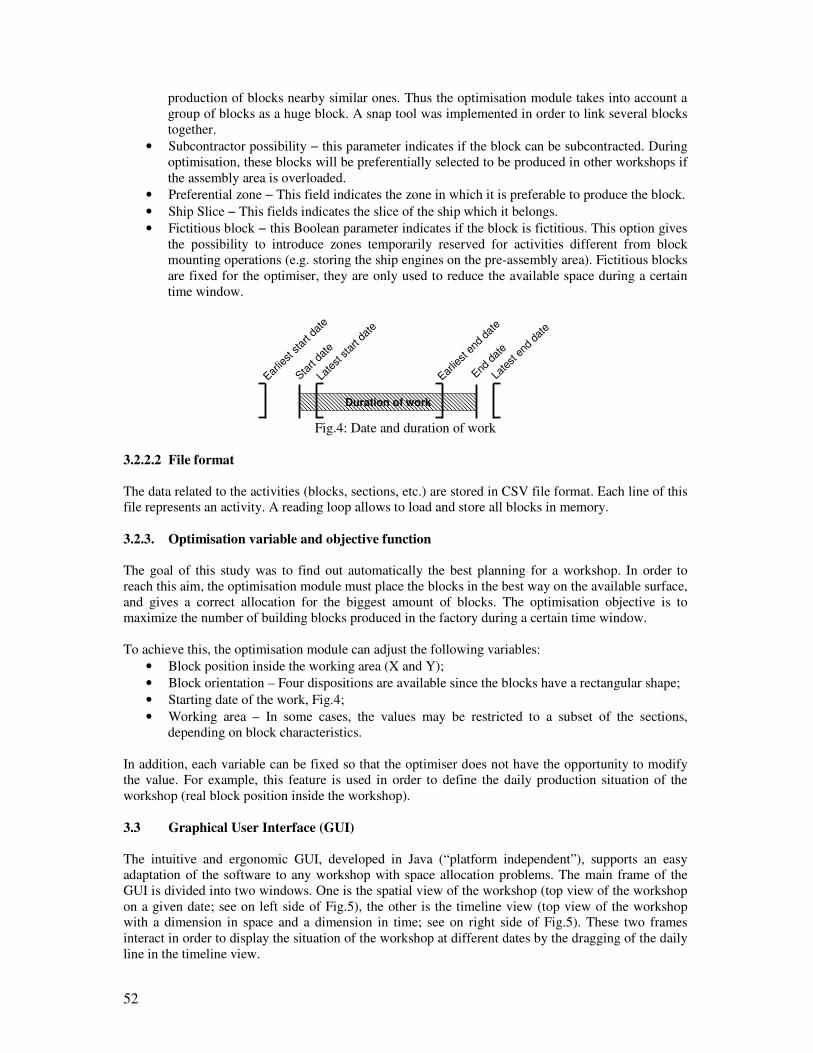
52

production of blocks nearby similar ones. Thus the optimisation module takes into account a

group of blocks as a huge block. A snap tool was implemented in order to link several blocks

together.

• Subcontractor possibility − this parameter indicates if the block can be subcontracted. During

optimisation, these blocks will be preferentially selected to be produced in other workshops if

the assembly area is overloaded.

• Preferential zone − This field indicates the zone in which it is preferable to produce the block.

• Ship Slice − This fields indicates the slice of the ship which it belongs.

• Fictitious block − this Boolean parameter indicates if the block is fictitious. This option gives

the possibility to introduce zones temporarily reserved for activities different from block

mounting operations (e.g. storing the ship engines on the pre-assembly area). Fictitious blocks

are fixed for the optimiser, they are only used to reduce the available space during a certain

time window.

Fig.4: Date and duration of work

3.2.2.2 File format

The data related to the activities (blocks, sections, etc.) are stored in CSV file format. Each line of this

file represents an activity. A reading loop allows to load and store all blocks in memory.

3.2.3. Optimisation variable and objective function

The goal of this study was to find out automatically the best planning for a workshop. In order to

reach this aim, the optimisation module must place the blocks in the best way on the available surface,

and gives a correct allocation for the biggest amount of blocks. The optimisation objective is to

maximize the number of building blocks produced in the factory during a certain time window.

To achieve this, the optimisation module can adjust the following variables:

• Block position inside the working area (X and Y);

• Block orientation – Four dispositions are available since the blocks have a rectangular shape;

• Starting date of the work, Fig.4;

• Working area – In some cases, the values may be restricted to a subset of the sections,

depending on block characteristics.

In addition, each variable can be fixed so that the optimiser does not have the opportunity to modify

the value. For example, this feature is used in order to define the daily production situation of the

workshop (real block position inside the workshop).

3.3 Graphical User Interface (GUI)

The intuitive and ergonomic GUI, developed in Java (“platform independent”), supports an easy

adaptation of the software to any workshop with space allocation problems. The main frame of the

GUI is divided into two windows. One is the spatial view of the workshop (top view of the workshop

on a given date; see on left side of Fig.5), the other is the timeline view (top view of the workshop

with a dimension in space and a dimension in time; see on right side of Fig.5). These two frames

interact in order to display the situation of the workshop at different dates by the dragging of the daily

line in the timeline view.

Duration of work

Sta

rtdate

Earlie

stst

art

date

Late

stend

date

End

date

Late

stst

art

date

Earlie

stend

date

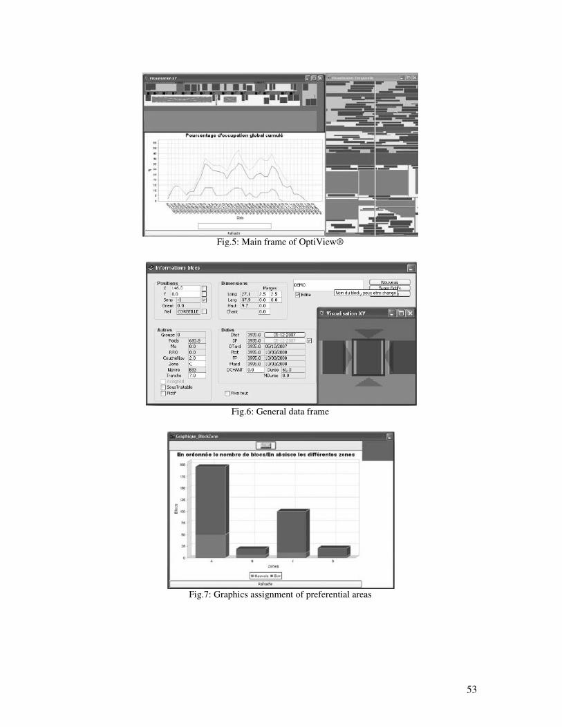
53

Fig.5: Main frame of OptiView®

Fig.6: General data frame

Fig.7: Graphics assignment of preferential areas

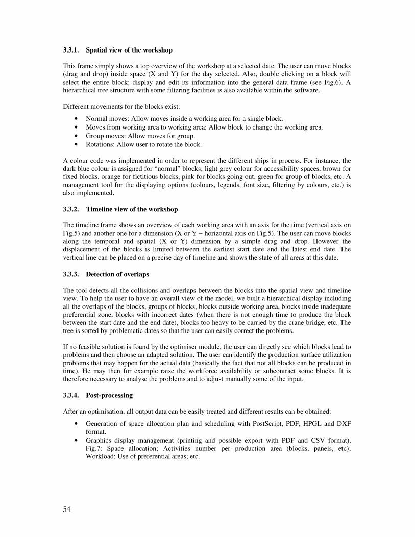
54

3.3.1. Spatial view of the workshop

This frame simply shows a top overview of the workshop at a selected date. The user can move blocks

(drag and drop) inside space (X and Y) for the day selected. Also, double clicking on a block will

select the entire block; display and edit its information into the general data frame (see Fig.6). A

hierarchical tree structure with some filtering facilities is also available within the software.

Different movements for the blocks exist:

• Normal moves: Allow moves inside a working area for a single block.

• Moves from working area to working area: Allow block to change the working area.

• Group moves: Allow moves for group.

• Rotations: Allow user to rotate the block.

A colour code was implemented in order to represent the different ships in process. For instance, the

dark blue colour is assigned for “normal” blocks; light grey colour for accessibility spaces, brown for

fixed blocks, orange for fictitious blocks, pink for blocks going out, green for group of blocks, etc. A

management tool for the displaying options (colours, legends, font size, filtering by colours, etc.) is

also implemented.

3.3.2. Timeline view of the workshop

The timeline frame shows an overview of each working area with an axis for the time (vertical axis on

Fig.5) and another one for a dimension (X or Y − horizontal axis on Fig.5). The user can move blocks

along the temporal and spatial (X or Y) dimension by a simple drag and drop. However the

displacement of the blocks is limited between the earliest start date and the latest end date. The

vertical line can be placed on a precise day of timeline and shows the state of all areas at this date.

3.3.3. Detection of overlaps

The tool detects all the collisions and overlaps between the blocks into the spatial view and timeline

view. To help the user to have an overall view of the model, we built a hierarchical display including

all the overlaps of the blocks, groups of blocks, blocks outside working area, blocks inside inadequate

preferential zone, blocks with incorrect dates (when there is not enough time to produce the block

between the start date and the end date), blocks too heavy to be carried by the crane bridge, etc. The

tree is sorted by problematic dates so that the user can easily correct the problems.

If no feasible solution is found by the optimiser module, the user can directly see which blocks lead to

problems and then choose an adapted solution. The user can identify the production surface utilization

problems that may happen for the actual data (basically the fact that not all blocks can be produced in

time). He may then for example raise the workforce availability or subcontract some blocks. It is

therefore necessary to analyse the problems and to adjust manually some of the input.

3.3.4. Post-processing

After an optimisation, all output data can be easily treated and different results can be obtained:

• Generation of space allocation plan and scheduling with PostScript, PDF, HPGL and DXF

format.

• Graphics display management (printing and possible export with PDF and CSV format),

Fig.7: Space allocation; Activities number per production area (blocks, panels, etc);

Workload; Use of preferential areas; etc.

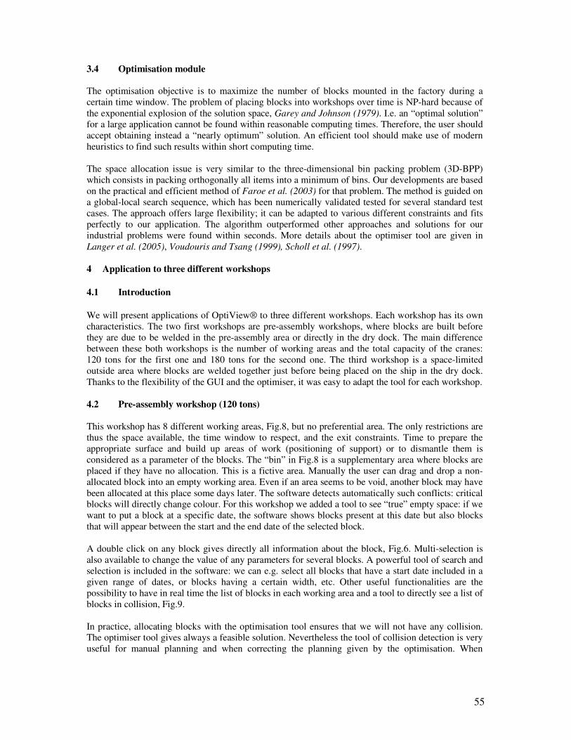
55

3.4 Optimisation module

The optimisation objective is to maximize the number of blocks mounted in the factory during a

certain time window. The problem of placing blocks into workshops over time is NP-hard because of

the exponential explosion of the solution space, Garey and Johnson (1979). I.e. an “optimal solution”

for a large application cannot be found within reasonable computing times. Therefore, the user should

accept obtaining instead a “nearly optimum” solution. An efficient tool should make use of modern

heuristics to find such results within short computing time.

The space allocation issue is very similar to the three-dimensional bin packing problem (3D-BPP)

which consists in packing orthogonally all items into a minimum of bins. Our developments are based

on the practical and efficient method of Faroe et al. (2003) for that problem. The method is guided on

a global-local search sequence, which has been numerically validated tested for several standard test

cases. The approach offers large flexibility; it can be adapted to various different constraints and fits

perfectly to our application. The algorithm outperformed other approaches and solutions for our

industrial problems were found within seconds. More details about the optimiser tool are given in

Langer et al. (2005), Voudouris and Tsang (1999), Scholl et al. (1997).

4 Application to three different workshops

4.1 Introduction

We will present applications of OptiView® to three different workshops. Each workshop has its own

characteristics. The two first workshops are pre-assembly workshops, where blocks are built before

they are due to be welded in the pre-assembly area or directly in the dry dock. The main difference

between these both workshops is the number of working areas and the total capacity of the cranes:

120 tons for the first one and 180 tons for the second one. The third workshop is a space-limited

outside area where blocks are welded together just before being placed on the ship in the dry dock.

Thanks to the flexibility of the GUI and the optimiser, it was easy to adapt the tool for each workshop.

4.2 Pre-assembly workshop (120 tons)

This workshop has 8 different working areas, Fig.8, but no preferential area. The only restrictions are

thus the space available, the time window to respect, and the exit constraints. Time to prepare the

appropriate surface and build up areas of work (positioning of support) or to dismantle them is

considered as a parameter of the blocks. The “bin” in Fig.8 is a supplementary area where blocks are

placed if they have no allocation. This is a fictive area. Manually the user can drag and drop a non-

allocated block into an empty working area. Even if an area seems to be void, another block may have

been allocated at this place some days later. The software detects automatically such conflicts: critical

blocks will directly change colour. For this workshop we added a tool to see “true” empty space: if we

want to put a block at a specific date, the software shows blocks present at this date but also blocks

that will appear between the start and the end date of the selected block.

A double click on any block gives directly all information about the block, Fig.6. Multi-selection is

also available to change the value of any parameters for several blocks. A powerful tool of search and

selection is included in the software: we can e.g. select all blocks that have a start date included in a

given range of dates, or blocks having a certain width, etc. Other useful functionalities are the

possibility to have in real time the list of blocks in each working area and a tool to directly see a list of

blocks in collision, Fig.9.

In practice, allocating blocks with the optimisation tool ensures that we will not have any collision.

The optimiser tool gives always a feasible solution. Nevertheless the tool of collision detection is very

useful for manual planning and when correcting the planning given by the optimisation. When

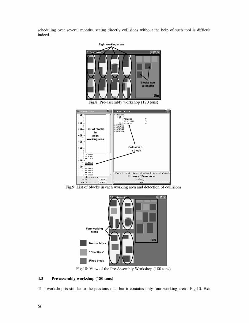
56

scheduling over several months, seeing directly collisions without the help of such tool is difficult

indeed.

Fig.8: Pre-assembly workshop (120 tons)

Fig.9: List of blocks in each working area and detection of collisions

Fig.10: View of the Pre Assembly Workshop (180 tons)

4.3 Pre-assembly workshop (180 tons)

This workshop is similar to the previous one, but it contains only four working areas, Fig.10. Exit

Bin

Eight working areas

Blocks non

allocated

List of blocks

in

each

working area

Collision of

a block

: Fixed block

: “Chantiers”

: Normal blockBin

Four working areas

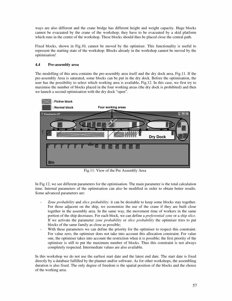
57

ways are also different and the crane bridge has different height and weight capacity. Huge blocks

cannot be evacuated by the crane of the workshop; they have to be evacuated by a skid platform

which runs in the centre of the workshop. These blocks should thus be placed close the central path.

Fixed blocks, shown in Fig.10, cannot be moved by the optimiser. This functionality is useful to

represent the starting state of the workshop: Blocks already in the workshop cannot be moved by the

optimisation!

4.4 Pre-assembly area

The modelling of this area contains the pre-assembly area itself and the dry dock area, Fig.11. If the

pre-assembly Area is saturated, some blocks can be put in the dry dock. Before the optimisation, the

user has the possibility to select which working area is available, Fig.12. In this case, we first try to

maximise the number of blocks placed in the four working areas (the dry dock is prohibited) and then

we launch a second optimisation with the dry dock “open”.

Fig.11: View of the Pre Assembly Area

In Fig.12, we see different parameters for the optimisation. The main parameter is the total calculation

time. Internal parameters of the optimisation can also be modified in order to obtain better results.

Some advanced parameters are:

- Zone probability and slice probability: it can be desirable to keep some blocks stay together.

For those adjacent on the ship, we economize the use of the crane if they are built close

together in the assembly area. In the same way, the movement time of workers in the same

portion of the ship decreases. For each block, we can define a preferential zone or a ship slice.

If we activate the parameter zone probability or slice probability the optimiser tries to put

blocks of the same family as close as possible;

- With these parameters we can define the priority for the optimiser to respect this constraint.

For value zero, the optimiser does not take into account this allocation constraint. For value

one, the optimiser takes into account the restriction when it is possible; the first priority of the

optimiser is still to put the maximum number of blocks. Thus this constraint is not always

completely respected. Intermediate values are also available.

In this workshop we do not use the earliest start date and the latest end date. The start date is fixed

directly by a database fulfilled by the planner and/or software. As for other workshops, the assembling

duration is also fixed. The only degree of freedom is the spatial position of the blocks and the choice

of the working area.

: Fictive block

: Normal block

Bin

Four working areas

Dry Dock

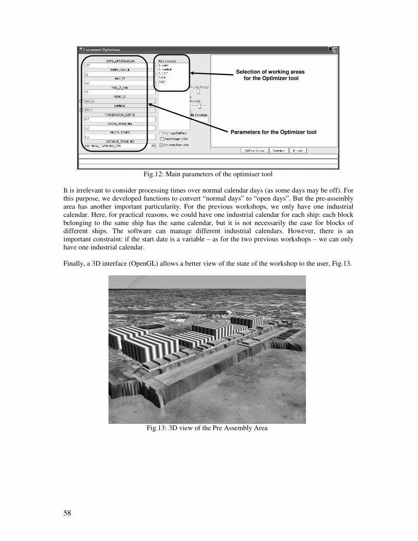
58

Fig.12: Main parameters of the optimiser tool

It is irrelevant to consider processing times over normal calendar days (as some days may be off). For

this purpose, we developed functions to convert “normal days” to “open days”. But the pre-assembly

area has another important particularity. For the previous workshops, we only have one industrial

calendar. Here, for practical reasons, we could have one industrial calendar for each ship: each block

belonging to the same ship has the same calendar, but it is not necessarily the case for blocks of

different ships. The software can manage different industrial calendars. However, there is an

important constraint: if the start date is a variable – as for the two previous workshops – we can only

have one industrial calendar.

Finally, a 3D interface (OpenGL) allows a better view of the state of the workshop to the user, Fig.13.

Fig.13: 3D view of the Pre Assembly Area

Selection of working areasfor the Optimizer tool

Parameters for the Optimizer tool

59

5 Conclusion

The software allows more efficient scheduling for the shipyard. The planner can now test different

alternatives and rapidly modify the scheduling to find the best one. But the preparation and

verification of data for the simulation is still a major stage to ensure the reliability of the results.

Gains obtained for the shipyard are substantial. The workshop productivity by using the OptiView®

tool is increased due to less time needed for the scheduling and better space utilization.

The main advantage of the software is its great flexibility. The software can be easily adapted to

different workshops. In shipbuilding, space allocation problems occur in most workshops. We have

shown three assembly workshops, but the software could also be used for painting halls, storing areas,

etc.

The software is easy to use and intuitive with a lot of useful functionalities: advanced search tool,

graphical visualization of results, easy access to each parameter for the user (colour, text, etc.),

generation of space allocation plans and scheduling with PostScript, PDF, HPGL and DXF format,

etc. Rather than to work in a 2D view, it is also possible to switch into a 3D mode and to navigate

easily in this mode.

As a conclusion, a complete and mature software tool has been developed with a large range of

application fields in shipbuilding industry, but potentially also in other industries.

Acknowledgement

We thank University of Liege, AKER YARDS FRANCE (Saint-Nazaire), for the collaboration within

sub-project II.1 of the IP INTERSHIP Project (6th Framework) and the MARSTRUCT - Network of

Excellence on Marine Structures.

References

FAROE, O.; PISINGER, D.; ZACHARIASEN, M. (2003), Guided local search for the three-

dimensional bin-packing problem, INFORMS Journal on Computing, Vol.15, No. 3, pp.267-283

GAREY, M.R.; JOHNSON, D.S. (1979), Computers and Intractability: A Guide to the Theory of NP-

Completeness, W.H. Freeman, New York

HUGHES, O.F. et al. (1994), Applied computer aided design, Report V.5 of Committee to ISSC, Inst.

Marine Dynamics, Newfoundland

LANGER, Y.; BAY, M.; CRAMA, Y.; BAIR, F.; CAPRACE, J.; RIGO, P. (2005), Optimization of

surface utilization using heuristic approaches, COMPIT'05, Hamburg, pp.419-425

SCHOLL, A.; KLEIN, R.; JURGENS, C. (1997), BISON: A fast hybrid procedure for exactly solving

the one-dimensional bin packing problem, Computers & Operations Research 24, pp.627-645

VOUDOURIS C.; TSANG E. (1999), Guided local search and its application to the travelling

salesman problem, European J. Operational Research 113, pp.469-499

60

A Functionally Oriented Vessel Data Model Used as Basis for Classification Vidar Vindøy, Det Norske Veritas, Oslo/Norway, Vidar.Vindoy@dnv.com

Abstract

A functionally oriented vessel data model has been developed for use as basis for DNV’s classification

activities. The data model covers all vessel types covered by DNV’s classification activities, i.e. ships,

light crafts and mobile offshore units. The data model is used in all phases of the vessels’ lifecycles,

i.e. design, construction, operation and decommissioning. The data model is based on a functionally

oriented description of the vessel, comprising a hierarchical function structure, a library of

components and definitions of legal connections between functions and components. The data model is

based on the principles outlined in ISO 15926. Procedural requirements related to classification, as

documentation requirements for plan approval, survey schemes and survey requirements are attached

to the model. In the future, also technical requirements to vessels and their equipment may be attached

to the model. Based on the generic vessel data model, vessel specific models (product models) are

defined for each vessel classed by DNV. Vessel specific procedural requirements are automatically

generated, while vessel specific data is assigned to the vessel specific models.

1. Introduction

DNV started to work with the establishment of a product model for vessels subject to classification in

the 1990s. A decision to implement this was made in 2001, and the basic design principles were

defined in 2002. The model was taken into use as a part of DNV’s ‘Nauticus Production System’ in

June 2005. The current system is primarily used for activities related to Ships in Operation. Extensions

aimed at covering DNV’s activities related to Newbuildings and Certification of Components and

Materials are currently under planning.

2. The Generic product model

2.1. Design Specifications

The purpose of the Generic product model is to provide a uniform framework for use in DNV’s

classification work. The framework shall be used for

• Structuring of governing documentation

• Storage, retrieval and analysis of generic and vessel specific information

The Generic product model shall be able to cover all aspects of DNV’s classification work:

• All types of vessels covered by DNV classification

• All lifecycle phases for a vessel, i.e. design, new building, operation and decommissioning

• All DNV Rules and the most common statutory regulations applicable for these vessels

• All engineering disciplines

The Generic product model shall

• be compliant with the modelling principles defined in ISO 15926, ISO (2003)

• be based on a functional oriented description of the vessel and its equipment

• contain a library of physical Components

• set up legal assignments between Components and Functions

• provide a unique set of names and codes for the Functions and Components

• provide descriptions that are suitable for practical classification work as plan approval or

survey

• have a granularity that is adapted to the use of the model

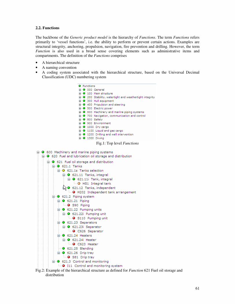
61

2.2. Functions

The backbone of the Generic product model is the hierarchy of Functions. The term Functions refers

primarily to ‘vessel functions’, i.e. the ability to perform or prevent certain actions. Examples are

structural integrity, anchoring, propulsion, navigation, fire prevention and drilling. However, the term

Function is also used in a broad sense covering elements such as administrative items and

compartments. The definition of the Functions comprises

• A hierarchical structure

• A naming convention

• A coding system associated with the hierarchical structure, based on the Universal Decimal

Classification (UDC) numbering system

Fig.1: Top level Functions

Fig.2: Example of the hierarchical structure as defined for Function 621 Fuel oil storage and

distribution

62

A total of about 2500 Functions are currently defined. Fig.1 shows the top-level Functions. Fig.2

shows an example of the hierarchy. The Function types are:

− Function leaves are the end nodes in the Function hierarchy, Fig.3. The Function leaves may

be connected to the physical representation of the vessel. This is called ‘normal assignment’

between a Function leaf and a Component or Component selection.

− Function compositions are groups of Functions with a parent and children, Fig.4. The

children together form the parent, i.e. the parent is composed of its children. The children may

not substitute each other. It is not required that all generic children shall be present in all

specific realisations.

− Function selections are groups of Functions with a parent and children, Fig.5. The children

are specialised instances of the parent. Any child may perform as the parent, and the children

may substitute each other. Function selections are defined locally only, i.e. Function selection

651.21s exists only in that Function. When applied to a vessel, it is generally allowed to select

more than one child. When the selection has been performed, the Function selection is

removed.

− Function groups are groups of Functions with a parent and children, Fig.6. The children are

organised under a common parent for convenience – the parent is a headline in the

organisation of the Functions. The children may generally not perform as the parent, nor may

the children substitute each other – the children are not specialisations. The children together

do generally not constitute the parent – the group is not a composition.

2.3 Equipment

The second main part of the Generic product model is the library of Components. The term Equipment

is used for groups of Components, e.g. electrical equipment. The definition of the Components

comprises

• A grouping structure

• A naming convention

• A coding system associated with the grouping structure

The Components are grouped according to engineering Disciplines, Fig.7.

The equipment types are:

− Components define the library of physical items. Examples are pumps, diesel engines,

generators, lifeboats and piping, Fig.8. The term Component is used in a broad sense covering

also elements as structural parts, compartments, systems, on board documentation and

software. Components may be given a detailed description through the use of Sub-functions.

Components may be assigned to Function leaves and Sub-function leaves. Components may

be the children of Component selections.

− Components selections are groups of Components with a parent and children. The children are

specialised instances of the parent. Any child may perform as the parent, and the children may

substitute each other. Component selections are defined globally, and may be assigned to

Function leaves and Sub-function leaves. When applied to a vessel, it is generally allowed to

select more than one child. This is accomplished by making several instances of the

corresponding Function. When the selection has been performed, the Component selection is

substituted by the selected child.

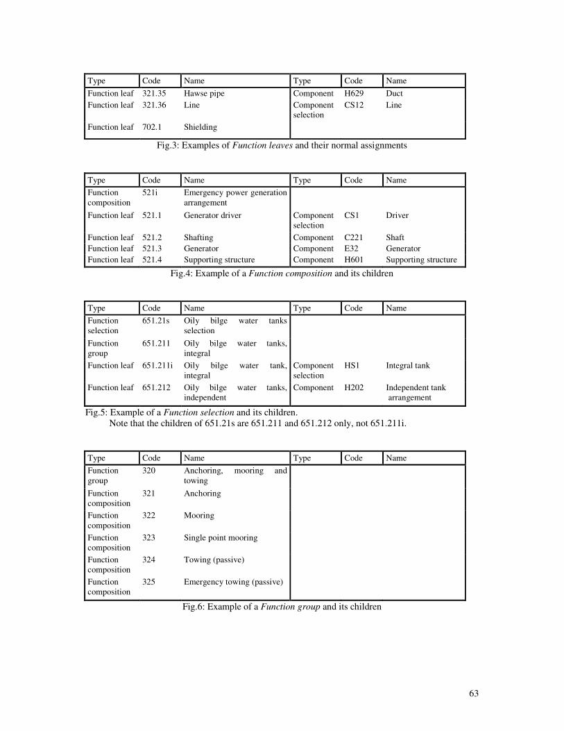
63

Type Code Name Type Code Name

Function leaf 321.35 Hawse pipe Component H629 Duct

Function leaf 321.36 Line Component

selection

CS12 Line

Function leaf 702.1 Shielding

Fig.3: Examples of Function leaves and their normal assignments

Type Code Name Type Code Name

Function

composition

521i Emergency power generation

arrangement

Function leaf 521.1 Generator driver Component

selection

CS1 Driver

Function leaf 521.2 Shafting Component C221 Shaft

Function leaf 521.3 Generator Component E32 Generator

Function leaf 521.4 Supporting structure Component H601 Supporting structure

Fig.4: Example of a Function composition and its children

Type Code Name Type Code Name

Function

selection

651.21s Oily bilge water tanks

selection

Function

group

651.211 Oily bilge water tanks,

integral

Function leaf 651.211i Oily bilge water tank,

integral

Component

selection

HS1 Integral tank

Function leaf 651.212 Oily bilge water tanks,

independent

Component H202 Independent tank

arrangement

Fig.5: Example of a Function selection and its children.

Note that the children of 651.21s are 651.211 and 651.212 only, not 651.211i.

Type Code Name Type Code Name

Function

group

320 Anchoring, mooring and

towing

Function

composition

321 Anchoring

Function

composition

322 Mooring

Function

composition

323 Single point mooring

Function

composition

324 Towing (passive)

Function

composition

325 Emergency towing (passive)

Fig.6: Example of a Function group and its children

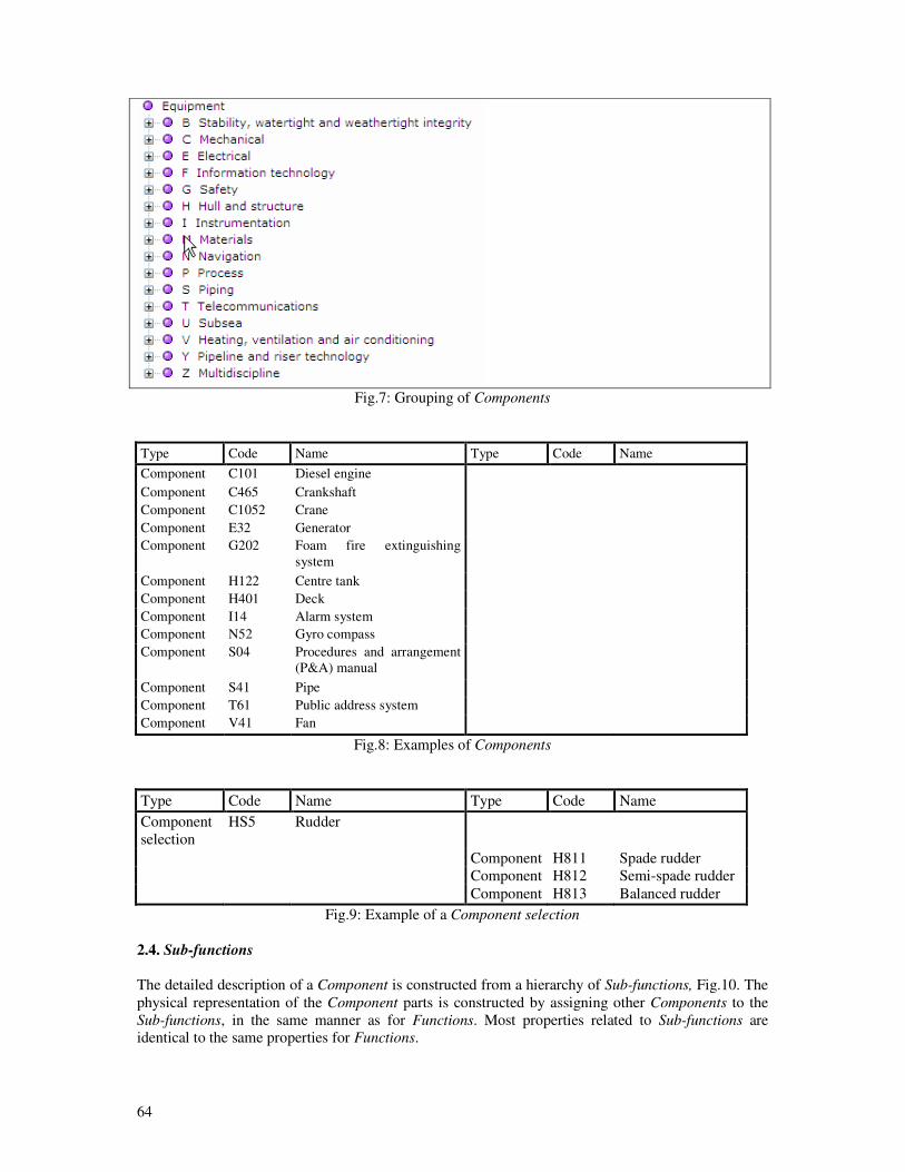
64

Fig.7: Grouping of Components

Type Code Name Type Code Name

Component C101 Diesel engine

Component C465 Crankshaft

Component C1052 Crane

Component E32 Generator

Component G202 Foam fire extinguishing

system

Component H122 Centre tank

Component H401 Deck

Component I14 Alarm system

Component N52 Gyro compass

Component S04 Procedures and arrangement

(P&A) manual

Component S41 Pipe

Component T61 Public address system

Component V41 Fan

Fig.8: Examples of Components

Type Code Name Type Code Name

Component

selection

HS5 Rudder

Component H811 Spade rudder

Component H812 Semi-spade rudder

Component H813 Balanced rudder

Fig.9: Example of a Component selection

2.4. Sub-functions

The detailed description of a Component is constructed from a hierarchy of Sub-functions, Fig.10. The

physical representation of the Component parts is constructed by assigning other Components to the

Sub-functions, in the same manner as for Functions. Most properties related to Sub-functions are

identical to the same properties for Functions.

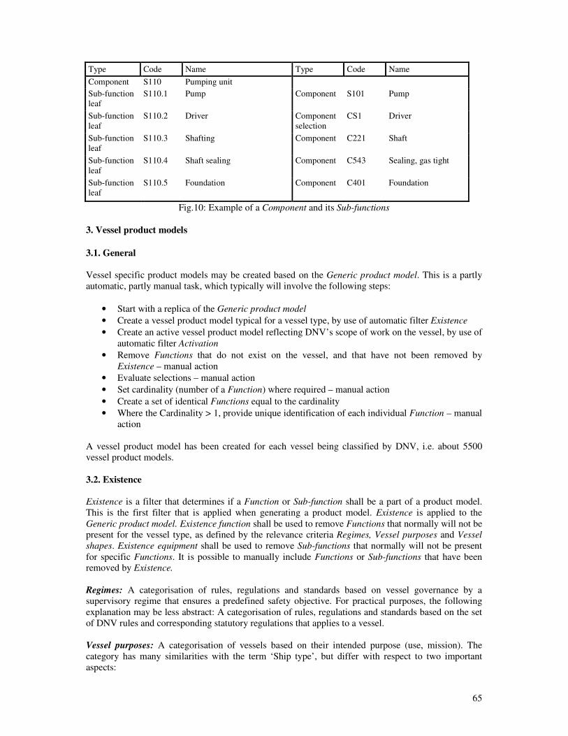
65

Type Code Name Type Code Name

Component S110 Pumping unit

Sub-function

leaf

S110.1 Pump Component S101 Pump

Sub-function

leaf

S110.2 Driver Component

selection

CS1 Driver

Sub-function

leaf

S110.3 Shafting Component C221 Shaft

Sub-function

leaf

S110.4 Shaft sealing Component C543 Sealing, gas tight

Sub-function

leaf

S110.5 Foundation Component C401 Foundation

Fig.10: Example of a Component and its Sub-functions

3. Vessel product models

3.1. General

Vessel specific product models may be created based on the Generic product model. This is a partly

automatic, partly manual task, which typically will involve the following steps:

• Start with a replica of the Generic product model

• Create a vessel product model typical for a vessel type, by use of automatic filter Existence

• Create an active vessel product model reflecting DNV’s scope of work on the vessel, by use of

automatic filter Activation

• Remove Functions that do not exist on the vessel, and that have not been removed by

Existence – manual action

• Evaluate selections – manual action

• Set cardinality (number of a Function) where required – manual action

• Create a set of identical Functions equal to the cardinality

• Where the Cardinality > 1, provide unique identification of each individual Function – manual

action

A vessel product model has been created for each vessel being classified by DNV, i.e. about 5500

vessel product models.

3.2. Existence

Existence is a filter that determines if a Function or Sub-function shall be a part of a product model.

This is the first filter that is applied when generating a product model. Existence is applied to the

Generic product model. Existence function shall be used to remove Functions that normally will not be

present for the vessel type, as defined by the relevance criteria Regimes, Vessel purposes and Vessel

shapes. Existence equipment shall be used to remove Sub-functions that normally will not be present

for specific Functions. It is possible to manually include Functions or Sub-functions that have been

removed by Existence.

Regimes: A categorisation of rules, regulations and standards based on vessel governance by a

supervisory regime that ensures a predefined safety objective. For practical purposes, the following

explanation may be less abstract: A categorisation of rules, regulations and standards based on the set

of DNV rules and corresponding statutory regulations that applies to a vessel.

Vessel purposes: A categorisation of vessels based on their intended purpose (use, mission). The

category has many similarities with the term ‘Ship type’, but differ with respect to two important

aspects:

66

a) One vessel may have more than one Vessel purpose. Example: Instead of making ‘Ship types’

with combined purposes, e.g. ‘Supply Vessel Anchor Handling Fire Fighter’, such a vessel

will be assigned three Vessel purposes.

b) The Vessel purpose does not provide information about the vessel’s structural design; this is

covered by the category Vessel shape. Example: Instead of making ‘Ship types’ combining

purpose and structural design information, e.g. ‘Ship-shaped drilling unit’, such a vessel will

be assigned Vessel shape ‘Ship’ and Vessel purpose ‘Drilling’.

Vessel shapes: A categorisation of vessels based on their structural design.

3.3. Activation

Activation is a filter that determines if a Function or Sub-function shall be assigned status active or

suspended. This is the second filter that is applied when generating a product model. Activation is

applied to the product models generated by Existence. Activation function shall be used to suspend

Functions that normally will not be DNV’s scope of work, as defined by the relevance criteria

Regimes, Class notations, Vessel certificates or Gross tonnage. Activation equipment shall be used to

suspend Sub-functions that normally will not be DNV scope of work for specific Functions. It is

possible to manually

• Activate Functions or Sub-functions that have been suspended by Activation

• Suspend Functions or Sub-functions that have been activated by Activation

Regimes: See Existence.

Class notations: Class notations are keywords referring to specific technical and operational standards

issued by DNV.

Vessel certificates: Vessel certificates are statements issued on basis of survey reports, confirming

compliance with specific rules, regulations or standards. Vessel certificates may be issued by DNV,

the flag state or other authorised organisations.

Gross tonnage: A Parameter used to define the volume of a vessel.

3.4. Manual removal of Functions

For many Functions, it is not possible to set up generic rules based on the relevance criteria used by

Existence in order to determine if they exist on board or not. In such cases, it has to be manually

considered if the Function exists, and if it does not, it must be manually removed.

Example: It is not possible to determine if the Function ‘Steam generation and distribution’ exists on

board a specific vessel based on the vessel type, as defined by Regimes, Vessel purposes and Vessel

shapes.

3.5. Evaluation of Selections

Selections must be evaluated manually, Fig.11.

3.6. Setting Cardinality

Setting of Cardinality (number off) is only relevant for Function compositions and Functions leaves

that are assigned a Component, and correspondingly for Sub-functions, Fig.12. Which Functions and

Sub-functions where Cardinality shall be set, is generically defined. Setting of the Cardinality is a

manual task. Where Cardinality > 1, a number of Functions corresponding to the Cardinality is

automatically created.

67

Type Code Name Type Code Name

Function leaf 411.1 Driver Component

selection

CS1 Driver

Type Code Name Type Code Name

Component

selection

CS1 Driver

Component C101 Diesel engine

Component C102 Steam turbine

Component C103 Gas turbine

Component E31 Electric motor

Type Code Name Type Code Name

Function leaf 411.1 Driver Component C101 Diesel engine

Fig.11: Selection of the propulsion driver

Type Code Name Type Code Name

Function leaf 612.53i Condensate cooler Component C624 Cooler

Function leaf 612.53i Condensate cooler Component C624 Cooler

Function leaf 612.53i Condensate cooler Component C624 Cooler

Fig.12: Resulting Vessel product model for Function 612.53i when Cardinality = 3

3.7. Identifying each individual

A unique tag must be set on each individual, this is a manual task. The tag is incorporated in the

individual Function name, Fig.13.

Type Code Name Type Code Name

Function leaf 612.53i Condensate cooler port Component C624 Cooler

Function leaf 612.53i Condensate cooler centre Component C624 Cooler

Function leaf 612.53i Condensate cooler starboard Component C624 Cooler

Fig.13: Resulting Vessel product model for Function 612.53i after identification of the individuals

68

4. Formulation of generic rule and regulatory requirements 4.1. General

Rule and regulatory requirements may be assigned to the Generic product model, to as well Functions

as Components or Sub-functions. Such requirements may be categorised as:

• Technical requirements to vessels and their equipment

• Procedural requirements for obtaining and retaining class or statutory certificates, e.g.

documentation requirements, survey schemes, or survey requirements.

Currently, only procedural requirements have been defined.

4.2. Implementation for the specific vessels

Only requirements assigned to the active vessel product model will be made applicable for the vessel.

Additional application rules may be assigned to each requirement, by the use of categories as

• Regimes

• Vessel purposes

• Vessel shapes

• Class notations

• Vessel certificates

• Flags

• Registries

• Main propulsion principles

• Age

• Gross tonnage

• Functions (for requirements assigned to Components only)

General logical combinations of the above categories may be set up for each requirement using logical

operators AND, OR and AND NOT.

5. Formulation of other generic information Generic information may be assigned to the Generic product model, to as well Functions as

Components or Sub-functions. Currently, the following categories have been defined:

• Parameters

• Predefined findings

Parameters are data fields for storage of vessel specific information. Parameters providing

information relating to the vessel are assigned to the Functions, while parameters providing

information relating to specific instances of a Component are assigned to the Component of one of the

Component’s Sub-functions.

Function parameters, examples:

• Vessel name

• Total number of persons accommodated by lifeboats

• Design temperature

Component parameters, examples for Component ‘Diesel engine’:

• Power

• Rotational speed

A total of about 4300 generic Parameters have been defined. An important use of Parameters is

issuing of certificates for vessels and Components on board. A data field in a certificate form will

correspond to a Parameter. When the Parameter value is defined in the database, it will be

automatically inserted in the certificate form.

69

Predefined findings are typical error conditions commonly observed on board the vessels. Under a

survey, the surveyor may select a Predefined finding instead of formulating the finding verbally. The

Predefined findings are effective in use and suitable for subsequent statistical analysis. A Predefined

finding is made up by a Finding category assigned to a Function, Component or Sub-function.

Example: For the Component ‘Diesel engine’, Sub-function ‘Engine block’, the following Finding

categories have been assigned: Cracked; Corroded; Leaking; Damaged.

6. Storage of vessel specific information

The vessel product model is a specific description of the vessel based upon a standardised format.

Correspondence, technical documentation and approval comments are tagged with one or both of the

categories ‘Functions’ and ‘Disciplines’.

Vessel specific Parameter values are stored in the generic Parameters described in section 5.

Findings are observations made during surveys. Findings may be based on the Predefined findings

described in section 5, or may be formulated by the surveyors. Currently, about 50.000 Predefined

findings are registered per year as a part of DNV’s surveys of vessels in operation. This number is

expected to increase in the future as surveyors are getting used to the Predefined findings, user

interfaces are improved, and the coverage is extended.

7. Data analyses

Cross fleet analyses may be performed for information assigned to the vessel product models, for

purposes as e.g. rule improvements and design evaluation. So far, only a limited set of data analyses

have been performed, and the results are currently not available for publication.

References

ISO (2003), ISO 15926 - Industrial automation systems and integration -- Integration of life-cycle

data for process plants including oil and gas production facilities, ISO Norm

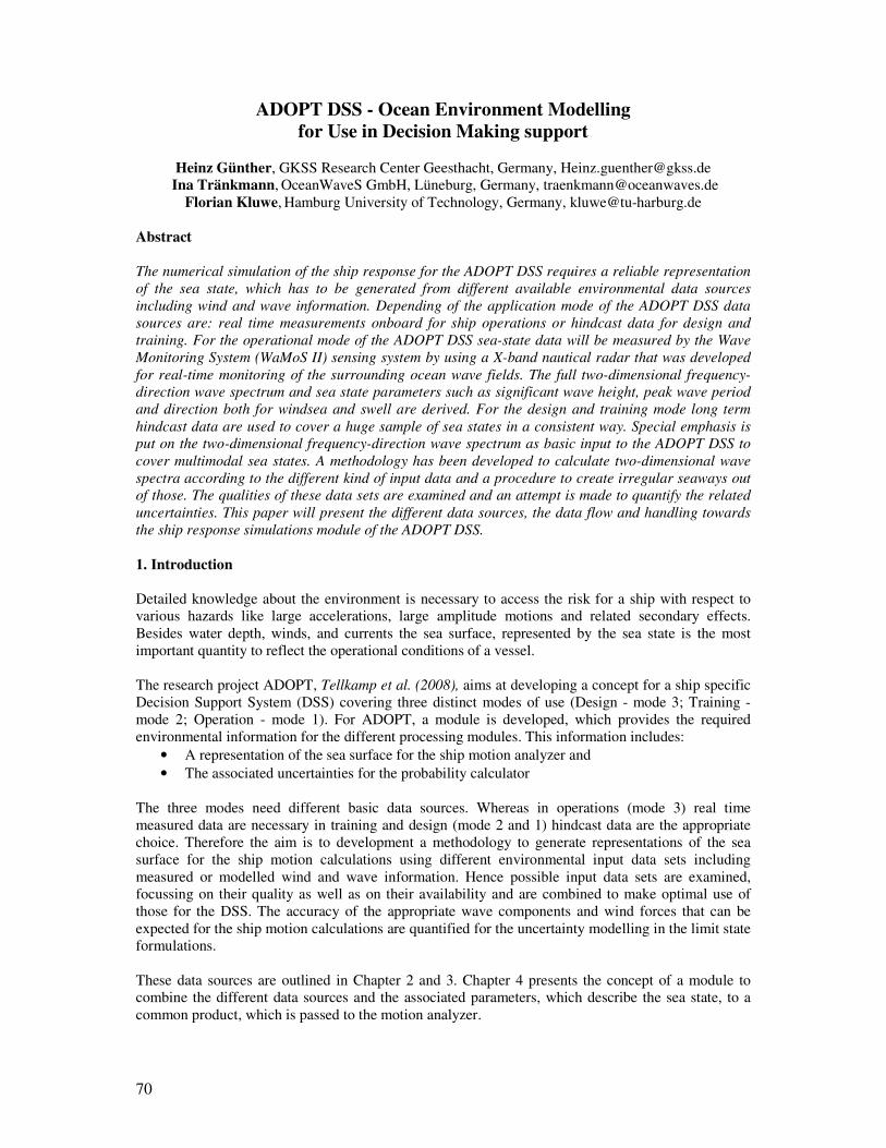
70

ADOPT DSS - Ocean Environment Modelling for Use in Decision Making support

Heinz Günther, GKSS Research Center Geesthacht, Germany, Heinz.guenther@gkss.de

Ina Tränkmann, OceanWaveS GmbH, Lüneburg, Germany, traenkmann@oceanwaves.de

Florian Kluwe, Hamburg University of Technology, Germany, kluwe@tu-harburg.de

Abstract

The numerical simulation of the ship response for the ADOPT DSS requires a reliable representation

of the sea state, which has to be generated from different available environmental data sources

including wind and wave information. Depending of the application mode of the ADOPT DSS data

sources are: real time measurements onboard for ship operations or hindcast data for design and

training. For the operational mode of the ADOPT DSS sea-state data will be measured by the Wave

Monitoring System (WaMoS II) sensing system by using a X-band nautical radar that was developed

for real-time monitoring of the surrounding ocean wave fields. The full two-dimensional frequency-

direction wave spectrum and sea state parameters such as significant wave height, peak wave period

and direction both for windsea and swell are derived. For the design and training mode long term

hindcast data are used to cover a huge sample of sea states in a consistent way. Special emphasis is

put on the two-dimensional frequency-direction wave spectrum as basic input to the ADOPT DSS to

cover multimodal sea states. A methodology has been developed to calculate two-dimensional wave

spectra according to the different kind of input data and a procedure to create irregular seaways out

of those. The qualities of these data sets are examined and an attempt is made to quantify the related

uncertainties. This paper will present the different data sources, the data flow and handling towards

the ship response simulations module of the ADOPT DSS.

1. Introduction

Detailed knowledge about the environment is necessary to access the risk for a ship with respect to

various hazards like large accelerations, large amplitude motions and related secondary effects.

Besides water depth, winds, and currents the sea surface, represented by the sea state is the most

important quantity to reflect the operational conditions of a vessel.

The research project ADOPT, Tellkamp et al. (2008), aims at developing a concept for a ship specific

Decision Support System (DSS) covering three distinct modes of use (Design - mode 3; Training -

mode 2; Operation - mode 1). For ADOPT, a module is developed, which provides the required

environmental information for the different processing modules. This information includes:

• A representation of the sea surface for the ship motion analyzer and

• The associated uncertainties for the probability calculator

The three modes need different basic data sources. Whereas in operations (mode 3) real time

measured data are necessary in training and design (mode 2 and 1) hindcast data are the appropriate

choice. Therefore the aim is to development a methodology to generate representations of the sea

surface for the ship motion calculations using different environmental input data sets including

measured or modelled wind and wave information. Hence possible input data sets are examined,

focussing on their quality as well as on their availability and are combined to make optimal use of

those for the DSS. The accuracy of the appropriate wave components and wind forces that can be

expected for the ship motion calculations are quantified for the uncertainty modelling in the limit state

formulations.

These data sources are outlined in Chapter 2 and 3. Chapter 4 presents the concept of a module to

combine the different data sources and the associated parameters, which describe the sea state, to a

common product, which is passed to the motion analyzer.

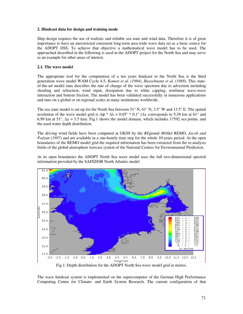
71

2. Hindcast data for design and training mode

Ship design requires the use of realistic and reliable sea state and wind data. Therefore it is of great

importance to have an unrestricted consistent long-term area-wide wave data set as a basic source for

the ADOPT DSS. To achieve that objective a mathematical wave model has to be used. The

approached described in the following is used in the ADOPT project for the North Sea and may serve

as an example for other areas of interest.

2.1. The wave model

The appropriate tool for the computation of a ten years hindcast in the North Sea is the third

generation wave model WAM Cycle 4.5, Komen et al. (1994), Hasselmann et al. (1988). This state-

of-the-art model runs describes the rate of change of the wave spectrum due to advection including

shoaling and refraction, wind input, dissipation due to white capping, nonlinear wave-wave

interaction and bottom friction. The model has been validated successfully in numerous applications

and runs on a global or on regional scales at many institutions worldwide.

The sea state model is set-up for the North Sea between 51° N, 61° N, 3.5° W and 13.5° E. The spatial

resolution of the wave model grid is ∆ϕ * ∆λ = 0.05° * 0.1° (∆x corresponds to 5,38 km at 61° and

6,99 km at 51°, ∆y = 5.5 km). Fig.1 shows the model domain, which includes 17592 sea points, and

the used water depth distribution.

The driving wind fields have been computed at GKSS by the REgional MOdel REMO, Jacob and

Podzun (1997) and are available in a one-hourly time step for the whole 10-years period. At the open

boundaries of the REMO model grid the required information has been extracted from the re-analysis

fields of the global atmosphere forecast system of the National Centres for Environmental Prediction.

At its open boundaries the ADOPT North Sea wave model uses the full two-dimensional spectral

information provided by the SAFEDOR North Atlantic model.

Fig.1: Depth distribution for the ADOPT North Sea wave model grid in metres.

The wave hindcast system is implemented on the supercomputer of the German High Performance

Computing Centre for Climate- and Earth System Research. The current configuration of that

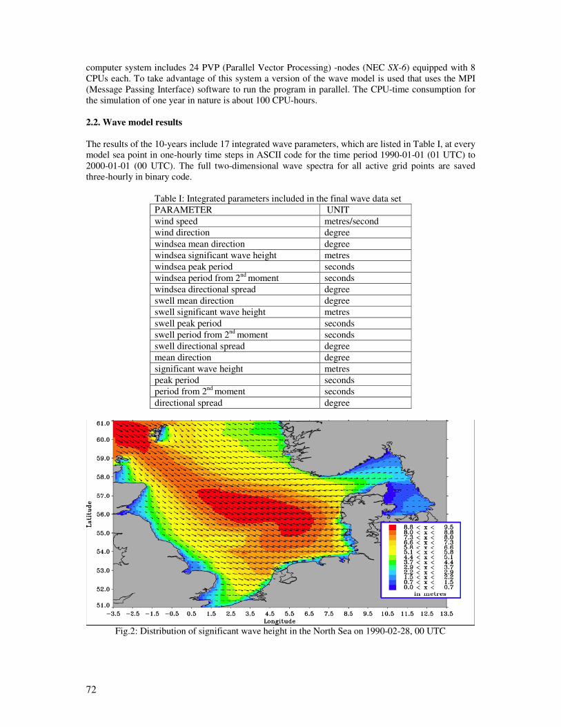
72

computer system includes 24 PVP (Parallel Vector Processing) -nodes (NEC SX-6) equipped with 8

CPUs each. To take advantage of this system a version of the wave model is used that uses the MPI

(Message Passing Interface) software to run the program in parallel. The CPU-time consumption for

the simulation of one year in nature is about 100 CPU-hours.

2.2. Wave model results

The results of the 10-years include 17 integrated wave parameters, which are listed in Table I, at every

model sea point in one-hourly time steps in ASCII code for the time period 1990-01-01 (01 UTC) to

2000-01-01 (00 UTC). The full two-dimensional wave spectra for all active grid points are saved

three-hourly in binary code.

Table I: Integrated parameters included in the final wave data set

PARAMETER UNIT

wind speed metres/second

wind direction degree

windsea mean direction degree

windsea significant wave height metres

windsea peak period seconds

windsea period from 2nd

moment seconds

windsea directional spread degree

swell mean direction degree

swell significant wave height metres

swell peak period seconds

swell period from 2nd

moment seconds

swell directional spread degree

mean direction degree

significant wave height metres

peak period seconds

period from 2nd

moment seconds

directional spread degree

Fig.2: Distribution of significant wave height in the North Sea on 1990-02-28, 00 UTC

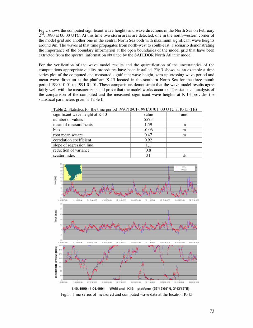
73

Fig.2 shows the computed significant wave heights and wave directions in the North Sea on February

2nd

, 1990 at 00:00 UTC. At this time two storm areas are detected, one in the north-western corner of

the model grid and another one in the central North Sea both with maximum significant wave heights

around 9m. The waves at that time propagates from north-west to south-east, a scenario demonstrating

the importance of the boundary information at the open boundaries of the model grid that have been

extracted from the spectral information obtained by the SAFEDOR North Atlantic model.

For the verification of the wave model results and the quantification of the uncertainties of the

computations appropriate quality procedures have been installed. Fig.3 shows as an example a time

series plot of the computed and measured significant wave height, zero up-crossing wave period and

mean wave direction at the platform K-13 located in the southern North Sea for the three-month

period 1990-10-01 to 1991-01-01. These comparisons demonstrate that the wave model results agree

fairly well with the measurements and prove that the model works accurate. The statistical analysis of

the comparison of the computed and the measured significant wave heights at K-13 provides the

statistical parameters given it Table II.

Table 2: Statistics for the time period 1990/10/01-1991/01/01, 00 UTC at K-13 (HS)

significant wave height at K-13 value unit

number of values 5575

mean of measurements 1.59 m

bias -0.06 m

root mean square 0.47 m

correlation coefficient 0.92

slope of regression line 1,1

reduction of variance 0.8

scatter index 31 %

Fig.3: Time series of measured and computed wave data at the location K-13

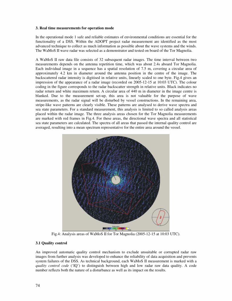
74

3. Real time measurements for operation mode In the operational mode 1 safe and reliable estimates of environmental conditions are essential for the

functionality of a DSS. Within the ADOPT project radar measurement are identified as the most

advanced technique to collect as much information as possible about the wave systems and the winds.

The WaMoS II wave radar was selected as a demonstrator and tested on board of the Tor Magnolia.

A WaMoS II raw data file consists of 32 subsequent radar images. The time interval between two

measurements depends on the antenna repetition time, which was about 2.4s aboard Tor Magnolia.

Each individual image in a sequence has a spatial resolution of 7.5 m, covering a circular area of

approximately 4.2 km in diameter around the antenna position in the centre of the image. The

backscattered radar intensity is digitised in relative units, linearly scaled to one byte. Fig.4 gives an

impression of the appearance of a radar image (recorded on 2005-12-15 at 10:03 UTC). The colour

coding in the figure corresponds to the radar backscatter strength in relative units. Black indicates no

radar return and white maximum return. A circular area of 440 m in diameter in the image centre is

blanked. Due to the measurement set-up, this area is not valuable for the purpose of wave

measurements, as the radar signal will be disturbed by vessel constructions. In the remaining area,

stripe-like wave patterns are clearly visible. These patterns are analysed to derive wave spectra and

sea state parameters. For a standard measurement, this analysis is limited to so called analysis areas

placed within the radar image. The three analysis areas chosen for the Tor Magnolia measurements

are marked with red frames in Fig.4. For these areas, the directional wave spectra and all statistical

sea state parameters are calculated. The spectra of all areas that passed the internal quality control are

averaged, resulting into a mean spectrum representative for the entire area around the vessel.

Fig.4: Analysis areas of WaMoS II for Tor Magnolia (2005-12-15 at 10:03 UTC).

3.1 Quality control

An improved automatic quality control mechanism to exclude unsuitable or corrupted radar raw

images from further analysis was developed to enhance the reliability of data acquisition and prevents

system failures of the DSS. As technical background, each WaMoS II measurement is marked with a

quality control code (‘IQ’) to distinguish between high and low radar raw data quality. A code

number reflects both the nature of a disturbance as well as its impact on the results.

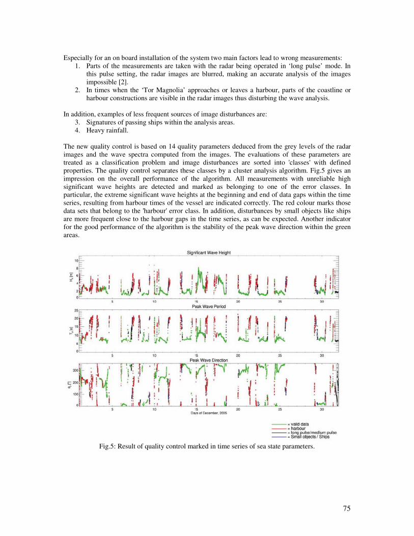
75

Especially for an on board installation of the system two main factors lead to wrong measurements:

1. Parts of the measurements are taken with the radar being operated in ‘long pulse’ mode. In

this pulse setting, the radar images are blurred, making an accurate analysis of the images

impossible [2].

2. In times when the ‘Tor Magnolia’ approaches or leaves a harbour, parts of the coastline or

harbour constructions are visible in the radar images thus disturbing the wave analysis.

In addition, examples of less frequent sources of image disturbances are:

3. Signatures of passing ships within the analysis areas.

4. Heavy rainfall.

The new quality control is based on 14 quality parameters deduced from the grey levels of the radar

images and the wave spectra computed from the images. The evaluations of these parameters are

treated as a classification problem and image disturbances are sorted into 'classes' with defined

properties. The quality control separates these classes by a cluster analysis algorithm. Fig.5 gives an

impression on the overall performance of the algorithm. All measurements with unreliable high

significant wave heights are detected and marked as belonging to one of the error classes. In

particular, the extreme significant wave heights at the beginning and end of data gaps within the time

series, resulting from harbour times of the vessel are indicated correctly. The red colour marks those

data sets that belong to the 'harbour' error class. In addition, disturbances by small objects like ships

are more frequent close to the harbour gaps in the time series, as can be expected. Another indicator

for the good performance of the algorithm is the stability of the peak wave direction within the green

areas.

Fig.5: Result of quality control marked in time series of sea state parameters.

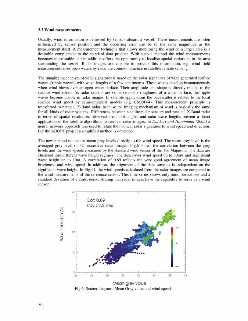
76

3.2 Wind measurements

Usually, wind information is retrieved by sensors aboard a vessel. These measurements are often

influenced by sensor position and the occurring error can be of the same magnitude as the

measurement itself. A measurement technique that allows monitoring the wind on a larger area is a

desirable complement to the standard data product. With such a method the wind measurements

becomes more stable and in addition offers the opportunity to localise spatial variations in the area

surrounding the vessel. Radar images are capable to provide this information, e.g. wind field

measurements over open waters by radar are common practice in satellite remote sensing.

The imaging mechanism of wind signatures is based on the radar signatures of wind generated surface

waves ('ripple waves') with wave lengths of a few centimetres. These waves develop instantaneously

when wind blows over an open water surface. Their amplitude and shape is directly related to the

surface wind speed. As radar sensors are sensitive to the roughness of a water surface, the ripple

waves become visible in radar images. In satellite applications the backscatter is related to the local

surface wind speed by semi-empirical models (e.g. CMOD-4). This measurement principle is

transferred to nautical X-Band radar, because the imaging mechanism of wind is basically the same

for all kinds of radar systems. Differences between satellite radar sensors and nautical X-Band radar

in terms of spatial resolution, observed area, look angles and radar wave lengths prevent a direct

application of the satellite algorithms to nautical radar images. In Dankert and Horstmann (2005) a

neural network approach was used to relate the nautical radar signatures to wind speed and direction.

For the ADOPT project a simplified method is developed.

The new method relates the mean grey levels directly to the wind speed. The mean grey level is the

averaged grey level of 32 successive radar images. Fig.6 shows the correlation between the grey

levels and the wind speeds measured by the standard wind sensor of the Tor Magnolia. The data are

clustered into different wave height regimes. The data cover wind speed up to 30m/s and significant

wave height up to 10m. A correlation of 0.89 reflects the very good agreement of mean image

brightness and wind speed. In addition, the alignment of the data samples is independent on the

significant wave height. In Fig.11, the wind speeds calculated from the radar images are compared to

the wind measurements of the reference sensor. This time series shows only minor deviations and a

standard deviation of 2.2m/s, demonstrating that radar images have the capability to serve as a wind

sensor.

Fig.6: Scatter diagram: Mean Grey value and wind speed.

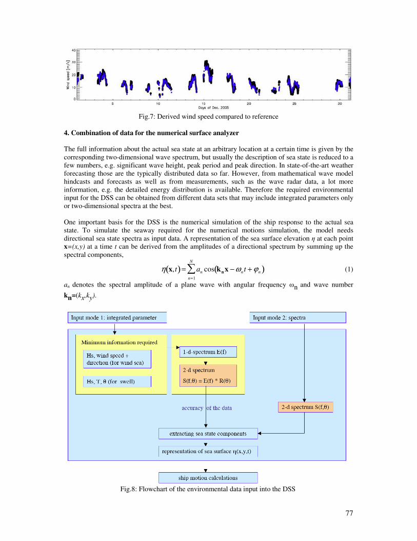
77

Fig.7: Derived wind speed compared to reference

4. Combination of data for the numerical surface analyzer

The full information about the actual sea state at an arbitrary location at a certain time is given by the

corresponding two-dimensional wave spectrum, but usually the description of sea state is reduced to a

few numbers, e.g. significant wave height, peak period and peak direction. In state-of-the-art weather

forecasting those are the typically distributed data so far. However, from mathematical wave model

hindcasts and forecasts as well as from measurements, such as the wave radar data, a lot more

information, e.g. the detailed energy distribution is available. Therefore the required environmental

input for the DSS can be obtained from different data sets that may include integrated parameters only

or two-dimensional spectra at the best.

One important basis for the DSS is the numerical simulation of the ship response to the actual sea

state. To simulate the seaway required for the numerical motions simulation, the model needs

directional sea state spectra as input data. A representation of the sea surface elevation η at each point

x=(x,y) at a time t can be derived from the amplitudes of a directional spectrum by summing up the

spectral components,

η x,t( )= an

n=1

N

∑ cos knx −ωnt + ϕn( ) (1)

an denotes the spectral amplitude of a plane wave with angular frequency ωn and wave number

kn=(kx,ky).

Fig.8: Flowchart of the environmental data input into the DSS

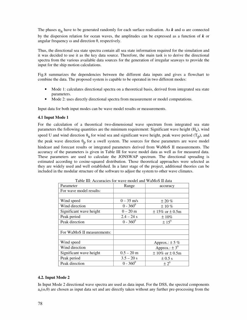
78

The phases φn have to be generated randomly for each surface realisation. As k and ω are connected

by the dispersion relation for ocean waves, the amplitudes can be expressed as a function of k or

angular frequency ω and direction θ, respectively.

Thus, the directional sea state spectra contain all sea state information required for the simulation and

it was decided to use it as the key data source. Therefore, the main task is to derive the directional

spectra from the various available data sources for the generation of irregular seaways to provide the

input for the ship motion calculations.

Fig.8 summarizes the dependencies between the different data inputs and gives a flowchart to

combine the data. The proposed system is capable to be operated in two different modes:

• Mode 1: calculates directional spectra on a theoretical basis, derived from integrated sea state

parameters.

• Mode 2: uses directly directional spectra from measurement or model computations.

Input data for both input modes can be wave model results or measurements.

4.1 Input Mode 1

For the calculation of a theoretical two-dimensional wave spectrum from integrated sea state

parameters the following quantities are the minimum requirement: Significant wave height (Hs), wind

speed U and wind direction θu for wind sea and significant wave height, peak wave period (Tp), and

the peak wave direction θp for a swell system. The sources for these parameters are wave model

hindcast and forecast results or integrated parameters derived from WaMoS II measurements. The

accuracy of the parameters is given in Table III for wave model data as well as for measured data.

These parameters are used to calculate the JONSWAP spectrum. The directional spreading is

estimated according to cosine-squared distribution. Those theoretical approaches were selected as

they are widely used and well established. In a later stage of the project, additional theories can be

included in the modular structure of the software to adjust the system to other wave climates.

Table III: Accuracies for wave model and WaMoS II data

Parameter Range accuracy

For wave model results:

Wind speed 0 – 35 m/s ± 20 %

Wind direction 0 - 3600

± 10 %

Significant wave height 0 – 20 m ± 15% or ± 0.5m

Peak period 2.4 – 24 s ± 10%

Peak direction 0 - 3600

± 150

For WaMoS II measurements:

Wind speed Approx.: ± 5 %

Wind direction Approx.: ± 30

Significant wave height 0.5 – 20 m ± 10% or ± 0.5m

Peak period 3.5 – 20 s ± 0.5 s

Peak direction 0 - 3600

± 20

4.2. Input Mode 2

In Input Mode 2 directional wave spectra are used as data input. For the DSS, the spectral components

an(ω,θ) are chosen as input data set and are directly taken without any further pre-processing from the

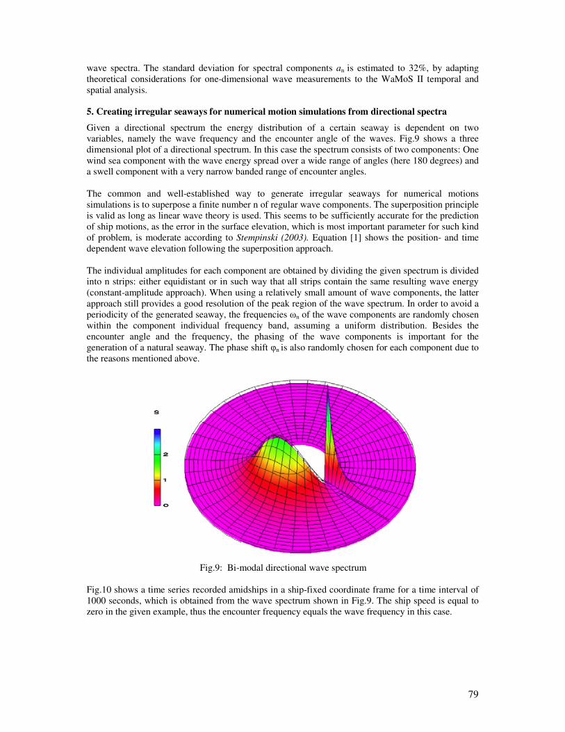
79

wave spectra. The standard deviation for spectral components an is estimated to 32%, by adapting

theoretical considerations for one-dimensional wave measurements to the WaMoS II temporal and

spatial analysis.

5. Creating irregular seaways for numerical motion simulations from directional spectra

Given a directional spectrum the energy distribution of a certain seaway is dependent on two

variables, namely the wave frequency and the encounter angle of the waves. Fig.9 shows a three

dimensional plot of a directional spectrum. In this case the spectrum consists of two components: One

wind sea component with the wave energy spread over a wide range of angles (here 180 degrees) and

a swell component with a very narrow banded range of encounter angles.

The common and well-established way to generate irregular seaways for numerical motions

simulations is to superpose a finite number n of regular wave components. The superposition principle

is valid as long as linear wave theory is used. This seems to be sufficiently accurate for the prediction

of ship motions, as the error in the surface elevation, which is most important parameter for such kind

of problem, is moderate according to Stempinski (2003). Equation [1] shows the position- and time

dependent wave elevation following the superposition approach.

The individual amplitudes for each component are obtained by dividing the given spectrum is divided

into n strips: either equidistant or in such way that all strips contain the same resulting wave energy

(constant-amplitude approach). When using a relatively small amount of wave components, the latter

approach still provides a good resolution of the peak region of the wave spectrum. In order to avoid a

periodicity of the generated seaway, the frequencies ωn of the wave components are randomly chosen

within the component individual frequency band, assuming a uniform distribution. Besides the

encounter angle and the frequency, the phasing of the wave components is important for the

generation of a natural seaway. The phase shift φn is also randomly chosen for each component due to

the reasons mentioned above.

Fig.9: Bi-modal directional wave spectrum

Fig.10 shows a time series recorded amidships in a ship-fixed coordinate frame for a time interval of

1000 seconds, which is obtained from the wave spectrum shown in Fig.9. The ship speed is equal to

zero in the given example, thus the encounter frequency equals the wave frequency in this case.

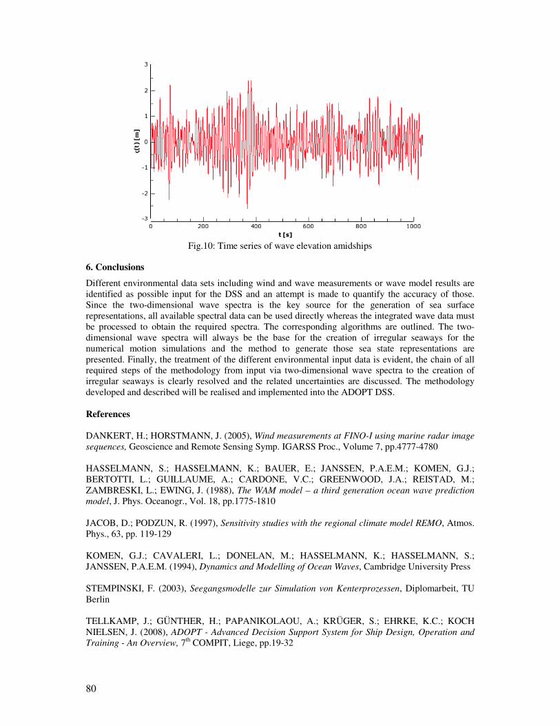
80

Fig.10: Time series of wave elevation amidships

6. Conclusions

Different environmental data sets including wind and wave measurements or wave model results are

identified as possible input for the DSS and an attempt is made to quantify the accuracy of those.

Since the two-dimensional wave spectra is the key source for the generation of sea surface

representations, all available spectral data can be used directly whereas the integrated wave data must

be processed to obtain the required spectra. The corresponding algorithms are outlined. The two-

dimensional wave spectra will always be the base for the creation of irregular seaways for the

numerical motion simulations and the method to generate those sea state representations are

presented. Finally, the treatment of the different environmental input data is evident, the chain of all

required steps of the methodology from input via two-dimensional wave spectra to the creation of

irregular seaways is clearly resolved and the related uncertainties are discussed. The methodology

developed and described will be realised and implemented into the ADOPT DSS.

References

DANKERT, H.; HORSTMANN, J. (2005), Wind measurements at FINO-I using marine radar image

sequences, Geoscience and Remote Sensing Symp. IGARSS Proc., Volume 7, pp.4777-4780

HASSELMANN, S.; HASSELMANN, K.; BAUER, E.; JANSSEN, P.A.E.M.; KOMEN, G.J.;

BERTOTTI, L.; GUILLAUME, A.; CARDONE, V.C.; GREENWOOD, J.A.; REISTAD, M.;

ZAMBRESKI, L.; EWING, J. (1988), The WAM model – a third generation ocean wave prediction

model, J. Phys. Oceanogr., Vol. 18, pp.1775-1810

JACOB, D.; PODZUN, R. (1997), Sensitivity studies with the regional climate model REMO, Atmos.

Phys., 63, pp. 119-129

KOMEN, G.J.; CAVALERI, L.; DONELAN, M.; HASSELMANN, K.; HASSELMANN, S.;

JANSSEN, P.A.E.M. (1994), Dynamics and Modelling of Ocean Waves, Cambridge University Press

STEMPINSKI, F. (2003), Seegangsmodelle zur Simulation von Kenterprozessen, Diplomarbeit, TU

Berlin

TELLKAMP, J.; GÜNTHER, H.; PAPANIKOLAOU, A.; KRÜGER, S.; EHRKE, K.C.; KOCH

NIELSEN, J. (2008), ADOPT - Advanced Decision Support System for Ship Design, Operation and

Training - An Overview, 7th COMPIT, Liege, pp.19-32

81

Enriching the Berth Allocation Problem

Rowan Van Schaeren, Antwerp Maritime Academy, Antwerp/Belgium rowan.vanschaeren@hzs.be Wout Dullaert, University of Antwerp, Antwerp/Belgium, wout.dullaert@ua.ac.be

Birger Raa, Ghent University, Ghent/Belgium, birger.raa@ugent.be Abstract This paper proposes a rich MIP model for the berth and crane allocation problem at a modern con-tainer terminal. Both vessel and operational features are included in this model. Compared to the ex-isting models available in the literature, this model is better capable of optimizing real-life quay op-erations and quay length utilization. It is validated using real-life data. 1 Introduction Since the 80s, the annual growth rate of seaborne trade has been 3.7 percent on average, Grossmann et al. (2007). Container growth rates, however, have been significantly larger. UNESCAP (2006) esti-mates that the total number of full containers shipped on worldwide trade routes (excluding transship-ment) in 2002 amounted to 77.8 million teu. Full container transport is expected to more than double to 177.6 million teu by 2015, which represents an average annual increase of 6.5%. During the period 2002-2010 average growth is estimated at 7.5% per year, which is in accordance with the 8% growth rates reported in Grossmann et al. (2007). For 2010 to 2015, a growth rate of 5% is expected, UNES-CAP (2006), lower than the 8% annual growth expected by Grossman et al. (2007) up to 2030. Additional container handling is generated by the hub strategy, in which larger ports (hubs) serve as ports of call and smaller ports offer additional cargo via feeder lines (spokes). Figures on total throughput handled by the world’s ports are therefore more suited to illustrate the increasing demand for container handling capacity. For 2005 the total volume handled at the world’s ports is estimated at 339.2 million teu, a figure expected to increase with nearly 85% up to 627.7 teu in 2010, Drewry (2006). As argued in Vernimmen et al. (2007), many shipping lines have anticipated on the increased demand for container transport by ordering additional and larger vessels, whereas port handling capacity has lagged behind in some parts of the world. Based on shipping lines’ order books on 01/12/2006 from AXS-Alphaliner (2006), 4.44 million teu or 50% additional slot capacity is to be added to the world-wide container vessel fleet by the end of 2008. Many planned investments in additional terminal infra-structure in Northern European ports such as Le Havre, Antwerp, Rotterdam, Wilhelmshaven, Flush-ing and the UK ports, have been cancelled or delayed for several years. If all these proposed projects would have been realized in accordance with their original time schedule, an extra capacity of no less than 11.4 million teu (nearly one third of the capacity available in 2004) would have been available in North European ports in 2005, Vernimmen et al. (2007). Increasing container handling capacity by expansion projects appears to be difficult for environmental, financial, technical and legal reasons. In many cases there is even no land available to build additional infrastructure. Optimizing the processes of existing infrastructure is therefore often a better – if not only – way to increase the handling capacity. The productivity of a container terminal is determined by the interaction of a number of processes. Based on the academic literature devoted to them, the best-known processes are probably berth planning (which allocates vessels at the available quays) and quay crane planning (which assigns the available cranes to the vessels alongside the quays). Other im-portant, but less studied processes are yard planning (for allocating all the containers handled by the terminal on a yard), vessel planning (positioning of the containers on board of vessels) and labor plan-ning (assigning people to all the jobs to be carried out). This paper will focus on the berth planning and quay crane planning processes, the most studied con-tainer terminal processes from the academic literature. Section 2 presents a focused literature review

82

on the Berth Allocation Problem (BAP) and the Crane allocation problem (CAP). In Section 3, we propose an extended model for the combined BAP and CAP, accommodating some of the shortcom-ings of the existing models identified in Section 2. The model is validated in Section 4 using real-life data. Section 5 concludes this paper with a conclusion. 2 Literature review and insights As many container berths are privately operated and the efficiency of terminal operations is essential to the terminal’s productivity and therefore its competitive power, several papers have already been published on optimizing container terminal operations. Most of these papers deal with the BAP and CAP workload optimization. Lai and Shih (1992) propose a heuristic algorithm for berth allocation with a first-come-first-serve (FCFS) queuing discipline for vessels. Brown et al. (1994,1997) propose an integer-programming model for vessel berthing in naval ports. They considered a quay with a finite set of berths at which berth shifting of moored vessels is allowed, a practice uncommon in commercial ports. Imai et al. (1997) propose a BAP for commercial ports questioning the FCFS principle. They propose a heuristic to find solutions maximizing berth performances whilst minimizing dissatisfactions of the vessels’ order of service. They assume a static BAP (SBAP), implying that all vessels to be served are present in the port before starting the planning of the berth allocation. Due to the unrealistic nature of this as-sumption they extended the model to a dynamic one (DBAP), Imai et al. (2001,2005a). The model was further extended by Nishimura et al. (2001) to include different water depths at the berths. Imai et al. (2003) also further extended their 2001 model by including vessel priorities. Already in 2001 Legato et al. (2001) rightfully point out that vessels can have different priorities for receiving service at a container terminal. They consider a case in which there are two sets of berths available. The primary vessels are handled upon arrival and have dedicated (or reserved) berths. This is enforced by assigning them a high priority. Secondary vessels are served on a FCFS principle. When only one quay is available, both types of vessels have to compete for the same berths. It is our belief that reserving berths for vessels is not the most efficient approach for guaranteeing high service levels and an optimization of the BAP. The moment reservations are made, more restrictions are im-posed on any optimization. Not only some vessels need to be optimized, the berth allocation of all ves-sels needs to be optimized simultaneously. It may also be possible that the reserved berth is not avail-able, e.g. when a vessel with a higher priority is still alongside it or when maintenance work is taking place (crane maintenance, dredging…). Focus should then be on servicing high priority vessels as close to their preferred berthing position as possible. We therefore prefer not to formulate a direct rela-tionship between priority and berth position. Instead, we only take priorities into account when balanc-ing the costs of two vessels competing for the same berth. The reasons for prioritization can be numer-ous: operational, commercial, number of containers to be handled, emergencies, tide restrictions, transshipment aspect between vessels etc. Priorities used like in Legato et al. (2001) and others should be used for making sure that vessels are served as soon as possible, not for reserving places. This idea is also found in Imai et al. (2003) in which the authors state that “any kind of weight/priority can be attached to individual vessels”. In Imai et al. (2007) mega-ships are given priority to guarantee that they will be served upon arrival at the right type of berth. Lokuge et al. (2007) use priorities to guaran-tee immediate service by forcing the waiting time to zero. The berthing place is only an aspect of han-dling time but not the only driving factor of it. Another distinction often made in literature concerns modeling the quay length. Many models assume the quay to consist of a discrete set of berthing locations. These so-called Discrete Berth Allocation problems (BAPD) often result in quay-length not being fully utilized because the berth lengths do not correspond exactly to all vessel lengths. The Continuous Berth Allocation Problem (BAPC) models the quay as a continuous line segment, Lim (1998). Li et al. (1998) formulate a BAPC solution ap-proach with and without fixed vessel positions. In both Park and Kim (2002) and Kim and Moon (2003) the BAPC is extended with handling priorities and preferred berth for vessels. They propose to add the priority aspect as an additional cost to the penalty cost of a vessel not meeting its departure

83

time. Guan and Cheung (2004) propose a BAPC with handling times proportional to the vessel sizes. It is our belief that this assumption is not justified because handling time is more related to the amount of containers to be handled than their size. Operational experiences show that small vessels sometimes have more containers to be handled than larger ones. Imai et al. (2005) develop a heuristic for a BAPC with the handling time being dependent of the berthing position. They assume that the handling time is defined by the physical relationship between the ship’s quay location and its container storage location in the yard. The handling time isn’t affected they also argue, if every ship employs a sufficient number of yard trailers (or straddle carriers) that haul containers between the ship and storage, resulting in no interruption or delay of the quay crane cycle. In our view the truth is a mixture of both previous state-ments: The handling time is in relation with the amount of yard trailers used but also e.g. the work-load, the amount of cranes used or abilities of the crane drivers. The importance of the berthing posi-tion should be reflected in the preferred berth aspect (see also further). Cordeau et al. (2005) present a tabu search heuristic for both the BAPD and BAPC. In literature, the time that vessels stay alongside the quay is sometimes named differently: e.g. “proc-essing time”, Guan et al. (2004), “handling time”, Imai et al. (2001,2007) and “duration of operation”, Wang et al. (2007). Not only the terminology is sometimes different, also its meaning often differs. Her follow some examples found in literature: For Nishimura et al. (2001) and Imai et al. (2007) the handling time is berth dependent. Guan and Cheung (2004) assume that handling times are propor-tional to vessel sizes. Because the containers to be handled (call size or workload) does not have to be proportional to vessel size, we do not want to make this assumption. The workload of a vessel is there-fore expressed as the number of containers to be handled and the total time needed for handling opera-tions is referred to as the handling time. This handling time is influenced by several aspects such as: workload, interruptions during the loading/unloading process, the number and types of cranes avail-able/used for loading and unloading, ability of the crane driver using the crane, amount of prime mov-ers feeding the cranes… Finally, the total time a berth is occupied by a vessel, the “berth occupancy”, is the sum of (i) time between arrival at the berth and starting the operations, (ii) the handling time, and (iii) the time between the end of operations and leaving the berth. The berth occupancy is there-fore endogenous to a berth allocation model: it is determined by solving the berth allocation model. Concerning the CAP and the combination of the BAP with the CAP, not many papers exist. In Da-ganzo (1989) and Peterkofsky et al. (1990) algorithms are proposed for quay crane assignments using vessel sections (bays). Both of these papers considered a static CAP and both minimized the total weighted completion times. Park and Kim (2003) suggest a two-phase solution procedure: the first phase determines the berthing position and berthing time of each vessel as well as the amount of cranes assigned to each vessel at each time segment while a detailed schedule for each crane is con-structed in the second phase. They used discrete berths and time intervals to design their dynamic model. Liu et al. (2005) assume the BAP to be solved and use a two-phase approach for the quay crane scheduling. In the first phase, they minimize each vessel’s processing time for various possible num-bers of quay cranes (QC) taking into account QC interaction constraints. During the second phase, QCs are assigned to vessels to minimize the tardiness of all vessels. Imai et al. (2007) introduce a for-mulation for minimizing total service time in the simultaneous berth and crane allocation problem by extending the model of Imai et al. (2001) with a decision variable for ship-berth-order assignment and with additional CAP constraints. As mentioned by Park and Kim (2003) the simultaneous solving of the BAP and CAP can be split up in two phases. We propose a decomposition at another level: the assignment of quay cranes to ships and ships to berths composes the first phase. The second phase consists of the detailed assignment of quay cranes to workloads per ship. Our approach is inspired by the decision-making structures at a major Antwerp container terminal: Because the containers to be loaded on a vessel start to arrive at the terminal well in advance of the vessel’s arrival, the vessels need to be assigned to a berth well in ad-vance of their arrival (see also remark concerning preferred berth in chapter 3). To estimate the ves-sels’ departure times, quay cranes have to be allocated in advance since they affect the handling time of the vessels. It is, however, impossible to determine the precise workload each crane will have in advance because the loading plans of the vessels are not known days in advance.

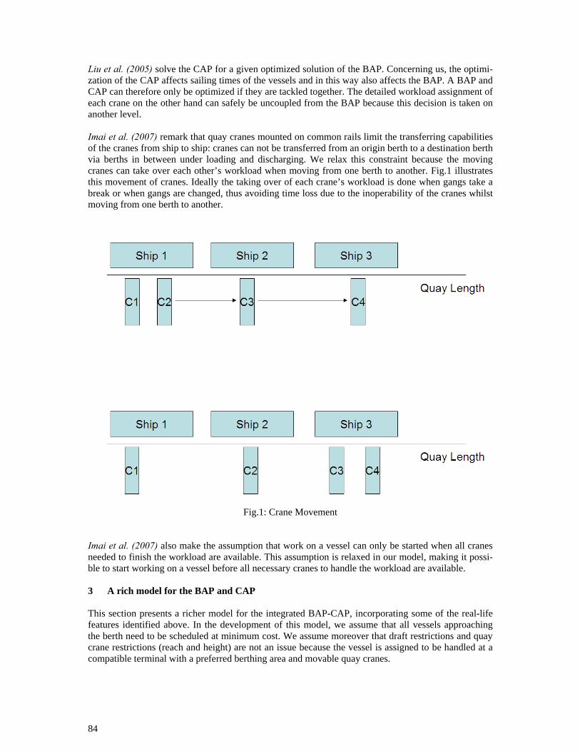
84

Liu et al. (2005) solve the CAP for a given optimized solution of the BAP. Concerning us, the optimi-zation of the CAP affects sailing times of the vessels and in this way also affects the BAP. A BAP and CAP can therefore only be optimized if they are tackled together. The detailed workload assignment of each crane on the other hand can safely be uncoupled from the BAP because this decision is taken on another level. Imai et al. (2007) remark that quay cranes mounted on common rails limit the transferring capabilities of the cranes from ship to ship: cranes can not be transferred from an origin berth to a destination berth via berths in between under loading and discharging. We relax this constraint because the moving cranes can take over each other’s workload when moving from one berth to another. Fig.1 illustrates this movement of cranes. Ideally the taking over of each crane’s workload is done when gangs take a break or when gangs are changed, thus avoiding time loss due to the inoperability of the cranes whilst moving from one berth to another.

Fig.1: Crane Movement

Imai et al. (2007) also make the assumption that work on a vessel can only be started when all cranes needed to finish the workload are available. This assumption is relaxed in our model, making it possi-ble to start working on a vessel before all necessary cranes to handle the workload are available. 3 A rich model for the BAP and CAP This section presents a richer model for the integrated BAP-CAP, incorporating some of the real-life features identified above. In the development of this model, we assume that all vessels approaching the berth need to be scheduled at minimum cost. We assume moreover that draft restrictions and quay crane restrictions (reach and height) are not an issue because the vessel is assigned to be handled at a compatible terminal with a preferred berthing area and movable quay cranes.

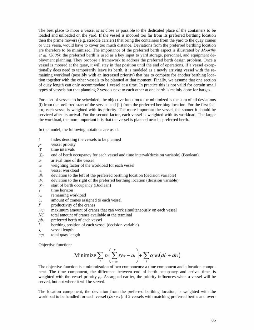
85

The best place to moor a vessel is as close as possible to the dedicated place of the containers to be loaded and unloaded on the yard. If the vessel is moored too far from its preferred berthing location then the prime movers (e.g. straddle carriers) that bring the containers from the yard to the quay cranes or vice versa, would have to cover too much distance. Deviations from the preferred berthing location are therefore to be minimized. The importance of the preferred berth aspect is illustrated by Moorthy et al. (2006): the preferred berth is used as a key input to yard storage, personnel, and equipment de-ployment planning. They propose a framework to address the preferred berth design problem. Once a vessel is moored at the quay, it will stay in that position until the end of operations. If a vessel excep-tionally does need to temporarily leave its berth, it is modeled as a newly arriving vessel with the re-maining workload (possibly with an increased priority) that has to compete for another berthing loca-tion together with the other vessels to be planned at that moment. Finally, we assume that one section of quay length can only accommodate 1 vessel at a time. In practice this is not valid for certain small types of vessels but that planning 2 vessels next to each other at one berth is mainly done for barges. For a set of vessels to be scheduled, the objective function to be minimized is the sum of all deviations (i) from the preferred start of the service and (ii) from the preferred berthing location. For the first fac-tor, each vessel is weighted with its priority. The more important the vessel, the sooner it should be serviced after its arrival. For the second factor, each vessel is weighted with its workload. The larger the workload, the more important it is that the vessel is planned near its preferred berth. In the model, the following notations are used: i Index denoting the vessels to be planned pi vessel priority τ time intervals

τiY end of berth occupancy for each vessel and time interval(decision variable) (Boolean) ai arrival time of the vessel αi weighting factor of the workload for each vessel wi vessel workload dli deviation to the left of the preferred berthing location (decision variable) dri deviation to the right of the preferred berthing location (decision variable)

τix start of berth occupancy (Boolean) T time horizon rit remaining workload cit amount of cranes assigned to each vessel P productivity of the cranes mci maximum amount of cranes that can work simultaneously on each vessel NC total amount of cranes available at the terminal pbi preferred berth of each vessel li berthing position of each vessel (decision variable) si vessel length mp total quay length Objective function:

( )∑∑ ∑ ++⎟⎠

⎞⎜⎝

⎛−

= iiiii

ii

T

aii drdlwayp

i

αττ

τ Minimize

The objective function is a minimization of two components: a time component and a location compo-nent. The time component, the difference between end of berth occupancy and arrival time, is weighted with the vessel priority pi. As argued earlier, the priority influences when a vessel will be served, but not where it will be served. The location component, the deviation from the preferred berthing location, is weighted with the workload to be handled for each vessel ( ii w*α ): if 2 vessels with matching preferred berths and over-

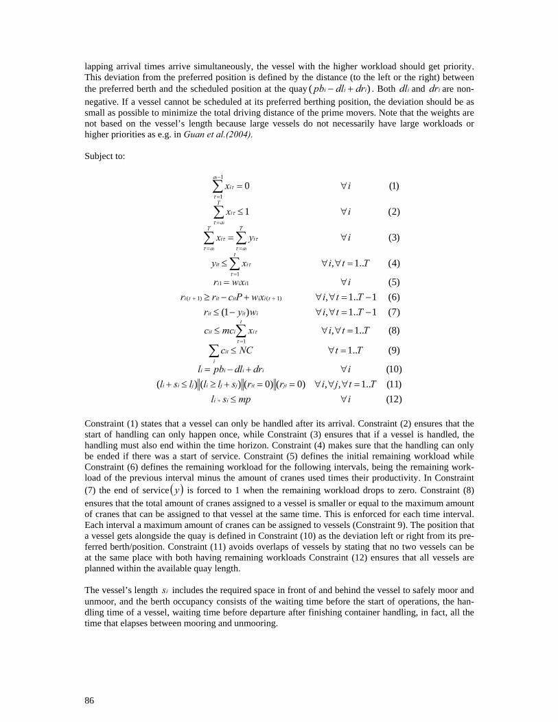
86

lapping arrival times arrive simultaneously, the vessel with the higher workload should get priority. This deviation from the preferred position is defined by the distance (to the left or the right) between the preferred berth and the scheduled position at the quay )( iii drdlpb +− . Both idl and idr are non-negative. If a vessel cannot be scheduled at its preferred berthing position, the deviation should be as small as possible to minimize the total driving distance of the prime movers. Note that the weights are not based on the vessel’s length because large vessels do not necessarily have large workloads or higher priorities as e.g. in Guan et al.(2004). Subject to:

)12()11(..1,,)0()0()()()10(

)9(..1

)8(..1,

)7(1..1,)1()6(1..1,)5(

)4(..1,

)3(

)2(1

)1(0

1

)1()1(

111

1

1

impslTtjirrslllsl

idrdlpbl

TtNCc

Ttixmcc

TtiwyrTtixwPcrr

ixwr

Ttixy

iyx

ix

ix

ii

jtitjjijii

iiiii

it

t

iiit

iitit

tiiititti

iii

t

iit

T

a

T

a

ii

T

a

i

a

i

i i

i

i

∀≤=∀∀∀==+≥≤+

∀+−=

=∀≤

=∀∀≤

−=∀∀−≤−=∀∀+−≥

∀=

=∀∀≤

∀=

∀≤

∀=

+

=

++

=

= =

=

−

=

∑∑

∑

∑ ∑

∑

∑

τ

τ

τ

τ

τ τ

ττ

τ

τ

τ

τ

Constraint (1) states that a vessel can only be handled after its arrival. Constraint (2) ensures that the start of handling can only happen once, while Constraint (3) ensures that if a vessel is handled, the handling must also end within the time horizon. Constraint (4) makes sure that the handling can only be ended if there was a start of service. Constraint (5) defines the initial remaining workload while Constraint (6) defines the remaining workload for the following intervals, being the remaining work-load of the previous interval minus the amount of cranes used times their productivity. In Constraint (7) the end of service ( )y is forced to 1 when the remaining workload drops to zero. Constraint (8) ensures that the total amount of cranes assigned to a vessel is smaller or equal to the maximum amount of cranes that can be assigned to that vessel at the same time. This is enforced for each time interval. Each interval a maximum amount of cranes can be assigned to vessels (Constraint 9). The position that a vessel gets alongside the quay is defined in Constraint (10) as the deviation left or right from its pre-ferred berth/position. Constraint (11) avoids overlaps of vessels by stating that no two vessels can be at the same place with both having remaining workloads Constraint (12) ensures that all vessels are planned within the available quay length. The vessel’s length is includes the required space in front of and behind the vessel to safely moor and unmoor, and the berth occupancy consists of the waiting time before the start of operations, the han-dling time of a vessel, waiting time before departure after finishing container handling, in fact, all the time that elapses between mooring and unmooring.

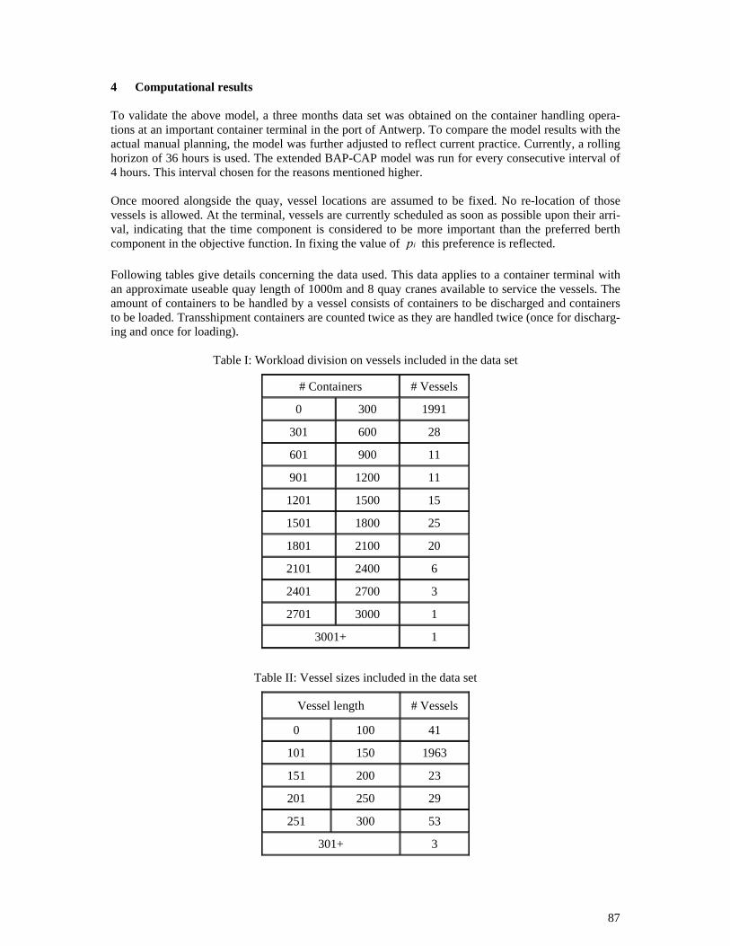
87

4 Computational results To validate the above model, a three months data set was obtained on the container handling opera-tions at an important container terminal in the port of Antwerp. To compare the model results with the actual manual planning, the model was further adjusted to reflect current practice. Currently, a rolling horizon of 36 hours is used. The extended BAP-CAP model was run for every consecutive interval of 4 hours. This interval chosen for the reasons mentioned higher. Once moored alongside the quay, vessel locations are assumed to be fixed. No re-location of those vessels is allowed. At the terminal, vessels are currently scheduled as soon as possible upon their arri-val, indicating that the time component is considered to be more important than the preferred berth component in the objective function. In fixing the value of ip this preference is reflected. Following tables give details concerning the data used. This data applies to a container terminal with an approximate useable quay length of 1000m and 8 quay cranes available to service the vessels. The amount of containers to be handled by a vessel consists of containers to be discharged and containers to be loaded. Transshipment containers are counted twice as they are handled twice (once for discharg-ing and once for loading).

Table I: Workload division on vessels included in the data set

# Containers # Vessels

0 300 1991

301 600 28

601 900 11

901 1200 11

1201 1500 15

1501 1800 25

1801 2100 20

2101 2400 6

2401 2700 3

2701 3000 1

3001+ 1

Table II: Vessel sizes included in the data set

Vessel length # Vessels

0 100 41

101 150 1963

151 200 23

201 250 29

251 300 53

301+ 3

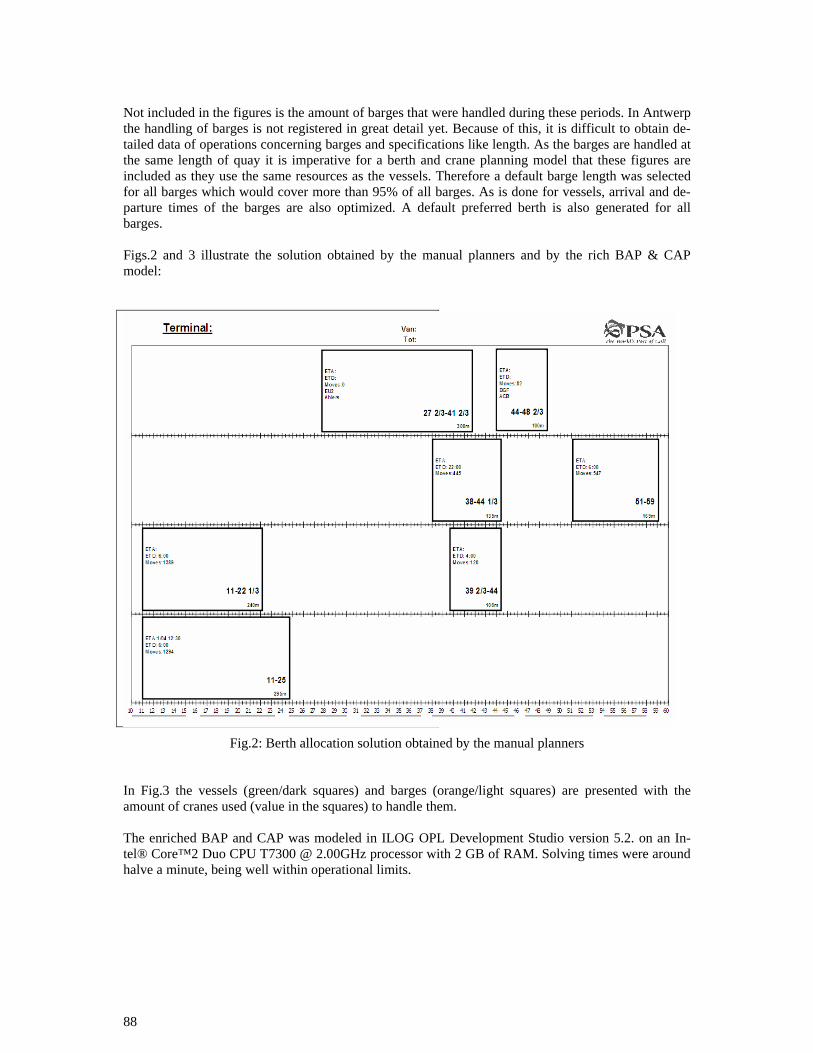
88

Not included in the figures is the amount of barges that were handled during these periods. In Antwerp the handling of barges is not registered in great detail yet. Because of this, it is difficult to obtain de-tailed data of operations concerning barges and specifications like length. As the barges are handled at the same length of quay it is imperative for a berth and crane planning model that these figures are included as they use the same resources as the vessels. Therefore a default barge length was selected for all barges which would cover more than 95% of all barges. As is done for vessels, arrival and de-parture times of the barges are also optimized. A default preferred berth is also generated for all barges. Figs.2 and 3 illustrate the solution obtained by the manual planners and by the rich BAP & CAP model:

Fig.2: Berth allocation solution obtained by the manual planners

In Fig.3 the vessels (green/dark squares) and barges (orange/light squares) are presented with the amount of cranes used (value in the squares) to handle them. The enriched BAP and CAP was modeled in ILOG OPL Development Studio version 5.2. on an In-tel® Core™2 Duo CPU T7300 @ 2.00GHz processor with 2 GB of RAM. Solving times were around halve a minute, being well within operational limits.

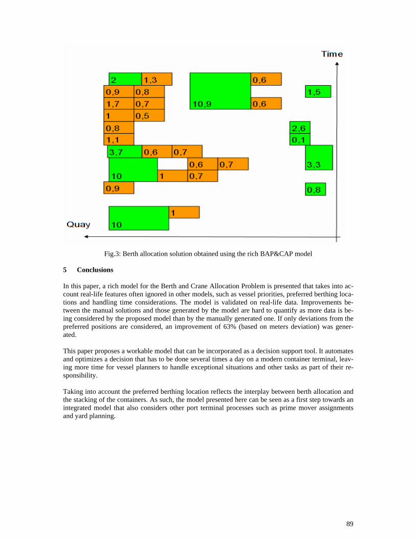
89

Fig.3: Berth allocation solution obtained using the rich BAP&CAP model

5 Conclusions In this paper, a rich model for the Berth and Crane Allocation Problem is presented that takes into ac-count real-life features often ignored in other models, such as vessel priorities, preferred berthing loca-tions and handling time considerations. The model is validated on real-life data. Improvements be-tween the manual solutions and those generated by the model are hard to quantify as more data is be-ing considered by the proposed model than by the manually generated one. If only deviations from the preferred positions are considered, an improvement of 63% (based on meters deviation) was gener-ated. This paper proposes a workable model that can be incorporated as a decision support tool. It automates and optimizes a decision that has to be done several times a day on a modern container terminal, leav-ing more time for vessel planners to handle exceptional situations and other tasks as part of their re-sponsibility. Taking into account the preferred berthing location reflects the interplay between berth allocation and the stacking of the containers. As such, the model presented here can be seen as a first step towards an integrated model that also considers other port terminal processes such as prime mover assignments and yard planning.

90

References AXS (2006), Cellular fleet forecast, AXS-Alphaliner, unpublished document BROWN, G.G.; LAWPHONGPANICH, S.; THURMAN, K.P. (1994), Optimizing ship berthing, Na-val Research Logistics 41, pp.1–15 BROWN, G.G.; CORMICAN, K.J.; LAWPHONGPANICH, S.; WIDDIS, D.B. (1997), Optimizing submarine berthing with a persistence incentive, Naval Research Logistics 44, pp.301–318 CORDEAU, J.-F.; LAPORTE, G.; LEGATO, P.; MOCCIA, L. (2005), Models and tabu search heu-ristics for the berth-allocation problem, Transportation Science 39, pp.526–538 DAGANZO, C.F. (1989), The crane scheduling problem, Transportation Research 23B (3), pp.159–175 DREWRY (2006), The Drewry container market quarterly, Vol.7, 1st ed., Drewry Shipping Consult-ants, London, 191 pp. HANSEN, P. et al. (2007), Variable neighborhood search for minimum cost berth allocation, Euro-pean J. Operational Research, doi:10.1016/j. ejor.2006.12.057 GROSSMANN, H.; OTTO, A.; STILLER, S.; WEDEMEIER, J. (2007), Growth potential for mari-time trade and ports in Europe, Intereconomics, July/August, pp.226-232, doi: 10.1007/s10272-007-0223-x GUAN Y., CHEUNG R. K. (2004), The berth allocation problem: models and solution methods, OR Spectrum, 26, pp.75–92 GÜNTHER H., KIM K. (2006), Container terminals and terminal operations, OR Spectrum 28, pp.437–445, DOI 10.1007/s00291-006-0059-y IMAI, A.; NAGAIWA, K.I.; TAT, C.W. (1997), Efficient planning of berth allocation for container terminals in Asia, J. Advanced Transportation 31, pp.75–94 IMAI, A.; NISHIMURA, E.; PAPADIMITRIOU, S. (2001), The dynamic berth allocation problem for a container port, Transportation Research Part B 35, pp.401–417 IMAI A.; NISHIMURA E.; PAPADIMITRIOU, S. (2003), Berth allocation with service priority, Transportation Research Part B 37, pp.437–457 IMAI, A.; NISHIMURA, E.; PAPADIMITRIOU, S. (2005a), Corrigendum to “The dynamic berth allocation problem for a container port’’ [Transportation Research Part B 35 (2001) pp.401–417], Transportation Research Part B 39, p.197 IMAI, A.; NISHIMURA, E.; PAPADIMITRIOU, S. (2005b), Berth allocation in a container port: using a continuous location space approach, Transportation Research Part B 39, pp.199–221 IMAI A.; NISHIMURA, E.; HATTORI, M.; PAPADIMITRIOU, S. (2007), Berth allocation at in-dented berths for mega-container ships, European J. Operational Research 179, pp.579–593 IMAI, A. et al. (2007), The simultaneous berth and quay crane allocation problem, Transport. Res. Part E, doi:10.1016/j.tre.2007.03.003

91

KIM, K.H.; MOON, K.C. (2003), Berth scheduling by simulated annealing, Transportation Research Part B 37, pp.541–560 LAI, K.K., SHIH, K. (1992), A study of container berth allocation, J. Advanced Transportation 26, pp.45–60 LEGATO, P.; MAZZA, R.M. (2001), Berth planning and resources optimization at a container ter-minal via discrete event simulation, European J. Operational Research 133, pp.537-547 LI, C.-L.; CAI, X.; LEE, C.-Y. (1998), Scheduling with multiple-job-on-one-processor pattern, IIE Transactions 30, pp.433–445 LIM, A. (1998), The berth planning problem, Operations Research Letters 22, pp.105–110 LIU, J.Y.; WAN, Y.W.; WANG, L. (2005), Quay crane scheduling at container terminals to minimize the maximum relative tardiness of vessel departures, Wiley InterScience, DOI 10.1002/nav.20108 LOKUGE, P.; ALAHAKOON, D. (2007), Improving the adaptability in automated vessel scheduling in container ports using intelligent software agents, European J. Operational Research 177, pp.1985–2015 MOORTHY, R.; TEO, C. (2006), Berth management in container terminal: the template design prob-lem, OR Spectrum 28, pp.495-518 NISHIMURA, E.; IMAI, A.; PAPADIMITRIOU, S. (2001), Berth allocation planning in the public berth system by genetic algorithms, European J. Operational Research 131, pp.282-292 PARK, Y.M.; KIM, K.H. (2003), A scheduling method for berth and quay cranes, OR Spectrum 25, pp.1-23 PETERKOFSKY, R.I.; DAGANZO, C.F. (1990), A branch and bound solution method for the crane scheduling problem, Transportation Research 24B (3), pp.159–172 ROELS, R. (2007), DP World presentation, Propeller Club, Antwerp UNESCAP (2005), Regional shipping and port development strategies – container traffic forecast, United Nations Economic and Social Commission for Asia and the Pacific, New York, vii + 52 pp. VERNIMMEN, B.; DULLAERT, W.; ENGELEN, S. (2007), The impact of liner schedule unreliabil-ity on ports and their actors, Maritime Economics and Logistics, 9(3), 19 p. WANG F.; LIM A. (2007), A stochastic beam search for the berth allocation problem, Decision Sup-port Systems 42, pp.2186–2196

92

IMPROVE - Design of Improved and Competitive Products using an Inte-grated Decision Support System for Ship Production and Operation

Philippe Rigo, ANAST-ULG (FNRS), Belgium, ph.rigo@ulg.ac.be

Djani Dundara, Uljanik, Croatia, Djani.Dundara@uljanik.hr

J-L Guillaume-Combecave, Akeryards, France, jean-louis.guillaume-combecave@akeryards.com

Stanislav Domagallo, SNN, Poland, sdomagallo@ssn.pl

Alan Klanac, TKK, Finland, alan.klanac@tkk.fi

Frank Roland, CMT, Germany, roland@cmt-net.org

Osman Turan, NAME, UK, o.turan@na-me.ac.uk

Vedran Zanic, UZ, Croatia, vedran.zanic@fsb.hr

Amirouche Amrane, ANAST-ULG, Belgium, A.Amrane@ulg.ac.be

Adrian Constantinescu, ANAST-ULG, Belgium, A.constantinescu@ulg.ac.be

Abstract

The paper gives an overview over the EC project IMPROVE. The project develops a decision support

system for a methodological assessment of ship designs to provide a rational basis for making deci-

sions pertaining to the design, production and operation of three next-generation ship types (LNG,

RoPax, chemical tanker).The system is expected to reduce life-cycle costs and improve ship perform-

ance.

1. Introduction

IMPROVE, http://www.improve-project.eu, is a three-year research project supported by the European

Commission under the Growth Programme of the 6th

Framework Programme. The project started in

October 2006. The main goal of IMPROVE is to develop three innovative products:

1. LNG Carrier, Fig.1 - AKERYARDS has designed and built 17 LNG carriers (from 50 000 m3,

75 000, 130 000 m3 to latest 154 500 m

3). In the framework of IMPROVE, they are studying

the design of a 220 000 m3 unit.

2. Large RoPax ship, Fig.2 - ULJANIK Shipyard (Croatia) in the last 5 years has designed sev-

eral car-carriers, ConRo and RoPax vessels. For a long period. ULJANIK has a strong coop-

eration with the GRIMALDI GROUP as respectable ship owner regarding market needs and

trends.

3. Chemical tanker, Fig.3 - SZCZECIN shipyard (SSN, Poland) has recently built several chemi-

cal tankers (40000 DWT)

As the proposed methodology is based on multi-criteria structural optimization, the consortium con-

tains not only designers, but also shipyards and ship-owners / operators (one per product). The re-

search activity has been divided in three main phases:

1. Definition of stakeholders’ requirements and specification of optimization targets and key per-

formance indicators, Table I. In addition, project partners (particularly the shipyards) designed

reference or prototype ships, one per each ship type, in a “first design loop”.

2. All technical developments related to the selected structural optimization tool. Several mod-

ules such as fatigue assessment, vibration level investigation, ultimate strength, load assess-

ment, production and maintenance cost, optimization robustness will be delivered and inte-

grated into the existing tools (LBR5, OCTOPUS, and CONSTRUCT).

3. Application of the developed optimization platforms for the three target products.

This paper focuses on the first two phases, and gives details and some guidelines related to the selec-

tion of design criteria and to the development of different modules. The applications are described in

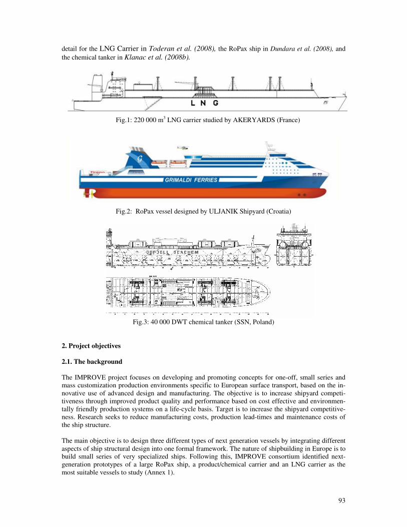
93

detail for the LNG Carrier in Toderan et al. (2008), the RoPax ship in Dundara et al. (2008), and

the chemical tanker in Klanac et al. (2008b).

Fig.1: 220 000 m3 LNG carrier studied by AKERYARDS (France)

Fig.2: RoPax vessel designed by ULJANIK Shipyard (Croatia)

Fig.3: 40 000 DWT chemical tanker (SSN, Poland)

2. Project objectives

2.1. The background

The IMPROVE project focuses on developing and promoting concepts for one-off, small series and

mass customization production environments specific to European surface transport, based on the in-

novative use of advanced design and manufacturing. The objective is to increase shipyard competi-

tiveness through improved product quality and performance based on cost effective and environmen-

tally friendly production systems on a life-cycle basis. Target is to increase the shipyard competitive-

ness. Research seeks to reduce manufacturing costs, production lead-times and maintenance costs of

the ship structure.

The main objective is to design three different types of next generation vessels by integrating different

aspects of ship structural design into one formal framework. The nature of shipbuilding in Europe is to

build small series of very specialized ships. Following this, IMPROVE consortium identified next-

generation prototypes of a large RoPax ship, a product/chemical carrier and an LNG carrier as the

most suitable vessels to study (Annex 1).

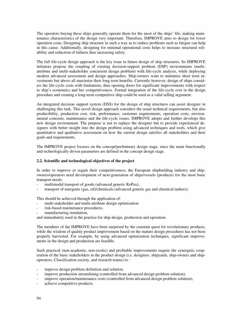
94

The operators buying these ships generally operate them for the most of the ships’ life, making main-

tenance characteristics of the design very important. Therefore, IMPROVE aims to design for lower

operation costs. Designing ship structure in such a way as to reduce problems such as fatigue can help

in this cause. Additionally, designing for minimal operational costs helps to increase structural reli-

ability and reduction of failures thus increasing safety.

The full life-cycle design approach is the key issue in future design of ship structures. So IMPROVE

initiators propose the coupling of existing decision-support problem (DSP) environments (multi-

attribute and multi-stakeholder concurrent design problem) with life-cycle analysis, while deploying

modern advanced assessment and design approaches. Ship-owners want to minimize short term in-

vestments but above all maximize their long term benefits. Currently however, design of ships consid-

ers the life-cycle costs with limitations, thus opening doors for significant improvements with respect

to ship’s economics and her competitiveness. Formal integration of the life-cycle cost in the design

procedure and creating a long-term competitive ship could be used as a valid selling argument.

An integrated decision support system (DSS) for the design of ship structures can assist designer in

challenging this task. This novel design approach considers the usual technical requirements, but also

producibility, production cost, risk, performance, customer requirements, operation costs, environ-

mental concerns, maintenance and the life-cycle issues. IMPROVE adopts and further develops this

new design environment. The purpose is not to replace the designer but to provide experienced de-

signers with better insight into the design problem using advanced techniques and tools, which give

quantitative and qualitative assessment on how the current design satisfies all stakeholders and their

goals and requirements.

The IMPROVE project focuses on the concept/preliminary design stage, since the main functionally

and technologically driven parameters are defined in the concept design stage.

2.2. Scientific and technological objectives of the project

In order to improve or regain their competitiveness, the European shipbuilding industry and ship-

owners/operators need development of next-generation of ships/vessels (products) for the most basic

transport needs:

- multimodal transport of goods (advanced generic RoPax),

- transport of energents (gas, oil)/chemicals (advanced generic gas and chemical tankers).

This should be achieved through the application of:

- multi-stakeholder and multi-attribute design optimization

- risk-based maintenance procedures,

- manufacturing simulation,

and immediately used in the practice for ship design, production and operation.

The members of the IMPROVE have been surprised by the constant quest for revolutionary products,

while the wisdom of quality product improvement based on the mature design procedures has not been

properly harvested. For example, by using advanced optimization techniques, significant improve-

ments in the design and production are feasible.

Such practical (non-academic, non-exotic) and profitable improvements require the synergetic coop-

eration of the basic stakeholders in the product design (i.e. designers, shipyards, ship-owners and ship-

operators, Classification society, and research teams) to :

- improve design problem definition and solution,

- improve production streamlining (controlled from advanced design problem solution),

- improve operation/maintenance costs (controlled from advanced design problem solution),

- achieve competitive products.

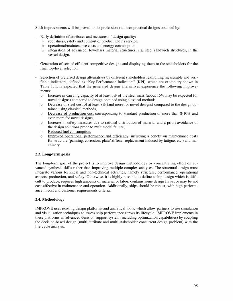
95

Such improvements will be proved to the profession via three practical designs obtained by:

- Early definition of attributes and measures of design quality:

o robustness, safety and comfort of product and its service,

o operational/maintenance costs and energy consumption,

o integration of advanced, low-mass material structures, e.g. steel sandwich structures, in the

vessel design.

- Generation of sets of efficient competitive designs and displaying them to the stakeholders for the

final top-level selection.

- Selection of preferred design alternatives by different stakeholders, exhibiting measurable and veri-

fiable indicators, defined as “Key Performance Indicators” (KPI), which are exemplary shown in

Table 1. It is expected that the generated design alternatives experience the following improve-

ments:

o Increase in carrying capacity of at least 5% of the steel mass (about 15% may be expected for

novel designs) compared to design obtained using classical methods,

o Decrease of steel cost of at least 8% (and more for novel designs) compared to the design ob-

tained using classical methods,

o Decrease of production cost corresponding to standard production of more than 8-10% and

even more for novel designs,

o Increase in safety measures due to rational distribution of material and a priori avoidance of

the design solutions prone to multimodal failure,

o Reduced fuel consumption,

o Improved operational performance and efficiency, including a benefit on maintenance costs

for structure (painting, corrosion, plate/stiffener replacement induced by fatigue, etc.) and ma-

chinery.

2.3. Long-term goals

The long-term goal of the project is to improve design methodology by concentrating effort on ad-

vanced synthesis skills rather than improving multiple complex analyses. The structural design must

integrate various technical and non-technical activities, namely structure, performance, operational

aspects, production, and safety. Otherwise, it is highly possible to define a ship design which is diffi-

cult to produce, requires high amounts of material or labor, contains some design flaws, or may be not

cost-effective in maintenance and operation. Additionally, ships should be robust, with high perform-

ance in cost and customer requirements criteria.

2.4. Methodology

IMPROVE uses existing design platforms and analytical tools, which allow partners to use simulation

and visualization techniques to assess ship performance across its lifecycle. IMPROVE implements in

these platforms an advanced decision support system (including optimization capabilities) by coupling

the decision-based design (multi-attribute and multi-stakeholder concurrent design problem) with the

life-cycle analysis.

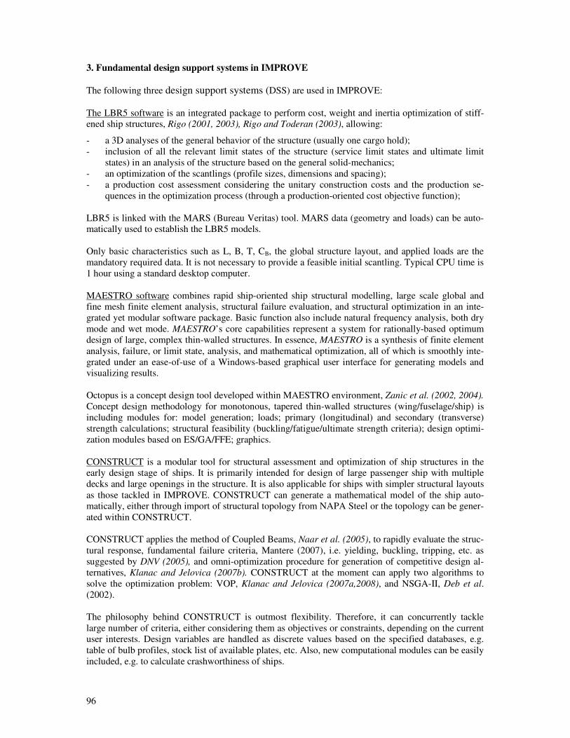
96

3. Fundamental design support systems in IMPROVE

The following three design support systems (DSS) are used in IMPROVE:

The LBR5 software is an integrated package to perform cost, weight and inertia optimization of stiff-

ened ship structures, Rigo (2001, 2003), Rigo and Toderan (2003), allowing:

- a 3D analyses of the general behavior of the structure (usually one cargo hold);

- inclusion of all the relevant limit states of the structure (service limit states and ultimate limit

states) in an analysis of the structure based on the general solid-mechanics;

- an optimization of the scantlings (profile sizes, dimensions and spacing);

- a production cost assessment considering the unitary construction costs and the production se-

quences in the optimization process (through a production-oriented cost objective function);

LBR5 is linked with the MARS (Bureau Veritas) tool. MARS data (geometry and loads) can be auto-

matically used to establish the LBR5 models.

Only basic characteristics such as L, B, T, CB, the global structure layout, and applied loads are the

mandatory required data. It is not necessary to provide a feasible initial scantling. Typical CPU time is

1 hour using a standard desktop computer.

MAESTRO software combines rapid ship-oriented ship structural modelling, large scale global and

fine mesh finite element analysis, structural failure evaluation, and structural optimization in an inte-

grated yet modular software package. Basic function also include natural frequency analysis, both dry

mode and wet mode. MAESTRO’s core capabilities represent a system for rationally-based optimum

design of large, complex thin-walled structures. In essence, MAESTRO is a synthesis of finite element

analysis, failure, or limit state, analysis, and mathematical optimization, all of which is smoothly inte-

grated under an ease-of-use of a Windows-based graphical user interface for generating models and

visualizing results.

Octopus is a concept design tool developed within MAESTRO environment, Zanic et al. (2002, 2004).

Concept design methodology for monotonous, tapered thin-walled structures (wing/fuselage/ship) is

including modules for: model generation; loads; primary (longitudinal) and secondary (transverse)

strength calculations; structural feasibility (buckling/fatigue/ultimate strength criteria); design optimi-

zation modules based on ES/GA/FFE; graphics.

CONSTRUCT is a modular tool for structural assessment and optimization of ship structures in the

early design stage of ships. It is primarily intended for design of large passenger ship with multiple

decks and large openings in the structure. It is also applicable for ships with simpler structural layouts

as those tackled in IMPROVE. CONSTRUCT can generate a mathematical model of the ship auto-

matically, either through import of structural topology from NAPA Steel or the topology can be gener-

ated within CONSTRUCT.

CONSTRUCT applies the method of Coupled Beams, Naar et al. (2005), to rapidly evaluate the struc-

tural response, fundamental failure criteria, Mantere (2007), i.e. yielding, buckling, tripping, etc. as

suggested by DNV (2005), and omni-optimization procedure for generation of competitive design al-

ternatives, Klanac and Jelovica (2007b). CONSTRUCT at the moment can apply two algorithms to

solve the optimization problem: VOP, Klanac and Jelovica (2007a,2008), and NSGA-II, Deb et al.

(2002).

The philosophy behind CONSTRUCT is outmost flexibility. Therefore, it can concurrently tackle

large number of criteria, either considering them as objectives or constraints, depending on the current

user interests. Design variables are handled as discrete values based on the specified databases, e.g.

table of bulb profiles, stock list of available plates, etc. Also, new computational modules can be easily

included, e.g. to calculate crashworthiness of ships.

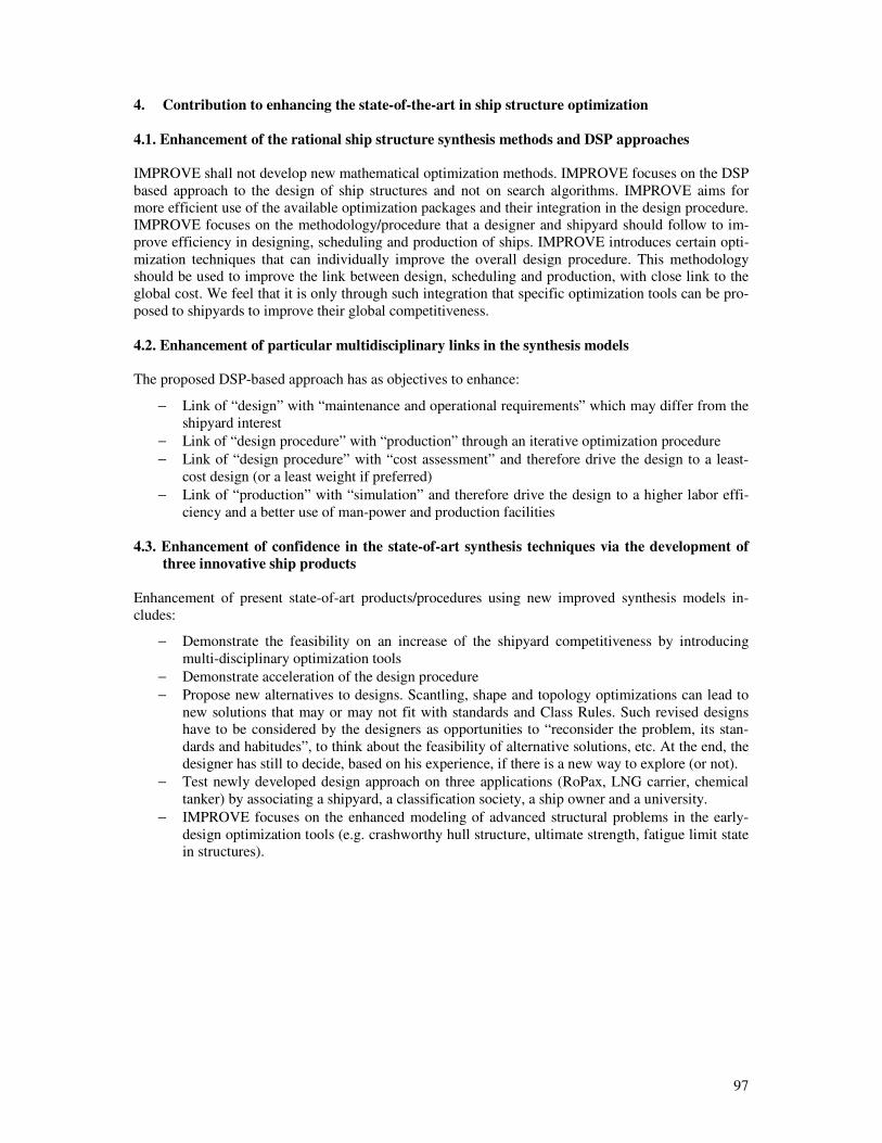
97

4. Contribution to enhancing the state-of-the-art in ship structure optimization

4.1. Enhancement of the rational ship structure synthesis methods and DSP approaches

IMPROVE shall not develop new mathematical optimization methods. IMPROVE focuses on the DSP

based approach to the design of ship structures and not on search algorithms. IMPROVE aims for

more efficient use of the available optimization packages and their integration in the design procedure.

IMPROVE focuses on the methodology/procedure that a designer and shipyard should follow to im-

prove efficiency in designing, scheduling and production of ships. IMPROVE introduces certain opti-

mization techniques that can individually improve the overall design procedure. This methodology

should be used to improve the link between design, scheduling and production, with close link to the

global cost. We feel that it is only through such integration that specific optimization tools can be pro-

posed to shipyards to improve their global competitiveness.

4.2. Enhancement of particular multidisciplinary links in the synthesis models

The proposed DSP-based approach has as objectives to enhance:

− Link of “design” with “maintenance and operational requirements” which may differ from the

shipyard interest

− Link of “design procedure” with “production” through an iterative optimization procedure

− Link of “design procedure” with “cost assessment” and therefore drive the design to a least-

cost design (or a least weight if preferred)

− Link of “production” with “simulation” and therefore drive the design to a higher labor effi-

ciency and a better use of man-power and production facilities

4.3. Enhancement of confidence in the state-of-art synthesis techniques via the development of three innovative ship products

Enhancement of present state-of-art products/procedures using new improved synthesis models in-

cludes:

− Demonstrate the feasibility on an increase of the shipyard competitiveness by introducing

multi-disciplinary optimization tools

− Demonstrate acceleration of the design procedure

− Propose new alternatives to designs. Scantling, shape and topology optimizations can lead to

new solutions that may or may not fit with standards and Class Rules. Such revised designs

have to be considered by the designers as opportunities to “reconsider the problem, its stan-

dards and habitudes”, to think about the feasibility of alternative solutions, etc. At the end, the

designer has still to decide, based on his experience, if there is a new way to explore (or not).

− Test newly developed design approach on three applications (RoPax, LNG carrier, chemical

tanker) by associating a shipyard, a classification society, a ship owner and a university.

− IMPROVE focuses on the enhanced modeling of advanced structural problems in the early-

design optimization tools (e.g. crashworthy hull structure, ultimate strength, fatigue limit state

in structures).

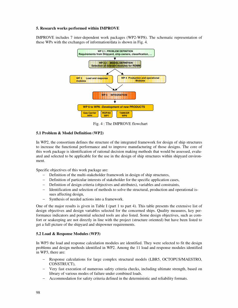
98

5. Research works performed within IMPROVE

IMPROVE includes 7 inter-dependent work packages (WP2-WP8). The schematic representation of

these WPs with the exchanges of information/data is shown in Fig. 4.

Fig. 4 : The IMPROVE flowchart

5.1 Problem & Model Definition (WP2)

In WP2, the consortium defines the structure of the integrated framework for design of ship structures

to increase the functional performance and to improve manufacturing of those designs. The core of

this work package is identification of rational decision making methods that would be assessed, evalu-

ated and selected to be applicable for the use in the design of ship structures within shipyard environ-

ment.

Specific objectives of this work package are:

− Definition of the multi-stakeholder framework in design of ship structures,

− Definition of particular interests of stakeholder for the specific application cases,

− Definition of design criteria (objectives and attributes), variables and constraints,

− Identification and selection of methods to solve the structural, production and operational is-

sues affecting design,

− Synthesis of needed actions into a framework.

One of the major results is given in Table I (part 1 to part 4). This table presents the extensive list of

design objectives and design variables selected for the concerned ships. Quality measures, key per-

formance indicators and potential selected tools are also listed. Some design objectives, such as com-

fort or seakeeping are not directly in line with the project (structure oriented) but have been listed to

get a full picture of the shipyard and shipowner requirements.

5.2 Load & Response Modules (WP3)

In WP3 the load and response calculation modules are identified. They were selected to fit the design

problems and design methods identified in WP2. Among the 11 load and response modules identified

in WP3, there are:

− Response calculations for large complex structural models (LBR5, OCTOPUS/MAESTRO,

CONSTRUCT),

− Very fast execution of numerous safety criteria checks, including ultimate strength, based on

library of various modes of failure under combined loads.

− Accommodation for safety criteria defined in the deterministic and reliability formats.

WP 2.1. PROBLEM DEFINITION

Requirements from Shipyard, ship-owners, classification, …

WP 2.2 MODEL DEFINITION

Selection of relevant modules for RDMM

WP 3 Load and response modules

WP 5 INTEGRATION

WP 6 to WP8 –Development of new PRODUCTS

Gas Carrier WP6

ROPAX WP7

TANKER WP8

WP 4 Production and operational Modules

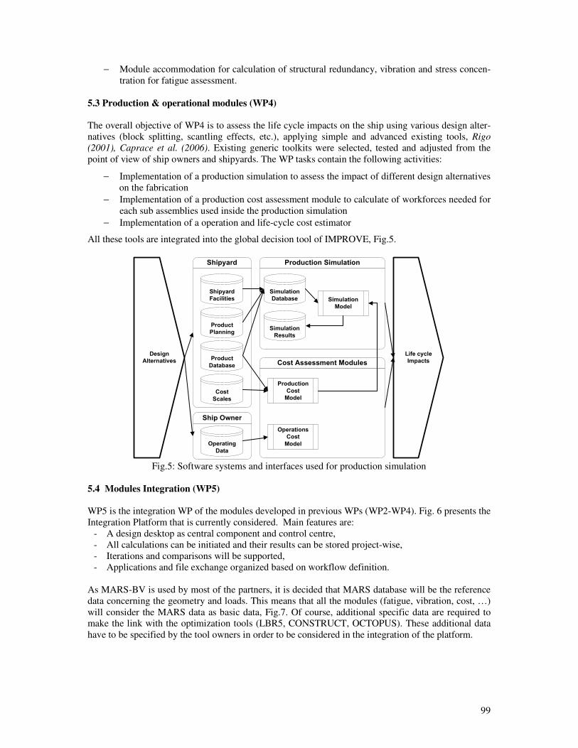
99

− Module accommodation for calculation of structural redundancy, vibration and stress concen-

tration for fatigue assessment.

5.3 Production & operational modules (WP4)

The overall objective of WP4 is to assess the life cycle impacts on the ship using various design alter-

natives (block splitting, scantling effects, etc.), applying simple and advanced existing tools, Rigo

(2001), Caprace et al. (2006). Existing generic toolkits were selected, tested and adjusted from the

point of view of ship owners and shipyards. The WP tasks contain the following activities:

− Implementation of a production simulation to assess the impact of different design alternatives

on the fabrication

− Implementation of a production cost assessment module to calculate of workforces needed for

each sub assemblies used inside the production simulation

− Implementation of a operation and life-cycle cost estimator

All these tools are integrated into the global decision tool of IMPROVE, Fig.5.

Fig.5: Software systems and interfaces used for production simulation

5.4 Modules Integration (WP5)

WP5 is the integration WP of the modules developed in previous WPs (WP2-WP4). Fig. 6 presents the

Integration Platform that is currently considered. Main features are:

- A design desktop as central component and control centre,

- All calculations can be initiated and their results can be stored project-wise,

- Iterations and comparisons will be supported,

- Applications and file exchange organized based on workflow definition.

As MARS-BV is used by most of the partners, it is decided that MARS database will be the reference

data concerning the geometry and loads. This means that all the modules (fatigue, vibration, cost, …)

will consider the MARS data as basic data, Fig.7. Of course, additional specific data are required to

make the link with the optimization tools (LBR5, CONSTRUCT, OCTOPUS). These additional data

have to be specified by the tool owners in order to be considered in the integration of the platform.

Shipyard

Shipyard

Facilities

Product

Planning

Product

Database

Production Simulation

Simulation

Database

Simulation

Results

Simulation

Model

Cost Assessment Modules

Cost

Scales

Production

Cost

Model

Ship Owner

Operating

Data

Design

Alternatives

Life cycle

Impacts

Operations

Cost

Model

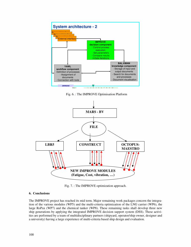
100

IMPROVE

9

Slide 9 --------1----2----3----4----5----6----7----8----9----10----------

System architecture - 2

YAWL workflow component

-Definition of processes

- Assignment of

documents

- Connection with tools

BAL.KMAN knowledge component

- Storage of input and

output documents

- Search for documents

and processes

- Document visualisation

IMPROVE

decision component

- Control process

execution

- Set parameters

- Compare results

-Initiate iterations

External interfaceExternal interface

External interfaceExternal interface

Fig. 6. : The IMPROVE Optimisation Platform

Fig. 7. : The IMPROVE optimization approach.

6. Conclusions

The IMPROVE project has reached its mid term. Major remaining work packages concern the integra-

tion of the various modules (WP5) and the multi-criteria optimization of the LNG carrier (WP6), the

large RoPax (WP7) and the chemical tanker (WP8). These remaining tasks shall develop three new

ship generations by applying the integrated IMPROVE decision support system (DSS). These activi-

ties are performed by a team of multidisciplinary partners (shipyard, operator/ship owner, designer and

a university) having a large experience of multi-criteria based ship design and evaluation.

MARS - BV

FILE

LBR5 CONSTRUCT OCTOPUS-

MAESTRO

NEW IMPROVE MODULES

(Fatigue, Cost, vibration, …)

101

Acknowledgements

The present paper was supported by the European Commission under the FP6 Sustainable Surface

Transport Programme, namely the STREP project IMPROVE (Design of Improved and Competitive

Products using an Integrated Decision Support System for Ship Production and Operation), Contract

No. FP6 – 031382. The European Community and the authors shall not in any way be liable or respon-

sible for the use of any such knowledge, information or data, or of the consequences thereof.

References

CAPRACE, J.D.; RIGO, P.; WARNOTTE, R.; LE VIOL, S. (2006), An analytical cost assessment

module for the detailed design stage, COMPIT’2006, Oegstgeest, pp.335-345

DEB, K.; PRATAP, A.; AGARWAL, S.; MEYARIVAN, T. (2002), A Fast and Elitist Multiobjective

Genetic Algorithm: NSGA-II, IEEE Transactions on Evolutionary Computation, vol.6, No.2, April

2002, pp.182-197

DUNDARA, D.; BOCCHETTI, D.; KUZMANOVIC, O.; ZANIC, V.; ANDRIC, J., PREBEG, P.

(2008), Development of a new innovative concept of RoPax ship, COMPIT’2008, Liege

KLANAC, A.; JELOVICA, J. (2007a), Vectorization in the structural optimization of a fast ferry,

Brodogradnja-Shipbuilding 58/1, pp.11-17

KLANAC, A.; JELOVICA, J. (2007b), A concept of omni-optimization for ship structural design, Ad-

vancements in Marine Structures, Proceedings of MARSTRUCT 2007, 1st

Int. Conf. on Marine Struc-

tures, Glasgow, UK., Guedes Soares & Das (eds), Taylor & Francis: London, pp.473-481

KLANAC, A.; JELOVICA, J. (2008a), Vectorization and constraint grouping to enhance optimization

of marine structures, submitted to Marine Structures

KLANAC, A.; NIEMELÄINEN, M.; JELOVICA, J.; REMES, H.; DOMAGALLO, S. (2008b), Struc-

tural omni-optimization of a tanker, COMPIT’2008, Liege

MAESTRO Version 8.5 (2005), Program documentation, Proteus engineering, Stensville, MD, USA

NAAR H.; VARSTA, P.; KUJALA, P. (2004), A theory of coupled beams for strength assessment of

passenger ships, Marine Structures 17(8), pp.590-611

RIGO, P. (2001), Least-cost structural optimization oriented preliminary design, J. Ship Production,

17/4, pp.202-215

RIGO, P. (2003), An integrated software for scantling optimization and least production cost, Ship

Technology Research 50, pp.126-141

RIGO P.; TODERAN, C. (2003), Least cost optimisation of a medium capacity gas carrier, COM-

PIT’03, Hamburg, pp.94-107

TODERAN, C.; GUILLAUME-COMBECAVE, J.L.; BOUCKAERT, M.; HAGE, A.; CARTIER, O.;

CAPRACE, J.D.; AMRANE, A.; CONSTANTINESCU, PIRCALABU, E.; A.; RIGO, P. (2008),

Structural optimization of a 220000 m3 LNG carrier, COMPIT’2008, Liege

ZANIC, V.; ROGULJ, A.; JANCIJEV, T.; BRALIĆ, S.; HOZMEC, J. (2002), Methodology for

evaluation of ship structural safety, 10th Int. Congress IMAM 2002, Crete

102

ZANIC, V.; PREBEG, P. (2004), Primary response assessment method for concept design of monoto-

nous thin-walled structures, 4th Int. Conf. on Advanced Engineering Design, Glasgow, pp.1-10

ANNEX 1

IMPROVE

DESIGN OF IMPROVED AND COMPETITIVE PRODUCTS USING AN INTEGRATED DECISION

SUPPORT SYSTEM FOR SHIP PRODUCTION AND OPERATION

The IMPROVE project proposes to deliver an integrated decision support system for a methodological

assessment of ship designs to provide a rational basis for making decisions pertaining to the design,

production and operation of three new ship generations. Such support can be used to make more in-

formed decisions, which in turn will contribute to reducing the life-cycle costs and improving the per-

formance of those ship generations.

IMPROVE Project

IMPROVE is a three-year research project which started on the 1st October 2006. The project is sup-

ported by the European Commission under the Growth Programme of the 6th Framework Programme.

Contract No. FP6 - 031382.

Project Partners:

ANAST, University of Liege Belgium (project coordinator)

Aker Yards shipyard France

Uljanik shipyard Croatia

Szczecin New Shipyard Poland

Grimaldi Italy

Exmar Belgium

Tankerska Plovidba Zadar Croatia

Bureau Veritas France

Design Naval & Transport Belgium

Ship Design Group Romania

MEC Estonia

Helsinki University of Technology Finland

University of Zagreb Croatia

NAME, Universities of Glasgow & Strathclyde United Kingdom

Centre of Maritime Technologies Germany

BALance Technology Consulting GmbH Germany

WEGEMT United Kingdom

Further Information

More information about the IMPROVE project can be found at the project website

http://www.improve-project.eu/ or http://www.anast-eu.ulg.ac.be/

Alternatively you can contact the project co-ordinator:

Prof. Philippe Rigo at ph.rigo@ulg.ac.be (+32-4-366 9366)

ANAST, University of Liege, Belgium

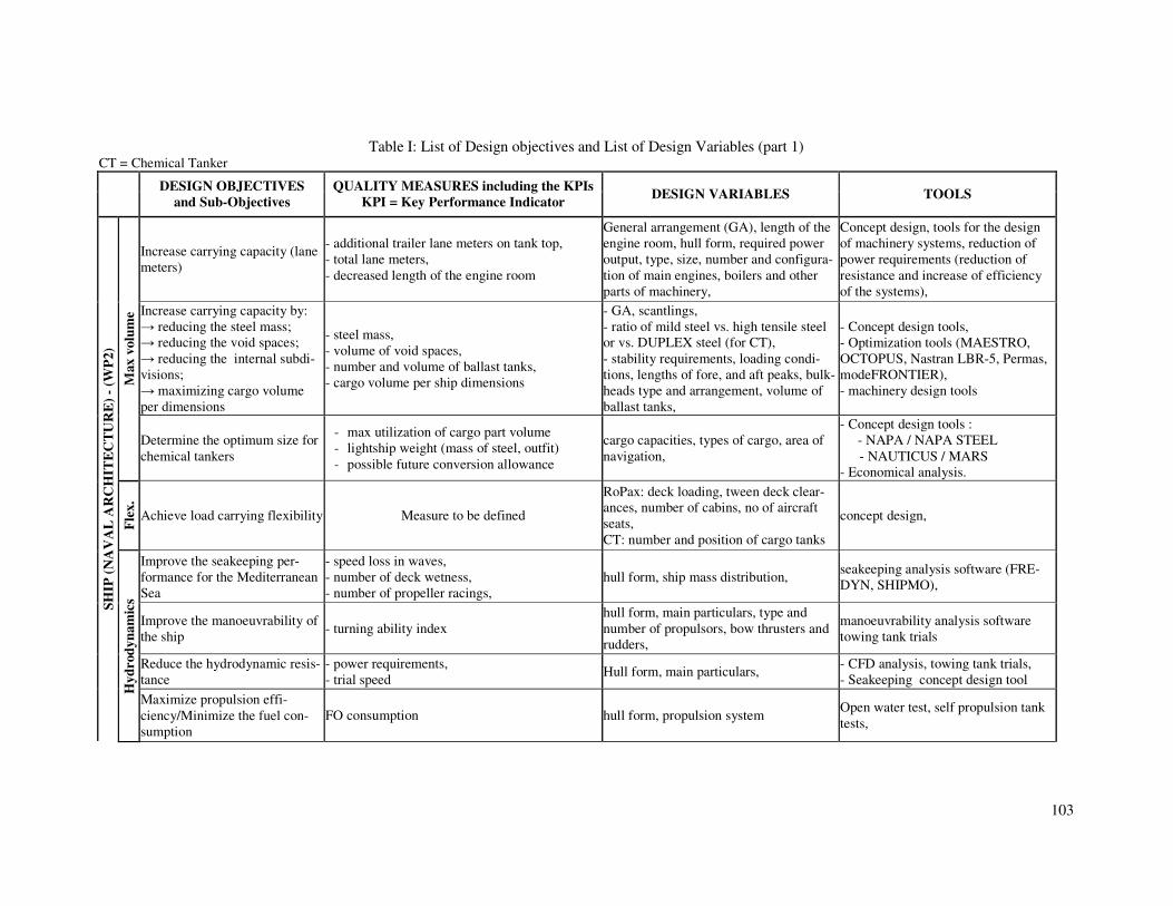
103

Table I: List of Design objectives and List of Design Variables (part 1) CT = Chemical Tanker

DESIGN OBJECTIVES

and Sub-Objectives

QUALITY MEASURES including the KPIs

KPI = Key Performance Indicator DESIGN VARIABLES TOOLS

Increase carrying capacity (lane

meters)

- additional trailer lane meters on tank top,

- total lane meters,

- decreased length of the engine room

General arrangement (GA), length of the

engine room, hull form, required power

output, type, size, number and configura-

tion of main engines, boilers and other

parts of machinery,

Concept design, tools for the design

of machinery systems, reduction of

power requirements (reduction of

resistance and increase of efficiency

of the systems),

Increase carrying capacity by:

→ reducing the steel mass;

→ reducing the void spaces;

→ reducing the internal subdi-

visions;

→ maximizing cargo volume

per dimensions

- steel mass,

- volume of void spaces,

- number and volume of ballast tanks,

- cargo volume per ship dimensions

- GA, scantlings,

- ratio of mild steel vs. high tensile steel

or vs. DUPLEX steel (for CT),

- stability requirements, loading condi-

tions, lengths of fore, and aft peaks, bulk-

heads type and arrangement, volume of

ballast tanks,

- Concept design tools,

- Optimization tools (MAESTRO,

OCTOPUS, Nastran LBR-5, Permas,

modeFRONTIER),

- machinery design tools

Max v

olu

me

Determine the optimum size for

chemical tankers

- max utilization of cargo part volume

- lightship weight (mass of steel, outfit)

- possible future conversion allowance

cargo capacities, types of cargo, area of

navigation,

- Concept design tools :

- NAPA / NAPA STEEL

- NAUTICUS / MARS

- Economical analysis.

Fle

x.

Achieve load carrying flexibility Measure to be defined

RoPax: deck loading, tween deck clear-

ances, number of cabins, no of aircraft

seats,

CT: number and position of cargo tanks

concept design,

Improve the seakeeping per-

formance for the Mediterranean

Sea

- speed loss in waves,

- number of deck wetness,

- number of propeller racings,

hull form, ship mass distribution, seakeeping analysis software (FRE-

DYN, SHIPMO),

Improve the manoeuvrability of

the ship - turning ability index

hull form, main particulars, type and

number of propulsors, bow thrusters and

rudders,

manoeuvrability analysis software

towing tank trials

Reduce the hydrodynamic resis-

tance

- power requirements,

- trial speed Hull form, main particulars,

- CFD analysis, towing tank trials,

- Seakeeping concept design tool

SH

IP (

NA

VA

L A

RC

HIT

EC

TU

RE

) -

(WP

2)

Hyd

rod

yn

am

ics

Maximize propulsion effi-

ciency/Minimize the fuel con-

sumption

FO consumption hull form, propulsion system Open water test, self propulsion tank

tests,

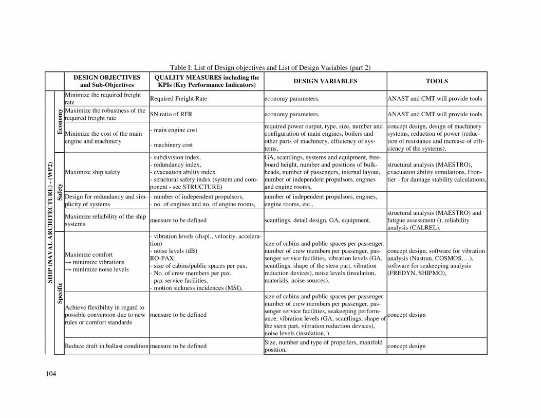
104

Table I: List of Design objectives and List of Design Variables (part 2)

DESIGN OBJECTIVES

and Sub-Objectives

QUALITY MEASURES including the

KPIs (Key Performance Indicators) DESIGN VARIABLES TOOLS

Minimize the required freight

rate Required Freight Rate economy parameters, ANAST and CMT will provide tools

Maximize the robustness of the

required freight rate SN ratio of RFR economy parameters, ANAST and CMT will provide tools

Eco

nom

y

Minimize the cost of the main

engine and machinery

- main engine cost

- machinery cost

required power output, type, size, number and

configuration of main engines, boilers and

other parts of machinery, efficiency of sys-

tems,

concept design, design of machinery

systems, reduction of power (reduc-

tion of resistance and increase of effi-

ciency of the systems),

Maximize ship safety

- subdivision index,

- redundancy index,

- evacuation ability index

- structural safety index (system and com-

ponent - see STRUCTURE)

GA, scantlings, systems and equipment, free-

board height, number and positions of bulk-

heads, number of passengers, internal layout,

number of independent propulsors, engines

and engine rooms,

structural analysis (MAESTRO),

evacuation ability simulations, Fron-

tier - for damage stability calculations,

Design for redundancy and sim-

plicity of systems

- number of independent propulsors,

- no. of engines and no. of engine rooms,

number of independent propulsors, engines,

engine rooms, etc., S

afe

ty

Maximize reliability of the ship

systems measure to be defined scantlings, detail design, GA, equipment,

structural analysis (MAESTRO) and

fatigue assessment (), reliability

analysis (CALREL),

Maximize comfort

→ minimize vibrations

→ minimize noise levels

- vibration levels (displ., velocity, accelera-

tion)

- noise levels (dB)

RO-PAX:

- size of cabins/public spaces per pax,

- No. of crew members per pax,

- pax service facilities,

- motion sickness incidences (MSI),

size of cabins and public spaces per passenger,

number of crew members per passenger, pas-

senger service facilities, vibration levels (GA,

scantlings, shape of the stern part, vibration

reduction devices), noise levels (insulation,

materials, noise sources),

concept design, software for vibration

analysis (Nastran, COSMOS,…),

software for seakeeping analysis

(FREDYN, SHIPMO),

Achieve flexibility in regard to

possible conversion due to new

rules or comfort standards

measure to be defined

size of cabins and public spaces per passenger,

number of crew members per passenger, pas-

senger service facilities, seakeeping perform-

ance, vibration levels (GA, scantlings, shape of

the stern part, vibration reduction devices),

noise levels (insulation, )

concept design

SH

IP (

NA

VA

L A

RC

HIT

EC

TU

RE

) -

(WP

2)

Sp

ecif

ic

Reduce draft in ballast condition measure to be defined Size, number and type of propellers, manifold

position, concept design

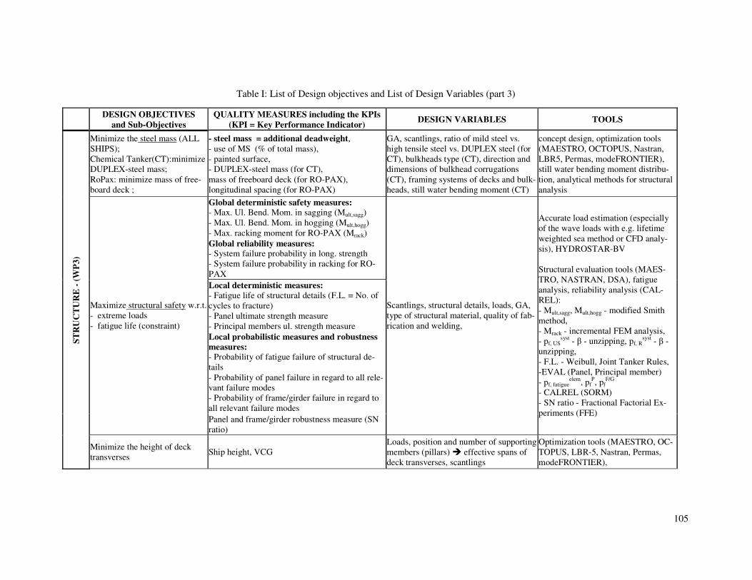
105

Table I: List of Design objectives and List of Design Variables (part 3)

Minimize the steel mass (ALL

SHIPS);

Chemical Tanker(CT):minimize

DUPLEX-steel mass;

RoPax: minimize mass of free-

board deck ;

- steel mass = additional deadweight,

- use of MS (% of total mass),

- painted surface,

- DUPLEX-steel mass (for CT),

mass of freeboard deck (for RO-PAX),

longitudinal spacing (for RO-PAX)

GA, scantlings, ratio of mild steel vs.

high tensile steel vs. DUPLEX steel (for

CT), bulkheads type (CT), direction and

dimensions of bulkhead corrugations

(CT), framing systems of decks and bulk-

heads, still water bending moment (CT)

concept design, optimization tools

(MAESTRO, OCTOPUS, Nastran,

LBR5, Permas, modeFRONTIER),

still water bending moment distribu-

tion, analytical methods for structural

analysis

Global deterministic safety measures: - Max. Ul. Bend. Mom. in sagging (Mult,sagg)

- Max. Ul. Bend. Mom. in hogging (Mult,hogg)

- Max. racking moment for RO-PAX (Mrack)

Global reliability measures: - System failure probability in long. strength

- System failure probability in racking for RO-

PAX

Local deterministic measures: - Fatigue life of structural details (F.L. = No. of

cycles to fracture)

- Panel ultimate strength measure

- Principal members ul. strength measure

Local probabilistic measures and robustness measures: - Probability of fatigue failure of structural de-

tails

- Probability of panel failure in regard to all rele-

vant failure modes

- Probability of frame/girder failure in regard to

all relevant failure modes

Maximize structural safety w.r.t.

- extreme loads

- fatigue life (constraint)

Panel and frame/girder robustness measure (SN

ratio)

Scantlings, structural details, loads, GA,

type of structural material, quality of fab-

rication and welding,

Accurate load estimation (especially

of the wave loads with e.g. lifetime

weighted sea method or CFD analy-

sis), HYDROSTAR-BV

Structural evaluation tools (MAES-

TRO, NASTRAN, DSA), fatigue

analysis, reliability analysis (CAL-

REL):

- Mult,sagg, Mult,hogg - modified Smith

method,

- Mrack - incremental FEM analysis,

- pf, USsyst

- β - unzipping, pf, Rsyst

- β -

unzipping,

- F.L. - Weibull, Joint Tanker Rules,

-EVAL (Panel, Principal member)

- pf, fatigueelem

, pfP, pf

F/G

- CALREL (SORM)

- SN ratio - Fractional Factorial Ex-

periments (FFE)

ST

RU

CT

UR

E -

(W

P3)

Minimize the height of deck

transverses Ship height, VCG

Loads, position and number of supporting

members (pillars) effective spans of

deck transverses, scantlings

Optimization tools (MAESTRO, OC-

TOPUS, LBR-5, Nastran, Permas,

modeFRONTIER),

DESIGN OBJECTIVES

and Sub-Objectives

QUALITY MEASURES including the KPIs

(KPI = Key Performance Indicator) DESIGN VARIABLES TOOLS

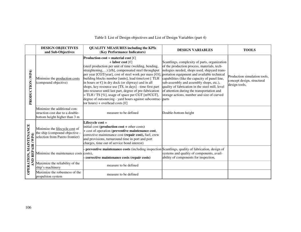
106

Table I: List of Design objectives and List of Design Variables (part 4)

DESIGN OBJECTIVES

and Sub-Objectives

QUALITY MEASURES including the KPIs

(Key Performance Indicators) DESIGN VARIABLES TOOLS

Minimize the production costs

(compound objective)

Production cost = material cost [€]

+ labor cost [€]

(steel production per unit of time (welding, bending,

straightening,…) [t/h], compensated steel throughput

per year [CGT/year], cost of steel work per mass [€/t],

building blocks number [units], lead time/cost [ TLH

in hours or €] in dry dock (or slipway) and in all

shops, key resource use [TS, in days] - time first part

into resource until last part, degree of pre-fabrication

= TLH / TS [%], usage of space per CGT [m²/CGT],

degree of outsourcing - yard hours against subcontrac-

tor hours) + overhead costs [€]

Scantlings, complexity of parts, organization

of the production process, materials, tech-

nologies needed, shops used, shipyard trans-

portation equipment and available technical

capabilities (like the capacity of panel line,

sub-assembly and assembly shops, etc.),

quality of fabrication in the steel mill, level

of attention during the transportation and

storage actions, number and size of curved

parts

Production simulation tools,

concept design, structural

design tools,

PR

OD

UC

TIO

N (

WP

4)

Minimize the additional con-

struction cost due to a double-

bottom height higher than 3 m

measure to be defined Double-bottom height

Minimize the lifecycle cost of

the ship (compound objective -

selection from Pareto frontier)

Lifecycle cost =

initial cost (production cost + other costs)

+ cost of operation (preventive maintenance cost, corrective maintenance cost (repair cost), fuel, crew

and provisions, turnaround time in port and port

charges, time out of service bond interest)

Minimize the maintenance costs

- preventive maintenance costs (including inspection

costs),

- corrective maintenance costs (repair costs)

Scantlings, quality of fabrication, design of

systems and quality of components, avail-

ability of components for inspection,

Maximize the reliability of the

ship’s machinery measure to be defined

OP

ER

AT

ION

, M

AIN

TE

NA

NC

E

AN

D R

EP

AIR

(W

P4)

Maximize the robustness of the

propulsion system measure to be defined

107

Structural Optimization of a 220 000 m³ LNG Carrier

Catalin Toderan, ANAST-ULG, Liege/Belgium, Catalin.Toderan@ulg.ac.be

Jean-Louis Guillaume-Combecave, Akeryards, Saint Nazaire/France,

jean-louis.guillaume-combecave@akeryards.com

Michel Boukaert, EXMAR, Antwerp/Belgium, improve@exmar.be

André Hage, DN&T, Liege/Belgium, a.hage@dn-t.be

Olivier Cartier, Bureau Veritas, Paris/France, olivier.cartier@bureauveritas.com

Jean-David Caprace, ANAST-ULG, Liege/Belgium, jd.caprace@ulg.ac.be

Amirouche Amrane, ANAST-ULG, Liege/Belgium, A.Amrane@ulg.ac.be

Adrian Constantinescu, ANAST-ULG, Liege/Belgium, A.constantinescu@ulg.ac.be

Eugen Pircalabu, ANAST-ULG, Liege/Belgium, Eugen.Pircalabu@ulg.ac.be

Philippe Rigo, ANAST-ULG, Liege/Belgium, ph.rigo@ulg.ac.be

Abstract

This paper relates to the development of a new concept of 220.000 m³ LNG designed by AKERYARDS

France. This work is performed in the framework of FP6 IMPROVE project. The first phase of the

activity related to the identification of stakeholder’s requirements and the definition of key

performance indicators. In parallel, several calculations have been performed to test the existing tools

and to evaluate the potential gain at the concept design. These activities, associated with the definition

of a 220000 m³ QuatarFlex prototype, including the aspects related to the naval architecture and

general arrangement, have been re-grouped in the so-called “first design loop”. The second phase

concerns the development of new modules to be integrated in the optimization tools in order to satisfy

the requirements defined in the first phase. The final phase will be the application of the new

(improved) optimization tools for the final LNG product. We highlight that the main target will be the

multi-objective structural optimization of the prototype defined by “the first design loop”. However,

some feed-back concerning the naval architecture point of view could be expected in this phase. The

aim of the paper is to present the results of the first phase, as well as an overview of the analyses

carried out during the “first design loop”. Details about the different methodologies proposed for the

second phase of the development are given.

1. Introduction

The development of a new LNG concept is one of the targets of the FP6 IMPROVE project, Rigo et

al. (2008). Obviously, the improved LNG product should satisfy the requirements from different

stakeholders involved in LNG market (shipyards and ship-owners / operators) and to take into account

the needs expressed by the design offices. In the same time, it is very important to assess the

performance of this development, so to quantify the improvement (gain).

A general overview of the IMPROVE framework, describing the different phases of the project and

the choice of different strategies for the development, is given in Rigo et al. (2008). We highlight the

fact that the major part of IMPROVE activity relates to the structural optimization and for this reason

all the investigations and analysis presented here are oriented to the structural design.

2. Shipyard and ship-owner requirements for a new generation of LNG carriers

One of the most important phase of IMPROVE activity was to identify, to investigate and to select

shipyards and ship-owners requirements related to LNG product. The main partners involved on this

task, AKERYARDS France (shipyard point of view) and EXMAR (ship-owner point of view),

formulated an exhaustive list of requirements reviewed, commented and clarified by ANAST and

DN&T (design office point of view).

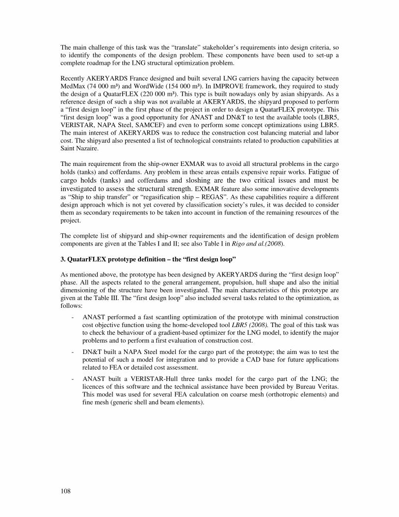
108

The main challenge of this task was the “translate” stakeholder’s requirements into design criteria, so

to identify the components of the design problem. These components have been used to set-up a

complete roadmap for the LNG structural optimization problem.

Recently AKERYARDS France designed and built several LNG carriers having the capacity between

MedMax (74 000 m³) and WordWide (154 000 m³). In IMPROVE framework, they required to study

the design of a QuatarFLEX (220 000 m³). This type is built nowadays only by asian shipyards. As a

reference design of such a ship was not available at AKERYARDS, the shipyard proposed to perform

a “first design loop” in the first phase of the project in order to design a QuatarFLEX prototype. This

“first design loop” was a good opportunity for ANAST and DN&T to test the available tools (LBR5,

VERISTAR, NAPA Steel, SAMCEF) and even to perform some concept optimizations using LBR5.

The main interest of AKERYARDS was to reduce the construction cost balancing material and labor

cost. The shipyard also presented a list of technological constraints related to production capabilities at

Saint Nazaire.

The main requirement from the ship-owner EXMAR was to avoid all structural problems in the cargo

holds (tanks) and cofferdams. Any problem in these areas entails expensive repair works. Fatigue of

cargo holds (tanks) and cofferdams and sloshing are the two critical issues and must be

investigated to assess the structural strength. EXMAR feature also some innovative developments

as “Ship to ship transfer” or “regasification ship – REGAS”. As these capabilities require a different

design approach which is not yet covered by classification society’s rules, it was decided to consider

them as secondary requirements to be taken into account in function of the remaining resources of the

project.

The complete list of shipyard and ship-owner requirements and the identification of design problem

components are given at the Tables I and II; see also Table I in Rigo and al.(2008).

3. QuatarFLEX prototype definition – the “first design loop”

As mentioned above, the prototype has been designed by AKERYARDS during the “first design loop”

phase. All the aspects related to the general arrangement, propulsion, hull shape and also the initial

dimensioning of the structure have been investigated. The main characteristics of this prototype are

given at the Table III. The “first design loop” also included several tasks related to the optimization, as

follows:

- ANAST performed a fast scantling optimization of the prototype with minimal construction

cost objective function using the home-developed tool LBR5 (2008). The goal of this task was

to check the behaviour of a gradient-based optimizer for the LNG model, to identify the major

problems and to perform a first evaluation of construction cost.

- DN&T built a NAPA Steel model for the cargo part of the prototype; the aim was to test the

potential of such a model for integration and to provide a CAD base for future applications

related to FEA or detailed cost assessment.

- ANAST built a VERISTAR-Hull three tanks model for the cargo part of the LNG; the

licences of this software and the technical assistance have been provided by Bureau Veritas.

This model was used for several FEA calculation on coarse mesh (orthotropic elements) and

fine mesh (generic shell and beam elements).

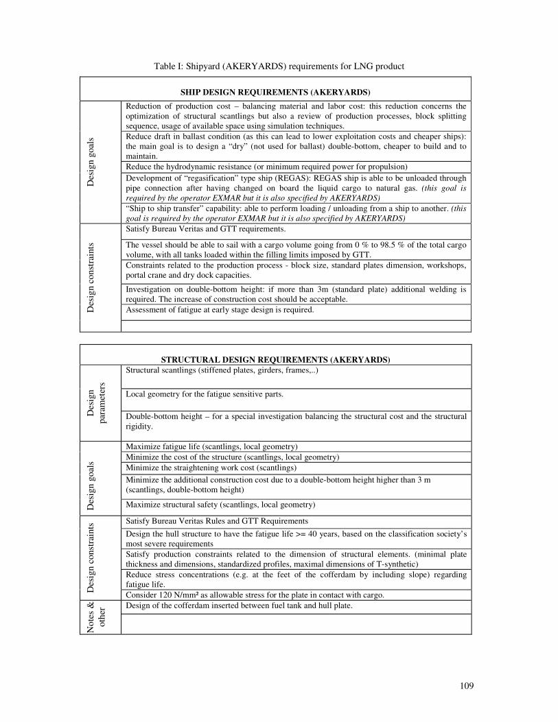
109

Table I: Shipyard (AKERYARDS) requirements for LNG product

SHIP DESIGN REQUIREMENTS (AKERYARDS)

Reduction of production cost – balancing material and labor cost: this reduction concerns the

optimization of structural scantlings but also a review of production processes, block splitting

sequence, usage of available space using simulation techniques.

Reduce draft in ballast condition (as this can lead to lower exploitation costs and cheaper ships):

the main goal is to design a “dry” (not used for ballast) double-bottom, cheaper to build and to

maintain.

Reduce the hydrodynamic resistance (or minimum required power for propulsion)

Development of “regasification” type ship (REGAS): REGAS ship is able to be unloaded through

pipe connection after having changed on board the liquid cargo to natural gas. (this goal is

required by the operator EXMAR but it is also specified by AKERYARDS)

Des

ign g

oal

s

“Ship to ship transfer” capability: able to perform loading / unloading from a ship to another. (this

goal is required by the operator EXMAR but it is also specified by AKERYARDS)

Satisfy Bureau Veritas and GTT requirements.

The vessel should be able to sail with a cargo volume going from 0 % to 98.5 % of the total cargo

volume, with all tanks loaded within the filling limits imposed by GTT.

Constraints related to the production process - block size, standard plates dimension, workshops,

portal crane and dry dock capacities.

Investigation on double-bottom height: if more than 3m (standard plate) additional welding is

required. The increase of construction cost should be acceptable.

Assessment of fatigue at early stage design is required. Des

ign c

on

stra

ints

STRUCTURAL DESIGN REQUIREMENTS (AKERYARDS)

Structural scantlings (stiffened plates, girders, frames,..)

Local geometry for the fatigue sensitive parts.

Des

ign

par

amet

ers

Double-bottom height – for a special investigation balancing the structural cost and the structural

rigidity.

Maximize fatigue life (scantlings, local geometry)

Minimize the cost of the structure (scantlings, local geometry)

Minimize the straightening work cost (scantlings)

Minimize the additional construction cost due to a double-bottom height higher than 3 m

(scantlings, double-bottom height)

Des

ign g

oal

s

Maximize structural safety (scantlings, local geometry)

Satisfy Bureau Veritas Rules and GTT Requirements

Design the hull structure to have the fatigue life >= 40 years, based on the classification society’s

most severe requirements

Satisfy production constraints related to the dimension of structural elements. (minimal plate

thickness and dimensions, standardized profiles, maximal dimensions of T-synthetic)

Reduce stress concentrations (e.g. at the feet of the cofferdam by including slope) regarding

fatigue life.

Des

ign c

onst

rain

ts

Consider 120 N/mm² as allowable stress for the plate in contact with cargo.

Design of the cofferdam inserted between fuel tank and hull plate.

No

tes

&

oth

er

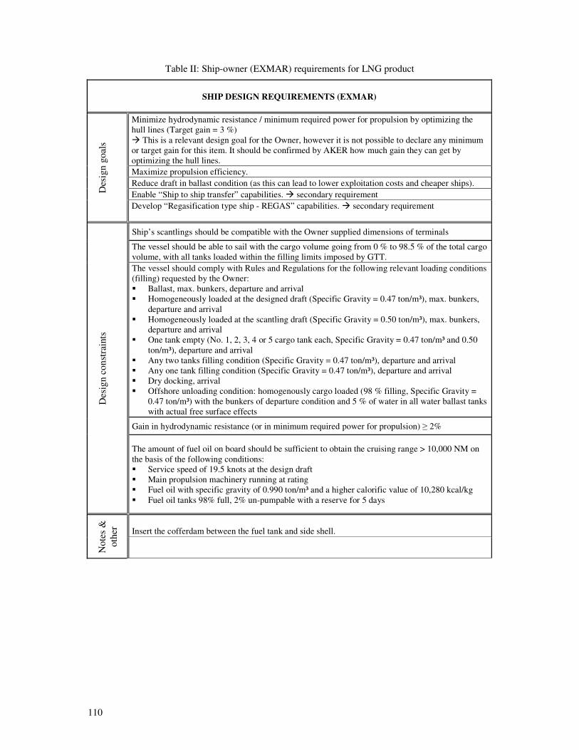
110

Table II: Ship-owner (EXMAR) requirements for LNG product

SHIP DESIGN REQUIREMENTS (EXMAR)

Minimize hydrodynamic resistance / minimum required power for propulsion by optimizing the

hull lines (Target gain = 3 %)

This is a relevant design goal for the Owner, however it is not possible to declare any minimum

or target gain for this item. It should be confirmed by AKER how much gain they can get by

optimizing the hull lines.

Maximize propulsion efficiency.

Reduce draft in ballast condition (as this can lead to lower exploitation costs and cheaper ships).

Enable “Ship to ship transfer” capabilities. secondary requirement

Des

ign g

oal

s

Develop “Regasification type ship - REGAS” capabilities. secondary requirement

Ship’s scantlings should be compatible with the Owner supplied dimensions of terminals

The vessel should be able to sail with the cargo volume going from 0 % to 98.5 % of the total cargo

volume, with all tanks loaded within the filling limits imposed by GTT.

The vessel should comply with Rules and Regulations for the following relevant loading conditions

(filling) requested by the Owner:

Ballast, max. bunkers, departure and arrival

Homogeneously loaded at the designed draft (Specific Gravity = 0.47 ton/m³), max. bunkers,

departure and arrival

Homogeneously loaded at the scantling draft (Specific Gravity = 0.50 ton/m³), max. bunkers,

departure and arrival

One tank empty (No. 1, 2, 3, 4 or 5 cargo tank each, Specific Gravity = 0.47 ton/m³ and 0.50

ton/m³), departure and arrival

Any two tanks filling condition (Specific Gravity = 0.47 ton/m³), departure and arrival

Any one tank filling condition (Specific Gravity = 0.47 ton/m³), departure and arrival

Dry docking, arrival

Offshore unloading condition: homogenously cargo loaded (98 % filling, Specific Gravity =

0.47 ton/m³) with the bunkers of departure condition and 5 % of water in all water ballast tanks

with actual free surface effects

Gain in hydrodynamic resistance (or in minimum required power for propulsion) ≥ 2%

Des

ign c

on

stra

ints

The amount of fuel oil on board should be sufficient to obtain the cruising range > 10,000 NM on

the basis of the following conditions: Service speed of 19.5 knots at the design draft

Main propulsion machinery running at rating

Fuel oil with specific gravity of 0.990 ton/m³ and a higher calorific value of 10,280 kcal/kg

Fuel oil tanks 98% full, 2% un-pumpable with a reserve for 5 days

Insert the cofferdam between the fuel tank and side shell.

Note

s &

oth

er

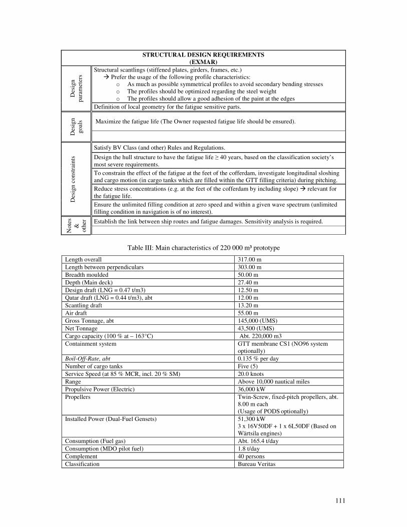
111

STRUCTURAL DESIGN REQUIREMENTS

(EXMAR)

Structural scantlings (stiffened plates, girders, frames, etc.)

Prefer the usage of the following profile characteristics:

o As much as possible symmetrical profiles to avoid secondary bending stresses

o The profiles should be optimized regarding the steel weight

o The profiles should allow a good adhesion of the paint at the edges

Des

ign

par

amet

ers

Definition of local geometry for the fatigue sensitive parts.

Maximize the fatigue life (The Owner requested fatigue life should be ensured).

Des

ign

go

als

Satisfy BV Class (and other) Rules and Regulations.

Design the hull structure to have the fatigue life ≥ 40 years, based on the classification society’s

most severe requirements.

To constrain the effect of the fatigue at the feet of the cofferdam, investigate longitudinal sloshing

and cargo motion (in cargo tanks which are filled within the GTT filling criteria) during pitching.

Reduce stress concentrations (e.g. at the feet of the cofferdam by including slope) relevant for

the fatigue life.

Des

ign

co

nst

rain

ts

Ensure the unlimited filling condition at zero speed and within a given wave spectrum (unlimited

filling condition in navigation is of no interest).

Establish the link between ship routes and fatigue damages. Sensitivity analysis is required.

Note

s

&

oth

er

Table III: Main characteristics of 220 000 m³ prototype

Length overall 317.00 m

Length between perpendiculars 303.00 m

Breadth moulded 50.00 m

Depth (Main deck) 27.40 m

Design draft (LNG = 0.47 t/m3) 12.50 m

Qatar draft (LNG = 0.44 t/m3), abt 12.00 m

Scantling draft 13.20 m

Air draft 55.00 m

Gross Tonnage, abt 145,000 (UMS)

Net Tonnage 43,500 (UMS)

Cargo capacity (100 % at – 163°C) Abt. 220,000 m3

Containment system GTT membrane CS1 (NO96 system

optionally)

Boil-Off-Rate, abt 0.135 % per day

Number of cargo tanks Five (5)

Service Speed (at 85 % MCR, incl. 20 % SM) 20.0 knots

Range Above 10,000 nautical miles

Propulsive Power (Electric) 36,000 kW

Propellers Twin-Screw, fixed-pitch propellers, abt.

8.00 m each

(Usage of PODS optionally)

Installed Power (Dual-Fuel Gensets) 51,300 kW

3 x 16V50DF + 1 x 6L50DF (Based on

Wärtsila engines)

Consumption (Fuel gas) Abt. 165.4 t/day

Consumption (MDO pilot fuel) 1.8 t/day

Complement 40 persons

Classification Bureau Veritas

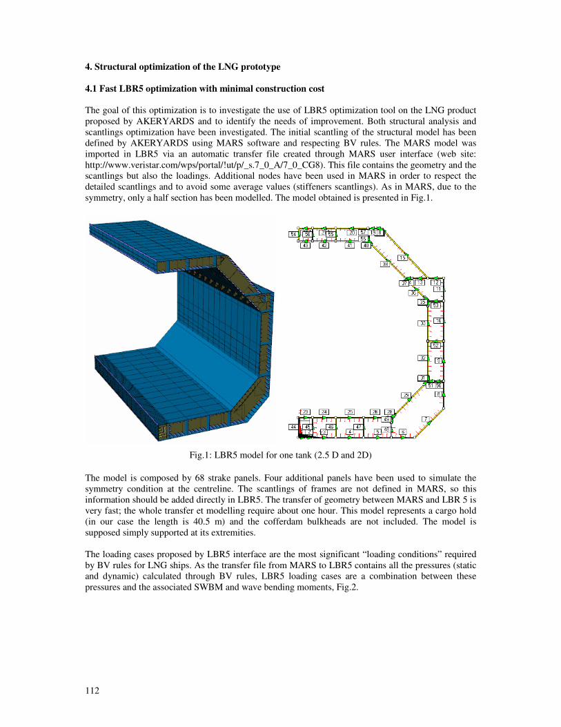
112

4. Structural optimization of the LNG prototype

4.1 Fast LBR5 optimization with minimal construction cost

The goal of this optimization is to investigate the use of LBR5 optimization tool on the LNG product

proposed by AKERYARDS and to identify the needs of improvement. Both structural analysis and

scantlings optimization have been investigated. The initial scantling of the structural model has been

defined by AKERYARDS using MARS software and respecting BV rules. The MARS model was

imported in LBR5 via an automatic transfer file created through MARS user interface (web site:

http://www.veristar.com/wps/portal/!ut/p/_s.7_0_A/7_0_CG8). This file contains the geometry and the

scantlings but also the loadings. Additional nodes have been used in MARS in order to respect the

detailed scantlings and to avoid some average values (stiffeners scantlings). As in MARS, due to the

symmetry, only a half section has been modelled. The model obtained is presented in Fig.1.

Fig.1: LBR5 model for one tank (2.5 D and 2D)

The model is composed by 68 strake panels. Four additional panels have been used to simulate the

symmetry condition at the centreline. The scantlings of frames are not defined in MARS, so this

information should be added directly in LBR5. The transfer of geometry between MARS and LBR 5 is

very fast; the whole transfer et modelling require about one hour. This model represents a cargo hold

(in our case the length is 40.5 m) and the cofferdam bulkheads are not included. The model is

supposed simply supported at its extremities.

The loading cases proposed by LBR5 interface are the most significant “loading conditions” required

by BV rules for LNG ships. As the transfer file from MARS to LBR5 contains all the pressures (static

and dynamic) calculated through BV rules, LBR5 loading cases are a combination between these

pressures and the associated SWBM and wave bending moments, Fig.2.

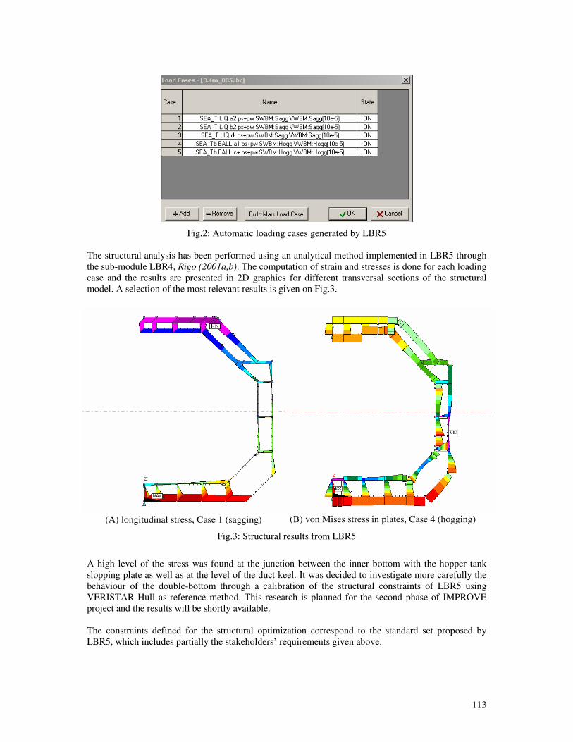
113

Fig.2: Automatic loading cases generated by LBR5

The structural analysis has been performed using an analytical method implemented in LBR5 through

the sub-module LBR4, Rigo (2001a,b). The computation of strain and stresses is done for each loading

case and the results are presented in 2D graphics for different transversal sections of the structural

model. A selection of the most relevant results is given on Fig.3.

(A) longitudinal stress, Case 1 (sagging) (B) von Mises stress in plates, Case 4 (hogging)

Fig.3: Structural results from LBR5

A high level of the stress was found at the junction between the inner bottom with the hopper tank

slopping plate as well as at the level of the duct keel. It was decided to investigate more carefully the

behaviour of the double-bottom through a calibration of the structural constraints of LBR5 using

VERISTAR Hull as reference method. This research is planned for the second phase of IMPROVE

project and the results will be shortly available.

The constraints defined for the structural optimization correspond to the standard set proposed by

LBR5, which includes partially the stakeholders’ requirements given above.

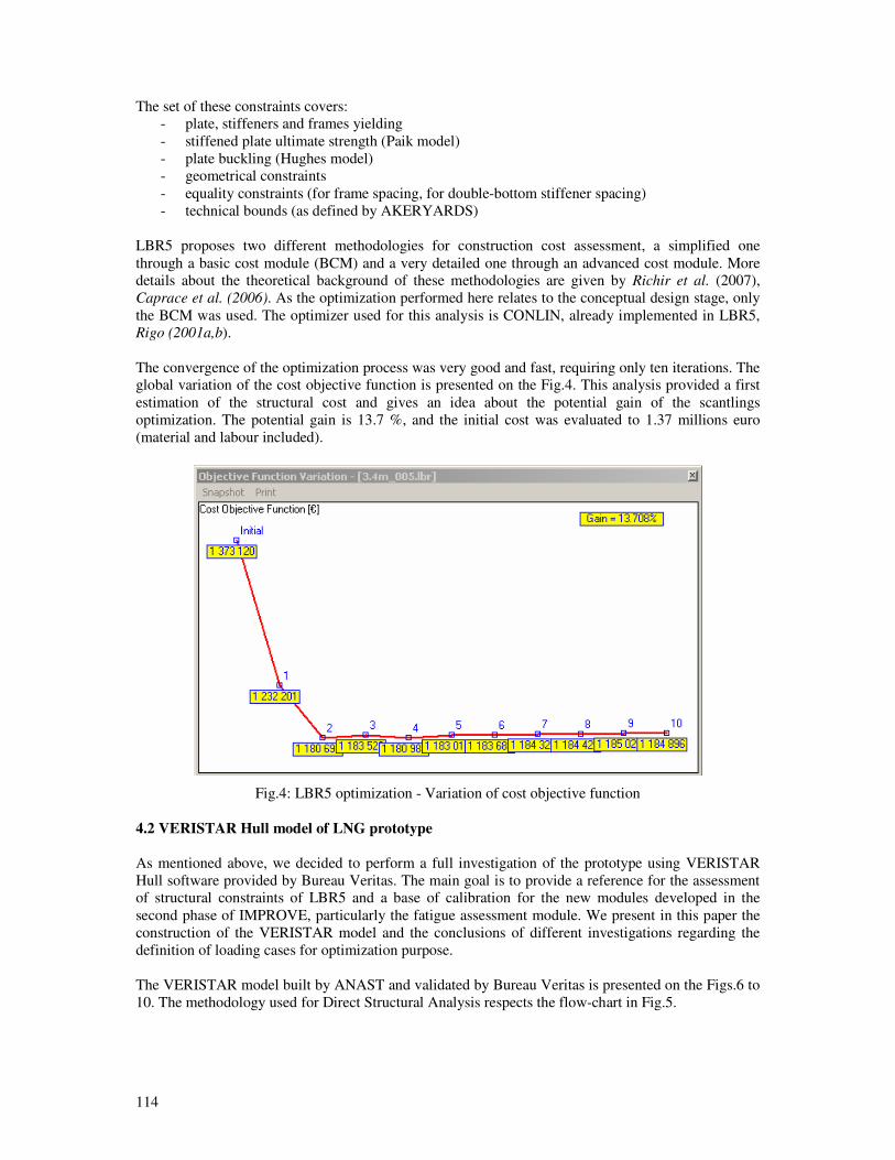
114

The set of these constraints covers:

- plate, stiffeners and frames yielding

- stiffened plate ultimate strength (Paik model)

- plate buckling (Hughes model)

- geometrical constraints

- equality constraints (for frame spacing, for double-bottom stiffener spacing)

- technical bounds (as defined by AKERYARDS)

LBR5 proposes two different methodologies for construction cost assessment, a simplified one

through a basic cost module (BCM) and a very detailed one through an advanced cost module. More

details about the theoretical background of these methodologies are given by Richir et al. (2007),

Caprace et al. (2006). As the optimization performed here relates to the conceptual design stage, only

the BCM was used. The optimizer used for this analysis is CONLIN, already implemented in LBR5,

Rigo (2001a,b).

The convergence of the optimization process was very good and fast, requiring only ten iterations. The

global variation of the cost objective function is presented on the Fig.4. This analysis provided a first

estimation of the structural cost and gives an idea about the potential gain of the scantlings

optimization. The potential gain is 13.7 %, and the initial cost was evaluated to 1.37 millions euro

(material and labour included).

Fig.4: LBR5 optimization - Variation of cost objective function

4.2 VERISTAR Hull model of LNG prototype As mentioned above, we decided to perform a full investigation of the prototype using VERISTAR

Hull software provided by Bureau Veritas. The main goal is to provide a reference for the assessment

of structural constraints of LBR5 and a base of calibration for the new modules developed in the

second phase of IMPROVE, particularly the fatigue assessment module. We present in this paper the

construction of the VERISTAR model and the conclusions of different investigations regarding the

definition of loading cases for optimization purpose.

The VERISTAR model built by ANAST and validated by Bureau Veritas is presented on the Figs.6 to

10. The methodology used for Direct Structural Analysis respects the flow-chart in Fig.5.

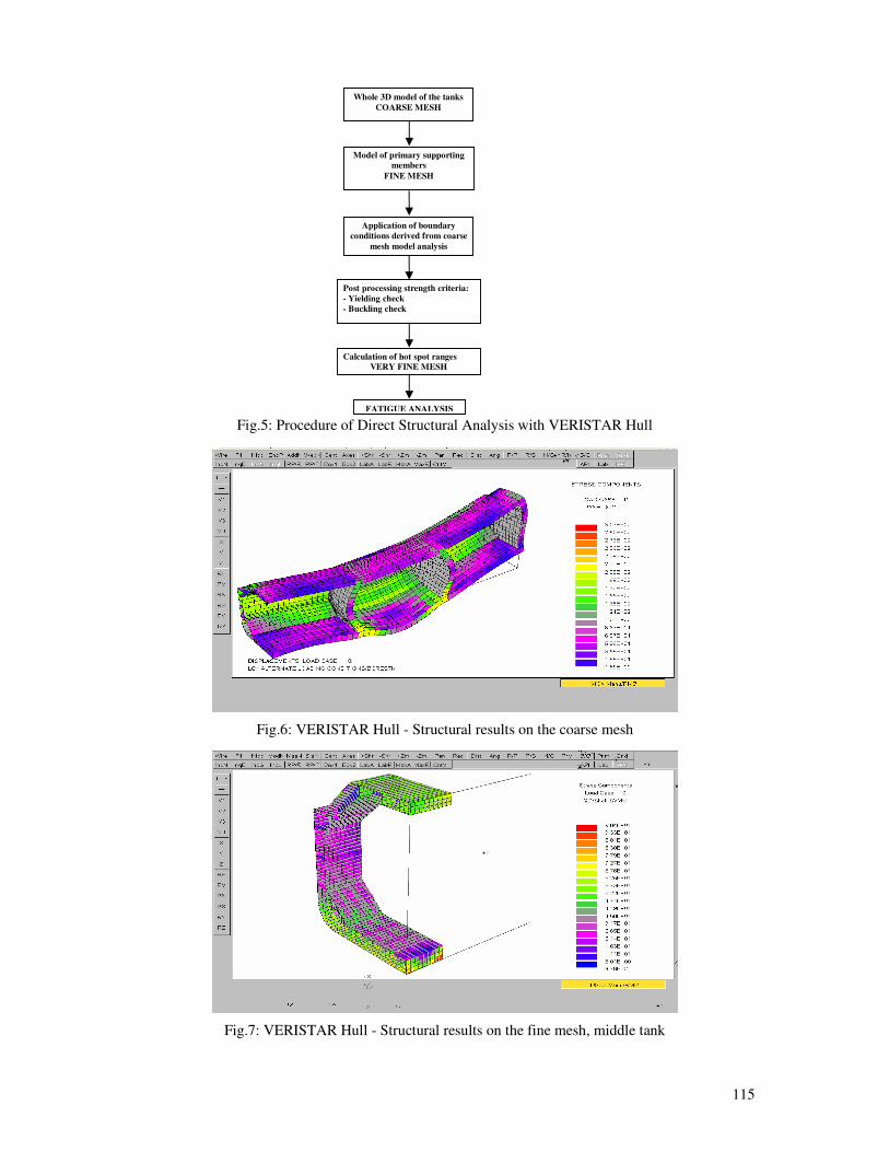
115

Fig.5: Procedure of Direct Structural Analysis with VERISTAR Hull

Fig.6: VERISTAR Hull - Structural results on the coarse mesh

Fig.7: VERISTAR Hull - Structural results on the fine mesh, middle tank

Whole 3D model of the tanks

COARSE MESH

Model of primary supporting members

FINE MESH

Post processing strength criteria:

- Yielding check

- Buckling check

Calculation of hot spot ranges VERY FINE MESH

Application of boundary

conditions derived from coarse

mesh model analysis

FATIGUE ANALYSIS

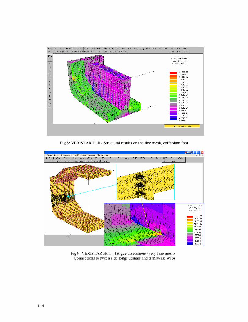
116

Fig.8: VERISTAR Hull - Structural results on the fine mesh, cofferdam foot

Fig.9: VERISTAR Hull – fatigue assessment (very fine mesh) -

Connections between side longitudinals and transverse webs

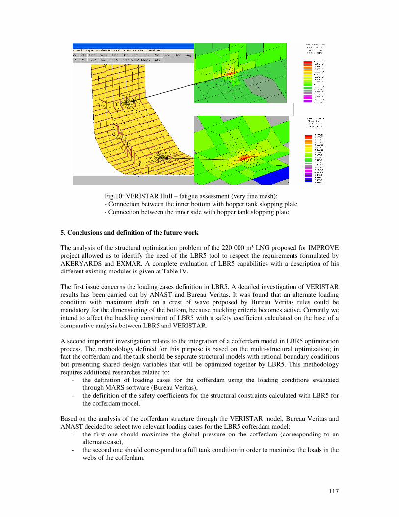
117

Fig.10: VERISTAR Hull – fatigue assessment (very fine mesh):

- Connection between the inner bottom with hopper tank slopping plate

- Connection between the inner side with hopper tank slopping plate

5. Conclusions and definition of the future work

The analysis of the structural optimization problem of the 220 000 m³ LNG proposed for IMPROVE

project allowed us to identify the need of the LBR5 tool to respect the requirements formulated by

AKERYARDS and EXMAR. A complete evaluation of LBR5 capabilities with a description of his

different existing modules is given at Table IV.

The first issue concerns the loading cases definition in LBR5. A detailed investigation of VERISTAR

results has been carried out by ANAST and Bureau Veritas. It was found that an alternate loading

condition with maximum draft on a crest of wave proposed by Bureau Veritas rules could be

mandatory for the dimensioning of the bottom, because buckling criteria becomes active. Currently we

intend to affect the buckling constraint of LBR5 with a safety coefficient calculated on the base of a

comparative analysis between LBR5 and VERISTAR.

A second important investigation relates to the integration of a cofferdam model in LBR5 optimization

process. The methodology defined for this purpose is based on the multi-structural optimization; in

fact the cofferdam and the tank should be separate structural models with rational boundary conditions

but presenting shared design variables that will be optimized together by LBR5. This methodology

requires additional researches related to:

- the definition of loading cases for the cofferdam using the loading conditions evaluated

through MARS software (Bureau Veritas),

- the definition of the safety coefficients for the structural constraints calculated with LBR5 for

the cofferdam model.

Based on the analysis of the cofferdam structure through the VERISTAR model, Bureau Veritas and

ANAST decided to select two relevant loading cases for the LBR5 cofferdam model:

- the first one should maximize the global pressure on the cofferdam (corresponding to an

alternate case),

- the second one should correspond to a full tank condition in order to maximize the loads in the

webs of the cofferdam.

118

In order to allow the automatic definition of these two loading cases, a new integration task has been

started. The goal is to allow the transfer of the load pressures calculated by Bureau Veritas Rules from

MARS to LBR5 optimization tool, in addition to the existing transfer file used for the tank structure.

The computation of the safety factors for structural constraints assessment is done by a comparative

analysis between FEA and LBR5. In order to take into account all the constraints defined in LBR5 and

not only those specified by Bureau Veritas rules, it was decided to perform a parallel FEA using the

generic code SAMCEF. This task is performed by DN&T and the final issue is expected for May

2008.

Finally, it is necessary to develop different modules to assess new constraints to optimization

corresponding to stakeholders requirements. A general overview of these developments is given in

Rigo et al. (2008) and summarised here at Table V.

Acknowledgements

The present paper was supported by the European Commission under the FP6 Sustainable Surface

Transport Programme, namely the STREP project IMPROVE (Design of Improved and Competitive

Products using an Integrated Decision Support System for Ship Production and Operation), Contract

No. FP6 – 031382. The European Community and the authors shall not in any way be liable or

responsible for the use of any such knowledge, information or data, or of the consequences thereof.

References

CAPRACE, J.D.; RIGO, P.; WARNOTTE, R.; LE VIOL, S. (2006), An analytical cost assessment

module for the detailed design stage, COMPIT’2006, Oegstgeest, pp.335-345

RICHIR, T.; LOSSEAU, N.; PIRCALABU, E.; TODERAN, C.; RIGO, P. (2007), Least cost

optimization of a large passenger vessel, MARSTRUCT ’07, Advancement in Marine Structures, Edt.

Soares-Das, Taylor&Francis Group, pp.483-488

RIGO, P. (2001a), A module-oriented tool for optimum design of stiffened structures, Marine

Structures 14/6, pp611-629

RIGO, P. (2001b), Scantling optimization based on convex linearizations and a dual approach,

Marine Structures 14/6, pp631-649

RIGO, P. (2005), Differential equations of stiffened panels of ship structures & Fourier series

expansions, Ship Technology Research 52, pp.82-100

RIGO, P.; TODERAN, C. (2003), Least cost optimisation of a medium capacity gas carrier,

COMPIT’03, Hamburg, pp.94-107

RIGO, P.; DUNDARA, D.; GUILLAUME-COMBECAVE, J.L.; DOMAGALLO, S.; KLANAC, A.;

ROLAND, F.; TURAN, O.; ZANIC, V.; AMRANE, A.; CONSTANTINESCU, A. (2008), IMPROVE

- Design of improved and competitive products using an integrated decision support system for ship

production and operation, COMPIT’2008, Liege, pp.92-106

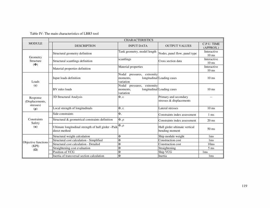
119

Table IV: The main characteristics of LBR5 tool

CHARACTERISTICS MODULE

DESCRIPTION INPUT DATA OUTPUT VALUES C.P.U. TIME

(APPROX.)

Structural geometry definition Tank geometry, model length

Nodes, panel flow, panel type Interactive

10 ms

Structural scantlings definition scantlings

Cross section data Interactive

10 ms

Geometry

Structure

(Φ)

Material properties definition Material properties

Interactive

10 ms

Input loads definition

Nodal pressures, extremity

moments, longitudinal

variation

Loading cases 10 ms

Loads

(ε)

BV rules loads

Nodal pressures, extremity

moments, longitudinal

variation

Loading cases 10 ms

3D Structural Analysis Φ, ε

Primary and secondary

stresses & displacements

-- Response

(Displacements,

stresses)

(ρ) Local strength of longitudinals Φ, ε Lateral stresses 10 ms

Side constraints Φ, Constraints index assessment 1 ms

Structural & geometrical constraints definition Φ, ρ Constraints index assessment 20 ms Constraints

Safety

(α)

Ultimate longitudinal strength of hull girder –Paik

direct method

Φ, ρ Hull girder ultimate vertical

bending moment 50 ms

Structural weight calculation Φ Ship module weight 1ms

Structural cost calculation - Simplified Φ Construction cost 1ms

Structural cost calculation - Detailed Φ Construction cost 10ms

Straightening cost evaluation Φ Straightening 5 ms

Position of VCG Φ Ship VCG 1ms

Objective functions

(KPI)

(Ω)

Inertia of transversal section calculation Φ Inertia 1ms

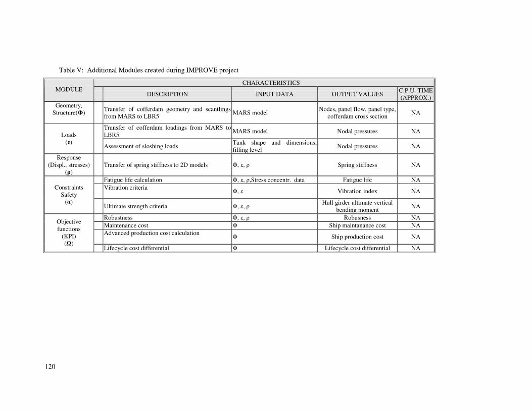
120

Table V: Additional Modules created during IMPROVE project

CHARACTERISTICS MODULE

DESCRIPTION INPUT DATA OUTPUT VALUES C.P.U. TIME

(APPROX.)

Geometry,

Structure(Φ)

Transfer of cofferdam geometry and scantlings

from MARS to LBR5 MARS model

Nodes, panel flow, panel type,

cofferdam cross section NA

Transfer of cofferdam loadings from MARS to

LBR5 MARS model Nodal pressures NA

Loads

(ε)

Assessment of sloshing loads Tank shape and dimensions,

filling level Nodal pressures NA

Response

(Displ., stresses)

(ρ)

Transfer of spring stiffness to 2D models Φ, ε, ρ Spring stiffness NA

Fatigue life calculation Φ, ε, ρ,Stress concentr. data Fatigue life NA

Vibration criteria

Φ, ε Vibration index NA

Constraints

Safety

(α) Ultimate strength criteria Φ, ε, ρ

Hull girder ultimate vertical

bending moment NA

Robustness Φ, ε, ρ Robusness NA

Maintenance cost Φ Ship maintanance cost NA

Advanced production cost calculation

Φ Ship production cost NA

Objective

functions

(KPI)

(Ω) Lifecycle cost differential Φ Lifecycle cost differential NA

121

Integrated Management of Ship Compartments

Fernando Alonso, SENER Ingeniería y Sistemas S.A., Madrid/Spain, fernando.alonso@sener.es

Carlos González, SENER Ingeniería y Sistemas S.A., Madrid/Spain, carlos.gonzalez@sener.es

Antonio Pinto, SENER Ingeniería y Sistemas S.A., Madrid/Spain, antonio.pinto@sener.es

Fernando Zurdo, SENER Ingeniería y Sistemas S.A., Madrid/Spain, fernando.zurdo@sener.es

Abstract

Ship functionality strongly depends on compartments design, which is one of the most relevant

activities in early stages of ship design. In addition, there is a need for this information to be reused

during later stages of the design of the different disciplines, where space reservation and weight

management are just some of the requirements. In order to handle properly compartments and spaces

reservation, a breakdown structure is required to allow the integrated management of compartments

and its associated data. This paper describes the most relevant characteristics of a new tool being

developed in FORAN System as a result of the experience gained during the development of an EU

funded Intership project.

1. Introduction

The ship general arrangement is one of the main tasks to be performed during the initial design of a

new vessel to fulfill all functional and operative requirements, complying with all the applicable

regulations at the same time. A fundamental part of this general arrangement is the definition and

management of all ship spaces as well as the preliminary layout of the main equipment, weapons (for

naval vessels) and accommodation items on these compartments and on the main deck areas.

As most of the cost related to the manufacturing and operation of a ship is compromised in the early

design stage, it is of paramount importance to define the ship with the largest precision and detail

possible at this stage. On the other hand, early designs are usually developed in very short period of

times and many alternatives and options have to be carefully analyzed in this period, so it is very

important to dispose of especially fast and flexible design tools for this stage. Especially relevant is

also the capability of sharing the information produced with the main naval architecture and

calculation tools used in early design.

This paper presents the most relevant characteristics of a new tool for the definition and management

of the ship compartments and for the generation of a ship general arrangement model at the early

design stages, using an efficient and innovative approach. This new approach is based on the

experience of SENER as ship designer and as developer of the FORAN CAD/CAM System for ship

design, but above all on the feedback and requirements of the main FORAN users.

2. The background: The Intership I-3 and I-4 Subprojects

The work developed in this paper is partly based on the results of the following Intership Subprojects:

- I-3 Early Design: Integrated Concept

- I-4 Early Design: Methods and Tools

SENER participated as the Main Technological Supplier in these two projects, together with the main

Intership Partners (Navantia, Fincantieri, Aker Yards, Meyer Werft) and other technological suppliers

(Sirenha, University of Strathclyde, etc). Navantia leaded the two projects.

The objective of the first Subproject was to define the main requirements for the development of

design tools for the early design stage.

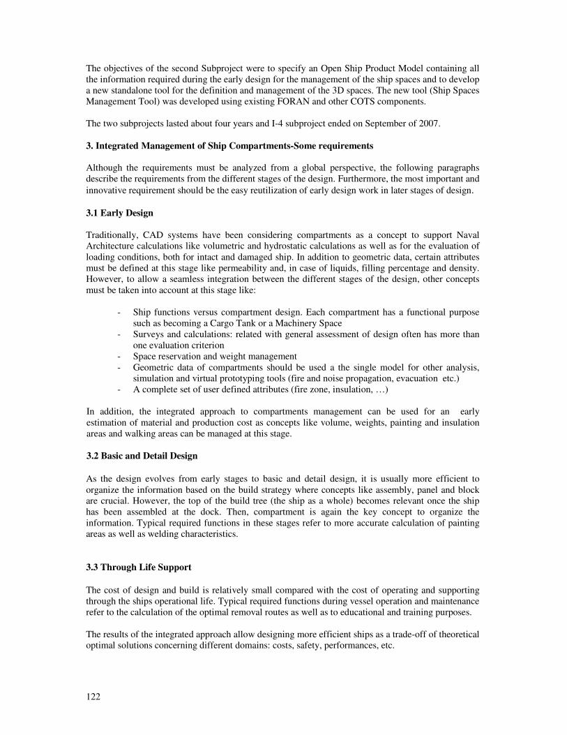
122

The objectives of the second Subproject were to specify an Open Ship Product Model containing all

the information required during the early design for the management of the ship spaces and to develop

a new standalone tool for the definition and management of the 3D spaces. The new tool (Ship Spaces

Management Tool) was developed using existing FORAN and other COTS components.

The two subprojects lasted about four years and I-4 subproject ended on September of 2007.

3. Integrated Management of Ship Compartments-Some requirements

Although the requirements must be analyzed from a global perspective, the following paragraphs

describe the requirements from the different stages of the design. Furthermore, the most important and

innovative requirement should be the easy reutilization of early design work in later stages of design.

3.1 Early Design

Traditionally, CAD systems have been considering compartments as a concept to support Naval

Architecture calculations like volumetric and hydrostatic calculations as well as for the evaluation of

loading conditions, both for intact and damaged ship. In addition to geometric data, certain attributes

must be defined at this stage like permeability and, in case of liquids, filling percentage and density.

However, to allow a seamless integration between the different stages of the design, other concepts

must be taken into account at this stage like:

- Ship functions versus compartment design. Each compartment has a functional purpose

such as becoming a Cargo Tank or a Machinery Space

- Surveys and calculations: related with general assessment of design often has more than

one evaluation criterion

- Space reservation and weight management

- Geometric data of compartments should be used a the single model for other analysis,

simulation and virtual prototyping tools (fire and noise propagation, evacuation etc.)

- A complete set of user defined attributes (fire zone, insulation, …)

In addition, the integrated approach to compartments management can be used for an early

estimation of material and production cost as concepts like volume, weights, painting and insulation

areas and walking areas can be managed at this stage.

3.2 Basic and Detail Design

As the design evolves from early stages to basic and detail design, it is usually more efficient to

organize the information based on the build strategy where concepts like assembly, panel and block

are crucial. However, the top of the build tree (the ship as a whole) becomes relevant once the ship

has been assembled at the dock. Then, compartment is again the key concept to organize the

information. Typical required functions in these stages refer to more accurate calculation of painting

areas as well as welding characteristics.

3.3 Through Life Support

The cost of design and build is relatively small compared with the cost of operating and supporting

through the ships operational life. Typical required functions during vessel operation and maintenance

refer to the calculation of the optimal removal routes as well as to educational and training purposes.

The results of the integrated approach allow designing more efficient ships as a trade-off of theoretical

optimal solutions concerning different domains: costs, safety, performances, etc.

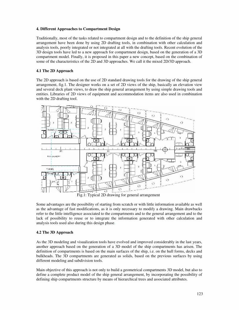
123

4. Different Approaches to Compartment Design

Traditionally, most of the tasks related to compartment design and to the definition of the ship general

arrangement have been done by using 2D drafting tools, in combination with other calculation and

analysis tools, poorly integrated or not integrated at all with the drafting tools. Recent evolution of the

3D design tools have led to a new approach for compartment design, based on the generation of a 3D

compartment model. Finally, it is proposed in this paper a new concept, based on the combination of

some of the characteristics of the 2D and 3D approaches. We call it the mixed 2D/3D approach.

4.1 The 2D Approach

The 2D approach is based on the use of 2D standard drawing tools for the drawing of the ship general

arrangement, fig.1. The designer works on a set of 2D views of the ship, basically an elevation view

and several deck plant views, to draw the ship general arrangement by using simple drawing tools and

entities. Libraries of 2D views of equipment and accommodation items are also used in combination

with the 2D drafting tool.

Fig.1: Typical 2D drawing for general arrangement

Some advantages are the possibility of starting from scratch or with little information available as well

as the advantage of fast modifications, as it is only necessary to modify a drawing. Main drawbacks

refer to the little intelligence associated to the compartments and to the general arrangement and to the

lack of possibility to reuse or to integrate the information generated with other calculation and

analysis tools used also during this design phase.

4.2 The 3D Approach

As the 3D modeling and visualization tools have evolved and improved considerably in the last years,

another approach based on the generation of a 3D model of the ship compartments has arisen. The

definition of compartments is based on the main surfaces of the ship, i.e. on the hull forms, decks and

bulkheads. The 3D compartments are generated as solids, based on the previous surfaces by using

different modeling and subdivision tools.

Main objective of this approach is not only to build a geometrical compartments 3D model, but also to

define a complete product model of the ship general arrangement, by incorporating the possibility of

defining ship compartments structure by means of hierarchical trees and associated attributes.

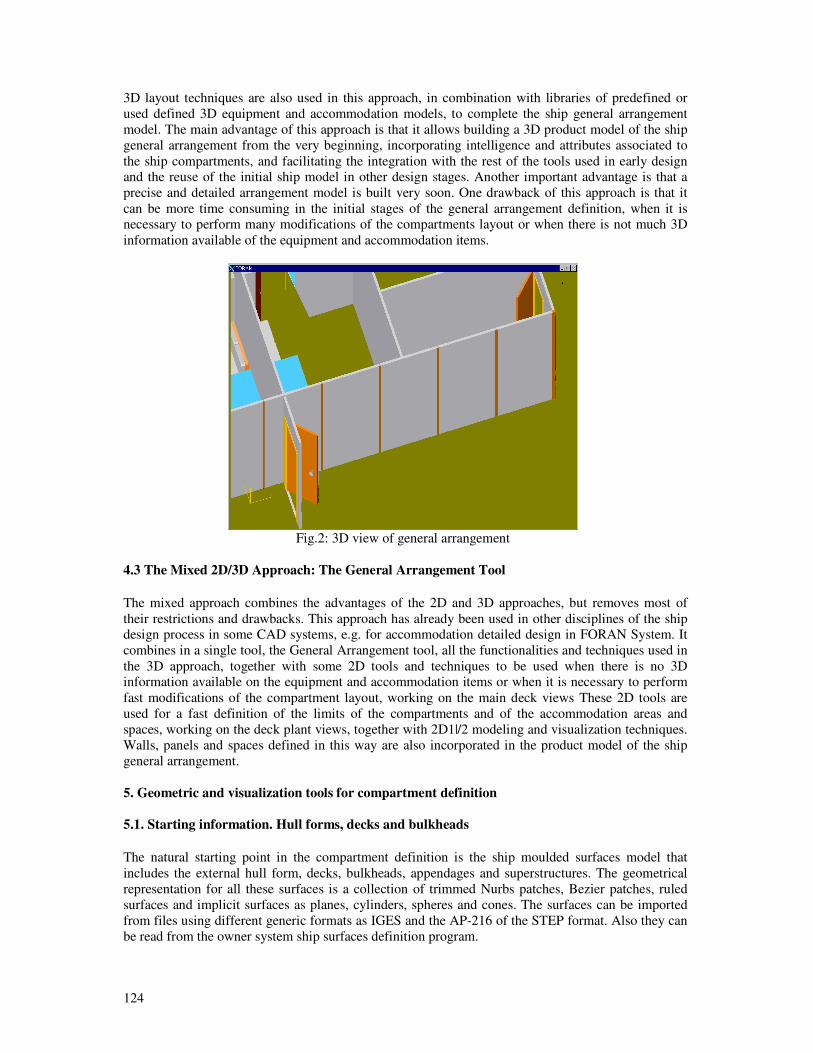
124

3D layout techniques are also used in this approach, in combination with libraries of predefined or

used defined 3D equipment and accommodation models, to complete the ship general arrangement

model. The main advantage of this approach is that it allows building a 3D product model of the ship

general arrangement from the very beginning, incorporating intelligence and attributes associated to

the ship compartments, and facilitating the integration with the rest of the tools used in early design

and the reuse of the initial ship model in other design stages. Another important advantage is that a

precise and detailed arrangement model is built very soon. One drawback of this approach is that it

can be more time consuming in the initial stages of the general arrangement definition, when it is

necessary to perform many modifications of the compartments layout or when there is not much 3D

information available of the equipment and accommodation items.

Fig.2: 3D view of general arrangement

4.3 The Mixed 2D/3D Approach: The General Arrangement Tool

The mixed approach combines the advantages of the 2D and 3D approaches, but removes most of

their restrictions and drawbacks. This approach has already been used in other disciplines of the ship

design process in some CAD systems, e.g. for accommodation detailed design in FORAN System. It

combines in a single tool, the General Arrangement tool, all the functionalities and techniques used in

the 3D approach, together with some 2D tools and techniques to be used when there is no 3D

information available on the equipment and accommodation items or when it is necessary to perform

fast modifications of the compartment layout, working on the main deck views These 2D tools are

used for a fast definition of the limits of the compartments and of the accommodation areas and

spaces, working on the deck plant views, together with 2D1|/2 modeling and visualization techniques.

Walls, panels and spaces defined in this way are also incorporated in the product model of the ship

general arrangement.

5. Geometric and visualization tools for compartment definition

5.1. Starting information. Hull forms, decks and bulkheads

The natural starting point in the compartment definition is the ship moulded surfaces model that

includes the external hull form, decks, bulkheads, appendages and superstructures. The geometrical

representation for all these surfaces is a collection of trimmed Nurbs patches, Bezier patches, ruled

surfaces and implicit surfaces as planes, cylinders, spheres and cones. The surfaces can be imported

from files using different generic formats as IGES and the AP-216 of the STEP format. Also they can

be read from the owner system ship surfaces definition program.

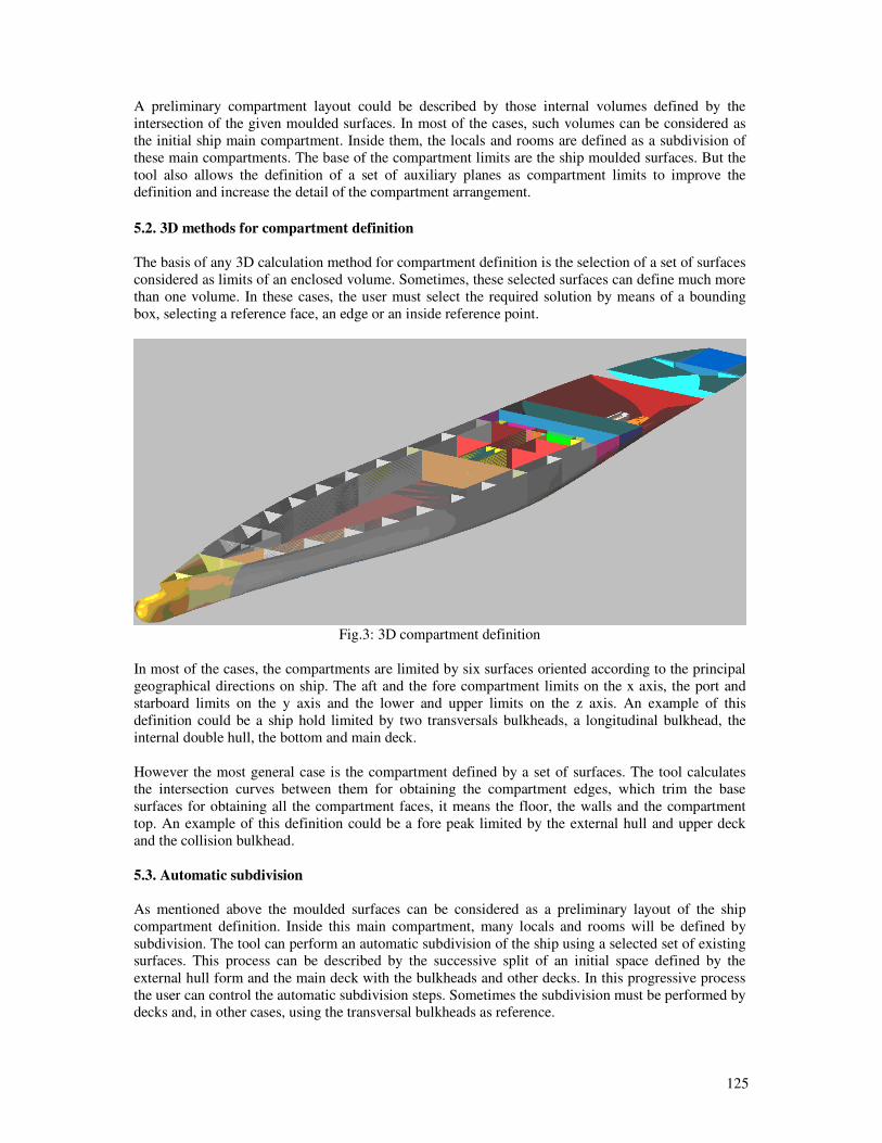
125

A preliminary compartment layout could be described by those internal volumes defined by the

intersection of the given moulded surfaces. In most of the cases, such volumes can be considered as

the initial ship main compartment. Inside them, the locals and rooms are defined as a subdivision of

these main compartments. The base of the compartment limits are the ship moulded surfaces. But the

tool also allows the definition of a set of auxiliary planes as compartment limits to improve the

definition and increase the detail of the compartment arrangement.

5.2. 3D methods for compartment definition

The basis of any 3D calculation method for compartment definition is the selection of a set of surfaces

considered as limits of an enclosed volume. Sometimes, these selected surfaces can define much more

than one volume. In these cases, the user must select the required solution by means of a bounding

box, selecting a reference face, an edge or an inside reference point.

Fig.3: 3D compartment definition

In most of the cases, the compartments are limited by six surfaces oriented according to the principal

geographical directions on ship. The aft and the fore compartment limits on the x axis, the port and

starboard limits on the y axis and the lower and upper limits on the z axis. An example of this

definition could be a ship hold limited by two transversals bulkheads, a longitudinal bulkhead, the

internal double hull, the bottom and main deck.

However the most general case is the compartment defined by a set of surfaces. The tool calculates

the intersection curves between them for obtaining the compartment edges, which trim the base

surfaces for obtaining all the compartment faces, it means the floor, the walls and the compartment

top. An example of this definition could be a fore peak limited by the external hull and upper deck

and the collision bulkhead.

5.3. Automatic subdivision

As mentioned above the moulded surfaces can be considered as a preliminary layout of the ship

compartment definition. Inside this main compartment, many locals and rooms will be defined by

subdivision. The tool can perform an automatic subdivision of the ship using a selected set of existing

surfaces. This process can be described by the successive split of an initial space defined by the

external hull form and the main deck with the bulkheads and other decks. In this progressive process

the user can control the automatic subdivision steps. Sometimes the subdivision must be performed by

decks and, in other cases, using the transversal bulkheads as reference.

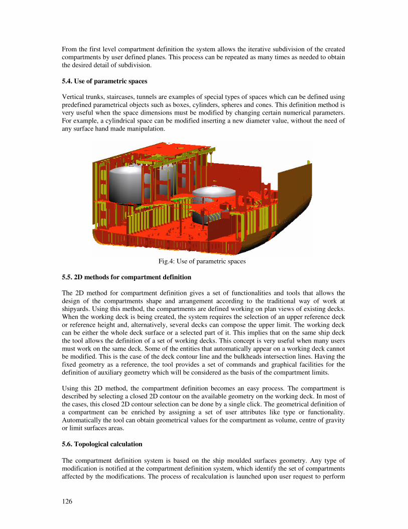
126

From the first level compartment definition the system allows the iterative subdivision of the created

compartments by user defined planes. This process can be repeated as many times as needed to obtain

the desired detail of subdivision.

5.4. Use of parametric spaces

Vertical trunks, staircases, tunnels are examples of special types of spaces which can be defined using

predefined parametrical objects such as boxes, cylinders, spheres and cones. This definition method is

very useful when the space dimensions must be modified by changing certain numerical parameters.

For example, a cylindrical space can be modified inserting a new diameter value, without the need of

any surface hand made manipulation.

Fig.4: Use of parametric spaces

5.5. 2D methods for compartment definition

The 2D method for compartment definition gives a set of functionalities and tools that allows the

design of the compartments shape and arrangement according to the traditional way of work at

shipyards. Using this method, the compartments are defined working on plan views of existing decks.

When the working deck is being created, the system requires the selection of an upper reference deck

or reference height and, alternatively, several decks can compose the upper limit. The working deck

can be either the whole deck surface or a selected part of it. This implies that on the same ship deck

the tool allows the definition of a set of working decks. This concept is very useful when many users

must work on the same deck. Some of the entities that automatically appear on a working deck cannot

be modified. This is the case of the deck contour line and the bulkheads intersection lines. Having the

fixed geometry as a reference, the tool provides a set of commands and graphical facilities for the

definition of auxiliary geometry which will be considered as the basis of the compartment limits.

Using this 2D method, the compartment definition becomes an easy process. The compartment is

described by selecting a closed 2D contour on the available geometry on the working deck. In most of

the cases, this closed 2D contour selection can be done by a single click. The geometrical definition of

a compartment can be enriched by assigning a set of user attributes like type or functionality.

Automatically the tool can obtain geometrical values for the compartment as volume, centre of gravity

or limit surfaces areas.

5.6. Topological calculation

The compartment definition system is based on the ship moulded surfaces geometry. Any type of

modification is notified at the compartment definition system, which identify the set of compartments

affected by the modifications. The process of recalculation is launched upon user request to perform

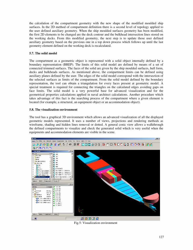
127

the calculation of the compartment geometry with the new shape of the modified moulded ship

surfaces. In the 2D method of compartment definition there is a second level of topology applied to

the user defined auxiliary geometry. When the ship moulded surfaces geometry has been modified,

the first 2D elements to be changed are the deck contour and the bulkhead intersection lines stored on

the working decks. From this modified geometry, the next step is to update those user defined

auxiliary geometry based on the previous one in a top down process which follows up until the last

geometry element defined on the working deck is recalculated.

5.7. The solid model

The compartment as a geometric object is represented with a solid object internally defined by a

boundary representation (BREP). The limits of this solid model are defined by means of a set of

connected trimmed surfaces. The faces of the solid are given by the ship moulded surfaces, hull form,

decks and bulkheads surfaces. As mentioned above, the compartment limits can be defined using

auxiliary planes defined by the user. The edges of the solid model correspond with the intersection of

the selected surfaces as limits of the compartment. From the solid model defined by the boundary

representation, the tool can obtain a triangulation for every faces present at geometric model. A

special treatment is required for connecting the triangles on the calculated edges avoiding gaps on

face limits. The solid model is a very powerful base for advanced visualization and for the

geometrical properties calculations applied in naval architect calculations. Another procedure which

takes advantage of this fact is the searching process of the compartment where a given element is

located (for example, a structural, an equipment object or an accommodation object).

5.8. The visualization environment

The tool has a graphical 3D environment which allows an advanced visualization of all the displayed

geometric models represented. It uses a number of views, projections and rendering methods as

wireframe, shading and hidden lines removal or dotted. A general conic view allows a walkthrough

the defined compartments to visualize and check the generated solid which is very useful when the

equipments and accommodation elements are visible in the scene.

Fig.5: Visualization environment

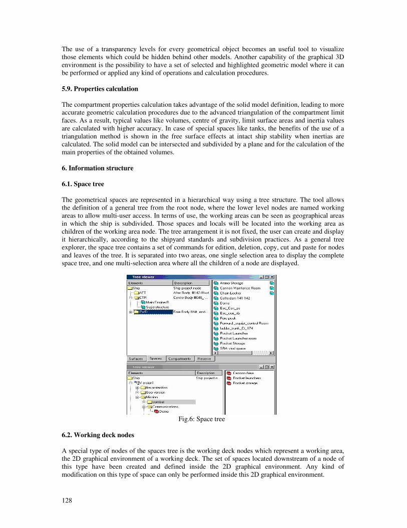
128

The use of a transparency levels for every geometrical object becomes an useful tool to visualize

those elements which could be hidden behind other models. Another capability of the graphical 3D

environment is the possibility to have a set of selected and highlighted geometric model where it can

be performed or applied any kind of operations and calculation procedures.

5.9. Properties calculation

The compartment properties calculation takes advantage of the solid model definition, leading to more

accurate geometric calculation procedures due to the advanced triangulation of the compartment limit

faces. As a result, typical values like volumes, centre of gravity, limit surface areas and inertia values

are calculated with higher accuracy. In case of special spaces like tanks, the benefits of the use of a

triangulation method is shown in the free surface effects at intact ship stability when inertias are

calculated. The solid model can be intersected and subdivided by a plane and for the calculation of the

main properties of the obtained volumes.

6. Information structure

6.1. Space tree

The geometrical spaces are represented in a hierarchical way using a tree structure. The tool allows

the definition of a general tree from the root node, where the lower level nodes are named working

areas to allow multi-user access. In terms of use, the working areas can be seen as geographical areas

in which the ship is subdivided. Those spaces and locals will be located into the working area as

children of the working area node. The tree arrangement it is not fixed, the user can create and display

it hierarchically, according to the shipyard standards and subdivision practices. As a general tree

explorer, the space tree contains a set of commands for edition, deletion, copy, cut and paste for nodes

and leaves of the tree. It is separated into two areas, one single selection area to display the complete

space tree, and one multi-selection area where all the children of a node are displayed.

Fig.6: Space tree

6.2. Working deck nodes

A special type of nodes of the spaces tree is the working deck nodes which represent a working area,

the 2D graphical environment of a working deck. The set of spaces located downstream of a node of

this type have been created and defined inside the 2D graphical environment. Any kind of

modification on this type of space can only be performed inside this 2D graphical environment.

129

The working deck nodes are represented at the space tree with another icon to establish an easy view

detection of them. Also the creation process is different from the way of definition for the general

working nodes. The working decks nodes are created from commands placed in the pop-up described

for the deck elements present at surfaces tree. These commands can be also selected from the pop-up

described for the root node of the space tree. The working deck nodes are specially designed for

allowing the access to the graphical edition of the working decks which is an important concept

because, on the same deck, the tool can define a set of working decks representing different areas of

the deck.

6.3. User defined attributes

User attributes is an easy way to add logical concepts to the geometrical model of the spaces. It is

completely free, not only in number, but also in the type of variable used for representing the logical

concept as tables, dates, numbers, etc. One example of user attributes is the fire resistance of a space

that can be described with a number representing a percentage, a numerical value between 0.0 to 1.0,

or by means of a table where user can insert a list with different levels of resistance. The user

attributes can be defined for the majority of entities that the tool can manage. Its use is recommended

in the development environment as it is the basis of the in- house procedures and calculations,

improving the reports, drawings, data extraction and grouping and searching for elements.

6.4. Compartment tree

The compartment tree is the way to group and arrange the spaces using as many logical concepts as

needed (i.e. fire zones, evacuation zones, accommodation zones, etc.). This tree structure can be seen

as another view of the spaces hierarchy but adding a functionality sense, with a different arrangement

of levels and nodes. The tool allows the definition of as many compartments trees as the user needs,

one for every main function of the ship to study. The compartment tree is created from the space tree

passing the spaces as a reference into every compartment tree created. It means that every

compartment has a reference to the geometrical space and a list of all the user attributes defined for

the entity. The values of the attributes assigned to every compartment can be calculated according to

the characteristics of the space and the compartment tree where is located with procedures made by

designers. A compartment tree does not need to have all the defined spaces, only those required for

the particular case of study. For example, for a compartment tree which describes an evacuation trunk,

only the spaces related will be assigned to the tree.

7. Preliminary Layouts

To complete the ship general arrangement, in addition to the definition of ship compartments, it is

necessary to perform a preliminary layout of the main equipment and accommodation items. In case

of naval vessels, it must include the main weapon systems. The preliminary distribution is usually

performed by positioning existing 3D models of the equipment in the compartments or in the deck

areas of the vessel. It is also very easy to define new models by reusing existing ones or by defining

them from scratch. If only 2D information is available, it is possible to perform a preliminary layout

of the existing 2D equipment views on the corresponding deck areas.

By using the available functionality, the designer can perform the following tasks related to the

preliminary ship layout:

- 3D equipment modeling

- Equipment layout

- Space reservation

- Definition of ladders, floors and other outfitting structural items

- Definition of main accommodation items

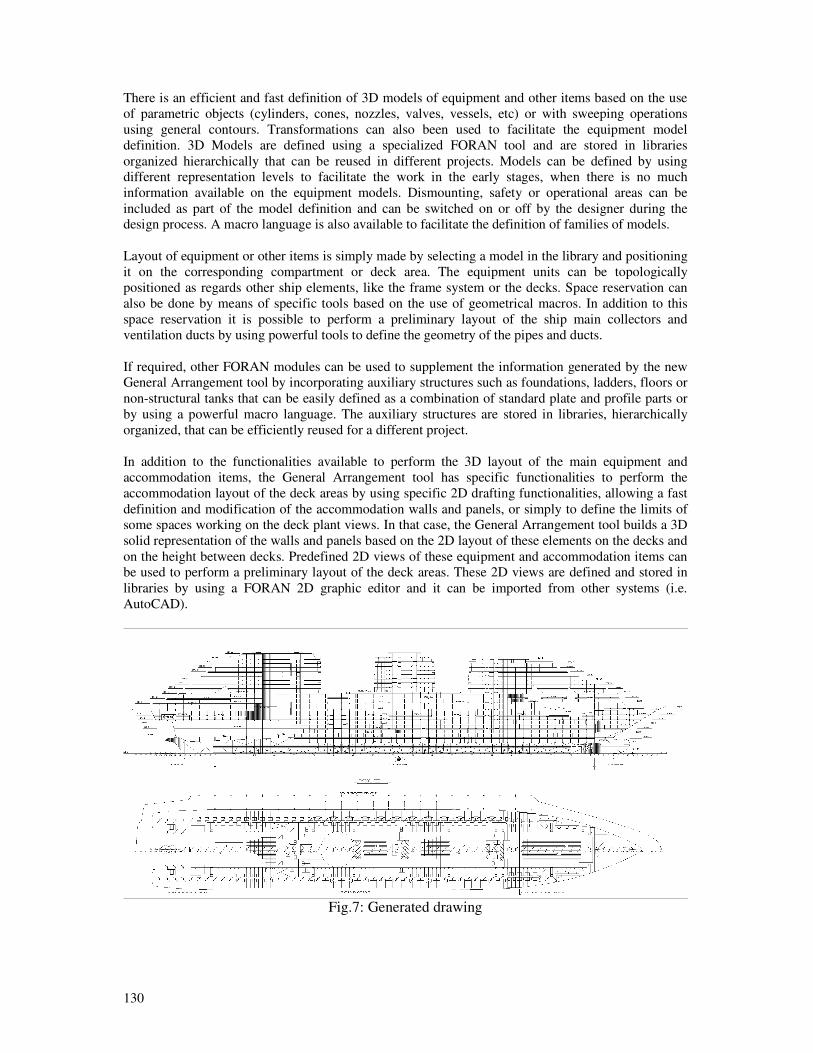
130

There is an efficient and fast definition of 3D models of equipment and other items based on the use

of parametric objects (cylinders, cones, nozzles, valves, vessels, etc) or with sweeping operations

using general contours. Transformations can also been used to facilitate the equipment model

definition. 3D Models are defined using a specialized FORAN tool and are stored in libraries

organized hierarchically that can be reused in different projects. Models can be defined by using

different representation levels to facilitate the work in the early stages, when there is no much

information available on the equipment models. Dismounting, safety or operational areas can be

included as part of the model definition and can be switched on or off by the designer during the

design process. A macro language is also available to facilitate the definition of families of models.

Layout of equipment or other items is simply made by selecting a model in the library and positioning

it on the corresponding compartment or deck area. The equipment units can be topologically

positioned as regards other ship elements, like the frame system or the decks. Space reservation can

also be done by means of specific tools based on the use of geometrical macros. In addition to this

space reservation it is possible to perform a preliminary layout of the ship main collectors and

ventilation ducts by using powerful tools to define the geometry of the pipes and ducts.

If required, other FORAN modules can be used to supplement the information generated by the new

General Arrangement tool by incorporating auxiliary structures such as foundations, ladders, floors or

non-structural tanks that can be easily defined as a combination of standard plate and profile parts or

by using a powerful macro language. The auxiliary structures are stored in libraries, hierarchically

organized, that can be efficiently reused for a different project.

In addition to the functionalities available to perform the 3D layout of the main equipment and

accommodation items, the General Arrangement tool has specific functionalities to perform the

accommodation layout of the deck areas by using specific 2D drafting functionalities, allowing a fast

definition and modification of the accommodation walls and panels, or simply to define the limits of

some spaces working on the deck plant views. In that case, the General Arrangement tool builds a 3D

solid representation of the walls and panels based on the 2D layout of these elements on the decks and

on the height between decks. Predefined 2D views of these equipment and accommodation items can

be used to perform a preliminary layout of the deck areas. These 2D views are defined and stored in

libraries by using a FORAN 2D graphic editor and it can be imported from other systems (i.e.

AutoCAD).

Fig.7: Generated drawing

131

8. Generation of drawings

The drawing generation in FORAN is managed by the FDESIGN module, which covers the output

drawings of all FORAN design disciplines (general, hull structure, outfitting, electrical and

accommodation) and it is completely user configurable. The final aspect of the drawings depends on

the user requirements. Drawings are generated directly from the 3D product model. The 2D entities

that represent the product model elements are linked to the 3D elements and are always updated with

the latest version of the product model. A symbolic representation for modeled elements is possible

and different visualization methods are available. Additional information (labels, dimensions,

including ship reference, bill of materials, texts) can be added into 2D drawings but remaining linked

to the product model elements. FDESIGN allows generating drawings based on FGA entities, either

to represent a single compartment, a group of compartments (i.e. machinery spaces layout) or the

complete General Arrangement drawing. The drawing may contain any combination of selected

elements of the 3D model of the ship and that can be represented by means of:

Main orthogonal projections

Sections by any plane

Perspective views with any orientation

A set of user defined templates can be used to customize the views generation. Due to the topological

nature of the 3D model, a drawing can be regenerated after changes in the 3D model and labels and

dimensioning are automatically updated. As a summary, standard FORAN drafting tools are

integrated and arrangement drawings can be easily generated with full associative with the 3D model.

For drawing make up, all standard FORAN drafting capabilities can be used.

9. A development environment for designers

With the main goal of providing users with the necessary features to self-customize the software, the

new tool comprises the FORAN Development Environment –FDE-, which allows designers to add

new capabilities to the application and to automate processes frequently repeated.

9.1. Basic characteristics

The FORAN Development Environment has been defined and developed keeping in mind the case of

use to be practical and efficient for users of different levels. This aim is behind the basic

characteristics of the FDE: it is based on the same standard as JavaScript –ECMAScript- and FDE

projects can be edited in a workbench embedded in the application, with no recompilation required.

The functionality provided by the FDE is divided into several packages or groups. For example, the

FCS package allows the user to create new commands and use them as any internal command of the

tool; the DBA package provides access to the database and the FDS package allows the generation of

fully customized documents and reports.

9.2. Access to compartment data and functionalities

In parallel with the development of the new tool, a new FDE package, FDT, has been created to allow

access to the information –geometric characteristics of the spaces and information associated with

them- handled by the new application. The most important compartment-related functionalities

available within the FDE can be divided into three main groups: geometric spaces, user attributes and

reserves of space functionalities.

9.2.1 Geometric spaces functionalities

The functionalities related with the geometry of the spaces can be split into two main sets, depending

on the type of data they access: purely geometric characteristics and hierarchic properties. The pure

geometric group holds characteristics of the space such as volume, centre of gravity co-ordinates, area

132

of limiting surfaces, dimensions of the bounding box and other magnitudes of the geometric model of

the space. In addition to the geometric characteristics, other properties, which could be labelled as

‘hierarchical’, can also be obtained by means of the FDT package. Examples of these properties are

the surfaces –hulls, decks, bulkheads- that serve as limit of the space, the position of the space within

the design tree and relations –mainly volume addition or subtraction- with other geometric spaces.

9.2.2 User attributes functionalities

As above explained, one of the main features of the new tool is the definition of user attributes that

are later assigned to compartments. This feature has its extension in the FORAN Development

Environment. The current values of the attributes for a compartment may be inquired and modified by

user programming which allows a fast check -and correction if necessary- of the attributes.

9.2.3 Reserves of space functionalities

The definition of the reserves of space is also open to the FDE. Since the geometry of a reserve of

space if defined in a parametric way, it is easy to create an FDE script to check the accuracy of the

main dimensions of a given piece of equipment. By the way of example, the following point describes

a practical application of this concept.

9.3. Design verification against rules One of the requirements of the tool created within the scope of the Intership Project was the fast

verification of designs in accordance with the rules imposed by classification societies, the IMO and

flag administrations. The final aim was to give a step towards the so-called Regulation Based Design.

The Ship Stability Research Centre of the University of Strathclyde was, in the ambit of the Intership

Project, responsible of identifying and describing the main regulations affecting the design and then

specifying the main functionalities required to complete the design validation. Most of the required

functionalities were related with the ability, from FDE, to query geometric properties of spaces and

relations between them and also with the definition of user attributes. As shown before, those

requirements are fulfilled by the current implementation.

An example of design verification performed by FDE scripts could be the checking of the minimum

width of stairs. First, the group of reserves of space would be traversed looking for reserves that use a

‘stair’ macro. For those spaces with stairs, the attribute ‘passenger’ could be checked, and, based on

the geometric characteristics of the space –see IMO A.757(18)-, the minimum value for the width of

the stair could be set. Then, the actual value of the width –which is a parameter of the macro- would

be queried and compared against the minimum value fixed by regulations.

9.4. Design merit evaluation

Sirenha, again inside the Intership Project, was responsible of collecting the most important

functionalities required to perform a Multi Disciplinary Optimization –MDO- of a design. Even if the

details of MDO are very complex and outside the scope of this paper, it is pertinent to point out that

FORAN Development Environment gives the possibility of comparing different preliminary designs

by obtaining a ‘merit’ index for each of them. A very simple and straight forward example of the

design merit evaluation could be the calculation of the payload based, in the case of a Ro-Ro, on the

walking area of spaces with the attribute ‘car-deck’

9.5. Report generation

Being the generation of fully customized reports, one of the main functionalities of FDE, it is clear

that the user of the tool may, by combining FDT and FDS packages, obtain tailored reports with

compartment-related data. For example, it is quite simple to obtain a document with the volume and

centre of gravity of spaces grouped by the default type of cargo.

133

10. Reuse of information in the complete ship lifecycle

There is a tight integration with all FORAN modules for end-to-end compartment creation and

management. Compartment objects created with FORAN General Arrangement tool (FGA) can be

used in downstream process to assist in the management of systems design. Ship designers can take

advantage of FGA to integrate their equipments and systems objects within a highly productive and

intuitive design environment.

10.1 Model refinement and reuse

Under FORAN, the single 3D Model becomes more detailed as the design evolves to later stages. In

general, the efficiency of the reuse is very much dependant on the ability of the system to handle

modifications as it is the case of FORAN due to its topological character.

Main discipline related FORAN modules (FHULL, FPIPE, FCABLE) will have access to the

compartments tree and will include a set of common commands to visualize, get information and

perform some actions, as follows:

• Read one or more compartments selected from the tree

• Visualize the compartment 3D solid model and its name

• Selection of compartment either from the tree or from the graphic area of the screen

• Get information about the compartment boundaries and its attributes

• Edition of user attributes

• Storage in data base the user attributes

• Associate and disassociate elements to a compartment (structure in FHULL, outfitting and

accommodation in FPIPE, electrical in FCABLE),

• Get information about the elements associated to a compartment

• Retrieve information of a compartment pointing to one of its elements

• Storage in data base the cross relationship between elements and compartments and user

attributes

• Obtain painting, insulation, welding, areas and weighting information of a compartment

10.2 Reuse of information during basic and detail design

As regards hull structure, the reuse affects to different aspects like more accurate painting area

calculations, automatic assignment of welding procedures based on compartment characteristics as

well as the handling of compartment concept as an additional hierarchy for the build strategy. With

respect to the equipment arrangement, the equipment associated to compartments in the preliminary

layout will be fully reused for subsequent assignment to zones and systems. Additional attributes can

be entered at any time for a full definition of equipment characteristics. Equipment models could be

also refined by using the possibility to define different levels of representation. Most of the elements

included in the ship model during the preliminary layout, can be reused in later stages when

developing Outfitting and Electrical detail layouts or coordination drawings. Accommodation

elements such as decks, bulkheads or walls, rooms, doors, windows and holes can be reused by means

of different options to define, modify and position the elements and, due to the topological references

to the main ship surfaces, automatic recalculation can be carried out, in case of modifications.

11. The General Arrangement Tool: Summary

The tool described in this paper can be considered not only as a specific tool for the definition and

management of ship compartments but as a complete General Arrangement tool, supplying most of

the functionality required during the early design phase. The tool combines the advantages of

designing in 2D and 3D environments, so facilitating the design tasks in the early stages of design

when the available information is poor or scarce.

134

The tool supplies specific functionalities for the definition and management of the ship compartments,

together with other capabilities oriented to equipment and accommodation layout, all of them working

on an advanced modeling and visualization environment.

Another interesting characteristic of the tool is the availability of a User Programming Environment,

to generate reports and to develop new design and checking functions, e.g. to verify the degree of

compliance of the design with some international or design rule.

One relevant characteristics of this tool is its integration within a shipbuilding CAD/CAM System

(FORAN System), so taking full advantage of the integrated use of other ship design tools, as the Hull

form definition or the Naval Architecture calculations, and the reuse of the information in other

design stages.

Finally, the tool has been conceived with several main objectives in mind:

• To reduce the design times during the early design stages

• To improve the quality of the initial designs

• To facilitate the analysis and study of different design alternatives

• To allow the reuse of the information in other design stages

References

SASAKI, D. (2005), ARMOGA An efficient multi-objective genetic algorithm, Technical Report,

University of Southampton

IMO (1991), The calculation procedure to assess the survivability characteristics of existing ro-ro

passenger ships when using a simplified method based upon resolution A265 (VIII), IMO MSC/Circ

574

IMCO (1974), Regulations on subdivision and stability of passenger ships (etc.), IMCO Resolution

A265 (VIII)

135

Flooding Simulation as a Practical Design Tool

Antti Metsä, Napa Ltd, Helsinki/Finland, antti.metsa@napa.fi Pekka Ruponen, Napa Ltd, Helsinki/Finland, pekka.ruponen@napa.fi

Christopher Ridgewell, Napa Ltd, Helsinki/Finland, christopher.ridgewell@napa.fi Pasi Mustonen, Foreship Ltd, Helsinki/Finland, pasi.mustonen@foreship.com

Abstract

Asymmetric flooding could result in dangerous situations. Quick counter flooding is required in compartments that are longitudinally divided, such as separated engine rooms. The physical background of flooding simulation is reviewed and a simulation tool, implemented into ship design software, is presented. Focus is on a practical example, flooding of an engine room. The modelling of the equipment and the flooded compartments is presented and some parameters are varied in order to show how to study their effect on the whole flooding process. In conclusions, the benefits of computer aided design of counter flooding arrangements are discussed, with comparisons to the simple rules of thumb.

1. Introduction Fast and efficient equalization of floodwater is an important factor in the survivability after damage. In voids this is usually arranged by installing passive flooding devices, such as cross-flooding ducts. In a longitudinally divided engine room the situation is more difficult, since the dividing bulkhead needs to prevent the propagation of fire and gases. One solution is to install flooding flaps that will be opened by the pressure of the floodwater. Generally, the efficiency of these flooding devices has been ensured by rules of thumb, based on Bernoulli’s equation (Resolution A.266). However, this simplified approach does not take into account the change in the actual floating position, nor the compression of air in a tank with restricted ventilation level or simultaneous flooding through several sequential openings. The development of time domain flooding simulation tools now allows a more detailed and realistic analysis of the effectiveness of various flooding devices. In this paper, a demonstrative example on the design of flooding devices in a longitudinally divided engine room of a large ropax ship is presented in detail. In addition to the steel structures, also large equipment can form notable flow obstructions for the floodwater. The European Gateway accident, described in Spouge (1986), is a good example of a situation, where transient asymmetric flooding of a symmetrical generator room resulted in a large transient heeling angle that allowed flooding of the vehicle deck, causing the capsizing. Thus also the effect of the main engines in the event of side damage with a relatively small penetration has been studied. With the benefits achieved through economies of scale, ships continue to increase in size. Also with the new widened Panama Canal new ships with larger beam are expected to replace the older tonnage. As the ships beam increases the subdivision, especially in the machinery spaces, will become more prevalent. The prevention of asymmetric flooding will be an important factor in the survivability for these designs. Cross flooding arrangements must also be designed to maintain the structural fire protection divisions of the ship. As the cross flooding flow rates increase it becomes difficult to maintain the fire protection properties. In some cases it is advantageous to direct the flood water under the engine room through dedicated voids, thus maintaining the functionality of the machinery. However this can reduce tank capacities and in some cases increase the centre of gravity. Therefore to achieve the optimal design of the cross flooding arrangement it becomes necessary to move away from the rules of thumb and apply a new method that better replicates the phenomena.

136

2. Applied Simulation Method 2.1. Background Napa Ltd and Helsinki University of Technology have in co-operation developed a flooding simulation method that has been implemented in the NAPA System. This novel method is based on the pressure-correction technique, allowing a time-accurate solution of progressive flooding and air compression inside the damage ship. The principles of the method are presented in the following sections. A detailed description of the simulation method is presented in Ruponen (2006,2007). The method has been thoroughly validated by comparing simulations and model test results. Some examples have been presented in Ruponen et al. (2006) and in Ruponen (2007). The developed simulation tool has been implemented into the NAPA system. 2.2. Governing Equations At each time step the conservation of mass must be satisfied in each flooded room, both for water and air. In general, the equation of continuity is:

∫∫ ⋅−=Ω∂∂

Ω S

ddt

Svρρ

(1)

where ρ is the density of the fluid, v is the velocity vector and S is the surface that bounds the control volume Ω. The normal vector of the surface points outwards from the control volume, hence the minus sign on the right hand side of the equation. The velocities in the openings are calculated by applying Bernoulli’s equation for a streamline from point A that is in the middle of a flooded room to point B in the opening. Consequently:

( ) ( ) 021 22 =−+−+∫ ABAB

B

A

hhguudpρ

(2)

where p is air pressure, u is flow velocity and h is the height from the reference level. It is also assumed that the flow velocity is negligible in the center of the room (uA = 0). Eq.(2) applies for inviscid and irrotational flow. The pressure losses in the openings and pipes are taken into account by applying semi-empirical discharge coefficients. Consequently, the mass flow through an opening is: AuCQm dρρ ==& (3)where Q is the volumetric flow through the opening, Cd is the discharge coefficient and A is the area of the opening. For pipes and ducts, the discharge coefficient is usually calculated from the sum of the pressure loss coefficients ki, following the “revised Resolution A.266”, IMO (2007a), so that:

∑=

ii

dk

C 1

(4)

The flooding process is assumed to be isothermal. Therefore, Boyle’s law can be applied and the density of air is assumed to be linearly dependent on the pressure:

ppa

0

0ρρ =

(5)

where ρ0 is the density of air at the atmospheric pressure p0.

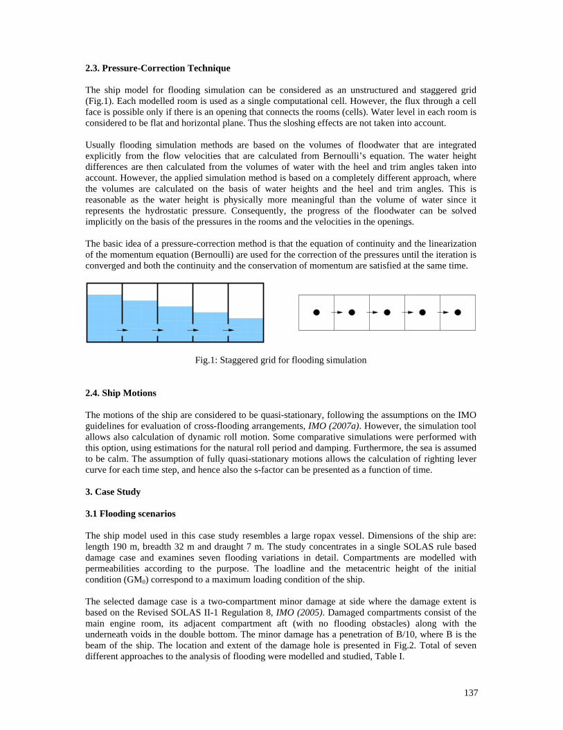
137

2.3. Pressure-Correction Technique The ship model for flooding simulation can be considered as an unstructured and staggered grid (Fig.1). Each modelled room is used as a single computational cell. However, the flux through a cell face is possible only if there is an opening that connects the rooms (cells). Water level in each room is considered to be flat and horizontal plane. Thus the sloshing effects are not taken into account. Usually flooding simulation methods are based on the volumes of floodwater that are integrated explicitly from the flow velocities that are calculated from Bernoulli’s equation. The water height differences are then calculated from the volumes of water with the heel and trim angles taken into account. However, the applied simulation method is based on a completely different approach, where the volumes are calculated on the basis of water heights and the heel and trim angles. This is reasonable as the water height is physically more meaningful than the volume of water since it represents the hydrostatic pressure. Consequently, the progress of the floodwater can be solved implicitly on the basis of the pressures in the rooms and the velocities in the openings. The basic idea of a pressure-correction method is that the equation of continuity and the linearization of the momentum equation (Bernoulli) are used for the correction of the pressures until the iteration is converged and both the continuity and the conservation of momentum are satisfied at the same time.

Fig.1: Staggered grid for flooding simulation

2.4. Ship Motions The motions of the ship are considered to be quasi-stationary, following the assumptions on the IMO guidelines for evaluation of cross-flooding arrangements, IMO (2007a). However, the simulation tool allows also calculation of dynamic roll motion. Some comparative simulations were performed with this option, using estimations for the natural roll period and damping. Furthermore, the sea is assumed to be calm. The assumption of fully quasi-stationary motions allows the calculation of righting lever curve for each time step, and hence also the s-factor can be presented as a function of time. 3. Case Study 3.1 Flooding scenarios The ship model used in this case study resembles a large ropax vessel. Dimensions of the ship are: length 190 m, breadth 32 m and draught 7 m. The study concentrates in a single SOLAS rule based damage case and examines seven flooding variations in detail. Compartments are modelled with permeabilities according to the purpose. The loadline and the metacentric height of the initial condition (GM0) correspond to a maximum loading condition of the ship. The selected damage case is a two-compartment minor damage at side where the damage extent is based on the Revised SOLAS II-1 Regulation 8, IMO (2005). Damaged compartments consist of the main engine room, its adjacent compartment aft (with no flooding obstacles) along with the underneath voids in the double bottom. The minor damage has a penetration of B/10, where B is the beam of the ship. The location and extent of the damage hole is presented in Fig.2. Total of seven different approaches to the analysis of flooding were modelled and studied, Table I.

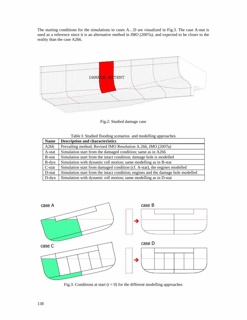
138

The starting conditions for the simulations in cases A…D are visualized in Fig.3. The case A-stat is used as a reference since it is an alternative method in IMO (2007a), and expected to be closer to the reality than the case A266.

DAMAGE−EXTENT

Fig.2: Studied damage case

Table I: Studied flooding scenarios and modelling approaches

Name Description and characteristics A266 Prevailing method, Revised IMO Resolution A.266, IMO (2007a) A-stat Simulation start from the damaged condition; same as in A266 B-stat Simulation start from the intact condition; damage hole is modelled B-dyn Simulation with dynamic roll motion; same modelling as in B-stat C-stat Simulation start from damaged condition (cf. A-stat), the engines modelled D-stat Simulation start from the intact condition; engines and the damage hole modelled D-dyn Simulation with dynamic roll motion; same modelling as in D-stat

Fig.3: Conditions at start (t = 0) for the different modelling approaches

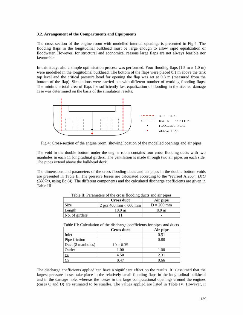
139

3.2. Arrangement of the Compartments and Equipments The cross section of the engine room with modelled internal openings is presented in Fig.4. The flooding flaps in the longitudinal bulkhead must be large enough to allow rapid equalization of floodwater. However, for structural and economical reasons large flaps are not always feasible nor favourable. In this study, also a simple optimisation process was performed. Four flooding flaps (1.5 m × 1.0 m) were modelled in the longitudinal bulkhead. The bottom of the flaps were placed 0.1 m above the tank top level and the critical pressure head for opening the flap was set at 0.3 m (measured from the bottom of the flap). Simulations were carried out with different number of working flooding flaps. The minimum total area of flaps for sufficiently fast equalization of flooding in the studied damage case was determined on the basis of the simulation results.

Fig.4: Cross-section of the engine room, showing location of the modelled openings and air pipes The void in the double bottom under the engine room contains four cross flooding ducts with two manholes in each 11 longitudinal girders. The ventilation is made through two air pipes on each side. The pipes extend above the bulkhead deck. The dimensions and parameters of the cross flooding ducts and air pipes in the double bottom voids are presented in Table II. The pressure losses are calculated according to the “revised A.266”, IMO (2007a), using Eq.(4). The different components and the calculated discharge coefficients are given in Table III.

Table II: Parameters of the cross flooding ducts and air pipes Cross duct Air pipe Size 2 pcs 400 mm × 600 mm D = 200 mm Length 10.0 m 8.0 m No. of girders 11 -

Table III: Calculation of the discharge coefficients for pipes and ducts Cross duct Air pipe Inlet - 0.51 Pipe friction - 0.80 Duct (2 manholes) 10 × 0.35 - Outlet 1.00 1.00 Σk 4.50 2.31 Cd 0.47 0.66

The discharge coefficients applied can have a significant effect on the results. It is assumed that the largest pressure losses take place in the relatively small flooding flaps in the longitudinal bulkhead and in the damage hole, whereas the losses in the large computational openings around the engines (cases C and D) are estimated to be smaller. The values applied are listed in Table IV. However, it

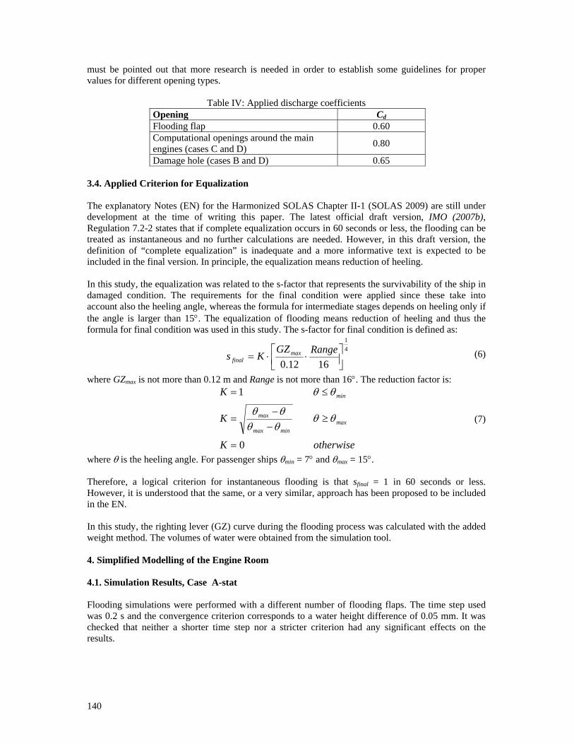
140

must be pointed out that more research is needed in order to establish some guidelines for proper values for different opening types.

Table IV: Applied discharge coefficients Opening Cd Flooding flap 0.60 Computational openings around the main engines (cases C and D) 0.80

Damage hole (cases B and D) 0.65 3.4. Applied Criterion for Equalization The explanatory Notes (EN) for the Harmonized SOLAS Chapter II-1 (SOLAS 2009) are still under development at the time of writing this paper. The latest official draft version, IMO (2007b), Regulation 7.2-2 states that if complete equalization occurs in 60 seconds or less, the flooding can be treated as instantaneous and no further calculations are needed. However, in this draft version, the definition of “complete equalization” is inadequate and a more informative text is expected to be included in the final version. In principle, the equalization means reduction of heeling. In this study, the equalization was related to the s-factor that represents the survivability of the ship in damaged condition. The requirements for the final condition were applied since these take into account also the heeling angle, whereas the formula for intermediate stages depends on heeling only if the angle is larger than 15°. The equalization of flooding means reduction of heeling and thus the formula for final condition was used in this study. The s-factor for final condition is defined as:

41

1612.0 ⎥⎦⎤

⎢⎣⎡ ⋅⋅=

RangeGZKs max

final (6)

where GZmax is not more than 0.12 m and Range is not more than 16°. The reduction factor is:

otherwiseK

K

K

maxminmax

max

min

0

1

=

≥−−

=

≤=

θθθθθθ

θθ

(7)

where θ is the heeling angle. For passenger ships θmin = 7° and θmax = 15°. Therefore, a logical criterion for instantaneous flooding is that sfinal = 1 in 60 seconds or less. However, it is understood that the same, or a very similar, approach has been proposed to be included in the EN. In this study, the righting lever (GZ) curve during the flooding process was calculated with the added weight method. The volumes of water were obtained from the simulation tool. 4. Simplified Modelling of the Engine Room 4.1. Simulation Results, Case A-stat Flooding simulations were performed with a different number of flooding flaps. The time step used was 0.2 s and the convergence criterion corresponds to a water height difference of 0.05 mm. It was checked that neither a shorter time step nor a stricter criterion had any significant effects on the results.

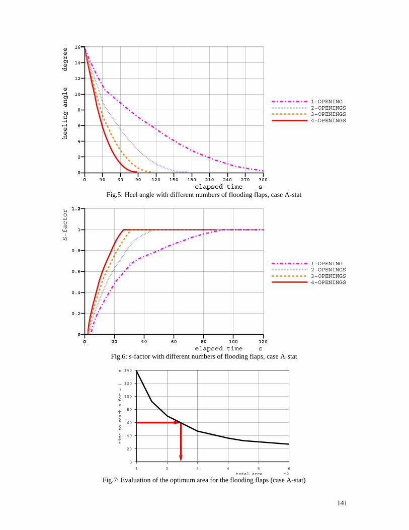
141

00

2

4

6

8

10

12

14

16

heeling angle degree

00 30 60 90 120 150 180 210 240 270 300

elapsed time s

4−OPENINGS3−OPENINGS2−OPENINGS1−OPENING

00 30 60 90 120 150 180 210 240 270 300

elapsed time s

00

2

4

6

8

10

12

14

16

heeling angle degree

Fig.5: Heel angle with different numbers of flooding flaps, case A-stat

00

0.2

0.4

0.6

0.8

1

1.21.2

S−factor

00 20 40 60 80 100 120

elapsed time s

4−OPENINGS3−OPENINGS2−OPENINGS1−OPENING

00 20 40 60 80 100 120

00

0.2

0.4

0.6

0.8

1

1.21.2

Fig.6: s-factor with different numbers of flooding flaps, case A-stat

0

20

40

60

80

100

120

140

1 2 3 4 5 6

time to reach s-fac = 1 s

total area m2 Fig.7: Evaluation of the optimum area for the flooding flaps (case A-stat)

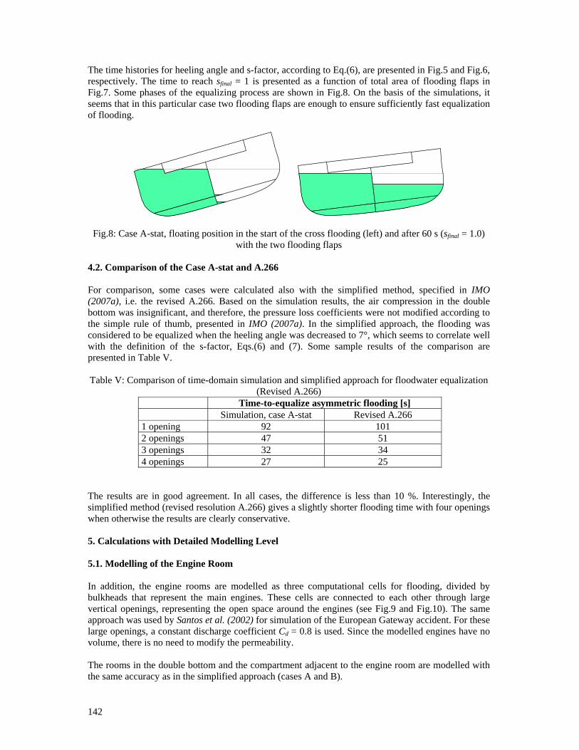
142

The time histories for heeling angle and s-factor, according to Eq.(6), are presented in Fig.5 and Fig.6, respectively. The time to reach sfinal = 1 is presented as a function of total area of flooding flaps in Fig.7. Some phases of the equalizing process are shown in Fig.8. On the basis of the simulations, it seems that in this particular case two flooding flaps are enough to ensure sufficiently fast equalization of flooding.

Fig.8: Case A-stat, floating position in the start of the cross flooding (left) and after 60 s (sfinal = 1.0) with the two flooding flaps

4.2. Comparison of the Case A-stat and A.266 For comparison, some cases were calculated also with the simplified method, specified in IMO (2007a), i.e. the revised A.266. Based on the simulation results, the air compression in the double bottom was insignificant, and therefore, the pressure loss coefficients were not modified according to the simple rule of thumb, presented in IMO (2007a). In the simplified approach, the flooding was considered to be equalized when the heeling angle was decreased to 7°, which seems to correlate well with the definition of the s-factor, Eqs.(6) and (7). Some sample results of the comparison are presented in Table V. Table V: Comparison of time-domain simulation and simplified approach for floodwater equalization

(Revised A.266) Time-to-equalize asymmetric flooding [s] Simulation, case A-stat Revised A.266 1 opening 92 101 2 openings 47 51 3 openings 32 34 4 openings 27 25

The results are in good agreement. In all cases, the difference is less than 10 %. Interestingly, the simplified method (revised resolution A.266) gives a slightly shorter flooding time with four openings when otherwise the results are clearly conservative. 5. Calculations with Detailed Modelling Level 5.1. Modelling of the Engine Room In addition, the engine rooms are modelled as three computational cells for flooding, divided by bulkheads that represent the main engines. These cells are connected to each other through large vertical openings, representing the open space around the engines (see Fig.9 and Fig.10). The same approach was used by Santos et al. (2002) for simulation of the European Gateway accident. For these large openings, a constant discharge coefficient Cd = 0.8 is used. Since the modelled engines have no volume, there is no need to modify the permeability. The rooms in the double bottom and the compartment adjacent to the engine room are modelled with the same accuracy as in the simplified approach (cases A and B).

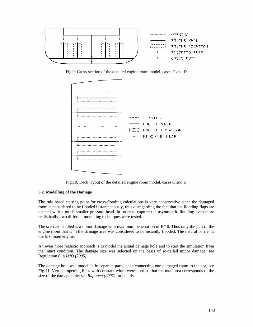
143

Fig.9: Cross-section of the detailed engine room model, cases C and D

Fig.10: Deck layout of the detailed engine room model, cases C and D

5.2. Modelling of the Damage The rule based starting point for cross-flooding calculations is very conservative since the damaged room is considered to be flooded instantaneously, thus disregarding the fact that the flooding flaps are opened with a much smaller pressure head. In order to capture the asymmetric flooding even more realistically, two different modelling techniques were tested. The scenario studied is a minor damage with maximum penetration of B/10. Thus only the part of the engine room that is in the damage area was considered to be instantly flooded. The natural barrier is the first main engine. An even more realistic approach is to model the actual damage hole and to start the simulation from the intact condition. The damage size was selected on the basis of so-called minor damage; see Regulation 8 in IMO (2005). The damage hole was modelled in separate parts, each connecting one damaged room to the sea, see Fig.11. Vertical opening lines with constant width were used so that the total area corresponds to the size of the damage hole; see Ruponen (2007) for details.

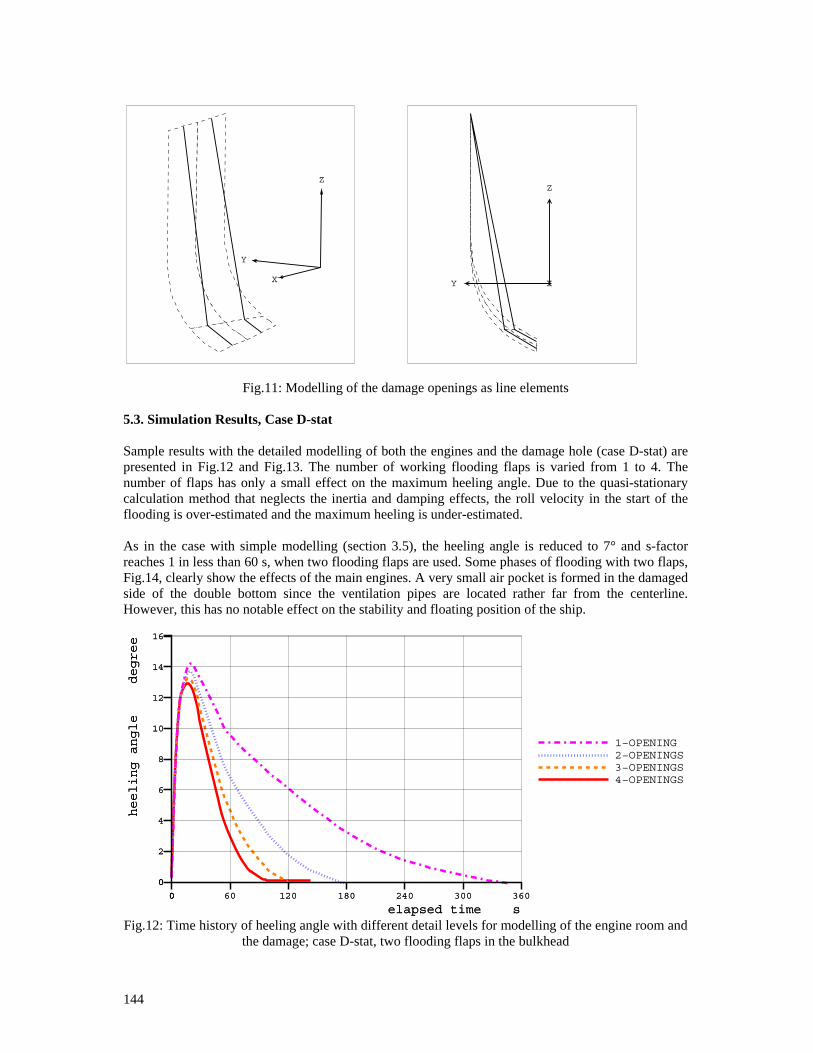
144

X

Y

Z

XY

Z

Fig.11: Modelling of the damage openings as line elements

5.3. Simulation Results, Case D-stat Sample results with the detailed modelling of both the engines and the damage hole (case D-stat) are presented in Fig.12 and Fig.13. The number of working flooding flaps is varied from 1 to 4. The number of flaps has only a small effect on the maximum heeling angle. Due to the quasi-stationary calculation method that neglects the inertia and damping effects, the roll velocity in the start of the flooding is over-estimated and the maximum heeling is under-estimated. As in the case with simple modelling (section 3.5), the heeling angle is reduced to 7° and s-factor reaches 1 in less than 60 s, when two flooding flaps are used. Some phases of flooding with two flaps, Fig.14, clearly show the effects of the main engines. A very small air pocket is formed in the damaged side of the double bottom since the ventilation pipes are located rather far from the centerline. However, this has no notable effect on the stability and floating position of the ship.

00

2

4

6

8

10

12

14

16

heeling angle degree

00 60 120 180 240 300 360

elapsed time s

4−OPENINGS3−OPENINGS2−OPENINGS1−OPENING

00 60 120 180 240 300 360

elapsed time s

00

2

4

6

8

10

12

14

16

heeling angle degree

Fig.12: Time history of heeling angle with different detail levels for modelling of the engine room and

the damage; case D-stat, two flooding flaps in the bulkhead

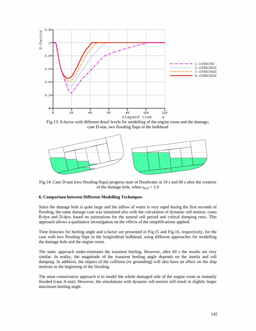
145

00

0.2

0.4

0.6

0.8

1

1.21.2

S−factor

00 20 40 60 80 100 120

elapsed time s

4−OPENINGS3−OPENINGS2−OPENINGS1−OPENING

00 20 40 60 80 100 120

00

0.2

0.4

0.6

0.8

1

1.21.2

Fig.13: S-factor with different detail levels for modelling of the engine room and the damage; case D-stat, two flooding flaps in the bulkhead

Fig.14: Case D-stat (two flooding flaps) progress state of floodwater at 10 s and 60 s after the creation of the damage hole, when sfinal = 1.0

6. Comparison between Different Modelling Techniques Since the damage hole is quite large and the inflow of water is very rapid during the first seconds of flooding, the same damage case was simulated also with the calculation of dynamic roll motion, cases B-dyn and D-dyn, based on estimations for the natural roll period and critical damping ratio. This approach allows a qualitative investigation on the effects of the simplifications applied. Time histories for heeling angle and s-factor are presented in Fig.15 and Fig.16, respectively, for the case with two flooding flaps in the longitudinal bulkhead, using different approaches for modelling the damage hole and the engine room. The static approach under-estimates the transient heeling. However, after 60 s the results are very similar. In reality, the magnitude of the transient heeling angle depends on the inertia and roll damping. In addition, the impact of the collision (or grounding) will also have an effect on the ship motions in the beginning of the flooding. The most conservative approach is to model the whole damaged side of the engine room as instantly flooded (case A-stat). However, the simulations with dynamic roll motion still result in slightly larger maximum heeling angle.

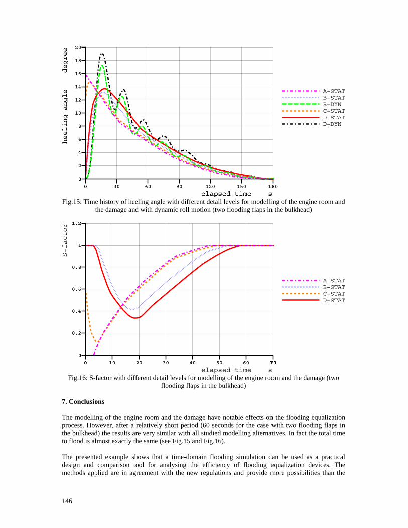
146

00

2

4

6

8

10

12

14

16

18

20

heeling angle degree

00 30 60 90 120 150 180

elapsed time s

D−DYND−STATC−STATB−DYNB−STATA−STAT

00 30 60 90 120 150 180

elapsed time s

00

2

4

6

8

10

12

14

16

18

20

heeling angle degree

Fig.15: Time history of heeling angle with different detail levels for modelling of the engine room and the damage and with dynamic roll motion (two flooding flaps in the bulkhead)

00

0.2

0.4

0.6

0.8

1

1.21.2

S−factor

00 10 20 30 40 50 60 7070

elapsed time s

D−STATC−STATB−STATA−STAT

00 10 20 30 40 50 60 7070

00

0.2

0.4

0.6

0.8

1

1.21.2

Fig.16: S-factor with different detail levels for modelling of the engine room and the damage (two flooding flaps in the bulkhead)

7. Conclusions The modelling of the engine room and the damage have notable effects on the flooding equalization process. However, after a relatively short period (60 seconds for the case with two flooding flaps in the bulkhead) the results are very similar with all studied modelling alternatives. In fact the total time to flood is almost exactly the same (see Fig.15 and Fig.16). The presented example shows that a time-domain flooding simulation can be used as a practical design and comparison tool for analysing the efficiency of flooding equalization devices. The methods applied are in agreement with the new regulations and provide more possibilities than the

147

restricted and simplified method, described in the revised version of Resolution A.266, IMO (2007a). The calculation of required area for cross flooding devices can easily be extended to a more complex analysis, involving different initial conditions and damage cases. The performance of cross-flooding ducts can also be confirmed. This is an important factor to ensure that the space is effectively utilised and the height of cofferdam structures and the cross flooding times can be optimised, taking into consideration the centre of gravity of main machinery inside the space. In addition the effects of air escaping through air pipes can also be studied. This can be significant in the case of large U-shaped voids where the effects of air pressure can have a significant impact on the cross flooding rate. With this new approach the designer is free to quickly study alternative arrangements whilst taking into account the physical phenomena that take place during the flooding process. Acknowledgments The authors would like to thank Mr. Toni Salmela for his efforts with the applied ship model. References IMO (2005), Resolution MSC.194(80) Adoption of Amendments to the International Convention for the Safety of Life at Sea, 1974, as amended (adopted 20 May, 2005) IMO (2007a), Resolution MSC.245(83) Recommendation on a Standard Method for Evaluating Cross-Flooding Arrangements, adopted on 12 October 2007 IMO (2007b), Interim Explanatory Notes to the SOLAS Chapter II-1 Subdivision and Damage Stability Regulations, MSC.1/Circ.1226 15 January 2007 RUPONEN, P. (2006), Pressure-Correction Method for Simulation of Progressive Flooding and Internal Air Flows, Ship Technology Research Vol. 53 No. 2, pp. 63-73 RUPONEN, P.; SUNDELL, T.; LARMELA, M. (2006), Validation of a Simulation Method for Progressive Flooding, 9th Int. Conf. Stability of Ships and Ocean Vehicles, Rio de Janeiro, Vol.2, pp.607-616 (also in: International Shipbuilding Progress Vol. 54 No. 4, pp. 305-321) RUPONEN, P. (2007), Progressive Flooding of a Damaged Passenger Ship, Doctoral Dissertation, Helsinki University of Technology, TKK Dissertations 94 RUPONEN, P.; ROUTI, A-L. (2007), Time-Domain Simulation of Cross-Flooding for Air Pipe Dimensioning, 9th Int. Ship Stability Workshop, Hamburg SANTOS, T. A.; WINKLE, I. E.; GUEDES SOARES, C. (2002), Time Domain Modelling of the Transient Asymmetric Flooding of Ro-Ro Ships, Ocean Engineering Vol. 29, pp.667-688 SPOUGE, J. R. (1986), The Technical Investigation of the Sinking of the Ro-Ro Ferry European Gateway, Trans. RINA 128, pp.49-72

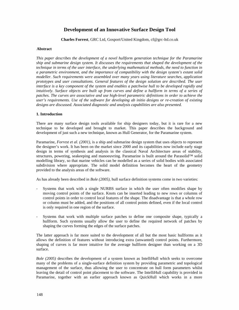
148

Development of an Innovative Surface Design Tool

Charles Forrest, GRC Ltd, Gosport/United Kingdom, cf@grc-ltd.co.uk Abstract This paper describes the development of a novel hullform generation technique for the Paramarine ship and submarine design system. It discusses the requirements that shaped the development of the technique in terms of the user interface, the underlying mathematical methods, the need to function in a parametric environment, and the importance of compatibility with the design system’s extant solid modeller. Such requirements were assembled over many years using literature searches, application prototypes and user consultations. General features of the design solution are described. The user interface is a key component of the system and enables a patchwise hull to be developed rapidly and intuitively. Surface objects are built up from curves and define a hullform in terms of a series of patches. The curves are associative and use high-level parametric definitions in order to achieve the user’s requirements. Use of the software for developing ab initio designs or re-creation of existing designs are discussed. Associated diagnostic and analysis capabilities are also presented. 1. Introduction There are many surface design tools available for ship designers today, but it is rare for a new technique to be developed and brought to market. This paper describes the background and development of just such a new technique, known as Hull Generator, for the Paramarine system. Paramarine, Forrest et al. (2001), is a ship and submarine design system that uses objects to represent the designer’s work. It has been on the market since 2000 and its capabilities now include early stage design in terms of synthesis and analysis in the classical Naval Architecture areas of stability, structures, powering, seakeeping and manoeuvring. Paramarine is built around the Parasolid™ solid modelling library, so that marine vehicles can be modelled as a series of solid bodies with associated subdivision where appropriate. The solid model definition becomes the heart of the geometry provided to the analysis areas of the software. As has already been described in Bole (2005), hull surface definition systems come in two varieties: - Systems that work with a single NURBS surface in which the user often modifies shape by

moving control points of the surface. Knots can be inserted leading to new rows or columns of control points in order to control local features of the shape. The disadvantage is that a whole row or column must be added, and the positions of all control points defined, even if the local control is only required in one region of the surface.

- Systems that work with multiple surface patches to define one composite shape, typically a

hullform. Such systems usually allow the user to define the required network of patches by shaping the curves forming the edges of the surface patches.

The latter approach is far more suited to the development of all but the most basic hullforms as it allows the definition of features without introducing extra (unwanted) control points. Furthermore, shaping of curves is far more intuitive for the average hullform designer than working on a 3D surface. Bole (2005) describes the development of a system known as IntelliHull which seeks to overcome many of the problems of a single-surface definition system by providing parametric and topological management of the surface, thus allowing the user to concentrate on hull form parameters whilst leaving the detail of control point placement to the software. The IntelliHull capability is provided in Paramarine, together with an earlier approach known as QuickHull which works in a more

149

rudimentary way to achieve a similar result for simple warship hullforms. Both QuickHull and IntelliHull work with a single hull surface and, perhaps surprisingly, Paramarine has never had a native multi-patch hullform design capability. However the embedded solid modeller is perfectly capable of sewing multiple surfaces together to form a single sheet or solid body with multiple faces. 2. Requirements Capture Early prototypes of a multi-patch hullform definition approach showed that there were significant difficulties in implementing a workable solution. It quickly became apparent that it was difficult to reconcile user demands with the capabilities of NURBS mathematics. A further problem was integrating the results of the approach into the existing Paramarine system, in particular the need for the surfaces produced to be usable with the solid modeller already embedded in the system. 2.1. User Requirements From the earliest stages of development, users’ views on the proposed functionality have been sought, paying particular attention to the views of UK shipbuilders and other Naval Architecture consultants. A summary of user feedback gained during a Hull Generation Workshop event is given in Table I. It is noteworthy that “speed of use” and “flexibility” emerge as clear primary requirements.

Table I: Summarised user requirements for hull generation system

Speed of use - Speed - Rapid generation of hulls and associated

hydrostatics - User interface, speed of use / learning curve - Should minimise the time needed to create a

surface (hull) in Paramarine - Generate and test a variety of hull forms

quickly for resistance / stability / seakeeping Flexibility - Robust and flexible - Ability to go into detail in particular parts - Ability to define novel hull forms - Parametric - Ability to define curves, straights and

knuckle lines - Reasonable fairness for presentation

purposes

Ease of use - Easy to use - Ease of use in editing the surface for fairness Audit trail / diagnostics - Coherent model - Understanding of the surface Miscellaneous requirements - Importing images - Library of parents - Compatibility with external software Future Capabilities - Ease of transformation - Generate and test a variety of hull forms

quickly for deformation / geosym

Naturally not all users want the same things in a hull generation system, but what became clear during this process was that basically users are wanting to define the hull in terms of 2D and 3D curves representing particular features, for example, flat of side, flat of keel, waterline and knuckle lines. Secondary curves can then be developed (mainly in 2D) to give key section lines, buttock lines and waterlines. Users then expect the hull generation system to calculate the shapes of 3D surface patches formed in between the curves as defined, ideally with slope and curvature continuity where expected. This is a very tall order for a patchwise hull generation system.

150

2.2. System Requirements The user requirement to be “Compatible with external software” means that there is only one suitable format for the surface patches: non-uniform rational b-splines, NURBS. In fact, even to work with Paramarine’s own modelling system, Parasolid, the NURBS route was essential. 2.2.1. Parasolid™ Parasolid is an industry-standard boundary-representation solid modelling system which uses NURBS as the underpinning representation for freeform curves and surfaces. Owing to the requirement to produce accurate and mathematically consistent geometry suitable for further modelling operations, Parasolid carries out rigorous checks on geometry used as input for sheet or solid bodies and will reject NURBS surfaces which fail the checks. Examples are: - Surfaces with incorrect knot vectors, or with control point weights that are zero or negative. - Degenerate surfaces, where too many control points are placed coincidentally in 3D space. - Self-intersecting surfaces, where the trajectory of the control polygon is such that the surface

doubles back on itself. - When sewing sheets together to form a composite sheet or solid, the edges of the sheets must lie

exactly adjacent to each other. (In fact Parasolid does provide an alternative mode, known as “tolerant modelling” in which gaps are allowed to exist, but the downstream implications of further modelling operations cause more problems than “tolerant modelling” solves.)

2.2.2. Paramarine As well as the need to work with the modeller, using NURBS, there was the need to integrate seamlessly into the Paramarine environment. As described by Forrest et al. (2001), Paramarine is a design system in which the user expresses the design using objects to represent both synthesis and analysis elements in the design. The objects are wired together in a manner analogous to the cells of a spreadsheet. Paramarine is object-oriented, both in terms of the computer language used to develop it (C++), and in terms of the objects manipulated by the user. Fig.1 illustrates the object hierarchy into which the hull generation objects were required to fit. In Paramarine each object has a list of objects that it depends on (known as its “ancestors”), and another list of objects that depend on it (its “descendents”). When recalculation takes place, a given object will ensure its ancestors are recalculated and up to date first before it itself recalculates. It is therefore essential when developing new objects for Paramarine to give careful consideration to the “ancestry”, that is, the path through which data will flow and recalculation will take place. In the context of hull generation, the design solution would clearly involve the use of curve objects and surface objects. The curve objects would be ancestors of the surface objects; but in the particular solution chosen, curve objects would become ancestors of each other when one curve was joined to another. A particular problem needing to be explicitly addressed and prevented is that of circular reference, in which an “ancestry” chain of objects forms into a loop. For this reason it is not possible for example to have Curve Object A dependent on Curve Object B if Curve Object B is already dependent on Curve Object A.

151

Fig.1: Paramarine class inheritance diagram, showing examples of instantiated objects 3. Design Solution The solution developed to satisfy the requirements of Section 2 is known as Hull Generator. It incorporates functionality known as “X-Topology”, a term that has been used in the description of patchwise hull generation systems before, for example Lee (2001). In the present context “X-Topology” refers to the process of forming a topological network from the curves supplied and using this topology to infer boundary conditions at the edges of the surface patches formed for the multi-patch hull. 3.1. General Features As has already been described, the core of the new hull generation system consists of curve and surface objects. Just as important as the design of these entities is the design of the user interface that supports them. A strong message coming through the user feedback and the pilot software developed earlier was that the user interface mattered enormously; the best hull generation technique in the world could be rendered nearly useless by a poor user interface. Also mentioned here are the diagnostic capabilities to help users when things go wrong, and what features have been provided to help users achieve the quality of surface they require. 3.1.1. Curves The characteristics of the XT_Curve objects are described in Fig.2. Curves are built up by appending or inserting points, and by applying the listed constraints to them. Curve points with no constraint become control points of the resultant b-spline curve. As such they are not interpolated by the curve. By contrast any point with a constraint applied will become an interpolated point. The individual curve constraints are described further in Table II, and illustrated graphically in Fig.3.

Object Base Class

Pointer Object Folder Object Choices Object

Folder of Outputs Object

Pointer to an XT_Curve

Object

Placeholder for Geometry

Objects

Choice of surface type in XT_Surface

Abstract Class

Instantiated Class

Folder of patches in XT_Surface

object

XT_Curve Object

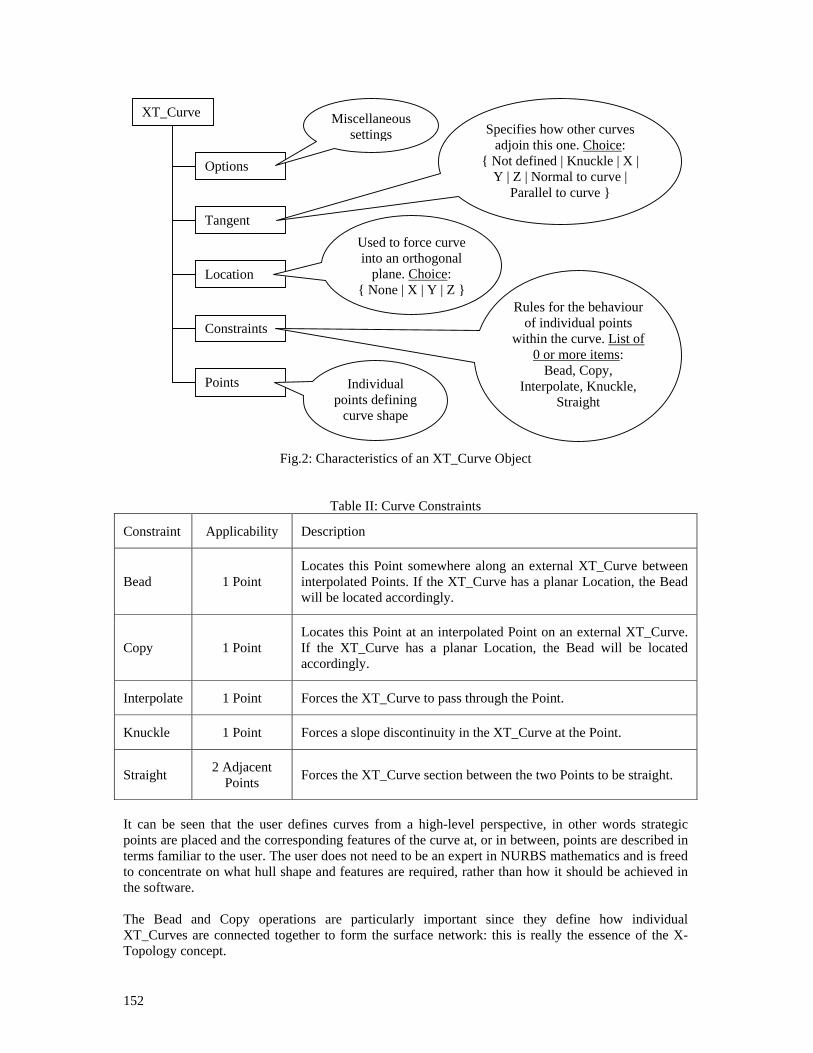
152

Fig.2: Characteristics of an XT_Curve Object

Table II: Curve Constraints

Constraint Applicability Description

Bead 1 Point Locates this Point somewhere along an external XT_Curve between interpolated Points. If the XT_Curve has a planar Location, the Bead will be located accordingly.

Copy 1 Point Locates this Point at an interpolated Point on an external XT_Curve. If the XT_Curve has a planar Location, the Bead will be located accordingly.

Interpolate 1 Point Forces the XT_Curve to pass through the Point.

Knuckle 1 Point Forces a slope discontinuity in the XT_Curve at the Point.

Straight 2 Adjacent Points Forces the XT_Curve section between the two Points to be straight.

It can be seen that the user defines curves from a high-level perspective, in other words strategic points are placed and the corresponding features of the curve at, or in between, points are described in terms familiar to the user. The user does not need to be an expert in NURBS mathematics and is freed to concentrate on what hull shape and features are required, rather than how it should be achieved in the software. The Bead and Copy operations are particularly important since they define how individual XT_Curves are connected together to form the surface network: this is really the essence of the X-Topology concept.

XT_Curve

Options

Tangent

Location

Points

Constraints

Specifies how other curves adjoin this one. Choice:

Not defined | Knuckle | X | Y | Z | Normal to curve |

Parallel to curve

Used to force curve into an orthogonal

plane. Choice: None | X | Y | Z

Miscellaneous settings

Rules for the behaviour of individual points

within the curve. List of 0 or more items:

Bead, Copy, Interpolate, Knuckle,

Straight Individual

points defining curve shape

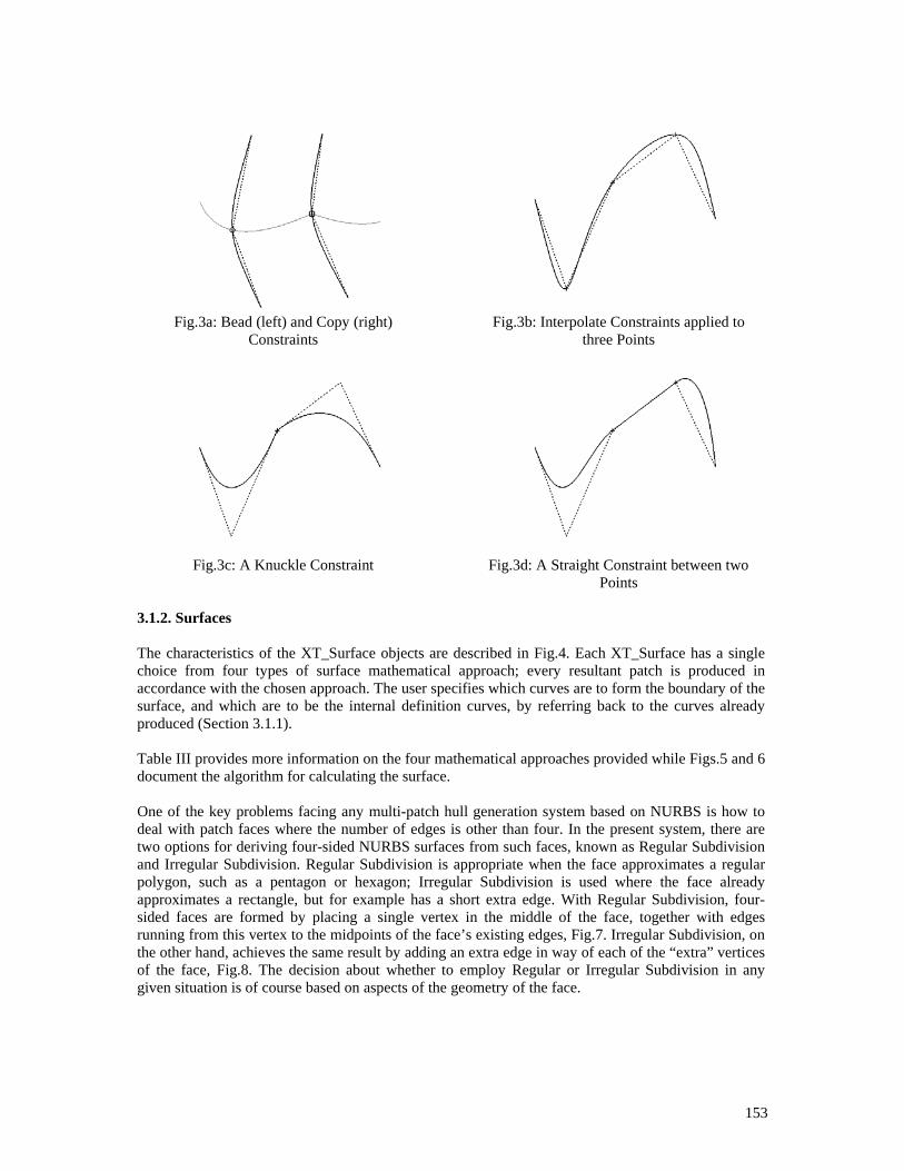
153

Fig.3a: Bead (left) and Copy (right)

Constraints

Fig.3b: Interpolate Constraints applied to three Points

Fig.3c: A Knuckle Constraint Fig.3d: A Straight Constraint between two

Points 3.1.2. Surfaces The characteristics of the XT_Surface objects are described in Fig.4. Each XT_Surface has a single choice from four types of surface mathematical approach; every resultant patch is produced in accordance with the chosen approach. The user specifies which curves are to form the boundary of the surface, and which are to be the internal definition curves, by referring back to the curves already produced (Section 3.1.1). Table III provides more information on the four mathematical approaches provided while Figs.5 and 6 document the algorithm for calculating the surface. One of the key problems facing any multi-patch hull generation system based on NURBS is how to deal with patch faces where the number of edges is other than four. In the present system, there are two options for deriving four-sided NURBS surfaces from such faces, known as Regular Subdivision and Irregular Subdivision. Regular Subdivision is appropriate when the face approximates a regular polygon, such as a pentagon or hexagon; Irregular Subdivision is used where the face already approximates a rectangle, but for example has a short extra edge. With Regular Subdivision, four-sided faces are formed by placing a single vertex in the middle of the face, together with edges running from this vertex to the midpoints of the face’s existing edges, Fig.7. Irregular Subdivision, on the other hand, achieves the same result by adding an extra edge in way of each of the “extra” vertices of the face, Fig.8. The decision about whether to employ Regular or Irregular Subdivision in any given situation is of course based on aspects of the geometry of the face.

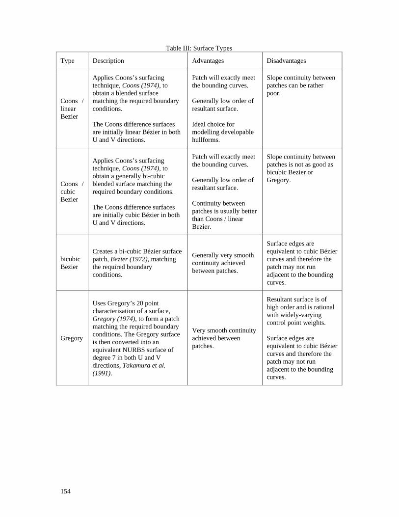
154

Table III: Surface Types

Type Description Advantages Disadvantages

Coons / linear Bezier

Applies Coons’s surfacing technique, Coons (1974), to obtain a blended surface matching the required boundary conditions. The Coons difference surfaces are initially linear Bézier in both U and V directions.

Patch will exactly meet the bounding curves. Generally low order of resultant surface. Ideal choice for modelling developable hullforms.

Slope continuity between patches can be rather poor.

Coons / cubic Bezier

Applies Coons’s surfacing technique, Coons (1974), to obtain a generally bi-cubic blended surface matching the required boundary conditions. The Coons difference surfaces are initially cubic Bézier in both U and V directions.

Patch will exactly meet the bounding curves. Generally low order of resultant surface. Continuity between patches is usually better than Coons / linear Bezier.

Slope continuity between patches is not as good as bicubic Bezier or Gregory.

bicubic Bezier

Creates a bi-cubic Bézier surface patch, Bezier (1972), matching the required boundary conditions.

Generally very smooth continuity achieved between patches.

Surface edges are equivalent to cubic Bézier curves and therefore the patch may not run adjacent to the bounding curves.

Gregory

Uses Gregory’s 20 point characterisation of a surface, Gregory (1974), to form a patch matching the required boundary conditions. The Gregory surface is then converted into an equivalent NURBS surface of degree 7 in both U and V directions, Takamura et al. (1991).

Very smooth continuity achieved between patches.

Resultant surface is of high order and is rational with widely-varying control point weights. Surface edges are equivalent to cubic Bézier curves and therefore the patch may not run adjacent to the bounding curves.

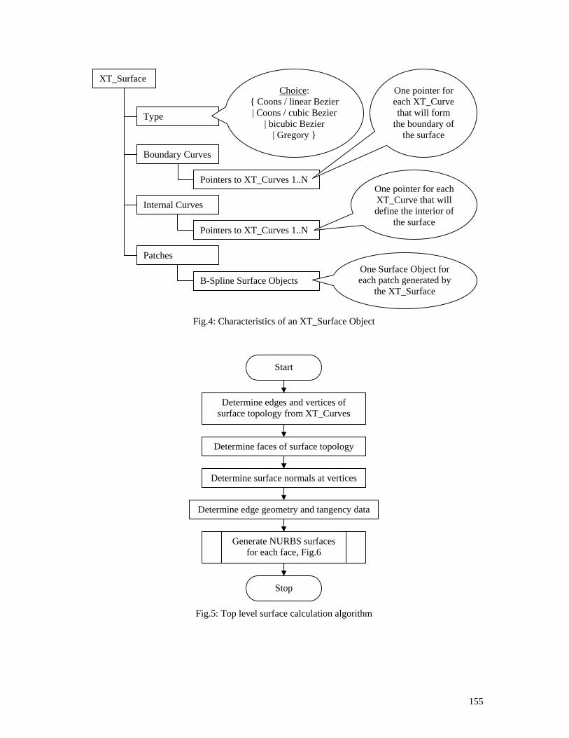
155

Fig.4: Characteristics of an XT_Surface Object

Fig.5: Top level surface calculation algorithm

XT_Surface

Type

Boundary Curves

Internal Curves

Patches

Choice: Coons / linear Bezier| Coons / cubic Bezier

| bicubic Bezier | Gregory

Pointers to XT_Curves 1..N

Pointers to XT_Curves 1..N

B-Spline Surface Objects One Surface Object for each patch generated by

the XT_Surface

One pointer for each XT_Curve that will define the interior of

the surface

One pointer for each XT_Curve that will form

the boundary of the surface

Determine edges and vertices of surface topology from XT_Curves

Determine faces of surface topology

Determine surface normals at vertices

Determine edge geometry and tangency data

Start

Generate NURBS surfaces for each face, Fig.6

Stop

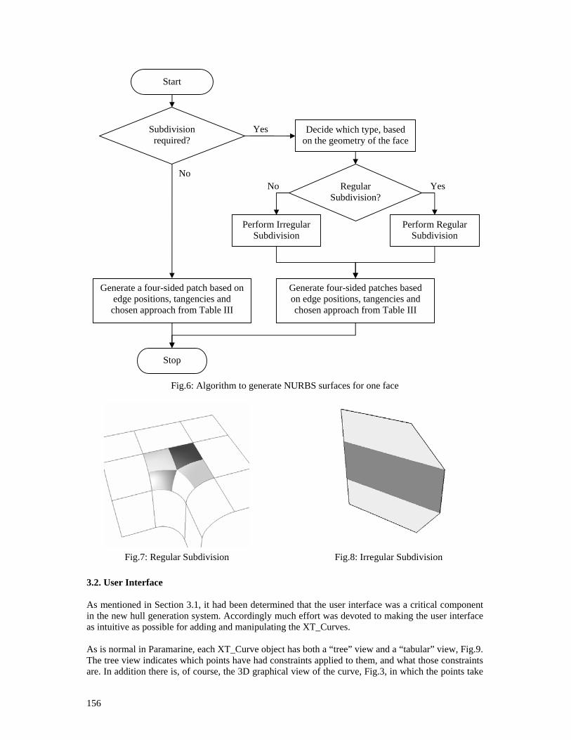
156

Fig.6: Algorithm to generate NURBS surfaces for one face

Fig.7: Regular Subdivision Fig.8: Irregular Subdivision

3.2. User Interface As mentioned in Section 3.1, it had been determined that the user interface was a critical component in the new hull generation system. Accordingly much effort was devoted to making the user interface as intuitive as possible for adding and manipulating the XT_Curves. As is normal in Paramarine, each XT_Curve object has both a “tree” view and a “tabular” view, Fig.9. The tree view indicates which points have had constraints applied to them, and what those constraints are. In addition there is, of course, the 3D graphical view of the curve, Fig.3, in which the points take

No

Yes

No Yes

Subdivision required?

Decide which type, based on the geometry of the face

Perform Irregular Subdivision

Start

Stop

Regular Subdivision?

Generate a four-sided patch based on edge positions, tangencies and chosen approach from Table III

Generate four-sided patches based on edge positions, tangencies and chosen approach from Table III

Perform Regular Subdivision

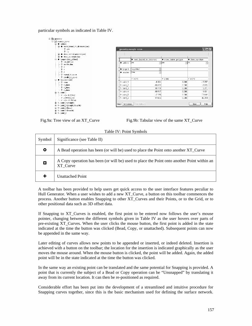
157

particular symbols as indicated in Table IV.

Fig.9a: Tree view of an XT_Curve Fig.9b: Tabular view of the same XT_Curve

Table IV: Point Symbols

Symbol Significance (see Table II)

A Bead operation has been (or will be) used to place the Point onto another XT_Curve

A Copy operation has been (or will be) used to place the Point onto another Point within an XT_Curve

Unattached Point

A toolbar has been provided to help users get quick access to the user interface features peculiar to Hull Generator. When a user wishes to add a new XT_Curve, a button on this toolbar commences the process. Another button enables Snapping to other XT_Curves and their Points, or to the Grid, or to other positional data such as 3D offset data. If Snapping to XT_Curves is enabled, the first point to be entered now follows the user’s mouse pointer, changing between the different symbols given in Table IV as the user hovers over parts of pre-existing XT_Curves. When the user clicks the mouse button, the first point is added in the state indicated at the time the button was clicked (Bead, Copy, or unattached). Subsequent points can now be appended in the same way. Later editing of curves allows new points to be appended or inserted, or indeed deleted. Insertion is achieved with a button on the toolbar; the location for the insertion is indicated graphically as the user moves the mouse around. When the mouse button is clicked, the point will be added. Again, the added point will be in the state indicated at the time the button was clicked. In the same way an existing point can be translated and the same potential for Snapping is provided. A point that is currently the subject of a Bead or Copy operation can be “Unsnapped” by translating it away from its current location. It can then be re-positioned as required. Considerable effort has been put into the development of a streamlined and intuitive procedure for Snapping curves together, since this is the basic mechanism used for defining the surface network.

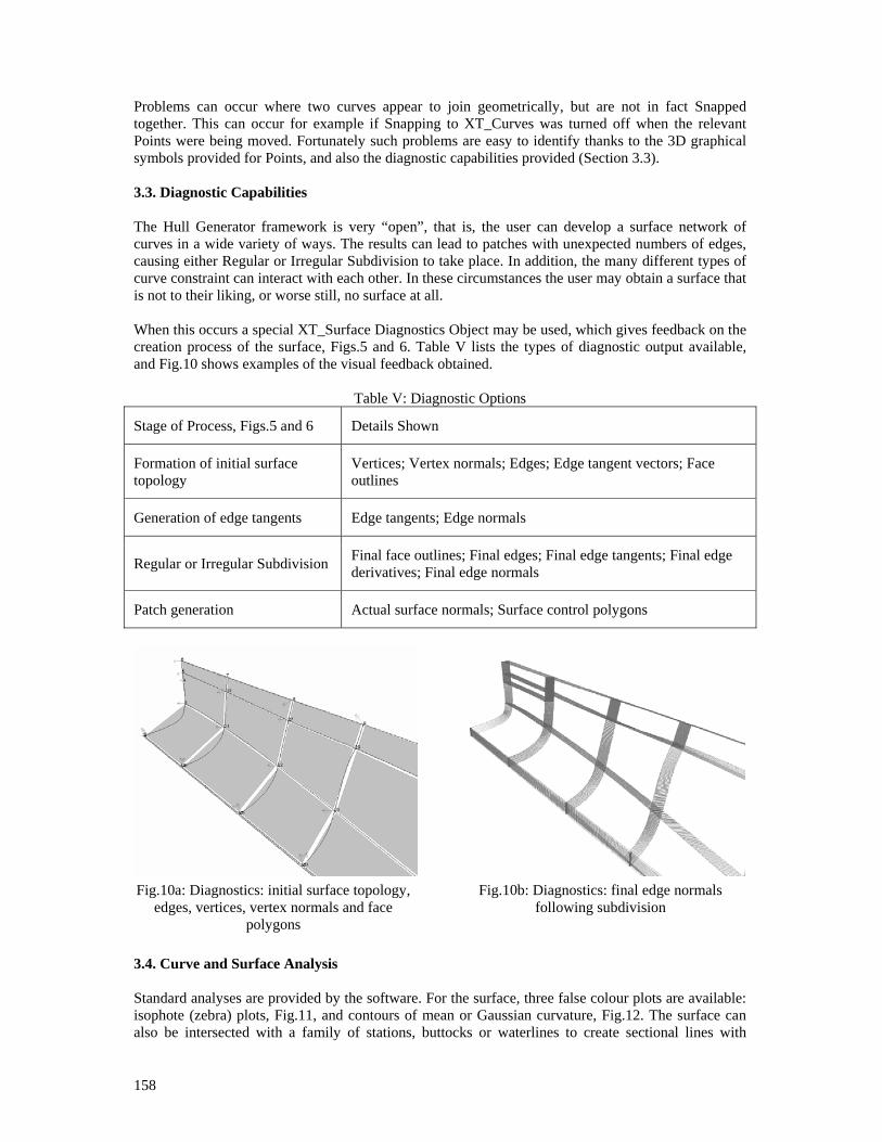
158

Problems can occur where two curves appear to join geometrically, but are not in fact Snapped together. This can occur for example if Snapping to XT_Curves was turned off when the relevant Points were being moved. Fortunately such problems are easy to identify thanks to the 3D graphical symbols provided for Points, and also the diagnostic capabilities provided (Section 3.3). 3.3. Diagnostic Capabilities The Hull Generator framework is very “open”, that is, the user can develop a surface network of curves in a wide variety of ways. The results can lead to patches with unexpected numbers of edges, causing either Regular or Irregular Subdivision to take place. In addition, the many different types of curve constraint can interact with each other. In these circumstances the user may obtain a surface that is not to their liking, or worse still, no surface at all. When this occurs a special XT_Surface Diagnostics Object may be used, which gives feedback on the creation process of the surface, Figs.5 and 6. Table V lists the types of diagnostic output available, and Fig.10 shows examples of the visual feedback obtained.

Table V: Diagnostic Options

Stage of Process, Figs.5 and 6 Details Shown

Formation of initial surface topology

Vertices; Vertex normals; Edges; Edge tangent vectors; Face outlines

Generation of edge tangents Edge tangents; Edge normals

Regular or Irregular Subdivision Final face outlines; Final edges; Final edge tangents; Final edge derivatives; Final edge normals

Patch generation Actual surface normals; Surface control polygons

Fig.10a: Diagnostics: initial surface topology, edges, vertices, vertex normals and face

polygons

Fig.10b: Diagnostics: final edge normals following subdivision

3.4. Curve and Surface Analysis Standard analyses are provided by the software. For the surface, three false colour plots are available: isophote (zebra) plots, Fig.11, and contours of mean or Gaussian curvature, Fig.12. The surface can also be intersected with a family of stations, buttocks or waterlines to create sectional lines with

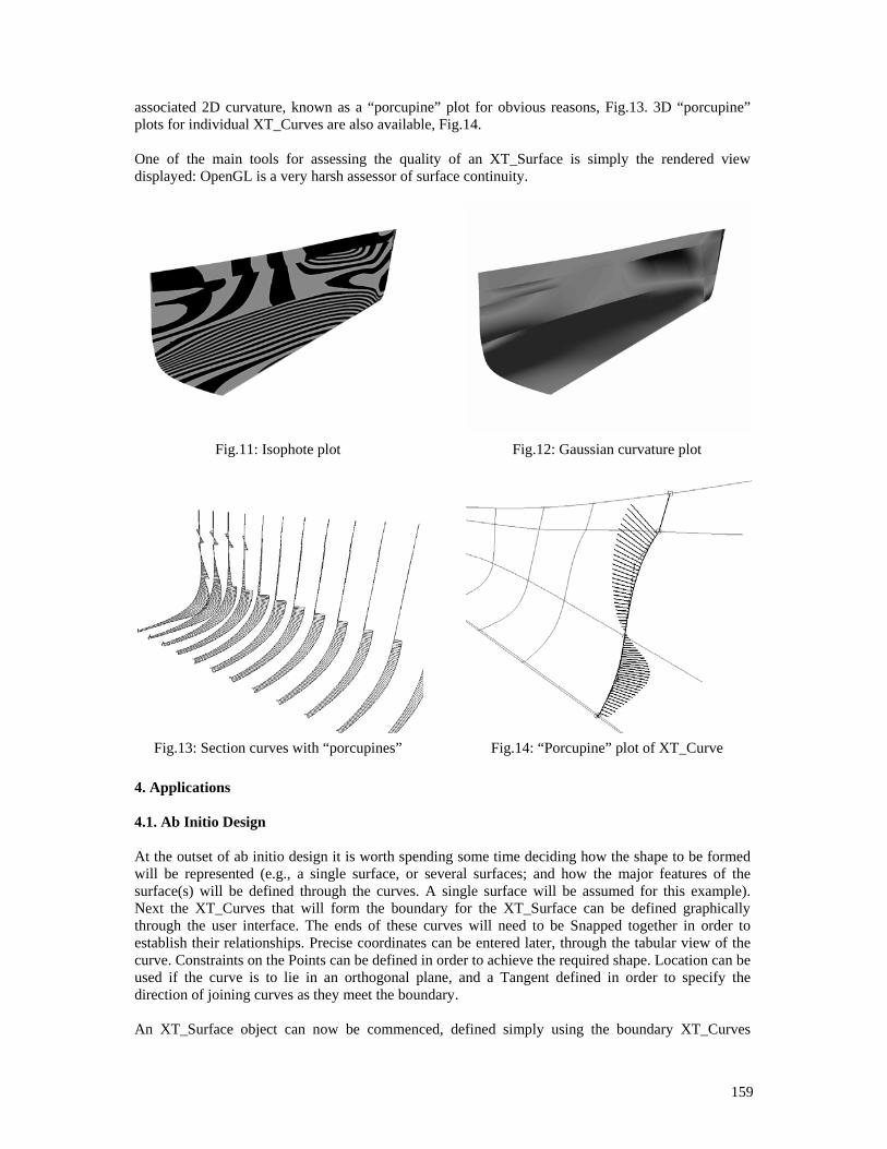
159

associated 2D curvature, known as a “porcupine” plot for obvious reasons, Fig.13. 3D “porcupine” plots for individual XT_Curves are also available, Fig.14. One of the main tools for assessing the quality of an XT_Surface is simply the rendered view displayed: OpenGL is a very harsh assessor of surface continuity.

Fig.11: Isophote plot Fig.12: Gaussian curvature plot

Fig.13: Section curves with “porcupines” Fig.14: “Porcupine” plot of XT_Curve 4. Applications 4.1. Ab Initio Design At the outset of ab initio design it is worth spending some time deciding how the shape to be formed will be represented (e.g., a single surface, or several surfaces; and how the major features of the surface(s) will be defined through the curves. A single surface will be assumed for this example). Next the XT_Curves that will form the boundary for the XT_Surface can be defined graphically through the user interface. The ends of these curves will need to be Snapped together in order to establish their relationships. Precise coordinates can be entered later, through the tabular view of the curve. Constraints on the Points can be defined in order to achieve the required shape. Location can be used if the curve is to lie in an orthogonal plane, and a Tangent defined in order to specify the direction of joining curves as they meet the boundary. An XT_Surface object can now be commenced, defined simply using the boundary XT_Curves

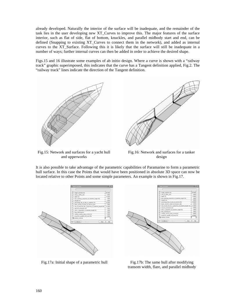
160

already developed. Naturally the interior of the surface will be inadequate, and the remainder of the task lies in the user developing new XT_Curves to improve this. The major features of the surface interior, such as flat of side, flat of bottom, knuckles, and parallel midbody start and end, can be defined (Snapping to existing XT_Curves to connect them in the network), and added as internal curves to the XT_Surface. Following this it is likely that the surface will still be inadequate in a number of ways; further internal curves can then be added in order to achieve the desired shape. Figs.15 and 16 illustrate some examples of ab initio design. Where a curve is shown with a “railway track” graphic superimposed, this indicates that the curve has a Tangent definition applied, Fig.2. The “railway track” lines indicate the direction of the Tangent definition.

Fig.15: Network and surfaces for a yacht hull and upperworks

Fig.16: Network and surfaces for a tanker design

It is also possible to take advantage of the parametric capabilities of Paramarine to form a parametric hull surface. In this case the Points that would have been positioned in absolute 3D space can now be located relative to other Points and some simple parameters. An example is shown in Fig.17.

Fig.17a: Initial shape of a parametric hull Fig.17b: The same hull after modifying transom width, flare, and parallel midbody

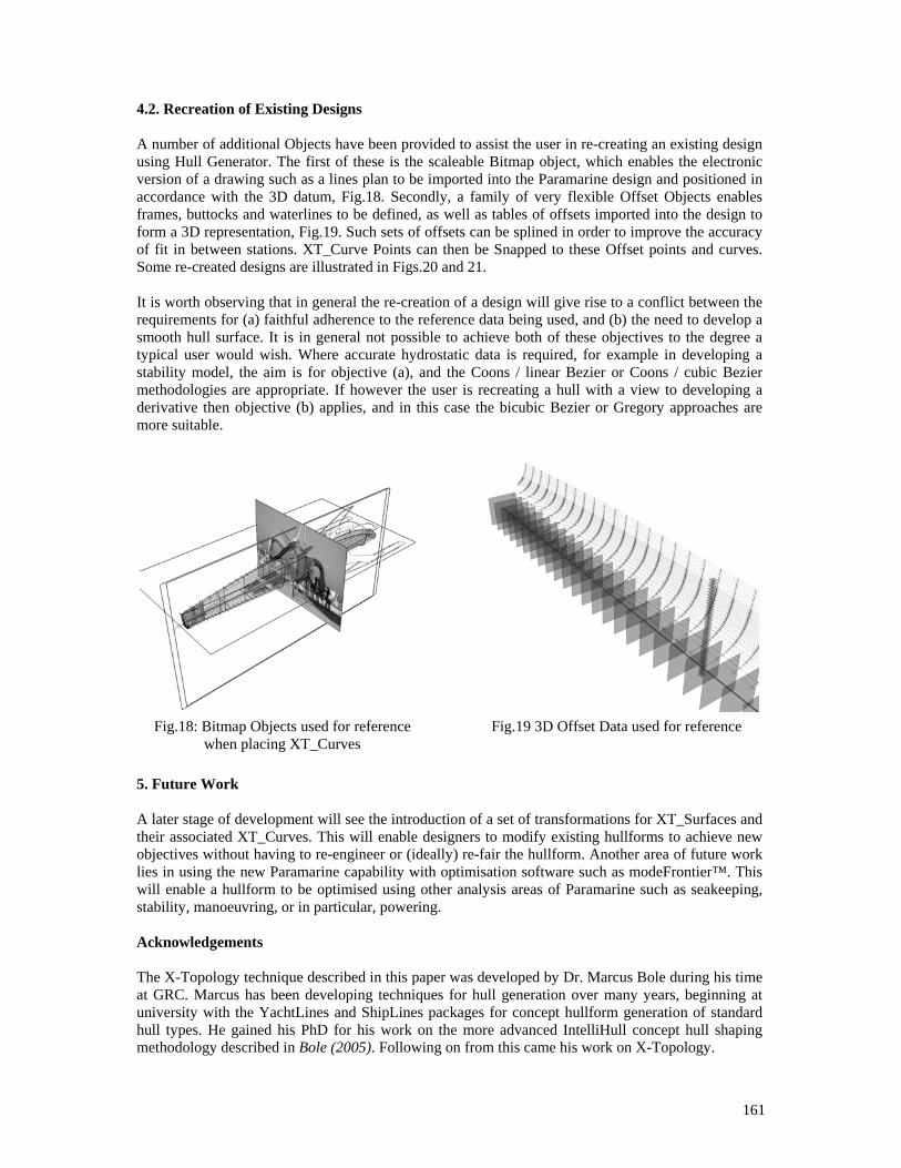
161

4.2. Recreation of Existing Designs A number of additional Objects have been provided to assist the user in re-creating an existing design using Hull Generator. The first of these is the scaleable Bitmap object, which enables the electronic version of a drawing such as a lines plan to be imported into the Paramarine design and positioned in accordance with the 3D datum, Fig.18. Secondly, a family of very flexible Offset Objects enables frames, buttocks and waterlines to be defined, as well as tables of offsets imported into the design to form a 3D representation, Fig.19. Such sets of offsets can be splined in order to improve the accuracy of fit in between stations. XT_Curve Points can then be Snapped to these Offset points and curves. Some re-created designs are illustrated in Figs.20 and 21. It is worth observing that in general the re-creation of a design will give rise to a conflict between the requirements for (a) faithful adherence to the reference data being used, and (b) the need to develop a smooth hull surface. It is in general not possible to achieve both of these objectives to the degree a typical user would wish. Where accurate hydrostatic data is required, for example in developing a stability model, the aim is for objective (a), and the Coons / linear Bezier or Coons / cubic Bezier methodologies are appropriate. If however the user is recreating a hull with a view to developing a derivative then objective (b) applies, and in this case the bicubic Bezier or Gregory approaches are more suitable.

Fig.18: Bitmap Objects used for reference when placing XT_Curves

Fig.19 3D Offset Data used for reference

5. Future Work A later stage of development will see the introduction of a set of transformations for XT_Surfaces and their associated XT_Curves. This will enable designers to modify existing hullforms to achieve new objectives without having to re-engineer or (ideally) re-fair the hullform. Another area of future work lies in using the new Paramarine capability with optimisation software such as modeFrontier™. This will enable a hullform to be optimised using other analysis areas of Paramarine such as seakeeping, stability, manoeuvring, or in particular, powering. Acknowledgements The X-Topology technique described in this paper was developed by Dr. Marcus Bole during his time at GRC. Marcus has been developing techniques for hull generation over many years, beginning at university with the YachtLines and ShipLines packages for concept hullform generation of standard hull types. He gained his PhD for his work on the more advanced IntelliHull concept hull shaping methodology described in Bole (2005). Following on from this came his work on X-Topology.

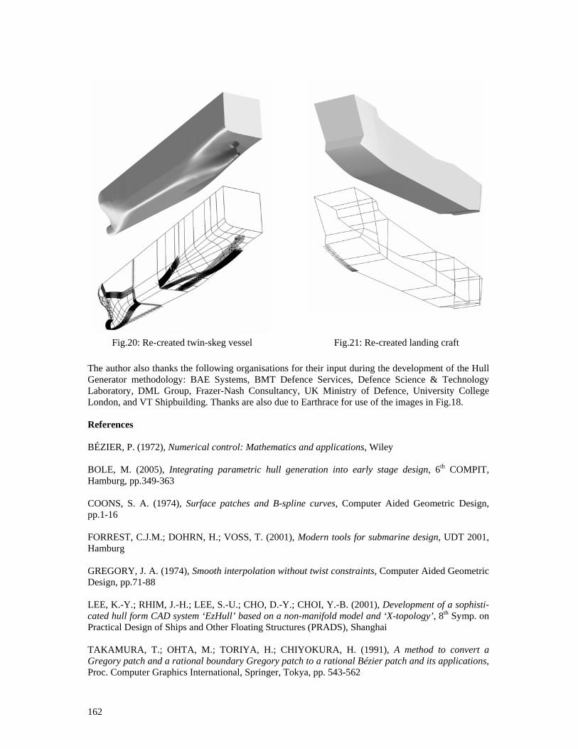
162

The author also thanks the following organisations for their input during the development of the Hull Generator methodology: BAE Systems, BMT Defence Services, Defence Science & Technology Laboratory, DML Group, Frazer-Nash Consultancy, UK Ministry of Defence, University College London, and VT Shipbuilding. Thanks are also due to Earthrace for use of the images in Fig.18. References BÉZIER, P. (1972), Numerical control: Mathematics and applications, Wiley BOLE, M. (2005), Integrating parametric hull generation into early stage design, 6th COMPIT, Hamburg, pp.349-363 COONS, S. A. (1974), Surface patches and B-spline curves, Computer Aided Geometric Design, pp.1-16 FORREST, C.J.M.; DOHRN, H.; VOSS, T. (2001), Modern tools for submarine design, UDT 2001, Hamburg GREGORY, J. A. (1974), Smooth interpolation without twist constraints, Computer Aided Geometric Design, pp.71-88 LEE, K.-Y.; RHIM, J.-H.; LEE, S.-U.; CHO, D.-Y.; CHOI, Y.-B. (2001), Development of a sophisti-cated hull form CAD system ‘EzHull’ based on a non-manifold model and ‘X-topology’, 8th Symp. on Practical Design of Ships and Other Floating Structures (PRADS), Shanghai TAKAMURA, T.; OHTA, M.; TORIYA, H.; CHIYOKURA, H. (1991), A method to convert a Gregory patch and a rational boundary Gregory patch to a rational Bézier patch and its applications, Proc. Computer Graphics International, Springer, Tokya, pp. 543-562

Fig.20: Re-created twin-skeg vessel Fig.21: Re-created landing craft

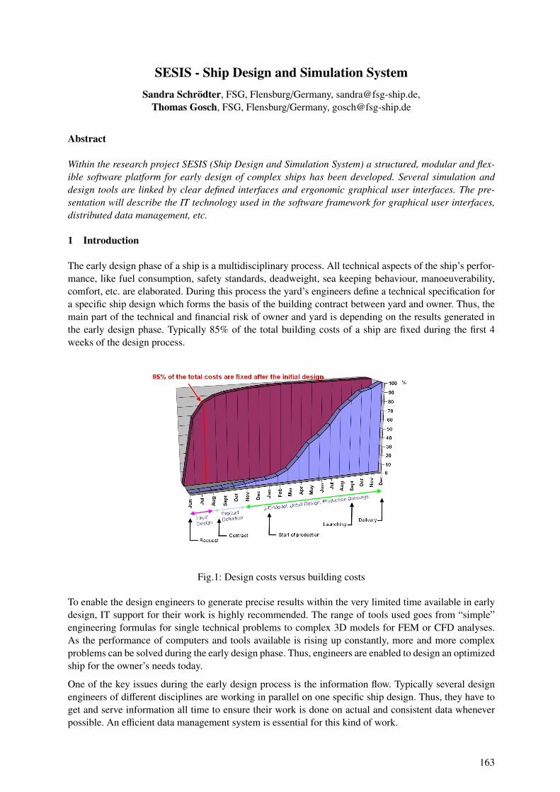
SESIS - Ship Design and Simulation SystemSandra Schrodter, FSG, Flensburg/Germany, sandra@fsg-ship.de,

Thomas Gosch, FSG, Flensburg/Germany, gosch@fsg-ship.de

Abstract

Within the research project SESIS (Ship Design and Simulation System) a structured, modular and flex-ible software platform for early design of complex ships has been developed. Several simulation anddesign tools are linked by clear defined interfaces and ergonomic graphical user interfaces. The pre-sentation will describe the IT technology used in the software framework for graphical user interfaces,distributed data management, etc.

1 Introduction

The early design phase of a ship is a multidisciplinary process. All technical aspects of the ship’s perfor-mance, like fuel consumption, safety standards, deadweight, sea keeping behaviour, manoeuverability,comfort, etc. are elaborated. During this process the yard’s engineers define a technical specification fora specific ship design which forms the basis of the building contract between yard and owner. Thus, themain part of the technical and financial risk of owner and yard is depending on the results generated inthe early design phase. Typically 85% of the total building costs of a ship are fixed during the first 4weeks of the design process.

Fig.1: Design costs versus building costs

To enable the design engineers to generate precise results within the very limited time available in earlydesign, IT support for their work is highly recommended. The range of tools used goes from “simple”engineering formulas for single technical problems to complex 3D models for FEM or CFD analyses.As the performance of computers and tools available is rising up constantly, more and more complexproblems can be solved during the early design phase. Thus, engineers are enabled to design an optimizedship for the owner’s needs today.

One of the key issues during the early design process is the information flow. Typically several designengineers of different disciplines are working in parallel on one specific ship design. Thus, they have toget and serve information all time to ensure their work is done on actual and consistent data wheneverpossible. An efficient data management system is essential for this kind of work.

163

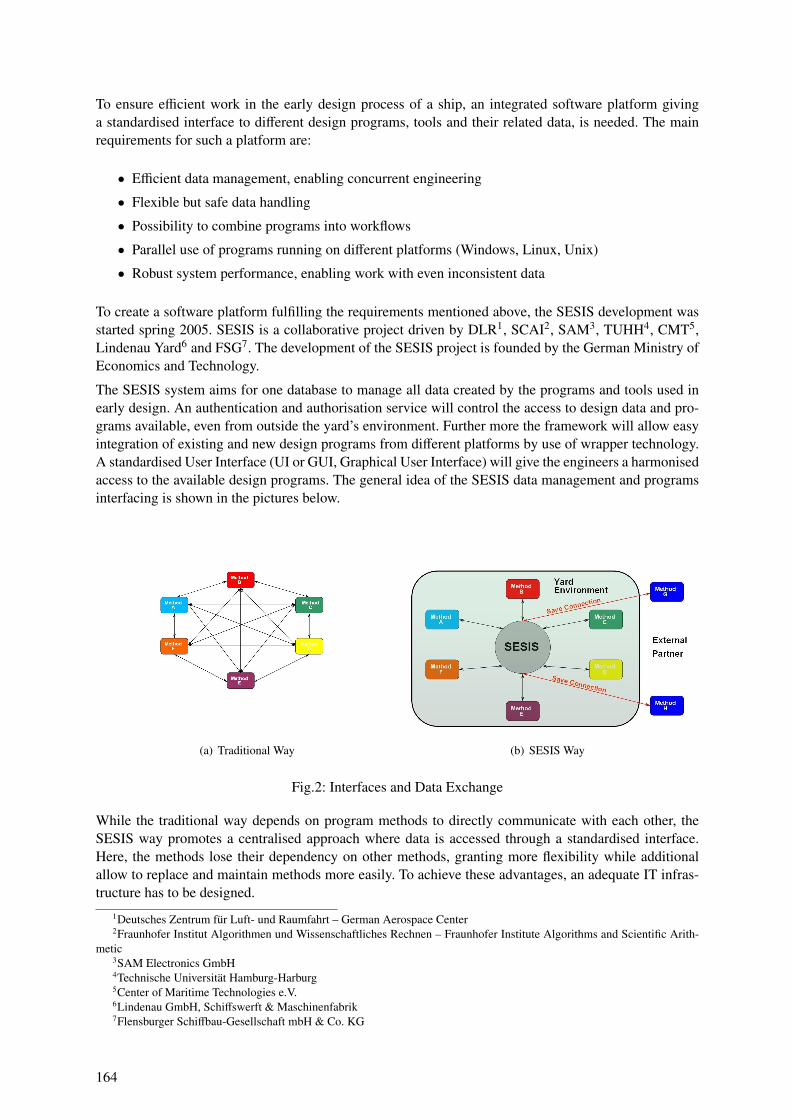
To ensure efficient work in the early design process of a ship, an integrated software platform givinga standardised interface to different design programs, tools and their related data, is needed. The mainrequirements for such a platform are:

• Efficient data management, enabling concurrent engineering

• Flexible but safe data handling

• Possibility to combine programs into workflows

• Parallel use of programs running on different platforms (Windows, Linux, Unix)

• Robust system performance, enabling work with even inconsistent data

To create a software platform fulfilling the requirements mentioned above, the SESIS development wasstarted spring 2005. SESIS is a collaborative project driven by DLR1, SCAI2, SAM3, TUHH4, CMT5,Lindenau Yard6 and FSG7. The development of the SESIS project is founded by the German Ministry ofEconomics and Technology.

The SESIS system aims for one database to manage all data created by the programs and tools used inearly design. An authentication and authorisation service will control the access to design data and pro-grams available, even from outside the yard’s environment. Further more the framework will allow easyintegration of existing and new design programs from different platforms by use of wrapper technology.A standardised User Interface (UI or GUI, Graphical User Interface) will give the engineers a harmonisedaccess to the available design programs. The general idea of the SESIS data management and programsinterfacing is shown in the pictures below.

(a) Traditional Way (b) SESIS Way

Fig.2: Interfaces and Data Exchange

While the traditional way depends on program methods to directly communicate with each other, theSESIS way promotes a centralised approach where data is accessed through a standardised interface.Here, the methods lose their dependency on other methods, granting more flexibility while additionalallow to replace and maintain methods more easily. To achieve these advantages, an adequate IT infras-tructure has to be designed.

1Deutsches Zentrum fur Luft- und Raumfahrt – German Aerospace Center2Fraunhofer Institut Algorithmen und Wissenschaftliches Rechnen – Fraunhofer Institute Algorithms and Scientific Arith-

metic3SAM Electronics GmbH4Technische Universitat Hamburg-Harburg5Center of Maritime Technologies e.V.6Lindenau GmbH, Schiffswerft & Maschinenfabrik7Flensburger Schiffbau-Gesellschaft mbH & Co. KG

164

2 Requirements from an IT Point of View

The requirements for the IT infrastructure and the framework concretise into the following:

Requirements for the Basement:

• Flexible and extendable

• Based on standard, state-of-the-art software components

• Easy maintenance

• Data management

• User management

• Communication services

• Security levels for data and integrated programs

• Platform independent or at least functional on different platforms

Requirements for Integration:

• Integration of existing software and applications

• Different levels of integration possible, depending on the availability of sourcecode or an API8

• Common user interface

• Centralized data handling

• Defining and carrying out of workflows

Requirements for Development:

• Software development kit (SDK) to support the development of new software for the framework

• Providing tested components

• Aid in keeping standards

Where to look for the solution? The market for collaboration software is growing. The world is shrinking,communication is the topic of today, not only connecting humans but hardware, programs and datamod-els. New software design paradigms are evolving, facing the problems of designing complex system in amanner that keeps them scalable and maintainable.

Only there is no such tool that combines the points above yet, nor is it likely to evolve at short notice, be-cause the above mentioned requirements are fairly extensive. Considering the task of integrating existinginhouse software solutions, it is often tried either by throwing away and rewriting the sourcecode basisusing new paradigms (high potential, but risky and time consuming) or patching it with software-gluelittle by little (downwards compatible but reduced maintainability and potential).

Both ways are examples of extremes that, as experience tells, often fail to reach their goal. But there is athird way: keep the well proven, gain the new and combine both into a framework.

Although developing software inhouse commits resources and has the peril of producing isolated appli-cations or reinventing the wheel, the list of benefits is long.

Once the know how is built up – which may take some time – it is possible to spezialise on an area ofexpertise and react faster to new or changing requirements than would ever be possible with software offthe shelf and waiting for the next version. If the requirements make it into the new version. If there is anew version.

So being independent may allow you to be the first – or only – one able to comply to a customer’s request.8Application Programming Interface, a source code interface provided by e.g. a software library.

165

3 Creating SESIS

The collaborated research project SESIS was started to create a framework as described above. Thepartners bring in the required experiences in IT development, engineering processes and how to connectboth sides.

The general conditions for the project were manifold and can be split into three sections:

3.1 Keeping the Well Proven

Regarded applications range from the inhouse written software where the sourcecode is available andadaptable, called white box, to the black box software without sourcecode, which is only changeable bythe vendor. Between them exists a span of grey box software, which can be, to an degree, customizedand controlled by input files or an programmable API.

Both the know how in grown applications, which is more or less palpable, and the efficiency of establishedprocesses, deliver reasons the keep them.

But the fact that software is in use for a longer time doesn’t make it well proven per definition. Thereare numerous reasons for remaining using it, like running contracts, licences or sometimes the fear ofchange which always contains a risk. These reasons have nothing to do with reliability.

Examples of well proven programs include the optimized and thoroughly tested solver or the efficientand for the internal processes highly customized prognose tool.

3.2 Gaining the New

A 20 year old car is still running, not least because its character is known so thoroughly that almost everyissue can be fixed. It keeps its driver warm and dry and gets him from A to B. There seems to be noreason to change this.

But moderns cars are more efficient, safe and faster. They contain a lot of fancy stuff – well that is a matterof taste, but the first points will show in the car owners purse and the safety of him and his passengers.

The statement from this is easy: being part of technological progress has advantages.

What needs to be carefully considered – in particular in the rapid changing IT – is not to fall for a “hype”,meaning a paradigm or software that shines brightly the one day, with its name all over the internet, anddisappears silently within a year or two.

Examples of technological progress include visualisation toolkits, communication support or data stor-ages. Due to advancements in computer hard- and software the modern realizations are much morepowerful and extensive and allow both software developers and engineers to concentrate on their actualchallenge.

3.3 Combining both in a Framework

Neither all new nor all established is the solution, but a combination of both it is. The main challenges tobe met on this road are:

• Find a common platform where all applications can be run and managed from. Common possibil-ities for this include Linux or Windows

• Present the user with as much of a common user interface as possible. This is always possible fornew software, once a standard is kept, but somewhat harder for existing ones

• Share data bases of the integrated applications, which may be solved via direct or indirect exchangeof data

166

Common to all points are their possible consequences for existing software, which may include portingand refactoring of white box code and buying new licences for black box software. So another challengecan be formulated:

• Keep changes to existing software as minor as possible

4 Realisation of SESIS

With the right decisions regarding fundamental technologies a number of achievements come for free.Open source software offers a heap of proven applications or functionalities and the support is, thanks toforums and communities often faster and more detailed than with commercial hotlines. On the other handsome precaution should be put into the selection of technologies because this rapidly changing marketcarries the above mentioned risk of falling for “hypes”.

More details will follow but some words about limiting implementation parameters first: The main pro-gramming language was chosen to be Java. Java is modern, object oriented and platform independent,thus supporting among other things maintainability and integration of applications that may be limitedto a platform. Apprehensions about poor performance are no matter anymore.

The base for flexibility and maintainability is delivered by the underlying Rich Client Platform (RCP) – asubset of Eclipse9. One part of RCP’s flexibility is based upon the OSGi standard that supports pluggablefunctionality10

Considering these technologies as base pillars, still more functionality needs to be added for the abovementioned requirements, as there are remote usage, security, data mangement, workflow and the integra-tion of different softwares on the list. Part of them can be found as stable and standarized open sourcesoftware, others need to be implemented.

Bundling all together defines the multi purpose framework RCE (Reconfigurable Computing Environ-ment), which can be utilized in diverse industries. SESIS extends RCE by adding applications for theshipbuilding industry.

4.1 Layered Architecture

An overview about the architecture of the new framework (see Figure 3) shows that it is made of differentlayers to separate components, which is an important constraint for complex software systems.

The basement is made up of 3 Components:

• As Java is the common programming language, the application runs in a JVM (Java Virtual Ma-chine).

• Eclipse Equinox, which is part of the above mentioned RCP, is an implementation of the OSGi coreframework specification. OSGi specificates an application life cycle management model whichenables a modular and customizable application with pluggable functionality and defines a scopefor modularity: the bundle.

• The Reconfigurable Computing Environment is based on the open tools platform RCP and extendsit in two ways: a core layer (yellow) and a number of additional bundles (blue).

The vertical blue bundles provide additional functionality like: data mangement, communication, secu-rity and distribution.

9Eclipse itself started as an Integrated Development Environment for Java years ago and advanced to a popular open-sourcesoftware framework

10The OSGi standard was formulated by the OSGi Alliance (formerly known as the Open Service Gateway initiative) whichis an open standards organization founded in 1999 with companies among their members like IBM, Oracle, Sun Microsystems,or Siemens.

167

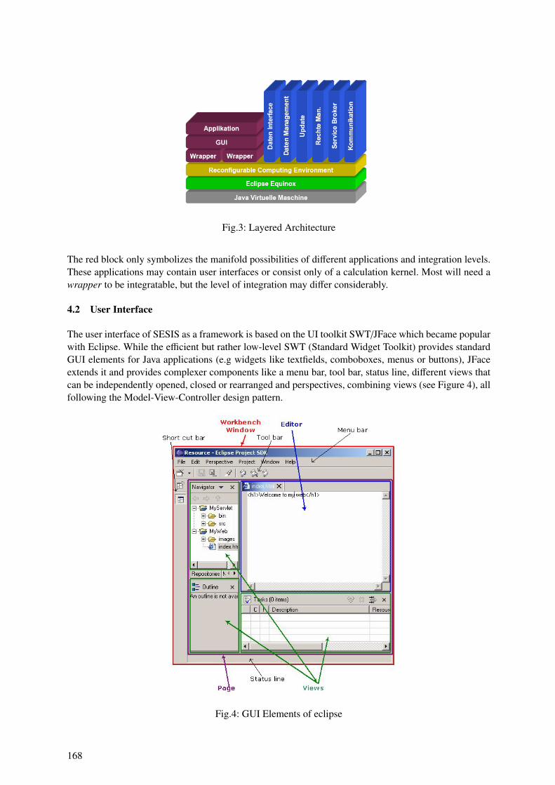
Fig.3: Layered Architecture

The red block only symbolizes the manifold possibilities of different applications and integration levels.These applications may contain user interfaces or consist only of a calculation kernel. Most will need awrapper to be integratable, but the level of integration may differ considerably.

4.2 User Interface

The user interface of SESIS as a framework is based on the UI toolkit SWT/JFace which became popularwith Eclipse. While the efficient but rather low-level SWT (Standard Widget Toolkit) provides standardGUI elements for Java applications (e.g widgets like textfields, comboboxes, menus or buttons), JFaceextends it and provides complexer components like a menu bar, tool bar, status line, different views thatcan be independently opened, closed or rearranged and perspectives, combining views (see Figure 4), allfollowing the Model-View-Controller design pattern.

Fig.4: GUI Elements of eclipse

168

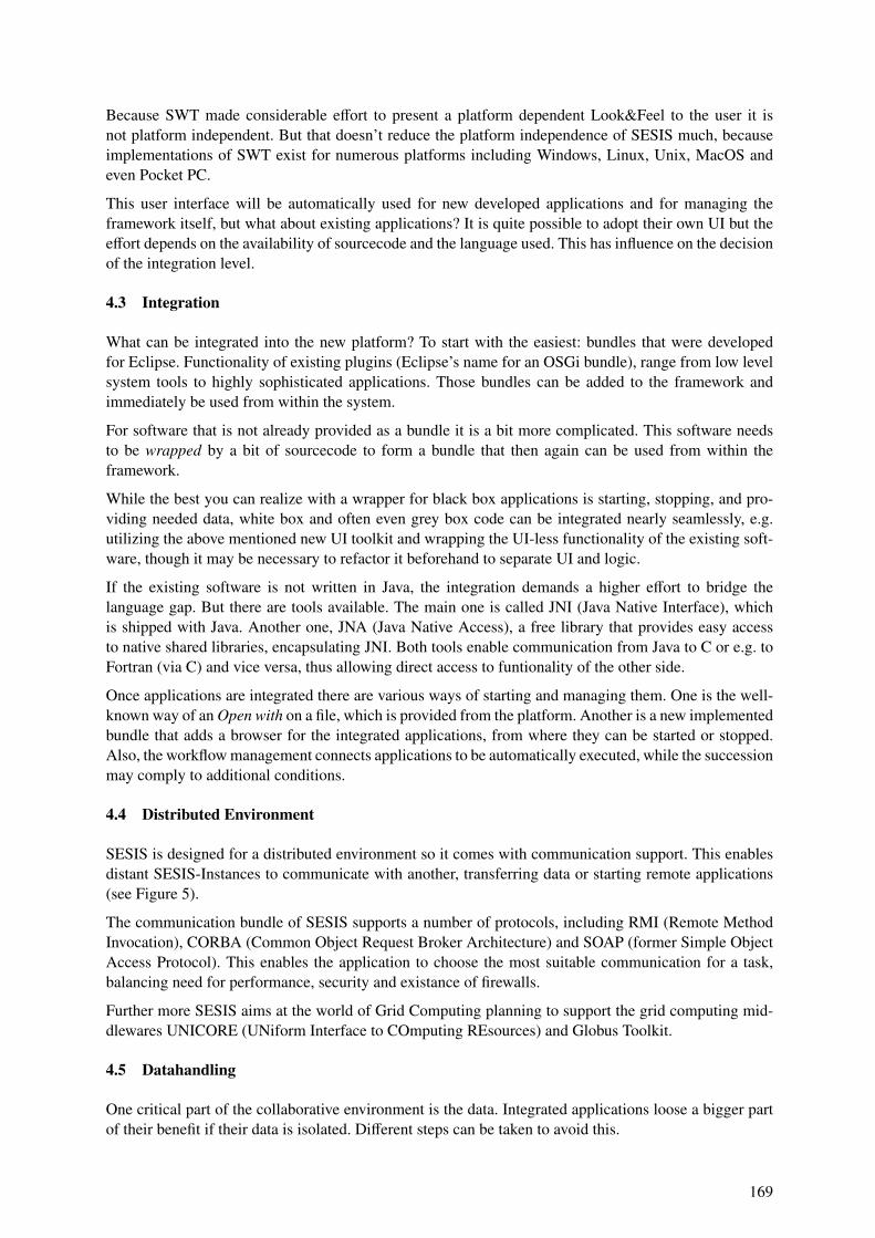
Because SWT made considerable effort to present a platform dependent Look&Feel to the user it isnot platform independent. But that doesn’t reduce the platform independence of SESIS much, becauseimplementations of SWT exist for numerous platforms including Windows, Linux, Unix, MacOS andeven Pocket PC.

This user interface will be automatically used for new developed applications and for managing theframework itself, but what about existing applications? It is quite possible to adopt their own UI but theeffort depends on the availability of sourcecode and the language used. This has influence on the decisionof the integration level.

4.3 Integration

What can be integrated into the new platform? To start with the easiest: bundles that were developedfor Eclipse. Functionality of existing plugins (Eclipse’s name for an OSGi bundle), range from low levelsystem tools to highly sophisticated applications. Those bundles can be added to the framework andimmediately be used from within the system.

For software that is not already provided as a bundle it is a bit more complicated. This software needsto be wrapped by a bit of sourcecode to form a bundle that then again can be used from within theframework.

While the best you can realize with a wrapper for black box applications is starting, stopping, and pro-viding needed data, white box and often even grey box code can be integrated nearly seamlessly, e.g.utilizing the above mentioned new UI toolkit and wrapping the UI-less functionality of the existing soft-ware, though it may be necessary to refactor it beforehand to separate UI and logic.

If the existing software is not written in Java, the integration demands a higher effort to bridge thelanguage gap. But there are tools available. The main one is called JNI (Java Native Interface), whichis shipped with Java. Another one, JNA (Java Native Access), a free library that provides easy accessto native shared libraries, encapsulating JNI. Both tools enable communication from Java to C or e.g. toFortran (via C) and vice versa, thus allowing direct access to funtionality of the other side.

Once applications are integrated there are various ways of starting and managing them. One is the well-known way of an Open with on a file, which is provided from the platform. Another is a new implementedbundle that adds a browser for the integrated applications, from where they can be started or stopped.Also, the workflow management connects applications to be automatically executed, while the successionmay comply to additional conditions.

4.4 Distributed Environment

SESIS is designed for a distributed environment so it comes with communication support. This enablesdistant SESIS-Instances to communicate with another, transferring data or starting remote applications(see Figure 5).

The communication bundle of SESIS supports a number of protocols, including RMI (Remote MethodInvocation), CORBA (Common Object Request Broker Architecture) and SOAP (former Simple ObjectAccess Protocol). This enables the application to choose the most suitable communication for a task,balancing need for performance, security and existance of firewalls.

Further more SESIS aims at the world of Grid Computing planning to support the grid computing mid-dlewares UNICORE (UNiform Interface to COmputing REsources) and Globus Toolkit.

4.5 Datahandling

One critical part of the collaborative environment is the data. Integrated applications loose a bigger partof their benefit if their data is isolated. Different steps can be taken to avoid this.

169

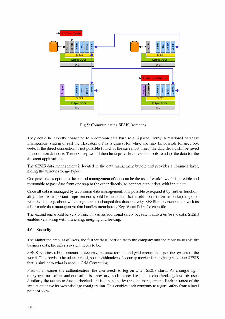
Fig.5: Communicating SESIS Instances

They could be directly connected to a common data base (e.g. Apache Derby, a relational databasemanagement system or just the filesystem). This is easiest for white and may be possible for grey boxcode. If the direct connection is not possible (which is the case most times) the data should still be savedin a common database. The next step would then be to provide conversion tools to adapt the data for thedifferent applications.

The SESIS data management is located in the data mangement bundle and provides a common layer,hiding the various storage types.

One possible exception to the central management of data can be the use of workflows. It is possible andreasonable to pass data from one step to the other directly, to connect output data with input data.

Once all data is managed by a common data management, it is possible to expand it by further function-ality. The first important improvement would be metadata, that is additional information kept togetherwith the data, e.g. about which engineer last changed this data and why. SESIS implements them with itstailor made data management that handles metadata as Key-Value-Pairs for each file.

The second one would be versioning. This gives additional safety because it adds a history to data. SESISenables versioning with branching, merging and locking.

4.6 Security

The higher the amount of users, the further their location from the company and the more valueable thebusiness data, the safer a system needs to be.

SESIS requires a high amount of security, because remote and grid operations open the system to theworld. This needs to be taken care of, so a combination of security mechanisms is integrated into SESISthat is similar to what is used in Grid Computing.

First of all comes the authentication: the user needs to log on when SESIS starts. As a single-sign-on system no further authentication is necessary, each successive bundle can check against this user.Similarly the access to data is checked – if it is handled by the data management. Each instance of thesystem can have its own privilege configuration. That enables each company to regard safety from a localpoint of view.

170

5 Conclusion

Although the requirements for a flexible and extendable framework for a distributed collaborative envi-ronment seemed ambitious, the majority of the requirements are solvable or already solved. Because ofcareful weighted design decisions it was possible to gain a lot from the open source market in terms ofsourcecode or standards and momentum from communities like Eclipse. This is also a potential for thefuture, for the community takes care of advancements and bug fixes.

Of course there is still work to be done. Especially regarding tests, integration tests in particular. Perfor-mance and scalability can best be tested during stress situations. Creating them is on the agenda for thenext half a year.

Considering the general conditions from the beginning, Keepin the Well Proven was realized with theintegration of white and black box code. One example presents the black box integration for ANSYS. Awrapper was implemented that fetches necessary data, asks the user for additional information it couldnnot gather from that data base and starts a calculation with ANSYS. Another example shows the whitebox integration of E4 Methods utilizing JNI, which will be replaced by JNA in the next step, because itis easier to maintain.

Gaining the New brought a new harmonized GUI based on JFace/SWT, standards like OSGi or CORBA,new potential with the use of existing Eclipse plugins and the application of object oriented designparadigms and Design Patterns.

In order to Combine both, integrated applications can be managed from a single point with a new projectand data management organizing their data. Thanks to the communication support, SESIS is able toconnect different platforms, diverse applications and distributed users.

An example for an application developed for the new framework is the Propeller Design Tool. It allowsinteractive modifications and hydrodynamic assessment of the propulsor, offering a flexible and modernGUI and keeping its data downwards compatible.

The resulting conclusion of developing a customized software framework is positive. It is possible tokeep the well proven in form of existing applications and functionalities so that no setback regardingrequired and established functionality is to be feared. On the other side the potential of new technologiescould be gained, supporting both the engineers and the developers with new standards and technologicalachievements.

Basing on tested, standarized and maintainable components, SESIS supports the demanding and time-critical concurrent engineering of the early design phase of a ship.

171

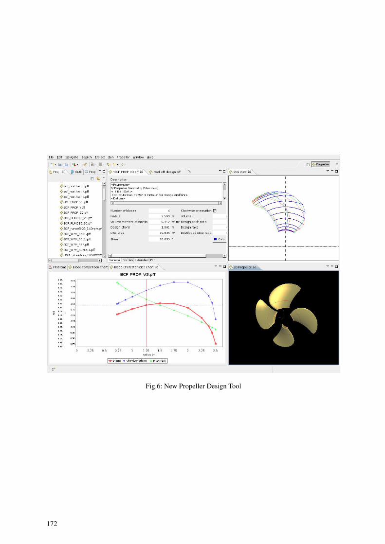
Fig.6: New Propeller Design Tool

172

References

SESIS – Integriertes Schiffsentwurfs- und Simulationssystem, www.sesis.de

KRUGER, S. (2003), The Role of IT in Shipbuilding, COMPIT’03, pp.525-533

FREEMAN, E.; FREEMAN, E.; SIERRA, K. (2004), Head First Design Patterns, O’Reilly Media

Java, java.sun.com

Eclipse, www.eclipse.org

OSGi, www.osgi.org

JNA - Java Native Access, jna.dev.java.net

Wikipedia, www.wikipedia.org

173

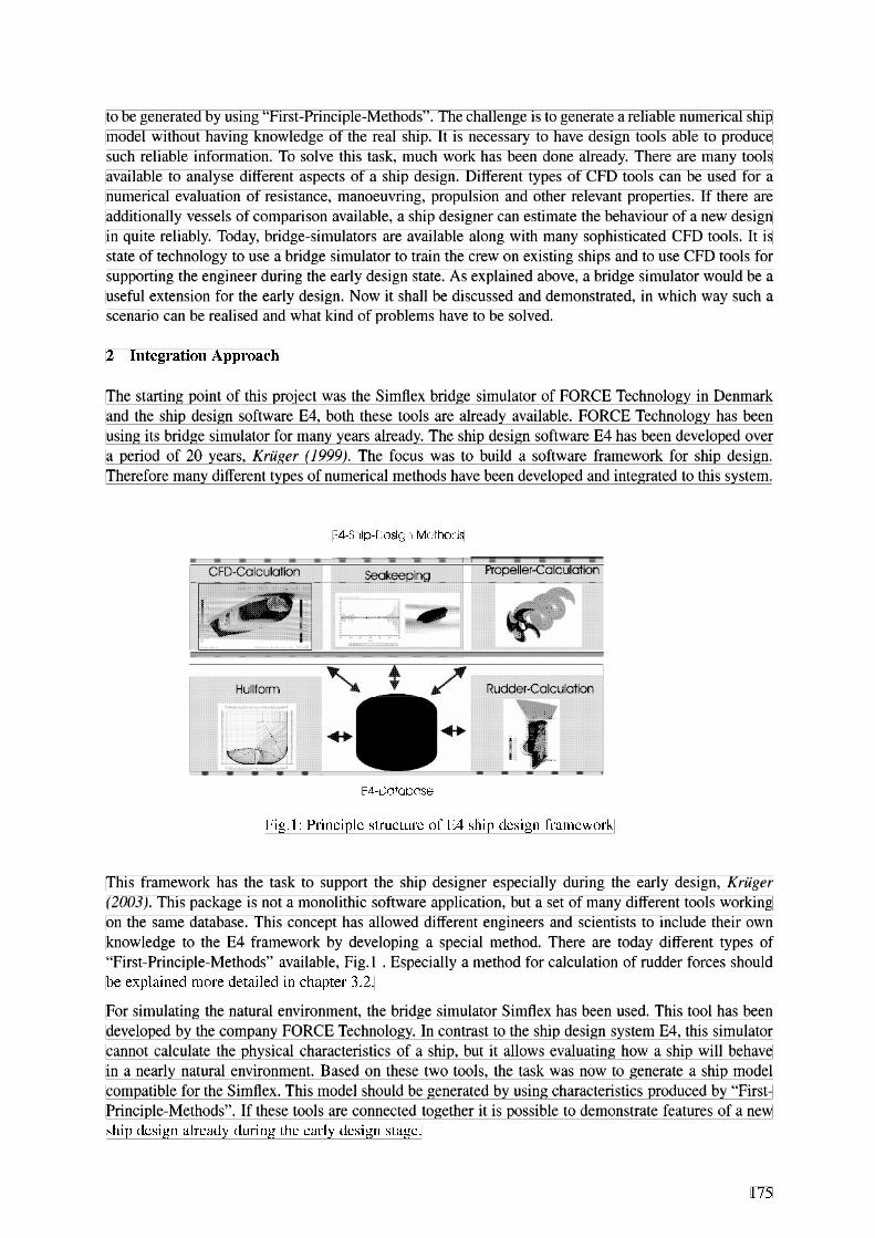
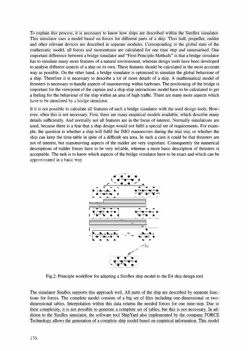
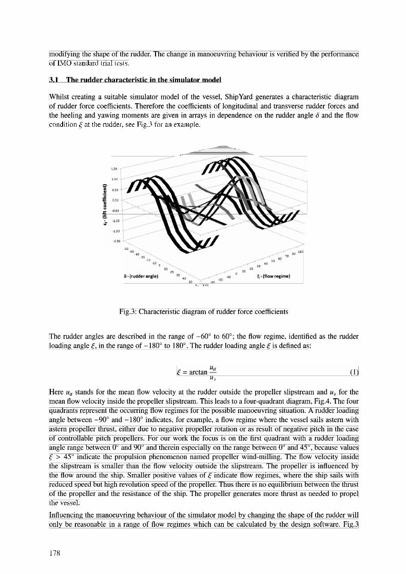
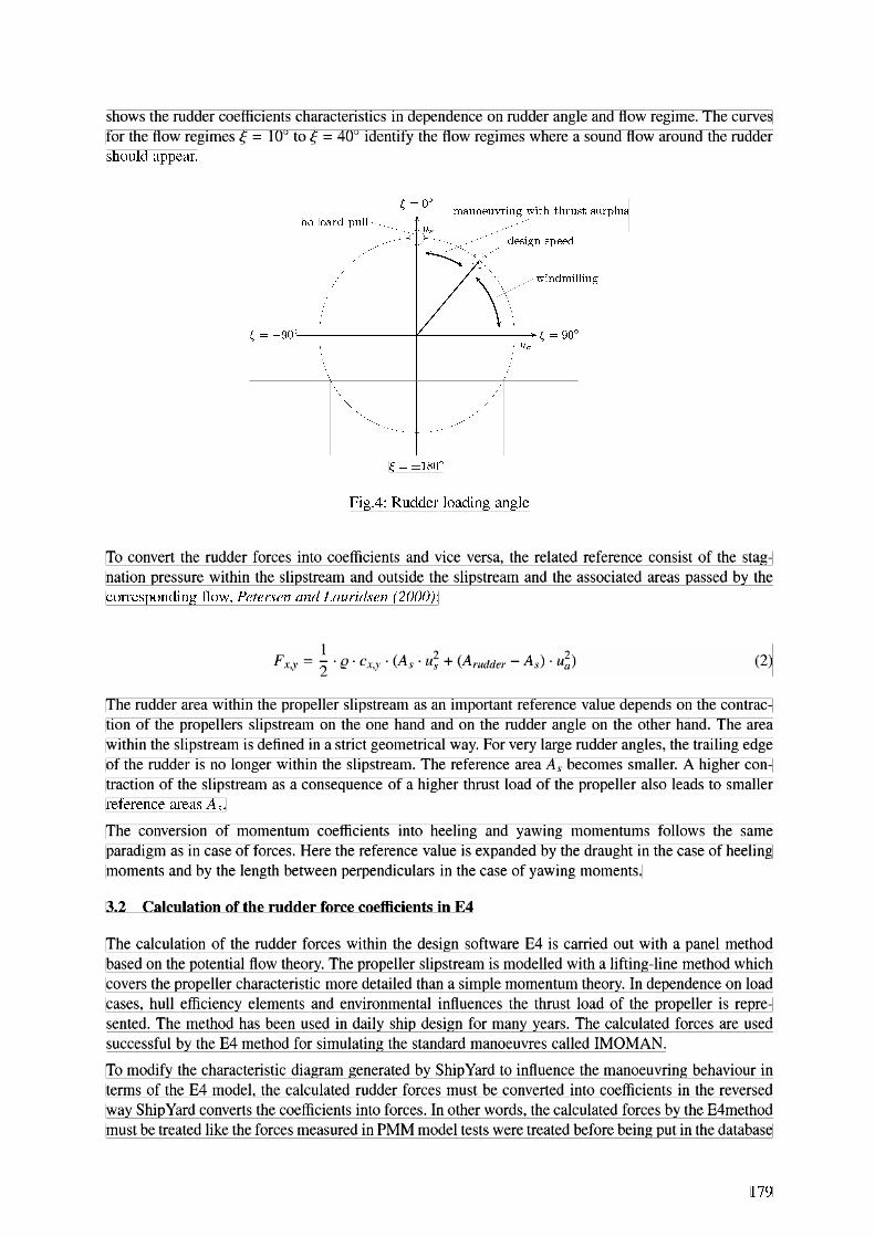
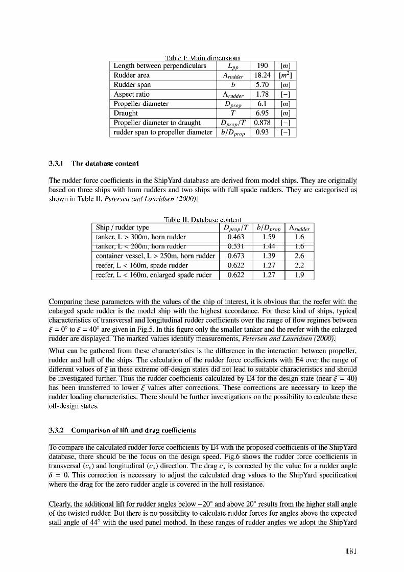
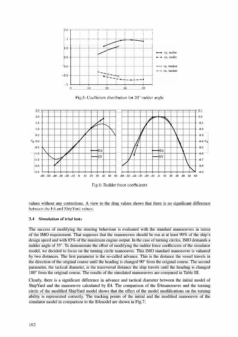
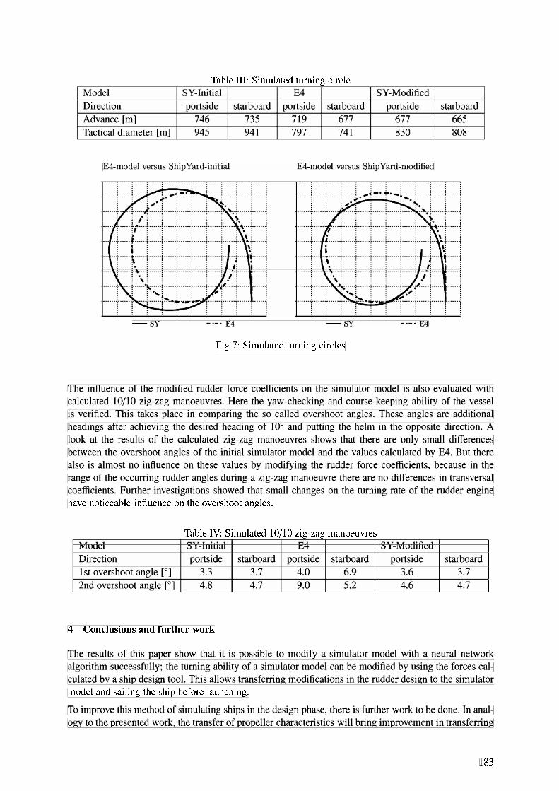
Multi System Mission Control for Teams of Unmanned Marine Vehicles – Software Structure for Online Replanning of Mission Plans

Thomas Glotzbach, Technische Universität Ilmenau; Fraunhofer Center for Applied Systems

Technology, Ilmenau/Germany, thomas.glotzbach@tu-ilmenau.deMatthias Schneider, Technische Universität Ilmenau/Germany, schneider.matthias@tu-ilmenau.de

Peter Otto, Technische Universität Ilmenau/Germany, peter.otto@tu-ilmenau.de

Abstract

The realization of cooperative Multiple Unmanned Marine Vehicles (MUMVs) is a real challenge, due to the conditions of the marine environment. In this paper we show the necessary steps of developments to enable already existing, single autonomous vehicles to participate in a team mission. We describe the design of the control software and put an emphasis on the task of Online Replanning of the vehicles’ mission plans. This Online Replanning is one of the critical issues in the realization of vehicle teams, as existing single autonomous vehicles usually do not use this functionality. 1. Introduction In this paper we give an account of the proceedings in the European Research Project GREX1, which aims to realize cooperating teams of single autonomous marine vehicles. Starting from the basics we discussed in Glotzbach et al. (2007a), where we gave a general overview of different concepts of autonomy and the realization of a simulator for Multiple Unmanned Marine Vehicles, we will now turn to the GREX dedicated hard- and software technologies that need to be integrated into the already existing vehicles to enable cooperative behavior. The GREX project is not for the development of new marine vehicles for cooperative behavior, but uses already existing vehicles of different supplier (‘heterogeneous vehicles’). This results in the requirement to consider the strict limitations of the vehicle providers concerning the implementation of hard- and software of their vehicles. We will summarize these demands and describe how they influenced our decision making for the final control strategy. In general it can be stated that the usual proceedings for single vehicle missions should also be applied to team missions: The mission need to be described using mission plans that will later be executed by the single vehicles. The mission plans should be adapted to each other, and there is need for adaptation of the plans during mission execution (what we refer to as Online Replanning). In this framework we will show the significance of an adequate Team-Oriented Mission Planning (TOMP) for both considering the requirements of the providers and dealing with the typical constraints in marine and underwater scenarios. We will show that a coordinated team behavior for heterogeneous marine vehicles requires a good adapted combination of offline mission planning and online replanning during execution. Especially, the communicational constraints of underwater environments demand a high level of autonomy for the vehicles. Thus, an optimal team mission plan need to be designed to minimize the needs of online replanning. Nevertheless, there will never be a realization of a coordinated vehicle team, where every vehicle only follows its own mission plan, even if these plans were designed with great care. So the online mission replanning has the same 1 GREX is the Latin word for herd, team, or swarm. The research project GREX is funded by the Sixth Framework Programme of the European Community (FP6-IST-2006-035223). Participants of the GREX- project are the following companies and institutions: ATLAS ELEKTRONIK GmbH (Germany), Centre of IMAR at Department of Oceanography and Fisheries at the University of the Azores (Portugal), Ifremer (France), Innova S.p.A. (Italy), Instituto Superior Tecnico IST - Lab: Institute for Systems and Robotics ISR (Portugal), MC Marketing Consulting (Germany), ORANGE ENERGY Consulting (Portugal), SeeByte Ltd. (United Kingdom), Institute for Automation and Systems Engineering of the Technische Universität Ilmenau (Germany). See GREX (2008) for further information.

185

importance as the pre-mission planning. While we demonstrated our proposal for a concept of Team-Oriented Mission Planning in Glotzbach et al. (2007b), we will concentrate on online mission replanning in this paper. The employed marine vehicles need to be provided with new hard- and software technologies to cover the needs of cooperative behavior. For example, the vehicles need to be equipped with communication technology, especially for inter-vehicle-communication. As most vehicles involved in the GREX project are underwater vehicles, the ability for both aerial and underwater communication is required. Specifically the last one is usually not part of the typical abilities of single autonomous underwater vehicles. A specific software module must be employed to organize the communication with other vehicles and a static/moving base station. There is also the need for a new navigation approach. As the avoidance of collision is one of the most important tasks, a certain software module is responsible to run time-continuous models of the position of all other vehicles, relative to the own position. These position estimations are based upon the messages sent between the vehicles and the calculated distances and directions. Another software module has the task to realize the interfaces between the existing hard- / software of the vehicles and the new, GREX specific ones. Last but not least, there will be a software module called Team Handler which has to monitor the mission progress under the aspects of the overall team mission and need to interact in any cases of discrepancies. This module will be responsible for the execution of the Multi System Mission Control, consisting of Mission Monitoring and Online Mission Replanning. We will describe the software structure of this module. Mission Monitoring has the task to monitor the progress of the mission and to generate replanning orders, whenever necessary. There will be several instances that are responsible for different tasks and have different possibilities for the creation of replanning orders. We will explain these instances and classify them in the framework of the Rational Behavior Model (RBM). Online Replanning is responsible for the execution of the replanning orders. This includes sorting, validation, communication between vehicles (if necessary) and finally the concrete changes of the mission plan. In this framework we will provide the current perceptions to the question whether hierarchical or peripheral realizations of the control software are more desirable. We raised this question in Glotzbach et al. (2007a). The online change of mission plans is always high problematic and not really desired by vehicle providers. It must be kept in mind that current autonomous marine vehicles are designed for single autonomous behavior. The implementation of new mission plan elements or the deleting of existing ones should be avoided. Within the GREX project as one of the first real application with Multiple Unmanned Marine Vehicles, the possibility for replanning will be limited to fit the absolutely necessary needs. For future applications, an advanced mission replanning is in the focus of interest. We will conclude our paper with an example mission, displayed in a Virtual Reality especially designed for Marine Vehicles. 2. Basic Conditions within the GREX- research project In this chapter we outline the general conditions for the realization of cooperating marine vehicles in general as well as the specific conditions within the GREX- project. 2.1. Consequences of the challenges in the marine scenarios Several technologies which are applied for the realization of cooperating unmanned land/ aerial vehicles cannot be used in the marine environment. Especially two topics shall be discussed here: Self localization and Communication. Self localization can generally be performed by absolute measurement systems (GPS, DGPS or other navigation systems) or by relative measurement of the vehicle’s movement (odometry, inertial navigation). Both methods have advantages and disadvantages. Absolute, satellite based measurement

186

systems depend on the reachability of the navigation signals, which requires usually sight contact to a certain numbers of satellites and maybe to a reference radio station. The resulting navigation values are faulty, but the error does not grow. Relative measurement systems deliver very exact values, but the errors grow with time. Land and air bound systems may use a coupled navigation system to combine the advantages of both methods. For ground vehicle, the reachability of the satellite (and/or radio) signal may be difficult, especially in scenarios in cities, valleys or deep forests. Autonomous underwater vehicles cannot use any absolute navigation while they are submerged. They can only rely on their internal navigation systems, which have to fulfill high requirements in reliability; otherwise the vehicles have to surface a lot for GPS- updates. In the last years, high-precision inertial navigation systems have been developed, but still they are very expensive; see Höbing-Hölscher and Larsen (2006), for instance. In exchange, marine surface vehicles may rely on satellite-based absolute navigation, as they usually have a very good reception of satellite and radio signals due to their position on the plane sea surface. In the vehicle teams, which are focus of the GREX- project, this aspect produces completely new possibilities for the navigation of the underwater vehicles. They may use their internal strategies and receive position updates from the surface vehicle(s), which, on their part, use an absolute navigation strategy. Of course this procedure requires good communication abilities between the vehicles, which is the other big problem in underwater scenarios. Although all GREX vehicles will be equipped with radio modems for surface communication, the submerged vehicles are only able to use acoustic communication to talk to each other or to surface vehicles. The first acoustic underwater communication modules are available on the market. The GREX vehicle will use modems similar to the ones described in Bannasch et al. (2006). It should be mentioned that the current abilities of acoustic underwater communications are still very bad. The communication suffers from a minor reliability and a low bandwidth. Broadcast communication was barley tested so far. These facts need to be kept in mind when developing control strategies for multiple unmanned marine vehicles. We will come back to this in chapter 3. On the other hand, several acoustic modems like the ones that will be used in GREX offer the possibility to determine range and bearing between transmitter and receiver. This leads to new ways for the navigation of the team vehicles. It is planed to perform team navigation, based on the already existing navigation procedures and the range and bearing information. The concept was demonstrated in Engel and Kalwa (2007). As a result, the vehicles can use a ‘relative’ team navigation to determine where they are in relation to their teammates. The advantage of this strategy is that it helps to prevent inter vehicle collision which is one of the biggest dangers during early GREX missions (these test missions will take place in secluded areas). If the strategy for inter vehicle collision avoidance is based on the navigation procedures of the single vehicles, the different individual error values may add up and lead to a dangerous situation where the vehicles are very close to each other while the navigation systems still assume them far away. 2.2. Consequences of the usage of heterogeneous marine vehicles It is one of the principles of the GREX project not to develop own unmanned marine vehicles for the cooperating team, but to use existing ones. The idea is to create a conceptual framework and middleware systems which can easily be installed on most existing unmanned marine vehicles. The tests and demonstrations will be performed by several heterogeneous vehicles which are the property of single project participants. Fig.1 provides an overview of the different vehicles. The decision not to develop an own vehicle was made in consideration of two important aspects. Firstly, as the price for a typical autonomous underwater vehicle today is a six-figure sum, the costs of a research project with the aim of both developing a new vehicle and the middleware system for

187

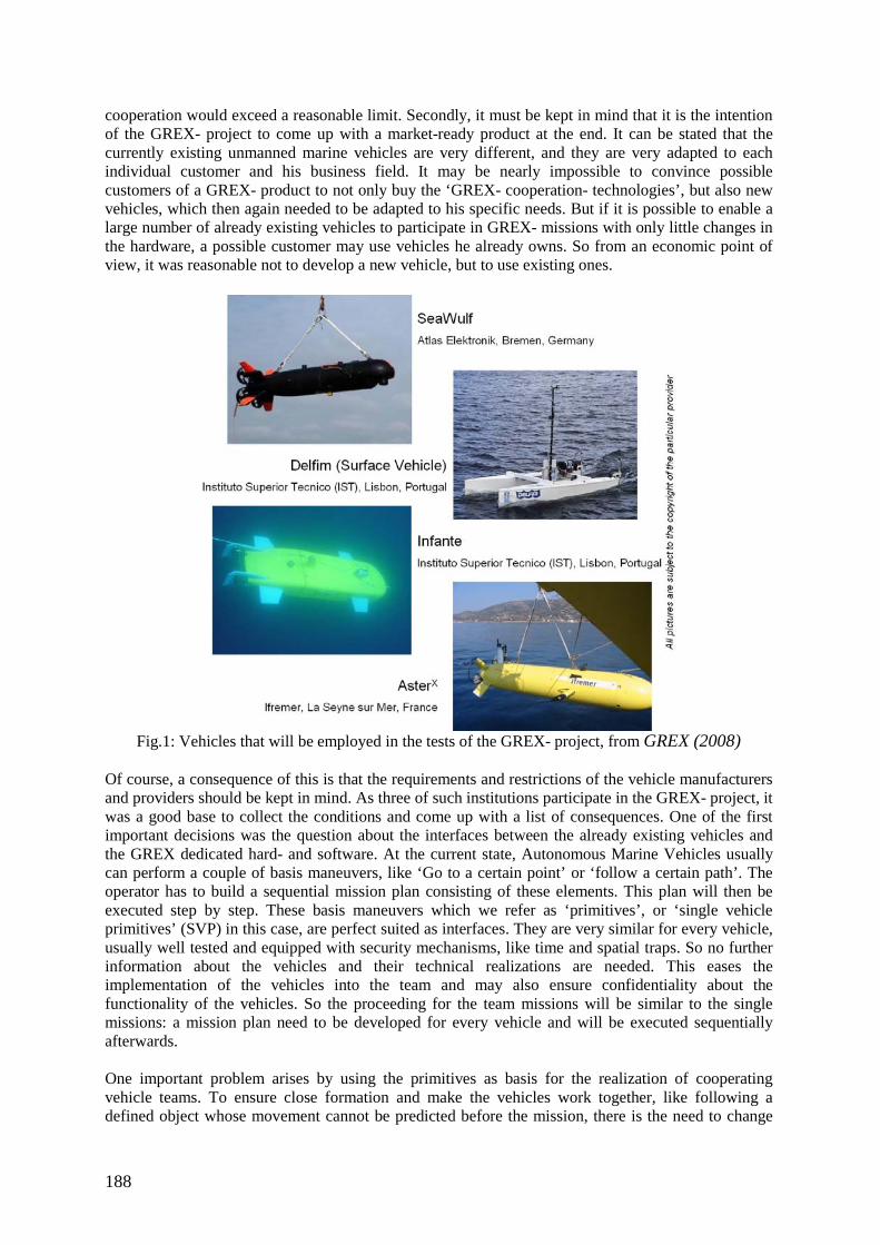
cooperation would exceed a reasonable limit. Secondly, it must be kept in mind that it is the intention of the GREX- project to come up with a market-ready product at the end. It can be stated that the currently existing unmanned marine vehicles are very different, and they are very adapted to each individual customer and his business field. It may be nearly impossible to convince possible customers of a GREX- product to not only buy the ‘GREX- cooperation- technologies’, but also new vehicles, which then again needed to be adapted to his specific needs. But if it is possible to enable a large number of already existing vehicles to participate in GREX- missions with only little changes in the hardware, a possible customer may use vehicles he already owns. So from an economic point of view, it was reasonable not to develop a new vehicle, but to use existing ones.

Fig.1: Vehicles that will be employed in the tests of the GREX- project, from GREX (2008)

Of course, a consequence of this is that the requirements and restrictions of the vehicle manufacturers and providers should be kept in mind. As three of such institutions participate in the GREX- project, it was a good base to collect the conditions and come up with a list of consequences. One of the first important decisions was the question about the interfaces between the already existing vehicles and the GREX dedicated hard- and software. At the current state, Autonomous Marine Vehicles usually can perform a couple of basis maneuvers, like ‘Go to a certain point’ or ‘follow a certain path’. The operator has to build a sequential mission plan consisting of these elements. This plan will then be executed step by step. These basis maneuvers which we refer as ‘primitives’, or ‘single vehicle primitives’ (SVP) in this case, are perfect suited as interfaces. They are very similar for every vehicle, usually well tested and equipped with security mechanisms, like time and spatial traps. So no further information about the vehicles and their technical realizations are needed. This eases the implementation of the vehicles into the team and may also ensure confidentiality about the functionality of the vehicles. So the proceeding for the team missions will be similar to the single missions: a mission plan need to be developed for every vehicle and will be executed sequentially afterwards. One important problem arises by using the primitives as basis for the realization of cooperating vehicle teams. To ensure close formation and make the vehicles work together, like following a defined object whose movement cannot be predicted before the mission, there is the need to change

188

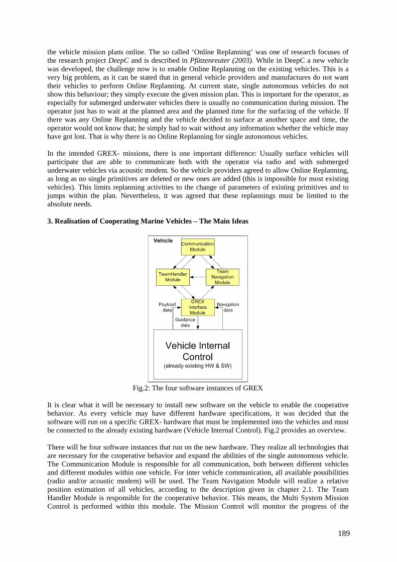
the vehicle mission plans online. The so called ‘Online Replanning’ was one of research focuses of the research project DeepC and is described in Pfützenreuter (2003). While in DeepC a new vehicle was developed, the challenge now is to enable Online Replanning on the existing vehicles. This is a very big problem, as it can be stated that in general vehicle providers and manufactures do not want their vehicles to perform Online Replanning. At current state, single autonomous vehicles do not show this behaviour; they simply execute the given mission plan. This is important for the operator, as especially for submerged underwater vehicles there is usually no communication during mission. The operator just has to wait at the planned area and the planned time for the surfacing of the vehicle. If there was any Online Replanning and the vehicle decided to surface at another space and time, the operator would not know that; he simply had to wait without any information whether the vehicle may have got lost. That is why there is no Online Replanning for single autonomous vehicles. In the intended GREX- missions, there is one important difference: Usually surface vehicles will participate that are able to communicate both with the operator via radio and with submerged underwater vehicles via acoustic modem. So the vehicle providers agreed to allow Online Replanning, as long as no single primitives are deleted or new ones are added (this is impossible for most existing vehicles). This limits replanning activities to the change of parameters of existing primitives and to jumps within the plan. Nevertheless, it was agreed that these replannings must be limited to the absolute needs. 3. Realisation of Cooperating Marine Vehicles – The Main Ideas

Fig.2: The four software instances of GREX

It is clear what it will be necessary to install new software on the vehicle to enable the cooperative behavior. As every vehicle may have different hardware specifications, it was decided that the software will run on a specific GREX- hardware that must be implemented into the vehicles and must be connected to the already existing hardware (Vehicle Internal Control). Fig.2 provides an overview. There will be four software instances that run on the new hardware. They realize all technologies that are necessary for the cooperative behavior and expand the abilities of the single autonomous vehicle. The Communication Module is responsible for all communication, both between different vehicles and different modules within one vehicle. For inter vehicle communication, all available possibilities (radio and/or acoustic modem) will be used. The Team Navigation Module will realize a relative position estimation of all vehicles, according to the description given in chapter 2.1. The Team Handler Module is responsible for the cooperative behavior. This means, the Multi System Mission Control is performed within this module. The Mission Control will monitor the progress of the

189

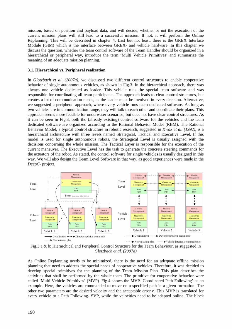
mission, based on position and payload data, and will decide, whether or not the execution of the current mission plans will still lead to a successful mission. If not, it will perform the Online Replanning. This will be described in chapter 4. Last but not least, there is the GREX Interface Module (GIM) which is the interface between GREX- and vehicle hardware. In this chapter we discuss the question, whether the team control software of the Team Handler should be organized in a hierarchical or peripheral way, introduce the term ‘Multi Vehicle Primitives’ and summarize the meaning of an adequate mission planning. 3.1. Hierarchical vs. Peripheral realization In Glotzbach et al. (2007a), we discussed two different control structures to enable cooperative behavior of single autonomous vehicles, as shown in Fig.3. In the hierarchical approach, there was always one vehicle dedicated as leader. This vehicle runs the special team software and was responsible for coordinating all team participants. The approach leads to clear control structures, but creates a lot of communication needs, as the leader must be involved in every decision. Alternative, we suggested a peripheral approach, where every vehicle runs team dedicated software. As long as two vehicles are in communication range, they will talk to each other and coordinate their plans. This approach seems more feasible for underwater scenarios, but does not have clear control structures. As it can be seen in Fig.3, both the (already existing) control software for the vehicles and the team dedicated software are organized according to the Rational Behavior Model (RBM). The Rational Behavior Model, a typical control structure in robotic research, suggested in Kwak et al. (1992), is a hierarchical architecture with three levels named Strategical, Tactical and Executive Level. If this model is used for single autonomous robots, the Strategical Level is usually assigned with the decisions concerning the whole mission. The Tactical Layer is responsible for the execution of the current maneuver. The Executive Level has the task to generate the concrete steering commands for the actuators of the robot. As stated, the control software for single vehicles is usually designed in this way. We will also design the Team Level Software in that way, as good experiences were made in the DeepC- project.

Fig.3 a & b: Hierarchical and Peripheral Control Structure for the Team Behaviour, as suggested in

Glotzbach et al. (2007a) As Online Replanning needs to be minimized, there is the need for an adequate offline mission planning that need to address the special needs of cooperative vehicles. Therefore, it was decided to develop special primitives for the planning of the Team Mission Plan. This plan describes the activities that shall be performed by the whole team. The primitive for cooperative behavior were called ‘Multi Vehicle Primitives’ (MVP). Fig.4 shows the MVP ‘Coordinated Path Following’ as an example. Here, the vehicles are commanded to move on a specified path in a given formation. The other two parameters are the desired velocity and the acceptable error ε. This MVP is translated for every vehicle to a Path Following- SVP, while the velocities need to be adapted online. The block

190

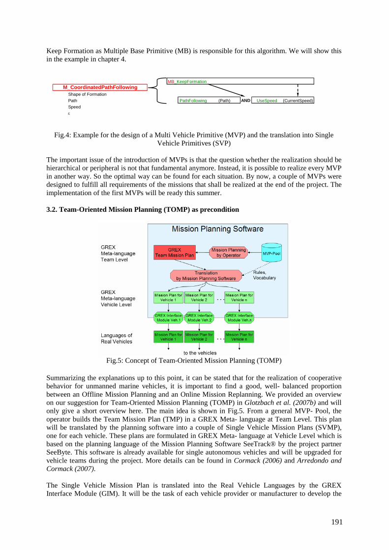
Keep Formation as Multiple Base Primitive (MB) is responsible for this algorithm. We will show this in the example in chapter 4.

MBM_CoordinatedPathFollowing

_KeepFormation

Shape of FormationPath PathFollowing (Path) AND UseSpeed (CurrentSpeed)Speedε

Fig.4: Example for the design of a Multi Vehicle Primitive (MVP) and the translation into Single

Vehicle Primitives (SVP) The important issue of the introduction of MVPs is that the question whether the realization should be hierarchical or peripheral is not that fundamental anymore. Instead, it is possible to realize every MVP in another way. So the optimal way can be found for each situation. By now, a couple of MVPs were designed to fulfill all requirements of the missions that shall be realized at the end of the project. The implementation of the first MVPs will be ready this summer. 3.2. Team-Oriented Mission Planning (TOMP) as precondition

Fig.5: Concept of Team-Oriented Mission Planning (TOMP)

Summarizing the explanations up to this point, it can be stated that for the realization of cooperative behavior for unmanned marine vehicles, it is important to find a good, well- balanced proportion between an Offline Mission Planning and an Online Mission Replanning. We provided an overview on our suggestion for Team-Oriented Mission Planning (TOMP) in Glotzbach et al. (2007b) and will only give a short overview here. The main idea is shown in Fig.5. From a general MVP- Pool, the operator builds the Team Mission Plan (TMP) in a GREX Meta- language at Team Level. This plan will be translated by the planning software into a couple of Single Vehicle Mission Plans (SVMP), one for each vehicle. These plans are formulated in GREX Meta- language at Vehicle Level which is based on the planning language of the Mission Planning Software SeeTrack® by the project partner SeeByte. This software is already available for single autonomous vehicles and will be upgraded for vehicle teams during the project. More details can be found in Cormack (2006) and Arredondo and Cormack (2007). The Single Vehicle Mission Plan is translated into the Real Vehicle Languages by the GREX Interface Module (GIM). It will be the task of each vehicle provider or manufacturer to develop the

191

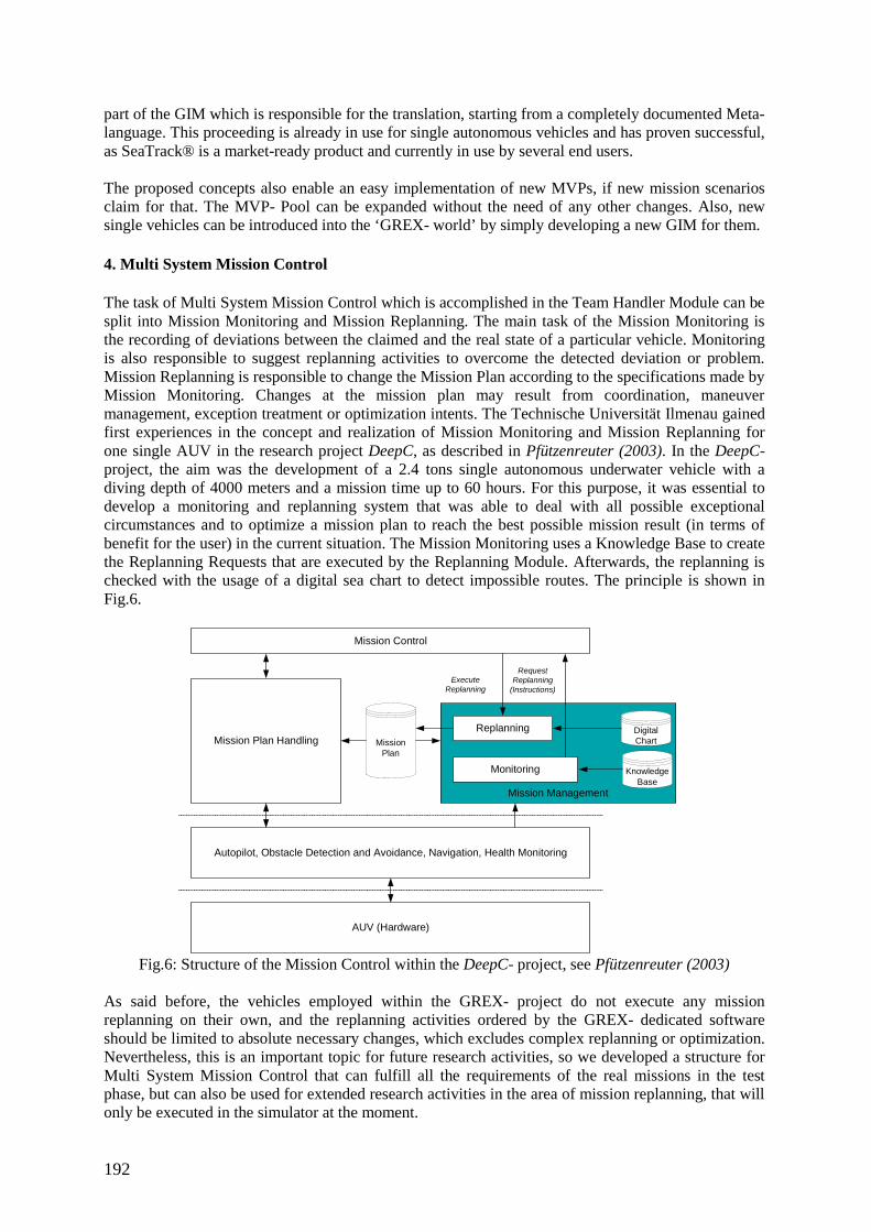
part of the GIM which is responsible for the translation, starting from a completely documented Meta- language. This proceeding is already in use for single autonomous vehicles and has proven successful, as SeaTrack® is a market-ready product and currently in use by several end users. The proposed concepts also enable an easy implementation of new MVPs, if new mission scenarios claim for that. The MVP- Pool can be expanded without the need of any other changes. Also, new single vehicles can be introduced into the ‘GREX- world’ by simply developing a new GIM for them. 4. Multi System Mission Control The task of Multi System Mission Control which is accomplished in the Team Handler Module can be split into Mission Monitoring and Mission Replanning. The main task of the Mission Monitoring is the recording of deviations between the claimed and the real state of a particular vehicle. Monitoring is also responsible to suggest replanning activities to overcome the detected deviation or problem. Mission Replanning is responsible to change the Mission Plan according to the specifications made by Mission Monitoring. Changes at the mission plan may result from coordination, maneuver management, exception treatment or optimization intents. The Technische Universität Ilmenau gained first experiences in the concept and realization of Mission Monitoring and Mission Replanning for one single AUV in the research project DeepC, as described in Pfützenreuter (2003). In the DeepC- project, the aim was the development of a 2.4 tons single autonomous underwater vehicle with a diving depth of 4000 meters and a mission time up to 60 hours. For this purpose, it was essential to develop a monitoring and replanning system that was able to deal with all possible exceptional circumstances and to optimize a mission plan to reach the best possible mission result (in terms of benefit for the user) in the current situation. The Mission Monitoring uses a Knowledge Base to create the Replanning Requests that are executed by the Replanning Module. Afterwards, the replanning is checked with the usage of a digital sea chart to detect impossible routes. The principle is shown in Fig.6.

Mission Management

Mission Plan Handling

Mission Control

Monitoring

ReplanningMission

Plan

ExecuteReplanning

Autopilot, Obstacle Detection and Avoidance, Navigation, Health Monitoring

RequestReplanning

(Instructions)

AUV (Hardware)

KnowledgeBase

Digital Chart

Fig.6: Structure of the Mission Control within the DeepC- project, see Pfützenreuter (2003)

As said before, the vehicles employed within the GREX- project do not execute any mission replanning on their own, and the replanning activities ordered by the GREX- dedicated software should be limited to absolute necessary changes, which excludes complex replanning or optimization. Nevertheless, this is an important topic for future research activities, so we developed a structure for Multi System Mission Control that can fulfill all the requirements of the real missions in the test phase, but can also be used for extended research activities in the area of mission replanning, that will only be executed in the simulator at the moment.

192

4.1. Mission Monitoring Mission Monitoring is responsible for the observation of all current states and for the creation of replanning commands in case of deviations. The prior execution of a Team- Oriented Mission Planning, as described above, is an important precondition to minimize the work of Mission Monitoring. Starting from this, the work of Mission Monitoring is separated into several instances that are executed simultaneously. Several monitoring tasks run at the same time and use different algorithms to create replanning commands. The concrete algorithms for each instance will usually depend on the current primitive of the mission plan. The following four instances were defined and will be realized:

Coordination of Mission Plans to guarantee the formation/ inter vehicle collision avoidance This instance will mainly adapt the velocities of the vehicles. This can be necessary whenever the preservation of a close formation is desired. As described before, the way to reach a close formation is to plan adequate paths for all vehicles in TOMP. Then the formation stays theoretically intact, as long as all vehicles use exactly the correct velocity. As this can never be achieved in reality, there is the need for velocity adaptation. A concrete example for this is shown in chapter 4.3. Other primitives may require similar algorithms. In every case this primitive has to guarantee for the prevention of inter collision avoidance. If there are intersections in the planed paths of the vehicles (at the present moment it is still not decided whether this should be prohibited), this instance has to adapt the velocities to prevent collisions.

Modification of Mission Plans to realize obstacle avoidance This instance will be responsible for a Team-Oriented Obstacle Avoidance. This does not include inter vehicle collision avoidance, because this task is executed by Team-Oriented Mission Planning and the Adjustment- Instance by creating paths with preferable few intersections and by the Coordination- instance by adjusting the velocities. Obstacle avoidance corresponds to the recognition and evading of all external objects which are not part of the team. Single vehicles may employ sonar systems and automatically avoid single obstacles. By the use of long-range sonar it is possible to plan and realize an optimal path through an area with many obstacles. For single autonomous vehicles, this was shown in Eichhorn (2004). The same principle can also be employed for vehicle teams, where the preservation of a formation or only slight formation changes is demanded. As this requires very specific vehicle equipment and the areas of the first demonstrations of the GREX scenarios are assumed to be held in secluded areas, this instance will only be realized in theoretical research.

Adjustment of Mission Plans to realize high-level coordination within a mission plan element

This instance is responsible for executing the current primitive in the correct way. This includes the monitoring of primitive time and area (if the primitive contains adequate time and spatial traps) as well as the replanning of vehicle paths to reach the goal of the primitive. If, for example, the vehicles have to follow a methane plume to find a hydrothermal vent, this instance has to replan the paths according to the values of the methane sensors of the vehicles. In this case, the team will have a hierarchical realization as one vehicle takes over the leadership, collects the values of all vehicles, calculates new track data and spreads them among the others.

Reorganization of Mission Plans in cases of special situations / emergencies

This instance can perform significant changes, like cancel the mission, reorganize the mission (if a single vehicle has to leave the team due to an error), optimize the plan (only for theoretical research)

193

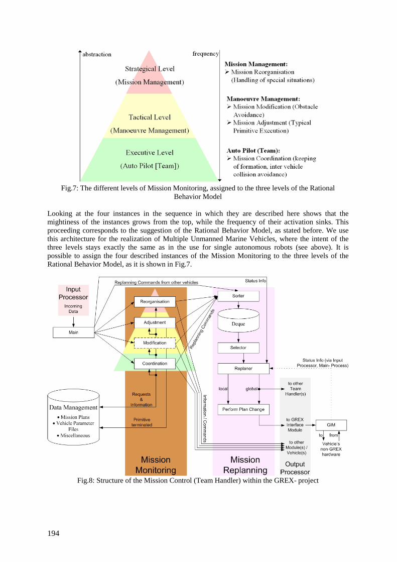
Fig.7: The different levels of Mission Monitoring, assigned to the three levels of the Rational

Behavior Model Looking at the four instances in the sequence in which they are described here shows that the mightiness of the instances grows from the top, while the frequency of their activation sinks. This proceeding corresponds to the suggestion of the Rational Behavior Model, as stated before. We use this architecture for the realization of Multiple Unmanned Marine Vehicles, where the intent of the three levels stays exactly the same as in the use for single autonomous robots (see above). It is possible to assign the four described instances of the Mission Monitoring to the three levels of the Rational Behavior Model, as it is shown in Fig.7.

Fig.8: Structure of the Mission Control (Team Handler) within the GREX- project

194

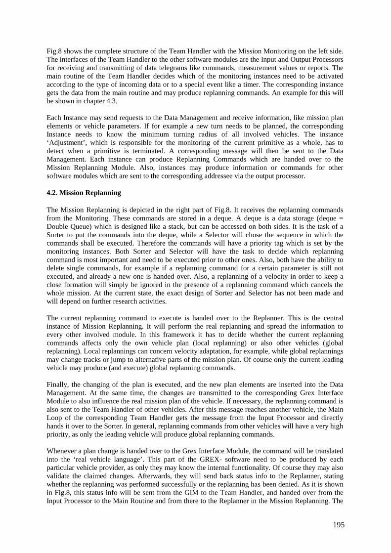
Fig.8 shows the complete structure of the Team Handler with the Mission Monitoring on the left side. The interfaces of the Team Handler to the other software modules are the Input and Output Processors for receiving and transmitting of data telegrams like commands, measurement values or reports. The main routine of the Team Handler decides which of the monitoring instances need to be activated according to the type of incoming data or to a special event like a timer. The corresponding instance gets the data from the main routine and may produce replanning commands. An example for this will be shown in chapter 4.3. Each Instance may send requests to the Data Management and receive information, like mission plan elements or vehicle parameters. If for example a new turn needs to be planned, the corresponding Instance needs to know the minimum turning radius of all involved vehicles. The instance ‘Adjustment’, which is responsible for the monitoring of the current primitive as a whole, has to detect when a primitive is terminated. A corresponding message will then be sent to the Data Management. Each instance can produce Replanning Commands which are handed over to the Mission Replanning Module. Also, instances may produce information or commands for other software modules which are sent to the corresponding addressee via the output processor. 4.2. Mission Replanning The Mission Replanning is depicted in the right part of Fig.8. It receives the replanning commands from the Monitoring. These commands are stored in a deque. A deque is a data storage (deque = Double Queue) which is designed like a stack, but can be accessed on both sides. It is the task of a Sorter to put the commands into the deque, while a Selector will chose the sequence in which the commands shall be executed. Therefore the commands will have a priority tag which is set by the monitoring instances. Both Sorter and Selector will have the task to decide which replanning command is most important and need to be executed prior to other ones. Also, both have the ability to delete single commands, for example if a replanning command for a certain parameter is still not executed, and already a new one is handed over. Also, a replanning of a velocity in order to keep a close formation will simply be ignored in the presence of a replanning command which cancels the whole mission. At the current state, the exact design of Sorter and Selector has not been made and will depend on further research activities. The current replanning command to execute is handed over to the Replanner. This is the central instance of Mission Replanning. It will perform the real replanning and spread the information to every other involved module. In this framework it has to decide whether the current replanning commands affects only the own vehicle plan (local replanning) or also other vehicles (global replanning). Local replannings can concern velocity adaptation, for example, while global replannings may change tracks or jump to alternative parts of the mission plan. Of course only the current leading vehicle may produce (and execute) global replanning commands. Finally, the changing of the plan is executed, and the new plan elements are inserted into the Data Management. At the same time, the changes are transmitted to the corresponding Grex Interface Module to also influence the real mission plan of the vehicle. If necessary, the replanning command is also sent to the Team Handler of other vehicles. After this message reaches another vehicle, the Main Loop of the corresponding Team Handler gets the message from the Input Processor and directly hands it over to the Sorter. In general, replanning commands from other vehicles will have a very high priority, as only the leading vehicle will produce global replanning commands. Whenever a plan change is handed over to the Grex Interface Module, the command will be translated into the ‘real vehicle language’. This part of the GREX- software need to be produced by each particular vehicle provider, as only they may know the internal functionality. Of course they may also validate the claimed changes. Afterwards, they will send back status info to the Replanner, stating whether the replanning was performed successfully or the replanning has been denied. As it is shown in Fig.8, this status info will be sent from the GIM to the Team Handler, and handed over from the Input Processor to the Main Routine and from there to the Replanner in the Mission Replanning. The

195

replanning process is finally finished when a positive Status Info is received by the Replanner. If the replanning was denied by the vehicle, a special situation occurs, that is difficult to handle. If the replanning command was a global one, maybe other vehicles have already executed it. If one vehicle denies the replanning, it may be necessary to undo all other changes, which is again replanning action for the other vehicles. If then another vehicle denies this ‘undoing’, a situation occurs where different vehicles have different mission plans which may lead to a disaster. For land vehicles, it may be a possible solution that all vehicles have to test a replanning, before they really execute it. Only if all vehicles agree, the replanning will finally be done. In the marine scenarios, this proceeding does not work due to the large latency in communication. If the Team Handler of a leading vehicle commands a plan change, it may take several minutes before all vehicles have sent back the status info. To overcome this problem, it was decided in the project group that at the moment every denying of a replanning command by a vehicle results in a mission abort. Then it can be checked by the engineers, why the replanning was denied. As the instances of the Mission Monitoring have access to the parameters of all involved vehicles, such a denying of replanning should not occur too often, at least after the test phase. 4.2. Example As an example we assume a situation where three vehicles have to perform a lawn mowing maneuver, for example to scan an area and to collect data. For this reason they have to establish and preserve a close triangle formation. The first step to solve this challenging task is an adequate Team-Oriented Mission Planning to provide all vehicles with a relevant mission plan. These plans contain paths for every vehicle; these path are designed in a way that if all vehicles will run absolutely the desired velocity, the formation will remain in the desired pattern. We showed in Glotzbach et al. (2007b) that it is possible to perform such a path planning. Of course it will never be possible that the vehicles run with absolute equal velocities, which is why the Online Replanning is necessary. In the described situation there is the MVP ‘M_CoordinatedPathFollowing’ active which was depicted in Fig.4. In this primitive, the Mission Monitoring will mainly employ the Coordination- Instance, while the other three instances will only be used in abnormal situations. The Coordination- Instance will be employed by the Main Routine whenever new position values are received from the Team Navigation Module. These telegrams will be sent from the Team Navigation to Team Handler in regular intervals; they contain the estimated current position of all vehicles, based on navigation data of the vehicles own navigation, range and bearing measurements of the acoustic modems and position estimations by Kalman Filters. With the position of all vehicles and the knowledge of the mission plans, the Coordination- Instance will calculate the ‘Level of performance’ Θ of the current path (straight line or arc) for all vehicles which runs from zero to one. The goal is to equalize these levels for all p participating vehicles. This task can be fulfilled individually by all vehicles. If Θm of vehicle m is smaller than the mean value of the team, vehicle m has to increase its velocity, and vice versa. The control algorithm used for this task is suggested from the project partner Instituto Superior Tecnico IST in Ghabcheloo et al. (2005). If there are p vehicles, vehicle k must adapt its velocity vk(t) according to the following equation:

( ) ( ) ( ) ( )(∑≠

=

Θ−Θ⋅+=kp

ikiikk ttKtvtv

,

1

' ) (1)

In equation 1, v’k(t) is the desired velocity for vehicle k according to the mission plan for the current situation. Ki is an individual proportional factor. The task of the controller is to equalize the values of Θi for all vehicles. This controller executes the function of the Multiple Base Primitive, as shown in Fig.4. The Coordination- Instance of the Mission Monitoring will employ this algorithm whenever new position values are available. The new velocities will be calculated not only for the own vehicle, but also for all other vehicles. The results of the calculation will be sent back to the Team Navigation

196

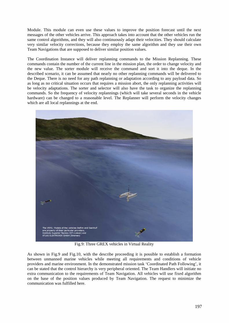
Module. This module can even use these values to improve the position forecast until the next messages of the other vehicles arrive. This approach takes into account that the other vehicles run the same control algorithms, and they will also continuously adapt their velocities. They should calculate very similar velocity corrections, because they employ the same algorithm and they use their own Team Navigations that are supposed to deliver similar position values. The Coordination Instance will deliver replanning commands to the Mission Replanning. These commands contain the number of the current line in the mission plan, the order to change velocity and the new value. The sorter module will receive the command and sort it into the deque. In the described scenario, it can be assumed that nearly no other replanning commands will be delivered to the Deque. There is no need for any path replanning or adaptation according to any payload data. So as long as no critical situation occurs that requires a mission abort, the only replanning activities will be velocity adaptations. The sorter and selector will also have the task to organize the replanning commands. So the frequency of velocity replannings (which will take several seconds in the vehicle hardware) can be changed to a reasonable level. The Replanner will perform the velocity changes which are all local replannings at the end.

Fig.9: Three GREX vehicles in Virtual Reality

As shown in Fig.9 and Fig.10, with the describe proceeding it is possible to establish a formation between unmanned marine vehicles while meeting all requirements and conditions of vehicle providers and marine environment. In the demonstrated mission task ‘Coordinated Path Following’, it can be stated that the control hierarchy is very peripheral oriented. The Team Handlers will initiate no extra communication to the requirements of Team Navigation. All vehicles will use fixed algorithm on the base of the position values produced by Team Navigation. The request to minimize the communication was fulfilled here.

197

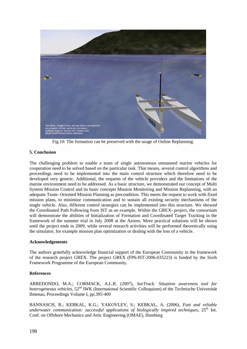
Fig.10: The formation can be preserved with the usage of Online Replanning.

5. Conclusion The challenging problem to enable a team of single autonomous unmanned marine vehicles for cooperation need to be solved based on the particular task. That means, several control algorithms and proceedings need to be implemented into the main control structure which therefore need to be developed very generic. Additional, the requests of the vehicle providers and the limitations of the marine environment need to be addressed. As a basic structure, we demonstrated our concept of Multi System Mission Control and its basic concepts Mission Monitoring and Mission Replanning, with an adequate Team- Oriented Mission Planning as precondition. This meets the request to work with fixed mission plans, to minimize communication and to sustain all existing security mechanisms of the single vehicle. Also, different control strategies can be implemented into this structure. We showed the Coordinated Path Following from IST as an example. Within the GREX- project, the consortium will demonstrate the abilities of Initialization of Formation and Coordinated Target Tracking in the framework of the summer trial in July 2008 at the Azores. More practical solutions will be shown until the project ends in 2009, while several research activities will be performed theoretically using the simulator, for example mission plan optimization or dealing with the loss of a vehicle. Acknowledgements The authors gratefully acknowledge financial support of the European Community in the framework of the research project GREX. The project GREX (FP6-IST-2006-035223) is funded by the Sixth Framework Programme of the European Community. References ARREDONDO, M.A.; CORMACK, A.L.R. (2007), SeeTrack: Situation awareness tool for heterogeneous vehicles, 52nd IWK (International Scientific Colloquium) of the Technische Universität Ilmenau, Proceedings Volume I, pp.395-400 BANNASCH, R.; KEBKAL, K.G.; YAKOVLEV, S.; KEBKAL, A. (2006), Fast and reliable underwater communication: successful applications of biologically inspired techniques, 25th Int. Conf. on Offshore Mechanics and Artic Engineering (OMAE), Hamburg

198

CORMACK, A.L.R. (2006), Providing a common operator interface for port and harbour security and shallow water mine warfare, Undersea Defence Technology Europe Conf. and Exhibition (UDT Europe), Hamburg EICHHORN, M. (2004), An obstacle avoidance system for an autonomous underwater vehicle, IEEE Int. Symp. Underwater Technology, Taipei, pp. 75-82 ENGEL, R.; KALWA, J. (2007), Coordinated navigation of multiple underwater vehicles, 17 Int. Offshore and Polar Engineering Conf. (ISOPE), Lisbon,

th

pp.1066-1072 GHABCHELOO, R.; PASCOAL, A.; SILVESTRE, C.; CARVALHO, D. (2005), Coordinated motion control of multiple autonomous underwater vehicles, Int. Workshop on Underwater Robotics, Genova GLOTZBACH, T.; PICINI, A.; ZANGRILLI, A., EICHHORN, M.; OTTO, P.; SCHNEIDER, M. (2007), Evaluation of different control strategies for teams of unmanned marine vehicles (UMVs) comparing the requirements of underwater communication and navigation in MATLAB® Simulations, 6th Int. Conf. Computer Applications and Information Technology in the Maritime Industries (COMPIT), Cortona, pp. 331-344 GLOTZBACH, T.; SCHNEIDER, M.; OTTO, P. (2007), Team-oriented mission planning (TOMP) for multiple unmanned marine vehicles: planning of cooperative lawnmowers, 4th Int. Conf. Computational Intelligence, Robotics and Autonomous Systems 2007 (CIRAS), Palmerston North, pp.50-55 GREX: Coordination and control of cooperating heterogeneous unmanned systems in uncertain environments, Home Page, http://www.grex-project.eu, visited on 14/03/2008 HÖBING-HÖLSCHER, U.; LARSEN, M.B. (2006), Aided inertial navigation system solutions - Application for synthetic aperture sonar, 25th Int. Conf. on Offshore Mechanics and Artic Engineering (OMAE), Hamburg KWAK, S.H.; MCGHEE, R.B.; BIHARI, T.E. (1992), Rational behavior model: A tri-level multiple paradigm architecture for robot vehicle control, Technical Report NPSCS-92-003, Naval Postgraduate School, Monterey PFÜTZENREUTER, T. (2003), Advanced mission management for long-range autonomous underwater vehicles, MTS/IEEE Oceans 2003, San Diego, pp.928 – 933

199

200

Process Modeling and Simulation using CAD Data and PDM in Early Stage of Shipbuilding Project

Marcus Bentin, Nordseewerke GmbH, Emden/Germany, marcus.bentin@thyssenkrupp.com Folgert Smidt, Nordseewerke GmbH, Emden/Germany, folgert.smidt@thyssenkrupp.com

Steffen Parth, FH OOW, Emden/Germany, steffen.parth@thyssenkrup.com

Abstract

Today planning and control of manufacturing processes are done in many systems. Some information is not available in a format for effective digital processing. The lack of connectivity and consistency makes automatism and simulated production planning difficult. To overcome the above described problems this paper suggests process modeling in “Teamcenter Engineering” using a product model that supports an assembling, room and system view of the ship. This enables a digital factory. A pert logic is generated out of the production plan for a ship building project on basis of process/operation model coupled with simulation.

1. Introduction Today planning and control of manufacturing processes are done in many systems. Some information is not available in a format for effective digital processing. The availability depends on the design stage. In early project stage usually document driven information is found that can not be used for digital processing. Later on in detail design stage digital product information is available but in some sections like outfitting the data is difficult to connect with planning and control data consistently. To minimize this problem less detailed aggregation levels are planned and product data is connected to these rough planning notes by a key number manually. The lack of connectivity and consistency makes automatism and simulated production planning difficult. This challenge is discussed in several ways. One way would be to build up a system that enables the modelling of a planning model that can be used afterwards for ERP systems if the integration level is high. Here the computer integrated planning and resource management system for shipbuilding developed by “logimatic” has to be mentioned, that supports the planner with a reference module library to model the product in an early stage. The engineering integration is low but the procurement and administrative integration is high e.g. Massow, et al. (2004). Also Fincantieri chose the way of modeling the planning model with modules from a standard library and connected this model with a simulation model to generate an assembly schedule e.g. Berlato, et al. (2007). The Meyer Shipyard built up a tool to generate product data in an early stage of a project using also libraries. These data are used for simulation to generate a schedule. The Meyer approach is deeply integrated into the planning and control systems e.g. Hartmann (2004). On the other side there are CAD vendors that support structuring of the CAD data for generating workshop data that can be used for ERP systems or robot control. But they do not focus the planning requirements in an early project level in shipbuilding e.g. Mütze (2006). To gain more flexibility in describing the product in an early stage for planning, more flexible tools has to be used than a library of standard modules. A consistent engineering and planning process has to be granted and the planning of the process should be done together with the required resources and capacities. The systems used in the business processes of engineering and planning should be integrated by a PLM system. In general this challenge fits to the ideas of Digital Factory e.g. Marczinski. (2005), Kühn (2006). The integration of planning and CAD product model data is assumed to be very efficient for process modeling e.g. Aoyama et al. (1999), Bentin et al. (2002). The project described in this paper proofs the possibility to overcome the above described problems

201

with process modeling in “Teamcenter Engineering” using a product model that supports an assembling, room and system view of the ship. This enables a digital factory. The different views support the organization of the design process as well as the production planning. A pert logic is generated out of the production plan for a ship building project on basis of process/operation model coupled with simulation. The processes and operations should mostly be modeled in an automatic way based on a library and attributes of the product to identify the required operations. This grants maximal productivity in modeling and consistency. The processes are needed to aggregate operations and represent the production structure of the project. The product data are varying during design lifecycle in quantity and quality. Mechanism has to be found that ensures the consistency of the processes and product structure. The process modeling has to cover all different planning views of shipbuilding project and in addition has to enable to plan the different views in relation. Therefore, a room consists of several steel blocks and a system component is installed in a room. Some system components like foundations or brackets are mounted in a steel block. For planning each operation’s working content has to be estimated most likely according CAD attributes, where possible. Hence a tool and a statistic have to be developed to automate this process. This tool is not focused in this research. It is only marked that it is need. It is a necessary task for future research. The processes/ operations modeled for one project has to be planned and simulated in the boundaries given by other already contracted projects. The result is a matched schedule for the project with the needed resources. The schedule is calculated with restricted resources! This is contrary to today’s business. Hence the requirements can be summarized like following:

− Product model driven process/operation modeling − Modeling of all relevant processes together with their logical relations. − Automatic modeling of operation according templates and product attributes. − The process structure has to be constant during the lifecycle otherwise new planning is

necessary. − Work content on hour basis has to be calculated beforehand by an application that yet has to

be developed. The Budgets are calculated according product attributes and statistic. − The process/operation model has to be good for a process-flow-simulation. − The result of the simulation has to be pert chart with correct predecessor successor

information. 2. Concept Based on the product model processes and operations are derived. Therefore a product structure is needed, Fig.1. The needed product structure depends on the planning view. For steel planning a section assembling view together with functional assembly groups are required. Each part of the product belongs to a structure and has attributes that describe the membership of a certain structure level. According this attributes and a library with predefined operations the affiliated operation of each part can be modeled. The process structure is modeled according the functional assembly groups. The beginning process of all functional assembly groups is the prefabrication process. The operation object contains the part of the product and the resources required for this operation. After modeling the operations, their working budget has to be estimated. Then a process-flow-simulation is carried out and a scheduled plan with a complete pert chart is retrieved. The simulation works with predecessor successor relationship information as constraints. This keeps the model simple. The steel view is the condition for the outfitting operations in the room view. A room can be outfitted when the room exists. That means all steel sections have to be welded describing the room. Furthermore, the steel is connected with the system view. Some foundations or brackets can be mounted in the steel section. During design lifecycle the product information changes in quality and quantity. The steel is modeled in another system than UGNX. Due to this a strategy has to be found that grants the consistency of the data. Data from the early project level has to be replaced consistently with data from the detail design level. Here, the process structure as a kind of super structure is helping, Fig.2.

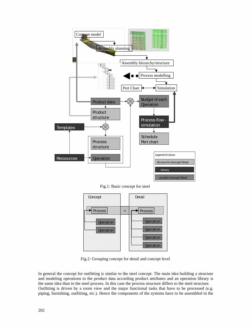
202

Fig.1: Basic concept for steel

Fig.2: Grouping concept for detail and concept level

In general the concept for outfitting is similar to the steel concept. The main idea building a structure and modeling operations to the product data according product attributes and an operation library is the same idea than in the steel process. In this case the process structure differs to the steel structure. Outfitting is driven by a room view and the major functional tasks that have to be processed (e.g. piping, furnishing, outfitting, etc.). Hence the components of the systems have to be assembled in the

Concept model

Assembly planning

Assembly hierarchy/structure

Process modelling

Pert Chart Simulation

Product data

Productstructure

Processstructure

Operation

Budget of eachOperation

Process-flow -simulation

SchedulePert chart

Templates

Ressources Strcture fix Concept/Detail

Library

variable Concept/Detail

Legend of colour:

Process Process

Operation

Operation

Operation

Operation

Operation

Operation

=

Concept Detail

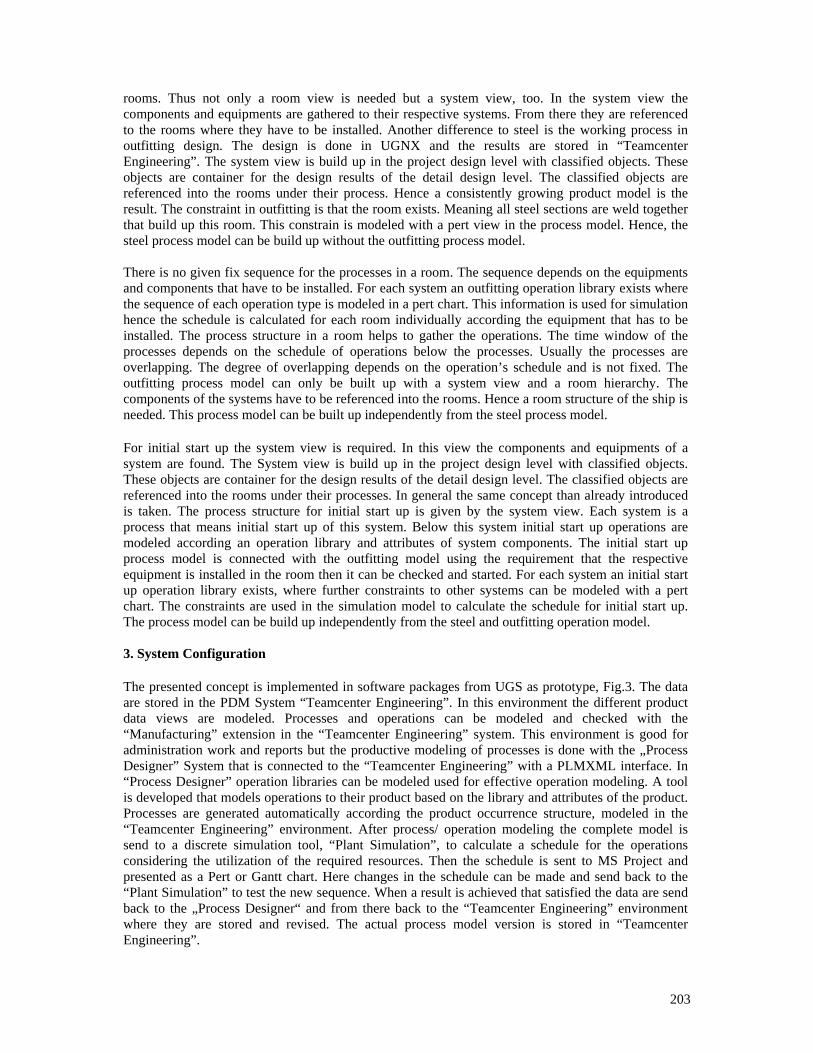
203

rooms. Thus not only a room view is needed but a system view, too. In the system view the components and equipments are gathered to their respective systems. From there they are referenced to the rooms where they have to be installed. Another difference to steel is the working process in outfitting design. The design is done in UGNX and the results are stored in “Teamcenter Engineering”. The system view is build up in the project design level with classified objects. These objects are container for the design results of the detail design level. The classified objects are referenced into the rooms under their process. Hence a consistently growing product model is the result. The constraint in outfitting is that the room exists. Meaning all steel sections are weld together that build up this room. This constrain is modeled with a pert view in the process model. Hence, the steel process model can be build up without the outfitting process model. There is no given fix sequence for the processes in a room. The sequence depends on the equipments and components that have to be installed. For each system an outfitting operation library exists where the sequence of each operation type is modeled in a pert chart. This information is used for simulation hence the schedule is calculated for each room individually according the equipment that has to be installed. The process structure in a room helps to gather the operations. The time window of the processes depends on the schedule of operations below the processes. Usually the processes are overlapping. The degree of overlapping depends on the operation’s schedule and is not fixed. The outfitting process model can only be built up with a system view and a room hierarchy. The components of the systems have to be referenced into the rooms. Hence a room structure of the ship is needed. This process model can be built up independently from the steel process model. For initial start up the system view is required. In this view the components and equipments of a system are found. The System view is build up in the project design level with classified objects. These objects are container for the design results of the detail design level. The classified objects are referenced into the rooms under their processes. In general the same concept than already introduced is taken. The process structure for initial start up is given by the system view. Each system is a process that means initial start up of this system. Below this system initial start up operations are modeled according an operation library and attributes of system components. The initial start up process model is connected with the outfitting model using the requirement that the respective equipment is installed in the room then it can be checked and started. For each system an initial start up operation library exists, where further constraints to other systems can be modeled with a pert chart. The constraints are used in the simulation model to calculate the schedule for initial start up. The process model can be build up independently from the steel and outfitting operation model. 3. System Configuration The presented concept is implemented in software packages from UGS as prototype, Fig.3. The data are stored in the PDM System “Teamcenter Engineering”. In this environment the different product data views are modeled. Processes and operations can be modeled and checked with the “Manufacturing” extension in the “Teamcenter Engineering” system. This environment is good for administration work and reports but the productive modeling of processes is done with the „Process Designer” System that is connected to the “Teamcenter Engineering” with a PLMXML interface. In “Process Designer” operation libraries can be modeled used for effective operation modeling. A tool is developed that models operations to their product based on the library and attributes of the product. Processes are generated automatically according the product occurrence structure, modeled in the “Teamcenter Engineering” environment. After process/ operation modeling the complete model is send to a discrete simulation tool, “Plant Simulation”, to calculate a schedule for the operations considering the utilization of the required resources. Then the schedule is sent to MS Project and presented as a Pert or Gantt chart. Here changes in the schedule can be made and send back to the “Plant Simulation” to test the new sequence. When a result is achieved that satisfied the data are send back to the „Process Designer“ and from there back to the “Teamcenter Engineering” environment where they are stored and revised. The actual process model version is stored in “Teamcenter Engineering”.

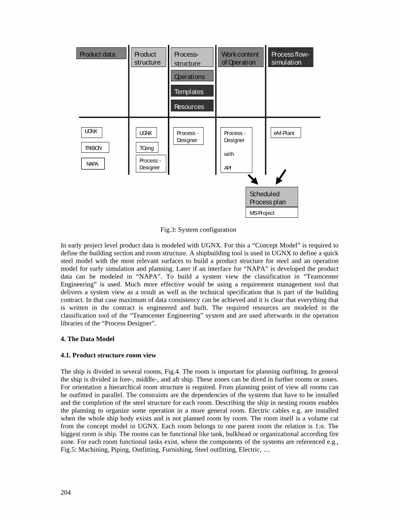
204

Fig.3: System configuration

In early project level product data is modeled with UGNX. For this a “Concept Model” is required to define the building section and room structure. A shipbuilding tool is used in UGNX to define a quick steel model with the most relevant surfaces to build a product structure for steel and an operation model for early simulation and planning. Later if an interface for “NAPA” is developed the product data can be modeled in “NAPA”. To build a system view the classification in “Teamcenter Engineering” is used. Much more effective would be using a requirement management tool that delivers a system view as a result as well as the technical specification that is part of the building contract. In that case maximum of data consistency can be achieved and it is clear that everything that is written in the contract is engineered and built. The required resources are modeled in the classification tool of the “Teamcenter Engineering” system and are used afterwards in the operation libraries of the “Process Designer”. 4. The Data Model 4.1. Product structure room view The ship is divided in several rooms, Fig.4. The room is important for planning outfitting. In general the ship is divided in fore-, middle-, and aft ship. These zones can be dived in further rooms or zones. For orientation a hierarchical room structure is required. From planning point of view all rooms can be outfitted in parallel. The constraints are the dependencies of the systems that have to be installed and the completion of the steel structure for each room. Describing the ship in nesting rooms enables the planning to organize some operation in a more general room. Electric cables e.g. are installed when the whole ship body exists and is not planned room by room. The room itself is a volume cut from the concept model in UGNX. Each room belongs to one parent room the relation is 1:n. The biggest room is ship. The rooms can be functional like tank, bulkhead or organizational according fire zone. For each room functional tasks exist, where the components of the systems are referenced e.g., Fig.5: Machining, Piping, Outfitting, Furnishing, Steel outfitting, Electric, …

Product data Product structure

Process-structure

Operations

Work contentof Operation

Process flow - simulation

Templates

Resources

UGNX UGNX TCeng

Process -Designer

Process - Designer

eM -Plant Process -Designer

with

API

TRIBON

ScheduledProcess plan MS-Project

NAPA

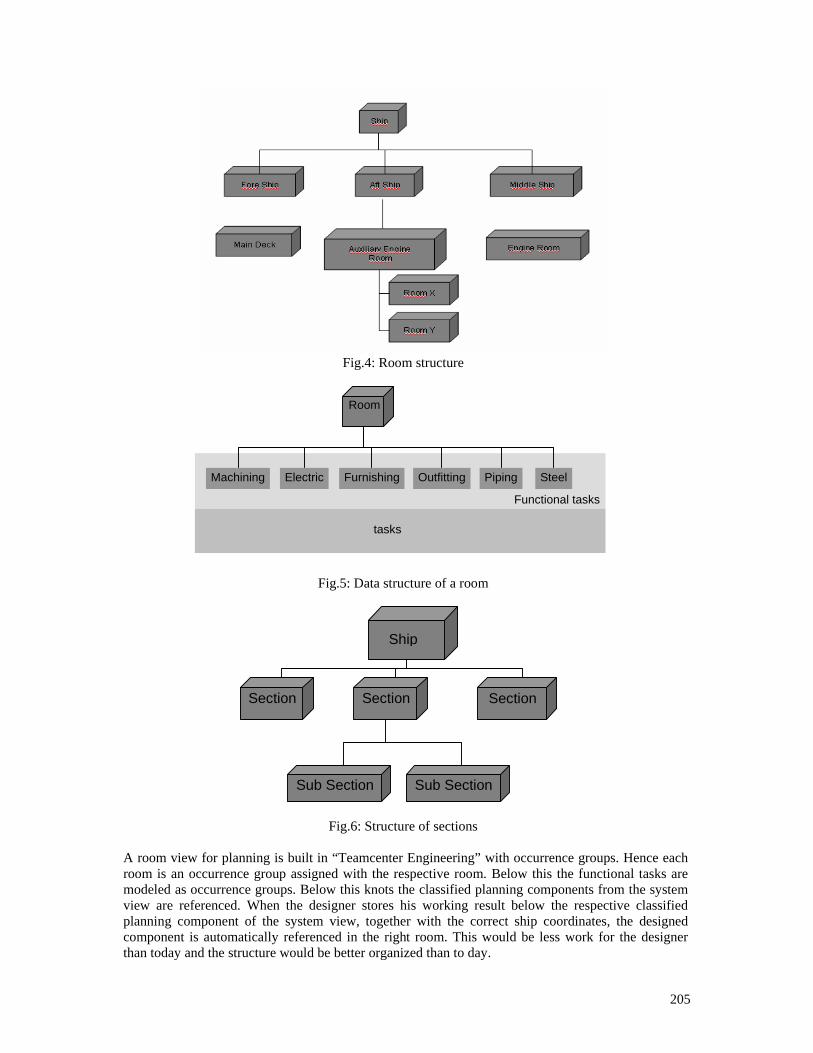
205

Fig.4: Room structure

Fig.5: Data structure of a room

Fig.6: Structure of sections A room view for planning is built in “Teamcenter Engineering” with occurrence groups. Hence each room is an occurrence group assigned with the respective room. Below this the functional tasks are modeled as occurrence groups. Below this knots the classified planning components from the system view are referenced. When the designer stores his working result below the respective classified planning component of the system view, together with the correct ship coordinates, the designed component is automatically referenced in the right room. This would be less work for the designer than today and the structure would be better organized than to day.

Ship

Section Section Section

Sub SectionSub Section

Room

PipingOutfittingFurnishingElectric Machining

Functional tasks

tasks

Steel

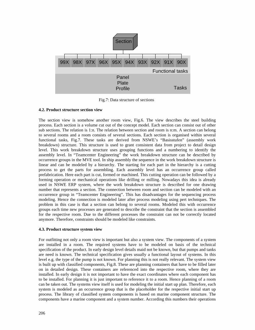
206

Fig.7: Data structure of sections

4.2. Product structure section view The section view is somehow another room view, Fig.6. The view describes the steel building process. Each section is a volume cut out of the concept model. Each section can consist out of other sub sections. The relation is 1:n. The relation between section and room is n:m. A section can belong to several rooms and a room consists of several sections. Each section is organised within several functional tasks, Fig.7. These tasks are derived from NSWE’s “Basisstufen” (assembly work breakdown) structure. This structure is used to grant consistent data from project to detail design level. This work breakdown structure uses grouping functions and a numbering to identify the assembly level. In “Teamcenter Engineering” the work breakdown structure can be described by occurrence groups in the MVE tool. In ship assembly the sequence in the work breakdown structure is linear and can be modeled by a hierarchy. The starting for each part in the hierarchy is a cutting process to get the parts for assembling. Each assembly level has an occurrence group called prefabrication. Here each part is cut, formed or machined. This cutting operation can be followed by a forming operation or mechanical operations like drilling or milling. Nowadays this idea is already used in NSWE ERP system, where the work breakdown structure is described for one drawing number that represents a section. The connection between room and section can be modeled with an occurrence group in “Teamcenter Engineering”. This has disadvantages for the sequencing process modeling. Hence the connection is modeled later after process modeling using pert techniques. The problem in this case is that a section can belong to several rooms. Modeled this with occurrence groups each time new processes are generated to describe the constraint that the section is assembled for the respective room. Due to the different processes the constraint can not be correctly located anymore. Therefore, constraints should be modeled like constraints. 4.3. Product structure system view For outfitting not only a room view is important but also a system view. The components of a system are installed in a room. The required systems have to be modeled on basis of the technical specification of the product. In early design level details maid not be known, but that pumps and tanks are need is known. The technical specification gives usually a functional layout of systems. In this level e.g. the type of the pump is not known. For planning this is not really relevant. The system view is built up with classified components, Fig.8. These are planning containers that have to be filled later on in detailed design. These containers are referenced into the respective room, where they are installed. In early design it is not important to have the exact coordinates where each component has to be installed. For planning it is just important to reference it to a room. Hence planning of a room can be taken out. The systems view itself is used for modeling the initial start up plan. Therefore, each system is modeled as an occurrence group that is the placeholder for the respective initial start up process. The library of classified system components is based on marine component structure. The components have a marine component and a system number. According this numbers their operations

Panel Plate

Profile

Section

99X 98X 97X 96X 95X 94X 93X 92X 91X 90X

Functional tasks

Tasks

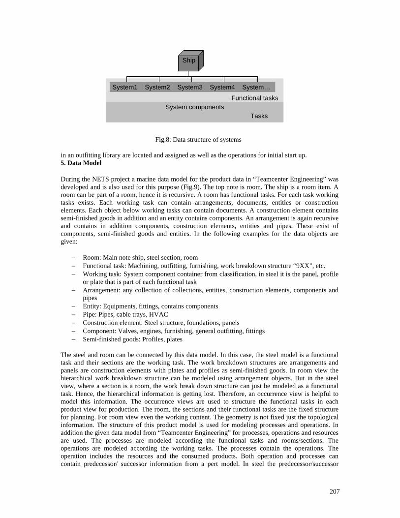
207

in an outfitting library are located and assigned as well as the operations for initial start up. 5. Data Model During the NETS project a marine data model for the product data in “Teamcenter Engineering” was developed and is also used for this purpose (Fig.9). The top note is room. The ship is a room item. A room can be part of a room, hence it is recursive. A room has functional tasks. For each task working tasks exists. Each working task can contain arrangements, documents, entities or construction elements. Each object below working tasks can contain documents. A construction element contains semi-finished goods in addition and an entity contains components. An arrangement is again recursive and contains in addition components, construction elements, entities and pipes. These exist of components, semi-finished goods and entities. In the following examples for the data objects are given:

− Room: Main note ship, steel section, room − Functional task: Machining, outfitting, furnishing, work breakdown structure “9XX”, etc. − Working task: System component container from classification, in steel it is the panel, profile

or plate that is part of each functional task − Arrangement: any collection of collections, entities, construction elements, components and

pipes − Entity: Equipments, fittings, contains components − Pipe: Pipes, cable trays, HVAC − Construction element: Steel structure, foundations, panels − Component: Valves, engines, furnishing, general outfitting, fittings − Semi-finished goods: Profiles, plates

The steel and room can be connected by this data model. In this case, the steel model is a functional task and their sections are the working task. The work breakdown structures are arrangements and panels are construction elements with plates and profiles as semi-finished goods. In room view the hierarchical work breakdown structure can be modeled using arrangement objects. But in the steel view, where a section is a room, the work break down structure can just be modeled as a functional task. Hence, the hierarchical information is getting lost. Therefore, an occurrence view is helpful to model this information. The occurrence views are used to structure the functional tasks in each product view for production. The room, the sections and their functional tasks are the fixed structure for planning. For room view even the working content. The geometry is not fixed just the topological information. The structure of this product model is used for modeling processes and operations. In addition the given data model from “Teamcenter Engineering” for processes, operations and resources are used. The processes are modeled according the functional tasks and rooms/sections. The operations are modeled according the working tasks. The processes contain the operations. The operation includes the resources and the consumed products. Both operation and processes can contain predecessor/ successor information from a pert model. In steel the predecessor/successor

Fig.8: Data structure of systems

Ship

System1 System2 System3 System4 System…

Functional tasksSystem components

Tasks

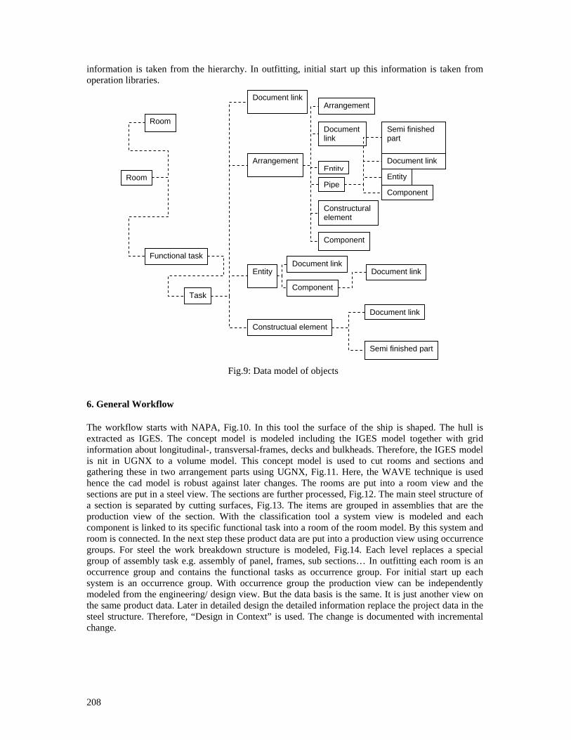
208

information is taken from the hierarchy. In outfitting, initial start up this information is taken from operation libraries.

6. General Workflow The workflow starts with NAPA, Fig.10. In this tool the surface of the ship is shaped. The hull is extracted as IGES. The concept model is modeled including the IGES model together with grid information about longitudinal-, transversal-frames, decks and bulkheads. Therefore, the IGES model is nit in UGNX to a volume model. This concept model is used to cut rooms and sections and gathering these in two arrangement parts using UGNX, Fig.11. Here, the WAVE technique is used hence the cad model is robust against later changes. The rooms are put into a room view and the sections are put in a steel view. The sections are further processed, Fig.12. The main steel structure of a section is separated by cutting surfaces, Fig.13. The items are grouped in assemblies that are the production view of the section. With the classification tool a system view is modeled and each component is linked to its specific functional task into a room of the room model. By this system and room is connected. In the next step these product data are put into a production view using occurrence groups. For steel the work breakdown structure is modeled, Fig.14. Each level replaces a special group of assembly task e.g. assembly of panel, frames, sub sections… In outfitting each room is an occurrence group and contains the functional tasks as occurrence group. For initial start up each system is an occurrence group. With occurrence group the production view can be independently modeled from the engineering/ design view. But the data basis is the same. It is just another view on the same product data. Later in detailed design the detailed information replace the project data in the steel structure. Therefore, “Design in Context” is used. The change is documented with incremental change.

Fig.9: Data model of objects

Room

Room

Functional task

Task

Document link

Arrangement

Entity

Constructual element

Document link

Semi finished part

Component

Document linkDocument link

Arrangement

Document link

Entity

Component

Constructural element

Pipe

Document link

Semi finished part

Entity

Component

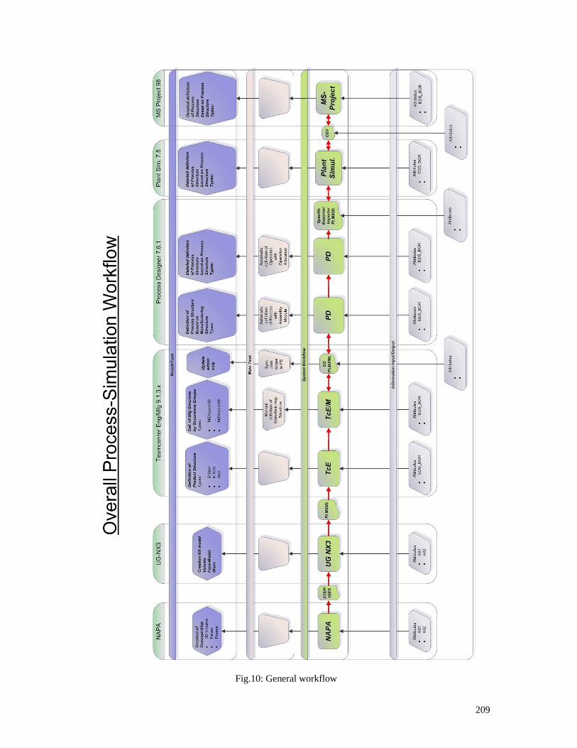
209

Fig.10: General workflow

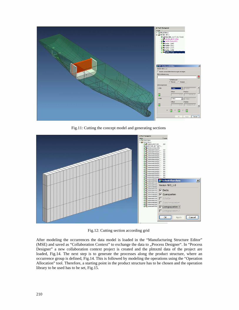
210

Fig.11: Cutting the concept model and generating sections

Fig.12: Cutting section according grid After modeling the occurrences the data model is loaded in the “Manufacturing Structure Editor” (MSE) and saved as “Collaboration Context” to exchange the data to „Process Designer“. In “Process Designer” a new collaboration context project is created and the plmxml data of the project are loaded, Fig.14. The next step is to generate the processes along the product structure, where an occurrence group is defined, Fig.14. This is followed by modeling the operations using the “Operation Allocation” tool. Therefore, a starting point in the product structure has to be chosen and the operation library to be used has to be set, Fig.15.

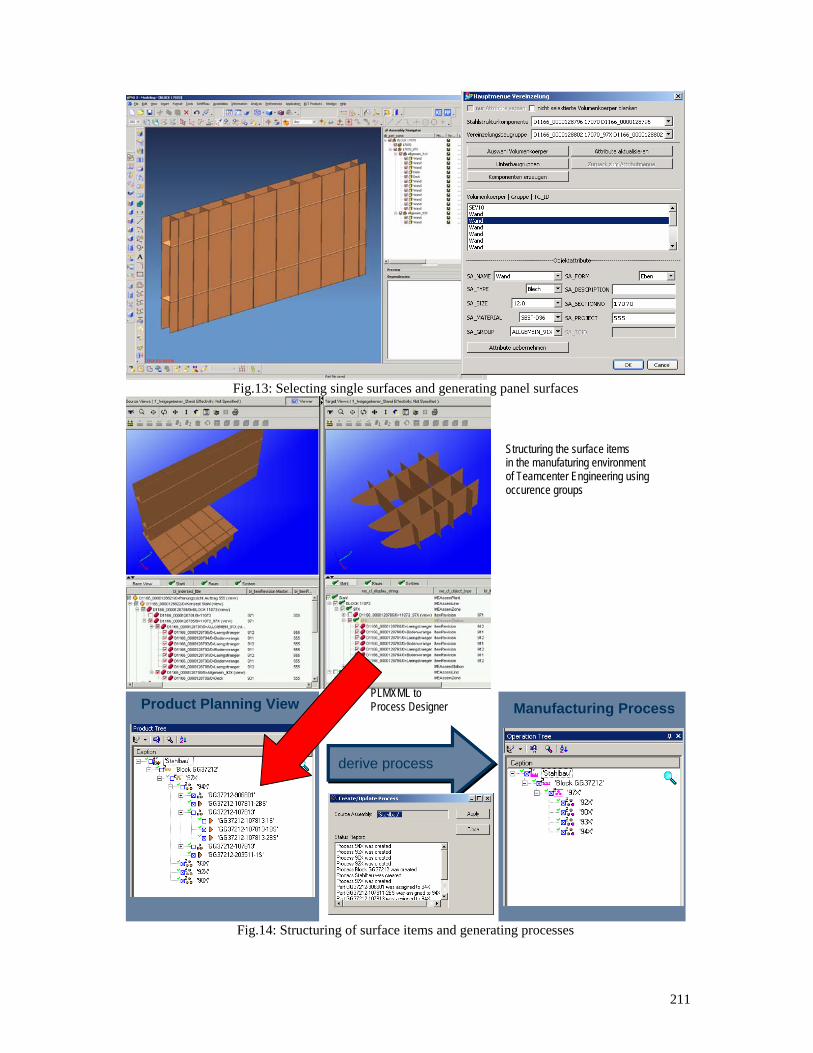
211

Fig.13: Selecting single surfaces and generating panel surfaces

Fig.14: Structuring of surface items and generating processes

Product Planning View Manufacturing Process

derive process

Structuring the surface items in the manufaturing environment of Teamcenter Engineering using occurence groups

PLMXML to Process Designer

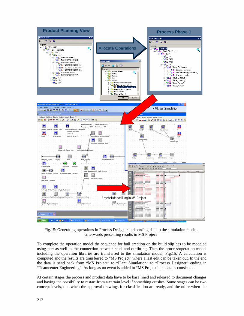
212

Fig.15: Generating operations in Process Designer and sending data to the simulation model, afterwards presenting results in MS Project

To complete the operation model the sequence for hull erection on the build slip has to be modeled using pert as well as the connection between steel and outfitting. Then the process/operation model including the operation libraries are transferred to the simulation model, Fig.15. A calculation is computed and the results are transferred to “MS Project” where a last edit can be taken out. In the end the data is send back from “MS Project” to “Plant Simulation” to “Process Designer” ending in “Teamcenter Engineering”. As long as no event is added in “MS Project” the data is consistent. At certain stages the process and product data have to be base lined and released to document changes and having the possibility to restart from a certain level if something crashes. Some stages can be two concept levels, one when the approval drawings for classification are ready, and the other when the

Product Planning View Process Phase 1

Allocate Operations

XML zur Simulation

Ergebnisdarstellung in MS Project

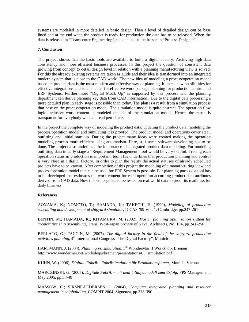
213

systems are modeled in more detailed in basic design. Then a level of detailed design can be base lined and at the end when the product is ready for production the data has to be released. When the data is released in “Teamcenter Engineering”, the data has to be frozen in “Process Designer“. 7. Conclusion The project shows that the basic tools are available to build a digital factory. Archiving high data consistency and more efficient business processes. In this project the question of consistent data growing from concept to detail design level in relation with a planning manufacturing view is solved. For this the already existing systems are taken as guide and their idea is transformed into an integrated modern system that is close to the CAD world. The new idea of modeling a process/operation model based on product data is the most modern and effective way of planning. It opens new possibilities for effective integrations and is an enabler for effective work package planning for production control and ERP Systems. Further more “Digital Mock Up” is supported by this process and the planning department can derive planning key data from CAD information.. Due to the digital data processing a more detailed plan in early stage is possible than today. The plan is a result from a simulation process that base on the process/operation model. The simulation model is quite abstract. The operation flow logic inclusive work content is modeled outside of the simulation model. Hence, the result is transparent for everybody who can read pert charts. In the project the complete way of modeling the product data, updating the product data, modeling the process/operation model and simulating it is proofed. The product model and operations cover steel, outfitting and initial start up. During the project many ideas were created making the operation modeling process more efficient using automatism. Here, still some software developing has to be done. The project also underlines the importance of integrated product data modeling. For modeling outfitting data in early stage a “Requirement Management” tool would be very helpful. Tracing each operation status in production is important, too. This underlines that production planning and control is very close in a digital factory. In order to plan the reality the actual statuses of already scheduled projects have to be known. After completion of this project the modeling of a manufacturing view and process/operation model that can be used for ERP System is possible. For planning purpose a tool has to be developed that estimates the work content for each operation according product data attributes derived from CAD data. Now this concept has to be tested on real world data to proof its readiness for daily business. References AOYAMA, K.; NOMOTO, T.; HAMADA, K.; TAKECHI, S. (1999), Modeling of production scheduling and development of shipyard simulator, ICCAS ’99 Vol. 1, Cambridge, pp.247-261 BENTIN, M.; HAMADA, K.; KITAMURA, M. (2002), Master planning optimization system for cooperative ship assembling, Trans. West-Japan Society of Naval Architects, No. 104, pp.241-256 BERLATO, G.; FACCIN, M. (2007), The digital factory in the field of the shipyard production activities planning, 4th International Congress “The Digital Factory”, Munich HARTMANN, J. (2004), Planning vs. simulation, 5th WonderMar II Workshop, Bremen http://www.wondermar.net/workshops/bremen/presentations/05_simulation.pdf KÜHN, W. (2006), Digitale Fabrik - Fabriksimulation für Produktionsplaner, Munich, Vienna MARCZINSKI, G. (2005), Digitale Fabrik – mit dem 4-Stufenmodell zum Erfolg, PPS Management, May 2005, pp.38-40 MASSOW, C.; SIKSNE-PEDERSEN, I. (2004), Computer integrated planning and resource management in shipbuilding, COMPIT 2004, Siguenza, pp.378-390

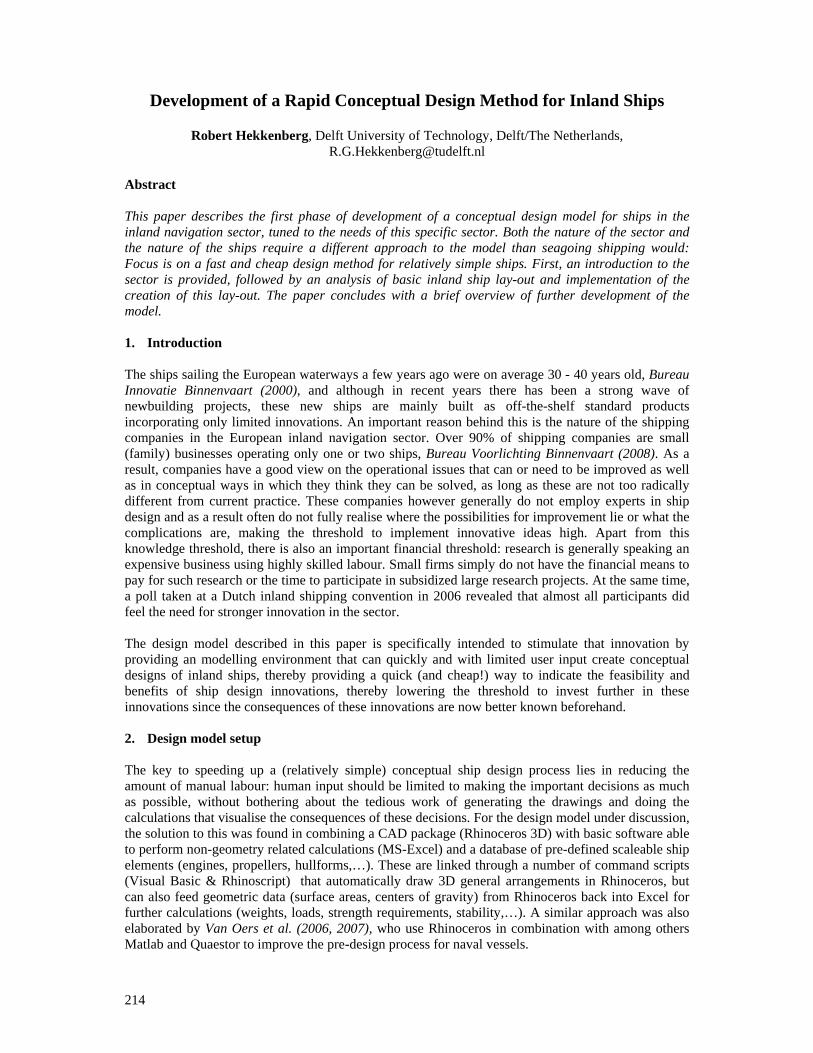
214

Development of a Rapid Conceptual Design Method for Inland Ships

Robert Hekkenberg, Delft University of Technology, Delft/The Netherlands, R.G.Hekkenberg@tudelft.nl

Abstract This paper describes the first phase of development of a conceptual design model for ships in the inland navigation sector, tuned to the needs of this specific sector. Both the nature of the sector and the nature of the ships require a different approach to the model than seagoing shipping would: Focus is on a fast and cheap design method for relatively simple ships. First, an introduction to the sector is provided, followed by an analysis of basic inland ship lay-out and implementation of the creation of this lay-out. The paper concludes with a brief overview of further development of the model.

1. Introduction

The ships sailing the European waterways a few years ago were on average 30 - 40 years old, Bureau Innovatie Binnenvaart (2000), and although in recent years there has been a strong wave of newbuilding projects, these new ships are mainly built as off-the-shelf standard products incorporating only limited innovations. An important reason behind this is the nature of the shipping companies in the European inland navigation sector. Over 90% of shipping companies are small (family) businesses operating only one or two ships, Bureau Voorlichting Binnenvaart (2008). As a result, companies have a good view on the operational issues that can or need to be improved as well as in conceptual ways in which they think they can be solved, as long as these are not too radically different from current practice. These companies however generally do not employ experts in ship design and as a result often do not fully realise where the possibilities for improvement lie or what the complications are, making the threshold to implement innovative ideas high. Apart from this knowledge threshold, there is also an important financial threshold: research is generally speaking an expensive business using highly skilled labour. Small firms simply do not have the financial means to pay for such research or the time to participate in subsidized large research projects. At the same time, a poll taken at a Dutch inland shipping convention in 2006 revealed that almost all participants did feel the need for stronger innovation in the sector. The design model described in this paper is specifically intended to stimulate that innovation by providing an modelling environment that can quickly and with limited user input create conceptual designs of inland ships, thereby providing a quick (and cheap!) way to indicate the feasibility and benefits of ship design innovations, thereby lowering the threshold to invest further in these innovations since the consequences of these innovations are now better known beforehand. 2. Design model setup The key to speeding up a (relatively simple) conceptual ship design process lies in reducing the amount of manual labour: human input should be limited to making the important decisions as much as possible, without bothering about the tedious work of generating the drawings and doing the calculations that visualise the consequences of these decisions. For the design model under discussion, the solution to this was found in combining a CAD package (Rhinoceros 3D) with basic software able to perform non-geometry related calculations (MS-Excel) and a database of pre-defined scaleable ship elements (engines, propellers, hullforms,…). These are linked through a number of command scripts (Visual Basic & Rhinoscript) that automatically draw 3D general arrangements in Rhinoceros, but can also feed geometric data (surface areas, centers of gravity) from Rhinoceros back into Excel for further calculations (weights, loads, strength requirements, stability,…). A similar approach was also elaborated by Van Oers et al. (2006, 2007), who use Rhinoceros in combination with among others Matlab and Quaestor to improve the pre-design process for naval vessels.

215

3. Inland ship lay-out When designing inland ships, it is important to realise that design criteria are often very different from those in seagoing shipping: Locks, fairways and bridges ensure that the optimization space for vessel length, beam, draught and air draught is highly limited. In practice for all but the largest parts of the main rivers, optimal dimensions of a vessel are the maximum allowable/possible dimensions on the waterways it intends to use. As a result inland ships nearly always have block coefficients of 0.8 and over, to ensure maximum cargo carrying capacity within the limited dimensions available. A second important design feature is the fact that installed power is generally much lower than in seagoing vessels, as is endurance (interval between refuelling or re-supplying stores). This results in relatively small equipment and little space occupied by fuel and stores. In turn, this means that the lay out of the ship is largely determined by the small number of large components/elements on board. A final key feature in the lay-out of inland ships, important for automation of the design process is the fact that their lay-out is generally fairly straightforward, which negates the need for complex algorithms in an automated design model to determine the optimal lay-out. This statement is elaborated further below: Virtually any inland cargo ship can be subdivided in 3 basic parts, each with its own limited range of required functionalities: These parts are:

- cargo section - aft section - bow section

The number of major functional elements to be placed in these parts is also fairly limited:

A) accommodation for 2 to 8 persons B) Wheelhouse/bridge C) main engine(s) D) Bow thruster E) Fore peak F) Cargo holds G) Ballast tanks H) steering gear

All other elements, such as fuel & oil tanks, electrical equipment, pumps and so on are generally small enough to fit as long as some space is reserved around the main components. 4. Design strategy

When generating the conceptual design of an inland ship, the starting point is the set of fixed main dimensions of the vessel in terms of, draught, beam, length and air draught, together with a set of operational boundary conditions such as service speed, endurance and sailing schedule. Once these are established, and a choice has been made concerning the number and type of propellers (normal shaft, Z-drive pod,…) and powering concept (diesel direct or diesel electric) we can start to subdivide the ship. Here, the goal is to minimize the amount of space used for functions other than the carriage of cargo. Once these space requirements are determined, whatever space is left inside the hull may be used for cargo holds Bow section Starting from the bow, the first space is always the fore peak, which incorporates the anchor chain locker. Behind this is the bow thruster room, the size of which is on one hand determined by the type

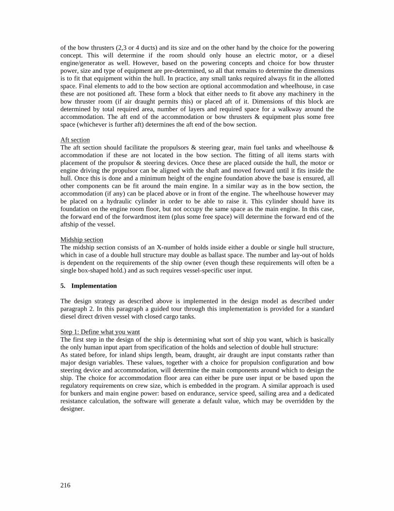
216

of the bow thrusters (2,3 or 4 ducts) and its size and on the other hand by the choice for the powering concept. This will determine if the room should only house an electric motor, or a diesel engine/generator as well. However, based on the powering concepts and choice for bow thruster power, size and type of equipment are pre-determined, so all that remains to determine the dimensions is to fit that equipment within the hull. In practice, any small tanks required always fit in the allotted space. Final elements to add to the bow section are optional accommodation and wheelhouse, in case these are not positioned aft. These form a block that either needs to fit above any machinery in the bow thruster room (if air draught permits this) or placed aft of it. Dimensions of this block are determined by total required area, number of layers and required space for a walkway around the accommodation. The aft end of the accommodation or bow thrusters & equipment plus some free space (whichever is further aft) determines the aft end of the bow section. Aft section The aft section should facilitate the propulsors & steering gear, main fuel tanks and wheelhouse & accommodation if these are not located in the bow section. The fitting of all items starts with placement of the propulsor & steering devices. Once these are placed outside the hull, the motor or engine driving the propulsor can be aligned with the shaft and moved forward until it fits inside the hull. Once this is done and a minimum height of the engine foundation above the base is ensured, all other components can be fit around the main engine. In a similar way as in the bow section, the accommodation (if any) can be placed above or in front of the engine. The wheelhouse however may be placed on a hydraulic cylinder in order to be able to raise it. This cylinder should have its foundation on the engine room floor, but not occupy the same space as the main engine. In this case, the forward end of the forwardmost item (plus some free space) will determine the forward end of the aftship of the vessel. Midship section The midship section consists of an X-number of holds inside either a double or single hull structure, which in case of a double hull structure may double as ballast space. The number and lay-out of holds is dependent on the requirements of the ship owner (even though these requirements will often be a single box-shaped hold.) and as such requires vessel-specific user input. 5. Implementation The design strategy as described above is implemented in the design model as described under paragraph 2. In this paragraph a guided tour through this implementation is provided for a standard diesel direct driven vessel with closed cargo tanks. Step 1: Define what you want The first step in the design of the ship is determining what sort of ship you want, which is basically the only human input apart from specification of the holds and selection of double hull structure: As stated before, for inland ships length, beam, draught, air draught are input constants rather than major design variables. These values, together with a choice for propulsion configuration and bow steering device and accommodation, will determine the main components around which to design the ship. The choice for accommodation floor area can either be pure user input or be based upon the regulatory requirements on crew size, which is embedded in the program. A similar approach is used for bunkers and main engine power: based on endurance, service speed, sailing area and a dedicated resistance calculation, the software will generate a default value, which may be overridden by the designer.

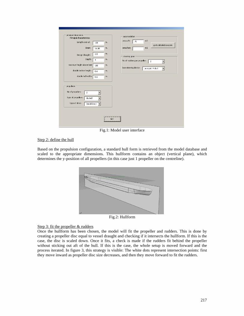
217

Fig.1: Model user interface Step 2: define the hull Based on the propulsion configuration, a standard hull form is retrieved from the model database and scaled to the appropriate dimensions. This hullform contains an object (vertical plane), which determines the y-position of all propellers (in this case just 1 propeller on the centreline).

Fig.2: Hullform Step 3: fit the propeller & rudders Once the hullform has been chosen, the model will fit the propeller and rudders. This is done by creating a propeller disc equal to vessel draught and checking if it intersects the hullform. If this is the case, the disc is scaled down. Once it fits, a check is made if the rudders fit behind the propeller without sticking out aft of the hull. If this is the case, the whole setup is moved forward and the process iterated. In figure 3, this strategy is visible: The white dots represent intersection points: first they move inward as propeller disc size decreases, and then they move forward to fit the rudders.

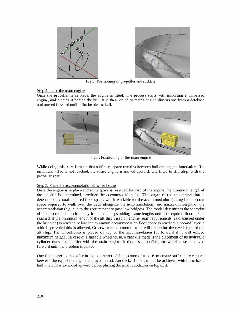
218

Fig.3: Positioning of propeller and rudders

Step 4: place the main engine Once the propeller is in place, the engine is fitted: The process starts with importing a unit-sized engine, and placing it behind the hull. It is then scaled to match engine dimensions from a database and moved forward until it fits inside the hull.

Fig.4: Positioning of the main engine

While doing this, care is taken that sufficient space remains between hull and engine foundation. If a minimum value is not reached, the entire engine is moved upwards and tilted to still align with the propeller shaft Step 5: Place the accommodation & wheelhouse Once the engine is in place and some space is reserved forward of the engine, the minimum length of the aft ship is determined, provided the accommodation fits. The length of the accommodation is determined by total required floor space, width available for the accommodation (taking into account space required to walk over the deck alongside the accommodation) and maximum height of the accommodation (e.g. due to the requirement to pass low bridges). The model determines the footprint of the accommodation frame by frame and keeps adding frame lengths until the required floor area is reached. If the minimum length of the aft ship based on engine room requirements (as discussed under the last step) is reached before the minimum accommodation floor space is reached, a second layer is added, provided this is allowed. Otherwise the accommodation will determine the new length of the aft ship. The wheelhouse is placed on top of the accommodation (or forward if it will exceed maximum height). In case of a raisable wheelhouse, a check is made if the placement of its hydraulic cylinder does not conflict with the main engine. If there is a conflict, the wheelhouse is moved forward until the problem is solved. One final aspect to consider in the placement of the accommodation is to ensure sufficient clearance between the top of the engine and accommodation deck. If this can not be achieved within the basic hull, the hull is extended upward before placing the accommodation on top of it.

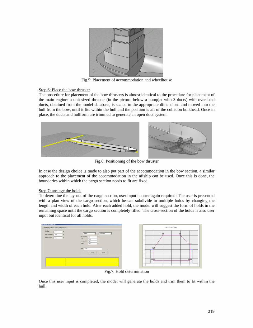
219

Fig.5: Placement of accommodation and wheelhouse

Step 6: Place the bow thruster The procedure for placement of the bow thrusters is almost identical to the procedure for placement of the main engine: a unit-sized thruster (in the picture below a pumpjet with 3 ducts) with oversized ducts, obtained from the model database, is scaled to the appropriate dimensions and moved into the hull from the bow, until it fits within the hull and the position is aft of the collision bulkhead. Once in place, the ducts and hullform are trimmed to generate an open duct system.

Fig.6: Positioning of the bow thruster

In case the design choice is made to also put part of the accommodation in the bow section, a similar approach to the placement of the accommodation in the aftship can be used. Once this is done, the boundaries within which the cargo section needs to fit are fixed. Step 7: arrange the holds To determine the lay-out of the cargo section, user input is once again required: The user is presented with a plan view of the cargo section, which he can subdivide in multiple holds by changing the length and width of each hold. After each added hold, the model will suggest the form of holds in the remaining space until the cargo section is completely filled. The cross-section of the holds is also user input but identical for all holds.

Fig.7: Hold determination Once this user input is completed, the model will generate the holds and trim them to fit within the hull.

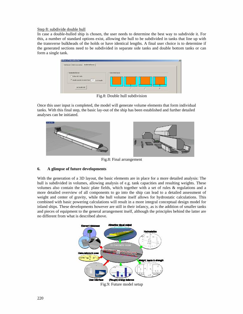
220

Step 8: subdivide double hull In case a double-hulled ship is chosen, the user needs to determine the best way to subdivide it. For this, a number of standard options exist, allowing the hull to be subdivided in tanks that line up with the transverse bulkheads of the holds or have identical lengths. A final user choice is to determine if the generated sections need to be subdivided in separate side tanks and double bottom tanks or can form a single tank.

Fig.8: Double hull subdivision

Once this user input is completed, the model will generate volume elements that form individual tanks. With this final step, the basic lay-out of the ship has been established and further detailed analyses can be initiated.

Fig.8: Final arrangement

6. A glimpse of future developments With the generation of a 3D layout, the basic elements are in place for a more detailed analysis: The hull is subdivided in volumes, allowing analysis of e.g. tank capacities and resulting weights. These volumes also contain the basic plate fields, which together with a set of rules & regulations and a more detailed overview of all components to go into the ship can lead to a detailed assessment of weight and center of gravity, while the hull volume itself allows for hydrostatic calculations. This combined with basic powering calculations will result in a more integral conceptual design model for inland ships. These developments however are still in their infancy, as is the addition of smaller tanks and pieces of equipment to the general arrangement itself, although the principles behind the latter are no different from what is described above.

Fig.9: Future model setup

221

References BUREAU INNOVATIE BINNENVAART (2003), Innovatiereader 2003 (in Dutch) BUREAU VOORLICHTING BINNENVAART (2008), Duurzaam transport 2007-2008, (In Dutch) VAN OERS B.J.; VAN HEES M. (2006), Combining a knowledge system with computer-aided design, 5th Int. Conf. on Computer Applications and Information Technology in the Maritime Industries (COMPIT), Hamburg, pp.65-73 VAN OERS B.J.; STAPERSMA D.; HOPMAN J.J. (2007), Improvements to a knowledge-based CAD system for Conceptual Ship Design, 6th Int. Conf. on Computer Applications and Information Technology in the Maritime Industries (COMPIT), Oegstgeest, pp.171-185

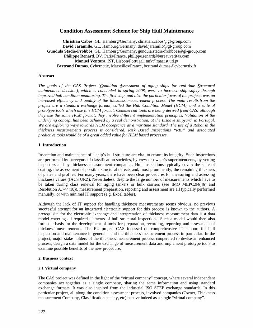
222

Condition Assessment Scheme for Ship Hull Maintenance

Christian Cabos, GL, Hamburg/Germany, christian.cabos@gl-group.com David Jaramillo, GL, Hamburg/Germany, david.jaramillo@gl-group.com

Gundula Stadie-Frohbös, GL, Hamburg/Germany, gundula.stadie-frohboes@gl-group.com Philippe Renard, BV, Paris/France, philippe.renard@bureauveritas.com

Manuel Ventura, IST, Lisbon/Portugal, mfv@mar.ist.utl.pt Bertrand Dumas, Cybernetix, Marseilles/France, bertrand.dumas@cybernetix.fr

Abstract The goals of the CAS Project (Condition Assessment of aging ships for real-time Structural maintenance decision), which is concluded in spring 2008, were to increase ship safety through improved hull condition monitoring. The first step, and also the particular focus of the project, was an increased efficiency and quality of the thickness measurement process. The main results from the project are a standard exchange format, called the Hull Condition Model (HCM), and a suite of prototype tools which use this HCM format. Commercial tools are being derived from CAS: although they use the same HCM format, they involve different implementation principles. Validation of the underlying concept has been achieved by a real demonstration, at the Lisnave shipyard, in Portugal. We are exploring ways towards HCM acceptance as a maritime standard. The use of a Robot in the thickness measurements process is considered. Risk Based Inspections “RBI” and associated predictive tools would be of a great added value for HCM based processes. 1. Introduction Inspection and maintenance of a ship’s hull structure are vital to ensure its integrity. Such inspections are performed by surveyors of classification societies, by crew or owner’s superintendents, by vetting inspectors and by thickness measurement companies. Hull inspections typically cover: the state of coating, the assessment of possible structural defects and, most prominently, the remaining thickness of plates and profiles. For many years, there have been clear procedures for measuring and assessing thickness values (IACS URZ). Nevertheless, despite the large number of measurements which have to be taken during class renewal for aging tankers or bulk carriers (see IMO MEPC.94(46) and Resolution A.744(18)), measurement preparation, reporting and assessment are all typically performed manually, or with minimal IT support (e.g. Excel tables). Although the lack of IT support for handling thickness measurements seems obvious, no previous successful attempt for an integrated electronic support for this process is known to the authors. A prerequisite for the electronic exchange and interpretation of thickness measurement data is a data model covering all required elements of hull structural inspections. Such a model would then also form the basis for the development of tools for preparation, recording, reporting and assessment of thickness measurements. The EU project CAS focussed on comprehensive IT support for hull inspection and maintenance in general – and the thickness measurement process in particular. In the project, major stake holders of the thickness measurement process cooperated to devise an enhanced process, design a data model for the exchange of measurement data and implement prototype tools to examine possible benefits of the new procedure. 2. Business context 2.1 Virtual company The CAS project was defined in the light of the “virtual company” concept, where several independent companies act together as a single company, sharing the same information and using standard exchange formats. It was also inspired from the industrial ISO STEP exchange standards. In this particular project, all along the condition assessment process, involved companies (Owner, Thickness measurement Company, Classification society, etc) behave indeed as a single “virtual company”.

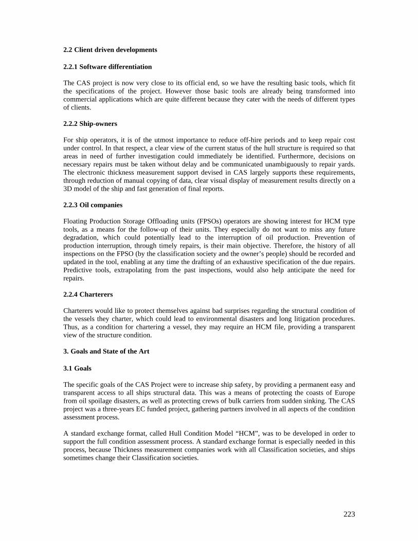
223

2.2 Client driven developments 2.2.1 Software differentiation The CAS project is now very close to its official end, so we have the resulting basic tools, which fit the specifications of the project. However those basic tools are already being transformed into commercial applications which are quite different because they cater with the needs of different types of clients. 2.2.2 Ship-owners For ship operators, it is of the utmost importance to reduce off-hire periods and to keep repair cost under control. In that respect, a clear view of the current status of the hull structure is required so that areas in need of further investigation could immediately be identified. Furthermore, decisions on necessary repairs must be taken without delay and be communicated unambiguously to repair yards. The electronic thickness measurement support devised in CAS largely supports these requirements, through reduction of manual copying of data, clear visual display of measurement results directly on a 3D model of the ship and fast generation of final reports. 2.2.3 Oil companies Floating Production Storage Offloading units (FPSOs) operators are showing interest for HCM type tools, as a means for the follow-up of their units. They especially do not want to miss any future degradation, which could potentially lead to the interruption of oil production. Prevention of production interruption, through timely repairs, is their main objective. Therefore, the history of all inspections on the FPSO (by the classification society and the owner’s people) should be recorded and updated in the tool, enabling at any time the drafting of an exhaustive specification of the due repairs. Predictive tools, extrapolating from the past inspections, would also help anticipate the need for repairs. 2.2.4 Charterers Charterers would like to protect themselves against bad surprises regarding the structural condition of the vessels they charter, which could lead to environmental disasters and long litigation procedures. Thus, as a condition for chartering a vessel, they may require an HCM file, providing a transparent view of the structure condition. 3. Goals and State of the Art 3.1 Goals The specific goals of the CAS Project were to increase ship safety, by providing a permanent easy and transparent access to all ships structural data. This was a means of protecting the coasts of Europe from oil spoilage disasters, as well as protecting crews of bulk carriers from sudden sinking. The CAS project was a three-years EC funded project, gathering partners involved in all aspects of the condition assessment process. A standard exchange format, called Hull Condition Model “HCM”, was to be developed in order to support the full condition assessment process. A standard exchange format is especially needed in this process, because Thickness measurement companies work with all Classification societies, and ships sometimes change their Classification societies.

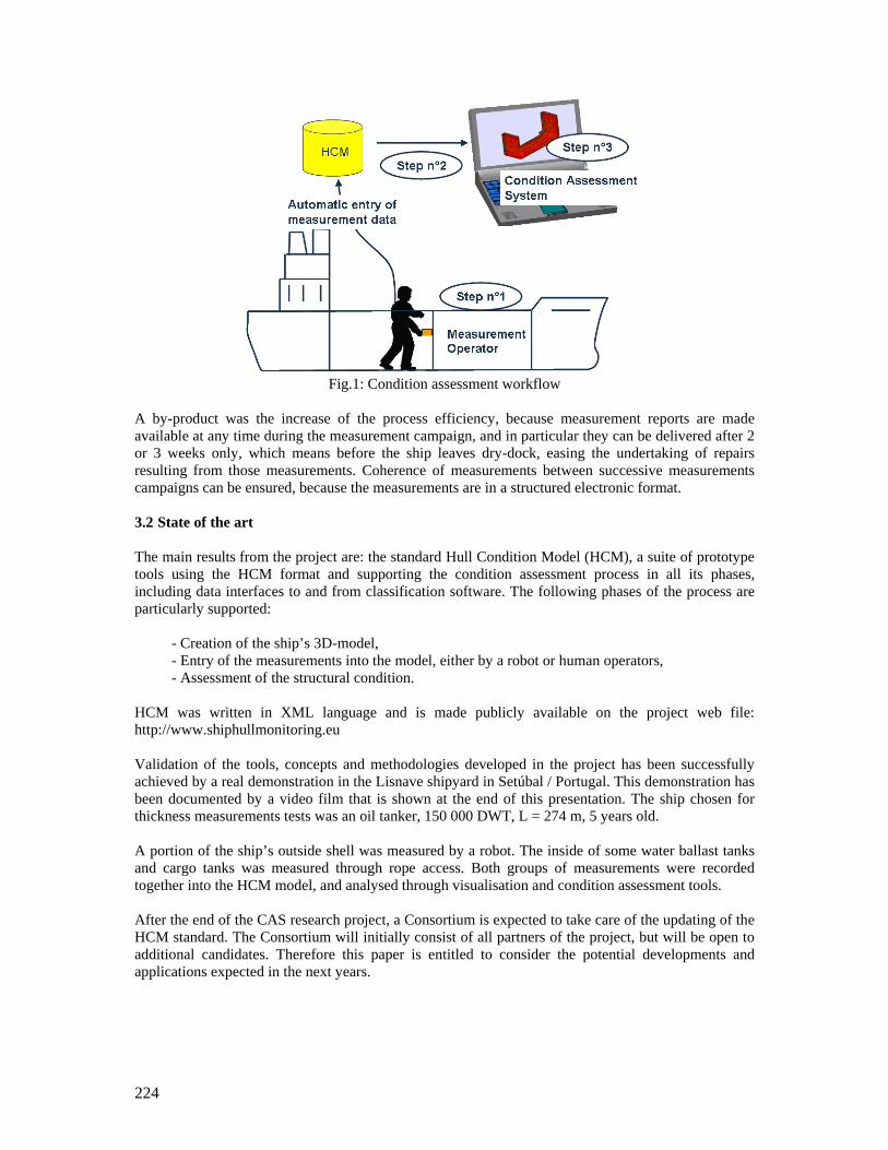
224

Fig.1: Condition assessment workflow

A by-product was the increase of the process efficiency, because measurement reports are made available at any time during the measurement campaign, and in particular they can be delivered after 2 or 3 weeks only, which means before the ship leaves dry-dock, easing the undertaking of repairs resulting from those measurements. Coherence of measurements between successive measurements campaigns can be ensured, because the measurements are in a structured electronic format. 3.2 State of the art The main results from the project are: the standard Hull Condition Model (HCM), a suite of prototype tools using the HCM format and supporting the condition assessment process in all its phases, including data interfaces to and from classification software. The following phases of the process are particularly supported:

- Creation of the ship’s 3D-model, - Entry of the measurements into the model, either by a robot or human operators, - Assessment of the structural condition.

HCM was written in XML language and is made publicly available on the project web file: http://www.shiphullmonitoring.eu Validation of the tools, concepts and methodologies developed in the project has been successfully achieved by a real demonstration in the Lisnave shipyard in Setúbal / Portugal. This demonstration has been documented by a video film that is shown at the end of this presentation. The ship chosen for thickness measurements tests was an oil tanker, 150 000 DWT, L = 274 m, 5 years old. A portion of the ship’s outside shell was measured by a robot. The inside of some water ballast tanks and cargo tanks was measured through rope access. Both groups of measurements were recorded together into the HCM model, and analysed through visualisation and condition assessment tools. After the end of the CAS research project, a Consortium is expected to take care of the updating of the HCM standard. The Consortium will initially consist of all partners of the project, but will be open to additional candidates. Therefore this paper is entitled to consider the potential developments and applications expected in the next years.

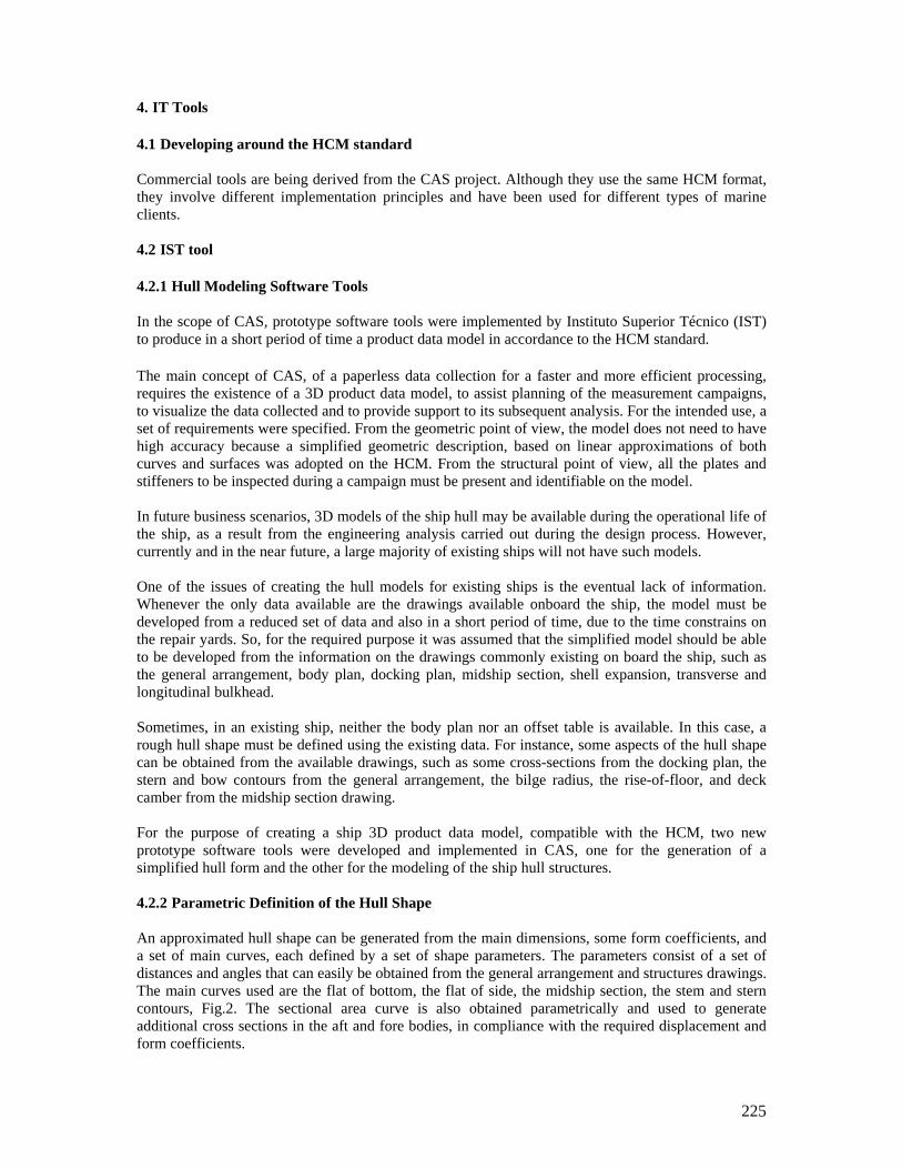
225

4. IT Tools 4.1 Developing around the HCM standard Commercial tools are being derived from the CAS project. Although they use the same HCM format, they involve different implementation principles and have been used for different types of marine clients. 4.2 IST tool 4.2.1 Hull Modeling Software Tools In the scope of CAS, prototype software tools were implemented by Instituto Superior Técnico (IST) to produce in a short period of time a product data model in accordance to the HCM standard. The main concept of CAS, of a paperless data collection for a faster and more efficient processing, requires the existence of a 3D product data model, to assist planning of the measurement campaigns, to visualize the data collected and to provide support to its subsequent analysis. For the intended use, a set of requirements were specified. From the geometric point of view, the model does not need to have high accuracy because a simplified geometric description, based on linear approximations of both curves and surfaces was adopted on the HCM. From the structural point of view, all the plates and stiffeners to be inspected during a campaign must be present and identifiable on the model. In future business scenarios, 3D models of the ship hull may be available during the operational life of the ship, as a result from the engineering analysis carried out during the design process. However, currently and in the near future, a large majority of existing ships will not have such models. One of the issues of creating the hull models for existing ships is the eventual lack of information. Whenever the only data available are the drawings available onboard the ship, the model must be developed from a reduced set of data and also in a short period of time, due to the time constrains on the repair yards. So, for the required purpose it was assumed that the simplified model should be able to be developed from the information on the drawings commonly existing on board the ship, such as the general arrangement, body plan, docking plan, midship section, shell expansion, transverse and longitudinal bulkhead. Sometimes, in an existing ship, neither the body plan nor an offset table is available. In this case, a rough hull shape must be defined using the existing data. For instance, some aspects of the hull shape can be obtained from the available drawings, such as some cross-sections from the docking plan, the stern and bow contours from the general arrangement, the bilge radius, the rise-of-floor, and deck camber from the midship section drawing. For the purpose of creating a ship 3D product data model, compatible with the HCM, two new prototype software tools were developed and implemented in CAS, one for the generation of a simplified hull form and the other for the modeling of the ship hull structures. 4.2.2 Parametric Definition of the Hull Shape An approximated hull shape can be generated from the main dimensions, some form coefficients, and a set of main curves, each defined by a set of shape parameters. The parameters consist of a set of distances and angles that can easily be obtained from the general arrangement and structures drawings. The main curves used are the flat of bottom, the flat of side, the midship section, the stem and stern contours, Fig.2. The sectional area curve is also obtained parametrically and used to generate additional cross sections in the aft and fore bodies, in compliance with the required displacement and form coefficients.

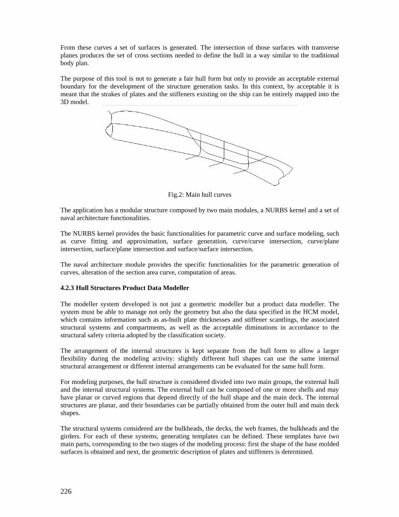
226

From these curves a set of surfaces is generated. The intersection of those surfaces with transverse planes produces the set of cross sections needed to define the hull in a way similar to the traditional body plan. The purpose of this tool is not to generate a fair hull form but only to provide an acceptable external boundary for the development of the structure generation tasks. In this context, by acceptable it is meant that the strakes of plates and the stiffeners existing on the ship can be entirely mapped into the 3D model.

Fig.2: Main hull curves

The application has a modular structure composed by two main modules, a NURBS kernel and a set of naval architecture functionalities. The NURBS kernel provides the basic functionalities for parametric curve and surface modeling, such as curve fitting and approximation, surface generation, curve/curve intersection, curve/plane intersection, surface/plane intersection and surface/surface intersection. The naval architecture module provides the specific functionalities for the parametric generation of curves, alteration of the section area curve, computation of areas. 4.2.3 Hull Structures Product Data Modeller The modeller system developed is not just a geometric modeller but a product data modeller. The system must be able to manage not only the geometry but also the data specified in the HCM model, which contains information such as as-built plate thicknesses and stiffener scantlings, the associated structural systems and compartments, as well as the acceptable diminutions in accordance to the structural safety criteria adopted by the classification society. The arrangement of the internal structures is kept separate from the hull form to allow a larger flexibility during the modeling activity: slightly different hull shapes can use the same internal structural arrangement or different internal arrangements can be evaluated for the same hull form. For modeling purposes, the hull structure is considered divided into two main groups, the external hull and the internal structural systems. The external hull can be composed of one or more shells and may have planar or curved regions that depend directly of the hull shape and the main deck. The internal structures are planar, and their boundaries can be partially obtained from the outer hull and main deck shapes. The structural systems considered are the bulkheads, the decks, the web frames, the bulkheads and the girders. For each of these systems, generating templates can be defined. These templates have two main parts, corresponding to the two stages of the modeling process: first the shape of the base molded surfaces is obtained and next, the geometric description of plates and stiffeners is determined.

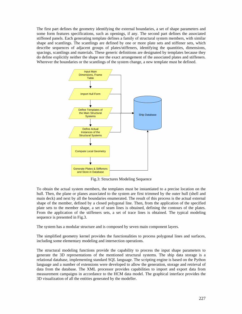
227

The first part defines the geometry identifying the external boundaries, a set of shape parameters and some form features specifications, such as openings, if any. The second part defines the associated stiffened panels. Each generating template defines a family of structural system members, with similar shape and scantlings. The scantlings are defined by one or more plate sets and stiffener sets, which describe sequences of adjacent groups of plates/stiffeners, identifying the quantities, dimensions, spacings, scantlings and materials. These generic definitions are designated by templates because they do define explicitly neither the shape nor the exact arrangement of the associated plates and stiffeners. Wherever the boundaries or the scantlings of the system change, a new template must be defined.

Input Main

Dimensions, FrameTable

Import Hull Form

Compute Local Geometry

Define Templates ofthe Main Structural

Systems

Define ActualInstances of the

Structural Systems

Generate Plates & Stiffenersand Store in Database

Ship Database

Fig.3: Structures Modeling Sequence

To obtain the actual system members, the templates must be instantiated to a precise location on the hull. Then, the plane or planes associated to the system are first trimmed by the outer hull (shell and main deck) and next by all the boundaries enumerated. The result of this process is the actual external shape of the member, defined by a closed polygonal line. Then, from the application of the specified plate sets to the member shape, a set of seam lines is obtained, defining the contours of the plates. From the application of the stiffeners sets, a set of trace lines is obtained. The typical modeling sequence is presented in Fig.3. The system has a modular structure and is composed by seven main component layers. The simplified geometry kernel provides the functionalities to process polygonal lines and surfaces, including some elementary modeling and intersection operations. The structural modeling functions provide the capability to process the input shape parameters to generate the 3D representations of the mentioned structural systems. The ship data storage is a relational database, implementing standard SQL language. The scripting engine is based on the Python language and a number of extensions were developed to allow the generation, storage and retrieval of data from the database. The XML processor provides capabilities to import and export data from measurement campaigns in accordance to the HCM data model. The graphical interface provides the 3D visualization of all the entities generated by the modeller.

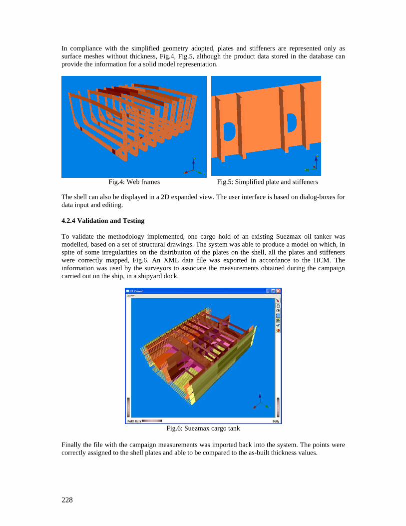
228

In compliance with the simplified geometry adopted, plates and stiffeners are represented only as surface meshes without thickness, Fig.4, Fig.5, although the product data stored in the database can provide the information for a solid model representation.

Fig.4: Web frames Fig.5: Simplified plate and stiffeners

The shell can also be displayed in a 2D expanded view. The user interface is based on dialog-boxes for data input and editing. 4.2.4 Validation and Testing To validate the methodology implemented, one cargo hold of an existing Suezmax oil tanker was modelled, based on a set of structural drawings. The system was able to produce a model on which, in spite of some irregularities on the distribution of the plates on the shell, all the plates and stiffeners were correctly mapped, Fig.6. An XML data file was exported in accordance to the HCM. The information was used by the surveyors to associate the measurements obtained during the campaign carried out on the ship, in a shipyard dock.

Fig.6: Suezmax cargo tank Finally the file with the campaign measurements was imported back into the system. The points were correctly assigned to the shell plates and able to be compared to the as-built thickness values.

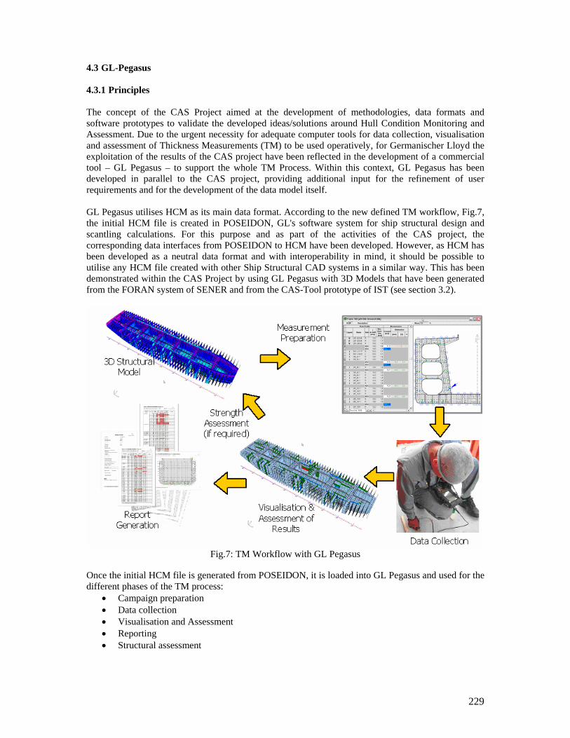
229

4.3 GL-Pegasus 4.3.1 Principles The concept of the CAS Project aimed at the development of methodologies, data formats and software prototypes to validate the developed ideas/solutions around Hull Condition Monitoring and Assessment. Due to the urgent necessity for adequate computer tools for data collection, visualisation and assessment of Thickness Measurements (TM) to be used operatively, for Germanischer Lloyd the exploitation of the results of the CAS project have been reflected in the development of a commercial tool – GL Pegasus – to support the whole TM Process. Within this context, GL Pegasus has been developed in parallel to the CAS project, providing additional input for the refinement of user requirements and for the development of the data model itself. GL Pegasus utilises HCM as its main data format. According to the new defined TM workflow, Fig.7, the initial HCM file is created in POSEIDON, GL's software system for ship structural design and scantling calculations. For this purpose and as part of the activities of the CAS project, the corresponding data interfaces from POSEIDON to HCM have been developed. However, as HCM has been developed as a neutral data format and with interoperability in mind, it should be possible to utilise any HCM file created with other Ship Structural CAD systems in a similar way. This has been demonstrated within the CAS Project by using GL Pegasus with 3D Models that have been generated from the FORAN system of SENER and from the CAS-Tool prototype of IST (see section 3.2).

Fig.7: TM Workflow with GL Pegasus

Once the initial HCM file is generated from POSEIDON, it is loaded into GL Pegasus and used for the different phases of the TM process:

• Campaign preparation • Data collection • Visualisation and Assessment • Reporting • Structural assessment

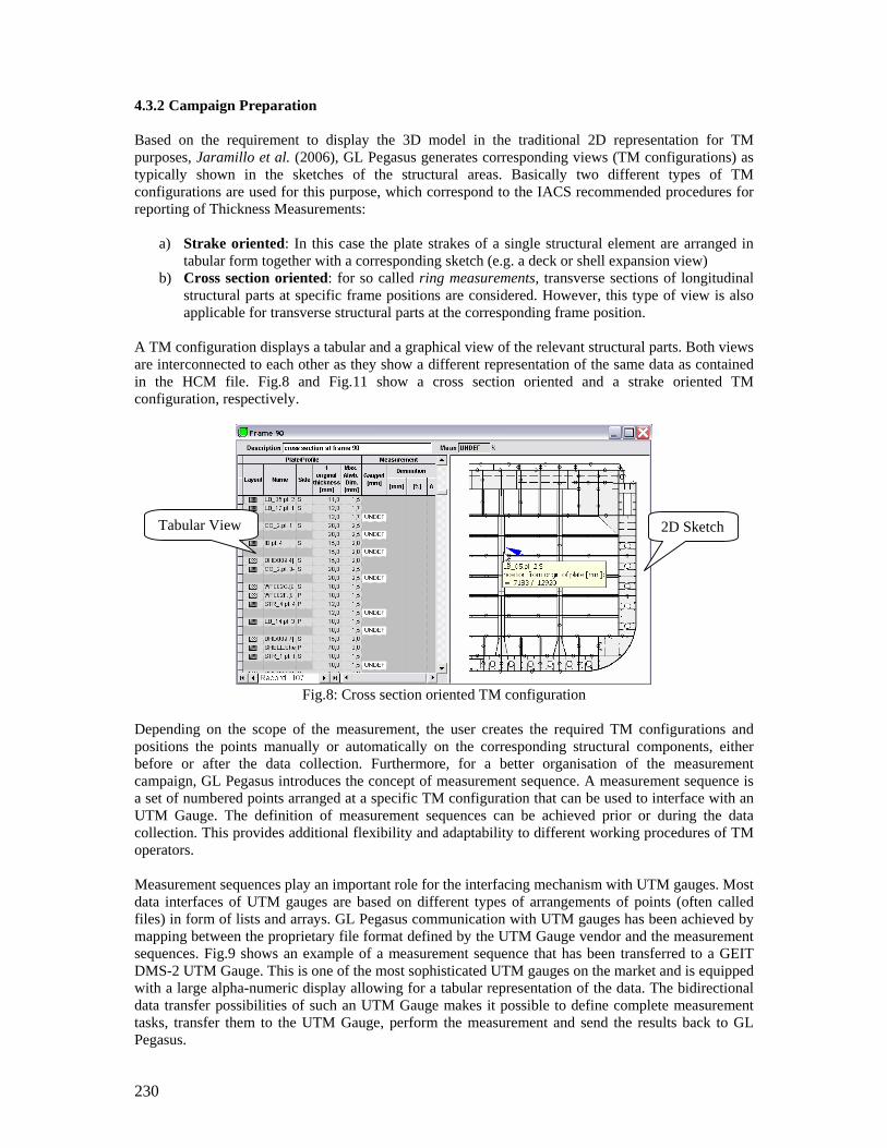
230

4.3.2 Campaign Preparation Based on the requirement to display the 3D model in the traditional 2D representation for TM purposes, Jaramillo et al. (2006), GL Pegasus generates corresponding views (TM configurations) as typically shown in the sketches of the structural areas. Basically two different types of TM configurations are used for this purpose, which correspond to the IACS recommended procedures for reporting of Thickness Measurements:

a) Strake oriented: In this case the plate strakes of a single structural element are arranged in tabular form together with a corresponding sketch (e.g. a deck or shell expansion view)

b) Cross section oriented: for so called ring measurements, transverse sections of longitudinal structural parts at specific frame positions are considered. However, this type of view is also applicable for transverse structural parts at the corresponding frame position.

A TM configuration displays a tabular and a graphical view of the relevant structural parts. Both views are interconnected to each other as they show a different representation of the same data as contained in the HCM file. Fig.8 and Fig.11 show a cross section oriented and a strake oriented TM configuration, respectively.

Fig.8: Cross section oriented TM configuration

Depending on the scope of the measurement, the user creates the required TM configurations and positions the points manually or automatically on the corresponding structural components, either before or after the data collection. Furthermore, for a better organisation of the measurement campaign, GL Pegasus introduces the concept of measurement sequence. A measurement sequence is a set of numbered points arranged at a specific TM configuration that can be used to interface with an UTM Gauge. The definition of measurement sequences can be achieved prior or during the data collection. This provides additional flexibility and adaptability to different working procedures of TM operators. Measurement sequences play an important role for the interfacing mechanism with UTM gauges. Most data interfaces of UTM gauges are based on different types of arrangements of points (often called files) in form of lists and arrays. GL Pegasus communication with UTM gauges has been achieved by mapping between the proprietary file format defined by the UTM Gauge vendor and the measurement sequences. Fig.9 shows an example of a measurement sequence that has been transferred to a GEIT DMS-2 UTM Gauge. This is one of the most sophisticated UTM gauges on the market and is equipped with a large alpha-numeric display allowing for a tabular representation of the data. The bidirectional data transfer possibilities of such an UTM Gauge makes it possible to define complete measurement tasks, transfer them to the UTM Gauge, perform the measurement and send the results back to GL Pegasus.

Tabular View 2D Sketch

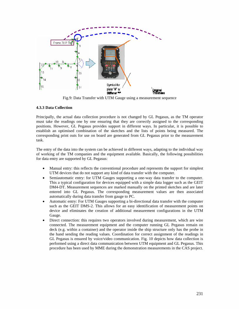
231

Fig.9: Data Transfer with UTM Gauge using a measurement sequence

4.3.3 Data Collection Principally, the actual data collection procedure is not changed by GL Pegasus, as the TM operator must take the readings one by one ensuring that they are correctly assigned to the corresponding positions. However, GL Pegasus provides support in different ways. In particular, it is possible to establish an optimised combination of the sketches and the lists of points being measured. The corresponding print outs for use on board are generated from GL Pegasus prior to the measurement task. The entry of the data into the system can be achieved in different ways, adapting to the individual way of working of the TM companies and the equipment available. Basically, the following possibilities for data entry are supported by GL Pegasus:

• Manual entry: this reflects the conventional procedure and represents the support for simplest UTM devices that do not support any kind of data transfer with the computer.

• Semiautomatic entry: for UTM Gauges supporting a one-way data transfer to the computer. This a typical configuration for devices equipped with a simple data logger such as the GEIT DM4-DT. Measurement sequences are marked manually on the printed sketches and are later entered into GL Pegasus. The corresponding measurement values are then associated automatically during data transfer from gauge to PC.

• Automatic entry: For UTM Gauges supporting a bi-directional data transfer with the computer such as the GEIT DMS-2. This allows for an easy identification of measurement points on device and eliminates the creation of additional measurement configurations in the UTM Gauge.

• Direct connection: this requires two operators involved during measurement, which are wire connected. The measurement equipment and the computer running GL Pegasus remain on deck (e.g. within a container) and the operator inside the ship structure only has the probe in the hand sending the reading values. Coordination for correct assignment of the readings in GL Pegasus is ensured by voice/video communication. Fig. 10 depicts how data collection is performed using a direct data communication between UTM equipment and GL Pegasus. This procedure has been used by MME during the demonstration measurements in the CAS project.

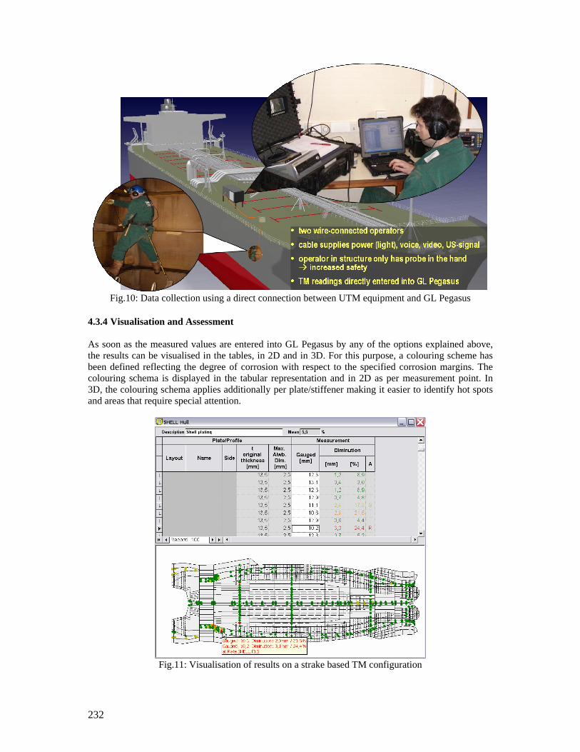
232

Fig.10: Data collection using a direct connection between UTM equipment and GL Pegasus

4.3.4 Visualisation and Assessment As soon as the measured values are entered into GL Pegasus by any of the options explained above, the results can be visualised in the tables, in 2D and in 3D. For this purpose, a colouring scheme has been defined reflecting the degree of corrosion with respect to the specified corrosion margins. The colouring schema is displayed in the tabular representation and in 2D as per measurement point. In 3D, the colouring schema applies additionally per plate/stiffener making it easier to identify hot spots and areas that require special attention.

Fig.11: Visualisation of results on a strake based TM configuration

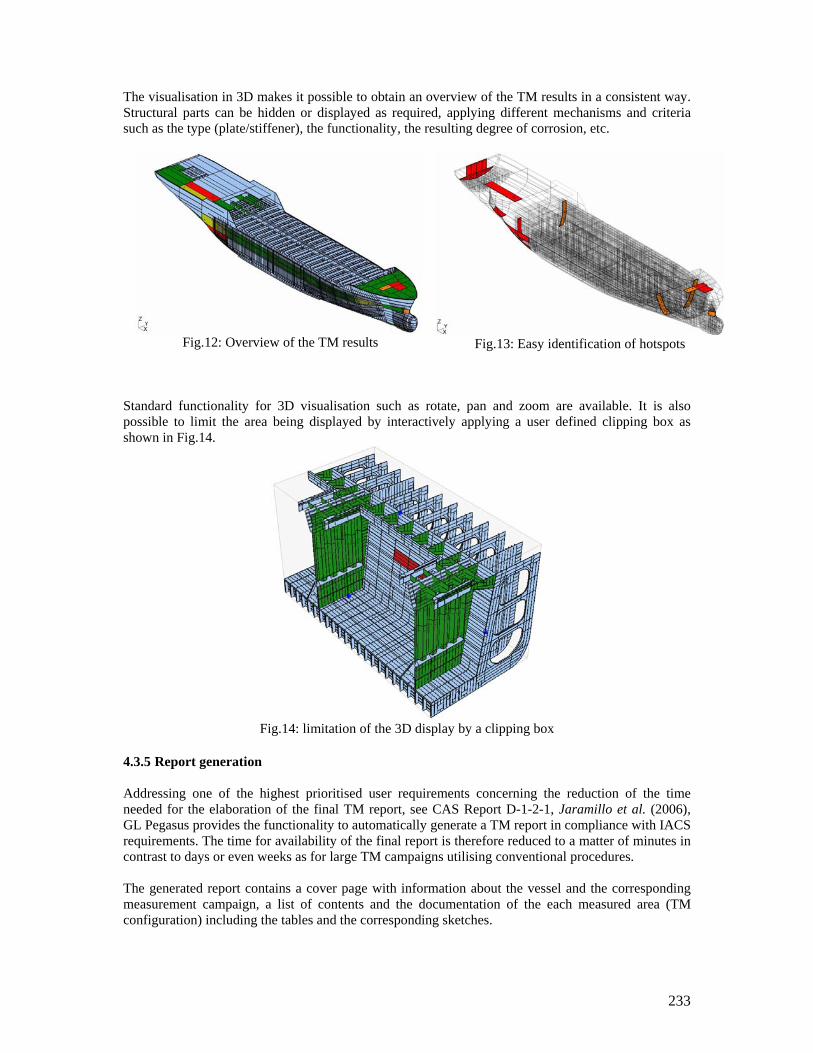
233

The visualisation in 3D makes it possible to obtain an overview of the TM results in a consistent way. Structural parts can be hidden or displayed as required, applying different mechanisms and criteria such as the type (plate/stiffener), the functionality, the resulting degree of corrosion, etc.

Fig.12: Overview of the TM results

Fig.13: Easy identification of hotspots

Standard functionality for 3D visualisation such as rotate, pan and zoom are available. It is also possible to limit the area being displayed by interactively applying a user defined clipping box as shown in Fig.14.

Fig.14: limitation of the 3D display by a clipping box

4.3.5 Report generation Addressing one of the highest prioritised user requirements concerning the reduction of the time needed for the elaboration of the final TM report, see CAS Report D-1-2-1, Jaramillo et al. (2006), GL Pegasus provides the functionality to automatically generate a TM report in compliance with IACS requirements. The time for availability of the final report is therefore reduced to a matter of minutes in contrast to days or even weeks as for large TM campaigns utilising conventional procedures. The generated report contains a cover page with information about the vessel and the corresponding measurement campaign, a list of contents and the documentation of the each measured area (TM configuration) including the tables and the corresponding sketches.

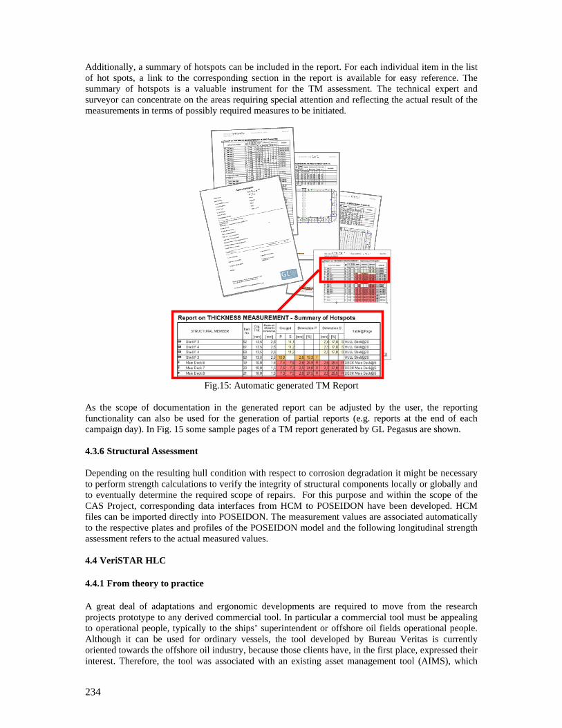
234

Additionally, a summary of hotspots can be included in the report. For each individual item in the list of hot spots, a link to the corresponding section in the report is available for easy reference. The summary of hotspots is a valuable instrument for the TM assessment. The technical expert and surveyor can concentrate on the areas requiring special attention and reflecting the actual result of the measurements in terms of possibly required measures to be initiated.

Fig.15: Automatic generated TM Report

As the scope of documentation in the generated report can be adjusted by the user, the reporting functionality can also be used for the generation of partial reports (e.g. reports at the end of each campaign day). In Fig. 15 some sample pages of a TM report generated by GL Pegasus are shown. 4.3.6 Structural Assessment Depending on the resulting hull condition with respect to corrosion degradation it might be necessary to perform strength calculations to verify the integrity of structural components locally or globally and to eventually determine the required scope of repairs. For this purpose and within the scope of the CAS Project, corresponding data interfaces from HCM to POSEIDON have been developed. HCM files can be imported directly into POSEIDON. The measurement values are associated automatically to the respective plates and profiles of the POSEIDON model and the following longitudinal strength assessment refers to the actual measured values. 4.4 VeriSTAR HLC 4.4.1 From theory to practice A great deal of adaptations and ergonomic developments are required to move from the research projects prototype to any derived commercial tool. In particular a commercial tool must be appealing to operational people, typically to the ships’ superintendent or offshore oil fields operational people. Although it can be used for ordinary vessels, the tool developed by Bureau Veritas is currently oriented towards the offshore oil industry, because those clients have, in the first place, expressed their interest. Therefore, the tool was associated with an existing asset management tool (AIMS), which

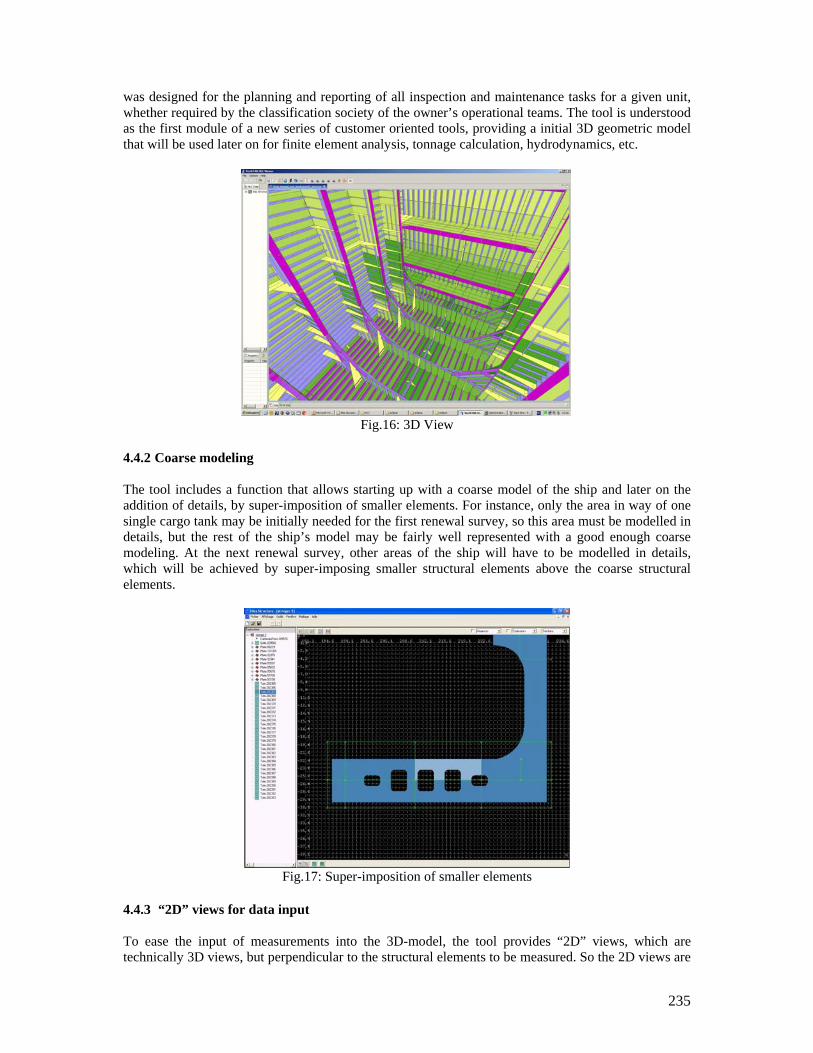
235

was designed for the planning and reporting of all inspection and maintenance tasks for a given unit, whether required by the classification society of the owner’s operational teams. The tool is understood as the first module of a new series of customer oriented tools, providing a initial 3D geometric model that will be used later on for finite element analysis, tonnage calculation, hydrodynamics, etc.

Fig.16: 3D View

4.4.2 Coarse modeling The tool includes a function that allows starting up with a coarse model of the ship and later on the addition of details, by super-imposition of smaller elements. For instance, only the area in way of one single cargo tank may be initially needed for the first renewal survey, so this area must be modelled in details, but the rest of the ship’s model may be fairly well represented with a good enough coarse modeling. At the next renewal survey, other areas of the ship will have to be modelled in details, which will be achieved by super-imposing smaller structural elements above the coarse structural elements.

Fig.17: Super-imposition of smaller elements

4.4.3 “2D” views for data input To ease the input of measurements into the 3D-model, the tool provides “2D” views, which are technically 3D views, but perpendicular to the structural elements to be measured. So the 2D views are

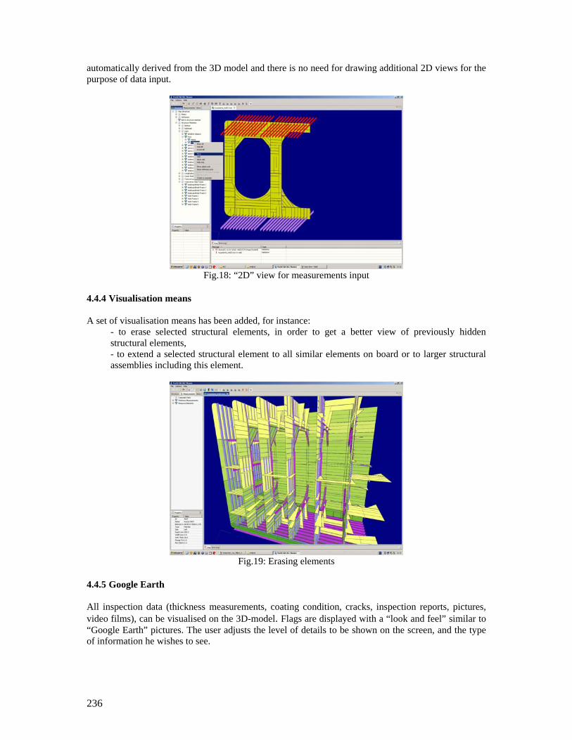
236

automatically derived from the 3D model and there is no need for drawing additional 2D views for the purpose of data input.

Fig.18: “2D” view for measurements input

4.4.4 Visualisation means A set of visualisation means has been added, for instance:

- to erase selected structural elements, in order to get a better view of previously hidden structural elements, - to extend a selected structural element to all similar elements on board or to larger structural assemblies including this element.

Fig.19: Erasing elements

4.4.5 Google Earth All inspection data (thickness measurements, coating condition, cracks, inspection reports, pictures, video films), can be visualised on the 3D-model. Flags are displayed with a “look and feel” similar to “Google Earth” pictures. The user adjusts the level of details to be shown on the screen, and the type of information he wishes to see.

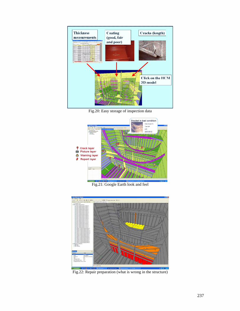
237

Fig.20: Easy storage of inspection data

Fig.21: Google Earth look and feel

Fig.22: Repair preparation (what is wrong in the structure)

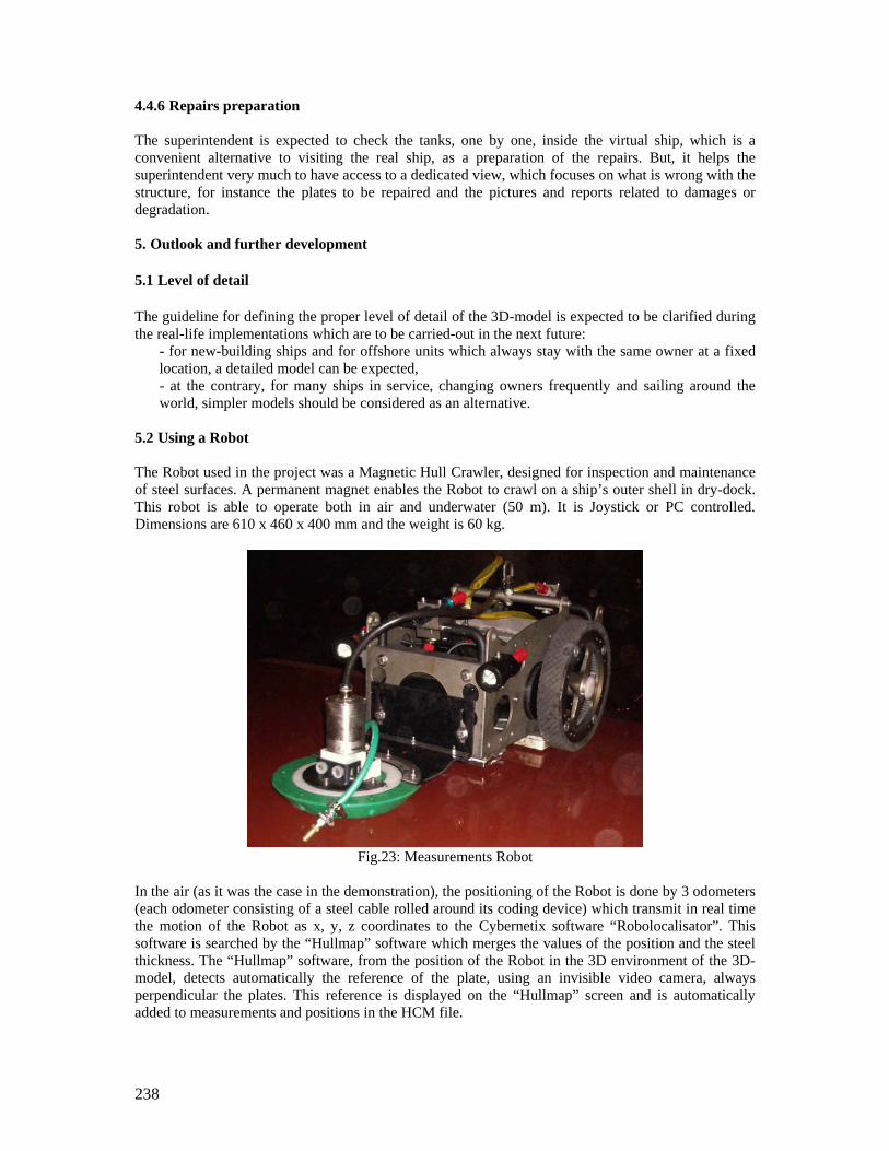
238

4.4.6 Repairs preparation The superintendent is expected to check the tanks, one by one, inside the virtual ship, which is a convenient alternative to visiting the real ship, as a preparation of the repairs. But, it helps the superintendent very much to have access to a dedicated view, which focuses on what is wrong with the structure, for instance the plates to be repaired and the pictures and reports related to damages or degradation. 5. Outlook and further development 5.1 Level of detail The guideline for defining the proper level of detail of the 3D-model is expected to be clarified during the real-life implementations which are to be carried-out in the next future:

- for new-building ships and for offshore units which always stay with the same owner at a fixed location, a detailed model can be expected, - at the contrary, for many ships in service, changing owners frequently and sailing around the world, simpler models should be considered as an alternative.

5.2 Using a Robot The Robot used in the project was a Magnetic Hull Crawler, designed for inspection and maintenance of steel surfaces. A permanent magnet enables the Robot to crawl on a ship’s outer shell in dry-dock. This robot is able to operate both in air and underwater (50 m). It is Joystick or PC controlled. Dimensions are 610 x 460 x 400 mm and the weight is 60 kg.

Fig.23: Measurements Robot

In the air (as it was the case in the demonstration), the positioning of the Robot is done by 3 odometers (each odometer consisting of a steel cable rolled around its coding device) which transmit in real time the motion of the Robot as x, y, z coordinates to the Cybernetix software “Robolocalisator”. This software is searched by the “Hullmap” software which merges the values of the position and the steel thickness. The “Hullmap” software, from the position of the Robot in the 3D environment of the 3D-model, detects automatically the reference of the plate, using an invisible video camera, always perpendicular the plates. This reference is displayed on the “Hullmap” screen and is automatically added to measurements and positions in the HCM file.

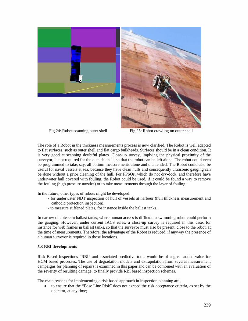
239

Fig.24: Robot scanning outer shell Fig.25: Robot crawling on outer shell The role of a Robot in the thickness measurements process is now clarified. The Robot is well adapted to flat surfaces, such as outer shell and flat cargo bulkheads. Surfaces should be in a clean condition. It is very good at scanning doubtful plates. Close-up survey, implying the physical proximity of the surveyor, is not required for the outside shell, so that the robot can be left alone. The robot could even be programmed to take, say, all bottom measurements alone and unattended. The Robot could also be useful for naval vessels at sea, because they have clean hulls and consequently ultrasonic gauging can be done without a prior cleaning of the hull. For FPSOs, which do not dry-dock, and therefore have underwater hull covered with fouling, the Robot could be used, if it could be found a way to remove the fouling (high pressure nozzles) or to take measurements through the layer of fouling. In the future, other types of robots might be developed:

- for underwater NDT inspection of hull of vessels at harbour (hull thickness measurement and cathodic protection inspection).

- to measure stiffened plates, for instance inside the ballast tanks. In narrow double skin ballast tanks, where human access is difficult, a swimming robot could perform the gauging. However, under current IACS rules, a close-up survey is required in this case, for instance for web frames in ballast tanks, so that the surveyor must also be present, close to the robot, at the time of measurements. Therefore, the advantage of the Robot is reduced, if anyway the presence of a human surveyor is required in those locations. 5.3 RBI developments Risk Based Inspections “RBI” and associated predictive tools would be of a great added value for HCM based processes. The use of degradation models and extrapolation from several measurement campaigns for planning of repairs is examined in this paper and can be combined with an evaluation of the severity of resulting damage, to finally provide RBI based inspection schemes. The main reasons for implementing a risk based approach in inspection planning are:

• to ensure that the “Base Line Risk” does not exceed the risk acceptance criteria, as set by the operator, at any time;

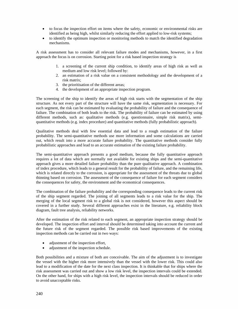
240

• to focus the inspection effort on items where the safety, economic or environmental risks are identified as being high, whilst similarly reducing the effort applied to low-risk systems;

• to identify the optimum inspection or monitoring methods to match the identified degradation mechanisms.

A risk assessment has to consider all relevant failure modes and mechanisms, however, in a first approach the focus is on corrosion. Starting point for a risk based inspection strategy is

1. a screening of the current ship condition, to identify areas of high risk as well as medium and low risk level; followed by:

2. an estimation of a risk value on a consistent methodology and the development of a risk matrix;

3. the prioritisation of the different areas; 4. the development of an appropriate inspection program.

The screening of the ship to identify the areas of high risk starts with the segmentation of the ship structure. As not every part of the structure will have the same risk, segmentation is necessary. For each segment, the risk can be estimated by evaluating the probability of failure and the consequence of failure. The combination of both leads to the risk. The probability of failure can be estimated by using different methods, such as: qualitative methods (e.g. questionnaire, simple risk matrix), semi-quantitative methods (e.g. index procedure) and quantitative methods (fully probabilistic approach). Qualitative methods deal with few essential data and lead to a rough estimation of the failure probability. The semi-quantitative methods use more information and some calculations are carried out, which result into a more accurate failure probability. The quantitative methods consider fully probabilistic approaches and lead to an accurate estimation of the existing failure probability. The semi-quantitative approach presents a good medium, because the fully quantitative approach requires a lot of data which are normally not available for existing ships and the semi-quantitative approach gives a more detailed failure probability than the pure qualitative approach. A combination of index procedure, which leads to a general result for the probability of failure, and the remaining life, which is related directly to the corrosion, is appropriate for the assessment of the threats due to global thinning based on corrosion. The assessment of the consequence of failure for each segment considers the consequences for safety, the environment and the economical consequences. The combination of the failure probability and the corresponding consequence leads to the current risk of the ship segment regarded. The joining of all segments leads to a risk value for the ship. The merging of the local segment risk to a global risk is not considered, however this aspect should be covered in a further study. Several different approaches exist in the literature, e.g. reliability block diagram, fault tree analysis, reliability networks. After the estimation of the risk related to each segment, an appropriate inspection strategy should be developed. The inspection effort and interval should be determined taking into account the current and the future risk of the segment regarded. The possible risk based improvements of the existing inspection methods can be carried out in two ways:

• adjustment of the inspection effort, • adjustment of the inspection schedule.

Both possibilities and a mixture of both are conceivable. The aim of the adjustment is to investigate the vessel with the higher risk more intensively than the vessel with the lower risk. This could also lead to a modification of the date for the next class inspection. It is thinkable that for ships where the risk assessment was carried out and show a low risk level, the inspection intervals could be extended. On the other hand, for ships with a high risk level, the inspection intervals should be reduced in order to avoid unacceptable risks.

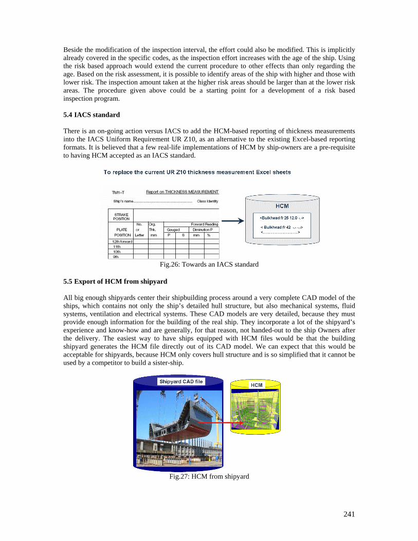
241

Beside the modification of the inspection interval, the effort could also be modified. This is implicitly already covered in the specific codes, as the inspection effort increases with the age of the ship. Using the risk based approach would extend the current procedure to other effects than only regarding the age. Based on the risk assessment, it is possible to identify areas of the ship with higher and those with lower risk. The inspection amount taken at the higher risk areas should be larger than at the lower risk areas. The procedure given above could be a starting point for a development of a risk based inspection program. 5.4 IACS standard There is an on-going action versus IACS to add the HCM-based reporting of thickness measurements into the IACS Uniform Requirement UR Z10, as an alternative to the existing Excel-based reporting formats. It is believed that a few real-life implementations of HCM by ship-owners are a pre-requisite to having HCM accepted as an IACS standard.

Fig.26: Towards an IACS standard

5.5 Export of HCM from shipyard All big enough shipyards center their shipbuilding process around a very complete CAD model of the ships, which contains not only the ship’s detailed hull structure, but also mechanical systems, fluid systems, ventilation and electrical systems. These CAD models are very detailed, because they must provide enough information for the building of the real ship. They incorporate a lot of the shipyard’s experience and know-how and are generally, for that reason, not handed-out to the ship Owners after the delivery. The easiest way to have ships equipped with HCM files would be that the building shipyard generates the HCM file directly out of its CAD model. We can expect that this would be acceptable for shipyards, because HCM only covers hull structure and is so simplified that it cannot be used by a competitor to build a sister-ship.

Fig.27: HCM from shipyard

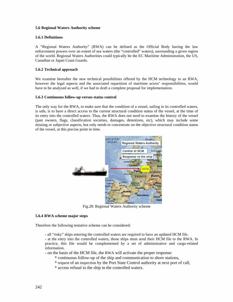
242

5.6 Regional Waters Authority scheme 5.6.1 Definitions A “Regional Waters Authority” (RWA) can be defined as the Official Body having the law enforcement powers over an extent of sea waters (the “controlled” waters), surrounding a given region of the world. Regional Waters Authorities could typically be the EC Maritime Administration, the US, Canadian or Japan Coast Guards. 5.6.2 Technical approach We examine hereafter the new technical possibilities offered by the HCM technology to an RWA, however the legal aspects and the associated repartition of maritime actors’ responsibilities, would have to be analysed as well, if we had to draft a complete proposal for implementation. 5.6.3 Continuous follow-up versus status control The only way for the RWA, to make sure that the condition of a vessel, sailing in its controlled waters, is safe, is to have a direct access to the current structural condition status of the vessel, at the time of its entry into the controlled waters. Thus, the RWA does not need to examine the history of the vessel (past owners, flags, classification societies, damages, detentions, etc), which may include some missing or subjective aspects, but only needs to concentrate on the objective structural condition status of the vessel, at this precise point in time.

Fig.28: Regional Waters Authority scheme

5.6.4 RWA scheme major steps Therefore the following tentative scheme can be considered:

- all “risky” ships entering the controlled waters are required to have an updated HCM file. - at the entry into the controlled waters, those ships must send their HCM file to the RWA. In practice, this file would be complemented by a set of administrative and cargo-related information. - on the basis of the HCM file, the RWA will activate the proper response:

* continuous follow-up of the ship and communication to shore stations, * request of an inspection by the Port State Control authority at next port of call, * access refusal to the ship in the controlled waters.

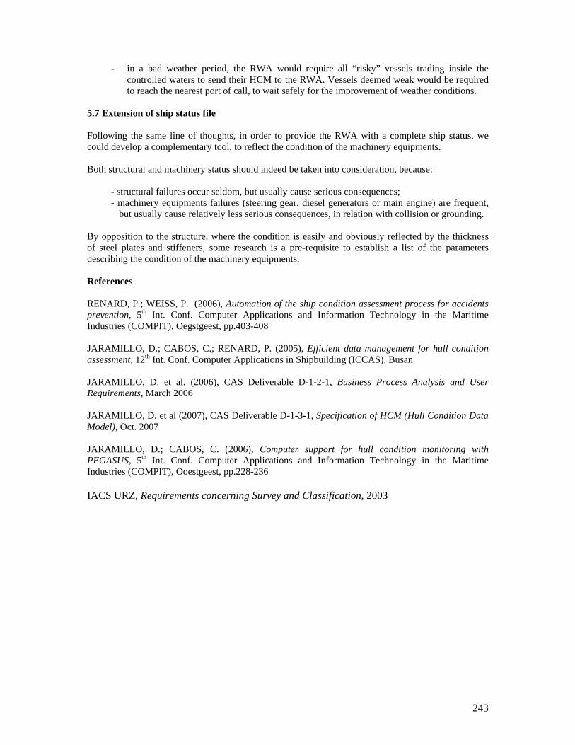
243

- in a bad weather period, the RWA would require all “risky” vessels trading inside the controlled waters to send their HCM to the RWA. Vessels deemed weak would be required to reach the nearest port of call, to wait safely for the improvement of weather conditions.

5.7 Extension of ship status file Following the same line of thoughts, in order to provide the RWA with a complete ship status, we could develop a complementary tool, to reflect the condition of the machinery equipments. Both structural and machinery status should indeed be taken into consideration, because:

- structural failures occur seldom, but usually cause serious consequences; - machinery equipments failures (steering gear, diesel generators or main engine) are frequent,

but usually cause relatively less serious consequences, in relation with collision or grounding.

By opposition to the structure, where the condition is easily and obviously reflected by the thickness of steel plates and stiffeners, some research is a pre-requisite to establish a list of the parameters describing the condition of the machinery equipments. References RENARD, P.; WEISS, P. (2006), Automation of the ship condition assessment process for accidents prevention, 5th Int. Conf. Computer Applications and Information Technology in the Maritime Industries (COMPIT), Oegstgeest, pp.403-408 JARAMILLO, D.; CABOS, C.; RENARD, P. (2005), Efficient data management for hull condition assessment, 12th Int. Conf. Computer Applications in Shipbuilding (ICCAS), Busan JARAMILLO, D. et al. (2006), CAS Deliverable D-1-2-1, Business Process Analysis and User Requirements, March 2006 JARAMILLO, D. et al (2007), CAS Deliverable D-1-3-1, Specification of HCM (Hull Condition Data Model), Oct. 2007 JARAMILLO, D.; CABOS, C. (2006), Computer support for hull condition monitoring with PEGASUS, 5th Int. Conf. Computer Applications and Information Technology in the Maritime Industries (COMPIT), Ooestgeest, pp.228-236 IACS URZ, Requirements concerning Survey and Classification, 2003

244

Representing Design Knowledge in Configuration-Based Conceptual Ship Design

Thomas Brathaug, NTNU, Trondheim/Norway, thomas@brathaug.no

Jon Olav Holan, NTNU, Trondheim/Norway, jon.holan@ntnu.no

Stein Ove Erikstad, NTNU, Trondheim/Norway, stein.ove.erikstad@ntnu.no

Abstract

Ship design companies handle a large number of requests for tender annually. These tendering

projects are typically resource-intensive, time critical, with a high risk. Though some of these projects

will be novel designs, the bulk will be customizations of an existing design platform. The traditional

approach to handle this process has been to copy an existing project, and incorporate the necessary

changes. However, this process is both inefficient and error-prone, and recent developments in

platform-based design and mass customization offer opportunities for improvements. In this paper, we

propose a configuration-based process for tender project development. It is specifically targeted

towards complex, arrangement-intensive ship types such as offshore support vessels, and it will seek

to exploit recent investment in module-based design platforms in the industry. One particular area

that is addressed is how to represent the particular design knowledge required for driving this

configuration process from a set of customer requirements and KPIs, into a complete tender package

comprising a diversity of elements, such as the vessel parametric description, a contract specification,

cost calculation, 2D arrangements and 3D visualisation models. Towards the end of the paper we

discuss how rule based frameworks can be used in an industry context to capture required knowledge,

such as company specific product platform rules (the existence, relevance, inferred properties and

derived performance of scalable modules), generic ship design rules, and external rules from class

societies and authorities.

1. Introduction

Ship design companies, such as those delivering offshore vessels designs to a global shipbuilding

marketplace, may handle hundreds of requests for tender annually. These tendering projects are

typically resource-intensive with strict time limits, and have a high risk both in terms of not being

rewarded, and in terms of committing to a legally binding contract with a satisfactory margin.

According to Coyne, Rosenman et al. (1990); Ashok (1997), design processes can be grouped into

three main classes based on the degree of novelty and innovation involved, namely; routine design, or

prototype refinement, involving the customization of an existing platform in which the main modules,

their interrelations and their underlying structure is already known; innovative design, or prototype

adaptation, in which the boundaries of existing designs are adjusted incrementally; and finally novel

design, or prototype creation, in which a totally new design is developed.

The bulk of the tendering projects at a typical ship design office will belong to the first of these

classes, namely routine design, while a few may be classified as innovative, either by the addition

and/or adaptation of new solutions on a modular level (propulsion systems, machinery systems, bow

form, etc.), or by extending the functional performance envelope of the vessel (large, multi-purpose

OCVs, offshore construction vessels, etc.). Rarely, if ever, can a vessel design be characterized as

completely novel.

The traditional approach to handle this process has been to copy an existing project, and incorporate

the necessary changes. This “copy-and-edit” approach incurs a considerable quality cost Hagen and

Erikstad (2002), in terms of over-specifications, errors and omissions, and fail to exploit recent

developments in platform-based design, modularization and mass customization.

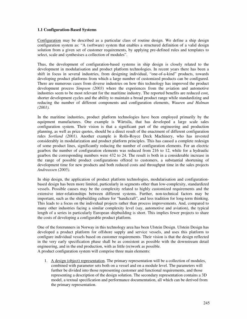
245

1.1 Configuration-Based Systems

Configuration may be described as a particular class of routine design. We define a ship design

configuration system as: “A (software) system that enables a structured definition of a valid design

solution from a given set of customer requirements, by applying pre-defined rules and templates to

select, scale and synthesises a collection of modules”.

Thus, the development of configuration-based systems in ship design is closely related to the

development in modularisation and product platform technologies. In recent years there has been a

shift in focus in several industries, from designing individual, “one-of-a-kind” products, towards

developing product platforms from which a large number of customized products can be configured.

There are numerous cases from diverse industries on how this technology has improved the product

development process Simpson (2003) where the experiences from the aviation and automotive

industries seem to be most relevant for the maritime industry. The reported benefits are reduced cost,

shorter development cycles and the ability to maintain a broad product range while standardizing and

reducing the number of different components and configuration elements, Wuuren and Halman

(2001).

In the maritime industries, product platform technologies have been employed primarily by the

equipment manufactures. One example is Wärtsila, that has developed a large scale sales

configuration system. Their vision is that a significant part of the engineering and production

planning, as well as price quotes, should be a direct result of the enactment of different configuration

rules Sortland (2001). Another example is Rolls-Royce Deck Machinery, who has invested

considerably in modularization and product platform principles. This has caused a complete redesign

of some product lines, significantly reducing the number of configuration elements. For an electric

gearbox the number of configuration elements was reduced from 216 to 12, while for a hydraulic

gearbox the corresponding numbers were 432 to 24. The result is both in a considerable increase in

the range of possible product configurations offered to customers, a substantial shortening of

development time for new products and both reduced costs and throughput time in the sales projects

Andreassen (2005).

In ship design, the application of product platform technologies, modularisation and configuration-

based design has been more limited, particularly in segments other than low-complexity, standardized

vessels. Possible causes may be the complexity related to highly customized requirements and the

extensive inter-relationships between different systems. Further, non-technical factors may be

important, such as the shipbuilding culture for “handicraft”, and less tradition for long-term thinking.

This leads to a focus on the individual projects rather than process improvements. And, compared to

many other industries facing a similar complexity level (say, automotive and aviation), the typical

length of a series in particularly European shipbuilding is short. This implies fewer projects to share

the costs of developing a configurable product platform.

One of the forerunners in Norway in this technology area has been Ulstein Design. Ulstein Design has

developed a product platform for offshore supply and service vessels, and uses this platform to

configure individual vessels based on customer requirements. Their vision is that the design reflected

in the very early specification phase shall be as consistent as possible with the downstream detail

engineering, and in the end production, with as little (re)work as possible.

A product configuration system will comprise three main elements:

1. A design (object) representation. The primary representation will be a collection of modules,

combined with parameter sets both on a vessel and on a module level. The parameters will

further be divided into those representing customer and functional requirements, and those

representing a description of the design solution. The secondary representation contains a 3D

model, a textual specification and performance documentation, all which can be derived from

the primary representation.

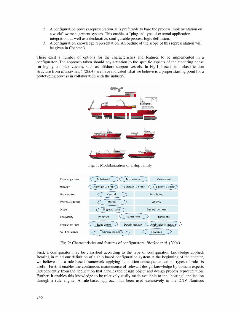
246

2. A configuration process representation. It is preferable to base the process implementation on

a workflow management system. This enables a “plug-in” type of external application

integration, as well as a declarative, configurable process logic definition.

3. A configuration knowledge representation. An outline of the scope of this representation will

be given in Chapter 3.

There exist a number of options for the characteristics and features to be implemented in a

configurator. The approach taken should pay attention to the specific aspects of the tendering phase

for highly complex vessels, such as offshore support vessels. In Fig.1, based on a classification

structure from Blecker et al. (2004), we have indicated what we believe is a proper starting point for a

prototyping process in collaboration with the industry.

Fig. 1: Modularization of a ship family

Fig. 2: Characteristics and features of configurators, Blecker et al. (2004)

First, a configurator may be classified according to the type of configuration knowledge applied.

Bearing in mind our definition of a ship based configuration system at the beginning of the chapter,

we believe that a rule-based framework applying “condition-consequence-action” types of rules is

useful. First, it enables the continuous maintenance of relevant design knowledge by domain experts

independently from the application that handles the design object and design process representation.

Further, it enables this knowledge to be relatively easily made available to the “hosting” application

through a rule engine. A rule-based approach has been used extensively in the DNV Nauticus

247

software suite, primarily for structural design, but also for modelling task automation in Nauticus

Early Design. Applications in conceptual ship design/tendering in industry applied application is still,

to our knowledge limited.

Even if the knowledge in a rule-based approach may be maintained independently, it will presuppose

a certain structure of the design object, i.e. what parameters and modelling elements are the rules

allowed to operate on. Thus, from a more pragmatic implementation point of view, there will always

be a choice when representing a certain unit of knowledge; should it be defined as an explicit rule, or

as part of the underlying behaviour of the design model. In many cases the latter is preferable for both

simplicity and performance, but may induce a long term maintainability cost as well as rendering the

complete knowledge base intractable. Still, referring to Table 1, a predominantly rule-based ship

tendering configurator is likely to include model-based aspects as well.

Case-based knowledge will still be important, but less for the direct configuration knowledge per se.

Rather; it will be important for the evaluation and benchmarking of the emerging solution, as well as a

basis for deriving the function-to-form type of relations from an existing design database.

For the configuration strategy, assemble-to-order is chosen as the dominant approach, assuming that

the design solution can be built by assembling design modules in a select-scale-arrange cycle. This

has many parallels to building block design as described by Andrews and Pawling (2007), and to

arrangement optimization Daniels and Parsons (2007, Oers et al. (2007). Still, the current level of

maturity in modularisation is not sufficient to avoid a considerable engineering content in the process.

Further, the initial focus will be a configurator for a non-distributed design team for the internal use

by the sales or design department (though the future possibility of external use has been voiced, for

the tender invitation development by customers, enabling a better understanding of design

opportunities and consequences of requirements - “requirements elucidation”).

The complexity level of a configurator can be classified according as primitive, interactive or

automatic. A primitive configurator will mainly provide a pre-defined structure in which the designer

fills out the blanks, resembling a pure template-based approach. It is useful for providing a structured

and quality assured process, but will be too limited in achieving the required level of decision support.

In an interactive configurator the human still has a significant role, but with added capacity of

checking the validity of decisions, and guiding the configuration process. Automatic configurators

further extend this into actually driving the configuration process forward in terms of adding parts and

determining parameter values. While this may be applicable for certain sub-processes, it is likely that

the general approach still need to be that the human designer will have a central and decisive role also

in a configuration-based design process.

Integration level is an important issue in determining the most efficient path towards a full scale

implementation. While it is required that a configurator will need to be tightly integrated towards

existing PDM, CAD and TDM applications, previous implementation projects have showed that

having to take into account the full complexity level of such solutions will impede the development of

the underlying processes, structures (modules) and knowledge base required for a long-term, robust

solution. Thus, we believe a stand-alone front-end is currently a better approach, alternatively an

application where the end result is a collection of production type rules that can be imported into

existing engineering systems to produce the tendering documentation at an appropriate level of detail.

2. The configuration process

A step by step configuration process can be made which is based on a modular design with scalable

modules. The process will start with a tender invitation from a customer containing a set of

requirements. Based on these requirements, a tender package must be produced. This means a

specification, 2D and 3D drawings and a budget. With offshore ship design in mind, the process as

shown in Fig.3 is developed.

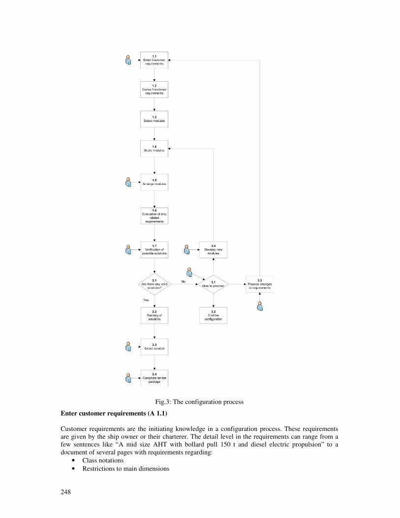
248

Fig.3: The configuration process

Enter customer requirements (A 1.1)

Customer requirements are the initiating knowledge in a configuration process. These requirements

are given by the ship owner or their charterer. The detail level in the requirements can range from a

few sentences like “A mid size AHT with bollard pull 150 t and diesel electric propulsion” to a

document of several pages with requirements regarding:

• Class notations

• Restrictions to main dimensions

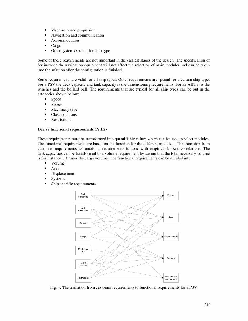
249

• Machinery and propulsion

• Navigation and communication

• Accommodation

• Cargo

• Other systems special for ship type

Some of these requirements are not important in the earliest stages of the design. The specification of

for instance the navigation equipment will not affect the selection of main modules and can be taken

into the solution after the configuration is finished.

Some requirements are valid for all ship types. Other requirements are special for a certain ship type.

For a PSV the deck capacity and tank capacity is the dimensioning requirements. For an AHT it is the

winches and the bollard pull. The requirements that are typical for all ship types can be put in the

categories shown below:

• Speed

• Range

• Machinery type

• Class notations

• Restrictions

Derive functional requirements (A 1.2)

These requirements must be transformed into quantifiable values which can be used to select modules.

The functional requirements are based on the function for the different modules. The transition from

customer requirements to functional requirements is done with empirical known correlations. The

tank capacities can be transformed to a volume requirement by saying that the total necessary volume

is for instance 1,3 times the cargo volume. The functional requirements can be divided into

• Volume

• Area

• Displacement

• Systems

• Ship specific requirements

Fig. 4: The transition from customer requirements to functional requirements for a PSV

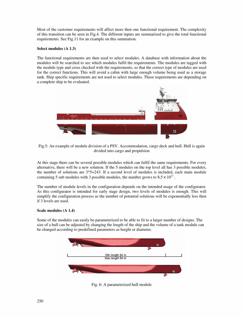
250

Most of the customer requirements will affect more then one functional requirement. The complexity

of this transition can be seen in Fig.4. The different inputs are summarized to give the total functional

requirements. See Fig.11 for an example on this summation.

Select modules (A 1.3)

The functional requirements are then used to select modules. A database with information about the

modules will be searched to see which modules fulfil the requirements. The modules are tagged with

the module type and cross checked with the requirements, so that the correct type of modules are used

for the correct functions. This will avoid a cabin with large enough volume being used as a storage

tank. Ship specific requirements are not used to select modules. These requirements are depending on

a complete ship to be evaluated.

Fig.5: An example of module division of a PSV. Accommodation, cargo deck and hull. Hull is again

divided into cargo and propulsion

At this stage there can be several possible modules which can fulfil the same requirements. For every

alternative, there will be a new solution. If the 5 modules on the top level all has 3 possible modules,

the number of solutions are 3^5=243. If a second level of modules is included, each main module

containing 5 sub modules with 3 possible modules, the number grows to 8,5 x 1011

.

The number of module levels in the configuration depends on the intended usage of the configurator.

As this configurator is intended for early stage design, two levels of modules is enough. This will

simplify the configuration process as the number of potential solutions will be exponentially less then

if 3 levels are used.

Scale modules (A 1.4)

Some of the modules can easily be parameterized to be able to fit to a larger number of designs. The

size of a hull can be adjusted by changing the length of the ship and the volume of a tank module can

be changed according to predefined parameters as height or diameter.

Fig. 6: A parameterized hull module

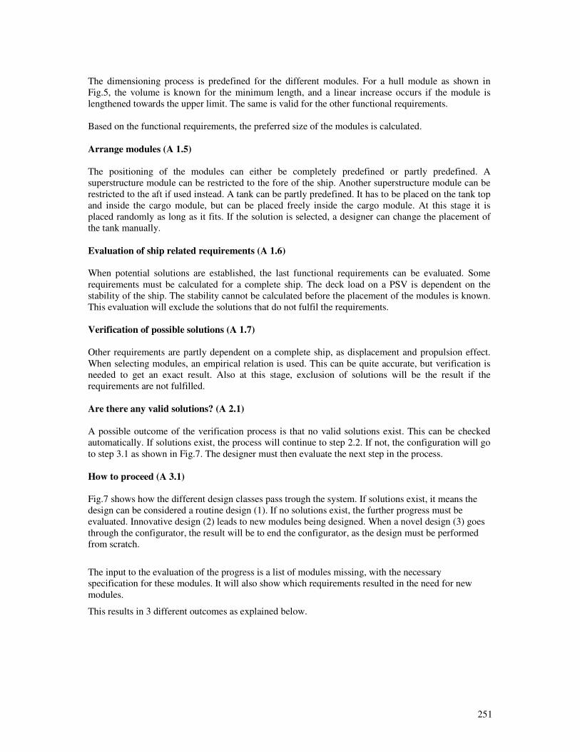
251

The dimensioning process is predefined for the different modules. For a hull module as shown in

Fig.5, the volume is known for the minimum length, and a linear increase occurs if the module is

lengthened towards the upper limit. The same is valid for the other functional requirements.

Based on the functional requirements, the preferred size of the modules is calculated.

Arrange modules (A 1.5)

The positioning of the modules can either be completely predefined or partly predefined. A

superstructure module can be restricted to the fore of the ship. Another superstructure module can be

restricted to the aft if used instead. A tank can be partly predefined. It has to be placed on the tank top

and inside the cargo module, but can be placed freely inside the cargo module. At this stage it is

placed randomly as long as it fits. If the solution is selected, a designer can change the placement of

the tank manually.

Evaluation of ship related requirements (A 1.6)

When potential solutions are established, the last functional requirements can be evaluated. Some

requirements must be calculated for a complete ship. The deck load on a PSV is dependent on the

stability of the ship. The stability cannot be calculated before the placement of the modules is known.

This evaluation will exclude the solutions that do not fulfil the requirements.

Verification of possible solutions (A 1.7)

Other requirements are partly dependent on a complete ship, as displacement and propulsion effect.

When selecting modules, an empirical relation is used. This can be quite accurate, but verification is

needed to get an exact result. Also at this stage, exclusion of solutions will be the result if the

requirements are not fulfilled.

Are there any valid solutions? (A 2.1)

A possible outcome of the verification process is that no valid solutions exist. This can be checked

automatically. If solutions exist, the process will continue to step 2.2. If not, the configuration will go

to step 3.1 as shown in Fig.7. The designer must then evaluate the next step in the process.

How to proceed (A 3.1)

Fig.7 shows how the different design classes pass trough the system. If solutions exist, it means the

design can be considered a routine design (1). If no solutions exist, the further progress must be

evaluated. Innovative design (2) leads to new modules being designed. When a novel design (3) goes

through the configurator, the result will be to end the configurator, as the design must be performed

from scratch.

The input to the evaluation of the progress is a list of modules missing, with the necessary

specification for these modules. It will also show which requirements resulted in the need for new

modules.

This results in 3 different outcomes as explained below.

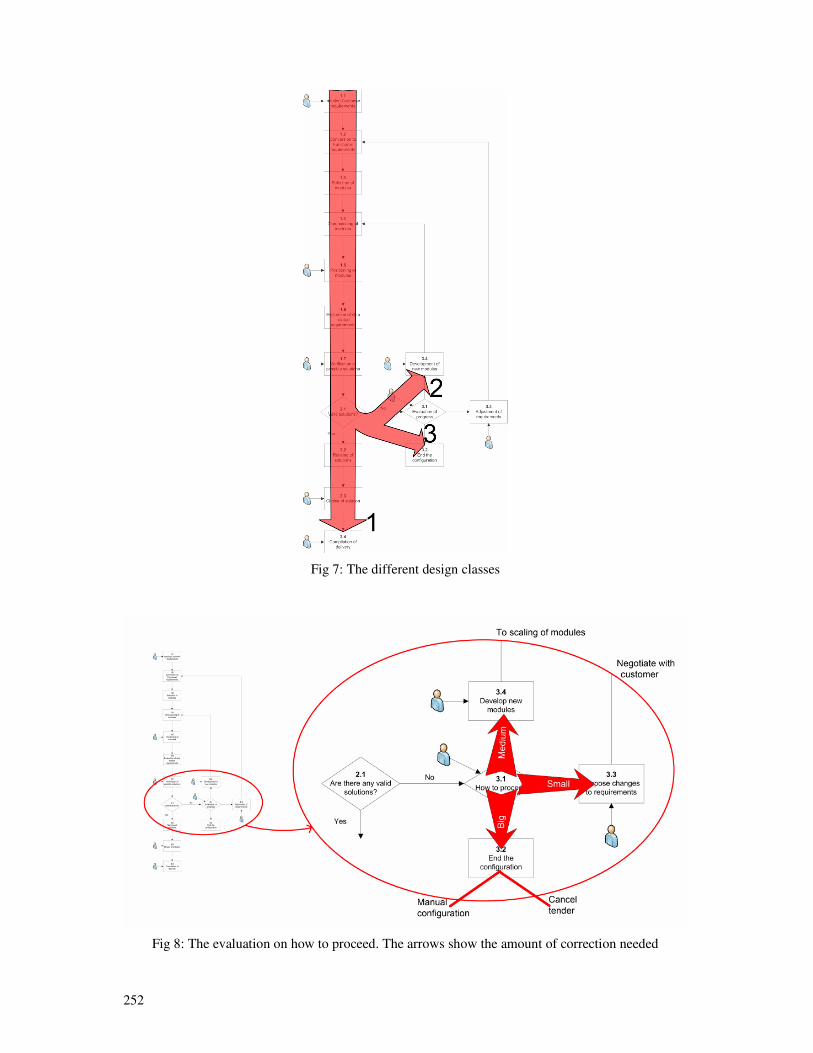
252

Fig 7: The different design classes

Fig 8: The evaluation on how to proceed. The arrows show the amount of correction needed

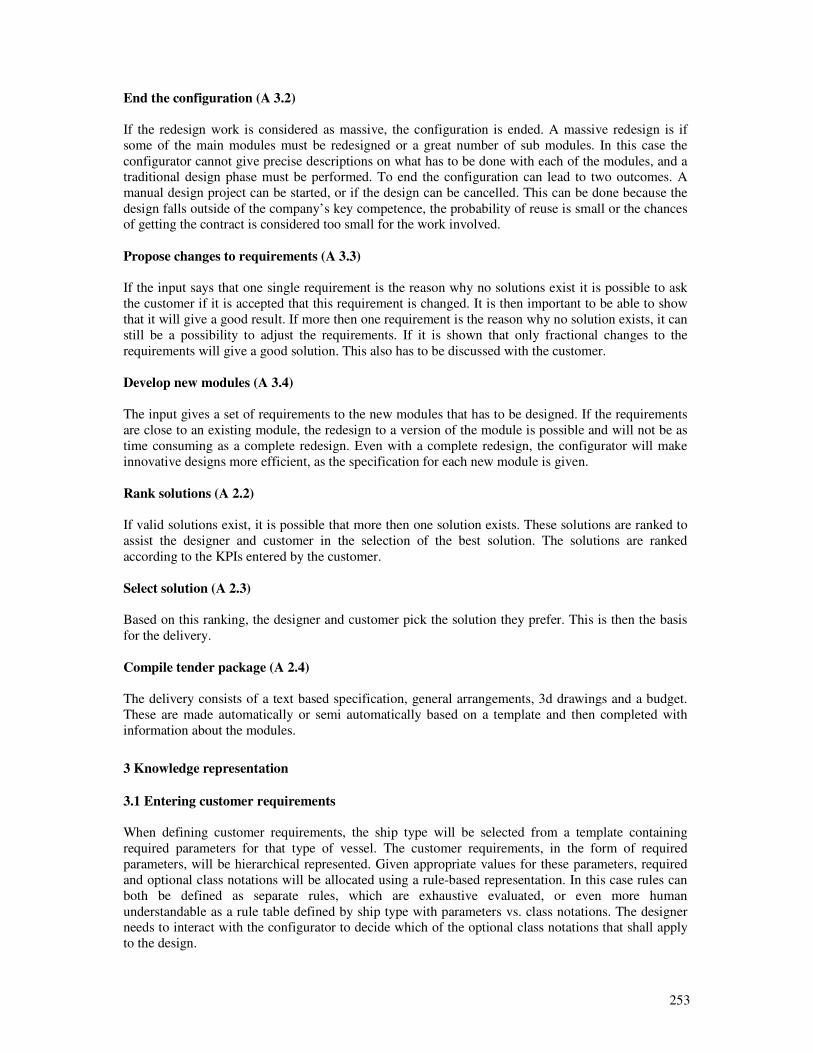
253

End the configuration (A 3.2)

If the redesign work is considered as massive, the configuration is ended. A massive redesign is if

some of the main modules must be redesigned or a great number of sub modules. In this case the

configurator cannot give precise descriptions on what has to be done with each of the modules, and a

traditional design phase must be performed. To end the configuration can lead to two outcomes. A

manual design project can be started, or if the design can be cancelled. This can be done because the

design falls outside of the company’s key competence, the probability of reuse is small or the chances

of getting the contract is considered too small for the work involved.

Propose changes to requirements (A 3.3)

If the input says that one single requirement is the reason why no solutions exist it is possible to ask

the customer if it is accepted that this requirement is changed. It is then important to be able to show

that it will give a good result. If more then one requirement is the reason why no solution exists, it can

still be a possibility to adjust the requirements. If it is shown that only fractional changes to the

requirements will give a good solution. This also has to be discussed with the customer.

Develop new modules (A 3.4)

The input gives a set of requirements to the new modules that has to be designed. If the requirements

are close to an existing module, the redesign to a version of the module is possible and will not be as

time consuming as a complete redesign. Even with a complete redesign, the configurator will make

innovative designs more efficient, as the specification for each new module is given.

Rank solutions (A 2.2)

If valid solutions exist, it is possible that more then one solution exists. These solutions are ranked to

assist the designer and customer in the selection of the best solution. The solutions are ranked

according to the KPIs entered by the customer.

Select solution (A 2.3)

Based on this ranking, the designer and customer pick the solution they prefer. This is then the basis

for the delivery.

Compile tender package (A 2.4)

The delivery consists of a text based specification, general arrangements, 3d drawings and a budget.

These are made automatically or semi automatically based on a template and then completed with

information about the modules.

3 Knowledge representation

3.1 Entering customer requirements

When defining customer requirements, the ship type will be selected from a template containing

required parameters for that type of vessel. The customer requirements, in the form of required

parameters, will be hierarchical represented. Given appropriate values for these parameters, required

and optional class notations will be allocated using a rule-based representation. In this case rules can

both be defined as separate rules, which are exhaustive evaluated, or even more human

understandable as a rule table defined by ship type with parameters vs. class notations. The designer

needs to interact with the configurator to decide which of the optional class notations that shall apply

to the design.

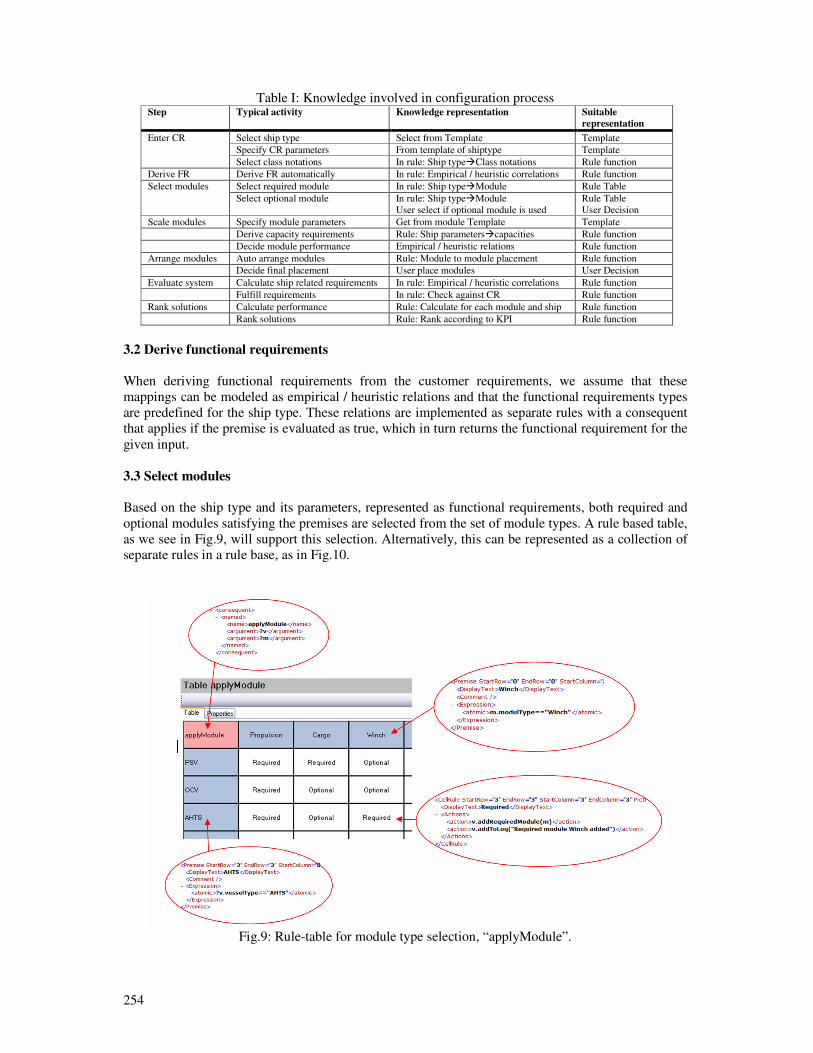
254

Table I: Knowledge involved in configuration process Step Typical activity Knowledge representation Suitable

representation

Select ship type Select from Template Template

Specify CR parameters From template of shiptype Template

Enter CR

Select class notations In rule: Ship typeClass notations Rule function

Derive FR Derive FR automatically In rule: Empirical / heuristic correlations Rule function

Select required module In rule: Ship typeModule Rule Table Select modules

Select optional module In rule: Ship typeModule

User select if optional module is used

Rule Table

User Decision

Scale modules Specify module parameters Get from module Template Template

Derive capacity requirements Rule: Ship parameterscapacities Rule function

Decide module performance Empirical / heuristic relations Rule function

Arrange modules Auto arrange modules Rule: Module to module placement Rule function

Decide final placement User place modules User Decision

Evaluate system Calculate ship related requirements In rule: Empirical / heuristic correlations Rule function

Fulfill requirements In rule: Check against CR Rule function

Rank solutions Calculate performance Rule: Calculate for each module and ship Rule function

Rank solutions Rule: Rank according to KPI Rule function

3.2 Derive functional requirements

When deriving functional requirements from the customer requirements, we assume that these

mappings can be modeled as empirical / heuristic relations and that the functional requirements types

are predefined for the ship type. These relations are implemented as separate rules with a consequent

that applies if the premise is evaluated as true, which in turn returns the functional requirement for the

given input.

3.3 Select modules

Based on the ship type and its parameters, represented as functional requirements, both required and

optional modules satisfying the premises are selected from the set of module types. A rule based table,

as we see in Fig.9, will support this selection. Alternatively, this can be represented as a collection of

separate rules in a rule base, as in Fig.10.

Fig.9: Rule-table for module type selection, “applyModule”.

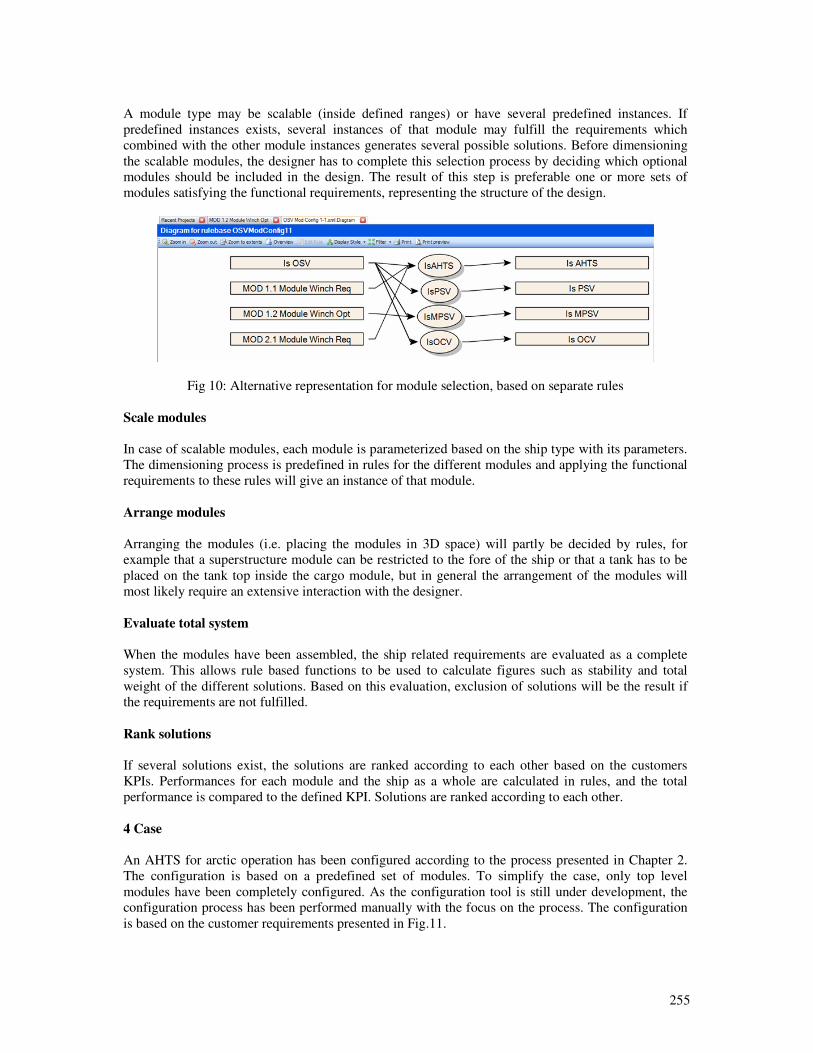
255

A module type may be scalable (inside defined ranges) or have several predefined instances. If

predefined instances exists, several instances of that module may fulfill the requirements which

combined with the other module instances generates several possible solutions. Before dimensioning

the scalable modules, the designer has to complete this selection process by deciding which optional

modules should be included in the design. The result of this step is preferable one or more sets of

modules satisfying the functional requirements, representing the structure of the design.

Fig 10: Alternative representation for module selection, based on separate rules

Scale modules

In case of scalable modules, each module is parameterized based on the ship type with its parameters.

The dimensioning process is predefined in rules for the different modules and applying the functional

requirements to these rules will give an instance of that module.

Arrange modules

Arranging the modules (i.e. placing the modules in 3D space) will partly be decided by rules, for

example that a superstructure module can be restricted to the fore of the ship or that a tank has to be

placed on the tank top inside the cargo module, but in general the arrangement of the modules will

most likely require an extensive interaction with the designer.

Evaluate total system

When the modules have been assembled, the ship related requirements are evaluated as a complete

system. This allows rule based functions to be used to calculate figures such as stability and total

weight of the different solutions. Based on this evaluation, exclusion of solutions will be the result if

the requirements are not fulfilled.

Rank solutions

If several solutions exist, the solutions are ranked according to each other based on the customers

KPIs. Performances for each module and the ship as a whole are calculated in rules, and the total

performance is compared to the defined KPI. Solutions are ranked according to each other.

4 Case

An AHTS for arctic operation has been configured according to the process presented in Chapter 2.

The configuration is based on a predefined set of modules. To simplify the case, only top level

modules have been completely configured. As the configuration tool is still under development, the

configuration process has been performed manually with the focus on the process. The configuration

is based on the customer requirements presented in Fig.11.

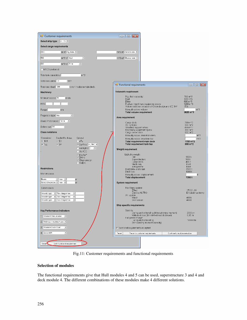
256

Fig.11: Customer requirements and functional requirements

Selection of modules

The functional requirements give that Hull modules 4 and 5 can be used, superstructure 3 and 4 and

deck module 4. The different combinations of these modules make 4 different solutions.

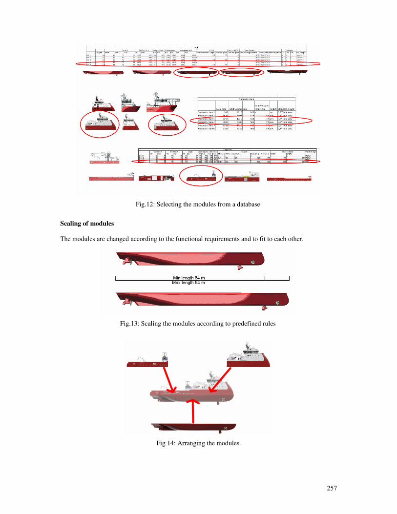
257

Fig.12: Selecting the modules from a database

Scaling of modules

The modules are changed according to the functional requirements and to fit to each other.

Fig.13: Scaling the modules according to predefined rules

Fig 14: Arranging the modules

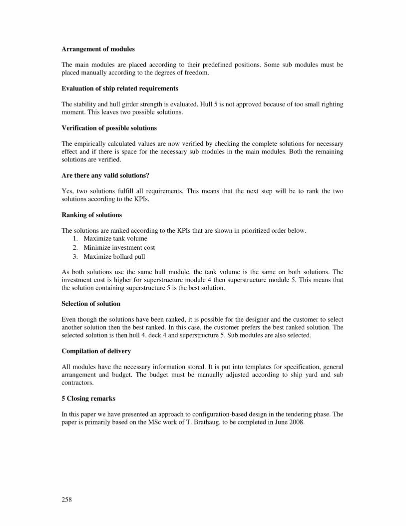
258

Arrangement of modules

The main modules are placed according to their predefined positions. Some sub modules must be

placed manually according to the degrees of freedom.

Evaluation of ship related requirements

The stability and hull girder strength is evaluated. Hull 5 is not approved because of too small righting

moment. This leaves two possible solutions.

Verification of possible solutions

The empirically calculated values are now verified by checking the complete solutions for necessary

effect and if there is space for the necessary sub modules in the main modules. Both the remaining

solutions are verified.

Are there any valid solutions?

Yes, two solutions fulfill all requirements. This means that the next step will be to rank the two

solutions according to the KPIs.

Ranking of solutions

The solutions are ranked according to the KPIs that are shown in prioritized order below.

1. Maximize tank volume

2. Minimize investment cost

3. Maximize bollard pull

As both solutions use the same hull module, the tank volume is the same on both solutions. The

investment cost is higher for superstructure module 4 then superstructure module 5. This means that

the solution containing superstructure 5 is the best solution.

Selection of solution

Even though the solutions have been ranked, it is possible for the designer and the customer to select

another solution then the best ranked. In this case, the customer prefers the best ranked solution. The

selected solution is then hull 4, deck 4 and superstructure 5. Sub modules are also selected.

Compilation of delivery

All modules have the necessary information stored. It is put into templates for specification, general

arrangement and budget. The budget must be manually adjusted according to ship yard and sub

contractors.

5 Closing remarks

In this paper we have presented an approach to configuration-based design in the tendering phase. The

paper is primarily based on the MSc work of T. Brathaug, to be completed in June 2008.

259

References

ANDREASSEN, T. (2005), Module-based and parametric configuration and engineering, Web-IT

Maritime, Ålesund

ANDREWS, D.J.; PAWLING, R. (2007), Research into the use of computer aided graphics in

preliminary ship design, ICCAS 2007, Portsmouth

ASHOK, K. G. (1997), Design, analogy, and creativity, IEEE Expert: Intelligent Systems and Their

Applications 12(3), pp.62-70

BLECKER, T.; ABDELKAFI, N.; KREUTLER, G.; FRIEDRICH, G. (2004), Product configuration

systems: State-of-the-Art, conceptualization and extensions, 8th Maghrebian Conf. on Software

Engineering and Artificial Intelligence, Tunisia, pp.25-36

COYNE, R.D.; ROSENMAN, M.A.; RADFORD, A.D.; BALACHANDRAN, M.; GERO, J.S.

(1990), Knowledge-Based Design Systems, Reading, Massachusetts, Addison-Wesley

DANIELS, A.S.; PARSONS, M.G. (2007), Development of a hybrid agent-genetic algorithm

approach to general arrangements, 6th Conf. Computer and IT Applications in the Maritime

Industries (COMPIT), Cortona, pp.197-211

HAGEN, A.; ERIKSTAD, S.O. (2002), Collaborative ship specification development - From MS

Word to Argus, Int. Conf. Computer Applications in Shipbuilding (ICCAS). Malmö

OERS, B.V.; STAPERSMA, D.; HOPMAN, H. (2007), Development and implementation of an

optimisation-based space allocation routine for the generation of feasible concept designs, 6th Conf.

Computer and IT Applications in the Maritime Industries (COMPIT), Cortona, pp.171-185.

SIMPSON, T.W. (2003), Product platform design and customization: Status and promise, ASME

Design Engineering Technical Conferences - Design Automation Conf., Chicago

SORTLAND, S. (2001), IT and net-based solutions in product configuration and sales, Web-IT

Maritime, Ålesund

WUUREN, W.; HALMAN, J.I.M. (2001), Platform-driven development of product families: Linking

theory with practice, The Future of Innovation Studies Conf., Eindhoven

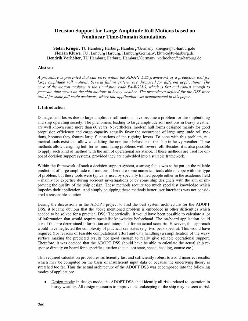
260

Decision Support for Large Amplitude Roll Motions based on Nonlinear Time-Domain Simulations

Stefan Krüger, TU Hamburg Harburg, Hamburg/Germany, krueger@tu-harburg.de Florian Kluwe, TU Hamburg Harburg, Hamburg/Germany, kluwe@tu-harburg.de

Hendrik Vorhölter, TU Hamburg Harburg, Hamburg/Germany, vorhoelter@tu-harburg.de

Abstract

A procedure is presented that can serve within the ADOPT DSS framework as a prediction tool for large amplitude roll motions. Several failure criteria are discussed for different applications. The core of the motion analyzer is the simulation code E4-ROLLS, which is fast and robust enough to generate time series on the ship motions in heavy weather. The procedures defined for the DSS were tested for some full-scale accidents, where one application was demonstrated in this paper. 1. Introduction Damages and losses due to large amplitude roll motions have become a problem for the shipbuilding and ship operating society. The phenomena leading to large amplitude roll motions in heavy weather are well known since more than 60 years. Nevertheless, modern hull forms designed mainly for good propulsion efficiency and cargo capacity actually favor the occurrence of large amplitude roll mo-tions, because they feature large fluctuations of the righting levers. To cope with this problem, nu-merical tools exist that allow calculating the nonlinear behavior of the ship in heavy weather. These methods allow designing hull forms minimizing problems with severe roll. Besides, it is also possible to apply such kind of method with the aim of operational assistance, if these methods are used for on-board decision support systems, provided they are embedded into a suitable framework. Within the framework of such a decision support system, a strong focus was to be put on the reliable prediction of large amplitude roll motions. There are some numerical tools able to cope with this type of problem, but these tools were typically used by specially trained people either in the academic field – mainly for expertise during accident investigations or by some ship designers with the aim of im-proving the quality of the ship design. These methods require too much specialist knowledge which impedes their application. And simply equipping these methods better user interfaces was not consid-ered a reasonable solution. During the discussions in the ADOPT project to find the best system architecture for the ADOPT DSS, it became obvious that the above mentioned problem is embedded in other difficulties which needed to be solved for a practical DSS: Theoretically, it would have been possible to calculate a lot of information that would require specialist knowledge beforehand. The on-board application could use of this pre-determined information and interpolate for an actual scenario. However, this approach would have neglected the complexity of practical sea states (e.g. two-peak spectra). This would have required (for reasons of feasible computational effort and data handling) a simplification of the wavy surface making the predicted results not good enough to really give reliable operational support. Therefore, it was decided that the ADOPT DSS should have be able to calculate the actual ship re-sponse directly on board for a specific situation (actual sea state, speed, heading, course etc.). This required calculation procedures sufficiently fast and sufficiently robust to avoid incorrect results, which may be computed on the basis of insufficient input data or because the underlying theory is stretched too far. Thus the actual architecture of the ADOPT DSS was decomposed into the following modes of application:

• Design mode: In design mode, the ADOPT DSS shall identify all risks related to operation in heavy weather. All design measures to improve the seakeeping of the ship may be seen as risk

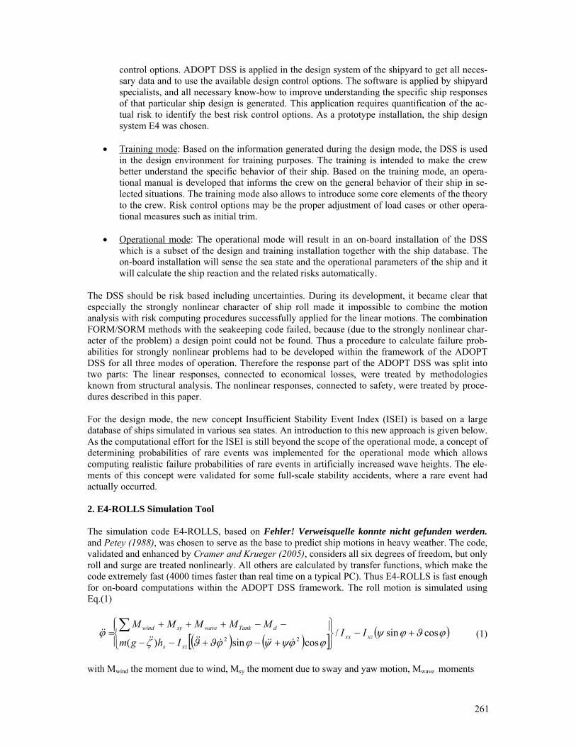
261

control options. ADOPT DSS is applied in the design system of the shipyard to get all neces-sary data and to use the available design control options. The software is applied by shipyard specialists, and all necessary know-how to improve understanding the specific ship responses of that particular ship design is generated. This application requires quantification of the ac-tual risk to identify the best risk control options. As a prototype installation, the ship design system E4 was chosen.

• Training mode: Based on the information generated during the design mode, the DSS is used

in the design environment for training purposes. The training is intended to make the crew better understand the specific behavior of their ship. Based on the training mode, an opera-tional manual is developed that informs the crew on the general behavior of their ship in se-lected situations. The training mode also allows to introduce some core elements of the theory to the crew. Risk control options may be the proper adjustment of load cases or other opera-tional measures such as initial trim.

• Operational mode: The operational mode will result in an on-board installation of the DSS

which is a subset of the design and training installation together with the ship database. The on-board installation will sense the sea state and the operational parameters of the ship and it will calculate the ship reaction and the related risks automatically.

The DSS should be risk based including uncertainties. During its development, it became clear that especially the strongly nonlinear character of ship roll made it impossible to combine the motion analysis with risk computing procedures successfully applied for the linear motions. The combination FORM/SORM methods with the seakeeping code failed, because (due to the strongly nonlinear char-acter of the problem) a design point could not be found. Thus a procedure to calculate failure prob-abilities for strongly nonlinear problems had to be developed within the framework of the ADOPT DSS for all three modes of operation. Therefore the response part of the ADOPT DSS was split into two parts: The linear responses, connected to economical losses, were treated by methodologies known from structural analysis. The nonlinear responses, connected to safety, were treated by proce-dures described in this paper. For the design mode, the new concept Insufficient Stability Event Index (ISEI) is based on a large database of ships simulated in various sea states. An introduction to this new approach is given below. As the computational effort for the ISEI is still beyond the scope of the operational mode, a concept of determining probabilities of rare events was implemented for the operational mode which allows computing realistic failure probabilities of rare events in artificially increased wave heights. The ele-ments of this concept were validated for some full-scale stability accidents, where a rare event had actually occurred. 2. E4-ROLLS Simulation Tool The simulation code E4-ROLLS, based on Fehler! Verweisquelle konnte nicht gefunden werden. and Petey (1988), was chosen to serve as the base to predict ship motions in heavy weather. The code, validated and enhanced by Cramer and Krueger (2005), considers all six degrees of freedom, but only roll and surge are treated nonlinearly. All others are calculated by transfer functions, which make the code extremely fast (4000 times faster than real time on a typical PC). Thus E4-ROLLS is fast enough for on-board computations within the ADOPT DSS framework. The roll motion is simulated using Eq.(1)

( ) ( )[ ] ( )ϕϑϕψϕϕψψϕϕϑϑζ

ϕ cossin/cossin)( 22

+−⎪⎭

⎪⎬⎫

⎪⎩

⎪⎨⎧

+−+−−

−−+++= ∑ xzxx

xzs

dTankwavesywind IIIhgm

MMMMM

&&&&&&&&&& (1)

with Mwind the moment due to wind, Msy the moment due to sway and yaw motion, Mwave moments

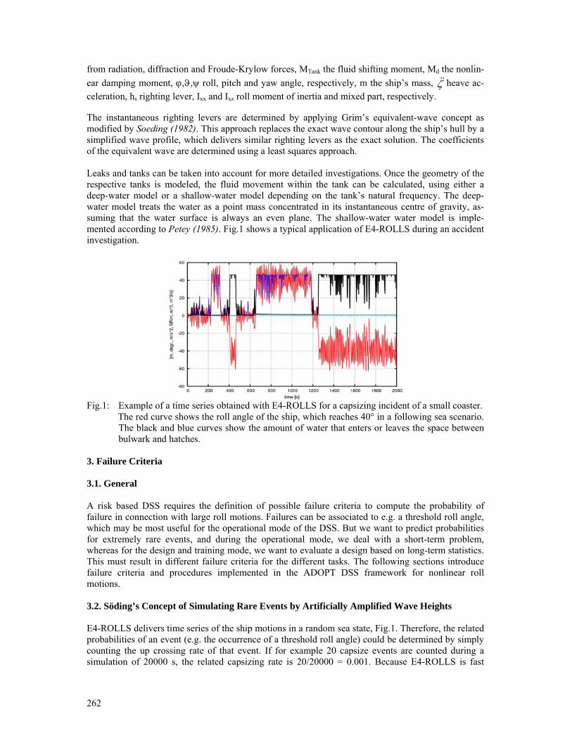
262

from radiation, diffraction and Froude-Krylow forces, MTank the fluid shifting moment, Md the nonlin-ear damping moment, ϕ,ϑ,ψ roll, pitch and yaw angle, respectively, m the ship’s mass, ζ&& heave ac-celeration, hs righting lever, Ixx and Ixz roll moment of inertia and mixed part, respectively. The instantaneous righting levers are determined by applying Grim’s equivalent-wave concept as modified by Soeding (1982). This approach replaces the exact wave contour along the ship’s hull by a simplified wave profile, which delivers similar righting levers as the exact solution. The coefficients of the equivalent wave are determined using a least squares approach. Leaks and tanks can be taken into account for more detailed investigations. Once the geometry of the respective tanks is modeled, the fluid movement within the tank can be calculated, using either a deep-water model or a shallow-water model depending on the tank’s natural frequency. The deep-water model treats the water as a point mass concentrated in its instantaneous centre of gravity, as-suming that the water surface is always an even plane. The shallow-water water model is imple-mented according to Petey (1985). Fig.1 shows a typical application of E4-ROLLS during an accident investigation.

Fig.1: Example of a time series obtained with E4-ROLLS for a capsizing incident of a small coaster.

The red curve shows the roll angle of the ship, which reaches 40° in a following sea scenario. The black and blue curves show the amount of water that enters or leaves the space between bulwark and hatches.

3. Failure Criteria 3.1. General A risk based DSS requires the definition of possible failure criteria to compute the probability of failure in connection with large roll motions. Failures can be associated to e.g. a threshold roll angle, which may be most useful for the operational mode of the DSS. But we want to predict probabilities for extremely rare events, and during the operational mode, we deal with a short-term problem, whereas for the design and training mode, we want to evaluate a design based on long-term statistics. This must result in different failure criteria for the different tasks. The following sections introduce failure criteria and procedures implemented in the ADOPT DSS framework for nonlinear roll motions. 3.2. Söding’s Concept of Simulating Rare Events by Artificially Amplified Wave Heights E4-ROLLS delivers time series of the ship motions in a random sea state, Fig.1. Therefore, the related probabilities of an event (e.g. the occurrence of a threshold roll angle) could be determined by simply counting the up crossing rate of that event. If for example 20 capsize events are counted during a simulation of 20000 s, the related capsizing rate is 20/20000 = 0.001. Because E4-ROLLS is fast

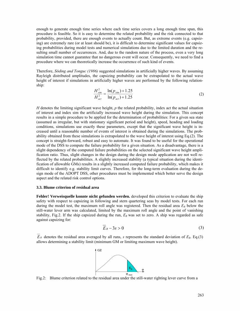
263

enough to generate enough time series where each time series covers a long enough time span, this procedure is feasible. So it is easy to determine the related probability and the risk connected to that probability, provided, there are enough events to actually count. But, as extreme events (e.g. capsiz-ing) are extremely rare (or at least should be), it is difficult to determine significant values for capsiz-ing probabilities during model tests and numerical simulations due to the limited duration and the re-sulting small number of occurrences. And, due to the random nature of the process, even a very long simulation time cannot guarantee that no dangerous event will occur. Consequently, we need to find a procedure where we can theoretically increase the occurrence of such kind of events. Therefore, Söding and Tonguc (1986) suggested simulations in artificially higher waves. By assuming Rayleigh distributed amplitudes, the capsizing probability can be extrapolated to the actual wave height of interest if simulations in artificially higher waves are performed by the following relation-ship:

25.1)ln(25.1)ln(

2

2

++

=act

sim

act

sim

pp

HH

(2)

H denotes the limiting significant wave height, p the related probability, index act the actual situation of interest and index sim the artificially increased wave height during the simulation. This concept results in a simple procedure to be applied for the determination of probabilities: For a given sea state (assumed as irregular, but with stationary significant period and height), speed, heading and loading conditions, simulations use exactly these parameters, except that the significant wave height is in-creased until a reasonable number of events of interest is obtained during the simulations. The prob-ability obtained from these simulations is extrapolated to the wave height of interest using Eq.(2). The concept is straight-forward, robust and easy to automate. It was found to be useful for the operational mode of the DSS to compute the failure probability for a given situation. As a disadvantage, there is a slight dependency of the computed failure probabilities on the selected significant wave height ampli-fication ratio. Thus, slight changes in the design during the design mode application are not well re-flected by the related probabilities. A slightly increased stability (a typical situation during the identi-fication of allowable GMs) results in a slightly increased computed failure probability, which makes it difficult to identify e.g. stability limit curves. Therefore, for the long-term evaluation during the de-sign mode of the ADOPT DSS, other procedures must be implemented which better serve the design aspect and the related risk control options. 3.3. Blume criterion of residual area Fehler! Verweisquelle konnte nicht gefunden werden. developed this criterion to evaluate the ship safety with respect to capsizing in following and stern quartering seas by model tests. For each run during the model test, the maximum roll angle was registered. Then the residual area ER below the still-water lever arm was calculated, limited by the maximum roll angle and the point of vanishing stability, Fig.2. If the ship capsized during the run, ER was set to zero. A ship was regarded as safe against capsizing for:

03 >− sER (3)

RE denotes the residual area averaged by all runs, s represents the standard deviation of ER. Eq.(3) allows determining a stability limit (minimum GM or limiting maximum wave height).

Fig.2: Blume criterion related to the residual area under the still-water righting lever curve from a

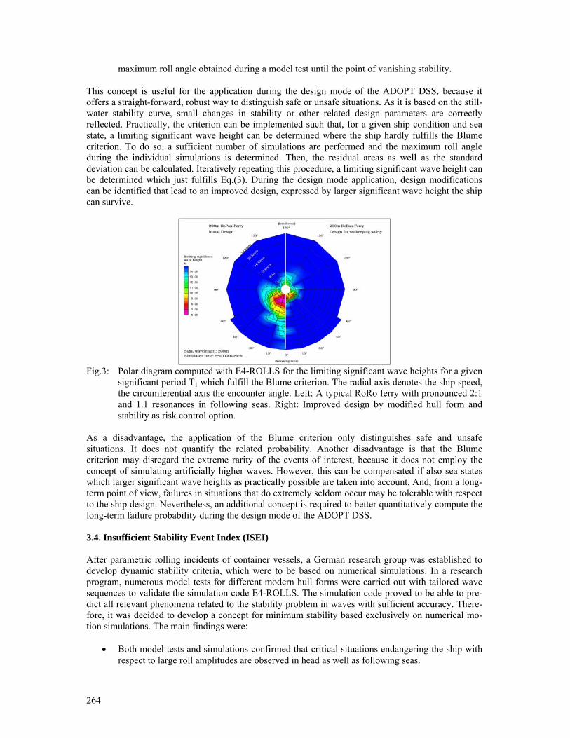
264

maximum roll angle obtained during a model test until the point of vanishing stability. This concept is useful for the application during the design mode of the ADOPT DSS, because it offers a straight-forward, robust way to distinguish safe or unsafe situations. As it is based on the still-water stability curve, small changes in stability or other related design parameters are correctly reflected. Practically, the criterion can be implemented such that, for a given ship condition and sea state, a limiting significant wave height can be determined where the ship hardly fulfills the Blume criterion. To do so, a sufficient number of simulations are performed and the maximum roll angle during the individual simulations is determined. Then, the residual areas as well as the standard deviation can be calculated. Iteratively repeating this procedure, a limiting significant wave height can be determined which just fulfills Eq.(3). During the design mode application, design modifications can be identified that lead to an improved design, expressed by larger significant wave height the ship can survive.

Fig.3: Polar diagram computed with E4-ROLLS for the limiting significant wave heights for a given

significant period T1 which fulfill the Blume criterion. The radial axis denotes the ship speed, the circumferential axis the encounter angle. Left: A typical RoRo ferry with pronounced 2:1 and 1.1 resonances in following seas. Right: Improved design by modified hull form and stability as risk control option.

As a disadvantage, the application of the Blume criterion only distinguishes safe and unsafe situations. It does not quantify the related probability. Another disadvantage is that the Blume criterion may disregard the extreme rarity of the events of interest, because it does not employ the concept of simulating artificially higher waves. However, this can be compensated if also sea states which larger significant wave heights as practically possible are taken into account. And, from a long-term point of view, failures in situations that do extremely seldom occur may be tolerable with respect to the ship design. Nevertheless, an additional concept is required to better quantitatively compute the long-term failure probability during the design mode of the ADOPT DSS. 3.4. Insufficient Stability Event Index (ISEI) After parametric rolling incidents of container vessels, a German research group was established to develop dynamic stability criteria, which were to be based on numerical simulations. In a research program, numerous model tests for different modern hull forms were carried out with tailored wave sequences to validate the simulation code E4-ROLLS. The simulation code proved to be able to pre-dict all relevant phenomena related to the stability problem in waves with sufficient accuracy. There-fore, it was decided to develop a concept for minimum stability based exclusively on numerical mo-tion simulations. The main findings were:

• Both model tests and simulations confirmed that critical situations endangering the ship with respect to large roll amplitudes are observed in head as well as following seas.

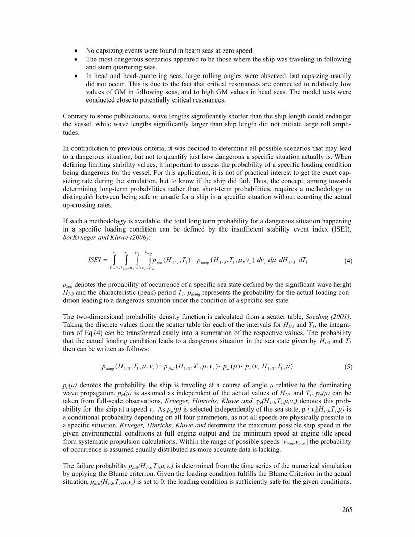
265

• No capsizing events were found in beam seas at zero speed. • The most dangerous scenarios appeared to be those where the ship was traveling in following

and stern quartering seas. • In head and head-quartering seas, large rolling angles were observed, but capsizing usually

did not occur. This is due to the fact that critical resonances are connected to relatively low values of GM in following seas, and to high GM values in head seas. The model tests were conducted close to potentially critical resonances.

Contrary to some publications, wave lengths significantly shorter than the ship length could endanger the vessel, while wave lengths significantly larger than ship length did not initiate large roll ampli-tudes. In contradiction to previous criteria, it was decided to determine all possible scenarios that may lead to a dangerous situation, but not to quantify just how dangerous a specific situation actually is. When defining limiting stability values, it important to assess the probability of a specific loading condition being dangerous for the vessel. For this application, it is not of practical interest to get the exact cap-sizing rate during the simulation, but to know if the ship did fail. Thus, the concept, aiming towards determining long-term probabilities rather than short-term probabilities, requires a methodology to distinguish between being safe or unsafe for a ship in a specific situation without counting the actual up-crossing rates. If such a methodology is available, the total long term probability for a dangerous situation happening in a specific loading condition can be defined by the insufficient stability event index (ISEI), borKrueger and Kluwe (2006):

13/113/10 0

2

013/1 ),,,(),(

1 3/1

max

min

dTdHddvvTHpTHpISEI ssdangT H

v

vvsea

s

μμπ

μ∫ ∫ ∫ ∫∞

=

∞

= = =

⋅= (4)

psea denotes the probability of occurrence of a specific sea state defined by the significant wave height H1/3 and the characteristic (peak) period T1. pdang represents the probability for the actual loading con-dition leading to a dangerous situation under the condition of a specific sea state. The two-dimensional probability density function is calculated from a scatter table, Soeding (2001). Taking the discrete values from the scatter table for each of the intervals for H1/3 and T1, the integra-tion of Eq.(4) can be transformed easily into a summation of the respective values. The probability that the actual loading condition leads to a dangerous situation in the sea state given by H1/3 and T1 then can be written as follows:

),,()(),,,(),,,( 13/113/113/1 μμμμ μ THvppvTHpvTHp svsfailsdang ⋅⋅= (5) pμ(μ) denotes the probability the ship is traveling at a course of angle μ relative to the dominating wave propagation. pμ(μ) is assumed as independent of the actual values of H1/3 and T1. pμ(μ) can be taken from full-scale observations, Krueger, Hinrichs, Kluwe and. pv(H1/3,T1,μ,vs) denotes this prob-ability for the ship at a speed vs. As pμ(μ) is selected independently of the sea state, pv(,vs|H1/3,T1,μ) is a conditional probability depending on all four parameters, as not all speeds are physically possible in a specific situation. Krueger, Hinrichs, Kluwe and determine the maximum possible ship speed in the given environmental conditions at full engine output and the minimum speed at engine idle speed from systematic propulsion calculations. Within the range of possible speeds [vmin,vmax] the probability of occurrence is assumed equally distributed as more accurate data is lacking. The failure probability pfail(H1/3,T1,μ,vs) is determined from the time series of the numerical simulation by applying the Blume criterion. Given the loading condition fulfills the Blume Criterion in the actual situation, pfail(H1/3,T1,μ,vs) is set to 0: the loading condition is sufficiently safe for the given conditions.

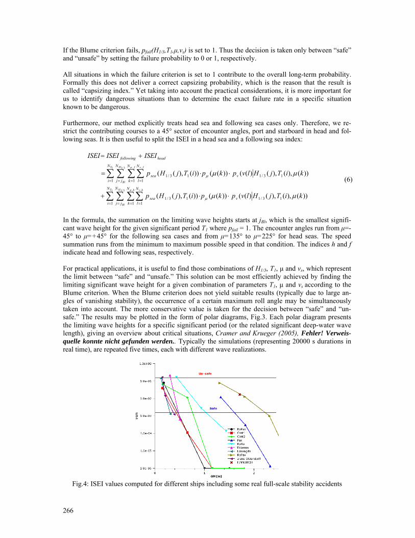
266

If the Blume criterion fails, pfail(H1/3,T1,μ,vs) is set to 1. Thus the decision is taken only between “safe” and “unsafe” by setting the failure probability to 0 or 1, respectively. All situations in which the failure criterion is set to 1 contribute to the overall long-term probability. Formally this does not deliver a correct capsizing probability, which is the reason that the result is called “capsizing index.” Yet taking into account the practical considerations, it is more important for us to identify dangerous situations than to determine the exact failure rate in a specific situation known to be dangerous. Furthermore, our method explicitly treats head sea and following sea cases only. Therefore, we re-strict the contributing courses to a 45° sector of encounter angles, port and starboard in head and fol-lowing seas. It is then useful to split the ISEI in a head sea and a following sea index:

))(,)(),()(())(())(),((

))(,)(),()(())(())(),((

13/11 1 1

13/1

13/11 1 1

13/1

1 3/1 , ,

1 3/1 , ,

kiTjHlvpkpiTjHp

kiTjHlvpkpiTjHp

ISEIISEIISEI

v

N

i

N

jj

N

k

N

lsea

v

N

i

N

jj

N

k

N

lsea

headfollowing

T H

Bl

h hv

T H

Bl

f fv

μμ

μμ

μ

μ

μ

μ

⋅⋅+

⋅⋅=

+=

∑ ∑ ∑∑

∑ ∑ ∑∑

= = = =

= = = =

(6)

In the formula, the summation on the limiting wave heights starts at jBl, which is the smallest signifi-cant wave height for the given significant period T1 where pfail = 1. The encounter angles run from μ=-45° to μ=+45° for the following sea cases and from μ=135° to μ=225° for head seas. The speed summation runs from the minimum to maximum possible speed in that condition. The indices h and f indicate head and following seas, respectively. For practical applications, it is useful to find those combinations of H1/3, T1, μ and vs, which represent the limit between “safe” and “unsafe.” This solution can be most efficiently achieved by finding the limiting significant wave height for a given combination of parameters T1, μ and vs according to the Blume criterion. When the Blume criterion does not yield suitable results (typically due to large an-gles of vanishing stability), the occurrence of a certain maximum roll angle may be simultaneously taken into account. The more conservative value is taken for the decision between “safe” and “un-safe.” The results may be plotted in the form of polar diagrams, Fig.3. Each polar diagram presents the limiting wave heights for a specific significant period (or the related significant deep-water wave length), giving an overview about critical situations, Cramer and Krueger (2005), Fehler! Verweis-quelle konnte nicht gefunden werden.. Typically the simulations (representing 20000 s durations in real time), are repeated five times, each with different wave realizations.

Fig.4: ISEI values computed for different ships including some real full-scale stability accidents

267

The ISEI concept allows identifying ship designs, which are vulnerable to stability problems in fol-lowing or head seas, taking into account all relevant phenomena. Unfortunately, as there is no limiting value for the ISEI, it is difficult to apply the concept to determine minimum stability requirements. In order to define such threshold values, borKrueger and Kluwe (2006) suggested analyzing the safety levels for many existing ships by using the ISEI as the quantitative measurement. Therefore, many full-scale capsizing events have been analyzed with the described procedure and the resulting ISEI values have been computed, Fig.4. As the ships actually capsized, it was straight-forward to identify ISEI values which will definitively lead to a long-term failure. For the DSS design mode application, if for a given ship design a critical ISEI value is calculated, this should result in design modifications. During our analyses of several stability accidents, we benchmarked the acci-dents against several stability criteria (empirical or theoretical) published by different sources, and we found that mostly all criteria converged in judging a specific ship as being safe. For this condition, we have again computed the related ISEI value, and, following this procedure, we obtained:

− ISEI < 0.001 represents a ship design and loading condition where it is extremely unlikely that a severe stability event will occur.

− ISEI ≈ 0.05 or more represents a ship design and/or loading condition where it is extremely likely that a severe stability event will occur.

− 0.001 < ISEI < 0.05 represent intermediate conditions, where a severe stability event may happen with reasonable probability.

The ISEI concept can be used to support the design and training mode, as it is possible to quantify the risk related to large amplitude rolling. If for a specific design and load case ISEI < 0.001 are calcu-lated, the design should be reviewed accordingly. During the training phase, risk control options can be identified which ensure an ISEI level well below that threshold value. The ISEI implies situations where a large rolling angle event may occur. These situations can be identified during the operational mode of the DSS and the crew can be informed accordingly. 4. Application example: The FINNBIRCH accident 4.1 Background The tools for predicting large amplitude roll motions are validated for an actual case. On 1.11.2006, the 8500 dwt RoRo Ferry MV FINNBIRCH capsized in heavy weather in the Baltic Sea. At the time of the accident, the vessel travelled south at an estimated course of 170°-190°, speed 16-17 knots. The vessel was bound for Aarhus with a cargo of RoRo trailers, several stowed on the top deck, Fig.5. During the time of the accident, conditions were rough with wind forces of 20-25 m/s (Bft 9-10) and significant wave heights of 5-6 m, significant period 8-8.5 s from NNE to NNW. MV FINNBIRCH was rolling significantly in the rough seas and around 16:15 h, it had around 50° heel. The vessel re-mained for a while in that intermediate equilibrium floating condition, until she finally capsized at 19:37 h. Except for two men, the crew could be rescued. The MV FINNBIRCH was built in 1978 and subsequently converted several times. In 1979, the ves-sel was additionally equipped with side sponsons to increase the stability. In 1986, the vessel was ret-rofitted with an additional top deck (4th trailer deck). These conversions significantly affected the de-sign and operational performance of the vessel, as the application of ADOPT DSS will show. At the time of delivery and subsequent conversions, no damage stability regulations were in force. Thus the stability of the vessel was governed by the relevant intact criteria. This explains the rela-tively low minimum freeboard of ~0.4 m for full-load draft. The side sponsons were fitted shortly af-ter delivery, probably to enable the vessel to carry containers in at least two tiers on the upper deck. According to our calculations (based on the original hull lines), the additional sponsons resulted in additional buoyancy of about 200 tons at the extreme draft. When the vessel was delivered without

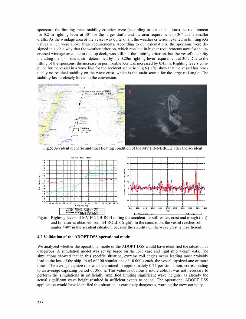
268

sponsons, the limiting intact stability criterion were (according to our calculations) the requirement for 0.2 m righting lever at 30° for the larger drafts and the area requirement to 30° at the smaller drafts. As the windage area of the vessel was quite small, the weather criterion resulted in limiting KG values which were above these requirements. According to our calculations, the sponsons were de-signed in such a way that the weather criterion, which resulted in higher requirements now for the in-creased windage area due to the top deck, was still not the limiting criterion, but the vessel's stability including the sponsons is still determined by the 0.20m righting lever requirement at 30°. Due to the fitting of the sponsons, the increase in permissible KG was increased by 0.45 m. Righting levers com-puted for the vessel in a wave like for the accident scenario, Fig.6 (left), show that the vessel has prac-tically no residual stability on the wave crest, which is the main source for the large roll angle. The stability loss is closely linked to the conversion.

Fig.5: Accident scenario and final floating condition of the MV FINNBIRCH after the accident

Fig.6: Righting levers of MV FINNBIRCH during the accident for still-water, crest and trough (left) and time series obtained from E4-ROLLS (right). In the simulation, the vessel reaches roll angles >40° in the accident situation, because the stability on the wave crest is insufficient. 4.2 Validation of the ADOPT DSS operational mode We analyzed whether the operational mode of the ADOPT DSS would have identified the situation as dangerous. A simulation model was set up based on the load case and light ship weight data. The simulations showed that in this specific situation, extreme roll angles occur leading most probably lead to the loss of the ship. In 65 of 100 simulations of 10.000 s each, the vessel capsized one or more times. The average capsize rate was determined to approximately 0.72 per simulation, corresponding to an average capsizing period of 38.6 h. This value is obviously intolerable. It was not necessary to perform the simulations in artificially amplified limiting significant wave heights, as already the actual significant wave height resulted in sufficient events to count. The operational ADOPT DSS application would have identified this situation as extremely dangerous, warning the crew correctly.

269

4.3 Validation of the ADOPT DSS training mode

Fig.7: Polar Diagrams with limiting significant wave heights according to the Blume criterion in the

simulated ADOPT DSS training environment. The limiting significant wave heights were computed for different significant wave lengths from 88 to 172 m. The accident wave length was about 113 m.

To simulate the training mode of the ADOPT DSS, it was assumed that the accident loading situation was equivalent with a design load case that may have been part of the stability booklet. For this load case, several polar diagrams were calculated which fulfill the Blume criterion. Some of the results are plotted in Fig.7 and may serve as examples on the information that can be obtained by the ADOPT training DSS. All polar diagrams indicate that the ship has a problem in following seas, especially at higher speeds and steeper waves. So the crew can be advised during the training mode: For this specific load case, in heavy weather, all following sea courses should be avoided unless the significant wave height and significant wave length are known with sufficient accuracy. For the longer waves, it might be possible to sail stern quartering courses if the stability is known with sufficient accuracy. For the accident situation (left polar diagram, right side) a slight alteration of course or speed would not help the vessel to escape from that situation. It would be a good advice to the crew not to start the voyage with this loading condition if heavy weather is expected. In fact, additional water ballast is required. Longer waves lead to less critical situations, because the righting lever alterations become less severe (although the right polar diagram, left side represents the case where the significant wave length equals ship length) and critical resonances are shifted to less problematic speeds. The vessel suffers additionally from the strong domination of the 2:1 roll resonance (at about 6 knots) and the 1:1 resonance (at about 16 knots), see left polar diagram in Fig.7. This phenomenon demonstrates that a linear estimation of a dangerous situation completely fails for this case: If the natural roll response period of the ship is determined based on the GM of the still-water curve, the 1:1 resonance would be computed for a speed of 9 kn in following seas, whereas the 2:1 resonance should not even exist in following seas. Clearly, one cannot obtain reliable results by a theory which linearizes the problem with respect to the still-water righting lever curve for small angles. This shows the demand for the correct nonlinear treatment of the rolling motion within the ADOPT DSS framework. The application also shows that during the training mode of the DSS, the crew could have been informed that the loading condition is problematic and should be improved. 4.4 Validation of the ADOPT DSS design mode To demonstrate the principal feasibility of the ADOPT DSS support in the design phase, the ISEI was computed for the given loading situation, Fig.4. The computations resulted in an ISEI value of 0.06 which indicates that a dynamic stability problem for the ship after the conversion. It was a design option to increase the stability of the ship up to a sufficient ISEI value, resulting in a KG shift 20 cm downwards. Then an ISEI value of 0.0003 is obtained. So the vessel would have most probably survived the situation if the design had foreseen about 20 cm more stability. This amounts to roughly half the value the of the possible KG shift after the retrofitting, and this is reasonable, because the

270

vessel has operated for more than 10 years in the original condition without capsizing. The ADOPT DSS would have helped to identify a possible risk in the future operation after the conversion, which was not identified by the existing stability rules. 5. Summary and Conclusions A procedure was presented that can serve within the ADOPT DSS framework as a prediction tool for large amplitude roll motions. Several failure criteria were introduced, which can serve the different application modes of the ADOPT DSS (design mode, operational mode, training mode). The core of the motion analyzer is the simulation code E4-ROLLS, which is fast and robust enough to generate time series on the ship motions in heavy weather. The procedures defined for the DSS were tested for some full-scale accidents, where one application was demonstrated in this paper. The results show that the accident could have been avoided if a DSS would have been applied either in the design, training or the operational phase of the ship. Acknowledgements The authors wish to thank the European Commission for funding the ADOPT project within the 6th

Framework. Without the support, this project and the achieved results would not have been possible. References BLUME, P.; HATTENDORF, H.G. (1987), Ergebnisse von systematischen Modellversuchen zur Kentersicherheit, Jahrbuch der Schiffbautechnischen Gesellschaft CRAMER, H.; KRÜGER, S. (2005), Numerical capsizing simulations and consequences for ship de-sign, Jahrbuch der Schiffbautechnischen Gesellschaft, Springer, 2005 KRÖGER, P. (1987), Simulation der Rollbewegung von Schiffen, IfS report 473, Univ. Hamburg KRÜGER, S. (2002), Performance based stability, DCAMM, Lyngby KRÜGER, S.; KLUWE, F. (2006), Development of dynamic stability criteria from seakeeping simula-tion, Int. Marine Design Conf. (IMDC2006), Ann Arbor KRÜGER, S.; HINRICHS, R.; KLUWE, F.; BILLERBECK, H. (2006), Towards the development of dynamic stability criteria, HANSA Maritime Journal, 10/2006, p.204 PETEY, F. (1985), Berechnung der Flüssigkeitsbewegung in teilgefüllten Tanks und Leckräumen, Schiffstechnik 32 PETEY, F. (1988), Ermittlung der Kentersicherheit lecker Schiffe im Seegang aus Bewegungs-simulationen, IfS report 487, Univ. Hamburg SÖDING, H. (1982), Leckstabilität im Seegang, TU Hamburg-Harburg, Schriftenreihe Schiffbau, Re-port Nr. 429 SÖDING, H. (2001), Global Seaway Statistics, TU Hamburg-Harburg, Schriftenreihe Schiffbau, Re-port Nr. 610 SÖDING, H.; TONGUC, E. (1986), Computing capsizing frequencies in a seaway, STAB, Gdansk

271

Optimum Routing of Piping in Real Ships under Real Constraints

Andi Asmara, Merwede Shipyard & Delft University of Technology, Delft /The Netherlands,

a.asmara@tudelft.nl

Ubald Nienhuis, Delft University of Technology, Delft/The Netherlands, u.nienhuis@tudelft.nl

Abstract

Finding optimum routing of a piping system in a ship does not only concern pipe material cost

minimization; it also has to comply with ship design constraints. In previous work, we presented an

automatic pipe routing system and its implementation in a real ship and shipbuilding environment.

However it was more focused on minimizing pipe material cost. In this paper, we present the

improved automatic pipe routing system to include the ship design constraints as well. This system is

designed as a modular system to keep its extendibility and maintainability. As the core of the system,

the hybrid optimization module is implemented, while the design constraints are implemented as

separate modules. To demonstrate the effectiveness of the proposed system, implementation of this

system to find the optimum routing of a particular piping subsystem is carried out in the real ship

design process. The result shows great promise of this system in the future to be applied in the real

ship design process.

1. Introduction

For years, the attempts to use the computer for automatic piping design in ship have been made in

many ways. The main reasons behind it are:

• Each ship usually has a different specification, which means that for each ship most of the

design process has to be redone, Van Dokkum (2003).

• A small change in ship specification, such as choosing a different type and/or capacity of the

engine or pump, will definitely affect the piping system, Harrington (1992). This will cause

the pipes that are already routed to be re-routed.

• Pipe routing is one of the most important activities during detail design because all other

detail design activities depend on it and this activity consumes a significant part of the detail

design man-hours because the piping systems in a ship typically consist of thousands of pipe

elements.

• Nowadays, pipe routing is largely done manually by a pipe designer using CAD software

which assists in checking for collision and defining e.g. the pipe bend radiuses. Therefore the

experience of the designers is the most important ingredient for this process.

Pipe routing is difficult because, among other reasons, the pipe is generally subject to multiple design

constraints. The most important constraint is that the pipe routing solution must comply with the naval

classification and regulations. In addition, usually the space available in ship that is allowed to be

used for pipes is limited. This condition is especially true for a certain area of ship, such as in the

machinery room of a ship. One more unavoidable aspect that makes this activity even harder is the

fact that the specifications of the ship are changing quite frequently during the design process.

1.1. Related Work

Many researches have been made to overcome the automatic routing activity in widespread areas like

in ship production application Roh et al. (2007), Asmara and Nienhuis (2006), Fan et al. (2006),

Zuurmond (2004), Storch and Park (2002), Kang et al. (1999), and Kuo et al. (1999), and in process

plant Ito (1999), Kim and Corne (1996), and Newell (1972).

Although many pipe-routing algorithms have already been developed, to date most of the algorithms

are verified to solve the pipe routing problem on academic systems, like on a system with only a few

pipes and in a simplified environment, and have paid little or no attention to the scalability of the

272

algorithm to be applied in the real ship design process which consists of much larger number of pipes.

Some of the researches also neglect the existence of pipe branches. Moreover, the algorithm is also

mainly used for the space problem - to find a pipe route without collision -, without considering the

most important thing that the solution must comply with the marine classification rules and

regulations.

From those researches mentioned above only Roh et al. (2007) can be applied immediately in the real

design process. However they focus on the adaptability of the generated pipe routing against the

change of the shape of the hull. For the routing itself, they mainly focus on improving function of

TRIBON capability to route pipes in pipe tray, and the pipe engineer should always define the bend

point and choose which tray to be used. The design constraints also need to be examined manually by

the pipe engineer.

Fan et al. (2006) addressed the problem with a heuristic optimization algorithm called ant colony

optimization, the meta-heuristic optimization algorithm that has been proven for its capabilities to

solve combinatorial problems. Kim and Corne (1996), and Ito (1999) proposed methods for

generating the optimal route of pipes using another flavour of heuristic optimization algorithm called

the genetic algorithm. They defined an objective function considering the total length of pipes and the

ratio of the closeness to obstacles and then found the best solution by minimizing the objective

function. However, these researches need much time to solve realistic problems of industry.

In his works, Zuurmond (2004) divided the workspace into cells, and applied the Dijkstra algorithm to

find a shortest path. He calculated the density of each cell to prevent congestion in the cell. The time

that is needed to find a solution is very short, however the final solution fails to certainly prevent pipe

collision. Storch and Park (2002) use another method for cell generation in order to generate the

optimal route. They also consider not only the length and number of bends of pipes but also consider

the installation cost and maintenance cost.

In their paper, Kang et al. (1999) stated that detail design is characteristically less creative and more

routine than the earlier steps in the design process. Based on that statement he used a knowledge

based expert system to find the optimal route, consisting of 167 rules and 106 supporting methods.

In Asmara and Nienhuis (2006), the automatic piping system is used to solve the pipe routing problem

on the real ship, and the result is verified by comparing with the actual pipe routes designed by the

pipe engineers. However the main consideration in that work was only to minimize the length and the

number of bends.

1.2. Introduction to the automatic routing system

In this paper, the automatic routing system, called delft.route is introduced. The main objectives of

this system are:

1. to minimize user input and user decision,

2. easily integrated with other system, such as existing CAD software,

3. nonproprietary, and expandable,

4. to be used in real shipyard design process,

To fulfill the first objective, the system should be user friendly and able to be used by the user to find

the pipe route, with less effort than manually routing using the existing CAD software. This includes

the ease with which the framework can be prepared and all the data that are needed gathered. In

addition to that, the solution that is found should be optimal and comply with the marine classification

rules and regulations.

Some data is needed by the automatic routing system before it can be used to find pipe route. The data

that is needed includes:

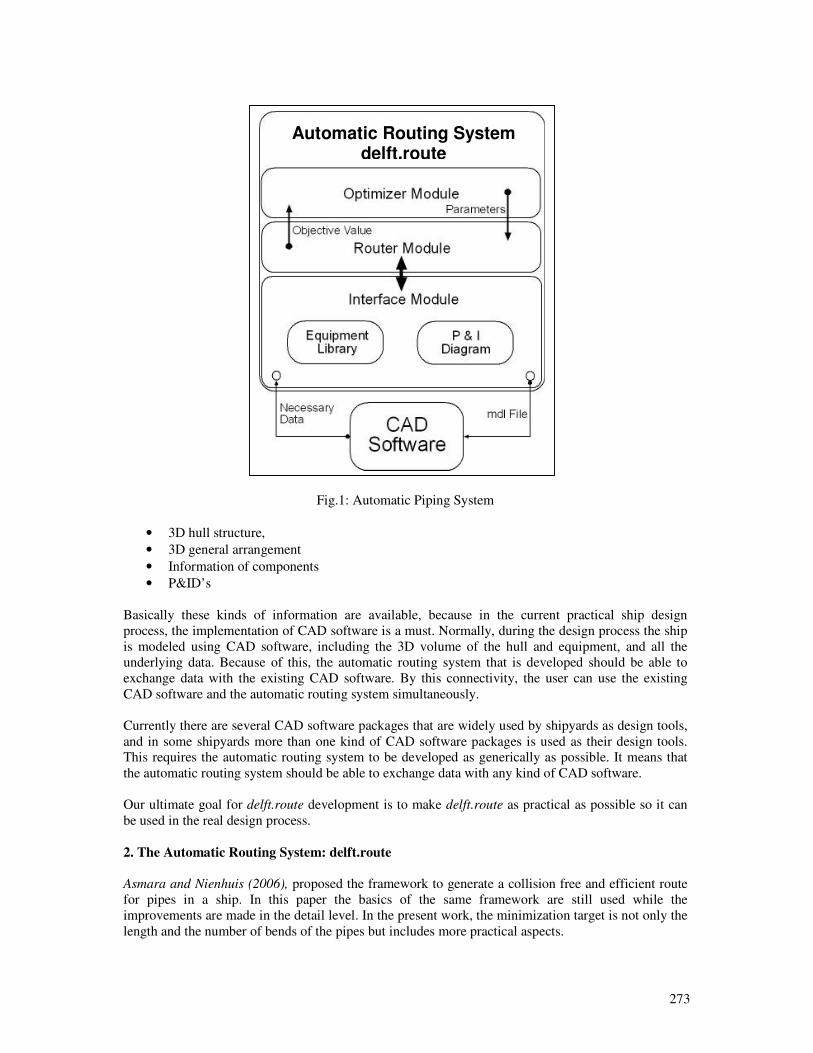
273

Fig.1: Automatic Piping System

• 3D hull structure,

• 3D general arrangement

• Information of components

• P&ID’s

Basically these kinds of information are available, because in the current practical ship design

process, the implementation of CAD software is a must. Normally, during the design process the ship

is modeled using CAD software, including the 3D volume of the hull and equipment, and all the

underlying data. Because of this, the automatic routing system that is developed should be able to

exchange data with the existing CAD software. By this connectivity, the user can use the existing

CAD software and the automatic routing system simultaneously.

Currently there are several CAD software packages that are widely used by shipyards as design tools,

and in some shipyards more than one kind of CAD software packages is used as their design tools.

This requires the automatic routing system to be developed as generically as possible. It means that

the automatic routing system should be able to exchange data with any kind of CAD software.

Our ultimate goal for delft.route development is to make delft.route as practical as possible so it can

be used in the real design process.

2. The Automatic Routing System: delft.route

Asmara and Nienhuis (2006), proposed the framework to generate a collision free and efficient route

for pipes in a ship. In this paper the basics of the same framework are still used while the

improvements are made in the detail level. In the present work, the minimization target is not only the

length and the number of bends of the pipes but includes more practical aspects.

Automatic Routing System delft.route

274

Fig.2: P & I Diagram Application

As shown in Fig.1, the main architecture of delft.route has 3 main parts:

1. Interface Module,

2. Router Module,

3. Optimizer Module.

2.1. Interface module

As can be seen in Fig.1, two small applications are included inside the interface module, the

equipment library and the P & I diagram. The equipment library is an internal library of delft.route

that consists of the 3D volume of the equipment model and all data behind it. The interface module

has one part called library grabber, which can be used to retrieve the 3D volume of the equipment

model and also the equipment data. By using the library grabber, the user can easily get the

information of all equipment in the CAD software.

Another part of the interface module is the project interface, which functions as an interface between

delft.route and the current project at hand in the CAD software. With the interface module, delft.route

and CAD software can easily exchange data with each other.

To maintain the nonproprietary nature of the proposed framework, all data exchange is done using

XML format as an intermediate media. In principal, delft.route should be able to be linked with any

CAD software that is available in the market.

At the moment this paper is written, delft.route has connectivity with Tribon M3 from Aveva, Nupas-

Cadmatic from NCG and Cadmatic Oy, and Delft Ship from Delft University of Technology.

Besides the entire interface mentioned above, the interface module also has a simple P & I diagram

application, as shown in Fig.2, which can be used to generated pipe connectivity using a nice and

simple graphic user interface. In this application all included elements, such as pipe, equipment, and

connection points have a data connection with the corresponding elements in the 3D model. The

existence of this application is needed due to limitations in the available commercial P & I diagram

applications that normally offer a 3D data connection to the 3D model only for specific components

such as valves and transducers.

2.2. Router module

The second part of delft.route is the router module which uses the data from the interface module and

calculates the route of all pipes. This is the part of the system that actually performs the routing.

The basic approach to the routing strategy is as follows:

• unobstructed space is decomposed into discrete elements,

• the elements are treated as nodes,

• the optimization algorithm walks through the possible path,

• an efficient and valid path through the graph is found,

• the above steps will be repeated until all pipes have been routed or if there is no solution

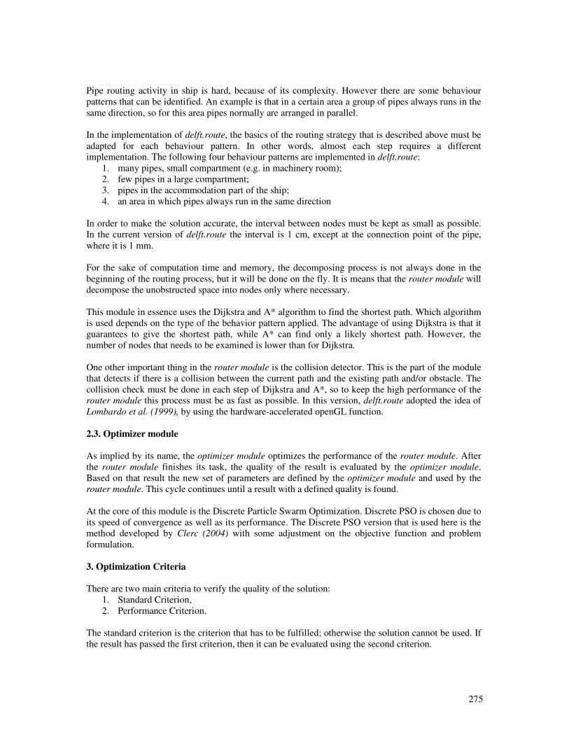
275

Pipe routing activity in ship is hard, because of its complexity. However there are some behaviour

patterns that can be identified. An example is that in a certain area a group of pipes always runs in the

same direction, so for this area pipes normally are arranged in parallel.

In the implementation of delft.route, the basics of the routing strategy that is described above must be

adapted for each behaviour pattern. In other words, almost each step requires a different

implementation. The following four behaviour patterns are implemented in delft.route:

1. many pipes, small compartment (e.g. in machinery room);

2. few pipes in a large compartment;

3. pipes in the accommodation part of the ship;

4. an area in which pipes always run in the same direction

In order to make the solution accurate, the interval between nodes must be kept as small as possible.

In the current version of delft.route the interval is 1 cm, except at the connection point of the pipe,

where it is 1 mm.

For the sake of computation time and memory, the decomposing process is not always done in the

beginning of the routing process, but it will be done on the fly. It is means that the router module will

decompose the unobstructed space into nodes only where necessary.

This module in essence uses the Dijkstra and A* algorithm to find the shortest path. Which algorithm

is used depends on the type of the behavior pattern applied. The advantage of using Dijkstra is that it

guarantees to give the shortest path, while A* can find only a likely shortest path. However, the

number of nodes that needs to be examined is lower than for Dijkstra.

One other important thing in the router module is the collision detector. This is the part of the module

that detects if there is a collision between the current path and the existing path and/or obstacle. The

collision check must be done in each step of Dijkstra and A*, so to keep the high performance of the

router module this process must be as fast as possible. In this version, delft.route adopted the idea of

Lombardo et al. (1999), by using the hardware-accelerated openGL function.

2.3. Optimizer module

As implied by its name, the optimizer module optimizes the performance of the router module. After

the router module finishes its task, the quality of the result is evaluated by the optimizer module.

Based on that result the new set of parameters are defined by the optimizer module and used by the

router module. This cycle continues until a result with a defined quality is found.

At the core of this module is the Discrete Particle Swarm Optimization. Discrete PSO is chosen due to

its speed of convergence as well as its performance. The Discrete PSO version that is used here is the

method developed by Clerc (2004) with some adjustment on the objective function and problem

formulation.

3. Optimization Criteria

There are two main criteria to verify the quality of the solution:

1. Standard Criterion,

2. Performance Criterion.

The standard criterion is the criterion that has to be fulfilled; otherwise the solution cannot be used. If

the result has passed the first criterion, then it can be evaluated using the second criterion.

276

3.1. Standard Criterion

Ideally the standard criterion requires that the solution should meet the Marine Classification, e.g.

Lloyd's Register's Rules and Regulations, Lloyd’s (2001). For this paper, the standard criterion that

was used is not yet fully complying with the Marine Classification, which is subject of subsequent

work not reported here. However the common rules such as that the pipe should always be routed to

the lower level for grey and black water has been applied.

This criterion is used in the router module of delft.route as a guidance to filter the invalid solutions

out of the solution space. This means that all solutions that come from the router module comply with

the standard criterion.

Because the number of rules is too large to be applied at once, the modularity concept is used. This

concept builds on the expandability concept of delft.route, and any new item in the criterion can be

added easily without the need to change the main system.

3.2. Performance Criterion

The quality of the valid solution is evaluated using the performance criterion. This criterion is used as

an objective value by the optimizer module.

From all the aspect of the quality of pipe routing, we define it in two definitions:

1. the aspects that actually affect production, maintenance, and the operational process, such as

the length and number of bends; ease to install; ease to maintain,

2. the aspects that do not directly have any influence with those processes, such as the aesthetic

aspect of the solution.

The second item concerns some kind of preferences of pipe routers, pipe producers, and ship owners.

For the simplicity these preference aspects are neglected in this paper, and we only consider

optimizing the first part above.

Inline with the work of Storch and Park (2002), the aspects that will be optimized are converted into

cost, and the objective of the optimizer module is to minimize this cost value.

The aspects that will be put into account are:

• Material cost

• Installation cost

• Maintenance cost

• Operational cost

3.2.1. Material cost

From four aspects mentioned above, the material cost is the most obvious part, and by calculating the

part of each pipe completely, the cost figure will be known. However in this paper, we consider only

the biggest part of the pipe cost:

• Pipe material

• Pipe length

• Pipe diameter

• Pipe treatment

• Number and type of bends

• Wall penetration

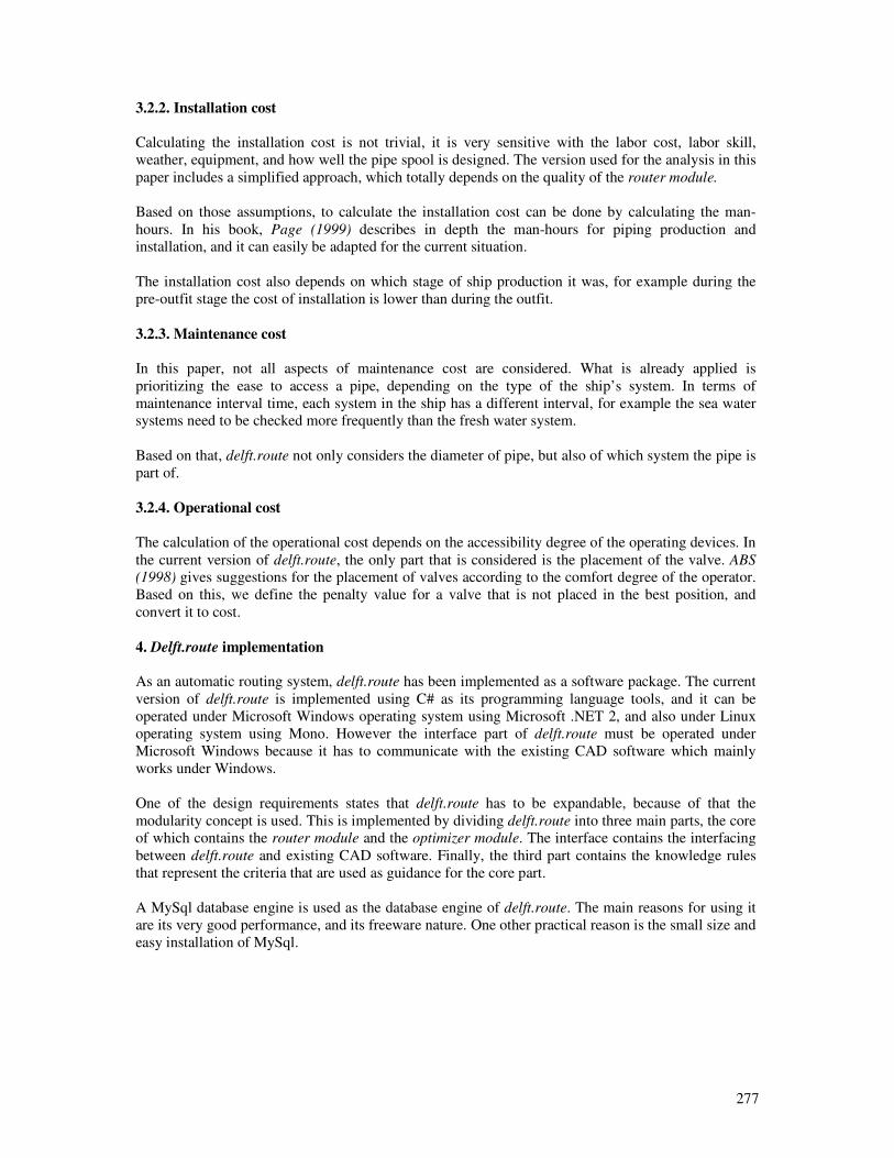
277

3.2.2. Installation cost

Calculating the installation cost is not trivial, it is very sensitive with the labor cost, labor skill,

weather, equipment, and how well the pipe spool is designed. The version used for the analysis in this

paper includes a simplified approach, which totally depends on the quality of the router module.

Based on those assumptions, to calculate the installation cost can be done by calculating the man-

hours. In his book, Page (1999) describes in depth the man-hours for piping production and

installation, and it can easily be adapted for the current situation.

The installation cost also depends on which stage of ship production it was, for example during the

pre-outfit stage the cost of installation is lower than during the outfit.

3.2.3. Maintenance cost

In this paper, not all aspects of maintenance cost are considered. What is already applied is

prioritizing the ease to access a pipe, depending on the type of the ship’s system. In terms of

maintenance interval time, each system in the ship has a different interval, for example the sea water

systems need to be checked more frequently than the fresh water system.

Based on that, delft.route not only considers the diameter of pipe, but also of which system the pipe is

part of.

3.2.4. Operational cost

The calculation of the operational cost depends on the accessibility degree of the operating devices. In

the current version of delft.route, the only part that is considered is the placement of the valve. ABS

(1998) gives suggestions for the placement of valves according to the comfort degree of the operator.

Based on this, we define the penalty value for a valve that is not placed in the best position, and

convert it to cost.

4. Delft.route implementation

As an automatic routing system, delft.route has been implemented as a software package. The current

version of delft.route is implemented using C# as its programming language tools, and it can be

operated under Microsoft Windows operating system using Microsoft .NET 2, and also under Linux

operating system using Mono. However the interface part of delft.route must be operated under

Microsoft Windows because it has to communicate with the existing CAD software which mainly

works under Windows.

One of the design requirements states that delft.route has to be expandable, because of that the

modularity concept is used. This is implemented by dividing delft.route into three main parts, the core

of which contains the router module and the optimizer module. The interface contains the interfacing

between delft.route and existing CAD software. Finally, the third part contains the knowledge rules

that represent the criteria that are used as guidance for the core part.

A MySql database engine is used as the database engine of delft.route. The main reasons for using it

are its very good performance, and its freeware nature. One other practical reason is the small size and

easy installation of MySql.

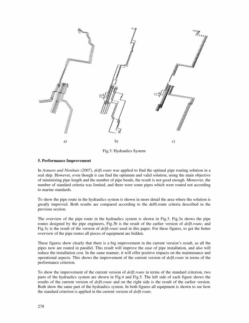
278

a)

b)

c)

Fig.3: Hydraulics System

5. Performance Improvement

In Asmara and Nienhuis (2007), delft.route was applied to find the optimal pipe routing solution in a

real ship. However, even though it can find the optimum and valid solution, using the main objective

of minimizing pipe length and the number of pipe bends, the result is not good enough. Moreover, the

number of standard criteria was limited, and there were some pipes which were routed not according

to marine standards.

To show the pipe route in the hydraulics system is shown in more detail the area where the solution is

greatly improved. Both results are compared according to the delft.route criteria described in the

previous section.

The overview of the pipe route in the hydraulics system is shown in Fig.3. Fig.3a shows the pipe

routes designed by the pipe engineers, Fig.3b is the result of the earlier version of delft.route, and

Fig.3c is the result of the version of delft.route used in this paper. For these figures, to get the better

overview of the pipe routes all pieces of equipment are hidden.

These figures show clearly that there is a big improvement in the current version’s result, as all the

pipes now are routed in parallel. This result will improve the ease of pipe installation, and also will

reduce the installation cost. In the same manner, it will offer positive impacts on the maintenance and

operational aspects. This shows the improvement of the current version of delft.route in terms of the

performance criterion.

To show the improvement of the current version of delft.route in terms of the standard criterion, two

parts of the hydraulics system are shown in Fig.4 and Fig.5. The left side of each figure shows the

results of the current version of delft.route and on the right side is the result of the earlier version.

Both show the same part of the hydraulics system. In both figures all equipment is shown to see how

the standard criterion is applied in the current version of delft.route.

279

a)

b)

Fig.4: Part of Hydraulics System

a)

b)

Fig.5: Part of Hydraulics System

One of the items in the standard criterion states that the flanges of hydraulics pipe are not allowed to

be routed above certain elements that have a danger of flame if there is a leak in the flange. Two of

those elements are the diesel engine and the cable tray.

As shown in Fig.4, in the old result some pipes are routed above the diesel engine and in the new

result those pipes are routed not directly above the diesel engine. This result shows the improvement

of the result by adding the new item to the list of criteria.

The same situation is also apparent in the other part of that system. Fig.5 shows that pipes are routed

above the cable tray in the old result, but no longer in the new result.

280

6. Conclusion

In this paper, the improvement of the automatic routing system – delft.route – has been described and

tested against the old version. The comparison shows that the current version gives more realistic pipe

route solutions. Issues such as “spaghetti pipes” can be eliminated by routing pipes in parallel.

Another interesting part of delft.route is the modularity concept that is used. This concept will make

delft.route easy to be improved and expanded. There are two parts of delft.route that use this concept.

The first part is the interface module which allows adding the interface to other existing CAD

software without changing any part of the remainder of the routing application. The second

modularity part is in the criteria. The list of criteria can be expanded easily by adding the new rules in

the knowledge rules database without the need to modify other parts of the software.

For further development, more criteria will be added in delft.route knowledge rules to improve the

solution. Currently work is under way to further improve the routing algorithm and collision detection

function to reduce calculation time.

References

ABS (1998), Guidance notes on the application of ergonomics to marine systems, The American

Bureau of Shipping

AL-KAZEMI, B.; MOHAN, C. (2002), Multi-phase discrete particle swarm optimization, 4th Int.

Workshop on Frontiers in Evolutionary Algorithms

ASMARA, A.; NIENHUIS, U. (2006), Automatic piping system in ship, 5th Int. Conf. on Computer

and IT Application Mar. Ind. (COMPIT), Oegstgeest, pp.269-279

ASMARA, A.; NIENHUIS, U. (2007), Automatic piping system implementation: a real case, 6th Int.

Conf. on Computer and IT Application Mar. Ind. (COMPIT), Cortona, pp.290-299

BUTLER, D. (2000), Guide to ship repair estimates (in man-hours), Butterworth-Heinemann

CLERC, M. (2004), Discrete particle swarm optimization, illustrated by the Travelling Salesman

Problem, New Optimization Techniques in Engineering

FAN, X.; LIN, Y.; JI, Z. (2006), The ant colony optimization for ship pipe route design in 3D space,

6th World Congress on Intelligent Control and Automation, Dalian, pp.3103-3108

HARRINGTON, R.L. (1992), Marine engineering, The Society of Naval Architects and Marine

Engineers

ITO, T (1999), A genetic algorithm approach to piping route path planning, J. Intelligent Manu-

facturing 10/1

KANG, S-S; MYUNG, S; HAN, S-H (1999), A design expert system for auto-routing of ship pipes, J.

Ship Production 15/1

KIM, D.G.; CORNE, D. (1996), Industrial plant pipe-route optimisation with genetic algorithms,

Parallel problem solving from nature IV, pp.1012–21

KUO, C; WU, J; SHAW, H (1999), Collision avoidance schemes for orthogonal pipe routing, J. Ship

Production 15/4

LLOYD’S (2001), Rules and regulations for classification of naval ships, Lloyd’s Register

281

LOMBARDO, J.C.; CANI, M.P.; NEYRET, F. (1999), Real-time collision detection for virtual

surgery, Proc. Computer Animation, pp. 82 - 90

MATSUI, Y.; TAKAGI, H. ; EMORI, S.; MASUDA, N.; SASABE, S.; YOSHIMURA, C.; SHIRAI,

T.; NIOH, S.; KINNO, B (1979), Automatic pipe routing and material take-off system for chemical

plant, 16th Conf. on Design Automation, pp.121-127

NEWELL, R (1972), An interactive approach to pipe routing in process plants, J. Information

Processing

PAGE, J.S. (1999), Estimator’s piping man-hour manual, fifth edition, Gulf Professional Publishing

PARK, J-H; STORCH, R (2002), Pipe-routing algorithm development: case study of a ship engine

room design, Expert Systems with Applications 23, pp.299–309

ROH, M-I.; LEE, K-Y.; CHOI, W-Y (2007), Rapid generation of the piping model having the

relationship with a hull structure in shipbuilding, Advances in Engineering Software 38, pp.215–228

RUBIN, F (1974), The Lee path connection algorithm, IEEE Trans. on Computers, Vol. C23, pp.907-

914

VAN DOKKUM, K (2003), Ship knowledge, a modern encyclopedia, Dokmar

WOUD, J.K.; STAPERSMA, D (2003), Design of propulsion and electric power generation systems,

IMAREST

ZUURMOND, R. J. (2004), Automatisch routeren van pijpleidingen in schepen, Delft

282

Building the Business Process View into Shipbuilding Data Exchange

Matthias Grau, PROSTEP, Hamburg/Germany, Matthias.Grau@prostep.com Carsten Zerbst, PROSTEP, Hamburg/Germany, Carsten.Zerbst@prostep.com

Markus Sachers, PROSTEP, Hamburg/Germany, Markus.Sachers@prostep.com

Abstract

Non-specific integration standards and approaches are discussed as an option for the shipbuilding industry. Particularly the PLM Services specification published under the Object Management Group (OMG) is advocated. This standard combines data and process integration on the basis of STEP and Service Oriented Architecture into one homogeneous approach. Recent development activities aim to bring the shipbuilding specific CAx tools - such as TRIBON - into this picture. Those activities include the adoption of mechanical CAD systems, including NX and Catia, virtual reality systems and last but not least the digital class approval based on 3D-PDF. 1. Requirement to collaborate implies integration of IT systems Collaboration across company and site boundaries becomes more and more important in the worldwide maritime industry. This leads to challenges with the integration of IT systems involved in the development process at a level not addressed so far. Collaboration scenarios, which are operational today, focus on vertical collaboration covering the supply chain. Up to 70% of the value creation for a ship is currently provided by suppliers. Shipyards increasingly move into a prime contractor role. The last years saw a consolidation process in Europe leading to multi-site type shipbuilding companies that require collaboration on a horizontal direction. Horizontal collaboration in consortia formed on a project basis is already common practice for military projects. Collaboration of business partners in shipbuilding ranges between the traditional supply chain and modern scenarios of project-driven partner networks. Whatever the scenario in question looks like, it is important to make it as efficient as possible using the necessary methods and tools. Parties involved in collaboration typically take their own point of view. In these specific views it is often not implicit to see the context of the whole project and product respectively. The big challenge of partner integration therefore is about representing processes and information in a way that enables the participants to see the relationships – especially dependencies – allowing them to share a common view with all parties involved and – at the same time – hide unnecessary or proprietary details. Reality typically looks different: Evolved IT system landscapes and isolated tools avoid seamless processes and cause incomplete information being exchanged. Data management processes are not coordinated at a sufficient level – companies use their own (or virtually no) means to manage their processes and data without sharing common conventions (naming and numbering, product structure, change processes …). A number of details need to be considered in this respect, playing thereby the role of predefined conditions for collaboration. This includes the role of the participants in the context of both, the overall scenario and the interest of the parties involved as well as aspects about departments, site specifics, planning- and budget-related topics; and the IT systems used to handle the related information. 2. Why the shipbuilding STEP protocols did not do the job years ago Addressing these issues many activities have been conducted over the last decade including international standardization of exchange data structures (namely STEP) and related R&D projects targeting the implementation of those commonly agreed conventions across various industries including aerospace, automotive, oil and gas and shipbuilding.

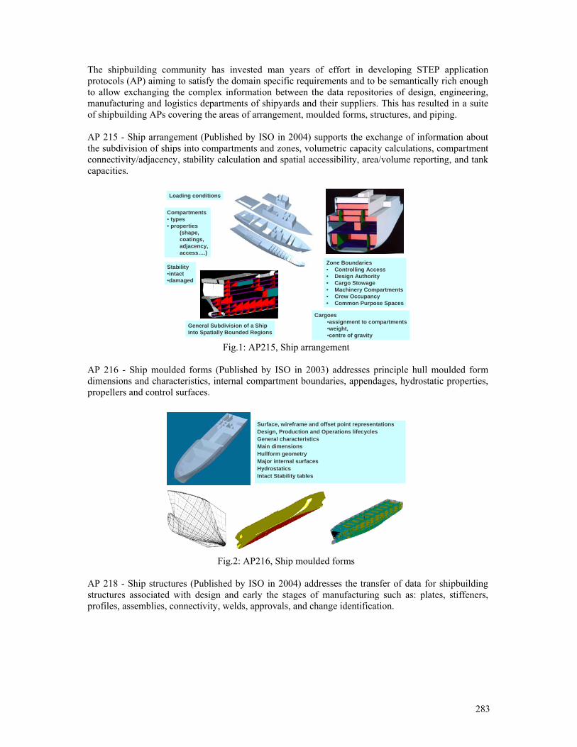
283

The shipbuilding community has invested man years of effort in developing STEP application protocols (AP) aiming to satisfy the domain specific requirements and to be semantically rich enough to allow exchanging the complex information between the data repositories of design, engineering, manufacturing and logistics departments of shipyards and their suppliers. This has resulted in a suite of shipbuilding APs covering the areas of arrangement, moulded forms, structures, and piping. AP 215 - Ship arrangement (Published by ISO in 2004) supports the exchange of information about the subdivision of ships into compartments and zones, volumetric capacity calculations, compartment connectivity/adjacency, stability calculation and spatial accessibility, area/volume reporting, and tank capacities.

Zone Boundaries• Controlling Access• Design Authority• Cargo Stowage• Machinery Compartments• Crew Occupancy• Common Purpose Spaces

Stability•intact•damaged

Compartments• types• properties

(shape, coatings,adjacency,access….)

Loading conditions

General Subdivision of a Shipinto Spatially Bounded Regions

Cargoes•assignment to compartments•weight, •centre of gravity

Fig.1: AP215, Ship arrangement AP 216 - Ship moulded forms (Published by ISO in 2003) addresses principle hull moulded form dimensions and characteristics, internal compartment boundaries, appendages, hydrostatic properties, propellers and control surfaces.

Surface, wireframe and offset point representationsDesign, Production and Operations lifecyclesGeneral characteristicsMain dimensionsHullform geometryMajor internal surfacesHydrostaticsIntact Stability tables

Fig.2: AP216, Ship moulded forms

AP 218 - Ship structures (Published by ISO in 2004) addresses the transfer of data for shipbuilding structures associated with design and early the stages of manufacturing such as: plates, stiffeners, profiles, assemblies, connectivity, welds, approvals, and change identification.

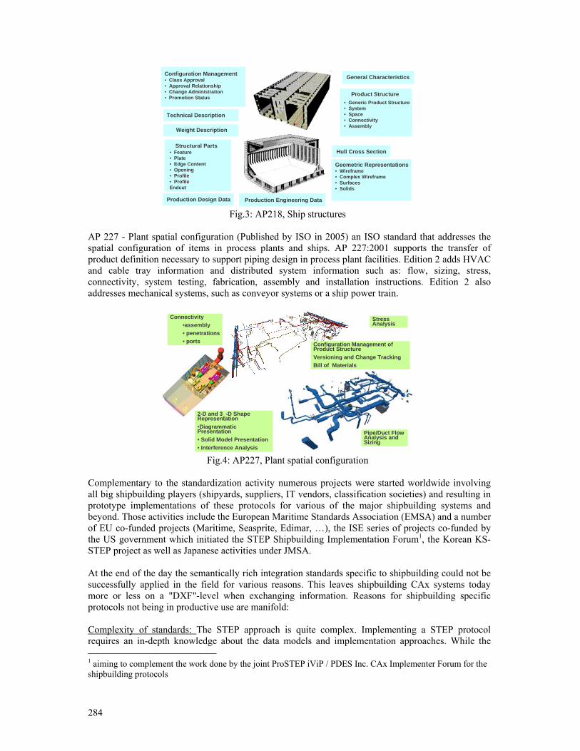
284

Technical Description

General CharacteristicsConfiguration Management • Class Approval• Approval Relationship• Change Administration• Promotion Status

Weight Description

Structural Parts• Feature• Plate • Edge Content• Opening• Profile• Profile Endcut

Production Engineering DataProduction Design Data

Geometric Representations• Wireframe• Complex Wireframe• Surfaces• Solids

Hull Cross Section

Product Structure• Generic Product Structure• System• Space• Connectivity• Assembly

Fig.3: AP218, Ship structures

AP 227 - Plant spatial configuration (Published by ISO in 2005) an ISO standard that addresses the spatial configuration of items in process plants and ships. AP 227:2001 supports the transfer of product definition necessary to support piping design in process plant facilities. Edition 2 adds HVAC and cable tray information and distributed system information such as: flow, sizing, stress, connectivity, system testing, fabrication, assembly and installation instructions. Edition 2 also addresses mechanical systems, such as conveyor systems or a ship power train.

Stress Analysis

Connectivity•assembly• penetrations• ports

Pipe/Duct Flow Analysis and Sizing

Configuration Management of Product StructureVersioning and Change TrackingBill of Materials

2-D and 3_-D Shape Representation•Diagrammatic Presentation• Solid Model Presentation• Interference Analysis

Fig.4: AP227, Plant spatial configuration Complementary to the standardization activity numerous projects were started worldwide involving all big shipbuilding players (shipyards, suppliers, IT vendors, classification societies) and resulting in prototype implementations of these protocols for various of the major shipbuilding systems and beyond. Those activities include the European Maritime Standards Association (EMSA) and a number of EU co-funded projects (Maritime, Seasprite, Edimar, …), the ISE series of projects co-funded by the US government which initiated the STEP Shipbuilding Implementation Forum1, the Korean KS-STEP project as well as Japanese activities under JMSA. At the end of the day the semantically rich integration standards specific to shipbuilding could not be successfully applied in the field for various reasons. This leaves shipbuilding CAx systems today more or less on a "DXF"-level when exchanging information. Reasons for shipbuilding specific protocols not being in productive use are manifold: Complexity of standards: The STEP approach is quite complex. Implementing a STEP protocol requires an in-depth knowledge about the data models and implementation approaches. While the 1 aiming to complement the work done by the joint ProSTEP iViP / PDES Inc. CAx Implementer Forum for the shipbuilding protocols

285

vendors might have been waited for the industry to provide the economic incentive to invest in this area the industry was waiting for the vendors to come up with working implementations. Protectionism: Although involved in development and validation of the protocols only very few vendors of shipbuilding specific CAx systems finally continued their prototypes into products to protect there systems from being too wide open without seeing the opportunity for a related margin. Too specific market: Especially suppliers (but also IT vendors) that are not exclusively serving shipbuilding didn't see the justification to support shipbuilding specific standards. The major players in the shipbuilding industry did not push hard enough to generate the need for suppliers to implement shipbuilding specific standards. Missing separation of data management and authoring tools: Due to the complexity of ships major shipbuilding CAx systems very early had a certain level of data management functionality (product structure, databases …). This was in place before the invention of the PDM paradigm to distinguish data management and authoring tools driven by the mechanical CAD system vendors. This legacy has influenced the shipbuilding protocols causing them seemingly not being in line with this paradigm. Missing process view: STEP as such has its root with IGES and carries the legacy of being data centric. While this is not a deficiency by itself the standard has not managed fast enough to provide the necessary enablers to be compatible with evolving methods/techniques for process integration. These topics are not specific to shipbuilding. Facing similar challenges other industries have gone part of the necessary way over the last years. Those approaches if not specific to one industry have the potential to provide synergies to shipbuilding from areas including mechanical engineering, auto and aerospace allowing the maritime industry to harvest the advantages of proven approaches and combining them with the existing branch-specific solutions to a new quality. 3. Adding the process view – OMG PLM Services A well proven representative of this kind is the PLM Services specification published under the Object Management Group (OMG). The PLM Services specification extends data integration based on STEP by a set of commonly agreed services to handle this data in the context of collaboration scenarios. This allows building workflows to realizing processes to manipulate or communicate information between the involved systems. Motivation for the development of the PLM Services specification were the lessons learnt from earlier activities (such as PDTnet, ProSTEP iViP (2004), and PDMEnablers, OMG (2000)) that already tried to overcome the missing process perspective of STEP in the automotive industry. Those lessons included the pitfalls of making an integration standard technology related (as technology has its own lifecycle) and underestimating the complexity and disharmony2 of the STEP application protocols. Building on the results of the PDTnet project and using the PDM Schema3, PDM Implementer Forum (2002), as data model a specification was developed and published under the Object Management Group (OMG) that had the main objective to standardize a platform independent reference model for product lifecycle data and services and to use the Model Driven Architecture (MDA) approach (rather than a specific technology) for implementation. 2 originally the STEP approach includes a "built-in harmonization" due to the common generic product model (integrated resources) that all application protocols have to be related to 3 data model covering the PDM data exchange requirements ("meta-data") that is harmonized across the STEP APs 203, 209, 212, 214 und 232

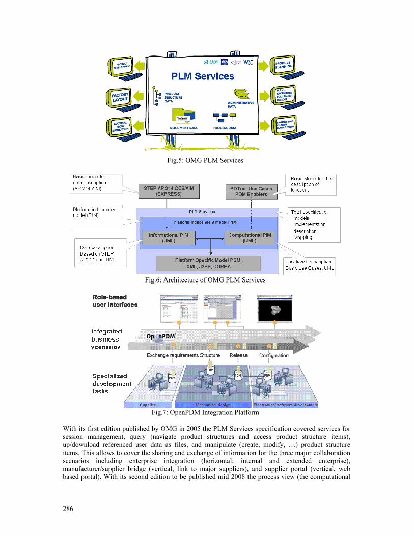
286

Fig.5: OMG PLM Services

Fig.6: Architecture of OMG PLM Services

Fig.7: OpenPDM Integration Platform

With its first edition published by OMG in 2005 the PLM Services specification covered services for session management, query (navigate product structures and access product structure items), up/download referenced user data as files, and manipulate (create, modify, …) product structure items. This allows to cover the sharing and exchange of information for the three major collaboration scenarios including enterprise integration (horizontal; internal and extended enterprise), manufacturer/supplier bridge (vertical, link to major suppliers), and supplier portal (vertical, web based portal). With its second edition to be published mid 2008 the process view (the computational

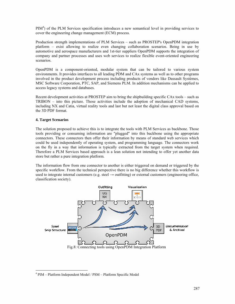
287

PIM4) of the PLM Services specification introduces a new semantical level in providing services to cover the engineering change management (ECM) process. Production strength implementations of PLM Services – such as PROSTEP's OpenPDM integration platform – exist allowing to realize even changing collaboration scenarios. Being in use by automotive and aerospace manufacturers and 1st-tier suppliers OpenPDM supports the integration of company and partner processes and uses web services to realize flexible event-oriented engineering scenarios. OpenPDM is a component-oriented, modular system that can be tailored to various system environments. It provides interfaces to all leading PDM and CAx systems as well as to other programs involved in the product development process including products of vendors like Dassault Systèmes, MSC Software Corporation, PTC, SAP, and Siemens PLM. In addition mechanisms can be applied to access legacy systems and databases. Recent development activities at PROSTEP aim to bring the shipbuilding specific CAx tools – such as TRIBON – into this picture. Those activities include the adoption of mechanical CAD systems, including NX and Catia, virtual reality tools and last but not least the digital class approval based on the 3D PDF format. 4. Target Scenarios The solution proposed to achieve this is to integrate the tools with PLM Services as backbone. Those tools providing or consuming information are "plugged" into this backbone using the appropriate connectors. These connectors then offer their information by means of standard web services which could be used independently of operating system, and programming language. The connectors work on the fly in a way that information is typically extracted from the target system when required. Therefore a PLM Services based approach is a lean solution not intending to offer yet another data store but rather a pure integration platform. The information flow from one connector to another is either triggered on demand or triggered by the specific workflow. From the technical perspective there is no big difference whether this workflow is used to integrate internal customers (e.g. steel → outfitting) or external customers (engineering office, classification society).

Fig.8: Connecting tools using OpenPDM Integration Platform

4 PIM – Platform Independent Model / PSM – Platform Specific Model

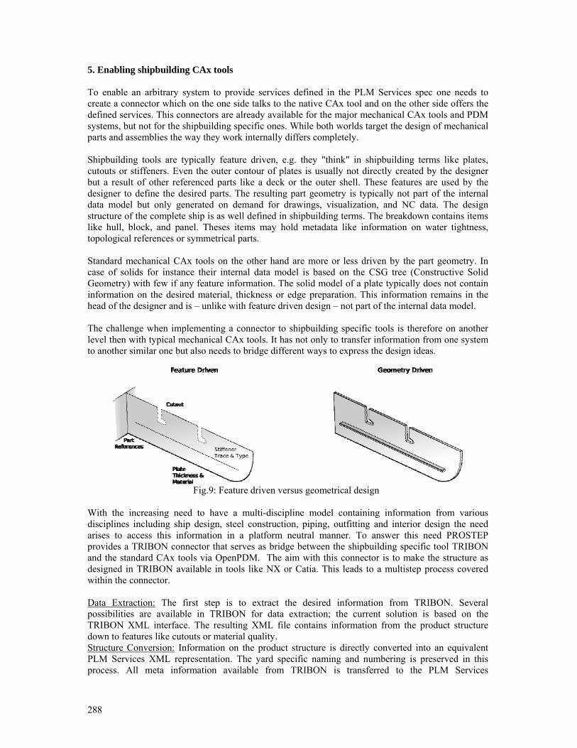
288

5. Enabling shipbuilding CAx tools To enable an arbitrary system to provide services defined in the PLM Services spec one needs to create a connector which on the one side talks to the native CAx tool and on the other side offers the defined services. This connectors are already available for the major mechanical CAx tools and PDM systems, but not for the shipbuilding specific ones. While both worlds target the design of mechanical parts and assemblies the way they work internally differs completely. Shipbuilding tools are typically feature driven, e.g. they "think" in shipbuilding terms like plates, cutouts or stiffeners. Even the outer contour of plates is usually not directly created by the designer but a result of other referenced parts like a deck or the outer shell. These features are used by the designer to define the desired parts. The resulting part geometry is typically not part of the internal data model but only generated on demand for drawings, visualization, and NC data. The design structure of the complete ship is as well defined in shipbuilding terms. The breakdown contains items like hull, block, and panel. Theses items may hold metadata like information on water tightness, topological references or symmetrical parts. Standard mechanical CAx tools on the other hand are more or less driven by the part geometry. In case of solids for instance their internal data model is based on the CSG tree (Constructive Solid Geometry) with few if any feature information. The solid model of a plate typically does not contain information on the desired material, thickness or edge preparation. This information remains in the head of the designer and is – unlike with feature driven design – not part of the internal data model. The challenge when implementing a connector to shipbuilding specific tools is therefore on another level then with typical mechanical CAx tools. It has not only to transfer information from one system to another similar one but also needs to bridge different ways to express the design ideas.

Fig.9: Feature driven versus geometrical design

With the increasing need to have a multi-discipline model containing information from various disciplines including ship design, steel construction, piping, outfitting and interior design the need arises to access this information in a platform neutral manner. To answer this need PROSTEP provides a TRIBON connector that serves as bridge between the shipbuilding specific tool TRIBON and the standard CAx tools via OpenPDM. The aim with this connector is to make the structure as designed in TRIBON available in tools like NX or Catia. This leads to a multistep process covered within the connector. Data Extraction: The first step is to extract the desired information from TRIBON. Several possibilities are available in TRIBON for data extraction; the current solution is based on the TRIBON XML interface. The resulting XML file contains information from the product structure down to features like cutouts or material quality. Structure Conversion: Information on the product structure is directly converted into an equivalent PLM Services XML representation. The yard specific naming and numbering is preserved in this process. All meta information available from TRIBON is transferred to the PLM Services

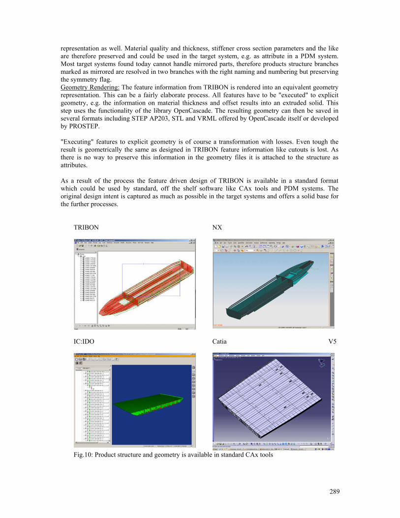
289

representation as well. Material quality and thickness, stiffener cross section parameters and the like are therefore preserved and could be used in the target system, e.g. as attribute in a PDM system. Most target systems found today cannot handle mirrored parts, therefore products structure branches marked as mirrored are resolved in two branches with the right naming and numbering but preserving the symmetry flag. Geometry Rendering: The feature information from TRIBON is rendered into an equivalent geometry representation. This can be a fairly elaborate process. All features have to be "executed" to explicit geometry, e.g. the information on material thickness and offset results into an extruded solid. This step uses the functionality of the library OpenCascade. The resulting geometry can then be saved in several formats including STEP AP203, STL and VRML offered by OpenCascade itself or developed by PROSTEP. "Executing" features to explicit geometry is of course a transformation with losses. Even tough the result is geometrically the same as designed in TRIBON feature information like cutouts is lost. As there is no way to preserve this information in the geometry files it is attached to the structure as attributes. As a result of the process the feature driven design of TRIBON is available in a standard format which could be used by standard, off the shelf software like CAx tools and PDM systems. The original design intent is captured as much as possible in the target systems and offers a solid base for the further processes.

TRIBON

NX

IC:IDO

Catia V5

Fig.10: Product structure and geometry is available in standard CAx tools

290

6. Conclusion The integration of shipbuilding specific tools like TRIBON with standard CAx tools as used in outfitting, piping and HVAC is a feasible task both, semantically as well as technically. Using OMG PLM Services as the basis for a common integration platform is a perfectly possible and sensible way to (re)use product structure, geometric and non-geometric information created in shipbuilding specific CAx tools like TRIBON Hull in other systems. The semantically different levels to represent this information in the internal data model of the connected systems have been bridged by a connector implementation providing the "intelligence" to carry out the semantic transformation. Tasks still to be addressed include the "way back", i.e. transformation of mechanical CAD models (such as outfitting or piping) into shipbuilding specific tools and the coverage of administrative information available from the connected systems (such as version and release status). The shown approach addresses several of the aforementioned issues, namely the last three: Too specific market: OMG PLM Services and implementations like OpenPDM originate from and are operational in other industrial branches without being specific to these industries Missing separation of data management and authoring tools: The PDM Schema basis enables this separation in a system independent and proven way Missing process view: The computational model complements the data exchange protocol by a specification of the functionality to control this exchange What is of course missing by nature in the OMG spec is any shipbuilding specific semantics. This however is well defined and commonly agreed in the STEP shipbuilding protocols. A harmonization of these protocols with the PDM Schema could provide the opportunity to align these branch specific requirements with an accepted and widely supported approach. The fact that the shipbuilding protocols are interoperable on the basis of a so called "Ship Common Model" which in turn is in parts close to the PDM Schema indicates this a promising and feasible way. References EUROPEAN COMMISSION (2003), LeaderSHIP 2015: Defining the Future of the European Ship-building and Shiprepair Industry - Competitiveness through Excellence, http://ec.europa.eu/enterprise/maritime/maritime_industrial/leadership_2015.htm SHIGO, N.; ERKENS, E.; KOPFER, H. (2004), Supply Chain Management im deutschen Schiffbau, Supply Chain Management, Issue IV/2004 (in German) ISO TC184/SC4 (2007), Ship STEP on-a-page, http://www.tc184-sc4-ustag.org/Pages/docs/ship-soap_2007-05-29.pdf ProSTEP iViP (2004), PDTnet Project - Product Data Technology and Communication in an OEM and Supplier Network, http://www.prostep.org/en/standards/pdtnet OMG (2000), PDM Enablers V2.0, http://mantis.omg.org/mfgevalpdmev2.htm OpenCascade, http://www.opencascade.org PDM Implementer Forum (2002), PDM Schema, http://www.pdm-if.org/pdm_schema/ ProSTEP iViP (2008), PLM Services 2.0, www.prostep.org/de/projektgruppen/plmservices PROSTEP AG (2008), OpenPDM®, http://www.prostep.com

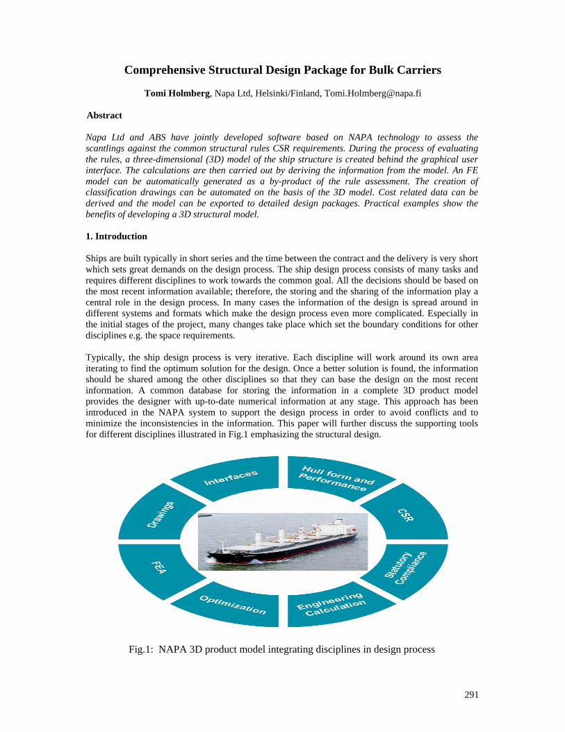
291

Comprehensive Structural Design Package for Bulk Carriers

Tomi Holmberg, Napa Ltd, Helsinki/Finland, Tomi.Holmberg@napa.fi

Abstract

Napa Ltd and ABS have jointly developed software based on NAPA technology to assess the scantlings against the common structural rules CSR requirements. During the process of evaluating the rules, a three-dimensional (3D) model of the ship structure is created behind the graphical user interface. The calculations are then carried out by deriving the information from the model. An FE model can be automatically generated as a by-product of the rule assessment. The creation of classification drawings can be automated on the basis of the 3D model. Cost related data can be derived and the model can be exported to detailed design packages. Practical examples show the benefits of developing a 3D structural model. 1. Introduction Ships are built typically in short series and the time between the contract and the delivery is very short which sets great demands on the design process. The ship design process consists of many tasks and requires different disciplines to work towards the common goal. All the decisions should be based on the most recent information available; therefore, the storing and the sharing of the information play a central role in the design process. In many cases the information of the design is spread around in different systems and formats which make the design process even more complicated. Especially in the initial stages of the project, many changes take place which set the boundary conditions for other disciplines e.g. the space requirements. Typically, the ship design process is very iterative. Each discipline will work around its own area iterating to find the optimum solution for the design. Once a better solution is found, the information should be shared among the other disciplines so that they can base the design on the most recent information. A common database for storing the information in a complete 3D product model provides the designer with up-to-date numerical information at any stage. This approach has been introduced in the NAPA system to support the design process in order to avoid conflicts and to minimize the inconsistencies in the information. This paper will further discuss the supporting tools for different disciplines illustrated in Fig.1 emphasizing the structural design.

Fig.1: NAPA 3D product model integrating disciplines in design process

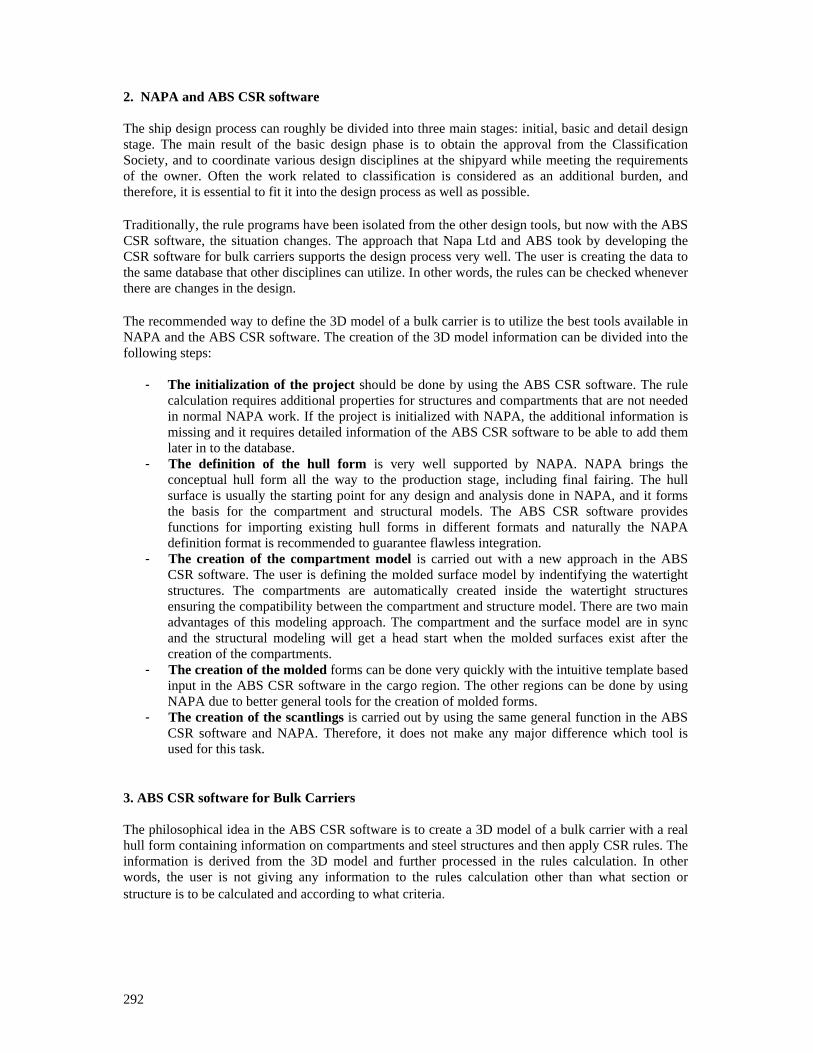
292

2. NAPA and ABS CSR software The ship design process can roughly be divided into three main stages: initial, basic and detail design stage. The main result of the basic design phase is to obtain the approval from the Classification Society, and to coordinate various design disciplines at the shipyard while meeting the requirements of the owner. Often the work related to classification is considered as an additional burden, and therefore, it is essential to fit it into the design process as well as possible. Traditionally, the rule programs have been isolated from the other design tools, but now with the ABS CSR software, the situation changes. The approach that Napa Ltd and ABS took by developing the CSR software for bulk carriers supports the design process very well. The user is creating the data to the same database that other disciplines can utilize. In other words, the rules can be checked whenever there are changes in the design. The recommended way to define the 3D model of a bulk carrier is to utilize the best tools available in NAPA and the ABS CSR software. The creation of the 3D model information can be divided into the following steps:

- The initialization of the project should be done by using the ABS CSR software. The rule calculation requires additional properties for structures and compartments that are not needed in normal NAPA work. If the project is initialized with NAPA, the additional information is missing and it requires detailed information of the ABS CSR software to be able to add them later in to the database.

- The definition of the hull form is very well supported by NAPA. NAPA brings the conceptual hull form all the way to the production stage, including final fairing. The hull surface is usually the starting point for any design and analysis done in NAPA, and it forms the basis for the compartment and structural models. The ABS CSR software provides functions for importing existing hull forms in different formats and naturally the NAPA definition format is recommended to guarantee flawless integration.

- The creation of the compartment model is carried out with a new approach in the ABS CSR software. The user is defining the molded surface model by indentifying the watertight structures. The compartments are automatically created inside the watertight structures ensuring the compatibility between the compartment and structure model. There are two main advantages of this modeling approach. The compartment and the surface model are in sync and the structural modeling will get a head start when the molded surfaces exist after the creation of the compartments.

- The creation of the molded forms can be done very quickly with the intuitive template based input in the ABS CSR software in the cargo region. The other regions can be done by using NAPA due to better general tools for the creation of molded forms.

- The creation of the scantlings is carried out by using the same general function in the ABS CSR software and NAPA. Therefore, it does not make any major difference which tool is used for this task.

3. ABS CSR software for Bulk Carriers The philosophical idea in the ABS CSR software is to create a 3D model of a bulk carrier with a real hull form containing information on compartments and steel structures and then apply CSR rules. The information is derived from the 3D model and further processed in the rules calculation. In other words, the user is not giving any information to the rules calculation other than what section or structure is to be calculated and according to what criteria.

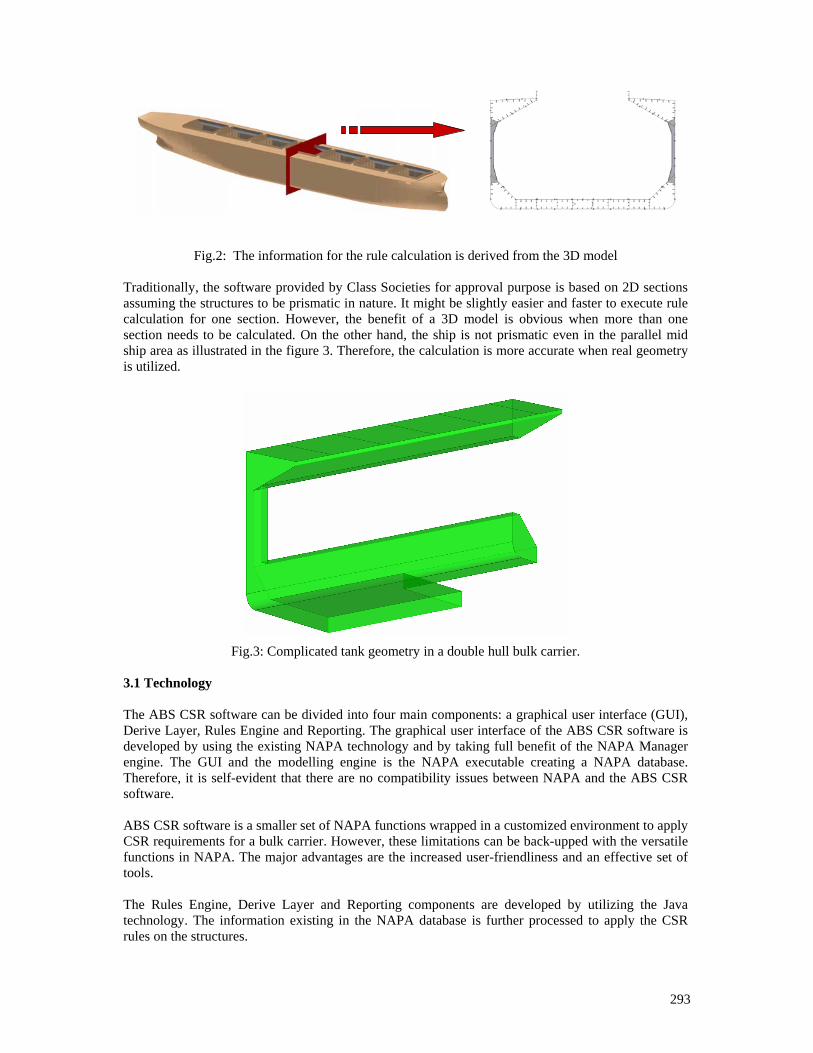
293

Fig.2: The information for the rule calculation is derived from the 3D model Traditionally, the software provided by Class Societies for approval purpose is based on 2D sections assuming the structures to be prismatic in nature. It might be slightly easier and faster to execute rule calculation for one section. However, the benefit of a 3D model is obvious when more than one section needs to be calculated. On the other hand, the ship is not prismatic even in the parallel mid ship area as illustrated in the figure 3. Therefore, the calculation is more accurate when real geometry is utilized.

Fig.3: Complicated tank geometry in a double hull bulk carrier. 3.1 Technology The ABS CSR software can be divided into four main components: a graphical user interface (GUI), Derive Layer, Rules Engine and Reporting. The graphical user interface of the ABS CSR software is developed by using the existing NAPA technology and by taking full benefit of the NAPA Manager engine. The GUI and the modelling engine is the NAPA executable creating a NAPA database. Therefore, it is self-evident that there are no compatibility issues between NAPA and the ABS CSR software. ABS CSR software is a smaller set of NAPA functions wrapped in a customized environment to apply CSR requirements for a bulk carrier. However, these limitations can be back-upped with the versatile functions in NAPA. The major advantages are the increased user-friendliness and an effective set of tools. The Rules Engine, Derive Layer and Reporting components are developed by utilizing the Java technology. The information existing in the NAPA database is further processed to apply the CSR rules on the structures.

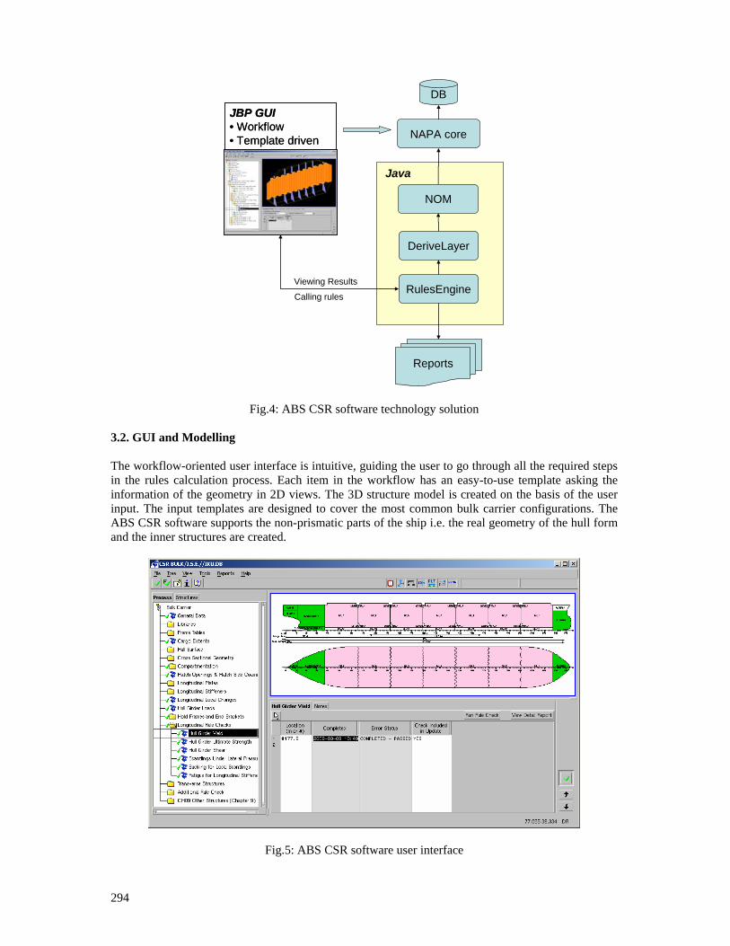
294

DB

DeriveLayer

RulesEngine

JBP GUI• Workflow• Template driven

JBP GUI• Workflow• Template driven

Reports

Viewing Results

Java

Calling rules

NOM

NAPA core

Fig.4: ABS CSR software technology solution 3.2. GUI and Modelling The workflow-oriented user interface is intuitive, guiding the user to go through all the required steps in the rules calculation process. Each item in the workflow has an easy-to-use template asking the information of the geometry in 2D views. The 3D structure model is created on the basis of the user input. The input templates are designed to cover the most common bulk carrier configurations. The ABS CSR software supports the non-prismatic parts of the ship i.e. the real geometry of the hull form and the inner structures are created.

Fig.5: ABS CSR software user interface

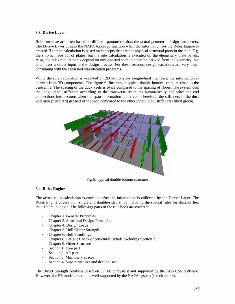
295

3.3. Derive Layer Rule formulae are often based on different parameters than the actual geometric design parameters. The Derive Layer utilizes the NAPA topology function when the information for the Rules Engine is created. The rule calculation is based on concepts that are not physical structural parts in the ship. E.g. the ship is made out of plates, but the rule calculation is executed on the elementary plate panels. Also, the rules requirements depend on unsupported span that can be derived from the geometry, but it is never a direct input in the design process. For these reasons, design variations are very time-consuming with the separated classification programs. While the rule calculation is executed on 2D sections for longitudinal members, the information is derived from 3D components. The figure 6 illustrates a typical double bottom structure close to the centreline. The spacing of the duck keels is twice compared to the spacing of floors. The system cuts the longitudinal stiffeners according to the transverse structures automatically and takes the end connections into account when the span information is derived. Therefore, the stiffeners in the duct keel area (filled red) get half of the span compared to the other longitudinal stiffeners (filled green).

Fig.6: Typical double bottom structure

3.4. Rules Engine The actual rules calculation is executed after the information is collected by the Derive Layer. The Rules Engine covers both single and double-sided ships including the special rules for ships of less than 150 m in length. The following parts of the rule book are covered:

- Chapter 1. General Principles - Chapter 3. Structural Design Principles - Chapter 4. Design Loads - Chapter 5. Hull Girder Strength - Chapter 6. Hull Scantlings - Chapter 8. Fatigue Check of Structural Details excluding Section 3. - Chapter 9. Other Structures - Section 1. Fore part - Section 2. Aft part - Section 3. Machinery spaces - Section 4. Superstructures and deckhouses

The Direct Strength Analysis based on 3D FE analysis is not supported by the ABS CSR software. However, the FE model creation is well-supported by the NAPA system (see chapter 4).

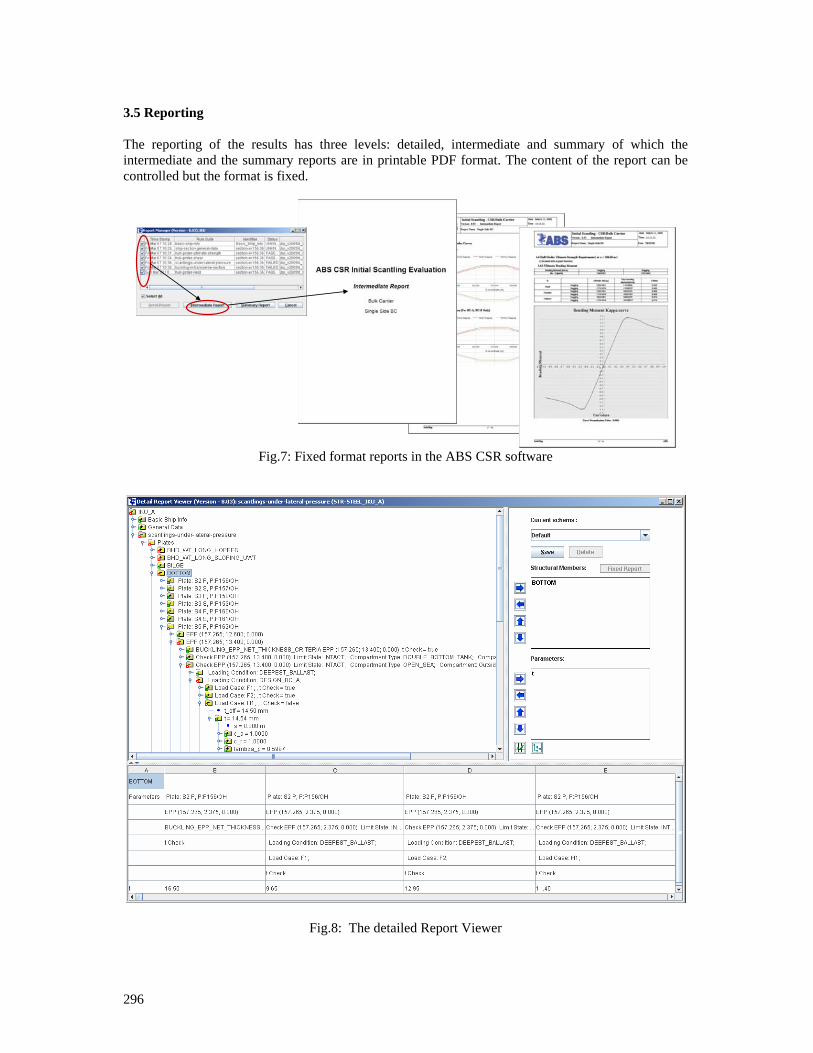
296

3.5 Reporting The reporting of the results has three levels: detailed, intermediate and summary of which the intermediate and the summary reports are in printable PDF format. The content of the report can be controlled but the format is fixed.

Fig.7: Fixed format reports in the ABS CSR software

Fig.8: The detailed Report Viewer

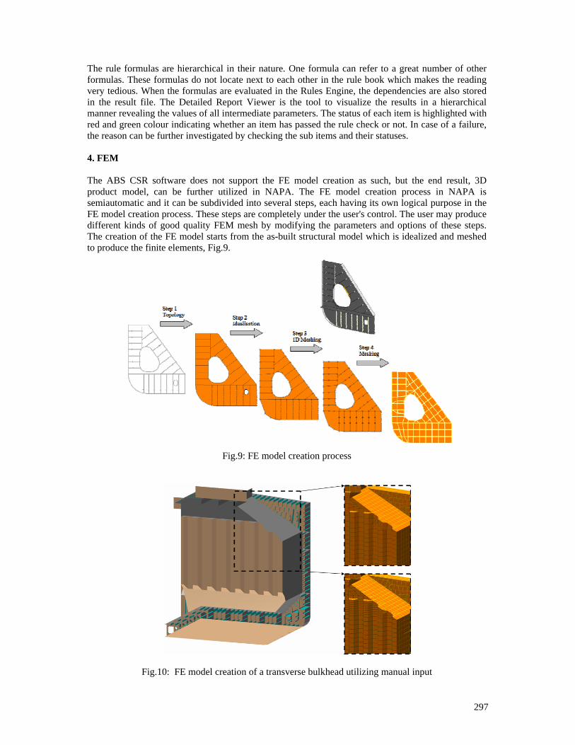
297

The rule formulas are hierarchical in their nature. One formula can refer to a great number of other formulas. These formulas do not locate next to each other in the rule book which makes the reading very tedious. When the formulas are evaluated in the Rules Engine, the dependencies are also stored in the result file. The Detailed Report Viewer is the tool to visualize the results in a hierarchical manner revealing the values of all intermediate parameters. The status of each item is highlighted with red and green colour indicating whether an item has passed the rule check or not. In case of a failure, the reason can be further investigated by checking the sub items and their statuses. 4. FEM The ABS CSR software does not support the FE model creation as such, but the end result, 3D product model, can be further utilized in NAPA. The FE model creation process in NAPA is semiautomatic and it can be subdivided into several steps, each having its own logical purpose in the FE model creation process. These steps are completely under the user's control. The user may produce different kinds of good quality FEM mesh by modifying the parameters and options of these steps. The creation of the FE model starts from the as-built structural model which is idealized and meshed to produce the finite elements, Fig.9.

Fig.9: FE model creation process

Fig.10: FE model creation of a transverse bulkhead utilizing manual input

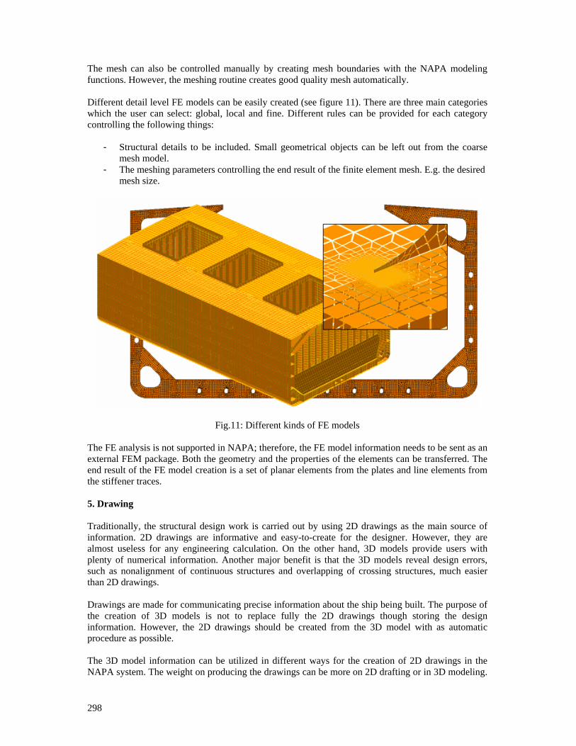
298

The mesh can also be controlled manually by creating mesh boundaries with the NAPA modeling functions. However, the meshing routine creates good quality mesh automatically. Different detail level FE models can be easily created (see figure 11). There are three main categories which the user can select: global, local and fine. Different rules can be provided for each category controlling the following things:

- Structural details to be included. Small geometrical objects can be left out from the coarse mesh model.

- The meshing parameters controlling the end result of the finite element mesh. E.g. the desired mesh size.

Fig.11: Different kinds of FE models The FE analysis is not supported in NAPA; therefore, the FE model information needs to be sent as an external FEM package. Both the geometry and the properties of the elements can be transferred. The end result of the FE model creation is a set of planar elements from the plates and line elements from the stiffener traces. 5. Drawing Traditionally, the structural design work is carried out by using 2D drawings as the main source of information. 2D drawings are informative and easy-to-create for the designer. However, they are almost useless for any engineering calculation. On the other hand, 3D models provide users with plenty of numerical information. Another major benefit is that the 3D models reveal design errors, such as nonalignment of continuous structures and overlapping of crossing structures, much easier than 2D drawings. Drawings are made for communicating precise information about the ship being built. The purpose of the creation of 3D models is not to replace fully the 2D drawings though storing the design information. However, the 2D drawings should be created from the 3D model with as automatic procedure as possible. The 3D model information can be utilized in different ways for the creation of 2D drawings in the NAPA system. The weight on producing the drawings can be more on 2D drafting or in 3D modeling.

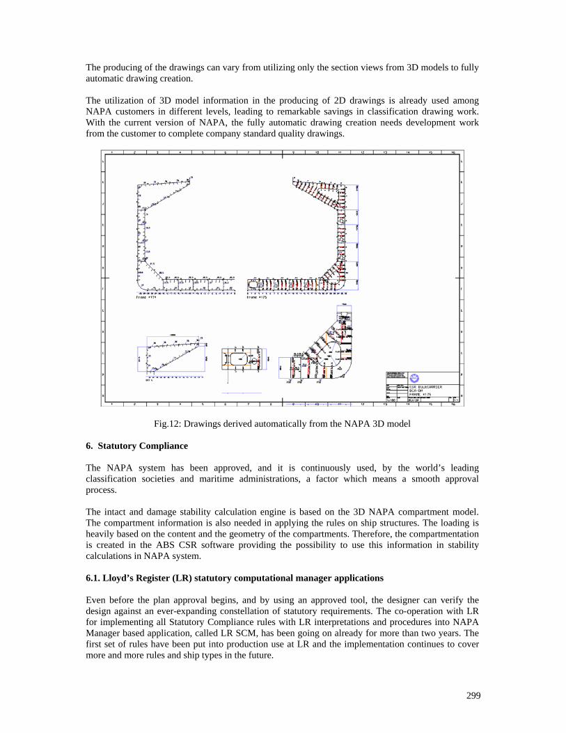
299

The producing of the drawings can vary from utilizing only the section views from 3D models to fully automatic drawing creation. The utilization of 3D model information in the producing of 2D drawings is already used among NAPA customers in different levels, leading to remarkable savings in classification drawing work. With the current version of NAPA, the fully automatic drawing creation needs development work from the customer to complete company standard quality drawings.

Fig.12: Drawings derived automatically from the NAPA 3D model 6. Statutory Compliance The NAPA system has been approved, and it is continuously used, by the world’s leading classification societies and maritime administrations, a factor which means a smooth approval process. The intact and damage stability calculation engine is based on the 3D NAPA compartment model. The compartment information is also needed in applying the rules on ship structures. The loading is heavily based on the content and the geometry of the compartments. Therefore, the compartmentation is created in the ABS CSR software providing the possibility to use this information in stability calculations in NAPA system. 6.1. Lloyd’s Register (LR) statutory computational manager applications Even before the plan approval begins, and by using an approved tool, the designer can verify the design against an ever-expanding constellation of statutory requirements. The co-operation with LR for implementing all Statutory Compliance rules with LR interpretations and procedures into NAPA Manager based application, called LR SCM, has been going on already for more than two years. The first set of rules have been put into production use at LR and the implementation continues to cover more and more rules and ship types in the future.

300

LR SCM provides very convenient tools to make sure that new designs fulfill the rules and regulations reducing the delivery time with higher quality. One of the main benefits is that the LR interpretations are built into the process. 7. Engineering calculation Once the 3D model of structures exists, it provides huge amount of information for different kinds of engineering calculation. When properties are added to the geometrical information of compartments, surfaces, stiffeners and seams, accurate estimations can be made for several purposes. On top of the traditional weight calculation, other exploitation possibilities have been found for 3D model information. A cost model has been developed in the NAPA environment for initial evaluation of the steel production cost. The considered costs are the direct material and labor costs. The cost evaluation method is based on the concept of relative fabrication cost, where labor costs are determined according to welding/cutting lengths and work content of individual production tasks. One of the largest workforce required in the ship building process is painting. The variety of manufactures and the number of coating systems make the estimation work very complex. By matching the information of the purpose of a space to the structures to be coated together with the coating schemes that are applied in particular compartments the total coating requirements can be accurately calculated. A variety of coating systems can be stored in the database and costs can be compared. 8. Optimization The new CSR rules have an impact on the new bulk carrier designs. The requirements for stiffeners and plates have changed and the optimum solution may not be based on the same design configuration as previously. The designs need to be changed causing extra work; therefore, this situation opens a new opportunity to look for the best solutions for bulk carrier structures utilizing the CSR rules and the optimization tools available in NAPA system. An application for general optimization purposes has been developed in the NAPA system. The optimization application has been designed to be used for all kinds of naval architectural tasks and applied in all NAPA subsystems. There are two optimization algorithms in NAPA: a simple linear programming algorithm and a Multi Objective Genetic Algorithm. The latter allows optimization to be made concurrently for multiple objectives. For example, the objectives can include the minimum total cost, the minimum number of structural parts, the minimum weight, the minimum man-hours and the maximum stability. Naturally, the CSR rules can be used as constraints. 9. Interfaces One design system is never able to cover all the needs in the ship design. In a typical major shipyard, a great number of IT systems of various kinds are used to support the design and building process. For this reason, interfaces with the other IT tools are needed. A remarkable saving in time can be achieved and human error can be avoided with well-established interfaces compared to re-entering the design. More than 50 interfaces have been developed over the years to integrate or interface NAPA with external IT systems. The interfaces allow the NAPA system to communicate efficiently with almost all computer software systems used in the shipbuilding industry. System-specific solutions exist to integrate NAPA with NUPAS-CADMATIC, FORAN and Tribon/VM systems. The other option is to use neutral interface formats, such as IGES or DXF, for transferring the design information from NAPA to other systems.

301

10. Conclusions Most of the shipyards and engineering offices are mainly using 2D tools for daily engineering process. However, it has been shown in many practical cases that the use of 3D modeling can reduce time considerably and improve the quality in the ship design process. NAPA and the ABS CSR software provide a comprehensive package for bulk carrier structural design taking full benefit of 3D modeling. The classification work can be fit into the design process by giving a good support to the other design disciplines. References KUUTTI, I. (2007), Integrating rules and practises with early design process, ICCAS 2007, Portsmouth KUUTTI, I.; UPPALA, V. (2005), Practical design approach to cost-optimized ship structures, ICCAS 2005, Pusan UPPALA, V. (2005), Least Cost structural optimisation of a tanker’s cargo area, M.Sc. Thesis, Helsinki University of Technology, Helsinki.

302

Production Simulation Applied to Military Shipbuilding

Carlos Vinícius Malheiros Santos, Brazilian Navy, Rio de Janeiro/Brasil, malheiros@cpn.mar.mil.br

Abstract The paper presents the results from a discrete event production simulation of a Landing Craft Unit by using the CAD/CAM software FORAN and its modules. Model and simulation approach are described, along with the workshop layout for the shipyard considered. The main goal of the paper is to present the engineering qualitative considerations involving military shipbuilding. 1. Introduction The construction of warships involves a series of complex activities. In general, the design of this kind of ship demands a lot of engineering related to anticipation of possible future problems in its production and even in its maintenance and operation. The complexity of warship design and production is mainly associated with two singular features, namely: compactness and high technology applied. The low scale of production of warships frequently forces designers and shipbuilders to find the optimum integration: design vs. shipbuilding process. Sometimes, it is necessary to reorganize the workshop layout in order to reach the best conditions to construct the ship according to modular shipbuilding practices. Sometimes, it is necessary to adjust the design in order to take into account the shipyard facilities. Production simulation is a very useful tool concerning the possibilities of gains in the process of production and as result, cost reduction. In order to achieve an optimum integration design vs. production, it is necessary to model not only the ship but also the shipyard facilities and integrate them into a single 3D animated model. Best results are achieved when this model is linked to other optimization systems. The simulation allows finding the best workshop layout and assembly sequence according to the building strategy of the ship. The present work is limited to present the engineering considerations on an animated model. Here, no consideration is going to be presented on numerical optimization. The paper is organized in three parts:

1. The first part presents considerations involving the building strategy definition of a Landing Craft Unit (LCU). It shows how the workshop layout and its facilities interfere on the design, in which concerns block size definition and its maximum allowable weight.

2. The second part shows how 3D simulation can help us visualizing and deciding on defining an outfitting assembly sequence. From 3D simulation we can have a qualitative idea of how we can avoid assembly interferences and, as a result, how we can profit avoiding reworks associated with assembly tasks.

3. The third part presents an animated 3D model showing the production simulation step by step concerning one specific block from inside the workshop to the slipway.

The Brazilian Navy has adopted the FORAN system as its CAD/CAE tool. Therefore, many engineering decisions were made from a FORAN database analysis considering both graphical and logical contents. The main goal of this paper is to present some engineering qualitative considerations involving military shipbuilding. Due to confidentiality, some information inserted in the presented model was modified from the original case.

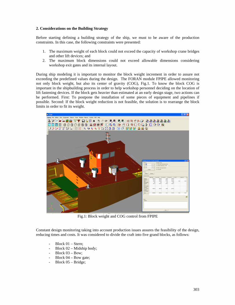
303

2. Considerations on the Building Strategy Before starting defining a building strategy of the ship, we must to be aware of the production constraints. In this case, the following constraints were presented:

1. The maximum weight of each block could not exceed the capacity of workshop crane bridges and other lift devices; and

2. The maximum block dimensions could not exceed allowable dimensions considering workshop exit gates and its internal layout.

During ship modeling it is important to monitor the block weight increment in order to assure not exceeding the predefined values during the design. The FORAN module FPIPE allowed monitoring not only block weight, but also its center of gravity (COG), Fig.1. To know the block COG is important in the shipbuilding process in order to help workshop personnel deciding on the location of lift fastening devices. If the block gets heavier than estimated at an early design stage, two actions can be performed. First: To postpone the installation of some pieces of equipment and pipelines if possible. Second: If the block weight reduction is not feasible, the solution is to rearrange the block limits in order to fit its weight.

Fig.1: Block weight and COG control from FPIPE

Constant design monitoring taking into account production issues assures the feasibility of the design, reducing times and costs. It was considered to divide the craft into five grand blocks, as follows:

- Block 01 – Stern; - Block 02 – Midship body; - Block 03 – Bow; - Block 04 – Bow gate; - Block 05 – Bridge;

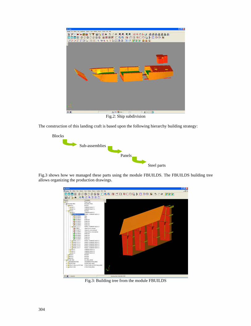
304

Fig.2: Ship subdivision

The construction of this landing craft is based upon the following hierarchy building strategy: Blocks

Sub-assemblies

Panels

Steel parts Fig.3 shows how we managed these parts using the module FBUILDS. The FBUILDS building tree allows organizing the production drawings.

Fig.3: Building tree from the module FBUILDS

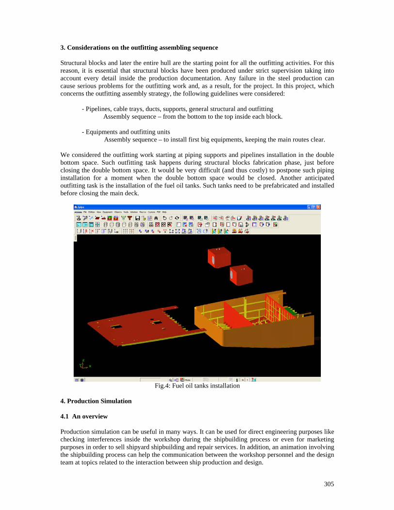
305

3. Considerations on the outfitting assembling sequence Structural blocks and later the entire hull are the starting point for all the outfitting activities. For this reason, it is essential that structural blocks have been produced under strict supervision taking into account every detail inside the production documentation. Any failure in the steel production can cause serious problems for the outfitting work and, as a result, for the project. In this project, which concerns the outfitting assembly strategy, the following guidelines were considered: - Pipelines, cable trays, ducts, supports, general structural and outfitting Assembly sequence – from the bottom to the top inside each block. - Equipments and outfitting units

Assembly sequence – to install first big equipments, keeping the main routes clear. We considered the outfitting work starting at piping supports and pipelines installation in the double bottom space. Such outfitting task happens during structural blocks fabrication phase, just before closing the double bottom space. It would be very difficult (and thus costly) to postpone such piping installation for a moment when the double bottom space would be closed. Another anticipated outfitting task is the installation of the fuel oil tanks. Such tanks need to be prefabricated and installed before closing the main deck.

Fig.4: Fuel oil tanks installation

4. Production Simulation 4.1 An overview Production simulation can be useful in many ways. It can be used for direct engineering purposes like checking interferences inside the workshop during the shipbuilding process or even for marketing purposes in order to sell shipyard shipbuilding and repair services. In addition, an animation involving the shipbuilding process can help the communication between the workshop personnel and the design team at topics related to the interaction between ship production and design.

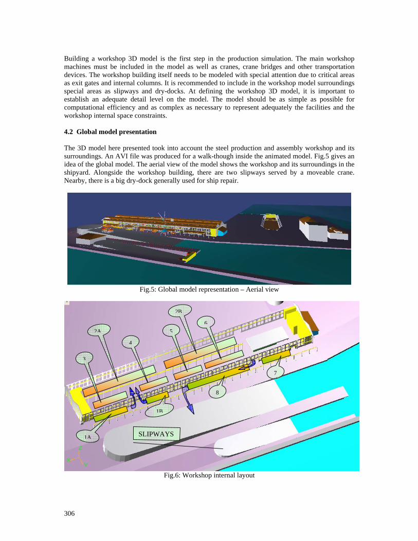
306

Building a workshop 3D model is the first step in the production simulation. The main workshop machines must be included in the model as well as cranes, crane bridges and other transportation devices. The workshop building itself needs to be modeled with special attention due to critical areas as exit gates and internal columns. It is recommended to include in the workshop model surroundings special areas as slipways and dry-docks. At defining the workshop 3D model, it is important to establish an adequate detail level on the model. The model should be as simple as possible for computational efficiency and as complex as necessary to represent adequately the facilities and the workshop internal space constraints. 4.2 Global model presentation The 3D model here presented took into account the steel production and assembly workshop and its surroundings. An AVI file was produced for a walk-though inside the animated model. Fig.5 gives an idea of the global model. The aerial view of the model shows the workshop and its surroundings in the shipyard. Alongside the workshop building, there are two slipways served by a moveable crane. Nearby, there is a big dry-dock generally used for ship repair.

Fig.5: Global model representation – Aerial view

Fig.6: Workshop internal layout

1A

1B

2A

8

3

4

2B

56

7

SLIPWAYS

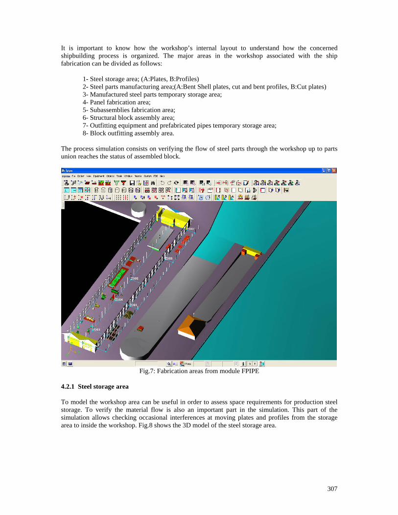
307

It is important to know how the workshop’s internal layout to understand how the concerned shipbuilding process is organized. The major areas in the workshop associated with the ship fabrication can be divided as follows: 1- Steel storage area; (A:Plates, B:Profiles)

2- Steel parts manufacturing area;(A:Bent Shell plates, cut and bent profiles, B:Cut plates) 3- Manufactured steel parts temporary storage area; 4- Panel fabrication area;

5- Subassemblies fabrication area; 6- Structural block assembly area;

7- Outfitting equipment and prefabricated pipes temporary storage area; 8- Block outfitting assembly area.

The process simulation consists on verifying the flow of steel parts through the workshop up to parts union reaches the status of assembled block.

Fig.7: Fabrication areas from module FPIPE

4.2.1 Steel storage area To model the workshop area can be useful in order to assess space requirements for production steel storage. To verify the material flow is also an important part in the simulation. This part of the simulation allows checking occasional interferences at moving plates and profiles from the storage area to inside the workshop. Fig.8 shows the 3D model of the steel storage area.

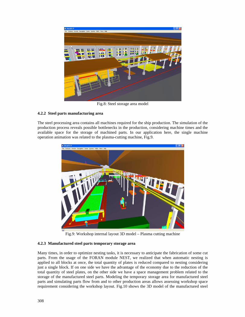
308

Fig.8: Steel storage area model

4.2.2 Steel parts manufacturing area The steel processing area contains all machines required for the ship production. The simulation of the production process reveals possible bottlenecks in the production, considering machine times and the available space for the storage of machined parts. In our application here, the single machine operation animation was related to the plasma-cutting machine, Fig.9.

Fig.9: Workshop internal layout 3D model – Plasma cutting machine

4.2.3 Manufactured steel parts temporary storage area Many times, in order to optimize nesting tasks, it is necessary to anticipate the fabrication of some cut parts. From the usage of the FORAN module NEST, we realized that when automatic nesting is applied to all blocks at once, the total quantity of plates is reduced compared to nesting considering just a single block. If on one side we have the advantage of the economy due to the reduction of the total quantity of steel plates, on the other side we have a space management problem related to the storage of the manufactured steel parts. Modeling the temporary storage area for manufactured steel parts and simulating parts flow from and to other production areas allows assessing workshop space requirement considering the workshop layout. Fig.10 shows the 3D model of the manufactured steel

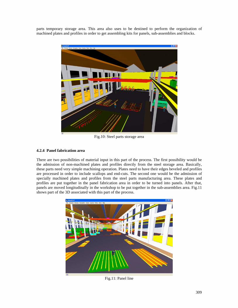
309

parts temporary storage area. This area also uses to be destined to perform the organization of machined plates and profiles in order to get assembling kits for panels, sub-assemblies and blocks.

Fig.10: Steel parts storage area

4.2.4 Panel fabrication area There are two possibilities of material input in this part of the process. The first possibility would be the admission of non-machined plates and profiles directly from the steel storage area. Basically, these parts need very simple machining operation. Plates need to have their edges beveled and profiles are processed in order to include scallops and end-cuts. The second one would be the admission of specially machined plates and profiles from the steel parts manufacturing area. These plates and profiles are put together in the panel fabrication area in order to be turned into panels. After that, panels are moved longitudinally in the workshop to be put together in the sub-assemblies area. Fig.11 shows part of the 3D associated with this part of the process.

Fig.11: Panel line

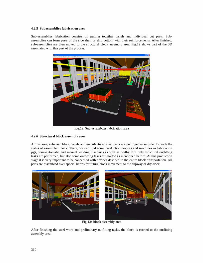
310

4.2.5 Subassemblies fabrication area Sub-assemblies fabrication consists on putting together panels and individual cut parts. Sub-assemblies can form parts of the side shell or ship bottom with their reinforcements. After finished, sub-assemblies are then moved to the structural block assembly area. Fig.12 shows part of the 3D associated with this part of the process.

Fig.12: Sub-assemblies fabrication area

4.2.6 Structural block assembly area At this area, subassemblies, panels and manufactured steel parts are put together in order to reach the status of assembled block. There, we can find some production devices and machines as fabrication jigs, semi-automatic and manual welding machines as well as berths. Not only structural outfitting tasks are performed, but also some outfitting tasks are started as mentioned before. At this production stage it is very important to be concerned with devices destined to the entire block transportation. All parts are assembled over special berths for future block movement to the slipway or dry-dock.

Fig.13: Block assembly area

After finishing the steel work and preliminary outfitting tasks, the block is carried to the outfitting assembly area.

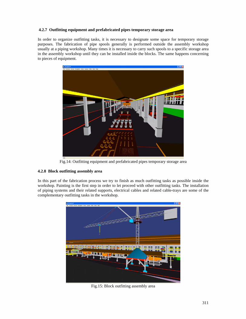
311

4.2.7 Outfitting equipment and prefabricated pipes temporary storage area In order to organize outfitting tasks, it is necessary to designate some space for temporary storage purposes. The fabrication of pipe spools generally is performed outside the assembly workshop usually at a piping workshop. Many times it is necessary to carry such spools to a specific storage area in the assembly workshop until they can be installed inside the blocks. The same happens concerning to pieces of equipment.

Fig.14: Outfitting equipment and prefabricated pipes temporary storage area

4.2.8 Block outfitting assembly area In this part of the fabrication process we try to finish as much outfitting tasks as possible inside the workshop. Painting is the first step in order to let proceed with other outfitting tasks. The installation of piping systems and their related supports, electrical cables and related cable-trays are some of the complementary outfitting tasks in the workshop.

Fig.15: Block outfitting assembly area

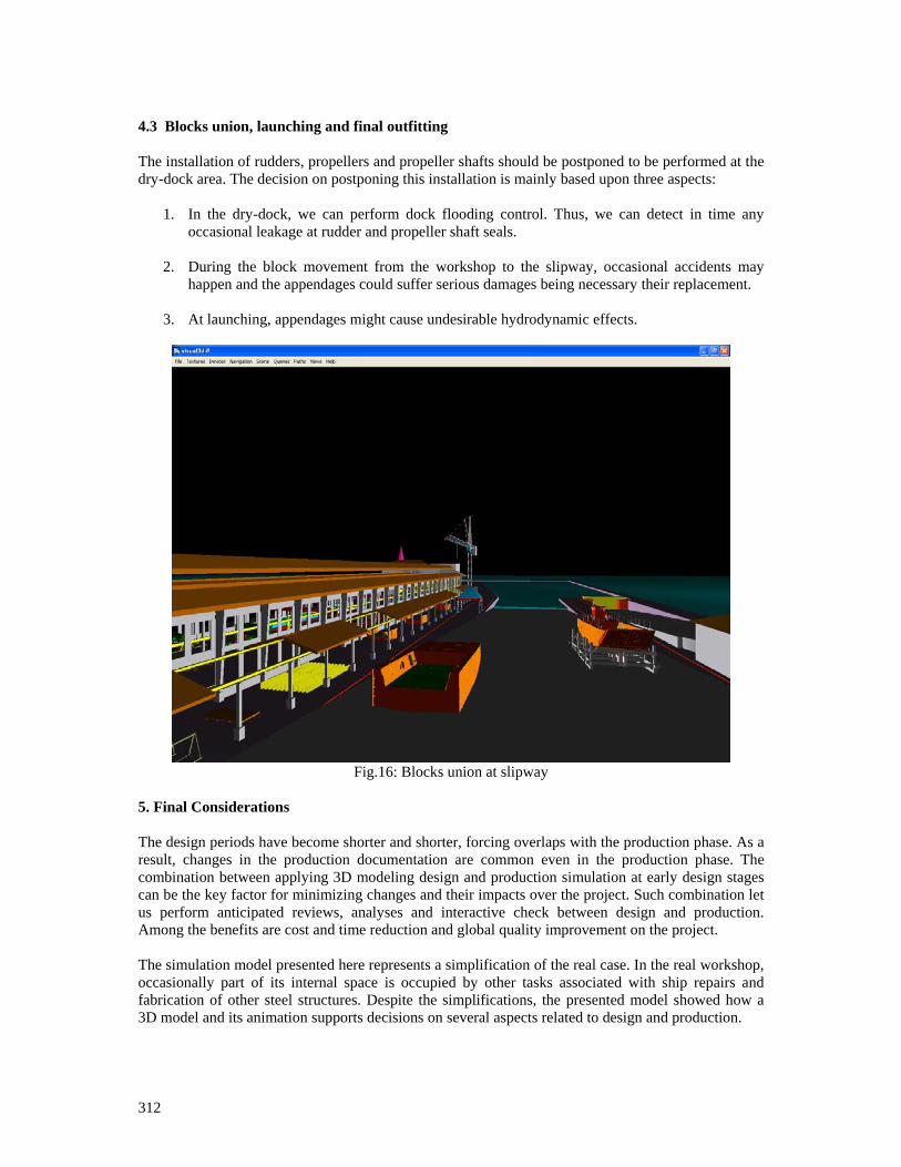
312

4.3 Blocks union, launching and final outfitting The installation of rudders, propellers and propeller shafts should be postponed to be performed at the dry-dock area. The decision on postponing this installation is mainly based upon three aspects:

1. In the dry-dock, we can perform dock flooding control. Thus, we can detect in time any occasional leakage at rudder and propeller shaft seals.

2. During the block movement from the workshop to the slipway, occasional accidents may

happen and the appendages could suffer serious damages being necessary their replacement.

3. At launching, appendages might cause undesirable hydrodynamic effects.

Fig.16: Blocks union at slipway

5. Final Considerations The design periods have become shorter and shorter, forcing overlaps with the production phase. As a result, changes in the production documentation are common even in the production phase. The combination between applying 3D modeling design and production simulation at early design stages can be the key factor for minimizing changes and their impacts over the project. Such combination let us perform anticipated reviews, analyses and interactive check between design and production. Among the benefits are cost and time reduction and global quality improvement on the project. The simulation model presented here represents a simplification of the real case. In the real workshop, occasionally part of its internal space is occupied by other tasks associated with ship repairs and fabrication of other steel structures. Despite the simplifications, the presented model showed how a 3D model and its animation supports decisions on several aspects related to design and production.

313

References ALPHEN, van H.; GUYT, A.; NIENHUIS, U.; WAGT, van der J.C. (2004), Virtual manufacturing in shipbuilding process, European Shipbuilding, Repair and Conversion – The Future, London BAIR, F.; LANGER, Y.; RICHIR, T.; RIGO, P. (2003), Simulation and optimization of a shipbuilding workshop, 2nd Conf. Computer and IT Applications in the Marine Industries (COMPIT), Hamburg DOIG, R.; KAEDING, P. (2007), Possible fields of application of virtual reality in shipbuilding, 6th

Conf. Computer and IT Application in the Maritime Industries (COMPIT), Cortona ERIKSTAD, S.O.; HAGEN, A. (2003), Web-based tendering collaboration in project-centric industries, 2nd Conf. Computer and IT Applications in the Marine Industries (COMPIT), Hamburg KRAUSE, M.; ROLAND, F.; STEINHAUER, D; HEINEMANN, M. (2004), Discrete event simulation: An efficient tool to assist shipyard investment and production planning, J. Ship Production 20/3, pp.176-182 STEINHAUER, D. (2003), The Virtual Shipyard – Simulation in production and logistics at Flensburger, 2nd Conf. Computer and IT Applications in the Marine Industries (COMPIT), Hamburg

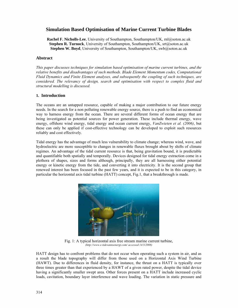
314

Simulation Based Optimisation of Marine Current Turbine Blades

Rachel F. Nicholls-Lee, University of Southampton, Southampton/UK, rnl@soton.ac.uk Stephen R. Turnock, University of Southampton, Southampton/UK, srt@soton.ac.uk Stephen W. Boyd, University of Southampton, Southampton/UK, swb@soton.ac.uk

Abstract

This paper discusses techniques for simulation based optimisation of marine current turbines, and the relative benefits and disadvantages of such methods. Blade Element Momentum codes, Computational Fluid Dynamics and Finite Element analyses, and subsequently the coupling of such techniques, are considered. The relevancy of design, search and optimisation with respect to complex fluid and structural modelling is discussed.

1. Introduction The oceans are an untapped resource, capable of making a major contribution to our future energy needs. In the search for a non polluting renewable energy source, there is a push to find an economical way to harness energy from the ocean. There are several different forms of ocean energy that are being investigated as potential sources for power generation. These include thermal energy, wave energy, offshore wind energy, tidal energy and ocean current energy, VanZwieten et al. (2006), but these can only be applied if cost-effective technology can be developed to exploit such resources reliably and cost effectively. Tidal energy has the advantage of much less vulnerability to climate change; whereas wind, wave, and hydroelectric are more susceptible to changes in renewable fluxes brought about by shifts of climate regimes. An advantage of the tidal current resource is that, being gravitation bound, it is predictable and quantifiable both spatially and temporally. Devices designed for tidal energy extraction come in a plethora of shapes, sizes and forms although, principally, they are all harnessing either potential energy or kinetic energy from the tide, and converting it into electricity. It is the second group that renewed interest has been focused in the past few years, and it is expected to be in this category, in particular the horizontal axis tidal turbine (HATT) concept, Fig.1, that a breakthrough is made.

Fig. 1: A typical horizontal axis free stream marine current turbine, (http://www.e-tidevannsenergi.com/ accessed 14/3/2008)

HATT design has to confront problems that do not occur when operating such a system in air, and as a result the blade topography will differ from those used on a Horizontal Axis Wind Turbine (HAWT). Due to differences in fluid density, for instance, the thrust on a HATT is typically over three times greater than that experienced by a HAWT of a given rated power, despite the tidal device having a significantly smaller swept area. Other forces present on a HATT include increased cyclic loads, cavitation, boundary layer interference and wave loading. The variation in static pressure and

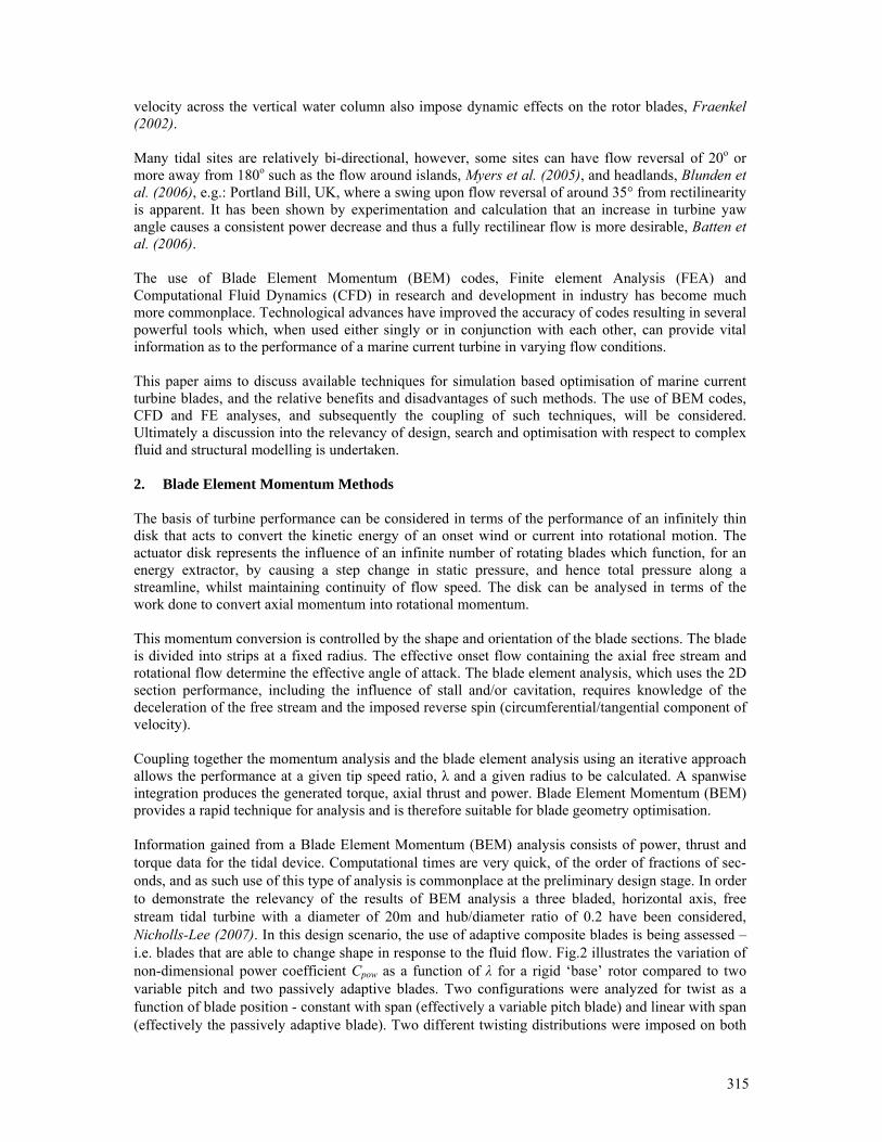
315

velocity across the vertical water column also impose dynamic effects on the rotor blades, Fraenkel (2002). Many tidal sites are relatively bi-directional, however, some sites can have flow reversal of 20o or more away from 180o such as the flow around islands, Myers et al. (2005), and headlands, Blunden et al. (2006), e.g.: Portland Bill, UK, where a swing upon flow reversal of around 35° from rectilinearity is apparent. It has been shown by experimentation and calculation that an increase in turbine yaw angle causes a consistent power decrease and thus a fully rectilinear flow is more desirable, Batten et al. (2006). The use of Blade Element Momentum (BEM) codes, Finite element Analysis (FEA) and Computational Fluid Dynamics (CFD) in research and development in industry has become much more commonplace. Technological advances have improved the accuracy of codes resulting in several powerful tools which, when used either singly or in conjunction with each other, can provide vital information as to the performance of a marine current turbine in varying flow conditions. This paper aims to discuss available techniques for simulation based optimisation of marine current turbine blades, and the relative benefits and disadvantages of such methods. The use of BEM codes, CFD and FE analyses, and subsequently the coupling of such techniques, will be considered. Ultimately a discussion into the relevancy of design, search and optimisation with respect to complex fluid and structural modelling is undertaken. 2. Blade Element Momentum Methods The basis of turbine performance can be considered in terms of the performance of an infinitely thin disk that acts to convert the kinetic energy of an onset wind or current into rotational motion. The actuator disk represents the influence of an infinite number of rotating blades which function, for an energy extractor, by causing a step change in static pressure, and hence total pressure along a streamline, whilst maintaining continuity of flow speed. The disk can be analysed in terms of the work done to convert axial momentum into rotational momentum. This momentum conversion is controlled by the shape and orientation of the blade sections. The blade is divided into strips at a fixed radius. The effective onset flow containing the axial free stream and rotational flow determine the effective angle of attack. The blade element analysis, which uses the 2D section performance, including the influence of stall and/or cavitation, requires knowledge of the deceleration of the free stream and the imposed reverse spin (circumferential/tangential component of velocity). Coupling together the momentum analysis and the blade element analysis using an iterative approach allows the performance at a given tip speed ratio, λ and a given radius to be calculated. A spanwise integration produces the generated torque, axial thrust and power. Blade Element Momentum (BEM) provides a rapid technique for analysis and is therefore suitable for blade geometry optimisation. Information gained from a Blade Element Momentum (BEM) analysis consists of power, thrust and torque data for the tidal device. Computational times are very quick, of the order of fractions of sec-onds, and as such use of this type of analysis is commonplace at the preliminary design stage. In order to demonstrate the relevancy of the results of BEM analysis a three bladed, horizontal axis, free stream tidal turbine with a diameter of 20m and hub/diameter ratio of 0.2 have been considered, Nicholls-Lee (2007). In this design scenario, the use of adaptive composite blades is being assessed – i.e. blades that are able to change shape in response to the fluid flow. Fig.2 illustrates the variation of non-dimensional power coefficient Cpow as a function of λ for a rigid ‘base’ rotor compared to two variable pitch and two passively adaptive blades. Two configurations were analyzed for twist as a function of blade position - constant with span (effectively a variable pitch blade) and linear with span (effectively the passively adaptive blade). Two different twisting distributions were imposed on both

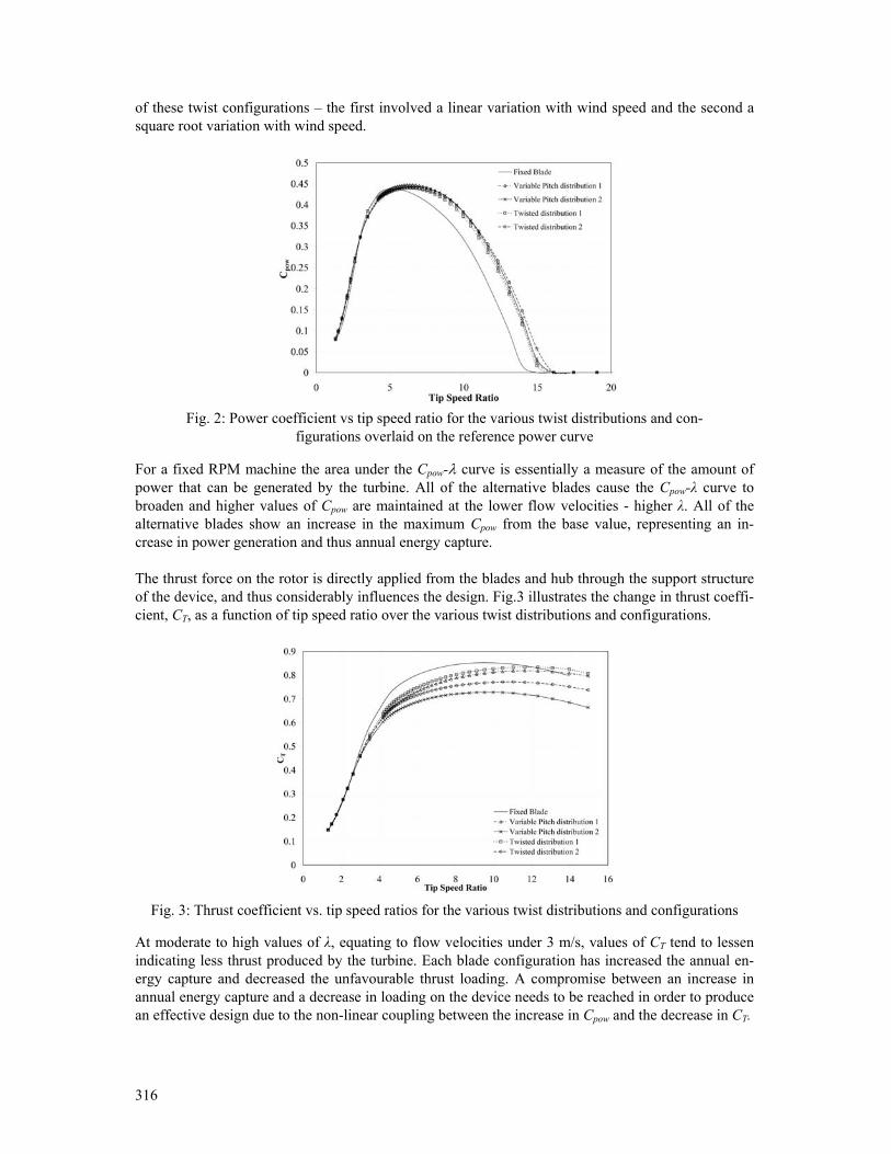
316

of these twist configurations – the first involved a linear variation with wind speed and the second a square root variation with wind speed.

Fig. 2: Power coefficient vs tip speed ratio for the various twist distributions and con-

figurations overlaid on the reference power curve

For a fixed RPM machine the area under the Cpow-λ curve is essentially a measure of the amount of power that can be generated by the turbine. All of the alternative blades cause the Cpow-λ curve to broaden and higher values of Cpow are maintained at the lower flow velocities - higher λ. All of the alternative blades show an increase in the maximum Cpow from the base value, representing an in-crease in power generation and thus annual energy capture. The thrust force on the rotor is directly applied from the blades and hub through the support structure of the device, and thus considerably influences the design. Fig.3 illustrates the change in thrust coeffi-cient, CT, as a function of tip speed ratio over the various twist distributions and configurations.

Fig. 3: Thrust coefficient vs. tip speed ratios for the various twist distributions and configurations

At moderate to high values of λ, equating to flow velocities under 3 m/s, values of CT tend to lessen indicating less thrust produced by the turbine. Each blade configuration has increased the annual en-ergy capture and decreased the unfavourable thrust loading. A compromise between an increase in annual energy capture and a decrease in loading on the device needs to be reached in order to produce an effective design due to the non-linear coupling between the increase in Cpow and the decrease in CT.

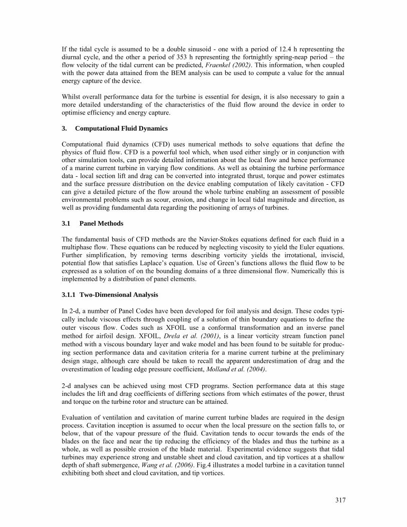
317

If the tidal cycle is assumed to be a double sinusoid - one with a period of 12.4 h representing the diurnal cycle, and the other a period of 353 h representing the fortnightly spring-neap period – the flow velocity of the tidal current can be predicted, Fraenkel (2002). This information, when coupled with the power data attained from the BEM analysis can be used to compute a value for the annual energy capture of the device. Whilst overall performance data for the turbine is essential for design, it is also necessary to gain a more detailed understanding of the characteristics of the fluid flow around the device in order to optimise efficiency and energy capture. 3. Computational Fluid Dynamics Computational fluid dynamics (CFD) uses numerical methods to solve equations that define the physics of fluid flow. CFD is a powerful tool which, when used either singly or in conjunction with other simulation tools, can provide detailed information about the local flow and hence performance of a marine current turbine in varying flow conditions. As well as obtaining the turbine performance data - local section lift and drag can be converted into integrated thrust, torque and power estimates and the surface pressure distribution on the device enabling computation of likely cavitation - CFD can give a detailed picture of the flow around the whole turbine enabling an assessment of possible environmental problems such as scour, erosion, and change in local tidal magnitude and direction, as well as providing fundamental data regarding the positioning of arrays of turbines.

3.1 Panel Methods The fundamental basis of CFD methods are the Navier-Stokes equations defined for each fluid in a multiphase flow. These equations can be reduced by neglecting viscosity to yield the Euler equations. Further simplification, by removing terms describing vorticity yields the irrotational, inviscid, potential flow that satisfies Laplace’s equation. Use of Green’s functions allows the fluid flow to be expressed as a solution of on the bounding domains of a three dimensional flow. Numerically this is implemented by a distribution of panel elements. 3.1.1 Two-Dimensional Analysis In 2-d, a number of Panel Codes have been developed for foil analysis and design. These codes typi-cally include viscous effects through coupling of a solution of thin boundary equations to define the outer viscous flow. Codes such as XFOIL use a conformal transformation and an inverse panel method for airfoil design. XFOIL, Drela et al. (2001), is a linear vorticity stream function panel method with a viscous boundary layer and wake model and has been found to be suitable for produc-ing section performance data and cavitation criteria for a marine current turbine at the preliminary design stage, although care should be taken to recall the apparent underestimation of drag and the overestimation of leading edge pressure coefficient, Molland et al. (2004). 2-d analyses can be achieved using most CFD programs. Section performance data at this stage includes the lift and drag coefficients of differing sections from which estimates of the power, thrust and torque on the turbine rotor and structure can be attained. Evaluation of ventilation and cavitation of marine current turbine blades are required in the design process. Cavitation inception is assumed to occur when the local pressure on the section falls to, or below, that of the vapour pressure of the fluid. Cavitation tends to occur towards the ends of the blades on the face and near the tip reducing the efficiency of the blades and thus the turbine as a whole, as well as possible erosion of the blade material. Experimental evidence suggests that tidal turbines may experience strong and unstable sheet and cloud cavitation, and tip vortices at a shallow depth of shaft submergence, Wang et al. (2006). Fig.4 illustrates a model turbine in a cavitation tunnel exhibiting both sheet and cloud cavitation, and tip vortices.

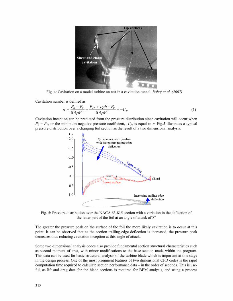
318

Fig. 4: Cavitation on a model turbine on test in a cavitation tunnel, Bahaj et al. (2007)

Cavitation number is defined as:

PVATVO C

VPghP

VPP

−=−+

=−

= 22 5.05.0 ρρ

ρσ (1)

Cavitation inception can be predicted from the pressure distribution since cavitation will occur when PL = PV, or the minimum negative pressure coefficient, -CP, is equal to σ. Fig.5 illustrates a typical pressure distribution over a changing foil section as the result of a two dimensional analysis.

Fig. 5: Pressure distribution over the NACA 63-815 section with a variation in the deflection of

the latter part of the foil at an angle of attack of 8°

The greater the pressure peak on the surface of the foil the more likely cavitation is to occur at this point. It can be observed that as the section trailing edge deflection is increased, the pressure peak decreases thus reducing cavitation inception at this angle of attack. Some two dimensional analysis codes also provide fundamental section structural characteristics such as second moment of area, with minor modifications to the base section made within the program. This data can be used for basic structural analysis of the turbine blade which is important at this stage in the design process. One of the most prominent features of two dimensional CFD codes is the rapid computation time required to calculate section performance data – in the order of seconds. This is use-ful, as lift and drag data for the blade sections is required for BEM analysis, and using a process

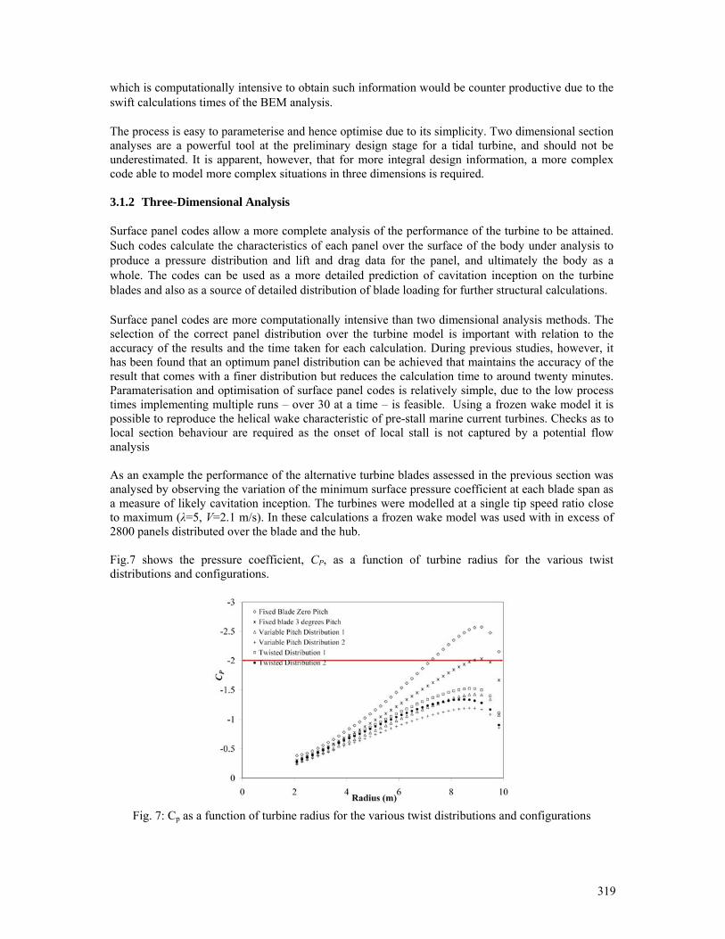
319

which is computationally intensive to obtain such information would be counter productive due to the swift calculations times of the BEM analysis. The process is easy to parameterise and hence optimise due to its simplicity. Two dimensional section analyses are a powerful tool at the preliminary design stage for a tidal turbine, and should not be underestimated. It is apparent, however, that for more integral design information, a more complex code able to model more complex situations in three dimensions is required. 3.1.2 Three-Dimensional Analysis Surface panel codes allow a more complete analysis of the performance of the turbine to be attained. Such codes calculate the characteristics of each panel over the surface of the body under analysis to produce a pressure distribution and lift and drag data for the panel, and ultimately the body as a whole. The codes can be used as a more detailed prediction of cavitation inception on the turbine blades and also as a source of detailed distribution of blade loading for further structural calculations. Surface panel codes are more computationally intensive than two dimensional analysis methods. The selection of the correct panel distribution over the turbine model is important with relation to the accuracy of the results and the time taken for each calculation. During previous studies, however, it has been found that an optimum panel distribution can be achieved that maintains the accuracy of the result that comes with a finer distribution but reduces the calculation time to around twenty minutes. Paramaterisation and optimisation of surface panel codes is relatively simple, due to the low process times implementing multiple runs – over 30 at a time – is feasible. Using a frozen wake model it is possible to reproduce the helical wake characteristic of pre-stall marine current turbines. Checks as to local section behaviour are required as the onset of local stall is not captured by a potential flow analysis As an example the performance of the alternative turbine blades assessed in the previous section was analysed by observing the variation of the minimum surface pressure coefficient at each blade span as a measure of likely cavitation inception. The turbines were modelled at a single tip speed ratio close to maximum (λ=5, V=2.1 m/s). In these calculations a frozen wake model was used with in excess of 2800 panels distributed over the blade and the hub. Fig.7 shows the pressure coefficient, CP, as a function of turbine radius for the various twist distributions and configurations.

Fig. 7: Cp as a function of turbine radius for the various twist distributions and configurations

320

At this flow velocity, the cavitation number is approximately 2; indicating that cavitation inception will occur on areas of the blade where the pressure coefficient is less than -2. Both of the fixed blades exhibit a maximum negative CP of less than -2, and thus these blades will cavitate at this flow velocity. Imposing a twist configuration on the blade causes the CP over the outer two thirds of the blade to decrease significantly, and therefore the likelihood of cavitation has been significantly reduced. Although it is possible to predict cavitation inception, once cavitation has occurred the use of surface panel techniques which include the presence of cavitation regions requires significant use of empirical information to define cavitation bubble shape, and analysis often becomes unstable unsuited to automated optimisation. Such codes also struggle to capture severe changes in the flow regime, i.e. separation, stagnation and recirculation, even when using coupled boundary layer approaches. It is therefore apparent that more advanced numerical simulation of the area around the turbine is necessary for a full design. 3.2 Reynolds Average Navier Stokes Equations The Reynolds-averaged Navier-Stokes (RANS) equations are time-averaged equations of motion for fluid flow. They are primarily used while dealing with turbulent flows. These equations can be used with approximations based on knowledge of the properties of flow turbulence to give approximate averaged solutions to the Navier-Stokes equations. The nature of RANS equations leads to the need for complex domain discretisation schemes as well as complex modelling with large numbers of elements or cells. This often leads to complex mesh structures on which the equations must be solved, and building such meshes is time consuming. Turbulent flows contain many unsteady eddies covering a range of sizes and time scales. The RANS equations are averaged in such a manner that unsteady structures of small sizes in space and time are eliminated and become expressed by their mean effects on the flow through the Reynolds, or turbulent, stresses. These stresses need to be interpreted in terms of calculated time-averaged variables in order to close the system of equations thereby rendering them solvable. This requires the construction of a mathematical model known as a turbulence model, involving additional correlations for the unknown quantities, Atkins (2003). 3.2.1 Turbulence Models Most flows of practical engineering interest are turbulent, and the turbulent mixing of the flow then usually dominates the behaviour of the fluid. The turbulent nature of the flow plays a crucial part in the determination of many relevant engineering parameters, such as frictional drag, flow separation, transition from laminar to turbulent flow, thickness of boundary layers, extent of secondary flows, and spreading of jets and wakes. It is possible to solve the Navier Stokes Equations directly without any turbulence model, using Direct Numerical Simulation (DNS). This requires that the whole range of spatial and temporal scales of the turbulence must be resolved, however this approach is extremely computationally expensive for com-plex problems, hence the need for turbulence models to represent the smallest scales of fluid motion. The simplest turbulence modelling approach rests on the concept of a turbulent viscosity. Such mod-els are widely used for simple shear flows such as attached boundary layers, jets and wakes. The one-equation models attempt to improve on the zero-equation models by using an eddy viscosity that no longer depends purely on the local flow conditions but takes into account the flow history, Atkins (2003). Two-equation turbulence models are frequently used. Models like the k-ε model, Launder (1974), and

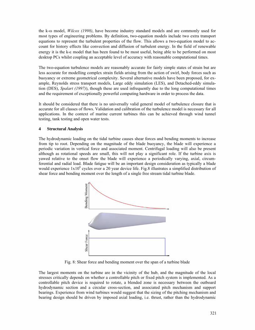
321

the k-ω model, Wilcox (1998), have become industry standard models and are commonly used for most types of engineering problems. By definition, two-equation models include two extra transport equations to represent the turbulent properties of the flow. This allows a two-equation model to ac-count for history effects like convection and diffusion of turbulent energy. In the field of renewable energy it is the k-ε model that has been found to be most useful, being able to be performed on most desktop PCs whilst coupling an acceptable level of accuracy with reasonable computational times. The two-equation turbulence models are reasonably accurate for fairly simple states of strain but are less accurate for modelling complex strain fields arising from the action of swirl, body forces such as buoyancy or extreme geometrical complexity. Several alternative models have been proposed, for ex-ample, Reynolds stress transport models, Large eddy simulation (LES), and Detached-eddy simula-tion (DES), Spalart (1997)), though these are used infrequently due to the long computational times and the requirement of exceptionally powerful computing hardware in order to process the data. It should be considered that there is no universally valid general model of turbulence closure that is accurate for all classes of flows. Validation and calibration of the turbulence model is necessary for all applications. In the context of marine current turbines this can be achieved through wind tunnel testing, tank testing and open water tests. 4 Structural Analysis The hydrodynamic loading on the tidal turbine causes shear forces and bending moments to increase from tip to root. Depending on the magnitude of the blade buoyancy, the blade will experience a periodic variation in vertical force and associated moment. Centrifugal loading will also be present although as rotational speeds are small, this will not play a significant role. If the turbine axis is yawed relative to the onset flow the blade will experience a periodically varying, axial, circum-ferential and radial load. Blade fatigue will be an important design consideration as typically a blade would experience 1x108 cycles over a 20 year device life. Fig.8 illustrates a simplified distribution of shear force and bending moment over the length of a single free stream tidal turbine blade.

Fig. 8: Shear force and bending moment over the span of a turbine blade

The largest moments on the turbine are in the vicinity of the hub, and the magnitude of the local stresses critically depends on whether a controllable pitch or fixed pitch system is implemented. As a controllable pitch device is required to rotate, a blended zone is necessary between the outboard hydrodynamic section and a circular cross-section, and associated pitch mechanism and support bearings. Experience from wind turbines would suggest that the sizing of the pitching mechanism and bearing design should be driven by imposed axial loading, i.e. thrust, rather than the hydrodynamic

322

moment about the blade generator. The cross-section of the blade is not equally thick in all directions and thus the direction of the loading will be of great importance; this, relative to the cross-section, will depend on the direction of the net force, and on the angle of the section, both of which vary along the span of a turbine blade. The direction in which the blade will bend is dependent upon the direction of the net loading and the second moment of area of the blade section. With a fixed pitch blade the loading scenario is much less complex, due to the lack of machinery required in the hub which is present in the variable pitch blades. A simple structural analysis is sufficient to give a basic understanding of the loads encountered at this point. The subject of Finite Element Analysis (FEA) has been used in the field of engineering for over half a century and has been continuously developed throughout this time. It has only been in the last few decades, with improvements in computational efficiency and power, that use of FEA has become more commonplace. FEA is based on subdividing the structure under investigation into elements, each element being of simpler geometry and thus easier to analyse than the whole structure. In essence, the complex solution is approximated by a model consisting of piecewise-continuous simple solutions, Cook et al. (1989). Various different types of code exist, although these tend to differ with respect to the discipline under examination (i.e. structural, thermal, electromagnetic and so forth) with additions to the equations, rather than in the mathematical formulations on which the code is based. The main advantage of this type of analysis is that complex design forms can be studied whereby an analytical solution is either not possible or not feasible. It is possible to undertake dynamic analyses, in order to simulate complex problems such as unsteady loading and time varying excitations. At the preliminary design stage, uncomplicated FE analyses can be carried out by imposing a point load the tip of the blade, and subsequently a uniformly distributed load over the length of the beam. This will ensure that the structure can be assumed to be a good basis from which improvements can be made. For more accurate modelling, the pressure distribution over the blade due to the fluid flowing over it can be attained using CFD and then input into the FEA code. The more complex the loading, and hence the model, becomes the more computationally intensive the problem. However, the structural mesh will differ considerably from a fluid mesh, and is likely to be simpler and therefore use less time to create. As for any body, the tidal turbine is subjected to pressure form the surrounding fluid. In addition to this it is a lifting body with rotational motion; hence it is subjected to further loading because of the lift it produces, and because of its rotation. Due to the complex loading scenario experienced by a tidal turbine, knowledge of the hydroelastic behaviour of the blades, hub, nacelle, and also the support structure under this regime could lead to a more thorough understanding of structural constraints and how performance of the turbine could be improved in order to bring the efficiency of the device ever closer to the Betz limit of 0.593. 5 Fluid Structure Interactions Fluid-structure interactions (FSI), that is interactions of some movable or deformable structure with an internal or surrounding fluid flow, are among the most important and, with respect to both modelling and computational issues, the most challenging multi-physics problems.

FSI occurs when a fluid interacts with a solid structure, exerting pressure that may cause deformation in the structure and, thus, alter the flow of the fluid itself. If a problem involving structure flexure, or possibly adaptive materials is to be analysed it is highly beneficial to couple both the fluid dynamics and the structural analysis programs to produce iterative solutions for complex problems. In the context of a tidal turbine blade, the flow interaction and flow field from the components of the device are complex, and produce a unique time-varying load distribution. Coincidentally, the complex

323

shapes and joining of the individual parts of the turbine, creates a highly non-linear stress distribution. Due to these complexities the hydrodynamic performance of the turbine cannot be determined from the application of foil theory, nor can the structural solution be gained from standard closed-form analytical solutions. In order to gain an insight into the hydroelastic behaviour of a horizontal axis tidal turbine, practical experimentation may be used to quantify and visualise the response of the device to a multitude of environments. Experimental investigations, however, are extremely costly, time consuming and difficult to design in order to gain credible and useful information from the test device. Alternatively, computational investigations have the ability to be much less expensive, with regards to both time and money – although there is a propensity both of these variables to increase with an increase in accuracy of results. It is therefore necessary to use both processes, the computational methods for the relative speed and ease of use, and the experimental work to validate the numerical modelling. There are three methods of joint fluid structural modelling in the time domain. These involve solving the governing equations in a coupled, an uncoupled or an integrated manner. Uncoupled simulations are computationally inexpensive but are rarely used as they are limited to small perturbations and minimal non-linearites. For non-linear flows and large perturbations a fully coupled or integrated method should be used. Integrated methods solve the fluid and structural equations simultaneously, while coupled methods solve the equations separately but in an iterative manner, Turnock and Wright (2000). Coupled methods are subdivided into strongly or fully coupled (single-domain) and loosely coupled (independent domains) approaches. The loosely coupled methodologies can be either integrated or modular. The integrated scheme modifies the source code of either the CFD or the FEA programs to include the coupling schemes; whilst the modular approach leaves both the FEA and CFD codes untouched, effectively making use of a “black box” which can manipulate the output of the CFD and/or the FEA and feed it into the other program respectively, thus allowing for a variety of software to be used. The key difficulty is ensuring the conservation of energy between frames of reference, from the kinetic energy of the fluid flow to the potential energy contained within the stress field of the deformed blade. The main advantage of the loosely coupled approach is that advanced purpose designed codes can be used for the tackling of specific problems. In additions to this the two domains are discretised to better suit the problem, as the CFD mesh will tend to require greater refinement in different areas of the structure than the FEA mesh, and vice versa. This ultimately leads to the main problem with loosely coupled analyses, the need to find a method to accurately pass boundary information from one simulation to the other. For the analysis of horizontal axis tidal turbines, a loosely coupled, modular approach is likely to be most successful. With such an approach, ultimately it is immaterial which CFD and FEA programs are used, as the pre and post processing of results is carried out in the “black box” phase of the simulation, and this may be tailored to suit any combination of software. Similar methods to this have been shown to be successful for propeller design by both Turnock and Wright(2000) and Casagrande (2000), and as such the concept of the use of a loosely coupled modular approach for marine structure analysis does not need to be proven, but can be modified in order to operate effectively for a tidal turbine. To carry out high-quality trade-off studies, designers must synthesize and analyze alternative design configurations. To do this cost effectively and quickly requires tools that support automation, evolu-tions and innovation. Automation stems mainly from the desire to reduce the high costs associated with professional manpower and, at the same time, to reduce design cycle times. A variety of tech-nologies are coming together in providing a new class of tool that automatically optimizes designs based on multiple variables. Mechanical design synthesis is a next-generation solution combining op-timization technologies with CAE simulation methods and parametric CAD into an integrated solu-

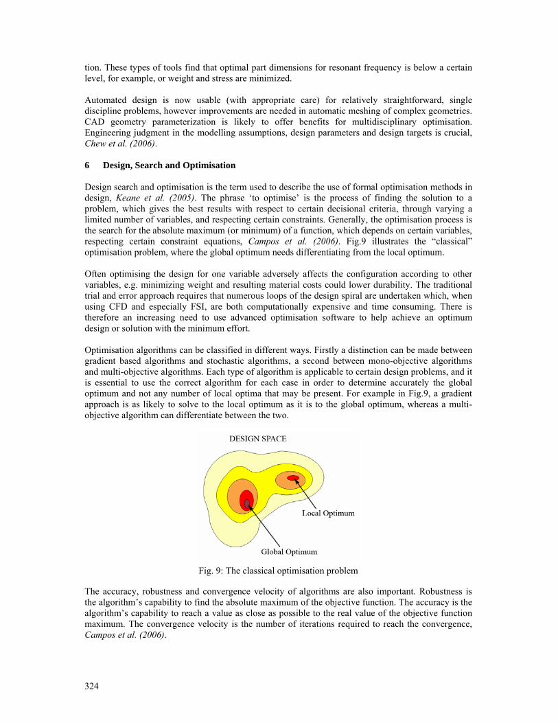
324

tion. These types of tools find that optimal part dimensions for resonant frequency is below a certain level, for example, or weight and stress are minimized. Automated design is now usable (with appropriate care) for relatively straightforward, single discipline problems, however improvements are needed in automatic meshing of complex geometries. CAD geometry parameterization is likely to offer benefits for multidisciplinary optimisation. Engineering judgment in the modelling assumptions, design parameters and design targets is crucial, Chew et al. (2006). 6 Design, Search and Optimisation Design search and optimisation is the term used to describe the use of formal optimisation methods in design, Keane et al. (2005). The phrase ‘to optimise’ is the process of finding the solution to a problem, which gives the best results with respect to certain decisional criteria, through varying a limited number of variables, and respecting certain constraints. Generally, the optimisation process is the search for the absolute maximum (or minimum) of a function, which depends on certain variables, respecting certain constraint equations, Campos et al. (2006). Fig.9 illustrates the “classical” optimisation problem, where the global optimum needs differentiating from the local optimum. Often optimising the design for one variable adversely affects the configuration according to other variables, e.g. minimizing weight and resulting material costs could lower durability. The traditional trial and error approach requires that numerous loops of the design spiral are undertaken which, when using CFD and especially FSI, are both computationally expensive and time consuming. There is therefore an increasing need to use advanced optimisation software to help achieve an optimum design or solution with the minimum effort. Optimisation algorithms can be classified in different ways. Firstly a distinction can be made between gradient based algorithms and stochastic algorithms, a second between mono-objective algorithms and multi-objective algorithms. Each type of algorithm is applicable to certain design problems, and it is essential to use the correct algorithm for each case in order to determine accurately the global optimum and not any number of local optima that may be present. For example in Fig.9, a gradient approach is as likely to solve to the local optimum as it is to the global optimum, whereas a multi-objective algorithm can differentiate between the two.

Fig. 9: The classical optimisation problem

The accuracy, robustness and convergence velocity of algorithms are also important. Robustness is the algorithm’s capability to find the absolute maximum of the objective function. The accuracy is the algorithm’s capability to reach a value as close as possible to the real value of the objective function maximum. The convergence velocity is the number of iterations required to reach the convergence, Campos et al. (2006).

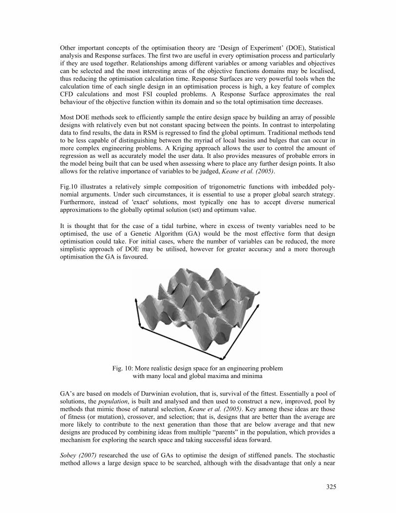
325

Other important concepts of the optimisation theory are ‘Design of Experiment’ (DOE), Statistical analysis and Response surfaces. The first two are useful in every optimisation process and particularly if they are used together. Relationships among different variables or among variables and objectives can be selected and the most interesting areas of the objective functions domains may be localised, thus reducing the optimisation calculation time. Response Surfaces are very powerful tools when the calculation time of each single design in an optimisation process is high, a key feature of complex CFD calculations and most FSI coupled problems. A Response Surface approximates the real behaviour of the objective function within its domain and so the total optimisation time decreases. Most DOE methods seek to efficiently sample the entire design space by building an array of possible designs with relatively even but not constant spacing between the points. In contrast to interpolating data to find results, the data in RSM is regressed to find the global optimum. Traditional methods tend to be less capable of distinguishing between the myriad of local basins and bulges that can occur in more complex engineering problems. A Kriging approach allows the user to control the amount of regression as well as accurately model the user data. It also provides measures of probable errors in the model being built that can be used when assessing where to place any further design points. It also allows for the relative importance of variables to be judged, Keane et al. (2005). Fig.10 illustrates a relatively simple composition of trigonometric functions with imbedded poly-nomial arguments. Under such circumstances, it is essential to use a proper global search strategy. Furthermore, instead of 'exact' solutions, most typically one has to accept diverse numerical approximations to the globally optimal solution (set) and optimum value. It is thought that for the case of a tidal turbine, where in excess of twenty variables need to be optimised, the use of a Genetic Algorithm (GA) would be the most effective form that design optimisation could take. For initial cases, where the number of variables can be reduced, the more simplistic approach of DOE may be utilised, however for greater accuracy and a more thorough optimisation the GA is favoured.

Fig. 10: More realistic design space for an engineering problem

with many local and global maxima and minima

GA’s are based on models of Darwinian evolution, that is, survival of the fittest. Essentially a pool of solutions, the population, is built and analysed and then used to construct a new, improved, pool by methods that mimic those of natural selection, Keane et al. (2005). Key among these ideas are those of fitness (or mutation), crossover, and selection; that is, designs that are better than the average are more likely to contribute to the next generation than those that are below average and that new designs are produced by combining ideas from multiple “parents” in the population, which provides a mechanism for exploring the search space and taking successful ideas forward. Sobey (2007) researched the use of GAs to optimise the design of stiffened panels. The stochastic method allows a large design space to be searched, although with the disadvantage that only a near

326

optimum result is sometimes found. Through the use of combining the elite results from a given generation and taking these on to the next it is ensured that the algorithm will evolve its way towards the optimum result. The level of mutations and crossover can be changed to increase the spread of the search space, or decreased so that the optimum value can be found as quickly as possible. It is the use of mutation that ensures that the GA will not search a local optimum, but will gradually investigate results from the entire search space to find the global optimum. The GA has developed by Sobey (2007) is still undergoing further refinement. It is intended that, with some minor alteration, this algorithm be tried and assessed for use in the optimisation of horizontal axis tidal turbine blade design. 7 Overview This section illustrates the manner in which the computational analysis methods discussed previously in the paper can be utilised with regards to the optimisation of a free stream marine current turbine. Expected timings are based on calculation times on a typical desktop PC workstation.

1) Using previous work and background knowledge choose initial airfoil sections for the blade with a selection based on an expected thickness/chord variation form root to tip.

2) Analyse these sections using a two dimensional coupled panel code in order to determine which of these sections performs most efficiently and obtain lift and drag data for the foil for use with BEM analysis – 5 minutes

3) Carry out a BEM analysis, using an automated process to optimise the performance turbine with regards to number of blades, diameter, pitch, and chord and twist distribution, for a range of tip speed ratio etc. – undertaking approximately 32,000 blade shape variations, the complete Cpow-λ performance can be determined in around 10 minutes.

4) For the best case for design Cpow use a three dimensional panel code at a single tip speed ratio to check the likelihood of cavitation inception – 10 minutes.

5) Use a two dimensional panel code to make modifications to the blade tip sections. Repeat steps 2-4 as necessary.

6) Carry out simple FEA with the blade under a point load at the tip and subsequently a uniformly distributed load in order to assess the structural stability of the initial device – 1 hour. Steps 2-4 may need to be carried out again in order to meet initial structural constraints.

7) Undertake steady RANS simulation with around 1.5 million cells in order to check the flow effects due to the presence of a three dimensional hub, the behaviour of the blade tips, and check possibility of cavitation inception – 6 hours.

8) Detailed design of the internal blade structure. More thorough FEA simulation of the blade, using the surface pressure data calculated during the CFD simulation for the load distribution. Repeat until blade is determined to be sufficiently strong.

9) Couple surface panel and FE analyses to run through a series of spatially varying inflow fields with variations due to waves, support structure, boundary layer, proximity of the free surface etc. Identify fatigue loadings present in the design.

10) Final design check using a full unsteady RANS calculation of the design running beneath the free surface within the actual bathymetry of a proposed channel site at the maximum spring peak current.

At stages 8 and 9 it could be beneficial to make use of a GA to optimise the design for a number of variables as calculations times at this point are substantial. 8 Conclusions With the need for renewable energy sources becoming ever more important, a focus is being brought to predictable and quantifiable marine sources such as marine currents, or tides. The design and opti-

327

misation of tidal energy extraction devices is paramount, to ensure they are rugged, robust and reliable and yet effective at capturing maximum available energy in the hostile sub sea environment. CFD is a powerful tool which, when used correctly, can provide valuable data regarding the perform-ance of such devices. It is important not to underestimate the use of simpler CFD techniques, such as panel codes, at the preliminary design stage where an insight into cavitation characteristics and energy extraction can be achieved, justifying the need for further work. At a more advanced design stage RANS solvers are required to model the complex flow situations occurring around the turbines. Ulti-mately coupled fluid-structural analysis is required to better understand how the flow affects the struc-tural integrity of both the rotor and supporting structure. Structural simulation is essential in order to sound out stress concentrations, determine wall thick-nesses, and areas that are susceptible to fatigue. FSI is particularly useful to both analyse and visualise how the blade will respond to the complex varying loads imposed upon it both through vertical and horizontal pressure and velocity fluctuations. Design, search and optimisation play a key role in the use of computationally expensive processes such as CFD and FEA, and especially FSI. The proper use of optimisation algorithms could signifi-cantly reduce the number of design iterations required, producing optimal answers without the ex-pense of huge amounts of both computational and human time. An example of the manner in which all of the computational simulation methods can be brought to together to optimise a free stream, horizontal axis, marine current turbine has been suggested. Whilst all the methods discussed in this paper require validation, be it through use of wind tunnel tests, towing tank data or open ocean experiments, ultimately the use of CFD, FSI and design, search and optimisation could cut design process times and allow more effective selection of model scale devices as well as greater confidence in the effectiveness of the blade structural design. Acknowledgements The authors gratefully acknowledge the support of the School of Engineering Sciences for part funding the PhD studentship of Ms. Nicholls-Lee. References ATKINS, W. (2003), MARNET best practice guidelines for marine applications of computational fluid dynamics, MARNET BAHAJ, A.S.; MOLLAND, A.F.; CHAPLIN, J.R.; BATTEN, W.M.J. (2007), Power and thrust measurements of marine current turbines under various hydrodynamic flow conditions in a cavitation tunnel and a towing tank, J. Renewable Energy 32(3): pp.407-426 BATTEN, W.M.J.; BAHAJ, A.S.; MOLLAND, A.F.; BLUNDEN, L.S. (2006), Yawed performance of horizontal axis marine current turbines, in conference on renewable energy in island maritime cli-mate, Dublin BLUNDEN, L.S.; BAHAJ, A.S. (2006), Initial evaluation of tidal stream energy resources at Port-landBbill, UK, J. Renewable Energy 31, pp. 121-132 CAMPOS, F.; WESTON, S.; SCHUMACHER, T. (2006), Automatic optimisation of CFD engineered designs, Automated Design & Optimisation Techniques using CFD, IMechE, London

328

CASAGRANDE, A. (2000), Coupled dynamic fluid structural model of a propeller at one time step, in school of engineering sciences, University of Southampton CHEW, J.; DOHERTY, J.; GILLIAN, M.; HILLS, N. (2006), Practical applications of automated design and optimisation techniques using CFD, Automated Design & Optimisation Techniques Using CFD, IMechE, London COOK, R.; MALKUS, D.; PLESHA, M. (1989), Concepts and applications of finite element analysis, 3rd Edition, John Wiley & Sons DRELA, M.; YOUNGREN, H. (2001), XFOIL 6.94 User Guide DTI (2003), Energy from tidal barrages technology route map, Department of Trade and Industry FRAENKEL, P.L. (2002), Power from marine currents, J. Power and Energy 216(1), pp.1-14 KEANE, A.; NAIR P. (2005), Computational approaches for aerospace design the pursuit of excel-lence, Chichester: John Wiley & Sons, Ltd. LAUNDER, B.; SPALDING, D. (1974), The numerical computation of turbulent flows, Computer Methods in Applied Mechanics and Engineering 3, pp.269-289 MOLLAND, A.F.; BAHAJ, A.S.; CHAPLIN, J.R.; BATTEN, W.M.J (2004), Measurements and predictions of forces, pressures and cavitation on 2-d sections suitable for marine current turbines, Proc. Institute of Mechanical Engineers 218(M), pp.127-138 MYERS, L.; BAHAJ, A.S. (2005), Simulated electrical power potential harnessed by marine current turbine arrays in the Alderney race, J. Renewable Energy 30, pp.1713-1731 NICHOLLS-LEE, R.; TURNOCK, S. (2007), Enhancing performance of a horizontal axis tidal turbine using adaptive blades, Oceans'07, IEEE, Aberdeen SOBEY, A. (2007), Concurrent engineering in fibre reinforced boats, 9 Month Report, Fluid Struc-ture Interactions Research Group, School of Engineering Sciences, University of Southampton SPALART, P.; JOU, W.; STRELETS, M.; ALLMARAS, S. (1997), Comments on the feasibility of LES for wings, and on a hybrid RANS/LES approach, in 1st AFOSR Int. Conf. on DNS/LES, Greyden Press: Rustin, LA TURNOCK, S.R. (2000), Technical manual and user guide for the surface panel code: PALISUPAN.. Ship Science Report No. 100, University of Southampton TURNOCK, S.R.; WRIGHT, A.M. (2000), Directly coupled fluid structural model of a ship rudder behind a propeller, Marine Structures 13(1), pp.53-72 VANZWIETEN, J.; DRISCOLL, F.R.; LEONESSA, A.; DEANE, G. (2006), Design of a prototype ocean current turbine - part i: mathematical modelling and dynamics simulation, Ocean Engineering WANG, D.; ATLAR, M. (2006), Experimental investigation on cavitation performance, noise char-acteristics and slipstream wash of an ocean stream turbine, World Maritime Technology Conference. IMarEST: London WILCOX, D. (1998), Turbulence modelling for CFD. 2nd ed.: DCW Industries

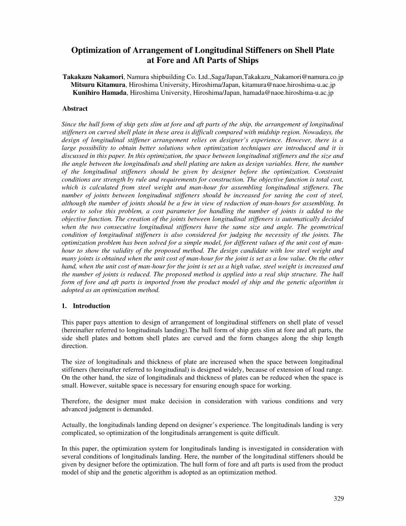
329

Optimization of Arrangement of Longitudinal Stiffeners on Shell Plate at Fore and Aft Parts of Ships

Takakazu Nakamori, Namura shipbuilding Co. Ltd.,Saga/Japan,Takakazu_Nakamori@namura.co.jp

Mitsuru Kitamura, Hiroshima University, Hiroshima/Japan, kitamura@naoe.hiroshima-u.ac.jp

Kunihiro Hamada, Hiroshima University, Hiroshima/Japan, hamada@naoe.hiroshima-u.ac.jp

Abstract

Since the hull form of ship gets slim at fore and aft parts of the ship, the arrangement of longitudinal

stiffeners on curved shell plate in these area is difficult compared with midship region. Nowadays, the

design of longitudinal stiffener arrangement relies on designer’s experience. However, there is a

large possibility to obtain better solutions when optimization techniques are introduced and it is

discussed in this paper. In this optimization, the space between longitudinal stiffeners and the size and

the angle between the longitudinals and shell plating are taken as design variables. Here, the number

of the longitudinal stiffeners should be given by designer before the optimization. Constraint

conditions are strength by rule and requirements for construction. The objective function is total cost,

which is calculated from steel weight and man-hour for assembling longitudinal stiffeners. The

number of joints between longitudinal stiffeners should be increased for saving the cost of steel,

although the number of joints should be a few in view of reduction of man-hours for assembling. In

order to solve this problem, a cost parameter for handling the number of joints is added to the

objective function. The creation of the joints between longitudinal stiffeners is automatically decided

when the two consecutive longitudinal stiffeners have the same size and angle. The geometrical

condition of longitudinal stiffeners is also considered for judging the necessity of the joints. The

optimization problem has been solved for a simple model, for different values of the unit cost of man-

hour to show the validity of the proposed method. The design candidate with low steel weight and

many joints is obtained when the unit cost of man-hour for the joint is set as a low value. On the other

hand, when the unit cost of man-hour for the joint is set as a high value, steel weight is increased and

the number of joints is reduced. The proposed method is applied into a real ship structure. The hull

form of fore and aft parts is imported from the product model of ship and the genetic algorithm is

adopted as an optimization method.

1. Introduction

This paper pays attention to design of arrangement of longitudinal stiffeners on shell plate of vessel

(hereinafter referred to longitudinals landing).The hull form of ship gets slim at fore and aft parts, the

side shell plates and bottom shell plates are curved and the form changes along the ship length

direction.

The size of longitudinals and thickness of plate are increased when the space between longitudinal

stiffeners (hereinafter referred to longitudinal) is designed widely, because of extension of load range.

On the other hand, the size of longitudinals and thickness of plates can be reduced when the space is

small. However, suitable space is necessary for ensuring enough space for working.

Therefore, the designer must make decision in consideration with various conditions and very

advanced judgment is demanded.

Actually, the longitudinals landing depend on designer’s experience. The longitudinals landing is very

complicated, so optimization of the longitudinals arrangement is quite difficult.

In this paper, the optimization system for longitudinals landing is investigated in consideration with

several conditions of longitudinals landing. Here, the number of the longitudinal stiffeners should be

given by designer before the optimization. The hull form of fore and aft parts is used from the product

model of ship and the genetic algorithm is adopted as an optimization method.

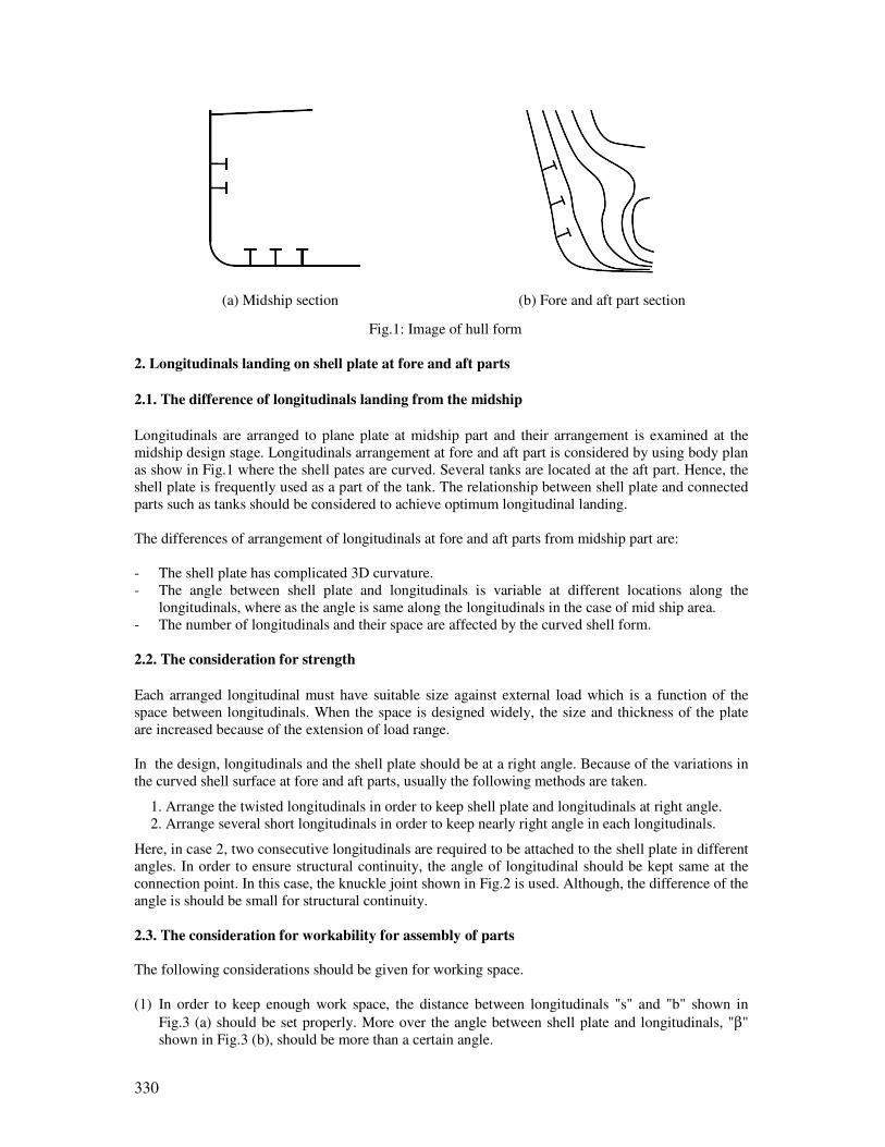
330

2. Longitudinals landing on shell plate at fore and aft parts

2.1. The difference of longitudinals landing from the midship

Longitudinals are arranged to plane plate at midship part and their arrangement is examined at the

midship design stage. Longitudinals arrangement at fore and aft part is considered by using body plan

as show in Fig.1 where the shell pates are curved. Several tanks are located at the aft part. Hence, the

shell plate is frequently used as a part of the tank. The relationship between shell plate and connected

parts such as tanks should be considered to achieve optimum longitudinal landing.

The differences of arrangement of longitudinals at fore and aft parts from midship part are:

- The shell plate has complicated 3D curvature.

- The angle between shell plate and longitudinals is variable at different locations along the

longitudinals, where as the angle is same along the longitudinals in the case of mid ship area.

- The number of longitudinals and their space are affected by the curved shell form.

2.2. The consideration for strength

Each arranged longitudinal must have suitable size against external load which is a function of the

space between longitudinals. When the space is designed widely, the size and thickness of the plate

are increased because of the extension of load range.

In the design, longitudinals and the shell plate should be at a right angle. Because of the variations in

the curved shell surface at fore and aft parts, usually the following methods are taken.

1. Arrange the twisted longitudinals in order to keep shell plate and longitudinals at right angle.

2. Arrange several short longitudinals in order to keep nearly right angle in each longitudinals.

Here, in case 2, two consecutive longitudinals are required to be attached to the shell plate in different

angles. In order to ensure structural continuity, the angle of longitudinal should be kept same at the

connection point. In this case, the knuckle joint shown in Fig.2 is used. Although, the difference of the

angle is should be small for structural continuity.

2.3. The consideration for workability for assembly of parts

The following considerations should be given for working space.

(1) In order to keep enough work space, the distance between longitudinals "s" and "b" shown in

Fig.3 (a) should be set properly. More over the angle between shell plate and longitudinals, "β"

shown in Fig.3 (b), should be more than a certain angle.

(a) Midship section (b) Fore and aft part section

Fig.1: Image of hull form

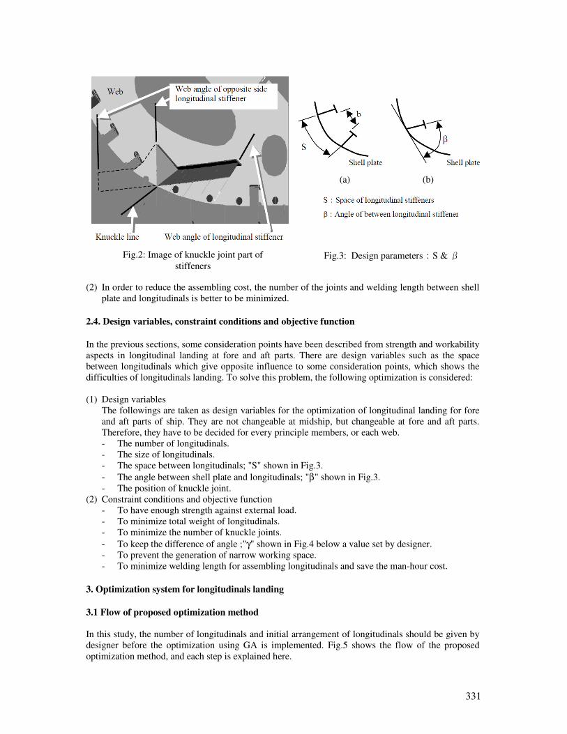
331

(2) In order to reduce the assembling cost, the number of the joints and welding length between shell

plate and longitudinals is better to be minimized.

2.4. Design variables, constraint conditions and objective function

In the previous sections, some consideration points have been described from strength and workability

aspects in longitudinal landing at fore and aft parts. There are design variables such as the space

between longitudinals which give opposite influence to some consideration points, which shows the

difficulties of longitudinals landing. To solve this problem, the following optimization is considered:

(1) Design variables

The followings are taken as design variables for the optimization of longitudinal landing for fore

and aft parts of ship. They are not changeable at midship, but changeable at fore and aft parts.

Therefore, they have to be decided for every principle members, or each web.

- The number of longitudinals.

- The size of longitudinals.

- The space between longitudinals; "S" shown in Fig.3.

- The angle between shell plate and longitudinals; "β" shown in Fig.3.

- The position of knuckle joint.

(2) Constraint conditions and objective function

- To have enough strength against external load.

- To minimize total weight of longitudinals.

- To minimize the number of knuckle joints.

- To keep the difference of angle ;"γ" shown in Fig.4 below a value set by designer.

- To prevent the generation of narrow working space.

- To minimize welding length for assembling longitudinals and save the man-hour cost.

3. Optimization system for longitudinals landing

3.1 Flow of proposed optimization method

In this study, the number of longitudinals and initial arrangement of longitudinals should be given by

designer before the optimization using GA is implemented. Fig.5 shows the flow of the proposed

optimization method, and each step is explained here.

(a) (b)

Fig.3: Design parameters：S & β Fig.2: Image of knuckle joint part of

stiffeners

332

1. Initialization

A product model is used to create the hull form of fore and aft parts. A part of longitudinals

arrangement of a real ship. The region which is surrounded by principal structural members is

picked up as the model of optimization. The number of the longitudinal stiffeners is given by

designer.

2. Generations of design plans

The design plans are generated by GA operation.

3. Calculations of constraint conditions and objective function

The constraint conditions and objective function mentioned in section 2.4 are determined for each

design plan is calculated.

4. Evaluations of design plans

Fitness of the design plans are calculated based on the results of the above step, and new design

plans are generated to get next generation.

3.2 Design variables

In this paper, the spaces between longitudinals, and the sizes and angles of them are taken as design

variables. Some examples of design variables considered in this study are shown in Fig.6. In the

figure, six longitudinals are arranged in the target area, and they are supported by web frames at the

edge. The spaces between longitudinals are defined at both ends of longitudinals. Nine design

variables for the spaces are required in the example. The spacing is given as the ratio to designer-input

spacing in order to utilize designer-input design plan. Design variables on the size and the angle are

set to each longitudinals. As for the size of longitudinals, eight types of different size of longitudinal

are prepared. 21 design variables (space: 9, size: 6, angle: 6) in total can be set for the longitudinal

arrangement shown in Fig. 6.

The joint of longitudinals is an important matter for longitudinals landing as discussed in section

2.4.In this study, necessity of joint is automatically checked and joints are automatically generated by

the system when two adjoining longitudinals do not satisfy the following conditions:

1. The size of longitudinals which are connected is the same.

Fig.4: Design parameters：γ Fig.5: Flow of proposed optimization method

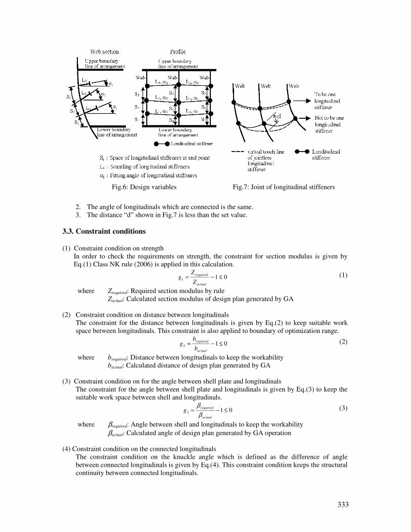
333

2. The angle of longitudinals which are connected is the same.

3. The distance “d” shown in Fig.7 is less than the set value.

3.3. Constraint conditions (1) Constraint condition on strength

In order to check the requirements on strength, the constraint for section modulus is given by

Eq.(1) Class NK rule (2006) is applied in this calculation.

011 ≤−=

actual

required

Z

Zg (1)

where Zrequired: Required section modulus by rule

Zactual: Calculated section modulus of design plan generated by GA

(2) Constraint condition on distance between longitudinals

The constraint for the distance between longitudinals is given by Eq.(2) to keep suitable work

space between longitudinals. This constraint is also applied to boundary of optimization range.

012 ≤−=

actual

required

b

bg (2)

where brequired: Distance between longitudinals to keep the workability

bactual: Calculated distance of design plan generated by GA

(3) Constraint condition on for the angle between shell plate and longitudinals

The constraint for the angle between shell plate and longitudinals is given by Eq.(3) to keep the

suitable work space between shell and longitudinals.

013 ≤−=

actual

requiredg

β

β (3)

where βrequired: Angle between shell and longitudinals to keep the workability

βactual: Calculated angle of design plan generated by GA operation

(4) Constraint condition on the connected longitudinals

The constraint condition on the knuckle angle which is defined as the difference of angle

between connected longitudinals is given by Eq.(4). This constraint condition keeps the structural

continuity between connected longitudinals.

Fig.6: Design variables Fig.7: Joint of longitudinal stiffeners

ｄ

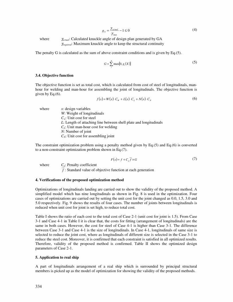
334

01max

4 ≤−=

γ

γ actualg (4)

where γactual: Calculated knuckle angle of design plan generated by GA

γrequired: Maximum knuckle angle to keep the structural continuity

The penalty G is calculated as the sum of above constraint conditions and is given by Eq.(5).

( )[ ]∑=

N

i

i XgG ,0max (5)

3.4. Objective function

The objective function is set as total cost, which is calculated from cost of steel of longitudinals, man-

hour for welding and man-hour for assembling the joint of longitudinals. The objective function is

given by Eq.(6).

( ) ( ) ( ) ( ) NLW CxNCxLCxWxf ⋅+⋅+⋅= (6)

where x: design variables

W: Weight of longitudinals

Cw: Unit cost for steel

L: Length of attaching line between shell plate and longitudinals

CL: Unit man-hour cost for welding

N: Number of joint

CN: Unit cost for assembling joint

The constraint optimization problem using a penalty method given by Eq.(5) and Eq.(6) is converted

to a non-constraint optimization problem shown in Eq.(7).

( ) GfCfxF p ×+= (7)

where Cp: Penalty coefficient

f : Standard value of objective function at each generation

4. Verifications of the proposed optimization method

Optimizations of longitudinals landing are carried out to show the validity of the proposed method. A

simplified model which has nine longitudinals as shown in Fig. 8 is used in the optimization. Four

cases of optimizations are carried out by setting the unit cost for the joint changed as 0.0, 1.5, 3.0 and

5.0 respectively. Fig. 9 shows the results of four cases. The number of joints between longitudinals is

reduced when unit cost for joint is set high, to reduce total cost.

Table I shows the ratio of each cost to the total cost of Case 2-1 (unit cost for joint is 1.5). From Case

3-1 and Case 4-1 in Table I it is clear that, the costs for fitting (arrangement of longitudinals) are the

same in both cases. However, the cost for steel of Case 4-1 is higher than Case 3-1. The difference

between Case 3-1 and Case 4-1 is the size of longitudinals. In Case 4-1, longitudinals of same size is

selected to reduce the joint cost, where as longitudinals of different size is selected in the Case 3-1 to

reduce the steel cost. Moreover, it is confirmed that each constraint is satisfied in all optimized results.

Therefore, validity of the proposed method is confirmed. Table II shows the optimized design

parameters of Case 2-1.

5. Application to real ship

A part of longitudinals arrangement of a real ship which is surrounded by principal structural

members is picked up as the model of optimization for showing the validity of the proposed methods.

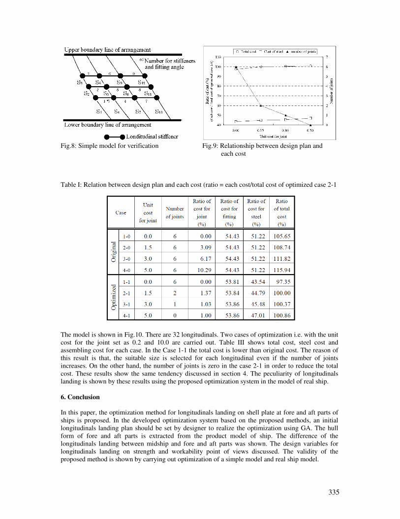
335

Fig.8: Simple model for verification Fig.9: Relationship between design plan and

each cost

Table I: Relation between design plan and each cost (ratio = each cost/total cost of optimized case 2-1

The model is shown in Fig.10. There are 32 longitudinals. Two cases of optimization i.e. with the unit

cost for the joint set as 0.2 and 10.0 are carried out. Table III shows total cost, steel cost and

assembling cost for each case. In the Case 1-1 the total cost is lower than original cost. The reason of

this result is that, the suitable size is selected for each longitudinal even if the number of joints

increases. On the other hand, the number of joints is zero in the case 2-1 in order to reduce the total

cost. These results show the same tendency discussed in section 4. The peculiarity of longitudinals

landing is shown by these results using the proposed optimization system in the model of real ship.

6. Conclusion

In this paper, the optimization method for longitudinals landing on shell plate at fore and aft parts of

ships is proposed. In the developed optimization system based on the proposed methods, an initial

longitudinals landing plan should be set by designer to realize the optimization using GA. The hull

form of fore and aft parts is extracted from the product model of ship. The difference of the

longitudinals landing between midship and fore and aft parts was shown. The design variables for

longitudinals landing on strength and workability point of views discussed. The validity of the

proposed method is shown by carrying out optimization of a simple model and real ship model.

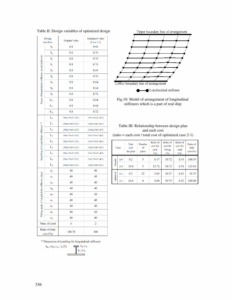
336

Table III: Relationship between design plan

and each cost

(ratio = each cost / total cost of optimized case 2-1)

Table II: Design variables of optimized design

Fig.10: Model of arrangement of longitudinal

stiffeners which is a part of real ship

337

References

KITAMURA, M.; HAMADA, K.; SUZUKI, H.; YANO, K.; TOKUOKA, K.; OHTSUKI, Y. (2008),

Practical optimal design of mid-ship section and development of high-speed optimization system, J.

Soc. Naval Arch. Japan 6,pp.141-149 (in Japanese)

MATSUO, M. (1998), Modeling of ship using VISION, Namura Techn. Review1, pp.7-12 (in

Japanese)

HAYASHI, K. (1999), Overview of block division function of VISION, Namura Techn. Review 2,

pp.54-57 (in Japanese)

NAKAMORI, T. (2002), Application of VISION at hull design section, Namura Techn. Review 5,

pp.82-85 (in Japanese)

338

ADOPT: Man-Machine Interface and Training

Dirk Wittkuhn, TUHH-ISSUS, Hamburg/Germany, wittkuhn@tu-harburg.de Karl-Christian Ehrke, SAM Electronics GmbH, Hamburg/Germany,

karl-christian.ehrke@sam-electronics.de John Koch Nielsen, Force Technology, Lyngby/Denmark, jnn@force.dk

Abstract

The present paper describes the Man-Machine-Interface and the training concepts that have been developed in the ADOPT project for heavy weather decision support systems. 1. Introduction 1.1. Man-Machine Interface The overall objective for the Man-Machine-Interface (MMI) is to display the information for decision making as received from the respective modes of the different decision support kernels. Due attention has to be paid to:

(1) What are the expectations of seafarers on DSS? (2) Present the data clearly and customized to the task in order to avoid misunderstandings (3) Allow for an easy "navigation" within the display and menus (4) To enable some customization regarding the kind of results and the "look and feel", while

keeping the system straight forward and basic (no fancy buttons and menus for confusion) (5) To support the user to leave or avoid potentially dangerous situations in ship operation

without entering the next one (6) Identify and define appropriate connections to existing systems already available on the

bridge 1.2. Training As the ADOPT-DSS consists of three main parts, training as one of them plays an important role in the overall system. The general approach of Training in ADOPT is that its purpose is not only the familiarisation with the system itself but also to give advise on the background of phenomena like parametric rolling and alike, as the purpose of the DSS only can be captured when the theoretical foundation is available. By this approach the training does not only customise the user on the system but also contributes to an improved situational awareness of the risks in specific sea states. The Training concept consists of four modules, starting with the theory. Since the ADOPT-DSS is ship specific, the theory will afterwards be consolidated by exercises in the simulator demonstrating the vulnerability of the specific ship in particular seas. Only then the issue how the DSS responds to the risks will be demonstrated. This again starts with the theoretical description how the DSS works, which are its modules and in which situations it can help. Afterwards, in the final module, the user will be customised in a simulator environment to get experience in using the system and improve his behaviour in critical situations. 2. Man-Machine Interface 2.1. Generic Layout of the Man-Machine-Interface In the development of the Man-Machine-Interface the focus was laid on the operation and training mode. In a design environment the naval architects use many different tools with which they are very familiar thus developing new interfaces for the design mode would have been of little gain. Thus the

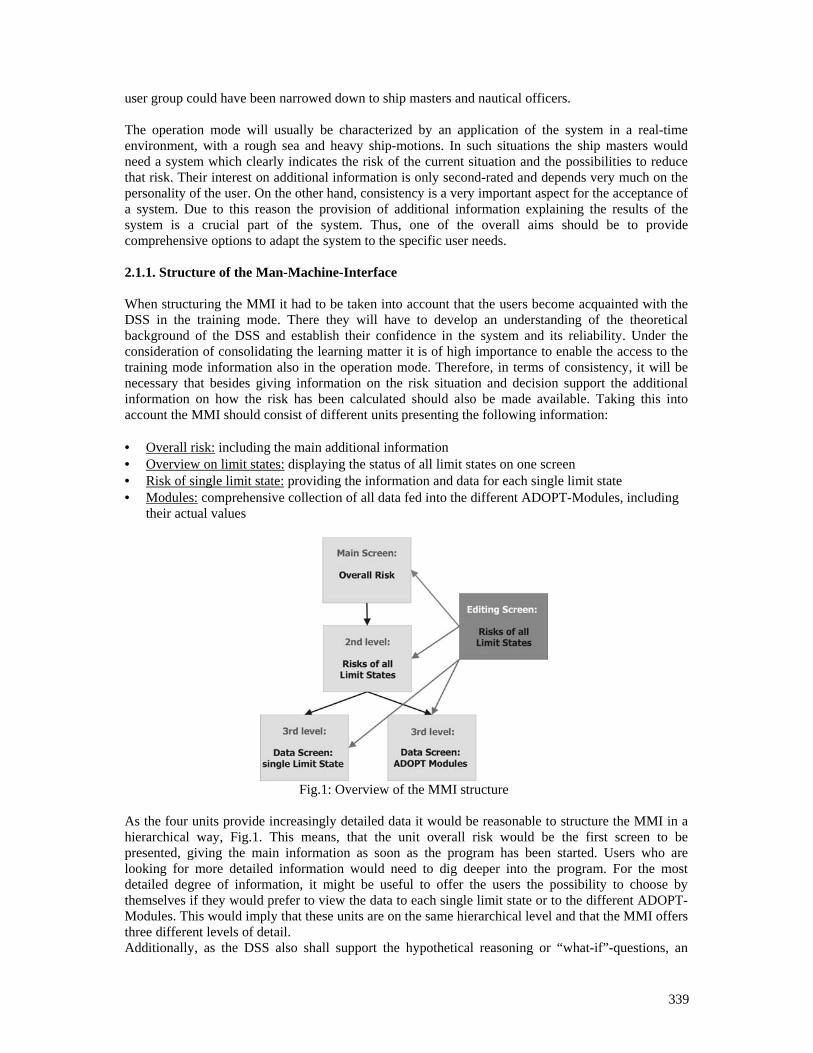
339

user group could have been narrowed down to ship masters and nautical officers. The operation mode will usually be characterized by an application of the system in a real-time environment, with a rough sea and heavy ship-motions. In such situations the ship masters would need a system which clearly indicates the risk of the current situation and the possibilities to reduce that risk. Their interest on additional information is only second-rated and depends very much on the personality of the user. On the other hand, consistency is a very important aspect for the acceptance of a system. Due to this reason the provision of additional information explaining the results of the system is a crucial part of the system. Thus, one of the overall aims should be to provide comprehensive options to adapt the system to the specific user needs. 2.1.1. Structure of the Man-Machine-Interface When structuring the MMI it had to be taken into account that the users become acquainted with the DSS in the training mode. There they will have to develop an understanding of the theoretical background of the DSS and establish their confidence in the system and its reliability. Under the consideration of consolidating the learning matter it is of high importance to enable the access to the training mode information also in the operation mode. Therefore, in terms of consistency, it will be necessary that besides giving information on the risk situation and decision support the additional information on how the risk has been calculated should also be made available. Taking this into account the MMI should consist of different units presenting the following information: • Overall risk: including the main additional information • Overview on limit states: displaying the status of all limit states on one screen • Risk of single limit state: providing the information and data for each single limit state • Modules: comprehensive collection of all data fed into the different ADOPT-Modules, including

their actual values

Fig.1: Overview of the MMI structure

As the four units provide increasingly detailed data it would be reasonable to structure the MMI in a hierarchical way, Fig.1. This means, that the unit overall risk would be the first screen to be presented, giving the main information as soon as the program has been started. Users who are looking for more detailed information would need to dig deeper into the program. For the most detailed degree of information, it might be useful to offer the users the possibility to choose by themselves if they would prefer to view the data to each single limit state or to the different ADOPT-Modules. This would imply that these units are on the same hierarchical level and that the MMI offers three different levels of detail. Additionally, as the DSS also shall support the hypothetical reasoning or “what-if”-questions, an

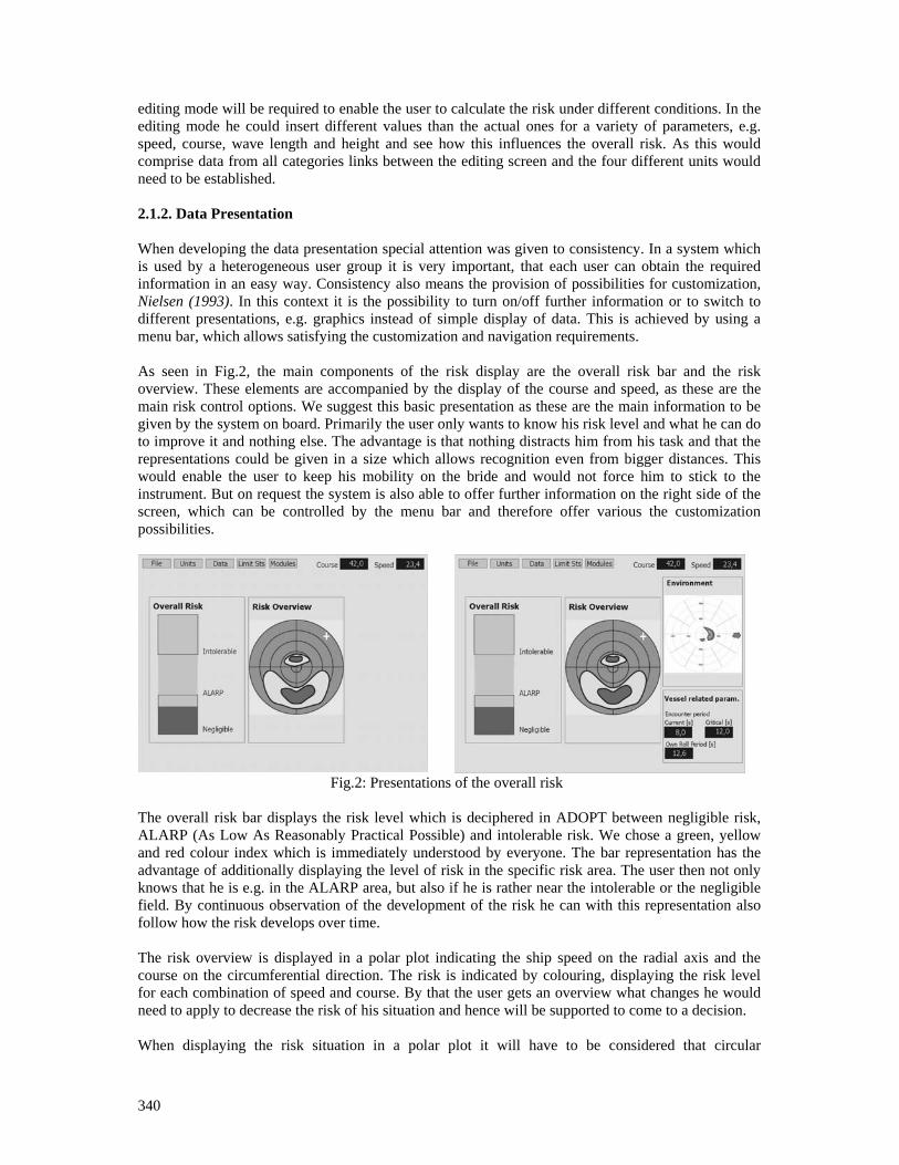
340

editing mode will be required to enable the user to calculate the risk under different conditions. In the editing mode he could insert different values than the actual ones for a variety of parameters, e.g. speed, course, wave length and height and see how this influences the overall risk. As this would comprise data from all categories links between the editing screen and the four different units would need to be established. 2.1.2. Data Presentation When developing the data presentation special attention was given to consistency. In a system which is used by a heterogeneous user group it is very important, that each user can obtain the required information in an easy way. Consistency also means the provision of possibilities for customization, Nielsen (1993). In this context it is the possibility to turn on/off further information or to switch to different presentations, e.g. graphics instead of simple display of data. This is achieved by using a menu bar, which allows satisfying the customization and navigation requirements. As seen in Fig.2, the main components of the risk display are the overall risk bar and the risk overview. These elements are accompanied by the display of the course and speed, as these are the main risk control options. We suggest this basic presentation as these are the main information to be given by the system on board. Primarily the user only wants to know his risk level and what he can do to improve it and nothing else. The advantage is that nothing distracts him from his task and that the representations could be given in a size which allows recognition even from bigger distances. This would enable the user to keep his mobility on the bride and would not force him to stick to the instrument. But on request the system is also able to offer further information on the right side of the screen, which can be controlled by the menu bar and therefore offer various the customization possibilities.

Fig.2: Presentations of the overall risk

The overall risk bar displays the risk level which is deciphered in ADOPT between negligible risk, ALARP (As Low As Reasonably Practical Possible) and intolerable risk. We chose a green, yellow and red colour index which is immediately understood by everyone. The bar representation has the advantage of additionally displaying the level of risk in the specific risk area. The user then not only knows that he is e.g. in the ALARP area, but also if he is rather near the intolerable or the negligible field. By continuous observation of the development of the risk he can with this representation also follow how the risk develops over time. The risk overview is displayed in a polar plot indicating the ship speed on the radial axis and the course on the circumferential direction. The risk is indicated by colouring, displaying the risk level for each combination of speed and course. By that the user gets an overview what changes he would need to apply to decrease the risk of his situation and hence will be supported to come to a decision. When displaying the risk situation in a polar plot it will have to be considered that circular

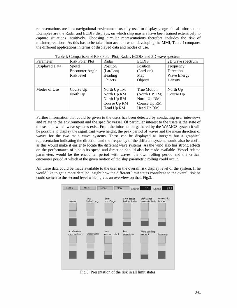
341

representations are in a navigational environment usually used to display geographical information. Examples are the Radar and ECDIS displays, on which ship masters have been trained extensively to capture situations intuitively. Choosing circular representations therefore includes the risk of misinterpretations. As this has to be taken into account when developing the MMI, Table I compares the different applications in terms of displayed data and modes of use.

Table I: Comparison of Risk Polar Plot, Radar, ECDIS and 3D wave spectrum

Parameter Risk Polar Plot Radar ECDIS 2D wave spectrum Displayed Data Speed

Encounter Angle Risk level

Position (Lat/Lon) Heading Objects

Position (Lat/Lon) Map Objects

Frequency Direction Wave Energy Density

Modes of Use Course Up North Up

North Up TM North Up RM North Up RM Course Up RM Head Up RM

True Motion (North UP TM) North Up RM Course Up RM Head Up RM

North Up Course Up

Further information that could be given to the users has been detected by conducting user interviews and relate to the environment and the specific vessel. Of particular interest to the users is the state of the sea and which wave systems exist. From the information gathered by the WAMOS system it will be possible to display the significant wave height, the peak period of waves and the mean direction of waves for the two main wave systems. These can be displayed as integers but a graphical representation indicating the direction and the frequency of the different systems would also be useful as this would make it easier to locate the different wave systems. As the wind also has strong effects on the performance of a ship its speed and direction should also be made available. Vessel related parameters would be the encounter period with waves, the own rolling period and the critical encounter period at which at the given motion of the ship parametric rolling could occur. All these data could be made available to the user in the overall risk display level of the system. If he would like to get a more detailed insight how the different limit states contribute to the overall risk he could switch to the second level which gives an overview on that, Fig.3.

Fig.3: Presentation of the risk in all limit states

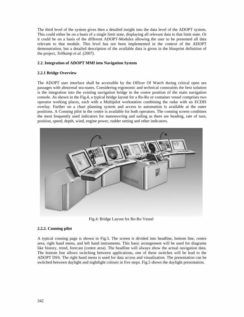
342

The third level of the system gives then a detailed insight into the data level of the ADOPT system. This could either be on a basis of a single limit state, displaying all relevant data to that limit state. Or it could be on a basis of the different ADOPT-Modules allowing the user to be presented all data relevant to that module. This level has not been implemented in the context of the ADOPT demonstration, but a detailed description of the available data is given in the blueprint definition of the project, Tellkamp et al. (2007). 2.2. Integration of ADOPT MMI into Navigation System 2.2.1 Bridge Overview The ADOPT user interface shall be accessible by the Officer Of Watch during critical open sea passages with abnormal sea-states. Considering ergonomic and technical constraints the best solution is the integration into the existing navigation bridge in the centre position of the main navigation console. As shown in the Fig.4, a typical bridge layout for a Ro-Ro or container vessel comprises two operator working places, each with a Multipilot workstation combining the radar with an ECDIS overlay. Further on a chart planning system and access to automation is available at the outer positions. A Conning pilot in the centre is available for both operators. The conning screen combines the most frequently used indicators for manoeuvring and sailing as there are heading, rate of turn, position, speed, depth, wind, engine power, rudder setting and other indicators.

Fig.4: Bridge Layout for Ro-Ro Vessel

2.2.2. Conning pilot A typical conning page is shown in Fig.5. The screen is divided into headline, bottom line, centre area, right hand menu, and left hand instruments. This basic arrangement will be used for diagrams like history, trend, forecast (centre area). The headline will always show the actual navigation data. The bottom line allows switching between applications, one of these switches will be lead to the ADOPT DSS. The right hand menu is used for data access and visualisation. The presentation can be switched between daylight and nightlight colours in five steps. Fig.5 shows the daylight presentation.

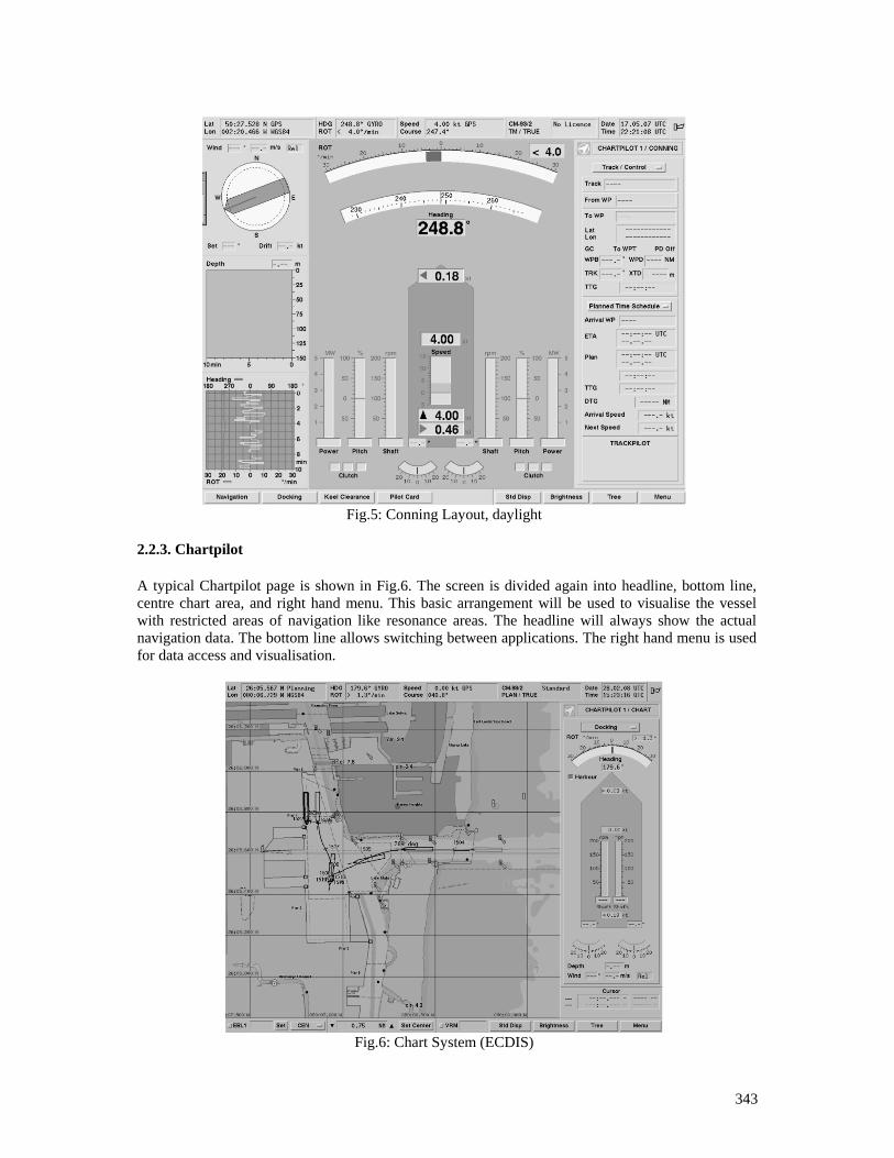
343

Fig.5: Conning Layout, daylight

2.2.3. Chartpilot A typical Chartpilot page is shown in Fig.6. The screen is divided again into headline, bottom line, centre chart area, and right hand menu. This basic arrangement will be used to visualise the vessel with restricted areas of navigation like resonance areas. The headline will always show the actual navigation data. The bottom line allows switching between applications. The right hand menu is used for data access and visualisation.

Fig.6: Chart System (ECDIS)

344

2.2.4. ADOPT User Interface Design Rules Based on the NACOS style-guide, which has been developed by taking into account main IEC and class rules for bridge design, the initial ADOPT design has been created as follows:

(1) Compatibility – all the navigational information is directly shown on the user surface, nothing is hidden in a sub-menu ensuring minimum re-coding for the user

(2) Consistency – only a very reduced set of dialogues is used in the user interface

(3) Structure – in order to assist the user in developing a conceptual representation of the structure of the system, the structured area and the grouped dialogue have been used,

(4) Feedback – user feedback is given with active buttons as well as switched background colours (5) Menu control and Display of Information – is implemented as recommended in the style-guide by

a smaller right part of the application area. It is divided into a top line with navigation data and track-pilot info, into a display scope for zoom, alarms, docking, depth, etc., into a target track data field, into a general data and menu area and into a bottom control area.

2.2.5. ADOPT User Interface Implementation The main ADOPT menu shows the status of the limit states. For each limit state a single bar is presented. In Fig.7 the bars are divided into three sections, a green one indicating safe level, a yellow one indicating uncertain level and a red one indicating warning level. The sum of limit states is shown in the right hand section of the screen. This bar is already available in conjunction with any conning menu. The set of bars in the centre shows up on user demand only.

Fig.7: ADOPT Limit State Presentation

The centre part can be switched over to a presentation of the actual wave situation as well. Fig.8 indicates wave height, wave period and direction for the actual sailing condition. The values are converted into symbolic bars in relation to the vessels hull size and sailing direction. The distance between two bars gives the period; the thickness of a bar indicates the wave height.

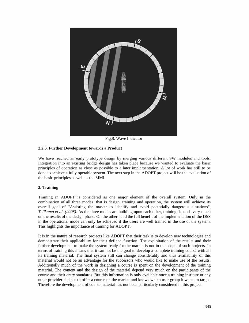
345

Fig.8: Wave Indicator

2.2.6. Further Development towards a Product We have reached an early prototype design by merging various different SW modules and tools. Integration into an existing bridge design has taken place because we wanted to evaluate the basic principles of operation as close as possible to a later implementation. A lot of work has still to be done to achieve a fully operable system. The next step in the ADOPT project will be the evaluation of the basic principles as well as the MMI. 3. Training Training in ADOPT is considered as one major element of the overall system. Only in the combination of all three modes, that is design, training and operation, the system will achieve its overall goal of "Assisting the master to identify and avoid potentially dangerous situations", Tellkamp et al. (2008). As the three modes are building upon each other, training depends very much on the results of the design phase. On the other hand the full benefit of the implementation of the DSS in the operational mode can only be achieved if the users are well trained in the use of the system. This highlights the importance of training for ADOPT. It is in the nature of research projects like ADOPT that their task is to develop new technologies and demonstrate their applicability for their defined function. The exploitation of the results and their further development to make the system ready for the market is not in the scope of such projects. In terms of training this means that it can not be the goal to develop a complete training course with all its training material. The final system still can change considerably and thus availability of this material would not be an advantage for the successors who would like to make use of the results. Additionally much of the work in designing a course is spent on the development of the training material. The content and the design of the material depend very much on the participants of the course and their entry standards. But this information is only available once a training institute or any other provider decides to offer a course on the market and knows which user group it wants to target. Therefore the development of course material has not been particularly considered in this project.

346

We rather decided to concentrate the work on training in ADOPT on the development of a course outline which identifies the main learning objectives and presents a detailed syllabus. This approach is comparable to what the IMO has done with its model course program. Its purpose is to assist maritime training institutes and their teaching staff in organizing and introducing new training courses without presenting them rigid "teaching packages" which they are expected to "follow blindly", IMO (1999). This approach takes into consideration that cultural backgrounds of trainees in maritime subjects vary considerably from country to country. If one only mentions the learning objectives and the required performances this leaves the instructor sufficient freedom to take the specific characteristics of his trainees into account. Additionally this generic approach gives the instructor the flexibility to develop a course which is tailored to his abilities in order to give a vivid class which attracts the interest of the participants. This facilitates the transfer of knowledge which is the main objective of training courses. It is obvious that one aim of the training in the context of ADOPT is to practice the use of the DSS itself. That means that familiarization with the system to enable the user to fully exploit the potential of the DSS is one of the main drivers for the development of a course outline. But as well as for the project it is also one aim of the training to assist the master to identify and avoid potentially dangerous situations. This includes that the training not only needs to be restricted to the familiarization aspect. Communication with masters of vessels has shown that their knowledge about how the motion of ships is influenced by the sea rests. They have had lessons on hydrodynamics during their education, but this kind of theoretical knowledge, which is not used in their daily work, is very difficult to be applied when it was not used for a long time. On the other hand the knowledge on what determines the movement of ships has been particularly increased in the last years, leading to the formulation of the phenomenon of parametric roll. But so far this knowledge is not transferred sufficiently to the users on board. As long as the master possesses many years of experience on board of ships this is not a big issue and can be compensated by his experience. But today the whole industry suffers a lack of qualified masters and officers making it possible to become much faster the captain of a vessel than twenty years ago. In this case the lacking knowledge on ship motions can be a problem and therefore needs to be tackled by training. With this approach the course outline of ADOPT could even be interesting for crews of ships without DSS, especially when it provides knowledge on the behavior of specific ships. 3.1. Course Outline and Teaching Syllabus The following three learning objectives have been detected for a training course:

1. Describe the theory of ship motions 2. Characteristics and behavior of a specific ship 3. Familiarization with a mode 1 DSS

These learning objectives can be broken down into the following required performances: 3.1.1. Describe the theory of ship motions

Required performance: Wave Theory 1. wave characteristics (regular waves) 2. superposition of waves 3. irregular waves 4. wave spectrum 5. directional spreading 6. Beaufort scale 7. ocean waves statistics 8. scatter diagrams

347

Required performance: Hydrostatics 1. description of the GM 2. calculation of the righting lever curves (wave trough and crest) 3. correlation between the GM and the righting levers 4. corrections for free surfaces 5. the influence of free surfaces on the righting levers 6. corrections on the moments of inertia due to free surfaces 7. determination of the centre of gravity and imponderableness within 8. fundamentals and restrictions of stabilizers Required performance: Critical Situations and potential hazards

1. large amplitude roll motion (capsize). 2. loss of lashed cargo. 3. loss of not secured cargo (cars/trucks, container). 4. shift of cargo / lashed RoRo cargo. 5. shift of cargo / not secured RoRo cargo (shift within cargo unit). 6. large acceleration / injuries. 7. large acceleration / reduced crew performance. 8. green water (relative motion, damage to equipment/outfitting on deck). 9. loss of course control. 10. loss of propulsion. 11. propeller racing (relative motion). 12. wave bending moment.

3.1.2. Characteristics and behavior of a specific ship Required performance: Illustrate the characteristics and the behavior of a specific ship

1. explain the design concept of the ship 2. performance of the ship in different sea states 3. particularities of the ship behavior in different sea states 4. actions to be taken to increase the safety of the vessel

3.1.3. Familiarization with a mode 1 DSS

Required performance: Describe the theory of a mode 1 DSS 1. describe the philosophy of the system 2. explain the risk based approach 3. which hazards are covered by the DSS 4. what limit states have been formulated 5. what are the limitations of the system 6. how reliable is the system 7. explain the concept of the MMI Required performance: Train the operation of a mode 1 DSS 1. operate the system to get to know the buttons 2. approval of correct interpretation of the situation 3. approval of being able to use the system to improve the risk situation

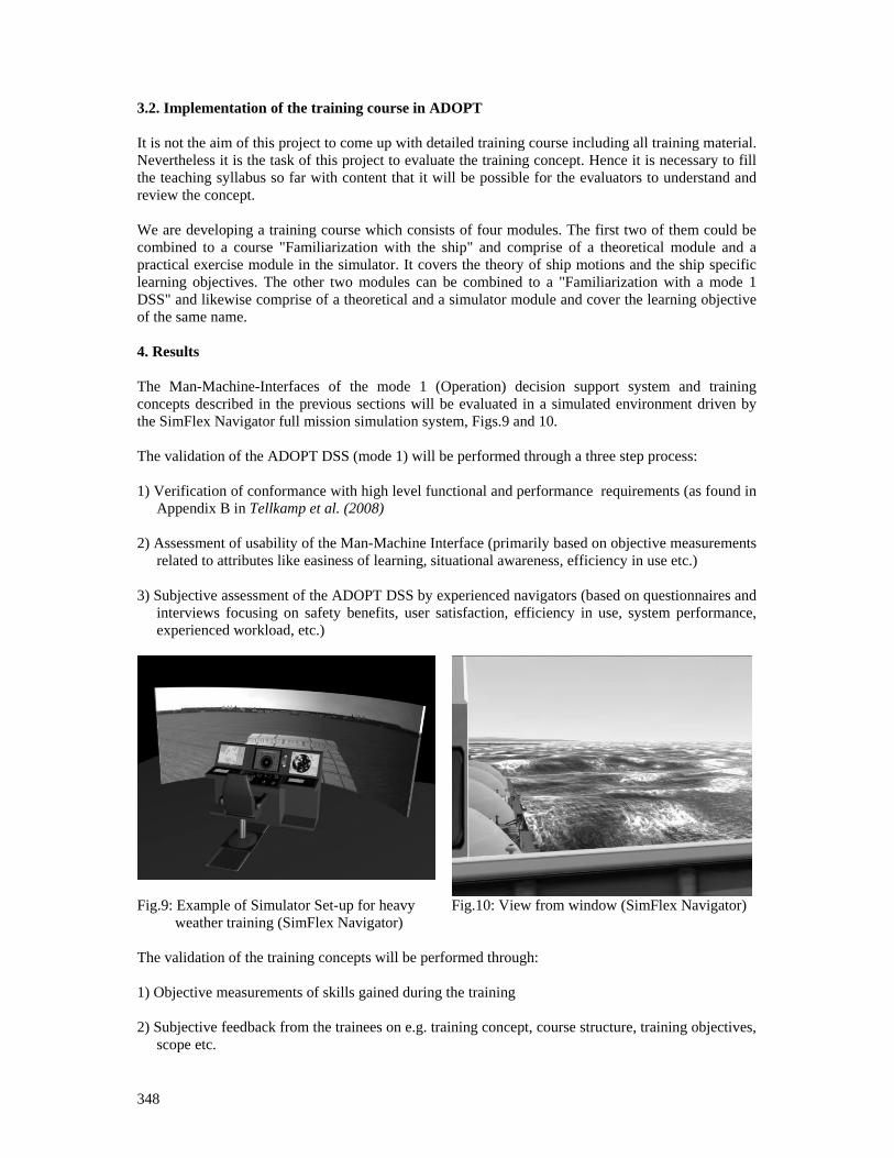
348

3.2. Implementation of the training course in ADOPT It is not the aim of this project to come up with detailed training course including all training material. Nevertheless it is the task of this project to evaluate the training concept. Hence it is necessary to fill the teaching syllabus so far with content that it will be possible for the evaluators to understand and review the concept. We are developing a training course which consists of four modules. The first two of them could be combined to a course "Familiarization with the ship" and comprise of a theoretical module and a practical exercise module in the simulator. It covers the theory of ship motions and the ship specific learning objectives. The other two modules can be combined to a "Familiarization with a mode 1 DSS" and likewise comprise of a theoretical and a simulator module and cover the learning objective of the same name. 4. Results The Man-Machine-Interfaces of the mode 1 (Operation) decision support system and training concepts described in the previous sections will be evaluated in a simulated environment driven by the SimFlex Navigator full mission simulation system, Figs.9 and 10. The validation of the ADOPT DSS (mode 1) will be performed through a three step process: 1) Verification of conformance with high level functional and performance requirements (as found in

Appendix B in Tellkamp et al. (2008) 2) Assessment of usability of the Man-Machine Interface (primarily based on objective measurements

related to attributes like easiness of learning, situational awareness, efficiency in use etc.) 3) Subjective assessment of the ADOPT DSS by experienced navigators (based on questionnaires and

interviews focusing on safety benefits, user satisfaction, efficiency in use, system performance, experienced workload, etc.)

Fig.9: Example of Simulator Set-up for heavy weather training (SimFlex Navigator)

Fig.10: View from window (SimFlex Navigator)

The validation of the training concepts will be performed through: 1) Objective measurements of skills gained during the training 2) Subjective feedback from the trainees on e.g. training concept, course structure, training objectives,

scope etc.

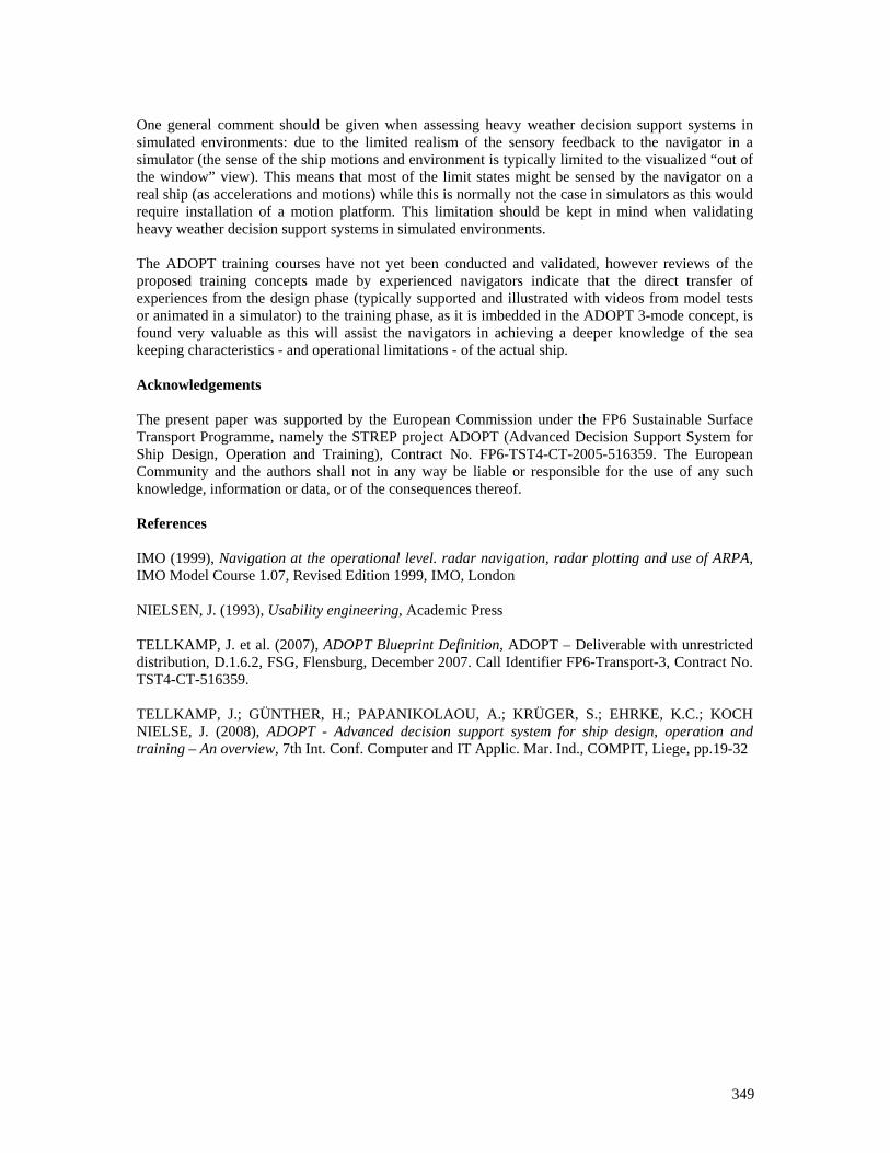
349

One general comment should be given when assessing heavy weather decision support systems in simulated environments: due to the limited realism of the sensory feedback to the navigator in a simulator (the sense of the ship motions and environment is typically limited to the visualized “out of the window” view). This means that most of the limit states might be sensed by the navigator on a real ship (as accelerations and motions) while this is normally not the case in simulators as this would require installation of a motion platform. This limitation should be kept in mind when validating heavy weather decision support systems in simulated environments. The ADOPT training courses have not yet been conducted and validated, however reviews of the proposed training concepts made by experienced navigators indicate that the direct transfer of experiences from the design phase (typically supported and illustrated with videos from model tests or animated in a simulator) to the training phase, as it is imbedded in the ADOPT 3-mode concept, is found very valuable as this will assist the navigators in achieving a deeper knowledge of the sea keeping characteristics - and operational limitations - of the actual ship. Acknowledgements The present paper was supported by the European Commission under the FP6 Sustainable Surface Transport Programme, namely the STREP project ADOPT (Advanced Decision Support System for Ship Design, Operation and Training), Contract No. FP6-TST4-CT-2005-516359. The European Community and the authors shall not in any way be liable or responsible for the use of any such knowledge, information or data, or of the consequences thereof. References IMO (1999), Navigation at the operational level. radar navigation, radar plotting and use of ARPA, IMO Model Course 1.07, Revised Edition 1999, IMO, London NIELSEN, J. (1993), Usability engineering, Academic Press TELLKAMP, J. et al. (2007), ADOPT Blueprint Definition, ADOPT – Deliverable with unrestricted distribution, D.1.6.2, FSG, Flensburg, December 2007. Call Identifier FP6-Transport-3, Contract No. TST4-CT-516359. TELLKAMP, J.; GÜNTHER, H.; PAPANIKOLAOU, A.; KRÜGER, S.; EHRKE, K.C.; KOCH NIELSE, J. (2008), ADOPT - Advanced decision support system for ship design, operation and training – An overview, 7th Int. Conf. Computer and IT Applic. Mar. Ind., COMPIT, Liege, pp.19-32

350

Shipyard Investment Planning by Use of Modern Process-Simulation and Layout-Planning Tools

Björn Weidemann, University of Rostock, bjoern.weidemann@uni-rostock.de

Ralf Bohnenberg, University of Rostock, ralf.bohnenberg@uni-rostock.de Martin-Christoph Wanner, Fraunhofer Anwendungszentrum Großstrukturen in der Produktionstechnik, mcw@hro.ipa.fhg.de

Abstract This article describes the integration of production capacity process simulation and interactive 3D shipyard layout planning tools as new and sufficient planning tools. The tools mentioned are established in the shipbuilding industry and can be used for different capacity planning purposes in shipbuilding and related industries. Large benefits can be gained for the companies by using these tools such as minimal investment costs, sufficient amount of production capacities required and an optimal arrangement of the shipyard facilities. 1. Introduction The shipbuilding industry is marked by a strong competition pressure due to the constant extension of the international shipbuilding capacities from countries. This alone is no new information, its importance, however, is increasing steadily because of the accompanying price decay for new ships on the market. Various projects for a development of strategies, e.g. for a product assortment, for production and assembly technologies, for production planning and control are carried out. They will strengthen the competition situation. The strategic planning of the capacities offered in the form of investment extensions and new investments and the integration of these investments in the shipyard layout has, however, been considered in marginal areas only. But the solutions resulting from this are highly interesting for the shipyards from the economic and the production point of view and may result in capacities of an overall optimised production at minimal investment costs. Basically, extension and new investments are to be invested in existing capacity-forming bottlenecks, i.e. the substitution of the bottleneck. When planning an investment, it is decisive to consider the complete production in all its individual production departments as an entity. For the maritime industry these departments can be subdivided into:

• Steel production in shipbuilding, e.g. the production departments component cutting, component bending, panel assembly, section assembly, block assembly, ring assembly or final assembly

• Production departments outfitting and furnishing components, e.g. the production departments pipe production and pre-assembly, air-conditioning canal production and pre-assembly or foundation production and pre-assembly.

Dependencies within the individual production departments themselves and between each other have to be taken into account when planning investments. Due to the complexity of production, identification and assessment of the production and the investment decisions derived from them are not carried out from the point of view of optimal investment. Subjective evaluations or inexact capacity calculations are the reasons for this situation. Typical questions to be solved when deciding upon an investment are e.g.

• Where are the bottlenecks in the chain of the individual production departments and which is the capacity-forming bottleneck?

• Which investment is optimal for the existing production? • Which bottlenecks have to be enlarged for capacity? • How and where are intermediate stores to be placed?

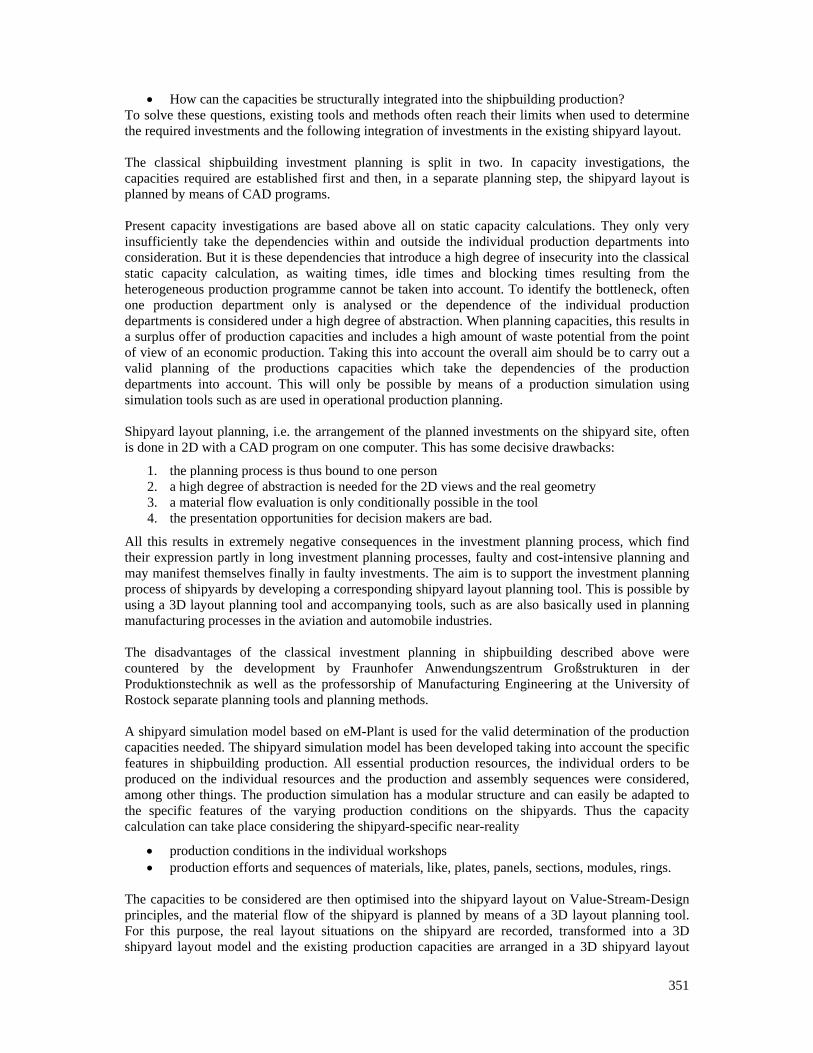
351

• How can the capacities be structurally integrated into the shipbuilding production? To solve these questions, existing tools and methods often reach their limits when used to determine the required investments and the following integration of investments in the existing shipyard layout. The classical shipbuilding investment planning is split in two. In capacity investigations, the capacities required are established first and then, in a separate planning step, the shipyard layout is planned by means of CAD programs. Present capacity investigations are based above all on static capacity calculations. They only very insufficiently take the dependencies within and outside the individual production departments into consideration. But it is these dependencies that introduce a high degree of insecurity into the classical static capacity calculation, as waiting times, idle times and blocking times resulting from the heterogeneous production programme cannot be taken into account. To identify the bottleneck, often one production department only is analysed or the dependence of the individual production departments is considered under a high degree of abstraction. When planning capacities, this results in a surplus offer of production capacities and includes a high amount of waste potential from the point of view of an economic production. Taking this into account the overall aim should be to carry out a valid planning of the productions capacities which take the dependencies of the production departments into account. This will only be possible by means of a production simulation using simulation tools such as are used in operational production planning. Shipyard layout planning, i.e. the arrangement of the planned investments on the shipyard site, often is done in 2D with a CAD program on one computer. This has some decisive drawbacks:

1. the planning process is thus bound to one person 2. a high degree of abstraction is needed for the 2D views and the real geometry 3. a material flow evaluation is only conditionally possible in the tool 4. the presentation opportunities for decision makers are bad.

All this results in extremely negative consequences in the investment planning process, which find their expression partly in long investment planning processes, faulty and cost-intensive planning and may manifest themselves finally in faulty investments. The aim is to support the investment planning process of shipyards by developing a corresponding shipyard layout planning tool. This is possible by using a 3D layout planning tool and accompanying tools, such as are also basically used in planning manufacturing processes in the aviation and automobile industries. The disadvantages of the classical investment planning in shipbuilding described above were countered by the development by Fraunhofer Anwendungszentrum Großstrukturen in der Produktionstechnik as well as the professorship of Manufacturing Engineering at the University of Rostock separate planning tools and planning methods. A shipyard simulation model based on eM-Plant is used for the valid determination of the production capacities needed. The shipyard simulation model has been developed taking into account the specific features in shipbuilding production. All essential production resources, the individual orders to be produced on the individual resources and the production and assembly sequences were considered, among other things. The production simulation has a modular structure and can easily be adapted to the specific features of the varying production conditions on the shipyards. Thus the capacity calculation can take place considering the shipyard-specific near-reality

• production conditions in the individual workshops • production efforts and sequences of materials, like, plates, panels, sections, modules, rings.

The capacities to be considered are then optimised into the shipyard layout on Value-Stream-Design principles, and the material flow of the shipyard is planned by means of a 3D layout planning tool. For this purpose, the real layout situations on the shipyard are recorded, transformed into a 3D shipyard layout model and the existing production capacities are arranged in a 3D shipyard layout

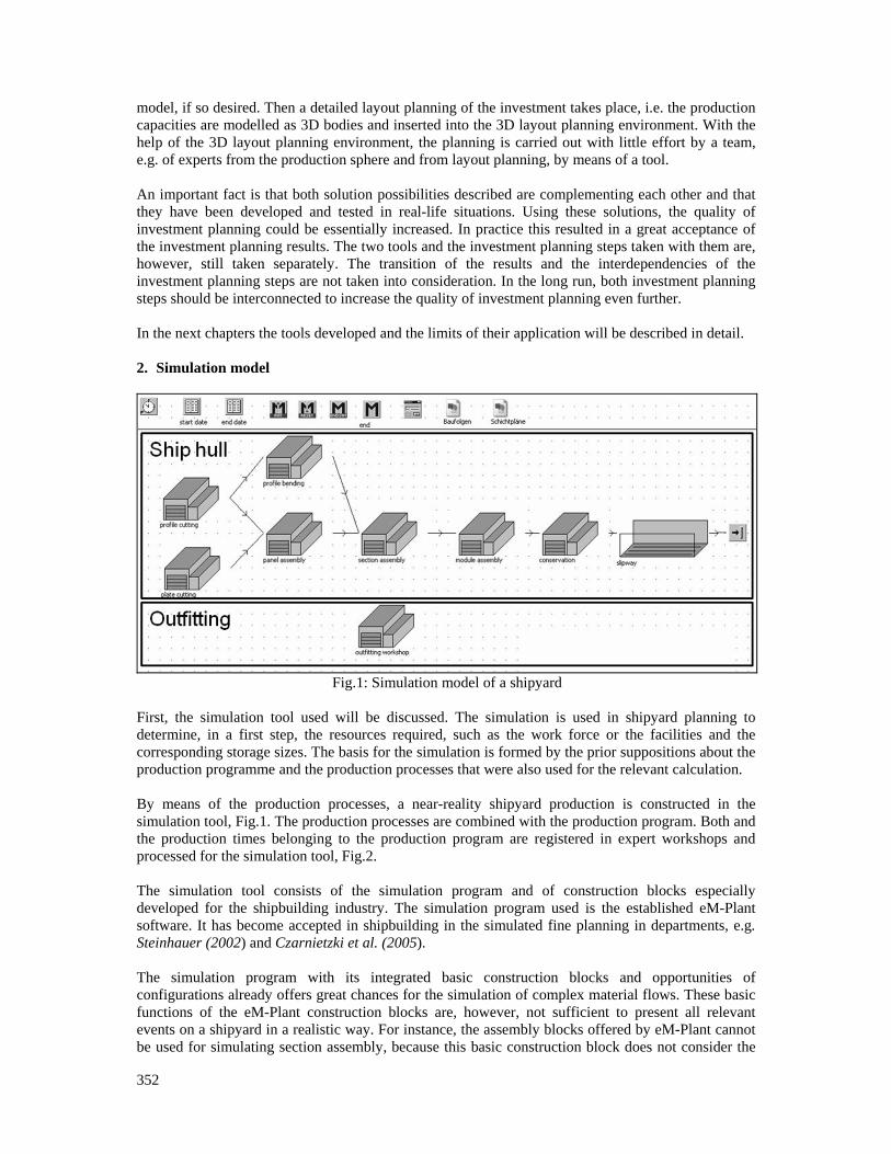
352

model, if so desired. Then a detailed layout planning of the investment takes place, i.e. the production capacities are modelled as 3D bodies and inserted into the 3D layout planning environment. With the help of the 3D layout planning environment, the planning is carried out with little effort by a team, e.g. of experts from the production sphere and from layout planning, by means of a tool. An important fact is that both solution possibilities described are complementing each other and that they have been developed and tested in real-life situations. Using these solutions, the quality of investment planning could be essentially increased. In practice this resulted in a great acceptance of the investment planning results. The two tools and the investment planning steps taken with them are, however, still taken separately. The transition of the results and the interdependencies of the investment planning steps are not taken into consideration. In the long run, both investment planning steps should be interconnected to increase the quality of investment planning even further. In the next chapters the tools developed and the limits of their application will be described in detail. 2. Simulation model

Fig.1: Simulation model of a shipyard First, the simulation tool used will be discussed. The simulation is used in shipyard planning to determine, in a first step, the resources required, such as the work force or the facilities and the corresponding storage sizes. The basis for the simulation is formed by the prior suppositions about the production programme and the production processes that were also used for the relevant calculation. By means of the production processes, a near-reality shipyard production is constructed in the simulation tool, Fig.1. The production processes are combined with the production program. Both and the production times belonging to the production program are registered in expert workshops and processed for the simulation tool, Fig.2. The simulation tool consists of the simulation program and of construction blocks especially developed for the shipbuilding industry. The simulation program used is the established eM-Plant software. It has become accepted in shipbuilding in the simulated fine planning in departments, e.g. Steinhauer (2002) and Czarnietzki et al. (2005). The simulation program with its integrated basic construction blocks and opportunities of configurations already offers great chances for the simulation of complex material flows. These basic functions of the eM-Plant construction blocks are, however, not sufficient to present all relevant events on a shipyard in a realistic way. For instance, the assembly blocks offered by eM-Plant cannot be used for simulating section assembly, because this basic construction block does not consider the

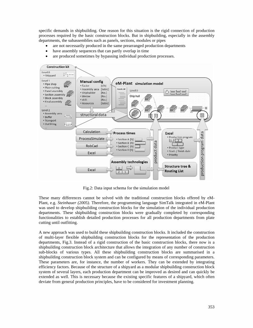
353

specific demands in shipbuilding. One reason for this situation is the rigid connection of production processes required by the basic construction blocks. But in shipbuilding, especially in the assembly departments, the subassemblíes such as panels, sections, modules or pipes

• are not necessarily produced in the same prearranged production departments • have assembly sequences that can partly overlap in time • are produced sometimes by bypassing individual production processes.

Fig.2: Data input schema for the simulation model These many differences cannot be solved with the traditional construction blocks offered by eM-Plant, e.g. Steinhauer (2005). Therefore, the programming language SimTalk integrated in eM-Plant was used to develop shipbuilding construction blocks for the simulation of the individual production departments. These shipbuilding construction blocks were gradually completed by corresponding functionalities to establish detailed production processes for all production departments from plate cutting until outfitting. A new approach was used to build these shipbuilding construction blocks. It included the construction of multi-layer flexible shipbuilding construction blocks for the representation of the production departments, Fig.3. Instead of a rigid construction of the basic construction blocks, there now is a shipbuilding construction block architecture that allows the integration of any number of construction sub-blocks of various types. All these shipbuilding construction blocks are summarised in a shipbuilding construction block system and can be configured by means of corresponding parameters. These parameters are, for instance, the number of workers. They can be extended by integrating efficiency factors. Because of the structure of a shipyard as a modular shipbuilding construction block system of several layers, each production department can be improved as desired and can quickly be extended as well. This is necessary because the existing specific features of a shipyard, which often deviate from general production principles, have to be considered for investment planning.

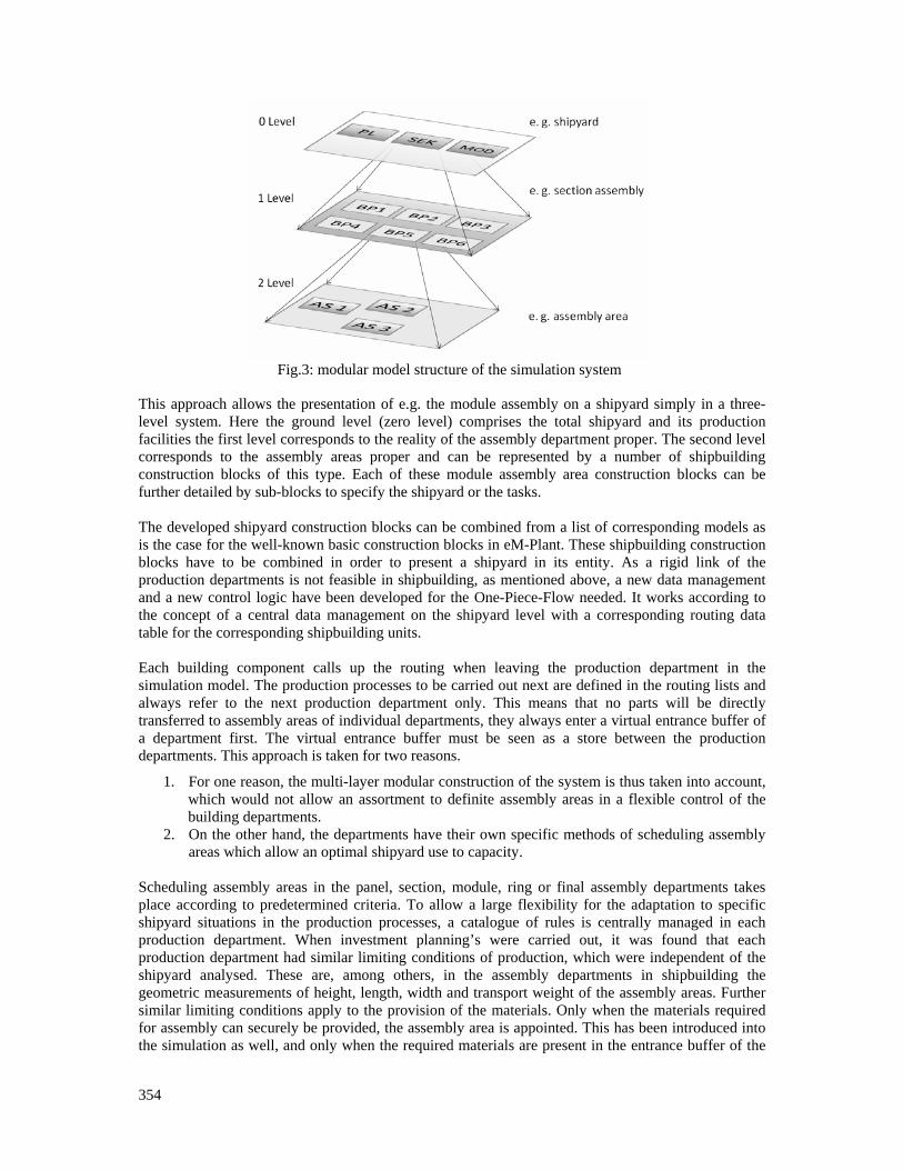
354

Fig.3: modular model structure of the simulation system

This approach allows the presentation of e.g. the module assembly on a shipyard simply in a three-level system. Here the ground level (zero level) comprises the total shipyard and its production facilities the first level corresponds to the reality of the assembly department proper. The second level corresponds to the assembly areas proper and can be represented by a number of shipbuilding construction blocks of this type. Each of these module assembly area construction blocks can be further detailed by sub-blocks to specify the shipyard or the tasks. The developed shipyard construction blocks can be combined from a list of corresponding models as is the case for the well-known basic construction blocks in eM-Plant. These shipbuilding construction blocks have to be combined in order to present a shipyard in its entity. As a rigid link of the production departments is not feasible in shipbuilding, as mentioned above, a new data management and a new control logic have been developed for the One-Piece-Flow needed. It works according to the concept of a central data management on the shipyard level with a corresponding routing data table for the corresponding shipbuilding units. Each building component calls up the routing when leaving the production department in the simulation model. The production processes to be carried out next are defined in the routing lists and always refer to the next production department only. This means that no parts will be directly transferred to assembly areas of individual departments, they always enter a virtual entrance buffer of a department first. The virtual entrance buffer must be seen as a store between the production departments. This approach is taken for two reasons.

1. For one reason, the multi-layer modular construction of the system is thus taken into account, which would not allow an assortment to definite assembly areas in a flexible control of the building departments.

2. On the other hand, the departments have their own specific methods of scheduling assembly areas which allow an optimal shipyard use to capacity.

Scheduling assembly areas in the panel, section, module, ring or final assembly departments takes place according to predetermined criteria. To allow a large flexibility for the adaptation to specific shipyard situations in the production processes, a catalogue of rules is centrally managed in each production department. When investment planning’s were carried out, it was found that each production department had similar limiting conditions of production, which were independent of the shipyard analysed. These are, among others, in the assembly departments in shipbuilding the geometric measurements of height, length, width and transport weight of the assembly areas. Further similar limiting conditions apply to the provision of the materials. Only when the materials required for assembly can securely be provided, the assembly area is appointed. This has been introduced into the simulation as well, and only when the required materials are present in the entrance buffer of the

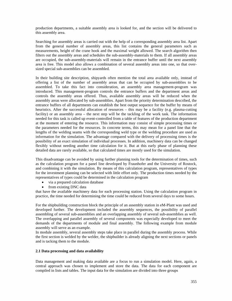
355

production departments, a suitable assembly area is looked for, and the section will be delivered to this assembly area. Searching for assembly areas is carried out with the help of a corresponding assembly area list. Apart from the general number of assembly areas, this list contains the general parameters such as measurements, height of the crane hook and the maximal weight allowed. The search algorithm then filters out the assembly areas and schedules the sub-assembly-materials to them. If all assembly areas are occupied, the sub-assembly-materials will remain in the entrance buffer until the next assembly area is free. This model also allows a combination of several assembly areas into one, so that over-sized special sub-assemblies can be assembled. In their building site description, shipyards often mention the total area available only, instead of offering a list of the number of assembly areas that can be occupied by sub-assemblies to be assembled. To take this fact into consideration, an assembly area management-program was introduced. This management-program controls the entrance buffers and the department areas and controls the assembly areas offered. Thus, available assembly areas will be reduced when the assembly areas were allocated by sub-assemblies. Apart from the priority determination described, the entrance buffers of all departments can establish the best output sequence for the buffer by means of heuristics. After the successful allocation of resources – this may be a facility (e.g. plasma-cutting facility) or an assembly area – the next step will be the tackling of the work task. The information needed for this task is called up event-controlled from a table of features of the production department at the moment of entering the resource. This information may consist of simple processing times or the parameters needed for the resources. In concrete terms, this may mean for a panel line that the lengths of the welding seams with the corresponding weld type or the welding procedure are used as information for the simulation. The advantage compared with the delivery of processing times is the possibility of an exact simulation of individual processes. In addition, machinery data can be changed flexibly without needing another time calculation for it. But at this early phase of planning these detailed data are rarely available, so that calculated times are mostly used for the simulation. This disadvantage can be avoided by using further planning tools for the determination of times, such as the calculation program for a panel line developed by Fraunhofer and the University of Rostock, and combining it with the simulation. By means of this calculation program, representatives of types for the investment planning can be selected with little effort only. The production times needed by the representatives of types could be determined in the calculation program

• via a prepared calculation database • from existing DNC data

that have the available machinery data for each processing station. Using the calculation program in practice, the time needed for determining the time could be reduced from several days to some hours. For the shipbuilding construction block the principle of an assembly station in eM-Plant was used and developed further. The development included the assembly sequences, the possibility of parallel assembling of several sub-assemblies and an overlapping assembly of several sub-assemblies as well. The overlapping and parallel assembly of several components was especially developed to meet the demands of the departments of module and final assembly. The following example from module assembly will serve as an example. In module assembly, several assembly steps take place in parallel during the assembly process. While the first section is welded by the welder, the shipbuilder is already aligning the next sections or panels and is tacking them to the module. 2.1 Data processing and data availability Data management and making data available are a focus to run a simulation model. Here, again, a central approach was chosen to implement and store the data. The data for each component are compiled in lists and tables. The input data for the simulation are divided into three groups

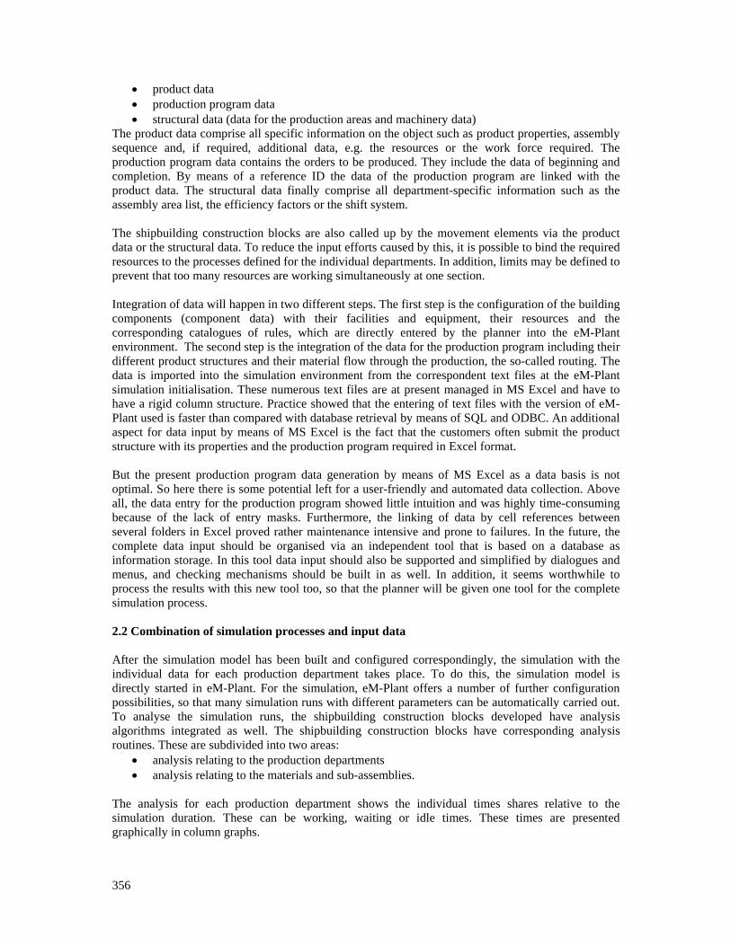
356

• product data • production program data • structural data (data for the production areas and machinery data)

The product data comprise all specific information on the object such as product properties, assembly sequence and, if required, additional data, e.g. the resources or the work force required. The production program data contains the orders to be produced. They include the data of beginning and completion. By means of a reference ID the data of the production program are linked with the product data. The structural data finally comprise all department-specific information such as the assembly area list, the efficiency factors or the shift system. The shipbuilding construction blocks are also called up by the movement elements via the product data or the structural data. To reduce the input efforts caused by this, it is possible to bind the required resources to the processes defined for the individual departments. In addition, limits may be defined to prevent that too many resources are working simultaneously at one section. Integration of data will happen in two different steps. The first step is the configuration of the building components (component data) with their facilities and equipment, their resources and the corresponding catalogues of rules, which are directly entered by the planner into the eM-Plant environment. The second step is the integration of the data for the production program including their different product structures and their material flow through the production, the so-called routing. The data is imported into the simulation environment from the correspondent text files at the eM-Plant simulation initialisation. These numerous text files are at present managed in MS Excel and have to have a rigid column structure. Practice showed that the entering of text files with the version of eM-Plant used is faster than compared with database retrieval by means of SQL and ODBC. An additional aspect for data input by means of MS Excel is the fact that the customers often submit the product structure with its properties and the production program required in Excel format. But the present production program data generation by means of MS Excel as a data basis is not optimal. So here there is some potential left for a user-friendly and automated data collection. Above all, the data entry for the production program showed little intuition and was highly time-consuming because of the lack of entry masks. Furthermore, the linking of data by cell references between several folders in Excel proved rather maintenance intensive and prone to failures. In the future, the complete data input should be organised via an independent tool that is based on a database as information storage. In this tool data input should also be supported and simplified by dialogues and menus, and checking mechanisms should be built in as well. In addition, it seems worthwhile to process the results with this new tool too, so that the planner will be given one tool for the complete simulation process. 2.2 Combination of simulation processes and input data After the simulation model has been built and configured correspondingly, the simulation with the individual data for each production department takes place. To do this, the simulation model is directly started in eM-Plant. For the simulation, eM-Plant offers a number of further configuration possibilities, so that many simulation runs with different parameters can be automatically carried out. To analyse the simulation runs, the shipbuilding construction blocks developed have analysis algorithms integrated as well. The shipbuilding construction blocks have corresponding analysis routines. These are subdivided into two areas:

• analysis relating to the production departments • analysis relating to the materials and sub-assemblies.

The analysis for each production department shows the individual times shares relative to the simulation duration. These can be working, waiting or idle times. These times are presented graphically in column graphs.

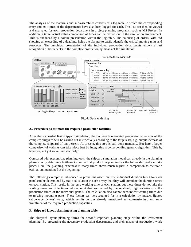
357

The analysis of the materials and sub-assemblies consists of a log table in which the corresponding entry and exit times of the departments have also been logged for each. This list can then be viewed and evaluated for each production department in project planning programs, such as MS Project. In addition, a target/actual value comparison of times can be carried out in the simulation environment. This is enhanced by a colour presentation within the log-table. The colouring of orders, with red showing an exceeding of a deadline, helps the planner to easily identify the critical moving units and resources. The graphical presentation of the individual production departments allows a fast recognition of bottlenecks in the complete production by means of the simulation.

Fig.4: Data analysing

2.2 Procedure to estimate the required production facilities After the successful first shipyard simulation, the bottleneck orientated production extension of the complete shipyard will be carried out interactively according to the targets set, e.g. output increase of the complete shipyard of ten percent. At present, this step is still done manually. But here a larger comparison of variants can take place just by integrating a corresponding generic algorithm. This is, however, not yet solved satisfactorily. Compared with present-day planning tools, the shipyard simulation model can already in the planning phase exactly determine bottlenecks, and a first production planning for the future shipyard can take place. Here, the planning exactness is many times above much higher in comparison to the static estimation, mentioned at the beginning. The following example is introduced to prove this assertion. The individual duration times for each panel can be determined by static calculation in such a way that they will cumulate the duration times on each station. This results in the pure working time of each station, but these times do not take the waiting times and idle times into account that are caused by the relatively high variations of the production times of the individual panels. The calculation also cannot account for waiting times due to missing mounting parts. These factors can be accounted for in a calculation by inexact figures (allowance factors) only, which results in the already mentioned mis-dimensioning and mis-investment of the required production capacities. 3. Shipyard layout planning using planning table

The shipyard layout planning forms the second important planning stage within the investment planning. By presenting the necessary production departments and their means of production, work

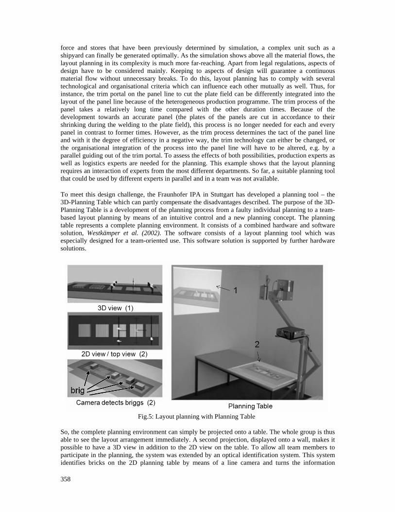
358

force and stores that have been previously determined by simulation, a complex unit such as a shipyard can finally be generated optimally. As the simulation shows above all the material flows, the layout planning in its complexity is much more far-reaching. Apart from legal regulations, aspects of design have to be considered mainly. Keeping to aspects of design will guarantee a continuous material flow without unnecessary breaks. To do this, layout planning has to comply with several technological and organisational criteria which can influence each other mutually as well. Thus, for instance, the trim portal on the panel line to cut the plate field can be differently integrated into the layout of the panel line because of the heterogeneous production programme. The trim process of the panel takes a relatively long time compared with the other duration times. Because of the development towards an accurate panel (the plates of the panels are cut in accordance to their shrinking during the welding to the plate field), this process is no longer needed for each and every panel in contrast to former times. However, as the trim process determines the tact of the panel line and with it the degree of efficiency in a negative way, the trim technology can either be changed, or the organisational integration of the process into the panel line will have to be altered, e.g. by a parallel guiding out of the trim portal. To assess the effects of both possibilities, production experts as well as logistics experts are needed for the planning. This example shows that the layout planning requires an interaction of experts from the most different departments. So far, a suitable planning tool that could be used by different experts in parallel and in a team was not available. To meet this design challenge, the Fraunhofer IPA in Stuttgart has developed a planning tool – the 3D-Planning Table which can partly compensate the disadvantages described. The purpose of the 3D-Planning Table is a development of the planning process from a faulty individual planning to a team-based layout planning by means of an intuitive control and a new planning concept. The planning table represents a complete planning environment. It consists of a combined hardware and software solution, Westkämper et al. (2002). The software consists of a layout planning tool which was especially designed for a team-oriented use. This software solution is supported by further hardware solutions.

Fig.5: Layout planning with Planning Table

So, the complete planning environment can simply be projected onto a table. The whole group is thus able to see the layout arrangement immediately. A second projection, displayed onto a wall, makes it possible to have a 3D view in addition to the 2D view on the table. To allow all team members to participate in the planning, the system was extended by an optical identification system. This system identifies bricks on the 2D planning table by means of a line camera and turns the information

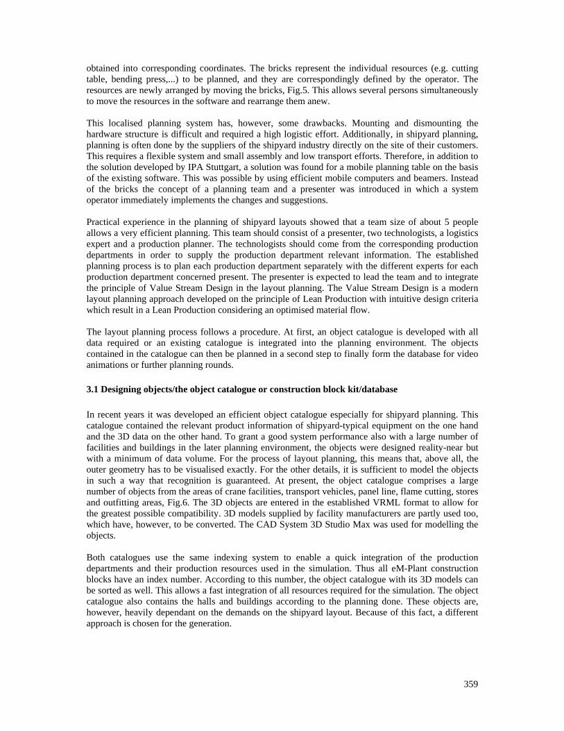
359

obtained into corresponding coordinates. The bricks represent the individual resources (e.g. cutting table, bending press,...) to be planned, and they are correspondingly defined by the operator. The resources are newly arranged by moving the bricks, Fig.5. This allows several persons simultaneously to move the resources in the software and rearrange them anew. This localised planning system has, however, some drawbacks. Mounting and dismounting the hardware structure is difficult and required a high logistic effort. Additionally, in shipyard planning, planning is often done by the suppliers of the shipyard industry directly on the site of their customers. This requires a flexible system and small assembly and low transport efforts. Therefore, in addition to the solution developed by IPA Stuttgart, a solution was found for a mobile planning table on the basis of the existing software. This was possible by using efficient mobile computers and beamers. Instead of the bricks the concept of a planning team and a presenter was introduced in which a system operator immediately implements the changes and suggestions. Practical experience in the planning of shipyard layouts showed that a team size of about 5 people allows a very efficient planning. This team should consist of a presenter, two technologists, a logistics expert and a production planner. The technologists should come from the corresponding production departments in order to supply the production department relevant information. The established planning process is to plan each production department separately with the different experts for each production department concerned present. The presenter is expected to lead the team and to integrate the principle of Value Stream Design in the layout planning. The Value Stream Design is a modern layout planning approach developed on the principle of Lean Production with intuitive design criteria which result in a Lean Production considering an optimised material flow. The layout planning process follows a procedure. At first, an object catalogue is developed with all data required or an existing catalogue is integrated into the planning environment. The objects contained in the catalogue can then be planned in a second step to finally form the database for video animations or further planning rounds.

3.1 Designing objects/the object catalogue or construction block kit/database In recent years it was developed an efficient object catalogue especially for shipyard planning. This catalogue contained the relevant product information of shipyard-typical equipment on the one hand and the 3D data on the other hand. To grant a good system performance also with a large number of facilities and buildings in the later planning environment, the objects were designed reality-near but with a minimum of data volume. For the process of layout planning, this means that, above all, the outer geometry has to be visualised exactly. For the other details, it is sufficient to model the objects in such a way that recognition is guaranteed. At present, the object catalogue comprises a large number of objects from the areas of crane facilities, transport vehicles, panel line, flame cutting, stores and outfitting areas, Fig.6. The 3D objects are entered in the established VRML format to allow for the greatest possible compatibility. 3D models supplied by facility manufacturers are partly used too, which have, however, to be converted. The CAD System 3D Studio Max was used for modelling the objects. Both catalogues use the same indexing system to enable a quick integration of the production departments and their production resources used in the simulation. Thus all eM-Plant construction blocks have an index number. According to this number, the object catalogue with its 3D models can be sorted as well. This allows a fast integration of all resources required for the simulation. The object catalogue also contains the halls and buildings according to the planning done. These objects are, however, heavily dependant on the demands on the shipyard layout. Because of this fact, a different approach is chosen for the generation.

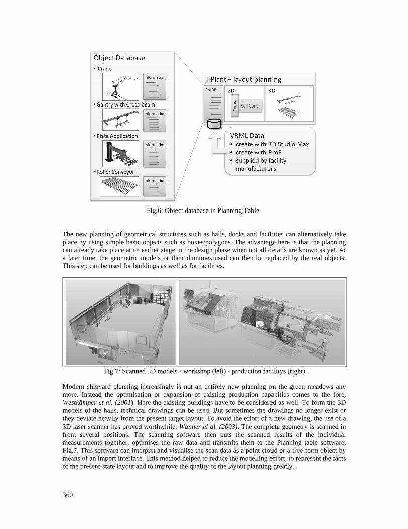
360

Fig.6: Object database in Planning Table

The new planning of geometrical structures such as halls, docks and facilities can alternatively take place by using simple basic objects such as boxes/polygons. The advantage here is that the planning can already take place at an earlier stage in the design phase when not all details are known as yet. At a later time, the geometric models or their dummies used can then be replaced by the real objects. This step can be used for buildings as well as for facilities.

Fig.7: Scanned 3D models - workshop (left) - production facilitys (right)

Modern shipyard planning increasingly is not an entirely new planning on the green meadows any more. Instead the optimisation or expansion of existing production capacities comes to the fore, Westkämper et al. (2001). Here the existing buildings have to be considered as well. To form the 3D models of the halls, technical drawings can be used. But sometimes the drawings no longer exist or they deviate heavily from the present target layout. To avoid the effort of a new drawing, the use of a 3D laser scanner has proved worthwhile, Wanner el al. (2003). The complete geometry is scanned in from several positions. The scanning software then puts the scanned results of the individual measurements together, optimises the raw data and transmits them to the Planning table software, Fig.7. This software can interpret and visualise the scan data as a point cloud or a free-form object by means of an import interface. This method helped to reduce the modelling effort, to represent the facts of the present-state layout and to improve the quality of the layout planning greatly.

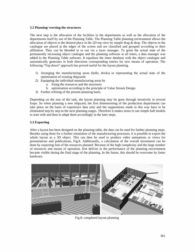
361

3.2 Planning/ erecting the structures The next step is the allocation of the facilities in the departments as well as the allocation of the departments itself by use of the Planning Table. The Planning Table planning environment allows the allocation of objects to the desired place in the 2D top view by simple drag & drop. The objects in the catalogue are placed at the edges of the screen and are classified and grouped according to their affiliation. They can be blended in or out via a layer manager. To grant the actual state of the permanently increasing object catalogue and the planning software at all times, a data manager was added to the Planning Table software. It equalises the inner database with the object catalogue and automatically generates in both directions corresponding entries for new means of operation. The following “Top down” approach has proved useful for the layout planning.

1) Arranging the manufacturing areas (halls, docks) or representing the actual state of the optimisation of existing shipyards

2) Equipping the individual manufacturing areas by a. fixing the resources and the structures b. optimisation according to the principle of Value Stream Design

3) Further refining of the present planning basis. Depending on the size of the task, the layout planning may be gone through iteratively in several loops. So when planning a new shipyard, the first dimensioning of the production departments can take place on the basis of experience data only and the suppositions made in this way have to be eliminated step by step in the next planning stages. Therefore it makes sense to use simple hall models to start with and then to adapt them accordingly in the later steps. 3.3 Exporting After a layout has been designed on the planning table, the data can be used for further planning steps. Besides using them for a further simulation of the manufacturing processes, it is possible to export the whole layout as a 3D object. This can then be used to produce video animations or views for presentations and publications, Fig.8. Additionally, a calculation of the overall investment can be done by exporting lists of the resources planned. Because of the high complexity and the large number of resources and means of operation, first deficits in the performance of the planning environment became visible during the final stage of the planning. In the future, this should be overcome by faster hardware.

Fig.8: completed layout planning

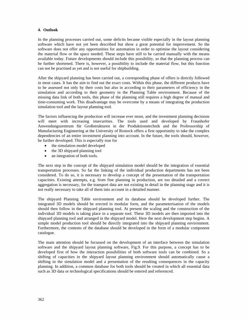
362

4. Outlook In the planning processes carried out, some deficits became visible especially in the layout planning software which have not yet been described but show a great potential for improvement. So the software does not offer any opportunities for automation in order to optimise the layout considering the material flow or the space needed. These steps have still to be carried manually with the means available today. Future developments should include this possibility, so that the planning process can be further shortened. There is, however, a possibility to include the material flow, but this function can not be practised as yet and is not useful for shipbuilding. After the shipyard planning has been carried out, a corresponding phase of offers is directly followed in most cases. It has the aim to find out the exact costs. Within this phase, the different products have to be assessed not only by their costs but also in according to their parameters of efficiency in the simulation and according to their geometry in the Planning Table environment. Because of the missing data link of both tools, this phase of the planning still requires a high degree of manual and time-consuming work. This disadvantage may be overcome by a means of integrating the production simulation tool and the layout planning tool. The factors influencing the production will increase ever more, and the investment planning decisions will meet with increasing insecurities. The tools used and developed by Fraunhofer Anwendungszentrum für Großstrukturen in der Produktionstechnik and the Professorship of Manufacturing Engineering at the University of Rostock offers a first opportunity to take the complex dependencies of an entire investment planning into account. In the future, the tools should, however, be further developed. This is especially true for

• the simulation model developed • the 3D shipyard planning tool • an integration of both tools.

The next step in the concept of the shipyard simulation model should be the integration of essential transportation processes. So far the linking of the individual production departments has not been considered. To do so, it is necessary to develop a concept of the presentation of the transportation capacities. Existing attempts, e.g. from fine planning in production, are too detailed and a correct aggregation is necessary, for the transport data are not existing in detail in the planning stage and it is not really necessary to take all of them into account in a detailed manner. The shipyard Planning Table environment and its database should be developed further. The integrated 3D models should be erected in modular form, and the parameterisation of the models should then follow in the shipyard planning tool. At present the scaling and the construction of the individual 3D models is taking place in a separate tool. These 3D models are then imported into the shipyard planning tool and arranged in the shipyard model. Here the next development step begins. A simple model production tool should be directly integrated into the shipyard planning environment. Furthermore, the contents of the database should be developed in the form of a modular component catalogue. The main attention should be focussed on the development of an interface between the simulation software and the shipyard layout planning software, Fig.9. For this purpose, a concept has to be developed first of how the interaction possibilities of both software tools can be combined. So a shifting of capacities in the shipyard layout planning environment should automatically cause a shifting in the simulation model and a presentation of the resulting consequences in the capacity planning. In addition, a common database for both tools should be created in which all essential data such as 3D data or technological specifications should be entered and referenced.

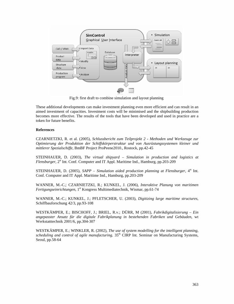
363

Fig.9: first draft to combine simulation and layout planning

These additional developments can make investment planning even more efficient and can result in an aimed investment of capacities. Investment costs will be minimised and the shipbuilding production becomes more effective. The results of the tools that have been developed and used in practice are a token for future benefits. References CZARNIETZKI, R. et al. (2005), Schlussbericht zum Teilprojekt 2 - Methoden und Werkzeuge zur Optimierung der Produktion der Schiffskörperstruktur und von Ausrüstungssystemen kleiner und mittlerer Spezialschiffe, BmBF Project ProPeene2010., Rostock, pp.42-45 STEINHAUER, D. (2003), The virtual shipyard – Simulation in production and logistics at Flensburger, 2st Int. Conf. Computer and IT Appl. Maritime Ind., Hamburg, pp.203-209 STEINHAUER, D. (2005), SAPP – Simulation aided production planning at Flensburger, 4st Int. Conf. Computer and IT Appl. Maritime Ind., Hamburg, pp.203-209 WANNER, M.-C.; CZARNIETZKI, R.; KUNKEL, J. (2006), Interaktive Planung von maritimen Fertigungseinrichtungen, 1st Kongress Multimediatechnik, Wismar, pp.61-74 WANNER, M.-C.; KUNKEL, J.; PFLETSCHER, U. (2003), Digitizing large maritime structures, Schiffbauforschung 42/3, pp.93-108 WESTKÄMPER, E.; BISCHOFF, J.; BRIEL, R.v.; DÜRR, M (2001), Fabrikdigitalisierung – Ein angepasster Ansatz für die digitale Fabrikplanung in bestehenden Fabriken und Gebäuden, wt Werkstatttechnik 2001/6, pp.304-307 WESTKÄMPER, E.; WINKLER, R. (2002), The use of system modelling for the intelligent planning, scheduling and control of agile manufacturing, 35th CIRP Int. Seminar on Manufacturing Systems, Seoul, pp.58-64

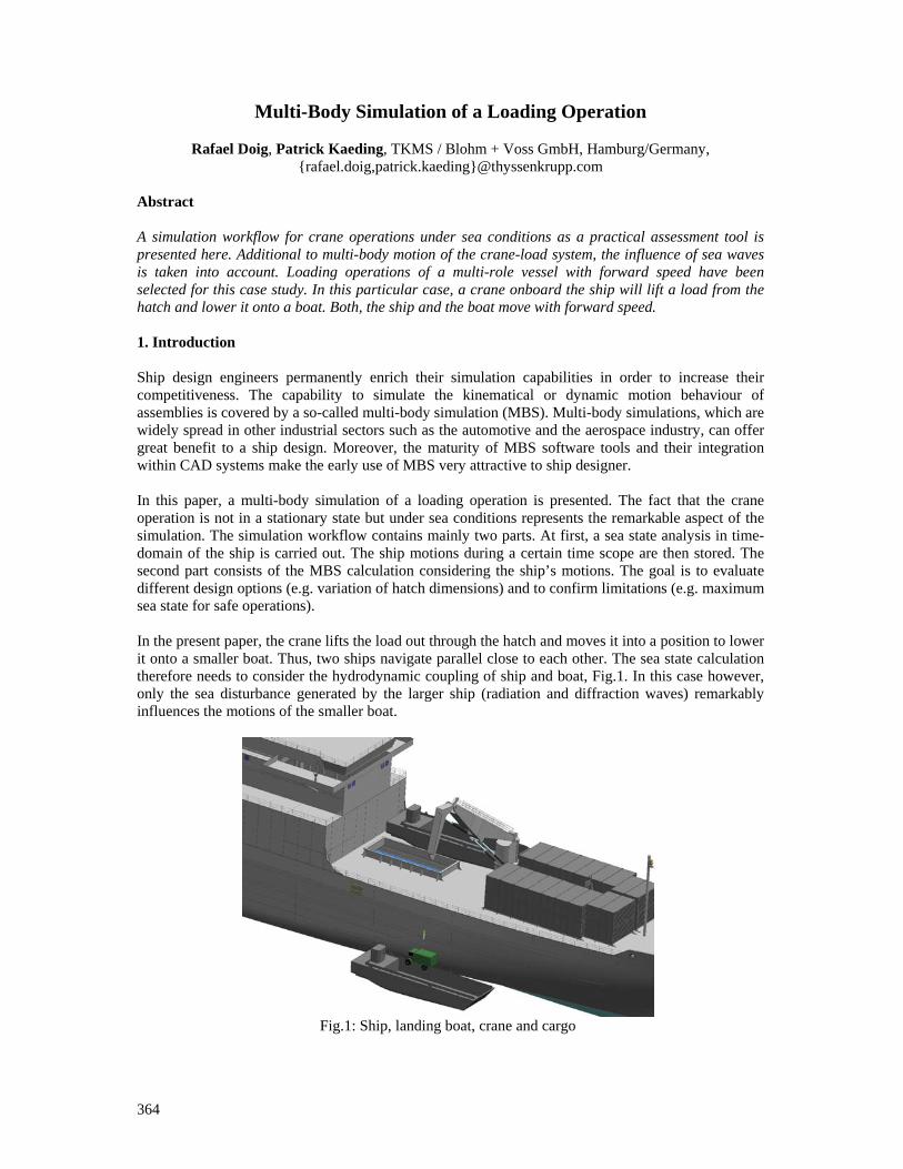
364

Multi-Body Simulation of a Loading Operation

Rafael Doig, Patrick Kaeding, TKMS / Blohm + Voss GmbH, Hamburg/Germany, rafael.doig,patrick.kaeding@thyssenkrupp.com

Abstract A simulation workflow for crane operations under sea conditions as a practical assessment tool is presented here. Additional to multi-body motion of the crane-load system, the influence of sea waves is taken into account. Loading operations of a multi-role vessel with forward speed have been selected for this case study. In this particular case, a crane onboard the ship will lift a load from the hatch and lower it onto a boat. Both, the ship and the boat move with forward speed.

1. Introduction Ship design engineers permanently enrich their simulation capabilities in order to increase their competitiveness. The capability to simulate the kinematical or dynamic motion behaviour of assemblies is covered by a so-called multi-body simulation (MBS). Multi-body simulations, which are widely spread in other industrial sectors such as the automotive and the aerospace industry, can offer great benefit to a ship design. Moreover, the maturity of MBS software tools and their integration within CAD systems make the early use of MBS very attractive to ship designer. In this paper, a multi-body simulation of a loading operation is presented. The fact that the crane operation is not in a stationary state but under sea conditions represents the remarkable aspect of the simulation. The simulation workflow contains mainly two parts. At first, a sea state analysis in time-domain of the ship is carried out. The ship motions during a certain time scope are then stored. The second part consists of the MBS calculation considering the ship’s motions. The goal is to evaluate different design options (e.g. variation of hatch dimensions) and to confirm limitations (e.g. maximum sea state for safe operations). In the present paper, the crane lifts the load out through the hatch and moves it into a position to lower it onto a smaller boat. Thus, two ships navigate parallel close to each other. The sea state calculation therefore needs to consider the hydrodynamic coupling of ship and boat, Fig.1. In this case however, only the sea disturbance generated by the larger ship (radiation and diffraction waves) remarkably influences the motions of the smaller boat.

Fig.1: Ship, landing boat, crane and cargo

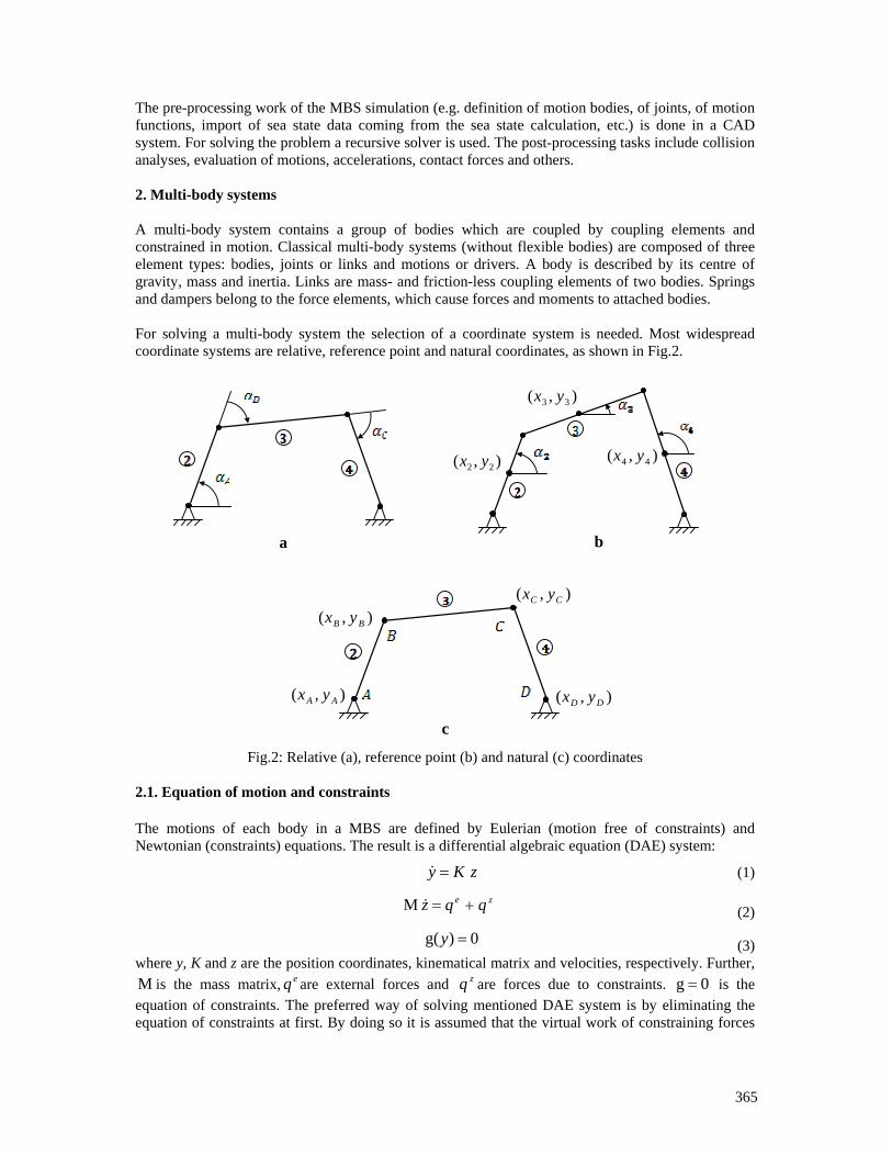
365

The pre-processing work of the MBS simulation (e.g. definition of motion bodies, of joints, of motion functions, import of sea state data coming from the sea state calculation, etc.) is done in a CAD system. For solving the problem a recursive solver is used. The post-processing tasks include collision analyses, evaluation of motions, accelerations, contact forces and others. 2. Multi-body systems

A multi-body system contains a group of bodies which are coupled by coupling elements and constrained in motion. Classical multi-body systems (without flexible bodies) are composed of three element types: bodies, joints or links and motions or drivers. A body is described by its centre of gravity, mass and inertia. Links are mass- and friction-less coupling elements of two bodies. Springs and dampers belong to the force elements, which cause forces and moments to attached bodies.

For solving a multi-body system the selection of a coordinate system is needed. Most widespread coordinate systems are relative, reference point and natural coordinates, as shown in Fig.2.

Fig.2: Relative (a), reference point (b) and natural (c) coordinates

2.1. Equation of motion and constraints The motions of each body in a MBS are defined by Eulerian (motion free of constraints) and Newtonian (constraints) equations. The result is a differential algebraic equation (DAE) system:

zKy =& (1)

ze qqz +=&M (2)

0)g( =y (3) where y, K and z are the position coordinates, kinematical matrix and velocities, respectively. Further, M is the mass matrix, eq are external forces and zq are forces due to constraints. 0g = is the equation of constraints. The preferred way of solving mentioned DAE system is by eliminating the equation of constraints at first. By doing so it is assumed that the virtual work of constraining forces

),( 22 yx

),( 33 yx

),( 44 yx

),( AA yx

),( BB yx),( CC yx

),( DD yx

a b

c

366

zF and moments zM , which appear in the system, vanishes:

0=+∑ zTzT MFv δωδ (4)

By solving Eq.(4) virtual linear vδ and angular δω velocities result, which are then applied to the motion equations free of constraints. The final equation system is an ODE system and can be solved more easily. This approach is applied by Lagrange, D’Alembert and Jourdain. The equation of motion can be described by a characteristic equation of order 3. Since the target is the use of standard integration methods, a reduction of order is conducted by applying time derivatives. By doing so, no longer a robust condition to the coordinates is ensured so that the coordinates drift. This effect is called drift-off. For this problem, stabilisation methods have been developed such as the Gear-Gupta-Leimkuhler and the Baumgarte stabilisation methods, Baumgarte (1972). 2.2. Numerical integration An appropriate numerical integration method for solving the remaining ODE system needs further to be selected. Explicit methods, which use values only from time t for calculating values at time t+h, are known as fast and sometimes unstable. Examples are the first order Euler integration and second order Heun integration methods. However, whenever the time step becomes too small, an implicit integration method is recommended, which at the same time is preferred for its strong stability. Implicit methods use values from time t as well as from time t+h for calculating values at time t+h. The computational time for a calculation step is however higher than with an explicit method. Examples for implicit methods are the first order Euler integration (implicit) and the second order trapezoidal rule. A known problem of integration methods is the appearance of numerical dissipation. In other words, the system loses energy by each time step. This leads e.g. for the simulation of a friction less, oscillation system, to wrong results (damping). However, many MBS engineers use this to simulate real dissipation by calibrating a so-called damping or dissipation factor within MBS programs. 3. Multi-body seakeeping

Typically multi-body systems are simulated with respect to a resting reference system. This is acceptable as far as the system is fixed to the earth or the motion can be ignored. However, this approach is not anymore applicable to the simulation of a ship crane under the effect of sea waves. It is easy to imagine that the load on the crane behaves differently in a seaway as on shore. Thus, an investigation of the ship’s seaway condition is necessary in order to consider the influence of wave forces. Furthermore, the wave interaction of a ship and a boat is crucial for simulating a realistic loading operation. Is this case, the sea keeping code must be able to consider hydrodynamic coupling effects. Especially, the wave distortion generated by the ship influences strongly the motion of the boat. The effect of the boat – on the other hand – can generally be neglected considering the remarkable size difference. Ship motions along and rotations about the axis, shown in Fig.3, are: - Motion along x is called surge - Motion along y is called sway - Motion along z is called heave

- Rotation about x is called roll - Rotation about y is called pitch - Rotation about z is called yaw

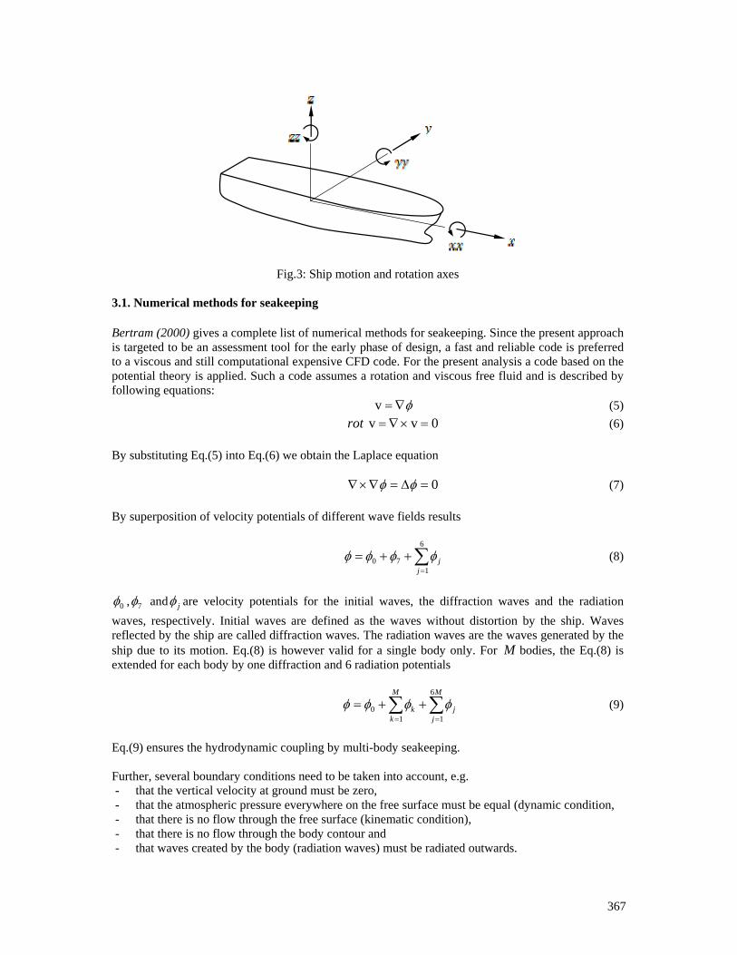
367

Fig.3: Ship motion and rotation axes 3.1. Numerical methods for seakeeping Bertram (2000) gives a complete list of numerical methods for seakeeping. Since the present approach is targeted to be an assessment tool for the early phase of design, a fast and reliable code is preferred to a viscous and still computational expensive CFD code. For the present analysis a code based on the potential theory is applied. Such a code assumes a rotation and viscous free fluid and is described by following equations:

φ∇=v (5) 0vv =×∇=rot (6)

By substituting Eq.(5) into Eq.(6) we obtain the Laplace equation

0=Δ=∇×∇ φφ (7)

By superposition of velocity potentials of different wave fields results

∑=

++=6

170

jjφφφφ (8)

0φ , 7φ and jφ are velocity potentials for the initial waves, the diffraction waves and the radiation

waves, respectively. Initial waves are defined as the waves without distortion by the ship. Waves reflected by the ship are called diffraction waves. The radiation waves are the waves generated by the ship due to its motion. Eq.(8) is however valid for a single body only. For M bodies, the Eq.(8) is extended for each body by one diffraction and 6 radiation potentials

∑∑==

++=M

jj

M

kk

6

110 φφφφ (9)

Eq.(9) ensures the hydrodynamic coupling by multi-body seakeeping. Further, several boundary conditions need to be taken into account, e.g. - that the vertical velocity at ground must be zero, - that the atmospheric pressure everywhere on the free surface must be equal (dynamic condition, - that there is no flow through the free surface (kinematic condition), - that there is no flow through the body contour and - that waves created by the body (radiation waves) must be radiated outwards.

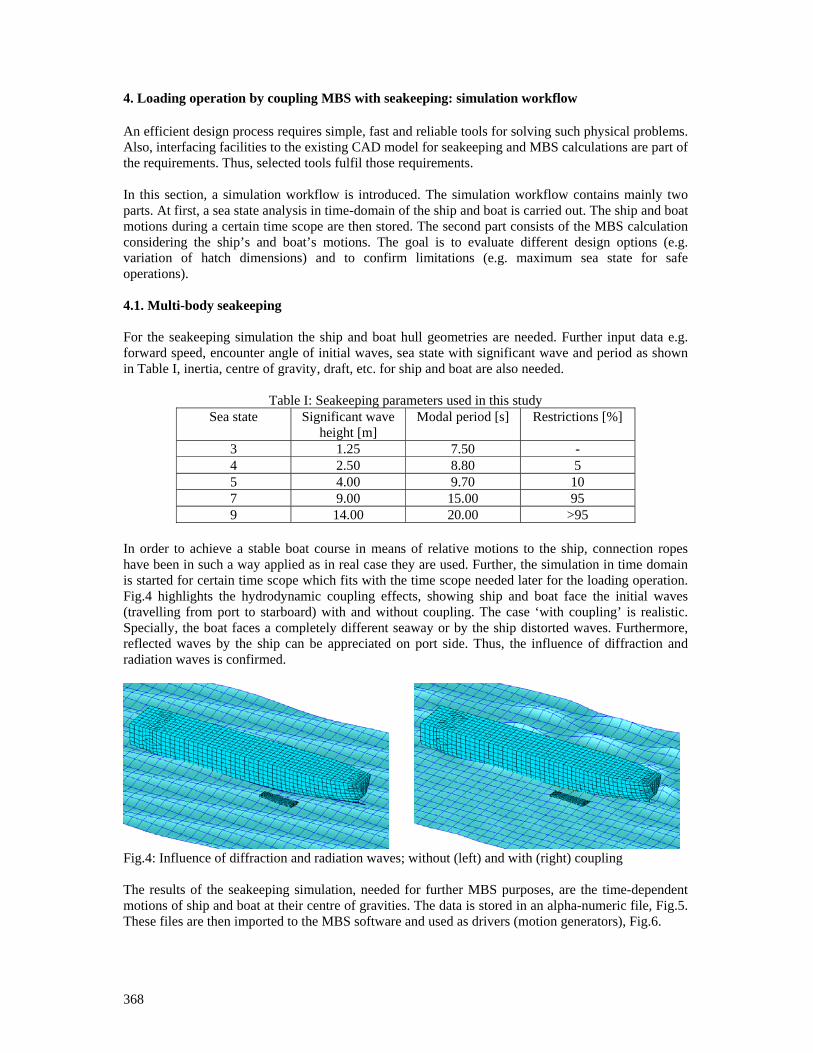
368

4. Loading operation by coupling MBS with seakeeping: simulation workflow An efficient design process requires simple, fast and reliable tools for solving such physical problems. Also, interfacing facilities to the existing CAD model for seakeeping and MBS calculations are part of the requirements. Thus, selected tools fulfil those requirements. In this section, a simulation workflow is introduced. The simulation workflow contains mainly two parts. At first, a sea state analysis in time-domain of the ship and boat is carried out. The ship and boat motions during a certain time scope are then stored. The second part consists of the MBS calculation considering the ship’s and boat’s motions. The goal is to evaluate different design options (e.g. variation of hatch dimensions) and to confirm limitations (e.g. maximum sea state for safe operations). 4.1. Multi-body seakeeping For the seakeeping simulation the ship and boat hull geometries are needed. Further input data e.g. forward speed, encounter angle of initial waves, sea state with significant wave and period as shown in Table I, inertia, centre of gravity, draft, etc. for ship and boat are also needed.

Table I: Seakeeping parameters used in this study Sea state Significant wave

height [m] Modal period [s] Restrictions [%]

3 1.25 7.50 - 4 2.50 8.80 5 5 4.00 9.70 10 7 9.00 15.00 95 9 14.00 20.00 >95

In order to achieve a stable boat course in means of relative motions to the ship, connection ropes have been in such a way applied as in real case they are used. Further, the simulation in time domain is started for certain time scope which fits with the time scope needed later for the loading operation. Fig.4 highlights the hydrodynamic coupling effects, showing ship and boat face the initial waves (travelling from port to starboard) with and without coupling. The case ‘with coupling’ is realistic. Specially, the boat faces a completely different seaway or by the ship distorted waves. Furthermore, reflected waves by the ship can be appreciated on port side. Thus, the influence of diffraction and radiation waves is confirmed.

Fig.4: Influence of diffraction and radiation waves; without (left) and with (right) coupling The results of the seakeeping simulation, needed for further MBS purposes, are the time-dependent motions of ship and boat at their centre of gravities. The data is stored in an alpha-numeric file, Fig.5. These files are then imported to the MBS software and used as drivers (motion generators), Fig.6.

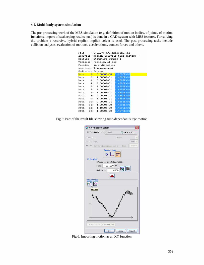
369

4.2. Multi-body system simulation The pre-processing work of the MBS simulation (e.g. definition of motion bodies, of joints, of motion functions, import of seakeeping results, etc.) is done in a CAD system with MBS features. For solving the problem a recursive, hybrid explicit-implicit solver is used. The post-processing tasks include collision analyses, evaluation of motions, accelerations, contact forces and others.

Fig.5: Part of the result file showing time-dependant surge motion

Fig.6: Importing motion as an XY function

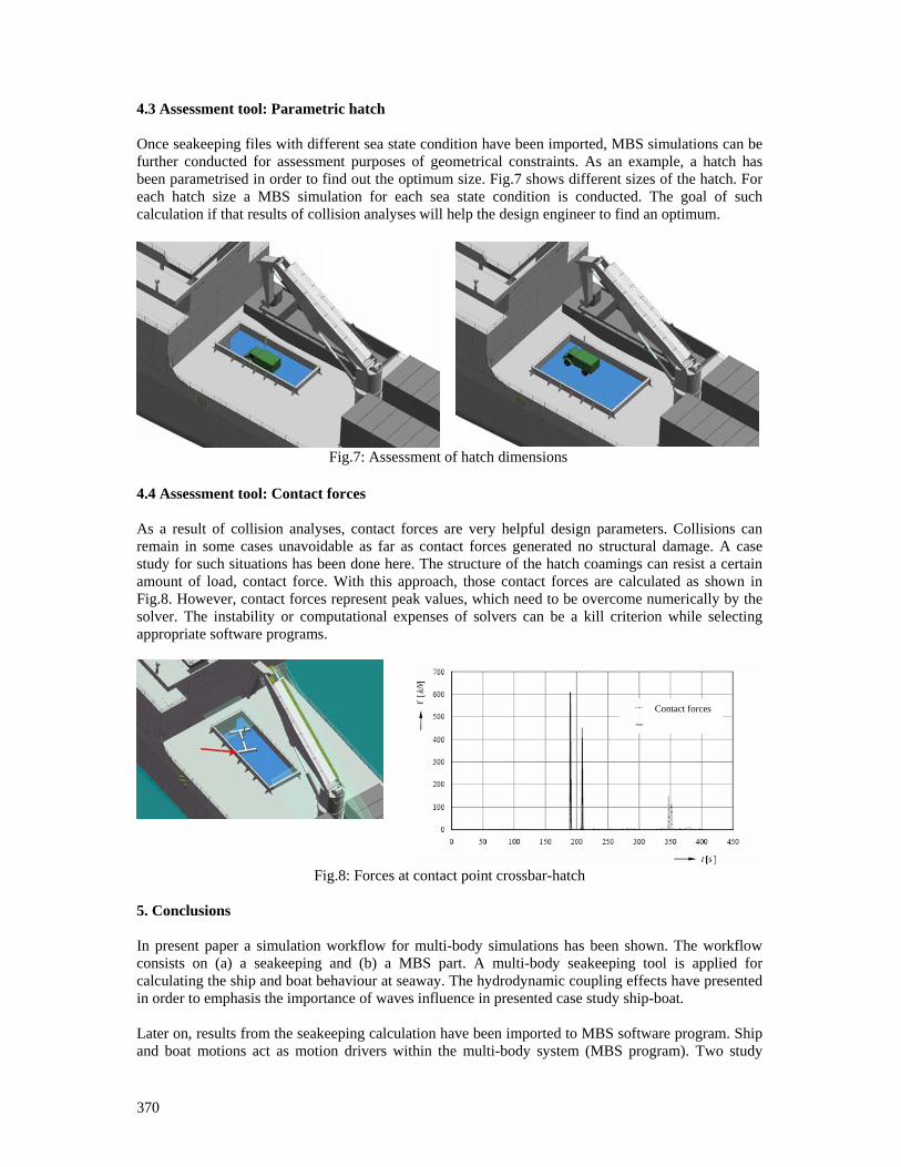
370

4.3 Assessment tool: Parametric hatch Once seakeeping files with different sea state condition have been imported, MBS simulations can be further conducted for assessment purposes of geometrical constraints. As an example, a hatch has been parametrised in order to find out the optimum size. Fig.7 shows different sizes of the hatch. For each hatch size a MBS simulation for each sea state condition is conducted. The goal of such calculation if that results of collision analyses will help the design engineer to find an optimum.

Fig.7: Assessment of hatch dimensions 4.4 Assessment tool: Contact forces As a result of collision analyses, contact forces are very helpful design parameters. Collisions can remain in some cases unavoidable as far as contact forces generated no structural damage. A case study for such situations has been done here. The structure of the hatch coamings can resist a certain amount of load, contact force. With this approach, those contact forces are calculated as shown in Fig.8. However, contact forces represent peak values, which need to be overcome numerically by the solver. The instability or computational expenses of solvers can be a kill criterion while selecting appropriate software programs.

Fig.8: Forces at contact point crossbar-hatch

5. Conclusions In present paper a simulation workflow for multi-body simulations has been shown. The workflow consists on (a) a seakeeping and (b) a MBS part. A multi-body seakeeping tool is applied for calculating the ship and boat behaviour at seaway. The hydrodynamic coupling effects have presented in order to emphasis the importance of waves influence in presented case study ship-boat. Later on, results from the seakeeping calculation have been imported to MBS software program. Ship and boat motions act as motion drivers within the multi-body system (MBS program). Two study

Contact forces

371

cases have been shown in order to confirm the suitability of presented workflow as an assessment tool for the early phase of ship design. The first study case was the variation of hatch dimensions for several sea state conditions. The hatch was parametrised within the CAD system. Different sizes were tested (collision analyses) with different sea state conditions. Collision analyses are helpful for engineers by finding an optimum size. However, collisions are not always avoidable. Thus, a second case study has been presented and deals with contact forces acting by collisions. Contact forces at a longitudinal hatch coaming has been evaluated and shown here. Theses forces can then applied for structural analyses in order to confirm no or less damage. References ASCHER U.M.; PETZOLD L.R. (1998) Computer methods for ordinary differential equations and differential – algebraic equations, Philadelphia: Society for Industrial and Applied Mathematics BAUMGARTE J. (1972) Stabilization of constraints and integrals of motion in dynamical systems, Computer Methods in Applied Mechanics and Engineering, Publ. Technology Massachusetts Institute, pp.1-16 BERTRAM, V. (2000), Practical Ship Hydrodynamics, Butterworth&Heinemann CLAUSS, G.; BIRK, L. (2001) Diffraktionstheorie, theoretische Grundlagen zum Programmiersystem WAMIT, TU Berlin EICH-SOELLNER, E.; FÜHRER, C. (1998) Numerical methods in multibody dynamics, Teubner GARCÍA DE JALÓN, J.; BAYO, E. (1994), Kinematic and dynamic simulation of multi-body systems: The real time challenge, Springer GEAR, C.W.; LEIMKUHLER, B.; GUPTA, G.K. (1985) Automatic integration of Euler-Lagrange equations with constrains, J. Computational Applied Mathematics 12 & 13, pp.77-90 GIPSER, M. (1999) Systemdynamik und Simulation, Teubner-Verlag HAIRER, E.; NØRSETT, S.P.; WANNER, G. (1993) Solving ordinary differential equations I, Nonstiff Problems, Springer HAUG E.J. (1989) Computer-Aided Kinematics and Dynamics of Mechanical Systems – Basic Methods, Boston: Allyn and Bacon. LENNARTSSON, A. (1990) Efficient multibody dynamics, Royal Institute of Technology, Stockholm, Ph.D. thesis LUGNER, P.; SPRINGER, H.; DESOYER, K. (2000) Dynamik von Mehrkörpersystemen, TU Vienna NEWMAN, J.N. (1978), The theory of ship motions, Advances in Applied Mechanics, Academic Press Inc., pp.222-283 PENNESTRÌ, E.; VITA, L. (2005), Multibody dynamics in advanced education, Advances in Computational Multibody Systems II, Springer SCHIEHLEN, W. (1990) Multibody systems handbook, Springer SHABANA A. (1998) Dynamics of multibody systems, Cambridge Univ. Press II UGS (2006) Parasolid XT Format Reference. - UGS Corporation.

372

Autonomous Traffic Model for Ship Maneuvering Simulations Based on Historical Data

Karl Gunnar Aarsæther, NTNU, Trondheim/Norway, aarsathe@ntnu.no

Torgeir Moan, NTNU, Trondheim/Norway, tormo@ntnu.no Abstract Computer simulation is frequently used in the assessment of human performance, training and risk analysis of ship maneuvering. An important component in such simulations is the surrounding environment, including both weather and traffic. Weather is often represented by time-domain realizations of meteorological data. We present a similar approach to modelling traffic lanes in an area, using data gathered from Automatic Identification System. The main contributions in this paper are (i) a model for dynamic ship traffic in an area guided by the IMO “International Regulations for Preventing Collisions at Sea”, and (ii) a method for calculation of the location and statistics of the main traffic lanes from a real-world area. The presented model can readily be integrated into ship maneuvering simulation environments and used as a time-domain traffic representation. The presented procedure groups 3200 AIS time-series into 5 main traffic-lanes

1. Introduction Ship maneuvering simulations have gained acceptance as a tool for risk analysis, autopilot development and crew training. Simulations are often focused on the interaction between the local ship and the natural environment and great effort has been devoted to the development of accurate models for ship dynamics e.g. Berlekom (1972) and Fossen (2002,2005). The environment in a ship maneuvering simulation is composed both of the weather conditions and the instantaneous traffic situation. Weather models are available from statistics meticulously gathered for decades and allow us to represent visibility, waves, wind speed and direction with time domain realizations. There are no comparable sources for description of ship traffic. The ever-increasing power of computers has made high complexity Mote-Carlo type studies feasible, and it has become possible to experiment with several ships in the same simulation. In past traffic simulation studies the navigation interaction between the local ship and other vessels have been simplified away in Hutchinson (2003) or ignored and replaced by “blind navigation” models, which ignore all navigation interaction in Gucma (2007) and Merrick et al. (2003). The overall ship traffic in an area is composed of vessels following different traffic lanes, each lane with different characteristics such as traffic density, points of origin and destination, speed, cross-track spread and course changes according to a predetermined program. A model for the traffic situation in an area would complement weather models and forms a more complete description of the maneuvering environment. Description of the geometric traffic features as well as quantification of variability in the traffic pattern has been in the domain of expert opinion, but the introduction of the Automatic Identification System (AIS) has, as a secondary effect, enabled mass collection of quantitative data of ship traffic. Data available from AIS can be used to construct ship track-lines and process these to obtain the geometric description of the traffic pattern and its dynamic variation in ship speed and cross-track error. In this context three separate definitions of traffic data is needed

- Time-series: Time ordered data of the state of a single ship - Track-line: The trace of the ship position over time - Traffic-lane: A collection of track-lines following a similar path

Traffic density on a traffic-lane can be measured by the arrival times of vessels. Inter-arrival time statistics can be determined and applied to represent the appearance of new vessels at the start of the traffic-lane. To explore the capabilities of traffic-lane modelling from AIS data the area around the harbour of Tananger on the southwest cost of Norway was selected. The area was selected due to

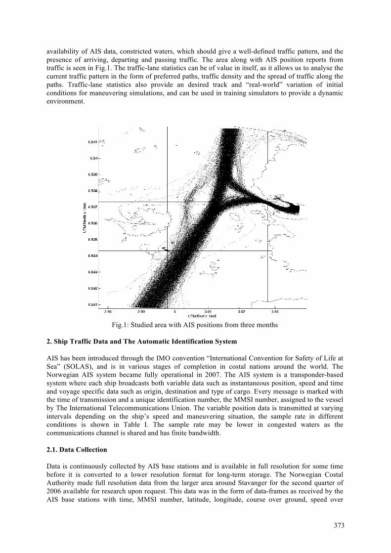
373

availability of AIS data, constricted waters, which should give a well-defined traffic pattern, and the presence of arriving, departing and passing traffic. The area along with AIS position reports from traffic is seen in Fig.1. The traffic-lane statistics can be of value in itself, as it allows us to analyse the current traffic pattern in the form of preferred paths, traffic density and the spread of traffic along the paths. Traffic-lane statistics also provide an desired track and “real-world” variation of initial conditions for maneuvering simulations, and can be used in training simulators to provide a dynamic environment.

Fig.1: Studied area with AIS positions from three months

2. Ship Traffic Data and The Automatic Identification System AIS has been introduced through the IMO convention “International Convention for Safety of Life at Sea” (SOLAS), and is in various stages of completion in costal nations around the world. The Norwegian AIS system became fully operational in 2007. The AIS system is a transponder-based system where each ship broadcasts both variable data such as instantaneous position, speed and time and voyage specific data such as origin, destination and type of cargo. Every message is marked with the time of transmission and a unique identification number, the MMSI number, assigned to the vessel by The International Telecommunications Union. The variable position data is transmitted at varying intervals depending on the ship’s speed and maneuvering situation, the sample rate in different conditions is shown in Table I. The sample rate may be lower in congested waters as the communications channel is shared and has finite bandwidth.

2.1. Data Collection Data is continuously collected by AIS base stations and is available in full resolution for some time before it is converted to a lower resolution format for long-term storage. The Norwegian Costal Authority made full resolution data from the larger area around Stavanger for the second quarter of 2006 available for research upon request. This data was in the form of data-frames as received by the AIS base stations with time, MMSI number, latitude, longitude, course over ground, speed over

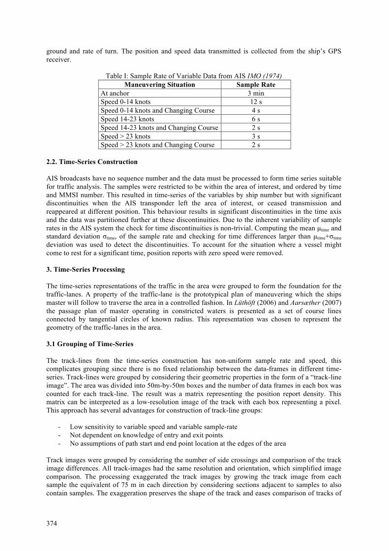
374

ground and rate of turn. The position and speed data transmitted is collected from the ship’s GPS receiver.

Table I: Sample Rate of Variable Data from AIS IMO (1974)

Maneuvering Situation Sample Rate At anchor 3 min Speed 0-14 knots 12 s Speed 0-14 knots and Changing Course 4 s Speed 14-23 knots 6 s Speed 14-23 knots and Changing Course 2 s Speed > 23 knots 3 s Speed > 23 knots and Changing Course 2 s

2.2. Time-Series Construction AIS broadcasts have no sequence number and the data must be processed to form time series suitable for traffic analysis. The samples were restricted to be within the area of interest, and ordered by time and MMSI number. This resulted in time-series of the variables by ship number but with significant discontinuities when the AIS transponder left the area of interest, or ceased transmission and reappeared at different position. This behaviour results in significant discontinuities in the time axis and the data was partitioned further at these discontinuities. Due to the inherent variability of sample rates in the AIS system the check for time discontinuities is non-trivial. Computing the mean µtime and standard deviation σtime, of the sample rate and checking for time differences larger than µtime+σtime deviation was used to detect the discontinuities. To account for the situation where a vessel might come to rest for a significant time, position reports with zero speed were removed. 3. Time-Series Processing The time-series representations of the traffic in the area were grouped to form the foundation for the traffic-lanes. A property of the traffic-lane is the prototypical plan of maneuvering which the ships master will follow to traverse the area in a controlled fashion. In Lüthöft (2006) and Aarsæther (2007) the passage plan of master operating in constricted waters is presented as a set of course lines connected by tangential circles of known radius. This representation was chosen to represent the geometry of the traffic-lanes in the area. 3.1 Grouping of Time-Series The track-lines from the time-series construction has non-uniform sample rate and speed, this complicates grouping since there is no fixed relationship between the data-frames in different time-series. Track-lines were grouped by considering their geometric properties in the form of a “track-line image”. The area was divided into 50m-by-50m boxes and the number of data frames in each box was counted for each track-line. The result was a matrix representing the position report density. This matrix can be interpreted as a low-resolution image of the track with each box representing a pixel. This approach has several advantages for construction of track-line groups:

- Low sensitivity to variable speed and variable sample-rate - Not dependent on knowledge of entry and exit points - No assumptions of path start and end point location at the edges of the area

Track images were grouped by considering the number of side crossings and comparison of the track image differences. All track-images had the same resolution and orientation, which simplified image comparison. The processing exaggerated the track images by growing the track image from each sample the equivalent of 75 m in each direction by considering sections adjacent to samples to also contain samples. The exaggeration preserves the shape of the track and eases comparison of tracks of

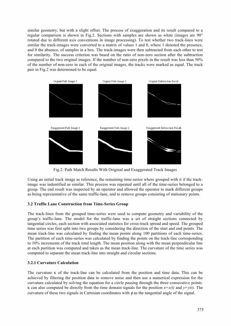
375

similar geometry, but with a slight offset. The process of exaggeration and its result compared to a regular comparison is shown in Fig.2. Sections with samples are shown as white (images are 90° rotated due to different axis conventions in image processing). To test whether two track-lines were similar the track-images were converted to a matrix of values 1 and 0, where 1 denoted the presence, and 0 the absence, of samples in a box. The track-images were then subtracted from each other to test for similarity. The success criterion was based on the ratio of non-zero section after the subtraction compared to the two original images. If the number of non-zero pixels in the result was less than 50% of the number of non-zero in each of the original images, the tracks were marked as equal. The track pair in Fig.2 was determined to be equal.

Fig.2: Path Match Results With Original and Exaggerated Track Images

Using an initial track image as reference, the remaining time-series where grouped with it if the track-image was indentified as similar. This process was repeated until all of the time-series belonged to a group. The end result was inspected by an operator and allowed the operator to mark different groups as being representative of the same traffic-lane, and to remove groups consisting of stationary points. 3.2 Traffic Lane Construction from Time-Series Group The track-lines from the grouped time-series were used to compute geometry and variability of the group’s traffic-lane. The model for the traffic-lane was a set of straight sections connected by tangential circles, each section with associated statistics for cross-track spread and speed. The grouped time series was first split into two groups by considering the direction of the start and end points. The mean track-line was calculated by finding the mean points along 100 partitions of each time-series. The partition of each time-series was calculated by finding the points on the track-line corresponding to 10% increments of the track total length. The mean position along with the mean perpendicular line at each partition was computed and taken as the mean track-line. The curvature of the time series was computed to separate the mean track-line into straight and circular sections. 3.2.1 Curvature Calculation The curvature κ of the track-line can be calculated from the position and time data. This can be achieved by filtering the position data to remove noise and then use a numerical expression for the curvature calculated by solving the equation for a circle passing through the three consecutive points. κ can also computed be directly from the time domain signals for the position x=x(t) and y=y(t). The curvature of these two signals in Cartesian coordinates with φ as the tangential angle of the signal.

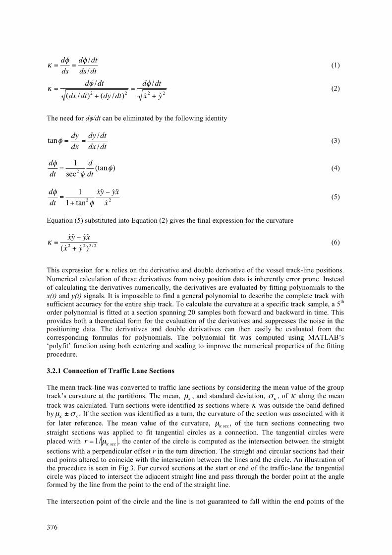
376

€

κ =dφds

=dφ /dtds /dt

(1)

€

κ =dφ /dt

(dx /dt)2 + (dy /dt)2=

dφ /dt˙ x 2 + ˙ y 2

(2)

The need for dφ/dt can be eliminated by the following identity

€

tanφ =dydx

=dy /dtdx /dt

(3)

€

dφdt

=1

sec2 φddt(tanφ) (4)

€

dφdt

=1

1+ tan2 φ˙ x y − ˙ y x

˙ x 2 (5)

Equation (5) substituted into Equation (2) gives the final expression for the curvature

€

κ =˙ x y − ˙ y x

( ˙ x 2 + ˙ y 2)3 / 2 (6)

This expression for κ relies on the derivative and double derivative of the vessel track-line positions. Numerical calculation of these derivatives from noisy position data is inherently error prone. Instead of calculating the derivatives numerically, the derivatives are evaluated by fitting polynomials to the x(t) and y(t) signals. It is impossible to find a general polynomial to describe the complete track with sufficient accuracy for the entire ship track. To calculate the curvature at a specific track sample, a 5th order polynomial is fitted at a section spanning 20 samples both forward and backward in time. This provides both a theoretical form for the evaluation of the derivatives and suppresses the noise in the positioning data. The derivatives and double derivatives can then easily be evaluated from the corresponding formulas for polynomials. The polynomial fit was computed using MATLAB’s ‘polyfit’ function using both centering and scaling to improve the numerical properties of the fitting procedure. 3.2.1 Connection of Traffic Lane Sections The mean track-line was converted to traffic lane sections by considering the mean value of the group track’s curvature at the partitions. The mean,

€

µκ , and standard deviation,

€

σκ , of

€

κ along the mean track was calculated. Turn sections were identified as sections where

€

κ was outside the band defined by

€

µκ ±σκ . If the section was identified as a turn, the curvature of the section was associated with it for later reference. The mean value of the curvature,

€

µκ sec , of the turn sections connecting two straight sections was applied to fit tangential circles as a connection. The tangential circles were placed with

€

r =1/µκ sec , the center of the circle is computed as the intersection between the straight sections with a perpendicular offset r in the turn direction. The straight and circular sections had their end points altered to coincide with the intersection between the lines and the circle. An illustration of the procedure is seen in Fig.3. For curved sections at the start or end of the traffic-lane the tangential circle was placed to intersect the adjacent straight line and pass through the border point at the angle formed by the line from the point to the end of the straight line. The intersection point of the circle and the line is not guaranteed to fall within the end points of the

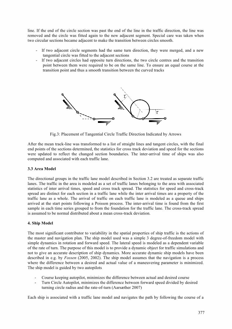
377

line. If the end of the circle section was past the end of the line in the traffic direction, the line was removed and the circle was fitted again to the new adjacent segment. Special care was taken when two circular sections became adjacent to make the transition between circles smooth.

- If two adjacent circle segments had the same turn direction, they were merged, and a new tangential circle was fitted to the adjacent sections

- If two adjacent circles had opposite turn directions, the two circle centres and the transition point between them were required to be on the same line. To ensure an equal course at the transition point and thus a smooth transition between the curved tracks

Fig.3: Placement of Tangential Circle Traffic Direction Indicated by Arrows

After the mean track-line was transformed to a list of straight lines and tangent circles, with the final end points of the sections determined, the statistics for cross track deviation and speed for the sections were updated to reflect the changed section boundaries. The inter-arrival time of ships was also computed and associated with each traffic lane. 3.3 Area Model The directional groups in the traffic lane model described in Section 3.2 are treated as separate traffic lanes. The traffic in the area is modeled as a set of traffic lanes belonging to the area with associated statistics of inter arrival times, speed and cross track spread. The statistics for speed and cross-track spread are distinct for each section in a traffic lane while the inter arrival times are a property of the traffic lane as a whole. The arrival of traffic on each traffic lane is modeled as a queue and ships arrived at the start points following a Poisson process. The inter-arrival time is found from the first sample in each time series grouped to from the foundation for the traffic lane. The cross-track spread is assumed to be normal distributed about a mean cross-track deviation. 4. Ship Model The most significant contributor to variability in the spatial properties of ship traffic is the actions of the master and navigation plan. The ship model used was a simple 3 degree-of-freedom model with simple dynamics in rotation and forward speed. The lateral speed is modeled as a dependent variable of the rate of turn. The purpose of this model is to provide a dynamic object for traffic simulations and not to give an accurate description of ship dynamics. More accurate dynamic ship models have been described in e.g. by Fossen (2005, 2002). The ship model assumes that the navigation is a process where the difference between a desired and actual value of a maneuvering parameter is minimized. The ship model is guided by two autopilots

- Course keeping autopilot, minimizes the difference between actual and desired course - Turn Circle Autopilot, minimizes the difference between forward speed divided by desired

turning circle radius and the rate-of-turn (Aarsæther 2007)

Each ship is associated with a traffic lane model and navigates the path by following the course of a

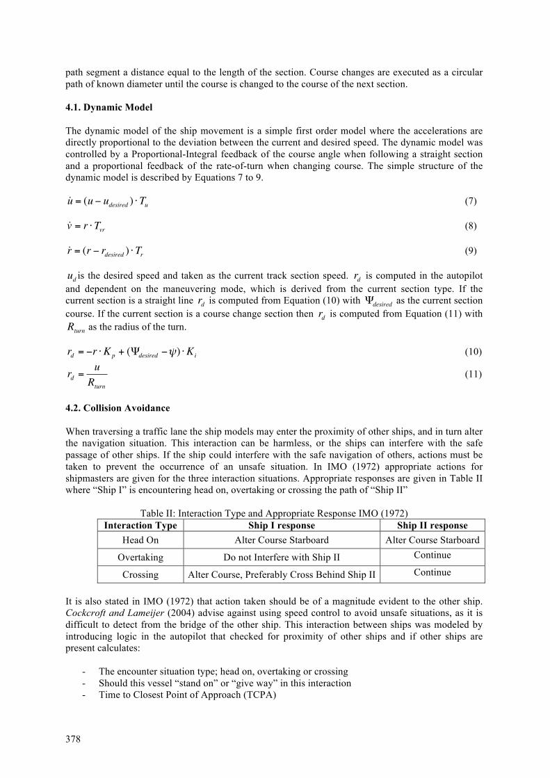
378

path segment a distance equal to the length of the section. Course changes are executed as a circular path of known diameter until the course is changed to the course of the next section. 4.1. Dynamic Model The dynamic model of the ship movement is a simple first order model where the accelerations are directly proportional to the deviation between the current and desired speed. The dynamic model was controlled by a Proportional-Integral feedback of the course angle when following a straight section and a proportional feedback of the rate-of-turn when changing course. The simple structure of the dynamic model is described by Equations 7 to 9.

€

˙ u = (u − udesired ) ⋅Tu (7)

€

˙ v = r ⋅Tvr (8)

€

˙ r = (r − rdesired ) ⋅Tr (9)

€

ud is the desired speed and taken as the current track section speed.

€

rd is computed in the autopilot and dependent on the maneuvering mode, which is derived from the current section type. If the current section is a straight line

€

rd is computed from Equation (10) with

€

Ψdesired as the current section course. If the current section is a course change section then

€

rd is computed from Equation (11) with

€

Rturn as the radius of the turn.

€

rd = −r ⋅Kp + (Ψdesired −ψ) ⋅Ki (10)

€

rd =uRturn

(11)

4.2. Collision Avoidance When traversing a traffic lane the ship models may enter the proximity of other ships, and in turn alter the navigation situation. This interaction can be harmless, or the ships can interfere with the safe passage of other ships. If the ship could interfere with the safe navigation of others, actions must be taken to prevent the occurrence of an unsafe situation. In IMO (1972) appropriate actions for shipmasters are given for the three interaction situations. Appropriate responses are given in Table II where “Ship I” is encountering head on, overtaking or crossing the path of “Ship II”

Table II: Interaction Type and Appropriate Response IMO (1972)

Interaction Type Ship I response Ship II response Head On Alter Course Starboard Alter Course Starboard

Overtaking Do not Interfere with Ship II Continue

Crossing Alter Course, Preferably Cross Behind Ship II Continue

It is also stated in IMO (1972) that action taken should be of a magnitude evident to the other ship. Cockcroft and Lameijer (2004) advise against using speed control to avoid unsafe situations, as it is difficult to detect from the bridge of the other ship. This interaction between ships was modeled by introducing logic in the autopilot that checked for proximity of other ships and if other ships are present calculates:

- The encounter situation type; head on, overtaking or crossing - Should this vessel “stand on” or “give way” in this interaction - Time to Closest Point of Approach (TCPA)

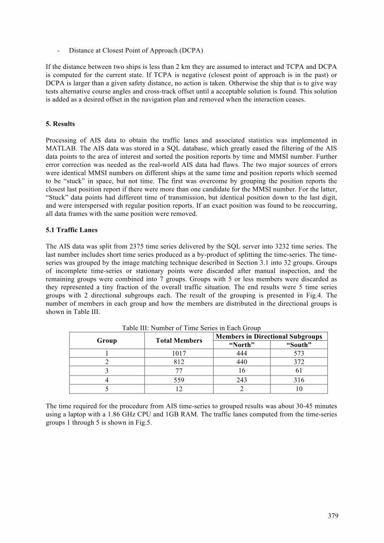
379

- Distance at Closest Point of Approach (DCPA) If the distance between two ships is less than 2 km they are assumed to interact and TCPA and DCPA is computed for the current state. If TCPA is negative (closest point of approach is in the past) or DCPA is larger than a given safety distance, no action is taken. Otherwise the ship that is to give way tests alternative course angles and cross-track offset until a acceptable solution is found. This solution is added as a desired offset in the navigation plan and removed when the interaction ceases. 5. Results Processing of AIS data to obtain the traffic lanes and associated statistics was implemented in MATLAB. The AIS data was stored in a SQL database, which greatly eased the filtering of the AIS data points to the area of interest and sorted the position reports by time and MMSI number. Further error correction was needed as the real-world AIS data had flaws. The two major sources of errors were identical MMSI numbers on different ships at the same time and position reports which seemed to be “stuck” in space, but not time. The first was overcome by grouping the position reports the closest last position report if there were more than one candidate for the MMSI number. For the latter, “Stuck” data points had different time of transmission, but identical position down to the last digit, and were interspersed with regular position reports. If an exact position was found to be reoccurring, all data frames with the same position were removed. 5.1 Traffic Lanes The AIS data was split from 2375 time series delivered by the SQL server into 3232 time series. The last number includes short time series produced as a by-product of splitting the time-series. The time-series was grouped by the image matching technique described in Section 3.1 into 32 groups. Groups of incomplete time-series or stationary points were discarded after manual inspection, and the remaining groups were combined into 7 groups. Groups with 5 or less members were discarded as they represented a tiny fraction of the overall traffic situation. The end results were 5 time series groups with 2 directional subgroups each. The result of the grouping is presented in Fig.4. The number of members in each group and how the members are distributed in the directional groups is shown in Table III.

Table III: Number of Time Series in Each Group Members in Directional Subgroups Group Total Members “North” “South”

1 1017 444 573 2 812 440 372 3 77 16 61 4 559 243 316 5 12 2 10

The time required for the procedure from AIS time-series to grouped results was about 30-45 minutes using a laptop with a 1.86 GHz CPU and 1GB RAM. The traffic lanes computed from the time-series groups 1 through 5 is shown in Fig.5.

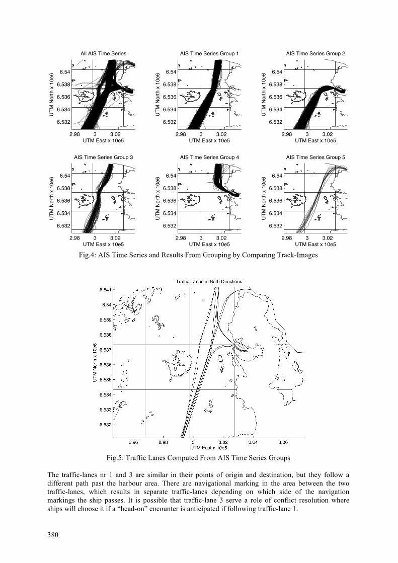
380

2.98 3 3.02

6.532

6.534

6.536

6.538

6.54

All AIS Time Series

UTM East x 10e5

UT

M N

ort

h x

10

e6

2.98 3 3.02

6.532

6.534

6.536

6.538

6.54

AIS Time Series Group 1

UTM East x 10e5

UT

M N

ort

h x

10

e6

2.98 3 3.02

6.532

6.534

6.536

6.538

6.54

AIS Time Series Group 2

UTM East x 10e5

UT

M N

ort

h x

10

e6

2.98 3 3.02

6.532

6.534

6.536

6.538

6.54

AIS Time Series Group 3

UTM East x 10e5

UT

M N

ort

h x

10

e6

2.98 3 3.02

6.532

6.534

6.536

6.538

6.54

AIS Time Series Group 4

UTM East x 10e5

UT

M N

ort

h x

10

e6

2.98 3 3.02

6.532

6.534

6.536

6.538

6.54

AIS Time Series Group 5

UTM East x 10e5

UT

M N

ort

h x

10

e6

Fig.4: AIS Time Series and Results From Grouping by Comparing Track-Images

Fig.5: Traffic Lanes Computed From AIS Time Series Groups The traffic-lanes nr 1 and 3 are similar in their points of origin and destination, but they follow a different path past the harbour area. There are navigational marking in the area between the two traffic-lanes, which results in separate traffic-lanes depending on which side of the navigation markings the ship passes. It is possible that traffic-lane 3 serve a role of conflict resolution where ships will choose it if a “head-on” encounter is anticipated if following traffic-lane 1.

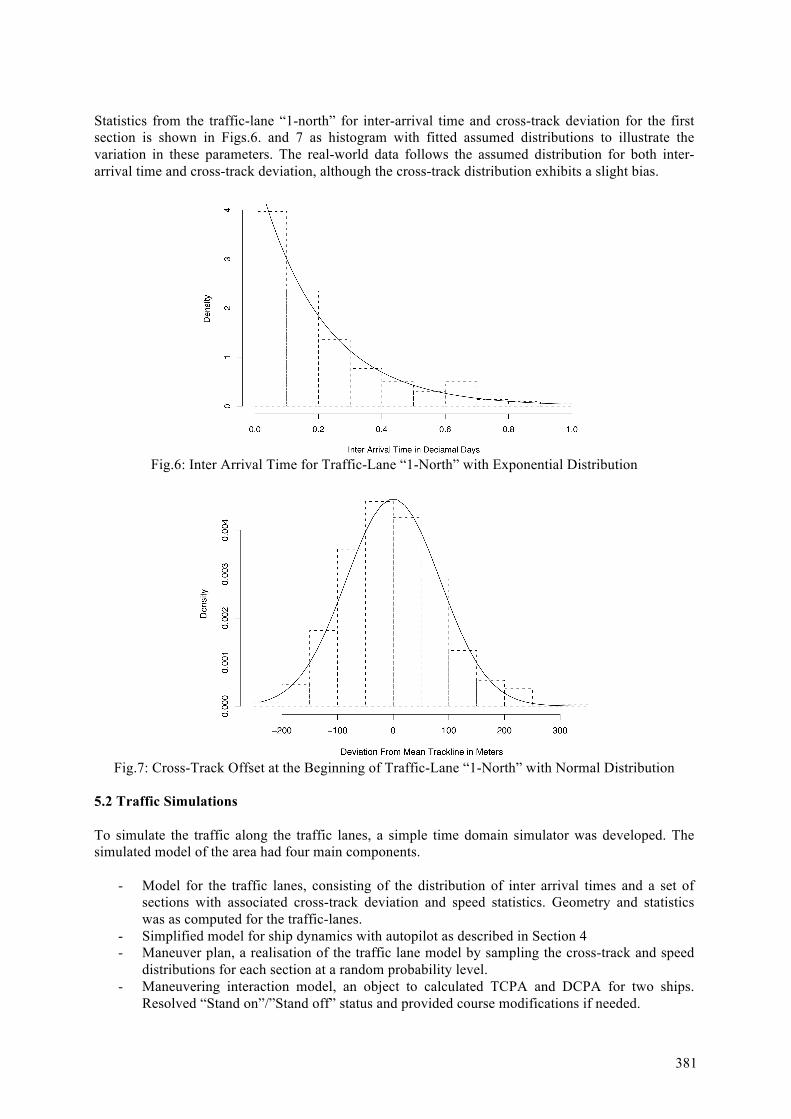
381

Statistics from the traffic-lane “1-north” for inter-arrival time and cross-track deviation for the first section is shown in Figs.6. and 7 as histogram with fitted assumed distributions to illustrate the variation in these parameters. The real-world data follows the assumed distribution for both inter-arrival time and cross-track deviation, although the cross-track distribution exhibits a slight bias.

Fig.6: Inter Arrival Time for Traffic-Lane “1-North” with Exponential Distribution

Fig.7: Cross-Track Offset at the Beginning of Traffic-Lane “1-North” with Normal Distribution

5.2 Traffic Simulations To simulate the traffic along the traffic lanes, a simple time domain simulator was developed. The simulated model of the area had four main components.

- Model for the traffic lanes, consisting of the distribution of inter arrival times and a set of sections with associated cross-track deviation and speed statistics. Geometry and statistics was as computed for the traffic-lanes.

- Simplified model for ship dynamics with autopilot as described in Section 4 - Maneuver plan, a realisation of the traffic lane model by sampling the cross-track and speed

distributions for each section at a random probability level. - Maneuvering interaction model, an object to calculated TCPA and DCPA for two ships.

Resolved “Stand on”/”Stand off” status and provided course modifications if needed.

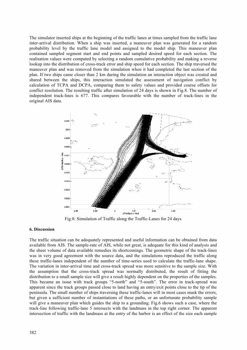
382

The simulator inserted ships at the beginning of the traffic lanes at times sampled from the traffic lane inter-arrival distribution. When a ship was inserted, a maneuver plan was generated for a random probability level by the traffic lane model and assigned to the model ship. This maneuver plan contained sampled segment start and end points and sampled desired speed for each section. The realisation values were computed by selecting a random cumulative probability and making a reverse lookup into the distribution of cross-track error and ship speed for each section. The ship traversed the maneuver plan and was removed from the simulation when it had completed the last section of the plan. If two ships came closer than 2 km during the simulation an interaction object was created and shared between the ships, this interaction simulated the assessment of navigation conflict by calculation of TCPA and DCPA, comparing them to safety values and provided course offsets for conflict resolution. The resulting traffic after simulation of 24 days is shown in Fig.8. The number of independent track-lines is 677. This compares favourable with the number of track-lines in the original AIS data.

Fig.8: Simulation of Traffic along the Traffic-Lanes for 24 days

6. Discussion The traffic situation can be adequately represented and useful information can be obtained from data available from AIS. The sample-rate of AIS, while not great, is adequate for this kind of analysis and the sheer volume of data available remedies its shortcomings. The geometric shape of the track-lines was in very good agreement with the source data, and the simulations reproduced the traffic along these traffic-lanes independent of the number of time-series used to calculate the traffic-lane shape. The variation in inter-arrival time and cross-track spread was more sensitive to the sample size. With the assumption that the cross-track spread was normally distributed, the result of fitting the distribution to a small sample size will give a result highly dependent on the properties of the samples. This became an issue with track groups “5-north” and “5-south”. The error in track-spread was apparent since the track groups passed close to land having an entry/exit points close to the tip of the peninsula. The small number of ships traversing these traffic-lanes will in most cases mask the errors, but given a sufficient number of instantiations of these paths, or an unfortunate probability sample will give a maneuver plan which guides the ship to a grounding. Fig.6 shows such a case, where the track-line following traffic-lane 5 intersects with the landmass in the top right corner. The apparent intersection of traffic with the landmass at the entry of the harbor is an effect of the size each sample

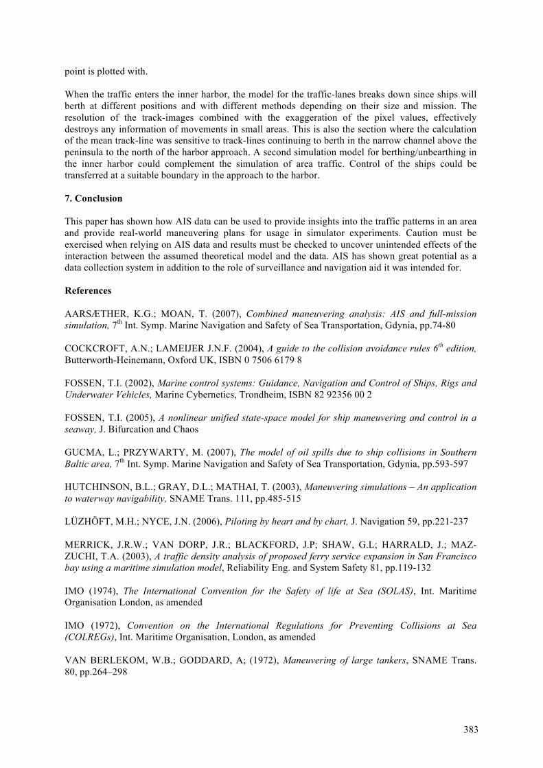
383

point is plotted with. When the traffic enters the inner harbor, the model for the traffic-lanes breaks down since ships will berth at different positions and with different methods depending on their size and mission. The resolution of the track-images combined with the exaggeration of the pixel values, effectively destroys any information of movements in small areas. This is also the section where the calculation of the mean track-line was sensitive to track-lines continuing to berth in the narrow channel above the peninsula to the north of the harbor approach. A second simulation model for berthing/unbearthing in the inner harbor could complement the simulation of area traffic. Control of the ships could be transferred at a suitable boundary in the approach to the harbor. 7. Conclusion This paper has shown how AIS data can be used to provide insights into the traffic patterns in an area and provide real-world maneuvering plans for usage in simulator experiments. Caution must be exercised when relying on AIS data and results must be checked to uncover unintended effects of the interaction between the assumed theoretical model and the data. AIS has shown great potential as a data collection system in addition to the role of surveillance and navigation aid it was intended for. References AARSÆTHER, K.G.; MOAN, T. (2007), Combined maneuvering analysis: AIS and full-mission simulation, 7th Int. Symp. Marine Navigation and Safety of Sea Transportation, Gdynia, pp.74-80 COCKCROFT, A.N.; LAMEIJER J.N.F. (2004), A guide to the collision avoidance rules 6th edition, Butterworth-Heinemann, Oxford UK, ISBN 0 7506 6179 8 FOSSEN, T.I. (2002), Marine control systems: Guidance, Navigation and Control of Ships, Rigs and Underwater Vehicles, Marine Cybernetics, Trondheim, ISBN 82 92356 00 2 FOSSEN, T.I. (2005), A nonlinear unified state-space model for ship maneuvering and control in a seaway, J. Bifurcation and Chaos GUCMA, L.; PRZYWARTY, M. (2007), The model of oil spills due to ship collisions in Southern Baltic area, 7th Int. Symp. Marine Navigation and Safety of Sea Transportation, Gdynia, pp.593-597 HUTCHINSON, B.L.; GRAY, D.L.; MATHAI, T. (2003), Maneuvering simulations – An application to waterway navigability, SNAME Trans. 111, pp.485-515 LÜZHÖFT, M.H.; NYCE, J.N. (2006), Piloting by heart and by chart, J. Navigation 59, pp.221-237 MERRICK, J.R.W.; VAN DORP, J.R.; BLACKFORD, J.P; SHAW, G.L; HARRALD, J.; MAZ-ZUCHI, T.A. (2003), A traffic density analysis of proposed ferry service expansion in San Francisco bay using a maritime simulation model, Reliability Eng. and System Safety 81, pp.119-132 IMO (1974), The International Convention for the Safety of life at Sea (SOLAS), Int. Maritime Organisation London, as amended IMO (1972), Convention on the International Regulations for Preventing Collisions at Sea (COLREGs), Int. Maritime Organisation, London, as amended VAN BERLEKOM, W.B.; GODDARD, A; (1972), Maneuvering of large tankers, SNAME Trans. 80, pp.264–298

Distributed Dynamic Programming for Adaptive On-line Planning ofAUVs Team Missions with Communication Constraints

Andrea Caiti, Giuseppe Casalino, Alessio Turetta, Riccardo Viviani,ISME, Interuniversity Research Center Integrated Systems for the Marine Environment,

Universities of Genova and Pisa/Italy, caiti@dsea.unipi.it

Abstract

An algorithm for adaptive on-line planning of environmental exploration missions with a team of Au-tonomous Underwater Vehicles (AUVs) is proposed. The algorithm has the primary goal of determiningan estimate of the sampled environmental quantity with an estimation error below a prescribed threshold.The additional degree of freedom of the algorithm is exploited in order to spread the team over the ex-ploration area, in order to minimize mission time, while at the same time preserving the communicationconnectivity of the team. A distributed dynamic programming approach is employed in order to satisfythese two conflicting requirements.

1 Introduction

Networked systems have recently experienced phenomenal growth in numerous engineering fields.Thanks to the increased capability in creating small and low-cost mobile platforms and the progressesin communication systems the deployment of networked mobile agent in a number of applications be-comes possible. In particular, multi-robot systems offer potential advantages in performance, robustness,and versatility for sensor-driven tasks such as survey, exploration, and environmental monitoring. Thereare many examples in the literature of applications of robot cooperation, from robotic soccer teams,Veloso (2003), to the exploration of unknown environments, Burgard et al. (2005), Danesi et al. (2003);other important examples come from the military field, where teams of unmanned vehicles (land, aerial,underwater) are asked to perform operations such as border patrol Girard et al. (2004) or mine countermeasurements, (Cecchi et al. (2005).

New interesting aspects about the topic of multi-robot cooperation have been summarized in Kumaret al. (2005), in particular with regard to formation control Tanner et al. (2004) and leader following,Balch and Arkin (1998). Research on Autonomous Underwater Vehicle (AUV) cooperation in the oceanenvironment had a somewhat slower start with respect to other fields, mainly as a consequence of thecommunication and localization constraints posed by the marine environment; in particular, the absenceof a GPS-like localization system, and the severe range and bandwidth limitation of underwater commu-nication make it very hard to simply transpose general robotic techniques to the underwater scenario.

An attempt to translate formation control in the marine context has been reported in Ikeda et al. (2005).In Arrichiello et al. (2006) a new behaviour-based approach has been introduced and applied to the con-trol of a fleet of surface vehicles, while in Boeraugh et al. (2006), Gabcheloo et al. (2006) formationcontrol has been extended to the coordinated path-following of marine vehicles, considering communi-cation delays and failures. A very succesfull approach within this line of research has been proposed andinvestigated in Leonard et al. (2004) as referred to ocean gliders with the task of identifying the gradientof environmental oceanographic quantities.

Specific applications require different types of communication technologies: wireless local area networkscan be easily established among surface vehicles through radio links, while acoustic modems are gener-ally used for communication between underwater vehicles. Underwater acoustic communication suffersfrom transmission delay, multi-path fading and limited range and bandwidth.

This paper tackles the problem of a behaviour-based adaptive mission planning for a team of AUVs co-operating in an environmental monitoring mission (e.g., measurement of the temperature field) subject tocommunication constraints, in the form of range-limited communication capabilities. Mission adaptationaims to maintain a desired accuracy on the reconstruction of the environmental field, through estimation

384

of the local smoothness properties of the field itself as new measurements become available. Followingour previous research Caiti et al. (2006,2007) the accuracy of the environmental map is ensured exploit-ing the approximation properties of Radial Basis Functions (RBFs). The innovative contribution of thiswork is in the exploitation of an additional degree of freedom of the adaptive algorithm: this is employedto spread the AUV team over the investigation area (hence attempting to minimize the mission time)while at the same time preserving the connectivity of the team in the form of a chained communicationstructure where the distance between two adjacent nodes is maintained below a prescribed threshold.This is accomplished with the application of a distributed dynamic programming approach. An inter-esting feature of the proposed approach is that, while nowhere in the algorithm vehicle formation isprescribed or programmed, the collective motion of the vehicles does indicate formation keeping duringthe mission.

The paper is organized as follows: in the next section the problem is formally stated and the cooperativeadaptive sampling algorithm is introduced in its general form, considering the preservation of the net-work links as additional requirements for the vehicles. In section 3 the adaptive constrained explorationalgorithm is described. In section 4 simulation results are presented and, in the last section, conclusionsare given.

2 Problem Statement

The general framework of the adaptive sampling problem has been presented in our previous works, Caitiet al. (2007); here the basic concepts are briefly recalled, for completeness, and the general framework isextended to the case in which additional range constraints among the vehicles are enforced. Let us sup-pose we have the availability of n AUVs, each one equipped with a network device to communicate withthe others up to a maximum range Dmax, and a sensor able to point-wise sample an environmental quan-tity θ at the geographical coordinates x = (x, y). The time-scale variation of the oceanographic field issupposed to be larger than the sampling mission time-scale . Let A be the geographical domain of interest,

i.e., x ∈ A. Let x j,kj be the kj-th measurement point of the vehicle j; let M( j) =n⋃

h=1

kh⋃i=1

xh,i

be the set of

sampling points known by the j-th vehicle after its last measurement, so I( j) =M( j); θ = θ (x)

∣∣∣x ∈ M( j)

is the information set available to the vehicle j. Let S be an estimation algorithm that computes an esti-mate θ j of the quantity θ over the whole region A on the basis of the current available information I( j),i.e. θ j (x) = S

(I( j)). On the basis of the estimation algorithm S and the available information set, one can

define the estimation error:ε j (x) =

∣∣∣θ (x) − θ j (x)∣∣∣ (1)

The main objective of the mission is to survey the region so that the estimation error is everywherebelow a given threshold. Moreover, it is desirable to spread the team over the region A, in order toobtain the maximum possible area coverage in the minimum time; however, since the vehicles share(some) information, communication connectivity must be preserved among the team. While in Caiti etal. (2007) it was assumed that a broadcasting node was always available to all vehicles (as for instance inthe case of vehicles re-surfacing and exploiting radio communication), in this work we assume that thecommunication takes place underwater through acoustic modems. To maintain communication links, itis assumed that the team has a chained serial structure: the team members are labeled from 1 to n, andeach vehicle is the node of a mobile serial network, with static topology. This means that the j-th vehicleis only connected to the vehicle ( j-1)-th and ( j+1)-th, as in Fig.(1). The index j indicates the position ofthe vehicle into the serial network.

The general cooperative strategy to attain the two mission goals proposed in this paper is based onthe approximation properties of RBFs and on the application of dynamic programming in a distributedfashion. Let us suppose the vehicles have an initial configuration such that the communication constraintsare satisfied. As soon as the vehicle j completes the kj-th sampling measurement and communicates it

to all the others in the team, the information set I( j)k becomes available. On the basis of the information

385

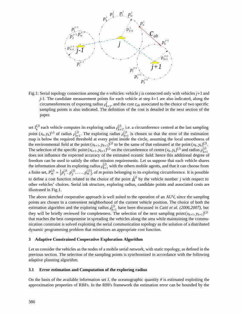
1jip -

1jmp -

11jp -

12jp -

jj-1

cab

1jp

2jp

3jp

jap

jmp

1jbp +

11jp +

12jp +

13jp +

j+1

jk 1+ρ

11

++j

kρ

11

−+j

kρ

Fig.1: Serial topology connection among the n vehicles: vehicle j is connected only with vehicles j+1 andj-1. The candidate measurement points for each vehicle at step k+1 are also indicated, along thecircumenferences of exporing radius ρjk+1, and the cost cab associated to the choice of two specificsampling points is also indicated. The definition of the cost is detailed in the next section of thepaper.

set I( j)k each vehicle computes its exploring radius ρ( j)

k+1, i.e. a circumference centred at the last sampling

point (xk, yk)( j) of radius ρ( j)k+1. The exploring radius ρ( j)

k+1 is chosen so that the error of the estimationmap is below the required threshold at every point inside the circle, assuming the local smoothness ofthe environmental field at the point (xk+1, yk+1)( j) to be the same of that estimated at the point (xk, yk)( j).The selection of the specific point (xk+1, yk+1)( j) on the circumference of centre (xk, yk)( j) and radius ρ( j)

k+1does not influence the expected accuracy of the estimated oceanic field: hence this additional degree offreedom can be used to satisfy the other mission requirements. Let us suppose that each vehicle sharesthe information about its exploring radius ρ( j)

k+1 with the others mobile agents, and that it can choose from

a finite set, P( j)m =

p( j)

1 , p( j)2 , . . . , p

( j)m

, of m points belonging to its exploring circumference. It is possible

to define a cost function related to the choice of the point p( j)a by the vehicle number j with respect to

other vehicles’ choices. Serial ink structure, exploring radius, candidate points and associated costs areillustrated in Fig.1.

The above sketched cooperative approach is well suited to the operation of an AUV, since the samplingpoints are chosen in a convenient neighborhood of the current vehicle position. The choice of both theestimation algorithm and the exploring radius ρ( j)

k+1 have been discussed in Caiti et al. (2006,2007), butthey will be briefly reviewed for completeness. The selection of the next sampling point(xk+1, yk+1)( j)

that reaches the best compromise in spreading the vehicles along the area while maintaining the commu-nication constraint is solved exploiting the serial communication topology as the solution of a distributeddynamic programming problem that minimizes an appropriate cost function.

3 Adaptive Constrained Cooperative Exploration Algorithm

Let us consider the vehicles as the nodes of a mobile serial network, with static topology, as defined in theprevious section. The selection of the sampling points is synchronized in accordance with the followingadaptive planning algorithm.

3.1 Error estimation and Computation of the exploring radius

On the basis of the available information set I, the oceanographic quantity θ is estimated exploiting theapproximation properties of RBFs. In the RBFs framework the estimation error can be bounded by the

386

following equation:ε(x) = |θ (x) − S (x)| ≤ ‖θ (x)‖Φ FΦ

(hρ (x)

)(2)

where θ (x) is the environmental quantity measured at x, S (x) the estimation of θ (x) on the basis of theavailable information set I, hρ (x) is the local fill distance and it depends on the local density of samplingpoints:

hρ (y) = supw∈B(y,ρ)

minx∈M( j)

‖w−x‖2 (3)

while FΦ (·) (the power function) is a known function that depends only on the specific RBF choice(gaussian, multiquadric, etc.); some common expressions of the power function are reported in Sch-abaack (1997) .

Under some additional technical assumptions (decay to zero of the RBF Fourier transform and θ(x)belonging to the native space having as reproducing kernel the chosen RBF basis) the j-th vehicle de-termines its next exploring radius ρj

k+1 as the local fill distance that allows to satisfy the mission errorrequirements through Equation (2). Since of course ‖θ(x)‖Φ is not known, it is replaced by its approxi-mation in terms of ‖S (x)‖Φ, which is convergent to unknown term.

3.2 Distributed dynamic programming: backward phase

The next sampling point for each vehicle is chosen as the solution of a minimum-cost path problem byadding to the network the virtual nodes S and E, whose arches have no cost, see Fig.(2). Starting fromthe last node of the network, i.e. the vehicle number n, the following procedure is repeated until the firstnode (the vehicle number 1) is reached:

• The ( j+1)-th vehicle determines its exploring radius ρ( j+1)k+1 , as described in the previous subsection,

and sends this information to the vehicle number j.

• The j-th vehicle computes the Cost Matrix Cj+1j : each element cab of the Cost Matrix is related to

the choice of the point p( j+1)b taken by the vehicle ( j+1) with respect to the choice of the point p( j)

a

taken by the vehicle number j. The value of the cost is given by the following rule:

cab =

⎧⎪⎪⎪⎪⎪⎨⎪⎪⎪⎪⎪⎩

+∞ pj+1b A

+∞∥∥∥∥pj

a − pj+1b

∥∥∥∥2> Dmax

ϕ(pj

a, pj+1b

)otherwise

(4)

where A is the geographical domain of interest, Dmaxthe maximum distance between two topologicallyadjacent vehicles that allows to maintain the network connection, ϕ

(pj

a, pj+1b

)is the value of a suitable

scalar potential field generated at the point pja by the past measurements points (xi ∈ M) and bypj+1

b as anew, hypothetical, measurement point for the vehicle ( j+1)-th.

• The potential field is defined as:

ϕ(pj

a, pj+1b

)=

= q

⎛⎜⎜⎜⎜⎝ 1∥∥∥∥pja−pj+1

b

∥∥∥∥n

2

+∑

xi∈M1∥∥∥∥pj

a−xi

∥∥∥∥n

2

⎞⎟⎟⎟⎟⎠ − Q∥∥∥∥pja−x f d

∥∥∥∥n

2

(5)

where q, Q, n, are positive numbers and xf d ∈ Ais the point, in the region A, where the fill distance isreached. The scalar potential field defined in (5) allows to spread the vehicles over the area taking in toaccount the past sampling points and the zones where the density of measurements is lower (the pointx f d ∈ A attracts the mobile agents).

387

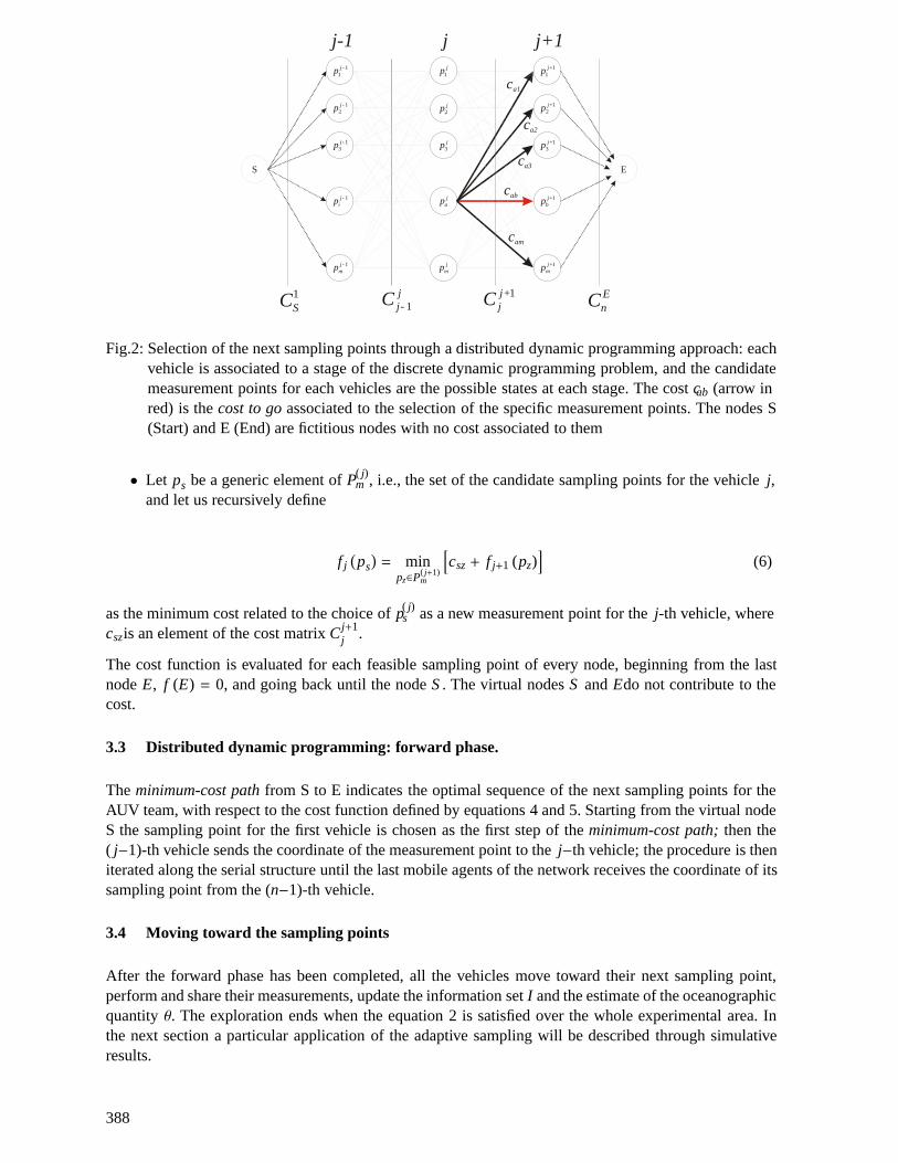
j-1 j+1j

cab

ca1

ca2

ca3

cam

1jjC +

1jjC -

S E

2jp

1jp

3jp

jap

jmp

12jp -

11jp -

13jp -

1jip -

1jmp -

12jp +

11jp +

13jp +

1jbp +

1jmp +

EnC1

SC

Fig.2: Selection of the next sampling points through a distributed dynamic programming approach: eachvehicle is associated to a stage of the discrete dynamic programming problem, and the candidatemeasurement points for each vehicles are the possible states at each stage. The cost cab (arrow inred) is the cost to go associated to the selection of the specific measurement points. The nodes S(Start) and E (End) are fictitious nodes with no cost associated to them

• Let ps be a generic element of P( j)m , i.e., the set of the candidate sampling points for the vehicle j,

and let us recursively define

f j(ps)= min

pz∈P( j+1)m

[csz + f j+1 (pz)

](6)

as the minimum cost related to the choice of p( j)s as a new measurement point for the j-th vehicle, where

cszis an element of the cost matrix Cj+1j .

The cost function is evaluated for each feasible sampling point of every node, beginning from the lastnode E, f (E) = 0, and going back until the node S . The virtual nodes S and Edo not contribute to thecost.

3.3 Distributed dynamic programming: forward phase.

The minimum-cost path from S to E indicates the optimal sequence of the next sampling points for theAUV team, with respect to the cost function defined by equations 4 and 5. Starting from the virtual nodeS the sampling point for the first vehicle is chosen as the first step of the minimum-cost path; then the( j−1)-th vehicle sends the coordinate of the measurement point to the j−th vehicle; the procedure is theniterated along the serial structure until the last mobile agents of the network receives the coordinate of itssampling point from the (n−1)-th vehicle.

3.4 Moving toward the sampling points

After the forward phase has been completed, all the vehicles move toward their next sampling point,perform and share their measurements, update the information set I and the estimate of the oceanographicquantity θ. The exploration ends when the equation 2 is satisfied over the whole experimental area. Inthe next section a particular application of the adaptive sampling will be described through simulativeresults.

388

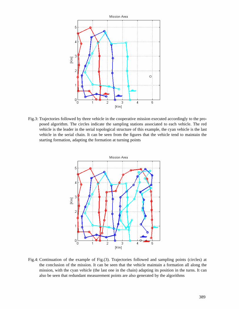
Fig.3: Trajectories followed by three vehicle in the cooperative mission executed accordingly to the pro-posed algorithm. The circles indicate the sampling stations associated to each vehicle. The redvehicle is the leader in the serial topological structure of this example, the cyan vehicle is the lastvehicle in the serial chain. It can be seen from the figures that the vehicle tend to maintain thestarting formation, adapting the formation at turning points

Fig.4: Continuation of the example of Fig.(3). Trajectories followed and sampling points (circles) atthe conclusion of the mission. It can be seen that the vehicle maintain a formation all along themission, with the cyan vehicle (the last one in the chain) adapting its position in the turns. It canalso be seen that redundant measurement points are also generated by the algorithms

389

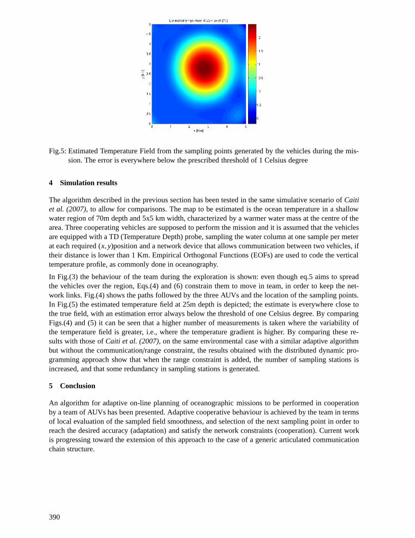
Fig.5: Estimated Temperature Field from the sampling points generated by the vehicles during the mis-sion. The error is everywhere below the prescribed threshold of 1 Celsius degree

4 Simulation results

The algorithm described in the previous section has been tested in the same simulative scenario of Caitiet al. (2007), to allow for comparisons. The map to be estimated is the ocean temperature in a shallowwater region of 70m depth and 5x5 km width, characterized by a warmer water mass at the centre of thearea. Three cooperating vehicles are supposed to perform the mission and it is assumed that the vehiclesare equipped with a TD (Temperature Depth) probe, sampling the water column at one sample per meterat each required (x, y)position and a network device that allows communication between two vehicles, iftheir distance is lower than 1 Km. Empirical Orthogonal Functions (EOFs) are used to code the verticaltemperature profile, as commonly done in oceanography.

In Fig.(3) the behaviour of the team during the exploration is shown: even though eq.5 aims to spreadthe vehicles over the region, Eqs.(4) and (6) constrain them to move in team, in order to keep the net-work links. Fig.(4) shows the paths followed by the three AUVs and the location of the sampling points.In Fig.(5) the estimated temperature field at 25m depth is depicted; the estimate is everywhere close tothe true field, with an estimation error always below the threshold of one Celsius degree. By comparingFigs.(4) and (5) it can be seen that a higher number of measurements is taken where the variability ofthe temperature field is greater, i.e., where the temperature gradient is higher. By comparing these re-sults with those of Caiti et al. (2007), on the same environmental case with a similar adaptive algorithmbut without the communication/range constraint, the results obtained with the distributed dynamic pro-gramming approach show that when the range constraint is added, the number of sampling stations isincreased, and that some redundancy in sampling stations is generated.

5 Conclusion

An algorithm for adaptive on-line planning of oceanographic missions to be performed in cooperationby a team of AUVs has been presented. Adaptive cooperative behaviour is achieved by the team in termsof local evaluation of the sampled field smoothness, and selection of the next sampling point in order toreach the desired accuracy (adaptation) and satisfy the network constraints (cooperation). Current workis progressing toward the extension of this approach to the case of a generic articulated communicationchain structure.

390

References

ALVAREZ, A.; CAFFAZ, A.; CAITI, A.; CASALINO, G.; CLERICI, E.; GIORGI, F.; GUALDESI, L.;TURETTA, A.; VIVIANI, R. (2005), Folaga: a very low cost autonomous underwater vehicle for coastaloceanography, 16th IFAC World Congress on Automatic Control, Prague

ARRICHIELLO, F.; CHIAVERINI, S.; FOSSEN, T.I. (2006), Formation control of marine surfacevessels using the null-space-based behavioral control, Group Coordination and Cooperative Control,Springer, pp.1-19

BALCH, T.; ARKIN, R.C. (1998), Behavior-based formation control for multi-robot teams, IEEE Trans.Robotics and Automation 14/6, pp.926939

BURGARD, W.; MOORS, M.; STACHNISS, C.; SCHNEIDER, F.E. (2005), Coordinated multi-robotexploration, IEEE Trans. on Robotics and Automation 21/3, pp.376-386

BØRHAUG, E.; PAVLOV, A.; GHABCHELOO, R.; PETTERSEN, K.Y.; PASCOAL, A.; SILVESTRE,C. (2006), Formation control of underactuated marine vehicles with communication constraints, 7thIFAC Conf. on Manoeuvring and Control of Marine Craft, Lisboa

CAITI, A.; MUNAFO, A.; VIVIANI, R. (2006), RBF-based adaptive on-line planning of AUV teamsenvironmental missions, 7th IFAC Conf. Manoeuvring and Control of Marine Craft (MCMC 2006),Lisbon

CAITI, A.; MUNAFO, A.; VIVIANI, R. (2007), Adaptive on-line planning of environmental samplingmissions with a team of cooperating autonomous underwater vehicles, Int. J. Control 79/9, pp.11451155

CECCHI, D.; CAITI, A.; FIORAVANTI, S.; BARALLI, F.; BOVIO, E. (2005), Target detection us-ing multiple autonomous underwater vehicles, IARP Int. Workshop on Underwater Robots IWUR 05,Genova

DANESI, A.; FONTANELLI, D.; MURRIERI, P.; SCORDIO, V.G.; BICCHI, A. (2003), Cooperativesimultaneous localization and map Building for servoing, Multiagent Robotic Systems Trends and In-dustrial Application, Padova

GHABCHELOO, R.; AGUIAR, A.P.; PASCOAL, A.; SILVESTRE, C. (2006), Coordinated path-following control of multiple AUVs in the presence of communication failures and time delays, 7th IFACConference on Manoeuvring and Control of Marine Craft (MCMC 2006), Lisbon

GIRARD, A.; HOWELL, A.; HEDRICK K. (2004), Border patrol and surveillance missions usingmultiple unmanned air vehicles, 43rd IEEE Conference on Decision and Control 1, pp.620-625

IKEDA, T.; MITA., T.; MASAKI, Y. (2005), Formation control of underwater autonomous vehicles, 16thIFAC World Congress, Prague

KUMAR, V.; LEONARD, N.E.; MORSE, A.S. (2005), Cooperative Control, LNCIS 309, Springer

LEONARD, N.E.; PALEY, D.; LEKIEN, F.; SEPULCHRE, R.; FRATANTONI, D.M.; DAVIS, R.(2007), Collective motion, sensor networks and ocean sampling, Proc. IEEE 95/1, pp.4874

SCHABACK, R. (1997), Reconstruction of multivariate functions from scattered data, www.num.math.uni-goettingen.de/schaback/research/group.html

TANNER, G.T.; PAPPAS, J.; KUMAR, V. (2004), Leader-to-formation stability, IEEE Trans.Roboticsand Automation 20/3, pp.443455.

VELOSO, M. (2003), Autonomous robot soccer teams, The Bridge 33/1, National Academy of Engi-neering

391

Computations for a US Navy Frigate Advancing in Head Waves inFixed and Free Conditions

Patrick Queutey, Centrale Nantes, Nantes/France, Patrick.Queutey@ec-nantes.frMichel Visonneau, Centrale Nantes, Nantes/France, Michel.Visonneau@ec-nantes.fr

Ganbo Deng, Centrale Nantes, Nantes/France, Ganbo.Deng@ec-nantes.frAlban Leroyer, Centrale Nantes, Nantes/France, Alban.Leroyer@ec-nantes.fr

Emmanuel Guilmineau, Centrale Nantes, Nantes/France, Emmanuel.Guilmineau@ec-nantes.frAji Purwanto, NUMECA, Brussels/Belgium, Aji.Purwanto@numeca.com

Abstract

This article addresses the computation of fixed or free hulls advancing in head waves with thefree-surface capturing viscous solver ISIS-CFD. ISIS-CFD, which is included in the computationalsuite FINET M/Marine, has been recently extended to account for six degrees of freedom motions(6DOF) for solid and deformable bodies and 1st to 3rd order Stokes waves generation. These newcharacteristics make possible the simulation of complex physical phenomena like manoeuvring,dynamic stability and sea-keeping within a unique mathematical and physical framework, theReynolds Averaged Navier-Stokes Equations for multi-fluid flows. This study is therefore devotedto a validation for a US Navy frigate (DTMB 5512) at model scale in various conditions rangingfrom moderate speed in long and smooth waves (Fr=0.28, λ = 1.5Lpp and Ak = 2πA

λ = 0.025) tohigh speed in short and steep waves (Fr=0.41, λ = 0.5Lpp and Ak = 0.075). These computationsare conducted with a hull in fixed position or free in trim and sinkage. Comparisons with theexperiments performed by the Iowa Institute of Hydraulic Research (IIHR) during the last yearsare used to assess the reliability of this free-surface capturing viscous computational approach.

1 Introduction

The impressive development achieved, during the last decade, both in hardware and softwaredevelopment, makes now possible the use of viscous solvers to compute full-scale free-surfaceflows of fully-appended hulls. Whereas our previous study presented in COMPIT’07 (Queuteyet al. (2007)) was focused on scale effects related with complex appendages, this study ad-dresses the computation of fixed or free hulls running in head waves. The recent extensions ofFINET M/Marine v2.0 devoted to the implementation of a six degrees of freedom (6DOF) couplingmodule and 1st to 3rd order Stokes waves generation used jointly with a general free-surfacecapturing approach, enable the simulation of new physical phenomena like manoeuvring, dynamicstability and sea-keeping within a unique mathematical and physical framework, the ReynoldsAveraged Navier-Stokes Equations for multi-fluid flows. The robustness of compressive free-surface capturing methodology associated with the flexibility of an unstructured finite-volumediscretisation method applied to locally-refined grids, creates a computational environment whichcan be used to simulate a large variety of flows from moderate to violent breaking waves (see Hayand Visonneau (2006) for recent illustrations). The ship forward speed diffraction and radiationproblem is a formidable mathematical challenge when formulated with the linearised inviscidboundary element tools. However, once treated in the fully non-linear environment of multi fluidRANS Equations, it becomes no more complex than the ship resistance problem in calm water,thanks to the use of a general non-linear mathematical framework.

Therefore, this paper proposes a validation study for a US Navy combatant (DTMB 5512) at modelscale in various conditions ranging from moderate speed in long and smooth waves (Fr=0.28,λ = 1.5Lpp and Ak = 2πA

λ = 0.025) to high speed in short and steep waves (Fr=0.41, λ = 0.5Lpp

392

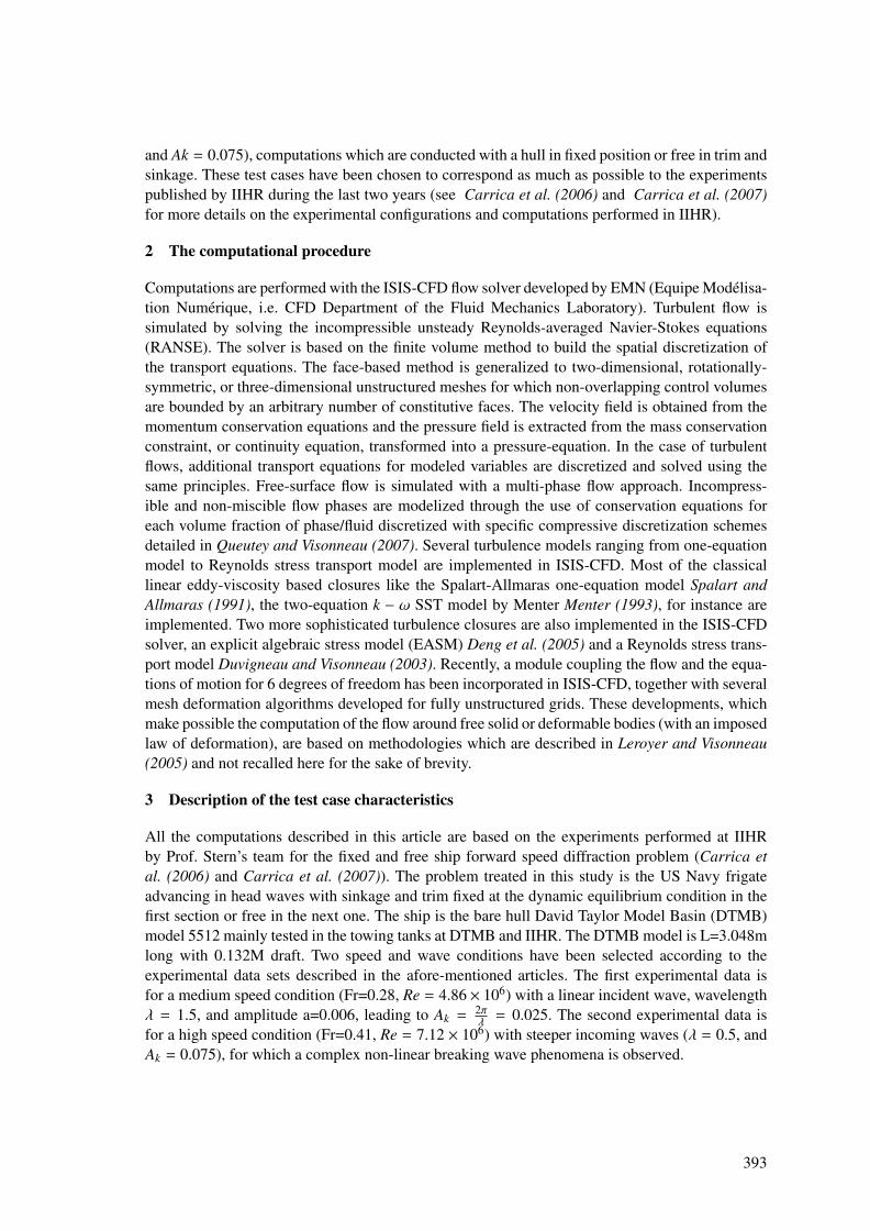
and Ak = 0.075), computations which are conducted with a hull in fixed position or free in trim andsinkage. These test cases have been chosen to correspond as much as possible to the experimentspublished by IIHR during the last two years (see Carrica et al. (2006) and Carrica et al. (2007)for more details on the experimental configurations and computations performed in IIHR).

2 The computational procedure

Computations are performed with the ISIS-CFD flow solver developed by EMN (Equipe Modelisa-tion Numerique, i.e. CFD Department of the Fluid Mechanics Laboratory). Turbulent flow issimulated by solving the incompressible unsteady Reynolds-averaged Navier-Stokes equations(RANSE). The solver is based on the finite volume method to build the spatial discretization ofthe transport equations. The face-based method is generalized to two-dimensional, rotationally-symmetric, or three-dimensional unstructured meshes for which non-overlapping control volumesare bounded by an arbitrary number of constitutive faces. The velocity field is obtained from themomentum conservation equations and the pressure field is extracted from the mass conservationconstraint, or continuity equation, transformed into a pressure-equation. In the case of turbulentflows, additional transport equations for modeled variables are discretized and solved using thesame principles. Free-surface flow is simulated with a multi-phase flow approach. Incompress-ible and non-miscible flow phases are modelized through the use of conservation equations foreach volume fraction of phase/fluid discretized with specific compressive discretization schemesdetailed in Queutey and Visonneau (2007). Several turbulence models ranging from one-equationmodel to Reynolds stress transport model are implemented in ISIS-CFD. Most of the classicallinear eddy-viscosity based closures like the Spalart-Allmaras one-equation model Spalart andAllmaras (1991), the two-equation k − ω SST model by Menter Menter (1993), for instance areimplemented. Two more sophisticated turbulence closures are also implemented in the ISIS-CFDsolver, an explicit algebraic stress model (EASM) Deng et al. (2005) and a Reynolds stress trans-port model Duvigneau and Visonneau (2003). Recently, a module coupling the flow and the equa-tions of motion for 6 degrees of freedom has been incorporated in ISIS-CFD, together with severalmesh deformation algorithms developed for fully unstructured grids. These developments, whichmake possible the computation of the flow around free solid or deformable bodies (with an imposedlaw of deformation), are based on methodologies which are described in Leroyer and Visonneau(2005) and not recalled here for the sake of brevity.

3 Description of the test case characteristics

All the computations described in this article are based on the experiments performed at IIHRby Prof. Stern’s team for the fixed and free ship forward speed diffraction problem (Carrica etal. (2006) and Carrica et al. (2007)). The problem treated in this study is the US Navy frigateadvancing in head waves with sinkage and trim fixed at the dynamic equilibrium condition in thefirst section or free in the next one. The ship is the bare hull David Taylor Model Basin (DTMB)model 5512 mainly tested in the towing tanks at DTMB and IIHR. The DTMB model is L=3.048mlong with 0.132M draft. Two speed and wave conditions have been selected according to theexperimental data sets described in the afore-mentioned articles. The first experimental data isfor a medium speed condition (Fr=0.28, Re = 4.86 × 106) with a linear incident wave, wavelengthλ = 1.5, and amplitude a=0.006, leading to Ak =

2πλ = 0.025. The second experimental data is

for a high speed condition (Fr=0.41, Re = 7.12 × 106) with steeper incoming waves (λ = 0.5, andAk = 0.075), for which a complex non-linear breaking wave phenomena is observed.

393

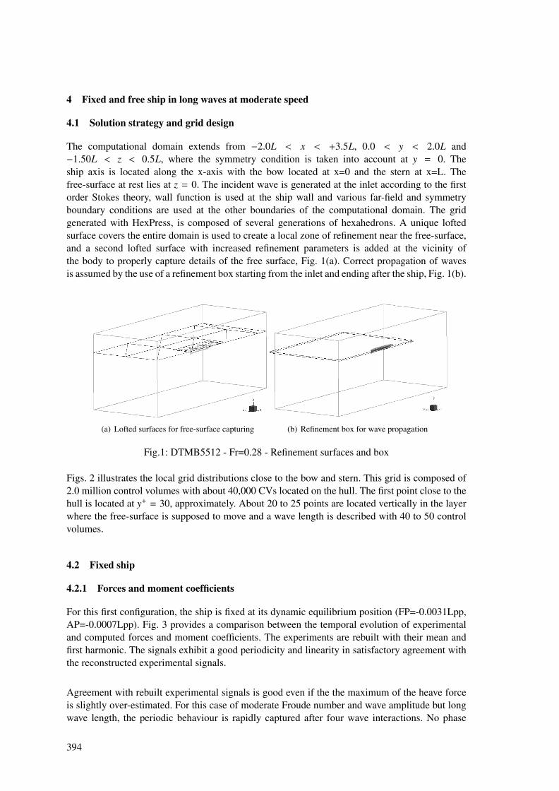
4 Fixed and free ship in long waves at moderate speed

4.1 Solution strategy and grid design

The computational domain extends from −2.0L < x < +3.5L, 0.0 < y < 2.0L and−1.50L < z < 0.5L, where the symmetry condition is taken into account at y = 0. Theship axis is located along the x-axis with the bow located at x=0 and the stern at x=L. Thefree-surface at rest lies at z = 0. The incident wave is generated at the inlet according to the firstorder Stokes theory, wall function is used at the ship wall and various far-field and symmetryboundary conditions are used at the other boundaries of the computational domain. The gridgenerated with HexPress, is composed of several generations of hexahedrons. A unique loftedsurface covers the entire domain is used to create a local zone of refinement near the free-surface,and a second lofted surface with increased refinement parameters is added at the vicinity ofthe body to properly capture details of the free surface, Fig. 1(a). Correct propagation of wavesis assumed by the use of a refinement box starting from the inlet and ending after the ship, Fig. 1(b).

(a) Lofted surfaces for free-surface capturing (b) Refinement box for wave propagation

Fig.1: DTMB5512 - Fr=0.28 - Refinement surfaces and box

Figs. 2 illustrates the local grid distributions close to the bow and stern. This grid is composed of2.0 million control volumes with about 40,000 CVs located on the hull. The first point close to thehull is located at y+ = 30, approximately. About 20 to 25 points are located vertically in the layerwhere the free-surface is supposed to move and a wave length is described with 40 to 50 controlvolumes.

4.2 Fixed ship

4.2.1 Forces and moment coefficients

For this first configuration, the ship is fixed at its dynamic equilibrium position (FP=-0.0031Lpp,AP=-0.0007Lpp). Fig. 3 provides a comparison between the temporal evolution of experimentaland computed forces and moment coefficients. The experiments are rebuilt with their mean andfirst harmonic. The signals exhibit a good periodicity and linearity in satisfactory agreement withthe reconstructed experimental signals.

Agreement with rebuilt experimental signals is good even if the the maximum of the heave forceis slightly over-estimated. For this case of moderate Froude number and wave amplitude but longwave length, the periodic behaviour is rapidly captured after four wave interactions. No phase

394

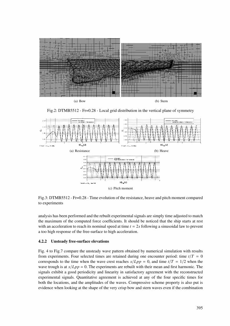
(a) Bow (b) Stern

Fig.2: DTMB5512 - Fr=0.28 - Local grid distribution in the vertical plane of symmetry

(a) Resistance (b) Heave

(c) Pitch moment

Fig.3: DTMB5512 - Fr=0.28 - Time evolution of the resistance, heave and pitch moment comparedto experiments

analysis has been performed and the rebuilt experimental signals are simply time adjusted to matchthe maximum of the computed force coefficients. It should be noticed that the ship starts at restwith an acceleration to reach its nominal speed at time t = 2s following a sinusoidal law to preventa too high response of the free-surface to high acceleration.

4.2.2 Unsteady free-surface elevations

Fig. 4 to Fig.7 compare the unsteady wave pattern obtained by numerical simulation with resultsfrom experiments. Four selected times are retained during one encounter period: time t/T = 0corresponds to the time when the wave crest reaches x/Lpp = 0, and time t/T = 1/2 when thewave trough is at x/Lpp = 0. The experiments are rebuilt with their mean and first harmonic. Thesignals exhibit a good periodicity and linearity in satisfactory agreement with the reconstructedexperimental signals. Quantitative agreement is achieved at any of the four specific times forboth the locations, and the amplitudes of the waves. Compressive scheme property is also put isevidence when looking at the shape of the very crisp bow and stern waves even if the combination

395

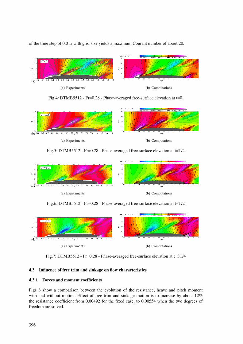
of the time step of 0.01s with grid size yields a maximum Courant number of about 20.

(a) Experiments (b) Computations

Fig.4: DTMB5512 - Fr=0.28 - Phase-averaged free-surface elevation at t=0.

(a) Experiments (b) Computations

Fig.5: DTMB5512 - Fr=0.28 - Phase-averaged free-surface elevation at t=T/4

(a) Experiments (b) Computations

Fig.6: DTMB5512 - Fr=0.28 - Phase-averaged free-surface elevation at t=T/2

(a) Experiments (b) Computations

Fig.7: DTMB5512 - Fr=0.28 - Phase-averaged free-surface elevation at t=3T/4

4.3 Influence of free trim and sinkage on flow characteristics

4.3.1 Forces and moment coefficients

Figs 8 show a comparison between the evolution of the resistance, heave and pitch momentwith and without motion. Effect of free trim and sinkage motion is to increase by about 12%the resistance coefficient from 0.00492 for the fixed case, to 0.00554 when the two degrees offreedom are solved.

396

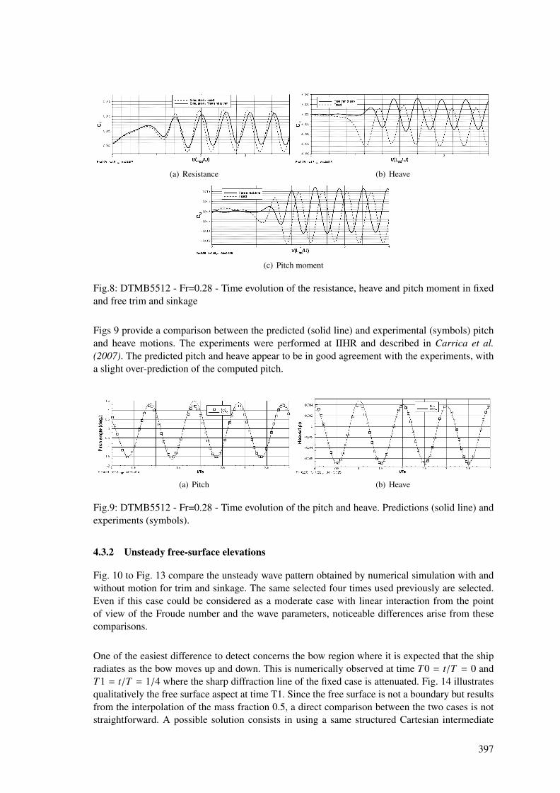
(a) Resistance (b) Heave

(c) Pitch moment

Fig.8: DTMB5512 - Fr=0.28 - Time evolution of the resistance, heave and pitch moment in fixedand free trim and sinkage

Figs 9 provide a comparison between the predicted (solid line) and experimental (symbols) pitchand heave motions. The experiments were performed at IIHR and described in Carrica et al.(2007). The predicted pitch and heave appear to be in good agreement with the experiments, witha slight over-prediction of the computed pitch.

(a) Pitch (b) Heave

Fig.9: DTMB5512 - Fr=0.28 - Time evolution of the pitch and heave. Predictions (solid line) andexperiments (symbols).

4.3.2 Unsteady free-surface elevations

Fig. 10 to Fig. 13 compare the unsteady wave pattern obtained by numerical simulation with andwithout motion for trim and sinkage. The same selected four times used previously are selected.Even if this case could be considered as a moderate case with linear interaction from the pointof view of the Froude number and the wave parameters, noticeable differences arise from thesecomparisons.

One of the easiest difference to detect concerns the bow region where it is expected that the shipradiates as the bow moves up and down. This is numerically observed at time T0 = t/T = 0 andT1 = t/T = 1/4 where the sharp diffraction line of the fixed case is attenuated. Fig. 14 illustratesqualitatively the free surface aspect at time T1. Since the free surface is not a boundary but resultsfrom the interpolation of the mass fraction 0.5, a direct comparison between the two cases is notstraightforward. A possible solution consists in using a same structured Cartesian intermediate

397

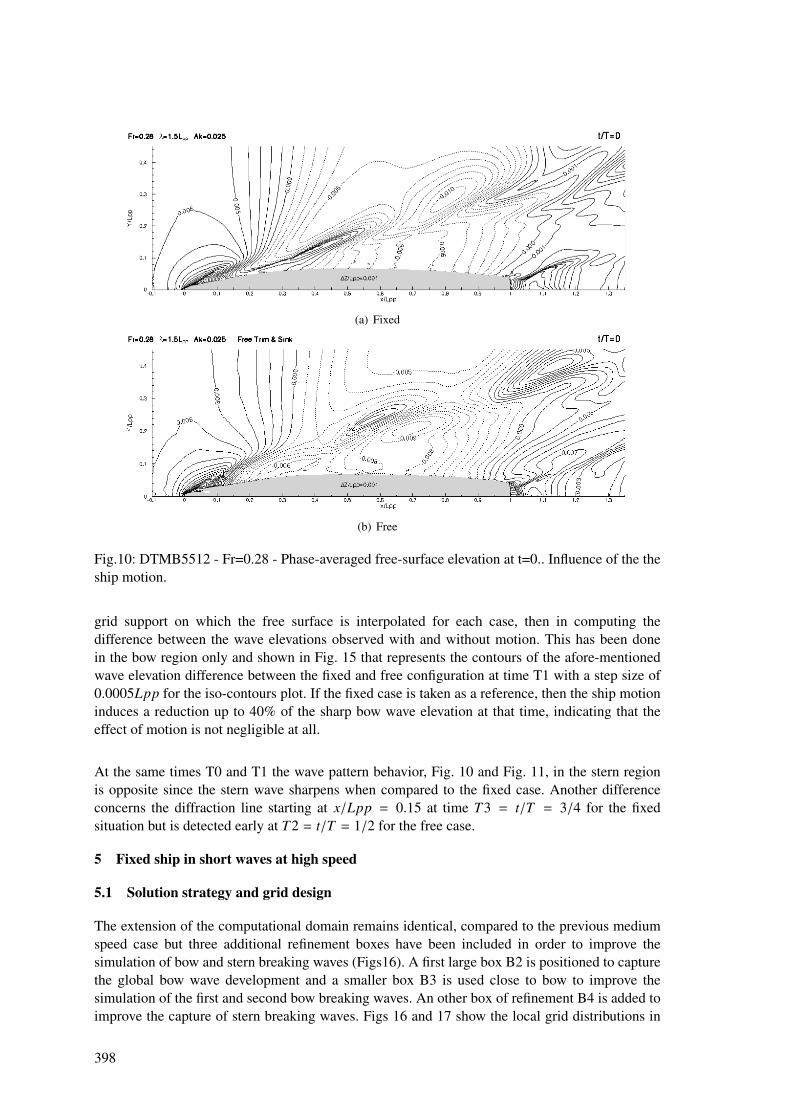
(a) Fixed

(b) Free

Fig.10: DTMB5512 - Fr=0.28 - Phase-averaged free-surface elevation at t=0.. Influence of the theship motion.

grid support on which the free surface is interpolated for each case, then in computing thedifference between the wave elevations observed with and without motion. This has been donein the bow region only and shown in Fig. 15 that represents the contours of the afore-mentionedwave elevation difference between the fixed and free configuration at time T1 with a step size of0.0005Lpp for the iso-contours plot. If the fixed case is taken as a reference, then the ship motioninduces a reduction up to 40% of the sharp bow wave elevation at that time, indicating that theeffect of motion is not negligible at all.

At the same times T0 and T1 the wave pattern behavior, Fig. 10 and Fig. 11, in the stern regionis opposite since the stern wave sharpens when compared to the fixed case. Another differenceconcerns the diffraction line starting at x/Lpp = 0.15 at time T3 = t/T = 3/4 for the fixedsituation but is detected early at T2 = t/T = 1/2 for the free case.

5 Fixed ship in short waves at high speed

5.1 Solution strategy and grid design

The extension of the computational domain remains identical, compared to the previous mediumspeed case but three additional refinement boxes have been included in order to improve thesimulation of bow and stern breaking waves (Figs16). A first large box B2 is positioned to capturethe global bow wave development and a smaller box B3 is used close to bow to improve thesimulation of the first and second bow breaking waves. An other box of refinement B4 is added toimprove the capture of stern breaking waves. Figs 16 and 17 show the local grid distributions in

398

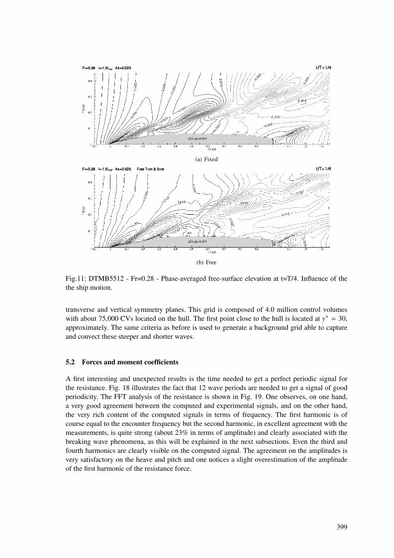
(a) Fixed

(b) Free

Fig.11: DTMB5512 - Fr=0.28 - Phase-averaged free-surface elevation at t=T/4. Influence of thethe ship motion.

transverse and vertical symmetry planes. This grid is composed of 4.0 million control volumeswith about 75,000 CVs located on the hull. The first point close to the hull is located at y+ = 30,approximately. The same criteria as before is used to generate a background grid able to captureand convect these steeper and shorter waves.

5.2 Forces and moment coefficients

A first interesting and unexpected results is the time needed to get a perfect periodic signal forthe resistance. Fig. 18 illustrates the fact that 12 wave periods are needed to get a signal of goodperiodicity. The FFT analysis of the resistance is shown in Fig. 19. One observes, on one hand,a very good agreement between the computed and experimental signals, and on the other hand,the very rich content of the computed signals in terms of frequency. The first harmonic is ofcourse equal to the encounter frequency but the second harmonic, in excellent agreement with themeasurements, is quite strong (about 23% in terms of amplitude) and clearly associated with thebreaking wave phenomena, as this will be explained in the next subsections. Even the third andfourth harmonics are clearly visible on the computed signal. The agreement on the amplitudes isvery satisfactory on the heave and pitch and one notices a slight overestimation of the amplitudeof the first harmonic of the resistance force.

399

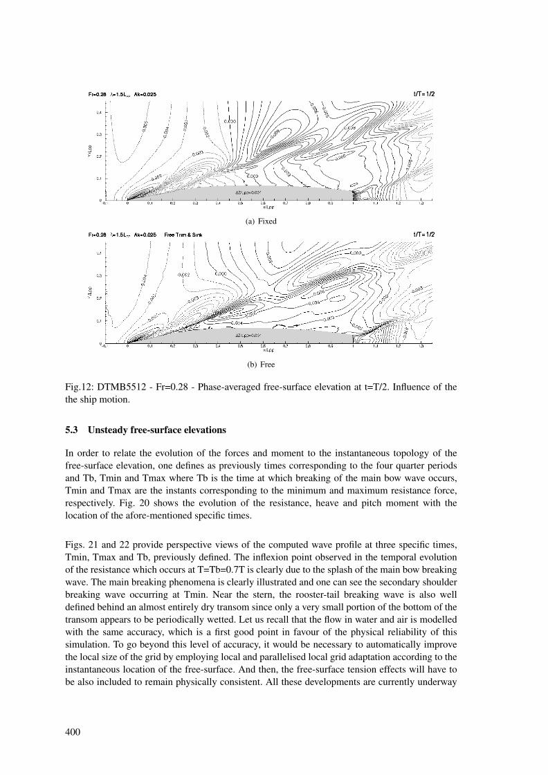
(a) Fixed

(b) Free

Fig.12: DTMB5512 - Fr=0.28 - Phase-averaged free-surface elevation at t=T/2. Influence of thethe ship motion.

5.3 Unsteady free-surface elevations

In order to relate the evolution of the forces and moment to the instantaneous topology of thefree-surface elevation, one defines as previously times corresponding to the four quarter periodsand Tb, Tmin and Tmax where Tb is the time at which breaking of the main bow wave occurs,Tmin and Tmax are the instants corresponding to the minimum and maximum resistance force,respectively. Fig. 20 shows the evolution of the resistance, heave and pitch moment with thelocation of the afore-mentioned specific times.

Figs. 21 and 22 provide perspective views of the computed wave profile at three specific times,Tmin, Tmax and Tb, previously defined. The inflexion point observed in the temporal evolutionof the resistance which occurs at T=Tb=0.7T is clearly due to the splash of the main bow breakingwave. The main breaking phenomena is clearly illustrated and one can see the secondary shoulderbreaking wave occurring at Tmin. Near the stern, the rooster-tail breaking wave is also welldefined behind an almost entirely dry transom since only a very small portion of the bottom of thetransom appears to be periodically wetted. Let us recall that the flow in water and air is modelledwith the same accuracy, which is a first good point in favour of the physical reliability of thissimulation. To go beyond this level of accuracy, it would be necessary to automatically improvethe local size of the grid by employing local and parallelised local grid adaptation according to theinstantaneous location of the free-surface. And then, the free-surface tension effects will have tobe also included to remain physically consistent. All these developments are currently underway

400

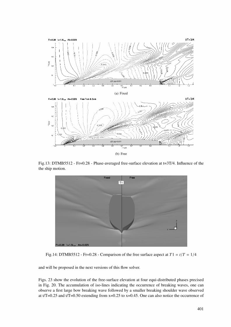
(a) Fixed

(b) Free

Fig.13: DTMB5512 - Fr=0.28 - Phase-averaged free-surface elevation at t=3T/4. Influence of thethe ship motion.

Fig.14: DTMB5512 - Fr=0.28 - Comparison of the free surface aspect at T1 = t/T = 1/4

and will be proposed in the next versions of this flow solver.

Figs. 23 show the evolution of the free-surface elevation at four equi-distributed phases precisedin Fig. 20. The accumulation of iso-lines indicating the occurrence of breaking waves, one canobserve a first large bow breaking wave followed by a smaller breaking shoulder wave observedat t/T=0.25 and t/T=0.50 extending from x=0.25 to x=0.45. One can also notice the occurrence of

401

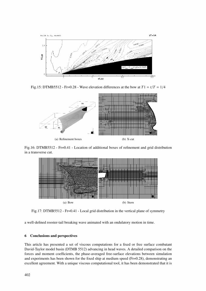
Fig.15: DTMB5512 - Fr=0.28 - Wave elevation differences at the bow at T1 = t/T = 1/4

(a) Refinement boxes (b) X-cut

Fig.16: DTMB5512 - Fr=0.41 - Location of additional boxes of refinement and grid distributionin a transverse cut.

(a) Bow (b) Stern

Fig.17: DTMB5512 - Fr=0.41 - Local grid distribution in the vertical plane of symmetry

a well-defined rooster-tail breaking wave animated with an ondulatory motion in time.

6 Conclusions and perspectives

This article has presented a set of viscous computations for a fixed or free surface combatantDavid-Taylor model basin (DTMB 5512) advancing in head waves. A detailed comparison on theforces and moment coefficients, the phase-averaged free-surface elevations between simulationand experiments has been shown for the fixed ship at medium speed (Fr=0.28), demonstrating anexcellent agreement. With a unique viscous computational tool, it has been demonstrated that it is

402

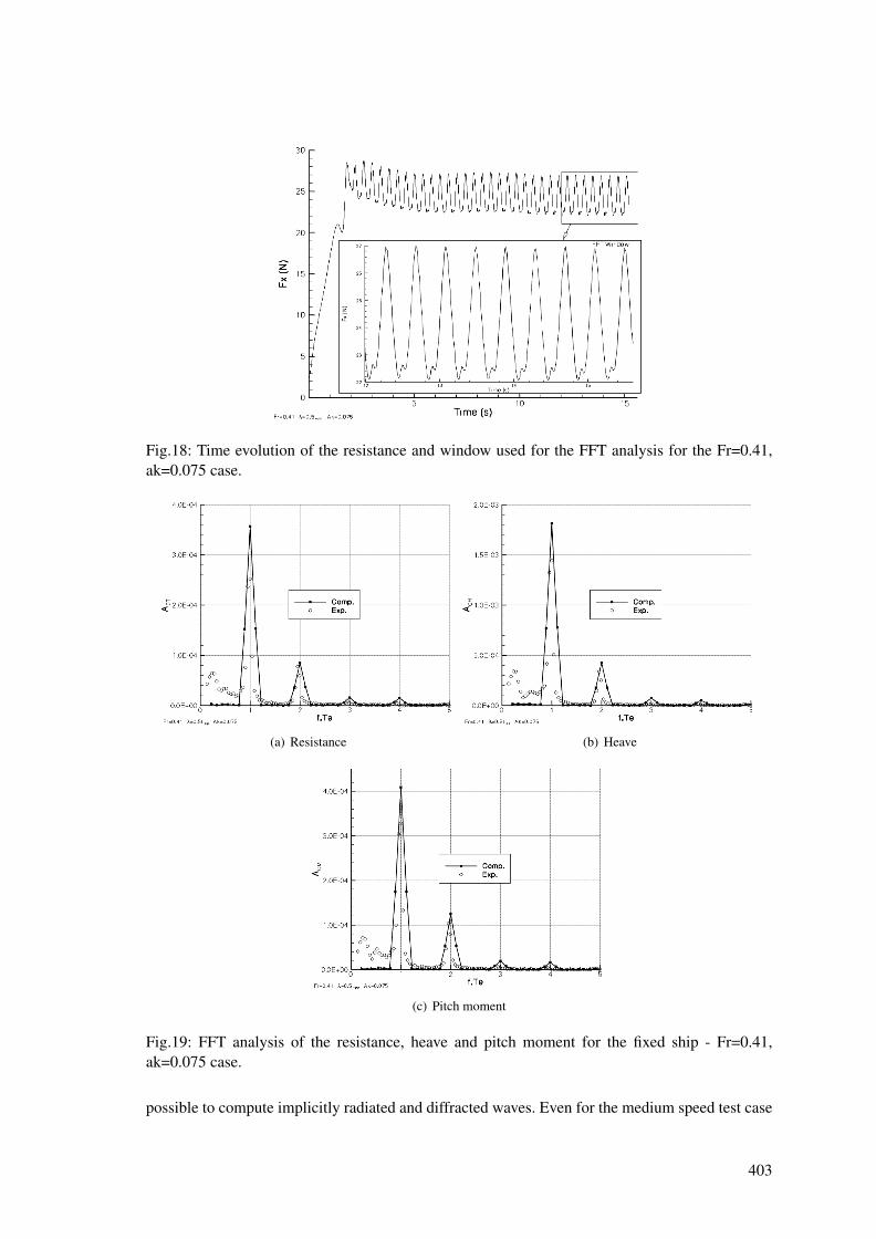
Fig.18: Time evolution of the resistance and window used for the FFT analysis for the Fr=0.41,ak=0.075 case.

(a) Resistance (b) Heave

(c) Pitch moment

Fig.19: FFT analysis of the resistance, heave and pitch moment for the fixed ship - Fr=0.41,ak=0.075 case.

possible to compute implicitly radiated and diffracted waves. Even for the medium speed test case

403

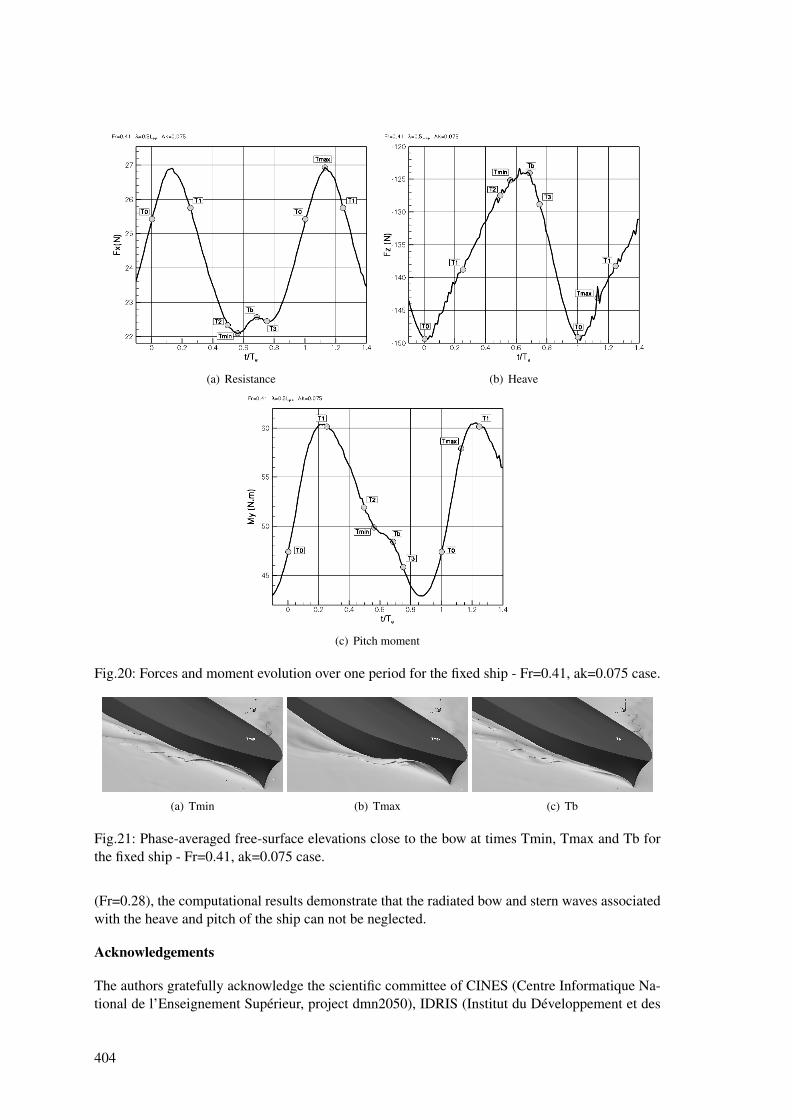
(a) Resistance (b) Heave

(c) Pitch moment

Fig.20: Forces and moment evolution over one period for the fixed ship - Fr=0.41, ak=0.075 case.

(a) Tmin (b) Tmax (c) Tb

Fig.21: Phase-averaged free-surface elevations close to the bow at times Tmin, Tmax and Tb forthe fixed ship - Fr=0.41, ak=0.075 case.

(Fr=0.28), the computational results demonstrate that the radiated bow and stern waves associatedwith the heave and pitch of the ship can not be neglected.

Acknowledgements

The authors gratefully acknowledge the scientific committee of CINES (Centre Informatique Na-tional de l’Enseignement Superieur, project dmn2050), IDRIS (Institut du Developpement et des

404

(a) Tmin (b) Tmax (c) Tb

Fig.22: Phase-averaged free-surface elevations close to the stern at times Tmin, Tmax and Tb forthe fixed ship - Fr=0.41, ak=0.075 case.

Ressources en Informatique Scientifique du CNRS, project 000129) for the attribution of CPUtime.

References

CARRICA, P.; WILSON, R.; STERN, F. (2006), Unsteady RANSE simulation of the ship forwardspeed diffraction problem, Computers & Fluids, 35/6, pp. 545–570

CARRICA, P.; WILSON, R.; NOACK, R.; STERN, F. (2007), Ship motions using single-phaselevel set with dynamic overset grids, Computers & Fluids, 36/9, pp. 1415–1433

QUEUTEY, P.; DENG, G.; VISONNEAU, M. (2007), Study of scale effects around fully-appendedships with an unstructured RANSE solver, in COMPIT’07, 6th Int. EuroConf. on Computer andIT Applications in the Maritime Industries, Cortona, Italy

HAY, A.; LEROYER, A.; VISONNEAU, M. (2006), H-adaptive Navier-Stokes simulations of free-surface flows around moving bodies, Journal of Marine Science and Technology, 11/1, pp. 1–18

QUEUTEY, P.; VISONNEAU, M. (2007), An interface capturing method for free-surface hydro-dynamic flows, Computers & Fluids, 36/9, pp. 1481–1510

SPALART, P.R.; ALLMARAS, S.R. (1991), A one-equation turbulence model for aerodynamicflows. AIAA Paper 92-0439

MENTER. F. (1993), Zonal two-equations k −ω turbulence models for aerodynamic flows, AIAAPaper, 93/2906

DENG, G.; QUEUTEY, P.; VISONNEAU, M. (2005), Three-dimensional flow computation withReynolds stress and algebraic stress models, Engineering Turbulence Modeling and Experiments,6, pp. 389–398

DUVIGNEAU, R.; VISONNEAU, M.; DENG, G. (2003), On the role played by turbulence clo-sures for hull shape optimization at model and full scale, Journal of Marine Science and Technol-ogy, 153, pp. 1–25

LEROYER, A.; VISONNEAU, M. (2005), Numerical methods for RANSE simulations of a self-propelled fish-like body, J. Fluid & Structures, 20/3, pp. 975–991

405

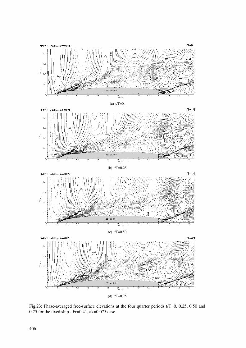
(a) t/T=0.

(b) t/T=0.25

(c) t/T=0.50

(d) t/T=0.75

Fig.23: Phase-averaged free-surface elevations at the four quarter periods t/T=0, 0.25, 0.50 and0.75 for the fixed ship - Fr=0.41, ak=0.075 case.

406

407

Interactive Computer Graphics and Simulation in Preliminary Ship Design

David Andrews, UCL DRC, London/UK, d_andrews@meng.ucl.ac.uk Lorenzo Casarosa, UCL DRC, London/UK, l_casarosa@meng.ucl.ac.uk Richard Pawling, UCL DRC, London/UK, r_pawling@meng.ucl.ac.uk

Abstract This paper gives an outline of the Design Building Block approach and the PARAMARINE-SURFCON software implementation, before describing its application to a range of preliminary ship design studies and investigations which demonstrate the utility of the approach and software tool. The paper then describes recently completed research focusing on the incorporation of personnel movement simulation into preliminary ship design, in particular the work on integrating a simulation tool and a preliminary ship design tool. The paper concludes by considering the use of interactive graphics in assessing the design and some key lessons for integrating simulation into preliminary ship design.

1. Introduction The UCL Design Research Centre (DRC) is a relatively new research organization, established in 2000, sitting alongside the long standing Ministry of Defence (MoD) sponsored Naval Architecture and Marine Engineering (NAME) Group within the Department of Mechanical Engineering at University College London. Its main area of research is in computer aided preliminary ship design, using the Design Building Block approach and its implementation in the SURFCON tool Andrews (2003), Andrews and Pawling (2006a). The UCL DRC also researches into the wider design environment and innovations, such as simulation based design and concurrent engineering, which are altering the way in which ships can be designed. Like the NAME Group, the DRC has an interest in the design of unconventional and innovative vessels, such as the trimaran, and technologies, such as the all electric ship, but with its own particular focus on the ship architecture typified by the Design Building Block approach and its realisation through the SURFCON tool. Over the last six years a range of design studies, using the DBB approach and the tool have been undertaken Andrews and Pawling (2006a). 2. The Design Building Block Approach 2.1 Outline of the Approach Traditionally, preliminary ship design processes have been largely numerical in nature, with the architectural aspects, such as internal layout, only being considered once the ship has been sized and a hullform generated. Analyses of performance are thus carried out on a design which is largely fixed, limiting the changes that can be made should a problem be identified. This is particularly the case with simulation based analyses of aspects, such as personnel movement and evacuation, which are highly dependent on the internal configuration of the vessel. The Design Building Block approach to early stage ship design seeks to encourage a more holistic approach to the development of the ship design solution. Instead of a set of numerical steps or a mechanistic approach, where each aspect of the performance of the design is examined separately and in turn, the integrated nature of the SURFCON implementation in PARMARINE allows all relevant aspects of the design’s effectiveness to be assessed at the earliest stages of design. In essence this approach focuses on ship architecture and how it is produced alongside the traditional numerical sizing and naval architectural balance. The Design Building Block approach to producing a new ship design was presented in Fig.5 of Andrews (2004), reproduced at Fig.1. This diagram summarises a comprehensive set of analysis processes, most of which are unlikely to be used in the initial setting up of the design or even early iterations around the sequence of building blocks, geometric definition and size balance. In fact several of the inputs shown in Fig.1 are either specific to the naval combatant case, such as topside features, or omit

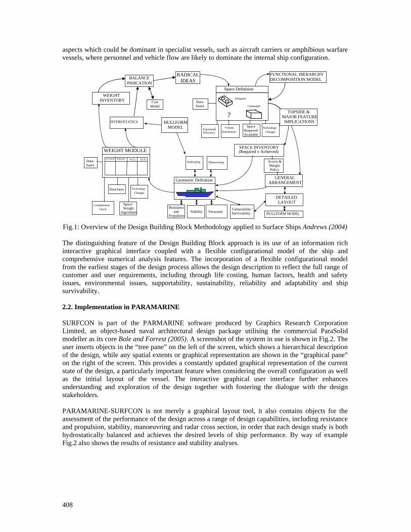
408

aspects which could be dominant in specialist vessels, such as aircraft carriers or amphibious warfare vessels, where personnel and vehicle flow are likely to dominate the internal ship configuration.

Space Definition

Geometric Definition

RADICAL IDEAS BALANCE

INDICATION

WEIGHT INVENTORY

HYDROSTATICS

WEIGHT MODULE SYSTEM WEIGHT VCG LCG

Completeness Check

Seakeeping

Data- bases

Structures

Data- bases

Functional Efficiency

SPACE INVENTORY (Required v Achieved)

VolumeDistribution

TechnologyChanges

GENERAL ARRANGEMENT

DETAILED LAYOUT

Space Required/ Available

Technology Changes

Stability Resistance

and Propulsion

Space/ Weight

Algorithms

Access & Margin Policy

FUNCTIONAL HIERARCHY DECOMPOSITION MODEL

Maneuvering

Cost Model

Personnel

HULLFORM MODEL

HULLFORM MODEL Vulnerability / Survivability

TOPSIDE & MAJOR FEATURE

IMPLICATIONS

Propuls

Weap?

Acc

ContWeapons Weapons

Command

?

Fig.1: Overview of the Design Building Block Methodology applied to Surface Ships Andrews (2004) The distinguishing feature of the Design Building Block approach is its use of an information rich interactive graphical interface coupled with a flexible configurational model of the ship and comprehensive numerical analysis features. The incorporation of a flexible configurational model from the earliest stages of the design process allows the design description to reflect the full range of customer and user requirements, including through life costing, human factors, health and safety issues, environmental issues, supportability, sustainability, reliability and adaptability and ship survivability. 2.2. Implementation in PARAMARINE SURFCON is part of the PARMARINE software produced by Graphics Research Corporation Limited, an object-based naval architectural design package utilising the commercial ParaSolid modeller as its core Bole and Forrest (2005). A screenshot of the system in use is shown in Fig.2. The user inserts objects in the “tree pane” on the left of the screen, which shows a hierarchical description of the design, while any spatial extents or graphical representation are shown in the “graphical pane” on the right of the screen. This provides a constantly updated graphical representation of the current state of the design, a particularly important feature when considering the overall configuration as well as the initial layout of the vessel. The interactive graphical user interface further enhances understanding and exploration of the design together with fostering the dialogue with the design stakeholders. PARAMARINE-SURFCON is not merely a graphical layout tool, it also contains objects for the assessment of the performance of the design across a range of design capabilities, including resistance and propulsion, stability, manoeuvring and radar cross section, in order that each design study is both hydrostatically balanced and achieves the desired levels of ship performance. By way of example Fig.2 also shows the results of resistance and stability analyses.

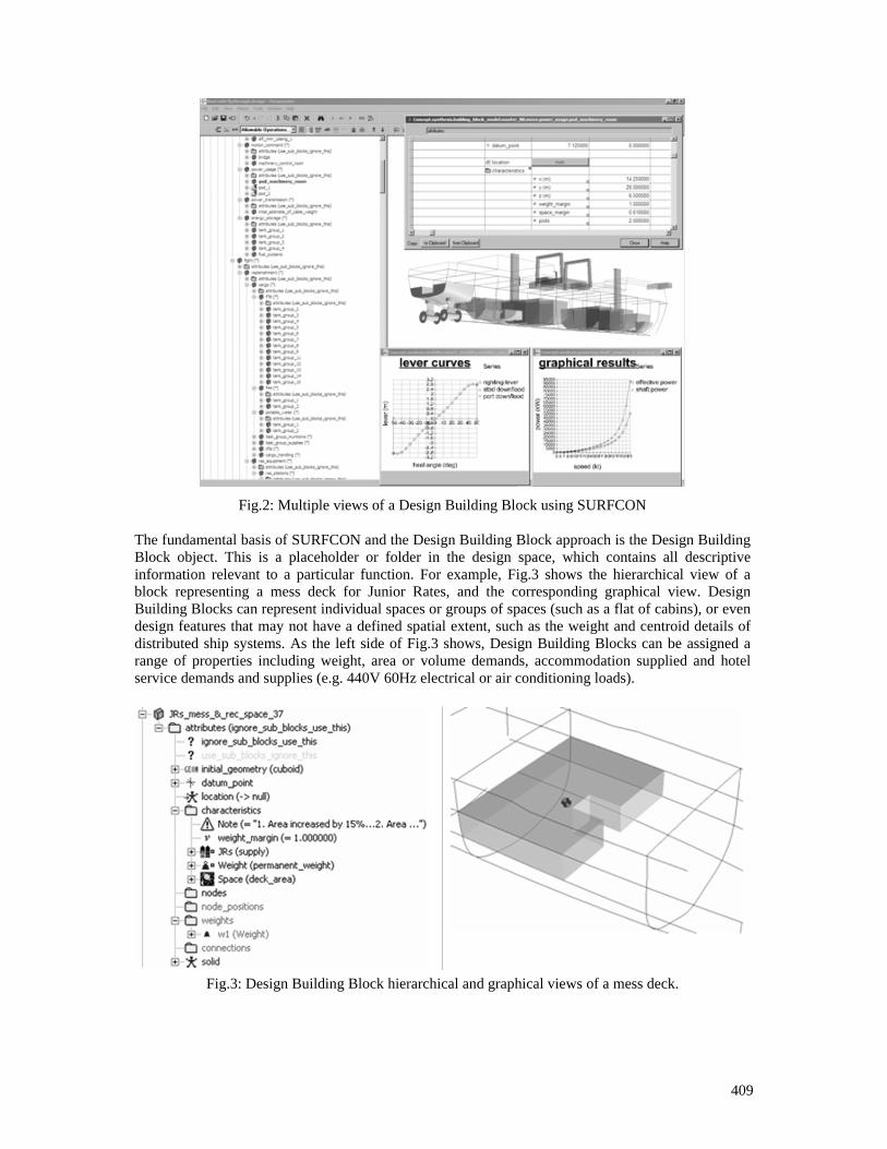
409

Fig.2: Multiple views of a Design Building Block using SURFCON

The fundamental basis of SURFCON and the Design Building Block approach is the Design Building Block object. This is a placeholder or folder in the design space, which contains all descriptive information relevant to a particular function. For example, Fig.3 shows the hierarchical view of a block representing a mess deck for Junior Rates, and the corresponding graphical view. Design Building Blocks can represent individual spaces or groups of spaces (such as a flat of cabins), or even design features that may not have a defined spatial extent, such as the weight and centroid details of distributed ship systems. As the left side of Fig.3 shows, Design Building Blocks can be assigned a range of properties including weight, area or volume demands, accommodation supplied and hotel service demands and supplies (e.g. 440V 60Hz electrical or air conditioning loads).

Fig.3: Design Building Block hierarchical and graphical views of a mess deck.

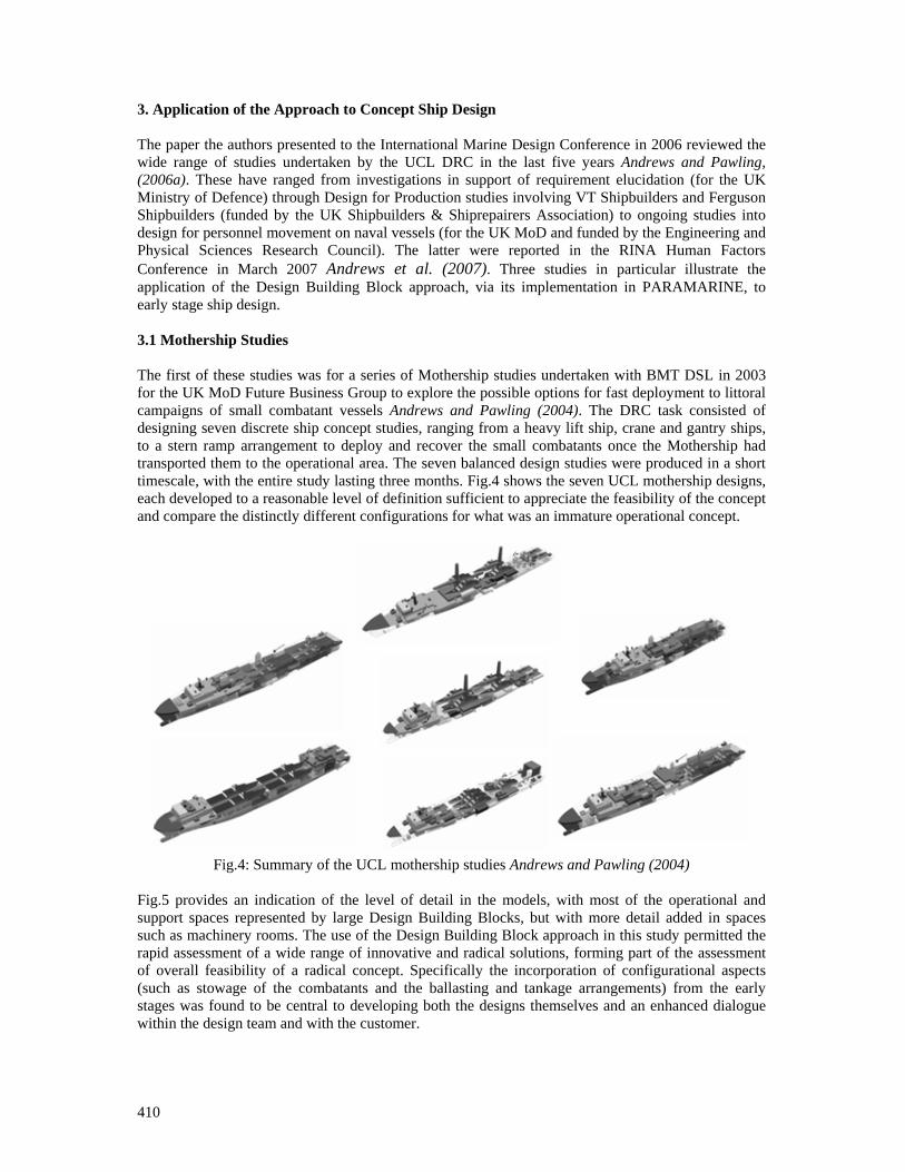
410

3. Application of the Approach to Concept Ship Design The paper the authors presented to the International Marine Design Conference in 2006 reviewed the wide range of studies undertaken by the UCL DRC in the last five years Andrews and Pawling, (2006a). These have ranged from investigations in support of requirement elucidation (for the UK Ministry of Defence) through Design for Production studies involving VT Shipbuilders and Ferguson Shipbuilders (funded by the UK Shipbuilders & Shiprepairers Association) to ongoing studies into design for personnel movement on naval vessels (for the UK MoD and funded by the Engineering and Physical Sciences Research Council). The latter were reported in the RINA Human Factors Conference in March 2007 Andrews et al. (2007). Three studies in particular illustrate the application of the Design Building Block approach, via its implementation in PARAMARINE, to early stage ship design. 3.1 Mothership Studies The first of these studies was for a series of Mothership studies undertaken with BMT DSL in 2003 for the UK MoD Future Business Group to explore the possible options for fast deployment to littoral campaigns of small combatant vessels Andrews and Pawling (2004). The DRC task consisted of designing seven discrete ship concept studies, ranging from a heavy lift ship, crane and gantry ships, to a stern ramp arrangement to deploy and recover the small combatants once the Mothership had transported them to the operational area. The seven balanced design studies were produced in a short timescale, with the entire study lasting three months. Fig.4 shows the seven UCL mothership designs, each developed to a reasonable level of definition sufficient to appreciate the feasibility of the concept and compare the distinctly different configurations for what was an immature operational concept.

Fig.4: Summary of the UCL mothership studies Andrews and Pawling (2004)

Fig.5 provides an indication of the level of detail in the models, with most of the operational and support spaces represented by large Design Building Blocks, but with more detail added in spaces such as machinery rooms. The use of the Design Building Block approach in this study permitted the rapid assessment of a wide range of innovative and radical solutions, forming part of the assessment of overall feasibility of a radical concept. Specifically the incorporation of configurational aspects (such as stowage of the combatants and the ballasting and tankage arrangements) from the early stages was found to be central to developing both the designs themselves and an enhanced dialogue within the design team and with the customer.

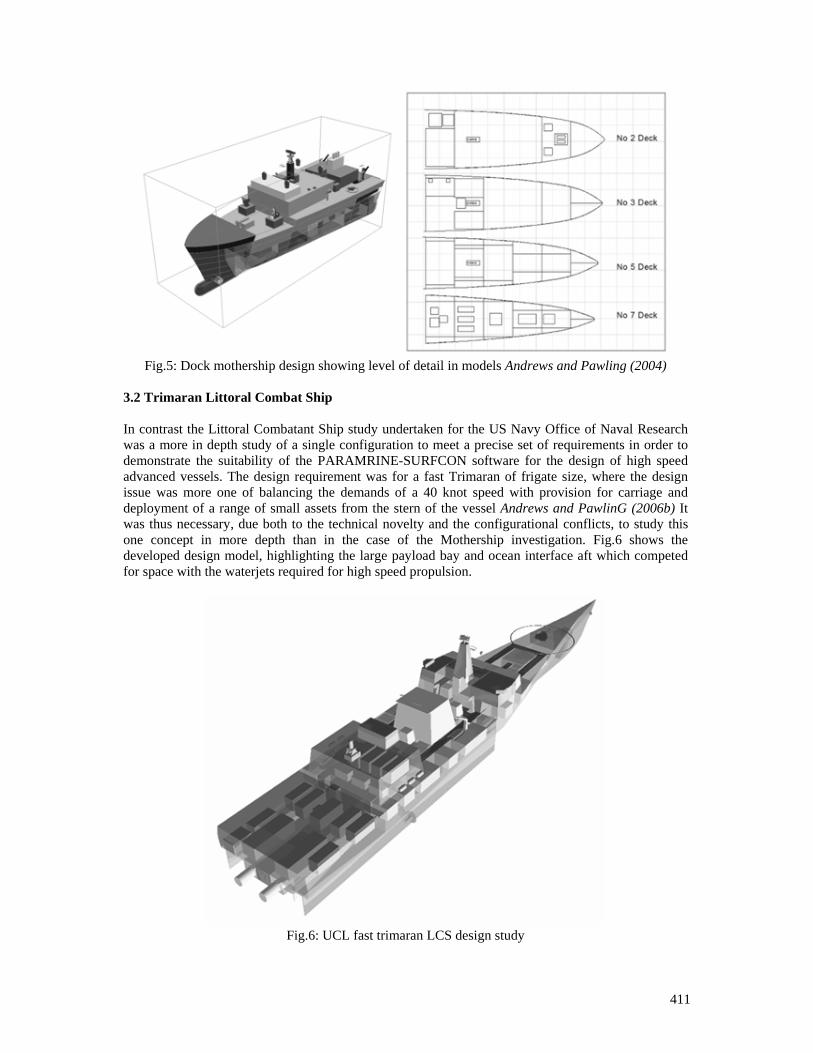
411

Fig.5: Dock mothership design showing level of detail in models Andrews and Pawling (2004)

3.2 Trimaran Littoral Combat Ship In contrast the Littoral Combatant Ship study undertaken for the US Navy Office of Naval Research was a more in depth study of a single configuration to meet a precise set of requirements in order to demonstrate the suitability of the PARAMRINE-SURFCON software for the design of high speed advanced vessels. The design requirement was for a fast Trimaran of frigate size, where the design issue was more one of balancing the demands of a 40 knot speed with provision for carriage and deployment of a range of small assets from the stern of the vessel Andrews and PawlinG (2006b) It was thus necessary, due both to the technical novelty and the configurational conflicts, to study this one concept in more depth than in the case of the Mothership investigation. Fig.6 shows the developed design model, highlighting the large payload bay and ocean interface aft which competed for space with the waterjets required for high speed propulsion.

Fig.6: UCL fast trimaran LCS design study

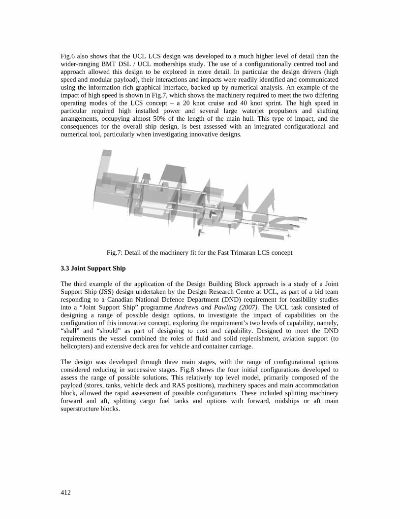
412

Fig.6 also shows that the UCL LCS design was developed to a much higher level of detail than the wider-ranging BMT DSL / UCL motherships study. The use of a configurationally centred tool and approach allowed this design to be explored in more detail. In particular the design drivers (high speed and modular payload), their interactions and impacts were readily identified and communicated using the information rich graphical interface, backed up by numerical analysis. An example of the impact of high speed is shown in Fig.7, which shows the machinery required to meet the two differing operating modes of the LCS concept – a 20 knot cruise and 40 knot sprint. The high speed in particular required high installed power and several large waterjet propulsors and shafting arrangements, occupying almost 50% of the length of the main hull. This type of impact, and the consequences for the overall ship design, is best assessed with an integrated configurational and numerical tool, particularly when investigating innovative designs.

Fig.7: Detail of the machinery fit for the Fast Trimaran LCS concept

3.3 Joint Support Ship The third example of the application of the Design Building Block approach is a study of a Joint Support Ship (JSS) design undertaken by the Design Research Centre at UCL, as part of a bid team responding to a Canadian National Defence Department (DND) requirement for feasibility studies into a “Joint Support Ship” programme Andrews and Pawling (2007). The UCL task consisted of designing a range of possible design options, to investigate the impact of capabilities on the configuration of this innovative concept, exploring the requirement’s two levels of capability, namely, “shall” and “should” as part of designing to cost and capability. Designed to meet the DND requirements the vessel combined the roles of fluid and solid replenishment, aviation support (to helicopters) and extensive deck area for vehicle and container carriage. The design was developed through three main stages, with the range of configurational options considered reducing in successive stages. Fig.8 shows the four initial configurations developed to assess the range of possible solutions. This relatively top level model, primarily composed of the payload (stores, tanks, vehicle deck and RAS positions), machinery spaces and main accommodation block, allowed the rapid assessment of possible configurations. These included splitting machinery forward and aft, splitting cargo fuel tanks and options with forward, midships or aft main superstructure blocks.

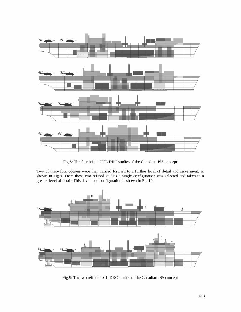
413

Fig.8: The four initial UCL DRC studies of the Canadian JSS concept Two of these four options were then carried forward to a further level of detail and assessment, as shown in Fig.9. From these two refined studies a single configuration was selected and taken to a greater level of detail. This developed configuration is shown in Fig.10.

Fig.9: The two refined UCL DRC studies of the Canadian JSS concept

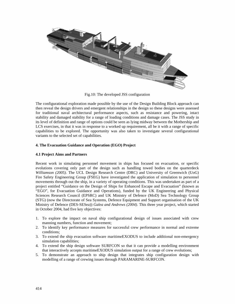
414

Fig.10: The developed JSS configuration

The configurational exploration made possible by the use of the Design Building Block approach can then reveal the design drivers and emergent relationships in the design so these designs were assessed for traditional naval architectural performance aspects, such as resistance and powering, intact stability and damaged stability for a range of loading conditions and damage cases. The JSS study in its level of definition and range of options could be seen as lying midway between the Mothership and LCS exercises, in that it was in response to a worked up requirement, all be it with a range of specific capabilities to be explored. The opportunity was also taken to investigate several configurational variants to the selected set of capabilities. 4. The Evacuation Guidance and Operation (EGO) Project 4.1 Project Aims and Partners Recent work in simulating personnel movement in ships has focused on evacuation, or specific evolutions covering only part of the design such as handling towed bodies on the quarterdeck Williamson (2005). The UCL Design Research Centre (DRC) and University of Greenwich (UoG) Fire Safety Engineering Group (FSEG) have investigated the application of simulation to personnel movements through out the ship, in a variety of operating conditions. This was undertaken as part of a project entitled “Guidance on the Design of Ships for Enhanced Escape and Evacuation” (known as “EGO”, for Evacuation Guidance and Operations), funded by the UK Engineering and Physical Sciences Research Council (EPSRC) and UK Ministry of Defence (MoD) Sea Technology Group (STG) (now the Directorate of Sea Systems, Defence Equipment and Support organisation of the UK Ministry of Defence (DES-SESea)) Galea and Andrews (2004). This three year project, which started in October 2004, had five key objectives: 1. To explore the impact on naval ship configurational design of issues associated with crew

manning numbers, function and movement; 2. To identify key performance measures for successful crew performance in normal and extreme

conditions; 3. To extend the ship evacuation software maritimeEXODUS to include additional non-emergency

simulation capabilities; 4. To extend the ship design software SURFCON so that it can provide a modelling environment

that interactively accepts maritimeEXODUS simulation output for a range of crew evolutions; 5. To demonstrate an approach to ship design that integrates ship configuration design with

modelling of a range of crewing issues through PARAMARINE-SURFCON.

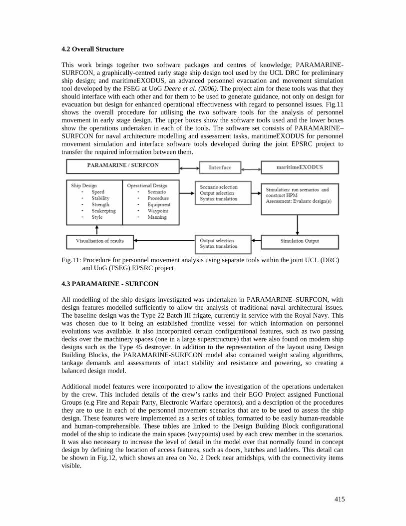
415

4.2 Overall Structure This work brings together two software packages and centres of knowledge; PARAMARINE-SURFCON, a graphically-centred early stage ship design tool used by the UCL DRC for preliminary ship design; and maritimeEXODUS, an advanced personnel evacuation and movement simulation tool developed by the FSEG at UoG Deere et al. (2006). The project aim for these tools was that they should interface with each other and for them to be used to generate guidance, not only on design for evacuation but design for enhanced operational effectiveness with regard to personnel issues. Fig.11 shows the overall procedure for utilising the two software tools for the analysis of personnel movement in early stage design. The upper boxes show the software tools used and the lower boxes show the operations undertaken in each of the tools. The software set consists of PARAMARINE–SURFCON for naval architecture modelling and assessment tasks, maritimeEXODUS for personnel movement simulation and interface software tools developed during the joint EPSRC project to transfer the required information between them.

Fig.11: Procedure for personnel movement analysis using separate tools within the joint UCL (DRC) and UoG (FSEG) EPSRC project 4.3 PARAMARINE - SURFCON All modelling of the ship designs investigated was undertaken in PARAMARINE–SURFCON, with design features modelled sufficiently to allow the analysis of traditional naval architectural issues. The baseline design was the Type 22 Batch III frigate, currently in service with the Royal Navy. This was chosen due to it being an established frontline vessel for which information on personnel evolutions was available. It also incorporated certain configurational features, such as two passing decks over the machinery spaces (one in a large superstructure) that were also found on modern ship designs such as the Type 45 destroyer. In addition to the representation of the layout using Design Building Blocks, the PARAMARINE-SURFCON model also contained weight scaling algorithms, tankage demands and assessments of intact stability and resistance and powering, so creating a balanced design model. Additional model features were incorporated to allow the investigation of the operations undertaken by the crew. This included details of the crew’s ranks and their EGO Project assigned Functional Groups (e.g Fire and Repair Party, Electronic Warfare operators), and a description of the procedures they are to use in each of the personnel movement scenarios that are to be used to assess the ship design. These features were implemented as a series of tables, formatted to be easily human-readable and human-comprehensible. These tables are linked to the Design Building Block configurational model of the ship to indicate the main spaces (waypoints) used by each crew member in the scenarios. It was also necessary to increase the level of detail in the model over that normally found in concept design by defining the location of access features, such as doors, hatches and ladders. This detail can be shown in Fig.12, which shows an area on No. 2 Deck near amidships, with the connectivity items visible.

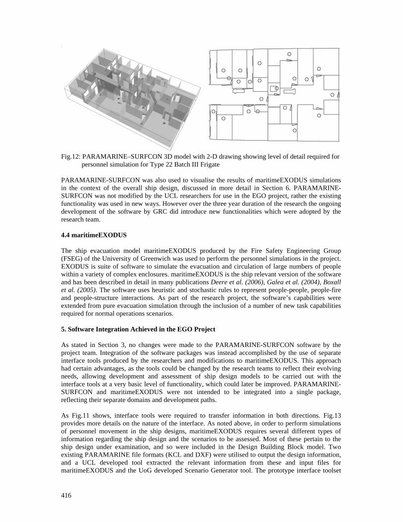
416

Fig.12: PARAMARINE–SURFCON 3D model with 2-D drawing showing level of detail required for personnel simulation for Type 22 Batch III Frigate PARAMARINE-SURFCON was also used to visualise the results of maritimeEXODUS simulations in the context of the overall ship design, discussed in more detail in Section 6. PARAMARINE-SURFCON was not modified by the UCL researchers for use in the EGO project, rather the existing functionality was used in new ways. However over the three year duration of the research the ongoing development of the software by GRC did introduce new functionalities which were adopted by the research team. 4.4 maritimeEXODUS The ship evacuation model maritimeEXODUS produced by the Fire Safety Engineering Group (FSEG) of the University of Greenwich was used to perform the personnel simulations in the project. EXODUS is suite of software to simulate the evacuation and circulation of large numbers of people within a variety of complex enclosures. maritimeEXODUS is the ship relevant version of the software and has been described in detail in many publications Deere et al. (2006), Galea et al. (2004), Boxall et al. (2005). The software uses heuristic and stochastic rules to represent people-people, people-fire and people-structure interactions. As part of the research project, the software’s capabilities were extended from pure evacuation simulation through the inclusion of a number of new task capabilities required for normal operations scenarios. 5. Software Integration Achieved in the EGO Project As stated in Section 3, no changes were made to the PARAMARINE-SURFCON software by the project team. Integration of the software packages was instead accomplished by the use of separate interface tools produced by the researchers and modifications to maritimeEXODUS. This approach had certain advantages, as the tools could be changed by the research teams to reflect their evolving needs, allowing development and assessment of ship design models to be carried out with the interface tools at a very basic level of functionality, which could later be improved. PARAMARINE-SURFCON and maritimeEXODUS were not intended to be integrated into a single package, reflecting their separate domains and development paths. As Fig.11 shows, interface tools were required to transfer information in both directions. Fig.13 provides more details on the nature of the interface. As noted above, in order to perform simulations of personnel movement in the ship designs, maritimeEXODUS requires several different types of information regarding the ship design and the scenarios to be assessed. Most of these pertain to the ship design under examination, and so were included in the Design Building Block model. Two existing PARAMARINE file formats (KCL and DXF) were utilised to output the design information, and a UCL developed tool extracted the relevant information from these and input files for maritimeEXODUS and the UoG developed Scenario Generator tool. The prototype interface toolset

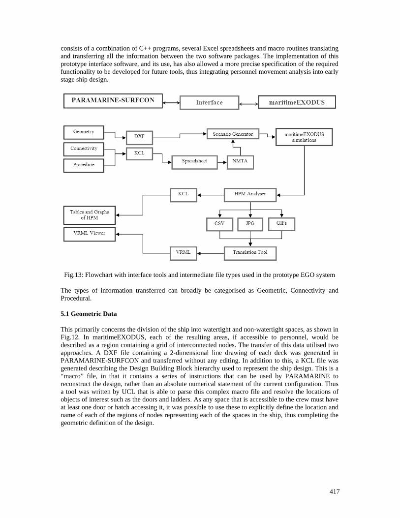
417

consists of a combination of C++ programs, several Excel spreadsheets and macro routines translating and transferring all the information between the two software packages. The implementation of this prototype interface software, and its use, has also allowed a more precise specification of the required functionality to be developed for future tools, thus integrating personnel movement analysis into early stage ship design.

Fig.13: Flowchart with interface tools and intermediate file types used in the prototype EGO system The types of information transferred can broadly be categorised as Geometric, Connectivity and Procedural. 5.1 Geometric Data This primarily concerns the division of the ship into watertight and non-watertight spaces, as shown in Fig.12. In maritimeEXODUS, each of the resulting areas, if accessible to personnel, would be described as a region containing a grid of interconnected nodes. The transfer of this data utilised two approaches. A DXF file containing a 2-dimensional line drawing of each deck was generated in PARAMARINE-SURFCON and transferred without any editing. In addition to this, a KCL file was generated describing the Design Building Block hierarchy used to represent the ship design. This is a “macro” file, in that it contains a series of instructions that can be used by PARAMARINE to reconstruct the design, rather than an absolute numerical statement of the current configuration. Thus a tool was written by UCL that is able to parse this complex macro file and resolve the locations of objects of interest such as the doors and ladders. As any space that is accessible to the crew must have at least one door or hatch accessing it, it was possible to use these to explicitly define the location and name of each of the regions of nodes representing each of the spaces in the ship, thus completing the geometric definition of the design.

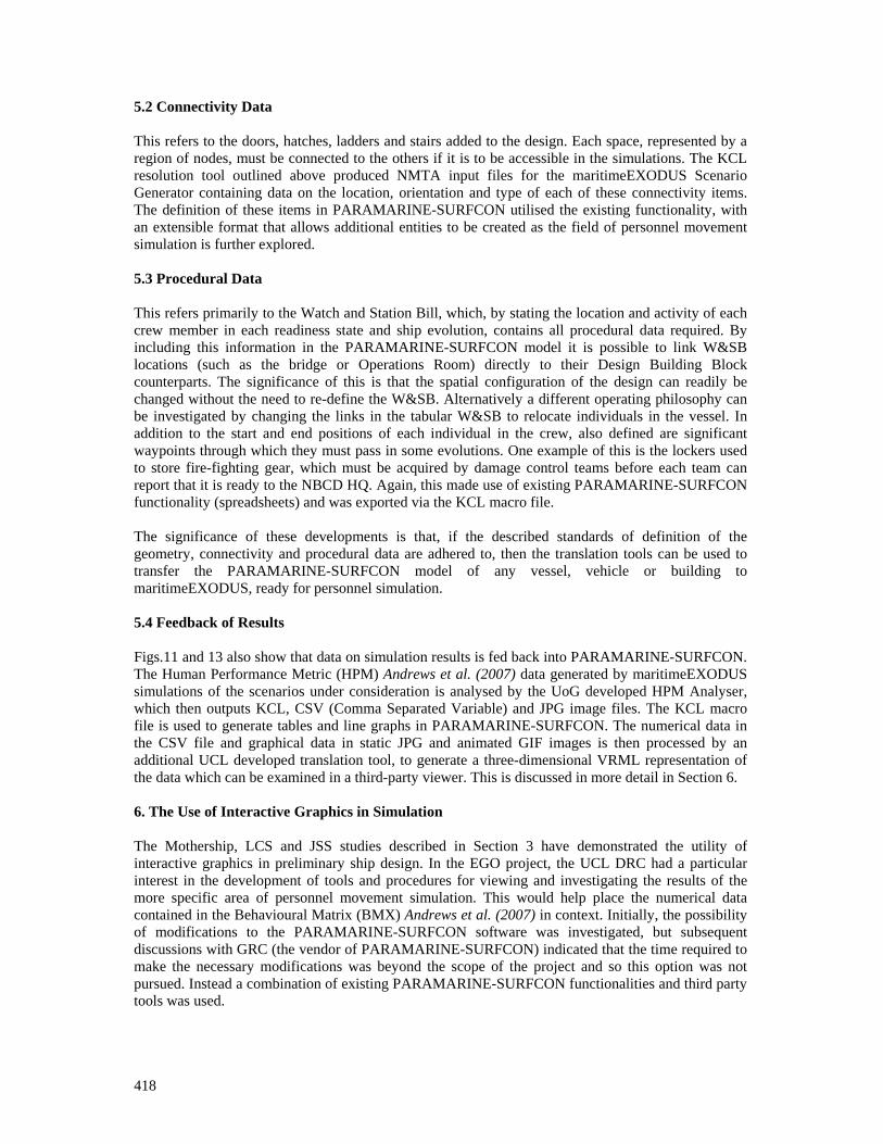
418

5.2 Connectivity Data This refers to the doors, hatches, ladders and stairs added to the design. Each space, represented by a region of nodes, must be connected to the others if it is to be accessible in the simulations. The KCL resolution tool outlined above produced NMTA input files for the maritimeEXODUS Scenario Generator containing data on the location, orientation and type of each of these connectivity items. The definition of these items in PARAMARINE-SURFCON utilised the existing functionality, with an extensible format that allows additional entities to be created as the field of personnel movement simulation is further explored. 5.3 Procedural Data This refers primarily to the Watch and Station Bill, which, by stating the location and activity of each crew member in each readiness state and ship evolution, contains all procedural data required. By including this information in the PARAMARINE-SURFCON model it is possible to link W&SB locations (such as the bridge or Operations Room) directly to their Design Building Block counterparts. The significance of this is that the spatial configuration of the design can readily be changed without the need to re-define the W&SB. Alternatively a different operating philosophy can be investigated by changing the links in the tabular W&SB to relocate individuals in the vessel. In addition to the start and end positions of each individual in the crew, also defined are significant waypoints through which they must pass in some evolutions. One example of this is the lockers used to store fire-fighting gear, which must be acquired by damage control teams before each team can report that it is ready to the NBCD HQ. Again, this made use of existing PARAMARINE-SURFCON functionality (spreadsheets) and was exported via the KCL macro file. The significance of these developments is that, if the described standards of definition of the geometry, connectivity and procedural data are adhered to, then the translation tools can be used to transfer the PARAMARINE-SURFCON model of any vessel, vehicle or building to maritimeEXODUS, ready for personnel simulation. 5.4 Feedback of Results Figs.11 and 13 also show that data on simulation results is fed back into PARAMARINE-SURFCON. The Human Performance Metric (HPM) Andrews et al. (2007) data generated by maritimeEXODUS simulations of the scenarios under consideration is analysed by the UoG developed HPM Analyser, which then outputs KCL, CSV (Comma Separated Variable) and JPG image files. The KCL macro file is used to generate tables and line graphs in PARAMARINE-SURFCON. The numerical data in the CSV file and graphical data in static JPG and animated GIF images is then processed by an additional UCL developed translation tool, to generate a three-dimensional VRML representation of the data which can be examined in a third-party viewer. This is discussed in more detail in Section 6. 6. The Use of Interactive Graphics in Simulation The Mothership, LCS and JSS studies described in Section 3 have demonstrated the utility of interactive graphics in preliminary ship design. In the EGO project, the UCL DRC had a particular interest in the development of tools and procedures for viewing and investigating the results of the more specific area of personnel movement simulation. This would help place the numerical data contained in the Behavioural Matrix (BMX) Andrews et al. (2007) in context. Initially, the possibility of modifications to the PARAMARINE-SURFCON software was investigated, but subsequent discussions with GRC (the vendor of PARAMARINE-SURFCON) indicated that the time required to make the necessary modifications was beyond the scope of the project and so this option was not pursued. Instead a combination of existing PARAMARINE-SURFCON functionalities and third party tools was used.

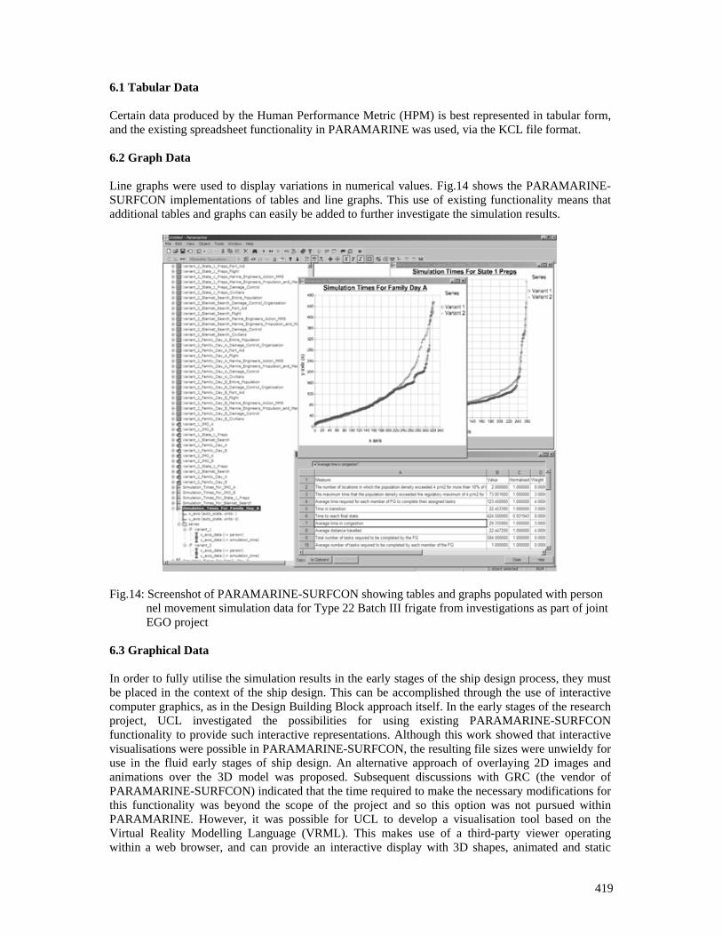
419

6.1 Tabular Data Certain data produced by the Human Performance Metric (HPM) is best represented in tabular form, and the existing spreadsheet functionality in PARAMARINE was used, via the KCL file format. 6.2 Graph Data Line graphs were used to display variations in numerical values. Fig.14 shows the PARAMARINE-SURFCON implementations of tables and line graphs. This use of existing functionality means that additional tables and graphs can easily be added to further investigate the simulation results.

Fig.14: Screenshot of PARAMARINE-SURFCON showing tables and graphs populated with person nel movement simulation data for Type 22 Batch III frigate from investigations as part of joint EGO project 6.3 Graphical Data In order to fully utilise the simulation results in the early stages of the ship design process, they must be placed in the context of the ship design. This can be accomplished through the use of interactive computer graphics, as in the Design Building Block approach itself. In the early stages of the research project, UCL investigated the possibilities for using existing PARAMARINE-SURFCON functionality to provide such interactive representations. Although this work showed that interactive visualisations were possible in PARAMARINE-SURFCON, the resulting file sizes were unwieldy for use in the fluid early stages of ship design. An alternative approach of overlaying 2D images and animations over the 3D model was proposed. Subsequent discussions with GRC (the vendor of PARAMARINE-SURFCON) indicated that the time required to make the necessary modifications for this functionality was beyond the scope of the project and so this option was not pursued within PARAMARINE. However, it was possible for UCL to develop a visualisation tool based on the Virtual Reality Modelling Language (VRML). This makes use of a third-party viewer operating within a web browser, and can provide an interactive display with 3D shapes, animated and static

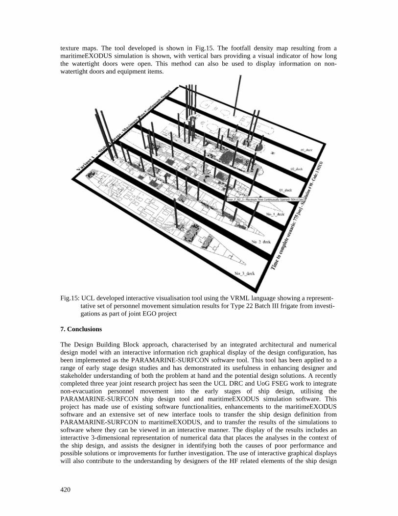
420

texture maps. The tool developed is shown in Fig.15. The footfall density map resulting from a maritimeEXODUS simulation is shown, with vertical bars providing a visual indicator of how long the watertight doors were open. This method can also be used to display information on non-watertight doors and equipment items.

Fig.15: UCL developed interactive visualisation tool using the VRML language showing a represent- tative set of personnel movement simulation results for Type 22 Batch III frigate from investi- gations as part of joint EGO project 7. Conclusions The Design Building Block approach, characterised by an integrated architectural and numerical design model with an interactive information rich graphical display of the design configuration, has been implemented as the PARAMARINE-SURFCON software tool. This tool has been applied to a range of early stage design studies and has demonstrated its usefulness in enhancing designer and stakeholder understanding of both the problem at hand and the potential design solutions. A recently completed three year joint research project has seen the UCL DRC and UoG FSEG work to integrate non-evacuation personnel movement into the early stages of ship design, utilising the PARAMARINE-SURFCON ship design tool and maritimeEXODUS simulation software. This project has made use of existing software functionalities, enhancements to the maritimeEXODUS software and an extensive set of new interface tools to transfer the ship design definition from PARAMARINE-SURFCON to maritimeEXODUS, and to transfer the results of the simulations to software where they can be viewed in an interactive manner. The display of the results includes an interactive 3-dimensional representation of numerical data that places the analyses in the context of the ship design, and assists the designer in identifying both the causes of poor performance and possible solutions or improvements for further investigation. The use of interactive graphical displays will also contribute to the understanding by designers of the HF related elements of the ship design

421

and improve the communication of results and outcomes of numerical simulations to design stakeholders. Importantly, the approach and toolset developed are flexible and extensible, allowing the early stage analysis of personnel movement to be extended beyond the surface combatant used in the developmental project, to encompass all other types of naval and merchant vessels and also land-based buildings terminals and the layout of large public events. Acknowledgements The authors gratefully acknowledge the support of the UK EPSRC and UK MoD under grants GR/T22100/01 and GR/T22117/01. References ANDREWS, D.J. (2004), A creative approach to ship architecture, RINA Int. J. Maritime Engineering, Sept 2003, Discussion and Author’s response IJME Sept 2003, Trans. RINA 2004 ANDREWS, D.J.; PAWLING, R. (2004), Fast motherships - A design challenge, RINA Int. Conf. Warship 2004: Littoral Warfare & the Expeditionary Force, London ANDREWS, D.J.; PAWLING, R. (2006a), The application of computer aided graphics to preliminary ship design, IMDC06, Ann Arbor ANDREWS, D J.; PAWLING, R. (2006b), Innovative ship design for high speed adaptable littoral warfare, RINA Int. Conf. Warship 2006: Future Surface Ships, London ANDREWS, D.J.; PAWLING, R. (2007), Concept studies for a joint support ship, RINA Int. Conf. Warship 2007: The Affordable Warship, Bath, pp.69-88 ANDREWS, D.J.; PAWLING, R.; CASAROSA, L.; GALEA, E.R.; DEERE, S.; LAWRENCE, P,. (2007), Integrating personnel movement simulation into preliminary ship design, RINA Int. Conf. on Human Factors in Ship Design, London, pp.117-128 BOLE, M.; FORREST, C. (2005), Early stage integrated parametric ship design, 12th Int. Conf. on Computer Applications in Shipbuilding, Busan BOXALL, P.; GWYNNE, S.; FILIPPIDIS, L.; GALEA, E.R.; COONEY, D. (2005), Advanced evacuation simulation software and its use in warships, RINA Int. Conf. on Human Factors in Ship Design, Safety & Operation, London, pp.49-56 DEERE, S.; GALEA, E.R.; LAWRENCE, P.; GWYNNE, S. (2006), The impact of the passenger response time distribution on ship evacuation performance, RINA Trans. 148, Part A1 (J. Maritime Engineering), ISSN 1479-8751 GALEA, E.R.; ANDREWS, D.J. (2004), Guidance on the design of ships for enhanced escape and operation, EPSRC Project Proposal Feb 2004 commenced Oct 2004 GALEA, E.R.; LAWRENCE, P.; GWYNNE, S.; SHARP, G.; HURST, N.; WANG, Z.; EWER, J. (2004), Integrated fire and evacuation in maritime environments, 2nd Int. Maritime Safety Conf. on Design for Safety, Sakai WILLIAMSON, M. (2005), Human factors program eliminates safety hazards of marine seismic streamer handling operations, RINA Int. Conf. on Human Factors in Ship Design, Safety & Operation, London, pp.23-32

422

An Improved Particle Swarm Optimisation (PSO) Approach in a

Multi Criteria Decision Making Environment

Hao Cui, Aykut Olcer, Osman Turan, Universities of Glasgow and Strathclyde, Glasgow/UK, o.turan@na-me.ac.uk

Abstract Particle Swarm Optimization (PSO) displays good performance in single objective optimization. However, in multi-objective optimization, because PSO focus on cooperation, it can not put enough pressure to push solution space to Pareto Surface. This article introduces an improved multi-PSO ap-proach to operate multiple criteria decision making in agent based ship design environment. The game theory is added to the PSO to give direction and selection abilities in optimization. A case is provided to demonstrate the application of the proposed approach. 1． Introduction The Particle Swarm Optimization (PSO) algorithm, Kennedy and Eberhart (1995), has been success-fully used in single-objective optimization problems. Since Moore and Chapman proposed the first extension of the PSO strategy for solving multi-objective problems in 1999, a great deal of interest has been shown to multi-objective optimization and many different approaches/techniques have been presented in literature. The sample parameters setting and effect optimization performance of PSO exhibit good capability for engineering optimization. Since Mistree et al. (1990) approached ship design from a decision perspective, decision making based ship design environment develops rapidly. In recent years, multi-agent based ship design deci-sion systems have received a great deal of attention and distributed synchronous cooperative ship de-sign method via internet is becoming a new research field. For this development, the multi criteria design making environment requires a new optimization approach which is suitable for multi-agent system while simple and efficient.. The internal hull subdivision in ship design is important for damage stability, survivability and cargo capacity performance, particularly for RORO passenger vessels, which have conform to SOLAS standards including SOLAS 90 (Stockholm Agreement). The ship design needs to be optimized to achieve these high safety standards and cost effectiveness. This paper introduces a novel hybrid co-evolution based multi-objective particle swarm optimization (HCPSO). The HCPSO combine co-evolution, game theory and extremum disturb to develop an ef-fective optimization approach. It performs remarkably well in a multi-agent system. The paper then explores application of multi-objective particle swarm optimization on hull subdivision design of Ro-Ro passenger vessel.

423

2. PSO and multi-objective PSO PSO is a global optimization algorithm and described as sociologically inspired. In a PSO algorithm, the candidate solution is the particle position in search space. Every particle is structured by two pa-rameters: position and velocity. Then the particle searches the solution space via updating position and velocity. There are two best positions in PSO. First one is Pbest, which represents the best position that the particle itself can reach; the other is Gbest, which is the best position for the whole swarm. The basic PSO is described as following,

11 1 2 2

1 1

( ) ( );

;

n n n n n n n nid id id id gd id

n n nid id id

v v c r p x c r p x

x x v

+

+ +

= + − + −

= + (1)

nidv is the velocity of particle i, in n-th iteration and d dimension; 1c and 2c are two coefficients;

1r and 2r are two random numbers with the range[0,1].

With the development in recent years, some improvements and changes have been introduced to achieve better performance. A new formula is suggested as:

11 1 2 2

1 1

( ) ( );

;

n n n n n n n nid id id id gd id

n n nid id id

v v c r p x c r p x

x x v

ω

χ

+

+ +

= + − + −

= + (2)

where ω is the inertia weight and χ is a construction factor. PSO has been proven as a simple but effective algorithm in single objective optimization and multi-objective research has rapidly developed in recent years. Since the first extension was proposed in 1999, many different multi-objective PSOs have been presented, Reyes-Rierra and Coello Coello (2006). Some are briefly given below. Aggregating approaches: They combine all the objectives of the problem into a single one and three types of aggregating functions are adopted: conventional linear aggregating function, dynamic aggre-gating function and the Bang-bang weighted aggregation approach, Parsopoulos and Vrahatis (2002), Baumgartner et al. (2004), Jin et al. (2001). Lexicographic ordering: In this algorithm, which was introduced by Hu and Eberhart (2002), only one objective is optimized at a time using lexicographic ordering Schema. Sub-Population approaches: These approaches involve the use of several subpopulations as sin-gle-objective optimizers. Then, the subpopulations somehow exchange information or recombine among themselves aiming to produce trade-offs among the different solutions previously generated for the objectives that were separately optimized. Parsopoulos et al. (2004), Chow and Tsui (2004), Zheng and Liu (2007) use this approach. Pareto-based approaches, these approaches use leader selection techniques based on Pareto domi-nance including Moore and Chapman (1999), Ray and Liew (2002), Fieldsend and Singh (2002), Coello Coello and Salazar Lechuga (2002), Coello Coello et al. (2004), Li (2003).

424

Some of the other approaches, which use different techniques, such as Combined Approach and maxmin approach can also be found in literature. 3. Description of HCPSO The hybrid Co-evolutionary based Multi-Objective Particle Swarm Optimization (HCPSO) combines the Pareto-based approach, Sub-Population approach, co-evolution approach and extremum disturb to form a new improved hybrid approach. At the same time, agent-based structure is adopted for distrib-uted synchronous cooperation. Sefrioui and Periaux (2000) introduced Nash optima of game theory into the multi-objective optimi-zation. We deploy this model to multi-objective PSO. For an optimization problem with population number N, number of design variables K and Number of objectives M, HCPSO divides N particles into M sub-swarm group according to M objectives. Then the design variables K also are divided into k1, k2, … km sub-groups. The HCPSO engages M agents to control optimisation. Every agent opti-mises relevant design variables in own sub-swam group via the sharing information from public board. After that, they send the results to public board for optimization next time. In every sub-swarm, in order to give enough pressure to push solution space to Pareto Surface ap-proaches, particles in two generation are compared to update the position. The HCPSO also uses the distance approach of NSGAII, Deb (2001), to measure the performance of particle. Algorithm HCPSO 1. initialize the population including position and velocity;

(i) construct context vector to store information as public-board; (ii) give the number of sub-swarm and size of sub-swarm; (iii) divide population into sub-swarm

2. every sub-swarm begins iteration; for example (mth sub-swarm with (N/M) particles and km design variables) 3. read information from context vector and evaluate fitness; 4. update Pbest via comparing individual history position according mth objective ; 5. non-dominated sorting 6. give pointed number of best ranking particles to context vector 7. collect all sub-swarm to context vector and form Gbest pool; 8. every sub-swam randomly select Gbest form pool; 9. comparing Pbest and Gbest with before for usage of extremum disturb 10. calculate velocity and give limit velocity; 11. update position and limit position; 12. Perform non-dominated sorting 13. select first (N/M) particles to update position and velocity 14. send corresponding information 15. If solution is satisfactory stop if it is not continue iteration 16. output

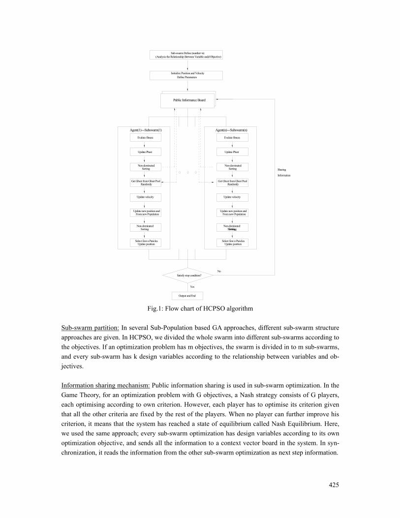
425

Sharing

Information

Sorting

Public Informance Board

No

Yes

Output and End

Satisfy stop condition?

Agent(n)---Subswarm(n)Agent(1)---Subswarm(1)

Non-dominatedSorting

Evalute fitness

Update Pbest

RandomlyGet Gbest from Gbest Pool

Update velocity

From new PopulationUpdate new position and

Non-dominatedSorting

Select first n PariclesUpdate posttionUpdate posttion

Select first n Paricles

SortingNon-dominated

Update new position and From new Population

Update velocity

Get Gbest from Gbest PoolRandomly

Update Pbest

Evalute fitness

SortingNon-dominated

Initialize Position and VelocityDefine Parameters

(Analysis the Relationship Between Variable andd Objective)Sub-swarm Define (number=n)

Fig.1: Flow chart of HCPSO algorithm

Sub-swarm partition: In several Sub-Population based GA approaches, different sub-swarm structure approaches are given. In HCPSO, we divided the whole swarm into different sub-swarms according to the objectives. If an optimization problem has m objectives, the swarm is divided in to m sub-swarms, and every sub-swarm has k design variables according to the relationship between variables and ob-jectives. Information sharing mechanism: Public information sharing is used in sub-swarm optimization. In the Game Theory, for an optimization problem with G objectives, a Nash strategy consists of G players, each optimising according to own criterion. However, each player has to optimise its criterion given that all the other criteria are fixed by the rest of the players. When no player can further improve his criterion, it means that the system has reached a state of equilibrium called Nash Equilibrium. Here, we used the same approach; every sub-swarm optimization has design variables according to its own optimization objective, and sends all the information to a context vector board in the system. In syn-chronization, it reads the information from the other sub-swarm optimization as next step information.

426

Pbest and Gbest updating: The Pbest updating in HCPSO adopts sub-swarm inside updating. The par-ticle in m-the sub-swarm compares corresponding objective fitness value between current position and previous best position. If the current position in the nth objective fitness is better than prior value, the Pbest is replaced by current value and else, it is kept. The Gbest selection uses outside updating - Gbest pool. Every sub-swarm gives a pointed proportion best value which is decided using NSGAII. The HCPSO randomly selects a particle as Gbest position. Particle updating: In order to prove give enough pressure to the pareto front, we use updating position approach to mutate the every particle. In every sub-swarm, the system will compare the fitness in last generation and the generation (size of population is 2*N/M), then select N/M position as this genera-tion, some particle hold their own position and others will be replaced by nearest neighbor. Extremum disturb: For multi-PSO, sometimes the approach will generate local optima value, the ex-tremum disturb is used to avoid this. We used stagnant step as burst mode, for a given step T, if stag-nant step ts > T, a random disturb is given to both Pbest and Gbest. 4 Experiments 4. 1 Test Function The standard two objective test functions from ZDT series are selected.

Name Variables n Ranger Test Function

ZDT1 30 [0,1]

1 1 1

22

1 1

( ) ,9( ,..., ) 1 ,

1

( , ) 1 / .

n

m ii

f x x

g x x xn

h f g f g=

⎧ =⎪⎪ = +⎨ −⎪⎪ = −⎩

∑

ZDT2 30 [0,1]

1 1 1

222

1 1

( ) ,9( ,..., ) 1 ,

1( , ) 1 ( / ) .

n

m ii

f x x

g x x xn

h f g f g=

⎧ =⎪⎪ = +⎨ −⎪⎪ = −⎩

∑

ZDT3 30 [0,1]

1 1 1

22

1 1 1 1

( ) ,9( ,..., ) 1 ,

1

( , ) 1 / ( / ) sin(10 ).

n

m ii

f x x

g x x xn

h f g f g f g fπ=

⎧ =⎪⎪ = +⎨ −⎪⎪ = − −⎩

∑

ZDT4 10 1 [0,1],

[ 5,5],2,...30;

xxii

∈∈ −

=

1 1 1

22

2

1 1

( ) ,

( ,..., ) 1 10( 1) ( 10cos(4 )),

( , ) 1 / .

n

m i ii

f x x

g x x n x x

h f g f g

π=

⎧ =⎪⎪ = + − + −⎨⎪⎪ = −⎩

∑

427

4.2 Parameters Setting and Performance Metrics The parameters were set as following: the population of swarm is 200 and generation is 100 iteration

steps. 1c and 2c were set to 2.0. ω was gradually decreased from 1.0 to 0.4. Vmax was set to the

bounds of decision variable ranges. χ was 0.72. Extremum disturb is 3 steps. The number of sub-swarm is 2 and population of sub-swarm is 100. Two Evaluation Criterions are selected, Deb (2001): (1) GD (Generational Distance) finds an average of the solutions of Q from P* (Q is solution and p*

is a known set of the Pareto-optimal) | |

1/

1

( )

| |

Qp p

ii

dGD

Q==∑

For a two objective problem (p=2), id is the Euclidean distance between the solution i Q∈

and nearest member of P*. (2) Spread: Deb (2001) suggested the following metric to alleviate the above difficulty

| |

1 1

1

| |

| |

QMem i

m iM

em

m

d d d

d Q d

= =

=

+ −Δ =

+

∑ ∑

∑

where d can be any distance measured between neighboring solution and d is the mean value

of the above distance measure. The parameter emd is the distance between the extreme solutions

of P* and Q corresponding to m-th objective function. 4.3 Results The HCPSO was run 10 times and performance metrics of the results are averaged and summarized in Table I. The non-dominated solutions found by HCPSO for ZDT 1, 2, 3 and 4 are displayed in Fig.2.

Table I: Mean and variance values of GD and Δ ZDT1 ZDT2 ZDT3 ZDT4

GD 1.12E-03 8.22E-04 6.19E-03 6.72E-03 δ2 7.68E-05 8.46E-04 3.81E-03 6.92E-03 Δ 3.86E-01 3.82E-01 6.12E-01 6.88E-01 δ2 1.82E-02 2.56E-02 2.82E-02 2.12E-02

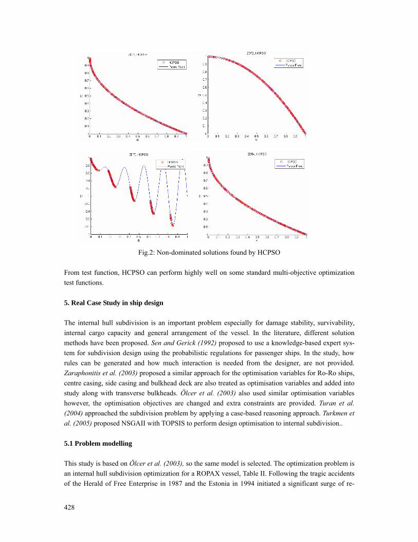
428

Fig.2: Non-dominated solutions found by HCPSO

From test function, HCPSO can perform highly well on some standard multi-objective optimization test functions. 5. Real Case Study in ship design The internal hull subdivision is an important problem especially for damage stability, survivability, internal cargo capacity and general arrangement of the vessel. In the literature, different solution methods have been proposed. Sen and Gerick (1992) proposed to use a knowledge-based expert sys-tem for subdivision design using the probabilistic regulations for passenger ships. In the study, how rules can be generated and how much interaction is needed from the designer, are not provided. Zaraphonitis et al. (2003) proposed a similar approach for the optimisation variables for Ro-Ro ships, centre casing, side casing and bulkhead deck are also treated as optimisation variables and added into study along with transverse bulkheads. Ölcer et al. (2003) also used similar optimisation variables however, the optimisation objectives are changed and extra constraints are provided. Turan et al. (2004) approached the subdivision problem by applying a case-based reasoning approach. Turkmen et al. (2005) proposed NSGAII with TOPSIS to perform design optimisation to internal subdivision.. 5.1 Problem modelling This study is based on Ölcer et al. (2003), so the same model is selected. The optimization problem is an internal hull subdivision optimization for a ROPAX vessel, Table II. Following the tragic accidents of the Herald of Free Enterprise in 1987 and the Estonia in 1994 initiated a significant surge of re-

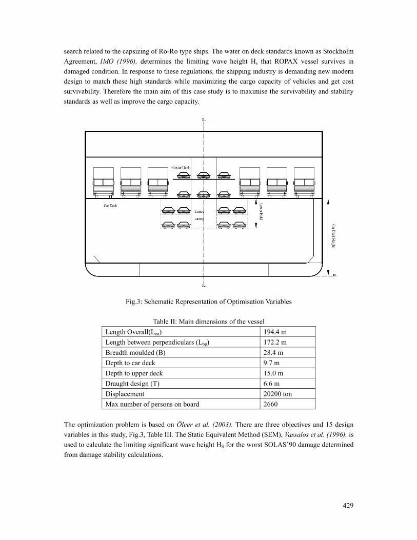
429

search related to the capsizing of Ro-Ro type ships. The water on deck standards known as Stockholm Agreement, IMO (1996), determines the limiting wave height Hs that ROPAX vessel survives in damaged condition. In response to these regulations, the shipping industry is demanding new modern design to match these high standards while maximizing the cargo capacity of vehicles and get cost survivability. Therefore the main aim of this case study is to maximise the survivability and stability standards as well as improve the cargo capacity.

Fig.3: Schematic Representation of Optimisation Variables

Table II: Main dimensions of the vessel Length Overall(Loa) 194.4 m Length between perpendiculars (Lbp) 172.2 m Breadth moulded (B) 28.4 m Depth to car deck 9.7 m Depth to upper deck 15.0 m Draught design (T) 6.6 m Displacement 20200 ton Max number of persons on board 2660

The optimization problem is based on Ölcer et al. (2003). There are three objectives and 15 design variables in this study, Fig.3, Table III. The Static Equivalent Method (SEM), Vassalos et al. (1996), is used to calculate the limiting significant wave height HS for the worst SOLAS’90 damage determined from damage stability calculations.

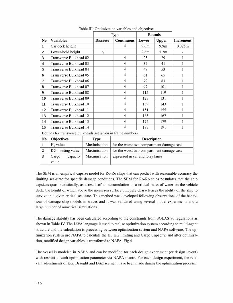
430

Table III: Optimization variables and objectives Type Bounds No Variables Discrete Continuous Lower Upper Increment1 Car deck height √ 9.6m 9.9m 0.025m 2 Lower-hold height √ 2.6m 5.2m - 3 Transverse Bulkhead 02 √ 25 29 1 4 Transverse Bulkhead 03 √ 37 41 1 5 Transverse Bulkhead 04 √ 49 53 1 6 Transverse Bulkhead 05 √ 61 65 1 7 Transverse Bulkhead 06 √ 79 83 1 8 Transverse Bulkhead 07 √ 97 101 1 9 Transverse Bulkhead 08 √ 115 119 1 10 Transverse Bulkhead 09 √ 127 131 1 11 Transverse Bulkhead 10 √ 139 143 1 12 Transverse Bulkhead 11 √ 151 155 1 13 Transverse Bulkhead 12 √ 163 167 1 14 Transverse Bulkhead 13 √ 175 179 1 15 Transverse Bulkhead 14 √ 187 191 1 Bounds for transverse bulkheads are given in frame numbers No Objectives Type Description 1 HS value Maximisation for the worst two compartment damage case 2 KG limiting value Maximisation for the worst two compartment damage case 3 Cargo capacity

value Maximisation expressed in car and lorry lanes

The SEM is an empirical capsize model for Ro-Ro ships that can predict with reasonable accuracy the limiting sea-state for specific damage conditions. The SEM for Ro-Ro ships postulates that the ship capsizes quasi-statistically, as a result of an accumulation of a critical mass of water on the vehicle deck, the height of which above the mean sea surface uniquely characterises the ability of the ship to survive in a given critical sea state. This method was developed following observations of the behav-iour of damage ship models in waves and it was validated using several model experiments and a large number of numerical simulations. The damage stability has been calculated according to the constraints from SOLAS’90 regulations as shown in Table IV. The JAVA language is used to realise optimization system according to multi-agent structure and the calculation is processing between optimization system and NAPA software. The op-timization system use NAPA to calculate the Hs, KG limiting and Cargo Capacity, and after optimiza-tion, modified design variables is transferred to NAPA, Fig.4. The vessel is modeled in NAPA and can be modified for each design experiment (or design layout) with respect to each optimisation parameter via NAPA macro. For each design experiment, the rele-vant adjustments of KG, Draught and Displacement have been made during the optimization process.

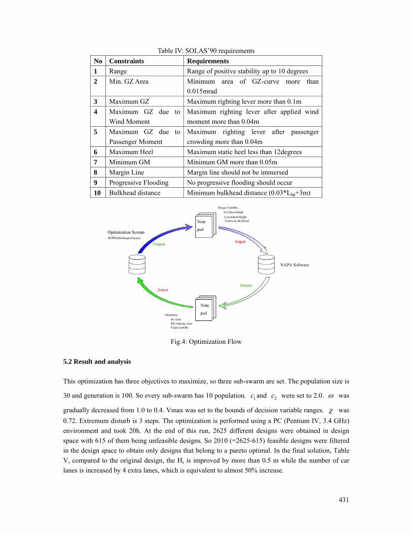
431

Table IV: SOLAS’90 requirements No Constraints Requirements 1 Range Range of positive stability up to 10 degrees 2 Min. GZ Area Minimum area of GZ-curve more than

0.015mrad 3 Maximum GZ Maximum righting lever more than 0.1m 4 Maximum GZ due to

Wind Moment Maximum righting lever after applied wind moment more than 0.04m

5 Maximum GZ due to Passenger Moment

Maximum righting lever after passenger crowding more than 0.04m

6 Maximum Heel Maximum static heel less than 12degrees 7 Minimum GM Minimum GM more than 0.05m 8 Margin Line Margin line should not be immersed 9 Progressive Flooding No progressive flooding should occur 10 Bulkhead distance Minimum bulkhead distance (0.03*Lbp+3m)

Fig.4: Optimization Flow

5.2 Result and analysis This optimization has three objectives to maximize, so three sub-swarm are set. The population size is

30 and generation is 100. So every sub-swarm has 10 population. 1c and 2c were set to 2.0. ω was

gradually decreased from 1.0 to 0.4. Vmax was set to the bounds of decision variable ranges. χ was 0.72. Extremum disturb is 3 steps. The optimization is performed using a PC (Pentium IV, 3.4 GHz) environment and took 20h. At the end of this run, 2625 different designs were obtained in design space with 615 of them being unfeasible designs. So 2010 (=2625-615) feasible designs were filtered in the design space to obtain only designs that belong to a pareto optimal. In the final solution, Table V, compared to the original design, the Hs is improved by more than 0.5 m while the number of car lanes is increased by 4 extra lanes, which is equivalent to almost 50% increase.

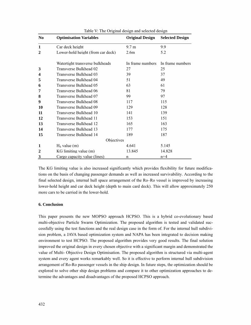
432

Table V: The Original design and selected design No Optimisation Variables Original Design Selected Design

1 Car deck height 9.7 m 9.92 Lower-hold height (from car deck) 2.6m 5.2 Watertight transverse bulkheads In frame numbers In frame numbers 3 Transverse Bulkhead 02 27 254 Transverse Bulkhead 03 39 375 Transverse Bulkhead 04 51 496 Transverse Bulkhead 05 63 617 Transverse Bulkhead 06 81 798 Transverse Bulkhead 07 99 979 Transverse Bulkhead 08 117 11510 Transverse Bulkhead 09 129 12811 Transverse Bulkhead 10 141 13912 Transverse Bulkhead 11 153 15113 Transverse Bulkhead 12 165 16314 Transverse Bulkhead 13 177 17515 Transverse Bulkhead 14 189 187

Objectives1 HS value (m) 4.641 5.1452 KG limiting value (m) 13.845 14.8283 Cargo capacity value (lines) n n+4 The KG limiting value is also increased significantly which provides flexibility for future modifica-tions on the basis of changing passenger demands as well as increased survivability. According to the final selected design, internal hull space arrangement of the Ro–Ro vessel is improved by increasing lower-hold height and car deck height (depth to main card deck). This will allow approximately 250 more cars to be carried in the lower-hold. 6. Conclusion This paper presents the new MOPSO approach HCPSO. This is a hybrid co-evolutionary based multi-objective Particle Swarm Optimization. The proposed algorithm is tested and validated suc-cessfully using the test functions and the real design case in the form of. For the internal hull subdivi-sion problem, a JAVA based optimization system and NAPA has been integrated to decision making environment to test HCPSO. The proposed algorithm provides very good results. The final solution improved the original design in every chosen objective with a significant margin and demonstrated the value of Multi- Objective Design Optimisation. The proposed algorithm is structured via multi-agent system and every agent works remarkably well. So it is effective to perform internal hull subdivision arrangement of Ro-Ro passenger vessels in the ship design. In future steps, the optimization should be explored to solve other ship design problems and compare it to other optimization approaches to de-termine the advantages and disadvantages of the proposed HCPSO approach.

433

References BAUMGARTNER, U.; MAGELE, C.; RENHART PARETO, W. (2004), Optimality and particle swarm optimization, IEEE Trans. on Magnetics 40/2, pp.1172-1175 CHOW, C.K.; TSUI, H.T. (2004), Autonomous agent response learning by a multi-species particle swarm optimization, Congress on Evolutionary Computation (CEC’2004), Vol.1, pp.778-785 COELLO COELLO, C.A.; SALAZAR LECHUGA, M. (2002), MOPSO: A proposal for multiple ob-jective particle swarm optimization, Congress on Evolutionary Computation (CEC’2002), Vol.2, pp.1051-1056 COELLO COELLO, C.A.; TOSCANO PULIDO, G. (2004), Handling multiple objectives with parti-cle swarm optimization, IEEE Trans. Evolutionary Computation 8/3, pp.256-279 DEB, K. (2001), Multi-objective optimization using evolutionary algorithms, Wiley&Sons FIELDSEND, J.E.; SINGH, S. (2002), A multiobjective algorithm based upon particle swarm opti-misation, an efficient data structure and turbulence, U.K. Workshop on Computational Intelligence, Birmingham, pp.37-44 HU, X.H.; EBERHART, R. (2002), Multiobjective optimization using dynamic neighborhood particle swarm optimization, Congress on Evolutionary Computation (CEC’2002), Vol.2, pp.1677-1681 IMO (1996), Ro-Ro passenger ship safety: guidance notes on Annex 3 of the agreement concerning specific stability requirements for Ro–Ro passenger ships undertaking regular scheduled interna-tional voyages between or to or from designated ports in north west Europe and the Baltic sea, SLF 40/INF.14 (Annex 1) KENNEDY, J.; EBERHART, R.(1995), Particle swarm optimization, IEEE Conf. on Neural Net-works, IV. Perth, pp.1942-1948 LI, X. (2003), A non-dominated sorting particle swarm optimizer for multiobjective optimization, Genetic and Evolutionary Computation Conf. (GECCO’2003), pp.37-48 MISTREE, F.; SMITH, W.F.; BRAS, B.; ALLEN, J.K.; MUSTER, A. (1990), Decision-based design: A contemporary paradigm for ship design, SNAME 98, pp.565-597 MOORE, J.; CHAPMAN, R. (1999), Application of particle swarm to multiobjective optimization, Dept. Computer Science and Software Engineering, Auburn University. ÖLCER, A.I.; TUZCU, C.; TURAN, O. (2003), Internal hull subdivision optimisation of Ro–Ro ves-sels in multiple criteria decision making environment, 8th Int. Marine Design Conf., Vol.1, pp.339-351

434

PARSOPOULOS, K.E.; TASOULIS, D.K.; VRAHATIS, M.N. (2004), Multiobjective optimization using parallel vector evaluated particle swarm optimization, IASTED Int. Conf. Artificial Intelli-gence and Applications (AIA 2004), Vol.2, pp.823-828 PARSOPOULOS, K.E.; VRAHATIS, M.N. (2002), Particle swarm optimization method in multi- objective problems, ACM Symp. Applied Computing (SAC’2002), pp.603–607. RAY, T.; LIEW, K.M. (2002), A swarm metaphor for multiobjective design optimization, Engineering Optimization 34/2, pp.141-153 REYES-RIERRA, M.; COELLO COELLO, C.A. (2006), Multi-objective particle swarm optimizers: A survey of the state-of-the-art, Int. J. Comp. Intelligence Research 2/3, pp.287-308 SEFRIOUI, M.; PERIAUX, J. (2000), Nash genetic algorithms: examples and applications, Congress on Evolutionary Computation, pp.509-516 SEN, P.; GERIGK, M. (1992), Some aspects of a knowledge-based expert system for preliminary ship subdivision design for safety, Int. Symp. PRADS’92, Vol. 2, pp.1187-1197 TURAN, O.; TURKMEN, B.; TUZCU, C. (2004), Case-based reasoning approach to internal hull subdivision design, (2004), 4th Int. Conf. Advanced Eng. Design, Glasgow, pp.5-8 TURKMEN, B. (2005), A multi-agent system based conceptual ship design decision support system, PhD thesis, Dept. NAME, Universities of Glasgow and Strathclyde VASSALOS, D.; PAWLOWSKI, M.; TURAN, O. (1996), A theoretical investigation on the capsizal resistance of passenger/ro-ro vessels and proposal of survival criteria, Final Report, Task 5, The North West European R&D Project ZARAPHONITIS, G.; BOULOUGOURIS, E.; PAPANIKOLAOU, A. (2003), An integrated optimi-sation procedure for the design of RO-RO passenger ships of enhanced safety and efficiency, 8th Int. Marine Design Conf., pp.313-324. ZHENG X.W.; LIU, H. (2007), A cooperative co-evolutionary and ε-dominance based MOPSO, J. Software18, pp.109−119 JIN, Y.; OLHOFER, M.; SENDHOFF (2001)‚ Dynamic weighted aggregation for evolutionary multi-objective optimisation: why does it work and how?, Genetic and Evolutionary Computation Conf., GECCOS 2001, San Francisco, pp.1042-1049

435

Development of a New Innovative Concept of Ropax Ship

Djani Dundara, Uljanik, Pula/Croatia, djani.dundara@uljanik.hr Dario Bocchetti, Grimaldi, Napoli/Italy, bocchetti.dario@grimaldi.napoli.it Obrad Kuzmanovic, Uljanik, Pula/Croatia, obrad.kuzmanovic@uljanik.hr

Bernard Cupic, (USCS), Pula/ CROATIA, bernard.cupic@uscs.hr Vedran Zanic, University of Zagreb, Zagreb/Croatia, vedran.zanic@fsb.hr

Jerolim Andric, University of Zagreb, Zagreb/Croatia, jerolim.andric@fsb.hr Pero Prebeg, University of Zagreb, Zagreb/Croatia, pero.prebeg@fsb.hr

Abstract This paper relates to the development of a new innovative concept of RoPax ship at the IT environment of Uljanik Shipyard. This work includes two levels of concept design: general and structural. The primary design focus is the general ship design involving various design oriented analyses tools for the first design loop. Selected design variants are compared, showing large savings through a novel propulsion concept. The second part of the paper presents the design methodology necessary to perform extensive multi-objective structural optimization of RoPax structures using the extended OCTOPUS-MAESTRO software. The multi-objective optimization, (minimum cost/minimum weight/maximum safety measures/etc.) satisfies structural constraints: yielding, buckling, displace-ments and ultimate strength of hull girder and ship panels. 1. Introduction The main objective of the IMPROVE project is to design 3 different types of next generation vessels by integrating different aspects of ship structural design into one formal framework and applying it, Rigo et al. (2008). Over the last 5 years, Uljanik Shipyard has designed several car-carriers, ConRo and RoPax vessels, Zanic et al. (2001), Zanic (2001,2007). For new designs, extensive structural analysis (global and detail finite element (FE) analysis) are performed to evaluate global structural feasibility and eliminate hard spots regarding stress concentrations. The arrangement of cargo space without pillars requires sophisticated structure solutions. Reducing the height of the deck structure is a demanding task, but offers many benefits for general ship design:

• Lower VCG (better stability). • Reduced light ship weight (increased deadweight) • Smaller Gross Tonnage

The challenge is to improve structural design at the early stage of design (concept stage), find an optimal design solution with the IMPROVE tools, and continue the design process in preliminary stage (where more detailed FE calculations are performed) with a better starting point/design. Decreased production costs (for the Uljanik shipyard environment) are the design objective.

Regarding general ship design the other targets are:

Selection of resistance friendly hull form Smaller propulsion engine for same speed Reduced fuel oil consumption Selection of hull form in order to reduce length of engine room (increased length of cargo space)

The objectives in the multi-criteria decision making process will be considered using rational models:

to assess sea keeping and manoeuvring performances, to assess design loads and accidental loads at the early design stage. to assess fatigue at the early design stage, for assessment of ultimate strength at the early design stage, to assess vibrations at the early design stage,

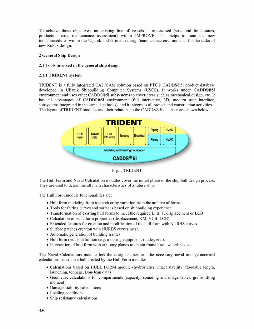
436

To achieve these objectives, an existing line of vessels is re-assessed (structural limit states, production cost, maintenance assessment) within IMPROVE. This helps to tune the new tools/procedures within the Uljanik and Grimaldi design/maintenance environments for the tasks of new RoPax design. 2 General Ship Design 2.1 Tools involved in the general ship design 2.1.1 TRIDENT system TRIDENT is a fully integrated CAD/CAM solution based on PTC® CADDS®5i product database developed in Uljanik Shipbuilding Computer Systems (USCS). It works under CADDS®5i environment and uses other CADDS®5i subsystems to cover areas such as mechanical design, etc. It has all advantages of CADDS®5i environment (full interactive, 3D, modern user interface, subsystems integrated in the same data bases), and it integrates all project and construction activities. The layout of TRIDENT modules and their relations to the CADDS®5i database are shown below.

Fig.1: TRIDENT

The Hull Form and Naval Calculation modules cover the initial phase of the ship hull design process. They are used to determine all main characteristics of a future ship. The Hull Form module functionalities are:

• Hull form modeling from a sketch or by variation from the archive of forms • Tools for fairing curves and surfaces based on shipbuilding experience • Transformation of existing hull forms to meet the required L, B, T, displacement or LCB • Calculation of basic form properties (displacement, KM, VCB, LCB) • Extended features for creation and modification of the hull form with NURBS curves • Surface patches creation with NURBS curves mesh • Automatic generation of building frames • Hull form details definition (e.g. mooring equipment, rudder, etc.). • Intersection of hull form with arbitrary planes to obtain frame lines, waterlines, etc.

The Naval Calculations module lets the designers perform the necessary naval and geometrical calculations based on a hull created by the Hull Form module:

• Calculations based on HULL FORM module (hydrostatics, intact stability, floodable length, launching, tonnage, Bon-Jean data)

• Geometric calculations for compartments (capacity, sounding and ullage tables, grainshifting moment)

• Damage stability calculations • Loading conditions • Ship resistance calculations

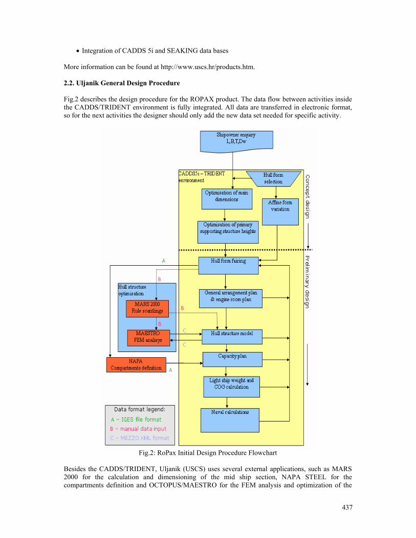
437

• Integration of CADDS 5i and SEAKING data bases More information can be found at http://www.uscs.hr/products.htm. 2.2. Uljanik General Design Procedure Fig.2 describes the design procedure for the ROPAX product. The data flow between activities inside the CADDS/TRIDENT environment is fully integrated. All data are transferred in electronic format, so for the next activities the designer should only add the new data set needed for specific activity.

Fig.2: RoPax Initial Design Procedure Flowchart

Besides the CADDS/TRIDENT, Uljanik (USCS) uses several external applications, such as MARS 2000 for the calculation and dimensioning of the mid ship section, NAPA STEEL for the compartments definition and OCTOPUS/MAESTRO for the FEM analysis and optimization of the

438

hull structure. Diagram description:

• The design process starts with the ship owner enquiry, which defines the main ship parameters, from dimensions, capacity, range of navigation, maximum speed etc.

• From the database of existing hull forms, the appropriate form is chosen. Based on it, the calculation and optimization of the ship’s main dimensions are performed. The processing is done with a program module inside the CADDS/TRIDENT environment, which calculates the needed power of the main engine and the estimated speed, taking into account the given range of parameters. Based on these results, a narrower range is selected and its metacentric height is estimated, which leads to the most appropriate final solution.

• According to the selected dimensions and given loads, the transverse strength primary elements are dimensioned in order to get the minimum ship height up to the strength deck.

• The affine form variation and hull fairing of the selected form is performed (inside the CADDS/TRIDENT environment), and it is the base for all following activities. Each change in the hull form implies the repetition and redefinition of the following activities.

• The General Arrangement plan and the Engine room arrangement plan are generated (inside the CADDS/TRIDENT environment).

• The mid ship section is defined and dimensioned according to the Classification society requirements using the program MARS 2000.

• The dimensions calculated with MARS can be analyzed and optimized with FEM tools (OCTOPUS/MAESTRO), but the rough 3D model of the ship structure has to be generated in order to have the correct data for the Centre of gravity and the Light ship weight. (CADDS/TRIDENT environment).

• The compartment definition can be done either by using NAPA software or by modules inside the CADDS/TRIDENT environment. Data concerning the hull form are transferred to NAPA via IGES format, and the same format is used to transfer data about the compartments to TRIDENT. Some post processing of transferred data is needed (e.g. control of data and, in certain cases, some manual correction).

• All the performed naval calculations are based on the Capacity plan, the Damage waterlines calculation being the most relevant for ROPAX product.

2.3 General concept design of ROPAX The design methodology in the IMPROVE project defines three design levels:

1. STANDARD SHIP is the existing ship or Yard prototype 2. NEW SHIP will be designed during the first period of the project. The design will be realized

using mainly the existing methodology and will include improvements to the main dimensions, general arrangement, hydrodynamics and propulsion

3. IMPROVE PROJECT SHIP will be obtained from Level 2 design using multicriterial structural optimization including the production and maintenance models

The project of RoPax, recently analyzed by Uljanik, will be considered as standard ship, Fig.3. The main characteristics of this ship are:

• Main dimensions: Length overall – 193 + 4 m, Breadth – 29.8 m, Draft design – 7.5 m • Trial speed – 24.5 knots • Cargo capacities – Trailers 3000 lane meters + 300 cars • Capacities: HFO – 1400 m3, DO – 250 t, FW – 1200 m3, SW – 600 m3 • Passengers: 350 cabins + 200 aircraft seats • Crew 200 persons

This design was developed in cooperation with Siemens Schottel and Sea Trade from Oslo. The designed ship was propelled by two pods behind two skegs. The main dimensions of ROPAX concept design are optimized using TRIDENT/SEAKING software (USCS software, http://www.uscs.hr) in order to obtain minimal main engine power and sufficient stability. A new application was developed,

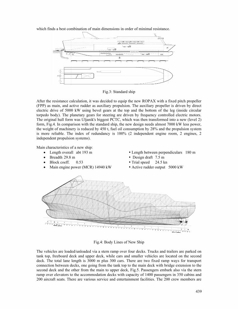
439

which finds a best combination of main dimensions in order of minimal resistance.

Fig.3: Standard ship After the resistance calculation, it was decided to equip the new ROPAX with a fixed pitch propeller (FPP) as main, and active rudder as auxiliary propulsion. The auxiliary propeller is driven by direct electric drive of 5000 kW using bevel gears at the top and the bottom of the leg (inside circular torpedo body). The planetary gears for steering are driven by frequency controlled electric motors. The original hull form was Uljanik's biggest PCTC, which was then transformed into a new (level 2) form, Fig.4. In comparison with the standard ship, the new design needs almost 7000 kW less power, the weight of machinery is reduced by 450 t, fuel oil consumption by 28% and the propulsion system is more reliable. The index of redundancy is 100% (2 independent engine room, 2 engines, 2 independent propulsion systems). Main characteristics of a new ship:

• Length overall abt 193 m Length between perpendiculars 180 m • Breadth 29.8 m Design draft 7.5 m • Block coeff. 0.53 Trial speed 24.5 kn • Main engine power (MCR) 14940 kW Active rudder output 5000 kW

Fig.4: Body Lines of New Ship The vehicles are loaded/unloaded via a stern ramp over four decks. Trucks and trailers are parked on tank top, freeboard deck and upper deck, while cars and smaller vehicles are located on the second deck. The total lane length is 3000 m plus 300 cars. There are two fixed ramp ways for transport connection between decks, one going from the tank top to the main deck with bridge extension to the second deck and the other from the main to upper deck, Fig.5. Passengers embark also via the stern ramp over elevators to the accommodation decks with capacity of 1400 passengers in 350 cabins and 200 aircraft seats. There are various service and entertainment facilities. The 200 crew members are

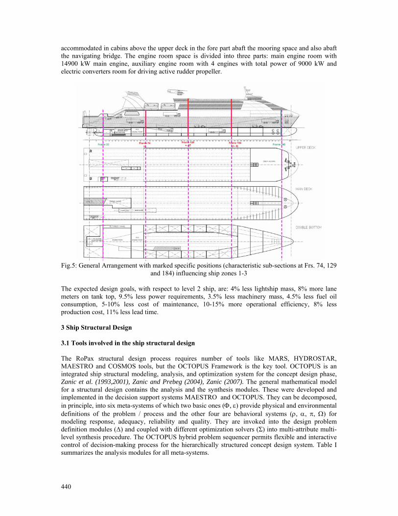
440

accommodated in cabins above the upper deck in the fore part abaft the mooring space and also abaft the navigating bridge. The engine room space is divided into three parts: main engine room with 14900 kW main engine, auxiliary engine room with 4 engines with total power of 9000 kW and electric converters room for driving active rudder propeller.

Fig.5: General Arrangement with marked specific positions (characteristic sub-sections at Frs. 74, 129

and 184) influencing ship zones 1-3 The expected design goals, with respect to level 2 ship, are: 4% less lightship mass, 8% more lane meters on tank top, 9.5% less power requirements, 3.5% less machinery mass, 4.5% less fuel oil consumption, 5-10% less cost of maintenance, 10-15% more operational efficiency, 8% less production cost, 11% less lead time. 3 Ship Structural Design 3.1 Tools involved in the ship structural design The RoPax structural design process requires number of tools like MARS, HYDROSTAR, MAESTRO and COSMOS tools, but the OCTOPUS Framework is the key tool. OCTOPUS is an integrated ship structural modeling, analysis, and optimization system for the concept design phase, Zanic et al. (1993,2001), Zanic and Prebeg (2004), Zanic (2007). The general mathematical model for a structural design contains the analysis and the synthesis modules. These were developed and implemented in the decision support systems MAESTRO and OCTOPUS. They can be decomposed, in principle, into six meta-systems of which two basic ones (Φ, ε) provide physical and environmental definitions of the problem / process and the other four are behavioral systems (ρ, α, π, Ω) for modeling response, adequacy, reliability and quality. They are invoked into the design problem definition modules (Δ) and coupled with different optimization solvers (Σ) into multi-attribute multi-level synthesis procedure. The OCTOPUS hybrid problem sequencer permits flexible and interactive control of decision-making process for the hierarchically structured concept design system. Table I summarizes the analysis modules for all meta-systems.

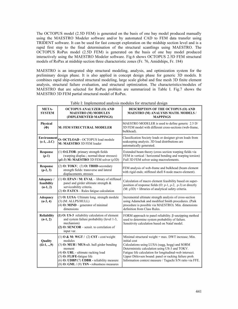
441

The OCTOPUS model (2.5D FEM) is generated on the basis of one bay model produced manually using the MAESTRO Modeler software and/or by automated CAD to FEM data transfer using TRIDENT software. It can be used for fast concept exploration on the midship section level and is a rapid first step to the final determination of the structural scantlings using MAESTRO. The OCTOPUS RoPax model (2.5D FEM) is generated on the basis of one bay model produced interactively using the MAESTRO Modeler software. Fig.6 shows OCTOPUS 2.5D FEM structural models of RoPax at midship section three characteristic zones (Fr. 76, Amidships, Fr. 184) MAESTRO is an integrated ship structural modeling, analysis, and optimization system for the preliminary design phase. It is also applied in concept design phase for generic 3D models. It combines rapid ship-oriented structural modeling, large scale global and fine mesh 3D finite element analysis, structural failure evaluation, and structural optimization. The characteristics/modules of MAESTRO that are selected for RoPax problem are summarized in Table I. Fig.7 shows the MAESTRO 3D FEM partial structural model of RoPax.

Table I: Implemented analysis modules for structural design META-

SYSTEM OCTOPUS ANALYZER (O) AND

MAESTRO (M) MODULES (IMPLEMENTED MAPPINGS)

DESCRIPTION OF THE OCTOPUS (O) AND MAESTRO (M) ANALYSIS MATH. MODELS /

MAPPINGS

Physical (Φ) M: FEM STRUCTURAL MODELER

MAESTRO MODELER is used to define generic 2.5 D/ 3D FEM model with different cross-sections (web-frame, bulkhead).

Environment (ε-1, ..LC) O: OCTLOAD - OCTOPUS load module

M: MAESTRO 3D FEM loader

Classification Society loads or designer given loads from seakeeping analysis. 3D load distributions are automatically generated.

Response (ρ-1)

(1) O:LTOR- primary strength fields (warping displac.; normal/shear stresses)

(ρ1-3) M: MAESTRO 3D FEM solver (ρ3D)

Extended beam theory (cross section warping fields via FEM in vertical / horizontal bending and warping torsion) Full 3D FEM solver using macroelements.

Response (ρ-2, 3)

(2) O: TOKV; (3) O: TBHD-secondary strength fields: transverse and lateral displacements; stresses

FEM analysis of web-frame and bulkhead (beam element with rigid ends; stiffened shell 8-node macro-element).

Adequacy / feasibility (α-1, 2)

(1) O: EPAN / M: EVAL – library of stiffened panel and girder ultimate strength & serviceability criteria.

(2) O: FATCS – Rules fatigue calculation

Calculation of macro element feasibility based on super-position of response fields (O: ρ-1, ρ-2, ρ-3) or directly (M: ρ3D) + libraries of analytical safety criteria.

Adequacy (α-3, 4)

(3) O: LUSA–Ultimate long. strength module (3) (M: ALLPS/HULL) (4) O: MIND – generator of minimal

dimensions

Incremental ultimate strength analysis of cross-section using Adamchak and modified Smith procedures. (Paik procedure is possible via MAESTRO). Min. dimensions definition from Class Rules.

Reliability (π-1, 2)

(1) O: US-3 reliability calculation of element and system failure probability (level 1-3, mechanism)

(2) O: SENCOR – sensit. to correlation of input var.

FORM approach to panel reliability. β-unzipping method used to determine system probability of failure. Sensitivity calculation based on Nataf model.

Quality

(Ω-1, ..,9)

(1) O & M: WGT / (2) CST - cost/weight modules

(3) O: MUH / MUS-ult. hull girder bending moment

(4) O: URL - ultimate racking load (5) O: FLIFE-fatigue life (6) O: UDBP/(7) UDBR - reliability measure (8) O: GML / (9) TSN - robustness measures

Minimal structural weight = max. DWT increase; Min. initial cost Calculations using LUSA (sagg, hogg) and SORM Deterministic calculation using US-3 and TOKV. Fatigue life calculation for longitudinal-web intersect. Upper Ditlevsen bound: panel or racking failure prob. Information context measure / Taguchi S/N ratio via FFE.

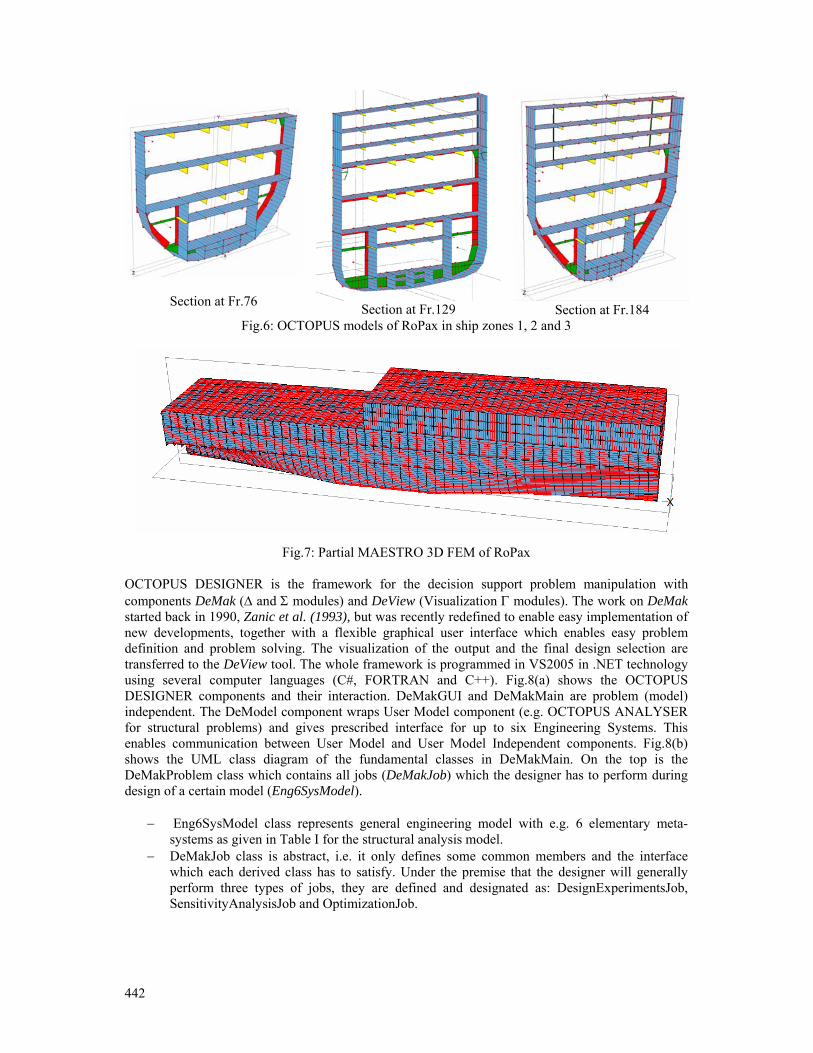
442

Section at Fr.76 Section at Fr.129

Section at Fr.184

Fig.6: OCTOPUS models of RoPax in ship zones 1, 2 and 3

Fig.7: Partial MAESTRO 3D FEM of RoPax OCTOPUS DESIGNER is the framework for the decision support problem manipulation with components DeMak (Δ and Σ modules) and DeView (Visualization Γ modules). The work on DeMak started back in 1990, Zanic et al. (1993), but was recently redefined to enable easy implementation of new developments, together with a flexible graphical user interface which enables easy problem definition and problem solving. The visualization of the output and the final design selection are transferred to the DeView tool. The whole framework is programmed in VS2005 in .NET technology using several computer languages (C#, FORTRAN and C++). Fig.8(a) shows the OCTOPUS DESIGNER components and their interaction. DeMakGUI and DeMakMain are problem (model) independent. The DeModel component wraps User Model component (e.g. OCTOPUS ANALYSER for structural problems) and gives prescribed interface for up to six Engineering Systems. This enables communication between User Model and User Model Independent components. Fig.8(b) shows the UML class diagram of the fundamental classes in DeMakMain. On the top is the DeMakProblem class which contains all jobs (DeMakJob) which the designer has to perform during design of a certain model (Eng6SysModel).

− Eng6SysModel class represents general engineering model with e.g. 6 elementary meta-systems as given in Table I for the structural analysis model.

− DeMakJob class is abstract, i.e. it only defines some common members and the interface which each derived class has to satisfy. Under the premise that the designer will generally perform three types of jobs, they are defined and designated as: DesignExperimentsJob, SensitivityAnalysisJob and OptimizationJob.

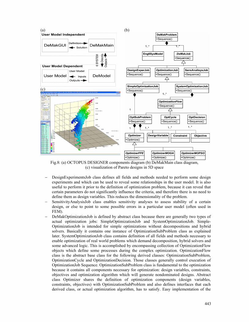
443

(a)

(c)

(b)

Fig.8: (a) OCTOPUS DESIGNER components diagram (b) DeMakMain class diagram, (c) visualization of Pareto designs in 5D space

− DesignExperimentsJob class defines all fields and methods needed to perform some design

experiments and which can be used to reveal some relationships in the user model. It is also useful to perform it prior to the definition of optimization problem, because it can reveal that certain parameters do not significantly influence the criteria, and therefore there is no need to define them as design variables. This reduces the dimensionality of the problem.

− SensitivityAnalysisJob class enables sensitivity analyses to assess stability of a certain design, or else to point to some possible errors in a particular user model (often used in FEM).

− DeMakOptimizationJob is defined by abstract class because there are generally two types of actual optimization jobs: SimpleOptimizationJob and SystemOptimizationJob. Simple-OptimizationJob is intended for simple optimizations without decompositions and hybrid solvers. Basically it contains one instance of OptimizationSubProblem class as explained later. SystemOptimizationJob class contains definition of all fields and methods necessary to enable optimization of real world problems which demand decomposition, hybrid solvers and some advanced logic. This is accomplished by encompassing collection of OptimizationFlow objects which define some processes during the complex optimization. OptimizationFlow class is the abstract base class for the following derived classes: OptimizationSubProblem, OptimizationCycle and OptimizationDecision. Those classes generally control execution of OptimizationJob Sequence. OptimizationSubProblem class is fundamental to the optimization because it contains all components necessary for optimization: design variables, constraints, objectives and optimization algorithm which will generate nondominated designs. Abstract class Optimizer shares the definition of optimization components (design variables, constraints, objectives) with OptimizationSubProblem and also defines interfaces that each derived class, or actual optimization algorithm, has to satisfy. Easy implementation of the

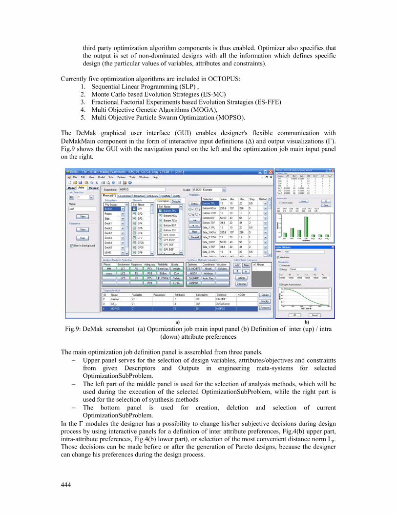
444

third party optimization algorithm components is thus enabled. Optimizer also specifies that the output is set of non-dominated designs with all the information which defines specific design (the particular values of variables, attributes and constraints).

Currently five optimization algorithms are included in OCTOPUS:

1. Sequential Linear Programming (SLP) , 2. Monte Carlo based Evolution Strategies (ES-MC) 3. Fractional Factorial Experiments based Evolution Strategies (ES-FFE) 4. Multi Objective Genetic Algorithms (MOGA), 5. Multi Objective Particle Swarm Optimization (MOPSO).

The DeMak graphical user interface (GUI) enables designer's flexible communication with DeMakMain component in the form of interactive input definitions (Δ) and output visualizations (Γ). Fig.9 shows the GUI with the navigation panel on the left and the optimization job main input panel on the right.

Fig.9: DeMak screenshot (a) Optimization job main input panel (b) Definition of inter (up) / intra

(down) attribute preferences The main optimization job definition panel is assembled from three panels.

− Upper panel serves for the selection of design variables, attributes/objectives and constraints from given Descriptors and Outputs in engineering meta-systems for selected OptimizationSubProblem.

− The left part of the middle panel is used for the selection of analysis methods, which will be used during the execution of the selected OptimizationSubProblem, while the right part is used for the selection of synthesis methods.

− The bottom panel is used for creation, deletion and selection of current OptimizationSubProblem.

In the Γ modules the designer has a possibility to change his/her subjective decisions during design process by using interactive panels for a definition of inter attribute preferences, Fig.4(b) upper part, intra-attribute preferences, Fig.4(b) lower part), or selection of the most convenient distance norm Lp. Those decisions can be made before or after the generation of Pareto designs, because the designer can change his preferences during the design process.

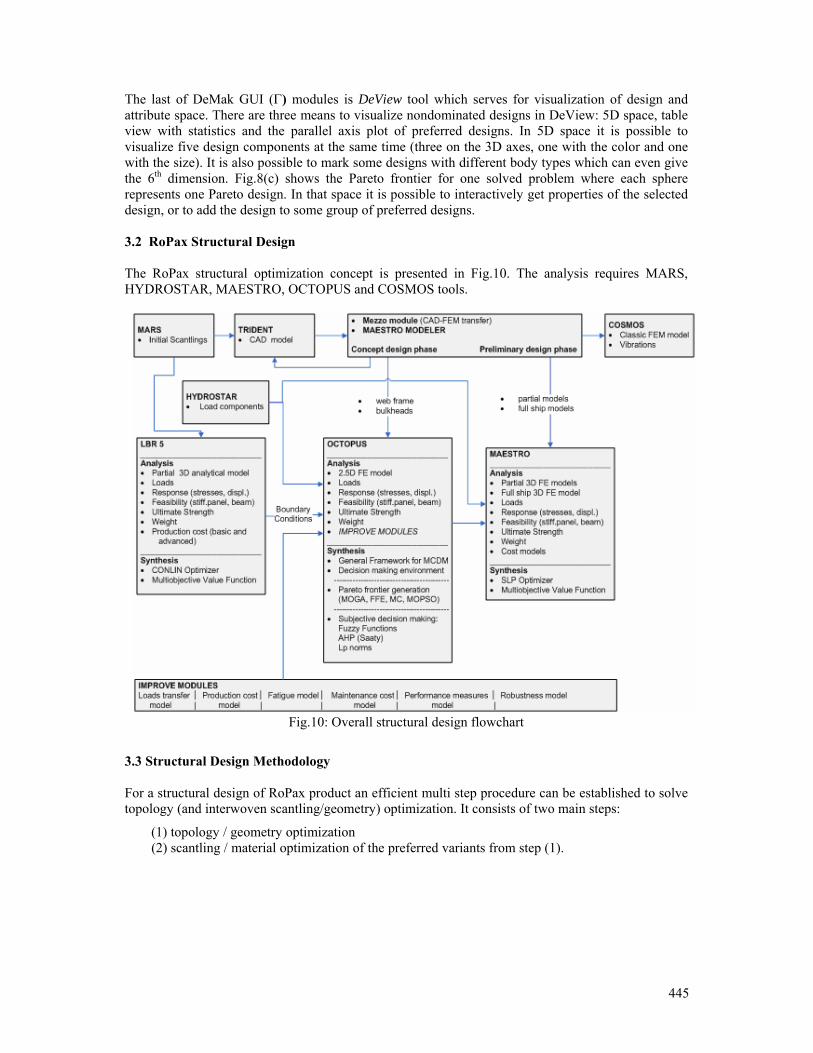
445

The last of DeMak GUI (Γ) modules is DeView tool which serves for visualization of design and attribute space. There are three means to visualize nondominated designs in DeView: 5D space, table view with statistics and the parallel axis plot of preferred designs. In 5D space it is possible to visualize five design components at the same time (three on the 3D axes, one with the color and one with the size). It is also possible to mark some designs with different body types which can even give the 6th dimension. Fig.8(c) shows the Pareto frontier for one solved problem where each sphere represents one Pareto design. In that space it is possible to interactively get properties of the selected design, or to add the design to some group of preferred designs. 3.2 RoPax Structural Design The RoPax structural optimization concept is presented in Fig.10. The analysis requires MARS, HYDROSTAR, MAESTRO, OCTOPUS and COSMOS tools.

Fig.10: Overall structural design flowchart

3.3 Structural Design Methodology For a structural design of RoPax product an efficient multi step procedure can be established to solve topology (and interwoven scantling/geometry) optimization. It consists of two main steps:

(1) topology / geometry optimization (2) scantling / material optimization of the preferred variants from step (1).

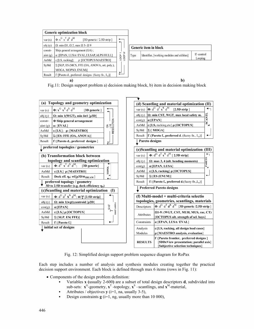
446

a) b)

Fig.11: Design support problem a) decision making block, b) item in decision making block

Fig. 12: Simplified design support problem sequence diagram for RoPax Each step includes a number of analysis and synthesis modules creating together the practical decision support environment. Each block is defined through max 6 items (rows in Fig. 11):

• Components of the design problem definition: Variables x (usually 2-600) are a subset of total design descriptors d, subdivided into

sub-sets: xG-geometry, xT -topology, xS –scantlings, and xM-material, Attributes / objectives y (i=1, na, usually 3-5), Design constraints g (i=1, ng, usually more than 10 000),

447

• Analysis modules (AnMd), described in more detail in Table I, • Synthesis modules (SyMd), • Achieved results.

Each item contains, Fig.11:

• Meta system identifier (e.g. Φ, Ω,.) and relevant parameters, • Applied modules denoted with brackets [ ], • If- control blocks, • Loops of the design procedure.

Fig.12 shows the complete procedure through interconnected optimization blocks (a)-(f). Step (1) of the concept design procedure for the multi-deck ships (containing topology and geometry optimization) is presented in the block (a) with the items used in the transformation block (b) is used as interface in the topology and scantlings optimization models. Step (2) of the concept design procedure containing scantling and material optimization is presented in the blocks (c) to (e). Requirement on all of those blocks is computational efficiency for e.g. reliability or ultimate strength nonlinear calculations. Step (2) is divided into three phases:

• Phase I is used for fast MODM exploration of the design space and educated generation of the initial population for Phase II.

• Phase II is the extensive scantling optimization with reduced analysis block. • Phase III is the complete analysis of the reduced number of the preferred Pareto de-signs

generated in Phase II.

Block (f) enables full application of the Decision Support Problem environment by the structural designer, Fig.12(a). The full analysis potentials of OCTOPUS and MAESTRO are applied. Subjective reasoning is performed through DeView modules and preference formulations in selection of the final design, Fig.12(b). 6. Conclusions The first part of the paper presented the RoPax general ship design procedure preformed at Uljanik shipyard (naval architecture calculations: speed, power, damage stability, etc.). Computer programs were developed to facilitate selection of main ship parameters from the aspect of resistance, stability and operability. The selected design variants were compared, including large savings through a novel propulsion concept. The second part of the paper has presented the design methodology necessary to perform extensive multi-objective structural optimization of RoPax structure at the early design stage using the OCTOPUS-MAESTRO software. Acknowledgments

Thanks are due to the support of the EU Commission for FP6 Project IMPROVE, Croatian Ministry of Science, Education and Sport: projects 0120-014 and TP-02/0120-23 and to all members of the IMPROVE team.

448

References

RIGO, P. ; DUNDARA, D.; GUILLAUME-COMBECAVE, J.L.; KARCZEWICZ, A.; KLANAC, A.; ROLAND, F.; TURAN, O.; ZANIC, V.; AMRANE, A.; CONSTANTINESCU, A. (2008), IMPROVE - Design of improved and competitive products using an integrated decision support system for ship production and operation, 7th Conf. Computer and IT Applications in the Maritime Industries (COMPIT), Liege, pp.92-106 ZANIC, V. (2007), Concept and preliminary structural design methods for the modern multi-deck ships, 2nd Int. Conf. on Marine Research and Transportation, Naples, Italy ZANIC, V.; DAS, P.K.; PU, Y.; FAULKNER, D. (1993), Multiple criteria synthesis techniques applied to reliability based design of SWATH ship structure, Integrity of Offshore Structures 5, Glasgow, pp.387-415 ZANIC, V.; JANCIJEV, T.; TRINCAS, G.; NABERGOJ, R.; ANDRIC, J. (2001), Structural design methodology for large roro/passenger ships, J. Ship and Ocean Technology 5/1, pp.14-29 ZANIC, V.; PREBEG, P. (2004), Primary response assessment method for concept design of monotonous thin-walled structures, 4th Int. Conf. on Advanced Engineering Design, Glasgow ZANIC, V.; SPONZA, D.; DUNDARA , D.; JANCIJEV, T.; ANDRIC, J.; FRANK, D.; BRALIC, S. (2001), Racking analysis of car-truck-carriers, Brodogradnja 49, pp.181-190

Appendix: RoPax Project Requirements A.1 Design Process Requirements/Objectives from Uljanik Shipyard:

Area of navigation: Mediterranean (sea keeping analysis); large variations in season trade (summer 3000 pax, winter 100 pax)

Hull form: Single hull; Superstructure made of steel or composite (no aluminium) Main dimensions: Up to the max. length of slipway: ≈ 230m; max. breadth: 30.40 m Engine selection and propulsion: Two stoke engines; combined propulsion (screw + pods) Life cycle: Goal to minimize the maintenance cost; 25 years life time with probable conversion

after 10 years due to new rules or comfort standards (to be flexible and easy for conversion) Cargo handling: Traditional – stern door and internal ramps Seakeeping: No fin stabilizer but internal active stabilizer tanks

Uljanik's Expectations From Improve Project:

Global goals: Reduced production cost 10 %; reduced fuel oil consumptions 12 %; reduced maintenance cost 10 %; increased lane metres on tank top 8 %

A.2 Owner’s Main Design Requirements/Objectives

• Increase carrying capacity (lane meters) on tank top by decreasing the length of the engine room

• Achieve load carrying flexibility • Improve the vessels’ operational performance and efficiency • Maximize the robustness of the required freight rate • Design for the redundancy and simplicity of systems • Increase ship’s manoeuvrability • Optimize the seakeeping performance for the Mediterranean Sea • Maximize comfort; minimize vibrations

449

A.3 IMPROVE Objectives / Tasks For The RoPax Carrier:

• Main dimensions should be optimised to improve the hydrodynamics • New designs of stern part will be preformed to reduce length of the engine room and to

increase cargo area (lane meters) on tank top • Selection of slow speed main engine to improve maintenance and consumption • Minimum height of deck transverses • Improvement in design using existing and improved tools for early design phase : • Rule calculation – simplified CAD model → simplified model (FEM, LBR5) → optimisation • Minimum weight of freeboard deck transverses • Minimum height of deck No3 and deck No4 transverses • Accurate calculation at the early design stage of building tolerances and deformation

constraints • Superstructure decks effectiveness in the longitudinal strength to be considered • Web frame spacing and longitudinals spacing, to be optimized • Sea keeping and manoeuvrability • Vibration of aft part • Fatigue analysis

Objectives for Production:

• Reduce production costs (production simulation) • Reduce the number of different parts (standardization) • Simplify production through the increase of subassembly work • Reduce handling and assembly operation on slipway or block assembly area • Reduce hull erection time on berth from 18 to 9 weeks (+3 for finishing) • Reduce number of erection blocks from 330 blocks (valid for the big car carriers) to 130 blocks

– the design should be performed accordingly to that • Reach an average of 2.8 erected blocks per day • Paint all the parts before erection

Structural Design Objectives:

• Maximize structural safety by means of maximizing global and local safety measures and maximizing structural robustness;

Operation, Maintenance and Repair Objectives:

• Minimize the lifecycle cost of the ship (major goal for Grimaldi) by minimizing the probability of potential repairs in the service time and by maximizing the maintainability of the ship.

Main Design Constraints:

• No pillars in cargo space; • Satisfy Bureau Veritas and IMO rules.

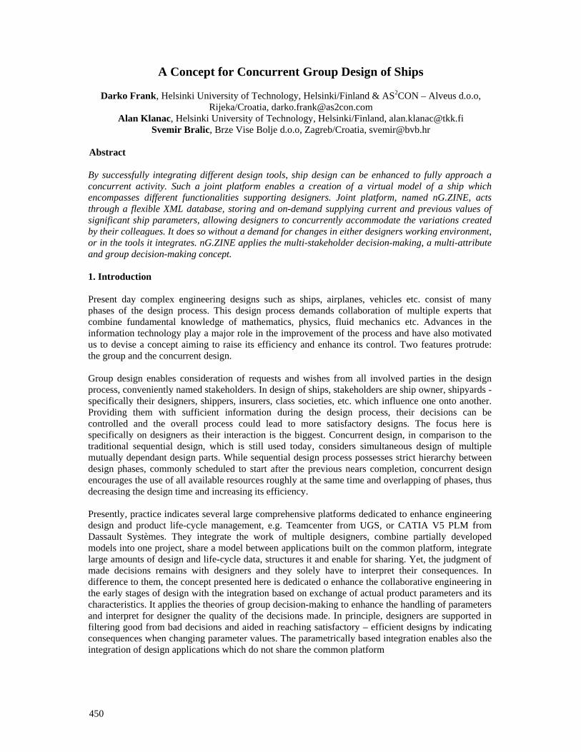
450

A Concept for Concurrent Group Design of Ships

Darko Frank, Helsinki University of Technology, Helsinki/Finland & AS2CON – Alveus d.o.o, Rijeka/Croatia, darko.frank@as2con.com

Alan Klanac, Helsinki University of Technology, Helsinki/Finland, alan.klanac@tkk.fi Svemir Bralic, Brze Vise Bolje d.o.o, Zagreb/Croatia, svemir@bvb.hr

Abstract

By successfully integrating different design tools, ship design can be enhanced to fully approach a concurrent activity. Such a joint platform enables a creation of a virtual model of a ship which encompasses different functionalities supporting designers. Joint platform, named nG.ZINE, acts through a flexible XML database, storing and on-demand supplying current and previous values of significant ship parameters, allowing designers to concurrently accommodate the variations created by their colleagues. It does so without a demand for changes in either designers working environment, or in the tools it integrates. nG.ZINE applies the multi-stakeholder decision-making, a multi-attribute and group decision-making concept. 1. Introduction Present day complex engineering designs such as ships, airplanes, vehicles etc. consist of many phases of the design process. This design process demands collaboration of multiple experts that combine fundamental knowledge of mathematics, physics, fluid mechanics etc. Advances in the information technology play a major role in the improvement of the process and have also motivated us to devise a concept aiming to raise its efficiency and enhance its control. Two features protrude: the group and the concurrent design. Group design enables consideration of requests and wishes from all involved parties in the design process, conveniently named stakeholders. In design of ships, stakeholders are ship owner, shipyards - specifically their designers, shippers, insurers, class societies, etc. which influence one onto another. Providing them with sufficient information during the design process, their decisions can be controlled and the overall process could lead to more satisfactory designs. The focus here is specifically on designers as their interaction is the biggest. Concurrent design, in comparison to the traditional sequential design, which is still used today, considers simultaneous design of multiple mutually dependant design parts. While sequential design process possesses strict hierarchy between design phases, commonly scheduled to start after the previous nears completion, concurrent design encourages the use of all available resources roughly at the same time and overlapping of phases, thus decreasing the design time and increasing its efficiency. Presently, practice indicates several large comprehensive platforms dedicated to enhance engineering design and product life-cycle management, e.g. Teamcenter from UGS, or CATIA V5 PLM from Dassault Systèmes. They integrate the work of multiple designers, combine partially developed models into one project, share a model between applications built on the common platform, integrate large amounts of design and life-cycle data, structures it and enable for sharing. Yet, the judgment of made decisions remains with designers and they solely have to interpret their consequences. In difference to them, the concept presented here is dedicated o enhance the collaborative engineering in the early stages of design with the integration based on exchange of actual product parameters and its characteristics. It applies the theories of group decision-making to enhance the handling of parameters and interpret for designer the quality of the decisions made. In principle, designers are supported in filtering good from bad decisions and aided in reaching satisfactory – efficient designs by indicating consequences when changing parameter values. The parametrically based integration enables also the integration of design applications which do not share the common platform

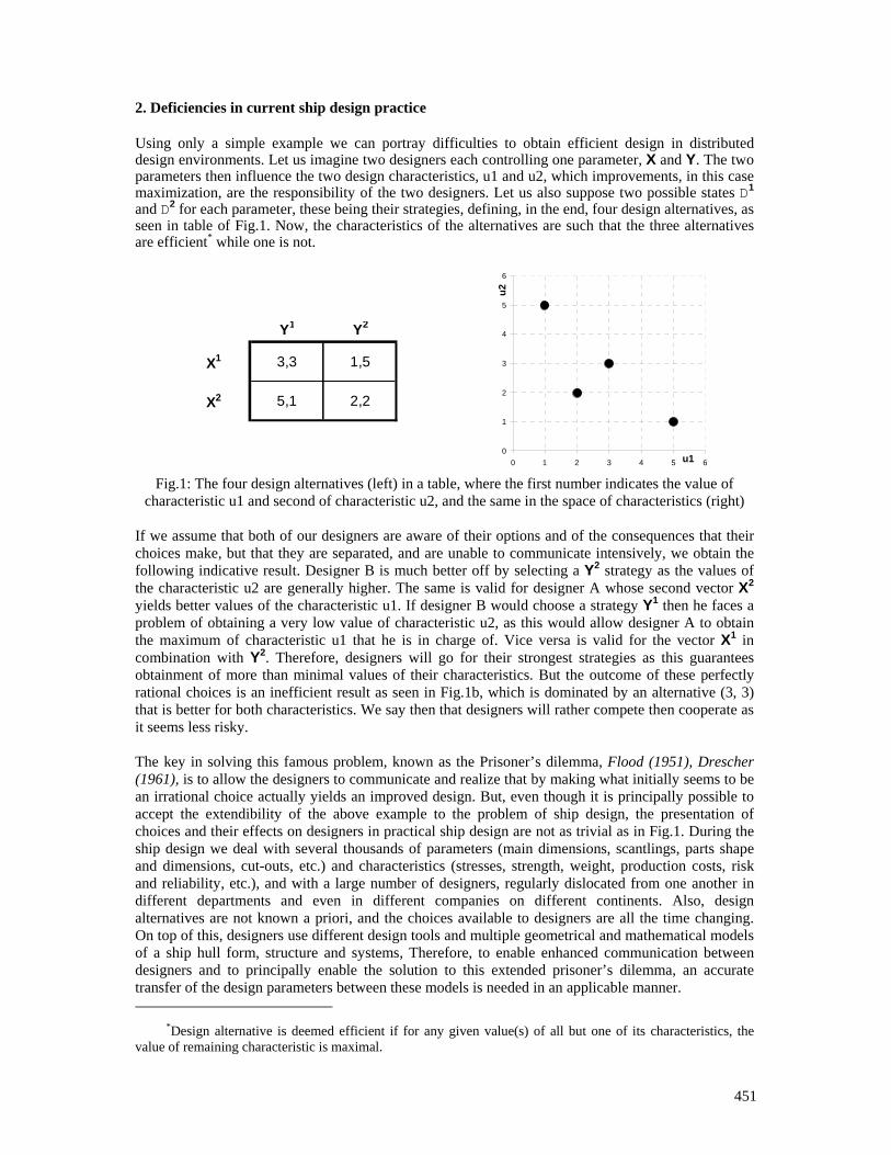
451

2. Deficiencies in current ship design practice Using only a simple example we can portray difficulties to obtain efficient design in distributed design environments. Let us imagine two designers each controlling one parameter, X and Y. The two parameters then influence the two design characteristics, u1 and u2, which improvements, in this case maximization, are the responsibility of the two designers. Let us also suppose two possible states D1 and D2 for each parameter, these being their strategies, defining, in the end, four design alternatives, as seen in table of Fig.1. Now, the characteristics of the alternatives are such that the three alternatives are efficient* while one is not.

Y1 Y2

X1 3,3 1,5

X2 5,1 2,2

0

1

2

3

4

5

6

0 1 2 3 4 5 6u1

u2

Fig.1: The four design alternatives (left) in a table, where the first number indicates the value of

characteristic u1 and second of characteristic u2, and the same in the space of characteristics (right) If we assume that both of our designers are aware of their options and of the consequences that their choices make, but that they are separated, and are unable to communicate intensively, we obtain the following indicative result. Designer B is much better off by selecting a Y2 strategy as the values of the characteristic u2 are generally higher. The same is valid for designer A whose second vector X2 yields better values of the characteristic u1. If designer B would choose a strategy Y1 then he faces a problem of obtaining a very low value of characteristic u2, as this would allow designer A to obtain the maximum of characteristic u1 that he is in charge of. Vice versa is valid for the vector X1 in combination with Y2. Therefore, designers will go for their strongest strategies as this guarantees obtainment of more than minimal values of their characteristics. But the outcome of these perfectly rational choices is an inefficient result as seen in Fig.1b, which is dominated by an alternative (3, 3) that is better for both characteristics. We say then that designers will rather compete then cooperate as it seems less risky. The key in solving this famous problem, known as the Prisoner’s dilemma, Flood (1951), Drescher (1961), is to allow the designers to communicate and realize that by making what initially seems to be an irrational choice actually yields an improved design. But, even though it is principally possible to accept the extendibility of the above example to the problem of ship design, the presentation of choices and their effects on designers in practical ship design are not as trivial as in Fig.1. During the ship design we deal with several thousands of parameters (main dimensions, scantlings, parts shape and dimensions, cut-outs, etc.) and characteristics (stresses, strength, weight, production costs, risk and reliability, etc.), and with a large number of designers, regularly dislocated from one another in different departments and even in different companies on different continents. Also, design alternatives are not known a priori, and the choices available to designers are all the time changing. On top of this, designers use different design tools and multiple geometrical and mathematical models of a ship hull form, structure and systems, Therefore, to enable enhanced communication between designers and to principally enable the solution to this extended prisoner’s dilemma, an accurate transfer of the design parameters between these models is needed in an applicable manner.

*Design alternative is deemed efficient if for any given value(s) of all but one of its characteristics, the value of remaining characteristic is maximal.

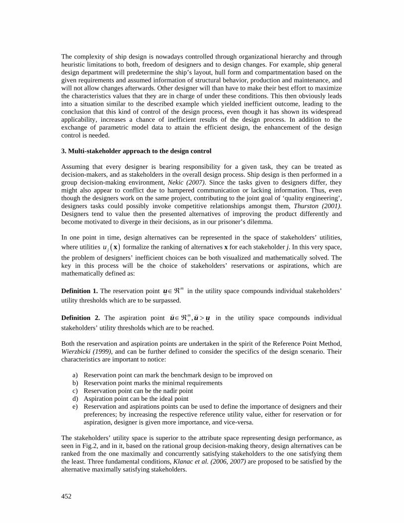
452

The complexity of ship design is nowadays controlled through organizational hierarchy and through heuristic limitations to both, freedom of designers and to design changes. For example, ship general design department will predetermine the ship’s layout, hull form and compartmentation based on the given requirements and assumed information of structural behavior, production and maintenance, and will not allow changes afterwards. Other designer will than have to make their best effort to maximize the characteristics values that they are in charge of under these conditions. This then obviously leads into a situation similar to the described example which yielded inefficient outcome, leading to the conclusion that this kind of control of the design process, even though it has shown its widespread applicability, increases a chance of inefficient results of the design process. In addition to the exchange of parametric model data to attain the efficient design, the enhancement of the design control is needed. 3. Multi-stakeholder approach to the design control Assuming that every designer is bearing responsibility for a given task, they can be treated as decision-makers, and as stakeholders in the overall design process. Ship design is then performed in a group decision-making environment, Nekic (2007). Since the tasks given to designers differ, they might also appear to conflict due to hampered communication or lacking information. Thus, even though the designers work on the same project, contributing to the joint goal of ‘quality engineering’, designers tasks could possibly invoke competitive relationships amongst them, Thurston (2001). Designers tend to value then the presented alternatives of improving the product differently and become motivated to diverge in their decisions, as in our prisoner’s dilemma. In one point in time, design alternatives can be represented in the space of stakeholders’ utilities, where utilities ( )ju x formalize the ranking of alternatives x for each stakeholder j. In this very space, the problem of designers’ inefficient choices can be both visualized and mathematically solved. The key in this process will be the choice of stakeholders’ reservations or aspirations, which are mathematically defined as: Definition 1. The reservation point m∈ℜ(u in the utility space compounds individual stakeholders’ utility thresholds which are to be surpassed. Definition 2. The aspiration point ,m

+∈ℜ >( ((u u u in the utility space compounds individual

stakeholders’ utility thresholds which are to be reached. Both the reservation and aspiration points are undertaken in the spirit of the Reference Point Method, Wierzbicki (1999), and can be further defined to consider the specifics of the design scenario. Their characteristics are important to notice:

a) Reservation point can mark the benchmark design to be improved on b) Reservation point marks the minimal requirements c) Reservation point can be the nadir point d) Aspiration point can be the ideal point e) Reservation and aspirations points can be used to define the importance of designers and their

preferences; by increasing the respective reference utility value, either for reservation or for aspiration, designer is given more importance, and vice-versa.

The stakeholders’ utility space is superior to the attribute space representing design performance, as seen in Fig.2, and in it, based on the rational group decision-making theory, design alternatives can be ranked from the one maximally and concurrently satisfying stakeholders to the one satisfying them the least. Three fundamental conditions, Klanac et al. (2006, 2007) are proposed to be satisfied by the alternative maximally satisfying stakeholders.

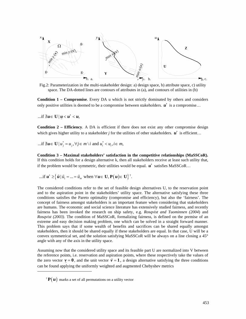
453

y 2

y 1

x2

x1

u2

u1

g1

g2

g3

XΩ

Y

min y 1(x

) min y 2(x)

max

u1(x

)

max u2(x)Z

U

a. b. c. Fig.2: Parameterization in the multi-stakeholder design: a) design space, b) attribute space, c) utility

space. The DA-dotted lines are contours of attributes in (a), and contours of utilities in (b)

Condition 1 – Compromise. Every DA u which is not strictly dominated by others and considers only positive utilities is deemed to be a compromise between stakeholders. ∗u is a compromise… ...if | ,∗∃ ∈ < </ U (u u u u Condition 2 – Efficiency. A DA is efficient if there does not exist any other compromise design which gives higher utility to a stakeholder j for the utilities of other stakeholders. ∗u is efficient…

* *...if | , \ and , ,j j i iu u j m i u u i m∃ ∈ = ∀ ∈ < ∈/ Uu Condition 3 – Maximal stakeholders’ satisfaction in the competitive relationships (MaSSCoR). If this condition holds for a design alternative k, then all stakeholders receive at least such utility that, if the problem would be symmetric, their utilities would be equal. ∗u satisfies MaSSCoR…

( ) 1 ...if | ... when ,mu u∗ ≥ = = ∀ ∈ ∈U U% % % Pu u u u †. The considered conditions refer to the set of feasible design alternatives U, to the reservation point and to the aspiration point in the stakeholders’ utility space. The alternative satisfying these three conditions satisfies the Pareto optimality (compromise and efficiency), but also the ‘fairness’. The concept of fairness amongst stakeholders is an important feature when considering that stakeholders are humans. The economic and social science literature has extensively studied fairness, and recently fairness has been invoked the research on ship safety, e.g. Rosqvist and Tuominnen (2004) and Rosqvist (2003). The condition of MaSSCoR, formalizing fairness, is defined on the premise of an extreme and easy decision making problem, one which can be solved in a straight forward manner. This problem says that if some wealth of benefits and sacrifices can be shared equally amongst stakeholders, then it should be shared equally if these stakeholders are equal. In that case, U will be a convex symmetrical set, and the solution satisfying MaSSCoR will be always on a line closing a 45° angle with any of the axis in the utility space. Assuming now that the considered utility space and its feasible part U are normalized into V between the reference points, i.e. reservation and aspiration points, where these respectively take the values of the zero vector = 0(v , and the unit vector = 1(v , a design alternative satisfying the three conditions can be found applying the uniformly weighted and augmented Chebyshev metrics

† ( )uP marks a set of all permutations on a utility vector

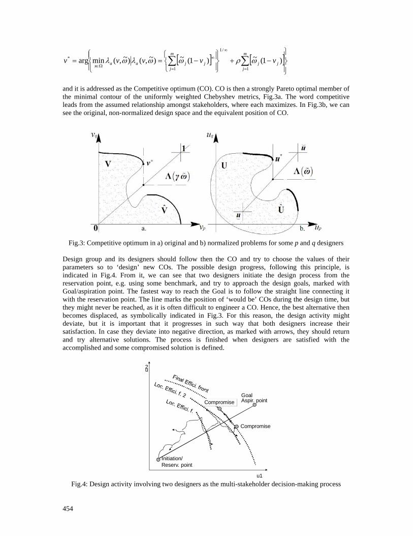
454

[ ] [ ]⎪⎭

⎪⎬⎫

−+⎪⎭

⎪⎬⎫

⎪⎩

⎪⎨⎧

−⎩⎨⎧

== ∑∑=

∞

∞

=Ω∈

)1(~)1(~)~,()~,(minarg1

/1

1

*j

m

jjj

m

jjaax

vvvvv ωρωωλωλ

and it is addressed as the Competitive optimum (CO). CO is then a strongly Pareto optimal member of the minimal contour of the uniformly weighted Chebyshev metrics, Fig.3a. The word competitive leads from the assumed relationship amongst stakeholders, where each maximizes. In Fig.3b, we can see the original, non-normalized design space and the equivalent position of CO.

Fig.3: Competitive optimum in a) original and b) normalized problems for some p and q designers

Design group and its designers should follow then the CO and try to choose the values of their parameters so to ‘design’ new COs. The possible design progress, following this principle, is indicated in Fig.4. From it, we can see that two designers initiate the design process from the reservation point, e.g. using some benchmark, and try to approach the design goals, marked with Goal/aspiration point. The fastest way to reach the Goal is to follow the straight line connecting it with the reservation point. The line marks the position of ‘would be’ COs during the design time, but they might never be reached, as it is often difficult to engineer a CO. Hence, the best alternative then becomes displaced, as symbolically indicated in Fig.3. For this reason, the design activity might deviate, but it is important that it progresses in such way that both designers increase their satisfaction. In case they deviate into negative direction, as marked with arrows, they should return and try alternative solutions. The process is finished when designers are satisfied with the accomplished and some compromised solution is defined.

u1

u2

Initiation/Reserv. point

Compromise

CompromiseGoalAspir. point

Fig.4: Design activity involving two designers as the multi-stakeholder decision-making process

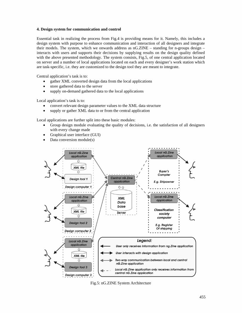
455

4. Design system for communication and control

Essential task in realizing the process from Fig.4 is providing means for it. Namely, this includes a design system with purpose to enhance communication and interaction of all designers and integrate their models. The system, which we onwards address as nG.ZINE – standing for n-groups design – interacts with users and supports their decisions by supplying results on the design quality defined with the above presented methodology. The system consists, Fig.5, of one central application located on server and a number of local applications located on each and every designer’s work station which are task-specific, i.e. they are customized to the design tool they are meant to integrate. Central application’s task is to:

• gather XML converted design data from the local applications • store gathered data to the server • supply on-demand gathered data to the local applications

Local application’s task is to:

• convert relevant design parameter values to the XML data structure • supply or gather XML data to or from the central application

Local applications are further split into these basic modules:

• Group design module evaluating the quality of decisions, i.e. the satisfaction of all designers with every change made

• Graphical user interface (GUI) • Data conversion module(s)

Fig.5: nG.ZINE System Architecture

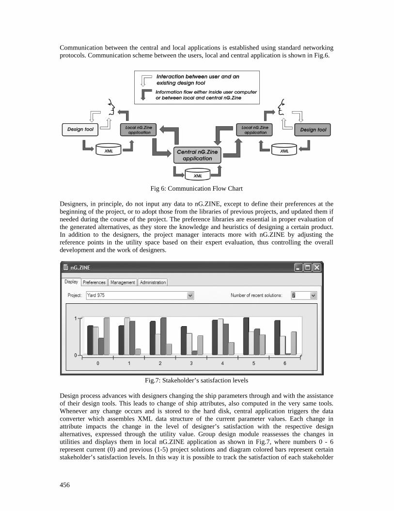
456

Communication between the central and local applications is established using standard networking protocols. Communication scheme between the users, local and central application is shown in Fig.6.

Fig 6: Communication Flow Chart

Designers, in principle, do not input any data to nG.ZINE, except to define their preferences at the beginning of the project, or to adopt those from the libraries of previous projects, and updated them if needed during the course of the project. The preference libraries are essential in proper evaluation of the generated alternatives, as they store the knowledge and heuristics of designing a certain product. In addition to the designers, the project manager interacts more with nG.ZINE by adjusting the reference points in the utility space based on their expert evaluation, thus controlling the overall development and the work of designers.

Fig.7: Stakeholder’s satisfaction levels

Design process advances with designers changing the ship parameters through and with the assistance of their design tools. This leads to change of ship attributes, also computed in the very same tools. Whenever any change occurs and is stored to the hard disk, central application triggers the data converter which assembles XML data structure of the current parameter values. Each change in attribute impacts the change in the level of designer’s satisfaction with the respective design alternatives, expressed through the utility value. Group design module reassesses the changes in utilities and displays them in local nG.ZINE application as shown in Fig.7, where numbers 0 - 6 represent current (0) and previous (1-5) project solutions and diagram colored bars represent certain stakeholder’s satisfaction levels. In this way it is possible to track the satisfaction of each stakeholder

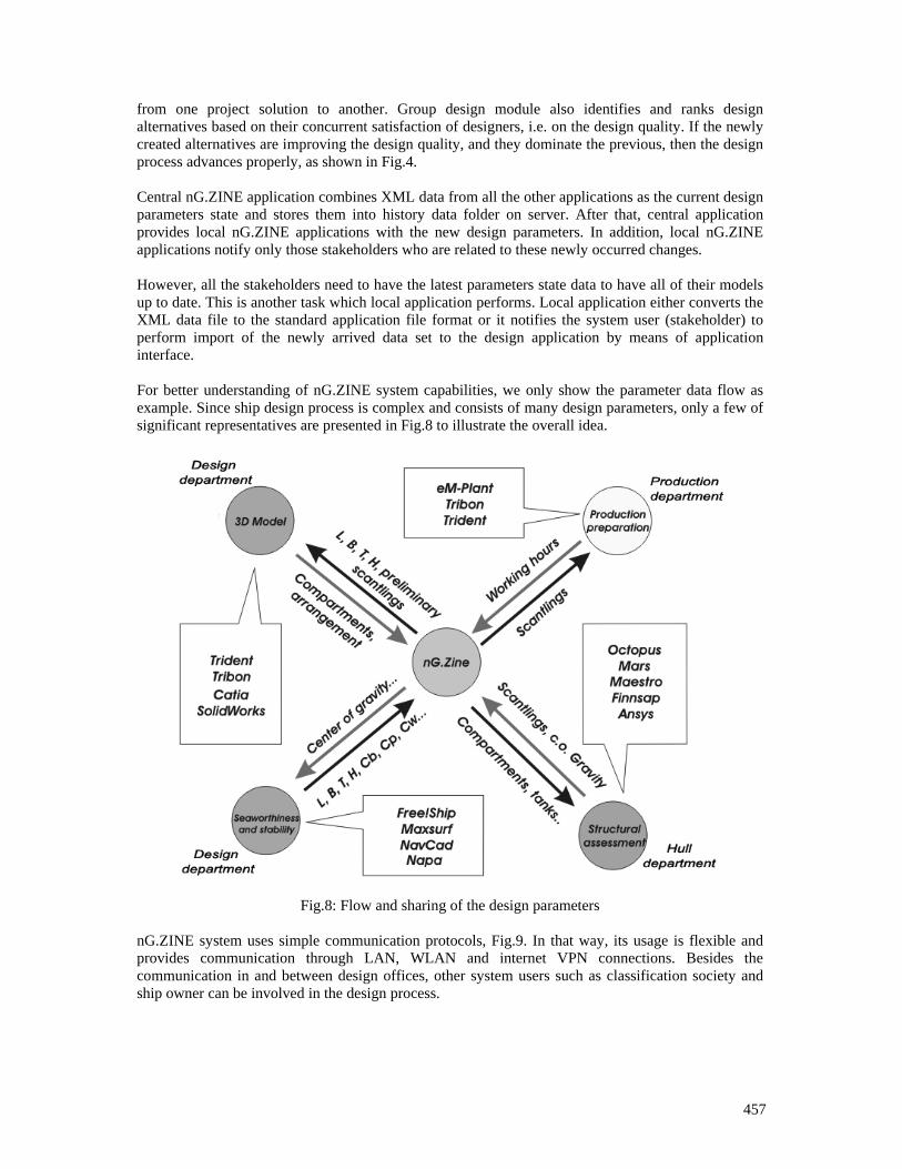
457

from one project solution to another. Group design module also identifies and ranks design alternatives based on their concurrent satisfaction of designers, i.e. on the design quality. If the newly created alternatives are improving the design quality, and they dominate the previous, then the design process advances properly, as shown in Fig.4. Central nG.ZINE application combines XML data from all the other applications as the current design parameters state and stores them into history data folder on server. After that, central application provides local nG.ZINE applications with the new design parameters. In addition, local nG.ZINE applications notify only those stakeholders who are related to these newly occurred changes. However, all the stakeholders need to have the latest parameters state data to have all of their models up to date. This is another task which local application performs. Local application either converts the XML data file to the standard application file format or it notifies the system user (stakeholder) to perform import of the newly arrived data set to the design application by means of application interface. For better understanding of nG.ZINE system capabilities, we only show the parameter data flow as example. Since ship design process is complex and consists of many design parameters, only a few of significant representatives are presented in Fig.8 to illustrate the overall idea.

Fig.8: Flow and sharing of the design parameters

nG.ZINE system uses simple communication protocols, Fig.9. In that way, its usage is flexible and provides communication through LAN, WLAN and internet VPN connections. Besides the communication in and between design offices, other system users such as classification society and ship owner can be involved in the design process.

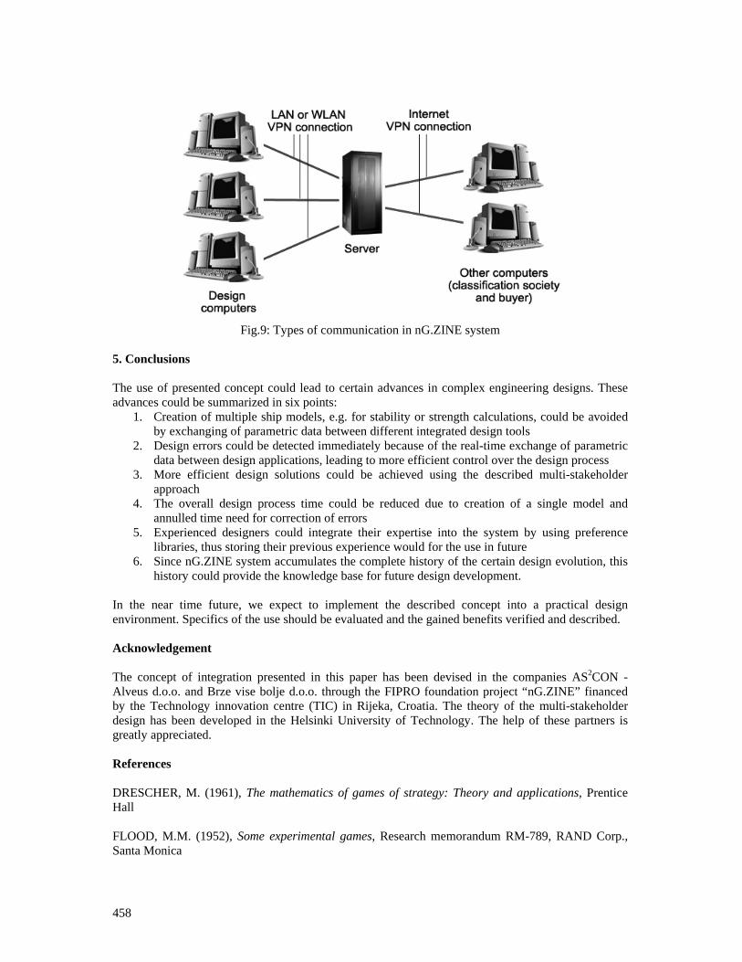
458

Fig.9: Types of communication in nG.ZINE system

5. Conclusions

The use of presented concept could lead to certain advances in complex engineering designs. These advances could be summarized in six points:

1. Creation of multiple ship models, e.g. for stability or strength calculations, could be avoided by exchanging of parametric data between different integrated design tools

2. Design errors could be detected immediately because of the real-time exchange of parametric data between design applications, leading to more efficient control over the design process

3. More efficient design solutions could be achieved using the described multi-stakeholder approach

4. The overall design process time could be reduced due to creation of a single model and annulled time need for correction of errors

5. Experienced designers could integrate their expertise into the system by using preference libraries, thus storing their previous experience would for the use in future

6. Since nG.ZINE system accumulates the complete history of the certain design evolution, this history could provide the knowledge base for future design development.

In the near time future, we expect to implement the described concept into a practical design environment. Specifics of the use should be evaluated and the gained benefits verified and described. Acknowledgement The concept of integration presented in this paper has been devised in the companies AS2CON - Alveus d.o.o. and Brze vise bolje d.o.o. through the FIPRO foundation project “nG.ZINE” financed by the Technology innovation centre (TIC) in Rijeka, Croatia. The theory of the multi-stakeholder design has been developed in the Helsinki University of Technology. The help of these partners is greatly appreciated. References DRESCHER, M. (1961), The mathematics of games of strategy: Theory and applications, Prentice Hall FLOOD, M.M. (1952), Some experimental games, Research memorandum RM-789, RAND Corp., Santa Monica

459

GALE, P.A. (2003), The ship design process, in Ship Design and Construction Vol.1, SNAME KLANAC, A.; TABRI, K.; EHLERS, S.; NEKIC, A. (2006), Multi-attribute design of crashworthy structures in the bi-stakeholder environment, Int. Marine Design Conf. (IMDC), Ann Arbor. KLANAC, A.; JALONEN, R.; VARSTA, P. (2007), Multi-stakeholder decision-making in the risk-based design of a RO-PAX double bottom for grounding, J. Engineering for the Maritime Environment 221/1, pp.1-15 NEKIC, A. (2007), Modelling structural design process of a cruise ship in the concept phase, Master thesis, University of Rijeka, Faculty of Engineering. ROSQVIST, T.; TUOMINNEN (2004), Qualification of formal safety assessment: an exploratory study, Safety Science 42/2, pp.99-120 ROSQVIST, T. (2003), Stakeholder compensation model based on decision analysis, J. Multi-Crit. Decis. Anal. 12, pp.219-223 THURSTON, D.L. (2001), Real and misconceived limitations to decision based design with utility analysis, J. Mech. Des. 123/2, pp.176-182 WIERZBICKI, A.P. (1980), The use of reference objectives in multiobjective optimization, 3rd Conf. on Multicriteria Decision Making, Lecture Notes in Economics and Mathematical Systems

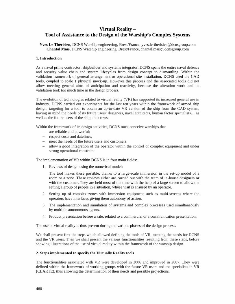
460

Virtual Reality – Tool of Assistance to the Design of the Warship’s Complex Systems

Yves Le Thérisien, DCNS Warship engineering, Brest/France, yves.le-therisien@dcnsgroup.com

Chantal Maïs, DCNS Warship engineering, Brest/France, chantal.mais@dcnsgroup.com

1. Introduction As a naval prime contractor, shipbuilder and systems integrator, DCNS spans the entire naval defence and security value chain and system lifecycles from design concept to dismantling. Within the validation framework of general arrangement or operational site installation, DCNS used the CAD tools, coupled to scale 1 physical mock-up. However this process and the associated tools did not allow meeting general aims of anticipation and reactivity, because the alteration work and its validation took too much time in the design process.

The evolution of technologies related to virtual reality (VR) has supported its increased general use in industry. DCNS carried out experiments for the last ten years within the framework of armed ship design, targeting for a tool to obtain an up-to-date VR version of the ship from the CAD system, having in mind the needs of its future users: designers, naval architects, human factor specialists… as well as the future users of the ship, the crews. Within the framework of its design activities, DCNS must conceive warships that

− are reliable and powerful; − respect costs and datelines; − meet the needs of the future users and customers; − allow a good integration of the operator within the control of complex equipment and under

strong operational constraint The implementation of VR within DCNS is in four main fields:

1. Reviews of design using the numerical model:

The tool makes these possible, thanks to a large-scale immersion in the set-up model of a room or a zone. These reviews either are carried out with the team of in-house designers or with the customer. They are held most of the time with the help of a large screen to allow the setting a group of people in a situation, whose visit is ensured by an operator.

2. Setting up of complex zones with immersion equipment such as multi-screens where the operators have interfaces giving them autonomy of action.

3. The implementation and simulation of systems and complex processes used simultaneously by multiple autonomous agents.

4. Product presentation before a sale, related to a commercial or a communication presentation.

The use of virtual reality is thus present during the various phases of the design process.

We shall present first the steps which allowed defining the tools of VR, meeting the needs for DCNS and the VR users. Then we shall present the various functionalities resulting from these steps, before showing illustrations of the use of virtual reality within the framework of the warship design. 2. Steps implemented to specify the Virtually Reality tools The functionalities associated with VR were developed in 2006 and improved in 2007. They were defined within the framework of working groups with the future VR users and the specialists in VR (CLARTE), thus allowing the determination of their needs and possible projections.

461

The future users of the VR can be: layout designers, ergonomics experts, system operators, crew, ILS staff, naval architects (...). Its use was evaluated by a team representative of the future users. The evaluation was carried out according to an ergonomic study, implemented by one of the ergonomic experts of the DCNS Human Factors’ group and carried out on the complex premises of submarines and surface vessels. This evaluation highlighted the advantages presented by this tool and made it possible to identify tracks of improvement for the functionalities that VR can offer. The first aspect taken into account is the representativeness of the tool compared to reality.

1. Criterion: Representativeness with respect to visual perception

It is a recurring topic in analyses with respect to the virtual experiments. It proves that the visual perception of the environment is satisfactory in a good realistic immersive view. Within this framework, the first tests of realistic feedback on lightings, thanks to computation software, are promising. The use of projectors of latest generation DLP with micro mirrors gives a good level of restitution with good luminous output.

2. Criterion: Representativeness with respect to tactile perception

The axis to be improved is that of the tactile perception of reality. The operator cannot detect with precision the interactions between the various parts of his body, except the hand, and the environment. Nowadays, the haptic solutions of interfaces are intrusive in the environment and can disturb the transfer virtual/real in the operator. These interfaces are interesting during handling at a fixed station, where a real effort feedback is felt. However, they are very quickly limited during displacement.

Other technologies available are those of multiple sensors laid out on the body and allowing the detection of position and the interferences announced by luminous or sound messages. It is what is implemented at the level of the data glove. In this case there is no effort feedback.

The operations of assembly/disassembling carried out with these accessories, open good prospects for use, training or maintenance actions, taking into account the maintainability associated to ergonomic criteria. The installation of some sensors with optical wireless detection on the human body parts can largely improve this aspect. The other aspect relates to the necessary functionalities and their implementation within the VR framework.

3. Criterion: Use of the functionalities

The use of measurement functionalities (linear, angular, minimal space, broken up into axes), of displacement of objects proved consolidated such as the use of object library, and of the mannequin articulated in opposite kinematics. Those are also available in the CAD software. The fact of using them in a virtual universe scale 1 in stereoscopy allows an objective evaluation of the virtual scene, essential to a total use of the model, while being associated to a qualitative perception due to the virtual environment.

4. Criterion: Utilisability of the functionalities

The functionalities are implemented by starting from an interactive drop-down menu controlled by the joystick. The various functions are called from it, in the course of work within the virtual scene. The functionalities must have the most intuitive operating mode possible, without disturbing the analysis of the virtual scene. The use of this type of tool is thus considered to be very positive, starting from the experiments and allowing the

462

appreciation of the above described criteria, even if various aspects (in particular at the physical interface level) must be improved. The implementation within DCNS is already effective on various projects. The future ships (frigates and submarines) obviously benefit from these technologies.

3. Means of Virtual Reality exploited by DCNS While profiting from progress in the interfaces of exploitation and the data-processing field, with recognized partners of the sector (centre CLARTE of Laval, CERV of Brest), DCNS implements the means of VR. There are:

− the immersive space of the SAS 3: an immersive cube with screen of four sides, with 3m length of edge,

− the DCNS workspace, a room with 7mx3m curved screen and a workroom with rear-projected screen of 2.5m x 2m and optical tracking.

Theses means allow the integration of numerical models coming from the DCNS CAD tools, with the need for the scene decomposition into elementary objects allowing the installation of behaviours, and enrichment with realistic textures for a better immersion. This allows evaluations on a first personae basis (the operator carries out the tasks himself) or on a third personae basis (through a mannequin introduced into the scene).

The functionalities implemented with this tool are:

− measurements (distances, angles)

This functionality enables the provision of the set-up components to be checked on scale 1; it also allows the viewing angles from the operator or the mannequin to be checked. The measurements are feasible in three dimensions and decomposable along the threee reference axes of the room or the ship. Functionality allows a calculation of the minimal dimension existing between two objects

− Mannequin

The incorporation of a mannequin allows external evaluation of situation by the operator. The articulated mannequin in opposite kinematics can be moved or put in posture in a scene, in order to check accessibility, angles of sight… collision detection at the time of its movements with the other objects is assured. It is possible to visualize the cone of vision of the mannequin, and the perception of its vision can be displayed on an autonomous window. The mannequin contains a library of postures, which can be enriched.

− Displacement and behaviour of objects

The objects in the scene can be removed with the handling interface. The operator can also move, either in walk mode, taking into account gravity, or in free mode. The objects can be allotted a behaviour representative of their vocation thus allowing their evaluation.

− Scale 1 in immersive space in stereoscopy

Immersive space is calibrated for the objects’ representation on scale 1.

− Library of objects

The various objects necessary to an environment can be contained in a library having a visual interface that can be put into motion within the course of work and allowing their incorporation into the scene, their hidden viewing or their final suppression.

− Interface and manipulation of the data glove

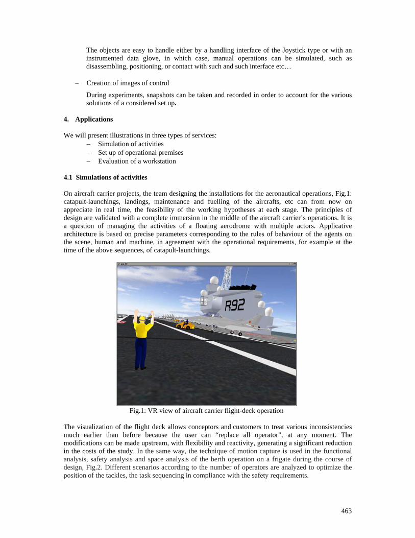
463

The objects are easy to handle either by a handling interface of the Joystick type or with an instrumented data glove, in which case, manual operations can be simulated, such as disassembling, positioning, or contact with such and such interface etc…

− Creation of images of control

During experiments, snapshots can be taken and recorded in order to account for the various solutions of a considered set up.

4. Applications We will present illustrations in three types of services:

− Simulation of activities − Set up of operational premises − Evaluation of a workstation

4.1 Simulations of activities On aircraft carrier projects, the team designing the installations for the aeronautical operations, Fig.1: catapult-launchings, landings, maintenance and fuelling of the aircrafts, etc can from now on appreciate in real time, the feasibility of the working hypotheses at each stage. The principles of design are validated with a complete immersion in the middle of the aircraft carrier’s operations. It is a question of managing the activities of a floating aerodrome with multiple actors. Applicative architecture is based on precise parameters corresponding to the rules of behaviour of the agents on the scene, human and machine, in agreement with the operational requirements, for example at the time of the above sequences, of catapult-launchings.

Fig.1: VR view of aircraft carrier flight-deck operation

The visualization of the flight deck allows conceptors and customers to treat various inconsistencies much earlier than before because the user can “replace all operator”, at any moment. The modifications can be made upstream, with flexibility and reactivity, generating a significant reduction in the costs of the study. In the same way, the technique of motion capture is used in the functional analysis, safety analysis and space analysis of the berth operation on a frigate during the course of design, Fig.2. Different scenarios according to the number of operators are analyzed to optimize the position of the tackles, the task sequencing in compliance with the safety requirements.

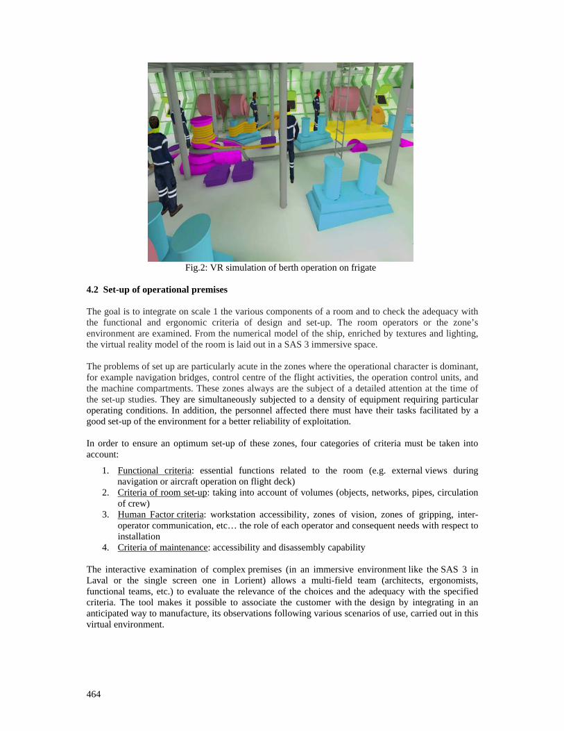
464

Fig.2: VR simulation of berth operation on frigate

4.2 Set-up of operational premises The goal is to integrate on scale 1 the various components of a room and to check the adequacy with the functional and ergonomic criteria of design and set-up. The room operators or the zone’s environment are examined. From the numerical model of the ship, enriched by textures and lighting, the virtual reality model of the room is laid out in a SAS 3 immersive space. The problems of set up are particularly acute in the zones where the operational character is dominant, for example navigation bridges, control centre of the flight activities, the operation control units, and the machine compartments. These zones always are the subject of a detailed attention at the time of the set-up studies. They are simultaneously subjected to a density of equipment requiring particular operating conditions. In addition, the personnel affected there must have their tasks facilitated by a good set-up of the environment for a better reliability of exploitation. In order to ensure an optimum set-up of these zones, four categories of criteria must be taken into account:

1. Functional criteria: essential functions related to the room (e.g. external views during navigation or aircraft operation on flight deck)

2. Criteria of room set-up: taking into account of volumes (objects, networks, pipes, circulation of crew)

3. Human Factor criteria: workstation accessibility, zones of vision, zones of gripping, inter-operator communication, etc… the role of each operator and consequent needs with respect to installation

4. Criteria of maintenance: accessibility and disassembly capability The interactive examination of complex premises (in an immersive environment like the SAS 3 in Laval or the single screen one in Lorient) allows a multi-field team (architects, ergonomists, functional teams, etc.) to evaluate the relevance of the choices and the adequacy with the specified criteria. The tool makes it possible to associate the customer with the design by integrating in an anticipated way to manufacture, its observations following various scenarios of use, carried out in this virtual environment.

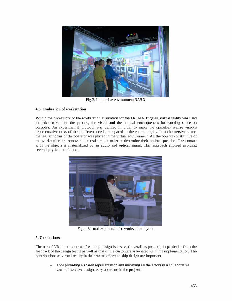
465

Fig.3: Immersive environment SAS 3

4.3 Evaluation of workstation Within the framework of the workstation evaluation for the FREMM frigates, virtual reality was used in order to validate the posture, the visual and the manual consequences for working space on consoles. An experimental protocol was defined in order to make the operators realize various representative tasks of their different needs, compared to these three topics. In an immersive space, the real armchair of the operator was placed in the virtual environment. All the objects constitutive of the workstation are removable in real time in order to determine their optimal position. The contact with the objects is materialized by an audio and optical signal. This approach allowed avoiding several physical mock-ups.

Fig.4: Virtual experiment for workstation layout

5. Conclusions The use of VR in the context of warship design is assessed overall as positive, in particular from the feedback of the design teams as well as that of the customers associated with this implementation. The contributions of virtual reality in the process of armed ship design are important:

− Tool providing a shared representation and involving all the actors in a collaborative

work of iterative design, very upstream in the projects.

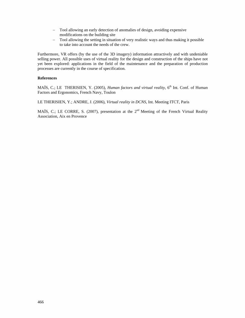
466

− Tool allowing an early detection of anomalies of design, avoiding expensive modifications on the building site

− Tool allowing the setting in situation of very realistic ways and thus making it possible to take into account the needs of the crew.

Furthermore, VR offers (by the use of the 3D imagery) information attractively and with undeniable selling power. All possible uses of virtual reality for the design and construction of the ships have not yet been explored: applications in the field of the maintenance and the preparation of production processes are currently in the course of specification.

References MAÏS, C.; LE THERISIEN, Y. (2005), Human factors and virtual reality, 6th Int. Conf. of Human Factors and Ergonomics, French Navy, Toulon LE THERISIEN, Y.; ANDRE, J. (2006), Virtual reality in DCNS, Int. Meeting ITCT, Paris MAÏS, C.; LE CORRE, S. (2007), presentation at the 2nd Meeting of the French Virtual Reality Association, Aix en Provence

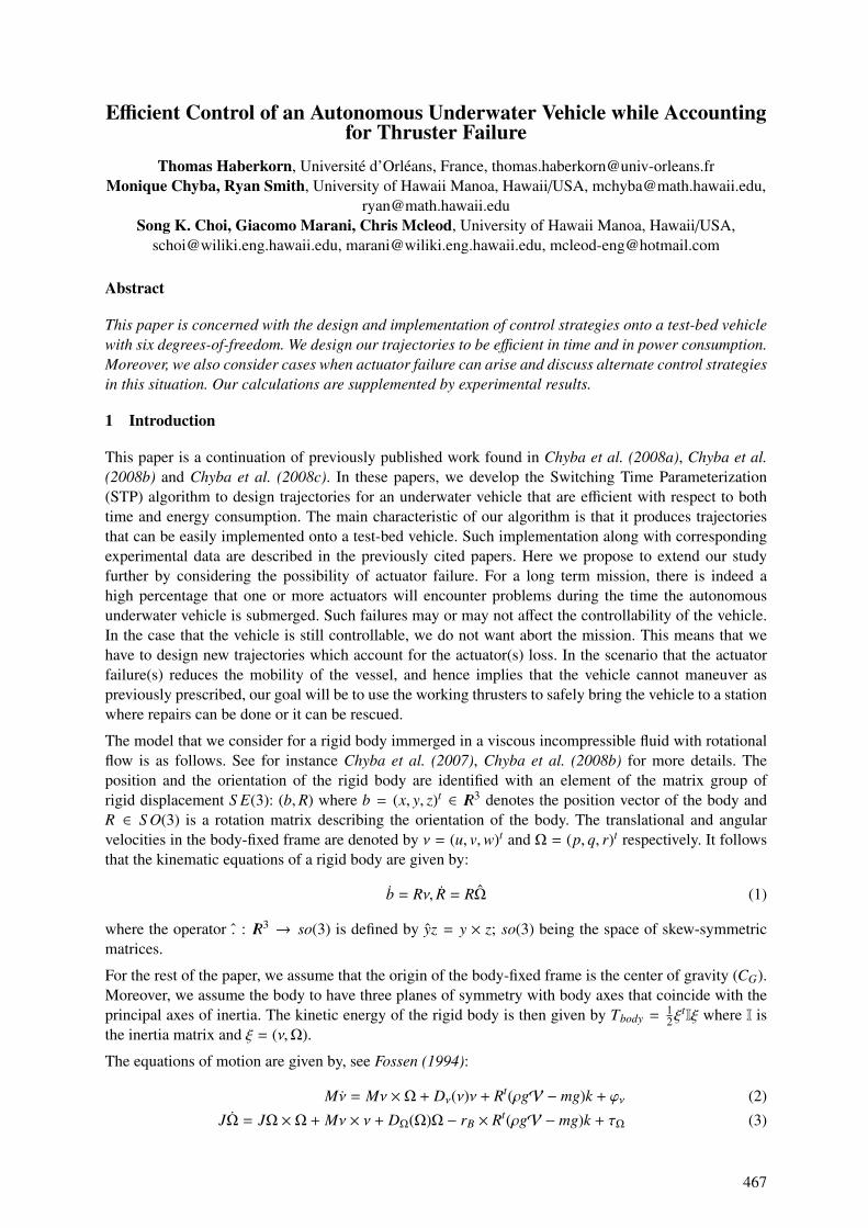
Efficient Control of an Autonomous Underwater Vehicle while Accountingfor Thruster Failure

Thomas Haberkorn, Universite d’Orleans, France, thomas.haberkorn@univ-orleans.frMonique Chyba, Ryan Smith, University of Hawaii Manoa, Hawaii/USA, mchyba@math.hawaii.edu,

ryan@math.hawaii.eduSong K. Choi, Giacomo Marani, Chris Mcleod, University of Hawaii Manoa, Hawaii/USA,

schoi@wiliki.eng.hawaii.edu, marani@wiliki.eng.hawaii.edu, mcleod-eng@hotmail.com

Abstract

This paper is concerned with the design and implementation of control strategies onto a test-bed vehiclewith six degrees-of-freedom. We design our trajectories to be efficient in time and in power consumption.Moreover, we also consider cases when actuator failure can arise and discuss alternate control strategiesin this situation. Our calculations are supplemented by experimental results.

1 Introduction

This paper is a continuation of previously published work found in Chyba et al. (2008a), Chyba et al.(2008b) and Chyba et al. (2008c). In these papers, we develop the Switching Time Parameterization(STP) algorithm to design trajectories for an underwater vehicle that are efficient with respect to bothtime and energy consumption. The main characteristic of our algorithm is that it produces trajectoriesthat can be easily implemented onto a test-bed vehicle. Such implementation along with correspondingexperimental data are described in the previously cited papers. Here we propose to extend our studyfurther by considering the possibility of actuator failure. For a long term mission, there is indeed ahigh percentage that one or more actuators will encounter problems during the time the autonomousunderwater vehicle is submerged. Such failures may or may not affect the controllability of the vehicle.In the case that the vehicle is still controllable, we do not want abort the mission. This means that wehave to design new trajectories which account for the actuator(s) loss. In the scenario that the actuatorfailure(s) reduces the mobility of the vessel, and hence implies that the vehicle cannot maneuver aspreviously prescribed, our goal will be to use the working thrusters to safely bring the vehicle to a stationwhere repairs can be done or it can be rescued.

The model that we consider for a rigid body immerged in a viscous incompressible fluid with rotationalflow is as follows. See for instance Chyba et al. (2007), Chyba et al. (2008b) for more details. Theposition and the orientation of the rigid body are identified with an element of the matrix group ofrigid displacement S E(3): (b,R) where b = (x, y, z)t ∈ IR3 denotes the position vector of the body andR ∈ S O(3) is a rotation matrix describing the orientation of the body. The translational and angularvelocities in the body-fixed frame are denoted by ν = (u, v,w)t and Ω = (p, q, r)t respectively. It followsthat the kinematic equations of a rigid body are given by:

b = Rν, R = RΩ (1)

where the operator . : IR3 → so(3) is defined by yz = y × z; so(3) being the space of skew-symmetricmatrices.

For the rest of the paper, we assume that the origin of the body-fixed frame is the center of gravity (CG).Moreover, we assume the body to have three planes of symmetry with body axes that coincide with theprincipal axes of inertia. The kinetic energy of the rigid body is then given by Tbody = 1

2ξtIξ where I is

the inertia matrix and ξ = (ν,Ω).

The equations of motion are given by, see Fossen (1994):

Mν = Mν ×Ω + Dν(ν)ν + Rt(ρgV − mg)k + ϕν (2)

JΩ = JΩ ×Ω + Mν × ν + DΩ(Ω)Ω − rB × Rt(ρgV − mg)k + τΩ (3)

467

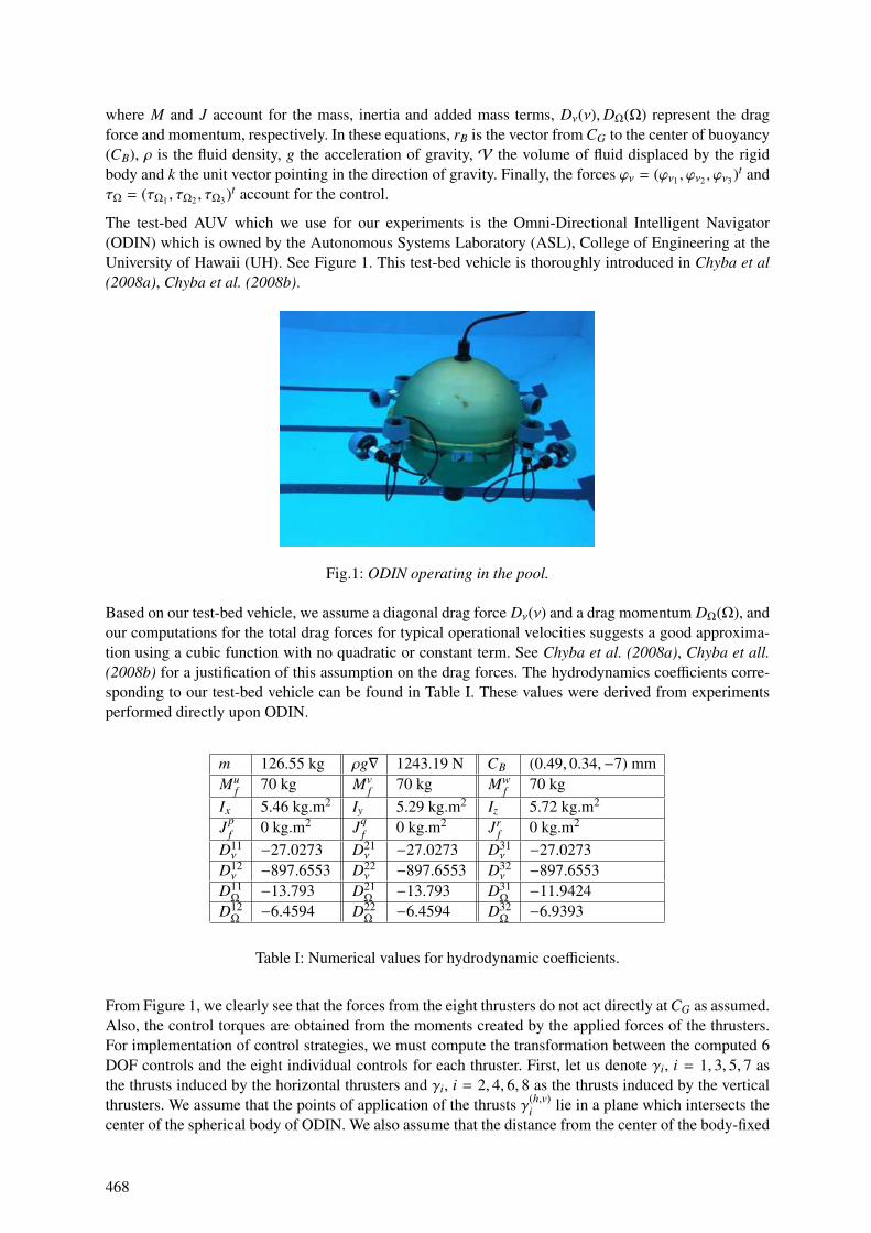
where M and J account for the mass, inertia and added mass terms, Dν(ν),DΩ(Ω) represent the dragforce and momentum, respectively. In these equations, rB is the vector from CG to the center of buoyancy(CB), ρ is the fluid density, g the acceleration of gravity, V the volume of fluid displaced by the rigidbody and k the unit vector pointing in the direction of gravity. Finally, the forces ϕν = (ϕν1 , ϕν2 , ϕν3)t andτΩ = (τΩ1 , τΩ2 , τΩ3)t account for the control.

The test-bed AUV which we use for our experiments is the Omni-Directional Intelligent Navigator(ODIN) which is owned by the Autonomous Systems Laboratory (ASL), College of Engineering at theUniversity of Hawaii (UH). See Figure 1. This test-bed vehicle is thoroughly introduced in Chyba et al(2008a), Chyba et al. (2008b).

Fig.1: ODIN operating in the pool.

Based on our test-bed vehicle, we assume a diagonal drag force Dν(ν) and a drag momentum DΩ(Ω), andour computations for the total drag forces for typical operational velocities suggests a good approxima-tion using a cubic function with no quadratic or constant term. See Chyba et al. (2008a), Chyba et all.(2008b) for a justification of this assumption on the drag forces. The hydrodynamics coefficients corre-sponding to our test-bed vehicle can be found in Table I. These values were derived from experimentsperformed directly upon ODIN.

m 126.55 kg ρg∇ 1243.19 N CB (0.49, 0.34,−7) mmMu

f 70 kg Mvf 70 kg Mw

f 70 kgIx 5.46 kg.m2 Iy 5.29 kg.m2 Iz 5.72 kg.m2

Jpf 0 kg.m2 Jq

f 0 kg.m2 Jrf 0 kg.m2

D11ν −27.0273 D21

ν −27.0273 D31ν −27.0273

D12ν −897.6553 D22

ν −897.6553 D32ν −897.6553

D11Ω−13.793 D21

Ω−13.793 D31

Ω−11.9424

D12Ω−6.4594 D22

Ω−6.4594 D32

Ω−6.9393

Table I: Numerical values for hydrodynamic coefficients.

From Figure 1, we clearly see that the forces from the eight thrusters do not act directly at CG as assumed.Also, the control torques are obtained from the moments created by the applied forces of the thrusters.For implementation of control strategies, we must compute the transformation between the computed 6DOF controls and the eight individual controls for each thruster. First, let us denote γi, i = 1, 3, 5, 7 asthe thrusts induced by the horizontal thrusters and γi, i = 2, 4, 6, 8 as the thrusts induced by the verticalthrusters. We assume that the points of application of the thrusts γ(h,v)

i lie in a plane which intersects thecenter of the spherical body of ODIN. We also assume that the distance from the center of the body-fixed

468

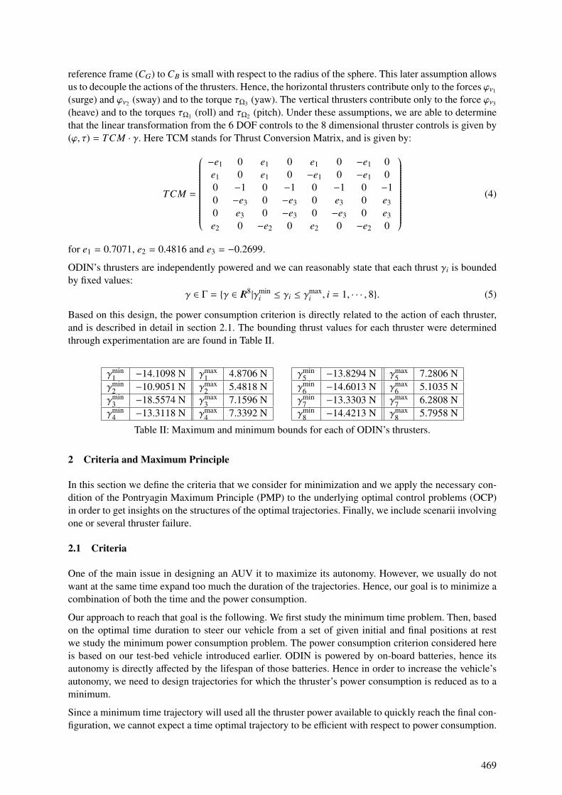
reference frame (CG) to CB is small with respect to the radius of the sphere. This later assumption allowsus to decouple the actions of the thrusters. Hence, the horizontal thrusters contribute only to the forces ϕν1

(surge) and ϕν2 (sway) and to the torque τΩ3 (yaw). The vertical thrusters contribute only to the force ϕν3

(heave) and to the torques τΩ1 (roll) and τΩ2 (pitch). Under these assumptions, we are able to determinethat the linear transformation from the 6 DOF controls to the 8 dimensional thruster controls is given by(ϕ, τ) = TCM · γ. Here TCM stands for Thrust Conversion Matrix, and is given by:

TCM =

−e1 0 e1 0 e1 0 −e1 0e1 0 e1 0 −e1 0 −e1 00 −1 0 −1 0 −1 0 −10 −e3 0 −e3 0 e3 0 e30 e3 0 −e3 0 −e3 0 e3e2 0 −e2 0 e2 0 −e2 0

(4)

for e1 = 0.7071, e2 = 0.4816 and e3 = −0.2699.

ODIN’s thrusters are independently powered and we can reasonably state that each thrust γi is boundedby fixed values:

γ ∈ Γ = γ ∈ IR8|γmini ≤ γi ≤ γ

maxi , i = 1, · · · , 8. (5)

Based on this design, the power consumption criterion is directly related to the action of each thruster,and is described in detail in section 2.1. The bounding thrust values for each thruster were determinedthrough experimentation are are found in Table II.

γmin1 −14.1098 N γmax

1 4.8706 Nγmin

2 −10.9051 N γmax2 5.4818 N

γmin3 −18.5574 N γmax

3 7.1596 Nγmin

4 −13.3118 N γmax4 7.3392 N

γmin5 −13.8294 N γmax

5 7.2806 Nγmin

6 −14.6013 N γmax6 5.1035 N

γmin7 −13.3303 N γmax

7 6.2808 Nγmin

8 −14.4213 N γmax8 5.7958 N

Table II: Maximum and minimum bounds for each of ODIN’s thrusters.

2 Criteria and Maximum Principle

In this section we define the criteria that we consider for minimization and we apply the necessary con-dition of the Pontryagin Maximum Principle (PMP) to the underlying optimal control problems (OCP)in order to get insights on the structures of the optimal trajectories. Finally, we include scenarii involvingone or several thruster failure.

2.1 Criteria

One of the main issue in designing an AUV it to maximize its autonomy. However, we usually do notwant at the same time expand too much the duration of the trajectories. Hence, our goal is to minimize acombination of both the time and the power consumption.

Our approach to reach that goal is the following. We first study the minimum time problem. Then, basedon the optimal time duration to steer our vehicle from a set of given initial and final positions at restwe study the minimum power consumption problem. The power consumption criterion considered hereis based on our test-bed vehicle introduced earlier. ODIN is powered by on-board batteries, hence itsautonomy is directly affected by the lifespan of those batteries. Hence in order to increase the vehicle’sautonomy, we need to design trajectories for which the thruster’s power consumption is reduced as to aminimum.

Since a minimum time trajectory will used all the thruster power available to quickly reach the final con-figuration, we cannot expect a time optimal trajectory to be efficient with respect to power consumption.

469

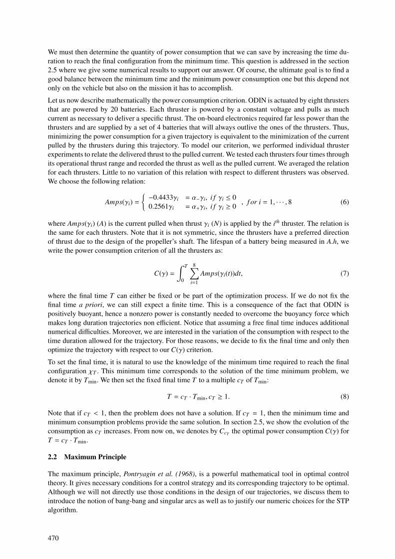
We must then determine the quantity of power consumption that we can save by increasing the time du-ration to reach the final configuration from the minimum time. This question is addressed in the section2.5 where we give some numerical results to support our answer. Of course, the ultimate goal is to find agood balance between the minimum time and the minimum power consumption one but this depend notonly on the vehicle but also on the mission it has to accomplish.

Let us now describe mathematically the power consumption criterion. ODIN is actuated by eight thrustersthat are powered by 20 batteries. Each thruster is powered by a constant voltage and pulls as muchcurrent as necessary to deliver a specific thrust. The on-board electronics required far less power than thethrusters and are supplied by a set of 4 batteries that will always outlive the ones of the thrusters. Thus,minimizing the power consumption for a given trajectory is equivalent to the minimization of the currentpulled by the thrusters during this trajectory. To model our criterion, we performed individual thrusterexperiments to relate the delivered thrust to the pulled current. We tested each thrusters four times throughits operational thrust range and recorded the thrust as well as the pulled current. We averaged the relationfor each thrusters. Little to no variation of this relation with respect to different thrusters was observed.We choose the following relation:

Amps(γi) =

−0.4433γi = α−γi, i f γi ≤ 00.2561γi = α+γi, i f γi ≥ 0

, f or i = 1, · · · , 8 (6)

where Amps(γi) (A) is the current pulled when thrust γi (N) is applied by the ith thruster. The relation isthe same for each thrusters. Note that it is not symmetric, since the thrusters have a preferred directionof thrust due to the design of the propeller’s shaft. The lifespan of a battery being measured in A.h, wewrite the power consumption criterion of all the thrusters as:

C(γ) =

∫ T

0

8∑i=1

Amps(γi(t))dt, (7)

where the final time T can either be fixed or be part of the optimization process. If we do not fix thefinal time a priori, we can still expect a finite time. This is a consequence of the fact that ODIN ispositively buoyant, hence a nonzero power is constantly needed to overcome the buoyancy force whichmakes long duration trajectories non efficient. Notice that assuming a free final time induces additionalnumerical difficulties. Moreover, we are interested in the variation of the consumption with respect to thetime duration allowed for the trajectory. For those reasons, we decide to fix the final time and only thenoptimize the trajectory with respect to our C(γ) criterion.

To set the final time, it is natural to use the knowledge of the minimum time required to reach the finalconfiguration χT . This minimum time corresponds to the solution of the time minimum problem, wedenote it by Tmin. We then set the fixed final time T to a multiple cT of Tmin:

T = cT · Tmin, cT ≥ 1. (8)

Note that if cT < 1, then the problem does not have a solution. If cT = 1, then the minimum time andminimum consumption problems provide the same solution. In section 2.5, we show the evolution of theconsumption as cT increases. From now on, we denotes by CcT the optimal power consumption C(γ) forT = cT · Tmin.

2.2 Maximum Principle

The maximum principle, Pontryagin et al. (1968), is a powerful mathematical tool in optimal controltheory. It gives necessary conditions for a control strategy and its corresponding trajectory to be optimal.Although we will not directly use those conditions in the design of our trajectories, we discuss them tointroduce the notion of bang-bang and singular arcs as well as to justify our numeric choices for the STPalgorithm.

470

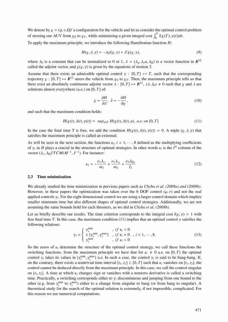
We denote by χ = (η, ν,Ω)t a configuration for the vehicle and let us consider the optimal control problemof steering our AUV from χ0 to χT , while minimizing a given integral cost

∫ T0 l(χ(T ), γ(t))dt.

To apply the maximum principle, we introduce the following Hamiltonian function H:

H(χ, λ, γ) = −λ0l(χ, γ) + λtχ(χ, γ), (9)

where λ0 is a constant that can be normalized to 0 or 1, λ = (λη, λnu, λΩ) is a vector function in IR12

called the adjoint vector, and χ(χ, γ) is given by the equations of motion 3.

Assume that there exists an admissible optimal control γ : [0,T ] 7→ Γ, such that the correspondingtrajectory χ : [0,T ] 7→ IR12 steers the vehicle from χ0 to χT . Then, the maximum principle tells us thatthere exist an absolutely continuous adjoint vector λ : [0,T ] 7→ IR12, (λ, λ0) , 0 such that χ and λ aresolutions almost everywhere (a.e.) on [0,T ] of:

χ =∂H∂λ

, λ = −∂H∂χ

, (10)

and such that the maximum condition holds:

H(χ(t), λ(t), γ(t)) = supu∈Γ H(χ(t), λ(t), u), a.e. on [0,T ] (11)

In the case the final time T is free, we add the condition H(χ(t), λ(t), γ(t)) = 0. A triple (χ, λ, γ) thatsatisfies the maximum principle is called an extremal.

As will be seen in the next section, the functions κi, i = 1, · · · , 8 defined as the multiplying coefficientsof γi in H plays a crucial in the structure of optimal strategies. In other words κi is the ith column of thevector (λν, λΩ)tTCM(M−1, J−1). For instance:

κ1 = −e1λν1

m1+

e1λν2

m2+

e2λΩ3

I3(12)

2.3 Time minimization

We already studied the time minimization in previous papers such as Chyba et al. (2008a) and (2008b).However, in these papers the optimization was taken over the 6 DOF control (ϕ, τ) and not the realapplied controls γi. For the eight dimensional control we are using a larger control domain which impliessmaller minimum time but also different shapes of optimal control strategies. Additionally, we are notassuming the same bounds hold for each thrusters, as we did in Chyba et al. (2008b).

Let us briefly describe our results. The time criterion corresponds to the integral cost l(χ, γ) = 1 withfree final time T . In this case, the maximum condition (11) implies that an optimal control γ satisfies thefollowing relations:

γi =

γmin

i , i f κi < 0∈ [γmin

i , γmaxi ] , i f κi = 0

γmaxi , i f κi > 0

, i = 1, · · · , 8. (13)

So the zeros of κi determine the structure of the optimal control strategy, we call these functions theswitching functions. from the maximum principle we have that for κi , 0 a.e. on [0,T ] the optimalcontrol γi takes its values in γmin

i , γmaxi a.e. In such a case, the control γi is said to be bang-bang. If,

on the contrary, there exists a nontrivial time interval [t1, t2] ⊂ [0,T ] such that κi vanishes on [t1, t2], thecontrol cannot be deduced directly from the maximum principle. In this case, we call the control singularon [t1, t2]. A time at which κi changes sign or vanishes with a nonzero derivative is called a switchingtime. Practically, a switching corresponds either to γi discontinuous and jumping from one bound to theother (e.g. from γmin

i to γmaxi ) either to a change from singular to bang (or from bang to singular). A

theoretical study for the search of the optimal solution is extremely, if not impossible, complicated. Forthis reason we use numerical computations.

471

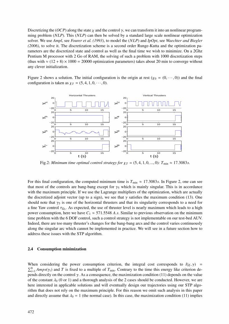
Discretizing the (OCP) along the state χ and the control γ, we can transform it into an nonlinear program-ming problem (NLP). This (NLP) can then be solved by a standard large scale nonlinear optimizationsolver. We use Ampl, see Fourer et al. (1993), to model the (NLP) and IpOpt, see Waechter and Biegler(2006), to solve it. The discretization scheme is a second order Runge-Kutta and the optimization pa-rameters are the discretized state and control as well as the final time we wish to minimize. On a 2GhzPentium M processor with 2 Go of RAM, the solving of such a problem with 1000 discretization steps(thus with ≈ (12 + 8) × 1000 = 20000 optimization parameters) takes about 20 min to converge withoutany clever initialization.

Figure 2 shows a solution. The initial configuration is the origin at rest (χ0 = (0, · · · , 0)) and the finalconfiguration is taken as χT = (5, 4, 1, 0, · · · , 0).

0 5 10 15−20

0

20Horizontal Thrusters

γ 1

0 5 10 15−20

0

20

γ 3

0 5 10 15−20

0

20

γ 5

0 5 10 15−20

0

20

γ 7

t (s)

0 5 10 15−20

0

20Vertical Thrusters

γ 2

0 5 10 15−20

0

20

γ 4

0 5 10 15−20

0

20

γ 6

0 5 10 15−20

0

20

γ 8

t (s)

Fig.2: Minimum time optimal control strategy for χT = (5, 4, 1, 0, ..., 0): Tmin ≈ 17.3083s.

For this final configuration, the computed minimum time is Tmin ≈ 17.3083s. In Figure 2, one can seethat most of the controls are bang-bang except for γ5 which is mainly singular. This is in accordancewith the maximum principle. If we use the Lagrange multipliers of the optimization, which are actuallythe discretized adjoint vector (up to a sign), we see that γ satisfies the maximum condition (13). Oneshould note that γ5 is one of the horizontal thrusters and that its singularity corresponds to a need fora fine Yaw control τΩ3 . As expected, the use of thruster level is nearly maximum which leads to a highpower consumption, here we have C1 ≈ 571.5548 A.s. Similar to previous observation on the minimumtime problem with the 6 DOF control, such a control strategy is not implementable on our test-bed AUV.Indeed, there are too many thruster’s changes for the bang-bang arcs and the control varies continuouslyalong the singular arc which cannot be implemented in practice. We will see in a future section how toaddress these issues with the STP algorithm.

2.4 Consumption minimization

When considering the power consumption criterion, the integral cost corresponds to l(χ, γ) =∑8i=1 Amps(γi) and T is fixed to a multiple of Tmin. Contrary to the time this energy like criterion de-

pends directly on the control γ. As a consequence, the maximization condition (11) depends on the valueof the constant λ0 (0 or 1) and a thorough analysis of the 2 cases should be conducted. However, we arehere interested in applicable solutions and will eventually design our trajectories using our STP algo-rithm that does not rely on the maximum principle. For this reason we omit such analysis in this paperand directly assume that λ0 = 1 (the normal case). In this case, the maximization condition (11) implies

472

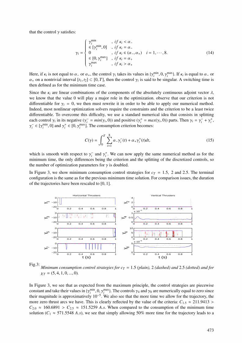
that the control γ satisfies:

γi =

γmini , i f κi < α−∈ [γmin

i , 0] , i f κi = α−0 , i f κi ∈ (α−, α+)∈ [0, γmax

i ] , i f κi = α+

γmaxi , i f κi > α+

i = 1, · · · , 8. (14)

Here, if κi is not equal to α− or α+, the control γi takes its values in γmini , 0, γmax

i . If κi is equal to α− orα+ on a nontrivial interval [t1, t2] ⊂ [0,T ], then the control γi is said to be singular. A switching time isthen defined as for the minimum time case.

Since the κi are linear combinations of the components of the absolutely continuous adjoint vector λ,we know that the value 0 will play a major role in the optimization. observe that our criterion is notdifferentiable for γi = 0, we then must rewrite it in order to be able to apply our numerical method.Indeed, most nonlinear optimization solvers require the constraints and the criterion to be a least twicedifferentiable. To overcome this difficulty, we use a standard numerical idea that consists in splittingeach control γi in its negative (γ−i = min(γi, 0)) and positive (γ+

i = max(γi, 0)) parts. Then γi = γ−i + γ+i ,

γ−i ∈ [γmini , 0] and γ+

i ∈ [0, γmaxi ]. The consumption criterion becomes:

C(γ) =

∫ T

0

8∑i=1

α−γ−i (t) + α+γ

+i (t)dt, (15)

which is smooth with respect to γ−i and γ+i . We can now apply the same numerical method as for the

minimum time, the only differences being the criterion and the splitting of the discretized controls, sothe number of optimization parameters for γ is doubled.

In Figure 3, we show minimum consumption control strategies for cT = 1.5, 2 and 2.5. The terminalconfiguration is the same as for the previous minimum time solution. For comparison issues, the durationof the trajectories have been rescaled to [0, 1].

0 0.2 0.4 0.6 0.8 1−20

−10

0Horizontal Thrusters

γ 1

0 0.2 0.4 0.6 0.8 1−20

−10

0

γ 3

0 0.2 0.4 0.6 0.8 1−20

−10

0

γ 5

0 0.2 0.4 0.6 0.8 1−20

−10

0

γ 7

t (s)

0 0.2 0.4 0.6 0.8 10

2

4Vertical Thrusters

γ 2

0 0.2 0.4 0.6 0.8 10

0.5

1x 10

−5

γ 4

0 0.2 0.4 0.6 0.8 10

5

10

γ 6

0 0.2 0.4 0.6 0.8 10

5x 10

−6

γ 8

t (s)

Fig.3:Minimum consumption control strategies for cT = 1.5 (plain), 2 (dashed) and 2.5 (dotted) and forχT = (5, 4, 1, 0, ..., 0).

In Figure 3, we see that as expected from the maximum principle, the control strategies are piecewiseconstant and take their values in γmin

i , 0, γmaxi . The controls γ4 and γ8 are numerically equal to zero since

their magnitude is approximatively 10−5. We also see that the more time we allow for the trajectory, themore zero thrust arcs we have. This is clearly reflected by the value of the criteria: C1.5 ≈ 211.9413 >

C2.0 ≈ 160.6891 > C2.5 ≈ 151.5259 A.s. When compared to the consumption of the minimum timesolution (C1 ≈ 571.5548 A.s), we see that simply allowing 50% more time for the trajectory leads to a

473

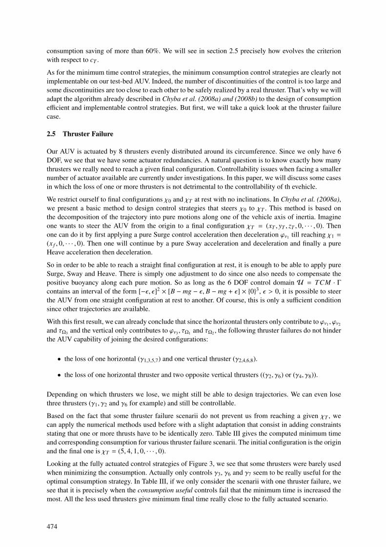
consumption saving of more than 60%. We will see in section 2.5 precisely how evolves the criterionwith respect to cT .

As for the minimum time control strategies, the minimum consumption control strategies are clearly notimplementable on our test-bed AUV. Indeed, the number of discontinuities of the control is too large andsome discontinuities are too close to each other to be safely realized by a real thruster. That’s why we willadapt the algorithm already described in Chyba et al. (2008a) and (2008b) to the design of consumptionefficient and implementable control strategies. But first, we will take a quick look at the thruster failurecase.

2.5 Thruster Failure

Our AUV is actuated by 8 thrusters evenly distributed around its circumference. Since we only have 6DOF, we see that we have some actuator redundancies. A natural question is to know exactly how manythrusters we really need to reach a given final configuration. Controllability issues when facing a smallernumber of actuator available are currently under investigations. In this paper, we will discuss some casesin which the loss of one or more thrusters is not detrimental to the controllability of th evehicle.

We restrict ourself to final configurations χ0 and χT at rest with no inclinations. In Chyba et al. (2008a),we present a basic method to design control strategies that steers χ0 to χT . This method is based onthe decomposition of the trajectory into pure motions along one of the vehicle axis of inertia. Imagineone wants to steer the AUV from the origin to a final configuration χT = (xT , yT , zT , 0, · · · , 0). Thenone can do it by first applying a pure Surge control acceleration then deceleration ϕν1 till reaching χ1 =

(x f , 0, · · · , 0). Then one will continue by a pure Sway acceleration and deceleration and finally a pureHeave acceleration then deceleration.

So in order to be able to reach a straight final configuration at rest, it is enough to be able to apply pureSurge, Sway and Heave. There is simply one adjustment to do since one also needs to compensate thepositive buoyancy along each pure motion. So as long as the 6 DOF control domain U = TCM · Γcontains an interval of the form [−ε, ε]2 × [B − mg − ε, B − mg + ε] × 03, ε > 0, it is possible to steerthe AUV from one straight configuration at rest to another. Of course, this is only a sufficient conditionsince other trajectories are available.

With this first result, we can already conclude that since the horizontal thrusters only contribute to ϕν1 , ϕν2

and τΩ3 and the vertical only contributes to ϕν3 , τΩ1 and τΩ2 , the following thruster failures do not hinderthe AUV capability of joining the desired configurations:

• the loss of one horizontal (γ1,3,5,7) and one vertical thruster (γ2,4,6,8).

• the loss of one horizontal thruster and two opposite vertical thrusters ((γ2, γ6) or (γ4, γ8)).

Depending on which thrusters we lose, we might still be able to design trajectories. We can even losethree thrusters (γ1, γ2 and γ6 for example) and still be controllable.

Based on the fact that some thruster failure scenarii do not prevent us from reaching a given χT , wecan apply the numerical methods used before with a slight adaptation that consist in adding constraintsstating that one or more thrusts have to be identically zero. Table III gives the computed minimum timeand corresponding consumption for various thruster failure scenarii. The initial configuration is the originand the final one is χT = (5, 4, 1, 0, · · · , 0).

Looking at the fully actuated control strategies of Figure 3, we see that some thrusters were barely usedwhen minimizing the consumption. Actually only controls γ3, γ6 and γ7 seem to be really useful for theoptimal consumption strategy. In Table III, if we only consider the scenarii with one thruster failure, wesee that it is precisely when the consumption useful controls fail that the minimum time is increased themost. All the less used thrusters give minimum final time really close to the fully actuated scenario.

474

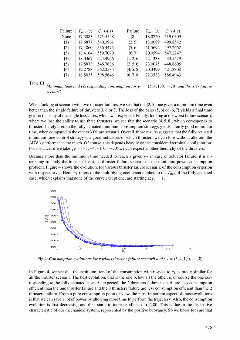
Failure Tmin (s) C1 (A.s)None 17.3083 571.55481 17.6877 540.39612 17.4860 536.44753 18.4164 559.70704 18.0367 524.49665 17.5873 546.76366 19.2788 562.25357 18.5035 598.5646

Failure Tmin (s) C1 (A.s)8 18.0720 519.03092, 5 18.0089 499.85425, 6 21.5692 497.26626, 7 20.0594 547.22471, 2, 6 22.1338 533.54792, 5, 6 23.0075 448.86054, 5, 8 20.3499 421.33086, 7, 8 22.3533 586.4943

Table III:Minimum time and corresponding consumption for χT = (5, 4, 1, 0, · · · , 0) and thruster failurescenarii.

When looking at scenarii with two thruster failures, we see that the 2, 5 one gives a minimum time evenbetter than the single failure of thrusters 3, 6 or 7. The loss of the pairs 5, 6 or 6, 7 yields a final timegreater than any of the single loss cases, which was expected. Finally, looking at the worst failure scenarii,where we lose the ability to use three thrusters, we see that the scenario 4, 5, 8, which corresponds tothrusters barely used in the fully actuated minimum consumption strategy, yields a fairly good minimumtime, when compared to the others 3 failure scenarii. Overall, those results suggests that the fully actuatedminimum time control strategy is a good indicators of which thrusters we can lose without alteratin theAUV’s performance too much. Of course, this depends heavily on the considered terminal configuration.For instance, if we take χT = (−5,−4,−1, 0, · · · , 0) we can expect another hierarchy of the thrusters.

Because more than the minimum time needed to reach a given χT in case of actuator failure, it is in-teresting to study the impact of various thruster failure scenarii on the minimum power consumptionproblem. Figure 4 shows the evolution, for various thruster failure scenarii, of the consumption criterionwith respect to cT . Here, cT refers to the multiplying coefficient applied to the Tmin of the fully actuatedcase, which explains that none of the curve except one, are starting at cT = 1.

1 1.5 2 2.5 3 3.5 4150

200

250

300

350

400

450

500

550

600

ctf

J (A.

s)

Fig.4: Consumption evolutions for various thruster failure scenarii and χT = (5, 4, 1, 0, · · · , 0).

In Figure 4, we see that the evolution trend of the consumption with respect to cT is pretty similar forall the thruster scenarii. The best evolution, that is the one below all the other, is of course the one cor-responding to the fully actuated case. As expected, the 2 thrusters failure scenarii are less consumptionefficient than the one thruster failure and the 3 thrusters failure are less consumption efficient than the 2thrusters failure. From a pure consumption point of view, the most important aspect of those evolutionsis that we can save a lot of power by allowing more time to perform the trajectory. Also, the consumptionevolution is first decreasing and then starts to increase after cT ≈ 2.80. This is due to the dissipativecharacteristic of our mechanical system, represented by the positive buoyancy. So we know for sure that

475

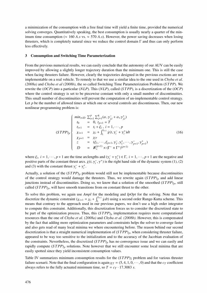
a minimization of the consumption with a free final time will yield a finite time, provided the numericalsolving converges. Quantitatively speaking, the best consumption is usually nearly a quarter of the min-imum time consumption (≈ 160 A.s vs. ≈ 570 A.s). However, the power saving decreases when losingthrusters, which is completely natural since we reduce the control domain Γ and thus can only performless effectively.

3 Consumption and Switching Time Parameterization

From the previous numerical results, we can easily conclude that the autonomy of our AUV can be easilyimproved by allowing a slightly longer trajectory duration than the minimum one. This is still the casewhen facing thrusters failure. However, clearly the trajectories designed in the previous esctions are notimplementable on a real vehicle. To remedy to that we use a similar idea to the one used in Chyba et al.(2008a) and Chyba et al (2008b), the so called Switching Time Parameterization Problem (S T PP). Werewrite the (OCP) into a particular (NLP). This (NLP), called (S T PP), is a discretization of the (OCP)where the control strategy is set to be piecewise constant with only a small number of discontinuities.This small number of discontinuities will prevent the computation of un-implementable control strategy.Let p be the number of allowed times at which one or several controls are discontinuous. Then, our newnonlinear programming problem is:

(S T PP)p

minz∈D∑p

i=1∑8

j=1(α−γ−j,i + α+γ+j,i)

t0 = 0, tp+1 = Tti+1 = ti + ξi , i = 1, · · · , pχi+1 = χi +

∫ ti+1

tiχ(t, γ−i + γ+

i )dtχp+1 = χT

z = (ξ1, · · · , ξp+1, γ−1 , γ

+1 , · · · , γ

−p+1, γ

+p+1)

D = IR(p+1)+ × (Γ− × Γ+)(p+1)

(16)

where ξi, i = 1, · · · , p + 1 are the time arclengths and (γ−i + γ+i ) ∈ Γ, i = 1, · · · , p + 1 are the negative and

positive parts of the constant thrust arcs. χ(t, γ−i , γ+) is the right hand side of the dynamic system (1), (2)

and (3) with the constant thrust γ−i + γ+i .

Actually, a solution of the (S T PP)p problem would still not be implementable because discontinuitiesof the control strategy would damage the thrusters. Thus, we rewrite again (S T PP)p and add linearjunctions instead of discontinuities. Doing so, we know that a solution of the smoothed (S T PP)p, stillcalled (S T PP)p, will have smooth transitions from on constant thrust to the other.

To solve this problem, we again use Ampl for the modeling and IpOpt for the solving. Note that wediscretize the dynamic constraint (χi+1 = χi +

∫ ti+1

tiχdt) using a second order Runge-Kutta scheme. This

means that contrary to the approach used in our previous papers, we don’t use a high order integratorto compute this constraint. Additionally, this discretization forces us to consider the discretized state tobe part of the optimization process. Thus, this (S T PP)p implementation requires more computationalresources than the one of Chyba et al. (2008a) and Chyba et al. (2008b). However, this is compensatedby the fact that adding more optimization parameters and constraints helps the solver to converge fasterand also gets read of many local minima we where encountering before. The reason behind our seconddiscretization is that a straight numerical implementation of (S T PP)p, when considering thruster failure,appeared to be way too sensitive to the initialization and to the accuracy of the Jacobian evaluation ofthe constraints. Nevertheless, the discretized (S T PP)p has no convergence issue and we can easily andrapidly compute (S T PP)p solutions. Note however that we still encounter some local minima that areeasily spotted since they yield inconsistent consumption values.

Table IV summarizes minimum consumption results for the (S T PP)2 problem and for various thrusterfailure scenarii. Note that the final configuration is again χT = (5, 4, 1, 0, · · · , 0) and that the cT coefficientalways refers to the fully actuated minimum time, so T = cT · 17.3083 s.

476

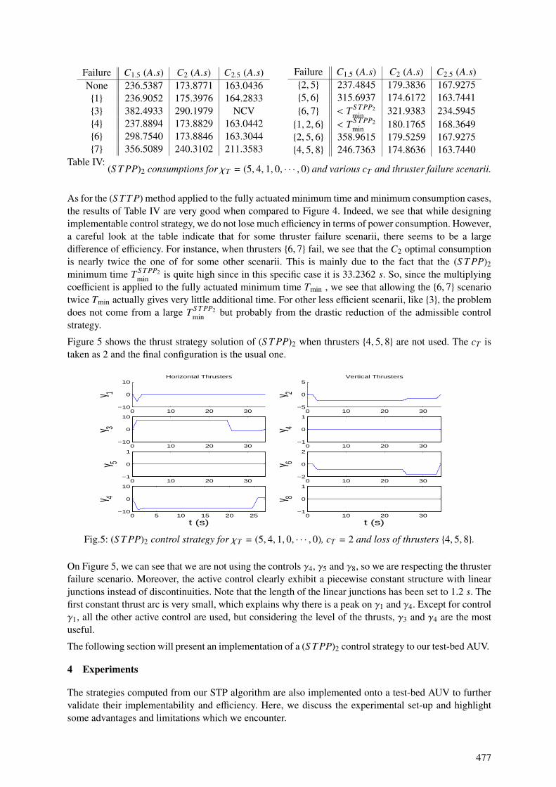
Failure C1.5 (A.s) C2 (A.s) C2.5 (A.s)None 236.5387 173.8771 163.04361 236.9052 175.3976 164.28333 382.4933 290.1979 NCV4 237.8894 173.8829 163.04426 298.7540 173.8846 163.30447 356.5089 240.3102 211.3583

Failure C1.5 (A.s) C2 (A.s) C2.5 (A.s)2, 5 237.4845 179.3836 167.92755, 6 315.6937 174.6172 163.74416, 7 < T S T PP2

min 321.9383 234.59451, 2, 6 < T S T PP2

min 180.1765 168.36492, 5, 6 358.9615 179.5259 167.92754, 5, 8 246.7363 174.8636 163.7440

Table IV:(S T PP)2 consumptions for χT = (5, 4, 1, 0, · · · , 0) and various cT and thruster failure scenarii.

As for the (S TT P) method applied to the fully actuated minimum time and minimum consumption cases,the results of Table IV are very good when compared to Figure 4. Indeed, we see that while designingimplementable control strategy, we do not lose much efficiency in terms of power consumption. However,a careful look at the table indicate that for some thruster failure scenarii, there seems to be a largedifference of efficiency. For instance, when thrusters 6, 7 fail, we see that the C2 optimal consumptionis nearly twice the one of for some other scenarii. This is mainly due to the fact that the (S T PP)2minimum time T S T PP2

min is quite high since in this specific case it is 33.2362 s. So, since the multiplyingcoefficient is applied to the fully actuated minimum time Tmin , we see that allowing the 6, 7 scenariotwice Tmin actually gives very little additional time. For other less efficient scenarii, like 3, the problemdoes not come from a large T S T PP2

min but probably from the drastic reduction of the admissible controlstrategy.

Figure 5 shows the thrust strategy solution of (S T PP)2 when thrusters 4, 5, 8 are not used. The cT istaken as 2 and the final configuration is the usual one.

0 10 20 30−10

0

10Horizontal Thrusters

γ 1

0 10 20 30−10

0

10

γ 3

0 10 20 30−1

0

1

γ 5

0 5 10 15 20 25−10

0

10

γ 4

t (s)

0 10 20 30−5

0

5Vertical Thrusters

γ 2

0 10 20 30−1

0

1

γ 4

0 10 20 30−2

0

2

γ 6

0 10 20 30−1

0

1

γ 8

t (s)

Fig.5: (S T PP)2 control strategy for χT = (5, 4, 1, 0, · · · , 0), cT = 2 and loss of thrusters 4, 5, 8.

On Figure 5, we can see that we are not using the controls γ4, γ5 and γ8, so we are respecting the thrusterfailure scenario. Moreover, the active control clearly exhibit a piecewise constant structure with linearjunctions instead of discontinuities. Note that the length of the linear junctions has been set to 1.2 s. Thefirst constant thrust arc is very small, which explains why there is a peak on γ1 and γ4. Except for controlγ1, all the other active control are used, but considering the level of the thrusts, γ3 and γ4 are the mostuseful.

The following section will present an implementation of a (S T PP)2 control strategy to our test-bed AUV.

4 Experiments

The strategies computed from our STP algorithm are also implemented onto a test-bed AUV to furthervalidate their implementability and efficiency. Here, we discuss the experimental set-up and highlightsome advantages and limitations which we encounter.

477

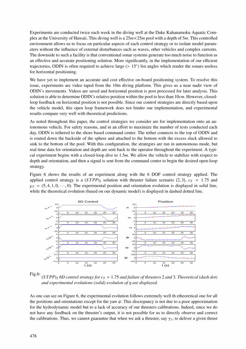
Experiments are conducted twice each week in the diving well at the Duke Kahanamoku Aquatic Com-plex at the University of Hawaii. This diving well is a 25m×25m pool with a depth of 5m. This controlledenvironment allows us to focus on particular aspects of each control strategy or to isolate model param-eters without the influence of external disturbances such as waves, other vehicles and complex currents.The downside to such a facility is that conventional sonar systems generate too much noise to function asan effective and accurate positioning solution. More significantly, in the implementation of our efficienttrajectories, ODIN is often required to achieve large (> 15) list angles which render the sonars uselessfor horizontal positioning.

We have yet to implement an accurate and cost effective on-board positioning system. To resolve thisissue, experiments are video taped from the 10m diving platform. This gives us a near nadir view ofODIN’s movements. Videos are saved and horizontal position is post processed for later analysis. Thissolution is able to determine ODIN’s relative position within the pool to less than 10cm. However, closed-loop feedback on horizontal position is not possible. Since our control strategies are directly based uponthe vehicle model, this open loop framework does not hinder our implementation, and experimentalresults compare very well with theoretical predictions.

As noted throughout this paper, the control strategies we consider are for implementation onto an au-tonomous vehicle. For safety reasons, and in an effort to maximize the number of tests conducted eachday, ODIN is tethered to the shore based command center. The tether connects to the top of ODIN andis routed down the backside of the sphere and attached to the bottom with the excess slack allowed tosink to the bottom of the pool. With this configuration, the strategies are run in autonomous mode, butreal time data for orientation and depth are sent back to the operator throughout the experiment. A typi-cal experiment begins with a closed-loop dive to 1.5m. We allow the vehicle to stabilize with respect todepth and orientation, and then a signal is sent from the command center to begin the desired open-loopstrategy.

Figure 6 shows the results of an experiment along with the 6 DOF control strategy applied. Theapplied control strategy is a (S T PP)2 solution with thruster failure scenario 2, 3, cT = 1.75 andχT = (5, 4, 1, 0, · · · , 0). The experimental position and orientation evolution is displayed in solid line,while the theoretical evolution (based on our dynamic model) is displayed in dashed dotted line.

0 5 10 15 20 25 30−10

0

106D Control

τ ν 1

0 5 10 15 20 25 30−5

0

5

τ ν 2

0 5 10 15 20 25 30−20

0

20

τ ν 3

0 5 10 15 20 25 30−5

0

5

τ Ω 1

0 5 10 15 20 25 30−5

0

5

τ Ω 2

0 5 10 15 20 25 30−0.2

0

0.2

τ Ω 3

t (s)

0 5 10 15 20 25 30−10

0

10Position

x

0 5 10 15 20 25 30−5

0

5

y

0 5 10 15 20 25 301

2

3

z

0 5 10 15 20 25 30−50

0

50

φ

0 5 10 15 20 25 30−50

0

50

θ

0 5 10 15 20 25 30−100

0

100

ψ

t (s)

Fig.6:(S T PP)2 6D control strategy for cT = 1.75 and failure of thrusters 2 and 3. Theoretical (dash dot)and experimental evolutions (solid) evolution of η are displayed.

As one can see on Figure 6, the experimental evolution follows extremely well th etheoretical one for allthe positions and orientations except for the yaw ψ. This discrepancy is not due to a poor approximationfor the hydrodynamic model but to a lack of accuracy of our thrusters calibrations. Indeed, since we donot have any feedback on the thruster’s output, it is not possible for us to directly observe and correctthe calibrations. Thus, we cannot guarantee that when we ask a thruster, say γ1, to deliver a given thrust

478

it is actually delivering exactly the demanded thrust. So we know that when we want to apply a surgeand sway control with no yaw (that is τΩ3 = 0), we inevitably get a phantom torque τΩ. This issue ofphantom thrust is of course present for all the 6 DOF control components. However, the yaw is moresensitive than the other state because its dynamic do not have any restoring forces that would dampen thecontrol inaccuracy. This discrepancy of the yaw evolution, implied that the AUV will not be orientatedas expected and that the surge and sway will not match perfectly the theoretical evolution. However, wecan see that while not being constant to zero, the yaw evolution does not explode and let the vehicle inthe good general direction: there is no discrepancy superior than 45 and the average of the yaw is notfar from 0.

5 Conclusion

As seen in the two previous sections, the control strategies we built have the advantage of both beingimplementable on our test-bed AUV and efficient in terms of power consumption. Our theoretical model,though not perfect, is very accurate when considering the inherent difficulties implied by the mediumthe vehicle is evolving in. Concerning the minimum consumption criterion as well as the thruster failurescenarii, we only uncovered the top of the iceberg and will need to study thoroughly and rigorously theimpact of various parameters such as buoyancy or final configuration. A central question to be answeredis the one of the controllability that was only scratched in this paper. Concerning our theoretical model, inorder to improve it we will need to work on a way to measure accurately the thrust applied by a thrusteror just the rotational speed of the shafts. Once this is done, we will need to work out a well definedinverse problem to identify each and every parameters intervening in our model.

6 Acknowledgments

Research supported by NSF grant DMS-030641 and DMS-0608583 and partially supported by ONRgrant N00014-03-1-0969, N00014-04-1-0751 and N00014-04-1-0751.

References

BERTRAM, V.; ALVAREZ, A. (2006), Hydrodynamic aspects of AUV design, 5th Int. Conf. ComputerApplications and Information Technology in the Maritime Industries, Leiden

BULLO, F.; LEWIS, A.D. (2004), Geometric Control of Mechanical Systems Modeling, Analysis, andDesign for Simple Mechanical Control Systems, Springer-Verlag, New York-Heidelberg-Berlin, 49 inTexts in Applied Mathematics

CHYBA, M.; HABERKORN, T.; SMITH, R.N.; WILKENS, G.R. (2007), Geometric Prop-erties of Singular Extremals for a Submerged Rigid Body, Preprint, University of Hawaii(http://www.hawaii.edu/ mchyba/publications/index.html)

CHYBA, M.; Haberkorn, T.; Smith, R.N.; Choi, S.K. (2008a), Design and Implementation of Time Ef-ficient Trajectories for Autonomous Underwater Vehicles, IEEE Journal of Ocean Engineering, 35/1,pp.63-76.

CHYBA, M.; Haberkorn, T.; Smith, R.N.; Choi, S.K. (2008b), Autonomous Underwater Vehicles: Devel-opment and Implementation of Time and Energy Efficient Trajectories, Ship technology Research, 55/2,pp.36-48.

CHYBA, M.; Haberkorn, T.; Singh, S.B.; Smith, R.N.; Choi, S.K. (2008c), Increasing Underwater Ve-hicle Autonomy by Reducing Energy Consumption, IEEE Journal of Ocean Engineering, submitted.

FOSSEN, T.I. (1994), Guidance and control of ocean vehicles, Wiley, New York

FOURER, R.; GAY, D.M.; KERNIGHAN, B.W. (1993), AMPL: A Modeling Language for MathematicalProgramming, Duxbury Press, Brooks-Cole Publ.

479

IMLAY, F.H. (1961), The complete expressions for added mass of a rigid body moving in an ideal fluid,Technical Report DTMB 1528

MACIVER, M.A.; FONTAINE, E.; BURDICK, J.W. (2004), Designing future underwater vehicles:Principles and Mechanisms of the Weakly Electric Fish, IEEE J. Oceanic Eng. 29/3

MOLNAR, L.; OMERDIC, E.; TOAL, D. (2005), Hydrodynamic aspects of AUV design, Ocean 2005Europe IEEE Conf., Brest

PONTRYAGIN, L.S.; BOLTYANSKI, B.; GAMKRELIDZE, R.; MICHTCHENKO, E.(1962), TheMathematical Theory of Optimal Processes Interscience, New York

WAECHTER, A.; BIEGLER, L.T. (2006), On the implementation of an interior-point filter-line searchalgorithm for large-scale nonlinear programming, Research Report RC 23149, IBM T.J. Watson Re-search Center, Yorktown

480

481

Shipbuilding Interim Product Identification and Classification System Based on Intelligent Analysis Tools

Cassiano M. de Souza, PENO/COPPE, Federal University of Rio de Janeiro, Rio de Janeiro/Brazil,

marins@peno.coppe.ufrj.br

Rafael Tostes, DENO/EP, Federal University of Rio de Janeiro, Rio de Janeiro/Brazil, tostes@ufrj.br

Abstract

The paper presents a methodology for application of Group Technology principles to shipbuilding by

developing a product classification system that uses artificial intelligence tools. The system is able to

classify in an effective way interim products considering the complex and multidimensional aspects of

manufacturing classification problems. A case study applies the system to a block classification problem.

1 Introduction

Shipbuilding industry is a unique industry and its organization models are found somewhere between the

construction industry and the manufacturing industry. World class shipbuilders have made an effort to

identify and apply the models and tools that best fit to their shipbuilding strategy in all different levels.

So, once their business plan, their shipbuilding policy and ship definition are established, the production

organization is set and the design and production tools are developed to support the shipyard’s activities.

High productivity shipyards tend to set their production models in order to consider different ship as a

different mix of similar interim products. This gives to the shipyard a more flexible product mix without

lowering the productivity levels. The way found to meet a flexible production and high productivity was

the adoption of Group Technology principles, where product design and manufacturing processes

similarities are identified and exploited in order to have an increase on the production scale for interim

products, even though the final product (ships) are different. In a production system with incorporated

Group Technology principles, interim products can be grouped in families with similar characteristics and

production processes. Usually two types of interim products attributes can be used to observe similarities:

(1) Design attributes such as shapes, material, dimensions and tolerances, and (2) Manufacturing

attributes such machine tools, operation sequence, batch size, production time. Depending on the family

size, a specialized process lane or work station can be implemented.

This work aims to develop an artificial intelligence system that is able to identify interim product families

and to classify a ship design accordingly to the identified families. So once a family has enough members,

specialized process lane can be designed based on this family’s attributes. The present work takes block

information from previous designs to identify block families based on similarities either on design or

manufacturing attributes. Specialized process lanes can be designed based on these attributes in order to

have different lanes for block families with significant different dimensions, steel and work contents. For

the identification of the block families, an unsupervised classification model (k-means) is used. A

database consisting of design and manufacturing attributes for different blocks is developed.

Using this database, an unsupervised classification model (k-means) is applied to identify block families

without any previous class information. Once families are identified, another classification model (neural

network) is applied to classify a new design. The input uses the previous database and the classes

obtained trough the k-means model. The neural network model is trained with this data and discriminant

functions are estimated to classify new data. The parameters of the tested neural network can be used to

apply this clustering strategy to other block sets.

482

2 Classification Problems

The need to recognize patterns in a quick and accurate way can be verified even on simple and daily basis

problem everyone faces. Recognizing faces and spoken words, reading handwritten characters,

interpreting images and making decisions based on the identified patterns are very simple tasks that

involve complex processes. Man has an impressive ability to identify patterns based on a continuous

development of highly sophisticated neural and cognitive systems. Pattern recognition problems are also

referred as classification problems and a vast literature is available showing considerable efforts to

develop computational systems to represent recognition and classification strategies.

There are a number of solutions proposed for classification problems. A regularly used and popular set of

tools between researchers in this area are clustering techniques. The main goal applying clustering

techniques is divide a group of objects in classes of similar elements called clusters. This division is made

through data analysis using mathematic algorithms that represent discriminant functions. A number of

authors have combined artificial intelligence with clustering techniques, developing intelligent data

analysis to build sophisticated classification models.

In this section a literature review will be presented concerning classification problems in the

manufacturing industry.

2.1 Manufacturing Industry

An important area of concern for manufacturing researchers is developing cellular manufacturing systems

(CMS) to enhance efficiency on production operations. The application of Group Technology (GT)

principles as a planning philosophy takes advantage of part similarity to reduce manufacturing costs,

Suresh and Slomp (2005). A main aspect of Group Technology is group parts with similarities in design

or manufacturing characteristics forming part families. Grouping similar parts leads to economies of scale

and allows flexible production with low costs. This problem is often referred in the literature as the Cell

Formation Problem (CFP).

When work is separated by problem categories using GT principles the statistical distribution of

productivity for each category will have well behaved statistical distribution. So, estimates for planning

and scheduling activities can be derived with a higher degree of certainty. Controlling project

performance is also facilitated if operations indicators are more predictable. Clustering models can be

used as a tool to identify product families accordingly to the principle of GT. The application of clustering

models to the CFP is common in the literature of manufacturing technology, Dagli (1994); Mujtaba and

Hussain (2001); Leondes (1997). The literature review related to clustering techniques applied to the CFP

indicates the suitability of artificial intelligence tools to develop efficient solutions. Onwubolu (1999)

uses self-organizing maps (SOM) neural network to recognize products and parts to identify feature

families and proposes the methodology for application in concurrent engineering where design and

manufacturing are integrated. Kao and Fu (2006) propose an ant-based clustering algorithm for

application on CFP and conclude that the methodology is able to solve these types of problems

effectively. Su (1995) uses fuzzy logic for part family formation and Kuo (1999) integrates neural

networks and fuzzy logic and develop an application of GT.

2.2 Shipbuilding Industry

Classification problems are also present in ship design and shipbuilding fields as in any other human

being activity. Nevertheless there have been just a few studies reported. Similar conclusion can be

considered regarding the application of artificial intelligence tools.

483

Kim et al. (2006) use a neural network to classify hull plates in order to consider in an effective way a cut-

down on processing costs in early stages of ship design. Caprace et al. (2007) present another application

of neural networks as part of a data mining analysis to filter data to yield straightening costs in

shipbuilding.

Group Technology (GT) in shipbuilding has been studied over 30 years, e.g. Gallagher et al. (1974),

Lamb (1988), Gribskov (1989). However the application of artificial intelligence tools to solve the CFP in

the shipbuilding industry has not yet been reported. Storch and Sukapanpotharam (2002,2003) have

presented interesting work in this direction developing the Common Generic Block (CGB) concept. This

work is in line with the work developed by Japanese builders and published in a series of studies edited

by the National Shipbuilding Research Program (NSRP). One of these studies, Okayama and Chirillo

(1982), introduces the Product Work Breakdown Structure (PWBS) that is concerned with applying GT

principles, so that the main product can be organized and planned to maintain productivity and

uninterrupted work flow. Chirillo (1989) highlights the importance of PWBS and the GT principles to

shipbuilding efficiency. This work proposes a methodology for GT principles application using artificial

intelligence tools to implement clustering models in the shipbuilding field.

3 Clustering Models

Clustering models using intelligent data analysis tools can be classified in two large groups: supervised

and unsupervised models. Basically, in a supervised model there is already information about classes and

the model estimates the existent discriminant function. Unsupervised models have the ability to classify

data without any previous class information. This section will present two methods for data preparation

(normalization and Principal Component Analysis) and two methods for data classification (k-means and

neural network).

3.1 Normalization

Clustering methods can be affected by difference of scale between attributes values. The problem solution

is normalizing all values of the attributes vector. The procedures that could be used to normalize these

vectors are:

− Procedure 1 - Normalize the attributes vector taking as a base the maximum and minimum

vectors, i.e. the vector with maximum values and another with minimum values of each attribute

from all objects. The expression used is:

)min()max(

)min()()(

^

xx

xtxtX

−

−=

x(t) is the attribute vector, min(x) is the minimum attribute vector and max(x) is the maximum

attribute vector.

− Procedure 2 - The normalization presented above can generate inaccurate results because of

outliers (attributes with values far different than other attributes values). So, this second

procedure is based on average values. Its expression is less sensitive to outliers:

)(

)()()(

^

xsdv

xavgtxtX

α

−=

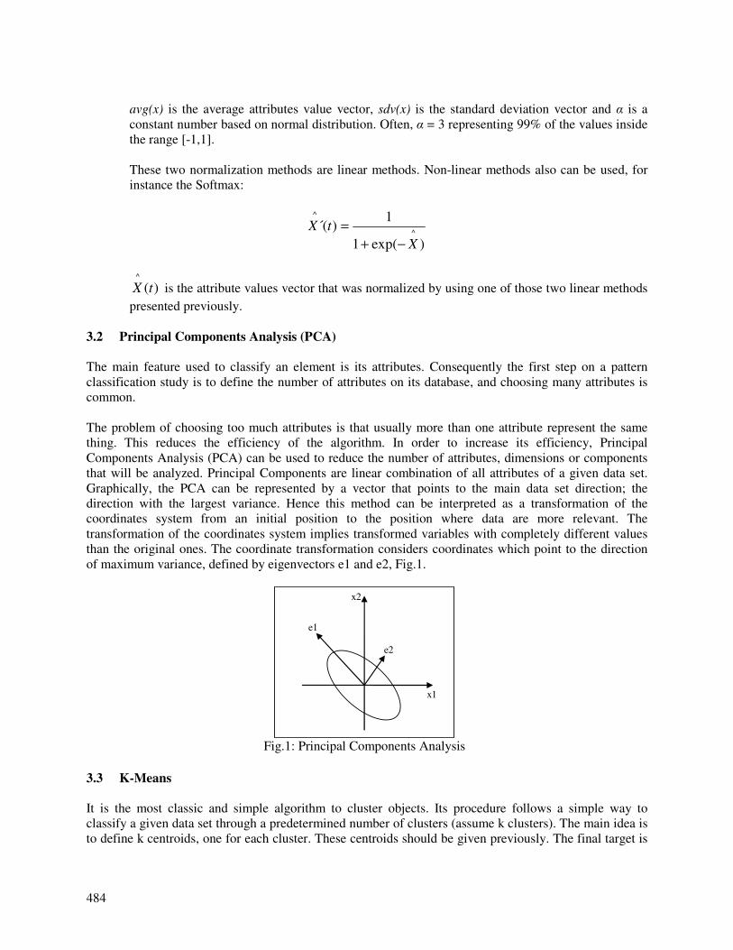
484

avg(x) is the average attributes value vector, sdv(x) is the standard deviation vector and α is a

constant number based on normal distribution. Often, α = 3 representing 99% of the values inside

the range [-1,1].

These two normalization methods are linear methods. Non-linear methods also can be used, for

instance the Softmax:

)exp(1

1)(

^

^

X

tX

−+

=

)(^

tX is the attribute values vector that was normalized by using one of those two linear methods

presented previously.

3.2 Principal Components Analysis (PCA)

The main feature used to classify an element is its attributes. Consequently the first step on a pattern

classification study is to define the number of attributes on its database, and choosing many attributes is

common.

The problem of choosing too much attributes is that usually more than one attribute represent the same

thing. This reduces the efficiency of the algorithm. In order to increase its efficiency, Principal

Components Analysis (PCA) can be used to reduce the number of attributes, dimensions or components

that will be analyzed. Principal Components are linear combination of all attributes of a given data set.

Graphically, the PCA can be represented by a vector that points to the main data set direction; the

direction with the largest variance. Hence this method can be interpreted as a transformation of the

coordinates system from an initial position to the position where data are more relevant. The

transformation of the coordinates system implies transformed variables with completely different values

than the original ones. The coordinate transformation considers coordinates which point to the direction

of maximum variance, defined by eigenvectors e1 and e2, Fig.1.

e2

e1

x1

x2

Fig.1: Principal Components Analysis

3.3 K-Means

It is the most classic and simple algorithm to cluster objects. Its procedure follows a simple way to

classify a given data set through a predetermined number of clusters (assume k clusters). The main idea is

to define k centroids, one for each cluster. These centroids should be given previously. The final target is

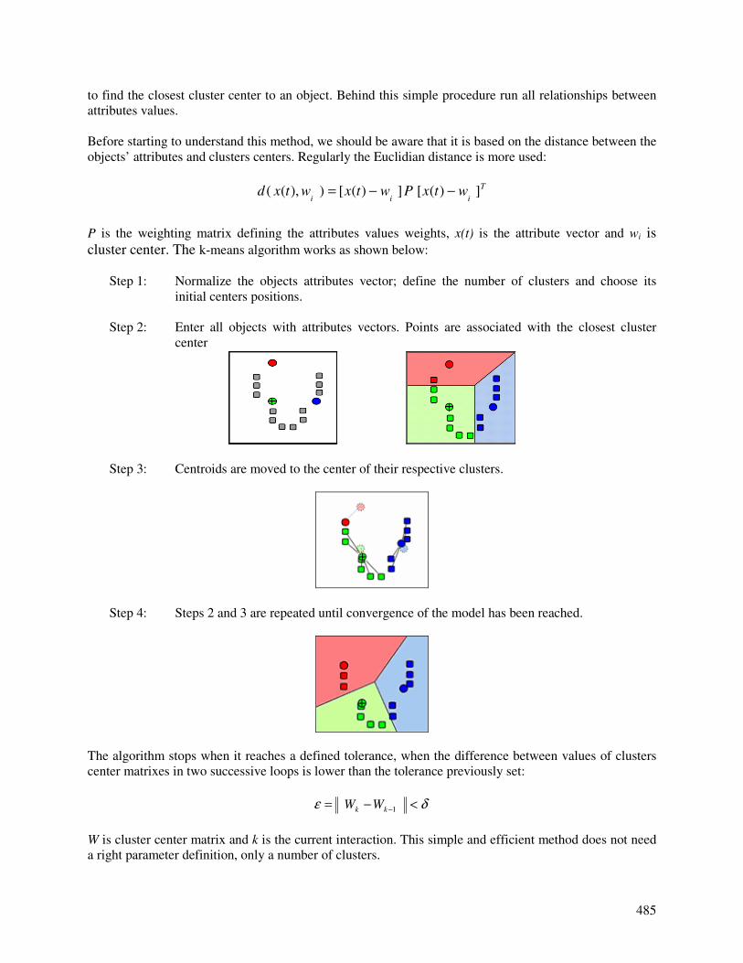
485

to find the closest cluster center to an object. Behind this simple procedure run all relationships between

attributes values.

Before starting to understand this method, we should be aware that it is based on the distance between the

objects’ attributes and clusters centers. Regularly the Euclidian distance is more used:

T

iiiwtxPwtxwtxd ])([])([)),(( −−=

P is the weighting matrix defining the attributes values weights, x(t) is the attribute vector and wi is

cluster center. The k-means algorithm works as shown below:

Step 1: Normalize the objects attributes vector; define the number of clusters and choose its

initial centers positions.

Step 2: Enter all objects with attributes vectors. Points are associated with the closest cluster

center

Step 3: Centroids are moved to the center of their respective clusters.

Step 4: Steps 2 and 3 are repeated until convergence of the model has been reached.

The algorithm stops when it reaches a defined tolerance, when the difference between values of clusters

center matrixes in two successive loops is lower than the tolerance previously set:

δε <−=−1kk WW

W is cluster center matrix and k is the current interaction. This simple and efficient method does not need

a right parameter definition, only a number of clusters.

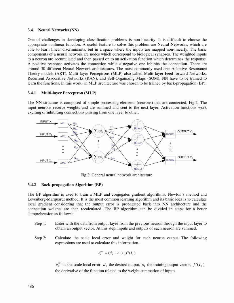
486

3.4 Neural Networks (NN)

One of challenges in developing classification problems is non-linearity. It is difficult to choose the

appropriate nonlinear function. A useful feature to solve this problem are Neural Networks, which are

able to learn linear discriminants, but in a space where the inputs are mapped non-linearly. The basic

components of a neural network are nodes which correspond to biological synapses. The weighted inputs

to a neuron are accumulated and then passed on to an activation function which determines the response.

A positive response activates the connection while a negative one inhibits the connection. There are

around 30 different Neural Network architectures. The most commonly used are: Adaptive Resonance

Theory models (ART), Multi layer Perceptrons (MLP) also called Multi layer Feed-forward Networks,

Recurrent Associative Networks (RAN), and Self-Organizing Maps (SOM). NN have to be trained to

learn the functions. In this work, an MLP architecture was chosen to be trained by back-propagation (BP).

3.4.1 Multi-layer Perceptron (MLP)

The NN structure is composed of simple processing elements (neurons) that are connected, Fig.2. The

input neurons receive weights and are summed and sent to the next layer. Activation functions work

exciting or inhibiting connections passing from one layer to other.

Fig.2: General neural network architecture

3.4.2 Back-propagation Algorithm (BP)

The BP algorithm is used to train a MLP and conjugates gradient algorithms, Newton’s method and

Levenberg-Marquardt method. It is the most common learning algorithm and its basic idea is to calculate

local gradient considering that the output error is propagated back into NN architecture and the

connection weights are then recalculated. The BP algorithm can be divided in steps for a better

comprehension as follows:

Step 1: Enter with the data from output layer from the previous neuron through the input layer to

obtain an output vector. At this step, inputs and outputs of each neuron are summed.

Step 2: Calculate the scale local error and weight for each neuron output. The following

expressions are used to calculate this information.

)('.)()0(

kkkk Ifode −=

)0(

ke is the scale local error, kd the desired output, ko the training output vector, kIf (' )

the derivative of the function related to the weight summation of inputs.

487

][]1[][][ ... s

ji

s

i

s

jcoef

s

ij wmxelw ∆+=∆−

][s

ijw∆ is the delta weight on connection joining i neuron in layer (s-1) to j neuron in layer

(s), coefl the learning coefficient, ][s

je the scale local error, ]1[ −s

ix the output vector, and

m the momentum coefficient.

Step 3: Calculate the same information for each layer using the expression:

).(.)0.1(. ]1[]1[][][][ ++

∑−=s

kj

s

kk

s

j

s

j

s

j wexxe

Step 4: Update all weights adding the previous weight with the delta weight.

3.4.2 Network setting

The number and values of the parameters used are different for each NN architecture. The parameters

used above are usually determined using research experience and trial-and-error. Examples of these

parameters are the number of hidden layers and the number of neurons that shall be given a priori. Other

important parameters are the learning coefficient that is responsible for adjusting the network weight

during the training and momentum coefficient that make the learning better by changing the weight from

the previous weight changes influence. Again, the researcher chooses based on experience or trial-and-

error. Finally, the data set must be divided in training and validation sets. The training set will be used to

train the NN and the validate set to check whether the network has the ability to classify rightly new data

sets or not.

4 Model Development

The GT application in this paper is developed using clustering models to solve the cell formation problem

(CFP) in order to identify possible alternatives to group blocks into families. The methodology is applied

here to block classification, but could be used to classify any interim product. The models were developed

from scratch using Matlab. The codes developed are listed below:

− Normalization normalizes the data set using the three methods described above

− Data analysis runs a PCA, checks database characteristics and returns plots to support data

analysis

− Distance calculator calculates distance between data points and clusters center using the

Euclidean and Manhattan distances

− K-means applies k-means classification allowing to choose the initial number of clusters, between

original and PCA transformed variables

− Neural network applies a three-layer MLP with back-propagation neural network to perform

classification allowing to choose the size of training and validation data sets, defines basic

topological aspects as number of neurons on each layer, the learning rate and number of epochs

The codes are applied to a database that consists of detailed design information for 30 blocks that form a

grand block (ring) of a Suezmax tanker. The database is restricted due to availability of information. All

blocks had to be modelled on a 3D product modelling system (Delmia V5) from scratch with very limited

resources to perform the task. Nevertheless, a bigger database can be used without additional coding

problems once codes were developed assuming larger databases could be available.

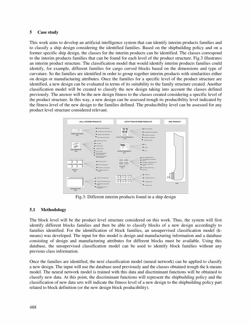
488

5 Case study

This work aims to develop an artificial intelligence system that can identify interim products families and

to classify a ship design considering the identified families. Based on the shipbuilding policy and on a

former specific ship design, the classes for the interim products can be identified. The classes correspond

to the interim products families that can be found for each level of the product structure. Fig.3 illustrates

an interim product structure. The classification model that would identify interim products families could

identify, for example, different families for cargo curved blocks based on the dimensions and type of

curvature. So the families are identified in order to group together interim products with similarities either

on design or manufacturing attributes. Once the families for a specific level of the product structure are

identified, a new design can be evaluated in terms of its suitability to the family structure created. Another

classification model will be created to classify the new design taking into account the classes defined

previously. The answer will be the new design fitness to the classes created considering a specific level of

the product structure. In this way, a new design can be assessed trough its producibility level indicated by

the fitness level of the new design to the families defined. The producibility level can be assessed for any

product level structure considered relevant.

FABRICATED PARTS(FP)

PARALLEL PART FROM PLATE

NON-PARALLEL PART FROM PLATE

INTERNAL PART FROM PLATE

PART FROM ROLLED SHAPE

SUB-ASSEMBLIES

(SA)

BLOCKS(B)

GRAND-BLOCKS

(GB)

SHIP

FRAME FOR FLAT PANEL

FLAT PANEL

CURVED PANEL

SUB-BLOCK PART

BUILT-UP PART

SMALL QUANTITY SIMILAR

SIZE SUB-ASSEMBLY

LARGE QUANTITY SIMILAR

SIZE SUB-ASSEMBLY

CARGO FLAT BLOCK

CARGO CURVED BLOCK

MACHINERY CURVED BLOCK

ACCOMMODATIONS FLAT

BLOCK

CARGO FLAT GRAND-BLOCK

CARGO CURVED GRAND-BLOCK

MACHINERY CURVED GRAND-

BLOCK

ACCOMMODATIONS FLAT

GRAND-BLOCK

HULL INTERIM PRODUCTS OUTFITTING INTERIM PRODUCTS

DECK COMPONENT

ACCOMMODATION COMPONENT

MACHINERY COMPONENT

ELECTRICAL COMPONENT

ELECTRICAL CABLE

OUTFITTING COMPONENTS

(OC)

PIPING COMPONENTS

(PC)

PIPE

FLANGE

VALVE

PALLETS(PL)

DECK COMPONENT PALLET

ACCOMMODATION COMPONENT

PALLET

MACHINERY COMPONENT PALLET

ELECTRICAL COMPONENT

PALLET

ELECTRICAL CABLE PALLET

PIPE PALLET

DECK UNIT

ACCOMMODATION UNIT

MACHINERY UNIT

ELECTRICAL UNIT

END PRODUCT

OU OU OU

OU OU OU

Fig.3: Different interim products found in a ship design

5.1 Methodology

The block level will be the product level structure considered on this work. Thus, the system will first

identify different blocks families and then be able to classify blocks of a new design accordingly to

families identified. For the identification of block families, an unsupervised classification model (k-

means) was developed. The input for this model is design and manufacturing information and a database

consisting of design and manufacturing attributes for different blocks must be available. Using this

database, the unsupervised classification model can be used to identify block families without any

previous class information.

Once the families are identified, the next classification model (neural network) can be applied to classify

a new design. The input will use the database used previously and the classes obtained trough the k-means

model. The neural network model is trained with this data and discriminant functions will be obtained to

classify new data. At this point, the discriminant functions will represent the shipbuilding policy and the

classification of new data sets will indicate the fitness level of a new design to the shipbuilding policy part

related to block definition (or the new design block producibility).

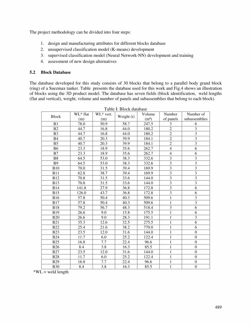
489

The project methodology can be divided into four steps:

1. design and manufacturing attributes for different blocks database

2. unsupervised classification model (K-means) development

3. supervised classification model (Neural Network-NN) development and training

4. assessment of new design alternatives

5.2 Block Database

The database developed for this study consists of 30 blocks that belong to a parallel body grand block

(ring) of a Suezmax tanker. Table presents the database used for this work and Fig.4 shows an illustration

of blocks using the 3D product model. The database has seven fields (block identification, weld lengths

(flat and vertical), weight, volume and number of panels and subassemblies that belong to each block).

Table I: Block database

Block WL* flat

(m)

WL* vert.

(m) Weight (t)

Volume

(m³)

Number

of panels

Number of

subassemblies

B1 78.0 50.9 58.7 247.5 3 6

B2 44.7 16.8 44.0 180.2 2 3

B3 44.7 16.8 44.0 180.2 2 3

B4 40.7 20.3 39.9 184.1 2 3

B5 40.7 20.3 39.9 184.1 2 3

B6 23.3 18.9 35.6 262.7 4 6

B7 23.3 18.9 35.6 262.7 4 6

B8 64.5 53.0 38.3 332.6 3 3

B9 64.5 53.0 38.3 332.6 3 3

B10 70.0 31.5 39.4 169.9 3 3

B11 62.8 38.7 39.4 169.9 3 3

B12 70.8 31.5 33.6 144.0 3 3

B13 70.8 31.5 33.6 144.0 3 3

B14 141.8 27.9 36.8 172.8 3 6

B15 126.0 43.7 36.8 172.8 3 6

B16 57.8 50.4 40.3 509.6 1 3

B17 57.8 50.4 40.3 509.6 1 3

B18 79.2 56.7 48.3 518.4 3 6

B19 26.6 9.0 15.8 175.5 1 6

B20 26.6 9.0 28.3 191.1 1 3

B21 35.3 12.6 32.5 275.5 1 6

B22 25.4 21.6 38.2 770.0 1 6

B23 23.5 12.0 31.6 144.0 1 0

B24 11.7 6.0 25.2 122.4 1 0

B25 16.8 7.7 22.4 96.6 1 0

B26 8.4 3.8 16.3 85.5 1 0

B27 23.5 12.0 31.6 144.0 1 0

B28 11.7 6.0 25.2 122.4 1 0

B29 16.8 7.7 22.4 96.6 1 0

B30 8.4 3.8 16.3 85.5 1 0

*WL = weld length

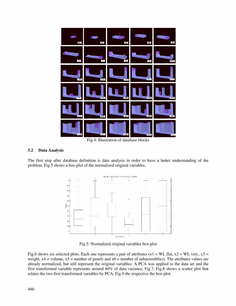
490

Fig.4: Illustration of database blocks

5.2 Data Analysis

The first step after database definition is data analysis in order to have a better understanding of the

problem. Fig.5 shows a box-plot of the normalized original variables.

Fig.5: Normalized original variables box-plot

Fig.6 shows six selected plots. Each one represents a pair of attributes (x1 = WL flat, x2 = WL vert., x3 =

weight, x4 = volume, x5 = number of panels and x6 = number of subassemblies). The attributes values are

already normalized, but still represent the original variables. A PCA was applied to the data set and the

first transformed variable represents around 60% of data variance, Fig.7. Fig.8 shows a scatter plot that

relates the two first transformed variables by PCA, Fig.9 the respective the box-plot.

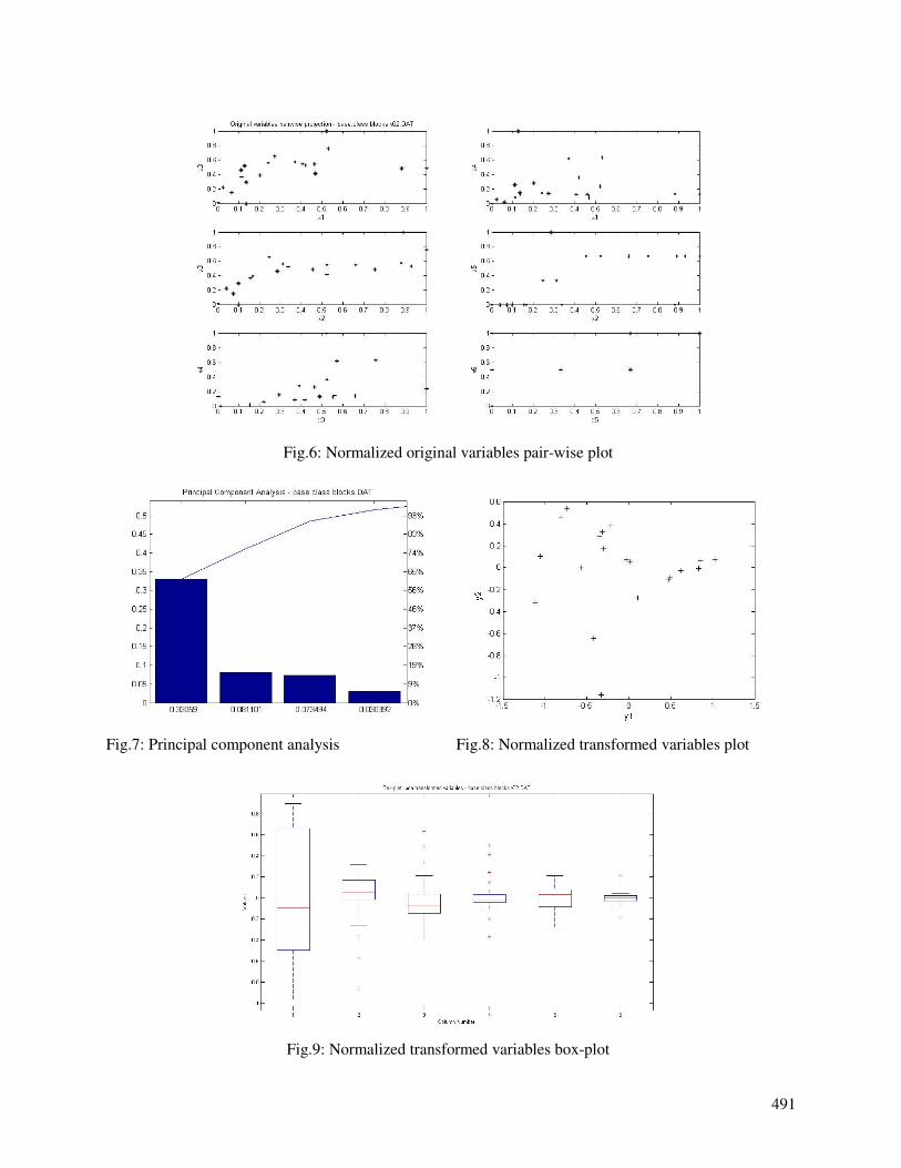
491

Fig.6: Normalized original variables pair-wise plot

Fig.7: Principal component analysis Fig.8: Normalized transformed variables plot

Fig.9: Normalized transformed variables box-plot

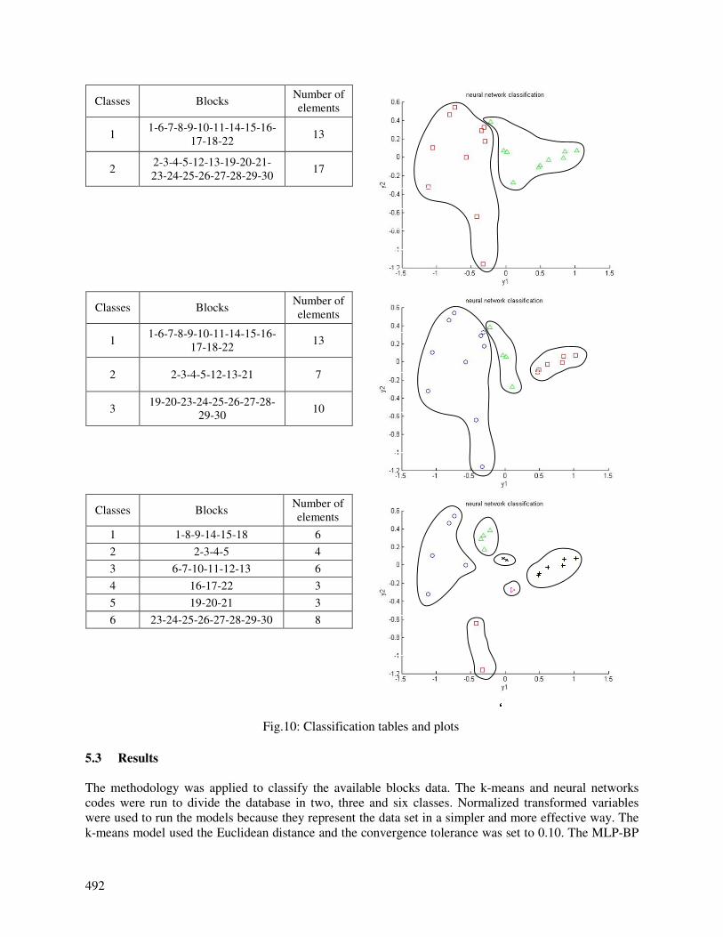
492

Classes Blocks Number of

elements

1 1-6-7-8-9-10-11-14-15-16-

17-18-22 13

2 2-3-4-5-12-13-19-20-21-

23-24-25-26-27-28-29-30 17

Classes Blocks Number of

elements

1 1-6-7-8-9-10-11-14-15-16-

17-18-22 13

2 2-3-4-5-12-13-21 7

3 19-20-23-24-25-26-27-28-

29-30 10

Classes Blocks Number of

elements

1 1-8-9-14-15-18 6

2 2-3-4-5 4

3 6-7-10-11-12-13 6

4 16-17-22 3

5 19-20-21 3

6 23-24-25-26-27-28-29-30 8

Fig.10: Classification tables and plots

5.3 Results

The methodology was applied to classify the available blocks data. The k-means and neural networks

codes were run to divide the database in two, three and six classes. Normalized transformed variables

were used to run the models because they represent the data set in a simpler and more effective way. The

k-means model used the Euclidean distance and the convergence tolerance was set to 0.10. The MLP-BP

493

neural network was configured to have six input neurons, one hidden layer with 10 neurons and two, three

and six output neurons for the two, three and six classes’ models respectively. The connection weights,

learning rate and tolerance were set to 0.5, 0.01 and 0.1 respectively. The activation function used was the

hyperbolic tangent and the maximum number of iterations was set to 100.

Due to limitations on database size, the data used to train the network was the same used to validate it,

although the code was developed to support any relation training/validation on the database. Fig.10 shows

the final results obtained using the neural network model. To apply the same NN that was validated to a

specific data set is necessary to save its topology and the main connection parameters. After that is

possible to classify any new single or set of block entries without any additional training and validation

effort. Saving the NN means to use the same discriminant functions estimated by the k-means algorithm.

To test how the system works considering different number of classes is necessary to go through the

whole process of running the k-means model, train and validate a NN. The ideal number of classes

depends on the numbers of specific process lanes planned to be implemented. However, the identification

of an ideal number of classes is another type of problem and is beyond the scope of this work.

6 Conclusions

The methodology presented on this work has shown a potential to be explored considering GT application

to shipbuilding. It combines an application of GT principles and intelligent clustering models to the CFP.

Understanding the product structure in a deeper way using intelligent data analysis gives an opportunity

to explore all the benefits of GT. The framework presented in this paper can be used to obtain a block

classification considering the complex and multidimensional aspects of the CFP. The results are

encouraging and indicate that the proposed methodology provides a reasonable solution to family

formation in the shipbuilding environment.

Additional research is being developed in order to assess different shipyards’ layout configurations

considering specific process lanes defined by the methodology proposed in this paper. Simulation models

are being developed in order to evaluate differences in production volume and productivity for different

process lanes configurations. By doing an evaluation of production flows will be possible to effectively

determine whether GT principles can lead to shipbuilding efficiency enhancements or not.

References

CAPRACE, J.D.; LOSSEAU, N.; ARCHAMBEAU, D.; RIGO, P. (2007), A data mining analysis

applied to a straightening process database, COMPIT’07, Cortona, pp.186-196

CHIRILLO, L.D. (1987), Flexible production indices, National Shipbuilding Research Program,

Maritime Administration in cooperation with Todd Pacific Shipyards Corporation

CHIRILLO, L.D. (1989), Product work breakdown - The challenge to production and design

engineers. J. Ship Production 5/2

DAGLI, C.H. (1994), Artificial neural networks for intelligent manufacturing, Chapman & Hall, New

York

DUDA, R.O.; HART, P.E.; STORK, D.G. (2001), Pattern classification, John Wiley, New York

GALLAGHER, C.C.; BANERJEE, S.K.E.; SOUTHERN, G. (1974), Group technology in the

shipbuilding industry, Int. J. Production Research 12/1

494

GRIBSKOV, J., (1989), A Group Technology Approach to Master Scheduling of Shipbuilding

Projects. J. of Ship Production, 5/4.

KAMRUZZAMAN, J.; BEGG, R.; SARKER, R. (2006), Artificial neural networks in finance

and manufacturing, Igi Global

KAO, Y.; FU, S.C. (2006), An ant-based clustering algorithm for manufacturing cell design, Int.

J. Adv. Manufacturing Technology 28, pp.1182-1189

KIM, S.Y.; MOON, B.Y.; KIM, D.E.; SHIN, S.C. (2006), Automation of hull plates classification

in ship design system using neural network method, Mech. Systems and Signal Proc. 20, pp.493-

504.

KUO, R.J.; CHI, S.C.; DEN, B.W. (1999), A fuzzy Kohonen's feature map neural network with

application to group technology, Neural Networks, IJCNN'99. Int. Joint Conf. 5, pp.3098-3101

KUO, R.J.; HO, L.M.; HU, C.M. (2002), Integration of self-organizing feature map and K-means

algorithm for market segmentation, Computers & Operations Research 29, pp.1475-1493

LAMB, T. (1988), Group technology in shipbuilding, J. Ship Production

LEONDES, C.T. (1997), Industrial & manufacturing systems (neural network systems techniques

and applications), Academic PR

MUJTABA, I.M.; HUSSAIN, M.A. (2001), Application of neural networks and other learning

technologies in process engineering, River Edge

OKAYAMA, Y.E.; CHIRILLO, L.D. (1982), Product work breakdown structure, Nat. Shipb.

Res. Program, Maritime Administration in cooperation with Todd Pacific Shipyards Corporation

ONWUBOLU, G.C. (1999), Design of parts for cellular manufacturing using neural network-

based approach, J. Intelligent Manufacturing 10, pp.251-265

PHAM, D.T.; DIMOV, S.S.; NGUYEN, C.D. (2004), An Incremental K-means algorithm, J.

Mech. Eng. Science 218, pp.783-795

RIBEIRO, J.F.F; MENGUELATI, S. (2002), Organização de um sistema de produção em células

de fabricação(in portuguese), Gestão e Produção 9/1, pp.62-77

STORCH, R.L.; SUKAPANPOTHARAM, S. (2002), Development of repeatable interim

products utilizing the common generic block concept, J. Ship Production 18/4, pp.195-202

STORCH, R.L.; SUKAPANPOTHARAM, S. (2003), Common generic block: mass

customization for shipbuilding, J. Engineering for the Maritime Environment 217, pp.79-94

SU, C.T. (1995), A fuzzy approach for part family formation, Industrial Automation and Control:

Emerging Technologies, International IEEE/IAS Conf., pp.289-292

SURESH, N.C.; SLOMP, J. (2005), Performance comparison of virtual cellular manufacturing

with functional and cellular layouts in DRC settings, Int. J. Production Res. 43/5, pp. 945-979

495

Towards a Consistent and Dynamic Simulation of Company Behaviour in the Maritime Sector

Jeroen F.J. Pruyn, Delft University of Technology, Delft/Netherlands, J.F.J.Pruyn@TUDelft.nl Ubald Nienhuis, Delft University of Technology, Delft/Netherlands, U.Nienhuis@TUDelft.nl Eddy van de Voorde, University of Antwerp, Antwerp/Belgium, eddy.vandevoorde@ua.ac.be

Hilde Meersman, University of Antwerp, Antwerp/Belgium, hilde.meersman@ua.ac.be Abstract This paper presents the general outline of an economic model dealing with company behaviour in the maritime sector, including, a macroeconomic sub-model from which various other sub-markets are derived. Shipyards, ship owners, suppliers, ports and banks operate and interact in that market. The aim is to be able to use the model both as a learning tool (game) and as a simulation tool. During the past year our work has been directed towards the selection and implementation of a multi country macroeconomic sub-model.

1. Introduction In the past economists and engineers have tried to create predictive models for the various shipping markets. With the development of econometrics in Holland in the 1930s, Tinbergen (1933) and Koopmans (1939) were one of the first to model the freight market. These efforts were focused towards the supply side of transport. Many of the later efforts were still focused on the bulk trade, both wet and dry, such as Norship (integrated tanker and bulk model), Hawdon’s tanker market model and Beenstock and Vergotis’ integrated tanker and bulk market. The integrated models are able to take into account the effects of OBO-ships as well, as these can trade in both markets, damping the profitability of both markets to some extend. On the other hand many national and international institutions continued to create econometric multi-country models to simulate the dynamics between the different nations in the world. One of the first global economic models was LINK which brought together several national economic models to create a global model. Next to that a number of central banks have their own models, in order to be able to monitor, amongst others, the effect of monetary policies. A third group offering dynamic simulations are models on a company level, some with great detail, others on a pure economic level, but with multiple enterprises and (limited) market functions. These contain a simplified (fixed) economic input and are used e.g. to predict possible production scenarios, but they are also a common tool in educational management games. This last option allows companies or persons to test out strategies without directly endangering the company itself. What would we get when we combine these three dynamic economic views and focus on the maritime market? A model would be obtained that is consistent on all three levels of economic activity, linking the macro-economic level with shipping markets, affecting individual players in those markets. This is exactly what we are trying to achieve within this part of the cooperation of Delft University of Technology and the University of Antwerp. 2. Model Outline It is attempted to develop a model where independent sub-models for maritime important country blocks create a global economy. From this model the demand for transport is derived and used as an input for the various maritime freight markets, like dry bulk, wet bulk and containerized goods. The changes in the freight markets have derived effects on the newbuilding, scrapping and second hand markets. The activities of ports, banks, ship owners, shipyards and suppliers within these markets are all represented in the model. To structure the model a modular approach has been chosen. Each

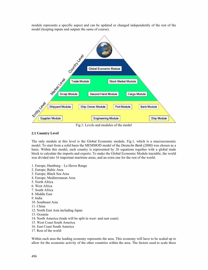
496

module represents a specific aspect and can be updated or changed independently of the rest of the model (keeping inputs and outputs the same of course).

Fig.1: Levels and modules of the model

2.1 Country Level The only module at this level is the Global Economic module, Fig.1, which is a macroeconomic model. To start from a solid basis the MEMMOD model of the Deutsche Bank (2000) was chosen as a basis. Within this model, each country is represented by 26 equations together with a global trade block to calculate the imports and exports. To make the Global Economic Module tractable, the world was divided into 16 important maritime areas, and an extra one for the rest of the world: 1. Europe; Hamburg – Le Havre Range 2. Europe; Baltic Area 3. Europe; Black Sea Area 4. Europe; Mediterranean Area 5. North Africa 6. West Africa 7. South Africa 8. Middle East 9. India 10. Southeast Asia 11. China 12. North East Asia including Japan 13. Oceania 14. North America (trade will be split in west- and east coast) 15. West Coast South America 16. East Coast South America 17. Rest of the world Within each area the leading economy represents the area. This economy will have to be scaled up to allow for the economic activity of the other countries within the area. The factors used to scale these

497

economies include population and total production, but others might be necessary as well. We are aware of the fact that there will be a loss of detail and accuracy in the information, yet the first goal of the project is a consistent economic environment to allow for the simulation of economic events. 2.2 Market Level The first module at this level is the trade module. It will take the values for import & export from the macroeconomic module and convert these into trade volumes and flows between the different trade blocks. To do this, imports and exports will need to be split into investments/service trade and money used for trade in goods. Elements other than import and export values could play a role here. We assume a fixed ratio between the goods transported between two countries, in order to establish a commodity price for the exports. Total trade and specific trade will follow. An extra step takes into account the efficiency of transport based on work by Eriksen (1977), who demonstrated that when prices for maritime transport rise, the trade patterns approach closer to their optimal state (as derived from common source-drain calculations used in Operations Research Hillier and Lieberman (2001)). This causes fluctuations in transport routes and distances. The Cargo module has two functions. First it calculates the various freight rates, using the demand from the trade module and the supply curve from the ship module (will be explained later). Next to that it determines the available cargo parcels for the active ship owners. A system for brokering will be developed as well. The combined effects of the freight rates for all the goods markets can be noticed in the next two modules, those of the second hand vessels and scrap market. Combined with the shipyard module, they provide a link between the various freight markets. Next to that the second hand and scrap market will also provide a market place for enterprises to sell their vessels against the current prices. The shipyard module will be discussed in more detail later. The last module at the market level is the stock market. This is not so much related to the other markets, but linked to the performance and trade in stocks of the companies represented as single enterprises in the model. It is only used for the gaming variant of the game and to allow the creation of a company active in the different fields and checking its performance against single players (e.g. a ship owner could also own a shipyard where he could buy ships at cost price. This would limit the profits of the shipyard, but increasing the potential profits for the fleet, as the vessel was bought at a price below market.) 2.3 The Entity level We referred already several times to the ship owners. This corresponding module does not only contain the total supply of shipping, but also incorporates entities that represent a ship owner. This role can be played by both humans and automatons. Automatons can be used to represent competition within the market, or to simulate all entities in this module, when the focus is on the shipbuilding area rather than the shipping area. On a macro-economic level Demand for ships is modelled, forming input for the Shipyard, Second hand and Scrap modules. The shipyard module shows a lot of analogy with the ship owner module. It is a macroeconomic representation of total global shipyard supply and either automatons or players can play the role of shipyard manager. As such they take in new orders, do the production planning, invest in research and new production development, etc. The engineering module is representing the shipyard’s design and engineering departments. Based on some limited targets, ship lay-out and properties, production time and cost, etc. are calculated; the amount of research and the technology level of the shipyard will also affect the outcome of the calculation. Each ship can be unique within the model, very similar to real life.

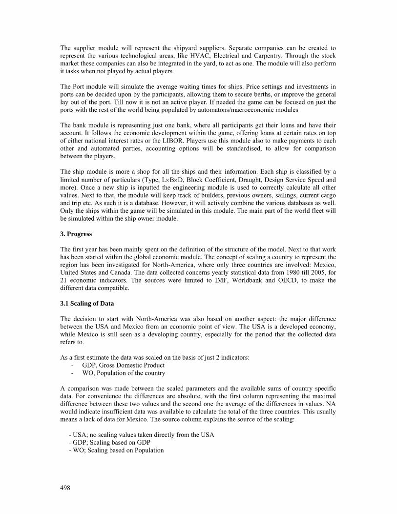
498

The supplier module will represent the shipyard suppliers. Separate companies can be created to represent the various technological areas, like HVAC, Electrical and Carpentry. Through the stock market these companies can also be integrated in the yard, to act as one. The module will also perform it tasks when not played by actual players. The Port module will simulate the average waiting times for ships. Price settings and investments in ports can be decided upon by the participants, allowing them to secure berths, or improve the general lay out of the port. Till now it is not an active player. If needed the game can be focused on just the ports with the rest of the world being populated by automatons/macroeconomic modules The bank module is representing just one bank, where all participants get their loans and have their account. It follows the economic development within the game, offering loans at certain rates on top of either national interest rates or the LIBOR. Players use this module also to make payments to each other and automated parties, accounting options will be standardised, to allow for comparison between the players. The ship module is more a shop for all the ships and their information. Each ship is classified by a limited number of particulars (Type, L×B×D, Block Coefficient, Draught, Design Service Speed and more). Once a new ship is inputted the engineering module is used to correctly calculate all other values. Next to that, the module will keep track of builders, previous owners, sailings, current cargo and trip etc. As such it is a database. However, it will actively combine the various databases as well. Only the ships within the game will be simulated in this module. The main part of the world fleet will be simulated within the ship owner module. 3. Progress The first year has been mainly spent on the definition of the structure of the model. Next to that work has been started within the global economic module. The concept of scaling a country to represent the region has been investigated for North-America, where only three countries are involved: Mexico, United States and Canada. The data collected concerns yearly statistical data from 1980 till 2005, for 21 economic indicators. The sources were limited to IMF, Worldbank and OECD, to make the different data compatible. 3.1 Scaling of Data The decision to start with North-America was also based on another aspect: the major difference between the USA and Mexico from an economic point of view. The USA is a developed economy, while Mexico is still seen as a developing country, especially for the period that the collected data refers to. As a first estimate the data was scaled on the basis of just 2 indicators:

- GDP, Gross Domestic Product - WO, Population of the country

A comparison was made between the scaled parameters and the available sums of country specific data. For convenience the differences are absolute, with the first column representing the maximal difference between these two values and the second one the average of the differences in values. NA would indicate insufficient data was available to calculate the total of the three countries. This usually means a lack of data for Mexico. The source column explains the source of the scaling:

- USA; no scaling values taken directly from the USA - GDP; Scaling based on GDP - WO; Scaling based on Population

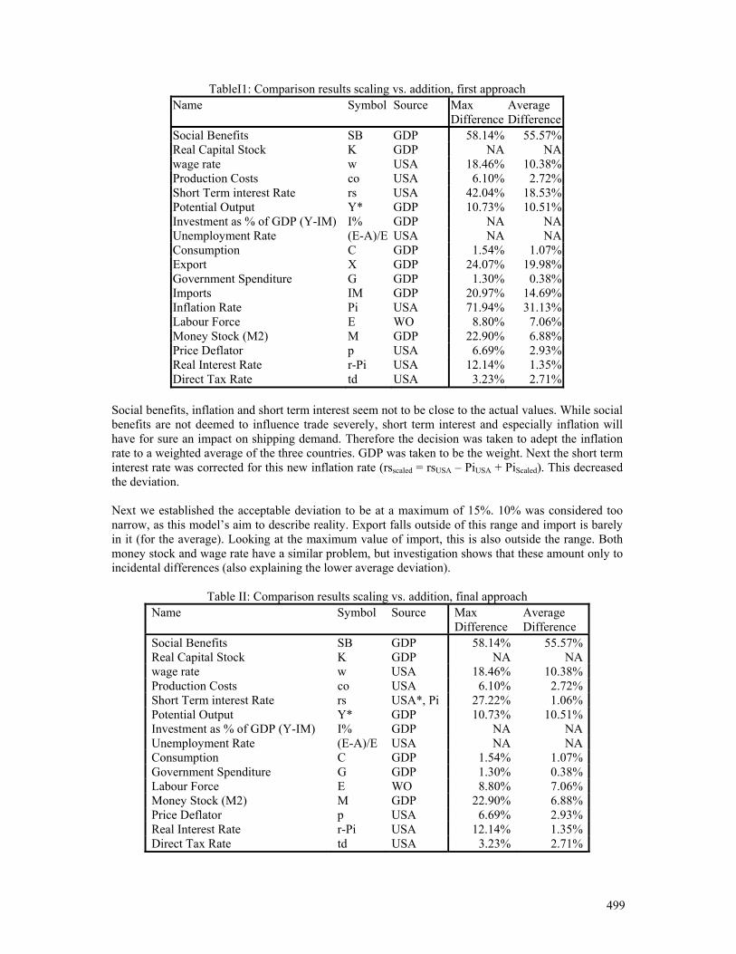
499

TableI1: Comparison results scaling vs. addition, first approach Name Symbol Source Max

DifferenceAverage Difference

Social Benefits SB GDP 58.14% 55.57% Real Capital Stock K GDP NA NA wage rate w USA 18.46% 10.38% Production Costs co USA 6.10% 2.72% Short Term interest Rate rs USA 42.04% 18.53% Potential Output Y* GDP 10.73% 10.51% Investment as % of GDP (Y-IM) I% GDP NA NA Unemployment Rate (E-A)/E USA NA NA Consumption C GDP 1.54% 1.07% Export X GDP 24.07% 19.98% Government Spenditure G GDP 1.30% 0.38% Imports IM GDP 20.97% 14.69% Inflation Rate Pi USA 71.94% 31.13% Labour Force E WO 8.80% 7.06% Money Stock (M2) M GDP 22.90% 6.88% Price Deflator p USA 6.69% 2.93% Real Interest Rate r-Pi USA 12.14% 1.35% Direct Tax Rate td USA 3.23% 2.71%

Social benefits, inflation and short term interest seem not to be close to the actual values. While social benefits are not deemed to influence trade severely, short term interest and especially inflation will have for sure an impact on shipping demand. Therefore the decision was taken to adept the inflation rate to a weighted average of the three countries. GDP was taken to be the weight. Next the short term interest rate was corrected for this new inflation rate (rsscaled = rsUSA – PiUSA + PiScaled). This decreased the deviation. Next we established the acceptable deviation to be at a maximum of 15%. 10% was considered too narrow, as this model’s aim to describe reality. Export falls outside of this range and import is barely in it (for the average). Looking at the maximum value of import, this is also outside the range. Both money stock and wage rate have a similar problem, but investigation shows that these amount only to incidental differences (also explaining the lower average deviation).

Table II: Comparison results scaling vs. addition, final approach Name Symbol Source Max

Difference Average Difference

Social Benefits SB GDP 58.14% 55.57% Real Capital Stock K GDP NA NA wage rate w USA 18.46% 10.38% Production Costs co USA 6.10% 2.72% Short Term interest Rate rs USA*, Pi 27.22% 1.06% Potential Output Y* GDP 10.73% 10.51% Investment as % of GDP (Y-IM) I% GDP NA NA Unemployment Rate (E-A)/E USA NA NA Consumption C GDP 1.54% 1.07% Government Spenditure G GDP 1.30% 0.38% Labour Force E WO 8.80% 7.06% Money Stock (M2) M GDP 22.90% 6.88% Price Deflator p USA 6.69% 2.93% Real Interest Rate r-Pi USA 12.14% 1.35% Direct Tax Rate td USA 3.23% 2.71%

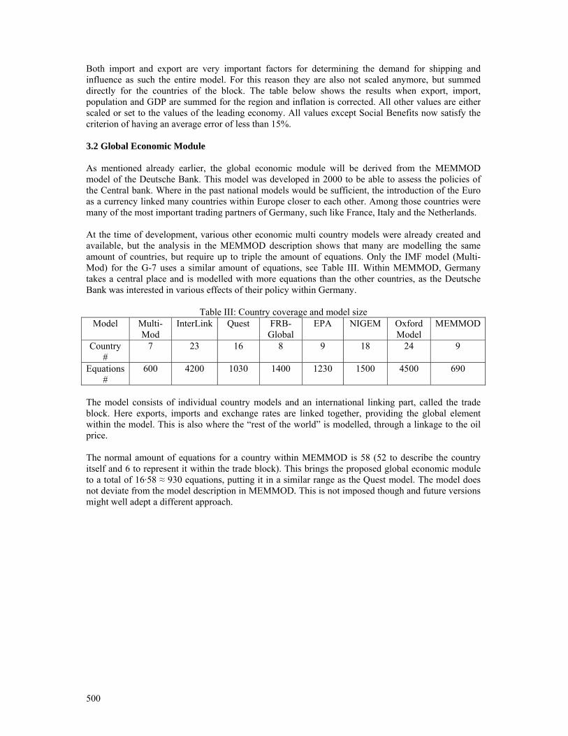
500

Both import and export are very important factors for determining the demand for shipping and influence as such the entire model. For this reason they are also not scaled anymore, but summed directly for the countries of the block. The table below shows the results when export, import, population and GDP are summed for the region and inflation is corrected. All other values are either scaled or set to the values of the leading economy. All values except Social Benefits now satisfy the criterion of having an average error of less than 15%. 3.2 Global Economic Module As mentioned already earlier, the global economic module will be derived from the MEMMOD model of the Deutsche Bank. This model was developed in 2000 to be able to assess the policies of the Central bank. Where in the past national models would be sufficient, the introduction of the Euro as a currency linked many countries within Europe closer to each other. Among those countries were many of the most important trading partners of Germany, such like France, Italy and the Netherlands. At the time of development, various other economic multi country models were already created and available, but the analysis in the MEMMOD description shows that many are modelling the same amount of countries, but require up to triple the amount of equations. Only the IMF model (Multi-Mod) for the G-7 uses a similar amount of equations, see Table III. Within MEMMOD, Germany takes a central place and is modelled with more equations than the other countries, as the Deutsche Bank was interested in various effects of their policy within Germany.

Table III: Country coverage and model size Model Multi-

Mod InterLink Quest FRB-

Global EPA NIGEM Oxford

Model MEMMOD

Country #

7 23 16 8 9 18 24 9

Equations #

600 4200 1030 1400 1230 1500 4500 690

The model consists of individual country models and an international linking part, called the trade block. Here exports, imports and exchange rates are linked together, providing the global element within the model. This is also where the “rest of the world” is modelled, through a linkage to the oil price. The normal amount of equations for a country within MEMMOD is 58 (52 to describe the country itself and 6 to represent it within the trade block). This brings the proposed global economic module to a total of 16·58 ≈ 930 equations, putting it in a similar range as the Quest model. The model does not deviate from the model description in MEMMOD. This is not imposed though and future versions might well adept a different approach.

501

References BEENSTOCK, M.; VERGOTTIS, A. (1993), Econometric modelling of world shipping, Chapman & Hall TINBERGEN, J. (1933), Vraag en aanbod van scheepsruimte, De Nederlandse Conjunctuur, March, pp.23-35 KOOPMANS, T.C. (1939), Tanker freight rates and tankship buildings, Haarlem DEUTSCHE BANK (2000). Macro-econometric multi-country model: MEMMOD, Deutsche Bank ERIKSEN, I.E. (1977), The demand for bulk ship services, Norwegian Maritime Research 2, pp.22-6 HILLIER; LIEBERMAN (2001), Introduction to operations research, 7th Ed. McGraw Hill IMF, World economic outlook database for October 2007, www.imf.org WORLDBANK, Worldbank Databank, www.worldbank.org OECD, Webbrowser for OECD Stat, stats.oecd.org

Optimization of Composite Boat Hull StructuresAdam Sobey, James Blake, Ajit Shenoi, University of Southampton, Southampton/England,

james@ship.soton.ac.uk

Abstract

There is growing competition amongst builders of mega- and super-yachts due to growth of new com-panies and improving capabilities of existing companies. This increases pressure on designers and pro-duction engineers to deliver high quality vessels at optimal prices. The ever tightening legislation onenvironmental issues will increase pressure to create green boats using cleaner production methods.Many boats utilise FRP in their structures and optimisation, minimising weight and cost, can lead toimproved performance. To this end the paper determines design solutions for top-hat stiffened panelsbased on first principles, in comparison with classification society rules, and optimised using geneticalgorithms.

Nomenclatureai Area of stiffener elements, i q(x,y) Pressure at a given point on plateamn Coefficient for grillage analysis Qmn,Qi j Reduced Stiffness termsAi j Laminate stiffness terms t,tk Thickness of laminate or ply, kb,g Number of transverse beams and longitudinal girders u0,v0,w0,φ0,φ0 Initial conditions of TSDTB,L Breadth and length of panels Umn,Vmn,Wmn,Xmn,Ymn Coefficients for initial conditions of TSDTdna Vertical distance to the neutral axis for each element, i w DeflectionDg,b Structural rigidity of girders and beams wn Genetic algorithm weighting variableE1,2 Young’s modulus of each ply, k, in each element, i Xn Genetic algorithm output variableG12 Shear modulus of ply, k, of element, i z Height of laminateIb,g Moment of inertia of beam or girder element, i Zb,g Vertical distance from the neutral axis of the beam or girderIcx Moment of inertia about the x-plane γ0,1 Stiffness functionsm,n Wave numbers ε0,1,2 Stiffness functionsMg,b Moments of girders or beams σmax Maximum stressp Pressure υ1,2 Poissons ratiopn Genetic algorithm importance weighting

1 Introduction

Boat design involves interdependencies between different subsystems of a vessel. It is the relationshipbetween these subsystems that determines the difference between a design that meets customer require-ments and makes a profit or one that fails to meet these criteria. “Concurrent engineering” uses paralleldesign processes with interdependent project teams to ensure that all the expertise of the design engi-neers are utilised during the entire span of the design. As a result, the relationships between the differentsubsystems of the boat are identified, impacts of changes readily assessed and ultimately producing aboat targeting customer requirements. As part of concurrent engineering, “design for production” cre-ates links between designing a boat for function while also producing at reduced cost, this leads to acost effective and efficient final product. Part of a concurrent engineering approach requires analysis ofstructural components, compromising customer requirements and cost whilst optimising the design forproduction.

Finding the optimum solution between effective design and low cost makes design complex due to nu-merous inputs and the interactions between each variable. It has been said that 5-7% of a product’s costcomes from the design and this can have an effect of 70-80% on the final cost Swift (2003). It is there-fore important that the design stage is done quickly while fulfilling customer requirements. Being first tomarket is also a factor governing overall sales, this combined with fast design, allows for either increasedquality or reduced cost and adds emphasis to a fast design process. Computational methods are increas-ingly being used to decrease the time taken to optimise these designs while still accurately finding theoptimum result.

Boat production works closely with classification society rules as conforming to these rules has a certainimplicit recognition in port legislation. It is therefore important to make sure that either classification

502

society rules are used, relevant to the country sold in, or that first principle methods are determined safeby those same societies. Classification society rules use safety factors to ensure that the boats producedwill not suffer failure during use. These safety factors, while ensuring a safe boat and fast design cycle,often mean that the topologies developed are heavier and thicker than can be calculated from first prin-ciple methods. ISO 12215-5 for scantling determination has recognised this fact and has tried to reducethese safety factors Curry (2004). However it might still be possible to produce boats that are cheaperto build but are also more efficient by design using first principles thereby increasing performance andenvironmental friendliness. First principle methods can be passed through classification societies but theprocess can be expensive as all calculations must be carefully checked and this process incurs added costand increased design time. It is therefore important that if these methods are to be used that they aremodeled accurately and give large increases in either cost effectiveness or boat efficiency.

This paper develops a method of structural optimisation for stiffened FRP boat panels allowing opti-misation between cost and mass of stiffened panels. The paper uses genetic algorithms for optimisationcombined with elastic stress modified grillage theory for stiffener structural analysis and third order sheardeformation theory for the plate structural analysis. The method also develops an optimisation algorithmusing classification society rules, the example of which is Lloyd’s Register Rules and Regulations for theClassification of Special Service Craft. This comparison allows a cost analysis between a first principlemethod and classification society rules to determine the benefits between the two methods and investi-gate potential cost savings. Combined with a concurrent engineering approach this method would alsogive a fast method to determine performance efficiencies that could be developed using hull scantlingsgenerated from first principles. This will allow development of “greener”, more efficient and cheaperboat hulls.

2 Structural Analysis

The method of structural analysis that has been used is based upon Navier method grillage theory as itcan be shown that the predictable response of a grillage can be matched to that of stiffened plates, whichin themselves are difficult to solve analytically. It can be seen from Maneepan (2007) that the valuesfrom the Navier method grillage analysis, developed by Vedeler (1945) gives a close approximationto the exact answer while also more computationally efficient than other grillage methods. The Naviermethod is based on the determination of deflections at the intersecting points found between longitudinalgirders (g) and the transverse beams (b) seen in Fig.1. It is then possible to determine the momentsin the stiffeners allowing an investigation of the stresses and strains. This method has been used formany years for structural analysis of isotropic plates. Datoo (1991) develops a method based on elasticstress analysis, covered in more detail in section 2.2, that allows orthotropic materials to be analysed.The elastic equivalent properties are developed by splitting each stiffener into four separate elements, i,labeled in Fig.2. Each of these elements can have different properties and each ply of each element, k,can also be analysed using different materials and ply angles.

2.1 Grillage analysis

The grillage analysis uses the Navier summations of points within the grillage to develop the deflectionof the stiffeners. In the examples shown in section 4 the values of the wave numbers, m and n, have beenkept at 17 as higher numbers extended computational time with only small increases in accuracy. Theequation giving deflection of the stiffened plate can be seen in Eq.1 and is a double summation dependenton the wave numbers given

w(x, y) =

∞∑m=1

∞∑n=1

amn sinmπx

Lsin

nπyB

(1)

where the value of amn is a coefficient found from Eq.2. The coefficient amn is dependent on the flexuralrigidities (Dg,b) found from Eq.13 as part of the elastic equivalent properties.

503

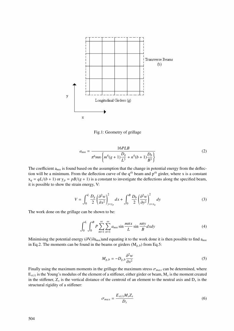
Fig.1: Geometry of grillage

amn =16PLB

π6mn

m4(g + 1)Dg

L3 + n4(b + 1)Db

B3

(2)

The coefficient amn is found based on the assumption that the change in potential energy from the deflec-tion will be a minimum. From the deflection curve of the qth beam and pth girder, where x is a constantxq = qL/(b + 1) or yp = pB/(g + 1) is a constant to investigate the deflections along the specified beam,it is possible to show the strain energy, V:

V =

∫ L

0

Dg

2

(∂2w∂x2

)2

y=yp

dx +

∫ B

0

Db

2

(∂2w∂y2

)2

x=xq

dy (3)

The work done on the grillage can be shown to be:

∫ L

0

∫ B

0P∞∑

m=1

∞∑n=1

amn sinmπx

Lsin

nπyB

dxdy (4)

Minimising the potential energy (∂V/∂amn)and equating it to the work done it is then possible to find amn

in Eq.2. The moments can be found in the beams or girders (Mg,b) from Eq.5:

Mg,b = −Dg,b∂2w∂x2 (5)

Finally using the maximum moments in the grillage the maximum stress σmax can be determined, whereEs(i) is the Young’s modulus of the element of a stiffener, either girder or beam, Ms is the moment createdin the stiffener, Zs is the vertical distance of the centroid of an element to the neutral axis and Ds is thestructural rigidity of a stiffener:

σmax =Es(i)MsZs

Ds(6)

504

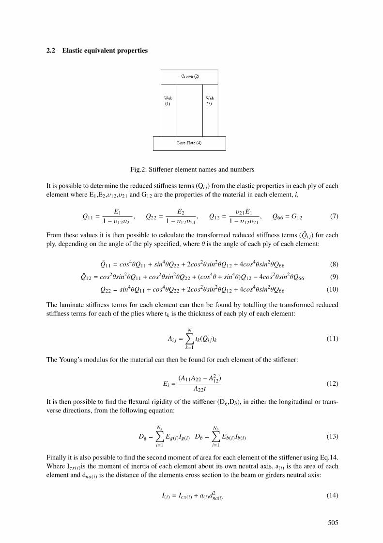
2.2 Elastic equivalent properties

Fig.2: Stiffener element names and numbers

It is possible to determine the reduced stiffness terms (Qi j) from the elastic properties in each ply of eachelement where E1,E2,υ12,υ21 and G12 are the properties of the material in each element, i,

Q11 =E1

1 − υ12υ21, Q22 =

E2

1 − υ12υ21, Q12 =

υ21E1

1 − υ12υ21, Q66 = G12 (7)

From these values it is then possible to calculate the transformed reduced stiffness terms (Qi j) for eachply, depending on the angle of the ply specified, where θ is the angle of each ply of each element:

Q11 = cos4θQ11 + sin4θQ22 + 2cos2θsin2θQ12 + 4cos4θsin2θQ66 (8)

Q12 = cos2θsin2θQ11 + cos2θsin2θQ22 + (cos4θ + sin4θ)Q12 − 4cos2θsin2θQ66 (9)

Q22 = sin4θQ11 + cos4θQ22 + 2cos2θsin2θQ12 + 4cos4θsin2θQ66 (10)

The laminate stiffness terms for each element can then be found by totalling the transformed reducedstiffness terms for each of the plies where tk is the thickness of each ply of each element:

Ai j =

N∑k=1

tk(Qi j)k (11)

The Young’s modulus for the material can then be found for each element of the stiffener:

Ei =(A11A22 − A2

12)A22t

(12)

It is then possible to find the flexural rigidity of the stiffener (Dg,Db), in either the longitudinal or trans-verse directions, from the following equation:

Dg =

Ng∑i=1

Eg(i)Ig(i) Db =

Nb∑i=1

Eb(i)Ib(i) (13)

Finally it is also possible to find the second moment of area for each element of the stiffener using Eq.14.Where Icx(i)is the moment of inertia of each element about its own neutral axis, a(i) is the area of eachelement and dna(i) is the distance of the elements cross section to the beam or girders neutral axis:

I(i) = Icx(i) + a(i)d2na(i) (14)

505

The flexural rigidity found using stress analysis can then be used to determine the stresses in the stiffenersusing the Navier grillage method.

2.3 Higher Order Shear Deformation Theory

The grillage method that has been used finds the maximum stresses in the stiffeners by assuming that allof the load is passed through to the stiffening members. It is also important to make sure that the plates ofthe hull are thick enough to withstand the expected loads. This can be done computationally easily usingclassical laminate plate theory and first order shear deformation theory for single plies. As more layersare required it is necessary to use higher order shear deformation theories but these are computationallymore expensive. Plate analysis has been calculated using third order shear deformation theory Reddy(2004) to determine the properties required for the failure criteria as this will allow the full benefits ofusing different layups in the material to be used.

First the boundary conditions for a plate can be defined from Eqs.15 to 19:

u0(x, y) =

∞∑n=1

∞∑m=1

Umn cosαx sin βy (15)

v0(x, y) =

∞∑n=1

∞∑m=1

Vmn sinαx cos βy (16)

w0(x, y) =

∞∑n=1

∞∑m=1

Wmn sinαx sin βy (17)

φx(x, y) =

∞∑n=1

∞∑m=1

Xmn cosαx sin βy (18)

φy(x, y) =

∞∑n=1

∞∑m=1

Ymn sinαx cos βy (19)

where each value (Umn, Vmn, Wmn, Xmn and Ymn) is a coefficient that must be determined from Eq.22,α = πm/L and β = πn/B. The forces at each point on the plate, q(x,y), are determined from Eq.20:

q(x, y) =

∞∑n=1

∞∑m=1

Qmn sinαx sin βy (20)

where Qmn is the lateral loading on the plate and is given by:

Qmn(z) =4

LB

∫ L

0

∫ B

0q(x, y) sin

mπxL

sinnπyB

(21)

It is then possible to find the coefficients of the boundary conditions using the stiffness matrix [C] bysubstituting into the equations of motion the Eqs.15 to 21.

[C][∆] =

∣∣∣∣∣∣∣∣∣∣∣∣∣∣

00

Qmn

00

∣∣∣∣∣∣∣∣∣∣∣∣∣∣[∆] =

∣∣∣∣∣∣∣∣∣∣∣∣∣∣

Umn

Vmn

Wmn

Xmn

Ymn

∣∣∣∣∣∣∣∣∣∣∣∣∣∣(22)

506

Where Qmn = −16q0π2mn and q0 is the load on the plate. The stiffness matrix [C], found from Eq.25, can be

used to show the relation between the stress resultants and the strains:

∣∣∣∣∣∣∣∣∣NMP

∣∣∣∣∣∣∣∣∣ =

∣∣∣∣∣∣∣∣∣[A] [B] [E][B] [D] [F][E] [F] [H]

∣∣∣∣∣∣∣∣∣∣∣∣∣∣∣∣∣∣ε(0)

ε(1)

ε(2)

∣∣∣∣∣∣∣∣∣ (23)

∣∣∣∣∣∣ QR∣∣∣∣∣∣ =

∣∣∣∣∣∣ [A] [D][D] [F]

∣∣∣∣∣∣∣∣∣∣∣∣ γ(0)

γ(2)

∣∣∣∣∣∣ (24)

The values relating to this matrix [C] can be found from the use of Eq.25

(Amn, Bi j,Dmn, Ei j, Fmn,Hi j) = (Qi j, Qmn)(1, z, z2, z3, z4, z6)dz

(i, j = 1, 2, 6), (m, n = 1, 2, 4, 6) (25)

It is then possible to determine the values of the strains from the displacement relations.

∣∣∣∣∣∣∣∣∣εxx

εyy

εxy

∣∣∣∣∣∣∣∣∣ =

∣∣∣∣∣∣∣∣∣∣∣∣∣∣∣

∂u0∂x + 1

2

(∂w0

∂x

)2

∂v0∂y + 1

2

(∂w0

∂y

)2

∂u0∂y +

∂v0∂x +

∂w0∂x

∂w0∂y

∣∣∣∣∣∣∣∣∣∣∣∣∣∣∣+ z

∣∣∣∣∣∣∣∣∣∣∣∣∣∂φx∂x∂φy

∂y∂φx∂y +

∂φy

∂x

∣∣∣∣∣∣∣∣∣∣∣∣∣+ z3

∣∣∣∣∣∣∣∣∣∣∣∣∣∣∣∣∣

−c1

(∂φx

∂x+∂2w0

∂x2

)−c1

(∂φy

∂y+∂2w0

∂y2

)−c1

(∂φx

∂y+∂y∂x

+ 2∂2w0

∂x∂y

)

∣∣∣∣∣∣∣∣∣∣∣∣∣∣∣∣∣(26)

∣∣∣∣∣∣ εyz

εxz

∣∣∣∣∣∣ =

∣∣∣∣∣∣∣ φy +∂w0∂y

φx +∂w0∂x

∣∣∣∣∣∣∣ + z2

∣∣∣∣∣∣∣∣∣∣∣−c2

(φy +

∂w0

∂y

)−c2

(φx +

∂w0

∂x

)∣∣∣∣∣∣∣∣∣∣∣ (27)

These strains can then be used with Eqs.26 and 27 to determine the stresses in the plate. The stresses andstrains then allow the use of failure mechanisms to determine whether a given thickness of plate will fail.In this presented method the maximum stress criteria is being used and the ultimate stresses are foundusing the material data from Lloyd’s Register rules.

2.4 Classification Society Rules

Structural modeling has also been carried out using classification society rules, in this paper Lloyd’sRegister rules for Special Service Craft were used. The classification society rules are based on devel-oping general rules, with safety factors, to determine the geometry of the panel and stiffeners based onthe expected conditions which were taken from Part 5 Chapter 2 Section 4. To allow for a fair compari-son between the two models it has been assumed that the panel was a side panel and that the horizontalposition chosen for analysis was at the point of maximum pressure. This would allow the plate to havea standard thickness throughout its dimensions. The pressure that has been used for both models hascome from that developed in Lloyd’s rules to allow a fair comparison. The dimensions of the panels havebeen kept the same for both designs, 12m long and 0.5m wide. The geometries were developed fromPart 8 Chapter 3 assuming that the craft was a mono-hull. For dimensions without a specified minimumthickness in Lloyd’s Register rules the values were generated using the genetic algorithms. The samecost models and genetic algorithms have been used in each comparison but Lloyd’s rules have been usedto determine failure for the classification society model.

507

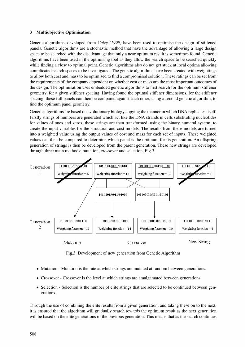
3 Multiobjective Optimisation

Genetic algorithms, developed from Coley (1999) have been used to optimise the design of stiffenedpanels. Genetic algorithms are a stochastic method that have the advantage of allowing a large designspace to be searched with the disadvantage that only a near optimum result is sometimes found. Geneticalgorithms have been used in the optimising tool as they allow the search space to be searched quicklywhile finding a close to optimal point. Genetic algorithms also do not get stuck at local optima allowingcomplicated search spaces to be investigated. The genetic algorithms have been created with weightingsto allow both cost and mass to be optimised to find a compromised solution. These ratings can be set fromthe requirements of the company dependent on whether cost or mass are the most important outcomes ofthe design. The optimisation uses embedded genetic algorithms to first search for the optimum stiffenergeometry, for a given stiffener spacing. Having found the optimal stiffener dimensions, for the stiffenerspacing, these full panels can then be compared against each other, using a second genetic algorithm, tofind the optimum panel geometry.

Genetic algorithms are based on evolutionary biology copying the manner in which DNA replicates itself.Firstly strings of numbers are generated which act like the DNA strands in cells substituting nucleotidesfor values of ones and zeros, these strings are then transformed, using the binary numeral system, tocreate the input variables for the structural and cost models. The results from these models are turnedinto a weighted value using the output values of cost and mass for each set of inputs. These weightedvalues can then be compared to determine which panel is the optimum for its generation. An offspringgeneration of strings is then be developed from the parent generation. These new strings are developedthrough three main methods: mutation, crossover and selection, Fig.3.

Fig.3: Development of new generation from Genetic Algorithm

• Mutation - Mutation is the rate at which strings are mutated at random between generations.

• Crossover - Crossover is the level at which strings are amalgamated between generations.

• Selection - Selection is the number of elite strings that are selected to be continued between gen-erations.

Through the use of combining the elite results from a given generation, and taking these on to the next,it is ensured that the algorithm will gradually search towards the optimum result as the next generationwill be based on the elite generations of the previous generation. This means that as the search continues

508

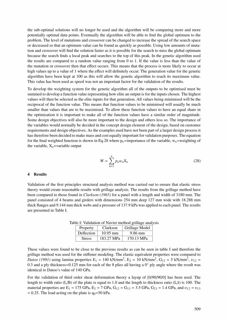
the sub-optimal solutions will no longer be used and the algorithm will be comparing more and morepotentially optimal data points. Eventually the algorithm will be able to find the global optimum to theproblem. The level of mutations and crossover can be changed to increase the spread of the search spaceor decreased so that an optimum value can be found as quickly as possible. Using low amounts of muta-tion and crossover will find the solution faster as it is possible for the search to miss the global optimumbecause the search finds a local peak and searches to the top of this peak. In the genetic algorithm usedthe results are compared to a random value ranging from 0 to 1. If the value is less than the value ofthe mutation or crossover then that effect occurs. This means that the process is more likely to occur athigh values up to a value of 1 where the effect will definitely occur. The generation value for the geneticalgorithm have been kept at 100 as this will allow the genetic algorithm to reach its maximum value.This value has been used as speed was not an important factor for the validation of the results.

To develop the weighting system for the genetic algorithm all of the outputs to be optimised must besummed to develop a function value representing how elite an output is for the inputs chosen. The highestvalues will then be selected as the elite inputs for that generation. All values being minimised will be thereciprocal of the function value. This means that function values to be minimised will usually be muchsmaller than values that are to be maximised. To allow these function values to have an equal share inthe optimisation it is important to make all of the function values have a similar order of magnitude.Some design objectives will also be more important to the design and others less so. The importance ofthe variables would normally be decided in the concept design element of the design, based on customerrequirements and design objectives. As the examples used have not been part of a larger design process ithas therefore been decided to make mass and cost equally important for validation purposes. The equationfor the final weighted function is shown in Eq.28 where pn=importance of the variable, wn=weighting ofthe variable, Xn=variable output

W =

n∑n=1

pnwnXn (28)

4 Results

Validation of the first principles structural analysis method was carried out to ensure that elastic stresstheory would create reasonable results with grillage analysis. The results from the grillage method havebeen compared to those found in Clarkson (1965) for a panel with a length and width of 3180 mm. Thepanel consisted of 4 beams and girders with dimensions 254 mm deep 127 mm wide with 18.288 mmthick flanges and 9.144 mm thick webs and a pressure of 137.9 kPa was applied to each panel. The resultsare presented in Table I.

Table I: Validation of Navier method grillage analysisProperty Clarkson Grillage Model

Deflection 10.95 mm 9.86 mmStress 183.27 MPa 170.13 MPa

These values were found to be close to the previous results as can be seen in table I and therefore thegrillage method was used for the stiffener modeling. The elastic equivalent properties were compared toDatoo (1991) using lamina properties E1 = 140 kN/mm2, E2 = 10 kN/mm2, G12 = 5 kN/mm2, υ12 =

0.3 and a ply thickness=0.125 mm for each of the 8 plies all having a 0 ply angle where the result wasidentical to Datoo’s value of 140 GPa.

For the validation of third order shear deformation theory a layup of [0/90/90/0] has been used. Thelength to width ratio (L/B) of the plate is equal to 1.0 and the length to thickness ratio (L/t) is 100. Thematerial properties are E1 = 175 GPa, E2 = 7 GPa, G12 = G13 = 3.5 GPa, G23 = 1.4 GPa, and υ12 = υ13= 0.25. The load acting on the plate is q0=50 kPa.

509

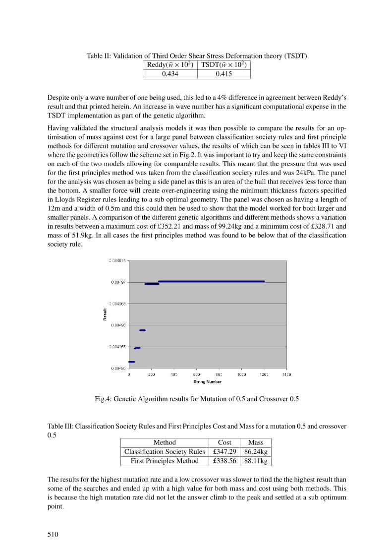
Table II: Validation of Third Order Shear Stress Deformation theory (TSDT)Reddy(w × 102) TSDT(w × 102)

0.434 0.415

Despite only a wave number of one being used, this led to a 4% difference in agreement between Reddy’sresult and that printed herein. An increase in wave number has a significant computational expense in theTSDT implementation as part of the genetic algorithm.

Having validated the structural analysis models it was then possible to compare the results for an op-timisation of mass against cost for a large panel between classification society rules and first principlemethods for different mutation and crossover values, the results of which can be seen in tables III to VIwhere the geometries follow the scheme set in Fig.2. It was important to try and keep the same constraintson each of the two models allowing for comparable results. This meant that the pressure that was usedfor the first principles method was taken from the classification society rules and was 24kPa. The panelfor the analysis was chosen as being a side panel as this is an area of the hull that receives less force thanthe bottom. A smaller force will create over-engineering using the minimum thickness factors specifiedin Lloyds Register rules leading to a sub optimal geometry. The panel was chosen as having a length of12m and a width of 0.5m and this could then be used to show that the model worked for both larger andsmaller panels. A comparison of the different genetic algorithms and different methods shows a variationin results between a maximum cost of £352.21 and mass of 99.24kg and a minimum cost of £328.71 andmass of 51.9kg. In all cases the first principles method was found to be below that of the classificationsociety rule.

Fig.4: Genetic Algorithm results for Mutation of 0.5 and Crossover 0.5

Table III: Classification Society Rules and First Principles Cost and Mass for a mutation 0.5 and crossover0.5

Method Cost MassClassification Society Rules £347.29 86.24kg

First Principles Method £338.56 88.11kg

The results for the highest mutation rate and a low crossover was slower to find the the highest result thansome of the searches and ended up with a high value for both mass and cost using both methods. Thisis because the high mutation rate did not let the answer climb to the peak and settled at a sub optimumpoint.

510

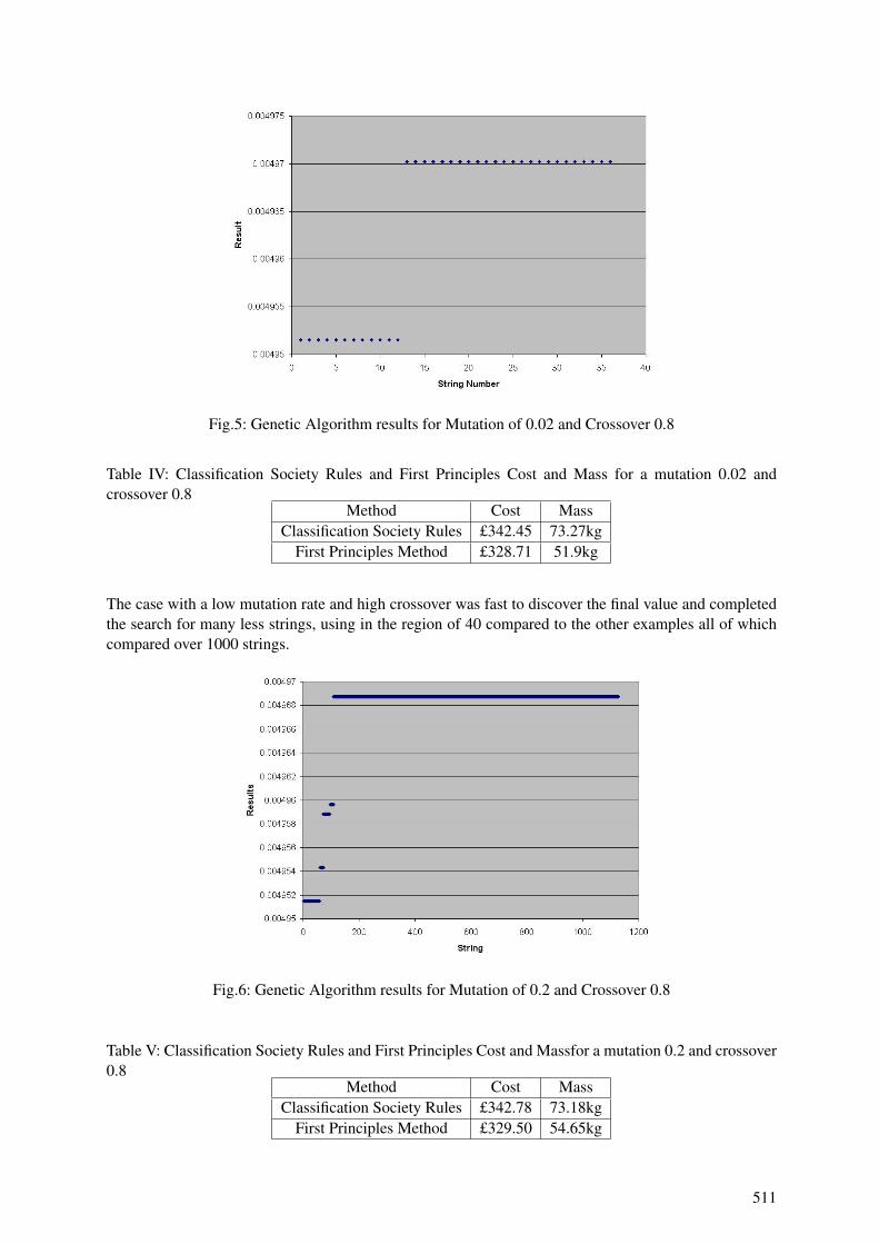
Fig.5: Genetic Algorithm results for Mutation of 0.02 and Crossover 0.8

Table IV: Classification Society Rules and First Principles Cost and Mass for a mutation 0.02 andcrossover 0.8

Method Cost MassClassification Society Rules £342.45 73.27kg

First Principles Method £328.71 51.9kg

The case with a low mutation rate and high crossover was fast to discover the final value and completedthe search for many less strings, using in the region of 40 compared to the other examples all of whichcompared over 1000 strings.

Fig.6: Genetic Algorithm results for Mutation of 0.2 and Crossover 0.8

Table V: Classification Society Rules and First Principles Cost and Massfor a mutation 0.2 and crossover0.8

Method Cost MassClassification Society Rules £342.78 73.18kg

First Principles Method £329.50 54.65kg

511

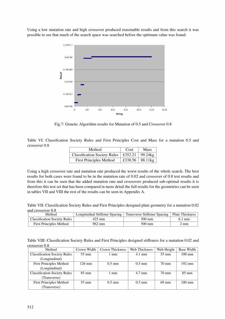
Using a low mutation rate and high crossover produced reasonable results and from this search it waspossible to see that much of the search space was searched before the optimum value was found.

Fig.7: Genetic Algorithm results for Mutation of 0.5 and Crossover 0.8

Table VI: Classification Society Rules and First Principles Cost and Mass for a mutation 0.5 andcrossover 0.8

Method Cost MassClassification Society Rules £352.21 99.24kg

First Principles Method £338.56 88.11kg

Using a high crossover rate and mutation rate produced the worst results of the whole search. The bestresults for both cases were found to be in the mutation rate of 0.02 and crossover of 0.8 test results andfrom this it can be seen that the added mutation rate and crossovers produced sub-optimal results it istherefore this test set that has been compared in more detail the full results for the geometries can be seenin tables VII and VIII the rest of the results can be seen in Appendix A.

Table VII: Classification Society Rules and First Principles designed plate geometry for a mutation 0.02and crossover 0.8

Method Longituidnal Stiffener Spacing Transverse Stiffener Spacing Plate ThicknessClassification Society Rules 425 mm 500 mm 6.1 mm

First Principles Method 962 mm 500 mm 2 mm

Table VIII: Classification Society Rules and First Principles designed stiffeners for a mutation 0.02 andcrossover 0.8

Method Crown Width Crown Thickness Web Thickness Web Height Base WidthClassification Society Rules 55 mm 1 mm 4.1 mm 55 mm 100 mm

(Longitudinal)First Principles Method 126 mm 0.5 mm 0.5 mm 70 mm 192 mm

(Longitudinal)Classification Society Rules 85 mm 1 mm 4.7 mm 70 mm 85 mm

(Transverse)First Principles Method 55 mm 0.5 mm 0.5 mm 69 mm 100 mm

(Transverse)

512

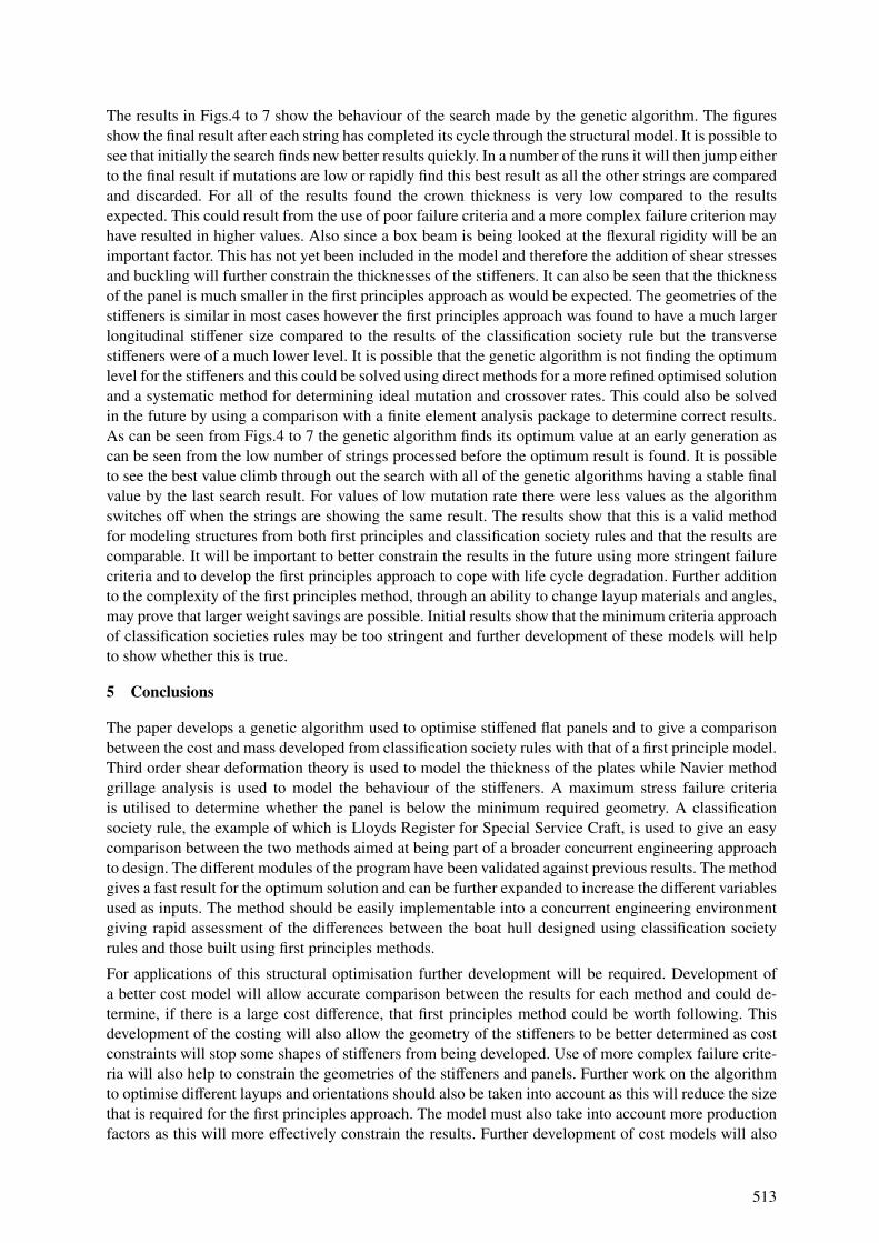
The results in Figs.4 to 7 show the behaviour of the search made by the genetic algorithm. The figuresshow the final result after each string has completed its cycle through the structural model. It is possible tosee that initially the search finds new better results quickly. In a number of the runs it will then jump eitherto the final result if mutations are low or rapidly find this best result as all the other strings are comparedand discarded. For all of the results found the crown thickness is very low compared to the resultsexpected. This could result from the use of poor failure criteria and a more complex failure criterion mayhave resulted in higher values. Also since a box beam is being looked at the flexural rigidity will be animportant factor. This has not yet been included in the model and therefore the addition of shear stressesand buckling will further constrain the thicknesses of the stiffeners. It can also be seen that the thicknessof the panel is much smaller in the first principles approach as would be expected. The geometries of thestiffeners is similar in most cases however the first principles approach was found to have a much largerlongitudinal stiffener size compared to the results of the classification society rule but the transversestiffeners were of a much lower level. It is possible that the genetic algorithm is not finding the optimumlevel for the stiffeners and this could be solved using direct methods for a more refined optimised solutionand a systematic method for determining ideal mutation and crossover rates. This could also be solvedin the future by using a comparison with a finite element analysis package to determine correct results.As can be seen from Figs.4 to 7 the genetic algorithm finds its optimum value at an early generation ascan be seen from the low number of strings processed before the optimum result is found. It is possibleto see the best value climb through out the search with all of the genetic algorithms having a stable finalvalue by the last search result. For values of low mutation rate there were less values as the algorithmswitches off when the strings are showing the same result. The results show that this is a valid methodfor modeling structures from both first principles and classification society rules and that the results arecomparable. It will be important to better constrain the results in the future using more stringent failurecriteria and to develop the first principles approach to cope with life cycle degradation. Further additionto the complexity of the first principles method, through an ability to change layup materials and angles,may prove that larger weight savings are possible. Initial results show that the minimum criteria approachof classification societies rules may be too stringent and further development of these models will helpto show whether this is true.

5 Conclusions

The paper develops a genetic algorithm used to optimise stiffened flat panels and to give a comparisonbetween the cost and mass developed from classification society rules with that of a first principle model.Third order shear deformation theory is used to model the thickness of the plates while Navier methodgrillage analysis is used to model the behaviour of the stiffeners. A maximum stress failure criteriais utilised to determine whether the panel is below the minimum required geometry. A classificationsociety rule, the example of which is Lloyds Register for Special Service Craft, is used to give an easycomparison between the two methods aimed at being part of a broader concurrent engineering approachto design. The different modules of the program have been validated against previous results. The methodgives a fast result for the optimum solution and can be further expanded to increase the different variablesused as inputs. The method should be easily implementable into a concurrent engineering environmentgiving rapid assessment of the differences between the boat hull designed using classification societyrules and those built using first principles methods.

For applications of this structural optimisation further development will be required. Development ofa better cost model will allow accurate comparison between the results for each method and could de-termine, if there is a large cost difference, that first principles method could be worth following. Thisdevelopment of the costing will also allow the geometry of the stiffeners to be better determined as costconstraints will stop some shapes of stiffeners from being developed. Use of more complex failure crite-ria will also help to constrain the geometries of the stiffeners and panels. Further work on the algorithmto optimise different layups and orientations should also be taken into account as this will reduce the sizethat is required for the first principles approach. The model must also take into account more productionfactors as this will more effectively constrain the results. Further development of cost models will also

513

allow different production techniques to be compared giving production designers an idea as to whichmethod of production could be the cheapest. Modeling of different sections of the hull structure willallow comparisons between whether a first principles approach could be useful. Finally for industrial ap-plications it will be important to use direct methods at the end of the genetic algorithm further increasingthe accuracy of the method and also decreasing the runtime required to gain optimum results.

References

CLARKSON, J. (1965), The elastic analysis of flat grillages, Cambridge University Press,Cambridge

COLEY, D.A. (1999), An introduction to genetic algorithms for scientists and engineers, World Scientific

CURRY, R. (2004), An Assessment of ISO 12215 Small Craft Hull Construction with ClassificationSociety Rules Transactions of The Royal Institution of Naval Architects Part B: International Journal ofSmall Craft Technology, Vol 147,(Part B1)

DATOO, M.H. (1991), Mechanics of Fibrous Composites, Elsevier Science Publishers Ltd., Essex, Eng-land

MANEEPAN, K.; SHENOI, R.A.; BLAKE, J.I.R. (2007), Genetic Algorithms (GAs) Based Optimisa-tion of FRP Composite Plated Grillages in Ship Structures Transactions of The Royal Institution of NavalArchitects Part A: International Journal of Maritime Engineering,Vol 149, (Part A3), 1-19

REDDY, J.N. (2004), Mechanics of Laminated Composite Plates and Shells, CRC Press Inc., London,England

SWIFT, K.G.; BROWN, N.J. (2003), Implementation strategies for design for manufacture methodolo-gies Proc. Instn Mech. Engrs Part B: J. Engineering Manufacture Vol.217

VEDELER, G. (1945), Grillage beams in ships and similar structures, Oslo:Grondahl & Son

A Appendix

The results for the sub-optimal geometries can be seen below:

Table IX: Classification Society Rules and First Principles designed plate geometry for a mutation 0.5and crossover 0.5

Method Longitudinal Stiffener Spacing Transverse Stiffener Spacing Plate ThicknessClassification Society Rules 615 mm 500 mm 7.2 mm

First Principles Method 272 mm 500 mm 2 mm

Table X: Classification Society Rules and First Principles designed stiffeners for a mutation 0.5 andcrossover 0.5

Method Crown Width Crown Thickness Web Thickness Web Height Base WidthClassification Society Rules 55 mm 1 mm 4.7 mm 55 mm 100 mm

(Longitudinal)First Principles Method 54 mm 0.5 mm 0.5 mm 70 mm 54 mm

(Longitudinal)Classification Society Rules 123 mm 1 mm 4.7 mm 70 mm 123 mm

(Transverse)First Principles Method 55 mm 0.5 mm 0.5 mm 69 mm 100 mm

(Transverse)

514

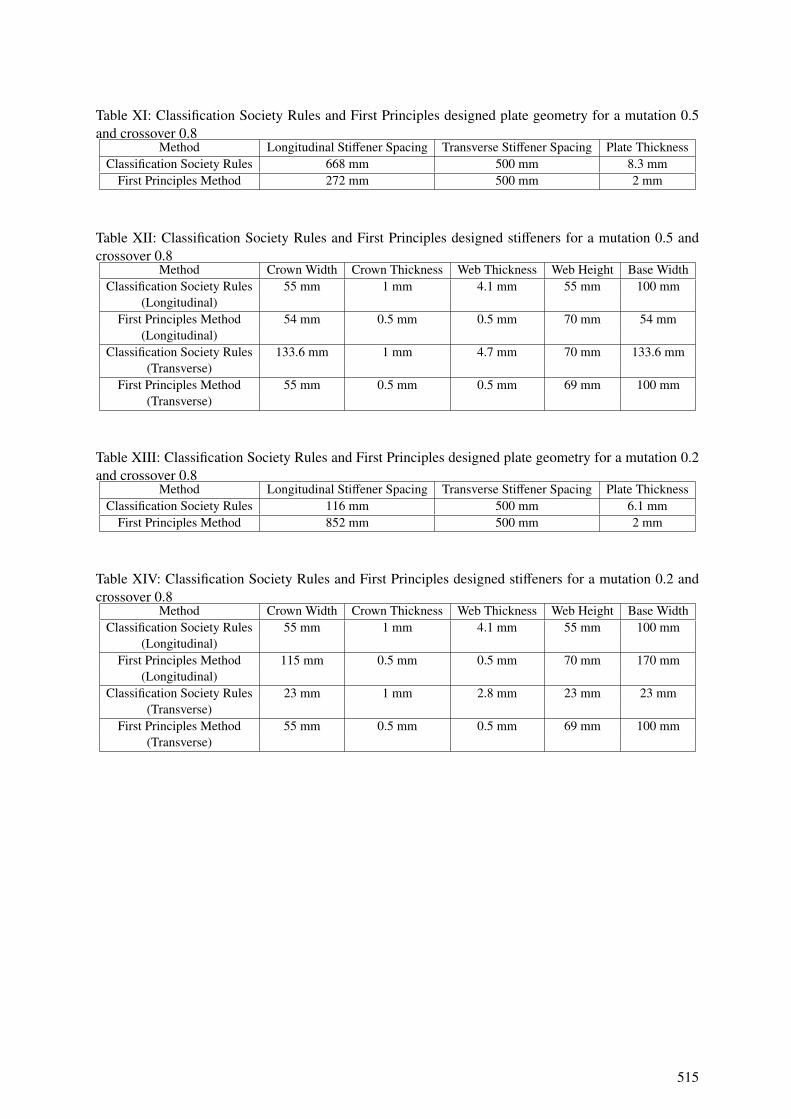
Table XI: Classification Society Rules and First Principles designed plate geometry for a mutation 0.5and crossover 0.8

Method Longitudinal Stiffener Spacing Transverse Stiffener Spacing Plate ThicknessClassification Society Rules 668 mm 500 mm 8.3 mm

First Principles Method 272 mm 500 mm 2 mm

Table XII: Classification Society Rules and First Principles designed stiffeners for a mutation 0.5 andcrossover 0.8

Method Crown Width Crown Thickness Web Thickness Web Height Base WidthClassification Society Rules 55 mm 1 mm 4.1 mm 55 mm 100 mm

(Longitudinal)First Principles Method 54 mm 0.5 mm 0.5 mm 70 mm 54 mm

(Longitudinal)Classification Society Rules 133.6 mm 1 mm 4.7 mm 70 mm 133.6 mm

(Transverse)First Principles Method 55 mm 0.5 mm 0.5 mm 69 mm 100 mm

(Transverse)

Table XIII: Classification Society Rules and First Principles designed plate geometry for a mutation 0.2and crossover 0.8

Method Longitudinal Stiffener Spacing Transverse Stiffener Spacing Plate ThicknessClassification Society Rules 116 mm 500 mm 6.1 mm

First Principles Method 852 mm 500 mm 2 mm

Table XIV: Classification Society Rules and First Principles designed stiffeners for a mutation 0.2 andcrossover 0.8

Method Crown Width Crown Thickness Web Thickness Web Height Base WidthClassification Society Rules 55 mm 1 mm 4.1 mm 55 mm 100 mm

(Longitudinal)First Principles Method 115 mm 0.5 mm 0.5 mm 70 mm 170 mm

(Longitudinal)Classification Society Rules 23 mm 1 mm 2.8 mm 23 mm 23 mm

(Transverse)First Principles Method 55 mm 0.5 mm 0.5 mm 69 mm 100 mm

(Transverse)

515

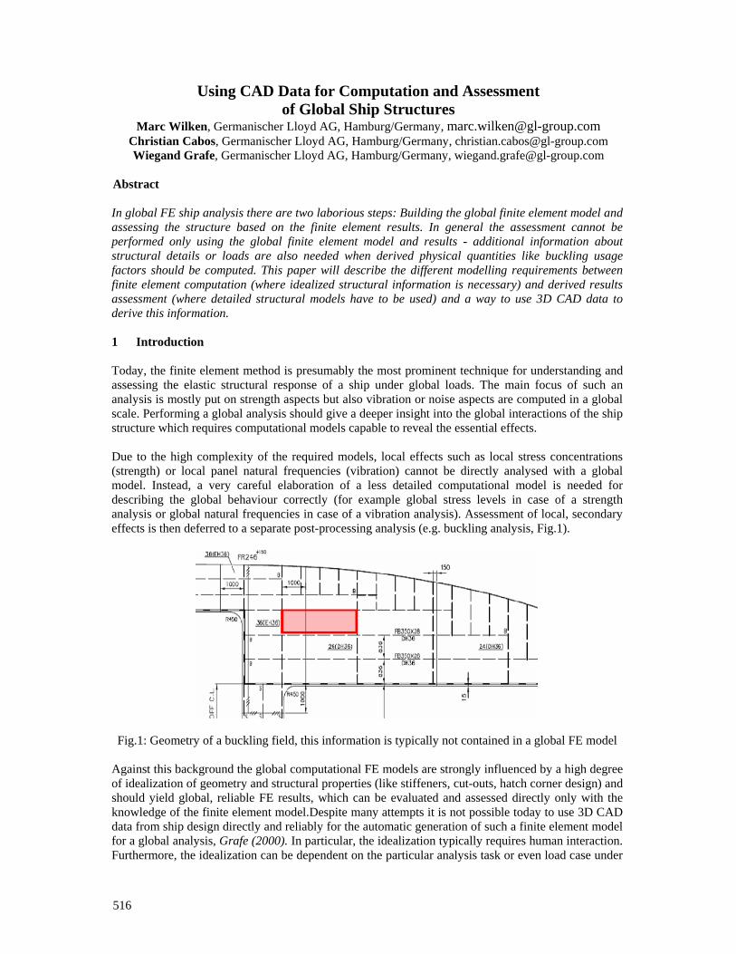
516

Using CAD Data for Computation and Assessment of Global Ship Structures

Marc Wilken, Germanischer Lloyd AG, Hamburg/Germany, marc.wilken@gl-group.com Christian Cabos, Germanischer Lloyd AG, Hamburg/Germany, christian.cabos@gl-group.com Wiegand Grafe, Germanischer Lloyd AG, Hamburg/Germany, wiegand.grafe@gl-group.com

Abstract In global FE ship analysis there are two laborious steps: Building the global finite element model and assessing the structure based on the finite element results. In general the assessment cannot be performed only using the global finite element model and results - additional information about structural details or loads are also needed when derived physical quantities like buckling usage factors should be computed. This paper will describe the different modelling requirements between finite element computation (where idealized structural information is necessary) and derived results assessment (where detailed structural models have to be used) and a way to use 3D CAD data to derive this information.

1 Introduction Today, the finite element method is presumably the most prominent technique for understanding and assessing the elastic structural response of a ship under global loads. The main focus of such an analysis is mostly put on strength aspects but also vibration or noise aspects are computed in a global scale. Performing a global analysis should give a deeper insight into the global interactions of the ship structure which requires computational models capable to reveal the essential effects. Due to the high complexity of the required models, local effects such as local stress concentrations (strength) or local panel natural frequencies (vibration) cannot be directly analysed with a global model. Instead, a very careful elaboration of a less detailed computational model is needed for describing the global behaviour correctly (for example global stress levels in case of a strength analysis or global natural frequencies in case of a vibration analysis). Assessment of local, secondary effects is then deferred to a separate post-processing analysis (e.g. buckling analysis, Fig.1).

Fig.1: Geometry of a buckling field, this information is typically not contained in a global FE model Against this background the global computational FE models are strongly influenced by a high degree of idealization of geometry and structural properties (like stiffeners, cut-outs, hatch corner design) and should yield global, reliable FE results, which can be evaluated and assessed directly only with the knowledge of the finite element model.Despite many attempts it is not possible today to use 3D CAD data from ship design directly and reliably for the automatic generation of such a finite element model for a global analysis, Grafe (2000). In particular, the idealization typically requires human interaction. Furthermore, the idealization can be dependent on the particular analysis task or even load case under

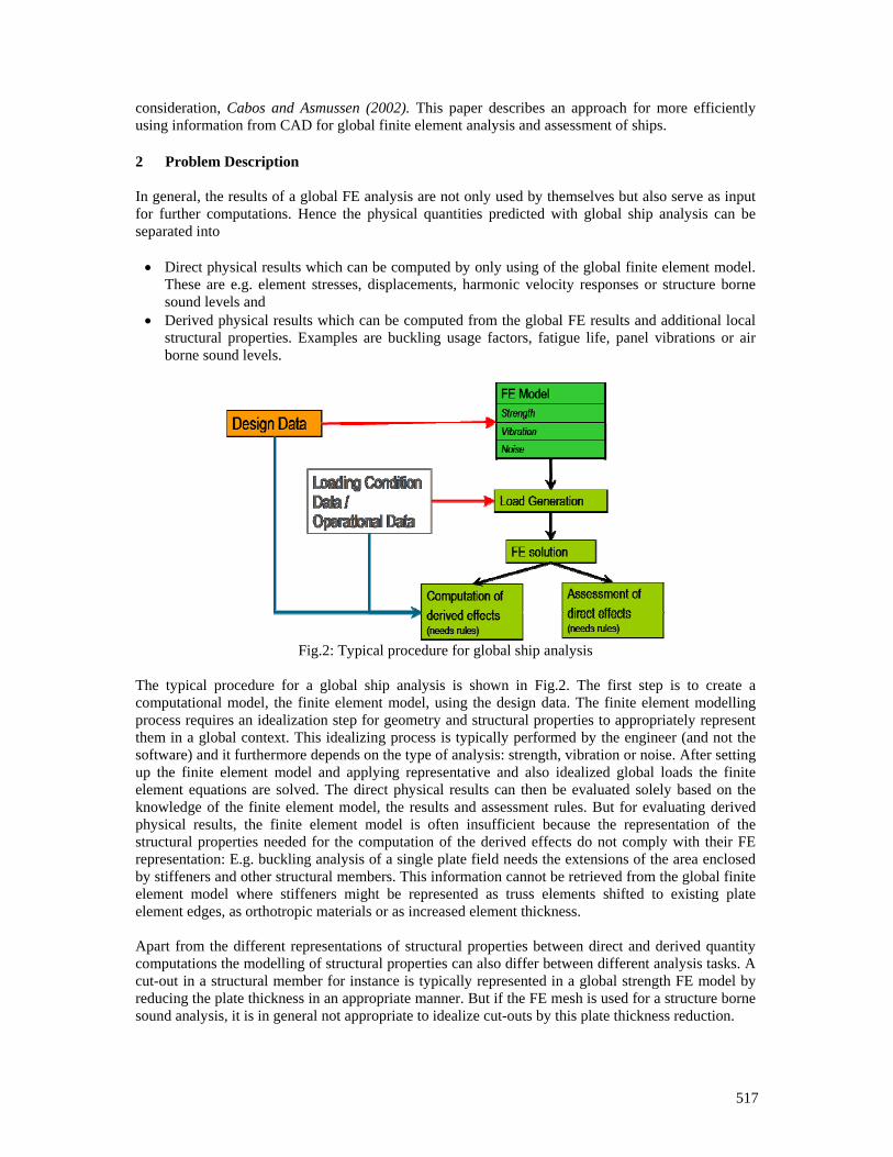
517

consideration, Cabos and Asmussen (2002). This paper describes an approach for more efficiently using information from CAD for global finite element analysis and assessment of ships. 2 Problem Description In general, the results of a global FE analysis are not only used by themselves but also serve as input for further computations. Hence the physical quantities predicted with global ship analysis can be separated into • Direct physical results which can be computed by only using of the global finite element model.

These are e.g. element stresses, displacements, harmonic velocity responses or structure borne sound levels and

• Derived physical results which can be computed from the global FE results and additional local structural properties. Examples are buckling usage factors, fatigue life, panel vibrations or air borne sound levels.

Fig.2: Typical procedure for global ship analysis

The typical procedure for a global ship analysis is shown in Fig.2. The first step is to create a computational model, the finite element model, using the design data. The finite element modelling process requires an idealization step for geometry and structural properties to appropriately represent them in a global context. This idealizing process is typically performed by the engineer (and not the software) and it furthermore depends on the type of analysis: strength, vibration or noise. After setting up the finite element model and applying representative and also idealized global loads the finite element equations are solved. The direct physical results can then be evaluated solely based on the knowledge of the finite element model, the results and assessment rules. But for evaluating derived physical results, the finite element model is often insufficient because the representation of the structural properties needed for the computation of the derived effects do not comply with their FE representation: E.g. buckling analysis of a single plate field needs the extensions of the area enclosed by stiffeners and other structural members. This information cannot be retrieved from the global finite element model where stiffeners might be represented as truss elements shifted to existing plate element edges, as orthotropic materials or as increased element thickness. Apart from the different representations of structural properties between direct and derived quantity computations the modelling of structural properties can also differ between different analysis tasks. A cut-out in a structural member for instance is typically represented in a global strength FE model by reducing the plate thickness in an appropriate manner. But if the FE mesh is used for a structure borne sound analysis, it is in general not appropriate to idealize cut-outs by this plate thickness reduction.

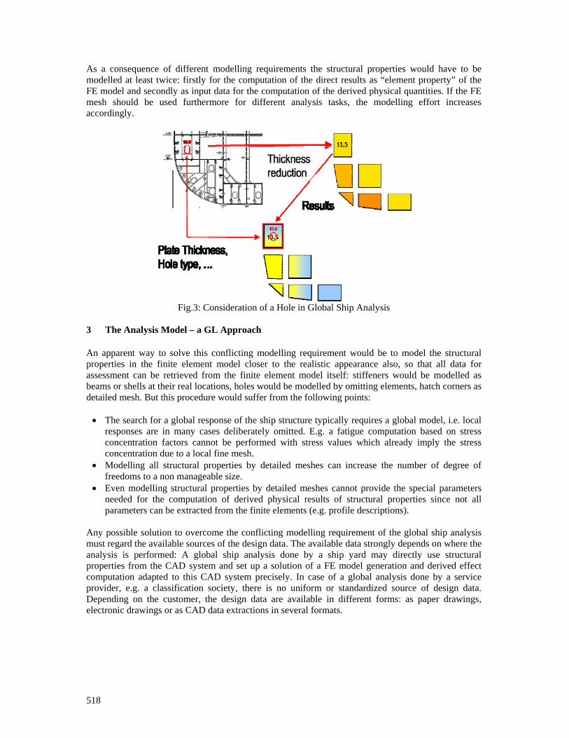
518

As a consequence of different modelling requirements the structural properties would have to be modelled at least twice: firstly for the computation of the direct results as “element property” of the FE model and secondly as input data for the computation of the derived physical quantities. If the FE mesh should be used furthermore for different analysis tasks, the modelling effort increases accordingly.

Fig.3: Consideration of a Hole in Global Ship Analysis

3 The Analysis Model – a GL Approach An apparent way to solve this conflicting modelling requirement would be to model the structural properties in the finite element model closer to the realistic appearance also, so that all data for assessment can be retrieved from the finite element model itself: stiffeners would be modelled as beams or shells at their real locations, holes would be modelled by omitting elements, hatch corners as detailed mesh. But this procedure would suffer from the following points: • The search for a global response of the ship structure typically requires a global model, i.e. local

responses are in many cases deliberately omitted. E.g. a fatigue computation based on stress concentration factors cannot be performed with stress values which already imply the stress concentration due to a local fine mesh.

• Modelling all structural properties by detailed meshes can increase the number of degree of freedoms to a non manageable size.

• Even modelling structural properties by detailed meshes cannot provide the special parameters needed for the computation of derived physical results of structural properties since not all parameters can be extracted from the finite elements (e.g. profile descriptions).

Any possible solution to overcome the conflicting modelling requirement of the global ship analysis must regard the available sources of the design data. The available data strongly depends on where the analysis is performed: A global ship analysis done by a ship yard may directly use structural properties from the CAD system and set up a solution of a FE model generation and derived effect computation adapted to this CAD system precisely. In case of a global analysis done by a service provider, e.g. a classification society, there is no uniform or standardized source of design data. Depending on the customer, the design data are available in different forms: as paper drawings, electronic drawings or as CAD data extractions in several formats.

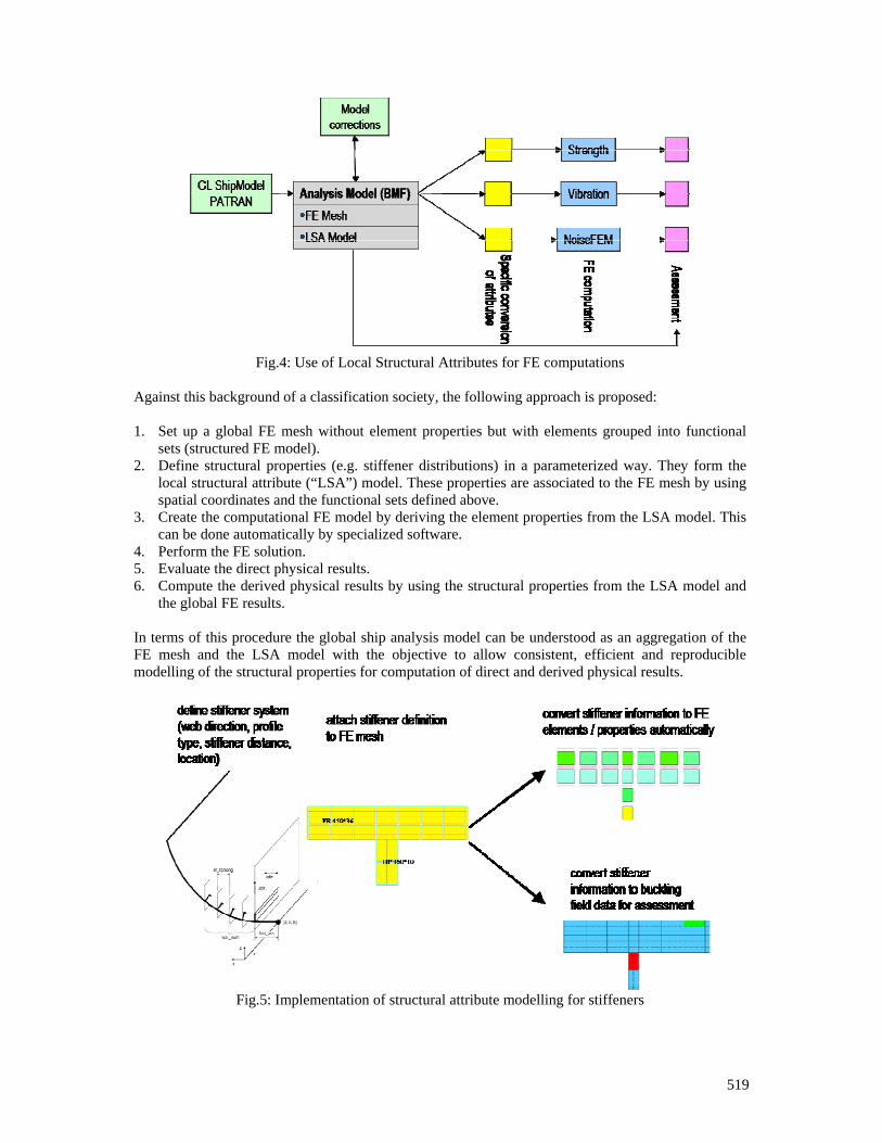
519

Fig.4: Use of Local Structural Attributes for FE computations

Against this background of a classification society, the following approach is proposed: 1. Set up a global FE mesh without element properties but with elements grouped into functional

sets (structured FE model). 2. Define structural properties (e.g. stiffener distributions) in a parameterized way. They form the

local structural attribute (“LSA”) model. These properties are associated to the FE mesh by using spatial coordinates and the functional sets defined above.

3. Create the computational FE model by deriving the element properties from the LSA model. This can be done automatically by specialized software.

4. Perform the FE solution. 5. Evaluate the direct physical results. 6. Compute the derived physical results by using the structural properties from the LSA model and

the global FE results. In terms of this procedure the global ship analysis model can be understood as an aggregation of the FE mesh and the LSA model with the objective to allow consistent, efficient and reproducible modelling of the structural properties for computation of direct and derived physical results.

Fig.5: Implementation of structural attribute modelling for stiffeners

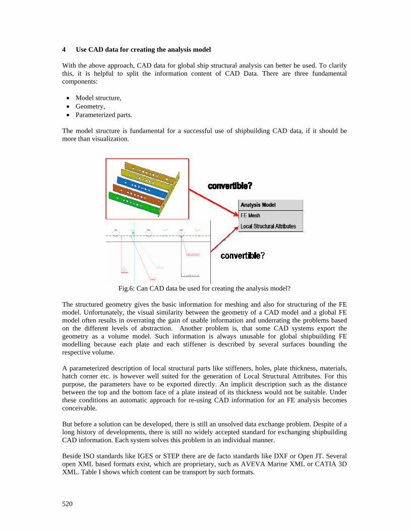
520

4 Use CAD data for creating the analysis model With the above approach, CAD data for global ship structural analysis can better be used. To clarify this, it is helpful to split the information content of CAD Data. There are three fundamental components: • Model structure, • Geometry, • Parameterized parts.

The model structure is fundamental for a successful use of shipbuilding CAD data, if it should be more than visualization.

Fig.6: Can CAD data be used for creating the analysis model?

The structured geometry gives the basic information for meshing and also for structuring of the FE model. Unfortunately, the visual similarity between the geometry of a CAD model and a global FE model often results in overrating the gain of usable information and underrating the problems based on the different levels of abstraction. Another problem is, that some CAD systems export the geometry as a volume model. Such information is always unusable for global shipbuilding FE modelling because each plate and each stiffener is described by several surfaces bounding the respective volume. A parameterized description of local structural parts like stiffeners, holes, plate thickness, materials, hatch corner etc. is however well suited for the generation of Local Structural Attributes. For this purpose, the parameters have to be exported directly. An implicit description such as the distance between the top and the bottom face of a plate instead of its thickness would not be suitable. Under these conditions an automatic approach for re-using CAD information for an FE analysis becomes conceivable. But before a solution can be developed, there is still an unsolved data exchange problem. Despite of a long history of developments, there is still no widely accepted standard for exchanging shipbuilding CAD information. Each system solves this problem in an individual manner. Beside ISO standards like IGES or STEP there are de facto standards like DXF or Open JT. Several open XML based formats exist, which are proprietary, such as AVEVA Marine XML or CATIA 3D XML. Table I shows which content can be transport by such formats.

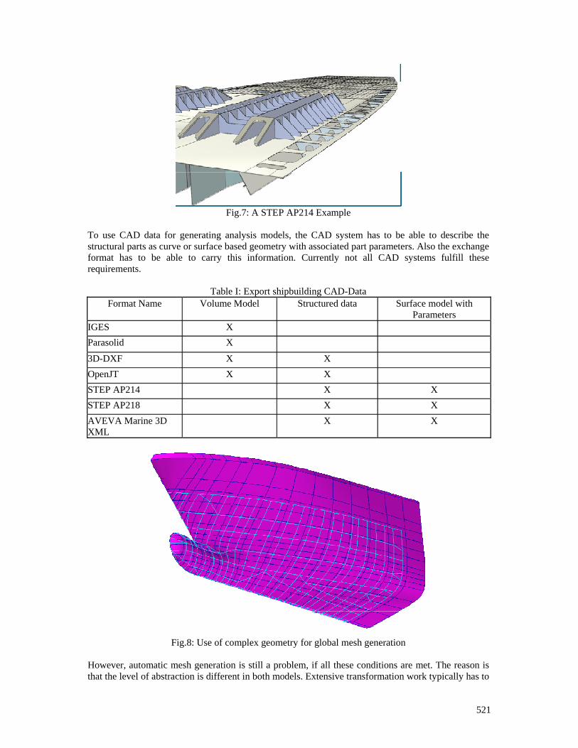
521

Fig.7: A STEP AP214 Example

To use CAD data for generating analysis models, the CAD system has to be able to describe the structural parts as curve or surface based geometry with associated part parameters. Also the exchange format has to be able to carry this information. Currently not all CAD systems fulfill these requirements.

Table I: Export shipbuilding CAD-Data Format Name Volume Model Structured data Surface model with

Parameters IGES X Parasolid X

3D-DXF X X OpenJT X X STEP AP214 X X STEP AP218 X X AVEVA Marine 3D XML

X X

Fig.8: Use of complex geometry for global mesh generation

However, automatic mesh generation is still a problem, if all these conditions are met. The reason is that the level of abstraction is different in both models. Extensive transformation work typically has to

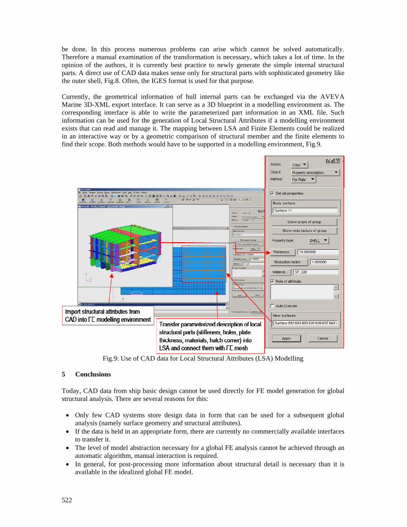
522

be done. In this process numerous problems can arise which cannot be solved automatically. Therefore a manual examination of the transformation is necessary, which takes a lot of time. In the opinion of the authors, it is currently best practice to newly generate the simple internal structural parts. A direct use of CAD data makes sense only for structural parts with sophisticated geometry like the outer shell, Fig.8. Often, the IGES format is used for that purpose. Currently, the geometrical information of hull internal parts can be exchanged via the AVEVA Marine 3D-XML export interface. It can serve as a 3D blueprint in a modelling environment as. The corresponding interface is able to write the parameterized part information in an XML file. Such information can be used for the generation of Local Structural Attributes if a modelling environment exists that can read and manage it. The mapping between LSA and Finite Elements could be realized in an interactive way or by a geometric comparison of structural member and the finite elements to find their scope. Both methods would have to be supported in a modelling environment, Fig.9.

Fig.9: Use of CAD data for Local Structural Attributes (LSA) Modelling

5 Conclusions Today, CAD data from ship basic design cannot be used directly for FE model generation for global structural analysis. There are several reasons for this: • Only few CAD systems store design data in form that can be used for a subsequent global

analysis (namely surface geometry and structural attributes). • If the data is held in an appropriate form, there are currently no commercially available interfaces

to transfer it. • The level of model abstraction necessary for a global FE analysis cannot be achieved through an

automatic algorithm, manual interaction is required. • In general, for post-processing more information about structural detail is necessary than it is

available in the idealized global FE model.

523

A path for overcoming the named problems has been drafted. It includes • use of a CAD systems with an appropriate representation of the design data, • implementation of interfaces to transfer this information, • add Local Structural Attributes to the FE mesh to from the analysis model, • derive the FE model for the actual computation from this analysis model, • access the Local Structural Attributes for post-processing.

With the named approach, the amount of manual interaction required for global structural analysis can be significantly reduced, if CAD data is available in appropriate form. References CABOS, C.; ASMUSSEN, I. (2002), Integrating global strength, vibration and noise analyses for ships using one computational model, 5th World Congress on Computational Mechanics (WCCM V) GRAFE, W. (2000), CADtoFE im Schiffbau – Ein Weg ins Nichts?, Schiffbauforschung Nr. 39, Universität Rostock

524

Customised Ship Design = Customised Ship Design Environments

Audun Grimstad, DNV proNavis AS, Trondheim/Norway, Audun.Grimstad@dnvpronavis.no

Arnulf Hagen, DNV proNavis AS, Trondheim/Norway, Arnulf.Hagen@dnvpronavis.no

Abstract

New demands on the shipbuilding and shipping industry indicate that a new ship design paradigm is

emerging. Designs and design processes alike will change, and as a consequence it may be prudent to

also redesign the tools and processes associated with ship design. DNV proNavis is involved in a

number of efforts to that end, and is currently looking at a concept design solution that will be

centered on a number approaches not normally seen in design tools – at least not all in one solution:

A customizable design environment, represented by workflows that will be configured according to

the design project at hand, a rules-based approach to workflow configuration and calculations, a

Service Oriented Architecture that will allow the workflow to call on the services required to do the

job, new tools that will decompose the project portfolio (the legacy data) in order to derive higher

order knowledge (parametric representations) etc. The solution will also focus more on identifying

the differential results of design changes, and less on finding an absolute figure, as the project will

invariably change significantly before the design is manifested.

1. Introduction

For European shipbuilding, the tendency is rather unequivocal: Yard turnover is increasing, not only

due to rising input costs, but also because the complexity of projects is increasing. In 2006, CESA

reported a 20% increase in delivered CGT, but an over 40% increase in turnover, CESA (2007). As

the high-volume business continues to go to Asia, European yards are continuing the shift from

integrated production to a role as a “system integration partner”, thereby also facilitating ever

increasing levels of customization.

Increased throughput and shorter project completion times will mean that a marked increase in tender

volume is a logical consequence: The largest Norwegian yards receive well in excess of 300

invitations for tender per year, which means that a significant effort is put into preparing more or less

well-conceived design proposals. Judging from past experience, the ambitions yard expansion plans

of “new” shipbuilding nations like Russia, India, Vietnam, Philippines, etc. will accelerate the move

of the three big Asian players into the high-end markets, which will in turn mean that they will be

facing the same situation shortly.

Thus design and tender processes need speeding up, and the tools designed for this task need to be

considerably sharper than is arguably the case today.

2. New central issues in ship design

Market laws will apply, physical constraints for instance in the form of Suez/Panama Canal

restrictions (both old and new) are well-known, and other constraints remain largely unchanged

except for smaller specialist segments, only operating conditions will be likely to change dramatically,

DNV (2008).

A number of trends may be observed or at least anticipated:

1. External conditions change rapidly, new performance paradigms emerge, new design

principles are required, possibly resulting in new vessel classes

525

a. New designs and design criteria = new design tools and methods?

b. Higher cost barriers for information re-use, extracting information from the project

portfolio will be more challenging: Shift from direct to parametric comparison, re-use

of direct information to be exchanged for higher order knowledge

2. New set of Key Performance Indicators (KPI) for the shipping industry: Environmental issues

to join CAPEX / OPEX as primary drivers for design changes

3. Unprecedented level of uncertainty with respect to operating conditions for ships for the

design lifespan (2010 – 2040+): Regulatory changes (particularly with respect to

environmental issues also here), cost of FO, manning, markets, etc. will require more robust

designs

All of the above will contribute to a shift away from the existing design principles, design processes

and design tools towards something different – something that can apply “old information” (or legacy

data) in new ways, and that can be easily adapted to match a wide range of design challenges.

The underlying requirement will remain that processes and tools will have to support a more rapid

design development process. In order to address this, DNV is now carrying out a number of related

studies, of which one in particular is focusing on the concept design phase. The internal working title

of the project is PCT, or “Pre-contract Tool”, which shall also be used in this paper as a generic term

for the tools and processes considered.

One of the main working hypotheses of the project is that as the new designs will be more adaptive or

flexible, so will also the design process itself be shifting from a more pre-defined path or process

towards a flexible and configurable process, albeit not necessarily as a result of the ship design

changes alone.

3. New ship design framework

A few clarifications need to be made with respect to the solution scope, both in terms of how and

when to use the solution, and the scope of services.

3.1 Area of application – design phases

Ship design processes will of course cover the entire range from just changing the vessel call-sign on

the GA drawing to an innovative design project starting from scratch. The prevailing time and cost

constraints will still dictate towards which of the extremes a new design process will lean. By

extension, where no external or internal forces would drive the process towards a complete rethink of

the solution, the best compromise between utilizing existing data and adding new elements would be

chosen so as to minimize work and still meet the new requirements – which is of course quite

sensible.

Opposite, where the requirements dictate that a brand new vessel design or an innovative design

different from previous projects is produced, the direct application of existing data and patterns may

represent a logical short-circuit and result in flawed solutions, or at least less efficient solutions.

This paper will discuss a general design process, but the proposed tools and solutions should be suited

to the task regardless of design- and design process variations; indeed, that is one of the main

distinguishing features of the proposed solution.

A clarification with respect to which phase or stage of the ship design process the solution is

addressing might thus be useful at this point.

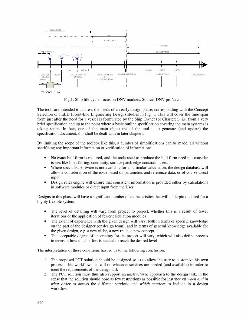
526

Fig.1: Ship life-cycle, focus on DNV markets, Source: DNV proNavis

The tools are intended to address the needs of an early design phase, corresponding with the Concept

Selection or FEED (Front-End Engineering Design) studies in Fig. 1. This will cover the time span

from just after the need for a vessel is formulated by the Ship Owner (or Charterer), i.e. from a very

brief specification and up to the point where a basic outline specification covering the main systems is

taking shape. In fact, one of the main objectives of the tool is to generate (and update) the

specification document; this shall be dealt with in later chapters.

By limiting the scope of the toolbox like this, a number of simplifications can be made, all without

sacrificing any important information or verification of information:

• No exact hull form is required, and the tools used to produce the hull form need not consider

issues like lines fairing, continuity, surface patch edge constraints, etc.

• Where specialist software is not available for a particular calculation, the design database will

allow a consideration of the issue based on parameters and reference data, or of course direct

input

• Design rules engine will ensure that consistent information is provided either by calculations

in software modules or direct input from the User

Designs in this phase will have a significant number of characteristics that will underpin the need for a

highly flexible system:

• The level of detailing will vary from project to project, whether this is a result of fewer

iterations or the application of fewer calculation modules

• The extent of experience with the given design will vary, both in terms of specific knowledge

on the part of the designer (or design team), and in terms of general knowledge available for

the given design, e.g. a new niche, a new trade, a new concept

• The acceptable degree of uncertainty for the project will vary, which will also define process

in terms of how much effort is needed to reach the desired level

The interpretation of these conditions has led us to the following conclusion:

1. The proposed PCT solution should be designed so as to allow the user to customize his own

process – his workflow – to call on whatever services are needed (and available) in order to

meet the requirements of the design task

2. The PCT solution must thus also support an unstructured approach to the design task, in the

sense that the solution should pose as few restrictions as possible for instance on when and in

what order to access the different services, and which services to include in a design

workflow

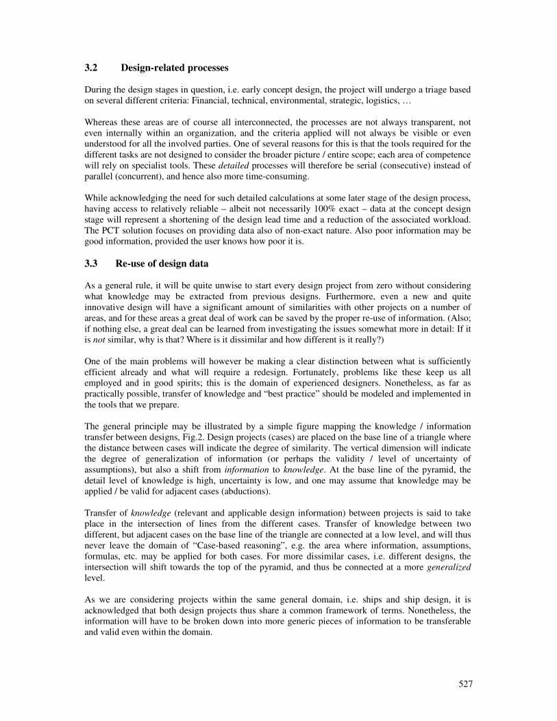
527

3.2 Design-related processes

During the design stages in question, i.e. early concept design, the project will undergo a triage based

on several different criteria: Financial, technical, environmental, strategic, logistics, …

Whereas these areas are of course all interconnected, the processes are not always transparent, not

even internally within an organization, and the criteria applied will not always be visible or even

understood for all the involved parties. One of several reasons for this is that the tools required for the

different tasks are not designed to consider the broader picture / entire scope; each area of competence

will rely on specialist tools. These detailed processes will therefore be serial (consecutive) instead of

parallel (concurrent), and hence also more time-consuming.

While acknowledging the need for such detailed calculations at some later stage of the design process,

having access to relatively reliable – albeit not necessarily 100% exact – data at the concept design

stage will represent a shortening of the design lead time and a reduction of the associated workload.

The PCT solution focuses on providing data also of non-exact nature. Also poor information may be

good information, provided the user knows how poor it is.

3.3 Re-use of design data

As a general rule, it will be quite unwise to start every design project from zero without considering

what knowledge may be extracted from previous designs. Furthermore, even a new and quite

innovative design will have a significant amount of similarities with other projects on a number of

areas, and for these areas a great deal of work can be saved by the proper re-use of information. (Also;

if nothing else, a great deal can be learned from investigating the issues somewhat more in detail: If it

is not similar, why is that? Where is it dissimilar and how different is it really?)

One of the main problems will however be making a clear distinction between what is sufficiently

efficient already and what will require a redesign. Fortunately, problems like these keep us all

employed and in good spirits; this is the domain of experienced designers. Nonetheless, as far as

practically possible, transfer of knowledge and “best practice” should be modeled and implemented in

the tools that we prepare.

The general principle may be illustrated by a simple figure mapping the knowledge / information

transfer between designs, Fig.2. Design projects (cases) are placed on the base line of a triangle where

the distance between cases will indicate the degree of similarity. The vertical dimension will indicate

the degree of generalization of information (or perhaps the validity / level of uncertainty of

assumptions), but also a shift from information to knowledge. At the base line of the pyramid, the

detail level of knowledge is high, uncertainty is low, and one may assume that knowledge may be

applied / be valid for adjacent cases (abductions).

Transfer of knowledge (relevant and applicable design information) between projects is said to take

place in the intersection of lines from the different cases. Transfer of knowledge between two

different, but adjacent cases on the base line of the triangle are connected at a low level, and will thus

never leave the domain of “Case-based reasoning”, e.g. the area where information, assumptions,

formulas, etc. may be applied for both cases. For more dissimilar cases, i.e. different designs, the

intersection will shift towards the top of the pyramid, and thus be connected at a more generalized

level.

As we are considering projects within the same general domain, i.e. ships and ship design, it is

acknowledged that both design projects thus share a common framework of terms. Nonetheless, the

information will have to be broken down into more generic pieces of information to be transferable

and valid even within the domain.

528

INFORMATION

INFORMATION

123

Inference

Deduction

Case basedreasoning

Abductions, analogies, direct application of

knowledge

Dissimilar projects, direct application of knowledge

Knowledge

Information

General principles

Fig.2: Principle sketch showing the flow of design-related information between projects

A description of the hull lines may serve as an example of the latter: Project designs of two rather

similar bulk vessels can easily be scaled to fit the need of the project at hand (using the Admiralty

constant or any other similar form-like change) without having to perform a new and complete

analysis of resistance and propulsion parameters. On the other hand, the connection between the hull

form for two rather similar-sized and –shaped vessels like e.g. a Container vessel and PCTC vessel

(car carrier) might not be as obvious, however, and will perhaps require that you have a parameterized

hull description method and a set of tools that can produce- and manipulate a hull from such data. You

might wish to change the block coefficient, bulb shape, entry angles, shift the LCB around, and so on,

and you wish to do this based on knowledge of what effects each change will have on which

parameters.

The newer generations of parametric hull design tools, e.g. Bole and Forrest (2005), Abt et al. (2003),

can produce a fairly good hull, including bulb, transom and typical descriptive features as flat of side,

flat of bottom, etc., from nothing but a few control curves and a limited set of descriptive parameters

specific to ship hulls / hull lines design. The upshot of this is that a given set of hull designs can be

reverse-engineered using the same definitions, thus producing a database of hulls with “meta-data”,

which will again provide the system with a higher-level, more generalized, description of ship hulls.

(Alternatively, having a huge lines library might provide the same data quality, but would most likely

not be practically feasible for most users.)

529

This is, on a more theoretical level, a shift from information to knowledge. Conceptually, this is then

not only a shift from a “cut-and-paste” -regime to a more generic design-regime, but also from a

deductive approach to an inductive approach; in its simplest form to be illustrated as follows:

Deductive: All Mondays are days. All days occur only once a week. Hence, Mondays occur

only once a week.

Inductive: Proportion Q of the known instances of population P has attribute A.

Individual I is another member of P. Therefore: There is a probability corresponding to Q

that I has A.

Whereas this approach is clearly not sufficiently advanced for the engineering phase of a project,

where parameters need to be quantified in more absolute terms, it will most likely do quite nicely for

the concept design / early tender phase. Choosing the appropriate approach – copy or start from

scratch – is most often a business decision more than a pure technical one, but it should nevertheless

involve experienced designers.

4. New design processes

We have previously pointed to several large-scale (even global) trends and influences that may

significantly affect the design criteria for the ships of the future. Under this assumption, that the Key

Performance Indicators (KPI) in the design process may change rather significantly and rather rapidly,

our work also aims at addressing / supporting whatever new processes may be required – and the

related calculations. Despite our best efforts, DNV (2008), not even DNV may foretell the future, so

the uncertainty with respect to said changes will apply also for PCT. One response would be to design

a solution that is customizable, i.e. that whatever the design process, ideally speaking, the tools may

be adapted to it.

A step in this direction would be to propose a solution that can configure and orchestrate the efforts

according to a best practice or some other alternative systematic approach:

A) Configure the working process and the tools, Fig.3:

• Definition of an efficient workflow and configure tools accordingly

• Call on the required services (tools), and – if required – easily introduce new tools or services

into the design environment

• Assistance in finding a good baseline for evaluations even when the starting design point is

quite different from earlier projects (i.e. belonging to a new design paradigm).

B) Continuously monitor and validate design KPI’s, Fig.3:

• Environmental performance / environmental index, footprint analyses, logistics chain

analyses

• Data mining, regression tools, comparison of design vs. reference data

• Nauticus 1 / “business intelligence” solutions: Case vessels, reference vessels, meta-data

C) Provide specialist support services, Fig.3:

• TenderSuite 2 specification assistance: Template-based specifications instead of document-

1 Software suite by DNV Software (http://www.dnv.com/services/software/products/nauticus/index.asp)

2 TenderSuiteTM – a customised software solution by DNV proNavis for the maritime industry, supporting the

tendering process

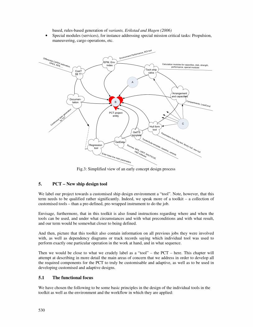
530

based, rules-based generation of variants, Erikstad and Hagen (2006)

• Special modules (services), for instance addressing special mission critical tasks: Propulsion,

maneuvering, cargo operations, etc.

Regressiontool

GetData

GetTS template

Hull form tool

Arrangement and capacities

Tech ship calcs

EPM, Env. index

Cost? $$ ??

Documen-tation

Enter base line main parameters

Sources: NPS, LRFP, NAUTICUS,

H&S software

Parameters from Reg.tool, library hull, new hull

Compartments, LoadCond

Calculation modules for capacities, stab, strength, performance, special moduies

Environm

ent Perfor

mance, RO

I tool

Differential CAPEX estimation,

OPEX, RFR, ...

Continuous sp

ec generation

by TS?

PCT projectentity

TenderSuite template, baseline, variants

A

B

C

Fig.3: Simplified view of an early concept design process

5. PCT – New ship design tool We label our project towards a customised ship design environment a “tool”. Note, however, that this

term needs to be qualified rather significantly. Indeed, we speak more of a toolkit – a collection of

customised tools – than a pre-defined, pre-wrapped instrument to do the job.

Envisage, furthermore, that in this toolkit is also found instructions regarding where and when the

tools can be used, and under what circumstances and with what preconditions and with what result,

and our term would be somewhat closer to being defined.

And then, picture that this toolkit also contain information on all previous jobs they were involved

with, as well as dependency diagrams or track records saying which individual tool was used to

perform exactly one particular operation in the work at hand, and in what sequence.

Then we would be close to what we crudely label as a “tool” – the PCT – here. This chapter will

attempt at describing in more detail the main areas of concern that we address in order to develop all

the required components for the PCT to truly be customisable and adaptive, as well as to be used in

developing customised and adaptive designs.

5.1 The functional focus

We have chosen the following to be some basic principles in the design of the individual tools in the

toolkit as well as the environment and the workflow in which they are applied:

531

Information refinement principles

Here we mean the structured (re)use of information and the analysis of such in e.g. regression tools.

We find two main paths to such reuse, Fig.2.

• Abduction (or case-based reasoning): We transfer experience on a case-based basis. The

challenge here is that the farther we move away from experience, the more novel and

customised the vessel is, and the more granular our reuse needs to be. In other words, while it

may not be possible to copy a project and fix some main characteristics or rescale the entire

design, it may still be possible to reuse certain patterns, solutions or modules.

• Inference and subsequent deduction. We use the collected experience – a subset of previous

projects – and extract relationships, key figures and formulas that create synthesized and

generalised knowledge, by this enabling the application to create more detailed design

knowledge in the new domain. Again, the farther away from our previous cases we go the

more generalised and abstract – the higher up in the triangle – we have to move. Herein we

also imply that the quality of the inference is highly dependent of how well the subset is

chosen – the adaptability and versatility of the instruments.

Information structuring

While such analyses as above are necessary in our context, they are not sufficient. The experience,

whether abstracted (generalised) or decomposed (modularised), needs to be made available to the

designer using PCT. We have chosen three main paths:

• Maintaining key figures. The analyses of the available experience may result in a repository

of known (or at least experienced) key figures (e.g. previously calculated or experienced

emission of CO2 per kW installed power of a certain configuration and make) and dominant

relationships (e.g. increasing the L/B ratio is a less power-influencing measure to increase the

displacement than increasing the B/T ratio).

• Maintaining regression formulas. The analyses of the available experience may result in

formulas that ideally would improve prediction of actual behaviour in absolute terms, and

thus also document a particular design with regards to main design criteria. However, more

importantly in the PCT is to ensure that such regressions can be used to identify the

differentials – the gradient of change – with regards to decisions that are relevant at different

stages in the design process. Knowing that a potential design change improves the emission

footprint is the first challenge; by how much is the second, and the exact emission footprint of

the manifested design the third.

• Maintaining templates. The analyses of the available experience may result in clusters of

vessel designs (or parts of vessel designs) that share fundamental and determining

characteristics. Again, there are two levels. First, if we cluster projects we in fact pre-select

projects that may be used to perform good analysis (e.g. through regression, by limiting the

subset). Hagen and Erikstad (2006) note: “... projects may be divided into distinct clusters, in

which the fraction of functions or systems relevant only for each cluster is high. A high such

fraction points to the establishment of different product families.”

Second, the outcome of this exercise represents a starting point for decomposing a vessel

design into more fine-grained sub-designs, or variants, or “the different options on a system

level that a [designer] typically may choose from.” [ibid].

Note that we implicitly extend this line of thinking beyond improving the vessel design in itself – we

532

also view these as fundamentals in improving the vessel design process. It will take us too far to go

into details here, but suffices it to say that on our agenda are workflow templates for the design

process also – not only the design object. And, if we learn about the correlation between design

parameters we implicitly also learn about the correlation between the individual instruments that use

or generate those parameters. The vision is a design process that adapts to the vessel design task at

hand, not vice versa.

Information use

Naturally following the discussion above is how PCT views the application of experience. We would

like to highlight three main objectives, of a host of others:

• Focus on speed. It has previously been stated that we cannot presume that the PCT user has

indefinite time at disposal (as if anyone has). Thus, we apply the concept of project templates

to rapidly create a starting point, the concept of variants to reuse predefined components, the

concept of families of designs to pre-select relevant subsets of data to perform analyses on.

We do not restrict the designer to use such – we merely give him/her the option to pre-think

and pre-structure based on own experience.

• Focus on impact. Earlier has also been highlighted that, without discounting the need for end-

figures to document the design to a client (internal or external), we view the ability to indicate

the impact of upcoming (or already made) decisions as a first. We will base the PCT on

impact assessment of design decisions rather than evaluation of the bottom-line performance

of the end-result of the design process. The description of the gradient of the relevant part of

the curve is to us more interesting than the exact formula describing the entire curve along the

whole segment of vessel sizes and types.

• Focus on risk. To be the third part of our manifest we have chosen the reduction of risk as the

most important, among several good candidates such as quality of the outcome and richness

of the potential analyses to be made. This is particularly because, in a time- and resource-

constrained design process, the first focus is to achieve “control” over the project and focus

on those areas that may impact the end result the most. In other words, the areas of perceived

highest risk, either by reducing the potential consequences (e.g. by designing robust) or

increasing the trustworthiness of the design (by applying adaptive analyses at the proper level,

and by enabling comparison of the current design to the relevant previous designs).

We could, as mentioned above, list several other underlying features of PCT:

− We could focus on a PCT scoreboard, where preselected KPIs are monitored with regards to

the effect the particular design decisions.

− We could focus on the conceived (Brix 3) rule engine that link the applications providing the

values of KPIs with the influencing design parameters. (Actually – we will revisit exactly this

point briefly.)

− We could focus on the PCT (Brix) workflow engine that applies the rules to trigger certain

events, in effect creating some automation with regards to certain analyses.

− We could focus on the need for interchange of data downstream, so as to be able to reuse

experience from manifested designs.

Instead, we will elaborate these at a later occasion and go in some more detail with regards to how we

foresee the individual applications having to be designed so as to facilitate the overall process. We

talk about the applications as services to be called upon, in a sequence not predefined, without a priori

3 Brix is a TradeMark of DNV Software, and comprises several frameworks including Brix Rules, Brix

Workflow, Prix Project Manager and others.

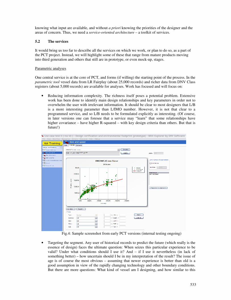
533

knowing what input are available, and without a priori knowing the priorities of the designer and the

areas of concern. Thus, we need a service-oriented architecture – a toolkit of services.

5.2 The services

It would bring us too far to describe all the services on which we work, or plan to do so, as a part of

the PCT project. Instead, we will highlight some of these that range from mature products moving

into third generation and others that still are in prototype, or even mock-up, stages.

Parametric analyses

One central service is at the core of PCT, and forms (if willing) the starting point of the process. In the

parametric tool vessel data from LR Fairplay (about 25,000 records) and richer data from DNV Class

registers (about 5,000 records) are available for analyses. Work has focused and will focus on:

• Reducing information complexity. The richness itself poses a potential problem. Extensive

work has been done to identify main design relationships and key parameters in order not to

overwhelm the user with irrelevant information. It should be clear to most designers that L/B

is a more interesting parameter than L/IMO number. However, it is not that clear to a

programmed service, and so L/B needs to be formulated explicitly as interesting. (Of course,

in later versions one can foresee that a service may “learn” that some relationships have

higher covariance – have higher R-squared – with key design criteria than others. But that is

future!)

Fig.4: Sample screenshot from early PCT versions (internal testing ongoing)

• Targeting the segment. Any user of historical records to predict the future (which really is the

essence of design) faces the ultimate question: When seizes this particular experience to be

valid? Under what conditions should I use it? And – if I use it nevertheless (in lack of

something better) – how uncertain should I be in my interpretation of the result? The issue of

age is of course the most obvious – assuming that newer experience is better than old is a

good assumption in view of the rapidly changing technology and other boundary conditions.

But there are more questions: What kind of vessel am I designing, and how similar to this

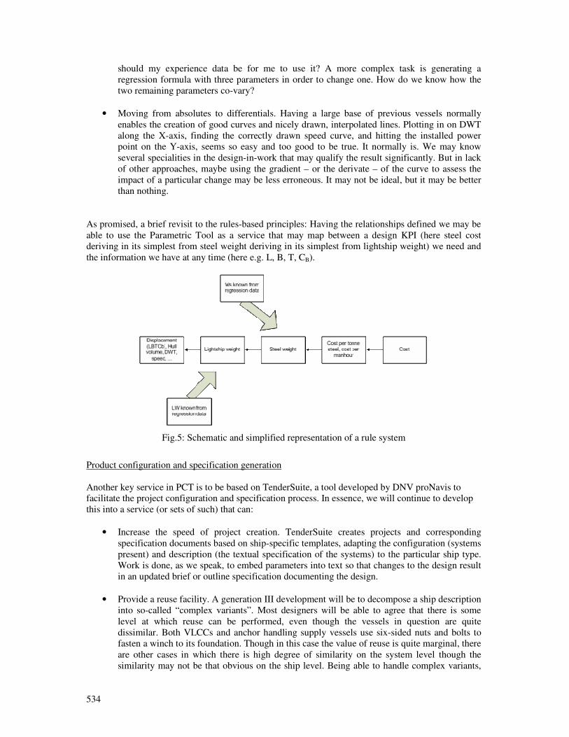
534

should my experience data be for me to use it? A more complex task is generating a

regression formula with three parameters in order to change one. How do we know how the

two remaining parameters co-vary?

• Moving from absolutes to differentials. Having a large base of previous vessels normally

enables the creation of good curves and nicely drawn, interpolated lines. Plotting in on DWT

along the X-axis, finding the correctly drawn speed curve, and hitting the installed power

point on the Y-axis, seems so easy and too good to be true. It normally is. We may know

several specialities in the design-in-work that may qualify the result significantly. But in lack

of other approaches, maybe using the gradient – or the derivate – of the curve to assess the

impact of a particular change may be less erroneous. It may not be ideal, but it may be better

than nothing.

As promised, a brief revisit to the rules-based principles: Having the relationships defined we may be

able to use the Parametric Tool as a service that may map between a design KPI (here steel cost

deriving in its simplest from steel weight deriving in its simplest from lightship weight) we need and

the information we have at any time (here e.g. L, B, T, CB).

Fig.5: Schematic and simplified representation of a rule system

Product configuration and specification generation

Another key service in PCT is to be based on TenderSuite, a tool developed by DNV proNavis to

facilitate the project configuration and specification process. In essence, we will continue to develop

this into a service (or sets of such) that can:

• Increase the speed of project creation. TenderSuite creates projects and corresponding

specification documents based on ship-specific templates, adapting the configuration (systems

present) and description (the textual specification of the systems) to the particular ship type.

Work is done, as we speak, to embed parameters into text so that changes to the design result

in an updated brief or outline specification documenting the design.

• Provide a reuse facility. A generation III development will be to decompose a ship description

into so-called “complex variants”. Most designers will be able to agree that there is some

level at which reuse can be performed, even though the vessels in question are quite

dissimilar. Both VLCCs and anchor handling supply vessels use six-sided nuts and bolts to

fasten a winch to its foundation. Though in this case the value of reuse is quite marginal, there

are other cases in which there is high degree of similarity on the system level though the

similarity may not be that obvious on the ship level. Being able to handle complex variants,

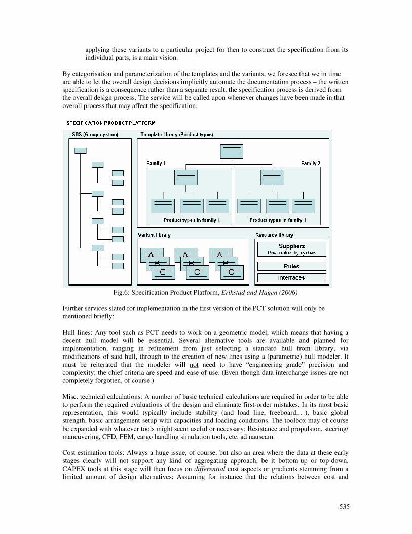
535

applying these variants to a particular project for then to construct the specification from its

individual parts, is a main vision.

By categorisation and parameterization of the templates and the variants, we foresee that we in time

are able to let the overall design decisions implicitly automate the documentation process – the written

specification is a consequence rather than a separate result, the specification process is derived from

the overall design process. The service will be called upon whenever changes have been made in that

overall process that may affect the specification.

Fig.6: Specification Product Platform, Erikstad and Hagen (2006)

Further services slated for implementation in the first version of the PCT solution will only be

mentioned briefly:

Hull lines: Any tool such as PCT needs to work on a geometric model, which means that having a

decent hull model will be essential. Several alternative tools are available and planned for

implementation, ranging in refinement from just selecting a standard hull from library, via

modifications of said hull, through to the creation of new lines using a (parametric) hull modeler. It

must be reiterated that the modeler will not need to have “engineering grade” precision and

complexity; the chief criteria are speed and ease of use. (Even though data interchange issues are not

completely forgotten, of course.)

Misc. technical calculations: A number of basic technical calculations are required in order to be able

to perform the required evaluations of the design and eliminate first-order mistakes. In its most basic

representation, this would typically include stability (and load line, freeboard,…), basic global

strength, basic arrangement setup with capacities and loading conditions. The toolbox may of course

be expanded with whatever tools might seem useful or necessary: Resistance and propulsion, steering/

maneuvering, CFD, FEM, cargo handling simulation tools, etc. ad nauseam.

Cost estimation tools: Always a huge issue, of course, but also an area where the data at these early

stages clearly will not support any kind of aggregating approach, be it bottom-up or top-down.

CAPEX tools at this stage will then focus on differential cost aspects or gradients stemming from a

limited amount of design alternatives: Assuming for instance that the relations between cost and

536

capacity for a main ship system are known, the cost consequences of choices related to this system

will then also be known and may be tracked.

Environmental performance analyses: A set of applications that will look at the carbon footprint of the

design, and also (to the extent possible and relevant) score the environmental performance against the

appropriate criteria. ROI calculations with respect to abatement measures and design changes will

also be within the scope.

6 Conclusions So in conclusion, our response to what is anticipated in way of changing environments, changing

designs, changing design processes, would be to design a solution that will subscribe to (have access

to) services to be called upon when needed, also with an eye on the particular nature of the design task

at hand (orchestration). In other words: A Service Oriented Architecture.

And more importantly: What the designer will experience as an end result is (hopefully) that

customised ship design will best be supported by solutions that provide customised ship design

environments.

As experience increases and exact information is scarce (in beginning of design process), it may be of

more value to know how poor the information truly is (and use it) rather than to spend time chasing

accuracy (and then maybe even end up not needing it).

The principles governing horisontal (known projects) reuse of information or vertical transfer and

reuse of information and knowledge (novel projects) will apply both for the designer working on a

particular task and for the designer of the PCT solution, who will have to facilitate such operations.

The final point shall be spent on emphasizing that focus will be put on impact evaluation – gradients,

derivates and differentials – rather than bottom-line guestimation under the assumption that this more

than likely will be wrong at the time the design is manifested.

References

DNV (2008), Technology Outlook 2015, DNV Research and Innovation

BOLE, M.; FORREST, C. (2005), Early Stage Integrated Parametric Ship Design, ICCAS 2005,

pp. 447-460

ABT, C.; BIRK, L.; HARRIES, S. (2003), Parametric hull design: The FRIENDSHIP-Modeler,

Int. Conf. Ship and Shipping Research (NAV 2003), Palermo

http://www.friendship-systems.com/company/papers.php

ERIKSTAD, S.O.; HAGEN, A. (2006), Applying product platform technologies in ship specification

development, IMDC 2006

CESA (2007), Annual report 2006-2007, Community of European Shipyards’ Associations

http://www.cesa-shipbuilding.org

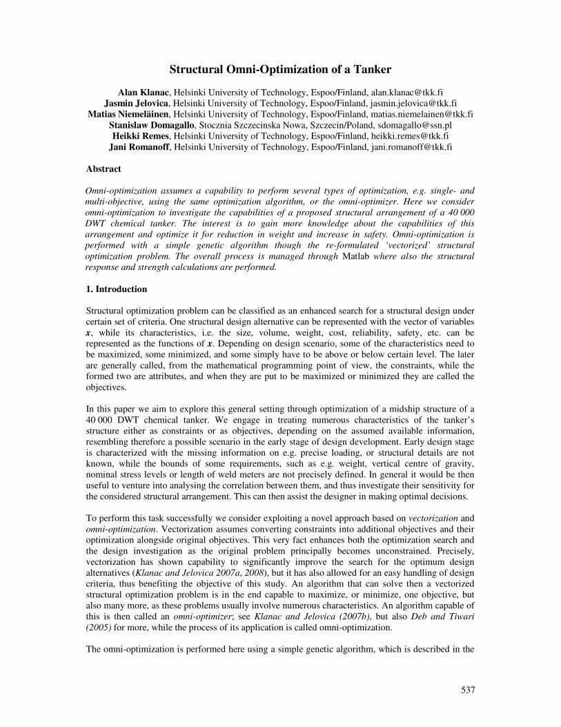
537

Structural Omni-Optimization of a Tanker

Alan Klanac, Helsinki University of Technology, Espoo/Finland, alan.klanac@tkk.fi

Jasmin Jelovica, Helsinki University of Technology, Espoo/Finland, jasmin.jelovica@tkk.fi

Matias Niemeläinen, Helsinki University of Technology, Espoo/Finland, matias.niemelainen@tkk.fi

Stanislaw Domagallo, Stocznia Szczecinska Nowa, Szczecin/Poland, sdomagallo@ssn.pl

Heikki Remes, Helsinki University of Technology, Espoo/Finland, heikki.remes@tkk.fi

Jani Romanoff, Helsinki University of Technology, Espoo/Finland, jani.romanoff@tkk.fi

Abstract

Omni-optimization assumes a capability to perform several types of optimization, e.g. single- and

multi-objective, using the same optimization algorithm, or the omni-optimizer. Here we consider

omni-optimization to investigate the capabilities of a proposed structural arrangement of a 40 000

DWT chemical tanker. The interest is to gain more knowledge about the capabilities of this

arrangement and optimize it for reduction in weight and increase in safety. Omni-optimization is

performed with a simple genetic algorithm though the re-formulated ‘vectorized’ structural

optimization problem. The overall process is managed through Matlab where also the structural

response and strength calculations are performed.

1. Introduction

Structural optimization problem can be classified as an enhanced search for a structural design under

certain set of criteria. One structural design alternative can be represented with the vector of variables

x, while its characteristics, i.e. the size, volume, weight, cost, reliability, safety, etc. can be

represented as the functions of x. Depending on design scenario, some of the characteristics need to

be maximized, some minimized, and some simply have to be above or below certain level. The later

are generally called, from the mathematical programming point of view, the constraints, while the

formed two are attributes, and when they are put to be maximized or minimized they are called the

objectives.

In this paper we aim to explore this general setting through optimization of a midship structure of a

40 000 DWT chemical tanker. We engage in treating numerous characteristics of the tanker’s

structure either as constraints or as objectives, depending on the assumed available information,

resembling therefore a possible scenario in the early stage of design development. Early design stage

is characterized with the missing information on e.g. precise loading, or structural details are not

known, while the bounds of some requirements, such as e.g. weight, vertical centre of gravity,

nominal stress levels or length of weld meters are not precisely defined. In general it would be then

useful to venture into analysing the correlation between them, and thus investigate their sensitivity for

the considered structural arrangement. This can then assist the designer in making optimal decisions.

To perform this task successfully we consider exploiting a novel approach based on vectorization and

omni-optimization. Vectorization assumes converting constraints into additional objectives and their

optimization alongside original objectives. This very fact enhances both the optimization search and

the design investigation as the original problem principally becomes unconstrained. Precisely,

vectorization has shown capability to significantly improve the search for the optimum design

alternatives (Klanac and Jelovica 2007a, 2008), but it has also allowed for an easy handling of design

criteria, thus benefiting the objective of this study. An algorithm that can solve then a vectorized

structural optimization problem is in the end capable to maximize, or minimize, one objective, but

also many more, as these problems usually involve numerous characteristics. An algorithm capable of

this is then called an omni-optimizer; see Klanac and Jelovica (2007b), but also Deb and Tiwari

(2005) for more, while the process of its application is called omni-optimization.

The omni-optimization is performed here using a simple genetic algorithm, which is described in the

538

following chapter. Chapter 3 follows with the problem description, while the Chapter 4 describes the

optimization process and shows the results. In Chapter 5 we discuss the results, but also the effects of

omni-optimization. Paper is concluded in Chapter 6.

2. Vectorization and the omni-optimizer

The omni-optimization is conceived here to lead from the capability of the algorithm, the optimizer,

to perform the multi-objective optimization. The choice has fallen on VOP (Klanac and Jelovica

2007b, 2008) – the genetic algorithm which features simple genetic operators, such as weighted

roulette wheel selection, single-point cross-over, binary encoding and bit-wise mutation. The

algorithm was until now applied in several different studies (Besnard et al. 2007, Romanoff and

Klanac 2007, Ehlers et al. 2007) and returned satisfactory results.

The only advanced feature that VOP possesses is its fitness function. It allows VOP to be used as the

omni-optimizer, following the vectorization of the original optimization problem. But first we briefly

present the applied concept of vectorization and then the algorithm.

2.1. Vectorization for structural omni-optimization

The original multi-objective structural optimization problem can be defined with the following

( ) ( ) [ ] 1min f ,...,f | ( ) 0, 1,M j j J∈

≥ ∈x X

x x g x , (1)

where X is the set of all possible alternatives defined between the lower and upper bounds of the

variables. The same problem can be written in the vectorized form following Klanac and Jelovica

(2007a, 2007b, 2008)

( ) ( ) ( ) ( ) ( ) 1 1min f ,..., f ,f ,...,f ,..., fM M M j M J+ + +∈x X

x x x x x . (2)

The constraints ( )jg x , which are now additional objectives ( ) ( ) 1f ,..., fM M J+ +x x in the equation

above, are converted applying the Heaviside representation (Osyczka et al. 2000, Deb 2001), given

as:

( )( ) ( )

[ ]g , if g 0

f , 1,0, othervise

j j

M j j J+

ìï - <ï= " Îíïïî

x xx (3)

The Heaviside representation is convenient when some of the criteria are treated both as constraint

and as objective. Typically, such a criterion is adequacy of the structural element, or the normalized

difference between the response and the strength of an element (Hughes et al. 1980), e.g. given for

the buckling criterion

( )( ) ( )

( ) ( )g

buckling response

j

buckling response

s s

s s

-=

+

x xx

x x. (4)

When adequacy is calculated to be negative for some design alternative, that design is infeasible and

the adequacy, following the Eq. (3), takes the positive value in the vectorized form and in this form it

can be then minimized during the optimization through Eq. (2).. When treated as objective to be

maximized, the same adequacy remains negative in the vectorized problem since in vectorization

objectives are not converted as constraints. This will then lead to the strong penalization of the

alternatives with large infeasibility, while those with smaller infeasibility will become preferred,

again leading to the increase in safety. If on the other hand, the adequacy of some alternative is

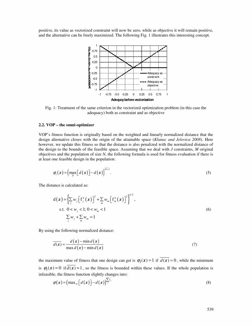
539

positive, its value as vectorized constraint will now be zero, while as objective it will remain positive,

and the alternative can be freely maximized. The following Fig. 1 illustrates this interesting concept.

-1

-0.75

-0.5

-0.25

0

0.25

0.5

0.75

1

-1 -0.75 -0.5 -0.25 0 0.25 0.5 0.75 1

Adequacy after vectorization

Adequcy before vectorization

Adequacy as

constraint

Adequacy as

objective

Fig. 1: Treatment of the same criterion in the vectorized optimization problem (in this case the

adequacy) both as constraint and as objective

2.2. VOP – the omni-optimizer

VOP’s fitness function is originally based on the weighted and linearly normalized distance that the

design alternative closes with the origin of the attainable space (Klanac and Jelovica 2008). Here

however, we update this fitness so that the distance is also penalized with the normalized distance of

the design to the bounds of the feasible space. Assuming that we deal with J constraints, M original

objectives and the population of size N, the following formula is used for fitness evaluation if there is

at least one feasible design in the population:

( ) ( ) ( )( )( )

1max .

d x

Nd dϕ = − x x x (5)

The distance is calculated as:

( ) ( ) ( ) 1/ 2

2 2n n

d f f ,

s.t. 0 1; 0 1

1

j j m mj m

j m

j mj m

w w

w w

w w

= ∑ +∑

< < < <

∑ +∑ =

x x x

(6)

By using the following normalized distance:

( ) ( )

( ) ( )

min( )

max min

d dd

d d

−

=

−

x xx

x x (7)

the maximum value of fitness that one design can get is 1( ) 1ϕ =x if ( ) 0d =x , while the minimum

is 1( ) 0ϕ =x if ( ) 1d =x , so the fitness is bounded within these values. If the whole population is

infeasible, the fitness function slightly changes into:

( ) ( ) ( )( )f

maxj

jN

d dϕ∑

= − x x x (8)

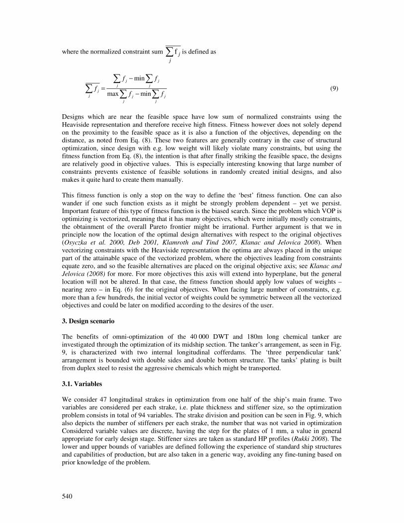
540

where the normalized constraint sum f j

j

∑ is defined as

min

max min

j j

j j

j

j j j

j j

f f

ff f

−

=

−

∑ ∑∑

∑ ∑ (9)

Designs which are near the feasible space have low sum of normalized constraints using the

Heaviside representation and therefore receive high fitness. Fitness however does not solely depend

on the proximity to the feasible space as it is also a function of the objectives, depending on the

distance, as noted from Eq. (8). These two features are generally contrary in the case of structural

optimization, since design with e.g. low weight will likely violate many constraints, but using the

fitness function from Eq. (8), the intention is that after finally striking the feasible space, the designs

are relatively good in objective values. This is especially interesting knowing that large number of

constraints prevents existence of feasible solutions in randomly created initial designs, and also

makes it quite hard to create them manually.

This fitness function is only a stop on the way to define the ‘best’ fitness function. One can also

wander if one such function exists as it might be strongly problem dependent – yet we persist.

Important feature of this type of fitness function is the biased search. Since the problem which VOP is

optimizing is vectorized, meaning that it has many objectives, which were initially mostly constraints,

the obtainment of the overall Pareto frontier might be irrational. Further argument is that we in

principle now the location of the optimal design alternatives with respect to the original objectives

(Osyczka et al. 2000, Deb 2001, Klamroth and Tind 2007, Klanac and Jelovica 2008). When

vectorizing constraints with the Heaviside representation the optima are always placed in the unique

part of the attainable space of the vectorized problem, where the objectives leading from constraints

equate zero, and so the feasible alternatives are placed on the original objective axis; see Klanac and

Jelovica (2008) for more. For more objectives this axis will extend into hyperplane, but the general

location will not be altered. In that case, the fitness function should apply low values of weights –

nearing zero – in Eq. (6) for the original objectives. When facing large number of constraints, e.g.

more than a few hundreds, the initial vector of weights could be symmetric between all the vectorized

objectives and could be later on modified according to the desires of the user.

3. Design scenario

The benefits of omni-optimization of the 40 000 DWT and 180m long chemical tanker are

investigated through the optimization of its midship section. The tanker’s arrangement, as seen in Fig.

9, is characterized with two internal longitudinal cofferdams. The ‘three perpendicular tank’

arrangement is bounded with double sides and double bottom structure. The tanks’ plating is built

from duplex steel to resist the aggressive chemicals which might be transported.

3.1. Variables

We consider 47 longitudinal strakes in optimization from one half of the ship’s main frame. Two

variables are considered per each strake, i.e. plate thickness and stiffener size, so the optimization

problem consists in total of 94 variables. The strake division and position can be seen in Fig. 9, which

also depicts the number of stiffeners per each strake, the number that was not varied in optimization

Considered variable values are discrete, having the step for the plates of 1 mm, a value in general

appropriate for early design stage. Stiffener sizes are taken as standard HP profiles (Rukki 2008). The

lower and upper bounds of variables are defined following the experience of standard ship structures

and capabilities of production, but are also taken in a generic way, avoiding any fine-tuning based on

prior knowledge of the problem.

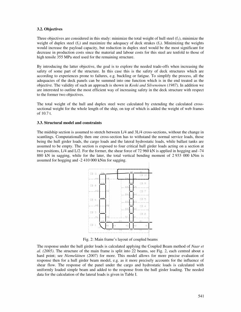
541

3.2. Objectives

Three objectives are considered in this study: minimize the total weight of hull steel (f1), minimize the

weight of duplex steel (f2) and maximize the adequacy of deck strakes (f3). Minimizing the weights

would increase the payload capacity, but reduction in duplex steel would be the most significant for

decrease in production costs since the material and labour costs for this steel are tenfold to those of

high tensile 355 MPa steel used for the remaining structure.

By introducing the latter objective, the goal is to explore the needed trade-offs when increasing the

safety of some part of the structure. In this case this is the safety of deck structures which are

according to experiences prone to failures, e.g. buckling or fatigue. To simplify the process, all the

adequacies of the deck panels can be summed into one function which is in the end treated as the

objective. The validity of such an approach is shown in Koski and Silvenoinen (1987). In addition we

are interested to outline the most efficient way of increasing safety in the deck structure with respect

to the former two objectives.

The total weight of the hull and duplex steel were calculated by extending the calculated cross-

sectional weight for the whole length of the ship, on top of which is added the weight of web frames

of 10.7 t.

3.3. Structural model and constraints

The midship section is assumed to stretch between L/4 and 3L/4 cross-sections, without the change in

scantlings. Computationally then one cross-section has to withstand the normal service loads, those

being the hull girder loads, the cargo loads and the lateral hydrostatic loads, while ballast tanks are

assumed to be empty. The section is exposed to four critical hull girder loads acting on a section at

two positions, L/4 and L/2. For the former, the shear force of 72 960 kN is applied in hogging and -74

880 kN in sagging, while for the later, the total vertical bending moment of 2 933 000 kNm is

assumed for hogging and -2 410 000 kNm for sagging.

Fig. 2: Main frame’s layout of coupled beams

The response under the hull girder loads is calculated applying the Coupled Beam method of Naar et

al. (2005). The structure of the main frame is split into 22 beams, see Fig. 2, each centred about a

hard point; see Niemeläinen (2007) for more. This model allows for more precise evaluation of

response then for a hull girder beam model, e.g. as it more precisely accounts for the influence of

shear flow. The response of the panel under the cargo and hydrostatic loads is calculated with

uniformly loaded simple beam and added to the response from the hull girder loading. The needed

data for the calculation of the lateral loads is given in Table I.

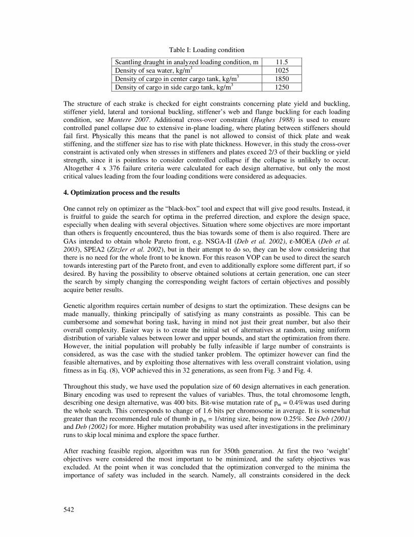
542

Table I: Loading condition

Scantling draught in analyzed loading condition, m 11.5

Density of sea water, kg/m3

1025

Density of cargo in center cargo tank, kg/m3 1850

Density of cargo in side cargo tank, kg/m3 1250

The structure of each strake is checked for eight constraints concerning plate yield and buckling,

stiffener yield, lateral and torsional buckling, stiffener’s web and flange buckling for each loading

condition, see Mantere 2007. Additional cross-over constraint (Hughes 1988) is used to ensure

controlled panel collapse due to extensive in-plane loading, where plating between stiffeners should

fail first. Physically this means that the panel is not allowed to consist of thick plate and weak

stiffening, and the stiffener size has to rise with plate thickness. However, in this study the cross-over

constraint is activated only when stresses in stiffeners and plates exceed 2/3 of their buckling or yield

strength, since it is pointless to consider controlled collapse if the collapse is unlikely to occur.

Altogether 4 x 376 failure criteria were calculated for each design alternative, but only the most

critical values leading from the four loading conditions were considered as adequacies.

4. Optimization process and the results

One cannot rely on optimizer as the “black-box” tool and expect that will give good results. Instead, it

is fruitful to guide the search for optima in the preferred direction, and explore the design space,

especially when dealing with several objectives. Situation where some objectives are more important

than others is frequently encountered, thus the bias towards some of them is also required. There are

GAs intended to obtain whole Pareto front, e.g. NSGA-II (Deb et al. 2002), ε-MOEA (Deb et al.

2003), SPEA2 (Zitzler et al. 2002), but in their attempt to do so, they can be slow considering that

there is no need for the whole front to be known. For this reason VOP can be used to direct the search

towards interesting part of the Pareto front, and even to additionally explore some different part, if so

desired. By having the possibility to observe obtained solutions at certain generation, one can steer

the search by simply changing the corresponding weight factors of certain objectives and possibly

acquire better results.

Genetic algorithm requires certain number of designs to start the optimization. These designs can be

made manually, thinking principally of satisfying as many constraints as possible. This can be

cumbersome and somewhat boring task, having in mind not just their great number, but also their

overall complexity. Easier way is to create the initial set of alternatives at random, using uniform

distribution of variable values between lower and upper bounds, and start the optimization from there.

However, the initial population will probably be fully infeasible if large number of constraints is

considered, as was the case with the studied tanker problem. The optimizer however can find the

feasible alternatives, and by exploiting those alternatives with less overall constraint violation, using

fitness as in Eq. (8), VOP achieved this in 32 generations, as seen from Fig. 3 and Fig. 4.

Throughout this study, we have used the population size of 60 design alternatives in each generation.

Binary encoding was used to represent the values of variables. Thus, the total chromosome length,

describing one design alternative, was 400 bits. Bit-wise mutation rate of pm = 0.4%was used during

the whole search. This corresponds to change of 1.6 bits per chromosome in average. It is somewhat

greater than the recommended rule of thumb in pm = 1/string size, being now 0.25%. See Deb (2001)

and Deb (2002) for more. Higher mutation probability was used after investigations in the preliminary

runs to skip local minima and explore the space further.

After reaching feasible region, algorithm was run for 350th generation. At first the two ‘weight’

objectives were considered the most important to be minimized, and the safety objectives was

excluded. At the point when it was concluded that the optimization converged to the minima the

importance of safety was included in the search. Namely, all constraints considered in the deck

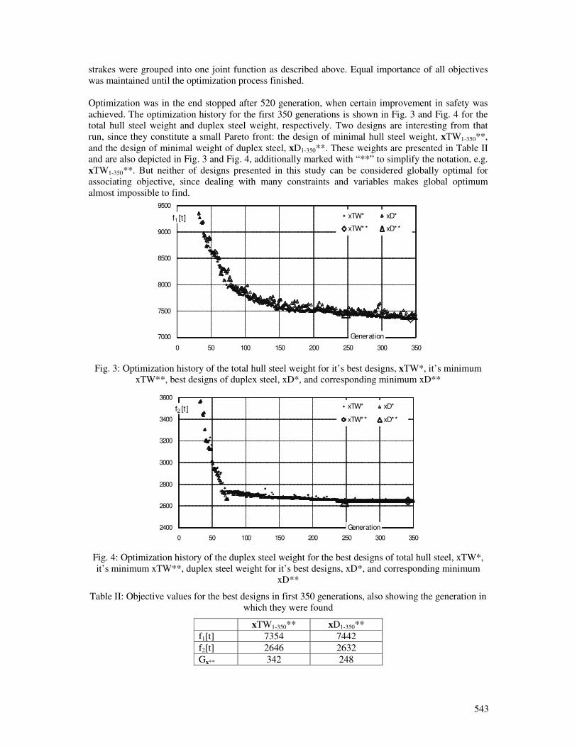
543

strakes were grouped into one joint function as described above. Equal importance of all objectives

was maintained until the optimization process finished.

Optimization was in the end stopped after 520 generation, when certain improvement in safety was

achieved. The optimization history for the first 350 generations is shown in Fig. 3 and Fig. 4 for the

total hull steel weight and duplex steel weight, respectively. Two designs are interesting from that

run, since they constitute a small Pareto front: the design of minimal hull steel weight, xTW1-350**,

and the design of minimal weight of duplex steel, xD1-350**. These weights are presented in Table II

and are also depicted in Fig. 3 and Fig. 4, additionally marked with “**” to simplify the notation, e.g.

xTW1-350**. But neither of designs presented in this study can be considered globally optimal for

associating objective, since dealing with many constraints and variables makes global optimum

almost impossible to find.

7000

7500

8000

8500

9000

9500

0 50 100 150 200 250 300 350

f1 [t]

Generation

xTW* xD*

xTW** xD**

Fig. 3: Optimization history of the total hull steel weight for it’s best designs, xTW*, it’s minimum

xTW**, best designs of duplex steel, xD*, and corresponding minimum xD**

2400

2600

2800

3000

3200

3400

3600

0 50 100 150 200 250 300 350

f2 [t]

Generation

xTW* xD*

xTW** xD**

Fig. 4: Optimization history of the duplex steel weight for the best designs of total hull steel, xTW*,

it’s minimum xTW**, duplex steel weight for it’s best designs, xD*, and corresponding minimum

xD**

Table II: Objective values for the best designs in first 350 generations, also showing the generation in

which they were found

xTW1-350** xD1-350**

f1[t] 7354 7442

f2[t] 2646 2632

Gx** 342 248

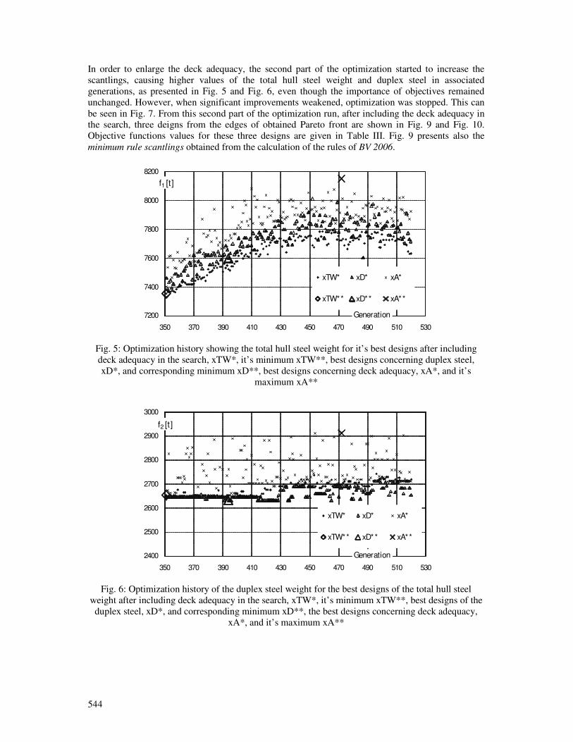
544

In order to enlarge the deck adequacy, the second part of the optimization started to increase the

scantlings, causing higher values of the total hull steel weight and duplex steel in associated

generations, as presented in Fig. 5 and Fig. 6, even though the importance of objectives remained

unchanged. However, when significant improvements weakened, optimization was stopped. This can

be seen in Fig. 7. From this second part of the optimization run, after including the deck adequacy in

the search, three deigns from the edges of obtained Pareto front are shown in Fig. 9 and Fig. 10.

Objective functions values for these three designs are given in Table III. Fig. 9 presents also the

minimum rule scantlings obtained from the calculation of the rules of BV 2006.

7200

7400

7600

7800

8000

8200

350 370 390 410 430 450 470 490 510 530

f1 [t]

Generation

xTW* xD* xA*

xTW** xD** xA**

Fig. 5: Optimization history showing the total hull steel weight for it’s best designs after including

deck adequacy in the search, xTW*, it’s minimum xTW**, best designs concerning duplex steel,

xD*, and corresponding minimum xD**, best designs concerning deck adequacy, xA*, and it’s

maximum xA**

2400

2500

2600

2700

2800

2900

3000

350 370 390 410 430 450 470 490 510 530

f2 [t]

Generation

xTW* xD* xA*

xTW** xD** xA**

Fig. 6: Optimization history of the duplex steel weight for the best designs of the total hull steel

weight after including deck adequacy in the search, xTW*, it’s minimum xTW**, best designs of the

duplex steel, xD*, and corresponding minimum xD**, the best designs concerning deck adequacy,

xA*, and it’s maximum xA**

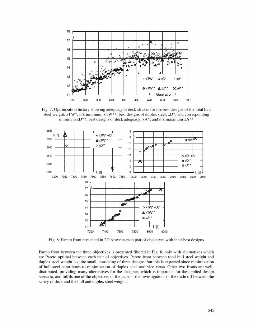
545

11

12

13

14

15

16

17

18

350 370 390 410 430 450 470 490 510 530

f3

Generation

xTW* xD* xA*

xTW** xD** xA**

Fig. 7: Optimization history showing adequacy of deck strakes for the best designs of the total hull

steel weight, xTW*, it’s minimum xTW**, best designs of duplex steel, xD*, and corresponding

minimum xD**, best designs of deck adequacy, xA*, and it’s maximum xA**

2630

2635

2640

2645

2650

2655

7300 7350 7400 7450 7500 7550 7600 7650

f2 [t]

f1 [t]

xTW*-xD*

xTW**

xD**

11

12

13

14

15

16

17

18

2600 2650 2700 2750 2800 2850 2900 2950

f3

f2 [t]

xD*-xA*

xD**

xA**

11

12

13

14

15

16

17

18

7200 7400 7600 7800 8000 8200

f3

f1 [t]

xTW*-xA*

xTW**

xA**

Fig. 8: Pareto front presented in 2D between each pair of objectives with their best designs

Pareto front between the three objectives is presented filtered in Fig. 8, only with alternatives which

are Pareto optimal between each pair of objectives. Pareto front between total hull steel weight and

duplex steel weight is quite small, consisting of three designs, but this is expected since minimization

of hull steel contributes to minimization of duplex steel and vice versa. Other two fronts are well-

distributed, providing many alternatives for the designer, which is important for the applied design

scenario, and fulfils one of the objectives of the paper – the investigations of the trade-off between the

safety of deck and the hull and duplex steel weights.

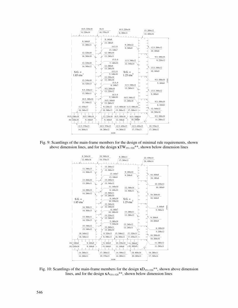
546

12.5; 370x15

17

970

16100

S.G. =

1.85 t/m3

S.G. =

1.25 t/m3

10.5; 370x15 12.5; 430x15 12.5; 430x15 19; 370x13

11; 430x17 9; 220x12 11.5; 400x16 11.5; 400x16

9.5; 180x10

10.5; 220x10 16; 0 10.5; 220x1013; 200x12

12; 340x12

13.5; 340x12

13.5; 340x12

12.5; 200x12

10.5; 340x12

11.5; 340x12

11.5; 340x12

9; 260x12

10.5; 160x9

9.5; 200x10

12; 220x10

12; 200x9

12; 180x10

9; 140x8

10.5; 180x10

9.5; 220x12

12; 240x10

12; 220x10

12; 220x10

9; 160x9

9.5; 180x10

9.5; 180x10

9.5; 180x10

14.5; 0

15.5; 0

15.5; 0

15.5; 0

14.5; 0

12; 220x1010.5; 180x10 10.5; 180x10 10.5; 180x10 10.5; 180x10

14; 260x11 18; 280x12 14; 280x12 17; 370x13 17; 280x12

18; 340x12 10; 300x13 15; 300x12 17; 300x11

11; 280x12

8; 220x10 10; 370x15 8; 280x1114; 400x16

10; 200x10

9; 200x9

10; 160x9

10; 180x8

13; 240x10

13; 280x11

12; 340x14

9; 200x9

13; 260x11

13; 220x12

12; 240x10

13; 240x10

13; 240x11

13; 180x9

15; 340x12

13; 300x11

14; 320x13

14; 300x12

16; 260x10

11; 280x11

6; 160x8

5; 160x8

9; 220x12

5; 140x10

6; 140x7

5; 140x10

7; 140x10

13; 140x7

10; 240x10 9; 160x9 9; 160x9 12; 160x8 10; 200x9

Fig. 9: Scantlings of the main-frame members for the design of minimal rule requirements, shown

above dimension lines, and for the design xTW351-520**, shown below dimension lines

179

70

16100

S.G. =

1.85 t/m3

S.G. =

1.25 t/m3

17; 280x12 14; 300x12 18; 400x16 19; 280x11

18; 340x12 9; 320x13 15; 300x12 17; 320x13

11; 280x12

8; 240x10 18; 340x14 8; 280x1122; 430x14

10; 200x10

9; 200x9

10; 260x10

14; 160x8

13; 240x12

13; 280x11

12; 340x14

9; 180x10

13; 260x11

13; 220x12

12; 240x10

13; 300x11

13; 240x11

13; 200x12

15; 340x12

13; 300x11

14; 300x11

14; 280x12

13; 260x10

11; 340x13

6; 180x10

5; 160x9

10; 220x12

5; 180x10

6; 140x7

9; 140x10

11; 140x10

13; 140x7

9; 160x910; 180x8 9; 160x9 10; 220x10 11; 200x9

14; 260x11 19; 370x13 14; 280x11 20; 280x11 17; 340x14

18; 340x12 9; 300x13 16; 300x12 17; 430x15

11; 280x11

12; 400x16 19; 370x13 17; 280x1226; 400x14

10; 200x10

10; 200x9

10; 160x9

24; 180x8

13; 240x11

13; 280x12

12; 300x11

9; 200x9

13; 260x10

13; 240x12

12; 240x10

13; 240x10

13; 340x12

13; 200x12

15; 340x12

14; 320x13

14; 300x13

14; 280x12

13; 280x11

11; 300x13

5; 200x12

5; 300x11

10; 180x9

7; 220x10

10; 180x10

10; 220x10

8; 140x10

13; 180x9

10; 240x10 9; 160x8 9; 160x9 11; 160x8 10; 160x8

14; 260x11

Fig. 10: Scantlings of the main-frame members for the design xD351-520**, shown above dimension

lines, and for the design xA351-520**, shown below dimension lines

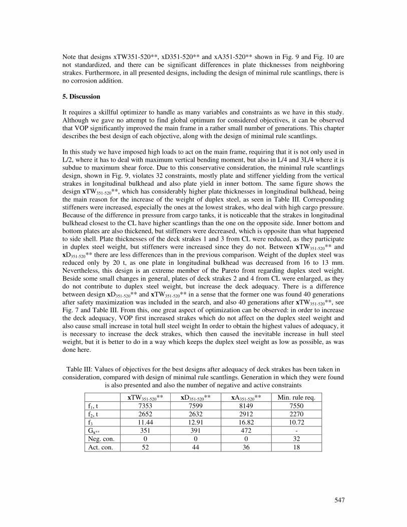
547

Note that designs xTW351-520**, xD351-520** and xA351-520** shown in Fig. 9 and Fig. 10 are

not standardized, and there can be significant differences in plate thicknesses from neighboring

strakes. Furthermore, in all presented designs, including the design of minimal rule scantlings, there is

no corrosion addition.

5. Discussion

It requires a skillful optimizer to handle as many variables and constraints as we have in this study.

Although we gave no attempt to find global optimum for considered objectives, it can be observed

that VOP significantly improved the main frame in a rather small number of generations. This chapter

describes the best design of each objective, along with the design of minimal rule scantlings.

In this study we have imposed high loads to act on the main frame, requiring that it is not only used in

L/2, where it has to deal with maximum vertical bending moment, but also in L/4 and 3L/4 where it is

subdue to maximum shear force. Due to this conservative consideration, the minimal rule scantlings

design, shown in Fig. 9, violates 32 constraints, mostly plate and stiffener yielding from the vertical

strakes in longitudinal bulkhead and also plate yield in inner bottom. The same figure shows the

design xTW351-520**, which has considerably higher plate thicknesses in longitudinal bulkhead, being

the main reason for the increase of the weight of duplex steel, as seen in Table III. Corresponding

stiffeners were increased, especially the ones at the lowest strakes, who deal with high cargo pressure.

Because of the difference in pressure from cargo tanks, it is noticeable that the strakes in longitudinal

bulkhead closest to the CL have higher scantlings than the one on the opposite side. Inner bottom and

bottom plates are also thickened, but stiffeners were decreased, which is opposite than what happened

to side shell. Plate thicknesses of the deck strakes 1 and 3 from CL were reduced, as they participate

in duplex steel weight, but stiffeners were increased since they do not. Between xTW351-520** and

xD351-520** there are less differences than in the previous comparison. Weight of the duplex steel was

reduced only by 20 t, as one plate in longitudinal bulkhead was decreased from 16 to 13 mm.

Nevertheless, this design is an extreme member of the Pareto front regarding duplex steel weight.

Beside some small changes in general, plates of deck strakes 2 and 4 from CL were enlarged, as they

do not contribute to duplex steel weight, but increase the deck adequacy. There is a difference

between design xD351-520** and xTW351-520** in a sense that the former one was found 40 generations

after safety maximization was included in the search, and also 40 generations after xTW351-520**, see

Fig. 7 and Table III. From this, one great aspect of optimization can be observed: in order to increase

the deck adequacy, VOP first increased strakes which do not affect on the duplex steel weight and

also cause small increase in total hull steel weight In order to obtain the highest values of adequacy, it

is necessary to increase the deck strakes, which then caused the inevitable increase in hull steel

weight, but it is better to do in a way which keeps the duplex steel weight as low as possible, as was

done here.

Table III: Values of objectives for the best designs after adequacy of deck strakes has been taken in

consideration, compared with design of minimal rule scantlings. Generation in which they were found

is also presented and also the number of negative and active constraints

xTW351-520** xD351-520** xA351-520** Min. rule req.

f1, t 7353 7599 8149 7550

f2, t 2652 2632 2912 2270

f3 11.44 12.91 16.82 10.72

Gx** 351 391 472 -

Neg. con. 0 0 0 32

Act. con. 52 44 36 18

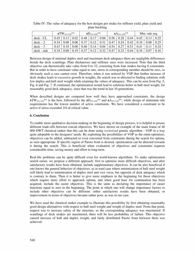
548

Table IV: The value of adequacy for the best designs per strake for stiffener yield, plate yield and

plate buckling

xTW351-520** xD351-520** xA351-520** Min. rule req.

deck - CL 0.45 0.13 0.02 0.48 0.17 0.06 0.56 0.28 0.44 0.45 0.13 0.25

deck – 2 0.34 0.08 0.06 0.37 0.12 0.31 0.47 0.24 0.42 0.34 0.08 0.25

deck – 3 0.43 0.10 0.00 0.46 0.14 0.04 0.54 0.27 0.51 0.41 0.11 0.24

deck - side 0.34 0.08 0.19 0.37 0.12 0.32 0.47 0.23 0.44 0.34 0.07 0.16

Between design of minimal duplex steel and maximum deck adequacy there are negligible differences

beside the deck scantlings. Plate thicknesses and stiffener sizes were increased. Note that the third

objective can theoretically take value from 0 to 32, consisting from four strakes having 8 constraints.

But in order to have constraint value equal to one, stress in corresponding member should be zero, so

obviously such a case cannot exist. Therefore, when it was noticed by VOP that further increase of

deck strakes leads to excessive growth in weights, the search was re-directed to finding solutions with

low duplex and hull steel weight while retaining the values of adequacy. This can be seen from Fig. 5,

Fig. 6 and Fig. 7. If continued, the optimization would lead to solutions better in hull steel weight, for

reasonably good deck adequacy, since that was the trend in last 10 generations.

When described designs are compared how well they have approached constraints, the design

xTW351-520** is the best, followed by the xD351-520** and xA351-520**, while design of minimum rule

requirements has the lowest number of active constraints. We have considered a constraint to be

active if stress exceeded 3/4 of critical value.

6. Conclusion

To enable more qualitative decision-making in the beginning of design process, it is helpful to posses

different trade-offs between crucial objectives. We have shown on example of the main frame of 40

000 DWT chemical tanker that this can be done using vectorized genetic algorithm - VOP in a way

quite adoptable to the designers' needs. By exploiting the possibilities of VOP as the omni-optimizer,

objectives can be added, subtracted or even converted from constraints during the search for optima,

as seen appropriate. If specific region of Pareto front is desired, optimization can be directed towards

it during the search. This is beneficial when evaluation of objectives and constraints requests

considerable time, saving money and effort in long-term.

Real-life problems can be quite difficult even for world-known algorithms. To make optimization

search easier, we propose a different approach: first to optimize more difficult objectives, and after

satisfactory results have been obtained, include supplementary objectives. It can be also beneficial if

one knows the general behavior of objectives, as in used case where minimization of hull steel weight

will likely lead to minimization of duplex steel and vice versa, but opposite of deck adequacy which

is contrary to them. Then it is better to give more emphasis in the beginning for those objectives

which require more effort to approach optima, and when good base for continuation has been

acquired, include the easier objectives. This is the same as declaring the importance of easier

functions equal to zero in the beginning. The point at which one will change importance factors to

include other objectives can be different: either satisfactory results have been obtained, or

improvement in terms of objectives became rather poor, as was in our case.

We have used the chemical tanker example to illustrate this possibility by first obtaining reasonably

good design alternatives with respect to hull steel weight and weight of duplex steel. From that point,

request was to increase safety of the structure, so the corresponding adequacy was maximized. If

scantlings of deck strakes are maximized, there will be less probability of failure. This objective

caused increase of hull and duplex weight, and fairly distributed Pareto front between them was

achieved.

549

Since for the problem of chemical tanker’s main frame VOP accomplished encouraging results, and

handled large-scale optimization with ease, it would we interesting to observe how well can it behave

with expanded problem. Additional frames could be included in the search so to optimize different

sections of the hull. Additional effort will be given to further improve the fitness assignment in VOP.

It would be also beneficial to devise more generic fitness function, one which does not make

difference between the selection schemes based on feasibility. Comparison with other optimizers is

necessary in order to claim how well can it perform, and this will be surely the topic of the future

studies.

Acknowledgements

This study has been supported by the European Union funded project IMPROVE and the project

CONSTRUCT, financed by the Technology centre of Finland – TEKES. This help is greatly

appreciated.

References

KLANAC, A.; JELOVICA, J. (2007a), Vectorization in the structural optimization of a fast ferry,

Brodogradnja, 58/1, pp. 11-17

KLANAC, A.; JELOVICA, J. (2008), Vectorization and constraint grouping to enhance optimization

of marine structures, submitted to Marine Structures

KLANAC, A.; JELOVICA, J. (2007b), A concept of omni-optimization for ship structural design, in

Guedes Soares, C.; Das, P.K. (Eds.), Advancements in marine structures, Taylor & Francis, London ,

pp. 471-480

DEB, K.; TIWARI, S. (2005), Omni-optimizer: A Procedure for Single and Multi-objective

Optimization, in Coello Coello, C.A. et al. (Eds.), EMO 2005, Springer-Verlag Berlin Heidelberg

2005, pp. 47-61

BESNARD, N.; CODDA, M.; UNGARO, A.; TODERAN, C.; KLANAC, A.; PECOT, F. (2007),

Benchmark on ship structural optimisation, in Coello Coello, C.A. et al. (Eds.), Advancements in

marine structures, Taylor & Francis, London, pp.453-463

ROMANOFF. J.; KLANAC, A. (2007), Optimization of a Steel Sandwich Hoistable Car-Decks

Applying Homogenized Plate Theory, 10th International Symposium on Practical Design of Ships and

Other Floating Structures – PRADS, Houston

EHLERS, S.; KLANAC, A.; TABRI, K. (2007), Increased safety of a tanker and a RO-PAX vessel by

implementing a novel sandwich structure, 4th International Conference on Collision and Grounding of

Ships. Hamburg, pp. 109-115

OSYCZKA, A.; KRENICH, S.; TAMURA, H.; GOLDBERG, D. (2000), A Bicriterion Approach to

Constrained Optimization Problems using Genetic Algorithm, Evolutionary Optimization – An

International Journal on the Internet, 2/1, pp. 43-54

DEB, K. (2001), Multi-objective Optimization Using Evolutionary Algorithms, Wiley, Chichester,

UK

HUGHES, O.F.; MISTREE, F.; ZANIC, V. (1980), A practical method for the rational design of ship

structures, J. Ship Research, 24/2, pp.101-113

RUKKI (2008), Hot Rolled Shipbuilding Profiles

550

KOSKI, J.; SILVENNOINEN, R. (1987), Norm Methods and Partial Weighting in Multicriterion

Optimization of Structures, International Journal for Numerical Methods in Engineering, Vol. 24,

pp.1101-1121

NAAR, H.; VARSTA, P.; KUJALA, P. (2004), A theory of coupled beams for strength assessment of

passenger ships, Marine Structures, 17/8, pp. 590-611

NIEMELÄINEN, M. (2007), Computational Method for Evaluation of Hull Girder Strength in

Concept Design Stage, Master’s thesis, Helsinki University of Technology

MANTERE, H. (2007), Strength Analysis for the Design of Local Ship Structures in Concept Stage,

Master’s thesis, Helsinki University of Technology

HUGHES, O.F. (1988), Ship Structural Design, Society of Naval Architects and Marine Engineers,

Wiley, New York

DEB, K.; PRATAP, A.; AGARWAL, S.; MEYARIVAN, T. (2002), A Fast and Elitist Multiobjective

Genetic Algorithm – NSGA-II, IEEE Transactions on Evolutionary Computation, 6/1, pp. 182-197

ZITZLER, E.; LAUMANNS, M.; THIELE, L. (2002), SPEA2: Improving the Strength Pareto

Evolutionary Algorithm for Multiobjective Optimization, in Giannakoghu, K.; Tsahalis, D.; Periaux,

J.; Papailiou, K.; Fogarty, T. (eds.), Evolutionary Methods for Design, Optimisation and Control,

CIMNE, Barcelona, Spain

BUREAU VERITAS (2006), Rules for the classification of steel ships

DEB, K.; MOHAN, M.; MISHRA, S. (2003), A Fast Multi-objective Evolutionary Algorithm for

Finding Well-Spread Pareto-Optimal Solutions, KanGAL Report Number 2003002

DEB, K. (2001), Multi-Objective Optimization using Evolutionary Algorithms, John Wiley and Sons,

Chichester

551

Multi-Disciplinary Synthesis Design and Optimization for Multi-Hull Ships

Hamid Hefazi, California State University, Long Beach/USA, hefazi@csulb.edu Adeline Schmitz, California State University, Long Beach/USA schmitz@csulb.edu

Igor Mizine, Computer Science Corporation, Washington DC/USA imizine@csc.com Geoffrey Boals, Computer Science Corporation, Washington DC, USA gboals@csc.com

Abstract

This paper describes a synthesis level multi-disciplinary design and optimization (MDO) method developed for multi-hull ships. This method is unique in utilizing advanced multi-objective optimization methods, in its broad scope, integrating powering, stability, seakeeping, hullforms definition, cost and payload capacity into a single design tool and in its use of neural networks as a response surface method. More specifically, neural networks, trained based on sets of CFD data, are used for estimation of powering and seakeeping through the optimization loop. Details of the method and multi-objective optimization results in the form of pareto optimum solutions for multi-hull concepts are presented. 1. Introduction The vast majority of current U.S. naval auxiliary ships are relatively large mono-hulls with limited speed capabilities. The OSD guidance known by the rubric “10-30-30” cites goals for the speeds at which deployments have to be executed that cannot be met with existing transportation vehicles, particularly the ships on which over 90% of the materiel needed by ground forces has to move. The desire for high-speed transit capabilities has resulted in increased interest in non-traditional and multi-hull platforms for naval missions. Multi-hull ships have many potential advantages over mono-hull ships; however, their design procedures are not as mature. Further, multi-hull ships also offer avenues of hydrodynamic design optimization that are not found on mono-hull ships – such as optimizing of hull spacing or relative hull proportions. Achieving many desirable sets of performances requires advances in our ability to predict (and explore) hydrodynamic effects in conjunction with other constraints such as dynamic structural loads when operating in high sea states and cost. Synthesis tools that are used to explore the ship design trade space in the concept design phase (ASSET, PASS) have been around for many years and are used widely by industry for mono-hull ships. While some synthesis tools have been developed for multi-hulls, they are not nearly comparable in depth or level of fidelity to the mono-hull tools. They are used to develop point solutions of ship designs to populate and study the trade space, but the difference in the point designs are determined by the design team. This process could be substantially enhanced by the application of multi-disciplinary design and optimization (MDO) tools to the design problem, and by further development of multi-hull synthesis tools. Comprehensive, computational MDO tools however can be prohibitively expensive considering the complexities that are involved in accurate analysis of hydrodynamics, structural loads, cost, etc. Advanced multi-objective optimization methods in conjunction with advances in our ability to accurately and efficiently predict these performances are needed if these tools are to be of practical value to the designer. Such advanced multi-disciplinary ship hull design/optimization tools will be a valuable resource equally applicable to the design of future commercial or military high speed vessels (dual-use). The advanced hull forms designed therewith potentially offer the advantage of reduced drag at a given speed, and thus increased fuel efficiency and range, and/or reduced structural weight and thus increased cargo lift capacity while meeting stability and seakeeping criteria. Most of the MDO works to-date are focused on application to mono-hulls. For example, Zalek (2007) describes multi-criterion evolutionary optimization of ship hullforms for propulsion and seakeeping. The problem formulation and development is applicable to mono-hull frigate type naval surface

552

vessels. Harries et al. (2001), investigate optimization strategies for hydrodynamic design of fast ferries. A commercial optimization system is used to integrate various CAD and CFD codes for calm water resistance and seakeeping. The method is applied to Ro-Ro ferry. Campana et al. (2007) present results of the MDO of the keel fin of a sailing yacht accounting for hydrodynamic and elasticity. Different MDO formulations are studied in the context of global optimization (GO) frame work. Studies applicable to multi-hull ships include, Tahara et al. (2007) who present a multi-objective optimization approach for a fast catamaran via a Simulation-Based Design (SBD) framework. A variable fidelity concept is also presented which allows for integration of accurate, yet time consuming RANS predictions together with fast potential flow results for optimization. The MDO method only considers resistance and seakeeping. Another study funded by the Office of Naval Research at University of Michigan, Beck (2007) is also focusing on the hydrodynamic (seakeeping and resistance) optimization of multi-hulls. Brown and Neu, (2008) in the phase I of a study entitled Naval Surface Ship Design Optimization for Affordability have applied a multi-objective optimization method to a number of case studies using a simple ship synthesis model, and the US Navy’s Advanced Ship and Submarine Evaluation Tool (ASSET) in the PHX ModelCenter (MC) design environment, ASSET (2008), ModelCenter (2008). Their case studies include LHA(R), a replacement for the US Navy amphibious assault ship, and DDG-51, a destroyer class vessel. Phase II of their study will include response surface modeling (RSM), a more detailed design of experiments (DOE) and focus on multi-hull high speed ships. Since 1998, CSULB, under programs funded by the Office of Naval Research (ONR), Besnard et al. (1998), and the Center for Commercial Development of Transportation Technology (CCDoTT) has been developing advanced automated optimization methods and computational fluid dynamics (CFD) methods for applications to fast ship design. Originally, the focus of these programs was shape optimization of underwater hull forms, such as the Pacific Marine’s blended wing body (BWB) which was optimized for its lift to drag ratio, Hefazi et al. (2002), Hefazi et al. (2003). Having demonstrated the feasibility of automated hydrodynamic shape optimization for lifting bodies using advanced methods such as neural networks, Schmitz (2007), CSULB in collaboration with Computer Science Corporation (CSC) initiated the current program to extend these technologies to multi-disciplinary design and optimization (MDO) of multi-hull ships. Our approach is unique in its broad scope and use of neural networks as a response surface method. Generally, the MDO design system consists of synthesis design method (SDM), hullforms definition and optimization sub-system, seakeeping, structural design optimization, general & cargo arrangement design optimization, propulsion machinery sub-systems and more local sub-systems such as: outfit, electrics, handling systems, etc. Seakeeping, power, and payload are primary functional relationships, which depending on the stage of the design, are analyzed at various degrees of fidelity. Two major challenges of MDO design system are: - MDO needs to formulate a design in which there are several criteria or design objectives, some of

which are conflicting. - Subsystem performance evaluations (such as powering, seakeeping, etc) are often very complex

and (computationally) intensive. Direct evaluation of these performances as part of the optimization process, may make the MDO method too costly and out of reach of most practical design problems.

To overcome these limitations, our approach, uses advanced multi-objective optimization methods such as Neighborhood Cultivation Genetic Algorithm (NCGA) for optimization. Unlike traditional design spiral approaches, multi-objective optimization keeps various objectives separate and concurrent in order to find the best possible design, which satisfies the (opposing) objectives and constraints. To address the subsystem performance evaluation challenge, artificial neural networks are trained based on model tests or computed data bases and are used in the optimization process to evaluate various subsystem performances. This innovative approach replaces the use of highly

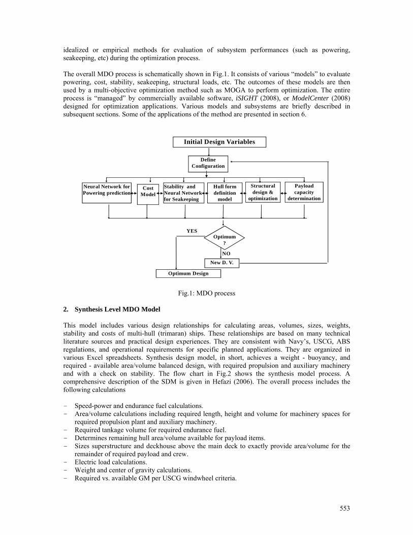
553

idealized or empirical methods for evaluation of subsystem performances (such as powering, seakeeping, etc) during the optimization process. The overall MDO process is schematically shown in Fig.1. It consists of various “models” to evaluate powering, cost, stability, seakeeping, structural loads, etc. The outcomes of these models are then used by a multi-objective optimization method such as MOGA to perform optimization. The entire process is “managed” by commercially available software, iSIGHT (2008), or ModelCenter (2008) designed for optimization applications. Various models and subsystems are briefly described in subsequent sections. Some of the applications of the method are presented in section 6.

Fig.1: MDO process

2. Synthesis Level MDO Model This model includes various design relationships for calculating areas, volumes, sizes, weights, stability and costs of multi-hull (trimaran) ships. These relationships are based on many technical literature sources and practical design experiences. They are consistent with Navy’s, USCG, ABS regulations, and operational requirements for specific planned applications. They are organized in various Excel spreadsheets. Synthesis design model, in short, achieves a weight - buoyancy, and required - available area/volume balanced design, with required propulsion and auxiliary machinery and with a check on stability. The flow chart in Fig.2 shows the synthesis model process. A comprehensive description of the SDM is given in Hefazi (2006). The overall process includes the following calculations - Speed-power and endurance fuel calculations. - Area/volume calculations including required length, height and volume for machinery spaces for

required propulsion plant and auxiliary machinery. - Required tankage volume for required endurance fuel. - Determines remaining hull area/volume available for payload items. - Sizes superstructure and deckhouse above the main deck to exactly provide area/volume for the

remainder of required payload and crew. - Electric load calculations. - Weight and center of gravity calculations. - Required vs. available GM per USCG windwheel criteria.

New D. V.

Initial Design Variables

Optimum Design

Neural Network for Powering prediction

Define Configuration

Optimum?

YES

NO

Structural design &

optimization

Stability and Neural Network for Seakeeping

Payload capacity

determination

Cost Model

Hull form definition

model

554

3. Cost Model The build strategy and cost estimate analysis for multi-hull (trimarans and catamarans) and mono-hull ships is performed using SPAR Associates proprietary cost estimating model called PERCEPTION ESTI-MATE. SPAR’s PERCEPTION ESTI-MATE cost model has evolved over nearly two decades of algorithm development and shipyard return cost data collection and evaluation, perception Esti-mate (2008). The cost models’ approach for an estimate is based first upon the composition of the hull’s structural components (decks, bulkheads, shell, double bottoms, etc.), then the ship systems (mechanical, piping, electrical, HVAC, etc.), and finally other ship characteristics. Factors considered, and applied, if relevant, are the general build strategy for on-unit, on-block and on-board construction; the type of shipyard and its established product line, its facilities and production capabilities; and the expected competence of the shipyard to plan and manage its resources, costs, and schedules. Each cost model employs a comprehensive set of cost estimating relationships, or CERs. They reside on SPAR’s estimating system called PERCEPTION ESTI-MATE and represent a wide cross-section of current and historical shipyard construction costs at many levels of detail. Adjustments can be made (and were made for the HALSS estimate) as necessary to reflect differing shipyard productivity factors, construction methods, and material costs. These CERs, while parametric in nature, focus on a specific area of cost (labor and material) and each reflects the specific material and the manufacturing and assembly processes required. Specialized CERs focus on structural component fabrication, assembly, and erection for installation of propulsion systems and for various support activities. The CERs are based on many different metrics, such as weld length, deck area, compartment volumes, number of crew (by type crew), kW of propulsion (by type), etc. Hull structural component costs are based upon component weight by type of structure and material. The cost estimates, applicable to a lead ship, are believed to be fair representations of anticipated true costs based upon the design information. Material costs have been adjusted to reflect a common year (2007) value. This assumes that for a multi-year program, appropriate contract escalation clauses have been defined to index actual costs relative to the base year. The cost estimates are based upon typical contract cost and schedule performance for three types of shipbuilders and shipbuilding processes: so-called Virtual Shipyard (US National Ship Research Program (NSRP) terminology), Dual Use Shipyard, and Large US Mid Tier Shipyard, as well as shipyards in other countries. 4. Using Neural Networks in Numerical Optimization As mentioned earlier, a unique feature of our approach is the utilization of artificial neural networks as a response surface method (RSM) to replace time consuming and costly direct CFD calculations of powering and seakeeping in the optimization loop. The method has wide range of other potential applications and is briefly reviewed here. The modern approach used in the design of a complex system (the ship or component inside the ship) usually includes at some level an optimization. In practical cases, the design tool may either be an optimization or design-of-experiment software, or a set of test cases identified by an experienced designer interested in conducting trade studies. The analyses performed at each subsystem level rely, in general, on a combination of semi-analytical models, advanced numerical methods such as computational fluid dynamics (CFD) and finite element analysis (FE), and use of existing databases.

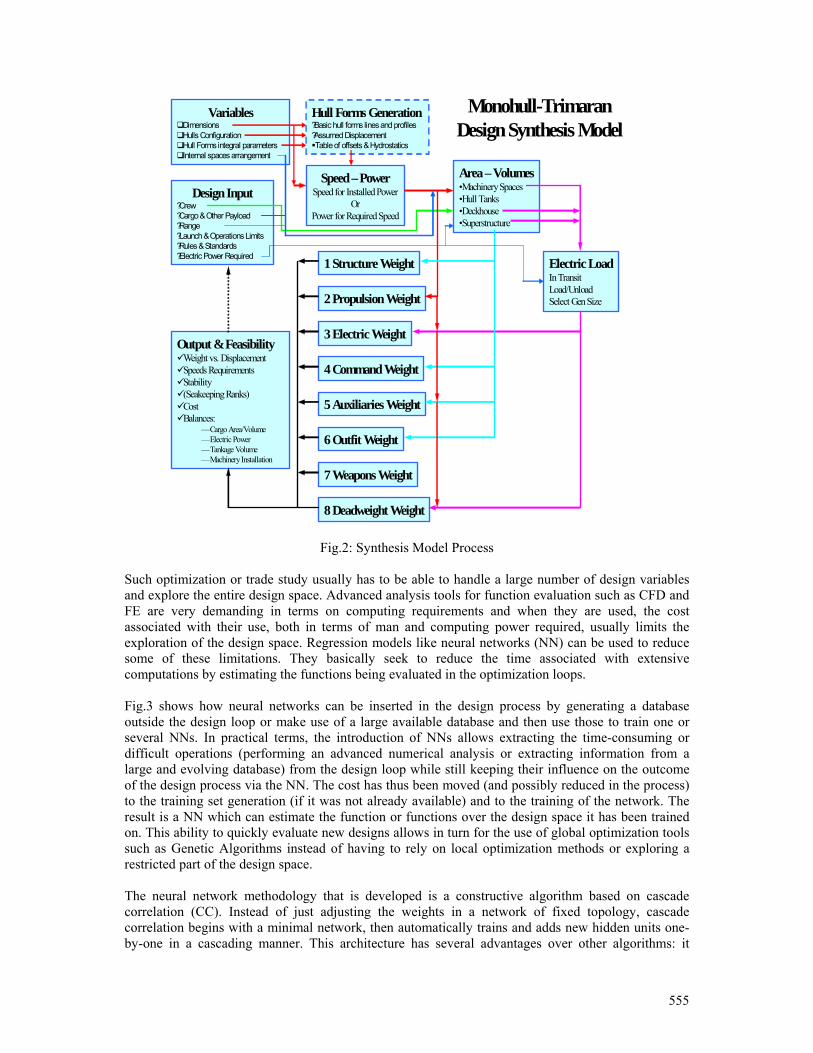
555

Monohull-Trimaran Design Synthesis Model

Design Input?Crew?Cargo & Other Payload?Range?Launch & Operations Limits?Rules & Standards?Electric Power Required

Speed –PowerSpeed for Installed Power

OrPower for Required Speed

Area –Volumes•Machinery Spaces•Hull Tanks•Deckhouse•Superstructure

Electric LoadIn TransitLoad/UnloadSelect Gen Size

7 Weapons Weight

6 Outfit Weight

5 Auxiliaries Weight

4 Command Weight

3 Electric Weight

2 Propulsion Weight

1 Structure Weight

8 Deadweight Weight

Output & FeasibilityWeight vs. DisplacementSpeeds RequirementsStability(Seakeeping Ranks)CostBalances:

—Cargo Area/Volume—Electric Power—Tankage Volume—Machinery Installation

VariablesDimensionsHulls ConfigurationHull Forms integral parametersInternal spaces arrangement

Hull Forms Generation?Basic hull forms lines and profiles?Assumed DisplacementTable of offsets & Hydrostatics

Fig.2: Synthesis Model Process Such optimization or trade study usually has to be able to handle a large number of design variables and explore the entire design space. Advanced analysis tools for function evaluation such as CFD and FE are very demanding in terms on computing requirements and when they are used, the cost associated with their use, both in terms of man and computing power required, usually limits the exploration of the design space. Regression models like neural networks (NN) can be used to reduce some of these limitations. They basically seek to reduce the time associated with extensive computations by estimating the functions being evaluated in the optimization loops. Fig.3 shows how neural networks can be inserted in the design process by generating a database outside the design loop or make use of a large available database and then use those to train one or several NNs. In practical terms, the introduction of NNs allows extracting the time-consuming or difficult operations (performing an advanced numerical analysis or extracting information from a large and evolving database) from the design loop while still keeping their influence on the outcome of the design process via the NN. The cost has thus been moved (and possibly reduced in the process) to the training set generation (if it was not already available) and to the training of the network. The result is a NN which can estimate the function or functions over the design space it has been trained on. This ability to quickly evaluate new designs allows in turn for the use of global optimization tools such as Genetic Algorithms instead of having to rely on local optimization methods or exploring a restricted part of the design space. The neural network methodology that is developed is a constructive algorithm based on cascade correlation (CC). Instead of just adjusting the weights in a network of fixed topology, cascade correlation begins with a minimal network, then automatically trains and adds new hidden units one-by-one in a cascading manner. This architecture has several advantages over other algorithms: it

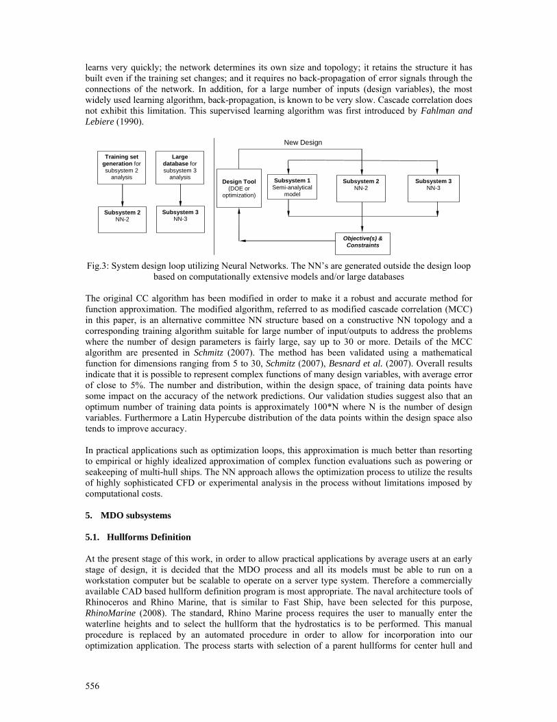
556

learns very quickly; the network determines its own size and topology; it retains the structure it has built even if the training set changes; and it requires no back-propagation of error signals through the connections of the network. In addition, for a large number of inputs (design variables), the most widely used learning algorithm, back-propagation, is known to be very slow. Cascade correlation does not exhibit this limitation. This supervised learning algorithm was first introduced by Fahlman and Lebiere (1990).

Subsystem 1Semi-analytical

model

Design Tool (DOE or

optimization)

New Design

Subsystem 2NN-2

Subsystem 3NN-3

Objective(s) & Constraints

Training set generation for subsystem 2

analysis

Subsystem 2 NN-2

Large database for subsystem 3

analysis

Subsystem 3 NN-3

Fig.3: System design loop utilizing Neural Networks. The NN’s are generated outside the design loop

based on computationally extensive models and/or large databases The original CC algorithm has been modified in order to make it a robust and accurate method for function approximation. The modified algorithm, referred to as modified cascade correlation (MCC) in this paper, is an alternative committee NN structure based on a constructive NN topology and a corresponding training algorithm suitable for large number of input/outputs to address the problems where the number of design parameters is fairly large, say up to 30 or more. Details of the MCC algorithm are presented in Schmitz (2007). The method has been validated using a mathematical function for dimensions ranging from 5 to 30, Schmitz (2007), Besnard et al. (2007). Overall results indicate that it is possible to represent complex functions of many design variables, with average error of close to 5%. The number and distribution, within the design space, of training data points have some impact on the accuracy of the network predictions. Our validation studies suggest also that an optimum number of training data points is approximately 100*N where N is the number of design variables. Furthermore a Latin Hypercube distribution of the data points within the design space also tends to improve accuracy. In practical applications such as optimization loops, this approximation is much better than resorting to empirical or highly idealized approximation of complex function evaluations such as powering or seakeeping of multi-hull ships. The NN approach allows the optimization process to utilize the results of highly sophisticated CFD or experimental analysis in the process without limitations imposed by computational costs. 5. MDO subsystems 5.1. Hullforms Definition At the present stage of this work, in order to allow practical applications by average users at an early stage of design, it is decided that the MDO process and all its models must be able to run on a workstation computer but be scalable to operate on a server type system. Therefore a commercially available CAD based hullform definition program is most appropriate. The naval architecture tools of Rhinoceros and Rhino Marine, that is similar to Fast Ship, have been selected for this purpose, RhinoMarine (2008). The standard, Rhino Marine process requires the user to manually enter the waterline heights and to select the hullform that the hydrostatics is to be performed. This manual procedure is replaced by an automated procedure in order to allow for incorporation into our optimization application. The process starts with selection of a parent hullforms for center hull and

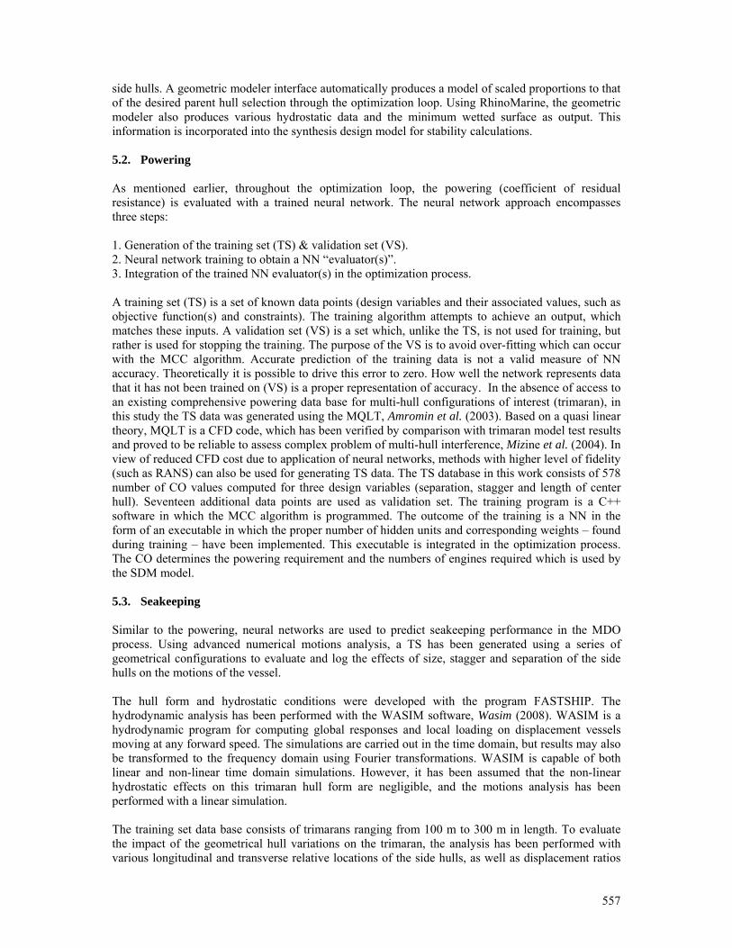
557

side hulls. A geometric modeler interface automatically produces a model of scaled proportions to that of the desired parent hull selection through the optimization loop. Using RhinoMarine, the geometric modeler also produces various hydrostatic data and the minimum wetted surface as output. This information is incorporated into the synthesis design model for stability calculations. 5.2. Powering As mentioned earlier, throughout the optimization loop, the powering (coefficient of residual resistance) is evaluated with a trained neural network. The neural network approach encompasses three steps: 1. Generation of the training set (TS) & validation set (VS). 2. Neural network training to obtain a NN “evaluator(s)”. 3. Integration of the trained NN evaluator(s) in the optimization process. A training set (TS) is a set of known data points (design variables and their associated values, such as objective function(s) and constraints). The training algorithm attempts to achieve an output, which matches these inputs. A validation set (VS) is a set which, unlike the TS, is not used for training, but rather is used for stopping the training. The purpose of the VS is to avoid over-fitting which can occur with the MCC algorithm. Accurate prediction of the training data is not a valid measure of NN accuracy. Theoretically it is possible to drive this error to zero. How well the network represents data that it has not been trained on (VS) is a proper representation of accuracy. In the absence of access to an existing comprehensive powering data base for multi-hull configurations of interest (trimaran), in this study the TS data was generated using the MQLT, Amromin et al. (2003). Based on a quasi linear theory, MQLT is a CFD code, which has been verified by comparison with trimaran model test results and proved to be reliable to assess complex problem of multi-hull interference, Mizine et al. (2004). In view of reduced CFD cost due to application of neural networks, methods with higher level of fidelity (such as RANS) can also be used for generating TS data. The TS database in this work consists of 578 number of CO values computed for three design variables (separation, stagger and length of center hull). Seventeen additional data points are used as validation set. The training program is a C++ software in which the MCC algorithm is programmed. The outcome of the training is a NN in the form of an executable in which the proper number of hidden units and corresponding weights – found during training – have been implemented. This executable is integrated in the optimization process. The CO determines the powering requirement and the numbers of engines required which is used by the SDM model. 5.3. Seakeeping Similar to the powering, neural networks are used to predict seakeeping performance in the MDO process. Using advanced numerical motions analysis, a TS has been generated using a series of geometrical configurations to evaluate and log the effects of size, stagger and separation of the side hulls on the motions of the vessel. The hull form and hydrostatic conditions were developed with the program FASTSHIP. The hydrodynamic analysis has been performed with the WASIM software, Wasim (2008). WASIM is a hydrodynamic program for computing global responses and local loading on displacement vessels moving at any forward speed. The simulations are carried out in the time domain, but results may also be transformed to the frequency domain using Fourier transformations. WASIM is capable of both linear and non-linear time domain simulations. However, it has been assumed that the non-linear hydrostatic effects on this trimaran hull form are negligible, and the motions analysis has been performed with a linear simulation. The training set data base consists of trimarans ranging from 100 m to 300 m in length. To evaluate the impact of the geometrical hull variations on the trimaran, the analysis has been performed with various longitudinal and transverse relative locations of the side hulls, as well as displacement ratios

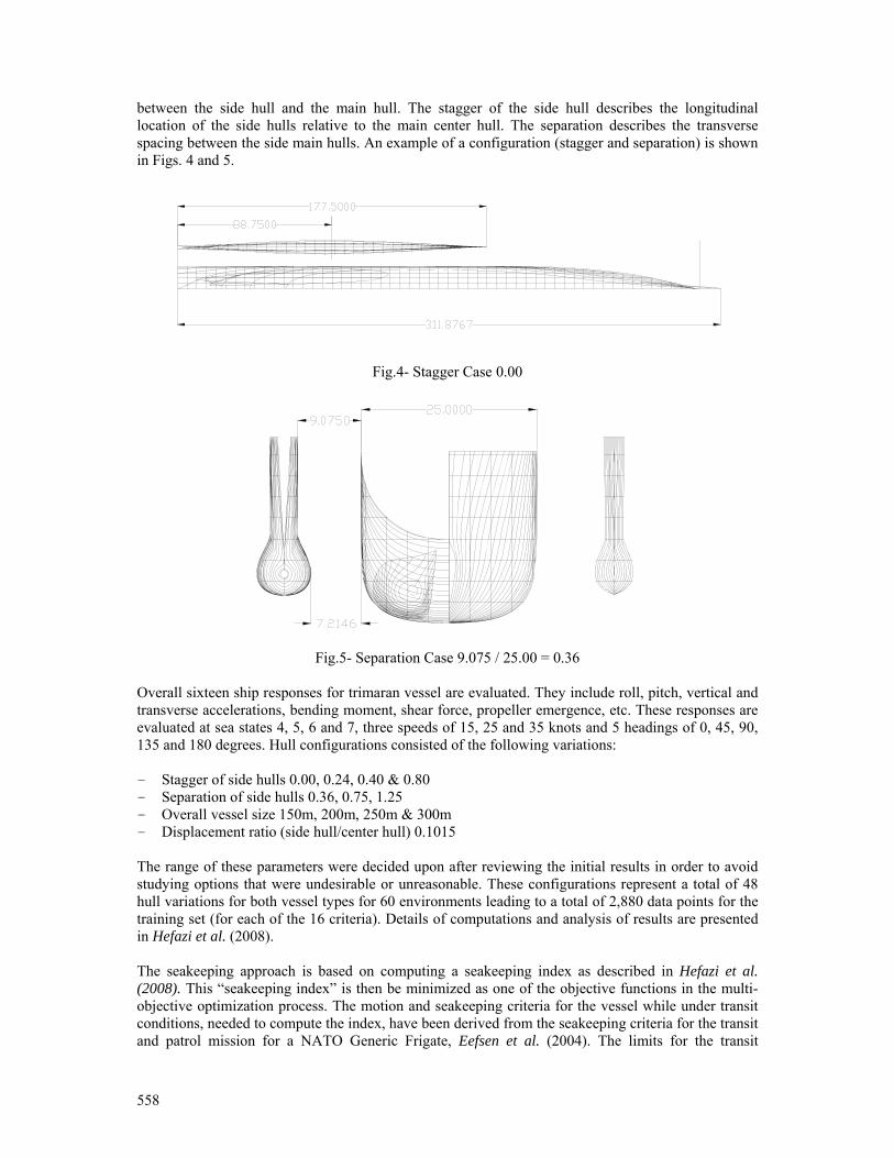
558

between the side hull and the main hull. The stagger of the side hull describes the longitudinal location of the side hulls relative to the main center hull. The separation describes the transverse spacing between the side main hulls. An example of a configuration (stagger and separation) is shown in Figs. 4 and 5.

Fig.4- Stagger Case 0.00

Fig.5- Separation Case 9.075 / 25.00 = 0.36

Overall sixteen ship responses for trimaran vessel are evaluated. They include roll, pitch, vertical and transverse accelerations, bending moment, shear force, propeller emergence, etc. These responses are evaluated at sea states 4, 5, 6 and 7, three speeds of 15, 25 and 35 knots and 5 headings of 0, 45, 90, 135 and 180 degrees. Hull configurations consisted of the following variations: - Stagger of side hulls 0.00, 0.24, 0.40 & 0.80 - Separation of side hulls 0.36, 0.75, 1.25 - Overall vessel size 150m, 200m, 250m & 300m - Displacement ratio (side hull/center hull) 0.1015 The range of these parameters were decided upon after reviewing the initial results in order to avoid studying options that were undesirable or unreasonable. These configurations represent a total of 48 hull variations for both vessel types for 60 environments leading to a total of 2,880 data points for the training set (for each of the 16 criteria). Details of computations and analysis of results are presented in Hefazi et al. (2008). The seakeeping approach is based on computing a seakeeping index as described in Hefazi et al. (2008). This “seakeeping index” is then be minimized as one of the objective functions in the multi-objective optimization process. The motion and seakeeping criteria for the vessel while under transit conditions, needed to compute the index, have been derived from the seakeeping criteria for the transit and patrol mission for a NATO Generic Frigate, Eefsen et al. (2004). The limits for the transit

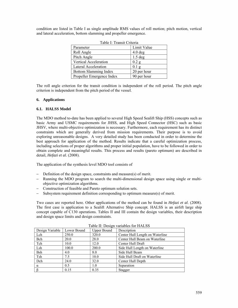
559

condition are listed in Table I as single amplitude RMS values of roll motion; pitch motion, vertical and lateral acceleration, bottom slamming and propeller emergence.

Table I: Transit Criteria Parameter Limit Value Roll Angle 4.0 deg Pitch Angle 1.5 deg Vertical Acceleration 0.2 g Lateral Acceleration 0.1 g Bottom Slamming Index 20 per hour Propeller Emergence Index 90 per hour

The roll angle criterion for the transit condition is independent of the roll period. The pitch angle criterion is independent from the pitch period of the vessel. 6. Applications 6.1. HALSS Model The MDO method to-date has been applied to several High Speed Sealift Ship (HSS) concepts such as basic Army and USMC requirements for JHSS, and High Speed Connector (HSC) such as basic JHSV, where multi-objective optimization is necessary. Furthermore, each requirement has its distinct constraints which are generally derived from mission requirements. Their purpose is to avoid exploring unreasonable designs. A very detailed study has been conducted in order to determine the best approach for application of the method. Results indicate that a careful optimization process, including selections of proper algorithms and proper initial population, have to be followed in order to obtain complete and meaningful results. This process and results (pareto optimum) are described in detail, Hefazi et al. (2008). The application of the synthesis level MDO tool consists of − Definition of the design space, constraints and measure(s) of merit. − Running the MDO program to search the multi-dimensional design space using single or multi-

objective optimization algorithms. − Construction of feasible and Pareto optimum solution sets. − Subsystem requirement definition corresponding to optimum measure(s) of merit. Two cases are reported here. Other applications of the method can be found in Hefazi et al. (2008). The first case is application to a Sealift Alternative Ship concept. HALSS is an airlift large ship concept capable of C130 operations. Tables II and III contain the design variables, their description and design space limits and design constraints.

Table II: Design variables for HALSS Design Variable Lower Bound Upper Bound Description Lch 250.0 320.0 Center Hull Length on Waterline Bch 20.0 28.0 Center Hull Beam on Waterline Tch 10.0 12.0 Center Hull Draft Lsh 100.0 200.0 Side Hull Length on Waterline Bsh 4.0 8.0 Side Hull Beam Tsh 7.5 10.0 Side Hull Draft on Waterline Dch 24.0 32.0 Center Hull Depth α 0.5 1.0 Separation β 0.15 0.35 Stagger

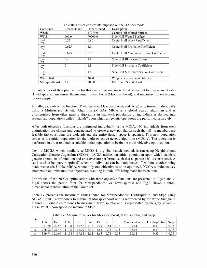
560

Table III: List of constraints imposed on the HALSS model Constraint Lower Bound Upper Bound Description WSch 0 17279.0 Center Hull Wetted Surface WSsh 600.0 90000.0 Side Hull Wetted Surface

chbC

0.55 0.90 Center Hull Block Coefficient

chpC

0.625 1.0 Center Hull Prismatic Coefficient

chmC

0.675 0.95 Center Hull Maximum Section Coefficient

shbC

0.4 1.8 Side Hull Block Coefficient

shpC

0 1.8 Side Hull Prismatic Coefficient

shmC

0.7 1.8 Side Hull Maximum Section Coefficient

Wtdisplbal 0 3000 Weight-Displacement Balance Maxspeedboost 33.0 200.0 Maximum Speed Boost

The objectives of the optimization for this case are to maximize the dead weight to displacement ratio (Dwtdisplratio), maximize the maximum speed boost (Maxspeedboost), and maximize the seakeeping index (Skpp). Initially, each objective function (Dwtdisplratio, Maxspeedboost, and Skpp) is optimized individually using a Multi-island Genetic Algorithm (MIGA). MIGA is a global search algorithm and is distinguished from other genetic algorithms in that each population of individuals is divided into several sub-populations called “islands” upon which all genetic operations are performed separately. After both objective functions are optimized individually using MIGA, 100 individuals from each optimization are chosen and concatenated to create a new population such that all its members are feasible (no constraints are violated) and the entire design space is spanned. This new population serves as the initial population for the multi-objective genetic algorithm (MOGA). This operation is performed in order to obtain a suitable initial population to begin the multi-objective optimization. Next, a MOGA which, similarly to MIGA is a global search method, is run using Neighborhood Cultivation Genetic Algorithm (NCGA). NCGA utilizes an initial population upon which standard genetic operations of mutation and crossover are performed such that a “pareto set” is constructed. A set is said to be “pareto optimal” when no individual can be made better off without another being made worse off. Unlike MIGA, where only one objective is to be optimized, NCGA simultaneously attempts to optimize multiple objectives, resulting in trade-offs being made between them. The results of the NCGA optimization with three objective functions are presented in Figs.6 and 7; Fig.6 shows the pareto front for Maxspeedboost vs. Dwtdisplratio and Fig.7 shows a three-dimensional representation of the Pareto set. Table IV presents the maximum values found for Maxspeedboost, Dwtdisplratio, and Skpp using NCGA. Point 1 corresponds to maximum Maxspeedboost and is represented by the white triangle in Figures 6. Point 2 corresponds to maximum Dwtdisplratio and is represented by the gray square in Fig.6. Point 3 corresponds to maximum Skpp.

Table IV: Maximum values for Maxspeedboost, Dwtdisplratio, and Skpp Point

Lch Bch Tch Lsh Bsh Tsh α β Maxspeedboost Dwtdisplratio Skpp 1 313.28 22.53 11.08 180.56 5.35 8.09 0.81 0.32 37.44 0.31 0.98 2 276.92 27.46 11.08 161.29 7.90 8.64 0.77 0.15 33.03 0.37 0.97 3 319.94 26.66 11.04 119.18 4.12 8.65 0.74 0.15 36.12 0.33 0.98

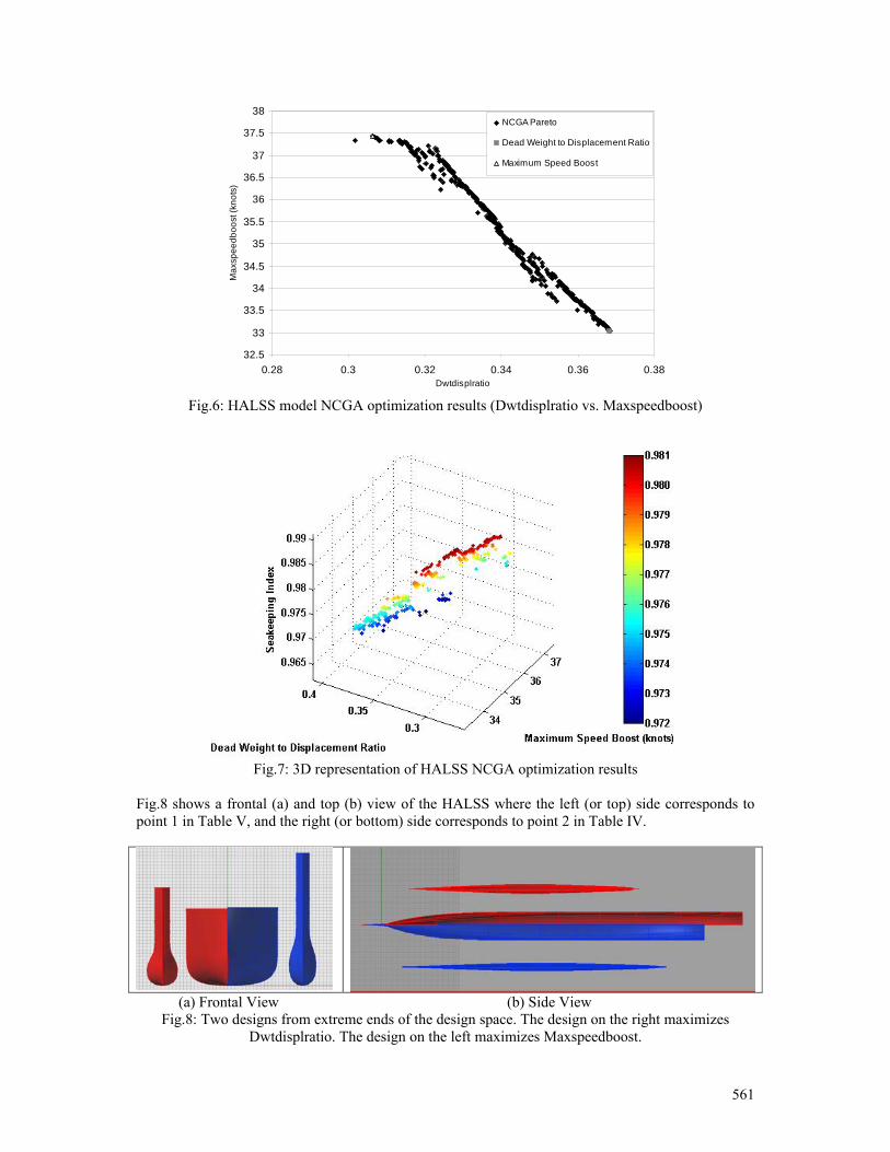
561

32.5

33

33.5

34

34.5

35

35.5

36

36.5

37

37.5

38

0.28 0.3 0.32 0.34 0.36 0.38Dwtdisplratio

Max

spee

dboo

st (k

nots

)

NCGA Pareto

Dead Weight to Displacement Ratio

Maximum Speed Boost

Fig.6: HALSS model NCGA optimization results (Dwtdisplratio vs. Maxspeedboost)

Fig.7: 3D representation of HALSS NCGA optimization results

Fig.8 shows a frontal (a) and top (b) view of the HALSS where the left (or top) side corresponds to point 1 in Table V, and the right (or bottom) side corresponds to point 2 in Table IV.

(a) Frontal View (b) Side View

Fig.8: Two designs from extreme ends of the design space. The design on the right maximizes Dwtdisplratio. The design on the left maximizes Maxspeedboost.

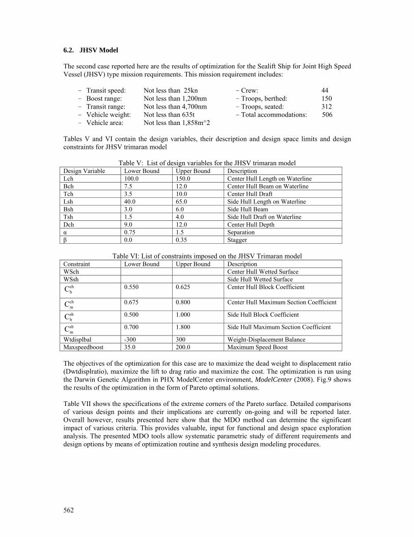
562

6.2. JHSV Model The second case reported here are the results of optimization for the Sealift Ship for Joint High Speed Vessel (JHSV) type mission requirements. This mission requirement includes:

- Transit speed: Not less than 25kn - Crew: 44 - Boost range: Not less than 1,200nm - Troops, berthed: 150 - Transit range: Not less than 4,700nm - Troops, seated: 312 - Vehicle weight: Not less than 635t - Total accommodations: 506 - Vehicle area: Not less than 1,858m^2

Tables V and VI contain the design variables, their description and design space limits and design constraints for JHSV trimaran model

Table V: List of design variables for the JHSV trimaran model Design Variable Lower Bound Upper Bound Description Lch 100.0 150.0 Center Hull Length on Waterline Bch 7.5 12.0 Center Hull Beam on Waterline Tch 3.5 10.0 Center Hull Draft Lsh 40.0 65.0 Side Hull Length on Waterline Bsh 3.0 6.0 Side Hull Beam Tsh 1.5 4.0 Side Hull Draft on Waterline Dch 9.0 12.0 Center Hull Depth α 0.75 1.5 Separation β 0.0 0.35 Stagger

Table VI: List of constraints imposed on the JHSV Trimaran model Constraint Lower Bound Upper Bound Description WSch Center Hull Wetted Surface WSsh Side Hull Wetted Surface

chbC

0.550 0.625 Center Hull Block Coefficient

chmC

0.675 0.800 Center Hull Maximum Section Coefficient

shbC

0.500 1.000 Side Hull Block Coefficient

shmC

0.700 1.800 Side Hull Maximum Section Coefficient

Wtdisplbal -300 300 Weight-Displacement Balance Maxspeedboost 35.0 200.0 Maximum Speed Boost The objectives of the optimization for this case are to maximize the dead weight to displacement ratio (Dwtdisplratio), maximize the lift to drag ratio and maximize the cost. The optimization is run using the Darwin Genetic Algorithm in PHX ModelCenter environment, ModelCenter (2008). Fig.9 shows the results of the optimization in the form of Pareto optimal solutions. Table VII shows the specifications of the extreme corners of the Pareto surface. Detailed comparisons of various design points and their implications are currently on-going and will be reported later. Overall however, results presented here show that the MDO method can determine the significant impact of various criteria. This provides valuable, input for functional and design space exploration analysis. The presented MDO tools allow systematic parametric study of different requirements and design options by means of optimization routine and synthesis design modeling procedures.

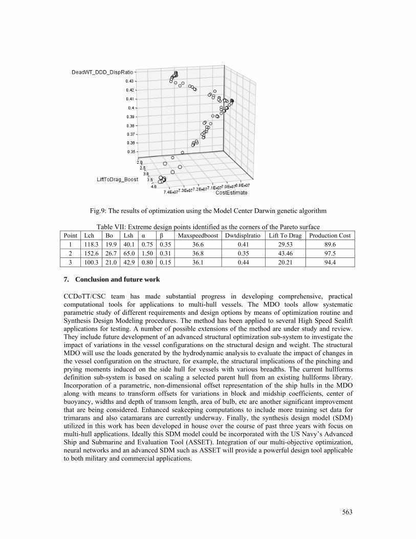
563

Fig.9: The results of optimization using the Model Center Darwin genetic algorithm

Table VII: Extreme design points identified as the corners of the Pareto surface

Point Lch Bo Lsh α β Maxspeedboost Dwtdisplratio Lift To Drag Production Cost 1 118.3 19.9 40.1 0.75 0.35 36.6 0.41 29.53 89.6 2 152.6 26.7 65.0 1.50 0.31 36.8 0.35 43.46 97.5 3 100.3 21.0 42.9 0.80 0.15 36.1 0.44 20.21 94.4

7. Conclusion and future work CCDoTT/CSC team has made substantial progress in developing comprehensive, practical computational tools for applications to multi-hull vessels. The MDO tools allow systematic parametric study of different requirements and design options by means of optimization routine and Synthesis Design Modeling procedures. The method has been applied to several High Speed Sealift applications for testing. A number of possible extensions of the method are under study and review. They include future development of an advanced structural optimization sub-system to investigate the impact of variations in the vessel configurations on the structural design and weight. The structural MDO will use the loads generated by the hydrodynamic analysis to evaluate the impact of changes in the vessel configuration on the structure, for example, the structural implications of the pinching and prying moments induced on the side hull for vessels with various breadths. The current hullforms definition sub-system is based on scaling a selected parent hull from an existing hullforms library. Incorporation of a parametric, non-dimensional offset representation of the ship hulls in the MDO along with means to transform offsets for variations in block and midship coefficients, center of buoyancy, widths and depth of transom length, area of bulb, etc are another significant improvement that are being considered. Enhanced seakeeping computations to include more training set data for trimarans and also catamarans are currently underway. Finally, the synthesis design model (SDM) utilized in this work has been developed in house over the course of past three years with focus on multi-hull applications. Ideally this SDM model could be incorporated with the US Navy’s Advanced Ship and Submarine and Evaluation Tool (ASSET). Integration of our multi-objective optimization, neural networks and an advanced SDM such as ASSET will provide a powerful design tool applicable to both military and commercial applications.

564

Acknowledgment This work is supported by the US Office of Naval Research, under cooperative agreement No. N00014-04-2-0003 with the California State University, Long Beach Foundation Center for the Commercial Deployment of Transportation Technologies (CCDoTT). The authors would like to sincerely thank the program manager Dr. Paul Rispin and Mr. Dan Sheridan from ONR for their support, and many important inputs. Mr. Steve Wiley from CSC has been the primary developer of the SDM. His experience with many Navy and commercial ships have been essential contributions to this work. We also thank Viking Systems of Annapolis Maryland for pioneering the systematic seakeeping calculations for multi-hulls. Their professional contribution helped to incorporate these comprehensive results in MDO process. Finally we would like to thank CCDoTT’s Principal Investigator Mr. Stan Wheatley, program coordinator Mr. Steven Hinds, and program administrator Ms. Carrie Scoville for their supports. Glossary of Acronyms: ABS - American Bureau of Ships CFD - Computational Fluid Dynamics HSS - High Speed Sealift Ship JHSS - Joint High Speed Sealift Ship JHSV - Joint High Speed Vessel LWT - Light Weight MCC - Modified Cascade Correlation MDO - Multi-disciplinary Design and Optimization MOGA – Multi-objective Genetic Algorithm MIGA – Multi-island Genetic Algorithm NN- Neural Network NLPQL - Sequential Quadratic Programming NCGA – Neighborhood Cultivation Genetic Algorithm TS – Training Set VS – Validation Set USCG – US Coast Guard USMC- US Marine Corp References AMROMIN, E.; MIZINE, I. (2003), Quasi-linear theory of ship resistance and cfd analysis of ship’s environmental impact, FEDSM’03, 4th ASME-JSME Joint Fluids Engineering Conf., Honolulu ASSET (2008), Advanced Surface Ship Evaluation Tool, NAVSEA, Carderock Division, available at http://www.dt.navy.mil/asset/ BECK, R. (2007), Tools for multi-hull design optimization, University of Michigan, Private Comm. BESNARD, E.; SCHMITZ, A.; et al. (1998) Hydrofoil design and optimization for fast ships, ASME Int. Congress & Exhibition, Anaheim BESNARD, E.; SCHMITZ, A.; HEFAZI, H.; SHINDE, R. (2007), Constructive neural networks and their application to ship multi-disciplinary design optimization, J. Ship Research 51/4, pp.297-312 BROWN, A.J.; NEU, W. (2008), Naval surface ship design optimization for affordability, available at http://www.aoe.vt.edu/~brown/VTShipDesign/VTDesignforAffordabilityFinalReport.htm#Theses CAMPANA, E.F. et al. (2007), Nonlinear programming approaches in the multidisciplinary design optimization of a sailing yacht keel fin, 9th Int. Conf. Numerical Ship Hydrodynamics, Ann Arbor

565

EEFSEN, T. et al. (2004), Development of Frigate Designs with good Seakeeping Characteristics, 9th Symposium on Practical Design of Ships and Other Floating Structures, Luebeck-Travemuende, Germany, Schiffbautechnische Gesellschaft e.V. FAHLMAN, S.E.; LEBIERE, C. (1990), The Cascade-Correlation Learning Architecture, Technical Report CMU-CS-90-100, School of Computer Science, Carnegie Mellon University, Pittsburgh, PA, USA. HARRIES, S. et al. (2001), Investigation on Optimization Strategies for the Hydrodynamic Design of Fast Ferries, FAST 2001, Southampton, UK, 4th-6th September. HEFAZI, H. et al. (2002), CFD Design Tool Development and Validation, CCDoTT FY00 Task 2.8, Center for the Commercial Deployment of Transportation Technologies, Long Beach, CA., available at ftp://www.cdott.org. HEFAZI, H.; et al. (2003), CFD design tool development and validation with accompanying technology demonstrator, CCDoTT FY02 Task 2.20, Center for the Commercial Deployment of Transportation Technologies, Long Beach, CA., available at ftp://www.cdott.org HEFAZI, H.; SCHMITZ, A.; SHINDE, R.; MIZINE, I. (2006), Automated multidisciplinary design optimization method for multi-hull vessels, CCDoTT FY05 Task 2.32, Center for the Commercial Deployment of Transportation Technologies, Long Beach, CA., available at ftp://www.cdott.org. HEFAZI, H.; SCHMITZ, A.; SHINDE, R.; MIZINE, I. (2008), Automated Multidisciplinary Design Optimization Method for Multi-Hull Vessels, CCDoTT FY06 Task 4.4, Center for the Commercial Deployment of Transportation Technologies, Long Beach, CA., available at ftp://www.cdott.org. ISIGHT (2008), Engineous Software available at http://www.engineous.com MIZINE, I.O.; AMROMIN, E.L.; CROOK, L.; DAY, W.; KORPUS, R. (2004), High-speed trimaran residuary drag: Numerical analysis and model tests, J. Ship Research 48, pp.248-259 MODELCENTER (2008), Optworks: ModelCenter by PiBlue available at http://www.piblue.com/products/optworks_mc.html PERCEPTION ESTI-MATE (2008), SPAR Associates Inc., available at http://www.sparusa.com/systemtechnology.htm RHINOMARINE (2008), RhinoCeros available at http://www.rhino3d.com/marine.htm SCHMITZ, A. (2007), Constructive neural networks for function approximation and their application to computational fluid dynamics shape optimization, PhD. Thesis, Claremont Graduate University. SCLAVOUNOS, P.D.; NAKOS, D.E. (1988), Stability analysis of panel methods for free surface flows with forward speed, 17th Symp. Naval Hydrodynamics, The Hague TAHARA, Y. et al. (2007) Global optimization and variable fidelity strategies in the single and multiobjective optimal design of fast multihull ships, 9th Int. Conf. Num. Ship Hydrodyn., Ann Arbor WASIM Software (2008), Det Norske Veritas, available at http://www.dnv.com ZALEK, S.F. (2007), Multicriterion evolutionary optimization of ship hull forms for propulsion and seakeeping, PhD thesis, Naval Architecture and Marine Engineering , University of Michigan.

566

On Board Assessment of Seakeeping for Risk-Based Decision Support to the Master

Dimitris Spanos, NTUA, Athens/Greece, spanos@deslab.ntua.gr

Apostolos Papanikolaou, NTUA, Athens/Greece, papa@deslab.ntua.gr George Papatzanakis, NTUA, Athens/Greece, gpap@deslab.ntua.gr

Jan Tellkamp, DNV, Hamburg/Germany, (former FSG, Germany), jan.tellkamp@dnv.com

Abstract

A probabilistic assessment method for the seakeeping of ships suitable for implementation in risk-based Decision Support Systems (DSS) aiming at the onboard navigational guidance to mitigate risks related to the ship’s seakeeping performance, has been investigated and is presented in this paper. The related probabilistic analysis is conducted by use of numerical simulation/sampling methods, like Monte Carlo simulation as well as FORM/SORM probabilistic methods known from their application so far to ship’s structural reliability analysis. The method proves practical computational efficiency for the demanding onboard risk evaluation.

1 Introduction For the assessment of the seakeeping of an intact ship in sea waves, first, the operational profile of possible conditions that the ship might encounter in the time period relevant to the assessment has to be established. When the assessment is applied to the ship design phase then the full ship life cycle conditions should be taken into account. In this case the seakeeping profile assumes considerably wide ranges for the ship loading, the wave environment and ship speed and course, which leads to a vast number of possible responses of the ship. On the other side, when the time frame of the seakeeping assessment and of related analysis is shortened, in the order of few hours, and regards specific loading and wave conditions then the profile becomes rather narrow, sometimes almost deterministic. In realistic situations like those encountered by a ship in open seas during a voyage, each parameter of the seakeeping problem, even sensitive to seakeeping ship inherent data like GM and radius of gyration, is related to a degree of uncertainty, whereas other parameters, like environmental data, are inherently random. Above uncertain parameters and random variables define an intricate probabilistic short time assessment problem, the solution of which has beyond complexity increased time calculation/processing and reliability requirements for onboard applications. With an onboard seakeeping assessment it is attempted to exploit the practically possible determination of the sailing conditions, which are the basis for the probabilistic estimation of seakeeping events. Probabilities, being the dominant and most onerous factor of the risk, combined with consequences, usually of economic and remotely of catastrophic nature, will provide important information for the navigational decisions of the ship master for a watch time ahead. In the subsequent sections a probabilistic seakeeping assessment suitable for onboard applications is presented, which makes use of advanced methods of probability simulation and reliability theory, to deal with all kind of related uncertainties. Alternative probability methods like Monte Carlo, first and second order reliability methods FORM and SORM respectively have been explored. The method can be directly integrated within a risk-based decision support system (DSS) like that of ADOPT-DSS, http://adopt.rtdproject.net/. Currently the method has been implemented and used for the analysis of the basic seakeeping behavior of a RoRo ship and for the estimation of corresponding probability distributions or probabilities of specific events.

567

2 Frequency Domain Implementation – FDI Seakeeping analysis is traditionally applied in the frequency domain and under the basic assumptions of linearity for the ship motion in response to the exciting waves. In this framework the practical evaluation of the ship motion in irregular waves is achieved by use of analytical spectral transformations. While a large range of ship responses could be addressed in this way, non-linear responses necessitate an extended formulation to deal with. Formulation of the ship dynamics and hydrodynamics in the time domain is currently the most efficient method for this purpose. In such cases, the ship hydrodynamics, being the most demanding computational part, either can be evaluated in the time domain or alternately, aiming to reduce the computational effort, to be evaluated in the frequency domain and then appropriately transformed to the time domain. Such treatments are familiar to ship hydrodynamicists, in anyway a time domain formulation would suffer necessary simplifications in order to reduce the related computational requirements to a practical level for application. In principle for a probabilistic assessment of the ship responses in waves both seakeeping formulations, frequency or time domain, could be applied and the probabilistic approach should remain independent to the domain of analysis. However, the computational performance of each formulation eventually determines if a probabilistic method would be appropriate to be combined with. The herein presented probabilistic approach has been based on a frequency domain seakeeping analysis adequate for a DSS and is accordingly called Frequency Domain Implementation – FDI, while when referring to a Time Domain Implementation – TDI it is implied that some time domain seakeeping method is applied in the background. 3 The Probabilistic Method within a Risk Assessment Framework 3.1 The Probabilistic Core of a Decision Support System The herein probabilistic seakeeping method has been developed for application within a risk assessment environment where the probability of specific events is routinely evaluated. Moreover, the risk assessment could be an integral part of a decision support method. The domain of the seakeeping analysis, the nature of the possible events and the frequency of the evaluations as imposed by the assumed decision process specify the set of requirements for a suitable probabilistic method. The Decision Support System of ADOPT (2005-2008) has been considered as the framework for the development of the risk assessment method. Within this framework a generic risk aversion approach of the DSS is assumed along with the more specific one recently introduced by Spanos et al. (2008) and which is also applicable to the ADOPT-DSS. The generic approach attempts the evaluation of the risk related to the current sailing conditions and on the basis of some existing risk requirements set by the ship operator and the society. In the latter the risk mitigation is rigorously based on the relative risk between alternative sailing conditions, searching for all feasible risk mitigation options, and as a consequence results to a more demanding performance for the probabilistic method. In the assumed onboard risk analysis the hazardous events related to seakeeping behavior of the intact ship are identified and appropriately formulated. Then the probability of those events can be numerically estimated exploiting specific information available onboard. Given these probabilities and assuming corresponding consequences (which may be economic or safety related) the risk evaluation follows. Alternative sailing conditions of lower risk can be explored by the DSS and any identified Risk Control Options (RCOs), the final outcome of the DSS process, can be disposed to the ship master in support of his navigational function. In Fig.1 the probability evaluation is defined as a nested module (dashed line) within the risk assessment of the DSS. The module is assumed appropriately interfaced to the data modules, which refer to the prevailing wave environment condition for which the risk is assessed, the specific ship

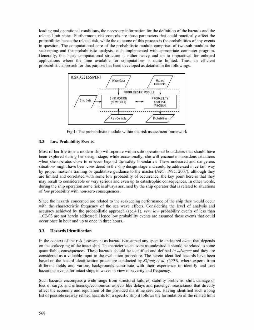
568

loading and operational conditions, the necessary information for the definition of the hazards and the related limit states. Furthermore, risk controls are those parameters that could practically affect the probabilities hence the related risk, while the outcome of this process is the probabilities of any events in question. The computational core of the probabilistic module comprises of two sub-modules the seakeeping and the probabilistic analysis, each implemented with appropriate computer program. Generally, this basic computational structure is rather heavy and up to impractical for onboard applications where the time available for computations is quite limited. Thus, an efficient probabilistic approach for this purpose has been developed as detailed in the followings.

Fig.1: The probabilistic module within the risk assessment framework

3.2 Low Probability Events Most of her life time a modern ship will operate within safe operational boundaries that should have been explored during her design stage, while occasionally, she will encounter hazardous situations when she operates close to or even beyond the safety boundaries. These undesired and dangerous situations might have been considered in the ship design stage and could be addressed in certain way by proper master’s training or qualitative guidance to the master (IMO, 1995, 2007); although they are limited and correlated with some low probability of occurrence, the key point here is that they may result to considerable or very serious and even up to catastrophic consequences. In other words, during the ship operation some risk is always assumed by the ship operator that is related to situations of low probability with non-zero consequences. Since the hazards concerned are related to the seakeeping performance of the ship they would occur with the characteristic frequency of the sea wave effects. Considering the level of analysis and accuracy achieved by the probabilistic approach (sec.4.1), very low probability events of less than 1.0E-03 are not herein addressed. Hence low probability events are assumed those events that could occur once in hour and up to once in three hours. 3.3 Hazards Identification In the context of the risk assessment as hazard is assumed any specific undesired event that depends on the seakeeping of the intact ship. To characterize an event as undesired it should be related to some quantifiable consequences. These hazards should be identified and defined in advance and they are considered as a valuable input to the evaluation procedure. The herein identified hazards have been based on the hazard identification procedure conducted by Skjong et al. (2005), where experts from different fields and various backgrounds contribute with their experience to identify and sort hazardous events for intact ships in waves in view of severity and frequency. Such hazards encompass a wide range from structural failures, stability problems, shift, damage or loss of cargo, and efficiency/economical aspects like delays and passenger seasickness that directly affect the economy and reputation of the provided maritime services. Having identified such a long list of possible seaway related hazards for a specific ship it follows the formulation of the related limit

RISK ASSESSMENT

PROBABILISTIC MODULE

Ship Data

Wave Data

SHIP MOTION (NEWDRIFT)

PROBABILITY ANALYSIS (PROBAN)

Probabilities

Hazard Thresholds

Risk Controls

569

states and the assessment of consequences. The formulation of a limit state (sec.3.6) is the expression of a hazard as function mainly of the ship responses and the definition of characteristic events by use of the threshold values (sec.3.4). Thus any hazard has eventually been translated into a mathematical expression, namely a single variable, that its probabilistic properties are quantified by application of the herein discussed probabilistic method. 3.4 Threshold Values The hazards are defined through a set of characteristic threshold values for the involved variables. For example suppose the hazard of the frequent propeller racing that may occur during severe pitching and subsequent propeller emergences. Such an event is undesired to the propulsion system. So, analyzing the capacity of the propulsion system and its tolerance to the racing, independently of the ship motions, then the threshold value for the racing rate can be determined as the maximum number of racings that consequences can be assumed to be negligible. If the racing frequency is higher than the determined threshold value then the related consequences will be encountered. Apparently for a hazard on a top level description several threshold values may be derived each one correlated to a different level of consequences. 3.5 Environmental conditions A powerful onboard guidance to the master is determined by its ability to assess the performance of the ship in response to the actual prevailing wave conditions. In case of lack of sufficient wave information then the embedded seakeeping assessment has to be based on assumptions, which inevitably lead to a broader assessment of possible events and their consequences that gradually may lead to failure to address the current situation. The presently assumed DSS and subsequently the probabilistic analysis incorporates provisions of measuring and reliably estimating the prevailing wave conditions and include anyway information about forecasted wave parameters. The final outcome of processing of this wave information is a two dimensional (encounter frequency and heading) wave spectrum and its integrated parameters like the significant wave height and peak period. Currently the assumed most advanced approach to this purpose are radar based measurements, which exploit installed nautical X-band radars on the ship to generate maps of the sea elevation around the sailing ship and then calculate the wave properties and related sea spectra, Dannenberg, (2007). The variable sea state during a trip, as measured onboard comprises the basic source of randomness of the probabilistic problem. 3.6 Hazards formulation Following a formulation likewise that used in structural reliability analysis any hazard of interest is formulated with a Limit State Function, which is a function of the basic variables and which is positively valued when the ship remains safe and negatively when unsafe, namely when the hazard occurs. The basic problem is reduced to the problem of calculating the small probability that ( ) 0,...,, 21 <NXXXg (1)

where X=(X1,X2,…,XN) is a vector of basic random variables and g is referred to as the limit state function. Failure is defined by an event that g(X)<0, which is trivially the convention for the definition of failure. The value of g-function is a random variable. Its distribution function is determined by the g-function itself and the probabilistic distribution of the basic random variables X. The variables describe functional relationships in the physical model as well as the randomness in the modeling. In simple cases the g-function can be reduced to some explicit mathematical/analytical formula. However in practical cases and especially when seakeeping is addressed this is a complicated function resulting from discrete calculations of numerical solvers, thus its evaluation results only numerically possible.

570

3.7 Ship Motion Model The formulation and the evaluation of the g-function are determined by the nature of the hazards. The present g-functions are mainly functions of ship responses in waves. As denoted by the next two equations (2) and (3), g is function of the wave and loading parameters X and the ship responses Y, for some given response control parameters C, while the S function is the employed ship motion model.

( )CYXgg |,= (2)

( )CXSY |= (3) For hazards for which a linear seakeeping analysis with respect to the incident seaway is satisfactory, a linear seakeeping code in frequency domain can be employed for the implementation of the S-function. In such cases the basic properties of linear systems are utilized to derive closed form expressions for the probability of the involved random variables. Independently of the possible linearity of the seakeeping analysis, it should be noted that both functions g and S are generally non-linear functions with respect to some X parameters and C response controls. On the other side, hazards related generally to non-linear ship responses in waves require suitable non-linear motion codes for their reliable assessment, which are implemented in the time domain. For instance the severe accelerations at bow of a ship in heavy seas may be treated within the frequency domain as they are dominated by the vertical plane ship motions (heave and pitch), which can be satisfactorily approached by linear ship motion theory and related numerical codes. For this case a Frequency Domain Implementation – FDI of a DSS would be adequate. Whereas, for the non-linear stability problem of the parametric rolling in waves the solution can be approached only by a code where appropriate non-linear equations of motion are solved in the time domain. In this case a Time Domain Implementation – TDI of a DSS is required. In the following sections, the probabilistic evaluation of the g-function with an FDI of the S-function is discussed. 3.8 Uncertainties In the ship motion problem there are input variables that are random like the incident seaway exciting forces, and dependent variables like the heave motion and responses in general, which are eventually random due to their dependence (S-function of sec. 3.7) on the random input variables. The ship motion problem is complemented by the parameters of the set problem, like the loading condition the ship forward speed and the heading to waves. In the herein formulation the set of parameters are assumed to be correlated to some degree of uncertainty, namely they are assumed to follow a probability model instead of having fixed values. Suppose the loading condition of a ship which is specified through the ship displacement her center of gravity and the mass moments of inertia. In the practice of ship operation these values can not be determined in absolute accuracy (in some cases, they not even known at all). Hence, each parameter is assumed following a probability model e.g. a normal distribution around the best estimated value and some empirical deviation. Other probability models for the uncertainties may be also employed in a straight forward way. Therefore all the parameters can be formulated as random variables, which extend the initial set of random variables. A parameter is considered for randomization (uncertainty) according to the impact of the uncertainty on the hazard probabilities. While if hazards probabilities are tolerable to such variations then parameter is still considered as deterministic. So far, it has been verified that the uncertainty of parameters affecting to the frequency dependence of ship’s seakeeping, cause a stronger variation of the ship responses. A typical example of this is the effect of the uncertainty on the GM and the roll radius of gyration on ship’s roll natural period, Papanikolaou et al. (1997). Two other examples are commented in the following: When a two parameters JONSWAP spectrum for the sea waves is

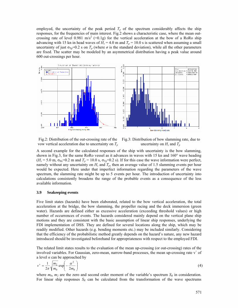
571

employed, the uncertainty of the peak period Tp of the spectrum considerably affects the ship responses, for the frequencies of main interest. Fig.2 shows a characteristic case, where the mean out-crossing rate of level 0.981 m/s2 (=0.1g) for the vertical acceleration at the bow of a RoRo ship advancing with 15 kn in head waves of Hs = 4.0 m and Tp = 10.0 s is scattered when assuming a small uncertainty of just σTp=0.2 s on Tp (where σ is the standard deviation), while all the other parameters are fixed. The scatter may be modeled by an asymmetrical distribution having a peak value around 600 out-crossings per hour.

Fig.2: Distribution of the out-crossing rate of the vow vertical acceleration due to uncertainty on Tp

Fig.3: Distribution of bow slamming rate, due to uncertainty on Hs and Tp

A second example for the calculated responses of the ship with uncertainty is the bow slamming, shown in Fig.3, for the same RoRo vessel as it advances in waves with 15 kn and 160° wave heading (Hs = 5.0 m, σHs=0.2 m and Tp = 10.0 s, σTp=0.2 s). If for this case the wave information were perfect, namely without any uncertainty on Hs and Tp, then an average value of 1.5 slamming events per hour would be expected. Here under that imperfect information regarding the parameters of the wave spectrum, the slamming rate might be up to 5 events per hour. The introduction of uncertainty into calculations consistently broadens the range of the probable events as a consequence of the less available information. 3.9 Seakeeping events Five limit states (hazards) have been elaborated, related to the bow vertical acceleration, the total acceleration at the bridge, the bow slamming, the propeller racing and the deck immersion (green water). Hazards are defined either as excessive acceleration (exceeding threshold values) or high number of occurrences of events. The hazards considered mainly depend on the vertical plane ship motions and they are consistent with the basic assumption of linear ship responses, underlying the FDI implementation of DSS. They are defined for several locations along the ship, which may be readily modified. Other hazards (e.g. bending moments etc.) may be included similarly. Considering that the efficiency of the probabilistic method greatly depends on the hazard’s nature, any new hazard introduced should be investigated beforehand for appropriateness with respect to the employed FDI. The related limit states results to the evaluation of the mean up-crossing (or out-crossing) rates of the involved variables. For Gaussian, zero-mean, narrow-band processes, the mean up-crossing rate v+ of a level α can be approached by

⎟⎟⎠

⎞⎜⎜⎝

⎛−=+

0

2

0

2

2exp

21

mmmv α

π (4)

where m0, m2 are the zero and second order moment of the variable’s spectrum SR in consideration. For linear ship responses SR can be calculated from the transformation of the wave spectrums

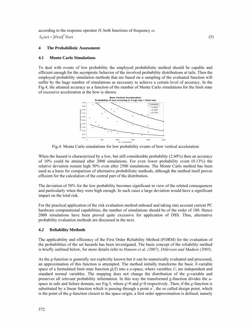
572

according to the response operator H, both functions of frequency ω. )()()( 2 ωωω SHSR = (5)

4 The Probabilistic Assessment 4.1 Monte Carlo Simulations To deal with events of low probability the employed probabilistic method should be capable and efficient enough for the asymptotic behavior of the involved probability distributions at tails. Then the employed probability simulation methods that are based on a sampling of the evaluated function will suffer by the huge number of simulations as necessary to achieve a certain level of accuracy. In the Fig.4, the attained accuracy as a function of the number of Monte Carlo simulations for the limit state of excessive acceleration at the bow is shown.

Bow Vertical AccelerationProbability of out-crossing (> 0.1g) rate > limit rate

0.00

0.10

0.20

0.30

0.40

0.50

0.60

0.70

0.80

0.90

1.00

0 500 1000 1500 2000 2500No. of Simulations

rel.

devi

atio

n =

(std

dev

) / (m

ean)

2.60%0.43%0.13%

Probability

Fig.4: Monte Carlo simulations for low probability events of bow vertical acceleration

When the hazard is characterized by a low, but still considerable probability (2.60%) then an accuracy of 10% could be attained after 2000 simulations. For even lower probability event (0.13%) the relative deviation remain high 50% even after 2500 simulations. The Monte Carlo method has been used as a basis for comparison of alternative probabilistic methods, although the method itself proves efficient for the calculation of the central part of the distribution. The deviation of 50% for the low probability becomes significant in view of the related consequences and particularly when they were high enough. In such cases a large deviation would have a significant impact on the total risk. For the practical application of the risk evaluation method onboard and taking into account current PC hardware computational capabilities, the number of simulations should be of the order of 100. Hence 2000 simulations have been proved quite excessive for application of DSS. Thus, alternative probability evaluation methods are discussed in the next. 4.2 Reliability Methods The applicability and efficiency of the First Order Reliability Method (FORM) for the evaluation of the probabilities of the set hazards has been investigated. The basic concept of the reliability method is briefly outlined below, for more details refer to Hansen et al. (2007), Ditlevsen and Madsen (2005). As the g-function is generally not explicitly known but it can be numerically evaluated and processed, an approximation of this function is attempted. The method initially transforms the basic X-variable space of a formulated limit state function g(X) into a u-space, where variables Ui are independent and standard normal variables. The mapping does not change the distribution of the g-variable and preserves all relevant probability information. In this way the transformed g-function divides the u-space in safe and failure domain, see Fig.5, where g>0 and g<0 respectively. Then, if the g-function is substituted by a linear function which is passing through a point u*, the so called design point, which is the point of the g-function closest to the space origin, a first order approximation is defined, namely

573

the FORM method. Thus, the failure probability is that corresponding to the sub-domain defined by the linear approximation instead of the actual g-function (the shaded set in Fig.5). Applying the same concept, but implementing a second order approximation then the SORM (Second Order Reliability) method is defined.

Obviously if the limit surface g of a hazard is not strongly non-linear then the approximation defined by FORM and corresponding probabilities could be satisfactory in view of the accuracy for the set problem. Therefore the efficiency of the method for the DSS purpose can be judged only by domain analysis and thorough understanding of each hazard and its dependence on the related variables.

Fig.5: 2D g-function approach with FORM

Slamming Rate (u-space)Heading = 160 deg, Speed = 15 Kn, GM = 1.615 m,

Hs (mean = 5.0 m, σ = 0.2 m), Tp (mean = 10.0 sec, σ = 0.2 sec)

-4

-3

-2

-1

0

1

2

3

4

-5 -4 -3 -2 -1 0 1 2 3 4 5U1(Hs)U

2(Tp

)

Design Point

failure set

safe set

Slamming Rate > 4/hr MC 2.2 % FORM 2.9 %

Fig.6: U-space for Hs and Tp in operational mode

Fig.6 presents the u-space mapping of a representative case, where the g-function (dashed line) divides the domain into failure (full symbols) and safe (open symbols) sub-domains. The straight line (full line) is the linear approximation of the g-function according to FORM. The shown samples (symbols) are the results of a corresponding Monte Carlo simulation. The elaboration of the hazards, considered herein, has indicated that the g-function is not strongly non-linear, while it mostly defines convex failure sets; hence the probabilities obtained with FORM were systematically overestimated. This bias on the probability estimations is obviously a valuable property for the reliability of the DSS, particularly when employ the differential risk evaluation, Spanos et al. (2008). With respect to accuracy and reliability of results, the method could be approved at least for the operational mode of DSS where two-dimensional limit states are addressed. When dealing with more complicated assessment problems, like with the design problem (design mode of DSS), where multiple variables need to be taken into consideration, relevant studies were not conclusive.

0.0

0.2

0.4

0.6

0.8

1.0

0.4 0.6 0.8 1.0 1.2 1.4

RMS (m/sec2), in head waves

Prob

abilit

y of

exc

eeda

nce

0.0

0.2

0.4

0.6

0.8

1.00.010 0.015 0.020 0.025 0.030 0.035 0.040

RMS (m/sec2), in following waves

MCFORMSORM

following head

Fig.7: Probability of the vertical bow acceleration

FORM SORM

U1

U2

Failure set g(u)<0

Safe set g(u)>0

g-function g(u)=0

Design point u*

2D u-space

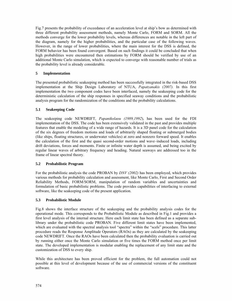
574

Fig.7 presents the probability of exceedance of an acceleration level at ship’s bow as determined with three different probability assessment methods, namely Monte Carlo, FORM and SORM. All the methods converge for the lower probability levels, whereas differences are notable in the left part of the diagram, namely for the higher probabilities, and the particular case of the following waves. However, in the range of lower probabilities, where the main interest for the DSS is defined, the FORM behavior has been found convergent. Based on such findings it could be concluded that when high probabilities were encountered then estimations by FORM should be verified by use of an additional Monte Carlo simulation, which is expected to converge with reasonable number of trials as the probability level is already considerable. 5 Implementation The presented probabilistic seakeeping method has been successfully integrated in the risk-based DSS implementation at the Ship Design Laboratory of NTUA, Papatzanakis (2007). In this first implementation the two component codes have been interfaced, namely the seakeeping code for the deterministic calculation of the ship responses in specified seaway conditions and the probabilistic analysis program for the randomization of the conditions and the probability calculations. 5.1 Seakeeping Code The seakeeping code NEWDRIFT, Papanikolaou (1989,1992), has been used for the FDI implementation of the DSS. The code has been extensively validated in the past and provides multiple features that enable the modeling of a wide range of hazards. It is a 3D panel code for the calculation of the six degrees of freedom motions and loads of arbitrarily shaped floating or submerged bodies (like ships, floating structures, or underwater vehicles) at zero and nonzero forward speed. It enables the calculation of the first and the quasi second-order motions and wave–induced loads, including drift deviations, forces and moments. Finite or infinite water depth is assumed, and being excited by regular linear waves of arbitrary frequency and heading. Natural seaways are addressed too in the frame of linear spectral theory. 5.2 Probabilistic Program For the probabilistic analysis the code PROBAN by DNV (2002) has been employed, which provides various methods for probability calculation and assessment, like Monte Carlo, First and Second Order Reliability Methods, FORM/SORM, manipulation of random variables and uncertainties and formulation of basic probabilistic problems. The code provides capabilities of interfacing to external software, like the seakeeping code of the present application. 5.3 Probabilistic Module Fig.8 shows the interface structure of the seakeeping and the probability analysis codes for the operational mode. This corresponds to the Probabilistic Module as described in Fig.1 and provides a first level analysis of the internal structure. Here each limit state has been defined as a separate sub-library under the probabilistic code PROBAN. Five different limit states have been implemented, which are evaluated with the spectral analysis tool “spectra” within the “scels” procedure. This latter procedure reads the Response Amplitude Operators (RAOs) as they are calculated by the seakeeping code NEWDRIFT. Once the RAOs have been calculated then the probability evaluation is carried out by running either once the Monte Carlo simulation or five times the FORM method once per limit state. The developed implementation is modular enabling the replacement of any limit state and the customization of DSS to every ship. While this architecture has been proved efficient for the problem, the full automation could not possible at this level of development because of the use of commercial versions of the constituent software.

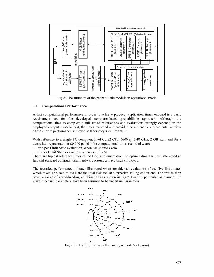
575

Fig.8: The structure of the probabilistic module in operational mode

5.4 Computational Performance A fast computational performance in order to achieve practical application times onboard is a basic requirement set for the developed computer-based probabilistic approach. Although the computational time to complete a full set of calculations and evaluations strongly depends on the employed computer machine(s), the times recorded and provided herein enable a representative view of the current performance achieved at laboratory’s environment. With reference to a single PC computer, Intel Core2 CPU 6600 @ 2.40 GHz, 2 GB Ram and for a dense hull representation (2x500 panels) the computational times recorded were: - 35 s per Limit State evaluation, when use Monte Carlo - 5 s per Limit State evaluation, when use FORM These are typical reference times of the DSS implementation; no optimization has been attempted so far, and standard computational hardware resources have been employed. The recorded performance is better illustrated when consider an evaluation of the five limit states which takes 12.5 min to evaluate the total risk for 30 alternative sailing conditions. The results then cover a range of speed-heading combinations as shown in Fig.9. For this particular assessment the wave spectrum parameters have been assumed to be uncertain parameters.

Fig.9: Probability for propeller emergence rate > (1 / min)

rnew

drift.

bat

DSS

run_

newd

rift.ex

e (in

itializ

ation

of

seak

eepin

g)

Funclib.dll (interface externals)

FUNCLB: NEWDRIFT (Definition Library)

SUBL

IB: B

owVe

rtAcc

(lim

it stat

e 1)

SUBL

IB: B

ridge

Acc

(limit s

tate 2

)

SUBL

IB: P

ropr

acing

(lim

it stat

e 4)

SUBL

IB: G

reen

Wate

r (lim

it stat

e 3)

SUBL

IB: S

lammi

ng

(limit s

tate 5

)

Scels.bat (spectral analysis)

Spec

tra_v

5_1.e

xe

(spe

ctral

calcs

.)

newd

rift_to

_spe

ctra_

Op

erati

onal2

.exe

(initia

lizati

on)

Upcro

ssing

_Ope

ratio

n.ex

e (e

vent

rate)

PROB

AN.ex

e (p

roba

bilist

ic an

alysis

) NE

WDR

IFT.

exe

(seak

eepin

g cod

e)

newd

rift_to

_spe

ctra_

Oper

.exe

(RAO

s man

ager

)

feed_

DSS.

exe

(retur

n res

ults t

o DSS

)

576

5.5 DSS Modes The DSS is assumed for application to both ship operation and to a risk-based design procedure. Since it aims at ensuring lower risk levels in ship’s operation correlated to a set of variables, the difference between the two modes for its use, namely design and operation, is the number of variables considered for each one. In the operational mode the ship may be assumed as a time invariant system, namely her loading condition is assumed satisfactorily determined at the beginning of the trip. The parameters treated in this mode as random variables are the environmental parameters (wave height, period, etc.), while the risk controls are the speed, the heading, etc. Therefore at a certain time calling the DSS the ship loading is provided by ship’s loadmaster software and the wave environment is measured by onboard instrumentation or best estimated by actualized forecasts; the DSS then searches for risk control options, namely alternative courses and speeds of lower risk (active risk measures). In the design mode, substantially more variables are considered. Herein the ship loading, the forward speed, the wave heading and other characteristics, thus much more parameters are all assumed as random variables; they may be set by the ship designer to account for the long term (ship life) evaluation of risk to be achieved by use of the DSS. The decision in the design process is the mitigation of risk in ship life by use of design controls (passive risk measures). 6 Conclusions A method for the onboard probabilistic assessment of the seakeeping of a ship subject to specific wave conditions has been introduced. The method has been specifically developed for application of risk-based navigational decision support systems DSS. The fundamental issues and properties have been discussed, while the necessity for an efficient probabilistic-seakeeping method in the core of the system has been highlighted. The developed method has been successfully integrated within the DSS prototype in the laboratory’s environment. Validation studies with the prototype have proved the efficiency of the employed probabilistic method FORM (and SORM) for most considered limit states and for the operational mode of the developed DSS in which the randomness of waves is taken into account. For cases for which above methods prove less reliable, a Monte Carlo simulation should be also applied, ensuring the DSS system’s reliability for the assessment of all envisaged operational conditions. Acknowledgements The presented work has been financially supported by the FP6 research project ADOPT (2005-2008) of the European Commission, Contract No FP6-TST4-CT-2005-516359. The European Community and the authors shall not in any way be liable or responsible for the use of any such knowledge, information or data, or of the consequences thereof. The authors like to acknowledge their fruitful collaboration with Professors P.F. Hansen and J.J. Jensen from the Technical University of Denmark DTU in the ADOPT project for the introduction and implementation of reliability assessment methods in the DSS concept. The license disposed by DNV to NTUA for use of the PROBAN code in the ADOPT project is acknowledged too.

577

References ADOPT (2005-2008). E.C. research project ADOPT, Advanced Decision Support System for Ship Design, Operation and Training, Contract No FP6-TST4-CT-2005-516359, FP6, Sustainable Surface Transport Programme, http://adopt.rtdproject.net/ DET NORSKE VERITAS, (2002), Proban theory, general purpose probabilistic analysis program, User Manual, program version 4.4, DNV Software Report No. 96-7017/Rev.1, Jun. 1st DANNENBERG, J. (2007), Sensing of the Environment, Report on EC research project ADOPT, Doc. No.D.2.3 DITLEVSEN, O.; MADSEN, H.O. (2005), Structural reliability methods, John Wiley & Sons, Internet edition 2.2.5, Dept. Mech. Eng. of Technical University of Denmark HANSEN, P.F.; NIELSEN, U.D.; HELMERS, J.B. (2007), Strategies for limit state evaluation in-cluding uncertainty analysis, Report on EC research project ADOPT, Doc: W3.1-DEL-20070531-FINAL-DTU IMO, (1995), Guidance to the master for avoiding dangerous situations in following and quartering seas, MSC/Circ.707, Oct.19 IMO, (2007), Revised guidance to the master for avoiding dangerous situations in adverse weather and sea conditions, MSC.1/Circ.1228, Jan.11 PAPANIKOLAOU, A. (1989), NEWDRIFT V.6: The six DOF three-dimensional diffraction theory program of NTUA-SDL for the calculation of motions and loads of arbitrarily shaped 3D bodies in regular waves, Internal Report, National Technical University of Athens PAPANIKOLAOU, Α.; SCHELLIN TH. (1992), Α three dimensional panel method for motions and loads of ships with forward speed, Ship Technology Research 39/4, pp.147-156. PAPANIKOLAOU, A.; GRATSOS, G.; BOULOUGOURIS, E.; ELIOPOULOU, E. (2000), Opera-tional measures of avoiding dangerous situations in extreme weather conditions, 7th Int. Conf. Stabil-ity of Ships and Ocean Vehicles (STAB’2000), Tasmania PAPANIKOLAOU, A.; BOULOUGOURIS, E.; SPANOS, D. (1997), On the specification of the roll radius of gyration for Ro-Ro passenger ships in view of SOLAS 95 Res. 14 equivalent model test method, 7th Int. Offshore and Polar Eng. Conf. (ISOPE), Honolulu, Vol. III, pp.499-506 PAPATZANAKIS, G. (2007), Development of probabilistic model for the investigation of ship dy-namic responses in waves and implementation by use of NEWDRIFT and PROBAN software, Master thesis, National Technical university of Athens, Ship Design Laboratory, (in Greek) SKJONG, R.; BITNER-GREGERSEN, E.; HELMERS, J.B.; VANEM, E. (2005), Hazard identifica-tion – Dynamic environmental loads, HAZID report on EC research project ADOPT Doc. No. D.1.1.1 SPANOS, D.; PAPANIKOLAOU, A.; PAPATZANAKIS, G. (2008), Risk-based on board guidance to the master for avoiding dangerous seaways, 6th Osaka Coll. Seakeeping and Stability of Ships, Osaka

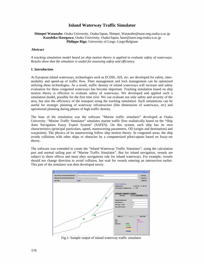
578

Inland Waterway Traffic Simulator

Shimpei Watanabe, Osaka University, Osaka/Japan, Shinpei_Watanabe@naoe.eng.osaka-u.ac.jp Kazuhiko Hasegawa, Osaka University, Osaka/Japan, hase@naoe.eng.osaka-u.ac.jp

Philippe Rigo, University of Liege, Liege/Belgium Abstract

A tracking simulation model based on ship motion theory is applied to evaluate safety of waterways. Results show that the simulator is useful for assessing safety and efficiency.

1. Introduction At European inland waterways, technologies such as ECDIS, AIS, etc. are developed for safety, inter-modality and speed-up of traffic flow. Fleet management and lock management can be optimized utilizing these technologies. As a result, traffic density of inland waterways will increase and safety evaluation for these congested waterways has become important. Tracking simulation based on ship motion theory is effective to evaluate safety of waterways. We developed and applied such a simulation model, possibly for the first time ever. We can evaluate not only safety and security of the area, but also the efficiency of the transport using the tracking simulation. Such simulations can be useful for strategic planning of waterway infrastructure (like dimensions of waterways, etc) and operational planning during phases of high traffic density. The base of the simulation was the software “Marine traffic simulator” developed at Osaka University. “Marine Traffic Simulator” simulates marine traffic flow realistically based on the “Ship Auto Navigation Fuzzy Expert System” (SAFES). On this system, each ship has its own characteristics (principal particulars, speed, maneuvering parameters, OD (origin and destination) and waypoints). The physics of its maneuvering follow ship motion theory. In congested areas, the ship avoids collisions with other ships or obstacles by a computerized pilot/captain based on fuzzy-set theory. The software was extended to create the “Inland Waterway Traffic Simulator”, using the calculation part and normal sailing part of “Marine Traffic Simulator”. But for inland navigation, vessels are subject to shore effects and must obey navigations rule for inland waterways. For example, vessels should not change direction to avoid collision, but wait for vessels entering an intersection earlier. This part of the simulator was then developed newly.

Fig.1: Sample output of inland waterway traffic simulator

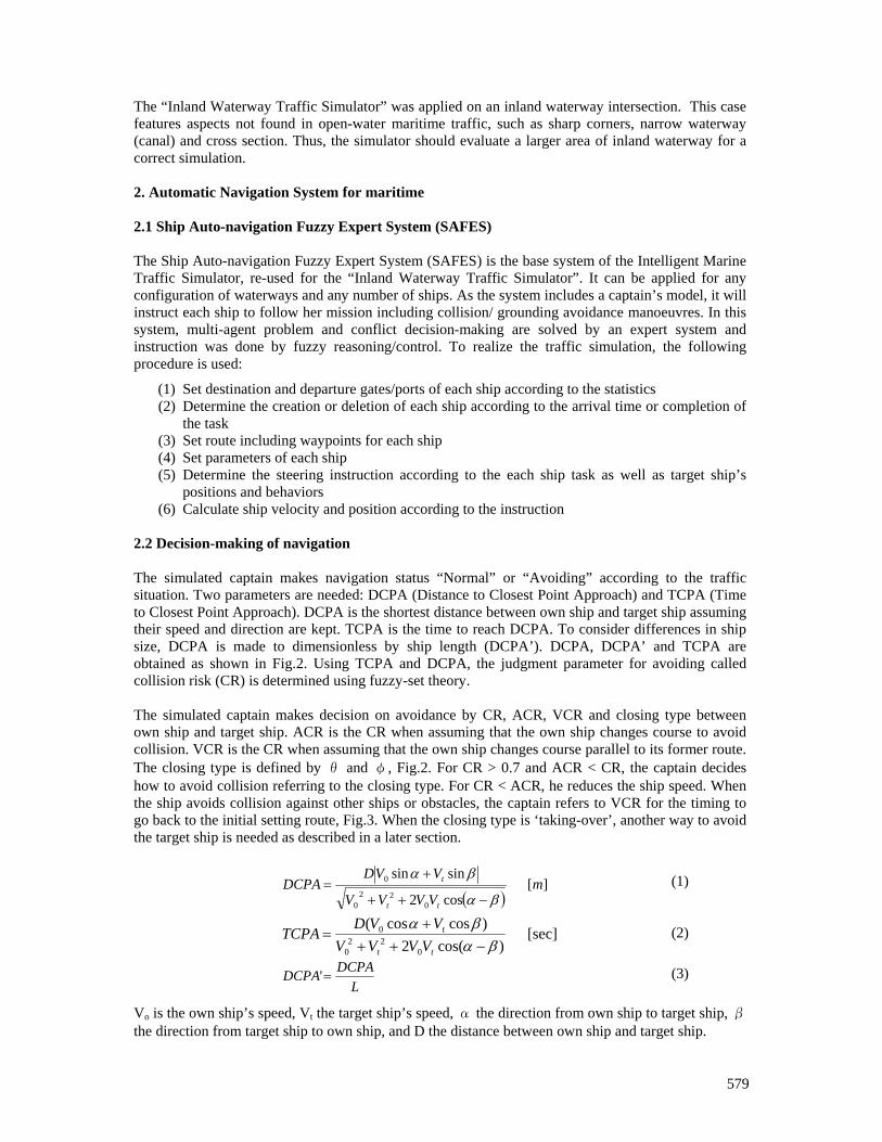
579

The “Inland Waterway Traffic Simulator” was applied on an inland waterway intersection. This case features aspects not found in open-water maritime traffic, such as sharp corners, narrow waterway (canal) and cross section. Thus, the simulator should evaluate a larger area of inland waterway for a correct simulation. 2. Automatic Navigation System for maritime 2.1 Ship Auto-navigation Fuzzy Expert System (SAFES) The Ship Auto-navigation Fuzzy Expert System (SAFES) is the base system of the Intelligent Marine Traffic Simulator, re-used for the “Inland Waterway Traffic Simulator”. It can be applied for any configuration of waterways and any number of ships. As the system includes a captain’s model, it will instruct each ship to follow her mission including collision/ grounding avoidance manoeuvres. In this system, multi-agent problem and conflict decision-making are solved by an expert system and instruction was done by fuzzy reasoning/control. To realize the traffic simulation, the following procedure is used:

(1) Set destination and departure gates/ports of each ship according to the statistics (2) Determine the creation or deletion of each ship according to the arrival time or completion of

the task (3) Set route including waypoints for each ship (4) Set parameters of each ship (5) Determine the steering instruction according to the each ship task as well as target ship’s

positions and behaviors (6) Calculate ship velocity and position according to the instruction

2.2 Decision-making of navigation The simulated captain makes navigation status “Normal” or “Avoiding” according to the traffic situation. Two parameters are needed: DCPA (Distance to Closest Point Approach) and TCPA (Time to Closest Point Approach). DCPA is the shortest distance between own ship and target ship assuming their speed and direction are kept. TCPA is the time to reach DCPA. To consider differences in ship size, DCPA is made to dimensionless by ship length (DCPA’). DCPA, DCPA’ and TCPA are obtained as shown in Fig.2. Using TCPA and DCPA, the judgment parameter for avoiding called collision risk (CR) is determined using fuzzy-set theory. The simulated captain makes decision on avoidance by CR, ACR, VCR and closing type between own ship and target ship. ACR is the CR when assuming that the own ship changes course to avoid collision. VCR is the CR when assuming that the own ship changes course parallel to its former route. The closing type is defined by θ and φ, Fig.2. For CR > 0.7 and ACR < CR, the captain decides how to avoid collision referring to the closing type. For CR < ACR, he reduces the ship speed. When the ship avoids collision against other ships or obstacles, the captain refers to VCR for the timing to go back to the initial setting route, Fig.3. When the closing type is ‘taking-over’, another way to avoid the target ship is needed as described in a later section.

( )][

cos2

sinsin

022

0

0 mVVVV

VVDDCPA

tt

t

βα

βα

−++

+= (1)

[sec])cos(2

)coscos(

022

0

0

βαβα−++

+=

tt

t

VVVVVVD

TCPA (2)

LDCPADCPA =' (3)

Vo is the own ship’s speed, Vt the target ship’s speed, α the direction from own ship to target ship, βthe direction from target ship to own ship, and D the distance between own ship and target ship.

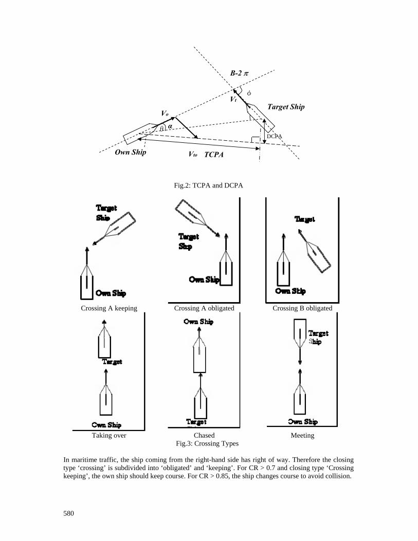
580

Fig.2: TCPA and DCPA

Crossing A keeping Crossing A obligated Crossing B obligated

Taking over Chased Meeting

Fig.3: Crossing Types In maritime traffic, the ship coming from the right-hand side has right of way. Therefore the closing type ‘crossing’ is subdivided into ‘obligated’ and ‘keeping’. For CR > 0.7 and closing type ‘Crossing keeping’, the own ship should keep course. For CR > 0.85, the ship changes course to avoid collision.

Β-2π

TCPA

Vo

Vt

α DCPA

Vto Own Ship

Target Ship

φ

θ

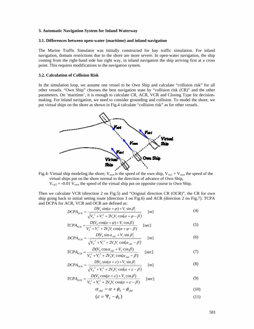
581

3. Automatic Navigation System for Inland Waterway 3.1. Differences between open-water (maritime) and inland navigation The Marine Traffic Simulator was initially constructed for bay traffic simulation. For inland navigation, domain restrictions due to the shore are more severe. In open-water navigation, the ship coming from the right-hand side has right way, in inland navigation the ship arriving first at a cross point. This requires modifications to the navigation system. 3.2. Calculation of Collision Risk In the simulation loop, we assume one vessel to be Own Ship and calculate “collision risk” for all other vessels. “Own Ship” chooses the best navigation state by “collision risk (CR)” and the other parameters. On ‘maritime’, it is enough to calculate CR, ACR, VCR and Closing Type for decision-making. For inland navigation, we need to consider grounding and collision. To model the shore, we put virtual ships on the shore as shown in Fig.4 calculate “collision risk” as for other vessels.

Fig.4: Virtual ship modeling the shore; Vown is the speed of the own ship, Vvir1 = Vown the speed of the virtual ships put on the shore normal to the direction of advance of Own Ship, Vvir2 = -0.01 Vown the speed of the virtual ship put on opposite course to Own Ship. Then we calculate VCR (direction 2 on Fig.5) and “Original direction CR (OCR)”, the CR for own ship going back to initial setting route (direction 3 on Fig.6) and ACR (direction 2 on Fig.7). TCPA and DCPA for ACR, VCR and OCR are defined as:

( )][

cos2

sin)sin(

022

0

0 mVVVV

VVDDCPA

tt

tACR

βϕα

βϕα

−+++

++= (4)

[sec])cos(2

)cos)cos((

022

0

0

βϕαβϕα−+++

++=

tt

tACR VVVV

VVDTCPA (5)

( )][

cos2

sinsin

022

0

0 mVVVV

VVDDCPA

oldtt

toldVCR

βα

βα

−++

+= (6)

[sec])cos(2

)coscos(

022

0

0

βαβα−++

+=

oldtt

toldVCR VVVV

VVDTCPA (7)

( )][

cos2

sin)sin(

022

0

0 mVVVV

VVDDCPA

tt

tOCR

βεα

βεα

−+++

++= (8)

[sec])cos(2

)cos)cos((

022

0

0

βεαβεα−+++

++=

tt

tOCR VVVV

VVDTCPA (9)

oldold φφαα −+= 0 (10)

)( 0φε −Ψ= I (11)

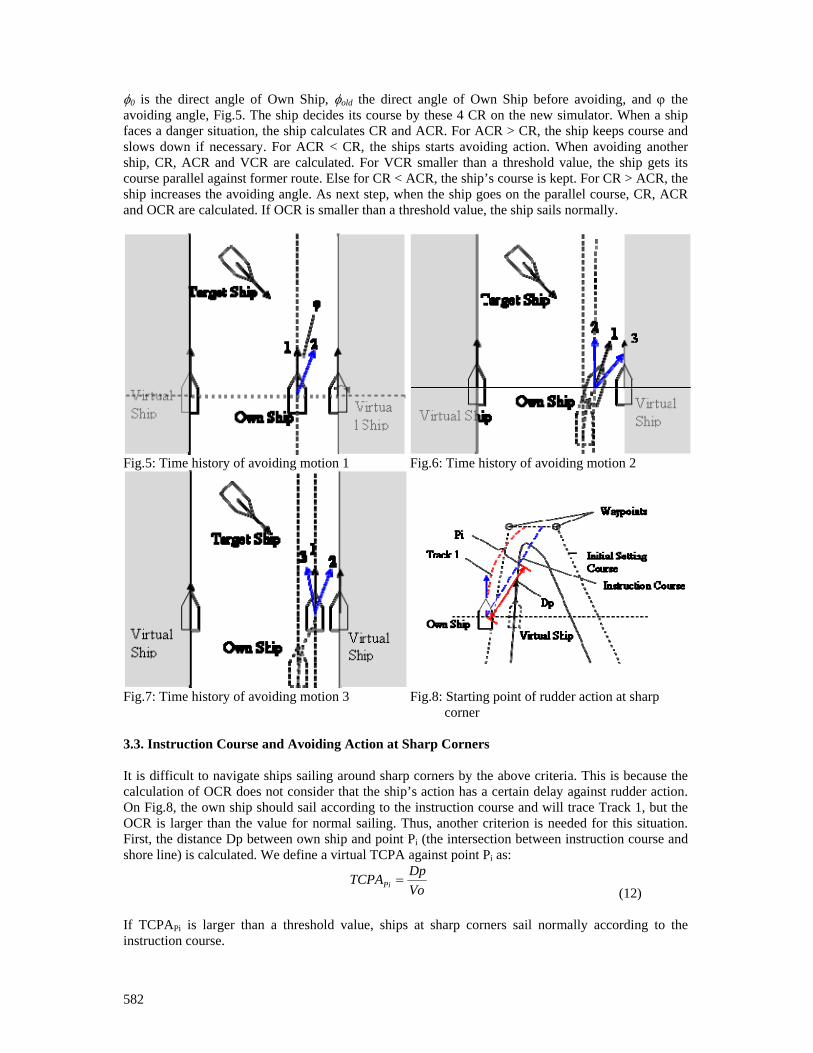
582

φ0 is the direct angle of Own Ship, φold the direct angle of Own Ship before avoiding, and ϕ the avoiding angle, Fig.5. The ship decides its course by these 4 CR on the new simulator. When a ship faces a danger situation, the ship calculates CR and ACR. For ACR > CR, the ship keeps course and slows down if necessary. For ACR < CR, the ships starts avoiding action. When avoiding another ship, CR, ACR and VCR are calculated. For VCR smaller than a threshold value, the ship gets its course parallel against former route. Else for CR < ACR, the ship’s course is kept. For CR > ACR, the ship increases the avoiding angle. As next step, when the ship goes on the parallel course, CR, ACR and OCR are calculated. If OCR is smaller than a threshold value, the ship sails normally.

Fig.5: Time history of avoiding motion 1 Fig.6: Time history of avoiding motion 2

Fig.7: Time history of avoiding motion 3 Fig.8: Starting point of rudder action at sharp corner

3.3. Instruction Course and Avoiding Action at Sharp Corners It is difficult to navigate ships sailing around sharp corners by the above criteria. This is because the calculation of OCR does not consider that the ship’s action has a certain delay against rudder action. On Fig.8, the own ship should sail according to the instruction course and will trace Track 1, but the OCR is larger than the value for normal sailing. Thus, another criterion is needed for this situation. First, the distance Dp between own ship and point Pi (the intersection between instruction course and shore line) is calculated. We define a virtual TCPA against point Pi as:

VoDpTCPAPi =

(12) If TCPAPi is larger than a threshold value, ships at sharp corners sail normally according to the instruction course.

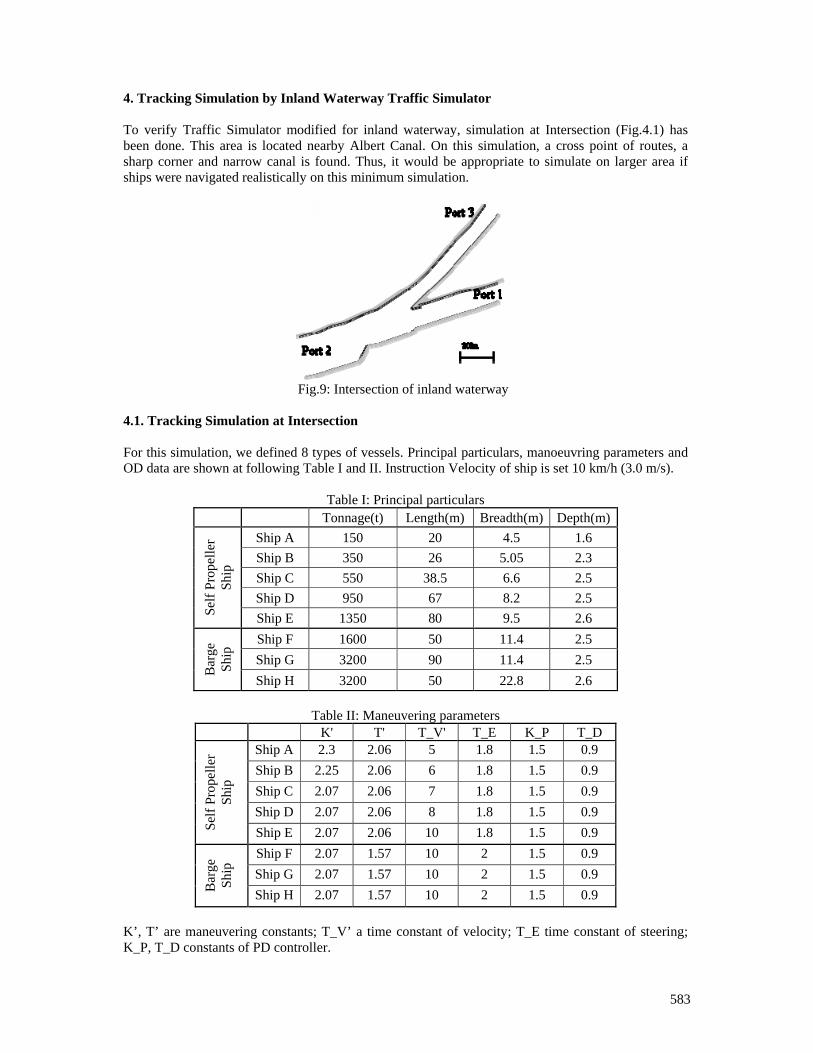
583

4. Tracking Simulation by Inland Waterway Traffic Simulator To verify Traffic Simulator modified for inland waterway, simulation at Intersection (Fig.4.1) has been done. This area is located nearby Albert Canal. On this simulation, a cross point of routes, a sharp corner and narrow canal is found. Thus, it would be appropriate to simulate on larger area if ships were navigated realistically on this minimum simulation.

Fig.9: Intersection of inland waterway

4.1. Tracking Simulation at Intersection For this simulation, we defined 8 types of vessels. Principal particulars, manoeuvring parameters and OD data are shown at following Table I and II. Instruction Velocity of ship is set 10 km/h (3.0 m/s).

Table I: Principal particulars Tonnage(t) Length(m) Breadth(m) Depth(m)

Ship A 150 20 4.5 1.6 Ship B 350 26 5.05 2.3 Ship C 550 38.5 6.6 2.5 Ship D 950 67 8.2 2.5

Self

Prop

elle

r Sh

ip

Ship E 1350 80 9.5 2.6 Ship F 1600 50 11.4 2.5 Ship G 3200 90 11.4 2.5

Bar

ge

Ship

Ship H 3200 50 22.8 2.6

Table II: Maneuvering parameters K' T' T_V' T_E K_P T_D

Ship A 2.3 2.06 5 1.8 1.5 0.9 Ship B 2.25 2.06 6 1.8 1.5 0.9 Ship C 2.07 2.06 7 1.8 1.5 0.9 Ship D 2.07 2.06 8 1.8 1.5 0.9

Self

Prop

elle

r Sh

ip

Ship E 2.07 2.06 10 1.8 1.5 0.9 Ship F 2.07 1.57 10 2 1.5 0.9 Ship G 2.07 1.57 10 2 1.5 0.9

Bar

ge

Ship

Ship H 2.07 1.57 10 2 1.5 0.9 K’, T’ are maneuvering constants; T_V’ a time constant of velocity; T_E time constant of steering; K_P, T_D constants of PD controller.

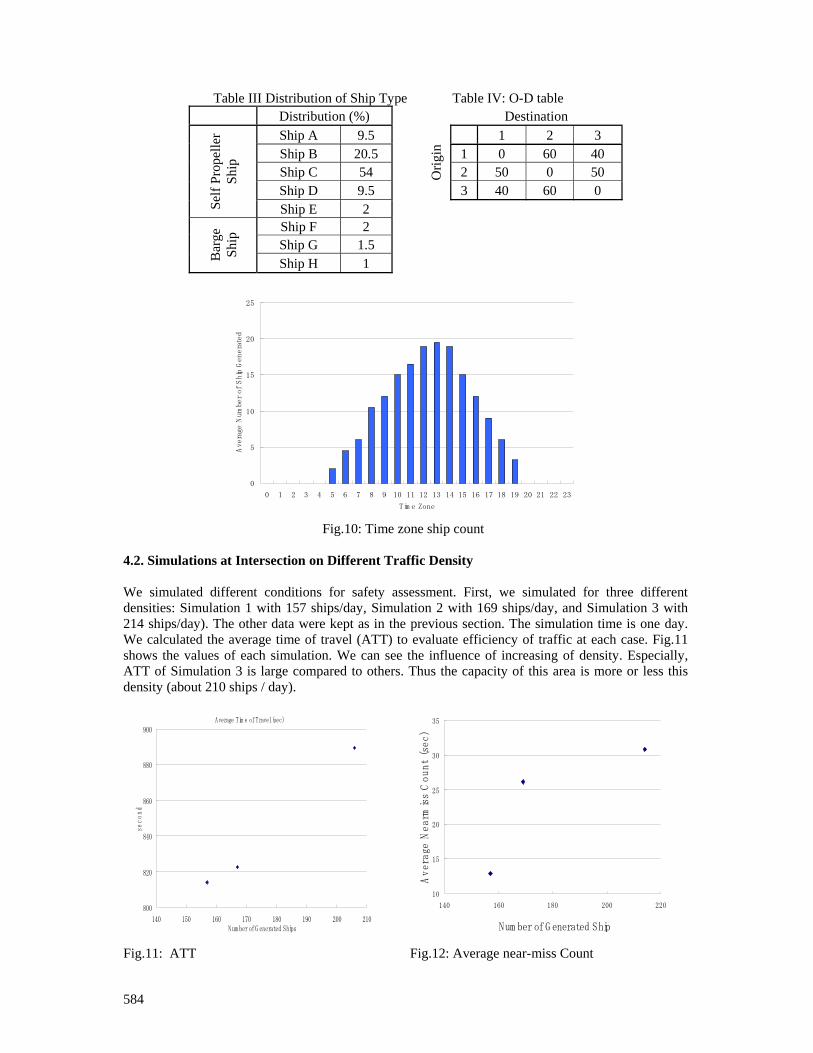
584

Table III Distribution of Ship Type Table IV: O-D table Distribution (%) Destination

Ship A 9.5 1 2 3 Ship B 20.5 1 0 60 40 Ship C 54 2 50 0 50 Ship D 9.5

Orig

in

3 40 60 0

Self

Prop

elle

r Sh

ip

Ship E 2 Ship F 2 Ship G 1.5

Bar

ge

Ship

Ship H 1

0

5

10

15

20

25

0 1 2 3 4 5 6 7 8 9 10 11 12 13 14 15 16 17 18 19 20 21 22 23

Tim e Zone

Ave

rage

Numbe

r of Ship G

enerated

Fig.10: Time zone ship count

4.2. Simulations at Intersection on Different Traffic Density We simulated different conditions for safety assessment. First, we simulated for three different densities: Simulation 1 with 157 ships/day, Simulation 2 with 169 ships/day, and Simulation 3 with 214 ships/day). The other data were kept as in the previous section. The simulation time is one day. We calculated the average time of travel (ATT) to evaluate efficiency of traffic at each case. Fig.11 shows the values of each simulation. We can see the influence of increasing of density. Especially, ATT of Simulation 3 is large compared to others. Thus the capacity of this area is more or less this density (about 210 ships / day).

Average Tim e of Travel (sec)

800

820

840

860

880

900

140 150 160 170 180 190 200 210Num ber of G enerated Ships

seco

nd

10

15

20

25

30

35

140 160 180 200 220

Num ber of G enerated Ship

Avera

ge N

earm

iss Count (sec)

Fig.11: ATT Fig.12: Average near-miss Count

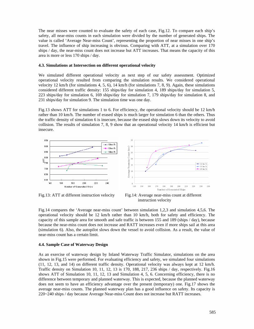
585

The near misses were counted to evaluate the safety of each case, Fig.12. To compare each ship’s safety, all near-miss counts in each simulation were divided by the number of generated ships. The value is called ‘Average Near-miss Count’, representing the proportion of near misses in one ship’s travel. The influence of ship increasing is obvious. Comparing with ATT, at a simulation over 170 ships / day, the near-miss count does not increase but ATT increases. That means the capacity of this area is more or less 170 ships / day. 4.3. Simulations at Intersection on different operational velocity We simulated different operational velocity as next step of our safety assessment. Optimized operational velocity resulted from comparing the simulation results. We considered operational velocity 12 km/h (for simulations 4, 5, 6), 14 km/h (for simulations 7, 8, 9). Again, these simulations considered different traffic density: 155 ships/day for simulation 4, 189 ships/day for simulation 5, 223 ships/day for simulation 6, 169 ships/day for simulation 7, 179 ships/day for simulation 8, and 231 ships/day for simulation 9. The simulation time was one day. Fig.13 shows ATT for simulations 1 to 6. For efficiency, the operational velocity should be 12 km/h rather than 10 km/h. The number of erased ships is much larger for simulation 6 than the others. Thus the traffic density of simulation 6 is insecure, because the erased ship slows down its velocity to avoid collision. The results of simulation 7, 8, 9 show that an operational velocity 14 km/h is efficient but insecure.

0

5

10

15

20

25

30

35

140 150 160 170 180 190 200 210 220 230 240

Num ber of G enerated Ships

Ave

rage

Nearmiss Count (sec)

12 km /h

14 km /h

10 km /h

Fig.13: ATT at different instruction velocity Fig.14: Average near-miss count at different instruction velocity

Fig.14 compares the ‘Average near-miss count’ between simulation 1,2,3 and simulation 4,5,6. The operational velocity should be 12 km/h rather than 10 km/h, both for safety and efficiency. The capacity of this sample area for smooth and safe traffic is between 155 and 189 (ships / day), because because the near-miss count does not increase and RATT increases even if more ships sail at this area (simulation 6). Also, the autopilot slows down the vessel to avoid collision. As a result, the value of near-miss count has a certain limit. 4.4. Sample Case of Waterway Design As an exercise of waterway design by Inland Waterway Traffic Simulator, simulations on the area shown in Fig.15 were performed. For evaluating efficiency and safety, we simulated four simulations (11, 12, 13, and 14) on different traffic density. Operational velocity was always kept at 12 km/h. Traffic density on Simulation 10, 11, 12, 13 is 170, 188, 217, 236 ships / day, respectively. Fig.16 shows ATT of Simulation 10, 11, 12, 13 and Simulation 4, 5, 6. Concerning efficiency, there is no difference between temporary and planned waterway. This is expected, because the planned waterway does not seem to have an efficiency advantage over the present (temporary) one. Fig.17 shows the average near-miss counts. The planned waterway plan has a good influence on safety. Its capacity is 220~240 ships / day because Average Near-miss Count does not increase but RATT increases.

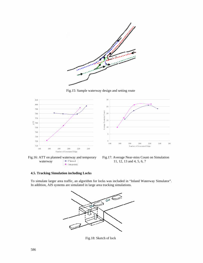
586

Planned

tem porary

Fig.15: Sample waterway design and setting route

710

720

730

740

750

760

770

780

790

800

810

140 160 180 200 220 240

N um ber of G enerated Ships

ATT

0

5

10

15

20

25

30

140 160 180 200 220 240 260

N um ber of G enerated Ships

Ave

rage

Nearmiss Count

Fig.16: ATT on planned waterway and temporary waterway

Fig.17: Average Near-miss Count on Simulation 11, 12, 13 and 4, 5, 6, 7

4.5. Tracking Simulation including Locks To simulate larger area traffic, an algorithm for locks was included in “Inland Waterway Simulator”. In addition, AIS systems are simulated in large area tracking simulations.

Fig.18: Sketch of lock

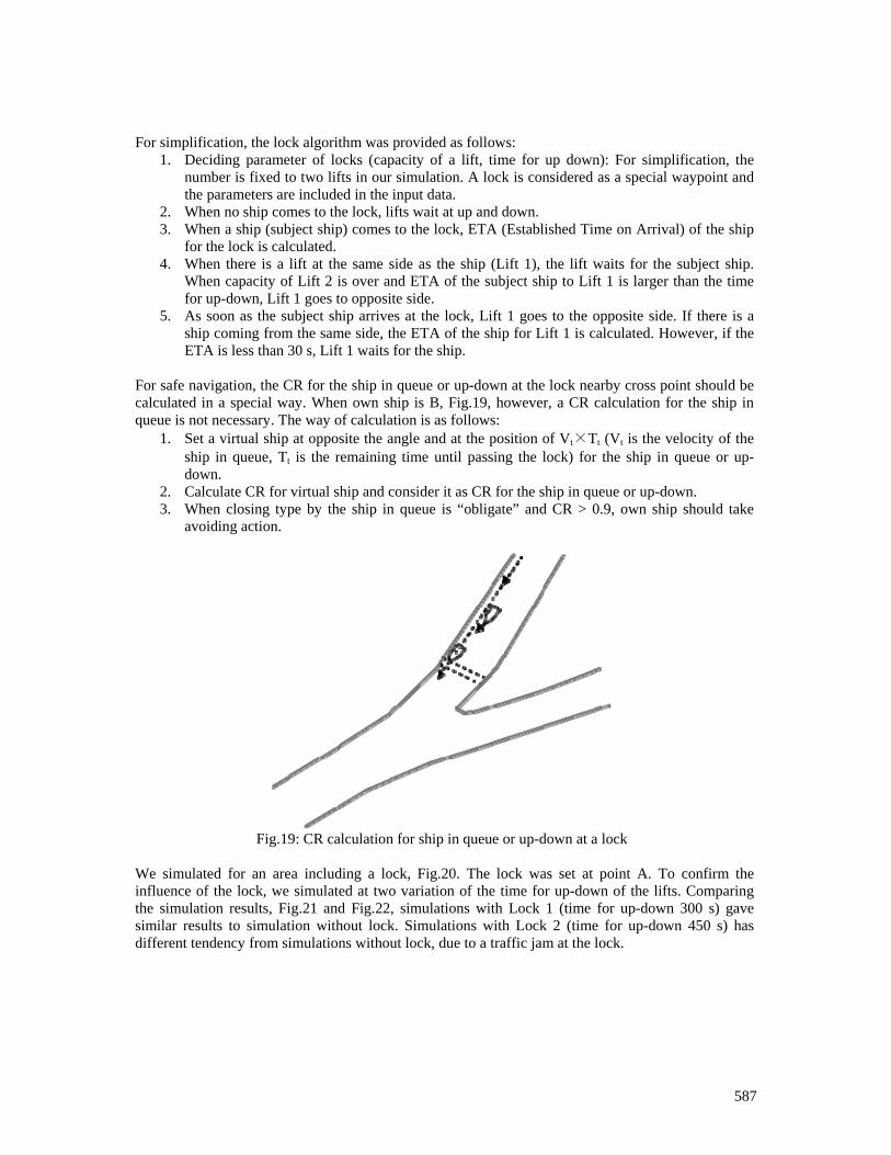
587

For simplification, the lock algorithm was provided as follows:

1. Deciding parameter of locks (capacity of a lift, time for up down): For simplification, the number is fixed to two lifts in our simulation. A lock is considered as a special waypoint and the parameters are included in the input data.

2. When no ship comes to the lock, lifts wait at up and down. 3. When a ship (subject ship) comes to the lock, ETA (Established Time on Arrival) of the ship

for the lock is calculated. 4. When there is a lift at the same side as the ship (Lift 1), the lift waits for the subject ship.

When capacity of Lift 2 is over and ETA of the subject ship to Lift 1 is larger than the time for up-down, Lift 1 goes to opposite side.

5. As soon as the subject ship arrives at the lock, Lift 1 goes to the opposite side. If there is a ship coming from the same side, the ETA of the ship for Lift 1 is calculated. However, if the ETA is less than 30 s, Lift 1 waits for the ship.

For safe navigation, the CR for the ship in queue or up-down at the lock nearby cross point should be calculated in a special way. When own ship is B, Fig.19, however, a CR calculation for the ship in queue is not necessary. The way of calculation is as follows:

1. Set a virtual ship at opposite the angle and at the position of Vt×Tt (Vt is the velocity of the ship in queue, Tt is the remaining time until passing the lock) for the ship in queue or up-down.

2. Calculate CR for virtual ship and consider it as CR for the ship in queue or up-down. 3. When closing type by the ship in queue is “obligate” and CR > 0.9, own ship should take

avoiding action.

Fig.19: CR calculation for ship in queue or up-down at a lock

We simulated for an area including a lock, Fig.20. The lock was set at point A. To confirm the influence of the lock, we simulated at two variation of the time for up-down of the lifts. Comparing the simulation results, Fig.21 and Fig.22, simulations with Lock 1 (time for up-down 300 s) gave similar results to simulation without lock. Simulations with Lock 2 (time for up-down 450 s) has different tendency from simulations without lock, due to a traffic jam at the lock.

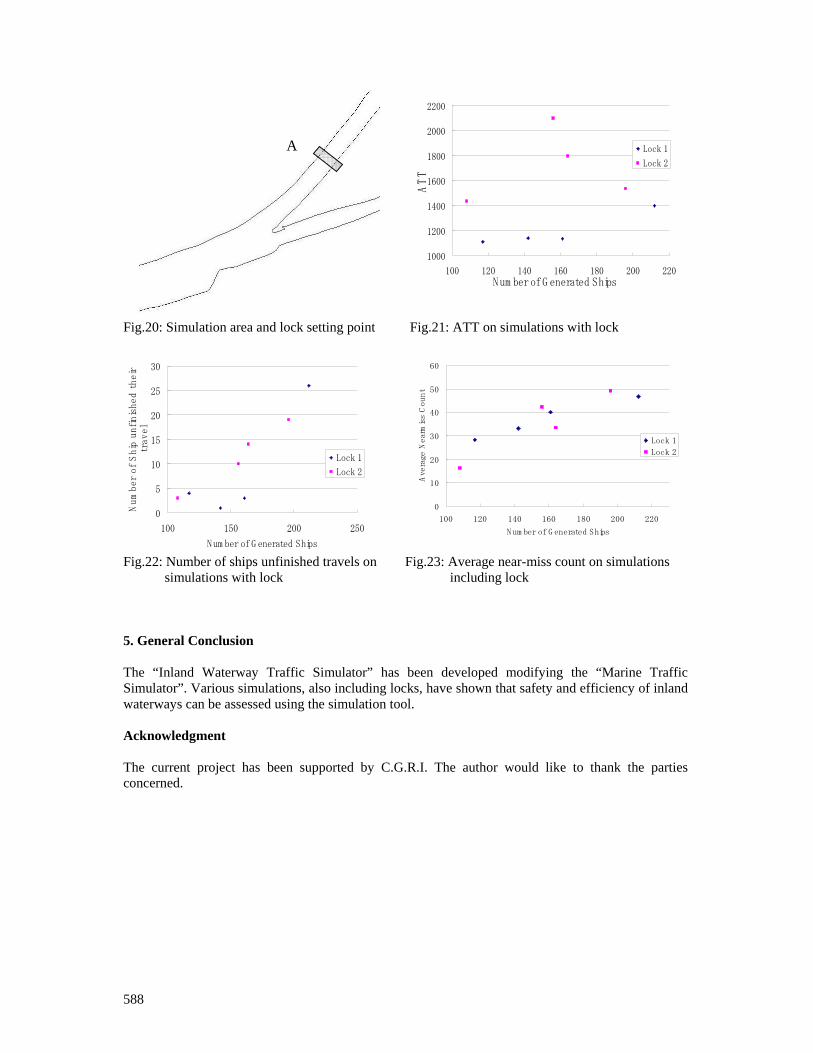
588

1000

1200

1400

1600

1800

2000

2200

100 120 140 160 180 200 220N um ber of G enerated Ships

ATT

Lock 1

Lock 2

Fig.20: Simulation area and lock setting point Fig.21: ATT on simulations with lock

0

5

10

15

20

25

30

100 150 200 250

Num ber of G enerated Ships

Num

ber of Ship unfinishe

d their

trav

el

Lock 1

Lock 2

0

10

20

30

40

50

60

100 120 140 160 180 200 220

N um ber of G enerated Ships

Average

Nearmiss Count

Lock 1

Lock 2

Fig.22: Number of ships unfinished travels on simulations with lock

Fig.23: Average near-miss count on simulations including lock

5. General Conclusion The “Inland Waterway Traffic Simulator” has been developed modifying the “Marine Traffic Simulator”. Various simulations, also including locks, have shown that safety and efficiency of inland waterways can be assessed using the simulation tool. Acknowledgment The current project has been supported by C.G.R.I. The author would like to thank the parties concerned.

A

589

Hull Monitoring System Development using a Hierarchical Framework for Data and Information Management

Liming W. Salvino, NSWC Carderock MD, West Bethesda/USA, liming.salvino@navy.mil

Thomas F. Brady, NSWC Carderock MD, West Bethesda/USA, thomas.brady@navy.mil

Abstract

The development of an effective structural health monitoring system is a critical mechanism to ensure

structural performance over the life of a ship, especially for lightweight high-speed ships. This paper

discusses a unique approach for data and information management of a current hull monitoring

system. Software developments range from real time indicators providing instantaneous information

and knowledge for the operators to background processes that include in-depth analyses, which can

be periodically obtained for decision-making purposes. This data and information management

architecture delivers an improved hull monitoring system which will ultimately include structural

diagnosis and prognosis capabilities.

1. Introduction

Sustainment and life-cycle engineering of ships and ship systems represent major and fast growing

challenges for the US Navy. The development of an effective structural health monitoring (SHM)

system is a critical mechanism to ensure structural performance over the life of a ship. An on board

SHM system to monitor the response of the hull girder and secondary structure to the seaway loads

was envisioned as early as two decades ago. The response data then will be continuously processed in

real time to provide warnings and recommendations to the operators and/or engineering crews

concerning structural integrity, required maintenance, as well as suggested operation modifications

that may extend the lifecycle of Navy ships. The system will provide the means for safer ship

operation by minimizing the possibility of structural damage and reducing structural fatigue damage

accumulation. Although a series of efforts were undertaken since the mid 1990s to support this SHM

vision, the development and implementation of such systems are still in a very limited stage at the

present time. An overview of the current status of monitoring marine structures and SHM

technologies required to realize real time structural diagnosis and prognosis vision as well as

challenges for shipboard implementation can be found in Salvino and Collette (2008).

A major objective of future US Navy ship design is the development of high-speed and high

performance vessels. Despite the lack of information on wave loads and local pressures in high speed

operations, high performance ship design will include many novel lightweight structural features as

well as possessing multi-mission adaptability and allowing for reduced levels of manning. For

example, to reduce weight as much as possible to allow higher speeds and increased cargo capacity,

high-speed vessels often employ novel and aggressive structural designs using composite, aluminum

alloys, or high strength steel with innovative arrangements and fabrications to maximize lightship

weight reduction. These structural features and high-speed operating profiles may increase possible

fatigue, buckling, and vibration problems as well as crew discomfort from increased wave slamming,

acceleration levels, and higher working stresses in the structure, Rawson and Tupper (2001). As a

result, secondary structural damage due to wave impacts and slamming occur frequently and

extensive damage can occur in a short amount of time while the ship is operating in heavy seas. To

minimize the risk of operating high-speed vessels in an unrestricted manner will require the ability to

monitor operational loads and to detect structural damage and structural performance degradation at

the earliest possible stage, i.e., the ability to implement structural diagnosis in real time. This

structural diagnostic information can then be used to predict the time to potential structural failure,

and to provide strategies for corrective actions in order to support future Navy operation and

maintenance.

The ultimate goal of a shipboard SHM system defines an integrated process, which includes continued

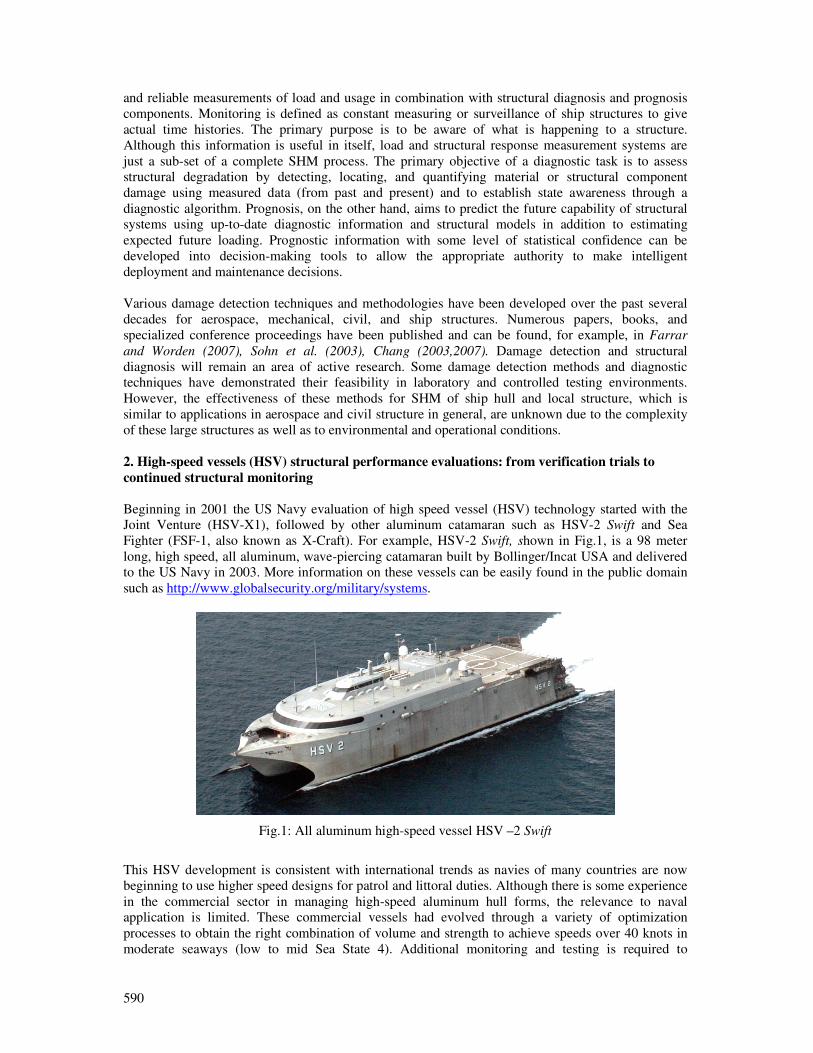
590

and reliable measurements of load and usage in combination with structural diagnosis and prognosis

components. Monitoring is defined as constant measuring or surveillance of ship structures to give

actual time histories. The primary purpose is to be aware of what is happening to a structure.

Although this information is useful in itself, load and structural response measurement systems are

just a sub-set of a complete SHM process. The primary objective of a diagnostic task is to assess

structural degradation by detecting, locating, and quantifying material or structural component

damage using measured data (from past and present) and to establish state awareness through a

diagnostic algorithm. Prognosis, on the other hand, aims to predict the future capability of structural

systems using up-to-date diagnostic information and structural models in addition to estimating

expected future loading. Prognostic information with some level of statistical confidence can be

developed into decision-making tools to allow the appropriate authority to make intelligent

deployment and maintenance decisions.

Various damage detection techniques and methodologies have been developed over the past several

decades for aerospace, mechanical, civil, and ship structures. Numerous papers, books, and

specialized conference proceedings have been published and can be found, for example, in Farrar

and Worden (2007), Sohn et al. (2003), Chang (2003,2007). Damage detection and structural

diagnosis will remain an area of active research. Some damage detection methods and diagnostic

techniques have demonstrated their feasibility in laboratory and controlled testing environments.

However, the effectiveness of these methods for SHM of ship hull and local structure, which is

similar to applications in aerospace and civil structure in general, are unknown due to the complexity

of these large structures as well as to environmental and operational conditions.

2. High-speed vessels (HSV) structural performance evaluations: from verification trials to

continued structural monitoring

Beginning in 2001 the US Navy evaluation of high speed vessel (HSV) technology started with the

Joint Venture (HSV-X1), followed by other aluminum catamaran such as HSV-2 Swift and Sea

Fighter (FSF-1, also known as X-Craft). For example, HSV-2 Swift, shown in Fig.1, is a 98 meter

long, high speed, all aluminum, wave-piercing catamaran built by Bollinger/Incat USA and delivered

to the US Navy in 2003. More information on these vessels can be easily found in the public domain

such as http://www.globalsecurity.org/military/systems.

Fig.1: All aluminum high-speed vessel HSV –2 Swift

This HSV development is consistent with international trends as navies of many countries are now

beginning to use higher speed designs for patrol and littoral duties. Although there is some experience

in the commercial sector in managing high-speed aluminum hull forms, the relevance to naval

application is limited. These commercial vessels had evolved through a variety of optimization

processes to obtain the right combination of volume and strength to achieve speeds over 40 knots in

moderate seaways (low to mid Sea State 4). Additional monitoring and testing is required to

591

understand all of the construction practices used by commercial industry. In addition, commercial

vessels usually operate on well-defined routes and have significantly different operational patterns

compared to a navy vessel which is required to perform a range of tasks over wide and variable

operational areas.

The initial evaluations of HSV-X1, HSV-2 and FSF-1 were to monitor structural responses during

dedicated rough water trails. In each case the trial objectives were to determine if the responses were

nominal or acceptable when the ship is operated within the Safe Operational Envelop (SOE) defined

by American Bureau of Shipping. The SOE provides guidance for the operation of the vessel since it

is not permitted to operate unrestricted in the open ocean. Thomas et al. (2003), presents an example

of such a trial conducted during the delivery voyage of a high-speed ferry, while Pegg et al. (1995)

give an overview of conducting a sea trial and finite element model verification through natural

frequency predictions of a SWATH vessel. Such design verification is fairly routine practice today;

however, both the sea condition and structural response monitoring equipment are typically removed

or de-activated at the completion of the trial.

In all evaluations of HSV-X1, HSV-2 and FSF-1, the SOE was adequate in defining the space of

operation as defined by speed and wave height. However, trial results did show that these vessels can

endure significant wave impact loadings, at high speed, when operated near the edge of the SOE. Not

all wave impacts, including slamming events, are detrimental but those that are can produce local

damage that could go unnoticed until the next visual inspection. It is very difficult to determine the

severity of these wave impacts during high-speed operations. Moreover, it is impossible to assess the

effect of these wave impacts on local structure without a continued shipboard hull monitoring system.

At a very basic level, a monitoring system would indicate to the operator when or if an overload has

occurred. Knowing when to inspect after operation in waves can save inspection time and help assess

operational readiness.

In the effort of further HSV structural performance evaluation to support the on going acquisition of

aluminum vessels, the Joint High Speed Vessel (JHSV) program funded a spectral-based fatigue

analysis for HSV-2. The findings are summarized in Kihl (2006). This report indicates that crack

initiation could begin early in the life of the vessel. It is accepted that aluminum does not have the

same fatigue strength as steel. Sielski (2007) stated that aluminum has a crack propagation rate under

fatigue loading that can be as much as 30 times greater than that of steel under the same applied

stress. In addition, marine grade aluminum will become sensitized over time when exposed to high

temperatures. The sensitized material forms a continuous film along the grain boundaries of the

material. It is possible for corrosion to rapidly spread along this film, resulting in a network of gaps in

the material. These gaps can lead to stress corrosion cracking and exfoliation in the alloy resulting in

total material/structural failure, Wong et al. (2006). At the present time, no techniques exist to indicate

if the on board aluminum is sensitized. These facts greatly accelerated the interest in equipping Navy

aluminum ships with an operational real-time monitoring system to find cracks and structural

anomalies early or at least to provide structural response data that can be useful in identifying portions

of the structure that require a more rigorous visual/local Non-destructive evaluations. Although visual

inspection cannot detect newly formed cracks, or cracks under insulation and machinery, it is the only

means to identify flaws in practice today. Obviously, a rigorous inspection will be time consuming

and costly so it should only be performed as needed. It is an important step forward if the information

derived from the hull monitoring database can assist the maintainers so that they execute inspections

and maintenance as required.

There is little experience on the long-term structural performance of aluminum HSVs, especially

those planned for future use by the US Navy. Currently, there are several US Navy acquisition

programs that contain ship and hull monitoring aspects. An example is a hull condition-monitoring

project for the JHSV program. The remainder of this paper discusses in detail the development of the

hull monitoring system for JHSV. In particular, the focus will be on current work that addresses issues

regarding data management and information technology development, including data collection and

conditioning, data processing, evaluation and management, as well as results presentation and storage.

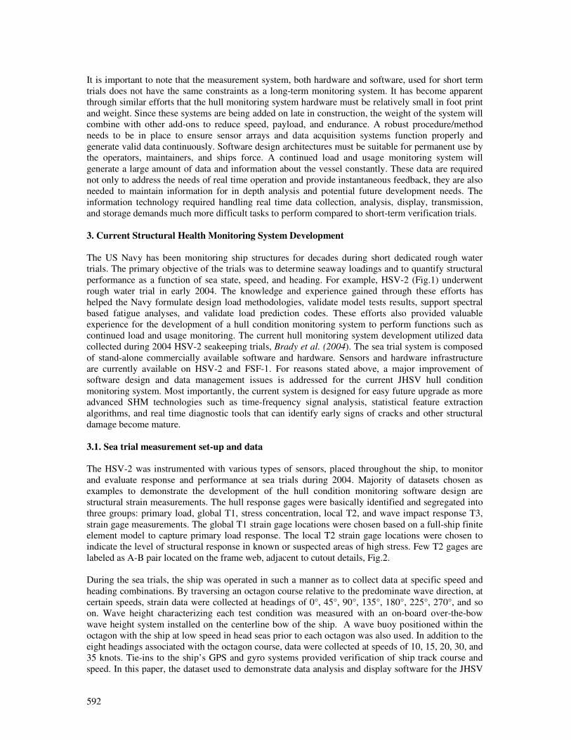
592

It is important to note that the measurement system, both hardware and software, used for short term

trials does not have the same constraints as a long-term monitoring system. It has become apparent

through similar efforts that the hull monitoring system hardware must be relatively small in foot print

and weight. Since these systems are being added on late in construction, the weight of the system will

combine with other add-ons to reduce speed, payload, and endurance. A robust procedure/method

needs to be in place to ensure sensor arrays and data acquisition systems function properly and

generate valid data continuously. Software design architectures must be suitable for permanent use by

the operators, maintainers, and ships force. A continued load and usage monitoring system will

generate a large amount of data and information about the vessel constantly. These data are required

not only to address the needs of real time operation and provide instantaneous feedback, they are also

needed to maintain information for in depth analysis and potential future development needs. The

information technology required handling real time data collection, analysis, display, transmission,

and storage demands much more difficult tasks to perform compared to short-term verification trials.

3. Current Structural Health Monitoring System Development

The US Navy has been monitoring ship structures for decades during short dedicated rough water

trials. The primary objective of the trials was to determine seaway loadings and to quantify structural

performance as a function of sea state, speed, and heading. For example, HSV-2 (Fig.1) underwent

rough water trial in early 2004. The knowledge and experience gained through these efforts has

helped the Navy formulate design load methodologies, validate model tests results, support spectral

based fatigue analyses, and validate load prediction codes. These efforts also provided valuable

experience for the development of a hull condition monitoring system to perform functions such as

continued load and usage monitoring. The current hull monitoring system development utilized data

collected during 2004 HSV-2 seakeeping trials, Brady et al. (2004). The sea trial system is composed

of stand-alone commercially available software and hardware. Sensors and hardware infrastructure

are currently available on HSV-2 and FSF-1. For reasons stated above, a major improvement of

software design and data management issues is addressed for the current JHSV hull condition

monitoring system. Most importantly, the current system is designed for easy future upgrade as more

advanced SHM technologies such as time-frequency signal analysis, statistical feature extraction

algorithms, and real time diagnostic tools that can identify early signs of cracks and other structural

damage become mature.

3.1. Sea trial measurement set-up and data

The HSV-2 was instrumented with various types of sensors, placed throughout the ship, to monitor

and evaluate response and performance at sea trials during 2004. Majority of datasets chosen as

examples to demonstrate the development of the hull condition monitoring software design are

structural strain measurements. The hull response gages were basically identified and segregated into

three groups: primary load, global T1, stress concentration, local T2, and wave impact response T3,

strain gage measurements. The global T1 strain gage locations were chosen based on a full-ship finite

element model to capture primary load response. The local T2 strain gage locations were chosen to

indicate the level of structural response in known or suspected areas of high stress. Few T2 gages are

labeled as A-B pair located on the frame web, adjacent to cutout details, Fig.2.

During the sea trials, the ship was operated in such a manner as to collect data at specific speed and

heading combinations. By traversing an octagon course relative to the predominate wave direction, at

certain speeds, strain data were collected at headings of 0°, 45°, 90°, 135°, 180°, 225°, 270°, and so

on. Wave height characterizing each test condition was measured with an on-board over-the-bow

wave height system installed on the centerline bow of the ship. A wave buoy positioned within the

octagon with the ship at low speed in head seas prior to each octagon was also used. In addition to the

eight headings associated with the octagon course, data were collected at speeds of 10, 15, 20, 30, and

35 knots. Tie-ins to the ship’s GPS and gyro systems provided verification of ship track course and

speed. In this paper, the dataset used to demonstrate data analysis and display software for the JHSV

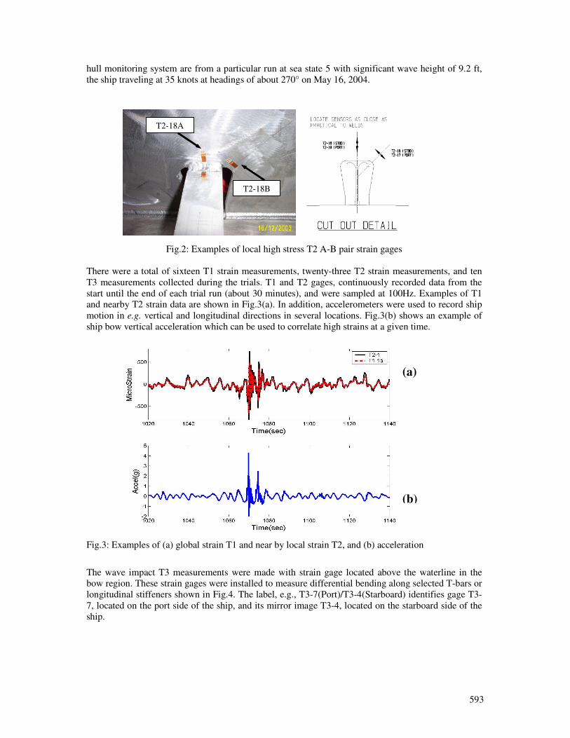
593

hull monitoring system are from a particular run at sea state 5 with significant wave height of 9.2 ft,

the ship traveling at 35 knots at headings of about 270° on May 16, 2004.

Fig.2: Examples of local high stress T2 A-B pair strain gages

There were a total of sixteen T1 strain measurements, twenty-three T2 strain measurements, and ten

T3 measurements collected during the trials. T1 and T2 gages, continuously recorded data from the

start until the end of each trial run (about 30 minutes), and were sampled at 100Hz. Examples of T1

and nearby T2 strain data are shown in Fig.3(a). In addition, accelerometers were used to record ship

motion in e.g. vertical and longitudinal directions in several locations. Fig.3(b) shows an example of

ship bow vertical acceleration which can be used to correlate high strains at a given time.

Fig.3: Examples of (a) global strain T1 and near by local strain T2, and (b) acceleration

The wave impact T3 measurements were made with strain gage located above the waterline in the

bow region. These strain gages were installed to measure differential bending along selected T-bars or

longitudinal stiffeners shown in Fig.4. The label, e.g., T3-7(Port)/T3-4(Starboard) identifies gage T3-

7, located on the port side of the ship, and its mirror image T3-4, located on the starboard side of the

ship.

T2-18A

T2-18B

(a)

(b)

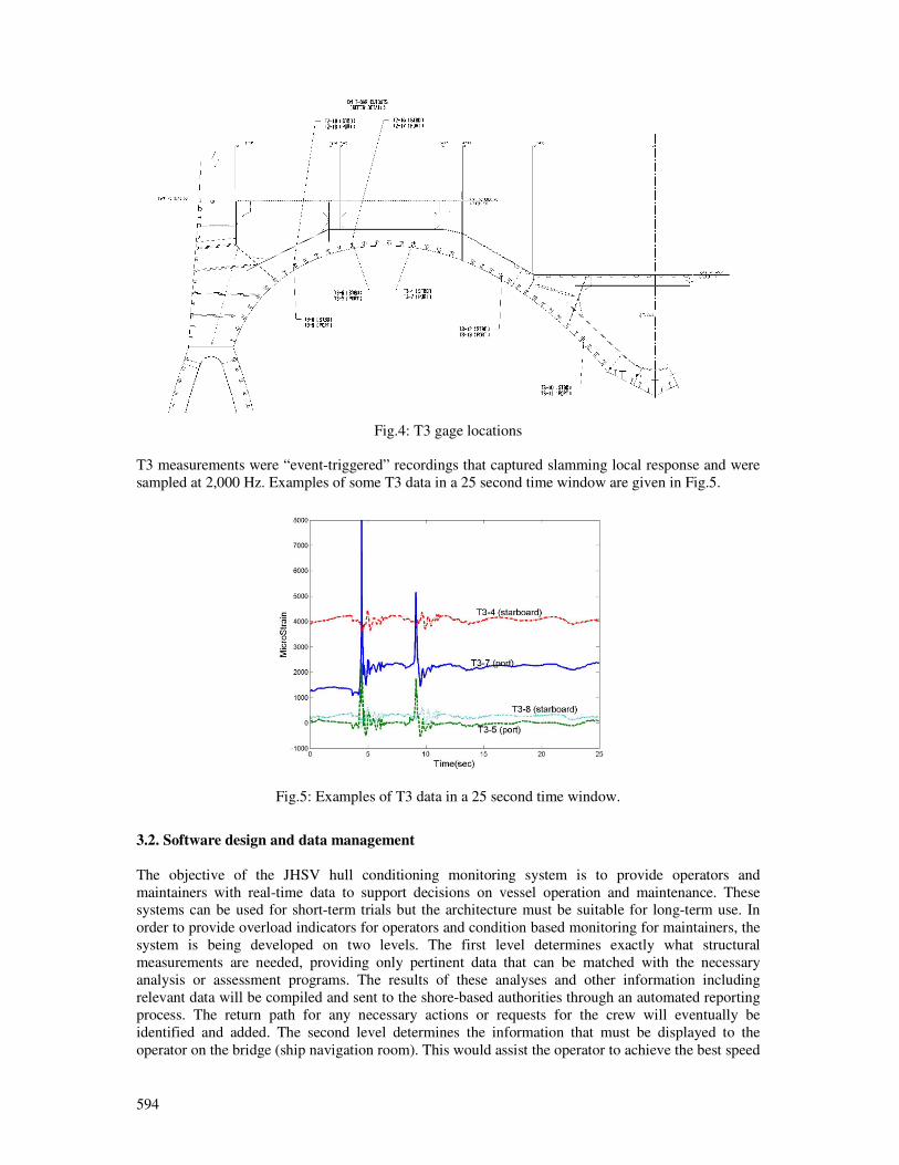
594

Fig.4: T3 gage locations

T3 measurements were “event-triggered” recordings that captured slamming local response and were

sampled at 2,000 Hz. Examples of some T3 data in a 25 second time window are given in Fig.5.

Fig.5: Examples of T3 data in a 25 second time window.

3.2. Software design and data management

The objective of the JHSV hull conditioning monitoring system is to provide operators and

maintainers with real-time data to support decisions on vessel operation and maintenance. These

systems can be used for short-term trials but the architecture must be suitable for long-term use. In

order to provide overload indicators for operators and condition based monitoring for maintainers, the

system is being developed on two levels. The first level determines exactly what structural

measurements are needed, providing only pertinent data that can be matched with the necessary

analysis or assessment programs. The results of these analyses and other information including

relevant data will be compiled and sent to the shore-based authorities through an automated reporting

process. The return path for any necessary actions or requests for the crew will eventually be

identified and added. The second level determines the information that must be displayed to the

operator on the bridge (ship navigation room). This would assist the operator to achieve the best speed

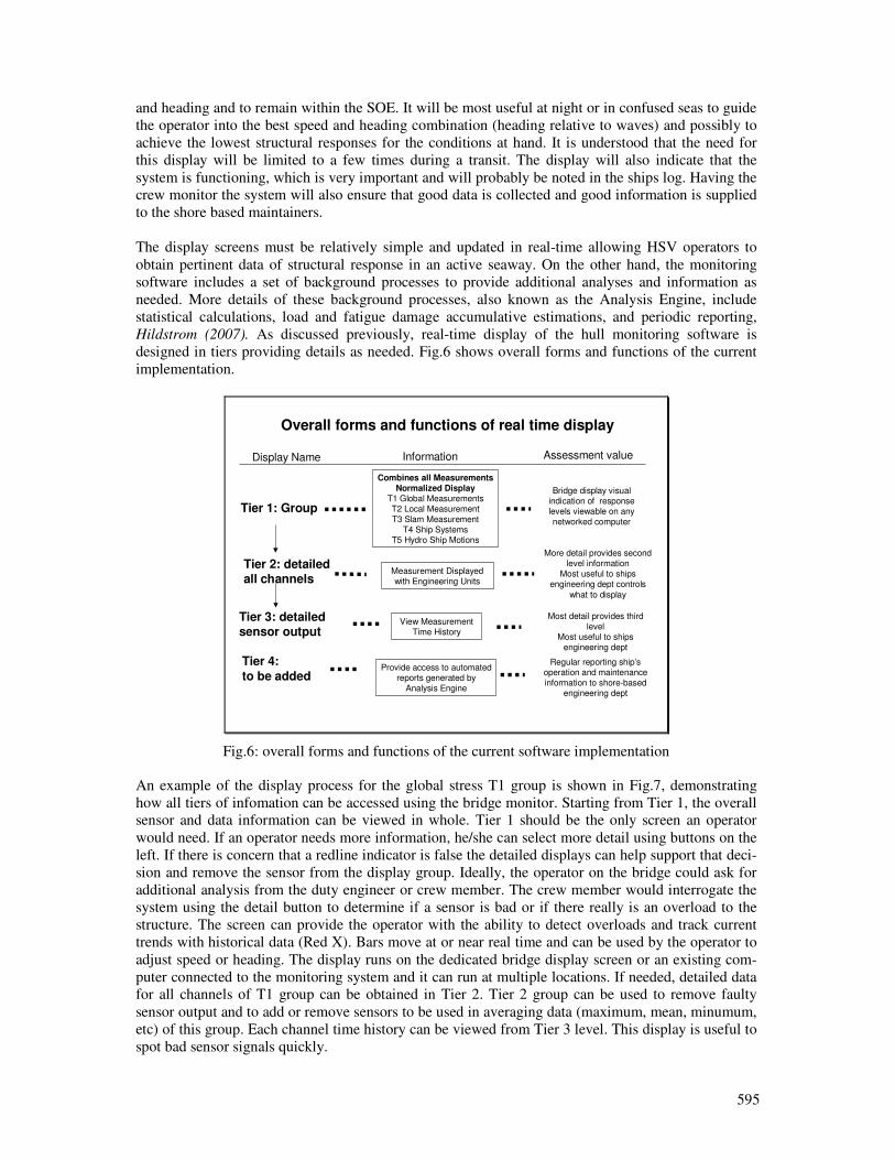
595

and heading and to remain within the SOE. It will be most useful at night or in confused seas to guide

the operator into the best speed and heading combination (heading relative to waves) and possibly to

achieve the lowest structural responses for the conditions at hand. It is understood that the need for

this display will be limited to a few times during a transit. The display will also indicate that the

system is functioning, which is very important and will probably be noted in the ships log. Having the

crew monitor the system will also ensure that good data is collected and good information is supplied

to the shore based maintainers.

The display screens must be relatively simple and updated in real-time allowing HSV operators to

obtain pertinent data of structural response in an active seaway. On the other hand, the monitoring

software includes a set of background processes to provide additional analyses and information as

needed. More details of these background processes, also known as the Analysis Engine, include

statistical calculations, load and fatigue damage accumulative estimations, and periodic reporting,

Hildstrom (2007). As discussed previously, real-time display of the hull monitoring software is

designed in tiers providing details as needed. Fig.6 shows overall forms and functions of the current

implementation.

Overall forms and functions of real time display

Tier 1: Group

Tier 2: detailed all channels

Tier 3: detailed sensor output

Combines all MeasurementsNormalized Display

T1 Global Measurements

T2 Local Measurement

T3 Slam Measurement

T4 Ship Systems

T5 Hydro Ship Motions

Bridge display visual

indication of response

levels viewable on any

networked computer

Measurement Displayed

with Engineering Units

More detail provides second

level information

Most useful to ships

engineering dept controls

what to display

View Measurement

Time History

Most detail provides third

level

Most useful to ships

engineering dept

Display Name Information Assessment value

Tier 4:

to be addedProvide access to automated

reports generated by

Analysis Engine

Regular reporting ship’s

operation and maintenance

information to shore-based

engineering dept

Fig.6: overall forms and functions of the current software implementation

An example of the display process for the global stress T1 group is shown in Fig.7, demonstrating

how all tiers of infomation can be accessed using the bridge monitor. Starting from Tier 1, the overall

sensor and data information can be viewed in whole. Tier 1 should be the only screen an operator

would need. If an operator needs more information, he/she can select more detail using buttons on the

left. If there is concern that a redline indicator is false the detailed displays can help support that deci-

sion and remove the sensor from the display group. Ideally, the operator on the bridge could ask for

additional analysis from the duty engineer or crew member. The crew member would interrogate the

system using the detail button to determine if a sensor is bad or if there really is an overload to the

structure. The screen can provide the operator with the ability to detect overloads and track current

trends with historical data (Red X). Bars move at or near real time and can be used by the operator to

adjust speed or heading. The display runs on the dedicated bridge display screen or an existing com-

puter connected to the monitoring system and it can run at multiple locations. If needed, detailed data

for all channels of T1 group can be obtained in Tier 2. Tier 2 group can be used to remove faulty

sensor output and to add or remove sensors to be used in averaging data (maximum, mean, minumum,

etc) of this group. Each channel time history can be viewed from Tier 3 level. This display is useful to

spot bad sensor signals quickly.

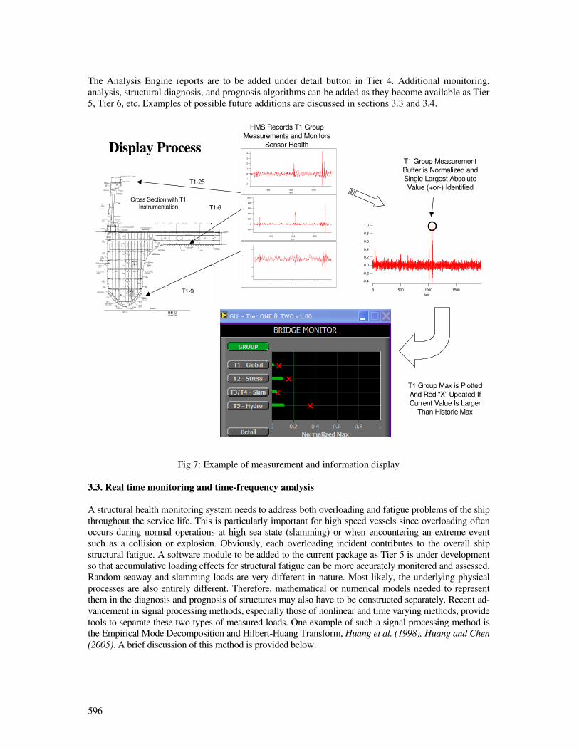
596

The Analysis Engine reports are to be added under detail button in Tier 4. Additional monitoring,

analysis, structural diagnosis, and prognosis algorithms can be added as they become available as Tier

5, Tier 6, etc. Examples of possible future additions are discussed in sections 3.3 and 3.4.

Display Process

300 C 6 BKT300 C 6 BKT

B 6 BKT

FWD

B 6 BKT

7 B 6 BKTS

TYP

1400

10

0

10

0

ENGINE GIRDER TRANSITION

6PL WEB w. 10PL RIDER

LVESSEL CGENSET FUEL

PENETRATIONREFER 23-008

GENSET FUEL

PENETRATIONREFER 23-008

90 x 10 FB ON AFT SIDE ALIGNS w. PORTAL RIDER

90 x 10 FB x 500 LONG FORWARD SIDE (SNIPED)

B 6 BKT

B 6 BKT

FWD

B 6 BKT

FWD

7 B 6 BKTS

TYP

B 6 BKT

FUEL SUPPLY LINE

REFER 23-008

200 C 6

BOTH SIDES

200 C 6

AFT SIDEONLY

300

B 6 BKT

HEAVY TRUCK DECK EXT NR 59253 PLUS EXT # ICT 078 UNDER,

BETWEEN PLANK & WEB.6PL INFILL PIECE

TO ENSURE WATERTIGHT

600x400PENETRATION

600x400PENETRATION

8PL INTERCOSTAL BHD

FWD I.W.O PILLAR

Do.(14200)

100x45x4/8 T (14160)

DD

Do

.(1

13

6)

DD

Do

.(1

13

6)

DD

Do

.(1

13

6)

DD

Do

.(1

13

6)

DD

Do

.(1

13

6)

DD

70

x40

'IT (

11

48

)

S

D

950

= = =

50x6 LANDING BAR

V/DECK 7693 A.B.

10

1165012048 7100 6250 5300 4400 3700 3450 2200 1500 600

MOULDED V/DECK

7637 A.B.

11

96

6441 A.B.

37

75

00

31

96

0

5PL INTERCOSTAL

LONG'L BULKHEAD

4623 AB

SPONSON

EXTRUSION

E26541

140x50 'IT ON CHINE

REFER HULL DETAIL BKLT

70

x5

0x

4/8

T (5

56

4)

Do

.(6

06

9)

Do

.(5

67

6)

Do

.(6

69

0)

Do

.(6

77

6)

Do

.(6

77

6)

Do

.(6

69

0)

Do

.(6

42

5)

Do

.(6

05

8)

Do

.(3

54

1)

Do

.(2

67

8)

Do

.(2

22

8)

SD

D

D D

S

D D D D D D D

S

D

D

D

D

D

D

D

S

D

D

FUEL LINE

PENETRATIONDWG.23-008

400 400 400 400 400 400 400 400 400 400 400

Do

.(6

79

7)

DD

S

S

S

S S

S

S

S

S140x5 WEB w. 140x12 RIDER (5857)

220x6 WEB w. 100x12 RIDER (5367)

220x6 WEB w. 100x12 RIDER (4673)

340x7 WEB w. 100x12 RIDER (4269)

340x7 WEB w. 100x12 RIDER (4119)

300 C 6

BOTH SIDES

300 C 6

BOTH SIDES

300 C 6 BOTH SIDES

300 C 6 BOTH SIDESREFER HULL DETAIL BKLT

300 C 6

BOTH SIDES

300 C 6

BOTH SIDES

300 C 6

BOTH SIDES

300 C 6BOTH SIDES

300 C 6

BOTH SIDES

6PL

5PL

5PL

7PL

6PL 6PL

280

8PL LONG'L INTERCOSTAL

WATERTIGHT BULKHEAD

B 8 BKT

BOTH SIDES

25PL KEEL PLATE SKEG

A 6 BOTH

SIDES TYP

400x10 WEB w.

200x20 RIDER

80x8 FB

S

LONGITUDINAL GIRDER

8PL WEB w. 100x12 RIDER

300 C 6 FWD

LONGITUDINAL GIRDER

8PL WEB w. 100x12 RIDER

300 C 6 FWD

S

220x6 WEB w. 100x12 RIDER (4513)

300

DD

70

x50

x4

/8T

(19

67

)

BASELINE

HULL CL BHD 22LOOKING FWD

S

BM 6 FWD200 C 6 AFT

20

Do

.(1

78

8)

DD

Do

.(1

66

8)

D

D300 300

8 PL

GUTTER

PORTAL TOP

12470 MLD A.B.248

1147

D

375 x 12 PL CARLIN

5 PL

10 PL

20

12

11415 OFF C.L.

950

100

50

B 6

FWD

SEAM 11750 A.B.

7693 A.B.

FRM 22

LOOKING AFT

10 PL

180x8 PLRIDER

SLOT RIDER 400

ENDS SNIPED 30°

281

D

550

MIN

WEB

554S

D

70x50x4/8 T

(L= 479)

FWD SIDE

10

0x

45

x4/8

T (

41

85

)

AFT

SID

E

DS

70x50x4/8 T

(L= 596)FWD SIDE

180x15 PL

RIDER

900MLD

1500670

D

320

180x8 PL

RIDER

4

3

2

1

0

-1

-2

10501000950

sec

1000

800

600

400

200

0

-200

10501000950

sec

- 1 0 0 0

- 5 0 0

0

5 0 0

1 0 5 01 0 0 09 5 0

s e c

1.0

0.8

0.6

0.4

0.2

0.0

-0.2

-0.4

150010005000

sec

T1-25

T1-9

T1-6

HMS Records T1 Group

Measurements and Monitors

Sensor Health

T1 Group Measurement

Buffer is Normalized and

Single Largest Absolute

Value (+or-) Identified

T1 Group Max is Plotted

And Red “X” Updated If

Current Value Is Larger

Than Historic Max

Cross Section with T1

Instrumentation

Fig.7: Example of measurement and information display

3.3. Real time monitoring and time-frequency analysis

A structural health monitoring system needs to address both overloading and fatigue problems of the ship

throughout the service life. This is particularly important for high speed vessels since overloading often

occurs during normal operations at high sea state (slamming) or when encountering an extreme event

such as a collision or explosion. Obviously, each overloading incident contributes to the overall ship

structural fatigue. A software module to be added to the current package as Tier 5 is under development

so that accumulative loading effects for structural fatigue can be more accurately monitored and assessed.

Random seaway and slamming loads are very different in nature. Most likely, the underlying physical

processes are also entirely different. Therefore, mathematical or numerical models needed to represent

them in the diagnosis and prognosis of structures may also have to be constructed separately. Recent ad-

vancement in signal processing methods, especially those of nonlinear and time varying methods, provide

tools to separate these two types of measured loads. One example of such a signal processing method is

the Empirical Mode Decomposition and Hilbert-Huang Transform, Huang et al. (1998), Huang and Chen

(2005). A brief discussion of this method is provided below.

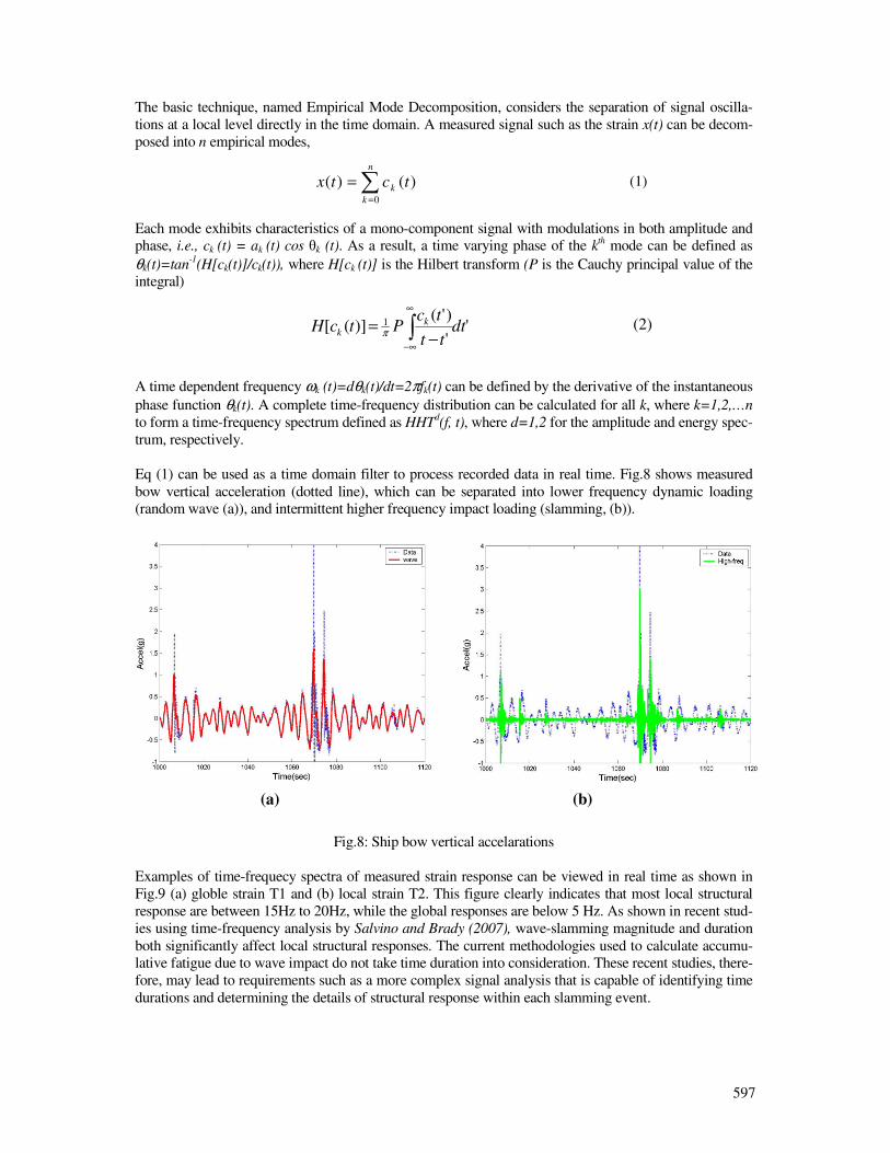
597

''

)'()]([ 1 dt

tt

tcPtcH k

k ∫∞

∞−−

=π

(2)

The basic technique, named Empirical Mode Decomposition, considers the separation of signal oscilla-

tions at a local level directly in the time domain. A measured signal such as the strain x(t) can be decom-

posed into n empirical modes,

Each mode exhibits characteristics of a mono-component signal with modulations in both amplitude and

phase, i.e., ck (t) = ak (t) cos θk (t). As a result, a time varying phase of the kth mode can be defined as

θk(t)=tan-1(H[ck(t)]/ck(t)), where H[ck (t)] is the Hilbert transform (P is the Cauchy principal value of the

integral)

A time dependent frequency ωk (t)=dθk(t)/dt=2πfk(t) can be defined by the derivative of the instantaneous

phase function θk(t). A complete time-frequency distribution can be calculated for all k, where k=1,2,…n

to form a time-frequency spectrum defined as HHTd(f, t), where d=1,2 for the amplitude and energy spec-

trum, respectively.

Eq (1) can be used as a time domain filter to process recorded data in real time. Fig.8 shows measured

bow vertical acceleration (dotted line), which can be separated into lower frequency dynamic loading

(random wave (a)), and intermittent higher frequency impact loading (slamming, (b)).

Fig.8: Ship bow vertical accelarations

Examples of time-frequecy spectra of measured strain response can be viewed in real time as shown in

Fig.9 (a) globle strain T1 and (b) local strain T2. This figure clearly indicates that most local structural

response are between 15Hz to 20Hz, while the global responses are below 5 Hz. As shown in recent stud-

ies using time-frequency analysis by Salvino and Brady (2007), wave-slamming magnitude and duration

both significantly affect local structural responses. The current methodologies used to calculate accumu-

lative fatigue due to wave impact do not take time duration into consideration. These recent studies, there-

fore, may lead to requirements such as a more complex signal analysis that is capable of identifying time

durations and determining the details of structural response within each slamming event.

∑=

=

n

k

k tctx0

)()( (1)

(a) (b)

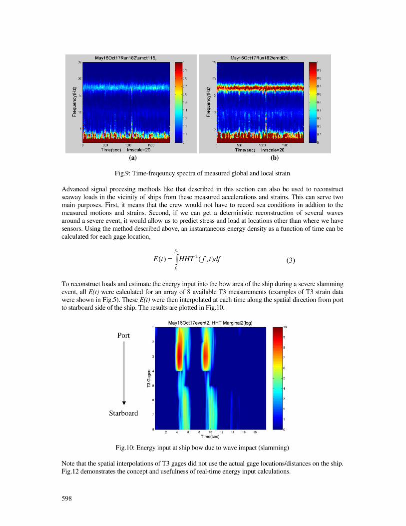
598

(a) (b)

Fig.9: Time-freqeuncy spectra of measured global and local strain

Advanced signal procesing methods like that described in this section can also be used to reconstruct

seaway loads in the vicinity of ships from these measured accelerations and strains. This can serve two

main purposes. First, it means that the crew would not have to record sea conditions in addtion to the

measured motions and strains. Second, if we can get a deterninistic reconstruction of several waves

around a severe event, it would allow us to predict stress and load at locations other than where we have

sensors. Using the method described above, an instantaneous energy density as a function of time can be

calculated for each gage location,

To reconstruct loads and estimate the energy input into the bow area of the ship during a severe slamming

event, all E(t) were calculated for an array of 8 available T3 measurements (examples of T3 strain data

were shown in Fig.5). These E(t) were then interpolated at each time along the spatial direction from port

to starboard side of the ship. The results are plotted in Fig.10.

Fig.10: Energy input at ship bow due to wave impact (slamming)

Note that the spatial interpolations of T3 gages did not use the actual gage locations/distances on the ship.

Fig.12 demonstrates the concept and usefulness of real-time energy input calculations.

(3) ∫=

2

1

),()( 2

f

f

dftfHHTtE

Port

Starboard

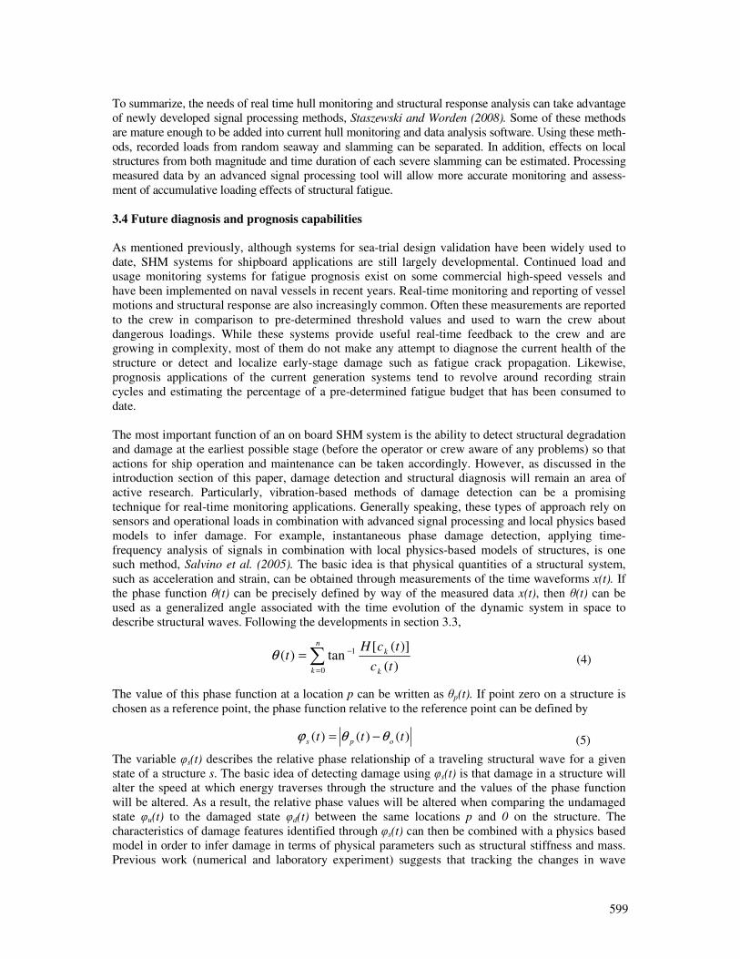
599

To summarize, the needs of real time hull monitoring and structural response analysis can take advantage

of newly developed signal processing methods, Staszewski and Worden (2008). Some of these methods

are mature enough to be added into current hull monitoring and data analysis software. Using these meth-

ods, recorded loads from random seaway and slamming can be separated. In addition, effects on local

structures from both magnitude and time duration of each severe slamming can be estimated. Processing

measured data by an advanced signal processing tool will allow more accurate monitoring and assess-

ment of accumulative loading effects of structural fatigue.

3.4 Future diagnosis and prognosis capabilities

As mentioned previously, although systems for sea-trial design validation have been widely used to

date, SHM systems for shipboard applications are still largely developmental. Continued load and

usage monitoring systems for fatigue prognosis exist on some commercial high-speed vessels and

have been implemented on naval vessels in recent years. Real-time monitoring and reporting of vessel

motions and structural response are also increasingly common. Often these measurements are reported

to the crew in comparison to pre-determined threshold values and used to warn the crew about

dangerous loadings. While these systems provide useful real-time feedback to the crew and are

growing in complexity, most of them do not make any attempt to diagnose the current health of the

structure or detect and localize early-stage damage such as fatigue crack propagation. Likewise,

prognosis applications of the current generation systems tend to revolve around recording strain

cycles and estimating the percentage of a pre-determined fatigue budget that has been consumed to

date.

The most important function of an on board SHM system is the ability to detect structural degradation

and damage at the earliest possible stage (before the operator or crew aware of any problems) so that

actions for ship operation and maintenance can be taken accordingly. However, as discussed in the

introduction section of this paper, damage detection and structural diagnosis will remain an area of

active research. Particularly, vibration-based methods of damage detection can be a promising

technique for real-time monitoring applications. Generally speaking, these types of approach rely on

sensors and operational loads in combination with advanced signal processing and local physics based

models to infer damage. For example, instantaneous phase damage detection, applying time-

frequency analysis of signals in combination with local physics-based models of structures, is one

such method, Salvino et al. (2005). The basic idea is that physical quantities of a structural system,

such as acceleration and strain, can be obtained through measurements of the time waveforms x(t). If

the phase function θ(t) can be precisely defined by way of the measured data x(t), then θ(t) can be

used as a generalized angle associated with the time evolution of the dynamic system in space to

describe structural waves. Following the developments in section 3.3,

The value of this phase function at a location p can be written as θp(t). If point zero on a structure is

chosen as a reference point, the phase function relative to the reference point can be defined by

The variable φs(t) describes the relative phase relationship of a traveling structural wave for a given

state of a structure s. The basic idea of detecting damage using φs(t) is that damage in a structure will

alter the speed at which energy traverses through the structure and the values of the phase function

will be altered. As a result, the relative phase values will be altered when comparing the undamaged

state φu(t) to the damaged state φd(t) between the same locations p and 0 on the structure. The

characteristics of damage features identified through φs(t) can then be combined with a physics based

model in order to infer damage in terms of physical parameters such as structural stiffness and mass.

Previous work (numerical and laboratory experiment) suggests that tracking the changes in wave

)(

)]([tan)(

0

1

tc

tcHt

k

kn

k

∑=

−

=θ (4)

(5) )()()( ttt ops θθϕ −=

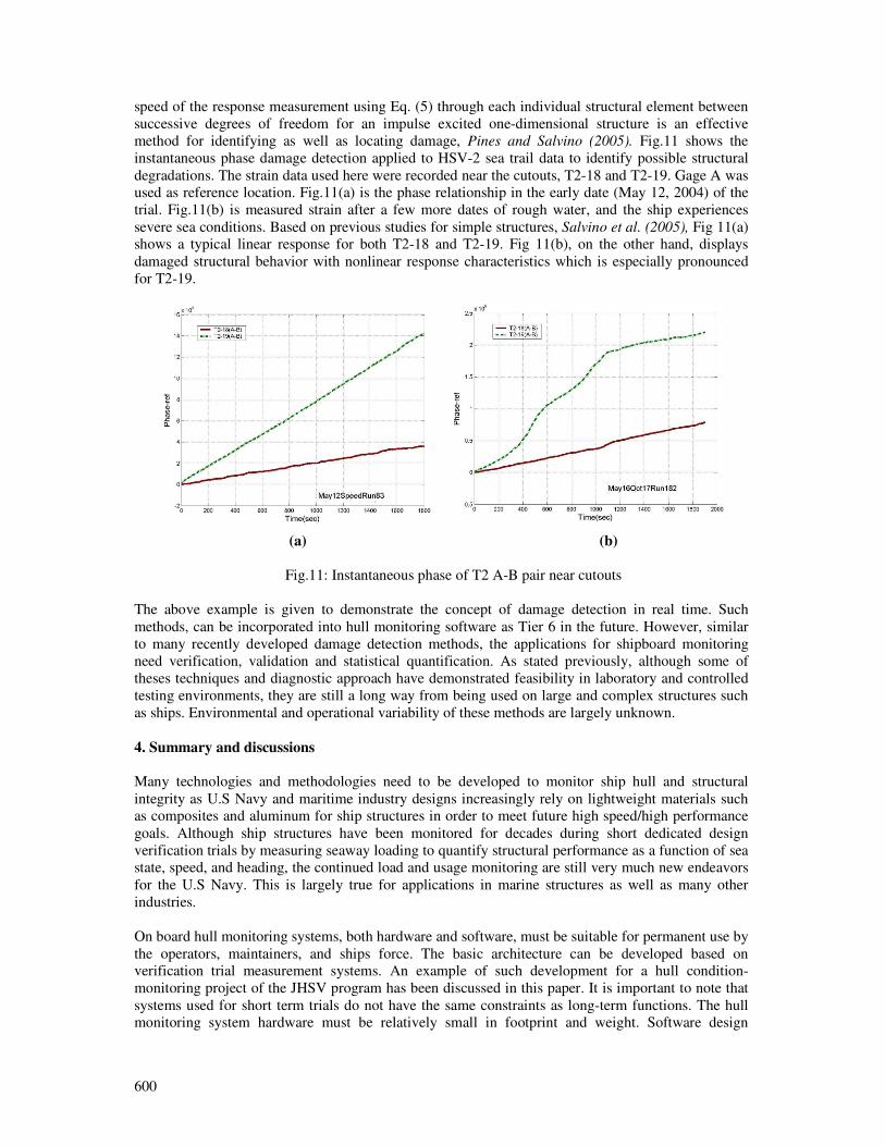
600

speed of the response measurement using Eq. (5) through each individual structural element between

successive degrees of freedom for an impulse excited one-dimensional structure is an effective

method for identifying as well as locating damage, Pines and Salvino (2005). Fig.11 shows the

instantaneous phase damage detection applied to HSV-2 sea trail data to identify possible structural

degradations. The strain data used here were recorded near the cutouts, T2-18 and T2-19. Gage A was

used as reference location. Fig.11(a) is the phase relationship in the early date (May 12, 2004) of the

trial. Fig.11(b) is measured strain after a few more dates of rough water, and the ship experiences

severe sea conditions. Based on previous studies for simple structures, Salvino et al. (2005), Fig 11(a)

shows a typical linear response for both T2-18 and T2-19. Fig 11(b), on the other hand, displays

damaged structural behavior with nonlinear response characteristics which is especially pronounced

for T2-19.

(a) (b)

Fig.11: Instantaneous phase of T2 A-B pair near cutouts

The above example is given to demonstrate the concept of damage detection in real time. Such

methods, can be incorporated into hull monitoring software as Tier 6 in the future. However, similar

to many recently developed damage detection methods, the applications for shipboard monitoring

need verification, validation and statistical quantification. As stated previously, although some of

theses techniques and diagnostic approach have demonstrated feasibility in laboratory and controlled

testing environments, they are still a long way from being used on large and complex structures such

as ships. Environmental and operational variability of these methods are largely unknown.

4. Summary and discussions

Many technologies and methodologies need to be developed to monitor ship hull and structural

integrity as U.S Navy and maritime industry designs increasingly rely on lightweight materials such

as composites and aluminum for ship structures in order to meet future high speed/high performance

goals. Although ship structures have been monitored for decades during short dedicated design

verification trials by measuring seaway loading to quantify structural performance as a function of sea

state, speed, and heading, the continued load and usage monitoring are still very much new endeavors

for the U.S Navy. This is largely true for applications in marine structures as well as many other

industries.

On board hull monitoring systems, both hardware and software, must be suitable for permanent use by

the operators, maintainers, and ships force. The basic architecture can be developed based on

verification trial measurement systems. An example of such development for a hull condition-

monitoring project of the JHSV program has been discussed in this paper. It is important to note that

systems used for short term trials do not have the same constraints as long-term functions. The hull

monitoring system hardware must be relatively small in footprint and weight. Software design

601

architectures need to be able to incorporate new technologies as they become mature. In addition, data

and information, which are being generated continuously, need to be properly managed, displayed,

and stored. These data are required not only to address the needs of real time operation and provide

instantaneous feedback to the operators; they are also needed for longer-term maintenance

considerations as well as more in depth analysis and potential future development. These

considerations are being implemented in the current JHSV hull-monitoring program. Software of this

hull monitoring system is designed in tiers, which will provide needed data and information about the

vessel. This development effort, although incremental, will provide valuable experience for future

Navy SHM development needs.

The long-term goal of real-time structural health monitoring and diagnosis is to identify signs of

fatigue or structural overload damage, i.e. to detect structural anomaly at the earliest possible stage

through on board sensor networks and diagnostic algorithms. Prognosis will then use real-time

diagnostic input to predict future structural conditions and remaining service life. The continued

advancement of pertinent technologies will ultimately enable a comprehensive structural health

monitoring system that includes these diagnostic methods and prognostic capabilities to proactively

manage future ship hull and structures.

Acknowledgements

The authors wish to acknowledge the support of JHSV program office for providing data and other

materials. The work was funded by NSWCCD In-house Lab. Independent Research Program and the

Office of Naval Research.

References

BRADY, T. F. (2004), Global structural response measurement of SWIFT (HSV-2) from JLOTS and

blue game rough water trials, NSWCCD-65-TR-2004/33, Naval Surface Warfare Center, Carderock

Division, West Bethesda, MD

CHANG, F.K, (Ed). (2003), Structural health monitoring 2003: From diagnostics & prognostics to

structural health management, EDStech Publications, Inc.

CHANG, F.K, (Ed). (2007), Structural health monitoring 2007: Quantification, validation, and

implementation, EDStech Publications, Inc.

FARRAR, C.R; WORDEN, K. (2007), An introduction to structural health monitoring, Structural

Heath Monitoring, Philosophical Trans. of the Royal Society A 365

HILDSTROM, G.A. (2007), JHSV analysis engine, NSWCCD-65-TR–2006/15, Naval Surface

Warfare Center, Carderock Division, West Bethesda, MD

HUANG, N.E., et al. (1998), The empirical mode decomposition and the Hilbert spectrum for

nonlinear and non-stationary time series analysis, Proc. Royal Soc. London, A 454

HUANG, N. E; CHEN, S. (2005), Hilbert-Huang transform: Introduction and applications, World

Scientific Publishing, Singapore

KIHL, D.P. (2006), JHSV full-scale trials based spectral fatigue assessment, NSWCCD-65-TR-

2006/35, Naval Surface Warfare Center, Carderock Division, West Bethesda, MD

PEGG, N.G.; GILROY, L.E.; KUMAR, R. (1995), Full scale verification of finite element modeling

of a 75 tonne SWATH vessel, Marine Structures, pp.211-228

PINES, D.J.; SALVINO, L.W. (2005), Structural health monitoring using empirical mode decompo-

602

sition and the Hilbert Phase, J. Sound and Vibration 294, pp.97-124

RAWSON, K.; TUPPER, E. (2001), Basic ship theory, Butterworth-Heinemann, pp.497-500

SALVINO, L.W.; COLLETTE, M.D. (2008), Monitoring marine structures, Encyclopedia of

Structural Health Monitoring, Vol. 10, John Wiley

SALVINO, L.W.; PINES, D.J.; TODD, M.; NICHOLS, J. (2005), EMD and instantaneous phase

detection of structural damage, Hilbert-Huang Transform: Introduction and Applications, World

Scientific Publishing, Singapore

SIELSKI, R.A. (2007), Research needs in aluminum structure, 10th Int. Symp. Practical Design of

Ships and Other Floating Structures (PRADS), Houston

SOHN, H., et al. (2003), A review of structural health monitoring literature: 1996 – 2001, Report No.

LA-13976-MS, Los Alamos National Laboratory

STASZEWSKI, W.J.; WORDEN, K. (2008), Signal Processing, Encyclopedia of Structural Health

Monitoring, John Wiley

THOMAS, G.A., et al. (2003), Slamming response of a large high-speed wave-piercer catamaran,

Marine Technology 40(2), pp.126-140

WONG, C.; et al. (2006), Material property and behavior, Office of Naval Research Aluminum

Structural Reliability Program 2006 Report, pp.44-67

603

Cognition-Centric Systems Design: A Paradigm Shift in System Design

Yvonne R. Masakowski, Naval Undersea Warfare Center, Newport/USA,

masakowskiyr@npt.nuwc.navy.mil

Abstract

Today, there are numerous advances in ambient intelligence technologies that incorporate seamless

networks, embedded intelligent agents, and wireless communication systems. This paper highlights

the critical role of ambient intelligence technologies in future ship designs. The emergence of

innovative technologies in the 21st century helps to shape the ways in which we think about systems

and ship designs. Given advances in technology and wireless communications, there is a need to

rethink system design from a human-centric to cognition-centric system design. Designers must shift

their perspectives from designing around the human to designing systems based upon the ways

humans think, i.e. human cognitive processing. The goal of the system designer is to effectively create

a system in which the performance of both the human and the system is optimized. To this end,

technologies can facilitate a seamless, symbiotic relationship between humans and systems that will

enable a system to operate more efficiently. System designers should explore opportunities to leverage

technologies to bridge the gap between humans and the system. To effectively address these

challenges, the paper presents the potential impact of implementing Ambient Intelligence

Technologies in system designs for future platforms.

“Solving a problem simply means representing it in a way that the solution is obvious.”

Herbert Simon (1996)

1. Introduction

As the operational environment becomes more complex, there is a need to develop advanced

technologies to support the 21st Century decision maker. Cognitive processes play a critical role in

knowledge acquisition and performance, Hanisch et al. (1991). Evidence suggests that pre-attentive

processes and attention control guides and may enhance visual search strategies, Triesman et al.

(1992), Bellenkes et al. (1997). There is a need to address ways in which designers can support the

decision maker’s cognitive processing abilities in view of the vast amount of information that

individuals must process daily.

Traditionally, human factors specialists focused their attention on the gap between the human and the

interface. Interface design was intended to bridge the gap between the system’s information

configuration and the user’s mental model, Cook and Masakowski (2007). However, given the

complexity of the current knowledge management environment, it is incumbent upon designers to

explore new approaches in providing decision support Cook et al. (2007). Specifically, system

designers must shift their perspective from human-centric to cognition-centric design which reflects

the roles, responsibilities and unique requirements of the decision maker. Cognition-centric design

affords the designer the means of developing systems to match the requirements and cognitive

processes of the end user. This can be achieved via intelligent agent networks that provide cueing,

guidance and/or alerts, as well as with adaptive interfaces and tools necessary for the user to achieve

total situational awareness (SA), Endsley (1995), Pew (2000). Systems should provide information

that is relevant and critical to the individual decision maker and in a manner which matches their

unique set of roles and requirements. Such profiled information will enhance situational awareness

and facilitate the operator/decision maker’s ability to be more effective in their roles and

responsibilities.

To this end, Ambient Intelligence (AmI) technologies provides a means of fulfilling the cognition-

centric design approach by generating an environment in which humans are supported by embedded

604

computing networks and wireless communication systems that can anticipate and/or respond to the

individual’s requirements for information and support. AmI technologies place the emphasis on

immersive, distributed information within a user-friendly environment which both empowers and

supports human interactions. To date, both the medical and architectural communities have advanced

this effort by embedding smart chips, wireless communication devices and sensors in mirrors, walls,

etc. as a means of managing individual health monitoring, managing the environment (i.e. temperature

and lighting of a room) and/or informing the observer. Cognition-centric design does not merely

augment an individual’s awareness but reflects a system that is aware of the user’s unique

requirements to complete their tasks. This approach is a shift away from traditional computing

platforms (i.e. PCs) to advanced wireless computing systems which are embedded in our environment

and are accessed via intelligent interfaces.

The AmI environment is one which utilizes advanced computing systems, i.e. unobtrusive hardware,

miniaturization, nanotechnology, embedded sensors, and seamless mobile/fixed web-based

communication infrastructures, Mukherjee et al. (2006). The dynamic nature of the information

environment mandates the need to rely on advanced computing systems, distributed networks,

intelligent agent architectures and multimodal interfaces to facilitate the decision maker’s ability to

function in the complex information environment. However, it is left to the creative systems designer

to adapt these technologies for ship design that will ensure operational readiness and effectiveness.

The emerging field of AmI technologies provides a unique environment for the human operator to

optimize their performance and manage information in an intuitive manner. Technologies which

provide decision support in a seamless environment play a pivotal role in the ways in which operators

can synthesize information, and support timely assessments required for effective decision making.

The goal of any decision support tool is to enhance the operator’s decision making by reducing the

time allotted to process information, increase the level of accuracy and optimize decision making. The

long term goal is to design automated systems that embed expert decision making strategies such that

these systems will facilitate and accelerate training, performance and knowledge management in the

distributed operational environment, Masakowski (2003a,b, 2008).

Cognition-centric design is contended to be a critical step toward developing systems that will

enhance operator and system performance. Future ship platforms will integrate these technologies to

provide self-sustaining maintenance, damage control support, environment support and facilitate the

life cycle of the platform itself.

Distributed networks in future platform designs will enable the system developer to shape the

presentation of information to be profiled to the end user’s requirements, Masakowski (2008). This

approach stands in stark contrast to traditional efforts in which the end user often reconfigures the

system on their own to meet their task requirements. This approach often short changes the end user

who does not benefit from the advantages of a human factor analysis that will optimize their

performance.

As ship designers utilize software programs to facilitate system and interface development, there is a

real risk to system and human performance. It is important to achieve an understanding of the roles of

each operator, their tasks, and requirements. The designer must address the ways in which they can

provide tools and technologies to support the knowledge requirements for the individual and for the

platform, Cook and Masakowski (2007), Masakowski (2008).

Today’s maritime environment is best characterized by dynamic and unexpected events where

decisions do not occur in isolation. Rather, decisions are made in complex environments and often

with competing sources of information. Therefore, there is a need to de-conflict information that will

enhance situational awareness and facilitate decision making in the distributed environment. Ship

designers must examine the technologies available and address these challenges by providing decision

makers tools to support situation analysis and their ability to make accurate and rapid decisions.

605

Today, we are presented with a new challenge to human cognitive processing. Multi-tasking has taken

on a new role in the environment with the advent of advanced computing technologies that often

present competing challenges in the course of daily work. Cognitive constraints, i.e. attention and

visual search strategies, similarly limit the amount of information which can be perceived and

managed. Visual processing and human attention mechanisms may be stressed by an overwhelming

amount of information presented to operators during the course of their daily work. Thus, system

designers must consider the ways in which operators will use the information presented in order to

effectively design a system. Human perceptual and cognitive processing capabilities must be taken

into consideration when designing future platforms.

Evidence shows that human visual search is guided by context and/or purpose, Yarbus (1967), Cai

(1986,2002) and humans anticipate things that are familiar in the environment, Rock (1966), Gibson

(1969). Studies have further shown the effects of perceptually salient features, i.e. features that “pop

out” of a display, Cai (1986), Treisman and Gormican (1988), Solso (1990), Treisman et al. (1992).

Theses studies highlight the role of perceptual and cognitive processes which ought to be considered

when designing interfaces and information systems that will support the ship platform.

The AmI technology environment provides an intuitive means for operators to assimilate information

in an unobtrusive manner. Technologies being developed by MIT, Carnegie Mellon University, The

Georgia Tech Research Institute and Penn State University, to name but a few, provide a means of

embedding information cues in the environment that can trigger the operator’s attention to a specific

point of interest.

One can envision that information demands will only continue to increase. Therefore, it is critical to

find new ways to support the decision maker working within the complex ship environment.

Technologies must be developed to reduce cognitive workload and enhance ship operational

effectiveness. There has been significant progress made in the development of technologies that serve

to modify data, reduce the clutter and present information/knowledge in an intuitive manner.

However, there is still a great deal of work yet to be done regarding the development of advanced

computing systems, wireless communications and integrated systems that will elevate the decision

maker’s capabilities. Specifically, the 21st century ship designer needs to acquire an understanding of

the platform’s mission, its crew and their environment.

Cognition-centric system design fosters the design of systems that will integrate distributed networks

of intelligent agents, enable humans to task and manage autonomous systems and provide wireless

communications systems that can be used to manage self-sustaining maintenance systems within the

platform design. Tools need to be developed that will enhance operator SA and facilitate the transition

from situational awareness to a state of action, Pew (2000), Endsley (1995). To that end, AmI

technologies provide the means to inform the end user in an unobtrusive manner and provide intuitive

guidance regarding information that is essential to complete tasks.

Designers must exploit AmI technologies that will extend human cognitive capacities in concert with

an understanding of human cognition, perception, attention and learning processes, Cai (2002),

Masakowski (2008). The designer of the future will need to incorporate the advances in computing

power and wireless systems in their designs to accommodate the vast amount of information

processing and data management required to sustain operations.

AmI technologies will advance ship designs by providing tools and technologies that will support a

self-sustaining platform, provide maintenance autonomously, monitor ship performance, navigation

and provide decision support tools for the crew/end users. AmI technologies will enable the

development of a new distributed network comprised of the human as a sensor node, netted intelligent

agents, robotics and a network of distributed data bases that will support the automated functioning of

the platform of the future. Advances in computing power and wireless technologies will afford the

designer a means of developing systems that will engage intelligent agent networks as crew members,

606

directing them to accomplish tasks, manage information and systems, as well as report back on the

level of success in their assignments.

The primary challenge for system designers is to understand the limitations of technology and seek to

employ it in a meaningful way. Striking the balance between human specific competencies and those

technologies that can reduce cognitive workload and support the decision maker will serve to develop

an optimized ship design of the future, Masakowski (2003), Cook et al. (2007). AmI technologies will

prove to be a critical tool for supporting the development of systems that will support the human

decision maker within the constraints of human attention and memory.

There are numerous risks associated with the aforementioned ideas, however, AmI technologies

afford the designer a means of mitigating risks by designing systems that will support the way that

humans think and process information within their environment.

Every new idea has its risks which must be evaluated during the design phase. It is left to future ship

designers to exploit the benefits of AmI technologies and shift from human-centric to cognition-

centric system design in the 21st Century.

References

BELLENKES, A.H.; WICKENS, C.D.; KRAMER, A. F. (1997), Visual scanning and pilot expertise:

The role of attention flexibility and mental model development, Aviation, Space, and Environmental

Medicine, 68, pp.569-579

CAI, Y. (1986), Pictorial thinking, Cognitive Science, Vol.1

CAI, Y. (2002), Texture measurement of visual appearance of recognition of oil paintings, IEEE

IMTC, Anchorage

COOK, M.; NOYES, J.; MASAKOWSKI, Y.R. (2007), Decision making in complex environments,

Ashgate Publishing, UK

COOK, M.; MASAKOWSKI, Y. (2007), Human Factors and Command and Control, JAPCC Journal

Edition, 5

ENDSLEY, M. (1995), Toward a theory of situation awareness in dynamic systems, Human

Factors, 37, pp.32-64

GIBSON, E. (1969), Principles of perceptual learning and development, Prentice-Hall, Inc.,

Englewood Cliffs, New Jersey

HANISCH, K.A., KRAMER, A.F.; HULIN, C.L. (1991), Cognitive representations, control, and

understanding of complex systems: A field study focusing on components of users' mental models and

expert/novice differences, Ergonomics, 34, pp.1129-1148

MASAKOWSKI, Y.R. (2003a), The role of the human in intelligent and automated system design: a

new frontier, Human Systems Integration Symposium, Vienna, Virginia

MASAKOWSKI, Y.R. (2003b), Knowledge warfare in the 21st Century: An extension in

performance, Naval Engineers Journal, Vol. 115, No. 2, pp. 29-36

MASAKOWSKI, Y.R. (2008), Knowledge forum: future submarine designs, Naval Undersea Warfare

Center, Newport, RI

607

MUKHERJEE, S.; AARTS, E.; ROOVERS, R.; WIDDERSHOVEN, F.; OUWERKERK, M. (2006),

AmIware: hardware technology drivers of ambient intelligence, Springer, edition 1, The Netherlands

PEW, R.W. (2000), The state of situation awareness measurement: Heading toward the next century,

in M. R. Endsley and D.J. Garland (eds.), Situation Awareness Analysis and Measurement, Lawrence

Erlbaum Associates Inc., Mahwah, pp.33-47

ROCK, I. (1966), The nature of perceptual adaptation, Basic Books, New York

SOLSO, R. (1990), Cognition and visual art, The MIT Press, Cambridge, MA

TREISMAN, A.; GORMICAN, S. (1988), Feature analysis in early vision: evidence from search

asymmetries, Psychological Review, 95, 15-48

TREISMAN, A.; VIEIRA, A.; HAYES, A. (1992), Automaticity and pre-attentive processing,

American Journal of Psychology, 105, 341-362

YARBUS, A.L. (1967), Eye movements during perception of complex objects, Plenum Press

608

Index by Authors

Aarsaether 372

Abels 174

Alonso 121

Amrane 92,107

Andrews 407

Andric 435

Asmara 271

Bair 48

Bentin 200

Bertram 6

Blake 502

Boals 551

Bocchetti 435

Bohnenberg 350

Boiteau 6

Bouckaert 107

Boyd 314

Brady 589

Bralic 450

Brathaug 244

Cabos 222,516

Caiti 384

Caprace 48, 107

Cartier 107

Casalino 384

Casarosa 407

Cheylan 6

Choi 467

Chyba 467

Constantinescu 92,107

Cui 422

Cupic 435

Deere 33

Deng 392

Doig 364

Domagallo 537

Dullaert 81

Dumas 222

Dumez 6

Dundara 92,435

Dupau 6

Ehrke 19,338

Erikstad 244

Forrest 148

Frank 450

Galea 33

Glotzbach 185

Gonzalez 121

Gosch 163

Grafe 516

Grau 282

Greitsch 174

Grimstad 524

Guillaume 92,107

Guilmineau 392

Günther 19, 70

Haberkorn 467

Hage 107

Hagen 524

Hamada 329

Hasegawa 578

Hefazi 551

Hekkenberg 214

Holan 244

Holmberg 291

Jaramillo 222

Jelovica 537

Kaeding 364

Kammerer 6

Karczewicz 92

Kitamura 329

Klanac 92,450,537

Kluwe 70,260

Koch Nielsen 19,338

Kolb

Krüger 19,260

Kuzmanovic 435

Lawrence 33

Le Therisien 460

Leroyer 392

Losseau 48

Maïs 460

Malheiros 302

Marani 467

Masakowski 603

McLeod 467

Meersman 495

Metsä 135

Mizine 551

Moan 372

Mogicato 6

Mustonen 135

Nakamori 329

Nicholls-Lee 314

Niemeläinen 537

Nienhuis 271,495

Ölcer 422

Otto 185

Papanikolaou 19,566

Papatzanikis 566

Parth 200

Pawling 407

Pinto 121

Pircalabu 107

Prebeg 435

Pruyn 495

Purwanto 392

Queutey 392

Raa 81

Remes 537

Renard 222

Ridgewell 135

Rigo 48, 92,107,578

Roland 92

Romanoff 537

Ruponen 135

Sachers 282

Salvino 589

Schaeren 81

Schmitz 551

Schneider 185

Schrödter 163

Shenoi 502

Smidt 200

Smith 467

Sobey 502

Souza 481

Spanos 566

Stadie-Frohbös 222

Tellkamp 19,566

Toderan 107

Tostes 481

Tränkmann 70

Turan 92,422

Turetta 384

Turnock 314

Ventura 222

Vindoy 60

Visonneau 392

Viviani 384

Voorde 495

Vorhölter 260

Wanner 350

Warnotte 48

Watanabe 578

Weidemann 350

Wilken 516

Wittkuhn 338

Zanic 92,435

Zerbst 282

Zurdo 121

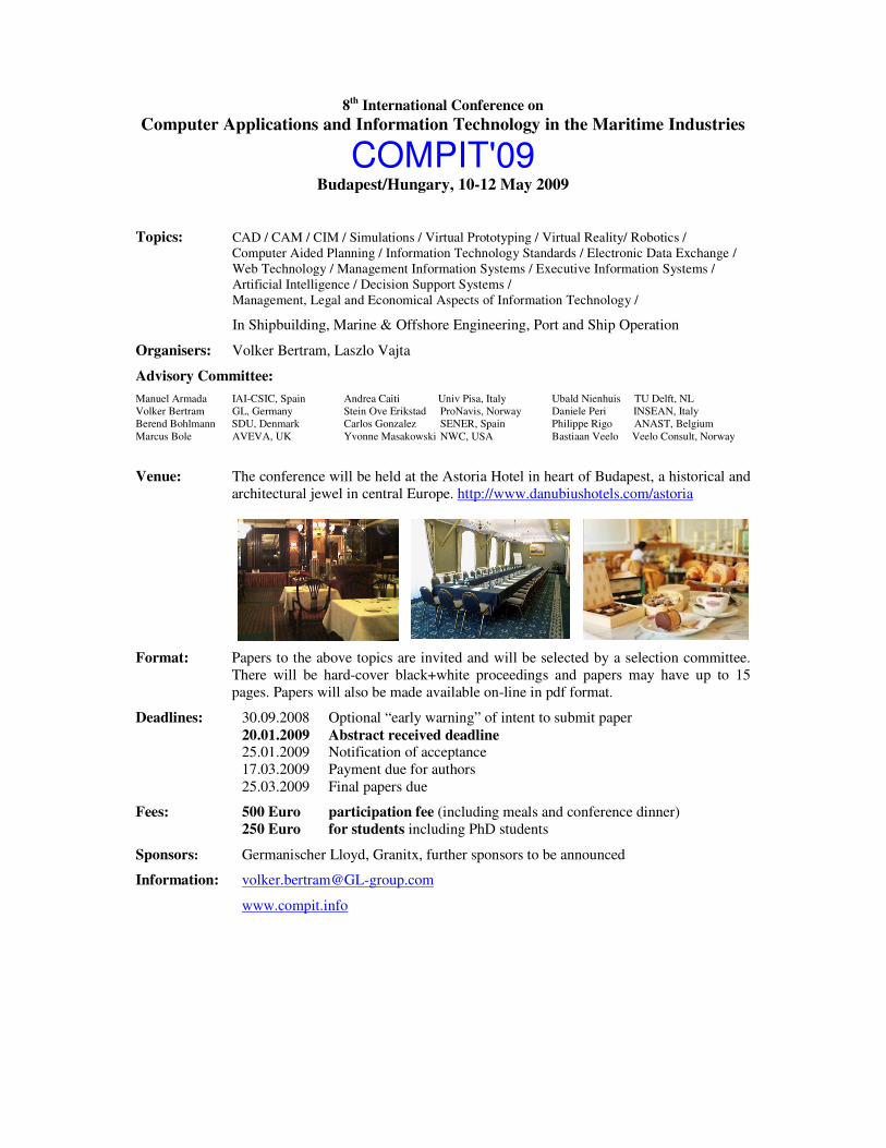
8th International Conference on

Computer Applications and Information Technology in the Maritime Industries

COMPIT'09 Budapest/Hungary, 10-12 May 2009

Topics: CAD / CAM / CIM / Simulations / Virtual Prototyping / Virtual Reality/ Robotics /

Computer Aided Planning / Information Technology Standards / Electronic Data Exchange /

Web Technology / Management Information Systems / Executive Information Systems /

Artificial Intelligence / Decision Support Systems /

Management, Legal and Economical Aspects of Information Technology /

In Shipbuilding, Marine & Offshore Engineering, Port and Ship Operation

Organisers: Volker Bertram, Laszlo Vajta

Advisory Committee:

Manuel Armada IAI-CSIC, Spain

Volker Bertram GL, Germany

Berend Bohlmann SDU, Denmark

Marcus Bole AVEVA, UK

Andrea Caiti Univ Pisa, Italy

Stein Ove Erikstad ProNavis, Norway

Carlos Gonzalez SENER, Spain

Yvonne Masakowski NWC, USA

Ubald Nienhuis TU Delft, NL

Daniele Peri INSEAN, Italy

Philippe Rigo ANAST, Belgium

Bastiaan Veelo Veelo Consult, Norway

Venue: The conference will be held at the Astoria Hotel in heart of Budapest, a historical and

architectural jewel in central Europe. http://www.danubiushotels.com/astoria

Format: Papers to the above topics are invited and will be selected by a selection committee.

There will be hard-cover black+white proceedings and papers may have up to 15

pages. Papers will also be made available on-line in pdf format.

Deadlines: 30.09.2008 Optional “early warning” of intent to submit paper

20.01.2009 Abstract received deadline 25.01.2009 Notification of acceptance

17.03.2009 Payment due for authors

25.03.2009 Final papers due

Fees: 500 Euro participation fee (including meals and conference dinner)

250 Euro for students including PhD students

Sponsors: Germanischer Lloyd, Granitx, further sponsors to be announced

Information: volker.bertram@GL-group.com

www.compit.info