Completeness of timed μCRL

Centrum voor Wiskunde en Informatica

REPORTRAPPORT

Completeness of Timed muCRL

J.F. Groote, M.A. Reniers, J.J. van Wamel, M.B. van der Zwaag

Software Engineering (SEN)

SEN-R0034 November 30, 2000

Report SEN-R0034ISSN 1386-369X

CWIP.O. Box 940791090 GB AmsterdamThe Netherlands

CWI is the National Research Institute for Mathematicsand Computer Science. CWI is part of the StichtingMathematisch Centrum (SMC), the Dutch foundationfor promotion of mathematics and computer scienceand their applications.SMC is sponsored by the Netherlands Organization forScientific Research (NWO). CWI is a member ofERCIM, the European Research Consortium forInformatics and Mathematics.

Copyright © Stichting Mathematisch CentrumP.O. Box 94079, 1090 GB Amsterdam (NL)

Kruislaan 413, 1098 SJ Amsterdam (NL)Telephone +31 20 592 9333

Telefax +31 20 592 4199

Completeness of Timed µCRL ∗

J.F. Groote1 M.A. Reniers1 J. van Wamel2 M.B. van der Zwaag2

{[email protected], [email protected], [email protected], [email protected]}1

Section Technical Applications

Eindhoven University of Technology

Eindhoven, The Netherlands2

Cluster Software Engineering, CWI

Amsterdam, The Netherlands

ABSTRACTIn [9], a straightforward extension of the process algebra µCRL was proposed to explicitly dealwith time. The process algebra µCRL has been designed especially to deal with data in a processalgebraic context. Using the features for data, only a minor extension of the language was neededto obtain a very expressive variant of time. But [9] contains syntax, operational semantics andaxioms characterising timed µCRL. It did not contain an in-depth analysis of timed µCRL. This paperfills this gap by providing soundness and completeness results. The main tool to establish these isa mapping of timed to untimed µCRL and employing the completeness results obtained for untimed µCRL.

2000 Mathematics Subject Classification: 68Q45; 68Q60; 68Q70; 68Q85

Keywords & Phrases: Real-time, Process Algebra, Completeness, µCRL

Note: Work carried out under project SEN2.1 “Process Specification and Analysis”.

1 Introduction

Process algebras are very nice tools to study fundamental concepts such as actions and interactions,non determinism and parallellism, behavioural equivalences and internal or hidden actions. In theirplain form (e.g. CCS [24], CSP [19] or ACP [5]), these languages are not very expressive in the sensethat only very simple protocols and distributed systems can properly be described. This is the reasonwhy these plain process algebras have been extended with data ([17, 12]). The most expressive [10]and by far the most developed is µCRL [12], being the process algebra ACP extended with equationalabstract datatypes. The process algebra µCRL is the basis of several novel proof methodologies [14, 13]and numerous verifications (see [11]), which for a large part have been computer checked. Also, it hasbeen the basis for several fundamental studies about for instance expressiveness and decidability [10],and visualisation of huge state spaces [27]. Finally, a toolset around µCRL has been constructed whichis not based on finite state spaces, but on linear process operators [6], allowing automatic treatmentof processes with huge or infinite state spaces.

As has widely been recognised, time is an important feature for interacting systems, and henceforthmany timed process algebras have been developed. In order to use the advantages that µCRL offersin a timed setting, timed µCRL has been defined [9]. In essence, it only consists of the addition of asingle operator p↪t, for p a process and t a value indicating a moment in time. Using the conditionaloperator ( � � ) and the sum (

∑) construct, we could express every timing aspect of systems

∗The authors thank all persons who assisted in developing µCRL throughout the years. For timed µCRL they have benefiteda lot from comments from Jos Baeten, Jan Bergstra, Bas Luttik, Radu Mateescu, Alban Ponse, Jan Springintveld, Jan-JorisVereijken and Tim Willemse.

2 Groote, Reniers, Van Wamel, Van der Zwaag

that we encountered, including time-outs, deadlines and intervals. Somewhat surprisingly, this timedextension even turned out to be able to express and analyse hybrid systems [15], in which continuoussignals and discrete events are combined.

The definition of timed µCRL has been guided by simplicity, elegance and its suitability to adaptmany of the existing proof technologies to the timed setting. In [9] the language was explained,syntax and operational semantics were given and an equational characterisation of the language wasprovided. There were no completeness results in the paper and a claim of soundness turned out tobe not completely justified. This paper fills these gaps by providing soundness and completenesstheorems, relative to some completeness assumptions on the datatypes. For simplicity and generality,the datatypes are assumed to be given as algebras satisfying a number of elementary properties,contrary to the definition in [9], where equational, inductive datatypes were employed.

The proof of completeness follows the approach of [26], where a timed µCRL is translated to un-timed µCRL, in such a way that the completeness results of [10] can directly be applied to achievecompleteness. Besides providing a completeness result in a relatively easy way, there is an additionaladvantage of this approach, which may turn out to be very helpful in the analysis of timed systems.As mentioned above, there are many analysis techniques and a very capable tool for untimed µCRL.Transfering these to the timed setting may be a costly and hard operation. However, if we translatetimed µCRL expressions to untimed µCRL, everything achieved for untimed µCRL carries over auto-matically. We have especially high hopes for the toolset, as the translation can be done automaticallyin this case.

Also, we hope that this approach may help to solve one of the longer standing open problemsin timed process algebra, namely a complete axiomatisation of branching or weak bisimulation in asetting as expressive as timed µCRL. There are numerous completeness results for weak bisimulationsin timed settings with restricted expressivity (e.g. [8]). The only attempt that we know where theexpressiveness of the language comes close to that of µCRL can be found in [21]. Here, an axiomfor branching bisimulation is given, which is claimed to be sound and complete. Although we do notdoubt soundness, the completeness claim has not been appropriately justified, and turns out not tobe easily reconstructable.

Timed process algebras have received a lot of attention, and many different formalisms have beenproposed. However, very few of these include data (see for an overview [28, 4]). The few that do so,have a very different focus than µCRL.

In the first place, there are timed automata [1] which have been extended to hybrid automata [23].The typical difference with timed µCRL is that timed automata are a semantical concept, much lessalgebraical, and as such there is no set of characteristic axioms or even a precisely defined set ofoperators to construct these. Timed automata are in a sense just finite state machines extendedwith clocks. This formalism sparked off a lot of research for instance in timed model checking andequivalence checking (using simulation relations). Using a technique known as convex regions, it ispossible to capture the infinite flow of time into a finite automaton. This result has been the basisfor various toolsets, such as HyTech [18], Uppaal [22] and Kronos [29], of which Uppaal allows simpledatatypes as natural numbers and lists.

At a different end of the spectrum, there are the timed specification languages of which extendedLOTOS [7] and LOTOS NT [25] are among the most ambitious, although older languages such asSDL [20] also combine time within an expressive context. The goal of these languages is to allow toexpress distributed timed systems as elegantly as possible. As such, the languages are rich in syntaxand much of the effort around these languages is in building tools around it. The difference withtimed µCRL is that these languages are not apt, and not intended for more fundamental research.

Completeness of Timed µCRL 3

2 The axiom system pCRLt

The axiom system pCRLt for pico CRL with time is presented. It serves as the basic framework for ourstudies. We work in a setting without the silent step τ , and without abstraction or general operatorsfor renaming. The addition of operators for parallelism in Section 5 leads to full µCRLt. We define anotion of basic terms and prove that all terms over the signature Σ(pCRLt) without process variablesare derivably equal to basic terms.

2.1 Abstract data types

The processes described in the language µCRL generally exchange data. For the specification of datawe use (equational) abstract data types with an explicit distinction between constructor functions and‘normal’ functions. Moreover, all properties of a data type must be explicitly declared, which makesit clear which assumptions can be used for proving properties of data or processes.

In this paper, we do not treat the syntactical details of the data language in depth. We simplyassume the existence of a data signature. A data signature consists of a set S of sort symbols and a setF of function declarations. We assume disjoint infinite sets of variables Vs for the sort symbols s ∈ S.Let V =

⋃s∈S Vs. The set of terms of sort s is denoted by Ts. Furthermore, we assume the existence

of a sort symbol B for the booleans with function declarations t and f, and the usual connectives ¬,∧, and ∨. For each sort symbol s, we assume a data algebra with universe Ds. The set DB has twoelements: the interpretation of t and the interpretation of f.

Finally, we assume the existence of a sort symbol T of time elements and we require that it is totallyordered and that it contains a least element. The total order is denoted ≤ and the least element isdenoted 0. Throughout this paper we abbreviate terms ¬(u ≤ t) to t < u. A term of the form t[e/d]denotes the term t with variable d replaced by term e.

Besides the above requirements one is free to specify the kind of time domain one requires. This isdone to accomodate those preferring discrete time, and others who prefer a notion of dense time. Onecan for instance define that DT has only a finite number of elements, or one can define an ordinal-likestructure on it.

2.2 The syntax of pCRLt

The signature of the theory pCRLt consists of a data signature and a process signature. The processsignature consists of the sort symbol P and the following function declarations:

1. action declarations a : s1 × · · · × sn → P for sort symbols si (i = 0, . . . , n) from the datasignature.

2. deadlock δ :→ P . Timed µCRL contains a constant δ, which can be used to express that fromnow on, no action can be performed any more. It models inaction, for instance in the case wherea number of computers are waiting for each other, and the whole system is blocked.

3. alternative composition + : P × P → P . The process represented by p + q behaves like p orq, depending on which of the two performs the first action.

4. sequential composition · : P × P → P . The process represented by p · q first performs theactions of p, until p terminates, and then continues with the actions in q.

5. conditional operator � � : P × B × P → P . The “ � � ”-operator is the conditionaloperator of µCRL, and it operates precisely as a then if else-construct. The process termp� b� q behaves like p if b is equal to t, and if b is equal to f it behaves like q.


6. alternative quantification∑v : P → P for each data variable v ∈ V . The sum operator

∑v p

behaves like p[d1/v] + p[d2/v] + . . . , i.e., as the possibly infinite choice between p[di/v] for anydata term di of the sort of v.

7. at-operator ↪ : P ×T → P . A key feature of timed µCRL is that it can be expressed at whichtime certain actions must take place. This is done using the “at”- operator. The process p↪t,behaves like the process p, with the restriction that the first action of p must take place at timet.

8. initialisation operator � : T × P → P . The process t� p behaves as the process p as if itwas started at time t. Thus the initialisation operator can be used to restrict the behaviour ofa process to the part that can idle until the specified moment of time.

In the sequel, we will call these function declarations operators. For action declarations we usuallywrite a : s1×· · ·×sn instead of a : s1×· · ·×sn → P . The set of all action declarations is denoted Act .Action terms are terms of the form a(d1, · · · , dn), where a : s1 × · · · × sn ∈ Act and di a data term ofsort si (for i = 0, · · · , n); the set of all action terms is denoted AT . We write AT δ for AT ∪ {δ}.

Furthermore, we assume the existence of an infinite set of process variables VP which is disjointfrom the set of data variables V .

Process terms are built from action terms, data terms, variables and process operators. The setof all process terms is denoted TP . For all operators in the language, characterising axioms areprovided following the process algebraic tradition, in order to define which equivalences hold betweenprocesses. In fact, axiomatic reasoning with processes forms the essence of µCRL. Examples ofequational manipulations with processes are given throughout this paper. Whereas the axioms providea more syntactical perspective, operational semantics are used to interpret process terms in terms ofpotential behaviours of a system (see Section 3.2).

We list the various operators of pCRLt in decreasing binding strength:

↪ , ·, �, � �,∑

, +.

2.3 The theory pCRLt

The axioms of pCRLt are the axioms given by the user for the data types such as the booleans B andthe time domain T , and the axioms given in Table 2. As proof theory we use generalised equationallogic with a congruence rule for binders. For a precise expository on this proof theory we refer to [10].In Table 1, we present the proof theory for pCRLt. Here, E represents the set of axioms of pCRLtand Σ is the signature of the theory pCRLt.

Process-closed terms are terms without process variables, but possibly with bound and free datavariables.

The two elementary operators to construct processes are the sequential composition operator, writ-ten as · and the alternative composition operator, written as +. The axioms A1–A5 in Table 2 describethe elementary properties of the sequential and alternative composition operators. For instance, theaxioms A1, A2 and A3 express that + is commutative, associative and idempotent. These laws mo-tivate why in some cases parentheses may be omitted. For instance, it is allowed to write a + b+ c,because, due to A2, it does not matter how brackets are put. The process algebra that consists ofatomic actions, alternative and sequential composition only and for which A1–A5 are the only axiomsis usually called Basic Process Algebra [5].

In the calculations in this paper we work modulo associativity and commutativity of +, and we donot mention the use of simple properties of the functions on data such as ¬, ∨, ∧, ≤, and eq.

In Table 2, pCRLt axioms for the sum operator are listed. The sum operator is a difficult operator,because it acts as a binder. This introduces a range of problems with substitutions. When wesubstitute a process p for a variable x in a term q, then no free variable in p may become bound.


t = t′ for every t = t′ ∈ E

t = t′

t[e/v] = t′[e/v]for every v ∈ Vs and e ∈ Ts

t1 = t′1 · · · tn = t′nF (t1, · · · , tn) = F (t′1, · · · , t′n)

for every F : s1 × · · · × sn → s′ ∈ Σ

t = t′∑v t =

∑v t′

t = tt = t′

t′ = t

t1 = t2 t2 = t3

t1 = t3

Table 1: Generalised equational logic for pCRLt.

If this appears to happen, we must first rename all bound occurrences of that variable in q into avariable that does not occur free in p. This renaming is called α-conversion. We consider processesmodulo α-conversion, so the terms

∑v p and

∑w p[w/v] are equal if w does not occur freely in v.

Consequently, we may only substitute the action a(v) for x in the left hand side of axiom SUM1, afterrenaming the bound variable v into w. So, SUM1 is a concise way of saying that if v does not appearin p, then we may omit the sum operator in

∑v p.

As another example, consider axiom SUM4. It says that we may distribute the sum operator overan alternative composition operator.

The process p↪t behaves like the process p, with the restriction that the first action of p must takeplace at time t. So, if we assume that the natural numbers denote moments in time, the processdescribed by a↪1 · b↪2 · c↪3 specifies that the actions a, b and c must take place at times 1, 2 and 3,respectively.

2.4 Time deadlocks

If an action happens at time t, then a subsequent action can take place at time t or afterwards. Thismeans that in a↪2 · b↪3 and a↪2 · b↪2 the action b can happen, and in a↪2 · b↪1 the action b is blocked.

Actually, the last example above is equivalent to a↪2 · δ↪2, which says that after action a we havea deadlock at time 2. In order to let b take place as prescribed, we have to reverse time. As this isclearly in conflict with reality, we choose to stop time at time 2. A process δ↪t is called a time deadlock.

Whenever a specification prescribes timing behaviour that cannot be realised, it will exhibit a timedeadlock, i.e., time is stopped at a certain point. Specifications with time inconsistencies can clearlynot be implemented.

An important property of δ is δ · p = δ. It says that the process p after the deadlock δ cannot beexecuted. It is formulated in Table 2 as axiom A7. The constant δ is the ‘classical’ deadlock of processalgebra, which cannot execute actions but which does not stop time. A time deadlock δ↪t exists atany moment before t and at t. The deadlock process δ exists at any time; we can derive δ =

∑v δ↪v.

As a consequence, we can not in general have p+ δ = p – an identity that is, in untimed pCRL, validfor every p. Consider for example the process a↪2 + δ. This process can perform the action a at time 2and then terminates, but it can also let time pass until after time 2. So, contrary to untimed pCRL, δis not a neutral element for alternative composition in pCRLt. This role is taken over by the process


A1 x+ y = y + xA2 x+ (y + z) = (x+ y) + zA3 x+ x = xA4 (x+ y) · z = x · z + y · zA5 (x · y) · z = x · (y · z)

SUM1∑v x = x

SUM3∑v p =

∑v p+ p

SUM4∑v(p+ q) =

∑v p+

∑v q

SUM5 (∑v p) · x =

∑v(p · x)

SUM12′ (∑v p) � b� δ↪0 =

∑v p� b� δ↪0

A6− a+ δ = aA6′ x+ δ↪0 = xA7 δ · x = δ

PE p� eq(v, w) � δ↪0 = p[v/w] � eq(v, w) � δ↪0

C1 x� t � y = xC2 x� f � y = yC3 x� b� y = x� b� δ↪0 + y � ¬b� δ↪0C4 (x� b1 � y) � b2 � y = x� (b1 ∧ b2) � yC5 x� b1 � δ↪0 + x� b2 � δ↪0 = x� (b1 ∨ b2) � δ↪0C6 (x� b� y) · z = x · z � b� y · zC7 (x+ y) � b� z = x� b� z + y � b� zSCA (x� b� δ↪0) · (y � b� δ↪0) = x · y � b� δ↪0

AT1 x =∑t x↪t

AT2 a↪t·x = a↪t·(t�x)

ATA1 a↪t↪u = (a↪t� u ≤ t� δ↪t) � t ≤ u� δ↪uATA2 (x+ y)↪t = x↪t+ y↪tATA3 (x·y)↪t = x↪t·yATA4 (

∑v p)↪t =

∑v p↪t

ATA5 (x� b� y)↪t = x↪t� b� y↪t

ATB1 t�a↪u = a↪u� t ≤ u� δ↪tATB2 t�(x+ y) = t�x+ t�yATB3 t�(x · y) = (t�x) · yATB4 t�

∑v p =

∑v t�p

ATB5 t�(x� b� y) = (t�x) � b� (t�y)

Table 2: Axioms of pCRLt: x, y, z ∈ VP , process-closed p, q ∈ TP , a ∈ AT δ, t, u ∈ VT , b, b1, b2 ∈ VB

and v, w ∈ V .


δ↪0. This can easily be seen, as every pCRLt process exists at time 0. In the axiomatisation, we seethat the pCRL axiom A6 (x+ δ = x) is absent , and has been replaced by axiom A6′.

In pCRLt, we have by axiom AT1 that δ =∑t δ↪t, so δ models the process that will never do a step,

terminate or exhibit a time deadlock. Therefore, a more appropriate name for δ would be livelock.We see that if a time deadlock δ↪u occurs in a process term with δ as an alternative, it vanishes:

δ + δ↪tAT1=

∑t

δ↪t+ δ↪tSUM3=

∑t

δ↪tAT1= δ.

For processes p that do not refer to time explicitly, we still like to have the identity p+ δ = p. Usingaxiom A6− this identity can be derived for untimed process-closed terms p.

2.5 Simple identities

Calculating in (timed) µCRL generally requires numerous basic identities. In this section, we presentsome identities as lemmas for easy future reference. In derivations in this section and the followingsections, we frequently apply the axioms for booleans and for the time domain. We will do so withoutexplicitly mentioning them.

Axiom SUM3 is typically used to extract a specific alternative from an alternative quantificationwhere the bound variable, say v, is replaced by a data term, say d, of the appropriate sort. Thefollowing lemma ensures the correctness of such an extraction.

Lemma 2.1 Let s be an arbitrary sort. For process-closed p ∈ TP , v ∈ Vs, and d ∈ Ts, it holds that∑v

p =∑v

p+ p[d/v].

Proof. Consider the following derivation:

∑v

p =

(∑v

p

)[d/v] SUM3=

(∑v

p+ p

)[d/v] =

(∑v

p

)[d/v] + p[d/v] =

∑v

p+ p[d/v].

Lemma 2.2 For x ∈ VP and b ∈ VB , it holds that x� b� x = x.

Proof. x� b� xC3= x� b� δ↪0 + x� ¬b� δ↪0 C5= x� t � δ↪0 C1= x.

Lemma 2.3 For t ∈ VT , it holds that δ↪0↪t = δ↪0.

Proof. δ↪0↪t ATA1= (δ↪0 � t ≤ 0 � δ↪0) � 0 ≤ t� δ↪t2.2= δ↪0 � 0 ≤ t� δ↪0 C1= δ↪0.

In the following lemma we present some facts about the initialisation operator.

Lemma 2.4 For t, u ∈ VT and a ∈ AT δ, it holds that

1. t�(t�a↪u) = t�a↪u;

2. t�δ↪0 = δ↪t.

Proof.

1. t� (t� a↪u) ATB1= t� (a↪u � t ≤ u � δ↪t) ATB5= (t� a↪u) � t ≤ u � (t� δ↪t) ATB1= (a↪u � t ≤u� δ↪t) � t ≤ u� δ↪t

C4= a↪u� t ≤ u� δ↪tATB1= t�a↪u.


2. t�δ↪0 ATB1= δ↪0 � t ≤ 0 � δ↪t = δ↪0 � eq(t,0) � δ↪tPE= δ↪t� eq(t,0) � δ↪t

2.2= δ↪t.

Lemma 2.5 For v ∈ VT and t ∈ VT , it holds that∑v δ↪v � v ≤ t� δ↪0 = δ↪t.

Proof. ∑v δ↪v � v ≤ t� δ↪0

2.1=∑v δ↪v � v ≤ t� δ↪0 + (δ↪v � v ≤ t� δ↪0)[t/v]

=∑v δ↪v � v ≤ t� δ↪0 + δ↪t� t ≤ t� δ↪0

C1=∑v δ↪v � v ≤ t� δ↪0 + δ↪t

AT1=∑v δ↪t↪v +

∑v δ↪v � v ≤ t� δ↪0

ATA1,2.2=

∑v δ↪t� t ≤ v � δ↪v +

∑v δ↪v � v ≤ t� δ↪0

C3=∑v(δ↪t� t ≤ v � δ↪0 + δ↪v � t > v � δ↪0) +

∑v δ↪v � v ≤ t� δ↪0

C5=∑v(δ↪t� t ≤ v � δ↪0 + δ↪v � t > v � δ↪0)

+∑v(δ↪v � eq(t, v) � δ↪0 + δ↪v � t > v � δ↪0)

C5,PE=

∑v(δ↪t� t < v � δ↪0 + δ↪t� eq(t, v) � δ↪0 + δ↪v � t > v � δ↪0)

+∑v(δ↪t� eq(t, v) � δ↪0 + δ↪v � t > v � δ↪0)

SUM4,A3=

∑v(δ↪t� t < v � δ↪0 + δ↪t� eq(t, v) � δ↪0 + δ↪v � t > v � δ↪0)

C5=∑v(δ↪t� t ≤ v � δ↪0 + δ↪v � t > v � δ↪0)

C3=∑v δ↪t� t ≤ v � δ↪v

ATA1,2.2=

∑v δ↪t↪v

AT1= δ↪t.

2.6 Basic terms

We provide a basic syntactic format for pCRLt-terms. In this format we use the notation∑~v to

represent a finite sequence of alternative quantifications∑v1

∑v2· · ·∑vn

(n ≥ 0).

Definition 2.1 (Basic terms) The set of basic terms is inductively defined as follows:

1.∑~v a↪t� b� δ↪0, with a ∈ AT δ, t a time term and b a boolean term, is a basic term;

2. if p is a basic term, then∑~v a↪t · p� b� δ↪0, with a ∈ AT , t a time term and b a boolean term,

is a basic term;

3. if p and q are basic terms, then p+ q is a basic term.

If a basic term is of the first form, then we say it is of type 1. Similarly for forms 2 and 3.

Theorem 2.1 (Basic Term Theorem) If q is a process-closed term over Σ(pCRLt), then there isa basic term p such that µCRLt ` q = p.

Proof. We apply induction on the number of symbols in process-closed term q. The following casescan be distinguished based on the structure of process-closed term q.

1. q ≡ a for some a ∈ AT δ. Obviously a AT1=∑t a↪t

C1=∑t a↪t� t � δ↪0. This is a type 1 basic term.

2. q ≡ q1 + q2 for some process-closed terms q1 and q2. By induction we have the existence of basicterms p1 and p2 such that q1 = p1 and q2 = p2. Hence, q = q1 + q2 = p1 + p2, which is a type 3basic term.


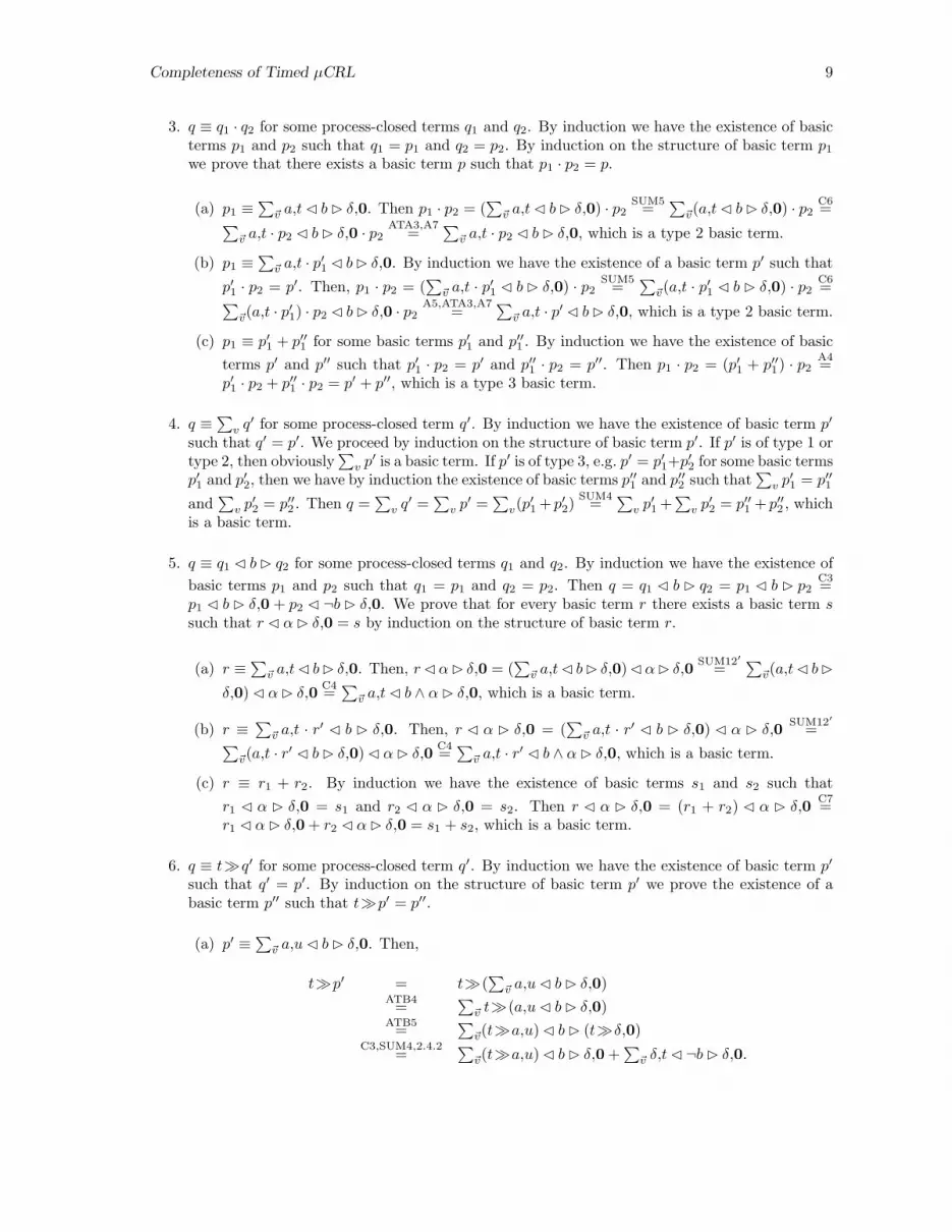
3. q ≡ q1 · q2 for some process-closed terms q1 and q2. By induction we have the existence of basicterms p1 and p2 such that q1 = p1 and q2 = p2. By induction on the structure of basic term p1

we prove that there exists a basic term p such that p1 · p2 = p.

(a) p1 ≡∑~v a↪t� b� δ↪0. Then p1 · p2 = (

∑~v a↪t� b� δ↪0) · p2

SUM5=∑~v(a↪t� b� δ↪0) · p2

C6=∑~v a↪t · p2 � b� δ↪0 · p2

ATA3,A7=

∑~v a↪t · p2 � b� δ↪0, which is a type 2 basic term.

(b) p1 ≡∑~v a↪t · p′1 � b� δ↪0. By induction we have the existence of a basic term p′ such that

p′1 · p2 = p′. Then, p1 · p2 = (∑~v a↪t · p′1 � b� δ↪0) · p2

SUM5=∑~v(a↪t · p′1 � b � δ↪0) · p2

C6=∑~v(a↪t · p′1) · p2 � b� δ↪0 · p2

A5,ATA3,A7=

∑~v a↪t · p′ � b� δ↪0, which is a type 2 basic term.

(c) p1 ≡ p′1 + p′′1 for some basic terms p′1 and p′′1 . By induction we have the existence of basicterms p′ and p′′ such that p′1 · p2 = p′ and p′′1 · p2 = p′′. Then p1 · p2 = (p′1 + p′′1) · p2

A4=p′1 · p2 + p′′1 · p2 = p′ + p′′, which is a type 3 basic term.

4. q ≡∑v q′ for some process-closed term q′. By induction we have the existence of basic term p′

such that q′ = p′. We proceed by induction on the structure of basic term p′. If p′ is of type 1 ortype 2, then obviously

∑v p′ is a basic term. If p′ is of type 3, e.g. p′ = p′1+p′2 for some basic terms

p′1 and p′2, then we have by induction the existence of basic terms p′′1 and p′′2 such that∑v p′1 = p′′1

and∑v p′2 = p′′2 . Then q =

∑v q′ =

∑v p′ =

∑v(p′1 + p′2) SUM4=

∑v p′1 +∑v p′2 = p′′1 + p′′2 , which

is a basic term.

5. q ≡ q1 � b� q2 for some process-closed terms q1 and q2. By induction we have the existence ofbasic terms p1 and p2 such that q1 = p1 and q2 = p2. Then q = q1 � b � q2 = p1 � b � p2

C3=p1 � b � δ↪0 + p2 � ¬b � δ↪0. We prove that for every basic term r there exists a basic term ssuch that r � α� δ↪0 = s by induction on the structure of basic term r.

(a) r ≡∑~v a↪t� b� δ↪0. Then, r�α� δ↪0 = (

∑~v a↪t� b� δ↪0) �α� δ↪0 SUM12′=

∑~v(a↪t� b�

δ↪0) � α� δ↪0 C4=∑~v a↪t� b ∧ α� δ↪0, which is a basic term.

(b) r ≡∑~v a↪t · r′ � b � δ↪0. Then, r � α � δ↪0 = (

∑~v a↪t · r′ � b � δ↪0) � α � δ↪0 SUM12′=∑

~v(a↪t · r′ � b� δ↪0) � α� δ↪0 C4=∑~v a↪t · r′ � b ∧ α� δ↪0, which is a basic term.

(c) r ≡ r1 + r2. By induction we have the existence of basic terms s1 and s2 such thatr1 � α � δ↪0 = s1 and r2 � α � δ↪0 = s2. Then r � α � δ↪0 = (r1 + r2) � α � δ↪0 C7=r1 � α� δ↪0 + r2 � α� δ↪0 = s1 + s2, which is a basic term.

6. q ≡ t�q′ for some process-closed term q′. By induction we have the existence of basic term p′

such that q′ = p′. By induction on the structure of basic term p′ we prove the existence of abasic term p′′ such that t�p′ = p′′.

(a) p′ ≡∑~v a↪u� b� δ↪0. Then,

t�p′ = t�(∑~v a↪u� b� δ↪0)

ATB4=∑~v t�(a↪u� b� δ↪0)

ATB5=∑~v(t�a↪u) � b� (t�δ↪0)

C3,SUM4,2.4.2=

∑~v(t�a↪u) � b� δ↪0 +

∑~v δ↪t� ¬b� δ↪0.


The second summand is a basic term. We continue with the first summand:∑~v(t�a↪u) � b� δ↪0

ATB1=∑~v(a↪u� t ≤ u� δ↪t) � b� δ↪0

C3=∑~v(a↪u� t ≤ u� δ↪0 + δ↪t� t > u� δ↪0) � b� δ↪0

C7,SUM4=

∑~v(a↪u� t ≤ u� δ↪0) � b� δ↪0 +

∑~v(δ↪t� t > u� δ↪0) � b� δ↪0

C4=∑~v a↪u� t ≤ u ∧ b� δ↪0 +

∑~v δ↪t� t > u ∧ b� δ↪0,

which is a basic term.(b) p′ ≡

∑~v a↪u · p′1 � b� δ↪0. Similar to the previous case only axiom ATB3 has to be applied

just before applying ATB1.(c) p′ ≡ p′1 + p′2. By induction we have the existence of basic terms p′′1 and p′′2 such that

t�p′1 = p′′1 and t�p′2 = p′′2 . Then, t�p′ = t� (p′1 + p′2) ATB2= t�p′1 + t�p′2 = p′′1 + p′′2 ,which is a basic term.

7. q ≡ q′↪t for some process-closed term q′. By induction we have the existence of basic term p′

such that q′ = p′. We prove that for every basic term p′ there exists a basic term p′′ such thatp′↪t = p′′ by induction on the structure of basic term p′.

(a) p′ ≡∑~v a↪u� b� δ↪0. Then,

p′↪t = (∑~v a↪u� b� δ↪0)↪t

ATA4=∑~v(a↪u� b� δ↪0)↪t

ATA5=∑~v a↪u↪t� b� δ↪0↪t

ATA1,2.3=

∑~v((a↪u� t ≤ u� δ↪u) � u ≤ t� δ↪t) � b� δ↪0

C3=∑~v((a↪u� t ≤ u� δ↪0 + δ↪u� t > u� δ↪0) � u ≤ t� δ↪0

+ δ↪t� u > t� δ↪0) � b� δ↪0C7,SUM4

=∑~v((a↪u� t ≤ u� δ↪0 + δ↪u� t > u� δ↪0) � u ≤ t� δ↪0) � b� δ↪0

+∑~v(δ↪t� u > t� δ↪0) � b� δ↪0

C7,SUM4=

∑~v((a↪u� t ≤ u� δ↪0) � u ≤ t� δ↪0) � b� δ↪0

+∑~v((δ↪u� t > u� δ↪0) � u ≤ t� δ↪0) � b� δ↪0

+∑~v(δ↪t� u > t� δ↪0) � b� δ↪0

C4=∑~v a↪u� t ≤ u ∧ u ≤ t ∧ b� δ↪0 +

∑~v δ↪u� t > u ∧ u ≤ t ∧ b� δ↪0

+∑~v δ↪t� u > t ∧ b� δ↪0

=∑~v a↪u� eq(t, u) ∧ b� δ↪0 +

∑~v δ↪u� t > u ∧ b� δ↪0

+∑~v δ↪t� t < u ∧ b� δ↪0,

which is a basic term.(b) p′ ≡

∑~v a↪u ·p′1 � b� δ↪0. Similar to the previous case: only axiom ATA3 has to be applied

just before applying ATA1.(c) p′ ≡ p′1 + p′2. By induction we have the existence of basic terms p′′1 and p′′2 such that

p′1↪t = p′′1 and p′2↪t = p′′2 . Then, p′↪t = (p′1 +p′2)↪t ATA2= p′1↪t+p′2↪t = p′′1 +p′′2 , which is a basicterm.

The main virtue of the basic term theorem is that in proving an identity for process-closed terms, wecan restrict the proof to basic terms. Instead of using induction on the structure of process-closedterms we can use induction on the structure of basic terms. This limits the cases to be consideredconsiderably. Another example of such a proof is the proof of the following lemma. In Section 3, wefrequently use induction on basic terms.


Lemma 2.6 For process-closed terms p we have t�(t�p) = t�p.

Proof. Without loss of generality we may assume that p is a basic term. We prove the lemma byinduction on the structure of basic term p.

1. p ≡∑~v a↪u � b � δ↪0. This case is similar to the next case albeit that axiom ATB3 does not

have to be applied.

2. p ≡∑~v a↪u · p′ � b� δ↪0. Then,

t�(t�p) = t�(t�∑~v a↪u · p′ � b� δ↪0)

ATB4=∑~v t�(t�(a↪u · p′ � b� δ↪0))

ATB5=∑~v t�(t�a↪u · p′) � b� t�(t�δ↪0)

ATB3=∑~v(t�(t�a↪u)) · p′ � b� t�(t�δ↪0)

2.4.1=∑~v(t�a↪u) · p′ � b� t�δ↪0

ATB3=∑~v t�a↪u · p′ � b� t�δ↪0

ATB5=∑~v t�(a↪u · p′ � b� δ↪0)

ATB4= t�∑~v a↪u · p′ � b� δ↪0

= t�p.

3. p ≡ p′ + p′′. This part follows easily from the induction hypothesis and axiom ATB2.

3 Semantics of timed pCRL

In this section, we present a model in which processes parameterised with data can be interpreted.With respect to the abstract data types we assume the existence of a data algebra with universeDs for each sort symbol s. For instance, for the booleans we have that the universe contains theinterpretation of t and the interpretation of f.

A valuation ν is a function from the set of variables V to the set of values⋃s∈S Ds such that

ν(v) ∈ Ds if and only if v ∈ Vs. This means that a variable can only be mapped to a value of theright data algebra. For valuations ν and ν′ and variable v ∈ V , we write ν[v]ν′, if for all u ∈ V , u 6= vimplies ν(u) = ν′(u). Thus ν[v]ν′ means that the valuations ν and ν′ are the same for all variablesexcept possibly for the variable v. Given a valuation ν, we write [[t]]ν for the interpretation of a termt.

The process terms are mapped to processes and on these we define a suitable notion of strong timedbisimulation. Soundness of the axioms is proved w.r.t. the model. Completeness of the axioms isproved under the assumption that the data is completely axiomatised and adheres to certain otherproperties. This notion of completeness will be called relative completeness.

3.1 Interpretation of process terms

Definition 3.1 Given some pCRLt specification with a set of action declarations Act , the set ofactions is defined by

A = {a(e1, · · · , en) | a : s1 × · · · × sn ∈ Act , ei ∈ Dsi}.

The set A∪{δ} is denoted by Aδ. The set P = Pω of processes is obtained by the following recursion:

P0 = Aδ,Pn+1 = Pn ∪ {p · q,

∑P ′, p↪t, t�p | p, q ∈ Pn, P ′ 6= ∅, P ′ ⊆ Pn, t ∈ DT}.


aa−−→t√ p

a−−→t√∑

({p} ∪ P ) a−−→t√

pa−−→t p

′∑({p} ∪ P ) a−−→t p

′p

a−−→t√

p↪ta−−→t√

pa−−→t p

′

p↪ta−−→t p

′

pa−−→t√

p · q a−−→t t�q

pa−−→t p

′

p · q a−−→t p′ · q

pa−−→t√

t′ ≤ tt′�p

a−−→t√

pa−−→t p

′ t′ ≤ tt′�p

a−−→t p′

Table 3: Transition rules for the pCRLt operators, where a ∈ A, p, p′, q ∈ P , t, t′ ∈ DT and P ⊆ P .

Definition 3.2 The interpretation of process-closed terms under a valuation ν is inductively definedby: for a : s1 × · · · × sn ∈ Act and di ∈ Tsi , process-closed terms p, q ∈ TP , b ∈ TB , and t ∈ TT

[[a(d1, · · · , dn)]]ν = a([[d1]]ν , · · · , [[dn]]ν),[[δ]]ν = δ,[[p+ q]]ν =

∑{[[p]]ν , [[q]]ν},

[[p · q]]ν = [[p]]ν · [[q]]ν ,[[p↪t]]ν = [[p]]ν ↪[[t]]ν ,[[t�p]]ν = [[t]]ν� [[p]]ν ,

[[p� b� q]]ν ={

[[p]]ν if [[b]]ν = [[t]]ν ,[[q]]ν if [[b]]ν = [[f]]ν ,

[[∑v p]]

ν =∑{[[p]]ν′ | ν[v]ν′}.

This summation operator, which takes a set of processes as argument, is taken from [10].

3.2 Operational semantics and strong bisimulation

In this section, we define an operational semantics of processes in terms of the timed execution ofactions. For this purpose we introduce action relations −−→ √

and −−→ . By p a−−→t√

we expressthat the process p can perform an action a at time t, and then terminate succesfully at t. By p a−−→t p

′

we express that the process p evolves into process p′ by performing action a at time t.

Definition 3.3 The action relations −−→ √ ⊆ P × A × DT and −−→ ⊆ P × A × DT × P aredefined by the transition rules in Table 3.

The execution of an action does not take time: it is possible that the process p′ can subsequentlyperform other actions at t, e.g.

a↪t · b↪t a−−→t t�b↪tb−−→t√.

Given the action relations we have a good understanding of the steps which can be performed by aprocess. An obvious question is when two processes are equivalent. Such a notion is required to justifythe axioms. Strong bisimulation is a commonly used process equivalence. Therefore, we provide atimed variant of strong bisimulation, called strong timed bisimulation. However, bisimulation cannotbe defined in terms of actions only, e.g. the processes δ↪t and δ↪u are considered equivalent only ift = u. We introduce the delay relation Ut(p), which expresses that p can at least idle until time t. Ithas the same purpose as the ultimate delay in [2, 3, 21].

Definition 3.4 The delay relation U ( ) ⊆ DT ×P is defined by the transition rules in Table 4.


Ut(a)Ut(p)Ut(p · q)

Ut(p)Ut(∑P ∪ {p})

Ut(p) t ≤ t′

Ut(p↪t′)Ut(p)

Ut(t′�p)t ≤ t′

Ut(t′�p)

Table 4: Transition rules for the delay relation, where a ∈ Aδ, p, q ∈ P, t, t′ ∈ DT and P ⊆ P.

Definition 3.5 A symmetric relation R ⊆ P ×P is a strong timed bisimulation if for all (p, q) ∈ R itholds that

1. if p a−−→t√

, then q a−−→t√

,

2. if p a−−→t p′, then there is a q′ such that q a−−→t q

′ and (p′, q′) ∈ R, and

3. if Ut(p), then Ut(q),

for all a ∈ A, t ∈ DT and p′ ∈ P .Processes p and q are strongly timed bisimilar, notation p↔––t

q, if and only if there is a strong timedbisimulation R such that (p, q) ∈ R. Observe that the union of any set of strong timed bisimulationsis again a strong timed bisimulation.

Lemma 3.1 (Congruence) Strong timed bisimilarity is a congruence with respect to the operatorsdefined on P .

Proof. It is not hard to prove that strong timed bisimilarity is an equivalence. We omit the proof.Next, we give bisimulations that witness the congruence of strong timed bisimilarity with respect tothe operators�, ·,

∑, and ↪. For · we give a more detailed proof.

1. �. Let R : p↔––tq. Let t ∈ DT . Obviously, the relation {(t� p, t� q), (t� q, t� p)} ∪ R is a

strong timed bisimulation.

2. ·. Let R1 : p1↔––tq1 and R2 : p2↔––t

q2. Define R = {(p′1 · p2, q′1 · q2), (q′1 · q2, p′1 · p2), (t�p2, t�

q2), (t� q2, t� p2) | t ∈ DT ∧ (p′1, q′1) ∈ R1} ∪ R2. We do not have to consider pairs in Rthat are also in R2 as for these we have already assumed that they are strongly timed bisimilar.We also do not have to consider the pairs in R of the form (t�p2, t� q2) and vice versa with(p2, q2) ∈ R2 as the strong timed bisimulation from the proof of congruence of� is contained inR. Thus, we only have to consider pairs of the form (p′1 · p2, q

′1 · q2) with (p′1, q

′1) ∈ R1. For pairs

of this form it is easy to prove that these satisfy the conditions of the definition of strong timedbisimulations. Hence the relation R is a strong timed bisimulation.

3.∑

. Let R be a strong timed bisimulation such that for all p ∈ P there exists q ∈ Q such that(p, q) ∈ R and vice versa for all q ∈ Q there exists p ∈ P such that (q, p) ∈ R. The relationR′ = {(

∑P,∑Q), (

∑Q,∑P )} ∪R is obviously a strong timed bisimulation.

4. ↪. Let R : p↔––tq. Let t ∈ DT . Obviously the relation {(p↪t, q↪t), (q↪t, p↪t)} ∪R is a strong timed

bisimulation.

Without further proof we state that the axioms are sound with respect to the model of closed termsmodulo strong timed bisimilarity. This means that any two derivably equal process-closed terms arestrongly timed bisimilar.

Theorem 3.1 (Soundness) With respect to strong timed bisimulation pCRLt is a sound axiomsystem.


4 Relative completeness

In this section, we prove completeness of the axiomatisation with respect to the operational semanticsmodulo strong timed bisimilarity. For pCRL a completeness result is given in [10], where it is shownthat the result can only be partial. It relies on the existence of built-in equality and Skolem functionsfor all data sorts involved.

Definition 4.1 A data algebra has built-in equality if, for every sort s, it has a function declarationeq : s × s → B , such that for all terms t1 and t2 of sort s, it holds that ` t1 = t2 if and only if` eq(t1, t2) = t.

Definition 4.2 A data algebra D has built-in Skolem functions if for every first-order formula φwith free variables {x, y1, · · · , yn} there exists a term tφ(y1, · · · , yn) such that D |= (∃x)φ impliesD |= φ(tφ(y1, · · · , yn), y1, · · · , yn).

For a more detailed treatment of these notions we refer to [10].As pCRLt is an extension of pCRL we also need these assumptions about the data sorts for the

completeness of pCRLt. In fact, as pCRLt is a syntactic extension of pCRL, the proof of completenessfor pCRLt contains the proof of completeness of pCRL. We do not repeat the proof presented in [10],but formulate our proof of completeness in such a way that the proof of completeness of pCRL isreused.

4.1 Well-timedness and deadlock-saturation

The main difference between pCRL and pCRLt is the addition of the at-operator. This can easily beseen by considering the basic terms. We can even conclude that the only difference is the applicationof the at-operator on atomic actions (including deadlock).

To reuse the proof of completeness of pCRL, we translate timed process terms as untimed processterms in such a way that strongly timed bisimilar process terms are strongly bisimilar after translatingthem, and vice versa. Furthermore, two untimed process terms that are derivably equal in pCRL arealso derivably equal after applying the inverse of the translation.

The only way to translate the timed process terms as untimed process terms is to consider the timeassignment to atomic actions as an additional data parameter of the atomic action. For example,the timed atomic action a(d)↪3 might be translated to the untimed atomic action a(d, 3). There are,however, two problems with such a translation.

First, there is the problem of ill-timedness. In pCRLt we have the following identity: a(d)↪3 ·(b(e)↪2+c(f)↪4) = a(d)↪3 ·c(f)↪4. Translating the timing assignment as an additional parameter yieldsthe identity a(d, 3) · (b(e, 2) + c(f, 4)) = a(d, 3) · c(f, 4). This identity does not hold in pCRL. Thereason for this is that timing assignments in pCRLt influence the behaviour in such a way that dataparameters attached to atomic action cannot simulate in pCRL. Our solution to this problem is theintroduction of the notion of well-timedness. We will prove that for every basic term there exists aderivably equal well-timed basic term.

Second, there is the more technical problem that deadlock cannot have a parameter in pCRL. Henceit is not clear how to translate δ↪3. We cannot simply translate δ↪3 as δ since in that case δ↪3 andδ↪4 are translated both as δ. Our solution to this problem comes from the following observation. Ina timed process term, there are many time deadlocks implicitly included. For example, the processterm a↪3 implicitly has time deadlock summands δ↪t for each t ≤ 3. If we can succeed in making allimplicit deadlocks explicitly visible, then we can translate a time deadlock as a special atomic actionwith one data parameter representing the time assignment of that deadlock. That is, we will translateδ↪3 as ∆(3). Making all implicit time deadlocks explicitly available is called deadlock-saturation. Weshow that for each basic term a deadlock-saturated basic terms exists that is derivably equal, andhence, that the restriction to deadlock-saturated basic terms is allowed.


By restricting our attention to deadlock-saturated well-timed basic terms we can prove that thetranslation sketched above satisfies the criteria mentioned.

Definition 4.3 (Well-timedness) The set of well-timed basic terms is inductively defined as follows:

1.∑~v a↪t� b� δ↪0 is well-timed;

2. if r is a well-timed basic term and t�r = r, then∑~v a↪t · r � b� δ↪0 is well-timed;

3. if r and r′ are well-timed basic terms, then r + r′ is well-timed.

The following theorem states that every basic term is derivably equal to a well-timed basic term.Combined with the Basic Term Theorem we thus have that every process-closed term is derivablyequal to a well-timed basic term. Thus, in cases where we want to prove an equality over process-closed terms, we can restrict ourselves to a proof that the equality holds for well-timed basic terms.

Theorem 4.1 (Well-timedness) For every basic term r there exists a well-timed basic term s suchthat r = s.

Proof. We prove this theorem by induction on the structure of basic term r.

1. r ≡∑~v a↪u� b� δ↪0. Then r is well-timed by definition.

2. r ≡∑~v a↪u · r′ � b� δ↪0. By induction we have the existence of a well-timed basic term s′ such

that r′ = s′. First we prove by induction on the structure of well-timed basic term r, that forevery well-timed basic term r and term t of sort T , there exists a well-timed basic term s suchthat t�r = s.

(a) r ≡∑~v a↪u� b� δ↪0. Then,

t�r = t�(∑~v a↪u� b� δ↪0)

ATB4=∑~v t�(a↪u� b� δ↪0)

ATB5=∑~v(t�a↪u) � b� (t�δ↪0)

ATB1,2.4.2=

∑~v(a↪u� t ≤ u� δ↪t) � b� δ↪t

C4=∑~v a↪u� t ≤ u ∧ b� δ↪t

C3,SUM4=

∑~v a↪u� t ≤ u ∧ b� δ↪0 +

∑~v δ↪t� ¬(t ≤ u ∧ b) � δ↪0,

which is a well-timed basic term.

(b) r ≡∑~v a↪u · r′ � b� δ↪0. As r is well-timed we have u�r′ = r′. Then,

t�r = t�(∑~v a↪u · r′ � b� δ↪0)

ATB4=∑~v t�(a↪u · r′ � b� δ↪0)

ATB5,ATB3=

∑~v(t�a↪u) · r′ � b� (t�δ↪0)

ATB1,2.4.2=

∑~v(a↪u� t ≤ u� δ↪t) · r′ � b� δ↪t

C6,ATA3,A7=

∑~v(a↪u · r′ � t ≤ u� δ↪t) � b� δ↪t

C4=∑~v a↪u · r′ � t ≤ u ∧ b� δ↪t

C3,SUM4=

∑~v a↪u · r′ � t ≤ u ∧ b� δ↪0 +

∑~v δ↪t� ¬(t ≤ u ∧ b) � δ↪0.

Obviously, this is a well-timed basic term.

(c) r ≡ r′ + r′′. By induction we have the existence of well-timed basic terms s′ and s′′ suchthat t�r′ = s′ and t�r′′ = s′′. Then, t�r = t�(r′ + r′′) ATB2= t�r′ + t�r′′ = s′ + s′′

which is a well-timed basic term.


Now, we have the existence of a well-timed basic term s′′ such that u�s′ = s′′. Then,

r =∑~v a↪u · r′ � b� δ↪0

=∑~v a↪u · s′ � b� δ↪0

AT2=∑~v a↪u · u�s′ � b� δ↪0

=∑~v a↪u · s′′ � b� δ↪0.

By Lemma 2.6 we have that u�s′′ = u� (u�s′) = u�s′ = s′′, and hence the above term iswell-timed.

3. r ≡ r′ + r′′. By induction we have the existence of well-timed basic terms s′ and s′′ such thatr′ = s′ and r′′ = s′′. Thus, r = r′ + r′′ = s′ + s′′ which is a well-timed basic term.

The fact that we can restrict ourselves to well-timed basic terms instead of arbitrary basic termsbrings us closer to our goal, the completeness result. As explained before we wish to embed timedprocesses into untimed processes. One of the major difficulties in this embedding is that time restrictsbehaviour. For well-timed basic terms, however, time is reduced to just an annotation with an actionterm. In the embedding we will simply add it to the parameter list of a corresponding action term.

In this section, we will present an even more specific notion of basic terms. To each basic term asmany deadlocks will be added as possible while keeping the result equal to the original. The reasonfor this deadlock-saturation is that later we will embed the timed process terms into untimed processterms by replacing timed deadlocks by a special atomic action with a parameter representing the timestamp.

Definition 4.4 (Deadlock-saturation) The set of deadlock-saturated basic terms is inductivelydefined as follows:

1.∑~v a↪t� b� δ↪0 +

∑~v,u δ↪u� u ≤ t ∧ b� δ↪0 is a deadlock-saturated basic term;

2. if r is a deadlock-saturated basic term, then∑~v a↪t · r� b� δ↪0 +

∑~v,u δ↪u� u ≤ t∧ b� δ↪0 is a

deadlock-saturated basic term;

3. if r and r′ are deadlock-saturated basic terms, then r + r′ is a deadlock-saturated basic term.

The following result states that every basic term can be transformed into a deadlock-saturated basicterm. Hence, it is allowed to restrict ourselves to deadlock-saturated basic terms in cases where weare only interested in closed terms.

Theorem 4.2 For every basic term p there exists a deadlock-saturated basic term q such thatpCRLt ` p = q.

Proof. We prove this theorem by induction on the structure of basic term p.

1. p ≡∑~v a↪t� b� δ↪0. Let q =

∑~v a↪t � b � δ↪0 +

∑~v,u δ↪u� u ≤ t ∧ b� δ↪0 where u is a fresh

variable. Then,

q =∑~v a↪t� b� δ↪0 +

∑~v,u δ↪u� u ≤ t ∧ b� δ↪0

SUM4=∑~v(a↪t� b� δ↪0 +

∑u δ↪u� u ≤ t ∧ b� δ↪0)

C4=∑~v(a↪t� b� δ↪0 +

∑u(δ↪u� u ≤ t� δ↪0) � b� δ↪0)

SUM12′=∑~v(a↪t� b� δ↪0 + (

∑u(δ↪u� u ≤ t� δ↪0)) � b� δ↪0)

2.5=∑~v(a↪t� b� δ↪0 + δ↪t� b� δ↪0)

C7=∑~v(a↪t+ δ↪t) � b� δ↪0

ATA2=∑~v(a+ δ)↪t� b� δ↪0

A6−=∑~v a↪t� b� δ↪0

= p.


2. p ≡∑~v a↪t · p′� b� δ↪0. By induction we have the existence of a deadlock-saturated basic term

q′ such that pCRLt ` p′ = q′. Let q =∑~v a↪t · q′ � b� δ↪0 +

∑~v,u δ↪u� u ≤ t ∧ b� δ↪0 where u

is a fresh variable. Then,

q =∑~v a↪t · q′ � b� δ↪0 +

∑~v,u δ↪u� u ≤ t ∧ b� δ↪0

SUM4=∑~v(a↪t · q′ � b� δ↪0 +

∑u δ↪u� u ≤ t ∧ b� δ↪0)

C4=∑~v(a↪t · q′ � b� δ↪0 +

∑u(δ↪u� u ≤ t� δ↪0) � b� δ↪0)

SUM12′=∑~v(a↪t · q′ � b� δ↪0 + (

∑u(δ↪u� u ≤ t� δ↪0)) � b� δ↪0)

2.5=∑~v(a↪t · q′ � b� δ↪0 + δ↪t� b� δ↪0)

C7=∑~v(a↪t · q′ + δ↪t) � b� δ↪0

ATA3,ATA2,A7,A4=

∑~v((a+ δ) · q′)↪t� b� δ↪0

A6−,ATA3=

∑~v a↪t · q′ � b� δ↪0

=∑~v a↪t · p′ � b� δ↪0

= p.

3. p ≡ p′+p′′. By induction we have the existence of deadlock-saturated basic terms q′ and q′′ suchthat pCRLt ` p′ = q′ and pCRLt ` p′′ = q′′. Then, pCRLt ` p = p′ + p′′ = q′ + q′′. Obviously,q′ + q′′ is a deadlock-saturated basic term.

As a consequence of the Theorems 4.1 and 4.2, for each basic term there exists a derivably equaldeadlock-saturated well-timed basic term.

Corollary 4.1 For every basic term p there exists a deadlock-saturated, well-timed basic term q suchthat pCRLt ` p = q.

Proof. By Theorem 4.1 there exists a well-timed basic term p′ such that pCRLt ` p = p′. Obviouslyp′ itself is a basic term. Hence, by Theorem 4.2, there exists a deadlock-saturated basic term q suchthat pCRLt ` p′ = q. By construction deadlock-saturation preserves well-timedness. Hence, q is bothwell-timed and deadlock-saturated.

4.2 Time-free abstraction

Next, we present an embedding of well-timed basic terms into basic terms in the theory pCRL.Thereto, we assume that for every action declaration a : s1 × · · · × sn in pCRLt, we have an actiondeclaration a : s1×· · ·× sn×T in pCRL. We prove that this embedding preserves strong bisimilarityin the sense that the embeddings of two strongly timed bisimilar process terms are strongly bisimilar.

Definition 4.5 (Time-free abstraction) The mapping πtf on basic terms is inductively defined asfollows:

πtf(∑~v a(~e)↪t� b� δ↪0) =

∑~v a(~e, t) � b� δ,

πtf(∑~v δ↪t� b� δ↪0) =

∑~v ∆(t) � b� δ,

πtf(∑~v a(~e)↪t · r � b� δ↪0) =

∑~v a(~e, t) · πtf(r) � b� δ,

πtf(r + r′) = πtf(r) + πtf(r′).

Theorem 4.3 For deadlock-saturated well-timed basic terms p and q and arbitrary valuations ν andξ: if [[p]]ν ↔––t

[[q]]ξ, then [[πtf(p)]]ν ↔–– [[πtf(q)]]ξ.


Proof. We prove this theorem by induction on the number of symbols of p and q. Suppose that[[p]]ν↔––t

[[q]]ξ for some valuations ν and ξ. Let R be defined as follows: if [[p]]ν↔––t[[q]]ξ for some deadlock-

saturated well-timed basic terms p and q and arbitrary valuations ν and ξ, then ([[πtf(p)]]ν , [[πtf(q)]]ξ) ∈R.

By induction on the structure of basic term p we can easily prove that the transitions of the processassociated with basic term p under valuation ν are of one of the following forms:

1. [[p]]ν a−−→t√

;

2. [[p]]ν a−−→t t� [[p′]]ν′

for some deadlock-saturated well-timed basic term p′ and valuation ν′.

Now, we first prove the following lemmata: for arbitrary deadlock-saturated well-timed basic terms pand p′, a ∈ Act , t ∈ DT , and valuations χ and χ′

1. if a 6= ∆ and [[πtf(p)]]χa(~d,t)−−−−→√, then [[p]]χ a(~d)−−−→t

√;

2. if [[p]]χ a(~d)−−−→t√

, then [[πtf(p)]]χa(~d,t)−−−−→√;

3. if [[πtf(p)]]χ∆(t)−−−→√, then Ut([[p]]χ);

4. if Ut([[p]]χ), then [[πtf(p)]]χ∆(t)−−−→√;

5. if [[πtf(p)]]χa(~d,t)−−−−→ [[πtf(p′)]]χ

′, then [[p]]χ a(~d)−−−→t t� [[p′]]χ

′and t� [[p′]]χ

′ ↔––t[[p′]]χ

′;

6. if [[p]]χ a(~d)−−−→t t� [[p′]]χ′, then [[πtf(p)]]χ

a(~d,t)−−−−→ [[πtf(p′)]]χ′.

Next, we prove that R is a strong timed bisimulation. First, suppose that [[πtf(p)]]νa(~d,t)−−−−→√. If

a = ∆, then Ut([[p]]ν). Therefore, Ut([[q]]ξ). Thus, [[πtf(q)]]ξ∆(t)−−−→ √. If a 6= ∆, then [[p]]ν a(~d)−−−→t

√.

Therefore, [[q]]ξ a(~d)−−−→t√

. Thus, [[πtf(q)]]ξa(~d,t)−−−−→√.

Second, suppose that [[πtf(p)]]νa(~d,t)−−−−→ [[πtf(p′)]]ν

′for some deadlock-saturated well-timed basic term

p′ and valuation ν′. Then [[p]]ν a(~d)−−−→t t� [[p′]]ν′. Therefore, [[q]]ξ a(~d)−−−→t t� [[q′]]ξ

′for some q′ and ξ′

such that t� [[p′]]ν′ ↔––t

t� [[q′]]ξ′. Thus, [[πtf(q)]]ξ

a(~d,t)−−−−→ [[πtf(q′)]]ξ′. As p and q are well-timed we also

have t� [[p′]]ν′ ↔––t

[[p′]]ν′

and t� [[q′]]ξ′ ↔––t

[[q′]]ξ′. Thus, ([[πtf(p)]]ν

′, [[πtf(q)]]ξ

′) ∈ R.

Next, we present a mapping πt from pCRL-terms to pCRLt-terms and we show that this mappingis the inverse of the mapping πtf for basic terms.

Definition 4.6 The mapping πt is defined as follows:

πt(x) = x,πt(δ) = δ↪0,πt(a) = δ↪0,πt(a(~d, t)) = a(~d)↪t,πt(∆) = δ↪0,πt(∆(t)) = δ↪t,

πt(∆(~d, t)) = δ↪0,πt(p+ q) = πt(p) + πt(q),πt(p · q) = πt(p) · πt(q),πt(p� b� q) = πt(p) � b� πt(q),πt(∑v p) =

∑v πt(p).


Lemma 4.1 For basic terms p we have

pCRLt ` πt(πtf(p)) = p.

Proof. We prove this lemma by induction on the structure of basic term p.

1. p ≡∑~v a(~d)↪t� b� δ↪0. Then,

pCRLt ` πt(πtf(p)) = πt(πtf(∑~v a(~d)↪t� b� δ↪0))

= πt(∑~v a(~d, t) � b� δ)

=∑~v πt(a(~d, t) � b� δ)

=∑~v πt(a(~d, t)) � b� πt(δ)

=∑~v a(~d)↪t� b� δ↪0

= p.

2. p ≡∑~v a(~d)↪t · p′ � b� δ↪0. By induction we have pCRLt ` πt(πtf(p′)) = p′. Then,

pCRLt ` πt(πtf(p)) = πt(πtf(∑~v a(~d)↪t · p′ � b� δ↪0))

= πt(∑~v a(~d, t) · πtf(p′) � b� δ)

=∑~v πt(a(~d, t) · πtf(p′) � b� δ)

=∑~v πt(a(~d, t) · πtf(p′)) � b� πt(δ)

=∑~v a(~d)↪t · πt(πtf(p′)) � b� δ↪0

=∑~v a(~d)↪t · p′ � b� δ↪0

= p.

3. p ≡ p′ + p′′. By induction we have pCRLt ` πt(πtf(p′)) = p′ and pCRLt ` πt(πtf(p′′)) = p′′.Then, pCRLt ` πt(πtf(p)) = πt(πtf(p′+ p′′)) = πt(πtf(p′) +πtf(p′′)) = πt(πtf(p′)) +πt(πtf(p′′)) =p′ + p′′ = p.

The following result indicates that the mapping πt preserves derivability.

Lemma 4.2 For pCRL-terms p and q we have

pCRL ` p = q =⇒ pCRLt ` πt(p) = πt(q).

Proof. As the proof systems underlying pCRL and pCRLt are identical, all we have to prove is thatthe πt-image of every axiom of pCRL is derivable from the axioms of pCRLt. The axioms of pCRLare given in Table 5.

This is easily established. Consider for example axiom A7. We must prove that pCRLt ` πt(δ ·x) =πt(δ). This is not difficult: pCRLt ` πt(δ · x) = πt(δ) · πt(x) = δ↪0 · x ATA3= (δ · x)↪0 A7= δ↪0 = πt(δ). Asanother example consider axiom Cond6:

pCRLt ` πt((x� b� δ) · y) = πt(x� b� δ) · πt(y)= (πt(x) � b� πt(δ)) · πt(y)= (x� b� δ↪0) · y C6= x · y � δ↪0 · y

ATA3= x · y � (δ · y)↪0A7= x · y � b� δ↪0= πt(x) · πt(y) � b� πt(δ)= πt(x · y) � b� πt(δ)= πt(x · y � b� δ).


A1 x+ y = y + xA2 x+ (y + z) = (x+ y) + zA3 x+ x = xA4 (x+ y) · z = x · z + y · zA5 (x · y) · z = x · (y · z)A6 x+ δ = xA7 δ · x = δ

PEa a(~x) � eq(~x, ~y) � δ = a(~y) � eq(~x, ~y) � δ

Cond1 x� t � y = xCond2 x� f � y = yCond3 x� b� y = x� b� δ + y � ¬b� δCond4 (x� b1 � δ) � b2 � δ = x� b1 ∧ b2 � δCond5 x� b1 � δ + x� b2 � δ = x� b1 ∨ b2 � δCond6 (x� b� δ) · y = x · y � b� δCond7 (x+ y) � b� δ = x� b� δ + y � b� δ

SCA (x� b� δ) · (y � b� δ) = x · y � b� δ

Sum1∑v y = y

Sum3∑v p =

∑v p+ p

Sum4∑v(p+ q) =

∑v p+

∑v q

Sum5 (∑v p) · x =

∑v p · x

Sum12 (∑v p) � b� δ =

∑v p� b� δ

Table 5: Axioms of pCRL.


Theorem 4.4 (Relative completeness) With respect to strong timed bisimulation pCRLt is acomplete axiom system for process-closed process terms under the assumptions that the data algebrais completely axiomatised and that the data algebra has built-in equality and Skolem functions.

Proof. Without loss of generality we may assume by Corollary 4.1 that p and q are deadlock-saturatedwell-timed basic terms. We use the completeness result of [10] for untimed pCRL. Suppose that[[p]]ν↔––t

[[q]]ν for all valuations ν. Then, by Theorem 4.3, we have [[πtf(p)]]ν↔–– [[πtf(q)]]ν for all valuationsν. Here we use the completeness of pCRL to obtain pCRL ` πtf(p) = πtf(q). By Lemma 4.2 we thushave pCRLt ` πt(πtf(p)) = πt(πtf(q)). Using Lemma 4.1 we have pCRLt ` p = q.

5 The axiom system µCRLt

One of the major strengths of timed µCRL is that it is possible to specify time-dependent, parallelprocesses with data. In this section, we incorporate operators for parallelism in the language andintroduce the axiom system µCRLt.

5.1 Axioms for parallelism

Concurrency is described by the binary operator ‖. A process p‖q, the parallel execution of p andq, can first perform an action of p, first perform an action of q, or start with a communication, orsynchronisation, between p and q. Hence, the first axiom for this operator is x‖y = x ‖ y+y ‖ x+x | y(see axiom CM1 in Table 6), where the auxiliary left merge operators ‖ and the communication merge| are defined below. The process p‖q exists at time t only if both p and q exist at time t.

The process p ‖ q is as p‖q, but the first action that is performed comes from p. As was the casefor parallel composition, the action can only be performed if the other party still exists at that time.For the axiomatisation of the left merge ‖ the auxiliary before-operator is defined; p� q should beinterpreted as the part of process p that starts before q gets definitely disabled. Otherwise p� qbecomes a time deadlock at time t0. Although the operator differs slightly from the similarily namedoperator in [2], we have decided to give it the same symbol. A small example may facilitate theunderstanding of the “�”-operator. For example, the process represented by (a↪2 + b↪4)�c↪3 cannotchoose to execute action b at time 4 since its first action must be executed not later than time 3.Using the axioms we can derive that (a↪2 + b↪4)�c↪3 = a↪2.

The process p | q also behaves as the process p‖q, except that the first action must be a communi-cation between its left and right operand. Furthermore, these actions must occur at the same time.The action resulting from such a communication is defined by the binary, commutative and associa-tive function γ, which is only defined on action declarations. In order for a communication to occurbetween action terms a(d), a′(e) ∈ AT , γ(a, a′) should be defined, and the data parameters d and eof the action terms should match according to axiom CF in Table 6.

The axioms for these operators are given in Table 6 and Table 7. These axioms are designed toeliminate the parallel operators in favour of the alternative and the sequential operator.

Sometimes we want to express that certain actions cannot happen, and must be blocked. Generally,this is only done when we want to force actions into a communication. The encapsulation operator∂H (H ⊆ Act) is specially designed for this task. In ∂H(p) it prevents all actions of which the actiondeclaration is mentioned in H from happening by renaming the corresponding action terms into δ.Consider, for example, the process a‖b = a·b+ b·a+ c. Often, this is not quite what is desired, as theintention generally is that a and b do not happen separately. Therefore, the encapsulation operatorcan be used. The process represented by ∂{a,b}(a‖b) is equal to c.

The axioms of µCRLt are the axioms of pCRLt, combined with the axioms in the Tables 7 and 6.The signature Σ(µCRLt) is as Σ(pCRLt), extended with the operators for parallelism and the “�”-operator.


The various operators of Σ(µCRLt) are listed in order of decreasing binding strength:

↪ , ∂H , ·, {�, �}, {� �, ‖, ‖ , | },∑

, +.

Parentheses are omitted from terms according to this convention.

CM1 x‖y = x ‖ y + y ‖ x+ x | yCM2 a↪t ‖ x = (a↪t�x)·xCM3 a↪t·x ‖ y = (a↪t�y)·(t�x‖y)CM4 (x+ y) ‖ z = x ‖ z + y ‖ zSUM6 (

∑v p) ‖ x =

∑v(p ‖ x)

H18 (x� b� y) ‖ z = (x ‖ z) � b� (y ‖ z)

CF a(~d) | a′(~e) =

γ(a, a′)(~d) � eq(~d,~e) � δif γ(a, a′) defined

δ otherwiseCD1 δ | a = δCD2 a | δ = δCM5 a·x | a′ = (a | a′)·xCM6 a | a′·x = (a | a′)·xCM7 a·x | a′·y = (a | a′)·(x‖y)CM8 (x+ y) | z = x | z + y | zCM9 x | (y + z) = x | y + x | zATA7 (x | y)↪t = x↪t | yATA8 (x | y)↪t = x | y↪tSUM7 (

∑v p) |x =

∑v(p |x)

SUM7′ x | (∑v p) =

∑v(x | p)

H8 x | (y � b� z) = (x | y) � b� (x | z)H8′ (x� b� y) | z = (x | z) � b� (y | z)

Table 6: Axioms for parallelism of µCRLt, where x, y, z ∈ VP , process-closed p ∈ TP , a, a′ ∈ AT δ,a, a′ ∈ Act , b ∈ VB , t ∈ VT , v ∈ V and H ⊆ Act .

Example 5.1. Data transfer between parallel components occurs very often. We describe as anexample a simplified instance of data transfer. One process sends a natural number n via action s,and another process reads it via action r and then announces it via action a. Using an encapsulationoperator we force the actions s and r to communicate: γ(s, r) = c.

p = ∂{r,s}(s(n)‖∑m

r(m)·a(m))

The process represented by p behaves the same as c(n)·a(n), so the n is transferred to action a, asexpected. 2

Processes that are put in parallel can have time constraints on their actions that are used forcommunication. It may happen that these constraints are incompatible. For instance, a process canbe able to perform a read action r at time 2, whereas the corresponding send action occurs at time3. This is expressed by ∂{s,r}(r↪2‖s↪3). This process is equivalent to δ↪2, expressing that up till time


DD ∂H(δ) = δ

D1 ∂H(a(~d)) = a(~d) if a /∈ HD2 ∂H(a(~d)) = δ if a ∈ HD3 ∂H(x+ y) = ∂H(x) + ∂H(y)D4 ∂H(x·y) = ∂H(x)·∂H(y)D5 ∂H(x� b� y) = ∂H(x) � b� ∂H(y)D6 ∂H(

∑v p) =

∑v ∂H(p)

D7 ∂H(x)↪t = ∂H(x↪t)

ATC1 x�a↪t =∑u x↪u� u ≤ t� x↪t

ATC2 x�(y + z) = x�y + x�zATC3 x�y·z = x�yATC4 x�

∑v p =

∑v x�p

ATC5 x�(y � b� z) = (x�y) � b� (x�z)

Table 7: Time related axioms of µCRLt, where x, y, z ∈ VP , process-closed p ∈ TP , a ∈ Act , a ∈ AT δ,b ∈ VB , t, u ∈ VT , v ∈ V and H ⊆ Act .

2, the process can go on without violating any timing constraint, but to reach any moment in timelarger than 2, a timing constraint of an individual process must be ignored. Hence, this process doesnot exist at time 3.

5.2 Elimination of parallel operators

In this section, we consider processes with parallel operators, and show that all process-closed termsare derivably equal to Σ(pCRLt)-terms. In [16], the elimination of the parallel operators has beenprovided for the version of timed µCRLt, as presented in [9]. Although this version of µCRLt differsfrom the version presented here the results are similar.

Lemma 5.1 Let p and q be basic terms. Then, ∂H(p) and p�q are derivably equal to basic terms.

Proof. First, we prove the existence of a basic term that is derivably equal to ∂H(p) by induction onthe structure of basic term p.

1. p ≡∑~v a↪t�b�δ↪0. Then, ∂H(p) = ∂H(

∑~v a↪t�b�δ↪0) D6=

∑~v ∂H(a↪t�b�δ↪0) D5=

∑~v ∂H(a↪t)�

b�∂H(δ↪0) D7=∑~v ∂H(a)↪t� b�∂H(δ)↪0 DD=

∑~v ∂H(a)↪t� b� δ↪0. Since ∂H(a) is an action term

or δ we have obtained a process-closed pCRLt-term. Hence a basic term exists for ∂H(p).

2. p ≡∑~v a↪t·p′�b�δ↪0. By induction we have the existence of basic term r′ such that ∂H(p′) = r′.

Then, ∂H(p) = ∂H(∑~v a↪t·p′�b�δ↪0) D6=

∑~v ∂H(a↪t·p′�b�δ↪0) D5=

∑~v ∂H(a↪t·p′)�b�∂H(δ↪0) D4=∑

~v ∂H(a↪t) ·∂H(p′)�b�∂H(δ↪0) D7=∑~v ∂H(a)↪t ·∂H(p′)�b�∂H(δ)↪0 DD=

∑~v ∂H(a)↪t ·r′�b�δ↪0.

Since ∂H(a) is an action term or δ, we have obtained a process-closed pCRLt-term. Hence, abasic term exists.

3. p ≡ p1 + p2. By induction we have the existence of basic terms p′1 and p′2 such that ∂H(p1) = p′1and ∂H(p2) = p′2. Then, ∂H(p) = ∂H(p1 + p2) D3= ∂H(p1) + ∂H(p2) = p′1 + p′2, which is a basicterm.


Second, we prove the existence of basic term that is derivably equal to p� q by induction on thestructure of basic term q.

1. q ≡∑~v a↪t � b � δ↪0. Then, p� q = p�

∑~v a↪t � b � δ↪0 ATC4=

∑~v p� (a↪t � b � δ↪0) ATC5=∑

~v(p�a↪t) � b� (p�δ↪0) ATC1=∑~v(∑u p↪u� u ≤ t� p↪t) � b� (

∑u p↪u� u ≤ 0 � p↪0). This

is a process-closed pCRLt-term, and hence it is derivably equal to a basic term.

2. q ≡∑~v a↪t ·q′�b�δ↪0. Then, p�q = p�

∑~v a↪t ·q′�b�δ↪0

ATC4=∑~v p�(a↪t ·q′�b�δ↪0) ATC5=∑

~v(p� a↪t · q′) � b � (p� δ↪0) ATC3=∑~v(p� a↪t) � b � (p� δ↪0) ATC1=

∑~v(∑u p↪u � u ≤

t � p↪t) � b � (∑u p↪u � u ≤ 0 � p↪0). This is a process-closed pCRLt-term, and hence it is

derivably equal to a basic term.

3. q ≡ q1 + q2. By induction we have the existence of basic terms p1 and p2 such that p�q1 = p1

and p� q2 = p2. Then, p� q = p� (q1 + q2) ATC2= p� q1 + p� q2 = p1 + p2, which is a basicterm.

Lemma 5.2 Let p and q be well-timed basic terms. Then, p ‖ q, p | q, and p‖q are derivably equal toa basic term.

Proof. The three statements are proven simultaneously by induction on the total number of symbolsof well-timed basic terms p and q. First, we consider the term p ‖ q. We distinguish three cases basedon the structure of basic term p:

1. p ≡∑~v a↪t � b � δ↪0. Then, p ‖ q = (

∑~v a↪t � b � δ↪0) ‖ q SUM6=

∑~v(a↪t � b � δ↪0) ‖ q H18=∑

~v(a↪t ‖ q) � b� (δ↪0 ‖ q) CM2=∑~v(a↪t�q) · q� b� (δ↪0�q) · q. This is a µCRLt-term in which

none of the operators ‖ , | , or ‖ occurs, and hence it is derivably equal to a basic term usingthe previous lemma and Theorem 2.1.

2. p ≡∑~v a↪t · p′ � b � δ↪0. By induction we have the existence of basic term r′ such that

p′‖q = r′. As p is well-timed we have t�p′ = p′. Then, p ‖ q = (∑~v a↪t · p′ � b� δ↪0) ‖ q SUM6=∑

~v(a↪t·p′�b�δ↪0) ‖ q H18=∑~v(a↪t·p′ ‖ q)�b�(δ↪0 ‖ q) CM3,CM2

=∑~v(a↪t�q)·(t�p′‖q)�b�(δ↪0�

q) · q =∑~v(a↪t� q) · (p′‖q) � b � (δ↪0� q) · q =

∑~v(a↪t� q) · r′ � b � (δ↪0� q) · q. This is a

µCRLt-term in which none of the operators ‖ , | , or ‖ occurs, and hence it is derivably equalto a basic term using the previous lemma and Theorem 2.1.

3. p ≡ p′ + p′′. By induction we have the existence of basic terms r′ and r′′ such that p′ ‖ q = r′

and p′′ ‖ q = r′′. Then, p ‖ q = (p′ + p′′) ‖ q CM4= p′ ‖ q + p′′ ‖ q = r′ + r′′, which is a basic term.

Second, we consider the term p | q. We distinguish cases based on the structure of the well-timed basicterms p and q:

1. p ≡∑~v a↪t� b� δ↪0 and q =

∑~w a′↪t′� b′� δ↪0. Then, p | q = (

∑~v a↪t� b� δ↪0) | (

∑~w a′↪t′� b′�

δ↪0)SUM7,SUM7′

=∑~v, ~w(a↪t� b� δ↪0) | (a′↪t′� b′� δ↪0) H8=

∑~v, ~w((a↪t� b� δ↪0) | a′↪t′) � b′� ((a↪t�

b� δ↪0) | δ↪0) H8′=∑~v, ~w((a↪t | a′↪t′) � b� (δ↪0 | a′↪t′)) � b′ � ((a↪t | δ↪0) � b� (δ↪0 | δ↪0))

ATA7,ATA8=∑

~v, ~w((a | a′)↪t↪t′ � b� (δ | a′)↪0↪t′) � b′ � ((a | δ)↪t↪0 � b� (δ | δ)↪0↪0)CD1,CD2

=∑~v, ~w((a | a′)↪t↪t′ �

b� δ↪0↪t′)� b′� (δ↪t↪0� b� δ↪0↪0). By axiom CF the process (a | a′) is equal to an atomic actionor δ. Hence, all parallel operators can be eliminated from the term p | q. By Theorem 2.1 thereexists a basic term r such that p | q = r.


2. p ≡∑~v a↪t� b� δ↪0 and q =

∑~w a′↪t′ · q′ � b′ � δ↪0. Then, p | q = (

∑~v a↪t� b� δ↪0) | (

∑~w a′↪t′ ·

q′ � b′ � δ↪0)SUM7,SUM7′

=∑~v, ~w(a↪t� b� δ↪0) | (a′↪t′ · q′ � b′ � δ↪0) H8=

∑~v, ~w((a↪t� b� δ↪0) | a′↪t′ ·

q′) � b′ � ((a↪t � b � δ↪0) | δ↪0) H8′=∑~v, ~w((a↪t | a′↪t′ · q′) � b� (δ↪0 | a′↪t′ · q′)) � b′ � ((a↪t | δ↪0) �

b � (δ↪0 | δ↪0))ATA3,ATA7,ATA8

=∑~v, ~w((a | a′ · q′)↪t↪t′ � b � (δ | a′ · q′)↪0↪t′) � b′ � ((a | δ)↪t↪0 �

b � (δ | δ)↪0↪0)CM6,CD1,CD2,A7

=∑~v, ~w((a | a′ · q′)↪t↪t′ � b � δ↪0↪t′) � b′ � (δ↪t↪0 � b � δ↪0↪0) CM6=∑

~v, ~w(((a | a′) · q′)↪t↪t′ � b� δ↪0↪t′) � b′ � (δ↪t↪0 � b� δ↪0↪0). By axiom CF the process (a | a′) isequal to an atomic action or δ. Hence, all parallel operators can be eliminated from the termp | q. By Theorem 2.1 there exists a basic term r such that p | q = r.

3. p ≡∑~v a↪t · p′ � b� δ↪0 and q =

∑~w a′↪t′ � b′ � δ↪0. This case is similar to the previous case.

4. p ≡∑~v a↪t·p′�b�δ↪0 and q =

∑~w a′↪t′ ·q′�b′�δ↪0. By induction we have the existence of a basic

term r′ such that p′‖q′ = r′. Then, p | q = (∑~v a↪t·p′�b�δ↪0) | (

∑~w a′↪t′ ·q′�b′�δ↪0)

SUM7,SUM7′

=∑~v, ~w(a↪t · p′ � b � δ↪0) | (a′↪t′ · q′ � b′ � δ↪0) H8=

∑~v, ~w((a↪t · p′ � b � δ↪0) | a′↪t′ · q′) � b′ � ((a↪t ·

p′ � b � δ↪0) | δ↪0) H8′=∑~v, ~w((a↪t · p′ | a′↪t′ · q′) � b � (δ↪0 | a′↪t′ · q′)) � b′ � ((a↪t · p′ | δ↪0) � b �

(δ↪0 | δ↪0))ATA3,ATA7,ATA8

=∑~v, ~w((a · p′ | a′ · q′)↪t↪t′� b� (δ | a′ · q′)↪0↪t′) � b′� ((a · p′ | δ)↪t↪0 � b�

(δ | δ)↪0↪0)CM5,CM6,CM7

=∑~v, ~w(((a | a′) · (p′‖q′))↪t↪t′� b� ((δ | a′) · q′)↪0↪t′)� b′� (((a | δ) · p′)↪t↪0�

b � (δ | δ)↪0↪0)CD1,CD2,A7

=∑~v, ~w(((a | a′) · (p′‖q′))↪t↪t′ � b � δ↪0↪t′) � b′ � (δ↪t↪0 � b � δ↪0↪0) =∑

~v, ~w(((a | a′) · r′)↪t↪t′ � b� δ↪0↪t′) � b′ � (δ↪t↪0 � b� δ↪0↪0). By axiom CF the process (a | a′) isequal to an atomic action or δ. Hence, all parallel operators can be eliminated from the termp | q. By Theorem 2.1 there exists a basic term r such that p | q = r.

5. p ≡ p′ + p′′. By induction we have the existence of basic terms r′ and r′′ such that p′ | q = r′

and p′′ | q = r′′. Then, p | q = (p′ + p′′) | q CM8= p′ | q + p′′ | q = r′ + r′′, which is a basic term.

6. q ≡ q′ + q′′. Similar to case 5.

Finally, we base the elimination of ‖ on the elimination of ‖ and | as follows: By the previous partsof the proof we have the existence of basic terms r1, r2, and r3 such that p ‖ q = r1, q ‖ p = r2, andp | q = r3. Hence, p‖q = p ‖ q + q ‖ p+ p | q = r1 + r2 + r3, which is a basic term.

Theorem 5.1 (Elimination theorem) If q is a process-closed term over Σ(µCRLt), then there isa basic term p such that µCRLt ` q = p.

Proof. By Lemma 5.1 and Lemma 5.2 any process-closed term q over Σ(µCRLt) with at most oneoperator from {�, ∂H , ‖, ‖ , | } is derivably equal to some basic term. Obviously, any term with n+ 1operators from this set contains subterms with only one such operator, such that after elimination ofone of these, a term with n parallel operators results. By induction on n we conclude that all theseoperators can be eliminated, so that q is derivably equal to some basic term p.

5.3 Semantics of timed µCRL

Definition 5.1 The set P = Pω of processes is obtained by the following recursion:

P0 = AδPn+1 = Pn

∪ {p · q,∑P ′, p↪t, t�p, p‖q, p ‖ q, p | q, p�q, ∂H(p)

| p, q ∈ Pn, P ′ 6= ∅, P ′ ⊆ Pn, t ∈ DT ,H ⊆ Act}.


pa−−→t√

Ut(q)p‖q a−−→t t�q

qa−−→t√

Ut(p)p‖q a−−→t t�p

pa−−→t√

Ut(q)p ‖ q a−−→t t�q

pa−−→t√

Ut(q)p�q

a−−→t√

pa−−→t p

′ Ut(q)p‖q a−−→t p

′‖t�q

qa−−→t q

′ Ut(p)p‖q a−−→t t�p‖q′

pa−−→t p

′ Ut(q)p ‖ q a−−→t p

′‖t�q

pa−−→t p

′ Ut(q)p�q

a−−→t p′

pa(~d)−−−→t

√q

b(~d)−−−→t√

γ(a, b) = c

p‖q c(~d)−−−→t√

pa(~d)−−−→t

√q

b(~d)−−−→t q′ γ(a, b) = c

p‖q c(~d)−−−→t q′

pa(~d)−−−→t p

′ qb(~d)−−−→t

√γ(a, b) = c

p‖q c(~d)−−−→t p′

pa(~d)−−−→t p

′ qb(~d)−−−→t q

′ γ(a, b) = c

p‖q c(~d)−−−→t p′‖q′

pa(~d)−−−→t

√q

b(~d)−−−→t√

γ(a, b) = c

p | q c(~d)−−−→t√

pa(~d)−−−→t

√q

b(~d)−−−→t q′ γ(a, b) = c

p | q c(~d)−−−→t q′

pa(~d)−−−→t p

′ qb(~d)−−−→t

√γ(a, b) = c

p | q c(~d)−−−→t p′

pa(~d)−−−→t p

′ qb(~d)−−−→t q

′ γ(a, b) = c

p | q c(~d)−−−→t p′‖q′

Table 8: Transition rules for the parallel operators, where a ∈ A, a, b, c ∈ Act , ~d ∈ Ds, p, q, p′, q′ ∈ P ,and t ∈ DT .

Definition 5.2 The interpretation of process-closed terms under a valuation, from Definition 3.2, isextended with the following clauses: for process-closed p, q ∈ TP , H ⊆ Act , and valuation ν

[[p�q]]ν = [[p]]ν� [[q]]ν ,[[p‖q]]ν = [[p]]ν‖[[q]]ν ,[[p ‖ q]]ν = [[p]]ν ‖ [[q]]ν ,[[p | q]]ν = [[p]]ν | [[q]]ν ,[[∂H(p)]]ν = ∂H([[p]]ν).

The operational semantics of these processes is described in terms of the action relations a−−→t√

anda−−→t and the delay relation Ut. For the new operators the definitions of these relations are extended

with the transition rules in the Tables 8, 9, and 10.Although the set of processes that we consider in this section is larger than the set of processes we

considered for pCRLt we have no reason to change our definition of strong timed bisimilarity as it isdefined in terms of the action relations and the delay predicate only.

Theorem 5.2 (Congruence) Strong timed bisimilarity is a congruence with respect to the operatorsdefined on P.


pa(~d)−−−→t

√a 6∈ H

∂H(p) a(~d)−−−→t√

pa(~d)−−−→t q a 6∈ H

∂H(p) a(~d)−−−→t ∂H(q)

Table 9: Transition rules for encapsulation, where p, q ∈ P , t ∈ DT , H ⊆ Act , a ∈ Act , and ~d ∈ Ds.

Ut(p) Ut(q)Ut(p�q)

Ut(p) Ut(q)Ut(p‖q)

Ut(p) Ut(q)Ut(p ‖ q)

Ut(p) Ut(q)Ut(p | q)

Ut(p)Ut(∂H(p))

Table 10: Transition rules for the delay relation, where p, q ∈ P , t ∈ DT , and H ⊆ Act .

Proof. We give bisimulations that witness the congruence of strong timed bisimilarity with respectto the operators�, ∂H , ‖, ‖ , and | . In each of these cases it is straightforward to prove that theconstructed set R is a strong timed bisimulation.

1. �. Let R1 : p1↔––tq1 and R2 : p2↔––t

q2. Define R = {(p1�p2, q1�q2), (q1�q2, p1�p2)} ∪R2.

2. ∂H . Let R1 : p↔––tq. Define R = {(∂H(p′), ∂H(q′)) | (p′, q′) ∈ R1,H ⊆ Act}.

3. ‖. Let R1 : p1↔––tq1 and R2 : p2↔––t

q2. Define R12 = R1 ∪R2. Define R′12 = R12 ∪ {(t�p′, t�q′) | (p′, q′) ∈ R12, t ∈ DT}. Define R = R′12 ∪ {(p′‖p′′, q′‖q′′) | (p′, q′), (p′′, q′′) ∈ R′12}.

4. ‖ . Let R1 : p1↔––tq1 and R2 : p2↔––t

q2. Define R12 = R1 ∪R2 and R′12 = R12 ∪{(t�p′, t�q′) |(p′, q′) ∈ R′12, t ∈ DT}. Define R = R′12 ∪ {(p1 ‖ p2, q1 ‖ q2), (q1 ‖ q2, p1 ‖ p2)} ∪ {(p′‖p′′, q′‖q′′) |(p′, q′), (p′′, q′′) ∈ R′12}.

5. | . Let R1 : p1↔––tq1 and R2 : p2↔––t

q2. Define R12 = R1 ∪R2 and R′12 = R12 ∪ {(t�p′, t�q′) |(p′, q′) ∈ R′12, t ∈ DT}. Define R = R′12∪{(p′ | p′′, q′ | q′′), (p′‖p′′, q′‖q′′) | (p′, q′), (p′′, q′′) ∈ R′12}.

5.4 Soundness and completeness

Theorem 5.3 (Soundness) With respect to strong timed bisimilarity, µCRLt is a sound axiomsystem.

Theorem 5.4 (Relative completeness) With respect to strong timed bisimilarity, µCRLt is acomplete axiom system for process-closed terms under the assumptions that the data algebra is com-pletely axiomatised and that the data algebra has built-in equality and Skolem functions.

Proof. Consider arbitrary process-closed µCRLt-terms p and q. Suppose that [[p]]ν ↔––t[[q]]ν for all

valuations ν. By the elimination theorem we have the existence of basic terms p′ and q′ such thatµCRLt ` p = p′ and µCRLt ` q = q′. By the soundness of the axioms we then also have [[p′]]ν↔––t

[[q′]]ν

for all valuations ν. By the completeness of pCRLt we then have pCRLt ` p′ = q′. Using thefact that all axioms of pCRLt are also axioms of µCRLt we find µCRLt ` p′ = q′. Thus we haveµCRLt ` p = p′ = q′ = q.


References

[1] Alur, R., and Dill, D. Automata for modelling real-time systems. In Proceedings of theInternational Colloquium on Algorithms, Languages and Programming (1990), vol. 443 of LectureNotes in Computer Science, pp. 322–335.

[2] Baeten, J., and Bergstra, J. Real time process algebra. Formal Aspects of Computing 3, 2(1991), 142–188.

[3] Baeten, J., and Bergstra, J. Discrete time process algebra. Formal Aspects of Computing8, 2 (1996), 188–208.

[4] Baeten, J., and Middelburg, C. Process algebra with timing: real time and discrete time.Tech. Rep. CSR 99-11, Eindhoven University of Technology, Department of Computing Science,1999. To appear in: Handbook of Process Algebra, editors, J.A. Bergstra, A. Ponse, S.A. Smolka,Elsevier 2000.

[5] Baeten, J., and Weijland, W. Process Algebra, vol. 18 of Cambridge Tracts in TheoreticalComputer Science. Cambridge University Press, 1990.

[6] Bezem, M., and Groote, J. Invariants in process algebra with data. In CONCUR’94: Con-currency Theory (Uppsala, Sweden, 1994), B. Jonsson and J. Parrow, Eds., vol. 836 of LectureNotes in Computer Science, Springer-Verlag, pp. 401–416.

[7] Brinksma, E. On the design of extended LOTOS: a specification language for open distributedsystems. PhD thesis, Twente University, 1988.

[8] Fokkink, W. Clock, Trees and Stars in Process Theory. PhD thesis, University of Amsterdam,1994.

[9] Groote, J. The syntax and semantics of timed µCRL. Tech. Rep. SEN-R9709, CWI, Amster-dam, 1997.

[10] Groote, J., and Luttik, S. Undecidability and completeness results for process algebras withalternative quantification over data. Tech. Rep. SEN-R9806, CWI, Amsterdam, 1998.

[11] Groote, J., Monin, F., and van de Pol, J. Checking verifications of protocols and dis-tributed systems by computer. In Proceedings CONCUR’98 (1998), D. Sangiorgi and R. de Si-mone, Eds., vol. 1466 of Lecture Notes in Computer Science, Sophia Antipolis, Springer-Verlag,pp. 629–655.

[12] Groote, J., and Ponse, A. The syntax and semantics of µCRL. In Algebra of CommunicatingProcesses, Utrecht 1994 (1995), A. Ponse, C. Verhoef, and S. v. Vlijmen, Eds., Workshops inComputing, Springer-Verlag, pp. 26–62.

[13] Groote, J., and Sellink, M. Confluence for process verification. Theoretical Computer Science170, 1-2 (1996), 47–81.

[14] Groote, J., and Springintveld, J. Focus points and convergent process operators. A proofstrategy for protocol verification. Tech. Rep. 142, University Utrecht, Department of Philosophy,1995.

[15] Groote, J., and van Wamel, J. Analysis of three hybrid systems in timed µCRL. Tech. Rep.SEN-R9815, CWI, Amsterdam, 1998. To appear in Science of Computer Programming.

[16] Groote, J., and van Wamel, J. Basic theorems for parallel processes in timed µCRL. Tech.Rep. SEN-R9808, CWI, Amsterdam, 1998.


[17] Hennessy, M., and Lin, H. Symbolic bisimulations. Theoretical Computer Science 138, 2(1995), 353–389.

[18] Henzinger, T., Ho, P., and Wong-Toi, H. Hytech: A model checker for hybrid systems.International Journal on Software Tools for Technology Transfer 1, 1-2 (1997), 110–122.

[19] Hoare, C. Communicating Sequential Processes. International Series in Computer Science.Prentice-Hall International, 1985.

[20] ITU-T. Recommendation Z.100: Specification and Description Language (SDL). ITU-T, Geneva,June 1994.

[21] Klusener, A. Models and Axioms for a Fragment of Real Time Process Algebra. PhD thesis,Eindhoven University of Technology, 1993.

[22] Larsen, K., Pettersson, P., and Yi, W. Uppaal in a nutshell. International Journal onSoftware Tools for Technology Transfer 1, 1-2 (1997), 134–152.

[23] Lynch, N., Segala, R., Vaandrager, F., and Weinberg, H. Hybid I/O automata. InHybrid Systems III: Verification and Control (DIMACS/SYCON Workshop on Verification andControl of Hybrid Systems, New Brunswick, New Jersey, October 1995) (1996), R. Alur, T. Hen-zinger, and E. Sontag, Eds., vol. 1066 of Lecture Notes in Computer Science, Elsevier SciencePublishers B.V., pp. 496–510.

[24] Milner, R. A Calculus of Communicating Systems, vol. 92 of Lecture Notes in ComputerScience. Springer-Verlag, 1980.

[25] Sighireanu, M. Contribution a la definition et a l’implementation de la norme “ExtendedLOTOS”. PhD thesis, Universite Joseph Fourier, Grenoble, France, 1999.

[26] van der Zwaag, M. Time-stamped axtions in pCRL algebras. Tech. Rep. SEN-R0002, CWI,Amsterdam, 2000.

[27] van Ham, F. Visualisation of state transition graphs. Master’s thesis, Eindhoven University ofTechnology, 2000.

[28] Vereijken, J. Discrete-time process algebra. PhD thesis, Eindhoven University of Technology,1997.

[29] Yovine, S. Kronos: A verification tool for real-time systems. International Journal on SoftwareTools for Technology Transfer 1, 1-2 (1997).

Documents

Completeness of timed μCRL